ELECTRIC POWER SYSTEMS

ELECTRIC POWERSYSTEMSA CONCEPTUAL INTRODUCTION

Alexandra von Meier

A JOHN WILEY & SONS, INC., PUBLICATION

ELECTRIC POWERSYSTEMS

ELECTRIC POWERSYSTEMSA CONCEPTUAL INTRODUCTION

Alexandra von Meier

A JOHN WILEY & SONS, INC., PUBLICATION

Copyright # 2006 by John Wiley & Sons, Inc. All rights reserved

Published by John Wiley & Sons, Inc., Hoboken, New Jersey

Published simultaneously in Canada

No part of this publication may be reproduced, stored in a retrieval system, or transmitted in any form

or by any means, electronic, mechanical, photocopying, recording, scanning, or otherwise, except as

permitted under Section 107 or 108 of the 1976 United States Copyright Act, without either the prior

written permission of the Publisher, or authorization through payment of the appropriate per-copy fee

to the Copyright Clearance Center, Inc., 222 Rosewood Drive, Danvers, MA 01923, (978) 750-8400,

fax (978) 750-4470, or on the Web at www.copyright.com. Requests to the Publisher for permission

should be addressed to the Permissions Department, John Wiley & Sons, Inc., 111 River Street, Hoboken,

NJ 07030, (201) 748-6011, fax (201) 748-6008, or online at http://www.wiley.com/go/permission.

Limit of Liability/Disclaimer of Warranty: While the publisher and author have used their best efforts

in preparing this book, they make no representations or warranties with respect to the accuracy or com-

pleteness of the contents of this book and specifically disclaim any implied warranties of merchantability

or fitness for a particular purpose. No warranty may be created or extended by sales representatives or

written sales materials. The advice and strategies contained herein may not be suitable for your situation.

You should consult with a professional where appropriate. Neither the publisher nor author shall be liable

for any loss of profit or any other commercial damages, including but not limited to special, incidental,

consequential, or other damages.

For general information on our other products and services or for technical support, please contact our

Customer Care Department within the United States at (800) 762-2974, outside the United States at

(317) 572-3993 or fax (317) 572-4002.

Wiley also publishes its books in a variety of electronic formats. Some content that appears in print may

not be available in electronic formats. For more information about Wiley products, visit our Web site at

www.wiley.com.

Library of Congress Cataloging-in-Publication Data:

Meier, Alexandra von.

Electric power systems: a conceptual introduction/by Alexandra von Meier.

p. cm.

“A Wiley-Interscience publication.”

Includes bibliographical references and index.

ISBN-13: 978-0-471-17859-0

ISBN-10: 0-471-17859-4

1. Electric power systems. I. Title

TK1005.M37 2006

621.31–dc22 2005056773

Printed in the United States of America

10 9 8 7 6 5 4 3 2 1

http://www.copyright.com

http://www.wiley.com/go/permission

http://www.wiley.com

To my late grandfather

Karl Wilhelm Clauberg

who introduced me to

The Joy of Explaining Things

&CONTENTS

Preface xiii

1. The Physics of Electricity 1

1.1 Basic Quantities 1

1.1.1 Introduction 1

1.1.2 Charge 2

1.1.3 Potential or Voltage 3

1.1.4 Ground 5

1.1.5 Conductivity 5

1.1.6 Current 6

1.2 Ohm’s law 8

1.2.1 Resistance 9

1.2.2 Conductance 10

1.2.3 Insulation 11

1.3 Circuit Fundamentals 11

1.3.1 Static Charge 11

1.3.2 Electric Circuits 12

1.3.3 Voltage Drop 13

1.3.4 Electric Shock 13

1.4 Resistive Heating 14

1.4.1 Calculating Resistive Heating 15

1.4.2 Transmission Voltage and Resistive Losses 17

1.5 Electric and Magnetic Fields 18

1.5.1 The Field as a Concept 18

1.5.2 Electric Fields 19

1.5.3 Magnetic Fields 21

1.5.4 Electromagnetic Induction 24

1.5.5 Electromagnetic Fields and Health Effects 25

1.5.6 Electromagnetic Radiation 26

2. Basic Circuit Analysis 30

2.1 Modeling Circuits 30

vii

2.2 Series and Parallel Circuits 31

2.2.1 Resistance in Series 32

2.2.2 Resistance in Parallel 33

2.2.3 Network Reduction 35

2.2.4 Practical Aspects 36

2.3 Kirchhoff’s Laws 37

2.3.1 Kirchhoff’s Voltage Law 38

2.3.2 Kirchhoff’s Current Law 39

2.3.3 Application to Simple Circuits 40

2.3.4 The Superposition Principle 41

2.4 Magnetic Circuits 44

3. AC Power 49

3.1 Alternating Current and Voltage 49

3.1.1 Historical Notes 49

3.1.2 Mathematical Description 50

3.1.3 The rms Value 53

3.2 Reactance 55

3.2.1 Inductance 55

3.2.2 Capacitance 58

3.2.3 Impedance 64

3.2.4 Admittance 64

3.3 Power 66

3.3.1 Definition of Electric Power 66

3.3.2 Complex Power 68

3.3.3 The Significance of Reactive Power 73

3.4 Phasor Notation 75

3.4.1 Phasors as Graphics 75

3.4.2 Phasors as Exponentials 78

3.4.3 Operations with Phasors 80

4. Generators 85

4.1 The Simple Generator 86

4.2 The Synchronous Generator 92

4.2.1 Basic Components and Functioning 92

4.2.2 Other Design Aspects 97

4.3 Operational Control of Synchronous Generators 100

4.3.1 Single Generator: Real Power 100

4.3.2 Single Generator: Reactive Power 101

4.3.3 Multiple Generators: Real Power 107

4.3.4 Multiple Generators: Reactive Power 112

viii CONTENTS

4.4 Operating Limits 115

4.5 The Induction Generator 118

4.5.1 General Characteristics 118

4.5.2 Electromagnetic Characteristics 120

4.6 Inverters 123

5. Loads 127

5.1 Resistive Loads 128

5.2 Motors 131

5.3 Electronic Devices 134

5.4 Load from the System Perspective 136

5.4.1 Coincident and Noncoincident Demand 137

5.4.2 Load Profiles and Load Duration Curve 138

5.5 Single- and Multiphase Connections 140

6. Transmission and Distribution 144

6.1 System Structure 144

6.1.1 Historical Notes 144

6.1.2 Structural Features 147

6.1.3 Sample Diagram 149

6.1.4 Topology 150

6.1.5 Loop Flow 153

6.1.6 Stations and Substations 156

6.1.7 Reconfiguring the System 158

6.2 Three-Phase Transmission 159

6.2.1 Rationale for Three Phases 160

6.2.2 Balancing Loads 163

6.2.3 Delta and Wye Connections 164

6.2.4 Per-Phase Analysis 166

6.2.5 Three-Phase Power 166

6.2.6 D.C. Transmission 167

6.3 Transformers 168

6.3.1 General Properties 168

6.3.2 Transformer Heating 170

6.3.3 Delta and Wye Transformers 172

6.4 Characteristics of Power Lines 175

6.4.1 Conductors 175

6.4.2 Towers, Insulators, and Other Components 179

6.5 Loading 182

6.5.1 Thermal Limits 182

6.5.2 Stability Limit 183

CONTENTS ix

6.6 Voltage Control 184

6.7 Protection 188

6.7.1 Basics of Protection and Protective Devices 188

6.7.2 Protection Coordination 192

7. Power Flow Analysis 195

7.1 Introduction 195

7.2 The Power Flow Problem 197

7.2.1 Network Representation 197

7.2.2 Choice of Variables 198

7.2.3 Types of Buses 201

7.2.4 Variables for Balancing Real Power 201

7.2.5 Variables for Balancing Reactive Power 202

7.2.6 The Slack Bus 204

7.2.7 Summary of Variables 205

7.3 Example with Interpretation of Results 206

7.3.1 Six-Bus Example 206

7.3.2 Tweaking the Case 210

7.3.3 Conceptualizing Power Flow 211

7.4 Power Flow Equations and Solution Methods 214

7.4.1 Derivation of Power Flow Equations 214

7.4.2 Solution Methods 217

7.4.3 Decoupled Power Flow 224

7.5 Applications and Optimal Power Flow 226

8. System Performance 229

8.1 Reliability 229

8.1.1 Measures of Reliability 229

8.1.2 Valuation of Reliability 231

8.2 Security 233

8.3 Stability 234

8.3.1 The Concept of Stability 234

8.3.2 Steady-State Stability 236

8.3.3 Dynamic Stability 240

8.3.4 Voltage Stability 249

8.4 Power Quality 250

8.4.1 Voltage 251

8.4.2 Frequency 253

8.4.3 Waveform 255

x CONTENTS

9. System Operation, Management, and New Technology 259

9.1 Operation and Control on Different Time Scales 260

9.1.1 The Scale of a Cycle 261

9.1.2 The Scale of Real-Time Operation 262

9.1.3 The Scale of Scheduling 264

9.1.4 The Planning Scale 267

9.2 New Technology 268

9.2.1 Storage 268

9.2.2 Distributed Generation 271

9.2.3 Automation 278

9.2.4 FACTS 280

9.3 Human Factors 281

9.3.1 Operators and Engineers 281

9.3.2 Cognitive Representations of Power Systems 282

9.3.3 Operational Criteria 285

9.3.4 Implications for Technological Innovation 291

9.4 Implications for Restructuring 292

Appendix: Symbols, Units, Abbreviations, and Acronyms 298

Index 302

CONTENTS xi

&PREFACE

This book is intended to bridge the gap between formal engineering texts and more

popularly accessible descriptions of electric power technology. I discovered this

gap as a graduate student struggling to understand power systems—especially trans-

mission and distribution systems—which had always fascinated me but which now

invited serious study in the context of research on implementing solar energy.

Although I had studied physics as an undergraduate, I found the subject of power

systems difficult and intimidating.

The available literature seemed to fall into two categories: easy-to-read, qualitat-

ive descriptions of the electric grid for the layperson, on the one hand, and highly

technical books and papers, on the other hand, written for professionals and

electrical engineering majors. The second category had the information I needed,

but was guarded by a layer of impenetrable phasor diagrams and other symbolism

that obviously required a special sort of initiation.

I was extremely fortunate to have access to some of the most highly respected

scholars in the field at the University of California, Berkeley, who were also gener-

ous, patient, and gifted teachers. Thus I survived Leon Chua’s formidable course on

circuit analysis, followed by two semesters of power engineering with Felix Wu.

This curriculum hardly made me an expert, but it did enable me to decipher the

language of the academic and professional literature and identify the issues relevant

to my work.

I enjoyed another marvelous learning opportunity through a research project

beginning in 1989 at several large nuclear and fossil-fueled steam generation

plants, where our team interviewed the staff as part of a study of “High-Reliability

Organizations.” My own subsequent research on power distribution took me into the

field with five U.S. utilities and one in Germany. Aside from the many intriguing

things we learned about the operating culture in these settings, I discovered how

clearly the power plant staff could often explain technical concepts about their

working systems. Their language was characteristically plain and direct, and was

always guided by practical considerations, such as what this dial tells you, or

what happens when you push that button.

In hindsight, the defining moment for inspiring this book occurred in the Pittsburg

control room when I revealed my ignorance about reactive power (just after having

boasted about my physics degree, to the operators’ benign amusement). They gener-

ously supplied me with a copy of the plant operating manual, which turned out to

contain the single most lucid and comprehensible explanation of electric generators,

xiii

including reactive power, I had seen. That manual proved to me that it is possible to

write about electric power systems in a way that is accessible to audiences who have

not undergone the initiation rites of electrical engineering, but who nevertheless

want to get the real story. This experience suggested there might be other people

much like myself—outside the power industry, but vitally concerned with it—

who could benefit from such a practical approach.

After finishing my dissertation in 1995, I decided to give it a try: My goal was to

write the book that I would have liked to read as a student six or seven years earlier.

Considering that it has taken almost a decade to achieve, this turned out to be a much

more ambitious undertaking than I imagined at the outset. A guiding principle

throughout my writing process was to assume a minimum of prior knowledge

on the part of the readers while trying to relate as much as possible to their direct

experience, thus building a conceptual and intuitive understanding from the

ground up. I hope the book will serve as a useful reference, and perhaps even as a

source of further inspiration for others to study the rich and complex subject of

electric power.

I envision two main audiences for this book. The first consists of students and

researchers who are learning about electric circuits and power system engineering

in an academic setting, and who feel that their understanding would be enhanced

by a qualitative, conceptual emphasis to complement the quantitative methods

stressed in technical courses. This audience might include students of diverse back-

grounds or differing levels of preparation, perhaps transferring into an engineering

program from other disciplines. Such students often need to solidify their

understanding of basic information presumed to be second nature for advanced

undergraduates in technical fields. As a supplement to standard engineering texts,

this volume aims to provide a clear and accessible review of units, definitions,

and fundamental physical principles; to explain in words some of the ideas conven-

tionally shown by equations; to contextualize information, showing connections

among different topics and pointing out their relevance; and to offer a glimpse

into the practical world of the electric power industry.

The second major audience consists of professionals working in and around the

power industry whose educational background may not be in electrical engineering,

but who wish to become more familiar with the technical details and the theoretical

underpinnings of the system they deal with. This group might include analysts

and administrators and managers coming from the fields of business, economics,

law, or public policy, as well as individuals with technical or multidisciplinary

training in areas other than power engineering. In view of the scope and importance

of contemporary policy decisions about electricity supply and delivery, both in the

United States and abroad—from the siting of power generation and transmission

facilities to market regulation and restructuring—a real need appears for a coherent,

general education on the subject of power systems. My hope is that this volume can

make a meaningful contribution.

xiv PREFACE

&ACKNOWLEDGMENTS

Many individuals and organizations have made the writing of this text possible. I am

deeply grateful to my teachers for their mentorship, inspiration, and clarity, most

especially Gene Rochlin, Felix Wu, and Oscar Ichazo. I am also indebted to the

many professionals who took the time to show me around power systems in

the field and teach me about their work. The project was supported directly and

indirectly by a University of California President’s Postdoctoral Fellowship,

the University of California Energy Institute (UCEI), the California Energy

Commission’s Public Interest Energy Research (PIER) program, and the California

Institute for Energy Efficiency (CIEE). I especially thank Carl Blumstein, Severin

Borenstein, Ron Hofmann, Laurie ten Hope, and Gaymond Yee for their encourage-

ment at various stages in the process of writing this book.

I also thank all my colleagues who graciously read, discussed, and helped

improve portions of the draft manuscript. They include Raquel Blanco, Alex

Farrell, Hannah Friedman, John Galloway, Chris Greacen, Sean Greenwalt,

Dianne Hawk, Nicole Hopper, Merrill Jones, Chris Marnay, Andrew McAllister,

Alex McEachern, Steve Shoptaugh, Kurt von Meier, and Jim Williams. My

gratitude also extends to all others who participated in the development of the

text—particularly my students who never cease to ask insightful and challenging

questions—and to my friends and family who offered encouragement and

support. Darcy McCormick, Thomas Harris, and Steve Shoptaugh helped prepare

illustrations, Cary Berkley organized the manuscript, and Trumbull Rogers

improved it by careful editing. Of course, I am solely responsible for any errors.

As an endeavor that has not, to my knowledge, been attempted before, this text

is necessarily a work in progress. Suggestions from readers for improving its

accuracy and clarity will be warmly welcomed.

ALEXANDRA VON MEIER

Sebastopol, California

August 2005

xv

&CHAPTER 1

The Physics of Electricity

1.1 BASIC QUANTITIES

1.1.1 Introduction

This chapter describes the quantities that are essential to our understanding of elec-

tricity: charge, voltage, current, resistance, and electric and magnetic fields. Most

students of science and engineering find it very hard to gain an intuitive appreciation

of these quantities, since they are not part of the way we normally see and make

sense of the world around us. Electrical phenomena have a certain mystique that

derives from the difficulty of associating them with our direct experience, but also

from the knowledge that they embody a potent, fundamental force of nature.

Electric charge is one of the basic dimensions of physical measurement, along

with mass, distance, time and temperature. All other units in physics can be

expressed as some combination of these five terms. Unlike the other four,

however, charge is more remote from our sensory perception. While we can

easily visualize the size of an object, imagine its weight, or anticipate the duration

of a process, it is difficult to conceive of “charge” as a tangible phenomenon.

To be sure, electrical processes are vital to our bodies, from cell metabolism to

nervous impulses, but we do not usually conceptualize these in terms of electrical

quantities or forces. Our most direct and obvious experience of electricity is to

receive an electric shock. Here the presence of charge sends such a strong wave

of nervous impulses through our body that it produces a distinct and unique sen-

sation. Other firsthand encounters with electricity include hair that defiantly

stands on end, a zap from a door knob, and static cling in the laundry. Yet these

experiences hardly translate into the context of electric power, where we can

witness the effects of electricity, such as a glowing light bulb or a rotating motor,

while the essential happenings take place silently and concealed within pieces of

metal. For the most part, then, electricity remains an abstraction to us, and we

rely on numerical and geometric representations—aided by liberal analogies from

other areas of the physical world—to form concepts and develop an intuition

about it.

1

Electric Power Systems: A Conceptual Introduction, by Alexandra von MeierCopyright # 2006 John Wiley & Sons, Inc.

1.1.2 Charge

It was a major scientific accomplishment to integrate an understanding of electricity

with fundamental concepts about the microscopic nature of matter. Observations of

static electricity like those mentioned earlier were elegantly explained by Benjamin

Franklin in the late 1700s as follows: There exist in nature two types of a property

called charge, arbitrarily labeled “positive” and “negative.” Opposite charges attract

each other, while like charges repel. When certain materials rub together, one type of

charge can be transferred by friction and “charge up” objects that subsequently repel

objects of the same kind (hair), or attract objects of a different kind (polyester and

cotton, for instance).

Through a host of ingenious experiments,1 scientists arrived at a model of the

atom as being composed of smaller individual particles with opposite charges,

held together by their electrical attraction. Specifically, the nucleus of an atom,

which constitutes the vast majority of its mass, contains protons with a positive

charge, and is enshrouded by electronswith a negative charge. The nucleus also con-

tains neutrons, which resemble protons, except they have no charge. The electric

attraction between protons and electrons just balances the electrons’ natural ten-

dency to escape, which results from both their rapid movement, or kinetic energy,

and their mutual electric repulsion. (The repulsion among protons in the nucleus

is overcome by another type of force called the strong nuclear interaction, which

only acts over very short distances.)

This model explains both why most materials exhibit no obvious electrical prop-

erties, and how they can become “charged” under certain circumstances: The oppo-

site charges carried by electrons and protons are equivalent in magnitude, and when

electrons and protons are present in equal numbers (as they are in a normal atom),

these charges “cancel” each other in terms of their effect on their environment. Thus,

from the outside, the entire atom appears as if it had no charge whatsoever; it is

electrically neutral.

Yet individual electrons can sometimes escape from their atoms and travel else-

where. Friction, for instance, can cause electrons to be transferred from one material

into another. As a result, the material with excess electrons becomes negatively

charged, and the material with a deficit of electrons becomes positively charged

(since the positive charge of its protons is no longer compensated). The ability of

electrons to travel also explains the phenomenon of electric current, as we will

see shortly.

Some atoms or groups of atoms (molecules) naturally occur with a net charge

because they contain an imbalanced number of protons and electrons; they are

called ions. The propensity of an atom or molecule to become an ion—namely, to

release electrons or accept additional ones—results from peculiarities in the geo-

metric pattern by which electrons occupy the space around the nuclei. Even electri-

cally neutral molecules can have a local appearance of charge that results from

1Almost any introductory physics text will provide examples. For an explanation of the basic concepts of

electricity, I recommend Paul Hewitt, Conceptual Physics, Tenth Edition (Menlo Park, CA: Addison

Wesley, 2006).

2 THE PHYSICS OF ELECTRICITY

imbalances in the spatial distribution of electrons—that is, electrons favoring one

side over the other side of the molecule. These electrical phenomena within mol-

ecules determine most of the physical and chemical properties of all the substances

we know.2

While on the microscopic level, one deals with fundamental units of charge

(that of a single electron or proton), the practical unit of charge in the context of

electric power is the coulomb (C). One coulomb corresponds to the charge of

6.25 � 1018 protons. Stated the other way around, one proton has a charge

of 1.6 � 10219 C. One electron has a negative charge of the same magnitude,

21.6 � 10219 C. In equations, charge is conventionally denoted by the symbol

Q or q.

1.1.3 Potential or Voltage

Because like charges repel and opposite charges attract, charge has a natural ten-

dency to “spread out.” A local accumulation or deficit of electrons causes a

certain “discomfort” or “tension”:3 unless physically restricted, these charges will

tend to move in such a way as to relieve the local imbalance. In rigorous physical

terms, the discomfort level is expressed as a level of energy. This energy (strictly,

electrical potential energy), said to be “held” or “possessed” by a charge, is analo-

gous to the mechanical potential energy possessed by a massive object when it is

elevated above the ground: we might say that, by virtue of its height, the object

has an inherent potential to fall down. A state of lower energy—closer to the

ground, or farther away from like charges—represents a more “comfortable”

state, with a smaller potential fall.

The potential energy held by an object or charge in a particular location can be

specified in two ways that are physically equivalent: first, it is the work4 that

would be required in order to move the object or charge to that location. For

example, it takes work to lift an object; it also takes work to bring an electron

near an accumulation of more electrons. Alternatively, the potential energy is the

work the object or charge would do in order to move from that location, through

interacting with the objects in its way. For example, a weight suspended by a

rubber band will stretch the rubber band in order to move downward with the pull

of gravity (from higher to lower gravitational potential). A charge moving toward

a more comfortable location might do work by producing heat in the wire

through which it flows.

2For example, water owes its amazing liquidity and density at room temperature to the electrical attraction

among its neutral molecules that results from each molecule being polarized: casually speaking, the elec-

trons prefer to hang out near the oxygen atom as opposed to the hydrogen atoms of H2O; a chemist would

say that oxygen has a greater electronegativity than hydrogen. The resulting attraction between these

polarized ends of molecules is called a hydrogen bond, which is essential to all aspects of our physical life.3The term tension is actually synonymous with voltage or potential, mainly in British usage.4In physics, work is equivalent to and measured in the same units as energy, with the implied sense of

exerting a force to “push” or “pull” something over some distance (Work ¼ Force � Distance).

1.1 BASIC QUANTITIES 3

This notion of work is crucial because, as we will see later, it represents the

physical basis of transferring and utilizing electrical energy. In order to make

this “work” a useful and unambiguous measure, some proper definitions are necess-

ary. The first is to explicitly distinguish the contributions of charge and potential to

the total amount of work or energy transferred. Clearly, the amount of work in

either direction (higher or lower potential) depends on the amount of mass or

charge involved. For example, a heavy weight would stretch a rubber band

farther, or even break it. Similarly, a greater charge will do more work in order

to move to a lower potential.

On the other hand, we also wish to characterize the location proper, independent

of the object or charge there. Thus, we establish the rigorous definition of the electric

potential, which is synonymous with voltage (but more formal). The electric poten-

tial is the potential energy possessed by a charge at the location in question, relative

to a reference location, divided by the amount of its charge. Casually speaking, we

might say that the potential represents a measure of how comfortable or uncomfor-

table it would be for any charge to reside at that location. A potential or voltage can

be positive or negative. A positive voltage implies that a positive charge would be

repelled, whereas a negative charge would be attracted to the location; a negative

voltage implies the opposite.

Furthermore, we must be careful to specify the “reference” location: namely, the

place where the object or charge was moved from or to. In the mechanical context,

we specify the height above ground level. In electricity, we refer to an electrically

neutral place, real or abstract, with zero or ground potential. Theoretically, one

might imagine a place where no other charges are present to exert any forces; in

practice, ground potential is any place where positive and negative charges are

balanced and their influences cancel. When describing the potential at a single

location, it is implicitly the potential difference between this and the neutral location.

However, potential can also be specified as a difference between two locations of

which neither is neutral, like a difference in height.

Because electric potential or voltage equals energy per charge, the units of

voltage are equivalent to units of energy divided by units of charge. These units

are volts (V). One volt is equivalent to one joule per coulomb, where the joule is

a standard unit of work or energy.5

Note how the notion of a difference always remains implicit in the measurement

of volts. A statement like “this wire is at a voltage of 100 volts” means “this wire is

at a voltage of 100 volts relative to ground,” or “the voltage difference between the

wire and the ground is 100 volts.” By contrast, if we say “the battery has a voltage of

1.5 volts,” we mean that “the voltage difference between the two terminals of the

battery is 1.5 volts.” Note that the latter statement does not tell us the potential of

either terminal in relation to ground, which depends on the type of battery and

whether it is connected to other batteries.

5A joule can be expressed as a watt-second; 1 kilowatt-hour ¼ 3.6 � 106 joules, as there are 3600 seconds

in an hour.


In equations, voltage is conventionally denoted by E, e, V, or v (in a rare and

inelegant instance of using the same letter for both the symbol of the quantity and

its unit of measurement).

1.1.4 Ground

The term ground has a very important and specific meaning in the context of electric

circuits: it is an electrically neutral place, meaning that it has zero voltage or poten-

tial, which moreover has the ability to absorb excesses of either positive or negative

charge and disperse them so as to remain neutral regardless of what might be elec-

trically connected to it. The literal ground outdoors has this ability because the Earth

as a whole acts as a vast reservoir of charge and is electrically neutral, and because

most soils are sufficiently conductive to allow charge to move away from any local

accumulation. The term earth is synonymous with ground, especially in British

usage. A circuit “ground” is constructed simply by creating a pathway for charge

into the earth. In the home, this is often done by attaching a wire to metal water

pipes. In power systems, ground wires, capable of carrying large currents if necess-

ary, are specifically dug into the earth.

1.1.5 Conductivity

To understand conductivity, we must return to the microscopic view of matter. In

most materials, electrons are bound to their atoms or molecules by the attraction

to the protons in the nuclei. We have mentioned how special conditions such as fric-

tion can cause electrons to escape. In certain materials, some number of electrons are

always free to travel. As a result, the material is able to conduct electricity. When a

charge (i.e., an excess or deficit of electrons) is applied to one side of such a conduct-

ing material, the electrons throughout will realign themselves, spreading out by

virtue of their mutual repulsion, and thus conduct the charge to the other side.

For this to happen, an individual electron need not travel very far. We can

imagine each electron moving a little to the side, giving its neighbor a repulsive

“shove,” and this shove propagating through the conducting material like a wave

of falling dominoes.

The most important conducting materials in our context are metals. The micro-

scopic structure of metals is such that some electrons are always free to travel

throughout a fixed lattice of positive ions (the atomic nuclei surrounded by the

remaining, tightly bound electrons).6 While all metals conduct, their conductivity

varies quantitatively depending on the ease with which electrons can travel, or the

extent to which their movement tends to be hampered by microscopic forces and

collisions inside the material.

6This property can be understood through the periodic table of the elements, which identifies metals as

being those types of atoms with one or a few electrons dwelling alone in more distant locations from

the nucleus (orbitals), from where they are easily removed (ionized) so as to become free electrons.


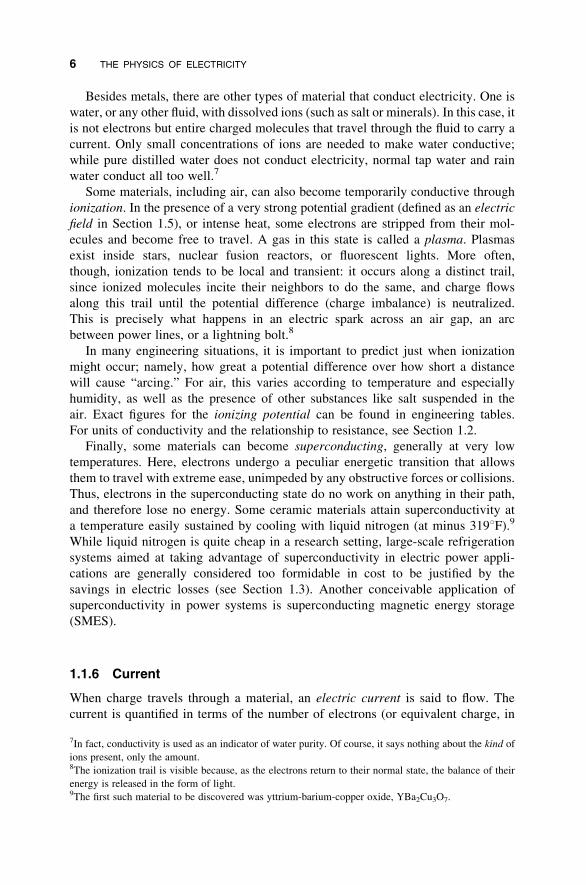
Besides metals, there are other types of material that conduct electricity. One is

water, or any other fluid, with dissolved ions (such as salt or minerals). In this case, it

is not electrons but entire charged molecules that travel through the fluid to carry a

current. Only small concentrations of ions are needed to make water conductive;

while pure distilled water does not conduct electricity, normal tap water and rain

water conduct all too well.7

Some materials, including air, can also become temporarily conductive through

ionization. In the presence of a very strong potential gradient (defined as an electric

field in Section 1.5), or intense heat, some electrons are stripped from their mol-

ecules and become free to travel. A gas in this state is called a plasma. Plasmas

exist inside stars, nuclear fusion reactors, or fluorescent lights. More often,

though, ionization tends to be local and transient: it occurs along a distinct trail,

since ionized molecules incite their neighbors to do the same, and charge flows

along this trail until the potential difference (charge imbalance) is neutralized.

This is precisely what happens in an electric spark across an air gap, an arc

between power lines, or a lightning bolt.8

In many engineering situations, it is important to predict just when ionization

might occur; namely, how great a potential difference over how short a distance

will cause “arcing.” For air, this varies according to temperature and especially

humidity, as well as the presence of other substances like salt suspended in the

air. Exact figures for the ionizing potential can be found in engineering tables.

For units of conductivity and the relationship to resistance, see Section 1.2.

Finally, some materials can become superconducting, generally at very low

temperatures. Here, electrons undergo a peculiar energetic transition that allows

them to travel with extreme ease, unimpeded by any obstructive forces or collisions.

Thus, electrons in the superconducting state do no work on anything in their path,

and therefore lose no energy. Some ceramic materials attain superconductivity at

a temperature easily sustained by cooling with liquid nitrogen (at minus 3198F).9

While liquid nitrogen is quite cheap in a research setting, large-scale refrigeration

systems aimed at taking advantage of superconductivity in electric power appli-

cations are generally considered too formidable in cost to be justified by the

savings in electric losses (see Section 1.3). Another conceivable application of

superconductivity in power systems is superconducting magnetic energy storage

(SMES).

1.1.6 Current

When charge travels through a material, an electric current is said to flow. The

current is quantified in terms of the number of electrons (or equivalent charge, in

7In fact, conductivity is used as an indicator of water purity. Of course, it says nothing about the kind of

ions present, only the amount.8The ionization trail is visible because, as the electrons return to their normal state, the balance of their

energy is released in the form of light.9The first such material to be discovered was yttrium-barium-copper oxide, YBa2Cu3O7.


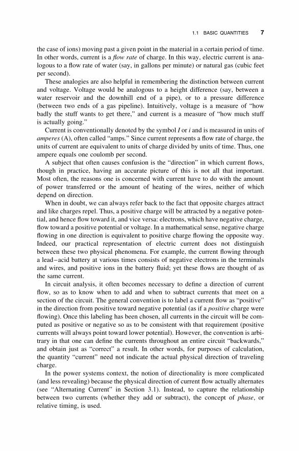
the case of ions) moving past a given point in the material in a certain period of time.

In other words, current is a flow rate of charge. In this way, electric current is ana-

logous to a flow rate of water (say, in gallons per minute) or natural gas (cubic feet

per second).

These analogies are also helpful in remembering the distinction between current

and voltage. Voltage would be analogous to a height difference (say, between a

water reservoir and the downhill end of a pipe), or to a pressure difference

(between two ends of a gas pipeline). Intuitively, voltage is a measure of “how

badly the stuff wants to get there,” and current is a measure of “how much stuff

is actually going.”

Current is conventionally denoted by the symbol I or i and is measured in units of

amperes (A), often called “amps.” Since current represents a flow rate of charge, the

units of current are equivalent to units of charge divided by units of time. Thus, one

ampere equals one coulomb per second.

A subject that often causes confusion is the “direction” in which current flows,

though in practice, having an accurate picture of this is not all that important.

Most often, the reasons one is concerned with current have to do with the amount

of power transferred or the amount of heating of the wires, neither of which

depend on direction.

When in doubt, we can always refer back to the fact that opposite charges attract

and like charges repel. Thus, a positive charge will be attracted by a negative poten-

tial, and hence flow toward it, and vice versa: electrons, which have negative charge,

flow toward a positive potential or voltage. In a mathematical sense, negative charge

flowing in one direction is equivalent to positive charge flowing the opposite way.

Indeed, our practical representation of electric current does not distinguish

between these two physical phenomena. For example, the current flowing through

a lead–acid battery at various times consists of negative electrons in the terminals

and wires, and positive ions in the battery fluid; yet these flows are thought of as

the same current.

In circuit analysis, it often becomes necessary to define a direction of current

flow, so as to know when to add and when to subtract currents that meet on a

section of the circuit. The general convention is to label a current flow as “positive”

in the direction from positive toward negative potential (as if a positive charge were

flowing). Once this labeling has been chosen, all currents in the circuit will be com-

puted as positive or negative so as to be consistent with that requirement (positive

currents will always point toward lower potential). However, the convention is arbi-

trary in that one can define the currents throughout an entire circuit “backwards,”

and obtain just as “correct” a result. In other words, for purposes of calculation,

the quantity “current” need not indicate the actual physical direction of traveling

charge.

In the power systems context, the notion of directionality is more complicated

(and less revealing) because the physical direction of current flow actually alternates

(see “Alternating Current” in Section 3.1). Instead, to capture the relationship

between two currents (whether they add or subtract), the concept of phase, or

relative timing, is used.


As for the speed at which current propagates, it is often said that current travels at

the speed of light (186,000 miles per second). While this is not quite accurate (just as

the speed of light actually varies in different materials), it is usually sufficient to

know that current travels very fast. Conceptually, it is important to recognize that

what is traveling at this high speed is the pulse or signal of the current, not the indi-

vidual electrons. For the current to flow, it is also not necessary for all the electrons

to physically depart at one end and arrive at the other end of the conductor. Rather,

the electrons inside a metal conductor continually move in a more or less random

way, wiggling around in different directions at a speed related to the temperature

of the material. They then receive a “shove” in one direction by the electric field

(see Section 1.5.2). We can imagine this shove propagating by way of the electrical

repulsion among electrons: each electron need not travel a long distance, just enough

to push its neighbor over a bit, which in turn pushes its neighbor, and so on. This

chain reaction creates a more orderly motion of charge, as opposed to the usual

random motion, and is observed macroscopically as the current. It is the signal to

“move over” that propagates at essentially the speed of light.10

The question of the propagation speed of electric current only becomes relevant

when the distance to be covered is so large that the time it takes for a current pulse to

travel from one point to another is significant compared to other timing parameters

of the circuit. This can be the case for electric transmission lines that extend over

many hundreds of miles.11 However, we will not deal with this problem explicitly

(see Chapter 7, “Power Flow Analysis,” for how we treat the concept of time in

power systems). A circuit that is sufficiently small so that the speed of current is

not an issue is called a lumped circuit. Circuits are treated as lumped circuits

unless otherwise stated.

1.2 OHM’S LAW

It is intuitive that voltage and current would be somehow related. For example, if the

potential difference between two ends of a wire is increased, we would expect a

greater current to flow, just like the flow rate of gas through a pipeline increases

when a greater pressure difference is applied. For most materials, including metallic

conductors, this relationship between voltage and current is linear: as the potential

difference between the two ends of the conductor increases, the current through the

conductor increases proportionally. This statement is expressed in Ohm’s law,

V ¼ IR

10We can draw an analogy with an ocean wave: the water itself moves essentially up and down, and it is

the “signal” to move up and down that propagates across the surface, at a speed much faster than the bulk

motion of water.11For example, traveling down a 500-mile transmission line at the speed of light takes 2.7 milliseconds.

Compared to the rate at which alternating current changes direction (60 times per second, or every 16.7

milliseconds), this corresponds to one-sixth of a cycle, which is not negligible.


where V is the voltage, I is the current, and R is the proportionality constant called

the resistance.

1.2.1 Resistance

To say that Ohm’s law is true for a particular conductor is to say that the resistance

of this conductor is, in fact, constant with respect to current and voltage. Certain

materials and electronic devices exhibit a nonlinear relationship between current

and voltage, that is, their resistance varies depending on the voltage applied. The

relationship V ¼ IR will still hold at any given time, but the value of R will be a

different one for different values of V and I. These nonlinear devices have special-

ized applications and will not be discussed in this chapter. Resistance also tends to

vary with temperature, though a conductor can still obey Ohm’s law at any one

temperature.12 For example, the resistance of a copper wire increases as it heats

up. In most operating regimes, these variations are negligible. Generally, in any situ-

ation where changes in resistance are significant, this is explicitly mentioned. Thus,

whenever one encounters the term “resistance” without further elaboration, it is safe

to assume that within the given context, this resistance is a fixed, unchanging

property of the object in question.

Resistance depends on an object’s material composition as well as its shape. For a

wire, resistance increases with length, and decreases with cross-sectional area.

Again, the analogy to a gas or water pipe is handy: we know that a pipe will

allow a higher flow rate for the same pressure difference if it has a greater diameter,

while the flow rate will decrease with the length of the pipe. This is due to friction in

the pipe, and in fact, an analogous “friction” occurs when an electric current travels

through a material.

This friction can be explained by referring to the microscopic movement of elec-

trons or ions, and noting that they interact or collide with other particles in the

material as they go. The resulting forces tend to impede the movement of the

charge carriers and in effect limit the rate at which they pass. These forces vary

for different materials because of the different spatial arrangements of electrons

and nuclei, and they determine the material’s ability to conduct.

This intrinsic material property, independent of size or shape, is called resistivity

and is denoted by r (the Greek lowercase rho). The actual resistance of an object is

given by the resistivity multiplied by the length of the object (l ) and divided by its

cross-sectional area (A):

R ¼rl

A

The units of resistance are ohms, abbreviatedV (Greek capital omega). By rearrang-

ing Ohm’s law, we see that resistance equals voltage divided by current. Units of

12If we graph V versus I, Ohm’s law requires that the graph be a straight line. With temperature, the slope

of this line may change.

1.2 OHM’S LAW 9

resistance are thus equivalent to units of voltage divided by units of current. By

definition, one ohm equals one volt per ampere (V ¼ V/A).The units of resistivity are ohm-meters (V-m), which can be reconstructed

through the preceding formula: when ohm-meters are multiplied by meters (for l )

and divided by square meters (for A), the result is simply ohms. Resistivity,

which is an intrinsic property of a material, is not to be confused with the resistance

per unit length (usually of a wire), quoted in units of ohms per meter (V/m). The

latter measure already takes into account the wire diameter; it represents, in

effect, the quantity r/A. The resistivities of different materials in V-m can be

found in engineering tables.

1.2.2 Conductance

It is sometimes convenient to refer to the resistive property of a material or object in

the inverse, as conductivity or conductance. Conductivity is the inverse of resistivity

and is denoted by s (Greek lowercase sigma): s ¼ 1/r. For the case of a simple

resistor, conductance is the reciprocal of resistance and is usually denoted by G

(sometimes g), where G ¼ 1/R.13 Not without humor, the units of conductance

are called mhos, and 1 mho ¼ 1/V. Another name for the mho is the siemens (S);

they are identical units. The conductance is related to the conductivity by

G ¼sA

l

and the units of s are thus mhos/m.

For the special case of an insulator, the conductance is zero and the resistance is

infinite. For the special case of a superconductor, the resistance is zero and the con-

ductance is, theoretically, infinite (a truly infinite conductance would imply an infi-

nitely large current, which does not actually occur since its magnitude is eventually

constrained by the number of electrons available).

Example

Consider two power extension cords, one with twice the wire diameter of the

other. If the cords are of the same length and same material, how do their

resistances compare?

Since resistance is inversely proportional to area, the smaller wire will have

four times the resistance. We can see this through the formula R ¼ rl/A,where r and l are the same for both. Thus, using the subscripts 1 and 2 to refer

to the two cords, we can write R1/R2 ¼ A2/A1. The areas are given by the fam-

iliar geometry formula, A ¼ p(d/2)2 (where p ¼ 3.1415. . .), which includes the

square of the diameter or radius. If the length of either cord were doubled, its

resistance would also double.

13See Section 3.2.4 for the complex case that includes both resistance and reactance.


To put some numbers to this example, consider a typical 25-ft, 16-gauge

extension cord, made of a copper conductor. The cross-sectional area of

16-gauge wire is 1.31 mm2 (or 1.31 � 1028 m2) and the resistivity of copper is

r ¼ 1.76 � 1028 V-m. The resistance per unit length of 16-gauge copper wire

is 0.0134 V/m, and a 25-ft length of it has a resistance of 0.102 V. By contrast,

a 10-gauge copper wire of the same length, which has about twice the diameter,

has a resistance of only 0.025 V.

Suppose the current in the 25-ft, 16-gauge cord is 5A. What is the voltage

difference between the two ends of each conductor?

The voltage drop in the wire is given by Ohm’s law, V ¼ IR. Thus,

V ¼ 5 A . 0.102 V ¼ 0.51 V. Because the voltage drop applies to each of the

two conductors in the cord, this means that the line voltage, or difference

between the two sides of the electrical outlet, will be diminished by about

one volt (say, from 120 to 119 V), as seen by the appliance at the end.

1.2.3 Insulation

Insulating materials are used in electric devices to keep current from flowing where

it is not desired. They are simply materials with a sufficiently high resistance (or suf-

ficiently low conductance), also known as dielectricmaterials. Typically, plastics or

ceramics are used. When an insulator is functional, its resistance is infinite, or the

conductance zero, so that zero current flows through it.

Any insulator has a specific voltage regime within which it can be expected to

perform. If the voltage difference between two sides of the insulator becomes too

large, its insulating properties may break down due to microscopic changes in the

material, where it actually becomes conducting. Generally, the thicker the insulator,

the higher the voltage difference it can sustain. However, temperature can also be

important; for example, plastic wire insulation may melt if the wire becomes too hot.

The insulators often seen on high-voltage equipment consist of strings of ceramic

bells, holding the energized wires away from other components (e.g., transmission

towers or transformers). The shape of these bells serves to inhibit the formation of

arcs along their surface. The number of bells is roughly proportional to the voltage

level, though it also depends on climate. For example, the presence of salt water dro-

plets in coastal air encourages ionization and therefore requires more insulation to

prevent arcing.

1.3 CIRCUIT FUNDAMENTALS

1.3.1 Static Charge

A current can only flow as long as a potential difference is sustained; in other words,

the flowing charge must be replenished. Therefore, some currents have a very short

duration. For example, a lightning bolt lasts only a fraction of a second, until the

charge imbalance between the clouds and the ground is neutralized.

1.3 CIRCUIT FUNDAMENTALS 11

When charge accumulates in one place, it is called static charge, because it is not

moving. The reason charge remains static is that it lacks a conducting pathway that

enables it to flow toward its opposite charge. When we receive a shock from static

electricity—for example, by touching a doorknob—our body is providing just such a

pathway. In this example, our body is charged through friction, often on a synthetic

carpet, and this charge returns to the ground via the doorknob (the carpet only gives

off electrons by rubbing, but does not allow them to flow back). As our fingers

approach the doorknob, the air in between is actually ionized momentarily, produ-

cing a tiny arc that causes the painful sensation.14 Static electricity occurs mostly in

dry weather, since moisture on the surface of objects makes them sufficiently con-

ductive to prevent accumulations of charge.

However startling and uncomfortable, static electricity encountered in everyday

situations is harmless because the amount of charge available is so small,15 and it is

not being replenished. This is true despite the fact that very high voltages can be

involved (recall that voltage is energy per charge), but these voltages drop instan-

taneously as soon as the contact is made.

1.3.2 Electric Circuits

In order to produce a sustained flow of current, the potential difference must be

maintained. This is achieved by providing a pathway to “recycle” charge to its

origin, and a mechanism (called an electromotive force, or emf16) that compels

the charge to return to the less “comfortable” potential. Such a setup constitutes

an electric circuit.

A simple example is a battery connected with two wires to a light bulb. The

chemical forces inside the battery do work on the charge to move it to the terminals,

where an electric potential is produced and sustained. Specifically, electrons are

moved to the negative terminal, and positive ions are moved to the positive elec-

trode, where they produce a deficit of electrons in the positive battery terminal.

The wires then provide a path for electrons to flow from the negative to the positive

terminal. Because the positive potential is so attractive, these electrons even do work

by flowing through the resistive light bulb, causing it to heat up and glow. As soon as

the electrons arrive at the positive terminal, they are “lifted” again to the negative

potential, allowing the current to continue flowing. In analogy with flowing water,

the wires are like pipes that carry water downhill, and the battery is like a pump

that returns the water to the uphill end of the circuit.

14Charge will accumulate more densely in the point, being attracted to the opposite charge across the gap.

The charge density in turn affects the gradient of the electric potential across the gap, which is what causes

the ionization. Therefore, approaching the doorknob with a flat hand can prevent the formation of an arc,

and charge will simply flow (unnoticeably) after the contact has been made. This is also why lightning

arresters work: a particularly pointed object like a metal rod will “attract” an electric arc toward its

high charge density. By the same token, lightning tends to strike tall trees and transmission towers.15The same is not true of electrical equipment that has been specifically designed to hold a very large

amount of static charge!16Unrelated to the EMF that stands for “Electromagnetic Fields.”


When the wires are connected to form a complete loop, they make a closed

circuit. If the wire were cut, this would create an open circuit, and the current

would cease to flow. In practice, circuits are opened and closed by means of switches

that make and break electrical contacts.

1.3.3 Voltage Drop

In describing circuits, it is often desirable to specify the voltage at particular points

along the way. The difference in voltage between two points in a circuit is referred to

as the voltage drop across the wire or other component in between. As in Ohm’s law,

V ¼ IR, this voltage drop is proportional to the current flowing through the

component, multiplied by its resistance.

As in the analogy of water pipes running downhill, the voltage drops continu-

ously throughout a circuit, from one terminal of the emf to the other. However,

just like the slope of the pipes may change, the voltage does not necessarily drop

at a steady rate. Rather, depending on the resistance of a given circuit component,

the voltage drop across it will be more or less: a component with high resistance

will sustain a greater voltage drop, whereas a component with low resistance such

as a conducting wire will have a smaller voltage drop across it, perhaps so small

as to be negligible in a given context. For small circuits, it is often reasonable to

assume that the wire’s resistance is zero, and that therefore the voltage is the

same all the way along the wire. In power systems, however, where transmission

and distribution lines cover long distances, the voltage drop across them is signifi-

cant and indeed accounts for some important aspects of how these systems function.

Importantly (and in contrast to the water analogy), the magnitude of the current

also determines the voltage drop (along with resistance). For example, at times of

high electric demand and thus high current flow, the voltage drop along transmission

and distribution lines is greater; that is, the voltage drops more rapidly with distance.

If this condition cannot be compensated for by other adjustments in the system (see

Section 6.7), customers experience lower voltage levels associated with dimmer

lights and impaired equipment performance, known as “brownouts.” Similarly, if

a piece of heavy power equipment is connected through a long extension cord

with too high a resistance, the voltage drop along this cord can result in damage

to the motor from excessively low voltage at the far end.

1.3.4 Electric Shock

Any situation where a high voltage is sustained by an electromotive force (or a very

large accumulation of charge) constitutes a shock hazard. Our bodies are not notice-

ably affected by being “charged up,” or raised to a potential above ground, just as

birds can sit on a single power line. Rather, harm is done when a current flows

through our body. A current as small as a few milliamperes across the human

heart can be lethal.17 For current to flow through an object, there must be a

17A saying goes, “It’s the volts that jolts, and the mils that kills.”

1.3 CIRCUIT FUNDAMENTALS 13

voltage drop across it. In other words, our body must be simultaneously in contact

with two sources of different potential—for example, a power line and the ground.

Though it is the current that causes biological damage, Ohm’s law indicates that

shock hazard is roughly proportional to the voltage encountered. However, the

resistance is also important. On an electrical path through the human body, the great-

est resistance is on the surface of the skin and clothing, while our interior conducts

very well. Thus, the severity of a shock received from a particular voltage can vary,

depending on how sweaty one’s palms are, or what type of shoes one is wearing.

The physical principles of electric current can be applied to suggest a number of

practical precautions for reducing electric-shock hazards. For example, when touch-

ing an object at a single high voltage, we are safe as long as we are insulated from the

ground. A wooden ladder might serve this purpose at home, while utility linemen

often work on “hot” equipment out of raised plastic “buckets.” Linemen can also

insulate themselves from the high-voltage source by wearing special rubber

gloves, which are commonly used for work on up to 12 kilovolts. The important

thing is to know the capability of the insulator in relation to the voltage encountered.

A different safety measure often used by electricians when touching a question-

able component (such as a wire that might be energized) is to make contact with

ground potential with the same hand, for example by touching the little finger to

the wall. In this way, a path of low resistance is created through the hand, which

will greatly reduce the current flowing through the rest of the body and especially

across the heart. Though the hand might be injured (improbable at household

voltage), such a shock is far less likely to be lethal.

Around high-voltage equipment, in order to avoid the possibility of touching two

objects at different potentials with a current pathway across the heart, a common

practice is to “keep one hand in your pockets.” Near very high potentials, where

the concern is not just about touching equipment, but even drawing an arc across

the air, the advice is to “keep both hands in your pockets” so as to avoid creating

a point with high charge density to attract an arc.

Finally, another factor to consider is the muscular contraction that often occurs in

response to an electric shock. Thus, a potentially energized wire is better touched

with the back of the hand, so as to prevent involuntary closing of the hand around it.

If a person is in contact with an energized source, similar precautions should be

exercised in removing them, lest there be additional casualties. If available, a device

like a wooden stick would be ideal; in the worst case, kicking is preferable to

grabbing.

1.4 RESISTIVE HEATING

Whenever an electric current flows through a material that has some resistance (i.e.,

anything but a superconductor), it creates heat. This resistive heating is the result of

“friction,” as created by microscopic phenomena such as retarding forces and col-

lisions involving the charge carriers (usually electrons); in formal terminology,

the heat corresponds to the work done by the charge carriers in order to travel to


a lower potential. This heat generation may be intended by design, as in any heating

appliance (for example, a toaster, an electric space heater, or an electric blanket).

Such an appliance essentially consists of a conductor whose resistance is chosen

so as to produce the desired amount of resistive heating. In other cases, resistive

heating may be undesirable. Power lines are a classic example. For one, their

purpose is to transmit energy, not to dissipate it; the energy converted to heat

along the way is, in effect, lost (thus the term resistive losses). Furthermore, resistive

heating of transmission and distribution lines is undesirable, since it causes thermal

expansion of the conductors, making them sag. In extreme cases such as fault con-

ditions, resistive heating can literally melt the wires.

1.4.1 Calculating Resistive Heating

There are two simple formulas for calculating the amount of heat dissipated in a

resistor (i.e., any object with some resistance). This heat is measured in terms of

power, which corresponds to energy per unit time. Thus, we are calculating a rate

at which energy is being converted into heat inside a conductor. The first formula is

P ¼ IV

where P is the power, I is the current through the resistor, and V is the voltage drop

across the resistor.

Power is measured in units of watts (W), which correspond to amperes � volts.

Thus, a current of one ampere flowing through a resistor across a voltage drop of one

volt produces one watt of heat. Units of watts can also be expressed as joules per

second. To conceptualize the magnitude of a watt, it helps to consider the heat

created by a 100-watt light bulb, or a 1000-watt space heater.

The relationship P ¼ IV makes sense if we recall that voltage is a measure of

energy per unit charge, while the current is the flow rate of charge. The product

of current and voltage therefore tells us how many electrons are “passing

through,” multiplied by the amount of energy each electron loses in the form of

heat as it goes, giving an overall rate of heat production. We can write this as

Charge

Time�Energy

Charge¼

Energy

Time

and see that, with the charge canceling out, units of current multiplied by units of

voltage indeed give us units of power.

The second formula for calculating resistive heating is

P ¼ I2R

where P is the power, I is the current, and R is the resistance. This equation could be

derived from the first one by substituting I .R for V (according to Ohm’s law). As we

1.4 RESISTIVE HEATING 15

discuss in Section 3.1, this second formula is more frequently used in practice to cal-

culate resistive heating, whereas the first formula has other, more general

applications.

As we might infer from the equation, the units of watts also correspond to

amperes2 . ohms (A2 .V). Thus, a current of one ampere flowing through a wire

with one ohm resistance would heat this wire at a rate of one watt. Because the

current is squared in the equation, two amperes through the same wire would heat

it at a rate of 4 watts, and so on.

Example

A toaster oven draws a current of 6 A at a voltage of 120 V. It dissipates 720 W in

the form of heat. We can see this in two ways: First, using P ¼ IV,

120 V . 6 A ¼ 720 W. Alternatively, we could use the resistance, which is

20 V (20 V . 6 A ¼ 120 V), and write P ¼ I2R: (6 A)2 . 20 V ¼ 720 W.

It is important to distinguish carefully how power depends on resistance, current,

and voltage, since these are all interdependent. Obviously, the power dissipated will

increase with increasing voltage and with increasing current. From the formula

P ¼ I2R, we might also expect power to increase with increasing resistance, assum-

ing that the current remains constant. However, it may be incorrect to assume that

we can vary resistance without varying the current.

Specifically, in many situations it is the voltage that remains (approximately)

constant. For example, the voltage at a customer’s wall outlet ideally remains at

120 V, regardless of how much power is consumed.18 The resistance is determined

by the physical properties of the appliance: its intrinsic design, and, if applicable, a

power setting (such as “high” or “low”). Given the standard voltage, then, the resist-

ance determines the amount of current “drawn” by the appliance according to Ohm’s

law: higher resistance means lower current, and vice versa. In fact, resistance and

current are inversely proportional in this case: if one doubles, the other is halved.

What, then, is the effect of resistance on power consumption? The key here is that

resistive heating depends on the square of the current, meaning that the power is

more sensitive to changes in current than resistance. Therefore, at constant

voltage, the effect of a change in current outweighs the effect of the corresponding

change in resistance. For example, decreasing the resistance (which, in and of itself,

would tend to decrease resistive heating) causes the current to increase, which

increases resistive heating by a greater factor. Thus, at constant voltage, the net

effect of decreasing resistance is to increase power consumption. An appliance

that draws more power has a lower internal resistance.

For an intuitive example, consider the extreme case of a short circuit, caused by

an effectively zero resistance (usually unintentional). Suppose a thick metal bar were

18This is generally true because (a) changes in power consumption from an individual appliance are small

compared to the total power supplied to the area by the utility, and (b) the utility takes active steps to regu-

late the voltage (see Section 6.6). Dramatic changes in demand do cause changes in voltage, but for the

present discussion, it is more instructive to ignore these phenomena and treat voltage as a fixed quantity.


placed across the terminals of a car battery. A very large current would flow, the

metal would become very hot, and the battery would be drawn down very

rapidly. If a similar experiment were performed on a wall outlet by sticking, say,

a fork into it, the high current would hopefully be interrupted by the circuit

breaker before either the fork or the wires melted (DO NOT actually try this!).

The other extreme case is simply an open circuit, where the two terminals are sep-

arate and the resistance of the air between them is infinite: here the current and the

power consumption are obviously zero.

Example

Consider two incandescent light bulbs, with resistances of 240 V and 480 V.

How much power do they each draw when connected to a 120 V outlet?

First we must compute the current through each bulb, using Ohm’s law:

Substituting V ¼ 120 V and R1 ¼ 240 V into V ¼ IR, we obtain I1 ¼ 0.5 A.

For R2 ¼ 480 V, we get I2 ¼ 0.25 A.

Now we can use these values for I and R in the power formula, P ¼ I2R, which

yields P1 ¼ (0.5 A)2 . 240 V ¼ 60 W and P2 ¼ (0.25 A)2 . 480 V ¼ 30 W.

We see that at constant voltage, the bulb with twice the resistance draws half

the power.

There are other situations, however, where the current rather than the voltage is

constant. Transmission and distribution lines are an important case. Here, the

reasoning suggested earlier does in fact apply, and resistive heating is directly pro-

portional to resistance. The important difference between power lines and appli-

ances is that for power lines, the current is unaffected by the resistance of the line

itself, being determined instead by the load or power consumption at the end of

the line (this is because the resistance of the line itself is very small and insignificant

compared to that of the appliances at the end, so that any reasonable change in the

resistance of the line will have a negligible effect on the overall resistance, and thus

the current flowing through it). However, the voltage drop along the line (i.e., the

difference in voltage between its endpoints, not to be confused with the line

voltage relative to ground) is unconstrained and varies depending on current and

the line’s resistance. Thus, Ohm’s law still holds, but it is now I that is fixed and

V and R that vary. Applying the formula P ¼ I2R for resistive heating with the

current held constant, we see that doubling the resistance of the power line will

double resistive losses. Since in practice it is desirable to minimize resistive

losses on power transmission and distribution lines, these conductors are chosen

with the minimal resistance that is practically and economically feasible.

1.4.2 Transmission Voltage and Resistive Losses

Resistive losses are the reason why increasingly high voltage levels are chosen for

power transmission lines. Recalling the relationship P ¼ IV, the amount of power

transmitted by a line is given by the product of the current flowing through it and

1.4 RESISTIVE HEATING 17

its voltage level (as measured either with respect to ground or between two lines or

phases of one circuit). Given that a certain quantity of power is demanded, there is a

choice as to what combination of I and Vwill constitute this power. A higher voltage

level implies that in order to transmit the same amount of power, less current needs

to flow. Since resistive heating is related to the square of the current, it is highly ben-

eficial from the standpoint of line losses to reduce the current by increasing the

voltage.

Before power transformers were available, transmission voltages were limited to

levels that were considered safe for customers. Thus, high currents were required,

causing so much resistive heating that it posed a significant constraint to the expan-

sion of power transmission. With increasing power carried at a given voltage,

an increasing fraction of the total power is lost on the lines, making transmission

uneconomical at some point. The increase in losses can be counteracted by reducing

the resistance of the conductors, but only at the expense of making them thicker and

heavier. A century ago, Thomas Edison found the practical limit for trans-

mitting electricity at the level of a few hundred volts to be only a few miles.

With the help of transformers that allow essentially arbitrary voltage conversion

(see Section 6.3), transmission voltage levels have grown steadily in conjunction

with the geographic expansion of electric power systems, up to about 1000 kilovolts

(kV), and with the most common voltages around 100–500 kV. The main factor

offsetting the economic benefits of very high voltage is the increased cost and

engineering challenge of safe and effective insulation.

1.5 ELECTRIC AND MAGNETIC FIELDS

1.5.1 The Field as a Concept

The notion of a field is an abstraction initially developed in physics to explain how

tangible objects exert forces on each other at a distance, by invisible means. Articu-

lating and quantifying a “field” particularly helps to analyze situations where an

object experiences forces of various strengths and directions, depending on its

location. Rather than referring to other objects associated with “causing” such

forces, it is usually more convenient to just map their hypothetical effects across

space. Such a map is then considered to describe properties of the space, even in

the absence of an actual object placed within it to experience the results, and this

map represents the field.

For example, consider gravity. We know that our body is experiencing a force

downward because of the gravitational attraction between it and the Earth. This

gravitational force depends on the respective masses of our bodies and the Earth,

but it also depends on our location: astronauts traveling into space feel less and

less of a pull toward the Earth as they get farther away. Indeed, though the effect

is small, we are even slightly “lighter” on a tall mountain or in an airplane at

high altitude. If we were interested in extremely accurate measurements of

gravity (for example, to calculate the exact flight path of a ballistic missile), we


could construct a map of a “gravitational field” encompassing the entire atmosphere,

which would indicate the strength of gravity at any point. This field is caused by the

Earth, but does not explicitly refer to the Earth as a mass; rather, it represents in

abstract terms the effect of the Earth’s presence. The field also does not refer to

any object (such as an astronaut) that it may influence, though such an object’s

mass would need to be taken into account in order to calculate the actual force on

it. Thus, the gravitational field is a way of mapping the influence of the Earth’s

gravity throughout a region of space.

An alternative interpretation is to consider the field as a physical entity in its own

right, even though it has no substance of its own. Here we would call gravity a prop-

erty of the space itself, rather than a map telling us about objects such as the Earth in

space. Indeed, the field itself can be considered a “thing” rather than a map, because

it represents potential energy distributed over space. We know of the presence of this

potential energy because it does physical work on objects: for example, a massive

object within the field is accelerated, and in that moment, the energy becomes obser-

vable. With this in mind, we can understand the field as the answer to the question,

Where does the potential energy reside while we are not observing it?

This notion of the field as a physical entity is a fairly recent one. Whereas classical

physics relied on the notion of action-at-a-distance, in which only tangible objects

figured as “actors,” the study of very large and very small things in the 20th

century has forced us to give up referring to entities that we can touch or readily visu-

alize when talking about how theworldworks. Instead,modern physics has cultivated

more ambiguity and caution in declaring the “reality” of physical phenomena, recog-

nizing that what is accessible to our human perception is perhaps not a definitive stan-

dard for what “exists.” Even what once seemed like the most absolute, immutable

entities—mass, distance, and time—were proved ultimately changeable and intract-

able to our intuition by relativity theory and quantum mechanics.

Based on these insights, we might conclude that any quantities we choose to

define and measure are in some sense arbitrary patterns superimposed on the vast

web of energy and movement that constitutes reality, for the purpose of helping

us apprehend this reality with our thoughts. In this sense, we are no more justified

in considering a planet a “thing that really exists” than we are a gravitational

field. What we really care about as scientists, though, is how useful such a concep-

tual pattern might be for describing the world in concise terms and making predic-

tions about how things will behave. By this standard, the notion of a “field” does

wonders. Physicists and engineers are therefore accustomed to regarding fields,

however devoid of substance, as real, manipulable, and legitimate physical entities

just like tangible objects. In any case, the reader should rest assured that it is quite all

right to simply accept the “field” as a strange instrument of analysis that grows more

palatable with familiarity.

1.5.2 Electric Fields

In Section 1.1, we characterized the electric potential as a property of the location at

which a charge might find itself. A map of the electric potential would indicate how

1.5 ELECTRIC AND MAGNETIC FIELDS 19

much potential energy would be possessed by a charge located at any given point.

The electric field is a similar map, but rather of the electric force (such as attraction

or repulsion) that would be experienced by that charge at any location. This force is

the result of potential differences between locations: the more dramatically the

potential varies from one point to the next, the greater the force would be on an elec-

tric charge in between these points. In formal terms, the electric field represents the

potential gradient.

Consider the electric field created by a single positive charge, just sitting in space.

Another positive charge in its vicinity would experience a repulsive force. This

repulsive force would increase as the two charges were positioned closer together,

or decrease as they moved father apart; specifically, the electric force drops off at

a rate proportional to the square of the distance. This situation can be represented

graphically by drawing straight arrows radially outward from the first charge, as

in Figure 1.1a. Such arrows are referred to as field lines. Their direction indicates

the direction that a “test charge,” such as the hypothetical second charge that was

introduced, would be pushed or pulled (in this case, straight away). The strength

Figure 1.1 Electric field of (a) a single charge and (b) two opposite charges.


of the force is indicated by the proximity of field lines: the force is stronger where

the lines are closer together.

This field also indicates what would happen to a negative charge: At any point, it

would experience a force of equal strength (assuming equal magnitude of charge),

but opposite direction as the positive test charge, since it would be attracted

rather than repelled. Thus, a negative test charge would also move along the field

lines, only backwards. By convention, the direction of the electric field lines is

drawn so as to represent the movement of a positive test charge.

For a slightly more complex situation, consider the electric field created by a

positive and a negative charge, sitting at a fixed distance from each other. We can

map the field conceptually by asking, for any location, “What force would

be acting on a (positive) test charge if it were placed here?” Each time, the net

force on the test charge would be a combination of one attractive force and one

repulsive force, in different directions and at different strengths depending on the

distance from the respective fixed charges. Graphically, we can construct an

image of the field by drawing an arrow in the direction that the charge would be

pulled. The arrows for points along the charge’s hypothetical path then combine

into continuous field lines. Again, these field lines will be spaced more closely

where the force is stronger. This exercise generates the picture in Figure 1.1b.

1.5.3 Magnetic Fields

The pattern of the electric field in Figure 1.1 may be reminiscent to some readers of

the pattern that many of us produced once upon a time in science class by sprinkling

iron filings on a sheet of paper over a bar magnet. The two phenomena, electric and

magnetic forces, are indeed closely linked manifestations of a common underlying

physics.

As we know from direct tactile experience, magnets exert force on each other:

opposite poles attract, and like poles repel. This is somewhat analogous to the

fact that opposite electric charges attract and like charges repel. But, unlike a posi-

tive or negative electric charge, a magnetic pole cannot travel individually. There is

no such thing as an individual north or south pole (a “monopole” in scientific terms,

which has never been found). Every magnet has a north and a south pole. Thus,

unlike electric field lines that indicate the direction of movement of an individual

test charge, magnetic field lines indicate the orientation of a test magnet. The iron

filings in the familiar experiment—which become little test magnets since they

are magnetized in the presence of the bar magnet—do not move toward one pole

or the other, but rotate and align themselves with the direction of the field lines.

It is important to emphasize that, despite the similar shape of field lines, magnetic

poles are not analogous to single electric charges sitting in space. Rather than think-

ing of magnetism as existing in the form of “stuff” like electric charge (which could

conceivably be decomposed into its “north” and “south” constituents), it is more

appropriate to think of magnetism as an expression of directionality, where north

is meaningless without south. If you cut a magnet in half, you get two smaller

magnets that still each have a north and a south pole.


If we pursued such a division of magnets again and again, down to the level of the

smallest particles, we would find that even individual electrons or protons appear as

tiny magnets. In ordinary materials, the orientation of all these microscopic magnets

varies randomly throughout space, and they therefore do not produce observable

magnetic properties at the macroscopic level. It is only in magnetized materials

that the direction of these myriad tiny magnets becomes aligned, allowing their mag-

netic fields to combine to become externally noticeable. This alignment stems from

the force magnets exert on each other, and their resulting tendency to position them-

selves with their north poles all pointing in the same direction. Some substances like

magnetite occur naturally with a permanent alignment, making the familiar magnets

that adhere to refrigerators and other things. Other materials like iron and steel can

be temporarily magnetized in the presence of a sufficiently strong external magnetic

field (this is what happens to the refrigerator door underneath the magnet), with the

particles returning to their disordered state after the external field is withdrawn.

The magnetic property of microscopic particles is due to their electric charge and

their intrinsic motion, which brings us to the fundamental connection between elec-

tricity and magnetism. Indeed, we can think of magnetism as nothing but a manifes-

tation of directionality associated with electric charge in motion, whereby moving

charges always exert a specific directional force on other moving charges. At the

level of individual electrons, their motion consists of both an orbital movement

around the atom’s nucleus and an intrinsic spin, which we can visualize as if the par-

ticle were spinning like a top.19 Both of these rotational motions combine to form

what is referred to as a magnetic moment. Similarly, the protons inside atomic

nuclei possess a magnetic moment due to their intrinsic spin.20

Knowing this, it would stand to reason that a large amount of moving charge such

as a measurable electric current should produce a magnetic field as well. This

phenomenon was in fact discovered in 1820, when Hans Christian Oersted observed

that a compass needle was deflected by an electric current through a nearby wire.

The magnetic field produced by an electric current points at a right angle to the

flow of charge, in a direction specified by the “right-hand rule” illustrated in

Figure 1.2. If the thumb of one’s right hand is pointing in the direction of the

current, then the curled fingers of the same hand indicate the direction of the mag-

netic field. Thus, the magnetic field lines surround the wire in a circular manner.

In order to make practical use of this phenomenon, we can alter the shape of the

current-carrying wire by winding it into a coil, which brings many turns of wire

closely together so that their magnetic fields will add to form a “straight” field in

the center of the coil that is comparable to that of a bar magnet (an illustration of

such a coil and its magnetic field is shown in Figure 3.4). This arrangement can

be thought of as “concentrating” the magnetic field in space.

19Such a mechanistic representation is not quite accurate in terms of quantum mechanics, but it is none-

theless useful for constructing some intuitive picture.20This effect is quite subtle and not important in our context, but is exploited in such technologies as

Magnetic Resonance Imaging (MRI) for medical diagnostic purposes, which discriminates among

tissues of different water content by way of the magnetic properties of the hydrogen nucleus.


Magnetic effects are essential for the generation and conversion of electric

power. In order to successfully navigate the literature on these applications, it is

important to be aware of a distinction between two types of quantities: one is

called the magnetic field and the other magnetic flux. Despite the earlier caution,

it is at times helpful (and indeed consistent with the Latin translation) to think of

the flux as the directional “flow” of something, however immaterial, created in

turn by the flow of electric current. Conceptually as well as mathematically, the

flux is a very convenient quantity for analyzing electrical machines, while the mag-

netic field is particularly useful for describing the basic principles of electromag-

netic induction in simplified settings.

Conventionally, the magnetic field is denoted by the symbol B and measured in

units of tesla (T) or gauss (G). One tesla, which equals 10,000 or 104 gauss, corre-

sponds to one newton (N) (a measure of force) per ampere (current) per meter:

1 T ¼ 1 N/A-m. Magnetic flux is denoted by f (the Greek phi) and is measured

in units of weber (Wb). One tesla equals one weber per square meter.

From this relationship between the units of flux and field, we can see that the

magnetic field corresponds to the density or concentration in space of the magnetic

flux. The magnetic field represents magnetic flux per unit area. Stated in reverse,

magnetic flux represents a measure of the magnetic field multiplied by the area

that it intersects.

Unless “concentrated” by a coil, the magnetic field associated with typical cur-

rents is not very strong. For example, a current of 1 ampere produces a magnetic

field of 2 � 1027 T or 0.002 G (2 milligauss) at a distance of 1 meter. By compari-

son, the strength of the Earth’s magnetic field is on the order of half a gauss.21

Figure 1.2 Magnetic field around a current-carrying wire.

21The exact value of the Earth’s magnetic field depends on geographic location, and it is less if only the

horizontal component (to which a compass needle responds) is measured.


1.5.4 Electromagnetic Induction

While electric current creates a magnetic field, the reverse effect also exists: mag-

netic fields, in turn, can influence electric charges and cause electric currents to

flow. However, there is an important twist: the magnetic field must be changing

in order to have any effect. A static magnetic field, such as a bar magnet, will not

cause any motion of nearby charge. Yet if there is any relative motion between

the charge and the magnetic field—for example, because either the magnet or the

wire is being moved, or because the strength of the magnet itself is changing—

then a force will be exerted on the charge, causing it to move. This force is called

an electromotive force (emf) which, just like an ordinary electric field, is distin-

guished by its property of accelerating electric charges.

The most elementary case of the electromotive force involves a single charged

particle traveling through a magnetic field, at a right angle to the field lines (the

direction along which iron filings would line up). This charge experiences a force

again at right angles to both the field and its velocity, the direction of which (up

or down) depends on the sign of the charge (positive or negative) and can be speci-

fied in terms of another right-hand rule, as illustrated in Figure 1.3.

This effect can be expressed concisely in mathematical terms of a cross product

of vector quantities (i.e., quantities with a directionality in space, represented in

boldface), in what is known as the Lorentz equation,

F ¼ qv� B

where F denotes the force, q the particle’s charge, v its velocity, and B the magnetic

field. In the case where the angle between v and B is 908 (i.e., the charge travels atright angles to the direction of the field) the magnitude or numerical result for F is

simply the arithmetic product of the three quantities. This is the maximum force

Figure 1.3 Right-hand rule for the force on a charge.


possible: as the term cross product suggests, the charge has to move across the field

in order to experience the effect. The more v and B are at right angles to each other,

the greater the force; the more closely aligned v and B are, the smaller the force. If v

and B are parallel—that is, the charge is traveling along the magnetic field lines

rather than across them—the force on the charge is zero.

Figure 1.3 illustrates a typical application of this relationship. The charges q

reside inside a wire, being moved as a whole so that each of the microscopic

charges inside has a velocity v in the direction of the wire’s motion. If we align

our right hand with that direction v and then curl our fingers in the direction of

the magnetic field B (shown in the illustration as pointing straight back into the

page), our thumb will point in the direction of the force F on a positive test

charge. Because in practice the positive charges in a metal cannot move but the

negatively charged electrons can, we observe a flow of electrons in the negative

or opposite direction of F. Because only the relative motion between the charge

and the magnetic field matters, the same effect results if the charge is stationary

in space and the magnetic field is moved (e.g., by physically moving a bar

magnet), or even if both the magnet and the wire are stationary but the magnetic

field is somehow made to become stronger or weaker over time. As we will see

in Chapter 4, a combination of these effects—movement through space of wires

and magnets, as well as changing magnetic field strength—is employed in the pro-

duction of electric power by generators.

The phenomenon of electromagnetic induction occurs when this electromagnetic

force acts on the electrons inside a wire, accelerating them in one direction along the

wire and thus causing a current to flow. The current resulting from such a changing

magnetic field is referred to as an induced current. This is the fundamental process

by which electricity is generated, which will be applied over and over within the

many elaborate geometric arrangements of wires and magnetic fields inside actual

generators.

1.5.5 Electromagnetic Fields and Health Effects

A current flowing through a wire, alternating at 60 cycles per second (60 Hz), pro-

duces around it a magnetic field that changes direction at the same frequency. Thus,

whenever in the vicinity of electric equipment carrying any currents, we are exposed

to magnetic fields. Such fields are sometimes referred to as EMF, for electromag-

netic fields, or more precisely as ELF, for extremely low-frequency fields, since

60 Hz is extremely low compared to other electromagnetic radiation such as radio

waves (which is in the megahertz, or million hertz range).

There is some concern in the scientific community that even fields produced by

household appliances or electric transmission and distribution lines may present

human health hazards. While such fields may be small in magnitude compared to

the Earth’s magnetic field, the fact that they are oscillating at a particular frequency

may have important biological implications that are as yet poorly understood.

Research on the health effects of EMFs or ELFs continues. Some results to date

seem to indicate a small but statistically significant correlation of exposure to ELFs


from electric power with certain forms of cancer, particularly childhood leukemia,

while other studies have found no effects.22 In any case, the health effects of ELFs

on adults appear to be either sufficiently mild or sufficiently rare that no obvious

disease clusters have been noted among workers who are routinely exposed—and

have been over decades—to vastly stronger fields than are commonly experienced

by the general population.

From a purely physical standpoint, the following observations are relevant: First,

the intensity of the magnetic field associated with a current in a wire is directly pro-

portional to the current; second, the intensity of this field decreases at a rate pro-

portional to the inverse square of the distance from the wire, so that doubling the

distance reduces the field by a factor of about 4. The effect of distance thus tends

to outweigh that of current magnitude, especially at close range where a doubling

may equate to mere inches. It stands to reason, therefore, that sleeping with an elec-

tric blanket or even an electric alarm clock on the bedside table would typically lead

to much higher exposure than living near high-voltage transmission lines. Measured

ELF data are published by many sources.

1.5.6 Electromagnetic Radiation

Although not vital in the context of electric power, another manifestation of electro-

magnetic interactions deserves at least brief discussion: namely, electromagnetic

waves or radiation, including what we experience as light. Visible light in fact rep-

resents a small portion of an entire spectrum of electromagnetic radiation, which is

differentiated by frequency or wavelength. The nonvisible (to us) regions of this

spectrum include infrared and ultraviolet radiation, microwaves, radio waves and

others used in telecommunications (such as cellular phones), X rays, as well as

gamma rays from radioactive decay. Physically, all these types of radiation are of

the same basic nature.

The concept of a wave is familiar to most of us as the periodic movement of some

material or medium: the surf on a Hawaiian beach, a vibrating guitar string, or the

coordinated motion of sports fans in the bleachers. What is actually “waving” when

electromagnetic radiation travels through space is much less tangible and challen-

ging to the imagination; we can describe it only as a pulse of rapidly increasing

and decreasing electric and magnetic fields, themselves completely insubstantial

and yet measurably affecting their environment. These electric and magnetic

fields are at right angles to each other, and at right angles again to the direction

of propagation of the wave, as illustrated in Figure 1.4.

The frequency of the electromagnetic wave refers to the rate at which either the

electric or magnetic field at any one point oscillates (i.e., changes direction back and

22Technical information and summaries of research have been published by the World Health Organiz-

ation, http://www.who.int/mediacentre/factsheets/ (accessed November 2004), and by the National

Institutes of Health, http://www.niehs.nih.gov/emfrapid/home.htm (accessed November 2004). See,

for example, C.J. Portier and M.S. Wolfe (eds.), Assessment of Health Effects from Exposure to

Power-Line Frequency Electric and Magnetic Fields, NIEHS Working Group Report (Research Triangle

Park, NC: National Institute of Environmental Health Sciences of the National Institutes of Health, 1998).


forth). Frequency is measured in cycles per second, or hertz (Hz). The wavelength

represents the distance in space from one wave crest to the next (analogously, the

period of a wave represents the separation in time from one wave crest to the

next). Depending on the range of the spectrum in question, wavelength may be

measured in meters or any small fraction thereof. For example, the wavelength of

a certain color of visible light might be quoted in microns (1 mm ¼ 1026 m),

nanometers (1 nm ¼ 1029 m), or angstroms (1 A ¼ 10210 m).

Wavelength is inversely proportional to the frequency; higher frequency implies

shorter wavelength, and vice versa. This is because wavelength and frequency mul-

tiplied together yield the speed of propagation of the wave, which is fixed: the speed

of light. Aside from the detail that the speed of an electromagnetic wave actually

varies slightly depending on the medium through which it is traveling, the constancy

of the speed of light is famously important.23

This constancy can be understood as a manifestation of the principle of the

conservation of energy: It is at this speed and only at this speed of propagation,

or rate of change of electric and magnetic fields, that they keep inducing each

other at the same magnitude. Were the wave to propagate more slowly, the fields

would decay (implying energy that mysteriously vanishes); were it to propagate

any faster, the fields would continually increase (implying a limitless creation of

energy). As we know from the first law of thermodynamics, energy can be neither

created nor destroyed in any physical process. From this basic principle it is possible

to derive the constant speed of light.

Electromagnetic radiation interacts with matter through charges—specifically,

electrons—that are accelerated and moved by the field. Let us consider first the

example of radio waves that are broadcast and received through conducting metal

Figure 1.4 An electromagnetic wave.

23In the fine print of the physics textbook we learn that 3 � 108 meters per second, or 186,000 miles per

hour, is the speed of light only in a vacuum. Light travels somewhat slower through various materials, and

these small differences in the speed of light—both as a function of the medium and of wavelength—give

rise to familiar optical phenomena like refraction in a lens, prism, or glass of water.


antennas, and then the more general case of photon absorption and emission in all

types of materials.

As the music plays at the radio station, its specially encoded electronic signal

travels in the form of a rapidly changing electric current into the station’s large

antenna, moving the electrons inside the metal up and down.24 These moving elec-

trons produce a pulse of a changing electric field that is “felt” in the region of space

surrounding the antenna. This oscillating electric field induces a magnetic field,

which in turn induces an electric field, and so forth, with the fields propagating

away in the form of a wave—an electromagnetic wave of a very specific time sig-

nature. The wave becomes weaker with increasing distance from the antenna in that

it spreads out through space, though the “pulse” itself is preserved as long as the

wave is detectable.

Another antenna at a distance can now “receive” the wave because the electrons

inside it will be accelerated by the changing electric field, in exactly the same

fashion as the electrons responsible for “sending” it. We can see that an antenna

needs to be conducting so as to allow the electrons to move freely according to

the changing field. When this induced motion of electrons is decoded by the radio

receiver, the electric signal travels through a wire and finally moves the magnet

of a loudspeaker back and forth, the specific signature of the electromagnetic

wave is translated back into sound.

This large-scale motion of electrons, as in radio antennas, is a special case of their

interaction with electromagnetic radiation. More generally, electrons stay within

their atomic orbitals, but they nevertheless undergo certain transitions that allow

them to “send out” or “receive” electromagnetic radiation. These transitions are

not readily represented in terms of physical motion, but can only be described in

the language of quantum mechanics. Physicists say that an electron changes its

energy level, and that the difference between the energy level before and after the

transition corresponds to the energy carried by a “packet” of electromagnetic radi-

ation. Such a packet is called a photon.25 As an electron moves to a state of lower

energy, it emits a photon, and conversely, as it absorbs a photon, it rises to a state

of higher energy.

Although the photon itself has no mass and can hardly be conceived of as an

“object,” it is nonetheless transporting energy through space. The amount of

energy is directly proportional to the frequency of the radiation: the higher the fre-

quency, the greater the energy. Thus, we can think of the “waving” electric and

24There are two standard types of encoding: amplitude modulation (AM) and frequency modulation (FM).

In each case, the sound signal (which itself is an electrical pulse of changing voltage and current that

mimics the corresponding sound wave) is superimposed on a carrier wave of a given frequency (the

broadcast frequency of that particular station, which, at many kilohertz or megahertz, is several orders

of magnitude higher than the frequency of the signal). In AM, the amplitude of the carrier wave is con-

tinually changed (modulated) according to the signal; in FM, the frequency is changed by a small

percentage.25It was one of the most stunning discoveries in early 20th-century physics that radiation occurs in such

packets, or quanta, that only interact with a single electron at a time; the crucial experiment that demon-

strated this (the photoelectric effect) is what actually won the 1921 Nobel Prize in Physics for Einstein.


magnetic fields in space as a form of potential energy, whose presence does not

become apparent until it interacts with matter.

The configuration of electrons within a given material, having a certain atomic

and molecular structure, determines what energy transitions are available to elec-

trons. They will interact with radiation only to the extent that the available tran-

sitions match precisely the energy of the photon, corresponding to its frequency

(wavelength). This explains why materials interact differently with radiation of

different frequencies, absorbing some and transmitting or reflecting others. A

glass window, for example, transmits visible light but not ultraviolet. And we find

ourselves—at this very moment—in a space full of radio waves, oblivious to their

presence because the waves pass right through our bodies: the energy of their indi-

vidual photons is insufficient to cause a transition inside our electrons.

In the context of electric power system operation, electromagnetic radiation does

not play much of an explicit role. This is because the conventional frequency of

alternating current at 50 or 60 hertz is so low that the corresponding radiation pro-

pagates with extremely little energy and is in practice unobservable. Stationary and

alternating electric and magnetic fields, however, are central to the workings of all

electric machinery.


&CHAPTER 2

Basic Circuit Analysis

2.1 MODELING CIRCUITS

As a general definition, a circuit is an interconnection of electric devices, or physical

objects that interact with electric voltages and currents in a particular manner. Typi-

cally, we would imagine the devices in a circuit to include a power source (such as a

battery, a wall outlet, or a generator), conductors or wires through which the electric

current can flow, and a load in which the electric power is being utilized (converted

to mechanical or thermal energy). To analyze a circuit means to account for the

properties of all the individual devices so as to predict the circuit’s electrical beha-

vior. By “behavior” we mean specifically what voltages and currents will occur at

particular places in the circuit given some set of conditions, such as a voltage

supplied by a power source. This behavior will depend on the nature of the

devices in the circuit and on how they are connected.

For the purpose of circuit analysis, individual devices are represented as ideal

objects or circuit elements that behave according to well-understood rules.1 From

the circuit perspective, the events inside these elements are irrelevant; rather, we

focus on measurements at the elements’ terminals, or points where the elements

connect to others.

The scale of analysis can shift depending on the information that is of interest.

For example, suppose we are analyzing a circuit in our house to see whether it

might be overloaded. We find that several appliances are plugged into this circuit,

including a radio. We would consider this radio as one of the loads and conceptual-

ize it simply as a box with two terminals (the two prongs of its plug) that draws a

particular amount of current when presented with 120 volts by the outlet. On the

other hand, suppose we wish to understand how the radio can be tuned to different

frequencies. Now we would draw a diagram that includes many of the radio’s

interior components. Still, we might not include every single little resistor or capaci-

tor; rather, we would group some of the many electronic parts together and represent

1Most real devices match their simple idealized versions very closely in behavior (for example, a resistor

that obeys Ohm’s law). If not, there is always some way of combining a set of abstract elements so as to

represent the behavior of the physical gadget to the desired accuracy.

30


them as a single element so as to eliminate unnecessary detail. Our choice of scale

for this grouping would be precisely such that what goes on inside the elements we

have defined is not relevant to the question at hand.

Grouping components into functional elements on whatever the appropriate scale

is a powerful technique in circuit analysis, and electrical engineers use it constantly

without even thinking about it. As we will see, there are precise rules for “scaling

up” or simplifying the representation of a circuit without altering the relevant

properties.

The most basic circuit elements, and those mainly of interest in power systems,

include resistors, capacitors, and inductors. These are also called linear circuit

elements because they exhibit linear relationships between voltage and current or

their rates of change. In electronics, nonlinear circuit elements such as transistors

and diodes are also extremely important, but we do not discuss these here.2

Finally, common circuit elements include d.c. and a.c. power sources, some of

which may be broken down further for analysis in certain contexts (e.g., the internal

modeling of electric generators).

Generally, the conducting wires that connect various elements are assumed to

have a negligible or zero resistance. Thus, they are simply drawn as lines, of arbi-

trary length and shape, with no particular significance other than the endpoints

they connect. For purposes of circuit analysis, two points connected by such a

wire might as well be immediately adjacent; they are, in electrical terms, the

same point.3 Formally, we would say that the voltage difference between any two

points connected by a zero-resistance conductor is nil; the points are at the same

electric potential. A notable difference in the power systems context is that when

one is dealing with transmission and distribution lines that extend over longer dis-

tances, the assumption of negligible resistance (or, more accurately, impedance)

no longer holds. Thus, depending again on the scale of analysis, conductors in

power systems may or may not be important as circuit elements in their own right.

2.2 SERIES AND PARALLEL CIRCUITS

When considering multiple devices in a circuit and their joint behavior, it is

obviously important to consider how they are connected. There are two basic

ways in which circuit devices can be connected together, referred to as series and

parallel.

A series connection is one in which the electric current flows first through one

element, then through the next. By necessity, all the current that goes through the

first also goes through the second (and third, etc.); in other words, the current

2Nonlinear circuit elements can be made out of semiconducting materials, whose conductive properties

are not fixed (as we assume for all other circuit elements), but change depending on ambient conditions,

such as the voltage that is being applied. Resistors, capacitors, and inductors can also be nonlinear, but we

will ignore those cases.3Mathematically speaking, we are only modeling the topology of the connections.

2.2 SERIES AND PARALLEL CIRCUITS 31

through elements in series is equal. This requirement follows intuitively from the

nature of current as a flow of charge. This charge is neither created nor destroyed

at any point along the connection of interest; we say it is conserved. Therefore,

what goes in one end must come out the other.

A parallel connection is one in which the devices present the current with two or

more alternate paths: there is a branch point. Any individual charge will only go

through one device, and thus the current flow divides. Conservation of charge in

this case requires that the sum of currents through all the alternate paths remain

constant; that is, they add together to equal the initial current that was divided up.

This notion is formalized in Kirchhoff’s current law (see Section 2.3).

Any network of circuit elements, no matter how intricate, can be decomposed

into series and parallel combinations.

2.2.1 Resistance in Series

The simplest kind of combination of multiple circuit elements has resistors con-

nected in series (Figure 2.1). The rule is easy: to find the resistance of a series com-

bination of resistors, add their individual resistances. For example, if a 10-V resistor

is connected in series with a 20-V resistor, their combined resistance is 30 V. This

means that we could replace the two resistors with a single resistor of 30V and make

no difference whatsoever to the rest of the circuit. In fact, if the series resistors were

enclosed in a box with only the terminal ends sticking out, there would be no way for

us to tell by electrical testing on the terminals whether the box contained a single

30-V resistor or any series combination of two or more resistors whose resistances

added up to 30 V. Thus, an arbitrary number of resistances can be added in series,

and their order does not matter.

Intuitively, the addition rule makes sense because if we think of a resistor as

posing an “obstacle” to the current, and note that the same current must travel

through each element in the series, each obstacle adds to the previous ones. This

notion can be formalized in terms of voltage drop (defined in Section 1.3.3).

Across each resistor in a series combination, there will be a voltage drop pro-

portional to its resistance. It is always true that, regardless of the nature of the

elements (whether they are resistors or something else), the voltage drop across a

set of elements connected in series equals the sum of voltage drops across the indi-

vidual elements. This notion reappears in the context of Kirchhoff’s Voltage Law

(see Section 2.3.1).

Figure 2.1 Resistors in series.

32 BASIC CIRCUIT ANALYSIS

2.2.2 Resistance in Parallel

When resistors are combined in parallel, the effect is perhaps less obvious than for

the series case: rather than adding resistance, we are in fact decreasing the overall

resistance of the combination by providing alternative paths for the current. This

is so because in the parallel case the individual charge is not required to travel

through every element, only one branch, so that the presence of the parallel elements

“alleviates” the current flow through each branch, and thereby makes it easier for the

charge to traverse. It is convenient here to consider resistors in terms of the inverse

property, conductance (Section 1.1.5). Thus, we think of the resistor added in par-

allel not as posing a further obstacle, but rather as providing an additional conduct-

ing option: after all, as far as the current is concerned, any resistor is still better than

no path at all. Accordingly, the total resistance of a parallel combination will always

be less than any of the individual resistances.

Using conductance (G ¼ 1/R), the algebraic rule for combining any number of

resistive elements in parallel is simply that the conductance of the parallel combi-

nation equals the sum of the individual conductances.

For example, suppose a 10-V and a 2.5-V resistor are connected in parallel, as in

Figure 2.2. We know already that their combined (parallel) resistance must be less

than 2.5 V. To do the math, it is convenient to first write each in terms of conduc-

tance: 0.1 mho and 0.4 mho. The combined conductance is then simply the sum of

the two, 0.5 mho. Expressed in terms of resistance, this result equals 2 V. In

equation form, we would write for resistors in parallel:

1

R¼

1

R1

þ1

R2

þ � � �

where R is the combined resistance, and R1, R2, and so forth are the individual

resistances.

Figure 2.2 Resistors in parallel.


In the case of only two resistances in parallel, it is often preferred to rearrange this

equation to read4

R ¼R1R2

R1 þ R2

With more than two resistances, however, this notation becomes increasingly

awkward. For example, in the case of three resistances in parallel it reads

R ¼R1R2R3

R1R2 þ R1R3 þ R2R3

Thus, when many resistances are combined in parallel, it is generally more con-

venient to express them in terms of conductance.

Note that the voltage drop across any number of elements in parallel is the

same. This can easily be seen because all the elements share the same terminals:

the points where they connect to the rest of the circuit are, in electrical terms, the

same.

While elements connected in parallel thus have a common voltage drop across

them, the current flowing through the various elements or branches5 will typically

differ. Intuitively, we might guess that more current will flow through a branch

with a lower resistance, and less current through one with a higher resistance.

This can be shown rigorously by applying Ohm’s law for each of the parallel resist-

ances: If V is the voltage drop common to all the parallel resistances, and R1 is the

individual resistance of one branch, then the current I1 through this branch is given

by V/R1. Thus, the amount of current through each branch is inversely proportional

to its resistance.

For example, in Figure 2.2, the current through the 2.5-V resistor will be four

times greater than that through the 10-V resistor, whatever the applied voltage. If

the voltage is, say, 10 V, then the currents will be 1 A and 4 A, respectively. Note

that the sum of these currents is consistent with applying Ohm’s law to the combined

resistance: 10 V/2 V ¼ 5 A.

To summarize, there is a tidy correspondence between the series and parallel

cases: In a series connection, the current through the various elements is the

same, but the voltage drops across them vary (proportional to their resistance); in

a parallel connection, the voltage drop across the various elements is the same,

but the currents through them vary (inversely proportional to their resistance).

This fundamental distinction has important practical implications, as we shall see

in Section 2.2.4.

4When memorizing this formula, it is helpful to keep in mind that the units of both sides of the equation

are resistance. Thus, the product term (units of resistance squared) must be in the numerator, and the sum

term (units of resistance) in the denominator.5The term “branch” for one path in a parallel connection is preferable because, in general, there could be

more than one element (in series) along each parallel path; see Section 2.2.4.


2.2.3 Network Reduction

As stated earlier, any network of circuit elements is composed of some mixture

of series and parallel combinations. To analyze the network, circuit branches

are sequentially aggregated from the bottom up as series or parallel combinations,

up to the desired scale. The point is best made through an illustrative example.

Suppose we wish to determine the equivalent resistance of the network of five

resistors shown in Figure 2.3, relying on the fact that any parallel and series combi-

nation of resistors can ultimately be reduced to a single resistance. Starting from the

largest scale, we note that the total resistance will be the sum of R5 and the combi-

nation of four resistors on the left-hand side. This combination, in turn, has a resist-

ance corresponding to the parallel combination of R4 and the branch on top with

three resistances, and so on. For computation, we begin at the smallest scale, eval-

uating first the combination of R1 and R2 and working our way up from there. As

demonstrated in the numerical example, it is convenient to switch back and forth

between units of resistance and conductance so as to facilitate the arithmetic for

evaluating the parallel combinations. Finally, by expressing the five individual

resistances as one combined resistance, we have converted our initial model into

a much simpler one with only a single circuit element, while its behavior in relation

to anything outside it remains unchanged. Thus we have effectively scaled up our

representation of the circuit. This kind of simplification process can be carried out

repeatedly at various levels.

Example

What is the combined resistance of the five resistors in the network in Figure 2.3?

We proceed by adding together conductances for parallel elements, and

resistances for series elements, starting with the combined conductance of

R1 and R2, which is G12 ¼ G1þG2 ¼ 0.5 mho. We then invert G12 to express

it as a resistance that can be added to R3. Thus, R12 ¼ 1/G12 ¼ 2 V, and

Figure 2.3 Network reduction.


R123 ¼ R12þR3 ¼ 5 V. We then invert to conductance, G123 ¼ 1/R123 ¼ 0.2

mho, and add it to G4 to obtain G1234 ¼ G123þG4 ¼ 0.25 mho. Finally, after

inverting again to resistance, R12345 ¼ R1234þ R5 ¼ 10 V.

In analyzing power systems, it is often necessary to model the system at different

scales, depending, for example, on whether the focus is on long-distance trans-

mission or power distribution. The scaling process primarily involves aggregating

individual loads within an area and representing them as a single block of load.

This could be the load on a distribution transformer, a distribution feeder, or on

an entire substation. In this case, however, the simplification is based on empirical

measurement (e.g., of loads at the substation), as opposed to an algebraic procedure

like the one just discussed, say, by combining the individual resistances or

impedances (see Section 3.2.3).

In general, circuit analysis, and especially the technique of network reduction,

gets more complicated when there is a large number of branches and circuit

elements, and also when there are circuit elements of different types whose charac-

teristics are not readily summarized in terms of resistance or impedance. For these

situations, electrical engineers carry an arsenal of more sophisticated reduction tech-

niques that are beyond the scope of this text.6 Still, as we will see in Chapter 7, the

complexity of power systems is such that elegant analytic procedures can be easily

exhausted well before a system appears tractable by pencil and calculator. At this

point, the task becomes assembling all the information neatly in tabular or matrix

form, and then preferably passing it along to a computer to work out the numerical

answers or approximations.

2.2.4 Practical Aspects

In real circuits for power delivery, we mostly think of circuit elements in terms of

power sources or loads, such as appliances in the house or several homes on the

distribution circuit that runs down the block. These loads are always connected in

parallel, not in series. The reason for this is that a parallel connection essentially

allows each load to be operated independently of the others, since each is supplied

with the same standard voltage but can draw a current depending on its particular

function (which determines the amount of power consumed; see Section 3.4).

Supplied by a constant voltage source, which we like to assume in the context of

power systems (although it is only an approximation), resistive loads in parallel are

essentially unaffected by each other. Interactive effects only occur as departures

from the idealized situation; for example, when a particularly heavy load affects

the local voltage, and thus indirectly the other loads.7 By contrast, independent oper-

ation of loads in series would be impossible, since elements in series share the same

6The most important of these techniques are representing circuits as so-called Thevenin and Norton

equivalents, where circuits containing multiple elements and power sources are modeled as a single

voltage or current source with a series or parallel resistance, respectively.7Dimming or flickering lights when a big motor switches on are a familiar example.


current. Thus, turning any one of them off will interrupt the current flow to all the

others.8 Even if all elements are operational, the amount of power consumed in

each one cannot easily be adjusted, and the voltage across each represents only

some fraction of the voltage across the combination.

The series connection is mostly relevant in power systems when elements are

considered that represent successive steps between power generation and consump-

tion. Thus, the loads are in series with a distribution line, a transmission line, and a

generator. Actually, these elements may also be in parallel with many others, since

the entire system forms a network with many links. Still, there is some minimum

number of elements in series that constitute a path from power source to load. For

example, if we are interested in the resistance of the conductors between a distri-

bution substation and a customer (where there is usually only a single path due to

the radial layout of the distribution system; see Section 6.1), we would have to

add all the contributions to resistance along the way.

The important conceptual point here is that because of this series connection,

there is no escaping the interdependence among the elements: there is literally no

way around the other elements on a series path. This becomes important in the

context of transmission constraints (see Sections 6.5, 8.2, 9.2) and excessive

voltage drops due to high loads (see Section 6.6). While it may be perfectly

obvious to an engineer that any devices through which the same current must

travel are necessarily dependent on each other, this presents a very fundamental

problem when legal and institutional arrangements concerning power systems

have these devices under the auspices of different parties.

2.3 KIRCHHOFF’S LAWS

Anything we learn about the behavior of a circuit from the connections among its

elements can be understood in terms of two constraints known as Kirchhoff’s

laws (after the 19th-century German physicist Gustav Robert Kirchhoff). Specifi-

cally, they are Kirchhoff’s voltage law and Kirchhoff’s current law. Their appli-

cation in circuit analysis is ubiquitous, sometimes so obvious as to be done

unconsciously, and sometimes surprisingly powerful. While Kirchhoff’s laws are

ultimately just concise statements about the basic physical properties of electricity

discussed in Chapter 1, when applied to intricate circuits with many connections,

they turn into sets of equations that organize our knowledge about the circuit in

an extremely elegant and convenient fashion.9

8Christmas tree lights of older vintages are a classic example of this phenomenon, and of the painstaking

process to identify the culprit element. Newer models have a contact that allows the current to bypass the

light bulb filament when it is broken. The other lights on the string will only go out if a bulb is removed

altogether.9In mathematical terms, Kirchhoff’s laws yield a number of linearly independent equations, often

arranged in matrix form, that are just sufficient to determine the voltages and currents in every circuit

branch, given information about all the circuit elements present.

2.3 KIRCHHOFF’S LAWS 37

2.3.1 Kirchhoff’s Voltage Law

Kirchhoff’s voltage law (often abbreviated KVL) states that the sum of voltages

around any closed loop in a circuit must be zero. In essence, this law expresses

the basic properties that are inherent in the definition of the term “voltage” or “elec-

tric potential.” Specifically, it means that we can definitively associate a potential

with a particular point that does not depend on the path by which a charge might

get there. This also implies that if there are three points (A, B, and C ) and we

know the potential differences between two pairings (between A and B and

between B and C ), this determines the third relationship (between A and C ).

Without thinking in such abstract and general terms, we apply this principle when

we move from one point to another along a circuit by adding the potential differ-

ences or voltages along the way, so as to express the cumulative voltage between

the initial and final point. Finally, when we go all the way around a closed loop,

the initial and final point are the same, and therefore must be at the same potential:

a zero difference in all.

The analogy of flowing water comes in handy. Here, the voltage at any given

point corresponds to the elevation. A closed loop of an electric circuit corresponds

to a closed system like a water fountain. The voltage “rise” is a power source—say, a

battery—that corresponds to the pump. From the top of the fountain, the water then

flows down, maybe from one ledge to another, losing elevation along the way and

ending up again at the bottom. Analogously, the electric current flows “down” in

voltage, maybe across several distinct steps or resistors, to finish at the “bottom”

end of the battery. This notion is illustrated by in the simple circuit in Figure 2.4

that includes one battery and two resistors. Note that it is irrelevant which point

we choose to label as the “zero” potential: no matter what the starting point,

Figure 2.4 Kirchhoff’s voltage law.


adding all the potential gains and drops encountered throughout the complete loop

will give a zero net gain.

2.3.2 Kirchhoff’s Current Law

Kirchhoff’s current law (KCL) states that the currents entering and leaving any

branch point or node in the circuit must add up to zero. This follows directly

from the conservation property: electric charge is neither created nor destroyed,

nor is it “stored” (in appreciable quantity) within our wires, so that all the charge

that flows into any junction must also flow out. Thus, if three wires connect at

one point, and we know the current in two of them, they determine the current in

the third.

Again, the analogy of flowing water helps make this more obvious. At a point

where three pipes are connected, the amount of water flowing in must equal the

amount flowing out (unless there is a leak). For the purpose of computation, we

assign positive or negative signs to currents flowing in and out of the node, respect-

ively. It does not matter which way we call positive, as long as we remain consistent

in our definition. Then, the sum of currents into (or out of) the node is zero. This is

illustrated with the simple example in Figure 2.5, where KCL applied to the branch

point proves that the current through the battery equals the sum of currents through

the individual resistors.

Figure 2.5 Kirchhoff’s current law.


Despite their simple and intuitive nature, the fundamental importance of Kirch-

hoff’s laws cannot be overemphasized. They lie at the heart of the interdependence

of the different parts and branches of power systems: whenever two points are elec-

trically connected, their voltages and the currents through them must obey KVL and

KCL, whether this is operationally and economically desirable or not. For example,

managing transmission constraints in power markets is complicated by the fact that

the flow on any one line cannot be changed independently of others. Thus the engin-

eer’s response to the economist’s lamentation of how hard it is to manage power

transmission: “Blame Kirchhoff.”

2.3.3 Application to Simple Circuits

When Kirchhoff’s laws are combined with information about the characteristics of

all the elements within a circuit (which specify the relationship between the voltage

across and the current through each element), the voltages and currents at every

location in a circuit can be specified regardless of the number of branch points, as

long as all the circuit elements behave according to certain rules and the topology

(connectedness) of the circuit meets certain criteria. Actually carrying out such a

calculation, however, can be quite tedious, and we will only give a qualitative

description of the process here.

The technique of choice is to write the relationships implied by Kirchhoff’s laws

as a list or table of equations. Such a table, when properly organized, is known as a

matrix. This matrix shows which branch point or node of the circuit is connected to

which other node, and also includes information about each branch, such as the

conductance (or, as in Chapter 7, the admittance) between pairs of nodes. For

large circuits, one writes this matrix in a systematic fashion by first labeling

nodes and assigning reference directions for voltages between nodes and for the

current through each branch (since it is important whether the voltage and current

in any one direction is to be considered positive or negative). When combined

according to the rules of linear algebra with current and voltage vectors, which

are just properly ordered listings of all the branch currents and voltages, this formu-

lation spells out Kirchhoff’s laws. It is then a matter of standard linear algebra pro-

cedure to solve for any unknown current and voltage variables, given a sufficient

number of “knowns.” This type of procedure is detailed in all standard textbooks

on circuit analysis.

Rather than analyzing complicated circuits, let us illustrate some simple, familiar

applications of Kirchhoff’s Laws through the following two examples.

Example

A string of Christmas lights that plugs into a 120 V outlet has 50 identical bulbs

connected in series. What is the voltage across each bulb?

The voltage across each bulb is 120 V/50 ¼ 2.4 V. This seems obvious, but is

a consequence of KVL, which requires that the voltage drops along the string add

up to the same amount as the voltage drop from one to the other terminal of the

wall outlet.


Example

A college student sets up a kitchen in his studio and decides to run several appli-

ances from the same extension cord: a hot plate with an internal resistance of

20 V, a light with 60 V, and a toaster oven with 10 V. The extension cord has

a resistance of 0.1 V on each of its two wires. What is the current through

each device, when all are in use?

To a first approximation, we would say that the appliances all “see” a voltage

of 120 V. The current through each is then given by Ohm’s law:

120 V/20 V ¼ 6 A, 120 V/60 V ¼ 2 A, and 120 V/10 V ¼ 12 A. KCL then

tells us that the current through the cord must equal the sum of all three, or

6 Aþ 2 Aþ 12 A ¼ 20 A. The complication, however, is that at the end of the

extension cord, the voltage is not exactly 120 V. Rather, with 20 A, there

would be a voltage drop according to Ohm’s law of 20 A . 0.1 V ¼ 2 V on

each “leg” of the cord. From KVL, it follows that the actual voltage as “seen”

by the appliances is only 120 V2 (2 . 2 V) ¼ 116 V.

To obtain an exact answer, the easiest approach is to write an expression for

the total resistance in the circuit, which is

R ¼ 0:1þ1

1

20þ

1

60þ

1

10

þ 0:1 ¼ 6:2V

The current in the cord is thus 120 V/6.2 V ¼ 19.35 A. This current results in a

voltage drop of twice 19.35 A . 0.1 V, leaving 120 V2 3.87 V ¼ 116.13 V for

the appliances. The current in each appliance comes out to be 5.8 A, 1.9 A,

and 11.6 A, respectively. Note that the three currents add up to the total

current through the cord, as required by KCL.

The moral of this story is that one ought to be careful about using extension cords,

especially when they are long and of narrow gauge (high resistance) and when using

powerful appliances. Some appliances—not the resistive kind in this example, but

those involving motors—will run less efficiently and may eventually even be

damaged when supplied with a voltage much less than the nominal 120 V. Worse

yet, the extension cord may become very hot and pose a fire hazard.

2.3.4 The Superposition Principle

In addition to applying Kirchhoff’s laws and scaling circuits up or down, a third

analysis tool is based on the superposition principle. This principle applies to cir-

cuits with more than one voltage or current source. It states that the combined

effect—that is, the voltages and currents at various locations in the circuits—from

the several sources is the same as the sum of individual effects. Knowing this

allows one to consider complicated circuits in terms of simpler components and

then combining the results.


In power systems, the superposition principle is used to conceptualize the inter-

actions among various generators and loads. For example, we may think of the

current or power flow along a transmission link due to a “shipment” of power

from one generator to one consumer, and we add to that the current resulting

from separate transactions in order to obtain the total flow on that link. With voltages

held fixed, the currents become synonymous with power flows, and we can add and

subtract megawatt flows superimposed along various transmission links. This pro-

cedure is illustrated in Section 6.1.5 on Loop Flow.

For a simple example where we can deal with currents and voltages explicitly,

consider the circuit in Figure 2.6. This circuit has two power sources. The first

source, labeled S1, is a battery that functions as a voltage source, delivering

12 volts. The second source, S2, is a current source that delivers 1.5 amperes.

This type of source is less familiar in power systems than in electronics; it has the

property of always delivering a specific current regardless of the resistance in the

circuit connected to it, while allowing the voltage at its terminals to vary (as

opposed to the more familiar voltage source that specifies terminal voltage while

the current depends on resistance in the circuit). We introduce the current source

here because it makes for a good illustration of the superposition principle.

Suppose we wish to predict the voltage level v and current i at the locations ident-

ified in the diagram. It is not immediately obvious what the voltages and currents at

various points in this circuit should be as a result of the combination of the two

sources. The superposition principle is an indispensable analytic tool here: it

states that we can consider separately the voltage and current that would result

from each individual source, and then simply add them together. This principle

applies regardless of the circuit’s complexity or the number of power sources; it

also holds true at any given instant in a circuit with time-varying sources.

In our example, the voltage v that would result from only S1—written as v(S1),

indicating that v for now is only a function of S1—is determined from the relative

magnitudes of the two resistances in the circuit, R1 and R2, while ignoring the

presence of the current source. Since R2 at 2 V represents one-third of the total

resistance in this simple series circuit, 2 Vþ 4 V, the voltage across R2 that we

want to find is simply one-third of the total:

v(S1) ¼ 12 V � 2 V=(4 Vþ 2 V) ¼ 12 V � 1=3 ¼ 4 V

Ignoring the current source technically means setting the current through it to zero,

or replacing it with an open circuit. Having gotten rid of the extra circuit branch, the

current i(S1) through the resistor R2 that would result from S1 alone is easy to find

with Ohm’s law:

i(S1) ¼ 12 V=(4Vþ 2V) ¼ 2A

Next, we ignore the voltage source, meaning that we set the voltage difference

across it to zero, or replace it with a short circuit. The current i(S2) through R2

based on the current source alone is found from the relative magnitudes of the resist-

ances in each branch: since R2 has half the resistance of R1, twice the current will


Figure 2.6 Superposition.


flow through it, or two thirds of the total:

i(S2) ¼ 1:5A � 4V=(4Vþ 2V) ¼ 1:5A � 2=3 ¼ 1A

The voltage v(S2) due to the current source alone is again found via Ohm’s law:

v(S2) ¼ 1A � 2V ¼ 2V

We can now superimpose the contributions from the two sources and find

v ¼ v(S1)þ v(S2) ¼ 4Vþ 2V ¼ 6V

and

i ¼ i(S1)þ i(S2) ¼ 2Aþ 1A ¼ 3A

Although this simple example could have been solved without the use of superposi-

tion, the technique is vital for analyzing larger and more complex circuits, including

those with time-varying sources.

2.4 MAGNETIC CIRCUITS

In Section 1.5 we introduced the notion of a magnetic field as a pattern of directional

forces resulting from the movement of electric charge. We first described fields as

analytic artifacts, or maps indicating what would happen to a test object situated

in a particular space. We also argued that the field can be appropriately regarded

as a physical entity in and of itself, despite the fact that it is devoid of material sub-

stance. In the context of magnetic circuits, the latter way of conceptualizing the field

is more apt. Here we definitely think of the magnetic field as a “thing” in its own

right: something that is present or absent, or present in a particular amount. And,

because the presence of a magnetic field indicates that an object can be moved by

it—that is, physical work can be done on the object—we consider the field (mag-

netic or electric) as containing stored or potential energy.

We also stated in Section 1.5 that the magnetic field in strict, formal terms re-

presents the density of another quantity, the magnetic flux, f. This flux is a

measure of something imagined to flow, for example, flowing in circles around a

current-carrying wire. A magnet can be represented in terms of a continuous,

more or less circular (depending on the magnet’s shape) flow of magnetic flux

along the familiar “lines” of the magnetic field. This flux is denser (the lines

closer together) inside the magnet and very close to it, and it becomes less dense

with increasing distance. In this representation, a solid bar magnet is basically

indistinguishable from an electromagnet created by a coil of wire (except for

some subtleties around the edges).

The flux representation establishes a crucial property of magnets: namely, that

they always appear as having two poles, rather than occurring as a single north or

south “monopole.” This property can be elegantly expressed in the mathematical


statement that the magnetic flux is always continuous, just as if it were a material

flowing. Flux lines neither begin nor end anywhere, but perpetually travel around

in closed loops. If one enclosed a space with a hypothetical boundary (such as a

balloon), no more and no less flux could enter than leave this boundary, since other-

wise the flux would have to be created or destroyed within the enclosed space.10 If a

single magnetic north (or south) pole existed, it would violate this condition, since

flux would emanate from it (or be absorbed by it) in all directions.

The flux, then, is the “stuff” that must always come back around. In this way, it is

analogous to an electric current traveling through a closed circuit, which, as we have

seen specifically in Sections 1.3 and 2.3, also has the property that “what goes in

must come out.” This analogy extends in such a way that we can speak of magnetic

circuits that obey similar rules as electric circuits. In an electric circuit, the flow

of charge can be associated with identifiable material particles; what is flowing in

the magnetic circuit is just the abstract “flux.” Thus, the concept of a magnetic

circuit functions similarly as an analytic device that keeps track of the quantity of

flux and also relates it to the properties of the materials that provide the circuit’s

physical path. Figure 2.7 illustrates a magnetic circuit.

Analogous to the electrical resistance, there is a property called reluctance that

indicates the relative difficulty or ease with which the magnetic flux may traverse

an element within a magnetic circuit. Reluctance is denoted by the symbol R.

The basic material property in this case is the magnetic permeability, which is ana-

logous to conductivity, and is denoted by m (Greek lowercase mu). Also in keeping

with the analogy, the reluctance of a magnetic circuit element is given by

R ¼l

mA

where l is the length and A the cross-sectional area of the element.

The permeability m can be regarded as a material’s propensity to carry magnetic

flux in response to an externally applied magnetic field. This is like a conductor’s

propensity to allow a current to flow through it in response to an applied electric

potential drop (electric field; see Section 1.5). We can visualize permeability in a

vague sense as the ability of the material’s particles to align with an externally

applied magnetic field. However, there will be some flux even in the absence of a

substantive medium. Thus, the permeability of a vacuum is not zero; rather, it is

assigned a value (so as to keep all other units and measurements consistent) of

m0 ¼ 4p � 1027 tesla . meters/ampere, and m0 is called the permeability constant.

The fact that magnetic flux can exist anywhere gives rise to an important practical

difference between electric and magnetic circuits: for an electric circuit, because the

conductivity of metal is so many orders of magnitude greater than that of the sur-

rounding air, it is a very good approximation to say that all the charge remains

confined to the conducting material—such a good approximation, in fact, that we

rarely stop to consider it. Magnetic flux, on the other hand, is “messy” to contain

10In mathematical notation, this statement constitutes one of the famous Maxwell’s equations.

2.4 MAGNETIC CIRCUITS 45

because the permeability of air is still some appreciable fraction of that of the

best magnetic materials. Thus, the amount of leakage flux, or flux “spilling out”

over the edges, is often significant and must be explicitly considered in engineering

analyses.

For an actual material under the influence of a magnetic field, the permeability is

not constant, but rather changes with the field strength or the degree of magnetiza-

tion. Furthermore, the permeability depends on the material’s recent history, that is,

whether it is in the process of being increasingly magnetized or demagnetized.11

Thus, the value of m over a range of conditions during the actual operation of

magnetic elements must be obtained empirically. Such data or magnetization

curves are published for the various materials in common use for these purposes,

primarily different types of iron and steel.

Quantitatively, we can write the relationship

B ¼ mH

where B is the flux density through the medium (flux per area), which is the same as

the familiar magnetic field, and H is called the magnetic field intensity or magnetic

field strength.12 B and H are written in boldface notation to indicate that they are

vector quantities, that is, they have an associated direction, which in this case is

the same for both.

As we know, an electric current “chooses” to flow along the path of least resist-

ance. More rigorously speaking, the amount of current flowing through any one

Figure 2.7 A magnetic circuit.

11The property of a material to follow a different “path” during magnetization and demagnetization is

known as hysteresis.12These terms are given here for the sake of completeness: in the power engineering context, phenomena

are less often described in terms of fields or field intensity, while the terms flux and permeability are fre-

quently encountered.


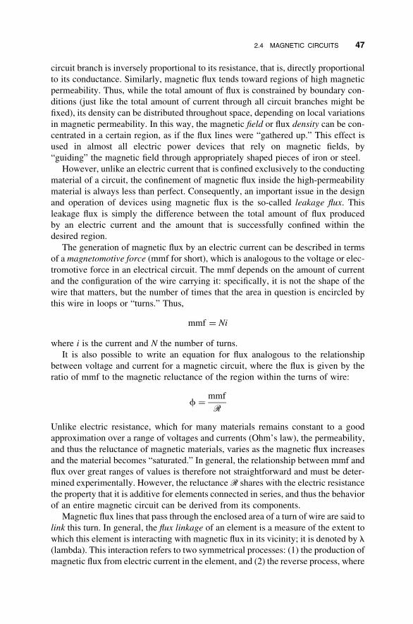
circuit branch is inversely proportional to its resistance, that is, directly proportional

to its conductance. Similarly, magnetic flux tends toward regions of high magnetic

permeability. Thus, while the total amount of flux is constrained by boundary con-

ditions (just like the total amount of current through all circuit branches might be

fixed), its density can be distributed throughout space, depending on local variations

in magnetic permeability. In this way, the magnetic field or flux density can be con-

centrated in a certain region, as if the flux lines were “gathered up.” This effect is

used in almost all electric power devices that rely on magnetic fields, by

“guiding” the magnetic field through appropriately shaped pieces of iron or steel.

However, unlike an electric current that is confined exclusively to the conducting

material of a circuit, the confinement of magnetic flux inside the high-permeability

material is always less than perfect. Consequently, an important issue in the design

and operation of devices using magnetic flux is the so-called leakage flux. This

leakage flux is simply the difference between the total amount of flux produced

by an electric current and the amount that is successfully confined within the

desired region.

The generation of magnetic flux by an electric current can be described in terms

of a magnetomotive force (mmf for short), which is analogous to the voltage or elec-

tromotive force in an electrical circuit. The mmf depends on the amount of current

and the configuration of the wire carrying it: specifically, it is not the shape of the

wire that matters, but the number of times that the area in question is encircled by

this wire in loops or “turns.” Thus,

mmf ¼ Ni

where i is the current and N the number of turns.

It is also possible to write an equation for flux analogous to the relationship

between voltage and current for a magnetic circuit, where the flux is given by the

ratio of mmf to the magnetic reluctance of the region within the turns of wire:

f ¼mmf

R

Unlike electric resistance, which for many materials remains constant to a good

approximation over a range of voltages and currents (Ohm’s law), the permeability,

and thus the reluctance of magnetic materials, varies as the magnetic flux increases

and the material becomes “saturated.” In general, the relationship between mmf and

flux over great ranges of values is therefore not straightforward and must be deter-

mined experimentally. However, the reluctanceR shares with the electric resistance

the property that it is additive for elements connected in series, and thus the behavior

of an entire magnetic circuit can be derived from its components.

Magnetic flux lines that pass through the enclosed area of a turn of wire are said to

link this turn. In general, the flux linkage of an element is a measure of the extent to

which this element is interacting with magnetic flux in its vicinity; it is denoted by l

(lambda). This interaction refers to two symmetrical processes: (1) the production of

magnetic flux from electric current in the element, and (2) the reverse process, where

2.4 MAGNETIC CIRCUITS 47

a current through the element is induced by magnetic flux linking it. The single

measure of l applies to both phenomena simultaneously. For a coil of wire, the

flux linkage is given approximately by the product of the number of turns and the

flux through them:

l ¼ Nf

This formula is approximate because it assumes that all the flux lines intersect every

turn, while in reality, there will be some leakage flux that only interacts with some

parts of the coil.

Finally, in anticipation of Section 3.2, where we discuss the inductance (L) as a

crucial property of electric circuit elements, we can state that the flux linkage is also

l ¼ Li

where i is the current through the element. Thus, we can think of inductance as a

measure of how much magnetic flux linkage is associated with a given amount of

current for a particular device.

Magnetic circuits play a role in electric power systems primarily in the context of

generators and transformers, where all the transmitted energy temporarily resides in

the form of magnetic fields. Flux lines are used to describe how these devices work,

and the analysis of the magnetic circuits they contain, including leakage flux, is

crucial in their design. Magnetic flux, and electrical interactions that result from it

(specifically, mutual inductance), is also important for transmission lines.


&CHAPTER 3

AC Power

3.1 ALTERNATING CURRENT AND VOLTAGE

Many of the important technical characteristics of power systems have to do with

their use of alternating current (a.c.) instead of direct current (d.c.). In a d.c.

circuit, the polarity always remains the same: the potential always stays positive

on one side and negative on the other, and the current always flows in the same direc-

tion. In an a.c. circuit, this polarity reverses and oscillates very rapidly. For power

systems in the United States, the a.c. frequency is 60 hertz (Hz) or 60 cycles per

second, meaning that the direction of voltage and current are reversed, and reversed

back again, 60 times every second.

3.1.1 Historical Notes

The main reason for using a.c. in power systems is that it allows raising and lowering

the voltage by means of transformers. As we will see in Section 6.2, transformers

cannot be operated with d.c. It is still possible to change the voltage in a d.c.

circuit, but it requires far more sophisticated and expensive equipment that had

not been invented in the early days of electric power. The first power systems,

which operated on d.c., were therefore limited to rather low transmission voltages:

although the generators could have been designed to produce power at a higher

voltage, safety considerations at the customer end dictated that the voltage be kept

low. Consequently, line losses were a major problem and in effect limited the geo-

graphic expansion of power systems. After the transformer was introduced in the

1880s, d.c. and a.c. systems spent some years in fierce competition (the “Battle of

the Currents”), with Edison and Westinghouse as prominent advocates on either

side. The major obstacles in the way of the alternating current approach—namely,

concerns about the safety of high-voltage transmission, as well as the challenge of

designing an a.c. motor—were largely resolved by the mid-1890s.1

1For a thorough and fascinating historical discussion of the development of electric power systems, see

Thomas P. Hughes, Networks of Power: Electrification in Western Society, 1880–1930 (Baltimore:

Johns Hopkins University Press, 1983).

49


The choice of frequency for a.c. power represented a compromise among the

needs of different types of equipment. During the early years of a.c. systems, numer-

ous different frequencies ranging from 25 to 133 13cycles were used.2 For generators,

lower frequencies tend to be preferable because this requires fewer magnetic poles

inside the rotor (see Section 4.1), though this constraint became less significant as

high-speed steam turbines supplemented and replaced slow-moving hydroturbines

and reciprocating steam engines. For transmission, lower frequencies are especially

desirable because a line’s reactance increases with frequency and constrains the

amount of power that can be transmitted on a given line (see Sections 3.2 and

6.5). For loads, on the other hand, higher frequencies are often preferable. This is

particularly true for incandescent lamps, whose flickering becomes more and

more noticeable to the human eye at lower frequencies. After due consideration

of the different types of equipment already in use and the prospects for adapting

new designs, efforts to standardize power frequency finally resulted in convergence

to a 60 cycle standard in the United States and 50 cycles in Europe.

3.1.2 Mathematical Description

A sine wave represents the cyclical increase and decrease of a quantity over time.

The oscillation of voltage and current in an a.c. system is modeled by a sinusoidal

curve, meaning that it is mathematically described by the trigonometric functions of

sine or cosine. In these functions, time appears not in the accustomed units of

seconds or minutes, but in terms of an angle.

A sinusoidal function is specified by three parameters: amplitude, frequency,

and phase. The amplitude gives the maximum value or height of the curve, as

measured from the neutral position. (The total distance from crest to trough is

thus twice the amplitude.) The frequency gives the number of complete oscillations

per unit time. Alternatively, one can specify the rate of oscillation in terms of the

inverse of frequency, the period. The period is simply the duration of one complete

cycle. The phase indicates the starting point of the sinusoid. In other words, the

phase angle specifies an angle by which the curve is ahead or behind of where it

would be, had it started at time zero. Graphically, we see the phase simply as a

shift of the entire curve to the left or right. The phase angle is usually denoted by

f, the Greek lowercase phi.

Expressing time as an angle allows us to take a sine or cosine of that number. For

example, the sine of 30 degrees is 12, but there is no such thing as the sine of 30

seconds. The argument of a sinusoidal function (the variable or object of which

we find the sine) must be dimensionless, that is, without physical dimension like

time, distance, mass, or charge. An angle, though measured in units of degrees or

radians, has no physical dimension; it really represents a ratio or fraction of a

whole. This is consistent with the fact that a sine function represents a relationship

between two quantities: in a right triangle, the sine of one angle is the ratio of lengths

2See Hughes, Networks of Power, pp. 127ff., and Benjamin G. Lamme, “The Technical Story of the

Frequencies,” IEEE Transactions 37, 1918.

50 AC POWER

of two of the sides (the reader may recall “opposite over hypotenuse” for sine, and

“adjacent over hypotenuse” for cosine). Time as an angle means time as a certain

fraction of a whole.

Turning time into an angle or fraction is logical only because in an oscillation,

time is cyclical; the process repeats itself. We do not care whether we are on our

first or four-hundredth swing, but rather about where in the oscillation we find

ourselves at a given instant. One complete oscillation, the duration or period of

which would be 1/60th of a second for 60 Hz, is taken to correspond to a full

circle of 360 degrees. Any angle can be understood, then, as specifying a fraction

or multiple of that complete oscillation.

Plotted against angle on the horizontal axis, the height of the sine curve is simply

the value of the sine for each angle, scaled up by a factor corresponding to the ampli-

tude. As the angle is increased, it eventually describes a complete circle, and the

function repeats itself.

In the context of sinusoidal functions, angles are often specified in units of

radians (rad) rather than degrees. Radians refer to the arc described by an angle.

The conversion is simple. Since the circumference of an entire circle is given by

2pr, where r is the radius and p (pi) ¼ 3.1415, 2p radians correspond to 3608. (Theradius is left out since the size of the circle is arbitrary; in this way, we are only refer-

ring to the angle itself.) Any fraction of a radian, then, represents a fraction of a circle,

or number of degrees: p rad ¼ 1808 or one-half cycle; p/2 rad ¼ 908 or one-quartercycle, and so on. Figure 3.1 illustrates a sine wave with both units of angle.

The frequency of a sinusoidal function is often given in terms of radians per

second, in which case it is called an angular frequency. Angular frequencies are

usually denoted by v, the Greek lowercase omega, as opposed to f or n (Greek

lowercase nu) for frequency. The angular frequency corresponding to 60 cycles/s is

v ¼ 60 cycles=s � 2p radians=cycle ¼ 377 rad=s

Figure 3.1 A sine function plotted against angle f(t) ¼ A sin(vt).

3.1 ALTERNATING CURRENT AND VOLTAGE 51

For 50 cycles, v ¼ 314 rad/s. An alternating current as a function of time can be

written as the following sinusoidal function:

I(t) ¼ Imaxsin(vt þ fI)

The quantity Imax is the maximum value or amplitude of the current. Since the value

of a sine or cosine varies between þ1 and 21, the actual current oscillates between

þImax and 2Imax. The time t is measured in seconds, and, when multiplied by the

angular frequency v, gives a number of radians. In the simplest case, shown in

the upper portion of Figure 3.2, there is no phase shift, meaning that f is zero

and the curve starts at zero. To illustrate the more general case, Figure 3.2 also

Figure 3.2 Sinusoidal alternating current.

52 AC POWER

shows the curve shifted over to the left by an angle f. Note that the phase

shift affects neither frequency nor amplitude of the curve; it simply amounts to a

difference in what time is considered “zero” in comparison to some other curve,

which will become important later when we consider the relative timing of

current and voltage. The same discussion as for current holds for the voltage,

which is written

V(t) ¼ Vmaxsin(vt þ fV )

The subscripts on the phase angles are there to indicate that current and voltage do

not necessarily have the same phase; that is, their maximum values do not necess-

arily coincide in time (Section 3.3 addresses the phase shift between current and

voltage).

In practice, current and voltage waveforms do not conform to this precise math-

ematical ideal; in some cases, interpreting them as sinusoidal requires a vivid

imagination. While they will always be periodic (i.e., repeating themselves), they

may not be round and smooth like the proper sinusoidal curve. The discrepancy

results in part from the internal geometry of the generators and in part from

harmonic distortion caused by loads and other utility equipment. The degree of

conformance to the shape of a sine curve, or “good waveform,” is one aspect of

power quality. Poor waveform may not be a problem, though, unless there are

sensitive loads.

3.1.3 The rms Value

For most applications, we are only interested in the overall magnitude of these func-

tions. Conceivably, we could just indicate the amplitude of the sine wave, but this

would not represent the quantity very well: most of the time, the actual value of

the function is much less than the maximum. Alternatively, we could take a

simple arithmetic average or mean. However, since a sine wave is positive half

the time and negative the other half, we would just get zero, regardless of the ampli-

tude; this average would contain no useful information. What we would like is some

way of averaging the curve that offers a good representation of how much current or

voltage is actually being supplied: a meaningful physical measure; something of an

equivalent to a d.c. value. Specifically, we would like average values of current and

voltage that yield the correct amount of power when multiplied (see Section 3.4).

Fortunately, such an average is readily computed: it is called the root mean

square (rms) value.

The rms value is derived by first squaring the entire function, then taking the

average (mean), and finally taking the square root of this mean. Squaring the

curve eliminates the negative values, since the square of a negative number

becomes positive. Figure 3.3 illustrates this process with the curves labeled V(t)

and V2(t)—though we could just as well have chosen the current I(t)—where the

squared sinusoid, while retaining the same basic shape, is now compressed in

half. If we arbitrarily label the vertical axis in units such that the amplitude

3.1 ALTERNATING CURRENT AND VOLTAGE 53

Vmax ¼ 1, it is obvious that the squared wave has the same amplitude (12 ¼ 1).

Because the squared curve resides entirely in the positive region, it is now possible

to take a meaningful average. Indeed, because the curve is still perfectly symmetric,

its average is simply one half the amplitude. The only counterintuitive step now

consists of renormalizing this average value to the original curve before squaring,

which is accomplished by taking the square root: basically, we are just going back-

wards and undoing the step that made the curve manageable for averaging purposes.

Since 12

is less than 1, its square root is greater than itself; it comes toffiffi12

p¼ 1=

ffiffiffi2

p¼ 0:707. Thus, the rms value of a sine curve is 0.707 of the original

amplitude.

Utility voltages and currents are almost always given as rms values. For example,

120 V is the rms voltage for a residential outlet. Note that when the rms voltage and

current are multiplied together, the product gives the correct amount of power

transmitted (see Section 3.3).

Example

If 120 V is the rms value of the household voltage, what is the amplitude?

Since Vrms ¼ 1=ffiffiffi2

p� Vmax, Vmax ¼

ffiffiffi2

p� 120V ¼ 169:7V.

The maximum instantaneous value of the voltage is also of interest because it

determines the requirements for electrical insulation on the wires and other ener-

gized parts. In fact, one argument against a.c. in the early days was that it would

be less economical due to its insulation requirements, which are greater by a

factor offfiffiffi2

pthan those for d.c. equipment transmitting the same amount of

power. For current, the instantaneous maximum is relatively uninteresting

because current limitations are related to resistive heating, which happens

cumulatively over time.

Figure 3.3 Derivation of the rms value.

54 AC POWER

3.2 REACTANCE

In Chapter 1, we discussed electrical resistance as the property of a material or elec-

tric device to resist the flow of direct current through it. Reactance is the property of

a device to influence the relative timing of an alternating voltage and current. By

doing so, it presents a sort of impediment of its own to the flow of alternating

current, depending on the frequency. Reactance is related to the internal geometry

of a device and is physically unrelated to the resistance. There are two types of reac-

tance: inductive reactance, which is based on inductance, and capacitive reactance,

based on capacitance. Finally, impedance is a descriptor that takes into account both

resistance and reactance. Resistance, reactance, and impedance are all measured in

ohms (V).

3.2.1 Inductance

The basic inductive device is a coil of wire, called an inductor or a solenoid. Its func-

tioning is based on the physical fact that an electric current produces a magnetic field

around it. This magnetic field describes a circular pattern around a current-carrying

wire; the direction of the field can be specified with a “right-hand rule.”3When a wire

is coiled up as shown in Figure 3.4, it effectively amplifies this magnetic field,

because the contributions from the individual loops add together. The sum of these

contributions is especially great in the center, pointing along the central axis of the

coil. The resulting field can be further amplified by inserting a material of high mag-

netic permeability (such as iron) into the coil; this is how an electromagnet is made.

Figure 3.4 A basic inductor, or solenoid.

3If the direction of one’s right thumb corresponds to the current flow (where current is taken by convention

to flow from positive to negative potential), the curled fingers of that hand indicate the direction of the

magnetic field.

3.2 REACTANCE 55

When such a coil is placed in an a.c. circuit, a second physical fact comes into

play, namely, that a changing magnetic field in the vicinity of a conducting wire

induces an electric current to flow through this wire. If the current through the

coil oscillates back and forth, then so does the magnetic field in its center.

Because this magnetic field is continuously changing, it induces another current

in the coil. This induced current is proportional to the rate of change of the magnetic

field. The direction of the induced current will be such as to oppose the change in the

current responsible for producing the magnetic field. In other words, the inductor

exerts an inhibitive effect on a change in current flow.4

This inhibitive effect results in a delay or phase shift of the alternating current

with respect to the alternating voltage.5 Specifically, an ideal inductor (with no

resistance at all) will cause the current to lag behind the voltage by a quarter

cycle, or 908, as shown in Figure 3.5.

This result is difficult to explain intuitively. We will not attempt to detail the

specific changes in the current and magnetic field over the course of a cycle. One

thing that can readily be seen from the graph, though, is that the current has its

maximum at the instant that the magnetic field changes most rapidly.

As the magnetic field increases and decreases during different parts of the cycle,

it stores and releases energy. This energy is not being dissipated, only repeatedly

exchanged between the magnetic field and the rest of the circuit. This exchange

process becomes very important in the context of power transfer. Because the

induced current in an inductor is related to the change in the field per unit time,

Figure 3.5 Current lagging voltage by 908. These functions could be written as V(t) ¼ Vmax

sin(vt) and I(t) ¼ Imaxsin(vt2 p/2). Note that the relative amplitudes are unimportant,

because they are measured on different scales.

4This result can be derived through right-hand rules, or simply by considering the law of energy conserva-

tion: if the induced current were in the same direction as the original (increasing) current, it would amplify

the magnetic field that produced it, which would in turn increase the induced current, and so on, indefi-

nitely—clearly an impossible scenario.5The shift between voltage and current is a shift in time, but is expressed in terms of an angle.

56 AC POWER

the frequency of the applied alternating current is important. The higher the fre-

quency, the more rapidly the magnetic field is changing and reversing, and thus

the greater the induced current with its impeding effect is. The lower the frequency,

the easier it is for the current to pass through the inductor.6

A direct current corresponds to the extreme case of zero frequency. When a

steady d.c. voltage is applied to an inductor, it essentially behaves like an ordinary

piece of wire. After a brief initial period, during which the field is established, the

magnetic field remains constant along with the current. An unchanging magnetic

field exerts no further influence on an electric current, so the flow of a steady

direct current through a coil of wire is unaffected by the inductive property.

Overall, the effect of an inductor on an a.c. circuit is expressed by its reactance,

denoted by X (to specify inductive reactance, the subscript L is sometimes added).

The inductive reactance is the product of the angular a.c. frequency7 and the induc-

tance, denoted by L, which depends on the physical shape of the inductor and is

measured in units of henrys (H). In equation form,

XL ¼ vL

Thus, unlike resistance, the reactance is not solely determined by the intrinsic

characteristics of a device. In the context of power systems, however, because the

frequency is always the same, reactance is treated as if it were a constant property.

When describing the behavior of electrical devices in the context of circuit

analysis, we are generally interested in writing down a mathematical relationship

between the current passing through and the voltage drop across the device. For a

resistor, this is simply Ohm’s law, V ¼ IR, where the resistance R is the proportion-

ality constant between voltage and current. It turns out that the inductance L also

works as a proportionality constant between current and voltage across an inductor,

but in this case the equation involves the rate of change of current, rather than

simply the value of current at any given time. Readers familiar with calculus

will recognize the notation dI/dt, which represents the time derivative or rate of

change of current with respect to time. Thus, we write

V ¼ LdI

dt

meaning that the voltage drop V across an inductor is the product of its inductance L

and the rate of change of the current I through it. This equation is used in circuit

analysis in a manner analogous to Ohm’s law to establish relationships between

current and voltage at different points in the circuit, except that it is more cumber-

some to manipulate owing to the time derivative.

6The discriminating response of inductors to different frequencies is put to use in electronics. Electronic

signals generally contain a multitude of frequencies. When such a signal is applied to an inductor, the

lower frequencies are conducted preferentially. For this reason, inductors are also referred to as “low-

pass filters.”7To obtain correct numerical results, it is important to remember that the angular frequency is measured in

radians/second (not cycles/second). The angular frequency with its implicit factor of 2p appears in this

formula because of the way the units of inductance are defined.

3.2 REACTANCE 57

Casually speaking, wemight say that this equation characterizes an inductor as the

kind of thing that does not like to see current change—indeed, it resists (or “reacts to”)

any change in current. This is consistent with the idea that any change in current will

cause a changing magnetic field that acts to oppose the new current. The greater

the inductance, the more voltage is required to effect a change in current. Conversely,

if the current is forced to change dramatically—say, by being interrupted elsewhere

in the circuit—we will observe a voltage spike caused by the inductor’s reaction to

this change. We can also identify the relationship between voltage and the rate of

change of current in Figure 3.5, where the voltage curve has a maximum at the

instant that the current curve shows the steepest increase.

Although we used a coil-shaped object to introduce the concept of inductance, the

same principles also apply to devices other than coils. The coil makes for the stron-

gest inductance and is easiest to understand because the contributions to the mag-

netic field from different sections of wire add together in a fairly obvious

direction. We do not attempt to extend this type of analysis to objects of different

shapes, except to say that inductance exists there, too, and that it depends on an

object’s geometry. In power systems, the most important example of inductors

that are not coil-shaped are transmission and distribution lines (see Section 6.2).

3.2.2 Capacitance

The other type of reactance is capacitive reactance, whose effect is opposite that of

inductive reactance. The basic capacitive device is a capacitor.

A capacitor consists of two conducting surfaces or plates that face each other and

are separated by a small gap (Figure 3.6). These plates can carry an electric charge;

specifically, their charges will be opposite. By having an opposite charge on the

opposing plate, very nearby but not touching, it is possible to collect a large

amount of charge on each plate. We might say that the charge “sees” the opposite

Figure 3.6 A basic capacitor.

58 AC POWER

charge across the gap and is attracted to it, rather than only being repelled by its like

charge on the same plate. In physical terms, there is an electric field across the gap

that serves to hold the accumulation of charge on the plates. The gap could simply be

air, but is often filled with a better insulating (dielectric) material to prevent sparks

from bridging the gap (though even such an insulating material can fail or leak

charge; this is known as dielectric breakdown). For compactness, the plates are

often made out of pliable sheets that are folded or rolled up inside a container.

Like inductance, capacitance also occurs in devices that do not conform to an

ideal shape; coaxial cables are an important example. Our discussion extends to

all devices with capacitance.

When presented with a d.c. voltage, a capacitor essentially behaves like a gap in

the circuit. Initially, there is a brief period of building up the charge on both plates.

But once the charge is built up and cannot go across, the capacitor acts as an open

circuit, and no current will flow.

An alternating current, however, can get across the capacitor. Recall from

Section 1.1 that although a current represents a flow of charge, individual electrons

do not actually travel a significant distance through a conductor; rather, each elec-

tron transmits an impulse or “push” to its neighbor. Because this impulse can be

transmitted across the gap by means of the electric field, it is not necessary for

electrons to physically travel across. This transmission only remains effective as

long as the impulse (in other words, the voltage) keeps changing, because once

the charge has accumulated on the capacitor plate and a steady electric field is

established, there is nothing more to transmit. Indeed, the current flow across a

capacitor is proportional to the rate of change of the electric field, which corre-

sponds to the rate of change of the voltage across the capacitor. As the voltage

oscillates, the electric field continually waxes and wanes in alternating directions.

The greater the frequency, the more readily the current is transmitted, since

the rate of change of the voltage will be greater.8 The capacitive reactance,

denoted by X or XC, is given by the inverse of the product of the angular frequency

and the capacitance, which is denoted by C and measured in farads (F). The

capacitance depends on the physical shape of the capacitor; it increases with the

area of the plates and with decreasing separation between them (since greater

proximity of the charges will cause a stronger electric field), as long as there is

no contact. In equation form,

XC ¼ �1

vC

The equation shows that the magnitude of the capacitive reactance (neglecting the

negative sign) increases with decreasing v, as it should. It also increases with

decreasing capacitance. This is intuitive because a decrease in capacitance means

that the plates are becoming less effective at supporting an electric field to transmit

anything. The negative sign in the equation has to do with the effect of capacitance

8In electronics, capacitors are therefore used as “high-pass filters.”

3.2 REACTANCE 59

on a circuit being opposite that of an inductor, as we see shortly. Thus, when induc-

tive and capacitive reactance are added together, they tend to cancel each other (see

the example in Section 3.2.3).

Like an inductor, a capacitor causes a phase shift between current and voltage in

an a.c. circuit, but the crucial point is that the shift is in the opposite direction. A

pure capacitance causes the current to lead the voltage by 908, as shown in

Figure 3.7. We can see that the moment of greatest current flow coincides with

the most rapid change in the voltage. A capacitor also stores and releases

energy during different parts of the cycle. This energy resides in the electric

field between the plates. The storage and release of energy by a capacitor occurs

at time intervals opposite to those of an inductor in the same circuit (this is

consistent with the phase shift being in opposite directions). A capacitor and an

inductor can therefore exchange energy between them in an alternating fashion.

Like an ideal inductor, an ideal capacitor (without resistance) only exchanges

but never dissipates energy.

Also analogous to an inductor, there is an equation relating voltage and current

for a capacitor. Here it is the voltage V that appears in terms of a rate of change

with respect to time, and the capacitance C is the proportionality constant linking

it to the current I:

I ¼ CdV

dt

This equation characterizes a capacitor as a thing that resists changes in voltage,

which makes sense if we consider the capacitor plates as a large reservoir of

charge: it takes a lot of current to effect a change in the potential. Again, the equation

is consistent with the graph (Figure 3.7) that shows the alternating current reaching

its maximum value at the instant that the voltage changes most rapidly.

Like inductance, capacitance is geometry dependent and occurs to some extent

with electrical devices of any shape. For example, there is a certain amount of

Figure 3.7 Current leading voltage by 908.

60 AC POWER

capacitance between a transmission line and the ground. The parallel-plate capacitor

is the strongest and simplest case, and it becomes much more difficult to derive a

capacitance value for objects with different shapes. Such calculations are treated

in standard electrical engineering texts.

COMPLEX REPRESENTATION

Complex numbers are a concise way to mathematically represent two aspects of a

physical system at the same time. This will be necessary for describing impe-

dance as a combination of resistance and reactance in the following section

(readers familiar with complex notation may skip ahead).

A complex number contains a real part, which is an ordinary number and

directly corresponds to a measurable physical quantity, and an imaginary part,

which is a sort of intangible quantity that, when projected onto physical

reality, represents oscillatory behavior.

An imaginary number is a multiple of the imaginary unit quantityffiffiffiffiffiffiffi�1

p.

This quantity is denoted by i for imaginary in mathematics, and j in electrical

engineering so as to avoid confusion with the label for current. The definition

of j ¼ffiffiffiffiffiffiffi�1

pis another way of saying that j2 ¼ 21. It also implies that

1/j ¼ 2j.

This entity j embodies the notion of oscillation, or time-varying behavior, in

its very nature. Consider the equation x2 ¼ 21. There is no real number that can

work in this equation if substituted for x. Pick any positive number for x, and x2 is

positive. Pick any negative number for x, and when you square it, the result is

also positive. Pick zero, and x2 is zero. So we devise an abstract object we call

j—not a real number, as we know it, but a thing which, it turns out, can also

be manipulated just like a regular number. We define j as that thing that makes

the equation x2 ¼ 21 true.

You can think of j as the number that cannot decide whether it wants to be

positive or negative. In fact, the equation x2 ¼ 21 can be translated into the

logical statement, “This statement is false.” The statement cannot decide

whether it is true or false; it flip-flops back and forth. The imaginary j is therefore

in essence “flippety.”9

The number j makes the most sense when we represent it graphically, as is

usually done in electrical engineering. Consider the number line with positive

and negative real numbers, the positive numbers extending to the right and the

negative numbers to the left of zero. Now think of multiplying a positive

number by 21. What does this operation do? It takes the number from the

right-hand side of the number line and drops it over to the left. For example,

9I owe this term to Heinz von Foerster, as rendered in the transcript of the 1973 AUM conference at Esalen

Institute with G. Spencer Brown (www.lawsofform.org/aum). For an unconventional and profound theor-

etical treatment offfiffiffiffiffiffiffi�1

p, see G. Spencer Brown, Laws of Form (New York: Crown Publishing, 1972).

3.2 REACTANCE 61

3 .21 ¼ 23. In other words, we can think of the multiplication by 21 as a

rotation by 180 degrees about the origin (the zero point).

Now we can take the result (say, 23) and multiply it again by 21. We get

23 .21 ¼ 3. In other words, the number was again rotated by 1808. Successiveapplications of the “multiplication by 21” operation result in successive

rotations.

So far, we have restricted our imagination to numbers that lie on the real

number line. Now suppose we “think outside the box” and ask the following

question: What if there were an operation that rotates a number not by 1808,but by only 908? Rotating by 908 does not immediately seem meaningful,

because it takes us off the number line into uncharted territory. But we do

know this: If performed twice in succession, a rotation by 908 corresponds to a

complete 1808 rotation. In other words, a rotation by 908, performed twice,

gives the same result as multiplying by 21.

But this leads us directly to the equation x2 ¼ 21, which asks for the number

that, when multiplied by itself, becomes negative. If we define “multiplying by j”

as “rotating by 908” and “multiplying by j2” is the same as “multiplying by j and

then multiplying by j again,” then to multiply by j2 is to rotate by 1808, which is

exactly the same thing as multiplying by21. In this sense we can say that j 2 and

21 are the same.

Based on this rotation metaphor, j is conceptualized as the number that is

measured in the new “imaginary” direction 908 off the real number line. We

can now extend this concept of being “off the real number line” to an entire

new, imaginary number line at right angles to the real one, intersecting at the

origin or zero point. Along this new axis we can measure multiples of j

upward and 2j downward.

With these two directions, we have in effect converted the one-dimensional

number line into a two-dimensional plane of numbers, called the complex

plane. This plane is defined by a real axis labeled Re (the old number line)

and an imaginary axis labeled Im (the new imaginary number line at right

angles to the real one). We can now conceive of numbers that lie anywhere

on this complex plane and represent a combination of real and imaginary

numbers. These are the complex numbers. The complex number C ¼ aþ jb

refers to the point a units to the right of the origin and b units above. We say

that a is the real part and b is the imaginary part of C. In Figure 3.8, a ¼ 3

and b ¼ 4.

Rather than specifying the real and imaginary components explicitly, another

way of describing the same complex number is in reference to an arrow (vector)

drawn from the origin to the point corresponding to the number. The length

of the arrow is the magnitude of the complex number. This magnitude is a

real number and is usually denoted by vertical lines, as in jCj. In addition,

the angle between the arrow and the real axis is specified, which we denote

by f. The representation in terms of magnitude and angle is called the

polar form.

62 AC POWER

These alternative representations can be converted into one another by using any

two of the relationships

jCj2 ¼ a2 þ b2 sinf ¼ b=C cosf ¼ a=C or tanf ¼ b=a

Adding or subtracting complex numbers is easily done in the rectangular com-

ponent format: one simply combines the real parts and the imaginary parts,

respectively. To multiply two complex numbers, both components of one are

multiplied by both components of the other, and the results are added (like in

a common binomial expression). However, multiplying, and especially dividing,

complex numbers is much easier in the polar format: the magnitudes are multi-

plied together (or divided) and the angles are added (for division, the divisor

angle is subtracted ).

The imaginary j and all the complex numbers that spring from it do not have

the same utilitarian properties that real numbers do. You cannot eat j eggs for

breakfast, and you cannot be the jth person in line at the post office. Nevertheless,

complex numbers as operational devices do obey rules of manipulation that

qualify them as “numbers” in the mathematical sense, and their special properties

in these manipulations make them useful tools for representing certain real

phenomena, especially phenomena that involve flippety, such as alternating

current.10

Figure 3.8 The number C ¼ 3þ j4 in the complex plane.

10More about the conceptualization offfiffiffiffiffiffiffi�1

pcan be found in George Lakoff and Rafael Nunez, Where

Mathematics Comes From: How the Embodied Mind Brings Mathematics into Being (New York:

Basic Books, 2000), who introduce the role of metaphor in mathematics from a linguistic perspective.

3.2 REACTANCE 63

3.2.3 Impedance

The combination of reactance and resistance that describes the overall behavior of a

device in a circuit is called the impedance, denoted by Z. However, Z is not a

straightforward arithmetic sum of R and X. Mathematically speaking, Z is the

vector sum of R and X in the complex plane. A boldface Z may be used to indicate

a vector or complex number with a real and an imaginary component. As shown in

Figure 3.9, the impedance Z is a complex number whose real part is the resistance

and whose imaginary part is the reactance:

Z ¼ Rþ jX

Any device found in an electric power system has an impedance. For different

devices and different circumstances, the resistive or reactive component may be neg-

ligible, but it is always correct to use Z.

Impedances can be combined according to the same rules for series and parallel

combination that we showed in Section 2.1 for pure resistances (although the arith-

metic grows tedious rather quickly). Qualitatively, we can note that inductive and

capacitive reactance tend to cancel each other, whether they are combined in

series or parallel.

When written in the polar format, the angle f of the impedance has an important

physical significance: it corresponds to the phase shift between current and voltage

produced by this device. By convention, when the reactance is inductive and the

current is lagging, f is positive. When the reactance is capacitive and the current

is leading, f is negative. Thus, what appears as an angle in space in the triangle

of Figure 3.9 can also be interpreted as an angle in time.

Example

An electrical device contains a resistance, an inductance, and a capacitance, all

connected in series. Their values are R ¼ 1V, L ¼ 0.01H and C ¼ 0.001F,

respectively. At an a.c. frequency of 60 cycles, what is the impedance of the

device?

The inductive reactance is XL ¼ vL ¼ 377 rad/s . 0.01H ¼ 3.77 V. The

capacitive reactance is XC ¼ 21/vC ¼ 21/377 rad/s . 0.001F ¼ 21/0.377¼2 2.65 V. Because the reactances are in series, they are added to find the

combined reactance: X ¼ XLþ XC ¼ 3.772 2.65 ¼ 1.12 V. The impedance is

the complex sum of the resistance and the combined reactance: Z ¼ 1 Vþ

j1.12 V. In the polar form, this corresponds to jZj ¼ 1.5 V, f ¼ 48.28. Casuallyspeaking, this impedance would simply be referred to as 1.5 V.

3.2.4 Admittance

The inverse of the complex impedance is called admittance, denoted by Y. The

complex Y is decomposed into its real and imaginary parts, the conductance G

64 AC POWER

and the susceptance B:

Y ¼ Gþ jB

We have already encountered the conductance in Section 1.2.2 as the inverse of

resistance, for the case of a pure resistor without inductance. In the complex case,

however, it is not true that G is the inverse of R and B the inverse of X; rather,

we require that

Y ¼ 1=Z

Because Y and Z are complex (vector) quantities, this entails two things: first, that

the magnitudes of Y and Z are reciprocal of each other,

Y ¼ 1=Z

and second, that the orientation (angle) in the complex plane remain the same. By

performing some algebra,11 we can derive the magnitudes of G and B, respectively:

Y ¼1

Z¼

1

Rþ jX¼

(R� jX)

(Rþ jX)(R� jX)¼

(R� jX)

R2 þ jRX � jRX þ X2

¼(R� jX)

R2 þ X2¼

(R� jX)

Z2¼

R

Z2� j

X

Z2¼ Gþ jB

where

G ¼R

Z2and B ¼ �

X

Z2

This means that while a greater impedance is associated with a smaller admittance

and vice versa, the relationship betweenG and B (considering only their magnitudes,

Figure 3.9 The complex impedance Z, with resistance R in the real direction and reactance

X in the imaginary direction.

11It is easiest to divide complex numbers in polar notation. Working explicitly with the real and imaginary

components, however, we use the technique of multiplying both numerator and denominator by the

complex conjugate of the denominator, which conveniently eliminates the denominator’s imaginary part.

3.2 REACTANCE 65

not the negative sign) is directly proportional to the relationship between R and X.

Thus, a device whose reactance outweighs its resistance also has a susceptance

that outweighs its conductance.

Example

Consider a transmission line that has a resistance R ¼ 1 V that is small com-

pared to its reactance X ¼ 10 V. What, approximately, are the conductance

and susceptance?

The magnitude of Z is very close to 10 (by the Pythagorean theorem, we find

Z ¼ffiffiffiffiffiffiffiffiffiffiffiffiffiffiffiffiR2 þ X2

p¼

ffiffiffiffiffiffiffiffi101

p¼ 10:05). From G ¼ R/Z2 we obtain G � 1/100 or

0.01 mho, and B ¼ X/Z2� 0.1 mho. Thus, the susceptance is ten times greater

than the conductance, just as the reactance is ten times the resistance.

3.3 POWER

3.3.1 Definition of Electric Power

Power is a measure of energy per unit time. Power therefore gives the rate of energy

consumption or production. The units for power are generally watts (W). For

example, the watt rating of an appliance gives the rate at which it uses energy.

The total amount of energy consumed by this appliance is the wattage multiplied

by the amount of time during which it was used; this energy can be expressed in

units of watt-hours (or, more commonly, kilowatt-hours).

As we saw in Section 1.3, the power dissipated by a circuit element—whether an

appliance or simply a wire—is given by the product of its resistance and the square

of the current through it: P ¼ I2R. The term “dissipated” indicates that the electric

energy is being converted to heat. This heat may be part of the appliance’s intended

function (as in any electric heating device), or it may be considered a loss (as in the

resistive heating of transmission lines); the physical process is the same.

Another, more general way of calculating power is as the product of current and

voltage: P ¼ IV. For a resistive element,12 we can apply Ohm’s law (V ¼ IR) to see

that the formulas P ¼ I2R and P ¼ IV amount to the same thing:

P ¼ IV ¼ I(IR) ¼ I2R

Example

Consider an incandescent light bulb, rated at 60 W. This means that the filament

dissipates energy at the rate of 60 W when presented with a given voltage, which

we assume to be the normal household voltage (120 V). The power equals the

12In the general case (where there may also be reactance), Ohm’s law becomes V ¼ IZ, so the substitution

is not as straightforward. It will still be true, though, that P ¼ I2R gives the power dissipated by resistive

heating.

66 AC POWER

voltage applied to the light bulb times the current through it. The current is 0.5 A:

60 W ¼ 0.5 A . 120 V. While the power rating is specific to a given voltage,

the one property of the light bulb that is always the same is its resistance

(in this case, 240 V). We could determine the resistance from Ohm’s law,

120 V ¼ 0.5 A . 240 V, and verify that the power also corresponds to I2R:

60 W ¼ (0.5 A)2 . 240 V.

Now consider a transmission line. We must distinguish between the power dissi-

pated and the power transmitted by the line. The dissipated power is simply given

by P ¼ I2R. We could also write this as P ¼ IV, but that would be less convenient

for two reasons. First, although it is tempting to think of a power line as just a

resistive wire, it actually has a significant reactance. Because of the phase shift

involved, the presence of reactance means that multiplying I and V together will

be more complicated. On the other hand, taking the square of the current magnitude

is always easy, regardless of phase shifts.

Second, if we tried to calculate dissipated power by using P ¼ IV, we would

have to be very careful about which V to use: remembering that Ohm’s law

refers to the voltage drop across a resistor, or between either end, we recognize

that the V must be the voltage difference between the two ends of the line, other-

wise known as the “line drop” (see Section 1.3.3). This line drop is distinct from

the line voltage, which specifies the line voltage with respect to ground, or between

one conductor (phase) and another. Typically, the line drop would be a few percent

of the line voltage, but it is usually not known precisely.13 For these reasons,

thermal losses are better calculated using P ¼ I2R, and are often referred to as

“I2R losses.”

When we ask about the power transmitted by the line, we can think of the

line as extended terminals (like battery terminals). The power that is available

to a load connected to this line can be calculated with the formula P ¼ IV,

but now V refers to the line voltage, which is that seen by the load between

the two terminals. We say that the power has been transmitted by the line at the

voltage V.

We can enhance our intuitive understanding of P ¼ IV by remembering that

voltage is a measure of energy per unit charge, while the current is the flow rate

of charge. The product of voltage and current therefore tells us how many electrons

are passing through, multiplied by the amount of energy each electron “carries.”

Energy is carried in the sense that an electron that has been propelled to a higher

voltage level has the potential to do more work as it returns to ground. In terms

of the units, we can see that the charge cancels, and we are left with the proper

units of power:

Charge=Time � Energy=Charge ¼ Energy=Time

13Ideally, if transmission lines had no resistance at all, there would be zero line drop.

3.3 POWER 67

3.3.2 Complex Power

Applying the simple formula P ¼ IV becomes more problematic when voltage and

current are changing over time, as they do in a.c. systems. In the most concise but

abstract notation, power, current, and voltage are all complex quantities, and the

equation for power becomes

S ¼ I�V

where S is the apparent power and the asterisk denotes the complex conjugate of the

current I, meaning that for purposes of calculation, the sign (positive or negative) of

its imaginary component is to be reversed. All this ought to make very little sense

without a more detailed discussion of complex quantities and their representation

by phasors. In the interest of developing a conceptual understanding of a.c.

power, let us postpone the elegant mathematics and begin by considering power,

voltage, and current straightforwardly as real quantities that vary in time.

The fundamental and correct way to interpret the statement P ¼ IV when I and V

vary in time is as a statement of instantaneous conditions. Regardless of all the com-

plexities to be encountered, it is always true that the instantaneous power is equal to

the instantaneous product of current and voltage. In other words, at any instant, the

power equals the voltage times the current at that instant. This is expressed by

writing each variable as a function of time,

P(t) ¼ I(t) � V(t)

where the t is the same throughout the equation (i.e., the same instant).

However, instantaneous power as such is usually not very interesting to us. In

power systems, we generally need to know about power transmitted or consumed

on a time scale much greater than 1/60 of a second. Therefore, we need an

expression for power as averaged over entire cycles of alternating current and

voltage.

Consider first the case of a purely resistive load. Voltage and current are in phase;

they are oscillating simultaneously. The average power (the average product of

voltage and current) can be obtained by taking the averages (rms values) of each

and then multiplying them together. Thus,

Pave ¼ IrmsVrms (resistive case)

Power for the resistive case is illustrated in Figure 3.10.

But now consider a load with reactance. The relative timing of voltage and

current has been shifted; their maxima no longer coincide. In fact, one quantity is

sometimes negative when the other is positive. As a result, the instantaneous

power transmitted or consumed (the product of voltage and current) is sometimes

negative. This is shown in Figure 3.11. We can interpret the negative instantaneous

power as saying that power flows “backwards” along the transmission line, or out of

68 AC POWER

the load and back into the generator. The energy that is being transferred back and

forth belongs to the electric or magnetic fields within these loads and generators.

Since instantaneous power is sometimes negative, the average power is clearly

less than it was in the resistive case. But just how much less? Fortunately, this is

very easy to determine: the average power is directly related to the amount of

phase shift between voltage and current. Here we skip the mathematical derivation

and simply state that the reduction in average power due to the phase shift is given

by the cosine of the angle of the shift:

Pave ¼ IrmsVrms cosf

Figure 3.11 Power as the product of voltage and current, with current lagging behind

voltage by a phase angle f.

Figure 3.10 Power as the product of voltage and current, with voltage and current in phase.

3.3 POWER 69

The factor of cos f is called the power factor, often abbreviated p.f. This same

equation can also be written as

Pave ¼1

2ImaxVmax cosf

which is identical because each rms value is related to the maximum value (ampli-

tude) by a factor of 1=ffiffiffi2

p.

This equation is true for any kind of load. In the special case where there is only

resistance and no phase shift, we have f ¼ 0 and cos f ¼ 1, so there is no need to

write down the cos f, and we get the formula from the previous page. In another

special case where the load is purely reactive (having no resistance at all), the

phase shift would be f ¼ 908 and cos f ¼ 0, meaning that power only oscillates

back and forth, but is not dissipated (the average power is zero).

The average power corresponds to the power actually transmitted or consumed by

the load. It is also called real power, active power or true power, and is measured in

watts.

There are other aspects of the transmitted power that we wish to specify. The

product of current and voltage, regardless of their phase shift, is called the apparent

power, denoted by the symbol S. Its magnitude is given by

S ¼ IrmsVrms

Although apparent and real power have the same units physically, they are expressed

differently to maintain an obvious distinction. Thus, the units of apparent power are

called volt-amperes (VA).

Apparent power is important in the context of equipment capacity. Actually,

the crucial quantity with respect to thermal capacity limits is only the current. In

practice, though, the current is often inconvenient to specify. Since the operating

voltage of a given piece of equipment is usually quite constant, apparent power

is a fair way of indicating the current. The point is that apparent power is a much

better measure of the current than real power, because it does not depend on the

power factor. Thus, utility equipment ratings are typically given in kVA or MVA.

Finally, we also specify what we might intuitively think of as the difference

between apparent and real power, namely, reactive power. Reactive power is the

component of power that oscillates back and forth through the lines, being

exchanged between electric and magnetic fields and not getting dissipated. It is

denoted by the symbol Q, and its magnitude is given by

Q ¼ IrmsVrmssinf

Again, note how the equation converges for the resistive case where f ¼ 0 and

sin f ¼ 0, as there will be no reactive power at all. Reactive power is measured

in VAR (also written Var or VAr), for volt-ampere reactive. We can represent

power as a vector in the complex plane: namely, an arrow of length S (apparent

power) that makes an angle f with the real axis. This is shown in Figure 3.12.

The angle f is the same as the phase difference between voltage and current.

70 AC POWER

The projection of the apparent power vector onto the real axis has length P and cor-

responds to the real power; the projection of apparent power onto the imaginary axis

has lengthQ and corresponds to reactive power. This agrees with the factors of cos f

and sin f in the formulas for P and Q, respectively. In mathematical terms, S is the

vector sum of P andQ. In this sense, it is completely analogous to the complex impe-

dance Z, which is composed of the resistance R in the real and the reactance X in the

imaginary direction.

Note that when Q and S are pointing upward as in Figure 3.12, f is positive and

the power factor is said to be lagging (in agreement with the current lagging behind

the voltage). For a leading power factor, f would be negative and Q and S would

point downward.

Example

Consider a vacuum cleaner that draws 750 W of real power, at a voltage of 120 V

a.c. and a power factor of 0.75 lagging. How much current does it draw?

Since the real power is given by the apparent power times the power factor, the

apparent power equals 750 4 0.75 ¼ 1000 VA ¼ 1 kVA. The rms current is the

apparent power divided by the rms voltage: 1000 VA 4 120 V ¼ 8.33 A.

When we say that a load “draws power,” we mean that as a result of its internal

characteristics (the impedance), when presented with a given voltage, a certain

amount of current will flow through this device, and accordingly a certain amount

of power will be dissipated or exchanged. Just as a load draws real power in relation

to its resistance, it draws reactive power in relation to its reactance. In fact, the ratio

of resistance to reactance determines the ratio of real to reactive power drawn by a

load. In other words, the angle f in Z is the same as the angle f in S.

Specifically, inductive loads are said to “consume” reactive power, whereas

capacitive loads are said to “supply” reactive power. This is merely a terminological

convention, and a rather misleading one. Recall that inductors and capacitors

produce opposite phase shifts. Either type of shift causes reactive power to oscillate

through the circuit. But because of the difference in timing, the contributions of

inductance and capacitance to reactive power are opposite: at the instant that the

Figure 3.12 The complex power S, with real power P in the real and reactive power Q in the

imaginary direction.

3.3 POWER 71

inductor magnetic field absorbs energy, the capacitor electric field in the same

circuit releases energy. Conversely, at the instant that the magnetic field releases

energy, the electric field absorbs it. Although on average neither inductor nor capaci-

tor gains or loses energy, their effects are complementary.

Following the law of energy conservation, the amount of energy going into the

circuit must equal the energy coming out of the circuit at every instant. In principle,

therefore, inductance and capacitance in a circuit must always be matched. Of

course, this is not always given by design. But nonetheless, a circuit will behave

in such a way as to provide equal absorption and release of reactive power at any

instant. The preferable way to satisfy the reactive power balance is by adjusting

the a.c. power source to compensate for the load’s circulation of reactive power.14

Thus, in operational terms, the problem of managing reactive power is analogous

to that of managing real power: just like the utility must supply the precise

amount of real power that is demanded at any instant, the utility must compensate

for the precise amount of reactive power that is being circulated at any instant. In

practice, electric loads are dominated by inductance, not capacitance, and utilities

therefore associate supplying real power with compensating for inductive reactance

(a lagging current). This operational perspective explains the use of the physically

improper terminology of “consuming” and “supplying” reactive power.

Example

For the preceding example, how much reactive power does the vacuum cleaner

draw?

With p.f. ¼ 0.75 lagging ¼ cos f, the phase shift is f ¼ 41.48, and

sinf ¼ 0.661. Thus, the reactive power is 1000 . 0.661 ¼ 661 VAR. Because the

power factor is lagging, the vacuum cleaner is said to “consume” reactive power.

What is the impedance of the vacuum cleaner?

The magnitude of the impedance is given by the voltage divided by the current

(rms values) according to Ohm’s law: 120 V 4 8.33 A ¼ 14.4V. The power

factor, being the ratio of real to apparent power, corresponds to the ratio of

resistance to impedance. Therefore, the magnitude of the resistive component is

R ¼ 0.75 . 14.4V ¼ 10.8V. The reactive component is proportional to the reactive

power, or sin f, and is given by X ¼ 0.661 . 14.4V ¼ 9.51V. We can express the

impedance as the complex sum of its components: Z ¼ 10.8þ j9.51 (V). Alterna-

tively, we can express it in terms of its magnitude and angle: Z ¼ 14.4V, 41.48.Because f and X are positive, the reactance is inductive (rather than capacitive).

The vast majority of loads are inductive rather than capacitive. Motors of all kinds

(pumps, refrigerators, air conditioners, power tools) are the most common inductive

load; ballasts for fluorescent lighting are another example.

14The alternative is to allow voltage and frequency changes in the circuit, which will occur so as to enforce

compliance with the law of energy conservation. The same is true for the conservation of real power.

Trouble in maintaining the reactive power balance will manifest primarily as variations in the voltage,

whereas over- or undersupply of real power primarily results in frequency fluctuations.

72 AC POWER

The different power factors of individual loads combine into an aggregate power

factor for the set of loads. The calculation is based directly on the combination of

impedances in series and parallel, as introduced in Section 2.1. Although straightfor-

ward in principle, because it involves complex numbers, this calculation becomes

quite tedious in practice, and we do not attempt to reproduce it here. Qualitatively,

we can note that if two loads of different power factors are connected in parallel,

their combined power factor will be somewhere in the middle, and it will be

closer to that of the bigger load. Just as an equivalent resistance can be defined

for any combination of individual resistors, one can specify a power factor for a

set of loads at any level of aggregation, from a single customer to a local area or

the entire utility grid. Overall utility power factors tend to be between unity and

0.8 lagging; a typical value would be 0.9 lagging.

While all the reactive power “consumed” in the grid has to be “supplied” by gen-

erators or capacitive devices, there is some operational discretion in how these con-

tributions to reactive power are allocated. This allocation is addressed in Section 4.3

on “Operational Control of Synchronous Generators,” and again in Section 6.6 on

“Voltage Control.”

3.3.3 The Significance of Reactive Power

A low power factor is undesirable for utilities in terms of operating efficiency and

economics. Most customers, especially small customers, are only charged for the

real power they consume.15 At the same time, the presence of reactive power oscillat-

ing through the lines and equipment is associated with additional current. While reac-

tive power as such is not consumed, it nonetheless causes the utility to incur costs,

both in the form of additional losses and in the form of greater capacity requirements.

Owing to its property of occupying lines and equipment while doing no useful work,

reactive power has been referred to jokingly as “the cholesterol of power lines.”

Example

To illustrate the effect of the power factor on line losses, consider a load of

100 kW at the end of a several-mile-long 12 kV distribution line. Suppose the

line’s resistance is 10 V. If the power factor is 0.8 lagging, the apparent power

drawn by the load is 125 kVA, and the reactive power is 75 kVAR. The

current to this load is 125 kVA 4 12 kV ¼ 10.4 A. The distribution line losses

due to this load are given by I2R ¼ (10.4 A)2 . 10 V ¼ 1.08 kW.16 This is signifi-

cantly more than we might have estimated just on the basis of real power demand:

using only 100 kW as the power, we would have obtained a current of 8.33 A and

losses of only 0.69 kW.

15When large customers are charged for reactive power, it is generally not on a per-kVAR basis, but by

means of a rate schedule for real power that is scaled up according to the customer’s power factor.16There may be other loads on the same line, but we take advantage of the superposition principle to con-

sider this load and its associated current and losses individually. Losses due to other loads would simply

be added.

3.3 POWER 73

In order to minimize losses and at the same time maximize available equipment

capacity, utilities take steps to improve the power factor with capacitors or other

means of “VAR compensation.” Preferably, this compensation is placed near the

load, so as to minimize the distance that reactive power must travel through the

lines. VAR compensation is discussed further in Section 6.6 on voltage control,

particularly with regard to the relationship between reactive power and voltage.

Example

For the preceding example, how much of a reduction in line losses could be

achieved by improving the power factor to 0.9, assuming that real power

remains unchanged?

The apparent power is now 100 kW 4 0.9 ¼ 111 kVA; reactive power is

54.5 kVAR. The current is 111 kVA 4 12 kV ¼ 9.25 A, and line losses are

(9.25 A)2 . 10 V ¼ 0.856 kW. Losses on this distribution line have been

reduced by 226 W as a result of increasing the power factor from 0.8 to 0.9.

Over the course of a year, 226 W . 8766 h ¼ 1981 kWh would be saved.17

How much capacity is freed up on the substation transformer that supplies

this line?

The transformer capacity is limited by current, which is related to apparent

power. The difference in apparent power before and after the power factor correc-

tion is 125 kVA2 111 kVA ¼ 14 kVA. This result is a first approximation. In

order to refine it, we would also consider the effect of the loss reduction, since

the transformer must supply the energy that is lost “downstream” from it. The

contribution from losses on this line is small (on the order of 1%), increasing

the saved capacity to about 14.2 kVA. To calculate the answer precisely, we

would also have to take into account the line’s reactance.

Line losses are real power losses and result in physical heating of the lines, even

when they are attributable to reactive power consumption. They are not to be

confused with the quantity termed reactive losses in power flow analysis (see

Chapter 7). Reactive losses are the difference between the reactive power supplied

by generators and that consumed by loads, and are measured in VAR. The extra

“consumption” of reactive power is due to the inductive reactance of the lines

and transformers in the system. From the standpoint of energy conservation, reactive

losses are irrelevant. They are important, however, in the context of planning and

scheduling reactive power generation.

Reactive power can arise as an issue in the context of renewable energy and

energy conservation. Specifically, wind turbines may be considered problematic

17It is a common habit, especially among eager students of science and engineering, to write down

numerical answers to a greater degree of precision than they are actually known, given the degree of

uncertainty of the input variables. In this example, the answer should be more realistically stated as

“2 MWh.” One reason for carrying extra significant figures is to avoid rounding errors if numbers are

to be used in further calculations. The reason they are shown here, though, is to keep the numbers recog-

nizable so that readers can easily compare their results.

74 AC POWER

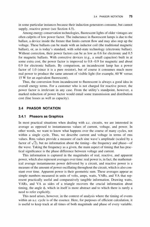
in some particular instances because their induction generators consume, but cannot

supply, reactive power (see Section 4.5).

Among energy conservation technologies, fluorescent lights of older vintages are

often culprits of low power factor. The inductance in fluorescent lamps is due to the

ballast, a device inside the fixture that limits current flow and may also step up the

voltage. These ballasts can be made with an inductor coil (the traditional magnetic

ballast), or, as is today’s standard, with solid-state technology (electronic ballast).

Without correction, their power factors can be as low as 0.6 for electronic and 0.5

for magnetic ballasts. With corrective devices (e.g., a small capacitor) built in at

some extra cost, the power factor is improved to 0.8–0.9 for magnetic and about

0.9 for electronic ballasts. By comparison, an incandescent lamp has a power

factor of 1.0 (since it is a pure resistor), but of course it consumes much more

real power to produce the same amount of visible light (for example, 60 W versus

15 W for an equivalent fluorescent).

Thus, the conversion from incandescent to fluorescent is always a good idea in

overall energy terms. For a customer who is not charged for reactive power, the

power factor is irrelevant in any case. From the utility’s standpoint, however, a

marked reduction of power factor would entail some transmission and distribution

cost (line losses as well as capacity).

3.4 PHASOR NOTATION

3.4.1 Phasors as Graphics

In most practical situations when dealing with a.c. circuits, we are interested in

average as opposed to instantaneous values of current, voltage, and power. In

other words, we want to know what happens over the course of many cycles, not

within a single cycle. Thus, we describe current and voltage in terms of rms

values. Rms values provide a measure of each sine wave’s amplitude (scaled by a

factor offfiffiffi2

p), but no information about the timing—the frequency and phase—of

the wave. Taking the frequency as a given, the main aspect of timing that has prac-

tical significance is the phase difference between voltage and current.

This information is captured in the magnitudes of real, reactive, and apparent

power, which also represent averages over time: real power is, in fact, the mathemat-

ical average instantaneous power delivered by a circuit, and reactive power is a

measure of the amount of power oscillating throughout the circuit, which is also con-

stant over time. Apparent power is their geometric sum. These averages appear as

simple numbers measured in units of volts, amps, watts, VARs, and VA that rep-

resent practically useful and comparatively tangible information. Drawing watts,

VARs, and VA as sides of a triangle recovers the crucial information about

timing, the angle f, which in itself is more abstract and to which there is rarely a

need to refer explicitly.

This need arises, however, in the context of analysis where the timing of events

within an a.c. cycle is of the essence. Here, for purposes of efficient calculation, it

is useful to keep track at all times of both magnitude and phase of every variable.

3.4 PHASOR NOTATION 75

This is where phasor notation comes in. Illustrated in Figure 3.13, a phasor is a

shorthand way to characterize a sine wave, specifying its magnitude (we will use

the convention that states the rms value as opposed to the full wave amplitude)

and angle (in relation to a reference, usually voltage).

To create a phasor, we map the sine wave onto a circle—that is, instead of visua-

lizing something that goes up and down over time (e.g., the voltage increases and

decreases), we visualize it as going around in a circle. So, instead of tracing out a

wave that keeps going and going along the time axis, we imagine the situation as

circling around and around, returning to the same point on the circle over and

over again.

This circle, representing the evolution of, for example, voltage over time, is

traced in the complex plane. Here’s how it makes sense: consider the sine wave

that describes voltage (or current or power), where the vertical axis on the graph rep-

resents the real, physical quantity. The horizontal axis represents time. Now, for

purposes of visualization, imagine adding to this graph a third dimension: a third

axis that extends out of the paper. This third dimension is the imaginary axis.

When looking straight at the sine wave—or making a physical measurement—we

cannot see an imaginary component; we see only its projection onto the real

plane, the plane of the paper. But treating the wave as a complex entity, we can

say that it also extends in the imaginary, front–back direction. It does so by describ-

ing a helix—the shape of an extended spring, for example, or a DNA molecule.

We can now imagine that the physical quantity (say, voltage or current) evolves

in time by spiraling around this helix. From the side, a helix looks precisely like a

sine wave. This is like compressing the imaginary front–back dimension into the

plane of the paper and looking at only the real projection of the helix: we see a

real, physical quantity changing, up–down, over the course of time. But looked at

from the end, the helix appears as a circle, with the quantity going around and

around. This viewing angle amounts to compressing the time dimension into the

Figure 3.13 A phasor.

76 AC POWER

plane of the paper. The complex notation thus encapsulates the time-varying

character of the physical quantity without having to make any explicit reference

to time. This is how circular motion in the complex plane comes to represent

sinusoidal oscillation in the physical world.

The complex mapping affords some great conveniences. Whereas an object

tracing a sine wave accelerates up and down, the circular motion has a constant

rotational speed. Thus, a sinusoidally varying voltage is represented as an arrow

of constant length, spinning around at the constant frequency v, where v is the

angular frequency that assigns the unit circle’s circumference, 2p, to a complete

revolution of 360 degrees.

Because in a.c. power systems we can generally assume voltages and currents to

be oscillating at the same constant frequency, we can ignore this circular spinning

to the extent that it will be the same for all quantities, and they are not spinning

in relation to each other. Thus, we can capture any moment in time and simply

indicate a quantity as a fixed point on the circle, or an arrow from the origin to

that point. This arrow is called the phasor. We know that it is supposed to be spin-

ning, but we do not have to draw that. What we really care about are two aspects of

the oscillating quantity we are representing: its magnitude, and its relative timing

or phase in relation to another sinusoidal function, as, for example, in the phase

difference between voltage and current. The magnitude is represented in the

phasor diagram simply as the length of the arrow. But the phase shift is now

also straightforward to represent, namely, as an angle within the circle in the

complex plane.

Consider the voltage and current waves in Figure 3.14 below. The current lags the

voltage by 30 degrees, meaning that the peak current always occurs with a delay of

one-twelfth of a cycle after the voltage peak. The notion that the voltage is zero at

time zero and peaks at exactly 90 degrees was an arbitrary choice, amounting to

when we decide to start counting time, and choosing that starting point so as to

be convenient for computation. But once we decided on how to label the timing

for voltage, we are committed to describing the timing of current properly in relation

to that voltage timing.

Figure 3.14 Voltage and lagging current phasor.


On the phasor diagram, we draw the voltage as an arrow—the voltage phasor. We

imagine that this arrow spins around the circle counterclockwise, but we just capture

for our diagram any snapshot in time. For convenience, let us draw the voltage with a

zero angle at this moment, so that it points right along the horizontal axis. In addition

to the timing or phase, we also care about the amplitude of the wave, or the magni-

tude of the voltage. We indicate this magnitude simply by the length of the arrow,

which corresponds to either the maximum or rms value.

Now we draw the current phasor in relation to the voltage phasor. Knowing it

will reach every point in the oscillation 30 degrees or 1/12 cycle after the voltage

in time, we draw the arrow so that it appears 30 degrees behind the voltage

(assuming the counterclockwise direction as forward). The result is as shown.

Note that in this case, although the length of the arrow represents magnitude,

the relative length of the two phasors on the diagram does not convey information

because voltage and current are measured in different units, meaning that the two

arrows can be drawn to different scales (just like the relative amplitudes of the two

sine waves).

In this way, we can combine any number of sinusoidally varying quantities (of

the same frequency!) as phasors on the same diagram in the complex plane. We

can also include in the same diagram static quantities like impedance that map

onto the complex plane. The beauty of this method is that we can actually

perform mathematical operations among these quantities by graphically combining

them. How and why this works will make more sense once we consider the phasors

as complex exponential functions, which are mathematical shorthand for sine

waves.

3.4.2 Phasors as Exponentials

A phasor written in exponential notation conveys all the relevant information about

the desired quantity—for example, voltage—without need for a diagram. The

voltage phasor becomes Ve jf, where V is the magnitude of the voltage and f is

the voltage phase angle. The current phasor would be Ie jf, with I the current mag-

nitude and f now the current phase angle. (Sometimes different letters or subscripts

like fV and fI are used to avoid confusing the phase angles with one another.)

The number e is the natural exponential base.18 Engineers also use an even more

abbreviated notation that simply drops the e and the j (assuming everyone knows

they are implicit) so that Ve jf becomes V/f, where the / symbol means

“angle.” Translated into a phasor diagram, V corresponds to the length of the

voltage phasor and f to the angle it makes with the x axis.

18The number e is known as the “natural base” for logarithms or exponential functions, because it allows

describing natural growth or decay phenomena with unique simplicity. In short, the function ex is that

which, for any value of x, equals its own slope or rate of change. This property can also be expressed

in terms of sines and cosines (see Footnote 20). Its numerical value, e ¼ 2.718281828459. . . , is rarely

seen in print (as with p ¼ 3.1415926. . . , the sequence of digits never repeats). A very readable expla-

nation of e and its interesting history can be found in Eli Maor, e: The Story of a Number (Princeton,

NJ: Princeton University Press, 1994).

78 AC POWER

What is the significance of the exponential here? It serves as a shorthand for a

sinusoidal wave, using the relationship known as Euler’s equation:

e jf ¼ cosfþ j sinf

It is not immediately obvious that the expressions on either side of this equation

should represent something moving in a circle, but they do. The combination

cos fþ j sin f indicates a superposition of two sinusoidal waves, one a quarter

cycle ahead of the other, with one oscillating in the real and the other in the

imaginary direction. Together, the two waves make up the helix we visualized

earlier. This helix looks like a circle head-on and like a sinusoidal up-and-down

motion from any side.

That the expression e jf should be equivalent to this combination of waves is a

hard concept to swallow. A mathematician might prove e jf ¼ cos fþ j sin f by

rewriting both sides of the equation in terms of a series expansion, where the

exponential and the sinusoids are expressed as sums over an infinite number of

terms that keep getting smaller (thus converging to a finite value), and show that

the two series are the same. While rigorous, this approach does little for our intuitive

understanding or visualization of the problem. For this, we must familiarize

ourselves a bit with the function’s behavior.

To try to make sense of the behavior of e jf, we first note that if it were not for the

imaginary j, then we would simply have exponential growth: ef would just get

bigger and bigger as f increases. But the j in the exponent does a very strange

thing. As in simple multiplication, j has the effect of “rotating” the value of the

expression in the complex plane.

Depending on their degree of familiarity with exponentials and complex

numbers, readers may wish to experiment by plugging in some sample values for

f (which can be any number), raise e to the power of imaginary f, and plot the

results. We immediately encounter a practical problem: How does one plug an

imaginary exponent into a calculator? And what does it even mean to raise a

number to an imaginary exponent?19 You do need a scientific calculator for this,

and enable the complex mode in which the machine expects every number to

consist of two separate coordinates, a real and an imaginary part (consult your

owner’s manual or a mathematically minded friend). However counterintuitive,

exponentiation with complex numbers is in fact a perfectly rigorous procedure in

that the rules of operation are well-defined and the results unique. When the

complex results are displayed in their real and imaginary components on a calcula-

tor, they can be plotted as such on the complex plane. Some sample points are shown

in Figure 3.15.

The key observation is this: As f increases, the value of e jf shows alternatingly a

greater real or a greater imaginary component, with both real and imaginary

19Clearly, you cannot multiply a number by itself an imaginary number of times. This is why we must

abandon the accustomed metaphor of exponentiation as multiplication of objects in favor of the

rotation-in-a-plane metaphor. Lakoff and Nunez discuss this problem in satisfying depth.


components oscillating between positive and negative values. However, the combi-

nation of real plus imaginary stays confined in a certain way, such that the distance

from the origin of all the plotted e jf points (the magnitude of e jf) remains the same

(1) for all f. Thus, e jf is like an arrow of constant length, rotating counterclockwise

about the origin as we let f increase. For some value of f—and this value, not

coincidentally, is 2p, the number of radians in a full circle—e jf comes back

around to where it started, at 1 in the real direction.

This image gives us a visual way to understand what is so special about the

number e. Try the same process using some number other than e as the base, say,

2 jf or 3 jf. In each case, the plot will start with 1 for f ¼ 0, since any number

raised to the 0th power is 1. Also, in each case the results will wander around the

complex plane counterclockwise. But with any number smaller than e, the results

will diminish in magnitude, and the plot will spiral inward toward the origin as f

increases. With any number greater than e, the plot will spiral outward to infinity.

The number e is that special number which, when raised to any imaginary exponent,

circles around forever.20 And so the phasor e jf comes to denote a quantity like alter-

nating current that keeps going around and around at a steady magnitude, meaning

that it physically oscillates with a constant amplitude.

3.4.3 Operations with Phasors

Phasor notation makes no explicit mention of the frequency of the implicit waves,

because we assume that we are operating in a situation where this frequency is

Figure 3.15 e jf for some values of f, plotted in the complex plane.

20This property is related to the fact that at any point along the circular rotation, one coordinate always

indicates the other’s rate of change (save for an occasional minus sign). Readers familiar with

calculus will recognize this phenomenon in terms of the sine and cosine functions being derivatives of

each other.

80 AC POWER

known and that it is the same for all the sinusoidally varying quantities. Instead,

phasors emphasize only the phase angle of each quantity, or the precise timing of

the zero (or the maximum) as compared to a reference. To establish that reference,

we conventionally define the timing of one particular voltage wave as having a zero

phase angle. In a simple a.c. circuit with one voltage and one current, we would arbi-

trarily set the voltage phase angle to zero; the current phase angle, if current is

lagging behind voltage by u degrees, will be negative u (Greek lowercase theta).

We write the phase angle with an “angle” symbol as /2u. (Note that u plays

exactly the same role as f above; both letters are commonly used to denote phase

angle, and it helps to be accustomed to seeing both.)

The phasor also specifies each quantity’s magnitude, and here there are two con-

ventions: either the wave’s maximum value (amplitude), or its rms value (amplitude

divided byffiffiffi2

p) can be stated. While theoretical texts tend to favor the former

convention, power systems engineers prefer the latter (which will be used here).

Magnitude and phase angle are then written side-by-side as two coordinates to

give a complete phasor, indicated in boldface: V ¼ Vrms/08 and I ¼ Irms/2u.

We omit the subscript from now on, with the understanding that all magnitudes

represent rms values.

When we represent a phasor graphically as a vector or an arrow, the magnitude

represents the length of the arrow and the phase angle is the angle between the

arrow and the reference axis (upward or counterclockwise from the x axis corre-

sponds to a positive angle, downward to a negative angle). The fact that we are

drawing a phasor quantity in two dimensions means we have exactly two pieces

of information about the quantity. Choosing phasor notation to specify a point

on a plane simply means choosing an angular coordinate system as opposed to

Cartesian (x and y) coordinates.

Although it is constant over time, the impedance vector can be treated along with

voltage and current. But now instead of decomposing the impedance Z into resist-

ance R and reactance X (its Cartesian components), we write it as a magnitude

(the length of Z) and a phase angle. For the impedance itself, this angle means a

ratio of components (as seen in Figure 3.9), not a time, but as we know this same

ratio physically determines the time lag of current with respect to voltage, and is

therefore consistent with the use of angles as representing time. We can write

Z ¼ Z/u.

Now we can begin to appreciate the conveniences of phasor notation. Ohm’s law

becomes

V ¼ IZ

or

V/08 ¼ I/�u � Z/u

which in one succinct statement captures the relationship among the respective mag-

nitudes of voltage, current, and impedance as well as the impact on the time lag

between voltage and current due to the reactive component of impedance.


The statement as written here illustrates a fundamental rule of doing arithmetic

with phasors: When multiplying two or more phasors together, first multiply their

magnitudes to find the magnitude of the result. (Thus, V ¼ IZ .) To find the angle

of the product, add the angles of the factors. Thus, 2uþ u ¼ 0. The reader may

deduce correctly the rule for dividing phasors: divide their magnitudes and subtract

the angle in the denominator from that in the numerator.

The process of adding and subtracting phase angles works because they actually

represent exponents of the same base, e. Thus, if we were to rewrite the previous

equation in longhand, it would be

Ve juV ¼ Ie juIZe juZ ¼ IZe j(uIþuZ)

Therefore, uV ¼ uIþ uZ.

Adding angles is a straightforward procedure to perform graphically. Thus, in

order to multiply the I and Z phasors together, we draw a new vector at an angle

with the x axis corresponding to the sum of the two angles, and with a length

corresponding to the product of lengths.

Note that because this product has different physical dimensions or units

(voltage) than its factors (current and impedance), the new arrow can be drawn

on the same diagram, but its length cannot be compared to phasors representing

other units. If two or more phasors are to be added together—which is done graphi-

cally with amazing ease by placing them end to end—they must represent quantities

of the same dimension drawn to the same scale.21

Consider, for example, the a.c. circuit in Figure 3.16. The phasor diagram is

drawn in terms of voltage. It simultaneously shows several things about the

circuit: First, it illustrates that the total voltage drop around the circuit adds up to

zero, as required by Kirchhoff’s voltage law (KVL) (see Section 2.3.1). It does

this very simply by placing voltage phasors head to tail, adding them just like

voltage drop is added in series along the circuit path, and requiring that the

destination or sum correspond to the voltage drop measured around the other side

of the circuit. (Note that a phasor’s position on the graph is arbitrary, so we can

shift it around as long as we preserve its length and angle.)

Second, the phasor diagram disaggregates the resistive and reactive components

of the impedance in the circuit and their respective impacts on voltage drop. Note

that the two arrows IR and IX each have units of volts, indicating the difference

in voltage across the (idealized) resistive and reactive circuit elements, respectively.

Owing to the two-dimensional representation, we see not only the effect of each

circuit element on voltage magnitude, but phase as well. Across the ideal resistor,

21A physical dimensionmeans the kind of thing being measured, such as length, time, or energy. The units

of that measurement are specific to the dimensionality, but there may be many different units or scales for

the same thing. For example, a length can be expressed in units of inches, meters, or miles, but all of these

have the same dimension. While measurements in different units but the same dimension can be added or

subtracted if proper care is taken with unit conversions—for example, one inch plus one meter equals

1.0254 meters—there is no mathematical meaning to the question: What is one inch plus two minutes?

Likewise, we cannot add a voltage to a current, numerically or graphically, because they have different

dimensions.

82 AC POWER

the voltage and current phasors point in the same direction: the length of the current

phasor in the diagram is arbitrary, but its angle is zero relative to the voltage IR

because a pure resistor does not sustain a phase shift. Yet we know that, because of

the inductor’s presence in the same circuit, the current (which must be the same every-

where along the series path) will lag the source voltage VS. Reconciling these facts,

we graphically decompose the source voltage (which is the same as the voltage

drop across the resistor–inductor combination) into a component collinear with

current (IR across the resistor) and one perpendicular to current. The perpendicular

component IX describes the voltage drop across the inductor, obeying the requirement

that current through an ideal inductor must lag the voltage across it by 908 (note theright angle between IX and I). The angle u is determined by the relative magnitudes of

R and X (compare Figure 3.9) so that IRþ IX ¼ VS.

If we allow all the phasors to rotate and plot their projection onto the horizontal

(real) axis, they generate sine waves for the respective voltages. These sinusoidally

varying voltages IR and IX with their distinct magnitude and phase could be phys-

ically measured across each circuit element if each element modeled here in fact

corresponded to a distinct physical object, rather than one abstracted property

(resistance or reactance) of a real object (like a wire coil) that actually manifests

both properties in the same space.

The phasor diagram in Figure 3.16 offers a visual explanation of how the phase

angle or power factor of a circuit is determined by the combination of its elements.

Note that each individual element could be drawn in any arbitrary direction—for

example, were we dealing with a resistance alone, we probably would have

chosen to make it horizontal—but that the combination of elements in the circuit

dictates the phasors’ relationship to each other. Thus, the relative magnitude of

resistance and reactance in the same circuit determines the proportions of the tri-

angle and the angle between voltage and current. Because the essential features of

the physical relationship in time are strictly preserved, the phasor diagram is a

powerful device for combining variables from different portions of an a.c. circuit

and for analyzing their interactions. The representation shown in the figure for a

Figure 3.16 Phasor addition.


simple series circuit works in an analogous way for parallel circuit branches, except

that we would choose to represent all goings on in terms of current rather than

voltage, using Kirchhoff’s current law (KCL) for the addition of currents at each

node.

Finally, let us turn to the phasor representation of power. Complex power S can

be written in vector form as the product of two complex numbers or phasors, voltage

and current:

S ¼ I�V

where the asterisk denotes the complex conjugate of the current I, meaning that for

purposes of calculation, the sign (positive or negative) of its imaginary component is

to be reversed. This reversal has to do with the definition of the positive direction of

angles in circuit analysis. By convention, a lagging current has a negative phase

angle (as compared to the voltage, which is taken to have a zero phase angle),

and the resulting power has a positive phase angle:

S ¼ Irms/�u� � Vrms/08

¼ Irms/u � Vrms/08

¼ IrmsVrms/u

Thus, the phase angle u of complex power S is the same as the angle by which

current is lagging voltage. This is the same result we claimed without further

justification in Section 3.3.2, where the angle f in the triangle in Figure 3.12 is

the same as the phase angle f between the sine waves in Figure 3.11.

Because complex, real, and reactive power all have the same physical dimension

(energy per time), despite their different labels (VA, watts, and VARs) for identifi-

cation purposes, they can usefully be combined in a phasor diagram. Indeed,

Figure 3.12 is precisely such a diagram, except that, when introducing it, we did

not mention any implicit rotation of the arrows, nor is it necessary to retain the

visual image of rotation in order to apply the diagram for calculation purposes in

practice. Considering the importance, simplicity, and explanatory richness of that

very basic drawing, we can appreciate why phasors are an electrical engineer’s

most essential tool for visualizing a.c. power.

84 AC POWER

&CHAPTER 4

Generators

An electric generator is a device designed to take advantage of electromagnetic

induction in order to convert movement into electricity. The phenomenon of

induction (introduced in Section 1.5.4) can be summarized as follows: an electric

charge, in the presence of a magnetic field in relative motion to it—either by dis-

placement or changing intensity—experiences a force in a direction perpendicular

to both the direction of relative motion and of the magnetic field lines. Acting

on the many charges contained in a conducting material—usually, electrons in a

wire—this force becomes an electromotive force (emf ) that produces a voltage or

potential drop along the wire and thus causes an electric current (the induced

current) to flow.

A generator is designed to obtain an induced current in a conductor (or set of con-

ductors) as a result of mechanical movement, which is utilized to continually change

a magnetic field near the conductor. The generator thus achieves a conversion of one

physical form of energy into another—energy of motion into electrical energy—

mediated by the magnetic field that exerts forces on the electric charges. In this

sense, a generator is the opposite of an electric motor, which accomplishes just

the reverse: the motor converts electrical energy into mechanical energy of

motion, likewise mediated by the magnetic field. As far as the physical principles

are concerned, electric generators and motors are very similar devices; in fact, an

actual generator can be operated as a motor and vice versa. To achieve the best poss-

ible performance, however, there are many subtleties of design that specialize a

given machine for one or the other task.1 These subtleties have to do almost exclu-

sively with geometry (though the choice of materials may also be important).

Indeed, geometry is what distinguishes the many different types of specialized gen-

erators: the particular way in which the conducting wires are arranged within the

generator determines the spatial configuration of the magnetic field, which in turn

affects the precise nature of the current produced and the behavior of the machine

under various circumstances.

1One example of a situation where it is practical to install a single machine for both generating and motor-

ing is in the case of pumped hydroelectric storage or tidal power plants, where large water pumps are oper-

ated reversibly as turbine generators.

85


A comprehensive discussion of the many specific types of generators in

common use would far exceed the scope of this text. This chapter instead concen-

trates on three cases: first, we discuss a greatly simplified device that can work as a

motor or generator (a small version of which the reader may actually build) in

order to illustrate the basic principles of generator function. Second, we describe

at some length the standard type of generator used in utility power systems, the

synchronous generator. Rather than going into the details of its construction and

the many subtle variations among specific designs, we focus on the operation of

generators in the system context, emphasizing the means by which synchronous

generators control such variables as voltage, frequency, real and reactive power,

and stressing in particular the interaction among generators, which is fundamental

to the overall performance and stability of an alternating current (a.c.) system.

Third, we briefly describe the induction generator, which is used in some specific

applications such as wind turbines and which has some distinct and important

properties.

Unlike most engineering texts on this subject, we do not discuss in any detail the

ramifications of various design choices for generators, nor do we use mathematical

derivations beyond the initial description of the basic induction phenomenon.

Rather, the goal is to develop a conceptual understanding of the workings of a gen-

erator, including its operating constraints and limitations, so as to appreciate its

function from the perspective of the power system as a whole.

This chapter also omits discussion of the prime mover, or whatever energy

source pushes the turbine, because those aspects of power plants are well

covered in standard texts on energy. The most common assumption for utility-

scale generators is that in some sort of boiler water is turned to high-pressure

steam, and that while being guided to expand through a set of fanlike turbine

blades, this steam forces the turbine to rotate. For our purposes of understanding

the electromagnetic phenomena inside a generator, it is irrelevant what boils the

water; it could be burning hydrocarbons, fissioning atoms, or concentrated sun-

shine, or the turbine might simply be pushed by cold water running downhill.

All we assume in this chapter is that any generator’s rotor, or the part that

rotates, is mechanically connected to something—usually by being mounted on

a single rotating steel shaft—that continually exerts a force and expends energy

to make it turn.

4.1 THE SIMPLE GENERATOR

For the purpose of developing a conceptual understanding of the generator, let us

begin by considering a greatly simplified setup that includes only a single wire

and a bar magnet. The objective is to induce a current in the wire; in a real generator,

this wire corresponds to the armature, or the conductors that are electrically con-

nected to the load. This can be accomplished by moving the wire relative to the

magnet, or the magnet relative to the wire, so that the magnetic field at the location

86 GENERATORS

of the wire increases, decreases, or changes direction. In order to maximize the

wire’s exposure to the magnet, since the field decreases rapidly with distance, we

form a loop of wire that surrounds the bar (with just enough space in between).

Now we can produce an ongoing relative motion by rotation: either we rotate the

magnet inside the loop, or we hold the magnet fixed and rotate the loop around it.

The analysis of the magnetic field is essentially the same in either case, but since

the first type of arrangement turns out to be generally more practical, we shall

choose it for our example (see Figure 4.1). We now have a bar magnet spinning

around inside a loop of wire. How do we analyze the effect of this rotating magnetic

field in terms of induced current? It might seem as though this would require some

tedious analysis of magnetic field lines, including their directions with respect to the

various sections of wire, and so forth. Fortunately, it is possible to use a compara-

tively simple approach. The key is to apply the notion of magnetic flux (see

Sections 1.5.3 and 2.4), which equals the magnetic field multiplied by the area it

crosses. Stated differently, the magnetic field represents the density of the flux in

space. The flux is a convenient quantity in this context because the total flux emanat-

ing from the bar magnet does not change. The flux is also more easily related to

the induced current, especially in a loop of wire. It turns out that the induced

current in a closed loop is directly proportional to the flux linking (i.e., going

through) this loop, irrespective of the spatial distribution of the flux inside the

enclosed area. This means that there is no need to consider individually every

point of the wire and its particular relationship to a magnetic field somewhere;

rather, the entire loop and all the flux through it can be treated as compact quantities,

joined in a straightforward relationship: the amount of current induced in the loop of

wire will be directly proportional to the rate of change of the magnetic flux linking it.

How, then, can we specify the rate of change of the flux over time as our bar

magnet spins? In actuality, the shape of the magnet would come into play, account-

ing for whatever particular bending of the magnetic field lines occurs, especially at

Figure 4.1 The simple generator.

4.1 THE SIMPLE GENERATOR 87

the edges of the poles. For the sake of this example, however, we imagine some

sort of ideal magnet that produces a uniform flux across the entire area enclosed

by the loop. The flux linkage of this loop then varies according to the intersected

area, which is in turn described by a sinusoidal mathematical function (see discus-

sion in Section 3.1). When the magnet points in a direction parallel to the plane of

the loop, none of its flux intersects the loop; we would say that the flux linkage of

the loop at that time is zero. As the magnet rotates, more and more of its flux goes

through the loop, reaching a maximum when the magnet is perpendicular to the

plane of the loop. As it continues to rotate, the flux linkage decreases and

becomes zero again. Then the magnet points across the loop in the opposite direc-

tion; we would now say that the flux linkage is negative. With continued rotation,

the flux over time could be plotted out as an oscillating function, resembling more

or less closely the mathematical sine or cosine wave. This progression is illustrated

in Figure 4.2.

The induced voltage or emf and current in the wire are in turn given by the rate of

change of the flux.2 Technically, we should say the negative rate of change, though

this sign convention is only to remind us that, because of energy conservation, any

induced current will have a direction so as to oppose, not enhance, the changing

magnetic field that created it. Regardless of direction, the emf is greatest while

the flux is changing the most, which actually occurs at the moment when the

value of the flux is zero. As the flux reaches its maximum (positive or negative),

its value momentarily does not change (in other words, the very top of the sine

curve is flat), and the emf at that instant is zero. Like the magnetic flux, the

induced voltage and current will also change direction during this cycle: for one

part of the cycle, with the positive flux decreasing and the negative flux increasing,

Figure 4.2 Changing flux and emf versus time.

2Assuming that the load connected to the generator is purely resistive (see Section 3.2.3), the

voltage and current in the wire will be exactly proportional to each other at all times. They can thus

be used interchangeably in the following discussion, and, for simplicity, we will only refer to the

current.

88 GENERATORS

the emf will be negative (with respect to the conventional reference direction), and

for the other part, with the negative flux decreasing and the positive flux increasing,

it will be positive. Mathematically, this emf and its resulting current could be plotted

as another (more or less) sinusoidal wave, but offset from the first.3 We have gen-

erated an alternating current! The frequency of this a.c. is the same as the rotational

frequency of the spinning magnet; that is, one complete oscillation of voltage or

current corresponds to one complete revolution of the magnet.

Since the wire or armature is carrying a voltage and current, it is in fact carrying

electric power: a load could be connected to it, and the moving charges in the wire

would do physical work while traversing that load, driven by the induction phenom-

enon in the generator. Thus, in abstract terms, energy is being transferred from the

generator to the load. Where did this energy come from, and how did it get into the

wire? From common sense, we know that energy was “put into” the generator by an

external source of mechanical energy: something spinning the magnet. For a real

generator, this energy source is the prime mover, which might be a steam turbine

with a shaft connected to the generator’s “magnet.” But spinning a magnet in

itself does not imply expending any energy. Rather, the magnet must offer some

resistance to being spun; there must be something to push against.4 Where does

this resistance come from?

The answer is that the magnetic field of the rotating magnet is pushing against a

second magnetic field that is the result of the induced current in the wire. This is

illustrated in Figure 4.3. As described in Section 1.5.3, a current-carrying wire is sur-

rounded by a magnetic field proportional to this current. For a straight wire, the field

lines describe a circular pattern around it; when the wire is bent into a loop, these

lines add together to form a magnetic field pointing straight down the middle,

Figure 4.3 Simple generator with armature reaction.

3Readers familiar with calculus will recall that the derivative of the sine is a cosine, or a curve of the same

shape, only shifted by 908.4In terms of physics, the mechanical work done equals the force applied multiplied by the distance an

object is being pushed. If the magnet offered no resistance to being pushed, it would be impossible to

exert a consistent force on it, and therefore impossible for it to do any work.


perpendicular to the plane of the loop. But, as we observed, the current in our wire is

alternating. This results in an alternating magnetic field, changing intensity and

direction in direct proportion to the current flowing; in a real generator this field

is called the armature reaction.

The two magnetic fields—the spinning magnet’s own field and the armature reac-

tion created by the induced current—interact with each other. This interaction is like

the repulsive force that we feel when we try to push the like poles of two magnets

together. It is not immediately obvious how to visualize this force changing over

time as the bar magnet rotates and the induced field waxes and wanes, but we can

imagine two magnets that resist being superimposed with their poles in the same

direction. Thus, as the bar magnet rotates toward a field in the same direction, it

will be repelled or slowed down in its rotation.

The force in this case will actually be a pulsating one, reaching a maximum at

the instant of maximum current as well as a momentary zero when the current is

zero. In any case, as we would predict based on considerations of energy conserva-

tion (namely, that energy cannot be created or destroyed), the force on the magnet

will always act in such a direction as to retard, not accelerate, its motion.

To summarize: an external force spins the bar magnet, resulting in a magnetic

field or flux that changes over time. This changing magnetic field induces an alter-

nating voltage and current in a loop of wire surrounding the space. The a.c. in turn

produces its own magnetic field, which acts to retard the motion of the spinning

magnet. In this way, the interaction of the magnetic fields mediates the transfer of

energy from mechanical movement into electricity. When the generator is operated

in reverse as a motor, the armature field is produced by an externally supplied

current, but the interaction between the two magnetic fields is completely analogous.

Now, the force between the two fields acts on the magnet in the center and forces it

to spin, converting electrical into mechanical energy.

In the simplest case, an electric generator produces a.c. However, if direct current

(d.c.) is desired as the output, there is a relatively straightforward way of rectifying

or converting the a.c. output into d.c. In this case, it is preferable to reverse the

arrangement and hold the magnet stationary while the armature rotates. The rotating

ends of the wire in which the current is generated are then connected to the load by

sliding contacts, in the form of brushes or slip rings, that reverse the connection

with each half turn. Thus, while the magnitude of the current still oscillates, its direc-

tionality in the terminals going out to the load always remains the same. An identical

setup with sliding contacts is used to operate d.c. motors.

THE PAPER CLIP MOTOR

Building something with our own hands often provides a new quality of insight,

not to mention fun. With a few inexpensive materials, you can build your own

d.c. electric motor. The process of fiddling with your motor to get it to work

well illustrates the principles of physics as no textbook description can, and

90 GENERATORS

watching it actually spin gives tremendous satisfaction. Putting your paper clip

motor together takes only a few minutes, and it is worth it!

Materials Needed

2 paper clips

1 small, strong magnet (from Radio Shack; most refrigerator magnets are too

weak)

1 C or D battery

1 yard of 20-gauge (AWG 20) coated copper wire

2 rubber bands or tape

1 small piece of sandpaper

Make a tidy wire coil by wrapping it 10 times or so around the battery. Leave a

few inches of wire at both ends. Tighten the ends around the coil on opposite

sides with an inch or more of wire sticking out straight from the coil to form

an axle on which the coil will spin (see Figure 4.4).

Attach themagnet to the side of the battery. Itmay stick by itself, or youmaywant

to secure it with a rubber band or tape. The magnet’s north or south pole should point

directly away from the battery (this is the way the magnet naturally wants to go).

Bend the two paper clips and attach them with a rubber band or tape to both

ends of the battery so as to form bearings on which the axle rests. The clips need

to be shaped so that they make good electrical contact with the battery terminals,

allow enough room for the coil to spin in front of the magnet, and keep the axle

in place with a minimum of friction.

After checking the fit of the axle on the bearings, use the sandpaper to remove

the red insulation coating on ONE end of the wire so that it can make electrical

contact with the paper clip. At the other end, remove the coating on only HALF

the wire by laying the wire coil flat down on a table and sanding only the top side.

This will interrupt the electrical contact during half the coil’s rotation, which is a

crude way to reproduce the effect of commutator brushes.

(Ideally, the direction of current flow through the coil should be reversed with

every rotation, which would then deliver a steady torque on the coil in one

direction; this is what commutator brushes do. If direct current were allowed

to flow continuously, the direction of the torque on the coil from the changing

magnetic flux would reverse with every half-turn of the coil. Simply interrupting

the current for half a turn interrupts the torque during just that period when it

would be pulling the wrong way. Once the spinning coil has enough momentum,

it will just coast through the half-turn without power until it meets the correct

torque again on the other side.)

When you place the coil on the bearings with the contact side down and current

flowing, you feel it being pulled in one direction by the interaction of the fields of

the permanent magnet and the coil (the “armature reaction”). Now give the coil a

little shove with your finger and watch it spin!


4.2 THE SYNCHRONOUS GENERATOR

4.2.1 Basic Components and Functioning

Having characterized the essence of the generator’s functioning in the simplified

version just discussed, we need only make some “cosmetic” changes in order to

turn our description into that of a real generator. Let us begin by clarifying the

nomenclature. The rotating assembly in the center of the generator is called the

rotor, and the stationary part on the outside the stator. In the majority of designs,

and the only ones considered here, the rotor contains the magnet and the stator

the armature that is electrically connected to the load. One simple rationale for

this choice is that the armature typically carries much higher voltages, where

fixed and readily insulated connections are preferable to the sliding contacts required

for the rotating part of the machine. Furthermore, making the armature the stationary

outside part of the machine provides more space for those windings that carry the

most current.

Our first modification of the hypothetical simple generator concerns the rotor.

With the exception of some very small-scale applications, using a permanent bar

magnet to spin around is impractical because such magnets’ fields are relatively

weak compared to their size and weight. Instead, we mimic the permanent

magnet by creating a magnetic field through a coil of wire (a solenoid, as described

in Section 3.2) wound around an iron or steel core of high permeability (see

Section 2.4) that enhances the magnetic field (Figure 4.5). This conducting coil is

called the rotor winding, and its magnetic field the rotor field or excitation field.

As will become relevant later, such an electromagnet has additional advantages

Figure 4.4 The paperclip motor. (From http://www.motors.ceresoft.org.)

92 GENERATORS

over a permanent magnet in the rotor, namely, that it is adjustable in strength

(one need only vary the amount of current flowing through the coil in order to

vary the field strength proportionately), and that it allows geometric configurations

that create the effect of not just two, but many more magnetic poles. During basic

operation, the rotor field is held constant and thus requires a constant direct

current, the rotor current or excitation current, to support it. This rotor current is

supplied by an external d.c. source called the exciter (see Section 4.2.2).

Next, consider the conductor in the stator. Instead of using just a single loop, we

increase the emf or voltage generated in the conductor by winding it many times

around successively, creating what is called the armature or stator winding. Each

turn of the conductor adds another emf in series along the length of wire, and

thus the voltages are additive. In theory, the magnitude of the generated voltage

is quite arbitrary; in practice, utility generators operate in the neighborhood of

10–20 kV (see Section 4.2.2).

Figure 4.5 Cylindrical rotor and its magnetic field.

4.2 THE SYNCHRONOUS GENERATOR 93

The many turns of the individual conductor are arranged in a staggered fashion,

which makes the curve or waveform of the outgoing voltage and current resemble a

mathematical sinusoid with reasonable accuracy. The details are beyond the scope

of this text, so let us simply note that the specific arrangement of the windings

through precisely machined slots in the armature is one important design aspect

of generators.

Another revision to our initial model is that instead of a single conductor, a set of

three conductors makes up the armature winding in standard utility equipment.

These three conductors are not electrically connected to each other, but together

they constitute three phases of a power circuit that correspond to the three wires

we are accustomed to seeing on transmission lines. The phases are conventionally

labeled A, B, and C. This three-phase design and its rationale are discussed in

some detail in Section 6.3. Each phase carries an alternating voltage and current

offset, or shifted in time from the others by one-third of a cycle (1208, where3608 corresponds to a complete oscillation). The phases are wound such that they

are also 1208 apart spatially on the stator, as shown in Figure 4.6. This spatial

configuration is responsible for the time delay of one-third cycle, since it takes

the rotor that much time to pass by the given points on the armature. Aside from

the engineering advantages the three-phase system offers for power transmission,

it provides for a much smoother conversion of energy in the generator. While in

our initial, single-phase version the force between the magnetic fields pulsated

during the rotation, the three-phase winding provides for a uniform force or

torque on the generator rotor.

The uniformity of the torque arises because the magnetic fields resulting from the

induced currents in the three conductors of the armature winding combine spatially

in such a way as to resemble the magnetic field of a single, rotating magnet. This

phenomenon can be illustrated by vector addition, or the geometric combination of

Figure 4.6 Schematic arrangement of three-phase stator winding.

94 GENERATORS

directional quantities, where these quantities (the three magnetic fields) vary over

time. Their relative timing, one-third of a cycle apart, is crucial for the result. The

alternating magnetic field due to just one phase is shown in Figure 4.7. The addition

of all three is illustrated in Figure 4.8, which shows the three magnetic fields of the

armature windings as vectors (arrows whose length corresponds to the intensity of

the field) at some distinct moments during the cycle.5 Owing to geometry, the

sum of the three oscillating fields remains constant in magnitude, but changes

direction in a cyclical fashion dictated by the relative timing of the three constituent

fields;6 in this case, the apparent motion is counterclockwise.7

The armature reaction of a three-phase generator thus appears as a steady,

rotating field called the stator field. The stator field spins at the same frequency

as the rotor, meaning that the two fields move in synchronicity and maintain a

fixed position relative to each other as they spin; this is why this type of generator

is called synchronous. As we see in Section 4.3.2, the exact relative position of the

rotor and stator fields can be adjusted operationally and relates to the generation of

reactive power or the generator’s power factor (see Section 3.3).

Figure 4.7 Contribution to armature reaction from one phase.

5One cycle here is synonymous with one complete revolution of the rotor (not shown), or one complete

oscillation of the alternating voltage or current, or one complete revolution of the resulting combined

magnetic field that now constitutes the armature reaction.6For readers not familiar with vector addition, we note that the sum of two or more vectors indicates the

combined effect of the fields or forces represented, simultaneously showing direction and magnitude. This

sum can be obtained geometrically by placing the arrows to be added tip-to-end and connecting the origin

with the final destination.7A clockwise motion would be obtained by reversing the relative timing of the three phases; for example,

Phase B would reach its maximum one-third of a cycle before instead of after Phase A. This is referred to

as positive sequence versus negative sequence.


While the rate of rotation of the rotor and the frequency of alternating current

in the synchronous generator are the same, they are conventionally specified in

different units: a.c. frequency is measured in hertz (Hz), equivalent to cycles per

second, and rotor rotation is usually given in revolutions per minute (rpm). Since

a minute equals 60 seconds, a rotational frequency of 60 Hz corresponds to

60 � 60 ¼ 3600 rpm.

A complication arises in situations where such a high rotational frequency is

impractical or impossible to obtain from a given prime mover or turbine. This

applies especially to hydroelectric turbines, because water simply does not flow

downhill that fast.8 The solution is to alter the design of the rotor so as to increase

the rate of change of its magnetic field compared to the rotation of the entire assem-

bly. This is accomplished by arranging the rotor windings in such a way as to

Figure 4.8 Three-phase armature reaction.

8Another intriguing case is that of very large steam turbines where, at 3600 rpm, the tangential velocity on

the outside edge of the turbine blades would exceed the speed of sound. Unlike helicopter blades, it is not

feasible to engineer an efficient steam turbine to withstand the associated mechanical stresses.

96 GENERATORS

produce the effect of more than two magnetic poles. Then, each physical revolution

of the rotor results in more magnetic poles moving past the armature windings,

where each passing of a north and south pole corresponds to a complete “cycle”

of a magnetic field oscillation. For example, if the rotor has eight magnetic poles

instead of two, each armature winding is exposed to four complete cycles of mag-

netic field reversal during one rotor revolution. Therefore, the rotor need only

spin at one-quarter the revolutions (900 rpm) in order to still produce an a.c.

frequency of 60 cycles per second. This relationship is usually specified in the

form of the following equation,

f ¼np

120

where f is the a.c. frequency in Hz, n is the rotational rate of the rotor in rpm, and p is

the number of magnetic poles. The factor of 120 comes from 60 seconds per minute

and two poles in a single magnet.

In theory, the number of poles on the rotor can be any even number, but powers of

two (4, 8, 16, 32) are especially common. Figure 4.9 illustrates a four-pole rotor and

its magnetic field lines. To produce these poles, the rotor windings are configured in

coils pointing outward from the center of the rotor, wound on more or less protruding

cores; this type of arrangement is known as a salient pole rotor. Two-pole generators

use a cylindrical or round rotor with rounded edges instead, whose field more

closely resembles the bar magnet of our initial example (Figure 4.5). This round

shape is important for minimizing drag (air resistance) at high rotational speeds.

4.2.2 Other Design Aspects

As mentioned earlier, the terminal voltage of most utility generators is on the order

of 10 kV. In general, a reasonable choice of generator voltage is bounded by two

Figure 4.9 Magnetic field of a four-pole rotor.


considerations. High voltage requires more insulation between the terminals and the

generator casing, and can represent a hazard of arcing or flashover. Ultimately,

there is also a space limitation, as the voltage is produced by many armature con-

ductor turns in series. Low voltage, on the other hand, becomes increasingly ineffi-

cient for large amounts of power. The reasoning here is the same as for transmission

lines: since power is the product of current and voltage, transmitting the same power

at a lower voltage requires a proportionately greater current to flow. Current,

however, is associated with resistive heating of the conductors, and thus with

thermal losses (recall that resistive heating is proportional to the square of the

current). Aside from wasting energy, the heating of the conductors inside a genera-

tor limits its output capacity. It is therefore desirable to use the highest practicable

voltage level.

Even so, the conductors on both the rotor and stator still need to carry very large

currents and must be designed to do so safely. For example, consider a utility-sized

generator producing 100 MW at 10 kV on three phases. Because P ¼ IV, the

current in each phase exceeds 3000 amperes. Since the limiting factor is the dis-

sipation of heat (I2R), both conductor diameter for lowering the resistance and

the cooling of the conductor are important. The cooling system is indeed a very

important component, especially of large generators. A quick calculation shows

that if, say, a 100-megawatt (MW) generator has an efficiency of 99%, the 1%

lost represents 1MW of heat—equivalent to several hundred residential space

heaters in the space of a single room!—continuously released into the generator’s

environment.

While smaller generators can be passively or actively air-cooled (the latter using

fans to force the air), the cooling medium of choice for larger generators is hydrogen

gas. Hydrogen conducts heat well and creates relatively little drag at high speeds.

The hydrogen coolant is kept at an overpressure inside the generator so as to

prevent infiltration of air, since a mixture of hydrogen and oxygen may ignite. It

was the development of hydrogen cooling systems that provided for the increase

in the size and efficiency of state-of-the-art generators in the 1940s and 1950s.

All the conductors inside a generator are coated with a thin layer of insulation to

force the current to flow around the loops rather than short-circuiting across wind-

ings or through the rotor or stator iron. This insulating layer can be thin because,

although the currents carried by these conductors are very large, the potential differ-

ences between adjacent windings are relatively small. The temperature tolerance of

the insulation material sets an important limit on the currents to which the generator

windings may be subjected, because overheating can cause embrittlement and

failure.

The geometry of generator design is primarily concerned with guiding and utiliz-

ing the magnetic fields in the most efficient way possible. This involves detailed

analysis of the air gap between rotor and stator, which is the actual locus of the inter-

action between the rotor and stator fields, where the physical force is transmitted. It

becomes especially important here to consider fringe effects such as leakage flux and

distortions around the edges of magnetic materials, since magnetic flux does not

remain perfectly confined to the high-permeability regions. Furthermore, one

98 GENERATORS

must account for eddy currents that develop in localized areas within a conducting or

magnetic material.9

Finally, there are several options for providing the d.c. field current to the

generator rotor. For most large, synchronous generators, this is done with an

auxiliary d.c. generator called the exciter. This exciter in turn requires its own

field current, which it may draw from its own output in a process called self-

excitation,10 or it may contain a permanent magnet. While the exciter need only

provide sufficient energy to overcome heating losses in the generator rotor, it is

convenient to mount it on the same shaft along with the a.c. generator and the

turbine and simply draw some of the mechanical turbine power for its purpose.

Alternatively, a synchronous generator could draw its field current from a battery,

but this is not generally practical. The third option is to draw directly upon the

a.c. grid for the excitation current by rectifying it, that is, converting it from a.c.

to d.c. Note that this latter approach only allows for the generator to be started up

with the help of the external a.c. system providing the proper voltage; such a

generator will not have the capability to start up in the event of a system blackout

known as black-start capability.

4.3 OPERATIONAL CONTROL OF SYNCHRONOUSGENERATORS

Ultimately, the operational control of interconnected synchronous generators in a

power system must be understood in terms of the interactive behavior among the

generators, as discussed in Sections 4.3.3 and 4.3.4. Let us begin, however, by

introducing the basic concepts for controlling an individual generator. While we

distinguish many specific quantities within a generator—fields, currents, and

voltages—these variables are so highly interdependent that there are only two real

control variables in actual operation, or two ways to adjust a generator’s behavior.

These variables are the rotational frequency of the generator, which is related to the

real power it supplies, and the voltage at its terminals (referred to as the generator

bus voltage), which is related to the reactive power it supplies.

The term bus is very important in the analysis of power systems. Derived from the

Latin omnibus (for all) the busbar is literally a bar of metal to which all the appro-

priate incoming and outgoing conductors are connected. To be more precise, the

busbar consists of three separate bars, one for each phase. Called bus for short, it

provides a reference point for measurements of voltage, current, and power flows.

9Electrical eddy currents are those that flow locally within a conductor rather than traveling its full length,

much like pools of whirling water in a stream.10It is not obvious that a generator should be able to supply its own excitation, since it cannot start to

produce an excitation current without a magnetic field. The answer is that after an initial external magne-

tization of the “virgin” generator, a small amount of residual magnetization remains as a memory in the

core material even after the generator is shut off. This small residual field is sufficient to interact in a

mutually amplifying way with its own emf once a torque is applied, so as to reconstitute the full magnetic

field.

4.3 OPERATIONAL CONTROL OF SYNCHRONOUS GENERATORS 99

In power flow analyses that encompass larger parts of the grid, buses constitute the

critical points that must be characterized, while the detailed happenings “behind” the

bus can be ignored from the system point of view. For a generator, voltage and

current measurements at its bus are the definitive measure of how the generator is

interacting with the grid.

4.3.1 Single Generator: Real Power

Real power output is controlled through the force or torque exerted by the prime

mover, for example, the steam turbine driving the generator rotor. Intuitively, this

is straightforward: if more electrical power is to be provided, then something

must push harder. The rotor’s rate of rotation has to be understood as an equilibrium

between two opposing forces: the torque exerted by the turbine, which tends to speed

up the rotor, and the torque exerted in the opposite direction by the magnetic field

inside the generator, which tends to slow it down. The slowing down is directly

related to the electric power being supplied by the generator to the grid. This is

because the magnetic field that provides the retarding effect (the armature reaction)

is directly proportional to the current in the armature windings, while the same

current also determines the amount of power transmitted.

For example, if the load on the generator suddenly increases (someone is turning

on another appliance), this means a reduction in the load’s impedance, resulting

in an increased current in the armature windings, and the magnetic field associated

with this increased current would slow down the generator. In order to maintain a

constant rotational frequency of the generator, the turbine must now supply an

additional torque to match. Conversely, if the load is suddenly reduced, the armature

current and thus its magnetic field decreases, and the generator would speed up.

To maintain equilibrium, the turbine must now push less hard so that the torques

are equal and the rotational frequency stabilizes.

The torque supplied by the prime mover is adjusted by a governor valve

(Figure 4.10). In the case of a steam turbine, this increases or decreases the steam

flow; for a hydro turbine, it adjusts the water flow.11 This main valve can be operated

manually (i.e., by deliberate operator action) or, as is general practice, by an auto-

mated control system. In any situation where a generator must respond to load fluc-

tuations, either because it is the only one in a small system or because it is designated

as a load-following generator in a large power system, automatic governor control

will be used; in this case, the generator is said to operate “on the governor.” The

automatic governor system includes some device that continually monitors the gen-

erator frequency. Any departure from the set point (e.g., 3600 rpm) is translated into

a signal to the main valve to open or close by an appropriate amount. Alternatively, a

generator may be operated at a fixed level of power output (i.e., a fixed amount of

steam flow), which would typically correspond to its maximum load (as for a base-

load plant); in this case, the generator is said to operate “on the load limit.”

11It is usually a good approximation to say that torque depends only on flow rate, which assumes a con-

stant pressure of the steam or falling water. In reality the pressure would tend to vary inversely with flow

rate, but not much.

100 GENERATORS

Various designs for governor systems are in use. Older ones may rely on a simple

mechanical feedback mechanism such as a flywheel that expands with increasing

rotational speed due to centrifugal force, which is then mechanically connected to

the valve operating components. Newer designs are based on solid-state technology

and digitally programmed, providing the ability to govern based on not just the

frequency measured in real time but its time rate of change (i.e., the slope). This

allows anticipation of changes and more rapid adjustment, so that the actual genera-

tor frequency ultimately undergoes much smaller excursions. In any case, such a

governor system allows the generator to follow loads within the range of the

prime mover’s capability, and without direct need for operator intervention.

4.3.2 Single Generator: Reactive Power

The other dimension of generator control has to do with voltage and reactive power,

which are controlled by the field current provided to the rotor windings by the

exciter. This effect is rather less obvious than the relationship between rate of

rotation and real power, and to understand it we must further discuss the magnetic

fields within the generator.

To begin, we can readily appreciate that increasing the d.c. current in the rotor

will result in a corresponding increase in the rotor magnetic field, which in turn

increases the electromotive force in the armature’s windings.12 The important

Figure 4.10 Controlling generator output with the governor valve.

12Of course, the emf is a function of the rate of change of the magnetic flux, which will increase with

greater magnitude of the rotor field. This rate of change could also be increased by a higher rotational

frequency (as it is in the induction generator; see Section 4.5), but for the synchronous generator we

assume frequency to remain constant during normal operation.


point to realize here is that a generator’s emf first manifests as a voltage, or potential

difference between the generator’s terminals, and that this emf is what causes

current to flow through the windings and to the load. But the magnitude of this

current is determined by the load impedance. Therefore, we must think of the arma-

ture current as reflecting what happens in the load, not the generator itself. The term-

inal voltage, on the other hand, is determined by the generator and is almost

completely independent of the load. (Although a very large load may cause a

voltage reduction if it exceeds the generator’s capability to sustain the desired

voltage, an absence of load does not act to increase the voltage because it does

not, in itself, create a potential difference between the generator’s terminals.)

Thus, the generator terminal voltage is primarily a function of the emf in the arma-

ture, controlled by the d.c. rotor field current: increasing the field current will

increase the generator bus voltage, and decreasing the field current will decrease

generator bus voltage.

What does this have to do with reactive power? Here it becomes necessary to

discuss in more detail the geometry of the magnetic field and the relative timing

or phase difference of the alternating voltage and current.13 Let us construct a

graph that shows the variation of the stator voltage and current over time in relation

to the rotation of the rotor (refer to Figures 4.11 and 4.12). We can represent these

phenomena for the entire stator by referring only to a single phase, even just a single

winding, in the armature. The horizontal axis indicates time, marked in terms of the

rotor angle (i.e., the position of the rotor at any given instant). The interval depicted,

ranging from 08 to 3608, thus corresponds to one complete revolution of the rotor. To

represent other windings, we would only need to shift the zero mark on the time axis.

The vertical axis indicates voltage or current, whose scales in the illustration are

arbitrary since they are in different units.

Figure 4.11 Flux, armature voltage, and current versus time, unity power factor.

13As the reader will recall from Section 3.3, reactive power refers to the transfer of power back and forth

between circuit components that is associated with a shift in the relative timing of voltage and current.

102 GENERATORS

The first curve shows the magnetic flux (the rotor field) as seen by the armature

winding. This flux varies sinusoidally, with its maximum occurring at the time that

the rotor field is pointing in a direction perpendicular to the plane of the winding.

The second curve shows the (negative) rate of change of this flux, which can also

be read as the emf or voltage in the armature winding. The third curve shows the

current in the armature winding, which also can be read as the magnitude of the

(stator) magnetic field due to this one winding. The armature current, including

its temporal relationship to the voltage, is determined by the load connected to

the generator. In Figure 4.11, the load is purely resistive, or the power factor

unity. Consequently, the timing of current and voltage coincides. Figure 4.12

shows a more typical operating condition with a lagging power factor, where the

load includes some inductive reactance (such as electric motors). The lagging

power factor means that the current lags or is delayed with respect to the voltage.

Accordingly, the third curve is shifted here from the second curve, so that its

maximum occurs some fraction of a cycle later. In this situation, the generator is

said to supply VARs or reactive power to the load (see Section 3.3.2).

The opposite situation, shown in Figure 4.13, is less often encountered in prac-

tice. It corresponds to a leading power factor, where the generator is taking in

VARs. Here the load has capacitive rather than inductive reactance, and, as a

result, the third curve is shifted in the other direction so that its maximum occurs

somewhat ahead of the voltage curve.

Let us now graph the same phenomena in a different way, one that accounts for

the whole armature and takes advantage of the synchronicity, or the fact that events

in the armature remain in step with the rotor’s rotation. Rather than charting voltage

and current over time, as observed at a particular location (one winding), we chart

the position of the rotor and stator magnetic fields in space, as observed at one

instant in time. Recall that the alternating magnetic fields of the stator (armature)

windings combine geometrically so as to resemble a single, rotating magnetic

field of constant magnitude. From the point of view of any given winding, the

Figure 4.12 Flux, armature voltage, and current versus time, lagging power factor.


maximum effect of the rotor magnetic field occurs at a specific time interval after the

rotor field has “passed by,” because that is when its maximum rate of change is

observed. At unity power factor, this time interval corresponds to 908, or one-

quarter of a cycle. With a lagging power factor, the time interval will be somewhat

longer than 908, since the armature current experiences an additional delay due to

the reactive load; with a leading power factor, it will be somewhat shorter than

908, since the armature current is accelerated with respect to the induced emf by

the capacitive load. However, no matter what the angle between rotor and stator

field, this angle remains fixed as both fields rotate in synchronicity. Thus, we can

adequately characterize the situation by drawing two arrows representing the two

fields at any arbitrary moment during their rotation. This is done in Figures 4.14

to 4.16 for unity, lagging, and leading power factors, respectively.

The significance of the stator field’s angle in relation to the rotor field is that it

affects the amount of physical force or torque exerted on the rotor. This force is

Figure 4.14 Rotor and stator field, unity power factor.

Figure 4.13 Flux, armature voltage, and current versus time, leading power factor.

104 GENERATORS

greater the more perpendicular the fields are to each other; if they were pointing in

the same direction, there would be no force between them at all. It therefore makes

sense, for analytic purposes, to decompose the stator field into two components, that

is, to treat the stator field as the sum of two separate phenomena that have distinct

physical effects: one component that is perpendicular to the rotor field, and one that

is parallel. This decomposition is easy to perform graphically. We need only draw

two arrows, one perpendicular and one parallel to the rotor field, which, when

placed tip-to-end, add up to the original stator field. The process is illustrated in

Figure 4.17 for the case of lagging power factor.

The perpendicular component represents the extent to which the rotor field is

physically acting to exert force on the stator field, thereby enabling the conversion

of mechanical power. The parallel component, on the other hand, is the one that acts

in conjunction with the rotor field. Thus, the parallel component of the rotor field

effectively represents an addition to the stator field. In the case of a lagging

power factor, this is a negative addition (subtraction) since the parallel component

of the stator field points in the opposite direction. Thus, when the power factor lags

Figure 4.16 Rotor and stator field, leading power factor.

Figure 4.15 Rotor and stator field, lagging power factor.


and the generator is supplying reactive power, the stator field acts in part to diminish

or weaken the rotor field. For a leading power factor, the stator field acts in part to

increase the rotor field.

As we said earlier, the magnitude of the rotor field determines the induced emf in

the armature, and thus the generator bus voltage. This establishes the connection

between reactive power and voltage. Suppose a single generator is supplying a resis-

tive load, and suddenly some purely reactive, inductive load (an ideal inductor) is

added. There is no change in the real power (watt) requirements, only an increase

in reactive power (VAR) drawn. The armature current (determined by the load)

now has added to it a component that lags 908 behind its voltage and previous

current. This addition amounts to a slight increase in the overall magnitude as

well as an overall phase shift of the armature current in the lagging direction. Con-

sequently, the stator field takes a new position with respect to the rotor field, now

lagging behind it by some angle greater than 908. Since the stator field grows slightlyin magnitude (owing to the increased current), its perpendicular component (related

to real power) does not change, but now it also has a component parallel and oppo-

site to the rotor field, diminishing it. This diminished rotor field now produces a

lower generator voltage.

An analogous process occurs if we add a capacitive instead of an inductive load.

If, before the addition, the load was purely resistive, then the chain of events is as

follows: the armature current has added to it a current 908 ahead of its voltage

and previous current, which constitutes an overall increase in magnitude and shift

in the leading direction; the stator field is now less than 908 ahead of the rotor

field and thus acts to strengthen the rotor field; the generator voltage increases;

the power factor is now negative (leading), and the generator is said to consume

reactive power (supplied by the load). It should be pointed out, though, that this

hypothetical situation is rarely encountered in practice, since most actual loads

are inductive in nature. Thus, the addition of a purely capacitive load in a real situ-

ation would probably just compensate for larger, inductive loads in the system and

therefore act to move the power factor closer to unity: armature current would be

Figure 4.17 Decomposition of the stator field.

106 GENERATORS

reduced, the stator field more perpendicular to the rotor field, and generator voltage

increased.

Without any further action, a change in generator voltage will result in a change

of real power supplied to the load. For example, if inductive load is added, the

generator voltage drops, and with that real power would also decrease. But here,

finally, is where operator action comes in. In response to the lower bus voltage,

the operator or an automatic control system will increase the rotor field current

(the exciter current) to compensate for its diminution by the stator field and return

the voltage to its original value. Conversely, if generator bus voltage increases

due to a reduction in reactive load, the field current is appropriately reduced by

operational control.

Most generating units are operated on an automatic voltage-control mechanism

that maintains the generator bus voltage constant at a particular set point and con-

tinually varies the field current, as required by the load. When it becomes desirable

to make a deliberate change in the field current (for example, to reallocate various

generators’ reactive power contributions), the operator typically intervenes by chan-

ging the voltage set point and allowing the automatic mechanism to adjust the field

current accordingly. It is important to recognize that in either case, reactive power

and generator voltage cannot be controlled independently. Given a particular

voltage that we choose for a generator to supply, the VARs produced by this gen-

erator (and thus the generator power factor) are dictated by the load.

To a first approximation, the rotor field current consumes no energy, and chan-

ging it therefore has no direct bearing on the amount of real power generated. In

reality, of course, there are thermal losses associated with rotor and stator currents

as well as the current on transmission lines, and this lost energy has to come from

somewhere. In this way, an increased reactive power requirement implies a small,

indirect increase in real power generation, though not necessarily by the same gen-

erator supplying the reactive power. Another complication may arise if a generator is

operating at its thermal limit, and its real power output needs to be curtailed in order

to accommodate the additional armature current due to reactive power (see Section

4.4 on operating limits). Reactive power therefore does ultimately bear on real

power generation, along with an associated monetary cost. It is important, though,

to distinguish these second-order effects (which, in a sense, result from imperfec-

tions in the system) from the fundamental, first-order relationships between real

power and frequency, on the one hand, and reactive power and voltage, on the

other hand, which arise from the essential properties of a.c. generation. The first-

order approximation is good enough that it is used not only for pedagogical

purposes, but relied upon in practice for predicting power system behavior.

4.3.3 Multiple Generators—Real Power

In the preceding sections, we considered an individual generator supplying a load

and discussed the operational changes necessary to accommodate varying real

and reactive power demands. In utility power systems, however, the interconnection

of many generators substantively affects their operation. Any change made to any


individual generator, whether torque or rotor current, has repercussions for all other

generators operated synchronous with the grid. We will first examine these genera-

tors’ relationship in terms of real power, which has to do with rotational frequency

and their synchronicity, and then, in the following section, turn to the problem of

how reactive power is allocated among generators, which relates to their respective

bus voltages.

All interconnected synchronous generators in an a.c. system not only rotate at

exactly the same frequency, but are also in step with each other, meaning that the

timing of the alternating voltage produced by each generator coincides very

closely. This is a physical necessity if all generators are simultaneously to supply

power to the system. As we will show, if any one generator speeds up to pull

ahead of the others, this generator immediately is forced to produce additional

power while relieving the load of the others. This additional power contribution

results in a stronger armature reaction and greater restraining torque on the

turbine, which tends to slow down the generator until an equilibrium is reached.

Conversely, if one generator slows down to fall behind the others, this change

will physically reduce this generator’s load while increasing that of the others,

relieving the torque on its turbine and allowing it to speed up until equilibrium is

again reestablished.

Equilibrium here means that a generator’s rotational frequency is constant over

time, in contrast to the transient period during which the generator gains or loses

speed. While all generators will settle into such an equilibrium at the system fre-

quency, usually within seconds following a disturbance, this equilibrium may

reside slightly ahead or behind in terms of the phase, or the exact instant at which

the maximum of the generated voltage occurs. This variation of the precise

timing among voltages as supplied by different generators (or measured at different

locations in the grid) is referred to as the power angle (Figure 4.18) or voltage angle,

Figure 4.18 The power angle.

108 GENERATORS

often denoted by the symbol d (lowercase delta). Each generator’s power angle is

directly related to its share of real power supplied: the more ahead the power

angle (expressed as a greater positive angle), the more power the generator is produ-

cing compared to the others.14

The power angles may only vary by a small fraction of a cycle, or else synchro-

nicity among the generators is lost. This problem is referred to as stability (see

Section 8.3). For interconnected generators, loss of synchronicity means that the

forces resulting from their electrical interaction no longer act to return them to a

stable equilibrium, as we assume in the present discussion, making their coordinated

operation impossible. In terms of power system management, such a condition

clearly spells disaster; it is therefore fortunate that, for most systems under

normal circumstances, synchronicity naturally follows from the inherent physics

of generators.

We now examine why an increase in one generator’s phase angle corresponds to

an increase in real power delivered to the system by that generator, and what the

forces are that tend to keep the generators in sync. For simplicity, we shall only con-

sider the interaction with one nearby generator, not the system as a whole. This

approximation is especially good for two generating units at the same power

plant. It is justified physically in that the impedance between two very nearby gen-

erating units is small compared to the impedance of the remaining system and the

load (i.e., the path between them is a preferred path for any current), meaning

that these units will interact more strongly with each other than with the rest of

the system. Although more complicated, the same analysis can in principle be

applied to the entire system. We refer here to a hypothetical case of two generators,

Units 1 and 2, at Plant A and observe their interaction as the power generation level

on Unit 1 is increased.15

We begin by increasing steam flow at Unit 1. The additional forward torque on

the turbine causes it to speed up. This acceleration of the rotor causes it to move

slightly ahead compared to the rotor in Unit 2, meaning that the maxima of the

emf or voltage produced in each phase of the armature windings at Unit 1 occur

slightly ahead of those in Unit 2: the voltage or power angle d is increased slightly.

Note that the two units are still considered synchronous in that they remain in step

with each other and their movement remains interdependent; only one marches a

small fraction of a step in front of the other. Indeed, the power angles would be iden-

tical only if both units supplied the same amount of power to a load exactly in the

middle.

This change in timing of the voltage results in a net difference between the

voltage of Unit 1 and the system, represented by Unit 2, as measured at any given

instant. Let us refer to this difference between the slightly ahead (V1) and normal

(V2) voltages as the difference voltage. If we graph the difference voltage over

time, we obtain a curve that is approximately 908 out of phase with both (see

14This relationship is observed quantitatively in power flow analysis.15The terms unit and generator are synonymous here, since a generating unit refers to a single turbine–

generator assembly.


Figure 4.19).16 From the perspective of Unit 1, this difference voltage is positive at

those times when V1 (its own voltage) is greater than V2, and negative when V1 is

less than V2; this is shown in the figure. From the perspective of Unit 2, of

course, we would draw the difference voltage just the opposite way and call it nega-

tive when V1 is greater than V2, positive when V1 is less than V2.

This difference voltage is associated with a current that flows between the two

generators. This current is called a circulating current because it essentially circu-

lates between the two units. (There is also a circulating current between Unit 1 and

the other generators in the system, but it is smaller because of the higher impedance

between them; this is why representing the whole system only by Unit 2 is a reason-

able approximation.) The timing of this circulating current is crucial. We must

recognize two things: First, because Units 1 and 2 have opposite perspectives

(they see a voltage of opposite sign), the circulating current measured in the arma-

ture windings of each generator will be opposite. Casually speaking, we could say

that the current is leaving one side as it enters the other. Second, we recognize

that the impedance of the circuit comprising two nearby generators is essentially

all inductive reactance and very little resistance, since the wires are thick and

coiled. Therefore, the circulating current will lag by almost 908 the difference

voltage that induced it to flow.

The result, as shown in Figure 4.20, is a circulating current that is approximately

in phase with the regular initial current generated by Unit 1, but approximately 1808out of phase (just opposite) with the same initial current generated at Unit 2. Thus,

the circulating current adds to the armature current at Unit 1, but subtracts from the

same current at Unit 2. Accordingly, one would observe an increase in the magni-

tude of the armature current at Unit 1 and a decrease in armature current at Unit

2. Since the magnitude of the generator voltage has not been changed in either

Figure 4.19 Power angle and circulating current.

16The smaller the power angle or relative phase shift, the closer to 908 will the difference curve be out ofphase with the two originals. In practice, the power angle is a small fraction of a cycle.

110 GENERATORS

case, and since power is the product of voltage and current, this means that the (real)

power output of Unit 1 increases, while the power output of Unit 2 decreases. Effec-

tively, Unit 1 pulling ahead in phase means that it will “push harder” and literally

take some of the load off of Unit 2. In fact, the load reduction will be shared

among all the generators in the system, with the most significant change in the

closest units.

It is important, then, to recognize that all interconnected synchronous generators

will be affected in principle by an increase or decrease in power output of any one

generator. Suppose that, in our example, Unit 1 pulls ahead of the others by increas-

ing its turbine power output, while no other changes are made in the system. As we

have shown, circulating current between generators will flow so as to take load off the

other generators. In response to the reduced mechanical resistance, these generators

will tend to speed up. It is reasonable to assume that their governor systems sense

the increasing speed and accordingly reduce the turbine power output. However, if

no such corrections were made, the frequency of the entire system would increase

as a result of total generation exceeding the total load. Conversely, if the total

power generated were less than the load, all the generators would slow down.17

When a synchronous generator is connected to an energized system that is

already operating at the specified frequency, a process of synchronization is

required, also referred to as paralleling the generator to the grid. In this process,

the generator is first brought up to its synchronous speed while still electrically

disconnected. With instrumentation on both circuits, the frequency as well as the

relative phase of the generator and the rest of the system are carefully compared,

and small adjustments made on the generator speed to match the phase precisely.

Once the match is achieved, the electrical connection is established by closing

Figure 4.20 Effect of circulating current on power generation.

17As stated earlier, this coupling among interconnected synchronous generators can be broken (losing syn-

chronicity) if an excursion from the equilibrium is too large. The precise value of the power angle at which

synchronicity is lost depends on a combination of generator and system characteristics; this problem is

discussed in Section 8.3 on power system stability.


a circuit breaker between the generator and its bus. Finally, with the generator

“floating” at zero load, turbine steam flow and field current are increased until the

generator is delivering its specified power output.

4.3.4 Multiple Generators—Reactive Power

From the principle of energy conservation, it is clear that the total amount of real

power supplied by a set of interconnected generators is dictated by the load: since

energy is neither created, destroyed, nor stored (in appreciable quantity) within

the transmission system, the instantaneous supply must equal the instantaneous

demand. If necessary, this principle will enforce itself: if operators tried to generate

a different amount of power than is being consumed, the system’s operating state—

first frequency, and ultimately voltage, too—would change so as to make energy

conservation hold true.

The energy associated with reactive power is similarly conserved. Although reac-

tive power involves no net transfer of energy over time from generators to load, the

instantaneous flow must still be accounted for. Specifically, the energy going into

the electric or magnetic field of one device in a circuit during some part of the

cycle must be coming out of some other device, which stores that energy during

the complementary part of the cycle. Therefore, while the nomenclature of “gener-

ating” and “consuming” reactive power is an arbitrary convention, it remains true

that the amount of reactive power generated at any instant must equal that consumed

at the same instant. Thus, the total reactive power or VAR output of a set of inter-

connected generators is dictated by the load, just as real power is. The conservation

of reactive power will also enforce itself, in this case primarily through changes in

voltage.

Just as the allocation of real power generation among interconnected generators

can be varied by means of the power angle or relative timing of the voltage, so can

the allocation of reactive power. Here, the means of control is the magnitude of the

supplied voltage in relation to other generators, which is in turn controlled by the

rotor field current. If all generators in a system were generating the same bus

voltage, their power factors would be the same, and thus their reactive power

output would be in the same proportion to the real power they generate. It may be

desirable to change this balance for any of a number of reasons: to maintain a

certain voltage profile throughout the system; to minimize cost (because one unit

might generate additional VARs at lower cost than another); or because some

generators are operating at their capability limit and can only produce more

VARs at the expense of real power. In general, though, it is not desirable to maintain

a gross imbalance between VAR generation at different units, because, as we will

show, a circulating current is associated with differences in voltage levels among

generators, and this current entails losses in the generator armature windings and

transmission lines.

To understand the interdependence of generator voltage levels and reactive

power contributions, consider again two nearby generators, Units 1 and 2.

Suppose also that we wish to increase Unit 1’s contribution to the system’s reactive

112 GENERATORS

power needs, while reducing that of Unit 2. This change is effected by increasing

the rotor field current to Unit 1, which in practice would be accomplished by

raising the voltage set point. The situation is illustrated in Figure 4.21 with V1

slightly greater than V2. Again, we can graph the change in voltage as a difference

voltage, but now this difference is perfectly in phase with the “normal” voltage

generated, and the change is therefore observed simply as an increase in the magni-

tude of that voltage. The increased voltage results in an increased current in the

armature windings of Unit 1. To a first approximation, this current circulates in

the local circuit composed of the two neighboring generator stators and the bus

connecting them.

As before, we note that since the impedance of this circuit is almost all inductive

reactance and no resistance, the circulating current is 908 out of phase with the

voltage. Thus, it has no effect on the real power generated by either generator.

Also, since Unit 2 has an “opposite” perspective, the circulating current in its arma-

ture is negative at the same time as it is positive in Unit 1. In Unit 1, the circulating

current is lagging and thus coincides with the lagging component of the armature

current that is associated with reactive power supplied to the load. In Unit 2, on

the other hand, the same circulating current is observed as a leading current

(since being just opposite or 1808 apart brings it from 908 lagging to 908 leading).Recall now that the magnetic field associated with a lagging or leading armature

current acts to weaken or strengthen the rotor field, respectively. Thus, the circulating

current weakens the rotor field in Unit 1 and strengthens that in Unit 2. Assuming that

all units were operating at a somewhat lagging power factor to begin with, the

magnitude of the armature current in Unit 2 is now less, since it is relieved of some

of its lagging component by the leading circulating current. As a result, the reactive

load on Unit 1 is now increased, while Unit 2 experiences a decrease in reactive load.

Let us suppose that the automatic voltage regulators in both units are out of

service, and all changes to field current are made manually. In Unit 1, operators

increase the field current to initiate the chain of events. The generator bus voltage

increases, but not as much as one would have expected before taking the circulating

Figure 4.21 Circulating current with Unit 1 providing more reactive power.


current into account. Indeed, the higher they attempt to raise Unit 1’s voltage com-

pared to other units, the more field current will be required in order to achieve a

further increase in rotor field strength and thus voltage. This condition is synon-

ymous with supplying more reactive power. In Unit 2, the voltage also increases

because the rotor field is strengthened by the circulating current and less reactive

power is supplied. In response, the Unit 2 operators may lower the field current

so that the voltage returns to its previous value.

In practice, with voltage regulators in service, Unit 1 operators would increase the

voltage set point and allow the regulator to increase the field current automatically.

The voltage regulator at Unit 2 would recognize the elevated voltage due to the

circulating current and reduce the field current appropriately.

Overall, we might say that the circulating current has the effect of equalizing the

voltages between generators, analogous to the way that a circulating current tends to

equalize the rotational frequencies and real power output between generators.

Again, this discussion extends qualitatively to other generators in the system,

with the closest ones being affected most. The electrical interaction between genera-

tors thus results in a stabilizing force that tends to equalize voltages, analogous to the

force that tends to equalize frequency.

Let us emphasize again that the total amount of reactive power supplied by all

generating units is determined by the load, and that this reactive load can be

shared among generators in whatever way is most economical, independent

(within reasonable bounds) of real power allocation. Typically, because of the

losses associated with circulating current, an economic allocation of reactive

power will have generators operating at fairly similar power factors (p.f.). A

simple example of how such an allocation might look is shown in Figure 4.22,

Figure 4.22 Sample allocation of reactive power among generators.

114 GENERATORS

where four units, located at two power plants, are supplying an area load. (For

clarity, the example ignores real and reactive line losses.) This example highlights

the fact that the system power factor, which is determined exclusively by the

load, is different from the individual generator power factors. Indeed, the plant oper-

ators have no way of knowing what the system power factor is, based on obser-

vations only at their own unit.

4.4 OPERATING LIMITS

The generating capacity of electric power plants is generally referred to in units of

real power output, such as kilowatts or megawatts. This is appropriate in that the

decisive constraint on how much power can be generated is the ability of the

prime mover to deliver mechanical power to the turbine. In a typical plant design,

the electric generator will be sized so as to be able to handle any amount of real

power the turbine can provide.18 However, generator performance limits are still

important in the operational context, because they also apply to reactive power,

which is independent of the prime mover. Indeed, the appropriate measure of

capacity for the electric generator as such is not in terms of real power, but rather

in units of apparent power, kilovolt-ampere (kVA) or megavolt-ampere (MVA).

It is thus a combination of real and reactive power that must be considered in

order to determine whether the generator is operating within its range or is in

danger of becoming overloaded.

“Overloading” for a generator primarily means overheating due to high current,

though some mechanical factors may also be relevant. Excessive temperature will

cause the insulating material on the generator windings to deteriorate and thus

lead to an internal fault or short circuit. Different rates of thermal expansion

between the winding conductors and the core at excessive temperatures can also

cause insulation damage through movement and abrasion. Depending on the

particular operating condition, “hot spots” may develop on different components,

which is problematic because the temperature cannot readily be measured every-

where inside the generator. Possible sources of mechanical damage under excessive

loading include rotor vibration due to imperfect balance, vibration due to fluctuat-

ing electromagnetic forces on the components, and loss of alignment between

turbine and generator shafts due to thermal expansion or distortion of the generator

frame.

Any of these types of damage are irreversible in that the generator will not

recover after the load is reduced. Therefore, rather than waiting for signs of distress

18Wind turbines are an interesting exception. Because of the wide variability of wind speed, it is unrea-

listic to install a wind generator capable of handling the maximum expected wind power—say, during a

storm. Instead, proper design calls for an optimization considering the expected range and frequency of

wind speeds, the cost of the generator in relation to its size, and the reduction in operating efficiency that

occurs when the generator is producing much less than its rated output. It is also necessary to include some

type of mechanical restraint that will shut down the wind turbine beyond a certain wind speed (the cutout

speed) and prevent it from overloading the generator.

4.4 OPERATING LIMITS 115

under high loads, generators are operated within limits specified by the manufacturer

that will allow for some margin of safety to assure the integrity of the equipment. To

a first approximation, these limits are indicated by the generator rating in kVA or

MVA. Since apparent power is directly proportional to current, regardless of the

relative proportions of real and reactive power, this is synonymous with a limit

on the current in the armature or stator windings.

Interestingly, there has been some historical change in the implicit conventions

for such ratings, not only for electric generators. In the engineering tradition, it

has long been customary to provide substantial safety margins in the design of

machinery, to the extent that an experienced operator can at times exceed the

nominal ratings with confidence. Yet over the past few decades, the philosophy of

building some slack into technical systems by generously oversizing components

has increasingly given way to a more refined approach where, aided by more

sophisticated instrumentation and computing, components can be matched more

precisely to needs and specifications. While such refinement in design has

obvious economic justifications, it does in some sense increase the vulnerability

of the system, as in the case of a generator being operated at 100% of its nominal

rating, which will now tend to have less tolerance for excursions from normal

operating conditions.

In most situations, the current in the armature windings can be used as a cri-

terion for the generator operating limit, indicated simply by a red line on the “gen-

erator current” display. Under certain operating conditions, however, it becomes

necessary to observe more stringent criteria on generator loading, especially if

there is little slack in the rating. These criteria have to do with heating of com-

ponents other than the armature windings, which tends to become more prohibitive

when operating at a power factor very different from unity. This comprehensive

information about a particular generator is captured in a diagram called the

reactive capability curve, which indicates a boundary on permissible combinations

of real and reactive power output: all points inside the area bounded by the curve

are achievable without risk of damage, and all points outside this area are

prohibited.

The curve consists in part of the circle that describes a constant amount of appar-

ent power, as in the kVA or MVA rating.19 Within the normal operating range,

where the power factor is relatively close to unity, this circle does indeed prescribe

the operating limit, imposed by the resistive (I2R) heating of the armature (stator)

conductors as a function of apparent power. For the typical case shown in

Figure 4.23, this operating range is defined between power factors of 0.85 lagging

19Recall from Section 3.3.2 that apparent power can be obtained by vector addition from real and reactive

power, where real power is represented by a horizontal arrow and reactive power by a vertical one, which

are placed tip to end. The length of the resulting vector indicates the magnitude of apparent power, and all

the possible vectors of the same length (starting at the origin) describe a circle. Here, we are interested

only in the right half of this circle that corresponds to positive real power generation; the omitted left

half would correspond to operation as a motor.

116 GENERATORS

and 0.95 leading.20 The applicable segment of the reactive capability curve is that

between the points labeled B and C in the figure.

For more lagging power factors, it turns out that the operating limit is more strin-

gent than what we would expect from extrapolating the circle. Instead, the limit is

described by a line closer to the origin, connecting points A and B. Physically, it

arises from the rotor field current or overexcitation required to supply large

amounts of reactive power (i.e., maintaining the desired voltage despite a large reac-

tive load). Beyond a certain power factor, heating of the rotor conductor due to this

field current becomes more constraining than for the stator conductor.

In the opposite case of underexcitation, where the field current is reduced in

response to the leading armature current beyond a certain power factor, a more strin-

gent limit also applies. Here the concern is again about heating in the stator, but

Figure 4.23 Reactive capability curve.

20In the figure, this region is bounded by straight lines at angles corresponding to the specified power

factors. Any point along a straight line from the origin indicates a combination of real and reactive

power in the same ratio. The horizontal axis corresponds to a p.f. of unity (1.0); the vertical axis to a

p.f. of zero (no real power generated at all).

4.4 OPERATING LIMITS 117

this time because of eddy currents that tend to develop within the stator core iron. The

part of the reactive capability curve that applies to this condition connects points C

and D.

In general, it is the operator’s responsibility to assure these limits are not

exceeded. Outside the normal operating range (in this example, between power

factors of 0.85 lagging and 0.95 leading), automatic controls are generally used to

assist the operator. For instance, voltage regulators may provide limitations that

prevent the field current from being increased or decreased beyond set limits,

depending on real power output.

Generator operating limits also apply to voltage. In conventional U.S. utility

practice, the tolerance for voltage is +5%. Thus, a generator nominally producing

a bus voltage of 20 kV might in practice be operated between 19 and 21 kV. Staying

within this range is more a matter of policy than of urgent technical necessity, since

it generally takes a larger voltage excursion to actually damage equipment.

However, accurate voltage is a key criterion of power quality, and is discussed

further in Section 6.6.

4.5 THE INDUCTION GENERATOR

4.5.1 General Characteristics

An induction or asynchronous generator is one that operates without an independent

source for its rotor field current, but in which the rotor field current appears by

electromagnetic induction from the field of the armature current. The rotor field

then interacts with the stator field to transmit mechanical torque just as it does in

a synchronous generator, regardless of the fact that it was the stator field that

created it (the rotor field) in the first place. This may seem reminiscent of pulling

yourself up by your own bootstraps, but it does actually work. The catch is that

some armature current must be provided externally; thus, an induction generator

cannot be started up without being connected to a live a.c. system. Another practical

concern is that, as we show later in this chapter, induction generators can only operate

at leading power factors. For both reasons, their use is quite limited.

Their one important application in power systems is in association with wind tur-

bines. In this case, induction generators offer an advantage because they can readily

absorb the erratic fluctuations of mechanical power delivered by the wind resource.

They also cost less than synchronous machines, especially in the size range up to one

megawatt.

In terms of mechanical operation, the most important characteristic of the

induction generator is that the rate of rotation is not fixed, as in the case of the

synchronous generator, but varies depending on the torque or power delivered.

The reference point is called the synchronous speed, which is the speed of rotation

of the armature magnetic field (corresponding to the a.c. frequency) and also

the speed at which a synchronous rotor would spin. The more power is being

generated, the faster the induction rotor spins in relation to the synchronous

speed; the difference is called the slip speed and typically amounts to several

118 GENERATORS

percent.21 The rotor may also spin more slowly than the armature speed, but in this

case, the machine is generating negative power: it is operating as a motor! While

induction machines are usually optimized and marketed for only one purpose,

either generating or motoring, they are all in principle reversible. (The same is

true for synchronous machines, though their design tends to be even more

specialized.)

Figure 4.24 shows a curve of torque versus slip speed for a generic induction

machine. Zero slip corresponds to synchronous speed, and at this point, the

machine delivers no power at all: neglecting friction, it spins freely in equilibrium.

This is called a no-load condition. If a forward torque is exerted on the rotor in this

equilibrium state (say, by a connected turbine), it accelerates beyond synchronous

speed and generates electric power by boosting the terminal voltage. If the rotor

is instead restrained (by a mechanical load), it slows down below synchronous

speed and the machine is operating as a motor. Now we call the torque on the

rotor negative, and it acts to push whatever is restraining it with power derived

from the armature current and voltage.

The synchronous speed of a given induction machine may be equal to the a.c. fre-

quency (3600 rpm for 60 Hz; 3000 rpm for 50 Hz) or some even fraction thereof

(such as 900 or 1800 rpm), depending on the number of magnetic poles, which in

this case are created by the armature conductor windings instead of the rotor.

Figure 4.24 Torque versus slip for an induction machine.

21The ratio of slip speed to synchronous speed, simply called the slip, is also sometimes expressed as a

decimal between 0 and 1.

4.5 THE INDUCTION GENERATOR 119

Note that unlike the synchronous generator, where the stator magnetic field has two

poles but the rotor field may have any even number of poles, an induction generator

must have the same number of poles in the rotor and stator field (because there is no

independent excitation).

4.5.2 Electromagnetic Characteristics

The rotor of an induction machine consists of a set of conductors arranged in such a

way that, when exposed to the armature magnetic field, a current will flow. This

can be done with regular windings of insulated wire in what is called a wound

rotor, or with a much simpler structure of conducting bars running parallel to the

generator shaft that are connected in rings at the end, known as a squirrel-cage

rotor. Squirrel-cage rotors are the most common since they are much less expensive

to fabricate.

When the armature is connected to an a.c. source, it produces a rotating magnetic

field just like the stator field of the synchronous generator. The rotor conductors

form loops that are now intersected (linked ) by a changing amount of magnetic

flux. As the stator field rotates, the flux linking any given rotor loop is zero whenever

the stator field points in a direction parallel to the plane of the loop, and reaches a

maximum when the field is perpendicular to the loop. This changing flux induces

a current to flow in each loop.

The timing of this current will vary from one loop to the next as the stator field

makes a complete revolution. In a wound rotor, the emfs add together for every turn

of a single conductor; rotors are typically wound for several phases. In a squirrel-

cage rotor, each pair of opposite bars represents one phase. It may seem counter-

intuitive that we can distinguish different currents flowing through conducting

parts that are all electrically connected. In fact, they are eddy currents in a single

conducting object. However, because of the object’s shape, these eddy currents

are very ordered, and their electromagnetic effect is similar to that of separate

currents traveling along individual, insulated wires. Thus, the rotor current for

each phase produces its own magnetic field, and the geometric combination of

these fields into a single rotating field of constant strength works just like it did

for the armature.

What is different for the rotor field, however, is the frequency. The frequency of

alternating current within the rotor loops, regardless of how they are physically con-

structed, is given by the rate of change of the flux through the rotor loops. This rate

of change depends not only on the a.c. frequency in the stator, but also the slip speed,

or relative speed between the rotor’s mechanical rotation and the apparent rotation

of the stator field.

Suppose that the rotor is initially at rest, while the stator field rotates at 60 revolu-

tions per second (rps) (assuming a two-pole stator). This start-up condition corre-

sponds to a slip, or ratio of slip speed to synchronous speed, of unity (100%). In

this case, the flux linkage through the rotor loops undergoes one complete reversal

with each revolution of the stator field. Accordingly, an alternating current of 60

cycles (Hz) is induced in the rotor. The resulting rotor field also rotates at 60

120 GENERATORS

cycles, which implies that it remains in a fixed position with respect to the stator

field, as it does in a synchronous generator.

As we will show later, the position between rotor and stator field is such that a

torque is exerted on the rotor. If the rotor is initially at rest, this torque will accelerate

it in the same direction of rotation as the stator field. But as the rotor accelerates

toward synchronous speed, the slip decreases.

Suppose the rotor has reached 57 rps, which corresponds to a slip speed of 3 rps

(or a slip of 1/20). The spinning stator field now undergoes a complete reversal with

respect to the rotor only three times per second, as the flux lines intersect the con-

ducting loops from a different direction. Therefore, the current induced in the

rotor now alternates at only three cycles.

From the perspective of the rotor, the resulting magnetic field—geometrically

composed of the individual fields from each phase alternating at three cycles in

different directions—appears to make a circular revolution three times per second.

But how does the rotor field appear from the perspective of the stator? In this station-

ary reference frame, the apparent speed of the rotor field, three cycles, is added to the

relative (mechanical) speed of the rotor itself, 57 cycles. The result is that the rotor

field still revolves at synchronous speed, 60 cycles, just like the stator field!

The same reasoning applies for any arbitrary slip speed, positive or negative.

Thus, unlike the mechanical rate of rotation of the rotor, which varies, the magnetic

rotation of its field is always at synchronous speed and therefore remains in a steady

relation to the rotating stator field.

As long as the rotor is mechanically spinning below synchronous speed, it experi-

ences a changing flux in its loops, and thus has current induced in it. But as the mech-

anical rotor speed approaches that of the revolving stator field, the rate of change of

this flux becomes less and less, as does the frequency of the induced current. Further-

more, the magnitude of the induced current diminishes, because it is proportional to

the rate of change of magnetic flux. Thus, the rotor field gets weaker as the rotor

approaches synchronous speed, and so does the torque between the rotor and

stator magnetic fields. Finally, when the rotor reaches synchronous speed, the

torque is zero.

If we now supply an external torque on the rotor, the machine speeds up beyond

synchronous speed and operates as a generator. Now we have relative motion

between the rotor loops and the revolving stator field, so that an alternating

current is again induced. Because the relative motion is in the other direction (the

rotor is revolving faster instead of slower than the stator field), the current is

reversed, and the magnetic torque now acts to restrain rather than accelerate the

rotor. This is the result we should expect based on energy conservation.

By forcing the rotor to maintain this faster speed, we are forcing a rotor field

of a certain strength and direction to coexist with the stator field. This rotor field

acts just like that of a synchronous generator: it induces an emf in the armature

windings that will cause current to flow to the load and thus transmit electric

power. Although there is already a current preestablished in the armature wind-

ings when the induction generator is first connected to the a.c. system, the

induced current is additive, since the induced emf acts to strengthen the potential

4.5 THE INDUCTION GENERATOR 121

difference at the generator terminals. By contrast, when the induction machine

is operating as a motor, the emf induced by the rotor field counteracts the

existing potential difference, resulting in the motor “drawing” current from the

a.c. grid.

The more the rotor speed deviates from the no-load equilibrium in either direc-

tion, the stronger the torque pushing it back toward synchronous speed. This

relationship remains true up to a point, beyond which the torque diminishes

(but still acts in the proper direction); this is shown by the decline in the slip–

torque characteristic on the far right-hand side in Figure 4.24. An induction gen-

erator is operated in the region between zero and maximum torque, because, as

the reader may convince herself, any operating point in this region is stable in

the sense that an excursion will be associated with a change in torque that

tends to restore the operating condition. Beyond the “knee” in the curve at

maximum torque, where the torque decreases with increasing speed, the operating

condition is unstable because an increase in rotor speed further reduces the

restraining torque. This is called an overspeed condition, which will ultimately

damage the generator and must be prevented by disconnecting the prime

mover if the rotor speed exceeds a given value. Correspondingly, when the

machine is operated as a motor, there is an unstable condition beyond the knee

at which the motor simply stops working, for example, when stopping the

motor of an electric toy with your hand.

The mechanical power transmitted is given by the product of torque and angular

frequency of rotation (rpm). Machines can be designed to produce maximum torque

and maximum power at different operating speeds, depending on the application.

Let us now return to the question of the relative orientation of the rotor and stator

fields in an induction machine, which (at least in principle) explains the constraint on

the power factor. Recall that, as seen from the stator’s reference frame, the rotor

magnetic field is spinning at synchronous speed, and the spatial relationship

between the two fields therefore remains fixed. Because there is no independent

excitation current to produce the rotor field, it can only come from two sources:

the stator field, and the relative movement or slip between rotor and stator. As in

Section 4.3.2, we can decompose the magnetic fields into two vector components.

Again, we would decompose the rotor field into a component parallel to the stator

field and one perpendicular to it. Recall also that when the rotor and stator fields

are parallel, there is no torque on the rotor. This is the situation in the no-load con-

dition with zero slip. We can then think of this parallel rotor field as the one created

by the stator field.

When slip is introduced, the relative motion between the rotor and stator creates

an additional component in the rotor field. This is the perpendicular component,

which is associated with torque. When the machine is operated as a motor, with a

mechanical force holding the rotor back, this rotor field component lags 908behind the parallel or stator field.22 When the machine is operated as a generator,

22This is because the rotor conductors have only inductive reactance and no appreciable resistance, and

the rotor current therefore lags by 908 the emf induced in the rotor by the stator field as it slips.

122 GENERATORS

with a mechanical force accelerating the rotor beyond synchronous speed, the rotor

field component instead leads the stator field by 908.Because there is no way to adjust the rotor field by external means, and the only

way to create the perpendicular component is through the relative motion or slip

between rotor and stator field, the induction generator can only generate at

leading power factor. This means that it “consumes” reactive power in the same

way an inductive load does.23 Consequently, in a power system, other generators

or capacitors installed close to the induction machines must compensate for the

difference and supply an appropriate amount of VARs to meet the requirements

of both the induction generators and the load. By itself, an induction generator

could only supply a load with capacitive reactance. This is not a relevant scenario,

however, because without another a.c. source around, the induction generator could

not get started in the first place.

4.6 INVERTERS

An inverter is a device that changes d.c. into a.c., meaning that it has to change the

current’s direction, or invert it, many times per second to produce the desired a.c.

frequency. Inverters are used wherever there is a d.c. electric source, such as a

battery, photovoltaic module or fuel cell, but a.c. power is needed to either serve

a specific appliance or inject power into the grid. Because d.c. sources are often

at a low voltage, inverters also include a transformer component to produce the

desired a.c. output voltage (usually 120 V). Common applications include rec-

reational vehicles, stand-alone systems for remote home power, and, increasingly,

distributed generation within the electric grid (see Section 9.2.2). Inverters are

also used as part of the process to convert a.c. frequencies, for example, the wild

a.c. output from a variable-speed wind turbine to a steady 60 Hz.

Inverter technology has undergone significant advances over the past years,

prompted by the increasing use of inverters in grid-connected applications where

power quality is of significant technical and institutional concern. A wide range

of models are now on the market that employ different methods of inversion and

power conditioning. The key criterion for inverter performance is the waveform,

or how closely the a.c. output resembles a mathematically ideal sinusoidal wave;

this is quantified in terms of harmonic content or total harmonic distortion (THD)

(see Section 8.4.3). Other differences among inverter designs involve size,

23The nomenclature can be confusing, because the terms “lagging” and “leading” are in a sense opposite

for loads and generators. A generator said to operate at a lagging power factor supplies a load with lagging

p.f., even though the generator is behaving like a leading load. Physically, it means that the relative timing

of current and voltage are complementary in the generator and the load, so that the generator absorbs reac-

tive power in the same instant as the load releases it. As for the labeling, the generator voltage is measured

in the opposite direction of that in the load because power is injected rather than dissipated; if the instan-

taneous voltage and power at the load are “positive,” those at the generator are “negative.” But flipping a

sine wave over by making it negative is equivalent to shifting it by 1808, which makes “lagging” as a

generator equivalent to “leading” as a load.

4.6 INVERTERS 123

reliability, tolerance with respect to varying input, and efficiency, which ranges from

below 60% to around 96% on the better units.

The oldest design is the rotary inverter, which essentially consists of a d.c. motor

powering an a.c. generator. As the reader can imagine, this type of machine is

large, heavy, and requires maintenance; it is also inefficient. Furthermore, it has

poor frequency regulation because a d.c. motor’s rotational speed is sensitive to

the input voltage.

The advent of solid-state technology made it possible to invert current with

rapidly switching electronic circuits instead of moving mechanical parts. The

Figure 4.25 Inverter waveforms.

124 GENERATORS

earliest such inverters, which appeared commercially in the 1970s, simply reversed

the direction of voltage and current 120 times per second, creating a square wave of

60-Hz frequency whose magnitude could then be easily stepped up with a transfor-

mer. While this is a simple and efficient design, the square wave tends to create pro-

blems for motors because of the extra power contained in the “corners” of the wave,

which is not physically usable for creating torque, and instead acts to overheat motor

windings. In addition, the square waveform has a very high harmonic content that

causes buzzing in electronic and especially audio equipment.

The modified sine wave, sometimes called a quasi-sine wave, represents an

improvement over the square wave (see Figure 4.25). It can be produced in essen-

tially the same way, using a switch and a transformer, except that the voltage and

current are kept at zero for a brief moment between every reversal. Another technique

is to first increase the d.c. voltage with a step-up converter (a device that creates a

high voltage by assaulting an inductor coil with extremely fast-changing current

obtained from rapid switching) and then chopping the output; this makes for

reduced weight and increased efficiency. In either case, the width of the nonzero

voltage pulse is made such that the area under the curve, which is proportional to

the amount of power transmitted, is the same as it would be for a sinusoidal wave

of equal amplitude, thus making the modified sine wave more compatible with

motor loads. The harmonic content is still high, but not as high as for a square wave.

With more elaborate switching schemes, the modification can be carried further

and the cycle divided into smaller segments, creating a stepped voltage function that

now resembles a sine wave much more closely. One approach is called pulse-width

modulation (PWM) and involves switching the voltage on and off very rapidly (at up

to tens of kilohertz) but in intervals that get longer and shorter throughout the a.c.

cycle, so as to create voltage and current pulses of varying width (Figure 4.26).

From the standpoint of power transfer, the changing duration of the pulse (known

as the duty cycle) has the same effect as a varying voltage magnitude, because we

can think of the voltage and current as being averaged over a small portion of the

a.c. cycle. Thus, during the portion of the cycle where the pulses are wide, the

circuit effectively sees the full voltage amplitude; when the pulses are narrow,

Figure 4.26 Pulse-width modulation

4.6 INVERTERS 125

they appear to the circuit as a diminished voltage. In that sense, PWM effectively

represents a signal of changing magnitude.

Another approach to creating a sine wave by rapid switching involves adding a

set of transformers with different turns ratios whose outputs can be combined to

yield different voltage magnitudes. For example, there are 27 possible combinations

for the sum of three voltage terms that can each be either positive, negative, or zero.

By comparison, modulating the pulse width can produce the equivalent of several

hundred steps per cycle, which is therefore smoother and offers the lowest harmonic

content. The transformer approach also makes for a heavier unit (due to the weight

of the transformer cores) but yields the highest efficiency.

Either device is referred to as a “sine wave inverter” (without modifying adjec-

tives) because the output is for most practical purposes indistinguishable from an

ideal sine wave—indeed, it could well resemble a sine wave more closely than

the existing utility waveform. Note that the illustrations in Figure 4.25 and 4.26

are simplified for clarity and show fewer steps than an actual inverter unit might

produce. The output can also be further “cleaned up” after the switching process

by filtering the harmonics, where a simple transformer winding can serve as a

low-pass filter (see Section 3.2.1) that converts the high-frequency components of

the wave into heat.

In addition, state-of-the-art inverters can perform a variety of functions to assure

power quality, including voltage and power factor corrections, while permitting

the voltage magnitude of the d.c. source to vary.24 Finally, like any generation

equipment, inverters must contain appropriate circuit breakers to protect both the

equipment from overload and the grid from being accidentally energized during

an outage.

24This is particularly useful in conjunction with photovoltaic cells, whose optimal operating voltage varies

with sunshine and temperature conditions.

126 GENERATORS

&CHAPTER 5

Loads

In the context of electric circuits, the term load refers to any device in which power

is being dissipated (i.e., consumed). From the circuit perspective, a load is defined

by its impedance, which comprises a resistance and a reactance. The impedance of

an individual device may be fixed, as in the case of a simple light bulb, or it may

vary, for example, if an appliance has several operating settings.

In the larger context of power systems, loads are usually modeled in an aggre-

gated way: rather than considering an individual appliance, “load” may refer to

an entire household, a city block, or all the customers within a certain region. In

the language of electric utilities, the term load therefore has attributes beyond impe-

dance that relate to aggregate behavior, such as the timing of demand.

From a physical perspective, we would think of loads in terms of the electrical

characteristics of individual devices. If we consider a load as being defined by its

impedance, there are theoretically three types of loads: purely resistive loads, induc-

tive loads, and capacitive loads. Resistive loads are those consisting basically of a

heated conductor, whether a heating element in a toaster oven or a glowing filament

in a light bulb. Inductive loads are the most common and include all types of motors,

fluorescent lights, and transformers like those used in power supplies for lower-

voltage appliances—basically, anything with a coil in it. Capacitors, by contrast,

do not lend themselves for doing mechanical or other practical work outside electri-

cal circuitry. We know of “capacitive loads” as standard components of electronic

circuits, but not on the macroscale among utility customers. While capacitance

occurs in small amounts deep within many appliances, it does not dominate the

overall electrical appearance of these appliances to the power system.

Loads also differ in the type of electric power they can use. Most motors are

designed for alternating current (a.c.) at a specific frequency and voltage, although

there are also direct current (d.c.) motors. Fluorescent lamps require a.c. because the

radiation discharge depends on the continuing reversal of the electric field across the

tube. Pure resistors are the most forgiving loads, being tolerant of low voltage and

completely indifferent to the direction of current flow; any resistor will operate inter-

changeably on a.c. or d.c. Electronic devices operate on d.c. internally, but are

manufactured to interface with the standard a.c. grid power. Conversely, many

127


common appliances are sold in d.c. versions for use in camper vehicles or remote

homes. Table 5.1 shows some examples of different types of loads. In the following

sections, we will discuss the characteristics of the most common loads: resistive

loads, motors, and electronic equipment. Section 5.4 examines aggregated loads

from the utility or system perspective, and Section 5.5 deals with the connection

between loads and the power distribution system.

5.1 RESISTIVE LOADS

The simplest type of load is a purely resistive load, that is, one without capacitive or

inductive reactance. The power factor of such a load is 1.0 (see Section 3.3). Many

familiar appliances fall into this category: incandescent light bulbs as well as all

kinds of resistive heaters, from toasters to electric blankets, space heaters, and

electric ranges. In each case, the heating element consists simply of a conductor

that dissipates power according to the relationship P ¼ I2R, which can be rewritten

as P ¼ IV or P ¼ V2/R by substituting Ohm’s law.

As can be recognized from P ¼ V2/R, the amount of power dissipated increases

with decreasing resistance, given that a constant voltage is supplied. Therefore the

strongest heaters are those with the lowest resistance. Although it is the resistance

that is the fixed physical property of a given device, the resistance in ohms is not

usually stated on the package or explicitly referred to in the rating of the device,

as most consumers would probably have no idea what to do with that information.

What people care about is how much power, in watts, a device consumes. To deter-

mine a power rating, it is necessary to assume a voltage at which this device is to be

operated. This assumption, usually 115 or 120 volts, is generally stated on the label

along with the power rating. Note that the same light bulb connected to a different

voltage supply will deliver a different number of watts.

In general, resistive loads are the simplest to operate and the most tolerant of vari-

ations in power quality, meaning variations in the voltage level above or below the

TABLE 5.1 Types of Loads

Pure resistive loads Incandescent lamps

Heaters (range, toaster, iron, radiant heater)

Motors Compressors (air conditioner, refrigerator)

Pumps (well, pool)

Fans

Household appliances (washer, mixer, vacuum cleaner)

Power tools

Large commercial three-phase motors (grocery store chiller)

Electronics Power supplies for computers and other electronics

Transformers (adapters, battery chargers)

Microwave ovens

Fluorescent lamps (ballast)

128 LOADS

nominal 120 V, or departures of a.c. frequency from the nominal 50 or 60 Hz. A

resistive heating element can be damaged by excessively high voltage, which will

cause it to overheat or wear out prematurely. The filaments of incandescent light

bulbs, for example, will burn out sooner if they are operated at a higher voltage.

Low voltage, on the other hand, causes no physical damage whatsoever in a resistive

device, though the heat or light output will be reduced. Resistive loads are essen-

tially indifferent to the frequency of a.c., or whether it alternates at all. For

example, the performance of an incandescent lamp at 120-V a.c. and 120-V d.c.

would be indistinguishable to the human eye.

As for voltage magnitude, despite the efforts of utilities to maintain it at a con-

stant level, the actual voltage as seen by an appliance plugged into an outlet

varies from one time and location to another. The tolerance for voltage supplied

by U.S. utilities is typically +5%, which corresponds to an actual range of 114–

126 V based on a nominal 120 V for residential customers. What happens to

loads and their power consumption when voltage changes? Unlike motor loads,

resistive loads are easily predictable in this regard. It follows from the equation

P ¼ V2/R that if the voltage is increased, the power drawn by resistive loads

increases as the square of the voltage.

Example

Compare the power consumption of a 100-W light bulb at 114 versus 126 V.

We may assume that the bulb was rated for a nominal voltage of 120 V;

thus, its resistance is (120 V)2/100 W ¼ 144 V. At 114 V, this bulb draws a

power of (114)2/144 V ¼ 90.25 W. At 126 V, it draws (126 V)2/144 V¼

110.25 W.

Another way to approach this calculation is to say that if the voltage is

increased or decreased by 5%, it is changed by a factor of 1.05 or 0.95, res-

pectively. To find the change in the amount of power, we can simply square

these factors, since power is proportional to voltage squared. Thus, the increase

in power is 1.1025 and the decrease is 0.9025. The new factors, multiplied by

100 W, give the correct results.

Voltage response is also relevant to dimmer circuits, where the brightness of a

light is controlled by way of reducing the effective root-mean-square (rms)

voltage across the lamp. A common dimmer switch contains solid-state circuitry

that “clips” or selectively turns the voltage on and off for a certain fraction of

each cycle, depending on the setting. Because resistive loads are indifferent to

a.c. waveform, it does not matter that such a dimmer produces a rather jagged

voltage curve; even to the extent that a light bulb filament cools off during the

flat part of the cycle, the human eye cannot discern any flicker. What we do see

is that the overall brightness is diminished in relation to the average amount of

power dissipated by the filament, which in turn is given by the average or rms

voltage over the course of each cycle. This average can be visualized in terms of

the area left under the voltage curve after it has been clipped.

5.1 RESISTIVE LOADS 129

It is important to note that such dimmer switches work only with incandescent

lights and with specially labeled (and more expensive) dimmable fluorescents.

This is because fluorescent lamps are not resistive loads; rather, their various

types of ballasts (the part that interfaces with the power supply) resemble inductors,

electronic loads, or some combination thereof. The majority of fluorescent lamps

and ballasts on the market today do not take well to having their supply voltage

lowered or their waveform brutalized in the preceding manner and are therefore

not dimmable. In general, reducing the voltage for appliances other than simple

resistors may damage them, or they may not work at all. Dimmer switches should

therefore only be installed in appropriate circuits.

The reader may wonder why it should be necessary to go through all the trouble

of electronic clipping. Could not the voltage be reduced simply by inserting another

resistance in series with the light bulb? A variable resistance used for this purpose is

called a rheostat, and is mostly found on circuits with small amounts of power. The

problem with the rheostat is its own power dissipation—that is, heat—which implies

not only waste but, in the case of power circuits, a risk of meltdown and fire.

As illustrated by the following example, the rheostat’s series resistance is added

to the resistance already present in the light bulb, which reduces the total current

(because it must now flow through both resistances; see Section 2.2.1). Because

of the lower current, the light bulb will dissipate less power and appear dimmer.

Also, the overall circuit voltage (say, 120 V), which remains unaffected, is now

split between the light bulb and the rheostat according to the relative proportion

of their resistances. The greater the resistance of the rheostat, the greater the fraction

of the overall voltage it will sustain. This effect, too, dims the light bulb, which sees

a lower voltage. At the same time, though, and despite the lower current, a signifi-

cant amount of power is now dissipated by the rheostat, which can easily get too hot

in a confined space. By contrast, the waste heat generated by an electronic dimmer is

small enough as to be insignificant both in terms of safety and losses when compared

to the savings from reduced lighting energy use.

Example

A 100-W incandescent light bulb in a 120-V circuit is dimmed to half its power

output using an old-fashioned rheostat, or variable resistor, as a dimmer.

What is the value of the resistance in the dimmer at this setting, and how much

power is being dissipated by the rheostat itself?

First, let us determine the resistance of the light bulb by considering its normal

operating condition, when the power is 100 W at 120 V. Rewriting P ¼ V2/R as

R ¼ V2/P, we obtainR ¼ (120 V)2/100 ¼ 14,400/100 ¼ 144 V.We are given the

information that with the dimmer in series, the power drops from 100 W to 50 W.

In this situation, we do not know the voltage drop across the light, because now

120 V ¼ Vlightþ Vdimmer according to Kirchhoff’s voltage law. But since we

know the light’s resistance and its power at the new operating condition, we can

determine the current using P ¼ I2R, which gives I ¼ffiffiffiffiffiffiffiffiffiffiffiffiffiffiffiffiffiffiffiffiffiffiffiffiffi50 W=144V

p¼ 0:59 A

(for comparison, the current at 100 W was 0.83 A). Knowing the current, we can

130 LOADS

now infer the total resistance in the circuit including the dimmer by using Ohm’s

law V ¼ IR, or R ¼ V/I ¼ 120 V/0.59 A ¼ 204 V. Thus, the rheostat’s resist-

ance at this setting is Rdim ¼ 2042 144 ¼ 60 V. The power dissipated within

the rheostat is P ¼ I2R ¼ (0.59 A)2 . 60 V ¼ 21 W. The light–dimmer combi-

nation consumes 50þ 21 ¼ 71 W. This is less than the 100-W light by itself,

but considerably more than the 50 watts we might have expected if we failed

to consider what happens inside the dimmer. Note that continually dissipating

21W inside an electrical box in the wall would easily pose a fire hazard—do

not try this at home!

When Rdim � 0, the dimmer has no effect, acting simply as a piece of conduct-

ing wire that, ideally, dissipates no power at all. As Rdim gets very large, the

current becomes very small until the light goes out. The fraction of power dissi-

pated within the dimmer switch increases with higher resistance setting, although

the total power (switch plus light) becomes less.1

5.2 MOTORS

Electric motors represent an important fraction of residential, commercial, and

industrial loads; in the neighborhood of 60% of the electric energy in the United

States is consumed by motors of some kind. Motor loads comprise fans, pumps of

all kinds including refrigerators and air conditioners, power tools from hand drill

to lawn mower, and even electric streetcars—basically, anything electric that

moves.

A motor is essentially the same thing as a generator operated backwards;

electrical and mechanical energy are converted into one another by means of a mag-

netic field that interacts with both the rotating part of the machine and the electrons

inside the conductor windings. The mechanical power output of a motor is con-

ventionally expressed in units of horsepower (hp), where 1 hp ¼ 0.746 kW, to

distinguish it from the electrical power expressed in kilowatts. The essential

physical properties of motors are analogous to those of generators discussed in

Chapter 4.

Aside from differences in size and power, there are three distinct types of motors

that correspond to the three main types of generators: induction, synchronous, and

d.c. In each case, the motor is similar to its generator counterpart. Induction

motors are the least expensive and by far the most common; they account for

roughly two-thirds of motors in use with about 90% of the motor energy consumed

in the United States.2

1The reader may entertain himself by finding the setting, expressed as a fraction of the light bulb’s resist-

ance, at which the rheostat itself dissipates the most heat (a first-year calculus problem whose solution

might be guessed intuitively).2Steven Nadel, R. Neal Elliott, Michael Shepard, Steve Greenberg, Gail Katz, and Anibal T. de Almeida,

Energy-Efficient Motor Systems: A Handbook on Technology, Program, and Policy Opportunities,

Second Edition (Washington, DC: American Council for an Energy-Efficient Economy, 2002).

5.2 MOTORS 131

Like the induction generator, the induction motor’s rotational speed varies with

the torque3 applied to the rotor, and thus the amount of power transferred. In order to

produce a torque by magnetic force, the induction motor requires slip, or a difference

between the motor’s mechanical rotation speed and the a.c. frequency. The rotor

magnetic field comes from an induced current in the rotor, which has no independent

electrical source, but receives electromagnetic induction from the stator windings

(supplied by the a.c. source) as a result of the motor’s internal geometry.4 When

an induction motor is started from rest, the rotor does not yet have any current

circulating inside it, and thus no magnetic field; the a.c. current supplied to the

stator windings thus encounters very little impedance for the first fraction of a

second. The resulting phenomenon characteristic of induction motors is called the

inrush current. The inrush current accounts for the familiar flicker of lights when

a heavy motor load is starting up, as the local line voltage is momentarily

reduced by the voltage drop associated with the high current flow.

Even after the rotor magnetic field has been established, any motor consumes

additional power and current as it mechanically accelerates to its operating speed;

this is the starting current. A typical motor’s starting current may be five to seven

times greater than the current under full load. Larger and more sophisticated com-

mercial motor systems include starting controls designed to soften the impact of

motor loads on the local electrical system while gradually ramping up their

rotational speed.

Because of the geometric relationship between the rotor and stator and the need to

induce a rotor current, an induction machine always consumes reactive power

(VAR; see Section 3.3). This is true regardless of whether the machine is operating

as a motor or generator (i.e., consuming or generating real power). Therefore, induc-

tion motors all have power factors less than unity; depending on the motor design

and rating, typical power factors range from below 60 to the low 90s of percent.

Induction motors are chiefly responsible for lowering a system’s overall power

factor, which is a combination of all connected loads. Fluorescent lamp ballasts,

the other important reactive loads, make a much smaller contribution.

Synchronous motors, by contrast, have an independent source of magnetization

for their rotor, which may be either a permanent magnet or an electromagnet

created by an external current (excitation). This independent magnetization allows

the machine to operate at synchronous a.c. speed—some fraction of 3600 rpm for

60 Hz, depending on the number of magnetic poles—regardless of load. Like a

synchronous generator, it is possible to operate a synchronous motor at different

3“Torque” implies the application of force to rotate something. Technically, it is the product of force (in

units of pounds or newtons) and the distance from the rotational axis (in feet or meters) where the force is

applied; thus, the units of foot-pounds is used for torque. As we know from direct experience, it is easier

(requiring less force) to turn something (apply a certain torque) by pushing at a point farther away from the

center of rotation—say, turning a nut with a longer wrench, or using a screwdriver with a thicker handle.

Oddly, in terms of physical dimension, units of torque are the same as units of energy. This makes sense

when we note that to produce units of power, we multiply torque by the rotational or angular frequency,

which has units of inverse time. Thus, power equals torque times revolutions per minute (rpm).4The rotor is the rotating part and the stator the stationary part of the machine; see Section 4.2.1.

132 LOADS

power factors. Synchronous motors are more complicated and expensive than induc-

tion motors of comparable size. They are characteristically used in industrial appli-

cations, especially those requiring high horsepower and constant speed.

D.c. motors also have independent magnetization. Most important, they require

commutation of the d.c. in order to produce the correct torque. Commutator rings

or brushes involve moving electrical contacts that are inherently prone to mechan-

ical wear; d.c. machines therefore tend to require more maintenance than a.c.

machines. D.c. motors are distinguished by a high starting torque, which is useful

in applications such as accelerating vehicles from rest. They also afford convenient

speed control, since the rotational speed varies directly with voltage, such as in a

model electric train, where the locomotive speed is controlled quite precisely with

a simple rheostat dial that varies the voltage between the tracks. While many

smaller d.c. motors are used in off-grid applications, the most important d.c.

motor loads in power systems throughout the last century have been electric

trains and streetcars. Other types of motors—for example, the switched reluctance

motor, which is a variation on the d.c. motor with electronic commutation—are

under development, but do not yet account for a significant market share.

Besides motor type, another important distinction is between single- and three-

phase motors. Like a generator, a motor benefits from the constant torque afforded

by three separate windings, staggered in space and time, that in combination

produce a rotating magnetic field of constant strength (this applies only to a.c., not

d.c. machines). Three-phase motors therefore operate more smoothly and much

more efficiently than single-phase motors, though they are also more expensive.

They are commonly used for large industrial and commercial applications where

high performance, including high horsepower output and high efficiency, is essential,

and where three-phase utility service is standard. Most smaller commercial and

almost all residential customers receive only single-phase service because of the

significant cost difference in distribution.5 Accordingly, there is not a significant

market for smaller three-phase motors to date. It is technically possible, however,

to operate a three-phase motor on single-phase service by inserting an electronic

phase-shifting device that effectively splits the voltage and current along several

circuits and changes their relative timing to produce three staggered sine waves.6

Because motors account for such a large portion of our society’s energy consump-

tion, they represent a significant opportunity for efficiency improvements. Typical

energy conversion efficiencies range from an average of 65% for small (fractional

horsepower) to over 95% for very large (over 500 hp) motors. The operating effi-

ciency depends both on the motor design and the operating condition, with most

motors running most efficiently near their rated capacity (the load for which they

were presumably designed). A variety of approaches exist to increase motor effi-

ciency, ranging from specificmotor designs to systemic aspects such as speed controls

and motor sizing in relation to the load. Short of replacing a motor with a more

5The standard combined 120–240-V service, though it affords different options for plugging in appli-

ances, is still a single phase; see Section 5.5.6For example, the PhaseAble device (Otto J. Smith, personal communication; www.phaseable.com).

5.2 MOTORS 133

efficient model, some of the standard options include rewinding existing motors

with conductors of lower resistance and adding adjustable or variable speed drives

(known as ASD or VSD) to allow for energy savings when less power is required.7

Today’s standard ASDs control speed by rectifying the a.c. supply to d.c. and

inverting it again to a.c. of variable frequency. The associated conversion losses

are easily outweighed by the significant savings in mechanical energy. When a

fan or pump motor moves a fluid (air or water),8 the volume moved and the

kinetic energy imparted to the fluid both increase with motor speed (the former lin-

early and the latter with the square of velocity), making the power theoretically pro-

portional to the cube of rotational speed. Friction may have an additional impact. A

doubling of motor speed thus implies roughly an eightfold increase in power, or, in

practical terms, a speed reduction of 20% can yield 50% energy savings.

It is interesting to note that motors can have a very long life, on the order of

100,000 operating hours. Depending on how heavily a motor is used, the lifetime

cost of supplying its energy can be much greater than the motor’s initial capital

cost; in fact, it is not unusual for a commercial motor’s annual electric bill to

exceed its purchase price by an order of magnitude. Therefore, the additional cost

of a more efficient motor system may be recovered in a reasonable time even if

the percentage efficiency gain appears small.

Unlike resistive loads, electric motors are sensitive to power quality, including

voltage, frequency, harmonic content and, in the case of three-phase machines,

phase imbalance. One of the key problems that tend to afflict motors is unequal

and excessive heating of the windings, which leads to energy and performance

losses, degradation of the insulating material, and possibly short-circuiting. Such

heating can be caused by voltage levels that are either too high, too low, or too

uneven across phases. Voltage also affects the power factor at which a motor oper-

ates. Excess heating and energy losses can further result from harmonic content in

the a.c. sine wave, in addition to undesirable vibration. Finally, transient disturb-

ances (brief spikes or notches) in voltage may impact motor controls, the commuta-

tion mechanism, or protective circuit breakers. Because of these sensitivities, it is

not uncommon for owners of expensive and sophisticated motor systems to install

their own protective or conditioning equipment, so as to guarantee power quality

beyond the standard provided by the local utility.

5.3 ELECTRONIC DEVICES

Consumer electronics—basically, anything that has little buttons on it—are powered

by low-voltage d.c. They may be operated either by batteries or through a power

7Nadel et al. (Energy-Efficient Motor Systems) offer an excellent review of strategies for increasing motor

efficiency.8This most common type of load is called a variable torque load, as opposed to constant torque loads

(where torque and speed are independent) and constant power loads (where torque and speed are inversely

related). The categorization alone illustrates some of the subtlety and complexity of electric motor

systems.

134 LOADS

supply that delivers lower-voltage d.c. by way of a step-down transformer and rec-

tifier. Power supplies may be external and plug directly into the outlet in the form of

the familiar adapter (for example, with a telephone answering machine), or they may

be hidden inside the larger appliance (for example, a computer). While individual

electronic loads tend not to be large power consumers, their proliferation in

number is turning them into a significant load category.

Unlike appliances designed to do real “work” in the physical sense, such as

heating or moving physical objects, the intended function of electronics is to

move information, encoded by way of many tiny circuits switched on or off in

some pattern. Moving information does not in and of itself require physical work,

except for the inadvertent heating of circuit elements when current flows through

them. The power consumption of any electronic appliance, from answering

machine to calculator, can be gauged by how warm it gets during operation. This

type of heat is very much like the waste heat resulting from mechanical friction,

which can be reduced by clever design but never completely eliminated.

Since the main job of an electronic circuit component is not to deliver power but

to relay the information whether a particular circuit is “on” or “off,” this job can be

performed with a very small current. Indeed, an important aspect of the continuing

evolution of electronics, from vacuum tubes to transistors to integrated circuit chips,

has been to reduce the operating currents to ever smaller amounts while fitting them

into ever smaller spaces without overheating.

“Pure” electronic devices, such as pocket calculators or digital wristwatches, use

very little energy, as evidenced by the fact that they can operate for a long time on a

small battery—if not on a few square centimeters of solar cells in indoor light. Then

there are those appliances whose external power supplies supply low-voltage d.c.

through a rather skinny electrical cord, which tells us that the power consumption

had better be small. Many of these devices require a modicum of mechanical

work, such as spinning a compact disk or moving a loudspeaker membrane, in

addition to their “brains.”

Even when electronic appliances require little physical work to operate, they also

contribute to energy use by way of standby power, which is consumed whenever the

machine is plugged in and ready to respond. For example, a television set that can be

switched on by remote control needs to keep some internal circuits activated to

enable it to recognize the infrared signal from the remote. This standby power,

which is typically on the order of several watts (comparable to a night light), can

sometimes be recognized as warmth on the back of the appliance. Similarly,

power supplies that remain plugged into an outlet continually dissipate heat from

their transformer coils. Though it does not sound like much, a constant drain of 4

watts, for example, adds up to 35 kWh of waste heat over the course of a year.

For a household full of electronic gadgets, an annual consumption of hundreds of

kilowatt-hours for standby appliances is not unusual. A simple power strip with a

switch allows energy-conscious consumers to avoid this phenomenon without too

much hassle.

Many of today’s conventional electronic loads are in fact combinations of elec-

tronic circuits and something that does relevant physical work. A microwave oven,

5.3 ELECTRONIC DEVICES 135

for example, may have an impressive array of buttons, beeps, and displays, but its

real job is to deliver hundreds of watts in the form of electromagnetic radiation

(which it does by running a current through coils at high frequency), to be picked

up by resonating water molecules in our food. Television and computer monitors

continually shoot electrons at a phosphorescent screen, which produces heat on

the order of hundreds of watts. Liquid crystal display (LCD) screens use con-

siderably less energy. Most computers need a fan for cooling their central pro-

cessing unit (thus the sound of the computer being “on”), and a laser printer uses

the bulk of its electrical energy to heat the drum. Again, it is the amount of

heating that gives us a direct measure of the electric power consumption involved,

as all of the energy entering an appliance from the outlet must eventually exit and be

dissipated as heat.9

To the power circuit, mixed electronic and power appliances appear as resistive

or inductive loads, depending on the feature that dominates energy consumption.

From the power system perspective, they differ from the plain variety of resistive

and inductive loads mainly in their sensitivity to power quality. Arguably, one of

the major cultural impacts of LED clocks has been to vastly increase consumer

awareness of momentary power fluctuations in the grid, with the blinking 12:00

on the video recorder display an indelible icon of late 20th-century technological

society.

5.4 LOAD FROM THE SYSTEM PERSPECTIVE

From the point of view of the power grid, individual customers and their appliances

are small, numerous, and hardly discernible as distinct loads. This section thus deals

with aggregate load, that is, the combined effect of many customers both in terms of

the magnitude and timing of electric demand.

While consumers typically think of their electricity usage in terms of a quantity of

energy (in kilowatt-hours) consumed over the course of a billing period, the quantity

of interest to system operators and planners is the power (in kilowatts or megawatts,

measuring the instantaneous rate of energy flow) demanded at any given time. The

term demand thus refers to a physical quantity of power, not energy. Serving that

instantaneous demand under diverse circumstances is the central challenge in

designing and operating power systems, and the one that calls for the majority of

investment and effort.

It is interesting to reflect upon the historical service philosophy that considers

demand as the independent variable that is to be met by supply at any costs. The

assumption embedded in both the hardware design and the operating culture of elec-

tric power systems is that customers freely determine how much power they want,

9Especially in commercial environments, this waste heat is often masked by aggressive air conditioning,

not only for human comfort but to protect the machines themselves from overheating. In this sense, heat-

producing electronics and computing equipment, in particular, represent a double energy load, and effi-

ciency improvements to such equipment—including “energy saver” features for turning devices off

when not in use—afford the additional benefit of reduced air-conditioning needs.

136 LOADS

and that it is the job of power system designers and operators to bend over back-

wards if necessary to accommodate this demand. In the same vein, power engineer-

ing texts refer to “load” as an externally given quantity, a variable beyond control,

in a completely unselfconscious manner. This assumption is codified in the social

contract between utilities as regulated monopolies—or even just as transmission

and distribution service companies—and the public, which insists upon the utilities’

fundamental obligation to serve the load.

More recently, though, with power system economics being scrutinized and

reconsidered from every angle, the philosophy by which demand rules the game

is being challenged in some respects. We are now beginning to expect customers

to vary their demand according to electricity prices (in turn driven by supply),

and research and development efforts are directed toward technological approaches

to make demand more responsive, including scenarios with remote-controlled and

automated devices. The profound nature of this conceptual shift cannot be over-

stated; it is probably the most significant change to the mission of electric power

systems since their inception. How the transition from a service-driven to a

market-driven system will eventually play with consumers remains to be seen.

For the time being, though, the modus operandi of power systems both in terms

of day-to-day operating decisions and hardware investments continues to be based

on demand as the key independent variable.

Consequently, an entire discipline is dedicated to predicting what that demand

might be at a given future time. Drawing on detailed statistics of past demand

behavior, meteorology, and any other factors (from school holidays to new

technologies) that might impact electricity use, load forecasting is both a science

and an art.

5.4.1 Coincident and Noncoincident Demand

In the utility context, analysts distinguish coincident and noncoincident demand.

Coincident demand refers to the amount of combined power demand that could

normally be expected from a given set of customers, say, a residential block on

one distribution feeder. By contrast, the noncoincident demand is the total power

that would be drawn by these customers if all their appliances were operating at

the same time. It is called noncoincident because all these demands do not

usually coincide. Coincident demand reflects the statistical expectation regarding

how much of these individual demands will actually overlap at any one time.

For example, suppose each of 10 residences had a 600-W refrigerator. The non-

coincident demand associated with these refrigerators would be 6000 W. Under

ordinary circumstances, however, the compressor in each refrigerator goes on and

off on a duty cycle, and so is operating only part of the time, let us say 20%. The

duty cycles of these 10 refrigerators will usually be at random in relation to each

other, so we could expect that at any given time, only one in five is operating.

The coincident demand in this case would be 20% of 6000 W, or 1200 W.

Clearly, this sort of statistical prediction becomes more reliable when greater

numbers of customers are involved.

5.4 LOAD FROM THE SYSTEM PERSPECTIVE 137

Although ordinarily the utility observes only the coincident demand, it must

be prepared to face noncoincident demand under certain circumstances. Suppose,

for example, that there is an outage that lasts for a sufficient time period—

an hour or so—to let all the refrigerator compartments warm up above their

thermostat settings. Now power is restored. What happens? All 10 compressors

will kick in simultaneously, and the 6000-W noncoincident demand suddenly

coincides!

What makes this particular scenario most troublesome, actually, is not just the

simultaneous operation of normal loads; rather, it is the split-second inrush

current of electric motors as they turn on and establish their internal magnetic

field. The sum of these inrush currents from refrigeration and air-conditioning

units can overload distribution transformers and even cause them to explode the

moment that power is restored after an outage. For this reason utilities often

request their customers to switch most appliances off during an outage until they

know the service is back.

5.4.2 Load Profiles and Load Duration Curve

Instantaneous demand, as it varies over the course of a day, is represented in a load

profile. A load profile may be drawn at any level of aggregation: for an individual

electricity user, a distribution feeder, or an entire grid. It may represent an actual

day, or a statistical average over typical days in a given month or season. The

maximum demand, which tends to be of greatest interest to the service provider,

is termed the peak load, peak demand, or simply the peak.

From the power system perspective, it is sometimes relevant to compare periods

of higher and lower demand over the course of a year. Thus, one might compile the

highest demand for each month and plot these 12 points, indicating the seasonal as

opposed to the diurnal rhythm. In warmer climates where air conditioning dominates

electric usage, demand will tend to be summer-peaking; conversely, heating-

dominated regions will see winter-peaking demand.

A different way to represent a load profile for this purpose is by way of a load

duration curve. The load duration curve still depicts instantaneous demand at

various times (generally in one-hour intervals), except that the hours are sorted

not in temporal sequence but according to the demand in each hour. Thus, the

highest demand hour of the year appears to be the first hour, followed by the

second highest demand hour (which may well have occurred on a different day),

and so on. Each of the 8760 hours of the year then appears somewhere on the

graph, with the night hours mostly at the low-demand end on the right-hand side.

Figures 5.1 and 5.2 illustrate a daily load profile and a load duration curve for

the state of California.10 The vertical scale is the same in both graphs, but the

10The daily load profile is published live on the internet by the California Independent System Operator

(CAISO), along with the load forecast for the day and available generation resources (not shown here).

While this particular day turned out to be slightly cooler than expected, the close proximity of forecast

and actual demand offer a glimpse into the sophistication of load forecasting.

138 LOADS

time axis has a different meaning in each. If the data were for the same year, we

might cross-reference the graphs as follows: at 5 P.M. on August 5 (a warm but

not excruciatingly hot day), the load was about 43,000 MW. By inspection of the

load duration curve, we see that this would put 5 P.M. August 5 within about

the top 250 or 300 demand hours of the year.

Figure 5.1 Load profile for an August day in California. [From California ISO (www.caiso.

com); August 15, 2005, 6 P.M.]

Figure 5.2 Load duration curve for California. [From California Energy Commission

(www.energy.ca.gov); California statewide demand, 2002.]

5.4 LOAD FROM THE SYSTEM PERSPECTIVE 139

The shape of the load duration curve’s peak, which is obvious at a glance, is a

useful way to characterize the pattern of demand. Quantitatively, the ratio

between peak and average demand is defined as the load factor. From the standpoint

of economics as well as logistics, a relatively flat load duration curve with a high

load factor is clearly desirable for utilities. This is because the cost of providing

service consists in large part of investments related to peak capacity, whereas

revenues are generally related to total energy consumed (i.e., average demand). A

pronounced peak indicates a considerable effort that the service provider must

undertake to meet demand on just a few occasions, although the assets required to

accomplish this will tend not to be utilized much during the remainder of the

year. For example, in the case illustrated in the last section, note that the resources

required to meet the top 5000 MW of demand—roughly 10% of the total capacity

investment—are called upon for less than 1% of the year, or all of three days.

The load factor obviously depends on climate, but it also depends on the diversity

within the customer base, or load diversity. For example, commercial loads that

operate during the day may be complemented by residential loads before and

after work hours. Improvement of the load factor through increased load diversity

was a major factor in the historical expansion of power systems, as was the

ability to share resources for meeting the peak.

5.5 SINGLE- AND MULTIPHASE CONNECTIONS

Taking full advantage of three-phase transmission, certain loads connect to all three

phases. These are almost exclusively large motors, such as those in heavy machinery

or commercial ventilation and refrigeration equipment, where efficiency gains from

smooth three-phase operation are worth the extra cost. Three-phase motors contain

three windings that make up three distinct but balanced circuits. A three-phase

machine plugs into its appropriate power outlet with three phase terminals and

one neutral to handle any current resulting from phase imbalance. Most utility

customers, however, do not have three-phase service. All the familiar loads from

residential and small commercial settings represent a single circuit with only two

terminals to connect.

The standard, 120-V nominal outlet thus has two terminals (Figure 5.3), a “hot”

or phase (black wire, small slot) and a neutral (white wire, large slot), in addition to

a safety ground (bare or green wire, round hole). In older buildings, ungrounded

outlets that predate electrical-code revisions can still be found.

The phase supplies an alternating voltage with an rms value of 120 V+ 5%

between it and the neutral terminal. The neutral terminal is ostensibly at zero

volts, but its voltage will tend to float in the range of a few volts or so, depending

on how well the loads in the neighborhood are balanced among the three phases,

and on the distance to the point where the neutral terminal is physically grounded.

The differently sized slots in the outlet accommodate the polarized plugs that are

standard for lighting appliances. The purpose is to reduce the risk of shock for

people changing a light bulb with the circuit energized: the small prong delivers

140 LOADS

the phase voltage to the back of the fixture where it is less likely to be touched

accidentally.11

The ground is not part of the power circuit except during malfunction. It should

connect to the earth nearby—typically, through a building’s water pipes—and

serves to protect against shock and fire hazards from appliances due to faulty

wiring, exposure to water, or other untoward events. Removing the ground prong

from a plug to fit it into an ungrounded outlet is not just contrary to the advice of

appliance manufacturers, but probably a bad idea. (The appropriate way to use an

adapter plug made for ungrounded outlets is to fashion an external ground with a

wire connecting to the small metal loop on the plug.)

Most utility customers also have wiring for higher voltage appliances, which may

provide 240 V or 208 V. This is why the utility service enters the house with three

wires, which are not the same as the three phases. Instead, they are one neutral and

two phase conductors.

In the 120/240 case, which is standard for residential service in the United

States, the two phase conductors tap a distribution transformer at different points.

The transformer has the correct turns ratio so that the secondary coil provides

240 V. By tapping the secondary coil at the halfway point, another wire can

supply half the voltage, or 120 V. In this case, both the 120 and 240 are coming

from the same phase (A, B, or C). Figure 5.4 illustrates the situation. Because

the primary and secondary circuits are linked only magnetically, not electrically,

and because voltage is inherently a relative, not an absolute quantity, the neutral

wire on the secondary side can be connected to any arbitrary part of the winding,

forcing that point of the winding to be at or near ground potential while the

voltage of other points is simply measured relative to this neutral terminal. For

example, if one end of the secondary winding were neutral, the two hot wires

would carry 120 V and 240 V, respectively. The typical arrangement, which

Figure 5.3 Standard electrical outlet.

11This paragraph seems to beg for some screw-in-a-lightbulb joke, but I can’t quite put my finger on it.

5.5 SINGLE- AND MULTIPHASE CONNECTIONS 141

allows for maximum use of the three wires, is to connect the neutral wire to the

center tap, as shown in the diagram. In this case, each hot or phase conductor

carries 120 V with respect to the neutral wire, and thus can serve any of the custo-

mer’s 120-V circuits. Because these 120 volts are measured in opposite directions,

however—that is, they are 1808 apart in phase—a load connected between these

two will see their sum, or 240 V.

In the 120/208 case, two different phase combinations are tapped. The 120 V

corresponds to the phase-to-ground voltage between one phase (say, A) and the

neutral terminal. The 208 V corresponds to the phase-to-phase voltage between

two different phases (say, A and B). Mathematically, this phase-to-phase voltage

corresponds to the difference between two sine curves of equal magnitude, shifted

by 120 degrees. As may be obvious only to connoisseurs of trigonometry, this

difference between two sine curves is itself a sine curve, but with a magnitude

that exceeds the phase-to-ground voltage by a factor offfiffiffi3

p, or about 1.732. (Note

that 208 � 120ffiffiffi3

p.)

Figure 5.4 Transformer taps and multiphase service.

142 LOADS

An arrangement where three loads are each connected between one phase and

ground is also called a wye connection, because the schematic diagram for all

three phases resembles the letter Y. By contrast, an arrangement where three

loads are each connected between one pair of phases is called a delta connection,

as in the Greek letter D. The term “load” here is usually understood in the aggregate

sense, as in a transformer. Delta and wye connections are discussed further in

Section 6.2.3.

5.5 SINGLE- AND MULTIPHASE CONNECTIONS 143

&CHAPTER 6

Transmission and Distribution

6.1 SYSTEM STRUCTURE

6.1.1 Historical Notes

Since the beginnings of commercial electric power in the 1880s, the systems for its

delivery from production sites to end users have become increasingly large and

interconnected. In the early days, the standard “power system” consisted of an indi-

vidual generator connected to an appropriately matched load, such as Edison’s

famous Pearl Street Sation in New York city that served a number of factories, resi-

dences, and street lighting. The trend since the early 1900s has been to interconnect

these isolated systems with each other, in addition to expanding them geographically

to capture an increasing number of customers. Owing to a considerable investment

in Public Works projects for rural electrification, most U.S. citizens had electricity

by World War II. The process of interconnecting regional systems into an expansive

synchronous grid has continued throughout the postwar era, leaving us today with

only three electrically separate alternating current (a.c.) systems in the United

States: the Western United States, Eastern United States, and Texas.1 Similarly,

the Western European system is completely interconnected and synchronous from

Portugal to Denmark, Austria, and Italy.

The continuing geographical expansion and interconnection of power systems

over the course of the last century has been motivated by a variety of technical,

social, and economic factors. For example, early drivers included a sense of cultural

progress associated with a connected grid; in recent years, economies of exchange,

or opportunities for sales of electricity, have been a key motivator for strengthening

transmission interconnections or interties between regions. The main technical

justifications for expansion and interconnection are threefold: economies of scale,

improvement of the load factor, and enhancement of reliability by pooling generat-

ing reserves.

1The state of Texas opted to forgo connectedness in the interest of avoiding interstate commerce

regulations and federal oversight.

144


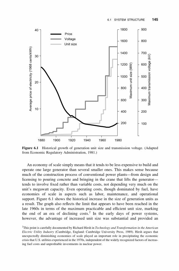
An economy of scale simply means that it tends to be less expensive to build and

operate one large generator than several smaller ones. This makes sense because

much of the construction process of conventional power plants—from design and

licensing to pouring concrete and bringing in the crane that lifts the generator—

tends to involve fixed rather than variable costs, not depending very much on the

unit’s megawatt capacity. Even operating costs, though dominated by fuel, have

economies of scale in aspects such as labor, maintenance, and operational

support. Figure 6.1 shows the historical increase in the size of generation units as

a result. The graph also reflects the limit that appears to have been reached in the

late 1960s in terms of the maximum practicable and efficient unit size, marking

the end of an era of declining costs.2 In the early days of power systems,

however, the advantage of increased unit size was substantial and provided an

Figure 6.1 Historical growth of generation unit size and transmission voltage. (Adapted

from Economic Regulatory Administration, 1981.)

2This point is carefully documented by Richard Hirsh in Technology and Transformation in the American

Electric Utility Industry (Cambridge, England: Cambridge University Press, 1989). Hirsh argues that

unexpectedly diminishing economies of scale played an important role in precipitating the economic

crisis that U.S. utilities experienced in the 1970s, independent of the widely recognized factors of increas-

ing fuel costs and unprofitable investments in nuclear power.

6.1 SYSTEM STRUCTURE 145

important incentive for utilities to connect enough customers so as to take full

advantage of economies of scale.

The load factor relates to the ratio of a load’s actual energy consumption over a

period of time to the maximum amount of power it demands at any one instant. This

is a key criterion for the economic viability of providing electric service, since the

cost of building the supply infrastructure is related to the maximum amount of power

(i.e., the capacity of generators and transmission lines), whereas the revenues from

electricity sales are related to the amount of energy (kilowatt-hours) consumed.

Thus, from the supply standpoint, the ideal customer would be demanding a constant

amount of power 24 hours a day. Of course, this does not match the actual usage

profile of real customers; nevertheless, a smoother consumption profile can be

accomplished by aggregating loads, that is, combining a larger number and different

types of customers within the same supply system whose times of power demand

do not coincide.

For example, an individual refrigerator cycles on and off, using a certain amount

of power during the time interval when it is on, and none the rest of the time. But if a

number of refrigerators are considered together, their cycles will not all coincide;

rather, they will tend to be randomly distributed over time. The larger the number

of individual loads thus combined, the greater the driving force of statistics to

level out the sum of power demand. By expanding their customer base to include

both a larger number of customers and customers with different types of needs

(such as machinery that operates during business hours versus lighting that is

needed at night) so as to deliberately combine complementary loads, utilities

improved their load factor and increased their revenues in relation to the infrastruc-

ture investment. Accordingly, electric power systems grew from the scale of city

neighborhoods to cover entire counties and states.3

The third main factor driving geographical expansion and interconnection has to

do with the ability to provide greater service reliability in relation to cost. The basic

idea is that when a generator is unavailable for whatever reason, the load can be

served from another generator elsewhere. To allow for unexpected losses of gener-

ation power or outages, utilities or independent system operators (ISOs) maintain a

reserve margin of generation, standing by in case of need (see Section 8.1). Consid-

ering a larger combined service area of several utilities, though, the probability of

their reserves being needed simultaneously is comparatively small. If neighboring

utilities interconnect their transmission systems in a way that enables them to

draw on each other’s generation reserves, they can effectively share their reserves,

each requiring a smaller percentage reserve margin at a given level of reliability.

More extensive interconnection of power systems also provides for more options

in choosing the least expensive generators to dispatch, or, conversely, for utilities

with a surplus of inexpensive generating capacity to sell their electricity. For

example, the north–south interconnection along the west coast of the United

3This argument is developed in detail with ample historical illustration by Thomas P. Hughes in Networks

of Power: Electrification in Western Society, 1880–1930 (Baltimore: Johns Hopkins University Press,

1983).

146 TRANSMISSION AND DISTRIBUTION

States allows the import of hydropower from the Columbia River system down

through California. In general, over the course of the development of electric

power systems during the 20th century, larger and more interconnected systems

have expanded the options for managing and utilizing resources for electric

supply in the most economic way.

As the distance spanned by transmission lines has increased, so has the signifi-

cance of energy losses due to resistive heating. Recall from Section 1.4.2 that

high voltage is desirable for power transmission in order to reduce current flow

and therefore resistive losses in the lines. Therefore, as systems have grown in

geographical extent, there has been an increasing incentive to operate transmission

lines at higher voltages. The maximum voltages used for transmission have thus

steadily increased over the decades, as shown in Figure 6.1 (note that the first

scale on the left indicates unit size in megawatts, the scale on the far right trans-

mission voltage in kilovolts).

There are also liabilities associated with larger size and interconnection of

power systems. Long transmission lines introduce the problem of stability (see

Section 8.3). More interdependence among areas also means greater vulnerability

to disturbances far away, including voltage and frequency fluctuations (see

Section 8.4). Still, conventional wisdom in the electric power industry holds that

the benefits of interconnection outweigh the drawbacks, at least up to the scale at

which power systems are currently operated. Thus, while individual utilities retained

their geographically delimited service territories throughout the era of regulated

monopolies, the strength and importance of their interties has increased to the

point where, when considering power systems from an operational standpoint, it

is often more meaningful to speak of a group of interconnected utilities than of an

individual corporate entity. Because the success of system operation depends on a

level of technical cooperation, such groups are administratively organized under

the North American Electric Reliability Council (NERC), shown in Figure 6.2,

where utilities in each regional council collaborate in planning and sharing

resources. The three major networks in the United States are synchronous internally

and connected to each other only by direct current (d.c.) links; not shown in the

figure are synchronous interties to Canada and Mexico.

6.1.2 Structural Features

High voltages are crucial for power transmission over long distances. Closer to the

end users of electricity, however, safety prohibits the use of equipment at exces-

sively high voltages lest people start electrical fires or electrocute themselves

(a point that every parent of a curious toddler can especially appreciate). The

sheer expense of properly insulating high-voltage equipment is also a consideration.

In the design of power delivery systems, the greater energy efficiency of high

voltage and low current must therefore be weighed against safety and capital cost.

Rather than having to settle for some intermediate voltage as a compromise, the

use of transformers (see Section 6.3) makes it possible to operate different parts


of the system at different voltages, retaining the respective advantages of higher and

lower voltages in those places where they are most consequential.

Power delivery systems are therefore divided into two general tiers: a trans-

mission system that spans long distances at high voltages on the order of hundreds

of kilovolts (kV), usually between 60 and 500 kV, and a more local distribution

system at intermediate voltages in the low tens of kV. The latter is more specifically

referred to as primary distribution, in contrast to the secondary distribution system,

which consists of the wires that directly connect most domestic and small com-

mercial customers, at voltages in the 100-V range (nominally 120 V in the United

States). Larger commercial and industrial customers often receive their service

at higher voltages, connected directly into the primary distribution system. The

transmission system is also further subdivided into subtransmission, operated in

the neighborhood of 100 kV, and longer-distance transmission at several hundred

kV.4 Collectively, the entire power delivery system is referred to as the transmission

and distribution (T&D) system.

The division between transmission and distribution is defined in terms of voltage

level, though individual utilities have different customs for where, exactly, to draw

the line. In general, “distribution” means below 60 or 70 kV. Physically, the bound-

ary between transmission and distribution systems is demarcated by transformers,

Figure 6.2 Main interconnections of the U.S. electric grid.

4In European usage, the terms translate as follows: subtransmission voltage ¼ high voltage; primary

voltage ¼ medium voltage; and secondary voltage ¼ low voltage. Owing to the smaller distances in

Europe (where line losses play a less important role), “high voltage” is generally limited to 380 kV,

whereas 500 kV and 750 kV are used in the United States. Worldwide, the highest voltages used to

date are 1200 kV a.c. for some very long transmission lines across Siberia and +600 kV d.c. in Brazil.


grouped at distribution substations along with other equipment such as circuit break-

ers and monitoring instrumentation. Organizationally, most utility companies have

separate corporate divisions responsible for the operation and maintenance of trans-

mission versus distribution systems; the substations themselves may be considered

to lie on either side, but most often fall under the jurisdiction of power distribution.

6.1.3 Sample Diagram

Figure 6.3 shows the basic structure and components of a transmission and distri-

bution system. First note that the illustration is not drawn to scale. Note also that

it is a one-line diagram, which does not show the three phases for each circuit

(see Section 6.2). The vertical lines represent buses, or common connections at

key points in the system, especially power plants and substations. With power

flowing from left to right, the diagram indicates the hierarchical relationship

among the important subsystems, along with some typical voltage values.

On the far left side of the diagram, two generators deliver power at 21 kV. They

connect to the transmission system through a transformer (indicated by the wavy

symbol reminiscent of wire coils) that steps up the voltage to 230 kV. The

squares on either side of the step-up transformer indicate circuit breakers that can

be opened to isolate the generator from the system. Circuit breakers also appear else-

where in the diagram; their functions will be discussed in more detail in Section 6.7

on protection.

The system shown includes both high-voltage transmission at 230 kV and sub-

transmission at 60 kV. The transmission and subtransmission systems meet in a

transformer at a transmission substation. At the distribution substation, the

voltage is stepped down further to the primary distribution voltage, in this case

12 kV. The primary distribution lines or feeders branch out from the substation to

serve local areas. These main feeders carry all three phases (see Section 6.2).

From the main feeders, lateral feeders (laterals for short) carry one or two phases

for a shorter distance, a few city blocks, for example. From the lateral, several

Figure 6.3 One-line diagram showing basic power system structure.


distribution transformers step the voltage down again to the secondary level at

which most customers are served, generally 120 V. Typically, one distribution

transformer serves several residences, up to one city block. Larger commercial or

industrial consumers (not shown here) usually have three-phase service directly

from the primary distribution level through their own dedicated transformer.

6.1.4 Topology

An important characteristic of transmission and distribution systems is their top-

ology, or how their lines are connected. The most important distinction is

between a radial configuration where lines branch out sequentially and power

flows strictly in one direction, and a network configuration that is more intercon-

nected. In a network, any two points are usually connected by more than one

path, meaning that some lines form loops within the system.

Transmission systems are generally networks. Local portions of a transmission

system can be radial in structure—for example, the simplified section shown in

Figure 6.3, with all the power being fed from only one side. Since generating

plants are more likely to be scattered about the service territory, though, the

system must be designed so that power can be injected at various locations and

power can flow in different directions along the major transmission lines, as necessi-

tated by area loads and plant availability. Thus, high-voltage transmission systems

consist of interconnected lines without a hierarchy that would distinguish a “front”

or “back” end.

It is true, of course, that due to the geography of generation and major load

centers, power will often tend to flow in one direction and not the other. Neverthe-

less, this kind of directionality is not built into the transmission hardware. For

example, in the state of New York, power tends to flow from north to south into

New York City, but as far as the transmission system is concerned, the power

could just as easily be sent from south to north. The system structure does finally

become hierarchical at the interfaces with the lower-voltage subsystems (subtrans-

mission or distribution), where power flows only from high to low voltage.

The network character of the transmission system allows for different operating

conditions in which power may flow in different directions. It also offers the crucial

advantage of redundancy. Because there are multiple paths for power to flow, if one

transmission line is lost for any reason, all the load can still be served (as long as

the remaining lines can carry the additional load). Indeed, a standard design criterion

for transmission systems requires that the entire system must continue to function if

any one link is interrupted (see Section 8.1 on reliability).

The basic radial design is that shown in Figure 6.4. The radial system has a strict

hierarchy: power flows only in one direction; there is always an “upstream” and

a “downstream.” The distribution lines or feeders extend and branch out in all

directions from a substation somewhat like spokes from a hub. Owing to this

hierarchy, any given line or component can only be energized from one direction.

This property is crucial in the context of circuit protection, which means the

interruption of circuits or isolation of sections in the event of a problem or fault


(see Section 6.7). In a radial system, circuit breakers can readily be located so as to

isolate a fault—for example, a downed line—immediately upstream of the problem,

interrupting service to all downstream components. Economically, radial systems

also have the advantage that smaller conductor sizes can be used toward the ends

of the feeders, as the remaining load connected downstream diminishes.

Figure 6.5 illustrates a loop system. One switch near the midpoint of the loop is

open (labeled N.O. for normally open) and effectively separates the loop into two

radial feeders, one fed by each transformer. Thus, under normal operation, the

Figure 6.4 Radial distribution system.

Figure 6.5 Loop system.


sections are not connected at that point, so that the system operates as a radial

system. But under certain conditions—for example, a failure of one of the two sub-

station transformers—the N.O. switch can be closed and one section of the distri-

bution system energized through the other. By choosing which one of the other

switches to open, sections of the loop can be alternatively energized from the left

or right side. This has the advantage of enabling one transformer to pick up

additional load if the other is overloaded or out of service, and of restoring

service to customers on both sides of a fault somewhere on the loop. While loops

are operated as radial systems at any given time, that is, with power flowing only

outward from the substation transformer, the hardware including protective

devices must be designed for power flow in either direction.

Finally, Figure 6.6 shows an example of a network distribution system. A net-

worked system is generally more reliable because of the built-in redundancy: if

one line fails, there is another path for the power to flow. The cost of a network

system to serve a given area is higher than a simple radial system, owing not only

to the number of lines but also the necessary equipment for switching and protection.

Networks are often used in downtown metropolitan areas where reliability is con-

sidered extremely important, and where the load density justifies the capital expense.

From the standpoint of circuit protection, a network is much more challenging

because there is no intrinsic upstream or downstream direction, meaning that a

given point in the system could be energized or receiving power from either side.

This means that any problem must be isolated on both sides, rather than just on

the upstream side. However, the objective is still to make the separation as close

to the fault as possible so as to minimize the number of customers affected by

service interruptions. As a result, the problem of coordinating the operation of mul-

tiple circuit breakers becomes much more complex. This is the main reason why

most distribution systems are radial or looped.

A special case of power system topology is the power island, or an energized

section of circuits separate from the larger system. An island would be sustained

by one or more generators supplying a local load, at whatever scale. For example,

Figure 6.6 Network.


in the event of a downed transmission line to a remote area in the mountains, a

hydroelectric plant in this area might stay on-line and serve customers in its vicinity,

an occurrence described by operators as “not by the book.” Similarly, small-scale

distributed generation such as rooftop photovoltaics could in theory sustain local

loads as a small island during a service interruption, if it were not for standard

requirements that they be disconnected from the grid in the event of an outage.

Islanding is not routinely practiced or condoned by U.S. utilities, except tempor-

arily while restoring loads after a widespread outage, where individual power islands

are reconnected as quickly as possible in a centrally orchestrated effort. Reasons to

avoid routine islanding include both safety and liability. First and foremost, the

safety of line crews could be jeopardized if they encountered a power island

while expecting to find a de-energized circuit. Second, the ability of the generators

in the island to maintain power quality (including voltage and frequency) is not guar-

anteed, potentially causing problems for some customers with sensitive equipment

for which the utility may then be held liable. However, with an increasing preva-

lence of small generators such as photovoltaics and fuel cells throughout distribution

systems, and considering also the control capabilities introduced by distribution

automation technology, the issue of islanding seems likely to be revisited and

perhaps become the subject of some controversy.

6.1.5 Loop Flow

In addition to protection, an important operational complexity introduced by a

network structure is loop flow (Figure 6.7). Loop flow can arise whenever there is

more than one path for the current to travel between two points in the system.

The basic problem is that current flow cannot be directed along any particular

branch in the network, but is determined by Kirchhoff’s laws (see Section 2.3)

Figure 6.7 Loop flow.


and the relative impedances of the various branches. The concept is best explained

by example, as shown in the simple case below. This example is intended to illus-

trate that actual line flows through network loops are not immediately obvious, even

in apparently simple cases. Calculating these amounts generally requires power flow

analysis, which is performed by computer.

How the power flows through a network tends to be of little interest until there is

congestion or overloading of transmission lines, at which point it suddenly becomes

critically important. In order for local transmission overloads to be relieved, oper-

ators need to know which generators could have their output adjusted so as to

most effectively achieve a reduction in line flows. In a competitive market, it may

be desirable to allocate the available transmission capacity in some economic

fashion. If an individual generator is to be allocated the rights to a certain power

transfer along a particular link, it is vital to know how this generator’s output con-

tributes to the total flow on any given transmission path. While this contribution

cannot readily be measured, it can be calculated or at least estimated by power

flow analysis (see Chapter 7). In the simplified situation shown in the Figure 6.7,

there is only one load, located at Bus 3, and two generators, Gen 1 and Gen

2. Suppose the load is 900 MW, of which Gen 1 supplies 600 MW and Gen 2

300 MW. What are the flows on the transmission lines A, B, and C? Although

line A is the most direct path from 1 to 3, not all of the 600 MW will flow along

A. Some will flow along the combination B–C, which constitutes another path

from 1 to 3. The magnitude of this portion depends on the relative impedance of

the path B–C as compared to A (see Section 2.2 about parallel circuits).

To make this example most transparent, let us suppose that the impedances of all

three links A, B, and C are exactly the same (a highly idealized situation). The impe-

dance of path B–C (in series) is therefore exactly twice that of path A, and the

current flowing through B–C is half that flowing through A (see Section 1.2). To

a very good approximation (assuming the voltages at 1, 2, and 3 have reasonable

values), the power (megawatts) transmitted along each path will be directly pro-

portional to the current (amperes) flowing though it; thus, twice as much power

flows through A as through B–C. If these are the only two paths from this generator

to the load, and their total is 600 MW, then 400 MW flow through A and 200 MW

through B–C.

Now there is an additional 300 MW supplied to the load at 3 from Gen 2. Again,

while line C is the most direct path, some of the current will flow around the loop

B–A. Given our previous assumption about the impedances, twice as much

current (or power) flows through C as through B–A; thus, we have 200 MW

through C and 100 MW through B–A, for a total of 300 MW.

The total flows on each line can now be calculated quite simply by taking advan-

tage of the superposition principle (see Section 2.3.4), which allows us to consider

each power source individually at first and then add the currents due to each source

in each link. We must only be careful about the direction and whether the currents in

fact add or subtract. On line A, power from Gen 1 and Gen 2 flow in the same direc-

tion, from 1 to 3. We can therefore add the currents (or power), and the total flow on

A is 500 MW. Similarly, on line C, we have 200 MW from Gen 1 and 200 MW from


Gen 2, each flowing in the direction from 2 to 3, for a total of 400 MW. But on line

B, 200 MW from Gen 1 flow to Gen 2, whereas 100 MW from Gen 2 flow from 2 to

1. These line flows subtract, and we have a net flow of 100 MW on line B from 1 to

2. We can do a reality check by confirming that the total power arriving at the load is

indeed 500þ 400 ¼ 900 MW.

This example shows that line flows in the presence of loops are not obvious. If

there were more possible paths connecting the buses, the result would be accord-

ingly more complicated and could hardly be calculated by hand. The example

also illustrates that the effect of one generator’s output may be to reduce rather

than increase the flow on a given link. For example, suppose line B is overloaded

and can only handle 90 MW, whereas there is plenty of capacity on lines A and

C. If both load at Bus 3 and generation at Gen 2 are now increased by 30 MW,

the result is that the flow on B is reduced by 10 MW, saving the day. (The reader

can verify that the new flows on A and C are 510 MW and 420 MW, respectively.)

Under some conditions, there may be a circulating current around a loop within

the network that does not actually serve a load but contributes to energy losses.

These cases show that designing and operating a power network for safety as well

as efficiency requires modeling the power flow under a diverse set of operating

conditions so as to avoid unpleasant surprises.

INTERNATIONAL DIFFERENCES IN DISTRIBUTION

SYSTEM DESIGN

In Europe, as well as in many countries formerly colonized by Europeans, power

distribution systems have a distinctively different look. Unlike the United States,

where there is usually a distribution transformer (typically single phase) for every

few customers, connected by short service drops, in Europe there are fewer and

larger transformers—usually hidden in vaults rather than mounted on poles—

from which a more extensive system of secondary lines branches out. Because

secondary (low-voltage) lines are less expensive to underground than the

primary (medium-voltage) lines that make up the larger part of the U.S.-style dis-

tribution system, distribution systems are more often undergrounded and thus

altogether less visible in Europe. These differences in design are consistent

with differences in geography, population and load density, and the historical

expansion of power systems.

Except when compared with downtown urban areas, the population density in

Europe is generally higher and individual loads smaller, making it more feasible

to extend secondary lines to many customers. Extension of secondary lines is

also more feasible because the standard secondary voltage is higher in Europe

(nominally 220 V). This design approach makes it relatively easy to geographi-

cally extend service areas by adding another secondary line to an existing trans-

former, though it becomes more difficult once the transformer capacity is

insufficient. The layout of the system is generally optimized around load level.


In North America, particularly in rural areas, the location of customers and

the size of the area to be covered are generally more important considerations

in determining system layout than load level. Because customers tend to be

much farther apart, higher voltage (primary) lines are needed to reach them.

Systems here tend to have a higher loading capacity per mile of circuit,

and load growth within the existing service area can usually be quite readily

accommodated by adding small transformers.5 Figure 6.8 illustrates the two

different types of layout (adapted from Carr and McCall, 1992), where the

heavier lines graphically represent primary and the lighter lines secondary

distribution wires. Note that the line weight does not reflect physical wire diam-

eter, since a lower-voltage line actually carries a greater current to transmit a

given amount of power.

6.1.6 Stations and Substations

Transmission and distribution stations exist at various scales throughout a power

system. In general, they represent an interface between different levels or sections

of the power system, with the capability to switch or reconfigure the connections

among various transmission and distribution lines. On the largest scale, a trans-

mission substation would be the meeting place for different high-voltage trans-

mission circuits. At the intermediate scale, a large distribution station would

receive high-voltage transmission on one side and provide power to a set of

primary distribution circuits. Depending on the territory, the number of circuits

may vary from just a few to a dozen or so. The major stations include a control

Figure 6.8 North American and European distribution systems.

5J. Carr and L.V. McCall, “Divergent Evolution and Resulting Characteristics among the World’s

Distribution Systems,” IEEE Transactions on Power Delivery 7(3), July 1992.


room from which operations are coordinated. Smaller distribution substations follow

the same principle of receiving power at higher voltage on one side and sending out

a number of distribution feeders at lower voltage on the other, but they serve a more

limited local area and are generally unstaffed.

The central component of the substation is the transformer, as it provides the

effective interface between the high- and low-voltage parts of the system. Other

crucial components are circuit breakers and switches. Breakers serve as protective

devices that open automatically in the event of a fault, that is, when a protective

relay indicates excessive current due to some abnormal condition. Switches are

control devices that can be opened or closed deliberately to establish or break a

connection. An important difference between circuit breakers and switches is that

breakers are designed to interrupt abnormally high currents (as they occur only in

those very situations for which circuit protection is needed), whereas regular

switches are designed to be operable under normal currents. Breakers are placed

on both the high- and low-voltage side of transformers. Finally, substations may

also include capacitor banks to provide voltage support. Because three phases are

used, all equipment comes in sets of three, referred to as a “bank”—for example,

a transformer bank is a set of three transformers, one for each phase.

A sample layout for a distribution substation is shown in Figure 6.9. Note that

schematic diagrams like this are not drawn to scale, nor do they necessarily

Figure 6.9 Distribution substation layout.


provide a good sense of the actual spatial arrangement of the switchyard for

those unfamiliar with the physical equipment represented here. Figure 6.10 shows

a photograph of a similar substation.

6.1.7 Reconfiguring the System

Operating a transmission and distribution system involves switching connections

among high-voltage power circuits. Switching operations can be carried out remo-

tely from the computer screen at a switching center through a supervisory control

and data-acquisition (SCADA) system. In many distribution systems, however,

switching is still performed manually by field crews per telephone instructions

from operators at a distribution switching center.

Reasons for switching include contingencies, work clearances, service restor-

ation following an outage, managing overloads, and enhancing system efficiency.

For example, a contingency might be a fault on one line that has to be isolated

from the system, and other connections need to be rearranged so as to redistribute

the load of the lost line among them. Similarly, in the case of maintenance work

or replacement of a line or system component, this component is electrically isolated

(cleared ) and the system “patched” around it. Clearances may also be issued for

work other than on the power system components themselves, including any con-

struction work that is sufficiently close to power lines that workers may accidentally

contact them.

In the event of an outage, or service interruption to some number of customers,

care is taken to follow a sequential procedure of restoring load. The idea is to recon-

nect sections of load one at a time in a given order so that each new load added

Figure 6.10 Distribution substation. (Courtesy of Marshal F. Merriam.)


does not jeopardize the stability of the remainder of the connected system.

This restoration process involves opening and closing switches in order to divide

loads into appropriately small sections, to connect them, and sometimes to transfer

sections temporarily. Restoration after a widespread outage is usually the only time

that utilities operate parts of the system as power islands. In this situation, local areas

with generation and load are brought back on line and then synchronized with each

other and reconnected.

At the transmission level, because the system is networked, and because outages

are less frequent, there tends to be less switching during normal operation. In

radial distribution systems, by contrast, well-defined local blocks of load can

readily and deliberately be shifted from one circuit to another. For example, if

one particular substation transformer threatens to overheat on a day of heavy

demand, part of the load of the corresponding distribution feeder can be switched

over to the adjacent transformer. This is easily done in a loop system by shifting

the position of the “gap” or open switch between the two ends of the loop (see

Figure 6.5.)

Under extreme overload conditions, where there is either no available distri-

bution capacity to reroute power, or if there is a shortfall in power generation,

load may be shed or selectively disconnected. For example, if the systemwide

generation is insufficient to meet demand, and consequently the system frequency

drops below a specified limit, a number of customers will be disconnected for the

sake of keeping the remainder of the system operational, as opposed to risking a

more extensive failure of potentially much longer duration (see Section 6.7). In

order to assure fairness in this procedure, customers are assigned rotating outage

block numbers that appear on the electric bill for taking turns in being shed.

Finally, it is possible to redistribute loads in distribution systems for the purpose

of load balancing, or equalizing the loads on distribution feeders or transformers in

order to increase operating efficiency by minimizing losses. Because resistive power

losses vary with the square of electric current (P ¼ I2R), they are minimized when

the currents are evenly balanced among alternative lines and transformers.6 To

achieve this, some load may be switched over from one to another, less heavily

loaded circuit. This procedure is not part of standard operations in the industry

today, but has been proposed as an economically viable procedure in the context

of automating distribution switching operations.

6.2 THREE-PHASE TRANSMISSION

In the preceding transmission and distribution system diagrams, each circuit was

indicated by a single line in what is known as a one-line diagram. In reality,

however, a standard a.c. circuit includes three electrically separate parts or

6Readers to whom this result is not obvious may wish to work through a numerical example: Consider two

currents that add up to 10. In an unbalanced combination—say, 9 and 1—the squares of the currents add

up to 82. In a balanced combination—that is, 5 and 5—the squares add up to only 50.

6.2 THREE-PHASE TRANSMISSION 159

phases. For example, transmission lines are generally seen to have three wires or

conductors. In this section we describe the three-phase concept—how it works,

why it was chosen, and basic aspects of analyzing three-phase circuits.

6.2.1 Rationale for Three Phases

In Chapter 4, we described power generators as having three sets of outgoing wind-

ings or phases, each carrying an a.c. of the same magnitude, but separated in timing

by one-third of a cycle or 120 degrees from the other two. We also stated one ration-

ale for this three-phase system; namely, that a three-phase generator experiences a

constant torque on its rotor as opposed to the pulsating torque that appears in a

single- or two-phase machine, which is obviously preferable from a mechanical

engineering standpoint.7

In the system context, another benefit of supplying a.c. in multiple phases lies in

its economy of transmission. As we show in this section, three-phase transmission

permits the use of fewer wires than common sense might suggest, and indeed less

conductor capacity than would be required to transmit an equivalent amount of

power using only a single phase of a.c.

In general, the completion of an electric circuit requires two conductors between

the power source and the load: one for the current to flow out, and one for it to return.

In principle, this is true regardless of whether the current is direct or alternating. In

practice, d.c. transmission can sometimes do away with one of the conductors and

allow the current to return through the ground, in what is called ground return.

For a.c., ground return is rarely feasible because the soil in most places presents

too high an impedance. In any case, multiphase transmission does not rely on

ground return to work.

Let us begin by imagining a.c. power being supplied from a source to a load in a

single phase. Two conductors between the source and the load form one complete

circuit. At any instant, the current everywhere along this circuit is the same. (This

implies that if the conductors to and from the load are placed side by side, their

currents would go in opposite directions.)

Suppose now that we want to supply three separate phases, one from each set of

generator windings, to three individual loads. Each of these circuits will again have

two conductors, one leading from one end of the generator armature winding to the

load, and one connecting back from the load to the other end of the winding. Thus,

we have a total of six conductor wires.

The secret of multiphase transmission is that the return conductors of each of

these three circuits can be combined into a single hypothetical return wire, and ulti-

mately that this combined return can be eliminated altogether, leaving us with only

three wires for three circuits. To appreciate how this can work, we must consider the

relative timing and magnitudes of the three individual phase currents, as shown in

7The constant torque results from the increasing and decreasing magnetic field components along the

direction of each phase’s coil that add up in space so as to emulate a rotating field of constant magnitude,

as illustrated in Section 4.2.1. This addition is geometrically impossible with fewer than three phases.


Figure 6.11. Specifically, consider the sum of the three currents at any particular

instant. This is the same as asking, if we were to physically combine all three

return wires into one, what would be the combined current in that wire?

In some places, it is obvious from inspection that the three curves add up to zero.

For example, at the instant when current A is zero, current B is exactly the negative

of current C. Or, when current A is at its maximum, B and C are both at one-half their

negative maximum. Elsewhere, it is not as easy to see, but the math holds up: the

sum of currents A, B, and C is always zero, anywhere along the graph. This is

true as long as two conditions are met: (1) that the three phases are exactly 1208apart, and (2) that the respective amplitudes or maxima are the same. What this

means in physical terms is that if we bundled together the return wires of the

three circuits, the current through this combined conductor would be zero. This

situation is shown in Figure 6.12.

Let us now think about the picture in terms of voltage or potential. The three

windings in the generator are producing an alternating potential across them. This

alternating potential is also seen by each load, which is connected to the two ends

of a winding. But now all three generator windings share a point of common poten-

tial, pointG, as do all three loads at point L. To determine what the actual potential is

at pointG (with respect to ground), we can add up a set of three sinusoidal waves just

as we did for the current, only now indicating the voltage generated in each phase

over time, and see that it remains zero at all times.

Figure 6.11 Three balanced single-phase a.c. circuits.


The same should be true for point L, assuming that all three loads (their impe-

dances, really) are identical. While the generator controls the voltages, the load

impedances determine the currents. To assume equal loads on the three phases is

to assume that both currents and voltages in the three phases are properly timed

and remain of equal magnitude. Thus, with equal loads, the currents will be balanced

and the potential with respect to ground at point Lwill also remain at a constant zero.

From this observation, we can conclude that there will be no current flowing

through the return conductor or neutral connectingG and L, since there is no potential

difference between G and L. Therefore, we can simply eliminate the wire. In reality,

because loads may not be balanced, some residual net return current may need to

flow. When the neutral points G and L are both grounded, this relatively small

residual current can flow through the soil. The situation is illustrated in Figure 6.13.

In summary, then, we are transmitting power to three circuits, but, owing to the

clever combination of phases staggered in time, we can do away with three of the six

wires we would expect to need. Some readers may note that this result is not unique

to three phases. In fact, any number of phases, spaced equally around the cycle and

with equal amplitudes, will have the same property of always adding up to zero. For

example, we could supply four circuits with four wires for four phases, spaced 908apart; five phases 728 apart; or even just two opposite phases, 1808 apart. Why, then,

choose three?

First, we recall the advantage of using at least three phases for generator design.

In addition, transmitting power with only two phases would mean a greater

Figure 6.12 Three phases with common return.

Figure 6.13 Three phases with neutral removed.


vulnerability to imbalances in the loading of the two circuits: if one circuit were

loaded more heavily than the other, the effects on voltage and current would be

more readily noticeable than they are with more phases to “absorb” the difference.

More than three phases, on the other hand, would become increasingly compli-

cated and expensive. If all the power on the system were supplied in four phases,

for instance, this would mean that all transmission and major distribution lines

consist of four separate conductors. In addition, each bank of transformers at

every substation would have to comprise four instead of three transformers, and

the same for circuit breakers. Although for the same amount of total power the

capacity of each of these four components could be proportionately smaller, their

total cost would be greater due to economies of scale (i.e., a transformer of twice

the capacity costs less than twice as much). Thus, three is the most practical

number of phases, and its use in a.c. power systems is a global standard.

Because the three phases are so interdependent, they are described as a single

circuit (in contrast to the nomenclature we used before, where we referred to

each individual phase as a circuit). In drawings, each three-phase circuit can be

represented by a single line. This perspective is generally applied in situations

that assume balanced and trouble-free operation. It is the more complicated, less-

than-ideal situations involving faults and unbalanced loads that call for a separate

analysis for each phase.

6.2.2 Balancing Loads

In deriving the result that a circuit of three a.c. phases does not require a ground return

conductor, we made the assumption that the impedance or total load connected to

each phase is identical, making the amplitudes of the three currents equal. But

how is this accomplished in reality? Certain loads such as large commercial

motors are connected to all three phases and draw power equally from all of them.

But, as we noted earlier, electric service to most residential and small commercial

customers generally consists of only one phase. The challenge for the distribution

planner is to distribute these customers among the phases as evenly as possible so

that the combined load on each phase is about the same. Where single-phase laterals

branch out from the main distribution feeders, distribution engineers take care that

the local areas served by these feeders comprise similar loads. If a three-phase

feeder runs down a street, transformers that serve several houses each will tend to

alternate among the phases, and when new customers are connected, the phase is

chosen by considering the balance with other loads in the vicinity.

As the reader can imagine, balancing loads8 is a rather approximate procedure,

unlike the idealized, perfectly balanced phases encountered in engineering texts.

For one, the physical equipment limits the precision with which loads can be

balanced, because loads come in chunks and not in arbitrarily small increments.

The balance will also fluctuate in real-time as customers connected to different

8This notion of balancing loads among individual phases is not to be confused with a similar term, load

balancing, that refers to the practice of equalizing loads among different distribution circuits or feeders so

as to avoid overloading one of them, or for the purpose of minimizing resistive losses (see Section 6.1.5).


phases turn their appliances on and off. In practice, the imbalance among current or

power delivered by each phase will be in the range of several percent, sometimes as

high as 10% or more. However, this variation will be greatest near the customers,

and will diminish at higher levels of aggregation (such as the transmission

system) by virtue of statistics, since the local imbalances are more likely to

cancel each other out once many loads are added together.

When the loads on all phases are not equal, the currents no longer add to zero.

This means that some return flow of current is needed. If only three conductors

are provided for three phases, the return current must travel through the ground.

Along distribution feeders, where more pronounced imbalances are to be expected,

a fourth neutralwire is often provided for just this purpose. In Figure 6.12, we would

observe a phase imbalance as a potential between points L and G that causes a

current to flow in the neutral conductor. The magnitude of this current will tend

to be on the order of a few percent of the phase current, as the voltage at L and G

with respect to ground will be a few percent of the regular line voltage, depending

on the extent of the imbalance. The conductor and insulator size of the neutral wire

therefore may be noticeably smaller than the three phase conductors.

6.2.3 Delta and Wye Connections

An individual load generally requires two conductors to connect to, as this constitutes

a closed circuit (an exception are three-phase motors that connect to all three con-

ductors). When power is delivered in three phases, the designer has two distinct

choices: a load can be connected either between one phase and ground, or

between one phase and another phase. In each case, the three phases will supply

three separate loads. The first arrangement, where three loads are connected

between one phase each and ground, is called a wye connection because the sche-

matic diagram resembles the letter Y, as in Figure 6.14b. The second arrangement,

in which three loads are connected between one pair of phases each, is called a delta

connection (Figure 6.14a) for the same reason.

For the wye connection, it is obvious that the voltages (known as phase-

to-ground voltages) and currents for each load will be spaced 1208 apart. The

same is true for the delta connection, but it is less obvious. The key is to remember

Figure 6.14 (a) Delta and (b) wye connections.


that the voltage “across” a load is in fact the difference between the voltage on one

side and the other. Thus, mathematically, we can simply plot a curve that shows the

difference between each pair of phase voltages at any moment in time, which gives

the phase-to-phase voltage as a function of time (as shown in Figure 6.15). Each of

these three possible curves (A–B, A–C, or B–C) is still sinusoidal (as we might

derive from trigonometry), but is shifted in time (phase) from the original phases

A, B, and C. It also has a different amplitude: as we could further derive from

trigonometry, the magnitude of the phase-to-phase voltage is greater than the

phase-to-ground voltage by a factor offfiffiffi3

p(about 1.73).

The choice of phase-to-phase versus phase-to-ground offers one way to select

different voltage levels for loads from the same three-phase power supply. This

is, in fact, how some utility customers (usually in the industrial or commercial

sector) obtain both 120 V and the so-called 220 V from two phases and a neutral

conductor. (The alternative approach for supplying dual voltages involves transfor-

mer taps and is discussed in Section 6.3.)

Example

A service line to a grocery store comprises three conductors—Phase A, Phase B,

and neutral—where each phase-to-ground voltage is 120 V. The 120-V loads

around the store, such as lights and regular outlets, may be alternatively connected

to Phase A or B. Heavier loads, such as big refrigerators, would be connected

phase-to-phase between A and B. The voltage they see isffiffiffi3

p� 120V ¼ 208V.

In general, generating equipment and loads are connected to power systems

through transformers. Because the wire coils in the transformer always involve a

Figure 6.15 Phase-to-phase voltage.


pair of conductors that constitute one circuit, everything has to have either a delta or

a wye connection, and both are common.

Aside from the difference in voltage level, the choice of delta or wye connection

has some ramifications for reliability, in case there should be a short circuit. The

delta configuration as a whole is ungrounded or floating, meaning that no point

on the circuit is connected to ground or to any point that has a particular, known

potential. The (time-varying) potential differences between and among the points

on the circuit are all that matters. The entire delta system can thus float at any

arbitrary, absolute value of potential. Consequently, if any part of the circuit acci-

dentally gets grounded—which would otherwise cause an outage—the delta

circuit can continue to operate on an emergency basis. (It is crucial, though, to

locate and fix the problem before a second one occurs elsewhere on the circuit,

which could now cause a very damaging fault current.) Because of this property,

the delta configuration is used where reliability is most important, such as auxiliary

equipment in power plants, or on smaller transformers.

The wye configuration, by contrast, is normally grounded at the center or neutral

point. Here, a single ground anywhere else in the system will immediately cause a

fault, and ground relay protection (see Section 6.7) is always used to open the circuit

breakers in such an event to protect the lines and equipment. In this case, the risk of

damage to equipment overrides the short-term reliability concern. The wye connec-

tion is typically used on generators, main transformer banks, and transmission lines.

It is also possible to switch between delta and wye connections, which is frequently

done by transformers that are wired in a delta configuration on one side and wye on

the other (see Section 6.3.3).

6.2.4 Per-Phase Analysis

Based on the assumption that the voltages and currents in the three phases are equal,

the analysis of a three-phase circuit can be simplified to a single phase that is then

representative of what happens in all three. Whereas phase imbalances are often

encountered in the operating context, they are not easily dealt with in the engineer-

ing context since the differences among loads that give rise to the different currents

and voltages are not by design and cannot readily be predicted. At the transmission

level, phases are generally assumed to be balanced. At the distribution level, there

are single-phase feeders, but main feeders are also assumed to be balanced among

their three phases. An important exception is the analysis of what happens during

a fault—say, if a single phase is accidentally connected to ground, or two phases

are short-circuited together. For the most part, though, there is no need to explicitly

keep track of the three phases individually. Therefore, one-line diagrams are often

used that are understood to represent a complete three-phase circuit.

6.2.5 Three-Phase Power

In order to calculate the power transmitted on a three-phase transmission or distri-

bution line, one essentially multiplies the voltage and current together for each

individual phase and multiplies by three. However, we must be careful to take


into account a factor offfiffiffi3

p. It arises in the case of a wye connection because the

effective voltage seen by the load is the line-to-ground, not the line-to-line

voltage. In the case of a delta connection, the current through each conductor con-

tributes to two phase pairs, so that the applicable current that can be “credited” to

each load is only 1=ffiffiffi3

pof the total current measured in the line (it is more than

half because the timing of the current is shifted by 1208 for each phase pair).

Thus, in the wye case, we have for apparent power

S ¼ 3Irms

Vrmsffiffiffi3

p

where Vrms refers to the phase-to-phase voltage (according to which line voltages are

conventionally labeled) and Irms to the actual current in each conductor. In the delta

case

S ¼ 3Irmsffiffiffi3

p Vrms

As we can readily see, both come out to the same formula,

S ¼ffiffiffi3

pIrmsVrms

regardless of how the load is connected.

For real and reactive power, it is only necessary to include the factors of cos f

and sin f, respectively, depending on the load power factor (p.f.).

6.2.6 D.C. Transmission

In some situations it is beneficial to use d.c. transmission. This is true despite the fact

that the transmission system is otherwise a.c., and the power has to be converted

both at the beginning and the tail end of the d.c. line through relatively costly

solid-state devices called thyristors. The reason this effort is worthwhile is that

d.c. eliminates the problem of a stability limit (see Section 6.5.2), which poses

a power transmission constraint on long lines with a significant inductance.

Because its effect depends on a.c. frequency, inductance is irrelevant for d.c., and

therefore only the thermal limit (determined by the resistance of the line) applies.

An overhead d.c. transmission line can be easily identified by the fact that it has

two, not three, conductors. D.c. is also used on undersea cables in order to avoid

the effect of capacitance on coaxial cables.

The use of d.c. in modern power systems is often confusing to those who

remember that d.c. was historically associated with excessive line losses, which

motivated the selection of a.c. as a national and international standard. The

crucial difference is that early d.c. systems were operated at low voltage—hence

the losses—because there was no practical way to step d.c. voltage up and

down between transmission and end users (since transformers do not work with

d.c.). By contrast, modern d.c. lines, connected to the high-voltage a.c. system

with advanced solid-state technology, carry very high voltages and are therefore

highly efficient.


Besides transmitting bulk power over long distances, another application for

a.c.-to-d.c.-and-back-to-a.c. conversion in modern power systems is to provide an

intertie between two a.c. systems that are not synchronous. In this way, power

can be shared between these systems even though their a.c. frequency and phase

may differ, and the systems are therefore neither subject to stability constraints

across the intertie nor vulnerable to frequency-related disturbances from each

other. The eastern and western United States are connected by such a d.c. intertie.9

6.3 TRANSFORMERS

6.3.1 General Properties

A transformer is a device for changing the voltage in an a.c. circuit. It basically con-

sists of two conductor coils that are connected not electrically but through magnetic

flux. As a result of electromagnetic induction, an alternating current in one coil will

set up an alternating current in the other. However, the comparative magnitude of

the current and voltage on each side will differ according to the geometry, that is,

the number of turns or loops in each coil.

Consider the diagram in Figure 6.16 of a very simple transformer. The coil on the

left-hand side, which we will label as the primary side, might be connected to a

power source such as a generator, while the right-hand or secondary coil would

supply a load. Looking at the electrical connections, we see two separate circuits

in this diagram: the circuit between the generator and the transformer (with

Figure 6.16 Transformer schematic.

9Another interesting example is the German power system. For four decades, East and West German

systems were operated completely independent of each other—one interconnected with eastern Europe

and the U.S.S.R., and the other with western Europe. Although much of the hardware infrastructure is

very similar, reconnecting these systems after the reunification in 1990 was complicated by different

operating standards: while the nominal frequency on both sides was 50 Hz, the tolerance for frequency

deviations was much less on the West German side, and the systems could not be kept synchronous. In

order to share generation resources without compromising stability, the first step was to install d.c.

interties at key points along the former border.


current I1 and voltage V1) and the circuit between the transformer and the load

(with current I2 and voltage V2). Yet electrical power is somehow transmitted

across the transformer from the generator to the load. In reality, a small percentage

of the power will be dissipated in the form of heat from the transformer, just

as some resistive heating will occur along the wires. But in the idealized

case, where there is no heating in the transformer, all the power is transmitted

across. In other words, the same amount of power goes into the transformer as

goes out.

Recalling that electric power is given by the product of current and voltage, we

can state that the product of current and voltage on each side of the transformer

must be the same. Referring to the labels in the diagram, we would write

I1 � V1 ¼ I2 � V2

However, based on examining only the electrical connections, we cannot say any-

thing more about how the voltage and current relate. For this, we must look to

what happens with the magnetic flux and induction inside the transformer.

First, in the primary coil, the a.c. supplied by a generator produces a magnetic

field, or flux inside the core of the coil. Like the conductors inside a generator, trans-

former coils are wound around a core of magnetically susceptible material, generally

some type of iron, to enhance the magnetic field.10 The magnetic flux resulting from

the current is proportional to both the current’s magnitude and the number of turns in

the coil.

Using the terminology introduced in Section 2.4, we can state that the product of

the current I and the number of turns n in the coil gives the magnetomotive force

(mmf ), which produces the magnetic flux (denoted by F, the Greek phi) inside its

core. The flux is enhanced because the iron core has a high magnetic permeability,

or a low magnetic reluctance (denoted by R). In equation form,

mmf ¼ nI

F ¼mmf

R

Because the reluctance of the transformer core is significantly lower than that of the

surrounding air, the flux is in effect “captured” inside the core, meaning that the

leakage flux outside the core is small.

As the current on the primary transformer winding alternates, the flux inside the

core changes direction back and forth 60 times per second (for 60-Hz a.c.). But this

same changing flux links the secondary winding around the same core. Proportional

to the rate of change of this flux, an electromotive force (emf) is induced in the

secondary winding. A current then flows in this winding as determined by the

10The choice of material for a transformer core affects its behavior under different a.c. frequencies, which

is relevant in contexts other than power systems. At high frequencies, it becomes more difficult for iron to

sustain the rapid reversal of the magnetic field, causing increased heat losses. Transformers do work in

principle even with nothing but air in the core.

6.3 TRANSFORMERS 169

impedance connected to it. The emf is also proportional to the number of turns,

denoted by n, of this winding around the core. This makes sense in that an emf is

induced in each turn, and the successive turns of the same conductor are effectively

in series, so that the voltages or emfs are additive.

With regard to changing the voltage from the primary to the secondary side, the

important measure is the turns ratio, or ratio of the number of turns in the primary

and secondary winding. If both primary and secondary windings had the same

number of turns, the voltage would be the same on either side of the transformer.

In order to increase or step up the voltage, the number of turns must be greater on

the secondary side; conversely, to step down voltage, the number of turns must be

less. For example, the primary winding in Figure 6.16 has eight turns and the

secondary winding four, so that the voltage is stepped down by a factor of 2. A

real transformer would have hundreds of turns in each winding so as to make the

magnetic induction process more efficient, but as long as the ratio of primary to sec-

ondary turns remains the same the effect on voltage is the same. Because power is

conserved (to a first approximation), and since power equals voltage times current,

the currents through either winding are inversely proportional to the number of

turns. In equation form,

V1

V2

¼n1

n2¼

I2

I1

The transformer in this example would be called a step-down transformer if the

greater number of turns is on the primary side, which is defined as the side to which

the power source is connected. An identical transformer, if connected to a generator

on the right and a load on the left, would be called a step-up transformer.

The voltage on the secondary side can be deliberately changed if there is a move-

able connection between the winding and the conductor. Such a connection is called

a transformer tap. Depending on where the conductor taps the secondary winding,

this circuit will effectively “see” a different number of turns, and the transformer

will have a different effective turns ratio. By moving the tap up or down along

the winding, the voltage can be adjusted. Distribution transformers, especially at

the substation level, generally have load tap changers (LTCs) to adjust the connec-

tion in a number of steps. These LTCs are moved to different settings in order to

compensate for the changes in voltage level that are associated with changes in

load (see Section 6.6).

6.3.2 Transformer Heating

In a real transformer, some power is dissipated in the form of heat. A portion of these

power losses occur in the conductor windings due to electrical resistance and are

referred to as copper losses. However, so-called iron losses from the transformer

core are also important. The latter result from the rapid change of direction of the

magnetic field, which means that the microscopic iron particles must continually

realign themselves—technically, their magnetic moment—in the direction of the


field (or flux). Just as with the flow of charge, this realignment encounters friction on

the microscopic level and therefore dissipates energy, which becomes tangible as

heating of the material.

Taking account of both iron and copper losses, the efficiency (or ratio of electrical

power out to electrical power in) of real transformers can be in the high 90% range.

Still, even a small percentage of losses in a large transformer corresponds to a sig-

nificant amount of heat that must be dealt with. In the case of small transformers

inside typical household adaptors for low-voltage d.c. appliances, we know that

they are warm to the touch. Yet they transfer such small quantities of power that

the heat is easily dissipated into the ambient air (bothering only conservation-

minded analysts, who note the energy waste that could be avoided by unplugging

all these adaptors when not in use). By contrast, suppose a 10-MVA transformer

at a distribution substation operates at an efficiency of 99%: A 1% loss here corre-

sponds to a staggering 100 kW.

In general, smaller transformers like those on distribution poles are passively

cooled by simply radiating heat away to their surroundings, sometimes assisted

by radiator vanes that maximize the available surface area for removing the heat.

Figure 6.17 Transformer. (Courtesy of Pacific Gas & Electric.)


Large transformers like those at substations or power plants require the heat to be

removed from the core and windings by active cooling, generally through circulat-

ing oil that simultaneously functions as an electrical insulator.

The capacity limit of a transformer is dictated by the rate of heat dissipation.

Thus, as is true for power lines, the ability to load a transformer depends in part on

ambient conditions including temperature, wind, and rain. For example, if a transfor-

mer appears to be reaching its thermal limit on a hot day, one way to salvage the

situation is to hose down its exterior with cold water—a procedure that is not “by

the book,” but has been reported to work in emergencies. When transformers are

operated near their capacity limit, the key variable to monitor is the internal or oil

temperature. This task is complicated by the problem that the temperature may not

be uniform throughout the inside of the transformer, and damage can be done by

just a local hot spot. Under extreme heat, the oil can break down, sustain an electric

arc, or even burn, and a transformer may explode.

A cooling and insulating fluid for transformers has to meet criteria similar to

those for other high-voltage equipment, such as circuit breakers and capacitors: it

must conduct heat but not electricity; it must not be chemically reactive; and it

must not be easily ionized, which would allow arcs to form. Mineral oil meets

these criteria fairly well, since the long, nonpolar molecules do not readily break

apart under an electric field.

Another class of compounds that performs very well and has been in widespread

use for transformers and other equipment is polychlorinated biphenyls, commonly

known as PCBs. Because PCBs and the dioxins that contaminate them were

found to be carcinogenic and ecologically toxic and persistent, they are no longer

manufactured in the United States; the installation of new PCB-containing utility

equipment has been banned since 1977.11 However, much of the extant hardware

predates this phase-out and is therefore subject to careful maintenance and disposal

procedures (somewhat analogous to asbestos in buildings).

Introduced in the 1960s, sulfur hexafluoride (SF6) is another very effective arc-

extinguishing fluid for high-voltage equipment. SF6 has the advantage of being

reasonably nontoxic as well as chemically inert, and it has a superior ability to with-

stand electric fields without ionizing. While the size of transformers and capacitors

is constrained by other factors, circuit breakers can be made much smaller with SF6than traditional oil-filled breakers. However, it turns out that SF6 absorbs thermal

infrared radiation and thus acts as a greenhouse gas when it escapes into the atmos-

phere; it is included among regulated substances in the Kyoto Protocol on global

climate change. SF6 in the atmosphere also appears to form another compound by

the name of trifluoromethyl sulfur pentafluoride (SF5CF3), an even more

potent greenhouse gas whose atmospheric concentration is rapidly increasing.12

11See http://www.epa.gov/history/topics/pcbs/01.htm (accessed December 2004).12SF5CF3 is the most potent greenhouse gas currently known in terms of radiative forcing per molecule;

it also has a very long residence time in the atmosphere. See W.T. Sturges et al., “A Potent Greenhouse

Gas Identified in the Atmosphere: SF5CF3,” Science 289: 611–613 (July 28, 2000); http://cdiac.esd.ornl.

gov/trends/otheratg/sturges/sturges.html; http://www.eia.doe.gov/oiaf/1605/gg01rpt/emission.html

(accessed December 2004).


This surprising and unfortunate characteristic may motivate future restriction of

SF6 use.

6.3.3 Delta and Wye Transformers

In the explanation given in the preceding section, each side of a transformer has one

winding, or a single conductor with two ends to connect to a circuit. What happened

to the three phases? Transforming three-phase power actually requires three trans-

formers, one for each phase. These three may be enclosed in a single casing,

labeled to contain a single three-phase transformer, or they may be three separate

units standing next to each other, called a transformer bank. In either case, the

three transformers are magnetically separate, meaning that they should not share

magnetic flux among their cores, because the magnetic field or flux in each one

oscillates in a different phase (i.e., with different timing). Figure 6.17 shows a

large, three-phase transformer at a utility substation.

The two distinct ways of connecting a set of single-phase loads to a three-phase

system, the delta and the wye connections (see Section 6.2.3), also apply to connect-

ing a set of transformers. In the wye connection, each transformer winding connects

between one phase and ground, or a common neutral point shared by all three wind-

ings. In the delta connection, each winding connects between one phase and another.

However, because the primary and secondary side of a transformer are electrically

separate, the type of connection on either side need not be the same. This provides

for four distinct possibilities for a three-phase transformer connection: D–D, Y–Y,

D–Y, and Y–D, all of which are commonly used. One of these four possibilities, the

D–Y connection, is illustrated in Figure 6.18, showing both the shorthand symbolic

representation and a schematic of the actual wiring. The letter n in the diagram

stands for neutral.

The choice of delta or wye connection has implications for the voltage.

Specifically, if the connection is different on either side, this will in itself affect

the apparent amount of voltage increase or decrease, in addition to the effect of

the turns ratio.

For the case of the delta–delta and the wye–wye connections, the change

in voltage from the primary to the secondary side is simply given by the turns

ratio. Here, delta and wye connections are relevant only with respect to

grounding, which is important in case of a fault. If the connections on the

primary and secondary sides differ, though, the voltage is modified, because the

transformer is in effect converting a phase-to-phase to a phase-to-ground voltage

or vice versa.

Suppose the delta–wye transformer in Figure 6.18 is connected on its left-hand

(primary) side to a transmission line with 115-kV phase-to-phase and 66.4-kV

phase-to-ground voltage. This transformer has a turns ratio of 1:1, so that the

voltage across any pair of windings is identical. On the primary side with the

delta connection, this voltage corresponds to the phase-to-phase voltage, 115 kV.

This same voltage on the secondary side with the wye connection, however, is

now made to correspond to the phase-to-ground voltage. Because the relationship


between phase-to-phase and phase-to-ground is mathematically fixed, the phase-to-

phase voltage on the secondary side will be raised by a factor offfiffiffi3

p, to 199 kV.

Comparing the phase-to-phase voltages on the primary and secondary side, we

find that the delta–wye transformer has effectively increased voltage by a factor

offfiffiffi3

p. A wye–delta transformer has the same effect in the opposite direction.

Note that theffiffiffi3

pvoltage change effected by a wye–delta or delta–wye transfor-

mer involves no difference in the number of turns in the primary and secondary

coils. For a step-down or step-up transformer that requires a voltage change by

more than a factor offfiffiffi3

p, the turns ratio will be chosen such that the combined

effect of turns ratio andffiffiffi3

pequals the desired voltage ratio.

Example

A wye–delta transformer with a 10:1 turns ratio steps voltage down from a 230-kV

transmission line to a distribution circuit. What is the voltage on the secondary

side?

Transmission-line voltages are labeled on the basis of phase-to-phase measure-

ments. The wye connection on the primary side indicates that on its primary side,

the transformer “sees” the phase-to-ground voltage, 230/ffiffiffi3

p¼ 133 kV. Due to

Figure 6.18 Three-phase transformer connections.


the turns ratio, the voltage across the secondary transformer winding is less by a

factor of 10, or 13.3 kV. Because of the delta connection on the secondary side,

this is the phase-to-phase voltage, and 13.3 kV is the correct label for the second-

ary voltage. All in all, the voltage has been stepped down by a factor of

10 �ffiffiffi3

p¼ 17:32.

Beyond the change in the voltage magnitude, the delta–wye conversion in trans-

formers also affects the phase angle. From the curves in Figure 6.15, we can appreci-

ate that there is a change in the timing when we compare the phase-to-ground with

the phase-to-phase voltage. The difference, as can be determined through trigon-

ometry or by inspection of the graph, is 308 (p/6 radians). This can pose a

problem if two parallel paths in a network have a different phase shift. In this

case, two voltages would meet again after having gone through their respective

transformers, one shifted 308 relative to the other. Such an addition within a

network loop creates a circulating current, which is wasteful (not to mention terribly

messy for the engineering calculations). Therefore, power system designers try to

ensure that any pair of parallel paths in a network have equal transformer gains in

terms of both voltage and phase. A system for which this is true is termed a

normal system.

6.4 CHARACTERISTICS OF POWER LINES

6.4.1 Conductors

Conductors of overhead transmission and distribution lines typically consist of

aluminum, which is lightweight and relatively inexpensive, and are often reinforced

with steel for strength. Stranded cable is often used, which, as the name suggests, is

twisted from many individual strands. At the same diameter or gauge, stranded cable

is much easier to bend and manipulate. For underground lines, cableswith insulation

are used. Here heat dissipation is more of an issue, whereas weight is not. Copper is

the material of choice for underground cables because, while it is more expensive, it

has a lower resistance than aluminum. Low resistance is generally desirable for

power lines to minimize energy losses, but also because heating limits the conduc-

tor’s ability to carry current.

Recall from Section 1.2 that resistance is given by R ¼ rl/A, where A is the

cross-sectional area, l is the length of the conductor, and r (rho) is the resistivity

(inverse of conductivity). The electrical resistance of a power line thus increases lin-

early with distance and decreases with the conductor cross section (which, in turn, is

proportional to the square of the radius or wire diameter). For the purpose of mini-

mizing resistance, then, conductors should be chosen large. However, resistance

must be weighed against other factors, including the cost of the conductor cable

itself and its weight that needs to be supported by the towers. Because even alumi-

num conducts so well, this trade-off comes out in favor of surprisingly slender lines

considering the amount of current and power transferred.

6.4 CHARACTERISTICS OF POWER LINES 175

Note that while resistance of lines is critical in the context of line losses, it is less

important in the context of power flow and stability. This is because the overall

impedance of a line tends to be dominated in practice by its inductive reactance,

to such an extent that it is sometimes appropriate in calculation to make an approxi-

mation where a line has zero resistance and only reactance—the lossless line. It is

perhaps surprising that transmission and distribution lines should have any induc-

tance at all, even though they do not resemble wire coils. Recall that inductance

is based on magnetic flux lines linking a loop of wire (see Section 2.4). This

notion extends to a straight wire, which can be considered an infinitely large

loop, and the magnetic flux around the wire does link it. Since there is only a fraction

of a turn in a straight line, this magnetic effect is quite weak. But it is cumulative on a

per–unit-length basis, and with a conductor that extends over tens or hundreds of

miles, it does eventually add up. Indeed, there are two contributions to line induc-

tance: the self-inductance, which is just a property of the individual conductor,

and the mutual inductance, which occurs between the conductors of the three differ-

ent phases.

Transmission lines have capacitance, too. It is a bit easier to see how two lines

traveling next to each other would vaguely resemble opposing plates with a gap

in between. In fact, there is also capacitance between a conductor and the ground.

Because the lines are small and the gap wide, the capacitance tends to be fairly

small. Capacitance is especially important, though, for coaxial cables where one

conductor surrounds another with insulation in between. Coaxial cables are used

where simplicity and compactness matters; for example, on underground or under-

sea cables for d.c. transmission.

In describing transmission-line parameters, the inductance is generally con-

sidered to be in series and the capacitance in parallel. Figure 6.19 illustrates the mod-

eling of a transmission line. Without delving into the details, we can appreciate

qualitatively that a line can be characterized in terms of an equivalent resistance,

Figure 6.19 Transmission-line modeling.


inductance, and capacitance on a per-meter or per-mile basis. Readers familiar with

calculus will recognize the logic of summing up the varying contributions from

many small segments of a transmission line over its length to obtain its equivalent

properties for that entire length. As the length increases, inductance and capacitance

both increase, as does resistance.

The ratio of series impedance (the combination of resistance and reactance) and

shunt admittance (the inverse of impedance) determines a quantity called the

characteristic impedance. In the case where resistance is negligible, this reduces

to the ratio of inductance to capacitance (actually, the square root of this ratio)

and is called the surge impedance of a line. The significance of the surge impedance

in telecommunications is that a voltage signal can be transmitted with minimal loss

if the resistance connected to the end of a line is equal in magnitude to the line’s

surge impedance. For power transmission, it is more common to speak of a line’s

surge impedance loading (SIL), an amount of real power in MW that is given by

the square of transmission voltage divided by the surge impedance. The SIL does

not measure a line’s power carrying capacity, but rather states the amount of real

power transmission in the situation where the line’s inductive and capacitive properties

are completely balanced. To system operators, this provides a benchmark: if the power

transmitted along a line (at unity power factor) is less than the SIL, the line appears

as a capacitance that injects reactive power (VARs) into the system; if transmitted

power exceeds the SIL (the more common situation), the line appears as an inductance

that consumes VARs, and thus contributes to reactive losses in the system.

The fact that the inductive property dominates at higher loading makes sense

because the line’s reactive power consumption is a function of the line current,

whereas the capacitive property of injecting reactive power is a function of the

voltage at which the line is energized. In equation form, Qloss ¼ I2XL and

Qprod ¼ V2/XC. From these equations we can also see that Qloss ¼ Qprod, when

XLXC ¼ V2/I2. Substituting XL ¼ vL and XC ¼ 1/vC (see Section 3.2), this gives

us the impedance (the ratio of voltage to current, as in Ohm’s law) of

V=I ¼ffiffiffiffiffiffiffiffiffiL=C

p, which is the surge impedance. The surge impedance loading is

then given by SIL ¼ V2=ffiffiffiffiffiffiffiffiffiL=C

p.

Figure 6.20 Sample transmission-line dimensions. (From EPRI, 1977.)


Figure 6.20 and Table 6.1 give some examples for physical dimensions and elec-

trical properties of transmission lines. Note that the inductance, since it is modeled

in series, corresponds to a relatively small impedance. The capacitance, by contrast,

is modeled in parallel and therefore corresponds to a large impedance (since the

larger a parallel impedance, the smaller its impact).

Conductors on transmission lines—especially high-voltage, high-capacity

lines—are sometimes bundled, meaning that what is electrically a single conductor

is actually composed of two, three, or four wires a few inches apart, held together

every so often with connectors known as conducting frames. There are several

reasons for bundling conductors: increasing heat dissipation, reducing corona

losses, and reducing inductance.

The first of these reasons is straightforward: by dividing a conductor in two (or

more), one can keep the cross-sectional area (and thus the resistance and the

weight) the same while increasing the surface area. This larger surface area

allows the conductor to more effectively radiate heat off into the surrounding

environment. Thus, for the same amount of power dissipated (at the same

current), the conductor’s equilibrium temperature will be lower.

The second reason for bundling conductors is to reduce corona losses. The corona

results from the electric field that surrounds the conductor at high voltage. As at the

top of a Tesla coil13 (though fortunately much less intense), microscopic arcs occur

between the conductor surface at high potential and ionized air molecules in the

vicinity. The high frequency in a Tesla coil results in an arc “boring” its way into

the air much farther than one would expect based on the ionization potential of

TABLE 6.1 Sample Transmission Line Data

Line Voltage (kV)

138 345 765

Conductors per phase 1 2 4

Number of strands aluminum/steel 54/7 45/7 54/19Diameter (in.) 0.977 1.165 1.424

Conductor geometric mean radius (ft) 0.0329 0.0386 0.0479

Current-carrying capacity per conductor (A) 770 1010 1250

Geometric mean diameter phase spacing (ft) 22.05 32.76 56.7

Inductance (H/m � 10–7) 13.02 9.83 8.81

Inductive reactance XL (Ohms/mi) 0.789 0.596 0.535

Capacitance (F/m � 10–12) 8.84 11.59 12.78

Capacitive reactance XC (MOhms/mi) 0.186 0.142 0.129

Resistance (Ohms/mi) 0.1688 0.0564 0.0201

Surge impedance loading (MVA) 50 415 2268

Source: Bergen, Arthur R.; Vittal, Vijay, Power Systems Analysis, 2nd Edition,# 2000, p. 85. Adapted by

permission of Pearson Education, Inc., Upper Saddle River, NJ.

13A device invented by Nikola Tesla (1856–1943) that produces very high voltages and lightning

discharges by transforming a rapidly alternating current.


air (see Section 1.3). A frequency of 60 Hz is less potent for producing this effect,

but still, the audible crackling sound around high-voltage a.c. equipment comes

from the corona of tiny arcs that discharge into the air. Because the arcs are so

small, they are not visible even at night. Yet there is a measurable energy loss associ-

ated with what is in fact a small electric current flowing to ground through the air.

The power associated with this current is the corona loss. When the surface area of

the conductor is increased, the electric potential or surface charge density is spread

out more, reducing the electric field strength. This in turn reduces the formation of

arcs, and thus reduces corona losses.

The third reason to bundle conductors is to reduce line inductance, which is the

least intuitive. Careful analysis of the flux both outside and within a conductor shows

that the inductance is less for a bigger wire diameter, and less if the three phases are

closer together.14 Changing a single wire into a bundled conductor makes it

resemble, as far as the magnetic field is concerned, a wire of larger diameter, and

reducing the magnetic field or flux linkage in turn reduces the line’s inductance.

The effective conductor size approximated by a set of bundled conductors is

described in terms of a geometric mean radius (GMR).

Occasionally, one sees transmission towers where the positions of the three

phases are changed or transposed. This is done to keep the mutual inductance

about equal on all three phases, which is desirable for purposes of balancing the

load (not to mention keeping up with the engineering analysis). Arranging the

three conductors symmetrically as an equilateral triangle solves the problem, but

is not always practical, depending on the tower or pole design. If three conductors

are in a row, there is an asymmetry because the one in the middle is closest to

both other conductors. Over a long distance, therefore, the wires are transposed

every so often, allowing each individual phase to cover roughly the same distance

in each of the three positions.

6.4.2 Towers, Insulators, and Other Components

The poles or towers that support overhead transmission and distribution lines are

usually made of wood or, for the larger transmission towers, metal. Designs used

by different utilities vary depending on line voltage, conductor size and weight,

terrain, aesthetic preferences, and tradition. Figure 6.21 shows a 500 kV line;

note the scale compared to the parked vehicle. Ideally, the distance between conduc-

tors is maximized while using a minimum amount of materials for tower construc-

tion. In any case, towers have to be made tall enough so that there is sufficient

clearance between the hanging conductor and the ground or any other objects that

may threaten to come into contact with an energized line. Of course, clearance

also has to be maintained between the conductors and the towers. Depending on

the line voltage, there are standard design criteria for minimum safe clearance,

which have to take into account the sagging of lines due to thermal expansion

14A thorough explanation can be found in A. Bergen, Power Systems Analysis (Englewood Cliffs, NJ:

Prentice Hall, 1986).


under high current. In order to achieve a given clearance, there is an engineering

trade-off between making the towers tall versus using more towers at closer

spacing. Sometimes the separation between towers is constrained; for example,

when crossing a body of water. Here, the towers have to be made extra tall in

order to allow for sufficient clearance.

Insulators serve to electrically separate the conductor from the tower. They are

made in carefully designed, rounded shapes consisting of one or several bells

made of a nonconducting ceramic or plastic. The surface of the bells is round and

smooth to minimize the potential for arcs to form. Dividing a long insulator into

a string of individual bells is more effective than a single cylindrical shape,

Figure 6.21 High-voltage transmission line. (Courtesy of Gene Rochlin.)


because it provides more surface area. This area helps spread out surface charge and

discourages a current from creeping along the surface, especially when the insulator

is wet. The length of insulators, or number of bells, is roughly proportional to the

line voltage, which corresponds to the potential difference that the insulator has to

maintain.15 As a rule of thumb, each one of the typical bells contributes to insulate

against a voltage on the order of 10 kV. Thus, counting the number of bells on the

insulators can give a rough idea of the voltage on a transmission or distribution line.

Single bells are used for primary distribution below or around 10 kV.

Most often, transmission lines hang down from the tower on a single insulator,

but sometimes one sees configurations with horizontally extended insulators and

the conductor describing a semicircle underneath. These are the places where hori-

zontal tension is applied to the conductors. In order to create a reasonable clearance

and not let the wires droop down, the amount of tension is several times greater than

the actual weight of the conductor.16

Owing to their shape and conductivity, metal transmission towers are a likely

target for lightning strike. The electric current associated with lightning can

usually travel through a metal tower into ground without doing any damage.

However, one wants to prevent lightning from traveling along the actual conductors,

where it would cause severe voltage fluctuations and potential equipment damage.

The metal top of a transmission tower serves to attract lightning and direct it straight

down into the tower to ground. In areas where lightning is common, wooden distri-

bution poles are specifically equipped with metal lightning arresters. In addition, it is

common to connect metal towers with a ground wire—usually a small diameter wire

at the top of the towers—that is electrically separate from the power circuit. In case

one tower experiences a change in potential due to lightning, the grounding wire

provides a path for current to flow and the potential to equalize among neighboring

towers. This minimizes the danger of an arc jumping across an insulator between

a tower and conductor and lightning current flowing along the conductor.

A curious item one sees on transmission lines are the small metallic objects,

usually with a round bulb on each end, attached to the conductors not far from

the tower. Their function is to reduce the amount of swinging and vibration of the

conductor in the wind, by changing its mechanical resonant frequency. Finally,

there are the large red and white plastic balls which, as most people guess correctly,

are intended for airplane and helicopter pilots to see.

15To be precise, the insulator must be able to sustain the maximum instantaneous line-to-ground voltage

(given that the tower or pole is at ground potential), whereas the “line voltage” is conventionally quoted as

the line-to-line rms value (see Section 3.1). The maximum is greater than the root mean squared (rms)

value by a factor offfiffiffi2

p, while the line-to-ground voltage is less than line-to-line by a factor of

ffiffiffi3

p.

The insulators on a 230-kV line, for example, must sustain an instantaneous potential difference

between conductor and tower of 230 kV .ffiffiffi2

p/

ffiffiffi3

p¼ 188 kV.

16Readers with some background in physics may enjoy the classic problem of deriving the parametric

equations that specify the shape described by the conductor suspended under tension (no, it is not

exactly a parabola). (Hint: Consider the angle relative to horizontal that the conductor makes at any

given point. Note that any given small segment of conductor is not accelerating (the forces on it are

equal in all directions), and that the force pulling it toward the bottom of the curve is determined by

the mass below it.)


6.5 LOADING

6.5.1 Thermal Limits

Distribution lines and short to medium transmission lines are limited in their capacity

to transmit power by resistive heating. It is thus the magnitude of the current, conti-

nuing over time and increasingly heating the conductor, that limits the loading; this is

the thermal limit. As the conductor heats up, it stretches from thermal expansion, and

the line sags. If it sags too far, the distortion becomes irreversible. This is bad for the

conductor and may violate the clearance requirement. Also, the resistance of the

conductor will increase with temperature. This is generally a small effect, but it

does eventually become noticeable, especially since increasing resistance in turn

will increase heating, not to mention losses. In the worst-case scenario—say, if a

fault did not get cleared—a conductor can actually melt off the pole.

Because conductor temperature is the real limiting factor, the rating of lines by

the amount of current they can safely carry is an approximation based on assump-

tions about the weather. If it is cold and windy, the line can dissipate more power

while remaining at the same temperature. General practice among transmission

and distribution engineers has been to err on the safe side and rate lines conserva-

tively for hot weather with no wind. However, in the interest of improved asset util-

ization, it has become common to adopt variable ratings that take into account

ambient conditions. A relatively crude approach is to have a summer and a winter

rating. Of course, this does not help very much if load peaks and transmission

congestion occur in the summer. Dynamic ratings are ones that are updated more

frequently with current weather information.

Besides the ambient conditions, it is also important to consider the loading

history of the line, since heating occurs gradually. In this vein, lines often have a

normal and an emergency rating. The emergency rating may be good for a

number of minutes or hours, which may be just long enough to sustain the load in

case of a contingency (such as the loss of another line).

Because current is the key variable for heating, line ratings are generally

expressed in terms of ampacity, or current-carrying capacity in amperes. This ampa-

city is independent of voltage. Thus, the amount of power that can actually be trans-

mitted by a given conductor depends on the operating voltage. Note that when the

current is translated into power, this means apparent power in volt-amperes (VA),

not real power in watts, since only the total magnitude and not the phase of the

current matters for heating purposes.

Heating also limits the operation of transformers at high current. The situation is

slightly more complicated, because the amount of energy dissipated within the trans-

former core depends to some extent on voltage (and on a.c. frequency, though this is

unimportant here), but the key concern is again temperature. Although transformers

are not as exposed to the elements as power lines, environmental factors such as

ambient temperature, wind, and rain do play a role, as does the circulation of oil

or coolant. Transformer ratings are given in terms of apparent power (kVA

or MVA).


Because of the importance of environmental factors as well as the time dimension in

overheating equipment, any thermal rating is inherently approximate. As mentioned in

the context of generators, there has been some historical and cultural trend from con-

servative toward more exact ratings, a trend that surely is not unique to the electric

power industry. Depending on the vintage and design of an individual piece of

utility equipment, its official nameplate rating may or may not coincide with an engin-

eer’s or operator’s judgment of what loading it can actually withstand at a given time

without damage. Variable ratings can be understood as an effort to formalize this

judgment while deriving maximum economic benefit from the extant hardware.

6.5.2 Stability Limit

Aside from heat, another type of limit on power transmission is sometimes important

for longer transmission lines: the stability limit. Stability refers to maintaining the

feedback between generators on either end of the line that keeps them locked in syn-

chronicity, by making each generator push harder if it tries to speed up and less hard if

it tries to slow down (see Section 4.2). Casually speaking, transmitting power along a

line requires that a generator on the sending end pushes harder than one on the receiv-

ing end. Accordingly, the sending generator has a power angle d that is somewhat

ahead of the receiving generator. This power angle indicates the exact timing of the

generator emf or voltage pulse in relation to the voltage maximum of the system.

As further discussed in Section 8.3, the amount of real power transmitted on an

ideal, lossless line (with no resistance, only reactance) is given by the equation

P ¼V1V2

Xsin d12

where d12 is the difference in power angles between the sending and receiving end of

the line,17 V1 and V2 are the voltage magnitudes at either end, and X is the reactance

of the line in between. In order to transmit a large amount of power on a given line, it

is necessary to increase the angle difference d12. However, this difference cannot be

made arbitrarily great, because the feedback between the generators becomes less

effective for large d12, and there is an increasing risk of loss of synchronism.

For short lines, the reactance X in the denominator is usually small, so that a small

d12 still results in a large amount of power transmitted. Consequently, if one were to

apply the maximum permissible d12 to such a line, the power transmitted could easily

exceed the line’s thermal capacity. For long lines, however, the reactance becomes

more significant. In this case, a dangerous d12 well may be reached before the

thermal limit of the line. Hence, a more stringent limit on power transmission

called the stability limit is imposed. While the thermal limit is expressed in terms

of either current (amps) or apparent power (MVA), the stability limit has units of

real power (MW).

17Note that a d can be assigned to any location within a power system, not necessarily just an individual

generator; it simply describes the time at which the voltage peaks at that location. In Chapter 7, in keeping

with the convention for power flow analysis, the same angle is called u.

6.5 LOADING 183

Figure 6.22 shows the stability limit and thermal limit as a function of length for a

hypothetical transmission line. The label P12/PSIL is a measure of the real power

transmitted between the two ends of the line, expressed as a ratio of the actual

power in watts and the surge impedance loading, which is a characteristic of a

given line.18 The curve shows the amount of power transmitted at a particular

value of d12, 458 in this case, that represents the maximum permissible phase separ-

ation between the two ends of the line before synchronicity is lost. The diagram

shows that for a short line the thermal limit applies, whereas beyond a certain

length the stability limit becomes more constraining.

6.6 VOLTAGE CONTROL

Voltage in power systems is controlled both at generators and on location throughout

the transmission and distribution system. As described in Section 4.3.2, the voltage at

a generator terminal or bus is controlled by the excitation or rotor field current, which

determines the rotor magnetic field strength and thus the magnitude of the induced

emf in the armature. Generator voltage is directly linked to reactive power generation;

the two variables cannot be controlled independently of each other. Since various

generators may be producing different amounts of real and reactive power, their

bus voltages vary slightly from the nominal voltage that is the same for all.

This variation is part of a subtle profile of voltage levels that rise and fall on the

order of several percent throughout any interconnected power system. Such a profile

Figure 6.22 Thermal and stability limits.

18The SIL represents the amount of power transferred when the impedance connected at the end of the line

matches the characteristic impedance of the line itself; see Section 6.4.1.


exists separately from the order-of-magnitude voltage changes introduced by trans-

formers. For example, within a network that is nominally operating at 230 kV, the

actual voltage at different locations may vary by thousands of volts (1% being

2.3 kV or 2300 V).19 The exact voltage level at each location depends mainly on

two factors: the amount of reactive power generated or consumed in the vicinity,

and the amount of voltage drop associated with resistive losses.

In radial distribution systems, the voltage-drop effect dominates. Here the voltage

simply decreases as one moves from the substation (the power source, in effect) out

toward the end of a distribution feeder. This change in voltage is known as the line

drop. The line drop is described by Ohm’s law, V ¼ IZ, where I is the current

flowing through the line, Z is the line’s impedance, and V is the voltage difference

between the two ends. Ohm’s law also shows us that the line drop depends on

the connected load, since a greater power demand implies a greater current.

While the line impedance stays the same, the voltage drop varies in proportion to

the load.

In practice, the voltage drops in distribution systems are quite significant,

especially for long feeders. Recognizing that it is physically impossible to maintain

a perfectly flat profile, operational guidelines in the United States generally pre-

scribe a tolerance of +5% of the nominal voltage. This range applies throughout

transmission and distribution systems, down to the customer level. For example, a

customer nominally receiving 120 V should expect to measure anywhere between

114 and 126 V at their service drop.

Figure 6.23 illustrates the problem of voltage drop along a feeder. If the feeder is

very long, the voltage drop may exceed the window of tolerance, so that if the first

customer is receiving no more than 126 V, the last would receive less than 114 V. In

order to maintain a permissible voltage level along the entire length of a feeder, it

may therefore be necessary to intervene and boost the voltage somewhere along

the way. Furthermore, because the voltage drop varies with load, this boost may

need to be adjusted at different times.

The two methods for controlling or supporting voltage in the transmission and

distribution system are transformer taps and reactive power injection (usually

capacitance). Transformer taps provide for a variable turns ratio, and thus a variable

amount of voltage change. The tap is simply where the conductor connects to the

transformer coil on the secondary or load side. By moving the tap up or down,

the effective number of turns of that transformer winding is changed. This mechan-

ism is called a load tap changer (LTC). An LTC typically has some number of

discrete settings to be adjusted by distribution operators according to conditions

on the circuit.

The same basic device, when installed midway on an individual feeder rather

than at the substation transformer, is called a voltage regulator. Voltage regulators

look like tall transformers on distribution poles, often with large fins for heat

19Birds sitting on power lines are famously unharmed because their entire bodies are at the same voltage

as the line, with no current flowing through them. In fact, this is only because their feet are so close

together. If a giant bird could straddle across many miles to touch two ends of the same line, it would

instantly get shocked.

6.6 VOLTAGE CONTROL 185

dissipation, but with no secondary lines going out to customers; they are simply

transformers between two segments of the same line. Their turns ratio is adjusted

to boost the voltage just enough to compensate for line drop.

Reactive power affects voltage in a very different manner. It is provided by

capacitors, static VAR compensators (SVCs), or synchronous condensors, which

are simply synchronous generators operating at zero real power output. All of

these devices provide capacitive reactance, meaning that they inject reactive

power into the system in order to boost the local voltage level. While the VAR

output of SVCs and synchronous condensors can be continually adjusted, capacitor

banks are controlled by being either switched in or out of the system. The latter are

the simplest and are most common at the distribution level. Capacitors can be auto-

matically controlled, either by sensing local variables such as voltage or current or—

very simply—by the time of day, which may be sufficiently well correlated with

load. Any of these capacitive devices are usually connected in parallel with

the load; a parallel capacitance is also known as a shunt capacitance.20 Series

capacitance is used in some specific applications, mostly on transmission lines.

Figure 6.23 Voltage drop along a distribution feeder.

20This makes sense if we consider that one would generally wish to make only a small adjustment, and ask

what size capacitor would be needed. In the series case, we can think of the capacitor as replacing a short

circuit, so in order to add only a small impedance, the capacitor needs to be huge. In the parallel case, the

capacitor is effectively replacing an open circuit (two previously unconnected parts of the circuit), and

adding a small capacitor means adding a small amount of admittance (or lowering the impedance by a

small amount).


The effect of voltage control through capacitance can be understood in terms of

a reduction in the line drop as a result of injecting reactive power. Compensating

for the inductive load with nearby capacitance brings the power factor of the

area load closer to unity. This means a reduction in current, since now a smaller

apparent power is needed to deliver the real power demanded by the load,

which in turn causes a reduction in the voltage drop along the line according to

Ohm’s law.

A more detailed way to see this is in terms of the circulating current required to

serve a reactive load, which has to travel between wherever reactive power is

“generated” and “consumed,” effectively swapping stored energy between

electric or magnetic fields during certain portions of the cycle. If reactive power

is injected at a generator bus to match the reactive demand, this circulating

current must travel throughout the transmission system to reach any given load.

If reactive power is injected locally instead, this circulating current does not

need to accompany the real power on its way from the power plant or along the

distribution feeder. Besides saving line losses, this means that the feeder current

up to the point of the reactive power injection is reduced, with an associated

reduction in voltage drop.

The effect of voltage regulation on a distribution feeder can be seen in Figures

6.24 and 6.25, which show the voltage profile on a distribution feeder as a function

of distance, with and without intervention.

Figure 6.24 Effect of voltage regulator.

6.6 VOLTAGE CONTROL 187

6.7 PROTECTION

6.7.1 Basics of Protection and Protective Devices

Circuit protection refers to a scheme for disconnecting sections or components of an

electric circuit in the event of a fault. A fault means that an inadvertent electrical

connection is made between an energized component and something at a different

potential. If two conductors are touching directly, this makes a short circuit, or con-

nection between two points that were initially at different potentials with essentially

zero resistance in between.

The basic types of faults in power systems are phase-to-ground and phase-to-

phase faults. A phase-to-ground fault means that one or more conductors make elec-

trical contact with the ground, or point of zero-volt potential, such as a line coming

in contact with a tree (which, owing to its moisture, will conduct a current to

ground). A phase-to-phase fault means that two different phases (or, rarely, all

three) come into direct or indirect contact with each other, for example, if a bird

with a large wingspan touches two conductors simultaneously.

When analyzing what would happen during any conceivable fault, the main quan-

tity of interest is the fault current. The fault current is determined by the fault impe-

dance—that is, the impedance of whatever it is between the two points that are

inadvertently connected—and by the ability of the power source to sustain the

voltage while an abnormally high current is flowing.

Figure 6.25 Effect of capacitor.


A fault is always something to be avoided, not only because it implies a wasteful

flow of electric current, but because there is a risk of fire or electrocution when

current flows where it was not intended to go. The object of circuit protection is

to reliably detect a fault when it happens and interrupt the power flow to it, clearing

the fault. A fault is generally detected by the magnitude of its associated current,

though it may also be sensed by way of a phase imbalance or other unusual

voltage differences between circuit components.

The simplest protective device that can detect an overcurrent and interrupt a

circuit is the fuse. It consists of a thin wire that simply melts when the current is

too high. While fuses are very reliable, they have practical drawbacks. First, it

takes a certain minimum amount of time before the wire heats up enough to melt.

Once installed, it is not possible to change the sensitivity of a fuse, or how much

current it will take to melt it. Then, once the wire has melted, it has to be physically

replaced before the connection can be reestablished; it cannot be reset. This usually

means a time delay for restoring the connection. Fuses are used for radial feeders in

distribution systems, generally for a lateral feeder where it connects to the main. In

these situations, the desired sensitivity of the fuse is fixed, and the time delay for

restoring service is considered acceptable because only a small number of customers

are affected. Fuses were installed in homes earlier in the 20th century (and are often

still in use) before circuit breakers became standard.

Circuit breakers differ from fuses in that they have movable contacts that can

open or close the circuit. This means that a circuit breaker can be reset and

reused after it opens. The mechanical opening or tripping of the breaker is actuated

by a relay that measures the current and, if the measurement is above a determined

value, sends the signal that opens the breaker. Such a relay can have multiple set-

tings, depending on the desired sensitivity.

While a circuit breaker can move more quickly than a melting fuse, it does take a

certain amount of time for a current to persist before the relay will actuate. This time

is inversely related to the magnitude of the current. At the same setting, the relay

could be tripped either by a very large current for a very short amount of time or

by a smaller current for a longer duration. The sensitivity of relays and fuses is

thus characterized by a time–current curve that indicates the combination of

current and duration that will cause a trip. A sample curve for a certain relay is

shown in Figure 6.26. Note that both current and time are plotted on a logarithmic

scale. For a large fault current, the fault clearing time should be a fraction of a

second, on the order of several or tens of cycles. In some situations it may be pro-

blematic to distinguish between what is a fault current and what is just a high load

current. This is especially true for high-impedance faults, where whatever is making

the improper connection between a conductor and ground does not happen to

conduct very well, and the fault current is therefore small. This problem is circum-

vented by another method of fault detection that compares the currents on the two or

three different phases, or between a phase and return flow. Even a small fault current

from one of the phases to ground will result in a difference between the currents in

each conductor. This difference is detected by a differential relay, which sends a

signal to an actuator that opens the circuit.

6.7 PROTECTION 189

Differential relays are used in transmission and distribution systems, but also in

the familiar ground-fault circuit interrupters (GFCIs) in residential settings where

outlets are close to water sources and there is a danger of appliances coming in

contact with water (which could cause persons who are also in contact with the

water to be electrocuted, the worst-case scenario being an appliance dropped into

the bathtub). Electrical code in the United States requires the installation of

GFCIs in kitchens and bathrooms of new homes. GFCIs not only can detect a

smaller fault current than a conventional circuit breaker, they can also operate

more quickly in situations where any fraction of a second may be crucial.

Switches and circuit breakers in power transmission and distribution systems

are collectively referred to as switchgear; they serve the purposes of deliberately iso-

lating individual pieces of equipment (say, for maintenance) and to automatically

isolate portions of the system (in case of a fault). An important distinction

between a circuit breaker and a regular switch is that the breaker can safely interrupt

a fault current, which may be much larger than a normal load current. In order to do

so, circuit breakers must be specifically designed to control and extinguish the arc of

plasma (see Section 1.1.5) drawn as the contacts separate. For simple air switches,

the design crux is in the shape of the contacts. To be able to operate at higher

voltages and currents, the contacts can be immersed in a tank of nonconducting

Figure 6.26 Time-current characteristic of a relay.


fluid such as transformer oil or sulfur hexafluoride (SF6; see Section 6.3.2) that is

also difficult to ionize and rapidly quenches the arc. (The key is to have a symmetric

molecule without free electrons that does not readily break apart under the influence

of an electric field.) More effective yet, the contacts can be placed in a vacuum.

Finally, there are air-blast circuit breakers and puffer-type arc interrupters in

which a burst of compressed gas such as SF6 or cleaned air is precisely directed

at the arc to quench it.

In the operation of a circuit breaker, time is of the essence, both in terms of

when the breaker first actuates and in terms of the physical movement of the con-

tacts. The key problem is that the ionization of the medium (air or otherwise)

between the contacts, which forms and sustains the arc, depends on both the

voltage across the gap and its width (for example, the ionization potential of air is

on the order of a million volts per meter). When the metallic contacts initially

move apart, they will necessarily draw an arc between them, just like the arc that

can be seen when an operating appliance is unplugged from its outlet, only

bigger. But within half a cycle, the alternating voltage and current become zero,

and the arc will naturally extinguish. (This, of course, is peculiar to a.c. and helps

explain why high-voltage d.c. circuit breakers present an even greater engineering

challenge.) By the time the voltage rises again in the opposite direction—and we

are talking about mere milliseconds—the breaker contacts may or may not have

already moved far enough apart to prevent the formation of a new arc, or restrike.

Restriking is undesirable because it wears out the breaker contacts, in addition to

prolonging the time before the fault is cleared. Ideally, the contacts can be physically

moved fast enough so that the growing distance between them outpaces the sinusoid-

ally increasing voltage. The properties of the circuit are relevant here, too, because

any reactance will affect the relative timing between current and voltage. Consider-

ing these complexities along with the fact that arc plasma temperatures are on the

order of tens of thousands of degrees Celsius, that large mechanical components

are accelerated to high speeds within thousandths of a second, and that pressurized

quenching gas flows at supersonic speeds, we can appreciate that the design of

power switchgear is a serious business indeed.

Many times faults are transient, meaning that their cause disappears. For

example, lightning strike may cause a fault current that will cease once the light-

ning is over; power lines may make contact momentarily in the wind; or a large

bird may electrocute itself across two phases and drop to the ground, removing

the connection. In these situations, it is desirable for the circuit to be restored to

normal operation immediately after the fault disappears. For this purpose, reclos-

ing breakers (or reclosers for short) are used. The idea is that the breaker opens

when the fault is detected, but then, after some time has passed—the reclosing

time—closes again to see if the fault is still there. If the current is back to

normal, the breaker stays closed and everything is fine; customers have only

suffered a very brief interruption. If the fault current is still there, the recloser

opens again. This cycle may repeat another time or two, and if the fault persists

on the last reclosing attempt, the breaker stays in the open or lockout position

until it is reset.

6.7 PROTECTION 191

The reclosing time and number of attempts can be adjusted as appropriate. In

distribution systems, reclosing times tend to be much longer than in transmission

systems—five seconds, perhaps, as compared to half a second. Primarily, this is

because distribution equipment tends to be closer to the ground and more exposed

to environmental factors that take a little longer to go away, including unfortunate

incidents with animals. Another consideration is the number of customers

exposed to the interruption, which is of course much greater for a transmission

fault. This shifts the desired reclosing time in transmission systems toward the

short side, especially if it can be made brief enough to escape customers’ notice

completely. Like time–current settings on a breaker, the choice of recloser settings

illustrates the fact that any circuit protection inherently involves some trade-off

between safety and convenience.

6.7.2 Protection Coordination

In order to cause the minimum interruption of service, power system protection is

carefully designed to interrupt the circuit as close as possible to the fault location.

There is also redundancy in protection, meaning that in the event one breaker

fails to actuate, another one will. With both of these considerations in mind, protec-

tion throughout the system is coordinated so that for any given fault, the nearest

breaker will trip first. Such a scheme is analyzed in terms of protection zones, or sec-

tions of the system that a given device is “responsible” for isolating. These zones are

nested inside each other, as illustrated in Figures 6.27 to 6.30.

In such a scheme, any one protective device may simultaneously serve as the

primary protection for its own zone and as backup for another. For example, Fuse 1

is the primary protection for the section of line between it and Fuse 2, while also

Figure 6.27 Example of protection zones. (OCB ¼ oil circuit breaker, REC ¼ recloser.)


serving as a backup in case Fuse 2 should fail to clear a fault in its own protection

zone. Of course, we do not wish for Fuse 1 to melt and unnecessarily inconvenience

customers in its own protection zone as the result of a problem beyond Fuse 2 on the

circuit. For this reason, Fuse 1 ought to be less sensitive, that is, tolerate a greater

current than Fuse 2. The illustrations show that the maximum current is greater

for devices upstream in the circuit, which is also necessary simply because there

is more load connected whose normal current must flow through them. The terms

symmetrical and asymmetrical refer to fault currents that are symmetrical about

the horizontal axis (i.e., the regular a.c.) versus those with a d.c. component. The

sample specifications on the recloser and circuit breaker relay illustrate the crucial

Figure 6.28 Protection zones—fuses.

Figure 6.29 Protection zones—recloser.

6.7 PROTECTION 193

time dimension of the protection problem: it is important not only whether a device

operates, but precisely when. With this we can begin to appreciate the multivariable

character of protection coordination as involving location, current magnitude, indi-

vidual phases, and time, all of which must be combined into a scheme that can be

expected to perform safely and reliably—yet without causing nuisance interrup-

tions—under any foreseeable circumstance.

Still, the example in the figure has a key simplicity: namely, that the distribution

system layout here is radial and power flow unidirectional. In a network, protection

coordination becomes even more challenging, because here the roles of primary and

backup protection (i.e., which one trips first) must be reversed depending on what

side the fault is on. Yet the only means of discriminating the distance to a fault is

by the impedance of the line in between. This complexity alone is sufficient

reason for the majority of power distribution systems to be laid out radially. It

also explains why protection engineering is a subtle business usually carried out

by highly specialized experts who draw not only upon mathematical analysis but

also on experience and intuition to make it work in practice.

Figure 6.30 Protection zones—relay.


&CHAPTER 7

Power Flow Analysis

7.1 INTRODUCTION

Power flow analysis is concerned with describing the operating state of an entire

power system, by which we mean a network of generators, transmission lines,

and loads that could represent an area as small as a municipality or as large

as several states. Given certain known quantities—typically, the amount of

power generated and consumed at different locations—power flow analysis

allows one to determine other quantities. The most important of these quantities

are the voltages at locations throughout the transmission system, which, for

alternating current (a.c.), consist of both a magnitude and a time element or

phase angle. Once the voltages are known, the currents flowing through every

transmission link can be easily calculated. Thus the name power flow or load

flow, as it is often called in the industry: given the amount of power delivered

and where it comes from, power flow analysis tells us how it flows to its

destination.

Owing mainly to the peculiarities of a.c., but also to the sheer size and complexity

of a real power system—its elaborate topology with many nodes and links, and

the large number of generators and loads—it turns out to be no mean feat to

deduce what is happening in one part of the system from what is happening

elsewhere, despite the fact that these happenings are intimately related through

well-understood, deterministic laws of physics. Although we can readily calculate

voltages and currents through the branches of small direct current (d.c.) circuits in

terms of each other (as seen in Chapter 2), even a small network of a handful of

a.c. power sources and loads defies our ability to write down formulas for the

relationships among all the variables: as a mathematician would say, the system

cannot be solved analytically; there is no closed-form solution. We can only get

at a numerical answer through a process of successive approximation or iteration.

In order to find out what the voltage or current at any given point will be, we

must in effect simulate the entire system.

Historically, such simulations were accomplished through an actual miniature

d.c. model of the power system in use. Generators were represented by small d.c.

195


power supplies, loads by resistors, and transmission lines by appropriately sized

wires. The voltages and currents could be found empirically by direct measurement.

To find out how much the current on line A would increase, for example, due to

Generator X taking over power production from Generator Y, one would simply

adjust the values on X and Y and go read the ammeter on line A. The d.c. model

does not exactly match the behavior of the a.c. system, but it gives an approximation

that is close enough for most practical purposes. In the age of computers, we no

longer need to physically build such models, but can create them mathematically.

With plenty of computational power, we can not only represent a d.c. system, but

the a.c. system itself in a way that accounts for the subtleties of a.c. Such a

simulation constitutes power flow analysis.

Power flow answers the question, What is the present operating state of the

system, given certain known quantities? To do this, it uses a mathematical algorithm

of successive approximation by iteration, or the repeated application of calculation

steps. These steps represent a process of trial and error that starts with assuming one

array of numbers for the entire system, comparing the relationships among the

numbers to the laws of physics, and then repeatedly adjusting the numbers until

the entire array is consistent with both physical law and the conditions stipulated

by the user. In practice, this looks like a computer program to which the operator

gives certain input information about the power system, and which then provides

output that completes the picture of what is happening in the system, that is, how

the power is flowing.

There are variations on what types of information are chosen as input and output,

and there are also different computational techniques used by different programs

to produce the output. Beyond the straightforward power flow program that

simply calculates the variables pertaining to a single, existing system condition,

there are more involved programs that analyze a multitude of hypothetical situations

or system conditions and rank them according to some desired criteria; such

programs are known as optimal power flow (OPF ), discussed in Section 7.5.

This chapter is intended to provide the reader with a general sense of what power

flow analysis is, how it is useful, and what it can and cannot do. The idea is

not necessarily to enable readers to perform power flow analysis on their own,

but to carry on an intelligent conversation with someone who does. The level of

mathematical detail here is intended to be just sufficient so the reader can appreciate

the complexity of the problem.

Section 7.2 introduces the problem of power flow, showing how the power

system is abstracted for the purpose of this analysis and how the known and

unknown variables are defined. Section 7.3 discusses the interpretation of power

flow results based on a sample case and points out some of the general features of

power flow in large a.c. systems. For interested readers—though others may skip

it without loss of continuity—Section 7.4 explicitly states the equations used

in power flow analysis and outlines a basic mathematical algorithm used to solve

the problem, showing also what is meant by decoupled power flow. Finally,

Section 7.5 addresses applications of power flow analysis, particularly optimal

power flow.

196 POWER FLOW ANALYSIS

7.2 THE POWER FLOW PROBLEM

7.2.1 Network Representation

In order to analyze any circuit, we use as a reference those points that are electrically

distinct, that is, there is some impedance between them, which can sustain a

potential difference. These reference points are called nodes. When representing a

power system on a large scale, the nodes are called buses, since they represent an

actual physical busbar where different components of the system meet (see

Section 4.3 and 6.1.3). A bus is electrically equivalent to a single point on a

circuit, and it marks the location of one of two things: a generator that injects

power, or a load that consumes power. At the degree of resolution generally

desired on the larger scale of analysis, the load buses represent aggregations of

loads (or very large individual industrial loads) at the location where they connect

to the high-voltage transmission system. Such an aggregation may in reality be a

transformer connection to a subtransmission system, which in turn branches out

to a number of distribution substations; or it may be a single distribution substation

from which originate a set of distribution feeders (see Section 6.1.3).1 In any case,

whatever lies behind the bus is taken as a single load for purposes of the power

flow analysis.

The buses in the system are connected by transmission lines. At this scale, one

does not generally distinguish among the three phases of an a.c. transmission

line (see Section 6.2). Based on the assumption that, to a good approximation, the

same thing is happening on each phase, the three are condensed by the model

into a single line, making a so-called one-line diagram. Most power engineering

textbooks provide a detailed justification of this important simplification, demon-

strating that what we learn about the single “line” from our analysis can legitimately

be extrapolated to all three phases. Indeed, a single line between two buses in the

model may represent more than one three-phase circuit. Still, for this analysis, all

the important characteristics of these conductors can be condensed into a single

quantity, the impedance of the one line (see Section 3.2.3). Since the impedance

is essentially determined by the physical characteristics of the conductors (such

as their material composition, diameter, and length), it is taken to be constant.2

Note that this obviates the need for geographical accuracy, since the distance

between buses is already accounted for within the line impedance, and the lines

are drawn in whatever way they best fit on the page.

1Of course, it is possible to run power flow analysis at different scales, including a smaller scale that expli-

citly incorporates more distribution system elements. In the present discussion we emphasize the largest

transmission scale because of its political and economic importance. Also note that distribution systems

usually succumb to simpler methods of analysis because of their radial structure (implying that power

flows in only one direction). Power flow analysis is indispensable, however, for the networks that charac-

terize the transmission system.2Ambient conditions such as conductor temperature have a sufficiently small effect on line impedance that

they are usually neglected.

7.2 THE POWER FLOW PROBLEM 197

Thus, the model so far represents the existing hardware of the power system,

drawn as a network of buses connected by lines. An example of such a one-line

diagram is shown in Figure 7.1. This topology or characteristic connection of the

network may in reality be changed by switching operations, whereby, for

example, an individual transmission line can be taken out of service. Such

changes, of course, must be reflected by redrawing the one-line diagram, where

now some lines may be omitted or assigned a new impedance value. For a given

analysis run, though, the network topology is taken to be fixed.

7.2.2 Choice of Variables

From the analysis of simple d.c. circuits in Chapter 2, we are familiar with the notion

of organizing the descriptive variables of the circuit into categories of “knowns” and

“unknowns,” whose relationships can subsequently be expressed in terms of

Figure 7.1 One-line diagram for a power system.


multiple equations. Given sufficient information, these equations can then be

manipulated with various techniques so as to yield numerical results for the hitherto

unknowns. As some readers may recall from high school algebra, the conditions

under which such a system of equations is solvable (meaning that it can yield unam-

biguous numerical answers) are straightforward: for each unknown quantity, there

must be exactly one equation for each unknown. Each equation represents one state-

ment relating one unknown variable to some set of known quantities. This set of

equations must not be redundant: if any one equation duplicates information

implied by the others, it does not tell us anything new and therefore does not

count toward making the whole system solvable. If there are fewer equations than

unknowns, we do not have enough information to decide which values the unknowns

must take (in other words, the information given does not rule out a multiplicity

of possibilities); if there are more equations than unknowns, the system is overspe-

cified, meaning that some equations are either redundant or mutually contradictory.

In order to determine whether an unambiguous, unique solution to a system of

equations such as those describing an electric power system can be found, one

must begin by taking an inventory of variables and information that translates

into equations for those variables.

As introduced in Section 1.1, there are two basic quantities that describe the flow

of electricity: voltage and current. Recognizing these quantities in simple d.c.

circuits in Chapter 2, we saw that both voltage and current will vary from one

location to another in a circuit, but they are everywhere related: the current

through each circuit branch corresponds to the voltage or potential difference

between the two nodes at either end, divided by the impedance of this branch

(see Section 2.1). It is generally assumed that the impedances throughout the

circuit are known, since these are more or less permanent properties of the hardware.

Thus, if we are told the voltages at every node in the circuit, we can deduce from

them the currents flowing through all the branches, and everything that is happening

in the circuit is completely described. If one or more pieces of voltage information

were missing, but we were given appropriate information about the current instead,

we could still work backwards and solve the problem. In this sense, the number of

variables in a circuit corresponds to the number of electrically distinct points in it:

assuming we already know all the properties of the hardware, we need to be told one

piece of information per node in order to figure out everything that’s going on in a

d.c. circuit.

For a.c. circuits, the situation is a bit more complicated, because we have intro-

duced the dimension of time: unlike in d.c., where everything is essentially static

(except for the instant at which a switch is thrown), with a.c. we are describing

an ongoing oscillation or movement. Thus each of the two main variables,

voltage and current, in an a.c. circuit really has two numerical components: a mag-

nitude component and a time component. By convention, a.c. voltage and current

magnitude are describes in terms of root-mean-squared (rms) values (see Section

3.1) and their timing in terms of a phase angle, which represents the shift of the

wave with respect to a reference point in time (see Section 3.1). To fully describe

the voltage at any given node in an a.c. circuit, we must therefore specify two


numbers: a voltage magnitude and a voltage angle. Accordingly, when we solve for

the currents in each branch, we will again obtain two numbers: a current magnitude

and a current angle. And when we consider the amount of power transferred at any

point of an a.c. circuit, we again have two numbers: a real and a reactive component

(see Section 3.3). An a.c. circuit thus requires exactly two pieces of information per

node in order to be completely determined. More than two, and they are either

redundant or contradictory; fewer than two, and possibilities are left open so that

the system cannot be solved.

A word of caution is necessary here: Owing to the nonlinear nature of the power

flow problem, it may be impossible to find one unique solution because more than

one answer is mathematically consistent with the given configuration.3 However, it

is usually straightforward in such cases to identify the “true” solution among the

mathematical possibilities based on physical plausibility and common sense.

Conversely, there may be no solution at all because the given information was hypo-

thetical and does not correspond to any situation that is physically possible. Still, it

is true in principle—and most important for a general conceptual understanding—

that two variables per node are needed to determine everything that is happening

in the system.

Having discussed voltage and current, each with magnitude and angle, as the

basic electrical quantities, which are known and which are unknown? In practice,

current is not known at all; the currents through the various circuit branches turn

out to be the last thing that we calculate once we have completed the power flow

analysis. Voltage, as we will see, is known explicitly for some buses but not for

others. More typically, what is known is the amount of power going into or out of

a bus. Power flow analysis consists of taking all the known real and reactive

power flows at each bus, and those voltage magnitudes that are explicitly known,

and from this information calculating the remaining voltage magnitudes and all

the voltage angles. This is the hard part. The easy part, finally, is to calculate the

current magnitudes and angles from the voltages.

From Section 3.3, we know how to calculate real and reactive power from voltage

and current: power is basically the product of voltage and current, and the relative

phase angle between voltage and current determines the respective contributions

of real and reactive power. Conversely, one can deduce voltage or current magnitude

and angle if real and reactive power are given, but it is far more difficult to work out

mathematically in this direction. This is because each value of real and reactive

power would be consistent with many different possible combinations of voltages

and currents. In order to choose the correct ones, we have to check each node

in relation to its neighboring nodes in the circuit and find a set of voltages and

3This can be understood as follows: Finding a solution to a set of equations like a power flow problem is in

some sense equivalent to finding the point where a curve crosses an axis. For a straight line (a linear

problem), there is one and only one crossing (except for the rare special case where the line is parallel

to the axis and there are zero crossings). But a bent, nonlinear curve may cross the axis more than

once: a parabola, for example, could cross it twice; a cubic function three times. In such a case, there

would be more than one mathematically correct solution.


currents that are consistent all the way around the system. This is what power flow

analysis does.

7.2.3 Types of Buses

Let us now articulate which variables will actually be given for each bus as inputs to

the analysis. Here we must distinguish between different types of buses based on

their actual, practical operating constraints. The two main types are generator

buses and load buses, for each of which it is appropriate to specify different

information. At the load bus, we assume that the power consumption is given—

determined by the consumer—and we specify two numbers, real and reactive

power, for each load bus.4 Referring to the symbols P and Q for real and reactive

power, load buses are referred to as P,Q buses in power flow analysis.

At the generator buses we could in principle also specify P and Q. Here we run

into two problems, however: the first has to do with balancing the power needs of the

system, and the second with the actual operational control of generators. As a result,

it turns out to be convenient to specify P for all but one generator, the slack bus, and

to use the generator bus voltage, V, instead of the reactive power, Q, as the second

variable. Generator buses are therefore called P,V buses.

7.2.4 Variables for Balancing Real Power

Balancing the system means that all the generators in the system collectively must

supply power in exactly the amount demanded by the load, plus the amount lost on

transmission lines. This applies to both real and reactive power, but let us consider

only real power first. If we tried to specify a system in which the sum of P generated

did not match the P consumed, our analysis would yield no solution, reflecting the

fact that in real life the system would lose synchronicity and crash. Therefore, for

all situations corresponding to a stable operation of the system, and thus a viable

solution of the power flow problem, we must require that real power generated

and consumed matches up. Of course, we can vary the contributions from individual

generators—that is, we can choose a different dispatch—so long as the sum of their

P’s matches the amount demanded by the system. As mentioned earlier, this total P

must not only match the load demand, it must actually exceed that amount in order to

make up for the transmission losses, which are the resistive I2R energy losses (see

Section 1.4).

Now we have a problem: How are we supposed to know ahead of time what

the transmission losses are going to be? Once we have completed the power flow

analysis, we will know what the current flows through all the transmission lines

4We make the assumption here that the load’s power demand is independent of the voltage at that bus. The

reader might object, recognizing that, for example, an appliance with a fixed impedance uses a different

amount of power depending on the voltage with which it is supplied. However, it is fair to assume that the

actual service voltage to customers is independent of bus voltage, owing to the transformers and voltage

regulators in the distribution system that keep the service voltage constant. The power drawn at the bus

then remains independent of bus voltage to very a good approximation.


are going to be, and combining this information with the known line impedances

will give us the losses. But we cannot tell a priori the amount of losses. The exact

amount will vary depending on the dispatch, or amount of power coming from

each generator, because a different dispatch will result in a different distribution

of current over the various transmission paths, and not all transmission lines are

the same. Therefore, if we were given a total P demanded at the load buses and

attempted now to set the correct sum of P for all the generators, we could not do it.

The way to deal with this situation mathematically reflects the way it would be

handled in actual operation. Knowing the total P demanded by the load, we begin

by assuming a typical percentage of losses, say, 5%. We now dispatch all the gen-

erators in the system in some way so that the sum of their output approximately

matches what we expect the total real power demand (load plus losses) to be: in

this case, 105% of load demand. But since we do not yet know the exact value of

the line losses for this particular dispatch (seeing that we have barely begun our

power flow calculation), we will probably be off by a small amount. A different

dispatch might, for example, result in 4.7% or 5.3% instead of 5% losses overall.

We now make the plausible assumption that this uncertainty in the losses constitutes

a sufficiently small amount of power that a single generator could readily provide it.

So we choose one generator whose output we allow to adjust, depending on the

system’s needs: we allow it to “take up the slack” and generate more power if

system losses are greater than expected, or less if they are smaller. In power flow

analysis, this one generator bus is appropriately labeled the slack bus, or sometimes

swing bus.

Thus, as the input information to our power flow analysis, we specify P for one

less than the total number of buses. What takes the place of this piece of information

for the last bus is the requirement that the system remain balanced. This requirement

will be built into the equations used to solve the power flow and will ultimately

determine what the as yet unknown P of the slack bus has got to be. The blank

space among the initial specifications for the slack bus, where P is not given, will

be filled by another quantity, the voltage angle, which will be discussed later in

this chapter, following the discussion of reactive power.

7.2.5 Variables for Balancing Reactive Power

Analogous to real power, the total amount of reactive power generated throughout

the system must match the amount of reactive power consumed by the loads.5

Whereas in the case of a mismatch of real power, the system loses synchronicity,

5Recall that in Section 3.3, we put quotation marks around the terms “supplied” and “consumed” as they

apply to reactive power because this is a somewhat arbitrary nomenclature: averaged over an entire cycle,

no net power is either produced or consumed in either generator or load. Rather, the reactive power dis-

tinguishes the exact time during the cycle at which a device takes in and releases the power that is trans-

ferred back and forth between the electric and magnetic fields within reactive devices. Balancing reactive

power thus really means balancing the instantaneous (not average) real power. When instantaneous power

is imbalanced, the difference is made up from the potential energy stored in the electric and magnetic

fields, until this stored energy runs out and the voltage collapses.


a mismatch of reactive power leads to voltage collapse (see Section 8.3). Also ana-

logous to real power transmission losses, there are reactive power losses. Reactive

losses are defined simply as the difference between reactive power generated and

reactive power consumed by the metered load.

Physically, these losses in Q reflect the fact that transmission lines have some

reactance (see Section 3.2) and thus tend to “consume” reactive power; in

analogy to I2R, we could call them I2X losses. The term “consumption,” however,

like the reactive power “consumption” by a load, does not directly imply an

energy consumption in the sense of energy being withdrawn from the system. To

be precise, the presence of reactive power does necessitate the shuttling around of

additional current, which in turn is associated with some real I2R losses “in

transit” of a much smaller magnitude. But these second-order I2R losses (i.e.,

the side effect of a side effect) are already captured in the analysis of real power

for the system. The term “reactive losses” thus does not refer to any physical

measure of something lost, but rather should be thought of as an accounting

device. While real power losses represent physical heat lost to the environment

and therefore always have to be positive,6 reactive losses on a given transmission

link can be positive or negative, depending on whether inductive or capacitive

reactance plays a dominant role.

In any case, what matters for both operation and power flow analysis is that Q,

just like P, needs to be balanced at all times. Thus, just as for real power, all the gen-

erators in the system must generate enough reactive power to satisfy the load

demand plus the amount that vanishes into the transmission lines.

This leaves us with the analogous problem of figuring out how much total Q our

generators should produce, not knowing ahead of time what the total reactive losses

for the system will turn out to be: as with real losses, the exact amount of reactive

losses will depend on the dispatch. Operationally, though, the problem of balancing

reactive power is considered in very different terms. When an individual generator is

instructed to provide its share of reactive power, in practice this is not usually done

by telling it to generate a certain number of MVAR (see Section 3.3). Instead,

the generator is instructed to maintain a certain voltage magnitude at its bus. The

voltage is continually and automatically adjusted through the generator’s field

current (see Section 4.3), and is therefore a straightforward variable to control.

Their own bus voltage is in fact the one immediate measure available to the

generators for determining whether the correct amount of reactive power is being

generated: when the combined generation of reactive power by all the generators

in the system matches the amount consumed, their bus voltage holds steady.

Conversely, if there is a need to increase or decrease reactive power generation,

adjusting the field current at one or more generators so as to return to the voltage

set point will automatically accomplish this objective.7 The new value of MVAR

produced by each generator can then be read off the dial for accounting purposes.

6Lest we violate the second law of thermodynamics, which forbids heat from flowing spontaneously from

the air into the wire and making electricity.7See Section 4.3.4 on how generators share MVAR load.


Conveniently for power flow analysis, then, there is no need to know explicitly

the total amount of Q required for the system. Specifying the voltage magnitude

is essentially equivalent to requiring a balanced Q. In principle, we could specify

P and Q for each generator bus, except for one slack bus assigned the voltage

regulation (and thus the onus of taking up the slack of reactive power). For this

“reactive slack” bus we would need to specify voltage magnitude V instead of Q,

with the understanding that this generator would adjust its Q output as necessary

to accommodate variations in reactive line losses. In practice, however, since

voltage is already the explicit operational control variable, it is customary to

specify V instead of Q for all generator buses, which are therefore called P,V

buses.8 In a sense, this assignment implies that all generators share the “reactive

slack,” in contrast to the real slack that is taken up by only a single generator.

7.2.6 The Slack Bus

We have now, for our power flow analysis, three categories of buses: P,Q buses,

which are generally load buses, but could in principle also be generator buses;

P,V buses, which are necessarily generator buses (since loads have no means of

voltage control); and then there is the slack bus, for which we cannot specify P,

only V. What takes the place of P for the slack bus?

As introduced in Section 4.3, real power balance manifests operationally as a

steady frequency such as 60 Hz. A constant frequency is indicated by an unchanging

voltage angle, which for this reason is also known as the power angle, at each

generator. When more power is consumed than generated, the generators’ rotation

slows down: their electrical frequency drops, and their voltage angles fall farther

and farther behind. Conversely, if excess power is generated, frequency increases

and the voltage angles move forward. While generators are explicitly dispatched

to produce a certain number of megawatts, the necessary small adjustments to

balance real power in real-time are made (by at least one or more load-following

generator) through holding the generator frequency steady at a specified value.

Not allowing the frequency to depart from this reference value is equivalent to

not letting the voltage angle increase or decrease over time.9

In power flow analysis, the slack bus is the one mathematically assigned to do

the load following. Its instructions, as it were, are to do whatever is necessary to

maintain real power balance in the system. Physically, this would mean holding

the voltage angle constant. The place of P will therefore be taken by the voltage

angle, which is the variable that in effect represents real power balance. We can

think of the voltage angle here as analogous to the voltage magnitude in the

context of reactive power, where balance is achieved operationally by maintaining

8It is important to remember that the V of the P,V bus represents only voltage magnitude, not angle. To

avoid any confusion, the careful notation P,jVj is sometimes used, where the vertical lines indicate

magnitude.9Mathematically speaking, the frequency departure from the reference value represents the time rate of

change of the voltage angle.


a certain voltage (magnitude) set point at the generator bus. Specifying that the bus

voltage magnitude should be kept constant effectively amounts to saying that

whatever is necessary should be done to keep the system reactive power balanced.

Similarly, specifying a constant voltage angle at the generator bus amounts to saying

that this generator should do whatever it takes to keep real power balanced.

We thus assign to the slack bus a voltage angle, which, in keeping with the con-

ventional notation for the context of power flow analysis, we will call u (lowercase

Greek theta). This u can be interpreted as the relative position of the slack bus

voltage at time zero. Note that this u is exactly the same thing that is elsewhere

called the power angle (see Section 4.3.3 and Section 8.3) and labeled as d (delta).

What is important to understand here is that the actual numerical value of this

angle has no physical meaning; what has physical meaning is the implication that

this angle will not change as the system operates. The choice of a numerical

value for u is a matter of convenience. When we come to the output of the power

flow analysis, we will discover a voltage angle u for each of the other buses through-

out the system, which is going to take on a different (constant) value for each bus

depending on its relative contribution to real power. These numerical values only

have meaning in relation to a reference: what matters is the difference between

the voltage angle at one bus and another, which physically corresponds to the

phase difference between the voltage curves, or the difference in the precise

timing of the voltage maximum.10

We now conveniently take advantage of the slack bus to establish a systemwide

reference for timing, and we might as well make things simple and call the reference

point “zero.” This could be interpreted to mean that the alternating voltage at the

slack bus has its maximum at the precise instant that we depress the “start”

button of an imaginary stopwatch, which starts counting the milliseconds (in units

of degrees within a complete cycle of 1/60th second) from time zero. In principle,

we could pick any number between 0 and 360 degrees as the voltage angle for the

slack bus, but 08 is the simple and conventional choice.

7.2.7 Summary of Variables

To summarize, our three types of buses in power flow analysis are P,Q (load bus),

P,V (generator bus), and u,V (slack bus). Given these two input variables per bus,

and knowing all the fixed properties of the system (i.e., the impedances of all the

transmission links, as well as the a.c. frequency), we now have all the information

required to completely and unambiguously determine the operating state of the

system. This means that we can find values for all the variables that were not

originally specified for each bus: u and V for all the P,Q buses; u and Q for the

P,V buses; and P and Q for the slack bus. The known and unknown variables for

each type of bus are tabulated later in the following paragraph for easy reference.

10Since the voltage continually alternates, it would be of little use to say that the voltage maximum at Bus

A occurs at exactly 3:00:00 P.M. Rather, we would want to know that the voltage maximum at Bus A

always occurs one-tenth of a cycle later than at Bus B.


Once we know u and V, the voltage angle and magnitude, at every bus, we can

very easily find the current through every transmission link; it becomes a simple

matter of applying Ohm’s law to each individual link. (In fact, these currents

have to be found simultaneously in order to compute the line losses, so that by

the time the program announces u’s and V’s, all the hard work is done.) Depending

on how the output of a power flow program is formatted, it may state only the basic

output variables, as in Table 7.1, it may explicitly state the currents for all trans-

mission links in amperes; or it may express the flow on each transmission link in

terms of an amount of real and reactive power flowing, in megawatts (MW) and

MVAR.

7.3 EXAMPLE WITH INTERPRETATION OF RESULTS

7.3.1 Six-Bus Example

Consider the six-bus example illustrated in Figure 7.2.11 This example is simple

enough for us to observe in detail, yet too complex to predict its behavior without

numerical power flow analysis.

Each of the six buses has a load, and four of the buses also have generators. Bus 1,

keeping with convention, is the slack bus. Buses 2, 3, and 4, which have both

generation and loads, are modeled as P,V buses; the local load is simply subtracted

from the real and reactive generation at each. Buses 5 and 6, which have only loads,

are modeled as P,Q buses.

The distribution of loads and the generation dispatch, for both real and reactive

power, are completely determined somewhere outside the power flow program,

whether in the real world or the program user’s fantasy. The one exception is the

generator at the slack bus, whose real power output varies so as to accommodate

systemwide losses. In addition to the MW and MVAR loads and the MW generation

levels for every generator (except the slack), the user specifies the voltage

magnitudes to be maintained at each generator bus; the program then computes

TABLE 7.1 Variables in Power Flow Analysis

Type of Bus Variables Given (Knowns) Variables Found (Unknowns)

Generator Real power (P)

Voltage magnitude (V)

Voltage angle (u)

Reactive power (Q)

Load or generator Real power (P)

Reactive power (Q)

Voltage angle (u)

Voltage magnitude (V )

Slack Voltage angle (u)

Voltage magnitude (V )

Real power (P)

Reactive power (Q)

11This example is taken from PowerWorld, a power flow software application available from www.

powerworld.com for both commercial and educational use; a short version is available as a free download.

The case illustrated here is from the menu of the standard demonstration cases in PowerWorld, labeled

“Contour 6-Bus” (accessed October 2004).


the MVAR generation necessary to maintain this voltage at each bus. (It is also

possible to specify MVAR generation and allow the program to determine the

voltage magnitudes, but, as mentioned earlier, the former method better resembles

real-life operations.)

By convention, the voltage angle at the slack bus is set to 0.00 degrees. The power

flow program computes the voltage angle at each of the other five buses in relation to

the slack bus. We may now begin to observe the relationship between real power and

voltage angle: a more positive voltage angle generally corresponds to an injection

of power into the system and a more negative voltage angle to a consumption of

real power. Buses 2 and 4, which both have generation exceeding local load, have

positive voltage angles of 2.778 and 1.038, respectively. Bus 3, though it has a

generator, is still a net consumer of real power, with 100 MW load and only

84 MW generated; its voltage angle is 23.688. Buses 5 and 6 have loads only

and voltage angles of 22.028 and 23.478, respectively.Note, however, that the voltage angles are not in hierarchical order depending on

the amount of power injected or withdrawn at each individual bus. This is because

we also must consider the location of each bus relative to the others in the system

and the direction of power flow between them. For example, consider Buses 2

and 4. Net generation at Bus 4 is greater than at Bus 2 (137 MW compared to

100 MW), yet the voltage angle at Bus 2 is more positive. We can see that this is

Figure 7.2 Six-bus power flow example.

7.3 EXAMPLE WITH INTERPRETATION OF RESULTS 207

due to the location of these buses in the system: real power is generally flowing from

north to south, that is, from Bus 2 to the neighborhood of Buses 5, 3, and 6

where there is more load and less generation. As indicated by the black arrow on

the transmission link, real power is flowing from Bus 2 to Bus 4. As a rule, real

power flows from a greater to a smaller voltage angle. This rule holds true for six

of the seven links in this sample case; the exception is Link 3–6, where both the

power flow and the difference in voltage angle are very small. The reader can

verify that throughout this case, while power flow and voltage angle are not

exactly proportional, a greater flow along a transmission link is associated with a

greater angle difference.

We now turn to the relationship between reactive power and voltage magnitude,

which is similar to that between real power and voltage angle. The nominal voltage

of this hypothetical transmission system is 138 kV. However, just as the timing or

angle of the voltage differs by a small fraction of a cycle at different locations in

the grid, the magnitude, too, has a profile across the system with different areas a

few percent higher or lower than the nominal value. Because it is this percentage,

not the absolute value in volts, that is most telling about the relationship among

different places in the grid, it is conventional to express voltage magnitude in

per-unit terms. Per-unit (p.u.) notation simply indicates the local value as a multiple

of the nominal value; in this case, 138 kV equals 1.00 p.u. The voltage magnitude at

Bus 1 is given as 1.02 p.u., which translates into 141 kV; at Bus 5, the voltage mag-

nitude of 0.99 p.u. means 137 kV.

As a rule, reactive power tends to flow in the direction from greater to smaller

voltage magnitude. In our example, this rule holds true only for the larger flows

of MVAR, along Links 1–5, 3–5, 4–5, and 3–6. The reactive power flows

along Links 1–2, 4–2, and 6–4 do not follow the rule, but they are comparatively

small.

Note that real and reactive power do not necessarily flow in the same direction

on a given link. This should not be surprising, because the “direction” of reactive

power flow is based on an arbitrary definition of the generation or consumption of

VARs; there is in fact no net transfer of energy in the direction of the gray arrow

for Q. Also, note that having Q flow opposite P does not imply any “relief” or

reduction in current. For example, on Link 3–5, the real power flow P is

20.3 MW and reactive flow Q is 31.0 MVAR. In combination, this gives apparent

power S of 37.1 MVA (using S2 ¼ P2þQ2), regardless of the direction of Q.

(Recall that MVA are the relevant units for thermal line loading limits, since total

current depends on apparent power.)

From Figure 7.2, it is possible to evaluate the total real and reactive system losses,

simply by observing the difference between total generation and total load. The four

generators are supplying 89, 200, 84, and 237 MW, respectively, for a total of

610 MW of real power generated. Subtracting the six loads of 100 MW each,

the total real power losses throughout the transmission system for this particular

scenario are therefore 10 MW. On the reactive side, total generation is

145 MVAR, while total reactive load is 140 MVAR, and system reactive losses

amount to roughly 5 MVAR.


The discerning reader may have noticed, however, that the stated line flows in

Figure 7.2, which are average values for each link, cannot all be reconciled with

the power balance at each bus. To account for losses in a consistent fashion, we

must record both the power (real or reactive) entering and exiting each link. In

Figure 7.3, these data are given for real power (MW) in black and reactive power

(MVAR) in gray. The numbers in parentheses represent the losses, which are the

difference between power flows at either end. Bus power, line flows, and losses

are rounded to different decimal places, but the numbers do add up correctly for

each bus and each link.

The most significant losses tend to occur on links with the greatest power flow. In

this case, Link 4–6 has the greatest power flow with 96.2 MW real and 7.6 MVAR

reactive, yielding 96.5 MVA apparent, and the greatest losses. While the real line

losses are all positive, as they should be, the negative signs on some of the reactive

losses indicate negative losses; we might consider them “gains,” although nothing is

actually gained. Reactive losses depend on operating conditions and impedance,

where the model of a transmission link may incorporate reactive compensation

such as capacitors. It is typical for system reactive losses to be positive overall, as

they are in this example. Like real losses, reactive losses are related to the current

and therefore apparent power flow. Thus, we also observe the greatest reactive

Figure 7.3 Six-bus power flow example with losses.


losses in our example on Link 4–6. The real and reactive losses for every link can be

totaled to confirm the estimated system losses given earlier.

7.3.2 Tweaking the Case

To gain a better sense of a power system’s behavior and the information provided by

power flow modeling, let us now make a small change to the operating state in

the six-bus example and observe how the model responds. We simply increase

the load at Bus 5 by 20% while maintaining the same power factor, thus changing

it from 100 MW real and 50 MVAR reactive to 120 MW real and 60 MVAR

reactive. This change is small enough for the generator at the slack bus to absorb,

so we need not specify increased generation elsewhere. Indeed, generation at Bus

1 increases from 89 to 110 MW. Note that the difference amounts to 21, not

20 MW, as the increased load also entails some additional losses in the system.

The new scenario is illustrated in Figure 7.4.

As we would expect, the line flows to Bus 5 increase by a total of 20 MW. The

bulk (about 14.5 MW) of this additional power comes from Bus 1, about 4 MW from

Bus 4, and the balance appears as a reduction of about 1.5 MW in the flow to Bus 3.

The changes do not stop here, however; they have repercussions for the remain-

der of the system. Three of the other buses are defined as P,V buses, and therefore

Figure 7.4 Modified six-bus power flow example.


have fixed voltage magnitudes. The voltage magnitude at Bus 6 (a P,Q bus) is

affected slightly (from 0.9951 to 0.9950 p.u.), although the change does not show

up after rounding. In order to maintain the preset voltages at the P,V buses, reactive

power generation increases at Buses 4 and 6, as it does at the slack bus. Indeed,

system reactive generation now totals 157 MVAR, which are needed to accommo-

date the additional reactive load introduced at Bus 5 as well as a substantial increase

in system reactive losses of 2.33 MVAR (up almost 50% from 4.74 to 7.07 MVAR).

While real power is fixed at all buses other than 1 and 5, their voltage angles change

as a result of the changed power flow pattern.

The most serious repercussion in this example occurs on Link 4–6, which was

fully loaded before the change to Bus 5 was made. Owing to the vagaries of

network flow, the change at Bus 5 results in a slight increase in real power flow

from Bus 4 to Bus 6. Link 4–6 now carries slightly more current and apparent

power, going from 100 to 101.5 MVA. This is significant because, in this hypo-

thetical scenario, each transmission link has a thermal limit of 100 MVA. The

power flow program thus shows the line becoming overloaded as a result of the

change at Bus 5, even though Buses 4 and 6 are located on the opposite geographic

end of the system, and neither generation nor load levels there were affected. In

reality, this violation would mean that the proposed change is inadmissible and

other options would have to be pursued—specifically, a generator other than Bus

1 would be required to increase generation—in order to meet the additional load

without violating any transmission constraints.

The reader is encouraged to further tinker with power flow scenarios, for

which the PowerWorldTM application is an invaluable tool. As this chapter

illustrates, it is very difficult to produce an intuitive comprehension of power

flow from the formal analytic description of the problem. Actual system oper-

ators, whose success hinges on just such an intuitive comprehension (see

Section 9.3), develop it over the course of time by empirical observation of

countless scenarios. Experimentation with a small network model like the one

just discussed offers students of power systems an opportunity both to create

some contextual meaning for the abstract mathematical power flow relationships,

and to appreciate the complexity and challenge of the task faced by system

operators and engineers.

7.3.3 Conceptualizing Power Flow

One interesting and conceptually somewhat difficult aspect of a.c. power systems

has to do with time. The synchronous oscillation along with its profile of voltage

angles across the network provides a consistent temporal reference frame for an

entire synchronous grid, which may span half a continent. The 60-cycle voltage

oscillation is like a pulse that pervades this grid. Indeed, we can imagine a universal

clock for the entire system, whose ticking marks the synchronized rhythm of all the

connected generators. Yet, as seen in the power flow analysis, a time difference

emerges and the oscillations do not coincide perfectly among the various buses.

After arbitrarily assigning one bus as the reference for the system clock


(a voltage angle of 0.00), some buses will be slightly anticipating and others slightly

dragging behind this pulse, like a group of musicians who fail to quite come together

on the downbeat (except that each player remains perfectly consistent from one

measure to the next). Converted into seconds, the time difference is minuscule:

one degree is 1/360th of a cycle, which is 1/60th of a second, making one

degree equal to about 46 microseconds (ms) (0.0000463 s).

It could be tempting to attribute this time differential to the propagation time of a

signal, but that would be incorrect. As mentioned in Chapter 1, transmission lines

can easily be long enough so that the time it would take for an electrical signal to

propagate at the speed of light from one end to the other is not negligible. Thus

we might wonder about a delay between the voltage maximum (which could be

considered a signal) occurring at different buses. Are the power-producing buses

senders and the power-consuming buses receivers of a signal that is delayed by

the distance between them?

Not exactly. The steady-state behavior we are concerned with differs from a

situation where a message originates from one distinct location and is being received

by another. A signal in the sense of “traveling message” in an a.c. grid would

actually consist of a disturbance or departure from the 60-cycle oscillation in the

background. Such disturbances (caused by faults, for example) do in fact propagate

from one distinct location to another at the speed of light in a conductor, and when

studying them, their “travel time” on transmission and distribution lines has to be

taken into account. These types of studies are complex and certainly beyond the

scope of this text. They are distinct from power flow analysis, which deals with a

steady operating state of the system. In power flow, rather than instabilities, we

are describing the stable equilibrium itself. This equilibrium consists of a pulse

that initially had to make its rounds through the system as a disturbance, while

the grid was being energized by the first generator on-line. But once it has been

echoed back from every direction and the transient effects have decayed, the

pulse is established as an ambient, steady-state condition and appears to reside

everywhere in the system at once.

The time differentials expressed in the voltage-angle profile arise not from long-

distance communication, but from the subtleties of a.c. power transfer: the precise

overlay of oscillating voltages and currents, each shifted by the influences of a

vast multitude of nearby and remote devices, multiplied together at every instant

to yield an energy transfer. Thus the voltage-angle difference between two ends

of a link is not explicitly a function of length; it depends on the amount of power

flow and the impedance of the link. Of course, the impedance of a given type of

conductor varies with length, which is why stability limits (where more power

flow would cause excessive separation of voltage angle) tend to be a concern only

for long transmission lines. But the same time delay or voltage-angle profile will

appear regardless of physical dimension for any network with the same power

flows and impedances, even a very small circuit.

One way to visualize power flow in a network is by way of a mechanical analogy

where transmission lines are represented by rubber bands tied together into a grid.

Each bus is a place where the rubber bands are either suspended by hooks


from the ceiling (generation) or have weights hanging from them (loads). The

real power in megawatts injected or consumed at each node corresponds to the

weight or amount of force pulling the node up or down. The voltage angle

roughly corresponds to the elevation of each point in the rubber-band grid.

The requirement that power injected equals power consumed corresponds to the

requirement that the rubber-band grid be in balance, that is, neither fall down nor

snap to the ceiling.

The rubber-band model helps visualize dynamic stability (Section 8.3.3), which is

analogous to what happens when a weight suddenly falls off (a load is lost) or a

hook pops out of the ceiling (a generator goes off-line). Even if we assume that

the remaining hooks can accommodate the weight (i.e., generators compensate for

the change in system load), the dynamic problem is that the network of rubber

bands will bounce up and down following the sudden change. Thus, dynamic

stability addresses the question of how much bouncing the hooks will tolerate

before the web of rubber bands starts falling off.

We can also use the model to appreciate the role of stability limits. Clearly,

any given rubber band can only be stretched so far before it breaks. This translates

into the observation that any given transmission link can only sustain a limited

difference in voltage angle between its two ends (steady-state stability; see

Section 8.3.2). Once this limit is exceeded and synchronicity is lost, the link no

longer transmits power, just as the broken rubber band no longer transmits a force

from weight to ceiling hook.

The analogy becomes a bit awkward if we try to stretch it further (so to speak) and

bring line impedance into it. We note that rubber bands may come in different

elasticities and strengths, referring to the amount by which they stretch under a

given tension and their ability to withstand tension without breaking. This could

roughly translate into line impedance, but not in an obvious way. A line with a

high impedance would have to correspond to a band that stretches farther under a

given tension, either because it is longer or because it is more elastic. (We encounter

a visualization problem here in that the dimension of linear distance in the rubber-

band model relates to energy or voltage angle, not geographical distance.) To make

the analogy work out, we must require that all rubber bands “break” (i.e., violate a

stability limit) when elongated by a certain number of inches. It would then hold

true that the stability limit is increasingly important for longer lines and those

with higher impedance.

The thermal limit, by contrast, would be related to the amount of tension that can

be sustained by each band, regardless of stretch. Physically, while the amount of

heat produced on a transmission line is a function of its resistance and current,

this heat is significant to power flow analysis only in terms of real power losses;

the conductor temperature and the associated operating limit are derived outside

the power flow calculation. In the analogy we would stipulate a certain tension or

force deemed safe for each rubber band.

An ideal superconducting transmission line would translate into a perfectly

strong and firm cord with no stretch at all. If all transmission links were supercon-

ducting, all the rubber bands would be replaced with perfect cords, nothing would


bounce or stretch, and the subject of power flow analysis would become utterly

boring.

This is about as far as the rubber-band analogy goes; incorporating reactive

power and voltage magnitude into the model is not obvious and, if possible at all,

too contrived to help develop intuition. A direct physical analogy to reactive

power would be a rapid vibration in the weight (load), which would have to be

met by a matching vibration in the suspension (generation). The mechanical

system would then need a way of allocating this “vibration” (reactive power) delib-

erately among different hooks (generators) by way of some property corresponding

to the bus voltage magnitude. Perhaps the most appropriate conclusion is that a.c.

power systems have a certain complexity which, in its defiance of human intuition,

is unmatched by any mechanical system.

7.4 POWER FLOW EQUATIONS AND SOLUTION METHODS

7.4.1 Derivation of Power Flow Equations

In Section 7.2, we stated the known and unknown variables for each of the different

types of buses in power flow analysis. The power flow equations show explicitly

how these variables are related to each other.

The complete set of power flow equations for a network consists of one equation

for each node or branch point in this network, referred to as a bus, stating that the

complex power injected or consumed at this bus is the product of the voltage at

this bus and the current flowing into or out of the bus. Because each bus can have

several transmission links connecting it to other buses, we must consider the sum

of power entering or leaving by all possible routes. To help with the accounting,

we will use a summation index i to keep track of the bus for which we are

writing down the power equation, and a second index k to keep track of all the

buses connected to i.

We express power in complex notation, which takes into account the two-

dimensionality—magnitude and time—of current and voltage in an a.c. system.

As shown in Section 3.3, complex power S can be written in shorthand notation as

S ¼ VI�

where all variables are complex quantities and the asterisk denotes the complex

conjugate of the current.12

Recall that S represents the complex sum of real power P and reactive power Q,

where P is the real and Q the imaginary component. While the real part represents a

tangible physical measurement (the rate at which energy is transferred), the imagin-

ary part can be thought of as the flippety component that oscillates. At different

12The complex conjugate of a complex number has the same real part but the opposite (negative)

imaginary part. It is used here to produce the correct relationship between voltage and current angle—

their difference, not their sum—for purposes of computing power (see Section 3.4.3).


times it may be convenient to either refer to P and Q separately or simply to S as the

combination.

In the most concise notation, the power flow equations can be stated as

Si ¼ ViI�i

where the index i indicates the node of the network for which we are writing the

equation. Thus, the full set of equations for a network with n nodes would look like

S1 ¼ V1I�1

S2 ¼ V2I�2

. . .

Sn ¼ VnI�n

We can choose to define power as positive either going into or coming out of that

node, as long as we are consistent. Thus, if the power at load buses is positive,

that at generator buses is negative.

So far, these equations are not very helpful, since we have no idea what the Ii are.

In order to mold the power flow equations into something we can actually work

with, we must make use of the information we presumably have about the

network itself. Specifically, we want to write down the impedances of all the

transmission links between nodes. Then we can use Ohm’s law to substitute

known variables (voltages and impedances) for the unknowns (currents).

Written in the conventional form, Ohm’s law is V ¼ IZ (where Z is the complex

impedance). However, when solving for the current I, this would require putting Z in

the denominator: I ¼ V/Z. It is therefore tidier to use the inverse of the impedance,

known as the admittance Y (where Y ¼ 1/Z ), so that Ohm’s law becomes I ¼ VY.

Not only does this avoid the formatting issues of division, it also allows us to

indicate the absence of a transmission link with a zero (for zero admittance)

instead of infinity (for infinite impedance), which vastly improves the appearance

of the imminent matrix algebra.

Recall from Section 3.2.4 the complex admittance Y ¼ Gþ jB, where G is the

conductance and B the susceptance. The admittances of all the links in the

network are summarized by way of an admittance matrix Y, where the lowercase

yik ¼ gikþ bik indicates that matrix element that connects nodes i and k. (Essentially,

the matrix notation serves the purpose of tidy bookkeeping.)

The relationship I ¼ VY is what we wish to write down and substitute for every Iithat appears in the power flow equations. But now we face the next complication: the

total current Ii coming out of any given node is in fact the sum of many different

currents going between node i and all other nodes that physically connect to i.

We will indicate these connected nodes with the index k, where k could theoretically

include all nodes other than i in the network from 1 to n. In practice, fortunately,

only a few of these will actually have links connecting to node i. For any node k

that is not connected to i, yik ¼ 0.

7.4 POWER FLOW EQUATIONS AND SOLUTION METHODS 215

For the current between nodes i and k, we can now write

Iik ¼ Vkyik

or, expanding the admittance into its conductance and susceptance components,

Iik ¼ Vk(gik þ bik)

Note that if this equation stood by itself, we would want Vk to mean “the

voltage difference between nodes i and k” rather than simply “the voltage at node

k.” However, we will see the voltage differences between nodes naturally

arise out of the complex conjugate once we expand the terms; specifically, the

voltage differences will appear in terms of differences between phase angles at

each node.

To complete the statement Si ¼ Vi Ii� for node i, we must now sum over all nodes

k that could possibly be connected to i.13 This summation over the index k means

accounting for all the current that is entering or leaving this one particular node,

i, by way of the various links it has to other nodes k. (For the complete system of

power flow equations, we also have to consider every value of the index i so as to

consider power flow for every node, but we do not need to write this out explicitly.)

Thus,

Si ¼ Vi I�i ¼ Vi

Xn

k¼1

yikVk

!�

Now we expand the y’s into g’s and b’s, noting that the complex conjugate gives us a

minus sign in front of the jb:

Si ¼ Vi

Xn

k¼1

(gik � jbik)V�k

After changing the order of terms to look more organized, we write the voltage

phasors out in longhand, first as exponentials and then broken up into sines and

cosines:

Si ¼Xn

k¼1

jVijjVkjej(ui�uk)(gik � jbik)

¼Xn

k¼1

jVijjVkj cos ðui � ukÞ þ j sinðui � ukÞ½ �(gik � jbik)

13The notation with the capital Greek sigma (for “sum”) indicates the sum of indexed terms, with the

index running from the value below the sigma (k ¼ 1) to the value above it (k ¼ n).


The term (ui � uk) in this equation denote the difference in voltage angle between

nodes i and k, where the minus sign came from having used the complex conjugate

of I initially, which gave us the complex conjugate of Vk. This angle difference is not

the same as the instantaneous difference in magnitude between the two voltages, but

it is the correct measure of separation between the nodes for the purpose of

calculating the power transferred.14

The equation we now have for Si entails the product of two complex quantities,

written out in terms of their real and imaginary components. By cross-multiplying

all the real and imaginary terms, we can separate the real and imaginary parts of

the result S, which will be the familiar P and Q. Remembering that j times j gives

21, we obtain:

Pi ¼Xn

k¼1

jVijjVkj½gikcos(ui � uk)þ biksin(ui � uk)�

Qi ¼Xn

k¼1

jVijjVkj½giksin(ui � uk)� bikcos(ui � uk)�

The complete set of power flow equations for a network of n nodes contains n

such equations for Si, or pairs of equations for Pi and Qi. This complete set will

account for every node and its interaction with every other node in the network.

7.4.2 Solution Methods

There is no analytical, closed-form solution for the set of power flow equations given

in the preceding section. In order to solve the system of equations, we must proceed

by a numerical approximation that is essentially a sophisticated form of trial

and error.

To begin with, we assume certain values for the unknown variables. For clarity,

let us suppose that these unknowns are the voltage angles and magnitudes at every

bus except the slack, making them all P,Q buses (it turns out that having some P,V

buses eases the computational volume in practice, but it does not help the theoretical

presentation). In the absence of any better information, we would probably choose

a flat start, where we assume the initial values of all voltage angles to be zero

(the same as the slack bus) and the voltage magnitudes to be 100% of the

nominal value, or 1 p.u. In other words, for lack of a better guess, we suppose

that the voltage magnitude and angle profile across the system is completely flat.

We then plug these values into the power flow equations. Of course, we know

they do not describe the actual state of the system, which was supposed to be

consistent with the known variables (P’s and Q’s). Essentially, this will produce a

contradiction: Based on the starting values, the power flow equations will predict

a different set of P’s and Q’s than we stipulated at the beginning. Our objective is

14In effect, it gives us the “difference voltage” described in Section 4.3.3 as being associated with power

transferred between generators that are out of phase with each other.


to make this contradiction go away by repeatedly inserting a better set of voltage

magnitudes and angles: As our voltage profile matches reality more and more

closely, the discrepancy between the P’s and Q’s, known as the mismatch, will

shrink. Depending on our patience and the degree of precision we require, we can

continue this process to reach some arbitrarily close approximation. This type

of process is known as an iterative solution method, where “to iterate” means to

repeatedly perform the same manipulation.

The heart of the iterative method is to know how to modify each guess in the right

direction and by the right amount with each round of computation (iteration), so as to

arrive at the correct solution as quickly as possible. Specifically, we wish to glean

information from our equations that tells us which value was too high, which was

too low, and approximately by how much, so that we can prepare a well-informed

next guess, rather than blindly groping around in the dark for a better set of

numbers. There are several standard techniques for doing this; the ones most

commonly used in power flow analysis are the Newton–Raphson, the Gauss, and

the Gauss–Seidel iterations. While an elementary version of Newton’s method is

shown in the following Box, a comparison among these algorithms is beyond the

scope of this text. Suffice it to say that the choice of algorithm for a particular

situation involves a trade-off among the number of iterations required to arrive at

the solution, the amount of computation required for each iteration, and the

degree of certainty with which the solution is found.

Regardless of which method is used, we will need to press our power flow

equations for the crucial information about the direction of the error. Some

readers may recognize this as a kind of sensitivity analysis, which asks how sensitive

one variable is with respect to another. We obtain this information by writing down

the partial derivatives of the power flow equations, or their rates of change with

respect to individual variables. Specifically, we need to know the rate of change

of real and reactive power, each with respect to voltage angle or magnitude. This

yields four possible combinations of partial derivatives.15 For example, @P/@u(read: “partial P partial theta”) is the partial derivative of real power with respect

to voltage angle, and similarly there are @P/@V, @Q/@u, and @Q/@V. Each of these

combinations is in fact a matrix (known as a Jacobian matrix) that, in turn, includes

every bus combined with every other bus. In expanded form, with three buses, @P/@uwould look like this:

@P

@u¼

@P1

@u1

@P1

@u2

@P1

@u3

@P1

@u1

@P2

@u2

@P2

@u3

@P3

@u1

@P3

@u2

@P3

@u3

8>>>>>>><

>>>>>>>:

15The partial derivative means the rate of change of a function with respect to only one of several vari-

ables, and is conventionally indicated by the curly @ instead of plain d for “differential element.”


Each of these four types of partial derivatives (@P/@u, @P/@V, @Q/@u, and @Q/@V ) constitutes one partition of the big Jacobian matrix J. Within each partition

there are rows for the u or V and columns for the P or Q belonging to every bus

(except the slack bus, so that the dimensionality of each partition is one less

than the number of buses in the system). Note that when we write V we mean the

magnitude of V, which would be more properly designated by jVj except that

the notation is already cumbersome enough without the vertical lines.

We must now combine the system of equations and its partial derivatives with our

guess for the unknown variables in such a way that it suggests to us a helpful modifi-

cation of the unknowns, which will become our improved guess in the next iteration.

ITERATIVE COMPUTATION

Our task can be stated as trying to find an unknown value of a function whose

explicit form we do not know, based on information from elsewhere along the

function. This can be done with a Taylor series expansion, which may be familiar

to readers who have studied calculus. The idea is that we can express the

unknown value of the function f (x) at some particular x in terms of two pieces

of information: the function’s value at a different, nearby x; and the rate of

change of the function with respect to x—its slope—at the same nearby x.

Suppose we already know the value f at location x, and we also know how

steep the function is there. Now we want to learn the value of f at the nearby

location that we call xþ Dx, so that Dx represents the difference between the

two x’s. If the function f (x) is a straight line, we can write

f (xþ Dx) ¼ f (x)þ f 0(x) Dx

where f 0(x) is the first derivative or slope of the line at location x.

In the more general case, where f (x) is not a straight line, but some type of

curve, this equation is incomplete; we would have to include additional

(“higher order”) terms that correct for the curvature. Specifically, we would

include the second derivative (the rate of change of the rate of change, which

describes the upward curvature) to correct the straight-line approximation,

multiplied once again by the increment Dx. We may also need to include the

third derivative or more, depending on how curvy the function is. Written out,

the Taylor series looks like

f (xþ Dx) ¼ f (x)þ f 0(x) Dxþ f 00(x) Dx2 þ f 000(x) Dx3 þ � � �

up to the point where the function’s higher-order derivatives are zero.

Fortunately, we are in the business of making approximations rather than

finding exact values. If the Dx is not too big and the function not too radically

curved, then the higher-order terms ought to be quite small compared to the

first derivative term. Thus, we can use the linear version for a general function,


with the understanding that it will not take us exactly to the new value f (xþ Dx),

but a good bit of the way there and almost certainly closer than we were before.16

The reader may wonder why we do not we simply plug the new x-value,

xþ Dx, into the function f (x) and be done. Usually, this is because we do not

know how to write down f (x) or f 0(x) in algebraic form, although we have a

numerical value for both f and f 0 at one particular x. In our application, we do

know what f (x) looks like algebraically—the power flow equations—but we

cannot solve it in the way that we would like. Specifically, we would like to

go backwards to find the x that will yield a particular value of f. Even though

we know how to get f from any given x, we cannot simply solve for x given

the f because the equation does not allow itself to be turned inside out. This is

precisely the situation for the power flow equations: given the u’s and V’s, we

can readily solve for the P’s and Q’s, yet we cannot go backwards from the

P’s and Q’s to explicitly solve for the u’s and V’s. Thus, we are forced to try

out different sets of u’s and V’s (which translate here into x’s) until we hit the

right P’s and Q’s (represented by the f ).

The standard way to proceed is to rearrange the equations as necessary so that

the target value is f (x) ¼ 0. The problem can then be stated in the tidy format,

“Find the x that makes f (x) ¼ 0 a true statement.” It is illustrated in

Figure 7.5, where we start with a certain x and a known value f (x) that is not

zero, but wish to find the Dx for which the value of the function f (xþ Dx) is

zero. Note that in this diagram Dx happens to be negative (i.e., measuring to

the left), but it could go either way. After writing down the first terms of the

Taylor series and declaring that f (xþ Dx) ¼ 0, it takes only a minor manipulation

Figure 7.5 Newton’s method.

16This is true unless the function is very badly behaved or we started in an awkward spot.


to solve explicitly for the Dx that makes this true:

f (xþ Dx) ¼ f (x)þ f 0(x)Dx

0 ¼ f (x)þ f 0(x)Dx

Dx ¼ �f (x)=f 0(x)

We have then found the Dx that must be added to the original x to obtain the new

x-value, for which the function is zero.

But because the function is curved, not straight, our answer will not be exactly

right. We have evaluated the derivative f 0(x) at the location of our original x,

meaning that we have used the slope at that location to extrapolate where the

function is going. But in reality, the function’s slope may change along

the way. The higher-order terms of the Taylor series would address this problem,

but they contain awkward squares and cubes. Instead of dealing with such

terms, we simply repeat the linear process: we use the new location, xþ Dx, as

our starting point for another iteration. Since xþ Dx is presumably much

closer to our target than the original x—which we can verify by checking that

f (xþ Dx) is closer to zero than f (x)—the next time it should be easier to get

even closer, with a smaller Dx. Depending on the precision we desire in

getting f to zero, we can repeat the process again with more iterations after

that, or call it a day. This, in essence, is Newton’s method for finding the zero-

crossing of a function.

In any case, we will probably have many x’s and Dx’s around and ought to

keep track of which iteration they belong to. One way to label them is with a

superscript like xn, where n (Greek lowercase nu) stands for the number of iter-

ations (x1, x2, . . . and Dx1, Dx2, . . .) and is not to be mistaken for an exponent.

The process of approaching a value of x for which f(x) � 0 is illustrated

in Figure 7.6 for two iteration steps. Clearly, the more the slope of the

curve changes between x0 and the solution (i.e., the more the function is

curved), the more steps will be required to get close. Based on the diagram, the

reader can also visualize how this approximation process can still succeed even

if the slope of the line drawn to choose the next xn is not precisely equal (but

bears a reasonable resemblance) to the actual slope of the curve; this property is

used in shortcut methods such as the decoupled power flow discussed later in

this chapter that avoid some of the tedious computation of the exact derivatives.

The Jacobian matrix is essentially a very large version of the derivative f 0(x) used

in Newton’s method, with multiple f’s and x’s tidily summarized into the single,

bulky object labeled J. The function f (x) itself appears essentially as the power

flow equations P(u,V ) and Q(u,V ). We write f(x) in boldface to indicate that it is

a vector containing an organized set of several numbers (one P and one Q for

each bus except the slack). However, in order to keep with the format of searching


for f (x) ¼ 0, we define f(x) as the difference between the P(u,V ), Q(u,V ) computed

and the actual values of P and Q at each of the buses, which are known at the outset.

In other words, f(x) represents the mismatch, which we want to get as close as is

reasonable to zero.

In principle, we are now able to combine all the information at our disposal

into improving our guess for the u’s and V’s (the x’s). Let us label our initial

guess for u and V as x0, where the boldface x indicates the vector composed of

one u and one V for each bus (except the slack) and the superscript 0 indicates

the zeroth iteration. Now we might simply adapt the expression for Dx from

Newton’s method (or some variation that corresponds to other solution methods,

though the basic idea is always the same),

Dx ¼ �f (x)=f 0(x)

and substitute our matrix and vector quantities

Dx ¼ �f(x)=J

But stop! We have just made every mathematician cringe, because dividing by a

matrix is not something one does. Our two options are to use the proper inverse

of the matrix, J21 (which is obtained by a cumbersome but tractable procedure in

linear algebra),

Dx ¼ �f(x)J�1

Figure 7.6 Iterative process of approximating f(x) ¼ 0.


or to rearrange the equation to read

JDx ¼ �f(x)

The latter choice does not get us around the algebraic awkwardness, because

we must still multiply vectors and matrices rather than individual numbers.

Moreover, the Dx no longer stands by itself, and extracting it amounts to solving

a system of many equations (one less than the number of buses). As with inverting

a matrix, this is mostly a tedious bookkeeping process. In the days of paper and

pencil, half a dozen rows and columns would have easily defeated a diligent

scribe. Computers, though, have turned repetitive procedures like linear algebra

operations into a trivial task, and we can now cheerfully approach systems

with hundreds if not thousands of buses (a capacity that is still best appreciated

through the character-building experience of solving smaller systems by hand).

Having thus identified the Dx, we simply add it to the old x and proceed to the

next iteration. To be precise, then, let us rewrite the last equation as

JnDxn ¼ �f(xn)

to indicate that we are on the nth (nuth) iteration. Eventually, we will find that f(xn)

is close enough to zero to satisfy us.

When f(xn) ¼ 0, it means that there is no more mismatch, and the xn—that is,

the u’s and V’s from the nth iteration—give us the operating state of the power

system that is consistent with the P’s and Q’s we specified initially. We may need

to verify, though, that xn is a realistic and true solution for our power system as

opposed to some mathematical fluke, which can occur when a function has more

than one zero-crossing.

We have now found u and V for each P,Q bus. For any P,V buses, we would

have found u and Q as part of our computational process. There are several steps

left to produce the complete output of the power flow analysis. First, by writing

the power flow equation for the slack bus, we determine the amount of real power

generated there. This tells us how many MW of losses there are in the system, as

we can now compare the total MW generated to the total MW of load demand.

Also, by using Ohm’s law for every transmission link, we solve explicitly for

each line flow, in amperes or MVA. Through the u’s and V’s at each bus, we

have information about the real and reactive power both going into and coming

out of each link, and by subtracting we can specify the real and reactive losses on

each link. Finally, we format the output and compare it to external constraints

such as line flow limits so as to flag any violations. We have now completely

described the system’s operating state based on a given generation dispatch and

combination of loads.

Although it is instructive to work through a numerical example, solving even a

three-bus system entails several pages of algebraic manipulation and is therefore

omitted here. With this conceptual introduction, though, any reader familiar with


calculus and linear algebra should be able to easily follow the examples in any

standard power systems engineering text.

7.4.3 Decoupled Power Flow

The general rule that relates voltage angle mainly to real power and voltage magni-

tude mainly to reactive power flow derives mathematically from two reasonable

assumptions: first, that the reactive properties of transmission lines tend to outweigh

the effect of their resistance, and second, that the voltage angle differences between

buses are small (usually less than 108). Specifically, we can pose the question,

Which variable does the real (or reactive) power coming out of a bus depend on

most—voltage angle or magnitude? In mathematical terms, we are asking, What

is the partial derivative of P or Q with respect to u or with respect to V? These

are the partial derivatives which, evaluated at each bus in relation to the u or V

from each of the other buses, constitute the four partitions of the Jacobian matrix.

Without inserting any numerical values, we can examine the mathematical form

of these partial derivatives and conclude, based on the two assumptions just cited,

which terms ought to be large and which ought to be small. What we find is that

the dependence of real power on voltage angle, @P/@u, ought to be substantial,

while the dependence of real power on voltage magnitude, @P/@V, ought to be

much smaller by comparison. For reactive power, we find the opposite: @Q/@uought to be small, but @Q/@V should be substantial.

Readers familiar with calculus can follow the process of taking each of the

four types of partial derivatives of the power flow equations. In fact, we must

also distinguish whether the index k of the independent variable (uk or Vk) is the

same or different from the index i of Pi or Qi—in other words, whether we mean

the dependence of real or reactive power on voltage angle or magnitude at the

same bus, or at a neighboring bus. We are especially interested, of course, in the

voltage relationships between neighboring buses (because we will want to draw con-

clusions about power flow from one bus to another as a result), so we will consider

only the derivatives with unequal indices (such as @P2/@u3, as opposed to @P2/@u2)for now.

Let us examine the derivatives for a sample bus pair 2 and 3. First, we write out

the derivatives @P2/@V3 and @Q2/@u3, which we will show to be small:

@P2

@V3

¼ jV2j½g23cos(u2 � u3)þ b23sin(u2 � u3)�

@Q2

@u3¼ jV2jjV3j½g23cos(u2 � u3)þ b23sin(u2 � u3)�

We now observe the implications of our two assumptions. If a transmission link’s

reactive effects substantially outweigh its resistive effects, this means its conduc-

tance g23 (to be general, we would write gik) is a much smaller number than its

susceptance b23. This makes the cosine terms small, as they are multiplied by the


g’s. The sine terms are multiplied by the b’s, so they could be substantial based on

that consideration. However, the sine terms are also small, for a different reason: if

the voltage angle difference u22 u3 between buses is small, then the sine of

(u22 u3) is also small. Thus, each of the preceding derivatives consists of the

sum of two small terms, and we might deem them small enough to be negligible.

By contrast, consider the derivatives @P2/@u3 and @Q2/@V3. Here, the g’s multiply

the sine terms, so these terms vanish on both accounts. But this leaves us with the

cosine terms multiplied by b’s, neither of which are negligible (since the cosine

of a small angle is nearly 1).

@P2

@u3¼ jV2jjV3j½g23sin(u2 � u3)� b23cos(u2 � u3)�

@Q2

@V3

¼ jV2j½g23sin(u2 � u3)� b23cos(u2 � u3)�

Indeed, if we consider the sine terms negligible and the cosine roughly equal to 1, we

obtain the following approximations:

@P

@u3� �jV2jjV3jb23

@Q

@V3

� �jV2jb23

Thus, the partial derivatives @P2/@u3 and @Q2/@V3 make up the “meat” of the

Jacobian matrix, and they inform us about the variables to which real and reactive

power are most sensitive.

We can take advantage of the these observations in what is called decoupled

power flow analysis, where the term “decoupling” refers to the separation of the

two pairs of variables (P and u, on one hand; Q and V, on the other hand). By assum-

ing the small derivatives to be zero, we greatly simplify the Jacobian matrix, which

is used in the iterative procedure to find a better xþ Dx, and thereby considerably

reduce the volume of computation. Of course, now that we are not using quite the

correct derivatives (i.e., we are only approximating the slope), we may not be

pointed toward the best Dx in each iteration. Nevertheless, if the decoupling was

a reasonably good assumption, then we will still be headed in the right general

direction (toward the x that makes f (x) ¼ 0), and with enough iterations we will

still arrive at the same solution.

An even more radical simplification of the Jacobian matrix is possible and makes

for fast-decoupled power flow. Here we make a third assumption: that the voltage

magnitude profile throughout the system is flat, meaning that all buses are very

near the same voltage magnitude (i.e., the nominal system voltage). We then

observe the effect of this assumption, combined with the previous two assumptions

about transmission lines and voltage angles, on the Jacobian matrix. By a process of

approximation and cancellation of terms, the assumption of a flat voltage profile


leads to a much handier version of the Jacobian, including a portion that stays the

same during each iteration and therefore saves even more computational effort.17

Again, this should affect only the process of converging on the correct solution,

not the solution itself. If the simplifying assumptions were reasonable—in other

words, if the simplified derivatives did not lead us in a grossly wrong direction—

the computation is vastly sped up.

Note that the power flow solution obtained by the decoupled or fast-decoupled

algorithm will expressly produce a certain profile of voltage angle and magnitude

throughout the system, which contradicts the literal assumption that these profiles

should be flat. Thus, we should think of the flat profiles as merely a procedural

crutch along the way to discovering what the true profiles are. The reason we can

get away with this apparent conflict is that the iteration process is self-correcting

in nature. We can thus incorporate a statement that we know to be false when

taken literally (i.e., the voltage profiles are flat) into the directional guidance for

where to go with our next iteration (the derivatives in the Jacobian matrix),

without contradicting the solution at which we ultimately arrive. This is a bit like

giving driving directions along a detour route with fewer stop signs, which leads

to the same destination—only faster.

Likewise, note the apparent contradiction between the existence of line losses,

which can result only from line resistance, and the approximation that the con-

ductances are negligible.18 Again, the simplifying assumption of ignoring the g’s is

only a crutch for the process of approaching the correct power flow solution, and

the solution itself will be consistent with the actual, nonzero values of conductance

and resistance. This solution combined with the explicit resistance values—which

are now are anything but negligible—then yields the losses for each transmission link.

7.5 APPLICATIONS AND OPTIMAL POWER FLOW

Power flow analysis is a fundamental and essential tool for operating a power

system, as it answers the basic question, What happens to the state of the system

if we do such-and-such? This question may be posed in the context of either

day-to-day operations or longer-term planning.

17In the preceding discussion of partial derivatives we have only considered pairs of variables from neigh-

boring buses, that is, the rate of change of real or reactive power at bus i (in our example, 2) with respect to

voltage angle or magnitude at one neighboring bus k (in our example, 3). Having chosen that neighboring

bus k ¼ 3 and taking the derivative, we were able to cheerfully drop the summation sign with all its

various k’s, since our rate of change is independent of what happens at all these other buses. However,

the Jacobian matrix also contains partial derivatives of power with respect to voltage at the same bus;

for example, @P2/@u2. These terms, which appear along the diagonal of the matrix, are the ones affected

by the assumption of a flat voltage profile. These diagonal terms look different in that they retain the sum-

mation over all the other k’s. They succumb, however, to approximation and cancellation of various b’s,

leading to vastly simplified expressions. A thorough discussion appears in Arthur Bergen, Power Systems

Analysis (Englewood Cliffs, NJ: Prentice Hall, 1986).18Recall from Section 3.2.4 that G ¼ R/Z2, so that when R approaches zero and there is only reactance

(Z � X ), G � 0 as well.


In the short run, a key part of a system operator’s responsibility is to approve gen-

eration schedules that have been prepared on the basis of some economic consider-

ations—whether by central corporate planning or by competitive bidding—and

scrutinize them for technical feasibility. This assessment hinges on power flow

studies to predict the system’s operating state under a proposed dispatch scenario;

if the analysis shows that important constraints such as line loading limits would

be violated, the schedule is deemed infeasible and must be changed.

Even with feasible schedules in hand, reality does not always conform to plans,

requiring operators to monitor any changes and, if necessary, make adjustments to

the system in real time. Power flow analysis is the only comprehensive way to

predict the consequences of changes such as increasing or decreasing generation

levels, increasing or decreasing loads, or switching transmission links and assessing

whether they are safe or desirable for the system. Specifically, operators need to

know impacts of any actions on voltage levels (are they within proper range?),

line flows (are any thermal or stability limits violated?), line losses (are they exces-

sive?) and security (is the operating state too vulnerable to individual equipment

failures?). Similarly, power flow analysis is a fundamental tool in the planning

context to evaluate changes to generation capacity or the transmission and distri-

bution infrastructure.

Sometimes it is necessary to compare several hypothetical operating scenarios

for the power system to guide operating and planning decisions. Specifically, one

often wishes to compare and evaluate different hypothetical dispatches of generation

units that could meet a given loading condition. Such an evaluation is performed by

an optimal power flow (OPF) program, whose objective is to identify the operating

configuration or “solution” that best meets a particular set of evaluation criteria.

These criteria may include the cost of generation, transmission line losses, and

various requirements concerning the system’s security, or resilience with respect

to disturbances.

An OPF algorithm consists of numerous power flow analysis runs, one for each

hypothetical dispatch scenario that could meet the specified load demand without

violating any constraints. (Clearly, this makes OPF more computation-intensive

than basic power flow analysis.) The output of each individual power flow run,

which is a power flow solution in terms of bus voltage magnitudes and angles, is

evaluated according to one or more criteria that can be wrapped into a single

quantitative metric or objective function, for example, the sum of all line losses in

megawatts, or the sum of all generating costs in dollars when line losses are

included. The OPF program then devises another scenario with different real and

reactive power contributions from the various generators and performs the power

flow routine on it, then another, and so on until the scenarios do not get any

better and one is identified as optimal with respect to the chosen metric. This

winning configuration with real and reactive power dispatches constitutes the

output of the OPF run. OPF solutions may then provide guidance for on-line

operations as well as generation and transmission planning.

Especially for applications in a market environment, where planning and operat-

ing decisions may have sensitive economic or political implications for various

7.5 APPLICATIONS AND OPTIMAL POWER FLOW 227

parties, it is crucial to recognize the inherently subjective nature of OPF. Power flow

analysis by itself basically answers a question of physics. By contrast, OPF answers

a question about human preferences, coded in terms of quantitative measures. Thus,

what is found to constitute an “optimal” operating configuration for the system

depends on how the objective function is defined, which may include the assignment

of prices, values, or trade-offs among different individual criteria. In short, “optim-

ality” does not arise from a power system’s intrinsic technical properties, but derives

from external considerations.

It is also important to understand that the translation of an OPF solution into

actual planning and operating decisions is not clear-cut and has always involved

some level of human judgment. For example, the computer program may be too

simplistic in its treatment of security constraints to allow for sensible trade-offs

under dynamically changing conditions, which then calls for some engineering

judgment in adapting the OPF recommendation in practice. At the same time, the

computational process is already complex enough that different OPF program

packages may not offer identical solutions to the same problem. Therefore, the

output of power flow analysis including OPF constitutes advisory information

rather than deterministic prescriptions. Indeed, the complexity of the power flow

problem underscores the difficulty of managing power systems through static for-

mulas and procedures that might some day lend themselves to automation,

especially if a system is expected to perform near its physical limits.


&CHAPTER 8

System Performance

8.1 RELIABILITY

Reliability generally describes the continuity of electric service to customers, which

depends both on the availability of sufficient generation resources to meet demand

and on the ability of the transmission and distribution system to deliver the power.

Historically, though, the analysis of reliability has emphasized the generation

aspect, especially at the system level. In part, this is because transmission systems

have been designed with sufficient excess capacity to merit the assumption that gen-

erated power could always be delivered, anywhere. However, as transmission systems

are being more fully utilized due to a combination of economic pressures, demand

growth, interconnections between territories, and difficulties in siting new lines, trans-

mission is playing an increasingly important role in system reliability. The integrity of

the transmission system is specifically analyzed in terms of security (Section 8.2).

8.1.1 Measures of Reliability

The simplest way in which utilities have traditionally described their system’s

reliability is in terms of a reserve margin of generation resources that are in

excess of the highest anticipated load. Before the economic pressures that began

to appear during the 1970s, reserve margins of 20% were standard, and some as

high as 25%. One weakness of this approach is that it does not take into consider-

ation the characteristics of specific generation units, notably their various failure

rates, which may differ significantly.

A more refined measure that has come into use since then is the loss-of-load

probability (LOLP), which states the probability that during any given time interval,

the systemwide generation resources will fall short of demand. This probability is

derived from the failure probabilities of the individual generators (i.e., the chance

of that generator being unavailable) by summing up the probabilities of all the poss-

ible combinations in which total capacity is less than the anticipated load. The LOLP

may be considered on a daily basis (looking at the peak load for that day) or for each

individual hour.

229


A closely related measure is the loss-of-load expectation (LOLE), in which the

probability of loss-of-load for each day is summed up over a time period and

expressed as an inverse, to state that we should expect one loss-of-load event

during this period. The smaller the LOLP, the longer on average we will go until

an outage happens. For example, if the LOLP is 0.00274 (1/3650) every day, this

corresponds to a LOLE of one day in ten years. In other words, the systemwide gen-

eration capacity is expected to fall short of demand, presumably at the peak demand

hour of that day, once every ten years. This latter figure has traditionally served as a

benchmark value for reliability—the “one-day-in-ten-years criterion”—throughout

the utility industry in the United States. Note that the loss-of-load probability or

expectation say nothing about the duration of an outage; in particular, one day in

ten years does not mean the load will be interrupted for all 24 hours of that day.

Finally, the expected unserved energy (EUE) can be calculated by combining the

probability of loss-of-load with the actual megawatt (MW) amount of load that

would be in excess of total generating capacity. This process assumes that the

excess load would be shed, or involuntarily disconnected so as to retain system

integrity and continue to serve the remaining load.

As measures of systemwide properties, the terms just cited describe the entire

grid (as defined traditionally by an individual utility’s service territory1) and

consider only outages due to generation shortfall, not local disturbances in the trans-

mission and distribution system. In truth, however, transmission and distribution

failures are by far the most common cause of service interruptions. For this

reason, service reliability varies regionally, depending in large part on topography

and climate as well as population density. In the mountains, for example, power

distribution lines are much more prone to storm damage, and it will take service

crews longer to reach and repair them. Moreover, where only a small number of cus-

tomers are affected by a damaged piece of equipment, its repair will tend to be lower

on the utility’s list of priorities, especially after a major event when line crews are

working around the clock to restore service. In downtown areas, by contrast, many

loads are considered so sensitive2 that special features are incorporated into the

design of distribution systems to minimize the LOLP, and the additional costs are

justified by the high load density. The actual service reliability for specific customers

within a power system is therefore a highly variable quantity that depends on a large

set of heterogeneous factors.

This actual service reliability can be quantified in terms of how often service to

certain loads is interrupted (an outage occurs), and how long the interruption lasts:

outage frequency and outage duration. The product of outage frequency and average

1The territory can be defined at any scale for the purpose of this analysis, since generation resources

outside the territory are simply considered as imports. The imports, like native generators, have some

probability of being available at any given time.2Such sensitive loads might include street lights in busy intersections, elevators in high-rise buildings,

commercial customers where loss of power may have a big economic impact, and government or corpor-

ate offices with perceived political significance. In hospitals, where service interruptions have immediate

life-threatening consequences, back-up generators or “uninterruptible power supplies” (UPS) are usually

in place, although these loads remain a top priority to restore.

230 SYSTEM PERFORMANCE

duration gives the total outage time. Since the most typical service interruptions

are those associated with events in the distribution system, many of which are

very brief (for example, the operation of a reclosing circuit breaker that remains

open for a half-second to clear a fault), outage frequency may be computed so

as to include only interruptions lasting longer than a specified time. However,

given the increasing number of sensitive appliances, such as computers or digital

clocks that reset themselves after even a momentary fluctuation, the nuisance of

frequent small outages has become a growing concern in the area of customer

satisfaction.

8.1.2 Valuation of Reliability

Generally speaking, the sudden loss of electric service entails some combination of

nuisance and/or loss of economic productivity for different customers. In some

cases, there is an actual threat to human health: classic situations where electricity

may be absolutely vital include winter heating, air conditioning on extremely hot

days, and traffic signals. Medical life support services are another case of vital

electricity, although hospitals are typically equipped with UPS fed by their own

backup generators.

Although the situations in which human lives depend on electric service consti-

tute only a small fraction of electricity uses, they characterize the urgent importance

generally ascribed to reliability. Considering all electric demand to be vitally

important makes sense in that an outage does not usually discriminate among

more and less important loads. For example, plugged in somewhere among the

lights, televisions and refrigerators on a city block might be a dialysis machine.

Unable to isolate the most vital loads to serve exclusively, power system operators

often find themselves responsible to maintain or restore service to all customers

with similar urgency.

In turn, this customary high standard of reliability has led industrialized societies

to become increasingly dependent on uninterrupted electric service without consid-

ering this a risk or vulnerability. For example, appliances such as clocks, VCRs, and

computers tend not to be equipped with batteries to safeguard information in the

event of an outage, and gas-fired furnaces and water heaters with electronic ignition

make their owners dependent on electricity to stay warm even though it is not

needed as the primary energy source.

As mentioned earlier, the one-day-in-ten-years criterion has served as a bench-

mark for service reliability in the U.S. electric utility industry for many years.

From a market perspective, though, the concept has been criticized for its arbitra-

riness and overgeneralization. An influential study in 1972 charged that much

more was being spent on overdesigning equipment than could rationally be justified

through the value of that increased reliability to consumers, and that, in this sense,

utilities were “gold-plating” their assets.3

3Michael Telson, “The Economies of Alternative Levels of Reliability for Electric Power Generating

Systems,” Bell Journal of Economics 6(2), 1975.

8.1 RELIABILITY 231

Historically, utilities’ pursuit of very high levels of service reliability has had

several reasons. One reason is their legal obligation to serve, as demanded by the

contractual regulatory contract that grants them a territorial monopoly in return

for the promise to serve all customers indiscriminately and to the best of their

ability. Associated with this obligation has been a ratemaking process that

allowed utilities to recover a wide range of reliability-related investments and

expenses through the rates they charge customers, in which persuading the Public

Utility Commissions of the “prudency” of these investments has not traditionally

been very difficult.

The commitment of utilities and regulators alike to investments in system

upgrades must also be viewed in the context of electric demand growth, which in

the United States was very high during the period following World War II until

the energy crises of the 1970s, and which subsequently tended to be overestimated

by analysts who projected continued exponential growth at similar rates. The

historical experience of continuous growth in combination with the fear of

energy shortages explains the readiness to invest large sums of money in added

generation capacity, as well as the focus on reliability measures that emphasize

generation shortfalls over other causes of service interruptions. Finally, commitment

to service reliability can also be understood in terms of a culture of workers who see

themselves in the role of providing a vital public service, and who have long

cultivated a sense of ownership of their vertically integrated system in which they

take considerable personal pride. The implications of changing this cultural variable

in the restructured market environment are far from clear.

From the economic perspective, it becomes necessary to explicitly consider

customers’ willingness to pay, which implies disaggregating various aspects of

service quality and distinguishing among customer groups with different prefer-

ences. Analytically, the problem is to determine what level of reliability is

“optimal” for a given type of customer, in that the amount of money spent on provid-

ing this level of service is commensurate with the amount this customer would be

willing to pay for it if given the option. Such a determination of course requires a

mechanism by which customers can express their preferences, and restructured

electricity markets aim to achieve this goal by providing customers with more

and increasingly differentiated choices. The most common approach is to offer

rate discounts in exchange for an agreement to disconnect loads whenever the

utility deems necessary, up to some maximum number of instances or duration

per year. To actually provide different levels of service reliability for various sets

of customers then requires a technical mechanism to discriminate among them, or

selectively interrupt their service, in order to verify or enforce compliance with

the interruptible load agreement (it is not unheard of for customers to gladly

receive the discount, but fail to switch off their load when the call comes at an incon-

venient time). To date, interruptible service contracts are relatively common for

large commercial and industrial customers, but not at the residential level.

There exists a literature on the valuation of electric-service reliability that

attempts to identify and distinguish how much service reliability is worth to different

types of customers, or to specifically estimate the costs these customers incur as a


result of outages. The simplest approach assumes a linear relationship between

outage cost and duration. Here, outage cost is expressed in terms of dollars per

kilowatt-hour (kWh) lost, where the lost kilowatt-hours are those that would have

been demanded over the course of the outage period. Such a cost might be

derived, for example, from the lost revenues of a business during that time. A

more refined approach estimates cost components of both outage frequency and

outage duration. In the absence of real choices, though, these estimates suffer the

same uncertainties as any contingent valuation data that are based on people’s

responses in surveys, which may differ from the preferences they would reveal in

an actual market. In any case, the nuisance and economic cost associated with

outages must be assumed to vary widely among different types of customers.

The application of value-of-service data in actual policies and markets is still

limited. The pricing system in the restructured electricity market of the United

Kingdom actually incorporates a figure for the value of service, which is used in

a calculation of payments to generators for providing capacity to enhance system

reliability, but it is a relatively simplistic and arguably subjective measure: it

uses a single, systemwide figure for the cost per kWh lost that is adjusted on an

hourly basis.

8.2 SECURITY

Security is a measure of the width of the operating envelope, or set of immediately

available operating configurations that will result in a successful outcome, that is,

no load is interrupted and no equipment is damaged. In other words, security describes

how many things can go wrong before service is actually compromised. A system in a

secure operating state can sustain one or several contingencies, such as a transmission

line going down or a generator unexpectedly going off-line, and continue to function

without interruption, by transitioning into a new configuration in which the burden is

shifted to other equipment (the load on other lines and/or generators is suddenly

increased). Such a transition also requires transient stability (see Section 8.3),

which, in the most general analysis of security, is assumed as given: the focus here

is not on whether the system is capable of making a smooth transition to an alternative

configuration, but on whether such alternatives exist at all.

Obviously, as a power system serves an increasing load, the number of alternative

operating configurations diminishes, and the system becomes increasingly vulner-

able to disturbances. In the extreme case, with all generators fully loaded (and all

options to purchase power from outside the system already exhausted), if one

generator fails, some service will inevitably be interrupted. To avoid this type of

situation, utilities have traditionally retained a reserve margin of generation. Increas-

ing interconnections among service territories over the past decades have enabled

the confident operation with lower reserve margins than the traditional 20%, since

reserves are in effect “pooled” among utilities. At the same time, this approach to

providing reliability through scale implies an increased dependence on transmission

links, as well as an increasing vulnerability to disturbances far away.

8.2 SECURITY 233

Analogous to generation reserve, system security relies on a “reserve” of trans-

mission capacity, or alternate routes for power to flow in case one line suddenly

goes out of service. The analysis of such scenarios is called contingency analysis.

A standard criterion in contingency analysis is the N-1 criterion (for “normal

minus one”), which holds that the system must remain functional after one contin-

gency, such as the loss of a major line. (For even greater security, an N-2 criterion

may be applied, in which case the system must be able to withstand two such

contingencies.) Note that the networked character of the transmission system

makes such criteria possible, which cannot be achieved in a strictly radial dis-

tribution system where the failure of one line interrupts the only service link to

all “downstream” sections.

Security criteria find expression in the form of line flow limits, which state the

amount of current or power transfer permissible on each transmission link. The

implication is that, as long as the currents on all the lines are within their limits,

then even if one line is lost, the resulting operating state does not violate any con-

straints. This means that loading on the other lines and transformers will not

exceed their ratings, and all voltages can be held within the permissible range. Line

ratings, in turn, are based on either thermal or stability limits (see Section 6.5 on

ratings and Section 8.3 on stability).

The computational part of contingency analysis is to run load flow scenarios (see

Chapter 7) for a set of load conditions, including peak loads, each time with a

different contingency (or combination of contingencies, if desired), and check that

all constraints are still met. Usually, the contingencies chosen for this analysis are

from a list of “credible contingencies” prepared by operators based on experience.

The results may then be used both to set limits for secure operation and to

suggest necessary reinforcements in transmission planning.

In the general form just described, this is a steady-state analysis, meaning that it

considers the system operating state before and after the contingency, but not during

the event and the transition into the new state. However, that transition itself may

pose potential problems; this is assessed in a dynamic analysis. Here, contingencies

are selected from a shorter list of more serious “dynamic contingencies,” and the

system is analyzed for transient and voltage stability (see the next section).

8.3 STABILITY

8.3.1 The Concept of Stability

In general, stability describes the tendency of an alternating current (a.c.) power

system to maintain a synchronous and balanced operating state. Most often, the

term stability refers to angle stability, which means that all the system’s components

remain locked “in step” at a given frequency (as opposed to voltage stability, which

is discussed separately in Section 8.3.4). While the voltage and current throughout

the interconnected a.c. system are oscillating at exactly the same frequency, there

are differences in phase or angle (the relative timing of the maximum) at various


locations that are associated with the flow of power between them (see Chapter 7).

Stability analysis is concerned with these differences in phase and their implications

for keeping the system locked in step. This “locking” phenomenon is based on the

electrical interaction among generators.

We distinguish steady-state and transient or dynamic stability. In the steady state,

we evaluate a system’s stability under some fixed set of operating conditions,

including constant generator outputs and loads. A crucial factor here is the length

of transmission lines in relation to the amount of power they transmit. Transient

stability has to do with the system’s ability to accommodate sudden changes,

such as faults (short circuits), loss of a transmission link, or failure of a large

generating unit, and return quickly through this transient condition to a sustainable

operating state.

“Stability” here is a rigorous application of the term from physics, where one

distinguishes different types of equilibria, stable or unstable, that describe the ten-

dency of a system to depart from or return to a certain resting condition in response

to a disturbance. A simple mechanical analog is useful. Consider a round bowl and

a marble, as shown in Figure 8.1a. Inside the bowl, the marble rests at the bottom

in the middle. If we displace the marble from this resting point, by moving it up

toward the rim of the bowl, its tendency is to return to the equilibrium location:

it will roll around or back and forth in the bowl until it settles again at the

bottom. This is a stable equilibrium. Gravity acts here as a restoring force that

pushes the system back toward its equilibrium state (i.e., pulls the marble to the

bottom).

Now imagine the bowl turned upside down, with the marble precariously

balanced on top. As long as the marble is situated precisely at the highest point,

without so much as a breath disturbing it, it will stay. But the slightest displacement

will make the marble roll off the side of the bowl, away from equilibrium. (Gravity

no longer acts as a restoring force, but rather pulls the marble away from equili-

brium.) This type of equilibrium is unstable.

Figure 8.1 Bowl and marble, ruler in equilibrium. (a) Marble in a bowl: stable equilibrium;

(b) balanced ruler: unstable equilibrium.

8.3 STABILITY 235

Another simple example is a ruler with a hole at one end, supported by a nail on

the wall. In its stable equilibrium, the ruler hangs down from the nail. Displace it by

lifting the other end, and the ruler will swing back and forth, eventually coming to

rest again in the vertical position. How do we make an unstable equilibrium with

this system? Turn the ruler upside down so that it stands vertically above the nail

(Figure 8.1b). Again, if positioned carefully enough and left alone, the ruler will

stay, but any disturbance will cause it to swing back around.

In an a.c. power system, the thing that is “moving” is the relative timing of the

voltage maximum, expressed as the voltage angle or power angle d. As we saw

in Section 4.3 on controlling the real power output of synchronous generators, a

generator’s power angle can move ahead or behind in time, and this movement is

associated with an exchange of power between this and other generators, mediated

by a circulating current. Further on, in Section 7.3, we came to think of the power

angle as a variable that, at any point in the system, indicates how much real

power is being injected into or drawn out of the system at that point. Our conceptual

challenge now is to combine these ideas and understand the power angle as a

dynamic variable—that is, one whose changes over time interest us—that relates

different and remote parts of a power system to each other.

8.3.2 Steady-State Stability

When considering steady-state stability, we are basically asking whether a particular

operating configuration of an a.c. power system represents a stable equilibrium. In

other words, is it possible to supply a given set of loads with a given set of power

contributions from generators through a given network of transmission lines,

and maintain synchronism among all components? Synchronism means that both

the frequency and the phase of two or more oscillating components match. When

synchronous generators are connected together, they must be spinning at the same

rate,4 and they must also be in step with each other, or their voltage output peak

at about the same time. Only in this way can all generators simultaneously contribute

to feed power into a network: if the timing of voltage and current did not match up

for each generator, it would have to alternately inject and absorb power over

different portions of the cycle (in practice, this would cause overloading of parts

of the generator windings, if the circuit breakers had not opened first).

Synchronism also requires a stable equilibrium condition where there is a restor-

ing force that tends to slow down a generator that has sped up and to speed up a

generator that has slowed down; otherwise, synchronism could not be maintained,

because the slightest disturbance would throw off individual generators and have

them go at different speeds. Such a restoring force indeed exists: it was explained

in terms of the power exchange between generators in Section 4.3.3. The force

results from the fact that a generator whose relative timing or power angle is

ahead of others must supply additional power (thus tending to restrain the

turbine more), whereas one whose power angle is behind supplies less power

4The frequency that matters here is that of the electrical a.c. output, not the frequency of mechanical

rotation.


(thus relieving the restraint on the turbine). This interaction provides for a negative-

feedback effect that serves to control and “hold steady” each generator.5

When we say that a power system is operating within a regime of steady-state

stability, we mean that it is in a regime where these stabilizing, restoring forces

exist. In the marble-in-a-bowl analogy, the marble being displaced represents the

individual generator rotor, and the marble’s position is the generator power angle,

d. The generator system is harder to conceptualize, though, because the equilibrium

position here is not one where things are simply at rest; rather, it is where the gen-

erator is spinning at synchronous frequency and at a certain power angle, d0, that

corresponds to the set power output. The point at the bottom of the bowl represents

this equilibrium power angle, d0. The generator may now speed up and slow down

relative to its synchronous speed, thus pulling the power angle ahead or behind its

equilibrium value. This relative movement of d is represented by the movement

of the marble. In terms of this analogy, then, steady-state stability addresses

whether the shape of the bowl is indeed concave, with the marble inside it.

What happens now is that depending on the differences in phase or power angles

at various locations in the system, the shape of the bowl changes. This is because the

effective exchange of power between generators depends on the relative timing of

their voltages and currents. As we illustrate in more detail later, the most effective

negative feedback or stabilizing interaction between generators occurs when their

phases are very close together. As the difference between their phase angles

grows, which corresponds to a greater difference in power generation, and thus a

greater transmission of power between them, the interaction, and thus the stabilizing

effect, weakens. Thus, the question for steady-state stability analysis is, How much

power can we transmit—say, along a given transmission line—and still maintain a

sufficiently concave shape of the bowl?

It is helpful here to consider the mathematical expression for the transmission

of power along a line, with generators (and loads) at either end. Each end is

characterized by a power angle, d, that indicates the relative amount of power

being injected or consumed at that location and that also describes the relative

timing of the generator there (the voltage angle u in Chapter 7). We are interested

now in the difference between power angles at the two ends, which we will call

d12. This difference is directly related to the amount of power transmitted on the

line: the bigger the difference, the more power is transmitted. Using a reasonable

approximation,6 it is possible to write a simple expression for the (real) power trans-

mitted as a function of the power angle (which is further discussed in Chapter 7).

This general expression is

P ¼V1V2

Xsin d12

5This is called a “negative feedback” because the force acts opposite (or in the negative direction) to the

displacement: when the generator speeds up, slow it down; when it slows down, speed it up.6The approximation requires that the resistance of the transmission line is negligible compared to its reac-

tance, which physically implies that there are no losses on the line. Mathematically, it means that real and

reactive power can be considered separately. This approximation is the same one used in power flow

analysis for “decoupled load flow” (Chapter 7).

8.3 STABILITY 237

where V1 and V2 are the voltage magnitudes on either end, X is the reactance of the

line (see Section 3.2), and sin d12 is the sine of the power angle difference. Note that

when the power angles on either side are the same, d12 and its sine become zero and

no real power is transmitted.

In order to transmit the maximum amount of power along the line, the question is,

How big can we make d12? In the preceding equation, it looks as if we could

make d12 equal to 908, where sin d12 would take its maximum value of 1.

However, this is not generally safe to do. Rather, there is a stability limit on d12,

which might be somewhere in the neighborhood of 458. This stability limit arises

because, as d12 increases, the negative feedback between the generators at nodes

1 and 2 diminishes. The object is to have d12 large enough to transmit plenty of

power, but not too large so as to risk losing the negative feedback between genera-

tors. This reasoning extends to an entire network, where each transmission link is

examined for the d12 between its two ends.

Let us now discuss in more depth why the negative feedback between generators

should depend on their difference in power angle. There are two approaches to illus-

trating this: first, referring to the mathematical expression just given, and second,

referring back explicitly to the circulating currents responsible for exchanging

power between generators, as introduced in Section 4.3.3. Consider the graph of

the preceding equation for the power P transmitted, which, if V1, V2, and X are

constant, is just a simple sine curve, sin d12, as shown in Figure 8.2. Our question

now is, for a given change in d12, how does P change? We can immediately see

that if d12 ¼ 908, this entails a problem, because if, for any reason, d12 were to fluc-

tuate slightly and increase beyond 908, the power would actually decrease. This

would represent an unstable equilibrium, since decreasing power would speed up

the generator and lead to a further increase in d12. Therefore, it is unrealistic to

operate a transmission line with a d12 of 908.Furthermore, we note the slope of the sine curve, which is steep for small d12 and

gets flatter as d12 increases. A flatter slope means that, for a given increment in d12,

there is only a small increment in P. However, for a good, stabilizing feedback

effect on the generator, we want the increment in P to be large. This is analogous

Figure 8.2 Power transmitted versus power angle.


to the slope of the sides of the bowl with the marble: a weak restoring force would

correspond to a shallow soup dish, which still tends to return the marble to the

center, but not as quickly and reliably as a deep salad bowl (Figure 8.3). Therefore,

from the stability standpoint, it is preferable to operate with a small d12 where the

slope of sin d12 and thus the incremental change in P is large.

In practice, this stability consideration is weighed against the incentive to

transmit larger amounts of power on a given line, which forces an increase of d12toward the shallower region, unless it is decided to upgrade the transmission

line by decreasing X, in which case, one can achieve higher P for the same d12.

The stability limit comes at the point where the slope of sin d12 is still just steep

enough for comfort. Based on experience, power engineers generally consider 408to 508 a reasonable limit on d12. Note that this stability limit tends to be relevant

only for long transmission lines that have a substantial reactance, whereas the

ability to transmit power on shorter lines tends to be limited by heating (see

Section 6.5).

The second explanation of negative feedback between generators as a func-

tion of power angle refers directly to the exchange of power between (and

among) generators, which lies at the heart of stability. In Section 4.3.3, we

introduced the notion of a “difference voltage” that arises due to a difference in

the timing of the voltage maximum because one generator has pulled ahead

(greater power angle) or fallen behind (smaller power angle). The difference

voltage results in a current that circulates between the armature windings of the

respective generators.

The key requirement is that this circulating current have a timing such that it

increases the load of the generator that is ahead of the other (Unit 1) and reduces

the load of the one that is behind (Unit 2). In Section 4.3.3, we argued this was

the case, based on the reasoning that follows: we assumed the difference in

timing between the two voltages maxima was a small fraction of a cycle. Accord-

ingly, the difference voltage is approximately 908 ahead of the main voltage

wave, as seen from the perspective of the ahead generator. Next, because the

impedance between the two sets of generator windings is almost purely inductive

reactance, the circulating current resulting from the difference voltage lags about

908 behind this voltage. This brings it just about into phase with the main voltage

output of the ahead generator, and also with the previously existing current

(which is in phase with the voltage if the power factor is unity). Thus, in Unit 1,

Figure 8.3 (a) Deep and (b) Shallow equilibria.

8.3 STABILITY 239

the circulating current is associated with an additional positive power output. By

contrast, from the perspective of Unit 2, the circulating current appears to be

negative or 1808 out of phase with its regular voltage and current, and therefore

acts to diminish its power output; in other words, power is being supplied to the

behind generator, or its load is reduced.

But what if the difference in the timing between the voltage maxima—that is, the

difference d12 in the power angle—grows larger? The effect is illustrated in

Figure 8.4. When the difference in power angle is small, the difference voltage

(i.e., the difference between the two voltage curves at any given instant) is also

small and almost exactly 908 ahead of the two main voltage waves, meaning that

its associated circulating current is almost exactly in phase with the generator

voltage that is ahead (V1). As d12 increases, the magnitude of the circulating

current increases dramatically, meaning that more power is transferred from Unit

1 to Unit 2. At the same time, the circulating current is shifted slightly out of

phase with V1. As d12 increases further, the current magnitude still increases

somewhat, but the phase shift becomes more pronounced. With the power angles

of the two generators 458 (one-eighth of a cycle) apart, the circulating current

instead peaks at 22.58 behind V1. As a result, the product of these two curves,

which describes the power transferred, is sometimes positive and sometimes

negative, which means that the generator is supplying additional power during

some portions of the cycle and absorbing power (from Unit 2) during other portions

of the cycle. Because there is now an oscillation of power back and forth, rather

than a continuous transfer of power from one generator to the other, the stabilizing

effect is gradually lost as the difference in power angles increases. The greater mag-

nitude of the circulating current at large d12 also becomes problematic in terms of

overloading the generators, especially to the extent that it is out of phase with the

load current and may be associated with eddy currents and uneven heating of the

windings. For these reasons, the effective control of interconnected synchronous

generators becomes more difficult with increasing difference in power angle, and

it is not desirable to let d12 become too large.

8.3.3 Dynamic Stability

In keeping with our marble-in-the-bowl analogy, while steady-state stability is con-

cerned with the shape of the bowl, dynamic stability is concerned with how far we

can displace the marble (i.e., the power angle) and how quickly it comes to rest

again. Dynamic stability is also called transient stability, because the displacement

of the power angle is generally due to a temporary, transient disturbance. The

question then is, How large a disturbance can the generator sustain and still

return to equilibrium? And will it return to equilibrium in a reasonable amount

of time?

To explain dynamic stability, most engineering texts use a different mechanical

analog to the generator, namely, a spring: as the spring is stretched or compressed, it

tends to return to its original shape, with some bouncing back and forth until

it comes to rest in its equilibrium position. If one translates all the variables, the


Figure 8.4 Effect of increasing d12 on circulating current.

8.3 STABILITY 241

mathematical representation of such a spring system quite accurately describes the

situation inside a generator, where the displacement of the spring is analogous to the

displacement of the power angle. For the purposes of intuitive understanding, and

especially for readers who are not already familiar with the analysis of the spring

system, let us stick with the marble in the bowl even though it is less accurate

mathematically.

As the marble moves around in the bowl—say, if we were to release it near

the rim and let it roll down, up again on the other side, and so on—we can

describe its behavior in terms of energy: it possesses a certain amount of gravita-

tional potential energy, depending on its height at any given moment, and it

possesses a certain amount of kinetic energy, depending on its speed. The

sum of kinetic and potential energy remains constant (owing to energy conserva-

tion), except that gradually, as the marble keeps rolling, this energy will be

consumed by friction (turning it into heat). Friction thus acts as a damping

force that slows the oscillation and allows the marble to finally come to rest at

the bottom.

Similarly, the electric generator has a certain amount of energy, a restoring force,

and a damping force. Mathematically, this situation is described by a power balance

equation, which is a statement of energy conservation: at any instant, the power

going into the spinning rotor must equal the power going out. Thus, in equilibrium,

the mechanical torque from the turbine shaft equals the electrical power that is

pushed out the armature windings through the magnetic field, plus a certain

amount of damping power that acts to slow down the rotor. This damping power

includes friction as well as an effect from the control system (excitation). When

there is excess mechanical power supplied from the turbine, the rotor speeds up;

when the power supplied from the turbine is less than the electrical and damping

power drawn out, the rotor slows down.

This power balance can be written as the generator swing equation, which is a

differential equation7 that implicitly describes the behavior of the power angle d.

This swing equation is conventionally written as

M €dþ D_dþ PG(d) ¼ P0M

Let us examine each term in this equation, from right to left: PM0 is the mechanical

power input from the turbine, where the superscript 0 indicates the value at equili-

brium (i.e., constant power generation at the equilibrium power angle d0). We

7A differential equation is one that relates a variable (say, the position of an object) to its rate of change

(say, the velocity and/or acceleration of the object). Such an equation can be written down by considering

basic laws of physics and the various forces acting on the object. A “solution” to a differential equation is a

function that states explicitly how the variable behaves (say, the object’s position as a function of time),

where this function must satisfy all the criteria stipulated by the differential equation. Usually more than

one function meets these criteria, but the solution can be further narrowed down by identifying boundary

values that the function must take on at certain points in order to fit a specific situation. For the differential

equation describing an oscillating object, the general solution is some sort of sinusoidal function (see

Section 3.1).


assume that PM0 does not change over the time period of interest (i.e., the turbine is

pushing with a constant force). This mechanical input power on the right must equal

the total on the left-hand side because of energy conservation.

The electrical power output is represented by PG(d). The notation with paren-

theses indicates that the power generated PG itself varies as a function of the

power angle d; this function is shown in Figure 8.5. Indeed, to a reasonable approxi-

mation, PG varies as the sine of d. (This is essentially the same as the equation for

power transmitted and Figure 8.2 in Section 8.3.2.) Therefore, over a reasonable

range of d, as d increases, so does PG.

However—and this is crucial—PG will not continue to increase indefinitely

for increasing d. In fact, for extremely large d, PG eventually becomes negative.

It makes sense that PG should eventually become negative because the power

angle d describes the position or timing of a generator relative to others, and

because we are dealing with a cyclical motion. At some point, it will lead so far

ahead of others that it appears to lag behind them. Mathematically, the fact that

PG does not just steadily increase with d is referred to as a nonlinear effect. In

terms of our previous analogy, the bowl with the marble flattens out near the rim

and then begins to curve downward. Thus, if the generator pulls ahead of others

by too great a phase angle, at some point it will be producing less instead of more

electrical power. Physically, we can think of PG as the restoring force that pushes

back on the rotor through the magnetic field: the farther we displace d, the harder

the magnetic force pushes back—up to some point. At the equilibrium point d0,

where the forces are balanced and d holds steady, PG equals PM0 , which is seen

graphically as the intersection of the PG curve with the horizontal line that marks

the value PM0 .

Figure 8.5 Power generated as a function of power angle.

8.3 STABILITY 243

The other two terms in the swing equation involve rates of change of the power

angle. The single overdot indicates the rate of change (the first derivative, for readers

familiar with calculus) of d with respect to time, which is analogous to velocity and

which in this case corresponds to the relative rotational speed: when d is positive,

the rotor’s frequency is greater than the system frequency of 60 cycles (i.e., in the

process of moving d ahead of other generators); when d is negative, the rotor

frequency is less than 60 cycles. The constant D is a measure of the damping

force, whose tendency is to resist any changes in d, and the term Dd represents

the power absorbed by friction.

The double overdot indicates the rate of change of the rate of change of d (the

second derivative in calculus), which represents the acceleration, or change of

speed, of the rotor. The constant M is a measure of the generator’s inertia, whose

effect is to resist changes in rotational speed. The power that goes into speeding

up or that comes out of slowing down the generator rotor is represented by Md.

Note how the swing equation accounts for the equilibrium condition: when d just

sits at the equilibrium value d0 that makes PG equal to PM0 , there is no change of d

with respect to time, meaning that the damping and acceleration terms in the

equation are zero. The generator keeps spinning and supplying electrical power at

a constant rate, which in this context means that the situation is basically at rest.

But when analyzing dynamic stability, we want to know how the generator will

respond to a disturbance of some sort, and whether it will be able to settle again in its

equilibrium. In other words, what will happen if d is somehow displaced from equi-

librium? The essence of this analysis is to determine just how far d can be displaced

before there is trouble.

The classic case for study is where a transmission link is momentarily interrupted

and then quickly reconnected. This type of event occurs, for instance, when a reclos-

ing circuit breaker operates. Suppose the transmission link is a generator’s only

connection to the grid. Thus, during the time period where the link is interrupted,

the generator cannot send out electric power. But because the time interval in ques-

tion is very short—perhaps half a second—the steam turbine output cannot be

adjusted. The turbine therefore continues to push the rotor with constant mechanical

power input, PM0 . Because no power goes out in the form of electricity, all of P0

M

goes into accelerating the rotor, except for a small amount to overcome friction.

During this interval where the generator is disconnected from the grid, the rotor

gains momentum, which means that the power angle d increases, as does its rate of

increase d (because it continues to accelerate under the turbine’s torque for the dur-

ation of the disconnect). The generator thus acquires a certain amount of excess

energy, which is just the accumulation of turbine power over that time interval.

Aside from the part that is dissipated by friction, this excess energy manifests as

kinetic energy of the rotor, which is now spinning at a higher than normal frequency.

The amount of this accumulated excess energy is crucial for determining

stability. Up to a certain amount, it can be dissipated; more than that, the generator

cannot return to equilibrium. Transient stability analysis is concerned with determin-

ing that critical amount of excess energy. Naturally, the longer the generator is

accelerating in its disconnected state, the more kinetic energy it will build up.


Therefore, the problem is often stated in terms of the length of the time interval of

disconnection. In other words, how long can the generator be disconnected before it

gains so much speed that it will not return to normal when reconnected?

This question can be answered by turning to the solution of the swing equation.

This equation was derived from the general principle of energy conservation, but it

also dictates very specifically how dmay evolve as a function of time. Its mathemat-

ical solution says that, if d is displaced a bit and then let go, it will oscillate back and

forth, going alternately ahead and behind of d0. Owing to the damping force, the

oscillation will diminish over time and d will eventually settle down into its equili-

brium, d0. This is analogous to the marble in the bowl, a pendulum, or a spring,

which will oscillate back and forth until they finally settle at the bottom (or in the

middle).

To see how this oscillation comes about, consider what happens at the end of the

transient disturbance, when the generator is reconnected. As the transmission link is

reestablished, the speeding generator can relieve itself of its excess energy into the

grid. Indeed, it suddenly encounters a P(d) that is very large, corresponding to the

now very large d, and that exceeds the turbine input power PM0 . The rotor decele-

rates. However, even after the rotor has begun to decelerate, there is a period

during which d still increases, because the rotor is still spinning faster than the

other generators in the system. This is analogous to the marble that has been

given a good push and rolls up the side of the bowl even though it is already

under the influence of gravity pulling it back. The rotor continues to decelerate

until d is less than d0, at which point P(d) is less than PM0 and the rotor begins to

accelerate again. As before, though, d continues to decrease despite the fact that

it already has positive acceleration, which is why it overshoots d0 until it reaches

a minimum where it turns around again. This movement would continue back and

forth indefinitely, save for the damping force that slows the motion of d and

causes the excursions to gradually diminish until d settles at d0.

If the initial displacement of dwas too far, however, it will not return. Essentially,

this is the point where the additional power that the generator supplies to the grid

when d is ahead is not sufficient to slow the generator back down because it has

already built up too much momentum, or acquired too much energy. Such a point

exists because of the nonlinear characteristic of P(d), which does not continue to

increase once d gets too large, and indeed eventually becomes negative. The

analogy is that the marble has been given too big a push so that the force of

gravity can no longer confine it below the rim of the bowl.

This situation can be more specifically analyzed in terms of the exchange of

potential and kinetic energy as the object (marble or rotor) oscillates. For the

marble in the bowl, we can easily see that a certain amount of energy corresponds

to the marble being confined to the bowl, while a greater amount of energy would

imply that the marble jumps over the rim. Notably, it does not matter whether we

are talking about kinetic or potential energy, since either can propel the marble

out of the bowl: if the marble has too much potential energy, this means it will be

located too high, that is, past the rim of the bowl; if it has too much kinetic

energy, it will move too fast and overshoot the rim on its next upward roll. We

8.3 STABILITY 245

can thus state that the marble will stay inside the bowl as long it has no more than a

certain maximum total energy, where this energy is the sum of potential and kinetic.

For the generator whose power angle is oscillating or swinging, there is an ana-

logous limit of total energy. In engineering texts, this is also described as the sum of

a potential and kinetic energy. However, while this nomenclature establishes an

easy mathematical analogy with other physical systems, it can also be confusing.

Therefore, while keeping in mind the rest of the grid, let us first consider what

physically happens to the energy during the generator’s oscillation.

Because the turbine power inputs and loads throughout the network do not

change, and because energy is conserved, the only place where energy can increase

or decrease is in the rotational kinetic energy of the generator rotors. During the

interval that the generator in question is disconnected and speeding up, other genera-

tors—for simplicity, let us say just one other generator—elsewhere in the system

is supplying the extra load and is therefore slowing down. After the connection is

reestablished, the two generators now have a symmetric power imbalance: one

is too fast, the other too slow. The ensuing oscillation is nothing other than the

exchange of energy back and forth between these two generators (by means of

the circulating currents we discussed in Section 4.3.3), in which the generators

alternately speed up and slow down until they again share the load according to

their set points.

We now focus only on the individual generator that is immediately affected by

the transient disturbance. This individual generator alternately gains and loses

rotational kinetic energy as its rotational speed increases and decreases. It has a

maximum amount of kinetic energy when the rotor is spinning fastest, meaning

that d is increasing most rapidly. Perhaps counterintuitively, this point does not

coincide with the point at which d itself is maximum (where d actually holds

steady momentarily and the rotor spins at its nominal 60 cycles), but rather when

the rotational frequency or d is maximum, while d increases and passes d0. This

point corresponds to the bottom of the bowl where the marble has maximum speed.

On the way back, as d decreases and passes d0, the rotor is physically moving the

slowest. If we were describing the rotational kinetic energy of the generator in strict

physical terms, we would say that it is at a minimum at this instant. However, for the

purpose of analyzing the oscillation, one construes a mathematical quantity called

“kinetic energy” that does not care whether the speed relative to the nominal 60

cycles is positive or negative, as if the power angle itself (which is really only a

label marking the position of the rotor relative to that of other generators) were

an actual physical object in motion. Given by ½Md2, this quantity is mathematically

analogous to the kinetic energy of ½mv2 of a rolling marble (where m is mass and v

is velocity), and it is the same regardless of the direction in which the marble is

rolling. Therefore, the so-called kinetic energy is again at a maximum as d passes

d0 in the opposite direction, when d is greatest in the negative direction.

Similarly, we can define a “potential energy” for the rotor, which is analogous to

the gravitational potential energy of the marble. When d is equal to d0, this “potential

energy” is zero (the marble is at the bottom of the bowl). As d is displaced, in either

direction, the generator acquires “potential energy.” We can think of this potential


energy as the accumulation of restoring power, or work the generator has performed

by squeezing excess power into the grid. As d is displaced farther, we can imagine

more and more capacity built up to push d back in the opposite direction, with a

maximum potential energy at the point of maximum d. The restoring power thus

accumulated is the difference between the electrical power output and the mechan-

ical power input. This difference is represented in Figure 8.6 as the portion of

the PG(d) curve that extends above the line representing PM0 . Mathematically, the

potential energy is the integral of the restoring power over d, or the area under

the curve between d0 and the given d. Note that the units on the horizontal axis

are degrees, which represent time, so that the area (power . time) has dimensions

of energy. The maximum potential energy occurs at the point of farthest displace-

ment of d, just like the marble has maximum potential energy at its highest point.

The curve of cumulative potential energy as a function of d, conventionally

labeled W(d), is shown in Figure 8.6. This curve is analogous to the bowl.

It may be counterintuitive that the generator ought to have a maximum of

potential energy at both maximum and minimum d (just as it has maximum

kinetic energy at both maximum and minimum physical speed). At maximum d,

Figure 8.6 Restoring power and “potential energy” W(d). (K.E. ¼ kinetic energy; P.E. ¼

potential energy.)

8.3 STABILITY 247

it has the greatest capability of doing work on other generators, that is, to relieve

their load by carrying extra power and thereby slowing down, sacrificing its own

“lead” in d. At minimum d, the situation is reversed, where the generator now has

the greatest capability to absorb the extra work of others. For the purposes of

stability analysis, these two situations are symmetric and are given the same label.

The peak of the potential energy curve in Figure 8.6—specifically, the one on the

right if we are concerned about a forward displacement of d—indicates the

maximum amount of restoring work that can be done on the generator to bring it

“back in line.” It is labeled Wmax. Physically, this means the maximum energy that

the generator can dump into the grid by running ahead of others. (Conversely, the

peak on the left shows the maximum amount of energy that the generator can absorb

from others if it is behind.) This corresponds to the accumulated restoring power

from d0 to the upper limit, labeled du, or the area between the PG(d) curve and P0M.

Finally, these definitions provide us with a concise way to state the transient

stability criterion. During the transient condition, the generator acquires both poten-

tial energy (because d is displaced) and kinetic energy (because d is in the process of

changing). The generator is transient stable if the total energy acquired during the

transient period is no more than the maximum amount of energy that can be

gotten rid of, Wmax. The beauty of this articulation is that it is very general and

assumes nothing about the peculiarities of the transient disturbance.

There are two ways of illustrating this condition graphically. The first is on theW

(d) curve, where the excess energy acquired by the generator is represented in

terms of height. It gains height as it moves out along the curve with increasing d.

During the oscillation, the total energy remains constant (save for damping),

which is indicated by the horizontal line E. This total energy is composed of a

potential energy component (the height of the W curve at a given d, labeled P.E.)

and a kinetic energy component (the difference between total and potential

energy at the same d, or the distance between the W curve and the horizontal line

E, labeled K.E.). Stability requires that the horizontal line E must not go above

Wmax. Note that this does not allow us to displace d as far as du by the end of the

transient period, because the displacement will also entail kinetic energy (i.e., still

be in the process of increasing) at the moment that it is “let go.” As a result,

given a certain total energy E, d will increase up to dmax and then swing back to

dmin before hopefully settling at d0. The stability limit is where dmax will never

exceed du, which is to say that the combination of potential and kinetic energy

always remains less than Wmax.

This representation establishes a perfect analogy to the condition that the marble

must not overshoot the rim of the bowl. In particular, we must not let go of the

marble near the rim if it has too much upward velocity! It also illustrates the fact

that instability can result from excessive slowing down of the generator, that is,

moving it out on the left side of the W curve, which would cause it to then oscillate

and overshoot the peak on the right. In practice, though, this situation is more diffi-

cult to construe as it requires a sudden, enormous load holding back the generator.

The other representation refers to the graph of electrical power PG(d) and turbine

power PM0 , shown in Figure 8.7. This representation provides us with a specific d as

the stability limit. Here, the stability criterion is articulated as the equal-area


criterion. It states that the generator is transient stable if the area below PM0 , between

d0 and the displaced dT at the end of the transient, is no greater than the area between

PG(d) and PM0 up to their intersection point, which occurs at du and represents the

maximum d for which there is still any restoring force at all. The first area represents

the amount of excess energy acquired by the generator during the transient

period (where the full turbine power is being absorbed); this is why it is called

the “acceleration area.” The second area, called the “deceleration area,” represents

the cumulative deceleration power, or the total amount of energy that the generator

can dump into the grid, minus the amount to which it is already committed due to

its displacement of d. In other words, there must be enough deceleration power

left to absorb the kinetic energy that is left once the potential energy has been

accounted for.

For a given generator, the manufacturer will specify a curve PG(d) as a basis for

this type of analysis.

8.3.4 Voltage Stability

While until now we have taken “stability” to refer to stability of the voltage angle or

power angle (angle stability), the stability of the voltage magnitude, referred to as

voltage stability, is also an issue. While the two are in fact interrelated, it is pedago-

gically helpful to consider them separately. Justification for doing so can be found in

the “decoupling” approximation often used in power flow analysis (Chapter 7),

Figure 8.7 Equal area criterion.

8.3 STABILITY 249

where voltage angle and magnitude are taken as unrelated variables, the former being

associated only with real power and the latter only with reactive power. In any case,

the interactions between voltage and angle instability are so complex that they are

well beyond the scope of this text. Empirically, it has been found that a system can

become unstable with respect to only voltage magnitude but not angle, or vice

versa, and voltage instability is therefore often treated as a separate subject.

As in the previous discussion, the basic concept of stable versus unstable equili-

bria applies. Recall that angle stability hinges on the condition that power output

increases with power angle in a generator. Voltage stability means that as load

increases (i.e., load impedance goes down), power consumption also increases

(i.e., voltage does not go down). Generally, this is the case up to some limit of

load, beyond which the voltage cannot be maintained as the load attempts to draw

more power. Voltage stability is enhanced, and thus the limit on power that can

be sent to the load is increased, by placing reactive compensation or voltage

support near the load.

Like the power angle, voltage exhibits an oscillatory behavior when displaced

from equilibrium. Usually, a departure from equilibrium (a voltage spike) is

expected to dampen out very quickly, though sometimes continuing oscillations

are observed, especially in the event of major disturbances. Voltage oscillations

can propagate far, and power systems appear to be more vulnerable to voltage oscil-

lations the larger they become. These effects on a large scale are not entirely well

understood.

When voltage and power cannot be controlled, this condition is termed voltage

instability. It may be possible to continue to operate a system at a reduced

voltage. In practice, though, other interactive effects may come into play. For

example, generator field excitations may increase, leading generator fields to be

overloaded and then deliberately reduced or the generator tripped; transmission

lines may trip, transformer tap changers and voltage regulators may attempt to

restore load voltage to normal and thereby further increase the load power. Angle

instability may also result, and finally, a smaller or larger part of the system may

be lost completely. This is the condition known as voltage collapse. Voltage

instability played a role, for example, in the August 14, 2003, blackout in the

Northeastern U.S.8 Analogous to the term security as it refers to the ability to

generate and deliver real power (Section 8.2), there is the concept of voltage

security, or width of the operating envelope with respect to voltage control.

8.4 POWER QUALITY

Power quality encompasses voltage, frequency, and waveform. From a theoretical

point of view, good power quality can be taken to mean that the voltage supplied

by the utility at the customer’s service entrance is steady and within the prescribed

8The very readable Final Report by the U.S.–Canada Power System Outage Task Force can be found at

http://www.nerc.com/�filez/blackout.html.


range; that the a.c. frequency is steady and very close to its nominal value (within a

fraction of a percent); and that the waveform or shape of the voltage curve versus

time very much resembles the smooth sine wave from mathematics textbooks (a

condition also described as the absence of harmonic distortion). In practice,

however, it makes more sense to consider power quality as the compatibility

between what comes out of an electric outlet and the load that is plugged into it.

The development and proliferation of electronic technologies over the past

several decades has turned “electric load” into a wide spectrum of devices that

vary tremendously in their response to changes in voltage, frequency, and wave-

form: what is perfect power quality for one appliance may be devastating to the

next, or cause it to do goofy things.9 Not surprisingly, how much power quality is

needed and by whom—and how much money it is worth—is the subject of some

controversy.

8.4.1 Voltage

The voltage received by a utility customer varies along with power flows in the

transmission and especially the distribution system. Initially, generators inject

their power at a fixed voltage magnitude, which would translate through several

transformers into a fixed supply voltage for customers. But as consumption and

thus line current increases, there is an increasing voltage drop along the power

lines according to Ohm’s law (Section 1.2). This means that the difference

between the voltage supplied at the generation end and that received by a given

load varies continuously with demand, both systemwide and local. The utility can

take diverse steps to correct for this variance, primarily at the distribution level

(see Section 6.6 on voltage control), but never perfectly. The traditional norm in

the United States is to allow for a tolerance of +5% for voltage magnitude,

which translates into a range of 114–126V for a nominal 120-V service.

Low voltage may result if a power system’s resources are overtaxed by exceed-

ingly high demand, a condition known as “brownout,” because lights become dim at

lower voltage. Aside from the nuisance of dimmer lights, operation at low voltage

can damage electric motors (see Section 5.2). Excessively high voltage, on the

other hand, can also damage appliances simply by overloading their circuits. Incan-

descent light bulbs, for example, have a shorter life if exposed to higher voltages

because of strain on the filament.

For utilities whose revenues depend on kilowatt-hour sales, there exists a finan-

cial incentive to maintain a higher voltage profile, as power consumption by loads

9With regard to the variation of power quality tolerance among electronic equipment, it is interesting to

note that electronics, and especially the power supplies that represent the crucial interface with the grid,

are usually designed and tested by engineers in laboratories where power quality tends to be better than at

the consumer’s location out on a typical distribution circuit. Thus, absent a specific testing protocol for

ensuring a new gadget’s resilience with respect to the voltage, frequency, and waveform variations that

might be expected, the design engineers may have no idea they are building a fragile piece of equipment

that will behave annoyingly, or worse, in real-life conditions. I am indebted to Alex McEachern for this

and other observations concerning power quality.

8.4 POWER QUALITY 251

generally increases with voltage. Conversely, it is possible in principle to reduce

electric energy use by reducing service voltage. Just how well this works has

been the subject of some debate throughout the industry, ever since conservation

voltage reduction (CVR) was proposed as a policy for energy conservation in the

late 1970s and early 1980s. Some of the difficulties in predicting the effects of

voltage reduction have to do with motor loads that respond differently to voltage

changes, and with the prevalence of loads such as thermostat-controlled heaters or

refrigerators that deliver a fixed amount of energy as demanded by the user.10 In

practice, given the vintage of most distribution system hardware currently in

place, there tends to be relatively little room for discretion in choosing a

preferred operating voltage; rather, most operators are probably glad simply to

keep voltage within tolerance everywhere.11 This situation could change with the

installation of new voltage-control technology, including equipment at customer

locations.

Beyond the average operating voltage, of concern in power quality are voltage

swells and sags, or sudden and temporary departures from normal voltage levels

that result from events in the distribution system. Abrupt voltage changes can be

caused by lightning strike, or by large inductive loads connecting and disconnecting

(like the familiar dimming of lights when the refrigerator turns on), but are

most often related to faults on nearby distribution circuits. Specifically, in the

time interval between the appearance of a fault and its isolation by a fuse or

circuit breaker, the fault current (which is much greater than the usual load

current) results in a significantly greater voltage drop along the entire feeder, as

well as other feeders connected to it in a radial distribution system (see Section

6.1.4 on distribution system design and Section 6.7 on protection). This time interval

before the circuit protection actuates may be anywhere from a fraction of a second to

several seconds, depending on the fault’s impedance, and thus the magnitude of the

fault current; this relationship explains why small voltage sags are usually observed

to last longer than large ones.

To describe temporary voltage increases, the term swell is generally used to

denote a longer event, whereas an impulse would last on the order of microseconds;

the word spike, though used colloquially and found in the common “spike

protector,” is frowned upon by experts because of its ambiguity, having been

used historically to describe rather diverse electrical occurrences. It is easy to see

how a voltage swell or impulse can actually damage loads because the proportion-

ally increased current may quickly overheat a small component inside an appliance,

or an arc may form between components that are insufficiently insulated, and the

equipment is “fried.” To protect against this obvious risk, power strips with spike

protectors have become very popular, especially for computers and other expensive

10For example, a resistive heating unit that draws less power as a result of lower voltage would simply stay

on for a longer time period until the desired temperature was reached.11For example, a conservation voltage reduction (CVR) program in California in the 1980s, intending for

utilities to narrow their voltage tolerance range from+5% toþ0%—5% so as to reduce energy consump-

tion, could not be implemented as planned because of limitations in utilities’ voltage-control hardware, in

addition to the logistical challenge and high cost of measurement and compliance verification.


circuitry. While they are probably a wise precaution, the actual incidence of

consumer equipment damaged by utility voltage spikes appears to be quite low.

Indeed, the more important job of a spike protector may be to mitigate temporary

decreases in voltage—sags to Americans and dips to the British—that can cause

electronic loads to shut off or otherwise behave strangely. One might expect

voltage sags to be essentially a nuisance, noticeable as a brief dimming of lights

and the occasional rebooting of a computer, but they surprisingly constitute the

most common power quality problem by an order of magnitude. Owing to the

large number of sensitive commercial and industrial loads, economic losses from

voltage sags in the United States are estimated at a staggering $5 billion per year.12

It is difficult to obtain empirical data on how often voltage sags and other

power quality problems occur because utilities, which are in a unique position to

measure and record them, are typically not keen on publishing this information.

More than just a matter of image, there is an issue of accountability and liability

if a particular performance level is quoted in writing but turns out not to be met

at some future time. It is important to recognize that many of the factors that sub-

stantially affect power quality—from squirrels and winter storms to drunk drivers

and digging backhoes—lie beyond the utility’s control, putting them in the

awkward position of being responsible for system performance, yet unable to

make firm guarantees such as zero voltage sags. This intrinsic problem also limits

the feasibility of contractual agreements with customers willing to pay more for

power quality, because an electric distribution system in the real world, though it

can be made relatively more robust, simply cannot be guaranteed to operate

without any disturbances whatsoever.13 As a result, customers with important

sensitive loads generally have to look to power conditioning equipment on their

own side of the utility service drop.

8.4.2 Frequency

Frequency departs from its nominal value if generation and demand are not

balanced. If the demand exceeds available real power generation, energy will be

drawn from the rotational kinetic energy of the generators, which will slow down

(see Section 4.3). At lower frequency, the amount of real power transmitted will

12Alex McEachern, personal communication. An example that vividly illustrates this point is a carpet

manufacturing plant, where the tension on each of the myriad threads is a function of the voltage

across the control equipment: we can easily imagine the mess, as well as the cost, when one thread

tears or bunches up momentarily, and the entire roll of carpet has to be thrown out. . . .13Alex McEachern offers the following amusing and instructive analogy: Imagine a secretary who does a

fantastic job in every respect, except for one very strange habit. Every so often, and completely unexpect-

edly, he comes up from behind and pokes you in the back with a knitting needle. Suppose this happens, on

average, six times per year. Since the secretary is so competent otherwise and you wish to retain him, you

ask whether you could perhaps raise his salary so that he would not poke you any more. The answer comes

back that with a raise, he could reduce the number of knitting needle incidents from six to three per year.

This deal does not seem very attractive! Similarly, a utility customer plagued by occasional voltage sags

might be willing to pay more money for better power quality, but what they want is zero incidents—which

the utility cannot offer.


be less, and so the loads are prevented from consuming more power than can be

generated. Conversely, in the case of overgeneration, frequency will increase.

Drifting frequency presents a risk mainly for synchronous machines, including

generators and synchronous motors, as some of their windings may experience irre-

gular current flows and become overloaded. For their own protection, synchronous

generators are equipped with relays to disconnect them from the grid in the event of

over- or underfrequency conditions. The sensitivity of these relays is a matter of

some discretion, but would typically be on the order of 1%.

Similarly, sections of the transmission and distribution systems may be separ-

ated by over- and underfrequency relays. For example, a transmission link in a

nominal 60-Hz system may have an underfrequency relay set between 58 and

59 Hz. Such a significant departure from the nominal frequency would indicate

a very serious problem in the system, at which point it becomes preferable to

deliberately interrupt service to some area and isolate functioning equipment,

rather than risking unknown and possibly more prolonged trouble. A key objective

is to prevent cascading blackouts, in which one portion of the grid that has lost its

ability to maintain frequency control pulls other sections down with it as genera-

tors become unable to stabilize the frequency and eventually trip off-line. The

situation is somewhat analogous to a group of mountain climbers who are roped

up to support each other in case of a fall—but under some dire circumstances, it

is necessary to cut the rope.

Unlike the large frequency excursions associated with crisis events, smaller

deviations can be treated by utilities or system operators with some degree of discre-

tion. In highly industrialized areas, the choice of tolerance is driven more by cultural

and regulatory norms than by the technical requirements of the grid itself. In

areas facing serious supply shortages, the frequency tolerance may be much wider

as the risk of damaging equipment is weighed against the need to provide any

service at all. Accordingly, there are international differences in the precision

with which nominal a.c. frequency is maintained.14 In U.S. power systems,

frequency can be expected to fall between 59.9 and 60.1 Hz, barring any major

disturbances, and usually within a much tighter range of 59.99 to 60.01 Hz.

One practical and intuitive reason for maintaining a very exact frequency is that

electric clocks (and any technology that depends on timekeeping based on the a.c.

frequency) will in fact go slower if the frequency is low and faster if it is high. Grid

operators in highly industrialized countries, where people and their equipment

might actually care about a fraction of a second lost or gained, keep track of

cycles lost during periods of underfrequency over the course of a week, and

14For example, the tolerance for frequency deviations from the nominal 50 Hz in East and West Germany

was so different that their grids could not be synchronized after the 1990 reunification, and the trans-

mission of electricity across the former border first required conversion to direct current. In another

example, a team that installed wind generators in a North Korean village in 1998 describes a failed

attempt to synchronize the output of an inverter with the nominal 60-Hz grid; they ended up using an

inverter designed for 50-Hz systems (Jim Williams and Chris Greacen, personal communication). The

remarkable thing is that the North Korean grid can physically continue to operate at all, presumably in

an islanded condition, in the face of extreme generation shortages.


make up those cycles on a certain evening or weekend, outside regular business

hours.15

Example

Suppose the nominal 60-Hz frequency remains low at 59.9 Hz for one day. How

much time is “lost” on a.c. clocks?

Normally, there are 60 complete a.c. cycles in each second. The time lost

corresponds to the number of cycles lost, where each cycle represents 1/60 of

a second. At 0.1 Hz below nominal, 1/10 of a cycle is lost every second, or

one full cycle lost every 10 s. This is equivalent to 60 cycles lost every 600 s,

or one second every 10min. Over the course of an hour, 6 s are lost, which

comes to 144 s or about two and a half minutes per day. Repeating the

exercise for a more realistic frequency of 59.99 Hz, the error comes to

one-tenth that, or 14.4 s per day.

A few seconds per day is a level of inaccuracy in timekeeping that most people

would hardly notice—indeed, it might compare to the error in a mechanical clock

of average quality. It would be a gross error, however, in any advanced technologi-

cal application that requires synchronization of components like communication

instruments, global positioning systems, cellular phones, and such. Any technol-

ogies today that depend on a precise time reference rely not on the a.c. grid but

on subatomic oscillators, like the quartz crystal in a wristwatch, powered by

uninterruptible power supplies. Thus, for practical purposes, the implications of

timekeeping errors due to frequency variations in the electric grid are relatively

minor.16 This statement does not apply to backup generators and uninterruptible

power supplies, whose output not uncommonly departs from the nominal frequency

by several hertz.

8.4.3 Waveform

A clean waveform means that the oscillation of voltage and current follow the

mathematical form of a sine or cosine function. This conformance arises naturally

from the geometry of the generator windings that produce the electromotive force

or voltage. Aside from transient disturbances, this sinusoidal waveform can be

altered by the imperfect behavior of either generators or loads. Any a.c. machine,

whether producing or consuming power, can “inject” into the grid time variations

of current and voltage, which can be observable some distance away from the

offending machine. Voltage waveform distortions are typically created by genera-

tors, while current distortion results from loads. These distortions of voltage or

current occur in the form of oscillations that are more rapid than 60 Hz and are

called harmonics, as in music, where a harmonic note represents a multiple of a

15Proving that time does, in fact, go by faster on the weekends.16An insightful commentary on the preoccupation with precise timekeeping in our culture can be found in

James Gleick, Faster: The Acceleration of Just About Everything (New York: Pantheon, 1999).


given frequency. While there are infinitely many possible higher-frequency

components that can distort a wave, we care here about those that are periodic,

that is, recurring with every cycle, and are therefore steadily observable. For this

to be true, they must be exact multiples of the basic a.c. frequency, thus entitling

them to the name “harmonic.”

When superimposed onto the basic 60-cycle wave, harmonics manifest as a

jagged or squiggly appearance instead of a smooth curve. Mathematically, such a

jagged periodic curve is equivalent to the sum of sinusoidal curves of different

frequencies and magnitudes.17 The relative contribution of these higher-frequency

harmonics compared to the base frequency can be quantified as harmonic content

or total harmonic distortion (THD). THD is expressed as a percentage indicating

the amount of power carried by the harmonic frequencies, as opposed to the

power contained in the basic 60-Hz wave. A common standard for power generation

equipment such as inverters is to produce voltage THD below 5%, although

the actual utility waveform may include much higher distortion levels (see

Figure 8.8) due to loads that cannot easily be identified or regulated.

A desirable waveform is one with low harmonic content, which is synonymous

with a smooth, round sine wave. While resistive loads are unaffected by waveform,

harmonics can cause vibration, buzzing, or other distortions in motors and electronic

equipment, as well as losses and overheating in transformers.

The key physical fact to recognize is that alternating currents of different fre-

quencies behave differently as they pass through electrical equipment because the

magnitude of reactance (inductive or capacitive) is frequency dependent. Transfor-

mers, which are essentially large inductive coils, present a higher impedance to

higher frequency current and therefore do not transmit power as readily. When a

transformer is supplied by power with high harmonic content, some fraction of

that power becomes “stuck” and converted to heat in the conductor coils, as well

as in the magnetic core, which resists rapid reversals. The overall result is that the

Figure 8.8 Poor waveform.

17The process of converting between the two representations is known as Fourier analysis.


transformer not only operates at lower efficiency but also faces a shortened life span

due to chronic overheating.

In addition, certain harmonics can exhibit special behavior owing to symmetries.

The most important such case involves any transformer with a delta connection

on its primary side (see Section 6.3.3). The voltage on each of its three primary

windings is the voltage difference between one pair of phases, A–B, B–C, or

C–A, where the 1208 phase (or time) difference between the same sine wave on

A, B, and C creates the relative voltage between them. But now consider the third

harmonic of the a.c. base frequency: in a 60-Hz system, this means a small oscil-

lation at 180 Hz. As illustrated in Figure 8.9, this third harmonic of Phase A is indis-

tinguishable from that of Phase B or C; the waves are superimposed on each other.

The same is true for all multiples of the third harmonic (6th, 9th, 12th, 15th, etc.).

But this means that, to the extent that a voltage component alternates at a multiple

of 180 Hz on all three phases, there is no phase-to-phase difference to be had, and no

power to be transferred by the transformer. Howmuch does this matter? One-third of

all the integer multiples of the base frequency are also multiples of three. Therefore,

one-third of all the power contained in harmonic components of a wave is blocked

by any delta connection, doomed to keep cycling through conductors until it meets

its fate as waste heat. If THD represents, say, 3% of the power carried by a wave, this

implies an immediate 1% loss, which is not insignificant.

Even beyond the practical and economic implications, a clean waveform entails a

certain degree of engineering pride; after all, the a.c. wave is the final product

delivered to the customer. Of course, everyone in the industry discovers at some

point how the reality of a.c. power systems differs from its textbook abstractions,

be it the waveform, balanced phases, or the behavior of generators. Because so

many of the factors and events that bear on power quality and performance are

beyond the control of the utility or system operator, the only realistic goal is a

working compatibility between the system and the job it is expected to do, not

mathematical perfection; this goes for waveform, frequency, and voltage as well

as for reliability. Yet there is also a human desire to at least approximate the ideal

condition as much as possible. Power quality has an additional poignancy in that

a problem may not be readily solvable by spending more money.

Figure 8.9 Third harmonic.


This tension may explain some of the past reticence among utility engineers

to welcome distributed generation into the grid—specifically, inverters whose

so-called “sine wave” output is in fact a stepwise assemblage of rapidly switched

signals and therefore has a certain intrinsic harmonic content (see Section 4.6).

The amount of this distortion may or may not be significant or even observable

compared to that already present in the circuit, but the stepwise waveform might

nevertheless look like an abomination to the power engineer. Conversely, some

discriminating utility customers might be outraged if they saw their waveform as

an oscilloscope trace, whether or not they actually experience a problem with

their load. The value of power quality thus includes an intangible aspect rooted in

the undeniable aesthetic appeal of a perfect, smooth sinusoid.


&CHAPTER 9

System Operation, Management,and New Technology

The electric grid is often referred to as a complex system. This makes perfect sense

colloquially, as the visual image of a vast array of metal hardware and moving

machinery resonates with the standard definition of complex as “consisting of

interconnected or interwoven parts” or “involved or intricate, as in structure;

complicated.”1 Indeed, a system’s complexity can be defined academically as the

product of the number of its components, their diversity, and the “tightness of

coupling” among them, meaning the strength, immediacy, and importance of their

interactions. Electric power systems certainly score very high on all of these criteria.

But asking what this complexity might mean in practice brings us to a more

poignant definition that captures a key property of the electric grid: a complex

system is one where no individual can, at any one time, understand the entire

thing.2 What might seem “complicated” or hard to understand to the lay person is

in fact not fully understandable even to the expert, because there is just so much

of it that by necessity every power system professional has a limited scope of exper-

tise and responsibility, and keeping track of the interactions of all these domains—

the performance of the system as a whole—is by necessity a team process. This

remains true regardless of whether the terms “individual,” “expert,” and “pro-

fessional” are taken to represent human beings or advanced computers. No single

entity can simultaneously monitor, control, and troubleshoot every generator,

every load, every piece of conductor in between, and every possible external dis-

turbance, any one of which, nevertheless, has the intrinsic ability to affect every

other system component almost instantaneously and sometimes severely. Such

complexity makes it possible for a system to surprise both its operators and its

designers. This essential property underlies and motivates this chapter.

1American Heritage Dictionary, Tenth Edition (Boston: Houghton Mifflin Company, 1981).2This definition follows Barbara Czarniawska, who writes that “an organization becomes complex when

no one can sensibly and comprehensibly account for all of it.” [B. Czarniawska-Joerges, Exploring

Complex Organizations (Newbury Park, CA: Sage Publications 1992).]

259


9.1 OPERATION AND CONTROL ON DIFFERENT TIME SCALES

The central challenge in the operation of electric power systems is often cited:

electricity must be generated in the exact moment that it is consumed. To move elec-

tric power through a grid is to obey the law of energy conservation; what goes in

must come out. Unlike a natural gas pipeline that can accommodate a variation in

gas pressure and thus serve simultaneously as conduit and storage reservoir, a

transmission line cannot store electricity. Some grids include storage facilities

like pumped hydroelectric plants to smooth out diurnal or seasonal variations in

demand and supply. But while a power plant that alternately absorbs and releases

power can help with saving up capacity for when it is needed, it does not allow

us to circumvent the fundamental problem of coordinating generation and load in

real time.

If we look carefully, we find that some physical energy storage is in fact provided

by the standard components of a power system; there just is not very much. In

reality, if there were exactly zero energy storage, it would be literally impossible

to operate a grid: every control action would need to be perfectly precise and

instantaneous, or the alternating voltage and current would collapse. What we

really mean when we say that generation and load have to be exactly balanced is

that they have to be equalized within the time scale permitted by the system’s

capacity to buffer the discrepancies, that is, to store and release energy, and to

adapt to new operating conditions. This time scale happens to be very short—

short enough that in most types of analysis it seems instantaneous.

The intrinsic energy storage capacity in a conventional power system resides

within large rotating machinery. As discussed in Section 8.3, generators provide

stability to the system by means of their rotational inertia, in effect absorbing and

releasing kinetic energy in response to changes in the electric load. This process

takes place in a fraction of a second, meaning that the amount of energy involved

is comparatively small, but it represents the first line of defense against power

imbalances in the grid.

On the load side there is also a certain degree of flexibility, because power

consumption is not precisely fixed. Although a load’s power demand is generally

modeled as an externally given, wholly independent variable that determines every-

thing else, it does in fact afford a modicum of stabilizing response to power

imbalances.

Specifically, if real power into the grid is less than real power out, the alternating-

current (a.c.) frequency will drop (as stored kinetic energy from the generators is

being used). But at a lower frequency, some loads (motors, in particular) will also

consume somewhat less power. The system is not designed to be operated in such

a state of underfrequency, as it implies poor power quality and ultimately the risk

of physical equipment damage. The point, however, is that on a very fine scale

load is not perfectly rigid.

Even more so than frequency, voltage level affects power consumption by loads.

A power deficit—particularly of reactive power, but ultimately real power as well—

causes voltage levels to sag and make lights dimmer. In the extreme, this produces

260 SYSTEM OPERATION, MANAGEMENT, AND NEW TECHNOLOGY

the oft-cited brownout condition. The fortunate tendency of the load is to respond to

low voltage by drawing less power, and vice versa in case of excess generation.

While power system operators do not take advantage of this feedback by design,

it represents a buffer of last resort that prevents immediate system collapse during

moderate, inadvertent mismatches of generation and load.

These small degrees of flexibility notwithstanding, the law of energy conserva-

tion is strictly enforced by nature, and what little wiggle room there is can be

quickly used up. It remains true, then, that the prime directive for power system

designers and operators is to balance generation and load at every instant. This

balancing act occurs on multiple levels, with control methods appropriate to each

time scale.

9.1.1 The Scale of a Cycle

The most sensitive aspects of maintaining equilibrium in a power system happen on

the time scale of a fraction of a second, where time is measured in cycles, from a

fraction of a cycle to several cycles (one cycle at 60 Hz measures 1/60 of a

second or about 16 ms). To the human observer, these events appear instantaneous,

and their speed certainly demands automatic responses of the technical system

components.

As described earlier and in Section 8.3 on stability, frequency regulation occurs

on this time scale. The first level of frequency regulation is the passive negative

feedback effect built into the physics of the synchronous generator: if the generator

speeds up, the torque holding it back increases as the result of an increasing

magnetic field; if the generator slows down, the restraining torque decreases.

Here, the term “passive” means that this effect requires no intervention on the

part of any human or machine to take place; it is intrinsic to the device and guaran-

teed by natural law.

By contrast, the second level of frequency regulation involves an active interven-

tion, though also automatic. This is the negative feedback between generator revolu-

tions per minute (rpms), which are directly proportional to the a.c. frequency

produced, and the rate at which power is delivered to the turbine—the flow rate

of steam in a thermal plant, water in a hydroelectric plant, or exhaust gas in a gas

turbine. The device connecting the generator speed measurement with the steam

or fluid valve is called the governor and is discussed further in Section 4.3.1. If

the generator is spinning too fast, the governor closes the valve to reduce the flow

rate; if the generator is too slow, the governor opens the valve.

By definition, measuring the frequency requires a time interval of several cycles.

The actual physical response of the fluid flow and thus the mechanical torque will

lag somewhat behind the governor’s frequency measurement, but still take place

on the order of seconds or fractions of a second. While some generators are set to

produce a fixed amount of power, operating at least some units in a power system

on the governor allows the system to follow loads—that is, respond to changes in

demand—just about instantaneously and without the need for immediate

supervision.

9.1 OPERATION AND CONTROL ON DIFFERENT TIME SCALES 261

Another important control function that occurs on the time scale of a cycle is

circuit protection, discussed further in Section 6.7. Protection means that in the

event of a fault, or an accidental contact or short circuit on any system component,

the current flow is interrupted automatically and as soon as possible or practical

in order to prevent harm to people or equipment. The challenge lies in distinguishing

a fault current from an unusually high but tolerable current, and maximizing safety

on the one hand while avoiding nuisance interruptions on the other hand. While

some devices, such as fuses, are triggered by heat and may require several

seconds of high current to melt, more sensitive solid-state relays can interrupt a

current within one or several cycles. Like load following, it is essential that

circuit protection occurs instantaneously and automatically without the need for

supervision or intelligent intervention.

9.1.2 The Scale of Real-Time Operation

Real-time operation refers to the time scale on which humans perceive and analyze

information, make decisions, and take action. Generally, this means on the order of

minutes, though some actions may be executed within seconds. Human intervention

in real-time may be called for at individual generation units, at the system operator

level where systemwide generation and load are balanced, and in transmission and

distribution switching.

While power plants are generally designed to provide constant power output

without human intervention, real-time operations are required during start-up or

shutdown and sometimes to implement changes in output. Starting up a steam gen-

eration unit is a demanding procedure that involves coordinating numerous pumps,

valves, flow rates, pressures, and temperatures throughout the plant. From a cold

start, it takes hours to bring a large steam plant into its hot operating equilibrium,

at which point it can be electrically connected or paralleled with the grid. Once

steady output is reached, operators focus on the general monitoring of automated

processes and stand by until major output changes are required.

It is possible but not part of standard procedure for human operators to manually

match a generation unit’s output with load when the load variations exceed the

normal range of the governor system. An experienced operator can do this by watch-

ing frequency and voltage levels and adjusting valve settings accordingly. Such skill

might be called upon in emergency situations where a plant is supplying a power

island or part of a severely disrupted grid.3

At the level of system operator or dispatcher, the object is to arrange for the

correct amount of real and reactive power actually demanded by the system, as

opposed to the amount previously estimated and contracted for. While power is

scheduled administratively on an hourly basis, these schedules cannot be physically

3For example, operators at Pittsburg Power Plant in California recalled keeping their units online “by the

seat of their pants” after the 1989 Loma Prieta earthquake. In a nearly complete communications blackout,

their only guide as to how much load might still be connected out there were their local frequency and

voltage measurements.


accurate for several reasons: first, load depends on consumer behavior and cannot be

known with certainty ahead of time; second, even if the forecast is generally correct,

the load may still vary throughout the hour; and third, generators may not actually

produce what they claimed they would. Another minor contribution to the uncer-

tainty comes from line losses. As a result, neither supply nor demand, nor any dis-

crepancies between them, can really be known until the moment they are measured

empirically.

To determine the actual relationship between generation and load, it is necessary

to define the boundary of the “system” to be balanced. While countries, states, or

regions within states may be separate politically and administratively, electric

power flows along any physical link connecting them. Ultimately, then, the

control of a synchronous grid like that in the eastern or western United States is a

team effort among a number of system operators with neighboring jurisdictions.

Historically, each regulated utility had its own system operator or control center

to coordinate its service territory. In the restructured market environment, this

function is being shifted to a separate administrative entity, an independent

system operator (ISO) responsible for a given region that typically spans several

utilities’ territories. In either case, the system operator’s jurisdiction or control

area has a clearly defined geographic boundary with a finite number of transmission

links crossing into neighboring areas. Whether contractually scheduled or not, these

transmission links carry a certain amount of power between jurisdictions according

to Kirchhoff’s laws. To determine the actual real-time balance of supply and demand

within their own territory, the system operator keeps track of these flows to and

from each adjacent one. The real-time difference between actual and scheduled

imports or exports can be expressed in a single number, the area control error

(ACE). A positive ACE means that there is more generation than load within the

territory, or that the exports resulting from actual power flow are greater than

scheduled, so that local generation can be reduced; a negative ACE conversely

means that local generation should be increased.

Based on the ACE, information about actual system needs must then be sent to

selected generators to respond. This information transfer occurs both automatically

and through human negotiation. Units equipped with automatic generation control

(AGC) can receive a signal directly from the system operator to their governor,

requesting an increase or decrease in output. This signal overrides or preempts

the response of the governor to its own measurement of generator rpms. When

the departure of actual system conditions from expected conditions exceeds the

range of automatic controls, it becomes the system operator’s task to call upon

generation operators to take action. Such calls are often made by telephone, and

in critical situations their success may depend on personal rapport.

If generation remains insufficient, the system operator’s options also include

shedding load. This may mean selectively disconnecting large customers with

specific contracts and remunerating them for being interruptible loads, or local

groups of customers in rotating outage blocks that are assigned to spread the

burden of power shortages evenly, with outage blocks taking turns of an hour or

so of blackout. The disconnection is physically carried out at the distribution level.


In addition to load shedding performed at the system operator’s request,

transmission and distribution switching in real-time includes reconfiguring the

system for maintenance and restoration purposes, or to preempt local problems

such as overloading a particular circuit. These processes essentially involve

opening and closing specific switches or circuit breakers according to a carefully

mapped sequence, so as to isolate and connect parts of the grid without overloading

any component and while maintaining appropriate circuit protection. Examples

of switching operations are given in Chapter 6 on transmission and distribution.

9.1.3 The Scale of Scheduling

Whereas real-time operation is dominated by technical criteria such as security

and stability, the scheduling context emphasizes optimization around economic

criteria, specifically, which generation units to operate when and at what power

level so as to minimize overall cost. While these economic and technical objec-

tives reside under the same administrative roof in the regulated utility setting,

they are explicitly separated in the restructured environment so as to prevent

the system operator from making economically motivated decisions (such as pre-

ferentially calling upon certain generating units) under the guise of technical

necessity; thus the ISO appellation. Instead, responsibility for the key economic

decisions is assigned to a separate organizational entity known as a scheduling

coordinator.

Scheduling generation units to match the forecast load, also known as unit

commitment, is done on a daily and hourly basis. In the “Old World” of vertically

integrated utilities that own and operate all the generation and transmission assets

within their service territory, the decision of which generator contributes how

much and when is traditionally made in a central scheduling process by means of

an economic dispatch algorithm.

This process uses the load duration curve (LDC) (see Section 5.5) as a reference,

“filling in” the area under the curve with various types of generation so as to mini-

mize overall cost while meeting all operating constraints. The cost minimization is

done by an optimization algorithm that takes into account the marginal cost of each

unit’s output in dollars of fuel and operational expense per additional megawatt-

hour, as well as the approximate line losses associated with supplying power from

each location (expressed as a mathematical penalty factor to adjust that generation

unit’s cost).

In practice, there are three general categories of generation: baseload generation

units, which produce the cheapest energy and are best operated on a continuous basis

(for example, coal or nuclear plants); load-following units that respond to changes in

demand (typically, hydroelectric and selected steam generation units); and peaking

units that are expensive to operate and are used to meet demand peaks (for example,

gas turbines).4 These are scheduled with baseload as a priority, load-following

4There may also be nondispatchable, intermittent generation such as solar or wind power, but it is gener-

ally treated as negative load in the sense of combining its statistical variability with that of demand.


plants added in as required, and peakers kept in reserve for the extreme days or

hours.

The allocation process is shown graphically in Figure 9.1. Note that as the verti-

cal axis of the LDC measures units of power (MW) and the horizontal axis measures

units of time (hours, where it does not matter that the hours do not occur sequen-

tially), the area under the curve corresponds to units of energy (MWh). The

energy output of baseload units throughout the year is represented by the rectangular

area filling the lower portion of the curve, with the combined power output of

baseload units remaining constant. Load following and other units operated at

variable power levels are shown together as filling in the central portion of the

curve. Their power output actually varies from hour to hour and day to day, as

can be seen on the left-hand portion of the diagram where time is shown sequen-

tially; the LDC simplifies this temporal profile while emphasizing the overall

energy contribution. Finally, the contribution from peaking units is immediately

recognizable as the area that fills the top of the curve.

The scheduling process as shown here is obviously somewhat idealized. In

reality, generation units have specific constraints on their operation that must be

taken into account. These constraints include scheduled outages for maintenance

(and refueling, in the case of nuclear units), unscheduled outages, and limitations

on the ramp rates at which particular units can safely increase and decrease their

output power. For large thermal plants, the ramp rates may significantly affect

scheduling. The combination of constraints on unit availability produces a continu-

ally changing menu of generation capacity throughout the system, from which the

optimal contribution levels are to be determined.

The underlying assumption in the competitive “New World” of electricity is that

an optimal allocation of generation resources is better achieved through market

transactions as opposed to some organization’s centralized planning. In restructured

markets, unit commitment can be determined through some combination of bilateral

contracts between individual generators and consumers and a power pool that serves

Figure 9.1 Generation scheduling with the load duration curve.


as a clearinghouse for power bought and sold. The detailed institutional arrange-

ments vary among systems and are beyond the scope of this text.

From the technical perspective, what is important is that some entity serves as a

scheduling coordinator that keeps track of megawatts to be bought and sold (there

may be more than one scheduling coordinator in the same geographical area).

The scheduling coordinator may solicit and schedule generation through some

form of auction, calling upon the lowest bidders to generate during each hour,

where the auction could include day-ahead and hour-ahead markets. Ideally, such

an auction should produce a picture similar to the one depicted in Figure 9.1,

with each part of the LDC filled in by the least expensive generation available at

that time.

While day-ahead and longer-term planning or contracting are thus intended to

create an economically optimal schedule, some modifications and adjustments are

always necessary on short notice to accommodate factors like changing unit

availability or maximum ramp rates. In an auction, these factors can in principle

be accounted for by each generator bidding its available power specifically for

each hour. In addition, though, the grid relies on generators to be responsive to

real-time changes in demand, or any other factors (say, an outage somewhere)

that affect the overall power balance. Such responsiveness may be specifically con-

tracted for as spinning reserve or automatic generation control, in which generating

units are remunerated not for the megawatt-hours of energy they provide but for

being “on call” to respond instantaneously to the grid’s needs. (The “spinning”

property of the generation reserve means that the turbine and rotor are literally spin-

ning at synchronous speed and able to pick up megawatt load without having to

warm up or even accelerate.)

Spinning reserve falls in the category of ancillary services provided by gen-

erators to the grid. Another component of ancillary services is the provision of

reactive power or MVAR (see Section 3.3). It usually does not cost a power

plant very much to provide reactive power (since, to a first-order approximation,

it uses no fuel energy) and one might therefore expect MVAR allocation to be a

somewhat casual, ad hoc process. On the contrary, though, it is necessary to

schedule reactive contributions from specific generators ahead of time in order

to achieve an optimization similar to the way real power is allocated—in this

case, maintaining a certain voltage profile across the grid while minimizing

overall line losses. In a competitive market, these services make for additional

business opportunities.

Given a proposed generation schedule, the system operator must ascertain that it

does not violate any technical operating constraints, such as transmission line

loading. The system operator requires schedules to be revised if a violation can

be identified in advance, or makes adjustments in real time as needed. With the

large number of generation and load variables, their intrinsic uncertainty, and the

difficulty of controlling them directly, it is not uncommon for much of what

would ideally be considered a scheduling task to become effectively a real-time

operations task, presenting a challenge to system operators that is not to be

underestimated.


Any crisis situation in a power system means that the time horizon for decisions

shortens, and the focus in operation shifts accordingly from economic optimization

to meeting the physical requirements of the grid at any cost. This shift is implicit in

the shared assumption by all participants that the electric grid as a whole is to be

kept functional at all times and under any circumstances if humanly possible. As

long as that assumption holds, the ideal of cost minimization in scheduling

always remains subject to being trumped by events in real-time, regardless of the

institutional framework.

9.1.4 The Planning Scale

Hourly and daily generation scheduling as well as the real-time operation of power

systems take place within a set of boundary conditions that include extant gener-

ation, transmission, and distribution capacity and loads. These boundary conditions

are addressed in the realm of planning, on a time scale of years.

Historically, the planning process has been driven almost entirely by load

forecasts.5 The premise of the traditional regulated monopoly framework is that

all demand within a given territory is to be served by means of prudent investments

sufficient to satisfy this demand. Planning then comes down to estimating load

growth in megawatts, locally and systemwide, and accommodating this growth

with appropriate upgrades in transmission and distribution hardware, new construc-

tion of generation units, or securing of electricity imports.

In view of consistently increasing electric demand and guaranteed future reven-

ues under the regulatory framework, it made sense for utilities to adopt a long time

horizon in their planning. This meant getting ahead of load growth with oversized

transmission and distribution (T&D) capacity that would come to be utilized over

the years (the analogy of children’s clothing comes to mind). Such investment

was justified by the cost structure of T&D upgrades, whose price is high but not

necessarily dominated by the physical size of installed equipment (in other words,

you are better off building it large the first time than to have to go back and

replace it), and by the operational benefit of a robust grid, recognizing that power

delivery is essential for serving loads and any constraints can present an insoluble

problem in the short term.

The case for anticipating load growth in generation planning is somewhat differ-

ent, but leads to a similar conclusion. In generation, the cost of excess capacity tends

to be more significant on a per-megawatt basis. Generation investments have also

received much more public scrutiny than those for transmission and distribution,

despite their comparable overall magnitude. For both technical and institutional

reasons, however, the lead time for conventional generation projects is considerable,

5The term “load forecast” is generally viewed within the industry as a purely technical parameter deter-

mined by population growth and consumption levels as independent variables. Of course, it can also be

understood as the expression of a more complicated social dynamic in which the industry itself plays a

role—say, through advertising campaigns or incentive programs. The latter sort of “strategic” planning

tends to be organizationally separate and conceptually remote from the “tactical” planning by power

system engineers.


with at least several years and sometimes a decade passing between a unit’s incep-

tion and its operation. It was also considered part of prudent practice in the regulated

U.S. industry to maintain a substantial generation reserve margin of 20% above

peak demand. Therefore, unit construction plans were typically based on con-

servative demand projections for ten or twenty years out. This approach made

sense until the 1980s, when electric demand growth fell behind projections and

many U.S. utilities suddenly found themselves with excess capacity.

The problem of anticipating demand and implementing appropriate levels of gen-

eration capacity remains difficult and controversial in the restructured environment.

For example, the design of the deregulated California market in the 1990s assumed

plenty of excess generation capacity to be in place and therefore failed to carefully

consider the system’s behavior under a hypothetical generation shortage. When a

dramatic shortage appeared in 2001 that resulted in extreme wholesale price

spikes and rotating outages, it was not immediately obvious to what extent this

crisis resulted from an actual physical generation scarcity, or to what extent it

was manufactured through profit-maximizing behavior on the part of power

generators. In theory, a competitive market ought to provide incentives not only

for short-term production but long-term investment, including generation and

power delivery. How such investment signals will occur in practice and how

closely the results will match society’s expectations is anything but clear; some of

the associated difficulties are outlined in Section 9.3.

9.2 NEW TECHNOLOGY

9.2.1 Storage

Energy storage alleviates the need to generate power at the same time as it is

demanded. This may be desirable both for economic reasons and to guarantee

sufficient supply during times of peak demand or when resources are unavailable.

On the subutility scale, electricity storage is practically synonymous with

batteries. Stand-alone power systems, whether residential or commercial, typically

use banks of lead–acid batteries to store intermittently generated energy from renew-

able sources or to provide a reliable backup in case of a generator failure. They are

similar to car batteries, but designed to be more tolerant of repeated deep discharge.

Batteries of different chemical makeup exist, but are very expensive and rarely used

on the scale of building energy supply. Even the cost of standard lead–acid batteries

to supply loads on the order of kilowatts for any appreciable duration is significant

compared to the cost of generating the energy itself. Besides being expensive, bat-

teries are toxic, corrosive, potentially explosive, and bulky; also, their performance

is sensitive to proper treatment and maintenance. If a convenient and affordable

alternative existed, it would no doubt revolutionize the field.

Batteries intrinsically work with direct current (d.c.), so that their use for a.c.

systems always requires an inverter. The basic principle of energy storage in a

battery is that an exothermic (energy-releasing) chemical reaction proceeds


subject to the flow of ions through the battery and electrons through the external

circuit. (Even though the electrons are tiny, they are unable to travel independently

through the battery fluid.) When an electric load provides a path between the

positive and negative terminals, the current can flow and the reaction proceed

until the stock of chemical reactants is depleted. The chemical energy released in

the reaction is equivalent to the work done by electrons in moving through the

load, plus any heat losses. The battery is recharged by forcing the chemical

reaction to reverse itself, which means forcing ions to flow backwards through the

battery by pushing a reverse current into the terminals with an electric power

source. This recharging process consumes an amount of electric energy commensu-

rate with the chemical energy to restore the original reactants, plus losses. The

round-trip efficiency for electric energy into and out of a well-functioning battery

bank is typically in the neighborhood of 75%.

Example

A car battery has a storage capacity of 80 amp-hours (Ah) at 12 V. Neglecting

losses, how many of these batteries would be needed to supply a residential

load of 5 kW for 24 hours?

The energy demanded is 5 kW � 24 h ¼ 120 kWh. The energy stored in one

battery is readily computed by combining volts with amp-hours, recalling that

1 volt � 1 ampere ¼ 1 watt. Thus, 80 Ah � 12 V ¼ 960 Wh. The number of

batteries required is 120,000 Wh/960 Wh ¼ 125.

On the scale of utility power systems, the amount of energy storage required to have

any operational impact is so huge by comparison that batteries are simply not a rea-

listic option. The most common and practical form of storage here is in the form of

pumped hydroelectric energy. A “pumped hydro” storage unit requires a reversible

turbine–generator and reservoirs uphill and downhill for water to be stored. The

idea is to draw electric power from the grid when it is readily available and

cheap, operating the turbine–generator as a motor to pump water uphill. This

water is then available to flow downhill and generate power, by pushing the

turbine as in a standard hydroelectric power plant, at a later time when electricity

is scarce and expensive.

The size of the reservoir determines the total amount of energy and thus the time

period for which power can be stored. Although water reservoirs also provide

seasonal storage, as in saving spring runoff for peak summer loads, the typical appli-

cation of pumped storage is for a diurnal cycle, pumping at night and generating

during the day. The difference in the value of electricity between night and

daytime peak hours easily compensates for the conversion losses: with the efficien-

cies of pumping and generating each in the neighborhood of 80–90%, a round-trip

efficiency of 75% is readily attained. In addition to the energy capacity, another

relevant measure of a storage unit is its power capacity, or the rate at which it

can absorb and redeliver the energy; this is a function of flow rates and machine

ratings.

9.2 NEW TECHNOLOGY 269

While the equipment is straightforward and the application convenient, the

construction of pumped hydro storage units is constrained by topography, because

large volumes of water and significant elevation gains are required to reach the

scale of megawatt-hours. One prominent example of using pumped hydropower

to great advantage is Switzerland, which serves as a storage bank of electric

energy for the western European grid. Alpine elevations with plenty of water,

centered geographically among dense loads, obviously make this an ideal

situation, not to mention a great business opportunity. In the United States there

are only few pumped hydro units, though their contributions are operationally

significant.

If storage capabilities in U.S. grids were to be expanded, some newer technol-

ogies in addition to pumped hydro storage might be drawn upon. Absent water reser-

voirs, it is possible to use compressed air as the storage medium. In compressed-air

energy storage (CAES), electric energy is used to operate pump motors that fill a

confined space such as an underground cavern with air at high pressure. To retrieve

the energy, the pumps are operated in reverse as generators. As with water, the

storage location is the key constraint on siting large CAES facilities.

Different approaches to electricity storage currently under research and develop-

ment include flywheels and superconducting magnetic energy storage (SMES). The

principle of a flywheel is that energy is stored in the form of rotational kinetic energy

of a spinning disk or wheel, where the energy can readily be supplied and extracted

by standard motor-generators. The fundamental design challenge is to produce a

wheel with high rotational inertia—which intrinsically requires it to be large

and massive—capable of withstanding extremely high rotational speeds while mini-

mizing the risk and hazards due to fracture, along with the ability to scale up the

system at a reasonable cost.

SMES hinges on the ability to sustain extremely high currents within supercon-

ducting material, which are associated with a strong magnetic field. The so-called

“high-temperature” superconducting materials known at present still require

cooling by liquid nitrogen, which has a boiling point of 21958C. Interestingly,SMES provides the ability to inject and withdraw electric power between the grid

and the storage unit with extreme sensitivity, on the time scale of a cycle. This

affords the option to correct power quality in addition to providing bulk-energy

storage.

Another way of storing electricity directly, without conversion into another

energy form, is by capacitor. A capacitor is a simple device designed to store electric

charge. Its opposite plates effectively coax like charges (positive or negative) onto

the same piece of conductor (see Section 3.2.2); their mutual repulsion, or the

electric field between the plates, represents stored potential energy. Capacitors are

widely used in power systems for reactive power compensation. Physically, this rep-

resents an extremely short-term energy storage, where power is alternately absorbed

and released within the duration of each a.c. cycle. Capacitors are also used in

uninterruptible power supply systems to bridge the very brief gap during switching

from one power source to another. However, expanding the storage capacity from


the scale of a single cycle to time spans of hours or even minutes would involve a

tremendous increase in scale and cost (one minute is 3600 times as long as one

cycle!). Capacitors therefore do not seem practical for bulk-storage applications

where the sheer quantity of energy is what matters, as opposed to the ability to

rapidly absorb and release power.

Electrical energy can also be stored by electrolyzing water into hydrogen and

oxygen, where the hydrogen gas becomes a convenient and clean chemical fuel

that can be stored in quantity, transported, and converted back to electricity by

means of fuel cells. While the technology for each conversion step is commercially

available, the efficiencies range in the sixties and seventies of percent, making for

a low round-trip efficiency. The key advantage of hydrogen is its suitability for

mobile as well as stationary applications, combined with the ease of extending

the storage time without local constraints.

With the exception of pumped hydroelectric storage, none of these technologies

are currently inexpensive enough to be implemented on a large scale. Conversely,

we might say that the value of energy storage to electric power systems is not

high enough to warrant large investments in such facilities at the present time. It

is important to note, however, that electric energy storage is fundamentally possible,

with technologies ranging from experimental to very well proven, and that the valua-

tion of storage capability in electric grids might change in the future. Possible

reasons for an increased value of storage include both generation and transmission

constraints leading to a high cost of accommodating demand peaks, as well as a

growing contribution of intermittent, nondispatchable generation such as solar

and wind power.

9.2.2 Distributed Generation

Distributed generation (DG) describes electric power generation that is geographi-

cally distributed or spread out across the grid, generally smaller in scale than tra-

ditional power plants and located closer to the load, often on customers’ property.

As an emerging and increasingly popular set of technologies, DG is associated

with interesting questions about the overall design of the grid, operating strategies,

economics, environmental impact of electricity production, and, ultimately, energy

politics. This section is intended as a brief and general introduction to the main

characteristics of DG and key related issues.

Since the beginning of the electric power industry in the late 1800s, there have

been essentially two types of power plants: hydroelectric turbines, which convert

the downhill movement of water into rotation of an electric generator, and steam

generation plants, which burn fossil fuels (coal, oil or natural gas) to boil water

and push a turbine–generator with the force of hot, expanding steam. Nuclear reac-

tors added uranium to the industry’s repertoire of fuels, but while the technology for

controlling the fission reaction and safely extracting its heat is highly sophisticated,

it is, from the power system point of view, just another way to boil water; the

turbine–generator components of a nuclear facility are essentially identical to


those of conventional fossil-fuel plants.6 The same presumably applies to any

nuclear fusion reactors built in the future. Likewise, solar thermal power plants

with mirrors that focus sunlight onto a collector, whether in the configuration of a

central tower, parabolic troughs, or parabolic dishes, are just another way to

harness a heat source and, again, boil water to make steam. Other resources for

steam generation include biomass (essentially, anything organic that burns) and

geothermal power (where steam or hot water is extracted directly from the

ground). Another renewable energy alternative, tidal power, is technically just a

variation on conventional hydroelectric power, with the turbines submerged in a

tidal basin instead of a river. Thus, a wide range of energy resources, while very

diverse in their economic, environmental, and political characteristics, are compati-

ble with the mainstay technology—the synchronous generator—to interface with the

electric grid.

By contrast, there exists another set of electric generation technologies quite

different in character from steam or hydro turbines; the most important of these

today are wind turbines, photovoltaics (PV), microturbines, and fuel cells. They

differ from conventional resources in the electrical properties of the generator

component, the patterns of resource availability (for the case of wind and solar),

their scale and the range of suitable locations for their deployment, making them

classic distributed generation technologies.

The generation of grid-connected wind generators that saw increasing deploy-

ment in the 1980s relied primarily on inexpensive induction generators. As

discussed in Section 4.5, the induction generator is not capable of controlling bus

voltage or reactive power output; it always “consumes” VARs in the course of

injecting watts to the grid. It also is not capable of controlling a.c. frequency or

starting up without an a.c. signal already present at the bus. Although this poses

no particular problem as long as the system penetration or percentage contribution

to the grid of induction generators is small,7 it does mean that they cannot be con-

sidered a fully controllable generation resource on a par with synchronous machines.

More recently, however, wind generators have been built with an a.c.-to-d.c.-and-

back-to-a.c. inversion step, which affords rather complete control over reactive

power, output voltage, and frequency. This change was motivated by the increase

in mechanical efficiency attained by permitting the wind rotor to operate at variable

rotational speeds as a function of wind speed (thus varying the a.c. frequency),

6This sentence calls for several qualifications. A minor technical one is that for safety reasons, the steam

temperatures and pressures used in nuclear plants are characteristically lower than in fossil-fuel plants,

implying some changes to turbine design and operating efficiency. More significantly, nuclear facilities

are unique in that the continuity of their operation has general public safety implications. These

warrant special efforts on the part of the entire power system to guarantee a continuous receptivity for

their output, avoiding rapid shutdowns or frequent changes of power level at nuclear plants. These subtle-

ties notwithstanding, the power system sees a nuclear generator essentially as a synchronous machine

moved by steam.7Just how small is “small” in this context remains an interesting technical research subject. The reactive

power problem is generally addressed by adding capacitance on location; the main constraint here is econ-

omic, not technical.


which easily outweighs the electrical losses from rectifying and then inverting

the output.

Similar conversion processes are used with microturbines, which tend to operate

at very high rotational speeds and whose a.c. output therefore must be adapted to the

grid frequency. Microturbines are powered by natural gas [essentially methane

(CH4)], which may be derived from renewable sources such as wastewater, landfill,

or manure digester gas. They are considerably smaller than steam turbines or even

gas turbines,8 with units in the range of tens to a few hundred kilowatts that can

readily fit into a basement. Although atmospheric emissions from microturbines

tend to be higher, they can provide systemic efficiency gains by way of a cogenera-

tion or combined heat and power (CHP) option, allowing customers to

simultaneously make use of electricity and waste heat, on a smaller scale than con-

ventional cogeneration facilities that use steam in industrial settings.

Unlike wind and microturbines, solar PV and fuel cells contain no rotating parts.

They naturally produce d.c., not a.c., and accordingly require inverters as an inter-

face with the grid (see Section 4.6). PV cells consist of a specially treated semicon-

ductor material (usually silicon) that produces an electric potential when exposed to

light;9 the working PV cell appears to the electric circuit somewhat like a battery

with a positive and a negative terminal on either side. A fuel cell resembles a

battery even more in that a chemical reaction forces electrons to one side, except

that the reactants (hydrogen and oxygen) are continually supplied from an external

source.10 The d.c. voltage supplied by both PV and fuel cells is determined by the

electrochemical properties of the materials and is on the order of one volt per

cell. In both cases, multiple individual cells are connected together in series to

form PV modules or fuel cell stacks with a convenient operating voltage on the

order of tens of volts. The inverter, then, is the crucial step that converts this d.c.

input to a.c. output of the desired voltage to connect to the power system.

PVs epitomize the notion of a modular technology in that a PV system can be

built at just about any scale, from pocket calculator to megawatt utility array.

8Gas turbines, fueled by natural gas, resemble jet engines in that the turbine blades are propelled directly

by the combustion exhaust gases. Being smaller but more expensive to operate than steam generation

units, the key advantage of gas turbines is being able to ramp power up and down very quickly; they

are characteristically used for peak generation. Combined cycle plants use a combination of steam and

gas turbines that affords greater overall efficiency.9Incoming bits of light or photons interact with electrons inside the semiconductor, making them free to

travel. The special treatment of the material creates an asymmetry called a p-n junction (for positive–

negative) which compels free electrons to move in one direction, toward the already negative terminal.

This asymmetry is never used up; the work done by the moving electrons comes entirely from the

light energy. A wide variety of PV technologies is both on the market and under development, using

different materials and manufacturing processes.10The electrical energy is released from the chemical reaction where hydrogen and oxygen combine to

form water. Although hydrogen as an energy storage medium can be produced by the reverse

process—electrolysis—from water and any electrical energy source, commercial hydrogen today is

obtained from natural gas in a process called reforming. Some types of fuel cells incorporate the reforming

step and use methane directly as a feedstock. The electrochemical process is more efficient in principle

than burning the gas to drive a turbine because it avoids the thermodynamic limitations of converting

heat into motion. A variety of fuel cell technologies are under development and commercially available.


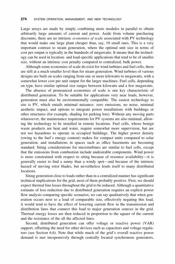
Large arrays are made by simply combining more modules in parallel to obtain

arbitrarily large amounts of current and power. Aside from volume purchasing

discounts, there are no intrinsic economies of scale associated with PV technology

that would make one large plant cheaper than, say, 10 small ones. This is a very

important contrast to steam generation, where the optimal unit size in terms of

cost per output is typically in the hundreds of megawatts. It means that the technol-

ogy can be used in location- and load-specific applications that tend to be of smaller

size, without an intrinsic cost penalty compared to centralized, bulk power.

Although some economies of scale do exist for wind turbines and fuel cells, these

are still at a much smaller level than for steam generation. Wind turbines of various

designs are built on scales ranging from one or more kilowatts to megawatts, with a

somewhat lower cost per unit output for the larger machines. Fuel cells, depending

on type, have similar optimal size ranges between kilowatts and a few megawatts.

The absence of pronounced economies of scale is one key characteristic of

distributed generation. To be suitable for applications very near loads, however,

generation must also be environmentally compatible. The easiest technology to

site is PV, which entails minimal nuisance: zero emissions, no noise, minimal

aesthetic impact, and options to integrate power installations with buildings or

other structures (for example, shading for parking lots). Without any moving parts

whatsoever, the maintenance requirements for PV systems are also minimal, allow-

ing the technology to be installed in remote locations. Fuel cells, whose benign

waste products are heat and water, require somewhat more supervision, but are

not too hazardous to operate in occupied buildings. The higher power density

(owing to the fuel’s energy content) makes for compact units compared to solar

generation, and installations in spaces such as office basements are becoming

standard. Siting considerations for microturbines are similar to fuel cells, except

that the emissions from combustion include undesirable components. Wind power

is more constrained with respect to siting because of resource availability—it is

generally easier to find a sunny than a windy spot—and because of the intrinsic

hazard of moving rotor blades, but nevertheless lends itself to many distributed

locations.

Siting generation close to loads rather than in a centralized manner has significant

technical implications for the grid, most of them probably positive. First, we should

expect thermal line losses throughout the grid to be reduced. Although a quantitative

estimate of loss reduction due to distributed generation requires an explicit power

flow analysis comparing specific scenarios, we can say qualitatively that when gen-

eration occurs next to a load of comparable size, effectively negating this load,

it would tend to have the effect of lowering current flow in the transmission and

distribution lines that connect this load to major generation sources in the grid.

Thermal energy losses are then reduced in proportion to the square of the current

and the resistance of the all the affected lines.

Second, distributed generation can offer voltage or reactive power (VAR)

support, offsetting the need for other devices such as capacitors and voltage regula-

tors (see Section 6.6). Note that while much of the grid’s overall reactive power

demand is met inexpensively through centrally located synchronous generators,


some portion of it must be injected locally, that is, near loads, in order to maintain an

acceptable voltage profile throughout the distribution system. If distributed gener-

ation can provide voltage support in a reliable manner such that other hardware

installations or upgrades can be avoided—for example, it might obviate the need

for a new capacitor bank, or it might reduce wear on a load tap changer—

there are systemwide economic savings. Realizing these savings requires that

the DG reliably coincides with demand, which tends to be true especially for

solar PV.11

Third, to the extent that distributed generation coincides with load, it tends to

reduce the demand on transmission and distribution capacity such as conductors

and transformers. Because this equipment has to be sized to accommodate the

peak, not average load, offsetting a small amount of load with distributed generation

during key hours can provide a significant relief for the T&D infrastructure. In areas

with substantial load growth, local generation can serve as an alternative to T&D

capacity, making it possible to avoid or at least defer capital intensive upgrades

(for example, the replacement of a substation transformer with a larger model)

while maintaining reliability.

Fourth, generation in the distribution system impacts protection needs and coor-

dination. This is generally regarded as a negative property, especially by utility

engineers faced with the challenge of adapting or redesigning circuit protection

to guarantee that any fault will be properly interrupted and cleared (see Section

6.7). The reason this can be problematic is that in the traditional radial system,

power flows in only one direction at the distribution level, from substation to

load, and the extant protection is designed and coordinated accordingly. Dis-

tributed generation introduces the radically new possibility of power flowing in

the other direction, and any section of line or piece of equipment therefore

being energized from the load side, on which there is no fuse or circuit breaker

to protect it. Beyond feeding power into a fault, this implies an electrocution

risk for utility line workers.12 This protection issue remains controversial in

the industry today. While manufacturers, owners, and advocates of DG tend to

feel confident that built-in protection features of the generation equipment

guarantee that it will separate from the grid in the event of any disturbance, utilities

typically require additional safety disconnect switches accessible only to their

crews.

11A second-order effect that is small but mentioned here for the sake of completeness is a reduction in

systemwide reactive losses due to distributed generation. As described in Section 7.2.5, reactive losses

represent the difference between the total reactive power Q injected to the grid at generator buses and

that withdrawn at load buses. Physically, this difference does not represent any actual energy like the

analogous I2R real power losses that are radiated into the air as heat. Nevertheless, reactive losses are

associated with some economic cost.12Note that the electrocution hazard is associated with voltage level, not necessarily the amount of power

provided by DG. For example, as long as a residential PV system remains connected to the grid by a

12-kV-to-120-V transformer, it energizes the primary side of that transformer with 12 kV regardless of

the fact that it could never by itself sustain the loads in the neighborhood. Thus, even a very small DG

installation could be deadly to line crews if not electrically isolated.


Another technical and controversial aspect of distributed generation is the

problem of control and availability. On the one hand, DG is generally nondispatch-

able, meaning that power system operators cannot call on it to provide power on

demand or at specified times. The resource may be intermittently available (solar

or wind) or controlled by the owner of the generation equipment; in either case,

the utility or system operator has no control over operating schedules. Indeed,

active centralized control over a large number of small DG units may be unrealistic

due to the sheer information and communications volume, unless it were completely

automated.

On the other hand, the lack of control is not necessarily problematic, because DG

can often be expected to coincide fairly well with local load. This is true in the case

of solar power in areas of summer-peaking demand, where the diurnal and seasonal

pattern of sunshine can match the utility demand profile almost perfectly. It also

tends to be true wherever customers use DG to meet their own demand or to

receive credit on net metering arrangements during peak demand hours when

utility rates are higher. To the extent that DG behaves in a predictable manner

and tends to level out rather than amplify load peaks, there is little reason for

active intervention on the part of system operators. Instead, they would tend to

consider DG as “negative load,” combining its statistical uncertainty with that of

the demand, which as a whole is also beyond operators’ direct control. Obviously,

this approach is sensible when the relative amount of DG in the system is small,

but may become problematic at some greater level of system penetration in the

future.

Last but not least among the systemic technical properties of distributed gener-

ation is that it would seem to reduce the grid’s vulnerability to sabotage. In part,

this is because any one smaller individual facility has less impact on the stability

of the power system as a whole, and thus would be less effective at causing broad

disruption (besides making a less attractive target in the first place). In part, too,

DG implies less reliance overall on long-distance transmission links, and therefore

would tend to reduce the scope of disruption caused by sabotage of individual

transmission lines or substations. In any case, DG introduces the possibility of

local self-sufficiency in power generation, which may dramatically reduce the

social impact of grid failures by making electricity available locally for vital

applications during a crisis.

DG also has institutional implications for power systems at large. As generation

is distributed geographically, it enters the jurisdiction of power distribution, as

opposed to transmission, where power plants traditionally interface with the grid.

For distribution engineers and operators, dealing with generation is a fundamentally

new responsibility—one, it might be noted, they cannot be expected to embrace with

unqualified enthusiasm, as it entails new demands, complexities, and failure possi-

bilities. Finally, there are important social and political dimensions of ownership of

resources and generation assets.

In sum, an electric power system with significant amounts of distributed

generation represents a radical departure from the centralized and strictly hierarch-

ical power system of the 20th century. Such a transition, which many analysts


consider all but inevitable, entails some important unanswered questions: while

it seems clear that the grid’s character is changing, it is not obvious what,

exactly, it is changing into.13

While the social and political aspects are beyond the scope of the present discus-

sion, we can identify some specific open questions about the grid’s evolution in the

face of distributed generation. One has to do with the problem of islanding, or

operating parts of the system while disconnected from others (see Section 6.1.4).

On the one hand, the option of islanding allows extracting the full benefit from

distributed generation resources, that is, supplying power locally while the rest of

the grid is unavailable. On the other hand, an interconnected system that could rou-

tinely operate with local or regional power islands—beyond individual customers

with self-generation who are carefully isolated from the distribution system—

represents yet another leap of technical and institutional transformation, with a

host of controversial aspects including safety, liability, accounting, and control.

Another issue of great practical consequence concerns the economic cost–benefit

analysis of distributed generation in relation to transmission and distribution

infrastructure. While it was suggested earlier that DG offers systemic savings (for

example, on line losses or T&D investments), it is not obvious how this information

can be used for strategic investment decisions when different corporate entities

pay out the capital and realize the savings, respectively. Even if markets or regu-

lation offer incentive mechanisms for DG, there remains the analytic problem of

comparing and trading off what are qualitatively different investments. Limited

experience exists in this area because, in vertically integrated and restructured

market environments alike, generation and transmission planning have almost

always been carried out by separate organizational entities, with separate accounting

and separate responsibilities for justifying investments. This problem also relates to

the economic evaluation of electric storage capacity within the context of the

grid. The kind of systematic and integrated three-way comparison of generation,

storage, and transmission capacity that one might imagine guiding the strategic

development of power systems is simply not yet part of the analytic arsenal

within the electricity sector.

Yet such an analytic framework will become crucial if future power systems

are to include increasing contributions from intermittent, renewable resources.

For example, we might want to compare the cost of solar thermal electricity pro-

duced at two locations with different weather and different transmission distances

to major loads, or that of a PV plant adjacent to a load with a fossil-fuel resource

some distance away. Alternatively, consider a region where wind is the cheapest

energy source available and supplies a substantial portion of local demand.

Here we might have to assess the maximum percentage of load that can be met

by wind power before it becomes too unpredictable, and then determine to

what extent the unpredictability ought to be compensated for by either

13This transformation is discussed in A. von Meier, “Integrating Supple Technologies into Utility Power

Systems: Possibilities for Reconfiguration” in Jane Summerton (ed.), Changing Large Technical Systems

(Boulder, CO: Westview Press, 1994).


introducing storage capacity, adding more expensive generation capacity from other

sources, strengthening transmission ties to other regions, or simply oversizing

the wind power plant. The analytic challenge for sensible decision making,

whether by market mechanism or an integrated planning entity, thus increases

with the introduction of distributed and intermittent resources because of a sensi-

tivity to time and geographic variables that 20th century technology simply did

not have.

How distributed generation technologies fare in view of these systemic chal-

lenges, parallel to their own intrinsic developmental hurdles, remains to be seen.

The results will have societal implications far beyond electric power, as the use

of distributed and renewable generation relates to diverse issues of resource scarcity,

environment, and the politics of ownership. With respect to technical control

issues, the role of DG will necessarily be intertwined with that of automation

technology, the subject of the following section.

9.2.3 Automation

Electric power systems today harbor a fascinating juxtaposition of old and new

technology. Finely tuned gas turbines and state-of-the-art inverters inject power

into the grid along with hydroelectric units dating back to the early 20th century.

The hardware of electric power systems represents some of the oldest industrial

machinery still in general use today. The fundamental task of transmission and dis-

tribution—that is, to connect pieces of conducting metal so as to form electric cir-

cuits—remains unchanged, as does a transformer’s job in stepping voltage up and

down. While advances have been made in the design and materials used in transfor-

mers, capacitors, and circuit breakers, the essential functions of these power system

components are stunningly simple. Synchronous generators also have experienced

only refinement, not fundamental changes of design. Many of today’s power

system components could be replaced with well-preserved models from the early

1900s without compromising their role in the grid.

The simplicity of the hardware, especially for T&D, stands in remarkable

contrast to the complexity of the system it constitutes. When the electric grid is con-

sidered as a whole that requires operation and coordination, it becomes a subtle and

sophisticated entity whose behavior and sensitivities are the subject of careful and

elaborate study. As the grid’s functioning has come under increased scrutiny

since the energy crises of the 1970s, the restructuring efforts of the new millennium,

and the occasional blackout, there is ever more incentive to tune its operation and

maximize its performance.

One key step toward streamlining or automating the operation of T&D systems

involves increased monitoring of circuit data by remote sensing along with

remote operation of equipment such as switches and circuit breakers to recon-

figure the system topology. This technology is known as supervisory control

and data acquisition (SCADA). The sensing and control nodes in the field may be

connected to a staffed control room by one of several types of communication

including dedicated telephone lines, microwave radio, or power line carrier


signals.14 SCADA has been implemented to various extents by U.S. utilities over the

past decades, first in transmission and subsequently at the distribution level. In its

absence, operators rely on field personnel to physically travel to each location in

order to report equipment status or undertake switching actions. Many areas,

especially rural distribution systems, are still operated in this manner.

It is interesting to note that without added communications systems, a trans-

mission or distribution operator has no way of determining whether customers are

connected or whether a problem has occurred somewhere in the field. Unless the

problem has proliferated to the level of a manned substation (say, by tripping a

circuit breaker), nobody but the customer might notice a local disturbance, as the

grid offers no intrinsic way of measuring from one location what is happening in

another. To reduce both the hazards of undetected faults and the duration of

service interruptions, many utilities have installed outage report systems that help

identify trouble spots by correlating customers’ telephone numbers with their

locations on the grid.

Beyond information gathering and remote control, a more radical or comprehen-

sive approach to automating power systems involves operation through expert

systems that either recommend actions to the operator (open-loop) or execute

them as well (closed-loop). Systems of various scope have been implemented or pro-

posed in power generation, ranging from straightforward automated mechanisms to

perform limited modifications (such as load following) to the highly controversial

substitution of computer systems for human decision making in hazardous places

like nuclear power plants.

In transmission and distribution, expert systems mean augmenting SCADA with

“intelligence” that allows for rapid computational analysis and thereby makes poss-

ible a more interventionist operating approach. For example, load balancing

involves reconfiguring distribution circuits in real time with the goal of increased

efficiency, as measured by reduced electric losses or greater asset utilization.

Another example is automated service restoration, where rapid data analysis and

execution of switching procedures can make for much reduced interruption times.

Despite the potential savings and performance improvements by means of such

expert systems, considerations of safety and human factors present significant

challenges to this type of innovation; these challenges are discussed further in

Section 9.3.

What seems certain at this time is that automation of various components of elec-

tric power systems will continue to see both lively debate and increased implemen-

tation. Aside from human factors, both the major justifications and the major

constraints on automation have been economic, with the bases for cost and

benefit calculations shifting rapidly. In general, as the cost of information decreases

in relation to the cost of energy, it makes ever more economic sense to carefully

14In communication by power line carrier, the information signal is simply superimposed onto the 60-Hz

power signal along the conductor. Having a smaller amplitude but much higher frequency, this signal is

readily isolated by equipment on the receiving end; nevertheless, the equipment must be designed to

safely interface with high voltage.


survey the grid and intervene in its operation through an increasing number of data

points and control nodes, deferring to computers where necessary to handle the

information volume or achieve the required reaction speed. In the context of DG,

the sheer volume of information and control opportunities associated with a

hypothetically large number of generators of diverse behavior would seem to

require some form of automation if resources are to be actively monitored,

coordinated, and their contributions optimized. It remains to be seen which areas

best lend themselves to the integration of information technology with extant and

new hardware, and how the overall character of power systems will change as a

consequence.

9.2.4 FACTS

Another dimension of automation in the case of transmission systems is the

direct modification of the grid’s properties with the aid of solid-state

technology—essentially, various types of transistors15 scaled up and combined to

handle large power applications—in a new category of hardware called flexible

a.c. transmission systems (FACTS). Transmission lines generally have physically

fixed parameters such as length and impedance that become firm constraints in

modeling and analysis. Other components such as transformers and capacitors

may have variable states or settings, but conventionally these settings are discrete

and require mechanical switching. FACTS technology offers ways to modify the

electrical characteristics of transmission components much more rapidly, even in

real time, so as to increase operating efficiency and relieve constraints without the

need for adding major hardware. FACTS devices include various types of reactive

compensation, phase shifting, and power flow control. The idea is to effectively

change the impedance of a given transmission link as seen by the system on an

instantaneous basis by means of an appropriately designed solid-state electronic

circuit.

For example, a long transmission line may have a stability limit less than its

thermal limit, meaning that no more than a certain amount of real power can be

transmitted along it without risking a loss of synchronicity between the generators

at either end (see Section 6.5.2). Conventionally, this limit poses a firm constraint

on permissible power flow scenarios. For instance, it could mean that generators

in location A must not inject more than a certain amount of power based on gener-

ation at B, lest the flow from A to B (specifically, the voltage phase angle difference

between A and B) become too great. The only way around the constraint would be

to upgrade the link with a larger or additional conductor that provides a lower

impedance. FACTS technology, by contrast, allows system operators to intervene

15A transistor is essentially a piece of semiconductor material that changes from a conducting to a non-

conducting state in response to a small voltage signal, making it act like an electrical switch. Because the

transition happens on the atomic level and involves no mechanical movement, it is not only very compact

but extremely fast, allowing circuits to be switched back and forth many thousands of times per second.

This process lies at the heart of information technology that represents data in terms of open and closed

circuits (0s and 1s).


directly by modifying the behavior of the transmission link in question: in this case,

a solid-state device would shift the voltage phase angle on the line between A and B

in such a way as to reduce the difference, despite the generators’ difference in pro-

duction. In essence, we could say that FACTS amounts to cheating the power flow

calculation by actively controlling flow along a particular link.

This should seem to contradict the basic principles emphasized throughout this

text, especially the notion that current and power flows are determined solely by

boundary conditions such as generation, load, and impedance, and are therefore

beyond our immediate control. But the key to achieving control lies in the time

dimension. In a conventional electric power circuit, we assume the properties of

the hardware components, including the connections among them, to be unchanging.

Solid-state technology, however, affords the ability to switch circuits around many

times within a single a.c. cycle. This means being able to strategically open and

close connections between elements such as transformers, inductors, or capacitors

that add or subtract a.c. waveforms at specific points during the cycle. As a result,

we can change the shape of a voltage wave (for example, to eliminate unwanted har-

monics or resonance), its timing or phase angle (as in the phase-shifting example

given earlier), its magnitude, or its relationship to current (in effect controlling

reactive power flow).

Since a growing variety of such devices is under development and initial deploy-

ment, FACTS technology suggests the possibility of a profound change in how

power systems operate. As with automation, the emphasis is on increased

information and control in lieu of larger hardware, with robustness giving way to

a more refined and interventionist approach to managing the grid. Also like auto-

mation, the implementation of FACTS is constrained by the relationship of

capital cost to operational gains. It will be interesting to observe its course over

the coming years.

9.3 HUMAN FACTORS

9.3.1 Operators and Engineers

This section characterizes some of the important differences between an academic

and a practical view of power systems.16 Specifically, it distinguishes between oper-

ations and engineering as two types of human expertise and activity that are essential

to the grid’s performance. The following is a summary of findings from research

conducted by the author that set out to explain differences of opinion about the

introduction of automation technology in distribution systems by examining how

different people conceptualize the power system as a whole.

A majority of readers, it is assumed, will be more familiar with engineering as an

activity and modeling framework. In the electric power industry, “engineering”

16Parts of this analysis have been previously published in A. von Meier, “Occupational Cultures as a

Challenge to Technological Innovation,” IEEE Transactions on Engineering Management 46(1):101–

114, February 1999.

9.3 HUMAN FACTORS 281

encompasses a great variety of specific job tasks. Engineers make design drawings,

calculate specifications, select components, evaluate performance, and analyze

problems. Their work has an important idealistic aspect, finding innovative solutions

and always striving to improve things. Some utility engineers are directly engaged

with physical hardware (for example, overseeing its installation); others work with

abstract models of the power system (for example, power flow analysis) or on its

indirect aspects (for example, instrumentation or computer systems). Those engin-

eers whose work is more remote from the field and of a more academic nature

best match the archetype of the present description.

Operators of technical systems, be they power plants, airplanes, or air traffic

control, must keep the system working in real time. In a thermal generation plant,

for example, operators have to assure that steam flows at a multitude of temperatures

and pressures between boiler, turbine, and condenser remain coordinated and in

balance with electrical load on the generator unit throughout a range of conditions.

In electric power transmission and distribution, operators monitor and direct

ongoing reconfigurations of their system of interconnected power lines and

components from switching stations and in the field. Unlike engineering, where

the object is to optimize performance, the goal in operations is to maintain the

system in a state of equilibrium or homeostasis in the face of external disturbances,

steering clear of calamities. An operating success is to operate without incident.

Depending on the particular system, maintaining such an equilibrium may be

more or less difficult, and the consequences of failure more or less severe.

Three types of challenges are generally characteristic of the operations job:

external influences, clustering of events, and uncertainties in real-time system

status. Especially in the case of power distribution systems, a large part of the

hardware is physically accessible and vulnerable to all kinds of disturbances,

whether they are automobiles crashing into poles or foxes electrocuting themselves

on substation circuit breakers. Events such as heavy storms or extreme loading

conditions entail cascading effects in the system and require a large number of

switching, diagnostic, and repair operations to be coordinated and carried out

under time pressure. At the same time, system parameters such as loading

status for certain areas or even hardware capabilities are often not exactly known

in real time. Operators are quite accustomed to working in this sort of situation,

and the way they view and imagine the electric grid, along with their values

and criteria for system performance, can be seen as specific adaptations to these

challenges.

9.3.2 Cognitive Representations of Power Systems

In the engineering framework, “the system” is considered as a composite of individ-

ual pieces, since these are the units that are readily described, understood, and

manipulated. The functioning of the system as a whole is understood as the result

of the functioning of these individual components: should the system not work,

the obvious first step is to ask which component failed. Engineering is therefore

analytic, not only in the colloquial sense of investigating a complex thing, but


analytic in the very literal sense of “taking apart,” or treating something in terms of

its separate elements.

Like any analytic process, engineering requires modeling, or representing the

actual physical system in abstracted and appropriately simplified terms that can

be understood and manipulated. Abstraction and simplification also requires that

the system elements be somehow idealized: each element is represented with its

most important characteristics, and only those characteristics, intact. An engineering

model will thus tend to consider system components in terms of their specified

design parameters and functions. Each component is assumed to work as it

should; components with identical specifications are assumed to be identical.

Similarly, the relationships among components are idealized in that only the most

important or obvious paths of interaction (generally the intended paths) are incorpor-

ated into the model. The parameters describing components and their interactions

are thought of as essentially time-invariant, and invariant with respect to conditions

not explicitly linked to these parameters.

The behavior of the system is thus abstracted and described in terms of formal

rules, derived from the idealized component characteristics and interactions.

These rules, combined with information about initial conditions, make the

system predictable: from the engineering point of view, it should be possible

in principle to know exactly what the system will do at any point in the

future, as long as all rules and boundary conditions are known with sufficient

accuracy. These rules also imply a well-understood causality: it is assumed that

things happen if and only if there is a reason for them to happen. Of course,

engineers know that there are random and unpredictable events, but in order to

design and build a technical system, it is essential to be able to understand

and interpret its behavior in terms of cause-and-effect relationships. Chains of

causality are generally hierarchical, like if–then decision-making systems. Sto-

chasticity is relegated to well-delimited problem areas that are approached with

probabilistic analysis.

In summary, then, the classic engineering representation of a technical system

can be characterized as abstract, analytic, formal, and deterministic. By contrast,

the operator representation of a technical system can be typified as physical,

holistic, empirical, and fuzzy. This representation is instrumental to operators in

two important ways: it lends itself to maintaining an acute situational awareness,

and it supports the use of intuitive reasoning.

Because operations involve much more immediate contact with the hardware,

system components are imagined as the real, physical artifacts in the way that

they are perceived through all the senses. For example, a particular overhead

distribution switch has a certain dimension, offers a certain resistance to being

moved, makes a certain noise, and shakes the pole in a certain way as it closes.

Even when looking at abstract depictions of these artifacts on a drawing or a

computer screen, operators “see” the real thing behind the picture. With all its phys-

ical properties considered, each artifact has much more of a unique individuality

than its abstract representation would suggest: one transformer may overheat

more than another of the same rating, or one relay may trip slightly faster than


another at the same setting. Thus, components that look the same on a drawing are

not necessarily identical to an operator.

To be sure, operators must also work with abstract representations. For distri-

bution operators, for example, this means primarily circuit maps and schematic

diagrams for switching. However, the abstractions they find useful and transparent

may differ from those preferred by engineers. While good maps for engineers are

those that do a thorough job of depicting selected objects and their formal relation-

ships, the most useful maps for experienced operators are those that most effectively

recall their physical image of the territory.

Another aspect of operators’ cognitive representation is that they conceptualize

the system more as a whole than in terms of individual pieces. Rather than con-

sidering the interactions among components as individual pathways that can be iso-

lated, the classic operator model is of one entire network phenomenon. Every action

taken somewhere must be assumed to have repercussions elsewhere in the system,

even if no direct interaction mechanism is known or understood. This is consistent

with operators’ experience, where they are often confronted with unanticipated or

unexplained interactions throughout the system.

Rather than using formal rules to predict system behavior, operators rely primar-

ily on a phenomenological understanding of the system, based on empirical obser-

vation. The underlying notion is that no number of rules and amount of data can

completely and reliably capture the actual complexity of the system. Therefore,

though one can make some good guesses, one cannot really know what will

happen until one has seen it happen. No component can be expected to function

according to its specifications until it has been proven to do so, and the effect of

any modification has to be demonstrated to be believed. While engineers would

tend to assume that something will work according to the rules, even if it did not

in the past, operators expect that it will work the way it did in the past, even if

analysis suggests otherwise. Many arguments between engineers and operators

can be traced to this fundamental difference in reasoning.

Finally, the operator representation is one that expects uncertainty rather than

deterministic outcomes. Whether due to the physical characteristics of the system,

insufficiency of available data, lack of a complete understanding of the system, or

simply external influences, uncertainty or “fuzziness” is taken to be inevitable

and, to some degree, omnipresent. Ambiguity, rather than being subject to confine-

ment, is seen to pervade the entire system, and operators suspect the unsuspected

at every turn. Thus, distribution operators have described their system as a “live,

undulating organism” that must somehow be managed.

This physical, holistic, empirical, and fuzzy view of the system is adaptive to the

challenge of operating the system in real time in that it allows one to quickly con-

dense a vast spectrum of information, including gaps and data pieces with different

degrees of uncertainty, into an overall impression or gestalt that can be consulted

with relative confidence to guide immediate action.

Finally, operators tend to draw on intuitive reasoning, especially when data are

insufficient but action is required nonetheless. Although there are manuals specify-

ing operating procedures, many situations occur that could not have been foreseen

in detail and courses of action recommended. To deal with the problem at hand,


analytic tools may not be able to provide answers quickly enough. Worse yet,

information on the books may be found to be untrustworthy under the circum-

stances; for example, if recent data appear to contradict what was thought to be

known about the system. In order to come to a quick decision, the operator’s

main recourse then is to recall past experience with similar situations. How did

the system behave then? Were people surprised? How did the particular equipment

respond? Based on such experience, an operator will have an intuitive “feel” for the

likelihood of success of a given procedure.

This experience-based approach is intuitive not because it is irrational, but

because it is nonalgorithmic. An operator might have difficulty articulating all the

factors taken into consideration for such a decision, and how, precisely, they were

mentally weighed and combined. He or she might not be able to cite the reasons

for feeling that something will work or not work. Nonetheless, the decision

makes use of factual data and logical cause–effect relationships, as they have

been empirically observed.

The use of intuitive processes is so deeply embodied in the culture of operations

that they are often chosen over analytic approaches by preference rather than

necessity. Obviously, both methods can fail; the question is about relative degrees

of confidence. While engineers may frown on operator justifications that seem

based on intractable, obscure logic or even superstition, operators delight in offering

accounts of situations where their intuition turned out to be more accurate than an

engineer’s prediction. In fact, both approaches are adaptive to the work contexts

of their proponents, and while both have a certain validity, either approach may

turn out to yield better results in a given situation. The important point here is

that substantive differences in cognitive representations and reasoning modes

underlie what may appear to be trivial conflicts or petty competition between cul-

tural groups. These differences will also have specific implications for the evaluation

of system design, operating strategies, and technological innovations.

9.3.3 Operational Criteria

The most important general properties of technical systems, or goals and criteria for

evaluating their performance, can be summarized as efficiency, reliability, and

safety. These goals tend to be shared widely and across subcultures throughout an

organization managing such a system. However, individuals or groups may hold

different interpretations of what these general goals mean in practice and how

they can best be realized. Accordingly, they will also have different expectations

regarding the promise of particular innovations.

When there are trade-offs among safety, reliability, and efficiency, cultural

groups may also emphasize different concerns, not only because they have different

priorities, but because they have different perceptions of how well various criteria

are currently being met. In the academic engineering context, it is often assumed

that certain standards of safety and reliability have already been achieved, and the

creative emphasis is placed on improving efficiency. In the case of power

systems, safety and reliability are problems that were academically solved a


long time ago, whereas new approaches to increase efficiency offer a continuing

intellectual challenge.

The efficiency criterion thus takes a special place in engineering. Efficiency

here can be taken in its specific energy-related sense as the ratio of energy or

kilowatt-hour output to energy input, or in a more general sense as the relationship

of output, production, or benefit to input, materials, effort, or cost. Efficiency is

often a direct performance criterion in that its numerator and denominator are

crucial variables of interest that appear on the company’s “bottom line” (for

example, electric generation and revenues). Even where efficiency measures

something more limited or obscure (for example, how many man-hours are required

for service restoration), a more efficient system will generally be able to deliver

higher performance at less cost while meeting the applicable constraints.

Conversely, low efficiency indicates waste or the presence of imperfections that

motivate further engineering. A more efficient system will also be considered

more elegant: beyond all its practical implications, efficiency is an aesthetic

criterion.

In addition, there is a set of indirect or supporting criteria that, according to the

cognitive framework of engineering, advance efficiency as well as safety and

reliability. While these criteria can be taken as qualitative standards for the

system as a whole, they also apply in evaluating technological innovations and

judging their promise. One such criterion is speed. It is an indirect criterion

because it does not represent an actual need or an immediate, measurable benefit.

However, the speed of various processes offers some indication of how well the

system is theoretically able or likely to succeed in being efficient. Generally, a

system that operates faster will involve less waste. For example, restoring service

more quickly means less waste of time, waste of man-hours, and waste of potential

revenues. Responding and adapting to changes faster can also mean higher effi-

ciency in terms of improved service quality or saved energy. Given the choice

between a slow- and a fast-operating device, all else being equal, most engineers

would tend to prefer the faster one.

Similarly, precision is generally considered desirable in engineering culture.

Actually, the desired criterion is accuracy: not only should information be given

with a high level of detail, but it should be known to be correct to that level. Accurate

measurements of system variables allow for less waste and thus support efficiency;

they also further safe and reliable operation. However, the accuracy of a given

piece of data is not known a priori and is subject to external disturbances, while

its degree of precision is obvious and inherent in design (e.g., the number of

significant figures on a digital readout). Precision can be chosen; accuracy cannot.

Although precision does not guarantee accuracy, it at least provides for the possi-

bility of accuracy and is therefore often taken in its place (and sometimes confused).

Given the choice between a less and a more precise indicator of system parameters

or variables, most engineers would prefer the more precise one.

More fundamentally, information in and of itself is desirable. Generally, the more

information is available, the better the system can be optimized, and information can

in many ways advance safety and reliability as well. In the event that there are


excess data that cannot be used for the purpose at hand, the cost to an engineer of

discarding these data is typically very low: skipping a page, scrolling down a

screen, or ignoring a number is no trouble in most engineering work. In selecting

hardware or software applications, all else being equal, most engineers would

prefer those offering more information.

Finally, the ability to control a system and its parts is another indication of how

successfully the system can be engineered, managed, and optimized. This is because

any variable that can be manipulated can also, in principle, be improved. As with

information, in the engineering context, there is hardly such a thing as too much

control. If the ability to control something is available but not needed, the engineer

can simply ignore it. Most engineers would prefer to design systems and choose

components that are controllable to a higher degree.

This set of criteria suggests a general direction for technological innovations that

would be considered desirable and expected to perform well. Specifically, from the

viewpoint of engineering, innovations that offer increased operational speed, pre-

cision, information, and control appear as likely candidates to further the overall

system goals of efficiency, reliability, and safety. While such expectations are

logical given the representational framework of engineering, the perspective of

operations yields quite a different picture.

Of the three general system criteria—safety, reliability, and efficiency—safety

takes a special priority in operations, while efficiency is less of a tangible

concern. From the point of view of managing the system in real time, efficiency

is an artifact of analysis and evaluation, a number tagged on after the fact, having

little to do with reality as it presents itself here and now. Although it may indicate

operating success, efficiency more directly measures the performance of engineers.

Most operators would agree that having an efficient system is nice, as long as it does

not interfere with their job.

Safety, on the other hand, takes on a profoundly tangible meaning for operators

because the consequences of errors face them with such immediacy. In power

systems, any single operation, performed at the wrong time, has the potential to

cause customers to lose power. Immediately, telephones will ring, voices on the

other end will shout and complain, and the control room may even fill with

anxious supervisors. Because of the interdependence of power system components,

the consequences may occur on a much larger scale than the initial error. Aside from

causing power outages, incorrect switching operations can damage utility and

customer equipment.

But even more serious is the risk of injury or death. Any steam generation plant,

for example, harbors the intrinsic hazard of water vapor at up to 10008F and several

hundred atmospheres of pressure; it is difficult to stand next to a roaring

primary steam valve without sensing that the smallest leak could be instantly

fatal. In transmission and distribution, the risk of electrocution looms for utility

crews as well as others who might be accidentally in contact with equipment (for

example, people in a car under downed power lines). The one action T&D operators

dread most in the course of switching operations is to energize a piece of equipment

that is still touching a person. Like operators of other technical systems, they carry a


personal burden of responsibility for injuries or fatalities during their shift that

goes far beyond their legal or procedural accountability. The difference between

an intellectual recognition and the direct experience of the hazards cannot be

overemphasized: hearing an accident described is not the same as watching one’s

buddy die in a flash of sparks a few feet away, with the smell of burning flesh.

This immediate awareness of the life-taking potential of system operation is omni-

present among operators of power systems and implicitly or explicitly enters any

judgment call they make, whether about day-to-day procedures or about implement-

ing new technology.

Their acute perception of safety colors operators’ interpretation of other system

goals and helps define their criteria for good system design and performance. The set

of criteria—speed, precision, information, and control—that, from the engineering

perspective, support not only efficiency but also safety and reliability may be seen

by operators as less important or even counterproductive. Instead, operators value

a different set of criteria that specifically support their ability to operate the

system safely.

Speed, generally advantageous in engineering, is more problematic in operations

because one is working in real time. Speed is desired by operators in the context of

obtaining information. They may also wish for their actions to be executable

quickly, so as to gain flexibility in coordinating operations. However, a system of

fast-responding components and quickly-executed operating procedures, where

effects of actions propagate faster and perhaps farther, also introduces problems:

it will tend to be less tractable for the operator, provide less time to observe and

evaluate events and think in between actions, and allow problems to become

more severe before they can be corrected. Power systems are inherently fast in

that electric effects and disturbances propagate at the speed of light, making cas-

cades of trips and blackouts practically instantaneous. Any delays or buffering of

such effects work toward the operator’s benefit. Thus, from the perspective of

operations, stability is generally more desirable than speed. Operators would

prefer a system that predictably remains in its state, or moves from equilibrium

only slowly, allowing for a greater chance to intervene and bring it back into

balance.

Information can also be problematic in the context of operations. To be sure,

there are many examples of information that operators say they wish they had, or

had more of. But more is not always better. Because one is gathering information

and acting upon it in real time, the cost of discarding irrelevant information is not

negligible. Deciding which data are important and which are not costs time and

mental effort; superfluous data may distract from what is critical. Specifically, too

much data may interfere with operators’ acute situational awareness. Operators

often give examples of information overload: many computer screens that must

be scanned for a few relevant messages, or many pages of printout reporting on a

single outage event. Generally, instead of greater quantity of information, operators

desire transparency, meaning that the available information is readily interpreted

and placed into context. It is more important for them to maintain an overview

of the behavior of the whole system than to have detailed knowledge about its


components: in terms of maintaining situational awareness, it is preferable to lack a

data point than to be confused about the big picture even for an instant. If more infor-

mation has the potential to create confusion, then for operators it is bad.

Suppose, for example, that a computer screen is to display real-time measure-

ments from throughout the system to operators in a control room. One option

might maximize information delivery, say, providing constantly updated figures

from 100 sensor nodes. In a situation where all 100 data points are equally likely

to be relevant, where it is important that no detail be missed, and where the data

need not be processed and acted upon with great time pressure, this may be most

desirable. By contrast, suppose that much of this information is irrelevant to

decisions that must be made very quickly. Here it may be appropriate to reduce

the amount of information in the interest of transparency, for example, by limit-

ing the number of points reported, or by displaying only those that changed

recently. The idea is that data should quickly and correctly characterize the situation

behind the numbers, even at the expense of breadth or depth.

Similarly, more precision is not always better for operators. While engineers can

make use of numbers with many significant digits, the last decimal places are

probably not useful for guiding operating decisions. In fact, operator culture

fosters a certain skepticism of any information, especially quantitative. This skepti-

cism is consistent with their keen awareness of the possibility of foul-ups like

mistaking one number for another, misplacing a decimal point, or trusting a faulty

instrument, and the grave potential consequences. Therefore, operators’ primary

and explicit concern about any given numerical datum is whether it basically tells

the true story, not how well it tells it. Moreover, precision can be distracting or

even misleading, suggesting greater accuracy than is in fact given. Thus, in

operations, veracity of information is emphasized over precision. Rather than

trusting a precise piece of information and running the chance of it being wrong,

operators would generally prefer to base decisions on a reliable confidence interval,

even if it is wide.

The difference between precision and veracity is that precision offers a narrow

explicit margin of error, while veracity offers confidence that the value in question

truly lies within that margin, and that the value really represents that which it is

assumed to represent. Suppose one measurement is taken with a crude and foolproof

device, while another is displayed by a sophisticated monitoring network. The latter

offers more precision, and yet the skeptic may wonder: Is it possible that the

instrument is connected to the wrong node? Could the display be off by an order

of magnitude? Or might it be telling me yesterday’s value instead of today’s?

And if so, would there be any discernible warning? If someone’s life depended

on our correct estimate of a quantity, we would prefer the former, more reliable

measurement, even though it is less precise.

Finally, more control is not always better. Of course, there may be variables over

which operators wish they had more control. But the crucial difference is that in

engineering, control always represents an option, whereas in operations there may

be an associated responsibility to exercise this control: the ability to control a vari-

able can create the expectation that it should be controlled, and produce pressure to


act. Operators tend to be wary of such pressure, primarily because it runs counter to a

basic attitude of conservatism fostered by their culture: When in doubt, do not touch

anything. Their reluctance to take action unless it is clearly necessary arises from the

awareness that any operation represents a potential error, with potentially severe

consequences. An interventionist approach that may allow greater optimization

and fine-tuning thus inherently threatens what operators see as their mission,

namely, to avoid calamities.

In pragmatic terms, more controlling options may mean that operators have more

to do and keep in mind, and thereby increase stress levels. Alternatively, they may

not have time to exercise the control at all, in which case their performance will be

implicitly devalued by the increased expectation. Because time and attention are

limited resources in operations, and because of the potential for error associated

with any action, the option not to control can be more desirable than the ability to

control. This option is provided by a system’s robustness, or its tendency to stay

in a viable equilibrium by itself.

Suppose that a technological innovation gives operators the ability to control

some system parameter (voltage, for example) within a narrower band, closer to

the desired norm. The potential downside of this innovation has to do with the fol-

lowing question: What happens if, for whatever reason, the control option is not

exercised? For example, is the parameter liable to drift farther outside of the

normal range if it is not actively controlled? In doing so, does it pose a safety

hazard? Does the new technology raise expectations for system performance,

leading to disappointment if control actions are not taken in the manner envisioned

by system designers? Will pressure to exercise control options create extra work for

operators? By contrast, robustness and stability characterize a situation where things

will be fine without active intervention.

Another example of efficiency versus robustness in the power distribution context

is the handling of load peaks in view of limited equipment capacity. An “efficient”

approach might call for transferring loads in real time among various pieces of

equipment so as to achieve the most even distribution and avoid overloading any

one piece. This approach both maximizes asset utilization (and may even help

avoid capacity upgrades to accommodate demand growth) and minimizes the

inefficiency due to lines losses (since collective I2R losses increase with uneven

allocation of current among lines). Its success hinges, however, on constant vigi-

lance and intervention. By contrast, a “robust” approach would emphasize strength

and simplicity: the idea is simply to have enough extra capacity built into the equip-

ment so that overloading is not an issue, and loads need not be tracked so carefully.

In summary, then, the system qualities that are most important for operators are

stability, transparency, veracity, and robustness, which support them in their task of

keeping the system in homeostasis. Not coincidentally, these criteria are generally

associated with older technologies, designed and built in an era where operability

by humans was more of a firm constraint than material resources. In power

systems, stability and robustness were provided largely by oversized equipment

and redundancy of components, while transparency and veracity were furnished

through simple mechanical and analog instrumentation and controls. From the


viewpoint of increasing the efficiency of such systems in today’s world, process

innovations guided by engineering criteria may be desirable indeed. From the oper-

ations perspective, however, such innovations may be expected to adversely affect

performance reliability and especially safety. Thus, when steps are proposed toward

more refined and sophisticated system operation, operators may identify potential

backlash effects, in which opportunities for system improvement also introduce

new vulnerabilities.

9.3.4 Implications for Technological Innovation

The cognitive representations used by engineers and operators, respectively, give

rise to different ideas about what system modifications may be desirable, and diver-

gent expectations for the performance of innovations. If one imagines a technical

system in terms of an abstraction in which interactions among components are

governed deterministically by formal and tractable rules, then (1) these formal

relationships suggest ways of modifying individual system parameters so as to

alter system performance in a predictable fashion according to desired criteria,

and (2) it is credible that such modifications will succeed according to a priori analy-

sis of their impacts on the system. From this point of view, innovative technologies

hold much positive promise and little risk.

On the other hand, if one imagines the system as an animated entity with uncer-

tainties that can never be completely isolated and whose behavior can be only

approximately understood through close familiarity, then (1) modifications are

inherently less attractive because they may compromise the tractability and

predictability of the system, and (2) any innovation must be suspected of having

unanticipated and possibly adverse consequences. From this point of view, efforts

to modernize or automate may imply an attempt to squeeze the system into a con-

ceptual mold it does not fit—treating an animal like a machine—and thus harbor the

potential for disaster.

This is not to suggest that modernization efforts are ill-advised or necessarily

conflict-ridden. Indeed, there are many examples of operators welcoming if

not actively campaigning for improved and more efficient information and control

technology. The preceding observations suggest that when concerns about

technological innovation do arise, they may be based on legitimate professional

considerations.

Consider the example of SCADA at the distribution level. Traditionally,

distribution operators sitting in the control room at the distribution switching

center have relied on their field crews as the main source—and sometimes the

only source—of information about system status, whether switches (open or

closed), loads (current through a given line or transformer), voltage levels, or the

operating status of various other equipment (circuit breakers, capacitors, voltage

regulators, etc.). The operators’ lifeline to information has been the telephone or

radio through which his “eyes and ears” in the field communicate. By the same

method, operating orders (often written out in hardcopy beforehand) are verified,

or modified orders communicated if necessary. The introduction of SCADA


implied a transition from operating through field personnel to directly accessing the

system via a computer terminal in the control room. The advantages are obvious:

fewer man-hours are needed to execute a given procedure; things can be done

much faster; the computer affords a clear, central overview—in short, the entire

operation, still largely based on 19th- and early 20th-century technology, finally

comes into the electronic age.

Nevertheless, the implementation of SCADA in the utility industry has not been

entirely unproblematic. While many distribution operators are quick to point out the

advantages of SCADA and indeed find it difficult to imagine how anyone ever

worked without it, some have also offered critiques. The main areas of concern

relate to safety (is the computer correct in reporting an open switch?), physical sur-

veillance (sacrificed chances to discover any developing problems early on in site

visits), time pressure (not having time to think while waiting for field crews to

execute orders), loss of redundancy (not necessarily having a second person review-

ing steps), and the loss of situational awareness (such as that afforded by audible

communication among operators, as opposed to silent interaction with computer

terminals).

As a result of such concerns, even when new information and control technology

is successfully installed, operators may not always choose to make full use of the

available capabilities. This must be expected especially if the technology

pertains to a more automated operation that may threaten to make the system less

stable, transparent, verifiable, and robust to operators. The key to successful

innovations seems to be ample consultation and discussion across occupational

and cultural groups, so as to make both engineering and operating concerns clear

to all parties in the design process.

9.4 IMPLICATIONS FOR RESTRUCTURING

As of this writing, the most passionately debated subject in the field of power

systems is the restructuring of the electric industry: the transition from a regulated,

vertically integrated monopoly—the utilities of the 20th century—to some form of

competitive marketplace for electricity. This can involve any aspect of production,

delivery, and consumption, though the focus until now has been primarily on whole-

sale energy. While the tone of the debate often suggests a battle between two

absolute alternatives—pure regulation versus pure market—every arrangement for

the buying and selling of electric power to date has in fact been some hybrid of

approaches, whether by economic incentives embedded within the regulated

system or by governmental definition of market rules and boundary conditions.

With efforts to deregulate electricity underway in the United States and abroad,

there exists a growing literature on the merits and failings of various market

designs, or ways of achieving a contemporary and effective hybridization. The

one thing on which experts tend to agree is that the consequences to society,

whether favorable or unfavorable, are important, profound, and potentially


far-reaching—so important that it is difficult to imagine publishing a text on electric

power systems without mention of market restructuring.

Yet it also seems impossible to do the subject justice in the context of a technical

reference book. Because electricity is such a central and indispensable part of our

culture, the restructuring debate is about much more than kilowatt-hours and

dollars. Our choice of means and institutions for dealing with electricity has to do

with very fundamental and contentious questions about how society and business

ought to be organized. A key set of questions concerns the extent to which com-

petitive markets can produce socially optimal outcomes, what constitutes market

failures, and when and how government intervention is required. At stake in the

debate is an entire weltanschauung about appropriate roles of public and private

sector, or degrees of faith in the “invisible hand” of the marketplace, issues

obviously beyond the scope of this text.

This section aims for a compromise by outlining some of the intrinsic difficulties

of electric power with respect to market function. Because of its physical nature and

the attendant technical constraints in its production and distribution, electricity is not

a commodity (like wheat, pork bellies, or petroleum) that one would find in the econ-

omics textbook. In an ideal competitive market, the intersection of demand and

supply curves yields an equilibrium price and quantity at which the market clears

and which, in theory, maximizes social utility or overall benefit to participants.

The central requirement of such a market is that demand and supply can vary

freely with respect to price. Yet for several reasons such a condition is very tricky

to achieve in the case of electricity.

Demand for electricity tends not to respond very much to price signals—in tech-

nical terms, the price elasticity of demand is low—in part simply because electricity

is so indispensable to our economy and our everyday lives. People and businesses

are organized around being able to consume electricity at any time they choose,

and many are willing to pay a considerable amount of money in order not to have

their service interrupted.

Demand elasticity is further limited by institutional and technical factors. The

entire planning and design philosophy of power systems and regulated utilities in

the 20th century presumed that electricity should be available to anyone in essen-

tially arbitrary amounts around the clock, at a known and fixed price deemed reason-

able by public regulators. Electric load was defined as the independent variable

whose satisfaction became the central objective of technical, organizational, and

regulatory efforts throughout the power industry. Consumers only experienced

rate changes on the time scale of years, from one utility rate case to another,

rather than a “price signal” according to the much more rapid fluctuations of

actual marginal generation cost. In many deregulated markets, consumers continue

to be shielded from short-term price volatility and therefore receive no direct

incentive to respond to power shortages by lowering their demand during critical

hours, thereby making demand almost perfectly inelastic with respect to varying

wholesale prices.

The ideal market solution would be to introduce real-time pricing or related

incentive mechanisms to encourage electric demand response. Such programs

9.4 IMPLICATIONS FOR RESTRUCTURING 293

may involve communication only or include direct control, either inviting a certain

customer behavior or physically disconnecting designated loads under specific

conditions. Demand response can be considered an extension of well-established

mechanisms such as time-of-use rates that discriminate among predetermined

on- and off-peak periods, or interruptible tariffs available primarily to larger

customers willing to trade service continuity for reduced rates.17 Nevertheless, gen-

eralizing such responsiveness with the expectation of routine implementation in real

time for many small and diverse customers represents a considerable innovation.

Fundamentally, demand response means turning upside down a century-old

design philosophy and requires addressing a broad set of factors ranging from

customer behavior, education, and economic preferences to control hardware, infor-

mation management, and communications protocols—factors that had no reason to

be considered in electric power systems until very recently. Thus, while it seems

plausible in theory to imagine aggregate electric demand as a well-behaved function

of price, such a transition in practice requires new ways of thinking as well as a new

generation of technology.

The supply side harbors equally if not more serious challenges. A competitive

market according to the economics textbook requires free entry and exit of firms

in response to scarce or excessive supply. Yet in practice, market entry and exit

are impeded by capital intensity, transaction costs, and construction schedules of

generation projects.

The capital-intensive nature of electric generation along with economies of scale

and a measure of risk make this industry intrinsically uninviting for smaller

businesses. In theory, it should be possible for any entrepreneur to join the fray

and supply kilowatt-hours when the market signals that they are needed. Yet in

practice, the initial investment is too large and near-term profits too unpredictable

for many small, independent companies to participate.

Interconnection arrangements, too, may be cumbersome if not prohibitive for

small producers. Under direct access, an arrangement aimed at fostering compe-

tition in the generation sector while preserving a T&D monopoly, any generator

can in principle avail themselves of the extant infrastructure by injecting electric

power to be consumed by a purchaser elsewhere. However, the transaction costs

of becoming an electricity seller through the grid are not negligible and may

include fees, bureaucratic procedures, and special equipment to interface with the

utility on its terms. At the same time, it remains illegal anywhere in the United

States to run independent lines from a supplier to a consumer—say, a wire from

my rooftop PV system to my neighbor across the street.18

17This is analogous to airline passengers accepting payment in return for yielding their seats on an over-

booked flight, except that the electric customer faces only the possibility, not the certainty of interrupted

service. Indeed, anecdotal evidence suggests that customers on interruptible tariffs are often surprised and

dismayed when an interruption actually occurs.18This restriction has been motivated by safety as well as the intention to avoid the inefficiency of dupli-

cating infrastructure, though it is also arguably the greatest barrier to a truly competitive electricity

market. One might imagine that the proliferation of distributed generation technologies could challenge

this status quo; if so, it would amount to nothing short of a radical reinvention of “the grid” as we know it.


Finally, the time scale on which conventional power plants are planned, built, and

licensed makes it all but impossible for new generation capacity to appear in

response to acute shortages. And because existing generation facilities cannot arbi-

trarily increase output beyond their rated capacity,19 the supply curve, too, becomes

more and more inelastic as the number of megawatts approach the system capacity

limit.

Not only is the quantity of supply constrained, so is the grid’s ability to transmit

it to the desired location. With increased utilization of transmission capacity and

long-distance sharing of generation resources, transmission congestion has

become as important as generation in limiting the available supply for many

areas. At the same time, upgrading transmission capacity tends to be slow, expens-

ive, and politically contentious, so that bottlenecks are not readily relieved by simply

constructing more power lines. And congestion cannot be made to go away by

administratively or economically “rerouting” power: as the previous chapters

have emphasized, electric power flow obeys only physical law; it is difficult

enough to predict, let alone control and direct. Therefore, the quantity of interest

in electric markets is not just aggregate supply (as it would be in the market for a

readily interchangeable and transportable commodity), but available supply to

any given region that would need to respond to price signals in a truly competitive

market.

As various designs for electricity markets have been discussed and tried, a central

concern has been the potential exercise of market power by sellers. The question

is whether market participants are price takers as in the textbook, or whether by

their individual actions they have the power to influence the market clearing price

and thereby manipulate outcomes in their favor—gaming the market. Anyone

who has followed the news about the California electricity crisis and its political

fallout is aware that gaming is possible; the interesting question is what factors

enable or prevent it. It would stand to reason that as long as no individual supplier

holds too large a market share, they cannot exercise market power. But because of

the particular properties of the electric grid, “too large” could be a very small per-

centage. The extreme inelasticity of demand and supply as the system nears its limits

makes it vulnerable to the withholding of even small amounts of generation

capacity.

Moreover, because line flows are sensitive to the amount of power injected at

specific locations, generation capacity can be used strategically not only to relieve

but, in the case of unabashedly profit-maximizing firms, to deliberately create trans-

mission congestion.20 The unique problem here lies both in the utter dependence of

the entire system on limited transmission assets and the subtlety of predicting

power flow. The effect of generation at a given node on congestion at a certain

19It is quite possible for an electric generator to exceed its nameplate rating at the expense of equipment

life span. Nevertheless, every generation unit ultimately encounters a firm, nonnegotiable physical limit

on the amount of power it can deliver.20Transmission congestion may raise regional wholesale prices, of which a company or financial interest

group can take advantage if they also own generation facilities located in that region.


link is sometimes obvious from geography, in which case most experts agree that

some form of regulatory intervention is warranted to prevent abuse of this

information. At other times, it remains the subject of speculation, keen interest by

calculating firms, and careful guarding by transmission system operators. The resul-

tant paradox is that key information about the system must be withheld rather than

openly shared in the interest of competitive market function, which is precisely the

opposite of what standard economics would suggest.

Considering market equilibrium in the broader context of maximizing social

utility, an additional problem pervades the energy sector: the external costs of

many of its components, primarily the environmental impacts of various generation

sources, that fail to be included in the apparent costs of production and consumption.

This problem is not unique to the restructured industry, but has been grappled with in

the context of regulated utilities since the 1970s and 1980s. Economists generally

agree that the presence of such externalities warrants regulatory intervention in

the form of financial incentives or explicit requirements to internalize these costs

in the market, so as to allow participants to make decisions based on correct price

signals. The “correct” price would then promote activities known to produce

social benefit while discouraging those with hidden costs to society. Examples of

such intervention range from portfolio standards for clean, renewable generation

resources to publicly funded campaigns to promote energy efficiency. While

analysts differ considerably on the type and extent of methods favored, it seems

quite clear that externalities will need to be confronted in any future market design.

This list of problems does not rule out the successful application of market

mechanisms to electricity in principle. Rather, it emphasizes that, owing to their

technical characteristics and the reality of their present design, electric power

systems pose serious, intrinsic challenges to the balancing of supply and demand

at an equilibrium price and quantity. Without passing judgment on the ultimate

possibility of overcoming them, it is fair to say that these challenges ought not to

be underestimated. Moreover, appreciation of the inherent difficulties suggests par-

ticularly careful and explicit consideration of what is to be gained by restructuring

the electric power industry.

Ultimately, a crucial problem in this regard concerns equity. Electric power

systems have historically served as instruments for the reallocation of significant

amounts of wealth across society—not in a revolutionary way but very much in

line with cultural norms, like the graduated income tax. In the 1930s, federally

subsidized rural electrification brought villages and farms onto the grid that never

could have been connected economically, as revenues from these accounts clearly

would not pay for the infrastructure investment. In fact, many of those rural areas

might have been far more cost-effectively supplied with local sources such as

wind power. But the electric grid was designed to reach out even to customers

who were expensive to serve, while splitting the price tag among everyone. In

this way, urban customers continue to subsidize rural customers, and large commer-

cial and industrial customers, who are much less expensive to serve on a per-kWh

basis, continue to subsidize smaller customers under regulated utility rates. A key

impetus for deregulation has been the desire of such larger customers to procure


less expensive electricity on their own through open market access, prompting con-

siderable argument as to their obligation to share the cost burden of past utility

investments. The debate about electric industry restructuring is thus very much

about what is fair, who pays how much, and how society should decide.

The historical dimension brings to light just how much the complex technical

system we call “the electric grid” is a social artifact as much as a fascinating incarna-

tion of physics and engineering. We can view the electrification of industrial society

not only as a logical result of technical and economic driving forces, but as an

embodiment of ideas and values. The idea of connectedness in and of itself rep-

resented the sophistication and unity of an advanced, civilized society; being “on

the grid” meant not only receiving electrons, but being part of progress in the

modern world. By the same token, living “off the grid” today often implies indepen-

dence, self-sufficiency, and sometimes environmentalism. Historically, the idea of

equal access to the grid has represented a fundamental sense of social equality,

with electricity considered not a privilege affordable to some but an entitlement

of all citizens. As electric power systems evolve with new technologies and new

organization, they will continue to embody social values, explicit or implicit. The

better and the more widely electric power systems in all their complexity are under-

stood, the greater the opportunity for people to guide this evolution with awareness

and conscious choice.


&APPENDIX

Symbols, Units, Abbreviations,and Acronyms

A ampere unit of current

A.C., a.c. alternating current

ACE area control error

AGC automatic generation control

AM amplitude modulation

amp ampere unit of current

ASD adjustable speed drive

B symbol for magnetic flux density

B, b symbol for susceptance

BTU British thermal unit, unit of energy

C, c symbol for capacitance

C coulomb unit of charge

CAES compressed-air energy storage

CAISO California Independent System Operator

cal calorie unit of energy

CHP combined heat and power

CVR conservation voltage reduction

D.C., d.c. direct current

DG distributed generation

e natural logarithm base, 2.71828. . .E, e symbol for voltage

E symbol for electric field

ELF extremely low-frequency fields

emf electromotive force

EMF electromagnetic fields

erg unit of energy

EUE expected unserved energy

F symbol for force

F farad unit of capacitance

f symbol for frequency

298


FACTS flexible a.c. transmission systems

FM frequency modulation

G, g symbol for conductance

G gauss unit of magnetic flux density

GFCI ground-fault circuit interrupter

GMD geometric mean diameter

GMR geometric mean radius

H henry unit of inductance

H symbol for magnetic field strength

hp horse power

Hz hertz unit of frequency

i imaginary number,ffiffiffiffiffiffiffi�1

p

I, i symbol for current

ISO independent system operator

j imaginary number,ffiffiffiffiffiffiffi�1

p

J joule unit of energy

KCL Kirchhoff’s current law

KVL Kirchhoff’s voltage law

kV kilovolt unit of potential difference, 1000 volts

kVA kilovolt-ampere unit of apparent power

kW kilowatt unit of power, 1000 watts

kWh kilowatt-hour unit of energy

l symbol for length

L, l symbol for inductance

LCD liquid crystal display

LDC load duration curve

LED light-emitting diode

LOLE loss-of-load expectation

LOLP loss-of-load probability

LTC load tap changer

mmf magnetomotive force

MRI magnetic resonance imaging

MVA megavolt ampere unit of apparent power

MVAR megavolt-ampere

reactive

unit of reactive power

MW megawatt unit of power, one million watts

MWh megawatt-hour unit of energy, one million watt-hours

N newton unit of force in m–kg–s system

n symbol for rotational rate

N, n symbol for number of turns in a coil

N.C., n.c. normally closed

NERC North American Electric Reliability Council

N.O., n.o. normally open

OCB oil circuit breaker

APPENDIX 299

OPF optimal power flow

P symbol for real power

PCB polychlorinated biphenyls

p.f. power factor

p.u. per unit

PV photovoltaic

PWM pulse-width modulation

Q symbol for reactive power

Q, q symbol for charge

R symbol for reluctance

R, r symbol for resistance

rad radian unit of angle

REC recloser

rms root mean squared

rpm revolutions per minute

rps revolutions per second

S symbol for complex power

SCADA supervisory control and data acquisition

SF6 sulfur hexafluriode

SIL surge impedance loading

SMES superconducting magnetic energy storage

SVC static VAR compensator

T tesla unit of magnetic flux density

T&D transmission and distribution

THD total harmonic distortion

UPS uninterruptible power supply

V, v symbol for voltage

V volt unit of voltage

VA volt-ampere unit of apparent power

VAR volt-ampere reactive unit of reactive power

VSD variable speed drive

W watt unit of real (active) power

Wb weber unit of magnetic flux

X, x symbol for reactance

Y wye symbol for set of three phase-to-ground

connections

Y, y symbol for admittance

Z, z symbol for impedance

D delta symbol for set of three phase-to-phase

connections

d delta symbol for voltage or power angle

u theta symbol for power or phase angle

h eta symbol for efficiency

l lambda symbol for wavelength

300 APPENDIX

m mu symbol for magnetic permeability

m micro- one-millionth

n nu symbol for frequency of a wave

p pi ratio of a circle’s circumference to diameter,

3.1415. . .r rho symbol for resistivity

s sigma symbol for conductivity

s sigma symbol for surface-charge density

s sigma symbol for Stefan–Boltzmann constant

F phi symbol for magnetic flux

f phi symbol for magnetic flux or phase angle

V ohm unit of resistance

v omega symbol for angular frequency

APPENDIX 301

&INDEX

Abstraction, 283, 291

Accuracy, 286

Adapter, 135

Adjustable speed drive (ASD), 134

Admittance, 40, 64, 215

Algebra, linear, 40, 222

Algorithm, 196, 264

Alternating current (a.c.), 7, 49, 127

in generator, 89

Ambiguity, 284

Amp-hours, 269

Ampacity, 182

Ampere, 7

Amplitude, 50

Angular frequency, 51, 77

Antenna, 28

Apparent power, 115, 167, 208

Arc, 6, 190–191

Area control error (ACE), 263

Armature, 86

current and load, 100

reaction, 90, 96

winding, 93

Automatic generation control

(AGC), 263

Automation, 159, 278–281, 291–292

Availability, 266

Base-load, 100, 264–265

Batteries, 268–269

and charge flow, 7, 12

Birds, 185

Black-start capability, 99

Blackout(s), 250, 263, 288

Brownout, 261

Bus(es), 100, 149, 197, 201, 207

and load, 201

P,V and P,Q, 204–206

slack, 202, 207

swing, 202

Busbar, 99, 197

California Independent System Operator

(CAISO), 138

Capacitance, 55

in loads, 127

of transmission lines, 176

shunt, 186

Capacitor(s), 58–60, 127, 270

control of, 186

Capacity of equipment, 70. See also

Ratings

and distributed generation, 275

Characteristic impedance, 177

Charge

electric, 1, 2

static, 1, 11

Christmas lights, example, 40

Circuit, 12, 30

behavior and analysis of, 30, 200

breakers, 151, 157, 189

closed, 13

elements, 30–31

lumped, 8

magnetic, 46

open, 13

short, 16

Circulating current, 155, 239, 241

and delta-wye connections, 175

between generators, 110–111, 113

302


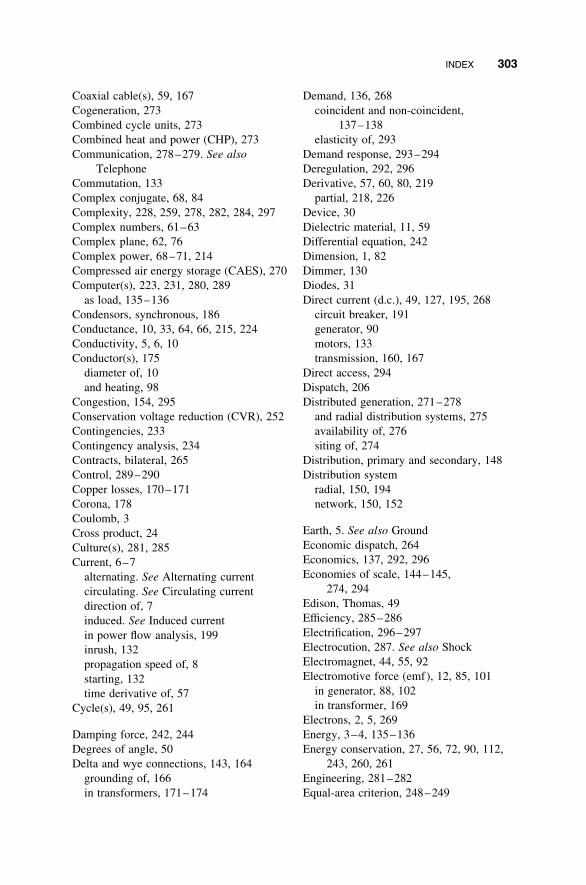
Coaxial cable(s), 59, 167

Cogeneration, 273

Combined cycle units, 273

Combined heat and power (CHP), 273

Communication, 278–279. See also

Telephone

Commutation, 133

Complex conjugate, 68, 84

Complexity, 228, 259, 278, 282, 284, 297

Complex numbers, 61–63

Complex plane, 62, 76

Complex power, 68–71, 214

Compressed air energy storage (CAES), 270

Computer(s), 223, 231, 280, 289

as load, 135–136

Condensors, synchronous, 186

Conductance, 10, 33, 64, 66, 215, 224

Conductivity, 5, 6, 10

Conductor(s), 175

diameter of, 10

and heating, 98

Congestion, 154, 295

Conservation voltage reduction (CVR), 252

Contingencies, 233

Contingency analysis, 234

Contracts, bilateral, 265

Control, 289–290

Copper losses, 170–171

Corona, 178

Coulomb, 3

Cross product, 24

Culture(s), 281, 285

Current, 6–7

alternating. See Alternating current

circulating. See Circulating current

direction of, 7

induced. See Induced current

in power flow analysis, 199

inrush, 132

propagation speed of, 8

starting, 132

time derivative of, 57

Cycle(s), 49, 95, 261

Damping force, 242, 244

Degrees of angle, 50

Delta and wye connections, 143, 164

grounding of, 166

in transformers, 171–174

Demand, 136, 268

coincident and non-coincident,

137–138

elasticity of, 293

Demand response, 293–294

Deregulation, 292, 296

Derivative, 57, 60, 80, 219

partial, 218, 226

Device, 30

Dielectric material, 11, 59

Differential equation, 242

Dimension, 1, 82

Dimmer, 130

Diodes, 31

Direct current (d.c.), 49, 127, 195, 268

circuit breaker, 191

generator, 90

motors, 133

transmission, 160, 167

Direct access, 294

Dispatch, 206

Distributed generation, 271–278

and radial distribution systems, 275

availability of, 276

siting of, 274

Distribution, primary and secondary, 148

Distribution system

radial, 150, 194

network, 150, 152

Earth, 5. See also Ground

Economic dispatch, 264

Economics, 137, 292, 296

Economies of scale, 144–145,

274, 294

Edison, Thomas, 49

Efficiency, 285–286

Electrification, 296–297

Electrocution, 287. See also Shock

Electromagnet, 44, 55, 92

Electromotive force (emf), 12, 85, 101

in generator, 88, 102

in transformer, 169

Electrons, 2, 5, 269

Energy, 3–4, 135–136

Energy conservation, 27, 56, 72, 90, 112,

243, 260, 261

Engineering, 281–282

Equal-area criterion, 248–249

INDEX 303

Equilibrium, 242, 261, 282

deep and shallow, 239

generator frequency, 108

stable and unstable, 235

Equity, 296

Euler’s equation, 79

Excitation, 92–93, 117, 132

Exciter, 93, 99

Expected unserved energy (EUE), 230

Expert systems, 279

Exponential base e, 78

Exponential function, complex, 79

Extension cord, 10, 41

External costs, 296

Farad, 59

Fault, 188

current, 193

transient, 191

Feeder, 149

lateral, 149

primary, 151

Field(s), 18–19

electric, 19

electromagnetic (EMF), 25

extremely low-frequency (ELF), 25

magnetic. See Magnetic field

Field lines, 20–21

Flat start, 217

Flexible a.c. transmission systems

(FACTS), 280

Flicker, 50

Fluorescent lamps, 127, 130

Flux, magnetic, 23, 44, 87, 169

density, 46

in generator, 103

leakage, 46, 169

linkage, 47, 88, 120

Force on a charge, 20–21, 24

Frequency, 49–50, 204, 236, 253–254

and power consumption, 260

and stability, 244

angular, 51

choice of a.c., 50

control, 261

tolerance, 168, 254

Friction, 242, 244

Fuel cells, 273

Fuse(s), 189, 192–193, 262

Gas turbines, 273

Gauss, 23

Generator(s)

capacity, 115, 295

conversion of energy in, 85

cooling, 98

damage, 115

induction. See Induction generator

rating, 116, 295. See also Ratings

synchronous. See Synchronous

generator

windings, 98

Geometric mean radius (GMR),

178–179

Governor, 101, 261

Gradient, potential, 20

Grid, design and evolution of, 144,

259, 277, 280, 296–297. See also

Power system

Ground, 4

in outlet, 140–141

Ground-fault circuit interrupter

(GFCI), 190

Ground return, 160

Harmonic(s), 126, 255–256

Harmonic distortion, 53, 123, 251

Heat dissipation, 136, 171–172, 178, 182.

See also power dissipation

Heating, resistive, 14–15. See also

Losses, resistive

Helix, 76, 79

Henry, 57

Hertz, 49

High-pass filter, 59

Horsepower (hp), 131

Hydrogen

energy storage, 271

generator cooling, 98–99

Imaginary axis, 76

Imaginary number i or j, 61

Impedance, 64, 72, 127, 197

characteristic. See Characteristic

impedance

Impulse, 252

Independent system operator (ISO),

146, 263, 264

Induced current, 25, 56, 85, 87

304 INDEX

Inductance, 55

as function of flux linkage, 48

of transmission lines, 176

mutual, 48

Induction, 24, 85

generator, 86, 118, 272

Inductor, 55

Information, 279, 286, 288, 296

Innovation, 287, 291

Insulator(s), 10, 11

on transmission lines, 180

Interconnection, 144–148

Intertie(s), 144, 168

Intuition, 284–285

Inverter(s), 123–126, 268

Ionization, 6, 191

Ions, 2, 6, 269

Iron losses, 170–171

Island(ing), 152–153, 277

Iteration, 195–196, 218, 223

Jacobian matrix, 218–219, 221, 225–226

Joule, 4

Kilowatt-hour, 66

Kirchhoff’s laws, 37, 153, 263

Kirchhoff’s current law (KCL), 32, 39

Kirchhoff’s voltage law (KVL), 32, 38

Lagging current, 56, 77

and phase angle, 64

Leading current, 60

and phase angle, 64

LED clocks, 136

Light, 26

speed of, 8, 27, 212, 288

Lightning, 6, 181

Limit, thermal and stability, 234.

See also Ratings

stability, 238

Line losses. See Losses

Line drop, 185. See also Voltage drop

Load, 127

aggregate, 136, 146

Load duration curve (LDC), 138–139,

264–265

Load balancing

among feeders, 159, 279

among phases, 163

Load factor, 140, 144, 146

Load flow, 195. See also power flow

Load forecast(ing), 137–138, 267

Load growth and distributed generation,

275

Load-following plant, 204, 264–265

Load profile, 138

Load tap changer (LTC), 170, 185

Loop flow, 153

Loop system, 151–152

Lorentz equation, 24

Loss-of-load-expectation (LOLE), 230

Loss-of-load-probability (LOLP), 229

Losses


and load balancing, 159

d.c. line, 49

heat. See resistive

line, 74, 201, 226, 263. See also

resistive

reactive, 74, 203, 208–209

resistive, 15, 17, 67, 203, 209.

See also line

Low-pass filter, 57

Magnetic field, 21, 23, 44, 46

in armature, 94–95

in inductor, 55

in generator, 87, 90

of rotor. See Rotor field

Magnetic flux. See Flux, magnetic

Magnetic moment, 22, 170

Magnetic poles, 21, 44

and rotor windings, 97

Magnetization, 22

curve, 46

Magnetomotive force (mmf), 47, 169

Maps, 284

Market(s), 266, 277, 292–294, 296

and power flow, 227

Market power, 295

Matrix, 36, 40, 215, 222

Metals, 5

Mho, 10

Microturbines, 273

Microwave oven, 135–136

Mismatch, 218, 222

Monitors, TV and computer, 136

Monopoly, 137, 147, 232, 292

INDEX 305

Motor(s), 85, 131–134

efficiency, 133–134

energy consumption by, 131

induction, 119, 122. See also Induction

generator

paper clip, 90–91

single- and three-phase, 133

Multiphase. See three-phase

Negative sequence, 95

Network reduction, 35

Neutral, 140, 162, 164

Newton’s method, 220–221

Node(s), 40, 197, 217, 289, 295

North American Electric Reliability

Council (NERC), 147

Nuclear power, 264, 271–272

Oersted, Hans Christian, 22

Ohm, 9

Ohm’s law, 8, 81, 223, 251

Oil, 172

One-line diagram, 149, 159, 166, 197–198

Operation

challenges, 227, 282. See also System

operator

skill, 262

Optimal power flow (OPF), 196

Oscillation, 61

Outage, 158–159, 230, 250, 263

Outlet, 140–141

Parallel connection, 31, 33, 36

Paralleling of generators, 111, 262

Peaking plant, 264–265

Penalty factor, 264

Per-unit (p.u.) notation, 208

Period, 27, 50

Permeability, 63, 92

constant, 45

Phase, 50

conductor, 140

in generator windings, 94

Phase angle, 199

complex power, 84

exponential notation, 82

FACTS, 280–281

Phase shift

between voltage and current, 69

in capacitor, 60

in inductor, 56

Phasor(s), 76, 80, 216

Phasor diagram, 77, 83

Phasors

notation of, 78, 81

operations with, 80–82

Philosophy, of electric service, 136

Photon(s), 28

Photovoltaics (PV), 126, 273, 294

Planning, 227, 267

Plasma, 6, 190

Polychlorinated biphenyls (PCBs), 172

Positive sequence, 95

Potential, 3, 4. See also Voltage

Power, 15, 136

active, 70

apparent, 68

average, 68, 70

complex, 84

dissipated and transmitted, 67. See also

Losses

dissipation in load, 128

instantaneous, 68

standby, 135

reactive. See Reactive power

real, 70

output from generator, 100

transmitted on line, 67, 183, 237

true, 70

Power angle, 110, 183, 204–205, 236–237,

239. See also Voltage angle

and circulating current, 110

difference between nodes, 240

in generator, 108

Power factor (p.f.), 70–72, 167

aggregate, 73

and induction generator, 122–123

and rotor field, 104

of fluorescent lamps, 75

of generator, 11, 123

significance of, 73

system, 115

Power flow, 195

analysis, 154

controlled by FACTS, 281

decoupled, 221, 224–225

direction of, 150

equations, 217

306 INDEX

nonlinearity of, 200

solution of, 195, 200

Power pool, 265

Power quality, 118, 250–258

and motors, 134

Power supplies, 135

Power system(s)

behavior, 210

design and evolution, 49. See also Grid

interconnection of, 146–147

operating state, 195

structure of, 149

Precision, 286, 289

Predictability, 283

Price, 137, 145, 268, 293, 295–296

Prime mover, 86, 89

Protection, 150, 188–194, 262


zones, 192–194

Protons, 2

Public Utility Commission (PUC), 232

Pulse-width modulation (PWM), 125–126

Pumped hydroelectric power, 269–270

Radians, 51

per second, 57

Radiation, 26

Radio, 28

as example of load, 30

Ramp rates, 265–266

Rating(s), 295

dynamic, 182

emergency, 182

generator, 116

historical trend of, 116, 183

Reactance, 55

capacitive, 58

inductive, 57

Reactive capability curve, 116–117

Reactive power, 70, 72, 102

allocation of, 112, 114

and distributed generation, 274–275

and generator, 102

and motors, 132

and voltage, 187

balance of, 202, 204, 260

conservation of, 112

consumed or supplied, 71

direction of flow, 208

from generator, 203

Recloser, 191–192

Redundancy, 150, 290, 292

Refrigerator, 137

Relay(s), 157, 189, 254, 262

Reliability, 229, 231–232, 285

Reluctance, 45, 169

Reserve(s), 144, 233

spinning, 266

Reserve margin, 146, 229, 268

Resistance, 9, 175

combined parallel and series, 33–35

effect on power consumption, 16

per unit length, 10

Resistivity, 9–10

Restoration, 159, 264

Rheostat, 130

Right-hand rule, 22–24, 55

Robustness, 290

Root-mean-square (rms), 53, 199

derivation of, 54

Rotational frequency, 96

Rotor, 86, 92

cylindrical, 97

round, 97

salient pole, 97

squirrel-cage, 120

wound, 120

Rotor current, 93

Rotor field, 92

in induction machine, 121–123

interaction with stator field, 90

Rotor winding, 92

Rubber bands, 212–213

Safety, 192, 285, 287

Sag, 253, 260

Scheduling coordinator, 264

Security, 229, 233

Self-excitation, 99

Series connection, 31–32

Service, 232

valuation of, 232–233

Shedding of load, 159, 230, 263

Shock, 13–14

Siemens, 10

Significant figures, 74

Sine function, 51–52, 80

argument of, 50

INDEX 307

Sine wave, 50

Sinusoid, 50, 88, 89, 256, 258

Situational awareness, 292

Slip, 118, 132

Solar power, 271. See also Photovoltaics

Solar thermal generation, 277

Solenoid, 55, 92

Solid-state technology, 124, 281

Source, current or voltage, 42

Speed, 286, 288

Spike, 252

Spin, 22

Square wave, 124–125

Stability, 109

angle and voltage, 234

as operational criterion, 288

dynamic, 213, 235, 240, 244. See also

transient

steady-state, 213, 235

transient, 233, 240, 248

voltage, 249

Stability limit, 167, 183, 212, 280

Static VAR compensators (SVC), 186

Stator, 92

Stator field, 95

decomposition of, 105

Steady-state condition, 211

Steam, 86

Steam generation, 271, 282, 287

Storage, 260, 268

valuation of, 271, 277

Substations, 149

distribution, 157–158

Subtransmission, 148

Sulfur hexafluoride (SF6), 171–172

Superconducting magnetic energy storage

(SMES), 270

Superconductivity, 6, 10, 213, 270

Superposition principle, 41, 73, 154

Supervisory Control and Data Acquisition

(SCADA), 158, 278, 291–292

Surge impedance, 177

Surge impedance loading (SIL), 177, 184

Susceptance, 65–66, 215, 224

Swell, 252

Swing equation, 242

Switch(es), 157, 292

Switchgear, 190

Switching operations, 264

Synchronicity of generators, 108, 111

Synchronism, 211, 236

Synchronization, 111

Synchronous generator, 86, 92–95

Synchronous speed, 118

System operator, 227, 262, 266. See also

Independent system operator

Taylor series, 219, 221

Telephone, 263, 278–279, 291

Tension, 3. See also Voltage

Terminal(s), 30

Territory(ies), 147, 263

Tesla, 23

Tesla coil, 178

Thermal limit, 182, 211, 213, 280.

See also Ratings

Thermodynamics

first law of, 27

second law of, 203

Three-phase

generator winding, 94

transmission, 140, 160–163, 166

Thyristors, 167

Time

and system frequency, 255

as angle, 51

as variable in a.c. circuits, 199

conceptualization in synchronous grid,

211–212

in operations, 260, 292

in stability analysis, 245

sensitivity of resources, 278

Time-of-use rates, 294

Torque, 100, 132, 160, 261

for induction machine, 119, 122

on generator rotor, 94

Total harmonic distortion (THD),

256–257

Transformer(s), 147, 157, 168

and a.c., 49

and harmonics, 256

capacity limit, 171

cooling, 171

core, 169

distribution, 150, 156

primary and secondary side, 168

tap(s), 141–142, 170

turns ratio, 170

308 INDEX

Transformer bank, 157, 173

Transistor(s), 45, 280

Transmission line(s)

capacity, 295

clearance, 180

dimensions of, 177–178

reactance of, 50

sagging, 180

Transmission system, 148

Transparency, 288

Turbine, 86, 96

and stability, 244

Uninterruptible power supply (UPS),

230, 231, 270

Unit commitment, 264

Utility(ies), 147, 232, 253, 258, 263

VAR compensation, 74.

See also Reactive power

Variable speed drive (VSD), 134

Variables in power flow, 198–199, 206

Vector(s), 40, 64, 95, 222

addition, 116

Veracity, 289

Voltage, 3

and power consumption, 260

and resistive loads, 129

at generator terminal, 93, 97, 102

at node, 216

control in generator, 107

difference between generators, 109

excessively high or low, 251

in power flow, 199

line-to-line and line-to-ground, 181.

See also phase-to-phase and

phase-to-ground, 142, 165,

174–175, 257

time derivative of, 60

transmission, 17, 147

tolerance, 118, 185, 251–252

Voltage angle, 204, 207, 217, 236

in generator, 108

Voltage dip, 253

Voltage drop, 13, 67, 251

Voltage level, 260

Voltage profile, 184, 187, 266

Voltage regulator, 185, 187

Volt-ampere (VA), 70, 182.

See also Apparent power

Volt-ampere reactive (VAR), 70.

See also Reactive power

supplied by generator, 103

Vulnerability, 147, 233, 276,

282, 291

Water

flow analogy with electricity,

38, 39

properties of, 3

Watt, 15

Watt-hours, 66

Wave, propagation of, 27

Waveform, 94, 257–258, 281

of inverters, 124–125

Weber, 23

Westinghouse, George, 49

Wild a.c., 123

Wind power, 264, 271–272, 277

and generator rating, 115

Work, 3–4, 89

Wye connection, 143, 164

grounding of, 166

INDEX 309

WILEY SURVIVAL GUIDES IN ENGINEERINGAND SCIENCE

Emmanuel Desurvire, Editor

Wiley Survival Guide in Global Telecommunications: Signaling Principles,Network Protocols, and Wireless Systems Emmanuel Desurvire

Wiley Survival Guide in Global Telecommunications: Broadband Access,Optical Components and Networks, and Cryptography Emmanuel Desurvire

Fiber to the Home: The New Empowerment Paul E. Green, Jr.

Probability and Random Processes Venkatarama Krishnan

Electric Power Systems: A Conceptual Introduction Alexandra von Meier

ELECTRIC POWER SYSTEMS

Documents

Transcript of ELECTRIC POWER SYSTEMS