Volume 77, number 5,6 OPTICS COMMUNICATIONS 15 July 1990

Full length article

EXPERIENCES WITH FINITE ELEMENT CALCULATIONS OF WAVEGUIDE COUPLING PROBLEMS

W. KAMMINGA and B.J. HOENDERS Institutefor Theoremal Physics, University of Groningen, Postbus 800, 9700 AV, Groningen, The Netherlands

Received 19 January 1990

Based upon first principles, the interconnection problem of two semi-infinite slab waveguides is modelled as a boundary value

problem. The discretisation and the solution of the set of indefinite difference equations generated by this problem is discussed.

Particularly a more accurate discretisation of one of the boundary conditions is necessary for accurate solutions. Applications on

various configurations illustrate the possibilities of the use of the numerical method.

1. Introduction

This study describes an appropriate numerical method for solving the interconnection of optical waveguides. We consider the coupling of two ideal symmetrical semi-infinite monomode dielectric slab waveguides each having a uniform cross section and a constant refractive index. Around the joining in- terface is found a transition region where the ho- mogeneity of the geometry is generally disturbed and the refractive index may be spatially dependent. An incident light beam passing the transition region will be optically affected by these irregularities. For ex- ample, an incident bound mode excited in the in- coming waveguide may result not only in a trans- mitted bound mode of the outgoing waveguide, but also in a reflected bound mode of the incoming waveguide and radiation modes in any direction. Propagation quantities to be investigated are the re- flected, transmitted and radiated power.

In the literature, the coupled mode theory is men- tioned for analysis of coupling problems for transi- tion regions having slowly varying properties [ 11. Papers dealing with finite element methods or re- lated techniques are less in number. Kriegsmann [ 2 ] shows numerical calculations on slab waveguides having metallic surroundings. Successful solutions are reported using the application of the boundary element method [ 31. The latter method is appro- priate for handling coupling problems which can be

described by a mathematical model consisting of only a few subregions with a constant value of the re- fractive index. Starting for each subregion with a weighted residual formulation with the fundamental solution of the governing Helmholtz equation as weighting function, an integral equation relating the electric field and its normal derivative at the bound- ary of that subregion can be derived. The continuity requirements of the electric field and its normal de- rivatives at all boundaries occurring in the model, define sufficient conditions to solve the set of inte- gral equations representing the electric field of the problem. As will be shown in the following, the ideas of the boundary element method will be applied to some parts of the coupling systems of this study.

In order to derive a mathematical model of the coupling configuration, it is assumed that both the incoming waveguide and the outgoing waveguide ex- tend to infinity. We are particularly interested in the optical propagation properties for different spatially varying values of the refractive index of the transi- tion region. Hence, the cladding surrounding the co- res of the waveguides and the transition region is chosen as simple as possible. For example, the outer radius of the cladding is taken to tend to infinity and its refractive index is a constant.

Starting from Maxwell’s equations, a boundary value problem for an appropriate electric field com- ponent, which satisfies the corresponding Helmholtz equation in the various regions, is formulated. The

0030-4018/90/$03.50 0 Elsevier Science Publishers B.V. (North-Holland 1 423

Volume 17. number 5-6 OPTICS COMMUNICATIONS I5 July 1990

optical quantities of interest can be calculated from this electric field.

At the interfaces of two regions with a different refractive index, the boundary conditions are de- fined by the continuity of both the components of the electric field and the magnetic field. The latter condition can be reduced to the continuity of the normal derivative of the electric field component.

An obvious way to handle numerically the bound- ary value problem of the coupling configuration is a combination of two methods: the finite element method for the transition region and the boundary element method for the cladding. In the transition region the Helmholtz equation has been discretis- ized using a finite element or finite difference pro- cedure, yielding difference equations of the electric field component in a limited number of net points. These net points are located within and at the boundary of the transition region. As the refractive index is constant at the cladding, the electric field component can be expressed as a boundary integral equation for that region. Appropriate discretisations of this integral equation taken at the same net points as before at the interface of the transition region and the cladding yield complicated difference equations. These equations relate the electric field components in the net points of the transition region at and near the interface. Together with the continuity condi- tions of the electric field and its normal derivative at the interface, a set of linear difference equations results which completely describes the numerical so- lution of the original interconnecting problem. Un- knowns of these equations are the electric field com- ponents in the net points of the transition region and the coefficients of reflection and transmission of the bound modes of the waveguides. The elements of the matrix of the set of equations may be complex. Moreover, the matrix turns out to be large, sparse, nonsymmetric and nonsingular and as the electric field obeys the Helmholtz equation, the matrix is in- definite as well.

An appropriate method for solving this particular type of a large set of indefinite equations was not easily found. In many textbooks the treatment of so- lution methods of systems of linear equations is mostly limited to the case of a positive definite set of equations. Typical simple iteration methods such as the Jacobi, Gauss-Seidel and relaxation methods,

424

leading to a convergent solution of a positive defi- nite system of equations cannot be applied in the case of an indefinite matrix. As recommended by Ney [ 41, more promising are the conjugate gradient methods. Originally published by Hestenes and Stiefel [ 51, these methods and their variants are described in survey papers and textbooks [ 6,7]. In our calcula- tions we have chosen for the variant of Craig’s method as given by Paige and Saunders [ 81.

In a preceding letter [9] the main features of the mathematical modelling of the coupling configura- tion are treated. Moreover, some preliminary nu- merical results of some simple case studies are given. In this paper, a more detailed description of the mo- delling and the optical aspects of the coupling system will be given. The discretisation of the model and the solution method of the indefinite set of equations will be discussed in detail. In particular, a careful for- mulation of some of the boundary conditions and a higher order of approximation of the difference equations turned out to be important for obtaining improved numerical results.

The usefulness of the method will be illustrated by the application to an example of a simple case study and to an example with a strongly varying refractive index of the transition region.

2. The modelling of the waveguide coupling

The mathematical model of the waveguide cou- pling problem will be explained by an example. We consider the coupling of two symmetric dielectric slab waveguides with no structural variations in the y-di- rection. The waveguides are assumed to be lossless and monomode, having the same symmetry-axis (z- axis) and the same width but different refractive in- dices n, and n,. The core region is surrounded by a medium with a constant refractive index pr3 on both sides. The whole problem is symmetric with respect to the z-axis, as illustrated in fig. 1. We will only con- sider the case of TE-polarisation; the transverse elec- tric field, denoted by E(x, z), is then polarised along the y-axis.

In this model, it is further assumed that at the po- sitions z= -L and z= L, located sufficiently far from the coupling at z=O, the radiation modes are van- ishingly small because of the Sommerfeld radiation

Volume 77, number 5,6 OPTICS COMMUNICATIONS 15 July 1990

_-- ---_ /’ , ‘--, / \

/ i

\ / \

/ \ / ri 1

/ \

/ \ / radiated .x

I ns\ 1 / i;- - - ---

6-l transmitted

Fig. I. The two-dimensional model of the coupling of symmetric slab waveguides. The regions of the practical extension of the incoming,

the reflected and transmitted bound modes are indicated.

condition. Referring to Marcuse [ 11, assuming a time dependence of exp (iot ), to the left of z= -L the to- tal field is the sum of the incident and reflected bound mode,

E(x,z)=Ai(x) exp(-iipiz)+~i(x) exp(iP,z), (2.1)

and to the right of z=L, equal to the transmitted bound mode

E(x, z) = TA,(x) exp( -i/&z) . (2.2)

PI and /I2 are the wave numbers in the z-direction. A,(x), i= 1, 2, represent the profiles of the bound modes in the transverse direction of the incoming and outgoing waveguide, respectively. These pro- files, mainly confined to the core, extend into the surrounding medium with an exponentially decreas- ing tail and are defined by

O<x<R,, (2.3)

A,(~)=[(~~~LoIP,)I(R~+~/~,)I~‘~cos(Ic,R~)

xexp[ -6,(x-R,)] , x>R,. (2.4)

The magnetic permeability of vacuum is given by pLo and o is the radian frequency of the bound mode. The characteristic parameters of the bound mode K,, S, and /$ are defined as [ 1 ]

Kf+j?f=nfk’, ~f+df=(nf-n:)k’,

6,=K,tan(K&) , (2.5)

k being the wavenumber of the exciting light beam. In order to normalize the time-averaged power car- ried by the corresponding bound mode (to be de- fined later on), the expressions (2.3) and (2.4) are rather complicated. The unknown coefficients R and T define the amplitudes of the reflected and trans- mitted modes, respectively. The part of the cores be- tween z= -L and z= L is a transition region in which the coupling occurs. Arising from this region, radia- tion modes may appear in the cores of the wave- guides of the transition region and in the surround- ing medium. In each point of the transition region the electric field component has been described by the Helmholtz equation [ 1 ]

d2E/ax2+a2E/dz2+k2n2(x, z)E=O , (2.6)

in which n(x, z) represents the locally varying re- fractive index.

In the surrounding medium an equation of the same type as (2.6) is valid. Only n(x, z) has to be replaced by the refractive index n3. As n3 is constant, we will represent E(x, z) by a boundary integral in the latter region. Referring to Brebbia and Walker [ lo] and fig. 1, E(x, z) could be represented as

$E(x, z) = GE-E= dy. >

(2.7)

The integrand of (2.7 ) is composed of the values of E and G and their derivatives with respect to the

425

Volume 77. number 5.6 OPTICS COMMUNICATIONS 15 July 1990

outer normal n at the points of r. The function G denotes the free-space Green function for a constant refractive index n3, satisfying the Sommerfeld radia- tion condition at infinity and is given by

G(kn,r)=-$[N,(kn,r)+iJ,,(kn,r)]. (2.8)

J, and No are the Bessel functions of the first and sec- ond kind and r is the distance between the point (x, z) considered and a point of T. The path of integra- tion T includes I-,, the interface between the tran- sition region and the surroundings, and is a closed boundary within the surrounding region. The re- maining parts of r are T2, TX and T4, as shown in fig. I. Under the assumption, that the latter boundaries are sufficiently far from the joining region near z=O, and the validity of the Sommerfeld radiation con- dition, the radiation modes can be neglected at TZ, Ti and r,. As a result, the contribution of the inte- grals on the right hand side of (2.7) along T4 can be neglected. The values of E(x, z) of these integrals at points of Tz are equal to (2.1) for z= -L and at points of rX equal to (2.2) for z= L. The relation (2.7) can be reduced to

fE(x, I) -

(2.9)

AsE(x,z)andaE/anareknownatz=-Landz=L the integrals on the right-hand side of (2.9) can be

calculated and expressed in terms of R and T. As a final integral equation for points of r, we find

+E(x, z) -

r-1

-F, -FIR-F,T=O, (2.10)

in which

F, =

E,=il,(x)exp[(-l)JP’i/3,L], j=l,2, (2.11)

E3 =A,(.r) exp( -i/&L) . (2.12)

At points of the interface r,, the values of E(x, 7)

and the normal derivatives are determined by both (2.6) valid in the transition region and by (2.10) valid in the surrounding medium. Using the conti- nuity conditions of the electric and magnetic field at r,, these values can be uniquely defined at r,.

Now, the waveguide coupling problem has been formulated as a boundary value problem for the elec- tric field component E(x, z) and the coefficients of reflection and transmission, R and T, defined in the transition region between z= -L and z=L. Within this region (2.6) holds and the boundary conditions consistof(2.1)atandtotheleftofz=-Land(2.2) at and to the right of z= L and the integral equation

(2.10) at the upper boundary. The boundary value problem above describes a

simple model of the coupling of waveguides. An analogous boundary value problem can be derived for configurations with complicated geometries, such as the coupling of two waveguides with a different cross section and necessarily having a variable width of the transition region. A different type of compli- cations occurs with the following. The locations 7- - L and z= L of the model have been chosen so -- far from z=O, that the radiation modes can be as- sumed to be vanishingly small. For practical calcu- lations it is required that the distance between z= -L and z= L is not too large. If the radiation modes de- crease very slowly with an increasing distance from z=O, this condition is not satisfied and the model has to be adapted. The corresponding extended model has been discussed in a different paper [ 91 and will not be treated here. It will be shown in the applications to be discussed later on, for example in the results of fig. 5, that the configurations for the maximum values of L/R, given, satisfy the condi- tion of vanishingly small radiation modes.

3. The discretisized numerical model

The boundary value problem will be numericall! solved by the application of a discretisation tech.

426

Volume 77, 5,6 OPTICS I5 July 1990

nique to the transition region. To this end, this re- gion is covered by a triangular net. The electric field component E(x, z) has been approximated by its values at the net points. Using a finite difference or

a finite element method, algebraic equations can be derived for these unknown values of the electric field in the net points.

In the particular case of our example, a regular net as shown in fig. 2 can be chosen. Also, the same set of net points can be considered as net points of a reg- ular square net. Within the transition region, the Helmholtz equation (2.6) is valid. A discretisation of (2.6) can easily be obtained by the application of a finite difference technique to the regular square net. As the results of our calculations are sensitive to the size of the mesh width, we preferred the use of the accurate difference equation of the “nine-points- molecule” to that of the lower order approximation of the “five-points-molecule”. For each internal net point with coordinates (x,, z,) (fig. 3), (2.6) can be approximated by [ 111

( -20+4h2k2fi;)E,,

+ (4+ fh2k2fi:)E, + (4+ jh2k2fi:)E2

+(4+thZkZn:)E,+(4+fh2kZn:)E,

+E5+E6+E7+Es=0, (3.1)

h being the mesh width and ?ii, i = 0, 1, 2, 3, 4, rep- resenting the refractive indices in the corresponding net points. The bar on the local rT, has been added to avoid confusion with the refractive indices n,, n2 and n3 already defined in the coupling configuration.

Defining for each internal net point (x,, Zj) of the transition region a relation of the type (3.1), a large number of sparse algebraic equations is obtained. For

net points of the transition region located at the sym-

metry axis x=0, the properties of symmetry can be used. For those points, the relation (3.1) can be straightforwardly modified.

At and near the boundaries z= -L and z= L the

bound mode expressions (2.1) and (2.2) are valid.

At first sight it seems obvious to choose as boundary conditions the values of E(x, z) in the net points of

z= -L and z=L by simply substituting the corre- sponding coordinates into (2.1) and (2.2), respec-

tively. As a result of calculations on particular cou- pling configurations using these boundary conditions shortly denoted as Dirichlet type, the solutions are

not very accurate. For example, for a range of dif- ferent values of L the constant R shows an oscillating

behaviour as exp ( - $iL) with an unacceptably large amplitude. A corresponding oscillating behaviour is

defined by the boundary condition given by (2.1) at z= -L for analogous values of L. Instead of the con-

ditions of Dirichlet type above, we looked for stronger conditions at z = -L and z = L. Observing that in fact

the Dirichlet conditions only prescribe the behav- iour of the bound modes in the transverse x-direc-

tion at z= -L and z= L, the alternative stronger conditions are required to enforce the behaviour of

the bound mode in the normal z-direction as well. The latter conditions may be formulated as follows. Limiting ourselves to the boundary condition at z= L,

it can easily be verified using (2.2) and (2.3) that at the net points of z=L, E(x, z) satisfies the

relations

(i) the Helmholtz equation (2.6),

d2E/dx2+a2E/dz2+k2n2(x, z)E=O , (3.2)

Fig. 2. The discretisation has been applied to the triangular or quadratic net covering the transition region

427

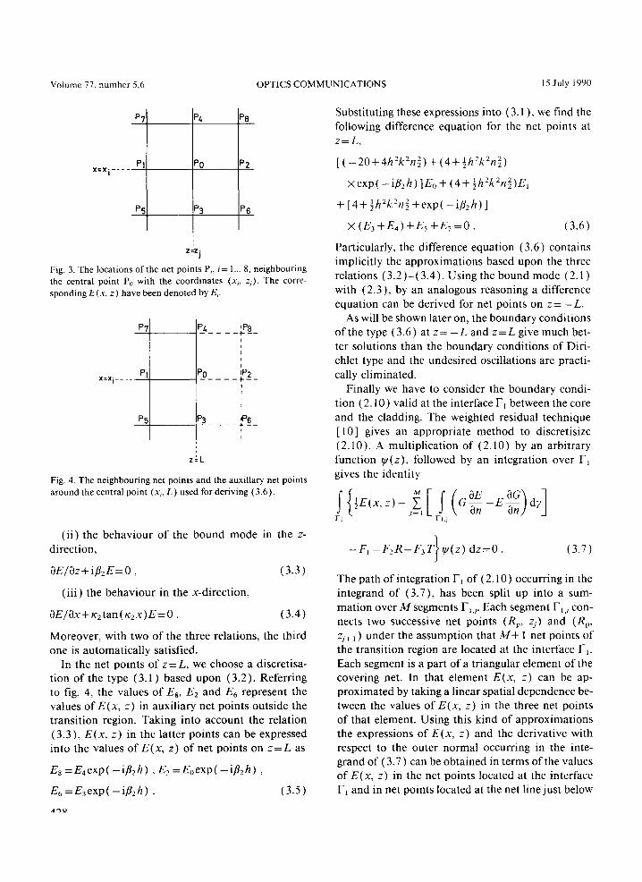
Volume 77, number j,6 OPTICS COMMUNICATIONS 15 July 1990

x-xi---

Fig. 3. The locations of the net points P,, i= l... 8, neighbouring

the central point P, with the coordinates (x,, z,). The corre-

sponding E(x, z) have been denoted by E,.

p7 +--I P& IPg --- __+-- I I

I

x:xi__ ._ Pl p_o_ - - -r2- c. ! p5 3 1% --_---+--

Z&L

Fig. 4. The neighbouring net points and the auxiliary net points

around the central point (x,, L) used for deriving (3.6).

(ii) the behaviour of the bound mode in the z- direction,

aElaz+i/&E=O,

(iii) the behaviour in the x-direction,

(3.3)

aE/ax+Kztan(Kzx)E=O. (3.4)

Moreover, with two of the three relations, the third one is automatically satisfied.

In the net points of z= L, we choose a discretisa- tion of the type (3.1) based upon (3.2). Referring to fig, 4, the values of Es, E2 and E6 represent the values of E(x, z) in auxiliary net points outside the transition region. Taking into account the relation ( 3.3), E(x, z) in the latter points can be expressed into the values of E(x, z) of net points on z=L as

Es =E4exp( -&h) , E2 =E,exp( -i/&h) ,

E6 =E,exp( -$,h) . (3.5)

n,o

Substituting these expressions into (3.1), we find the following difference equation for the net points at z=L,

[ ( -20+4h2k2n:)+ (4+th2k2n;)

xexp(-i/12h)]E0+(4+th2k2n:)E,

+ [4+fh2k2n$ +exp( -i,&h)]

x(E3+Eq)+ES+E7=0. (3.6)

Particularly, the difference equation (3.6) contains implicitly the approximations based upon the three relations (3.2)-( 3.4). Using the bound mode (2.1) with (2.3 ), by an analogous reasoning a difference equation can be derived for net points on z= -L.

As will be shown later on, the boundary conditions of the type (3.6) at z= -L and z=L give much bet- ter solutions than the boundary conditions of Diri- chlet type and the undesired oscillations are practi- cally eliminated.

Finally we have to consider the boundary condi- tion (2. IO) valid at the interface F, between the core and the cladding. The weighted residual technique [ lo] gives an appropriate method to discretisize (2.10) A multiplication of (2.10) by an arbitrary function v(z), followed by an integration over IY, gives the identity

-F, -F2R-F,T I

y(z) dz=O. (3.7)

The path of integration F, of (2.10) occurring in the integrand of (3.7), has been split up into a sum- mation over Msegments FIJ. Each segment FIJ con- nects two successive net points (R,, z,) and (R,,

z,+ , ) under the assumption that M+ 1 net points of the transition region are located at the interface F,. Each segment is a part of a triangular element of the covering net. In that element E(x, z) can be ap- proximated by taking a linear spatial dependence be- tween the values of E(x, z) in the three net points of that element. Using this kind of approximations the expressions of E(x, z) and the derivative with respect to the outer normal occurring in the inte- grand of (3.7) can be obtained in terms of the values of E(x, z) in the net points located at the interface r, and in net points located at the net line just below

Volume 77, number 5,6 OPTICS COMMUNICATIONS I5 July 1990

that interface. An appropriate choice of v(z) is the definition of w( z) equal to the linear shape function, also denoted as the Galerkin method [ 12 1. Corre- sponding with the segments rlj and rlj+, with the central net point (R,, z,) the function is defined as

w(z) =o 3 ZI <z<z,_,, zj+l<z<zM+I~

= 1+ (z-Z,)/h) z,_, <z<z,,

=l-(Z-Zj)/h, z, <z<z,,, , j=2...M.

(3.8)

Substituting (3.8) into (3.7) and integrating (3.7) analytically as far as possible, for each net point (R,, z,) of the interface, the identity (3.7) can be re- placed by an algebraic equation in terms of the un- known values of E(x, z) in the net points of I-, and the net line just below r, and of course R and T. Be- cause of these latter unknowns R and T, two addi- tional conditions are required to define the complete set of equations. Again we use the identity (3.7) with the approximation of E(x, z) made at the segments as discussed. Apparent choices of two different in- dependent functions of v(z) are shape functions which correspond to the end segments. Defining, respectively,

v(z)= l- (Z-z,)/h ) z1 <z<z*

=o, z2 <z<zA4+, 1 (3.9)

and

c//(z)=0 > z, <Z<Z,)

= 1+ (Z-zM+,)/h ) z,+f<z<z~+~ ) (3.10)

analogously as above, two algebraic equations cor- responding with the end net points of rI can be de- rived. Now, the complete set of equations has been obtained.

4. The solution of the coeffkients of reflection and transmission and the electric field

The set of linear equations can be denoted as

Ax=b, (4.1)

in which x represents the unknown electric field component E(x, z) at the net points of the transition region and the unknown coefficients of reflection, R,

and transmission, T, of the bound modes in the waveguides. The elements of the matrix A and of the vector b representing the known parts of the equa- tions, may be complex. The matrix A turns out to be large, sparse, nonsymmetric and nonsingular. As the values of E(x, z) given in x are solutions of the Helmholtz equation, A is indefinite as well.

The conjugate gradient technique [ 51 appears to be an appropriate method for solving (4.1 ). Starting from the standard algorithm of the conjugate gra- dient method, the steps of iteration for the particular set of indefinite equations can be derived. Several variants are described in textbooks [ 6,7]. Alterna- tively the method leading to very equivalent steps of iteration can be developed from a different starting point. Originated by Golub and Kahan [ 131, the al- gorithm is based on the construction of two series of vectors by which the matrix A can be bidiagonalised. Using this modified form of A, an efficient iteration procedure can be derived for solving a set of equa- tions in particular for the case of a sparse matrix. A number of variants of the latter method are de- scribed and discussed in refs. [ 8,141. In our calcu- lations we used the variant of Craig’s method, also denoted as the CRAIG algorithm.

Referring to the extensive literature of the con- jugate gradient methods, in this paper the derivation of iteration procedures will be limited to a short de- scription of Craig’s algorithm by the alternative method. Following Paige’s papers [ 8,141, on using the construction of particular series of respectively the vectors u, and vi, i= 1, 2, . . . . a diagonalisation of the matrix A can be obtained, having the properties

that

ATU=VLT, AV=lJL, UTU=vV=I. (4.2)

AT represents the transpose of the conjugate of A,

~=[u,,~2>~3,...1, V=[~,,~2,4,.-1, (4.3)

and

PI 0 0

L= q2 P2 0 .

[ 1 (4.4)

0 43 P3

This result can be obtained with the initial choice of

~1 =blq, > ql= (b, b)“’ > (4.5)

429

Volume 77. number 5.6 OPTICS COMMUNICATIONS I5 July 1990

and a successive construction of

p,c,=‘A=u,-q,u_, ) uo=o . (4.6)

4,+lU*+I - -AL?, -p,u, , i= 1, 2, 3, . . . , (4.7)

p, and q, being positive scalars defined by

(UT> u,)=(v;,c:)=l. (4.8)

Introducing the vector y by the definition of

x=vy, (4.9)

and using (4.2), the original system (4.1) trans- forms into

Ax=AVy= ULy=b,

or

(4.10)

Ly= UTb=q, UTul . (4.11)

The latter equation can simply be solved, yielding the elements (qr, q2, q3, . ..) of the vector y as

41 =4,/P, >

)I,=-4,rl,-rIP,, i=2,3,4, . (4.12)

The method just described can be considered as an iterative one. Having obtained in the ith step the re- sults of the corresponding quantities, the solution can be iteratively approximated by

x,=x,_] +q,c:, x0=0, i= 1,2, 3... ,

and particularly the residual by

(4.13)

r,=b-Ax,=r,_, -q,Ac:. (4.14)

Theoretically, if the number of iteration cycles ex- ceeds the dimension N of the system (4.1), the re- sidual rN+ , = 0 and the procedure will be stopped. In practice because of roundoff errors vanishing values of the residuals are not found and the process will be stopped by the criterion that for a certain value of i the magnitude of (r:, r, ) is smaller than an arbi- trarily chosen positive number.

With respect to the use of computer memory, the algorithm is very efficient. As shown in the relations (4.6), (4,7), (4.13) and (4.14), the quantities in each cycle can be completely constructed from the results of the preceding cycle. The main storage con- suming operations are the factors of the type ATu, and Au,, occurring in eqs. (4.6) and (4.7). Espe- cially in the case of a sparse matrix A the storage size

430

required for the calculation of these latter factors, can be substantially reduced. In that case, the storage re- quired for the sparse equations can be avoided by regenerating the original sparse equations in each cycle of the iteration process.

5. Applications

The numerical procedure has been applied to cou- pling configurations of the type of fig. 1 for a range

of choices of n,, n,, n3 and n ( X, z) . Using the net of fig. 2, many calculations have been made for a fixed half width of R, equal to 1 urn and excitations of the waveguides with a beam of a fixed wavelength in vacuum of A,,=3 urn. In order to get insight in the behaviour of the radiation modes radiated into the surroundings, different values of L are considered. The accuracy of the numerical results are tested by using different choices of the mesh width h.

Apart from the direct results of the coefficients of reflection, R, and transmission, T, also the time-av- eraged power, P, is important. This latter quantity carried by a bound mode at a fixed value of z outside the transition region can be expressed as [ 1 ]

II:

p= JL 2UPo s E*(x, z)E(x, z) d_x.

0 (5.1)

E*(x, z) is the complex conjugate of E(x, z) and B is the wavenumber in the z-direction of the bound mode under consideration. The incident and re- flected power can be found by the substitution of re-

spectively the first and second term of (2.1) at z= -L into (5.1) and the transmitted power by the substitution of (2.2) at z=L into (5.1), giving

p,,, = 1 1 Prcfl=R*R, P,,=T*T. (5.2)

As a first example we consider the configuration of fig. 1 with the choices of the refractive indices of the transition region as

n(x, z)=n, for -L<z<O,

=n2 forO<z<L. (5.3)

Calculations are made for the combinations n3 = 1.25, n, = 1.60 and n2= 1.40 and 1.60 respectively. As a representative example, the results of the configu- ration with nz = 1.40 are shown in more detail for a

Volume 77, number 5,6 OPTICS COMMUNICATIONS 15 July 1990

range of values of L and the mesh width h. Figs. 5 behaviour tending to a constant value. Clearly it can and 6 illustrate the behaviour of the real and ima- be concluded that in this example at locations of z ginary parts of the coefficients of transmission, T, near L/R,= 15, the radiation modes have practically and T,, and reflection, RR and RI, respectively. For vanished. As most acceptable approximations of TR a fixed mesh width, fig. 5 shows for both T, and TI and T, we take the results at the maximal available for an increasing value of L a very slow exponential value of L/R,, in this case at L/R,= 16.

TRIl rn’

1.00

.99

.90

i

TR:f _i_: : : +

.97

.96 t

.OL-

.03-

.02 - T,: m

.

Ol-

O- 1L 15 16 * LIRp

Fig. 5. The real and imaginary parts of the coefficient of trans-

mission as function of L for the configuration with n, = 1.60,

nz= 1.40, rr3= 1.25 calculated for the mesh widths h/R,= l/6

(+),andh/R,=l/S(A).

Fig. 6. The real and imaginary parts of the coefficient of reflec-

tion for quantities given in fig. 5.

The coefficients of RR and RI, fig. 6, show with re- spect to L/R, weak oscillations of the type exp( -$,L) with an amplitude of about 0.01 and consequently a period of AL = 2n//3,. These oscilla- tions represent the behaviour of the errors connected with the bound mode expression (2.1)) which prop- erties (3.2) and (3.3) are used in the boundary con- dition at the net points of z= -L. Obviously the same periodical behaviour of exp( - $,L) appears for z= -L in (2.1) for varying values of L. As approx- imations of RR and R, we have chosen the mean val- ues of RR and R, respectively averaged over a range of AL calculated for a number of values of L between L/R,= 14 and L/R,= 16 in this case.

The plots of figs. 5 and 6 also depend on the mesh width. From the presented results calculated for h/R,= l/6 and h/R,= l/8 and additional numeri- cal experiments for different mesh widths (not given here), it can be determined that the coefficients R and T behave of the order h2. This property gives us the possibility to improve the approximations for TR, T,, RR and RI by the extrapolation to h= 0 [ 151, us- ing the results for h/R,= l/6 and h/R,= l/8, ac- cording to the relation

y(WR,=O)

=[16y(h/R,=1/8)-9y(h/R,=1/6)]/7,(5.4)

in which y(. ) represents each of the quantities con- sidered for the indicated meshwidth.

The results of the various coefficients obtained by the approximation defined by (5.4) are plotted in figs. 7 and 8. In the particular case of the combi- nation n1 = n2 = 1.60; n3= 1.25 the electric field com- ponent E(x, z) is analytically known and is in the whole field equal to the bound mode

E(x, z) =Ai (x) exp( -iPiz) , (5.5)

A,(x) being defined by (2.3) and (2.4). The real and imaginary part of the complex coefficient of transmission are equal to one and zero respectively and the complex coefficient of reflection is equal to

431

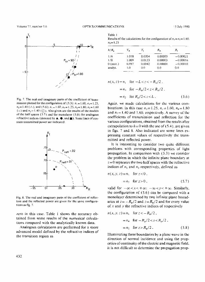
Volume 17. number 5.6 OPTICS COMMUNICATIONS 15 July 1990

Ptr’.90/ /

,I?

,Lptr=l.OO

‘/ /

Fig. 7. The real and imaginary parts of the coefficient of trans-

mission plotted for the configuration of (5.3): n, = 1.60, n3= 1.25,

n,=1.40(A),and (5.6):n,=1.60,n~=1.25,n,=1.80,n,=1.60

(o ) and hz = I .40 (0 ). Also given are the results of the models

of the half spaces (5.7) and the monolayer (5.8) for analogous

refractive indices (denoted by A, 0, and n ). Some lines ofcon-

stant transmitted power are indicated.

-. <refl =.02

\

‘\

0 l

.P ref,‘\Ol\ \ \

-JYk--dRR -05

Fig. 8. The real and imaginary parts of the coefficient of reflec-

tion and the reflected power are given for the same contigura-

tions as fig. 7.

zero in this case. Table 1 shows the accuracy ob- tained from some results of the numerical calcula- tions compared with the analytically known data.

Analogous calculations are performed for a more advanced model defined by the refractive indices of the transition region as

Table 1 Results ofthe calculations for the configuration of n, =nz= 1.60,

n3= 1.25

hlR,

l/6

1/g 0 (extr.)

analyt.

TR T, RH Rl

1.018 0.0204 0.00005 -0.00021

1.009 0.0133 0.00003 -0.00016

0.997 0.0042 0.00000 -0.00010

1.0 0.0 0.0 0.0

n(x, z)=n, for -L<z< -R,/2,

=r24 for -R,/2<z<R,/2,

= 112 forR,/2<z<L. (5.6)

Again, we made calculations for the various com- binations, in this case n,= 1.25, n, = 1.60, n4= 1.80 and n2 = 1.40 and 1.60, respectively. A survey of the coefficients of transmission and reflection for the various configurations, obtained from the results after extrapolation to h = 0 with the use of ( 5.4)) are given in figs. 7 and 8. Also indicated are some lines ex- pressing constant values of respectively the trans- mitted and reflected power.

It is interesting to consider two quite different problems with corresponding properties of light propagation. In comparison with (5.3) we consider the problem in which the infinite plane boundary at z=O separates the two half spaces with the refractive indices of n, and n, respectively, defined as

n(x,y,z)=n, forz<O,

=n2 forz>O, (5.7)

valid for --03<x< +oo; -co<y< +CXJ. Similarly, the configuration of (5.6) can be compared with a monolayer determined by two infinite plane bound- aries at z= - R,/2 and z= R,/2 and for every value of x and y the refractive indices of respectively

n(x, y, z)=n, for z< -R,/2 ,

=n4 for -R,/2cztR,/2,

=n, forz>R,/2. (5.8)

Illuminating these boundaries by a plane wave in the direction of normal incidence and using the prop- erties of continuity of the electric and magnetic field, it is not difficult to determine the propagation prop-

432

Volume 77, number 5,6 OPTICS COMMUNICATIONS 15 July 199G

erties such as the coefficients of transmission and re- flection [ 16 1. For reason of comparison results of these coefficients calculated at the same combina- tions of refractive indices as above are also indicated in figs. I and 8.

As a final example a model will be treated, in which high values of the reflected power occur. As is well known this property is present in a dielectric mirror, consisting of a series of double layers with appro- priate refractive indices. An illumination by normal incidence of light within a band of appropriate wave- lengths shows that a high reflectance can be ob- tained. We have chosen a particular structure of four double layers defined by the nine infinite planes at the positions z=O.SjR*, j= -4, - 3, . . . 3, 4 and the

refractive indices

n(x,y, z)=n, > z< -2R,, z> 2R,,

=n,+An, ijR,<z<{(j+l)R,,

=n,-An, t(j+l)R,<z<;(j+2)R,,

j= -4, -3, . ..2. (5.9)

valid for each x and y. Referring again to Pedrotti and Pedrotti [ 161, the coefficients of reflection and transmission can be calculated with the use of matrix methods. Fig. 9 contains the results of the reflected

la1

f---

Fig. 9. The reflected power as function of the wavelength I,, for the models of the dielectric mirror (a), and the coupling wave-

guides with the stepwise (b) and the sinusoidal (c) oscillating

refractive indices, determined for n, = 1.60 and An~0.3, and

n, = 1.60 and An=0.6.

power for a range of wavelengths in vacuum between Lo/R,=2 and &JR,=2.5 and the refractive indices of n,= 1.60 and An=0.3 and 0.6.

A comparable model for the coupling configura- tion of two waveguides of the model of fig. 1, is ob- tained by the choice of n, =nZ= 1.60, n3= 1.25 and the refractive indices of the transition region shown in fig. 10. A variant of the latter model is obtained by replacing the stepwise oscillations by the sinu- soidal behaviour

n(x, z)=n, +An sin(zrc/Rp) ,

O<x<R,, -2R,<z<2R,. (5.10)

The coefficients of transmission and reflection are approximated with the use of the numerical method for various values ofAO/R, and the refractive indices of n,=l.60 and An=0.3 and An=0.6. The corre- sponding results of the reflected power, determined for h/R,= l/8 and L/R,= 16, are plotted in fig. 9. We remark that in comparison with the dielectric mirror the reflected power has a very similar behav- iour in the case of the coupling waveguides. Only there is a small shift of the reflected power into the direction of lower wavelengths and a decrease of the maxima of the reflected power in the defined order of respectively the dielectric mirror and the wave- guide models of successively the stepwise oscillating and the sinusoidal varying refractive indices.

6. Conclusions

In this paper coupling problems of slab wave- guides are mathematically modelled in terms of a boundary value problem defined for a suitable elec- tric field component. The discretisation of the prob- lem leads to an indefinite set of difference equations. The solution is iteratively found using a conjugate gradient method. In the above, important points of discussion have been the various methods improv- ing the results. We mention a finite difference ap- proximation of the Helmholtz equation by a “nine- points-molecule” and a precise formulation of the boundary conditions in the regions of the bound modes. Corresponding results calculated for two dif- ferent meshwidths, can be used to improve the ap- proximations with an extrapolation to a meshwidth

433

Volume 77, number 5.6 OPTICS COMMUNICATIONS I5 July 1990

“3 I I !RP

I I I 1 1 I I I I I I

I I I I I ! I I I I I I

I I I I 1 n, I n, ’ n, ’

I I I I I nr I m n1 1 m ’ nr

I i +A”; nl I nl 1 nt I nj 1

I -An; +Anf -An; +Ani -An! *AnI -An; I I -------- I_~__L_L_I_~__L_I__L_______I__ -L -2RP -RP 0 RP 2RP L z

Fig. 10. The coupling configuration with the stepwise oscillating refractive indices of the transition region.

of zero. The numerical method has been applied to some particular examples with more or less compli- cated refractive indices of the transition region. The results show that accurate approximations of the various propagation properties can be obtained by this method.

We have limited ourselves to the coupling of wave- guides of the same width. As has been mentioned at the end of section 2, configurations with a more complicated geometry of a variable width are pos- sible. The extension of the method to that kind of problems is not given in this paper. At least, much more effort is required for the implementation of the computer programs, in that case.

References

[ 1] D. Marcuse, Theory of dielectric optical waveguides

(Academic Press, New York, (1974).

[ 21 G.A. Kriegsmann, SIAM J. Sci. Stat. Comput. 3 ( 1982) 318.

[3] S. Kagami and 1. Fukai, IEEE Trans. Microwave Theory

Tech. MTT-32 (1984) 455.

[4] M.M. Ney, IEEE Trans. Microwave Theory Tech. MTT-33

(1985) 972.

[ 51 M.R. Hestenes and E. Stiefel, J. Res. Nat. Bur. Standards

49 ( 1952) 409.

J.R. Westlake, A handbook of numerical matrix inversion

and solution of linear equations (Wiley, New York, 1968 ).

D.K. Faddeev and V.N. Faddeeva, Computational methods

of linear algebra (Freeman, San Francisco, I963 )

C.C. Paige and M.A. Saunders, ACM Trans. Math. Software

8 (1982) 43.

[9] W. Kamminga and B.J. Hoenders, Optics Comm. 67 ( 1988)

277.

[ IO] CA. Brebbia and S. Walker, Boundary element techniques

in engineering (Newnes-Butterworths, London. 1980).

[ I 1 ] F.B. Hildebrand. Finite-difference equations and

simulations (Prentice-Hall, Englewood Cliffs, 1968).

[ 121 O.C. Zienkiewicz, The finite element method (McGraw-

Hill, London, 1977).

[ 131 G. Golub and W. Kahan, SIAM J. Numer. Anal. 2 ( I965 )

205.

C.C. Paige, SIAM J. Numer. Anal. 11 (1974) 197.

K.J. Binns and P.J. Lawrenson, Analysis and computation

of electrical and magnetic field problems (Pergamon,

Oxford. 1963).

F.L. Pedrotti and L.S. Pedrotti, Introduction to optics

(Prentice-Hall, Englewood Cliffs, 1987).

434