0

EXCHANGE RATE PASS-THROUGH IN GHANA

March 2014

Francis White Loloh1

Abstract

In this paper, we estimate the pass-through impact of exchange rate movements on

domestic prices between January 1994 and December 2012, using a recursive VAR. The

model consists of six variables, which are ordered as: oil prices, output gap, exchange

rate, non-food prices, overall consumer prices, and money market interest rates with the

implicit assumption that the identified shocks contemporaneously impact variables

ordered after the shock without a contemporaneous feedback. We establish that the effect

of a nominal exchange rate shock on domestic prices is incomplete, broadly modest and

decays within 18-24 months, but such effects are mostly felt within 12 months.

Generally, the impact of the exchange rate shock on overall CPI inflation is more benign

than for non-food inflation. We also find evidence in support of Taylor’s hypothesis that

the exchange rate pass-through is positively correlated with the level of inflation.

Key words: Exchange Rate Pass-through, Recursive VAR, Impulse response, Variance

decomposition.

Author’s Email Address: Francis.loloh@bog.gov.gh

1 Francis White Loloh is currently an economist at the Financial Stability Department of the Bank of Ghana

1

Table of Contents

Abstract ......................................................................................................... 0

1. Introduction .................................................................................................. 2

Figure 1: Nominal Exchange Rate Movements and Domestic Prices ........................ 3

2. Literature Review .......................................................................................... 4

2.1 Theoretical Literature ................................................................................ 4

2.2 Empirical Literature .................................................................................. 4

3. Data and Methodology ................................................................................... 6

3.1 Methodology ........................................................................................... 6

3.2 Data Issues .............................................................................................. 9

3.3 Limitations of the Study ........................................................................... 10

4. Empirical Results ........................................................................................ 10

4.1 Stationarity Test ..................................................................................... 10

4.2 Estimates of Size and Magnitude of Pass-Through ........................................ 11

4.3 Variance Decomposition of Non-food and CPI Inflation ................................. 15

4.4 Taylor’s Hypothesis, Single-Digit Inflation and Pass-Through ......................... 16

4.5 Alternative Ordering and Robustness .......................................................... 17

5. Concluding Remarks .................................................................................... 18

References ..................................................................................................... 20

List of Figures

Figure1:Nominal Exchage Rate Movements and Domestic Prices……………..3

Figure 2: Impulse Response to a one standard innovation in the exchange rate .......... 122

Figure 3: Estimated Cumulative Pass-Through Coefficients .................................. 133

Figure 4: Changes in the Pass-Through over time ................................................ 144

List of Tables

Table 1: ADF Unit Root Test ……………………………………………………………11

Table 2: Estimated Cumulative Pass-Through Coefficients ……………………….........13

Table 3: Variance Decomposition of Non-Food Inflation ………………………………16

Table 4: Variance Decomposition of CPI Inflation ……………………………………..16

Table 5: Cumulative Pass-Through Based on Taylor’s Hypothesis……………………..17

Table 6: Cumulative Pass-Through from Alternative Ordering …………………...........28

2

1. Introduction

The primary objective of most central banks remains the attainment and maintenance of

low and stable inflation. This holds irrespective of the monetary policy framework being

employed (Blejer, 1998). Even the Fed, the best known example of a dual mandate

central bank2, has had to deal decisively with high and volatile inflation in the Volcker

years (1979-1987) despite its short run dampening impacts on output3 (Goodfriend and

King, 2004). One macroeconomic variable that is known from monetary policy

perspective to underpin the behaviour of prices is exchange rate. It is therefore,

essentially important to understand the impact of exchange rate movements and the speed

with which such impacts are exerted on prices with a view to formulating appropriate

policy reaction to exchange rate volatility.

Small open economies like Ghana have a particularly peculiar problem because the

exchange rate movements may not reflect the economic fundamentals. For instance the

advent of the global financial crisis in 2008 brought in its wake volatile capital flows and

increasing risk appetite of international investors. These developments triggered

significant exchange rate volatility beyond its fundamental equilibrium path in most

small open economies, including Ghana (Warjiyo, 2013).

For instance, the Ghanaian Cedi depreciated by 20.2 percent and 14.8 percent in 2008

and 2009 respectively compared with 5 percent depreciation in 2007 and 3.1 percent in

2010. Such volatilities may be exacerbated by shallow and inefficient domestic foreign

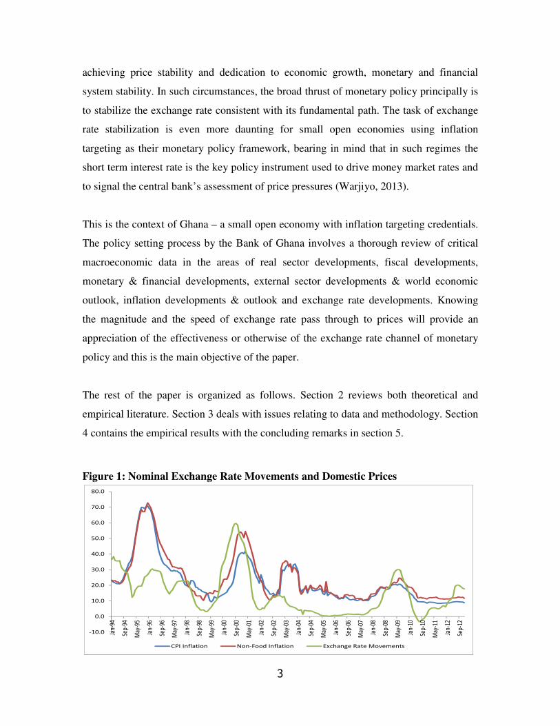
exchange market. The inflationary implications of the exchange rate movements in the

case of Ghana is depicted in Figure 1, which corroborates the point that bouts of

exchange rate instability are usually followed by episodes of high inflationary pressures

while exchange rate stability precedes periods of disinflation.

Given these contexts, small open economies usually consider exchange rate policy as an

essential element of their overall monetary–macroprudential policy mix aimed at

2 Dual mandate central banks equally weight inflation and output

3 In fact, during this period the US experienced two recessions usually blamed on the Fed’s aggressive

disinflationary policies.

3

achieving price stability and dedication to economic growth, monetary and financial

system stability. In such circumstances, the broad thrust of monetary policy principally is

to stabilize the exchange rate consistent with its fundamental path. The task of exchange

rate stabilization is even more daunting for small open economies using inflation

targeting as their monetary policy framework, bearing in mind that in such regimes the

short term interest rate is the key policy instrument used to drive money market rates and

to signal the central bank’s assessment of price pressures (Warjiyo, 2013).

This is the context of Ghana – a small open economy with inflation targeting credentials.

The policy setting process by the Bank of Ghana involves a thorough review of critical

macroeconomic data in the areas of real sector developments, fiscal developments,

monetary & financial developments, external sector developments & world economic

outlook, inflation developments & outlook and exchange rate developments. Knowing

the magnitude and the speed of exchange rate pass through to prices will provide an

appreciation of the effectiveness or otherwise of the exchange rate channel of monetary

policy and this is the main objective of the paper.

The rest of the paper is organized as follows. Section 2 reviews both theoretical and

empirical literature. Section 3 deals with issues relating to data and methodology. Section

4 contains the empirical results with the concluding remarks in section 5.

Figure 1: Nominal Exchange Rate Movements and Domestic Prices

-10.0

0.0

10.0

20.0

30.0

40.0

50.0

60.0

70.0

80.0

Jan-

94

Sep-

94

May

-95

Jan-

96

Sep-

96

May

-97

Jan-

98

Sep-

98

May

-99

Jan-

00

Sep-

00

May

-01

Jan-

02

Sep-

02

May

-03

Jan-

04

Sep-

04

May

-05

Jan-

06

Sep-

06

May

-07

Jan-

08

Sep-

08

May

-09

Jan-

10

Sep-

10

May

-11

Jan-

12

Sep-

12

CPI Inflation Non-Food Inflation Exchange Rate Movements

4

2. Literature Review

The last two decades have witnessed a huge economic literature on exchange rate pass-

through. This section therefore focuses on reviewing related theoretical and empirical

literature.

2.1 Theoretical Literature

Goldberg and Knetter (1997) define exchange rate pass-through as the percentage change

in local currency import prices resulting from a percentage change in the exchange rate

between the exporting and importing countries. In the context of the current paper, we

define exchange rate pass-through as the impact of exchange rate movements on import

and consumer prices over time.

There is consensus in the empirical literature that exchange rate pass-through as defined

above is incomplete. Dornbusch (1987), for instance, rationalizes incomplete pass-

through as emanating from firms operating in markets characterized by imperfect

conditions and therefore adjust their mark-up in response to exchange rate shock. On

their part, Burstein et al. (2003) stress the role played by non-traded (domestic) inputs in

the chain of distribution of tradable goods. Burstein et al. (2005) identify measurement

problems inherent in consumer price index, which does not account for quality

adjustment of tradable goods with significant adjustment in the exchange rate. Gagnon

and Ihrig (2004) point to the role of fiscal and monetary authorities, which partially offset

the effect of changes in the exchange rate on domestic prices. Another possible reason for

incomplete pass-through is the practice of pricing in the local currency (Devereux and

Engel 2001, and Bacchetta and van Wincoop 2003). Krugman (1986) points to “pricing

to market” by foreign suppliers as the reason why US import prices do not fully mirror

exchange rate movements.

2.2 Empirical Literature

There is a burgeoning number of empirical literature on the exchange rate pass-through to

domestic prices. McCarthy (1999) investigates the effect of exchange rate changes and

import prices on producer and consumer prices in a recursive vector autoregressive

5

(VAR) model. Relying on data from 6 industrialized OECD nations, he discovers that

exchange rate movements have modest impact on domestic consumer prices.

Goldfajn and Werlang (2000) study a panel of 71 countries and find that the exchange

rate pass-through is correlated with the business cycle, the size of the initial real

exchange rate misalignment, the initial rate of inflation and the degree of openness of the

economy. They also ascertain that the exchange rate pass-through coefficient is positively

time-varying after devaluation, and is maximized after one year (12 months).

Burstein et al. (2002) investigate the behaviour of consumer prices following large

devaluations in nine countries4 and ascertain a low pass-through from the exchange rate

to consumer prices. Following the floating of the exchange rate in Brazil in 1999,

Rabanal and Schwartz (2000) investigate the behaviour of inflation in that country and

find that the initial shock has worked through the system after 20 months.

Zorzi et al. (2007) employ vector autoregressive models to examine the degree of

exchange rate pass-through to prices in 12 emerging markets in Asia, Latin America, and

Central and Eastern Europe. Their findings were partially inconsistent with conventional

wisdom that exchange rate pass-through to domestic prices are always higher in emerging

than developed countries. They also discover that for emerging markets with single digit

inflation, pass-through to import and consumer prices is low and not different from the

levels of developed economies. The paper also finds robust evidence for a positive

relationship between the degree of the exchange rate pass-through and inflation,

consistent with Taylor’s hypothesis.

Leigh and Rossi (2002) employ a recursive vector autoregressive model to investigate the

impact of exchange rate movements on prices in Turkey. They find that (i) the impact of

the exchange rate on prices is over after about a year, but is mostly felt in the first four

months, (ii) the pass-through to wholesale prices is more pronounced compared to the

4 The countries are Brazil, Finland, Indonesia, Korea, Malaysia, Mexico, Philippines, Sweden, and

Thailand

6

pass-through to consumer prices, and (iii) the estimated pass-through is complete in a

shorter time and is larger than that estimated for other key emerging countries.

Acheampong (2004)5 uses recursive VAR to estimate the cumulative pass-through for

Ghana and concludes that the pass-through is incomplete, modest and slow. He also finds

that the pass-through to non-food prices is more pronounced compared to the pass-

through to consumer prices and that the pass-through to consumer prices has not changed

over time but the pass-through to non-food prices has gone up6.

Even though this study is similar in approach to Acheampong (2004), there are two main

gaps this study fills. First, the ordering of the policy or money market variable (broad

money aggregate) before the exchange rate variable could lessen the impact of the

demand and supply shocks on the exchange rate and prices. This study therefore re-orders

the reaction of the money market and/or monetary policy last to allow the money market

and in particular monetary policy to react contemporaneously to all the shocks. Second, it

has been almost a decade since his study was done. It has been almost a decade since his

study was done. It is important to re-examine the pass-through of the exchange rate shock

on account of the macroeconomic and policy changes that have occurred since 2004 to

examine their impact.

3. Data and Methodology

3.1 Methodology

The study is based on the seminal work of McCarthy (1999) as adapted by Leigh and

Rossi (2002). We estimate the pass-through of exchange rate movements to domestic

prices using a six-variable recursive VAR approach instead of the seven-variable model

estimated by McCarthy (1999) or the five-variable model by Leigh and Rossi (2002)

5 See Frimpong and Adam (2010) and Sanusi (2010) for other studies on Ghana. We deliberately omitted

details of these studies because of their inability to estimate the cumulative pass-through of exchange rate

as proposed by McCarthy (1999). 6 Within three months, 14.79 percent and 5.64 percent of the exchange rate movement reflect into non-food

and overall consumer prices respectively. After six months, the pass-through was 21.82 percent for non-

food inflation, and 9.05 for overall consumer inflation. The pass-through after one year was 27.51 percent

and 14.53 percent for non-food and overall CPI inflation. And in two years, the pass-through was 35.01

percent and 22.94 percent for non-food inflation and overall CPI inflation respectively.

7

ordered as follows: oil prices7, output gap, the nominal exchange rate of the Cedi to the

US dollar, non-food price index, consumer price, short term interest rate (t-bill rate)8. The

key variables in the framework are the two price variables and the exchange rate. The

inclusion of oil price and the output variable are intended to capture impacts on the real

side of the economy. Finally, we include interest rate to allow the money market as well

as the impact of monetary policy to influence the pass-through linkage.

The model is specified as follows:

�1�� = E�� ���� +���

�2�∆y� = ��� �∆��� + � ����� + ��∆�

�3�∆�� = ��� �∆��� + ����� + !��∆� + ��∆"

�4�$%

&'()* = �%−1�$%&'()* � + ,1�%-*. + ,2�%

∆� + ,3�%∆� + �%&'()*

�5�$�01� = ��� �$�

01�� + ∅ ����� + ∅!��∆� + ∅3��∆" + ∅4��

561� + ��01�

�6�∆*� = ��� �∆*�� + 8 ����� + 8!��

∆� + 83��∆" + 84��561� + 89��

01� + ���

In the specified model above, $��� denotes changes in oil prices (i.e. oil price inflation),

∆� refers to the first log difference of GDP gap, ∆� is the first log difference of the

bilateral cedi-dollar exchange rate, $561�and $01� are non-food and CPI inflation

respectively, and ∆*is the rate of interest rate changes, capturing the money market,

including monetary policy response to the supply shock. The supply, demand and

exchange rate shocks are captured by ����, �∆� and �∆" respectively, while �561�, �01�

and �� are shocks to non-food inflation, CPI inflation and money market respectively.

The time dimension t corresponds to one month with ��� �� denoting expectation about a

variable subject to information available in time% − 1. A crucial assumption

underpinning the behaviour of the model is that the conditional expectations in equations

7 We use benchmark Brent crude price, converted into the Ghanaian Cedi by multiplying by the Cedi/dollar

exchange rate. 8 The choice of variables and ordering is consistent with the approach of McCarthy (2000), Hahn (2003)

and Zorzi et al. (2007).

8

[1] to [6] can be substituted by linear projections based on lags of the six dependent

variables.

Specifying the framework using a recursive identification design means that there is no

contemporaneous feedback impact in the model. That is, the identified shocks

contemporaneously impact subsequent variables and other variables ordered afterwards,

but have no contemporaneous effect on the variables, which are ordered before them.

Thus, it is customary to order the most exogenous variable first, which, in this paper is

the oil price. Therefore, oil price shocks may impact all other variables in the model

contemporaneously but oil prices are not contemporaneously impacted by other shocks.

Next, we order output gap and exchange rate with the implicit assumption of a

contemporaneous effect of the demand shocks on the exchange rate and that the exchange

rate shock will only impact the output gap with a certain time lag. Next to be ordered are

the price variables, imported inflation and CPI inflation, and are thus impacted

contemporaneously by all the variables ordered before them. In line with the pricing

chain, import prices lead CPI inflation so that import price shocks contemporaneously

impact consumer prices but not vice versa. The last variable to be ordered is the short

term interest rate allowing the money market and crucially monetary policy to respond

contemporaneously to all shocks in the system. The ordering scheme as described above

can be summarized as follows:

$��� → ∆� → ∆� → ∆$5601� → ∆$01� → ∆*

The model is estimated in a VAR framework with Cholesky decomposition employed to

recover the structural shocks from the VAR residuals.

Next, we estimate the cumulative pass-through coefficients from the impulse response

functions, which is accomplished by dividing the cumulative impulse responses of each

price index after n months by the cumulative response of the exchange rate to the

exchange rate shock after n months, given as:

9

[7] <=�,�>5 =?@,@ABC@,@AB

, where <�,�>5 denotes the cumulative change in the

particular price variable and ��,�>5 is the cumulative change in exchange rate.

In order to examine the stationarity properties of the variables in the study with a view to

avoiding spurious regression analysis, the following Augmented Dickey-Fuller (ADF)

test is performed on each series:

[8] ∆D� = � + �EF − 1GD�� + ∑ FI1IJ ∆D�� + ��

where ∆ is the first-difference operator; % is a linear time trend; � is a covariance

stationary random error term and Fis determined by the Schwarz criterion to ensure

serially uncorrelated residuals. The null hypothesis is that D� is a nonstationary series and

is rejected if EF − 1G < 0 and statistically significant. The model specification demands

that all the variables are difference stationary, I(1).

3.2 Data Issues

We use monthly data spanning January 1994 to December 2012, a sample size

determined ultimately by the availability and quality of data. The supply shock in the

model is measured by benchmark Brent crude oil price in US dollars but converted into

the domestic currency (Cedi) using the average monthly cedi-dollar nominal exchange

rate. The demand shock is captured by the output gap measured as the difference between

the unobserved potential output and actual output level. We estimate the potential output

with the help of Hodric-Prescott (HP) Filter. Since the GDP numbers were mostly

available in low frequency annual series, we convert the annual series to high frequency

monthly series using conversion scheme available in E-views. The exchange rate is

captured by the average monthly bilateral nominal exchange rate between the Cedi and

the US dollar. For the import price index variable, we use non-food price index as a

proxy due to unavailability of import price index. The inflation variable is the CPI

inflation. We also include a dummy variable that takes the value of 1 and -1 if domestic

10

oil prices were adjusted upwards and downwards respectively, and 0 otherwise9. The data

are seasonally adjusted.

3.3 Limitations of the Study

Some of the limitations of the study include the use of non-food Inflation as a proxy for

imported inflation due to unavailable data on the latter. It is often expected that exchange

rate shock is more pronounced on import prices than non-food prices. The estimation of

the unobserved potential output using HP filter may not be without problems as the filter

is known to suffer from end-point and structural break problems (see Baxter and King,

1999, and Chagny and Dopke, 2002). Nevertheless, the HP filter remains the most

popular approach to estimating the unobserved potential output level. The conversion of

the low frequency annual GDP series to high frequency monthly series may introduce

dynamics which may be inconsistent with the structural dynamics of the Ghanaian

economy.

4. Empirical Results

4.1 Stationarity Test

The result of the ADF tests conducted on all variables in the model based on equation [8]

is presented in Table 1. In the case of the levels of the series, the null hypothesis of

nonstationarity cannot be rejected for any of the series. Therefore, the levels of the series

are non-stationary. Applying the same tests to first differences to determine the order of

integration, the critical value is (are) less (in absolute terms) than the calculated values of

the test statistic for both series. Given that all the variables are integrated of the same

order we proceed to estimate the VAR in first difference.

9 The usual dummy that takes the value 1 if oil prices were adjusted and 0 otherwise did not perform well.

11

Table 1: ADF Unit Test

Note: * denotes significance at 1%

Critical values are: 1% level =-3.458973; 5% level=-2.874029; 10% level = 2.573502

Critical values and one-sided p-values are taken from MacKinnon (1996) and reported in

E-Views 8.0

4.2 Estimates of Size and Magnitude of Pass-Through

The VAR from equations [1] to [6] is estimated with two lags selected based on Schwarz

information criterion (SIC). The estimated VAR satisfies the stability condition as no root

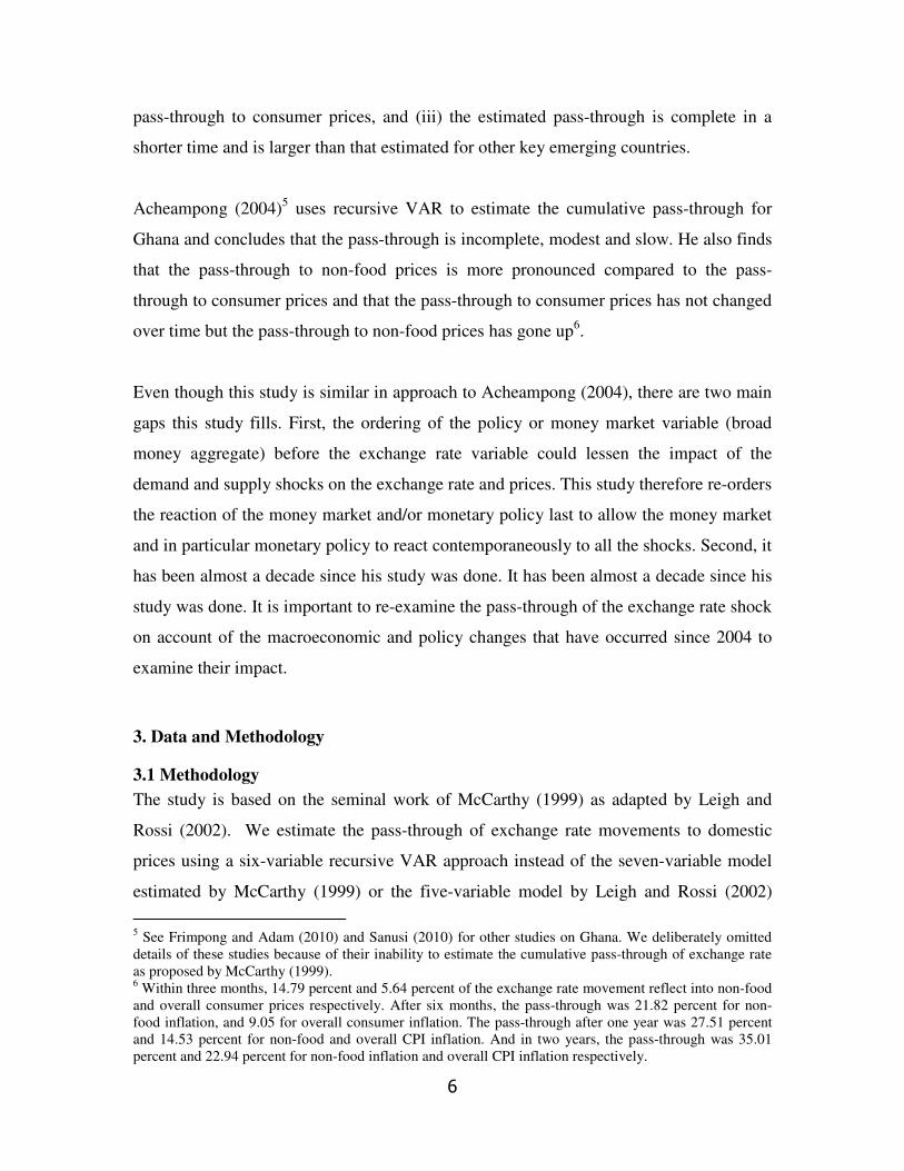
lies outside the unit circle. The impulse response functions from the estimated VAR are

then used to ascertain the effect of exchange rate changes on domestic prices. The

estimated orthogonalized impulse response functions for non-food and CPI inflation to a

one standard deviation innovation in the exchange rate is shown in Figure 210

. The

derivation of the size and speed of the cumulative pass-through coefficients is based on

equation [8]. The estimated coefficients indicate the model’s predicted response of

domestic prices to nominal exchange rate shock once the disturbances of other

endogenous variables are accounted for.

10

Other impulse functions are not reported deliberately since the main focus of the study is on the impact

of exchange rate shocks on domestic prices.

Variables Levels p-values First Difference p-values

Oil Prices -1.15409 0.6943 -13.9290 0.0000*

Exchange Rate -1.4913 0.5364 -3.7510 0.0040*

Output Gap -1.9875 0.2381 -4.4844 0.0003*

Non-food prices -1.96626 0.3014 -11.0483 0.0000*

Consumer prices -1.87219 0.3451 -7.0014 0.0000*

Interest Rates -2.08052 0.2528 -5.2590 0.0000*

12

Figure 2: Impulse Response to a one standard innovation in the

exchange rate

Response of the Bilateral Nominal Exchange rate

-.004

.000

.004

.008

.012

.016

5 10 15 20 25 30 35

Response of Non-food inflation

-.0050

-.0025

.0000

.0025

.0050

.0075

.0100

.0125

.0150

5 10 15 20 25 30 35

Response of Overall CPI Inflation

-.004

-.002

.000

.002

.004

.006

.008

.010

.012

5 10 15 20 25 30 35

13

Figure 3: Estimated Cumulative Pass-Through Coefficients

Table 2: Estimated Cumulative Pass-Through Coefficients

The estimated cumulative pass-through coefficients shown in Figure 3 and Table 2 points

to the fact that the effect of a nominal exchange rate shock on domestic prices are

incomplete and broadly modest and fade within 18-24 months, but such impacts are

mostly felt within 12 months. This is supported by the impulse response to a one standard

innovation in the exchange rate as evidenced in Figure 2. Within the first three months of

an exchange rate shock, for instance, the pass-through to non-food and CPI inflation were

0.0

5.0

10.0

15.0

20.0

25.0

30.0

35.0

40.0

1 3 5 7 9 11 13 15 17 19 21 23 25 27 29 31 33 35

Pe

rce

nt

Periods (Months)

Non-Food Inflation Overall CPI Inflation

Periods Non-Food Overall CPI

(Months) Inflation Inflation

3 13.3 6.5

6 23.2 13.9

9 28.6 19.0

12 31.8 22.1

15 33.6 24.0

18 34.7 25.1

21 35.4 25.8

24 35.8 26.2

27 36.0 26.4

30 36.1 26.5

33 36.2 26.6

36 36.3 26.7

14

13.3 percent and 6.5 percent respectively. However, as prices are adjusted over time to

reflect the exchange rate movements, the pass-through rises steadily to 23.2 percent and

13.9 percent for non-food and CPI inflation respectively within six months. After 12

months (i.e. 1 year) 31.8 percent and 22.1 percent of the shock are reflected in non-food

and CPI inflation respectively. Beyond 12 months, the speed of the pass-through becomes

significantly dawdling with the magnitude reaching 35.8 percent and 26.2 percent of non-

food and CPI inflation respectively after 24 months. The impact of the exchange rate

shocks disappears completely after 36 months (3 years) as the pass-through tapers off at

36.3 percent and 26.7 percent for non-food inflation and CPI inflation. The disappearance

of the impact of the pass-through is reinforced by Figure 4.

The pass-through also drops along the pricing chain in that it is higher for non-food

prices (our proxy for import prices) than for consumer prices (CPI inflation) and is

generally consistent with the overall consensus on exchange rate pass-through along the

pricing chain. This could be attributed to the fact that the non-food CPI contains

proportionately larger share of tradable items.

Figure 4: Changes in the Pass-Through over time

0.0

1.0

2.0

3.0

4.0

5.0

6.0

7.0

8.0

2 4 6 8 10 12 14 16 18 20 22 24 26 28 30 32 34 36

Per

cen

t

Periods (Months)

Non-Food inflation CPI Inflation

15

4.3 Variance Decomposition of Non-food and CPI Inflation

In contrast to the pass-through coefficients, variance decomposition helps us in assessing

the importance of exchange rate shocks in explaining the behaviour of non-food and CPI

inflation. In the context of variance decomposition, a variable is said to explain the

fluctuations in another variable if it accounts for a large proportion of that variable’s

forecast error variance. Therefore, we decompose variations in non-food and CPI

inflation into the shocks to the endogenous variables in the VAR model.

The result of the variance decomposition seems to suggest that exchange rate movements

accounts for a small proportion of the fluctuations in non-food and CPI inflation. As

shown in Table 3, the variation in non-food inflation is mainly explained by its own

innovations of about 75 percent, exchange rate shocks account for barely 12 percent with

the remainder coming from innovations to oil prices, output, CPI inflation, and Interest

rates.

In line with empirical regularity and consistent with the pass-through coefficients

estimates, the effect of the exchange shock on CPI inflation fluctuations is more benign

than for non-food inflation. As stated elsewhere in this paper, this outcome reflects the

larger share of tradables in the non-food basket. In Table 4, only about 7 percent of the

variation of CPI inflation is explained by the exchange rate shock, non-food inflation

innovations account for about 58 percent, own-innovations explain about 30 percent

while the remainder of the variation is explained by the other variables. These results not

only confirm the high persistence of inflation in Ghana but also identify innovations to

non-food inflation as the main source of the persistence.

16

Table 3: Variance Decomposition of Non-Food Inflation

Table 4: Variance Decomposition of CPI Inflation

4.4 Taylor’s Hypothesis, Single-Digit Inflation and Pass-Through

Ghana has had over one-and-half years of single-digit inflation for the first time in its

history, starting from June 201011

. Here, we investigate the likely impact of this episode

of low inflation on the exchange rate pass-through drawing from Taylor’s hypothesis that

the exchange rate pass-through is positively correlated with the level of inflation,

11

With index 2002=100, inflation for January 2013 was 8.8 percent, but with index 2012=100, inflation for

January 2013 was 10.1 percent.

Percentage of forecast error variance attributed to:

Forecst Oil Output Exchange Non-Food CPI Interest

Horizon Prices Gap Rate Inflation Inflation Rates

3 2.74 0.31 4.04 87.36 3.65 1.90

6 3.03 0.47 8.88 79.98 4.34 3.29

9 3.16 0.50 11.19 76.98 4.27 3.90

12 3.21 0.50 12.18 75.76 4.20 4.15

15 3.22 0.50 12.57 75.28 4.18 4.25

18 3.23 0.50 12.72 75.09 4.16 4.30

21 3.23 0.50 12.78 75.02 4.16 4.31

24 3.23 0.50 12.80 75.00 4.16 4.32

27 3.23 0.50 12.81 74.99 4.16 4.32

30 3.23 0.50 12.81 74.98 4.16 4.32

33 3.23 0.50 12.81 74.98 4.16 4.32

36 3.23 0.50 12.81 74.98 4.16 4.32

Percentage of forecast error variance attributed to:

Forecast Oil Output Exchange Non-Food CPI Interest

Horizon Prices Gap Rate Inf lation Inf lation Rates

3 0.86 0.22 1.27 62.49 33.98 1.19

6 1.15 0.44 3.88 61.03 31.35 2.15

9 1.36 0.53 5.73 59.66 30.04 2.69

12 1.45 0.54 6.65 58.96 29.49 2.91

15 1.48 0.54 7.04 58.66 29.28 3.00

18 1.49 0.54 7.19 58.54 29.20 3.04

21 1.50 0.54 7.25 58.49 29.17 3.06

24 1.50 0.54 7.27 58.48 29.15 3.06

27 1.50 0.54 7.28 58.47 29.15 3.07

30 1.50 0.54 7.28 58.47 29.15 3.07

33 1.50 0.54 7.28 58.47 29.15 3.07

36 1.50 0.54 7.29 58.47 29.15 3.07

17

implying that a low inflation in itself could imply a low pass-through. This is achieved by

introducing exogenously into the VAR model a dummy variable, which takes the value of

1 from June 2010 to December 2012 and 0 otherwise. The results as presented in Table 5

show that, on average, the estimated pass-through coefficients are at least two (2)

percentage points below the estimates in the baseline model shown in Table 2, giving

support to the Taylor’s hypothesis of a positive correlation between the level of inflation

and the size of the exchange rate pass-through.

Table 5: Cumulative Pass-Through Based on Taylor’s Hypothesis

4.5 Alternative Ordering and Robustness

This section ascertains the sensitivity of the results based on the identification scheme.

The model is therefore re-estimated based on the alternative ordering of the variables in

the Cholesky decomposition as follows: oil prices, output gap, interest rates, exchange

rate, non-food inflation, and CPI inflation. Here, the interest rate is ordered before the

exchange rate as proposed by Choudhri et al. (2002) and used by Acheampong (2004)12

.

$��� → ∆� → ∆* → ∆� → ∆$5601� → ∆$01� This permits a contemporaneous reaction of the exchange rate to changes in monetary

policy and based on the belief that higher interest rate makes investment in money market

securities more attractive and reduces pressure on the local currency. The estimated pass-

through coefficients presented in Table 6 broadly indicates that the coefficients are at

least 100 basis points below those obtained from the baseline ordering (see Table 1),

12

Acheampong for instance used a money supply variable instead of interest rate.

Perioids Non-Food Overall CPI

(Months) Inflation Inflation

3 12.0 5.9

6 21.0 12.5

9 26.0 17.0

12 28.9 19.7

15 30.6 21.4

18 31.6 22.4

21 32.2 22.9

24 32.5 23.3

27 32.7 23.5

30 32.8 23.6

33 32.9 23.7

36 33.0 23.7

18

vindicating our position that such an ordering could potentially reduce the size of the

pass-through coefficients.

Table 6: Cumulative Pass-Through Coefficients from Alternative Ordering

5. Concluding Remarks

We use a recursive VAR based on the seminal work of McCarthy (1999) as used by

Leigh and Rossi (2002) and Acheampong (2004) to estimate the pass-through impact of

exchange rate movements on domestic prices between January 1994 and December 2012.

The model consists of six variables, which are ordered as: oil prices, output gap,

exchange rate, non-food prices, overall consumer prices, and money market interest rates

with the implicit assumption that the identified shocks contemporaneously impact

variables ordered after the shock without a contemporaneous feedback. Based on the

estimates of the size and magnitude of the pass-through coefficients, and variance

decomposition of the pass-through of non-food and CPI inflation, we draw the following

conclusions.

The effect of a nominal exchange rate shock on domestic prices is incomplete and

broadly modest and fades within 18-24 months, but such impacts are mostly felt within

12 months. This is plausible given that Ghana’s monetary policy transmission mechanism

has a lag of about 18 months.

Generally, the impact of the exchange shock on CPI inflation is more benign than for

non-food inflation. This, as noted earlier, might be due to the fact that non-food inflation

Periods Non-Food Overall CPI

(Months) Inflation Inflation

3 13.2 5.4

6 22.2 12.4

9 27.3 17.2

12 30.3 20.2

15 32.1 22.0

18 33.1 23.1

21 33.8 23.8

24 34.1 24.1

27 34.3 24.4

30 34.5 24.5

33 34.5 24.6

36 34.6 24.6

19

contains a greater share of tradable goods and services compared to CPI inflation. It is

also possible that producers do not have the pricing power to fully adjust their prices to

reflect the exchange rate shock thereby forcing profit margins to contract in order to

absorb the exchange rate shock with consumer prices minimally impacted. Profit margin

contraction is inimical to future investment, output growth and employment generation,

implying a stable currency is a necessary pre-requisite for sustainable growth.

The pass-through coefficient estimates in this study appears larger in size and shorter in

speed compared to estimated pass-through coefficients for other EMEs. For South Africa,

for instance, Bhundia (2002) discovers that pass-through of a 1 percent exchange rate

shock is only 8.3 percent after four (4) quarters and 12 percent after eight (8) quarters.

The speed of the estimated pass-through in this study seems faster than that of

Acheampong (2004). For example, he reports 14.5 percent pass-through for CPI inflation

after 12 months following nominal exchange rate shock, within the same time frame our

estimated pass-through was 22.1 percent. We also find evidence in support of Taylor’s

hypothesis that the inflation environment is an important influence on the exchange rate

pass-through

Oil prices explain just a minimal variance in non-food and CPI inflation, reflecting, in our

opinion, non-automatic adjustment in domestic ex-pump price of oil to reflect conditions

in the international market. It is expected that the regular application of the automatic

adjustment formula with exchange rate movements as one of its underlying triggers will

increase oil price’s contribution to the variance of domestic prices; in effect suggesting

exchange rate stability will greatly support price stability and enhance macroeconomic

stability.

Finally, evidence from the variance decomposition suggests that the influence of demand

pressures measured by the output gap on domestic prices may have been grossly

overstated.

20

References

Acheampong, Kwasi (2004), “The Pass-Through From Exchange Rate To Domestic

Prices in Ghana”, BOG working Paper No. 05/14, Accra, Bank of Ghana.

Bacchetta, P. and van Wincoop, E. (2003), “Why do Consumer Prices React Less than

Import Prices to Exchange Rates?” Journal of European Economic Association, 1, 662-

670.

Baxter, M. and R. King (1999), “Measuring Business Cycles: Approximate bandpass

filters for economic time series”, Review of Economics and Statistics 8, 575-593.

Bhundia, A. (2002), “An Empirical Investigation of Exchange Rate Pass-Through in

South Africa”, IMF Working Paper No. 20/165, Washington, IMF.

Billmeier, A., and L. Bonato (2002), “Exchange Rate Pass-Through and Monetary in

Croatia”, IMF Working Paper No. 02/109, Washington, IMF.

Blejer, Mario I. (1998), “Central Banks and the Price Stability: Is a Single Objective

Enough?”. Journal of Applied Economics, Vol. I, No. 1, 105-122.

Burstein, A., B. Eichenbaum, and S. Rebelo (2002), “Why Is Inflation So Low After

Large Devaluations?” NBER Working Paper No. 8748, Cambridge, Massachusetts,

NBER.

Burstein, A., B. Eichenbaum, and S. Rebelo (2005), “Large Devaluations and the Real

Exchange Rate”, Journal of Political Economy, 113, 742-784.

Burstein, A., J. Neves and S. Rebelo (2003), “Distribution Costs and Real Exchange

Rates Dynamics During Exchange-Based-Stabilizations?” Journal of Monetary

Economics, 50, 1189-1214.

Chagny, O. and J. Dopke (2002), “Mesuares of the output gap in the Euro-zone: An

empirical assessment of selected methods”, Quarterly Journal of Economic Research 70,

310-330.

Choudri, E.U., and D. S. Hakura (2001), “Exchange Rate Pass-Through to Domestic

Prices: Does the Inflationary Environment Matter?” IMF Working Paper No. 01/194,

Washington, IMF

Choudri, E.U., Faruqee, H. and D. S. Hakura (2002), “Exchange Rate Pass-Through in

Different Prices”, IMF Working Paper No. 02/224, Washington, IMF.

Devereux, M., and Engel, C. (2001), “Endogenous Currency of Price Setting in a

Dynamic Open Economy Model”, NBER Working Paper No. 8559.

21

Dornbusch, R. (1987), “Exchange Rate and Prices”, American Economic Review, 77, 93-

106.

Frimpong, S. and A. M. Adam (2010), “Exchange Rate Pass-Through in Ghana”,

International Business Research, 3(2), 186-192.

Goldberg, P. K. and M. M. Knetter (1997), “Goods Prices and Exchange Rates: What

Have We Learned?” Journal of Economic Literature, 35(3): 1243

Goldfajn, I., and Werlang (2000), “The Pass-Through from Depreciation to inflation: A

Panel Study”, Working Paper No. 423, Rio de Janeiro, Department of Economics,

Pontificia Universidade Catolica.

Goodfriend, M. and Robert G. King (2004), “The Incredible Volcker Disinflation”.

Prepared for the Carnegie-Rochester Conference on Public Policy.

Hahn, E. (2003), “Pass-Through of External Shocks to Euro Area Inflation”, European

Central Bank Working Paper No. 243.

Krugman, P. (1986), “Pricing to Market When Exchange Rate Changes”, NBER

Working Paper No. 1926, Cambridge, Massachusetts, NBER.

Leigh, D., and M. Rossi (2002), “Exchange Rate Pass-Through in Turkey”, IMF Working

Paper No. 02/204, IMF.

McCarthy, J. (1999), “Pass-Through of Exchange Rates and Import Prices to Domestic

Inflation in Some Industrialized Economies”, BIS Working Paper No. 79, Basel, BIS.

Rabanal, P., and G. Schwartz (2001), “Exchange Rate Changes and Consumer Price

Inflation: 20 Months After the Floating of the Real in Brazil: Selected Issues and

Statistical Appendix”, IMF Country Report No. 01/10, Washington, IMF.

Taylor, J. (2000), “Low Inflation, Pass-Through and the Pricing Power of Firms”,

European Economic Review, 44, 1389-1408.

Warjio, Perry (2013), “Indonesia: Stabilising the exchange rate along its fundamental”, In

“market volatility and foreign exchange rate intervention in EMEs: what has changed?”

BIS Papers 73, Monetary and Economic Department.

Zorzi, M. C., E. Hahn, and M. Sanchez (2007), “Exchange Rate Pass-Through in

Emerging Markets”, ECB Working Papers Series No. 739, EU.