Excel Workbook for automatic parameter calculation of EPG data

This article appeared in a journal published by Elsevier. The attachedcopy is furnished to the author for internal non-commercial researchand education use, including for instruction at the authors institution

and sharing with colleagues.

Other uses, including reproduction and distribution, or selling orlicensing copies, or posting to personal, institutional or third party

websites are prohibited.

In most cases authors are permitted to post their version of thearticle (e.g. in Word or Tex form) to their personal website orinstitutional repository. Authors requiring further information

regarding Elsevier’s archiving and manuscript policies areencouraged to visit:

http://www.elsevier.com/copyright

http://www.elsevier.com/copyright

Author's personal copy

Computers and Electronics in Agriculture 67 (2009) 35–42

Contents lists available at ScienceDirect

Computers and Electronics in Agriculture

journa l homepage: www.e lsev ier .com/ locate /compag

Excel Workbook for automatic parameter calculation of EPG data

E. Sarriaa, M. Cidb, E. Garzob, A. Fereresb,∗

a Departamento de Mejora Vegetal, Estación Experimental ‘La Mayora’ (EELM), Consejo Superior de Investigaciones Científicas (CSIC),Algarrobo-Costa, 29760 Málaga, Spainb Departamento de Proteccion Vegetal, Instituto de Ciencias Agrarias (ICA), Centro de Ciencias Medioambientales (CCMA),Consejo Superior de Investigaciones Científicas (CSIC), C/ Serrano 115 dpdo, 28006 Madrid, Spain

a r t i c l e i n f o

Article history:Received 22 July 2008Received in revised form29 December 2008Accepted 14 February 2009

Keywords:AphidsMealybugInsect feedingBehaviorHemipteraElectrical penetration graphs

a b s t r a c t

The electrical penetration graph (EPG) technique is a powerful tool for studying feeding behavior of pierce-sucking insects, because it allows quantification of complex insect–plant interactions occurring inside theplant. However, this technique has an important limitation related to the time-consuming analysis of theacquired data, mainly due to the length of the EPG recordings and the complexity of the parameters usedto explore insect behavior. This paper presents a Microsoft Excel Workbook that simplifies the analyses ofEPG data and automatically calculates a large number of EPG parameters that characterize insect probingand ingestion behavior. These parameters arise from a wide review of EPG papers related to differentaspects of insect–plant and virus–insect vector interactions. Another advantage of this application is thatdata input can be entered from both AC- and DC-based amplifiers and from different software packagesused to acquire EPG data (e.g. MacStylet, WINDAQ and PROBE). The workbook summarizes the resultsand generates an output sheet for further statistical analysis. In this report, we explain how the workbookcan be used to analyze the probing and ingestion behavior of two hemipteran species, demonstrating itsflexibility and potentiality for efficient and rapid analysis of EPG data.

© 2009 Elsevier B.V. All rights reserved.

1. Introduction

Hemipteran species are serious pests in agriculture causing yieldlosses in a wide variety of crops. Many of them have an inti-mate and long-lasting interaction with plant cells since they usestylets to pierce cells and to feed on epidermal, mesophyl or vas-cular tissues (Walling, 2000). The amount of damage caused by thefeeding mode and by the intake of fluids as a nutritional sourcevaries tremendously depending upon the hemipteran species. Theindirect damages caused by the transmission of several viruses,phytoplasmas and bacteria should also be considered, becausehemipterans have been described as the most important group ofvectors of plant pathogens (Nault, 1997).

The study of hemipteran probing and ingestion behavior wasrevolutionized by the introduction of the first electronic feedingmonitor developed by Mclean and Kinsey (1964) that made anaphid and a plant part of an electrical circuit. The original moni-toring device used an alternating current (AC) circuit. This systemwas posteriously improved by Backus and Bennett (1992) and it waslater referred as AC system (Backus, 1994). Nevertheless, the mostsignificant modification has been the substitution of the AC circuitwith direct current (DC) circuit and it was referred to as the DC

∗ Corresponding author. Tel.: +34 915627620; fax: +34 915640800.E-mail address: [email protected] (A. Fereres).

System (Tjallingii, 1978, 1985). All EPG monitors, whether they areAC or DC, measure the changes in electrical resistance in the plantand the insect. In addition, Tjallingii’s DC system also measureschanges in voltage that originate as biopotentials or bio-voltages inthe plant and the insect (also called electromotive forces), obtain-ing a more detailed picture of insect behavior, more detailed andcharacteristic waveforms allowing exact measurements of subfre-quencies of the different components of each waveform, and acareful matching of the input resistor to the insect–plant systemunder study (Tjallingii, 1978; Van Helden and Tjallingii, 2000). Thistechnique is a powerful tool for studying hemipteran feeding behav-ior since it allows the quantification of complex insect activitiesoccurring inside the plant. The EPG technique has been appliedto investigate insect–plant interactions, including the localizationand characterization of host plant resistance to hemipterans (Garzoet al., 2002) and to understand the transmission mechanisms ofplant pathogens by their insect vectors (Martin et al., 1997; Joostet al., 2006). Also, this technique has been used in phloem phys-iology studies (Will et al., 2008) and to understand the mode ofaction of pesticides (Harrewijn and Kayser, 1997; Kaufmann et al.,2004).

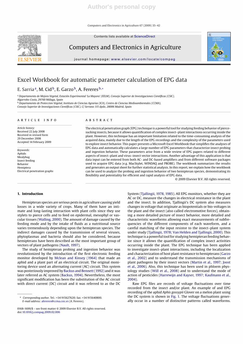
Raw EPG files are records of voltage fluctuations over timerecorded from the insect and/or plant. An example of and EPGrecording of the aphid Aphis gossypii Glover on a melon plant usingthe DC system is shown in Fig. 1. The voltage fluctuations gener-ally occur in a number of distinctive patterns called waveforms.

0168-1699/$ – see front matter © 2009 Elsevier B.V. All rights reserved.doi:10.1016/j.compag.2009.02.006


36 E. Sarria et al. / Computers and Electronics in Agriculture 67 (2009) 35–42

Fig. 1. EPG recording of A. gossypii and detailed waveforms occurred in the record. The main events occurring in the record are indicated through dashed lines (a), operationsmade with this event allows the obtention of the sequential parameters. Arrow heads and asterisks under the waveforms indicate points used to mark the different waveformsand intracellular penetrations, respectively, marks of the beginning of the waveforms of intracellular penetrations are shown in detail in b. (c) Part of data obtained after theEPG recording interpretation with the two columns format, waveform code and time. Some different EPG waveforms are also shown in detail: (d) derailed stylet mechanics;(e) xylem ingestion phase; (f) phloem salivation phase; (g) phloem ingestion phase. Abbreviations: np, non-probing phase; C, probing phase; F, stylet work phase; G, xylemingestion phase; E1, phloem salivation phase; E2, phloem ingestion phase; Pd, intracellular penetration; II-2 and II-3, subphases of the Pd. Grey bar: 5 min, black bar: 1 seg.

Different waveforms represent different behaviors as it is shownin Fig. 1b–g. These waveforms are identified on the basis of theirfrequency, amplitude, electrical origin, shape and voltage levelaccording to existing correlations for each specific group of insects(aphids, whiteflies, leafhoppers, psyllids, etc.) and the kinds of EPGsystem used (AC or DC). EPG data analysis starts by marking thebeginning of each occurrence of waveforms throughout the rawEPG data file (arrowheads in Fig. 1a and b). The waveform categoriesare non-overlapping, so marking the beginning of one waveformalso marks the end of the previously occurring waveform. Anexample of data produced after the marking of the waveforms ofan EPG recording is shown in Fig. 1c. EPG data analysis is usuallyconducted by specific software such as MacStylet (Febvay et al.,1996) or PROBE 3.0 (Tjallingii, 2004), available for the Macintoshand for PC platforms, respectively (Fig. 2). However, one of the lim-itations of the EPG technique is the calculation and interpretationof the durations and number of occurrence of waveform events(nonsequential parameters), and many additional parametersbased on the durations and sequences of these waveforms thatquantitatively describe EPG data (sequential parameters) (VanHelden and Tjallingii, 2000; Backus et al., 2007).

Nowadays, MacStylet (Febvay et al., 1996) and a workbookdescribed by Van Giessen and Jackson (1998) are the only alterna-tives to calculate a limited number of EPG parameters. The softwaredeveloped by Van Giessen and Jackson (1998) is very practical tocalculate nonsequential parameters. Backus et al. (2007) publishedan entirely different set of parameters focusing on nonsequen-tial parameters, that devised a broader, more general, hierarchicalsystem for designing and naming new parameters. The nonsequen-tial parameters are independent of any sequence in the probingbehavior and they are very usable to study nonsheath-feedinghemipterans that are rarely sequential in their feeding behavior,being the nonsequential parameters more appropriated than thesequential one in those cases (Backus et al., 2007). On the contrary,

aphids and other sheath-feeding hemipterans perform stereotypi-cal behavioral sequences during stylet penetration, then, sequentialparameters are related to a specific sequence as recorded in EPGs.Often, their calculation is very time consuming due to the lengthand the high number of the recorded files. Consequently, EPG-device users have to calculate the parameters by designing theirown formulas in spreadsheets or statistical programs. This is timeconsuming and prevents a standardization in the calculation meth-ods used for determining the EPG parameters most commonlyused.

The aim of this work is to develop a new tool to analyze EPGdata and calculate the most relevant parameters generally neededfor interpretation of insect probing and ingestion behavior. This toolis based on a Microsoft Excel® Workbook that automatically calcu-lates 112 EPG parameters from EPG data acquired by PROBE 3.0,MacStylet or any other compatible software.

2. Materials and methods

2.1. Plants, insects and experimental conditions

Cucumis melo L. cv. ‘Bola de Oro’ and Vitis vinifera cv. ‘Cabernetfranc’ plants were used to evaluate the feeding behavior of the cot-ton aphid, A. gossypii Glover and the citrus mealybug, Planococcuscitri (Risso), respectively. Only newly emerged adult insects wereused in the experiments. Aphids were maintained on the meloncultivar ‘ANC-57’ in a growth chamber at 25 ◦C (light) and 20 ◦C(dark) with a photoperiod of 16:8 h (L:D). Mealybugs were main-tained on potato tubers in dark conditions at room temperature (at25 ± 3 ◦C). Electrical monitoring of feeding behavior of both insectspecies was conducted at room temperature during 6 h long. Onlyone individual per species was evaluated for the purpose of explain-ing the workbook parameter calculation procedure and showed inthis report.


E. Sarria et al. / Computers and Electronics in Agriculture 67 (2009) 35–42 37

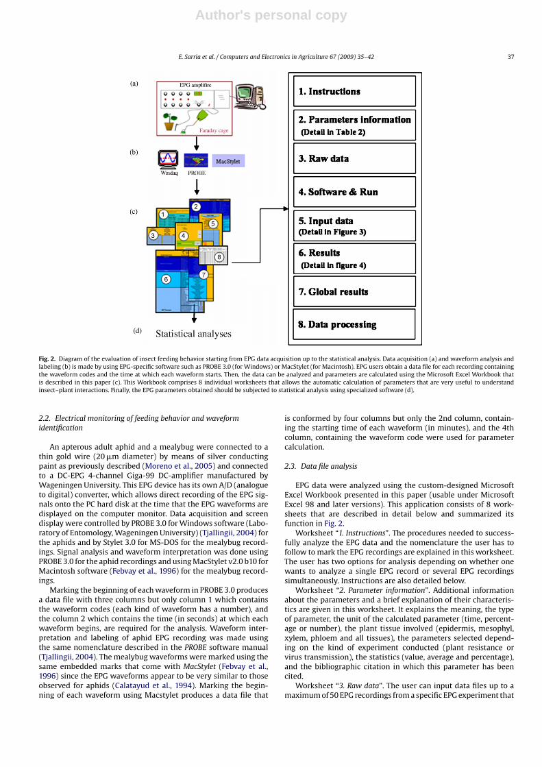
Fig. 2. Diagram of the evaluation of insect feeding behavior starting from EPG data acquisition up to the statistical analysis. Data acquisition (a) and waveform analysis andlabeling (b) is made by using EPG-specific software such as PROBE 3.0 (for Windows) or MacStylet (for Macintosh). EPG users obtain a data file for each recording containingthe waveform codes and the time at which each waveform starts. Then, the data can be analyzed and parameters are calculated using the Microsoft Excel Workbook thatis described in this paper (c). This Workbook comprises 8 individual worksheets that allows the automatic calculation of parameters that are very useful to understandinsect–plant interactions. Finally, the EPG parameters obtained should be subjected to statistical analysis using specialized software (d).

2.2. Electrical monitoring of feeding behavior and waveformidentification

An apterous adult aphid and a mealybug were connected to athin gold wire (20 �m diameter) by means of silver conductingpaint as previously described (Moreno et al., 2005) and connectedto a DC-EPG 4-channel Giga-99 DC-amplifier manufactured byWageningen University. This EPG device has its own A/D (analogueto digital) converter, which allows direct recording of the EPG sig-nals onto the PC hard disk at the time that the EPG waveforms aredisplayed on the computer monitor. Data acquisition and screendisplay were controlled by PROBE 3.0 for Windows software (Labo-ratory of Entomology, Wageningen University) (Tjallingii, 2004) forthe aphids and by Stylet 3.0 for MS-DOS for the mealybug record-ings. Signal analysis and waveform interpretation was done usingPROBE 3.0 for the aphid recordings and using MacStylet v2.0 b10 forMacintosh software (Febvay et al., 1996) for the mealybug record-ings.

Marking the beginning of each waveform in PROBE 3.0 producesa data file with three columns but only column 1 which containsthe waveform codes (each kind of waveform has a number), andthe column 2 which contains the time (in seconds) at which eachwaveform begins, are required for the analysis. Waveform inter-pretation and labeling of aphid EPG recording was made usingthe same nomenclature described in the PROBE software manual(Tjallingii, 2004). The mealybug waveforms were marked using thesame embedded marks that come with MacStylet (Febvay et al.,1996) since the EPG waveforms appear to be very similar to thoseobserved for aphids (Calatayud et al., 1994). Marking the begin-ning of each waveform using Macstylet produces a data file that

is conformed by four columns but only the 2nd column, contain-ing the starting time of each waveform (in minutes), and the 4thcolumn, containing the waveform code were used for parametercalculation.

2.3. Data file analysis

EPG data were analyzed using the custom-designed MicrosoftExcel Workbook presented in this paper (usable under MicrosoftExcel 98 and later versions). This application consists of 8 work-sheets that are described in detail below and summarized itsfunction in Fig. 2.

Worksheet “1. Instructions”. The procedures needed to success-fully analyze the EPG data and the nomenclature the user has tofollow to mark the EPG recordings are explained in this worksheet.The user has two options for analysis depending on whether onewants to analyze a single EPG record or several EPG recordingssimultaneously. Instructions are also detailed below.

Worksheet “2. Parameter information”. Additional informationabout the parameters and a brief explanation of their characteris-tics are given in this worksheet. It explains the meaning, the typeof parameter, the unit of the calculated parameter (time, percent-age or number), the plant tissue involved (epidermis, mesophyl,xylem, phloem and all tissues), the parameters selected depend-ing on the kind of experiment conducted (plant resistance orvirus transmission), the statistics (value, average and percentage),and the bibliographic citation in which this parameter has beencited.

Worksheet “3. Raw data”. The user can input data files up to amaximum of 50 EPG recordings from a specific EPG experiment that



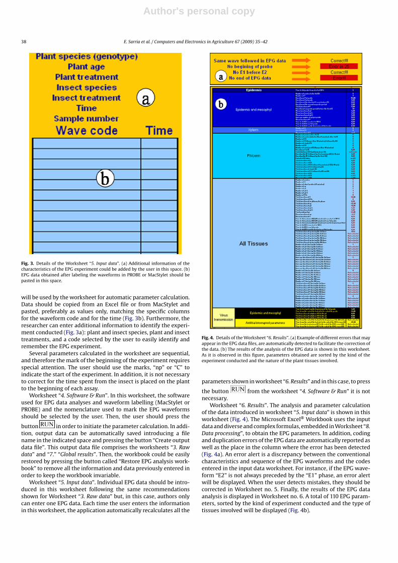
Fig. 3. Details of the Worksheet “5. Input data”. (a) Additional information of thecharacteristics of the EPG experiment could be added by the user in this space. (b)EPG data obtained after labeling the waveforms in PROBE or MacStylet should bepasted in this space.

will be used by the worksheet for automatic parameter calculation.Data should be copied from an Excel file or from MacStylet andpasted, preferably as values only, matching the specific columnsfor the waveform code and for the time (Fig. 3b). Furthermore, theresearcher can enter additional information to identify the experi-ment conducted (Fig. 3a): plant and insect species, plant and insecttreatments, and a code selected by the user to easily identify andremember the EPG experiment.

Several parameters calculated in the worksheet are sequential,and therefore the mark of the beginning of the experiment requiresspecial attention. The user should use the marks, “np” or “C” toindicate the start of the experiment. In addition, it is not necessaryto correct for the time spent from the insect is placed on the plantto the beginning of each assay.

Worksheet “4. Software & Run”. In this worksheet, the softwareused for EPG data analyses and waveform labelling (MacStylet orPROBE) and the nomenclature used to mark the EPG waveformsshould be selected by the user. Then, the user should press the

button in order to initiate the parameter calculation. In addi-tion, output data can be automatically saved introducing a filename in the indicated space and pressing the button “Create outputdata file”. This output data file comprises the worksheets “3. Rawdata” and “7.” “Global results”. Then, the workbook could be easilyrestored by pressing the button called “Restore EPG analysis work-book” to remove all the information and data previously entered inorder to keep the workbook invariable.

Worksheet “5. Input data”. Individual EPG data should be intro-duced in this worksheet following the same recommendationsshown for Worksheet “3. Raw data” but, in this case, authors onlycan enter one EPG data. Each time the user enters the informationin this worksheet, the application automatically recalculates all the

Fig. 4. Details of the Worksheet “6. Results”. (a) Example of different errors that mayappear in the EPG data files, are automatically detected to facilitate the correction ofthe data. (b) The results of the analysis of the EPG data is shown in this worksheet.As it is observed in this figure, parameters obtained are sorted by the kind of theexperiment conducted and the nature of the plant tissues involved.

parameters shown in worksheet “6. Results” and in this case, to press

the button from the worksheet “4. Software & Run” it is notnecessary.

Worksheet “6. Results”. The analysis and parameter calculationof the data introduced in worksheet “5. Input data” is shown in thisworksheet (Fig. 4). The Microsoft Excel® Workbook uses the inputdata and diverse and complex formulas, embedded in Worksheet “8.Data processing”, to obtain the EPG parameters. In addition, codingand duplication errors of the EPG data are automatically reported aswell as the place in the column where the error has been detected(Fig. 4a). An error alert is a discrepancy between the conventionalcharacteristics and sequence of the EPG waveforms and the codesentered in the input data worksheet. For instance, if the EPG wave-form “E2” is not always preceded by the “E1” phase, an error alertwill be displayed. When the user detects mistakes, they should becorrected in Worksheet no. 5. Finally, the results of the EPG dataanalysis is displayed in Worksheet no. 6. A total of 110 EPG param-eters, sorted by the kind of experiment conducted and the type oftissues involved will be displayed (Fig. 4b).



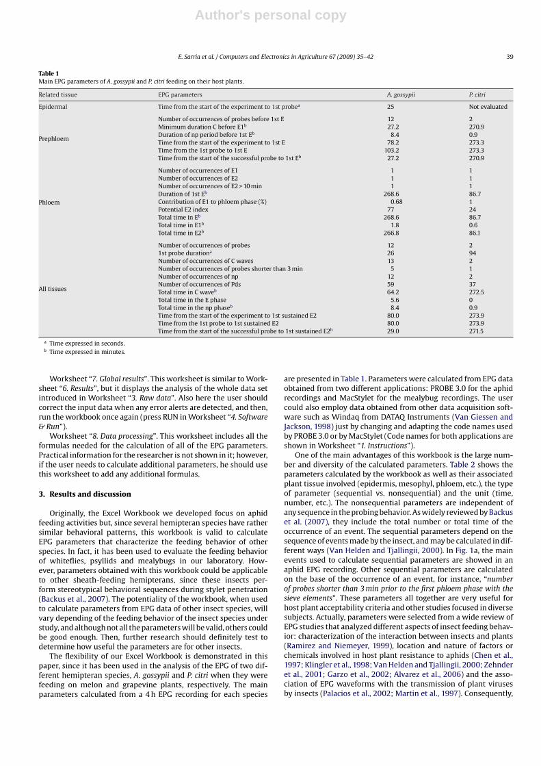
Table 1Main EPG parameters of A. gossypii and P. citri feeding on their host plants.

Related tissue EPG parameters A. gossypii P. citri

Epidermal Time from the start of the experiment to 1st probea 25 Not evaluated

Prephloem

Number of occurrences of probes before 1st E 12 2Minimum duration C before E1b 27.2 270.9Duration of np period before 1st Eb 8.4 0.9Time from the start of the experiment to 1st E 78.2 273.3Time from the 1st probe to 1st E 103.2 273.3Time from the start of the successful probe to 1st Eb 27.2 270.9

Phloem

Number of occurrences of E1 1 1Number of occurrences of E2 1 1Number of occurrences of E2 > 10 min 1 1Duration of 1st Eb 268.6 86.7Contribution of E1 to phloem phase (%) 0.68 1Potential E2 index 77 24Total time in Eb 268.6 86.7Total time in E1b 1.8 0.6Total time in E2b 266.8 86.1

All tissues

Number of occurrences of probes 12 21st probe durationa 26 94Number of occurrences of C waves 13 2Number of occurrences of probes shorter than 3 min 5 1Number of occurrences of np 12 2Number of occurrences of Pds 59 37Total time in C waveb 64.2 272.5Total time in the E phase 5.6 0Total time in the np phaseb 8.4 0.9Time from the start of the experiment to 1st sustained E2 80.0 273.9Time from the 1st probe to 1st sustained E2 80.0 273.9Time from the start of the successful probe to 1st sustained E2b 29.0 271.5

a Time expressed in seconds.b Time expressed in minutes.

Worksheet “7. Global results”. This worksheet is similar to Work-sheet “6. Results”, but it displays the analysis of the whole data setintroduced in Worksheet “3. Raw data”. Also here the user shouldcorrect the input data when any error alerts are detected, and then,run the workbook once again (press RUN in Worksheet “4. Software& Run”).

Worksheet “8. Data processing”. This worksheet includes all theformulas needed for the calculation of all of the EPG parameters.Practical information for the researcher is not shown in it; however,if the user needs to calculate additional parameters, he should usethis worksheet to add any additional formulas.

3. Results and discussion

Originally, the Excel Workbook we developed focus on aphidfeeding activities but, since several hemipteran species have rathersimilar behavioral patterns, this workbook is valid to calculateEPG parameters that characterize the feeding behavior of otherspecies. In fact, it has been used to evaluate the feeding behaviorof whiteflies, psyllids and mealybugs in our laboratory. How-ever, parameters obtained with this workbook could be applicableto other sheath-feeding hemipterans, since these insects per-form stereotypical behavioral sequences during stylet penetration(Backus et al., 2007). The potentiality of the workbook, when usedto calculate parameters from EPG data of other insect species, willvary depending of the feeding behavior of the insect species understudy, and although not all the parameters will be valid, others couldbe good enough. Then, further research should definitely test todetermine how useful the parameters are for other insects.

The flexibility of our Excel Workbook is demonstrated in thispaper, since it has been used in the analysis of the EPG of two dif-ferent hemipteran species, A. gossypii and P. citri when they werefeeding on melon and grapevine plants, respectively. The mainparameters calculated from a 4 h EPG recording for each species

are presented in Table 1. Parameters were calculated from EPG dataobtained from two different applications: PROBE 3.0 for the aphidrecordings and MacStylet for the mealybug recordings. The usercould also employ data obtained from other data acquisition soft-ware such as Windaq from DATAQ Instruments (Van Giessen andJackson, 1998) just by changing and adapting the code names usedby PROBE 3.0 or by MacStylet (Code names for both applications areshown in Worksheet “1. Instructions”).

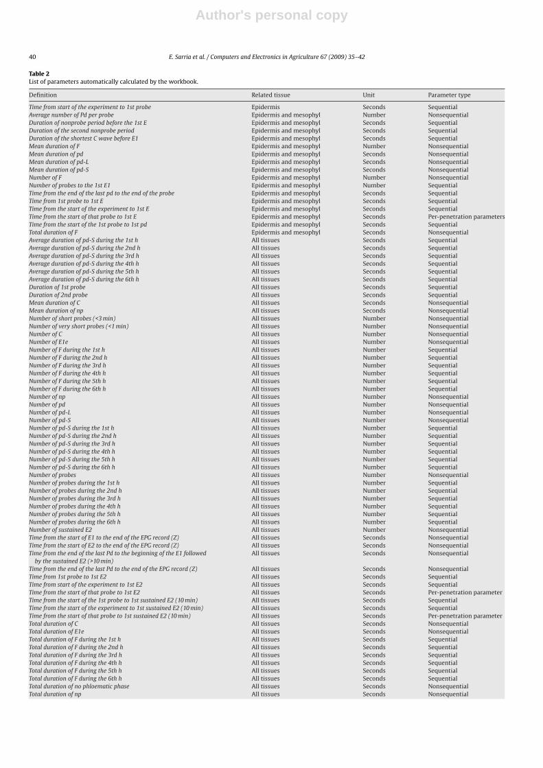
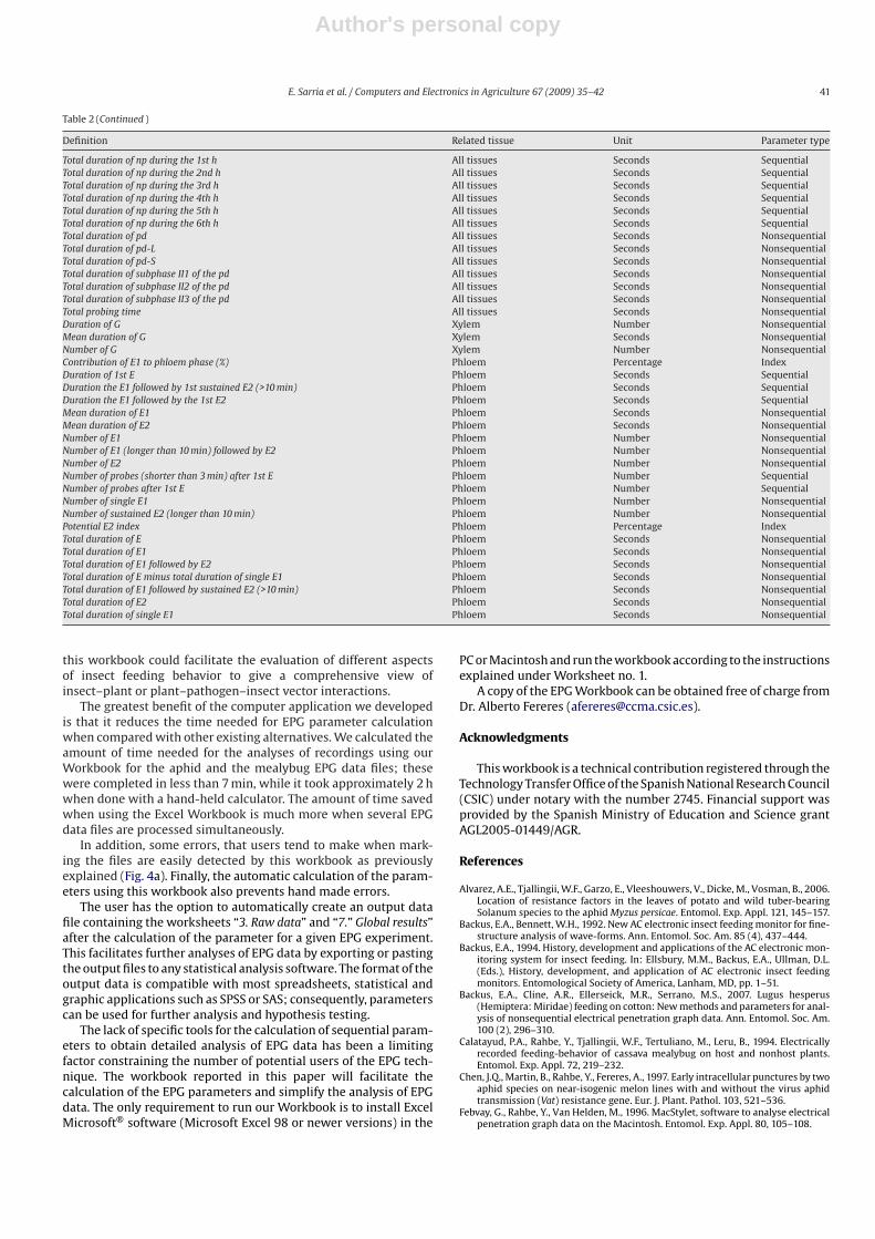
One of the main advantages of this workbook is the large num-ber and diversity of the calculated parameters. Table 2 shows theparameters calculated by the workbook as well as their associatedplant tissue involved (epidermis, mesophyl, phloem, etc.), the typeof parameter (sequential vs. nonsequential) and the unit (time,number, etc.). The nonsequential parameters are independent ofany sequence in the probing behavior. As widely reviewed by Backuset al. (2007), they include the total number or total time of theoccurrence of an event. The sequential parameters depend on thesequence of events made by the insect, and may be calculated in dif-ferent ways (Van Helden and Tjallingii, 2000). In Fig. 1a, the mainevents used to calculate sequential parameters are showed in anaphid EPG recording. Other sequential parameters are calculatedon the base of the occurrence of an event, for instance, “numberof probes shorter than 3 min prior to the first phloem phase with thesieve elements”. These parameters all together are very useful forhost plant acceptability criteria and other studies focused in diversesubjects. Actually, parameters were selected from a wide review ofEPG studies that analyzed different aspects of insect feeding behav-ior: characterization of the interaction between insects and plants(Ramirez and Niemeyer, 1999), location and nature of factors orchemicals involved in host plant resistance to aphids (Chen et al.,1997; Klingler et al., 1998; Van Helden and Tjallingii, 2000; Zehnderet al., 2001; Garzo et al., 2002; Alvarez et al., 2006) and the asso-ciation of EPG waveforms with the transmission of plant virusesby insects (Palacios et al., 2002; Martin et al., 1997). Consequently,



Table 2List of parameters automatically calculated by the workbook.

Definition Related tissue Unit Parameter type

Time from start of the experiment to 1st probe Epidermis Seconds SequentialAverage number of Pd per probe Epidermis and mesophyl Number NonsequentialDuration of nonprobe period before the 1st E Epidermis and mesophyl Seconds SequentialDuration of the second nonprobe period Epidermis and mesophyl Seconds SequentialDuration of the shortest C wave before E1 Epidermis and mesophyl Seconds SequentialMean duration of F Epidermis and mesophyl Number NonsequentialMean duration of pd Epidermis and mesophyl Seconds NonsequentialMean duration of pd-L Epidermis and mesophyl Seconds NonsequentialMean duration of pd-S Epidermis and mesophyl Seconds NonsequentialNumber of F Epidermis and mesophyl Number NonsequentialNumber of probes to the 1st E1 Epidermis and mesophyl Number SequentialTime from the end of the last pd to the end of the probe Epidermis and mesophyl Seconds SequentialTime from 1st probe to 1st E Epidermis and mesophyl Seconds SequentialTime from the start of the experiment to 1st E Epidermis and mesophyl Seconds SequentialTime from the start of that probe to 1st E Epidermis and mesophyl Seconds Per-penetration parametersTime from the start of the 1st probe to 1st pd Epidermis and mesophyl Seconds SequentialTotal duration of F Epidermis and mesophyl Seconds NonsequentialAverage duration of pd-S during the 1st h All tissues Seconds SequentialAverage duration of pd-S during the 2nd h All tissues Seconds SequentialAverage duration of pd-S during the 3rd h All tissues Seconds SequentialAverage duration of pd-S during the 4th h All tissues Seconds SequentialAverage duration of pd-S during the 5th h All tissues Seconds SequentialAverage duration of pd-S during the 6th h All tissues Seconds SequentialDuration of 1st probe All tissues Seconds SequentialDuration of 2nd probe All tissues Seconds SequentialMean duration of C All tissues Seconds NonsequentialMean duration of np All tissues Seconds NonsequentialNumber of short probes (<3 min) All tissues Number NonsequentialNumber of very short probes (<1 min) All tissues Number NonsequentialNumber of C All tissues Number NonsequentialNumber of E1e All tissues Number NonsequentialNumber of F during the 1st h All tissues Number SequentialNumber of F during the 2nd h All tissues Number SequentialNumber of F during the 3rd h All tissues Number SequentialNumber of F during the 4th h All tissues Number SequentialNumber of F during the 5th h All tissues Number SequentialNumber of F during the 6th h All tissues Number SequentialNumber of np All tissues Number NonsequentialNumber of pd All tissues Number NonsequentialNumber of pd-L All tissues Number NonsequentialNumber of pd-S All tissues Number NonsequentialNumber of pd-S during the 1st h All tissues Number SequentialNumber of pd-S during the 2nd h All tissues Number SequentialNumber of pd-S during the 3rd h All tissues Number SequentialNumber of pd-S during the 4th h All tissues Number SequentialNumber of pd-S during the 5th h All tissues Number SequentialNumber of pd-S during the 6th h All tissues Number SequentialNumber of probes All tissues Number NonsequentialNumber of probes during the 1st h All tissues Number SequentialNumber of probes during the 2nd h All tissues Number SequentialNumber of probes during the 3rd h All tissues Number SequentialNumber of probes during the 4th h All tissues Number SequentialNumber of probes during the 5th h All tissues Number SequentialNumber of probes during the 6th h All tissues Number SequentialNumber of sustained E2 All tissues Number NonsequentialTime from the start of E1 to the end of the EPG record (Z) All tissues Seconds NonsequentialTime from the start of E2 to the end of the EPG record (Z) All tissues Seconds NonsequentialTime from the end of the last Pd to the beginning of the E1 followed

by the sustained E2 (>10 min)All tissues Seconds Nonsequential

Time from the end of the last Pd to the end of the EPG record (Z) All tissues Seconds NonsequentialTime from 1st probe to 1st E2 All tissues Seconds SequentialTime from start of the experiment to 1st E2 All tissues Seconds SequentialTime from the start of that probe to 1st E2 All tissues Seconds Per-penetration parameterTime from the start of the 1st probe to 1st sustained E2 (10 min) All tissues Seconds SequentialTime from the start of the experiment to 1st sustained E2 (10 min) All tissues Seconds SequentialTime from the start of that probe to 1st sustained E2 (10 min) All tissues Seconds Per-penetration parameterTotal duration of C All tissues Seconds NonsequentialTotal duration of E1e All tissues Seconds NonsequentialTotal duration of F during the 1st h All tissues Seconds SequentialTotal duration of F during the 2nd h All tissues Seconds SequentialTotal duration of F during the 3rd h All tissues Seconds SequentialTotal duration of F during the 4th h All tissues Seconds SequentialTotal duration of F during the 5th h All tissues Seconds SequentialTotal duration of F during the 6th h All tissues Seconds SequentialTotal duration of no phloematic phase All tissues Seconds NonsequentialTotal duration of np All tissues Seconds Nonsequential



Table 2 (Continued )

Definition Related tissue Unit Parameter type

Total duration of np during the 1st h All tissues Seconds SequentialTotal duration of np during the 2nd h All tissues Seconds SequentialTotal duration of np during the 3rd h All tissues Seconds SequentialTotal duration of np during the 4th h All tissues Seconds SequentialTotal duration of np during the 5th h All tissues Seconds SequentialTotal duration of np during the 6th h All tissues Seconds SequentialTotal duration of pd All tissues Seconds NonsequentialTotal duration of pd-L All tissues Seconds NonsequentialTotal duration of pd-S All tissues Seconds NonsequentialTotal duration of subphase II1 of the pd All tissues Seconds NonsequentialTotal duration of subphase II2 of the pd All tissues Seconds NonsequentialTotal duration of subphase II3 of the pd All tissues Seconds NonsequentialTotal probing time All tissues Seconds NonsequentialDuration of G Xylem Number NonsequentialMean duration of G Xylem Seconds NonsequentialNumber of G Xylem Number NonsequentialContribution of E1 to phloem phase (%) Phloem Percentage IndexDuration of 1st E Phloem Seconds SequentialDuration the E1 followed by 1st sustained E2 (>10 min) Phloem Seconds SequentialDuration the E1 followed by the 1st E2 Phloem Seconds SequentialMean duration of E1 Phloem Seconds NonsequentialMean duration of E2 Phloem Seconds NonsequentialNumber of E1 Phloem Number NonsequentialNumber of E1 (longer than 10 min) followed by E2 Phloem Number NonsequentialNumber of E2 Phloem Number NonsequentialNumber of probes (shorter than 3 min) after 1st E Phloem Number SequentialNumber of probes after 1st E Phloem Number SequentialNumber of single E1 Phloem Number NonsequentialNumber of sustained E2 (longer than 10 min) Phloem Number NonsequentialPotential E2 index Phloem Percentage IndexTotal duration of E Phloem Seconds NonsequentialTotal duration of E1 Phloem Seconds NonsequentialTotal duration of E1 followed by E2 Phloem Seconds NonsequentialTotal duration of E minus total duration of single E1 Phloem Seconds NonsequentialTotal duration of E1 followed by sustained E2 (>10 min) Phloem Seconds NonsequentialTotal duration of E2 Phloem Seconds NonsequentialTotal duration of single E1 Phloem Seconds Nonsequential

this workbook could facilitate the evaluation of different aspectsof insect feeding behavior to give a comprehensive view ofinsect–plant or plant–pathogen–insect vector interactions.

The greatest benefit of the computer application we developedis that it reduces the time needed for EPG parameter calculationwhen compared with other existing alternatives. We calculated theamount of time needed for the analyses of recordings using ourWorkbook for the aphid and the mealybug EPG data files; thesewere completed in less than 7 min, while it took approximately 2 hwhen done with a hand-held calculator. The amount of time savedwhen using the Excel Workbook is much more when several EPGdata files are processed simultaneously.

In addition, some errors, that users tend to make when mark-ing the files are easily detected by this workbook as previouslyexplained (Fig. 4a). Finally, the automatic calculation of the param-eters using this workbook also prevents hand made errors.

The user has the option to automatically create an output datafile containing the worksheets “3. Raw data” and “7.” Global results”after the calculation of the parameter for a given EPG experiment.This facilitates further analyses of EPG data by exporting or pastingthe output files to any statistical analysis software. The format of theoutput data is compatible with most spreadsheets, statistical andgraphic applications such as SPSS or SAS; consequently, parameterscan be used for further analysis and hypothesis testing.

The lack of specific tools for the calculation of sequential param-eters to obtain detailed analysis of EPG data has been a limitingfactor constraining the number of potential users of the EPG tech-nique. The workbook reported in this paper will facilitate thecalculation of the EPG parameters and simplify the analysis of EPGdata. The only requirement to run our Workbook is to install ExcelMicrosoft® software (Microsoft Excel 98 or newer versions) in the

PC or Macintosh and run the workbook according to the instructionsexplained under Worksheet no. 1.

A copy of the EPG Workbook can be obtained free of charge fromDr. Alberto Fereres ([email protected]).

Acknowledgments

This workbook is a technical contribution registered through theTechnology Transfer Office of the Spanish National Research Council(CSIC) under notary with the number 2745. Financial support wasprovided by the Spanish Ministry of Education and Science grantAGL2005-01449/AGR.

References

Alvarez, A.E., Tjallingii, W.F., Garzo, E., Vleeshouwers, V., Dicke, M., Vosman, B., 2006.Location of resistance factors in the leaves of potato and wild tuber-bearingSolanum species to the aphid Myzus persicae. Entomol. Exp. Appl. 121, 145–157.

Backus, E.A., Bennett, W.H., 1992. New AC electronic insect feeding monitor for fine-structure analysis of wave-forms. Ann. Entomol. Soc. Am. 85 (4), 437–444.

Backus, E.A., 1994. History, development and applications of the AC electronic mon-itoring system for insect feeding. In: Ellsbury, M.M., Backus, E.A., Ullman, D.L.(Eds.), History, development, and application of AC electronic insect feedingmonitors. Entomological Society of America, Lanham, MD, pp. 1–51.

Backus, E.A., Cline, A.R., Ellerseick, M.R., Serrano, M.S., 2007. Lugus hesperus(Hemiptera: Miridae) feeding on cotton: New methods and parameters for anal-ysis of nonsequential electrical penetration graph data. Ann. Entomol. Soc. Am.100 (2), 296–310.

Calatayud, P.A., Rahbe, Y., Tjallingii, W.F., Tertuliano, M., Leru, B., 1994. Electricallyrecorded feeding-behavior of cassava mealybug on host and nonhost plants.Entomol. Exp. Appl. 72, 219–232.

Chen, J.Q., Martin, B., Rahbe, Y., Fereres, A., 1997. Early intracellular punctures by twoaphid species on near-isogenic melon lines with and without the virus aphidtransmission (Vat) resistance gene. Eur. J. Plant. Pathol. 103, 521–536.

Febvay, G., Rahbe, Y., Van Helden, M., 1996. MacStylet, software to analyse electricalpenetration graph data on the Macintosh. Entomol. Exp. Appl. 80, 105–108.



Garzo, E., Soria, C., Gomez-Guillamon, M.L., Fereres, A., 2002. Feeding behavior ofAphis gossypii on resistant accessions of different melon genotypes (Cucumismelo). Phytoparasitica 30, 129–140.

Harrewijn, P., Kayser, H., 1997. Pymetrozine, a fast-acting and selective inhibitor ofaphid feeding. In-situ studies with electronic monitoring of feeding behaviour.Pestic. Sci. 49 (2), 130–140.

Joost, P.H., Backus, E.A., Morgan, D., Yan, F., 2006. Correlation of stylet activities bythe glassy-winged sharpshooter, Homalodisca coagulata (Say), with electricalpenetration graph (EPG) waveforms. J. Insect Physiol. 52 (3), 327–337.

Kaufmann, L., Schurmann, F., Yiallouros, M., Harrewijn, P., Kayser, H., 2004. The sero-tonergic system is involved in feeding inhibition by pymetrozine. Comparativestudies on a locust (Locusta migratoria) and an aphid (Myzus persicae). Comp.Biochem. Phys. C 138 (4), 469–483.

Klingler, J., Powell, G., Thompson, G.A., Isaacs, R., 1998. Phloem specific aphid resis-tance in Cucumis melo line AR 5: effects on feeding behavior and performanceof Aphis gossypii. Entomol. Exp. Appl. 86, 79–88.

Martin, B., Collar, J.L., Tjallingii, W.F., Fereres, A., 1997. Intracellular ingestion and sali-vation by aphids may cause the acquisition and inoculation of non-persistentlytransmitted plant viruses. J. Gen. Virol. 78, 2701–2705.

Mclean, D.L., Kinsey, M.G., 1964. Technique for electronically recording aphid feed-ing + salivation. Nature 202, 1358.

Moreno, A., Palacios, I., Blanc, S., Fereres, A., 2005. Intracellular salivation is the mech-anism involved in the inoculation of Cauliflower mosaic virus by its major vectors.Brevicoryne brassicae and Myzus persicae. Ann. Entomol. Soc. Am. 98 (6), 763–769.

Nault, L.R., 1997. Arthropod of plant viruses: a new synthesis. Ann. Entomol. Soc. Am.90, 521–541.

Palacios, I., Drucker, M., Blanc, S., Leite, S., Moreno, A., Fereres, A., 2002. Cauliflowermosaic virus is preferentially acquired from the phloem by its aphid vectors. J.Gen. Virol. 83, 3163–3171.

Ramirez, C.C., Niemeyer, H.M., 1999. Salivation into sieve elements in relation toplant chemistry: the case of the aphid Sitobion fragariae and the wheat, Triticumaestivum. Entomol. Exp. Appl. 91, 111–114.

Tjallingii, W.F., 1978. Electronic recording of penetration behavior by aphids. Ento-mol. Exp. Appl. 24, 721–730.

Tjallingii, W.F., 1985. Electrical nature of recorded signals during stylet penetrationby aphids. Entomol. Exp. Appl. 38, 177–186.

Tjallingii, W.F., 2004. PROBE 3.0 Manual, Release May 2004. Wageningen University,Laboratory of Entomology. [email protected].

Van Giessen, W.A., Jackson, D.M., 1998. Rapid analysis of electronically monitoredhomopteran feeding behavior. Ann. Entomol. Soc. Am. 91, 145–154.

Van Helden, M., Tjallingii, W.F., 2000. Experimental design and analysis in EPG exper-iments with emphasis on plant resistance research. In: Walker, G.P., Backus, E.A.(Eds.), Principles and applications of electronic monitoring and other techniquesin the study of homopteran feeding behavior. Entomological Society of America,Lanham, MD, pp. 144–171.

Walling, L.L., 2000. The myriad plant responses to herbivores. J. Plant Growth Regul.19, 195–216.

Will, T., Hewer, A., van Bel, A.J.E., 2008. A novel perfusion system shows that aphidfeeding behaviour is altered by decrease of sieve-tube pressure. Entomol. Exp.Appl. 127 (3), 237–245.

Zehnder, G.W., Nichols, A.J., Edwards, O.R., Ridsdill-Smith, T.J., 2001. Electronicallymonitored cowpea aphid feeding behavior on resistant and susceptible lupins.Entomol. Exp. Appl. 98, 259–269.

Excel Workbook for automatic parameter calculation of EPG data

Documents

Transcript of Excel Workbook for automatic parameter calculation of EPG data