Example 13.8: Paracetamol Last update 22.3.2021

Data Topic Level

Electron diffraction Complete procedure from data reduction to

structure refinement using the dynamical

approach.

Intermediate

Input data

Data

Electron diffraction data were measured on a transmission electron microscope Philips CM120 with a precession device DigiStar. Accelerating voltage 120 kV

Input files

directory “dp-130” with the set of experimental data (diffraction patterns) APAP.pts: input file for PETS APAP_reference.cif_pets: result of the data processing. This file is provided so that this example can be solved without the data processing part, and to warrant reproducibility of the solution and refinement part. File APAP.cif_pets will be the output of the data reduction. APAP_dyn_reference.cif_pets: result of the data processing for dynamical refinement. This file is provided so that the dynamical approach can be used without the processing part, and to warrant the reproducibility of the refinement. A set of intermediate structure refinements in directory “refinements”. These refinements are provided to allow finishing the example in shorter time, because the last part dynamical refinement) may be time consuming.

References For further information about the data processing in PETS2.0 see: - L. Palatinus et al. Specifics of the data processing of precession electron diffraction tomography data and their implementation in the program PETS2.0. Acta Cryst. B 75: 512-522 (2019). - PETS2.0 manual pets.fzu.cz/download/ For further information about the dynamical refinement and associated parameters: - L. Palatinus et al. Structure refinement using precession electron diffraction tomography and dynamical diffraction: theory and implementation. Acta Cryst. A71: 235–244 (2015). - L. Palatinus et al. Structure refinement using precession electron diffraction tomography and dynamical diffraction: tests on experimental data. Acta Crystallogr B71: 740–751 (2015)

PART 1: Data treatment in PETS2.0

1. Prepare (check) input file for PETS2.0

File APAP.pts is the input for PETS. The file was prepared by the software used for the collection of the diffraction data. However, you can prepare easily such input file for your own data. Open file APAP.pts in any plain-text editor (Notepad, Wordpad, Notepad++, Vim, … ) At beginning of the file you see conditions of our experiment. These are irrelevant to PETS. The important part starts here: lambda 0.0335

Aperpixel 0.001558

phi 1.40

omega 22.07

bin 2

reflectionsize 20

noiseparameters 3.5 38

center 976 1077

dp-130\001.tif -52.01 0.00

dp-130\002.tif -50.49 0.00

dp-130\003.tif -48.99 0.00

....

Endimagelist

lambda: relativistic wavelength of the incident electrons in Angstroms (100kV=0.0370A, 120kV=0.0335A, 200kV=0.0251A, 300kV=0.0197A) Aperpixel: Scale of the images given as the size of one pixel in reciprocal angstroms phi: Precession angle in degrees used during the data collection. Can be zero, of course. omega: orientation of the tilt axis of the sample holder with respect to the positive horizontal axis of the image. Must be estimated either by calibration, or by visual inspection of the series of images. Should be close to the correct value within +/-20 deg. Can be refined later in PETS. bin: Binning of the images prior to any treatment. Saves time, makes nicer pictures, and seems to make the whole analysis somewhat more robust. bin 2 is a good choice from my experience for most data sets. Important: All parameters in the input file that are given in pixels refer to the original, unbinned images. This concerns Aperpixel, center, reflectionsize, mask. reflectionsize: Diameter of the spots on the images in pixels. Used for peak search and integration, should be large enough to encompass also the strong spots, but small enough to avoid overlaps of neighboring spots. noiseparameters: two parameters for the determination of σ(I). The first value is Gγ, the second is ψ. The uncertainty on each pixel γ is then calculated as: σ2(p)=Gγp+ψ For more information, see Waterman, D. & Evans, G. (2010). J. Appl. Cryst. 43, 1356-1371. center: Initial position of the primary beam on the images in pixels. Center is given by X and Y coordinates of the unbinned images. The center is then refined for each image separately during peak search. imagelist – endimagelist: Multiline keyword. Each line contains one image. The format is: name alpha beta. Name is the file name of the image (including possible relative or absolute path), alpha is the tilt angle, and beta is the possible second tilt value of the double tilt holder. Save and close APAP.pts

2. Run PETS and prepare files for indexation

Start PETS by double clicking the executable

In the upper menu, go to File → Open Open the file APAP.pts In the Main panel (Image data tab) you can view individual diffraction images (frames) of APAP dataset stored in the directory “dp-130” using the arrows at the bottom of the panel. The contrast of the images can be adjusted by changing the value in the Cutoff-box.

3. Peak search

This action as well as all other steps are run by clicking the action button (see image below). The parameters can be modified in the panel, which opens after clicking the small arrow next to the action button: Click the arrow next to the action button “Parameters”. No parameters must be changed. The default values are OK: (binned) reflection diameter 10 (pixel), max d* for integration 1.4 (Å-1), max d* for peak search 1.4 (Å-1), min d* 0.05 (Å-1), beam stop No;

Click the arrow next to the action button “Peak search”. Again, no parameters must be changed: “Always accept center” checked, “use Friedel pairs”. From the PTS file (line “center 976 1077”) the initial coordinates were correctly read. The values in the PTS file correspond to the unbinned images, the values shown within the program correspond to the binned images. Keep unchecked “Automatic initial direct beam coordinates”, “I/sigma” 10. Click the action button “Peak search” to start the procedure Look at the Image data tab in the main panel to see the progress of the Peak search In the main panel diffraction images are sequentially displayed with circles at points found by PETS as significant peaks (above I/sigma specified in the Peak search parameters). Crosses appear in the circles for whose peak’s Friedel pair was detected. Note that PETS follows the position of the primary beam, and corrects for small shifts. At the end, the evolution of the x- (red) and y-coordinates (green) of the estimated direct-beam position is displayed in the Main panel (tab Graph):

Action button

Arrow to open parameter panels

At the end, the following message is displayed in the console: Minimum, average and maximum position of the primary beam: 487.58 488.83

490.01 | 536.81 538.14 490.01 in mine

Finished reading 4811 peaks from the file APAP.rpl.

4. Rotation axis

The next step after peak hunting is the refinement of the angle between the horizontal axis (x axis of the diffraction image) and the projection of the rotation axis. This angle depends on the experimental setup, and needs to be refined for each data set. Click the action button “Rotation axis” to start the procedure. In the main panel a plot of the cylindrical projection of the difference space of the extracted peak positions automatically opens. A correct azimuthal angle refinement results in the image containing sharp peaks aligned on sinusoidal curves. This step provides a first estimation of data quality. At the end of the refinement the omega angle is 22.3669 for a score of 1.00879

5. Peak analysis

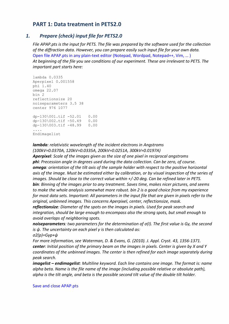
Click the action button “Peak analysis”. PETS starts the analysis of the peak positions obtained in the peak hunting procedure. In the first step, distance distribution between peaks in the image plane is analyzed. A sorted plot of inter-peak distances is displayed in the Graph tab (red curve) with its derivative (green):

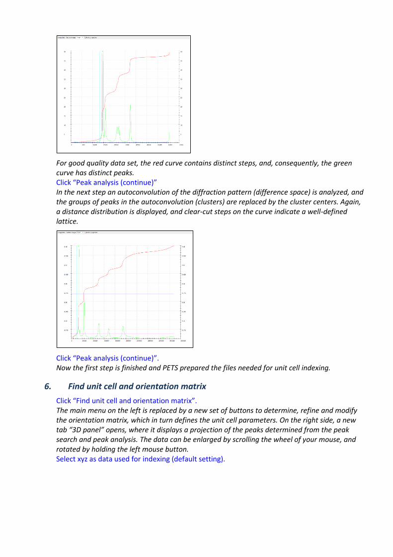
For good quality data set, the red curve contains distinct steps, and, consequently, the green curve has distinct peaks. Click “Peak analysis (continue)” In the next step an autoconvolution of the diffraction pattern (difference space) is analyzed, and the groups of peaks in the autoconvolution (clusters) are replaced by the cluster centers. Again, a distance distribution is displayed, and clear-cut steps on the curve indicate a well-defined lattice.

Click “Peak analysis (continue)”. Now the first step is finished and PETS prepared the files needed for unit cell indexing.

6. Find unit cell and orientation matrix

Click “Find unit cell and orientation matrix”. The main menu on the left is replaced by a new set of buttons to determine, refine and modify the orientation matrix, which in turn defines the unit cell parameters. On the right side, a new tab “3D panel” opens, where it displays a projection of the peaks determined from the peak search and peak analysis. The data can be enlarged by scrolling the wheel of your mouse, and rotated by holding the left mouse button. Select xyz as data used for indexing (default setting).

Open the details by clicking on the arrow next to the action button “Find possible cells automatically”. You see the parameters used in the procedure as wells as the possible unit cells found by PETS. Keep the other parameters at their default values, Click “Find possible cells automatically”. The best hit is automatically defined as the current cell. You could change the cell by selecting another solution and click “Rewrite current unit cell”.

The cell angles are close to 90 degrees and the “Bravais class” was automatically defined to be “oP”. Click “FINISH”.

7. Create reciprocal-space sections

Click “Reciprocal-space sections”; OK (use the standard set). You can open Reciprocal-space setions” by clicking on (v). In the parameters, you can change the size of pixels in the reconstruction images and the thickness of the slab that is projected into the section in Å-1. Too small numbers may result in “holey” reconstructions. We will proceed with the default values.

Click on “Section images” tab.

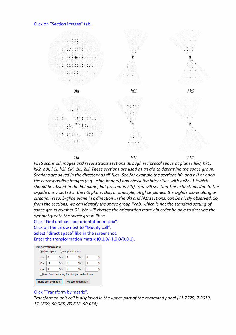
0kl h0l hk0

1kl h1l hk1

PETS scans all images and reconstructs sections through reciprocal space at planes hk0, hk1, hk2, h0l, h1l, h2l, 0kl, 1kl, 2kl. These sections are used as an aid to determine the space group. Sections are saved in the directory as tif-files. See for example the sections h0l and h1l or open the corresponding images (e.g. using ImageJ) and check the intensities with h=2n+1 (which should be absent in the h0l plane, but present in h1l). You will see that the extinctions due to the a-glide are violated in the h0l plane. But, in principle, all glide planes, the c-glide plane along a-direction resp. b-glide plane in c direction in the 0kl and hk0 sections, can be nicely observed. So, from the sections, we can identify the space group Pcab, which is not the standard setting of space group number 61. We will change the orientation matrix in order be able to describe the symmetry with the space group Pbca. Click “Find unit cell and orientation matrix”. Click on the arrow next to “Modify cell”. Select “direct space” like in the screenshot. Enter the transformation matrix (0,1,0/-1,0,0/0,0,1).

Click “Transform by matrix”. Transformed unit cell is displayed in the upper part of the command panel (11.7725, 7.2619, 17.1609, 90.085, 89.612, 90.054)

Click on the arrow next to “Refine cell”. Keep the default “Refine UB + cell” and select “orthorhombic”. Click “Refine Cell”. The refined unit cell parameters are 11.7696, 7.2464, 17.1598 Leave the indexing panel by clicking “FINISH”. The file APAP.celllist was now produced. This file contains the orientation matrix and the unit cell parameters Note that the sections were constructed before we transformed the lattice to the standard setting Pbca. Therefore, we should calculate new reciprocal space sections: Click “Reciprocal-space sections”; OK (use the standard set).

8. Integrate intensities

(a) Process frames for integration

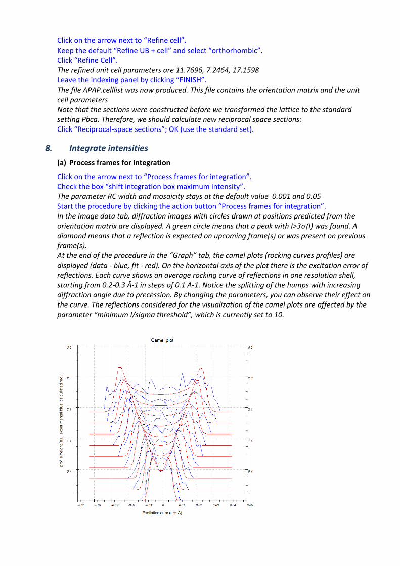
Click on the arrow next to “Process frames for integration”. Check the box “shift integration box maximum intensity”. The parameter RC width and mosaicity stays at the default value 0.001 and 0.05 Start the procedure by clicking the action button “Process frames for integration”. In the Image data tab, diffraction images with circles drawn at positions predicted from the orientation matrix are displayed. A green circle means that a peak with I>3𝜎(I) was found. A diamond means that a reflection is expected on upcoming frame(s) or was present on previous frame(s). At the end of the procedure in the “Graph” tab, the camel plots (rocking curves profiles) are displayed (data - blue, fit - red). On the horizontal axis of the plot there is the excitation error of reflections. Each curve shows an average rocking curve of reflections in one resolution shell, starting from 0.2-0.3 Å-1 in steps of 0.1 Å-1. Notice the splitting of the humps with increasing diffraction angle due to precession. By changing the parameters, you can observe their effect on the curve. The reflections considered for the visualization of the camel plots are affected by the parameter “minimum I/sigma threshold”, which is currently set to 10.

(b) Optimize geometry and integration parameters

Go to the options in “Optimize geometry and integration parameters” Check that the “refinement using rocking curve profile” is checked as well as the “RC width” and “apparent mosaicity” parameters. Start the fitting procedure by clicking on the action button “Optimize geometry and integration parameters”. The fit results in the RC width of ~0.00364 Å-1 and mosaicity ~0.126°. The fit is not satisfying, as can be seen in the plot on the tab Graph:

In this case the curves of the first four (1st: 0.2-0.3, 2nd: 0.3-0.4, 3rd: 0.4-0.5 and 4th: 0.5-0.6) resolution shells (in Å-1) don’t match properly the experimental curves. Change manually the parameters RC width to 0.0015 Å-1 and mosaicity to 0.20 deg.

As can be seen, the fit describes the first camel plots much better than before. With the manual adjustment of the parameters on the other hand, a worse description of the turning points of the camel plots of higher resolution shells is accompanied. Nevertheless, it is more likely that a

good description of the first resolution shells leads to better parameters and another reason pushes the refinement to higher mosaicity.

(c) Finalize integration

Open the parameters for “Finalize integration”. Check that both “kinematical” and “dynamical” integrations are checked. Select the radio button “fit profile” next to “intensity estimation”. Default value for intensity estimation is “integrate profile”, which is the more robust technique and works well even for poorer data. However, for good data the “fit profile” option gives better results. Check “frame scaling” and choose “Laue class for scaling” mmm.

You will get a graph showing individual frame scales.

Run the procedure by clicking the action button. After the integration, PETS shows the list of Rint values depending on the Laue classes in the console. For Laue class mmm, Rint(obs) is 16.26% for 767/1837 observed/all independent reflections.

9. Frame orientation refinement

The frame orientation refinement optimizes the overall scale, rotation angles α, β and ω together with the position of the diffraction patterns center. The routine generates diffraction patterns based on the previous finalized integration. The least-squares minimization routine tries then to reduce the pixel-wise differences of the generated pattern from the background-subtracted experimental diffraction pattern. You can find more details about the method in Palatinus, L. et al. (2019). Acta Cryst B 75, 512-522.

(a) Optimize geometry and integration parameters

In the “Optimize geometry and integration parameters”, uncheck the box “refinement using rocking curve profile (camel plot)” and check the box “refinement using frame simulation”. Define the optimization parameters following the picture below: Uncheck the box “RC width”. Check the boxes “center of the diffraction patterns” “mosaicity” and “distortions”. Check the radio button “integrated intensity”. Run “Optimize geometry and integration parameters”.

The frame orientation refinement will take a few seconds. In the Graph tab, a plot showing the corrections to the tilt angles α (red), β (green) and ω (blue) obtained by the orientation refinement is displayed:

There is no clear trend observable for the correction of α and β dependent on the frame number. In this case the crystal was bigger than the diameter of the electron beam used for the diffraction experiment. Due to the beam sensitivity of the material the experimenter decided to change the position of the beam on the crystal with the progressing tilt angles. Organic molecule crystals have usually a relatively low lattice energy and are so called “soft materials”. Consequently, crystal bending is frequent - which becomes nicely visible in this graph.

Another way to visualize the optimization is to go in the "Image data" tab where one can place side by side or even overlay the generated and the experimental diffraction patterns.

(b) Process frames for integration

The paraameters have changed and it is therefore necessary to reprocess the images to extract new intensities. Start the procedure by clicking the action button “Process frames for integration”.

(c) Optimize geometry and integration parameters

Click on the arrow next to “Optimize geometry and integration parameters”. Uncheck the box “refinement using frame simulation”. Check the box “refinement using rocking curve profile (camel plot)” including RC width and mosaicity parameters. Start the fitting procedure by clicking on the action button “Optimize geometry and integration parameters”. The fit results in the RC width of 0.00124 Å-1 and mosaicity of 0.2°. The rocking curves fit significantly improved, as it can be seen in the plot on the tab Graph (see left curve below):

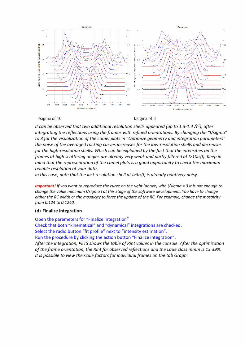
I/sigma of 10 I/sigma of 3

It can be observed that two additional resolution shells appeared (up to 1.3-1.4 Å-1), after integrating the reflections using the frames with refined orientations. By changing the “I/sigma” to 3 for the visualization of the camel plots in “Optimize geometry and integration parameters” the noise of the averaged rocking curves increases for the low-resolution shells and decreases for the high-resolution shells. Which can be explained by the fact that the intensities on the frames at high scattering angles are already very weak and partly filtered at I>10𝜎(I). Keep in mind that the representation of the camel plots is a good opportunity to check the maximum reliable resolution of your data. In this case, note that the last resolution shell at I>3𝜎(I) is already relatively noisy. Important! If you want to reproduce the curve on the right (above) with I/sigma = 3 it is not enough to change the value minimum I/sigma I at this stage of the software development. You have to change either the RC width or the mosaicity to force the update of the RC. For example, change the mosaicity from 0.124 to 0.1240.

(d) Finalize integration

Open the parameters for “Finalize integration” Check that both “kinematical” and “dynamical” integrations are checked. Select the radio button “fit profile” next to “intensity estimation”. Run the procedure by clicking the action button “Finalize integration”. After the integration, PETS shows the table of Rint values in the console. After the optimization of the frame orientation, the Rint for observed reflections and the Laue class mmm is 13.39%. It is possible to view the scale factors for individual frames on the tab Graph:

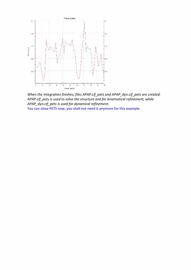
When the integration finishes, files APAP.cif_pets and APAP_dyn.cif_pets are created. APAP.cif_pets is used to solve the structure and for kinematical refinement, while APAP_dyn.cif_pets is used for dynamical refinement. You can close PETS now; you shall not need it anymore for this example.

PART 2: Structure solution and kinematical refinement in Jana2020

1. Create new structure

Important! The data-processing procedure is almost never perfectly reproducible. Small differences in the indexing and cell refinement procedure may result in small differences of integrated intensities. If you want to be sure that you can reproduce the following part of the tutorial, do not use the file APAP.cif_pets that you just created, but use the file APAP_reference.cif_pets provided with the example files (Copy the file to APAP.cif_pets). Using your own cif_pets file is also possible, but your results may slightly differ from the results described in this tutorial. Start Jana2020

In the Main menu bar, use “Structure → New” and open new structure “APAP” in directory of the Example 13.8.

2. Import Wizard

[On the screen: Specify type of the file to be imported] Select “Single crystal: Known diffractometer formats”; NEXT. [On the screen: Data reduction file from] Select “Pets electron diffractometer”. The file name automatically changes to APAP.cif_pets, which is a file produced by PETS containing all important information, including the list of intensities. NEXT. Change Temperature to 100 K; Leave all other settings unchanged (note the wavelength of 0.0335 Å for 120 kV electrons!); NEXT. Leave all settings unchanged; NEXT. The program reads 7738 reflections from the file OK. For absorption correction select “None or done before importing”; NEXT. FINISH; OK to accept the data set. You just read in the cell parameters and the intensity list. If you do not have the data in the cif_pets format, you can read them in from a general hkl file using the option “reflection file corrected for LP and absorption” at the beginning of the import wizard. You then have to input the radiation type, wavelength and cell parameters by hand.

3. Symmetry Wizard

NEXT to close the information window and start the symmetry wizard. Symmetry Wizard can be started separately by “Reflection file → Make space group Test”. The default settings are prepared for x-ray diffraction. For electron diffraction we have to increase the tolerances. Change the tolerances according to this screenshot:

Leave other settings default; NEXT; OK. [On the screen: Select Laue point group]

Select orthorhombic mmm; NEXT. The internal R-values would be rather high for x-rays, but are good for electron diffraction data.

Select primitive unit cell; NEXT. [On the screen: Select space group] The window shows possible space groups. The list of the strongest reflections contradicting the selected space group can be displayed by “Details” button.

It is difficult to select the correct space group. In particular, presence or absence of the glide planes and screw axes is hard to asses, knowing that kinematically absent reflections may have significant intensities due to dynamical diffraction effects. Select Pbca; NEXT. Accept the space group in the standard setting; FINISH. Symmetry is saved in file APAP.m50.

4. Creating refinement reflection file

In this step the program creates file APAP.m90 containing the data set merged by symmetry and with discarded forbidden reflections. This file will be used for refinement. NEXT; 7738 reflections were read, 842 reflections were rejected as systematically extinct, 6885 reflections were written to the output file. OK; OK; NEXT The Rint(obs/all) is 13.18%/16.99% for 1574 unique reflections averaged from 6896 reflections. OK; FINISH

5. Structure Solution Wizard

OK to close the information window and start the solution wizard [On the screen: window of Commands for Superflip] Structure solution wizard can be executed separately through the Command tree “Structure solution → Commands for Superflip”. Jana2020 does not contain solution procedures, it calls external programs. By default, Jana uses Superflip (using charge flipping as the solution method). Superflip is distributed with Jana2020. In “Formula” textbox type the list of elements: C8 H9 N O2. Superflip does not need information about chemical composition but it will be required for peak assignment based on electrostatic potential map calculated by Superflip. If Jana2020 is used for peak assignment, a list of expected chemical elements is sufficient. If you know the expected formula, you may enter it and use EDMA for peak picking (at the bottom of the window). If the formula is correct, EDMA often gives cleaner and more complete interpretations of the solution. Click the checkbox next to “Use a specific random seed” and enter the value 111. Choose AAR as the iteration scheme.

AAR tends to give better results than CF for electron diffraction data, although in many cases the difference is negligible. Select “EDMA – fixed composition” for peak search. “Run Superflip”.

The specific random seed is used just to guarantee reproducibility of the results. For standard work random seed need not be defined. [On the screen: window of Superflip appears with iteration running. After ten runs, listing of Superflip log file is displayed]. A window pops-up with the information about space group and symmetry match after the trials finished. The result of the structure solution may slightly differ.

Click OK. Click on “Replace the result with tutorial files” for reproducibility of the results;OK. You can switch between your solution and tutorial one by clicking on the same button. Click on “Open the listing” for reproducibility of the results;OK. At the bottom you find the result of the structure solution: Properties of the saved density: Run Rvalue Peaks Symm. Der.SG 8 45.42 2.47 12.73 Pbca The space group proposed by Superflip is the same as our initial guess. “Close” the listing Click “Draw 3D map”. VESTA opens with a density shown as isosurfaces, and an atomic model overlaid. Rotate the view to inspect the structure (C - brown, N - blue, O - red). Click in VESTA “Edit”, “Bonds…”

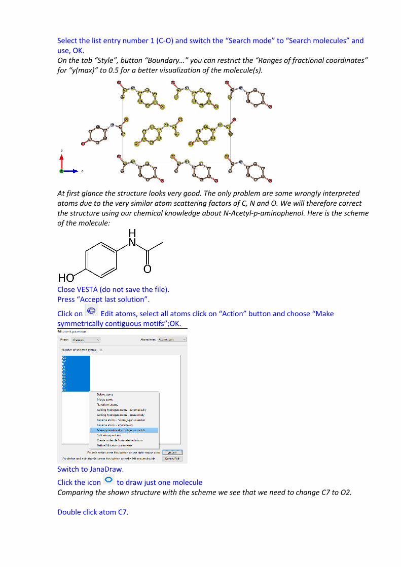
Select the list entry number 1 (C-O) and switch the “Search mode” to “Search molecules” and use, OK. On the tab “Style”, button “Boundary…” you can restrict the “Ranges of fractional coordinates” for “y(max)” to 0.5 for a better visualization of the molecule(s).

At first glance the structure looks very good. The only problem are some wrongly interpreted atoms due to the very similar atom scattering factors of C, N and O. We will therefore correct the structure using our chemical knowledge about N-Acetyl-p-aminophenol. Here is the scheme of the molecule:

Close VESTA (do not save the file). Press “Accept last solution”.

Click on Edit atoms, select all atoms click on “Action” button and choose “Make symmetrically contiguous motifs”;OK.

Switch to JanaDraw.

Click the icon to draw just one molecule Comparing the shown structure with the scheme we see that we need to change C7 to O2. Double click atom C7.

In the dialog that opens change the atomic type to O, rename it to Ox to avoid the clash with the O2, which is in fact C7; OK. Repeat for atom O2 (change to C7). Now you can rename the Ox to O2. The next step changes the names of atoms according to their chemical type and assigns a sequential number to each atom.

Click on the quick button “Edit Atoms” . Select all atoms, click “Action” and select “Rename selected atoms to atom_type + number”; OK. YES.

The corrected model should look like this:

6. Initial Refinement

[On the screen: basic window of Jana] In the Command tree, double click “Refinement → Refinement commands” [On the screen: Refine commands] Change the number of cycles to 100. Go to “Select/Listings”.

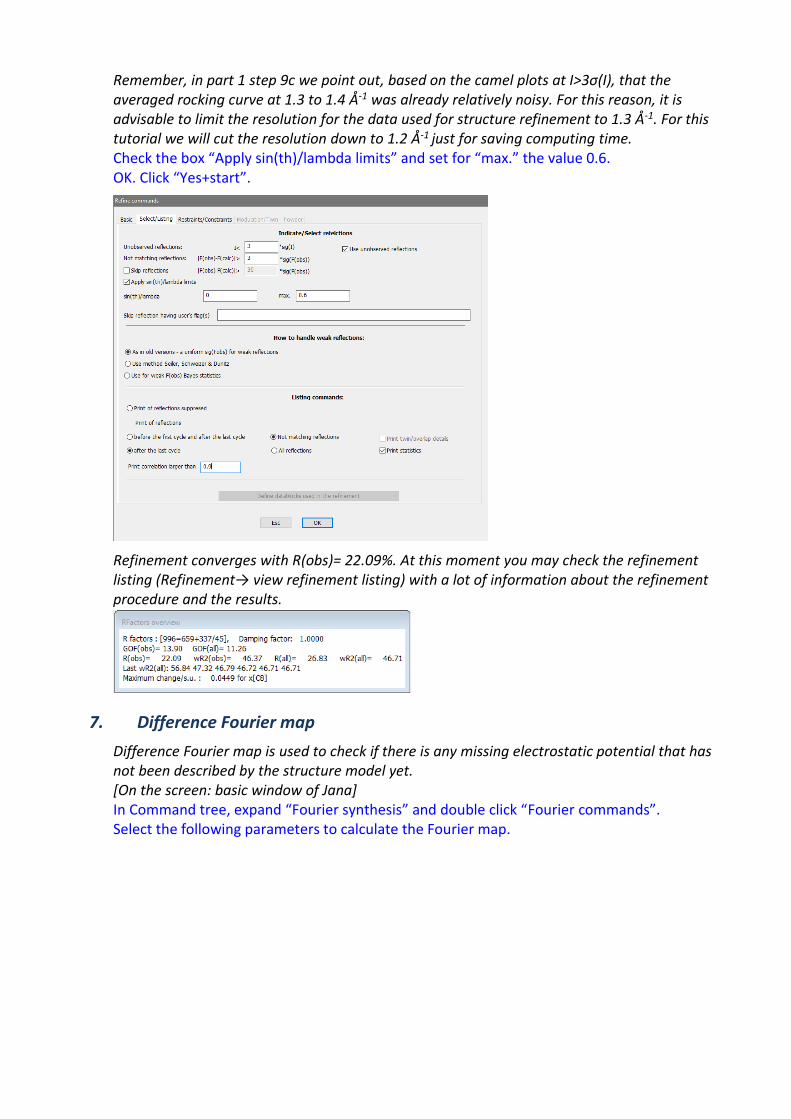
Remember, in part 1 step 9c we point out, based on the camel plots at I>3σ(I), that the averaged rocking curve at 1.3 to 1.4 Å-1 was already relatively noisy. For this reason, it is advisable to limit the resolution for the data used for structure refinement to 1.3 Å-1. For this tutorial we will cut the resolution down to 1.2 Å-1 just for saving computing time. Check the box “Apply sin(th)/lambda limits” and set for “max.” the value 0.6. OK. Click “Yes+start”.

Refinement converges with R(obs)= 22.09%. At this moment you may check the refinement listing (Refinement→ view refinement listing) with a lot of information about the refinement procedure and the results.

7. Difference Fourier map

Difference Fourier map is used to check if there is any missing electrostatic potential that has not been described by the structure model yet. [On the screen: basic window of Jana] In Command tree, expand “Fourier synthesis” and double click “Fourier commands”. Select the following parameters to calculate the Fourier map.

Click “OK”. “Yes+start”. Choose “NO” to avoid the procedure for including new atoms. Choose “NO” to avoid opening the listing. Have a look at the calculated map using VESTA as when looking at the solution. Click “Run Contour”, expand “Use old Fourier map”, and double click “draw maps as calculated”; OK. On the upper menu, go to “Run→Vesta” (alternatively click the Vesta icon in the bottom toolbar) Go to “Properties”, tab “Isosurfaces”. Click on Isosurfaces No 1 and change it to Positive and its level to 0.22 (3σ level); OK. Go to “Boundary” and set the y(max) to 0.5; OK.

A few weak positive peaks can be observed close to the atoms where we expect hydrogen atoms. It seems that at least 6 out of 9 hydrogens are visible in the difference Fourier map of the kinematical structure refinement. Close VESTA. Close Contour and return to the main window of Jana. We will add the hydrogen atoms on O1 and N1 as freely refined atoms, and add the hydrogens on the carbon atoms as riding. First, we will add the hydrogen atoms to O1 and N1 Expand the Command tree for “New”, double click “New atom”; OK. Select Max1 and click “Include the peak at the specified position”. Fill in Name of the Atoms as H*. Set the “Atomic type” to “H”; Accept. Repeat with the maximum close to O1 (Max10).

Click “Finish” and “Yes” to include the two new atoms. Edit structure parameters → Edit atomic parameters Select carbon atoms C1, C3, C5, C7 and C8. Press Action→Adding hydrogen atoms interactivelly. Set ADP ext. factor to 2; OK.

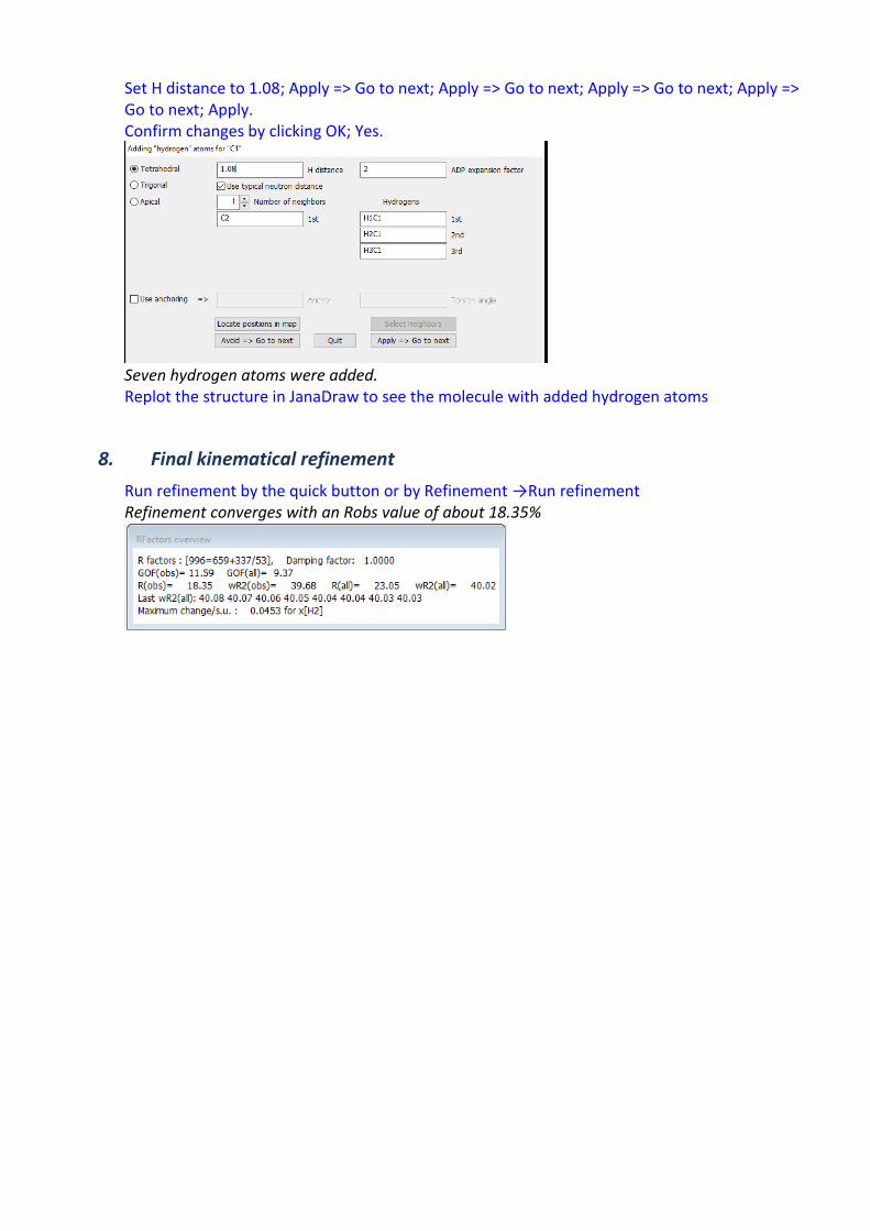
Set H distance to 1.08; Apply => Go to next; Apply => Go to next; Apply => Go to next; Apply => Go to next; Apply. Confirm changes by clicking OK; Yes.

Seven hydrogen atoms were added. Replot the structure in JanaDraw to see the molecule with added hydrogen atoms

8. Final kinematical refinement

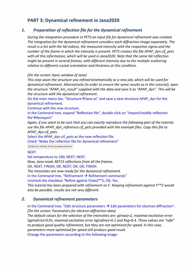
Run refinement by the quick button or by Refinement →Run refinement Refinement converges with an Robs value of about 18.35%

PART 3: Dynamical refinement in Jana2020

1. Preparation of reflection file for the dynamical refinement

During the integration procedure in PETS an input file for dynamical refinement was created. The integration for the dynamical refinement considers each diffraction image separately. The result is a list with the hkl indices, the measured intensity with the respective sigma and the number of the frame in which the intensity is present. PETS creates the file APAP_dyn.cif_pets with all this information, which will be used in Jana2020. Note that the same hkl reflection might be present in several frames, with different intensity due to the multiple scattering relative to different crystal orientation and thickness at this condition. [On the screen: basic window of Jana] This step saves the structure you refined kinematically as a new job, which will be used for dynamical refinement. Alternatively (in order to ensure the same results as in this tutorial), open the structure “APAP_kin_result” supplied with the data and save it as “APAP_dyn”. This will be the structure with the dynamical refinement. On the main menu bar, “Structure→Save as” and save a new structure APAP_dyn for the dynamical refinement. Continue with the new structure. In the Command tree, expand “Reflection file”, double click on “Import/modify reflection file→Reimport” Again, if you want to be sure that you can exactly reproduce the following part of the tutorial, use the file APAP_dyn_reference.cif_pets provided with the example files. Copy this file to APAP_dyn.cif_pets. Select the APAP_dyn.cif_pets as the new reflection file. Check “Make the reflection file for dynamical refinement”

NEXT. Set temperature to 100; NEXT; NEXT. Now, Jana reads 38713 reflections from all the frames. OK, NEXT, FINISH, OK, NEXT; OK; OK; FINISH. The intensities are now ready for the dynamical refinement. In the Command tree, “Refinement → Refinement commands” Uncheck the checkbox “Refine against F(obs)**2; OK; Yes. This tutorial has been prepared with refinement on F. Keeping refinement against F**2 would also be possible, results are not very different.

2. Dynamical refinement parameters

In the Command tree, “Edit structure parameters → Edit parameters for electron diffraction”. [On the screen: Parameters for electron diffraction data] The default values for the selection of the intensities are: g(max)=2, maximal excitation error Sg(matrix)=0.01, maximal excitation error Sg(refine)=0.1 and Rsg=0.4. These values are “safe” to produce good quality refinement, but they are not optimized for speed. In this case, parameters more optimized for speed still produce good result. Change the parameters according to the following image:

You can set the number of threads to the number of cores on your processor to speed up the calculation.

3. Sample thickness

The sample thickness is an important parameter of the dynamical refinement. Therefore, we have to set an initial value of the sample thickness. To save time, we will set the value to 700 Å. “Select zones for editing→ Select all → OK” and type 700 for “EDThick”. OK; YES. If you have time and are interested to try, you can follow the procedure below for finding the initial thickness. Otherwise go directly to point 4: Initial refinement. Back in the “Edit parameters for electron diffraction”, enable “Except of scale, optimize also: Thickness” Click “Run optimizations” [On the screen: Intensity calculation for optimizing of thickness]. Dyngo calculates wR-factor for the thickness varying from 0 to 2000 Å. “Show thickness plots”. Check the variation of the thickness of the crystal for the frames. Quit. Most frames have well defined wR-factor minima for one thickness. However, some frames either have poorly defined minimum or the minimum is at a very different thickness. You can check the wR(all) going through the zones in the main window of “parameters for electron diffraction data” or while viewing the graphs. Looking at the typical position of the minimum across the frames you can see that 700 Å is indeed a reasonable starting point for the refinement. “Select zones for editing→ Select all → OK” and type 700 for “EDThick”. OK; YES.

4. Initial refinement

To speed up the calculation we are going to use only part of the data in the initial stage of the refinement, specifically every 3rd frame. Go to “Edit Parameters for electron diffraction”. Click “Select zones for refinement” and “select each” 3rd zone. OK.

Click “Run optimizations” (neither the “Thickness” nor the “Orientation” check box should be checked!). This optimizes scale factors of individual frames and sets a good starting point for the least-squares refinement. Click OK; YES to return to the main screen of Jana2020. To compare the kinematical and the dynamical refinements on their ability to reveal hydrogen atoms, we are going to delete the hydrogens of the kinematical refinement.

Click on the quick button “Edit Atoms” or in the Command tree, expand “Edit structure parameters” and double click on “Edit atomic parameters”. Select all hydrogen atoms. Click “Action”, “Delete selected atoms”, “Yes to all”, OK; YES. First, we will refine the thickness with a fixed structure. In “Command tree”, expand “Refinement”, double click “Refinement commands”. Confirm the number of cycles is set to 100. On tab “Restraints/Constraints →Fixed commands”, write “*” into the field “Atoms/parameters”, click “Rewrite”; OK. Click OK, “Yes+Start”. The refinement converges after 8 cycles with Robs= 14.46% for 1493/3019 observed/all reflections, each cycle takes about 1-2 minutes (depending on your computer). In a next step we will let the structure free. Right click on the quick button “Refinement”; Click on tab “Restraints/Constraints → Fixed commands”. Select the first line “fixed all *”; Click “Delete”, OK. Click OK; “Yes+Start”. The refinement needs to run 5 more cycles to converge, each cycle takes about 2-18 minutes (depending on your computer). The state of the refinement after convergence is provided in the folder “refinements” as APAP_dyn1_initial. You may continue with those files if you want to save time. Open APAP_dyn1_initial in Jana2020. You can see the details of the refinement in the file APAP_dyn.ref (Refinement → View refinement listing). The refinement converges with R(obs)= 12.82%. It is important to check the

ratio observed reflections to refined parameters, which is around 24 in the present case (1493/62). It is recommended to keep this ratio above 10. Another important thing to check is the number of observed reflections per zone (frame). Also, in the APAP_dyn.ref file, you can see “R-factors for individual zones”, where the list of zones with the respective R-factors and number of reflections is shown.

5. Difference Fourier map - inserting hydrogens

Difference Fourier map is used to check if there is any missing electrostatic potential that is not described by the structure model yet. In this case we expect to identify the missing hydrogen atoms. [On the screen: basic window of Jana] In the Command tree, expand “Fourier synthesis”, double click “Fourier commands”. Select the following parameters to calculate the Fourier map:

Click “OK”, “Yes(+Start)” to start the calculation. Choose “NO” to avoid the procedure for including new atoms. Choose “NO” to avoid opening the listing. Have a look at the calculated map using VESTA. Click “Run Contour”, expand “Use old Fourier map”, and double click “draw maps as calculated”. To adjust the display of the potential map, On the upper menu, go to “Run→Vesta” In Properties → Isosurfaces select only positive isosurfaces and set the isosurface level to 0.13 (about 2.5 sigma); OK. Go to “Boundary” and set the y(min) to 0.5; OK. You should see an image similar to this:

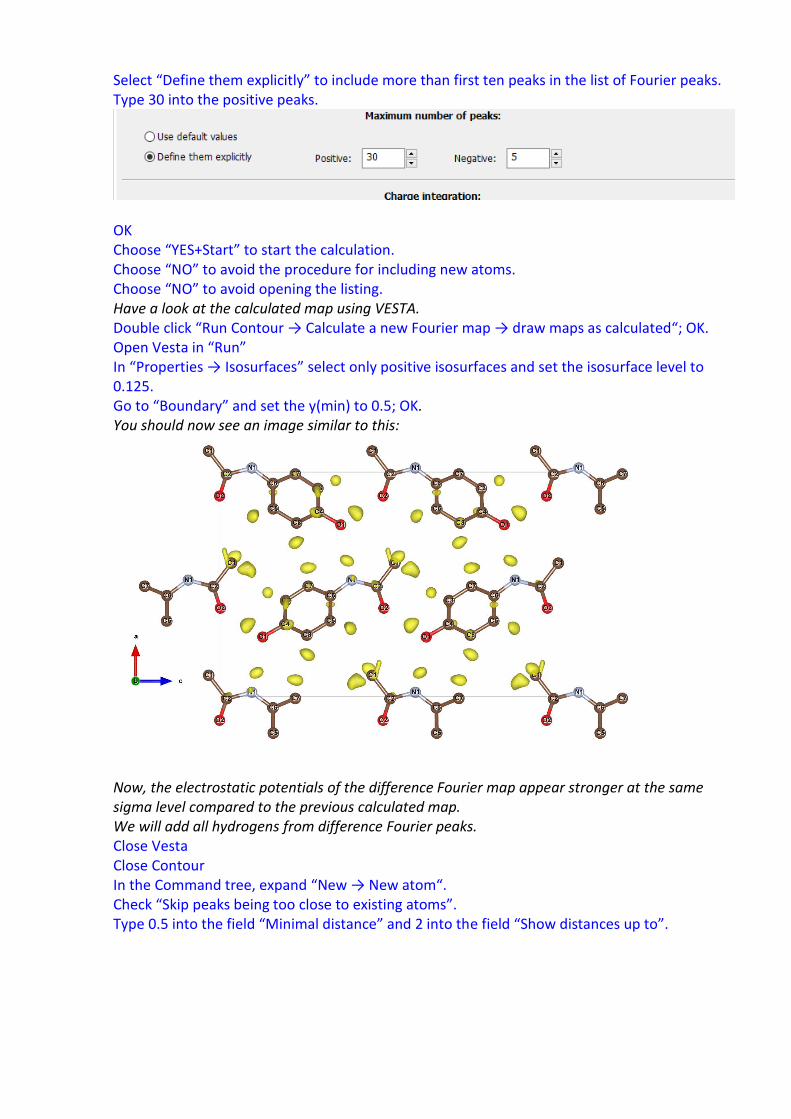
Even with just refining on every 3rd frame the difference Fourier map looks already better resolved and defined than in the case of the kinematical refinement. Let us use all frames for the calculation of the difference Fourier map to improve the significance of the residual electrostatic potentials. Close Vesta, close Contour.

6. Refinement using all frames

[On the screen: basic window of Jana] In the main menu bar, “Structure→ Save as”, find APAP_dyn in the previous directory and replace it. OK, YES, YES. Go to “Edit structure parameters → Edit parameters for electron diffraction”. [On the screen: Parameters for electron diffraction data] Click “Select zones for refinement” and “select all”. OK. Click “Run optimizations” (neither the “Thickness” nor the “Orientation” check box should be checked!). OK; YES. [On the screen: basic window of Jana] We need to run zeroth refinement cycle after adding additional frames. Right-click on the quick button “Refine”, click on tab “Basic” and set “Number of cycles” to 0. OK, “Yes+Start”. Robs is 13.00% after the zeroth cycle. IMPORTANT! Note that the R-value compared to the refinement on every 3rd frame increased just by 0.18 % without refining any parameter. Of course, it would be better to let the refinement run until convergence. Unfortunately, this step would be too time consuming for the tutorial. The structure file APAP_dyn2_all (R(obs) = 12.80%) is available for interested participants, but is not used in this tutorial. Click on “Fourier synthesis → Fourier commands”. Switch to the card “Peaks”

Select “Define them explicitly” to include more than first ten peaks in the list of Fourier peaks. Type 30 into the positive peaks.

OK Choose “YES+Start” to start the calculation. Choose “NO” to avoid the procedure for including new atoms. Choose “NO” to avoid opening the listing. Have a look at the calculated map using VESTA. Double click “Run Contour → Calculate a new Fourier map → draw maps as calculated“; OK. Open Vesta in “Run” In “Properties → Isosurfaces” select only positive isosurfaces and set the isosurface level to 0.125. Go to “Boundary” and set the y(min) to 0.5; OK. You should now see an image similar to this:

Now, the electrostatic potentials of the difference Fourier map appear stronger at the same sigma level compared to the previous calculated map. We will add all hydrogens from difference Fourier peaks. Close Vesta Close Contour In the Command tree, expand “New → New atom“. Check “Skip peaks being too close to existing atoms”. Type 0.5 into the field “Minimal distance” and 2 into the field “Show distances up to”.

We will assign hydrogens to the following maxima: Max 1 -H1, Max 2 - H2, Max 3 - H3, Max 4 - H4, Max 5 -H5, Max 6 – H6, Max 7 – H7, Max 9 – H8 Max 11 – H9 (Max 8 and 10 spurious peaks). Select Max1 and click “Include the peak at the specified position”. The first maximum is at a distance of 0.94 Å from C1. Click “Accept” to include the new atom. Repeat for the other Maxima. Click “FINISH”; “YES” to include the new atoms. Have a look at the Hydrogens calculated map using VESTA. Double click “Run Contour → Calculate a new Fourier map → draw maps as calculated“; OK. “Run → Vesta”; In “Properties → Isosurfaces” select only positive isosurfaces and set the isosurface level to 0.125. Boundary y(max) 0.5. Edit>bonds>C-H max length 1.4. Delete H-N bond. Create a new bond by clicking on New, set atom 1 and 2 as N and H. OK.

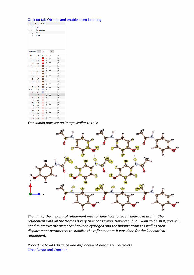
Click on tab Objects and enable atom labelling.

You should now see an image similar to this:

The aim of the dynamical refinement was to show how to reveal hydrogen atoms. The refinement with all the frames is very time consuming. However, if you want to finish it, you will need to restrict the distances between hydrogen and the binding atoms as well as their displacement parameters to stabilize the refinement as it was done for the kinematical refinement. Procedure to add distance and displacement parameter restraints: Close Vesta and Contour.

Click on “Refinement →Refinement commands”, select tab “Restraints/Constraints→Distance restraints”. Into the field “Atoms” write “H1 C5; H4 C5; H9 C5” (or the corresponding pairs of atmos according to your structure) Change “Value” to 1.08 to restrict the distance to 1.08 Å Click “Rewrite” Proceed to other atom pairs. d(H-C)=1.08 Å, d(H-N)=1.01 Å and d(H-O)=0.98 Å. Add the remaining hydrogen atoms in a similar way. OK. On tab “Restraints/Constraints”, click “Keep commands”. Select radio button “ADP”, set the number of hydrogen atoms to 3 Fill in C5 as “Central”, 2 as “Extension” and H1, H4 and H9 as “1st, 2nd and 3rd hydrogens” Click “Rewrite”. Add the remaining hydrogens in a similar way. OK.

On the tab “Basic” set the number of refinement cycles to 100. OK and “Yes+start” to start the refinement. Click “Use all” to confirm that you want to use the distance restraints you just set. IMPORTANT! The refinement needs more than 25 cycles to converge and each cycle takes about 12-90 minutes (depending on your computer). To proceed with the tutorial, you may use structure APAP_dyn3_final, which contains the result of the final refinement. You can see the details of the refinement in the file APAP_dyn3_final.ref (Edit/View→ View of Refine). The refinement converges with R(obs)= 9.22%, hence a decrease of about 3.6% after the insertion of nine hydrogen atoms compared to the refinement without hydrogens (which was not done in this tutorial – check the structure file APAP_dyn2_all). The resulting structure You can view the resulting structure using your favorite program associated with Jana2020 by selecting Plot structure (Draw + return). In this tutorial we use VESTA:

The result is satisfying considering that the structure has just been refined against the reflections of 50 frames. The bond angles of the hydrogens to the methyl group carbon C5 differ too much from the typical expected 110° of a tetrahedron. The hydrogen bond-angles to the nitrogen and other carbon atoms are almost as expected between 115° and 125°. The dihedral angles to the hydrogens are reasonable except for the methyl group. An even higher accuracy and stability of the refinement can be achieved by refining the structure against more data sets at the same time. In this case it might be possible to refine the hydrogen positions without restrictions.