Examining the Progression of Ecological Theory Through ...

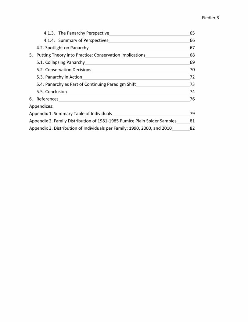
Examining the Progression of Ecological Theory Through

Arachnid Recovery of Mount St. Helens: Why Panarchy is Next

in the Successional Line

Katherine Fiedler ENVS Program

Lewis & Clark College 2011

Abstract:

Ecological theories attempt to make sense of the noise of ecological systems. The way we consider the recovery of ecosystems following a disturbance has changed over time, progressing from Clementsian succession to alternative stable states and now to panarchy. In this evolution of thought, the notions of recovery, stability, and resilience have also changed. Panarchy acts as a paradigm presenting new considerations regarding these concepts, and in turn powerful implications for conservation and management. In order to fully grasp the implications of these theories, we must consider them in the context of a living ecological system. When applied to a quantitative analysis of arachnid recovery of Mount St. Helens following the 1980 eruption, we can begin to see how each theory considers recovering systems differently. The same data elicit different understandings depending on the language and framework that are applied. Through this analysis, I have illuminated how panarchy can further our thought regarding ecological recovery.

Fiedler 2

Table of Contents 1. Introduction 4

1.1. Mount St. Helens as a Model System 5 1.2. Ecological Theories of System Recovery 7 1.3. Argument 9

2. Music from the Noise: Reviews of Ecological Theories 10 2.1. Review of Clementsian Successional Theory 10

2.1.1. Successional Theory in the Field of Ecology 13 2.1.2. Critiques of Clementsian Succession 13

2.2. Review of Alternative Stable State Theory 14 2.3. Review of Panarchy 19 2.4. Comparing the Theories 26

2.4.1. How These Theories Will Be Tested 27 3. Listening to the Landscape: A Case Study 29

3.1. Arachnid Recovery of Mount St. Helens 31 3.1.1. Arachnid Sampling Methodology 32

3.1.1.1. Limitations of Sampling Methodology 37 3.1.2. Arachnid Dispersal Methods 39 3.1.3. Spider Feeding Guilds 42 3.1.4. Spider Habitat Preferences 43 3.1.5. Results 44

3.1.5.1. Total number of taxa 45 3.1.5.2. Ballooners 46 3.1.5.3. Feeding Guilds 48 3.1.5.4. Habitat Preferences 50 3.1.5.5. Representative Patterns 53

3.1.5.5.1. Higher Abundance in Less Disturbed Sites 54 3.1.5.5.2. Higher Abundance in More Disturbed Sites 55 3.1.5.5.3. Similar Distribution Across All Research Sites 56 3.1.5.5.4. Successful invaders 57

3.1.6. First on the Scene 58 3.1.7. Comparison to Beetle Data 60

4. When Theories and Data Collide 60 4.1. Deconstructing the Theories in Context 61

4.1.1. The Clementsian Succession Perspective 61 4.1.2. The Alternative Stable States Perspective 63

Fiedler 3

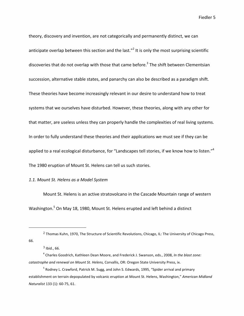
4.1.3. The Panarchy Perspective 65 4.1.4. Summary of Perspectives 66

4.2. Spotlight on Panarchy 67 5. Putting Theory into Practice: Conservation Implications 68

5.1. Collapsing Panarchy 69 5.2. Conservation Decisions 70 5.3. Panarchy in Action 72 5.4. Panarchy as Part of Continuing Paradigm Shift 73 5.5. Conclusion 74

6. References 76 Appendices: Appendix 1. Summary Table of Individuals 79 Appendix 2. Family Distribution of 1981-‐1985 Pumice Plain Spider Samples 81 Appendix 3. Distribution of Individuals per Family: 1990, 2000, and 2010 82

Fiedler 4

1. Introduction

We all use theories and models to understand variation and change, to make

predictions, and to better inform our actions. Ecologists use them to make sense of systems

lacking borders in time or place, in which relevant variables seem infinite and much is due to

randomness or endless cascades of response. Perhaps ecologists are envious of those sciences

that have the luxury of laws rather than highly contested theories; however Daniel Simberloff

notes that, “What physicists view as noise is music to the ecologist.”1 While they may embrace

this complexity, ecologists do try to create some order from the noise, although even the

theories themselves cannot be described as static.

Understanding community response to disturbance is one such example. Ecologists have

attempted to quantify recovery through complex mathematical models or to simply visualize

such change with ball-‐in-‐cup diagrams. The last century witnessed the progression of ecological

thought in this field, from Clementsian succession to alternative stable state theory, and now,

to panarchy. This progression reflects perhaps a successional theory of theories, in which each

builds upon the last, and thus is not wholly independent. Thomas Kuhn details this notion in his

discussion of scientific revolutions as paradigm shifts. He wrote, “…that in sciences fact and

1 Daniel Simberloff, A Succession of Paradigms in Ecology: Essentialism to Materialism and Probabilism, p.

63-‐99, In: Esa Saarinen ed., 1982, Conceptual Issues in Ecology, Boston, MA: D. Reidel Publishing Company, 85.

Fiedler 5

theory, discovery and invention, are not categorically and permanently distinct, we can

anticipate overlap between this section and the last.”2 It is only the most surprising scientific

discoveries that do not overlap with those that came before.3 The shift between Clementsian

succession, alternative stable states, and panarchy can also be described as a paradigm shift.

These theories have become increasingly relevant in our desire to understand how to treat

systems that we ourselves have disturbed. However, these theories, along with any other for

that matter, are useless unless they can properly handle the complexities of real living systems.

In order to fully understand these theories and their applications we must see if they can be

applied to a real ecological disturbance, for “Landscapes tell stories, if we know how to listen.”4

The 1980 eruption of Mount St. Helens can tell us such stories.

1.1. Mount St. Helens as a Model System

Mount St. Helens is an active stratovolcano in the Cascade Mountain range of western

Washington.5 On May 18, 1980, Mount St. Helens erupted and left behind a distinct

2 Thomas Kuhn, 1970, The Structure of Scientific Revolutions, Chicago, IL: The University of Chicago Press,

66. 3 Ibid., 66. 4 Charles Goodrich, Kathleen Dean Moore, and Frederick J. Swanson, eds., 2008, In the blast zone:

catastrophe and renewal on Mount St. Helens, Corvallis, OR: Oregon State University Press, ix. 5 Rodney L. Crawford, Patrick M. Sugg, and John S. Edwards, 1995, “Spider arrival and primary

establishment on terrain depopulated by volcanic eruption at Mount St. Helens, Washington,” American Midland

Naturalist 133 (1): 60-‐75, 61.

Fiedler 6

disturbance gradient amidst an unrecognizable landscape. The range of volcanic forces,

landslides, pyroclastic flows (hot gas and rock), tephra (volcanic ash and rock) fall, and the blast

itself, created a patchwork of environments altered to different degrees. The pyroclastic flow

completely scoured and sterilized the immediate landscape. The force of the blast leveled trees

and scorched the vegetation as far as seventeen miles away. Even further away, tephra rained

down onto forests, covering the ground and low-‐lying vegetation.6 After the eruption, much of

the landscape appeared to be lifeless. However, the barren landscape was soon overcome as

surviving pockets of life and the recolonization of many populations began to transform the

land.

Mount St. Helens has become a working field laboratory for researchers in almost every

biological and geophysical field.7 The ecological recovery following the eruption has provided

information regarding the recovery of populations and entire ecosystems following

disturbances. Congress passed the National Volcanic Monument Act in 1982, creating an

110,000-‐acre national monument, within which the recovery of these systems could occur

without human interference or exploitation. An ideal natural experiment of ecosystem recovery

had begun. In just one day, Mount St. Helens became a model system for the observation of

6 Goodrich et al. eds. 2008, x.

7 Virginia H. Dale, Frederick J. Swanson, and Charles M. Crisafulli, eds., 2005, Ecological Responses to the

1980 Eruption of Mount St. Helens, New York, NY: Springer.

Fiedler 7

countless environmental processes, including the recovery of ecosystems following a range of

disturbances.

1.2. Ecological Theories of System Recovery

Ecological theories have long aimed to describe complex living systems that have

continually evaded the confines of strict patterns and equations. Many ecological theories

attempt to describe ecosystem recovery, or the trajectory of ecosystem response toward its

previous state or some newly organized state, following a disturbance. Over time, the theories

themselves have evolved to acknowledge and incorporate more complexity and new

interpretations of stability, while still aiming to be broadly applicable.

The following is only a brief introduction to the three theories I will be considering, as I

will explain each in detail shortly thereafter. Ecological succession, in short, was the first of such

theories regarding community change over time, describing a linear and predictable pattern of

recovery toward a single and repeatable climax state.8 However, ecologists have moved away

from this notion of a predictable trajectory toward a monoclimax in favor of alternative stable

states theory. The theory of alternative stable states focuses on the potential for systems to

settle in different states of stability, triggered by an internal or external disturbance. This theory

8 Frederic E. Clements, 1916, Plant Succession, an Analysis of the Development of Vegetation, p. 140-‐143,

In: Edward J. Kormondy, ed., 1965, Readings in Ecology, Englewood Cliffs, NJ: Prentice-‐Hall, Inc., 140.

Fiedler 8

still focuses on these stable states themselves.9 Panarchy branches from alternative stable

states theory describing systems as being constantly in flux. Community change within systems

can be viewed as series of dynamic cycles of different temporal and spatial scales. Disturbances

act as a trigger to prompt these cycles to either continue on their same adaptive cycles or to

allow for novelty.10 This theory has yet to take hold in ecological discourse; however it may

present us with new ways of discussing the responses of living systems to ecological

disturbances.

We can better understand these theories when we consider them in the context of real

living systems. It is only then that we can see exactly what they focus on and what they largely

ignore. The disturbance zones of Mount St. Helens provide a context through which we can

consider the theory of panarchy and its place in ecological theory. Within these communities, it

is helpful to center our focus on specific taxonomic groups in order to properly manage the

complexity of ecosystems as a whole. Arthropods play important roles in the structuring of

communities. They can provide information regarding the vegetation and other organisms

9 B. E. Beisner, D. T. Haydon, and K. Cuddington, 2003, “Alternative stable states in ecology,” Frontiers in

Ecology and the Environment 1 (7), 376. 10 C.S. Holling, 2001, “Understanding the Complexity of Economic, Ecological, and Social Systems,”

Ecosystems, 4:390-‐405, 390.

Fiedler 9

present in a system by considering their prey items, predators, and preferred habitats.11

Ecological theories of recovery are traditionally considered through investigations of plant

communities, looking at the base of food chains, which act as a necessary predecessor to

consumers. Consumers can prove to be equally valuable in these analyses, as they reflect both

the presence of vegetation and predators of themselves. Consumers might show slow recovery

initially, followed by a rapid influx of taxa following the establishment of plant communities.

However, the diversity and complexity of consumer species interactions might result in a

recovery quite similar to that of plants, in terms of niche diversity. For the purpose of my

analysis, I consider ecosystem recovery with a focus on arachnids.

1.3. Argument

The different theories of ecosystem recovery are not correct or incorrect, but rather

they may or may not be sufficient to explain the recovery of ecological systems. They may also

prove to illuminate certain aspects of the process of recovery while ignoring others, altering our

perceptions of stability and conservation. In this paper, I focus on the language and modeling of

panarchy as a paradigm describing the dynamism and recovery of ecosystems, as compared to

11 Robert R. Parmenter et al., 2005, Posteruption Arthropod Succession on the Mount St. Helens Volcano:

The Ground-‐Dwelling Beetle Fauna (Coleoptera), p. 139-‐150, In: Virginia H. Dale, Frederick J. Swanson, and Charles

M. Crisafulli eds., 2005, Ecological Responses to the 1980 Eruption of Mount St. Helens, New York, NY: Springer,

139.

Fiedler 10

Clementsian succession and alternative stable states. I will apply these theories to the recovery

of arachnids in the disturbance zones of Mount St. Helens following the 1980 eruption. The

theory of panarchy focuses on the dynamism of ecological systems and challenges the idea of

stability, serving as the next step in this ecological paradigm shift. Furthermore, due to its new

and relevant perspectives on conservation, panarchy should be considered in environmental

discourse and its subsequent application.

2. Music from the Noise: Reviews of Ecological Theories

In order to apply these theories to empirical data, we must first understand their

history, framework, and language. I will present these theories independently of each other and

of the Mount St. Helens arachnid case study in order to first focus on the applicability of these

theories as they were conceived. Even though each theory describes distinct ecological

processes, while often not addressing them directly, I will avoid augmenting these theories with

other ecological discourse. This will display each theory as it is presented in its founding

discourse and subsequent evolution.

2.1. Review of Clementsian Successional Theory

Succession, in its simplest form, means the occurrence of events in a particular temporal

or spatial sequence. The term was first used in an ecological context by a French biologist,

Adolphe Dureau de la Malle in 1825. However, the idea of ecological succession is said to be

Fiedler 11

much older, perhaps dating as far back as the scientific wonderings of William King in 1685.12 It

was not until Frederic Clements published Plant Succession: An Analysis of the Development of

Vegetation in 1916 that succession became widely accepted among ecologists.13 Clements

described succession as a series of plant communities, or seres, that culminate in a stable

monoclimax. Each sere is progressively more complex and constructed of life forms of higher

trophic levels that might also require more intricate habitats. The process is an explicitly

deterministic response to some disturbance, as each sere is a step in the development of this

climax formation.14 In Clements’ own words:

As an organism the formation arises, grows, matures, and dies…Furthermore, each climax formation is able to reproduce itself, repeating with essential fidelity the stages of its development. The life-‐history of a formation is a complex but definite process, comparable in its chief feature with the life-‐history of an individual plant.15

Clements believed that, like the development of an organism, an ecosystem experiences

distinct life stages that can be replicated. Each time a certain system recovers from a

disturbance, it will follow the same path to its climax state.

12 Frank B. Golley ed., 1977, Ecological succession, Stroudsburg, Pa: Dowden, Hutchinson & Ross, 1. 13 William H. Drury and Ian C.T. Nisbet, 1973, Succession, p. 287-‐368. In: Frank B. Golley, ed., 1977,

Ecological Succession, Stroudsburg, PA: Dowden, Hutchinson & Ross, 289. 14 Clements, 1916, 140-‐141. 15 Clements 1916, 140.

Fiedler 12

A system at the climax state resembles an organism of the highest order and

complexity.16 The system functions in the most energy efficient manner, in terms of biomass

and organismal interactions.17 According to Clements, the path to reach this state is predictable

and replicable, each step dependent on the last. Furthermore, Clements claimed that climate

determines the specific characteristics of these climax states through the large and constant

control that it has over the system. For each unique climatic region, there must only exist one

climax state. If any other state appears within that region, it must be that the system has not

yet reached this most mature and complex stage.18 Yet inevitably, the system will reach its

climax state. As Worster described, “…eventually nature will find a way to get back on track.”19

Once the climax state is reached, assuming external conditions remain constant, it can remain

there indefinitely,20 or as Clements, himself, wrote, “Such a climax is permanent because of its

entire harmony with a stable habitat.”21 He even goes so far as to say that the term stabilization

is synonymous with succession.22

16 Donald Worster, 1994, Nature's economy: a history of ecological ideas, Cambridge: Cambridge

University Press, 210. 17 Eugene P. Odum, 1969, The Strategy of Ecosystem Development, p. 278-‐286, In: Frank B. Golley ed.,

1997, Ecological Succession, Stroudsburg, PA: Dowden, Hutchinson & Ross, 278-‐279. 18 Worster 1994, 210. 19 Ibid., 210. 20 Ibid., 210. 21 Clements 1916, 143. 22 Ibid., 142.

Fiedler 13

2.1.1. Successional Theory in the Field of Ecology

Clementsian succession integrated the ideas behind many ecological processes.

Clements explains the progression from the initial disturbance to the final monoclimax as, “…(1)

nudation, (2) migration, (3) ecesis [or establishment of local populations], (4) competition, (5)

reaction, (6) stabilization.”23 Community ecologists have since detailed out these processes,

with the ideas of primary succession, in which the disturbed site holds no memory of the

previous community, and secondary succession, in which ecosystems still contain pieces of the

old community structure. Furthermore, Clementsian thought echoes the concept of

dominance-‐controlled communities, or the process of competition, where only a few dominant

species out of the colonizers successfully remain in an area.24

2.1.2. Critiques of Clementsian Succession

While much of Clementsian succession still dominates ecological thought, the idea of a

monoclimax was met with much resistance. Ecologists contested that due to the inherent

variation of environmental factors—such as soil, microclimate, geography, and topography—it

is unlikely that only one climax state can be attributed to a climatic region. Instead, we might

23 Ibid., 141. 24 Michael Begon, Colin R. Townsend, and John L. Harper, 2006, Ecology: from individuals to ecosystems,

Malden, MA: Blackwell Pub, 489.

Fiedler 14

observe a continuum of climax states.25 H.A. Gleason, one of Clementsian succession’s

strongest critics, stated that, “…succession is an extraordinarily mobile phenomenon whose

processes are not to be stated as fixed laws, but only as general principles of exceedingly broad

nature, and whose results need not, and frequently do not, ensue in any definitely predictable

way.”26 Other critics noted the role of chance in community development. An organism must

not only disperse into an area, but the proper resources must be available at that time for it to

survive and establish. Thus, chance also strongly challenges this notion of a monoclimax.27

Modern definitions of succession still strongly reflect the thoughts of Clements and the

progression toward a stable ecosystem. However, ecologists largely treat succession as a way of

understanding how ecosystems reassemble after a disturbance and have reconsidered the

nature of the climax state, as can be seen in alternative stable state theory.

2.2. Review of Alternative Stable State Theory

Alternative stable state theory provides an alternative to the monoclimax. The roots of

this theory are traced back to Richard C. Lewontin’s 1969 paper, The Meaning of Stability, in

which Lewontin uses mathematical ecological modeling to justify the possibility of multiple

25 Ibid., 488. 26 Edward Goldsmith, “Ecological succession rehabilitated,” Edward Goldsmith,

http://www.edwardgoldsmith.org/page119.html (16 November 2010), 2. 27 R.H. Whittaker, 1953, A Consideration of Climax Theory: The Climax as a Population and Pattern, p. 240-‐

277, In: Frank B. Golley, ed., 1977, Ecological Succession, Stroudsburg, PA: Dowden, Hutchinson & Ross, 254.

Fiedler 15

stable states for a given system.28 C.S. Holling’s 1973 paper, Resilience and Stability of

Ecological Systems,29 and John P. Sutherland’s 1974 paper, Multiple Stable Points in Natural

Communities,30 fleshed out the theory of alternative stable states, which has now taken hold in

modern ecological thought.

If the state variables of a system can exist in multiple arrangements, each at an

equilibrium that is stable at the local scale, then that system has alternative stable states. These

state variables include abundances of species or feeding guilds, population demographics,

spatial distributions, or abiotic factors. This idea can be considered in two ways. First, as the

community perspective describes, a certain community may exist in a number of different

states, even under the same external environmental conditions (Figure 1, left). Different stable

states are capable of being achieved under the same conditions. In order for the system to

move from one stable state to another, a large disturbance to the state variables must occur.

These variables describe the internal characteristics of the community. For example, drastic

changes in population demographics or densities might cause this shift. On the other hand, the

ecosystem perspective attributes the existence of alternative stable states to changes in the

28 Richard C. Lewontin,1969, "The meaning of stability," Brookhaven Symposia in Biology, 22: 13-‐24, 13. 29 C. S. Holling, 1973, "Resilience and Stability of Ecological Systems," Annual Review of Ecology and

Systematics, 4: 1-‐23. 30 John P. Sutherland, 1974, "Multiple Stable Points in Natural Communities," American Naturalist, 108

(964): 859-‐873.

Fiedler 16

parameters that determine the behavior of or interactions between populations, such as birth

and death rates or predation (Figure 1, right). Environmental changes might shift these

parameters, causing the stable states to shift. The new stable state need not have been

possible under the previous parameters.31 These two perspectives differ from one another in

whether the shift originates in the community itself (variables) or in the ecosystem containing

that community (parameters).

Figure 1: Ball-‐in-‐cup diagram depicting the community perspective (left) and the ecosystem perspective (right) of alternative stable state theory.32

Shifts between stable states can occur at varying degrees and rates. A smooth response

occurs when a small change to variables or parameters results in a small change in the state of

the system. A threshold response occurs when most changes in conditions result in a small shift

31 Beisner et al. 2003, 376. 32 Ibid., 377.

Fiedler 17

in the system state, but when small changes in conditions, around a threshold value, result in a

drastic shift, or a critical transition.

For a system to return to a previous stable state it is often more difficult than simply

shifting the conditions back to where they were before. Hysteresis occurs when a system must

shift back to conditions far beyond those at the point of the critical transition in order to return

to a previous stable state (Figure 2).33 However, hysteresis is not a necessary condition for

alternative stable states. Minor changes can be absorbed by a system, yet large disturbances or

small changes around a critical point might result in a transition to a different stable state.

Figure 2. A model of a system exhibiting hysteresis. Small changes in conditions near point F1 or F2 result in a critical transition to the alternative stable state. Forward shift and backward shift show that the system must return to conditions far beyond points F1 and F2 in order to return to the original stable state.34

33 Marten Scheffer, Alternative Stable States and Regime Shifts in Ecosystems, p. 395-‐406, In: Simon A.

Levin ed., 2009, The Princeton Guide to Ecology, Princeton, NJ: Princeton University Press, 396. 34 Ibid., 397.

Fiedler 18

This theory requires the distinction between a system that can reach multiple stable

states and one that entirely lacks stability. Alternative stable states theory allows for a shift in

the location of the stable point of a given system, yet still maintains the notion that there do

exist several stable states that the system shifts between. Lewontin explains:

...it is a stable point, since a small perturbation of the system will result in the system returning to that point. It is necessary to specify that the perturbation is small because there may be several such stable points in the space and each will have its own basin of attraction. If the perturbation is sufficiently large to carry the system out of one basin of attraction into another, the original point is still a stable point even though the system did not return to it.35

Thus, a system is at a stable point if the state variables and parameters remain constant for a

given time and place, despite outside changes that threaten to affect them. Of course, the

spatial and temporal scale in which the system is considered must be appropriate in order to

understand its stability.36

Alternative stable state theory has received much attention in the field of ecology,

particularly due to increasing evidence of alternative stable states prompted by human

activities.37 It has modified successional theory to allow for systems to have multiple stable

states, while transforming our views of disturbed systems, and in turn conservation. However,

35 Lewontin 1969, 15. Original emphasis. 36 Sutherland 1974, 860. 37 Michael L. Cain, William D. Bowman, and Sally D. Hacker, 2008, Ecology, Sunderland, MA: Sinauer

Associates, Inc., 358.

Fiedler 19

the notion of “stable states” in itself can be contested in ecological thought. Panarchy has

recently begun to challenge this idea, and once again to transform our perspectives on stability

and conservation.

2.3. Review of Panarchy

The ideas behind panarchy as a whole was first presented in Lance Gunderson and C.S.

Holling’s 2001 synthesis, Panarchy: Understanding Transformation in Human and Natural

Systems.38 Panarchy provides a way to understand natural systems as a series of nested

adaptive cycles, continually in flux between growth, accumulation, restructuring, and renewal

throughout their life cycles.39 The paradigm of panarchy does not allow for any state of

stability, as did succession and alternative stable states. An adaptive cycle can describe any

dynamic system under consideration, which is influenced by other adaptive cycles of larger,

slower scale in conjunction with those of smaller, faster scale. These cycles are represented by

Gunderson and Holling as a figure-‐eight shape (Figure 3). Adaptive cycles progress through

scales of both potential and connectedness. Potential, or wealth, describes the possibilities for

change of a system. A higher potential means that the system has more future alternative

states. Connectedness, or controllability, describes the control a system has over its own

38 Lance H. Gunderson and C. S. Holling eds., 2002, Panarchy: understanding transformations in human

and natural systems, Washington, DC: Island Press, 21. 39 Holling 2001, 392.

Fiedler 20

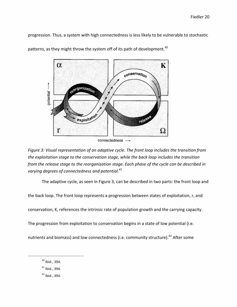
progression. Thus, a system with high connectedness is less likely to be vulnerable to stochastic

patterns, as they might throw the system off of its path of development.40

Figure 3: Visual representation of an adaptive cycle. The front loop includes the transition from the exploitation stage to the conservation stage, while the back loop includes the transition from the release stage to the reorganization stage. Each phase of the cycle can be described in varying degrees of connectedness and potential.41

The adaptive cycle, as seen in Figure 3, can be described in two parts: the front loop and

the back loop. The front loop represents a progression between states of exploitation, r, and

conservation, K, references the intrinsic rate of population growth and the carrying capacity.

The progression from exploitation to conservation begins in a state of low potential (i.e.

nutrients and biomass) and low connectedness (i.e. community structure).42 After some

40 Ibid., 394. 41 Ibid., 394. 42 Ibid., 394.

Fiedler 21

disturbance, the system begins with “biotic legacies,” or those species that survived, and other

abiotic factors that remain unchanged. Vegetation that can withstand this disturbed

environment will quickly gain dominance in the r phase, taking advantage of the low

connectedness. As new species immigrate into the system, “A period of contest competition

among entrepreneurial pioneers and surviving species from previous cycles ensues.”43 As new

and surviving species compete and populations become established, a more structured

community is developed, with increasing nutrients, biomass, and species interactions, and thus

increasing connectedness, quite similar to the progression described in succession.44 At the

height of this period of intense competition, we might find a peak in species diversity, as

thereafter species will begin to die out if they are unfit competitors, even if they were able to

take advantage of the disturbed environment. Again, reflecting successional thought, the

transition from the r-‐phase to the K-‐phase is a period of increasing control and less variability.

As the system approaches K, or the conservation phase of the cycle, the system is less likely to

experience novelty, or some alternative ecosystem structure.45 In ecological terms, the final

trajectory of the system can be either dominance-‐ or founder-‐controlled. The composition of

dominance-‐controlled communities, as described under successional theory, is dictated by

43 Gunderson and Holling eds. 2002, 43. 44 Ibid., 43-‐44. 45 Ibid., 44.

Fiedler 22

those species that are more competitively dominant than others.46 The composition of founder-‐

controlled communities, however, is dictated by a competitive lottery: no species is

competitively dominant, thus the composition is either determined by random population

fluctuations or the first colonizers of the area.47

However, the adaptive cycle of panarchy does not describe this increasing control and

connectedness as synonymous with stability, like succession and alternative stable states

theory suggest. Instead, panarchy views this increasing connectedness as rigidity. As the system

becomes more structured, it actually becomes more vulnerable to disturbances. Each species

has settled in a unique niche, thus any slight perturbation puts the entire system at risk.48 Once

a disturbance occurs, “a gale of creative destruction can be released in the resulting Ω

phase.”49 Potential drops as the disturbance destroys many of the resources that had

accumulated.

The disturbance moves the system into the back loop of the adaptive cycle. The back

loop is defined by the release (Ω) phase and the reorganization (α) phase (Figure 3). The length

of the back loop is defined by the nature of the disturbance, and whether it acts slowly or

46 Begon et al. 2006, 489. 47 Ibid., 493. 48 Holling 2001, 394. 49 Gunderson and Holling eds. 2002, 45.

Fiedler 23

suddenly. As the disturbance is acting, connectedness is destroyed in the system, thus allowing

for novelty in reorganization to follow. This process is unpredictable, rather than

deterministic.50 New relationships can be formed between variables, or immigrants can

dominate a system, where they otherwise would be outcompeted. The entire system can follow

a new trajectory due to the events during the reorganization phase.51 The adaptive cycle

continues into the exploitation phase and connectedness increases once again. The very nature

of this connectedness may be vastly different than it was before because of the events of the

back loop.

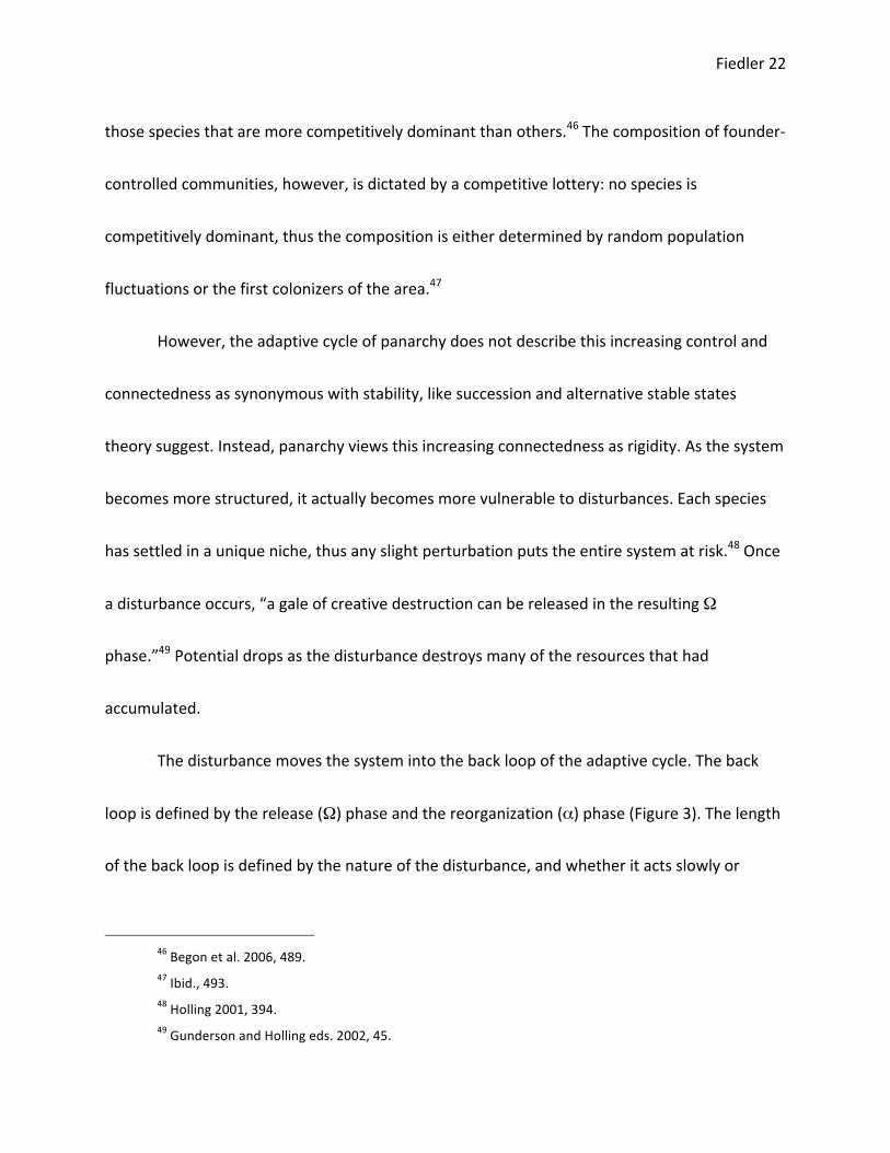
The phases of panarchical adaptive cycles can be better understood when we consider

them as nested cycles of different temporal and spatial scales (Figure 4). Forces of different

scales will influence any system considered. Larger and slower forces will cause the system to

“remember,” as these forces are less likely to fluctuate and maintain constant control. The

larger and slower cycle might be climatic control, source populations of immigrants, or the

remnants of potential in soil nutrients or stored seeds from the system prior to the disturbance.

The smaller and faster cycle that acts upon the system being considered might cause it to

50 Holling 395. 51 Gunderson and Holling eds. 2002, 46.

Fiedler 24

“revolt.” Its processes are quick and fluctuating and might spark novelty.52

Figure 4. Visual representation of nested adapted cycles.53

This force could be rooted in an invasive entering a disturbed system and establishing a strong

population, thus altering the trajectory of recovery, for example. The release of a system may

lead to revolt, but does not require this to be so. As C.S. Holling describes the nature of

panarchical cycles, “The conservative nature of established panarchies certainly slows change,

while at the same time accumulating potential that can be released periodically if the decks are

cleared of constraining influences by large, extreme events.”54 Whether a system revolts or

remembers is triggered not only by the influences of adaptive cycles of different scales, but also

52 Holling 2001, 398. 53 Ibid., 398. 54 Ibid., 399.

Fiedler 25

the scale of the disturbance and the variables that either remain or were eliminated. The

theory of panarchy cannot predict whether a system will revolt or remember after a

disturbance, yet it can describe conditions that influence each option.

Notions of resilience underlie the theory of panarchy, and balance its discussion of

rigidity and revolt. The concept of rigidity is contrary to that of resilience, or, “…the magnitude

of disturbance that can be absorbed before the system changes its structure by changing the

variables and processes that control behavior.”55 That is to say that not every disturbance will

project the system into the back loop, and certainly not every disturbance will occur in the

conservation phase. The resilience of a system is not a constant quality, but changes depending

on where the system is in the adaptive cycle. For example, as the system progresses through

the back loop, at levels of high potential and low connectedness, resilience is high. Thus, if the

system undergoes a disturbance at this point in the cycle, it will very easily return back to its

previous state. Resilience is low during the conservation phase of the front loop, where rigidity

is high. When a disturbance occurs during this phase, it is less likely that it will be able to return

to that state.56 This idea echoes that of hysteresis of alternative stable state theory.

55 Gunderson and Holling eds. 2002, 28. 56 Holling 2001, 395.

Fiedler 26

Panarchy adapts ideas from successional and alternative stable state theory, while

progressing ecological theory of recovery to account for non-‐linearity in adaptive cycles. It is

difficult to classify panarchy as a theory (however, I am comparing it to theories here), as it is

not testable or falsifiable, rather it is a paradigm that can illuminate ecological realities that we

observe. Panarchy has not taken hold of ecological discourse, perhaps due to its goals of acting

as a way of explaining human and natural systems in conjunction. It aims to apply to economic,

political, and ecological systems, and their intersection. However, despite the ambitious nature

of this paradigm, it is capable of thoroughly explaining living ecological systems. The application

of panarchy will illuminate its new perspective.

2.3. Comparing the theories

These three theories or paradigms are not independent from one another. Alternative

stable state theory was developed largely in response to succession, while panarchy is now

continuing the development of ecological theory or paradigms of response to disturbance. In

many ways, the later theories echo that which came before them. However, each theory also

uses a unique language and new perspectives in developing thought regarding ecosystem

recovery from disturbances. While much of the distinction between these theories can only be

illuminated when they are applied to living ecological systems, we can still begin to see how

Fiedler 27

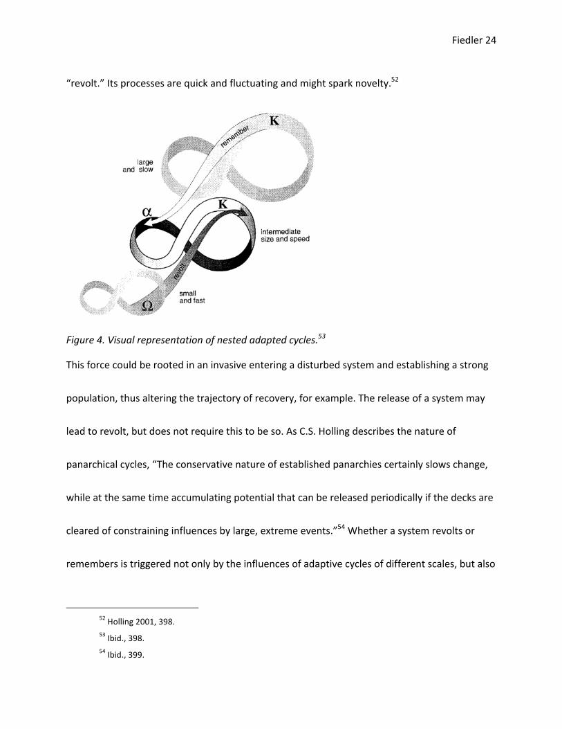
they differ from and reflect one another. In Table 1, I have deconstructed these theories and

compared them to one another, applying language from each.

Table 1. Qualitative comparison of theories using language from each. Clementsian

Succession Alternative Stable

States Panarchy

Disturbance defined as: variable or parameter shift

Parameter shift Variable or parameter shift

Variable or parameter shift

Opportunity for novelty? No Shift in stable point for a given system

Presented in the back loop, resulting in revolt

Deterministic? Linear and deterministic

No No

Accumulation of potential, increasing complexity?

Yes Yes Yes: front loop

Influences across scale Climate dictates monoclimax

Not applicable in language of theory

Nested adaptive cycles

Dominance vs. founder controlled

Dominance Dominance or founder Dominance or founder

Rigidity vs. resilience Systems inherently resilient

Considers both resilience and rigidity

Considers both resilience and rigidity

Stable vs. unstable equilibrium

Stable Stable Increasingly unstable

Monoclimax? Yes No, multiple possible climax states

No

Hysteresis? No Yes, inherent to theory

Yes, through language of rigidity, revolt, novelty

Used in ecological discourse? Yes Yes Limited

2.4.1 How These Theories Will Be Tested

In the following application of these theories or paradigms to arachnid recovery near

Mount St. Helens, I will highlight how the panarchy informs our thought on the subject of

ecological recovery. The data I have for arachnid diversity on Mt. St. Helens provide two axes of

information that are relevant for ecological recovery: (1) an axis of time since a major

disturbance event (1990, 2000, and 2010) and (2) an axis of habitats that experienced different

Fiedler 28

levels of disturbance in that event (pumice plain, blowdown forest, tephra forest, and reference

forest). To consider the application of theories of ecological recovery for this system, I will

apply my data in several ways. First, analyses of the total number of taxa in each research site

across time will provide an example of how one aspect (species diversity) of ecosystem

complexity has changed throughout recovery. Second, an analysis of the ballooning and

cursorial spider species present in each site over time will show how the species pool of

potential inhabitants and, subsequently, successful colonizers are dependent on what species

are capable of reaching the site. I expect to see more ballooning species than cursorial species

in disturbed sites, yet over time the number of each should increase, as would be consistent

with each of the three theories.

Through an analysis of feeding guilds and habitat preferences, I will consider ecosystem

complexity and how it differs between research sites and over time. Each theory predicts an

increase in ecosystem complexity as a part of recovery. However, the character of that

complexity is allowed to diverge from the preexisting state, according to alternative stable state

theory and panarchy only. Finally, I will isolate patterns of individual families or species that are

relevant to the course of recovery. Patterns that exhibit higher abundance of a particular taxon

in less or more disturbed sites might suggest different trajectories of recovery, while similar

abundance of a taxon across all sites would suggest the potential for the same trajectory of

Fiedler 29

recovery. Successful invaders in disturbed sites might indicate the occurrence of novelty and

creativity within the course of recovery, as panarchy and alternative stable states theory

describe. While any fluctuations in the reference forest samples will indicate that the site has

not reached its climax or stable state in successional and alternative stable state theories,

respectively, it could also simply indicate that the system is in the conservation phase of

panarchy and increasing in rigidity. As each theory builds off of that which came before it, many

of the predictions each theory makes might reflect those found in another theory, yet with

different language. Ultimately, however, panarchy emphasizes the dynamism of systems, while

succession and alternative stable states do not.

3. Listening to the Landscape: A Case Study

The 1980 eruption of Mount St. Helens captured the interest of natural scientists in

virtually every discipline. Scientists were able to examine ecological response and recovery

immediately after the eruption, rather than decades or centuries after, as is often the case. This

research has contributed not only to a better understanding of ecosystem recovery at Mount

St. Helens, but recovery following any volcanic disturbance, or even after disturbances in

Fiedler 30

general. Today, more than half of all studies published globally on the ecosystem responses to

volcanic eruptions were done on Mount St. Helens.57

One such study, Parmenter et al. (2005), done at Mount St. Helens examined the

succession of ground-‐dwelling beetles following the eruption. This study used the same

research sites and sampling dates that were used in the collection of my samples, as will be

explained in the following sections. The study also used pitfall trap sampling, also used for my

study, which is a common method of collecting and preserving ground dwelling arthropods.

This sampling method is biased towards those taxa who are most active on the ground.58

Parmenter et al. (2005) found a total of 27,074 beetles of 279 species and 39 families in four

research sites and four sampling years (1987, 1990, 1995, 2000).59 The authors found that

beetle species sequentially replaced other species throughout time in the disturbed sites as

conditions, such as vegetation and prey availability, changed. As would be expected, the most

disturbed site, the pumice plain, least resembled the undisturbed reference forest. Even in the

year 2000, 20 years after the eruption, the beetle species composition of each disturbed

57 Virginia H. Dale, Frederick J. Swanson, and Charles M. Crisafulli, 2005, Disturbance, Survival, and

Succession: Understanding Ecological Responses to the 1980 Eruption of Mount St. Helens, p. 3-‐11, In: Virginia H.

Dale, Frederick J. Swanson, and Charles M. Crisafulli eds., 2005, Ecological Responses to the 1980 Eruption of

Mount St. Helens, New York, NY: Springer, 3-‐4. 58 Parmenter et al. 2005. 59 Ibid., 142.

Fiedler 31

research site still did not resemble that of the reference forest. Thus, the authors hypothesized

that we will continue to see changes in community structure in the future.60 This study can

serve as an example of how we can understand data obtained from this sampling methodology,

and a comparison of another arthropod taxon’s recovery.

3.1. Arachnid Recovery of Mount St. Helens

Arachnids have been able to colonize virtually every terrestrial habitat. Of course, not

every species of arachnid can itself successfully live in different habitats. Each species is limited

by physical factors of the microhabitat, including humidity and temperature. Biological factors,

such as prey type and vegetation, also limit the distribution of species. Thus, many species have

distinctly defined ecological niches, which can be described by both habitat preference and

feeding guild.61 Where they live, arachnids serve a variety of ecological roles. Spiders (Order

Araneae) are entirely predatory, while Opiliones (harvestmen) and Acari (mites and ticks) can

be predators, herbivores, or detritivores. Even among predatory spiders, taxa have evolved

specific feeding biologies that take place in different parts of the ecosystem. Some may wander

or build foraging webs off of the ground, while others are only found on the ground or in leaf

litter.62

60 Ibid., 148-‐149. 61 Jan Beccaloni, 2009, Arachnids, Berkeley: University of California Press, 17. 62 Ibid.

Fiedler 32

From the identification of an arachnid, we can deduce information about the ecosystem

by using our knowledge of the individual’s habitat requirements. In my analysis, I will use

habitat preference and feeding guild to describe the ecological niche of arachnids. By focusing

on arachnid recovery, we can explore the potential to understand ecosystem recovery as a

whole. Furthermore, spiders have a history of being some of the first colonizers in the most

devastated areas following volcanic eruptions. Within just a year of the 1883 eruption of

Krakatoa, which left the island completely devoid of life, a linyphiid became the first to

successfully colonize. Within 50 years, there were over 90 species of spiders on the island.63

3.1.1. Arachnid Sampling Methodology

Samples were collected by a National Forest Service crew, working under Charlie

Crisafulli, from four study sites at Mount St. Helens: reference forest, tephra forest, blowdown

forest, and pumice plain (Figure 5). All four sites are located at similar elevations, from 1040 m

to 1175 m. Each research site was a standing old-‐growth forest, which had never been logged,

at the time of the 1980 eruption, yet each was disturbed differently and to varying degrees.

Each of these four sites was affected differently by the eruption, and thus may present different

courses of recovery. The reference forest is located 40km northeast of Mount St. Helens on

Lonetree Mountain. Parmenter et al. (2005) claims that the reference forest was unaffected by

63 Rainer F. Foelix, 1996, Biology of spiders, New York: Oxford University Press, 235.

Fiedler 33

the 1980 eruption and treats the site as a reference for the populations and communities that

were present before the eruption in the three disturbance sites.64 However, due to the scale of

the eruption it is possible that this site was still subject to at least ash fall, which in turn could

affect small arthropods.

Figure 5. Locations of research sites. Sites labeled as “beetle sites” are those from which arachnids were collected.65

64 Parmenter et al. 2005, 140. 65 Ibid., 141.

Fiedler 34

The reference forest consists of trees with an understory that is predominantly leaf litter

and bryophytes cover (Table 2). The tephra forest site is located directly east of the blowdown

forest, in the Hemlock Forest area. In this site, the eruption buried leaf litter and much of the

understory vegetation with tephra fall. Thirty years later, new leaf litter has covered much of

the tephra, and seedlings and shrubs have reemerged.66 The blowdown forest site is located

near Norway Pass, northeast of the pumice plain where the old-‐growth forest was leveled by

the strength of the blast, leaving no standing trees and minimal surviving vegetation. The

majority of ground cover for this site is downed wood and herbaceous vegetation. The pumice

plain sample site is located within the pyroclastic flow, south of Spirit Lake. This site is

dominated by bare ground and rock as it was entirely scoured and covered by pumice from the

eruption. Only a few pockets of vegetation survived these pyroclastic flows. Small amounts of

herbaceous vegetation and bryophyte vegetation have recovered at this site.

These four research sites represent a disturbance gradient in which different aspects of

the communities were disturbed and at varying degrees. This gradient is arranged spatially,

where the most disturbed sites are closest to the crater of the volcano, and the least disturbed

sites are located farthest away. The undisturbed site (the reference forest) and other

corresponding undisturbed localities which represent intact source populations are also

66 Ibid., 140-‐141.

Fiedler 35

farthest away from the crater and, in turn, the pumice plain. As the level of disturbance

decreases, the distance from source populations also decreases, potentially impacting the rate

of immigration and recovery. It is important to note this distance gradient from source

populations when considering the data, as each of these sites does not act independently. Each

disturbance area acts as a corridor for the movement of species. Overtime, the intermediately

disturbed sites will become source populations for the most disturbed site, which is furthest

from the reference forest. Thus, each site is interconnected temporally and spatially in terms of

the movement of taxa.

Table 2. Mean cover values (%) for four research sites, as measured in 1995. 67 Disturbance Zone Habitat Variable

Bryophyte Herb Shrub Tree Litter Wood Rock/ground Reference Forest 23.3 1.5 12.8 34.1 76.3 14.1 0.0 Tephra Forest 1.5 0.0 12.6 15.7 91.1 11.7 4.5 Blowdown Forest 11.5 26.9 1.9 0.0 12.7 28.6 12.4 Pumice Plain 5.9 7.9 0.0 0.0 3.1 0.0 83.2

Arachnids and other ground-‐dwelling arthropods were collected in pitfall traps at the

four research sites each year since the eruption. The pitfall traps were comprised of six inch

deep plastic cups placed into the ground, with the tops of the cups flush with the ground

surface. The cups were filled with propylene glycol to act as a preservative for the samples

67 Charles M. Crisafulli, James A. MacMahon, and Robert R. Parmenter, 2005, Small Mammal Survival and

Colonization on the Mount St. Helens Volcano: 1980-‐2002, p. 199-‐218, In: Virginia H. Dale, Frederick J. Swanson,

and Charles M. Crisafulli eds., 2005, Ecological Responses to the 1980 Eruption of Mount St. Helens, New York, NY:

Springer, 203.

Fiedler 36

collected. Ten pitfall traps were placed 10m apart along a transect within each study site. Traps

were set from late May through October and were emptied every three weeks. Once removed,

samples were stored in 70% ethanol.68

For my investigation, I used samples collected in 1990, 2000, and 2010, to provide a

summary of the changes in arachnid populations since the eruption. Though the eruption

occurred in 1980, I chose the 1990 trap data because it was the oldest complete and

methodologically consistent data set and could therefore be compared to those from 2000 and

2010. I used samples from three sampling dates per year, one each in July, August, and

September. I summed the data within each year, thus including the three sampling dates with

ten pitfall traps each, in order to account for any seasonal variation in the activity of certain

taxa and the variation within each site.

I separated the arachnids from the other ground-‐dwelling arthropods in the pitfall trap

samples. I identified the spiders to the finest taxonomic level possible, using Vincent D. Roth et

al.’s Spiders of North America: an Identification Manual69, a dichotomous key, and personal

communications with Rod Crawford.70 I identified the opilionids to the genus or species level

68 Parmenter et al. 2005, 140-‐141. 69 Vincent D. Roth, Darrell Ubick, and N. Dupérré, 2005, Spiders of North America: an identification

manual, Poughkeepsie, NY: American Arachnological Society. 70 Rod Crawford, personal communication, March 2, 2011.

Fiedler 37

under the guidance of Shahan Derkarabetian.71 Mites were separated and counted, but were

not identified for this study. Identifications were performed in a random order, thus avoiding

any sampling bias due to improving identification skills.

3.1.1.1. Limitations of Sampling Methodology

While pitfall trap sampling can provide a general understanding of the species

composition of the research sites, it does present some biases that must be taken into account

when analyzing the data. This trapping methodology will preferentially trap wandering ground

species. Sit-‐and-‐wait or arboreal species will be highly underrepresented or not trapped at all.

Thus, the data from this sampling technique does not represent absolute density, but rather

the relative activity of the species present.72 Furthermore, pitfall trap sampling might better

represent certain research sites, as opposed to others, due to habitat complexity. I predict that

the data collected using this sampling method will best represent the species diversity of the

pumice plain research site, as the limited vegetation will result in mostly ground-‐dwelling taxa.

The species diversity reference forest will most likely be the most underrepresented, as its

habitat complexity implies that a large number of taxa live in vegetation or trees far above the

ground.

71 Shahan Derkarabetian, personal communication, February 11, 2011. 72 Crawford et al. 1995, 67.

Fiedler 38

I am only considering pitfall trap samples from three sampling years. While this will

provide an overview of the changes in community composition over time, it may present

problems in understanding the underlying processes that dictate the changes that I observe.

However, similar analyses have been done on the recovery of beetles following the Mount St.

Helens eruption with only four sampling years, summing together the beetles found in all the

pitfall traps of a single sampling site and year in their analyses.73 My latest sampling date is a

mere 30 years after the eruption, thus my samples do not represent ecosystem recovery to its

completion. Moreover, I am not able to assess the degree of change in the first ten years after

the disturbance. Crawford et al. (1995), however, does provide some initial observations in the

years immediately following the eruption that can only be loosely compared with my data set

due to differing sampling methodology.74 Thus, the trajectory of ecosystem recovery can be

hypothesized and estimated from the data I have obtained. Finally, due to time and resource

constraints, not all samples were identified to species or even family level. Again, this must be

taken into account, as taxon numbers and certain ecological classifications might be

misrepresented. This limitation, however, applies uniformly to all research sites and sampling

years.

73 Parmenter et al. 2005. 74 Crawford et al. 1995.

Fiedler 39

As discussed in Section 2.4.1., I will present a summary of my data in a way that will

facilitate a better understanding of the three ecological theories. Table 2 summarizes what each

category of data provides for my assessment of these theories. While each data categorization

will describe certain aspects of recovery, they are interpreted differently by each theory.

Table 2. Summary of how each data category will be applied to theory analysis. Data What Data Provide Analysis

Total Number of Taxa Species diversity reflecting ecosystem complexity Ballooners vs. Cursorial Dispersers Species pool, limitations of individuals to disperse and

reach disturbed research sites Feeding Guilds Ecosystem complexity, compare to reference forest Habitat Preferences Ecosystem complexity, compare to reference forest Higher Abundance in Less Disturbed Sites

Potential for different trajectories of recovery, revolt

Higher Abundance in More Disturbed Sites

Potential for different trajectories of recovery

Similar Distribution Across All Research Sites

Potential for similar trajectories of recovery, remember

Successful Invaders Potential for novelty, revolt 3.1.2. Arachnid Dispersal Methods

Understanding the dispersal methods of arachnids is essential in applying these data to

each ecological theory. Dispersal ability is a likely influence on which species are able to

successfully colonize a disturbed area and the development of the community thereafter. From

those species that are able to reach an area, only those that can meet their specific habitat

needs upon arrival have the potential to establish populations. Arachnids can disperse by

ballooning, walking, rafting on physical objects, or phoresy (using other organisms for

Fiedler 40

transport).75 Ballooning and walking are the dispersal methods most relevant to the

recolonization of the disturbed environments of Mount St. Helens. Juvenile or small spiders, as

well as some mites, can employ ballooning as an active mode of dispersal. Large spiders, due to

physical constraints, and those arachnids without the ability to produce silk threads, are unable

to balloon. In order to balloon, spiders stand in an exposed area on their tiptoes, extend a

strand of thread, and face the wind. This strand is caught by the wind, carrying the spider up

into the air. These spiders can travel vast distances, and have even been spotted at altitudes of

several thousand meters in the air.76 While aloft, they can, to some extent, control where they

land by pulling on their threads or by re-‐ballooning until they have reached an appropriate

destination. However, the direction of travel is dominated by the wind currents and can result

in spiders dispersing to less than preferable environments.77

The act of ballooning is a high-‐risk method of dispersal due to the low probability that

the spider will land in a habitat more, or even just equally, suitable to the one from which it

travelled. In habitats that are patchily distributed across a landscape, much like the landscape

that resulted from the Mount St. Helens eruption, ballooning is even more of a risk. If another

75 Beccaloni 2009, 17. 76 Foelix 1996. 77 Rodney L. Crawford and John S. Edwards, 1986, "Ballooning Spiders as a Component of Arthropod

Fallout on Snowfields of Mount Rainier, Washington, U.S.A.," Arctic and Alpine Research, 18 (4): 429-‐437, 429.

Fiedler 41

suitable patch is potentially far away, there is a small likelihood of a spider reaching the site

with low wind speeds.78

Ballooning and other modes of dispersal are likely promoted by natural selection.

Habitat variability, competition with relatives, and the avoidance of inbreeding will all select for

dispersal methods, while a temporally stable environment, diverse habitat, and niche

specialization will all select against dispersal.79 Spiders that are highly specialized are far less

likely to balloon than their generalist counterparts. Environmental pressures will promote

dispersal into new habitats, as long as the potential benefits of doing so outweigh the risks of

landing in an unsuitable habitat.80

It is important to note that quantifying dispersal is difficult, as resident individuals

cannot be differentiated from incoming dispersers. However, in heavily disturbed environments

where no resident populations are present, newly arriving individuals can be readily

identified.81 It is also important to differentiate between newly arriving dispersers and

78 Dries Bonte, Nele Vandenbroecke, Luc Lens, and Jean-‐Pierre Maelfait, 2003, "Low propensity for aerial

dispersal in specialist spiders from fragmented landscapes," The Royal Society, 270 (1524): 1601-‐7, 1601. 79 Dries Bonte, Jeroen Vanden Borre, Luc Lens, and Jean-‐Pierre Maelfait, 2006, "Geographical variation in

wolf spider dispersal behaviour is related to landscape structure," Animal Behaviour, 72 (3): 655-‐662, 655. 80 Bonte 2003, 1601. 81 Crawford et al. 1995.

Fiedler 42

successful colonizers. Many incoming individuals are not able to successfully establish

populations.

3.1.3. Spider Feeding Guilds

Spiders are some of the most common predators in terrestrial ecosystems, filling this

role in two hugely different ways. Feeding guilds can describe foraging behavior, prey type, and

how the habitat is used. Spider predators can either be web builders or wanderers. Web

builders utilize one of four types of webs to capture prey: orbs, tangles, sheets, and funnel

webs.82 Meanwhile, wandering spiders do not use webs to capture prey. Instead, some spiders

actively hunt prey, while others wait in one place to surprise their prey. For example, jumping

spiders (Salticidae) actively hunt and stalk their prey, while crab spiders (Thomisidae) wait on

flowers, leavers, or bark to attack.83 Both wandering and sit-‐and-‐wait spiders can be found on

the ground or vegetation.84

Insects and other arthropods are the most common prey types for spiders. In general,

very few spiders consume vertebrates, yet some are capable of eating fish (such as the spider

Dolomedes) or geckos (such as the spider Leucorchestris). Insects that are found in significantly

82 David H. Wise, 1993, Spiders in ecological webs, Cambridge: Cambridge University Press, 17. 83 Ibid., 17. 84 Crawford 2011.

Fiedler 43

large numbers, like flies and Collembola, are naturally quite important in the diet of spiders.85

However, the feeding guild will often determine the type of prey a spider will consume. Web-‐

builders will only consume those prey that become ensnared, thus insects who are capable of

avoiding webs or who do not inhabit the areas where webs are built will be avoided.

Meanwhile, spiders that wait on vegetation before attacking their prey will also only encounter

certain prey types. However, despite the selective nature of these feeding types, most spiders

are generalists. As an extreme example, one spider, Linyphia triangularis, consumed 150 out of

153 prey types in an experimental setting.86

3.1.4. Spider Habitat Preferences

Spiders tend to be found in highly specific habitats, dependent on abiotic factors such as

temperature, humidity, wind, and light, and biotic factors, such as vegetation, prey availability,

competitors, and predators. Habitats can be delineated vertically in an ecosystem, as physical

conditions, or microclimate, often vary accordingly. Thus, some spiders are most commonly

found on the ground, while others are found on low vegetation, shrubs, tree trunks, or

treetops.87 The diverse range of habitats in which spiders exist may be determined by their

85 Foelix 1996, 240-‐241. 86 Ibid., 241. 87 Ibid., 236.

Fiedler 44

feeding guild and prey type; however, it may also be a result of the avoidance of interspecific

competition or other environmental requirements.88

3.1.5. Results

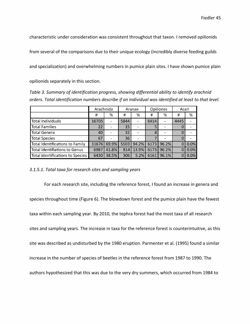
Samples from 1990, 2000, and 2010, with three sample collections per year, contained

16,705 arachnids. Of these individuals, 70% were identified at least to the family level, 42% at

least to genus, and 39% to species. These identifications included 22 different families, 40

genera, and 67 species (summarized in Table 3). I was differentially able to identify arachnid

orders to generic and species levels with greater success for Opiliones, less so for spiders

(Araneae), and minimally for Acari. Considering spiders alone, I was able to identify 94, 14, and

5% to family, genus, and species respectively. A complete list of identifications divided by

research site and year is included in Appendix 1.

The following is a summary of results and patterns observed. Information regarding

arachnid dispersal methods, feeding guilds, and habitat preferences was provided by Rod

Crawford through personal communication.89 Results assessed by taxa were done using the

finest resolution of identification possible. Thus, the total number of taxa includes families,

genera, and species. However, families and genera were only considered when the

88 Ibid., 238. 89 Crawford 2011.

Fiedler 45

characteristic under consideration was consistent throughout that taxon. I removed opilionids

from several of the comparisons due to their unique ecology (incredibly diverse feeding guilds

and specialization) and overwhelming numbers in pumice plain sites. I have shown pumice plain

opilionids separately in this section.

Table 3. Summary of identification progress, showing differential ability to identify arachnid orders. Total identification numbers describe if an individual was identified at least to that level.

3.1.5.1. Total taxa for research sites and sampling years

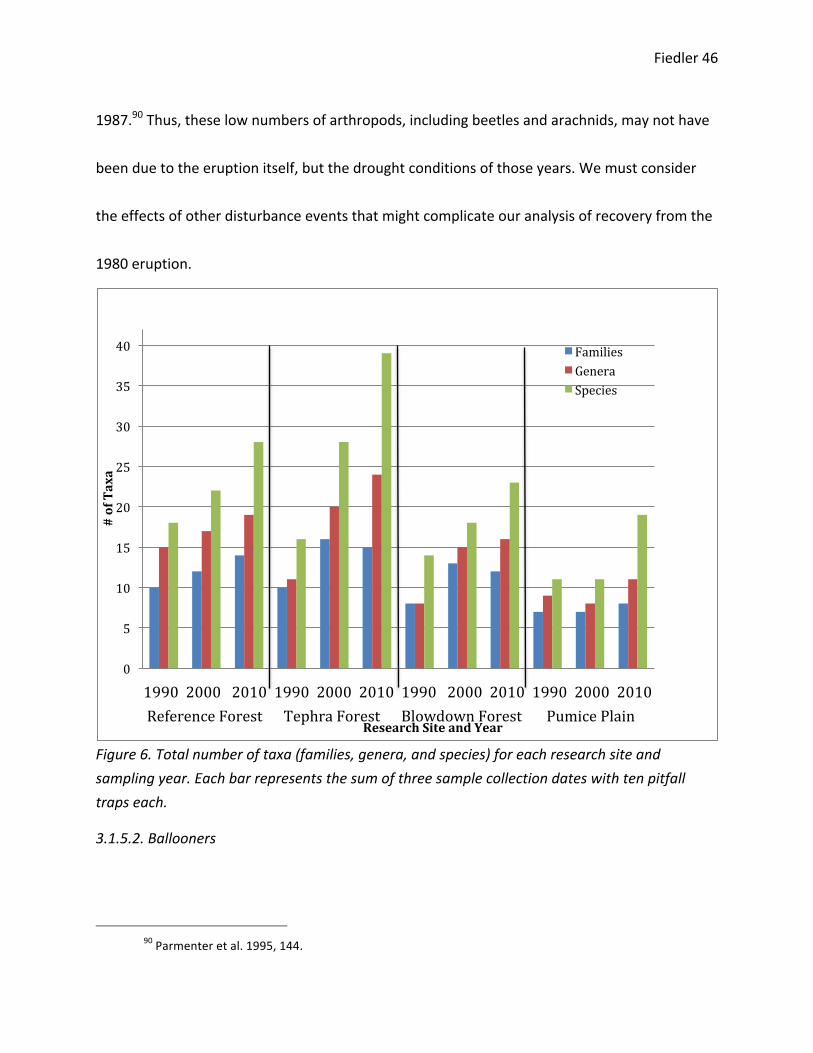
For each research site, including the reference forest, I found an increase in genera and

species throughout time (Figure 6). The blowdown forest and the pumice plain have the fewest

taxa within each sampling year. By 2010, the tephra forest had the most taxa of all research

sites and sampling years. The increase in taxa for the reference forest is counterintuitive, as this

site was described as undisturbed by the 1980 eruption. Parmenter et al. (1995) found a similar

increase in the number of species of beetles in the reference forest from 1987 to 1990. The

authors hypothesized that this was due to the very dry summers, which occurred from 1984 to

Fiedler 46

1987.90 Thus, these low numbers of arthropods, including beetles and arachnids, may not have

been due to the eruption itself, but the drought conditions of those years. We must consider

the effects of other disturbance events that might complicate our analysis of recovery from the

1980 eruption.

Figure 6. Total number of taxa (families, genera, and species) for each research site and sampling year. Each bar represents the sum of three sample collection dates with ten pitfall traps each.

3.1.5.2. Ballooners

90 Parmenter et al. 1995, 144.

0

5

10

15

20

25

30

35

40

# of Taxa

Research Site and Year

Families Genera Species

1990 2000 2010 1990 2000 2010 1990 2000 2010 1990 2000 2010 Reference Forest Tephra Forest Blowdown Forest Pumice Plain PR

Fiedler 47

Each research site had a distinct temporal pattern in the number of ballooning and

cursorial dispersing taxa (Figure 7). The reference forest shows relatively similar numbers of

ballooning and cursorial taxa, with numbers of both increasing overall. The tephra forest shows

a consistent increase in both ballooning and cursorial taxa throughout time. This site has many

more ballooning taxa than cursorial taxa, and it has the highest numbers of ballooning taxa for

each year of any site. The blowdown forest shows no pattern throughout time. In 1990 and

2010, there are many more ballooning taxa than cursorial taxa; however 2000 does not follow

this pattern. The number of ballooning taxa in the pumice plain increased consistently

throughout time, while I saw only one cursorial taxon each year.

Figure 7. Total number of ballooning and cursorial taxa for each research site and sampling year. Each bar represents the sum of three sample collection dates with ten pitfall traps each.

0

5

10

15

20

25

# of Taxa


Ballooner

Cursorial

1990 2000 2010 Reference Forest

1990 2000 2010 Tephra Forest

1990 2000 2010 Blowdown Forest

1990 2000 2010 Pumice Plain

Intact Source Pop. Closest to Source -‐-‐-‐-‐-‐-‐-‐-‐-‐-‐-‐-‐-‐-‐-‐-‐-‐-‐-‐-‐-‐-‐-‐-‐-‐-‐-‐-‐-‐-‐> Farthest from Source

Fiedler 48

3.1.5.3. Feeding Guilds

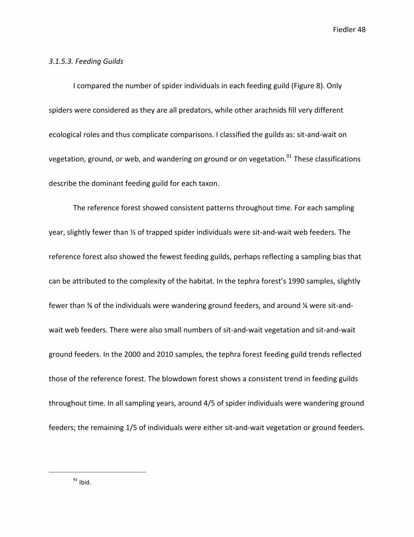
I compared the number of spider individuals in each feeding guild (Figure 8). Only

spiders were considered as they are all predators, while other arachnids fill very different

ecological roles and thus complicate comparisons. I classified the guilds as: sit-‐and-‐wait on

vegetation, ground, or web, and wandering on ground or on vegetation.91 These classifications

describe the dominant feeding guild for each taxon.

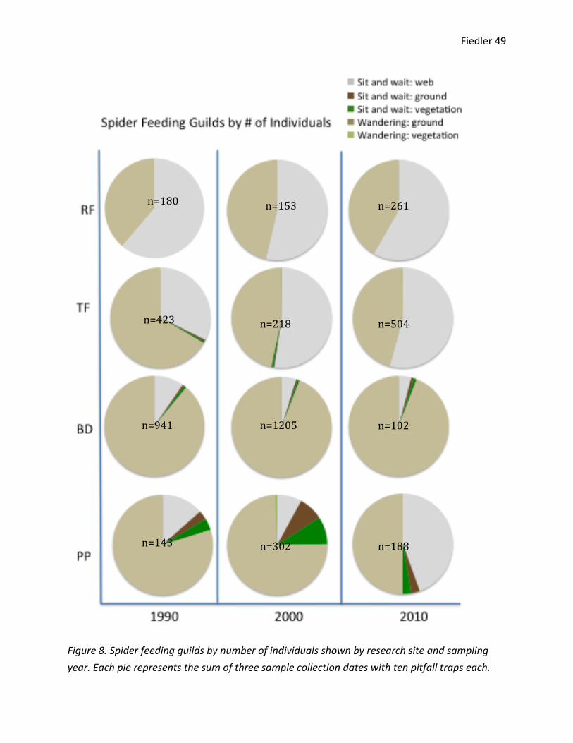
The reference forest showed consistent patterns throughout time. For each sampling

year, slightly fewer than ½ of trapped spider individuals were sit-‐and-‐wait web feeders. The

reference forest also showed the fewest feeding guilds, perhaps reflecting a sampling bias that

can be attributed to the complexity of the habitat. In the tephra forest’s 1990 samples, slightly

fewer than ¾ of the individuals were wandering ground feeders, and around ¼ were sit-‐and-‐

wait web feeders. There were also small numbers of sit-‐and-‐wait vegetation and sit-‐and-‐wait

ground feeders. In the 2000 and 2010 samples, the tephra forest feeding guild trends reflected

those of the reference forest. The blowdown forest shows a consistent trend in feeding guilds

throughout time. In all sampling years, around 4/5 of spider individuals were wandering ground

feeders; the remaining 1/5 of individuals were either sit-‐and-‐wait vegetation or ground feeders.

91 Ibid.

Fiedler 49

Figure 8. Spider feeding guilds by number of individuals shown by research site and sampling year. Each pie represents the sum of three sample collection dates with ten pitfall traps each.

n=180

n=153 n=261

n=423

n=218

n=504

n=941

n=1205

n=1022

n=143

n=302 n=188

Fiedler 50

In the pumice plain, there were major shifts in feeding guilds throughout time. In the

1990 samples, around ¾ of spider individuals were wandering ground feeders, 1/6 were sit-‐and-‐

wait wandering feeders, and the remaining individuals were wither sit-‐and-‐wait vegetation or

sit-‐and-‐wait ground feeders. In the 2000 samples, around ¾ of the individuals were wandering

ground feeders, and the remaining 25% of individuals was evenly divided between sit-‐and-‐wait

web, sit-‐and-‐wait ground, and sit-‐and-‐wait vegetation feeders. There were also a small number

of wandering vegetation feeders. In the 2010 sample, around ½ of spider individuals were

wandering ground feeders, less than ½ were sit-‐and-‐wait web feeders, and the remaining

individuals were either sit-‐and-‐wait ground or sit-‐and-‐wait vegetation feeders.

3.1.5.4. Habitat Preferences

I considered patterns of change in primary habitat preferences of the spiders collected

(Figure 9). Habitat preferences were categorized in the following categories: tree

canopy/trunk/understory foliage, deciduous and coniferous litter, moss, dead wood, and

exposed environments.92 Spiders were categorized into the habitat that they would are most

commonly found in, regardless of the habitat of the site in which they were collected. The

reference forest, tephra forest, and blowdown forest were all relatively consistent over time in

92 Ibid.

Fiedler 51

the distribution of habitat preferences of spider individuals, while the pumice plain was more

variable.

In 1990, slightly less than ½ of individuals collected in the reference forest are known to

inhabit dead wood habitats, while ¼ live in exposed environments, ¼ in deciduous and

coniferous litter, and very few in moss habitats. In the 2000 samples, around ½ of the collected

individuals are known to live in exposed environments, ½ in dead wood, and the rest either in

deciduous and coniferous litter, moss, or tree habitats. In 2010, around ½ of the individuals

collected are known to live in exposed environments, ½ in dead wood habitats, and around 1/6

in deciduous and coniferous litter. The tephra forest was even more consistent throughout time

than the reference forest. In 1990, around ½ of the individuals collected are known to live in

exposed environments, slightly less than ½ in dead wood, and the remaining individuals in leaf

litter. In the 2000 and 2010 samples, the distribution of habitat preferences remained similar to

that in 1990, with also a few individuals who are known to live in tree and moss habitats.

Fiedler 52

Figure 9. Spider habitat preferences by number of individuals shown by research site and sampling years. Each pie represents the sum of three sample collection dates with ten pitfall traps each.

n=180

n=153 n=261

n=423

n=218

n=504

n=941

n=1205

n=1022

n=143

n=302 n=188

Fiedler 53

The blowdown forest is again even more consistent throughout time. In all three

sampling years, around ½ of the individuals collected are known to live in exposed

environments and ½ in dead wood. In the 1990 samples, there were also a few individuals who

inhabit leaf litter. The pumice plain was highly variable throughout time. In the 1990 samples, ½

of the spider individuals collected are known to live in exposed environments, slightly less than

½ in dead wood, and some individuals in leaf litter and tree habitats. In 2000, ½ of the spider

individuals collected are known to live in exposed environments, slightly less than ½ in dead

wood habitats, and some individuals in leaf litter and moss. In 2010, 1/3 are known to live in

exposed environments, 1/3 in dead wood habitats, and 1/3 in leaf litter.

3.1.5.5. Representative Patterns

By considering patterns of individual taxa between research sites and across time, I

observed several patterns that represented larger trends in the community development of

these communities. Some taxa are found primarily in the least disturbed sites, others are found

mostly in disturbed sites, and some are found in high numbers in all four research sites. Some

invasive taxa have established strong numbers in the disturbed sites, yet they still remain few in

number in the less disturbed sites. Each of the following examples represents one of these

patterns that are observed across several taxa in my data set.

Fiedler 54

3.1.5.5.1. Higher Abundance in Less Disturbed Sites

Cybaeids are non-‐ballooning spiders that prefer dead wood or exposed environments.93

They are primarily sit-‐and-‐wait web or wandering ground feeders. I found individuals in the

family Cybaeidae primarily in the least disturbed sites: the reference forest and tephra forest

(Figure 10). Many other taxa in my samples follow this distributional trend, such as mites or

individuals of the genus Antrodiaetus.

Figure 10: Number of individuals of the family Cybaeidae in research sites over time. Each bar represents the sum of three sample collection dates with ten pitfall traps each.

93 Ibid.

106 122

187

131 107

304

9

54

21 1 0 0

0

50

100

150

200

250

300

# of Individuals






Less disturbed -‐-‐-‐-‐-‐-‐-‐-‐-‐-‐-‐-‐-‐-‐-‐-‐-‐-‐-‐-‐-‐-‐-‐-‐-‐-‐-‐-‐-‐-‐-‐-‐-‐-‐-‐-‐-‐-‐-‐-‐-‐-‐-‐-‐-‐-‐-‐-‐-‐-‐-‐-‐-‐-‐-‐-‐-‐-‐-‐-‐-‐-‐-‐-‐-‐-‐> More disturbed

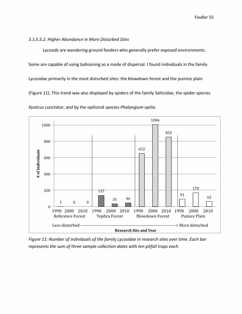
Fiedler 55

3.1.5.5.2. Higher Abundance in More Disturbed Sites

Lycosids are wandering ground feeders who generally prefer exposed environments.

Some are capable of using ballooning as a mode of dispersal. I found individuals in the family

Lycosidae primarily in the most disturbed sites: the blowdown forest and the pumice plain

(Figure 11). This trend was also displayed by spiders of the family Salticidae, the spider species

Xysticus cunctator, and by the opilionid species Phalangium opilio.

Figure 11: Number of individuals of the family Lycosidae in research sites over time. Each bar represents the sum of three sample collection dates with ten pitfall traps each.

1 0 0

137

35 46

652

1006

852

91 170

62

0

200

400

600

800

1000

# of Individuals






Less disturbed -‐-‐-‐-‐-‐-‐-‐-‐-‐-‐-‐-‐-‐-‐-‐-‐-‐-‐-‐-‐-‐-‐-‐-‐-‐-‐-‐-‐-‐-‐-‐-‐-‐-‐-‐-‐-‐-‐-‐-‐-‐-‐-‐-‐-‐-‐-‐-‐-‐-‐-‐-‐-‐-‐-‐-‐-‐-‐-‐-‐-‐-‐-‐-‐-‐-‐> More disturbed

Fiedler 56

3.1.5.5.3. Similar distribution across all research sites

Linyphiids are sit-‐and-‐wait web feeders that prefer deciduous and coniferous leaf litter

or dead wood in forested environments.94 Linyphiids are also prolific ballooners, known for

their mass dispersal during autumn and winter months of juveniles and adults alike.95

I found spider individuals of this family in relatively high numbers in each research site and

sampling year (Figure 12).

Figure 12. Number of individuals of the Family Linyphiidae in research sites over time. Each bar represents the sum of three sample collection dates with ten pitfall traps each.

94 Ibid. 95 Eric Duffey, 1956, "Aerial Dispersal in a Known Spider Population," The Journal of Animal Ecology 25 (1):

85-‐111, 86.

64

16

61

48 48

116

83

4

20 17 25

79

0

20

40

60

80

100

120

# of Individuals






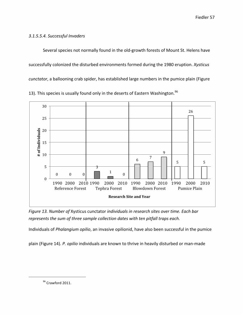
Fiedler 57

3.1.5.5.4. Successful Invaders

Several species not normally found in the old-‐growth forests of Mount St. Helens have

successfully colonized the disturbed environments formed during the 1980 eruption. Xysticus

cunctator, a ballooning crab spider, has established large numbers in the pumice plain (Figure

13). This species is usually found only in the deserts of Eastern Washington.96

Figure 13. Number of Xysticus cunctator individuals in research sites over time. Each bar represents the sum of three sample collection dates with ten pitfall traps each.

Individuals of Phalangium opilio, an invasive opilionid, have also been successful in the pumice

plain (Figure 14). P. opilio individuals are known to thrive in heavily disturbed or man-‐made

96 Crawford 2011.

0 0 0

3 1 0

6 7 9

5

26

5

0

5

10

15

20

25

30

# of Individuals






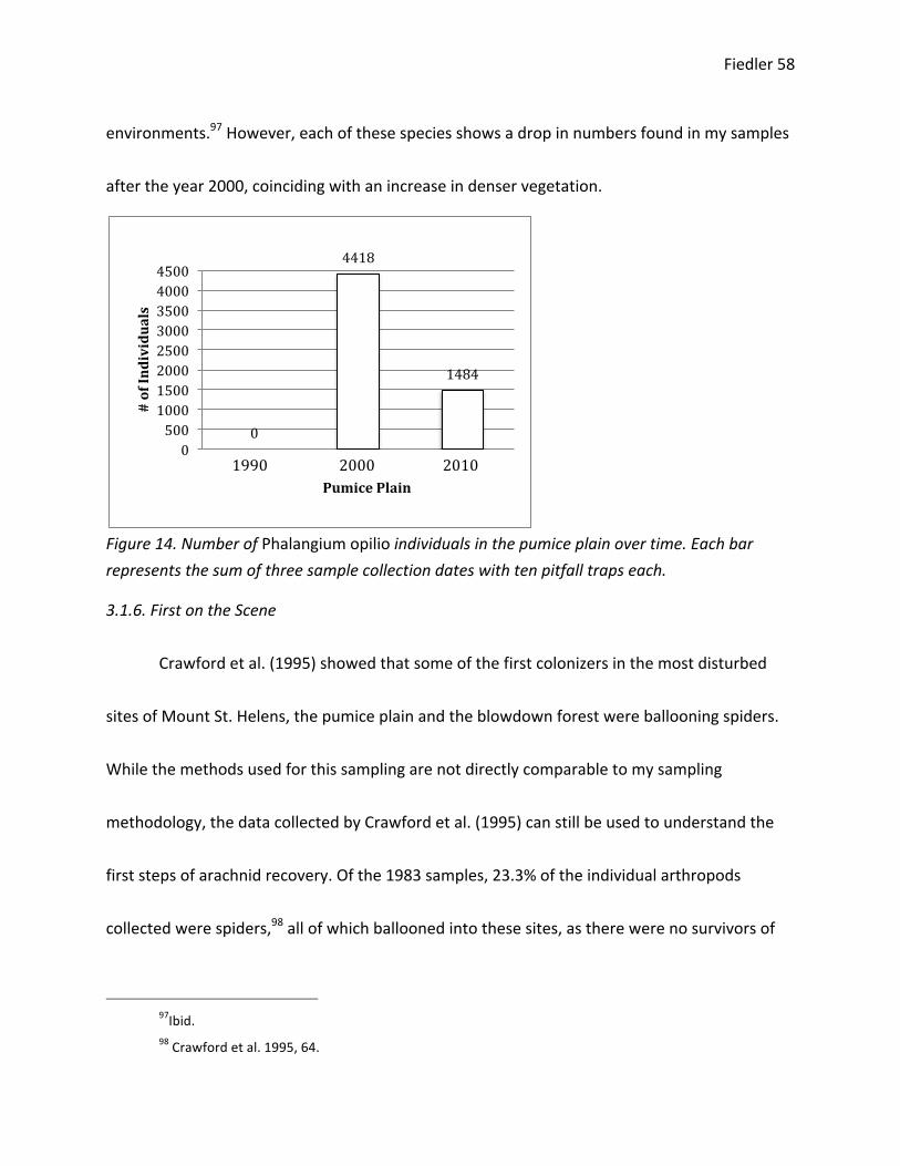
Fiedler 58

environments.97 However, each of these species shows a drop in numbers found in my samples

after the year 2000, coinciding with an increase in denser vegetation.

Figure 14. Number of Phalangium opilio individuals in the pumice plain over time. Each bar represents the sum of three sample collection dates with ten pitfall traps each.

3.1.6. First on the Scene

Crawford et al. (1995) showed that some of the first colonizers in the most disturbed

sites of Mount St. Helens, the pumice plain and the blowdown forest were ballooning spiders.

While the methods used for this sampling are not directly comparable to my sampling

methodology, the data collected by Crawford et al. (1995) can still be used to understand the

first steps of arachnid recovery. Of the 1983 samples, 23.3% of the individual arthropods

collected were spiders,98 all of which ballooned into these sites, as there were no survivors of

97Ibid. 98 Crawford et al. 1995, 64.

0

4418

1484

0 500 1000 1500 2000 2500 3000 3500 4000 4500

# of Individuals

Pumice Plain 1990 2000 2010

Fiedler 59

the initial blast in the pumice plain.99 From 1981 to 1986, 14,324 spider individuals were

collected in the pumice plain, representing 125 species (see Appendix 2 for Crawford et al. 1995

figures and Appendix 3 for corresponding figures from my sampling data).

The family Lycosidae contributed the largest number of individuals during this sampling

period, with 49% of all individuals. Linyphiids represented 34% of all individuals, and 50% of all

species.100 Crawford et al. noted that most of the spiders arriving on the pumice plain

immediately after the eruption did not become permanent residents or establish local

populations. Distant populations simply continually supplemented their numbers. However, by

1986, Crawford et al. found two lycosid species and four linyphiid species to be the first

successful colonists, as defined by evidence of successful local reproduction. By 1986, some

vegetation had also successfully colonized, thus provided protected habitat and a greater

source of arthropod prey.101 Lycosids and linyphiids still hold strong numbers on the pumice

plain, despite their differing habitat preferences and feeding guilds, suggesting some habitat

complexity at this site.

99 Ibid., 61. 100 Ibid., 64. 101 Ibid., 72.

Fiedler 60

3.1.7. Comparison to Beetle Data

Despite the later time frame of my sampling, I observed several patterns similar to those

in Parmenter et al. (2005). There appear to be several arachnid taxa that have replaced other

over time, as is seen in the fluctuations in feeding guilds and habitat preferences. Furthermore,

even 30 years after the eruption, the pumice plain arachnid populations appear to be quite

different than those in the reference forest. While the trajectory of the recovery of these

communities is unknown, we can assume that their composition is still rapidly changing.

4. When Theories and Data Collide

The communities impacted by the 1980 Mount St. Helens eruption are still undergoing

recovery. Only 30 years have passed since the eruption occurred, thus we cannot quantitatively

depict the full course of recovery for each of the disturbed sites. These preliminary data can,

however, be used to predict the trajectories of recovery. Each theory interprets these data

differently in terms of ecosystem recovery, and provides different predictions for the future of

each of these systems. I will compare how the data may be interpreted through the lens of each

theory in order to better understand the corresponding evolution of thought regarding

ecosystem recovery. I will follow the framework established in Table 1 to systematically assess

these theories. In this analysis, we must consider the limitations of my methodology, and how

these will impact the subsequent analysis. As my data only represent three points in time, any

Fiedler 61

fluctuations that are observed could be misinterpreted. These fluctuations can be signs of a

long-‐term trend or simply stochastic variation about a stable long-‐term trend. This confusion

cannot be avoided given my data and will be addressed accordingly in my analysis.

4.1. Deconstructing the Theories in Context

The 1980 eruption of Mount St. Helens acted as a disturbance impacting old-‐growth

forests to varying degrees as a function of proximity and orientation relative to the blast. Thus,

this disturbance can be classified as a parameter shift, as external forces altered the

accumulated potential and variables of the system. Each theory accounts for external

disturbances with Clementsian succession calling this disturbance ‘nudation,’ alternative stable

states using the term ‘parameter shift,’ and panarchy classifying it as ‘release.’ However,

because the eruption occurred on such a brief temporal scale, panarchy might predict that this

release will lead to revolt. Each theory describes the subsequent process differently, providing

its own language and predictions.

4.1.1. The Clementsian Succession Perspective

Each disturbed site’s responses to the eruption can be interpreted differently according

to the lens being used. Clementsian succession predicts a linear, deterministic pattern of

recovery, not allowing for novelty, and is the only theory of these three with the ability to

provide any such predictions. As the reference forest was unaffected by the blast, we can

Fiedler 62

assess the stages of recovery for each site through a comparison with the reference forest. The

data regarding habitat preference and feeding guilds show the tephra forest most closely

reflecting the reference forest, or the state from which it was disturbed. The blowdown forest

and pumice plain, however, show much more fluctuation in these patterns over the ten-‐year

periods, and more deviation from those patterns observed in the reference forest. Clementsian

succession suggests that the tephra forest is farther along in its progression towards returning

to its monoclimax. The fluctuations in the more disturbed sites do not suggest a different

trajectory, but rather the stages of migration, ecesis, competition, and reaction. Disturbed sites

with different species compositions can be interpreted as simply exhibiting different

fluctuations within these stages. Thus, these sites, according to succession, are still in the

beginning stages of recovery. As this theory follows the idea of dominance-‐controlled

community development, these disturbed sites will experience a decrease in species richness as

the most successful competitors take control.

The stages of succession, as the theory explains, result in a community of increasing

complexity and efficiency, yet as dominant competitors increase in number, less successful

species are eliminated from the community. Thus, a successional analysis of the number of taxa

for each disturbed site suggests that none of them have reached the climax state. Each

disturbed site appears to be increasing in the number of taxa throughout time, and should

Fiedler 63

exhibit a drop as the system proceeds into its climax state. Clementsian succession insists on

the existence of a monoclimax, so it is to be predicted that each of these sites, given enough

time without a disturbance, will all reach the same climax state. Again, due to the fluctuating

nature of the reference forest, successional theory would suggest that this undisturbed site has

yet to reach its climax state as well. Thus, despite being an old-‐growth forest, the reference

sites are still undergoing periodic disturbances of varying scales that have at least impacted

arachnids, if not other organisms as well. However, the reference forest is farther along in its

successional progress, as it was unaffected by the 1980 eruption, a disturbance that could

affect the entire ecosystem, rather than just certain taxa. According to succession, each

research site is moving along the same trajectory. However, each is experiencing a different

stage due to the variation of the data between sites.

4.1.2. The Alternative Stable States Perspective

Alternative stable state theory provides a much different interpretation of the

responses of these disturbed research sites. This theory suggests a relatively linear process of

recovery, but allows for multiple trajectories towards different stable states. With these

alternatives, this theory is hard to test and falsify. A shift in parameters, or in this case the 1980

eruption, created the opportunity for the variables of the system to achieve a different stable

state that was not available before, as the ecosystem perspective describes, or perhaps pushed

Fiedler 64

the site past a threshold point into a state of hysteresis. The eruption, as it disturbed the

communities that had existed in these sites, created opportunities for different arrangements

of the previously existing and newly arriving variables. Thus, the success of certain species in

the pumice plain, such as Phalangium opilio or Xysticus cunctator, could be indicative of the

system’s progression towards a different stable state. As the tephra forest is already seen to

reflect many of the patterns found in the reference forest, alternative stable state theory might

expect this research site to be returning to its previous state. This theory could allow for either

dominance or founder controlled stability, yet since these systems are still progressing, it is too

soon to determine which will dictate their recovery.

As Clementsian succession also explains, the system will increase in complexity and

efficiency throughout its recovery before reaching a final stable state. This process is reflected

in the increasing numbers of taxa in each of the research sites. As this pattern includes the

reference forest, alternative stable states theory would also suggest that this site has also not

reached its stable state. However, this theory allows these sites to be much farther along in

recovery, unlike succession, as each site is not required to be on the same trajectory. If these

sites are given enough time without a disturbance, each will reach a stable state, either similar

to the trajectory that they were previously on or a different assemblage of variables.

Fiedler 65

4.1.3. The Panarchy Perspective

Panarchy treats the 1980 eruption as a release that results in a rapid dissolution of

connectedness of the disturbed system. Following the disturbance, the system enters into the

back loop where there exists the possibility of novelty as potential increases. This process of

reorganization is reflected in rapid shifts in feeding guilds and habitat preferences in the pumice

plain. The lack of connectedness of the system, according to panarchy, has allowed for novelty

in the forms of new colonizers who otherwise would be unsuccessful in the previously intact

system, such as Phalangium opilio and Xysticus cunctator. These species have taken advantage

of this new environment and its limited competition. Their success could dictate what occurs

during the system’s progression into the front loop, or the progression from exploitation to

conservation. On the other hand, these two populations could be overwhelmed as local

competitors return or as increasing habitat complexity begins to support local forest species.

As each research site undergoes recovery, panarchy predicts that forces of opposing

scale will influence their course. Adaptive cycles of smaller and faster scale will prompt the

system in question to revolt. Thus, the invasion of ballooning spiders into disturbed sites might

cause the system to not recover in the direction of how it was before the disturbance. Adaptive

cycles of larger and slower scale, such as climate and location, will cause the system to

Fiedler 66

remember, or limit the system’s ability to adopt novel forms. For instance, while desert

dwelling Xysticus cunctator has successfully established a population in the pumice plain, it may

not be able to persist if forests do reestablish, eliminating the current desert-‐like habitat.

The progression of a system through the front loop of the adaptive cycle in a panarchy

resembles the steps outlined in Clementsian succession. Competition and immigration shifts

the species composition of the ecosystem, while the potential and connectedness of the system

increase. However, as the system progresses it becomes increasingly rigid, and thus vulnerable

to disturbances. Panarchy, therefore, suggests that the reference forest is in the conservation

stage of the adaptive cycle. Due to the rapid increase in taxa in the disturbed sites, the tephra

forest, blowdown forest, and pumice plain all appear to be in the reorganization phase of the

adaptive cycle. The pumice plain, as it is undergoing the most rapid shifts in community

composition, is the furthest away from the front loop, and the most vulnerable to novelty, if the

larger adaptive cycles allow.

4.1.4. Summary of Perspectives

Each theory interprets the same data in different ways. Using their own language and

perspective, each theory allows us to make predictions regarding the trajectory of the research

sites. These systems are rapidly changing, and only time will tell what direction they are

heading. Table 4 describes how each theory assesses the current state of each research site.

Fiedler 67

While no theory is correct or incorrect, each can drastically alter our perceptions of recovery

and ecosystem development.

Table 4. Comparison of each theory’s assessment of the state of research sites. Clementsian Succession Alternative Stable

States Panarchy

Reference Forest Reaction phase, prior to stabilization

Still transitioning to stable state

Conservation phase, building rigidity

Tephra Forest Reaction phase, prior to stabilization

Signs of resilience, transitioning to stable state along previous trajectory

Exploitation phase, remember

Blowdown Forest Migration, ecesis, competition, and reaction

Initial stages of recovery, potentially leading towards alternative stable state

Reorganization phase, likely to revolt

Pumice Plain Migration, ecesis, competition, and reaction

Initial stages of recovery, potentially leading towards alternative stable state

Reorganization phase, farthest from front loop, likely to revolt

4.2. Spotlight on Panarchy

Each of these three ecological theories interprets the same data in radically different

ways. Panarchy acts as a paradigm, integrating the Clementsian succession and alternative

stable state theories, in understanding the progression from immigration, establishment,

competition, and reorganization, and also the opportunity for alternative trajectories of

recovery. However, panarchy focuses on the transitions of a system from one stage to another,

and that it is in the constant flux that an ecosystem is most resilient. Panarchy treats

equilibrium as a transient state, as rigidity builds alongside connectedness. Panarchy might also

serve as a theoretical model to understanding the compound effects of disturbances; for

Fiedler 68

instance, the effects of a volcanic eruption, invasive species, and climate change, and how each

of these might dictate ecosystem development alone and together.

5. Putting Theory Into Practice: Conservation Implications

Even though the 1980 eruption of Mount St. Helens was a natural disturbance, we can

still use the subsequent recovery as a case study to begin to understand how Clementsian

succession, alternative stable states theory, and panarchy can be applicable to conservation

and management decisions for human disturbances. Our perspectives on recovery, stability,

rigidity, and resilience define how we consider conservation. If we consider stability to mean

“…efficiency, control, constancy, and predictability,”102 as succession and alternative stable

states would define the term, then conservation goals would reflect the desire to maintain a

system within the confines of a single state and level of efficiency. Any fluctuations in the

conditions of that system call for a response. On the contrary, if we consider stability to mean

“…persistence, adaptiveness, variability, and unpredictability,”103 as the theory of panarchy

invokes, then our goals of conservation will shift. Conservation will acknowledge the constant

flux of systems, and emphasize the need to maintain function rather than the efficiency of

specific conditions.104 Thus, we accept the multiplicity of states that an ecosystem can achieve,

102 Gunderson and Holling eds. 2002, 27. 103 Ibid., 27. 104 Ibid., 28.

Fiedler 69

as long as it continues to flow through the adaptive cycle. In this case, novelty can only be

deemed negative under panarchy if the system looses its function; otherwise, no judgment is

made by the theory. Another distinction of language that must be made is between panarchy

and resilience, as these terms are often interchanged in discourse. Panarchies describe the

ecological realities of dynamic systems, yet the term resilience reflects the goal of conservation

that follows from the theory of panarchy. Through our understanding of the dynamism of

adaptive cycles of ecological systems, we aim to maintain the resilience, and in turn the

function, of systems through conservation and preservation work.

5.1. Collapsing Panarchy

While panarchy embraces the lack of predictability and learning of systems, the cycle

can become detrimental to the health of the system. ‘Poverty traps’ occur when the adaptive

cycle collapses due to the elimination of all potential and connectedness, resulting in low

resilience. This can be prompted by a strong disturbance that continues to break down the

potential and connectedness of a system, keeping the system out of the reorganization phase

and in a constant state of release. If a system falls into a poverty trap, the effects can cascade

down to adaptive cycles of different scales. Systems can also collapse into ‘rigidity traps,’ with

high connectedness, potential, and resilience. This system would essentially preserve any

disturbances, creating maladaptive feedback. Eventually, this system would suffer from a

Fiedler 70

disturbance to a degree much greater than would be expected.105 These two traps must be

avoided by restricting perpetual disturbance or the complete lack thereof.

In order to consider conservation in the context of panarchy, it is important to know

what stage of the adaptive cycle the system is in, and what stage is most appropriate to do

some conservation action. Often times, the state of release in the back loop provides the

greatest opportunity for conservation efforts to be applied, allowing the system to reorganize

with these efforts in place.106 Panarchy also emphasizes the importance of some level of

disturbance, in order to promote learning and the resilience of a system, running counter to

successional thought.

5.2. Conservation Decisions

An example of how these theories treat conservation and restoration, and how they

result in vastly different agendas and priorities, lies in current forest management techniques in

the Pacific Northwest. Forest managers fight to balance efficient resource extraction, fire

management, and overall ecosystem health. We have found ourselves in a sort of rigidity trap

as fires have long been suppressed in many of the Northwest forests, yet at the same time

some of these forests are kept within a poverty trap, as ecosystems are not allowed enough

105 Holling 2001, 400. 106 Ibid., 402.

Fiedler 71

time to fully recover after a timber harvest. Douglas County Commissioner Joe Laurance has

testified in support of returning forests to their conditions from the year 1800. This date marks

the period before European Americans were present in the region and, according to Laurance, a

time when these forests were not dangerously packed with fuels (and thus before the

panarchic collapse).107

This restoration approach strongly reflects Clementsian successional theory, in that it is

seeking to return these forests to a former state. Alternative stable state theory would insist

that these forests are trapped in a state of hysteresis, in which they cannot be easily returned

to any previous state at all. Furthermore, these forests are actually able to reach a similar state

of productivity as in 1800, yet under vastly different conditions, or variables. Thus, we might

need to reconsider our perception of what these forests should look like. Panarchy would

declare an extreme sense of urgency in changing our current practices of maintaining what

seems to be both a poverty and rigidity trap. However, panarchical thinking would note that

any goal of a static system is unreasonable and harmful to that system’s resilience. Panarchy

might suggest that a more dynamic approach to restoration and conservation is necessary in

protecting our forests, while maintaining their function. While some environmental problems,

107 SOS Forests: Western Institute for Study of the Environment Commentary, “Douglas Co. Commissioner

Joe Laurance July 15 Testimony,” Last modified July 15, 2010, http://westinstenv.org/sosf/2010/07/15/douglas-‐co-‐

commissioner-‐joe-‐laurance-‐july-‐15-‐testimony/.

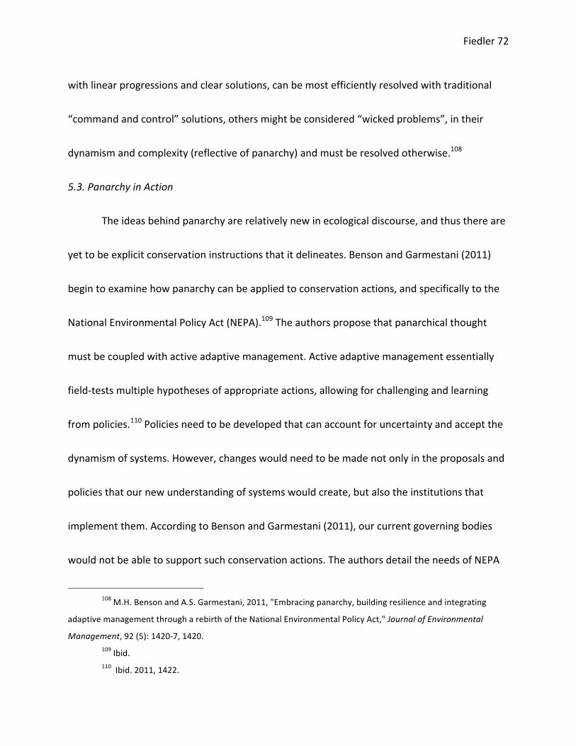
Fiedler 72

with linear progressions and clear solutions, can be most efficiently resolved with traditional

“command and control” solutions, others might be considered “wicked problems”, in their

dynamism and complexity (reflective of panarchy) and must be resolved otherwise.108

5.3. Panarchy in Action

The ideas behind panarchy are relatively new in ecological discourse, and thus there are

yet to be explicit conservation instructions that it delineates. Benson and Garmestani (2011)

begin to examine how panarchy can be applied to conservation actions, and specifically to the

National Environmental Policy Act (NEPA).109 The authors propose that panarchical thought

must be coupled with active adaptive management. Active adaptive management essentially

field-‐tests multiple hypotheses of appropriate actions, allowing for challenging and learning

from policies.110 Policies need to be developed that can account for uncertainty and accept the

dynamism of systems. However, changes would need to be made not only in the proposals and

policies that our new understanding of systems would create, but also the institutions that

implement them. According to Benson and Garmestani (2011), our current governing bodies

would not be able to support such conservation actions. The authors detail the needs of NEPA

108 M.H. Benson and A.S. Garmestani, 2011, "Embracing panarchy, building resilience and integrating

adaptive management through a rebirth of the National Environmental Policy Act," Journal of Environmental

Management, 92 (5): 1420-‐7, 1420. 109 Ibid. 110 Ibid. 2011, 1422.

Fiedler 73

to integrate iterative conservation methods, thorough and continual monitoring, and a

reaffirmed responsibility for mitigation. In doing so, conservation actions will better respect the

dynamism suggested by panarchy and tackle those “wicked problems.”111

5.4. Panarchy as Part of a Continuing Paradigm Shift

Panarchy has yet to find its place in the field of ecology, but its discourse is continually

developing. Today, much of the development of the theory can be attributed to the work of the

Resilience Alliance, an organization focused on research on the “resilience, adaptability, and

transformability” of social-‐ecological systems.112 The organization aims to further the

theoretical basis for resilience thinking and to test the ideas of adaptive cycles and applied

adaptive management.113 As the development of all ecological theories aim to do, the

Resilience Alliance promotes this research so we can better understand the complex realities of

the environment, and understand how our actions can reflect these realities the best. The

development of the theory is happening right now, as is seen in Resilience 2011 conference

held in March 2011.114 It is in the actions of the Resilience Alliance and other ecological thinkers

111 Ibid., 1425-‐1426. 112 Resilience Alliance, “About RA,” Last modified January 8, 2004,

http://www.resalliance.org/index.php/about_ra. 113 Ibid. 114 Ibid.

Fiedler 74

and scientists that we will see the development of the theory of panarchy, and, in turn, see it

reflected in future conservation actions.

5.5. Conclusion

There is no perfect ecological theory that can accurately explain and predict any change

within an ecosystem. While ecological realities remain the same, different theories will assess

and understand these realities in vastly different ways. By considering these theories in the

context of numbers and tangible patterns, we can better understand what each theory

illuminates in our understanding of ecological recovery. Panarchy progresses our thought

regarding ecological recovery and should be considered in ecological discourse and

conservation considerations. It embraces change and learning, thus acknowledging the need to

allow systems to exist in their naturally fluctuating states, or to allow for dynamism through our

conservation actions. Our frequent desire to maintain stability and eliminate any sort of change

in living systems is unrealistic and detrimental to overall ecosystem health and resilience.

Panarchy addresses these considerations, while also building from ecological thought of past

theories. However, panarchy acts as more of a paradigm, in teasing out the complexities of

dynamic systems, while deepening our understanding of potential trajectories and past

changes.

Fiedler 75

The arachnid recovery of Mount St. Helens has allowed us to deeply consider the

potential for panarchy to be applied to living ecological systems, and how it compares to

Clementsian succession and alternative stable states theory. While we have only been able to

look at the first steps of recovery of this system, comparing the predictions that each theory

makes to the recovery we may observe in the future will be even more telling of each theory’s

applicability and potential. On the other hand, conservation decisions are rarely made with

ideal data sets, but rather must be made with a limited understanding of the system in question

and its trajectory of recovery. Thus, the limitations of my data set might actually reflect realities

of the choices we make in doing conservation. Again, no theory will be deemed correct or

incorrect in its predictions, but panarchy does prove to be the best in illuminating the

dynamism of natural systems, and thus should be used in any conservation or preservation

considerations. Future analyses for better understanding how these theories describe the

recovery of ecological systems would span a longer time frame and consider the numbers more

frequently in order to observe fluctuations in community composition. However, this analysis of

arachnid recovery has already exemplified how panarchy presents a new perspective regarding

ecosystem recovery, which subsequently changes how we might view conservation and

preservation. Panarchy should be the next in the successional line of ecological thought.

Fiedler 76

6. References

Beccaloni, Jan. 2009. Arachnids. Berkeley: University of California Press. Begon, Michael, Colin R. Townsend, and John L. Harper. 2006. Ecology: from individuals to ecosystems. Malden, MA: Blackwell Pub. Beisner, B. E., D. T. Haydon, and K. Cuddington. 2003. “Alternative stable states in ecology.” Frontiers in Ecology and the Environment 1 (7). Benson, M.H., and A.S. Garmestani. 2011. "Embracing panarchy, building resilience and integrating adaptive management through a rebirth of the National Environmental Policy Act." Journal of Environmental Management. 92 (5): 1420-‐7. Bonte, Dries, Jeroen Vanden Borre, Luc Lens, and Jean-‐Pierre Maelfait. 2006. "Geographical variation in wolf spider dispersal behaviour is related to landscape structure." Animal Behaviour. 72 (3): 655. Bonte, Dries, Nele Vandenbroecke, Luc Lens, and Jean-‐Pierre Maelfait. 2003. "Low propensity for aerial dispersal in specialist spiders from fragmented landscapes." The Royal Society. 270 (1524): 1601-‐7. Cain, Michael L., William D. Bowman, and Sally D. Hacker. 2008. Ecology. Sunderland, MA: Sinauer Associates, Inc. Clements, Frederic E. 1916. Plant Succession, an Analysis of the Development of Vegetation, p. 140-‐143. In: Edward J. Kormondy, ed. 1965. Readings in Ecology. Englewood Cliffs, NJ: Prentice-‐Hall, Inc. Crawford, Rodney L., and John S. Edwards. 1986. "Ballooning Spiders as a Component of Arthropod Fallout on Snowfields of Mount Rainier, Washington, U.S.A." Arctic and Alpine Research. 18 (4): 429-‐437. Crawford, Rodney L., Patrick M. Sugg, and John S. Edwards. 1995. “Spider arrival and primary establishment on terrain depopulated by volcanic eruption at mount St. Helens, Washington.” American Midland Naturalist 133 (1): 60-‐75. Crawford, Rod. Personal communication. March 2, 2011. Crisafulli, Charles M., James A. MacMahon, and Robert R. Parmenter. 2005. Small-‐Mammal Survival and Colonization on the Mount St. Helens Volcano: 1980-‐2002, p. 199-‐218. In: Virginia H. Dale, Frederick J. Swanson, and Charles M. Crisafulli eds. 2005. Ecological Responses to the 1980 Eruption of Mount St. Helens. New York, NY: Springer. Dale, Virginia H., Frederick J. Swanson, and Charles M. Crisafulli. 2005. Disturbance, Survival, and Succession: Understanding Ecological Responses to the 1980 Eruption of Mount St. Helens, p. 3-‐11. In: Virginia H. Dale, Frederick J. Swanson, and Charles M. Crisafulli eds.

Fiedler 77

2005. Ecological Responses to the 1980 Eruption of Mount St. Helens. New York, NY: Springer. Dale, Virginia H., Frederick J. Swanson, and Charles M. Crisafulli, eds. 2005. Ecological Responses to the 1980 Eruption of Mount St. Helens. New York, NY: Springer. Derkarabetian, Shahan. Personal communication. February 11, 2011. Drury, William H. and Ian C.T. Nisbet. 1973. Succession, p. 287-‐368. In: Frank B. Golley, ed. 1977. Ecological Succession. Stroudsburg, PA: Dowden, Hutchinson & Ross. Duffey, Eric. 1956. "Aerial Dispersal in a Known Spider Population." The Journal of Animal Ecology. 25 (1): 85-‐111. Foelix, Rainer F. 1996. Biology of spiders. New York: Oxford University Press. Goldsmith, Edward. “Ecological succession rehabilitated.” Edward Goldsmith, http://www.edwardgoldsmith.org/page119.html (16 November 2010). Golley, Frank B. 1977. Ecological succession. Stroudsburg, Pa: Dowden, Hutchinson & Ross. Goodrich, Charles, Kathleen Dean Moore, and Frederick J. Swanson, eds. 2008. In the blast zone: catastrophe and renewal on Mount St. Helens. Corvallis, OR: Oregon State University Press. Gunderson, Lance H., and C. S. Holling. 2002. Panarchy: understanding transformations in human and natural systems. Washington, DC: Island Press. Holling, C. S. 1973. "Resilience and Stability of Ecological Systems." Annual Review of Ecology and Systematics. 4: 1-‐23. Holling, C.S. 2001. Understanding the Complexity of Economic, Ecological, and Social Systems. Ecosystems, 4:390-‐405. Kuhn, Thomas S. 1970. The Structure of Scientific Revolutions. Chicago, IL: The University of Chicago Press. Lewontin, Richard C. 1969. "The meaning of stability." Brookhaven Symposia in Biology. 22: 13-‐24. Odum, Eugene P. 1969. The Strategy of Ecosystem Development, p. 278-‐286. In: Frank B. Golley,

ed. 1997. Ecological Succession. Stroudsburg, PA: Dowden, Hutchinson & Ross. Parmenter, Robert R. et al. 2005. Posteruption Arthropod Succession on the Mount St. Helens Volcano: The Ground-‐Dwelling Beetle Fauna (Coleoptera), p. 139-‐150. In: Virginia H. Dale, Frederick J. Swanson, and Charles M. Crisafulli eds. 2005. Ecological Responses to the 1980 Eruption of Mount St. Helens. New York, NY: Springer. Resilience Alliance. “About RA.” Last modified January 8, 2004. http://www.resalliance.org/index.php/about_ra. Roth, Vincent D., Darrell Ubick, and N. Dupérré. 2005. Spiders of North America: an identification manual. Poughkeepsie, NY: American Arachnological Society.

Fiedler 78

Scheffer, Marten. Alternative Stable States and Regime Shifts in Ecosystems, p. 395-‐406. In: Simon A. Levin ed. 2009. The Princeton Guide to Ecology. Princeton, NJ: Princeton University Press. Simberloff, Daniel. A Succession of Paradigms in Ecology: Essentialism to Materialism and Probabilism, p. 63-‐99. In: Esa Saarinen ed. 1982. Conceptual Issues in Ecology. Boston, MA: D. Reidel Publishing Company. SOS Forests: Western Institute for Study of the Environment Commentary. “Douglas Co. Commissioner Joe Laurance July 15 Testimony.” Last modified July 15, 2010. http://westinstenv.org/sosf/2010/07/15/douglas-‐co-‐commissioner-‐joe-‐laurance-‐july-‐ 15-‐testimony/. Sutherland, John P. 1974. "Multiple Stable Points in Natural Communities." American Naturalist. 108 (964): 859-‐873. Whittaker, R.H. 1953. A Consideration of Climax Theory: The Climax as a Population and Pattern, p. 240-‐277. In: Frank B. Golley, ed. 1977. Ecological Succession. Stroudsburg, PA: Dowden, Hutchinson & Ross. Wise, David H. 1993. Spiders in ecological webs. Cambridge: Cambridge University Press. Worster, Donald. 1994. Nature's economy: a history of ecological ideas. Cambridge: Cambridge University Press.

Fiedler 79

Appendix 1. Summary table of identifications.

!"#$%& '()*+,+-(.$(+ /001 2111 21/1 /001 2111 21/1 /001 2111 21/1 /001 2111 21/1 345"%

6&.4+$7"( / 1 1 /89 8: ;< <:2 /11< =:2 0/ /91 <2 81:2

')"->4+$7"( 8 2 1 /2 ; 1 /0 :2 81 /: 88 2 /92

!"#$%"&'&(() 1 1 1 1 1 : 1 80 :; 1 = < //2

!"#$%"&'*+,) 1 1 1 1 1 1 1 1 / 1 1 1 /

!"#$%"&'-./0/"- 1 1 1 1 1 1 1 1 / 1 1 1 /

!"#$%"&'(+-/%.0+& 1 1 1 1 1 1 1 1 / 1 1 1 /

!"#$%"&'1-.%-/& 1 1 1 1 1 / 1 1 1 1 1 1 /

2$3$4/$0'*+,) 1 1 1 1 1 / 1 1 1 1 1 1 /

5-.&&6##+&'3"(-"&&+& 1 1 1 1 1 1 1 1 / 1 1 1 /

7/4.-/.'&(() 1 1 1 =0 2 / /91 88 < 1 88 /< 8:1

7/4.-/.'4$0&%-/4%. 1 1 1 1 1 1 1 1 1 1 1 2 2

7/4.-/.'"8"-%$0/ 1 1 1 1 1 1 1 1 1 1 1 / /

7/4.-/.'-$&&/4. 1 1 1 1 1 1 1 1 1 1 1 2 2

?&@"($7"( /1< //8 /99 /8/ /19 2=1 0 :; 2/ / 1 1 000

96:."+&'&(() 1 : ; 1 1 28 1 1 1 1 1 1 82

96:."+&'*+,) 1 1 1 1 1 / 1 1 1 1 1 1 /

96:".+&'"+%6(+& 1 1 < 1 1 1 1 1 1 1 1 1 <

96:."$%.'&(() 1 ; 1 1 1 1 1 1 1 1 1 1 ;

A)5B47$"(C7"( 1 1 1 1 1 1 1 1 1 1 1 1 1

;0%-$3/."%+&'&(() 1 /1 8 / < ; 1 8 /1 1 1 1 89

D$-%*B$7"( 1 1 1 1 1 1 1 1 1 1 1 1 1

7/4-$<"=+-.'/3.<$.0. ; 1 2 1 2 / 1 / 1 1 1 1 /1

E"%C.$7"( 1 1 1 / / 1 / : /1 : 2 < 8/

3>4#$+$7"( 1 1 1 / 1 1 1 1 1 0 / 1 //

>6&?4+&'4+04%.%$- 1 1 1 8 / 1 < 9 0 ; 2< : </

>6&?4+&'*+,) 1 1 1 1 1 1 / 1 1 / / 1 8

@</#$3-$8+&'

*$&"8/%"0&/& 1 1 1 1 1 1 1 1 1 1 / 1 /

@</#$3-$8+&'-+1+& 1 1 1 1 / 1 1 1 1 1 / 1 2

7/&+8"0.'&(() 1 1 1 1 1 1 1 1 1 1 1 1 1

AF(%()$7"( 1 1 1 1 1 / 1 1 1 1 1 1 /

A"B"0"-/.'&(() 1 1 1 1 1 / 1 1 1 1 1 1 /

D$.5&)$7"( 1 1 1 1 1 1 1 1 / 1 1 1 /

9/4+-/0.'&/8(#"= 1 1 1 1 / 1 1 1 1 1 1 1 /

G">)$$7"( 1 1 1 1 1 1 1 1 1 1 1 1 1

C%<$:+"##.'&(() 1 / 1 1 1 1 1 1 1 1 1 1 /

9.#688.-/.'"8"-%$0/ 1 1 1 1 1 1 1 1 / 1 1 1 /

9-6(<$"4.'"=#/0"." 1 1 1 1 / 1 1 1 1 1 1 1 /

6$)&->$$7"( 1 1 ; 1 1 / 1 1 2 1 1 1 9

9"-.?0"##.'.4"-". 2 / 1 1 ; 2 1 1 1 1 1 / /1

9"-.?0$(&'/0D.%+& 9 1 1 1 1 / 1 1 1 1 1 1 =

9$-"$-B$0.#'8$0$4"-$& 1 1 1 1 1 / 1 1 1 1 1 1 /

E"(%<6(<.0%"&'

8"-4"3"& 2 2 22 8 1 /0 1 1 / / 1 1 :1

FE"(%<6(<.0%"&F'0"G'

&("4/"& 1 1 1 1 1 = 1 1 1 1 1 1 =

E"(%<6(<.0%"&'H"#.%+& 1 1 2 1 1 / 1 1 1 1 1 1 8

E/06(<.0%"&'(+.##. 1 1 / 1 1 1 1 1 1 1 1 1 /

76%<$(#.&%$/3"&'"-"4%+& 1 1 1 1 1 / 1 1 1 1 1 1 /

H(I(B().(,!4B(+5 3(->B",!4B(+5 J%4K74K),!4B(+5 L*#$.(,L%"$)

Fiedler 80

!"#$%#&'#()*+,-./0( ! ! " ! ! ! ! ! ! ! ! ! "

1,/2$3243.%/#().+&-#4( ! ! ! ! ! " ! ! ! ! ! ! "

1,/2$3243.%/#()

"05"$6.(-,./0( ! " ! ! ! ! ! ! " " ! ! #

7-,"$%,()(,8. "$ " % # & "" ' ! " " ! " ()

9.4,%$-25.)',#/",-3, ! ! ! ! ! ! ! ! ! ! ! & &

:.+-;#%.#",.)-$+085,. ! & & ! " ) ! ! ! ! ! ! "(

:.+-;#%.#",.)-$"%0#++. ! ! " ! " ( ! ! ! ! ! ! %

:.+-;#%.#",.)4#++.< ! ! ! ! ! ! ! ! ! ! ! " "

*+,-." % ( / & " ( "& " " # ! ! ("

*+,-.& #& $ ' #( #" &' $% # "& "" &( #% &'!

*+,-./ ! ! ! ( ! % $ ! ! ! ! ! "$

*+,-."! ! ! / ! & % ! ! ! ! ! $ &!

*+,-."" ! ! ! ! & ! ! ! " ! " #" #$

*+,-."$ ! ! ! ! ! / ! ! ! ! ! ! /

*+,-."% ! ! ! ! ! ! ! ! " ! ! & #

*+,-."/ ! ! ! & ( % & ! ! ! ! ! "(

*0-1232234- ! ! ! ! ! ! ! ! ! ! ! ! !

7/#./$'.).+5$8.-0+./. ! ! ! ! " ! ! ! ! ! " & (

=$5#"/0()>,?#"#%( ! ! " ! ! " ! ! ! ! ! ! &

56471892234- ! ! ! ! ! ! ! ! ! ! ! ! !

@.++,$4+0()A@25.#$4(,(B)

(4CDE ! ! " ! / & ! " ! ! ! ! ""

@25.#$4(,()F0>C ! ! ! ! ! " ! ! ! ! ! ! "

:;7928<234- ! ! ! ! ! ! ! ! ! ! ! ! !

@+05,$%.)F0>C ! ! ! ! ! " ! ! ! ! ! ! "

*-;-6234- ! ! ! ! ! ! ! ! ! ! ! ! !

G($*+.)4.-,*-. ! ! " ! ! ! ! ! ! ! ! ! "

*+,-.' & & & ! " % ! ! ! ! ! ! "#

*+,-.) ! ! & ! ! ! ! ! " ! ! $ '

*+,-."& ! ! " ! ! # ! ! ! ! ! ! (

*+,-."# ! ! ! ! ! ' ! ! # ! ! ! ""

*+,-."( ! ! ! ! ! " ! ! ! ! ! ! "

!"#$%&"'&()*&+ ! " " ! ! ! ! ! ! ! ! ! &

,*-$" &!% #! &%! ""' ('/ &%"& "% (") &(# (( ! "! ((($

.)*/*&+$" &/ # ( &) "!" &/ (' & ! ! ! ! &("

=04;4<>2234- 13.+.%?,08)$4,+,$ ! " $ ! / $$ ! ! ! ! (("' "('( $)/!

?494@8<234- 9.".-0()(44C " ! $ ! " ! ! # & ! ! ! "&

*124-<8<+@0234- 1.".%$%2-30()5"0%%#0( ! ! ! ! " " ! ! ! ! ! ! &

:-14A8;4B64C34-

H#(4#"$%#8.(/$8.)

8$'#(/. " & " ! ! ! ! ! ! ! ! ! (

D-64BA864C34- I#%'"$+.(8.)8,".5,+# $ " ( $ & % ! ) ! ! ! ! #&

*124-<8<+@0234-

7-+#"$50%0()

%$%',8$"43,$0( & ! " ! ! ! ! & & ! ! ! /

*124-<8<+@0234- J#/.%$%2-30()(#/0+0( ! " ! ! ! ! ! " ! ! ! ! &

?494@8<234- 7.5.-$%)$--,'#%/.+,( &% "/ && & / %" ' " ! ! ! ! "((

E<23-<CF-3 &! #% #) () #% #& "/ "( #" / "$ ' #!(

*8A4; G<32H2374;B (%' &($ %!# %&% '%! #&)' "!#! "%$% "#!! ")( (/#$ "%)!

I462;2-B "! "& "( "! "% "$ ' "# "& / / '

J-<-14 "$ "/ ") "" &! &( ' "$ "% ) ' ""

?,-@2-B "' && &' "% &' #) "( "' &# "" "" ")

Fiedler 81

Appendix 2. Distribution of 1981-‐1985 pumice plain spider samples. 2a shown as number of individual specimens per family. 2b shown as number of species per family.115

115 Crawford et al. 1995, 65.

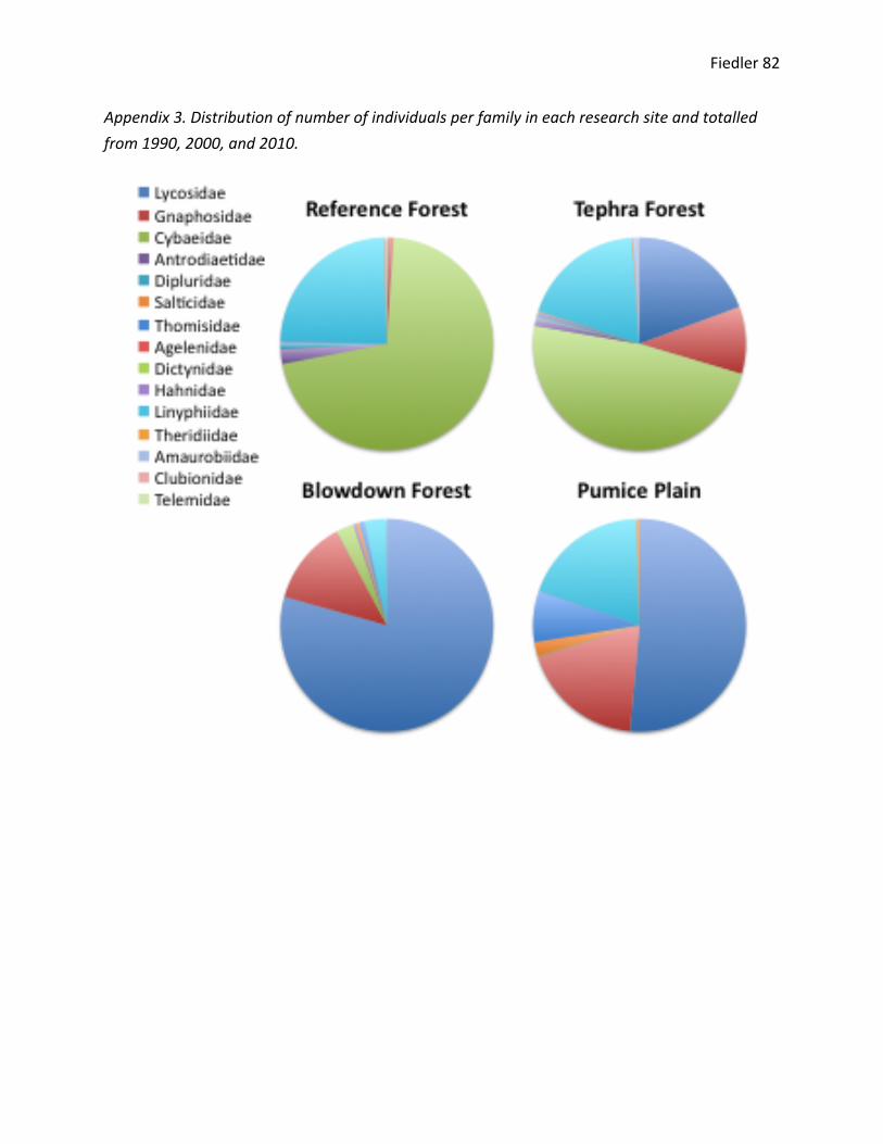
Fiedler 82

Appendix 3. Distribution of number of individuals per family in each research site and totalled from 1990, 2000, and 2010.

Examining the Progression of Ecological Theory Through ...

Documents

Transcript of Examining the Progression of Ecological Theory Through ...