Exact analytical solutions to the master equation of quantum Brownian motion for ageneral environment

C. H. Fleming and B. L. HuJoint Quantum Institute and Department of Physics,

University of Maryland, College Park, Maryland 20742

Albert RouraMax-Planck-Institut fur Gravitationsphysik (Albert-Einstein-Institut), Am Muhlenberg 1, 14476 Golm, Germany

We revisit the model of a quantum Brownian oscillator linearly coupled to an environment ofquantum oscillators at finite temperature. By introducing a compact and particularly well-suitedformulation, we give a rather quick and direct derivation of the master equation and its solutionsfor general spectral functions and arbitrary temperatures. The flexibility of our approach allows foran immediate generalization to cases with an external force and with an arbitrary number of Brow-nian oscillators. More importantly, we point out an important mathematical subtlety concerningboundary-value problems for integro-differential equations which led to incorrect master equationcoefficients and impacts on the description of nonlocal dissipation effects in all earlier derivations.Furthermore, we provide explicit, exact analytical results for the master equation coefficients andits solutions in a wide variety of cases, including ohmic, sub-ohmic and supra-ohmic environmentswith a finite cut-off.

CONTENTS

I. Introduction 2A. New Results placed in Background

Context 2B. Key Points and Organization 3

II. The Langevin Equation 4A. General Theory 4B. Solutions of the Langevin Equation 5

1. Meromorphic Spectra 52. Phase-Space Representation 6

C. Evolution of States 7D. General Correlations 7

III. Master Equation 8A. General Theory 8B. Derivation of the Master Equation 8

1. Simplification of the Master EquationCoefficients 9

C. Master Equation Solutions 101. Method of Characteristic Curves 102. Equivalence with the Result from the

Langevin Equation 11

IV. Evolution of States 11A. General Solutions 11

1. Trajectories of the Cumulants 112. Thermal Covariance 123. Linear Entropy 134. Decoherence of a Quantum

Superposition 14B. Late-Time Dynamics 15

1. Late-Time Propagator 152. Late-Time Diffusion and Covariance 16

V. Ohmic Case with Finite Cut-off 16

A. The Nonlocal Propagator 16B. Initial Jolts 18C. Full-Time Diffusion Coefficients for Large

Cut-off 19D. Late-Time Covariance for Finite Cut-off 20

VI. Sub-ohmic and Supra-ohmic Cases 22A. Sub-ohmic with no Cut-off 22B. Supra-ohmic with Finite Cut-off 23

VII. Generalizations of the Theory 24A. Influence of a Classical Force 24B. N -Oscillator Master Equation 25

VIII. Discussion 25

Acknowledgement 27

A. Special Functions 271. Harmonic Number 272. Exponential Integral 273. Error Function 27

B. Some properties of Laplace Transforms 27

C. System-Environment Interaction andRenormalization 281. Frequency Renormalization and the

Damping Kernel 282. Initial-Time Divergences, Coupling

Switch-on and Initial-State Distortion 29a. Initial-Time Divergences and Coupling

Switch-on 29b. Initial Kick (finite cut-off, vanishing

switch-on time) 29c. Initial Kick (large cut-off, non-vanishing

switch-on time) 30d. Initial-State Distortion 30

arX

iv:1

004.

1603

v2 [

quan

t-ph

] 1

1 D

ec 2

010

2

D. Peculiarities of Propagators and GreenFunctions Associated with Integro-differentialEquations 31

E. Derivation of the Late-Time ThermalCovariance 33

F. Moderate-Time Diffusion for Ohmic Case withLarge Cut-off 34

References 37

I. INTRODUCTION

A. New Results placed in Background Context

An open quantum systems (OQS) [1] refers to a quan-tum system interacting with an environment, which couldbe multi-partite, possessing many more degrees of free-dom (it could also be identified as the remaining “irrel-evant” degrees of freedom of the system itself). An en-vironment in some simplified modeling can be describedin terms of its spectral density and parametrized by itstemperature. Its influence on the open system can beexpressed in terms of fluctuations (vacuum and thermal)and noises (the most general form can be colored andmultiplicative). A theory of OQS describes the natureand dynamics of this system as a result of such interac-tions, which manifest in quantum dissipation and diffu-sion and can alter significantly the quantum coherence,entanglement and correlation properties of the otherwiseclosed quantum system. The familiar quantum statisticalmechanics is the extreme limiting case when the systemremains in equilibrium through interaction with a ther-mal or chemical reservoir.

Open quantum system is the theoretical construct suit-able for the investigation of the properties and dynamicsof nonequilibrium quantum systems in the Langevin vein(as distinguished from the Boltzmann vein, which consid-ers closed systems albeit often with a hierarchical struc-ture; see, e.g., Ref. [2]). It plays an important role in ad-dressing the fundamental issues such as the quantum-to-classical transition through the environment-induced de-coherence mechanism [3, 4]. For practical purposes it hasbeen effectively applied to exciting phenomena in manynew directions of micro- and meso-physics in the lasttwo decades, made possible by innovative experimentsaided by technological advances in high-precision instru-mentation. These include the areas of superconductiv-ity such as quantum dissipative tunneling in SQUIDs [5–7], atomic and quantum optical systems using ultrafastlasers with atoms in cavities and optical lattices [8–10],as well as nanoelectromechanical devices [11, 12] whichhave great potential in physical, chemical and bioscienceapplications. For an accurate description of the system’sproperties and evolution in these processes, the effects ofits interaction with the environment are essential.

Quantum Brownian motion (QBM) of an oscillatorcoupled to a thermal bath of quantum oscillators hasbeen extensively studied as a canonical model for openquantum systems because there is a considerable amountof insight that one can learn from it while being treat-able analytically to a significant degree. In this paper wecontinue the lineage of work on QBM via the influencefunctional path-integral method of Feynman and Vernon[13] used by Caldeira and Leggett [14] to derive a mas-ter equation for a high-temperature ohmic environment,which corresponds to the Markovian regime. Followingthis, Caldeira, Cerdeira and Ramaswamy [15] derived theMarkovian master equation for the system with weakcoupling to an ohmic bath, which was claimed to be validat arbitrary temperature (see Sec. V C for a critique ofthis claim). At the same time Unruh and Zurek [16] de-rived a more complete and general master equation thatincorporated a colored noise at finite temperature, butthere is a problem with their fluctuation-dissipation re-lation (see Ref. [17]). Finally, in a path-integral calcula-tion from first principles, Hu, Paz and Zhang (HPZ) [17]derived a master equation for a general environment (ar-bitrary temperature and spectral density), barring cer-tain subtle errors in the coefficients, which lead to in-accurate treatment of the nonlocal dissipation cases, aswe will discuss. After that, this equation has been red-erived by a number of authors. Halliwell and Yu [18] ex-ploited the phase-space transformation properties of theWigner function for the full system plus environment andderived a Fokker-Planck equation corresponding to theHPZ equation. Calzetta, Roura and Verdaguer (CRV)[19, 20] derived it using a stochastic description for openquantum systems based on Langevin equations, whereasFord and O’Connell [21] employed a somewhat relatedmethod via the quantum Langevin equation [22] and ob-tained also the solution to the HPZ equation for a Gaus-sian wave-packet.

The present paper’s contribution to this legacy is three-fold:

1. We have completely determined the precise form ofthe HPZ master equation coefficients and pointedout a problem with earlier derivations for nonlocaldissipation (Sec. III B).

2. We have found concise and efficient solutions to themaster equation with a number of exact nonpertru-bative analytical results (Sec. IV).

3. We have extended the theory to that of a systemof multiple oscillators bilinearly coupled amongstthemselves and to the bath in an arbitrary fashionwhile acted upon by classical forces (Sec. VII).

In this paper we will follow the approach of CRV inRefs. [19, 20] and make use of a stochastic descriptionwhose central element is a Langevin equation for thedynamics of the open quantum system. This offers anefficient mathematical tool for obtaining all the quan-tum properties of the system. An important feature of

3

the present approach is the reformulation in phase-space(rather than position space) together with the use of vec-tor and matrix notation. The combination of all theseelements makes this new approach far more flexible andcompact. For example, we are able to derive the generalexpression for the solution of the master equation in es-sentially two short lines [see Eq. (36)]. The flexibility ofour formalism is also illustrated by the straightforwardgeneralizations to the cases of an external force (this isnontrivial for nonlocal dissipation) and an arbitrary num-ber of system oscillators that will be presented. Thisgoes far beyond previous generalizations of the theory[23] which assume specific forms of coupling.

One of our key contributions, however, is uncoveringa significant shortcoming of earlier results for the masterequation coefficients. We point out a subtlety involvingboundary conditions for solutions of integro-differentialequations and explain how certain properties that holdfor ordinary differential equations are not true for non-local dissipation. These properties had always been em-ployed erroneously, in one way or another, when derivingthe expressions for the master equation coefficients, eventhose which were then evaluated numerically. This long-standing error could have deep implications for regimeswhere the effects of nonlocal dissipation are significantand one should be cautious with all results for those casesreported in the literature.

Taking into account the aspect mentioned in the pre-vious paragraph, and using our compact formulation, wehave provided a relatively simplified expression for thecorrect master equation. Moreover, one can also ob-tain the general solution to the master equation in termsof the matrix propagator of a linear integro-differentialequation, and see that at late times it tends to a Gaussianstate completely characterized by a constant covariancematrix. For odd meromorphic spectral functions, andmany others, we are able to reduce the calculation of thiscovariance matrix to a simple contour integral and obtainexact nonperturbative results for finite cut-off and arbi-trarily strong coupling. This includes examples of ohmic,sub-ohmic and supra-ohmic environments; and from thislate-time covariance one can immediately obtain the late-time diffusion coefficients as well. Our results generalizethe work of Anastopoulos and Halliwell [24] as well asFord and O’Connell [21], who already found the late timestate to be a Gaussian, and the earlier work of Hu andZhang [25, 26] on the generalized uncertainty function forGaussian states.

In addition, working with Laplace transforms and thentransforming back to time domain, we manage to findthe exact solutions for the propagators associated withthe integro-differential equations corresponding to ohmic,sub-ohmic and supra-ohmic environments with a finitecut-off. This enables us to gain very valuable informa-tion on the dynamics of the system. For instance, foran ohmic environment one can show that using the localapproximation for the propagator is a valid approxima-tion in the large cut-off limit, which makes it possible

to obtain relatively manageable analytic results for thediffusion coefficients at all times. Furthermore, the exactsolution of a specific sub-ohmic environment reveals thatlong-time correlations (due to excessive coupling with IRmodes of the environment) give rise to contributions tothe propagator that decay at late times like power laws.This invalidates the use of an effectively local descrip-tion at late times, whose contributions decay exponen-tially, and provides a clear example of a situation wherenonlocal dissipation needs to be properly dealt with. Fi-nally, studying the exact solutions for some particularsupra-ohmic environment we also find significant nonlo-cal effects which are due in this case to the UV regulatorfunction. This leads to a marked cut-off sensitivity of themomentum covariance that had not been noticed before.

B. Key Points and Organization

Those readers who want to find out quickly the prob-lem with earlier derivations of the master equation cansimply read Sec. II to get acquainted with our nota-tion and formalism and go to Sec. III B, where the mas-ter equation is derived, aided perhaps by D, which ex-plains in detail the key mathematical subtlety concerningintegro-differential equations and its implications for theexisting derivations. They may also find Sec. VI valuablesince it contains specific examples where nonlocal dissi-pation effects give dominant contributions and can leadto significant discrepancies from previous results.

The other useful results are mentioned below alongsidea description of how this paper is organized.

The key framework providing the stochastic descrip-tion for an open quantum system in terms of a Langevinequation and its compact phase-space formulation is in-troduced in Sec. II, where a very simple derivation ofthe general solution for the state evolution of the sys-tem is given. The problems with previous derivationsare pointed out and the correct derivation of the masterequation is given in Sec. III. The master equation is thensolved using the method of characteristic curves and thesolution is shown to be equivalent to that obtained in amore straightforward manner from the Langevin equa-tion.

The general solution of the master equation is em-ployed in Sec. IV to discuss general properties of the stateevolution of the QBM subsystem, tending to a Gaussianstationary state at late times. A very simple and intuitivepicture of environment-induced decoherence in terms ofthe reduced Wigner function can be directly extracted,which could easily be made quantitative and precise. Inaddition, a generic discussion of late-time dynamics isprovided.

In Sec. V we find the exact nonlocal propagator for anohmic environment with finite cut-off and identify a newregime at ultra-strong coupling. We provide exact non-pertrubative results for the late-time thermal covarianceand full-time results for the diffusion coefficients in the

4

large cut-off limit.Explicit examples of sub-ohmic and supra-ohmic spec-

tral functions are considered in Sec. VI for which the ex-act propagator is computed and dominant contributionsfrom nonlocal dissipation effects are found (of IR originin one case and UV in the other).

The generalization to a system of multiple oscillatorsbilinearly coupled to themselves and the bath in arbitraryfashion and acted upon by classical forces is presented inSec. VII. Finally, in Sec. VIII we summarize our resultsand discuss their main implications as well as possibleapplications.

In addition to a couple of appendices on special func-tions and properties of Laplace transforms for referencepurposes, C contains technical aspects concerning diver-gences of the dissipation kernel and frequency renormal-ization, as well as initial kicks and a discussion of diver-gences associated with uncorrelated initial states.

D contains a detailed explanation of the mathematicalsubtlety involving boundary-value problems for integro-differential equations and a discussion of how it affecteddifferent classes of earlier derivations of the master equa-tions. The important formula for the late-time covariancein terms of a single frequency integral is derived in E, andthe explicit analytic results for the diffusion coefficientsof an ohmic environment at all times in the large cut-offlimit are computed in F.

Throughout the paper we use units with ~ = kB = 1.

II. THE LANGEVIN EQUATION

A. General Theory

The Lagrangian of a closed system consisting of aquantum Brownian oscillator with mass M , natural fre-quency Ω and coordinate x, bilinearly coupled with cou-pling constants cn to an environment consisting of oscilla-tors with mass mn, natural frequency ωn and coordinatesxn, is most straightforwardly given by

L =1

2M(x2 − Ω2

barex2)

(1)

+∑n

1

2mn

(x2n − ω2

nx2n

)−∑n

cnxxn .

One introduces a “bare” frequency Ωbare because theinteraction with the environment shifts the coefficientof the potential term by a certain amount δΩ2, givenby Eq. (C3), so that the square of the actual fre-quency characterizing the subsystem of interest is givenby Ω2

bare − δΩ2. Alternatively, one can consider the fol-lowing Lagrangian:

L =1

2M(x2 − Ω2x2

)(2)

+∑n

1

2mn

(x2n − ω2

n

(xn −

cnθs(t)

mnω2n

x

)2),

where Ω corresponds to the actual frequency of the Brow-nian oscillator. For θs(t) = 1 and provided that oneidentifies Ω2 with Ω2

bare − δΩ2, this new Lagrangian isequivalent to that of Eq. (1) (further details on frequencyrenormalization and related issues are provided in C). Inaddition, we included a switch-on function θs(t) whichvanishes at the initial time and smoothly increases toreach a constant unit value after a characteristic time-scale ts. While we consider initially uncorrelated statesfor the Brownian oscillator and the environment through-out the paper, which can sometimes lead to certain un-physical results, introducing a smooth switch-on functionprovides a way of effectively generating well-behaved ini-tial states with the high-frequency modes of the environ-ment properly correlated with the Brownian oscillator.Further discussion on this point can be found in C 2, butthroughout the rest of the paper we will take θs(t) = 1(or, equivalently, ts = 0) unless stated otherwise, and willonly occasionally describe how the results would differ fora non-vanishing switch-on time.

The subsystem corresponding to the quantum Brown-ian oscillator constitutes an open quantum system: whilethe evolution of the whole closed system is unitary, theBrownian oscillator (referred to as the “system” fromnow on) evolves non-unitarily due to the entanglementgenerated by the interaction with the environment. Animportant object characterizing the open system is thereduced density matrix, which results from taking thedensity matrix of the closed system and tracing out theenvironment: ρr = TrEρ. The expectation value of ob-servables O that only depend on the system variablesand are local in time can be directly obtained from it:〈O〉(t) = Tr [O ρr(t)]. Given the density matrix for acontinuous degree of freedom in position representation,one can always define the corresponding Wigner function:

Wr(X, p, t) =1

2π

∫ +∞

−∞d∆ eip∆ ρr

(X−∆

2, X+

∆

2, t

),

(3)which contains the same amount of information. See forinstance Ref. [27] for a detailed description of the mainproperties of Wigner functions. In addition, the so-calleddissipation and noise kernels (which involve respectivelythe commutator and anticommutator of the environmentposition operators in interaction picture) play an im-portant role when studying the open system dynamics[28, 29]. The case of a time-dependent coupling has beenconsidered by Hu and Matacz [30], wherein all param-eters of the system and bath oscillators and their cou-plings were allowed to be time-dependent. When onlythe system-environment coupling is time-dependent, asin our case, and the initial state of the environment isa thermal state with temperature T , the dissipation and

5

noise kernels are given respectively by

µ(t, τ) = −∫ ∞

0

dω sin[ω(t−τ)] I(ω) θs(t)θs(τ), (4)

ν(t, τ) = +

∫ ∞0

dω coth( ω

2T

)cos[ω(t−τ)] I(ω) θs(t)θs(τ),

(5)

where I(ω) is the spectral density function defined by

I(ω) =∑n

c2n2mnωn

δ(ω−ωn). (6)

It is often taken to be ohmic, i.e. I(ω) = (2/π)Mγ0 ω,but with a cut-off regulator so that it vanishes (or de-cays sufficiently fast) above some high-frequency scale Λ.However, more general spectral functions have been con-sidered before and will be considered here as well.

It was shown in Ref. [19] that the quantum proper-ties of this kind of open systems can be entirely studiedusing a stochastic description whose central element is aLangevin equation of the form (L·x)(t) = ξ(t), where ξ(t)is a Gaussian stochastic source with a vanishing meanand correlation function equal to the noise kernel, i.e.〈ξ(t)〉ξ = 0 and 〈ξ(t)ξ(τ)〉ξ = ν(t, τ). The dissipationkernel in turn appears in the Langevin integro-differentialoperator L, which is defined by

(L · x)(t) = Mx(t) +MΩ2x(t) + 2

∫ t

0

dτ µ(t, τ)x(τ)

+MδΩ2 θ2s (t)x(t) , (7)

and where δΩ2 is given by Eq. (C3). One can then ex-press the time-evolving reduced Wigner function in termsof solutions of the Langevin equation and a double av-erage over their initial conditions, weighed with the re-duced Wigner function at the initial time, and over therealizations of the stochastic source [see Eq. (29) below].Furthermore, one can also obtain the quantum correla-tion functions for system observables at multiple times(which in general cannot be obtained from the reducedWigner function and its evolution via the master equa-tion) in terms of the solutions of the Langevin equation[19], as briefly illustrated in Sec. II D. See also Ref. [22]for a similar formulation involving a Langevin equationfor operators in the Heisenberg picture.

If we take a vanishing switch-on time, which amountsto discarding the switch-on function entirely, both thenoise and dissipation kernels become time-translation in-variant. Moreover, it is convenient to introduce a damp-ing kernel γ(t−τ) which is related to the dissipation kernelby µ(t, τ) = µ(t−τ) = M(∂/∂t)γ(t−τ) and is hence givenby

γ(t, τ) = γ(t−τ) =1

M

∫ ∞0

dω cos[ω(t−τ)]I(ω)

ω. (8)

Note that this kernel is symmetric and positive definitelike the noise kernel. Integrating by parts, the left-hand

side of the Langevin equation can be written as follows(see C for further details):

(L · x)(t) = Mx(t) + 2M

∫ t

0

dτ γ(t−τ) x(τ) +MΩ2x(t)

+ 2Mγ(t)x(0), (9)

The damping-kernel representation provides a cancela-tion of the frequency renormalization while introducinga slip in the initial conditions. This is caused by thelast term on the right-hand side of Eq. (9), which cor-responds to a transient driving term proportional to theposition of the system at the initial time. Leaving theslip term aside, one can show that all the (accumulated)energy dissipated through the nonlocal damping kernelterm will be strictly positive (no amplification) as a con-sequence of the damping kernel being positive-definite.

B. Solutions of the Langevin Equation

The Langevin equation can be written as

L · x = M(x+ 2 γ ∗ x+ Ω2x

)+ 2Mx0γ = ξ, (10)

where ∗ denotes the Laplace convolution, i.e. (A∗B)(t) =∫ t0dτA(t−τ)B(τ), and x0 is the initial condition at t = 0.

It is, thus, convenient to perform a Laplace transform

f(s) = Lf(s) =

∫ ∞0

dt e−stf(t), (11)

under which the equation becomes purely algebraic. TheLaplace transform of Eq. (10) is given by

M(s2 + 2sγ(s) + Ω2

)x(s) = M (sx0 + x0) + ξ(s), (12)

whose solution is

x(s) = M (sx0 + x0) G(s) + G(s)ξ(s), (13)

G(s) =1/M

s2 + 2sγ(s) + Ω2, (14)

where terms proportional to the initial conditions x0 andx0 correspond to the homogeneous solution while thenoise term corresponds to the driven solution. G(t) satis-

fies the initial boundary conditions G(0) = 0, G(0) = 1M

and fully determines the retarded Green function or prop-agator. In the time domain, the solution can be expressedas

x(t) = M(x0G(t) + x0G(t)

)+ (G ∗ ξ)(t). (15)

1. Meromorphic Spectra

For an ohmic environment in the infinite cut-off limitone has γ(s) = γ0. More realistically, γ(s) will decaysufficiently fast at high s, implying a certain degree of

6

nonlocal dissipation (non-polynomial behavior in Laplacespace). Thus, as illustrated by this example, one will gen-erally need to deal with non-polynomial damping kernelsγ(s). If γ(s) is a meromorphic function (i.e. analyticexcept for an isolated set of poles), obtaining the inverse

Laplace transform of G(s) amounts to calculating a sim-ple contour integral.

On the other hand, given expression (8) for the damp-ing kernel, one can easily compute its Laplace transform:

γ(s) =1

M

∫ ∞0

dωI(ω)

ω

s

ω2 + s2. (16)

If we take the odd extension of the spectral density fornegative frequencies, i.e. I(−|ω|) ≡ −I(|ω|), then theintegral can be recast as

γ(s) =1

2M

∫ +∞

−∞dω

I(ω)

ω

s

ω2 + s2, (17)

which can be easily evaluated if the odd extension of I(ω)is meromorphic, e.g. for I(ω) ∼ ω but not I(ω) ∼ ω2.This is still less than ideal as the difficulty of solving theLangevin equation is more directly determined by the na-ture of the damping kernel. One would rather make thechoice of damping kernel first (preferably in the Laplacedomain) than derive it from the spectral density. Nev-ertheless, since the spectral density is still required tocompute the noise kernel, we need the inverse relation-ship. Furthermore, as shown below, not every γ(s) (evensufficiently regular ones) can be obtained from a spectralfunction through Eq. (17).

Fortunately, Eq. (8) implies a simple relation betweenthe spectral density and the Fourier transform of thedamping kernel: I(ω) = M

π ωγ(ω), and using Eq. (B14)applied to γ(ω) we get the following result for I(ω) interms of the Laplace transform of the damping kernel:

I(ω) =1

πMω lim

ε→0[γ(ε+ıω) + γ(ε−ıω)] . (18)

From this we see that meromorphic damping kernels re-sult in spectral densities which are odd meromorphicfunctions. Conversely, we have also seen that odd mero-morphic spectral densities lead to a meromorphic damp-ing kernel in Laplace space that can be obtained via con-tour integration through Eq. (17). We will thus referto this class of odd meromorphic spectral densities andcorresponding damping kernels as meromorphic spectra.Moreover, as we will see in later sections, given thatBromwich’s formula for the inverse Laplace transformcan also be computed as a contour integral, all the im-portant quantities for these meromorphic spectra are cal-culable via contour integration.

Note that, as mentioned above, not every meromorphicfunction γ(s) corresponds to a damping kernel that canbe obtained from a spectral function through Eq. (17).This point can be seen by realizing that according toEq. (18) different γ(s) will give rise to the same spectraldensity as long as γ(ε+ıω)+γ(ε−ıω) is the same. Hence,

if one wants to consider a candidate function γ(s), oneshould proceed as follows. Eq. (18) is first used to ob-tain the spectral density, which is then substituted intoEq. (17). If the initial candidate is recovered, it was asatisfactory one to begin with, otherwise it should be dis-carded, but the new damping kernel obtained in the laststep is a valid one, which can be used instead.

2. Phase-Space Representation

If we introduce the phase-space coordinates zT =(x, p), the Langevin equation (10), together with the rela-tion p = mx, can be recast as a first-order linear integro-differential system of equations:

z + H ∗ z = ξ, (19)

where we introduced the boldface notation for vectorsand matrices, ξT = (0, ξ) and the time-nonlocal pseudo-Hamiltonian H(t, τ) = H(t−τ) is given by

H(τ) =

[0 − 1

M δ(τ)MΩ2δ(τ) 2 γ(τ)

]. (20)

Performing the Laplace transform of Eq. (19), which be-comes a purely algebraic equation, and rearranging theterms to express the solution in terms of the initial con-ditions and the stochastic source, one gets

z(s) = Φ(s) z0 + Φ(s) ξ(s), (21)

Φ(s) =

[MsG(s) G(s)

M2s2G(s)−M MsG(s)

], (22)

where G(s) is the same propagator derived in the posi-tion representation and given by Eq. (14). Transformingback to the time domain, we can express the initial-valuesolutions as

z(t) = Φ(t) z0 + (Φ ∗ ξ)(t), (23)

Φ(t) =

[MG(t) G(t)

M2G(t) MG(t)

], (24)

and Φ(t) can be identified as the matrix propagator as-sociated with the phase-space version of the Langevinequation, Eq. (19).

Combining the result for z(t) as given by Eq. (23) withan analogous expression for the solution z(τ) evaluatedat an earlier time τ < t, one can write z(τ) in terms ofz(t) and the stochastic source as follows:

z(τ) = Φ(τ, t) z(t)−∫ t

τ

dτ ′Φ(τ, t) Φ(t−τ ′) ξ(τ ′)

−∫ τ

0

dτ ′ [Φ(τ, t) Φ(t−τ ′)−Φ(τ−τ ′)] ξ(τ ′),(25)

where we introduced the transition matrix Φ(t, τ), whichis defined as

Φ(t, τ) = Φ(t) Φ−1(τ). (26)

7

Note that Φ(t, τ) 6= Φ(t−τ) unless one has local dissi-pation. Thus, in the general case of nonlocal dissipationthe last term on the right-hand side of Eq. (25) doesnot vanish and z(τ) also depends on ξ(τ ′) with τ ′ < τ .This means that, unlike with ordinary differential equa-tions, when boundary conditions z(t) are specified at afinal time t, there is no truly advanced propagator forthe inhomogeneous solutions of the integro-differentialequation. One can still express the solution of such afinal-value problem in terms of a matrix propagator (orGreen’s function in position space) with the right bound-ary conditions:

z(τ) = Φ(τ, t) z(t) +

∫ t

0

dτ ′Φf (τ, τ ′) ξ(τ ′), (27)

where

Φf (τ, τ ′) = −Φ(τ, t) Φ(t−τ ′) + θ(τ−τ ′) Φ(τ−τ ′), (28)

but one only has Φf (τ, τ ′) = 0 for τ > τ ′ in the case ofstrictly local dissipation.

Such mathematical subtleties of final-value problemsfor integro-differential equations have been missed in theexisting literature on the derivation of the master equa-tion for QBM models and could lead to significant dis-crepancies whenever the nonlocal effects of dissipationare important. A detailed discussion of this and relatedpoints is provided in D.

C. Evolution of States

As found in Ref. [19], the reduced Wigner function canbe expressed in terms of the solutions of the Langevinequation and a double average over their initial condi-tions and the realizations of the stochastic source. Usingthe vector notation for phase-space variables introducedin the previous subsection, the result can be written as

Wr(z, t) =⟨〈δ(z(t)−z)〉ξ

⟩z0

, (29)

with the averages over the initial conditions and thestochastic source defined as follows:

〈· · · 〉z0 =1

2π

∫dz · · ·Wr(z, 0), (30)

〈· · · 〉ξ =1√

2π det(ν)

∫Dξ · · · e− 1

2 ξ·ν−1·ξ, (31)

where the right-hand side of Eq. (31) corresponds to thefunctional integral associated with the Gaussian stochas-tic source. The characteristic function of the Wignerfunction, regarded as a phase-space distribution, is givenby its Fourier transform and it can be shown to take a

rather simple form:

Wr(k, t) =

∫dz e−ik

Tz⟨〈δ[z−z(t)]〉z0

⟩ξ, (32)

=

⟨⟨e−ik

Tz(t)⟩z0

⟩ξ

, (33)

=⟨e−ik

TΦ(t)z0

⟩z0

⟨e−ik

T(Φ∗ξ)(t)⟩ξ, (34)

=Wr

(ΦT(t) k, 0

)e−

12kTσT (t) k, (35)

where the thermal covariance matrix σT (t) is given by

σT (t) =

∫ t

0

dτ

∫ t

0

dτ ′Φ(t−τ)ν(τ, τ ′) ΦT(t−τ ′), (36)

ν(τ, τ ′) =

[0 00 ν(τ, τ ′)

]. (37)

In the third equality above we used the initial-value so-lution (23) for z(t) to get Eq. (34), and in the last stepwe completed the square to calculate the Gaussian func-tional integral corresponding to the noise average in orderto obtain the final result in Eq. (35). Note that for ourLagrangian, the stochastic force ξ only has a momen-tum component and, therefore, all the components of itscovariance matrix ν vanish except for the momentum-momentum component, which coincides with the noisekernel.

The form of the solution is rather simple: all initialcumulants of the Wigner function undergo damped os-cillations (for the underdamped case) while the ther-mal covariance starts from a vanishing value and evolvesto the asymptotic values corresponding to the thermalequilibrium state for the system coupled to the environ-ment. We will discuss these solutions more thoroughlyin Sec. IV.

D. General Correlations

Using the initial-value solution of the Langevin equa-tion given by Eq. (23) and following the same approachas in Ref. [19], it is straightforward to calculate quan-tum correlations between system observables at differenttimes. For instance, the symmetrized two-point quantumcorrelation function for position and momentum opera-tors in the Heisenberg representation is given by:

1

2

⟨z(t1) zT(t2) + z(t2) zT(t1)

⟩=

1

2

⟨⟨z(t1) zT(t2) + z(t2) zT(t1)

⟩ξ

⟩z0

, (38)

which with our solutions in Eq. (23) and some basicproperties of the stochastic Gaussian source, namely〈ξ(t)〉ξ = 0 and 〈ξ(t)ξ(τ)〉ξ = ν(t, τ), will produce thetwo-time correlation⟨⟨

z(t1) zT(t2)⟩ξ

⟩z0

= Φ(t1)σ0 ΦT(t2) +σT (t1, t2) , (39)

8

in terms of the two-time thermal covariance

σT (t1, t2) =

∫ t1

0

dτ1

∫ t2

0

dτ2 Φ(t1−τ1) ν(τ1, τ2) ΦT(t2−τ2) .

(40)The result for the coincidence-time limit, t1 = t2 =t, agrees with that of our master equation solution,Eqs. (35)-(36), as discussed in Sec. IV A 1. Higher-ordercorrelations can be calculated in a similar manner, butwe can see from the form of our solution in Eq. (35)and the Gaussian character of the stochastic source andits vanishing mean that only the homogeneous part ofthe solution contributes to cumulants different from thesecond-order one, which are therefore entirely character-ized by the initial state of system and the homogeneoussolutions of the Langevin equation.

III. MASTER EQUATION

A. General Theory

Given the microscopic QBM model of Sec. II A, theHPZ master equation for the reduced density matrix op-erator ρr and for the reduced Wigner function are givenrespectively by

∂

∂tρr = − ı [HR, ρr]− ıΓ [x, p, ρr] (41)

−MDpp [x, [x, ρr]]−Dxp [x, [p, ρr]] ,

∂

∂tWr = HR,Wr+ 2Γ

∂

∂p(pWr) (42)

+MDpp∂2

∂p2Wr −Dxp

∂2

∂x∂pWr,

where HR corresponds to the system Hamiltonian withΩ2 replaced by a time-dependent frequency Ω2

R(t) ∼ Ω2

whose detailed form, together with that of the time-dependent dissipation coefficient Γ(t) and the diffusioncoefficients Dxp(t) and Dpp(t), can be found in Ref. [17].

However, as discussed in D, previous derivations of thismaster equation missed a mathematical subtlety concern-ing the Green functions of integro-differential equations,which renders the existing results for the master equa-tion coefficients invalid whenever the nonlocal aspects ofdissipation become important. In the next subsection weprovide a compact rederivation of the master equationwhere this issue is properly dealt with, and obtain thecorrect expressions for the coefficients in the general case(including the case of nonlocal dissipation). In addition,in Sec. III C we will provide an analytic expression forthe solutions of the master equation and show its equiv-alence with the result for the state evolution obtained inthe previous section using the Langevin equation.

B. Derivation of the Master Equation

At this point, the quickest derivation of the QBM mas-ter equation would merely consist of taking the timederivative of Eq. (35) and calculating the inverse Fouriertransform. Nevertheless, in order to point out the differ-ences with previous derivations, which missed the sub-tleties of propagators associated with integro-differentialequations, we will now provide a more traditional deriva-tion involving the propagator associated with final-valueboundary conditions and show that, when done correctly,the two are equivalent. We will follow the derivation byCalzetta, Roura and Verdaguer (CRV) [19, 20] adaptingit to our compact notation in terms of phase-space vec-tors and matrices.

We start by considering the stochastic representationof the Wigner function

Wr(z, t) =⟨〈δ(z(t)−z)〉ξ

⟩z0

, (43)

and differentiate with respect to time:

∂

∂tWr(z, t) = −∇T

z

⟨〈z(t) δ(z(t)−z)〉ξ

⟩z0

. (44)

One can then use the Langevin equation z +H ∗z = ξ tosubstitute z(t) and rewrite Eq. (44) as

∂

∂tWr(z, t) = (45)

∇Tz

⟨⟨(∫ t

0

dτ H(t, τ) z(τ)− ξ(t)

)δ(z(t)−z)

⟩ξ

⟩z0

.

Next, using Eq. (27) one can express z(τ) in terms of thefinal value z(t) = z and the propagator Φf(τ, τ

′) givenby Eq. (28). As already pointed out in Sec. II B anddiscussed in detail in D, Φf(τ, τ

′) will only be a trulyadvanced propagator [with Φf(τ, τ

′) = 0 for τ > τ ′] whenconsidering a strictly local damping kernel, contrary towhat had been previously assumed. After using Eq. (27)we are left with a homogeneous term and two more termsinvolving the stochastic source:

∂

∂tW(z, t) = ∇T

z

∫ t

0

dτ H(t, τ) Φ(τ, t) zW(z, t)

+ ∇Tz

⟨⟨∫ t

0

dτ

∫ t

0

dτ ′H(t, τ) Φf(τ, τ′) ξ(τ ′) δ(z(t)−z)

⟩ξ

⟩z0

−∇Tz

⟨〈ξ(t) δ(z(t)−z)〉ξ

⟩z0

. (46)

The expectation value of the terms proportional to thestochastic source ξ can be evaluated with the help ofNovikov’s formula

〈ξ(τ ′) δ(z(t)−z)〉ξ = (47)

−∫ t

0

dτ ′′ ν(τ ′, τ ′′)

⟨[δz(t)

δξ(τ ′′)

]T∇z δ(z(t)−z)

⟩ξ

,

9

which can be derived by using Eq. (31) and function-ally integrating by parts with respect to ξ. The func-tional Jacobian matrix appearing in Eq. (47) can be eas-ily obtained by functionally differentiating with respectto ξ(τ ′′) the solution of the Langevin equation as givenby Eq. (23), and one gets[

δz(t)

δξ(τ ′′)

]= Φ(t−τ ′′) . (48)

Putting these elements together we finally get the follow-ing result for the master equation:

∂

∂tWr(z, t) =

∇T

z H(t) z + ∇Tz D(t)∇z

Wr(z, t), (49)

with the time-local pseudo-Hamiltonian and diffusionmatrices given respectively by

H(t) ≡∫ t

0

dτ H(t, τ) Φ(τ, t), (50)

D(t) ≡ Sy

∫ t

0

dτ ν(t, τ) ΦT(t−τ)− (51)

Sy

∫ t

0

dτ

∫ t

0

dτ ′∫ t

0

dτ ′′H(t, τ) Φf(τ, τ′) ν(τ ′, τ ′′) ΦT(t−τ ′′) ,

and where Φf(τ, τ′) was defined in Eq. (28), and only the

symmetric part, Sy(M) ≡(M + MT

)/2, of the diffusion

matrix contributes to the master equation. These matri-ces relate to the conventional representation as follows:

H(t) =

[0 − 1

MMΩ2

R(t) 2Γ(t)

], (52)

D(t) =

[0 − 1

2Dxp(t)− 1

2Dxp(t) MDpp(t)

]. (53)

The result for the master equation coefficients is ex-pressed here in a form analogous to that of previousderivations, but this is not the simplest representation.We will next proceed to simplify them by eliminatingthe explicit dependence on the time-nonlocal pseudo-Hamiltonian H(t, τ).

1. Simplification of the Master Equation Coefficients

Let us start with the pseudo-Hamiltonian matrix

H(t) = (H ·Φ)(t) Φ−1(t). (54)

Taking into account that Φ satisfies the integro-differential equation Φ(t) = −(H · Φ)(t), the pseudo-Hamiltonian can be rewritten as

H(t) = −Φ(t) Φ−1(t). (55)

This new expression for H(t) immediately reveals thatthe homogenous solutions of the nonlocal Langevin equa-tion can be equivalently related to the solutions of linear

ordinary differential equation with time-dependent coef-ficients. Indeed, the nonlocal propagator also satisfiesthe dual local equation

Φ(t) + H(t) Φ(t) = 0. (56)

Hence, for local dissipation one would simply have a time-independent H and Φ(t) = e−tH, whereas for nonlo-cal dissipation H(t) would be time-dependent and Φ(t)would be given by a time-ordered exponential.

One can proceed analogously for the diffusion matrix.In order to do so we need to simplify the following inte-gral:∫ t

0

dτ H(t, τ) Φ(τ−τ ′) θ(τ−τ ′) =

∫ t

τ ′dτ H(t−τ) Φ(τ−τ ′),

(57)

which reduces to∫ t

τ ′dτ H(t−τ) Φ(τ−τ ′) =

∫ t−τ ′

0

dτ H(t−τ ′−τ) Φ(τ)

= −Φ(t−τ ′). (58)

where we made use of the stationary property of the dis-sipation kernel and introduced a simple change of vari-ables. Using Eqs. (55) and (58), Eq. (51) can be simpli-fied to the following form, which involves terms with atmost two time integrals:

D(t) = Sy

∫ t

0

dτ ν(t, τ) ΦT(t−τ) + (59)

Sy

∫ t

0

dτ

∫ t

0

dτ ′[

d

dt+ H(t)

]Φ(t−τ)

ν(τ, τ ′) ΦT(t−τ ′) ,

where one can clearly see that the second term on theright-hand side vanishes for local dissipation, when thetransition matrix is the exponential matrix e−tH. How-ever, it can play a crucial role whenever the effects ofnonlocal dissipation are important, as in the example ofa sub-ohmic environment of Sec. VI A.

From our new expression (59) one can see that thediffusion matrix can be easily related to the thermal co-variance, as given by Eq. (36), and its time derivative.Our simplified representation of the master equation isthen

∂

∂tWr(z, t) =

∇T

z H(t) z + ∇Tz D(t)∇z

Wr(z, t), (60)

H(t) = −Φ(t) Φ−1(t), (61)

D(t) =1

2

H(t)σT (t) + σT (t)HT(t) + σT (t)

,

(62)

with the phase-space propagator Φ(t) given by Eq. (24)and the thermal covariance σT (t) given by Eq. (36). Thisrepresentation contains fewer integrals than the conven-tional representation and is completely determined interms of Φ(t) and the noise kernel.

10

C. Master Equation Solutions

In this section we will show that the master equation it-self can be solved to produce the same solution as derivedin Sec. II C. We consider the general master equation

∂

∂tWr =

(∇T

z D(t)∇z + ∇Tz H(t) z

)Wr . (63)

This is a hyperbolic second-order partial differentialequation (PDE). The equation is not separable in timenor phase-space. The nature of the PDE suggests takinga Fourier transform of the phase-space variables as thederivatives are of higher order than the algebraic param-eters. Furthermore, not only does a Fourier transformreduce the PDE to first order, but the computation ofexpectation values also becomes trivial since we are thenworking with the characteristic function of the distribu-tion.

The Fourier transform is defined as

Ff(k) =

∫ +∞

−∞dx

∫ +∞

−∞dp e−ık·zf(z), (64)

and it exhibits the usual properties:

ın∂nFf∂knj

(0) =

∫ +∞

−∞dx

∫ +∞

−∞dp qnj f(z). (65)

The master equation becomes then(∂

∂t+ kTH∇k

)Wr = −kTD kWr. (66)

where Wr = FWr and the normalization of Wr(z, t)implies Wr(0, t) = 1.

From Eq. (66) it is clear that if the master equationcoefficients asymptote to constant values, then we willhave a stationary Gaussian solution in the late-time limitgiven by

W∞T = e−12kTσ∞T k , (67)

with σ∞T uniquely determined by the Lyapunov equation

H∞ σ∞T + σ∞T HT∞ = 2 D∞ . (68)

To zeroth-order in the system-environment coupling, thiscorresponds to the free thermal state of the system. Itis also reasonable to believe that more generally this cor-responds to the thermal state of our system coupled tothe environment (i.e. the reduced density matrix of thethermal state of the whole system including the system-environment interaction). For arbitrary systems this hasbeen proven to second order in the system-environmentcoupling (here first order in damping, e.g. γ0) [? ].

1. Method of Characteristic Curves

The method of characteristic curves involves lookingfor parameterized curves in the domain (t,k) along which

the first order PDE becomes a set of first-order ODEs.For each one of those curves we have

Wr[k, t] =Wr[k(τ), t(τ)] , (69)

d

dτWr =

dt

dτ

∂

∂tWr +

dk

dτ

T

∇kWr , (70)

Next, we attempt to match the right-hand side of Eq. (70)to the left-hand side of Eq. (66). This results in a systemof ODEs in the parameter τ . We will look for curvesthat synchronize with the initial time so that t(0) = 0,k(0) = k0. The solution for the parameterization of thetime coordinate is simple:

dt

dτ= 1 ⇒ t(τ) = τ . (71)

On the other hand, finding the parameterization for theFourier transform of the phase-space variables is a bitmore involved. It is characterized by the linear ODEsystem

d

dτkT(τ) = +kT(τ)H(τ). (72)

and its solutions can be written as

k(τ) = Φk(τ) k0, (73)

where Φk(τ) is the matrix propagator associated with thetranspose of Eq. (72) and equals the identity matrix atτ = 0. For local dissipation, H is time independent andthe propagator is simply given by ΦT

k (τ) = e+τH, whichequals Φ−1(τ). Such a relation between the matrix prop-agator of the integro-differential Langevin equation (19)and the local equation (72) actually holds in general. In-deed, taking into account Eq. (55), it follows that the

propagator for the characteristic curves ΦTk (τ) must sat-

isfy the equation

d

dτΦTk (τ) = −ΦT

k (τ) Φ(t) Φ−1(t), (74)

which is equivalent to the relation

d

dτ

(ΦTk (τ) Φ(τ)

)= 0. (75)

Together with ΦTk (0) Φ(0) = I, since both Φk(τ) and

Φ(τ) equal the identity matrix at the initial time, this

implies that ΦTk (τ) = Φ−1(τ).

We now have the rules for transforming back and forthbetween the domain coordinates (t,k) and the character-istic curve coordinates (τ,k0); k0 uniquely specifies eachcharacteristic curve parameterized by τ . Using these re-sults, we can immediately apply the method of charac-teristic curves to solving Eq. (66) as follows:

d

dτWr[k(τ), t(τ)] = − kTD(t) kWr[k(τ), t(τ)] ,

(76)

d

dτWr[Φk(τ)k0, t(τ)] = − kT

0 ΦTk (τ) D(τ) Φk(τ) k0

×Wr[Φk(τ)k0, t(τ)] . (77)

11

The last equation is a linear ODE whose solution can beeasily found to be

Wr[Φk(τ)k0, τ ] = (78)

Wr[k0, 0] e−∫ τ0dτ ′(kT

0 ΦTk (τ ′) D(τ ′) Φk(τ ′)k0),

where Wr[k0, 0] is the initial characteristic function att = 0. We can now express the solution back in terms ofk and Φ to get the final result

Wr[k, t] =Wr

[ΦT(t) k, 0

]e−

12kTσT (t) k, (79)

with thermal covariance defined

σT (t) ≡ 2

∫ t

0

dτ Φ(t, τ) D(τ) ΦT(t, τ), (80)

and note that Φ(t, τ) here does not have time-translational invariance for nonlocal dissipation, whereΦ(t, τ) = Φ(t) Φ−1(τ) 6= Φ(t−τ); see the discussion inD.

2. Equivalence with the Result from the Langevin Equation

We have shown that the form of the solution fromthe master equation is equivalent to that derived fromthe Langevin equation in Sec. II B. What remains to beshown is that the thermal covariances are indeed equiv-alent. To do this one can differentiate Eq. (80) withrespect to time and get the following result:

σT (t) = −H(t)σT (t)− σT (t)HT(t) + 2 D(t). (81)

This equation is also satisfied by the thermal covarianceexpression directly derived from the Langevin equation,as can be seen from Eq. (62). Furthermore, the ther-mal covariances given by Eqs. (80) and (36) both havevanishing initial conditions: σT (0) = 0. Therefore, sincethey are both solutions of the same ordinary differentialequation and have the same initial conditions, they mustbe equivalent.

IV. EVOLUTION OF STATES

A. General Solutions

Whether derived via the Langevin equation in Sec. II Cor solving the master equation in Sec. III C, the evolutionof the system state is most easily represented in terms ofthe characteristic function (the Fourier transform) of thereduced Wigner distribution:

Wr[k, t] =Wr

[ΦT(t) k, 0

]e−

12kTσT (t) k, (82)

with the thermal covariance σT (t) given by

σT (t) =

∫ t

0

dτ

∫ t

0

dτ ′Φ(t−τ)ν(τ, τ ′) ΦT(t−τ ′), (83)

where Φ(t) is the phase-space propagator for theLangevin equation defined in Eq. (22).

The solution in Eq. (82) consists of two factors. Thefirst one tends to unity in the long time limit and en-codes the disappearance of the initial state (we will callit the death factor). The second factor describes the ap-pearance of a Gaussian state that evolves in time andtends asymptotically to a state that corresponds to ther-mal equilibrium (we will refer to this as the birth factor).Assuming dissipation, all initial distributions evolve to-wards this final Gaussian state, with thermal covarianceσT (t). This state does not look like the thermal stateof a free harmonic oscillator because of the coupling tothe environment. It more likely results from consideringthe thermal equilibrium state for the whole system (sys-tem plus environment) including the system-environmentinteraction, which gives rise to a non-trivial correlationbetween them, and tracing out the environment.

The death factor contains the information on the ini-tial conditions; it describes the gradual disappearanceof the initial distribution and it is always temperatureindependent. The free evolution of the Wigner func-tion corresponds to rotation in phase space (when prop-erly rescaled) at constant angular velocity. Dissipationwill modify this rotation to inspiralling of the trajecto-ries down to the origin, or decay to the origin withoutcompleting a full rotation in the case of overdamping.More generally, for nonlocal dissipation the trajectorieswill correspond to those of a parametrically damped os-cillator, which in some cases could be quite complicated.

The birth factor describes the complicated birth andsettlement of a state of thermal equilibrium. This fac-tor is always Gaussian with a covariance matrix given byEq. (83), which involves a convolution of the noise kernelwith propagators that reflect the natural oscillatory de-cay of the system. This covariance matrix vanishes at theinitial time and tends at late times to an equilibrium co-variance matrix which can be easily determined from theLyapunov equation (68). The thermal covariance matrixis always positive definite.

1. Trajectories of the Cumulants

As we have already mentioned, the Fourier transfomof the reduced Wigner function corresponds to its char-acteristic function, from which the correlation functionsfor the phase-space variables can be easily derived usingEq. (65). The general expressions for the cumulants canbe obtained straightforwardly from the logarithm of thereduced Wigner function in Fourier space as follows:

∞∑n=1

1

n!κ

(n)i1...in

(t)

n∏l=1

ıkil = logWr(k, t), (84)

where kil denotes the components of the vector k and weused the Einstein summation convention for pairs of re-peated indices (i.e., it is implicitly understood that a sum

12∑2il=1 should be preformed over each pair of repeated in-

dices il). κ(n) is the nth cumulant and acts as a tensor oforder n contracted with n copies of k. Using the resultfor Wr(t,k) from Eq. (82) we have

∞∑n=1

1

n!κ

(n)i1...in

(t)

n∏l=1

ıkil =

∞∑n=1

1

n!κ

(n)i1...in

(0)

n∏l=1

ı(ΦT(t) k

)il− 1

2kTσT (t) k, (85)

where κ(n)j1...jn

(0) are the cumulants associated with the

initial distribution. Eq. (85) implies

κ(n)i1...in

(t) = κ(n)j1...jn

(0)

n∏l=1

ı(ΦT(t)

)jlil+ δn2 σ

i1i2T (t).

(86)We can see that the only cumulant with a non-vanishingasymptotic value, which is a consequence of the thermalfluctuations, is the covariance matrix (with n = 2). Theclosely related second momenta of the distribution aregiven by

〈zzT〉(t) = Φ(t) 〈zzT〉q0 ΦT(t) + σT (t), (87)

where 〈· · · 〉q0 denotes the expectation value with respectto the reduced Wigner function at the initial time, 1 asdefined in Eq. (30). All other cumulants experience what-ever oscillatory decay is inherent in the homogeneous so-lution of the Langevin equation. In particular, the ex-pectation value

〈z〉(t) = Φ(t) 〈z〉q0 , (88)

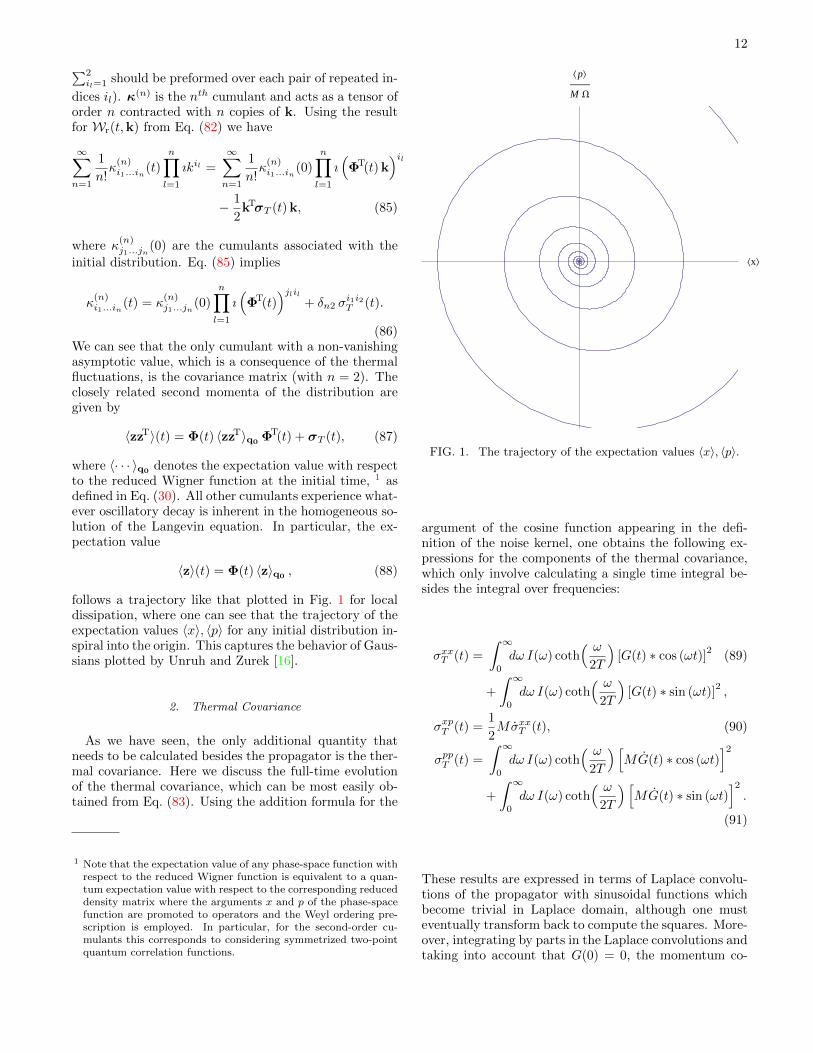
follows a trajectory like that plotted in Fig. 1 for localdissipation, where one can see that the trajectory of theexpectation values 〈x〉, 〈p〉 for any initial distribution in-spiral into the origin. This captures the behavior of Gaus-sians plotted by Unruh and Zurek [16].

2. Thermal Covariance

As we have seen, the only additional quantity thatneeds to be calculated besides the propagator is the ther-mal covariance. Here we discuss the full-time evolutionof the thermal covariance, which can be most easily ob-tained from Eq. (83). Using the addition formula for the

1 Note that the expectation value of any phase-space function withrespect to the reduced Wigner function is equivalent to a quan-tum expectation value with respect to the corresponding reduceddensity matrix where the arguments x and p of the phase-spacefunction are promoted to operators and the Weyl ordering pre-scription is employed. In particular, for the second-order cu-mulants this corresponds to considering symmetrized two-pointquantum correlation functions.

Xx\

X p\M W

FIG. 1. The trajectory of the expectation values 〈x〉, 〈p〉.

argument of the cosine function appearing in the defi-nition of the noise kernel, one obtains the following ex-pressions for the components of the thermal covariance,which only involve calculating a single time integral be-sides the integral over frequencies:

σxxT (t) =

∫ ∞0

dω I(ω) coth( ω

2T

)[G(t) ∗ cos (ωt)]

2(89)

+

∫ ∞0

dω I(ω) coth( ω

2T

)[G(t) ∗ sin (ωt)]

2,

σxpT (t) =1

2MσxxT (t), (90)

σppT (t) =

∫ ∞0

dω I(ω) coth( ω

2T

) [MG(t) ∗ cos (ωt)

]2+

∫ ∞0

dω I(ω) coth( ω

2T

) [MG(t) ∗ sin (ωt)

]2.

(91)

These results are expressed in terms of Laplace convolu-tions of the propagator with sinusoidal functions whichbecome trivial in Laplace domain, although one musteventually transform back to compute the squares. More-over, integrating by parts in the Laplace convolutions andtaking into account that G(0) = 0, the momentum co-

13

variance can be expressed in the alternative form

σppT (t) =

∫ ∞0

dω ω2I(ω) coth( ω

2T

)[MG(t) ∗ cos (ωt)]

2

+

∫ ∞0

dω ω2I(ω) coth( ω

2T

)[MG(t) ∗ sin (ωt)]

2

+M2 ν(0)G(t)2, (92)

which is completely analogous to that for the positioncovariance, but with an effectively higher-order spectraldensity due to the additional factor of ω2, plus a simplecut-off sensitive transient term which decays with thecharacteristic relaxation rate. It becomes then obviousthat the momentum covariance will contain the domi-nant contribution to any potential ultraviolet sensitivityof the thermal covariance, whereas the position covari-ance will contain the dominant contribution to any pos-sible infrared sensitivity.

In order to compute the evolution of the thermal co-variance, especially when calculating it numerically, itis often convenient to use the following alternative ex-pressions, which can be derived by differentiating withrespect to time the xx and pp components of Eq. (83):

σxxT (t) = 2G(t) [ν(t) ∗G(t)] , (93)

σppT (t) = 2M2G(t)d

dt[ν(t) ∗G(t)] , (94)

σxpT (t) =M

2σxxT (t) = M G(t) [ν(t) ∗G(t)] , (95)

where the convolution of the propagator with the noisekernel should be performed before the frequency integralof the noise kernel. This will typically result in expres-sions more amenable to numerics since one can avoid in-creasingly oscillatory integrands.

For odd meromorphic spectral functions the frequencyintegral can be evaluated by contour integration (and theresidue theorem) using the rational expansion of the hy-perbolic cotangent

coth( ω

2T

)=

2T

ω+

2

π

∞∑k=1

ω2πT

k2 +(ω

2πT

)2 . (96)

One should then be left with a sum of terms ratio-nal in the Laplace domain, which can be contractedinto digamma or harmonic-number functions [respec-tively ψ(z) or H(z)], which are asymptotically logarith-mic. When transforming back to the time domain, theresidues of the hyperbolic cotangent additionally give riseto products of rational functions of k with e−2πTtk. Theseterms contain all effects which decay at temperature-dependent rates and can be expressed in terms of Lerchtranscendent functions, Φ

(z, 1, e−2πTt

), which are useful

for numerical calculations but not particularly insightful.Fortunately, one can also derive a simple analytic ex-

pression for the late-time thermal covariance, as shownin E:

σT (∞) =

∫ ∞0

dω I(ω) coth( ω

2T

)|G(ıω)|2

[1 00 M2ω2

],

(97)

which reduces the calculation of late-time uncertaintiesto a single integral. This relation confirms that for latetimes the momentum covariance has precisely ω2 morefrequency sensitivity in its integrand.

3. Linear Entropy

In this subsection we investigate the linear entropy [31],which can be easily obtained from the Wigner distribu-tion as follows:

SL = 1− Tr(ρ2r ) = 1− 2π

∫d2zW 2

r (z, t). (98)

In Fourier space it becomes

SL = 1− 1

2π

∫d2k |Wr(k, t)|2, (99)

and using the result in Eq. (82) we finally get

SL = 1− 1

2π

∫d2k

∣∣∣Wr

(0,ΦT(t) k

)∣∣∣2 e−kTσT (t) k. (100)

At the initial time the linear entropy is that of the initialstate, and at late times it tends to

SL = 1− 1

2√

detσ∞T. (101)

Alternatively, one can express the linear entropy interms of an integral of the Fourier-transformed reducedWigner function at the initial time by introducing thechange of variables k0 = ΦT(t) k. Eq. (100) can then bewritten as

SL = 1− 1

2π

∫d2k0

1

det[Φ(t)]|Wr(0,k0) |2

× e−kT0 Φ−1(t)σT (t) Φ−T(t) k0

= 1− 1

2√

det[σT (t)]

∫d2k0 |Wr(0,k0) |2

×N(

0,1

2ΦT(t)σ−1

T (t) Φ(t); k0

), (102)

where N(µ,σ; k0) is a normalized Gaussian distributionfor the variable k0 with mean µ and covariance σ. Forsmall times this integral is similar to that for the initialstate, whereas for long times the normalized Gaussiandistribution becomes increasingly close to a delta func-tion.

For a Gaussian initial state

Wr(0,k0) = exp(−kT

0 σ0 k0 − ıkT0 〈z〉0

), (103)

the integral in Eq. (100) can be explicitly computed:

SL = 1− 1

2π

∫d2k e−kT(Φ(t)σ0 ΦT(t)+σT (t))k

= 1− 1

2

√det[Φ(t)σ0 ΦT(t) + σT (t)

] . (104)

14

For these Gaussian states, reasonable linear entropy issynonymous with reasonable uncertainty functions (i.e.,the linear entropy will be positive if and only if theHeisenberg uncertainty principle is satisfied). We willfind that the late time uncertainty is well behaved. Theuncertainty at the initial and intermediate times shouldnot violate the Heisenberg uncertainty principle either.

4. Decoherence of a Quantum Superposition

In this section we will illustrate how one can geta useful qualitative picture of the phenomenon ofenvironment-induced decoherence from the the solutionsof the master equation given by Eqs. (82)-(83). In or-der to do that we will consider a quantum superposition,|ψ〉 =

(|ψ+〉+ |ψ−〉

)/√K, of a pair of states |ψ±〉 which

correspond to a pair of Gaussian wavefunctions in posi-tion space separated by a distance 2δx and where K isan appropriate normalization constant. Specifically, wehave

ψ±(x) = ψ0(x∓ δx), (105)

ψ0(x) =√N(0, σxx0 ;x). (106)

where N(µ, σ2;x) is a normalized Gaussian distributionfor the variable x with mean µ and variance σ2, and ψ0(x)is a reference Gaussian state centered at the origin.

Taking into account the definition of the Wigner func-tion,

W(x, p) =1

2π

∫ +∞

−∞dy eipyρ(x−y/2, x+y/2), (107)

and applying it to the density matrix ρ(x, x′) =〈x|ψ〉〈ψ|x′〉 we get

W(z) =1

K

[W+(z) +W−(z) + 2 cos(2δxp)W0(z)

],

(108)

where W+, W− and W0 are respectively the Wigner func-tions of the states |ψ+〉, |ψ−〉 and |ψ0〉. This Wignerfunction, plotted in Fig. 2, exhibits oscillations of size1/δx along the p direction. These oscillations are closelyconnected to the coherence of the quantum superposition(and the existence of non-diagonal terms in the densitymatrix) and are absent in the Wigner function for theincoherent mixture W(z) = (1/2)[W+(z) +W−(z)].

In this context the decoherence effect due to the inter-action with the environment corresponds to the washing-out of the oscillations in the reduced Wigner function asit evolves according to the master equation. This canbe seen rather simply from the result for the solutions ofthe master equation obtained in this section and givenby Eqs. (82)-(83). Taking into account that the inverseFourier transform of Eq. (82) corresponds to a convolu-tion of the homogeneously evolving initial state and aGaussian function with the thermal covariance σT (t) as

Xp

FIG. 2. Wigner function associated with a state |ψ〉 =(|ψ1〉 + |ψ2〉

)/√K which corresponds to the coherent quan-

tum superposition of two Gaussian wavefunctions in positionspace shifted by a distance δx.

its covariance matrix, the Wigner function can then beexpressed as

Wr(t, z) =

∫dz′

N(0,σT (t); z−z′)

det[Φ(t)]Wr

(0,Φ−1(t) z′

),

(109)where the thermal Gaussian acts as a Gaussian smear-ing function which starts as a delta function at the ini-tial time and broadens with the passage of time untilit eventually reaches its asymptotic thermal-equilibriumvalue. Therefore, several aspects will be at play. Onthe one hand, the initial state evolves as a phase-spacedistribution with trajectories corresponding to the ho-mogeneous solutions of the Langevin equation (19) andwith the same qualitative behavior depicted in Fig. 1for the trajectories of 〈x〉 and 〈p〉. On the other hand,by diagonalizing σT (t) at each instant of time one getsthe principal directions and the widths (σ1, σ2) of theGaussian smearing function, which will average out anydetails of those sizes along the corresponding directions.When σT (t) along the direction of the interference os-cillations of the Wigner function becomes comparable totheir wavelength, they get washed out and the Wignerfunction becomes equivalent to that of the completelyincoherent mixture. The time it takes for this to happenis known as the decoherence time tdec.

Knowledge of the qualitative behavior of σT (t), com-bined with the fact that the phase-space distributiondet[Φ(t)]

−1Wr

(0,Φ−1(t) z′

)is rotating with the charac-

teristic oscillation frequency and shrinking with the char-acteristic relaxation time is all that one needs to un-derstand how different initial states decohere as timegoes by. In particular, if the decoherence time-scale,given by tdec, is much shorter than the characteristicoscillation period and the relaxation time (but suffi-

15

ciently longer than 1/Λ), one can approximate the phase-space distribution by the initial reduced Wigner func-tion (after any possible initial kick). For instance, foran Ohmic environment in the high-temperature regimeone can, under those circumstances, approximately takeσppT (t) ∼ D∞pp t with D∞pp ∼ 2Mγ0T and from the con-

dition√σpp(t) ∼ 1/δx obtain an estimated decoherence

time tdec ∼ 1/(2Mγ0Tδ2x), in agreement with the stan-

dard result for this situation [32, 33]. On the other hand,if M , γ0 or δx are very small tdec can become compara-ble or larger than the dynamical timescales 1/Ω or 1/γ,and the previous estimate can no longer be applied be-cause one needs to take into account the evolution ofσT (t), which is then less simple (it will roughly oscillatewith frequency Ω around a central value which increaseswith a characteristic timescale 1/γ until it approachesthe asymptotic thermal value), as well as the rotationand shrinking of the initial Wigner function under thehomogeneous evolution. Note also that if we had consid-ered an initial superposition of Gaussian states peaked atthe same location but with different momenta, which cor-responds to a Wigner function along the position ratherthan momentum direction, the decoherence time wouldtypically be much longer, since σxxT (t) vanishes at theinitial time and grows with a characteristic timescale oforder 1/Ω. In that case, the rotation of the Wigner func-tion becomes important since the oscillations can thenbe averaged out due to the larger values of σppT (t).

The zero-temperature regime for an Ohmic environ-ment is also qualitatively different. There is a substan-tial contribution to σppT (t) from a jolt of the diffusioncoefficient Dpp for times of order 1/Λ. However, this isactually regarded as an unphysical consequence of hav-ing considered a completely uncorrelated initial state forthe system plus environment, and this kind of highlycut-off sensitive features at early times of order 1/Λshould disappear if one considers a finite (cut-off inde-pendent) preparation time for the initial state of the sys-tem coupled to the environment [34]. For further discus-sion on this point as well as a possible way of avoidingthese spurious effects and generating a properly corre-lated initial state by using a finite switch-on time for thesystem-environment interaction see C 2. For sufficientlyweak coupling, M , or δx, tdec can become comparableor larger than the relaxation time more easily than athigh temperatures since the components σT (t) are muchsmaller in this case. For example, the asymptotic ther-mal value of σpp is of order MΩ (for weak coupling),much smaller than the high-temperature results, whichis of order MT . In such situations, the main effect of con-sidering a sufficiently long time is through the shrinkingof det[Φ(t)]

−1Wr

(0,Φ−1(t) z′

)and the size of its oscilla-

tions.

We have focused in this subsection on describing thequalitative features of the environment-induced decoher-ence of an initial coherent superposition that can be eas-ily inferred from our general result for the evolution ofthe reduced Wigner function. A much more quantitative

study is possible by using the exact analytical resultsfor the diffusion coefficients and, especially, σT (t), whichwill be presented in Secs. V and VI. We expect agreementwith the numerical results obtained in Ref. [33], althoughsignificant deviations may appear when the nonlocal ef-fects of dissipation are important (such as in the sub-ohmic case) since previously obtained master equationsare not valid in those regimes.

B. Late-Time Dynamics

We now focus our attention on the dynamics generatedby the stationary limit of the master equation, assumingthat one exists. For an Ohmic spectrum with a large cut-off the pseudo-Hamiltonian H will reach its asymptoticvalue within the cut-off timescale, whereas the diffusionD within the typical system timescales (although certainterms contributing to the diffusion coefficients will decayat a temperature-dependent rate whenever this is faster);see Sec. V for a detailed analysis of all these questions. Inthe weak-coupling regime this leaves the majority of thesystem evolution within this late-time regime wherein themaster equation is effectively stationary. However, theexistence of such a regime is not guaranteed in general.For instance, in the sub-ohmic case the evolution can bepersistently nonlocal and the effectively local late-timeregime discussed here need not exist, as will be shown inSec. VI A.

1. Late-Time Propagator

If the late-time stationary limit of the master equa-tion exists, the late-time pseudo-Hamiltonian operatorwill take the form

H =

[0 − 1

MMΩ2

R 2Γ

], (110)

and can be effectively represented as arising from thepropagator

GR(s) =1M

s2 + 2Γs+ Ω2R

, (111)

GR(t) =1

M ΩR

sin(

ΩRt)e−Γt, (112)

with ΩR =√

Ω2R − Γ2. This effective propagator GR(t)

is not equivalent to the late time limit of the true prop-agator G(t), but they should share the same asymptoticdynamics. Specifically if one can take the asymptoticexpansion

G(t) = G∞(t) + δG(t), (113)

where G∞(t) contains the asymptotic limiting behaviorand δG(t) contains the early time corrections, which de-cay faster at late times, then G∞(t) should directly yield

16

ΩR and Γ in its arguments, although a phase and am-plitude difference between G∞(t) and GR(t) may exist.

This can be rigorously justified if γ(s) and, thus, G(s)are rational, which implies that the time dependenceof G(t) corresponds to damped oscillations with varioustimescales. On the other hand, the sub-ohmic spectraldistribution that will be studied in Sec. VI A provides apertinent counter-example [in that case G(t) decays asa negative power-law rather than exponentially] whichshows that this situations does not necessarily exist whenthe spectral density function is not meromorphic.

If we indeed have a rational spectral density, then fromthe nonlocal propagator one only needs to solve the char-acteristic equation

f2 + 2γ(f) f + Ω2 = 0, (114)

to obtain all the rates f associated with the propagator(this is the same equation whose roots need to be foundwhen decomposing the propagator in Laplace domaininto simple fractions). From Eq. (114) and the positivityof the damping kernel, it follows that the real part of fwill always be negative definite. Those with the smallestreal part in absolute value give the late-time coefficients:the real part corresponds to −Γ and the imaginary one toΩR. A specific example can be found in Sec. V, where theOhmic case with a finite cut-off is studied in detail. Onthe other hand, if one treats the system-environment in-teraction perturbatively, one can show that the late-timeweak-coupling coefficients take the following form:

f± = −Γ± ıΩR, (115)

Γ = Re[γ(ıΩ)] +O(γ2), (116)

ΩR = Ω− Im[γ(ıΩ)] +O(γ2), (117)

which is in agreement with the results for the weak-coupling master equation obtained in Ref. [? ]. Anyadditional timescales would then be perturbations of thecut-off or other timescales intrinsic to the spectral func-tion.

It should be noted that in general the late-time prop-agator discussed here cannot be employed to calculatethe diffusion coefficients or the thermal covariance, noteven at late times. This is because both quantities eval-uated at an arbitrary time t get non-negligible contribu-tions involving the propagator at early times, as can beseen for instance from Eqs. (59) and (83). Nevertheless,one can still employ the late-time propagator to obtainthe late-time evolution of the thermal covariance (andthe diffusion coefficients) provided that one already hasan accurate result for its constant asymptotic value [ob-tained for example with Eq. (97)], as will be illustratednext. In addition, one can also use the propagator GR(t)given by Eq. (112), which corresponds to the limit of lo-cal dissipation, to calculate the thermal covariance anddiffusion coefficients for an Ohmic environment with asufficiently large cut-off, since in that case the contribu-tion from the extra early-time term of the propagator canbe neglected when calculating these quantities for timeslater than Λ−1, as will be shown in Sec. V.

2. Late-Time Diffusion and Covariance

Given late-time master equation coefficients whichhave all taken their asymptotic values, one can show thatthe evolution of the covariance in that regime is given by

σ(t) = σ∞T + Φ(t−ti) [σ(ti)− σ∞T ] ΦT(t−ti), (118)

which is a solution of Eq. (81) as long as one assumesH(t) and D(t) to be time-independent after some time tiin the late-time regime. Note that we have assumed thatthe master equation coefficients reached their asymptoticvalues much faster than the relaxation time (as illus-trated in F with the example of the ohmic distribution,this may be the case for finite temperature, but not nec-essarily so for zero temperature).

The asymptotic value of the late-time thermal covari-ance σ∞T has been reduced to a single integral in E. Fromthis single integral formulation, it is actually easier toobtain first σ∞T , and then obtain the late-time diffusioncoefficients using the Lyapunov equation (68). However,it is interesting to note the inverse relation

σ∞T =

[1

MΩ2R

(1

2ΓD∞pp −D∞xp

)0

0 M2ΓD

∞pp

], (119)

for the following reason. As we have pointed out inSec. IV A 2, only the momentum covariance can containthe highest frequency sensitivities. From the Lyapunovsolution we can see that the regular diffusion coefficientwould also contain such high-frequency sensitivities asit alone determines the late-time momentum covariance.Therefore, the anomalous diffusion coefficients must actas an “anti-diffusion” coefficient in keeping the positioncovariance free of such sensitivities. On the other hand,only the position covariance can contain the lowest fre-quency sensitivities and these must, therefore, be entirelycontained in the anomalous diffusion coefficient if theyexist.

In summary, any specific features of the initial dis-tribution decay away and at late times the state tendsgenerically to a Gaussian with a covariance matrix givenby Eq. (97). As follows from Eq. (87), the late-time posi-tion and momentum uncertainties are, therefore, entirelygiven by the asymptotic values of the thermal covariance:

(∆x)2 = (σ∞T )xx, (120)

(∆p)2 = (σ∞T )pp. (121)

V. OHMIC CASE WITH FINITE CUT-OFF

A. The Nonlocal Propagator

The arguably simplest example of ohmic dissipationwith finite cut-off that one can construct corresponds tothe following damping kernel:

γ(s) =γ0

1 + sΛ

. (122)

17

This damping kernel is constant at frequencies muchsmaller than the cut-off, but vanishes in the high fre-quency limit. The corresponding spectral density also ex-hibits a rational cut-off function, which decays quadrat-ically for large frequencies:

I(ω) =2

πMγ0 ω

[1 +

(ωΛ

)2]−1

. (123)

Calculating the Green function amounts to factoringa cubic polynomial. Specifically, one needs to factor(s2 +Ω2)(s+Λ)+2γ0Λs in the denominator of the Green

function G(s). For the underdamped system the effect ofa large finite cut-off is to shift the system relaxation andoscillation timescales slightly:

γ? = γ0

[1 + 2

γ0

Λ+O

(1

Λ2

)], (124)

Ω2? =

Λ

Λ− 2γ?Ω2. (125)

and to add an additional relaxation timescale comparableto the cut-off:

Λ? = Λ− 2γ?. (126)

If we parametrize everything in terms of these phe-nomenological frequencies, the Green function for thefully nonlocal damping kernel can always be expressedas

G(s) =1

M

s+ Λ

(s+ Λ?) (s2 + 2γ?s+ Ω2?), (127)

without the need to explicitly factor a cubic polynomial,while the original parameters are given by

γ0 =Λ2? + 2γ?Λ? + Ω2

?

(Λ? + 2γ?)2γ?, (128)

Ω2 =Λ?

Λ? + 2γ?Ω2?, (129)

Λ = Λ? + 2γ?. (130)

then we never have to actually factor the cubic polyno-mial.

After using partial fraction decomposition in Eq. (127),one can easily transform back to the time domain andobtain the exact propagator for the nonlocal case:

G(t) =Λ2? + Ω2

?

(Λ?−γ?)2+Ω2?

[GR(t)− 2γ?

Λ2?+Ω2

?

(GR(t)− e

−Λ?t

M

)],

(131)

where GR(t) is the late-time local propagator introducedin Eq. (112). Note that as long as Λ? > γ? the termproportional to e−Λ?t can be neglected at sufficientlylate times, when the terms involving GR(t) dominate.This corresponds to the late-time regime discussed inSec. IV B 1 [the term proportional to GR(t) simply causes

a phase shift] and the late-time master equation coeffi-cients are, therefore,

Γ = γ?,ΩR = Ω?. (132)

In the high cut-off limit one recovers the usual coefficientsγ0 and Ω. Furthermore, in that limit one can approxi-mate G(t) by GR(t) since the extra terms are suppressedby inverse powers of Λ2. For G(t) this is true even atarbitrarily early times of order Λ−1: although the ex-ponential factor is not suppressed, the prefactor 1/Λ2

?

is sufficient to suppress its contribution to G(t). This

is not true, however, for G(t) (or higher-order deriva-tives), which also appears in Φ(t). From Eqs. (36) and

(24) we can see that the component involving G(t) doesnot contribute to the thermal covariance, but whether itcontributes to its time derivative σT (t) as well as to thediffusion coefficients, which are related to σT (t) throughEq. (62), is a bit more subtle. In order to analyze thispoint it is convenient to consider Eq. (59). On the onehand, the time derivative acting on Φ(t−τ) in the secondterm on the right-hand side of that equation will giverise to G(t−τ) and an unsuppressed contribution frome−Λ?(t−τ). [Analogously to what was explained above forEq. (36), there is no contribution from the components

of the transition matrix involving G(t), and it can onlyarise when time derivatives act on other components.]On the other hand, the additional time integral in thatterm when considering such a contribution will generatean extra 1/Λ? factor as compared to the first term on theright-hand side of Eq. (59). Thus, the final conclusion isthat we can use the approximate local propagator GR(t)to calculate the diffusion coefficients at arbitrary times inthe large cut-off limit. Comparison of the results evalu-ated using the exact expressions and plotted in Sec. V Band the approximate results for the large cut-off limitalso support this conclusion.

We close this subsection with a brief discussion of thepossible dissipative regimes when considering finite val-ues of the cut-off in our spectral function, since the pres-ence of this new scale can give rise to a richer set ofpossibilities. For our rational cut-off function we havethree different dissipative regimes corresponding to thethree shaded regions in Fig. 3. The boundary betweendifferent regions corresponds to the values of the param-eters for which a pair of roots of the denominator of G(s)degenerate and change character, i.e. they change froma complex conjugate pair to two real ones. Atop the di-agram where Λ Ω, lies the regime of local dissipation,whereas along the bottom of the diagram where Λ Ω,lies an effectively sub-ohmic regime as Λ becomes an IRcut-off. The white shaded vertical stripe to the left liescompletely in the weak coupling regime and constitutesthe underdamped regime. This regime is as describedpreviously with slowly decaying oscillations and a cut-off-dependent decay rate. The grey shaded middle regiondenotes the overdamped regime. This regime is also anal-ogous to that of the simple and overdamped harmonicoscillator but with an additional cut-off-dependent decay

18

0 2 4 6 8 10

0

20

40

60

80

100

Γ

W

L W

FIG. 3. Dissipative phases for Ohmic damping with finiterational cut-off. From left to right they are underdamped inwhite, overdamped in grey, and strong coupling in black.

rate. The black shaded region to the right denotes a newnonlocal strong-coupling regime that emerges for a suffi-ciently strong coupling (such that γ0 is large comparedto the cut-off). Specifically, as derived from Eqs. (128)-(130), the relevant scales for this regime in the limit ofvery strong coupling are

Λ? =Ω2

2γ0− Ω4

4Λγ20

+O(

1

γ30

), (133)

γ? =Λ

2− Ω2

4γ0+O

(1

γ20

), (134)

Ω? = 2Λγ0 + Ω2 +O(

1

γ0

). (135)

Hence, we can see that one has moderately damped, rapidoscillations plus an additional slow decay rate.

B. Initial Jolts

Early studies by Unruh and Zurek [16] as well as HPZ[17] already revealed that at low temperatures the nor-mal diffusion coefficient Dpp(t) of an ohmic environmentexhibited a strong cut-off sensitivity for very early timesof order 1/Λ. As shown in the next section and F, inthe large cut-off limit where the use of the local propa-gator is a good approximation one can obtain relativelysimple analytic results. They confirm that for zero tem-perature the normal diffusion coefficient, which vanishesat the initial time, exhibits an initial jolt with an ampli-tude of order Λ peaked around a time of order 1/Λ and

then decays roughly like 1/t (for times much earlier than1/Ω and 1/γ0).

Alternatively, one can obtain the exact analytic resultsfor finite cut-off by computing σT (t) using Eqs. (93)-(95),as explained in Sec. IV A 2. The resulting expressions arerather lengthy and not particularly insightful, and willnot be reported here, but they have been employed toplot some examples of exact results for the diagonal com-ponents of σT (t) and σT (t) in Figs. 4 and 5. From thedifferent components of the thermal covariance and itstime derivative one can obtain the diffusion coefficientsusing Eq. (81), and in particular one can see from Fig. 5the presence of the jolt mentioned above.

2 4 6 8 10W* t

-0.1

0.1

0.2

0.3

0.4

Σ

T

2 4 6 8 10W* t

0.1

0.2

0.3

0.4

0.5

0.6

0.7

ΣT

FIG. 4. Exact thermal covariance dynamics for · normalizedposition uncertainty MΩ?σ

Txx(t) and · · · normalized momen-

tum uncertaintyσTpp(t)

MΩ?in the highly non-Markovian regime

with T = γ? = Ω?10

, Λ? = 100 Ω?.

0.02 0.04 0.06 0.08 0.10W* t

2

4

6

8

Σ

T

0.02 0.04 0.06 0.08 0.10W* t

0.05

0.10

0.15

0.20

0.25

0.30

0.35

ΣT

FIG. 5. Same plot as in the previous figure, but with a muchlarger time resolution, which reveals the presence of the initialjolt in σpp(t) peaked around t ∼ 1/Λ∗, while σxx(t) and σxx(t)remain essentially zero at those timescales.

It is important to emphasize that such kind of behav-ior, as well as an associated rapid growth of σpp(t) anda slower growth of σxx(t) (which eventually decays ex-ponentially within the relaxation time-scale 1/Γ) untilthey both reach values which depend logarithmically onΛ for large values of Λ, is a consequence of having startedwith a completely uncorrelated initial stated. A possibleway of generating a properly correlated initial state isby smoothly switching on the system-environment inter-action within a time-scale much longer than 1/Λ, butlonger than the other relevant time-scales of the system.This is discussed in some detail in C 2. It also contains anumber of technical details concerning the effects of theswitch-on function appearing in the dissipation kernel,which can be be mainly reabsorbed in redefinition of theinitial sate. The key point, however, is the role played

19

by the switch-on function appearing in the noise kernel,which eliminates the strong cut-off sensitivities and joltsmentioned above when calculating correlation functions(the covariance matrix) and its derivatives.

We conclude this subsection briefly mentioning somegenerally applicable bounds on the growth of the differ-ent thermal covariance components. First, we note fromEq. (83) that the thermal covariance is positive definiteas the noise kernel is a positive definite function. We alsonote that the thermal covariance begins with σT (0) = 0and σT (0) = 0. Given that this matrix is positive def-inite, the off-diagonal entries must be smaller than theaverage (arithmetic or geometric) diagonal entries. Butthe off-diagonal σxpT (t) is proportional to σxxT (t) and wehave, therefore, the constraint

|σxxT (t)| ≤ 2

M

√σxxT (t)σppT (t), (136)

which is also generally less than the late-time uncertaintyas both σxxT (t) and σppT (t) begin increasing and then pro-ceed to undergo damped oscillations, wherein each cyclethere is a net increase in uncertainty. This constrainsthe growth of position uncertainty. If the uncertaintyfunction takes reasonable values, then the position un-certainty must have reasonable growth.

An analogous constraint can be placed upon thegrowth in momentum uncertainty by considering the pos-

itive definite matrix Φ · ν · ΦTwhich yields

|σppT (t)| ≤ 2M

√σppT (t)

(G · ν · G

)(t). (137)

So while the growth in position uncertainty is well con-strained, growth in momentum is much less constrained.Corresponding to this, we show in Sec. IV B 2 that thelate-time momentum uncertainty has much more sensi-tivity to the high frequency modes of the bath. In termsof ohmic coupling, the initial linear jolts, σTpp ∼ Λ, andlate-time logarithmic cut-off sensitivity only occurs in themomentum uncertainty. The position uncertainty is rel-atively well behaved in both respects, having only initiallogarithmic jolts and no late-time cut-off sensitivity atall. The (linear) momentum jolting occurs only for ashort period of time, ∆t ∼ Λ−1. The result is a rapidmomentum dispersion near the initial time, but boundedlogarithmically.

C. Full-Time Diffusion Coefficients for LargeCut-off

Full-time solutions for finite cut-off are completely pos-sible given our analytic spectrum, the exact nonlocalpropagator in Sec. V A, and the contour integrals de-tailed in Sec. IV A 2. Such resulting solutions were usedto plot the early time evolution in Fig. 4, but they are abit cumbersome for publishing. Therefore, for pedagog-ical reasons we will restrict ourselves to the high cut-off

regime in this subsection since substantial additional sim-plifications can be employed in that case. For nonlocaldissipation it is in general much easier to calculate firstthe thermal covariance than the diffusion coefficients, butthe situation will be different here. The key point thatwill be exploited in this subsection is that for large cut-offthe propagator in the ohmic case can be approximatedby the local one, GR(t), as discussed in Sec. V A. The ad-vantage of using the local propagator GR(t) is that onlythe term involving a single time integral contributes tothe expression for the diffusion coefficients in Eq. (59).On the other hand, if one is only interested in the late-time asymptotic values of the diffusion coefficients, onecan obtain simple analytic results without the need torestrict oneself to large values of the cut-off by using theresults that will be presented in the next subsection.

The details of the derivation and the complete resultsfor the diffusion coefficients at arbitrary times are pro-vided in F. Here we simply highlight the main results anddiscuss some of their implications. Both diffusion coeffi-cients can be written in the following compact form:

Dxp(t) = Dxp(∞) (138)

−Mγ0

GR(t) +GR(t)

(2γ0−

d

dt

)DF(t),

Dpp(t) = Dpp(∞) (139)

−Mγ0

GR(t)

(γ0+

d

dt

)+GR(t) Ω2

DF(t),

where Dxp(∞) and Dpp(∞) are immediately obtained bymultiplying Eqs. (F3)-(F4) by s and taking the limits → 0. The general expression for DF(t) is given byEq. (F11), but a simple result for the zero temperaturecase is provided in Eq. (F14). Essentially, DF(t) decaysin a manner slightly more complicated than that of expo-nential integrals with system, coupling, and temperaturetimescales but such that temperature is the most domi-nant.

It is important to note that the coefficients Dxp(t) andDpp(t) both exhibit logarithmic divergences in the limitΛ→∞. This has been pointed out for Dxp(t) in Ref. [35],where the coefficients of the master equation were cal-culated perturbatively to second order in the system-environment coupling constants (linear order in γ0). Thefact that there is also a logarithmic divergence in Dpp(t)was not seen in that reference because it is quartic inthe system-environment coupling constants (quadratic inγ0). Moreover, strictly speaking such kinds of perturba-tive calculations cannot be employed to study the longtime behavior since they are only valid for t γ−1

0 andthey miss for instance the exponential decay of the secondand third terms on the right-hand side of Eqs. (F7)-(F8).

We close this subsection with some remarks aboutthe late-time diffusion coefficients in the weak couplingregime. Expanding Eqs. (F3)-(F4) perturbatively in γ0

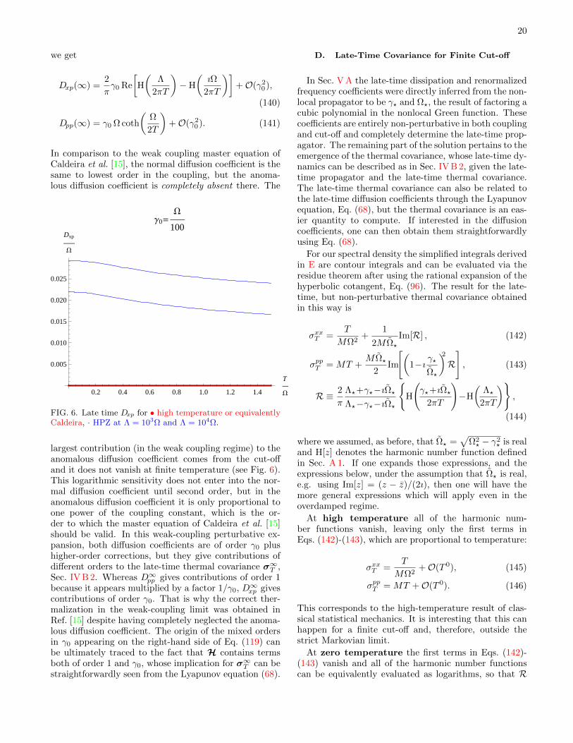
20

we get

Dxp(∞) =2

πγ0 Re

[H

(Λ

2πT

)−H

(ıΩ

2πT

)]+O(γ2

0),

(140)

Dpp(∞) = γ0 Ω coth

(Ω

2T

)+O(γ2

0). (141)

In comparison to the weak coupling master equation ofCaldeira et al. [15], the normal diffusion coefficient is thesame to lowest order in the coupling, but the anoma-lous diffusion coefficient is completely absent there. The

0.2 0.4 0.6 0.8 1.0 1.2 1.4

T

W

0.005

0.010

0.015

0.020

0.025

Dxp

W

Γ0=W

100

FIG. 6. Late time Dxp for • high temperature or equivalentlyCaldeira, · HPZ at Λ = 103Ω and Λ = 104Ω.

largest contribution (in the weak coupling regime) to theanomalous diffusion coefficient comes from the cut-offand it does not vanish at finite temperature (see Fig. 6).This logarithmic sensitivity does not enter into the nor-mal diffusion coefficient until second order, but in theanomalous diffusion coefficient it is only proportional toone power of the coupling constant, which is the or-der to which the master equation of Caldeira et al. [15]should be valid. In this weak-coupling perturbative ex-pansion, both diffusion coefficients are of order γ0 plushigher-order corrections, but they give contributions ofdifferent orders to the late-time thermal covariance σ∞T ,Sec. IV B 2. Whereas D∞pp gives contributions of order 1because it appears multiplied by a factor 1/γ0, D∞xp givescontributions of order γ0. That is why the correct ther-malization in the weak-coupling limit was obtained inRef. [15] despite having completely neglected the anoma-lous diffusion coefficient. The origin of the mixed ordersin γ0 appearing on the right-hand side of Eq. (119) canbe ultimately traced to the fact that H contains termsboth of order 1 and γ0, whose implication for σ∞T can bestraightforwardly seen from the Lyapunov equation (68).

D. Late-Time Covariance for Finite Cut-off

In Sec. V A the late-time dissipation and renormalizedfrequency coefficients were directly inferred from the non-local propagator to be γ? and Ω?, the result of factoring acubic polynomial in the nonlocal Green function. Thesecoefficients are entirely non-perturbative in both couplingand cut-off and completely determine the late-time prop-agator. The remaining part of the solution pertains to theemergence of the thermal covariance, whose late-time dy-namics can be described as in Sec. IV B 2, given the late-time propagator and the late-time thermal covariance.The late-time thermal covariance can also be related tothe late-time diffusion coefficients through the Lyapunovequation, Eq. (68), but the thermal covariance is an eas-ier quantity to compute. If interested in the diffusioncoefficients, one can then obtain them straightforwardlyusing Eq. (68).

For our spectral density the simplified integrals derivedin E are contour integrals and can be evaluated via theresidue theorem after using the rational expansion of thehyperbolic cotangent, Eq. (96). The result for the late-time, but non-perturbative thermal covariance obtainedin this way is

σxxT =T

MΩ2+

1

2M Ω?Im[R] , (142)

σppT = MT +M Ω?

2Im

[(1−ı γ?

Ω?

)2R

], (143)

R ≡ 2

π

Λ?+γ?−ıΩ?Λ?−γ?−ıΩ?

H

(γ?+ıΩ?

2πT

)−H

(Λ?

2πT

),

(144)

where we assumed, as before, that Ω? =√

Ω2? − γ2

? is realand H[z] denotes the harmonic number function definedin Sec. A 1. If one expands those expressions, and theexpressions below, under the assumption that Ω? is real,e.g. using Im[z] = (z − z)/(2ı), then one will have themore general expressions which will apply even in theoverdamped regime.

At high temperature all of the harmonic num-ber functions vanish, leaving only the first terms inEqs. (142)-(143), which are proportional to temperature:

σxxT =T

MΩ2+O(T 0), (145)

σppT = MT +O(T 0). (146)

This corresponds to the high-temperature result of clas-sical statistical mechanics. It is interesting that this canhappen for a finite cut-off and, therefore, outside thestrict Markovian limit.

At zero temperature the first terms in Eqs. (142)-(143) vanish and all of the harmonic number functionscan be equivalently evaluated as logarithms, so that R

21

simplified as follows:

H

(γ?+ıΩ?

2πT

)−H

(Λ?

2πT

)= ı cos−1

(γ?Ω?

)−log

(Λ?Ω?

)+O(T ). (147)

This generalizes the results of Unruh and Zurek [16], whoexplored the zero temperature regime in the limit of localdissipation.

Finally, in the weak coupling limit these expressionscorrectly reproduce the free thermal state:

σxxT =1

2MΩcoth

(Ω

2T

)+O(γ0), (148)

σppT =MΩ

2coth

(Ω

2T

)+O(γ0). (149)

One can also see that at weak coupling the uncertaintyfunction agrees with the weak coupling approximationfor moderate values of the cut-off scale, as shown inFig. 7. Had one naively tried to have finite diffusion

0.2 0.4 0.6 0.8 1.0 1.2 1.4

T

W

0.5

1.0

1.5

DxDp

Γ0=W

100

FIG. 7. Late time ∆x∆p for • high temperature, classi-cal statistical mechanics, · · · weak coupling approximation12

coth Ω2T· HPZ at Λ = 103Ω and Λ = 104Ω.

in the limit Λ → ∞, subtracting by hand the log(Λ/Ω)term, one would find a violation of the Heisenberg uncer-tainty principle at low temperature and strong coupling(see Fig. 8), which renders the theory unphysical. Ofcourse this does not happen with the unsubtracted the-ory, as seen in Fig. 9. It is, thus, clear that the logarith-mic dependence on the ultraviolet cut-off that appearsin the diffusion is a physically important parameter andnot something that can be subtracted away.

While the logarithmic sensitivity appears in both dif-fusion coefficients, it is suppressed in the position un-certainty by inverse powers of the cut-off. For the mo-mentum uncertainty, the logarithmic sensitivity appearsalready to first order in γ0 (which is itself quadratic in

0

0.5

1

Γ0

W

0

0.5

1

T

W

0

0.5

1

DxDp

FIG. 8. Late time ∆x∆p for the unphysical, subtracted the-ory.

0

0.5

1

Γ0

W

0

0.5

1

T

W

0.5

1

DxDp

FIG. 9. Late time ∆x∆p for the Λ = 103Ω theory.

the system-environment coupling constant) and is oth-erwise unsuppressed. This behavior had already beennoticed for Gaussian wave-packets in the Ohmic environ-ment [16, 36], and as we have discussed in Sec. IV B 2,the position uncertainty will be free of the highest cut-offsensitivities for any spectral density.

Finally, given that our results are nonperturbative, it isalso interesting to point out what happens in the highlynonlocal strong coupling regime mentioned Sec. V A.The late-time thermal covariance for this case essen-tially corresponds to taking the large Ω? limit limit of

22

Eqs. (142)-(143):

σxxT =T

MΩ2+

1

2MΩ?+O

(1

Ω2?

), (150)

σppT =MΩ?

2+O(Ω0

?). (151)

For this model of strong coupling to the environment,and yet finite cut-off, the Brownian particle will becomestrongly localized in position at late time and sufficientlylow temperatures. And although the particle is localizedin position, the uncertainty principle is not violated butat most minimized in the zero temperature limit.

VI. SUB-OHMIC AND SUPRA-OHMIC CASES

A. Sub-ohmic with no Cut-off

As an example where the nonlocal effects of dissipationare important, we will consider one of the most commonand well-behaved sub-ohmic spectral densities, I(ω) ∝√ω, which requires neither a UV nor an IR cut-off in the

final results (although one still needs to renormalize thefrequency introducing a logarithmically divergent barecounterterm). Our formulas will take a simpler form ifwe express our spectral density in terms of a quadraticcoupling constant γ? as follows:

I(ω) =2

πMγ?

√ω? ω, (152)

ω2? ≡ Ω2 + γ2

? . (153)

It is then a straightforward calculation to find the prop-agator

G(s) =1M

s2 + 2Γ√

2ω? s+ Ω2, (154)

which is amenable to partial fraction decomposition in√s since s is strictly positive. As we have defined our

nonlinear coupling strength in anticipation of this poly-nomial, the roots of the quartic denominator rk : k ∈1, 2, 3, 4 can be shown to be the conjugate pairs

r1,2 =1√2

(+√ω? ± ı

√ω? + 2γ?

), (155)

r3,4 =1√2

(−√ω? ± ı

√ω? − 2γ?

). (156)

After partial fraction decomposition, we may cast ourpropagator in the form

G(s) =

4∑k=1

AkM

1√s− rk

, (157)

Aj =

4∏k=1k 6=j

1

rj − rk, (158)

with inverse Laplace transform

G(t) =

4∑k=1

AkMrk e

r2kt erfc(−rk√t), (159)

where erfc(z) is the cumulative error function of the nor-mal distribution, defined in A 3. There are additionalterms from the individual Laplace transforms, like t−1/2,but they vanish in the sum. Using Eq. (A15) for theasymptotic expansion of erfc(z) in order to expand theGreen function in Eq. (159) at late times, we obtain termsof the form

z ez2

erfc(z) =1√π

∑k=0

(−1)k(2k)!

k!

1

(2z)2k

+

0 Re[z] ≥ 0

2z ez2

Re[z] ≤ 0, (160)

which we can use to expand the Green function inEq. (159). After grouping all the contributions together,

5 10 15 20W t

-0.2

0.2

0.4

0.6

M W G

1

20

1

30

1

40

1

50

1

100

1

W t

-0.006

-0.004

-0.002

0.002

0.004

0.006M W G

FIG. 10. Asymptotic expansion of sub-ohmic · propagatorG(t) into · · · the local contribution and • the nonlocal con-tribution for γ? = Ω

4. The local contribution is initially more

significant, but the nonlocal contribution dominates eventu-ally.

we will find exponential terms with characteristic fre-quencies f = −Γ±ı

√ω2? + 2γ?ω? , which are actually the

solutions to the characteristic rate equation (114) withsmallest negative real part. These are the only termsthat one would have considered if the local propagatorGR(t) within the late-time approximation of Sec. IV Bhad been employed. In addition, and more importantlyare the power-law decay terms which admit no local rep-resentation.

This sub-ohmic model provides a perfect exampleshowing when effectively local treatments, such as thatin Sec. IV B, will fail completely. At first the local con-tribution will dominate and the master equation coeffi-cients will appear to trend towards Γ ≈ γ? and ΩR ≈ω? + γ?. However, the nonlocal contribution (the power-law terms) will eventually dominate the more swiftly de-caying local contribution (the exponential terms) and acorrect treatment of the nonlocal dynamics will be re-quired. In fact, as the nonlocal contribution becomescomparable to the local contribution, the master equa-tion coefficients will become periodically divergent [thisis related to the fact that det Φ(t) vanishes and changessign at those times.]. The underlying homogeneous evolu-tion is well behaved and strictly dissipative (the damping

23

kernel is positive definite), but the localizing perspectiveof the master equation becomes divergently unnatural.Any errors, numeric or analytic, can be catastrophic inthe master equation perspective. In this respect, the sub-tleties missed in previous derivations of the master equa-tion, as pointed out in Sec. III B and which are relevantwhenever nonlocal effects are important, will likely giverise to substantial discrepancies in this case.

The full-time evolution is rather complicated, but thelate-time limit is very manageable. For example, fromEq. (97) we can express the late-time thermal positionuncertainty as

σxxT (∞) = 2

∫ ∞0

I(ω) coth( ω

2πT

)|G(ıω)|2 2

√ω d√ω,

(161)where we have used the relation dω = 2

√ω d√ω. The

integrand is amenable to partial fraction decomposition,after a rational expansion of the hyperbolic cotangentwith Eq. (96), and can therefore be integrated withoutresorting to numerics. Additionally, and in contrast tothe ohmic case, the integrand is even in

√ω for all tem-

peratures, including zero, and contour integration tech-niques are more generally applicable.

Strictly speaking we cannot compare exact sub-ohmicsolutions to those obtained with an incorrect masterequation since the master equation will yield nonsense,but we can compare the exact nonlocal dynamics to thoseobtained by extracting the local dynamics and assumingit to be the dominant behavior. Obviously the effectivelylocal approximation is incorrect, but it should be good tozeroth order in the coupling and one might naively expectthat it might also behave reasonably for finite couplingstrength. However, in Fig. 11 we compare the late-timeuncertainty functions and show there to be sharp dis-agreement to the first two orders in the coupling constantsquared (the slope and the curvature of the curves on theplot).

B. Supra-ohmic with Finite Cut-off

The conventional wisdom has been to consider supra-ohmic spectral densities of the form

In(ω) =2

πM γn ω

(ωΛ

)nχ(ω

Λ

), (162)

where χ : [0,∞) → [1, 0) denotes the cut-off regulator.Without a cut-off regulator, all supra-ohmic couplingshave greater than logarithmic high frequency divergencein the diffusion and thermal covariance integrals (see Efor exact integrals in the infinite time limit). Even whenregulated, the mere potential for divergence therefore cor-responds to cut-off sensitivity from the high frequencyportion of noise integrals, which is balanced by the ex-tra inverse powers of the cut-off in the pre-factor of theabove spectral density.

0.1 0.2 0.3 0.4 0.5

Γø

W

0.26

0.28

0.30

0.32

ΣxxΣpp

FIG. 11. Late-time sub-ohmic uncertainty function at zerotemperature with the · exact nonlocal solution and · · · ficti-tious effectively local solution. In the limit of vanishing dis-sipation, one has the minimal uncertainty ground state (zerotemperature thermal state) in each case.

Here we will restrict our investigation to the followingspectral density

I(ω) =2

πM γ2 ω

(ωΛ

)2(1 +

(ωΛ

)2)2 , (163)

because this example is exactly solvable. The corre-sponding damping kernel in Laplace space is

γ(s) =γ2

2

sΛ(

1 + sΛ

)2 . (164)

One might be inclined to view this damping kernel asa tiny mass renormalization plus even less significanthigher order terms, but the effect quite different fromthat, as we will see. After factoring the fourth-orderpolynomial, the fully nonlocal propagator can be decom-posed by partial fractions into two sets of timescales. Ex-panding perturbatively in γ2, the first set of timescalescorrespond to the system frequency with weak damping

γ? = γ2

(ΩΛ

)2(1 +

(ΩΛ

)2)2 +O(γ22), (165)

Ω? = Ω

1− γ2

Λ

1−(

ΩΛ

)2(1 +

(ΩΛ

)2)2 +O(γ22)

, (166)

while the second set of timescales correspond to quicklydecaying nonlocal contributions associated with the cut-off scale:

γΛ = Λ− γ?, (167)

ΩΛ =Ω

Ω?Λ. (168)

24

The situation is analogous to ohmic case with a finitecut-off except that the nonlocal part of the propagator isalso oscillating at the rate ΩΛ ≈

√γ2Λ, for weak coupling

and high cut-off.This form of spectral density was constructed only

with well-behaved high frequency contributions in mind.Nevertheless, as shown in Fig. 12, we find the conven-

0.2 0.4 0.6 0.8 1.0

Γ2

W

1

2

3

4

5

6

ΣxxΣpp

0.2 0.4 0.6 0.8 1.0

Γ2

W

BL

W

F

0.25

0.30

0.35

0.40

0.45

0.50

ΣxxΣpp

FIG. 12. Late-time supra-ohmic uncertainty function at zerotemperature for cut-offs between 100Ω and 500Ω. The leftplot is with a conventional coupling scale, while the right plothas decreased the coupling strength by an extra power of thecut-off.

tional form of spectral density to be inadequate. There isclearly some cut-off sensitivity in the thermal covariancewhich is remedied by introducing an additional power ofcut-off suppression. E.g. the conventional form of spec-tral density is not well behaved, but the substitution

γ2 →Ω

Λγ2, (169)

is well behaved.An explanation only emerges after a more thorough ex-

amination of the contour integrals. The high-frequencyregime, ω Λ, is already rendered well behaved bythe conventional cut-off-dependent prefactor. The near-resonance regime, ω ≈ Ω, which produces the weak cou-pling limit, also appears to be well behaved. There isonly one remaining suspect and it proves to be the cul-prit. The previously unaccounted for cut-off sensitivityarises here from the nonlocal timescales of the propa-gator, i.e. the ω ≈ Λ regime. This is quite surprisingas unlike sub-ohmic coupling, supra-ohmic coupling doesyield a well-behaved local representation for its late-timedynamics. But residues of the contour integral whichcorrespond to the nonlocal timescales reveal the correctdominant behavior σpp ≈ 1

2M ΩΛ = 12M√γ2Λ, for weak

coupling and high cut-off. Therefore the conventional,linear coupling γ2 must be suppressed by an additionalfactor of the cut-off, else the momentum covariance willbe plagued by a

√Λ sensitivity.

VII. GENERALIZATIONS OF THE THEORY

A. Influence of a Classical Force

In this section we consider the case of a classical forceF (t) acting on the quantum oscillator. This is done by

adding a time-dependent potential −F (t)x to the systemLagrangian:

Ls =1

2M(x2 − Ω2x2

)+ F (t)x, (170)

which gives rise to the following additional source on theright-hand side of Eq. (19):

F(t) =

[0

F (t)

]. (171)

Following our master equation derivation in Sec. III B,it is easy to see that such a deterministic source in theLangevin equation simply adds a driving term to the mas-ter equation, which becomes

∂

∂tWr(z, t) = (172)∇T

z H(t) z−∇Tz Feff(t) + ∇T

z D(t)∇z

Wr(z, t) ,

where the effective force Feff(t) is given by

Feff(t) ≡ F(t) +

∫ t

0

dτ

[d

dt+ H(t)

]Φ(t−τ)

F(τ).

(173)Note that the last term in Eq. (173) is a consequence ofhaving nonlocal dissipation and, as we saw in Sec. III B,it vanishes for local dissipation.

Similarly, the method of Sec. II C, based on the solu-tions of the Langevin equation, can be straightforwardlygeneralized to this case and one obtains the followingresult for the time evolution of the reduced Wigner func-tion:

Wr[t,k] =Wr

[0,ΦT(t) k

]e−

12kTσT (t) k e−ık

T〈z〉F (t),

(174)with a driven mean 〈z〉F (t) given by

〈z〉F (t) = (Φ ∗ F)(t). (175)

On the other hand, one can alternatively use the methodof characteristic curves to solve the master equation, asdone in Sec. III C 1. Fourier-transforming Eq. (172), onegets an equation analogous to Eq. (66) but with an extraterm −ıkTFeff(t) on the right-hand side. Following thesame procedure as in Sec. III C 1, one finally obtains thesame result as in Eq. (174) but with

〈z〉F (t) =

∫ t

0

dτ Φ(t, τ) Feff(τ). (176)

Eqs. (175) and (176) can be shown to be equivalent asfollows. First, one rewrites Eq. (173) as

Feff(τ) =

[d

dτ+ H(τ)

] ∫ τ

0

dτ Φ(τ−τ ′)F(τ ′). (177)

Next, one substitutes Eq. (177) into Eq. (176) and per-forms an integration by parts of the derivative term.

25

Finally, one takes into account that (d/dτ)(Φ−1(τ)

)= Φ−1(τ)H(τ), which follows from Eq. (55), and theresult in Eq. (175) is recovered. Hence, we see that al-though Φ(t, τ) and Φ(t−τ) are different for nonlocal dis-sipation, this is exactly compensated by the contributionfrom the second term on the right-hand side of Eq. (173),which does not vanish in that case.

Note that just as all the temperature dependence ap-pears entirely in the second cumulant, or covariance, theexternal force only affects the first cumulant, or mean.Eq. (174) shows that the mean, 〈z〉(t), is shifted by〈z〉F (t), which characterizes the response to the drivingforce. In fact, using Eq. (22) one can immediately seethat it corresponds to shifting 〈x〉 and 〈p〉 respectively

by (G ∗ F )(t) and (MG ∗ F )(t), as one would expect.

B. N-Oscillator Master Equation

Our compact matrix notation allows a number of gen-eralizations in a fairly straightforward fashion. As an il-lustration we present the generalization of our results forthe master equation and its solutions to the case of mul-tiple system oscillators xα (which includes the case ofa higher dimensional oscillator) with arbitrarily bilinearcoupling to themselves and to the bath oscillators yj.We consider the system Lagrangian for N oscillators anda generic bilinear term for the system-bath interaction:

Ls =1

2

(xTM x− xTMΩ2 x

), (178)

=1

2

(xαMαβ x

β − xαMΩ2αβx

β),

Lint = yTc x = yiciβxβ , (179)

where we used Einstein’s summation convention for re-peated indices and the matrix c connects system posi-tions (denoted by Greek indices) to bath positions (de-noted by Latin indices). The matrices M and MΩ2 aresymmetric and positive definite. The eigenvalues of Ωcorrespond to the normal-mode frequencies, as can beinferred from our Langevin equation (183).

The effects of the environment for the generalized sit-uation described by Eqs. (178)-(179) can be entirely en-coded in a simple generalization of the spectral densityas well as the noise and damping kernels:

Iαβ(ω) =∑k

δ(ω−ωk)ckαckβ2mkωk

, (180)

ν(t, τ) =

∫ ∞0

dω I(ω) coth( ω

2T

)cos[ω(t−τ)] , (181)

Mγ(t, τ) =

∫ ∞0

dωI(ω)

ωcos[ω(t−τ)] . (182)

In fact, one can directly specify the system-environmentcoupling by giving the spectral density matrix I(ω),which must be symmetric and positive semi-definite, as

implied by Eq. (180). After taking the Laplace transform,the Langevin equation in position space is then given by

M(s2 + 2s γ(s) + Ω2

)x(s) = M (sx0 + x0) + ξ(s),

(183)

which can be solved via matrix inversion to find G(s),with which one can construct Φ(t) and σT (t). However,closed-form evaluation of G(t) can be rather involved:even for local dissipation the two-oscillator problem re-quires factoring a fourth-order polynomial. In general,the N -oscillator problem will require factoring a polyno-mial of order 2N for local dissipation and of order 2N+1or more for nonlocal dissipation. We leave more thoroughdiscussion to future work, where we will derive block-matrix equations for the positon and momentum parts inthe phase-space representation analogous to those herein.

VIII. DISCUSSION

Quantum Brownian motion of an oscillator coupled toa thermal reservoir of quantum oscillators has been thecanonical model for the study of open quantum systemswhere one can use it to investigate all the environmen-tal effects on an open quantum system it interacts with,even of macroscopic scale, such as quantum dissipation,diffusion, decoherence and entanglement. It also pro-vides important information on quantum measurement,such as noise, fluctuations, correlations, uncertainty re-lation and standard quantum limit in mesoscopic sys-tems. Many experiments have been carried out for test-ing these processes. An exact master equation was re-ported some years ago [17] governing the reduced densitymatrix of an open quantum system coupled to a generalenvironment of arbitrary spectral density and tempera-ture. Subsequently there have also been claims of exactsolutions [21]. We have found many previous derivationsto be correct for local dissipation, but containing errorsor omissions for nonlocal dissipation; in their place wehave presented the most complete and correct derivationof the QBM master equation to date. In this paper wereport on solutions to this equation for a fairly general setof physical conditions and a generalization of the QBMmaster equation to a system with an arbitrary number ofoscillators. Most of the previous results required one tosolve integro-differential equations numerically, whereaswe have reduced everything to quadrature, which can befurther simplified in many cases using contour integra-tion techniques. We expect these results to be useful inrealistic settings for the analysis of many problems whichcan be described by this model.

More specifically, we have found a compact expressionfor the general solution of this master equation, show-ing that at late times it tends to a Gaussian state en-tirely characterized by its asymptotic covariance matrix.For odd meromorphic spectral densities, and many oth-ers, the result for this late-time covariance matrix can

26

be evaluated as a simple contour integral. As an ex-ample we provide explicit exact nonperturbative resultsfor an ohmic environment with a finite cut-off which arevalid for an arbitrarily strong coupling. At sufficientlylow temperatures and strong coupling this equilibriumstate becomes highly squeezed and the system becomesextremely localized in position space, a phenomenon withpotentially interesting applications in the realm of meso-scopic systems.

The general solution of the master equation involvesthe matrix propagator of a linear integro-differentialequation. We have been able to solve these equationsexactly for several ohmic, sub-ohmic and supra-ohmicenvironments with a finite cut-off and studied the evo-lution of the system for finite times. This is achieved us-ing Laplace transforms and eventually transforming backto time domain. From such exact (and simple) solutionsfor the propagator one gains highly valuable information.For instance, one can justify that using the local propaga-tor is a valid approximation for the ohmic environment inthe large cut-off limit. This approximation leads to greatsimplifications and we are then able to provide relativelysimple analytic expressions for the diffusion coefficientsof the master equation at all times. Similarly, our ex-act solutions for the propagator in specific examples ofsub-ohmic and super-ohmic environments reveal a dom-inant contribution from nonlocal dissipation effects. Inthe first case it is a consequence of long-time correlations,due to the low-frequency modes of the environment, thatbecome important at late times. In contrast, the sourceof nonlocality in the supra-ohmic case is the UV regula-tor function, and it gives rise to a marked cut-off sensi-tivity of the momentum covariance which had not beennoticed so far. On the other hand, it should be pointedout that although the results for the exact propagator ofthe integro-differential equation are rather simple, someof the general expressions for the solutions of the masterequation are rather lengthy and have not been reportedhere. They have, nevertheless, been employed to eval-uate and plot the exact time evolution of the thermalcovariance for an ohmic environment with a finite cut-offin Sec. V B.

It is important to discuss the cut-off sensitivity ofthe late-time covariance and diffusion coefficients for anohmic environment in the weak coupling regime. Whileσ∞xx is finite in the infinite cut-off limit, σ∞pp dependslogarithmically on Λ for large Λ already at order γ0

[Eq. (143)]. This means that it is absolutely necessaryto consider a finite cut-off. The kind of divergences thatappear otherwise cannot be dealt with by renormalizingthe frequency or other bare parameters of the theory. Infact, as shown in Sec. V D, subtracting the divergent termwould lead to inconsistencies (violation of Heisenberg’suncertainty principle). Furthermore, from the late-timethermal covariance one can immediately obtain the late-time diffusion coefficients as well (see the discussion atthe end of Sec. V C). One finds then that both the normaland anomalous diffusion coefficients are logarithmically

sensitive to large cut-offs. However, while this depen-dence appears in Dxp [Eq. (140)] at order γ0, in Dpp itonly appears at order γ2

0 , and it had been missed in pre-vious analytic studies which treated γ0 perturbatively tolowest order.

We would also like to stress the following point. Whenstudying an ohmic environment with a finite but largecut-off, it can be a good approximation to consider localdissipation (infinite cut-off limit for the damping kernel)while keeping the cut-off finite in the noise kernel. Thishas already been discussed above and justifies calcula-tions like those of Ref. [16] up to corrections suppressedby inverse powers of the cut-off. However, the opposite isnot true: it is essential to keep a finite cut-off in the noisekernel to avoid the divergences discussed in the previousparagraph. This is precisely the origin of the divergencesand pathological behavior found in Ref. [21], where a fi-nite cut-off was employed in the damping kernel but notin the noise kernel. Instead one should use the samespectral function everywhere, which means having a fi-nite cut-off in both kernels, and everything would be welldefined then. Note that these divergences would appearin the momentum covariance even at asymptotically latetimes, as discussed in the previous paragraph. There is adifferent kind of sensitivity to large values of the cut-offthat is due to having started with a uncorrelated statefor the system and the environment. This gives rise toa jolt in the normal diffusion coefficient at early timesof order 1/Λ with an amplitude proportional to Λ, aswell as a logarithmic dependence on the cut-off of σxx(and σpp) that decays exponentially with the relaxationtime-scale 1/Γ. They would not be present if one hadstarted with an appropriately correlated initial sate, andthen prepared the system in a finite time (not suddenly).Alternatively, this can be implemented by switching onthe system-environment interaction smoothly in a finitetime much larger than 1/Λ, but shorter than the otherdynamical scales of the system. 2

As a further generalization of the QBM master equa-tion we have included the influence of external forces.This modifies the dynamics by driving the mean positionand momentum just as with a classical driven system(even for nonlocal dissipation). In this model we foundthat the force has no effect upon the width of the wave-packet or any cumulant other than the mean. Theseresults may be useful for the study of low-temperaturemeasurements of driven oscillators, which are relevantfor experiments with nanomechanical resonators [11, 12].They also play a crucial role in future schemes for thedetection of gravitational waves with high-intensity laser

2 A detailed discussion is provided in C 2. There are plenty oftechnical details concerning the initial kick and the effect of theswitch-on function on the damping kernel, but the real key pointis the effect of the switch-on function in the noise kernel, whenevaluating either the diffusion coefficients or the correlation func-tions (the covariance matrix).

27

interferometers, where the radiation pressure effects onthe cavity mirrors are important [37, 38].

Finally, we have extended the model of one quantumoscillator bilinearly coupled to a thermal reservoir of os-cillators to a model of multiple oscillators bilinearly cou-pled to themselves and the bath in an arbitrary fash-ion. With this generalization, the potential for applica-tion [39, 40] becomes almost endless and we leave furtherstudy to future research [41].

ACKNOWLEDGEMENT

We would like to thank Juan Pablo Paz for interestingconversations which encouraged us to look into the sub-ohmic case. C. F. and B. L. H. are supported in partby grants from the NSF-ITR program (PHY-0426696)and the DARPA-QuEST program (DARPAHR0011-09-1-0008). A. R. was partly supported by LDRD fundsfrom Los Alamos National Laboratory and by a DOEgrant.

Appendix A: Special Functions

1. Harmonic Number

The harmonic number H(n) is a function similar to alogarithm, whose definition and main properties are

H(n) =

n∑k=1

1

k, n ∈ Z+ (A1)

H(0) = 0, (A2)

γE = limn→∞

[H(n)− log (n))], (A3)

where γE is known as the Euler-Mascheroni constant. Itsgeneralization to the complex plane exhibits similar prop-erties and is given by

H(z) = γE + ψ(z+1), z ∈ C, (A4)

where ψ(z) is the digamma function, defined as

ψ(z) =Γ′(z)

Γ(z). (A5)

It satisfies the recurrence relation

ψ(z + 1) = ψ(z) +1

z, (A6)

and its Taylor expansion around 1 as well as its asymp-totic expansion for |z| → ∞ are given respectively by

ψ(z+1) = − γE +

∞∑k=1

ζ(k+1)(−z)k

for |z| < 1, (A7)

ψ(z) ∼ ln z − 1

2z− 1

12z2+ · · ·

if |arg (z)| < π, (A8)

where ζ(n) is the Riemann zeta function.

2. Exponential Integral

The exponential integral is a special function which isdefined for |arg(z)| < π as

E1(z) =

∫ ∞z

e−z′

z′dz′, (A9)

and has a branch cut along |arg(z)| = π. Its series ex-pansion is

E1(z) = −γE − ln z −∞∑n=1

(−1)n

nn!zn, (A10)

and its asymptotic expansion for |z| → ∞ is given by

E1(z) =e−z

z

(1− 1

z+

2

z2+ · · ·

). (A11)

3. Error Function

The error function is defined as

erf(z) =2√π

∫ z

0

e−w2

dw, (A12)

where the path integration is subject to the restrictionlim|w|→∞ |arg(w)| < π/4. In addition, the complemen-tary error function is defined as

erfc(z) =2√π

∫ ∞z

e−w2

dw = 1− erf(z). (A13)

The series expansion is

erf(z) =2√π

∞∑n=1

(−1)n

(2n+1)n!z2n+1, (A14)

and the asymptotic expansion for |z| → ∞ (and|arg(z)| < 3π/4) is given by

erfc(z) =e−z

2

√π z

(1− 1

2z2+

3

4z4+ · · ·

), (A15)

which along with the fact that erf(z) is odd, is suffi-cient to create an accompanying asymptotic expansionfor |arg(z)| > 3π/4

Appendix B: Some properties of Laplace Transforms

Given a real function f(t), defined for all real numberst ≥ 0, its Laplace transform is defined as

f(s) = Lf(t)

(s) =

∫ ∞0−e−stf(t)dt, (B1)

28

where the one-sided limit from the left for the lower limitof integration is chosen so that the transform of the Diracdelta function is one, i.e. Lδ(t) = 1. The main prop-erties used in the paper are the following. First, theLaplace transform of a derivative is given by

Lf(t)

(s) = sf(s)− f(0). (B2)

And from this one can easily infer that the Laplace trans-form of an integral:

L∫ t

0

dτ f(τ)

(s) =

1

sf(s). (B3)

Second, multiplying f(t) by an exponential correspondsto a translation of the Laplace transform:

Leatf(t)

(s) = f(s−a). (B4)

Third, if the inverse Laplace transform of f(s) is f(t) θ(t),

multiplying f(s) by an exponential corresponds to atranslation of the inverse Laplace transform:

L−1easf(s)

(s) = f(t+a) θ(t+a). (B5)

Fourth, the Laplace transform of a Laplace convolutionis given by the product of the Laplace transforms:

L

(f ∗ g)(t)

(s) = f(s) g(s), (B6)

where

(f ∗ g)(t) =

∫ t

0

dt′f(t−t′)g(t′). (B7)

Fifth, the initial value theorem relates the initial valueof a function f(t) and the infinite limit of its Laplacetransform as follows:

f(0+) = lims→∞

sf(s). (B8)

Sixth, the final value theorem relates the infinite limitof a function f(t) and the initial value of its Laplacetransform as follows:

f(∞) = lims→0

sf(s), (B9)

provided that all the poles of f(s) are on the Re(s) < 0half of the s complex plane.

Seventh, the inverse Laplace transform of f(s) can becalculated using Bromwich’s integral, which involves an

analytic continuation of f(s) in the complex plane:

f(t) = L−1f(s)

(s) =

1

2πı

∫ α+ı∞

α−ı∞estf(s) ds, (B10)

where α is a real number chosen so that the integration

path lies within the region of convergence of f(s), i.e.,

α > Re(sj) for every singularity sj of f(s).

Bromwich’s integral illustrates the close relationshipbetween the Laplace transform and the Fourier transformthrough analytic continuation. However, even if all the

singularities of f(s) lie on the Re(s) < 0 half of the com-plex plane, the relation is not direct because the Laplacetransform involves an integral with domain [0,∞) ratherthan (−∞,∞). The precise relationship can be under-stood as follows. Consider a real function f(t) defined for

all real values of t and whose Fourier transform is f(ω). Itis useful to define the following additional Fourier trans-forms:

f±(ω) =

∫ +∞

−∞dt e−ıωtf(t) θ(±t) , (B11)

such that f(ω) = f+(ω) + f−(ω) and which satisfy the

property f±(−ω) =(f±(ω)

)∗since f(t) is real. Assum-

ing that the Laplace transform f(s) has no singularitiesfor Re(s) > 0, it can be related by analytic continuation

to f+(ω):

f+(ω) = limε→0

f(ε+ıω). (B12)

If f(t) is an even function, one has f−(ω) = f+(−ω), andusing Eq. (B12) one can then write

f(ω) = f+(ω) + f+(−ω) = limε→0

[f(ε+ıω) + f(ε−ıω)

].

(B13)

Similarly, if f(t) is an odd function, one has f−(ω) =

−f+(−ω), which implies

f(ω) = f+(ω)− f+(−ω) = limε→0

[f(ε+ıω)− f(ε−ıω)

].

(B14)

Appendix C: System-Environment Interaction andRenormalization

1. Frequency Renormalization and the DampingKernel

In this subsection we discuss the relationship betweenthe Lagrangians in Eqs. (1) and (2). The question offrequency renormalization plays a central role in this dis-cussion and it will be analyzed by rewriting the equa-tion of motion in terms of the damping kernel, given byEq. (8), rather than the dissipation kernel. Here we willtake θs(t) = 1 and leave the examination of effects due toa non-vanishing switch-on time for the next subsection.

If one starts with the Lagrangian in Eq. (1), the homo-geneous part of the Langevin integro-differential equationanalogous to Eq. (7) is then

(L · x)(t) = Mx(t) +MΩ2bare x(t) + 2

∫ t

0

dτ µ(t−τ)x(τ).

(C1)

29

Using the expression for the dissipation kernel in termsof the damping kernel, µ(t−τ) = M(∂/∂t)γ(t−τ), andintegrating by parts, one obtains

(L · x)(t) = Mx(t) + 2M

∫ t

0

dτ γ(t−τ) x(τ) (C2)

+M(Ω2

bare−δΩ2)x(t) + 2Mγ(t)x(0),

where the time-independent frequency renormalizationδΩ2 is given by

δΩ2 = 2 γ(0) =2

M

∫ ∞0

dωI(ω)

ω. (C3)

By choosing a bare frequency with an appropriate coun-terterm in order to cancel the frequency renormalization,Ω2

bare = Ω2 + δΩ2, one would be finally left with Eq. (9)and an effective frequency for the system oscillator Ω.This is the same equation that one obtains if one startswith the Lagrangian in Eq. (2) and takes θs(t) = 1, whichcan be easily understood as follows. Recalling the defi-nition of the spectral function I(ω) in terms of the cou-pling constants cn, it is immediate to see that the squareof the last term on the right-hand side of Eq. (2) gives−(1/2)MδΩ2x2. Therefore, the Lagrangians in Eqs. (1)and (2) are equivalent provided that one makes the choicementioned above for Ω2

bare.

2. Initial-Time Divergences, Coupling Switch-onand Initial-State Distortion

a. Initial-Time Divergences and Coupling Switch-on

The derivation of the HPZ master equations reliesupon the key assumption that the system and environ-ment are initially uncorrelated. For an ohmic environ-ment, this gives rise to an initial “jolt” in the normaldiffusion coefficient of the master equation with a char-acteristic time-scale of order Λ−1 and an amplitude pro-portional to Λ. Similarly, the frequency Ω2

R(t) in themaster equation starts with a large value of the order ofΛ and decreases to moderate values in a time of orderΛ−1.

The physical origin of the jolts in the coefficients ofthe master equation as well as other initial time diver-gences, such as the divergent contributions to correlationfunctions of system observables that are due to diver-gent boundary terms at the initial time (see Appendix Din Ref. [42]), can be understood as follows. In generalwhen a system couples to an environment with an infi-nite number of modes, well-behaved states exhibit cor-relations with arbitrarily high-frequency modes. In con-trast, states that are uncorrelated for sufficiently highfrequencies (such as completely factorizable states) arepathological. For instance, in the limit of infinite cut-offthey have infinite energy (even with an origin of ener-gies such that the ground state of the whole interact-ing system has vanishing energy) and their Hilbert space

is unitarily inequivalent to the space of physical states,spanned by the basis of energy eigenvectors of the wholesystem Hamiltonian including the system-environmentinteraction. (Of course for a finite UV cut-off there areno divergences or unitary inequivalence, but the poten-tially divergent terms are very sensitive to changes inthe value of the cut-off.) Physically acceptable initialstates that correspond to the thermal equilibrium statefor the whole system can be obtained using Euclideanpath integrals [43]. However, the instantaneous prepa-ration functions employed in Ref. [43] to produce otherstates in addition to the thermal equilibrium state stillgive rise to initial divergences, as explained in Ref. [44].In order to obtain finite results, one needs to prepare thenew initial state within a non-vanishing time [34], whichcorresponds to a physically more realistic situation. Thealternative approach that we follow here is to switch onthe system-environment interaction smoothly within atime ts much longer than Λ−1 but shorter than any otherrelevant time-scale of the problem. In this way the fac-torized initial state, which is perfectly acceptable in theuncoupled case, becomes adequately correlated with thearbitrarily high-frequency modes in a regular fashion.

When adding the short time switch-on function to thesystem-environment coupling to turn on the interactiongradually, as in Eq. (2), the initial jolt is no longer presentin the results for the diffusion coefficients, which behavesmoothly during the switch-on time. Furthermore, fortimes much longer than ts the contribution to Eq. (59)from the switch-on period is negligible and one can sim-ply use that equation without including any switch-onfunction. This point is implicitly exploited throughoutthe paper: unless explicitly stated, our calculations of thediffusion coefficients do not take into account the switch-on functions and the results for those coefficients shouldonly be regarded as valid for times sufficiently largerthan ts, while their values during that period should besmoothly interpolated so that they vanish at the initialtime.

Either the quick transition from the bare frequency tothe renormalized one (in the absence of a smooth switch-on function) or switching on the interaction in a finitetime ts can have a non-negligible effect on the homoge-nous solutions of the Langevin equation even for timesmuch larger than Λ−1 or ts. Fortunately, as we will showin the remaining subsections, the effect can be entirelyaccounted for by a finite shift of the initial momentumand the corresponding transformation of the initial state.

b. Initial Kick (finite cut-off, vanishing switch-on time)

We start by considering the case in which there is noswitch-on time and analyze the effect of the slip term,which corresponds to the last term on the right-handside of Eq. (9) for the Langevin operator. It can be in-terpreted as a transient driving force

Fγ(t) = 2γ(t)x0, (C4)

30

whose contribution to the solution is simply adding aterm G(t) ∗ Fγ(t). The infinite cut-off limit can be ana-lyzed using distributions in the time domain or workingwith Laplace transforms. As derived in Eqs. (13)-(14),the solution of Eq. (9) (including the slip term) is givenin Laplace space by

x(s) = M (sx0 + x0) G(s) + G(s)ξ(s), (C5)

whereas one can easily infer that the solution without theslip term would be

y(s) = M (sy0 + y0 + 2γ(s) y0) G(s) + G(s)ξ(s). (C6)

In the limit of local dissipation (large cut-off limit) γ(s) =γ0 and one can see that the effect of the slip term is aninitial kick to the homogeneous solutions, whose valuesbefore and after the kick can be related via

y0 = x0, (C7)

y0 = x0 − 2γ0x0. (C8)

This induces a distortion of the reduced Wigner func-tion associated with the transformation x0 → x0−2γ0x0

which occurs within the cut-off timescale. The effect ofsuch an initial kick can be entirely absorbed in a redefini-tion of the initial state, as will be discussed in Sec. C 2 d.

c. Initial Kick (large cut-off, non-vanishing switch-on time)

Next, we consider the case with a non-vanishingswitch-on time ts and smooth switch-on function suchthat θs(0) = 0 and θs(t) = 1 for t ≥ ts. Integrating thedissipation kernel by parts in Eq. (7), the homogeneouspart of the Langevin equation becomes

x(t) + 2

∫ t

0

dτ γP(t, τ) x(τ) + Ω2x(t) =

− 2 θs(t)

∫ t

0

dτ γ(t−τ) θs(τ)x(τ), (C9)

in terms of the positive-definite kernel

γP(t, τ) ≡ γ(t−τ) θs(t)θs(τ), (C10)

where we have not made any approximations concern-ing the timescales of the dissipation kernel and switch-onfunction yet, but have expressed our result in terms ofthe damping kernel defined in Eq. (8) and taken into ac-count Eq. (C3). Either in the limit of local dissipationor vanishing switch-on time, the term on the right-handside of Eq. (C9) gives rise to a slip term analogous to thatfound in the previous subsection. This is because for x(t)evolving slowly compared to Λ−1 or ts, one has a a con-volution of the distributions γ(t) and θs(t), which is alsoa distribution localized near the initial time. In partic-ular, it is immediate to see that the results of Sec. C 2 bare recovered in the limit of vanishing ts [see the remark

below about θs(t) in that limit].

If we take the high cut-off limit γ(t−τ) = γ0 δ(t−τ),which should be a good approximation for Λ t−1

s , theright-hand side of Eq. (C9) takes a simple form and weare left with

x(t) + 2γ0 θ2s (t) x(t) + Ω2x(t) = −γ0 δs(t)x(t) (C11)

δs(t) ≡d

dtθ2

s (t), (C12)

where δs(t) is a representation of the delta function inthe limit of vanishing switch-on time; however, its sup-port is entirely contained in the t ≥ 0 interval, so that∫∞

0δs(t)dt = 1. [We also took the local dissipation limit

on the left-hand side of Eq. (C11) for simplicity, but weneedn’t have done so: that is a slowly varying term whichdoes not play an important role here.] For a very rapidswitch-on function we have δs(t)x(t) ≈ δs(t)x(0) andthis term produces an initial kick, x0 → x0 − γ0x0, anal-ogous to that described in the previous subsection. Thiskick of the homogeneous solutions will produce a distor-tion of reduced Wigner function which occurs within theswitch-on timescale. For times much larger than ts, thiseffect can also be entirely absorbed into a redefinition ofthe initial state, as described in the next subsection.

d. Initial-State Distortion

In Sec. C 2 b we calculated that in a particular limitof Ω Λ t−1

s one obtains a kick to the initial stateof x0 → x0 − 2γ0x0 which occurs within the slower cut-off timescale. Whereas in Sec. C 2 c we calculated thatin a particular limit of Ω t−1

s Λ one obtains akick to the initial state of x0 → x0 − γ0x0 which occurswithin the slower switch-on timescale. From the exactrelation in Eq. (C9), if one tries to enforce both highcut-off and short switch-on time then there will be a kickx0 → x0− cγ0x0 which occurs in the slower of the cut-offand switch-on timescales. And if the stationary damp-ing kernel γ(t) and switch-on function’s derivative θs(t)are suitably well-behaved distributions, then this kick isbounded so that 0 ≤ c ≤ 2.

From these results one might be tempted to con-sider modifying the Lagrangian by introducing a suitabletime-dependent frequency renormalization countertermδΩ2

kick(t) = −cγ0δ(t). However, even though an appro-priate choice of time-dependent counterterm could com-pensate and effectively remove the effect of the initialkick in either case, a truly finite cut-off is still necessaryto have a finite thermal covariance, and the switch-onfunction for the system-environment interaction is stillessential to avoid the highly cut-off sensitive initial joltin the normal diffusion coefficient and other irregulari-ties associated with an uncorrelated initial state [the keypoint in these cases is the dependence on the switch-onfunction of the noise kernel shown in Eq. (5)].

Moreover, the effect of any such kick can easily be ac-counted for by simply distinguishing between the “bare”

31

initial state before the kick and the “renormalized” stateimmediately after the kick. Following the approach inRef. [19] one can easily see that this initial kick trans-lates into a distortion of the Wigner distribution fromthe bare initial state to a shifted one

Wbare(x, p)→Wren(x, p) = Wbare(x, p−cMγ0x). (C13)

This phase-space transformation has a Jacobian matrixK with determinant equal to one:

K =

[1 0

−cMγ0 1

]det K = 1. (C14)

Therefore, it is simple to calculate renormalized expecta-tion values in terms of bare expectation values and viceversa:

〈A(x, p)〉 renorbare

=

∫∫dxdpA(x, p)Wren

orbare

(x, p), (C15)

〈A(x, p)〉ren = 〈A(x, p+cMγ0x)〉bare . (C16)

We can immediately see that the normalization, linearentropy (see Sec. IV A 3) and state overlap are all un-changed by the kick. We can also check explicitly thatthe Heisenberg uncertainty relation is preserved as fol-lows. First, we start with the covariance matrix for xand p corresponding to the Wigner distribution

σ =

[σxx σxpσpx σpp

], (C17)

with σxx = 〈xx〉ren, σxp = σpx = 〈xp〉ren and σpp =σpp = 〈pp〉ren, and which transforms in the following wayunder linear phase-space transformations:

σ → KσKT . (C18)

Hence, from Eq. (C14) we have

detσbare = detσren . (C19)

Finally, one takes into account that

(detσ) ≥ ~2

4, (C20)

corresponds to the formulation in terms of the Wignerfunction of the generalized Heisenberg uncertainty rela-tion due to Schrodinger [45, 46]:

⟨∆x2

⟩ ⟨∆p2

⟩−⟨

1

2∆x,∆p

⟩2

≥ ~2

4, (C21)

where A, B ≡ AB + BA.Furthermore, by switching to the density matrix for-

malism, we can see that pure states are mapped to purestates and positivity is preserved. It is a straightforwardcalculation to show that

ρbare(x, y)→ ρren(x, y), (C22)

ρren(x, y) = e+ıcMγ0

2 x2

ρbare(x, y) e−ıcMγ0

2 y2 . (C23)

Therefore, if we start in a pure state, which acts as aprojection operator

ρ2bare = ρbare , (C24)

then it is fairly easy to see that this will hold for the dis-torted state. Additionally, given the positivity condition

〈ψ|ρbare|ψ〉 ≥ 0, (C25)

for all vectors |ψ〉, then it is easy to see that the distortedstate will also fulfill this condition by simply considering

the vectors eıcMγ0x2/2ψ(x) in position representation.

In summary, the new Wigner function that results fromthe transformation defined by Eq. (C13) always corre-sponds to a physical density matrix since the transforma-tion preserves the normalization and the real-valuednessof the Wigner function (implying the normalization andhermiticity of the density matrix) as well as the pos-itivity of the associated density matrix. Therefore, ifone is interested in analyzing the evolution of a certainstate of the system better correlated with the environ-ment, one can simply take such a state as Wren(x, p) andstudy its evolution for t max[ts,Λ

−1] by consideringthe Langevin equation without the term that gives riseto the initial kick. However, given any Wren(x, p) it isalways possible to follow in detail the evolution duringthe switch-on time by inverting Eq. (C13) to obtain thecorresponding initial Wigner function before the interac-tion was switched on and using the full Langevin equa-tion with the contribution from the right-hand side ofEq. (C9) included. In general this approach can be re-garded simply as a formal procedure to generate a bet-ter correlated initial state, but the explicit constructioninvolving unitary evolution for the whole system at alltimes guarantees that the result is well defined (i.e. theexact solutions of the master equation obtained in thisway preserve the positivity of the density matrix).3

Appendix D: Peculiarities of Propagators and GreenFunctions Associated with Integro-differential

Equations

In this Appendix we discuss a subtle mathematicalpoint which, to the best of our knowledge, has beenmissed in the existing literature on master equations of

3 Using this approach the system-environment correlations at highfrequencies will be the same as those of other properly corre-lated states (such as the global equilibrium states considered inRef. [43] or states prepared from those in a finite time). However,in general the correlations for low frequencies will differ and thestates of the whole system plus environment will not be equiv-alent even if their reduced Wigner functions are the same. Inparticular this implies that even if the reduced Wigner functionsof the two states coincide at some given time, they will in gen-eral evolve differently (until thermal equilibrium for the wholesystem is reached).

32

QBM models. It has to do with properties of Green func-tions which are satisfied for ordinary differential equa-tions but not for integro-differential equations. Thus, itbecomes particularly relevant whenever the nonlocal as-pects of the dissipation kernel cannot be neglected.

Consider an integro-differential equation of the form

z(t) +

∫ t

0

dτ H(t−τ) z(τ) = ξ(t), (D1)

with the kernel H(t−τ) given by Eq. (20). Its solutionscan be written as

z(t) = Φ(t) z0 + (Φ ∗ ξ)(t), (D2)

where z0 specifies the initial conditions and the matrixpropagator Φ(t) is given by Eq. (24). As far as the homo-geneous solutions are concerned, the values of a solutionat two different times τ and t are related by the transi-tion matrix Φ(t) Φ−1(τ). On the other hand, for somegiven initial conditions the inhomogeneous solutions areobtained by integrating the source with the retarded ma-trix propagator Φret(t−τ) = Φ(t−τ) θ(t−τ), as shown inEq. (D2).

In the case of a linear differential equation (i.e. for alocal damping kernel), the retarded matrix propagatorand the transition matrix are related in a simple way:Φret(t−τ) = Φ(t) Φ−1(τ) θ(t−τ). This can be seen by re-alizing that Φ(t) θ(t−τ) satisfies the differential equationexcept for a delta function that results from differentiat-ing the theta function, and that the two expressions areequal to the identity matrix at t = τ . In contrast, for anintegro-differential equation (a nonlocal damping kernel)Φ(t) Φ−1(τ) θ(t−τ) no longer corresponds to the retardedmatrix propagator because Φ(t) θ(t−τ) does not satisfythe integro-differential equation, which can be seen (fort > 0) as follows:

Φ(t) = −∫ t

0

dτ ′H(t−τ ′) Φ(τ ′) 6= −∫ t

τ

dτ ′H(t−τ ′) Φ(τ ′),

(D3)

where the right-hand side equates to

−∫ t

τ

dτ ′H(t−τ ′) Φ(τ ′) = −∫ t

0

dτ ′H(t−τ ′) Φ(τ ′) θ(τ ′−τ).

(D4)

The discrepancy is due to a term of the form∫ τ

0dτ ′H(t−

τ ′) Φ(τ ′) (with t > τ), which vanishes in the case of non-local damping kernel and hence a nonlocal kernel H(t−τ ′),but does not vanish in the nonlocal case. On the otherhand, Φret(t−τ) does satisfy the integro-differential equa-tion with a delta source, as it should. This point, whichcan be alternatively seen in Laplace space fairly easily,follows from the fact that Φ(t) is a solution of the integro-differential equation by construction, together with thetranslational invariance of this kind of solutions [i.e. if

Φ(t) is a solution, Φ(t− τ) is also a solution4]. Sucha translational invariance follows quite straightforwardlyfrom the causal and translationally-invariant nature ofthe kernel H(t−τ ′) as well as the matrix propagator’ssupport only for non-negative values of its argument:

Φret(t−τ) = −∫ t−τ

0

dτ ′H(t−τ−τ ′) Φ(τ ′) + I δ(t−τ)

= −∫ t

τ

dτ ′′H(t−τ ′′) Φ(τ ′′−τ) + I δ(t−τ)

= −∫ t

0

dτ ′′H(t−τ ′′) Φ(τ ′′−τ) + I δ(t−τ),

(D5)

where I is the identity matrix and we used the fact thatΦ(τ ′) = 0 for τ ′ < 0 in the last equality.

From the previous discussion it immediately follows(taking t > τ) that, contrary to the local case, the matrixpropagator does not factorize in the nonlocal case, i.e.

Φ(t−τ) 6= Φ(t) Φ−1(τ). (D6)

This lack of factorizability also implies that the Greenfunction or, equivalently, the matrix propagator Φf(t, τ)for the integro-differential equation when the boundaryconditions are specified at some final time [and given byEq. (28)] is no longer an advanced propagator, i.e. it isno longer true that Φf(t, τ) = 0 for t > τ . This can beproved by contradiction. If one considers τ > t > τ ′ inEq. (28) and assumes that Φf(τ, τ

′) = 0, one is left with

0 = −Φ(τ, t) Φ(t−τ ′) + Φ(τ−τ ′). (D7)

Taking the limit τ ′ → t− of Eq. (28) and taking intoaccount that limu→0+ Φ(u) = I, one finally obtainsΦ(τ− t) = Φ(τ) Φ−1(t), which is in contradiction withEq. (D6). Therefore, the assumption Φf(τ, τ

′) = 0 forτ > τ ′ cannot be true in the nonlocal case.

These facts or closely related ones have been missedin the existing literature on master equations for QBMmodels. As a consequence, the existing results for thecoefficients of the master equation are mathematicallyincorrect unless strictly local dissipation is considered,and can give rise to significant discrepancies whenevernonlocal effects are important. We close this appendixby briefly describing how this affects the different exist-ing approaches to deriving the exact master equation forQBM models. One class of derivations [18–20] involvean intermediate step where the solution of an integro-differential equation like Eq. (D1) with specified bound-ary conditions (position and velocity) at a final time isneeded. The previous discussion directly applies to thisclass of derivations and the main consequences are that

4 Note that if one uses a convention according to which Φ(t) = 0for t < 0, then the notation Φ(t) θ(t) is redundant.

33

the Green functions appearing there are not advancedand the explicit expressions which were provided, basedon the assumption that those Green functions were ad-vanced, are incorrect. Nevertheless, the results in thosereferences can be easily corrected by removing the quali-fication of “advanced” propagator and discarding the ex-plicit expressions for that Green function. The resultswould then become equivalent to the general result thatwe have obtained in Sec. III B, although one would needto find a way to construct the Green function explicitly.We provide such an explicit construction of the corre-sponding matrix propagator Φf(τ, τ

′) in Eq. (28), whereit is expressed in terms of known quantities, namely, Φ(t)as given by Eq. (24). Note, by the way, that if onehad truly advanced propagators, one could show thatthe terms involving triple time integrals in the resultsfor the diffusion coefficients [such as Eqs. (B.17)-(B.18)in Ref. [19]] actually vanish. In fact, these terms cor-respond to the last term on the right-hand side of ourEq. (51), which only vanishes for local dissipation, as canbe seen from Eqs. (59), (55) and the discussion above.

A second class of derivations, including HPZ’s originalderivation for arbitrary temperature and spectral func-tion, relies on the use of Green functions for the sameintegro-differential equation, but associated with mixedboundary conditions which correspond to specifying theposition at the initial and final times. Explicit expres-sions are provided for those Green functions G(t, s) interms of homogeneous solutions u1(τ) and u2(τ) whichvanish at the final and initial times respectively. Unfor-tunately, although those expressions are standard resultsfor ordinary differential equations, they are not valid fornonlocal integro-differential equations. This is becausethey involve the sum of two terms, each one of thembeing a certain solution of the homogeneous integro-differential equation times θ(t−s) and θ(s−t) respectively[see Eq. (2.34) in Ref. [17]]. However, for similar reasonsto those given above and illustrated by Eq. (D3), whenmultiplied by the theta functions those solutions cease tosatisfy the integro-differential equation.

Finally, a third class of derivations [21] are basedon showing that the solutions of the Langevin equa-tion can be equivalently understood as solutions of a lo-cal ordinary differential equation rather than an integro-differential one. This is true for the homogenous solutionsof the Langevin equation and corresponds to the equiva-lence (after inverting and transposing) between the ma-trix propagator Φ(t) associated with the Langevin equa-tion and the matrix propagator Φk(t) associated withthe ordinary differential equation (72), which we found inSec. III C 1. However, such an equivalence is not true forinhomogenous solutions of the nonlocal Langevin equa-tion. One way of seeing this is by realizing that sinceEq. (72) is an ordinary differential equation, its retardedmatrix propagator does factorize. But if the inhomoge-neous solutions of the local equation constructed withthat propagator were also solutions of the inhomoge-neous Langevin equation, it would imply that the re-

tarded propagator associated with the latter also fac-torizes, which is not true for nonlocal dissipation, aswe showed above. 5 In particular, the derivation ofEq. (2.18) in Ref. [21] is valid if one takes a vanishinginhomogeneous source F (t). Nevertheless, when deriv-ing Eq. (2.18) for a non-vanishing source, the authorsimplicitly assumed that if the homogenous solutions ofthe Langevin equations satisfy a local differential equa-tion, the inhomogeneous solutions of the Langevin equa-tion should also satisfy the inhomogeneous version of thesame local equation. As we have explained, it turns outthat this is only true for local dissipation. Not surpris-ingly, making use of Eq. (2.18) the authors derive a mas-ter equation with diffusion coefficients lacking the termswith triple time integrals mentioned above, which in re-ality should only vanish for strictly local dissipation.

Appendix E: Derivation of the Late-Time ThermalCovariance

Here we present the derivation of the general single-integral representation of the late-time thermal covari-ance. For the sake of brevity we will work out the ex-plicit case of the late-time position uncertainty. Thelate-time momentum uncertainty is analogous and thecross-correlation vanishes at late times, as implied byσxpT (t) = (M/2) σxxT (t) if σxxT (t) tends to a constantasymptotic value.

We start with the full-time, exact expression

σxxT (t) =

∫ ∞0

dω I(ω) coth( ω

2T

)(E1)

×∫ t

0

dτ1

∫ t

0

dτ2G(τ1) cos[ω(τ1−τ2)]G(τ2),

where we have made the simple change of variables τ ′i =t − τi for i = 1, 2. Introducing the additional change ofvariables τ = τ1 + τ2, the result can be rewritten as

σxxT (t) =

∫ ∞0

dω I(ω) coth( ω

2T

)(E2)

×∫ t

0

dτ2

∫ τ2+t

τ2

dτ G(τ−τ2) cos[ω(τ−2 τ2)]G(τ2).

The double time integration can then be split into twoparts:∫ t

0

dτ2

∫ τ2+t

τ2

dτ =

∫ t

0

dτ2

∫ t

τ2

dτ +

∫ t

0

dτ2

∫ t+τ2

t

dτ . (E3)

5 To use this argument directly one should consider the equationsatisfied by [ΦT

k (t)]−1 rather than Eq. (72), which is satisfied byΦk(t). That equation can be easily obtained by transposing andtaking the matrix inverse of Eq. (72) applied to Φk(t), and it isstill a local linear differential equation.

34

At sufficiently late times the contribution form the secondintegration domain can be neglected and we can approx-imate the whole integral as follows:∫ t

0

dτ2

∫ τ2+t

τ2

dτ ≈∫ t

0

dτ2

∫ t

τ2

dτ =

∫ t

0

dτ

∫ τ

0

dτ2, (E4)

The next step is to express the cosine in complex formwith exponential functions. Once that is done, it isnot difficult to manipulate the result into the form ofa Laplace convolution:

σxxT (t) ≈∫ ∞

0

dω I(ω) coth( ω

2T

)(E5)

×∫ t

0

dτ Re[e−ıωτG(τ)

]∗[e+ıωτG(τ)

],

where we renamed τ as τ . Using the property of fre-quency shifting in the Laplace domain, i.e. Leλtf(t) =

f(s−λ), we obtain

σxxT (s) ≈∫ ∞

0

dω I(ω) coth( ω

2T

) 1

sG(s+ıω) G(s−ıω).

(E6)

Application of the final value theorem, as given byEq. (B9), then immediately reveals the exact late-timecovariance

σxxT (∞) =

∫ ∞0

dω I(ω) coth( ω

2T

)G(+ıω) G(−ıω). (E7)

Proceeding in a completely analogous way, one can ob-tain the result for the momentum covariance and thecross correlation. For the cross correlation, the timederivative of one of the propagators gives an extra fac-tor (s + ıω) in the expression in Laplace space. Whentaking the real part, as in Eq. (E6), one is left only withs, which cancels out the factor 1/s in Eq. (E7). Appli-cation of the final value theorem, as given by Eq. (B9),gives then a vanishing result for the asymptotic value ofthe cross-correlation: σxpT (∞) = 0. As for the momen-tum covariance, the two time derivatives, one for eachpropagator, give an extra factor (s2 + ω2) in the expres-sion in Laplace space. When taking the real part andapplying the final value theorem, one is left with

σppT (∞) = M2

∫ ∞0

dω I(ω) coth( ω

2T

)ω2G(+ıω) G(−ıω).

(E8)

Taking into account Eqs. (E7)-(E8) and the vanishingvalue of the asymptotic cross correlation, the asymptoticvalue of the thermal covariance matrix can be written as

σT (∞) = Sy

∫ ∞0

dω I(ω) coth( ω

2T

)Φ(+ıω) [ 0 0

0 1 ] ΦT(−ıω),

(E9)

where Sy denotes matrix symmetrization.

Appendix F: Moderate-Time Diffusion for OhmicCase with Large Cut-off

In this appendix we calculate the diffusion coefficientsfor the ohmic case using the local propagator GR(t) in-stead of the exact one, which is a valid approximation inthe high cut-off regime, as discussed in Sec. V A. The bigadvantage of using GR(t) is that only the first term on theright-hand side of Eq. (59), which involves a single timeintegral, will give a non-vanishing contribution. Further-more, the Laplace transforms of the corresponding equa-tions for the diffusion coefficients exhibit a rather simpleform if one takes the following steps. First, one writesthe cosine of the noise kernel in exponential form; next,manipulates the time integral until one has a Laplace con-volution; and then uses frequency shifting in the Laplace

domain, i.e. eλtf(t) → f(s−λ). After some algebraicmanipulations one finally gets

Dxp(s) = −1

s

∫ ∞0

dω I(ω) coth( ω

2T

)Re[GR(s+ıω)

],

(F1)

Dpp(s) = +1

s

∫ ∞0

dω I(ω) coth( ω

2T

)Re[

ˆGR(s+ıω)].

(F2)

Our late-time Green function (112) is rational inthe Laplace domain [with late-time coefficients givenby Eq. (132)]. Moreover, the spectral density I(ω) inEq. (123) is meromorphic with a finite number of poles.Together with the rational expansion of the hyperboliccotangent in Eq. (96), this implies that the frequency in-tegrals over ω in the above diffusion coefficients becomesums over k of trivial contour integrals in the Laplacedomain. Still in the Laplace domain, these sums can beidentified as harmonic number functions (or, equivalently,digamma functions): 6

Dxp(s) = −2γ0T

ΛsFs +

γ0

sIm[Is] , (F3)

Dpp(s) =2γ0T

s

(1 +

s

Λ

)Fs +

γ0

sIm[(γ0+ıΩ

)Is], (F4)

6 Many of the expressions derived throughout this paper assume

underdamping, i.e. γ0 < Ω with Ω =√

Ω2 − γ20 . They can be

used for the overdamping regime by making the following analyt-

ical continuation: Ω → ıγ with γ =√γ2

0 − Ω2 real. Therefore,

Eqs. (F3)-(F4) can be applied to the overdamping case if the Imand Re terms are first expanded assuming that Ω is real, e.g.using Im[z] = (z − z)/(2ı), and then the analytical continuationΩ→ ıγ is made.

35

in terms of the dimensionless quantities Fs and Is defined

Fs ≡

(1 +γsΛ

)2+

(Ω

Λ

)2−1

, (F5)

Is ≡2

π

ı+ γsΩ

1−(γs+ıΩ

Λ

)2

H

(Λ

2πT

)−H

(γs+ıΩ

2πT

), (F6)

and where γs = γ0 + s. Note that by making use ofthe final value theorem in Eq. (B9), we only need todiscard the overall 1/s factor and replace γs with γ0 inEqs. (F3)-(F4) to obtain the late-time asymptotic valuesDxp(∞) and Dpp(∞). The H(z) functions are the har-monic number function discussed in A 1. These termsmake up, among other things, the well known log(Λ/Ω)divergence. They behave asymptotically like logarithmsbut with H(0) = 0, making both their high and zerotemperature limits trivial. At high temperature, all ofthe harmonic number functions vanish, leaving only thesecond terms which are proportional to the temperature.At zero temperature, all of the harmonic number func-tions can be equivalently evaluated as logarithms.

The diffusion coefficients can be expressed in the timedomain as their asymptotic values plus damped oscillat-ing differential operators acting on the same decay func-tion DF(t) (although the sums over k cannot in generalbe identified with any simply behaved special functions):

Dxp(t) = Dxp(∞) (F7)

−Mγ0

GR(t) +GR(t)

(2γ0−

d

dt

)DF(t),

Dpp(t) = Dpp(∞) (F8)

−Mγ0

GR(t)

(γ0+

d

dt

)+GR(t) Ω2

DF(t),

with the thermal decay function

DF(t) = −cot(

Λ2T

)e−Λt(

1 + γ0Λ

)2+(

ΩΛ

)2 +2

πTS(t), (F9)

TS(t) =

∞∑k=1

(Λ

2πT

)2(Λ

2πT

)2 − k2

k e−2πTkt(k+ γ0

2πT

)2+(

Ω2πT

)2 . (F10)

For numerical evaluation purposes, it is useful to expressthis thermal sum in terms of Lerch transcendent func-tions:

TS(t) = Re

1− ıγ0Ω

1−(γ0+ıΩ

Λ

)2 Φ1

(γ0+ıΩ

2πT; 2πTt

)− SyΛ

Φ1

(Λ

2πT ; 2πTt)

(1− γ0

Λ

)2+(

ΩΛ

)2

, (F11)

with the definitions of Φ1(z;λ), which is related to theLerch transcendent function by Φ1(z;λ) = Φ

(e−λ, 1, z

)−

1/z, and of the symmetric part being

Φ1(z;λ) =

∞∑k=1

e−λ k

k + z, (F12)

Syz [f(z)] =f(+z) + f(−z)

2. (F13)

The decay function is such that at the initial time itcauses cancelation with the asymptotic values and thediffusion coefficients vanish. In this (asymptotic) hightemperature perspective, the decay function contains twoterms. The first decays at a cut-off dependent rate andcan be expressed in closed form. The second decays withprimarily temperature dependent rates and cannot beexpressed in closed form with intuitive functions. It con-tains the initial time cancelation of the log(Λ/Ω) diver-gence. Although well convergent at moderate times, thesum’s contribution to the regular diffusion coefficient isvery slow to converge at the initial time, even for mod-erate temperatures; see Fig. 14.

While our expressions (F3)-(F4) can easily give us thezero temperature diffusion coefficients at asymptoticallylate time, they cannot easily give us the correspond-ing moderate time behavior in closed form. Moreover,the zero temperature limit of coth(ω/2T ) → sgn(ω)means that our diffusion coefficient integrals cannot becast as closed contour integrals. Nevertheless, the fre-quency integrals can be performed and the results ex-pressed in terms of exponential integrals with predictabletime scales. At zero temperature (and in the high cut-offlimit) we find the decay function to take the followingform:

limT→0

DF(t) = (F14)

2

π

d

dt

Re

E1

([γ0+ıΩ

]t)

ıΩ e−(γ0+ıΩ)t

− SyΛ

[E1(Λt)

Λ e−Λt

] ,

where E1(z) is the exponential integral, defined in A 2,which behaves like e−z/z for large z. It should be notedthat unlike the asymptotic limits of the diffusion coeffi-cients, the full time behavior is highly sensitive to theform of the cut-off regulator at low temperature. For oursmooth regulator, we find relatively smoothly evolvingdiffusion coefficients (similar to the result in Ref. [17] atT = 10 Ω) all the way down to zero temperature. In con-trast, a sharp cut-off of the form I(ω) ∝ θ(ω−Λ) wouldproduce the same average behavior, but with a slowly de-caying envelope modulating of considerable oscillationsat the cut-off frequency.

Analogous functions appear when we approximate thethermal sum in (F10) [together with the first term onthe right-hand side of (F9), which cancels any spuriouspoles at Λ = 2πTk] as an integral with a comparably soft

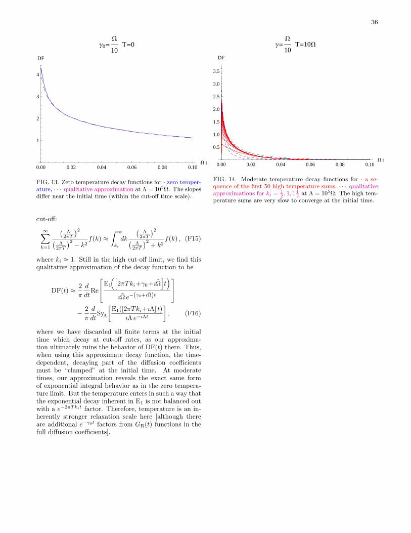
36

0.00 0.02 0.04 0.06 0.08 0.10W t

1

2

3

4

DF

Γ0=W

10T=0

FIG. 13. Zero temperature decay functions for · zero temper-ature, · · · qualitative approximation at Λ = 103Ω. The slopesdiffer near the initial time (within the cut-off time scale).

cut-off:

∞∑k=1

(Λ

2πT

)2(Λ

2πT

)2 − k2f(k) ≈

∫ ∞ki

dk

(Λ

2πT

)2(Λ

2πT

)2+ k2

f(k) , (F15)

where ki ≈ 1. Still in the high cut-off limit, we find thisqualitative approximation of the decay function to be

DF(t) ≈ 2

π

d

dtRe

E1

([2πTki+γ0+ıΩ

]t)

ıΩ e−(γ0+ıΩ)t

− 2

π

d

dtSyΛ

[E1([2πTki+ıΛ] t)

ıΛ e−ıΛt

], (F16)

where we have discarded all finite terms at the initialtime which decay at cut-off rates, as our approxima-tion ultimately ruins the behavior of DF(t) there. Thus,when using this approximate decay function, the time-dependent, decaying part of the diffusion coefficientsmust be “clamped” at the initial time. At moderatetimes, our approximation reveals the exact same formof exponential integral behavior as in the zero tempera-ture limit. But the temperature enters in such a way thatthe exponential decay inherent in E1 is not balanced outwith a e−2πTkit factor. Therefore, temperature is an in-herently stronger relaxation scale here [although thereare additional e−γ0t factors from GR(t) functions in thefull diffusion coefficients].

0.00 0.02 0.04 0.06 0.08 0.10W t

0.5

1.0

1.5

2.0

2.5

3.0

3.5

DF

Γ=W

10T=10W

FIG. 14. Moderate temperature decay functions for · a se-quence of the first 50 high temperature sums, · · · qualitativeapproximations for ki = 1

2, 1, 1 1

2at Λ = 105Ω. The high tem-

perature sums are very slow to converge at the initial time.

37

[1] H. P. Breuer and F. Petruccione, The Theory of OpenQuantum Systems (Oxford University Press, Oxford,2002).

[2] E. A. Calzetta and B. L. Hu, Nonequilibrium QuantumField Theory (Cambridge University Press, Cambridge,2008).

[3] D. Giulini, E. Joos, C. Kiefer, J. Kupsch, L. O. Sta-matescu, and H. D. Zeh, Decoherence and the Appear-ance of a Classical World in Quantum Theory (Springer-Verlag, Berlin, 1996).

[4] W. H. Zurek, Rev. Mod. Phys. 75, 715 (2003).[5] A. O. Caldeira and A. J. Leggett, Ann. Phys. (N.Y.) 149,

374 (1983).[6] A. J. Leggett, S. Chakravarty, A. T. Dorsey, M. P. A.

Fisher, A. Garg, and W. Zwerger, Rev. Mod. Phys. 59,1 (1987).

[7] U. Weiss, Quantum dissipative systems (World Scientific,Singapore, 1999).

[8] M. O. Scully and M. S. Zubairy, Quantum Optics (Cam-bridge University Press, Cambridge, 2007).

[9] P. Meystre, Atom Optics (Springer-Verlag, Berlin, 2001).[10] H. Wisman and G. Milburn, Quantum Measurement and

Control (Cambridge University Press, Cambridge, 2010).[11] A. Naik et al., Nature 443, 193 (2006).[12] M. D. LaHaye, O. Buu, B. Camarota, and K. C. Schwab,

Science 304, 74 (2004).[13] R. P. Feynman and F. L. Vernon, Ann. Phys. (N.Y.) 24,

118 (1963).[14] A. O. Caldeira and A. J. Leggett, Physica A 121, 587

(1983).[15] A. O. Caldeira, H. A. Cerdeira, and R. Ramaswamy,

Phys. Rev. A 40, 3438 (1989).[16] W. G. Unruh and W. H. Zurek, Phys. Rev. D 40, 1071

(1989).[17] B. L. Hu, J. P. Paz, and Y. Zhang, Phys. Rev. D 45,

2843 (1992).[18] J. J. Halliwell and T. Yu, Phys. Rev. D 53, 2012 (1996).[19] E. Calzetta, A. Roura, and E. Verdaguer, Physica A 319,

188 (2003), arXiv:quant-ph/0011097.[20] E. Calzetta, A. Roura, and E. Verdaguer, Int. J. Theor.

Phys. 40, 2317 (2001).[21] G. W. Ford and R. F. O’Connell, Phys. Rev. D 64,

105020 (2001).[22] G. W. Ford, J. T. Lewis, and R. F. O’Connell, Phys. Rev.

A 37, 4419 (1988).[23] C.-H. Chou, B. L. Hu, and T. Yu, Physica A 387, 432

(2008).[24] C. Anastopoulos and J. J. Halliwell, Phys. Rev. D 51,

6870 (1995).[25] B. L. Hu and Y. Zhang, Mod. Phys. Lett. A 8, 3575

(1993).[26] B. L. Hu and Y. Zhang, Int. J. Mod. Phys. A 10, 4537

(1995).[27] M. Hillery, R. F. O’Connell, M. O. Scully, and E. P.

Wigner, Phys. Rep. 106, 121 (1984).[28] C. W. Gardiner and M. J. Collett, Phys. Rev. A 31, 3761

(1985).[29] A. Roura and E. Verdaguer, Phys. Rev. D 60, 107503

(1999).[30] B. L. Hu and A. Matacz, Phys. Rev. D 49, 6612 (1994).[31] J. J. W lodarz, Int. J. Theor. Phys. 42, 1075 (2003).[32] W. H. Zurek, Physics Today 44, 36 (1991).[33] J. P. Paz, S. Habib, and W. H. Zurek, Phys. Rev. D 47,

488 (1993).[34] J. R. Anglin, J. P. Paz, and W. H. Zurek, Phys. Rev. A

55, 4041 (1997).[35] F. C. Lombardo and P. I. Villar, Phys. Lett. A 336, 16

(2005).[36] V. Hakim and V. Ambegaokar, Phys. Rev. A 32, 423

(1985).[37] H. J. Kimble et al., Phys. Rev. D 65, 022002 (2002).[38] A. Buonanno and Y. Chen, Phys. Rev. D 64, 042006

(2001).[39] J. P. Paz and C. A. Roncaglia, Phys. Rev. Lett. 100,

220401 (2008).[40] J. P. Paz and C. A. Roncaglia, Phys. Rev. A 79, 032102

(2009).[41] C. H. Fleming, A. Roura, and B. L. Hu, in preparation.[42] B. L. Hu, A. Roura, and E. Verdaguer, Phys. Rev. D 73,

044002 (2004).[43] H. Grabert, P. Schramm, and G. L. Ingold, Phys. Rep.

168, 115 (1988).[44] L. D. Romero and J. P. Paz, Phys. Rev. A 55, 4070

(1997).[45] H. P. Robertson, Phys. Rev. 46, 794 (1934).[46] D. A. Trifonov, Eur. Phys. J. B 29, 349 (2002).