Evidence for Multiple Labor Market Segments:

An Entropic Analysis of US Earned Income, 1996-2007

Markus P. A. Schneidermarkus.schneider@du.edu

Economics Department - University of Denver

July 18, 2014

Abstract

This paper revisits the fitting of parametric distributions to earned income data. In linewith Camilo Dagum’s dictum that candidate distribution should not only be chosen for fit,but that economic content should also play a role, a new candidate is proposed. The fit of asimple finite mixture performs as well or better than the widely used generalized beta of thesecond kind (GB2) and is argued to be easier to interpret economically. Specifically, the goodfit is taken as evidence for a finite number of distinct labor market segments with qualitativelydifferent generating mechanism. It is speculated that this could be reconciled with either mod-ern search-and-match models in which agent and / or firm heterogeneity can lead to multipleequilibria, or an older theory of labor market segmentation. Regardless, the use of the mixturemodel addresses one of the central weaknesses of testing the older theory of dual labor marketsempirically. The approach taken in this paper is also motivated by the work of E. T. Jaynes, thefather of maximum entropy approaches to statistical inference and related to the recent workby physicists on the distribution of income.∗

Subject Codes C16 - Specific Distributions; D31 - Personal Income, Wealth, and Their Dis-tribution; J01 - Labor Economics: General

Keywords Income Distribution; Informational Entropy; Informational Distinguishability; Sta-tistical Mechanics; Dual Labor Markets

∗I am grateful for the copious and insightful feedback I received from Duncan K. Foley regarding this research.Especially his suggestions regarding the empirical measurement of entropy have made this work stronger. DanieleTavani also provided me with invaluable comments regarding the structure of the paper as well as improvements tothe analysis. Of course, I take full responsibility for all errors herein.

1

1 Introduction

Despite considerable attention across several literatures, the question as to the shape of the ob-

served earnings distribution remains unsettled. In part, this is because different authors - even

whole literatures - have diverse interpretations of the goal of finding a functional description

for the observed distribution. This paper returns to an old idea that the exercise of fitting a

parametric distribution should yield theoretic insights about the underlying generating mech-

anism. Unlike the existing work, however, not only single-distribution models are considered,

thus allowing for explicit (yet finite) heterogeneity in the generating mechanisms. The analy-

sis focuses on the informational content of the observed distribution as captured by Shannon’s

entropy, which permits an informal discussion of how the findings may be reconciled with the

characteristics of the underlying labor market mechanics.

Over the past, several literatures have emerged that attempt to grapple with the shape

of the observed income distribution. Most recently, this has crystalized into two dominant

strands of reasoning: one that focuses on rote fit of a flexible distribution that is then used

for imputation (e.g., Jenkins, Burkhauser, Feng, and Larrymore, 2011) or the calculation of

inequality measures (e.g., Jenkins, 2009; Schneider, 2013), the other focused more on connecting

the fitted distribution with the theoretical implications for labor market mechanics (e.g., Dagum,

1977). This paper offers a new alternative that seems to have been largely overlooked in the

literature to date: there is no reason to believe that incomes are generated by a single mechanism

that should be expected to give rise to a single stationary distribution. Rather, there maybe

good reason to believe that different labor market segments operate in a qualitatively different

way, thus generating different stationary distributions. In fact, the use of a finite mixture model

addresses a key concern when it came to empirically testing older theories of labor market

segmentation. The novel approach taken in this paper is to explore the informational content of

the observed distribution of earned income over a 12 year period to see whether a mixture model

that allows for this kind of heterogeneity performs on par or better than single-distribution

models. The good fit of such a mixture would suggest that the difficulty in reconciling the

observed data with salient stochastic signatures of well-understood processes was unaccounted

for heterogeneity, not the lack of stochastic regularity in the generating process(es).

There is also a literature in physics that started around 2000 with Dragulescu and Yakovenko

(2000) that implicitly proposed a mixture fit to the observed distribution of income. Much of

2

the present work was motivated by that “econophysics” literature, but critical of its eschewing of

formal statistical techniques. In the course of my analysis, several of the claims originating from

the physics literature are evaluated. The results is a set of nuanced conclusions that indicates

that neither complete refutation nor simple vindication of their collective work are warranted.

There is also a key inference issue that makes it difficult to link an observed distribution

to a specific generating mechanism (i.e. concrete micro foundations), as was pointed out by

Jaynes (1979) with respect to classical thermodynamics. The lesson of that paper should be

taken very seriously by economists working with distributional data in general, and even more so

since physicists have started to work with economic data (including the distribution of income).

The information-theoretic approach taken in this paper both introduces it into this literature

in economics, and provides a bridge between physicists’ thinking and econometric intuitions.

The fundamental thinking is actually very close to Camilo Dagum’s: the distribution fit to the

observed data should be chosen to either directly reveal characteristics of the underlying generat-

ing mechanism or at least capture the important identifiable regularities of the microeconomics

(even if all their specifics cannot not be identified, as Jaynes, 1979, would point out). These

regularities can be formalized as the moment constraints in a maximum entropy (ME) program.

The primary criteria for whether a proposed candidate distribution remain distinguishable from

the data is Soofi, Ebrahimi, and Habibullah (1995)’s informational distinguishability index based

on their Kullback-Leibler divergence.

After a more detailed discussion of the literatures connected by this paper, I present the

six candidate distributions whose fit of the earnings data is evaluated. All six simple candidate

distributions imply particular constraints in the ME program, although the GB2 could prove

difficult to interpret rigorously. The exponential and log-normal are chosen for their known

ties to stochastic processes (Champernowne and Cowell, 1998; Silva and Yakovenko, 2005), and

the proposed mixture combines these two for the same reason. The gamma, Weibull and GB2

are chosen for their appearance in the literature as candidates for “good fit” (for examples, see

McDonald, 1984; Bordley, McDonald, and Mantrala, 1997; Kleiber and Kotz, 2003). While the

results are not exhaustive, but they are provocative and insightful. Furthermore, the informal

exploration of their theoretical implications is novel to the recent economics literature.

3

2 Previous Work in Economics and Physics

In his seminal paper, Dagum (1977) spells out three criteria how various authors have chosen

which parametric distribution to fit to income data. In his first and third categories respectively,

distributions are chosen because they may arise out of a stochastic process related to a function-

ing labor market (e.g., the log-normal arising from Gibrat’s Law) or satisfy a set of differential

equations that capture observed regularities (e.g., the Pareto or Dagum distributions). In either

case, the distributions are chosen in some connection to the underlying economics. Dagum also

pointed to a number of authors who’s choice of distribution seemed to be solely based on fit,

among them the gamma, beta, Weibull, and generalized gamma distributions. The generalized

beta of the second kind (GB2) that has become popular recently (e.g. Feng, Burkhauser, and

Butler, 2006; Jenkins, 2009) arguably also belongs in this category.

It is still too common that at least implicitly the distribution of earned income is assumed

to be log-normal. This proposition originates from Gibrat (see Sutton, 1997) and was given

rigorous treatment as early as Kalecki (1945); Champernowne (1953).1 But in so far as the

log-normal is the preferred distribution in Camilo Dagum’s first category of distributions that

can be derived from an explicit stochastic process, it is not supported by the evidence: the fit

of the log-normal was questioned as early as Lydall (1959) and is generally agreed to be lacking

(Champernowne and Cowell, 1998).

Physicists have offered an alternative (and simpler) distribution that should be considered

in Dagum’s first category: the exponential. Suffice it to say that it also does not provide

a satisfactory fit of the income data upon closer inspection, although applying the statistical

mechanics that give rise to it to economics is conceptually intriguing. Since the publication of

Dragulescu and Yakovenko (2000), Dragulescu and Yakovenko (2001a) (who compare Census

and IRS data) and Dragulescu and Yakovenko (2001b), a growing group of physicists has been

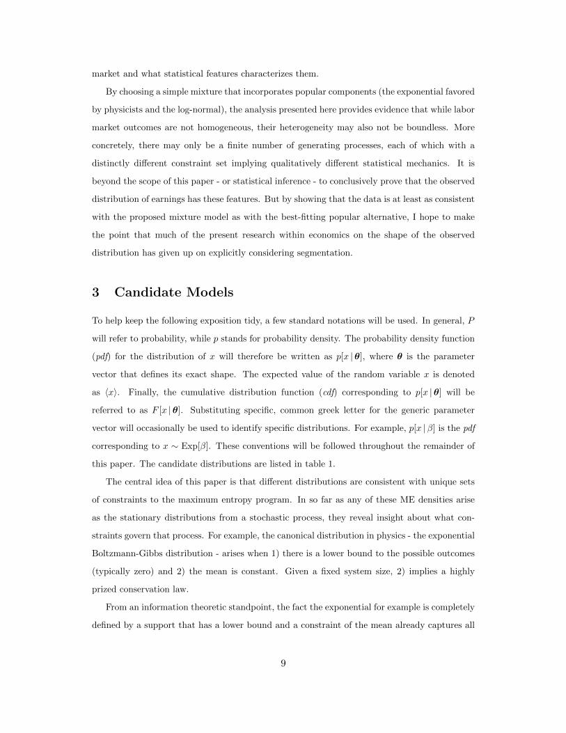
concerned with the characterization of the observed distribution of income. Primarily using

publicly available IRS data of individually filed tax returns, they created graphs like the one

show in figure 1. To arrive at this plot, all incomes in a given year were rescaled by dividing

them by the mean income for that year. Physicists contend that this reveals two striking

features: 1) the cumulative distributions from different years collapse onto the same normalized

1Actually, Kalecki (1945) already pointed out that the original statement by Gibrat was ambiguous as to whetherit would generate a log-normal or power-law stationary distribution.

4

curve (pointed out explicitly in Silva and Yakovenko, 2005)2, and 2) the normalized curve is

roughly linear for a broad range of incomes. These two features have lead to the conclusion that

at a first level of analysis the distribution of income is well-approximated by an exponential

Boltzmann-Gibbs distribution.

ëëëëëëëëëëëëëëëëëëëëëëëëëëëëëëëëëëëëëëëëëëëëëëëëëëëëëëëëëëëëëëëëëëëëëëëëëëëëëëëëëëëëëëëëëëëëëëëëëëëëëëëëëëëëëëëëëëëëëëëëëëëëëëëëëëëëëëëëëëëëëëëëëëëëëëëëëëëëëëëëëëëëëëëëëëëëëëëëëëëëëëëëëëëëëëëëëëëëëëëëëëëëëëëëëëëëëëëëëëëëëëëëëëëëëëëëëëëëëëëëëëëëëëëëëëëëëëëëëëëëëëëëëëëëëëëëëëëëëëëëëëëëëëëëëëëëëëëëëëëëëëëëëëëëëëëëëëëëëëëëëëëëëëëëëëëëëëëëëëëëëëëëëëëëëëëëëëëëëëëëëëëëëëëëëëëëëëëëëëëëëëëëëëëëëëëëëëëëëëëëëëëëëëëëëëëëëëëëëëëëëëëëëëëëëëëëëëëëëëëëëëëëëëëëëëëëëëëëëëëëëëëëëëëëëëëëëëëëëëëëëëëëëëëëëëëëëëëëëëëëëëëëëëëëëëëëëëëëëëëëëëëëëëëëëëëëëëëëëëëëëëëëëëëëëëëëëëëëëëëëëëëëëëëëëëëëëëëëëëëëëëëëëëëëëëëëëëëëëëëëëëëëëëëëëëëëëëëëëëëëëëëëëëëëëëëëëëëëëëëëëëëëëëëëëëëëëëëëëëëëëëëëëëëëëëëëëëëëëëëëëëëëëëëëëëëëëëëëëëëëëëëëëëëëëëëëëëëëëëëëëëëëëëëëëëëëëëëëëëëëëëëëëëëëëëëëëëëëëëëëëëëëëëëëëëëëëëëëëëëëëëëëëëëëëëëëëëëëëëëëëëëëëëëëëëëëëëëëëëëëëëëëëëëëëëëëëëëëëëëëëëëëëëëëëëëëëëëëëëëëëëëëëëëëëëëëëëëëëëëëëëëëëëëëëëëëëëëëëëëëëëëëëëëëëëëëëëëëëëëëëëëëëëëëëëëëëëëëëëëëëëëëëëëëëëëëëëëëëëëëëëëëëëëëëëëëëëëëëëëëëëëëëëëëëëëëëëëëëëëëëëëëëëëëëëëëëëëëëëëëëëëëëëëëëëëëëëëëëëëëëëëëëëëëëëëëëëëëëëëëëëëëëëëëëëëëëëëëëëëëëëëëëëëëëëëëëëëëëëëëëëëëëëëëëëëëëëëëëëëëëëëëëëëëëëëëëëëëëëëëëëëëëëëëëëëëëëëëëëëëëëëëëëëëëëëëëëëëëëëëëëëëëëëëëëëëëëëëëëëëëëëëëëëëëëëëëëëëëëëëëëëëëëëëëëëëëëëëëëëëëëëëëëëëëëëëëëëëëëëëëëëëëëëëëëëëëëëëëëëëëëëëëëëëëëëëëëëëëëëëëëëëëëëëëëëëëëëëëëëëëëëëëëëëëëëëëëëëëëëëëëëëëëëëëëëëëëëëëëëëëëëëëëëëëëëëëëëëëëëëëëëëëëëëëëëëëëëëëëëëëëëëëëëëëëëëëëëëëëëëëëëëëëëëëëëëëëëëëëëëëëëëëëëëëëëëëëëëëëëëëëëëëëëëëëëëëëëëëëëëëëëëëëëëëëëëëëëëëëëëëëëëëëëëëëëëëëëëëëëëëëëëëëëëëëëëëëëëëëëëëëëëëëëëëëëëëëëëëëëëëëëëëëëëëëëëëëëëëëëëëëëëëëëëëëëëëëëëëëëëëëëëëëëëëëëëëëëëëëëëëëëëëëëëëëëëëëëëëëëëëëëëëëëëëëëëëëëëëëëëëëëëëëëëëëëëëëëëëëëëëëëëëëëëëëëëëëëëëëëëëëëëëëëëëëëëëëëëëëëëëëëëëëëëëëëëëëëëëëëëëëëëëëëëëëëëëëëëëëëëëëëëëëëëëëëëëëëëëëëëëëëëëëëëëëëëëëëëëëëëëëëëëëëëëëëëëëëëëëëëëëëëëëëëëëëëëëëëëëëëëëëëëëëëëëëëëëëëëëëëëëëëëëëëëëëëëëëëëëëëëëëëëëëëëëëëëëëëëëëëëëëëëëëëëëëëëëëëëëëëëëëëëëëëëëëëëëëëëëëëëëëëëëëëëëëëëëëëëëëëëëëëëëëëëëëëëëëëëëëëëëëëëëëëëëëëëëëëëëëëëëëëëëëëëëëëëëëëëëëëëëëëëëëëëëëëëëëëëëëëëëëëëëëëëëëëëëëëëëëëëëëëëëëëëëëëëëëëëëëëëëëëëëëëëëëëëëëëëëëëëëëëëëëëëëëëëëëëëëëëëëëëëëëëëëëëëëëëëëëëëëëëëëëëëëëëëëëëëëëëëëëëëëëëëëëëëëëëëëëëëëëëëëëëëëëëëëëëëëëëëëëëëëëëëëëëëëëëëëëëëëëëëëëëë

ëëëëëëëëëëëëëëëëëëëëëëëëëëëëëëëëëëëëëëëëëëëëëëëëëëëëëëëëëëëëëëëëëëëëëëëëëëëëëëëëëëëëëëëëëëëëëëëëëëëëëëëëëëëëëëëëëëëëëëëëëëëëëëëëëëëëëëëëëëëëëëëëëëëëëëëëëëëëëëëëëëëëëëëëëëëëëëëëëëëëëëëëëëëëëëëëëëëëëëëëëëëëëëëëëëëëëëëë

ëëëëëëëëëëëëëëëëëëëëëëëëëëëëëëëëëëëëëëëëëëëëëëëëëëëëëëëëëëëëëëëëëëëëëëëëëëëëëëëëëëëëëëëëëëëëëëëëë

ëëëëëëëëëëëëëëëëëëëëëëëëëëëëëëëëëëëëëëëëëëëëëëëëëëëëëëëëëëëëëëëëëëëëëëëëëëëëëëëëëëëëëëëëëëëëëëëëëëëëëëëëëëëëëëëëëëëëëëëëëëëëëëëëëëëëëëëëëëëëëëëëëë

ëëëëëëëëëëëëëëëëëëëëëëëëëëëëëëëëëëëëëëëëëëëëëëëëëëëë

ëëëëëëëëëëëëëëëëëëëëëëëëëëëëëëëëëëëëëëëë

ëëëëëëëëëëëëëëëëëëëëëëëëëëëëë

ëëëëëëëëëëëëëëëëëëëëëëëëëëëëëëëëëëëëëëëëëëëëëëëë

ëëëëëëëëëëëëëëëëëë

ëëëëëëëëëë

ëëëëëëëëëëëëëëëëëëëëë ëë

ëëëëëëëëëëëëëëëëëë ëëëëë

ëëë ëëëëëëëëëëë ëëëë ëëëë

ëëëëëëë

ëë ë

ëë

ëë

ëë

ëë

ë

DDDDDDDDDDDDDDDDDDDDDDDDDDDDDDDDDDDDDDDDDDDDDDDDDDDDDDDDDDDDDDDDDDDDDDDDDDDDDDDDDDDDDDDDDDDDDDDDDDDDDDDDDDDDDDDDDDDDDDDDDDDDDDDDDDDDDDDDDDDDDDDDDDDDDDDDDDDDDDDDDDDDDDDDDDDDDDDDDDDDDDDDDDDDDDDDDDDDDDDDDDDDDDDDDDDDDDDDDDDDDDDDDDDDDDDDDDDDDDDDDDDDDDDDDDDDDDDDDDDDDDDDDDDDDDDDDDDDDDDDDDDDDDDDDDDDDDDDDDDDDDDDDDDDDDDDDDDDDDDDDDDDDDDDDDDDDDDDDDDDDDDDDDDDDDDDDDDDDDDDDDDDDDDDDDDDDDDDDDDDDDDDDDDDDDDDDDDDDDDDDDDDDDDDDDDDDDDDDDDDDDDDDDDDDDDDDDDDDDDDDDDDDDDDDDDDDDDDDDDDDDDDDDDDDDDDDDDDDDDDDDDDDDDDDDDDDDDDDDDDDDDDDDDDDDDDDDDDDDDDDDDDDDDDDDDDDDDDDDDDDDDDDDDDDDDDDDDDDDDDDDDDDDDDDDDDDDDDDDDDDDDDDDDDDDDDDDDDDDDDDDDDDDDDDDDDDDDDDDDDDDDDDDDDDDDDDDDDDDDDDDDDDDDDDDDDDDDDDDDDDDDDDDDDDDDDDDDDDDDDDDDDDDDDDDDDDDDDDDDDDDDDDDDDDDDDDDDDDDDDDDDDDDDDDDDDDDDDDDDDDDDDDDDDDDDDDDDDDDDDDDDDDDDDDDDDDDDDDDDDDDDDDDDDDDDDDDDDDDDDDDDDDDDDDDDDDDDDDDDDDDDDDDDDDDDDDDDDDDDDDDDDDDDDDDDDDDDDDDDDDDDDDDDDDDDDDDDDDDDDDDDDDDDDDDDDDDDDDDDDDDDDDDDDDDDDDDDDDDDDDDDDDDDDDDDDDDDDDDDDDDDDDDDDDDDDDDDDDDDDDDDDDDDDDDDDDDDDDDDDDDDDDDDDDDDDDDDDDDDDDDDDDDDDDDDDDDDDDDDDDDDDDDDDDDDDDDDDDDDDDDDDDDDDDDDDDDDDDDDDDDDDDDDDDDDDDDDDDDDDDDDDDDDDDDDDDDDDDDDDDDDDDDDDDDDDDDDDDDDDDDDDDDDDDDDDDDDDDDDDDDDDDDDDDDDDDDDDDDDDDDDDDDDDDDDDDDDDDDDDDDDDDDDDDDDDDDDDDDDDDDDDDDDDDDDDDDDDDDDDDDDDDDDDDDDDDDDDDDDDDDDDDDDDDDDDDDDDDDDDDDDDDDDDDDDDDDDDDDDDDDDDDDDDDDDDDDDDDDDDDDDDDDDDDDDDDDDDDDDDDDDDDDDDDDDDDDDDDDDDDDDDDDDDDDDDDDDDDDDDDDDDDDDDDDDDDDDDDDDDDDDDDDDDDDDDDDDDDDDDDDDDDDDDDDDDDDDDDDDDDDDDDDDDDDDDDDDDDDDDDDDDDDDDDDDDDDDDDDDDDDDDDDDDDDDDDDDDDDDDDDDDDDDDDDDDDDDDDDDDDDDDDDDDDDDDDDDDDDDDDDDDDDDDDDDDDDDDDDDDDDDDDDDDDDDDDDDDDDDDDDDDDDDDDDDDDDDDDDDDDDDDDDDDDDDDDDDDDDDDDDDDDDDDDDDDDDDDDDDDDDDDDDDDDDDDDDDDDDDDDDDDDDDDDDDDDDDDDDDDDDDDDDDDDDDDDDDDDDDDDDDDDDDDDDDDDDDDDDDDDDDDDDDDDDDDDDDDDDDDDDDDDDDDDDDDDDDDDDDDDDDDDDDDDDDDDDDDDDDDDDDDDDDDDDDDDDDDDDDDDDDDDDDDDDDDDDDDDDDDDDDDDDDDDDDDDDDDDDDDDDDDDDDDDDDDDDDDDDDDDDDDDDDDDDDDDDDDDDDDDDDDDDDDDDDDDDDDDDDDDDDDDDDDDDDDDDDDDDDDDDDDDDDDDDDDDDDDDDDDDDDDDDDDDDDDDDDDDDDDDDDDDDDDDDDDDDDDDDDDDDDDDDDDDDDDDDDDDDDDDDDDDDDDDDDDDDDDDDDDDDDDDDDDDDDDDDDDDDDDDDDDDDDDDDDDDDDDDDDDDDDDDDDDDDDDDDDDDDDDDDDDDDDDDDDDDDDDDDDDDDDDDDDDDDDDDDDDDDDDDDDDDDDDDDDDDDDDDDDDDDDDDDDDDDDDDDDDDDDDDDDDDDDDDDDDDDDDDDDDDDDDDDDDDDDDDDDDDDDDDDDDDDDDDDDDDDDDDDDDDDDDDDDDDDDDDDDDDDDDDDDDDDDDDDDDDDDDDDDDD

DDDDDDDDDDDDDDDDDDDDDDDDDDDDDDDDDDDDDDDDDDDDDDDDDDDDDDDDDDDDDDDDDDDDDDDDDDDDDDDDDDDDDDDDDDDDDDDDDDDDDDDDDDDDDDDDDDDDDDDDDDDDDDDDDDDDDDDDDDDDDDDDDDDDDDDDDDDDDDDDDDDDDDDDDDDDDDDDDDDDDDDDDDDD

DDDDDDDDDDDDDDDDDDDDDDDDDDDDDDDDDDDDDDDDDDDDDDDDDDDDDDDDDDDDDDDDDDDDDDDDDDDDDDDDDDDDDDDDDDDDDDDD

DDDDDDDDDDDDDDDDDDDDDDDDDDDDDDDDDDDDDDDDDDDDDDDDD

DDDDDDDDDD

DD

DDDDD DDD

++++++++++++++++++++++++++++++++++++++++++++++++++++++++++++++++++++++++++++++++++++++++++++++++++++++++++++++++++++++++++++++++++++++++++++++++++++++++++++++++++++++++++++++++++++++++++++++++++++++++++++++++++++++++++++++++++++++++++++++++++++++++++++++++++++++++++++++++++++++++++++++++++++++++++++++++++++++++++++++++++++++++++++++++++++++++++++++++++++++++++++++++++++++++++++++++++++++++++++++++++++++++++++++++++++++++++++++++++++++++++++++++++++++++++++++++++++++++++++++++++++++++++++++++++++++++++++++++++++++++++++++++++++++++++++++++++++++++++++++++++++++++++++++++++++++++++++++++++++++++++++++++++++++++++++++++++++++++++++++++++++++++++++++++++++++++++++++++++++++++++++++++++++++++++++++++++++++++++++++++++++++++++++++++++++++++++++++++++++++++++++++++++++++++++++++++++++++++++++++++++++++++++++++++++++++++++++++++++++++++++++++++++++++++++++++++++++++++++++++++++++++++++++++++++++++++++++++++++++++++++++++++++++++++++++++++++++++++++++++++++++++++++++++++++++++++++++++++++++++++++++++++++++++++++++++++++++++++++++++++++++++++++++++++++++++++++++++++++++++++++++++++++++++++++++++++++++++++++++++++++++++++++++++++++++++++++++++++++++++++++++++++++++++++++++++++++++++++++++++++++++++++++++++++++++++++++++++++++++++++++++++++++++++++++++++++++++++++++++++++++++++++++++++++++++++++++++++++++++++++++++++++++++++++++++++++++++++++++++++++++++++++++++++++++++++++++++++++++++++++++++++++++++++++++++++++++++++++++++++++++++++++++++++++++++++++++++++++++++++++++++++++++++++++++++++++++++++++++++++++++++++++++++++++++++++++++++++++++++++++++++++++++++++++++++++++++++++++++++++++++++++++++++++++++++++++++++++++++++++++++++++++++++++++++++++++++++++++++++++++++++++++++++++++++++++++++++++++++++++++++++++++++++++++++++++++++++++++++++++++++++++++++++++++++++++++++++++++++++++++++++++++++++++++++++++++++++++++++++++++++++++++++++++++++++++++++++++++++++++++++++++++++++++++++++++++++++++++++++++++++++++++++++++++++++++++++++++++++++++++++++++++++++++++++++++++++++++++++++++++++++++++++++++++++++++++++++++++++++++++++++++++++++++++++++++++++++++++++++++++++++++++++++++++++++++++++++++++++++++++++++++++++++++++++++++++++++++++++++++++++++++++++++++++++++++++++++++++++++++++++++++++++++++++++++++++++++++++++++++++++++++++++++++++++++++++++++++++++++++++++++++++++

++++++++++++++++++++++++++++++++++++++++++++++++++++++++++++++++++++++++++++++++++++++++++++++++++++++++++++++++++++++++++++++++++++++++++++++++++++++++++++++++++++++++++++++++++++++++++++++++++++++++++++

++++++++++++++++++++++++++++++++++++++++++++++++++++++++++++++++++++

++++++++++++++++++++++++++++++++++++++++++++++++++++++++++++++++++++++++++++++++++++

+++++++++++++++++++++++++++++++++++++++++++++++++++++++

++++++++++++++++++++++++++++++++++

++++++++++++++

0 1 2 3 4 5 6 70.01

0.1

1

10

100

Earned Income HRescaledL

Cum

ulat

ive

Perc

ento

fO

bser

vatio

ns,%

Earned Income Distribution - All Income Earners

+ 2006

D 2001

ë 1996

Figure 1: The figure shows the complimentary cumulative distribution of rescaledincomes for single respondents to the CPS (who would file individual tax returns)as plotted by physicists to demonstrate exponential behavior.

Silva and Yakovenko (2005) proposed that the bulk of the income distribution is exponential

with a power-law tail for high incomes, which has been interpreted as a two-class structure to the

income distribution.3 The same graphical arguments discussed above lead to these conclusions

(see Yakovenko, 2009, for a summary of this research project). Silva and Yakovenko (2005)

furthermore claim that the exponential portion of the income distribution corresponds to wage

and salary income, while the power-law portion corresponds to investment income. The first

claim is of central interest to the research presented in this paper, as the questions whether the

distribution of wage and salary income is exponential is addressed directly herein.

Physicists are eager to find exponential behavior in distributional data, because they are

2This collapsing of the distributions from different years would be expected when only the value of a pure locationparameter changes from year to year. More importantly it suggests that type of distribution that fits the data doesnot appear to have changed over time.

3In fact, this has become the received wisdom in “econophysics” as seen in the summary provided by Chatterjee,Sinha, and Chakrabarti (2007).

5

extremely familiar with processes leading to an exponential stationary distribution. This is

the canonical distribution of kinetic energies in a fixed volume of a perfect gas, for example,

and generally processes with a single conservation law. Assuming that the process is entropy

maximizing, the exponential implies a single constraint on the first moment (together with a

finite lower bound of the support of the distribution). Given a fixed volume, the moment con-

straint is consistent with a conservation law and the core group of researchers quickly postulated

that money was conserved in the transactions underlying the distribution of income - at least

in the time frame necessary for labor markets to reach some kind of statistical equilibrium.

They quickly proposed several agent-based models with random binary interactions in which

the amount of money exchanged is conserved to reproduce a stationary exponential distribution

of money incomes (again see Yakovenko, 2009).

This work has been largely ignored by economists for several reasons, not the least of which is

that the conservation of money is an implausible proposition as even Dragulescu and Yakovenko

(2001a) acknowledge (McCauley, 2006, provides a scathing review). Furthermore, the central

features taken as conclusive evidence for exponential behavior in the distribution of income are

less convincing than the physicists are willing to admit. (They are not helped by their general

distrust of formal statistical techniques in this regard.) Perceiving linearity in figure 1 (or those

featured for example in Dragulescu and Yakovenko, 2001a, , especially B in the inset of Figure

2) is largely in the eye of the beholder. May be the data appears linear, but clearly it has a

slope different from one as would be consistent with Z ∼ Exp[1]. It is also not at all clear that

more rigorous fit criteria would not reject the fit of an exponential distribution. To validate

the physicists’ claim, the fit of the exponential is evaluated for all respondents in the dataset4

and for single respondents using both the ID index as well as several other well-established fit

criteria.

In the opposing category are distributions chosen only for their fit of the data. These

include the gamma and Weibull (Dagum, 1977), GB2 (McDonald, 1984; Feng et al., 2006), and

the multi-parameter generalized exponential found by Wu (2003). The analysis offered by Wu

(2003) illustrates that the blind search for a better functional fit need not provide greater insight

about how the observed distribution is generated. The algorithm suggested by Wu (2003) is to

add pairs of polynomial constraints until the fit of the resulting pdf cannot be rejected based

4The result for all respondents was implicitly foreshadowed by the findings presented in Wu (2003), who byconstruction ruled out the exponential distribution.

6

on whatever fit criteria the researcher chooses. The underlying ME program is shown in (1) for

k moment constraints that incorporate the actual data by substituting the sample estimates µi

for µi. The general solution to this constrained maximization is given by (2) where the λs are

the Lagrange multipliers.

p∗[x] = argmaxp[x]

∫∞−∞ p[x] ln p[x] dx

s.t.∫∞−∞ xi p[x] dx = µi ∀ i = 0, 1, . . . , k

(1)

p∗[x] = exp

[−λ0 −

k∑i=1

λi gi[x]

](2)

where g0[x] = 1 and µ0 = 1 guarantees that p[x] is a proper continuous probability density

function over the support x ∈ [−∞,∞].

Wu (2003)’s method is attractive because it self-selects relevant information to include in

the estimation in the form of moment constraints, but the types of constraints used by Wu

(2003) limit the type of information that is used. Specifically, he does not include moment

constraints on the log of x, precluding either log-normal or power-law behavior in the data

and fundamentally failing to capture scale effects that have long been implicitly recognized as

relevant (for example, as implied by Gibrat’s Law). On the contrary, characterizing the income

distribution as a 8- to 12-parameter member of the exponential family provides little meaningful

insight. One possibility for Wu (2003)’s discovery that so many constraints are needed is that

his automatic method is attempting to provide a polynomial approximation for missing log-

constraints. Extensions to Wu (2003) that incorporate more general constraints can be found

in Wu and Perloff (2003), Wu and Stengos (2005), and Wu and Perloff (2007), but these are not

applied to the individual income data that is the focus of this study.

Despite the shortcomings in Wu (2003)’s analysis as applied to the income distribution, the

idea of searching for binding constraints in the ME program is worthwhile. If the data was

generated by an entropy-maximizing stochastic process, then these suggest what the character-

istics of that process are. Foley (1994) argues that markets are in fact entropy maximizing in a

very formal sense because agents with imperfect information are continuously seeking to exploit

7

open trades, and this could be seen as providing explicit justification to the fitting of a ME

densities to the observed distribution of prices. Furthermore, Jaynes (1979) writes that even if

the underlying process is not entropy maximizing, fitting the data in a manner consistent with

an ME program is the appropriate thing to do because it should provide the most appropriate

description of the data and the identifiable characteristics of the generating mechanism with-

out inferential over-reach. All six base candidate distributions considered in this paper can be

constructed as maximum entropy probability densities revealing the binding constraints on the

ME program (Borzadaran and Behdani, 2009).

The idea of fitting an explicit (or implicit mixture) model to income data is not new.5

However, in the context of uncovering the shape of the observed distribution of earned incomes,

and extrapolating features of the underlying generating mechanism, finite mixture models seem

to be underutilized. Yet as Arcidiacono and Jones (2003) point out, they are a useful tool for

uncovering unaccounted for heterogeneity (extensive reviews of finite mixture models are given in

Lindsay, 1995; McLachlan and Peel, 2000). Recent approaches along this line of thinking come

from Silva and Yakovenko (2005) and Li, Wang, and Chen (2004), though neither considers

models that allow the mixture components to overlap (see also Yuqing, 2007; Gonzalez-Estevez,

Cosenza, Lopez-Ruiz, and Sanchez, 2008). Their modeling implausibly implies that there are

hard cut-off incomes that separate the different labor market processes characterized in their

discussions of the mixtures that they fit to the data.

The underlying economic question is whether we can distinguish the number and shapes of

the most likely statistical distributions of various types of workers’ earnings without appealing to

measurable characteristics of each worker type or artificially imposing hard boundaries between

expected outcomes.6 This approach actually answers an old question in the literature on labor

market segmentation, which struggled to empirically characterize outcomes in each segment

without ad hoc sorting workers into each proposed segment (see Osterman, 1975). By comparing

the fit of a mixture of ME densities to an equally complex single parametric distribution that

might be interpreted to simply represent an unspecified amalgam of many generating processes’

signatures, the present analysis begins to address the how many segments are there in the labor

5Simplistically, any wage equation containing one or more dummy variables could be described as fitting a mixturemodel to economic data. Quandt and Ramsey (1978) discuss the potential difficulties of estimating mixture models,but also provide an illustrative example where a mixture model is used to identify the heterogeneity in wage bargainingbased on a threshold in changes of costs of living (based on Hamermesh, 1970).

6In a sense, this amounts to a clustering analysis or a version of random effects analysis, though the latter is morefocused on controlling for said effects than characterizing them.

8

market and what statistical features characterizes them.

By choosing a simple mixture that incorporates popular components (the exponential favored

by physicists and the log-normal), the analysis presented here provides evidence that while labor

market outcomes are not homogeneous, their heterogeneity may also not be boundless. More

concretely, there may only be a finite number of generating processes, each of which with a

distinctly different constraint set implying qualitatively different statistical mechanics. It is

beyond the scope of this paper - or statistical inference - to conclusively prove that the observed

distribution of earnings has these features. But by showing that the data is at least as consistent

with the proposed mixture model as with the best-fitting popular alternative, I hope to make

the point that much of the present research within economics on the shape of the observed

distribution has given up on explicitly considering segmentation.

3 Candidate Models

To help keep the following exposition tidy, a few standard notations will be used. In general, P

will refer to probability, while p stands for probability density. The probability density function

(pdf) for the distribution of x will therefore be written as p[x |θ], where θ is the parameter

vector that defines its exact shape. The expected value of the random variable x is denoted

as 〈x〉. Finally, the cumulative distribution function (cdf) corresponding to p[x |θ] will be

referred to as F [x |θ]. Substituting specific, common greek letter for the generic parameter

vector will occasionally be used to identify specific distributions. For example, p[x |β] is the pdf

corresponding to x ∼ Exp[β]. These conventions will be followed throughout the remainder of

this paper. The candidate distributions are listed in table 1.

The central idea of this paper is that different distributions are consistent with unique sets

of constraints to the maximum entropy program. In so far as any of these ME densities arise

as the stationary distributions from a stochastic process, they reveal insight about what con-

straints govern that process. For example, the canonical distribution in physics - the exponential

Boltzmann-Gibbs distribution - arises when 1) there is a lower bound to the possible outcomes

(typically zero) and 2) the mean is constant. Given a fixed system size, 2) implies a highly

prized conservation law.

From an information theoretic standpoint, the fact the exponential for example is completely

defined by a support that has a lower bound and a constraint of the mean already captures all

9

the relevant features of the generating mechanism.7 The only concern here is which ME density

(or combination of ME densities) actually appears most consistent with the distribution of

earnings data. For example, jumping from the exponential to the Gamma distribution adds

a log-constraint that implies the importance of scale effects in the data.8 All the candidate

distributions considered are supported on x ∈ [0,∞] since negative earnings have no economic

meaning.

The use of a mixture model is one way of looking for heterogeneity that is not captured

by single-distribution models and may be difficult to account for explicitly a priori. Suffice

it to say that the mixture model proposed here is well-behaved in the sense that estimation

and identification are not issues. The pooled distribution’s pdf is the weighted average of the

component distributions, (3), where A ∈ [0, 1] is the contribution of component 1 to the final

mixture. The specific mixture model used in this analysis combines the two most popular ME

densities in both the physics and economics literature respectively: the exponential (p[x |β])

and log-normal distributions (p[x |µ, σ]).

p[x |A, β, µ, σ] = A p[x |β] + (1−A) p[x |µ, σ] (3)

The proposed mixture does not address the possibility of a fat tail on the distribution of

earnings. This consideration is omitted for several reasons, the most basic being that the data

is inappropriate for estimating the weight and shape of the tail of the distribution. My analysis

thus only focuses on fitting the proposed candidate models to the truncated lower majority of

all earnings. Additionally, adding a power-law component to the mixture could easily lead to

a specification that violates the required conditions for identifiability of the parameters. Before

turning to the practical issues related to the data in section 5, I want to first clarify how the fit

of each of the candidate models will be assessed.

TABLE 1 HERE

7While physicists have been quick to jump to the conclusion that there is a similar conservation law in economics,this need not be the case. For example, it has not been explored whether competition for relative wages could also bemean-preserving and therefore provide the appropriate constraint to give rise to a exponential distribution of wagesin equilibrium.

8Further substituting the mean constraint with a constraint on⟨xβ

⟩leads to the Weibull, which is a flexible,

two-parameter distribution whose cdf can have segments that appear exponential for limited ranges of the support.Both the Gamma and Weibull degenerate into the exponential distribution when the shape parameter is equal toone.

10

4 Assessing Fit

Conceptually the information-theoretic analysis presented in this paper is modeled on E. T.

Jaynes’s analysis of Wolf’s dice data (Jaynes, 1979). The Swiss astronomer R. Wolf tossed a

die 20,000 times and tabulated the outcomes as part of a series of probability experiments.

The calculated mean of the recorded observations turned out to be 3.5983, raising the question

whether the die was indeed “fair” or if the data suggested unaccounted for information. By

looking only at the measured entropy, Jaynes deduced that Wolf’s die had imperfections and

further used the maximum entropy formalism to postulate two missing constraints. These turned

out to accurately identify the die’s geometric imperfections in two dimensions!

Given the correct parameterization, each of these distributions implies a unique entropy, S[θ].

If noiseless data was generated from one of these distributions, then the measured empirical

entropy, S, should be less than the entropy of the distribution from which it was generated.

S ≤ S[θ]

Furthermore, it has been shown that the difference between S and S[θ] is exponentially

distributed and depends on the sample size in such a way that when n is large, the empirical

entropy should be very close to that of the correctly parameterized underlying distribution. If

the empirical entropy is larger than that suggested by a distributional model parameterized with

θ, then the model implies too many binding constraints in the ME program: the model is more

restrictive than the data justifies.9 Conversely, if S is much less than S[θ], then the information

provided by the data has not been completely exploited and there are additional constraints

that appear to be binding that were not included in the underlying ME program.10

Jaynes (1979)’s analysis of Wolf’s dice data based on raw entropy comparisons is the concep-

tual archetype for the approach taken in this paper based on the relationships outlined above.

But rather than relying on a comparison of raw entropy, the present analysis is based on the

informational distinguishability of an ME density from the data due to Soofi et al. (1995). The

entropy difference between two distributions is formalized by the Kullback-Leibler divergence,

9A different way of understanding this is to say the data is consistent with a multitude of other combinations ofmicro-states that are ruled out by the constraints included in the ME program.

10An easy example is to suppose the distribution of income is uniform, implying that the only binding constraintsare a lower and upper limit to observed incomes. The entropy consistent with this assumption is much greater thanthe entropy measured from the income data, suggesting that it is far from exploiting all the information provided bythe data.

11

DKL, and Soofi et al. (1995) propose an index, (4), as a measure of distinguishability between

two distributions: the observed data, p, and an ME density, p∗[x |θ] (shortened to p∗ below).

ID [p : p∗] = 1− exp [DKL[p : p∗]] (4)

This index of informational distinguishability, ID, takes a value between 0 and 1, and has

two uses according to Soofi et al. (1995). First, the observed distribution is not distinguishable

from a proposed ME density if ID[p : p∗] ≈ 0. Furthermore, two distributions, p1 and p2, are

not distinguishable based on a reference density if ID[p1 : p∗] ≈ ID[p2 : p∗]. Consistent with

the examples given by Soofi et al. (1995), the observed distribution, p, is the earned income

distribution based on CPS data and remains fixed and p∗ represents the candidate ME density.

The leap is that ID[p : p∗1] ≈ ID[p : p∗2] is interpreted as the data not providing sufficient

information to differentiate which candidate density (p∗1 or p∗2) better describes the observed

distribution.11

Changes in ID can be assessed using the relative information (RI) being taken advantage of

by adding a constraint (Soofi et al., 1995). For example, fitting an exponential (p∗1[x |β]) and a

gamma (p∗2[x |α, β]) distribution to the data means that in the latter instance, a constraint on

the first moment of the log of x is added to the ME program. This will decrease ID by some

amount, with the relevant question being whether the addition of the constraint provides a big

enough improvement in fit to favor the Gamma over the exponential. The relative information

provides an indicator of how much of a contribution the added constraint makes. It is also

indexed to take a value between 0 and 1, with a value close to 0 indicating that the contribution

was negligible.

RI = 1− ID [p : p∗2]

ID [p : p∗1](5)

where p∗1 is the density with fewer constraints to ensure that 0 < RI < 1.

There are two potential pitfalls to using the method alone to make judgements about which

distribution best fits the data. The first is that θ has to be estimated. There is theoretically no

guarantee that S[θ] = S[θ], but for sufficiently large samples the differences should be small.

11This leap is justified by recognizing that ID is a distance measure and therefore necessarily symmetric. A furthermodification is that a mixture of ME densities is proposed, so that ID[p : p+[x |A,θ1,θ2]] (where p+ is the pdf ofthe mixture) is used to assess the distinguishability of the observed distribution from a reference density that is notan ME density.

12

The bigger caveat to this approach is that the data being used in this study is not noiseless

(shown in the next section) as ME analysis presumes (Jaynes, 1982).

The analysis is based on the assumption is that the data is error free or at least that the

observational errors have a negligible impact on the measured entropy. It is trivially untrue that

the data is error-free, but a simulation based analysis suggests that the impact on measured

entropy may indeed be small (see Appendix). To provide a sense for the robustness of the re-

sults, in addition to the index of informational distinguishability (ID), the Kolmogorov-Smirnov

statistic (DKS) and the Bayesian and Akaike Information Criteria (BIC and AIC respectively)

are also calculated for each candidate distribution.

4.1 Measuring Entropy

The relevant definition of entropy is a reduced version of Jaynes-Shannon’s informational entropy

as given by (6). This entropy captures the amount of uncertainty represented by a particular

distribution given by p[x;θ].12

S = −∫ ∞−∞

p[x |θ] · ln[p[x |θ]

m[x]

]dx (6)

The Lebesgue measure, m[x], is used to normalize p[x;θ] over the event space in order to

adjusts for how the support of p[x;θ] is divided. Typically, the support of the pdf is broken

up into equal intervals, which means that m[x] is a constant, m. To simplify things further,

it is often assumed that this reference measure is uniform and of magnitude one, which is the

equivalent of stating that reference intervals into which the support is divided are even-sized,

unit-length intervals. This is often a casual assumption, but it is important to make this very

clear when empirical measurements of entropy are compared to hypothetical maxima based on

a fitted distribution. Given a discrete set of observations sorted into k even-sized consecutive

bins of width ∆x, the entropy can be approximated by the Riemann sum:

S = −k∑i=1

pi · ln [ pi ] ∆x

The probability density assignment, pi, depends only on the observed data, and the implicit

12As stated, x is a continuous variable that can take all values between −∞ and ∞. Limiting the support ofp[x] to a finite range of values of x simply requires letting p[x |θ] = 0 ∀x /∈ [a, b], effectively changing the boundsof integration. For discrete distributions, the integration is replaced by a summation, but no substantive differencesarise.

13

prior assumption in my analysis is that each observation is equally likely. The height associated

with each bin then becomes the number of observations that fall into that bin, fi, which can be

converted into a probability density by dividing by the bin-width and normalizing so that the

probabilities of all bins sum to one. Hence, the probability density induced by the observations of

x falling into the ith bin is pi = fin∆x . Substituting this expression into the equation above leads

to an easily calculable measure of the empirical entropy, (7). Note that the bin-width appears

in the log term of (7). This is no coincidence: it effectively adjusts the probability density

assignment for a bin-size that is different from the assumption that the Lebesgue measure in

(6) is m = 1.

S = −k∑i=1

fin· ln[

fin∆x

](7)

The entropy of the data, S, can now be compared to the entropy implied by a particular

density fit to the data, S[θ]. Given the large n available via the CPS data used in this study, it

makes sense to re-write the guiding principle behind my analysis based on entropy comparison

as (8). The practical evaluation of (8) relies on Soofi et al. (1995)’s ID index discussed above.

S ≈ S[θ] (8)

The estimated parameters, θ, for each candidate distribution were found by maximizing the

likelihood of observing the data given the particular parameters, as suggested by Soofi et al.

(1995). Given that the observation xj appears νj times in the data, the expression for the

log-likelihood adjusted for the truncated sample (see next section) is (9).

lnL =

n∑j

νj lnp[xj |θ]

1− F [xmax |θ](9)

The log-likelihood function was maximized using Mathematica’s internal numerical maxi-

mization function NMaximize.

14

5 Annual Earnings Data

The data used for this study comes from the Annual Socio-Economic survey (ASEC),13 which

is a supplement to the Current Population Survey (CPS) published by the Census Bureau. The

ASEC collects economic and demographic information at the individual and household level.

Weights (MARSUPWT) are provided that match the representativeness of observations in the

ASEC to the larger CPS. In the analysis that follows, the weights are rescaled so that they add

to the number of actual observations collected, and interpreted as the frequency with which

each observation appears in the data, νj .

Since the variable of interest is earned labor income, the variable used is WSAL VAL, which

combines the total wage and salary income reported from a primary job before deductions

(ERN VAL) and earnings from other job(s). All reported earnings are for the previous year,

e.g. the recorded earnings for 2001 reflect the respondents best estimate of his or her earnings

in 2000. The population of interest is the working-age workforce defined as all individuals

between ages 18 to 64 reporting a positive, non-zero wage and salary income less than or equal

to $150,000. The cut-off value was chosen because the CPS data is top-coded for incomes above

$150,000 from a primary job, and is incorporated into how parameters are estimate but treating

all observations as coming from a truncated distribution in (9).

The top-coding of reported incomes unfortunately also affects incomes below the top-code

limit thanks to the imputation of missing values. The imputation procedure combined with low

top-coding limits for income from secondary sources (see Appendix) means that the produced

distortion are not restricted to high incomes (Burkhauser, Feng, Jenkins, and Larrimore, 2008;

Federal Committee on Statistical Methodology, 2005). By ignoring observations from the upper

tail and treating the individual income reports below the top-code limit as coming from a

truncated sample, the bulk all of the distortions should nonetheless be addressed - at least this

is an implicit assumption of the present analysis.

There is also strong evidence for power-law behavior in the upper tail of the distribution

(Silva and Yakovenko, 2005; Bloomquist and Tsvetovat, 2007), which could distort the results of

the present analysis since many of the simpler ME densities considered14 nor the mixture model

as specified in (3) can account for a fat tail. For all years from 1996 to 2007, more than 97.5% of

13The March Supplement to the CPS.14The Dagum and GB2 distribution are capable of modeling fat tails, but the shape of the tail is beyond the scope

of this study.

15

the wage and salary income distribution was included in the present analysis, and the focus of

my analysis is really the characterization of this bottom majority of the observed earnings data.

Sample sizes vary from year to year, with a notable jump due to a procedural change after 2001.

Data sets range from 59,800 to 62,400 observations for the years from 1996 to 2001, and from

92,100 to 98,900 observations for the years from 2002 to 2007 (see table 4 in the Appendix).

The studies by physicists (Dragulescu and Yakovenko, 2000, 2001a,b; Silva and Yakovenko,

2005) primarily used income reported on individually-filed tax returns as their sample.15 Using

the ASEC data, it is not possible to recreate the same subsample since filing status is not

reported. Instead, marital status is used as a proxy to select income reports from individuals

that would not be eligible or likely to file a joint return. “Single” respondents are defined as

all respondents who reported “never married,” “divorced,” “widowed,” or “separated” as their

marital status. The results for “singles” serve as a baseline to compare to those presented by

physicists using IRS data, but no other significance is attached to looking at that particular

sub-group.

The calculation of the entropy of an empirical distribution requires the data to be binned.

Simulations have shown that the calculated value of the entropy is relatively insensitive to bin-

size as long as the bins are sufficiently large. For the purposes of entropy calculations, the data

was sorted into $5000-bins, with each binned assigned an observed frequency equal to the sum

of the re-weighted MARSUPWT of all the observations falling into a particular bin. The other

fit criteria (DKS , BIC, and AIC) are not calculated using the binned data and therefore are

unaffected by changes in bin-size.

6 Results

Consider the hypothetical situation that income observations where uniformly distributed be-

tween $0 and $150,000, and that the data was binned into 30 $5,000-wide bins. The maximum

entropy consistent with these minimal constraints is ln[30 · 5000] = 11.92 nats. The empirical

entropy calculated from the binned data ranges from 11.07 nats in 1996 to 11.41 nats in 2007,

suggesting the obvious: incomes are not uniformly distributed and the observed distribution

15The justification for the econophycisists’ choice to use only individually filed income returns is that this excludesthe effects of household decisions about job choice and the allocation of work in the home. This argument is dubious inthe U.S. since being married does not legally require spousal partners to file jointly. The decision to file as individuals,therefore, is a household decision.

16

suggests more structure than is provided by a uniform distribution. Each candidate distribution

shown in table 1 that was fit to the data represents a different constraint set that might better

capture the unaccounted for information provided by the data.

Proceeding systematically, one could ask whether adding a single constraint to the ME pro-

gram is sufficient to explain the entropy discrepancy. Representing the entropy discrepancy

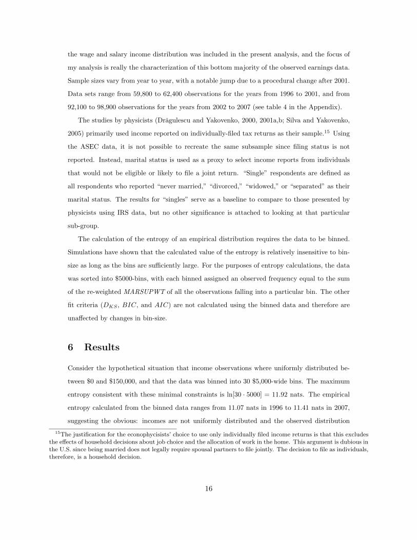
using the index of informational distinguishability, ID, the fit of all candidate distributions

applied to the earned income data from 1996 to 2007 can be seen in figure 2. A lower value of

ID suggests a better match between the information provided by the data and the candidate

distribution relative to a common reference (the uniform distribution). Adding only a mean

constraint (i.e. fitting an exponential to the observed distribution) does not appear to be suf-

ficient to explain the entire entropy discrepancy. Notably however, the exponential provides a

better - certainly more parsimonious - description of the data than the log-normal (which adds

to log moment constraints) for all years. That said, neither the exponential or log-normal alone

provide as good of a match in entropy as the other candidates considered.

Considering also scale effects by fitting the gamma distribution provides a further notable

improvement over either the simpler exponential or the similarly complex log-normal. Addi-

tionally replacing the first moment constraint with a constraint on⟨xβ⟩

(Weibull) improves fit

slightly further. Increasing the complexity of the candidate distribution to the Dagum, a further

substantial improvement is achieved, while going to the GB2 or the mixture model yields only

a minor improvement over the Dagum in most years. If parsimonious fit were the only criteria,

the results shown in figure 2 might well be interpreted as favoring the Dagum distribution as

the best functional description of the distribution of earned income below $150k.

The average information gain in terms of the relative information, RI, by going from the

exponential to the gamma is 0.60, suggesting that 60% of the information left unused by the

exponential is taken advantage of by the gamma distribution. The Dagum, by contrast, yields

an average relative information gain of 0.80 over the exponential and 0.46 over the Weibull

(which is slightly preferable to the gamma).

By contrast, the improvement of using the GB2 instead of the Dagum is only 0.054 on

average. Looking at the raw entropy calculations, the Dagum distribution’s average entropy is

about 0.07 nats less than that of the data, while the GB2’s is 0.14 nats less. Strictly speaking

this suggests that both models are overly restrictive. The mixture model’s entropy is on average

only 0.03 less than the data’s and indeed the relative information gain of the mixture is 0.56

17

+

+ +

+

+

++ +

++ +

+

ëë

ë

ë

ë

ëë ë

ëë

ëë

DD D D

D D DD

D D D D

�� � �

�� �

�� �

� �

´´ ´ ´ ´

´ ´´

´´ ´

´

×× × × ×

× ××

×× ×

×

–– – – –

– ––

–– –

–

1996 1997 1998 1999 2000 2001 2002 2003 2004 2005 2006 2007Year

0.01

0.02

0.03

0.04

0.05

0.06

0.07

ID@p,p*@xDD

Informational Distinguishability of ME Densities from the Earned Income Distrbution

HCPS ASEC Data for All Respondents, 1996 - 2007L

+ Exponential

ë log-Normal

D Gamma

� Weibull

´ Dagum

× GB2

– Mixture

Figure 2: The figure shows the calculated value of the distinguishability index,ID [p : p∗[x]], for each ME density and the exponential / log-normal mixture fit tothe ASEC income data for every year from 1996 to 2007 (all respondents).

over the Dagum and 0.66 over the GB2.16 Hence upon closer inspection, the mixture model

composed of an exponential and a log-normal component appears to exploit the information

provided by the earned income data notably better than either the Dagum or the GB2 by

imposing a less restrictive set of constraints.

The mixture model also offers some very favorable features with regards to economic in-

terpretation: it suggests that the observed distribution of earned income is the pooled set of

outcomes from a finite number of labor market segments, each of which has a simple distri-

butional signature that can be modeled as arising from a tractable stochastic process. While

especially the GB2 is a flexible distributions that fits the data well, interpreting it as a stationary

distributions resulting from a specific generating mechanism has little precedent in economics.

Worse, its apparent good fit implies both imposing informationally overly restrictive model that

nonetheless leaves information provided by the data unused.

To evaluate the robustness of these conclusion, two other fit criteria are considered below.

First, the K-S statistic also shows that the exponential / log-normal mixture model provides

an improvement over all the other candidates except the GB2 in all years, as shown in figure

3. The mixture model and the GB2 perform on par based on the K-S statistic. Note that no

formal statistical test of fit is provided to accompany the K-S statistic. One reason for not being

able to formally test fit is that the sampling distributions of the K-S statistic are only valid if

16The least RI gain by the mixture is 0.41 over the Dagum and 0.49 over the GB2 in 1997 for both cases.

18

the parameters of the fitted distribution are not estimated from the data. This would be easy

to get around using bootstrap standard error estimates, but doing so would not address the

second, more fundamental issue: the data is assumed to be error-free, which turns out to be a

poor assumption.

++ +

++

+

++

+ + + +

ë

ë ë

ë

ë

ë

ë

ë

ë

ë ëë

D D DD

D D

D D D D D D

* * * ** *

* * * * * *

� �� � � �

�� � �

� �

ë ëë

ë ëë

ëë

ëë ë

ë

´ ´´ ´ ´ ´

´ ´ ´ ´ ´´

1996 1997 1998 1999 2000 2001 2002 2003 2004 2005 2006 2007Year

5

10

15

20

25

30

DKS

K-S Statistic: ME Density vs. Earnings Data

HAll Respondents, 1996 - 2007L

+ Exponential

ë log-Normal

D Gamma

* Weibull

� Dagum

ë GB2

´ Mixture

Figure 3: Values of the Kolmogorov-Smirnov fit statistics across years and can-didate distributional models. The fit of the 3-parameter Dagum distribution, the4-parameter GB2, and 2-component (4-parameter) mixture appear similar, and allfit notably better than the 2-parameter alternatives.

Without specifying an error process or smoothing the data, the K-S statistic can be mislead-

ing because absolute deviations between the observed cumulative distribution and the candidate

cdf might arise from either misfit or observational errors. Note that the data is clearly noisy as

apparent in both figures 4a and 4b. Using a filter to smooth the data distribution or comparing

the candidate model to a kernel density estimated cdf instead of the raw data might allow one

to recover a statistical test for fit based on the K-S statistic, but developing such a technique is

beyond the scope of this paper. For most of the candidates - like the Weibull - the deviations

due to misfit are of a different magnitude than the deviations due to noise (i.e. fit can be soundly

rejected). However, comparing the GB2 and the mixture model requires a more subtle analy-

sis. The GB2 does show signs of systematic misfit at low incomes across all years. While the

magnitude of the largest absolute deviation offers little distinction as shown in figure 3, looking

at all the deviations across the range of the data does suggest a substantively better fit of the

mixture model as illustrated for 2006 in figure 4.

Wu (2003) likely encountered similar issue in fitting his general ME density to the income

19

1000 2000 3000 4000 5000i

-6

-4

-2

2

4

6

DKS

Kolmogorov-Smirnov Statistic Plot

Divergence between fitted CDF and Cumulative Frequencies

(a) GB2 Distribution

1000 2000 3000 4000 5000i

-4

-2

2

4

6

DKS

Kolmogorov-Smirnov Statistic Plot

Divergence between fitted CDF and Cumulative Frequencies

(b) Exponential / Log-Normal Mixture

Figure 4: The plots above (shown for the 2006 data) show the discrepancy betweenthe observed cumulative distribution and a fitted distribution. The solid red lineindicates the critical value of the K-S statistic at the 5% significance level if theparameters had not been estimated from the data. Note the systematic mismatchbetween the cdf of the GB2 and the cumulative distribution of the data over thefirst 2500 observations.

data. To arrive at a solution that “fit” the data, he randomly sampled 5,000 observations

from the CPS data, effectively relaxing the fit requirement by reducing the√n term in the

K-S statistic. Despite this tactic, the conclusion Wu (2003) reached was that 8 to 12 moment

constraints in the ME program where necessary to provide a satisfactory fit of the observed

data. The most complicated models presented here, the GB2 and the exponential / log-normal

mixture, have only four parameters and are both far more parsimonious in this sense.

Interpreting the mixture as implying that there are two independent stochastic processes

that have ME densities as their stationary signature, we are left with a total of three moment

constraints to interpret (a mean constraint for the exponential and two log moment constraints

for the log-normal). The mixture model, therefore, presents a considerably more parsimonious

description of the income data than what was suggested by Wu (2003), while providing a fit

that is at least as good - and arguably better - than the similarly complex and widely used GB2.

Before exploring the economic implications, it is worth looking at a fit criteria designed

to explicitly consider the trade-off between fit and parsimony.17 The calculated values of the

Bayesian Information Criterion (BIC) are listed in table 2. A smaller BIC is always preferable,

with a reduction of 10 or greater typically deemed a decision-justifying improvement. Across 9

of the 12 years from 1996 to 2007, the exponential / log-normal mixture suggested in this paper

17The BIC / AIC are also not sensitive to the noise consideration discussed above.

20

provides the best fit of the data with an improvement in the BIC of more than 10. In 1997,

1998, and 1999, the GB2 appears to offer a better fit.18 The BIC therefore provides further

evidence that the exponential / log-normal mixture is a better candidate for fitting the earned

income data than the GB2, and conclusive evidence that it fits better than any of the simpler

candidates considered in this paper.

TABLE 2 HERE

A final note worth making is that the shape parameter of the log-normal component (σ) of

the mixture does not vary much from year to year (it increases gradually from 0.61 to 0.66, as

can be seen in the table listing raw parameter estimates in the appendix). Under this condition,

rescaling the data should indeed collapse it onto a single distribution. Furthermore, the graph

of 1−F [x |A, β, µ, σ] on a log-plot (similar to what was shown in figure 1) appears quite linear

for values of A in the range estimated from the ASEC data, providing a caution against relying

on a visual assessment of linearity as a criteria of fit.

Figure 5 illustrates “good fit” by imposing the best fitting candidate distributions to the

observed data for 2006. Figure 5a shows the GB2 distribution on top of a histogram of the

observed distribution of earned income. Clearly, the GB2 distribution fails to match the bi-

modality of the data at low incomes. The tighter fit of the mixture model is shown in figure 5b;

a visual that is backed up by every fit criteria discussed above.

6.1 Single Respondents

Physicists have been looking at the income distribution based on individually filed tax returns.

To make the results presented here comparable to their research, the sub-population of “singles”

was considered separately, but the overall results remain largely the same regarding which model

fits the data the best. Based on the values of ID (shown in figure 6), the K-S statistic, and

the BIC, the exponential / log-normal mixture performs at least as well as the GB2, and both

significantly outperform all other candidates (including the exponential). (The values of the

K-S statistic and BIC for the “singles” data can found in the Appendix.)

Notable is that the contribution of the exponential component to the mixture is larger than

it is for all respondents (see figure 7). In some sense, this validates the econophysicists’ finding

18Note that in two of those years (1997 and 1999), the Dagum fits as well as the mixture. Since these results aredriven by the value of the maximized log-likelihood, the results are qualitatively identical if the AIC is used (seeAppendix).

21

20 000 40 000 60 000 80 000 100 000 120 000 140 000

GB2 fit to 2006 Earnings

All Respondents

Reference Distribution

Dat

aD

istr

ibuti

on

Q-Q Plot

(a) GB2 Distribution

20 000 40 000 60 000 80 000 100 000 120 000 140 000

Mixture Model fit to 2006 Earnings

All Respondents

Reference Distribution

Dat

aD

istr

ibuti

on

Q-Q Plot

(b) Exponential / Log-Normal Mixture

Figure 5: The pdf of the GB2 (left) and exponential / log-normal mixture fittedto the histogram of the 2006 earned income distribution. The scaled componentsof the mixture are shown with a black dashed outline.

that if only the log-normal is considered as an alternative, the exponential provides both an

improvement in fit and a more parsimonious description of the data especially when the data

consists of income reported on individually filed tax returns. However, these results also indicate

that relying on only the exponential is not justified: it’s fit is inferior to alternatives like the

Dagum or GB2, nor is it the only component in the mixture.

++

+

+

+

++ +

+

+ + +

ë

ë

ë

ë

ë

ë

ë

ëë

ë

ë

ë

DD

DD D D D

D D D D D

��

� � � � �� � � � �

´ ´ ´ ´ ´ ´ ´ ´ ´ ´ ´´

× × × × × × × × × × ××

– – – – – – – – – – ––

1996 1997 1998 1999 2000 2001 2002 2003 2004 2005 2006 2007Year

0.01

0.02

0.03

0.04

0.05

0.06

0.07

ID@p,p*@xDD

Informational Distinguishability HIDL of ME Densities from the Earned Income Distrbution

HCPS ASEC Data for Single Respondents, 1996 - 2007L

+ Exponential

ë log-Normal

D Gamma

� Weibull

´ Dagum

× GB2

– Mixture

Figure 6: Shown above are the calculated values of distinguishability, ID [p : p∗[x]],for each ME density and the exponential / log-normal mixture fit to the ASECincome data for single respondents for every year from 1996 to 2007.

In summary, the fit of the exponential to the distribution of wage and salary income proposed

by physicists can be rejected in favor of better alternatives, even if it fits better than the log-

22

normal historically favored by economists. The best alternative is either to jump to a complex

single distribution (e.g. Dagum or GB2) or a mixture with simple components. Given that one

of the components of the mixture explored in this analysis is the exponential, the work physicists

have been doing turns out to remain quite relevant. Even if only one segment of the labor market

results in an exponential distribution, every indication is that this is a substantial segment

(accounting for more than 40% of the total distribution for singles). Economists should very

seriously consider whether a salient economic story can explain both the apparent segmentation

of the earned income distribution and the features of each of the components.

��

��

� ��

� � �� �

´

´ ´´

´´ ´ ´ ´ ´

´´

1996 1998 2000 2002 2004 2006Year

0.2

0.4

0.6

0.8

1.0

A

Exponential Contribution to Mixture

H1996 - 2007L

� All

´ Single

Figure 7: The graph above shows the estimated contribution of the exponential,A, to the exponential / log-normal mixture for every year from 1996 to 2007.

7 Implications

If the results presented in the previous section are taken at face-value, they imply that there are

two functionally independent generating mechanisms and I will speculate that these represent

distinct labor market segments in what follows. What is less speculative is that each appears

to have its own distinct distributional signature in the mixture that provides the preferred fit

of the data. This suggests two things to consider: it may be fundamentally incorrect to model

a single labor market, but similarly incorrect to throw up one’s hands and claim that there are

two many market segments to think a functional fit of the observed data reveals anything about

their generating mechanics.

A salient starting point is to explore the known implications of each component of the

mixture. According to Gibrat’s law, the log-normal can arise when current income evolves such

that it is on average proportional to previous income, suggesting that experience (and education)

are key determinants of income. Agents subject to a process like Gibrat’s law would have normal

23

career experiences in the sense that they may expect their income to increase on average from

year to year. They may experience larger increases some years (e.g. tied to promotions) or

they may experience wage reductions in other years (e.g. due to layoffs in a recession). What

is central is that whatever income changes the individual agent experiences, they are directly

linked to his or her previous income, and through that to the skills and abilities of the agent as

valued by the labor market for the given position the agent holds.

By contrast, the exponential distribution is “memoryless,” implying that current income

is independent from previous income and agents who are subject to the process leading to

the exponential distribution have a very different experience. On average, the remuneration

these agents receive is close to constant (reflecting the implied constraint on the mean). In

a real-world setting, actors in a labor market that generates an exponential would likely feel

expendable as they would necessarily be treated as identical by employers. From the employers

perspective, they can be hired and let go with relative ease at whatever wage makes sense given

current circumstances. Individual agent’s moves up in the distribution would be matched in the

aggregate by other agents’ move down.

An explicit statistical mechanical model of the labor market that resulted in an exponential

distribution of wages was proposed by Foley (1996). Modeling the hiring decision as a pure

exchange between employer and employee, and assuming that all agents have identical offer

sets and accept any utility increasing offer, Foley showed that the labor market approaches

competitive equilibrium asymptotically. Over time the market reaches statistical equilibrium as

remaining exchange opportunities are exploited and a stationary distribution of wages charac-

terizing statistical equilibrium emerges. An important feature of this view of market outcomes is

that wage dispersion among identical workers is possible since agents accept sub-optimal offers.

Under the rather restrictive assumptions made in Foley (1996), the stationary distribution in

equilibrium is an exponential distribution of wages. Although this does not completely explain

why incomes - which reflect also the decision of how much to work at that wage - might be

exponentially distributed, the fact that all employees were assumed to have identical offer sets

emphasizes the nature of systems leading to a exponential distribution: agents are treated as

identical by employers and the emergent distribution of wages shows no sign of corresponding

to their individual attributes (including accumulated experience).

Keeping these generalities in mind, it is useful to take a closer look at the characteristics

and evolution of the two components of the mixture fit to the data. The estimated mean of

24

the exponential component (β−1) is always less than the mean of the log-normal component

(exp[µ+ σ2

]). Since the mixture was fit to nominal incomes, each reflects a nominal estimated

mean of the respective component. Both series of estimates were adjusted for price changes

using the CPI and are graphed in 8a. It is immediately apparent that the two components of

the mixture moved quite differently in the 1996 - 2007 time frame. The mean of the log-normal

component shows a modest real gain, while the mean of the exponential actually decreases in

real terms after 2000. Focusing only on the 2000 - 2007 sub period, the mean of the log-normal

increased just shy of 4% while the mean of the exponential decreased by almost 15% (see figure

8b).

�� �

��

��

� � ��

�

´ ´´ ´ ´ ´

´ ´ ´ ´ ´´

ë

ë ë

ë

ëë

ëë

ë

ëë ë

++

+ + + + + + ++ + +

1996 1998 2000 2002 2004 2006Year

5000

10 000

15 000

20 000

25 000

30 000

35 000

$1996

Estimated Real Means vs. Real Min Wage FT Income

� Β-1 HAllL

´ Β-1 HSingleL

ë ãΜ+

1

2Σ2

HAllL

+ ãΜ+

1

2Σ2

HSingleL

Min Wage

Equiv. Inc.

(a) Estimated Component Means

�

�

�

�

�

�

�

�

�

�

�

�

´´

´´ ´ ´

´ ´´

´´

´

1996 1998 2000 2002 2004 2006 2008Year

70

80

90

100

$1996

Estimated Real Means vs. Real Min Wage FT Income

HIndexed 1999 = 100L

� Β-1 HAllL

´ ãΜ+

1

2Σ2

HAllL

Min Wage

Equiv. Inc.

(b) Indexed Component Means

Figure 8: The graphs above illustrate the evolution of the estimated mean of eachcomponent to the exponential / log-normal mixture fit to the data. The estimatedmean was adjusted for inflation using the CPI (left) and then indexed so that thevalue in 1999 is 100 (right). For comparison, the equivalent real income of workingfull-time at the Federal minimum wage is also shown.

The contribution of the exponential also declined from 1999 to 2007 (see figure 7). Similarly,

the percentage of 18-21 year olds in sample increased through 2000, then declined until 2007,

and this may offer some hint as to what the different movements of the two components are

capturing. Younger workers are more likely to find themselves in entry-level jobs that presume

no prior experience and therefore do not pay for it. For reference, both graphs in 8 show the

evolution of the income associated with working at the real minimum wage for 40 hours per

week for 52 weeks. The real minimum wage income declined steadily from 1997 to 2006 and

parallels the trend in the mean of the exponential component for much of this 12 year period.

However, the decline the real minimum wage income started after the 1997 increase, while the

mean of the exponential did not begin to decline until after 1999. Clearly, this offers a partial

25

explanation and a missing factor may be overall labor market conditions linked to the business

cycle.

To explain the mixture suggested in this paper, we might imagine two different production

strategies (recently suggested by van den Berg, 2003): one requires selecting employees based

on their individual skills and abilities, while the other simply requires hiring enough workers to

perform tasks that are insensitive to the individual workers’ abilities. Workers hired to perform

the latter category of jobs would necessarily have much less bargaining power, since they are

by definition much easier to replace and such workers would likely be treated as identical by

firms, and differences in bargaining power were show to lead to multiple equilibria by Cahuc,

Postel-Vinay, and Robin (2006). Empirically the difficulty is that these two kinds of jobs may

be located side-by-side within the same firm, presenting the problem of identifying them as one

or the other.

The idea that two dominant strategies in production resulting in two equilibria with distinct

distributional characteristics resembles an older economic theory of the labor market. Reich,

Gordon, and Edwards (1973) proposed that there are two major labor markets, which could

be divided into three distinct segments. Jobs that are reliant on the individual attributes and

ability of employees to work autonomously constitute the primary labor market, which was

further broken up into two tiers. The upper tier of the primary labor market is governed by

formal and informal hierarchies, leading to a power-law distribution of wages, and is not relevant

here since tail of the earned income distribution was excluded from consideration.19

Descriptions of the lower tier of the primary labor market and the secondary labor market are

however quite relevant to the results presented in this paper. The lower tier of the primary labor

market is consistent of how most economists think of the labor market in so far as it is consistent

with Gibrat’s Law and the idea that labor supply is based on the leisure / labor trade-off made

by households and wage-offers by firms that reflect an assessment of each workers marginal

productivity (search costs, asymmetries in information, etc. notwithstanding). By contrast, the

secondary labor market encompasses jobs for which employees are hired with little regard for

their individual characteristics. As Reich et al. (1973) wrote “secondary jobs do not require

and often discourage stable working habits; wages are low; turnover is high; and job ladders are

few,” while “subordinate primary jobs . . . encourage personality characteristics of dependability,

19The distributional implications of long histories and strong hierarchies are well-established, with Simon (1957)and Lydall (1959) being among the first to recognize that the result would be a power-law distribution.

26

discipline, responsiveness to rules and authority, and acceptance of a firm’s goals.”

A formal model of these ideas was developed by Weitzman (1989), although no attempt was

made to derive insights about the observed distribution of earnings. Labor market segmentation

was tested empirically by Osterman (1975), who found that compensation for primary sector

jobs was related to education and experience, while compensation for secondary sector jobs

depended only on the number of hours worked. Osterman also identified a central problem

for empirical work based on this theory of labor market segmentation: testing for the defining

characteristics of each segment required the researcher to use his/her discretion to categorize

jobs as belonging to the primary or secondary labor market.

Probably the most important and controversial aspect of this study centers on the

criteria used to determine which occupation goes into which segment. Unfortunately,

the procedure used is subjective and obviously open to criticism. (Osterman, 1975)

The approach taken in this paper gets around this problem by not a priori associating any

given observation with a specific segment, instead letting the mixture model capture the evidence

for different segments and their particular characteristics. The components of the mixture fit to

the data suggests segments with characteristics that are broadly consistent with those implied

by Reich et al. (1973) without any arbitrary assignment of jobs to one or the other segment.

The results presented here, however, hardly provide conclusive evidence in favor of the older

theories of labor market segmentation. If modern search-and-match models can be used to show

not only that multiple equilibria are possible but might arise contemporaneously, then they may

also be consistent with my findings. As already mentioned, van den Berg (2003) shows that

multiple equilibria may exist due to heterogeneous production technology, while Uren (2006)

shows that a search model with heterogeneous agents and directed search can also produce

multiple equilibria. It is, however, unknown whether their different equilibrium configurations

can be linked to the different distributional characteristics consistent with the components of

mixture model. Some work along these lines has been done (Postel-Vinay and Robin, 2002), but

much of it seems as of yet unconvincing or inconclusive. The most relevant work appears to be

Cahuc et al. (2006), who suggest that in search models with wage bargaining, bargaining power

may not be uniformly distributed across skill-levels. Specifically, the authors find that high-skill

employees in France have considerably more bargaining power than low- or intermediate-skill

employees. Cahuc et al. (2006) arrive at a wage distribution that they describe as “log-normal-

27

like”, but it remains to be seen under what conditions the search framework might yield an

exponential distribution of wages, and whether a multiple-equilibrium model with different

distributional characteristics for each equilibrium is tractable.

But regardless of whether viewed as vindication of the dual labor market theory or modeled

using a two-strategy search-and-match model yet to be developed, the present results present

a challenge to economists: we must explain the heterogeneity in the observed distribution of

earned incomes, and specifically the sizable exponential contribution to the fitted mixture.

7.1 Implications for Inequality

With so much recent interest in economic inequality, it seems worthwhile to make a few com-

ments on the implications of my findings for the observed changes in inequality among the

bottom majority of income earners. Whether what is described below is interpreted as struc-

tural changes in the labor market(s) is up to the reader. I will only note the most obvious

empirical features based on the fitted mixture model. First, the size of the exponential compo-

nent has been declining since around 1999 as noted earlier (see figure 7). In addition, the means

of the two components diverged (see figure 8).

Since the exponential distribution implies a fixed Gini coefficient of 0.5 (derived in Dragu-

lescu and Yakovenko, 2001a), the overall level of inequality represented by the given mixture

depends only on the size of the exponential distribution, the variance parameter of the log-

normal component (σ), and the difference in the mean of each component. The shrinking

contribution of the exponential therefore reduced inequality. However, the growing divergence

between the mean of each component contributed to increasing inequality. Furthermore, the

level of inequality associated with the log-normal component increased steadily after 1999 from

around 0.33 to 0.36. Earnings inequality among workers making less than $150,000 therefore net

increased, and that increase was driven by a growing between-components inequality as well as

growing inequality within the log-normal component of the fitted mixture. Of course, this does

not capture the increase in inequality due to top income earners making more than $150,000

annually pulling away from the rest of the distribution that has been rigorously documented

by Atkinson, Piketty, and Saez (2011). This results is somewhat counter to the findings of

Schneider (2013), who found evidence of decreasing inequality among low-income earners.

28

8 Conclusion

While there is an extensive existing literature on fitting parametric distributions to the observed

distribution of incomes, the analysis presented in this paper is the first that tests for unaccounted

for heterogeneity as captured by a finite mixture model. The particular model - composed of

an exponential and a log-normal component - fits the earned income distribution truncated at

$150,000 better than the commonly used GB2, suggesting that the ASEC data represents a

pooled sample with two distinct components. The approach taken in this paper also adresses

one of the problems for making statistical inferences based on the dual labor market theory: it

was typically believed that doing so required an a priori assignment of observations to one labor

market segment or another. The use of the finite mixture model gets around this problem and

this alone represents an important contribution of this paper. However, it is premature to claim

that this analysis provides conclusive vindication of the dual labor market theory.

Assuming that each component is the stationary distribution arising from an underlying en-

tropy maximizing process, then the mixture not only hints at heterogeneity in average outcomes

but also in the characteristics of the generating mechanisms. The implications of this line of rea-

soning were explored in a largely speculative manner, but it appears plausible that both modern

search-and-match models and the older theory of dual labor markets could be reconciled with

these results. (It is also not clear that these explanations are necessarily mutually exclusive.)

Looking at the results, there appears to be a structural change around 2000 associated with

worsening conditions in the labor market segment associated with the exponential component of

the mixture. Whether this precipitated a migration of workers from one segment to the other,

or whether the shrinking of this component is solely explained by the aging of the population, is

unknown. There may also be other factors like the general state of the economy, international

competition, continued off-shoring of manufacturing and services, etc. that contribute to the

observed changes. What is important to note is that by fitting a mixture to the observed

distributional data, it becomes apparent that different labor market segments reacted differently

to the changing economic environment. Fitting a single parametric distribution to the data

makes this kind of insight much harder to come by.

Finally, this paper tried to bridge the gap between literatures that implicitly assume some-

thing like Gibrat’s law and therefore imply a log-normal distribution of incomes (long empirically

discredited by economists themselves), and those that simply fit general distributions to the data

29

with little or no regard for their economic implication. In addition, it evaluated physicists’ re-

cent work with the income distribution claiming that wage and salary incomes are exponentially

distributed. The good fit of the proposed mixture model makes a case that both the ideas

that economists’ had traditionally developed and the new finding by econophysicists have some

relevance. How they are connected - and more generally, how the two implied labor market

segments are connected and interact - remains an open question, but one that in light of these

results can be framed more coherently.

30

References

Arcidiacono, P. and J. B. Jones (2003). Finite Mixture Distributions, Sequential Likelihood andthe EM Algorithm. Econometrica 71, 933–936.

Atkinson, A. B., T. Piketty, and E. Saez (2011). Top Incomes in the Long Run of History.Journal of Economic Literature 49 (1), 3–71.

Bloomquist, K. M. and M. Tsvetovat (2007). Pareto Distribution of U.S. Wage and SalaryIncome. Presented at WEHIA/ESHIA.

Bordley, R. F., J. B. McDonald, and A. Mantrala (1997). Something New, Something Old: Para-metric Models for the Size of Distribution of Income. Journal of Income Distribution 6 (1),91–103.

Borzadaran, G. R. M. and Z. Behdani (2009). Maximum Entropy and the Entropy of Mixingfor Income Distributions. Journal of Income Distribution 18 (2), 179–186.

Burkhauser, R. C., S. Feng, S. P. Jenkins, and J. Larrimore (2008). Estimating Trends in USIncome Inequality using the Current Population Survey: The Importance of Controlling forCensoring. Journal of Economic Inequality 9 (3), 393–415.

Cahuc, P., F. Postel-Vinay, and J.-M. Robin (2006). Wage Bargaining with On-the-Job Search:Theory and Evidence. Econometrica 74, 323–364.

Champernowne, D. G. (1953). A Model of Income Distribution. The Economic Journal 63,318–351.

Champernowne, D. G. and F. A. Cowell (1998). Economic Inequality and income distribution.Cambridge University Press.

Chatterjee, A., S. Sinha, and B. K. Chakrabarti (2007). Economic Inequality: Is it natural?Current Science 92, 1383–1389.

Dagum, C. (1977). A new model of personal income distribution: Specification and estimation.Economie Appliquee 30, 413–426.

Dragulescu, A. A. and V. M. Yakovenko (2000). Statistical Mechanics of Money. EuropeanPhysical Journal B 17, 723–729.

Dragulescu, A. A. and V. M. Yakovenko (2001a). Evidence for the exponential distribution ofincome in the USA. European Physical Journal B 20, 585–589.

Dragulescu, A. A. and V. M. Yakovenko (2001b). Exponential and power-law probability distri-butions of wealth and income in the United Kingdom and the United States. Physica A 299,213–221.

Federal Committee on Statistical Methodology (2005). Report on Statistical Disclosure Limita-tion Methodology. Statistical Policy Working Paper 22, 1–137.

Feng, S., R. V. Burkhauser, and J. Butler (2006). Levels and long-term trends in earningsinequality: overcoming current population survey censoring problems using the gb2 distribu-tion. Journal of Business & Economic Statistics 24 (1), 57–62.

Foley, D. K. (1994). A Statistical Equilibrium Theory of Markets. Journal of Economic The-ory 62 (2), 321–345.

31

Foley, D. K. (1996). Statistical Equilibrium in a Simple Labor Market. Metroeconom-ica 47 (1996), 125–147.

Gonzalez-Estevez, J., M. Cosenza, R. Lopez-Ruiz, and J. Sanchez (2008). Pareto andBoltzmann-Gibbs behaviors in a deterministic multi-agent system. Physica A 387, 4637–4642.

Hamermesh, D. S. (1970). Wage Bargains, Threshold Effects, and the Philips Curve. QuarterlyJournal of Economics 84, 501–517.

Jaynes, E. T. (1979). The Maximum Entropy Formalism, Chapter Where do we stand onmaximum entropy?, pp. 15. Cambridge: MIT Press.

Jaynes, E. T. (1982). On the rationale of maximum-entropy methods. Proceeding of the IEEE 70,939–952.

Jaynes, E. T. (2003). Probability Theory - The Logic of Science. Cambridge University Press.

Jenkins, S., R. V. Burkhauser, S. Feng, and J. Larrymore (2011). Measuring inequality usingcensored data: A multiple-imputation approach to estimation and inference images. Journalof the Royal Statistical Society: Series A (Statistics in Society) 174 (1), 63–81.

Jenkins, S. P. (2009). Distributionally-sensitive inequality indices and the GB2 income distri-bution. Review of Income and Wealth 55 (2), 392–398.

Kalecki, M. (1945). On the Gibrat Distribution. Econometrica 13, 161–170.

Kleiber, C. and S. Kotz (2003). Statistical Size Distributions in Economics and the ActuarialSciences. John Wiley.

Li, H., D. Wang, and X. Chen (2004). Job match and income distributions. Physica A 341,569–574.

Lindsay, B. G. (1995). Mixture Models: Theory, Geometry and Applications. Volume 5 ofRegional Conference Series in Probability and Statistics, pp. 1–163. NSF-CBMS: Institute ofMathematical Statistics.

Lydall, H. A. (1959). The Distribution of Employment Incomes. Econometrica 27, 110–115.

McCauley, J. L. (2006). Response to “Worrying Trends in Econophysics”. Physica A 371,601–609.

McDonald, J. B. (1984). Some Generalized Size Functions for the Size Distribution of Income.Econometrica 52, 647–663.

McLachlan, G. and D. Peel (2000). Finite Mixture Models. Wiley-Interscience. John Wiley &Sons, Inc.

Osterman, P. (1975). An Empirical Study of Labor Market Segmentation. Industrial and LaborRelations 28, 508–523.

Postel-Vinay, F. and J.-M. Robin (2002). The Distribution of Earnings in an Equilibrium SearchModel with State-Dependent Offers and Counteroffers. International Economic Review 43,989–1016.

Quandt, R. E. and J. B. Ramsey (1978). Estimating Mixtures of Normal Distributions andSwitching Regressions. Journal of American Statistical Association 73, 730–738.

32

Reich, M., D. M. Gordon, and R. C. Edwards (1973). A Theory of Labor Market Segmentation.Quarterly Journal of Economics 63, 359–365.

Schneider, M. P. A. (2010). Essays on the Statistical Mechanics of the Labor Market andImplications for the Distribution of Earned Income. ProQuest Dissertations And Theses 71-05 (AAI3402393), 1745–1889. ISBN: 9781109744941.

Schneider, M. P. A. (2013). Illustrating the Implications of How Inequality is Measured: De-composing Earnings Inequality by Race and Gender. Journal of Labor Research 34, 476–514.

Schweitzer, M. E. and E. K. Severance-Lossin (1996). Rounding in Earnings Data. WorkingPapers of the Federal Reserve Bank of Cleveland 22 (9612), 1–37.

Silva, A. C. and V. M. Yakovenko (2005). Temporal evolution of the ‘thermal’ and ‘superthermal’income classes in the USA during 1983-2001. Europhysics Letters 69, 304–310.

Simon, H. (1957). The Compensation of Executives. Sociometry 20, 32–35.

Soofi, E., N. Ebrahimi, and M. Habibullah (1995). Information Distinguishability with Ap-plication to Analysis of Failure Data. Journal of the American Statistical Association 90,657–668.

Sutton, J. (1997). Gibrat’s Legacy. Journal of Economic Literature 35, 40–59.

Tricker, A. R. (1984). Effects of Rounding on the Moments of a Probability Distribution. TheStatistician 33 (4), 381–390.

Uren, L. (2006). The Allocation of Labor and Endogenous Search Decisions. Topics in Macroe-conomics 6 (1), 1–31.

van den Berg, G. J. (2003). Multiple Equilibria and Minimum Wages in Labor Markets withInformational Frictions and Heterogeneous Production Technologies. International EconomicReview 44, 1337–1357.

Weitzman, M. (1989). A Theory of Wage Dispersion and Job Market Segmentation. TheQuarterly Journal of Economics TBD, 121–137.

Wu, X. (2003). Calculation of maximum entropy densities with application to income distribu-tion. Journal of Econometrics 115, 347–354.

Wu, X. and J. Perloff (2003). Maximum entropy density estimation with grouped data. InInformation and Entropy Econometrics Conference. NA.

Wu, X. and J. Perloff (2007). GMM estimation of a maximum entropy distribution with intervaldata. Journal of Econometrics 138, 532–546.

Wu, X. and T. Stengos (2005). Partially adaptive estimation via the maximum entropy densities.Econometrics Journal 9, 1–15.

Yakovenko, V. M. (2009). Encyclopedia of Complexity and System Science, Chapter Econo-physics, Statistical Mechanics Approach to, pp. 2800–2826. Springer.

Yuqing, H. (2007). Income distribution: Boltzmann analysis and its extension. Physica A 377,230–240.

33

Tables

Distribution pdf # of Parameters

Exponential p[x |β] 1Log-Normal p[x |µ, σ] 2Gamma p[x |α, β] 2Weibull p[x | a, b] 2Dagum p[x | p, a, b] 3GB2 p[x | p, q, a, b] 4Mixture p[x |A, β, µ, σ] 4

Table 1: The candidate distributional models explored in this paper.

Year Exponential log-Norm. Gamma Weibull Dagum GB2 Mixture

1996 1331053 1340394 1329309 1328894 1327720 1327711 13276471997 1360996 1370448 1358948 1358490 1357305 1357286 13573051998 1355015 1364013 1352899 1352457 1351213 1351151 13511951999 1375318 1382986 1372402 1371902 1370792 1370745 13708192000 1409303 1417122 1406534 1406052 1405025 1404989 14049472001 1363956 1370124 1360515 1360071 1359162 1359132 1359053

2002 2247625 2257888 2242519 2241769 2240164 2240035 22399262003 2212661 2222385 2207819 2207165 2205524 2205329 22052482004 2174438 2183885 2170241 2169626 2168014 2167788 21677522005 2138603 2147480 2134182 2133587 2132139 2131949 21319062006 2131186 2139641 2126734 2126191 2124615 2124346 21242752007 2115639 2123740 2110981 2110397 2108952 2108724 2108634

Table 2: Listed is the BIC for each distribution fit to the income data for everyyear from 1996 - 2007. Note the effect of changing the sampling size after 2001.The smallest BIC for each year appears in bold. Differences of > 10 are usuallyinterpreted as a notable improvement in fit.

34

Appendix

Top-Coding of the ASEC Earnings Data

The table below lists the top-code limits imposed on different income sources reported via theASEC.

Income Source Top-Code Value

1996 - 2000

Primary Earnings (ERN VAL) $150,000

Wages from Secondary Source(s) $25,000

2001 - 2007

Primary Earnings (ERN VAL) $200,000

Wages from Secondary Source(s) $35,000

Table 3: Top-codes for different income sources that contribute to wage & salaryearnings.

Fit Criteria

For completeness, the fit criteria central to this investigation will now be briefly discussed,although the reader is likely familiar with these. The Kullback-Leibler divergence measure is adistance measure that quantifies the additional message length required to describe the actualdistribution generated by p using the “incorrect” distribution function p∗. The Kullback-Leiblerdistance, DKL, is given by (10), where S[p, p∗] is the cross-entropy with probability density pinduced by the observed data and p∗ representing the pdf of a candidate distributional model.20

DKL = S[p, p∗]− S (10)

S[p, p∗] =

k∑i=1

fin

ln

[P ∗i∆x

]where fi is the number of observations in the ith bin and P ∗i is the probability of an observationoccurring in the ith bin under the assumption of the particular distributional model beingconsidered. This formulation assumes that there are k bins of width ∆x. The probability P ∗iis evaluated using the cdf, F ∗[x |θ], consistent with the reference density p∗ (bi is the ith bin’slower bound).

P ∗i = F ∗[bi + ∆x |θ]− F ∗[bi |θ]

Another common fit criteria is the Kolmogorov-Smirnov (K-S) statistics, which comparesthe cumulative distribution of the data to the cdf implied by the model. The largest absolutedivergence between the two is used to assess fit, (11). A major advantage of the K-S test is thatit does not rely on binned data.

DKS = sup‖ F [xi]− F ∗[xi |θ] ‖ (11)

20Jaynes (1979) argues that the χ2 statistic itself lacks Bayesian foundations but approximates the Kullback-Leiblerdivergence when the observed errors are small.

35

where F [xi] is the relative cumulative frequency of the observation xi and F ∗[xi |θ] the cdfbased on the model being tested evaluated at xi. The sampling distribution of the Kolmogorov-Smirnov measure is sup‖B [F ∗[t]] ‖, where B[t] is the Beta distribution. When at a significancelevel of 5%, the critical value is 1.358 meaning that if

√nDKS is greater than 1.358, the data

suggests there is less than a 5% probability of a Type I error if “H0 : Fit” is rejected.Information criteria are another approach often used to test model specification and partic-

ularly over-parameterization. If a parsimonious description of the data is being sought, then acriteria must be introduced that directly penalizes models for increasing the number of param-eters that need to be estimated. The Bayesian and Akaike Information Criteria (BIC and AICrespectively) are standard measures for model selection that are designed to select the mostparsimonious model.

BIC = −2 lnL+ κ ln[n] (12)

AIC = −2 lnL− 2κ (13)

The first term of these information criteria is determined by the value of the log-likelihood,lnL, evaluated at the ML parameter estimates. The second term penalizes the criterion formodel complexity as captured by the number of parameters κ (AIC), or model complexity andamount of available data (BIC). In all cases, a smaller BIC or AIC is always desirable. A modelthat decreases the value of the BIC compared to another model by 10 or more are considered toprovide a notable improvement over the other candidate, suggesting that whatever additionalcomplexity was imposed is justified by the improvement in fit.

36

Sample Sizes & Parameter Estimates

The following tables list the sample sizes (table 4) and the ML parameter estimates (table 5)for each distribution fit to the ASEC earned income data.

Year Sample Size Unique Values Sample Size Unique Values

All Respondents Observed Single Respondents Observed

1996 59,832 6,104 23,023 2,973

1997 61,004 5,760 23,782 2,827

1998 60,470 5,815 23,739 2,965

1999 61,118 5,488 24,294 2,916

2000 62,444 5,541 25,067 2,907

2001 60,166 4,831 24,314 2,595

2002 98,929 6,672 37,880 3,437

2003 97,235 6,099 37,244 3,154

2004 95,354 5,945 36,390 3,115

2005 93,610 5,615 36,077 2,991

2006 93,077 5,638 36,328 2,992

2007 92,132 5,109 35,997 2,750

Table 4: Sample size, n, for the distribution of earned income of all respondentsand single respondents in the ASEC data. The apparent jump in sample size after2001 reflects a decision to increase the CPS sample by the Census Bureau. In everyyear, there is only limited number of unique income values observed, which is alsolisted.

As suggested in the paper, the Gamma and Weibull distributions can degenerate to becomeexponential if the shape parameter is one. This suggests the obvious alternative approach totesting for exponentiality: fit a Gamma or Weibull distribution to the data and then test thenull hypothesis that the shape parameter is one. The log-likelihood provides an easily attainableestimate of the relevant standard errors and the shape parameters of the Gamma and Weibullare both highly significantly different from unity. Of course, this is necessarily true becauseotherwise the Gamma and Weibull would not appear as informational distinguishable from theexponential distribution in their ability to describe the data as indicated in figure 2.

37

Exponential

log-N

orm

al

Gamma

Weibull

Dagum

GB2

Mixtu

reYear

βµ

σa

ba

bp

ab

pq

ab

Aβ

µσ

1996

0.000

0394

9.82

1.27

01.

257

1999

01.

175

2644

00.

287

3.36

4056

00.

244

0.76

63.

9037

620

0.41

40.

0000

784

10.2

50.

607

1997

0.000

0380

9.87

1.26

61.

280

2029

01.

188

2740

00.

291

3.37

4160

00.

236

0.71

34.

0837

930

0.44

00.

0000

688

10.2

80.

604

1998

0.000

0360

9.94

1.27

41.

289

2123

01.

193

2887

00.

301

3.30

4310

00.

216

0.58

74.

5137

590

0.40

90.

0000

690

10.3

20.

614

1999

0.000

0340

10.0

01.

228

1.35

121

300

1.22

830

540

0.30

93.

3344

630

0.22

80.

613

4.42

3931

00.

442

0.00

0056

710

.36

0.604

2000

0.000

0327

10.0

61.

251

1.33

722

320

1.22

231

610

0.31

93.

2345

820

0.24

50.

641

4.14

4054

00.

409

0.00

0059

210

.38

0.620

2001

0.000

0307

10.1

31.

212

1.39

922

540

1.25

333

550

0.34

23.

1646

770

0.26

70.

650

3.99

4141

00.

390

0.00

0053

710

.41

0.629

2002

0.000

0297

10.1

71.

240

1.37

623

610

1.24

334

440

0.33

93.

1548

410

0.22

90.

520

4.54

4077

00.

369

0.00

0057

210

.44

0.630

2003

0.000

0290

10.2

01.

248

1.36

924

240

1.23

935

140

0.34

73.

0948

930

0.21

60.

459

4.82

4021

00.

344

0.00

0060

710

.46

0.637

2004

0.000

0281

10.2

51.

277

1.34

425

440

1.22

736

080

0.34

63.

0650

620

0.20

50.

426

4.99

4095

00.

340

0.00

0061

310

.49

0.641

2005

0.000

0273

10.2

91.

273

1.36

125

740

1.23

637

000

0.35

63.

0251

280

0.21

80.

442

4.78

4162

00.

348

0.00

0056

410

.51

0.646

2006

0.000

0263

10.3

41.

281

1.36

726

460

1.23

938

160

0.36

62.

9752

140

0.20

80.

393

5.04

4137

00.

313

0.00

0060

210

.52

0.653

2007

0.000

0250

10.4

11.

290

1.38

327

240

1.25

139

740

0.37

22.

9653

990

0.22

00.

411

4.84

4310

00.

318

0.00

0054

110

.56

0.662

Table

5:

ML

Ep

aram

eter

sfo

rth

eva

riou

sd

ensi

ties

fit

toth

eob

serv

edd

istr

ibu

tion

of

earn

edin

com

efo

rall

resp

on

den

ts.

38

Fit Criteria Tables

The Kullback-Leibler divergence between the observed data and each distributional model un-derlies the notion of informational distinguishability used in this paper. When the value ofDKL is zero, then the two distributions are identical. As Table 6 indicates, the exponential /log-normal mixture model is consistently closer to the data than any of the other distributionstested. On average, the value of DKL for the mixture model is half the value of DKL for theWeibull distribution. That does not imply, however, that the fit of the mixture model is insome sense twice as good as the fit of the Weibull distribution because DKL is a non-linearmeasure. Because the K-L divergence is an entropy based measure, “small” divergences canimply significant differences between the data and the model. Raw entropy values calculatedfor the data for each year and each fitted distribution are listed in table 7.

Year Exponential log-Norm. Gamma Weibull Dagum GB2 Mixture

1996 0.0295 0.0737 0.0127 0.0110 0.0039 0.0038 0.00361997 0.0331 0.0747 0.0139 0.0121 0.0054 0.0052 0.00541998 0.0338 0.0730 0.0140 0.0124 0.0050 0.0046 0.00491999 0.0394 0.0702 0.0142 0.0123 0.0057 0.0054 0.00572000 0.0364 0.0675 0.0131 0.0113 0.0054 0.0051 0.00472001 0.0437 0.0643 0.0139 0.0126 0.0072 0.0070 0.0063

2002 0.0416 0.0648 0.0143 0.0128 0.0069 0.0065 0.00602003 0.0423 0.0650 0.0165 0.0152 0.0088 0.0081 0.00762004 0.0411 0.0656 0.0180 0.0166 0.0101 0.0093 0.00892005 0.0430 0.0645 0.0185 0.0173 0.0116 0.0110 0.01062006 0.0441 0.0641 0.0195 0.0185 0.0120 0.0110 0.01052007 0.0462 0.0636 0.0201 0.0191 0.0135 0.0128 0.0126

Table 6: Above are the values of the K-L distance for each distributional modelfit for every year from 1996 - 2007. There is also no notable jump in values of theDKL after 2001 despite the change in sample size.

39

Year Data Exponential log-Norm. Gamma Weibull Dagum GB2 Mixture

1996 11.071 11.096 10.700 11.098 11.099 11.058 11.048 11.0771997 11.098 11.121 10.694 11.125 11.127 11.084 11.070 11.1051998 11.147 11.158 10.658 11.169 11.173 11.120 11.092 11.1441999 11.188 11.189 10.699 11.206 11.213 11.157 11.128 11.1852000 11.225 11.208 10.636 11.235 11.244 11.178 11.146 11.2082001 11.268 11.231 10.658 11.272 11.287 11.206 11.168 11.2422002 11.295 11.240 10.579 11.291 11.309 11.222 11.155 11.2582003 11.312 11.244 10.539 11.303 11.324 11.227 11.139 11.2652004 11.338 11.248 10.443 11.318 11.342 11.238 11.131 11.2782005 11.356 11.249 10.413 11.330 11.358 11.245 11.132 11.2872006 11.381 11.246 10.344 11.343 11.376 11.249 11.102 11.2932007 11.412 11.236 10.241 11.358 11.398 11.259 11.106 11.301

Table 7: Calculated entropy for the data and the various distributions comparedto the data (all respondents).

Year Exponential log-Norm. Gamma Weibull Dagum GB2 Mixture

1996 21.43 23.97 12.17 9.61 4.57 4.15 4.051997 21.96 23.46 12.05 9.31 4.48 4.13 4.231998 22.27 23.29 12.16 9.48 5.05 4.49 4.781999 23.47 22.75 12.67 9.71 5.29 4.73 4.702000 23.93 23.48 12.00 9.22 5.22 4.66 4.282001 24.70 21.95 11.85 9.00 5.44 4.99 4.32

2002 31.50 28.56 15.45 11.87 7.20 5.89 6.352003 30.79 27.89 15.41 12.05 7.64 6.22 6.232004 29.59 27.38 15.05 11.88 7.44 6.46 6.112005 29.73 26.81 15.07 11.95 7.81 6.15 6.302006 29.45 26.79 15.14 12.19 8.28 6.24 6.322007 29.75 26.44 14.92 11.97 8.23 6.57 6.87

Table 8: Above are the values of the K-S statistic for each distribution fit tothe data for every year from 1996 - 2007. The critical value to reject fit at 5%significance is 1.358; at 1% significance, the critical value is 1.628.

40

Simulations: Impact of Error on Measured Entropy

The contention in this paper is that simulations can be used to gauge the distortions in themeasured entropy based on specific noise processes. In general, however, it is fair to say that arandom noise process (the simplest being a zero-mean Gaussian observational error) increasesthe empirically measured entropy. Not accounting for the specific noise process thus again raisesthe possibility that the inequality given above does not hold.

A more notable feature of noise effecting the CPS data is that consecutive bins seem tooscillate very regularly in height (frequency observations in adjacent bins alternate regularlyfrom being above trend to being below trend as can be seen in the left panel of figure 9).21

The same features in the histogram lead to the step-like structure in the cdf that can be seenin figure 1. Such features were generated by Schweitzer and Severance-Lossin (1996) throughthe rounding of observations, and Tricker (1984) presented a model and GMM estimation fordealing with data that may be rounded to a given sequence of rounding points. Tricker (1984)and Schweitzer and Severance-Lossin (1996), and simulations presented in this study, show thatthe particular errors arise when respondents round off the income they report to different levels ofprecision. As a consequence, there are clusters of observations at values that respondents preferto round their income to. The total noise in the data makes an unaccounted contribution to theentropy of the observed data distribution and it is assumed that only the random rounding errorhas a significant impact, given how recognizable it is in the histograms of the data. Simulationsare used to assess the severity and impact of the rounding noise on the measured entropy.

20 000 40 000 60 000 80 000 100 000 120 000 140 000$US

5. ´ 10-6

0.00001

0.000015

0.00002

0.000025

0.00003

ProbabilityDensity

Earned Income DistributionAll Respondents 1996

20 000 40 000 60 000 80 000 100 000 120 000 140 000$US

5. ´ 10-6

0.00001

0.000015

0.00002

0.000025

0.00003

ProbabilityDensity

Weibull Distributionwith Simulated Random Rounding

Figure 9: A histogram of the simulated rounded data (right) shows the samefeatures visible in the histogram of the ASEC income data (left).

The Entropy of Random Rounding

The CPS data is collected via phone interviews, during which every respondent is asked howmuch they earned last year. In addition to some expected random observational error, a moreparticular error occurs when different respondents round the income they report to different lev-els of significant digits. This study does not develop the effects of this error process analytically,but offers some simulations as an approximation for the impact on the results.

The actual income, x, will be reported as x, which is the nearest number divisible by 5U [0,1]×10η where η is a random integer such that η ∈ [0, Log10[x]]. The 5U [0,1] term (where U [0, 1]stand for random uniformly distributed integer taking the value 0 or 1) ensures that agents canround to multiple of five as seems likely. The effect of this kind of rounding is to clump the data

21Similar distortions are visible in the histogram for family income that makes up figure 1 in Wu (2003).

41

together at values that offer a broader base of attraction for different values of x to be roundedto. For example, an income of $23,452.19 may be reported as $23,452 or $23,450 or $23,500or $23,000 or $20,000 or $25,000; but there are more incomes that are likely to be roundedto $23,000 than to $23,450. Hence, random rounding results in concentrations of observationsat large values with few significant digits and many trailing zeros. In the actual income data,this results in distinct, irregular up-and-down pattern between successive bins in the histogram(figure 9) when bins are small, and the large notable steps in the cumulative distribution atvalues that attract a lot of rounded incomes (figure 1).

To simulate the random rounding process, data consistent with some of the distributionalmodels considered in this study was created. The data was then subjected to random rounding,with η chosen from a discrete uniform distribution that allowed the respondent to round to thenearest integer or report only the leading digit and magnitude of his or her income. For each runof the simulation, a data set of 100,000 observations is created. It was then truncated at $150,000and binned into $5,000-bins. The entropy for the the ideal entropy based on the distributionfrom which the data was created, the simulated data, and the data subject to random roundingwas then calculated. Repeated simulations show that random rounding of responses causesa negligible increase in the measured entropy for most underlying distributions.22 For 500repetitions of drawing 100,000 observations from a Weibull distribution with an expected entropyof 11.104, the average empirical entropy for the noiseless data was 11.106 and the empiricalentropy of the randomly rounded data was 11.113 (see figure 10). While the impact on themeasured entropy appears to be small, the visual distortions in a histogram of the data due torandom rounding are notable as seen in figure 9.

11.100 11.105 11.110 11.115 11.120Entropy

Entropy for Simulated DataHWeibull Distribution; 500 runsL

Expected Entropy

Noiseless Data

Noisy Data

Figure 10: The entropy impact of random rounding is simulated by drawingrepeated samples (n = 100, 000) from a Weibull distribution and calculating theempirical entropy for each sample when there was no rounding and when incomeswere rounded off.

It is important to note that this simulation provides a rough upper bound on the entropyimpact of the random rounding. No effort was made to estimate the level of precision individualrespondents might actually be rounding their income. (It may not be reasonable to assumethat income earners receiving $23,452 annually would be equally likely to report their earnings$20,000 as $23,000.) By assigning a uniform distribution to η and allowing responses to berounded to only one significant digit, the simulation results represent a worst-case scenario ofrandom rounding.23 While the entropy contribution of the random rounding noise in the data

22Only for exponentially distributed data does the rounding noise seem to produce a very small reduction inmeasured entropy.

23Respondents all rounding to the same level of precision (e.g. to the nearest $1,000) was also investigated, but the

42

is small, it does present some problems for arriving at a clear conclusion regarding fit using theKolmogorov-Smirnov statistic, as will be seen when the results are presented.

simulation results failed to reproduce the notable features seen in the data.

43