Evidence for Model-based Computations in the Human Amygdala during Pavlovian Conditioning

Evidence for Model-based Computations in the HumanAmygdala during Pavlovian ConditioningCharlotte Prevost1,2, Daniel McNamee3, Ryan K. Jessup2,4, Peter Bossaerts2,3, John P. O’Doherty1,2,3*

1 Trinity College Institute of Neuroscience and School of Psychology, Dublin, Ireland, 2 Division of Humanities and Social Sciences, California Institute of Technology,

Pasadena, California, United States of America, 3 Computation and Neural Systems Program, California Institute of Technology, Pasadena, California, United States of

America, 4 Department of Management Sciences, Abilene Christian University, Abilene, Texas, United States of America

Abstract

Contemporary computational accounts of instrumental conditioning have emphasized a role for a model-based system inwhich values are computed with reference to a rich model of the structure of the world, and a model-free system in whichvalues are updated without encoding such structure. Much less studied is the possibility of a similar distinction operating atthe level of Pavlovian conditioning. In the present study, we scanned human participants while they participated in a Pavlovianconditioning task with a simple structure while measuring activity in the human amygdala using a high-resolution fMRIprotocol. After fitting a model-based algorithm and a variety of model-free algorithms to the fMRI data, we found evidence forthe superiority of a model-based algorithm in accounting for activity in the amygdala compared to the model-freecounterparts. These findings support an important role for model-based algorithms in describing the processes underpinningPavlovian conditioning, as well as providing evidence of a role for the human amygdala in model-based inference.

Citation: Prevost C, McNamee D, Jessup RK, Bossaerts P, O’Doherty JP (2013) Evidence for Model-based Computations in the Human Amygdala during PavlovianConditioning. PLoS Comput Biol 9(2): e1002918. doi:10.1371/journal.pcbi.1002918

Editor: Olaf Sporns, Indiana University, United States of America

Received July 3, 2012; Accepted December 27, 2012; Published February 21, 2013

Copyright: � 2013 Prevost et al. This is an open-access article distributed under the terms of the Creative Commons Attribution License, which permitsunrestricted use, distribution, and reproduction in any medium, provided the original author and source are credited.

Funding: This work was funded by Science Foundation Ireland grant 08/IN.1/B1844 to JPOD. The funders had no role in study design, data collection andanalysis, decision to publish, or preparation of the manuscript.

Competing Interests: The authors have declared that no competing interests exist.

* E-mail: [email protected]

Introduction

Neural computations mediating instrumental conditioning are

suggested to depend on two distinct mechanisms: a model-based

reinforcement learning system, in which the value of actions are

computed on the basis of a rich knowledge of the states of the

world and the nature of the transitions between states, and a

‘‘model-free’’ reinforcement learning system in which action-

values are updated incrementally via a reward prediction error

without using a rich representation of the structure of the decision

problem [1–6]. Accumulating evidence supports the existence of

model-based representations during instrumental conditioning in a

number of brain regions, including the ventromedial prefrontal

cortex, striatum and parietal cortex [7–9]. However, instrumental

conditioning is not the only associative learning mechanism in

which model-based computations might play a role.

Pavlovian conditioning can also be framed as a model-based

learning process, in which the animal begins with a model of the

possible structure of the world: the stimuli within it, and sets of

possible contingencies that could exist between conditioned stimuli

and unconditioned stimuli, as well as assumptions about how these

contingencies might change over time. In essence, learning within

such a system corresponds to determining the statistical evidence for

which structure out of the set of possible causal structures best

describes the environment, as well as determining whether or when

the relevant causal processes have changed as a function of time.

Model-based approaches to classical conditioning to date have used

Bayesian methods to yield inference over structure space [10].

Very little is known about the extent to which such model-based

algorithms are implemented in the brain during Pavlovian

conditioning. The aim of the present study was to address this

question using computational fMRI. Human participants were

scanned while undergoing a Pavlovian conditioning procedure with

a sufficiently complex structure to enable the predictions of model-

based and model-free algorithms to be compared and contrasted

(see Figure 1). We then constructed a Bayesian algorithm

incorporating a model of the structure of the learning problem

and compared the predictions of this algorithm against two widely

adopted prediction-error driven ‘‘model-free’’ algorithms for

Pavlovian conditioning: the Rescorla-Wagner (RW) learning rule

[11] and the Pearce-Hall (PH) learning rule [12] as well as a recently

developed model which combines the two: the Hybrid model [13].

In order to test for model-based signals in the brain we focused on

the amygdala, a structure heavily implicated in Pavlovian condition-

ing in both animal and human studies [14–17]. To obtain signals

from this region with sufficient fidelity, we used a high-resolution

fMRI protocol in which we acquired images with more than four

times the resolution of a standard 3 mm isotropic scan, alongside an

amygdala specific normalization procedure [18]. We hypothesized

that the model-based algorithm would account better for both

behavioral and fMRI data acquired during both the appetitive and

aversive conditioning phases than would the models of Pavlovian

conditioning which do not contain such structured knowledge.

Results

Behavioral resultsAffective ratings for the liquid outcomes. Subjects were

asked to give subjective ratings of the pleasant and neutral tasting

PLOS Computational Biology | www.ploscompbiol.org 1 February 2013 | Volume 9 | Issue 2 | e1002918

liquids before and after the appetitive session and of the unpleasant

and neutral tasting liquids before and after the aversive session.

The pleasant, neutral and unpleasant tasting liquids (uncondi-

tioned stimuli or USs) were reported to be highly pleasant, neutral

and unpleasant by subjects as indicated by their ratings averaged

across before and after conditioning (Figure 2a). There was no

significant difference in the pleasantness ratings of any of the liquid

outcomes before and after conditioning (paired t-tests, all p.0.05).

Revealed preference rankings for the cue stimuli.

Subjects made binary preferences between the visual cues used

in the conditioning protocols before and after the experiment

(Figure 2b). Subjects showed increased preference rankings for the

cues displayed in the appetitive session (averaging across both CS+and CS2 cues as both were paired with reward and neutral

outcomes over the course of the experiment due to the reversal)

after as compared to before the experiment (p,0.001). Further-

more, the set of cues used in the aversive sessions showed

a significant decrease in their relative preference rankings

(p,0.001). Preference rankings for the control cues (cues not

included in either the appetitive or aversive conditioning sessions)

showed no significant changes from before to after the experiment.

These results indicate that while the cues displayed in the

appetitive session have acquired an increased positive value, those

displayed in the aversive session have acquired a negative value;

indicating that subjects showed a modulation in their affective

responses to the cue stimuli as a function of the context in which

these stimuli had been conditioning (appetitive versus aversive).

Pleasantness ratings for the cue stimuli. We also obtained

pleasantness ratings from subjects while in the scanner during the

conditioning procedure. In the middle of the appetitive session, a

few trials after a new pair of cue was presented, subjects rated the

cue paired with the pleasant liquid significantly higher than the

cue paired with the neutral liquid (p,0.01) (Figure 2c). Subjective

ratings were obtained at the end of the appetitive session, hence

following reversal of the last pair of cues and although they still

rated the cue paired with the pleasant liquid higher than the one

Figure 1. Task and equations. a, Appetitive Pavlovian learning task. b, Aversive Pavlovian learning task. Sequence and timing of events in theappetitive and aversive sessions are shown. On each trial, a cue was presented on one side of the screen for 4 s, followed by some liquid delivery 60%of the time. The trial ended with a 2–11 s inter-trial interval. Each session started with the presentation of cue 1 and cue 2, leading 60% of the time toa pleasant or a neutral liquid delivery in the appetitive session or an unpleasant or a neutral liquid delivery in the aversive session. After a number oftrials, a reversal occurred so that cue 1 now led to the liquid associated with cue 2, and cue 2 led to the liquid associated with cue 1. Subsequently, anew pair of cues was presented, which also reversed after a number of trials. In total, three new pair of cues were presented, and each of these pairsreversed once. c, Computational models used to estimate expected reward on each trial (Qj). The expected rewards generated by the model-freelearning algorithms (Rescorla-Wagner (RW), Pearce-Hall (PH) and the Hybrid models) were compared against a model-based learning algorithm(Hidden Markov Model or HMM) at both the behavioral and neural levels. d, Graphical model representation of the Bayesian HMM.doi:10.1371/journal.pcbi.1002918.g001

Author Summary

A hot topic in the neurobiology of learning is the idea thatthere may be two distinct mechanisms for learning in thebrain: a model-based learning system in which predictionsare made with respect to a rich internal model of thelearning environment, versus a ‘‘model-free’’ mechanism inwhich trial-and-error learning occurs without any richinternal representation of the world. While the focus in theliterature to date has been on the role of thesemechanisms in instrumental conditioning, almost nothingis known about whether more fundamental kinds oflearning such as Pavlovian conditioning also involvemodel-based processes. Furthermore, nothing is knownabout the extent to which the amygdala, which is knownto be a core structure for Pavlovian learning, containsneural signals consistent with a model-based mechanism.To address this question, we used a novel Pavlovianconditioning task and scanned human volunteers with aspecial high-resolution fMRI sequence that enabled us toobtain signals within the amygdala with over four timesthe resolution of conventional imaging protocols. Usingthis approach in combination with sophisticated compu-tational analyses, we find evidence to suggest that thehuman amygdala is involved in model-based computa-tions during Pavlovian conditioning.

Model-based Computations in the Amygdala


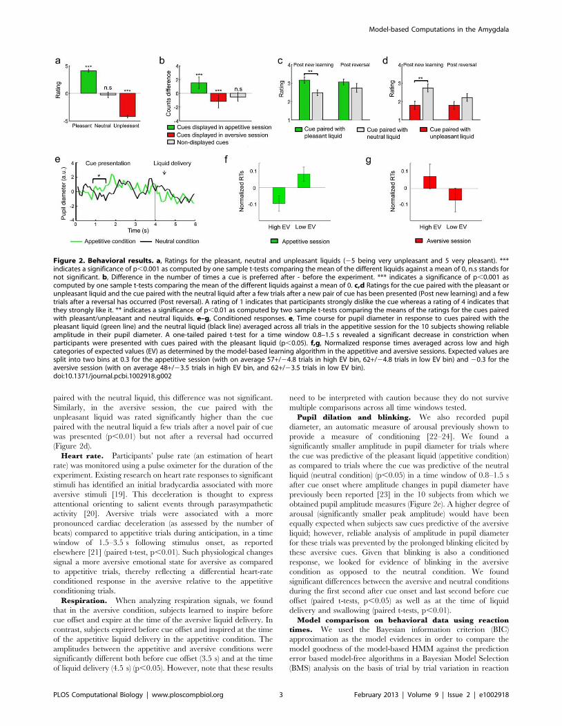
paired with the neutral liquid, this difference was not significant.

Similarly, in the aversive session, the cue paired with the

unpleasant liquid was rated significantly higher than the cue

paired with the neutral liquid a few trials after a novel pair of cue

was presented (p,0.01) but not after a reversal had occurred

(Figure 2d).

Heart rate. Participants’ pulse rate (an estimation of heart

rate) was monitored using a pulse oximeter for the duration of the

experiment. Existing research on heart rate responses to significant

stimuli has identified an initial bradycardia associated with more

aversive stimuli [19]. This deceleration is thought to express

attentional orienting to salient events through parasympathetic

activity [20]. Aversive trials were associated with a more

pronounced cardiac deceleration (as assessed by the number of

beats) compared to appetitive trials during anticipation, in a time

window of 1.5–3.5 s following stimulus onset, as reported

elsewhere [21] (paired t-test, p,0.01). Such physiological changes

signal a more aversive emotional state for aversive as compared

to appetitive trials, thereby reflecting a differential heart-rate

conditioned response in the aversive relative to the appetitive

conditioning trials.

Respiration. When analyzing respiration signals, we found

that in the aversive condition, subjects learned to inspire before

cue offset and expire at the time of the aversive liquid delivery. In

contrast, subjects expired before cue offset and inspired at the time

of the appetitive liquid delivery in the appetitive condition. The

amplitudes between the appetitive and aversive conditions were

significantly different both before cue offset (3.5 s) and at the time

of liquid delivery (4.5 s) (p,0.05). However, note that these results

need to be interpreted with caution because they do not survive

multiple comparisons across all time windows tested.

Pupil dilation and blinking. We also recorded pupil

diameter, an automatic measure of arousal previously shown to

provide a measure of conditioning [22–24]. We found a

significantly smaller amplitude in pupil diameter for trials where

the cue was predictive of the pleasant liquid (appetitive condition)

as compared to trials where the cue was predictive of the neutral

liquid (neutral condition) (p,0.05) in a time window of 0.8–1.5 s

after cue onset where amplitude changes in pupil diameter have

previously been reported [23] in the 10 subjects from which we

obtained pupil amplitude measures (Figure 2e). A higher degree of

arousal (significantly smaller peak amplitude) would have been

equally expected when subjects saw cues predictive of the aversive

liquid; however, reliable analysis of amplitude in pupil diameter

for these trials was prevented by the prolonged blinking elicited by

these aversive cues. Given that blinking is also a conditioned

response, we looked for evidence of blinking in the aversive

condition as opposed to the neutral condition. We found

significant differences between the aversive and neutral conditions

during the first second after cue onset and last second before cue

offset (paired t-tests, p,0.05) as well as at the time of liquid

delivery and swallowing (paired t-tests, p,0.01).

Model comparison on behavioral data using reaction

times. We used the Bayesian information criterion (BIC)

approximation as the model evidences in order to compare the

model goodness of the model-based HMM against the prediction

error based model-free algorithms in a Bayesian Model Selection

(BMS) analysis on the basis of trial by trial variation in reaction

Figure 2. Behavioral results. a, Ratings for the pleasant, neutral and unpleasant liquids (25 being very unpleasant and 5 very pleasant). ***indicates a significance of p,0.001 as computed by one sample t-tests comparing the mean of the different liquids against a mean of 0, n.s stands fornot significant. b, Difference in the number of times a cue is preferred after - before the experiment. *** indicates a significance of p,0.001 ascomputed by one sample t-tests comparing the mean of the different liquids against a mean of 0. c,d Ratings for the cue paired with the pleasant orunpleasant liquid and the cue paired with the neutral liquid after a few trials after a new pair of cue has been presented (Post new learning) and a fewtrials after a reversal has occurred (Post reversal). A rating of 1 indicates that participants strongly dislike the cue whereas a rating of 4 indicates thatthey strongly like it. ** indicates a significance of p,0.01 as computed by two sample t-tests comparing the means of the ratings for the cues pairedwith pleasant/unpleasant and neutral liquids. e–g, Conditioned responses. e, Time course for pupil diameter in response to cues paired with thepleasant liquid (green line) and the neutral liquid (black line) averaged across all trials in the appetitive session for the 10 subjects showing reliableamplitude in their pupil diameter. A one-tailed paired t-test for a time window 0.8–1.5 s revealed a significant decrease in constriction whenparticipants were presented with cues paired with the pleasant liquid (p,0.05). f,g, Normalized response times averaged across low and highcategories of expected values (EV) as determined by the model-based learning algorithm in the appetitive and aversive sessions. Expected values aresplit into two bins at 0.3 for the appetitive session (with on average 57+/24.8 trials in high EV bin, 62+/24.8 trials in low EV bin) and 20.3 for theaversive session (with on average 48+/23.5 trials in high EV bin, and 62+/23.5 trials in low EV bin).doi:10.1371/journal.pcbi.1002918.g002



times (Table 1). For validation, we also compared these models to

a baseline model (Table 2). We found that the model-based HMM

fit better than each of the other algorithms that were tested

including the baseline model, indicating that this algorithm was

providing the best account of trial by trial variation in conditioning

as reflected in reaction times. On the other hand, neither the RW

nor the PH learning rules provided a better fit to the data than did

the baseline model, suggesting that these algorithms cannot

account for changes in reaction time as a function of conditioning

any better than a random actor (Table 1 and 2). Note that we also

constructed a simpler reduced-model version of our HMM which

functioned in a manner more closely resembling a ‘‘model-free’’

algorithm. The essential difference between these two HMMs is

that the reduced-model HMM does not incorporate knowledge of

when contingencies are expected to reverse. The EV signals from

these two models are essentially indistinguishable as they are

almost completely correlated (r = 0.987 in the appetitive session,

r = 0.986 in the aversive session). Hence, we did not include the

reduced-model HMM EV signal in the behavioral model

comparison described above, and therefore cannot rule out this

type of algorithm based on the behavioral data alone. Instead we

must turn to the neural data to discriminate these two possible

accounts (see below).

The normalized RT data is shown plotted against the value

signal predictions of the HMM model in Figure 2f,g, indicating

that RTs become slower under situations where the cue presented

is associated with a stronger prediction of an aversive outcome in

the aversive condition, and become faster as cues are associated

with a stronger prediction of an appetitive outcome in the

appetitive condition.

fMRI resultsWe report results from our analyses based on our model-based

learning algorithm (the HMM model) within the amygdala using a

height threshold of p,0.005, with an extent threshold significant

at p,0.05 corrected for multiple comparisons. We first report

signals correlating with signals generated by our model-based

HMM, and then we compare the performance of our model-based

algorithm against its model-free counterparts in terms of the

capacity of these models to account for BOLD activity in the

amygdala.

Expected value signals. We first investigated BOLD activity

in the amygdala correlating with expected value (EV) signals at the

time of cue presentation (see Figure 3 a for an illustration of EV

signals). In the appetitive session, we found significant activity

positively correlating with expected value in the medial part of the

right amygdala, corresponding to the basolateral complex

(Figure 4a in green, MNI [x y z] [10 210 218], T = 6.29,

k = 28 voxels). In the aversive session, activity positively correlating

with expected value was found in the centromedial complex of the

left amygdala (Figure 4a in red, [x y z] [227 22 29], T = 5.63,

k = 44 voxels; [x y z] [217 215 214], T = 5.41, k = 69 voxels),

such that the greater the activity in these areas, the less an aversive

outcome is predicted to occur. We also looked for areas correlating

negatively with EV in both the appetitive and aversive sessions,

that is, areas showing an increase in activity the less a positive

outcome was predicted to occur given the cue. We did not find

evidence for such activity in the amygdala in either the appetitive

or the aversive session at our statistical threshold.

Precision signals. Next, we examined amygdala activity

correlating positively with precision or else correlating negatively

with precision during both the appetitive and aversive sessions (see

Figure 3b for an illustration of precision signals). While no

significant negative correlation was found with precision, we did

find significant positive correlations with precision signals during

both the appetitive and aversive sessions within our centromedial

complex ROI (appetitive session: [x y z] [25 21 210], T = 4.12,

k = 44; aversive session: [x y z] [27 25 210], T = 5.31, k = 115; [x

y z] [18 22 216], T = 4.75, k = 44)(Figure 5a). To test whether

there was a significant overlap between these clusters in the

appetitive and aversive sessions, we performed a formal conjunc-

tion analysis (at our omnibus threshold of p,0.005 with a cluster

extent of p,0.05). In this contrast we found a common area

activated by precision signals in the appetitive and aversive

sessions in the centromedial complex of the amygdala ([x y z] [24

24 29], T = 3.52, k = 23) (Figure 5c).

Table 1. Behavioral BMS analysis.

HMM RW PH Hybrid

Appetitive session xp = 0.99 xp = 361026 xp = 461026 xp = 661026

pp = 0.84 pp = 0.05 pp = 0.06 pp = 0.05

Aversive session xp = 0.99 xp = 361023 xp = 2.961025 xp = 2.161025

pp = 0.71 pp = 0.19 pp = 0.05 pp = 0.05

Behavioral Bayesian Model Selection (BMS) analysis using the BIC approximation as the model evidences across model-based (HMM) and prediction-error driven model-free (RW, PH and Hybrid) learning algorithms. xp represent exceedance probabilities, pp represent posterior probabilities.doi:10.1371/journal.pcbi.1002918.t001

Table 2. Model validation.

HMM,Baseline RW,Baseline PH,Baseline Hybrid,Baseline

Aversive Session ,0.05 0.93 1 1

Appetitive Session ,0.001 1 1 1

A random effects test of the models versus a baseline model was performed by simulating random expected value estimates (10,000 repetitions) and then computing anon-parametric p-value per subject as the fraction of repetitions in which the baseline BIC is lower than the model BIC (indicating a better fit). These p-values were thencombined across subjects using Fisher’s combined probability test. Only HMM outperforms the baseline model in both the appetitive and aversive sessions.doi:10.1371/journal.pcbi.1002918.t002



Model-comparison on BOLD data. In order to determine

whether BOLD activity in the amygdala is better accounted for by

the model-based HMM than by the prediction-error driven

model-free learning algorithms, we performed a Bayesian Model

Selection (BMS) analysis (Table 3). The expected value contrasts

from our model-based hidden state Markov switching model

(HMM) and the prediction error driven ‘‘model-free’’ Rescorla-

Wagner (RW), Pearce-Hall (PH) and Hybrid models were used to

compare BOLD activity in the amygdala separately for the

aversive and appetitive sessions. In this model comparison, we

included voxels within a 4 mm sphere centered on the peak voxels

of amygdala activities correlating with either expected value

signals for the model-based HMM or expected value signals for the

model-free algorithms using the leave-one out method, thereby

avoiding a non-independence bias in the voxel selection. We found

that the model-based HMM outperformed all prediction-error

driven model-free algorithms with an exceedance probability of

0.94 (posterior probability = 0.64) for the aversive session and of

0.93 (posterior probability = 0.55) for the appetitive session.

As noted earlier, we also constructed a ‘‘reduced-model’’ version

of our HMM. While the EV signals generated by the model-based

and reduced-model HMM are virtually identical, the precision

signals are in fact quite distinct, enabling the predictions of these

two models to be compared against the neural data. We extracted

BOLD activity within the contrasts showing activity positively

correlating with precision signals including voxels within a 4 mm

sphere centered on the peak voxels of the amygdala activities

correlating either with precision signals for the model-based HMM

or the ‘‘model-free’’ HMM using the leave-one out method,

thereby avoiding a non-independence bias in the voxel selection.

We found that activity was better explained by precision signals

estimated by the model-based HMM in both the aversive and

appetitive sessions (aversive session: exceedance probability = 0.99,

posterior probability = 0.75; appetitive session: exceedance prob-

ability = 0.68, posterior probability = 0.55). Thus, our fMRI

findings in the amygdala clearly support the superiority of our

model-based HMM over the reduced model alternative, especially

in the aversive session.

Discussion

In this study, we used a Pavlovian conditioning task with a

rudimentary higher-order structure in both appetitive and aversive

domains to investigate whether neural activity in the human

amygdala reflects learning that requires access to model-based

representations. By comparing neural activity correlating with

expected value signals generated by model-based versus model-

free learning algorithms using a Bayesian model selection (BMS)

procedure, we have been able to show that in at least some parts of

the human amygdala activity during Pavlovian conditioning is

better accounted for by a model-based algorithm rather than by

prediction error driven model-free algorithms.

One of the critical distinctions between the prediction error

driven model-free and model-based learning algorithms in the

present study is that while the expected value of a stimulus

previously paired with the unpleasant outcome is still low following

reversal of contingencies because that was the value it had before

reversal in a model-free system, the expected value of this stimulus

will become high in a model-based system because it incorporates

the knowledge that after a reversal, stimulus values switch (i.e.

there is full resolution of uncertainty when a reversal occurs). We

have captured model-based representations in formal terms using

an elementary Bayesian hidden Markov computational model that

Figure 3. Expected value and precision signals. a, Plots showingexpected value signals. b, Precision signals from the model-basedlearning algorithm for the appetitive (green) and aversive (red) sessionsfor a typical participant.doi:10.1371/journal.pcbi.1002918.g003

Figure 4. Expected value signals from the model-based learning algorithm model in the amygdala. a, Blood oxygen level-dependent(BOLD) signals positively correlating with the magnitude of the expected value of the cue were found in the basolateral complex in the appetitivesession (in green) and in the centromedial complex in the aversive session (in red). b, Plots showing the beta estimates for low, medium and highcategories of expected rewards in the appetitive (green) and aversive (red) sessions in the clusters activated using the leave-one out method.doi:10.1371/journal.pcbi.1002918.g004



incorporates the task structure (by encoding the inverse relation-

ship between the cues and featuring a known probability that the

contingencies will reverse).

Our behavioral analysis demonstrated that participants showed

evidence of conditioned responses to the conditioned stimuli and

thus successfully learnt the associations between the different cues

and outcomes. In a trial-by-trial analysis in which we correlated

reaction times against the model predictions, we found that the

HMM model predicted changes in reaction times over time as a

function of learning better than the prediction-error driven model-

free alternatives, and that the prediction error model-free

algorithms did not predict variation in reaction times significantly

better than chance.

In the neuroimaging data, we found trial-by-trial positive

correlations of model-based expected values in an area consistent

with the basolateral complex of the amygdala according to the Mai

atlas in the appetitive session, and in areas in the likely vicinity of

the centromedial complex in the aversive session [25]. It is

interesting to note that activity in these same areas (i.e. basolateral

versus centromedial complex) has been found to correlate with

expected value signals generated by a simple RW model in a

recent reward versus avoidance instrumental learning task (in an

appetitive versus aversive context respectively) [18]. Using a BMS

procedure, we found that amygdala activity correlating with

expected value was best explained by the model-based than by the

prediction error driven model-free learning algorithms. Whereas

the model-free system has received considerable attention in the

past [26], the more sophisticated and flexible model-based system,

has been more sparsely studied particularly in relation to its role in

Pavlovian learning. Thus, our results point to the need for

integrating model-based representations and their rich adaptability

into our understanding of Pavlovian conditioning in general, and

of the role of the amygdala in implementing this learning process

in particular.

Another important feature of the model-based algorithm

featured in this study, is that as well as keeping track of expected

value, this model also keeps track of the degree of precision in the

prediction of expected value over the course of learning. This

precision starts off low at the beginning of a learning session with a

new stimulus because the expected value computation is very

uncertain at this juncture, but once outcomes are experienced in

response to specific cues, the precision in the estimate quickly

Figure 5. Precision signals from the model-based learning algorithm in the amygdala. a, Blood oxygen level-dependent (BOLD) signalscorrelating with the precision of the cue were found in the centromedial complex of the amygdala in both the appetitive session (in green) andaversive session (in red). b, Plots showing the beta estimates for low, medium and high categories of precision in the appetitive (green) and aversive(red) sessions in the clusters activated using the leave-one out method. c, Results from formal conjunction analysis of precision signals from theappetitive and aversive sessions in the centromedial complex.doi:10.1371/journal.pcbi.1002918.g005

Table 3. Neural BMS analysis.

HMM RW PH Hybrid

Appetitive session xp = 0.93 xp = 0.05 xp = 761023 xp = 0.02

pp = 0.50 pp = 0.21 pp = 0.12 pp = 0.17

Aversive session xp = 0.95 xp = 7.961025 xp = 0.05 xp = 1.561024

pp = 0.61 pp = 0.05 pp = 0.28 pp = 0.06

Neural Bayesian Model Selection (BMS) analysis in the amygdala for Expected value signals generated by the model-based (HMM) and prediction-error driven model-free (RW, PH and Hybrid) learning algorithms. xp represent exceedance probabilities, pp represent posterior probabilities.doi:10.1371/journal.pcbi.1002918.t003



increases. However, this precision lessens again as the trial

progresses because a reversal in the contingencies is increasingly

expected to occur (hence the expected value becomes more and

more uncertain). Signals correlating with precision were found to

be located in the vicinity of the centromedial complex in both the

appetitive and aversive sessions. Precision signals might play an

important role in the directing of attentional resources toward

stimuli in the environment. The presence of a precision signal in

the centromedial amygdala in the present paradigm could be a key

computational signal underpinning the putative role of this

structure in directing attention and orienting toward affectively

significant stimuli.

The presence of a precision-related signal in the amygdala

during Pavlovian conditioning may relate to other findings in

which the amygdala has been suggested to play a role in

‘‘associability’’ as implemented in a model-free algorithm such as

the Pearce-Hall learning rule [13,27]. Associability as defined in

such a model is essentially a model-free computation of

uncertainty, the inverse of precision: associability is maximal

when the absolute value difference between expected and actual

rewards is greatest. However, in our case, an associability signal is

clearly distinct from the signal we observe in the amygdala in the

centromedial complex (even leaving aside the fact the signal we

found is negatively as opposed to positively correlated with

uncertainty). First of all, because the signal in our HMM is model-

based, it changes to reflect anticipated changes in task structure

(such as a reversal), whereas Pearce-Hall associability does not

change to reflect anticipated changes in task structure, both rather

changes only reflexively once contingencies have reversed.

Further evidence that the amygdala is involved in model-based

computations came from an additional analysis in which we

compared the signals generated by our model-based HMM

against signals generated by a reduced version of our HMM in

which knowledge of when contingencies are expected to reverse

was not incorporated. Although this reduced model still generated

very similar expected value signals as the model-based HMM and

thus made similar predictions about behavior, the precision signals

generated by these two algorithms are quite distinct and can

therefore be compared against neural activity in the amygdala. In

a direct comparison, activity in the amygdala was best accounted

for by the precision signal generated by the full HMM. It is

interesting to note that evidence for model-based processing in the

amygdala was more robust in the aversive case given the

traditional view of the amygdala as being associated especially

with aversive processing. However, it is unlikely that this pattern of

results reflects a qualitative difference in the way that appetitive

and aversive learning is mediated by the amygdala, particularly in

the light of considerable evidence implicating this structure in both

reward-related as well as aversive-learning [28,29].

Finally, we checked the correlation between the precision signal

we found here and an associability signal generated by the Pearce-

Hall learning rule, and we found the correlation between these

signals to be essentially negligible (with r ranging from 20.06 to

20.14), as opposed to being strongly negatively or positively

correlated as would be anticipated were these signals to tap similar

underlying processes.

The fact that in the present study we found model-based signals

in the amygdala does indicate that this structure is capable of

performing model-based inference even during Pavlovian condi-

tioning. However, it is important to note that the findings of the

present study do not rule out a role for this structure in prediction

error driven model-free computations during Pavlovian condi-

tioning. Indeed, while the prediction error driven model-free

learning rules we used did not work very well in accounting for

behavior on the task (as indexed by changes in reaction times), we

did find some evidence (albeit weakly) of model-free value signals

in the amygdala as generated by either a Rescorla-Wagner, a

Pearce-Hall or a Hybrid learning rule. Indeed, while using our

HMM model we did not find evidence for aversive-going expected

value signals in the aversive session (i.e. by showing an increase in

activity the more the unpleasant tasting liquid was expected), we

did find such a signal correlating with expected value as computed

by a Pearce-Hall learning rule. As a consequence, we cannot rule

out a contribution for the amygdala in model-free computations. It

is important to note however, that in many tasks in which

neuronal activity was found in the amygdala to correlate with the

predictions of model-free learning algorithms [18,30–32], such

tasks were either not set up to discriminate the predictions of

model-free versus model-based learning rules, or else the relevant

model comparisons were not performed. Thus, it is entirely

feasible that many of the computations found in the amygdala in

previous studies correspond more closely to model-based as

opposed to model-free learning signals. More generally, if indeed,

both model-based and model-free signals are present in the

amygdala during Pavlovian conditioning, then an important

question for future research will be to address how and when

these signals interact with each other.

To conclude, we have found in the present study evidence for

the existence of model-based learning signals in the human

amygdala during performance of a Pavlovian conditioning task

with a simple task structure. These findings provide an important

new perspective into the functions of the amygdala by suggesting

that this structure may participate in model-based computations in

which abstract knowledge of the structure of the world is taken

into account when computing signals leading to the elicitation of

Pavlovian conditioned responses. The findings also resonate with

an emerging theme in the neurobiology of reinforcement learning

whereby value signals are suggested to be computed via two

mechanisms: a model-based and a model-free approach [1,3].

Whereas up to now, theoretical and experimental work on this

distinction has tended to be focused on the domain of instrumental

conditioning [4,7,8], the present study illustrates how similar

principles may well apply even at the level of Pavlovian

conditioning. Thus the distinction between model-based and

model-free learning systems may apply at a much more general

level across multiple types of associative learning in the brain.

Furthermore, the present results provide evidence that model-

based computations may be present not only in prefrontal cortex

and striatum, but also in other brain structures such as the

amygdala.

Materials and Methods

SubjectsNineteen right-handed subjects (8 females) with a mean age of

22.2163.47 participated in the study. All subjects were free of

neurological or psychiatric disorders and had normal or correct-to-

normal vision. Written informed consent was obtained from all

subjects, and the study was approved by the Trinity College

School of Psychology research ethics committee.

Task descriptionSubjects participated in a Pavlovian task where they had to

learn associations between different cues (fractal images) and a

pleasant (blackcurrant juice [Ribena, Glaxo-Smithkline, UK]),

affectively neutral (artificial saliva made of 25 mM KCl and

2.5 mM NaHCO3) or unpleasant (salty tea made of 2 black tea

bags and 29 g of salt per liter) flavor liquid. The task consisted of



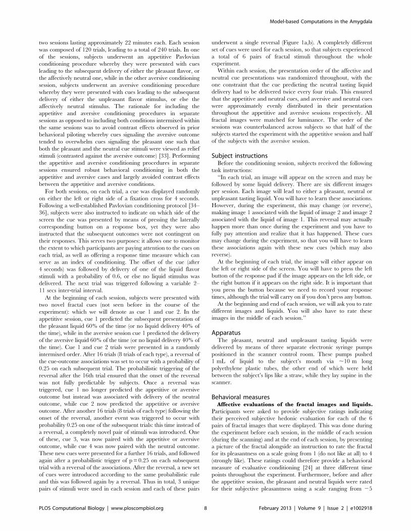
two sessions lasting approximately 22 minutes each. Each session

was composed of 120 trials, leading to a total of 240 trials. In one

of the sessions, subjects underwent an appetitive Pavlovian

conditioning procedure whereby they were presented with cues

leading to the subsequent delivery of either the pleasant flavor, or

the affectively neutral one, while in the other aversive conditioning

session, subjects underwent an aversive conditioning procedure

whereby they were presented with cues leading to the subsequent

delivery of either the unpleasant flavor stimulus, or else the

affectively neutral stimulus. The rationale for including the

appetitive and aversive conditioning procedures in separate

sessions as opposed to including both conditions intermixed within

the same sessions was to avoid contrast effects observed in prior

behavioral piloting whereby cues signaling the aversive outcome

tended to overwhelm cues signaling the pleasant one such that

both the pleasant and the neutral cue stimuli were viewed as relief

stimuli (contrasted against the aversive outcome) [33]. Performing

the appetitive and aversive conditioning procedures in separate

sessions ensured robust behavioral conditioning in both the

appetitive and aversive cases and largely avoided contrast effects

between the appetitive and aversive conditions.

For both sessions, on each trial, a cue was displayed randomly

on either the left or right side of a fixation cross for 4 seconds.

Following a well-established Pavlovian conditioning protocol [34–

36], subjects were also instructed to indicate on which side of the

screen the cue was presented by means of pressing the laterally

corresponding button on a response box, yet they were also

instructed that the subsequent outcomes were not contingent on

their responses. This serves two purposes: it allows one to monitor

the extent to which participants are paying attention to the cues on

each trial, as well as offering a response time measure which can

serve as an index of conditioning. The offset of the cue (after

4 seconds) was followed by delivery of one of the liquid flavor

stimuli with a probability of 0.6, or else no liquid stimulus was

delivered. The next trial was triggered following a variable 2–

11 secs inter-trial interval.

At the beginning of each session, subjects were presented with

two novel fractal cues (not seen before in the course of the

experiment): which we will denote as cue 1 and cue 2. In the

appetitive session, cue 1 predicted the subsequent presentation of

the pleasant liquid 60% of the time (or no liquid delivery 40% of

the time), while in the aversive session cue 1 predicted the delivery

of the aversive liquid 60% of the time (or no liquid delivery 40% of

the time). Cue 1 and cue 2 trials were presented in a randomly

intermixed order. After 16 trials (8 trials of each type), a reversal of

the cue-outcome associations was set to occur with a probability of

0.25 on each subsequent trial. The probabilistic triggering of the

reversal after the 16th trial ensured that the onset of the reversal

was not fully predictable by subjects. Once a reversal was

triggered, cue 1 no longer predicted the appetitive or aversive

outcome but instead was associated with delivery of the neutral

outcome, while cue 2 now predicted the appetitive or aversive

outcome. After another 16 trials (8 trials of each type) following the

onset of the reversal, another event was triggered to occur with

probability 0.25 on one of the subsequent trials: this time instead of

a reversal, a completely novel pair of stimuli was introduced. One

of these, cue 3, was now paired with the appetitive or aversive

outcome, while cue 4 was now paired with the neutral outcome.

These new cues were presented for a further 16 trials, and followed

again after a probabilistic trigger of p = 0.25 on each subsequent

trial with a reversal of the associations. After the reversal, a new set

of cues were introduced according to the same probabilistic rule

and this was followed again by a reversal. Thus in total, 3 unique

pairs of stimuli were used in each session and each of these pairs

underwent a single reversal (Figure 1a,b). A completely different

set of cues were used for each session, so that subjects experienced

a total of 6 pairs of fractal stimuli throughout the whole

experiment.

Within each session, the presentation order of the affective and

neutral cue presentations was randomized throughout, with the

one constraint that the cue predicting the neutral tasting liquid

delivery had to be delivered twice every four trials. This ensured

that the appetitive and neutral cues, and aversive and neutral cues

were approximately evenly distributed in their presentation

throughout the appetitive and aversive sessions respectively. All

fractal images were matched for luminance. The order of the

sessions was counterbalanced across subjects so that half of the

subjects started the experiment with the appetitive session and half

of the subjects with the aversive session.

Subject instructionsBefore the conditioning session, subjects received the following

task instructions:

‘‘In each trial, an image will appear on the screen and may be

followed by some liquid delivery. There are six different images

per session. Each image will lead to either a pleasant, neutral or

unpleasant tasting liquid. You will have to learn these associations.

However, during the experiment, this may change (or reverse),

making image 1 associated with the liquid of image 2 and image 2

associated with the liquid of image 1. This reversal may actually

happen more than once during the experiment and you have to

fully pay attention and realize that it has happened. These cues

may change during the experiment, so that you will have to learn

these associations again with these new cues (which may also

reverse).

At the beginning of each trial, the image will either appear on

the left or right side of the screen. You will have to press the left

button of the response pad if the image appears on the left side, or

the right button if it appears on the right side. It is important that

you press the button because we need to record your response

times, although the trial will carry on if you don’t press any button.

At the beginning and end of each session, we will ask you to rate

different images and liquids. You will also have to rate these

images in the middle of each session.’’

ApparatusThe pleasant, neutral and unpleasant tasting liquids were

delivered by means of three separate electronic syringe pumps

positioned in the scanner control room. These pumps pushed

1 mL of liquid to the subject’s mouth via ,10 m long

polyethylene plastic tubes, the other end of which were held

between the subject’s lips like a straw, while they lay supine in the

scanner.

Behavioral measuresAffective evaluations of the fractal images and liquids.

Participants were asked to provide subjective ratings indicating

their perceived subjective hedonic evaluation for each of the 6

pairs of fractal images that were displayed. This was done during

the experiment before each session, in the middle of each session

(during the scanning) and at the end of each session, by presenting

a picture of the fractal alongside an instruction to rate the fractal

for its pleasantness on a scale going from 1 (do not like at all) to 4

(strongly like). These ratings could therefore provide a behavioral

measure of evaluative conditioning [24] at three different time

points throughout the experiment. Furthermore, before and after

the appetitive session, the pleasant and neutral liquids were rated

for their subjective pleasantness using a scale ranging from 25



(very unpleasant) to +5 (very pleasant), and similarly the aversive

and neutral liquids were rated before and after the aversive session.

Preference ranking test. Before the experiment started and

after the experiment was over, participants were asked to make

binary choices indicating their relative preferences for each of 16

different fractals (12 of which were included in the experiment; 6

each in the appetitive and aversive sessions respectively; while 4 of

the fractals were not featured in either session). Each of the 16

fractals was paired with each other fractal. This test allowed us to

estimate a preference ranking for each of the fractals, thereby

potentially providing an additional even more direct behavioral

metric of evaluative conditioning beyond the pleasantness ratings.

Pupillary dilation. Pupil diameter was continuously mea-

sured during scanning using an MRI compatible integrated goggle

and infrared eye tracking system (NordicNeuroLab AS, Bergen,

Norway). Pupil reflex amplitude has been shown to be modulated

by arousal level and can therefore be used as a physiological index

of conditioning [22–24]. Pupil measurements could not be taken

from 9 participants because space constraints within the head-coil

alongside variations in head size meant that in some individuals

the eye-tracker could not fit them comfortably.

Fluctuations in respiration and heart rate. Estimates of

heart rate and respiration were recorded using a pulse oximeter

positioned on the forefinger of subjects’ left hand and a pressure

sensor placed on the umbilical region. The time courses derived

from these measures were used as a further physiological index of

conditioning as well as being used separately to remove

physiological noise from the fMRI data analysis (see fMRI data

analysis).

Data acquisitionFunctional imaging was performed on a 3T Philips scanner

equipped with an 8-channel SENSE (sensitivity encoding) head coil.

Since the focus of our study was on the amygdala, we only acquired

partial T2*-weighted images centered to include the amygdala

while subjects were performing the task. These images also

encompassed the ventral part of the prefrontal cortex, the ventral

striatum, the insula, the hippocampus, the ventral part of the

occipital lobe and the upper part of the cerebellum (amongst other

regions). Nineteen contiguous sequential ascending slices of echo-

planar T2*-weighted images were acquired in each volume, with a

slice thickness of 2.2 mm and a 0.3 mm gap between slices (in-plane

resolution: 1.5861.63 mm; repetition time (TR): 2000 ms; echo

time (TE): 30 ms; field of view: 1966196647.2 mm; matrix:

1286128). A whole-brain high-resolution T1-weighted structural

scan (voxel size: 0.960.960.9 mm) and three whole-brain T2*-

weighted images were also acquired for each subject. To address the

problem of spatial EPI distortions which are particularly prominent

in the medial temporal lobe (MTL) and especially in the amygdala,

we also acquired gradient field maps. To provide a measure of

swallowing motion, a motion-sensitive inductive coil was attached to

the subjects’ throat using a Velcro strap. The time course derived

from this measure was used as a regressor of no interest in the fMRI

data analysis. Finally, to account for the effects of physiological noise

in the fMRI data, subjects’ cardiac and respiratory signals were

recorded with a pulse oximeter and a pressure sensor placed on the

umbilical region and further removed from time-series images. We

discarded the first 3 volumes before data processing and statistical

analysis to compensate for the T1 saturation effects.

PreprocessingAll EPI volumes (‘partial’ scans acquired while subjects were

performing the task and the three whole-brain functional scans

acquired prior to the experiment) were corrected for differences

in slice acquisition and spatially realigned. The mean whole-

brain EPI was co-registered with the T1-weighted structural

image, and subsequently, all the partial volumes were co-

registered with the registered mean whole-brain EPI image.

Partial volumes were then unwarped using the gradient field

maps. After the structural scan was normalized to a standard T1

template, the same transformation was applied to all the partial

volumes with a resampled voxel size of 0.960.960.9 mm. In

order to maximize the spatial resolution of our data, no spatial

smoothing kernel was applied to the data. These preprocessing

steps were performed using the statistical parametric mapping

software SPM5 (Wellcome Department of Imaging Neurosci-

ence, London, UK).

Amygdalae segmentation. Amygdalae Regions of Interest

(ROIs) were manually segmented for each subject by a single

observer using a pen tablet (Wacom Intuos3 Graphics Tablet) in

FSL View (FSL 4.1.2). This program allows magnification and the

simultaneous viewing of volumes in coronal, sagittal and

horizontal orientations. Amygdalae were manually outlined on

each coronal image containing the amygdala using detailed tracing

guidelines based on the Atlas of the Human Brain [25]. Outlines

were checked in horizontal and sagittal planes when they proved

more valuable for the identification of structure boundaries. The

anterior limit of the amygdala was defined using the horizontal

and sagittal planes. The following guidelines were used: In its

rostral part, the amygdala is bordered ventromedially by the

entorhinal cortex, ventrally by the temporal horn of the lateral

ventricle and subamygdaloid white matter and laterally by white

matter of the temporal lobe. Midrostrocaudally, the amygdala

increases in size and is bordered ventromedially by a thin tract of

white matter separating the amygdala and the entorhinal cortex,

laterally by the white matter of the temporal lobe and medially by

the semiannular sulcus. Caudally, the amygdala is bordered

dorsally by the substantia innominata and fibers of the anterior

commissure, laterally by the putamen, ventrally by the temporal

horn of the lateral ventricle and the alveus of the hippocampus and

medially by the optic tract.

Amygdalae normalization. Because structures in the MTL

exhibit significant inter-individual anatomic variability, the signal-

to-noise ratio in group analyses is substantially limited in this area

[37]. Atlas-based approaches used to register whole-brain EPI

images across subjects (such as SPM) look for a global optimum

alignment which is achieved under the limitations imposed by the

available degrees of freedom, and which is at the expense of

regional accuracy. Consequently, BOLD signals in the MTL may

be underestimated or possibly missed [38]. Alignment of the MTL

is substantially improved by a ROI-alignment (ROI-AL) ap-

proach, where segmentations of regions of interest (ROIs) are

drawn on structural images and aligned directly, resulting in an

increased statistical power [39]. The last iteration of this alignment

tool is ROI-Demons, which has proven to be exceptionally

accurate in the alignment of hippocampal subfields for instance

(http://darwin.bio.uci.edu/,cestark/roial/roial.html). Thirion’s

original demons algorithm has been implemented by Vercauteren

and enforces smooth deformations by operating on a diffeo-

morphic space of displacement fields [40,41]. Here, we used the

implementation of ROI-Demons in the DemonsRegistration

command-line tool (http://www.insight-journal.org/browse/

publication/154). Our segmented amygdalae ROIs were regis-

tered with our amygdalae template based on 20 subjects from a

previous study [18] to serve as an initial model and to align all

amygdalae using DemonsRegistration. The resulting registered

amygdalae were then averaged in SPM5 (using ImCalc) to create a

first model. Subsequently, the initial non-registered amygdalae



were registered with this first model and the newly registered

amygdalae were averaged to create a second model. We repeated

the last two steps three more times in order to generate a more

accurate model. We finally registered our initial amygdalae ROIs

with the fifth model to generate the resulting displacement fields

(or transformation calculations). These individual displacement

fields were then applied to each subject’s normalized EPI scans in

order to specifically normalize their amygdalae to our template

amygdalae. We applied the same transformation to each subject’s

structural scan before averaging all the aligned structural scans, to

create an amygdalae-aligned average structural brain of our 19

subjects. Finally, amygdalar subdivisions were hand-drawn on our

template amygdalae using the Atlas of the Human Brain [25]. We

delineated three sub-areas within the amygdala: the basolateral

complex comprised of the basomedial, basolateral and lateral

nuclei; the centromedial complex comprised of the central and

medial nuclei; and the cortical complex (or cortical nucleus). In its

most rostral part, the amygdala is exclusively composed of the

basolateral complex. The cortical nucleus appears in the dorso-

medial part of mid-rostral amygdala. The centromedial complex

appears slightly more caudally than the cortical nucleus in the

most dorsal part of the amygdala. The basolateral complex

increases in size as one moves caudally from the anterior

amygdala, has its maximal size midrostrocaudally and then

decreases as one moves further back toward the caudal amygdala,

whereas the cortical nucleus and centromedial complex slightly

enlarge midrostrocaudally, but do not decrease in size as one

moves further caudally within the amygdala. The cortical nucleus

ends midcaudally, the basolateral complex ends in caudal

amygdala while the centromedial complex ends in the most

caudal part of amygdala.

Computational model analysisTo test whether amygdala activity was better explained by

model-based or model-free learning algorithms, we correlated

brain activity in this region with expected value signals estimated

by a number of different computational models. In model-free

learning algorithms, the agent is surprised when a reversal occurs

and starts learning again after it happens, whereas in model-based

learning algorithms, the agent expects the reversal and considers it

as resolution of uncertainty and does not need to relearn. The two

modes of learning are diametrically opposed in the current task,

therefore allowing us to test whether amygdala is tracking model-

based or model-free computations.

Model-based learning algorithm: HMM with dynamic

expectation of change. For the model-based learning algo-

rithm, we used a Hidden Markov Model (HMM). In this HMM,

the inferred state of the environment is defined in terms of an

association between cues and outcomes and is represented by the

psychological variable S. There are three possible liquid outcomes

in the experiment (pleasant and neutral in the appetitive session

and unpleasant and neutral in the aversive session) and two cues

on any given trial. The state values St are the possible

combinations of cues and outcomes, for example St = (cue 2, neutral

liquid). Although the subjects were unaware that pleasant and

unpleasant outcomes could not be delivered concurrently, this

possible state value was omitted since it did not affect the results of

the analyses. We also incorporated a binary-valued variable H in

this HMM. The values of this hidden node determine whether

(H = 1) or not (H = 0) the subject is expecting a reversal. A third

random variable O represents the observed cue-outcome combi-

nation (see Figure 1d for a simple graphical representation of the

model).

The transition probabilities of the reversal variable H are:

P HtDHt{1ð Þ~1{a a

0 1

� �

Variable values are enumerated along the row and column axes.

Each entry of the matrix represents the probability of moving from

one value on trial t21 (rows) to another on trial t (columns). At

position (1,2), the a parameter is the probability of moving to the

state of expecting a reversal (H = 1) from the H = 0 state. Once a

subject begins expecting a reversal, they do not switch back. This is

encoded in the asymmetry of the transition matrix. The time

evolution of H represents a subject’s growing expectation of a

reversal in the cue-outcome association. After the presentation of a

novel pair of cues, H is set to the zero state. The transitions for the

state variable S are conditionally dependent on the reversal

variable:

P StDSt{1,Htð Þ~1{b b

b 1{b

� �

State reversals are inferred with a non-zero probability b when H is in

the reversal expectation state (Ht = 1), otherwise b = 0 and P(St|St-

1,Ht = 0) is the identity matrix. Note that after the first trial following

the presentation of novel cues, the subject has a nonzero probability

of being in the reversal expectation state thus they are always

expecting a reversal to some degree and are prepared to react to an

observation indicative of a contingency reversal. The posterior

probability distribution P(St) over the state values on trial t is

determined by the prior state probability distribution P(St-1), the cue-

outcome observation Ot, and the state transition probabilities:

Prior Stð Þ~X

St{1 states

XHt states

P StDSt{1,Htð ÞP Htð ÞPosterior St{1ð Þ

Posterior Stð Þ~P OtDStð ÞPrior(St)P

Ststates P OtDStð ÞPrior(St)

The prior over the state values at the beginning of a new set of cues is

uniform. Beliefs are updated based on the likelihood of observing an

outcome for a given cue and assuming a state such as ‘‘cue j is

rewarding and this is likely to reverse soon.’’ For instance, if no

reward is observed for cue j, then this state is given less credence

because the likelihood that this occurs is low (0.4), and the expectation

of reward for cue j is decreased. Significantly, expectations for the

other cue are updated simultaneously, even if it is not implicated in

the current trial. This is because a lower chance for the state ‘‘cue j is

rewarding and this is likely to reverse soon’’ implies that the state ‘‘the

other cue is rewarding and this is unlikely to reverse soon,’’ is more

likely, and hence, the mathematical expectation of the reward upon

presentation of the other cue increases.

The expected reward Qj when presented with a given cue j is

Qj tð Þ~E RDcue j,trial t½ �~X

R rewards

XSt states

R P RDSt,cue cð ÞP Stð Þ

The reward R takes the values 21, 0, 1 for unpleasant, neutral,

and pleasant rewards respectively. Here, ‘‘E’’ denotes the

mathematical expectation operator. This means that the forecast

is correct on average for all possible outcomes given a specific

history of past rewards for both cues.



Confidence in, or precision about, the identity of the current

state can be measured by the extent to which there are differences

in the posterior probabilities of the possible states given past

experience and the cues presented. When these differences are

high, one posterior probability is necessarily high, and hence,

precision is high. Conversely, if all posterior probabilities are the

same, precision is lowest. We measure precision on a given trial t

using the inverse Shannon entropy of the posterior distribution of

the state variable S

Entropy Stð Þ~{X

Ststates

P(St) log P Stð Þ

As more and more trials with no reward are experienced, the H

node inputs a growing uncertainty about the identity of the current

state into the HMM (since a reversal may have occurred in the

absence of a rewarding outcome). Every time a new pair of cues is

presented, precision is low but increases dramatically when the

agent knows what particular state they are in (i.e. what the cue-

liquid association is). Precision lowers again until the agent knows

that a reversal has occurred, after which precision increases again.

A random effects Bayesian approach was used for parameter

fitting and model comparisons (note that we excluded one subject

who failed to make motor responses from this analysis). Model

parameters (such as a and b) were fixed a priori and the model fits

were not sensitive to the specific values of these parameters. HMM

estimation was performed via forward smoothing using the HMM

toolbox for MATLAB (http://www.cs.ubc.ca/,murphyk/

Software/HMM/hmm.html).

Model-free learning algorithms. A. Rescorla Wagner algo-

rithm. In the Rescorla Wagner (RW) model, the new expected

value at trial t+1 for a given cue is based on the sum of the current

expected value and the prediction error between the reward

obtained and the expected value at time t, weighted by the

learning rate [11]:

Qj tz1ð Þ~Qj tð Þza. R tð Þ{Qj tð Þð Þ

When j is a given cue, a is the learning rate with a range 0#a#1,

and R(t) is the reward received on the current trial. If the valenced

(pleasant or unpleasant) liquid was obtained on the current trial,

R(t) = 1, else R(t) = 0. Hence there is one free parameter in this

model, a. Note that using a random effects approach, we found

that the optimal free parameters in the appetitive and aversive

sessions averaged across subjects were 0.54 (SEM = 0.09) and 0.18

(SEM = 0.05) respectively.

B. Pearce Hall algorithm. This model differs from the Rescorla

Wagner model (RW) in that it introduces an associability

component and allows the effectiveness of the reinforcer to remain

constant throughout conditioning. The associability values esti-

mated by this model will decrease as the consequences of the

conditioned stimulus become accurately predicted [12]. The

expected values Q(t) of a given cue were updated according to:

Qj tz1ð Þ~Qj tð ÞzS.DR t{1ð Þ{Qj t{1ð ÞD.R tð Þ

When j is a given cue, S is a free parameter governing the intensity

of the CS, and R(t) is the reward received on the current trial. If

the valenced (pleasant or unpleasant) liquid was obtained on the

current trial, R(t) = 1, else R(t) = 0. In the Pearce Hall model (PH),

the new expected value at trial t+1 for a given cue is based on the

sum of the current expected value and the product of the absolute

value of the difference between the outcome obtained on the

previous trial and the expected reward on the previous trial, and

the outcome obtained on the current trial; this product is weighted

by the free parameter. Hence there is one free parameter in this

model, S. Note that using a random effects approach, we found

that the optimal free parameters in the appetitive and aversive

sessions averaged across subjects were 0.58 (SEM = 0.09) and 0.40

(SEM = 0.10) respectively.

C. Hybrid algorithm. In addition to the Rescorla-Wagner and

Pearce-Hall models, we also tested a hybrid model introduced by

Li et al., (2011) in which the Rescorla-Wagner rule is used to

update value expectations, while the Pearce-Hall rule is used to set

the learning rate. The expected values Q(t) of a given cue were

updated according to:

aj tz1ð Þ~aj tð ÞzS.DR t{1ð Þ{aj t{1ð ÞD.R tð Þ

D. Reduced HMM. In order to set an even stronger test for our

model-based HMM, we constructed a simpler version of the

HMM. In this version of the HMM, H is always set to the H = 1

state and thus the chance of a reversal happening is constant over

time. As a result, in this HMM, there is no change in the

expectation of when a reversal is going to occur over the course of

a trial. In that sense this reduced model behaves more like the

model-free algorithms, although it still incorporates knowledge of

the CS-US state-space structure (namely, that one CS is paired

with an affectively significant outcome while the other is associated

with a neutral outcome), the algorithm cannot be said to be

completely model-free in the same way as the prediction-error

driven learning rules described above.

The expected reward signals from the reduced HMM are very

similar to that generated by the full model-based HMM (with

correlations of r = 0.987 in the appetitive session, r = 0.986 in the

aversive session). Nevertheless, the precision signals generated by

the reduced HMM are very different to those generated by the

model-based HMM. Precision starts low every time a new pair of

cues is presented and increases substantially when the agent knows

in which state they are, but because the chance of a reversal

occurring does not increase over time, the precision remains high

through the rest of the learning with that cue until a new pair of

cues is introduced. In other words, there is no decrease in precision

related to the anticipation of a change in the contingencies (which

would come from having a model of when the contingencies are

predicted to reverse), but instead a decrease in precision occurs

only once a contingency change has occurred and been detected

through trial and error experience.

E. Baseline model. Our baseline model simply assumes that

rewards occur completely at random and no learning takes place.

Hence, expected values for all trials are kept at a constant value of

0.5.

Model comparison on behavioral dataTo perform a formal model comparison on the behavioral

conditioning data, we used the trial-by-trial reaction time data

(measuring the length of time taken on each trial for participants to

press a button to indicate which side of the screen the Pavlovian

cue stimulus had been presented). Many previous studies have

shown that changes in RTs to a Pavlovian cue are correlated with

changes in associative encoding between cues and behaviorally

significant outcomes [13,34,36,42]. For each session separately, we

log transformed and adjusted the RT data to account for a linear

trend in RTs over time independently of trial type, as well as to

remove the effects of changes in reaction time related to switching

responses from one side of the screen to the other. This was done



by regressing the log transformed RTs against a matrix containing

a column of ones, a column accounting for the linear trend over

time and a column indicating whether participants switched their

response from left to right or vice versa between the current and

previous trial using the function regress in Matlab.

Using the same function, we then regressed these adjusted

response times against the expected values generated by our

model-based HMM our model-free RW, PH and Hybrid

algorithms and our baseline model (for the baseline model, a

small amount of noise was added to each expected value in order

to compute the regression; without any noise the regression would

not be calculable). This second regression analysis was run for each

of these models, and cycled through all the possible learning rate

parameters for the RW model and CS intensity parameters for the

Pearce-Hall and hybrid models between 0 and 1, with increments

of 0.001. This method returned Sum Squared Error (SSE) values

for each of these parameter values thereby allowing us to obtain

the best fitting value for the free parameter for the appetitive and

aversive sessions (i.e. the free parameter associated with the lowest

SSE value). In order to compare the model goodness between

these four different algorithms, we converted the best SSE value of

each session (appetitive and aversive) and each model into a

Bayesian information criterion (BIC) value. The BIC adds a

penalty proportional to the number of additional free parameters

to the SSE value of each model, depending also on the number of

degrees of freedom which in this case, is the total number of trials

per session across all subjects [43]. Using this procedure, we found

that in both the appetitive and aversive sessions, the model-based

HMM outperformed the prediction-error driven model-free

algorithms (Table 1). In the model validation analyses, where we

compared the prediction-error driven models against a random

baseline model, only the model-based HMM fit our behavioral

data significantly better than the baseline model (Table 2). Hence,

unlike RW, PH and the Hybrid model, the model-based HMM

predicted RTs better than chance performance. Note that we did

not regress the expected values generated by our reduced HMM

since they were highly correlated with that of our model-based

HMM.

fMRI data analysisThe event-related fMRI data were analyzed by constructing sets

of d (stick) functions at the time of cue presentation and at the time

of outcome for the appetitive and aversive sessions. For our main

GLM (illustrated in Figures 4 and 5), additional regressors were

constructed by using the expected values and the precision values

generated by the model-based HMM as modulating parameters at

the time of cue presentation. In order to compare model-based

versus model-free learning algorithms in the amygdala, we ran

three additional GLMs. For RW, the regressors were similar to our

model-based HMM except that we did not have a regressor for

precision which is not estimated by RW, and we added a

modulating parameter for prediction error at the time of outcome.

The regressors used in the GLM computed using PH model were

the same as the ones used in our model-based HMM, except that

the precision modulating parameter was replaced with an

associability modulating parameter at the time of cue presentation

(note that similar regressors were used for the Hybrid model).

Finally, we ran an analysis using our reduced model HMM using

the same regressors as for our model-based HMM. All of these

regressors were convolved with a canonical hemodynamic

response function (HRF). The six scan-to-scan motion parameters

derived from the affine part of the realignment procedure were

included as regressors of no interest to account for residual motion

effects. To account for motion of the subjects’ throat during

swallowing, we added a regressor of no interest for swallowing

motion. Finally, we also included thirteen additional regressors to

account for physiological fluctuations (4 related to heart rate, 9

related to respiration) which were estimated using the RETRO-

ICOR algorithm [44]. Six of the 38 (2 sessions619 subjects) log

files could not be used to estimate these regressors due to a

technical problem during data collection, and the missing

physiological regressors were simply omitted for those sessions.

All of these regressors were entered into a general linear model

and fitted to each subject individually using SPM5. The resulting

parameter estimates for regressors of interest were then entered

into second-level one sample t-tests to generate the random-effects

level statistics used to obtain the results shown in figures 4 and 5.

All reported fMRI statistics and p values arise from group random-

effects analyses. We present our statistical maps at a threshold of

p,0.005, corrected for multiple comparisons at p,0.05. To

correct for multiple comparisons, we first used the 3dFWHMx

function in AFNI to estimate the intrinsic smoothness of our data,

within the area defined by a mask corresponding to our amygdala

template. We then used the AlphaSim function in AFNI to

estimate via Monte Carlo simulation an extent threshold for

statistical significance that was corrected for multiple comparisons

at p,0.05 for a height threshold of p,0.005 within the amygdala

ROI.

Model comparison on BOLD dataIn order to test whether amygdala activity was better accounted

for by the model-based than model-free learning algorithms, we

used a Bayesian model selection procedure (BMS) [45]. For both

the appetitive and aversive sessions, we included in this model

comparison individual betas averaged across voxels within a 4 mm

sphere centered on the peak voxels of the amygdalar activities

correlating with either expected value signals for the HMM or the

model-free algorithms using the leave-one out method, thereby

avoiding a non-independence bias in the voxel selection [46].

Using the spm_BMS function in SPM8, we compared expected

value signals across all model-based (HMM) and model-free

models separately for the appetitive and aversive sessions.

We used a similar approach to compare neural activity

pertaining to precision signals estimated by our model-based and

reduced model HMMs. The difference between these two HMMs

is that the model-based HMM does not allow for a reversal

without moving from a ‘‘non-reversal state’’ to a ‘‘possible reversal

state’’. As a consequence, the precision values generated by these

models are clearly distinguishable and thus easily comparable

using a BMS (whereas the estimated expected rewards are strongly

correlated). Again, we included in this model comparison voxels

within a 4 mm sphere centered on the peak voxels of the

amygdalar activities correlating with precision signals for either the

model-based HMM or the reduced model HMM using the leave-

one out method. Here, we compared activity correlating with

precision signals between the model-based and reduced HMM

separately for the appetitive and aversive sessions (see Results

section for the exceedance probabilities).

ROI analysesFunctional regions of interest (ROIs) were defined using the

MarsBaR toolbox (http://marsbar.sourceforge.net/). Beta esti-

mates were extracted for each subject from the functional clusters

of interest as they appeared on the statistical maps of a given

contrast using the leave-one out method to avoid a non-

independence bias. They were then averaged across subjects to

plot expected reward (Figure 4b) and precision (Figure 5b)



according to 3 categories (category 1 corresponding to the lowest

values and category 3 corresponding to the highest values).

Acknowledgments

We thank Simon Dunne for helpful assistance.

Author Contributions

Conceived and designed the experiments: CP JPOD. Performed the

experiments: CP. Analyzed the data: CP DM RKJ PB. Contributed

reagents/materials/analysis tools: PB. Wrote the paper: CP DM PB JPOD.

References

1. Doya K, Samejima K, Katagiri K, Kawato M (2002) Multiple model-based

reinforcement learning. Neural Comput 14: 1347–1369.

2. Corrado G, Doya K (2007) Understanding neural coding through the model-based analysis of decision making. J Neurosci 27: 8178–8180.

3. Dayan P, Daw ND (2008) Decision theory, reinforcement learning, and thebrain. Cogn Affect Behav Neurosci 8: 429–453.

4. Daw ND, Niv Y, Dayan P (2005) Uncertainty-based competition between

prefrontal and dorsolateral striatal systems for behavioral control. Nat Neurosci8: 1704–1711.

5. Gershman SJ, Blei DM, Niv Y (2010) Context, learning, and extinction. PsycholRev 117: 197–209.

6. Dayan P, Kakade S, Montague PR (2000) Learning and selective attention. Nat

Neurosci 3 Suppl: 1218–1223.7. Glascher J, Daw N, Dayan P, O’Doherty JP (2010) States versus rewards:

dissociable neural prediction error signals underlying model-based and model-free reinforcement learning. Neuron 66: 585–595.

8. Hampton AN, Bossaerts P, O’Doherty JP (2006) The role of the ventromedialprefrontal cortex in abstract state-based inference during decision making in

humans. J Neurosci 26: 8360–8367.

9. Daw ND, Gershman SJ, Seymour B, Dayan P, Dolan RJ (2011) Model-basedinfluences on humans’ choices and striatal prediction errors. Neuron 69: 1204–

1215.10. Courville AC, Daw ND, Touretzky DS (2006) Bayesian theories of conditioning

in a changing world. Trends Cogn Sci 10: 294–300.

11. Rescorla RA (1972) A theory of Pavlovian conditioning: Variations ineffectiveness of reinforcement and nonreinforcement. . In: Century-Crofts N-

YA, editor. Classical conditioning II: Current research and Theory: Black A.H,P.W.H.

12. Pearce JM, Hall G (1980) A model for Pavlovian learning: variations in theeffectiveness of conditioned but not of unconditioned stimuli. Psychol Rev 87:

532–552.

13. Li J, Schiller D, Schoenbaum G, Phelps EA, Daw ND (2011) Differential roles ofhuman striatum and amygdala in associative learning. Nat Neurosci 14: 1250–

1252.14. Buchel C, Dolan RJ (2000) Classical fear conditioning in functional

neuroimaging. Curr Opin Neurobiol 10: 219–223.

15. Fanselow MS, LeDoux JE (1999) Why we think plasticity underlying Pavlovianfear conditioning occurs in the basolateral amygdala. Neuron 23: 229–232.

16. Johansen JP, Cain CK, Ostroff LE, LeDoux JE (2011) Molecular mechanisms offear learning and memory. Cell 147: 509–524.

17. Delgado MR, Olsson A, Phelps EA (2006) Extending animal models of fearconditioning to humans. Biol Psychol 73: 39–48.

18. Prevost C, McCabe JA, Jessup RK, Bossaerts P, O’Doherty JP (2011)

Differentiable contributions of human amygdalar subregions in the computa-tions underlying reward and avoidance learning. Eur J Neurosci 34: 134–145.

19. Libby WL, Jr., Lacey BC, Lacey JI (1973) Pupillary and cardiac activity duringvisual attention. Psychophysiology 10: 270–294.

20. Bradley MM (2009) Natural selective attention: orienting and emotion.

Psychophysiology 46: 1–11.21. Nicotra A, Critchley HD, Mathias CJ, Dolan RJ (2006) Emotional and

autonomic consequences of spinal cord injury explored using functional brainimaging. Brain 129: 718–728.

22. Bitsios P, Szabadi E, Bradshaw CM (2004) The fear-inhibited light reflex:importance of the anticipation of an aversive event. Int J Psychophysiol 52: 87–

95.

23. Seymour B, Daw N, Dayan P, Singer T, Dolan R (2007) Differential encoding oflosses and gains in the human striatum. J Neurosci 27: 4826–4831.

24. Bray S, Rangel A, Shimojo S, Balleine B, O’Doherty JP (2008) The neuralmechanisms underlying the influence of pavlovian cues on human decision

making. J Neurosci 28: 5861–5866.

25. Mai Jk, Paxinos G, Voss T (2008) Atlas of the Human Brain: Elsevier.

26. O’Doherty JP, Hampton A, Kim H (2007) Model-based fMRI and its

application to reward learning and decision making. Ann N Y Acad Sci 1104:

35–53.

27. Roesch MR, Calu DJ, Esber GR, Schoenbaum G (2010) Neural correlates of

variations in event processing during learning in basolateral amygdala. J Neurosci

30: 2464–2471.

28. Murray EA (2007) The amygdala, reward and emotion. Trends Cogn Sci 11:

489–497.

29. Baxter MG, Murray EA (2002) The amygdala and reward. Nat Rev Neurosci 3:

563–573.

30. Hampton AN, Adolphs R, Tyszka MJ, O’Doherty JP (2007) Contributions of

the amygdala to reward expectancy and choice signals in human prefrontal

cortex. Neuron 55: 545–555.

31. Elliott R, Newman JL, Longe OA, William Deakin JF (2004) Instrumental

responding for rewards is associated with enhanced neuronal response in

subcortical reward systems. Neuroimage 21: 984–990.

32. Yacubian J, Glascher J, Schroeder K, Sommer T, Braus DF, et al. (2006)

Dissociable systems for gain- and loss-related value predictions and errors of

prediction in the human brain. J Neurosci 26: 9530–9537.

33. Seymour B, O’Doherty JP, Koltzenburg M, Wiech K, Frackowiak R, et al.

(2005) Opponent appetitive-aversive neural processes underlie predictive

learning of pain relief. Nat Neurosci 8: 1234–1240.

34. O’Doherty J, Dayan P, Schultz J, Deichmann R, Friston K, et al. (2004)

Dissociable roles of ventral and dorsal striatum in instrumental conditioning.

Science 304: 452–454.

35. Gottfried JA, O’Doherty J, Dolan RJ (2002) Appetitive and aversive olfactory

learning in humans studied using event-related functional magnetic resonance

imaging. J Neurosci 22: 10829–10837.

36. Gottfried JA, O’Doherty J, Dolan RJ (2003) Encoding predictive reward value in

human amygdala and orbitofrontal cortex. Science 301: 1104–1107.

37. Insausti R, Juottonen K, Soininen H, Insausti AM, Partanen K, et al. (1998) MR

volumetric analysis of the human entorhinal, perirhinal, and temporopolar

cortices. AJNR Am J Neuroradiol 19: 659–671.

38. Miller MI, Beg MF, Ceritoglu C, Stark C (2005) Increasing the power of

functional maps of the medial temporal lobe by using large deformation

diffeomorphic metric mapping. Proc Natl Acad Sci U S A 102: 9685–9690.

39. Yassa MA, Stark CE (2009) A quantitative evaluation of cross-participant

registration techniques for MRI studies of the medial temporal lobe. Neuro-

image 44: 319–327.

40. Vercauteren T, Pennec X, Perchant A, Ayache N (2007) Non-parametric

diffeomorphic image registration with the demons algorithm. Med Image

Comput Comput Assist Interv 10: 319–326.

41. Thirion JP (1998) Image matching as a diffusion process: an analogy with

Maxwell’s demons. Med Image Anal 2: 243–260.

42. Bray S, O’Doherty J (2007) Neural coding of reward-prediction error signals

during classical conditioning with attractive faces. J Neurophysiol 97: 3036–

3045.

43. Schwarz (1978) Estimating the dimension of a model. The annals of statistics:

461–464.

44. Glover GH, Li TQ, Ress D (2000) Image-based method for retrospective

correction of physiological motion effects in fMRI: RETROICOR. Magn Reson

Med 44: 162–167.

45. Stephan KE, Penny WD, Daunizeau J, Moran RJ, Friston KJ (2009) Bayesian

model selection for group studies. Neuroimage 46: 1004–1017.

46. Kriegeskorte N, Simmons WK, Bellgowan PS, Baker CI (2009) Circular analysis

in systems neuroscience: the dangers of double dipping. Nat Neurosci 12: 535–

540.



Evidence for Model-based Computations in the Human Amygdala during Pavlovian Conditioning

Documents

Transcript of Evidence for Model-based Computations in the Human Amygdala during Pavlovian Conditioning