arX

iv:c

ond-

mat

/060

5492

v1 [

cond

-mat

.sof

t] 1

9 M

ay 2

006

Evaluation of phenomenological one-phase criteria

for the melting and freezing of softly repulsive particles

Franz Saija,1, ∗ Santi Prestipino,2, † and Paolo V. Giaquinta2, ‡

1Istituto per i Processi Chimico-Fisici del CNR, Sezione di Messina,

Via La Farina 237, 98123 Messina, Italy

2Universita degli Studi di Messina,

Dipartimento di Fisica, Contrada Papardo, 98166 Messina, Italy

(Dated: February 5, 2008)

Abstract

We test the validity of some widely used phenomenological criteria for the localization of the

fluid-solid transition thresholds against the phase diagrams of particles interacting through the exp-

6, inverse-power-law, and Gaussian potentials. We find that one-phase rules give, on the whole,

reliable estimates of freezing/melting points. The agreement is ordinarily better for a face-centered-

cubic solid than for a body-centered-cubic crystal, even more so in the presence of a pressure-driven

re-entrant transition of the solid into a denser fluid phase, as found in the Gaussian-core model.

PACS numbers: 05.20.Jj, 61.20.Ja, 64.10.+h, 64.70.Kb

Keywords: fluid-solid phase transition; solid-solid phase transitions; freezing criteria; melting criteria; exp-6

model; inverse-power-law potentials; Gaussian-core model

1

I. INTRODUCTION

Predicting the phase diagram of a real substance is an issue of outstanding importance

in materials science, with manifest connections with both basic and applied research. Over

the last decades, many theoretical and computational efforts have been devoted to deriving

the phase diagram of a variety of model systems, also with the aim at gaining a more

global perspective on the fundamental link between the macroscopic phase behaviour and

the underlying atomic or molecular interactions1,2. Fluid-solid phase transitions are among

the most studied discontinuous phase changes. With the advent of advanced numerical-

simulation methods for the calculation of free energies, the accuracy of the estimated fluid-

solid coexistence boundaries has significantly improved2. Thermodynamic equilibria can

be easily computed once one knows the Gibbs free energy of the competing phases. In

fact, the stable macroscopic phase of a substance at equilibrium is the one that minimizes

the appropriate thermodynamic potential for a given choice of extensive and/or intensive

parameters. However, calculating the free energy of either a dense fluid or a hot solid still

remains a demanding computational task that requires intensive simulations to be carried

out at several state points as well as some preliminary selection of the most likely candidate

solid structures. For such reasons, a number of empirical rules have been proposed since the

early times of statistical mechanics in an attempt to correlate phase-transition thresholds

with the thermodynamic or structural properties of the solid and fluid phases, respectively2,3.

All such criteria are typically based on the properties of one phase only and, in general, can

be easily implemented with a modest computational effort.

The recent availability of more accurate results on the phase diagrams of some reference

models for effective pair interactions in simple and complex fluids4,5,6 provides an opportunity

to test the reliability of some well known one-phase criteria for the fluid-solid transition. We

refer, in particular, to the celebrated Lindemann7 and Hansen-Verlet8 rules for melting and

freezing, respectively. In this paper, we shall also analyze the relative performances of other

two criteria, viz., the Raveche-Mountain-Streett freezing rule9 and an entropy-based ordering

criterion originally proposed by Giaquinta and Giunta for hard spheres10 and later extended

to other continuum as well as lattice-gas models11.

2

II. ONE-PHASE RULES FOR THE FLUID-SOLID TRANSITION

A. Lindemann’s melting law

The Lindemann ratio L is defined as the root mean square displacement of particles in a

crystalline solid about their equilibrium lattice positions, divided by their nearest-neighbor

distance a:

L =1

a

⟨

1

N

N∑

i=1

(∆Ri)2

⟩1/2

, (1)

where N is the number of particles and the brackets 〈· · · 〉 denote the average over the

dynamic trajectories of the particles. The Lindemann criterion states that the crystal melts

when L overcomes some “critical” (yet not specified a priori) value Lc7. Obviously, one

would hope this latter quantity to be approximately the same for different pair potentials

and thermodynamic conditions. In fact, the Lindemann ratio is not universal at all, its

values spanning in the range 0.12− 0.19. More specifically, Lc is reported to be 0.15− 0.16

in a face-centered-cubic (FCC) solid and 0.18 − 0.19 in a body-centered-cubic (BCC) solid

(see, e.g.,12).

B. Hansen-Verlet freezing rule

The Hansen-Verlet rule is a statement on the height, Smax, of the first peak of the liquid

structure factor at freezing. According to this criterion, Smax ≃ 2.85 along the freezing curve

of simple fluids 8. Indeed, also the value of Smax at freezing has been found to depend on

the softness of the potential as well as on the dimensionality of the hosting space13.

C. Raveche-Mountain-Streett freezing criterion

Raveche, Mountain, and Streett proposed an empirical criterion for the freezing of a clas-

sical Lennard-Jones system that is based, instead, on the radial distribution function (RDF)

of the liquid9. They focused on the ratio between the values of the RDF at distances corre-

sponding to the first non-zero minimum and to the largest maximum, Γ = g(rmin)/g(rmax).

As the Authors actually noted, one should expect that the magnitude of the maxima and

minima of the RDF are not entirely arbitrary as the area under g(r) is proportional to the

3

number of nearest neighbors which is fixed for a given lattice. Raveche, Mountain, and

Streett indicated 0.20 ± 0.02 as the value of Γ at freezing.

D. An entropy-based ordering criterion

The residual multiparticle entropy (RMPE) of a homogeneous and isotropic fluid

∆s = sex − s2 (2)

is the difference between the excess entropy per particle, sex, and the integrated contribution

of pair density correlations to the entropy of the fluid14:

s2 = −1

2ρ

∫

dr [g(r) ln g(r) − g(r) + 1] , (3)

where ρ is the number density. In Eqs. 2 and 3, entropies are given in units of the Boltzmann

constant, kB. The RMPE has been found to vanish10,11 whenever a disordered (or, even,

partially ordered) fluid transforms into a more structured phase, in both two and three

dimensions15,16. In fact, this criterion is not restricted to the fluid-solid phase transition but

also yields reliable information on the location of other first-order phase transitions, such

as the phase separation of binary mixtures17 and the formation of mesophases (nematic,

smectic) in liquid crystals18. Moreover, at variance with other phenomenological rules, the

zero-RMPE criterion is a self-contained statement whose implementation does not hinge

upon an external, context-dependent input. The relation of this criterion with the Hansen-

Verlet rule was discussed in16.

III. INTERACTION MODELS

A. The modified Buckingam potential

It is usually thought that the thermal behaviour of rare gases is well accounted for by

the Lennard-Jones potential. However, it turns out that very dense rare gases are better

described by a pair potential with a softer repulsive shoulder. In this respect, a better choice

is the modified Buckingam potential, also known as the exp-6 potential:

vB(r) =

+∞ , r < σ

ǫα−6

6 exp[

α(

1 − rrmin

)]

− α(

rmin

r

)6

, r ≥ σ, (4)

4

where α > 6 controls the softness of the repulsion and ǫ > 0 is the depth of the potential

minimum at rmin. The value of σ in Eq. (4) is such that, for assigned values of α and rmin,

the function in the second line of Eq. (4) attains its maximum at r = σ. Ross and McMahan

showed that, for a suitable choice of the parameters α, ǫ, and rmin, vB(r) yields a faithful

representation of many thermodynamic properties of heavy rare gases at high densities19.

At extreme thermodynamic conditions (very high pressure and temperature), the struc-

ture of the fluid is largely determined by the short-range repulsive part of the potential. A

recent computational study of the exp-6 potential, with parameters appropriate for Xenon,

has shown that, at low temperatures and for pressures as large as 60 GPa, the stable crys-

talline phase is a FCC solid6. However, for still larger pressures, a BCC phase shows up,

over a narrow range of temperatures, between the fluid and the FCC phase. This finding is

consistent with recent diamond-anvil-cell data on Xenon20.

The Hansen-Verlet criterion has been tested against the low-pressure part of the exp-6

freezing line21,22. As anticipated in Sec. 2, Smax was found to depend at freezing on α, its

value decreasing from 3.5 to 2.85 as α increases from 11.5 to 14.5.

B. Inverse-power-law repulsive potentials

Inverse-power-law (IPL) potentials

vI(r) = ǫ(σ

r

)n

(5)

provide a continuous path from hard spheres (n → ∞) to the one-component plasma (n =

1)23,24,25. This model has also been used to describe the effective interatomic repulsion

(ǫ > 0) in a metal subject to extreme thermodynamic conditions. Once n is fixed, the

thermodynamic properties of the model can be expressed in terms of one single quantity γ =

ρ∗T ∗−3/n, ρ∗ = ρσ3 and T ∗ = kBT/ǫ being the reduced density and temperature, respectively.

For large values of n, the BCC phase is unstable with respect to shear modes and the fluid

freezes into a FCC solid. As n decreases, the potential becomes increasingly softer and

longer ranged until, for n ≈ 8, the BCC phase becomes mechanically stable. For smaller

values of n, the entropy of the BCC solid turns out to be larger than that of the FCC phase

in the freezing region. Upon reducing γ, a FCC-BCC transition becomes possible before

melting. Exact free-energy calculations have recently confirmed this scenario5. According

5

to this study, the BCC phase is thermodynamically stable for values of the inverse-power

exponent less than 7.1.

C. The repulsive Gaussian potential

The Gaussian-core model (GCM) describes a system of particles interacting through the

bounded repulsive potential26:

vG(r) = ǫ exp(−r2/σ2) . (6)

This potential has been used to represent the effective entropic repulsion originated by the

self-avoidance of beads in a dilute dispersion of polymers. Nothwistanding its apparent

simplicity, the GCM has a rich phase diagram4,5,27. A peculiarity of this model is that

no solid phase is stable for temperatures above kBTmax/ǫ = 0.00874. A re-entrant melting

behavior is observed below this temperature. Upon compression and for temperatures in

the range 0.0038 < kBT/ǫ < 0.00874, the low-density fluid freezes into a BCC solid which

eventually melts at higher densities. At lower temperatures, 0.0031 < kBT/ǫ < 0.0038,

the BCC phase is stable at low densities over a tiny region. In fact, upon compression, it

soon transforms into a FCC phase to re-enter the phase diagram at higher densities, before

melting. For kBT/ǫ < 0.0031, the sequence of phases exploited by the GCM with increasing

densities is just fluid-FCC-BCC-fluid.

IV. MONTE CARLO SIMULATION

We performed canonical Monte Carlo (MC) simulations of the three models presented

in Sec. 3, using the standard Metropolis algorithm for the sampling of the equilibrium

distribution function in configurational space. The number of particles N was chosen so as

to fit the chosen crystalline structure in a cubic simulation box with an integer number of

cells, specifically: N = 4m3 for a FCC solid and N = 2m3 for a BCC solid, m being the

number of cells along any spatial direction. Our samples consisted of 1372 particles for the

FCC solid (as well as for the fluid phase), and of 1458 particles for the BCC solid. Such sizes

are large enough to ensure that finite-size corrections of the quantities we are interested in

are typically smaller than numerical errors5.

6

Periodic conditions were applied to the cell boundaries. For given N , the length ℓ of

the box was chosen so as to fulfill the density constraint, namely ℓ = (N/ρ)1/3. The dis-

tance a between two nearest-neighbour lattice sites was (√

2/2)(ℓ/m) for a FCC crystal and

(√

3/2)(ℓ/m) for a BCC crystal. For each ρ and T , the equilibration of the sample typi-

cally took 2× 103 MC sweeps, a sweep consisting of one attempt to sequentially change the

positions of all the particles. The relevant thermodynamic averages were computed over a

trajectory whose length ranged between 2× 104 and 6× 104 sweeps. The excess energy per

particle uex, the pressure P , and (in the solid phase) the mean square deviation 〈(∆R)2〉 of

a particle from its reference lattice position were especially monitored. We computed the

RDF of the fluid up to a distance ℓ/2 and calculated the structure factor

S(q) = 1 + ρ

∫

dr exp(−iq · r) [g(r) − 1] . (7)

More technical details about the estimate of statistical errors affecting thermal averages and

the computation of free energies can be found in the original references4,5,6. We just note

here that the value of sex follows immediately once we know the energy and the free energy

of the system in a given thermodynamic state.

In principle, when calculating the Lindemann ratio, one may encounter a technical prob-

lem arising from particles that jump from one lattice site to another. In this case, one has

the problem of deciding which lattice site the position of a given particle should be referred

to. In practice, such an exchange is very rare and was never observed in our simulations but

for the IPL potential model with n = 5. We finally note that, in order to take care of the

small drift of the system’s center of mass after each accepted MC move, the reference lattice

was shifted by the same amount the center of mass of the particles had diffused during the

move.

V. RESULTS

The values of the Lindemann and Raveche-Mountain-Streett ratios, calculated at a num-

ber of points along the melting/freezing lines of the three interaction models, are given in

Tables I – III. The estimated numerical accuracy of such values does not exceed a few units

in the third decimal figure. We found that the Lindemann ratio is very close to 0.15 at the

melting point of a FCC solid; it is larger, approximately 0.18, for a BCC structure. The only

7

current exception is the re-entrant melting of the GCM where Lc ≃ 0.16, notwithstanding

the BCC nature of the melting solid. Our results for the Raveche-Mountain-Streett ratios

are close to the reference value (0.20) reported in the literature but, again, for the fluid-solid

transition undergone by the GCM model at high densities that is characterized by larger

values of Γ, in the range 0.23 − 0.24.

The freezing thresholds predicted by the Hansen-Verlet rule and by the entropy-based

ordering criterion are drawn in Figs. 1 – 3. Overall, the agreement with the numerical sim-

ulation data is satisfactory. The Hansen-Verlet rule almost systematically underestimates

the freezing density while the entropy-based criterion overestimates the range of fluid sta-

bility. The distance between the predictions given by the two criteria decreases with the

temperature in the exp-6 model and with the steepness of the potential – i.e., for increasing

values of the power exponent – when the particles interact through an IPL potential. As

far as this latter model is concerned, we recall that in the limit 1/n → 0 one does actually

recover hard spheres which freeze at a reduced density ρσ3 = 0.94. At this density the

height of the first peak of the structure factor of hard spheres is precisely 2.85, the value

on which Hansen and Verlet based, a posteriori, their solidification rule for simple fluids8.

Correspondingly, Giaquinta and Giunta noted that the RMPE of hard spheres vanishes at

freezing, an observation that gave rise to the entropy-based ordering criterion10.

As for the GCM, the predictions of both criteria are extremely accurate at low temper-

ature and density, all along the fluid-FCC border. However, the Hansen-Verlet rule works

better along the fluid-BCC border, in a region where the fluid phase eventually shows non-

conventional features associated with the re-entrant melting phenomenon.

VI. CONCLUDING REMARKS

In this paper we tested the predictions of a few popular one-phase criteria, frequently

used to estimate melting and freezing points, on some classical reference systems for the

liquid state: the modified Buckingam potential, the inverse-power-law potential, and the

Gaussian core model. Phenomenological rules, such as those discussed in this paper, can-

not replace the proper thermodynamic prescriptions for the coexistence of liquid and solid

phases at equilibrium. However, also the present analysis confirms that their predictions

are usually sound and reliable. In some cases, the agreement of such empirical estimates

8

with the rigorous indications provided by free-energy calculations for the coexisting phases

is more than qualitative. We conclude that approximate rules based on thermodynamical,

structural, or dynamical properties of one phase only can be very helpful in gaining, with

a low computational cost, preliminary information on the location of the fluid-solid phase

boundaries of a given substance. Such a positive assessment on the overall reliability of

one-phase criteria, that is coherently supported by many independent studies on a variety

of model systems, may also give confidence in the use of some of them – specifically, the

freezing criteria, estimating the stability threshold of the disordered phase –, even when the

crystalline structure of the coexisting solid cannot be easily anticipated.

∗ Corresponding author; Electronic address: saija@me.cnr.it

† Electronic address: Santi.Prestipino@unime.it

‡ Electronic address: Paolo.Giaquinta@unime.it

1 D. A. Young, Phase Diagrams of the Elements, University of California Press, Berkeley (1991).

2 P. A. Monson and D. A. Kofke, Adv. Chem. Phys. 115, 113 (2000).

3 H. Lowen, Phys. Rep. 237, 249 (1994).

4 S. Prestipino, F. Saija and P. V. Giaquinta, Phys. Rev. E 71, 050102(R) (2005).

5 S. Prestipino, F. Saija and P. V. Giaquinta, J. Chem. Phys. 123, 144110 (2005).

6 F. Saija and S. Prestipino, Phys. Rev. B 72, 024113 (2005).

7 F. A. Lindemann, Phys. Z. 11, 609 (1910).

8 J.-P. Hansen and L. Verlet, Phys. Rev. 184, 151 (1969).

9 H. J. Raveche, R. D. Mountain, W. B. Streett, J. Chem. Phys. 61, 1970 (1974).

10 P. V. Giaquinta and G. Giunta, Physica A 187, 145 (1992).

11 P. V. Giaquinta, “Entropy revisited: The interplay between ordering and correlations”, in High-

lights in the quantum theory of condensed matter (Edizioni della Normale, Pisa, 2005; ISBN:

88-7642-170-X).

12 E. J. Meijer and D. Frenkel, J. Chem. Phys. 94, 2269 (1991).

13 J.-P. Hansen and D. Schiff, Mol. Phys. 25, 1281 (1973).

14 R. E. Nettleton and M. S. Green, J. Chem. Phys. 29, 1365 (1958).

15 F. Saija, S. Prestipino, and P. V. Giaquinta, J. Chem. Phys. 113, 2806 (2000).

9

16 F. Saija, S. Prestipino, and P. V. Giaquinta, J. Chem. Phys. 115, 7586 (2001).

17 F. Saija, G. Pastore, and P. V. Giaquinta, J. Chem. Phys. 102, 10368 (1998); F. Saija and P. V.

Giaquinta, J. Phys. Chem. B 106, 2035 (2002); F. Saija and P. V. Giaquinta, J. Chem. Phys.

117, 5780 (2002).

18 D. Costa, F. Micali, F. Saija, and P. V. Giaquinta, J. Chem. Phys. 106, 12297 (2002); D. Costa,

F. Saija, and P. V. Giaquinta, J. Phys. Chem. B 107, 9514 (2003).

19 M. Ross and A. K. McMahan, Phys. Rev. B 21, 1658 (1980).

20 M. Ross, R. Boehler, and P. Soderlind, Phys. Rev. Lett. 95, 257801 (2005).

21 H. L. Vortler, I. Nezbeda, and M. Lisal, Mol. Phys. 92, 813 (1997).

22 M. Lisal, I. Nezbeda, and H. L. Vortler, Fluid Phase Equilibria 154, 49 (1999).

23 W. G. Hoover, M. Ross, K. W. Johnson, D. Henderson, J. A. Barker, and B. C. Brown, J.

Chem. Phys. 52 , 4931 (1970); W. G. Hoover, S. G. Gray, and K. W. Johnson, J. Chem. Phys.

55, 1128 (1971).

24 B. B. Laird and A. D. J. Haymet, Mol. Phys. 75, 71 (1992).

25 R. Agrawal and D. A. Kofke, Phys. Rev. Lett. 74, 122 (1995); Mol. Phys. 85, 23 (1995).

26 F. H. Stillinger, J. Chem. Phys. 65, 3968 (1976).

27 A. Lang, C. N. Likos, M. Watzlawek, and H. Lowen, J. Phys.: Condens. Matter 12, 5087 (2000).

10

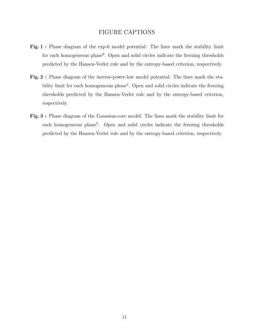
FIGURE CAPTIONS

Fig. 1 : Phase diagram of the exp-6 model potential: The lines mark the stability limit

for each homogeneous phase6. Open and solid circles indicate the freezing thresholds

predicted by the Hansen-Verlet rule and by the entropy-based criterion, respectively.

Fig. 2 : Phase diagram of the inverse-power-law model potential: The lines mark the sta-

bility limit for each homogeneous phase4. Open and solid circles indicate the freezing

thresholds predicted by the Hansen-Verlet rule and by the entropy-based criterion,

respectively.

Fig. 3 : Phase diagram of the Gaussian-core model: The lines mark the stability limit for

each homogeneous phase5. Open and solid circles indicate the freezing thresholds

predicted by the Hansen-Verlet rule and by the entropy-based criterion, respectively.

11

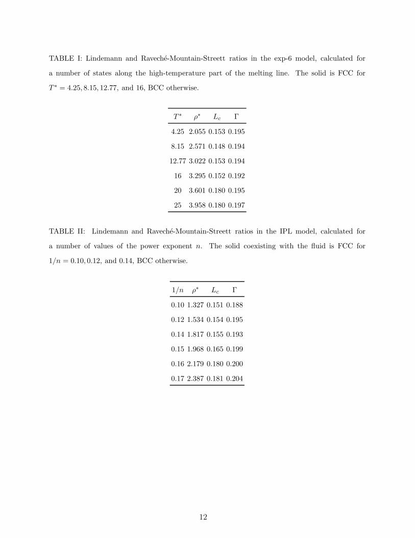
TABLE I: Lindemann and Raveche-Mountain-Streett ratios in the exp-6 model, calculated for

a number of states along the high-temperature part of the melting line. The solid is FCC for

T ∗ = 4.25, 8.15, 12.77, and 16, BCC otherwise.

T ∗ ρ∗ Lc Γ

4.25 2.055 0.153 0.195

8.15 2.571 0.148 0.194

12.77 3.022 0.153 0.194

16 3.295 0.152 0.192

20 3.601 0.180 0.195

25 3.958 0.180 0.197

TABLE II: Lindemann and Raveche-Mountain-Streett ratios in the IPL model, calculated for

a number of values of the power exponent n. The solid coexisting with the fluid is FCC for

1/n = 0.10, 0.12, and 0.14, BCC otherwise.

1/n ρ∗ Lc Γ

0.10 1.327 0.151 0.188

0.12 1.534 0.154 0.195

0.14 1.817 0.155 0.193

0.15 1.968 0.165 0.199

0.16 2.179 0.180 0.200

0.17 2.387 0.181 0.204

12

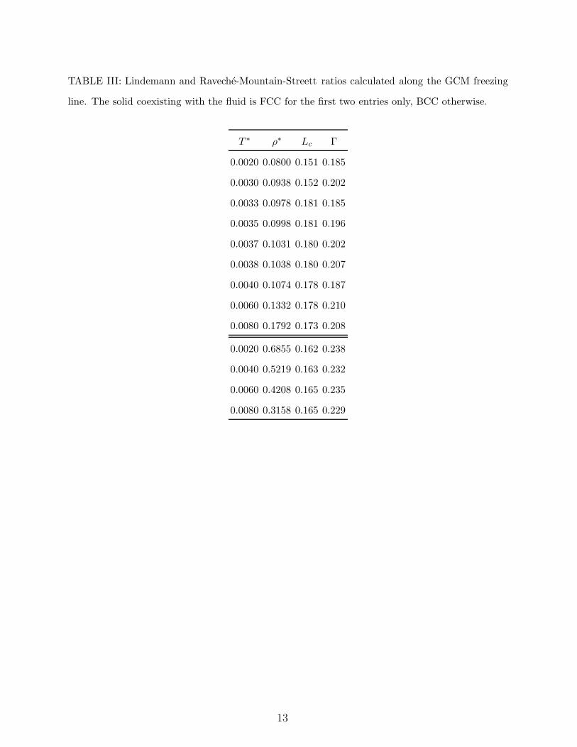
TABLE III: Lindemann and Raveche-Mountain-Streett ratios calculated along the GCM freezing

line. The solid coexisting with the fluid is FCC for the first two entries only, BCC otherwise.

T ∗ ρ∗ Lc Γ

0.0020 0.0800 0.151 0.185

0.0030 0.0938 0.152 0.202

0.0033 0.0978 0.181 0.185

0.0035 0.0998 0.181 0.196

0.0037 0.1031 0.180 0.202

0.0038 0.1038 0.180 0.207

0.0040 0.1074 0.178 0.187

0.0060 0.1332 0.178 0.210

0.0080 0.1792 0.173 0.208

0.0020 0.6855 0.162 0.238

0.0040 0.5219 0.163 0.232

0.0060 0.4208 0.165 0.235

0.0080 0.3158 0.165 0.229

13

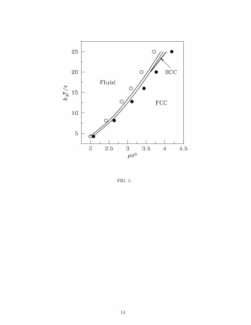
FIG. 1:

14

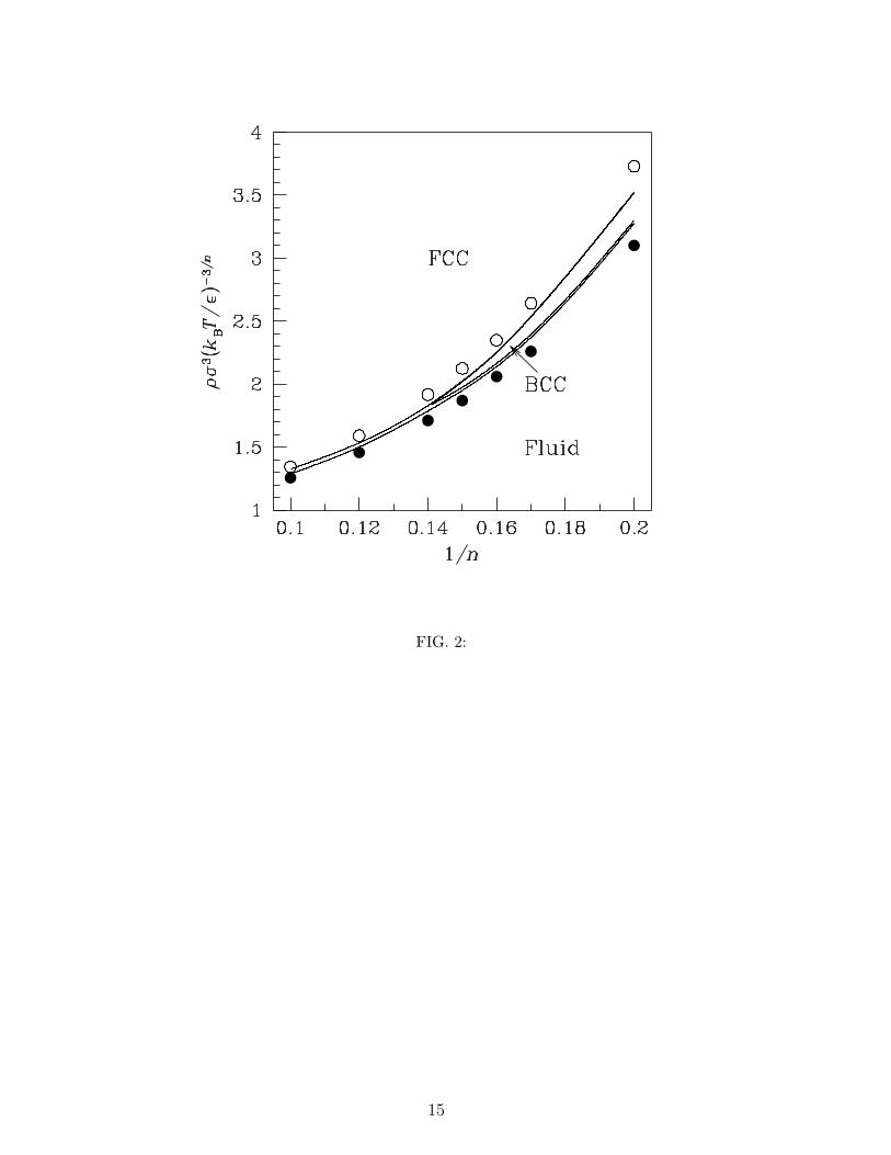
FIG. 2:

15

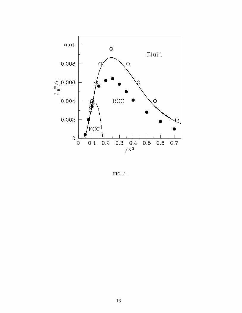
FIG. 3:

16