Journal of

Low Power Electronicsand Applications

Article

Evaluation of In Vivo Spike Detection Algorithms forImplantable MTA Brain—Silicon Interfaces

Mattia Tambaro 1,* , Elia Arturo Vallicelli 2 , Gerardo Saggese 3 , Antonio Strollo 3,Andrea Baschirotto 2 and Stefano Vassanelli 4

1 Padova Neuroscience Center, University of Padua, 35131 Padua, Italy2 Department of Physics, University of Milano Bicocca, 20126 Milan, Italy;

e.vallicelli@campus.unimib.it (E.A.V.); andrea.baschirotto@unimib.it (A.B.)3 Department of Electrical Engineering and Information Technology, University of Naples Federico II,

80125 Naples, Italy; g.saggese@outlook.com (G.S.); astrollo@unina.it (A.S.)4 Department of Biomedical Sciences, University of Padua, 35131 Padua, Italy; stefano.vassanelli@unipd.it* Correspondence: mattia.tambaro@phd.unipd.it

Received: 10 July 2020; Accepted: 29 August 2020; Published: 2 September 2020�����������������

Abstract: This work presents a comparison between different neural spike algorithms to findthe optimum for in vivo implanted EOSFET (electrolyte–oxide-semiconductor field effect transistor)sensors. EOSFET arrays are planar sensors capable of sensing the electrical activity of nearby neuronpopulations in both in vitro cultures and in vivo experiments. They are characterized by a highcell-like resolution and low invasiveness compared to probes with passive electrodes, but exhibita higher noise power that requires ad hoc spike detection algorithms to detect relevant biologicalactivity. Algorithms for implanted devices require good detection accuracy performance and lowpower consumption due to the limited power budget of implanted devices. A figure of merit (FoM)based on accuracy and resource consumption is presented and used to compare different algorithmspresent in the literature, such as the smoothed nonlinear energy operator and correlation-basedalgorithms. A multi transistor array (MTA) sensor of 7 honeycomb pixels of a 30 µm2 area is simulated,generating a signal with Neurocube. This signal is then used to validate the algorithms’ performances.The results allow us to numerically determine which is the most efficient algorithm in the case ofpower constraint in implantable devices and to characterize its performance in terms of accuracy andresource usage.

Keywords: digital signal processing; signal detection; real-time systems; neuroscience; low power

1. Introduction

Intracortical brain computer interfaces have recently seen an increase in research and usage, withscientists from various fields showing increasing interest in their fabrication and adoption. Theseneural sensors can be used to monitor the extracellular electrical activity of neurons in both short-and long-lasting in vivo implants. Particularly, in this last case, low invasiveness and limited powerconsumption are required. The EOSFET MTA [1] are very promising in this scenario as they allow oneto integrate the neural interface, the electronics of signal conditioning, and the interface to outsidethe cutis on a single silicon chip. EOSFETs are composed of a standard complementary metal-oxidesemiconductor (CMOS) transistor [2] combined with a biocompatible oxide covering the metal gate [3,4],which creates a capacitive coupling between the neuron and the electronics [5]. This approach isinvasive but tissue-compatible [6], as there is a distance between neurons and the sensor surface thathelps limit damage to cells and allows for lasting implants. Such devices usually provide a limitedsignal-to-noise ratio (SNR, 3 to 6 dB) per channel compared to standard passive electrodes [7], but

J. Low Power Electron. Appl. 2020, 10, 26; doi:10.3390/jlpea10030026 www.mdpi.com/journal/jlpea

J. Low Power Electron. Appl. 2020, 10, 26 2 of 12

the smallest size and pitch of the pixels on the grid allows for a high spatial resolution [8], providingmore sensing points for each cell on the chip surface. This, together with post-processing algorithms,allows one to extract the biological signal from the background noise with comparable or evenmore confidence than passive metallic electrodes. These algorithms take advantage of the density ofthe sensor and the knowledge of the action potential (AP) shape—frequency band between 300 Hzand 3 kHz—to detect spikes. While, for example, in real-time in vitro experiments, these algorithmsare usually implemented on field programmable gate array (FPGA) and there are no narrow powerconstraints, in the view of an implantable device without any skin-penetrating wire, the power budgetis very limited under various aspects:

• An implanted chip receives power from a battery or from harvesting systems that are intrinsicallycapable of providing limited power;

• The wireless data transmission between the sensor and the external interface cannot managea flow of raw data coming from the entire sensor (at least 10 kS/sec/pixel);

• Being in contact with living tissue, the temperature of the device must remain within the heatdissipation capacity of the tissue to avoid damage.

For these reasons, this paper aims to compare different spike detection algorithms to understandwhich one can be suitable to be implemented in an implantable device relying on two main criteria:the possibility to be implemented in real-time with a low resource footprint and to be adapted toexploit the spatial correlation of the high density pixel matrix of an MTA sensor. The boundary wherethese algorithms are evaluated are the detection and extraction of the relevant features (spikes) froma high amount of raw recording data. This is crucial to reduce the communication overhead requiredby the high sampling rate and channel number of an MTA sensor that can easily have thousands ofpixels. Such a scenario allows one to reduce the communication bandwidth from tens of MB/s to fewkB/s, without precluding an external post-processing elaboration that can include verification andsorting of the extracted spikes, doable mostly without power and performances constraints.

Although the literature presents many different spike detection approaches, several are mainlydeveloped for post-processing analysis, where there are not any particular time and resource constraintsand, thus, are adequate for the purpose of this paper. The compatibility with the boundaries has beenrecognized in three of the most used spike detection algorithms:

• The standard deviation-based threshold crossing [9], a golden standard for most of the real-timesystems due to its extremely low resource footprint combined with a performance sufficient towork as a spike sorting preprocessing step;

• A correlation algorithm exploiting the spatial and temporal information of the signal developedexplicitly for the MTA sensors [10–12];

• The well-known smoothed nonlinear energy operator (SNEO) [13–15], an algorithm used toestimate the instantaneous frequency and amplitude of a sinusoid that, due to its response toaction potentials, has become widely used for spike detection in neural signals.

The final aim of this paper is therefore to find which algorithm should be chosen for animplantable MTA sensor, depending on variables such as SNR, available resources and requiredaccuracy. The algorithm performances are evaluated by using a toolbox for synthetic neural datageneration (Neurocube [16]) based on detailed neuron models to reproduce realistic simulations ofextracellular recordings. This allows us to evaluate the algorithms’ performances on a well-knownspiking dataset, bypassing the lack of a ground truth typical of experimental recording (which isa serious limitation in the accuracy evaluation correctness) and allowing the study of algorithmbehavior in different SNR conditions.

J. Low Power Electron. Appl. 2020, 10, 26 3 of 12

2. Materials and Methods

2.1. Figure of Merit for Implanted Spike Detection Algorithms

The figure of merit (FoM) compares the quality of an algorithm in relation to its cost. To evaluatethe quality of an implantable device algorithm, it is necessary to consider the performances of analgorithm to detect a true positive (TP) while minimizing the number of false positives (FP) and falsenegatives (FN). A TP indicates a detection in the window of samples corresponding to a spike inthe dataset; conversely, an FN reflects a missed detection. An FP corresponds to a detection thatdoes not correspond to a spike shape or a spike detected multiple times. It must be considered thatthe number of FNs affects the quality of the data generated by the sensor, as part of the electricalactivity of the neural network is not detected. Instead, the number of FPs generated by the backgroundnoise increases the amount of data to be transmitted to the external unit, thus increasing the powerconsumption of the device. Therefore, the total performance of a spike detection algorithm strictlydepends on TP, FP and FN, and it can be summarized by the accuracy. The detection accuracy isdefined as in Equation (1), where TP and FP are defined as above and NS is the total number of spikes(TP + FN).

Accuracy =TP

NS + FP(1)

For each algorithm, the accuracy highly depends on the SNR. It is more difficult to detect a spikein the case of low SNR, while most of the spikes are correctly detected with a high SNR, as can bededuced from Figure 1. A good algorithm allows one to achieve a high accuracy with a low SNR value,detecting even the weakest spikes. Therefore, the effectiveness of the algorithm is evaluated with anSNR of 3 dB per pixel, an expectable value in a real scenario. The FoM is produced as the ratio betweenthe accuracy and the cost of the algorithm.

J. Low Power Electron. Appl. 2020, 10, x FOR PEER REVIEW 3 of 12

The figure of merit (FoM) compares the quality of an algorithm in relation to its cost. To evaluate the quality of an implantable device algorithm, it is necessary to consider the performances of an algorithm to detect a true positive (TP) while minimizing the number of false positives (FP) and false negatives (FN). A TP indicates a detection in the window of samples corresponding to a spike in the dataset; conversely, an FN reflects a missed detection. An FP corresponds to a detection that does not correspond to a spike shape or a spike detected multiple times. It must be considered that the number of FNs affects the quality of the data generated by the sensor, as part of the electrical activity of the neural network is not detected. Instead, the number of FPs generated by the background noise increases the amount of data to be transmitted to the external unit, thus increasing the power consumption of the device. Therefore, the total performance of a spike detection algorithm strictly depends on TP, FP and FN, and it can be summarized by the accuracy. The detection accuracy is defined as in Equation (1), where 𝑇𝑃 and 𝐹𝑃 are defined as above and 𝑁𝑆 is the total number of spikes 𝑇𝑃 𝐹𝑁 . 𝐴𝑐𝑐𝑢𝑟𝑎𝑐𝑦 𝑇𝑃𝑁𝑆 𝐹𝑃 (1)

For each algorithm, the accuracy highly depends on the SNR. It is more difficult to detect a spike in the case of low SNR, while most of the spikes are correctly detected with a high SNR, as can be deduced from Figure 1. A good algorithm allows one to achieve a high accuracy with a low SNR value, detecting even the weakest spikes. Therefore, the effectiveness of the algorithm is evaluated with an SNR of 3 dB per pixel, an expectable value in a real scenario. The FoM is produced as the ratio between the accuracy and the cost of the algorithm.

(a) (b)

Figure 1. (a) A simulated extracellular spike template. (b) Spike template with noise at 3 dB signal-to-noise ratio (SNR).

The algorithm’s cost is evaluated as the resource consumption in terms of logic gates required by the algorithm operations. Generically, complexity in operations corresponds to a larger digital circuit and therefore more power requirement. For this reason, each algorithm is characterized by the number of logic gates required by its per-sample operations. The logic gates number is used to evaluate the cost in the FoM as a parameter that depends only on the algorithm and not on the technological node chosen or on the size of the sensor in terms of the number of the obtained pixels.

Figure 1. (a) A simulated extracellular spike template. (b) Spike template with noise at 3 dBsignal-to-noise ratio (SNR).

The algorithm’s cost is evaluated as the resource consumption in terms of logic gates required bythe algorithm operations. Generically, complexity in operations corresponds to a larger digital circuitand therefore more power requirement. For this reason, each algorithm is characterized by the numberof logic gates required by its per-sample operations. The logic gates number is used to evaluate the cost

J. Low Power Electron. Appl. 2020, 10, 26 4 of 12

in the FoM as a parameter that depends only on the algorithm and not on the technological nodechosen or on the size of the sensor in terms of the number of the obtained pixels.

Finally, the FoM is designed as the ratio between the accuracy achieved at 3 dB of SNR per pixel—arealistic signal and noise amount in real data acquisitions—and the number of logic gates required byeach algorithm, as in Equation (2).

FoM =Accuracy

Logic Gates(2)

In this way, with the FoM parameter, a greater score can be assigned to a method with a loweraccuracy but a light footprint in resource usage than a high performance but greedy algorithm.

2.2. Generation of Neural Signals

The algorithms were tested on signal created using Neurocube, a tool for the generation of realisticsimulation of extracellular recordings using detailed neuron models. The generated signal (Figure 2shows 50 milliseconds activity of one channel) emulates a signal from an in vivo experiment where anarray of seven honeycomb channels records the activity of a neuron spaced by 8.5 µm from the centerof the array surface, plus other “far” neurons placed randomly in a cubic volume of 0.25 mm lengthabove the sensor. The sampling frequency of each channels is set to 10 kHz, while the pixel size is set to6 µm, spaced by 2 µm. Both sizes and sample rate lay in the range of the current MTA recording systemcharacteristic. The neurons density is set to 300,000 neurons/mm2, with 10% active neurons firing at100 Hz. The entire record is 30,000 samples, corresponding to a 3 s duration for a total of 299 spikes.The synthetic dataset representing the noiseless electrical activity of the neural network is initiallygenerated. Then, thermal noise is added to the dataset to allow for observations of the accuracy atdifferent SNR levels. From the synthetic dataset, 10 datasets were obtained by adding the thermalnoise at 21 different SNR levels (from −10 to 10 dB). Each algorithm was tested on all datasets andthe results for each SNR level were averaged.

J. Low Power Electron. Appl. 2020, 10, x FOR PEER REVIEW 4 of 12

Finally, the FoM is designed as the ratio between the accuracy achieved at 3 dB of SNR per pixel—a realistic signal and noise amount in real data acquisitions—and the number of logic gates required by each algorithm, as in Equation (2). 𝐹𝑜𝑀 𝐴𝑐𝑐𝑢𝑟𝑎𝑐𝑦𝐿𝑜𝑔𝑖𝑐 𝐺𝑎𝑡𝑒𝑠 (2)

In this way, with the FoM parameter, a greater score can be assigned to a method with a lower accuracy but a light footprint in resource usage than a high performance but greedy algorithm.

2.2. Generation of Neural Signals

The algorithms were tested on signal created using Neurocube, a tool for the generation of realistic simulation of extracellular recordings using detailed neuron models. The generated signal (Figure 2 shows 50 milliseconds activity of one channel) emulates a signal from an in vivo experiment where an array of seven honeycomb channels records the activity of a neuron spaced by 8.5 μm from the center of the array surface, plus other “far” neurons placed randomly in a cubic volume of 0.25 mm length above the sensor. The sampling frequency of each channels is set to 10 kHz, while the pixel size is set to 6 μm, spaced by 2 μm. Both sizes and sample rate lay in the range of the current MTA recording system characteristic. The neurons density is set to 300,000 neurons/mm2, with 10% active neurons firing at 100 Hz. The entire record is 30,000 samples, corresponding to a 3 s duration for a total of 299 spikes. The synthetic dataset representing the noiseless electrical activity of the neural network is initially generated. Then, thermal noise is added to the dataset to allow for observations of the accuracy at different SNR levels. From the synthetic dataset, 10 datasets were obtained by adding the thermal noise at 21 different SNR levels (from −10 to 10 dB). Each algorithm was tested on all datasets and the results for each SNR level were averaged.

(a) (b)

Figure 2. (a) Fifty milliseconds of extracellular simulated activity without noise on a single channel of a pyramidal neuron generated by Neurocube. (b) Noisy dataset created from the noiseless template adding white noise to achieve an SNR of 3 dB.

2.3. Spike Detection Algorithms

Three of the most used algorithms for spike detection, i.e., threshold crossing, the correlation-based algorithm, and the smoothed nonlinear energy operator (SNEO), were chosen for the comparison. Their performances are assessed through an FoM as introduced in Section 2.1. These

Figure 2. (a) Fifty milliseconds of extracellular simulated activity without noise on a single channel ofa pyramidal neuron generated by Neurocube. (b) Noisy dataset created from the noiseless templateadding white noise to achieve an SNR of 3 dB.

2.3. Spike Detection Algorithms

Three of the most used algorithms for spike detection, i.e., threshold crossing, the correlation-basedalgorithm, and the smoothed nonlinear energy operator (SNEO), were chosen for the comparison.

J. Low Power Electron. Appl. 2020, 10, 26 5 of 12

Their performances are assessed through an FoM as introduced in Section 2.1. These methods wereadapted to take advantage of the signal correlation provided by the high spatial resolution to findspikes even in the case of very poor SNR, since it is expected to sense the deterministic event of a spikesimultaneously on all the pixels surmounted by a neuron, drowned in a mostly uncorrelated thermalnoise. The first step is common for all these methods and consists of filtering of the raw signal witha second order passband Butterworth with a cutoff at 300 and 3000 Hz. Thus, from here onwards,the signal is defined as a filtered signal.

2.3.1. Threshold Crossing

Threshold crossing is the simplest and hardware-friendliest method between the three chosenspike detection algorithms. It consists of a comparison between the peaks of the filtered signal anda threshold. The comparison of the positive or the negative signal peaks is chosen depending onthe most preponderant one in the spike shape. To conduct a fair comparison with the other twomethods that exploit the spatial correlation of the activity, the filtered signal of the 7 pixels is summedand compared with a threshold dependent on the standard deviation of the sum, as shown in the blockdiagram in Figure 3.

J. Low Power Electron. Appl. 2020, 10, x FOR PEER REVIEW 5 of 12

methods were adapted to take advantage of the signal correlation provided by the high spatial resolution to find spikes even in the case of very poor SNR, since it is expected to sense the deterministic event of a spike simultaneously on all the pixels surmounted by a neuron, drowned in a mostly uncorrelated thermal noise. The first step is common for all these methods and consists of filtering of the raw signal with a second order passband Butterworth with a cutoff at 300 and 3000 Hz. Thus, from here onwards, the signal is defined as a filtered signal.

2.3.1. Threshold Crossing

Threshold crossing is the simplest and hardware-friendliest method between the three chosen spike detection algorithms. It consists of a comparison between the peaks of the filtered signal and a threshold. The comparison of the positive or the negative signal peaks is chosen depending on the most preponderant one in the spike shape. To conduct a fair comparison with the other two methods that exploit the spatial correlation of the activity, the filtered signal of the 7 pixels is summed and compared with a threshold dependent on the standard deviation of the sum, as shown in the block diagram in Figure 3.

Figure 3. Threshold crossing block diagram. STD represents the signal standard deviation calculation, while ThMult is the constant by which the standard deviation is multiplied to find the comparison threshold.

The algorithm was optimized to achieve the best performances. For this method, the only parameter that can be varied is the threshold value. Figure 4 shows the results of accuracy using different threshold multipliers varying the SNR level. The threshold was set to recognize the negative peak of the spike, with a value of −2 times the noise standard deviation σ, a value that demonstrates the best performance in detection accuracy. The accuracy in the case of −1σ is seems to be higher for lower SNR (<2 dB), but it presents a tremendous number of FPs that makes the threshold unusable.

Figure 4. Threshold crossing accuracy using −σ, −2σ and −3σ as threshold values.

2.3.2. Correlation Algorithm

Figure 3. Threshold crossing block diagram. STD represents the signal standard deviationcalculation, while ThMult is the constant by which the standard deviation is multiplied to findthe comparison threshold.

The algorithm was optimized to achieve the best performances. For this method, the onlyparameter that can be varied is the threshold value. Figure 4 shows the results of accuracy usingdifferent threshold multipliers varying the SNR level. The threshold was set to recognize the negativepeak of the spike, with a value of −2 times the noise standard deviation σ, a value that demonstratesthe best performance in detection accuracy. The accuracy in the case of −1σ is seems to be higher forlower SNR (<2 dB), but it presents a tremendous number of FPs that makes the threshold unusable.

J. Low Power Electron. Appl. 2020, 10, x FOR PEER REVIEW 5 of 12

methods were adapted to take advantage of the signal correlation provided by the high spatial resolution to find spikes even in the case of very poor SNR, since it is expected to sense the deterministic event of a spike simultaneously on all the pixels surmounted by a neuron, drowned in a mostly uncorrelated thermal noise. The first step is common for all these methods and consists of filtering of the raw signal with a second order passband Butterworth with a cutoff at 300 and 3000 Hz. Thus, from here onwards, the signal is defined as a filtered signal.

2.3.1. Threshold Crossing

Threshold crossing is the simplest and hardware-friendliest method between the three chosen spike detection algorithms. It consists of a comparison between the peaks of the filtered signal and a threshold. The comparison of the positive or the negative signal peaks is chosen depending on the most preponderant one in the spike shape. To conduct a fair comparison with the other two methods that exploit the spatial correlation of the activity, the filtered signal of the 7 pixels is summed and compared with a threshold dependent on the standard deviation of the sum, as shown in the block diagram in Figure 3.

Figure 3. Threshold crossing block diagram. STD represents the signal standard deviation calculation, while ThMult is the constant by which the standard deviation is multiplied to find the comparison threshold.

The algorithm was optimized to achieve the best performances. For this method, the only parameter that can be varied is the threshold value. Figure 4 shows the results of accuracy using different threshold multipliers varying the SNR level. The threshold was set to recognize the negative peak of the spike, with a value of −2 times the noise standard deviation σ, a value that demonstrates the best performance in detection accuracy. The accuracy in the case of −1σ is seems to be higher for lower SNR (<2 dB), but it presents a tremendous number of FPs that makes the threshold unusable.

Figure 4. Threshold crossing accuracy using −σ, −2σ and −3σ as threshold values.

2.3.2. Correlation Algorithm

Figure 4. Threshold crossing accuracy using −σ, −2σ and −3σ as threshold values.

J. Low Power Electron. Appl. 2020, 10, 26 6 of 12

2.3.2. Correlation Algorithm

The Correlation algorithm searches for an equivalent pixel using both consecutive samples intime and adjacent pixels in space. In the implementation presented in [12], it exploits the temporaloversampling by summing three consecutive squared samples vp

2 for each channel, but we testedthe accuracy level using different temporal sum lengths. After the temporal sum, the algorithmthen normalizes these values by each pixel standard deviation σ2

p, to assign it a reliability. Everychannel value is then summed with that of its six surrounding neighbors and is compared with a fixed,precomputed threshold ThMult, as explained in [12], to achieve one false positive per second onthe 7-pixel group. The process is summarized in Equation (3), where N is the number of samples usedfor the temporal sum, and it is shown in Figure 5.

CA(vp(n)

)=

7∑p=1

∑N−1k=0 vp(n− k)2

σ2p

, (3)

J. Low Power Electron. Appl. 2020, 10, x FOR PEER REVIEW 6 of 12

The Correlation algorithm searches for an equivalent pixel using both consecutive samples in time and adjacent pixels in space. In the implementation presented in [12], it exploits the temporal oversampling by summing three consecutive squared samples 𝑣 for each channel, but we tested the accuracy level using different temporal sum lengths. After the temporal sum, the algorithm then normalizes these values by each pixel standard deviation 𝜎 , to assign it a reliability. Every channel value is then summed with that of its six surrounding neighbors and is compared with a fixed, precomputed threshold 𝑇ℎ𝑀𝑢𝑙𝑡, as explained in [12], to achieve one false positive per second on the 7-pixel group. The process is summarized in Equation (3), where N is the number of samples used for the temporal sum, and it is shown in Figure 5.

𝐶𝐴 𝑣 n ∑ , (3)

Figure 5. Correlation algorithm block diagram. Mem block defines a memory containing the last three samples for each channel, STD block computes the standard deviation of the square of the signal, and ThMult is the threshold used for the output comparison.

Figure 6 shows the results, where the better accuracy, in our simulations, is achieved without summing any consecutive temporal sample. Note that an accuracy over 99% is not reached by design, since the threshold is estimated and empirically adjusted to allow for a single false positive per second.

Figure 6. Correlation algorithm accuracy with a temporal summation of two and three samples and without summation (N = 1), where N is the number of summed samples.

2.3.3. SNEO

Figure 5. Correlation algorithm block diagram. Mem block defines a memory containing the last threesamples for each channel, STD block computes the standard deviation of the square of the signal, andThMult is the threshold used for the output comparison.

Figure 6 shows the results, where the better accuracy, in our simulations, is achieved withoutsumming any consecutive temporal sample. Note that an accuracy over 99% is not reached by design,since the threshold is estimated and empirically adjusted to allow for a single false positive per second.

J. Low Power Electron. Appl. 2020, 10, x FOR PEER REVIEW 6 of 12

The Correlation algorithm searches for an equivalent pixel using both consecutive samples in time and adjacent pixels in space. In the implementation presented in [12], it exploits the temporal oversampling by summing three consecutive squared samples 𝑣 for each channel, but we tested the accuracy level using different temporal sum lengths. After the temporal sum, the algorithm then normalizes these values by each pixel standard deviation 𝜎 , to assign it a reliability. Every channel value is then summed with that of its six surrounding neighbors and is compared with a fixed, precomputed threshold 𝑇ℎ𝑀𝑢𝑙𝑡, as explained in [12], to achieve one false positive per second on the 7-pixel group. The process is summarized in Equation (3), where N is the number of samples used for the temporal sum, and it is shown in Figure 5.

𝐶𝐴 𝑣 n ∑ , (3)

Figure 5. Correlation algorithm block diagram. Mem block defines a memory containing the last three samples for each channel, STD block computes the standard deviation of the square of the signal, and ThMult is the threshold used for the output comparison.

Figure 6 shows the results, where the better accuracy, in our simulations, is achieved without summing any consecutive temporal sample. Note that an accuracy over 99% is not reached by design, since the threshold is estimated and empirically adjusted to allow for a single false positive per second.

Figure 6. Correlation algorithm accuracy with a temporal summation of two and three samples and without summation (N = 1), where N is the number of summed samples.

2.3.3. SNEO

Figure 6. Correlation algorithm accuracy with a temporal summation of two and three samples andwithout summation (N = 1), where N is the number of summed samples.

J. Low Power Electron. Appl. 2020, 10, 26 7 of 12

2.3.3. SNEO

The smoothed nonlinear energy operator (SNEO) gives an instantaneous estimation of the energycontained in a signal oscillation. Due to its energy answer, it has been proved to fit well the detection ofspikes. This algorithm strictly depends on a parameter called k, which in turn depends on the samplingfrequency and the average spike duration. After computing the nonlinear energy response (NEOblock) of the signal samples, the SNEO soothes it using a Hamming window w(4k + 1) with a sizeof 4k + 1 and compares the result with a threshold multiple of the standard deviation of the output.Even in this case, the spatial correlation is exploited. In fact, as an input of this operator, the average ofthe 7-pixel group is considered. The operator is described in Equation (4) and shown in Figure 7.

SNEO = NEO⊗w(4k + 1), NEO(x(n)) = x(n)2− x(n + k)·x(n− k), x(n) =

7∑p=1

vp(n)7

(4)

J. Low Power Electron. Appl. 2020, 10, x FOR PEER REVIEW 7 of 12

The smoothed nonlinear energy operator (SNEO) gives an instantaneous estimation of the energy contained in a signal oscillation. Due to its energy answer, it has been proved to fit well the detection of spikes. This algorithm strictly depends on a parameter called 𝑘, which in turn depends on the sampling frequency and the average spike duration. After computing the nonlinear energy response (NEO block) of the signal samples, the SNEO soothes it using a Hamming window 𝑤 4𝑘 1 with a size of 4𝑘 1 and compares the result with a threshold multiple of the standard deviation of the output. Even in this case, the spatial correlation is exploited. In fact, as an input of this operator, the average of the 7-pixel group is considered. The operator is described in Equation (4) and shown in Figure 7.

𝑆𝑁𝐸𝑂 𝑁𝐸𝑂 ⊗ 𝑤 4𝑘 1 , 𝑁𝐸𝑂 𝑥 𝑛 𝑥 𝑛 𝑥 n 𝑘 ∙ 𝑥 n 𝑘 , x 𝑛 𝑣 𝑛7 (4)

Figure 7. Smoothed nonlinear energy operator (SNEO) blocks diagram. Mem contains the last 2 × k + 1 samples, and STD block and ThMult are used to estimate the threshold for an SNEO detection.

The performance was tuned changing the 𝑘 parameter. Figure 8 shows the different performances of this operator testing 𝑘 at different SNR level. With greater 𝑘 value, the accuracy increases at a higher SNR level due to the reduced false positive amount, but the best tradeoff at the medium level SNR is achieved with 𝑘 2, where other widths are too conservative.

Figure 8. SNEO accuracy using different k values.

3. Results

The algorithms’ performances were evaluated on synthetic datasets described in Section 2.2. For each SNR level, 10 datasets were created. The performances measured for each algorithm at each SNR level are the average of the 10 results achieved on these datasets.

3.1. Algorithm Accuracy

Figure 7. Smoothed nonlinear energy operator (SNEO) blocks diagram. Mem contains the last 2 × k + 1samples, and STD block and ThMult are used to estimate the threshold for an SNEO detection.

The performance was tuned changing the k parameter. Figure 8 shows the different performancesof this operator testing k at different SNR level. With greater k value, the accuracy increases at a higherSNR level due to the reduced false positive amount, but the best tradeoff at the medium level SNR isachieved with k = 2, where other widths are too conservative.

J. Low Power Electron. Appl. 2020, 10, x FOR PEER REVIEW 7 of 12

The smoothed nonlinear energy operator (SNEO) gives an instantaneous estimation of the energy contained in a signal oscillation. Due to its energy answer, it has been proved to fit well the detection of spikes. This algorithm strictly depends on a parameter called 𝑘, which in turn depends on the sampling frequency and the average spike duration. After computing the nonlinear energy response (NEO block) of the signal samples, the SNEO soothes it using a Hamming window 𝑤 4𝑘 1 with a size of 4𝑘 1 and compares the result with a threshold multiple of the standard deviation of the output. Even in this case, the spatial correlation is exploited. In fact, as an input of this operator, the average of the 7-pixel group is considered. The operator is described in Equation (4) and shown in Figure 7.

𝑆𝑁𝐸𝑂 𝑁𝐸𝑂 ⊗ 𝑤 4𝑘 1 , 𝑁𝐸𝑂 𝑥 𝑛 𝑥 𝑛 𝑥 n 𝑘 ∙ 𝑥 n 𝑘 , x 𝑛 𝑣 𝑛7 (4)

Figure 7. Smoothed nonlinear energy operator (SNEO) blocks diagram. Mem contains the last 2 × k + 1 samples, and STD block and ThMult are used to estimate the threshold for an SNEO detection.

The performance was tuned changing the 𝑘 parameter. Figure 8 shows the different performances of this operator testing 𝑘 at different SNR level. With greater 𝑘 value, the accuracy increases at a higher SNR level due to the reduced false positive amount, but the best tradeoff at the medium level SNR is achieved with 𝑘 2, where other widths are too conservative.

Figure 8. SNEO accuracy using different k values.

3. Results

The algorithms’ performances were evaluated on synthetic datasets described in Section 2.2. For each SNR level, 10 datasets were created. The performances measured for each algorithm at each SNR level are the average of the 10 results achieved on these datasets.

3.1. Algorithm Accuracy

Figure 8. SNEO accuracy using different k values.

3. Results

The algorithms’ performances were evaluated on synthetic datasets described in Section 2.2. Foreach SNR level, 10 datasets were created. The performances measured for each algorithm at each SNRlevel are the average of the 10 results achieved on these datasets.

J. Low Power Electron. Appl. 2020, 10, 26 8 of 12

3.1. Algorithm Accuracy

The accuracy was estimated for each algorithm depending on the detection performances of trueand false positives at 3 dB SNR as explained in Section 2.1, and Figure 9 shows the results. The SNEOdetector provides the best detection accuracy from the lowest SNR level, followed by the correlationalgorithm. The threshold crossing method requires from 2 to 4 dB SNR to achieve the same results asthe others, but it also achieves 2–3% more accuracy from 5 dB SNR.

J. Low Power Electron. Appl. 2020, 10, x FOR PEER REVIEW 8 of 12

The accuracy was estimated for each algorithm depending on the detection performances of true and false positives at 3 dB SNR as explained in Section 2.1, and Figure 9 shows the results. The SNEO detector provides the best detection accuracy from the lowest SNR level, followed by the correlation algorithm. The threshold crossing method requires from 2 to 4 dB SNR to achieve the same results as the others, but it also achieves 2–3% more accuracy from 5 dB SNR.

Figure 9. Algorithm accuracy (averaged) at different SNR levels. The red vertical line corresponds to 3 dB. Threshold crossing has a threshold of 2∙σ, the correlation algorithm averages three samples in time and the SNEO has a 𝑘 parameter of 2.

3.2. Resource Consumption

As introduced in Section 2.1, resource consumption is estimated as the amount of operations required by each algorithm. The filtering operation is common to all the spike detection methods and is considered once for each algorithm during the FoM evaluation. Each method requires the estimation of the standard deviation (STD) of the signal or of its output, computed as in Equation (5). The mean μ is assumed 0 as a consequence of the high-pass filtering of the data. The STD can be estimated over a power of 2 number of samples, allowing us to perform the division as a bit-shift operation, reducing the required resources.

𝑆𝑇𝐷 1𝑁 𝑥 𝑛 µ, 𝑤ℎ𝑒𝑟𝑒 µ 0 (5)

For each operation, the logic gate amount is estimated, in detail (including operational pre-registers): adder is 23𝑁, multiplicator is 18𝑁 6𝑁 , comparator is 25𝑁, divisor is 28𝑁 and other registers are 9𝑁 logic gates each. 𝑁 is the number of the operand bits. Each operation is assumed in the integer domain—division included—and in a canonical form. For each operation, different algorithms exist, varying the amount of logic gates required, especially in implementation exploiting resource reutilization. Hopefully, the tradeoff between operation complexity and clock frequency in the case of resource reutilization leads to approximately comparable power consumption. For this reason, even if these resource estimation can be subjected to variation depending on the implementation, it can be considered sufficiently accurate to perform algorithm comparison. Table 1 shows the resource estimation results for every considered algorithm.

Figure 9. Algorithm accuracy (averaged) at different SNR levels. The red vertical line corresponds to 3dB. Threshold crossing has a threshold of 2·σ, the correlation algorithm averages three samples in timeand the SNEO has a k parameter of 2.

3.2. Resource Consumption

As introduced in Section 2.1, resource consumption is estimated as the amount of operationsrequired by each algorithm. The filtering operation is common to all the spike detection methods andis considered once for each algorithm during the FoM evaluation. Each method requires the estimationof the standard deviation (STD) of the signal or of its output, computed as in Equation (5). The mean µ

is assumed 0 as a consequence of the high-pass filtering of the data. The STD can be estimated overa power of 2 number of samples, allowing us to perform the division as a bit-shift operation, reducingthe required resources.

STD =

√√√1N

N∑n=1

x(n)2− µ, where µ ≈ 0 (5)

For each operation, the logic gate amount is estimated, in detail (including operationalpre-registers): adder is 23N, multiplicator is 18N + 6N2, comparator is 25N, divisor is 28N andother registers are 9N logic gates each. N is the number of the operand bits. Each operation is assumedin the integer domain—division included—and in a canonical form. For each operation, differentalgorithms exist, varying the amount of logic gates required, especially in implementation exploitingresource reutilization. Hopefully, the tradeoff between operation complexity and clock frequency inthe case of resource reutilization leads to approximately comparable power consumption. For thisreason, even if these resource estimation can be subjected to variation depending on the implementation,it can be considered sufficiently accurate to perform algorithm comparison. Table 1 shows the resourceestimation results for every considered algorithm.

J. Low Power Electron. Appl. 2020, 10, 26 9 of 12

Table 1. Resources required by the hardware implementation of the algorithms.

Filter StandardDeviation

ThresholdCrossing

CorrelationAlgorithm SNEO

Adder 4 1 + 1 1 6 20 1 1 + 6 1 + (4 k) 2

Multiplicator 5 1 2 * 3 + 2 * 2 + (4 k + 1) 1 + 2 *

Comparator 0 1 1 1 2 1 2

Divisor 0 0 0 7 0

Register 4 1 1 1 0 21 1 2 k + (4 k + 1) 1

STD 0 - 1 7 1

Weighted Total 254 N + 30 N 2 121 N + 6 N 2 235 N + 6 N 2 +STD

995 N+42 N 2 +7 * STD

557 N + 602 kN + 36N 2 + 48 kN 2 + STD 1

5-bit, k = 2 2020 755 2080 11,310 13,615

8-bit, k = 4 3952 1352 3616 20,112 25,2401 the operation occurs after a multiplication and it is weighted as 2N. 2 the operation occurs after two multiplicationsand it is weighted as 4N. * one is for the threshold computation; one is to avoid the STD square root.

4. Discussion

From the accuracy performance and resource consumption of each algorithm shown in Sections 3.1and 3.2, we can finally observe the FoM results in Figure 10. The curves show the ratio betweenthe accuracy at 3 dB of SNR and the resources required for algorithm implementation with differentsample widths. Detailed results are shown in Table 2.

J. Low Power Electron. Appl. 2020, 10, x FOR PEER REVIEW 9 of 12

Table 1. Resources required by the hardware implementation of the algorithms.

Filter Standard Deviation

Threshold Crossing

Correlation Algorithm

SNEO

Adder 4 1 + 1 1 6 20 1 1 + 6 1 + (4 k) 2

Multiplicator 5 1 2 * 3 + 2 * 2 + (4 k + 1) 1 + 2 * Comparator 0 1 1 1 2 1 2

Divisor 0 0 0 7 0 Register 4 1 1 1 0 21 1 2 k + (4 k + 1) 1

STD 0 - 1 7 1 Weighted

Total 254 N + 30 N 2 121 N + 6 N 2 235 N + 6 N 2 +

STD

995 N+42 N 2 + 7 * STD

557 N + 602 kN + 36 N 2 + 48 kN 2 + STD 1

5-bit, k = 2 2020 755 2080 11,310 13,615 8-bit, k = 4 3952 1352 3616 20,112 25,240

1 the operation occurs after a multiplication and it is weighted as 2𝑁. 2 the operation occurs after two multiplications and it is weighted as 4𝑁. * one is for the threshold computation; one is to avoid the STD square root.

4. Discussion

From the accuracy performance and resource consumption of each algorithm shown in Sections 3.1 and 3.2, we can finally observe the FoM results in Figure 10. The curves show the ratio between the accuracy at 3 dB of SNR and the resources required for algorithm implementation with different sample widths. Detailed results are shown in Table 2.

Figure 10. Figure of merit (FoM) of algorithms, ratio of accuracy at 3 dB of SNR and logic gates required for implementation with different width of samples bits.

Table 2. Algorithm performances at 3 dB SNR.

Threshold Crossing Correlation Algorithm SNEO True Positive (%) 73 93 96 False Positive (%) 4 1 2

Accuracy (%) 70 93 95 Resources (8 bit) 3616 20,320 41,016

FoM (3 dB) 0.40 0.12 0.10

As can be observed, according to the FoM, the threshold crossing method outperforms by a factor of about 2.5× the others two algorithms, despite its poor accuracy, due to its light footprint in logic gate requirements (5× and 8× compared to SNEO and the correlation algorithm, respectively).

Figure 10. Figure of merit (FoM) of algorithms, ratio of accuracy at 3 dB of SNR and logic gates requiredfor implementation with different width of samples bits.

Table 2. Algorithm performances at 3 dB SNR.

ThresholdCrossing Correlation Algorithm SNEO

True Positive (%) 73 93 96False Positive (%) 4 1 2

Accuracy (%) 70 93 95Resources (8 bit) 3616 20,320 41,016

FoM (3 dB) 0.40 0.12 0.10

J. Low Power Electron. Appl. 2020, 10, 26 10 of 12

As can be observed, according to the FoM, the threshold crossing method outperforms by a factorof about 2.5× the others two algorithms, despite its poor accuracy, due to its light footprint in logicgate requirements (5× and 8× compared to SNEO and the correlation algorithm, respectively). Despitethis consideration, a real winner must be chosen carefully, strictly depending on the scenario wherethe detector must lay. If there are tight constrains on power that can be provided to the circuit,the threshold crossing approach must be preferred, considering also that if the transmission bandwidthallows it, it is possible to sacrifice the accuracy lowering the threshold multiplier. A more relaxedthreshold causes a higher number of FP, but it also increases the correct detections, as shown in the caseof the threshold set to −σ in Figure 4; an external sorting/clustering of the detected spikes eventuallydiscards the FP in the second step without a power constraint.

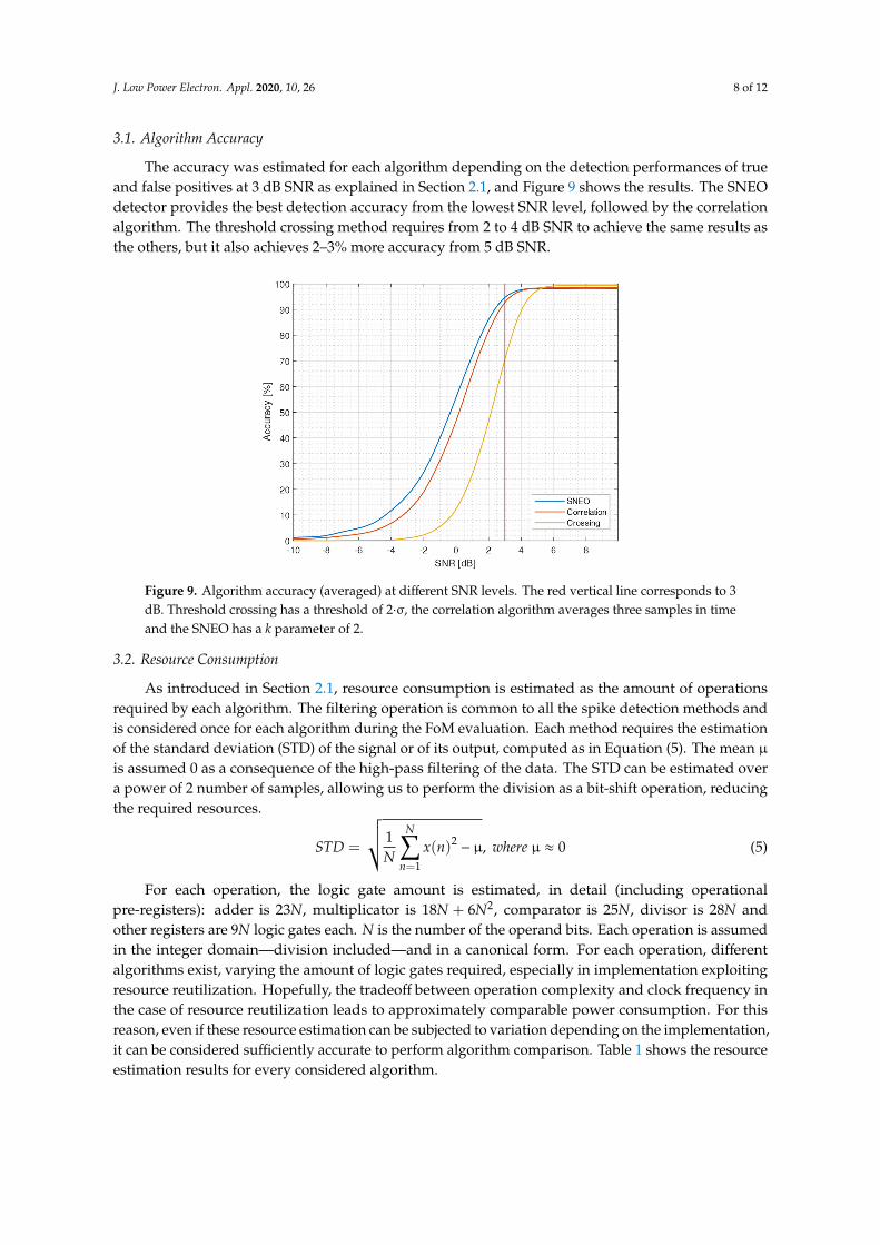
These considerations change for SNR above 4–5, as can be seen in Figure 9, where the thresholdcrossing method can be considered the best approach without exception, providing over 90% accuracy,and having 3–4× higher FoM than the competitors. Conversely, as shown in Figure 11, in the case ofSNR lower than 1, the threshold crossing method lose its supremacy due to the very poor performancesachieved. Here, the correlation and the SNEO algorithms can be considered equivalent in appearanceof the FoM. Paying about 1.2×more logic gates when compared to the correlation algorithm, the SNEOclearly provides the better performances, with 5–7% better accuracy depending on the SNR. The kparameter of the SNEO algorithm can considerably change the resource requirements of the algorithm,especially because of the convolution operation that makes the resources grow quadratically. However,for typical sampling frequency of up to 30 kHz, a k lower than 6 should be sufficient for an accuratedetection in most scenarios. A similar discussion can be applied where less constrained power limitsare required; in fact, the better accuracy provided by these last two methods should be preferredover threshold crossing’s light footprint, at least below 5 dB of SNR. Results achieved under the 0dB SNR level cannot surpass 50% accuracy with any of the proposed methods and are probably notsuitable to extract relevant activity from the observed neuronal population. In this case, similarly towhat was suggested with threshold crossing, the SNEO algorithm with a relaxed threshold and anoff-the-MTA-chip processing step can help to increase the detections but, as consequence, the algorithmrequires that both are paid more resources and that a greater amount of data is transmitted.

J. Low Power Electron. Appl. 2020, 10, x FOR PEER REVIEW 10 of 12

Despite this consideration, a real winner must be chosen carefully, strictly depending on the scenario where the detector must lay. If there are tight constrains on power that can be provided to the circuit, the threshold crossing approach must be preferred, considering also that if the transmission bandwidth allows it, it is possible to sacrifice the accuracy lowering the threshold multiplier. A more relaxed threshold causes a higher number of FP, but it also increases the correct detections, as shown in the case of the threshold set to −σ in Figure 4; an external sorting/clustering of the detected spikes eventually discards the FP in the second step without a power constraint.

These considerations change for SNR above 4–5, as can be seen in Figure 9, where the threshold crossing method can be considered the best approach without exception, providing over 90% accuracy, and having 3–4× higher FoM than the competitors. Conversely, as shown in Figure 11, in the case of SNR lower than 1, the threshold crossing method lose its supremacy due to the very poor performances achieved. Here, the correlation and the SNEO algorithms can be considered equivalent in appearance of the FoM. Paying about 1.2× more logic gates when compared to the correlation algorithm, the SNEO clearly provides the better performances, with 5–7% better accuracy depending on the SNR. The 𝑘 parameter of the SNEO algorithm can considerably change the resource requirements of the algorithm, especially because of the convolution operation that makes the resources grow quadratically. However, for typical sampling frequency of up to 30 kHz, a 𝑘 lower than 6 should be sufficient for an accurate detection in most scenarios. A similar discussion can be applied where less constrained power limits are required; in fact, the better accuracy provided by these last two methods should be preferred over threshold crossing’s light footprint, at least below 5 dB of SNR. Results achieved under the 0 dB SNR level cannot surpass 50% accuracy with any of the proposed methods and are probably not suitable to extract relevant activity from the observed neuronal population. In this case, similarly to what was suggested with threshold crossing, the SNEO algorithm with a relaxed threshold and an off-the-MTA-chip processing step can help to increase the detections but, as consequence, the algorithm requires that both are paid more resources and that a greater amount of data is transmitted.

Figure 11. FoM of algorithms, ratio of accuracy and logic gates required for 8-bit implementation at different SNR levels.

As a side note, the sample number of bits alone has appeared incapable of changing the consideration drawn until now, since it does not vary the relative distance of the algorithms in the FoM. As a general hint, a small quantization step—and so wider data samples in a bit—cannot carry any useful information about the signal depending on the SNR level. This reduces the FoM of each algorithm, increasing the resources required by each operation without bringing any advantages. It is possible to define a typical samples bit range laying under 8–10 bits, but the literature present

Figure 11. FoM of algorithms, ratio of accuracy and logic gates required for 8-bit implementation atdifferent SNR levels.

As a side note, the sample number of bits alone has appeared incapable of changingthe consideration drawn until now, since it does not vary the relative distance of the algorithmsin the FoM. As a general hint, a small quantization step—and so wider data samples in a bit—cannot

J. Low Power Electron. Appl. 2020, 10, 26 11 of 12

carry any useful information about the signal depending on the SNR level. This reduces the FoM ofeach algorithm, increasing the resources required by each operation without bringing any advantages.It is possible to define a typical samples bit range laying under 8–10 bits, but the literature presentdifferent methods that allow one to improve the analog to digital converter (ADC) performances inpower-constrained applications [17], lowering the required bit number without losing precision.

5. Conclusions

This paper focused on the accuracy and resource consumption of spike detection methods thatare suitable for an in vivo low-power implantable MTA sensor, depending on the signal quality andavailable power. With an SNR over 4 dB, the threshold crossing method can provide good performancesand is easily preferred over the more complex method. In the case of lower SNR (<2), the SNEOalgorithm provides the absolute better detection accuracy between the compared methods.

Author Contributions: Conceptualization, E.A.V.; methodology, M.T. and E.A.V.; software, G.S. and M.T.;validation, M.T. and G.S.; formal analysis, M.T.; investigation, G.S. and M.T.; resources, S.V., A.S. and A.B.;data curation, G.S.; writing—original draft preparation, E.A.V. and M.T.; writing—review and editing, M.T.;visualization, M.T. and G.S.; supervision, S.V., A.S. and A.B.; project administration, E.A.V. and M.T.; fundingacquisition, S.V., A.S. and A.B. All authors have read and agreed to the published version of the manuscript.

Funding: This research was funded by the SYNCH project, founded by Horizon 2020—Future and EmergingTechnologies and the Brain28 nm PRIN project, founded by MIUR.

Conflicts of Interest: The authors declare no conflict of interest.

References

1. Thewes, R.; Bertotti, G.; Dodel, N.; Keil, S.; Schroder, S.; Boven, K.-H.; Zeck, G.; Mahmud, M.; Vassanelli, S.Neural tissue and brain interfacing CMOS devices—An introduction to state-of-the-art, current and futurechallenges. In Proceedings of the 2016 IEEE International Symposium on Circuits and Systems (ISCAS),Montreal, QC, Canada, 22–25 May 2016; pp. 1826–1829. [CrossRef]

2. Hutzler, M.; Fromherz, P. Silicon chip with capacitors and transistors for interfacing organotypic brain sliceof rat hippocampus. Eur. J. Neurosci. 2004, 19, 2231–2238. [CrossRef] [PubMed]

3. Schröder, S.; Cecchetto, C.; Keil, S.; Mahmud, M.; Brose, E.; Dogan, O.; Bertotti, G.; Wolanski, D.; Tillack, B.;Schneidewind, J.; et al. CMOS-compatible purely capacitive interfaces for high-density in-vivo recordingfrom neural tissue. In Proceedings of the 2015 IEEE Biomedical Circuits and Systems Conference (BioCAS),Atlanta, GA, USA, 22–24 October 2015; pp. 1–4. [CrossRef]

4. Jang, H.-J.; Cho, W.-J. High performance silicon-on-insulator based ion-sensitive field-effect transistor usinghigh-k stacked oxide sensing membrane. Appl. Phys. Lett. 2011, 99, 043703. [CrossRef]

5. Vassanelli, S.; Mahmud, M.; Girardi, S.; Maschietto, M. On the Way to Large-Scale and High-ResolutionBrain-Chip Interfacing. Cogn. Comput. 2012, 4, 71–81. [CrossRef]

6. Eversmann, B.; Jenkner, M.; Hofmann, F.; Paulus, C.; Brederlow, R.; Holzapfl, B.; Fromherz, P.; Merz, M.;Brenner, M.; Schreiter, M.; et al. A 128 × 128 cmos biosensor array for extracellular recording of neuralactivity. IEEE J. Solid-State Circuits 2003, 38, 2306–2317. [CrossRef]

7. Voelker, M.; Fromherz, P. Signal Transmission from Individual Mammalian Nerve Cell to Field-EffectTransistor. Small 2005, 1, 206–210. [CrossRef]

8. Girardi, S.; Maschietto, M.; Zeitler, R.; Mahmud, M.; Vassanelli, S. High resolution cortical imaging usingelectrolyte-(metal)-oxide-semiconductor field effect transistors. In Proceedings of the 2011 5th InternationalIEEE/EMBS Conference on Neural Engineering, Cancun, Mexico, 27 April–1 May 2011; pp. 269–272.[CrossRef]

9. Lewicki, M. A review of methods for spike sorting: The detection and classification of neural action potentials.Netw. Comput. Neural Syst. 1998, 9, R53–R78. [CrossRef]

10. Lambacher, A.; Vitzthum, V.; Zeitler, R.; Eickenscheidt, M.; Eversmann, B.; Thewes, R.; Fromherz, P.Identifying firing mammalian neurons in networks with high-resolution multi-transistor array (MTA). Appl.Phys. A 2011, 102, 1–11. [CrossRef]

J. Low Power Electron. Appl. 2020, 10, 26 12 of 12

11. Vallicelli, E.A.; Reato, M.; Maschietto, M.; Vassanelli, S.; Guarrera, D.; Rocchi, F.; Collazuol, G.; Zeitler, R.;Baschirotto, A.; De Matteis, M. Neural Spike Digital Detector on FPGA. Electronics 2018, 7, 392. [CrossRef]

12. Tambaro, M.; Vallicelli, E.A.; Tomasella, D.; Baschirotto, A.; Vassanelli, S.; Maschietto, M.; De Matteis, M. A 10MSample/Sec Digital Neural Spike Detection for a 1024 Pixels Multi Transistor Array Sensor. In Proceedingsof the 2019 26th IEEE International Conference on Electronics, Circuits and Systems (ICECS), Genoa, Italy,27–29 November 2019; pp. 711–714. [CrossRef]

13. Mukhopadhyay, S.; Ray, G.C. A new interpretation of nonlinear energy operator and its efficacy in spikedetection. IEEE Trans. Biomed. Eng. 1998, 45, 180–187. [CrossRef] [PubMed]

14. Ng, A.K.; Ang, K.K.; Guan, C.; Guan, C. Automatic selection of neuronal spike detection threshold viasmoothed Teager energy histogram. In Proceedings of the 2013 6th International IEEE/EMBS Conference onNeural Engineering (NER), San Diego, CA, USA, 6–8 November 2013; pp. 1437–1440. [CrossRef]

15. Choi, J.H.; Jung, H.K.; Kim, T.; Taejeong, K. A New Action Potential Detector Using the MTEO and ItsEffects on Spike Sorting Systems at Low Signal-to-Noise Ratios. IEEE Trans. Biomed. Eng. 2006, 53, 738–746.[CrossRef] [PubMed]

16. Kim, D.; Kung, J.; Chai, S.; Yalamanchili, S.; Mukhopadhyay, S. Neurocube: A Programmable DigitalNeuromorphic Architecture with High-Density 3D Memory. In Proceedings of the 2016 ACM/IEEE43rd Annual International Symposium on Computer Architecture (ISCA), Seoul, Korea, 18–22 June 2016;pp. 380–392. [CrossRef]

17. Hirai, Y.; Matsuoka, T.; Tani, S.; Isami, S.; Tatsumi, K.; Ueda, M.; Kamata, T. A Biomedical Sensor System withStochastic A/D Conversion and Error Correction by Machine Learning. IEEE Access 2019, 7, 21990–22001.[CrossRef]

© 2020 by the authors. Licensee MDPI, Basel, Switzerland. This article is an open accessarticle distributed under the terms and conditions of the Creative Commons Attribution(CC BY) license (http://creativecommons.org/licenses/by/4.0/).