Evaluation of Environmental Factors Affecting Yields of Major ...
44
Evaluation of Environmental Factors Affecting Yields of Major Dissolved Ions of Streams in the United States United States Geological Survey Water-Supply Paper 2228
-
Upload
khangminh22 -
Category
Documents
-
view
1 -
download
0
Transcript of Evaluation of Environmental Factors Affecting Yields of Major ...

Evaluation of Environmental Factors Affecting Yields of Major Dissolved Ions of Streams in the United States
United States Geological SurveyWater-Supply Paper 2228

Evaluation of Environmental Factors Affecting Yields ofMajor Dissolved Ions of Streams in the United States
By NORMAN E. PETERS
U.S. GEOLOGICAL SURVEY WATER-SUPPLY PAPER 2228

UNITED STATES DEPARTMENT OF THE INTERIOR
WILLIAM P. CLARK, Secretary
GEOLOGICAL SURVEY
Dallas L. Peck, Director
UNITED STATES GOVERNMENT PRINTING OFFICE: 1984
For sale by Distribution Branch Text Products Section U.S. Geological Survey 604 South Pickett Street Alexandria, Virginia 22304
Library of Congress Cataloging in Publication Data
Peters, Norman E.Evaluation of environmental factors affecting yields
of major dissolved ions of streams in the U nited States.
(Geological Survey water-supply paper; 2228)Bibliography: p.Supt. of Docs, no.: 119.13:22281. WaterChemistry. 2. Ions. 3. Rivers-United
States. (.Title. 11. Series. GB857.P47 1983 551.483 83-600059

CONTENTS
Abstract 1 Introduction 1
Purpose and scope 2 Previous studies 2
Relationship between bedrock and ion concentration in streams 2 Relationship between atmospheric precipitation quality and ion concentration
or transport in streams 3 Relationship between atmospheric precipitation quantity and ion concentration
or transport in streams 3Relationship between stream temperature and ion concentration or trans
port in streams 4 Relationship between human activity and ion concentration or transport in
streams 4 Methods 5
Basin selection 5Estimates of basin and stream characteristics 6
Atmospheric precipitation 6 Stream temperature 8 Population density 8 Major-dissolved-ion yields 8
Prediction of dissolved-ion yields 8 Results and discussion 10
Effect of rock type on yields 10 Effect of atmospheric precipitation on yields 13
Annual runoff 13 Sodium, chloride, and potassium 19 Magnesium, calcium, bicarbonate, and dissolved solids 19 Sulfate 21
Effect of human activity on yields 21 Effect of average stream temperature on yields 22
Uses and limitations of the multiple-linear-regression equations for predicting dissolved- ion yields 22
Considerations for future studies 24 Summary 25 References cited 26Appendix: Published references on basin geology 29 Conversion factors and abbreviations 39
FIGURES
1. Map showing locations of gaged sites for drainage basins underlain by single bedrock types 6
2. Graphs showing basin-population density in relation to average stream temperature and annual precipitation quantity 11
Contents III

3-10. Graphs showing constituent yield of streams in relation to annual precipitation quantity for basins with zero population and for all basins combined
3. Sodium 134. Potassium 145. Magnesium 146. Calcium 157. Chloride 158. Sulfate 169. Bicarbonate 16
10. Dissolved solids 17 11-17. Graphs showing relations of:
11. Annual runoff and annual precipitation quantity in the drainage basins 18
12. Annual dissolved-solids yield of streams and annual runoff in the drainage basins 18
13. Sodium yields and basin-population densities 2314. Chloride yields and basin-population densities 2315. Calcium yields and average stream temperature in the drainage ba
sins 2416. Bicarbonate yields and average stream temperature in the
drainage basins 2417. Annual precipitation quantity and average stream temperature in
the drainage basins 25
TABLES
1. Basin and streamflow characteristics of sites studied 72. Annual yields in streams of the major dissolved ions from basins in the conterminous
United States and Hawaii 93. Comparison of constituent yields and basin characteristics among rock
types 124. Multiple-linear-regression equations for the prediction of major-dissolved-ion
yields 125. Relationship between constituent yield and annual precipitation quantity in basins
with zero population 176. Contribution from atmospheric deposition to yields of major dissolved-ions of
streams 207. Regression weights for coefficients of standardized log-transformed independent vari
ables 228. Contribution from human activities to sodium and chloride yield of
streams 23
IV Contents

Evaluation of Environmental Factors Affecting Yields of Major Dissolved Ions of Streams in the United States
By Norman E. Peters
Abstract
The seven major dissolved ions in streams sodium, potassium, magnesium, calcium, chloride, sul- fate, and bicarbonate and their sum dissolved solids from 56 basins in the conterminous United States and Hawaii were correlated with bedrock type, annual pre cipitation, population density, and average stream tem perature of their respective basins through multiple- linear-regression equations to predict annual yields. The study was restricted to basins underlain by limestone, sandstone, or crystalline rock. Depending on the con stituent, yields ranged from about 10 to 100,000 kilo grams per square kilometer. Predicted yields were within 1 order of magnitude of measured yields.
The most important factor in yield prediction was annual precipitation, which accounted for 58 to 71 per cent of all yields. Rock type was second in importance. Yields of magnesium, calcium, bicarbonate, and dissol ved solids from limestone basins were 4 to 10 times larger than those from sandstone or crystalline basins as a result of carbonate weathering. Population density was an ineffective indicator of all constituents except sodium and chloride; it accounted for 13 percent of the annual sodium yield and 20 percent of the annual chloride yield. Average stream temperature was significant only for cal cium and bicarbonate in limestone basins. Its relation ship with yields was consistently negative. Either carbo nate dissolution increases at low temperatures, or weath ering in northern basins, which contain glacial deposits and have the lowest stream temperatures, is greater than in southern basins.
Average ion contributions from atmospheric depos ition accounted for 30 percent of the sodium and chloride and 60 percent of the sulfate in annual yields. The amount of sulfate derived from atmospheric con tributions was higher in sandstone and crystalline basins (65 and 80 percent, respectively) than limestone basins (38 percent). This disparity is attributed to the lack of available sulfate in crystalline rock and the chemical pre cipitation of sulfate in the sandstone basins, most of which are in semi-arid or arid areas.
INTRODUCTION
Streamwaters of the United States differ widely in chemical composition (Clarke, 1924; Livingston, 1963; Briggs and Ficke, 1977), especially in the major cations (potassium, sodium, magnesium, and calcium) and major anions (chloride, sulfate, and bicarbonate). The annual yields of dissolved ions in stream water are derived mainly from only a few sources. Three major ones are the rocks and soils of the drainage basin, atmospheric deposi tion, and substances derived from man's activities (Hem, 1970). These sources, in turn, are affected by four main environmental factors climate, geology, topography, and biota and by time (Gorham, 1961; Gibbs, 1970; Hem, 1970). Because the relationships between the amount of dissolved ions contributed by specific sources and the amount actually transported in streams are complex and variable, the influence of a specific source on a stream or drainage system is difficult to quantify.
The studies described below indicate a certain con sistent relationship between concentration or transport of a dissolved constituent in streams and various basin charac teristics. Streams in basins underlain by noncalcareous and nonevaporitic bedrock generally have low dissolved-solids concentrations; streams draining sedimentary terrain gen erally have high dissolved-solids concentrations. In basins adjacent to an ocean or containing no major internal source of a given constituent, atmospheric deposition may be a direct and major contributor of that constituent to streams. Basins having large annual precipitation quantity generally yield large quantities of dissolved material. Also, areas receiving large amounts of precipitation gener ally contain more organic material than arid regions and, therefore, through the supply of carbonic acid from or ganic decay, undergo more intense weathering, which in turn affects stream composition. Man's activities also con tribute a variety of constituents to streams; these contribu tions are related to the type of activity and population den-
Introduction i

sity and may be independent of climate or basin lithol-ogy-
Purpose and Scope
This study was conducted to delineate the relation ships between the environment and the sources and yields of major dissolved ions in streams. Through multiple- linear-regression analysis, annual ion yields from basins in the conterminous United States and Hawaii were examined as a function of the four major environmental factors: (1) rock type underlying a drainage area, (2) amount of annual precipitation, (3) population density, and (4) average stream temperature.
Although the purpose was to quantify the effects that these factors have on stream-water chemistry, the re sults may also be used in investigations of crustal and oceanic evolution to determine transport of major dissol ved ions to ancient oceans and by water-resource planners to select long-term stream monitoring sites for assessing changes in the chemical composition of streams.
Previous Studies
Many aspects of stream chemistry have been ad dressed in previous studies. Results of these studies are summarized for the following factors: bedrock type, pre cipitation quality, precipitation quantity, stream tempera ture, and human activity.
Relationship between Bedrock and
Ion Concentration in Streams
The type of rock underlying a drainage basin is a major influence on the chemical composition of stream water draining that basin (Miller, 1961; Garrels, 1967; Douglas, 1968; Reeder and others, 1972; Johnson and Reynolds, 1977).
Many investigators have been able to identify rock types within drainage areas from the dissolved-solids con centration in streamflow. Dissolved-solids concentration is a summation of all dissolved ions and is, therefore, a measure of the contribution from all sources. Of the dis solved solids carried to the ocean by streams, 95 to 99 percent consists of the major ions noted above plus silica (Mackenzie and Garrels, 1966; Meybeck, 1977).
Con way (1942) related waters with salinity (dissol ved solids minus organic matter) of less than 50 mg/L to crystalline (igneous) rock basins, and waters with salinity exceeding 200 mg/L to sedimentary terrains. He attributed salinity values between 50 and 200 mg/L to a combination of both rock types. He also noted that, as salinity in
creases toward 200 mg/L, the percentage of calcium, magnesium, and carbonate in these waters increases in re lation to the other ions, a phenomenon he ascribed to the weathering of carbonate minerals within the sedimentary rocks.
In a study comparing the chemical character of streams in the Sangre De Cristo Range, N.Mex., Miller (1961) reported that the ratio of dissolved-solids concen tration in streams draining quartzite basins to that in gra nite basins was 1:2.5 and to that in sandstone basins was 1:10. He attributed the higher dissolved-solids concentra tion in the sandstone basins to the weathering of carbonate cement and thin limestone interbeds and also noted that the size of the drainage basin did not affect the dissolved- solids concentration of these streams.
In a similar study of headwater streams in Vermont and New Hampshire, Johnson and Reynolds (1977) ob served that the lowest dissolved-solids concentrations in streams (12.8 to 18.6 mg/L) were associated with basins underlain by plutonic (granitic) rock and that basins con taining metamorphic and sedimentary bedrock had sub stantially higher dissolved-solids concentrations (32 to 224 mg/L). They also noted that the bedrock types could be identified on the basis of combined ion percentages in stream water.
In a study of relationships between net dissolved- solids yields (dissolved solids minus precipitation con tribution) and discharge in streams draining basins of vari ous rock types in the Northeastern United States, Feltz and Wark (1962) found that the lowest dissolved-solids yields were associated with basins underlain by granite or sandstone and that the highest were associated with basins underlain by limestone or dolomite. They also reported that the smallest change in net dissolved-solids concentra tion for a unit change in discharge was in a stream drain ing granite.
Biesecker and Leifeste (1975) examined the re lationship between maximum TDS concentration and aver age annual runoff (average volume of water discharged by a stream per year divided by the basin drainage area) for streams draining single rock types in the United States. The intercept from the relationship was larger and the slope steeper for granite and sandstone basins than for either limestone or volcanic basins. They suggested that granite or sandstone is less permeable than limestone or volcanic rock; that, because low permeability results in longer residence time of waters within the rocks, the maximum dissolved-solids concentration of waters from granite or sandstone is higher than that of waters derived from limestone or volcanic rocks. Biesecker and Leifeste also found that mineral dissolution is slower in the granite or sandstone basins and that, as precipitation and runoff increase, water draining granite and sandstone basins be comes more diluted than water from limestone or volcanic basins.
2 Environmental Factors Affecting Yields of Major Dissolved Ions of Streams

Hack (1960), in a study of streams in the Shenan- doah River Valley, found the lowest concentrations of sol utes to be in streams draining quartzite basins and the highest to be in streams from carbonate basins. Also, the ratio of magnesium plus calcium to sodium plus potassium was lower in waters draining the quartzite basins than in those draining the carbonate basins, which corroborates Conway's (1942) observation that waters with high salin ity are associated with carbonate mineral weathering.
Reynolds and Johnson (1972), in a study of stream waters, rocks, and soils of the Northern Cascade Moun tains, suggested that the composition of stream waters there is controlled by bedrock composition and not by pre cipitation, aerosol infall, or evaporation.
A multivariate statistical analysis of 101 water sam ples from streams in the MacKenzie River basin, Canada, by Reeder and others (1972), indicated rock type to be the major factor controlling the solute concentration of streams draining that basin. In that region the principal rock types controlling stream composition were evaporates and carbonates, marine shales, noncalcareous shales, and igneous and metamorphic rocks.
In summary, associations made between stream- water composition and the type of rock underlying the drainage basin suggest that, aside from dilution by atmos pheric precipitation, rock type is a major control on the chemical composition of stream waters. In general, streams having the lowest dissolved-solids concentration drain noncalcareous and nonevaporitic terrains, whereas those with the highest dissolved-solids concentration drain sedimentary terrains.
Relationship between Atmospheric Precipitation Quality and Ion Concentration or Transport in Streams
Many investigators have related the composition and transport of constituents in streams to the quality and quantity of atmospheric precipitation. The atmosphere is a major source of ions in stream water. Although no ade quate network of precipitation-quality monitoring stations had been established over the United States at the time of this study (October 1971-March 1978), atmospheric con tributions of the major ions have been measured in some watersheds, and some regional trends have been dis cerned.
Within basins underlain by rocks containing stable mineral assemblages, such as granites or quartzites, the ions found in streamwater are derived mostly from atmos pheric precipitation (Conway, 1942; Hembree and Rain water, 1961; Miller, 1961; Feth, Roberson, and Polzer, 1964; Gambel and Fisher, 1966; Juang and Johnson, 1967; Fisher, 1968; Fisher and others, 1968; Meade, 1969; Cleaves and others, 1970; Gibbs, 1970; Janda,
1971; Reynolds and Johnson, 1972; Likens and others, 1977; Ceasar and others, 1976). In particular, waters draining many basins composed of stable weather-resistant minerals reflected large atmospheric contributions of sul- fate and chloride. In many of these, the atmospheric con tributions were equivalent to the entire chloride and sul- fate yields from the basins (Fisher and others, 1968; Cleaves and others, 1970; Likens and others, 1977).
The highest concentrations of sodium, potassium, and chloride in precipitation occur in coastal regions (Conway, 1942; Eriksson, 1955; Junge and Gustafson, 1957; Junge and Werby, 1958; Gorham, 1961; Carroll, 1962; Whitehead and Feth, 1964; Douglas, 1968; Fisher, 1968; Goudie, 1970; Baldwin, 1971); these substances are derived largely, although not solely, from marine aerosols. Conway (1942) attempted to quantify the aver age concentration of chloride in precipitation as a function of distance from the coast of the Northeastern United States and found a reasonable relationship within distances of 100 mi. Beyond 100 mi, chloride concentrations stabilized at 0.2 to 0.3 mg/L, an order of magnitude less than the concentrations nearer the coast.
In a study of the chemical mass balance between rivers and oceans, Mackenzie and Garrels (1966) suggested that the dominant sources of atmospheric sulfate are sea spray, industrial activities, and oxidation by photo chemical processes of hydrogen sulfide (H2S) formed by the decomposition of organic matter. The burning of fossil fuel and smelting of metal sulfides releases to the atmos phere gaseous sulfur dioxide (SO2), which is subsequently converted to sulfate through oxidation and hydrolysis and then washed out of the atmosphere by precipitation (Robinson and Robins, 1970; Berner, 1971; Likens, 1976; Hales, 1977). Studies have suggested that in the North eastern United States, localized industrial areas are the source of most sulfate found in streams draining rocks made up of stable mineral assemblages (Fisher and others, 1968; Gambel and Fisher, 1968; Likens, 1976; Likens and others, 1977).
In the Southwestern United States, where industrial emissions are relatively small, Junge and Werby (1958) observed high concentrations of sulfate in precipitation, and attributed this predominantly to the oxidation of H2S produced by decaying organic matter.
Relationship between Atmospheric Precipitation Quantity and Ion Concentration or Transport in Streams
The amount of annual precipitation affects weather ing rates. A qualitative assessment of North American river basins by Clarke (1924), which addressed the inter play between biota, rainfall, and basin lithology, suggested that streams in regions having abundant rainfall
Introduction 3

and fertile soil typically contain high concentrations of bicarbonate and carbonate, whereas streams in arid re gions tend to have higher concentrations of sulfate and chloride than bicarbonate. In that study, Clarke attributed the high carbonate concentrations of streams in humid re gions to the reaction of carbonic acid (formed by the hy drolysis of CO2 produced through decomposition of or ganic matter) with rocks and soils, which results in the ad dition of bicarbonate and carbonate ions to solution. In contrast, chemical precipitation of calcite in soils of arid regions (caliche) reduces the amount of carbonate in solu tion, which results in relatively higher concentrations of sulfate and chloride.
The amount of dissolved material transported annu ally by a stream is related to the amount of runoff (pre cipitation minus evapotranspiration). Langbein and Dawdy (1964) found that the annual dissolved-solids yield (mass per unit area) carried by rivers in the United States in creased directly with annual runoff up to 7.6 cm/yr, at which point the dissolution rate of the rock-forming min erals becomes a limiting factor. Therefore, as runoff in creases beyond 7.6 cm/yr, the increase in dissolved-solids yield is small, and dissolved-solids yield approaches a constant.
Relationship between Stream Temperature and Ion Concentration or Transport in Streams
Although few field studies have specifically ad dressed the effect of stream temperature on stream chemistry, the effect of temperature on mineral solubility has been investigated and summarized by Garrels and Christ (1965), Stumm and Morgan (1970), and Garrels and Mackenzie (1971). As water temperature increases, mineral solubility generally increases, but the relationship is complicated by the effects of carbonic acid on mineral weathering.
At low temperatures, water in equilibrium with a given amount of gaseous carbon dioxide (CO2) contains more CO2 than at higher temperatures. Thus, cold water may have more carbonic acid available for weathering than warm water. In a chemical weathering study of a temperate glacial environment in the Northern Cascade Mountains, Reynolds and Johnson (1972) confirmed that carbonation reactions proceed more vigorously in cold re gions than in warm regions. This hypothesis is compli cated, however, by the production of CO2 by decomposi tion of organic matter, (Clarke, 1924), the mass of which increases in relation to the humidity (annual precipitation) of an area.
An additional effect of stream temperature on stream-water composition, also related to the gaseous up take of CO2 , is that carbonate mineral dissolution is fa vored more at low temperatures than at high temperatures
(Stumm and Morgan, 1970). In a study of waters draining limestone in northern England, Sweeting (1966) observed an increase in carbonate-mineral dissolution with decreas ing stream temperature and also observed that pH de creased with decreasing stream temperature.
Finally, air temperature as reflected by stream tem peratures, combined with precipitation quantity may indi rectly affect the dissolution rate of minerals. In areas re ceiving similar amounts of precipitation, high air tempera tures result in higher evaporation and lower runoff than low temperatures (Blatt, Middleton and Murray, 1972); higher evaporation and lower runoff, in turn, would result in higher dissolved-solids concentrations but smaller dis solved-solids yields.
Relationship between Human Activity and Ion Concentration or Transport in Streams
Human activities have been shown to influence the ion concentration of streams both indirectly and directly. Activities having indirect effects include quarrying or ag ricultural operations, in which disaggregation of rocks and soils increases the surface area of weatherable material; and emissions of sulfur and nitrogen oxides and particu- late fly ash from the combustion of fossil fuel. These gases and aerosols undergo changes in the atmosphere (for example, SO2 > SO4) and are subsequently returned to the lithosphere, often at a considerable distance from the basin from which they were derived (Miller and others, 1978; Sampson and others, 1978). Direct influences (point sources) include sewage and wastewater disposal, urban runoff, and the release of industrial effluents to surface waters. The ways in which human activity affects the composition and loads of dissolved constituents in streams are the subject of many reports, a few of which are de scribed below.
Clarke (1924) addressed the composition of North American rivers and noted that river water represents the average of all its tributaries plus rain and ground water, and that many rivers contain effluents from towns and fac tories. He also stated that the greatest compositional dif ferences are found among small streams, which are pre sumably more sensitive to local conditions than large streams.
Con way (1942), in attempting a mass balance for chloride transported by rivers in the United States, quan tified three main chloride sources resulting from human activity: salt production or salt mining, human excretion (sewage), and combustion of fossil fuel with chloride vol- atization. He was able to attribute only 10 percent of the river chloride to these sources, however. In contrast, he found that 44 percent came from atmospheric precipitation and 11 percent from rock weathering. He could not ac count for the remaining 35 percent.
4 Environmental Factors Affecting Yields of Major Dissolved Ions of Streams

Since Conway's study, a principal source of sodium and chloride in streams in the northern latitudes has been road salting for removal of snow and ice (Hanes and others, 1970). The amount of salt used is related to cli mate, miles of roadway, and traffic density, which in turn are related to population density. Some site-specific studies have evaluated the changes in sodium and chloride loads during selected time periods and calculated what part of the noted increases may be attributed to road salt (Frost, 1976; Lipka and Aulenbach, 1976; Peters and Turk, 1981). For example, Peters and Turk (1981) de tected a 145-percent chloride increase in the Mohawk River, N.Y., from the 1950's to the 1970's and attributed 96 percent of this increase to the use of road salt in the basin.
Musser and Whetstone (1964) monitored stream- water chemistry in the Beaver Creek basin, Kentucky, be fore and during strip-mining operations. The disturbance of the land surface of one of the basins placed unweath- ered, fine-grained, pyrite-rich sandstone, siltstone, and clay stone at or near the surface, and streams draining this exposed area contained noticeably higher concentrations (and loads) of chemical constituents (notably sulfate) than streams draining undisturbed basins.
Anderson and Faust (1965), in a study of the dissol- ved-solids concentration of the Passaic River, N.J., found that the dissolved-solids concentration per volume of water discharged by the river increased from 1947 to 1964, whereas dissolved oxygen decreased over the same period. They attribute these changes to the disposal of in creasing volumes of municipal and industrial wastewaters within the river basin.
Ceasar and others (1976) studied the mass transport of the major ions plus phosphorus in the Merrimack River in New England. They first measured the atmospheric contributions, then applied population density as a master variable to represent the contributions from man's ac tivities. They then summed the contributions and sub tracted the total from the actual river yield to obtain the contribution from weathering. They found that population density correlated well with all constituents transported in the river except phosphorus and silica.
Lystrom and others (1978) predicted yields of vari ous nitrogen and phosphorous species from streams in the Susquehanna River basin through multiple-linear-regres sion equations. They related water-quality characteristics of 80 subcatchments to 57 basin chacteristics within the major categories of climate, topography, geology, soils, streamflow, and land use. They found that land use recurred most often in these equations, particularly ag ricultural land use, because farming is the dominant fea ture of that basin.
In summary, human activities affect the composition of streams by contributing constituents directly through both point and nonpoint sources and indirectly by altering
the soils and underlying rocks. Both population density and land-use data have been used successfully to assess the impact of man's activities on the composition of streams.
METHODS
Gaged streams within 56 areas of the conterminous United States and Hawaii that have drainage basins under lain by sandstone, limestone, or crystalline (igneous and metamorphic) rocks were selected for study. For each basin, the following data sets were compiled: (1) annual yields of major dissolved ions (sodium, potassium, mag nesium, calcium, chloride, sulfate, bicarbonate, and dis solved solids), (2) annual precipitation quantity, (3) popu lation density, and (4) average stream temperature. These data were computed from basin and stream characteristics gathered from the literature and U.S. Geological Survey water-data computer files. Relationships among these fac tors were calculated through linear- and multiple-linear-re gression equations to predict dissolved-ion yields for each basin. The following paragraphs describe methods of basin selection, methods of estimating basin and stream characteristics, and the application of multiple linear re gression to predict yields of the major dissolved ions.
Basin Selection
The basins were selected from the U.S. Geological Survey's National Stream Quality Accounting Network (NASQAN) (Ficke and Hawkinson, 1975) and National Benchmark Network (Cobb and Biesecker, 1971). Pri mary considerations for selection were that the basin be underlain predominantly by a single bedrock type and that at least 2 years of concurrent streamflow quality and quan tity data be available. Sites were selected throughout the United States to provide a wide range in stream-water tem peratures and precipitation quantities. Gage-site locations and rock type of the drainage basin are indicated in figure 1; corresponding basin and streamflow characteristics are summarized in table 1.
The rock types were chosen to represent extremes in the range of type and quantity of chemical-weathering products expected in streamflow. Limestone was selected because it is composed primarily of easily weathered cal cium and magnesium carbonate minerals and because it is relatively abundant. (Limestone constitutes 20 percent by volume of the world's sedimentary rocks, which in turn make up 75 percent of the rocks exposed at the Earth's surface (Pettijohn, 1957).) Sandstone containing little or no carbonate was chosen because it generally consists of silicate minerals, which are more resistant to weathering
Methods 5

EXPLANATION
Basin underlain by limestone bedrock
O Basin underlain by sandstone bedrock
A Basin underlain by crystalline bedrock
Figure 1 . Locations of gaged stream sites for drainage basins underlain by single bedrock types. (Corresponding gage site locations and basin characteristics are listed in table 1.)
than carbonates. Crystalline rock, igneous and metamor- phic, constitutes 75 percent by volume of the Earth's crust and was chosen for contrast with the other two types; also it has the widest range in composition and mineral texture. Crystalline basins containing marble were eliminated be cause marble and limestone are similar in composition. Of the 56 basins selected, 19 were limestone, 12 were sandstone, and 25 were crystalline.
The type of bedrock underlying a basin was deter mined initially from national and State geologic maps and more thoroughly from the literature (References to basin geology are listed in the appendix). Many of the large ba sins contain a mixture of rock types. Basins designated as limestone were those in which more than 50 percent of the bedrock contained carbonate. Basins designated as sandstone were those in which carbonate minerals were virtually absent. (Sandstone basins may contain lenses of carbonates, but the strata containing them constitute less than 10 percent of the bedrock. Both limestone and sandstone basins also contained shale in varying quan
tities.) Basins designated as crystalline contained more than 80 percent metamorphic or igneous rock.
Estimates of Basin and Stream Characteristics
Atmospheric Precipitation
Annual precipitation-quantity data were obtained from a computer file of basin characteristics maintained by the U.S. Geological Survey. These data were compiled by an isohyetal method (Linsley and others, 1975) from long- term averages for some basins. (The isohyetal method consists of contouring the precipitation-quantity data and, in part, accounts for both orographic effects and the den sity of measurement stations in an area.) For basins where these data were unavailable, values were calculated from the arithmetic average of monthly quantity data pub lished by U.S. National Oceanic and Atmospheric Admin istration (1970-78).
6 Environmental Factors Affecting Yields of Major Dissolved Ions of Streams

Table 1 . Basin and streamflow characteristics of sites studied.[Rock type and location of sites is shown in figure 1]
Site Station No. No.
123456789
10111213141516171819
23130002320500232900023680003085000
* 32540003290500342500035430053571850
* 35930054045500
* 4057004* 4108690* 4126520* 4132052
41655008103900
13018300
Station name
Period of record used in study
Limestone Bedrock
Wlthlacoochee River near Holder, Fla. 04/01/72Suwanee River at Stanford, Fla.Ochlockonee River at Havana, Fla.Yellow River at Mllllgan, Fla.Monongahela River at Braddock, Penn.Licking River at Butler, Ky.Kentucky River at Lock 2 at Lockport, Ky.Cumberland River at Carthage, Tenn.Tennesee River at Watts Bar Dam, Tenn.Tennessee River at South Plttsburg, Tenn.Tennessee River at Pickwick Landing Dam, Tenn.Tahquamenon River near Tahquamenon, Mlch.Itanlstlque River at Manlstlque, Mlch.Kalamazoo River at Saugatuck, Mlch.Manlstee River at Manistee, Mich.Cheboygan River at Cheboygan, Mich.Clinton River at Mt. Clemens, Mlch.South Fork Rocky Creek near Brlggs, Tex.Cache Creek near Jackson, Uyo.
10/01/7110/01/7110/01/7104/01/7204/01/7504/01/7302/01/7510/01/7404/01/7510/01/7404/01/7510/01/7504/01/7404/01/75U4/01/7504/01/7404/01/7204/01/72
03/31/7709/30/7609/30/7609/30/7603/31/7703/31/7703/31/7801/31/7709/30/7703/31/7809/30/7803/31/7709/30/7703/31/7803/31/7703/31/7703/31/7703/31/7703/31/76
Drain age area (km2)
4,20,2,1,
19,8,
16.27,44,58,85,2,3,5,5,3,1,
727.0047.0953.0616.0003.0741.0006.0687.0833.0638.0004.0046.0756.0232.0180.0900.0901.087.625.6
Popula tion density
(persons/ km2 )
8.512.715.417.961.713.328.714.835.736.236.64.01.2
70.84.68.3
116.0.0.0
Precipi tation quantity (cm/yr)
137.4124.0130.3148.8133.6111.8116.8132.1129.2149.7149.776.276.286.478.776.278.774.976.2
Runoff (cm/yr)
13.637.241.382.665.335.657.165.059.968.864.038.545.136.042.935.637.817.450.1
Average stream temper ature (C e )
21.9420.4119.3419.0015.1114.1114.8814.2216.1516.4918.269.009.22
11.549.999.67
11.0019.413.60
Sandstone Bedrock.
123456789
101112
1545600* 3049625
3237280643930064520006478500702600072315007232500723400072375007245000
Young Womans Creek near Renovo, Penn.Allegheny River at New Kensington, Penn.Upper Twin Creek at McGraw, OhioCheyenne River at Cherry Creek, S. Dak.White River near Oacoma, S. Dak.James River near Scotland, S. Dak.Oblon River at Oblon, Tenn.Canadian River at Calvin, Okla.Beaver River near Guymon, Okla.Beaver River at Beaver, Okla.North Canadian River at Woodward, Okla.Canadian River near Whltefleld, Okla.
04/01/7204/01/7504/01/7210/01/7204/01/7404/01/7504/01/7510/01/7110/01/7110/01/7111/01/7410/01/71
03/31/7703/31/7803/31/7809/30/7603/31/7803/31/7703/31/7809/30/7609/30/7509/30/7610/31/7609/30/76
29,
61,26,55,4,
72,5,
20,30,
123,
118.3800.0
33.2901.0418.0815.0797.0396.0540.0603.0016.0222.0
0.033.4
.02.11.43.5
25.94.62.61.21.66.6
102.4113.0109.243.743.249.0
127.055.940.948.351.661.2
73.264.635.6
.91.6.4
51.41.9
.1
.3
.15.1
9.0612.0713.4010.6010.5912.5015.6717.3714.5215.2015.8516.03
Crystalline Bedrock
123456789
10111213141516171819202122232425
1059400106600040145005124480662380073112008431700935290094306009508300
103960001126450012447390131695001333150014048000141030001411300016031000162130001622930016400000166180001670400016717000
Androscoggin River near Auburn, MaineSaco River at Cornish, MaineBaptism River near Beaver Bay, Minn.Kawlshlwl River near Ely, Minn.Encampment River near Encampment, Uyo.Blue Beaver Creek near Cache, Okla.Llmpla Creek above Ft.Davis, Tex.Valleclto Creek near Bayfield, Colo.Mogollon Creek near Cliff, N. Mex.Wet Bottom Creek near Chllds, Arlz.Donner und Blltzen River near Frenchglen, Oreg.Merced River near Yosemite, Calif.Andrews Creek near Mazama, Wash.Big Jacks Creek near Bruneau, IdahoMl nan River at Ml nan, Oreg.John Day River at McDonald Ferry, Oreg.Deschutes River at Moody near Biggs, Oreg.Klichetat River near Pitt, Wash.Waimea River near Waimea, Kauai, HawaiiWalkele Stream at Waipahu, Oahu, HawaiiKalihi Stream at Kalihl, Oahu, HawaiiHalawa Stream near Halawa, Molokai, HawaiiKahakuloa Stream near Honohohau, Maul, HawaiiWailuku River at Plihonua, Hawaii, HawaiiHonolli Stream near Papalkou, Hawaii, Hawaii
11/01/7510/01/7410/01/7404/01/7204/01/7204/01/7210/01/7210/01/7110/01/7510/01/7104/01/7504/01/7204/01/7204/01/7204/01/7204/01/7511/01/7410/01/7210/01/7505/01/7204/01/7504/01/7504/01/7504/01/7504/01/72
10/31/7709/30/7809/30/7603/31/7703/31/7703/31/7709/30/7609/30/7609/30/7709/30/7603/31/7703/31/7703/31/7803/31/7803/31/7703/31/7710/31/7609/30/7809/30/7704/30/7803/31/7803/31/7803/31/7803/31/7803/31/77
8,436.03,362.0
363.0655.3188.363.0
135.7184.6176.693.2
518.0468.8
56.6647.7614.4
19,632.027,195.0
359.0150.0118.013.012.09.0
324.029.7
18.64.91.4.0.0.0.0.0.0.0.0.0.0.0.0.6
2.02.6.0
302.01,600.0
.0
.0
.0
.0
132.7121.769.866.066.068.652.9
116.829.263.535.6
137.288.933.095.548.355.991.4
172.7182.9264.4233.7558.8266.7457.2
73.280.138.226.452.418.22.5
70.64.2
11.623.662.155.8
.772.537.021.245.746.423.735.6
145.1119.867.2
375.3
9.589.607.408.934.18
15.1122.314.33
12.3016.926.986.872.82
10.256.53
11.6011.269.61
22.7622.5322.3420.2520.1318.5718.43
* Water-quality stations with discharge estimated from another station. The corresponding discharge station names, locations, and areas are listed below.
Water-quality station Drainage area (km 2 ) Name and location
3049625325400035930054057004410869041265204132052
29,8008,741
85,0043,7565,3235,1803,900
Allegheny River at Natrona, Penn. Licking River at Catawaba, Ky. Tennessee River at Savannah, Tenn. Manlatlque River near Manistique, Mich. Kalamazoo River near Fennville, Mich. Manlstee River near Manistse, Mich. Cheboygan River at Cheboygan, Mich.
Discharge station Drainage area (km 2 )
3049500325350035939004056500410850041260004130000
29,5508,547
85,8302,8494,1444,6102,240
Methods

Within the last few years, precipitation quality in several areas in the United States, particularly the North east, has been monitored. However, standards for collec tion and analysis have not been uniform; in addition, the areas in which precipitation quality has been documented form only a fraction of the area considered in this study. Therefore, the data used in this study were taken from published records (Junge and Werby, 1958), which pre sent average annual concentrations (contoured) of sodium, potassium, calcium, 1954 and 1955 at 200 sites distri buted uniformly over the conterminous United States.
In this study, annual direct atmospheric contribution of each constituent within each of the 49 basins in the conterminous United States was calculated by multiplying average annual concentration of bulk precipitation by an nual precipitation quantity. (The seven basins in Hawaii were eliminated from this analysis because the precipita tion collectors were located only in the continental United States.) Percent atmospheric contribution of each ion to annual yield in streamflow was then calculated and aver aged for each rock type.
Stream Temperature
Stream temperatures fluctuate seasonally. A simple arithmetic mean of the temperature data might not accurately represent the mean annual stream temperature because inaccessibility and other factors could result in a nonrepresentative distribution of data. Therefore, the temperature data were fitted to a sine curve with an annual wavelength, a technique known as harmonic analysis (Steele, 1979). Adjusting the curve both horizontally along the time axis and vertically along the temperature axis to produce a best fit for the data yielded a mean temperature about which the seasonal values oscillate (table 1).
Population Density
Population density (in persons per km2) was deter mined from the 1970 population census (U.S. Bureau of Census, 1972) and basin drainage area.
Major-Dissolved-lon Yields
Average annual yields (kg/km2) were calculated for sodium, potassium, magnesium, calcium, chloride, sul- fate, bicarbonate, and for their sum, dissolved solids by multiplying the respective arithmetic-mean concentration by the total volume per unit area of streamwater dis charged and then dividing by the number of years rep
resented (table 2). Discharge, major-ion concentration, and stream temperature were retrieved from the National Water Data and Retrieval System (WATSTORE), a com puter file maintained by the U.S. Geological Survey (Hutchinson, 1975).
For basins in which water-quality and discharge data were obtained from two adjacent stations rather than a single station, the discharge was area-weighted to corres pond with the basin area above the water-quality station.
Prediction of Dissolved-lon Yields
To evaluate the effect that rock type, population den sity (persons/km2), annual precipitation quantity (cm), and average stream temperature (°C) have on annual dis- solved-ion yields (kg/km2), empirical relationships be tween ion yields and these factors were calculated. Al though several multivariate statistical techniques are avail able to determine the correlation between these indepen dent variables and yields, the linear and multiple linear regressions used in this study were judged most suitable to provide quantitative information on the relationship be tween characteri sties and yields (Lystrom and others ,1978).
The general form of the multiple-linear-regression re lationship is
+b2X2 + . . .bjn ; (1)
where
andYj = the annual yield of a major dissolved ion, /,
X { , X2 , etc. = the basin and stream characteristics.
The method for computing the regression coefficients is described by Edwards (1979). Computations, data trans formations, linear- and multiple-linear-regression analyses, and other statistical tests were performed on a computer through a set of programs from the Statistical Analysis Sys tems (S AS) (Barr and others, 1976).
The reliability of multiple-linear-regression equations to accurately represent the relationship among variables is di minished by nonnormal distributions of the variables through unequal weighting by extreme values (Daniel and Wood, 1971; Edwards, 1979). Extreme values may also diminish the value of simple linear-regression relationships (Daniel andWood, 1971).
The distributions of yields, annual precipitation quan tity, and population density were nonnormal, as determined by the Kolomogorov-Smirnov test at the 95-percent level of significance (Davis, 1973). Furthermore, they were posi tively skewed; that is, values smaller than the mean were more common than values larger than the mean, which is typical of hydrologic data (Gray, 1970). Accordingly, these data groups were transformed through the common (base 10)
8 Envi ronmental Factors Affecting Yields of Major Dissolved Ions of Streams

Table 2. Annual yields in streams of the major dissolved ions from basins in the conterminous United States and Hawaii.
[Annual yields are in kilograms per square kilometer, except dissolved solids, which are in 1,000 kilograms per square kilometer]
Site No.
St ationNo. Sodium Potassium Magnesium Calcium Chloride Sulfate Bicarbonate
Dissolved solids
Limestone Bedrock
123456789
10111213141516171819
23130002320500232900023680003085000325400032905003425000354300535718503593005404550040570044108690412652041320524165500810390013018300
726.01,690.03,980.01,800.0
13,600.01,403.84,170.01,820.03,210.01,470.02,978.5
599.0821.0
11,914.06,578.61,113.7
17,800.01,349.41,108.5
54.6246.0698.0420.0
1,600.0896.1
1,380.0838.0868.0379.0960.9292.0409.2979.0678.6292.7
1,720.0290.1318.6
609.01,800.0
804.0906.0
5,690.02,266.23,930.02,740.02,690.01,100.02,227.42,150.03,626.09,272.25,231.84,532.58,070.04,247.66,656.3
6,600.09,700.02,220.04,970.021.600.012,975.919,800.013,800.011,800.05,020.012,742.88,210.016,446.529,785.025,589.215,462.328,300.09,686.6
21,859.6
1,410.02,140.05,940.02,980.08,320.01,745.76,010.01,710.03,940.01,700.03,936.8
845.01,157.7
14,063.723,724.41,476.3
28,800.01,955.4
492.1
3,720.04,470.02,130.01,340.0
79,400.010,023.319,800.011,900.07,580.03,260.010,282.35,100.015,255.121,108.55,335.43,729.6
24,100.02,874.93,289.3
17,196.031,500.07,265.018,100.016,700.037,555.053,500.040,500.047,900.016,900.040,922.031,300.053,872.0113,442.078,736.068,894.094,400.048,174.098,938.0
30.351.523.030.5
146.966.9108.673.378.029.874.148.591.6200.6145.995.5203.268.6132.7
Sandstone Bedrock
123456789101112
154560030496253237280643930064520006478500702600072315007232500723400072375007245000
613.88,029.01,305.4i, 720.0
648.0393.0
2,900.82,440.0
38.81,160.0
353.01,840.0
650.11,341.6872.8114.040.266.0
1,015.3102.0
7.023.09.3
172.0
3,193.54,869.22,051.3
647.027.9
231.01,186.2
573.034.2
170.058.2
528.0
2,952.616,938.62,615.91,620.0
229.0545.0
3,133.91,460.0
66.6341.0228.0
1,620.0
960.99,375.8
973.8445.0210.0203.0
2,268.84,250.0
20.71,840.0
502.02,980.0
5,076.449,728.011,577.38,170.0
635.01,840.03,185.71,830.0
71.2978.0570.0
1,460.0
7,772.616,912.76,708.11,840.01,520.01,240.0
15,565.94,280.0
366.7586.0314.0
5,440.0
21.2107.226.114.63.34.529.314.90.65.12.0
14.0
Crystalline Bedrock
I23456789
10111213141516171819202122232425
1059400106600040145005124480662380073112008431700935290094306009508300103960001126450012447390131695001333150014048000141030001411300016031000162130001622930016400000166180001670400016717000
7,511.02,305.11,230.0
323.71,206.92,385.4
161.6800.3246.0
1,642.11,080.01,137.01,248.4
75.11,750.81,080.01,990.01,841.53,807.312,043.58,495.29,971.58,521.11,818.29,816.1
704.5505.0175.0106.2538.7305.676.4
450.734.4111.4291.0217.6282.327.7
789.9180.0373.0637.1331.5797.7497.3885.8
1,030.8334.1
1,258.7
616.4360.0
1,340.0367.8787.4787.4106.4
1,307.9102.6678.6708.0162.4497.319.2
1,090.4854.0
1,000.01,434.94,428.91,927.03,211.61,743.12,693.6
963.57,899.5
4,221.72,266.24,160.01,023.03,936.82,874.9
287.56,578.6
466.22,362.11,860.01,442.63,470.6
82.94,558.41,830.01,600.03,159.83,418.82,478.65,827.52,191.14,454.82,152.314,711.2
8,054.93,082.11,214.0
238.3471.4
1,486.766.6
603.560.1
849.5229.0
1,585.1341.932.9
660.4201.0454.0629.4
5,490.815,773.112,250.715,902.611,577.31,999.5
11,266.5
7,485.13,418.83,960.01,333.82,421.62,481.2
546.55,905.2
647.5955.7725.0
1,023.01,279.5
50.01,665.4
667.0596.0
1,546.21,621.34,791.53,496.55,705.84,014.51,771.68,547.0
12,328.47,640.5
14,600.03,574.217,171.713,571.61,960.6
20,512.81,701.6
12,069.410,800.05,646.215,824.9
417.021,781.911,500.013,800.018,881.131,857.015,177.431,080.010,437.727,454.011,292.482,362.0
40.919.626.77.0
26.523.93.2
36.23.318.715.711.222.90.7
32.316.319.828.151.053.064.946.859.720.3135.9
Methods 9

logarithm (Gray, 1970). Average stream temperatures were also log transformed to provide uniform data for assessing the relative effect of each characteristic on yields. In addi tion, because the logarithm of zero is undefined and 21 of the basins had zero population, a constant of 1.0 was added to each population density value. Rock type was treated as a class variable in the multiple-linear-regression analysis of the data. (A class variable is one that has discrete values for each member of the class.) The form of the equations de veloped was
log Yi = log a + fr ,X, + b2logX2 + b3 logX3 + b4logX4 (2)
where
Y = constituent yield,
Xi = rock type,
and
X2, etc. = remaining basin and stream characteristics
The accuracy of yield prediction from the regression equations was judged from the standard error of estimate of the equation (Snedecor, 1949; Ezekiel and Fox, 1959). The standard error of estimate was derived from the relationships of log-transformed data and is presented as both the standard error in log units and an average percentage for the back- transformed empirical relationships according to the method described by Riggs (1968). The best fitting equations derived for each ion included variables with partial correlation coef ficients that were statistically significant at the 95-percent level according to Student's f-test of significance (Draper and Smith, p. 305, 966). The overall closeness of fit of the regression equation was determined from a Mest on /?, the coefficient of multiple correlation (Edwards, 1979). The coefficient of multiple determination, R 2 , used herein,is equal to the fractional percent of the variance in a log-trans formed yield that is explained by the regression relationship (Edwards, 1979).
It is important to compare the effects that selected independent variables have on the yield of a constituent so that those having a direct relationship can be identified. The regression coefficients of the multiple-linear-regres sion equations do not provide this information directly be cause their magnitude and range differ among the vari ables (Davis, 1973). To assess the sensitivity of these var iables to predicting yields, all were standardized by sub tracting the mean from each value and dividing the re mainder by the standard deviation (Edwards, p. 23, 1979). The multiple-linear-regression equations were then recomputed, and the regression coefficients, more appro priately called regression weights, were compared. Each standardized variable then has a mean of zero and a stan dard deviation of 1.
The reliability of multiple-linear-regression equa tions is also diminished by relationships among presumed independent variables. Although no relationship between population density and average stream temperature is ap parent (fig. 2A), a noticeable trend between population density and annual precipitation is evident in basins hav ing a population density greater than zero (fig. 2B).
To compensate for possible colinearity among an nual precipitation quantity and population density, an ad ditional approach was used to assess the relationship be tween yield and annual precipitation quantity from basins containing no permanent population. Linear relationships were developed between the transformed yields and an nual precipitation; yields associated with annual precipita tion were estimated from these relationships, and their percentages of the total yields were calculated. These amounts will be referred to henceforth as indirect amounts estimated from the relationship between yield and annual precipitation. These amounts may reflect both the direct contribution from atmospheric deposition and the transport from within the basin of solutes which are derived from weathering and human activities.
RESULTS AND DISCUSSION
Yields of the major dissolved ions in streams can be predicted by multiple-linear-regression equations with a standard error of estimate of about 0.4 logarithmic units. Annual yields measured in this study ranged generally from 10 to 100,000 kg/km2 depending on the ion (table 3), and can, therefore, be predicted to within an order of magnitude of the observed values.
The factors that had the greatest effect on ion yields in this study were annual precipitation quantity (which represents climate) and rock type, the predominant source of most constituents. Population density and average stream temperature had less effect on yields of most con stituents, although a direct relationship with certain con stituents was apparent. The following discussion describes the relationships between annual yields and the respective sources, or environmental factors, and evaluates the ion contributions from each source as a percentage of total yield in streams draining the respective basin. The factors examined are rock type, atmospheric precipitation, popu lation density, and stream temperature.
Effect of Rock Type on Yields
Rock type had a significant effect on solute yields from all basins. The statistical evaluation of differences in mean yields among rock types (table 3) indicates that the yields of all constituents except sodium were larger in
10 Environmental Factors Affecting Yields of Major Dissolved Ions of Streams

10,000
LLJcc
aCO
OCOcc
CO
LLJ O
Q_ O Q_
1000
100
10
o-
+ Limestone Sandstone D Crystalline
D + on nn QUO o»nrrf-in
10,000
1000-
aCO
je 100-
oCOa:
z ioh
COzLLJQ
§ II-
Q_ Oa.
1 10 100 A AVERAGE STREAM TEMPERATURE, IN DEGREES CELSIUS D
+ Limestone Sandstone D Crystalline
.* t
DCE D On)*-CUP D D DP an -10 100 1000
ANNUAL PRECIPITATION, IN CENTIMETERS
Figure 2. Population density in relation to (A) average stream temperature; and (B) annual precipitation, within drainage basins underlain by single bedrock types in the United States.
limestone basins than in sandstone or crystalline basins and that yields of calcium, bicarbonate, and dissolved sol ids were larger in crystalline basins than in sandstone ba sins. The multiple-linear-regression results (table 4) suggest that these differences are significant only in pre dicting yields of magnesium, calcium, sulfate, bicarbo nate, and dissolved solids. Furthermore, the antilog of the rock-type coefficient from these logarithmic relationships suggests that yields of magnesium, calcium, and bicarbo nate in limestone basins were about 10 times greater than those in sandstone basins. Also, magnesium, bicarbonate, and dissolved-solids yields were about 4 times greater in limestone basins than in crystalline basins, and calcium yields were about 6 times greater. The larger yields of magnesium, calcium, and bicarbonate from limestone ba sins reflect the greater solubility of carbonate minerals over aluminosilicate minerals, which make up the sandstone and crystalline basins.
In limestone basins, calcium and bicarbonate yields were much larger than those of the other constituents (table 3) and generally contributed the most to dissolved- solids yields. In this study, the dissolved-solids yield in
limestone basins was about 4 times greater than that in sandstone and crystalline basins. This difference is com parable to results for average dissolved-solids concentra tion in streams draining sandstone and granite in the Sangre De Cristo Range, N. Mex., (Miller, 1964). The sandstone in that study behaved similarly to the limestone in this study, presumably because the sandstone contained carbonate cement and thin limestone interbeds (Miller, 1964).
The coefficients for sulfate by rock type from the multiple-linear-regression relationships indicate that the sulfate yields in limestone basins were 3 times greater than those in crystalline basins and that yields in sandstone basins were twice those in the crystalline ba sins. Reasons for these differences are discussed in the sec tion "Sulfate."
Although the mean yields of potassium and chloride were higher in limestone basins than in sandstone or crys talline basins, they could not be differentiated between sandstone and crystalline basins. How other factors may affect these constituents is more thoroughly discussed in the section "Sodium, Chloride, and Potassium."
Results and Discussion 11

Table 3. Summary statistics of annual yields, basin characteristics, and statistical comparison of yields among rock types.
[Yields are reported in kilograms per square kilometer per year, except dissolved solids, which are in 1,000 kilograms per square kilometer per year. Mean values are reported as the mean (antilog) of the log-transformed values]
Rock type (minimum-maximum) /mean
Constituent
Sodium
Potassium
Magnesium
Calcium
Chloride
Sulfate
Bicarbonate
Dissolved solids
Limestone (LS)
(630-15, 800)/2, 500
(50-1,600)/500
(630-10, 000)/2500
(2, 000-32, 000) /1 2, 600
(500-25, 000)/3, 200
(1, 300-79, 000)/6, 300
(7, 900-100, 000)/40, 000
(25-200)/79
Sandstone (SS)
(40-7, 900) /1 ,000
(6-l,300)/126
(25-5,000)/400
(63-15, 800)/1, 000
(20-10, 000)/790
(63-50,000)/2,000
(320-15, 800)/2, 500
(0.6-100)/10
Crystalline (XX)
(79-12, 600)/1, 600
(25-l,260)/320
(20-7,900)/790
(79-15, 800)/2, 000
(32-15, 800)/1, 000
(50-7, 900)/1, 600
(400-79, 000)/10, 000
(0.6-126)/20
Comparison of log-tranafmrm among rock typea
All basins
(40-15, 800)/1, 600 LS-SS LS-XX SS-XX
(6-l,600)/320 LS-SS LS-XX SS-XX
(20-10,000)71,000 LS-SS LS-XX SS-XX
(63-32, 000)/3, 200 LS-SS LS-XX SS-XX
(20-25, 000)/1, 600 LS-SS LS-XX SS-XX
(50-7, 900)/3, 200 LS-SS LS-XX SS-XX
(320-100, 000)/12, 600 LS-SS LS-XX SS-XX
(0.6-200)/25 LS-SS LS-XX SS-XX
t test*/
NS NS NS
P<.01 P<.05 P<.05
P<.01 P<.05NS
P<.01 NS P<.10
NS P<.05 NS
P<.05 NS P<.10
P<.05 NSNS
P<.01 P<.05 US
P<.05 N3 NS
-
NS
P<.01
P<.01
NS
P<.01
P<.01 P<.01
P<.10
ed yields
Mann b/ . Whitney ' If test
K.K) N» NS
P<.05 P<.10 NS
P<.01 P<.91 NS
P<.01
P<.10
P<.05 P<.05 NS
P<.0iNS
P<.01 F<,01 P<.01
P<.01 P<.01 P<.10
Population density (0-126)/13 (persons/km^)
Annual precipitation (79-160)/100 (cm)
(0-32)/4
(40-126)/63
(0-1600)/2.5
(32-500)/100
Temperature (*C) (4-22)/13
(0-1600)/5
(32-500)/100
(3-23)/12
£' F test is for determining equality of variances for the selected rock type pairs with the null hypothesis, H0:varlances are equal.NS indicates nonsignificant.
_' Mann Whitney U test and t test are for determining equality of means for the selected rock type pairs with the null hypothesis,H0 .-means are equal. Dashes under the t-test indicate that test is inappropriate because variances are unequal. NS indicates nonsignificant.
Table 4. Multiple-linear-regression equations for the prediction of major-dissolved-ion yields derived from basins under lain by single bedrock types in the United States.
[Back-transformed equations are in the form Y = a lO^^O^X^' where Y is annual yield, in kilograms per square kilometer (except dissolved solids, which are in 1,000 kilograms per square kilometer); a is the regression constant; XT is rock type; X 2 is annual precipitation quantity, in centimeters; X3 is basin-population density, in persons per square kilometer; X4 is average stream temperature, in degrees Celsius. No value indicates the partial correlation of that particular coefficient was not statistically significant at the 95 percent level and that the variable was, therefore, not included in the multiple-linear-regression relationship]
bl
Rock typeConstituent Limestone Sandstone Crystalline
Sodium
Potassium
Magnesium 3.6 0.32 1.00
Calcium 6.3 .63 1.00
Chloride
Sulfate 3.3 2.3 1.00
Bicarbonate 4.0 .46 1.00
Total dissolved solids 3.9 .93 1.00
b, bl b4Annual Average
precipitation Population stream quantity density temperature
1.09
1.43
1.14
1.23
1.59
1.20
1.15
1.26
0.2«
.23 -0.98
~
-1.00
.36
.20 -.86
-.83
-.70
a
RegressionStandard error of estimate
constant (logarithmic units) (percent)
7.8
3.8
3.8
83.2
0.60
44.
400.
3.1
0.38
.38
.47
.36
.45
.42
.37
.35
107
107
150
99
140
124
102
96
Percentage variance explained (100R2 )
52
56
48
69
62
53
67
63
12 Environmental Factors Affecting Yields of Major Dissolved Ions of Streams

Effect of Atmospheric Precipitation on Yields
Of the factors investigated, annual precipitation quantity had the strongest correlation with constituent yields. Graphs showing the relationship between yields and annual precipitation for basins with zero population and for all basins combined are displayed respectively as pairs in figures 3-10 for sodium, potassium, magnesium, calcium, chloride, sulfate, bicarbonate, and dissolved sol ids. For basins with zero population, least-squares linear relationships of the log-transformed variables, henceforth referred to as logarithmic relationships, were statistically significant at the 99-percent level, except for calcium and bicarbonate, which were significant at the 90-percent and 95-percent level, respectively (table 5). The slopes are slightly less than or equal to 1.0 for all constituents except sodium and chloride, which have considerably larger slopes. The positive relationship for all constituents im plies that the greater the quantity of water running over or through a soil-rock system, the more effective is the trans port of constituents from that system. (For sodium and chloride, the rate of increase in yield becomes larger with increasing annual precipitation, but for the other con stituents the rate of increase remains constant or di minishes slightly.)
This trend is supported by the slopes associated with annual precipitation from the multiple-linear-regression equations (exponents of the back-transformed equations), which were greater than 1.0 for all constituents (table 5). This suggests that the rate of increase in yield becomes larger with increasing annual precipitation.
The apparent increase in transport rate of dissolved solutes with increasing mean annual precipitation may be related to more effective carbonic acid weathering in humid regions than in dry regions. Areas receiving large amounts of atmospheric precipitation have, in general, a higher biological productivity (Clarke, 1924). The release of CO2 in soils from the decay of organic material produc es more carbonic acid in the soil water than in water in equilibrium with the atmosphere, and this increasing acid ity promotes more active weathering (Berner, 1978).
Annual Runoff
The relationship between annual precipitation quan tity and runoff (fig. 11) aids in explaining the high corre lation between ion yields and precipitation. As annual pre cipitation increases, the amount of water entering streams (runoff) also increases. The distribution of points about
cc 100,000UJ
o
UJ QC
oCO
10,000
O
QUJ
ID Q OCO
1000
100+ Limestone Sandstone D Crystalline
10 100 1000ANNUAL PRECIPITATION, IN CENTIMETERS
10.000OCO
QC UJ Q_
CO
QUJ
Q OCO
1000
100
10
D 0 °D
X'D D
+ D
+ Limestone Sandstone D Crystalline
B10 100
ANNUAL PRECIPITATION,1000
CENTIMETERS
Figure 3. Annual dissolved-sodium yield of streams in relation to annual precipitation within drainage basins underlain by single bedrock types in the United States. A, basins with zero population; B, all basins combined.
Resu Its and Discussion 13

OC IU.UUU LU
LU
0
LUDC
ID 1000aCO
ocLU CL
CO
^OC
<£ 100O_j
zQ _JLU
2 1013CO CO
5CL
1 1 7
I
./ a D * ^ s^ /"^
a ./D^/
D '-V Q^ a
/./
./ [& ^ a
aa
+ Limestone - Sandstonea Crystalline
i
CC IU.UUU LUt LU
g
LUOC
=5 1000OCO
DCLU Q_
CO
^^CD 100o
zo" ILU
^ 1° )
CO CO
OQ_
~~> 1
~ + ^-* + D D ^ Q D
^- r- 1 ^ ID
D fl aa + * a
O * ^T Q
_D »Q
- »t5i .D
aD
. + Limestone - Sandstone
D Crystalline
I 10 100 1000 i 10 100 1000< /A ANNUAL PRECIPITATION, IN CENTIMETERS < B ANNUAL PRECIPITATION, IN CENTIMETERS
Figure 4. Annual dissolved-potassium yield of streams in relation to annual precipitation within drainage basins underlain by single bedrocktypes in the United States. A, basins with zero population; B, all basins combined.
1 n fwi 1 n nnnI U.UUU
ocLU^ LU
O_J
LUOC^f
IDoCO
oc 1C00CL
CO2
OCCDo
zQQj IOO
^3COLUZ
<
_J
IDZ m
D
+ /- /
// °/' /U
a /
/am /a a /
/ a
//
/ o
_ a a -
+ Limestone Sandstonea Crystalline
D
I
IU.UUU DC LUt
5 o^
DC<^rIDoCO
oc 1000LUCLCO
PcrC3O
zQd 100
Z)COL1J^*
CJ
_J
7 m
+ a+
+£ * D+ +
Q+ D
~f~ i° ~^~ , o
+ 0
a . +jji ""D Q
* a
a a
a
_ a a _
. + Limestone Sandstonea Crystalline
*
D
1^ ID _, i ^5 10 100 1000 i 10 100 1000A ANNUAL PRECIPITATION, IN CENTIMETERS B ANNUAL PRECIPITATION, IN CENTIMETERS
Figure 5. Annual dissolved-magnesium yield of streams in relation to annual precipitation within drainage basins underlain by single bed rock types in the United States. A, basins with zero population; B, all basins combined.
14 Environmental Factors Affecting Yields of Major Dissolved Ions of Streams

cc iuu,uuuLUh-LU
20_J^LUDC
=5 10,000OCO
DC LUCL
2<
o 1000oE2z
D _JLU>-
2 100ID
o<o_ I<ID
1 10
+
D
+ .x" -n s'
D nD ^S °D D V/xf
o °/ DDS* D
^-^ D s'
D
D
+ Limestone - a Sandstone
d Crystalline
-
n* i uu.uuu 1 1 1h-LU
O
^LUDC
o 10,000aCO
DC LUQ_
CO
<
CT 1000O
^2
Q_JLU
5 100ID
o_J
CJ
_l
ID
9 10
I
±+f +
+ ++ D
+ +D++ nQ^I D
P|0 n
D ° '^ ° DD
* ** a-a
,a
a
_ + Limestone _ n Sandstone
a Crystalline
- I -10 100 1000
ANNUAL PRECIPITATION, IN CENTIMETERS B10 100 1000
ANNUAL PRECIPITATION, IN CENTIMETERS
Figure 6. Annual dissolved-calcium yield of streams in relation to annual precipitation within drainage basins underlain by single bedrock types in the United States. A, basins with zero population; B, all basins combined.
100,000
O v:LU
< 10,000 OCO
DCLU Q_
CO
DCOo
D
O DCO
1000
100
1010
+ Limestone Sandstone a Crystalline
100,000
10,000aCO
DC LUQ_
g 1000 O
D_jLU
100Q
DC O_J Xo
100 100010
a an no
a +
a +
n .» n+ Limestone Sandstone o Crystalline
^ 10 100 1000"" /4 ANNUAL PRECIPITATION, IN CENTIMETERS B ANNUAL PRECIPITATION, IN CENTIMETERS Figure 7. Annual dissolved-chloride yield of streams in relation to annual precipitation within drainage basins underlain by single bedrock types in the United States. A, basins with zero population; B, all basins combined.
Results and Discussion 15

100,000
aCO
Q_
CO
ac O O
10,000
1000
z. z. <
100
+ Limestone Sandstone a Crystalline
100,000
o
o_CO
CC OO
10,000 -
1000
z.
<10 100
ANNUAL PRECIPITATION,1000
100
Of
G «Dff + Limestone Sandstone a Crystalline
CENTIMETERS10 100 1000
B ANNUAL PRECIPITATION, IN CENTIMETERS
Figure 8. Annual dissolved-sulfate yield of streams in relation to annual precipitation within drainage basins underlain by single bedrock types in the United States. A, basins with zero population; B, all basins combined.
1,000,000
cc
05
I>- ^
^ LLJ
^1
2o< 0=O LLJ
10,000
< ^=3 <"Z. ac Z. O < O
^ 1000
100
+ Limestone Sandstone D Crystalline
100.000
£o
< 0=O LLJrri CL.
10,000
=3<~z. cc
< OF^ 1000
10 100 1000 ANNUAL PRECIPITATION, IN CENTIMETERS
100
D D
+ Limestone Sandstone a Crystalline
B10 100
ANNUAL PRECIPITATION,1000
CENTIMETERS
Figure 9. Annual dissolved-bicarbonate yield of streams in relation to annual precipitation within drainage basins underlain by single bed rock types in the United States. A, basins with zero population; B, all basins combined.
16 Environmental Factors Affecting Yields of Major Dissolved Ions of Streams

1000.0
100.0
10.0
<q
<° 1.0
a D
+ Limestone Sandstone D Crystalline
IUUU.U
DCLU
LU
QO 100.0 ^s
§iooCO CO
Q
>£ 10.0OcoCO -=5
°s
<8 1.0o"Z.
n 1
I
-H-
$ + D
* "*+ D "
n °^.+
DQ D ^ D J-3 9
_ D _
D
t
D D
~ + Limestone ~° Sandstone
D Crystalline
I'10 100 1000
A ANNUAL PRECIPITATION, IN CENTIMETERS D'10 100 1000
ANNUAL PRECIPITATION, IN CENTIMETERS
Figure 10. Annual dissolved-solids yield of streams in relation to annual precipitation within drainage basins underlain by single bedrock types in the United States. A, basins with zero population; B, all basins combined.
Table 5. Relationship between constituent yield and pre cipitation quantity for basins having no permanent resi dents.
[Equation is of the form log Y = a + trlog X where Y = annual yield, in kilograms per square kilometer (except dissolved solids, which are in 1,000 kilograms per square kilometer), X = annual precipitation quantity, in centimeters, and 100R2 yield explained by the relation ship between yield and precipitation quantity]
Constituent
Sodium
Potassium
Magnesslum
Calcium
Chloride
Sulfate
Bicarbonate
Dissolved solids
al/
0.55
.50
.62
1.75t
-.82
1.39t
2.27**
-.72
bi/
1.27**
.98**
1.16**
.82t
1.87**
.94**
.89*
1.02**
100R 2
64
54
37
26
77
39
30
41
Number of observations
21
21
21
21
21
21
21
21
\J t indicates statistical significance a<0.10
* indicates statistical significance a<0.05
** Indicates statistical significance a<0.01
the logarithmic relationship in figure 11 suggests that the relationship is curvilinear, particularly for the sandstone basins. The slope of the relationship is high at low annual precipitation and is low at high annual precipitation. Ba sins receiving low annual precipitation and having low runoff are in the far Midwest and Southwest, (table 1 and fig. 1), where much of the precipitation either returns to the atmosphere through evaporation or leaves the basins as ground water, without discharging to a stream. Indeed, high evaporation has been observed in this area (U.S. En vironmental Science Service Administration, 1968). The percentage of water leaving these basins as streamflow, in general, is much smaller than that in regions receiving greater precipitation, and the transport of constituents from soils and rocks into streams is further inhibited by evaporation. In the southwest, this phenomenon is exemplified by the formation of caliche.
Because increases in precipitation cause a greater in crease in basin runoff in areas having low annual precipi tation than in areas with high annual precipitation, the re lationship between yield and runoff for sandstone basins is also curvilinear, as shown qualitatively for dissolved sol ids in figure 12. The distribution of dissolved-solids yields
Results and Discussion 17

1000.0
100.0-
1.0
0.1
RUNOFF= PRECIPITATION
+ Limestone Sandstone a Crystalline
Best linear relationship
1000.0
10 100 1000 ANNUAL PRECIPITATION, IN CENTIMETERS
Figure 11. Annual runoff in relation to annual precipitation quan tity within drainage basins underlain by single bedrock types in the United States.
100.0
oc _j <o =>oo oQ 00
E 10.0
Q <
1.0
0.1
+ Limestone Sandstone a Crystalline
LIMESTONE
SANDSTONE
CRYSTALLINE
0.1 1.0 10.0 100.0 1000.0 ANNUAL RUNOFF, IN CENTIMETERS
Figure 12. Annual dissolved-solids yield of streams in relation to annual runoff within drainage basins underlain by single bedrock types in the United States.
in sandstone basins suggests that as annual runoff in creases, the rate of change in yield increases until annual runoff reaches 3 to 4 cm. Above this level, the rate of change in yield decreases with increasing runoff. In con trast, the rate of change in dissolved-solids yields in crys talline basins decreases with increasing annual runoff (slope <1.0) over the full range of observed runoff. An assessment of dissolved-solids yields from rivers worldwide by Meybeck (1976) yielded the same result as that observed for crystalline basins.
In a study of streams in the United States, Langbein and Dawdy (1964) observed the same general configuration for dissolved-solids yields and runoff as described above for sandstone basins. They attributed the relationship to a gen eral increase in transport with increasing runoff until a point is reached at which the rate of dissolution becomes a control ling factor and transport approaches a constant. This would also apply in part to the yields from crystalline basins be cause a slope less than 1 on this type of log-log plot indicates that increases in runoff diminishes the rate at which yield in creases.
It is also possible that where annual precipitation in creases, the amount of water infiltrating the soils and rocks decreases in relation to the amount entering streams
as surface runoff. If this is true, the flow paths along which water travels to the streams would be an additional controlling factor on stream composition.
A possible explanation for the increase in dissolved- solids yields with low runoff in sandstone basins could be chemical precipitation of minerals as a result of evapora tion. As runoff increases slightly, yields will increase dis proportionately until all soluble precipitated salts are de pleted. Thus, in areas where evaporation is high and runoff low, slight annual changes in climate could pro duce a considerable change in the transport of dissolved constituents by streams.
The dissolved-solids yields from limestone basins show no relationship to annual runoff (fig. 12). However, the range in runoff within limestone basins is small com pared with that for either sandstone or crystalline basins, which makes a general comparison, from which the ef fects of runoff in limestone basins could be judged, virtu ally impossible.
It is possible that the relationships between the vari ables and the yields investigated in this study are distinct for each rock type. An evaluation of these relationships for basins in this study cannot give meaningful results, however, because the basins within each rock type are too
18 Environmental Factors Affecting Yields of Major Dissolved Ions of Streams

few and the values of the independent variables are not comparable among rock types because of their range, as exemplified by dissolved-solids yields from limestone ba sins.
In conclusion, the relationship between annual runoff and precipitation quantity suggests that precipita tion may be a surrogate for the amount of water trans ported out of the basin as streamflow. Furthermore, chem ical denudation is predominantly controlled by the amount of water a basin receives from precipitation.
Sodium, Chloride, and Potassium
The direct contribution of atmospherically derived sodium to stream yields averaged 26 percent for all basins and was consistent among rock types (table 6). Direct chloride contributions to stream yield averaged 28 percent for all basins; they were lowest in limestone basins (17 percent), intermediate in sandstone basins (26 percent), and highest in crystalline basins (42 percent). These direct values are a little less than 50 percent of the indirect amount esti mated from the relationship between yield and annual pre cipitation quantity (table 6). The positive relationship be tween population density and precipitation quantity (fig. 2) suggests that the remaining contribution of sodium and chloride may have been derived mainly from human ac tivities.
Previous estimates of the contribution of atmos pheric sodium to river yields worldwide are 35 percent (Garrels and Mackenzie, 1971) and 46 percent (Livingston, 1963b). Estimates for chloride are 55 percent (Garrels and Mackenzie, 1971) and 44 percent (Conway, 1942). These estimates of direct contributions are higher than those calculated in this study but are slightly lower than the indirect amounts of 63 percent for sodium and 62 percent for chloride estimated from the relationship be tween yield and annual precipitation quantity (table 6). A possible explanation for the low estimates of direct con tributions in this study is that they were made solely for basins in the conterminous United States, only a few of which were in coastal areas (fig. 1), where direct atmos pheric contributions to streams are large (Conway, 1942).
The mean direct contribution of atmospherically de rived potassium to stream yields was 45 percent for all ba sins (table 6); the indirect estimate of potassium yield from the relationship between yield and precipitation was 67 percent. Garrels and Mackenzie (1971) estimated 15 percent to be directly contributed from atmospheric depos ition. Cycling of dust at inland sites may explain the dis parity among estimates. The highest average direct con tribution (70 percent of the stream yield) occurred within sandstone basins, and most of these basins are in arid to semiarid areas, where dust may contribute a significant amount to the total bulk deposition.
Average concentrations of potassium in bulk atmos pheric precipitation were very low, ranging from 0.1 to 0.3 mg/L (Junge and Werby, 1958). The insensitivity of these data therefore could produce errors as large as 100 percent in the estimated contributions.
Magnesium, Calcium, Bicarbonate, and Dissolved Solids
The direct atmospheric contribution of calcium to stream yields averaged 34 percent for all basins (table 6) and was much lower in limestone basins (7 percent) than in sandstone basins (69 percent) or crystalline basins (40 percent). Weathering of carbonate minerals that are high in calcium could account for this difference. Although magnesium and bicarbonate were not reported by Junge and Werby (1958), the direct atmospheric contribution of these two constituents would probably also be extremely small because they are products of carbonate mineral dis solution. The same would be true for dissolved solids be cause calcium and bicarbonate are the principal con stituents.
The indirect amount of calcium estimated from the relationship between yield and annual precipitation was 53 percent for all basins (table 6). For calcium, more than any other constituent, there was a pronounced difference in limestone basins between the indirect estimate and the amount contributed directly from atmospheric deposition. Thirty percent of the total stream yield was indirectly re lated to precipitation quantity, whereas the direct contribu tion from atmospheric deposition accounted for only 7 percent. Furthermore, a worldwide estimate of the amount of calcium atmospherically recycled from the oceans by rivers is only 0.7 percent (Garrels and Mackenzie, 1971). The difference between that estimate and estimates pre sented in this study the 34-percent direct atmospheric contribution estimated for all basins and even the 7-per cent direct atmospheric contribution estimated for limes tone basins is significant. The estimates herein suggest that more calcium may be recycled from the oceans annu ally than had been estimated by Garrels and Mackenzie (1971).
If these estimates represent the true atmospheric re cycling of calcium, then the time estimated by Garrels and Mackenzie (1971) for calcium transported in streams, which is derived from weathering, to attain the current amount in the oceans may be low by more than an order of magnitude. They estimate this time to be 1.24 x 10⁶ years. Adjusting this for the order-of-magnitude difference noted for atmospheric recycling would make it comparable to the 10.7 x 10⁶ years that they estimated for magne sium. The estimates of atmospherically recycled calcium in this study are probably high, however, because dust may contribute significant amounts of calcium to bulk at mospheric precipitation (Galloway and Likens, 1976).
Results and Discussion 19

TableS. Percentages of annual constituent yields from streams in the conterminous United States related directly to atmos pheric deposition and indirectly to annual precipitation quantity.[The indirect amount was determined from the relationship between yield and precipitation quantity for basins with zero population density; the direct, or atmospherically derived, contribution was determined from precipitation-quality data (Junge and Werby, 1958). Contributions exceeding stream yields are reported as 100 percent]Site No.
Station No.
SodiumIndirect Direct
Potassium Indirect Direct
Calcium ChlorideIndirect Direct Indirect Direct
SulfateIndirect Direct
Limestone Bedrock
123456789
10111213141516171819
23130002320500232900023680003085000325400032905003425000354300535718503593005404550040570044108690412652041320524165500810390013018300
100994510014
1003710056
10075
10096813715
5771
1003716503
166
221231151391170
2821
100100571002637254846100497150253271127065
1005019358
128
1615391626199
12265
3924
Mean percent +_ standard deviation 66+36 20+23 57+28 25+22
5632
10085162014252885341786695
146
30+30
106
23933344
126
1363362
153
9956225216591877329340695053
402
29100
974613303
134
157
188
14101080
1131
7855100100
321112335100322276
22305
3834
555061100
52211172669224314124461115246
7+5 45+32 17+23 38+33 38+25
Sandstone Bedrock
123456789101112
154560030496253237280643930064520006478500702600072315007232500723400072375007245000
10018
1002051
1006020
10034
10031
100488
2037135
1008
297
462537911001003810010010010092
241313
10010010013
10010010010071
771697341001001005710010010059
285
2954
1001006177
10010010076
9411
10058
100100559
100166614
644
22153136142
1004
153
364
176
7030803710055
10054
617
2511
100806455
10099
10075
Mean percent +_ standard deviation 61+36 28+35 77+31 70+41 78+30 69+34 60+39 26+29 49+33 65+34
Crystalline Bedrock
123456789
101112131415161718
10594001066000401450051244806623800731120084317009352900943060095083001039600011264500124473901316950013331500140480001410300014113000
257156
1005328
1001007336231008010064362557
5161141116
100292412263628
10022311730
5873
100100325910077
10010028
1008810034653841
1924406212451005210086129594
10012271514
8310029
100284110043604321
1005210044355260
162717651736
1006210081102913
10010131714
16384210010034
10010010053838710010010010082100
7166
28147
100199711314310010029603744
377025663738
10038378745100100100978010097
5010035995550
100598110049100100100868710089
Mean percent +_ standard deviation 63+29 30+27 72+28 50+36 61+29 40+34 80+29 42+35 70+29 80+23
Total mean percent +_ standard deviation 63+33 26+28 67+29 45+36 53+35 34+36 62+35 28+30 52+34 60+32
20 Environmental Factors Affecting Yields of Major Dissolved Ions of Streams

Sulfate
Sulfate derived from atmospheric deposition has re ceived considerable attention in the last few years because it is a major component of acid precipitation (Likens, 1976). Watershed studies in Tennessee, an area rich in limestone (Kelly, 1980), indicate that about 4 times more sulfate is deposited from the atmosphere than is trans ported in streams. In contrast, atmospheric contributions to basins underlain by granitic to calcareous rock types in Norway (Wright and Johannessen, 1980), to a granitic basin in Nova Scotia (Kerekes, 1980), and to three grani tic basins in the Adirondack Mountains of New York (Galloway and others, 1980) were found to approximately equal the amounts in streams.
The amount of atmospheric sulfate deposited that was calculated herein equaled a substantial percentage of the total sulfate yields in streams and averaged 60 percent for all basins (table 5). Furthermore, 39 of the 49 basins in the conterminous United States received greater direct contributions from atmospheric deposition than the indi rect amounts estimated from the relationship between sul fate yield and annual precipitation. In contrast to sodium and chloride yields, of which about 30 percent was di rectly contributed from atmospheric deposition and more than 60 percent was indirectly related to annual precipita tion quantity, the relationship between sulfate yield and annual precipitation suggests that a significant fraction of the sulfate yield in streams is derived directly from atmos pheric deposition.
An analysis by rock type of the average percent sul fate contribution derived directly from atmospheric depos ition reveals that contributions to total yield were largest in crystalline basins, averaging 80 percent (table 6); 11 of the 19 crystalline basins received contributions exceeding 85 percent. Direct atmospheric contributions in sandstone basins averaged 65 percent, and 4 of the 12 basins had contributions exceeding 85 percent. The atmospheric sul fate contribution to yields in limestone basins averaged only 38 percent, much less than that in either the sandstone or crystalline basins, and only 1 of the 19 limestone basins had a contribution exceeding 85 percent.
The availability of sulfur minerals for weathering can partly explain these results. In general, sedimentary rocks contain more sulfur than crystalline rocks. Clarke (1924), in summarizing weight percent SO3 in rocks indi cated that limestones and sandstones contain about 0.1 percent and that igneous rocks (excluding some highly sulfurous extrusives) generally contain variable amounts, usually much less than 0.1 percent. These values are con sistent with the observations above. These observations are further supported by the abundance of sulfur in shales (averaging 0.7 weight percent SO3), because shales are present in most of the limestone and sandstone basins.
The sulfate yields from limestone basins are gener ally larger than those from sandstone basins (table 3). This
may be related to both climate and farming practices. The limestone basins studied generally have a higher popula tion density and higher annual precipitation than the sandstone basins (table 3). The high precipitation in limes tone basins may bring in or release larger quantities of sul fate to streams than occurs in the more arid sandstone ba sins, where low precipitation coupled with proportionately higher evaporation may enhance retention of sulfate through chemical precipitation. This possibility is sup ported by the abundance of gypsum in soils in arid to semiarid regions (Donner and Lynn, 1977). Also, fer tilizer application and disaggregation of soils and rocks through farming and construction in the more humid limestone basins may have provided proportionately more sulfate than atmospheric deposition to the total yield in streams than in sandstone basins.
Effect of Human Activity on Yields
Results of the multiple-linear-regression analysis suggest that the effect of human activities, as measured by basin-population density, on the yields of the major dis solved ions in streams is generally not as important as cli mate or rock type. The only constituents for which popu lation density was a valid predictor were sodium, chloride, potassium, and sulfate (table 4). For potassium and sulfate, population density was an even less signifi cant factor than average stream temperature, as deter mined by the regression weights (table 7). Thus, human activities were indicated to be a major source of contribu tions only for sodium and chloride (figures 13 and 14).
Human contributions to the total yield of sodium and chloride in streams probably result from road salting, which is used in northern latitudes for snow and ice re moval, and from the disposal of sewage and industrial wastes. The contributions from human activities were quantified by calculating the population-related yield from a logarithmic relationship between residual yield and population density; residual yield was determined by sub tracting the amount related to precipitation from the total yield. These relationships and the average estimated con tributions from population are listed in table 8.
The average contribution from human sources to all basins was 13 percent of the sodium yield and 20 percent of the chloride yield. The exponents of these back-trans formed equations (table 8) are considerably larger than those in the multiple-linear-regression equations (table 4) so that estimates of population-related contributions de rived from equations developed from residual yields are higher than those derived from multiple-linear-regression equations. The results indicate that, even in extreme cases, the contributions of sodium and chloride from human activities are small, yet, as noted in previous studies, human influences on local stream composition may actually be quite large (Peters and Turk, 1981).
Results and Discussion 21
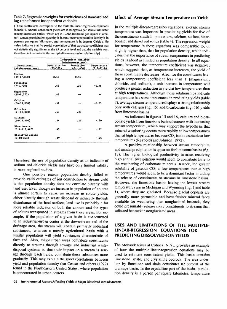
Table 7. Regression weights for coefficients of standardized log-transformed independent variables.[These coefficients correspond to the multiple-linear-regression equations in table 4. Annual constituent yields are in kilograms per square kilometer (except dissolved solids, which are in 1,000 kilograms per square kilome ter); annual precipitation quantity is in centimeters; population density is in persons per square kilometer, and temperature is in degrees Celsius. No value indicates that the partial correlation of that particular coefficient was not statistically significant at the 95 percent level and that the variable was, therefore, not included in the multiple-linear-regression relationship]
Constituent(minimum-maximum)
Sodium (39-17,800)
Potassium (7-1,720)
Magnesium (19-9,270)
Calcium (66-29,800)
Chloride (21-28,800)
Sulfate (50-79,400)
Bicarbonate (314-113,442)
Diaaolved solids (0.60-203)
Independent variable (minimum-maximum)
Precipitation Population Temperature (29-559) (0-1,600) (2.8-22.8)
0.53
.68
.48
.52
.59
.54
.49
.59
0. 36
.30 -0.36
_
-0.33
.38
.25 -.30
-.27
-.26
Therefore, the use of population density as an indicator of sodium and chloride yields may have only limited validity in most regional studies.
One possible reason population density failed to provide valid estimates of ion contribution to stream yield is that population density does not correlate directly with land use. Even though an increase in population of an area is almost certain to cause an increase in solute yields, either directly through waste disposal or indirectly through disturbance of the land surface, land use is probably a far more reliable indicator of both the amount and the types of solutes transported in streams from these areas. For ex ample, if the population of a given basin is concentrated in an industrial-urban center at the downstream end of the drainage area, the stream will contain primarily industrial substances, whereas a mostly agricultural basin with a similar population will yield substances characteristic of farmland. Also, major urban areas contribute constituents directly to streams through sewage and industrial waste- disposal systems so that their impact on a stream is sew age through leach fields, contribute these substances more gradually. This may explain the good correlations between yield and population density that Ceasar and others (1972) found in the Northeastern United States, where population is concentrated in urban centers.
Effect of Average Stream Temperature on Yields
In the multiple-linear-regression equations, average stream temperature was important in predicting yields for five of the constituents studied potassium, calcium, sulfate, bicar bonate, and dissolved solids (table 4). The regression weight for temperature in these equations was comparable to, or slightly higher than, that for population density, which indi cates that the importance of stream temperature in predicting yields is about as limited as population density. In all equa tions, however, the temperature coefficient was negative, which suggests that, as temperature increases, the yield of these constituents decreases. Also, for the constituents hav ing a temperature coefficient less than 1 (magnesium, chloride, and sodium), a unit increase in temperature will produce a greater reduction in yield at low temperatures than at high temperatures. Although these relationships indicate temperature has some importance in predicting yields (table 7), average stream temperature displays a strong relationship only with calcium (fig. 15) and bicarbonate (fig. 16) yields from limestone basins.
As indicated in figures 15 and 16, calcium and bicar bonate yields from limestone basins decrease with increasing stream temperature, which may support the hypothesis that mineral weathering occurs more rapidly at low temperatures than at high temperatures because CO2 is more soluble at low temperatures (Reynolds and Johnson, 1972).
A positive relationship between stream temperature and annual precipitation is apparent for limestone basins (fig. 17). The higher biological productivity in areas receiving high annual precipitation would seem to contribute little to the weathering of carbonate minerals. Rather, the greater solubility of gaseous CO2 at low temperatures than at high temperatures would seem to be a dominant factor in aiding the release of constituents to streams in limestone basins. However, the limestone basins having the lowest stream temperatures are in Michigan and Wyoming (fig. 1 and table 1), where they are glaciated. Because glacial deposits are generally more permeable and have fresher mineral faces available for weathering than nonglaciated bedrock, they could presumably release more constituents to streams than soils and bedrock in nonglaciated areas.
USES AND LIMITATIONS OF THE MULTIPLE- LINEAR-REGRESSION EQUATIONS FOR PREDICTING DISSOLVED-ION YIELDS
The Mohawk River at Cohoes, N.Y., provides an example of how the multiple-linear-regression equations may be used to estimate constitutent yields. This basin contains limestone, shale, and crystalline bedrock. The area under lain by limestone and shale constitutes 82 percent of the drainage basin. In the crystalline part of the basin, popula tion density is 1 person per square kilometer, temperature
22 Environmental Factors Affecting Yields of Major Dissolved Ions of Streams

Q.- IUU.UUULU
UJ
o_J
UJ
^ 10,000OCO
ccUJQ_
CO
1 <5 10000=;
2
Q
UJ>-_ 100 '
QOCO
^2 1 n
i i i i i
+ & ++ n
D * D
3 + +4±
3 n »1 ] -)*»-
| D » + + *
3 + +
* +
D *D
3 + Limestone Sandstone
3 a Crystalline
0
III!!
CC 1 UU.UUU LU
LU
|
LU DC
=3 10,000oCO
DCLU0.
CO^.
5 1000O
&
?Q
LU
LU 100 Q
DCO
XO
z m
I - I I
+
3 + .0
3 D
3 + +
a +0 1*i i
3 +
3 D
3
3 D
+ Limestone Sandstone _ a Crystalline
3
j
0
1 1
1 10 100 1000POPULATION DENSITY,
PERSONS PER SQUARE KILOMETER
10,000
Figure 13. Annual dissolved-sodium yield of streams in relation to basin-population density within drainage basins underlain by single bedrock types in the United States.
1 10 100 1000POPULATION DENSITY,
IN PERSONS PER SQUARE KILOMETER
10,000
Figure 14. Annual dissolved-chloride yield of streams in relation to basin-population density within drainage basins underlain by single bedrock types in the United States.
Table 8. Average percentage of total annual sodium and chloride yield attributed to basin-population density and the relationships between annual yield and population density.[Values are in percent. Annual yields are in kilograms per square kilometer. Population density is in persons per square kilometer]
Constituent
Sodium
Chloride
Limestone basin
!Vf9
23±19
Sandstone basin
17+27
24+30
Crystalline basin
10+21
17^28
All basins
13+19
20+25
Annual Sodium Yield - 30(Fopulatlon density)0 - 82
Annual Chloride Yield - 20(Populatlon density) 1 - 21
averages about 9°C, and annual precipitation is about 140 cm. In the limestone and shale part of the basin, popula tion density is 70 persons per km2 , stream temperature av erages about 13°C, and annual precipitation is about 105 cm. The annual chloride yield may be computed by using the appropriate equation in table 4 and adding the yields associated with the fractional area of the basin underlain by a specific bedrock type. For this example, limestone
and shale were grouped together and treated as limestone. Because only precipitation and population density are needed, the computation is as follows:
Yd = 0.18(0.6)(140)' 59(1.0)°- 36+ 0.82(0.6X10⁵)' 59 (70)°- 36
= 279 + 3,714 = 3,993 kg/km2
The computed yield compares well with the ob served chloride yield, 3,040 kg/km2 for 1952-53 and 7,450 for 1970-74, estimated by Peters and Turk (1981) for the basin. (Almost all of the chloride increase from the 1950's to the 1970's was attributed to increased use of road salt for snow and ice removal (Peters and Turk, 1981.))
A similar computation for sulfate, using all vari ables, and grouping the limestone and shale as limestone, is as follows:
ys04 =0.18(1.00)(44)(140) 1 20(1.0)°- 20(9.0) -° 86 + 0.82(3.3)(44)(105) 1 - 20(70)°- 20(13) -°- 86
= 450+8,170 = 8,620 kg/km2
Multiple-Linear-Regression Equations 23

0=100,000
10,000OCO
orLLJ Q_
CO
g 1000
QLU
O
<O
100
10
+ Limestone Sandstone D Crystalline
LIMESTONE BASINS
10AVERAGE STREAM TEMPERATURE,
IN DEGREES CELSIUS
100
Figure 15. Annual dissolved-calcium yield of streams in relation to average stream temperature within basins underlain by single bedrock types in the United States.
1.000,000
100,000
LULUt oc
00CD CO
!of;O'O
10,000
^ 1000
100
LIMESTONE BASINS
+ Limestone Sandstone a Crystalline a
1 10AVERAGE STREAM TEMPERATURE,
IN DEGREES CELSIUS
100
Figure 16.Annual dissolved-bicarbonate yield of streams in rela tion to average stream temperature within basins underlain by single bedrock types in the United States.
The computed sulfate yield is about 50 percent lower than that estimated for 1970-74 by Peters and Turk (1981), but it is within the order of magnitude (862 to 86,200 kg/km2) accuracy determined for the equation.
As noted in the example, yields estimated from the multiple-linear-regression equations compare well with the observed yields. Discretion should be used, however, when estimating yields and interpreting their results be cause the standard error of estimate of these equations (table 4) suggests that the predicted yield will be only within an order of magnitude of the actual yield. Further more, estimated yields may not be accurate for drainages where other major constituent sources, such as evaporite minerals or cultural and industrial contributions, are known.
Also, application of these equations to basins that have values of the independent variables (annual precipita tion, population density, or average stream temperature) outside the range of values for which these equations were derived may yield erroneous results because the relation ship may not be valid. The equations, however, could be used to provide an initial estimate of yields, particularly in areas where stream chemistry data are unavailable.
CONSIDERATIONS FOR FUTURE STUDIES
Results of this study indicate that, of the four fac tors analyzed, annual precipitation and the type of rock underlying a basin are the most important in determining the yields of dissolved major ions in streams. Con sequently, a more refined analysis to assess the interaction between climate and rock types in relation to stream com position would provide data on assessing how climatic changes affect the weathering of basin materials. Such an analysis could also address contributions of constituents from the atmosphere, which, as results of this study suggest, may be substantial in most basins. It would be preferable to use basins underlain by single rock types having comparable and known ranges in mineral composi tion so that deviations in the relationships could be attri buted to the correct source(s).
The use of population density to assess contributions of human activities to streams, which was only partly suc cessful in this study, could be replaced with a more specific measure, such as land use, which can be divided into categories that correspond to known types of con tributions.
24 Environmental Factors Affecting Yields of Major Dissolved Ions of Streams

100
COIDCO
DC CD LU Q
< 10DC
LIMESTONE BASINS
LUCD
+ Limestone Sandstone a Crystalline
10 100ANNUAL PRECIPITATION, IN CENTIMETERS
1000
Figure 17. Average stream temperature in relation to annual pre cipitation within basins underlain by single bedrock types in the United States.
Results from this study indicate that yield of all con stituents is an exponential function of precipitation quan tity. Yet, the method of averaging yields and the use of aver age precipitation from long-term data may have com pounded the error associated with assessing the relation ship between yield and precipitation quantity. An investi gation of the relationship between annual precipitation and annual yield over a long period of record at basins repre senting a wide range in climatic conditions should be made to assess the associated errors.
SUMMARY
The yields in streams of the seven major dissolved ions sodium, potassium, magnesium, calcium, chloride, sulfate, and bicarbonate and yields of dissolved solids from basins can be predicted to within about 0.4 logarithmic units through multiple- linear-regression equa tions combining data on rock type, annual precipitation, basin-population density, and average stream temperature. The range in annual yields of these constituents was 3 to 4 orders of magnitude 10 to 100,000 kg/km2 . The equa
tions presented herein can be used to predict the yield of a constituent to within an order of magnitude of the ob served yield.
The most important basin characteristics for predict ing yields were annual precipitation quantity and rock type. Average yields from limestone basins were larger than those from sandstone or crystalline basins. Only the yields of calcium, bicarbonate, and dissolved solids could be differentiated between sandstone and crystalline basins. In limestone basins, the dissolved-solids yields were dominated by contributions of calcium and bicarbonate from carbonate minerals weathering. In sandstone basins, dissolved-solids yields were dominated by bicarbonate and sulfate; in crystalline basins, dissolved-solids yields were dominated by bicarbonate.
The regression coefficients in the multiple-linear-re gression equations indicate that the ratio of constituent yields in limestone basins to those in crystalline basins and in sandstone basins was as follows: magnesium, 11:3:1; calcium, 10:1.6:1; sulfate, 1.4:0.4:1; bicarbonate, 8.7:2.2:1; and dissolved solids, 4.2:1.1:1.
The percentage of yield that could be related to annual precipitation quantity averaged between 58 and 71 for all ba sins. Smaller percentages for most constituents, particularly calcium, were associated with limestone basins, which are rich in carbonate minerals, so that a larger percentage of yield is derived from the rock than from the atmosphere. As a consequence, these appear relatively unaffected by precipi tation quantity.
An assessment of direct atmospheric contributions of sodium, potassium, calcium, chloride, and sulfate from pre cipitation-quality data (Junge and Werby, 1958) suggests that 30 percent of the sodium and chloride yield and 60 per cent of the sulfate yield could be derived from precipitation. In this study, the sulfate percentage was greater in crystalline basins (80 percent) than in limestone basins (38 percent), presumably because crystalline rocks contain less sulfur. Al though the atmospheric contribution of calcium averaged 34 percent of the annual yields of all basins, the amount contrib uted to yields from limestone basins was small (7 percent), which suggests that most of the calcium is derived from weathering of carbonate minerals within the basin.
Population density was effective in predicting only the yields of sodium, potassium, chloride, and sulfate in consort with other variables. In each case population density was of lesser importance than precipitation quantity, rock type, or average stream temperature. Annual precipitation and popu lation density combined were the most reliable predictors of sodium and chloride yields, however. The amount of these constituents in annual yields that could be attributed directly to population density averaged only 13 percent for sodium and 20 percent for chloride.
The relationship between average stream temperature and yields indicated that temperature has a negative effect on the yields of potassium, calcium, sulfate, bicarbonate, and
Summary 25
dissolved solids. This effect is most pronounced for calcium and bicarbonate yields from limestone basins and may result from increased dissolution of carbonate minerals at low tem peratures as well as from the large weathering potential of glacial deposits in northern basins, where stream tempera tures were the lowest.
The prediction of a constituent yield may be improved by determining the amount contributed from atmospheric de position. Yield prediction may also be improved by replac ing population density in the multiple-linear-regression equ ations with a more specific measure of contributions from man's activities, such as land use. Also, multiple-linear-re gression relationships developed for each rock type sepa rately might improve yield prediction because the effect that these environmental factors have on yield is probably partly related to basin mineralogy.
REFERENCES CITED
Anderson, P. W., and Faust, S. D., 1965, Changes in quality of water in the Passaic River at Little Falls, New Jersey, as shown by long-term data: U.S. Geological Survey Professional Paper 525-D,p.D214-D218.
Baldwin, A. D., 1971, Contribution of atmospheric chloride in water from selected coastal streams in central California: Water Re sources Research, v. 7, no. 4, p. 1007-1012.
Barr, A. J., Goodnight, J. H., Sail, J. P., andHelwig, J. T., 1976, A users's guide to SAS 76: Raleigh, N.C., SAS Institute, Inc., 329 p.
Berner, R. A., 1971, Worldwide sulfur pollution of rivers: Journalof Geophysical Research, v. 76, p. 6597-6600.
1978, Rate control of mineral dissolution under earth sur face conditions: American Journal of Science, v. 278, p. 1235-1252.
BieseckerJ. E., andLeifeste, D. K., 1975, Water quality of hydro- logic benchmarks an indicator of water quality in the natural environment: U.S. Geological Survey Circular 460-E, 21 p.
Briggs, J. C.,andFicke, J. F., 1975, Quality of rivers of the United States, 1975 water year based on the national stream quality accounting network (NASQAN): U.S. Geological Survey Open-File Report 78-200,436 p.
Carroll, Dorothy, 1962, Rainwater as a chemical agent of geologic process a review: U.S. Geological Survey Water-Supply Paper 1535-G, 19 p.
Ceasar, J., Collier, R., Edmond, J., Frey, F., Matisoff, G., and Stallard, R., 1976, Chemical dynamics of a polluted watershed, the Merrimack River in northern New England: Environmental Science and Technology, v. 10, no. 7, p. 697- 704.
Clarke, F. W., 1924, Data of geochemistry, 5th edition: U.S. Geological Survey Bulletin 770, 841 p.
Cleaves, E. T., Godfrey, A. E., and Bricker, O. P., 1970, Geochemical balance of a small watershed and its geomorphic implications: Geological Society of America Bulletin 81, p. 3015-3032.
Cobb, E. D., and Biesecker, J. E., 1971, The national hydrologic bench-mark network: U.S. Geological Survey Circular 460- D,38p.
Conway, E. J., 1942, Mean geochemical data in relation to oceanic evolution: Royal Irish Academy of Science Proceedings, v. 48, sec. B, p. 119-159.
Daniel, C. D., and Wood, F. S., 1971, Fitting equations to data, computer analysis of multifactor data for scientists and en gineers: New York, Wiley Interscience, 342 p.
Davis, J. C., 1973, Statistics and data analysis in geology: New York, John Wiley and Sons, Inc., 550 p.
Donner, H. C., andLynn, W. C., 1977, Carbonate, halide, sulfate, and sulfide minerals in Minerals in Soil Environments, R. C. Dinauer, ed.: Madison, Wis., Soil Science Society of Ameri ca, p. 75-98.
Douglas, lan, 1968, The effects of precipitation chemistry and catchment area lithology on the quality of river water in selected catchments in eastern Australia: Earth Science Jour nal, v. 2, no. 2, p. 126-144.
Draper, N. R., and Smith, H., 1966, Applied regression analysis: New York, John Wiley and Sons, Inc., 407 p.
Edwards, A. L., 1979, Multiple regression and the analysis of var iance and covariance: San Francisco, W. H. Freeman and Co., 212p.
Eriksson, Erik, 1955, Airborne salts and the chemical composition of river waters: Tellus, v. 7, p. 243-250.
Ezekiel, Mordecai, and Fox, K. A., 1959, Methods of correlation and regression analysis: New York, John Wiley and Sons, Inc., 548 p.
Feltz, H. R., and Wark, J. W., 1962, Solute degradation in the Potomac River basin: U.S. Geological Survey Professional Paper450-D, p. D186-D187.
Feth, J. H., Roberson, C., and Polzer, W., 1964, Sources of min eral constituents in water from granitic rocks, Sierra Nevada, California and Nevada: U.S. Geological Survey Water-Supply Paper 1535-1,70 p.
Ficke, J. F., and Hawkinson, R. O., 1975, The national stream quality accounting network (NASQAN) some questions and answers:U.S. Geological Survey Circular 719, 23p.
Fisher, D. W., 1968, Annual variations in chemical composition of atmospheric precipitation, eastern North Carolina and southeastern Virginia: U.S. Geological Survey Water-Supply Paperl535-M,21p.
Fisher, D. W., and others, 1968, Atmospheric contributions to water quality of streams in the Hubbard Brook Experimental Forest, New Hampshire: Water Resources Research, v. 4, no. 5,p. 1115-1126.
Freeze, R. A., and Cherry, J. A., 1979, Ground water: Englewood Cliffs, NJ, Prentice-Hall Inc., pp. 237-297.
Frost, L. R., Jr., 1976, Effect of deicing chemicals on the hydro- logic environment in Massachusetts Evaluation of surface water data collection: U.S. Geological Survey Open-File Re port 76-353,34 p.
Galloway, J. N., and Likens, G. E., 1876, Calibration of collection procedures for the determination of precipitation chemistry: Water, Air, and Soil Pollution, v. 6, p. 241-258.
1978, The collection of precipitation for chemical analysis, Tellus, v. 30, p. 71-82.
Galloway, J. N., Schofield, C. L., Hendrey, G. R., Altwicker, E. R., and Troutman, D. E., 1980, An analysis of lake acidifica tion using annual budgets, in International conference on the impact of acid precipitation and associated air-borne pollutants on the natural environment, Sandefjord, Norway, 1980, Pro-
26 Environmental Factors Affecting Yields of Major Dissolved Ions of Streams

ceedings: As- NLH, Norway, SNSF-Project, p. 254-255.Gambell, A. W., and Fisher, D. W., 1966, Chemical composition
of rainfall, eastern North Carolina and southeastern Virginia: U.S. Geological Survey Water-Supply Paper 1535-K, 41 p.
Garrels, R. M., 1967, Genesis of some ground waters from igneous rocks, in Researches in Geochemistry, v. 2, P. H. Abelson, ed.: New York, John Wiley and Sons, Inc., p. 405^420.
Garrels, R. M., and Christ, C. L., 1965, Solutions, minerals and equilibria: New York, Harper and Row, 450 p.
Garrels, R. M., and Mackenzie, F. T., 1971, Evolution of sedimen tary rocks: New York, W. W. Norton & Co., 397 p.
Garrels, R. M., and Thompson, M. E,, 1962, A chemical model for sea water: American Journal of Science, v. 260, p. 57.
Gibbs, R. J., 1970, Mechanisms controlling world water chemis try: Science, no. 170, p. 1088-1090.
Gorham, E., 1961, Factors influencing supply of major ions to in land waters with special reference to the atmosphere: Geologi cal Society of America Bulletin 72, p. 795-840.
Goudie, A., 1970, Input and output considerations in estimating rates of chemical denudation: Earth Science Journal, v. 4, no. 2, p. 59-65.
Gray, D. M., 1970, Statistical methods fitting frequency curves, regression analysis, in Handbook on the Principles of Hydro logy, D. M. Gray, ed.: National Research Council of Canada, sec. 12,34p.
Hack, J. T., 1960, Interpretation of erosional topography in humid temperate regions: American Journal of Science, v. 258-A, p. 80-87.
Hales, J. M., 1977, Wet removal of sulfur compounds from the at mosphere: Atmospheric Environment, v. 12, p. 389-399.
Hanes, R. E., Zelazny, L. W., and Blaser, R. E., 1970, Effects of deicing salts on water quality and biota: Washington, D.C., National Academy of Sciences, National Cooperative High way Research Program Report 91,70 p.
Hem, J. D., 1948, Fluctuations in concentration of dissolved solids of some southwestern streams: American Geophysical Union Transactions, v. 29, no. 11, p. 80-84.
1970, Study and interpretation of the chemical characteris tics of natural water: U.S. Geological Survey Water-Supply Paper 1473, 363 p.
Hembree, C. H., and Rainwater, F. H., 1961, Chemical degrada tion on opposite flanks of the Wind River Range, Wyoming: U.S. Geological Survey Water-Supply Paper 1535-E, 9p.
Hutchinson, N. E., 1975, WATSTORE, user's guide, v. 1: U.S. Geological Survey Open-File Report 75^426.
Janda, R. J., 1971, An evaluation of procedures used in computing chemical deundation rates: Geological Society of America Bulletin 82, no. 1, p. 67-79.
Johnson, A. H., and Reynolds, R. C., Jr., 1977, Chemical charac ter of headwater streams in Vermont and New Hampshire: Water Resources Research, v. 13, no. 2, p. 469^473.
Jones, H. C., 1974, Pre-operational monitoring in the Cumberland stream plant area the pH and sulfate content of precipitation: Tennessee Valley Authority Report, E-EB-74-1,27 p.
Juang, F. H. T., and Johnson, N. M., 1967, Cycling of chlorine through a forested watershed in New England: Journal of Geophysical Research, v. 72, no. 22, p. 5641-5647.
Junge, C. E., and Gustafson, P. E., 1957, On the distribution of sea salt over the United States and its removal by precipitation: Tellus,v.9,p. 164-173.
Junge, C. E., and Werby, R. T., 1958, The concentration of chloride, sodium, potassium, and sulfate in rainwater over the United States: Journal of Meteorology, v. 15, p. 417^25.
Kelly, J. M., 1980, Sulfur distribution and flux in two forested watersheds in eastern Tennessee, in International conference on the impact of acid precipitation and associated air-borne pollutants on the natural environment, Sandefjord, Norway, 1980, Proceedings: As-NLH, Norway, SNSF-Project, p. 230- 231.
Kerekes, J. J., 1980, Preliminary characterization of three lake ba sins sensitive to acid precipitation in Nova Scotia, Canada, in International conference on the impact of acid precipitation and associated air-borne pollutants on the natural environ ment, Sandefjord, Norway, 1980, Proceedings: As-NLH, Norway, SNSF-Project, p. 232-233.
Langbein, W. B., and Dawdy, D. R., 1964, Occurrence of dissol ved solids in surface waters in the United States: U.S. Geologi cal Survey Professional Paper 501-D, p. Dl 15-D117.
Likens, G. E., 1976, Acid precipitation: Chemical and Engineering News, v. 54, no. 48, p. 29-44.
Likens, G. E., Bormann, F. H., Pierce, R. S., Eaton, J. S., and Johnson, N. M., 1977, Biogeochemistry of a forested ecosys tem: New York, Springer Verlag, 146p.
Linsley, R. K., Jr., Kohler, M. A., and Paulhus, J. L. H., 1975, Hydrology for Engineers, 2nd edition: New York, McGraw- Hill,482p.
Lipka, G. S., and Aulenbach, D. B., 1976, The effects of highway deicing salt on chloride budgets at Lake George, New York: Fresh Water Institute Report 76-2, Troy, N.Y., Rensselaer Polytechnic Institute, 17 p.
Livingston, D. A., 1963a, Data of geochemistry, chapter G chemical composition of rivers and lakes: U.S. Geological Survey Professional Paper 440-G, 64 p.
I963b, The sodium cycle and the age of the ocean: GeochimicaetCosmochimicaActa,v. 27, p. 1055-1069.
Lystrom, D. J., and others, 1978, Regional analysis of the effects of land use on stream water quality, methodology, and appli cation in the Susquehanna River basin, Pennsylvania and New York: U.S. Geological Survey Water-Resources Investigation 78-12,60 p.
Mackenzie, F. T., and Garrels, R. M., 1966, Chemical mass bal ance between rivers and oceans: American Journal of Science, v. 264, p. 507-525.
Meade, R. H., 1969, Errors in using modern stream-load data to estimate natural rates of denudation: Geological Society of America Bulletin 80, p. 1265-1274.
Meybeck, M., 1976, Total mineral dissolved transport by world major rivers: Hydrological Sciences Bulletin, v. 2, no. 21, p. 265-284.
1977, Dissolved and suspended matter carried by rivers, composition, time and space variations, and world balance, in Interactions between sediments and fresh water, Proceedings of an International Symposium, Amsterdam, Netherlands, Sept. 6-10, 1976: Wagerminger, Netherlands, Centre for Ag ricultural Publishing and Documentation, p. 25-32.
Miller, J. M., Galloway, J. N., and Likens, G. E., 1978, Origins of air masses producing acid precipitation at Ithaca, New York A preliminary report: Geophysical Research Letters, v. 5, p. 757-760.
Miller, J. P., 1961, Solutes in small streams draining single rock
References Cited 27
types, Sangre de Cristo Range, New Mexico: U.S. Geological Survey Water-Supply Paper 1535-F, 23 p.
Miller, W. R., and Drever, J. I., 1977, Water chemistry of a stream following a storm, Absaroka Mountains, Wyoming: Geologi cal Society of America Bulletin 88, no. 2, p. 286-290.
Musser, J. J., and Whetstone, G. W., 1964, Geochemistry of water, in Influences of strip mining on the hydrologic environ ment of parts of Beaver Creek basin, Kentucky, 1955-59, C. R. Collier and others, eds.: U.S. Geological Survey Profes sional Paper 427-B, p. B25-B48.
Peters, N. E., and Turk, J. T., 1981, Increases in sodium and chloride in the Mohawk River, New York from 1950's to 1970's attributed to road salt: Water Resources Bulletin (in press).
Pettijohn, F. J., 1957, Sedimentary rocks: New York, Harper and Brothers, 718 p.
Reeder, S. W., Hitchon, Brian, andLevinson, A. A., 1972, Hydro- geochemistry of the surface waters of the Mackensie River drainage basin, Canada 1. factors controlling inorganic composition: Geochemica et Cosmochemica Acta, v. 36, p. 825-865.
Reynolds, R. C., and Johnson, N. M., 1972, Chemical weathering in the temperate glacial environment of the northern Cascade Mountains: Geochemica et Cosmochemica Acta, v. 36, p. 537-554.
Riggs, H. C., 1968, Some statistical tools in hydrology: U.S. Geological Survey Techniques of Water-Resources Investiga tions, Book 4, Chapter A 1,39 p.
Robinson, Elmer, andRobbins, R. C., 1970, Gaseous sulfur pollut ants from urban and natural sources: Journal of the Air Pollu tion Control Association, v. 20, no. 4, p. 233-235.
Sampson, P. J., 1978, Ensemble trajectory analysis of summertime sulfate concentrations in New York State: Atmospheric Envi ronment^. 12,p. 1889-1893.
Snedecor, G. W., 1946, Statistical methods, 4th edition: Ames,
Iowa, Iowa State College Press, 485 p.Steele, T. D., 1974, Harmonic analysis of stream temperatures:
U.S. Geological Survey Computer Contribution, USGS- WRD-75-007,47p.
Stumm, Werner, and Morgan, J. J., 1970, Aquatic chemistry: New York, John Wiley and Sons, Inc., 583 p.
Sweeting, M. M., 1966, The weathering of limestones, in Essays in Geomorphology, Dury, G. E., ed.: New York, American Elsevier Publishing Co., p. 177-210.
U.S. Bureau of the Census, 1972, Census of population, 1970, characteristics of the population, number of inhabitants, United States: Washington, U.S. Department of Commerce, Social Economic Statistics Administration, U.S. Bureau of Census, v. 1, pt. A, sec. 1-2.
U.S. Environmental Science Services Administration, 1968, Cli mate atlas of the United States: Washington, U.S. Department of Commerce, Environmental Data Service, 80 p.
U.S. National Oceanic and Atmospheric Administration, Climatological data: Ashville, N.C., National Climatic Cen ter, issued monthly for each 45 sections (States, possessions, or group of States), period of record 1970-1978.
Van Denburgh, A. S., and Feth, J. H., 1965, Solute erosion and chloride balance in selected river basins of the western conter minous United States: Water Resources Research, v. 1, p. 537-541.
Whitehead, H. C., and Feth, J. H., 1964, Chemical composition of rain, dry fallout, and bulk precipitation at Menlo Park, California, 1957-1959: Journal of Geophysical Research, v. 69,p.3319-3333.
Wright, R. F., and Johannessen, M., 1980, Input-output budgets of major ions at gauged catchments in Norway, in Interna tional conference on the impact of acid precipitation and as sociated air-borne pollutants on the natural environment, San- defjord, Norway, 1980, Proceedings: As-NLH, Norway, SNSF-Project, p. 250-251.
28 Environmental Factors Affecting Yields of Major Dissolved Ions of Streams

APPENDIX
Published References to Basin Geology
A. By rock type and USGS station number. (Locations are given in fig. 1 and table 1.)
B. By author, in alphabetical order.

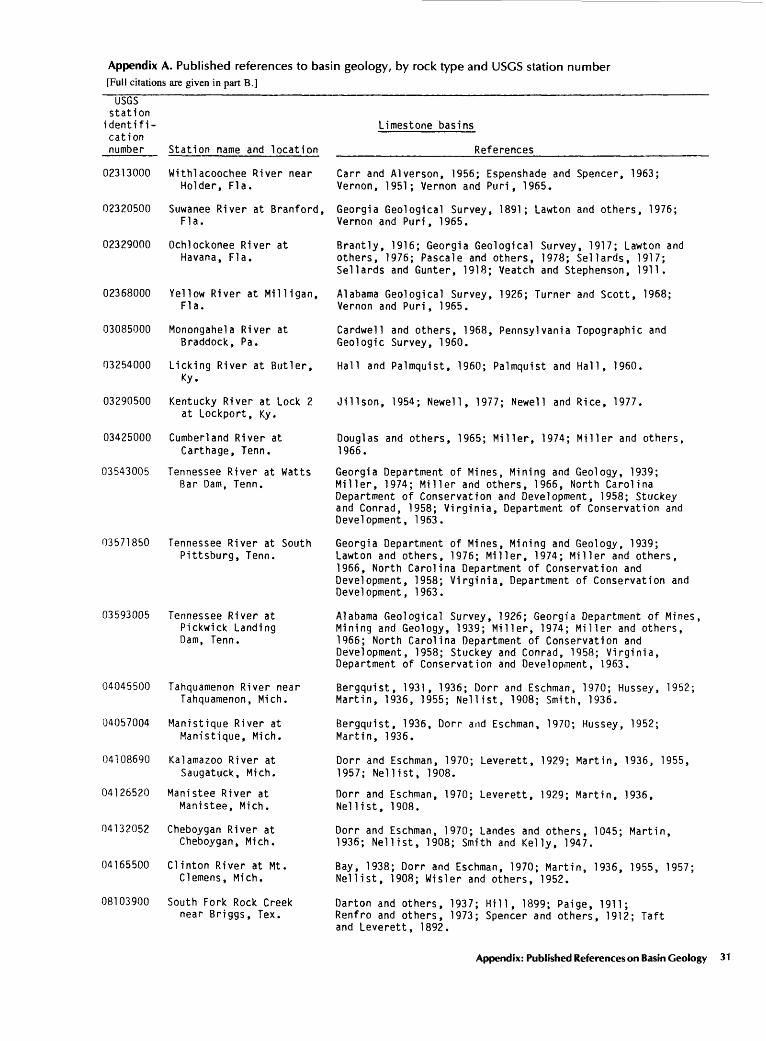
Appendix A. Published references to basin geology, by rock type and USGS station number[Full citations are given in part B.]
USGSstation
identifi'cationnumber
Limestone basins
02313000
02320500
02329000
02368000
03085000
03254000
Station name and location
Withlacoochee River near Holder, Fla.
Suwanee River at Branford, Fla.
Ochlockonee River at Havana, Fla.
Yellow River at Milligan, Fla.
Monongahela River at Braddock, Pa.
References
Cam and Alverson, 1956; Espenshade and Spencer, 1963; Vernon, 1951; Vernon and Puri, 1965.
Georgia Geological Survey, 1891; Lawton and others, 1976; Vernon and Puri, 1965.
Brantly, 1916; Georgia Geological Survey, 1917; Lawton and others, 1976; Pascale and others, 1978; Sellards, 1917; Sellards and Gunter, 1918; Veatch and Stephenson, 1911.
Alabama Geological Survey, 1926; Turner and Scott, 1968; Vernon and Puri, 1965.
Cardwell and others, 1968, Pennsylvania Topographic and Geologic Survey, 1960.
Licking River at Butler, Hall and Palmquist, 1960; Palmquist and Hall, 1960.
03290500 Kentucky River at Lock 2 at Lockport, Ky.
03425000 Cumberland River at Carthage, Tenn.
03543005 Tennessee River at Watts Bar Dam, Tenn.
03571850 Tennessee River at South Pittsburg, Tenn.
03593005 Tennessee River at Pickwick Landing Dam, Tenn.
04045500 Tahquamenon River near Tahquamenon, Mich.
04057004 Manistique River at Manistique, Mich.
04108690 Kalamazoo River at Saugatuck, Mich.
04126520 Manistee River at Manistee, Mich.
04132052 Cheboygan River at Cheboygan, Mich.
04165500 Clinton River at Mt. Clemens, Mich.
08103900 South Fork Rock Creek near Briggs, Tex.
Oillson, 1954; Newell, 1977; Newell and Rice, 1977.
Douglas and others, 1965; Miller, 1974; Miller and others, 1966.
Georgia Department of Mines, Mining and Geology, 1939; Miller, 1974; Miller and others, 1966, North Carolina Department of Conservation and Development, 1958; Stuckey and Conrad, 1958; Virginia, Department of Conservation and Development, 1963.
Georgia Department of Mines, Mining and Geology, 1939; Lawton and others, 1976; Miller, 1974; Miller and others, 1966, North Carolina Department of Conservation and Development, 1958; Virginia, Department of Conservation and Development, 1963.
Alabama Geological Survey, 1926; Georgia Department of Mines Mining and Geology, 1939; Miller, 1974; Miller and others, 1966; North Carolina Department of Conservation and Development, 1958; Stuckey and Conrad, 1958; Virginia, Department of Conservation and Development, 1963.
Bergquist, 1931, 1936; Dorr and Eschman, 1970; Hussey, 1952; Martin, 1936, 1955; Nellist, 1908; Smith, 1936.
Bergquist, 1936, Dorr and Eschman, 1970; Hussey, 1952; Martin, 1936.
Dorr and Eschman, 1970; Leverett, 1929; Martin, 1936, 1955, 1957; Nellist, 1908.
Dorr and Eschman, 1970; Leverett, 1929; Martin, 1936, Nellist, 1908.
Dorr and Eschman, 1970; Landes and others, 1045; Martin, 1936; Nellist, 1908; Smith and Kelly, 1947.
Bay, 1938; Dorr and Eschman, 1970; Martin, 1936, 1955, 1957; Nellist, 1908; Wisler and others, 1952.
Darton and others, 1937; Hill, 1899; Paige, 1911; Renfro and others, 1973; Spencer and others, 1912; Taft and Leverett, 1892.
Appendix: Published References on Basin Geology 31
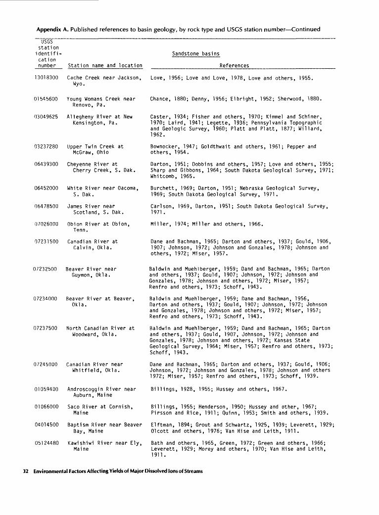
Appendix A. Published references to basin geology, by rock type and USGS station number Continued
USGS station
identifi cation number
13018300
01545600
03049625
03237280
06439300
06452000
06478500
07026000
07231500
Sandstone basins
Station name and location
Cache Creek near Jackson, Wyo.
Young Womans Creek near Renovo, Pa.
Allegheny River at New Kensington, Pa.
Upper Twin Creek at McGraw, Ohio
Cheyenne River at Cherry Creek, S. Dak,
White River near Oacoma, S. Dak.
James River near Scotland, S. Dak.
Obion River at Obion, Tenn.
Canadian River at Calvin, Okla.
References
Love, 1956; Love and Love, 1978, Love and others, 1955.
Chance, 1880; Denny, 1956; Elbright, 1952; Sherwood, 1880.
Caster, 1934; Fisher and others, 1970; Kimmel and Schiner, 1970; Laird, 1941; Legette, 1936; Pennsylvania Topographic and Geologic Survey, 1960; Platt and Platt, 1877; Willard, 1962.
Bownocker, 1947; Goldthwait and others, 1961; Pepper and others, 1954.
Darton, 1951; Dobbins and others, 1957; Love and others, 1955; Sharp and Gibbons, 1964; South Dakota Geological Survey, 1971; Whitcomb, 1965.
Burchett, 1969; Darton, 1951; Nebraska Geological Survey, 1969; South Dakota Geological Survey, 1971.
Carlson, 1969, Darton, 1951; South Dakota Geological Survey, 1971 .
Miller, 1974; Miller and others, 1966.
Dane and Bachman, 1965; Darton and others, 1937; Gould, 1906, 1907; Johnson, 1972; Johnson and Gonzales, 1978; Johnson and others, 1972; Miser, 1957.
07232500 Beaver River near Guymon, Okla.
07234000 Beaver River at Beaver, Okla.
07237500 North Canadian River at Woodward, Okla.
07245000 Canadian River near Whitfield, Okla.
01059400 Androscoggin River near Auburn, Maine
01066000 Saco River at Cornish, Maine
04014500 Baptism River near Beaver Bay, Maine
05124480 Kawishiwi River near Ely, Maine
Baldwin and Muehlberger, 1959; Dand and Bachman, 1965; Darton and others, 1937; Gould, 1907; Johnson, 1972; Johnson and Gonzales, 1978; Johnson and others, 1972; Miser, 1957; Renfro and others, 1973; Schoff, 1943.
Baldwin and Muehlberger, 1959; Dane and Bachman, 1956, Darton and others, 1937; Gould, 1907; Johnson, 1972; Johnson and Gonzales, 1978; Johnson and others, 1972; Miser, 1957; Renfro and others, 1973; Schoff, 1943.
Baldwin and Muehlberger, 1959; Dand and Bachman, 1965; Darton and others, 1937; Gould, 1907, Johnson, 1972; Johnson and Gonzales, 1978; Johnson and others, 1972; Kansas State Geological Survey, 1964; Miser, 1957; Renfro and others, 1973; Schoff, 1943.
Dane and Bachman, 1965; Darton and others, 1937; Gould, 1906; Johnson, 1972; Johnson and Gonzales, 1978; Johnson and others 1972; Miser, 1957; Renfro and others, 1973; Schoff, 1939.
Billings, 1928, 1955; Hussey and others, 1967.
Billings, 1955; Henderson, 1950; Hussey and other, 1967; Pirsson and Rice, 1911; Quinn, 1953; Smith and others, 1939.
Elftman, 1894; Grout and Schwartz, 1925, 1939; Leverett, 1929; Olcott and others, 1976; Van Hise and Leith, 1911.
Bath and others, 1965, Green, 1972; Green and others, 1966; Leverett, 1929; Morey and others, 1970; Van Hise and Leith, 1911.
32 Environmental Factors Affecting Yields of Major Dissolved Ions of Streams
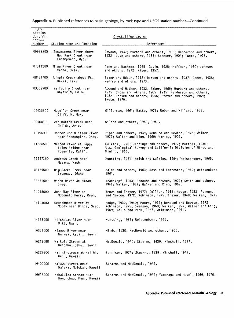
Appendix A. Published references to basin geology, by rock type and USGS station number Continued
usesstation
identifi-cationnumber
06623800
07311200
08431700
09352900
Station name and location
Encampment River above Hog Park Creek near Encampment, Wyo.
Blue River Creek near Cache, Okla.
Limpia Creek above Ft. Davis, Tex.
Valleciio Creek near Bayfield, Colo.
Crystalline basins
References
Atwood, 1937; Burbank and others, 1935; Henderson and others, 1932; Love and others, 1955; Spencer, 1904; Tweto, 1976.
Dane and Bachman, 1965; Govin, 1928; Hoffman, 1930; Johnson and others, 1972; Miser, 1957.
Baker and Udden, 1918; Darton and others, 1937; Jones, 1938; Renfro and others, 1973.
Atwood and Mather, 1932, Baker, 1969; Burbank and others, 1935; Cross and others, 1905, 1935; Henderson and others, 1932; Larsen and others, 1956; Steven and others, 1969; Tweto, 1976.
09430600 Mogollon Creek near Cliff, N. Mex.
09508300 Wet Bottom Creek near Childs, Ariz.
10396000 Donner und Blitzen River near Frenchglen, Oreg.
11264500 Merced River at Happy Isles Bridge near Yosemite, Calif.
12247390 Andrews Creek near Mazama, Wash.
03169500 Big Jacks Creek near Bruneau, Idaho
13331500 Minam River at Minam, Oreg.
14048000 John Day River atMcDonald Ferry, Oreg.
14103000 Deuschutes River atMoody near Biggs, Oreg,
Gillerman, 1964; Ratte, 1975; Weber and Willard, 1959.
Wilson and others, 1959, 1969.
Piper and others, 1939, Renound and Newton, 1972; Walker, 1977; Walker and King, 1969; Waring, 1909.
Calkins, 1970; Jennings and others, 1977; Matthes, 1930; U.S. Geological Survey and California Division of Mines and Mining, 1966.
Huntting, 1961; Smith and Calkins, 1904; Weissenborn, 1969.
Malde and others, 1963; Ross and Forrester, 1959; Weissenborn 1964.
Kranskopf, 1943; Renound and Newton, 1972; Smith and others, 1941; Walker, 1977; Walker and King, 1969.
Brown and Thayer, 1977; Collier, 1914; Hodge, 1932; Renound and Newton, 1972; Robinson, 1975; Thayer, 1940; Walker, 1977.
Hodge, 1932, 1940; Moore, 1937; Renound and Newton, 1972; Robinson, 1975; Swanson, 1968; Walker, 1977; Walker and King, 1969; Wells and Peck, 1967, Wilkinson, 1940.
14113000 Klichetat River near Pitt, Wash.
16031000 Wiamea River nearWaimea, Kauai, Hawaii
16213000 Waikele Stream atWaipahu, Oahu, Hawaii
16229300 Kalihi stream at Kalihi, Oahu, Hawaii
16400000 Halawa stream nearHalawa, Molokai, Hawaii
16618000 Kahakuloa stream nearHonohohau, Maui, Hawaii
Huntting, 1961; Weissenborn, 1969.
Hinds, 1930; MacDonald and others, 1960.
MacDonald, 1940; Stearns, 1939, Winchell, 1947,
Bennison, 1974; Stearns, 1939; Winchell, 1947.
Stearns and MacDonald, 1947.
Stearns and MacDonald, 1942; Yamanaga and Huxel, 1969, 1970.
Appendix: Published References on Basin Geology 33

Appendix A. Published references to basin geology, by rock type and USGS station number Continued
usesstationidentifi- Crystalline basins cation number Station name and location References
16704000 Wailuku River at MacDonald, 1949, Stearns and MacDonald, 1946. Piihonau, Hawaii, Hawaii
16717000 Honolii stream near MacDonald, 1949; Stearns and MacDonald, 1946. Papaikou, Hawaii, Hawaii
34 Environmental Factors Affecting Yields of Major Dissolved Ions of Streams

APPENDIX B. PUBLISHED REFERENCES TO BASIN GEOLOGY, BY AUTHOR
Alabama Geological Survey, 1926, Geologic map of Alabama: Montgomery, Ala., Alabama Geological Survey, scale 1:500,000.
Atwood, W. W., Jr., 1937, Records of Pleistocene glaciers in the Medicine Bow and Park Ranges: Journal of Geology, v. 45, p. 113-140.
Atwood, W. W., Jr., and Mather, K. F., 1932, Physiography and Quaternary geology of the San Juan Mountains, Col orado: U.S. Geological Survey Professional Paper 166, 176P-
Baker, C. L., and Udden, J. A., 1918, Geologic exploration of the southeastern front range of Trans-Pecos, Texas: Texas University Bureau Economic Geology Bulletin 1735, p. 60- 177.
Baldwin, Brewster, and Muehlberger, W. R., 1959, Geologic studies of Union County, New Mexico: New Mexico Bu reau Mines and Mineral Resources Bulletin 63, 171 p.
Barker, Fred, 1969, Precambrian geology of the Needle Moun tains, southwestern Colorado: U.S. Geological Survey Pro fessional Paper 644-A, 35 p.
Bath, G. D., Schwartz, G. M., and Gilbert, F. P., 1965, Aeromagnetic and geologic map of northeastern Minnesota: U.S. Geological Survey Geophysical Investigation Map GP-472, scale 1:250,000.
Bay, J. W., 1938, Glacial history of the streams of southeastern Michigan: Bloomfield Hills, Michigan, Cranbrook Institute Science Bulletin 12, 68 p., 3 pis.
Bennison, A. P., compiler, 1974, Geological highway map of the state of Hawaii and the state of Alaska: Tulsa, Ok lahoma, American Association Petroleum Geologists, U.S. Geological Highway Map Series 8.
Bergquist, S. G., 1931, Surface geology of Luce County: Michi gan Academy of Science Papers, v. 14, p. 437-^52.
, 1936, Pleistocene history of the Tahquamenen and Manistique drainage region of the northern peninsula: Michigan Geological Survey Publication 40, Geology Series 34, pt. 1, p. 7-148.
Billings, M. P., 1928, The petrology of the North Conway quadrangle in the White Mountains of New Hampshire: American Academy Arts and Science Proc., v. 63, no. 3, p. 67-137, 1 pi., scale 1:93,750.
, 1955, Geologic map of New Hampshire: U.S. Geologi cal Survey, scale 1:250,000.
Bownocker, J. A., 1947, Geologic map of Ohio, with a revision of glacial boundary by George Willard White: Columbus, Ohio Geological Survey, scale 1:500,000.
Brandy, J. E., 1916, A report of the limestones and marls of the coastal plain of Georgia: Georgia Geological Survey Bulle tin 21, 300 p.
Brown, C. E., and Thayer, T. P., 1977, Geologic map of the pre-Tertiary rocks in the eastern Aldrich Mountains and ad jacent areas to the south, Grant County, Oregon: U.S. Geological Survey Miscellaneous Investigation Series Map 1-1021, scale 1:62,500 (1978).
Burbank, W. S., and others, 1935, Geologic map of Colorado: U.S. Geological Survey, scale 1:500,000.
Calkins, F. C., 1970, Map of bedrock geology of Yosemite Valley, California: U.S. Geological Survey Open-File Map, scale 1:24,000.
Cardwell, D. H., Erwin, R. B., and Woodward, H. P., comps., 1968, Geologic map of West Virginia: Morgantown, West Virginia Geologic and Economic Survey, scale 1:250,000, 2 sheets.
Carlson, C. G., 1969, Bedrock geologic map of North Dakota: North Dakota Geological Survey Miscellaneous Map 10, scale 1:1,000,000.
Carr, W. J., and Alverson, D. C., 1956, Stratigraphy of Middle Tertiary rocks in part of west-central Florida: U.S. Geological Survey Bulletin 1092,112 p., 3 pis.
Caster, K. E., 1934, Stratigraphy and paleontology of northwestern Pennsylvania: Bulletin American Paleontology, v. 21, no. 71, Iv.
Chance, H. M., 1880, Part I, The geology of Clinton County, Part II, A special study of the Carboniferous and Devonian strata along the west branch of the Susquehanna River: Harrisburg, Pa., Board of Commissions for the Second Geological Survey, v. 1.
Collier, A. J., 1914, Geology and mineral resources of the John Day region: Oregon Bureau Mines and Geology, Mineral Re sources of Oregon, v. 1, no. 3,47 p.
Cross, Whitman, and Larsen, E. S., Jr., 1935, A brief review of the geology of the San Juan region of southwestern Colorado: U.S. Geological Survey Bulletin 843,138 p.
Cross, Whitman, and others, 1905, Folios of the geologic atlas of the United States, Needle Mountains, Colorado: U.S. Geolog ical Survey Folio 131,14p., 4maps, scale 1:62,500.
Dane, C. H., and Bachman, G. B., 1965, Geologic map of New Mexico: U.S. Geological Survey, scale 1:500,000,2 sheets.
Darton, N. H., 1951, Geologic map of South Dakota: U.S. Geolog ical Survey, scale 1:500,000.
Darton, N. H., Stephenson, L. W., and Gardner, J. A., 1937, Geologic map of Texas: U.S. Geological Survey, scale 1:500,000,4 sheets.
Denny, C. S., 1956, Surficial geology and geomorphology of Pot ter County, Pennsylvania: U.S. Geological Survey Profes sional Paper 288,72 p.
Dorr, J. A., Jr., and Eschman, 1970, Geology of Michigan: Ann Arbor, University of Michigan Press, 476 p.
Douglas, W. B., Jr., Calvert, W. L., and Webb, E. J., 1965, Cambrian and Ordovician formations in the vicinity of the Cumberland overthrust block of Tennesee and Virginia: Col umbus, Ohio Geological Society, Field Trip Guidebook, 21 p.
Ebright, J. R., 1952, The Hyner and Ferney anticlines and adjacent areas, Centre, Clinton, and Lycoming Counties, Pennsyl vania: Pennsylvania Topographic and Geologic Survey Bulle tin M35, 32 p.
Elftman, A. H., 1894, Geologic notes on northeastern Minnesota, in Minnesota geological and natural history survey 22nd an nual report: St. Paul, Minn., Office of Press Printing, p. ISO- 180.
Espenshade, G. H., and Spencer, C. W., 1963, Geology and phos phate deposits of northern peninsular Florida: U.S. Geological Survey Bulletin 1118,115 p., 12 pis.
Fisher, D. W., and others, 1970, Geologic map of New York State: New York State Museum and Science Service, Map and Chart Series 15,6 sheets.
Appendix: Published References on Basin Geology 35

Georgia, Department of Mines, Mining and Geology, 1939, Geologic map of Georgia: Atlanta, Dept. of Mines, Mining and Geology, scale 1:500,000.
Georgia Geological Survey, 1891, Geologic report on southwest Georgia and Polk County, in Georgia Geological Survey 1st report on progress, administrative report of the state geologist, 1890/91, v. l,p. 11-12.
Gillerman, Elliot, 1964, Mineral deposits of western Grant County, New Mexico: Bureau of Mines and Minerals Resources, Bul letin 83, 213 p.
Georgia Geological Survey, 1891, Geologic report on southwest Georgia and Polk County, in Georgia Geological Survey 1st report on progress, administrative report of the state geologist, 1890/91, v. l,p. 11-12.
Gillerman, Elliot, 1964, Mineral deposits of western GrantCounty, New Mexico: Bureau Mines and Mineral Resources, Bulletin 83,213p.
Gould, C. N., 1906, The geology and water resources of the eastern portion of the Panhandle of Texas: U.S. Geological Survey Water-Supply Paper 154,64 p.
, 1907, The geology and water resources of the western por tion of the Panhandle of Texas: U.S. Geological Survey Water-Supply Paper 191,70 p.
Golvin, Frank, 1928, Geology of Comanche County: Oklahoma Geological Survey Bulletin 40, v. 2, chap. DD, 25 p., 2 pis.
Green, J. C., 1972, Bedrock geologic map of Lake and parts of St. Louis Counties, Minnesota: Minneapolis, Minnesota Geologi cal Survey, unpublished map, scale 1:25,000.
Green, J. C., Phinney, W. C., and Weiblen, P. W., 1966, Geologic map of Gabbro Lake quadrangle, Lake County, Minnesota: Minnesota Geological Survey Miscellaneous Map Series M- 2,scale 1:31,680
Grout, F.F., and Schwartz, G.M., 1939, The geology of the anor- thosites of the Minnesota coast of Lake Superior: Minnesota Geological Survey Bulletin 28,119 p.
Henderson, C. W., and others, 1932, Colorado: International Geological Conference, 16th, 1933, Guidebook 19, Excursion C-l, 146 p., 19 pis.
Henderson, D. M., 1950, Metamorphic development of the eastern part of the Crawford Notch quadrangle, New Hampshire: Il linois State Academy Science Transactions, v. 43, p. 165- 170,1 pi., scale 1:187,500.
Hill, R. T., 1899, Geography and geology of the Black and Grand Prairies: U.S. Geological Survey 21st Annual Report, pt. 7, 666p. (1901).
Hinds, N. E. A., 1930, The geology of Kauai and Niihau: Bernice P. Bishop Museum Bulletin 71,103 p., 13 pis.
Hodge, E. T., 1932, Geological map of north-central Oregon: Ore
gon University Publication, Geological Service, v. 1, no. 5, scale 1:250,000, accompanying text 7 p.
, 1940, Geology of the Madras quadrangle: Oregon StateCollege, Oregon State Monographs, Studies in geology no. 1,v. 1.
Hoffman, M. G., 1930, Geology and petrology of the WichitaMountains Comanche and Kiowa Counties: OklahomaGeological Survey Bulletin 52,82 p., 22 pis.
Huntling, M. T., 1961, Geologic map of Washington: Olympia,Washington Department of Conservation, scale 1:500,000.
Hussey, A. M., and others, 1967, Preliminary geologic map ofMaine: Augusta, Maine Geological Survey, scale 1:500,000.
Jennings, C. W., and others, 1977, Geologic map of California: Sacramento, California Division of Mines and Geology, scale 1:750,000.
Jillson, W. R., 1954, Geologic map of Kentucky: Lexington, Ken tucky Geological Survey, scale 1:1,000,000.
Johnson, K. S., 1972, Guidebook for geologic field trips in Ok lahoma, book II, northwest Oklahoma: Oklahoma Geologi cal Survey Educational Publication 3.
Johnson, K. S., and others, 1972, Geology and earth resources of Oklahoma; an atlas of maps and cross sections: Oklahoma Geological Survey Educational Publication 1, 8 p.
Johnson, K. S., and Gonzales, Serge, 1978, Salt deposits in the United States and regional geologic characteristics important for storage of radioactive waste: Athens, Ga., Earth Resources Associates, 188 p.
Jones, C. T., 1938, Cretaceous and Eocene stratigraphy of Barilla and eastern Davis Mountains of Trans-Pecos, Texas: Ameri can Association Petroleum Geology Bulletin, v. 22, p. 1423- 1439.
Kansas State Geological Survey, 1964, Geologic map of Kansas: Lawrence, University of Kansas and Kansas State Geological Survey, scale 1:500,000.
Kimmel, G. E., and Schiner, G. R., 1970, The Shenango formation (Mississippian) in northwestern Pennsylvania: U.S. Geologi cal Survey Bulletin 1294-C, 13 p.
Krauskopf, K. B., 1943, Wallowa batholith: American Journal Sci ence, v. 241,p.607-628.
Laird, W. L., 1941, The upper Devonian and lower Mississippian of southwestern Pennsylvania: Pennsylvania Geological Sur vey, 4th, Progress Report 126,23 p.
Landes, K. K., Ehlers, G. M., and Stanley, G. M., 1945, Geology of the MacKinac Straits region and sub-surface geology of northern southern peninsula: Michigan Department of Conser vation, Geological Survey Division Publication 44, Geology Series 37,204 p.
Lawton, D. E., and others, 1976, Geologic map of Georgia: At lanta, Georgia Geological Survey.
Leggette, R. M., 1936, Ground water in northwestern Pennsyl vania: Pennsylvania Geological Survey, 4th edition, Bulletin W3,215p.
Leverett, Frank, 1929, Moraines and shore lines of the Lake Superior basin: U.S. Geological Survey Professional Paper 154-A,72p.
Love, J. D., 1956, Geologic map of Teton County, in Wyoming Geological Association Annual Field Conference, llth edi tion, Guidebook, Jackson Hole, p. 158-168.
Love, J. D., and Love, C. M., 1978, Geologic map of the Cache Creek quadrangle, Teton County, Wyoming: U.S. Geological Survey Open-File Report 78-480, scale 1:24,000,1 pi.
Love, J. D., Weitz, J. L., and Hose, R. K., 1955, Geologic map of Wyoming: U.S. Geological Survey, scale 1:500,000.
Macdonald, G. A., 1940, Petrography of the Waianae Range,Oahu: Hawaii Division Hydrography Bulletin 5, p. 61-91.
, 1949, Petrography of the Island of Hawaii: U.S. Geologi cal Survey Professional Paper 214-D, p. 51-96.
Macdonald, G. A., Davis, D. A., and Cox, D. C., 1960, Geology and ground-water resources of the Island of Kauai: Hawaii Di vision Hydrography Bulletin 13,212p.
Malde, H. E., Powers, H. A., and Marshall, C. N., 1963, Recon naissance geologic map of west-central Snake River plain,
36 Environmental Factors Affecting Yields of Major Dissolved Ions of Streams

Idaho: U.S. Geological Survey Miscellaneous Geologic In vestigation Map 1-373, scale 1:125,000.
Martin, H. M., 1936, Centennial geological map of Michigan: Michigan Geological Survey Publication 33, Geology Series 33, scale 1:500,000.
, 1955, Map of the surface formations of Michigan: Michi gan Geological Survey Publication 49, scale 1:500,000, 2 sheets.
-, 1957, Map of the surface formations of the southern peninsula: Michigan Geological Survey Division Publication 49, 2 maps, scale 1:500,000.
Matthes, F. E., 1930, Geologic history of the Yosemite Valley: U.S. Geological Survey Professional Paper 160,137 p.
Miller, R. A., 1974, The geologic history of Tennessee: Tennessee Division Geologic Bulletin 74,63 p.
Miller, R. A., and others, 1966, Geologic map of Tennessee: Nashville, Tennessee Division Geology Bulletin, scale 1:125,000.
Miser, H. D., 1957, Geologic map of Oklahoma: Oklahoma Geological Survey Educational Series, Map 1.
Moore, B. N., 1937, Nonmetalic mineral resources of eastern Ore gon: U.S. Geological Survey Bulletin 875,180p.
Morey, G. B., and others, 1970, Stratigraphy of the lower Pre- cambrian rocks in the Vermillion district, northeastern Min nesota: Minnesota Geological Survey Report of Investigation 14,33 p.
Nebraska Geological Survey, 1969, Geologic bedrock map of Neb raska: Lincoln, Nebraska Geological Survey, scale 1:2,500,000.
Nellist, J. F., 1908, Summary of the surface geology of Michigan, in Michigan Geological Survey Annual Report for 1907: Lans- ing, Michigan Geological Survey, p. 89-143.
Newell, W. L., 1977, Surficial geologic map of Kentucky River area development district, southeastern Kentucky: U.S. Geological Survey Miscellaneous Field Studies Map MF- 865-B, scale 1:125,000.
Newell, W. L., and Rice. C. L., 1977, Bedrock geologic map of Kentucky River area development district and vicinity, eastern Kentucky: U.S. Geological Survey Miscellaneous Studies MapMF-865-A, scale 1:125,000.
North Carolina Department of Conservation and Development, Di vision of Mineral Resources, 1958, Geologic map of North Carolina: Raleigh, North Carolina Division of Mineral Re sources, scale 1:500,000.
Olcott, P. G., and others, 1976, Water resources of the Lake Superior watershed, northeastern Minnesota: U.S. Geological Survey Open-File Report 76-276, sheet 1, scale 1:500,000.
Paige, Sidney, 1911, Mineral resources of the Llano-Burnet region, Texas, with an account of Precambrian geology: U.S. Geolog ical Survey Bulletin 451,103 p.
Palmquist, W. N., and Hall, F. R., 1960, Availability of ground water in Boone, Campbell, Grant, Kenton, and Pendleton Counties, Kentucky: U.S. Geological Survey Hydrologic In vestigations Atlas HA-15, scale 1:125,000, 3 sheets.
Pascale, C. A., Wagner, J. R., and Sohm, J. E. ,1978, Hydrologic, geologic, and water-quality data, Ochlockonee River basin area, Florida: U.S. Geological Survey Water-Resources In vestigations 78-97,515 p.
Pennsylvania Topographic and Geologic Survey, 1960, Geologic map of Pennsylvania: Harrisburg, Pennsylvania Topographic
and Geologic Survey, scale 1:125,000.Pepper, J. F., deWitt, Wallace, Jr., and Demarest, D. F., 1954,
Geology of the Bedford shale and Berea sandstone in the Ap palachian basin: U.S. Geological Survey Professional Paper 259, lllp.,14pls.
Piper, A. M., Robinson, T. W., and Park, C. F., Jr., 1939, Geol ogy and groundwater resources of the Harney basin: U.S. Geological Survey Water-Supply Paper 841,189 p.
Platt, Franklin, and Platt, W. G., 1877, Report of progress in the Cambria and Somerset district of the bituminous coal fields of western Pennsylvania: Harrisburg, Pennsylvania Board of Commissioners for the Second Geological Survey, 2 v.
Quinn, A. W., 1953, Geology of the Wolfeboro quadrangle: Con cord, New Hampshire State Planning and Development Com mission, 24 p.
Ratte, J. C., and Gaskill, D. L., 1975, Reconnaissance geologic map of the Gila wilderness study area, southwestern New Mexico: U.S. Geological Survey Miscellaneous Investigation Series 1-886, scale 1:62,500.
Renfro, H. B., Feray, D. B., and King, P. B., 1973, Geological highway map of Texas: Tulsa, Ok., American Association of Petroleum Geologists.
Renound, S. R., and Newton, V. C., 1972, Geologic map of Ore gon, in Newton, V. C., and Peterson, N. V., Geologic criteria for siting nuclear power plants in Oregon: Portland, Oregon Department of Geology and Mineral Industries, 65 p.
Robinson, P. T., 1975, Reconnaissance geologic map of the John Day formation in the southwestern part of the Blue Mountains and adjacent area, northcentral Oregon: U.S. Geological Sur vey Miscellaneous Investigation Series Map 1-872.
Ross, C. P., and Forrester, J. D., 1959, Geologic map of the state of Idaho: U.S. Geological Survey.
Schiner, G. R., and Kimmel, G. E., 1972, Mississippian stratig raphy of northwest Pennsylvania: U.S. Geological Survey Bulletin 1331-A, 27p.
Schoff, S. L., 1939, Geology and groundwater resources of Texas County, Oklahoma: Oklahoma Geological Survey Bulletin 59,248 p.
, 1943, Geology and groundwater resources of Cimarron County, Oklahoma, with a section on Mesozoic stratigraphy by J. W. Stovall: Oklahoma Geological Survey Bulletin 64, 317 p., 2 pis.
Schwartz, G. M., 1925, A guidebook to Minnesota trunk highway no. 1: Minnesota Geological Survey Bulletin 20, 128 p., 11 pis.
Sellards, E. H., 1917, Geology between the Ocklocknee and Au- cilla Rivers in Florida: Florida Geological Survey, 9th annual report, p. 85-139.
Sellards, E. H., and Gunter, Herman, 1918, Geology between the Apalachicola and Ocklocknee Rivers in Florida: Florida Geological Survey, 10th annual report, p. 11-55.
Sherwood, Andrew, 1880, The geology of Potter County: Harris burg, Pa., Board of Commissioners for the Second Geological Survey, 1. v.
Smith, A. P., Kingsley, Louise, and Quinn, Alonzo, 1939, Geol ogy of the Mt. Chocrua quadrangle, New Hampshire: Con cord, New Hampshire State Planning and Development Com mission, 24 p.
Smith, G. O., and Calkins, F. C., 1904, Geologic reconnaissance across the Cascade Range near the forty-ninth parallel: U.S.
Appendix: Published References on Basin Geology 37

Geological Survey Bulletin 235, 103 p.Smith, G. W., and Kelly, W. A., 1947, Stratigraphy and structure
of the traverse group in Afton-Onaway area: American Associ ation Petroleum Geologist Bulletin 31, p. 447-469.
Smith, R. A., ed., 1936, Occasional papers on the geology of Michigan: Michigan Department of Conservation, Geological Survey Division, Publication 40, Geologic Series 34, 260p.
Smith, W. D., and others, 1941, Geology and physiography of the northern Wallowa Mountains: Oregon Department of Geology and Mineral Industries Bulletin 12, 64 p.
South Dakota Geological Survey, 1971, Generalized glacial map of South Dakota: Vermillion, South Dakota Geological Sur vey, scale 1:2,500,000.
Spencer, A. C., 1904, Copper deposits of the Encampment district: U.S. Geological Survey Professional Paper25,107 p.
Spencer, A. C., and others, 1912, Folios of the geologic atlas of the United States, Llano-Burnet quadranges: U.S. Geological Survey Folio 183, 115 p.
Stearns, H. T., 1939, Geologic map and guide of the island of Oahu, Hawaii: Hawaii Division of Hydrography Bulletin 2, 75 p., 7pis.
Stearns, H. T., and Macdonald, G. A., 1942, Geology and ground- water resources of the island of Maui, Hawaii: Hawaii Divi sion of Hydrography Bulletin 7,344 p.
, 1946, Geology and ground-water resources of the island of Hawaii: Hawaii Division of Hydrography Bulletin 9, 363P-
, 1947, Geology and ground-water resources of the island of Molokai, Hawaii: Hawaii Division of Hydrography Bulletin
Steven, T. A., and others, 1969, Mineral resources of the San Juan primitive area, Colorado: U.S. Geological Survey Bulletin 1261-F,187 p.
Stuckey, J. L., and Conrad, S. G., 1958, Explanatory text for geologic map of North Carolina: North Carolina Department of Conservation and Development, Bulletin 71, 51 p.
Swanson, D. A., 1968, Reconnaissance geologic map of the east half of the Bend quadrangle, Crook, Wheeler, Jefferson, Wasco, and Deschutes Counties: U.S. Geological Survey Open-File Map.
Taft, J. A., andLeverett, 1892, Report on the Cretaceous area north of the Colorado River: Austin, Texas Geological Survey 4th Annual Report, p. 269-379.
Thayer, T. P., 1940, Chromite deposits of Grant County, Oregon, a preliminary report: U.S. Geological Survey Bulletin 922-D, p.75-113.
Tomikel, J. C., andShepps, V. C., 1967, The geography and geol ogy of Erie County, Pennsylvania: Pennsylvania Geological Survey, 4th series, Information Circular 56, 64 p.
Turner, J. D., and Scott, J. C., 1968, Geologic map of Covington County, Alabama: Alabama Geological Survey Map 66, scale 1:126720.
Tweto, Ogden, 1976, Preliminary geologic map of Colorado: U.S. Geological Survey Miscellaneous Field Studies Map MF-788, scale 1:500,000, 2 sheets.
U.S. Geological Survey and California Division of Mines and Geology, 1966, Geologic map of California: U.S. Geological Survey Miscellaneous Geologic Investigation Map 1-812, scale 1:2,500,000.
Van Hise, C. R., and Leith, C. K., 1911, Geology of the Lake Superior region: U.S. Geological Survey Monograph 52, 641 P-
Veatch, J. O., and Stephenson, L. W., 1911, Preliminary report on the geology of the coastal plain of Georgia: Georgia Geological Survey Bulletin 26, 466 p.
Vernon, R. O., 1951, Geology of Citrus and Levy Counties, Florida: Florida Geological Survey Bulletin 33, 256 p.
Vernon, R. O., and Puri, H. S., 1965, Geologic map of Florida: Tallahassee, Florida Division of Geology, Map Series 18, scale 1:2,000,000.
Virginia Department of Conservation and Development, Divi sion of Mineral Resources, 1963, Geologic map of Virginia: Charlottesville, Virginia Division of Mineral Resources, scale 1:500,000.
Walker, G.W., 1977, Geologic map of Oregon, east of the 121st meridian: U.S. Geological Survey Miscellaneous Investiga tion Series Map 1-902.
Walker, G. W., and King, P. B., 1969, Geologic map of Oregon: U.S. Geological Survey Miscellaneous Investigation Series Map 1-595.
Waring, C. A., 1909, Geology and water resources of the Harney basin region, Oregon: U.S. Geological Water-Supply Paper 231,93 p.
Weber, R. H., and Willard, M. E., 1959, Reconnaissance geologic map of Mogallon thirty-minute quadrangle: New Mexico Bu reau of Mines and Mineral Resources Geologic Map 10, scale 1:126,720.
Weissenhorn, A. E., 1964, Geologic map of Idaho: U.S. Geologi cal Survey, scale 1:3,500,000.
, 1969, Geologic map of Washington: U.S. Geological Sur vey Miscellaneous Investigation Series Map 1-583, scale 1:2,000,000.
Wells, F. G., and Peck, D. L., 1967, Geologic map of Oregon, west of the 121st meridian: U.S. Geological Survey Miscel laneous Investigation Series Map 1-325.
Wilkinson, W. D., 1940, Geology of the Round Mountain quad rangle, Oregon: Oregon Department Geology and Mineral In dustries, geologic map with text on back.
Willard, Bradford 1962, Pennsylvania geology summarized: Pennsylvania Topographic and Geologic Survey, Educational Series No. 4, 17 p.
Wilson, E. D., and others, 1959, Geologic map of Gila County, Arizona: Tucson, Arizona Bureau of Mines, scale 1:375,000.
Wilson, E. D., Moore, R. T., and Cooper, J. R., 1969, Geologic map of Arizona: Arizona Bureau of Mines and U.S. Geologi cal Survey, scale 1:500,000.
Winchell, Horace, 1947, Honolulu series, Oahu, Hawaii: Geologi cal Society American Bulletin, v. 58, no. l,p. 1^8.
Wisler, C. O., Strand, G. J., and Laird, L. B., 1952, Water re sources of the Detroit area: U.S. Geological Survey Circular 183, 36p.
Yamanaga, George, and Huxel, C. J., 1969, Preliminary report on the water resources of the Lahaina District, Maui: Hawaii Di vision Water and Land Development Circular C-51,47 p.
- , 1970, Preliminary report on the water resources of the Wailuku area, Maui: Hawaii Division Water and Land De velopment Circular C-61,43 p.
38 Environmental Factors Affecting Yields of Major Dissolved Ions of Streams

Conversion Factors and Abbreviations
The following factors may be used to convert the International System
of units (SI) of measure used in this report to inch-pound units.
Multiply
millimeter (mm)
centimeter (cm)
meter (m)
kilometer (km)
square kilometer (km 2 )
square meter (m 2 )
liter (L)
milliliter (ml)
gram (g)
Length
0.0394
0.394
3.28
0.6214
Area
0.3861
10.76
Volume
0.2642
0.0610
Mass
0.0353
To obtain
inch (in)
inch (in)
foot (ft)
mile (mi)
square mile (mi 2 )
square foot (ft 2 )
gallon (gal)
cubic inch (in^)
ounce (oz)
Other abbreviations used in this report:
, kilograms per square kilometer
persons/km^, persons per square kilometer
°C, degrees Celsius
cm/yr, centimeters per year
Conversion Factors and Abbreviations 39