Evaluation of a Programmable Hydraulic Valve forDrill Rig Applications

Jonathan de Brun Mangs and Mikael Tillquist

Division of Fluid and Mechatronic SystemsMaster thesis

Department of Management and EngineeringLIU-IEI-TEK-A–18/03026–SE

Linköping University | Division of Fluid and Mechatronic SystemsMaster Thesis | Mechanical Engineering | Electrical Engineering

Spring 2018 | LIU-IEI-TEK-A–18/03026–SE

Evaluation of a ProgrammableHydraulic Valve for Drill RigApplications

Jonathan de Brun Mangs and Mikael Tillquist

Supervisor:Magnus Sethson

Examiner:Liselott Ericson

Linköping UniversitySE-581 83 Linköping

013-28 10 00, www.liu.se

Avdelning, InstitutionDivision, Department

Institutionen för ekonomisk och industriell utvecklingFluida och mekatroniska systemDepartment of Management and EngineeringFluid and Mechatronic Systems

Datum 2018-06-15Date

SpråkLanguage

Svenska/Swedish Engelska/English

RapporttypReport category

Licentiatavhandling Examensarbete C-uppsats D-uppsats övrig rapport

URL för elektronisk version

http://www.ep.liu.se

ISBN—

ISRNLIU-IEI-TEK-A–18/03026–SE

Serietitel och serienummerTitle of series, numbering

ISSN—

TitelTitle Evaluation of a Programmable Hydraulic Valve for Drill Rig Applications

FörfattareAuthor Jonathan de Brun Mangs and Mikael Tillquist

SammanfattningAbstract

The increase of intelligent systems can be seen in every industry. Integratedsensors and processors are used with internal control systems to create betterperformance for mobile hydraulic applications.

The report describes how an evaluation was made to see if the productivity ofa drill rig could be increased. This was done by implementing a programmablehydraulic valve to control the hydraulic drilling functions. The productivity wouldbe increased by reducing the downtime due to jamming in the drill hole. Jammingoccur when the system does not compensate for changes in rock conditions. Byconducting a series of tests in a controlled environment with simulated loads, theresponse time of the CMA system and original system could be determined andcompared. The CMA system had a response time that was 60-64% faster than theoriginal system.

Two different implementations of a controller was tested. Ziegler-Nicholsmethod was used to get the initial value of the PI parameters. The controllerthat was implemented onboard the valve’s CPU was considered more successfullto reduce jamming.

A drill test was conducted to ensure that the programmable valve could handlea drilling procedure with the controller that was implemented onboard the valve’sCPU. The valve handled the drilling procedure well.

NyckelordKeywords Hydraulic valve, CAN, Drill rig, Rock drill, Blast hole drilling, Time delays,

Ziegler-Nichols, PI-control

UpphovsrättDetta dokument hålls tillgängligt på Internet — eller dess framtida ersättare — under 25 årfrån publiceringsdatum under förutsättning att inga extraordinära omständigheter uppstår.

Tillgång till dokumentet innebär tillstånd för var och en att läsa, ladda ner, skriva utenstaka kopior för enskilt bruk och att använda det oförändrat för ickekommersiell forskningoch för undervisning. Överföring av upphovsrätten vid en senare tidpunkt kan inte upphävadetta tillstånd. All annan användning av dokumentet kräver upphovsmannens medgivande.För att garantera äktheten, säkerheten och tillgängligheten finns det lösningar av teknisk ochadministrativ art.

Upphovsmannens ideella rätt innefattar rätt att bli nämnd som upphovsman i den omfatt-ning som god sed kräver vid användning av dokumentet på ovan beskrivna sätt samt skyddmot att dokumentet ändras eller presenteras i sådan form eller i sådant sammanhang som ärkränkande för upphovsmannens litterära eller konstnärliga anseende eller egenart.

För ytterligare information om Linköping University Electronic Press se förlagets hemsidahttp://www.ep.liu.se/

CopyrightThe publishers will keep this document online on the Internet — or its possible replacement —for a period of 25 years from the date of publication barring exceptional circumstances.

The online availability of the document implies a permanent permission for anyone to read,to download, to print out single copies for his/her own use and to use it unchanged for any non-commercial research and educational purpose. Subsequent transfers of copyright cannot revokethis permission. All other uses of the document are conditional on the consent of the copyrightowner. The publisher has taken technical and administrative measures to assure authenticity,security and accessibility.

According to intellectual property law the author has the right to be mentioned when his/herwork is accessed as described above and to be protected against infringement.

For additional information about the Linköping University Electronic Press and its proce-dures for publication and for assurance of document integrity, please refer to its www homepage: http://www.ep.liu.se/

c© Jonathan de Brun Mangs and Mikael Tillquist

AbstractThe increase of intelligent systems can be seen in every industry. Integrated sensorsand processors are used with internal control systems to create better performance formobile hydraulic applications.

The report describes how an evaluation was made to see if the productivity of adrill rig could be increased. This was done by implementing a programmable hydraulicvalve to control the hydraulic drilling functions. The productivity would be increasedby reducing the downtime due to jamming in the drill hole. Jamming occur when thesystem does not compensate for changes in rock conditions. By conducting a series oftests in a controlled environment with simulated loads, the response time of the CMAsystem and original system could be determined and compared. The CMA system hada response time that was 60-64% faster than the original system.

Two different implementations of a controller was tested. Ziegler-Nichols methodwas used to get the initial value of the PI parameters. The controller that was imple-mented onboard the valve’s CPU was considered more successfull to reduce jamming.

A drill test was conducted to ensure that the programmable valve could handle adrilling procedure with the controller that was implemented onboard the valve’s CPU.The valve handled the drilling procedure well.

vii

Acknowledgments

We would like to give a special thanks to the supervisor Magnus Sethson for valuableinputs along the way. We would also like to thank our examiner Liselott Ericson. Thethesis was conducted at Epiroc Rock Drills AB. The resources and support receivedfrom the company have been increadibly valuable. A special thanks to our industrial su-pervisors Fredrik Öhman, Dan Storås and Simon Magnusson for helping us understandthe drill rig. We would also like to express our gratitude to the valve manufacturer,Eaton, for all the support regarding the CMA valve.

ix

Contents

1 Introduction 11.1 Background . . . . . . . . . . . . . . . . . . . . . . . . . . . . . . . . . . 21.2 Purpose and Objectives . . . . . . . . . . . . . . . . . . . . . . . . . . . 41.3 Limitation . . . . . . . . . . . . . . . . . . . . . . . . . . . . . . . . . . . 4

2 Theory 72.1 Drilling . . . . . . . . . . . . . . . . . . . . . . . . . . . . . . . . . . . . 7

2.1.1 Rotation Pressure Controlled Feed, RPCF and Jamming . . . . . 82.2 Hydraulic Valve . . . . . . . . . . . . . . . . . . . . . . . . . . . . . . . . 82.3 Control . . . . . . . . . . . . . . . . . . . . . . . . . . . . . . . . . . . . 9

2.3.1 Ziegler-Nichols . . . . . . . . . . . . . . . . . . . . . . . . . . . . 92.3.2 Time Delays . . . . . . . . . . . . . . . . . . . . . . . . . . . . . 10

3 System Overview 133.1 Drill Rig . . . . . . . . . . . . . . . . . . . . . . . . . . . . . . . . . . . . 133.2 Feed Boom . . . . . . . . . . . . . . . . . . . . . . . . . . . . . . . . . . 133.3 Communication . . . . . . . . . . . . . . . . . . . . . . . . . . . . . . . . 17

3.3.1 Controller Area Network, CAN . . . . . . . . . . . . . . . . . . . 173.4 Electro-proportional Valve . . . . . . . . . . . . . . . . . . . . . . . . . . 173.5 CMA Valve . . . . . . . . . . . . . . . . . . . . . . . . . . . . . . . . . . 173.6 PLC . . . . . . . . . . . . . . . . . . . . . . . . . . . . . . . . . . . . . . 19

4 Control 214.1 Control Algorithm . . . . . . . . . . . . . . . . . . . . . . . . . . . . . . 21

4.1.1 Rotational Pressure Controlled Feed . . . . . . . . . . . . . . . . 214.1.2 Controller on the PLC . . . . . . . . . . . . . . . . . . . . . . . . 224.1.3 Controller on the VSM . . . . . . . . . . . . . . . . . . . . . . . . 234.1.4 Anti-jamming Mode . . . . . . . . . . . . . . . . . . . . . . . . . 234.1.5 PID Tuning . . . . . . . . . . . . . . . . . . . . . . . . . . . . . . 24

4.2 Set up of PLC . . . . . . . . . . . . . . . . . . . . . . . . . . . . . . . . 244.3 Control Required for Drilling . . . . . . . . . . . . . . . . . . . . . . . . 25

4.3.1 Implementation of Manual Control . . . . . . . . . . . . . . . . . 25

xi

xii Contents

5 Testing 275.1 Hardware Setups . . . . . . . . . . . . . . . . . . . . . . . . . . . . . . . 27

5.1.1 Wiring . . . . . . . . . . . . . . . . . . . . . . . . . . . . . . . . . 275.1.2 Hardware Simulation . . . . . . . . . . . . . . . . . . . . . . . . . 285.1.3 Hardware Drilling Environment . . . . . . . . . . . . . . . . . . . 335.1.4 Initialization of CMA Valves . . . . . . . . . . . . . . . . . . . . 36

5.2 Response Time Test . . . . . . . . . . . . . . . . . . . . . . . . . . . . . 365.2.1 Test Plan . . . . . . . . . . . . . . . . . . . . . . . . . . . . . . . 365.2.2 Calibration for the Response Time Test . . . . . . . . . . . . . . 375.2.3 Test Procedure . . . . . . . . . . . . . . . . . . . . . . . . . . . . 385.2.4 Data Processing . . . . . . . . . . . . . . . . . . . . . . . . . . . 38

5.3 Tuning Test . . . . . . . . . . . . . . . . . . . . . . . . . . . . . . . . . . 395.3.1 Test Plan . . . . . . . . . . . . . . . . . . . . . . . . . . . . . . . 395.3.2 Calibration of Control Parameters . . . . . . . . . . . . . . . . . 405.3.3 Test Procedure . . . . . . . . . . . . . . . . . . . . . . . . . . . . 405.3.4 Data Processing . . . . . . . . . . . . . . . . . . . . . . . . . . . 41

5.4 Anti-jamming Test . . . . . . . . . . . . . . . . . . . . . . . . . . . . . . 415.4.1 Test Plan . . . . . . . . . . . . . . . . . . . . . . . . . . . . . . . 425.4.2 Calibration for Anti-jamming Test . . . . . . . . . . . . . . . . . 425.4.3 Test Procedure . . . . . . . . . . . . . . . . . . . . . . . . . . . . 435.4.4 Data Processing . . . . . . . . . . . . . . . . . . . . . . . . . . . 43

5.5 Drill Test . . . . . . . . . . . . . . . . . . . . . . . . . . . . . . . . . . . 435.5.1 Test Plan . . . . . . . . . . . . . . . . . . . . . . . . . . . . . . . 445.5.2 Calibration for the Drill Test . . . . . . . . . . . . . . . . . . . . 445.5.3 Test Procedure . . . . . . . . . . . . . . . . . . . . . . . . . . . . 455.5.4 Data Processing . . . . . . . . . . . . . . . . . . . . . . . . . . . 45

6 Result 476.1 Electro-proportional Valve Map . . . . . . . . . . . . . . . . . . . . . . . 476.2 Response Time Test . . . . . . . . . . . . . . . . . . . . . . . . . . . . . 48

6.2.1 Original System . . . . . . . . . . . . . . . . . . . . . . . . . . . 486.2.2 CMA system . . . . . . . . . . . . . . . . . . . . . . . . . . . . . 50

6.3 Tuning Test PLC . . . . . . . . . . . . . . . . . . . . . . . . . . . . . . . 546.4 Tuning Test VSM . . . . . . . . . . . . . . . . . . . . . . . . . . . . . . . 566.5 Anti-jamming Test . . . . . . . . . . . . . . . . . . . . . . . . . . . . . . 566.6 Drill Test . . . . . . . . . . . . . . . . . . . . . . . . . . . . . . . . . . . 58

7 Discussion 617.1 Hardware . . . . . . . . . . . . . . . . . . . . . . . . . . . . . . . . . . . 617.2 Response Time Test . . . . . . . . . . . . . . . . . . . . . . . . . . . . . 627.3 Tuning Test . . . . . . . . . . . . . . . . . . . . . . . . . . . . . . . . . . 627.4 Drill test . . . . . . . . . . . . . . . . . . . . . . . . . . . . . . . . . . . . 63

8 Conclusions 65

Contents xiii

9 Future Work 67

Bibliography 69

Appendices 71

A Test Equipment 73

B Wiring Diagram 77

C CAN Message Structure 79

xiv Contents

List of Figures

1.1 SmartROC T40 drill rig . . . . . . . . . . . . . . . . . . . . . . . . . . . 21.2 RPCF function . . . . . . . . . . . . . . . . . . . . . . . . . . . . . . . . 31.3 The CMA valve . . . . . . . . . . . . . . . . . . . . . . . . . . . . . . . . 4

2.1 The principles of drilling . . . . . . . . . . . . . . . . . . . . . . . . . . . 72.2 Derivation a model from a step response . . . . . . . . . . . . . . . . . . 10

3.1 Feed boom . . . . . . . . . . . . . . . . . . . . . . . . . . . . . . . . . . 143.2 Rock drill . . . . . . . . . . . . . . . . . . . . . . . . . . . . . . . . . . . 143.3 Hydraulic schematic of the CMA system . . . . . . . . . . . . . . . . . . 163.4 Valve cross section . . . . . . . . . . . . . . . . . . . . . . . . . . . . . . 18

4.1 Schematic of CMA controller . . . . . . . . . . . . . . . . . . . . . . . . 224.2 Control mode flowchart . . . . . . . . . . . . . . . . . . . . . . . . . . . 244.3 Drill modes . . . . . . . . . . . . . . . . . . . . . . . . . . . . . . . . . . 26

5.1 Schematic of the hardware setup . . . . . . . . . . . . . . . . . . . . . . 295.2 Drill rig position . . . . . . . . . . . . . . . . . . . . . . . . . . . . . . . 305.3 Schematic of the feed subsystem . . . . . . . . . . . . . . . . . . . . . . 315.4 Feed subsystem . . . . . . . . . . . . . . . . . . . . . . . . . . . . . . . . 315.5 Schematic of the rotational subsystem . . . . . . . . . . . . . . . . . . . 325.6 Rotational subsystem . . . . . . . . . . . . . . . . . . . . . . . . . . . . 325.7 CMA assembly for drill test . . . . . . . . . . . . . . . . . . . . . . . . . 345.8 Rock drill assembly for drill test . . . . . . . . . . . . . . . . . . . . . . 355.9 CMA valve assembly for drill test . . . . . . . . . . . . . . . . . . . . . . 355.10 Drill test positioning . . . . . . . . . . . . . . . . . . . . . . . . . . . . . 46

6.1 Current to pressure map for the electro-proportional valve . . . . . . . . 476.2 Response time test for the original system (increasing rotational pressure) 486.3 Response time test for the original system (decreasing rotational pressure) 496.4 Response time measurements for the original system (increasing rota-

tional pressure) . . . . . . . . . . . . . . . . . . . . . . . . . . . . . . . . 496.5 Response time measurements for the original system (decreasing rota-

tional pressure) . . . . . . . . . . . . . . . . . . . . . . . . . . . . . . . . 506.6 Response time test for the CMA system (increasing rotational pressure) 516.7 Response time test for the CMA system (decreasing rotational pressure) 516.8 Response time measurements for the CMA system (increasing rotational

pressure) . . . . . . . . . . . . . . . . . . . . . . . . . . . . . . . . . . . . 526.9 Response time measurements for the CMA system (decreasing rotational

pressure) . . . . . . . . . . . . . . . . . . . . . . . . . . . . . . . . . . . . 536.10 Step response for the Ziegler Nichols method . . . . . . . . . . . . . . . 546.11 Tuning test for PLC controller . . . . . . . . . . . . . . . . . . . . . . . 556.12 Tuning test for VSM controller . . . . . . . . . . . . . . . . . . . . . . . 566.13 Anti-jamming Exiting . . . . . . . . . . . . . . . . . . . . . . . . . . . . 57

Contents xv

6.14 Anti-jamming Exceeded . . . . . . . . . . . . . . . . . . . . . . . . . . . 576.15 Drill test unfiltered . . . . . . . . . . . . . . . . . . . . . . . . . . . . . . 586.16 Drill test filtered . . . . . . . . . . . . . . . . . . . . . . . . . . . . . . . 596.17 Percussion affecting rotational pressure in drill test . . . . . . . . . . . . 59

A.1 Portable data logger. . . . . . . . . . . . . . . . . . . . . . . . . . . . . . 73A.2 Electro-proportional valve. . . . . . . . . . . . . . . . . . . . . . . . . . . 73A.3 Flow sensor. . . . . . . . . . . . . . . . . . . . . . . . . . . . . . . . . . . 73A.4 Variable orifice with a lever. . . . . . . . . . . . . . . . . . . . . . . . . . 73A.5 Pressure sensor and temperature sensor. . . . . . . . . . . . . . . . . . . 73A.6 M12 wires. . . . . . . . . . . . . . . . . . . . . . . . . . . . . . . . . . . 73A.7 Quick couplings . . . . . . . . . . . . . . . . . . . . . . . . . . . . . . . . 74A.8 Parallell connection of the systems . . . . . . . . . . . . . . . . . . . . . 75A.9 The switch controlling percussion manually. . . . . . . . . . . . . . . . . 75A.10 Joysticks that is controlling the rotation and feed manually. . . . . . . . 75A.11 Valve attachment. . . . . . . . . . . . . . . . . . . . . . . . . . . . . . . 75

B.1 Wiring diagram of the internal CAN cable for the CMA valve . . . . . . 77B.2 Wiring diagram of the power- and external CAN cable for the CMA valve 78B.3 Wiring diagram of CAN-card cable . . . . . . . . . . . . . . . . . . . . . 78

C.1 Packaging of demand message to the CMA valve . . . . . . . . . . . . . 79C.2 Packaging of the limit message to the CMA valve . . . . . . . . . . . . . 80C.3 Unpacking the rotational pressure . . . . . . . . . . . . . . . . . . . . . 80C.4 Packing SDO messages . . . . . . . . . . . . . . . . . . . . . . . . . . . . 81

xvi Contents

List of Tables2.1 Tuning method for Ziegler-Nichols PID-controller . . . . . . . . . . . . . 10

5.1 Drill rig parameters for the response time test . . . . . . . . . . . . . . . 385.2 Electro-proportional valve settings . . . . . . . . . . . . . . . . . . . . . 405.3 Pressure parameters for the anti-jamming test . . . . . . . . . . . . . . . 435.4 Drill rig parameters for the drill test . . . . . . . . . . . . . . . . . . . . 44

6.1 Ziegler Nichols model parameters . . . . . . . . . . . . . . . . . . . . . . 546.2 Calculated initial PI parameters . . . . . . . . . . . . . . . . . . . . . . 556.3 Final control parameters PLC . . . . . . . . . . . . . . . . . . . . . . . . 556.4 Final control parameters VSM . . . . . . . . . . . . . . . . . . . . . . . 56

Nomenclature

∆ L Change in response time s

G Modelled transfer function -

ωcut,off Cut off frequency for the low pass filter in the controller Hz

b Steepest gradient of the step bar/s

e Control error -

F Controller -

G Transfer function -

Gc Closed loop transfer function -

iv Control current mA

K The pressure to current ratio of the feed pressure mA/bar

Kp Proportional gain -

M Current offset for the electro-proportional valve mA

nrot Rotation motor speed rpm

pdamp,pump Damping pressure reference for pump 1 bar

pdeadband Minimum control error bar

pfeed,drill Desired feed pressure for drilling bar

pfeed,max Maximium feed pressure bar

pfeed,min Lower pressure limit for the feed bar

pfeed,ms Mode switch feed pressure bar

pfeed,ref Reference feed pressure bar

pfeed,ss Steady state feed pressure bar

pfeed Feed pressure bar

xvii

xviii Contents

pjamming Rotational pressure limit to enter anti-jamming mode bar

pperc,collaring Desired percussion pressure for collaring bar

pperc,drill Desired percussion pressure for drilling bar

prot,drill Desired rotational pressure for drilling bar

prot,ms Mode switch rotational pressure bar

prot,pump Rotational pressure reference for pump 2 bar

prot,ss Steady state rotational pressure bar

Td Derivative parameter -

Ti Integrational parameter -

TS Sample time s

T1,2 Time s

u Control signal -

L Time delay s

Acronyms

CAN Controller Area Network 17

CMA Controls Mobile Advanced 3

CPU Central Processing Unit 17

CSV Comma Separated Value files 38, 41, 43, 45

EDS Electronic Data Sheet 19, 24

IFC Intelligent Flow Control 18

IIR Infinite Impulse Response 39

PDO Process Data Object 17

PID Proportional Integral Derivative 9

PLC Programmable Logic Controller 19

PWM Pulse Width Modulation 18

RPCF Rotation Pressure Controlled Feed 3

SDO Service Data Object 17

UFC Universal Flow Control 18

VSM Valve System Module 17

xix

Chapter 1

Introduction

Drill rigs are used to drill holes in rock. The drilled holes are normally between 64to 127 mm in diameter and nearly 30 m in depth during blast hole drilling, for thedrill rig type used in this project. A top hammer rock drill is crushing the rock inthe drill hole while rotating. A feed force is applied to make sure that the drill toolalways have contact with the rock. Blast hole drilling is a mining and constructionconcept that drills a hole on the rock surface or in an underground environment. Theholes are filled with explosives that are detonated to make the rock crack and breakup into smaller fragments. The holes are strategically planned beforehand to make therock crack efficiently for easy excavation. Ore can then be extracted from the smallerfragments and be used for other applications.

When quarrying, the task could be to process limestone into aggregate or cementthat are used for civil infrastructure and urban development. If aggregate and cementare combined into a mixture, the compound will be concrete.[1] The demand for pro-cessed limestone is high, since it is also used in products like paper, paint and plastic.[1]During mining, metals such as gold, silver, platinum, copper and zinc are extracted tobe used in everyday products, infrastructure or vehicles.

During drilling the drill tool can get stuck in the hole. This creates downtime forthe drill rig which is undesirable. The length of the downtime depends. It can take 30seconds to one hour to get the drill tool loose from the rock. In some cases, it is notpossible to get the drill tool out in one piece which will require that a new hole have tobe made. When taking this into account, there can be a lot of downtime that preventsthe operators to keep the time frame of their work. The time it takes for drilling mustbe minimized. A faster system could prevent the rock drill from getting stuck whichreduce the downtime. A reduced downtime would result in greater drilling economy.The environmental impact from the drill rig would also be reduced, since the drill rigwill only use fuel to conduct the drilling instead of using it to get lose from the rock. Therock drill can get stuck caused by a change in friction or other varying rock conditions.At first, the rotational speed of the rock drill will slow down and then the drill stringjams in the rock. This problem can be prevented by reducing the feed force when therotational speed slow down. This project is about evaluating this controlling processwith a new valve. The method for the evaluation will be to reconstruct the drill rig’shardware, on its hydraulic systems, with simulated loads instead of actuators. The feed

1

2 Introduction

cylinder and hydraulic rotational motor are disconnected and an electro-proportionalvalve simulates the load on the rotational motor meanwhile a variable orifice simulatesthe load on the feed cylinder. This approach will give a controlled test environmentand repeatable results while the drill rig will be drilling in air instead of rock. Testsand experiments will be conducted on the drill rig until the hardware and software isready for a drill test. Then the actuators will be connected to the programmable valvewhich will then be evaluated while drilling in rock.

1.1 Background

More sensors and electronics are integrated with mechanics which generates high-intelligent and smarter products. There is a continuous demand for short developmenttime and new technologies that increase the productivity and efficiency. This requiresconstant evaluation of new components. There are new programmable hydraulic valvesavailable on the market which can be set up and be adjusted by software algorithms.These valves show great potential to improve performance and lead time for hydraulicapplications.

Figure 1.1: A SmartROC T40 drill rig that is used for blast hole drilling.

Epiroc is a global company that is within the mining and rock excavation techniquebusiness area. Surface and Exploration Drilling, SED, is a division within the com-pany. They develop, manufacture, and market rock and exploration drilling equipmentfor various applications. These applications are in the areas of civil and geotechnicalengineering, quarrying and both surface and underground mining. Epiroc wanted to

1.1 Background 3

evaluate a programmable hydraulic valve to see its benefits and potential when imple-menting it on a drill rig, which can be seen in figure 1.1. The programmable valve usedin this project is called Controls Mobile Advanced (CMA) valve, which can be seen infigure 1.3.

Different functions can be used to have good drilling conditions. One functionthat is used during drilling is called Rotation Pressure Controlled Feed (RPCF). Thisfunction has a constant rotational speed and it also aims to keep the rotational torquewithin given limits. The torque depends on the friction in the hole. The friction isaffected by the force pressing down the rock drill and this force can be changed withthe feed pressure. Thus, the RPCF function uses the rotational pressure, which isproportional to the rotational torque, to calculate the required feed pressure in orderto keep rotational torque at the desired level. The friction will also depend on the rockconditions and the type and state of the drilling tool that is in contact with the rock.The rock conditions are unknown and changing for different depths in the drill hole. Ifthese rock conditions change quickly, the RPCF might not be fast enough to compensatefor the change. Then the rotational pressure can reach a limit value which put the drill

pfeed

protprot,drill pjamming

pfeed,drill

pfeed,min

Figure 1.2: The figure show how the RPCF function operates. The desired rotationalpressure is prot,drill. If prot increases, pfeed decreases to compensates the change inpressure. This is done between the dotted lines. The rock drill goes into anti-jammingmode if prot is higher than pjamming for a specific amount of time.

rig into a safe mode. The safe mode ensures that the drilling equipment does not getdamaged during operation. The safe mode starts if the drill string is jammed and cantake away valuable time from the drilling operation if it is not detected at the righttime.[2] With the CMA valve, the system response time might become faster comparedto the original system. The CMA system should detect anomalies on the rotationalpressure faster and compensate the rotational pressure with the feed pressure beforethe drill rig enters the safe mode.

4 Introduction

1.2 Purpose and ObjectivesThe purpose of this project was to evaluate the use of a CMA valve, made by Eaton, indrill rig applications. This was done to see if the functionality of the drilling procedurecould be improved with the CMA valve. The evaluation was made by comparing theCMA valve with the original valve system. The objectives were the following questions:

• How fast is the response time, the time that it takes to detect and act on differen-tiates in rotational pressure during varying rock conditions, of the CMA systemcompared to the original system?

• Can the CMA valve be used in drill rig applications?

• Are the original control modes of the CMA valve enough for good drilling perfor-mance?

• Can the CMA system handle a drilling operation well (the drilling is smooth andcontinuous)?

The objectives that was studied should contribute in making the RPCF work moreefficient, prevent unwanted downtime and make the drilling operation smooth andcontinuous to increase the drill rig’s productivity.

Figure 1.3: The programmable CMA valve from Eaton. [3]

1.3 Limitation• The custom control algorithm was implemented on the CMA valve by the valvemanufacturer.

• The time frame for this project was until June 2018.

• A PLC was used to control the CMA valve. CoDeSys, version 2.3.9.42 was usedto program the software on the PLC. The CANopen standard was used for thecommunication between the PLC and the CMA valve.

1.3 Limitation 5

• This project only evaluated one programmable valve and compared it to theoriginal valve system on a drill rig from Epiroc. The tests were only conductedon a specific drill rig, the smartROC T40, with a top-hammer rock drill that isused for blast hole drilling and only on the RPCF function.

6 Introduction

Chapter 2

Theory

2.1 Drilling

The four hydraulic principles required for rock drilling are percussion, rotation, feedand damping. Some of the principles can be seen in figure 2.1.

Figure 2.1: Illustration of the principles required for rock drilling.[4]

Percussion uses a piston. The force that accelerates the piston is the pressuremultiplied by the working area. The magnitude of the impact energy depends on themass and velocity of the piston. The velocity depends on the working pressure andstroke length of the piston. The piston is released in a defined frequency and generatesan impact force that is crushing the rock. The rotation is made by a hydraulic motorthat is connected through a gearbox in the rock drill. The rotation makes sure that newuncrushed rock is crushed with each impact stroke. If the rotation speed is too high orlow, it results in poor drilling economy and quick ware of the tool that is penetratingthe rock. The rotational speed is set depending on the rock type and its characteristics.Feed force is used to overcome the impulse reflex from the impact and is also workingas a normal force to keep the drilling tool in constant contact with the rock. The feed

7

8 Theory

force is generated by the feed pressure that is pressing down the feed piston along withthe weight of the drill string and rock drill. In good drilling conditions, the feed forceis kept constant regardless of the drill depth or rock type. A feed force that is too highcauses the rotational speed to decrease and it can also have an impact on the shapeof the hole. Too low feed force causes the drill string to vibrate and the penetrationrate is decreased. A hydraulic damping system is used to absorb impulse wave reflexfrom the rock and is also used to see if there is contact between the drill tool and rock.When the actual drilling is about to start, the rock drill is set to collaring mode. Thismode decreases the percussion and feed force when the drill string is collaring towardsthe rock. When the drill string has contact, collaring mode is switched to drill modeand the percussion and feed is increased to forces that are optimal for good penetrationrate.

2.1.1 Rotation Pressure Controlled Feed, RPCF and Jamming

The RPCF function is used to protect the drill tool from getting stuck in the hole orloosing contact with the ground. The feed pressure is actively changing depending onthe rotational pressure in order to obtain good drilling conditions. For example, whenthe rotational pressure is increased to a level above normal condition, due to deviationof friction or difficult rock types, the RPCF function reduces the feed pressure tocounteract the increase of the rotational pressure. If the RPCF fails to compensate thefeed pressure, the drilling tool can be jammed into the rock. The characteristics of theoriginal RPCF can be seen in figure 1.2.

The rotational pressure has a maximum limit when the RPCF fails to compensatefor the increasing rotational pressure. When the limit is reached, the drill rig detectsjamming and enters anti-jamming mode. In this mode the drill string is retracted byreversing the direction of the feed flow until one of two things happens. Either therotational pressure is low enough to begin the drilling operation again or the rock drillhas been in anti-jamming mode for too long. If the time limit for the anti-jammingmode is reached, the rock drill enters an idle state and waits for a manual measureby the operator. It is not desirable to enter anti-jamming mode unless the drill stringhas actually jammed. However, when jamming is detected, it is important to enteranti-jamming mode quickly enough to prevent the drill tool from getting stuck in thedrill hole.

During drilling it is important that the operator is focused. By listening for differentsounds the operator can hear if something is wrong in the hole. A ringing sound occursif the threads are not tightened enough which entails that the rotational torque is toolow. A swooshing sound occurs if the drilling tool has gone loose. The crushed rockthat is extracted from the hole is analyzed visually. It is normally smaller than the sizeof a thumbnail. The feed pressure need to be reduced if the crushed rock is bigger. [2]

2.2 Hydraulic Valve

A hydraulic valve’s function is to control the the flow through it. The flow is regulatedby orifices. The flow can have different characteristics depending on the velocity, orifice

2.3 Control 9

geometry and the viscosity of the fluid. The viscosity of the hydraulic oil is temperaturedependent. The temperature varies due to the working temperature of the drill rig andthe pressure drop over the valve. A temperature rise of 15 C can reduce the viscosityto half.[5]

The orifice controls the flow or pressure of the hydraulic oil generated by a hydraulicpump. The actuators are affected by the friction between the drilling tool and the rockwhich varies with different rock types and cavities. Since the friction is changing andoccasional cavities in the rock can occur, the valves need to compensate the flow andpressure for this. If the valves fail to do it quickly enough, the drill rig will enter a safemode and stop the drilling.

A conventional valve uses electrical current to control the spool position and externalsensors to regulate the pressure and flow in the system. The CMA valve has on boardelectronics and built-in sensors which eliminate the need to integrate them. The sensorsmeasure pressures, spool positions and temperatures which help detect anomalies inthe system faster. The demand is controlled by CAN to achieve functionality andhigh precision on the machine. The CMA valve has a software interface that can beused to tune the valve’s performance electronically instead of having parts manuallycalibrated, which saves time. Each spool can control its designated work port becauseof the independent metering. This allows a smooth and effective load control. Thesensor feedback allows to use different control modes in the same valve. It is alsobeneficial for the control algorithms used in mobile applications.

2.3 Control

A controller measures a systems output signal and modifies its input signal in regard ofan error value. Commonly, for industrial applications, a Proportional Integral Deriva-tive (PID) controller is used. It can be modified to be more flexible to the system it isused for. It uses a proportional gain, P, integrational gain, I, and derivative gain, D. Acommon expression of it can be seen in equation 2.1.[6]

u(t) = Kp

(e(t) + 1

Ti

t∫0

e(τ)dτ + Tdde(t)dt

)(2.1)

2.3.1 Ziegler-Nichols

The Ziegler-Nichols method for tuning a PID controller can use the Ziegler-Nicholsmodel to do it. It will give starting values of the controller. The model is derived froman open loop step response, with a unit step.[7] The structure of the model can be seenin equation 2.2.

G(s) = b

se−sL (2.2)

Parameters can be determined by using the open loop step response. The parameterL is determined as the time delay and b is the steepest gradient.[6] An example of this

10 Theory

can be seen in figure 2.2. If the input signal is not a unit step response (from 0 to 1),the coefficient has to be divided with the magnitude of the step.[7]

L

b

time

output

Figure 2.2: The model is derived from the step response as shown in the graph. L isthe time delay and b is the steepest gradient.

Ziegler-Nichols discrete time PID is described in equation 4.1.[8] The tuning pa-rameters are based on the model parameters and can be seen in table 2.1.

Table 2.1: Ziegler-Nichols tuning method for a PID-controller is shown in the table,based on a Ziegler-Nichols model from a step response.[6]

Parameter PI controller PID controllerK 0.9/bL 1.2/bLTi 3L 2LTd 0 L/2

The model used in this method does not specify what is happening during steadystate. When using this method, it is more important what happens during changes inthe system.

2.3.2 Time Delays

Time delays occur in different parts of a system. In this project, the time delays occurin the communication system, the mechanical system and the control program. For afixed communication cycle, the messages are sent continuously at a specific time. Whena value changes during the cycle, it will not be sent until the next communication cyclehas started. A maximum time delay of one communication loop may occur because ofthis. The mechanical time delay is the time it takes to move the mechanical parts inthe system. It takes one program cycle to calculate the new values after receiving theupdated values.

A time delay in a system results in a negative phase shift.[9] The phase shift resultsin a smaller phase margin which limits the maximum stable gain of the controller. Thelimitation of the gain results in a slower controller. One way to reduce the effect of a

2.3 Control 11

time delay is to use a Smith predictor. The Smith predictor changes the feedback tothe controller. This creates a controller that attempts to eliminate a time delay on thefeedback.

Gc = FGe−sL

1 + F(G(1− e−sL) +Ge−sL

) (2.3)

The closed loop transfer function Gc can be calculated with equation 2.3. In theequation, G is the systems transfer function without time delay and G is the model ofthat transfer function. L is the time delay and F is the controller.

Gc = FGe−sL

1 + FG(2.4)

If the modelled transfer function G is equal to the system transfer function G, the timedelays in the denominator cancel each other out. This leads to the closed loop transferfunction described in equation 2.4. This closed loop transfer function has the sametime delay as the open loop transfer function.

The Smith predictor requires an accurate and linear model of the system to beimplemented in the controller.[10] There are ways to extend the Smith predictor tononlinear systems like a hydraulic system.[11] However, this is a complex procedurewhich requires more computational power. Because of this, it is desirable to minimizethe time delay in a system. Especially if the system can not be modelled.

12 Theory

Chapter 3

System Overview

3.1 Drill Rig

The system is powered by a diesel engine. The engine powers the hydraulic systemthrough hydraulic pumps. There are three pumps supplying the hydraulic system.The hydraulic oil used in the drill rig had a viscosity of 46 cSt at 40 C.[12] Insidethe operator cabin, there was screen with a graphical user interface that was usedto enable drilling functions and set drill rig parameters such as rotational speed anddifferent pressures.

3.2 Feed Boom

The feed boom consists of several components such as the rock drill, button bit, drillrods, shank adapter and coupling sleeves. They can be seen in figures 3.1 and 3.2. Thebutton bit is the drill tool that crushes the rock with the impulse wave generated bythe percussion. Drill rods are used to connect the button bit with the rock drill. Thedrill rods are threaded to coupling sleeves to connect drill rods to each other and tothe shank adapter. When the drill hole gets deeper, more drill rods are connected tocreate a longer drill string.

13

14 System Overview

Figure 3.1: The feed boom.[4]

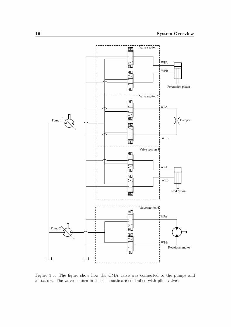
The rock drill is located on the feed boom which can be seen in figure 3.1. Therotation, percussion and damping subsystems is located inside the rock drill. The feedsubsystem is located on the feed boom. These four hydraulic subsystems each havetheir purpose for the drilling principles showed in figure 2.1.

Figure 3.2: The rock drill components. 1: Flushing system. 2: Damper. 3: Percussionpiston. 4: Shank adapter. 5: Gearbox. 6: Rotational motor.[4]

The purpose of the rotational subsystem is to move the button bit to uncrushedrock. The subsystem is powered by one of the hydraulic pumps, which is called pump2 in the report. The rotational motion comes from a hydraulic motor that is connectedto a gearbox and then to the drill string. This motor receives a constant flow to keepa constant rotational speed during the drilling. In figure 3.2 the rotational motor canbe seen on the rock drill.

The feed subsystem makes sure that the drill string always has contact with therock. The feed subsystem is supplied by a different pump than the rotational subsystem,which is called pump 1 in the report. The actuator of the feed subsystem can be acylinder. This cylinder is controlled by a pressure controlled valve, which means that

3.2 Feed Boom 15

the valve outputs a constant pressure corresponding to the control signal. The feedcylinder can be seen in figure 3.1.

The percussion subsystem creates the impact force that generates the impulse wavethrough the drill string. The percussion subsystem is supplied by the same pump as thefeed subsystem, pump 1. It consists of a piston and a control valve. The valve increasesthe pressure behind the piston to accelerate it. The piston generates an impact force,when hitting the shank adapter, that will travel through the drill string down to thebutton bit. The percussion piston can be seen on the rock drill in figure 3.2.

The damping subsystem damps out the impulse wave reflex. It is supplied by thesame pump as the feed- and percussion subsystem, pump 1. The damper can be seenon the rock drill in figure 3.2.

A hydraulic schematic of how the actuators are connected can be seen in figure 3.3.

16 System Overview

Pump 1

Pump 2

WPA

WPB

Valve section 1

Valve section 2

Valve section 3

Valve section 4

WPB

WPB

WPB

WPA

WPA

WPA

Percussion piston

Damper

Feed piston

Rotational motor

Figure 3.3: The figure show how the CMA valve was connected to the pumps andactuators. The valves shown in the schematic are controlled with pilot valves.

3.3 Communication 17

3.3 CommunicationThe information that is sent and received by the valve need to be packed and unpackedaccording to the CMA valve’s communication protocol. The CMA valve uses a CANnetwork with the CANopen standard. In this project the drilling functions controlledby the CMA system have a separate communication system from the rest of the drillrig. This communication system have a shorter loop time, which has to be taken intoaccount when evaluating the response times for the different systems.

3.3.1 Controller Area Network, CAN

Controller Area Network (CAN) is used to send and receive information with a CentralProcessing Unit (CPU). In this application there are two CPUs, one for each node of theCAN network. The first node is the PLC, which is used to initialize the CAN network.This node also has the user interface. The other node is the CMA valve’s VSM,which is the interface from the internal CAN network on the valve. The information istransferred in a specified baud rate by using two wires, CAN-high and CAN-low. Signalreflection is suppressed by having a 120 Ω resistance to terminate each end of the busline. The information is placed on bits that are either a one or a zero. A CAN messageis sent as an array of bytes (each byte is eight bits). The messages can either be sentby the type Process Data Object (PDO) or Service Data Object (SDO). The structureof these messages can be seen in appendix C. The PDOs are sent continuously duringoperation meanwhile the SDOs can only be sent during the pre-operational mode whenthe valve in inactive.

3.4 Electro-proportional ValveAn electro-proportional valve was used to simulate a load on rotation and replacedthe rotational motor during response time measurements in this project. This valve iscontrolled with a current controlled PWM signal which will result in a spool position.There is a current feedback on the PWM signal.

3.5 CMA ValveThe CMA valve is the programmable valve that was compared with the original valvesthat are controlling the rock drills hydraulic subsystems. It is a CAN-enabled electro-hydraulic sectional mobile valve and can be seen in figure 1.3. The valve has predefinedcontrol modes that are setup by a controller on a PLC. It also has a custom madecontrol mode for the RPCF drilling function that was built-in to the valve’s VSM. Across-section of one valve section can be seen in figure 3.4. The valve measures supplypressure and uses it for control. The Valve System Module (VSM) is the interfacemodule for the valve that is acting like a CPU. The VSM is used as a CAN gatewayand is the main controller in the valve system. This means that there was one internalCAN bus for the valve and one external for the drill rig. The advantage with the VSMis the internal high speed closed loop control which give the valve a faster response

18 System Overview

time. By using a separate CAN bus, the load on the drill rig’s CAN bus is reduced. Ituses sensors along with software control algorithms to make independent metering ofmultiple states. There are pressure sensors situated on all load sensing line, pressureline, tank line and workports which enables monitoring and pressure control.

Figure 3.4: Cross section of a work section on the programmable CMA valve fromEaton.[3]

The setup of the valve enables flow sharing, passive and overrunning load control.The Intelligent Flow Control (IFC), is a twin spool controller that enables flow con-trol on one workport and pressure control on the other. Flow control is used on theinlet workport and pressure control is used on the output workport when the load ispassive. Flow control is used on the output workport and pressure control on the in-let workport when the load is overrunning.[13] The Universal Flow Control (UFC), isa twin spool mode during which both spools operate in a pressure compensated flowcontrol mode.[13] The valve has the possibility to read the load demand of the rotationpressure difference from one section to control feed pressure in another section. This isonly possible if the motor load is passive during the entire operation.

The programmable valve has two spools that can be working together to controldouble acting functions in each work section. They can also be working separately andbe controlled from any of the work sections. An independent pilot spool is controllingthe main stage spools and closed loop control can be made for each work section locallyby sensors.

Six different control modes (not including the custom RPCF mode) can be chosendepending on how applicable they are to the RPCF function. The six modes are flow,pressure, spool position, PWM, float and idle. In flow control mode, the valve deliversa constant flow out of the valve without regard to the pressure. The pressure controlmode keeps a constant load pressure for the feed pressure. It adjusts the flow to makesure that the pressure do not drop below the required level. The spool position controlmode allows the user to control the system by changing the desired spool position.Pulse Width Modulation (PWM) lets the user specify how much of the maximum

3.6 PLC 19

control current that should be used to control the spool (a value between 0 and 100%).Float control mode opens both of the spools to get a specific flow until the pressure inboth workports is dropped below a set pressure. When the pressure is reached, bothspools is opened completely. Idle is the natural state of the valve. If the valve stopreceiving command messages, it enters this state after 200 ms.[14] In this mode thevalve is closed.

The CMA valve uses the supply pressure in the control algorithms. It has a built-in sensor that measures this pressure. The system is designed to be supplied by thesame pressure for all sections. In this drilling application, the rotational valve sectionis supplied by a different pump. Because of this, the rotational work section will bepositioned nearby pump 2 that is supplying the rotational subsystem. The supplypressure to this work section has to be measured and sent via the VSM with a specialSDO that can be sent during operational mode. The other work sections, along withthe VSM, that are controlling the feed, percussion and damper were positioned on thefeed beam. A hydraulic schematic of the system can be seen in 3.3.

3.6 PLCThe Programmable Logic Controller (PLC) used in this project was a IFM CR7132. Itwas used to control components for the thesis. The PLC has 4 MB of flash memory,which was enough for the thesis since only a few functions was programmed on to thePLC. The PLC was programmed using CoDeSys V2.3.9.42. The electro-proportionalvalve used to simulate the load in the rotational subsystem was controlled with acurrent. This current could be controlled with a resolution of 1-2 mA.[15]

An Electronic Data Sheet (EDS) file was loaded onto the PLC for the CAN com-munication with the programmable valve. This file contained predefined PDOs thatwas used to write control programs in CoDeSys.[16]

20 System Overview

Chapter 4

Control

This project worked with an actual drill rig. This required that safety functions werecoded into the controller. The controller had an idle state. When the idle state wasentered, all the hydraulic systems were shut down. The feed system was load holdingwhile the others subsystems pressures were set to zero.

Software for the CMA system was developed for the tests in this project. Thecontroller made for drilling automatically controlled the feed pressure to keep a constantrotational pressure. Another controller worked similar as the original RPCF function,see figure 1.2. This controller was used to compare the response time of the CMA valvesystem with the original system. Software for control of the damping and percussionwas also developed.

4.1 Control AlgorithmThe control algorithm was designed to be stable and fast. Thus, the derivative of thecontrol signal, du

dt , was not limited more than the standard limitation in the CMAvalve. The standard limitation in the CMA system contained a maximum of 300 bar/sin pressure change or a taper off filter with a filter frequency of 3 Hz. The signal wasprocessed through both filters and the method with the smallest difference betweenthe old value and the new value was used for that sample. Oscillations in the systemwere undesirable, but if the oscillations had a high frequency and a limited amplitude,it might have been damped out by the hydraulic system. The controller was tuned sothat the oscillations would not induce movement in the mechanical parts. The energyof the control signal was not important for this controller. The reason for this was thatthe feed pressure were supplied by the same pump as the percussion that had a muchhigher pressure. Thus, the feed pressure was not affect by the pressure settings on thepump.

4.1.1 Rotational Pressure Controlled Feed

The rotational reference pressure was calculated for a specific drill rig, drilling conditionand hardware setup. This value usually does not change during the drilling operation.Thus, the RPCF function could be treated as a regulator problem instead of a servo

21

22 Control

problem. This means that the controller should keep the controlled signal on a constantlevel and eliminate the effects of disturbances on the system. For a regulator problem,a controller that uses the control error is suitable. In this case, the control error was thedifference between the actual rotational pressure and the reference rotational pressure.Other possible control features was a feedback from the disturbance. For a drillingapplication, the disturbance can be the friction in the hole and the flow out of thefeed cylinder. The friction in the hole can be estimated with measurements of thefeed and rotational pressure, but it was changing in an unpredictable way that makeit unsuitable for this application. Measuring the flow is considered easier since it doesnot change as much. However, because of the low flows to the feed cylinder, the flowmeasuring method was not accurate enough for this application. Thus, there was nofeedback from disturbances in the controller used in this project.

4.1.2 Controller on the PLC

Frot Ffeed GrotGfeederotprot,ref

LP-filter

Made by valve manufacturer

pfeed,ref pfeed prot

Figure 4.1: A schematic over the transfer function that was implemented for the CMAvalve. Frot is the outer controller that outputs the reference feed pressure. Ffeed isthe inner controller, made by the valve manufacture, which outputs the feed pressure.LP-filter is a low pass filter.

The PLC controller could only use the six predefined valve modes. For the RPCFfunction, the pressure control mode and the flow control mode were used during normaloperation. The flow control mode was used for the rotational motor and the referenceflow was set to 40 l/min. This control mode was chosen to keep a constant rotationalspeed for the rock drill. The rotational pressure was controlled using a cascade loop.The outer controller (Frot) was a discrete time PID controller, which can be seen inequation 4.1.[8]

uk = Kp

(ek + TS

Ti

k∑n=0

en + Tdek − ek−1

TS

)(4.1)

By using the valve manufacturer’s pressure control mode as the inner control loop,the outer controller only had to provide a reference feed pressure. The changed feed

4.1 Control Algorithm 23

pressure would then affect rotational pressure through the change of friction in thehole. By saturating the feed pressure control signal at the maximum and minimumfeed pressure limits, the feed pressure was contained. This can be seen in equation 4.2.Anti windup was added to the integrational part of the PID if the control signal wouldbe saturated.

pfeed,ref =

pfeed,max, if u(t) > pfeed,max

u(t), if pfeed,min < u(t) < pfeed,max

pfeed,min, if u(t) < pfeed,min

(4.2)

To avoid instability, the outer control loop was made slower than the inner controlloop. The inner control loop, in this case, was the pressure control mode. A schematicof the controller can be seen in figure 4.1.

A deadband for the acceptable error can also be used which can be seen in equation4.3. This was used since the demanded pressure of the outer controller was discrete.The precision of the control signal was 0.125 bar.

ek =

0, if |erot| < pdeadband

erot, if |erot| ≥ pdeadband

(4.3)

4.1.3 Controller on the VSM

A new control mode was created for the VSM controller. This mode used the internalcommunication loop of the CMA valve for the outer controller (Frot). The same controlstrategy was applied here as in the PLC controller. However, the tuning parametersdiffered since the program loop time was different. A schematic over this controller canbe seen in figure 4.1. The valve manufacturer implemented the derived code for thiscontroller based on the specification that was worked out for this project.

4.1.4 Anti-jamming Mode

The drill rig enters the anti-jamming mode if the filtered rotational pressure reachthe limit for jamming. This means that the regular RPCF controller is overriddenby the anti-jamming controller. This can be seen in figure 4.2. The anti-jammingcontroller used the pressure control mode of the CMA valve. It sent a constant referencefeed pressure to the valve, with a reversed flow direction. This controller was onlyprogrammed on to the PLC.

24 Control

START

RPCF

prot > pjamming Anti-jamming

prot < pexit,jammingTRUE

FALSEFALSE

TRUE

Figure 4.2: The flowchart shows how the controller starts and how it switches betweenmodes during operation.

4.1.5 PID Tuning

The friction in the system was unpredictable and also expected to change a lot, whichmeans that the system would not stay in steady state for a long time. Thus, the Ziegler-Nichols method was deemed to work well with this application. The method was usedwith the Ziegler-Nichols model generated from a step response. Another method thatcould have been used was an oscillation test, since the system handle high pressure thestep response method were considered to be more safe.

4.2 Set up of PLC

ProFX (software from the valve manufacturer) was used to reconfigure CAN-addressesto be able to receive the rotational pressure to programs in the PLC. An EDS wasprovided by the valve manufacturer and implemented in the PLC program. This filehelped with the initialization of the CAN network. The programming of the PLC wasdone with function block diagrams and structured text. Programs were created formost cases, but the packaging of CAN messages was created by function blocks. Thefunction blocks could be used in more than one program.

The CMA valve used the supply pressure for the control modes. If the supplypressure differed from the measured value, the valves control modes might not work

4.3 Control Required for Drilling 25

properly. Since this project used two different pumps with different pressure settingsto supply the CMA valve, the PLC had to send a measurement of the supply pressurefor the rotation to the VSM. The supply pressure from the other pump was measuredby a sensor inside the CMA valve.

4.3 Control Required for DrillingDuring actual drilling, feed and rotation were not the only drilling principles that wererequired to be controlled. There was also a need to control the percussion and thedamping, which is stated in section 2.1. The percussion was controlled to a constantpressure and the damping to a constant flow. The drill- and the anti-jamming modeswere the only modes used during the hardware simulation. However, for the drill test, afew more modes had to be developed. A manual mode was developed to be able to turnthe percussion on and off and to change the rotational flow and feed pressure. In orderto start the drilling mode, the rock drill would first enter collaring mode. In collaringmode, the percussion pressure and the feed pressure were lower than during drilling.The RPCF was disabled since the low feed pressure would not give the desired rotationalpressure. The feed pressure was instead kept at a constant level. The rotational flowand damping flow were the same in the collaring mode as in the drilling mode. An idlemode was created to tie all these modes together. The idle mode was also the startingmode that the drill rig entered after initialization. From the idle mode it was possibleto update parameters that were sent to the CMA valve as SDOs. A flow chart overthese modes and how to move between them can be seen in figure 4.3.

Since the percussion used a much higher pressure than the rotation, the two pumpssupplied two different pressures levels. This required that a rotation supply pressuremeasurement was sent to the CMA valve. It was sent using an SDO, which would holdthe value until the previous value got overwritten by the new value.

4.3.1 Implementation of Manual Control

The joysticks were configured to output a zero value in center position. The value wasproportionally increased until it reached the end position which outputted the specifiedmaximum value. The two different end positions corresponded to the two differentflow directions. This enabled the drill rig to be able to switch the feed pressure androtational flow from positive to negative direction in a smooth, controlled operation.The switch enabled the percussion to be on or off and the percussion pressure parametercould be set in the graphical user interface if different pressures were required.

26 Control

Start

Initialize

Idle

ManualActivateActivate

Activate

Collaring

Drilling

10 seconds

Anti-jammingprot > pjamming

prot < pexit,jamming

Runtime

True

True

True

True

True

True

True

False

False

FalseFalse

False

False

ManualCollaring

Drilling in collaring exceeded

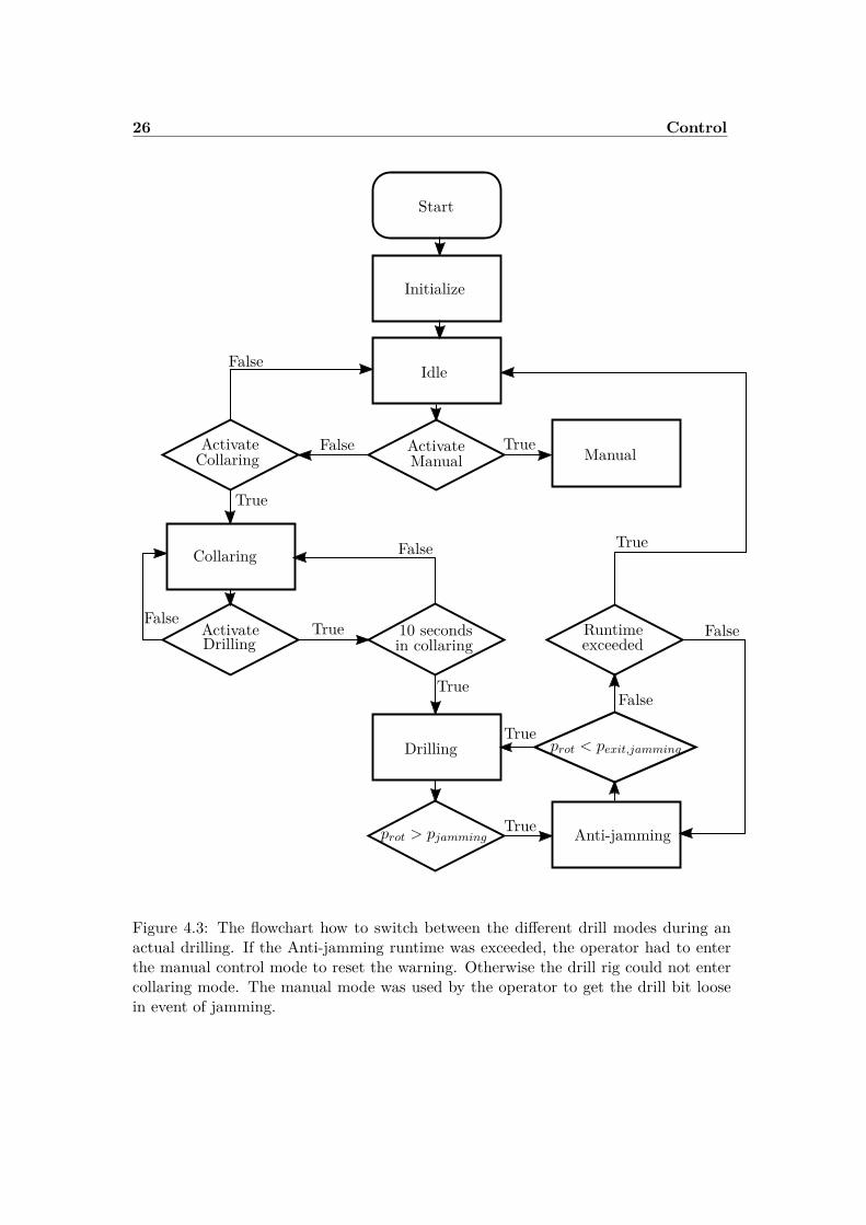
Figure 4.3: The flowchart how to switch between the different drill modes during anactual drilling. If the Anti-jamming runtime was exceeded, the operator had to enterthe manual control mode to reset the warning. Otherwise the drill rig could not entercollaring mode. The manual mode was used by the operator to get the drill bit loosein event of jamming.

Chapter 5

Testing

Conducting tests on the drill rig required several safety aspects to ensure that nothingwas damaged or affected the surroundings or the people operating it. Proper safetyequipment was used when the drill rig was running such as safety glasses, proper cloth-ing, gloves and shield walls to prevent any hydraulic oil injection accident.

In this chapter the different hardware setups are described along with the differenttests. It summarizes why the tests were done and how they were executed. The re-sponse time test evaluated, with a repeatable result, how fast the CMA valve systemwas compared to the original valve system. The tuning test evaluated if the controllerworked effectively. The anti-jamming test evaluated if the CMA system worked cor-rectly and safely during jamming. The drill test was performed last to see if the valvecould handle a drilling procedure using the result of the tuning- and anti-jamming test.

5.1 Hardware Setups

There were two different hardware setups for the testing equipment. The first setupwas used to perform hardware simulations on both the original system and the CMAsystem. The second was used to perform tests in a real drilling environment with theCMA system.

5.1.1 Wiring

Shielded wires were used for CAN connections to prevent unwanted disturbances onthe measurements.

The VSM connection cable was split into two parts. The first part was a powercablethat was connected to a lamp outlet (24 V). The second part was the CAN connectionthat could be connected to either the PLC or the CAN-card. The valve section for therotation was separate from the other valve sections. This required a long CAN-cableto connect it to the internal CAN bus. The PLC was powered from a 24 V cigaretteoutlet on the drill rig. The wiring diagram for the cables can be seen in appendix B.

27

28 Testing

5.1.2 Hardware Simulation

The hardware simulation setup was used to have a controlled environment. The drillingprocedure was modeled using hardware and software. The tests performed with thissetup had to be repeatable and have the possibility to compare the results for thedifferent valve systems. A schematic of how to setup the hardware is shown in figure5.1.

iv = K · pfeed +M (5.1)

The electro-proportional valve was controlled with a current calculated from equa-tion 5.1. The loads were simulated with orifices. Both the feed piston and the rotationalmotor were disconnected. The feed piston was replaced with a variable orifice and therotational motor with an electro-proportional valve. The feed beam was tilted to ahorizontal position, showed in figure 5.2, that enabled easy access to the valve blocksand hydraulic hoses.

Test Equipment

• A portable data logger. It was used to read and record flow, pressure and tem-perature using the existing channels.

• An electro-proportional valve. It was used to be able to simulate the counteractingtorque when drilling with different friction interference by changing the rotationalpressure.

• Variable orifice controlled by levers. It was used to simulate a normal force fromthe rock.

• Adapters. They were used to connect the equipment and hoses.

• Hoses. Used to connect the equipment.

• A flow sensor. It was used to measure the flow rate.

• Pressure sensors. They were used to measure feed and rotational pressure.

• Temperature sensor. It was used to read the working temperature of the hydraulicoil.

• Display. It was used to read and change the parameter for the current reference.

• PLC hardware. It was used for controlling the electro-proportional valve.

• M12 wires. They were used to connect the sensors to the portable data logger’schannels.

• CAN-card. It was used to enable the software to communicate with the CMAvalve.

5.1 Hardware Setups 29

Connect

p

q

p

p

T

ConnectConnect Connect

Control valveRotation

Control valveFeed

PLC

Figure 5.1: The figure shows a schematic of how the hardware was set up for the hard-ware simulation. There was one flow sensor and one pressure sensor for measurementson the rotational subsystem. Then there was two pressure sensors for measurement ofthe feed. One for the PLC and one for the data logger. The connect blocks were quickcouplings which makes it easier to switch between the original and the CMA controlvalves.

Assembly of Hardware

The hoses that connected the outgoing ports of the feed valve block to the feed pistonwere removed and thereby disabled the feed piston. Instead, a feed subsystem wasmade that consisted of a variable orifice with a control lever, see figure A.4 in appendix,connected in series with a pressure and temperature sensor which can be seen in figureA.5 in appendix. The schematic of the feed subsystem can be seen in figure 5.3. Thesensors were connected to the data logger using M12 wires. They can be seen in figures

30 Testing

Figure 5.2: The feed beam was put in a horizontal position to enable easy access to theequipment.

A.1 and A.6 in appendix. The temperature was recorded to be able to ensure that thehydraulic oil had reached working temperature before all tests. Also, another pressuresensor was assembled in series with the other sensors that was connected to the PLC.The PLC then uses this to control the electro-proportional valve. The assembled feedsubsystem can be seen in figure 5.4. The hoses that were connected to the rotationalmotor ports were also disconnected. This disabled the rotational motor and preventedunwanted disturbances when the shank adapter rotates. Instead, a rotational subsystemwas made that consisted of the flow and pressure sensor which was connected in serieswith the electro-proportional valve. The rotational subsystem can be seen in figure 5.5.Both of the sensors were connected to the data logger. The function of the electro-proportional valve was to change the rotational pressure. It was only work port A, tankport and pump port that were used on the electro-proportional valve and the rest of theworking ports were plugged. The assembled rotational subsystem can be seen in figure5.6. A display was connected to the PLC. This display (if enabled) set the currentvalue parameter which the PLC used to control the electro-proportional valve. Thedisplay changed the parameter with five milliampere increments. It was programmedusing CoDeSys and initial values were set near the desired working area.

To be able to measure the response time, the feed pressure had to change when

5.1 Hardware Setups 31

p

p

Quick couplingfemale

T

To PLC

To data logger

Quick couplingfemale

Figure 5.3: Schematic of the feed subsystem containing pressure and temperature sen-sors with a variable orifice. An image of the quick coupling can be seen in figure A.7in appendix.

Figure 5.4: The assembled feed subsystem containing pressure and temperature sensorswith a variable orifice controlled by a lever.

the rotational pressure changed. This required that the rotational pressure was higherthan prot,drill and lower than pjamming (see figure 1.2). The rotational pressure wascontrolled with a control current for the electro-proportional valve. By staying insidethis pressure range there were no internal delays and the anti-jamming function did notstart. The drill rig had its rotational flow calibrated to maintain a rotational pressurewithin the range of the RPCF. The feed pressure were also calibrated to a level withinthe range of the RPCF.

32 Testing

p

q

Quick couplingfemale

Quick couplingfemale

Todata

logger

From PLC

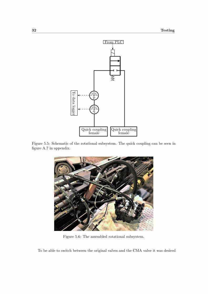
Figure 5.5: Schematic of the rotational subsystem. The quick coupling can be seen infigure A.7 in appendix.

Figure 5.6: The assembled rotational subsystem.

To be able to switch between the original valves and the CMA valve it was desired

5.1 Hardware Setups 33

to connect them in parallel with each other. This was done by adding a T-coupling fromthe pump to the supply and tank hoses. From this, T-coupling hoses were connectedto both control valves. See figure A.8 in appendix. The feed piston subsystem wasmodified to have two quick couplings that could be pulled off one valve and put onthe other. The quick couplings can be seen in figure A.7 in appendix. The valve, thatwas not used, was thereby plugged by using the quick couplings. The supply- and tankhoses from the rotational pump were also T-connected and branched to both worksections that control the rotation, to the original- and the CMA valve. The rotationalsubsystem was also given quick couplings.

The percussion and damping were disconnected to make the hydraulic system simpleand to make sure that the tests were not interfered with external factors. All hydraulichoses and work ports were converted by adapters to 3/4" in diameter to have the samedimension for the response time tests. The length of the hoses that were T-connectedhad a similar length to not make any time delays occur during tests.

5.1.3 Hardware Drilling Environment

This setup was used for an actual drilling environment. The tests performed with thissetup generated a perception on how the CMA valve works during a drilling operation.

Test Equipment

• A portable data logger. It was used to read and record flow, pressure and tem-perature using the existing channels.

• Adapters. They were used to connect the equipment and hoses.

• Hoses. They were used to connect the equipment.

• Pressure sensors. They were used to measure pump, feed and rotational pressure.

• Temperature sensor. It was used to read the working temperature of the hydraulicoil.

• PLC hardware. It was used for controlling the drill functions.

• CAN-card. It was used to enable the software to communicate with the CMAvalve.

• M12 wires. They were used to connect the sensors to the portable data logger’schannels.

• Joysticks. They were used to manually operate the rotation and feed.

• Switch. It was used to manually operate the percussion.

• Valve attachment. It was used to mount the valve in a safe position on the feedbeam.

34 Testing

Supply Pressure for Rotation

In this test the supply pressure for the rotation was measured and sent to the CMAvalve. This allowed the two pumps to produce different supply pressures.

Assembly of Hardware

In order to make a drill test with the CMA system, the drill rig made several hardwarechanges. The feed piston, rotational motor, percussion and damping were connected tothe CMA valve. The CMA valve was mounted to the feed beam with a custom madeattachment. The attachment can be seen in figure A.11 in appendix. This was done tosecure the valve when it was positioned vertically on the feed beam during drilling. Theassembled hardware can be seen in figure 5.7 and 5.9. The pressure sensor for rotationwas assembled on the inlet of the rotational motor which can be seen in figure 5.8.

Figure 5.7: The CMA valve assembled on the attachment with percussion, dampingand feed actuators connected to it.

The hydraulic subsystems needed the ability to be controlled manually in case thatjamming would occur or if the drill string needed to get up from the hole during thetest. Two joysticks and a switch were provided to be able to control the feed, rotationand percussion, which can be seen in figures A.9 and A.10 in appendix. Flat pins wasassembled to them in order to connect them to the PLC.

5.1 Hardware Setups 35

Figure 5.8: Down in the left hand corner of the figure, it can be seen where the rotationalpressure sensor was assembled on the rock drill.

Figure 5.9: The CMA valve rotational work section assembled on the drill rig withthe rotational actuator connected to it. Two pressure sensor are located on the inletwork port that is connected to the PLC and data logger for monitoring of the differentpressures.

36 Testing

5.1.4 Initialization of CMA Valves

An airbleed was made to get rid of all the air in valves. It was done automatically bya software that came with the valves which cycled the spools from pressure to tankrepeatably until the process was done. It was performed with low pressure, which wasset to 30 bar for safety reason.

5.2 Response Time TestThe original system was used as a benchmark and compared with the CMA system.The purpose was to decide how long it takes for the systems to change the feed pressureafter detecting a change in rotational pressure.

5.2.1 Test Plan

Conditions

The drill rig will be set up according to the description of hardware simulation in section5.1. The electro-proportional valve will be controlled manually by stepping the currentup and down. This will be done by setting the K coefficient in equation 5.1 to zeroand stepping with the M coefficient. An open loop controller will be developed for theCMA system to have similar functionality as the original RPCF controller.

Measured Quantities

All measured quantities will be stored with their corresponding time.

• Feed pressure

• Rotational pressure

• Rotational flow

• Oil temperature

The rotational flow and oil temperature will be monitored to ensure that the testconditions do not change. The feed and rotational pressure will be presented in theresult.

Description

Two electric currents which generate pressures inside the RPCF control range will beselected. One of the electric currents should generate a pressure close to the upper limitwhile the other current should generate a pressure close to the lower limit. Measure-ments will be taken between the limits when stepping both up and down. When thecurrent stepped up, the rotational pressure will decrease and when the current steppeddown the rotational pressure will increase. This will result in two response times forthe system. One for the compensation of an increasing rotational pressure, when it isa risk for jamming, and one for the compensation of a decreasing rotational pressure.

5.2 Response Time Test 37

After the Test

The response times will be analyzed and divided into three parts. One part for theprogram loop time, a second part for the mechanical response time and the third partfor the communication time.

5.2.2 Calibration for the Response Time Test

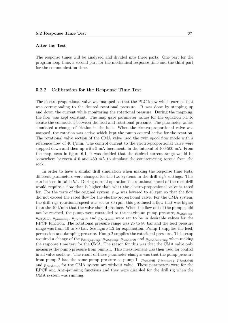
The electro-proportional valve was mapped so that the PLC knew which current thatwas corresponding to the desired rotational pressure. It was done by stepping upand down the current while monitoring the rotational pressure. During the mapping,the flow was kept constant. The map gave parameter values for the equation 5.1 tocreate the connection between the feed and rotational pressure. The parameter valuessimulated a change of friction in the hole. When the electro-proportional valve wasmapped, the rotation was active which kept the pump control active for the rotation.The rotational valve section of the CMA valve used the twin spool flow mode with areference flow of 40 l/min. The control current to the electro-proportional valve werestepped down and then up with 5 mA increments in the interval of 400-500 mA. Fromthe map, seen in figure 6.1, it was decided that the desired current range would besomewhere between 410 and 430 mA to simulate the counteracting torque from therock.

In order to have a similar drill simulation when making the response time tests,different parameters were changed for the two systems in the drill rig’s settings. Thiscan be seen in table 5.1. During normal operation the rotational speed of the rock drillwould require a flow that is higher than what the electro-proportional valve is ratedfor. For the tests of the original system, nrot was lowered to 40 rpm so that the flowdid not exceed the rated flow for the electro-proportional valve. For the CMA system,the drill rigs rotational speed was set to 80 rpm, this produced a flow that was higherthan the 40 l/min that the valve should produce. When the flow out of the pump couldnot be reached, the pump were controlled to the maximum pump pressure, prot,pump.prot,drill, pjamming, pfeed,drill and pfeed,min were set to be in desirable values for theRPCF function. The rotational pressure range was 25 to 80 bar and the feed pressurerange was from 10 to 80 bar. See figure 1.2 for explanation. Pump 1 supplies the feed,percussion and damping pressure. Pump 2 supplies the rotational pressure. This setuprequired a change of the pdamp,pump, prot,pump, pperc,drill and pperc,collaring when makingthe response time test for the CMA. The reason for this was that the CMA valve onlymeasures the pump pressure from pump 1. This measurement was then used for controlin all valve sections. The result of these parameter changes was that the pump pressurefrom pump 2 had the same pump pressure as pump 1. prot,drill, pjamming, pfeed,drill

and pfeed,min for the CMA system are without value. These parameters were for theRPCF and Anti-jamming functions and they were disabled for the drill rig when theCMA system was running.

38 Testing

Table 5.1: The drill rig parameters that were set for the response time tests. When thedrill rig parameters are set for the CMA system, the supply pressure is 100 bar for therotation and 100 bar for the feed.

Parameter Original System CMA system Unitnrot 40 80 rpmprot,drill 25 - barpjamming 55 - barpfeed,drill 80 - barpfeed,min 10 - barprot,pump 115 100 barpdamp,pump 100 100 barpperc,drill 200 100 barpperc,collaring 200 100 bar

5.2.3 Test Procedure

Before measurements could be made, the equipment had to get up to the workingtemperature. This was done by starting rotation and feed drill mode on the drill rigand stepping between the two current levels without measuring. When the hydraulic oiltemperature saturated at its working temperature of 40-45C, the measurements weremade. The control current interval, for the electro-proportional valve, differed fromthe original system and the CMA system. It was changed to make the systems workin the same pressure range when stepping between the currents. A controller for theelectro-proportional valve was developed to be able to change the simulated resistanceover the rotational subsystem repeatably without stationary errors. The current thatwas sent to it was always monitored to make sure that this did not happen. The currentlevel was set in the user interface on the PLC, this enabled online stepping during thetests.

Original System When testing on this system, the CMA valve was powered downto not interfere with the tests. The lower current level on the electro-proportional valvefor this test was set to 405 mA and the upper was set to 440 mA.

CMA System For the testing on this system the drill rigs RPCF and Anti-jammingfunction were turned off. The lower current level on the electro-proportional valve wasset to 410 mA and the upper was set to 470 mA.

5.2.4 Data Processing

The recordings were exported to Comma Separated Value files (CSV), that were im-ported to MATLAB for further graphical analyzing. 40 different measurements weremade for each system to ensure repeatability. The measurement data was filtered foreasier identification of the response time. The data was filtered after the measurementusing MATLAB’s filtfilt function to avoid phase distortion. A digital lowpass filter was

5.3 Tuning Test 39

used of the type Infinite Impulse Response (IIR). The passband frequency was set to4 Hz and the stopband frequency to 10 Hz. The passband ripple was set to 0.45 andthe stopband attenuation to 60. The samplerate was 2000 Hz during the measurement.The response time was calculated with equations 5.2 and 5.3.

L = T2 − T1 (5.2)

∆L = Loriginal − LCMA

Loriginal(5.3)

5.3 Tuning TestThe purpose of the tuning test was to tune the controller parameters for the RPCFfunction. The RPCF should try to keep a constant rotational pressure by changingthe feed pressure. The CMA system was iterated with this test until it had desirableperformance. The rotational flow had to be kept constant during the test.

5.3.1 Test Plan

Conditions

The drill rig will be set up according to the description of hardware simulation in section5.1. The rotational pressure’s dependency on the feed pressure will change during thetest.

Measured Quantities

All measured quantities will be stored with their corresponding time.

• Feed pressure

• Rotational pressure

• Rotational flow

• Oil Temperature

The rotational flow and oil temperature will be monitored to ensure that the testconditions do not change. The feed and rotational pressure will be presented in theresult.

Description

To get initial values for the PID parameters, the open system will be tested beforeactivating the RPCF controller. Open loop step responses will be taken for all differentrock conditions that the test used.

The RPCF controller parameters will be set before the start of the test. The testwill start with normal conditions, then the rotational pressure’s dependency on the

40 Testing

feed pressure will change and the regulator should adjust the feed pressure to keep therotational pressure constant. The rotational flow should not be affected by this. Whenthe system reach steady state the dependency will be changed again.

After the Test

If the controller sufficiently handle the interference and counteracts the changes inrotational pressure, the controller pass the test. Otherwise further work with the valuesof the controller parameters will be required. The data will be analyzed to observe anydeviations of the desirable control signal.

5.3.2 Calibration of Control Parameters

During normal drilling conditions, the feed pressure are operating in the range of 50-60bar according to an experienced operator.[2] The control settings were therefore setto be able to control around this range. By using the map of the electro-proportionalvalve and the desired feed pressure, different parameter settings were developed. Theparameter settings for equation 5.1 can be seen in table 5.2.

Table 5.2: The table shows different control modes for the electro-proportional valve.The two modes corresponded to different rock drilling conditions, mode 1 correspondsto a softer drilling condition and mode 2 corresponds to hard drilling conditions. Themodes were divided into two groups. Mode 1.1 and 1.2 is one group and mode 2.1 and2.2 another. Switching within the group gave a pressure change of about 20 bar. prot,ss

and pfeed,ss were the steady state pressures for the system. prot,ms and pfeed,ms arethe pressures that the system should have gone towards when switching between themodes in one group. The K and M parameters are described in equation 5.1.

Mode prot,ss prot,ms pfeed,ss pfeed,ms K M

1.1 50 bar 30 bar 60 bar 40 bar -2 5351.2 50 bar 70 bar 40 bar 60 bar -3/4 4452.1 50 bar 30 bar 60 bar 50 bar -4 6552.2 50 bar 70 bar 50 bar 60 bar -3/2 490

5.3.3 Test Procedure

A step response was made to get the PID parameters using the Ziegler Nichols method.A reference signal that showed when a change happened in the system was needed forthis method. The portable data logger had an input channel which could read signalssent from the PLC. An M12 wire was made to connect them. The electro-proportionalvalve had one of the modes set and had the group changed which induced a step. Thestep response was made when the equipment had the correct working temperature.

It was observed that the control error was noisy. The derivative gain catches thederivative of the noise which gave two options. The first option was to filter therotational pressure but this would reduce the effectiveness of the derivative gain since

5.4 Anti-jamming Test 41

it could fail to detect changes in the system. It would also affect the proportional gainand the integrational gain since the filtration would take place in the VSM. Anotheroption was to set the derivative gain to something small or zero. The parameter Td

was set to zero which made it a PI-controller.

System with the Controller on the PLC The step response gave values of b andL which generated initial Kp and Ti parameters, which can be seen in table 6.2. Themost defensive PI parameters within the range were set in the PLC and different controlmodes for the electro-proportional valve were tested. The different electro-proportionalcontrol modes were created to see how the controller managed to compensate for differ-ent drilling conditions. The system started out as stable when the RPCF was enabled.But the system became unstable when switching to a different control mode for theelectro-proportional valve. Kp was decreased by a factor ten and Ti was increased bya factor ten. The instability was gone on the second try, but the controller was consid-ered slow. The proportional and integrational gains were slowly changed over severaliterations. The final PI-controller was a compromise between speed and steady stateoscillations. It was tested for all cases within the two groups which ensured that thecontroller was acceptable for the different drilling conditions.

System with the Controller on the VSM The control parameters were tunedby using ProFX (a software that came with the valve). The CMA valve needed to bein pre-operational mode on the CAN bus when the control parameters were changedsince they were sent with SDO messages. The initial values were calculated by usingthe result of the controller on the PLC. The controller worked but more iterations weremade to see if it could be even better. The proportional and integrational gains wereslowly increased during several iterations until the control performance was fast androbust. A steady state error on the rotational pressure might occur during the tuningof the controller on the VSM. The reason for this was that the valve used the pressurevalue which would have been sent to the pump instead of the measured pressure. Thepressure sent to the pump was most likely filtered to give a stable value to the pump,it might also have a margin to ensure that the pump pressure was sufficient to supplythe valve.

5.3.4 Data Processing

The recordings were exported to CSV, that was imported to MATLAB for furthergraphical analyzing.

5.4 Anti-jamming Test

This test was only performed on the CMA system with the RPCF controller on theVSM. It tested the functionality of the controller to make sure that the system enteranti-jamming mode when the pressure is higher than the jamming pressure, pjamming.

42 Testing

5.4.1 Test Plan

Conditions

The drill rig will be setup according to the description of hardware simulation in section5.1. The K coefficient in equation 5.1 will be zero and the M coefficient will be usedto increase the rotational pressure to a level above the jamming pressure.

Measured Quantities

All measured quantities will be stored with their corresponding time.

• Feed pressure

• Rotational pressure

• Rotational flow

• Oil temperature

The rotational flow and oil temperature will be monitored to ensure that the testconditions do not change. The feed and rotational pressure will be presented in theresult.

Description

By increasing the rotational pressure rapidly, it will exceed the maximum limit beforethe RPCF can compensate for the change of pressure. The drill rig should enter anti-jamming mode when jamming is detected. The drill rig should exit anti-jamming modeand go back to drilling mode if the rotational pressure is decreased below the exit-jamming pressure. The drill rig should enter an idle state, and wait for the operator totake control, if the rotational pressure is not decreased below the exit-jamming pressurebefore the runtime of the anti-jamming mode is exceeded.

After the Test

The result of this test will show if the drill rig can handle anti-jamming and perform asafe drill test.

5.4.2 Calibration for Anti-jamming Test

The control current, for the electro-proportional valve, used the control mode 2.1 (de-scribed in table 5.2). Jamming was induced by lowering the value of M to 350. Theproportional gain was set to 0.78 and the integrational gain to zero. The reason forthis was because of how the electro-proportional valve was controlled. The feed pres-sure dropped to zero when anti-jamming mode was entered since the variable orificewas fully closed. This caused oscillations in the system and that is why the integra-tional gain was zeroed (Ti went towards infinity). The different pressure parametersfor rotational can be seen in table 5.3.

5.5 Drill Test 43

Table 5.3: The parameters used during the anti-jamming test.

Parameter CMA system Unitpjamming 80 barpexit,jamming 70 barprot,drill 40 bar

5.4.3 Test Procedure

The anti-jamming test was made in two steps. The first step was to validate thatthe drill rig enters anti-jamming mode when the rotational pressure exceeds the anti-jamming pressure and leaves the mode when the pressure is lower than the exit pressurefor anti-jamming. The second step also ensured that anti-jamming mode is enteredwhen the rotational pressure exceed the anti-jamming pressure. The rotational pressurewas not lowered in time to exit anti-jamming mode, instead it should enter the idlestate and wait for the operator to take action.

Exiting Anti-jamming Mode The anti-jamming mode program was activated onthe PLC. The electro-proportional valve was controlled with the drilling control cur-rent. Then the electro-proportional valve current was switched to the jamming controlcurrent. This caused the rotational pressure to increase above the anti-jamming pres-sure of 80 bar. After about five seconds in anti-jamming mode, the control currentwas set to the drilling control current again to ensure that the anti-jamming mode wasexited when the rotational pressure decreased.

Anti-jamming Runtime Exceeded The anti-jamming mode program was acti-vated on the PLC. The electro-proportional valve was controlled with the drilling con-trol current. Then the control current was switched to the jamming control current.This caused the system to enter anti-jamming mode. The system went to idle modeafter about 10 seconds in anti-jamming mode.

5.4.4 Data Processing

The recordings were exported to CSV, which was imported to MATLAB for furthergraphical analyzing.

5.5 Drill Test

This test was only performed on the CMA system with the RPCF controller on theVSM. The purpose was to let an experienced operator get an indication of how theCMA valve is perceived to affect the drill rig system.

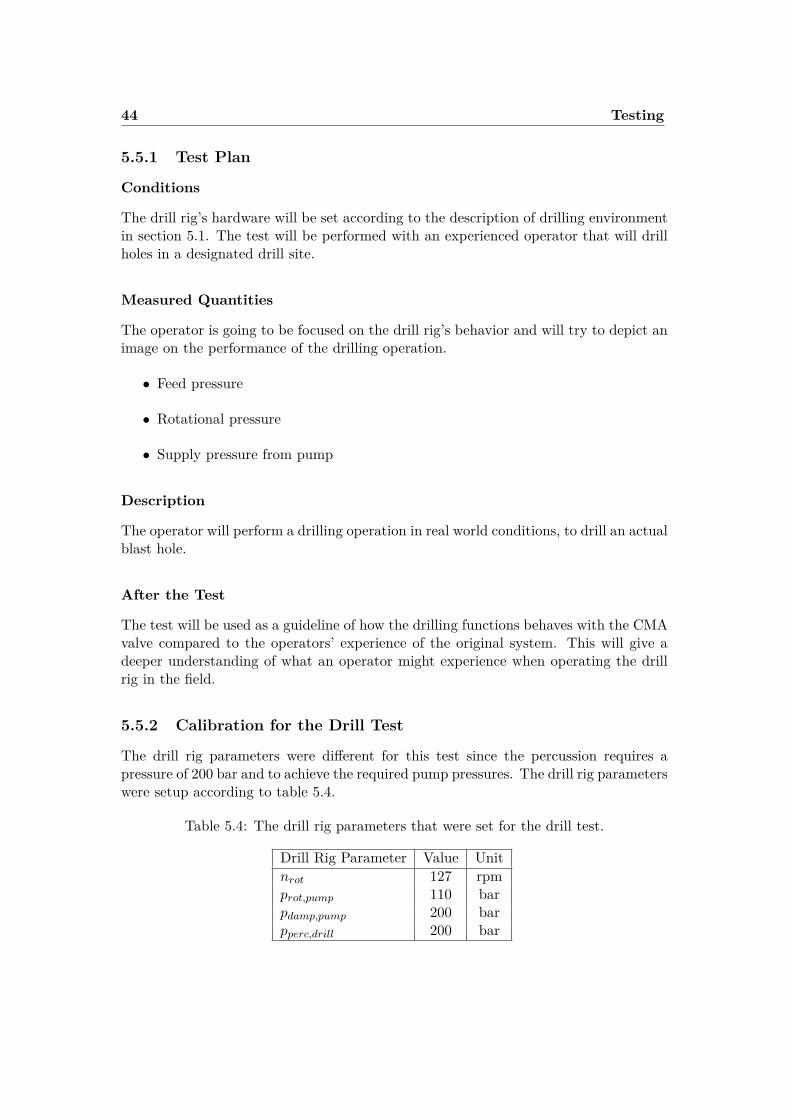
44 Testing

5.5.1 Test Plan

Conditions

The drill rig’s hardware will be set according to the description of drilling environmentin section 5.1. The test will be performed with an experienced operator that will drillholes in a designated drill site.

Measured Quantities

The operator is going to be focused on the drill rig’s behavior and will try to depict animage on the performance of the drilling operation.

• Feed pressure

• Rotational pressure

• Supply pressure from pump

Description

The operator will perform a drilling operation in real world conditions, to drill an actualblast hole.

After the Test

The test will be used as a guideline of how the drilling functions behaves with the CMAvalve compared to the operators’ experience of the original system. This will give adeeper understanding of what an operator might experience when operating the drillrig in the field.

5.5.2 Calibration for the Drill Test

The drill rig parameters were different for this test since the percussion requires apressure of 200 bar and to achieve the required pump pressures. The drill rig parameterswere setup according to table 5.4.

Table 5.4: The drill rig parameters that were set for the drill test.

Drill Rig Parameter Value Unitnrot 127 rpmprot,pump 110 barpdamp,pump 200 barpperc,drill 200 bar

5.5 Drill Test 45

5.5.3 Test Procedure

The drill rig was fueled up and positioned at the drill site. The lube oil, drill rodsand drill bit were inspected to ensure that they were in good shape for drilling. Thedrill rig was run until the correct working temperature was achieved. The drill stringwas positioned on top of the rock manually, see figure 5.10, and the collaring modewas enabled. In this mode the rock drill had a constant feed pressure applied onthe rock drill. The rotational motor started to rotate and the percussion pressurehad its collaring pressure. After about ten seconds, the drilling mode was turned onwhich enabled the custom RPCF onboard the CMA valve and the percussion pressureincreased to drilling pressure. The drilling proceeded until a two meter deep drill holewas made vertically down in the rock.

5.5.4 Data Processing

The recordings were exported to CSV, which was imported to MATLAB for furthergraphical analyzing. The data was filtered after the measurement using MATLAB’sfiltfilt function to avoid phase distortion. A digital lowpass filter was used of the typeIIR. The passband frequency was set to 2 Hz and the stopband frequency to 3 Hz. Thepassband ripple was set to 1 and the stopband attenuation to 60. The sample rate wasgiven at 1000 Hz.

46 Testing

Figure 5.10: The figure shows how the feed beam was positioned for the drill test atthe drill site. CAN cable and M12 cables are connected to the PLC and data logger ata safe distance from the drill hole.

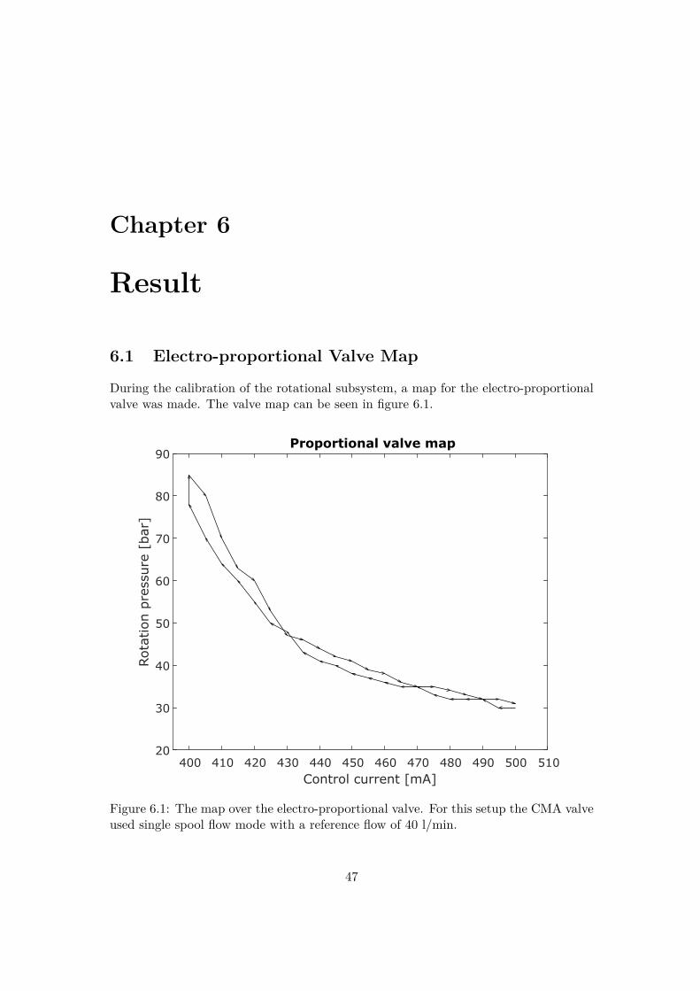
Chapter 6

Result

6.1 Electro-proportional Valve Map

During the calibration of the rotational subsystem, a map for the electro-proportionalvalve was made. The valve map can be seen in figure 6.1.

400 410 420 430 440 450 460 470 480 490 500 510Control current [mA]

20

30

40

50

60

70

80

90

Rot

atio

n p

ress

ure

[bar

]

Proportional valve map

Figure 6.1: The map over the electro-proportional valve. For this setup the CMA valveused single spool flow mode with a reference flow of 40 l/min.

47

48 Result

6.2 Response Time Test

The response time was calculated by using equation 5.2. The response time was de-creased by 60% for a decreasing rotational pressure and 64% for an increasing rotationalpressure with the CMA valve. The mechanical response time was decrease by 58% fora decreasing rotational pressure and 64% for an increasing rotational pressure. Thiswas calculated with equation 5.3.

6.2.1 Original System

Figures 6.2 and 6.3 show measurements of response time tests for the original system.A total of 40 measurements were made, 20 for a rising rotational pressure and 20 for afalling rotational pressure. The response time has an uncertainty of one communicationloop time.

Time

Pro

t

Pfe

ed

Response time original

Prot

Unfiltered

Prot

Filtered

Pfeed

Unfiltered

Pfeed

Filtered

X: T1

X: T2

Figure 6.2: A response time test for the original system when the rotational pressurewas increased. The data displayed is from measurement 11. The response time is T2subtracted by T1. The data was filtered with a lowpass filter after the measurement.

Figures 6.4 and 6.5 display the measured response times. The response time for thesystem is displayed as a line. The response time measurements were divided into threeparts. The program loop time, the mechanical response time and the communicationtime.

6.2 Response Time Test 49

Time

Pro

t

Pfe

ed

Response time original

Prot

Unfiltered

Prot

Filtered

Pfeed

Unfiltered

Pfeed

Filtered

X: T1

X: T2

Figure 6.3: A response time test for the original system when the rotational pressurewas decreased. The data displayed is from measurement 9. The response time is T2subtracted by T1. The data was filtered with a lowpass filter after the measurement.

Response Time Original

1 2 3 4 5 6 7 8 9 10 11 12 13 14 15 16 17 18 19 20Measurement number [#]

Res

pon

se t

ime

Program Loop TimeMechanical Response TimeCommunication TimeSystem Response Time

Figure 6.4: The response times for the original system when the rotational pressurewas increased. The response times are divided into three parts. The first part is theprogram loop time. The second part is the mechanical response time. The third partis the communication time, it has a maximum value of one communication loop.

50 Result

Response Time Original

1 2 3 4 5 6 7 8 9 10 11 12 13 14 15 16 17 18 19 20Measurement number [#]

Res

pon

se t

ime

Program Loop TimeMechanical Response TimeCommunication TimeSystem Response Time

Figure 6.5: The response times for the original system when the rotational pressurewas decreased. The response times are divided into three parts. The first part is theprogram loop time. The second part is the mechanical response time. The third partis the communication time, it has a maximum value of one communication loop.

6.2.2 CMA system

The response time in the CMA system were different depending on if the pressurewas increasing or decreasing. It was ∼9% higher when the rotational pressure wasdecreased. Measurements of the increasing and decreasing rotational pressure can beseen in figure 6.6 and 6.7. The communication loop time was shorter for this test, whichgave a smaller uncertainty for the response time.

Figures 6.8 and 6.9 display the measured response times. The response time for thesystem is displayed as a line. The response time measurements were divided into threeparts. The program loop time, the mechanical response time and the communicationtime.

6.2 Response Time Test 51

Time

Pro

t

Pfe

ed

Response time CMA

Prot

Unfiltered

Prot

Filtered

Pfeed

Unfiltered

Pfeed

Filtered

X: T1

X: T2

Figure 6.6: A response time test for the CMA system when the rotational pressurewas increased. The data displayed is from measurement 18. The response time is T2subtracted by T1. The signals is filtered with a lowpass filter.

Time

Pro

t

Pfe

ed

Response time CMA

Prot

Unfiltered

Prot

Filtered

Pfeed

Unfiltered

Pfeed

Filtered

X: T1

X: T2

Figure 6.7: A response time test for the CMA system when the rotational pressurewas decreased. The data displayed is from measurement 10. The response time is T2subtracted by T1. The signals is filtered with a lowpass filter.

52 Result

Response Time CMA

1 2 3 4 5 6 7 8 9 10 11 12 13 14 15 16 17 18 19 20Measurement number [#]

Res

pon

se t

ime

Program Loop TimeMechanical Response TimeCommunication TimeSystem Response Time

Figure 6.8: The response times for the CMA system when the rotational pressurewas increased. The response times are divided into three parts. The first part is theprogram loop time. The second part is the mechanical response time. The third partis the communication time, it has a maximum value of one communication loop.

6.2 Response Time Test 53

Response Time CMA

1 2 3 4 5 6 7 8 9 10 11 12 13 14 15 16 17 18 19 20Measurement number [#]

Res

pon

se t

ime

Program Loop TimeMechanical Response TimeCommunication TimeSystem Response Time

Figure 6.9: The response times for the CMA system when the rotational pressurewas decreased. The response times are divided into three parts. The first part is theprogram loop time. The second part is the mechanical response time. The third partis the communication time, it has a maximum value of one communication loop.

54 Result

6.3 Tuning Test PLCThe initial step response can be seen in figure 6.10. There was an offset between theCMA valves pressure sensor and the measuring equipments sensor for the rotationalpressure. This offset was 4 bar and the values in the graphs have been compensated toshow the steady state value which corresponds to the CMA valves measurements.

2000 4000 6000 8000 10000 12000 14000Time [ms]

36

38

40

42

44

46

Pro

t [b

ar]

40

45

50

55

60

Pfe

ed [

bar

]

Open Loop Step response Mode 1.2

Prot

Measured

Pfeed

Reference

X: 6704Y: 38.31

X: 7114Y: 40.07

X: 6466Y: 37.29

X: 6218Y: 60

Figure 6.10: A step response for the PLC system when the feed pressure was takinga step. The electro-proportional control mode 1.2 is used in this case and the feedpressure was increased.

Table 6.1: The PI parameters calculated with the Ziegler Nichols method for a stepresponse. The PI parameters were calculated using two step responses (one up and onedown) for each simulated rock condition.

Parameter b L

Mode 1.1 (inc pfeed) 0.205 0.358Mode 1.1 (dec pfeed) 0.600 0.250Mode 1.2 (inc pfeed) 0.215 0.248Mode 1.2 (dec pfeed) 0.275 0.500Mode 2.1 (inc pfeed) 2.460 0.193Mode 2.1 (dec pfeed) 2.260 0.309Mode 2.2 (inc pfeed) 3.040 0.413Mode 2.2 (dec pfeed) 1.130 0.145

The model parameters for the different step responses can be seen in table 6.1. The

6.3 Tuning Test PLC 55

b and L parameters generated the PI parameter ranges which can be seen in table 6.2.

Table 6.2: Ziegler-Nichols tuning method and the range of initial values for a PI-controller based on a Ziegler-Nichols model from a step response.[6]

Parameter PI controllerK 1.2874-16.8792Ti 0.4360-1.4988

The values calculated with Ziegler Nichols (table 6.2) gave unstable behaviour whenswitching between modes for the electro-proportional controller. The PI parametersafter the tuning can be seen in table 6.3.

Table 6.3: The final PI parameters after tuning the initial values for the PI-controller.

Parameter PI controllerK 0.700Ti 2.800

The pressure compensation for the tuning test, when the start mode was 2.1 whichwas then switched to mode 2.2, can be seen in figure 6.11.

0.5 0.6 0.7 0.8 0.9 1 1.1 1.2 1.3 1.4 1.5Time [ms] x 104

32

34

36

38

40

42

44

46

48

50

52

54

Pro

t [b

ar]

25

30

35

40

45

50

55

60

Pfe

ed [

bar

]

Tuning test PLC

Prot

P feed

X: 7595Y: 36.88

X: 9707Y: 39.05

Figure 6.11: The figure shows how the feed pressure was compensating to maintain therotational pressure for a switch between the electro-proportional valves mode 2.1 to 2.2.There was an overshoot in the feed pressure, but this did not show in the rotationalpressure during controlled state.

56 Result

6.4 Tuning Test VSM

Table 6.4: The final PI parameters after tuning the initial values for the PI-controller.

Parameter PI controllerK 3.008Ti 1.540ωcutt,off 10 Hz

The pressure compensation for the tuning test, when the start mode was 2.1 which wasthen switched to mode 2.2, can be seen in figure 6.11.

0 1000 2000 3000 4000 5000 6000 7000 8000 9000 10000Time [ms]

32

34

36

38

40

42

44

46

48

50

52

54

Pro

t [b

ar]

30

35

40

45

50

55

60

65

Pfe

ed [

bar

]

Tuning test VSM

Prot

P feed

X: 4137Y: 37.2

X: 4708Y: 41.4

Figure 6.12: The figure shows how the feed pressure is compensating to maintain therotational pressure for a switch between the electro-proportional valves mode 2.1 to2.2. There was a steady state error. This comes from the fact that the controller usethe valve sections required pump pressure and not the sensor value.

6.5 Anti-jamming Test

The result of the anti-jamming test can be seen in figures 6.13 and 6.14. There was anoffset between the CMA valves pressure sensor and the measuring equipment’s sensorfor the rotational pressure.

6.5 Anti-jamming Test 57

0 0.2 0.4 0.6 0.8 1 1.2 1.4 1.6 1.8 2Time [ms] x 104

20

40

60

80

100

120

140

160P

rot [b

ar]

0

5

10

15

20

25

Pfe

ed [

bar

]

Exiting Anti-jamming Mode

Prot

P feed

Figure 6.13: The figure shows that the rock drill exited anti-jamming mode when therotational pressure has decreased to a specified limit.

0 0.2 0.4 0.6 0.8 1 1.2 1.4 1.6 1.8 2Time [ms] x 104

0

20

40

60

80

100

120

140

160

Pro

t [b

ar]

0

5

10

15

20

25

Pfe

ed [

bar

]

Anti-jamming Runtime Exceeded

Prot

P feed

Figure 6.14: The figure shows that the anti-jamming run time was exceeded and thatthe idle mode started.

The result for this test made sure that it was safe to proceed and make the drill

58 Result

test.

6.6 Drill TestAccording to an experienced operator, the drilling was considered good. There wereno noticeable problems and it looked promising for the future. However, he pointedout that further testing need to be made to ensure that the valve perform well.[17]The measurements from the drill test can be seen in figure 6.15. Figure 6.16 showsthe filtered data. The control parameters used in this test are described in table 6.4.During the drill test there were some small changes in rock conditions. When the

4 4.1 4.2 4.3 4.4 4.5 4.6 4.7 4.8 4.9 5Time [ms] x 104

50

55

60

65

70

75

80

85

90

Pro

t [b

ar]

15

20

25

30

35

40

45

50

55

60

Pfe

ed [

bar

]

Drill Test - Unfiltered

Prot

Pfeed

Figure 6.15: The graph show the unfiltered measurement’s data for a change in rockconditions during the drill test. The rotational pressure (red) had a high-frequent noisecaused by the percussion. The rotational pressure started to increase at ∼45000 ms.The feed pressure (blue) reacted by decreasing short after. When the rotational pressuredecreased the feed pressure started to increase again. At ∼47000 ms the system wasback in steady state. It took about 2 seconds for the system to compensate this time.

changes in rock condition occurred, the RPCF caused the feed pressure to decreaseuntil the rotational pressure reached the reference pressure. This can be seen in figures6.15 and 6.16. The percussion interfered with the rotational pressure, creating a noisein the rotational pressure. These pressure spikes caused pressure drops for the feedpressure which can be seen in figure 6.17.

6.6 Drill Test 59

1 2 3 4 5 6 7Time [ms] x 104

35

40

45

50

55

60

65

70

75P

rot [b

ar]

10

20

30

40

50

60

70

80

90

100

110

Pfe

ed [

bar

]

Drill Test - Filtered

Prot

Pfeed

Figure 6.16: The graph show filtered data for the drill test. The major pressure changesin the rotational pressure are followed by opposite pressure changes in the feed pressure.

3.001 3.002 3.003 3.004 3.005 3.006 3.007 3.008 3.009 3.01 3.011Time [ms] x 104

56

58

60

62

64

66

68

70

72

74

76

Pro

t [b

ar]

49

50

51

52

53

54

55

56

57

Pfe

ed [

bar

]

Drill Test - Percussion

Prot

Pfeed

Figure 6.17: During the drill test the rotational pressure showed interference from thepercussion pressure. There were pressure spikes of ∼20-25 bar. The pressure spikeshave the same frequency as the percussion. The pressure spikes caused the feed pressureto drop after each impact blow.

60 Result

Chapter 7

Discussion

7.1 Hardware

There were oscillations with a frequency of about 3 Hz in the rotational pressure andflow during the initial measurements. To locate where the oscillations originated from,the rotational load were disconnected along with the flow sensor. The rotational systemwas run alone (feed, damping and percussion inactive). The oscillations in the rotationalpressure were still there. After the hydraulic oil was warmed up and reached its workingtemperature the oscillations were reduced to a high frequent noise with much loweramplitude (this can be seen in figure 6.2). The oscillations most likely originated in therotational pump.

The feed cylinder was replaced with an variable orifice to be able to achieve thesmall flow which occur during drilling. However, the precision of the variable orificewas not good enough to achieve a representative flow. The lowest open setting on theorifice gave a flow which made it impossible for the original system to produce a feedpressure higher than 60 bar. Because of this, the orifice was fully closed and there wasno flow through the feed subsystem during the hardware simulation of the system.

The different electric current ranges for the electro-proportional valve during theresponse time test may depend on the accuracy of the pump pressure setting. Sincethe CMA valve uses the pump pressure to control the correct flow a difference betweenthe pressures of pump 1 and pump 2 would result in a different flow than the one setin the controller. The flow was deemed close enough not to impact the measurement.During the test it was important that the change in rotational pressure was repeated.Thus, the electric current were not exactly the same for the two systems.

The electro-proportional valve has some hysteresis in the control as well as thenonlinear correlation between current and pressure drop. This makes the exact feedpressure corresponding to the right rotational pressure hard to predict. By makinglarge steps in pressure the effect of this uncertainty were reduced.

61

62 Discussion

7.2 Response Time TestThe electro-proportional valve was rated for flows that were lower than the flow duringdrilling. Because of this, the flow during these tests was lower than during actualdrilling. This should not have affected the system too much since the RPCF only usesthe rotational pressure and not the flow.

The result might have been influenced by the fact that there was no feed flow. Witha feed flow the systems might have been slower at increasing the feed pressure comparedto decreasing it. This behavior was observed for the CMA valve, but it is believed thatthis depended on the tuning parameters of the pressure control mode implemented onthe valve. There are a lot of parameters that can be tuned for the CMA valves controlsystem. However there was no attempt on tuning these parameters during the thesisbecause of the short time frame of the project.

The decrease in program loop time and communication time depend on the fact thatthe system is controlled by a separate PLC. If the system were to be manufactured andsold, it is most likely that it would only have one CPU for the drill rig. Thus, theshortening of these times would only occur if the controller is located in the valve, sincethe valve have a separate CPU from the drill rig.

7.3 Tuning TestThe calculated PI parameters derived from the Ziegler-Nichols method gave an unstableregulator for the system with a controller on the PLC during tests with the simulatedloads. The most simple explanation is that the linearized model (equation 2.2) was notgood enough to describe the nonlinear system. Another explanation for this might bethat the simulated rock conditions were constant during the step response and changedduring the tuning test. However, the initial PI parameters were deemed close enoughto help us know in which span they would be in. It took considerable less time tofind regulator parameters to our satisfaction with this method compared to earlierexperiences.

For the system with a controller on the VSM, the PI parameters were closer to thecalculated ones. The gain (Kp) was within range and the integrational constant (Ti)was just outside of the range.

The controller that was implemented on the VSM was faster than the controllerimplemented on the PLC. The VSM controller’s higher sample rate made filtration ofthe rotational pressure easier. When comparing the result of the two controllers, itwas observed that the time it took to compensate a change of rotational pressure toreach its steady state value depended on the rock conditions. For the simulated rockconditions in this project the controller on the VSM was more than twice as fast as thecontroller on the PLC. Because of the faster controller the rotational pressure increasewas lower, since the valve compensated before the pressure reached the peak value. ThePLC controller’s control signal were more stable. However, since the feed is suppliedby the same pump as the percussion, this did not affect the drilling economy. Sincethe VSM controller uses the required pump pressure and not the actual measurement,it gave a static error which depends on the load. In this application, a static error

7.4 Drill test 63

as small as the one in the measurement, did not affect the drill hole quality. Anotheradvantage with a controller on the PLC is that the structure of the controller can bechanged without the valve manufacturer changing the control mode. In this project thevalve manufacturer responded quickly when changes needed to be fixed in the controlleron the VSM, thus this drawback did not matter. The controller implemented on thePLC gave acceptable preformance with simulated loads. However, since the onboardcontroller implemented on the VSM gave better preformance, this controller was usedfor the drill test.

7.4 Drill testThe drill test is considered successful due to the fact that the rotational pressure main-tained at the reference pressure. The controller behaved as expected with the PIparameters that were developed during the tuning test and did not need any extratuning during the drilling. During the drill test, there was a significant increase of therotational pressure. It can be seen in figure 6.15. The feed pressure was compensatingfor the increase in rotational pressure. The rotational pressure during drilling was 20-25bars higher than expected. This affected the RPFC negatively since the reference rota-tional pressure was a lot lower than the measured value. This caused the feed pressureto saturate at the lower limit. After increasing the reference rotational pressure with20-25 bar, the RPCF worked fine.

This was the first time that the percussion was enabled during measurements and ithad an predicted impact of the noise level. The percussion was set to generate impulsewaves with 50 Hz before the drill test started. Figure 6.17 shows a zoomed view of themeasurement and the spikes in rotational pressure had the same frequency as the per-cussion. These pressure spikes caused the feed pressure to decrease continuously rightafter the percussion blows. However, this did not affect the general drilling performanceduring the test.

The rock drill had 1/2" hoses connected to the in- and out port of the rotationalmotor. This is something that was used eight years ago but today the normal size ofthe hoses connected to the rotational motor are 3/4" in diameter to allow more flowand less back pressure.

64 Discussion

Chapter 8

Conclusions

• The CMA system with the PLC controller has a response time that is 60-64%faster than the original valve system. The mechanical response time is 58-64%faster for the CMA system compared to the original valve system.

• The CMA system can be used in drill rig applications to control the hydraulicdrilling principles.

• The original control modes are good enough to achieve acceptable drilling perfor-mance with simulated loads.

• By using the onboard RPCF function on the VSM and the original control modes,the CMA valve handles a drilling procedure well.

65

66 Conclusions

Chapter 9

Future Work

The CMA valve has only been tested in a real drilling environment once. It needs to betested further on other drill rigs and drill sites to map eventual problems. The thesisshows the potential of the CMA and has given a foundation for Epiroc to further testthe valve for other drill functions in the future.

It was observed that the noise level in the system was rather high during all tests.The pump control used on this test rig is eight years old and the pump manufacturerhave released a new pump control since then. In this project the valve was given aconstant supply pressure to control the actuators. It will be more energy efficient if thevalve’s load sense function is used to control the displacement of the pump when theload varies on the actuators.

With the CMA valve, a lot more sensors are used for control purpose. It would alsobe possible to use these sensors for data collections that can be sent from the drill rigto a central server. The data could then be used for auto tuning the regulator or fordiagnostics of the drill rig. If it is used for auto tuning the regulator, the drill rig woulduse standard parameters to start the drilling. During the operation the drill rig wouldsend data continuously to a server which would calculate more optimal parametersbased on the data received from the drill rig and from other drill rigs around the world.The CMA valve already have some diagnostic functions (e.g., hose burst detection).However there are possibilities to further develop this for drill rig specific diagnostics.

67

68 Future Work

Bibliography

[1] Science Learning Hub. Limestone uses. www.sciencelearn.org.nz/resources/472-limestone-uses, September 2012.

[2] P. Blom. Interview about the drilling procedure, January 2018. Örebro.

[3] Eaton. Eaton CMA90 Advanced Sectional Mobile Valves, e-vlvm-cc006-e1 edition,September 2016.

[4] T. Johansson. How do we drill. Internal presentation from Atlas Copco, 2017.

[5] L. Ericson & K. Rydberg. Basic fluid power - components and systems. Pre-printversion, August 2016.

[6] M. Enquist et al. Industriell Reglerteknik, chapter 5. Reglerteknik, Institutionenför systemteknik, 2014.

[7] M. Enquist et al. Industriell Reglerteknik, chapter 3. Reglerteknik, Institutionenför systemteknik, 2014.

[8] M. Enquist et al. Industriell Reglerteknik, chapter 6. Reglerteknik, Institutionenför systemteknik, 2014.

[9] T. Glad & L. Ljung. Reglerteknik Grundläggande teori, chapter 5. Studentlitter-atur, 4:8 edition, 2006.

[10] T. Glad & L. Ljung. Reglerteknik Grundläggande teori, chapter 7. Studentlitter-atur, 4:8 edition, 2006.

[11] C. Kravis & R. A. Wright. Deadtime Compensation for Nonlinear Processes.AIChE Journal, 35(9), 1989.

[12] Shell. Shell tellus s2 v 46, April 2018.

[13] Eaton. Cma terminology. www.eaton.com/ecm/groups/public/@pub/@eaton/@hyd/documents/content/pct_1559007.pdf, August 2015.

[14] Eaton, Route de la Longeraie 7,1110 Morges, Switzerland. CMA - CANopenApplication Developers’ Guide, January 2010.

[15] ifm electronic, Friedrichstr. 1, 45128 Essen, Germany. CR7132, January 2018.

69

70 Bibliography

[16] IXXAT Automation GmbH, Leibnizstr. 15, D-88250 Weingarten. CANopen EDSEditor, 1.02.0165-manual-e-2.1 edition.

[17] P. Blom. Interview about the drill test, May 2018. Örebro.

[18] H. Boterenbrood. CANopen high-level protocol for CAN-bus. NIKHEF, Version3.0 edition, March 2000.

Appendices

71

Appendix A

Test Equipment

Figure A.1: Portable datalogger.

Figure A.2: Electro-proportional valve. Figure A.3: Flow sensor.

Figure A.4: Variable orificewith a lever.

Figure A.5: Pressure sensorand temperature sensor. Figure A.6: M12 wires.

73

74 Test Equipment

Figure A.7: The quick couplings that were used to connect the feed- and rotationsubsystem to the control valves. The male quick coupling can be seen to the left andthe female quick coupling can be seen to the right.

75

Figure A.8: T-connections from pump and tank going in to a valve and fast couplingsconnected on the work ports.

Figure A.9: The switchcontrolling percussion man-ually.

Figure A.10: Joysticks thatis controlling the rotationand feed manually.

Figure A.11: Valve attach-ment.

76 Test Equipment

Appendix B

Wiring Diagram

1 Supply +24

6 Supply -

2 CAN high

5 CAN low

4 Shield

3 Daisy chain

Con

tact:DT06

-6Sfemale

Con

tact:DT06

-6Sfemale

1 Supply +24

6 Supply -

2 CAN high

5 CAN low

4 Shield

3 Daisy chain

Figure B.1: Wiring diagram of the CAN-connection between CMA valve’s work sec-tions. [3]

77

78 Wiring DiagramCon

tact:DT04

-2P

female

1 Supply 24 V +

2 Supply -

1 Supply 24 V +

12 Supply -

7 ICAN terminate

11 ICAN low B

6 UCAN terminate

4 UCAN low B

3 UCAN low A

5 UCAN high A

2 Shield

5 CAN low

4 CAN high

1 CAN shield

Con

tact:M12

male

Con

tact:DT06

-12S

Bfemale

Figure B.2: Wiring diagram of the power and CAN-connection between the PLC andthe VSM on the CMA valve. [3]

5 CAN low

4 CAN high

1 CAN shield

Con

tact:M12

female

2 CAN low

7 CAN high

3 CAN shield

Con

tact:DE0

9female

Figure B.3: Wiring diagram between the CAN-card and the VSM on the CMA valve.[3]

Appendix C

CAN Message Structure

The maximum data length in one message is eight bytes with the CANopen standard.The bytes are numbered 1-8 in this application. [14] The valve manufacturer specifiedhow to read and write the messages to and from the valve. The demand messages thatare sent to the work sections only use four bytes. It send information about whichmode (5 bits) the valve should be in, some modes have different sub-modes (3 bits).The demand (12 bits), the direction of flow/pressure (1 bit) and the load sense (1 bit)are also packaged. There are some unused bits in the four bytes and some bits arereserved by the valve. The complete message structure can be seen in figure C.1. [14]

DemandDataByteBit

DataByteBit

Reserved LS DIR

Sub-mode Unused Mode Reserved

0 1 2 3 4 5 6 71 2

3 4

0 1 2 3 4 5 6 7

0 1 2 3 4 5 6 7 0 1 2 3 4 5 6 7

Figure C.1: The figure shows how to pack the demand message before sending it to thevalve. The demand specify the requested pressure, flow etc. The reserved bits is usedby the valve and is therefor 0 from the PLC. The load sense and direction of pressure,flow etc. is also specified. The mode and possible sub-mode are specified in byte threeand four. Some bits are unused.

The limit message is sent to limit pressure or flow for the workports. The messagecontains the limit value (24 bits), the parameter id (4 bits) and the work section (4bits). The message structure can be seen in figure C.2. [14]

79

80 CAN Message Structure

DataByteBit

DataByteBit

0 1 2 3 4 5 6 71 2

3 4

0 1 2 3 4 5 6 7

0 1 2 3 4 5 6 7 0 1 2 3 4 5 6 7

Limit Value

Limit Value (continues) Parameter ID Work Section

Figure C.2: The figure shows how to pack the limit message before sending it tothe valve. The limit value specify the limit level. The Parameter ID specify whichparameter is limited (i.e. pressure work port 1) and the work section specify whichwork section that is limited.

There are ten PDOs that are mappable for states in the CMA valve which can beconfigured with SDOs. If it is configured to send a pressure measurement from thevalve, the message is 4 bytes which specify the measured value in the unit centibar.The message structure can be seen in figure C.3.

DataByteBit

DataByteBit

0 1 2 3 4 5 6 71 2

3 4

0 1 2 3 4 5 6 7

0 1 2 3 4 5 6 7 0 1 2 3 4 5 6 7

Rotational Pressure

Rotational Pressure (continues)

Figure C.3: The figure shows how to unpack the rotational pressure message. Theentire message describes the measured pressure.

The SDO parameters is updated with messages that are packed according to figureC.4. To send updated SDO parameters, the valve has to be in pre-operational mode.[18]

81

DataByteBit

DataByteBit

0 1 2 3 4 5 6 71 2

3 4

0 1 2 3 4 5 6 7

0 1 2 3 4 5 6 7 0 1 2 3 4 5 6 7

DataByteBit

DataByteBit

0 1 2 3 4 5 6 75 6

7 8

0 1 2 3 4 5 6 7

0 1 2 3 4 5 6 7 0 1 2 3 4 5 6 7

Data

Data (continues)

Command Index

Index (continues) Subindex

Figure C.4: The figure shows how to pack the SDO messages according to the CANopenstandard.

82 CAN Message Structure