Evaluating the impact of a mandatory job search

program: evidence from a large longitudinal dataset

Luis CentenoCEETA, Lisbon

lcenteno@telepac.pt

Mario CentenoBanco de Portugal and ISEG

mcenteno@bportugal.pt

Alvaro A. NovoBanco de Portugal and ISEGI

anovo@bportugal.pt

Draft versionPlease do not quote

16th April 2004

Abstract

We assess the impact on unemployment duration of a large scale employment pro-gram implemented in Portugal during the late 1990’s and early 2000’s. Based on adataset covering over 1.5 million individuals, we construct over time nine sets of treat-ment and control groups to infer the effect of the program. We test the programeffectiveness on the unemployment duration outcome. The results across the ninecomparison sets based on the three econometric methods that we use – matching onpropensity scores, duration models and difference-in-differences methods – point to-wards an average effect of the treatment on the treated raging from 1 to 4 months.Even though this reduction is statistically significant, it is rather small in the contextof quite long unemployment spells, as the ones observed in Portugal.

Keywords: job search assistance; unemployment duration; policy evaluationJEL Classification: J18, J23, J64, J68

1

1 Introduction

It is a well-known fact in many European countries that unemployment duration is rather

long, generating problems associated with long-term unemployment, such as weak labor

market attachment. In Portugal, despite the low level of the unemployment rate, long-term

unemployment is quite common, making the low unemployment level a social and economic

issue. This pattern of unemployment duration can be seen as a trap, making long periods

in that state increasingly harder to leave due to some sort of skills depreciation or because

it sends a negative signal to the market about the unemployed.

In response to the high unemployment figures for specific labor market groups, such as

young workers, women and those aged 45 or more, European Union countries increased their

spending on active labor market policy and most countries implemented large scale programs

targeted to these specific groups. In this paper, we assess the impact on unemployment

duration of a large (mandatory) job search program implemented in Portugal during the late

1990’s and early 2000’s. The Portuguese program’s goal was to increase the employability of

the long-term unemployed (the REAGE program) and to act earlier on youth unemployment

preventing episodes of long-term unemployment at the beginning of their labor market career

(the InserJovem program).

The objective of this paper is to determine the effects of the programs comparatively to

the outcome of the individual had he/she continued to search for a job in the absence of

the job search support provided by the program. The focus is on the direct effects of the

programs; no attempt is made to assess the general equilibrium implications. However, we

should stress that displacement effects, the ones that we would expect to identified in general

equilibrium approaches, are more likely in employment assistance program (for example,

with wage subsidies) than through the kind of job search programs we are evaluating here.

With this objective in mind and the estimation issues that arise in non-experimental

studies, mainly due to the problem of missing data, we select a set of methods developed to

address such settings. The methodologies used include: (i) matching methods (Heckman,

Ichimura & Todd 1998), in which the propensity score matching is based on different defi-

nitions of neighbor; (ii) regression methods – in particular, duration models to estimate the

shift in the unemployment hazard attributable to the program, and, finally, (iii) difference-

in-difference-in-differences (Meyer 1995) modeling strategy to tackle the problems associated

with selection on non-observables.

Previous microeconometric studies of active labor market programs include Blundell,

2

Dias, Meghir & Reenen (2003) and Larsson (2003). The results of these studies are mixed.

Whereas Blundell et al for the UK find an important “program introduction effect”, the

program effect is much larger in the first quarter than later on, Larsson finds no significant

effect in the Swedish programs, and if any thing she finds a negative impact of certain aspects

of the program.

Our results point out to a small effect of the programs on unemployment duration. We

estimate that unemployment duration is reduced by 1 to 4 months, which does not represent

a large decrease in duration given that some workers can spend several years unemployed.

The paper is organized as follows. The evaluation problem, as well as the identification

and estimation of average treatment effects is addressed in section 2. The labor market

program and the data are described in Section 3. Section 5 presents the results and section

6 concludes.

2 Econometric evaluation strategies

The problem of evaluating active labor market programs has been extensively studied in

the literature (Heckman, LaLonde & Smith 1999). In recent years, a wealth of methods

to address the main problem of missing data present in all non-experimental studies has

been proposed. These methods suggest different solutions to the problem of generating

conveniently designed comparison groups necessary to perform program evaluations. Given

the non-experimental feature of these programs, the feasibility of any evaluation exercise

depends crucially on the ability that researchers have to generate such comparison groups

from the data available on the program implementation. The methodologies proposed in-

clude: (i) matching methods (Heckman et al. 1998), in which the propensity score matching

is based on different definitions of neighbor; (ii) regression methods – in particular, duration

models to estimate the shift in the unemployment hazard attributable to the program, and,

finally, (iii) difference-in-difference-in-differences (Meyer 1995) modeling strategy to tackle

the problems associated with selection on non-observables.

2.1 The evaluation problem

Active job search programs have the objective of easying/speeding the transition from un-

employment to employment. The evaluation problem faced in this study is precisely to

measure the impact of such a program in the duration of unemployment spells of the target

population – young experiencing short-lived unemployment (under 25 years and unemploy-

ment spell above 6 months) and older individuals with long-term unemployment (over 25

3

years old and spell over 12 months).

As with all non-experimental cases, this study also faces the problem of missing data in

the evaluation problem. The fact that the same individual is not observed simultaneously

in the two states – treatment and control – conditions the entire evaluation. It is, therefore,

necessary to devise sampling strategies and use methods that attempt to overcome such

observational limitations, which may have deeper statistical consequences (e.g. due to self-

selection, Heckman (1979)) in the estimation process.

2.2 Econometric Methods

2.2.1 Matching as an evaluation estimator

One of the most important issues in the evaluation of non-experimental employment pro-

grams is that of the comparision of individuals who are indeed comparable (Rubin 1977).

How such concern is addressed is key to identifying the effect of the treatment.

For that purpose, the selection of the control group can be achieved with recourse to

the non-parametric method of matching in the propensity score. In short, the methodology

compresses the indivuals’ observable multivariate information, and as such difficult to com-

pare, in an indicator – the propensity score. The distance between the individual propensity

scores is minimized to construct a control group comparable in the observables with the

treatment group (Rubin 1977, Rosenbaum & Rubin 1983).

The propensity score is defined as the conditional probability, on the observable pre-

treatment characteristics, of receiving treatment. Formally,

p(X) = Pr[T = 1|X] = E[T |X], (1)

where T is a binary variable equal to 1 if treatment is received and 0 otherwise and X is a

vector of observable characteristics. The selection of the control in p(X), rather than X, is

possible if the following conditions are verified:

1. Balancing of score.

T ⊥ X | p(X). (2)

2. Unconfoundness. If

Y1, Y0 ⊥ T | X, (3)

then

Y1, Y0 ⊥ T | p(X). (4)

4

Intuitively, the first condition requires that given the propensity score, exposition to the

treatment (or not) is independent of the observable characteristics (X). Relatively to the

unconfoundness condition, this states that if, conditional on X, the treatment status is

independent of the expected outcome resulting from treatment Y1 and from no treatment

Y0, then conditioning on p(X) preserves this important condition of independence. While

the first condition can be tested, and the samples redefined until it is verified, the second

condition cannot be tested.

p(X) is computed with regression models for binary variables, such as the probit and

logit. Because propensity scores are continuous variables, the probability that any two p(X)

are equal is zero, requiring the use of matching methods to construct comparable treatment

and control groups. The most commom matching methods are (i) stratification matching,

(ii) nearest neighbor matching, (iii) radius matching and (iv) kernel matching.1 Applications

of these statistical methods to the evaluation of active labor market programs can be found

in Blundell & Dias (2000) and Larsson (2003).

2.2.2 Duration analysis

The effect employment programs on unemployment spells can be also analyzed with dura-

tion models (see for example Richardson & der Berg (2002) and Lalive, Ours & Zweimueller

(2001)). These models estimate transition rates between the two states of interest (un-

employment and employment) as a function of the unemployment experience and other

observable characteristics of the individuals.

The duration of an unemployment spell can be represented by an hazard rate, h, or

transition rate from the unemployment state to employment. This rate is the product of

the rate at which individuals receive job offers, λ, and the probability that such an offer is

accepted by the individual given his/her reservation wage, w∗. If the distribution of wage

offers is given by F , then the hazard rate is equal to:

h = λ{1− F (w∗)}. (5)

Such models can be estimated with non-parametric methods such as the Kaplan-Meier

estimator (Kaplan & Meier 1958) or with Cox (1972) semi-parametric models. We will

report results based on the latter.

Duration models identify as risks the different exit states available to the individuals.

Our dataset identifies several options to terminate the program. Thus, we will estimate1See Becker & Ichino (2002) for a concise review of each of propensity score matching methods and an

estimation algorithm.

5

two versions of the duration modelos. Initially, we will pool together all risks, resulting in

a model that yields information on the variables that influence the transition rate. Later,

we estimate competing risks models, considering that there are two types of risks, namely,

(i) exit directly attributable to developments/actions in the treatment, and (ii) exit due to

self job search efforts conducted by the treated individuals. We will assume that risks are

independent.

2.2.3 Difference-in-difference-in-differences

The above methods control for observed characteristics to infer the impact of the treatment.

However, there are situations in which the treatment and control groups differ in terms of

unobserved characteristics, resulting in two groups that are not fully comparable. In such

circunstances, the difference-in-differences method offers a possible solution.

Let Y Dit be the potential outcome for individual i at time t given that he/she is in state

D, where D = 1, if the individual received treatment and 0 otherwise. Let treatment take

place at time t = 1. The fundamental identification problem lies in the fact that we do

not observe, at time t = 1, individual i in both states. Therefore, we cannot compute the

individual treatment effect, Y 1i1 − Y 0

i1. One can, however, estimate the average effect of the

treatment on the treated, E[Y 1i1 − Y 0

i1 | D = 1]. In order to achieve

identification, the following assumption is fundamental:

E[Y 0i1 − Y 0

i0 | D = 1] = E[Y 0i1 − Y 0

i0 | D = 0] (6)

It states that the temporal evolution of the outcome variable of treated individuals (D = 1)

in the event that they had not been exposed to the treatment would have been the same

as the observed for the individuals not exposed to the treatment D = 0. If the assumption

expressed in (6) holds, then the average treatment effect on the treated can be estimated by

the sample analogs of

{E[Yi1 | D = 1]− E[Yi1 | D = 0]} − {E[Yi0 | D = 1]− E[Yi0 | D = 0]}. (7)

There are two threats to the validity of the difference-in-differences estimator. First, if

cross-sectional data are used, compositional changes over time may invalidate the results.

Second, if the dynamic evolution of the outcome variable depends on non-observables, iden-

tification breaks down.

Meyer (1995) proposed a difference-in-difference-in-differences approach that attempts

to further correct for non-observables that threatment the validity of the difference-in-

6

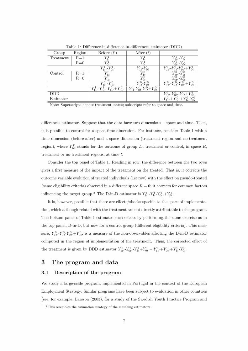
Table 1: Difference-in-difference-in-differences estimator (DDD)Group Region Before (t′) After (t)

Treatment R=1 Y 11t′ Y 1

1t Y 11t′ -Y

11t

R=0 Y 10t′ Y 1

0t Y 10t′ -Y

10t

Y 11t′ -Y

10t′ Y 1

1t-Y10t Y 1

1t′ -Y11t-Y

10t′+Y 1

0t

Control R=1 Y 01t′ Y 0

1t Y 01t′ -Y

01t

R=0 Y 00t′ Y 0

0t Y 00t′ -Y

00t

Y 01t′ -Y

00t′ Y 0

1t-Y00t Y 0

1t′ -Y01t-Y

00t′+Y 0

0t

Y 11t′ -Y

10t′ -Y

01t′+Y 0

0t′ Y 11t-Y

10t-Y

01t+Y 0

0t

DDD Y 11t′ -Y

10t′ -Y

11t+Y 1

0t

Estimator -Y 01t′+Y 0

0t′+Y 01t-Y

00t

Note: Superscripts denote treatment status; subscripts refer to space and time.

differences estimator. Suppose that the data have two dimensions – space and time. Then,

it is possible to control for a space-time dimension. For instance, consider Table 1 with a

time dimension (before-after) and a space dimension (treatment region and no-treatment

region), where Y DRt stands for the outcome of group D, treatment or control, in space R,

treatment or no-treatment regions, at time t.

Consider the top panel of Table 1. Reading in row, the difference between the two rows

gives a first measure of the impact of the treatment on the treated. That is, it corrects the

outcome variable evolution of treated individuals (1st row) with the effect on pseudo-treated

(same eligibility criteria) observed in a different space R = 0; it corrects for common factors

influencing the target group.2 The D-in-D estimator is Y 11t′ -Y

11t-Y

10t′+Y 1

0t.

It is, however, possible that there are effects/shocks specific to the space of implementa-

tion, which although related with the treatment are not directly attributable to the program.

The bottom panel of Table 1 estimates such effects by performing the same exercise as in

the top panel, D-in-D, but now for a control group (different eligibility criteria). This mea-

sure, Y 01t′ -Y

01t-Y

00t′+Y 0

0t, is a measure of the non-observables affecting the D-in-D estimator

computed in the region of implementation of the treatment. Thus, the corrected effect of

the treatment is given by DDD estimator Y 11t′ -Y

10t′ -Y

11t+Y 1

0t − Y 01t′+Y 0

0t′+Y 01t-Y

00t.

3 The program and data

3.1 Description of the program

We study a large-scale program, implemented in Portugal in the context of the European

Employment Strategy. Similar programs have been subject to evaluation in other countries

(see, for example, Larsson (2003), for a study of the Swedish Youth Practice Program and

2This resembles the estimation strategy of the matching estimators.

7

Blundell et al. (2003) for the British New Deal Program). The Portuguese program is funda-

mentally a job search support program and its main goal is to improve the employability of

two specific groups of unemployed individuals: those aged less than 25 years old and unem-

ployed more than six months (the Programa InserJovem) and those over 25 and unemployed

longer than 12 months (the Programa REAGE). The program was launched in a period of

quite low unemployment rate, but with a poor performance of the unemployed in terms of

duration, and specific demographic groups were doing poorly in the labor market, namely

the less educated young and females. These two groups are more likely to be registered in

the National Employment Offices, representing a large share of our sample.

The program is composed of intensive job-search assistance and small basic skills courses.

Each individual is enrolled in a number of interviews with placement officers to help her

improve her job-search skills. In case the placement team considers necessary, the individuals

can enter a number of vocational or non-vocational training courses. The whole process

of job-search assistance ended in most cases, but not necessarily, with the elaboration of

a “Personal Job Plan”, that included detailed information on the unemployed job search

effort. According to this Plan, the unemployed was expected to meet on a regular basis

with the placement officer at the local employment office and to actively search for a job.

Unjustified rejection of job offers lead to a cancellation of any subsidies being received by the

unemployed. The program is mandatory in the sense that failing to comply with it results

in a cancellation of the workers registration and possibly of all subsidies he might have been

receiving.

The design of the program does not exclude the possibility of spillover effects from its

implementation to other workers not participating in the program. However, these general

equilibrium effects are likely to be small given the nature of the program, for example, there

are no wage subsidies.

3.2 Description of the data

The Portuguese employment agency collected data from all registered unemployed regard-

less of their “treatment status”. The dataset, comprising over 2 million observations for

over 1.5 million individuals, monitors the different features of the program and individuals

during their complete spells of unemployment. The information in the dataset includes most

demographic variables used in labor market studies (age, sex, nationality, schooling, place

of residence), including also a large number of variables related with previous labor market

experience (previous occupation, desired sector of employment, unemployment duration,

8

Table 2: Summary statitics local Employment OfficesTreatment group Control group

Variable Mean Std. Dev. Mean Std. Dev.Age (in years) 31.9269 12.8478 33.3517 43.6103Sex (Male =1) 0.3728 0.4835 0.4139 0.4941UI recipient 0.2259 0.4182 0.2831 0.4505Foreigner 0.0065 0.0805 0.0152 0.1223Disabled 0.0073 0.0850 0.0075 0.0863Marital status

Married 0.4800 0.4996 0.4867 0.4998Divorced 0.0087 0.0931 0.0101 0.1000Other 0.0253 0.1569 0.0258 0.1586Single 0.4747 0.4994 0.4658 0.4988Widow 0.0114 0.1061 0.0116 0.1069

Schooling4 years 0.2780 0.4480 0.2785 0.44826 years 0.2408 0.4276 0.2249 0.41759 years 0.1708 0.3763 0.1718 0.377211 years 0.0926 0.2898 0.0995 0.299312 years 0.0978 0.2971 0.0977 0.29703 years college 0.0254 0.1572 0.0269 0.16195 years college 0.0277 0.1642 0.0449 0.2072Mestra. 0.0001 0.0075 0.0001 0.0116Ph. D. 0.0000 0.0000 0.0000 0.0045Illiterate 0.0296 0.1695 0.0214 0.1448No school, reads 0.0373 0.1894 0.0341 0.1815

Reason to registerStudent 0.1139 0.3176 0.1027 0.3036Finished school 0.0613 0.2398 0.0510 0.2200Finished training 0.0095 0.0973 0.0045 0.0667Worked at home 0.0136 0.1160 0.0148 0.1207Laid-off 0.2004 0.4003 0.2624 0.4399Quit job 0.0321 0.1762 0.0350 0.1838End job mutual aggreement 0.0164 0.1270 0.0264 0.1605End of temporary job 0.4701 0.2854 0.4516Retired 0.0004 0.0212 0.0005 0.0217Bad working conditions 0.0062 0.0787 0.0048 0.0690Previoulsy self-employed 0.0001 0.0114 0.0001 0.0118New registration 0.0021 0.0459 0.0028 0.0527Law 17 0.0008 0.0277 0.0005 0.0231Other 0.2133 0.4096 0.2090 0.4066

Number of observations 53407 201149

9

reason for job displacement). The unemployed is observed for the complete duration of the

unemployment spell and, at the moment of termination, we can observe the destination

state (either employment, training or out of the labor force). Additionally, we have some

information of the vacancies posted in the labor office, which are possibly matched with each

unemployed.

The main limitations of our data are the lack of wage information and the difficulty

in following up the individuals after they leave the program. In fact, there is no income-

related information at the Employment Services and follow up interviews were not carried

out (although they were part of the original program design).

3.3 Sample construction

We take advantage of the wealth of information the dataset contains and of the character-

istics of the program to construct treatment and control groups using different criteria. In

particular, we explore (i) the longitudinal nature of the data, and (ii) the two sources of

variation coming from the eligibility criteria and the different implementation phases (which

generate spatial/regional and time differences).

The program design and implementation generated a natural way to construct treatment

and control groups along several dimensions. One such dimension is the eligibility criteria

(based on age and unemployment duration) and the other is the phased implementation of

the program across the Portuguese territory that generated a sequence of pilot areas. The

program implementation was gradual. The local offices of the Employment Services were

assigned to the program at different moments in time, divided by June and October of 1998,

February, May, July and November of 1999 and by April, June and September of 2000.

The treatment group includes all individuals eligible to participate in the InserJovem and

REAGE programs in the first six months of their implementation in each locacl Employment

Office. This generates a large group of individuals already unemployed at the moment the

programs were initiated in each office (see Table 2 for the dimensions of treatment and

control groups).

The choice of the comparison group was dictated by the eligibility criteria and the loca-

tion outside the initial pilot areas. Thus the comparison group takes all eligible individuals

living in the area covered by local Offices that did not implement the programs. This allows

us to have nine possible comparisons between treatment and control groups that correspond

to each of the nine dates at which different local offices started implementing the programs.

The timing of program implementation can be considered random. It was not dictated

10

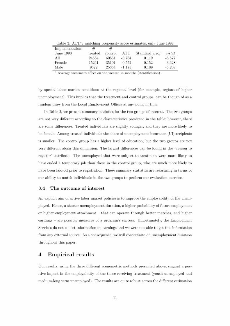
Table 3: ATT∗: matching propensity score estimates, only June 1998Implementation: # #June 1998 treated control ATT Standard error t-statAll 24584 60551 -0.784 0.119 -6.577Female 15261 35191 -0.552 0.152 -3.628Male 9322 25354 -1.175 0.189 -6.208∗ Average treatment effect on the treated in months (stratification).

by special labor market conditions at the regional level (for example, regions of higher

unemployment). This implies that the treatment and control groups, can be though of as a

random draw from the Local Employment Offices at any point in time.

In Table 2, we present summary statistics for the two groups of interest. The two groups

are not very different according to the characteristics presented in the table; however, there

are some differences. Treated individuals are slightly younger, and they are more likely to

be female. Among treated individuals the share of unemployment insurance (UI) recipients

is smaller. The control group has a higher level of education, but the two groups are not

very different along this dimension. The largest differences can be found in the “reason to

register” attribute. The unemployed that were subject to treatment were more likely to

have ended a temporary job than those in the control group, who are much more likely to

have been laid-off prior to registration. These summary statistics are reassuring in terms of

our ability to match individuals in the two groups to perform our evaluation exercise.

3.4 The outcome of interest

An explicit aim of active labor market policies is to improve the employability of the unem-

ployed. Hence, a shorter unemployment duration, a higher probability of future employment

or higher employment attachment – that can operate through better matches, and higher

earnings – are possible measures of a program’s success. Unfortunately, the Employment

Services do not collect information on earnings and we were not able to get this information

from any external source. As a consequence, we will concentrate on unemployment duration

throughout this paper.

4 Empirical results

Our results, using the three different econometric methods presented above, suggest a pos-

itive impact in the employability of the those receiving treatment (youth unemployed and

medium-long term unemployed). The results are quite robust across the different estimation

11

Table 4: ATT’s∗ at the local Employment OfficesImplementation† # #

treated control ATT Standard error t-statJune 1998 24584 60551 -0.784 0.119 -6.577October 1998 2137 59586 -0.664 0.355 -1.571February 1999 3354 36917 -1.350 0.278 -4.850May 1999 12835 34626 -0.576 0.177 -3.259July 1999 2250 33120 -1.675 0.326 -5.135November 1999 852 29549 -0.986 0.498 -1.979April 2000 985 23446 -3.605 0.476 -7.578June 2000 2375 22605 0.851 0.317 2.686September 2000 3448 14217 -0.971 0.272 -3.566∗ Average treatment effect on the treated in months computed with stratification

matching on the propensity scores.† Dates of implementation at the local Employment Office level.

methods. The reduction in the average unemployment spell varies typically between 1 and

4 months.

4.1 Matching on the propensity score

The implementation of the matching method follows Becker & Ichino (2002). We first define

the treatment group of interest (there are nine such treatment groups) and then from workers

registered in local Employment Offices not yet in the program we pick the control group.

The matching process leads to a balanced treatment and control groups. For these two

groups (matched on the observables, implying a common support) the mean unemployment

duration is computed.

Table 3 and 4 present the results obtained for the first group of Offices implementing the

program, namely in June 1998. They show a positive effect of the program, which translates

into smaller unemployment duration for the treated. In Figure 1, we summarize the results

of the matching on the propensity score approach to the evaluation problem for all nine

episodes in the program implementation. The results are quite robust across the different

alternatives for the matching process that we implemented, namely stratification, nearest

neighbor and kernel methods. The estimated impact of the program suggests a reduction in

the average unemployment spell ranging from -0.6 to -3.6 months.3 The results do not show

significant differences for men and women, while the program seems to be more efficient at

reducing the unemployment duration for young individuals.3Except in June 2000, where there is an increase in the duration of 0.8 months.

12

●

● ●

●

●

●

●

●

●

−6

−4

−2

02

4

● YoungOlderAll

9806

9810

9902

9905

9907

9911

0004

0006

0009

All all−exits: ATT − Propensity score matching

●

● ●

●

●

●

●

●

●

−6

−4

−2

02

4

● YoungOlderAll

9806

9810

9902

9905

9907

9911

0004

0006

0009

Men all−exits: ATT − Propensity score matching

●● ●

●

●

●

●

●

●

−6

−4

−2

02

4

● YoungOlderAll

9806

9810

9902

9905 9907

9911

0004

0006

0009

Women all−exits: ATT − Propensity score matching

Figure 1: Propensity scores matching

13

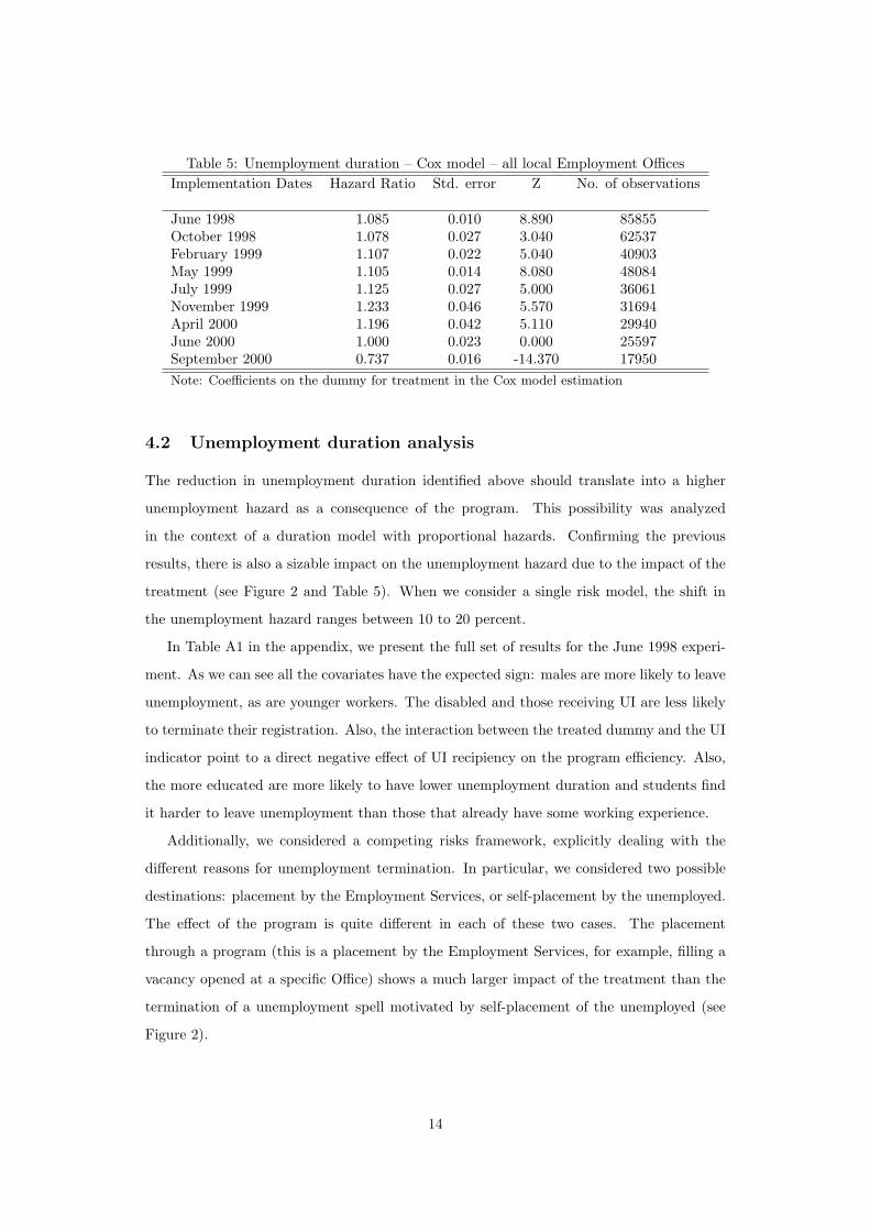
Table 5: Unemployment duration – Cox model – all local Employment OfficesImplementation Dates Hazard Ratio Std. error Z No. of observations

June 1998 1.085 0.010 8.890 85855October 1998 1.078 0.027 3.040 62537February 1999 1.107 0.022 5.040 40903May 1999 1.105 0.014 8.080 48084July 1999 1.125 0.027 5.000 36061November 1999 1.233 0.046 5.570 31694April 2000 1.196 0.042 5.110 29940June 2000 1.000 0.023 0.000 25597September 2000 0.737 0.016 -14.370 17950Note: Coefficients on the dummy for treatment in the Cox model estimation

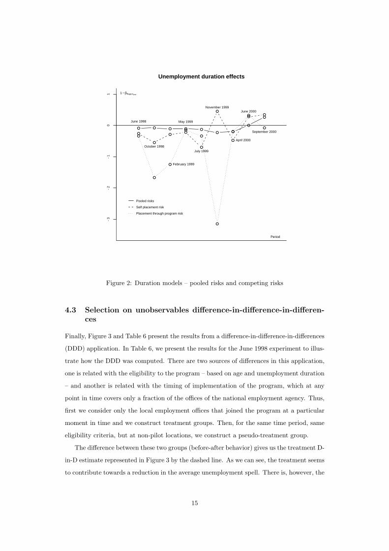
4.2 Unemployment duration analysis

The reduction in unemployment duration identified above should translate into a higher

unemployment hazard as a consequence of the program. This possibility was analyzed

in the context of a duration model with proportional hazards. Confirming the previous

results, there is also a sizable impact on the unemployment hazard due to the impact of the

treatment (see Figure 2 and Table 5). When we consider a single risk model, the shift in

the unemployment hazard ranges between 10 to 20 percent.

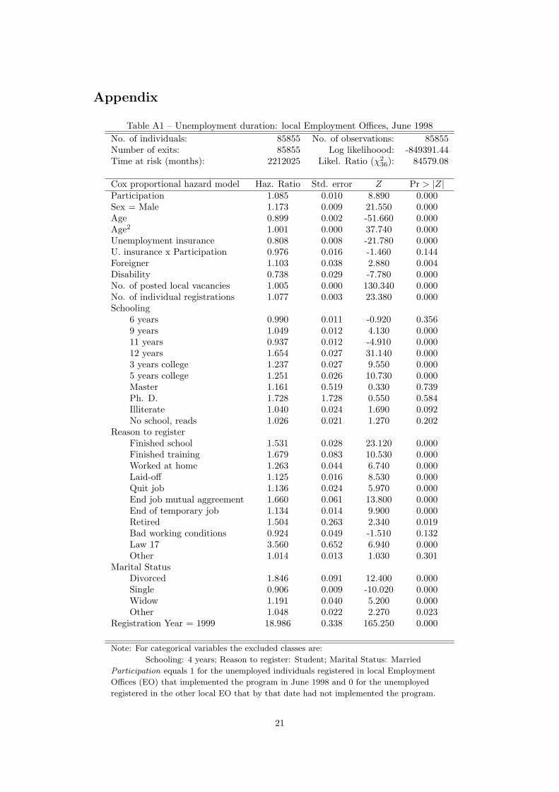
In Table A1 in the appendix, we present the full set of results for the June 1998 experi-

ment. As we can see all the covariates have the expected sign: males are more likely to leave

unemployment, as are younger workers. The disabled and those receiving UI are less likely

to terminate their registration. Also, the interaction between the treated dummy and the UI

indicator point to a direct negative effect of UI recipiency on the program efficiency. Also,

the more educated are more likely to have lower unemployment duration and students find

it harder to leave unemployment than those that already have some working experience.

Additionally, we considered a competing risks framework, explicitly dealing with the

different reasons for unemployment termination. In particular, we considered two possible

destinations: placement by the Employment Services, or self-placement by the unemployed.

The effect of the program is quite different in each of these two cases. The placement

through a program (this is a placement by the Employment Services, for example, filling a

vacancy opened at a specific Office) shows a much larger impact of the treatment than the

termination of a unemployment spell motivated by self-placement of the unemployed (see

Figure 2).

14

● ● ● ● ●● ●

●

●

−3

−2

−1

01

●

●

●●

●

●

●

●●

●

●

●

●

●

●

●

●

●

Period

1 − βRegionyear

June 1998

October 1998

February 1999

May 1999

July 1999

November 1999

April 2000

June 2000

September 2000

Unemployment duration effects

Pooled risks

Self placement risk

Placement through program risk

Figure 2: Duration models – pooled risks and competing risks

4.3 Selection on unobservables difference-in-difference-in-differen-ces

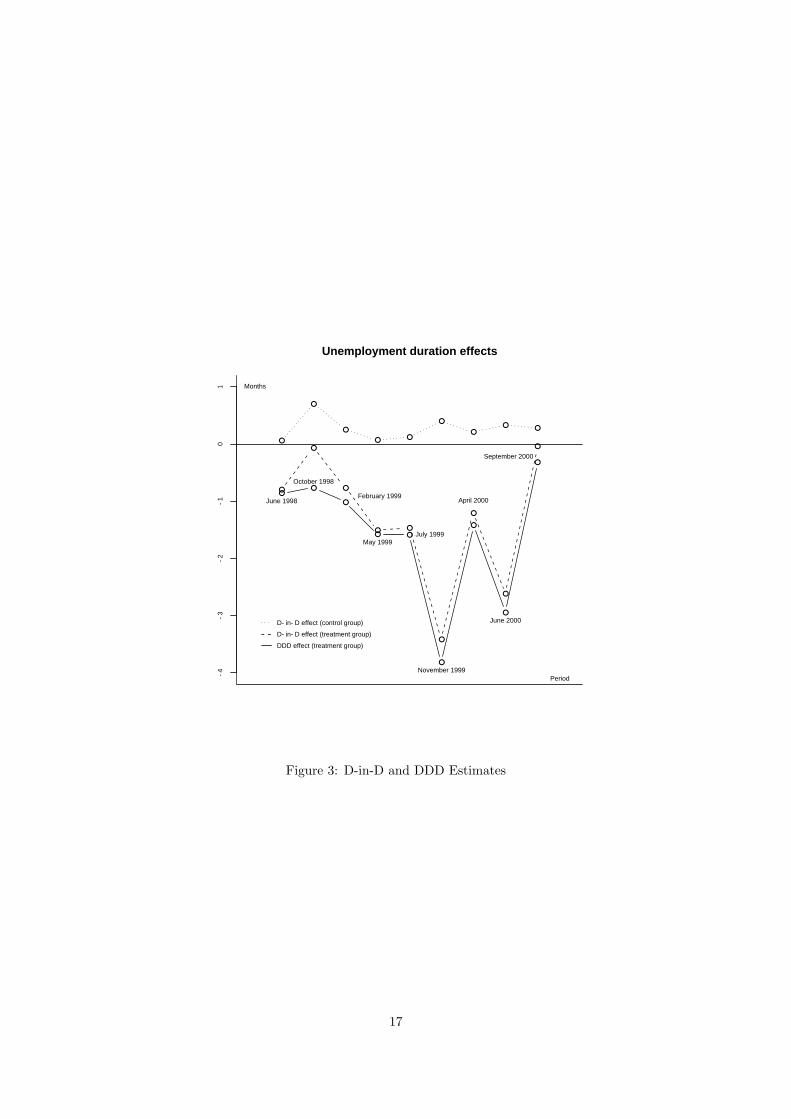
Finally, Figure 3 and Table 6 present the results from a difference-in-difference-in-differences

(DDD) application. In Table 6, we present the results for the June 1998 experiment to illus-

trate how the DDD was computed. There are two sources of differences in this application,

one is related with the eligibility to the program – based on age and unemployment duration

– and another is related with the timing of implementation of the program, which at any

point in time covers only a fraction of the offices of the national employment agency. Thus,

first we consider only the local employment offices that joined the program at a particular

moment in time and we construct treatment groups. Then, for the same time period, same

eligibility criteria, but at non-pilot locations, we construct a pseudo-treatment group.

The difference between these two groups (before-after behavior) gives us the treatment D-

in-D estimate represented in Figure 3 by the dashed line. As we can see, the treatment seems

to contribute towards a reduction in the average unemployment spell. There is, however, the

15

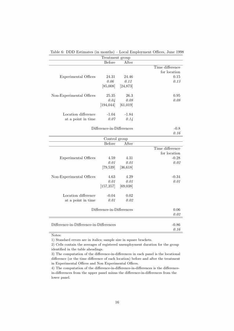
Table 6: DDD Estimates (in months) – Local Employment Offices, June 1998Treatment group

Before AfterTime difference

for locationExperimental Offices 24.31 24.46 0.15

0.06 0.12 0.13[85,008] [24,873]

Non-Experimental Offices 25.35 26.3 0.950.04 0.08 0.08

[194,044] [61,019]

Location difference -1.04 -1.84at a point in time 0.07 0.14

Difference-in-Differences -0.80.16

Control groupBefore After

Time differencefor location

Experimental Offices 4.59 4.31 -0.280.01 0.01 0.02

[79,539] [36,618]

Non-Experimental Offices 4.63 4.29 -0.340.01 0.01 0.01

[157,357] [69,038]

Location difference -0.04 0.02at a point in time 0.01 0.02

Difference-in-Differences 0.060.02

Difference-in-Difference-in-Differences -0.860.16

Notes:

1) Standard errors are in italics; sample size in square brackets.

2) Cells contain the averages of registered unemployment duration for the group

identified in the table aheadings.

3) The computation of the difference-in-differences in each panel is the locational

difference (or the time difference of each location) before and after the treatment

in Experimental Offices and Non Experimental Offices.

4) The computation of the difference-in-difference-in-differences is the difference-

in-differences from the upper panel minus the difference-in-differences from the

lower panel.

16

●●

●

● ●

●

●

●

●

−4

−3

−2

−1

01

●

●

●

● ●

●

●

●

●●

●

●

● ●

●

●● ●

Period

Months

June 1998

October 1998

February 1999

May 1999July 1999

November 1999

April 2000

June 2000

September 2000

Unemployment duration effects

D−in−D effect (control group)

D−in−D effect (treatment group)

DDD effect (treatment group)

Figure 3: D-in-D and DDD Estimates

17

possibility that at the time of implementation of the program there were shock to the pilot

areas that, even though might not be directly attributable to the program, are correlated

with the program. For example, the simple awareness of the program might increase the

firms’ willingness to hire. Thus, we create another level of control. For that purpose, we

repeat the above procedure, but this time we consider only the individuals that do not

meet the eligibility criteria to participate in the program. Thus, we have control groups

at pilot-agencies and at non-pilot agencies. We obtain the D-in-D estimate represented

in the Figure 3 by the dotted line. Therefore, if we take the difference between the two

D-in-D estimates, we obtain the final corrected measure of the impact of the program on

the average unemployment spell, the solid line labeled DDD, which again results in values

similar to those reported earlier.

5 Conclusions

The purpose of this study has been to evaluate labor market programs for youth and long-

term unemployed in Portugal using employment probability as a measure of effectiveness.

The programs evaluated are REAGE and InserJovem, which are mainly job-search support

programs.

We identified the average treatment effect based on the hypothesis that participation in

the various treatments, including the no-treatment state, is independent of the post-program

outcomes conditional on observable exogenous factors (as well as non-observable factors in

our diff-in-diff-in-diffs implementation). The mandatory and phased implementation char-

acteristics imposed on the design of the program allows us to be quite confident about our

identification strategy, namely the comparability of our treatment and control groups.

The results from our analysis point to a positive, but small, effect of the treatment on

unemployment duration on the treated group. We estimate a reduction between 1 and

4 months on unemployment duration. Given the generally high levels of unemployment

duration in Portugal (that can reach several years) these numbers are not impressive. They

are in fact, in line with what has been obtained for other countries and surveyed in Heckman,

Lalonde and Smith (1999).

In order to check the robustness of these findings we plan to carry out several sensitivity

checks with the data. First, looking at male and female separately. Secondly, looking

individually at the two programs might reveal some age related heterogeneity, improving

the results for the younger unemployment program. More important would be to carry out

the analysis using different measures of effectiveness, namely wages. This would be possible

18

if we can match data from different administrative sources available in Portugal.

References

Becker, S. O. & Ichino, A. (2002), ‘Estimation of average treatment effects based on propen-

sity scores’, The Stata Journal 2(4), 358–377.

Blundell, R. & Dias, M. (2000), ‘Evaluation methods for non-experimental data’, Fiscal

Studies March.

Blundell, R., Dias, M., Meghir, C. & Reenen, J. V. (2003), ‘Evaluating the employment im-

pact of a mandatory job search assistance program’, University College London 03/20.

Cox, D. R. (1972), ‘Regression models and life-tables’, Journal of the Royal Statistical Society

Series B 34, 187–220.

Heckman, J. (1979), ‘Sample selection bias as a specification error’, Econometrica 47, 153–

161.

Heckman, J., Ichimura, H. & Todd, P. (1998), ‘Matching as an economic estimator’, The

Review of Economic Studies 62(2), 261–294.

Heckman, J., LaLonde, R. & Smith, J. (1999), ‘The economics and econometrics of active

labor market programs in’, Handbook of Labor Economics 3A.

Kaplan, E. L. & Meier, P. (1958), ‘Nonparametric estimation from incomplete observations’,

Journal of the American Statistical Association 53, 457–481.

Lalive, R., Ours, J. C. & Zweimueller, J. (2001), ‘The impact of active labor market programs

on the duration of unemployment’, IEW, University of Zurich 51, Working paper.

Larsson, L. (2003), ‘Evaluation of swedish youth labor market programs’, 38(4), 891–927.

Meyer, B. D. (1995), ‘Natural and quasi-experiments in economics’, Journal of Business &

Economic Statistics 13, 151–162.

Richardson, K. & der Berg, G. V. (2002), ‘The effect of vocational employment training on

the individual transition rate from unemployment to work’, IFAU 2002:8.

Rosenbaum, P. & Rubin, D. (1983), ‘The central role of the propensity score in observational

studies for causal effects’, Biometrika 70, 41–55.

19

Rubin, D. (1977), ‘Assignment to a treatment group on the basis of a covariate’, Journal of

Educational Statistics 2, 1–26.

20

Appendix

Table A1 – Unemployment duration: local Employment Offices, June 1998No. of individuals: 85855 No. of observations: 85855Number of exits: 85855 Log likelihoood: -849391.44Time at risk (months): 2212025 Likel. Ratio (χ2

36): 84579.08

Cox proportional hazard model Haz. Ratio Std. error Z Pr > |Z|Participation 1.085 0.010 8.890 0.000Sex = Male 1.173 0.009 21.550 0.000Age 0.899 0.002 -51.660 0.000Age2 1.001 0.000 37.740 0.000Unemployment insurance 0.808 0.008 -21.780 0.000U. insurance x Participation 0.976 0.016 -1.460 0.144Foreigner 1.103 0.038 2.880 0.004Disability 0.738 0.029 -7.780 0.000No. of posted local vacancies 1.005 0.000 130.340 0.000No. of individual registrations 1.077 0.003 23.380 0.000Schooling

6 years 0.990 0.011 -0.920 0.3569 years 1.049 0.012 4.130 0.00011 years 0.937 0.012 -4.910 0.00012 years 1.654 0.027 31.140 0.0003 years college 1.237 0.027 9.550 0.0005 years college 1.251 0.026 10.730 0.000Master 1.161 0.519 0.330 0.739Ph. D. 1.728 1.728 0.550 0.584Illiterate 1.040 0.024 1.690 0.092No school, reads 1.026 0.021 1.270 0.202

Reason to registerFinished school 1.531 0.028 23.120 0.000Finished training 1.679 0.083 10.530 0.000Worked at home 1.263 0.044 6.740 0.000Laid-off 1.125 0.016 8.530 0.000Quit job 1.136 0.024 5.970 0.000End job mutual aggreement 1.660 0.061 13.800 0.000End of temporary job 1.134 0.014 9.900 0.000Retired 1.504 0.263 2.340 0.019Bad working conditions 0.924 0.049 -1.510 0.132Law 17 3.560 0.652 6.940 0.000Other 1.014 0.013 1.030 0.301

Marital StatusDivorced 1.846 0.091 12.400 0.000Single 0.906 0.009 -10.020 0.000Widow 1.191 0.040 5.200 0.000Other 1.048 0.022 2.270 0.023

Registration Year = 1999 18.986 0.338 165.250 0.000

Note: For categorical variables the excluded classes are:

Schooling: 4 years; Reason to register: Student; Marital Status: Married

Participation equals 1 for the unemployed individuals registered in local Employment

Offices (EO) that implemented the program in June 1998 and 0 for the unemployed

registered in the other local EO that by that date had not implemented the program.

21