Georgia Southern University

Digital Commons@Georgia Southern

Electronic Theses and Dissertations Graduate Studies, Jack N. Averitt College of

Spring 2013

Evaluating the Efficacy of a Childhood Lead Poisoning Risk Model as an Accurate Predictor of Lead Exposure Christopher R. Rustin

Follow this and additional works at: https://digitalcommons.georgiasouthern.edu/etd

Part of the Public Health Commons

Recommended Citation Rustin, Christopher R., "Evaluating the Efficacy of a Childhood Lead Poisoning Risk Model as an Accurate Predictor of Lead Exposure" (2013). Electronic Theses and Dissertations. 48. https://digitalcommons.georgiasouthern.edu/etd/48

This dissertation (open access) is brought to you for free and open access by the Graduate Studies, Jack N. Averitt College of at Digital Commons@Georgia Southern. It has been accepted for inclusion in Electronic Theses and Dissertations by an authorized administrator of Digital Commons@Georgia Southern. For more information, please contact digitalcommons@georgiasouthern.edu.

EVALUATING THE EFFICACY OF A CHILDHOOD LEAD POISONING RISK MODEL AS

AN ACCURATE PREDICTOR OF LEAD EXPOSURE

by

R. CHRISTOPHER RUSTIN

(Under the Direction of Simone Charles)

ABSTRACT

Lead poisoning is a significant public health problem with paint from old housing exposing

thousands of children and leading to negative health and social outcomes. Identifying the

highest risk children exposed to lead is important to public health agencies. The purpose of this

study was to evaluate and assess the efficacy of a new geographically-based lead risk model that

when combined with a child’s physical address, predicts the extent of a child’s risk of lead

poisoning on a numeric risk scale. This model is unique because it calculates risk at the address

level from parcel attributes of age and type of housing (rental or owner-occupied) combined and

adjusted with historic blood lead surveillance data to create a final predictive risk map. If found

efficacious, the model would assist lead poisoning prevention programs in being more cost-

effective by creating a verified approach for targeting prevention efforts. To assess the models

efficacy, a pilot study was conducted using three years (N=2429) of blood lead records from

Macon-Bibb County, which has the second highest prevalence rate of lead exposure in Georgia.

Physical addresses obtained from the blood lead records were geocoded and assigned a risk by

the model. The predictive risk was compared to blood lead results and statistically analyzed to

determine if risk increased with increased blood lead results. Results demonstrated the risk

model accurately estimated risk when compared to blood lead levels with statistical significance.

This model can be used to target the highest risk homes and children for public health

interventions and to identify low risk Medicaid children for exemption from lead testing.

Index Words: GIS lead risk model, Lead exposure predictive map, Childhood lead exposure

EVALUATING THE EFFICACY OF A CHILDHOOD LEAD POISONING RISK MODEL AS

AN ACCURATE PREDICTOR OF LEAD EXPOSURE

by

R. CHRISTOPHER RUSTIN

B.S., Armstrong Atlantic State University, 2000

M.T., Georgia Southern University, 2004

A Dissertation Submitted to the Graduate Faculty of Georgia Southern University in

Partial Fulfillment of the Requirements for the Degree

DOCTOR OF PUBLIC HEALTH

with a concentration in

Community Health Behavior and Education

STATESBORO, GEORGIA

2013

iii

© 2013

R. CHRISTOPHER RUSTIN

All Rights Reserved

iv

EVALUATING THE EFFICACY OF A CHILDHOOD LEAD POISONING RISK MODEL AS

AN ACCURATE PREDICTOR OF LEAD EXPOSURE

by

R. CHRISTOPHER RUSTIN

Major Professor: Simone Charles Committee: Simone Charles John Luque Robert Vogel

Electronic Version Approved: May, 2013

v

DEDICATION

This dissertation is dedicated to my wife Catrina and our children, Christian and Olivia.

There were days when I wanted to quit and spend more time with you all. Without your love and

support through this long process, I would not have finished. This dissertation is also dedicated

to my parents and sisters, who always encouraged me to continue my education.

I would like to also dedicate this work to all the public health professionals, friends and

colleagues standing on the frontlines everyday protecting the public’s health. From the local

health department to the State health department, working in the field of public health can be a

thankless, but necessary job. It is your dedication that keeps this country safe and healthy and I

consider it an honor to stand with you.

vi

ACKNOWLEDGMENTS

I started this journey in 2007 as part of the inaugural class of the Jiann-Ping Hsu College

of Public Health. I would like to thank all the students in the inaugural class for their support

and friendship. I would like to thank my committee members, Dr. Charles, Dr. Luque, and Dr.

Vogel for guiding me in the right direction and offering sound advice. I would like to thank Dr,

Douglas Skelton, Dr. Kathryn Martin and Dr. Diane Weems for encouraging and supporting me

to continue my education back in 2006, allowing me time-off from work to attend class, and

lending an ear when needing to discuss class projects or ideas.

A special thanks to Mr. Forrest Staley, Lead Hazard Control Program Director and the

GIS team lead by Mr. Jeff McMichael at the Georgia Department of Public Health for the many

hours of consultation and development of the GIS risk model. Thank you to Dr. Yu Sun for your

assistance with statistical analysis and using SAS. A special thanks to my boss, Mr. Scott

Uhlich, Director of Environmental Health at the Georgia Department of Public Health for

allowing me the necessary time to attend classes and complete the dissertation and for promoting

the value of education.

I would also like to thank all the Professors who recognized the challenges of students

that work full time and in my case had to drive 460 miles roundtrip to attend class for 2 years.

Last, but certainly not least, thank you to my wife who spent countless weekends

entertaining our children without me, so I could study and write and for the hours she spent

reading and proofreading my work.

vii

TABLE OF CONTENTS

ACKNOWLEDGMENTS ................................................................................................. vi

LIST OF TABLES ............................................................................................................. xi

LIST OF FIGURES .......................................................................................................... xii

CHAPTER

1 BACKGROUND/SIGNIFICANCE, AND LITERATURE REVIEW ......................1

Introduction ...........................................................................................................1

Modern Lead Use and Subsequent Ban ...........................................................2

Lead Poisoning History....................................................................................3

Lead Exposure as a Current Problem...............................................................7

Research Problem .................................................................................................9

Elevated Blood Lead Levels ............................................................................9

Ecological Assessment...................................................................................10

Prevention Programs ......................................................................................13

Issues with Testing as Secondary Prevention ................................................14

New Primary Prevention Focus .....................................................................16

Purpose of the Study ...........................................................................................17

Theoretical Framework .......................................................................................19

Literature Review................................................................................................20

Introduction ....................................................................................................20

Health Effects.................................................................................................23

Disease/Disability Burden .............................................................................26

Natural History of Disease .............................................................................27

Juvenile and Adult Delinquency ....................................................................29

viii

IQ Loss and School Performance ..................................................................29

Costs Associated with Lead Poisoning… ......................................................31

GIS Risk Models in Health Promotion ..........................................................32

State of Georgia Lead Statistics ..........................................................................35

Georgia Children Tested for Lead .................................................................39

Significance of Study ..........................................................................................41

2 HYPOTHESIS, RESEARCH QUESTIONS, STUDY AIMS ..................................44

Research Aims .....................................................................................................44

Hypotheses ..........................................................................................................46

Research Questions .............................................................................................47

3 METHODS AND MATERIALS ..............................................................................48

Design of Study...................................................................................................48

Risk Model Construction ...............................................................................48

Predictive Parcel Map ....................................................................................49

Adjusted BLL Surveillance Risk Map ...........................................................52

Combined Final Risk Map .............................................................................53

Setting ............................................................................................................55

Data Collection ..............................................................................................56

Data Exclusion ...............................................................................................57

Data Analysis and Interpretation ...................................................................58

Data Used for Analysis ..................................................................................59

4 RESULTS…………………………………………………………………………..61 GIS Risk Model Descriptive Statistics and Validation..………………………..61

ix

Parcel Descriptive Statistics and Maps ..........................................................61

Parcel Risk Map Spatial Analysis ..................................................................66

Adjusted Risk Map Spatial Analysis .............................................................67

Spatial Autocorrelation Test ..........................................................................68

Final Combined Risk Map .............................................................................71

Final Combined Risk Map Spatial Analysis ..................................................72

Research Question # 1 ...................................................................................73

Descriptive Statistics of Population used to Construct and Evaluate Model ......74

Research Question # 2 (Hypothesis # 2) ........................................................74

Demographic Cluster Analysis ......................................................................78

Medicaid Status ..............................................................................................81

Research Question # 3 (Hypothesis # 3) ........................................................82

Statistical Analysis of Models Predicted Risk Compared to BLL Records ........84

Pearson Correlation ........................................................................................84

Research Question # 4 (Hypothesis #1 and #4) .............................................85

Chi Square Analysis .......................................................................................86

Analysis of the Variance (ANOVA) ..............................................................86

2 x 2 Table Analysis ......................................................................................88

Sensitivity and Specificity Analysis ..............................................................89

Research Question # 5 (Hypothesis # 5) ........................................................90

Logistic Regression ........................................................................................90

5 SUMMARY DISCUSSION AND CONCLUSTIONS ............................................94

Summary of Results ............................................................................................94

Findings Summary…………………………………………………………….105

x

Discussion of Findings ......................................................................................108

Strengths and Limitations .................................................................................111

Policy and Public Health Implications ..............................................................113

Risk Communication ...................................................................................113

Low-Risk Children Exemption ....................................................................114

Community Health .......................................................................................115

Recommendations for Future Research ............................................................115

REFERENCES ................................................................................................................117

APPENDICES .................................................................................................................132

A Georgia Department of Public Health Districts-Lead Risk Map ..........................133

B Definition of Terms ..............................................................................................135

C Georgia Department of Public Health IRB Approval Letter .................................137

D Georgia Southern University IRB Approval Letter ..............................................139

xi

LIST OF TABLES

Table 1.1: Prevention Techniques ....................................................................................13

Table 1.2: National Average Blood Lead Level Comparison from NHANES Data (1991-94 and 1999-02) ..................................................................................22 Table 1.3: Lead Exposure Burden ...................................................................................27 Table 1.4: Number of Children ≥6 Years Old Screened for Lead, Georgia 2011 ...........39 Table 3.1: Parcel Risk Algorithm ....................................................................................50 Table 3.2: Parcel Risk ......................................................................................................51 Table 3.3: Weighted Risk Adjustment Algorithm ...........................................................52 Table 3.4: Centrus LCODES ...........................................................................................57 Table 4.1: Bibb County Housing Statistics ......................................................................62 Table 4.2: Homestead Exemption Statistics Compared to Census Data .........................65 Table 4.3: Parcel Risk Cross Validation Statistics...........................................................67 Table 4.4: Final Predicted Risk Cross Validation Statistics ............................................73 Table 4.5: Bibb County Georgia Descriptive Statistics From BLL Data (2004-2012, N=7,860) .........................................................................................................75 Table 4.6: Pearson Correlation Results Comparing Risk to BLL ....................................85 Table 4.7: Chi Square Results Comparing Risk to EBL ..................................................86 Table 4.8: ANOVA Results Comparing Risk and BLL Means .......................................87 Table 4.9: 2 x 2 Table Results Comparing EBL with Elevated Risk Levels ...................88 Table 4.10: Sensitivity and Specificity Results ...............................................................89 Table 4.11: Logistic Regression Results ..........................................................................91

xii

LIST OF FIGURES

Figure 1.1: Average BLL Decline Compared with Phase Out of Leaded Gasoline (1976-1980).......................................................................................................6

Figure 1.2: National Blood Lead Level Decline (1971-2008) ..........................................7

Figure 1.3: Blood Lead Levels and Race ........................................................................11

Figure 1.4: Percentage of Children aged 1-5 by Race/Ethnicity with BLL ≥10ug/dL (1988-2002) ...................................................................................................12

Figure 1.5: Odds of Having Medicaid Compared to BLL adapted from NHANES (1988-1994)....................................................................................................12

Figure 1.6: Georgia Blood Lead Surveillance Report Highlighting Percent of those Tested having EBL Levels ≥10ug/dL (1997-2008). ............................21 Figure 1.7: Elevated Blood Lead Levels (10ug/dL) in U.S. Children (0-6 yrs) since 1965 ...................................................................................................24

Figure 1.8: Age of Residence Compared to Percent of Children Lead Poisoned by Demographics (NHANES III, Phase 2, 1991-1994). ....................................25

Figure 1.9: Health Effects at Varying Blood Lead Levels................................................28

Figure 1.10: Georgia High Risk Counties.........................................................................37

Figure 1.11: Geocoded Children Exposed to Lead ...........................................................37

Figure 1.12: Macon-Bibb County Lead Risk Map ...........................................................38

Figure 1.13: Testing Rates for Children by Neighborhood Risk ......................................41

Figure 3.1: Risk Model Steps to Development ...............................................................54 Figure 4.1: Bibb County Parcel Risk Map using Age of Housing and Homestead Exemption ......................................................................................................63 Figure 4.2: Bibb County Parcel Risk Map Neighborhood Subset ....................................64

Figure 4.3: Parcel Risk Raster Illustrating Predictive Parcel Map ...................................65

Figure 4.4: Parcel Risk Cross Validation Graph ...............................................................66

Figure 4.5: Adjusted Predictive Risk Map ........................................................................67

Figure 4.6: Surveillance BLL Spatial Autocorrelation Report .........................................70

xiii

Figure 4.7: Bibb County Parcel Risk Map with Surveillance BLL Data..........................71

Figure 4.8: Final Combined Risk Maps ............................................................................72

Figure 4.9: Final Predicted Risk Cross Validation ...........................................................73

Figure 4.10: Descriptive Analysis Using BLL Data-RACE .............................................77

Figure 4.11: Descriptive Analysis Using BLL Data-SEX ................................................78 Figure 4.12: Assessing BLL Data With Bibb County Demographic Cluster Map (2004-2005, 2012, N=2,429) .......................................................................80

Figure 4.13: Mean BLL by Age Group ............................................................................83

Figure 4.14: Mean Age of EBL Child ..............................................................................84

1

CHAPTER 1

BACKGROUND/SIGNIFICANCE, AND LITERATURE REVIEW

Introduction

Lead is a bluish-white lustrous metal that is derived primarily from smelting the mineral

Galena (its chemical formula being PbS) (ATSDR, 2007) and constitutes 0.002% of the earth’s

crust (WHO, 2010). Galena is mined from natural deposits around the United States and other

parts of the world, with its ore, lead, used as the primary component in lead acid batteries and

other industrial applications such as lead alloys, pipe solder, and ammunition (EPA, 2012). The

use for lead is increasing due to a need for energy efficient vehicles and batteries (WHO, 2010).

Lead was mined and used throughout history due to its unique properties. It is believed

lead was discovered when the mineral Galena was smelted in camp fires for its silver properties

(Waldron, 1973). Lead is listed as one of the six metals found in the earliest writings of the Old

Testament of the Christian Bible. As early as 4000 BC, lead was mined by the ancient Hebrews

and Egyptians for use as weights in fishing nets, coating utensils, and cosmetics with the earliest

known writings of lead toxicity found on ancient Egyptians scrolls (Hernberg, 2000; Jewish,

2012). As the most prolific consumer, the Romans used lead to glaze pottery, construct pipes and

aqueducts, in make-up, and as a flavoring additive to sweeten the taste of wine (Needleman,

1999). The modern use of the word plumbing to describe water or sewer pipes is from the Latin

word Plumbum, which means lead and is where the chemical symbol for lead Pb is derived from

(Needleman, 1999). As heavy wine drinkers, the use of lead as a wine preservative and

sweetener prompted some scholars to theorize that the toxic effects of lead may have assisted

with the downfall of the Roman Empire (Lessler, 1988; Gilfillan, 1965). However, this has been

debated for years with many Roman scholars discounting this theory. Nevertheless, lead held a

2

prominent place in history and can still be found in ancient figurines, Roman and English public

baths, paint on Chinese vases and throughout the Roman ruins.

While lead has excellent properties for building and molding pipes, coating items to

prevent corrosion, preserving wine, and providing lustrous colors for paint, the toxic effects of

lead exposure was quickly discovered and described throughout early history. As early as the 2nd

century BC, the Greek physician, Nikander described lead toxicity as a “…colic and paralysis

that followed lead ingestion” which typically affected the wealthy from drinking wine and slaves

that mined for lead (Needleman, 2004, p. 209). Hippocrates (460 BC-c. 370 BC), the father of

medicine, has been credited with describing early symptoms of lead colic without linking the

symptom to lead exposure (Hernberg, 2000). Lead was so ubiquitous in ancient times that the

deleterious effects of exposure were described by an anonymous hermit in the following

translation as reported by Lewis (1985):

______________________________________________________________________________

Hence gout and stone afflict the human race;

Hence lazy jaundice with her saffron face;

Palsy, with shaking head and tott'ring knees.

And bloated dropsy, the staunch sot's disease;

Consumption, pale, with keen but hollow eye,

And sharpened feature, shew'd that death was nigh.

The feeble offspring curse their crazy sires,

And, tainted from his birth, the youth expires.

______________________________________________________________________________

Modern Lead Use and Subsequent Ban

In the early 20th century, lead was heavily mined and used as a performance additive in

residential paint. This additive provided durability, a lustrous appearance, repelled mold and

3

mildew, resisted corrosion, and provided flexibility to the paint (San Diego, 2012; EPA, 2000).

Millions of homes were painted with indoor and outdoor lead paint to preserve the wood and

improve appearance. In addition to lead paint, the auto industry, in 1922, began using tetraethyl

lead as an additive in gasoline to prevent engine knock and improve performance, without

knowing that over time, the deposition of lead from vehicle exhaust would contribute to the

contamination of soil in the yards of homes adjacent to highways (Teichman, Coltrin, Prouty &

Bir, 1993). Though lead appeared to be the “wonder” metal of its time, physicians and scientists

started taking notice of the health effects of lead exposure in industrial workers and children very

early on.

Lead Poisoning History

At the turn of the 20th century, mining for lead increased exponentially to satisfy the

needs of a growing industrial U.S. economy. Lead paint was in demand to satisfy the growing

building market and the fast growing automobile industry were powered by leaded gasoline. Two

World Wars required a demand for paint in munitions, jeeps and aircraft and the post war

building boom needed paint to satisfy the demand of building homes for returning soldiers.

These uses of lead in several commercial and residential applications resulted in lead being

ubiquitous in the environment resulting in a dramatic increase in blood lead levels (BLL) of

children between 1900 and 1970 (CDC, 2012b). Consequently, numerous epidemiological

studies and medical research began to link the toxic effects of lead exposure on the health of

young children and adults who were exposed to leaded paint chips and dust, contaminated soil,

and gasoline deposition as far back as the late 1800s (Markowitz & Rosner, 2000). Since lead is

measured in micrograms per deciliter (ug/dL) of blood, these studies prompted the Centers for

4

Disease Control (CDC) to establish scientifically defensible blood lead standards where health

effects occur and these standards have decreased over time.

U.S. medical authorities first diagnosed a child with lead poisoning in 1887 with little

fanfare, but it was Jefferis Turner from Australia who presented the first scientific study on

childhood lead poisoning in 1897 that garnered the attention of public health experts (Rosner et

al., 2005). In 1904, J. Lockhart Gibson, a colleague of Turner identified lead poisoning in his

patients having eye problems and linked their exposure to indoor paint and in follow-up studies

to paint on veranda (porch) railings (Rosner et al., 2005; Rabin, 1989; Markowitz & Rosner,

2000). Gibson went on to declare that laws should be developed to ban lead paint within a child’s

reach while Turner lectured that the route of lead exposure was paint dust on the fingers of

children as cited by Markowitz & Rosner (2000). In 1914, Johns Hopkins physicians, Thomas

and Blackfan, described the lead poisoning death of a child linked to chewing crib paint (Thomas

& Blackfan, 1914). The conclusive results of these studies led Australia and most of Europe to

ban interior leaded paint between 1909 and 1930 (Hernberg, 2000). However, the United States

was slow to ban lead based paint due to a strong lead industry lobby tactics and the popularity of

lead paint, even when the research clearly pointed to a link between childhood illness and paint

(Markowitz & Rosner, 2000). The following timeline outlines the U.S. delay in banning lead in

household paint (Toxipedia, 2012):

• 1887 – U.S. medical authorities diagnose childhood lead poisoning

• 1904 - Child lead poisoning linked to lead-based paints

• 1914- Pediatric lead-paint poisoning death from eating crib paint is described by Johns

• Hopkins physicians

• 1921 - National Lead Company admits lead is a poison

• 1922 - League of Nations bans white-lead interior paint; U.S. declines to adopt

• 1943- Report concludes eating lead paint chips causes physical and neurological disorders in children

• 1971- Lead-Based Paint Poisoning Prevention Act passed phasing our tetraethyl lead

• 1978- Consumer Product Safety Commission banned lead in household paint

5

In addition to lead in residential paint, leaded gasoline was a major contributor of

childhood and adult lead poisoning prior to 1985. Tetraethyl lead was added to gasoline to curb

engine knock and improve engine performance. Lead by-products in the exhaust of vehicles

were a major inhalation exposure pathway as approximately 76% of the lead in gasoline was

deposited on the ground or in the air after combustion (Billick et al, 1980). As far back as 1922,

the U.S. Public Health Service (USPHS) was warned by scientists against the dangers of

tetraethyl lead production and potential environmental problems from leaded fuels (Rosner &

Markowitz, 1985). However, industry scientists assured the USPHS of the safety of its product,

while agreeing to fund a study on the health effects of tetraethyl lead exposure (Rosner &

Markowitz, 1985). In 1924, New York and New Jersey governments banned tetraethyl leaded

fuels after several workers at a Standard Oil research lab became sick and died from lead

exposure. The continued focus on tetraethyl lead exposure and pressure from the media resulted

in a federal committee that reviewed all the research of tetraethyl lead exposure. The committee

interviewed scientists from industry and academia and conducted a short-term study of exposure

in gas station workers to finally declare there was not enough evidence to prohibit tetraethyl lead

use, but recommended additional long term studies (Rosner & Markowitz, 1985).

Researchers and scientists would spend another 47 years researching and documenting

medical evidence to disprove a strong industry lobby that the negative health effects of tetraethyl

lead exposure out-weighed the benefits of leaded gasoline. In 1972, the U.S. Environmental

Protection Agency (EPA) recognized the volume of research supporting these negative health

effects and gave official notice to phase out leaded gasoline. The following timeline outlines the

history of tetraethyl lead (Toxipedia, 2012):

• 1854 - Tetraethyl lead discovered by German chemist’s

6

• 1921 – Thomas Midgley discovers that tetraethyl lead curbs engine knock

• 1922 - Public Health Service warned of dangers of lead production, leaded fuel

• 1923 - Leaded gasoline goes on sale in selected markets

• 1936 - 90 percent of gasoline sold in U.S. contains Ethyl

• 1972 - EPA gives notice of proposed phase out of lead in gasoline.

• 1986 - Primary phase out of leaded gas in U.S. completed

It would take approximately 90 years and millions of children lead poisoned before the

U.S. adopted laws to prevent lead exposure in children from these two primary sources (Rabin,

1989). The practice of adding lead to residential paint was banned in 1978 by the Consumer

Product Safety Commission and leaded gasoline was banned and phased out by the Environment

Protection Agency (EPA) between 1972-1986 (EPA, 2012; Bridbord & Hanson, 2009).

Banning lead from residential paint in 1978 and phasing out leaded fuels between 1972 -

1986 were the two most important public health interventions that resulted in a steep drop in

childhood lead levels between 1976 and 1991. In a study by Pirkle et al., (1994), U.S. blood-

lead levels declined by 78% from 1978 to 1991, and this decline is largely attributed to removing

lead soldering from cans, banning leaded residential paint and removing lead from gasoline.

From 1976 to 1980, research has shown blood-lead levels dropped 37% as removal of lead in

gasoline commenced (Annest et al., 1983) as shown in Figure 1.1.

_____________________________________________________________________________

7

Bellinger et al., 2006 Reprinted with Permission from the Journal of Clinical Investigations

Figure 1.1-Average Blood Lead Level Decline Compared with Phase Out of Leaded Gasoline (1976-1980). ______________________________________________________________________________

The importance of enacting laws to reduce lead exposure is demonstrated in Figure 1.2 as

the prevalence of blood lead levels ≥10ug/dL in children age 1-5 was 88.2% in the 1970s (CDC,

2012b) and declined sharply as new laws were adopted over the next thirty-seven (37) years.

CDC, 2012b

Figure 1.2-National Blood Lead Level Decline (1971-2008). __________________________________________________________________________________________

Lead Exposure as a Current Problem

Today, residential paints cannot exceed 0.06% lead, or 600 parts per million lead and

tetraethyl lead is no longer added to consumer gasoline. While the U.S. has made great strides in

reducing exposures in children with laws banning lead, increased public health funding, and

housing rehabilitation programs, there are many potential routes of lead exposure that continue to

poison children (Jacobs & Nevin, 2006). These exposure routes can include imported toys or

foreign candy (CDC, 1998), but the primary source of lead exposure is associated with living in

8

or visiting homes built prior to 1978 (Landrigan et al., 2010; Rauh et al., 2008; Lanphear et al.,

2005; CDC, 2004) before lead paint was banned. There are an estimated twenty-four (24) million

housing units at risk for lead hazards built before 1978 with approximately four (4) million of

these homes with children residing in them (CDC, 2012a; CDC, 2000). Of serious concern are

homes built prior to 1950 because the concentration of lead used in paints was higher, with lead

by weight of paint ranging between 10-50% (Markowitz & Rosner, 2000; Rabin, 1989).

Stratifying risk in homes built before 1978, low valued rental homes have been found to

be the primary location and highest risk for lead exposure in children (Lanphear et al., 2005; Farr

& Dolbeare, 1996). The literature has shown that older rental homes are typically inhabited by

lower income minority families and are poorly maintained, thus leading to potential

environmental exposures from peeling paint and dust (National Association of Realtors Research

Division, 2012; Landrigan, et al., 2010; Rauh et al., 2008; Lanphear et al., 2005; Cummins &

Jackson, 2001; Griffin et al., 1998; Lanphear & Roghmann, 1997; Mayer, 1981). Compounding

this problem is many of these older rental homes are clustered in urban areas where poor children

have more opportunities to be exposed, regardless if they move.

Pathways to exposure for children that live in these older homes include ingestion of

paint chips and dust, inhalation of dust or exposure to contaminated soil in play areas (Rauh et

al., 2008; Farley, 1998). While public health agencies have been successful at reducing overall

numbers of children exposed to lead, the majority of children vulnerable to lead exposure today

lives in poverty and are disproportionately African American (CDC, 2012d; Landrigan et al.,

2010; Miranda et al., 2010). Ironically, lead paint’s durability once featured as a selling point

by industry, allows paint to linger in homes built prior to 1978 and is the primary focus of public

health professionals in targeting lead exposure today (CDC, 2012d; CDC, 2004a).

9

Research Problem

There is a growing body of evidence that links environmental toxicants in the built

environment, such as lead paint, with poor health and social outcomes in children (Landrigan et

al. 2010; Jacobs et al., 2009; Rauh et al., 2008; Kellet, 1990). Clearly associated with the built

environment, lead poisoning continues to be a significant public health problem with old

deteriorating lead paint exposing thousands of vulnerable children every day and costing billions

of dollars in medical care with untold social costs (CDC, 2012d; NCHH, 2012; PEW, 2010). It is

estimated over 535,000 children in the United States have blood lead levels that exceed what is

now considered an elevated BLL of ≥5 ug/dL (CDC, 2013). Locating these vulnerable children

for screening and medical follow-up can be challenging. Many of these children live in areas

with limited access to quality healthcare and have parents or caregivers with minimal education

or transportation, making it difficult to manage this problem. Utilizing tools such as Geographic

Information System (GIS) technology to prioritize locating and targeting children at highest risk

for lead exposure in their home or neighborhood and focus screening, case management, housing

rehabilitation, and outreach and education efforts on these children is crucial. This is the number

one goal of lead programs across the country and the impetus for this study.

Elevated Blood Lead Levels

Childhood exposure to lead occurs primarily via inhalation and ingestion of lead dust and

paint chips with minor exposure occurring dermally. Lead poisoning is particularly hazardous to

young children (≤6 years of age) due to their developing brain and organs, having the potential to

cause a reduction in I.Q., learning and cognitive disabilities, behavioral problems, seizures, colic,

coma, and even death (Canfield, et al., 2008; CDC, 2008; Binns, Cambell, & Brown, 2007;

Miranda et al., 2007; Needleman et al., 2002). As an environmental toxicant, research has not

10

established a safe threshold of lead in the body due to the potential damage it inflicts on a child’s

health (Rauh et al., 2008). In 1990, the CDC designated a BLL of ≥10 ug/dL as the level of

concern or elevated blood lead level (EBL), with this standard used to justify public health

investigations and establish lead poisoning prevention laws for many states including Georgia

(CDC, 2012d; Jones, et al., 2009; Bellinger, 2008; CDC, 2005c).

However, current research continues to link cognitive health effects at BLLs <10 ug/dL

from chronic exposures and this prompted the CDC to eliminate the elevated blood lead (EBL)

level of concern at ≥10ug/dL and recognize a new reference level of ≥5 ug/dL (CDC, 2012c).

The CDC recommends states use this new reference BLL as the target for high risk children and

to conduct education, follow-up and case management when diagnosed (CDC, 2012c). The

United States Housing and Urban Development (HUD) agency, which funds housing projects to

eliminate lead exposure has taken this recommendation one step further and adopted ≥5ug/dL as

its new EBL and created a new term defined as “elevated blood investigation lead level

(EBILL),” which allows States to decide at what level they want to conduct an environmental

investigation of lead exposure (HUD, 2012a). HUD guidelines require preference be given to

home rehabilitation projects using HUD funds that have children residing in the home with a

BLL of ≥5ug/dL. The State of Georgia follows HUD guidelines and defines its target at ≥5ug/dL

and EBILL at ≥10ug/dL, thus meeting CDC and HUD guidelines. This means that Georgia now

targets education, follow-up screening and case management for children with BLL ≥5ug/dL, but

conducts an environmental investigation for a child’s with a BLL of ≥10ug/dL.

Ecological Assessment

There are significant disparities in children exposed to lead. Children across all ethnic

and socioeconomic backgrounds have the potential to be exposed, but impoverished children

11

who are African American, on Medicaid, and reside in pre-1950/1978 urban rental housing are at

the greatest risk for lead poisoning (Alliance, 2012; CDC, 2011; CDC, 2008; Lanphear et al.,

2005; Trepka, 2005; CDC, 2004a; McLaughlin et al., 2004; Bernard et al., 2003; Jacobs et al.,

2002; Litaker, et al., 2000; Lanphear et al., 1998; Sargent et al., 1995). According to the

Alliance for Healthy Homes (2012), African American children are twice as likely to be exposed

to lead as white children. Miranda et al. (2009) and (2007) concluded that lead exposure

contributed to the achievement gap and low end-of-year test scores between poor African

American and middle to upper class white students in North Carolina, since African American

children on average experienced higher lead exposure. A study by Oyana & Margai (2010)

evaluated spatial patterns and health disparities in pediatric lead exposures in Chicago

neighborhoods and found a significant association between older housing, low income,

minorities and high-risk neighborhoods. Medicaid insurance as a proxy for poverty, is

associated with lead poisoning; the CDC contends that 83% of children with blood lead levels

(BLL) of ≥ 20 ug/dL are enrolled in Medicaid (CDC, 2000a). Physicians who accept Medicaid

patients are required to test children for lead due to the strong association with lead poisoning.

Figures 1.3, 1.4 and 1.5 describe the racial and economic disparities associated with lead

poisoning across all BLLs.

______________________________________________________________________________

12

CDC, 2003

Figure 1.3- Blood Lead Levels and Race. ___________________________________________________________________________________________

MMWR, 2005

Figure 1.4-Percentage of Children aged 1-5 by Race/Ethnicity with BLL ≥10ug/dL (1988-2002).

_____________________________________________________________________________

Adapted from Bernard et al., 2003

Figure 1.5- Odds of Having Medicaid Compared to BLL adapted from NHANES (1988-1994). _____________________________________________________________________________________________

13

Prevention Programs

While the number of children being exposed to lead has declined significantly in the last

40 years due to the success of federal and state public health programs, lead poisoning is still a

major public health problem, with identifying and targeting resources to the highest risk children

crucial. Managing and reducing childhood lead exposure is divided into primary and secondary

prevention techniques for health and housing (GHHLPPP, 2004). Tertiary prevention techniques

are equally important and have been added to Table 1.1.

______________________________________________________________________________ Table 1.1: Prevention Techniques ______________________________________________________________________________

Primary and secondary prevention programs addressed in Georgia’s prevention model

follow CDC and HUD recommendations and guidelines. The CDC’s document titled “Building

Blocks for Primary Prevention,” offers several primary prevention strategies to improve outreach

and education and strategies for code enforcement and high risk housing rehabilitation programs

(2005b). Primary health strategies range from utilizing GIS to target high risk neighborhoods in

city council districts, demonstration homes to educate policy makers and lead prevention

neighborhood coalitions to educate citizens on lead hazards (CDC, 2005b). Primary housing

strategy examples include code enforcement with financial incentive options for home

rehabilitation and methods for funding code enforcement through annual inspection fees of rental

properties (CDC, 2005b). Georgia followed the GIS strategy to encourage state legislatures to

Primary Secondary Tertiary

Health Education and Outreach Case Management

Early Education

(Head Start) and

Lead Testing

Housing

Code Enforcement

Rehabilitation Programs

Abatement of

Hazards

Parent Education

Programs (Lead Safe

Cleaning Methods)

14

change the lead poisoning enforcement law and has partnered with several organizations around

the state to focus resources on prevention education and increased testing. In addition, HUD

awarded Georgia a grant to rehabilitate homes and make them lead safe in a high risk county,

with focus on homes that have children.

Secondary health and housing prevention strategies offered by CDC include evidence

based case management guidelines, while HUD offers national guidance on lead hazard

abatement procedures (CDC, 2012c; HUD, 2012b). In 2012, Georgia updated its case

management guidelines to reflect CDC’s recommendations and as a HUD grant recipient,

follows all HUD guidelines for remediation of lead hazards.

Tertiary prevention, such as early education offsets the potential damage caused by lead

poisoning and compliments the federal policy that requires all Head Start and Medicaid children

to be tested for lead (Anderson, et al., 2003). The majority of Head Start children is low-income

and has many of the risk factors discussed earlier for lead poisoning, i.e. African American,

poverty, lives in older rental homes. These programs are important in prepping children from

backgrounds that limit their learning environments and prevent delays in achievement prior to

entering primary school (Anderson et al., 2003).

Issues with Testing as Secondary Prevention

A major impediment to primary prevention programs is public health practitioners have

focused on identifying children at risk through secondary prevention techniques of testing a child

for lead exposure. This technique allows officials to offer appropriate follow-up case

management with education on preventing lead exposure and abating the lead hazards. Many

states require blood lead results to be reported to public health agencies, so these records have

become the “low-hanging fruit” in identifying high risk children. While screening and case

15

management are important aspects of a comprehensive lead program and should be continued,

the CDC (2004b) contended that the “…benefits of secondary prevention are limited…” (p. 9)

because damage to the child may have already occurred and case management may not achieve

success if the hazards are not fully abated.

Testing children is an important focus of any lead poisoning prevention program because

it alerts physicians and public health officials to a poisoned child and puts focus on

environmental problems that can be corrected. Since 1978, the CDC has recommended that

universal screening of children be an integral part of a comprehensive lead prevention program

and the Centers for Medicaid and Medicare Services (CMS) requires all children receiving

Medicaid to be tested at 12 and 24 months of age or tested once between 36 and 72 months if not

previously tested (CDC, 2009; CMS, 1998). However, the success of screening programs across

the country and in Georgia has been limited due to physician apathy of lead risks and lax

enforcement of federal requirements requiring mandated testing of Medicaid children. Jones et

al. (2009) analyzed NHANES lead exposure data from1988-2004 and found only 41.9% of all

Medicaid children were tested for lead nationally. Testing rates for Georgia Medicaid children

are low with approximately 27% of children tested in 2011, which compares to national testing

rates of approximately 19-41.9% of children on Medicaid (F. Staley, personal communication,

2012; Jones et al., 2009; CDC, 2000a).

Focusing on testing children alone can be problematic if physicians are not sufficiently

educated on the risk of lead exposure in their community. One study surveyed physicians to

ascertain why they did not test Medicaid children and 70% of those physicians reported they

practiced medicine in low risk areas for lead exposure, when in actuality 35% of them practiced

in areas of high risk (Kemper & Clark, 2005). In addition, the screening questionnaire used by

16

many physicians focused on the age of home as a primary risk factor of lead exposure with the

opportunity for parents to report inaccurate answers, which may prompt physicians to not test the

child. Schwab et al. (2003) compared parent’s responses on age of their home from a lead risk

questionnaire to the actual age of their home found in tax records and discovered only 52% of

parents accurately answered the question correctly. Additional studies have confirmed that risk

questionnaires used by physicians to decide if a child requires testing may not accurately predict

a child’s risk of lead exposure due to inaccuracies in answers reported by parents/caregivers

(Binns et al., 1999; France et al., 1996).

In light of limited funding, the CDC and others now contend universal testing may not be

cost effective, difficult to achieve and results in many children being tested who are not at risk

for lead exposure (Kaplowitz et al., 2010; CDC, 2000a). Nevertheless, universal testing

continues with rates dismally low for Medicaid children across the country (CDC, 2000a). The

need to focus on primary prevention techniques such as identifying and targeting housing at risk

for lead exposure, encouraging land lords to remove hazards before a child is exposed and

educating physicians on the dangers and sources of lead so testing rates of the highest risk

children will increase is the most effective way to reduce the problem (CDC, 2004b, CDC,

2000a). Positive findings from this study will assist in these intervention areas.

New Primary Prevention Focus

In 2009, the CDC softened its approach to requiring universal screening of all Medicaid

children and recommended States use a targeted approach to testing the highest risk children

(CDC, 2009). In addition, the CMS recently aligned their program requirements for testing

children with CDC’s recommendation by allowing states to develop targeted testing approaches

17

and exempting low risk Medicaid children from testing provided the State could demonstrate

effectiveness through improved surveillance (CMS Bulletin, 2012).

Targeting the location of high risk children for educational outreach, housing

rehabilitation, and testing programs is an important primary prevention technique. Public health

practitioners need tools such as GIS models to locate the highest risk children and implement

primary prevention programs before the child gets poisoned by lead. These children can be made

a priority and tested for lead quickly to establish a baseline, while the parent/caregivers can be

provided education on lead safe cleaning practices. In addition, targeting education and resources

to make high risk homes lead safe before children are exposed is more cost effective than testing

and treating a child for lead exposure (USPSTF, 2006; Rolnick, Nordin, & Cherney, 1999).

Identifying new and unique ways to locate children who live in the highest risk homes for lead

exposure and ensuring physicians screen the right children to determine if they have been

exposed to lead are important goals to eliminating the lead problem in this country.

Purpose of the Study

The purpose of this study is to evaluate the efficacy of a new geographically-based risk

model that predicts a child’s risk of lead exposure at the individual parcel level from known lead

risk factors and targets high risk homes. This model was developed by the Georgia Department

of Public Health using ArcMap GIS spatial technology that incorporates accepted risk factors of

housing age and type of housing (rental or non-rental) combined with BLL surveillance data to

calculate an adjusted risk for any given residential address at the parcel level. Spatial data is

available in various scales ranging from largest to smallest, i.e. county level, census tracts, block

groups, blocks, and parcels. The parcel is the smallest unit of measure for spatial data and thus

the most precise for predictive models. Data from this model can be used to support a targeted

18

approach to lead prevention that quickly alerts physicians and public health officials to the

highest risk homes and children. If proven accurate, the State of Georgia would follow long

standing recommendations by the CDC in utilizing GIS technology to “…target lead poisoning

prevention interventions” (CDC, 2004a, p. 1) and affect policy change for the Georgia lead

program.

Why use a lead risk model? In a study by Kim et al. (2008), lead risk models can be

used to effectively identify children most at risk for lead poisoning and target homes for housing

based prevention programs. The prevention strategy of the Georgia Healthy Homes and Lead

Poisoning Prevention Program (GHHLPPP) has focused on secondary prevention methods of

testing children discussed earlier. Utilizing a GIS risk model to predict risk and target children is

important because the majority of children in Georgia being tested are not the highest risk

children and, subsequently, these high risk children are not being identified for appropriate

follow-up case management and environmental evaluation according to Mr. Forrest Staley,

Director of the GHHLPPP (F. Staley, personal communication, 2012). This is largely attributed

to universal screening approaches that capture more children in lower risk areas, physicians not

testing the highest risk children due to lack of physician understanding of the child’s lead risk,

and parents not accurately answering questions on physician lead screening questionnaires (F.

Staley, personal communication, 2012; Kemper & Clark, 2005). In addition, many high risk

children live in areas with limited access to healthcare and the combination of all these factors

increase these children’s health disparities in Georgia (Landrine & Corral, 2009).

Utilizing a risk model that calculates a child’s risk based on the child’s address compared

to known risk factors of age and type of housing (rental vs. owner-occupied) and neighborhood

lead prevalence rates and then communicates that risk to public health officials and physicians

19

will result in a targeted approach to managing childhood lead exposure that incorporates primary,

secondary, and tertiary prevention strategies.

Theoretical Framework

The results of this research and utilization of the GIS model to target high risk homes and

children for lead poisoning prevention activities is informed by the socio-ecological and

community theory of change. According to Stokols (1996) (as cited in Whittemore et al, 2004, p.

90), “the social ecological theory begins to address the complexities and interdependencies

between socioeconomic, cultural, political, environmental, organizational, psychological, and

biological determinants of health.” This framework allows a multi-tiered approach to

understanding various factors that may influence behaviors that lead to poor home maintenance

and improper cleaning practices that result in child lead exposures. By linking these

determinants of health together, one can better understand the reasons a person’s behavior leads

to negative health outcomes and provides insight into tailoring interventions that can change the

behavior.

Once high risk neighborhoods are identified and targeted for lead poisoning risk

outreach, the community must embrace the problem and work together for meaningful change.

Community theory of change involves identifying a problem and developing solutions with

community input through critical thinking exercises that identifies the steps to achieving short

and long term goals for resolving the problem (Harvard, 2012). This could lead to a

comprehensive targeted, culturally appropriate lead poisoning outreach and education campaign

that encourages parents and caregivers to have their children tested if they live in high risk

homes and offers solutions to reducing a home’s risk of lead hazards.

20

Literature Review

Introduction

The World Health Organization (WHO) outlines nine principles that serve as the basis for

human health, beginning with a statement that defines health as “a state of complete physical,

mental, and social well-being and not merely the absence of infirmity” (WHO, 2005).

Environmental health comprises aspects of human health, including quality of life, that are

determined by the interaction between man and the physical, biological, social, and psychosocial

factors in the environment. Another statement from the nine basic WHO principles focuses on

the health of children, denoting “healthy development of the child is of basic importance; the

ability to live harmoniously in a changing total environment is essential to such development”

(WHO, 2005, p. 1). Using the basic WHO principles of health, environmental health, and healthy

development of children as a foundation, this research project will determine if a GIS lead risk

model is efficacious at predicting a child’s risk of lead exposure in their community.

As stated before, the primary risk factor for lead exposure in young children today occurs

from living in homes built prior to 1978 from lead paint that may be flaking and deteriorated and

producing dust and soil contamination (CDC, 2012d; Jones, et al., 2009; Woolf, Goldman, &

Bellinger, 2007; CDC, 2010, CDC, 2004a). While the United States banned the use of lead paint

in 1978, there are over 4 million housing units with lead hazards where children live (CDC,

2012d). In Georgia, over 348,000 homes or approximately ~ 9% of the housing stock was built

before 1950 (Census, 2012). Georgia ranks 18th in the country for percentage of homes built

before 1970 with approximately 40% of its homes built prior to 1980, or 1.60 million housing

units at risk for lead hazards (Census, 2012a). Of serious concern are homes built prior to 1950

because the concentration of lead used in paints during that time was higher than those built

21

between 1950 and the 1978 and thereafter (HUD, 1995). It is these older homes that are

currently poisoning our most vulnerable population and why housing is the primary focus of lead

hazard reduction programs across the nation.

With the removal of tetraethyl lead in in gasoline, banning lead above 600 ppm in

residential paint and the work of the CDC and State Health Departments, the number of children

exposed to lead has dropped every year while testing rates have increased (CDC, 2000a). This is

demonstrated for Georgia in Figure 1.6 below. However, while the increase in testing rates is a

sign of a successful program, it remains to be questioned if the highest risk children are being

tested. Georgia contends that universal testing of Medicaid children results in many lower risk

children being tested, with the most vulnerable high risk children not being screened (F. Staley,

personal communication, 2012).

___________________________________________________________________________

CDC, 2012d

Figure 1.6- Georgia Blood Lead Surveillance Report Highlighting Percent of Those Tested having EBL Levels ≥10ug/dL (1997-2008). ____________________________________________________________________________________________________

22

A comparison of NHANES data between 1991-1994 and 1999-2002 further demonstrates overall

blood lead levels have dropped significantly in the last 20 years. Table 1.2, adapted from the

CDC MMWR (2005a) shows this comparison and reduction in BLL with overall rates dropping

from 4.4 % to 1.6%:

______________________________________________________________________________

Table 1.2 National Average Blood Lead Level Comparison from NHANES Data (1991-94 and

1999-02) ______________________________________________________________________________

§ Significantly different from non-Hispanic blacks at p<0.05, with Bonferroni adjustment + Significantly different from Mexican Americans at p<0.05, with Bonferroni adjustment ¶ Significantly different from non-Hispanic Whites at p<0.05, with Bonferroni adjustment * Significantly different from NHANES 1991-94 and 1999-02 at p<0.05, with Bonferroni adjustment ++ Does not meet standard of statistical reliability and precision and significant testing was not performed ________________________________________________________________________________________________________

As the national data demonstrates in Table 1.2, it is a public health success story that lead

exposure has been reduced so dramatically, but there remain a significant number of children

currently at risk for lead poisoning. According to the CDC, over 250,000 U.S. children ≤ 6 years

of age have elevated blood lead levels (BLL) ≥ 10 ug/dL (CDC, 2010) and 535,000 children at

the new reference level ≥5ug/dL (CDC, 2013). The majority of these children with the highest

risk are impoverished African American children that live in older pre-1978 rental homes and on

Medicaid (Raymond, et al., 2009; Litaker et al., 2000; CDC, 1997). Lead is toxic to humans and

no evidence of a safe blood lead level threshold has been found, but the CDC recommends

public health intervention for a BLL ≥5ug/dL, which is now considered elevated (CDC, 2012c;

1991-1994

Sex/Age No. in Sample All Racial Grps White, non-hispanic Black, non-hispanic Mexican American

Both Sexes

≥ 1 13,472 2.2 (1.6-2.8) 1.5 (0.9-2.2)§+ 5.3 (3.8-6.9)+¶ 2.9 (2.0-4.0)§¶

Age 1-5 2,392 4.4 (2.7-6.5) 2.3 (0.8-4.5)++ 11.2 (5.9-18.0) 4 (1.8-6.9)

1999-2002

≥ 1 16,825* 0.7 (0.5-0.9)* 0.5 (0.4-0.7)§+* 1.4 (0.9-1.9)¶* 1.5 (1.0-2.1)¶*

Age 1-5 1,160 1.6 (1.1-2.2)* 1.3 (0.6-2.5)++ 3.1 (1.7-4.9)* 2 (0.5-4.4)++

23

CDC, 2010; Bernard and McGeehin, 2003). This intervention includes venous confirmation,

education, medical case management and environmental investigation to ascertain the source.

Health Effects

Since 1990 when the CDC lowered the EBL to ≥ 10ug/dL, there have been numerous

studies that indicate negative health effects from blood lead levels lower than 10ug/dL, including

attention deficit disorder, reduced education outcomes, lowered IQs, concentration issues, and

delinquency (Canfield, et al., 2008; Binns et al., 2007; Gilbert & Weiss, 2006; Tellez-Rojo, et al.,

2006). This led the CDC’s Advisory Committee on Childhood Lead Poisoning Prevention in

2012 to recommend removing the “level of concern” for BLL ≥10ug/dL and establish a new

“reference level” of ≥5 ug/dL due to the volume of research and evidence supporting the

negative health effects of lead exposure at lower levels (CDC, 2012d; NCHH, 2012). This new

reference level will be used to identify children at risk by establishing a BLL baseline, provide

education to the parent/caregiver, and start case management on the child (CDC, 2012d; NCHH,

2012). As a result of this change by CDC in 2012, the State of Georgia revised its case

management guidelines to ensure focus on education and case management follow-up by public

health practitioners and physicians at BLLs ≥5ug/dL and lowered its environmental investigation

level from 15 ug/dL to 10 ug/dL. This continues a trend by the GHHLPPP of focusing on

children with lower levels of lead exposure to prevent negative health effects as supported by

new research (GHHLPPP, 2012).

From 1960-1990, the CDC responded to research on the effects of lead exposure in

children and gradually lowered what is considered an EBL level by 88%, from 60ug/dL to

10ug/dL (Miranda, et al., 2002). Each time the CDC lowered the EBL level, states have focused

time and resources on identifying those children being exposed at the new level, thus

24

contributing to the decline of children being exposed and poisoned in the last 40 years. Figure

1.7 demonstrates the CDCs effort in lowering EBL levels as a result of research supporting

health effects at lower levels of lead exposure, with the most recent change in 2012.

____________________________________________________________________________

Adapted from Gilbert & Weiss, 2006

Figure 1.7- Elevated Blood Lead Levels (10ug/dL) in U.S. Children (0-6 yrs) since 1965. _____________________________________________________________________________________________

Establishing an EBL level is important because it provides States scientifically defensible

evidence to establish policy, rules and protocols for investigating lead poisoned children. This is

important because blood lead levels (BLLs) peak in children between the ages of 12-36 months

when young children are vulnerable to lead poisoning and has a continuing negative association

with IQ as children reach elementary school age and throughout a person’s lifetime (Binns,

Cambell, & Brown, 2007). Having an established EBL allows states and state agencies

justification for implementation of strategies to address lead poisoning. These policies provide a

standard to ensure prompt investigation of EBLs, which is key to successful outcomes.

60

40

30

25

15

10

50

10

20

30

40

50

60

70

19

65

19

67

19

69

19

71

19

73

19

74

19

75

19

77

19

79

19

81

19

83

19

84

19

85

19

86

19

88

19

89

19

90

19

92

19

94

19

96

19

98

20

00

20

02

20

04

20

06

20

08

20

10

20

12

Blo

od

Le

ad

Le

ve

ls (

ug

/dL)

Elevated Blood Lead Levels

Year

25

Along with the CDC, the HUD agency recognized the importance of identifying homes

with lead based paint that children may be exposed to. The agency created the Office of Healthy

Homes and Lead Hazard Control “…to eliminate lead-based paint hazards in America's

privately-owned and low-income housing and to lead the nation in addressing other housing-

related health hazards that threaten vulnerable residents” (HUD, 2012b). HUD established

investigation protocols and guidelines for remediating homes with lead paint. These guidelines

provide a consistent national framework for reducing lead exposure in homes. According to the

EPA, people spend more than 90% of their time indoors with indoor pollutants found to be 2-5

times higher than outdoor pollutants (EPA, 2009), thus increasing the risk of children that live in

older homes being exposed to lead. Research by HUD (2006) and Bashir (2002) supports the

notion that a person’s residential location has a significant impact on a person’s health. Figure

1.8 demonstrates the link between older housing, socio-demographics and elevated blood lead

levels illustrating that African American and low-income children living in older homes have

higher BLLs compared to all children:

______________________________________________________________________________

CDC, 2000b

26

Figure 1.8- Age of Residence Compared to Percent of Children Lead Poisoned by Demographics (NHANES III, Phase 2, 1991-1994).

____________________________________________________________________________________________

Disease/Disability Burden

While lead exposure is harmful to anyone, it is particularly hazardous to young children

because their bodies absorb lead at a much higher rate than adults. All children have the

potential to be exposed to lead, but those children living at or below poverty in older housing

possess the greatest risk (CDC, 2008). Of particular concern are the effects of lead on a child’s

central nervous system (Needleman, 2004). According to Koller et al. (2004), children are more

vulnerable to lead exposure than adults for three reasons: (1) young children will ingest

environmental lead dust by placing their contaminated fingers in their mouth or chewing on paint

chips (GCLPPP, 2010; CDC, 2004a; Needleman, 2004); (2) the lead absorption rate of children

exceeds that of adults (ATSDR, 2007; Needleman, 2004) and (3) a child’s developing nervous

system is more vulnerable to leads toxic properties than the adult’s nervous system (Needleman,

2004; Lidsky & Schneider, 2003) with lead having the unfortunate ability to pass through the

blood brain barrier and damage the brain (Sanders et al., 2009; Finklestein et al., 1998).

Developing organ systems exposed to lead can cause damage to organs and result in permanent

health issues (Landrigan et al., 2002), hence the importance of early detection of lead exposure in

children. The burden of lead exposure is summarized in Table 1.3 below (GCLPPP, 2010):

27

______________________________________________________________________________ Table 1.3: Lead Exposure Burden

______________________________________________________________________________

Low Levels of Lead (< 10ug/dL) Health Effects

• Speech, language, and behavioral problems

• Lower IQ

• Learning disabilities and attention deficit disorder

• Nervous system damage

Higher Levels of Lead (≥10ug/dL) Health Effects

• Colic

• Mental retardation

• Coma

• Convulsions

• Seizures

• Death

Natural History of Disease

When lead enters the body, it is absorbed rapidly and spreads to various organs ultimately

getting deposited in the bones and teeth if chronic exposure occurs (EPA, 2012; ATSDR, 2007).

Children absorb lead at a much higher rate than adults, with approximately 50% of lead absorbed

in children vs. 6% in adults (ATSDR, 2007; NCHH, 2012), which is why lead programs focus on

children. In addition, adults excrete about 99% of lead taken in the body as waste, while children

only excrete about 32% of lead taken into the body due to their higher absorption capacity

(ATSDR, 2007). Lead exposure can present itself in children with a wide range of symptoms,

with acute lead poisoning causing severe abdominal pain and neurological symptoms such as

headaches and confusion, renal complications, anemia and extreme cases resulting in coma or

death (Koller, Brown, Spurgeon, & Levy, 2004; Meyer, McGeehin, & Falk, 2003). Chronic

exposure to lead may lead to behavioral changes, IQ reductions, anemia, systolic blood pressure

increases in middle age and bone abnormalities (ATSDRb, 2012) and is of serious concern

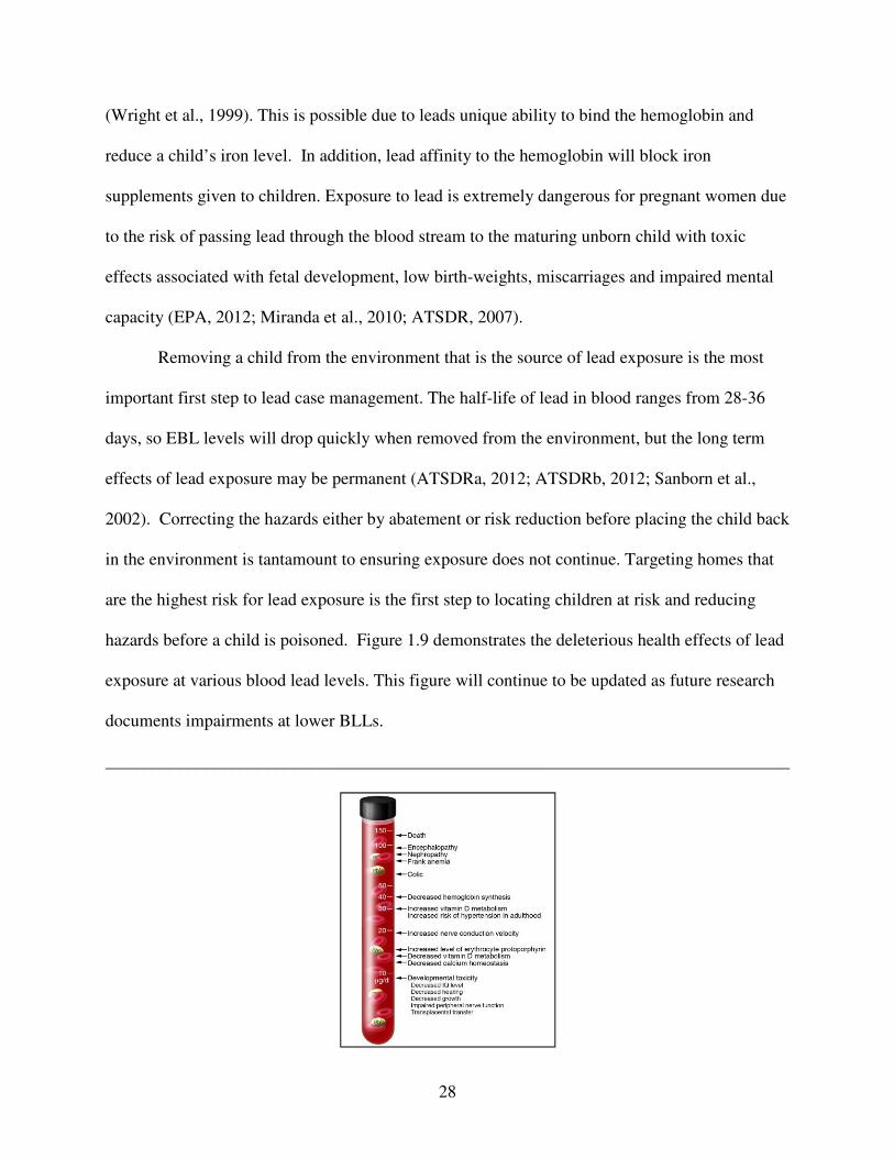
because these symptoms may go unnoticed. Studies have shown that anemia, an important

nutritional deficiency in children is associated with chronic exposure to low levels of lead

28

(Wright et al., 1999). This is possible due to leads unique ability to bind the hemoglobin and

reduce a child’s iron level. In addition, lead affinity to the hemoglobin will block iron

supplements given to children. Exposure to lead is extremely dangerous for pregnant women due

to the risk of passing lead through the blood stream to the maturing unborn child with toxic

effects associated with fetal development, low birth-weights, miscarriages and impaired mental

capacity (EPA, 2012; Miranda et al., 2010; ATSDR, 2007).

Removing a child from the environment that is the source of lead exposure is the most

important first step to lead case management. The half-life of lead in blood ranges from 28-36

days, so EBL levels will drop quickly when removed from the environment, but the long term

effects of lead exposure may be permanent (ATSDRa, 2012; ATSDRb, 2012; Sanborn et al.,

2002). Correcting the hazards either by abatement or risk reduction before placing the child back

in the environment is tantamount to ensuring exposure does not continue. Targeting homes that

are the highest risk for lead exposure is the first step to locating children at risk and reducing

hazards before a child is poisoned. Figure 1.9 demonstrates the deleterious health effects of lead

exposure at various blood lead levels. This figure will continue to be updated as future research

documents impairments at lower BLLs.

______________________________________________________________________________

29

Bellinger et al., 2006 Reprinted with permission from the Journal of Clinical Investigations

Figure 1.9- Health Effects at Varying Blood Lead Levels. ______________________________________________________________________________

Juvenile and Adult Delinquency

Needleman et al. (2002) and (1996) studied the health effects of lead on children and

surmised that lead poisoning results in permanent cognitive loss and the subsequent development

of juvenile delinquency, socially disruptive behavior and adult incarceration. Research by

Dietrich et al. (2001) validates studies that have argued a link between lead exposure and

disruption in classroom behavior, delinquency and the inability to concentrate. This is further

supported in a prospective study by Wright et al. (2008) that established a strong association

between lead exposure in children and criminal behavior in adulthood. Research has consistently

shown an association between chronic low-level (≥5ug/dL) lead exposure and attention deficit

hyperactivity disorder (Braun et al. 2006), which may cause a child to be disruptive, delinquent,

and have poor academic outcomes.

Nevin (2007) evaluated lead exposure in preschool years and found a strong association

with crime trends across the globe and the individuals exposed. Cecil et al. (2008) studied the

physical effects of lead exposure on the adult brain and found reductions in brain gray matter in

regions of the brain that controls executive functions which may lead to negative behaviors and

decision making. Stretesky and Lynch (2001) evaluated adult exposure to lead in the air and

found an association between this exposure and violent homicidal behavior. The vast amount of

evidence clearly suggests that early exposure to lead may influence juvenile delinquency that can

result in negligent adult behavior and criminal activity.

IQ Loss and School Performance

30

Research has shown a strong association between lead poisoning and a decrease in IQ

and earnings loss. In his influential study, Swartz et al. (1994) estimated that for every 1 ug/dL

drop in childhood BLL, IQ increased 0.245 points and $5.060 billion dollars in net earnings loss

are averted. Salkever (1995) expanded upon Swartz et al. (1994) study and suggested that net

earnings loss thwarted are approximately $7.5 billion dollars. According to an analysis

conducted for the CDC and cited by Needleman (1998), “…a 1-ug/dL increase in blood lead

level resulted in an IQ decrease of 0.25 points…[and]…a decrease in …schooling of 0.131

years” per child exposed (p.1872). Grosse et al. (2002) analyzed blood lead declines in children

between 1976-1999 and suggested that children in the 1990s compared to the 1970s have on

average a lower BLL that results in a 2.2-4.7 increase in IQ points. This IQ increase improved

worker productivity by 1.76%-2.38% for an economic benefit of $110-$319 billion dollars for

the birth cohort each year (Grosse et al., 2002). Surkan et al. (2007) evaluated associations

between low blood lead levels (5-10 ug/dL) and cognition in children and after adjusting for

confounders found a 5 point reduction in I.Q., lower scores in reading and math, and reduced

attention and memory skills as compared to children with lower BLLs of 1-2 ug/dL.

Studies indicate that lead exposures lead to negative outcomes in school performance.

Lead poisoning risk factors such as low income and extensive poverty at the community level

contributes to “…racial and ethnic achievement gaps…” in learning (Anderson et al., 2003 p. 32)

A higher prevalence of IQ losses of 3.9 to 7.4 points have been documented when children are

exposed to low levels of lead (NCHH, 2012) and have a negative association with school

performance (Strayhorn, et al., 2012; Miranda et al, 2009; Chen et al., 2007). Lanphear et al.

(2000) argued that IQ in children is most affected by chronic exposure to low levels of lead

versus an acute high BLL (as cited by the National Center for Healthy Housing, 2012), with

31

“…IQ loss per 1 ug/dL…greatest at lead levels below 10ug/dL” (NCHH, 2012 p. 2). The link

between lead exposure is inversely associated with IQ loss (Sanders et al., 2009; Canfield, et al.,

2008; Lanphear et al., 2005) and has been associated with poor performance in schools (NCHH,

2012) with some schools designating children as “exceptional” due to learning or behavioral

problems (Miranda, Maxson & Dohyeong, 2010).

Strayhorn et al. (2012) demonstrated associations between EBL levels and school

achievement in English and Math for 3rd and 8th graders, while controlling for income. A study

by Jusko et al. (2008) proved an association between BLLs below 10 ug/dL and intellectual

function of children while Chen et al. (2007) posits that at 7 years of age, there are significant

associations between BLL, externalizing, and problems in school. When children exposed to

high and chronically low lead levels reach adulthood, they may not reach their full cognitive

potential due to the effects of exposure (WHO, 2010). According to Needleman et al. (2002),

these adults will never be the productive members of society they could have been if lead

exposure had not occurred.

Costs Associated with Lead Poisoning

With ever shrinking Federal and State dollars to support lead prevention programs, it is

important to compare and contrast the social and medical costs of lead poisoning versus the cost

of prevention programs. The social cost of lead poisoning is permanent cognitive impairments

that can lower IQ and lead to a 2.39% reduction in lifetime earnings (Salkever,1995) and many

would argue is the most important if not also an ethical consideration. Landrigan et al. (2002)

conservatively estimated the annual cost of pediatric disease from lead poisoning at $43.4 billion

dollars. More recently, the PEW Charitable Trust (2010) estimated the cost of lead exposure per

birth cohort is $192-$270 billion dollars annually. This birth cohort estimate is calculated based

32

on the lifetime cost of healthcare, IQ and lifetime earnings loss, educational needs, and the cost

of behavioral problems and adjudication (PEW, 2010).

Lead prevention programs are cost effective because they work to reduce lead hazards in

the environment and prevent children from being exposed. In the PEW issue brief (2010), it was

estimated that spending $1.2-$11 billion dollars on lead hazard prevention programs would save

the country $181-$269 billion taxpayer dollars in social benefits (PEW, 2010). As noted by

Gould (2009), for every $1 dollar invested in lead hazard prevention, there is a $17-$221 dollar

return on that investment lending significant cost savings.

Brown et al. (2001) evaluated the effectiveness of housing policies on preventing

additional lead exposures in previous addresses where lead exposed children resided and found

that in communities with limited housing code enforcement, the risk of repeat lead poisoning

cases was four (4) times more likely than in communities with a strong housing code

enforcement program. In additional studies, Brown (2002) compared housing code enforcement

programs to preventing additional cases of children with EBL levels in two urban areas and

suggested that strict enforcement of housing laws reduced additional cases of EBL level children

and saved approximately $45,360 in medical, social and education costs.

Investing dollars in prevention programs is not popular because it is difficult to show

immediate gains in the dollars invested. However, from a cost benefit analysis, the benefits of

investing in lead prevention programs on the front end far outweigh the healthcare and social

costs of lead poisoning in the long term.

GIS Risk Models in Health Promotion

GIS is an information system for the “…input, storage, processing, and retrieving of

spatial data…,” which is important to public health programs (Kurland & Wilpen, 2009). Spatial

33

technology allows analysis and identification of health trends, construction of threat scenarios,

mapping environmental issues, developing public health interventions (Jerret, et al., 2010;

Hopfer et al., 2008; Peng, 2001), mapping arboviral cases such as West Nile Virus, disease

clusters and childhood obesity rates (Drewnowski et al., 2007; Allen & Wong, 2006). GIS

allows one to integrate data in a spatial picture that is easy to interpret, identify trends and

present to the public (Bell et al., 2006). The CDC encouraged states to utilize GIS spatial

technology in their lead prevention programs as far back as 2004 due to its effectiveness in

targeting high risk children (CDC, 2004a).

Over the past decade, the use of GIS risk models to map and predict lead exposure risk

has increased. Kim et al. (2008) postulated that GIS technology is a promising approach to

addressing the childhood lead problem through the use of highly-spatially resolved lead risk

models. While no model is perfect, spatial technology is a tool that continues to improve in

specificity and with creative algorithms allows accurate prediction of risk. The use of predictive

models allows public health practitioners to focus on primary prevention techniques by

potentially addressing a lead hazard before it poisons a child or at the very least targeting

education and testing to the highest risk children (Miranda et al., 2002).

The CDC has long recommended state and local lead poisoning prevention programs

develop a targeted approach to identifying and screening the highest risk children (Vaidyanathan

et al., 2009; CDC, 2009). Over the last decade, researchers and public health practitioners have

utilized spatial technology at various defined geographic levels to develop models. According to

Mushak (1998), lead exposure models vary in their statistical analysis ability and how they are

applied. Models have been developed to predict areas at risk for lead exposure at the parcel,

census, block, and zip-code levels (Vaidyanathan et al., 2009; Kim et al., 2008; Haley & Talbot,

34

2004; Roberts et al., 2003; Miranda et al., 2002; Kim et al., 2002; Reissman et al., 2001; Litaker

et al., 2000; Sargent et al., 1997). These risk maps have allowed states to develop GIS based risk

models at various spatially defined scales to predict lead exposure risk.

As far back as the 1990s when modern computer GIS technology was in its infancy,

Sargent et al. (1997) evaluated census track and blood screening data to determine where the

highest risk children for lead exposure resided and demonstrated that targeted approaches to lead

prevention programs could be achieved. Litaker et al. (2000) utilized a logistic regression model

to analyze Ohio’s lead screening strategies and enhanced the model to assign a scoring system

for high and low risk areas. This model assigned risk to “geographic units” as opposed to

individual children, but the authors postulated that the model could be partnered with mapping

software to assign individual risk in a clinical setting (Litaker et al., 2000). Reissman et al.

(2001) demonstrated the importance of spatial technology by mapping high risk neighborhood in

Louisville, Kentucky and overlaying children exposed to lead. This study was one of the first to

develop a spatial map where public health practitioners could target lead screening and

educational efforts to the highest risk areas of the county.

Kim et al. (2002) utilized GIS technology to show an association between age and value

of housing as a risk factor for lead exposure in children. This association supported conclusions

that older housing is a risk factor for lead poisoning and is associated lower valued homes with

flaking paint. Miranda et al. (2002) utilized GIS technology with blood screening, census, and

tax assessor data to develop a risk model that could predict a risk index at the tax parcel level in

6 North Carolina counties. While small in scale, this model demonstrated that lead exposures

could be predicted at certain scales for use by public health practitioners and led to a 600%

increase in screening and identifying EBL level children (Kim et al, 2008). Roberts et al. (2003)

35

demonstrated through the use of GIS that children living in pre-1950 homes were more likely to

be at risk for lead poisoning and created spatial maps for targeted screening programs. In

addition, this research identified a cluster of low risk children with lead exposures living in

homes built after 1978 suggesting an offsite exposure source such as older homes or

contaminated soil in the area (Roberts et al., 2003).

Haley et al. (2004) demonstrated areas across New York State with high prevalence of

lead exposure using postal zip codes as the geographical unit. This study identified locations to

target and recommended future studies evaluate risk at the individual level for more precise

analysis. Vaidyanathan et al. (2009) developed a geospatial approach to assigning neighborhood

risk for childhood lead exposure utilizing census block groups. This approach worked off the

premise that parents identify with their neighborhood and by assigning neighborhoods a risk

level, health officials can ascertain a child’s risk through pre-identified high risk areas and

interviewing the parent/caregivers.

The various GIS models found in the literature support the concept that a child’s risk of

lead exposure can be predicted accurately and improve lead prevention program goals of

reducing childhood lead exposure. GIS is a powerful tool for developing these risk models and

with improved technology, the models continue to become more precise in their predictions.

State of Georgia Lead Statistics

A combination of the CDC establishing a new lead reference level of ≥5 ug/dL, merging

the healthy home and lead program, HUD adopting ≥5ug/dL as its EBL, and the new Healthy

People 2020 goals, the Georgia Department of Public Health renamed its program the “Georgia

Healthy Homes and Lead Poisoning Prevention Program” (GHHLPPP). This allows the State to

focus its resources on the importance of the built environment and its link to the health of

36

families and children. The GHHLPPP mission is to eliminate childhood lead poisoning in

Georgia through achieving the following goals (2012):

• Update and implement the statewide lead poisoning screening plan utilizing targeted

methods.

• Improve and redefine statewide lead poisoning surveillance system that incorporates electronic reporting of all blood lead levels and ensures the timely dissemination of information.

• Establish policies and procedures that ensure the appropriate screening and follow-up of children at risk for lead poisoning.

• Create health education, communication, and technical assistance programs for the general public, professionals, and staff that highlight the importance of lead poisoning prevention.

• Develop multi-faceted and culturally appropriate primary prevention activities. • Evaluate the program completely in terms of process and impact. • Pursue federal funding to make housing lead safe in Georgia which has been identified as

containing lead hazards complemented by enforcement.

A major focus of the GHHLPPP is to develop a targeted approach to lead testing and high

risk (of lead exposure) home identification as recommended by the CDC (CDC, 2009). This

dissertation supports this focus with positive results allowing the use of a GIS tool to focus on

primary prevention efforts. Utilizing GIS technology, tax assessor, census data, and blood lead

levels, a map of high risk counties in Georgia was created to focus resources as shown in Figure

1.10. From this figure, one notes that 14 counties in Georgia have the highest risk for lead

exposure based on select risk factors. The risk variables used to develop this map include homes

built before 1978 and percent of rental property. Geocoding and mapping the location of

children exposed to lead matches up with the high risk counties, as demonstrated in Figure 1.11.

This figure illustrates geocoded addresses of children exposed to lead with clustering in high

risk areas.

37

_____________________________________________________________________________

Figure 1.10- Georgia High Risk Counties.

Figure 1.11- Geocoded Children Exposed to Lead. ______________________________________________________________________________

The setting for this study is Macon-Bibb County as circled in Figure 1.10, due to a high

proportion of risk factors such as older housing, rental property, poverty, and Medicaid children

38

that contributes to the second highest lead prevalence in the State at 4.2% (GHHLPPP, 2012).

Figure 1.12 demonstrates Macon-Bibb County children overlaid on Census block groups (BG)

color coded by risk derived from age of housing. The shaded green areas are the lower risk BGs

with the bright red areas the highest risk BGs in the county. Each dot is a geocoded child that has

been exposed to lead and the color of the dot represents the child’s risk based on BLL. Black

dots indicate children tested with elevated BLLs and these dots correspond to the highest risk

areas of the county. This risk map supports prediction maps displayed in Chapter 4 developed

from this study’s risk model at the parcel level. This map also demonstrates the need for smaller

scale (parcel) predictions of risk as a large north west cluster of children exposed to lead is found

in a lower risk block group, thus supporting the purpose of this study.

____________________________________________________________________________

Figure 1.12- Macon-Bibb County Lead Risk Map. ______________________________________________________________________________

For a more detailed map of high risk public health districts in Georgia, see Appendix A (see

“Georgia – Average Health District Housing Based Risk Elimination Plan Update (2012)”.

39

Targeting lead prevention is important because Georgia has 159 counties, which is ranked

second in the nation for the most counties and targeting resources to the highest risk counties

versus all 159 counties provides the greatest benefits to the highest risk children. The map in

Figure 1.12 was the genesis to develop a GIS lead risk model that assigns individual risk to a

child and evaluation of the model is the focus of this study. If effective, the risk model will be

utilized as a tool to identify high risk children for testing, case management, and environmental

interventions in Georgia.

Georgia Children Tested for Lead

In 2011, there were over 120,000 children screened for lead in Georgia. Out of the

120,797 children screened, 4,583 children less than 6 years of age had an EBL level of ≥ 5ug/dL

and 778 children exceeded ≥10ug/dL, which required an environmental investigation. This data

is presented in Table 1.4 and supports a targeted approach to lead poisoning prevention.

______________________________________________________________________________

Table 1.4: Number of Children ≥6 Years Old Screened for Lead, Georgia 2011 ______________________________________________________________________________

Total Number

Screened

(1-1) Northwest (Rome) 6,498 234 3.6 60 0.92

(1-2) North Georgia (Dalton) 5,366 174 3.24 39 0.73

(2) North (Gainesville) 8,188 268 3.27 37 0.45

(3-1) Cobb/Douglas (Marietta) 8,326 221 2.65 46 0.55

(3-2) Fulton (Atlanta) 16,128 442 2.74 72 0.45

(3-3) Clayton (Morrow) 3,944 94 2.38 9 0.23

(3-4) East Metro (Lawrenceville) 12,908 313 2.42 52 0.4

(3-5) DeKalb (Decatur) 8,388 314 3.74 26 0.31

(4) LaGrange 7,780 292 3.75 33 0.42

(5-1) South Central (Dublin) 2,351 189 8.03 31 1.32

(5-2) North Central (Macon) 6,546 293 4.48 51 0.78

(6) East Central (Augusta) 2,625 180 6.86 23 0.88

(7) West Central (Columbus) 2,870 138 4.81 33 1.15

(8-1) South (Valdosta) 2,468 151 6.11 31 1.26

(8-2) Southwest (Albany) 6,055 354 5.85 58 0.96

(9-1) Coastal (Savannah) 9,038 442 4.89 91 1.01

(9-2) Southeast (Waycross) 5,736 291 5.07 53 0.92

(10) Northeast (Athens) 5,582 193 3.46 33 0.59

State 120,797 4,583 3.79 778 0.74

Health District 5 - 9ug/dL ≥10ug/dL% Tested % Tested

40

GHHLPPP, 2012 ________________________________________________________________________________________________________

The BLL data in Table 1.4 corresponds to the county risk map in Figure 1.10 as the number of

EBL level children is higher in the 14 highest risk counties. The collection of data on children

with BLLs of 5-9ug/dL demonstrates Georgia’s commitment to following the CDC’s and

HUD’s new case management recommendations for children with a BLL reference level of ≥ 5

ug/dL as prior to 2011, BLLs ≥5ug/dL were not collected by the Georgia program. In addition, a

BLL of 15ug/dL was the level where environmental intervention commenced and ≥10ug/dL was

considered a pre-EBL prior to 2012. In 2011-12, the GHHLPPP adopted new case management

guidelines recognizing the CDC’s new reference level and the level that required an

environmental investigation were lowered to ≥ 10ug/dL. With research indicating strong

evidence of the negative health effects of low-level chronic lead exposure (Lanphear et al.,

2000), Georgia continually revamps its program to focus new prevention and education efforts

on children exposed at lower levels.

With the 14 high risk counties in Georgia being the most urban and populous, the number

of EBL level children may be low due to the practice of universal screening of Medicaid children

versus targeted screening of high risk children. This approach spreads public health resources

across the entire state and limits focus on the highest risk counties. Figure 1.13 is a neighborhood

map of Fulton County (Atlanta) that demonstrates how testing rates do not match neighborhood

risk by pin size. The larger pins indicate a higher testing rate and these pins disproportionately

fall on lower risk neighborhoods shaded as pink, versus small pins falling on higher risk

neighborhoods shaded as red. This contributes to health disparities as children in high risk areas

may lack access to healthcare and suffer from undiagnosed lead poisonings.

41

______________________________________________________________________________

GHHLPPP, 2012

Figure 1.13-Testing Rates for Children by Neighborhood Risk. _____________________________________________________________________________________________

Significance of Study

This study is significant because a model that assigns lead exposure risk accurately will

allow the State of Georgia to target its most vulnerable populations and maximize resources. To

the author’s knowledge, this is the first time that a GIS predictive risk model has been developed

that takes a parcel map with a weighted risk scale based on age and type of housing (homestead

exemption as a proxy for a rental unit) derived from individual parcels, an adjusted risk map

developed from weighted BLL surveillance data and mathematically combines the two maps,

thus adjusting the parcel risk based on its proximity to previous poisoned children. This

combination creates a final predictive risk map exported as a continuous raster surface that

assigns a risk level to an individual child based on the child’s address. If the model is successful,

this lead exposure risk model could be applied statewide through the Georgia immunization

42

database to alert physicians and public health officials of the child’s exposure risk status so

appropriate case management and environmental investigations can takes place.

Homestead exemption (HE) as a proxy for rental status is unique to this model and study.

Homestead exemption is a tax benefit that can be claimed by any Georgian with an owner

occupied home. This exemption provides a tax credit that is deducted from the assessed value of

the home, thus lowering ones property taxes. It is common practice in Georgia and other states

for county tax assessor’s and GIS consultants to ascertain the number of rental units in a county

utilizing homestead exemption status as a proxy (F. Staley, personal communication, 2012;

Fleming & Vedhuis, 2003). While homestead exemptions are offered in many states, the use of

homestead exemption status as a proxy to determine if the housing unit is a rental unit versus an

owner occupied unit is unique to this study and has not been found in the literature as a common

proxy of rental status in GIS risk model studies. Homestead exemption is a good proxy because

secondary homes, apartment complexes, duplexes, for example, are not eligible for a homestead

exemption because these domiciles are not the owners primary occupied residence; moreover,

this information is available and updated each year from the county tax assessor records and can

very simply be incorporated in a GIS risk model (Zandbergen & Hart, 2009; Allen, 2009). In

addition, the county tax assessor offices in Georgia notifies all homeowners of their right to

claim this tax saving exemption on their primary residence yearly, thus decreasing the likelihood

that an owner will not claim the exemption if eligible.

All GIS studies found in the literature that used rental status as a risk variable in their GIS

model obtained the information from aggregated census level data as a percentage of rental

properties in a county. Assigning risk to an individual parcel utilizing aggregated data spread

across a large geographical area may introduce ecological bias in a study due to large differences

43

that may exist across the area in question (Mather et al., 2004). It is believed the methodology

used in this study is more precise because it derives risk from attributes assigned to each

individual parcel, which is the smallest unit of geographical scale, thus reducing ecological bias.

Should the evaluation of this risk model indicate efficacy in assigning risk, the model has

policy implications for Georgia that includes a shift in focus to primary prevention via improved

targeted outreach and education, identification of homes at risk, and improved secondary

prevention techniques that involves focusing resources on testing the highest risk children. In

addition, the CMS, which oversees federal policy for the Medicaid insurance program has

relaxed its requirement for physicians to test all Medicaid children for lead if the state can prove

that a targeted approach to lead testing will ensure that the highest risk children are being tested,

thus allowing better use of dwindling federal dollars (CMS, 2012). This model may be utilized to

meet CMS’s requirements and exempt lower risk children from testing if found efficacious.

Success of this study will also assist the State of Georgia with meeting the following

Healthy People 2020 Environmental Health objectives of (2012):

• Reduce blood lead levels in children

• Increase the proportion of persons living in pre-1978 housing that have been tested for the presence of lead-based paint or related hazards

• Reduce the number of U.S. homes that are found to have lead-based paint or related hazards

Meeting the Healthy People 2020 objectives will improve the overall health of Georgia’s

children by reducing lead hazards in the environment, thus, improving a child’s ability to learn

and grow in a safe community. This will lead to better health and educational outcomes for

Georgia’s children and improve a community’s health.

44

CHAPTER 2

HYPOTHESIS AND RESEARCH QUESTIONS

The Georgia Department of Public Health’s Environmental Health Section, where the

author is employed, and the Office of Health Indicators for Planning GIS team collaborated to

develop the GIS risk model used in this study. The goal was to develop a practical tool that could

be used to target high risk children and focus on primary versus secondary prevention efforts to

reduce lead poisoning in the State. Knowing where the highest risk children reside will allow

targeted approaches to testing, lead educational outreach, hazard abatement activities, and better

enforcement of lead exposure rules and laws. This study will test five hypotheses related to lead

poisoning demographics and statistical associations between elevated BLLs and predicted risk,

differences between predicted risk levels and BLL means and that ultimately, the risk model can

accurately estimate the risk of EBL children based on the child’s physical address.

Risk is defined by the Merriam-Webster (2012) Dictionary as the possibility of loss or

injury. In this study, risk implies an opportunity exists for lead exposure to occur. Previous

studies have confirmed various risk variables for lead exposure such as age of housing, rental

status, poverty, and neighborhood lead prevalence. For this study, a child that lives in a rental

home built before 1978 or 1950 in a neighborhood with previously lead exposed children is at a

higher risk for lead poisoning compared to a child that lives in an owner occupied home built

before 1978/1950 or any home built after 1978. The level of risk is based on variables such as

the exact age of the home, rental status and its proximity to homes where other children have

been exposed. This risk model does not imply that a child will be lead poisoned, just that the

child lives in an environment where there is a potential risk for exposure to occur.

Research Aims

45

The goal of this study was to determine if the Georgia Department of Public Health’s

lead poisoning risk model is efficacious at estimating a child’s risk of lead exposure. The GDPH

would like to use this model as a tool to target high risk children and potentially exempt lower

risk Medicaid children from required lead testing. This allows public health resources to be

focused on children and homes with the greatest need. Results from this study will inform the

GHHLPPP and assist them with making a decision on moving forward with deploying this risk

model statewide. The study’s goals are to achieve the following aims:

1. Assist with constructing the GIS risk model that ensures 100% parcel mapping and risk

assignment for Macon-Bibb County by constructing a parcel risk map from attributes of

age and type of housing using homestead exemption as a rental proxy.

2. Geocode six years of blood lead surveillance data, categorize and weight the data based

on an algorithm to construct an adjusted predictive map. Combine both maps

mathematically for a final adjusted predictive risk map surface.

3. Develop descriptive statistics for children exposed to lead in Macon-Bibb County to

better inform the GDPH Lead Program.

4. Statistically analyzing the risk model to determine if a significant association exists

between the models dependent variable of BLL and independent variable of predicted

risk at the p ≤ 0.05 level of significance.

5. Statistically analyze the risk model to determine if weighted surveillance data contributes

to the strength of the final predicted risk.

6. Review and describe all statistics and determine if the risk model is efficacious with

statistical confidence.

46

7. Reject or accept the hypotheses and make recommendations to the Georgia Department

of Public Health on utilization of the risk model based on the evidence found in this

study.

The following hypotheses were tested:

Hypothesis # 1 There will be no statistical relation between elevated blood lead level and the models predicted risk. Hypothesis # 2

100% of children with a measurable BLL used to test the risk model will not live in EASI Census demographic clusters that have all the predominant risk factors for lead poisoning. Hypothesis # 3

The mean age of children used in this risk model with an EBL (≥5ug/dL) will not be approximately 30 months of age when BLLs typically peak.

Hypothesis # 4 There are no statistical differences measured between risk levels when compared to BLL means.

Hypothesis # 5 The lead risk model developed by the Georgia Department of Public Health will not predict a risk of elevated lead exposure ≥5ug/dL.

47

The following research questions were explored: Research Question # 1 Does the risk model estimate and assign a risk of lead exposure to the childhood blood lead records for years 2004, 2005 and 2012 for Macon-Bibb County?

Research Question # 2 What are the demographics of children being tested for lead in Macon-Bibb County using BLL data? Research Question # 3 What is the mean age of a child with a blood lead level of <5ug/dL and ≥ 5ug/dL?

Research Question # 4

Does the risk model estimate moderate-high risk (3-5) in children when compared to elevated blood lead levels of ≥5ug/dL?

Research Question # 5

Does BLL surveillance data influence the models predictive ability when comparing parcel risk to the final combined risk model?

48

CHAPTER 3

METHODS AND MATERIALS

Design of the Study

Risk Model Construction

The risk model was developed utilizing ESRI ArcMap Geographical Information System

(GIS) version 10.0 by the GDPH GIS team with contributions from the author. The model

calculates risk based on parcel attributes of housing age and rental status (HE proxy) multiplied

by six (6) years of weighted BLL surveillance data. Risk is assigned to a child by geocoding the

child’s address and spatially joining to the parcels using the extract to values feature in GIS. The

assigned risk can then be communicated to physicians and public health officials through the

Georgia Registry of Immunization Transactions and Services (GRITS) immunization system. A

prompt in the system will alert the physician or public health official to the child’s risk status as a

reminder to test the child if high risk or ask additional risk questions if low risk is predicted.

The risk model was constructed by creating two surface layer predictive maps using

inverse distance weighting interpolation, exporting both maps to a raster surface, and

mathematically combining the two maps to form a final continuous raster risk map.

Interpolation simply means predicting a value for a location with missing data. County level

parcel data may have missing numerical attributes such as age of housing. With interpolation,

GIS will evaluate surrounding data to predict a value for the missing parcel, i.e. age of housing.

With ArcMap GIS, there are two major interpolation options to choose from in building a risk

model, inverse distance weighting (IDW) or Kriging. Inverse distance weighting is a simple

deterministic method based on the idea that points closer to the missing point carries more

weight than points farther away, thus resulting in a weighted average used to predict the missing

49

value (GIS, 2012). The distance, number of points and power function used to predict the

missing values can be set by the builder to emphasize more weight placed on closer data points.

This interpolation procedure works well when there is a sufficient number of data points

distributed across a surface (GIS, 2012). Kriging is a more advanced geostatistical procedure

that analyzes the “statistical properties of measured points” to interpolate and predict missing

values (GIS, 2012). This procedure works well for scattered data across a surface and is typically

used when there are minimal data points available for interpolation that can impact the accuracy

of the final map.

The GIS team at GDPH chose to build this risk model using inverse distance weighting

because the parcel data had sufficient values in close proximity needed to predict missing values,

there were sufficient BLL surveillance data, is simpler and more straight forward for replication

of the model across the state, and requires less computer processing power as needed to build

Kriging models. In addition, prediction errors for the IDW model were small suggesting model

accuracy. Once concern with IDW is the model is sensitive to spatial clustering and outliers.

Miranda et al. (2002) found that corrections for spatial autocorrelation (clustering) were negated

when geographical resolution was high, such as parcel level data versus aggregated census tract

data. Since the variables used to build this risk model are based on age of house and homestead

exemption at the individual parcel level, spatial autocorrelation corrections were not included.

Concerns for outliers were controlled by establishing a search radius that limited the distance of

points used for interpolation.

Predictive Parcel Map

The first map layer was created by obtaining GIS tax parcel and 2010 census shape data

from Macon-Bibb County Tax Assessor’s office. Tax assessor parcel data contains variables

50

linked to the individual parcel such as age of house, home value, homestead exemption and

ownership status. The quality of the data may vary from county to county, but is generally

reliable and consistent. From the tax parcel data, attributes of age of housing and homestead

exemption status (proxy for rental vs. owner occupied status) was ascertained from the tabular

data for each parcel. A parcel that did not have a homestead exemption, listed as qualified or

unqualified, linked to a parcel or had a commercial zoning code assigned was considered non-

residential as instructed by the Bibb County Tax Assessor’s office and was excluded.

Homestead exemption is a good proxy of rental status and is commonly used to ascertain the

percentage of rental property in a county because by Georgia law, only owner-occupied property

can have homestead exemption status claimed for tax savings (F. Staley, personal

communication, 2012; J. McMichael, personal communication, 2012). This was coded as

qualified (homestead exemption) and unqualified (no homestead exemption) in the tabular data

for the parcels with all residential property used for the model having this designation. As

outlined in Table 3.1, a parcel risk algorithm code was written to calculate risk for each parcel on

a scale of 1-5. This risk was calculated by using the GIS geostatistical wizard field calculator

and multiplying the algorithm with the Bibb County parcel data that included the tabular

attributes of age of housing and homestead exemption status (coded as qualified or unqualified).

______________________________________________________________________________ Table 3.1: Parcel Risk Algorithm ______________________________________________________________________________

If [yr_built] >= 1978 Then Output = 1 ElseIf [yr_built] < 1978 And [yr_built] > 1950 And [homeexempt] = "Y" Then Output = 2 ElseIf [yr_built] < 1978 And [yr_built] > 1950 And [homeexempt] = "N" Then Output = 3

51

ElseIf [yr_built] < 1950 And [yr_built] > 0 And [homeexempt] = "Y" Then Output = 4 ElseIf [yr_built] < 1950 And [yr_built] > 0 And [homeexempt] = "N" Then Output = 5 ElseIf [yr_built] = 0 Then Output = 0 ____________________________________________________________________________

In layman terms, Table 3.2 explains the risk assigned to each parcel with a risk of one (1) being

the lowest risk and a risk of five (5) the highest risk. If the parcel had a risk assigned as 0, then

the model did not calculate a risk. The goal was to avoid a 0 and to ensure 100% parcel

matching. No parcels in Macon-Bibb County were assigned a 0, which indicated a risk was

determined for all parcels.

______________________________________________________________________________ Table 3.2: Parcel Risk ______________________________________________________________________________ Risk Risk Factors Risk Type

5 Pre 1950, No Homestead Exemption Highest Risk 4 Pre 1950, Homestead Exemption Moderate-High Risk 3 Pre 1978, No Homestead Exemption Moderate Risk 2 Pre 1978, Homestead Exemption Low Risk 1 Post 1978 Lowest Risk 0 Risk not determined ______________________________________________________________________________

Once the risk was calculated for each parcel, the GIS geostatistical wizard was used and

inverse distance weighting selected to create an interpolated surface prediction map exported to a

continuous raster surface. Inverse distance weighting (IDW) was chosen because there were

enough data points to interpolate missing parcel data. As stated before, interpolation is a GIS

procedure that predicts a cell (parcel) value for any parcel that lacked sample points (Childs,

2004). For example, if a residential parcel was missing an attribute such as age of housing, GIS

52

would use a mathematical function of inverse distance weighting to evaluate the surrounding

parcel data in a given distance from the parcel with the missing value, take a weighted average

and assign an estimated age to the parcel. For this model, the IDW function was limited to

analyzing 15 parcels from the parcel with missing data to predict or interpolate the data to ensure

accurate interpolation. This base layer map served as the foundation for the model and included

all residential parcels in Macon-Bibb County.

Adjusted Surveillance Risk Map

A second surface layer predictive map utilizing BLL surveillance data was constructed to

test the assumption that historic BLL data has an influence on the overall models predictive

ability. In addition to age and type of housing, it is believed that proximity to parcels with

historic lead exposures can influence the risk of children being exposed. Through an algorithm in

Table 3.3, the proximity of historic exposures can be used to mathematically adjust the risk of

adjacent parcels by weighting the surveillance BLL data. Six years (2006-2011) or 6,729

neighborhood blood lead surveillance records for Macon-Bibb County were obtained from the

GHHLPPP. All BLL records were address mapped with Centrus Desktop software version

5.02.00.N (Pitney-Bowes, 2011), screened for Bibb County address level accuracy and merged

to form one shape file. After screening and exclusion, 5,431 addresses were used. An algorithm

was written to weight the BLL data based on categorizing the surveillance data (<5ug/dL, ≥5-

9ug/dL, ≥10-20ug/dL, >20ug/dL) as shown in Table 3.3.

______________________________________________________________________________ Table 3.3: Weighted Risk Adjustment Algorithm ______________________________________________________________________________ BLL- <5ug/dL- adjust risk by - 20% (x .8)

Pre-EBL- ≥5ug/dL-9ug/dL- adjust risk by + 10% (x 1.10)

EBL- ≥10ug/dL-20ug/dL- adjust risk by + 30% (x 1.30)

Very EBL- >20ug/dL adjust risk by + 50% (x 1.50)

53

______________________________________________________________________________

These weights were chosen as a reasonable conservative approach to adjust adjacent

parcel risk. The weights increase with increased BLLs, thus signifying more emphasis on

adjacent parcels with historically higher exposures. The field calculator was used to multiply the

weighed risk adjustment algorithm in Table 3.3 with the merged BLL surveillance shape file.

Through the IDW interpolation procedure, each parcel was assigned a weight based on proximity

to parcels with historic lead exposures. For example, a home that was in close proximity to a

parcel with surveillance BLL data indicating historic exposures of 20 ug/dL or greater would

have its final risk increased by 50 %, thus implying a higher risk for a child living on that parcel.

The geostatistical wizard was opened and IDW selected to create an adjusted risk predictive

map. The surveillance data adjustment is important for lower risk parcels because children may

visit or play with higher risk children near their home and become exposed to lead, even though

their home is low risk. The adjusted risk predictive map was exported to a raster surface layer

map for eventual combination with the parcel risk raster map.

Combined Final Risk Map

The two predictive raster maps were combined mathematically by multiplying the parcel

risk map raster with the adjusted risk map raster using the spatial analyst tools in the GIS Arc

toolbox to form a final predictive risk map. The combined map has an interpolated continuous

risk range of 0.8-6.4 (low risk-high risk) due to the combination of parcel risk and the adjusted

BLL weighted risk. These data were statistically analyzed using the continuous risk scale and by

rounding the risk to the nearest whole number and combining risk levels five (5) and six (6).

The -0.20% weight was negated by rounding the lowest risk to one (1) after minimal predictive

influence was found from initial statistical analysis. The upper risk-level of 6.4 was combined

54

with risk level 5 because this was the risk ceiling designated by the author, which are rental

homes built before 1950. Rounding the risk to the nearest whole number converted the

continuous scale back to the original 1-5 risk scale, which normalized and made the data easier

to understand and statistically analyze. Figure 3.1 describes the model construction.

GIS RISK MODEL CONSTRUCTION

Parcel Risk Map Adjusted Surveillance Map

Parcel Data Six years BLL - HE Surveillance data -Year Merged to .shp file

Calculate Risk Calculate Risk (Field Calculator) (Field Calculator)

Parcel Data x Risk BLL surveillance x Algorithm (1-5) Weights Algorithm

Geostatistical Wizard Geostatistical Wizard

IDW-Prediction Map IDW-Prediction Map

Export to Raster Export to Raster

Parcel Risk Raster BLL Surveillance Raster

Arc Tool Box Spatial Analyst Select Math Select Times

Values to be Multiplied: Parcel Risk Raster Values to be Multiplied by: BLL Surv. Raster

FINAL PREDICTIVE RISK RASTER

55

Figure 3.1-Risk Model Steps to Development

Setting

Macon-Bibb County was the setting for evaluating the risk model due to the volume of

pre-1978 homes, historic low testing rates, number of rental properties and prevalence of

children exposed to lead as compared to the State prevalence. Bibb County was created out of

Houston, Twiggs, Jones, and Monroe Counties and incorporated in 1852 (Georgiagov, 2012).

The County is approximately 250 square miles in size with areas ranging from rural to its urban

core anchored by the City of Macon and has a population of 155,216 people (Georgiagov, 2012;

Census, 2012b). The two primary races in Bibb County are African American and White

making up 96.1% of the population with a small percent of Asians, Indians and Hispanics

(Census, 2012b).

According to the U.S. Census Bureau, there are significant health and economic

disparities in Macon-Bibb County that may contribute to the increase in lead prevalence such as

poverty, race, and residing in older housing (Census, 2012b). This is important because poverty

and race is strongly correlated as an important contributing risk factor for disease (CDC, 2011;

Krieger et al., 2003; Krieger & Higgins, 2002; Sargent et al., 1995; Macbeth, 1991). The

following statistics provide a demographic snapshot of Macon-Bibb County and outline many

risk factors for lead exposure (Census, 2012a; Census, 2012b):

• African Americans make up 52.5% of the population as compared to 44.1% Whites in Bibb County

• In the City of Macon, 67.9% are African Americans compared to 28.6% White

• Approximately 9,536 (13.8%) higher risk pre-1950 housing units, compared to the State at 8.1%

• Approximately 39,350 (56.8%) moderate-high risk pre-1979 housing units compared to the State at 37.2%

56

• Approximately 53.2% of the housing units in the City of Macon are rental units compared to the State at 33.2%

• Majority of pre-1950 and 1978 housing lies within the city of Macon, which is a moderate-high risk area where children are exposed to lead

• Families below poverty in the City of Macon are 25.5% as compared to the State average of 13%, or approximately 50% higher

• Individual poverty rate in the City of Macon is 31.9% as compared to the State average of 16.5%

• 32.6 % of African Americans in Macon live in poverty as compared to 15.6% of Whites leading to a disproportionate rate of African American children being poor and potentially exposed to lead from lower valued older rental homes

• Approximately 40.5% of children in Macon-Bibb County live in poverty compared to the State at 22.7%

______________________________________________________________________________

In discussion with Mr. Forrest Staley, Director of the GDPH Childhood Lead Program,

the average State prevalence of lead poisoned children was approximately 0.80% in 2012. This

is compared to an average prevalence rate of 4.2% for Macon-Bibb County located in Public

Health District 5-2 (See Appendix A) (F. Staley, personal communication, August, 2012). In

addition, only 16.5% of Medicaid children in Macon-Bibb County were tested for lead in 2011

as compared to the State average of 27%, even though it is a federal requirement for any

physician treating a Medicaid child to test that child for lead (F. Staley, 2012; CMS, 2012).

Data Collection

This study was approved by the Georgia Department of Public Health and Georgia

Southern University’s Institutional Review Board prior to data collection and analysis (See

Appendix C and D). Lead exposure is a reportable disease and the Georgia Department of Public

Health maintains a registry of all children tested with a blood lead level. Retrospective Macon-

Bibb County BLL data was acquired in December and January 2012 for years 2006-2011 (used

in model construction-adjusted risk map) and 2004, 2005 and 2012 (used for model analysis)

from the GDPH Lead Hazard Control Program without identifiers.

57

Data Exclusion

All BLL records were address matched (geocoded) using Centrus Desktop Geocoder

software and assigned a risk by the GIS model. Address matching is a procedure that assigns

geographic coordinates in latitude and longitude to the BLL data, and displayed by a geocoded

dot on the associated parcel. Centrus was used for address matching due to its positional

accuracy compared to the GIS geocoding tool as studies have demonstrated the accuracy of

Centrus exceeds that of the GIS geocoding tool (Zhan et al., 2006). All matched addresses were

assigned an LCODE by Centrus Desktop that detailed the accuracy level of the address match.

Table 3.4 lists the Centrus LCODES and address matched accuracy level.

______________________________________________________________________________

Table 3.4: Centrus LCODES

______________________________________________________________________________

A = Address level accuracy

ZB= Block Group level accuracy

ZT= Census tract level accuracy

ZC= County level accuracy

Each code has additional sub-codes at varying levels of accuracy. The most accurate LCODEs

are the ASO codes as these addresses are matched to the exact parcel address. Since the accuracy

of the risk model is dependent upon parcel level risk, all addresses with Z codes and any A coded

addresses that were not ASO codes were excluded from data analysis. In addition, any BLL

address that was not located in Macon-Bibb County was excluded from data analysis. The data

were screened for duplicate BLL records and if duplicates were found, the highest BLL was

excluded if a retest indicated a significant decrease in BLL.

According to 2010 census data, there were approximately 13,845 children ≤ 6 years old

living in Macon-Bibb County. According to the survey system calculator,(Survey, 2012), a

58

sample size of 2,046 children with a confidence interval of 2 is required to be an adequate

sample size of children for Macon-Bibb County. A total of 3,352 BLL records from 2004, 2005

and 2012 were available for model analysis. After address mapping, 151 BLL records were

excluded for not being located in Bibb County. An additional, 772 BLL records were not

addressed matched at the parcel level with an ASO LCODE assignment due to a Post Office Box

address or the address accuracy relied on zip code, block group or census level data and thus

excluded. This left 2,429 childhood BLL records for Macon-Bibb County that were used for final

statistical analysis. This resulted in a 76% address match accuracy rate, which is consistent with

the literature for address matching (Dohyeong, et al., 2008; Miranda et al., 2002). BLL records

were not randomly selected because all records of children tested in Macon-Bibb County were

used after exclusion procedures.

Data Analysis and Interpretation

BLLs were compared to predicted risk and statistically analyzed using SAS® 9.3 STAT

(Cary, NC: SAS Institute) to assess efficacy of the models prediction. Parcel and final risk

model construction was validated with ArcMap version 10 spatial analysis tools and comparison

to Census housing data. BLL was treated as the dependent variable with the CDC reference level

of ≥5ug/dL treated as an EBL level. Actual BLL values were analyzed versus means due to a

potential variation in laboratory testing procedures (Haley et al., 2004). Quantitative data that

includes child characteristics, socio-demographics, and average BLLs are reported in Chapter 4.

A correlation analysis was run to determine if an association existed between the

predicted risk and the dependent variable BLL for the overall risk model. A chi-square analysis

was completed to determine if an overall significant relation existed between risk and elevated

BLL controlling for age and gender. An Analysis of the Variance (ANOVA) was conducted to

59

test differences in grouped BLL means when compared to risk levels. P-values were adjusted

using the Hochberg method to control for family wise errors. A 2x2 table was constructed to

explore the models predictive power in predicting moderate-high risk (3-5) children by obtaining

a chi square and odds ratio to explain the likelihood of having an EBL in homes with a risk of

≥3. Controlling for age and gender, a final logistic regression model was built to test the

probability of having an EBL compared to risk level, evaluate the log odds as risk increases of a

positive outcome (≥5ug/dL), and to evaluate the odds ratio of having an EBL ≥5ug/dL as risk

increases. The parcel risk model was compared to the final adjusted risk model to determine if

BLL surveillance data influences the models predictive strength. Statistical significance was

established using α ≤ 0.05 significance level.

Data Used for Analysis

Research Question # 1- All BLL data from 2004, 2005 and 2012 were address matched using

Centrus Desktop software and joined to the parcels in the risk model to ascertain a predicted risk.

Research Question # 2- Child (< 6 years of age) blood lead records for years 2004-2012 were

exported to Microsoft Excel, sorted and analyzed to ascertain demographics variables.

Research question # 3- Child (< 6 years of age) blood lead records for years 2004-2012 were

exported to Microsoft Excel, sorted and analyzed to ascertain average age of children exposed to

lead at <5ug/dL and ≥ 5ug/dL and additional age group variables.

Research Question # 4 - All BLL data from 2004, 2005 and 2012 were analyzed to see if a

statistical association existed between the models estimated moderate-high risk (3-5 risk level)

compared to elevated blood lead levels of ≥5ug/dL or in categories of <5ug/dL and ≥5 ug/dL

respectively.

60

Research Question # 5- The parcel level risk model was compared to the final combined risk

model via logistic regression analysis to determine if difference exists between the predictive

models and if BLL surveillance data influenced the models predictive ability.

Socio-demographic data on the children used to analyze the model was reported with the

blood lead data that included age, race, gender, and Medicaid status and is reported in a

frequency statistics table in Chapter 4. Census level socio-demographics, location of rental

housing and Medicaid eligible children in comparison to pre-1978 housing was collected and is

reported in Chapter 4 via a table and spatial map.

61

CHAPTER 4

RESULTS

The purpose of this study was to evaluate the efficacy of a geographically-based risk

model’s ability to predict a child’s risk of lead exposure at the individual parcel level. Risk was

assigned to each child from BLL data in 2004, 2005, and 2012 by the risk model using lead

poisoning risk factors of age of housing and rental status combined with blood lead surveillance

data. The 2004, 2005, and 2012 BLL was then compared to the models predicted risk for each

address to evaluate the accuracy of the results. The results are presented in the following order to

answer research questions and test hypotheses: (1) Risk model descriptive statistics and

validation; (2) Descriptive statistics of study population used to evaluate the model; (3)

Statistical analysis of models predictive risk in comparison to BLL records.

GIS Risk Model Descriptive Statistics and Validation

Parcel Descriptive Statistics and Maps

The GIS risk model was constructed with ESRI ArcMap version 10.0 by building a

predictive parcel risk map, a weighted adjusted surveillance risk map and combining the two

maps mathematically to form a final predictive risk map. As each map was constructed,

geospatial analysis tools were used to test the accuracy and validity of each predictive map. As

discussed in a previous chapter, a parcel risk of 1-5 was calculated via a weighted algorithm

using parcels attributes of age of housing and homestead exemption status as a proxy for rental

status. In Table 4.1, Bibb County housing statistics were generated by the risk model.

62

______________________________________________________________________________ Table 4.1: Bibb County Housing Statistics

______________________________________________________________________________ Residential Parcels (N=49,222) No. (%) Parcels

Homestead Exemption 16,485 (33.50%)

No Homestead Exemption (rental proxy) 32,737 (66.50 %)

Risk Levels

Risk 1 (≥ 1978) 16,602 (33.72%)

Risk 2 (< 1978 and > 1950, HS Exemption) 5,987 (12.16%)

Risk 3 (< 1978 and > 1950, No HS Exemption) 16,396 (33.31%)

Risk 4 (< 1950, HS Exemption) 2,332 (4.73%)

Risk 5 (< 1950, No HS Exemption) 7,905 (16.05%)

There were 49,222 residential parcels analyzed by the risk model and assigned a risk.

This should not be confused with number of individual housing units assigned a risk, as the U.S.

Census Bureau defines a housing unit as an occupied or vacant dwelling with separate living

quarters and there will be more housing units than parcels. For example, a single parcel with an

apartment complex that has 10 apartments would be counted as 10 housing units. The risk

model would assign a risk to the parcel and that risk is implied for all 10 apartments. Using

homestead exemption as a proxy for rental status, the risk model estimates 32,737 (66.50%) of

the parcels have housing units that are potentially rental. From this data, 16,602 (32.72%) of the

parcels were assigned the lowest risk of one (1), indicating homes built after 1978 and the

subsequent lead paint ban. Of importance, 32,620 (66.27%) of the parcels were assigned a risk

of two (2) or higher indicating housing units on these parcels built prior to 1978 carry increasing

levels of risk for lead exposure. The highest number of parcels predicted at risk for lead exposure

by the model were potential rental housing units built between 1950 and 1978, with 16,396

(33.31%) assigned a risk level of three (3). The lowest number of parcels at risk for lead

exposure were owner occupied units built before 1950, with 2,332 (4.73%) units assigned a risk

level of four (4).

63

Of extreme significance for targeting the highest risk children are the 7,905 (16.05%)

parcels with a predicted risk of five (5). These parcels have housing units that are potential

rental units built before 1950 carrying the highest risk of lead exposure. Knowing these statistics

are important in evaluating the model because a predicted risk of 3-5 (moderate-highest) is

assigned to the majority of the parcels in the county, thus, increasing the chance of more children

being exposed to lead. To spatially demonstrate this risk, the following GIS maps of Bibb

County were generated by the risk model as shown in Figures 4.1 and 4.2. The parcels are

assigned a color that corresponds to a risk level, with the majority of the risk in Bibb County

displayed as moderate-highest risk. The moderate-highest risk parcels are color coded as orange

(3), blue (4), and red (5). There is a significant clustering pattern of higher risk parcels as shown

in the center of the Bibb County map in Figure 4.1. This coincides with the urban core of the

city. The white areas are green space around the Ocmulgee River and commercial parcels not

mapped.

64

Figure 4.1: Bibb County Parcel Risk Map using Age of Housing and Homestead Exemption.

Figure 4.2: Bibb County Parcel Risk Map Neighborhood Subset. ______________________________________________________________________________

To test the accuracy of using homestead exemption as a proxy for rental status, the

number of parcels considered rental were compared to Bibb County U.S. Census housing data

for owner occupied and rental occupied units. While some margin of error is expected, a general

acceptance of the models assumptions can be made. In discussion with GIS experts, parcels

without homeowner exemption claimed (unqualified) is assumed to have rental occupied housing

units. In Table 4.2, a comparison of the models estimate and U.S. Census housing statistics is

provided.

65

___________________________________________________________________________ Table 4.2: Homestead Exemption Statistics Compared to Census Data

______________________________________________________________________________

Type of Home Risk Model (49,222 parcels) Census (69,274 Units)

Estimated

Owner Occupied (HE) 16,485 (33.50%) 33,352 (48.1 %)

Rental (No HE) 32,737 (66.50%) 35,922 (52.0 %)

Source: US Census American Fact Finder, 2012

As with all GIS data, some parcels may have missing attributes such as age of housing.

With inverse distance weighting used to build the maps, GIS corrects for any missing parcel

attributes by taking a weighted average of the surrounding parcel data in close proximity and

interpolates or predicts a value for the missing parcel. To build the final risk model, the

interpolated parcel risk map shown in Figure 4.1 was exported to a final continuous surface

raster map as shown in Figure 4.3. Exporting to raster is required for further mathematical

manipulations. The range in color from blue to red displays the increasing level of risk found

across Bibb County. The orange to red color is the highest risk areas where children have a

greater chance of being exposed to lead.

66

Figure 4.3: Parcel Risk Raster Illustrating Predictive Parcel Map. (Inversed Distance Weighting) ______________________________________________________________________________

Parcel Risk Map Spatial Analysis

The interpolated parcel risk map was spatially analyzed via cross validation to measure

the accuracy of the inverse distance weighting procedure by comparing the map’s predicted risk

values with its measured risk values. Accuracy of the predictive map is measured by its root

mean square predicted error (RMSPE), mean and slope trend. Since the data is interpolated, it is

not expected for the map to have a perfect root mean square error, but a small RMSPE and a

predicted mean close to zero (0) indicates accuracy of the models prediction. The parcel risk map

was analyzed by the GIS geostatistical analyst with statistics presented in Figure 4.4 and Table

4.3. These statistics suggest strength and accuracy of the interpolated parcel risk map with a root

mean square predicted error of 0.81, a predicted mean of -0.01 and the slope of the predicted line

trending with the measured line. This is important because the accuracy of the parcel risk map’s

predictive ability is the foundation of this risk model.

Figure 4.4: Parcel Risk Cross Validation Graph. _____________________________________________________________________________

67

______________________________________________________________________________ Table 4.3: Parcel Risk Cross Validation Statistics

______________________________________________________________________________

Regression Function 0.762* x + 0.565

Samples (Parcels) 49222 of 49222

Mean -0.01

Root Mean Square 0.81

Adjusted Risk Map Spatial Analysis

As discussed in the previous chapter, a second adjusted predictive risk map was created

utilizing six years of surveillance BLL data (N=5,431 geocoded addresses) to determine if

historic BLL data influences the models predictive power when the two predictive risk maps are

combined to form the final risk model. The surveillance BLL data was address matched, merged

to form a shape file and multiplied with the algorithm in Table 3.3 to weight the BLL data and

through interpolation, assigned a weight to each parcel in the county. Figure 4.5 illustrates the

adjusted predictive risk map exported to a continuous raster map using inverse distance

weighting with BLL surveillance data overlaid. This map will be mathematically combined with

the parcel risk map to form the final risk model. The BLL surveillance data will adjust the

original parcel risk based on its weighted contribution and proximity to the parcels.

68

Figure 4.5: Adjusted Predictive Risk Map (Inverse Distance Weighting). ______________________________________________________________________________

Spatial Autocorrelation Test

Spatial clustering of surveillance BLL data may visually demonstrate a relationship

between children with a measured BLL and higher risk parcels. To test the adjusted predictive

map for clustering, a Global Moran’s Index spatial autocorrelation analysis was run to determine

if the surveillance BLL data had a systematic positive clustering pattern around higher risk

parcels or was randomly distributed throughout the county. This statistic rejects or accepts the

null hypothesis of “No Spatial Clustering” and measures the distance between points. A Moran’s

Index value close to +1.0 and statistically significant z-score with a p-value less than α = 0.05

indicates spatial clustering of the BLL data. As Figure 4.6 demonstrates, the surveillance data

used to develop the adjusted risk map has a statistically significant z-score of 4.61 with a p-value

of 0.000004 and a Moran’s Index of 0.346. The surveillance BLL data falls within the right tail

of the distribution thus having a 1% chance that the clustered pattern is a result of random

chance.

However, the Moran’s Index score of 0.346 is small and may be irrelevant due to a

chance the significant p-value is a function of the large BLL surveillance sample size (N=5,431

records). This could also be a result of the lead data being spread out across the county with

hotspots of clustering, thus diluting the overall clustering effect. This hotspot clustering pattern,

which would violate an independent normal distribution, implies similar geographic variables

may result in lead exposures, such as older housing. A normal distribution of underlying rates

from environmental exposure data will not naturally occur like biological data such as

hemoglobin or cholesterol rates, which can be expected to follow a bell curve. Environmental

exposures are a result of prevalence and with lead exposure rates can vary across a county due to

69

clustering of older housing and neighborhoods. Expected values staying constant in all areas

potentially conflicting with unequal, but spatially uncorrelated underlying rates may possibly be

explained by the fact that children who are typically exposed to lead (poor, African American)

tend to move often, thus spreading unequal lead rates to parcels with varying levels of risk across

the county.

While there is the possibility that the clustering pattern could be a result of a type one

error, a disproportionate number of pre-elevated (1-4ug/dL) and elevated (≥5ug/dL) geocoded

children drop on parcels that are postulated to be moderate to highest risk. This can be seen

visually when comparing the location of the geocoded dots to the predicted moderate-highest

risk parcels across Bibb County, especially in the downtown urban core of Macon. Griffin et al.

(1998) studied clustered patterns of lead exposed children and found that part of this

autocorrelation can be attributed to multiple siblings in the same household testing positive for

lead, and a large number of poor African American children living in older, lower valued homes

clustered in neighborhoods. Since lead is not naturally found in the body, these children are

being exposed from their environment and the most likely exposure point is the home, which will

not show a normal distribution.

70

.

Global Moran’s I Summary

Moran's index 0.346

Expected Index -0.002

Variance 0.006

z-score 4.61

p-value 0.000004

Dataset Information

Figure 4.6: Surveillance BLL Spatial Autocorrelation Report. ______________________________________________________________________________

The potential hotspot clustering of surveillance BLL data around higher risk parcels

suggests a strong relationship between older rental housing and children with elevated BLLs and

Input Feature Class 2006-2011BLLsurveillance Data

Input Field PB_Result

Conceptualization Inverse_Distance

Distance Method Euclidean

Row Standardization FALSE

Distance Threshold 669226.6274

Weights Matrix File None

71

allows public health officials to target areas of higher risk. The clustering pattern of BLL around

higher risk variables is supported by the literature and linked to lead paint found in pre-1978

housing as the primary risk factor for lead exposure (Griffin et al, 1998). Sufficient surveillance

data and clustering may strengthen the argument that historic BLL data improves the accuracy of

the final risk model in predicting a child’s risk of being exposed to lead ≥ 5 ug/dL because any

lower risk home in proximity to a parcel that had previously poisoned children will have its risk

increased. Figure 4.7 compares high risk parcels with the geolocation of BLL surveillance data

(blue dots). This visual image demonstrates a disproportionate number of lead exposures occur

in relation to moderate-highest risk parcels shaded as red and blue.

Figure 4.7: Bibb County Parcel Risk Map with Surveillance BLL Data. _____________________________________________________________________________

Final Combined Risk Map

The two predictive raster maps (parcel and adjusted maps) were combined

mathematically to form a final predictive risk raster. Figure 4.8 demonstrates the combined

predictive risk raster map with green denoting the lowest risk and red the highest risk. Through

multiplying the two maps, each parcel risk was adjusted based on the weighted contribution of

surveillance BLL data in proximity to the parcels. If there were multiple BLL surveillance points

72

on a parcel, the highest BLL value was weighted to adjust the parcel risk. Statistical analysis of

the data indicated the -20% weight had minimal impact on the predictive risk due to a large

number of < 5ug/dL BLLs and was eliminated by rounding risk of 0.8 to 1.0. In addition,

research continues to show negative health effects of chronic low-level exposure, contributing to

the author’s decision to remove the -20% weight and not adjust an adjacent parcels risk down.

Figure 4.8: Final Combined Risk Maps. (Inverse Distance Weighting). ______________________________________________________________________________

Final Combined Risk Map Spatial Analysis

To test the final risk models accuracy of predicting risk, the risk model was analyzed

using the GIS geostatistical wizard inverse distance weighting cross validation tool. The merged

73

2004, 2005 and 2012 BLL projected shape file was compared to the models final predicted and

measured risk. Figure 4.9 illustrates a linear relationship between BLL and final risk with

supporting statistics in Table 4.4 showing a small root mean square predicted error of 0.404, a

small predicted mean of -0.001, with the predicted risk slope closely matching the measured risk

slope line. BLL points are clustered around the slope line suggesting the models predictive

accuracy and demonstrates as risk increases there is an increase in BLL.

Figure 4.9: Final Predicted Risk Cross Validation. ______________________________________________________________________________ Table 4.4: Final Predicted Risk Cross Validation Statistics ______________________________________________________________________________

Regression Function 0.919* x + 0.195

Samples 2429 BLL

Mean -0.001

Root Mean Square 0.404

These BLL geocoded points are overlaid on the final risk map (blue dots) in Figure 4.8 with each

point having an assigned risk value that was exported to a table for final statistical analysis.

Research Question # 1

Does the risk model estimate and assign a risk of lead exposure to the childhood blood lead

records for years 2004, 2005 and 2012 for Macon-Bibb County?

74

To determine if the combined final risk model estimated a risk of lead exposure for each

BLL record, 2,429 addresses from 2004, 2005, and 2012 BLL records were address matched

using Centrus desktop software and merged into one shape file. Utilizing the GIS Arc Toolbox

spatial analyst tool, “Extract Values to Points,” a predicted risk was assigned to 100% of the

2,429 BLL addresses, thus conclusively answering research question # 1. This risk is assigned

based on the child’s address from residential home risk variables and proximity to parcels with

historic lead poisoned children. These data will be used to statistically analyze the accuracy of

the risk model.

Descriptive Statistics of Population Used to Construct and Evaluate Model

BLL records from children tested in Macon-Bibb County for years 2004-2012 used to

construct and evaluate the risk model were analyzed for descriptive statistics. The BLL records

were derived from a study population of children ≤ 6 years of age.

Several variables were explored to describe characteristics of the study population such

as race, gender, mean BLL by age, mean EBL by age, and Medicaid status. Surveillance data

used to construct the model was included to better describe the overall population. Table 4.5

summarizes the demographic characteristics of the study population used to evaluate and

construct the risk model and answer Research Question #2 and #3.

Research Question #2 (Hypothesis #2)

What are the demographics of children being tested for lead in Macon-Bibb County using

BLL data?

Hypothesis # 2: 100% of children with a measurable BLL used to test the risk model will not live in EASI census demographic clusters that have predominant risk factors for lead poisoning.

75

______________________________________________________________________________ Table 4.5: Bibb County Georgia Descriptive Statistics From BLL Data (2004-2012, N=7,860) ______________________________________________________________________________

Year 2004 2005 2006 2007 2008 2009 2010 2011 2012

N=7860 437 619 681 617 716 1017 1036 1364 1373

Race

Black 125

28.60%

319

51.53%

265

38.91%

183

29.66%

226

31.56%

152

14.95%

212

20.46%

114

8.36%

85

6.19%

White 63

14.41%

229

36.99%

130

19.09%

77

12.48%

106

14.80%

36

3.54%

44

4.25%

37

2.71%

44

3.20%

Asian 4

0.91%

7

1.10%

11

1.62%

33

5.35%

5

0.70%

46

4.52%

111

10.71%

58

4.25%

9

0.65%

Indian 0 0 1

0.15%

2

0.32%

3

0.42%

29

2.85%

53

5.12%

20

1.47%

3

0.22%

Multi 0 3

0.48%

0 0 0 6 16

1.54%

6

0.44%

3

0.22%

Unknown 245

56.06%

61

9.85%

274

40.23%

322

52.18%

376

52.51%

745

73.25%

594

57.34%

1128

82.70%

1222

89.00%

Other 0 0 0 0 0 3

0.29%

6

0.58%

1

0.07%

7

0.51%

Gender

Male 231

52.86%

320

51.69%

347

50.95%

306

49.60%

241

33.66%

449

44.15%

540

52.12%

682

50.00%

604

43.99%

Female 200

45.76%

293

47.33%

312

45.81%

293

47.49%

242

33.80%

461

45.33%

493

47.59%

633

46.41%

634

46.17%

Unknown 6

1.37%

6

0.97%

22

3.23%

18

2.92%

233

32.54%

107

10.52%

3

0.29%

49

3.60%

135

9.83%

Mean BLL

by Age

0-11

months

2.4 3.35 2.58 4.81 2.55 2.48 2.54 1.62 2.54

12-24

months

2.89 2.89 2.39 2.21 2.21 2.1 1.65 1.73 1.58

25-36

months

3.37 3.42 3.38 3.31 2.77 2.55 2.14 2.23 1.86

37-48

months

2.28 5.47 4.50 5.00 3.54 3.00 2.26 2.09 2.03

> 48

months

3.64 2.65 3.00 3.64 2.89 2.71 2.57 1.59 2.08

Mean Age

EBL (mo)

< 5 ug/dL 19.33 19.62 18.31 18.58 19.36 19.68 20.64 20.89 20.96

≥ 5ug/dL 22.4 21.87 23.14 23.71 23.07 23.24 26.24 22.56 23.28

Medicaid

Status

76

Overall ~72.75

%

80.12% 81.50% 60.29% 48.74% 79.25% 92.08% 83.65% 56.37%

Black not

reporte

d

263

42.48%

220

32.31%

117

18.96%

75

10.47%

114

11.21%

199

19.21%

107

7.84%

55

4.01%

White not

reporte

d

181

29.24%

101

14.83%

57

9.24%

50

6.98%

27

2.65%

39

3.76%

33

2.42%

30

2.18%

Asian not

reporte

d

5

0.81%

9 10

1.62%

2

0.28%

45

4.42%

104

10.04%

58

4.25%

9

0.65%

Indian not

reporte

d

0 0 1

0.16%

0 29

2.85%

53

5.12%

19

1.39%

3

0.22%

Multi not

reporte

d

3

0.48%

0 0 0 5

0.49%

16

1.54%

6

0.44%

3

0.22%

Unknown not

reporte

d

44

7.11%

225

33.04%

187

30.31%

222

31.01%

584

57.42%

537

51.84%

917

67.23%

669

48.73%

Other 0 0 0 0 0 2

0.19%

6

0.58%

1

0.07%

5

0.36%

N=2429 (2004, 2005, 2012) BLL data used for model analysis N=5431 (2006-2011) BLL surveillance data used to construct risk model

Descriptive statistics in Table 4.5 characterize and describe the population demographics

at risk for lead poisoning and support demographic trends for lead exposure in the literature.

Overall data for the nine years used in this study suggests that African American children are

more likely to have a lead exposure than White children with 1,681 (21.39%) vs. 766 (9.75%)

reported as exposed respectively. While other races tested for lead were insignificantly reported

for comparison purposes, the overall data suggest that Asians are more likely to be exposed to

lead compared to Indians and multiracial at 284 (3.61%) vs. 111 (1.41%) and 34 (0.43%)

respectively. In 2009, GDPH added an “other” category to capture additional race data for

individuals that felt their race does not fit the standard categories, but a minimal number of

exposures were reported in this category. Unfortunately, the majority of the data, 4,967 records

(63.19%), were reported as “unknown” for the child’s race and this reporting problem trend

77

increased across the nine years of data, with major increases in 2011 and 2012. This may impact

the overall quality of the racial data analyzed and results presented. However, the demographics

of Bibb-County reported in Chapter 3 strongly suggest that African American children are most

likely to be exposed to lead than White children. These data are described in Figure 4.10.

Figure 4.10: Study Population by Race. ______________________________________________________________________________

Gender was analyzed to determine if lead exposures were higher based on a child’s sex. For all

nine years of data analyzed, boys have a slightly higher rate of lead exposure (47%) than girls

(45%), but the differences are negligible as supported by the literature (Griffin et al., 1998). This

is illustrated in Figure 4.11.

0%

10%

20%

30%

40%

50%

60%

70%

80%

90%

100%

2004 2005 2006 2007 2008 2009 2010 2011 2012

Other

Unknown

Multi

Indian

Asian

White

Black

Descriptive Analysis Using BLL Data-RACE

Year

Pe

rce

nt

78

Figure 4.11: Study Population by Sex. ______________________________________________________________________________

Demographic Clusters Analysis

The Georgia Department of Public Health, Office of Health Indicators for Planning

assigned demographic clusters to every county in Georgia using EASI Census Block data. These

data include variables related to demographics, age of housing, income, age, education and

employment (GDPH-OASIS, 2012). This data is found through an online portal on the GDPHs

website called the Online Analytical Statistical Information System (OASIS). Exploring the

variables in the Bibb County demographic clusters and comparing the cluster imagery with the

risk models imagery of moderate to highest risk parcels and the descriptive statistics from

children tested for lead, an association between BLL and age of housing, poverty, rental

property, and race is suggested.

When comparing Figure 4.1, Bibb County Risk Map to the Demographic Cluster Map in

Figure 4.12, one can clearly ascertain similarities that support the strength of the risk models

predicted moderate-highest risk parcels as the clusters with lead risk variables match the models

47%

45%

8%

Male

Female

Unknown

Descriptive Analysis Using BLL Data-SEX

79

predicted moderate-highest risk parcels. BLL data from 2004, 2005 and 2012 was overlaid on

the demographic clusters and summarized by count in the table on Figure 4.12. For example, an

overwhelming 55.16% or 1,340 out of 2,429 children with a measurable BLL live in clusters

D.7, D.6, D.3, D.4, D.5, and D.1, which all have various risk factors associated with lead

exposure such as older pre-1978 rental homes inhabited by low-income African Americans.

Cluster D.7 is characterized by young African American female heads of households with a high

school diploma or less, low-incomes and domiciles in rental units (GDPH-OASIS, 2012).

Cluster D.6 is made up of older African Americans with a high school diploma or less who

works in the service industry and earns low wages (GDPH-OASIS, 2012). Cluster D.3 is the

oldest urban cluster inhabited by elderly African Americans living in old homes and making low

wages (GDPH-OASIS, 2012).

Cluster D.4 is characterized as an urban cluster inhabited by young African-American

families between the ages of 18-34 with a high school diploma or less, resides in rental homes or

apartments and makes 30% less than the State average income (GDPH-OASIS, 2012). Cluster

D.5 is a mixed ethnic group of Hispanics and African Americans with blue collar jobs earning

low wages. About 50% of the population in this cluster own homes while the other 50% rent

their homes, with many vacant homes found in this cluster (GDPH-OASIS, 2012). Cluster D.1

is characterized as an urban cluster with mixed races inhabiting older homes with low values or

rental apartments, a high school diploma or less, and low wages (GDPH-OASIS, 2012). All of

these clusters described have risk variables for lead exposure, i.e., old rental homes, poverty, and

a large African American population, and this supports why many children are being exposed to

lead. A careful review indicates these clusters are found in the downtown urban core and

80

eastside fringe of Macon-Bibb County, which has been identified as moderate to highest risk for

lead exposure in Figure 4.1.

Subsequently, Figure 4.1 demonstrates lower risk parcels shaded as green and yellow

with a mix of high risk parcels displayed in the north-west quadrant of Bibb County, which

compares to A.1 and A.2 and A-3 demographic clusters in Figure 4.12. These demographic

clusters are characterized by the suburbs, exurbs and metro suburbs and are inhabited by mixed

ethnicity to white, moderately to highly educated married couples with adolescent to grown

children and high incomes (GDPH-OASIS, 2012). In addition, clusters C.2 are rural clusters

made up of mostly whites that work in construction jobs and have above average incomes

(GDPH-OASIS, 2012). It should be noted that approximately 30.3% or 737 children with a

measurable BLL reside in clusters A.1, A.2, A.3 and C.2, potentially indicating older homes

poisoning more affluent children. However, since these clusters are reported at the block group

level, this could also suggest there are pockets of affluence surrounded by poorer neighborhoods,

thus skewing this result.

81

Figure 4.12: Assessing BLL Data with Bibb County Demographic Cluster Map (2004-2005, 2012, N=2,429). ______________________________________________________________________________

Medicaid Status

Medicaid data were analyzed as a proxy for poverty due to its association as a risk factor

for lead poisoning. It should be noted that for year 2004, the overall percentage of children on

Medicaid was estimated at 72.75% by averaging the percentages for the other years, as this

information was missing from the dataset provided by GHHLPPP. For all nine years of data,

children most likely to be tested for lead are on Medicaid insurance, which suggests that

exposure occur the highest in poorer children. Overall, African American children have the

highest percentage of Medicaid enrollment, with 1,150 (14.63%) compared to White children at

518 (6.59%). There are a significant number of children on Medicaid with an unknown race,

thus decreasing the validity of these percentages. The percentage of reported unknowns

increased significantly in 2009, suggesting a change in reporting requirements or procedures.

However, according to the GHHLPPP (2012), the majority of children on Medicaid in the State

are African American children, thus supporting African American children as the majority

Medicaid recipient in Bibb County. With consideration given to the limitations of the data set, it

appears the majority of children tested for lead in 2004-2012 live in poverty using Medicaid as a

proxy. This is important because poverty is a major risk factor for lead exposure.

Demographic data is clearly described in this section and outlined in Table 4.5 answering

research question # 2. There is a failure to reject Hypothesis # 2 due to a large percentage

(30.3%) of children living in demographic clusters A.1, A.2, A.3 and C.2 that are characterized

by wealth, higher parental education, marriage, owner occupied homes and a majority Caucasian

82

demographic. These clusters lack the significant risk factors typically associated with lead

exposure.

Research Question # 3 (Hypothesis #3)

What is the mean age of a child with a blood lead level of <5ug/dL and ≥ 5ug/dL?

Hypothesis # 3: The mean age of children used in this risk model with an EBL (≥5ug/dL) will not be approximately 30 months of age when BLLs typically peak.

Mean BLL by age was categorized based on lead screening recommendations from the

Georgia Healthy Homes and Lead Poisoning Prevention Program. GHHLPPP (2012)

recommends children have their first lead test by 12 months of age and a second test by 24

months of age. If a child has not been previously tested, they should be tested at least once

between 36-72 months of age. These recommendations are based on the mobility of a child as

he/she ages, with toddlers more active and most likely to be exposed to lead from crawling and

touching surfaces (Binns et al., 2007). For all nine years, children tested between 0-11 months of

age had an average mean BLL of 2.76 ug/dL, indicating lead absorption prior to crawling and

walking. For year 2007, the mean BLL for this age category is 4.81 ug/dL, which is much higher

when compared to all other years.

Lead absorption is the highest and typically peaks between 12-36 months of age, with a

peak of 30 months common in the literature, so it is important to compare these age ranges

(Binns et al., 2007). BLL means of children tested between 12-23 months compared with 24-35

months of age increased every year, with an overall averaged increase of 27.52%, supporting the

notion that children in this age range are more mobile, inquisitive and touching surfaces.

Comparing 25-35 months with 36-47 months, there is an overall trend of BLLs continuing to

increase with the exception of a slight decrease in 2004 and 2011. However, the overall trend

83

indicates an average mean increase of 20.50% in this comparison, with marked increases in

2005, 2006 and 2007. Comparing mean BLL at 37-48 months with 49-72 months for all years

indicate an overall BLL decrease of 17.91%, suggesting overall BLLs peaked between 36-47

months of age. These data are displayed in Figure 4.13.

Figure 4.13: Mean BLL by Age Group. ______________________________________________________________________________

The mean age of children with an elevated blood lead level (EBL) (≥5ug/dL) was

explored to determine when children are getting poisoned in Bibb County. For all nine years of

data, the mean age for an EBL child was 23.28 months compared to 19.71 months for a non-EBL

child, or 3.57 months difference, thus answering Research Question # 3. Hypothesis # 3 is failed

to be rejected because the mean age of EBL children in Macon-Bibb County is 23.28 months,

indicating lead poisoning at an earlier age. Figure 4.14 illustrates the mean age of an EBL child

compared to non-EBL children for the nine years of data.

0

1

2

3

4

5

6

0-11 months 12-23 months 24-35 months 36-47 months > 48 months

2004

2005

2006

2007

2008

2009

2010

2011

2012

84

Figure 4.14: Mean Age of EBL Child. ______________________________________________________________________________

Statistical Analysis of Models Predicted Risk Compared to BLL Records

Childhood blood lead levels from 2004, 2005, and 2012 (N=2,429) were compared to the

models predicted risk to test for significant statistical relationships. These years were chosen

because data prior to 2004 is considered inaccurate by the GHHLPPP and surveillance data from

2006-2011 were used to construct the risk model, thus precluding its use for statistical

comparison. Various statistical tests were employed with BLL treated as the dependent variable.

Statistical significance was tested at the α ≤ 0.05 for all statistical tests. To test the hypotheses

and research questions, a correlation analysis, chi-square test, analysis of the variance

(ANOVA), 2x2 table and binary logistic regression analysis was conducted using SAS to test the

relationship between risk and BLL.

Pearson Correlation

A Pearson correlation coefficient was calculated to test for an overall association between

the models predicted risk and BLL. A correlation coefficient ranges from -1.0, (indicating a

0

5

10

15

20

25

30

2004 2005 2006 2007 2008 2009 2010 2011 2012

< 5 ug/dL

≥ 5ug/dL

85

negative relation) to +1.0 (indicating a positive relation) between the variables in question. Table

4.6 provides the data derived from the correlation analysis.

______________________________________________________________________________

Table 4.6: Pearson Correlation Results Comparing Risk to BLL

______________________________________________________________________________

Variable N Sample Correl Fisher's z Bias Adj Correl Est 95% CL p-value

Risk x Pb 2429 0.13 0.13 0.0000271 0.13 0.09-0.17 <0.0001*

*Statistically significant p ≤0.05 _____________________________________________________________________________________________

A significant (p-< 0.0001) correlation coefficient of 0.13 indicates a positive linear association

between the models predicted risk and BLL. While the correlation is weak, it indicates an

upward slope that supports the model’s calculations and assumptions that BLL should increase

with increasing risk. It has been shown in the literature that environmental agents, such as lead,

are not always proportional to the exposure environment (Mather et al., 2004). BLL data that is

highly elevated, and much higher than the model’s highest predictive risk level of five (5), may

contribute to a weak positive correlation as a 1:1 relationship is diminished and the means

between the two datasets vary. This is an example of where the statistics may indicate a small R2

value, but in the real world of lead exposure, it is a known fact that children are lead poisoned

from older rental homes.

Research Question # 4 (Hypothesis #1 and #4)

Does the risk model estimate moderate-highest risk (3-5) in children when compared to

elevated blood lead levels ≥5ug/dL?

Hypothesis # 1: There will be no statistical relation between elevated blood lead level and the models predicted risk.

86

Chi Square Analysis

To test hypothesis # 1, BLL categorized as elevated (≥5ug/dL) and non-elevated

(<5ug/dL) was compared to risk as a categorical variable. Table 4.7 presents results of the

bivariate analysis used to test the association between BLL and predicted risk. The association

between EBL and risk was significant, X2 (2, N=2429) =50.01, p <0.0001 and indicates overall

statistical differences between risk and categorized BLL for the model. Hypothesis # 1 is rejected

and the relation between EBL and risk was further explored using ANOVA statistics since chi

square does not explain these differences.

______________________________________________________________________________ Table 4.7: Chi Square Results Comparing Risk to EBL

______________________________________________________________________________

X2 Analysis N DF Value p-value

BLL (≥5, <5) x Predictive Risk (1-5) 2429 4 50.01 <0.0001* *Statistically significant p ≤0.05 _____________________________________________________________________________________________

Hypothesis # 4: There are no statistical differences measured between risk levels when compared to BLL means.

Analysis of the Variance (ANOVA)

An ANOVA analysis was run to test differences in the means of BLL partitioned across

the 5 risk levels. Results were evaluated for significant differences in BLL means as risk

increases. In addition, risk levels 1-5 were compared against each other to evaluate where the

risk models predictive strengths are found. This is important because for the risk model to be

successful, it must accurately demonstrate that an increase in BLL significantly corresponds to

an increase in risk. The means and standard errors are presented in Table 4.8.

87

______________________________________________________________________________ Table 4.8: ANOVA Results Comparing Risk and BLL Means

______________________________________________________________________________

Source DF Sum of Sqs Mean Sq F-Value p-value

Overall Risk Model 4 290.95 72.74 12.22 <0.0001*

Parameter Estimate SE t-value p-value Adj p-value*

level_1 vs. level_2 -0.19 0.13 -1.42 0.1555 0.1555

level_1 vs. level_3 -0.39 0.15 -2.54 0.0112* 0.0336*

level_1 vs. level_4 -0.85 0.17 -5.04 < 0.0001* 0.0006*

level_1 vs. level_5 -1.78 0.34 -5.19 <0.0001* 0.0006*

level_2 vs. level_3 -0.2 0.13 -1.5 0.1326 0.1555

level_2 vs. level_4 -0.66 0.15 -4.38 < 0.0001* 0.0006*

level_2 vs. level_5 -1.59 0.33 -4.76 < 0.0001* 0.0006*

level_3 vs. level_4 -0.46 0.17 -2.72 0.0065* 0.0325*

level_3 vs. level_5 -1.39 0.34 -4.05 <0.0001* 0.0006*

level_4 vs. level_5 -0.93 0.35 -2.64 0.0083* 0.0332*

*Statistically significant p ≤0.05 *Hochberg Adjustment

_____________________________________________________________________________

The overall results of the ANOVA analysis indicate significant differences between the

BLL means compared to risk levels (f-12.22, p-<0.0001). Exploring the least squared mean

results, there is a parallel increase in mean BLLs and predicted risk at a significant level (p-

<0.0001) for risk levels with small standard errors. To explore these differences, each risk level

was compared to determine where significant differences were found between risk and BLL.

This demonstrates where the risk model has the highest predictive strength. To control for

family wise errors, p-values were adjusted using the Hochberg test. Significant differences in

prediction of risk were not found between risk level 1 vs. 2 (Adj. p= 0.1555) and 2 vs. 3 (Adj. p=

0.1555). However, significant effects were found between all other risk levels indicating

accuracy of the risk model predicting moderate-highest risk (3-5) parcels. These findings lend

support for research question # 4 and hypothesis # 5. Hypothesis # 4 was rejected as significant

differences were found between risk levels.

88

2 x 2 Table Analysis

To test the significant differences found in the ANOVA and the suggestion that the model is

accurate at predicting moderate-highest risk (3-5) children with an EBL, a 2x2 table was

constructed. This compares the probability of having an EBL (≥5ug/dL) and non EBL

(<5ug/dL) from living in homes with a risk of ≥3 and <3. These risk categories are important to

test because 54.2% of all residential parcels with housing units in Bibb County carry a risk level

of three (3) or higher and it is these parcels that have the greatest chance of lead poisoning

children in Bibb County. The results of this analysis are found in Table 4.9.

______________________________________________________________________________ Table 4.9: 2x2 Table Results Comparing EBL with Elevated Risk Levels

______________________________________________________________________________

Table 4.9: 2x2 Table Results

Analysis of Max Likelihood Est N DF Estimate SE X2

p-value

Intercept 2282 1 -2.99 0.19 256.89 <0.001*

Risk (<3 & >=3) 1 0.68 0.15 19.09 <0.0001*

Age_month 1 0.02 0.006 8.04 0.0046*

Sex 1 0.06 0.15 0.16 0.6892

Odd Ratio Estimate Point Est 95% Wald Confidence Limit

Risk 1.9 1.45 2.67

Age_month 1.01 1.006 1.03

Sex 1.06 0.79 1.42

*Statistically significant p ≤0.05 ______________________________________________________________________________

Results of this analysis indicate a significant association between EBL and the model’s

ability to predict moderate-highest risk (3-5), X2 (1, N=2282) =19.09, p-<0.0001. Sex and age

were treated as covariates, with sex having an insignificant effect on risk (p= 0.6892) and age

having a significant effect (p=0.0046). Controlling for age and sex, the adjusted odds of having a

child with an EBL increases 1.9 times if he/she resides in a home with a risk of 3 or higher

compared to living in a home of with a lower risk of 1-2.

89

Sensitivity and Specificity Analysis

To further test the models ability to predict low risk (1-2) and moderate-highest risk (3-5), a

sensitivity and specificity analysis was conducted. The results of the sensitivity and specificity

analysis are presented in Table 4.10. The major goal of the risk model is to avoid Type II errors

because this could result in a child living in a home with a predicted low risk (1-2), but have an

EBL. This is possible if a child frequents a higher risk home or recently moved from a higher

risk home to a lower risk home.

______________________________________________________________________________ Table 4.10: Sensitivity and Specificity Results

______________________________________________________________________________

Results of the models ability to predict low risk and high risk children indicate a

moderate sensitivity of 39.11% (32.32%-46.21%) and higher specificity of 75.75% (73.92%-

77.52%) A high negative predictive value indicates a 93.20% chance of having a BLL <5ug/dL

in children that live in homes with a low predictive risk (1-2). The positive predictive value

indicates a 12.76 % chance of having a BLL ≥5ug/dL in children that reside in homes with a

moderate to highest risk (3-5). This low positive predictive risk can be associated with the

mobility of low income children moving frequently, thus creating a potential for EBL children to

move in homes predicted with low risk. In addition, there was a limited number of BLL ≥5ug/dL

available for data analysis, indicating unstable prevalence of EBL (CDC, 2013).

95% Confidence Interval

Sensitivity 39.11% 32.34% 46.21%

Specificity 75.75% 73.92% 77.52%

Positive Predictive Value 12.76% 10.24% 15.65%

Negative Predictive Value 93.20% 91.95% 94.32%

Disease Prevalence 8.32% 7.25% 9.49%

90

Based on the significant relation found between EBL and moderate to highest predictive

risk, increased odds of having an EBL when associated with a risk ≥3 and the sensitivity and

specificity analysis, results suggest accuracy of the risk models ability to predict moderate-

highest risk (3-5) in children with an EBL of ≥5 ug/dL, thus answering research question # 4.

Research Question # 5 (Hypothesis #5)

Does BLL surveillance data contribute and influence the models predictive ability when

comparing parcel risk to the final combined risk model?

Hypothesis # 5: The lead risk model developed by the Georgia Department of Public Health will not predict a risk of elevated lead exposure ≥5ug/dL.

Logistic Regression

Logistic regression models were constructed testing the probability of having an EBL as

risk increases and to see if there is an overall statistical relation between independent variable

(Risk) and the dependent variable (BLL). Models were constructed to compare the parcel

predictive risk assigned to each BLL address (parcel risk model with age of housing x homestead

exemption only) to the final combined predictive risk assigned to each BLL address (Parcel risk

model x Surveillance BLL adjustment = Final Risk Model). This statistical test was conducted

to determine if historic BLL surveillance data incorporated in the final risk model made a

significant contribution to the models predictive ability with age and sex of the child controlled

for. Results of this bivariate analysis are presented in Table 4.11.

91

______________________________________________________________________________ Table 4.11: Logistic Regression Results (Final Risk Map vs Parcel Risk Map)

______________________________________________________________________________

FINAL RISK (BLL Adjusted)

Overall Model X2

N DF X2

p-value

Test 2282 6 49.2 <0.0001*

Effect

Risk 2282 4 40.68 <0.0001*

Age_month 1 7.18 0.0074*

Sex 1 0.28 0.597

Analysis of Max Likelihood Est N DF Estimate SE X2

p-value

Intercept 2282 1 -3.42 0.27 160.06 <0.0001*

Risk 2 1 0.45 0.25 3.21 0.0733

Risk 3 1 0.81 0.27 9.31 0.0023*

Risk 4 1 1.16 0.27 18.09 <0.0001*

Risk 5 1 2.03 0.38 28.42 <0.0001*

Age_month 1 0.02 0.006 7.18 0.0074*

Sex M 1 0.08 0.15 0.28 0.597

Parcel Risk OnlyPARCEL RISK ONLY

Overall Model X2

N DF X2

p-value

Test 2282 6 37.95 <0.0001*

Effect

Risk 2282 4 29 <0.0001*

Age_month 1 6.71 0.0096*

Sex 1 0.29 0.593

Analysis of Max Likelihood Est N DF Estimate SE X2

p-value

Intercept 2282 1 -3.4 0.29 134.95 <0.0001*

Risk 2 1 0.29 0.32 0.82 0.366

Risk 3 1 0.65 0.27 5.58 0.0182*

Risk 4 1 0.89 0.31 8.47 0.0036*

Risk 5 1 1.49 0.31 21.11 <0.0001*

Age_month 1 0.02 0.006 6.71 0.0096*

Sex M 1 0.08 0.15 0.28 0.593

*Statistically significant p ≤0.05

Odd Ratio Estimate 95% CL

Parcel Risk Final Risk(BLL Adj)

Risk 2 vs 1 1.3 0.71-2.49 1.6 0.96-2.58

Risk 3 vs 1 1.9 1.12-3.28 2.3 1.34-3.81

Risk 4 vs 1 2.4 1.34-4.42 3.2 1.87-5.43

Risk 5 vs 1 4.1 2.26 -7.57 7.7 3.64-16.39

Age_month 1.01 1.00 -1.03 1.02 1.01-1.03

Sex 1.1 0.81 -1.46 1.08 0.80-1.46

Point Estimate 95% CL

92

For both the final risk (BLL Adj) model and parcel risk model only, there is an overall

significant relation between elevated BLL (≥5ug/dL) and predicted risk. Controlling for

covariates, a significant relation is reported as X2 (4, N=2282) =40.68, p-<0.0001 for the final

risk model (BLL Adjusted) and for parcel risk, a significant relation it is reported as X2 (4,

N=2282) = 29.00, p-<0.0001. This overall significant relation attests to the accuracy of the GIS

models ability to predict risk for EBL children.

Exploring the data in the “Analysis of Maximum Likelihood Estimate” table, differences

began to emerge between the final risk (BLL Adj) and parcel risk levels. It should first be noted

that for both risk models, for every one unit increase in risk, the difference in log odds of a

positive outcome (EBL ≥5ug/dL) increases. For both final and parcel risk models, risk level 2

has an insignificant relationship with EBL, but the final risk model (BLL Adj) is closer to being

significant than the parcel risk with p=0.073 vs. p=0.366, respectively. In addition, risk levels 3

and 4 for final(BLL Adj) and parcel risk are significant, but again the final risk model (BLL Adj)

has a much smaller p-value than the parcel risk level of 3 and 4 with p=0.002 and p-<0.0001 vs.

p=0.018 and p=0.004 respectively. Risk level 5 for both risk models is significant with a p-

<0.0001, but the chi square statistic is larger for the final risk model (BLL Adj) compared to the

parcel risk model. These comparisons support the theory that historic BLL surveillance data

contributes and influences the final model’s predictive accuracy.

When the adjusted odds ratios are analyzed and compared between both risk models, the

impact of incorporating historic surveillance BLL data in the final model has important effects

on the odds of having an EBL child. As risk increases, the adjusted odds of having a lead

poisoned child increases dramatically for the final adjusted risk model compared to the parcel

risk model. The adjusted odds of a child being lead poisoned increases approximately 6.2 times

93

from a risk level 1 home to a risk level 5 home, or an OR of 1.6 to 7.8 in the final risk model.

This is compared to the parcel risk models odds of having a lead poisoned child increasing 2.8

times from a risk level 1 to 5 homes, or an OR of 1.3 to 4.1. The data presented in the logistic

regression models answer research question # 5 by confirming BLL surveillance data influences

the models predictive ability when comparing odds ratio from the final risk model to the parcel

risk model.

After reviewing all the statistical data presented in the analysis of this risk model,

hypothesis # 5 is rejected.

94

CHAPTER 5

SUMMARY DISCUSSIONS AND CONCLUSTION

The purpose of this study was to evaluate the efficacy of the Georgia Department of

Public Health’s (GDPH) geographically-based risk models ability to predict a child’s risk of lead

exposure at the individual parcel level. GDPH can use this risk model as a tool to target homes

and children that have the highest risk for lead exposure. Lead poisoning is the perfect disease

model to use with GIS spatial tools because it is one of the few diseases that can be positively

identified with a geographical location. This relationship allows the development of predictive

risk models that can predict a level of lead exposure risk important for primary prevention

programs.

This chapter is presented in the following order: (1) Summary of results; (2) Findings

summary; (3) Discussion of findings; (4) Strengths and limitations; (5) Policy implications; (6)

Recommendations for future research.

Summary of Results

Risk Model Construction: The construction of the risk model allows the parcel risks to be

spatially displayed across the county with different colors to denote risk level. This is important

when targeting at risk housing and children for primary and secondary prevention activities and

to demonstrate the highest risk areas of the county to local policy makers. Analysis of the data

reveals the most concentrated moderate-highest risk areas in the county are located in the urban

downtown core neighborhoods of Macon. In addition, moderate-highest risk areas include S.

Bibb, NW Bibb and SW Bibb County. This seems logical because with older towns, the

downtown core would be built first and over time, building moves out to the periphery of the

county.

95

It has been demonstrated in the literature that rental property is a major risk factor for

lead poisoning. In general, rental property has been associated with lower valued, older homes

that are poorly maintained, thus increasing the risk of exposure to chipping or flaking lead paint

(National Association of Realtors Research Division, 2006; Rohe & Stewart, 1996; Mayer,

1981). Using homestead exemption status to classify parcels as rental property for risk

assignment is unique as it is believed to be the first time this methodology is used in lead

poisoning research. The idea to use homestead exemption in this model was based on the

assumption that individuals who own their home and live in it as a primary residence will claim

the homestead exemption for a significant tax savings. Property that is not owner occupied or

used as a primary residence would not qualify for a homestead exemption and thus assumed to

be rental property. This assumption is supported by County Tax Assessor’s Departments and has

been used to estimate the percentage of rental property in Georgia counties.

It is somewhat difficult to test the accuracy of this assumption because the risk model

assigns a risk to the parcel and not the individual housing unit. There will always be more

housing units in a county than parcels as demonstrated in Table 4.2 with 49,222 parcels versus

69,274 housing units. However, from the tax assessor data, the model estimates 32,737

(66.50%) parcels without a homestead exemption claimed (assumed rental property by the risk

model) compared to the Census estimate of 35,922 housing units (52.0%) that are considered

rental housing units. While these two numbers do not match perfectly, the overall trend of a

higher percentage of rental parcels predicted by the model and the higher percentage of rental

housing units from the Census data is supported. It should be pointed out that the risk model and

Census data are estimates and will always have some margin of error due to the fact that one

parcel can have a multi-story apartment building with several housing units. However, for the

96

purposes of assigning risk, the predicted risk is assigned to all housing units within the apartment

complex so any address geocoded for the apartment complex will be assigned the risk.

The spatial analysis of the risk model construction is important to ensure some level of

confidence with the models prediction. While there are different methodologies to constructing a

risk model with pros and cons for each, the GDPH GIS team chose to build this risk model using

the inverse distance weighting procedure for reasons described in Chapter 3. The goal of this

study was to evaluate the efficacy of the risk models prediction capability and not debate the

merits of model construction. To test the accuracy of the models construction, the parcel and

final risk maps (parcel and adjusted risk maps combined) were analyzed with the GIS

geostatistical wizard and results demonstrated small prediction errors and closely matching slope

lines in comparison to measured and predicted values. Unfortunately, these prediction errors

cannot be compared to other interpolation methodologies that could have been used to build the

risk model such as Kriging to ascertain which model had the smallest prediction errors.

Research Question # 1: After excluding all property with missing homestead exemption

qualifiers and parcels with commercial zoning codes, the final predictive parcel map estimated

49,222 residential parcels in Bibb County. Linking the risk algorithm to the parcels, 100% of the

parcels were assigned a risk by the risk model and color coded for visual display of risk. To test

the accuracy of this parcel assignment interpolation, the parcel map was analyzed using spatial

analysis tools and found to have small prediction errors with a predicted slope line closely

matching the measured line, suggesting model accuracy. This is an important observation

because the foundation of the risk model is dependent upon the accuracy of the assigned parcel

risk. A secondary method used to ensure accurate parcel risk assignment was to randomly screen

the housing unit age and homestead exemption assignment from the tabular data and compare to

97

the assigned risk. While tedious, this ensured no errors occurred from the models calculations

and risk assignment.

After geocoding 2,429 BLL records from 2004, 2005, and 2012, the risk model assigned

a risk to 100% of the BLL records. This demonstrates the risk model will assign a risk to a child

when the child’s physical address is geocoded. These geocoded points can be displayed visually

by projecting them on the parcel map and color coded to show which children had an EBL

versus a non EBL and where they live in association to low-high risk parcels. This is important

when educating policy makers and focusing public health resources on the highest risk children.

Research Question #2: Results revealed that for the nine years of BLL data used to construct

and analyze the risk model, African American children were more likely reported to have a lead

exposure as compared to White children. This was not surprising as African Americans makes

up 52.5% of the populations as compared to 44.1% Caucasian in Bibb County. This increases in

the City of Macon where 67.9% of the populations is African American as compared to 28.6%

Caucasian, thus leading to a disproportionate number of African American children having the

potential to be exposed to lead in the downtown urban core of the city. One important

observation from the data is the number of unknowns reported on the BLL records for race. For

all data used in this model (2004-2012), 63.19% of the children’s race was reported as unknown.

Rates of unknown race reporting were high for every year of data, with marked increases

beginning in 2009, decreasing in 2010 and increasing sharply in 2011 and 2012. This may

coincide with the State privatizing the Medicaid system into care managed organizations in 2009

and should be analyzed further. This limits the ability to analyze the data and accurately describe

the racial make-up of children being tested for lead. However, with the majority of the

98

population in Bibb County African American, a strong argument can be made that the overall

majority of children tested and exposed to lead are African American.

There was a small percentage (5.45%) of Asian, multiracial, and Indian children tested

for lead and was insignificant for data comparison. This is not surprising as these racial groups

make up a small percentage of the overall population in Bibb County according to the Census

Bureau, at 1.7%, 1.3% and 0.3% respectively. It is important to note the marked increase in

Asian children tested in 2010 and 2011, ranking the second highest race ested in 2010 at 10.71%.

The percentage of Asians tested increased 141% from 2009 to 2010 suggesting improved

education of physicians or a specific testing event, but decreased in the following years. The lack

of Hispanic children tested for lead is surprising, as this group makes up 3.1% of the population

in Bibb County and like African Americans, is considered an at risk demographic for lead

exposure (Jones et al., 2009). Due to the large number of unknown races reported on the BLL

records, it is possible that Hispanic children were tested, but reported as unknowns.

Medicaid status is a proxy for poverty because a family must meet the federal poverty

threshold to qualify. Since poverty is a risk factor for lead poisoning, these data were analyzed

from the BLL records. For all years, approximately 5,753 (73.19%) of children tested for lead

received Medicaid benefits. Medicaid status was not reported in the 2004 BLL records, but it

was estimated that approximately 72% of children received Medicaid extrapolating from the

2005- 2012 records and this assumption was agreed upon by the GHHLPPP. Medicaid statistics

are important because physicians that accept Medicaid payments are required to test all children

on Medicaid as required by the Centers for Medicaid and Medicare Services (CMS). Georgia

along with the rest of the nation experiences low rates of Medicaid children tested for lead due to

inadequate enforcement by the CMS and possible physician apathy.

99

Of the children with race reported on Medicaid, these findings suggest African

Americans make up the majority of children receiving Medicaid benefits compared to all other

races. Since this racial group makes up the majority of the population in Bibb County, it suggests

that African American children on Medicaid are at greater risk for lead exposure than Caucasian

children, which follows national trends. Unfortunately, these statistics are limited due to 2004

lacking any Medicaid data reported and a large percentage of unknown races reported for all

other years.

Evaluating BLL data from the demographic clusters, data revealed the majority of

children, (55.16 %) with a measurable and elevated BLL live in the downtown core of the City

and East Macon. The demographic cluster analysis indicated this area is mostly inhabited by

lower income African Americans that live in older rental homes or apartments. These

demographic variables are supported by the Census data for the City of Macon and are primary

risk factors for lead exposure. Overall, demographic cluster data supports the model’s parcel risk

accuracy as BLL records used to test the model were associated with parcels predicted by the

model to be moderate to highest risk and contained risk variables of race, older homes and rental

homes as described by the clusters data. It is also important to consider that 30.3% of children

with a lead exposure live in demographic clusters that are considered highly educated and more

affluent suggesting two scenarios: (1) education on lead poisoning prevention is needed in areas

lacking risk variables such as poverty, minority demographics, and older rental homes, or (2) due

to the larger geographic scale of these demographic clusters, further analysis is needed to see if

there are pockets of affluence surrounded by poorer neighborhoods that may skew this data.

Research Question #3 Data reveal that the mean age of a child in Bibb County with an EBL

(≥5ug/dL) across the nine years of BLL data analyzed is 23.27 months of age. This is compared

100

to 19.70 months of age for children with a non-elevated BLL (<5ug/dL). A child that is 23.27

months of age is considered a toddler, and having an EBL at this age group supports the

literature that as children begin to crawl and walk, they become more active and increase hand

and mouthing behaviors, thus increasing their chance of lead exposure. This also supports the

GDPH case management guidelines to have a child tested for lead at 12 and 24 months to

establish a BLL baseline and to monitor a child’s BLL so public health environmental

interventions can be accomplished if necessary. However, the data indicated that BLL continued

to rise well beyond 30 months of age, which is considered the age that BLLs typically peak.

Analyzing mean BLL by age group identified interesting trends. Case management

guidelines recommend that children receive their first lead test by age 12 months, with

anticipatory guidance provided prior to that age (GHHLPP, 2012). This is recommended

because children are crawling and beginning to walk at this age, thus increasing the chance of

coming in contact with lead contaminated surfaces such as floors and window sills. In the 0-11

month age group, it is surprising to see that for all nine years, children had an average mean BLL

of 2.76 ug/dL, which is over half that of an EBL (≥5ug/dL). This could be attributed to lack of

education or anticipatory guidance provided by physicians who may be uninformed of the risks

of lead exposure or recognize that the child lives in a higher risk home or this BLL could have

been passed to the child during pregnancy, indicating exposures in the mother (F. Staley,

personal communication, 2012; Gardella, 2001; Kaufmann et al., 2000). It may also demonstrate

a need for more physician outreach by the GDPH Lead Program to ensure physicians and their

nurses understand case management guidelines. Considering the case management guidelines

recommend a child be first tested at 12 months, it is surprising that many physicians chose to test

101

their patients prior to this age, lending to a question of what prompted the physician to test at this

early of an age.

Beginning at 12 months of age, differences emerged in the mean BLL for all age groups.

For all nine years of data and with the exception of 2004, 2010 and 2011, overall mean BLLs

increased through 47 months of age suggesting a child increases their chance of lead exposure as

he/she becomes more active in the environment. The literature has shown that a child’s BLL

typically peaks around 30 months of age (Binns et al., 2007; Lanphear et al., 2005), but

Georgia’s data indicated overall BLLs peaking around 47 months of age, suggesting children

continuing to be exposed after testing. This was surprising to see, but a review of the data

indicates this could be a result of averaging with extremely high BLLs increasing the overall

mean BLL for the age groups in a given year. It should be noted that the GHHLPPP instituted

new case management guidelines in 2012 that places focus on follow-up, monitoring and

education for children with BLL <10ug/dL. The inconsistent increase and decrease in BLL for

data used in this study may suggest that parent/caregivers are not being properly educated on the

risks associated with lead poisoning or that parental/caregiver apathy of following

recommendations to decrease their child’s risk is an issue, both of which should be explored.

Research Question #4 Analysis of the results from the various statistical tests used to

examine the association between predicted risk and BLL indicate overall acceptance that the

final risk model can predict moderate to highest risk children. Results of the Pearson’s

correlation analysis (0.13, p-<0.0001) indicates a significant linear association between predicted

risk and BLL. It is not surprising to have a small correlation estimate since children at risk for

lead exposure tend to move frequently and this analysis is based on where they are living at a

point in time (National Association of Realtors Research Division, 2006; Rohe & Stewart, 1996;

102

Mayer, 1981). This would impact the statistical analysis because a child with an EBL obtained

from a higher risk home may now live in a lower risk home. It is important to remember that the

model only predicts a level of risk for lead exposure and this will not always correlate with BLL,

but real world data will always support higher risk homes poison children. It is also important to

know the risk of a child regardless of BLL so public health intervention can take place when

warranted and BLL can be ascertained. The overall correlation analysis indicated that risk

increases with increased BLL and is considered a strong statistic for this study.

Chi square results indicate an overall significant relation between EBL and the final

model’s predictive risk. While this statistic does not characterize or explain the association, it

provides a good overall acceptance of the risk models ability to predict children with an EBL

≥5ug/dL and led to additional statistical tests. This significance was further explored by

analyzing the BLL data with an ANOVA analysis. Results of this analysis indicated overall

model significance (p-<0.0001) with significant differences between BLL means and a parallel

increase in BLL means as risk increased. This is an important observation because BLL

increases with a corresponding increase in predictive risk, thus supporting the theory and known

fact that higher risk children living in older rental homes will have higher BLLs. Equally

important, this indicates the model has the ability to predict risk corresponding to increasing

BLL. Significant differences in the BLL means were explored between risk levels. Significant

differences were found between comparing risk levels 1 and 3-5, 2 and 4-5, and 3 and 4-5, thus

highlighting the models highest predictive strength. P-values were adjusted to control for family

wise error rates to ensure type I errors were not made during multiple comparisons between risk.

This prompted a 2x2 analysis to determine if the final risk model was accurate at

predicting an EBL in homes with a predictive risk of 3-5, or moderate to high-risk. It is

103

important to note that the model predicts the majority of parcels in Bibb County have a moderate

to highest risk designation (3-5) or 54.2% of the parcels. According to the Census Bureau,

56.8% of all housing units in Bibb County were built before 1979, thus supporting the risk

model’s prediction (Census, 2012a). Results from the 2x2 table analysis indicate an overall

significant association between EBL and homes with a risk of 3-5 (p<0.0001). Controlling for

sex and age, the odds of having a child with an EBL increased 1.9 times if they resided in a home

with a predicted risk of 3-5 compared to living in a lower risk home (1-2). These results were

not surprising because up to this point, the statistics support the model’s predictive ability and

further confirm a strong relationship between older rental housing and risk of an EBL. To further

analyze the models ability to predict low BLL children in low risk homes (1-2) and EBL children

in moderate to high risk homes (3-5), a sensitivity and specificity analysis was conducted.

Results indicate a moderate sensitivity (39.11%) and high specificity (75.75%), with a high

negative predictive value of 93.20% and positive predictive value of 12.76%. This is consistent

with Lanphear et al. (2005) that analyzed housing risk characteristics of lead poisoning. The high

negative predictive value is very important because 93.20% of children with low BLLs were

predicted to live in low risk homes, thus avoiding Type II errors. These errors could result in a

child with a high BLL living in a home with a low predictive risk, resulting in less emphasis

placed on the child for testing or case management follow-up.

The potential of the model predicting false positives (24.25%) was not surprising as many

children are initially screened by pricking the child’s finger and capturing the blood in a capillary

tube. This is subject to contamination, with false positives common. This is mediated by having

the BLL confirmed with a venous blood sample, which is the gold standard for confirming any

EBL. It was somewhat surprising for the model to have a potential of predicting (60.89%) false

104

negatives. However, it is believed this percentage can be explained due to the nature of low-

income children living in rental homes moving frequently as children with an EBL most likely

moved from a higher risk home to a lower risk home, skewing the analysis. Low income renters

move more often than homeowners and are subjected to living in homes that are in poorer

condition and maintained less than owner occupied housing (National Association of Realtors

Research Division, 2006; Rohe & Stewart, 1996; Mayer, 1981). False negatives (BLL <5ug/dL)

in low risk homes will be mediated by having the physician ask additional follow-up questions to

ascertain previous address information, diet, and age of homes visited frequently. This risk

questionnaire was developed by the GHHLPPP since 2004 and is currently in use. However, it is

important to remember that the model only predicts a risk and not a BLL and the risk level can

start a conversation between a physician and a parent or caregiver. In addition, if a child has an

EBL obtained from a high risk home and moves to a low risk home, the child’s BLL will drop

rapidly because moving out of the exposure environment is the first important step to case

management of an EBL.

Research Question #5 Significant results of the logistic regression analysis and adjusted odds

ratios offer strong evidence that incorporating historic BLL surveillance data in the final risk

model influences the strength of the model’s predictive ability and supports the idea that children

living near an address of a previously exposed child are at higher risk for exposure. For both the

parcel and final combined risk models, model chi square results from the logistic regression

indicate an overall significant relation between predicted risk and EBLs. In addition, individual

chi square results comparing risk and EBL for both parcel and the final risk models showed

differences with stronger results and smaller standard errors reported for the final risk model

compared to the parcel risk model. In both risk models, for every one unit increase in risk, the

105

difference in log odds of a positive outcome (EBL ≥5ug/dL) increases significantly. These

results were expected as previous statistics comparing BLL and risk support the models

predictions.

However, it was surprising to see the stark difference in the adjusted odds of having an

EBL child in the final risk model compared to the parcel risk model. For the final model, the

odds are higher in having an EBL across all risk levels compared to the parcel risk model. This

supports the overall assumption that the risk variables of previously lead exposed children

combined with age and type of housing are a good predictor of future children being exposed.

This is especially important for low risk homes due to the fact that children play outside and visit

other homes and yards that may be higher risk. What is important from these statistics is age of

home and rental status alone can be used to predict the risk of a child having an EBL, but

incorporating historic BLL surveillance data to adjust the risk of the parcel data provides a more

robust and accurate predictive model. Ultimately, the data indicates that the odds of having an

EBL child increases with each level of risk and supports the literature that older rental homes in

neighborhoods with previously exposed or poisoned children is a good indicator of future risk.

Findings Summary

After reviewing the statistical analysis of the models construction and predictive capability, and

in line with the study’s aims, the following conclusions are presented:

1. Based on the models algorithms, model development using IDW, and assumptions of

homestead exemption as a proxy for rental units, the GIS risk model correctly assigned a

final risk to 100% of the residential parcels in Macon-Bibb County and 100% of all

addressed matched BLL records used to analyze the risk model (Research Question #1).

106

2. The descriptive statistics suggest the majority of children exposed to lead in Macon-Bibb

County are African American and on Medicaid, indicating poverty. This supports

national trends and Census data for Macon-Bibb County as the majority of the population

is African American. Spatial data analysis from demographic clusters confirm the

majority of children (55.16 %) exposed to lead live in the downtown urban core, and east

Bibb County, which the risk model predicted as moderate-highest risk. Census

demographic cluster analysis confirms these areas have significant risk variables for lead

exposure that include older rental homes, poverty and a majority African American racial

profile thus supporting the model’s predictive accuracy for these areas were predicted as

moderate to high risk. The demographic cluster analysis also revealed that approximately

30.3% of children with a lead exposure or EBL lived in more affluent areas of the county.

This may indicate exposures from older homes occur in wealthier, better educated and

owner occupied neighborhoods as well as low-income residences. This signifies that age

of home and proximity to previously exposed children versus income level and rental

status should also be considered when developing targeted lead outreach programs.

However, demographic variables in these clusters should be explored further due to the

larger geographic scale of demographic cluster data that may mask pockets of affluence

surrounded by poverty. (Research Question #2)

3. The mean age of a child with an EBL is 23.27 months compared to 19.70 months of age

for non-EBL. This confirms existing research that demonstrates as children become more

active through crawling and walking, BLLs increase. The data also revealed that for all 9

years of BLL records used for model development and data analysis, the children had a

mean BLL of 2.76 ug/dL in the 0-11 age group. This seems to contradict case

107

management guidelines of having the first blood lead test at 12 months because children

become more active through crawling and learning to walk at this age. The literature has

shown that BLL typically peak around 30 months of age, but the BLL data used to

analyze the risk model indicated BLLs peaking around 47 months of age, which does not

support the literature. These data suggest that children are getting poisoned at ≥5ug/dL

well before the typical 30 month peak with BLLs continuing to increase in the 36-47

month age range. Targeted lead education for parents and physicians that live and

practice in high risk neighborhoods should be considered. (Research Question #3)

4. The statistical results indicate a significant relation between risk and EBLs and

demonstrate BLLs increase with increased risk. This supports the fact that children who

live in older rental homes with a neighborhood history of lead exposed or poisoned

children have a higher risk of being lead poisoned. The results also demonstrated

significant differences in the mean BLL between risk levels, with significant predictive

power demonstrated for homes with a risk level of 3 or higher. Based on these statistical

results, the GIS risk model predicts moderate- highest risk levels (3-5) in children when

compared to an EBL of ≥5ug/dL with statistical confidence and low risk in children with

BLL <5ug/dL. These predictions are further supported by Census data as 56.8% of all

housing in Bibb County was built before 1979 compared to the model predicting 54.2%

of all parcels having a moderate to highest risk designation (Research Question #4)

5. When combined with lead poisoning risk variables of housing unit age and homestead

exemption (rental proxy) to adjust the parcel risk, surveillance BLL data significantly

influenced and increased the strength of the models final predictive ability and the odds

of having an EBL child. Overall, the adjusted odds of having a lead poisoned child

108

increased with each successive level of increased risk supporting the risk variables used

to build the final risk model. (Research Question #5)

6. All data from the Georgia Department of Public Health’s GIS Risk Model compared to

corresponding BLLs suggests accuracy in its prediction of a child’s risk of being lead

poisoned at the reference level of ≥5ug/dL with statistical significance. This model is

recommended as a tool for targeting the highest risk homes and children for public health

intervention and to demonstrate a validated methodology to exempt low risk Medicaid

children from lead testing.

Discussion of Findings

The literature supports the odds of a child being lead poisoned increases as the age of the

home increases with the highest odds associated with poverty and pre-1950 homes (Vivier et al.,

2010). As with most laws that prohibit environmental exposures, there are always vulnerable

populations who continue to be exposed and suffer negative health outcomes. The majority of

these vulnerable children are characterized as being poor, African American and living in lower-

valued older rental homes (CDC, 2004b), thus contributing to health disparities. Findings from

this study indicate a major problem with physicians or laboratories reporting accurate race data

with BLL records. This limited demographic data impacts the GDPHs ability to develop tailored

education campaigns and programs to reduce lead exposure in high risk groups such as Hispanics

and African Americans. This issue should be explored to determine the root of the reporting

problem so future data has a minimal number of ‘unknowns’ reported.

Findings from this study support a national trend of lower income African American

children living in homes built prior to 1978 having a higher risk of lead exposure in the State of

Georgia, with risk increasing in older rental homes associated with historic lead poisoned

109

children. The vast majority of children exposed to lead used in this study had lower levels of lead

exposure in the 1-10 ug/dL range. The State of Georgia recognizes the new CDC reference level

of ≥5 ug/dL and recommends physicians monitor children at this level and offer anticipatory

guidance and education to parents or caregivers. This is important because BLL records used to

evaluate this risk model had an overall geometric mean of 2.27 ug/dL (SD 2.46) and a range of

1-59 ug/dL, N=2429. This exceeds the national geometric mean of 1.3 ug/dL by 74% (CDC,

2013) and suggests interventions are needed to reduce chronic low-level lead exposure. This low

overall BLL geometric mean may indicate chronic low level exposure of children that would

have received minimal attention prior to the CDC removing their level of concern at ≥10ug/dL.

These findings also demonstrated that the mean BLL of children less than 12 months of age was

2.76 ug/dL or over half of the EBL (≥5ug/dL) used to test this risk model. While low, this

warrants consideration in revising education to physicians and parents advising that children

younger than 12 months of age may be exposed to lead from the activities of parents and

caregivers such as improper cleaning methods in older homes that cause lead dust to become

airborne, work or hobbies, food items that may expose the infant, and exposed nursing mothers.

Findings from this study could be used to support future research that documents the negative

health effects of chronic low-level lead exposure, lending to an argument that there is no safe

threshold of lead in humans (Canfield, et al., 2008; Gilbert & Weiss, 2006; CDC, 2004) by

comparing the children to their future academic and social outcomes.

Lead poisoning prevention requires partnerships between public health, physicians and the

affected communities. Over the last few years, budget cuts have forced the CDC to reduce

funding for the State lead programs. Findings from this study allows the State of Georgia to

target the highest risk neighborhoods to ensure best use of dwindling federal and State resources

110

and to leverage future home rehabilitation grant opportunities from HUD. HUD funding gets to

the root of the lead poisoning problem in this country by ensuring funded states spend money on

reducing lead hazards in the highest risk homes, thus preventing a child from being exposed in

the first place. The risk model developed by GDPH can be utilized to provide supporting

evidence to HUD that Georgia can target high risk homes with children, thus providing the best

uses of HUD dollars.

Positive findings from statistically analyzing the risk model demonstrate a novel

approach to targeting the State’s highest risk children and homes by zooming in on individual

parcels and assigning a weighted risk to a child from age and type of home combined with

surveillance BLL data. This risk can ultimately be communicated to physicians and public

health officials and relegate the use of inaccurate risk questionnaires as the primary screening

tool to follow up questions on low risk children. While risk does not guarantee a child will be

poisoned, it can prompt the physician or public health official to have a conversation with the

parent or caregiver and explain the child’s risk, provide education, and test the child if necessary

to establish a BLL baseline.

This risk model will allow public health officials to zero in on areas of the State where

children have been historically poisoned and locate the homes that are identified as potentially

having a high risk of poisoning children with lead. In addition, the findings and results of

evaluating this risk model improves upon existing studies that have focused on models that place

risk on larger geographic scales such as the Census tract, zip code or block groups by

incorporating risk variables from aggregated Census data. Utilizing this risk model to target high

risk areas could prompt future studies that focus on novel interventions to reduce lead exposure

111

in vulnerable neighborhoods or explore barriers to testing, supported by community health

theoretical models like the socio-ecological or community change models.

This study supports the GIS risk model being used to target Georgia’s highest risk

children and reduce the burden of lead exposure in the State, which in turn will assist the state in

meeting Healthy People 2020 goals. These initial findings have implications for understanding

spatial patterns of lead exposure while the simple methodology used to build the model allows

for easy replication statewide. In addition, this study supports the GHHLPPP goal of

communicating risk to physicians through a child’s immunization record, targeting primary

prevention activities around the state that focus on the home, and serves as evidence to CMS that

Georgia can target high risk Medicaid children and potentially exempt lower risk Medicaid

children from testing. This could be a considerable cost savings to the State, which in turn could

result in a portion of these funds used to focus on primary prevention activities to reduce the lead

exposure burden.

The following quote as cited by Kellet (1990), summarizes the long struggle to improve

housing for children and is important today as it was in 1930: "For every child a dwelling-place

safe, sanitary and wholesome, with reasonable provisions for privacy; free from conditions

which tend to thwart his development; and a home environment harmonious and enriching”

(White House Conference on Child’s Health called by President Hoover). In closing, safe

housing that is free of lead paint or its risk reduced is crucial to eliminating the lead poisoning

problem in this country.

Strengths and Limitations

Strengths: This study improves upon existing research that used GIS technology to

develop lead poisoning risk matrixes by demonstrating how risk variables of age of housing,

112

homestead exemption as a proxy for rental status combined with historic BLL surveillance data

can be used to predict lead exposure risk at the individual parcel level, with risk assigned to

children. The strengths of this study include the ability to predict lead exposure at the individual

parcel level using additional risk variables of homestead exemption as a proxy for rental status to

compliment age of housing and adjusting risk with historic surveillance data, versus

extrapolating rental data from Census estimates as found in previous studies. This ensures

preciseness with the predicted risk assigned to a child and reduces ecological bias. Additional

strengths of this study include the large BLL surveillance sample size (N=5,431) used to build

the risk model, the large sample size (N=2,429) used to analyze the model across multiple years,

and records addressed matched with Centrus Desktop software. Instead of randomly selecting

BLL records for analysis, all BLL records for 2004-2012, were used to construct and analyze the

risk model after exclusion inaccurate records. Lastly, the IDW methodology used to construct

this risk model can be replicated quickly for development of a statewide lead poisoning risk

model.

Limitations: This risk model was built using one interpolation technique versus building

multiple models for comparison and selection of the most accurate model. Tax parcel data entry

is subject to human error and it is possible that parcels could be coded incorrectly as qualified

(homestead exemption) or unqualified (no homestead exemption), which could impact the risk

assigned to a child. In addition, there are a large number of parcels in this data set without a

homestead exemption claimed (unqualified) implying that the parcel is rental property.

However, property owners may not have claimed this exemption due to ignorance of the law,

thus inflating the models estimate of rental properties in the county. The laboratory reporting

quality and missing data for the BLL demographic data limits the ability to analyze and describe

113

demographic trends for lead exposure. Lastly, low income children move frequently which will

impact the statistical analysis of the model. Children with high BLLs that lived in low risk homes

were not analyzed to see if they recently moved. Pockets of affluence surrounded by poverty

may exist in Demographic Clusters A.1, A.2 and A.3 found in Figure 4.12 due to the larger block

group scale. While this has no influence on the models efficacy, it may limit conclusions drawn

about more affluent children being poisoned without a closer analysis of the neighborhoods the

children reside in.

Policy and Public Health Program Implications

This study has implications for setting new policy and improving public health practice in

the State of Georgia. The CDC has recommended that states develop a method to target the

highest risk children for public health interventions. The State of Georgia has long relied on a

model that focused on secondary prevention techniques of testing all children for lead, regardless

of the child’s risk. This has resulted in lower risk children being tested more frequently than

higher risk children due to better access to healthcare and better informed more educated

caregivers. In addition, many physicians in Georgia are not aware of the current lead exposure

risk their patients may face or the requirements to test all Medicaid children, thus leaving many

children at risk for lead exposure not being tested and limiting public health intervention.

Risk Communication

If adopted for use by the GDPH, this risk model will allow the Georgia Healthy Homes

and Lead Poisoning Prevention Program to target the highest risk homes and children for

outreach education, home rehabilitation and testing programs in the state. Due to the precision

of the models risk assignment at the parcel level, maps can be created of individual

neighborhoods for targeted education and public health outreach. GDPH could partner with the

114

local public health districts risk communication officers to craft tailored messages that focus on

the risk variables for lead poisoning that inform community risk perceptions of lead exposures.

Capitalizing on the local public health department’s knowledge and trust of the community, these

tailored messages and outreach campaigns may improve the low perceived risk of lead exposures

in the targeted communities and ultimately reduce lead exposures in the high risk counties.

These primary prevention techniques may prevent a child from being poisoned in the first place

and save innumerable health and social costs for the child and the State.

In addition, the models risk assignment can be communicated to a child’s physician and

public health officials through the GRITS immunization system. By providing the physician

with this notification through a prompt in GRITS, the physician can make an educated decision

to test a child based on his or her risk level and has clear documentation for billing purposes.

Either way, testing rates should improve with focus placed on the highest risk children in

Georgia.

Low-Risk Children Exemption

The Centers for Medicaid and Medicare Services (CMS) has recently changed its policy

of requiring lead testing for all children on Medicaid if a State can demonstrate, through

improved surveillance methods, their ability to accurately identify and target the highest risk

children for lead exposure. If a state can demonstrate this targeted approach, CMS will allow

lower risk children on Medicaid to be exempt from testing. It is believed the risk model

evaluated in this study can meet the requirements of exempting low risk children as outlined by

CMS, thus potentially saving the State of Georgia money from testing children that are the

lowest risk for lead exposure. A portion of these dollars could be rerouted to GDPH and used to

115

focus public health resources on the highest risk counties in the State such as improved

education, outreach, and environmental investigations.

Community Health

Lastly, the ultimate goal of public health is to improve the overall health of a community.

This starts with ensuring our most vulnerable children live in an environmental that is free from

conditions that reduce a child’s health and potential to be successful. Lead is a neurological

toxicant that can cause health problems in children that range from poor bone and muscle

development, kidney problems, and brain damage which can ultimately lead to a reduction in IQ,

speech, language issues, and behavioral problems. This will reduce a child’s ability to be

successful in school and may contribute to delinquency and adult criminal activity. Utilization of

this risk model to target the highest risk areas of the State will improve community health by

focusing public health resources on children and their families, thus reducing the potential for

poor health and education outcomes. This risk model could serve as an example for other States

to use as a tool in targeting high risk children for lead exposure.

Recommendations for Future Research

The focus of this study was using risk variables that have been shown in the literature as

being the most important for lead exposures. However, future research could focus on new risk

variables that can be incorporated in the model to improve the preciseness of the predicted risk.

It may be beneficial to consider anemia rates and housing value as potential risk variables.

Research has shown that anemic children may be lead poisoned due to leads ability to bind the

hemoglobin. These data could be used to influence the predictive ability of the risk model

similar to how the surveillance BLL data was used. In addition, lower housing value has been

associated with lead exposures due to the quality and maintenance of low valued housing. A

116

new algorithm and risk scale could be written that recognizes this housing value data and

expands the models potential for predicting risk.

Using different interpolation techniques in ArcMAP GIS, such as Kriging methods in

developing the risk model is recommended. This would allow a comparison with the current

models predicted errors to see if one model is more accurate than the other in its prediction

abilities. Lastly, the CDC and HUD have recommended that State Lead programs incorporate a

“Healthy Homes” approach to improving a child’s health. This includes focusing on multiple

housing conditions that may contribute to a family’s health such as lead, asthma triggers, safety

hazards, and pests. Preliminary research has shown that children with asthma are associated with

the same lead exposure risk variables of poorer quality, older homes (Joseph et al., 2005).

Research could focus on incorporating healthy homes variables in the risk model to predict

asthma and lead risk simultaneously.

117

REFERENCES

Annest J.L., Pirkle J.L., Makuc D., Neese J.W., Bayse D.D. & Kovar M.G. (1983). Chronological trends in blood lead levels between 1976 and 1980. New England Journal

of Medicine, 308(3), 1373-1377. Agency for Toxic Substance and Disease Registry (ATSDR). (2012a). Environmental health and

medicine education. Retrieved from http://www.atsdr.cdc.gov/csem/csem.asp?csem=7&po=9

Agency for Toxic Substances and Disease Registry (ATSDR). (2012b). Medical management

guidelines for lead. Retrieved from http://www.atsdr.cdc.gov/mmg/mmg.asp?id=1203&tid=22

Agency for Toxic Substances and Disease Registry (ATSDR) (2007). Toxicology profile for

lead. Toxicity. U.S. Department of Health and Human Services, Public Health Service. Retrieved from http://www.atsdr.cdc.gov/toxprofiles/tp13.pdf

Allen, R. (2009). The unraveling of the American dream: Foreclosures in the immigrant

community of Minneapolis. Report To the Minneapolis Public Schools. Retrieved from http://www.hhh.umn.edu/people/rallen/pdf/unraveling_american_dream.pdf

Allen, T.R. & Wong, D.W. (2006). Exploring GIS, spatial statistics and remote sensing for risk

assessment of vector-borne diseases: A West Nile virus example. International Journal of

Risk Assessment and Management, 6(4), 253-275. Alliance for Health Homes (2012). Disparities in Risk. Retrieved on November 12, 2012, from

http://www.afhh.org/chil_ar/chil_ar_disparities.htm. Anderson, L.M., Shinn, C., Fullilove, M.T., Scrimshaw, S.C., Fielding, J.E., Normand, J. …

Task Force on Community Prevention Services. (2003). The effectiveness of early childhood development programs: A systematic review. American Journal of Preventive

Medicine, 24(3S), 32-46. Bashir, S.A. (2002). Home is where the harm is: Inadequate housing as a public health crisis.

American Journal of Public Health, 92(5), 733-738. Bell, B., Hoskins, R., Pickle, L., Wartenberg, D. (2006). Current practices in spatial analysis of

cancer data: mapping health statistics to inform policymakers and the public. International Journal of Health Geographics, 5(49), Retrieved from http://www.ncbi.nlm.nih.gov/pmc/articles/PMC1647272/

118

Bellinger, D.C. (2008). Very low lead exposures and children’s neurodevelopment. Current Opinion in, Pediatrics, 20(2), 172-177.

Bellinger, D.C. & Bellinger, A.M. (2006). Childhood lead poisoning: The torturous path from

science to policy. Journal of Clinical Investigations, 116(4), 853-857. Bernard, S.M. &, McGeehin, M.A. (2003). Prevalence of blood lead levels > or = 5 micro g/dL

among U.S. children 1 to 5 years of age and socioeconomic and demographic factors associated with blood of lead levels 5 to 10 micro g/dL, Third National Health and Nutrition Examination Survey, 1988–1994. Pediatrics, 112(6), 1308–1313.

Billick, I.H., Curran, A.S. & Shier, D.R. (1980). Relation of pediatric blood lead levels to lead in

gasoline. Environmental Health Perspectives, 34, 213-217. Binns, H. J., Cambell, C., & Brown, M. J. (2007). Interpreting and managing blood lead levels of

less than 10 µg/dL in children and reducing childhood exposure to lead: Recommendations of the Centers for Disease Control and Prevention Advisory Committee on childhood lead poisoning prevention. Pediatrics, 120(5), e1285-e1298.

Binns, H.J., LeBailly, S.A., Fingar, A.R. & Saunders, S. (1999). Evaluation of risk assessment

questions used to target blood lead screening in Illinois. Pediatrics, 103(1), 100-106. Braun, J.M., Kahn, R.S., Froehlich, T., Auinger, P. & Lanphear, B.P. (2006). Exposures to

environmental toxicants and attention deficit hyperactivity disorder in U.S. children. Environmental Health Perspectives, 114(12), 1904-1909.

Brown, M.J. (2002). Costs and benefits of enforcing housing policies to prevent childhood lead

poisoning. Medical Decision Making, 22(6), 482-492. Brown, M.J., Gardner, J., Sargent, J.D., Swartz, K., Howard, H. & Timperi, R. (2001). The

effectiveness of housing policy in reducing children’s lead exposure. American Journal

of Public Health, 91(4), 621-624. Bridbord, K. & Hanson, D. (2009). A personal perspective on the initial federal health-based

regulation to remove lead from gasoline. Environmental Health Perspectives, 117(8), 1195-1201.

Canfield, R.L., Henderson, C.R., Cory-Slechta, D.A., Cox, C., Jusko, T.A., & Lanphear, B.P.

(2003). Intellectual impairment in children with blood lead concentrations below 10 ug per deciliter. The New England Journal of Medicine, 348(16), 1517-1526.

Cecil, K.M., Brubaker, C.J., Adler, C.M., Deitrich, K.N., Altaye, M., Egelhoff, J.C. … Lanphear,

B.P. (2008). Decreased brain volume in adults with childhood lead exposure. PLoS

Medicine, 5(5), e112.

119

Centers for Disease Control and Prevention (CDC). (2013). Blood lead levels in children aged 1-5 years-United States, 1999-2010. Morbidity and Mortality Weekly Reports, 62(13), 245-248.

Centers for Disease Control and Prevention (CDC). (2012a). Prevention Tips. Retrieved on February 5, 2012 from http://www.cdc.gov/nceh/lead/tips.htm Centers for Disease Control and Prevention (CDC). (2012b). Lead in drinking water and human

blood lead levels in the United States. Morbidity and Mortality Weekly Reports, 61(04), 1-9. Retrieved from http://www.cdc.gov/mmwr/preview/mmwrhtml/su6104a1.htm

Centers for Disease Control and Prevention-ACCLP (CDC). (2012c). CDC response to advisory

committee on childhood lead poisoning prevention. Retrieved from http://www.cdc.gov/nceh/lead/acclpp/cdc_response_lead_exposure_recs.pdf

Centers for Disease Control and Prevention (CDC). (2012d). Recommendations in “Low Level

Lead Exposure Harms Children: A Renewed Call of Primary Prevention” Retrieved from http://www.cdc.gov/nceh/lead/

Centers for Disease Control and Prevention (CDC). (2011). CDC health disparities and

inequalities report-United States, 2011. Morbidity and Mortality Weekly Reports, 60, 1-113. Retrieved from http://www.cdc.gov/mmwr/pdf/other/su6001.pdf

Centers for Disease Control and Prevention (CDC). (2010). Childhood Lead Poisoning

Prevention. Retrieved on August 27, 2012, from http://www.cdc.gov/lead/ Centers for Disease Control and Prevention (CDC). (2009) Recommendations for blood lead

screening of Medicaid-eligible children aged 1--5 years: an updated approach to targeting a group at high risk. Mortality and Morbidity Weekly Reports, 58(RR09), 1-11. Retrieved from http://www.cdc.gov/mmwr/preview/mmwrhtml/rr5809a1.htm

Centers for Disease Control and Prevention (CDC). (2008). About the childhood lead poisoning

prevention program. Retrieved on September 15, 2012, from http://www.cdc.gov/nceh/lead/about/program.htm

Centers for Disease Control and Prevention (CDC). (2005a). Blood lead levels---United States,

1999-2002. Morbidity and Mortality Weekly Report, 54(20), p. 513-516. Retrieved from http://www.cdc.gov/mmwr/preview/mmwrhtml/mm5420a5.htm

Centers for Disease Control and Prevention (CDC). (2005b). Building blocks for primary

prevention. Retrieved from http://www.cdc.gov/nceh/lead/publications/Building_Blocks_for_Primary_Prevention.pdf

120

Centers for Disease Control and Prevention (CDC). (2005c). Preventing lead poisoning in young children. Retrieved on September 3, 2012, from http://www.cdc.gov/nceh/lead/publications/prevleadpoisoning.pdf

Centers for Disease Control and Prevention (CDC). (2004a). Using GIS to assess and direct

childhood lead poisoning prevention: Guidance for state and local childhood lead poisoning prevention programs. Retrieved from http://www.cdc.gov/nceh/lead/publications/UsingGIS.pdf

Centers for Disease Control and Prevention (CDC). (2004b). Preventing lead exposure in young children: A housing-based approach to primary prevention of lead poisoning. Retrieved

from http://www.cdc.gov/nceh/lead/publications/PrimaryPreventionDocument.pdf

Centers for Disease Control and Prevention (CDC). (2003). Surveillance for elevated blood lead levels among children --- United States, 1997—2001. Mortality and Morbidity Weekly

Reports, 52(SS10), 1-21.Retrieved from http://www.cdc.gov/mmwr/preview/mmwrhtml/ss5210a1.htm

Centers for Disease Control and Prevention (CDC). (2000a). Recommendations for blood lead

screening of young children enrolled in Medicaid: Targeting a group at high risk. Mortality and Morbidity Weekly Report, 49(RR14), 1-13. Retrieved from http://www.cdc.gov/mmwr/preview/mmwrhtml/rr4914a1.htm

Centers for Disease Control and Prevention (CDC). (2000b) Eliminating childhood lead poisoning: A federal strategy targeting lead paint hazards. Retrieved from http://www.cdc.gov/nceh/lead/about/fedstrategy2000.pdf

Centers for Disease Control and Prevention (CDC). (1998). Lead poisoning associated with

imported candy and powdered food coloring-California and Michigan. Morbidity and

Mortality Weekly Reports, 47(48), 1041-1043. Retrieved from http://www.cdc.gov/mmwr/preview/mmwrhtml/00055939.htm

Centers for Disease Control and Prevention (CDC). (1997). Update: blood lead levels. Morbidity

and Mortality Weekly Reports, 46(07), 141-146. Retrieved from http://www.cdc.gov/mmwr/preview/mmwrhtml/00048339.htm

Centers for Medicaid and Medicare Services (2012) Targeted lead screening plans: Informational

Bulletin. Retrieved from http://www.medicaid.gov/Federal-Policy-Guidance/Downloads/CIB-06-22-12.pdf

Centers for Medicaid and Medicare Services (1998). Early and periodic screening, diagnosis, and

treatment (EPSDT). In: State Medicaid manual. Health Care Financing Administration. Part 5.Publication no. 45-5. Sect 5123.2. Transmittal no. 12.

121

Chen, A., Cai, B., Dietrich, K.N., Radcliffe, J. & Rogan, W.J. (2007). Lead exposure, IQ, and behavior in urban 5-7 year olds: Does lead affect behavior only by lowering IQ? Pediatrics,119(3), e650-e658.

Childs, C. (2004). Interpolating sufaces in ArcGis spatial analyst. ArcUser, 32-35. City of San Diego, Environmental Services Department (2012) Retrieved from

http://www.sandiego.gov/environmental-services/ep/leadsafety/leadbackground.shtml Cory-Slechta, D.A., & Schaumburg, H.H. (2000). Lead Inorganic. P.S. Spencer, H.H.,

Schaumburg, A.C. Ludolph (Eds). New York: Oxford University Press Cummins, S. & Jackson, R. (2001). The built environmental and children’s health. Pediatric

Clinics of North America, 48(5), 1241-1252. Dietrich, K.N., Ris, M.D., Succop, P.A., Berger, O.G. & Bornschein, R.L. (2001). Early

exposure to lead and juvenile delinquency. Neurotoxicology and Teratology, 23, 511-518. Drewnowski, A., Rehm, C.D. & Solet, D. (2007). Disparities in obesity rates: Analysis by zip

code area. Social Science and Medicine, 65(12), 2458-2463. Environmental Protection Agency (2012). Lead compounds. Retrieved from

http://www.epa.gov/ttn/atw/hlthef/lead.html Environmental Protection Agency. (2009). Buildings and their impact on the environment. A

statistical summary. Retrieved from http://www.epa.gov/greenbuilding/pubs/gbstats.pdf Environmental Protection Agency (2000). Economic analysis of toxic substances control act

section 403: Lead-based paint hazards standards. Retrieved from http://www.epa.gov/lead/pubs/403_ea_d21.pdf

Farley D. (1998). Dangers of lead still linger. FDA Consumer, 6-21. Farr, N. & Dolbeare, C.N. (1996). Childhood lead poisoning: Solving a health and housing

problem. Cityscape, 2(3), 167-181. Finklestein, Y., Markowitz, M.E. & Rosen, J.F. (1998). Low-level lead-induced neurotoxicity in

children: an update on central nervous system effects. Brain Research Reviews, 27, 168-176.

Fleming, G. & Vedhuis, F. (2003). Forecasting housing trends in the City of Stuart, Florida.

Retrieved from http://proceedings.esri.com/library/userconf/proc03/p0886.pdf

122

France, E.K., Gitterman, B.A., Melinkovich, P. & Wright, R.A. (1996). The accuracy of a lead questionnaire in predicting elevated pediatric blood lead levels. Archives of Pediatric and

Adolescent Medicine, 150(9), 958-963. Gardella, C. (2001). Lead exposure in pregnancy: A review of the literature and argument for

routine prenatal screening. Obstetrical & Gynecological Survey, 56(4), 231-238. Georgia Childhood Lead Poisoning Prevention Program (2010) Retrieved from

http://health.state.ga.us/programs/lead/faq.asp Georgia Department of Public Health-OASIS (2012). Demographic clusters. Retrieved on

February 17, 2012, from http://oasis.state.ga.us/GADemoProfile/DemoClusters2011.htm Georgiagov. (2012). Bibb County. Retrieved from http://georgia.gov/cities-counties/bibb-county Georgia Healthy Homes and Lead Poisoning Prevention Program. (2012). Mission. Retrieved on

September 3, 2012, from http://health.state.ga.us/programs/lead/

Georgia Childhood Lead Poisoning Prevention Program (GCLPPP). (2004). Childhood lead poisoning in Georgia: A needs assessment. Retrieved from http://health.state.ga.us/pdfs/epi/lead/needsassessment.05.pdf

Gilbert, S.G. & Weiss, B. (2006). A rationale for lowering the blood lead action level from 10 to 2 µg/dL. Journal of Neurotoxicology, 27(5), 693-701.

Gilfillan, S.C. (1965). Lead poisoning and the fall of Rome. Journal of Occupational Medicine,

7, 53-60. GIS (2012) Interpolation techniques. Retrieved from

http://resources.arcgis.com/en/help/main/10.1/index.html#//009z00000069000000 Gould, E. (2009). Childhood lead poisoning: conservative estimates of the social and economic

benefits of lead hazard control. Environmental Health Perspectives, 117(7), 162-1167. Griffin, D.A., Doyle, P.G., Wheeler, D.C. & Johnson, D.L. (1998). A tale of two swaths: Urban

childhood blood-lead levels across Syracuse, New York. Annals of the Association of

American Geographers, 88(4), 640-665. Grosse, S.D., Matte, T.D., Schwartz, J. & Jackson, R.J. (2002). Economic gains resulting from

the reduction in children's exposure to lead in the United States. Environmental Health

Perspectives, 110(6), 563-569. Haley, V.B. & Talbot, T.O. (2004). Geographic analysis of blood lead levels in New York state

children born 1994-1997. Environmental Health Perspectives, 112(15), 1577-1582.

123

Harvard Family Research Project. (2012). An introduction to the theory of change. Retrieved from http://www.hfrp.org/evaluation/the-evaluation-exchange/issue-archive/evaluation-methodology/an-introduction-to-theory-of-change

Haurin, D.R., Parcel, T.L. & Haurin, R.J. (2000). The impact of homeownership on child

outcomes. Retrieved from http://dx.doi.org/10.2139/ssrn.218969

Healthy People 2020. Environmental health objectives. Retrieved on August 25, 2012, from http://www.healthypeople.gov/2020/default.aspx

Hernberg, S. (2000). Lead poisoning in historical perspective. American Journal of Industrial

Medicine, 38, 244-254.

Hopfer, S., Chadwick, A., Parrot, R., Ghetian, C. & Lengerich, E. (2008). Assessment of training needs and preferences for geographic information systems (GIS) mapping in state comprehensive cancer-control programs. Health Promotion and Practice [online], Retrieved from http://hpp.sagepub.com/content/10/4/579.short

Housing and Urban Development (HUD). (2012a). Office of Healthy Homes and Lead Hazard

Control. Retrieved from http://portal.hud.gov/hudportal/HUD?src=/program_offices/healthy_homes

Housing and Urban Development (HUD). (2012b). Guidelines for the evaluation and control of

lead-based paint hazards in housing. Retrieved from http://portal.hud.gov/hudportal/HUD?src=/program_offices/healthy_homes/lbp/hudguidelines

Housing and Urban Development (HUD). (2006). Healthy homes issues: Residential assessment.

Retrieved from http://portal.hud.gov/hudportal/documents/huddoc?id=DOC_12486.pdf Housing and Urban Development. (1995). Guidelines for evaluation and control of lead-based

paint hazards in housing. Retrieved from http://www.hud.gov/offices/lead/guidelines/hudguidelines/index.cfm.

Jacobs, D.E., Wilson, J., Dixon, S.L., Smith, J. & Evens, A. (2009). The relationship of housing

and population health: A 30-year retrospective analysis. Environmental Health

Perspectives, 117(4), 597-604. Jacobs, D.E. & Nevin, R. (2006). Validation of a twenty-year forecast of U.S. childhood lead

poisoning: Updated prospects for 2010. Environmental Research, 102(3), 352-36. Jacobs, D.E., Clickner, R.P., Zhou, J.Y., Viet, S.M., Marker, D.A., Rogers, J.W., Zeldin, D.C.,

Broene, P. & Friedman, W. (2002)., The prevalence of lead-based paint hazards in U.S. housing. Environmental Health Perspectives, 110(10), 599-606.

124

Jerritt, M., Gale, S. & Kontgis, C. (2010). Spatial modeling in environmental and public health research. International Journal of Environmental Research and Public Health, 7, 1302-1329.

Jewish Virtual Library. (2012). Metals and mining. Retreived from

http://www.jewishvirtuallibrary.org/jsource/judaica/ejud_0002_0014_0_13750.html Jones, R.L., Homa, D.M., Meyer, P.A., Brody, D.J., Caldwell, K.L., Pirkle, J.L. & Brown, M.J.

(2009). Trends in blood lead levels and blood lead testing among US children aged 1 to 5 Years, 1988 –2004. Pediatrics, 123(e376), 376-385.

Joseph, C.L.M., Havstad, S., Ownby, D.R., Peterson, E.L., Maliarik, M., McCabe, M.J., Barone,

C. & Johnson C.C. (2005). Blood lead level and risk of asthma. Environmental Health

Perspectives, 113(7), 900-904. Jusko, T.A., Henderson, C.R., Lanphear, B.P., Cory-Slechta, D.A., Parsons, P.J. & Canfield,

R.L. (2008). Blood lead concentrations <10 ug/dL and child intelligence at 6 years of age. Environmental Health Perspectives, 116(2), 243-248.

Kaplowitz, S.A., Perlstadt H. & Post, L.A. (2010) Comparing lead poisoning risk assessment

methods: Census block group characteristics vs. zip codes as predictors. Public Health

Reports, 125, 234-245. Kaufmann, R.B, Clouse, T.L. Olson, D.R. & Matte, T.D. (2000). Elevated blood lead levels and

blood screening among US children aged one to five years: 1988-1994. Pediatrics,

106(6), e79. Kellet, P. (1990). Housing and health: Interrelationship and community impact. Bulletin of the

New York Academy of Medicine, 66(5), 379-381. Kempler, A.R. & Clark, S.J. (2005). Physician barriers to lead testing of Medicaid-enrolled

children. Journal of Ambulatory Pediatrics 5(5), 2990-2993. Kim, D.Y., Staley, F., Curtis, G. & Buchanan, S. (2002). Relation between housing age, housing

value, and childhood blood lead levels in children in Jefferson County, Ky. American

Journal of Public Health, 92(5), 769-770. Kim, D., Galeano, M.A, Hull, A. & Miranda M.L. (2008). A framework for widespread

replication of a highly spatially resolved childhood lead exposure risk model. Environmental Health Perspectives, 116(12), 1735-1739.

Koller, K., Brown, T., Spurgeon, A., Levy, L. (2004). Recent developments in low-level lead

exposure and intellectual impairment in children. Environmental Health Perspectives,

112(9), 987-994.

125

Krieger N., Chen, J.T., Waterman, P.D., Soobader, M-J., Subramanian, S.V. & Carson, R. (2003). Choosing area based socioeconomic measures to monitor social inequalities in low birth weight and childhood lead poisoning: The public health disparities geocoding project (US). Journal of Epidemiology and Community Health, 57, 186-199.

Krieger, J. & Higgins, D.L. (2002). Housing and health: Time again for public health action.

American Journal of Public Health, 92(5), 758-768. Kurland, K.S. & Wilpen, G.L. (2009). GIS tutorial for health. Third edition. Redlands, CA: ESRI

Press. Landrigan, P.J., Rauh, V.A. & Galvez, M.P. (2010). Environmental justice and the health of

children. Mount Sinai Journal of Medicine, 77, 178-187. Landrigan, P.J., Schechter, C.B., Lipton, J.M., Fahs, M.C. & Schwartz, J. (2002). Environmental

pollutants and disease in American children: Estimates of morbidity, mortality, and costs for lead poisoning, asthma, cancer, and developmental disabilities. Environmental Health

Perspectives, 110(7), 721-728. Landrine, H. & Corral, I. (2009). Separate and unequal: Residential segregation and black health

disparities. Ethnicity and Disease, 19, 179-184. Lanphear, B.P., Hornung, R. & Ho, M. (2005). Screening housing to prevent lead toxicity in

children. Public Health Reports, 120, 305-310, Retrieved from http://www.ncbi.nlm.nih.gov/pmc/articles/PMC1497723/pdf/16134573.pdf

Lanphear, B.P., Hornung, R., Khoury, J., Yolton, K., Baghurst, P., Bellinger, D.C., . . .Roberts,

R. (2005). Low-level environmental lead exposure and children’s intellectual function: An international pooled analysis. Environmental Health Perspectives, 113(7), 894-899.

Lanphear, B.P., Dietrich, K., Auinger, P. & Cox, C. (2000) Cognitive deficits associated with

blood lead concentrations. Public Health Reports, 115(6), 521–529.

Lanphear, B.P., Byrd, R.S., Auinger, P., & Schaffer, S.J. (1998). Community characteristics associated with elevated blood lead levels in children. Pediatrics, 101(2), 264-271.

Lanphear, B.P. & Roghmann, K.J. (1997). Pathways of lead exposure in urban children.

Environmental Research, 74(1), 67-73. Lessler, M.A. (1988). Lead and lead poisoning from antiquity to modern times. Ohio Journal of

Science, 88(3), 78-84. Lewis, J. (1985). Lead poisoning: A historical perspective. EPA Journal. Retrieved from

http://www.epa.gov/history/topics/perspect/lead.html

126

Lidsky, T. I., & Schneider, J. S. (2003). Lead neurotoxicity in children: basic mechanisms and clinical correlates. Brain, 126, 5-19.

Litaker, D., Kippes, C.M., Gallagher, T.E. & O’Connor, M.E. (2000). Targeting lead screening:

The Ohio lead risk score. Pediatrics, 106(5), 1-6. Retrieved from http://www.pediatricsdigest.mobi/content/106/5/e69.full.pdf+html

Markowitz, G. & Rosner, D. (2000). “Cater to the children”: The role of the lead industry in a

public health tragedy, 1900-1955. American Journal of Public Health, 90(1), 36-46. Mather, F.J., White, L.E., Langlois, E.C., Shorter, C.F., Swalm, C.M., Shaffer, J.G. & Hartley,

W.R. (2004). Statistical methods for linking health, exposures, and hazards. Environmental Health Perspectives, 112(14), 1440-1445.

Mayer, N.S. (1981). Rehabilitation decision in rental housing: An empirical analysis. Journal of

Urban Economics, 10(1), 76-94. McBeth W. (1991). Health for all: A public health vision. American Journal of Public Health,

81, 1560-1565. Merriam-Webster Online. (2012). Dictionary and thesaurus. Retrieved from

http://www.merriam-webster.com/dictionary/risk Meyer, P.A., McGeehin, M.A. & Falk, H. (2003). A global approach to childhood lead poisoning

prevention. International Journal of Hygiene and Environmental Health, 206(4-5), 363-369.

McLaughlin, T., Humphries, O., Nguyen, T., Maljanian, R., & McCormack, K. (2004). “Getting

the Lead Out” in Hartford, Connecticut: A multifaceted lead-poisoning awareness campaign. Environmental Health Perspectives, 112(1), 1-5.

McMichael, J. Director, Spatial Analysis and GIS Team. Georgia Department of Public Health. Office of Health Indicators for Planning (OHIP)

Miranda, M.L., Edwards, S.E., Swamy, G.K., Paul, C.J. & Neelon, B. (2010). Blood lead levels

among pregnant women: Historical versus contemporaneous exposures. International

Journal of Environmental Research and Public Health, 7(4), 1508-1519. Miranda, M.L., Maxson, P. & Kim, D. (2010). Early childhood lead exposure and exceptionality

designations for students. International Journal of Child Health and Human

Development, 3(1), 77-84. Miranda, M.L., Kim, D., Reiter, J., Galeano, M.A. & Maxson, P. (2009). Environmental

contributors to the achievement gap. Neurotoxicology, 30(6), 1019-1024.

127

Miranda, M.L., Kim, D., Galeano, M.A., Paul, C.J., Hull, A.P. & Morgan, S.P. (2007). The relationship between early childhood blood lead levels and performance on end-of-grade tests. Environmental Health Perspectives, 115(8), 1242-1247.

Miranda, M.L., Dolinoy, D.C. & Overstreet, M.A. (2002). Mapping for prevention: GIS models

for directing childhood lead poisoning prevention programs. Environmental Health

Perspectives, 110(9), 947-953. Mushak, P. (1998). Uses and limits of empirical data in measuring and modeling human lead

exposure. Environmental Health Perspectives, 106(6), 1467-148. National Association of Realtors Research Division. (2012). Social benefits of homeownership

and stable housing. Retrieved from at http://www.realtor.org/sites/default/files/social-benefits-of-stable-housing-2012-04.pdf

National Center for Healthy Housing (NCHH). (2012). Issue brief: Childhood lead exposure and

educational outcomes. Retrieved from http://www.nchh.org/Portals/0/Contents/Childhood_Lead_Exposure.pdf

Needleman, H.L. (2004). Lead poisoning. Annual Review of Medicine, 55, 209-222.

Needleman, H. L., McFarland, C., Ness, R. B., Fienberg, S. E., & Tobin, M. J. (2002). Bone lead

levels in adjudicated delinquents. A case control study. Neurotoxicology Teratology, 24,

711-717. Needleman, H.L. (1999). History of lead poisoning in the world. Presented at the International

Conference on Lead Poisoning. Retrieved from http://www.lead.org.au/history_of_lead_poisoning_in_the_world.htm

Needleman, H.L. (1998). Public health then and now: Childhood lead poisoning: The promise

and abandonment of primary prevention, American Journal of Public Health, 88(12), 1871-1877.

Needleman, H.L., Riess, J.A., Tobin, M.J., Biesecker, G.E. & Greenhouse, J.B. (1996). Bone

lead levels and delinquent behavior. Journal of the American Medical Association,

275(5), 363-369. Nevin, R. (2007). Understanding international crime trends: The legacy of preschool lead

exposure. Environmental Research, 104(3), 315-336. Office of Management and Budget (OMB). (2013). Giving a hand up to low-income families.

Retrieved on March 17, 2013, from http://www.whitehouse.gov/omb/factsheet/giving-a-hand-up-to-low-income-families

128

Oyana, T.J. & Margai, F.M. (2010). Spatial patterns and health disparities in pediatric lead exposure in Chicago: Characteristics and profiles of high risk neighborhoods. The

Professional Geographer, 62(1), 46-65. Peng, Z. (2001). Internet GIS for public participation. Environmental and Planning B: Planning

and Design, 28, 889-905. PEW Charitable Trusts. (2010) Issue Brief #14: Cutting lead poisoning and public costs.

Retrieved from http://www.pewtrusts.org/our_work_report_detail.aspx?id=57423 Pirkle, J.L., Brody, D.J., Gunter, E.W., Kramer, R.A., Paschal, D.C., Flegal, K.M. & Matte, T.D.

(1994). The decline in blood lead levels in the United States. The National Health and Nutrition Examination Surveys (NHANES). Journal of the American Medical

Association, 272(4), 284-291. Rabin, R. (1989). Warnings unheeded: A history of child lead poisoning. American Journal of

Public Health, 79(12), 1668-1674. Rauh, V.A., Landrigan, P.J. & Claudio, L. (2008). Housing and health: Intersection of poverty

and environmental exposures. Annals of the New York Academy of Sciences, 1136(1), 276-288.

Raymond, J.S., Anderson, R., Feingold, M., Homa, D. & Brown, M.J. (2009). Risk for elevated

blood lead levels in 3-and-4-year old children. Maternal and Child Health Journal, 13(1), 40-47.

Reissman, D.B., Staley, F., Curtis, G.B. & Kaufmann, R.B. (2001). Use of geographical

information system technology to aid health department decision making about childhood lead poisoning prevention activities. Environmental Health Perspectives, 109(1), 89-94.

Roberts, J.R., Hulsey, T.C., Curtis, G.B. & Reigart, J.R. (2003). Using geographic information

systems to assess risk for elevated blood lead levels in children. Public Health Reports,

118, 221-229. Rohe, W.M. & Stewart, L.S. (1996). Homeownership and neighborhood stability. Housing

Policy Debate, 7(1), 37-81. Rolnick, S.J., Nordin, J. & Cherney, L.M. (1999). A comparison of costs of universal versus

targeted lead screening for young children. Environmental Research, 80(1), 84-91. Rosner, D., Markowitz, G. & Lanphear, B. (2005). J. Lockhart Gibson and the

discovery of the impact of lead pigments on children’s health: A review of a century of Kknowledge. Public Health Reports, 120, 296-300.

129

Rosner, D. & Markowitz, G. (1985). A “gift of god”?: The public health controversy over leaded gasoline during the 1920s. American Journal of Public Health, 75(4), 344-352.

Salkever, D.S. (1995). Updated estimates of earnings benefits from reduced exposure of children

to environmental lead. Environmental Research, 70, 1-6. Sampson, R.J. (2003). The neighborhood context of well-being. Perspectives in Biology and

Medicine, 46(3) s53-s64. Sanborn, M.D., Abelsohn, A., Campbell, M. & Weir, E. (2002). Identifying and managing

adverse environmental health effects: 3. Lead exposure. Canadian Medical Association

Journal, 166(10), 1287-1292.

Sanders, T., Liu, Y., Buchner, V., Tchounwou, P.B. (2009). Neurotoxic effects and biomarkers of lead exposure: A review. Reviews on Environmental Health, 24(1), 15-45.

Sargent, J., Brown, M.J., Freeman, J. & Bailey, A. (1995). Childhood lead poisoning in

Massachusetts communities: its associations with sociodemographic and housing characteristics. American Journal of Public Health, 85, 528-532.

Sargent, J.D., Bailey, A., Simon, Blake, M. & Dalton, M.A. (1997). Census tract analysis of lead

exposure in Rhode Island children. Environmental Research, 74(2), 159-168. Schwartz, J. (1994). Societal benefits of reducing lead exposure. Environmental Research, 66(1),

105-124. Staley, F. Program Director, Georgia Healthy Homes and Lead Poisoning Prevention Program.

Georgia Department of Public Health, Environmental Health Section. Surkan, P.J., Zhang, A., Trachtenberg, F., Daniel, D.B., McKinlay, S. & Bellinger, D.C. (2007).

Neuropsychological function in children with blood lead levels <10ug/dL. Neurotoxicology, 28(6), 1170-1177.

Strayhorn, J.C. & Strayhorn, J.M. (2012). Lead exposure and the 2010 achievement test scores of

children in New York counties. Child & Adolescent Psychiatry & Mental Health, 6(4). Retrieved from http://www.ncbi.nlm.nih.gov/pmc/articles/PMC3292821/pdf/1753-2000-6-4.pdf

Stretesky, P.B. & Lynch M.J. (2001). The relationship between lead exposure and homicide.

Archives of Pediatric and Adolescent Medicine, 155(5), 579-582. Survey System (2012). Retrieved from http://www.surveysystem.com/sscalc.htm

130

Schwab, L.T., Roberts, J.R. & Reigart, J.R. (2003). Inaccuracy of parental reporting of the age of their home for lead-screening purposes. Archives of Pediatric and Adolescent Medicine,

157(6), 584-586. Tellez-Rojo, M.M., Bellinger, D.C., Arroyo-Quiroza, C., Lamadrid-Fiqueroa, H., Mercado-

Garcia, A., Schnaas-Arrieta, … Hu, H. (2006). Longitudinal associations between blood lead concentrations lower than 10 microg/dL and neurobehavioral development in environmentally exposed children in Mexico City. Journal of Pediatrics, 118(2), 323-330.

Thomas, H.M. & Blackfan, K.D. (1914). Recurrent meningitis, due to lead, in a child of 5 years.

American Journal of Diseases in Children, 8. Retrieved from http://books.google.com/books?id=zGg1AQAAMAAJ&pg=PA490&lpg=PA490&dq=Thomas,+HM+and+Blackfan,+KD&source=bl&ots=SdTokmk8G4&sig=F2dl4J9SrLM33weRPtmfV15CEzc&hl=en&sa=X&ei=kxIpUZShLIb68gSsu4DoCA&ved=0CE4Q6AEwBw#v=onepage&q=Thomas%2C%20HM%20and%20Blackfan%2C%20KD&f=false.

Toxipedia: Connecting Science and People (2012). History of lead use. Retrieved from

http://toxipedia.org/display/toxipedia/History+of+Lead+Use Teichman, J., Coltrin, D., Prouty, K. & Bir, W.A. (1993). A survey of lead contamination in soil

along interstate 880, Alameda County, California. American Industrial Hygiene

Association Journal, 54(9), 557-559. Trepka, M.J. (2005). Using surveillance data to develop and disseminate local childhood lead

poisoning screening recommendations: Miami-Dade County’s experience. American

Journal of Public Health, 95(4), 556-558. USPFTS (United States Prevention Taskforce) (2006). Screening for elevated blood lead levels

in children and pregnant women. Recommendation statement. Retrieved from http://www.uspreventiveservicestaskforce.org/uspstf06/lead/leadrs.pdf

United States Census Bureau. (2012a). American fact finder. Retrieved on March 3, 2013, from

http://factfinder2.census.gov/faces/tableservices/jsf/pages/productview.xhtml?pid=ACS_11_1YR_DP04&prodType=table

United States Census Bureau. (2012b). State and county quick facts. Retrieved on February 11,

2012, from http://quickfacts.census.gov/qfd/states/13/13021.html Vaidyanathan, A., Staley, F., Shire, J., Muthukumar, S., Kennedy, C., Meyer, P.A. & Brown,

M.J. (2009). Screening for lead poisoning: A geospatial approach to determine testing of children in at-risk neighborhoods. The Journal of Pediatrics, 154(3), 409-414.

Waldron, H.A. (1973) Lead poisoning in the ancient world. Medical History, 17(4), 391-399.

131

Whittemore, R., Melkus, G.D., & Grey, M. (2004). Applying the social ecological theory to type 2 diabetes prevention and management. Journal of Community Health

Nursing, 21(2), 87-99. World Health Organization (WHO). (2010). Childhood lead poisoning. Retrieved from http://www.who.int/ceh/publications/leadguidance.pdf World Health Organization (WHO). (2005). Retrieved from http://www.int/gbbdPDF/bd46/e-

bd46_p2pdf Woolf, A., Goldman, R., & Bellinger, D. (2007). Update on the clinical management of

childhood lead poisoning. Pediatric Clinics of North America, 54(2), 271-294 Wright, J.P., Dietrich, K.N., Ris, M.D., Hornung, R.W., Wessel, S.D., Lanphear, B.P., Ho, M. &

Rae, M.N. (2008). Association of prenatal and childhood blood lead concentrations with criminal arrests in early adulthood. PLoS Medicine, 5(5), 732-740. Retrieved from http://www.plosmedicine.org/article/info%3Adoi%2F10.1371%2Fjournal.pmed.0050101

Wright, R.O., Shannon, M.W., Wright, R.J. & Hu, H. (1999). Association between iron

deficiency and low-level lead poisoning in an urban primary care clinic. American

Journal of Public Health, 89(7), 1049-1053.

Zandbergen, P.A. & Hart, T.C. (2009). Availability and spatial distribution of affordable housing in Miami-Dade county and implication of residency restriction zone for registered sex offenders. Retreived from http://www.paulzandbergen.com/PUBLICATIONS_files/Zandbergen_ACLU_2009.pdf

Zhan, F.B., Brender, J.D., Lima, I.D.E., Suarez, L. & Langlois, P.H. (2006). Match rate and

positional accuracy of two geocoding methods for epidemiologic research. Annals of

Epidemiology, 16(11), 842-849.

.

132

APPENDICES

133

APPPENDIX A

GEORGIA DEPARTMENT OF PUBLIC HEALTH DISTRICTS-LEAD RISK MAP

134

135

APPENDIX B

DEFINITIONS OF TERMS

136

Georgia Department of Public Health (GDPH)- DPH is the lead department entrusted by the people of the state of Georgia with the ultimate responsibility for the health of communities and the entire population. Centers for Disease Control and Prevention (CDC)- An federal agency within the Health and Human Services Department whose mission is to collaborate to create the expertise, information, and tools that people and communities need to protect their health – through health promotion, prevention of disease, injury and disability, and preparedness for new health threats. Environmental Health Section- A section within the Georgia Department of Public health whose mission is to provide primary prevention through a combination of surveillance, education, enforcement, and assessment programs designed to identify, prevent and abate the environmental conditions that adversely impact human health. Blood Lead Level (BLL) - A measurable amount of lead in the blood of a human being measured in micrograms per deciliter (ug/dL). Elevated Blood Lead Level (EBL) - A BLL of 5 ug/dL or greater as defined by the Centers for Disease Control and Prevention which requires public health intervention Lead Risk Model- GIS spatial model that combines lead exposure risk factors with spatial data and through an algorithm, estimates lead exposure risk in a child ≤ 6 years of age. Georgia Registry of Immunization Transactions and Services (GRITS) - A system to collect and maintain accurate, complete and current vaccination records to promote effective and cost-efficient disease prevention and control. Georgia Healthy Homes and Childhood Lead Poisoning Prevention Program (GHHCLPP)- A unit within the Environmental Health Section of the Georgia Department of Public Health whose mission is to eliminate childhood lead poisoning in the State of Georgia by providing expertise, surveillance, consultation on case management, and developing lead prevention programs that are implemented at county health department. Office of Health Indicators for Planning- A unit within the Georgia Department of Public Health whose major purpose is to provide valid and reliable evidence about the health status of the population of Georgia.

Toxicant- An environmental medium that is a toxic substance or a poison in humans.

137

APPENDIX C

GEORGIA DEPARTMENT OF PUBLIC HEALHT IRB APPROVAL LETTER

138

139

APPENDIX D

GEORGIA SOUTHERN UNIVERSITY IRB APPROVAL LETTER

140