Evaluating regional cloud-permitting simulations of the WRF model for the Tropical Warm Pool...

Evaluating regional cloud-permitting simulations of the WRF model

for the Tropical Warm Pool International Cloud Experiment

(TWP-ICE), Darwin, 2006

Yi Wang,1,2 C. N. Long,1 L. R. Leung,1 J. Dudhia,3 S. A. McFarlane,1 J. H. Mather,1

S. J. Ghan,1 and X. Liu2

Received 24 June 2009; revised 6 August 2009; accepted 18 August 2009; published 5 November 2009.

[1] Data from the Tropical Warm Pool International Cloud Experiment (TWP-ICE)were used to evaluate Weather Research and Forecasting (WRF) model simulations withfoci on the performance of three six-class bulk microphysical parameterizations (BMPs).Before the comparison with data from TWP-ICE, a suite of WRF simulations werecarried out under an idealized condition, in which the other physical parameterizationswere turned off. The idealized simulations were intended to examine the interaction ofBMP at a ‘‘cloud-resolving’’ scale (250 m) with the nonhydrostatic dynamic core ofthe WRF model. The other suite of nested WRF simulations was targeted on theobjective analysis of TWP-ICE at a ‘‘cloud-permitting’’ scale (quasi-convectiveresolving, 4 km). Wide ranges of discrepancies exist among the three BMPs whencompared with ground-based and satellite remote sensing retrievals for TWP-ICE.Although many processes and associated parameters may influence clouds, it is stronglybelieved that atmospheric processes fundamentally govern the cloud feedbacks throughthe interactions between the atmospheric circulations, cloudiness, and the radiative andlatent heating of the atmosphere. Based on the idealized experiments, we suggest thatthe discrepancy is a result of the different treatment of ice-phase microphysicalprocesses (e.g., cloud ice, snow, and graupel). Because of the turn-off of the radiationand other physical parameterizations, the cloud radiation feedback is not studied inidealized experiments. On the other hand, the ‘‘cloud-permitting’’ experiments engageall physical parameterizations in the WRF model so that the radiative heating processesare considered together with other physical processes. Common features between thesetwo experiment suites indicate that the major discrepancies among the three BMPs aresimilar. This strongly suggests the importance of ice-phase microphysics. To isolate theinfluence of cloud radiation feedback, we further carried out an additional suite ofsimulations, which turns off the interactions between cloud and radiation schemes. It isfound that the cloud radiation feedback plays a secondary, but nonnegligible role incontributing to the wide range of discrepancies among the three BMPs.

Citation: Wang, Y., C. N. Long, L. R. Leung, J. Dudhia, S. A. McFarlane, J. H. Mather, S. J. Ghan, and X. Liu (2009), Evaluating

regional cloud-permitting simulations of the WRF model for the Tropical Warm Pool International Cloud Experiment (TWP-ICE),

Darwin, 2006, J. Geophys. Res., 114, D21203, doi:10.1029/2009JD012729.

1. Introduction

[2] It is well established that understanding cloud climatefeedbacks are crucial to future climate prediction [Stephens,2005; Randall et al., 2007]. It is also well known that thewater vapor (one of most effective greenhouse gases)

content of large parts of the atmosphere is controlledeffectively by cloud and precipitation processes throughcondensation, transportation, and evaporation. To resolvecloud and precipitation processes at subgrid scales, globaland/or regional climate models employ parameterizations.One of the most widely used parameterization is the bulkmicrophysical parameterization (hereafter, BMP). Originaldevelopment of BMPs is based on the works of Lin et al.[1983] and Rutledge and Hobbs [1984]. Over the last twodecades, more sophisticated/advanced BMPs have beendeveloped [Hong et al., 2004; Thompson et al., 2004;Morrison et al., 2005; Hong and Lim, 2006; Tao et al.,2003; Tao, 2007; Thompson et al., 2008]. Compared toexplicit size-resolved (bin spectrum) microphysics, BMPs

JOURNAL OF GEOPHYSICAL RESEARCH, VOL. 114, D21203, doi:10.1029/2009JD012729, 2009

1Pacific Northwest National Laboratory, Richland, Washington, USA.2SKLLQG, Institute of Earth Environment, Chinese Academy of

Sciences, Xi’an, China.3Mesoscale and Microscale Meteorology Division, ESSL, National

Center for Atmospheric Research, Boulder, Colorado, USA.

This paper is not subject to U.S. copyright.Published in 2009 by the American Geophysical Union.

D21203 1 of 21

have the advantage due to their economic treatments andmore practical applications. Recent development of BMPs[Thompson et al., 2008; Morrison et al., 2009] has adaptedtechniques generally found only in spectral bin microphys-ical schemes through the use of lookup tables.[3] Because of the scarcity of detailed (in situ) observa-

tions, the constrained modeling studies are more limited inthe tropics [Xu and Randall, 1996c; Grabowski et al., 1998]than in middle (high) latitudes [Ghan et al., 2000;Khairoutdinov and Randall, 2003; Xie et al., 2005, 2006,2008]. In particular, large uncertainties [Zhang et al., 2006;Zhang and Mu, 2005; Xie et al., 2006] occurred in simulatedcloud systems regarding their microphysical properties (e.g.,cloud liquid water content, ice water content, shortwave,longwave radiative, and latent heating rates). This is particu-larly true when detailed cloud microphysical processes cannotbe resolved realistically in large-scale model grid boxes. Thesubgrid-scale nature of cloud formation and interactions withthe atmosphere can be addressed partially when a globalclimate model is run at quasi cloud resolving scales [Miuraet al., 2007], but this is computationally expensive.[4] Recently, one of the most complete data sets of

tropical deep convection and cloud formation was collectedduring the Tropical Warm Pool International Cloud Exper-iment (hereafter, TWP-ICE) in Darwin, Australia, in 2006[May et al., 2008]. This field campaign was intended to

examine convective cloud systems from their initial todecaying stages and the resulting thin high-level cirrus withparticular emphasis on their microphysics (MP) [Frederickand Schumacher, 2008]. The TWP-ICE design includes anunprecedented array of soundings and other in situ andremotely sensed observation platforms (see Figure 1 andSection 2 for details). Although the duration of TWP-ICE isnot long enough to help us extract the statistics of tropicaldeep convection and cloud formation, the unprecedentedobservations are useful to evaluate the performance ofBMPs in global and/or regional climate models, and hencemay improve the understanding of the causes of modelbiases and critical feedbacks between cloud and climate ingreater details.[5] The comparison between observations and models

has proven to be extremely challenging [Ghan et al.,2000; Jakob et al., 2004]. Because of the different temporaland spatial scales, time- and domain-averaging have beenroutinely used in such a task [Xu and Randall, 1996c; Ghanet al., 2000; Xie et al., 2002, 2005, 2008]. This is primarilydue to the short-term intensive observation period, whichwould not grant a statistical characterization or probabilisticextraction of observations that could be used as the basis fora statistical model-observation intercomparison. Alterna-tively, objective (variational) analysis techniques have beendeveloped for intercomparison between observations and

Figure 1. The detailed domain of TWP-ICE and instrumentation. Five radiosondes (blue pentagons)sites surrounding the ACRF Darwin site (131� E, 12� S, northern Australia) constitute the objectiveanalysis domain.

D21203 WANG ET AL.: EVALUATING WRF SIMULATIONS FOR TWP-ICE

2 of 21

D21203

models [Zhang et al., 2001] and to reconcile the samplingand measurement errors[Ghan et al., 2000]. This article willutilize the objective analysis data set from TWP-ICE toprovide information to evaluate quasi convective resolving(cloud permitting) studies of three advanced BMPs (PurdueLin [Chen and Sun, 2002], WSM6 [Hong and Lim, 2006],and Thompson scheme [Thompson et al., 2004, 2008]) in aconsistent WRF modeling framework. The systematic de-velopment of the WRF modeling framework ensures anunbiased intercomparison in the same physical parameteri-zation packages and dynamical core, except for BMPs,while previous modeling intercomparison studies [Xu andRandall, 1996c; Ghan et al., 2000; Xu et al., 2002; Xie etal., 2008] were given using different physical parameteri-zation packages and/or dynamical cores. Our approachreduces the uncertainties associated with modeling discrep-ancy that might be caused by using different physicalparameterizations other than BMPs. Detailed bin micro-physical schemes that explicitly predict evolution of the sizedistribution and mass concentration are computationallychallenging and therefore not feasible for applicationsdeveloped in this study.

[6] The primary focus of this paper is to evaluate theperformance of WRF simulations for an idealized two-dimensional thunderstorm case and for the TWP-ICE caseusing the developed objective analysis data set[Zhang et al.,2001]. To illustrate the sensitivity of cloud simulationsamong different BMPs, we first conduct a suite of idealizedthunderstorm simulations. By the comparison in an ideal-ized condition, we can identify the strength and weakness ofthe three BMPs in the WRF, which will guide our real-timecase study for TWP-ICE. Our focus for the TWP-ICE caseis assessing the performance of three sophisticated BMPsduring the ‘‘active’’ and ‘‘dry’’ monsoon periods (seeSection 2 for more details). With the same modelingplatform, we can assume that the resulting discrepanciesamong different simulations are caused primarily by thedifferent BMPs, and their interactions with other physicalschemes. In order to attribute the effect of cloud-radiationinteractions to the wide discrepancy of WRF TWP-ICEsimulations, we further carry out a suite of experiments, inwhich the cloud radiation feedback is disabled. Our paper isorganized as follows. Section 2 details the instrumentation,and major synoptic features during TWP-ICE. Section 3

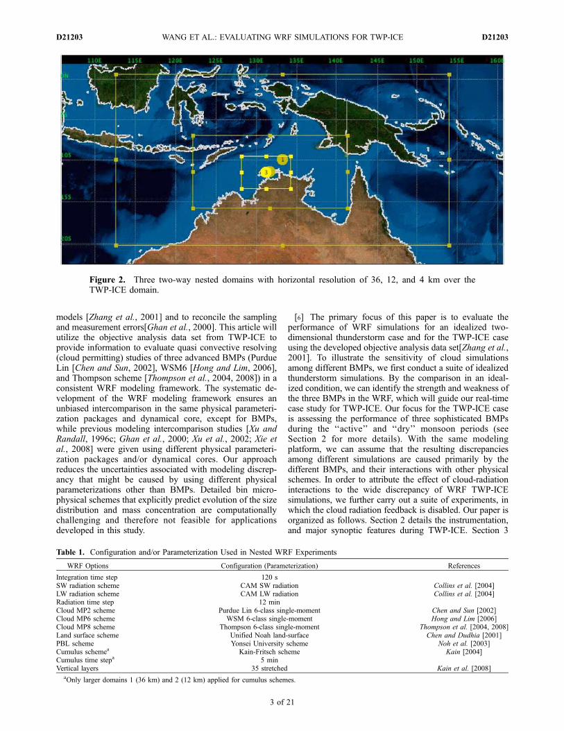
Figure 2. Three two-way nested domains with horizontal resolution of 36, 12, and 4 km over theTWP-ICE domain.

Table 1. Configuration and/or Parameterization Used in Nested WRF Experiments

WRF Options Configuration (Parameterization) References

Integration time step 120 sSW radiation scheme CAM SW radiation Collins et al. [2004]LW radiation scheme CAM LW radiation Collins et al. [2004]Radiation time step 12 minCloud MP2 scheme Purdue Lin 6-class single-moment Chen and Sun [2002]Cloud MP6 scheme WSM 6-class single-moment Hong and Lim [2006]Cloud MP8 scheme Thompson 6-class single-moment Thompson et al. [2004, 2008]Land surface scheme Unified Noah land-surface Chen and Dudhia [2001]PBL scheme Yonsei University scheme Noh et al. [2003]Cumulus schemea Kain-Fritsch scheme Kain [2004]Cumulus time stepa 5 minVertical layers 35 stretched Kain et al. [2008]

aOnly larger domains 1 (36 km) and 2 (12 km) applied for cumulus schemes.


3 of 21

D21203

describes the WRF model and the experimental designs.Section 4 briefly summarizes the major difference among thethree BMPs. Model evaluations are presented in Section 5,with a focus on the performance of the model in simulat-ing cloud ice-phase microphysical properties and thecloud-radiation interactions. Finally, conclusions and futureperspectives are given in Section 6.

2. Tropical Warm Pool International CloudExperiment

[7] TWP-ICE was a large multiagency field campaign,including substantial contributions from the U.S. Depart-ment of Energy’s Atmospheric Radiation Measurement(ARM) Program, U.S. National Aeronautics and SpaceAdministration, the Australian Bureau of Meteorology,and Commonwealth Scientific and Industrial ResearchOrganization. Beginning January 19 and ending February14, 2006, the experiment was located near Darwin, Aus-tralia (Figure 1) and included: 1) the ARM Climate Re-search Facility (ACRF) site, which is fully equipped withsophisticated instruments for measuring cloud and otheratmospheric properties; 2) a fleet of five research aircraft; 3)a research ship located in the Timor Sea west of Darwin; 4)six radiosonde sites launching at 3 hour intervals; 5) a broadcoverage of four surface energy flux sites, including broad-band radiometer measurements; and 6) radar wind andcloud profilers, including a 35 GHz millimeter wavelengthcloud radar (MMCR), a cloud lidar (micropulse lidar), a

microwave radiometer (MWR), and two scanning C bandDoppler radars (C-POL) [Frederick and Schumacher, 2008;May et al., 2008].[8] The timing of TWP-ICE was synchronized with the

onset of the Australian summer monsoon season. FromJanuary 13 to February 2, 2006, the summer monsoon cameacross north Australia [May et al., 2008]. In particular, fromJanuary 13 to 25, ‘‘active’’ monsoon dominated the exper-iment domain with numerous deep convective storms. FromJanuary 26 to February 2, suppressed ‘‘dry’’ monsooncontrolled the experiment domain with relatively shallowstorms, which was followed by three completely clear daysending on February 5, 2006. At the end of TWP-ICE, a‘‘break’’ period occurred from February 6 to 13, 2006. Themaximum daily precipitation (about 100 mm) was recordedat Darwin on January 24 and was closely associated with anovernight mesoscale convection system that developed onJanuary 23. The break period was generated due to an inlandheat trough across north Australia [May et al., 2008]. Thesuccession of these events was associated with a largeamplitude Madden-Julian Oscillation (MJO) [Madden andJulian, 1972, 1994; Zhang, 2005; Y. Wang et al., Convectivesignals from surfacemeasurements at ARMTropicalWesternPacific site: Manus, submitted to Climate Dynamics, 2009].[9] The raw observational data set, including MMCR

retrievals, radiosondes, and surface fluxes, has been com-bined with large-scale background information from theEuropean Centre for Medium-Range Forecasts (ECMWF)operational analysis and satellite measurements using the

Figure 3. (left) One hour snapshot and (right) two hour snapshot of mixing ratios (units g/kg) for snow(shading) and rain (contours) from idealized thunderstorm experiments. Contour levels for MP2, MP6,and MP8 (0.4, 0.8, 1.6, 3.2, and 6.4). The melting line is marked as a thicker, red line.


4 of 21

D21203

constrained variational objective analysis [Zhang et al.,2001] (hereafter referred to as objective analysis). Theobjective analysis data cover the period from January 17to February 12, 2006, and are available at both 25 hpa and10 hpa vertical resolution. The objective analysis domaincan be found in Figure 1 and details of the data set used canbe found at http://acrf-campaign.arm.gov/twpice/. The ob-jective analysis grid points overlap the five boundarysounding stations (Figure 1, blue pentagons) that are avail-able during the field campaign. During TWP-ICE, soundingballoons were launched to measure the vertical profiles oftemperature, relative humidity, and winds every 3 hours atthe five boundary sounding stations from January 22 toFebruary 13, 2006. Soundings also are available every6 hours from the ACRF Darwin site (the center of thedomain). The measured upper air data are first analyzedusing the analysis scheme of [Cressman, 1959] with thebackground field from the ECMWF operational analysis andforecasting system (see http://www.arm.gov/xds/static/ecmwf.stm for details). The domain-averaged surface andtop-of-the-atmosphere fluxes required by the objective anal-ysis are obtained from the TWP-ICE surface and satellitemeasurements (i.e., Japan’s Multifunctional Transport Sat-ellite). Surface precipitation is from the C-POL precipitationradar data [May et al., 2008].[10] The radiative heating profiles are derived following

the methodology of Mather et al. [2007]. Radiosondes,surface temperature, and MWR precipitable water vaporare combined to produce a continuous atmospheric profile

[McFarlane et al., 2007; Mather et al., 2007]. Themeasured radar reflectivity from the MMCR, the liquidwater path from the MWR, and the temperature profilesare used to retrieve cloud ice water content (IWC) [Liu andIllingworth, 2000]. A four-stream correlated k distributionradiative transfer model is used to calculate the radiativeheating given the retrieved cloud properties and atmo-spheric profile. Mather et al. [2007] described the methodand discussed the uncertainty associated with the radiativeheating calculations.[11] The retrieval of ice cloud by the MMCR is affected

by both sensitivity and attenuation of the radar. Undernormal operating conditions, the minimum detectable cloudIWC by the radar is approximately 10�4 gm�3 [Mather etal., 2007], and the MMCR misses a large percentage of thincirrus with optical depths less than 0.1 [Comstock et al.,2007] and clouds above 15 km in the tropics [Comstock etal., 2002]. Prior to TWP-ICE, the MMCR was damaged bya lightning strike, resulting in a loss of sensitivity of 10 to15 dB, which was not detected until after the experiment;thus the minimum detectable IWC was reduced probably toabout 10�3 gm�3 and the MMCR likely missed the top partsof cirrus clouds and thin isolated cirrus, which are oftendominated by smaller ice crystals. The MMCR reflectivityis attenuated also by underlying hydrometeors, especiallyduring heavy precipitation, so the retrieval of cloud IWClikely is underestimated during precipitation. To overcome theuncertainty related to MMCR retrievals, a combined remote

Figure 4. (left) One hour snapshot and (right) two hour snapshot of mixing ratios (units g/kg) forgraupel (shading) and cloud ice (contours) from idealized thunderstorm experiments. Contour levels forMP2, MP6, and MP8 (0.01, 0.05, 0.1, 0.2, and 0.4). The melting line is marked as a thicker, red line.


5 of 21

D21203

sensor retrieval is under development (J. M. Comstock andS. A. McFarlane, personal communication, 2009).[12] Because of the larger uncertainty of the MMCR

retrievals during TWP-ICE, three-dimensional cloud IWCalso is examined [Seo and Liu, 2005, 2006] over the10 degree by 10 degree area centered near the ACRF Darwinsite retrieved by combining ground cloud radar and satellitehigh-frequency microwave measurements. For TWP-ICE,measurements from four satellites (NOAA 15, 16, 17, and18) were used. We averaged the satellite retrieved IWC overan 80 km by 80 km area centered at the ACRF Darwin sitefor a comparison with the MMCR retrieval and modelsimulations.

3. Model Description and Experimental Design

[13] Themodeling framework used in the paper is based onthe Weather Research Forecasting (WRF, version 3) model,developed at the National Center for Atmospheric Research(NCAR) [Michalakes et al., 2001, 2005; Skamarock et al.,2005; Skamarock and Klemp, 2008], with support frommultiple partners (the National Centers for EnvironmentalPrediction (NCEP) and the Forecast Systems Laboratory ofthe National Oceanic and Atmospheric Administration

(NOAA), Air Force Weather Agency, and Naval ResearchLaboratory). The WRF is a community model suitable forboth research and forecasting. The dynamical core of WRFis based on the fully compressible, nonhydrostatic Eulerequations, with terrain following Eta coordinate [Skamarocket al., 2005]. The model has been used in weather forecast-ing [Hong et al., 2004; Hong and Lim, 2006; Xiao et al.,2008], ice cloud microphysical studies[Thompson et al.,2004, 2008; Morrison et al., 2009], and regional climateresearch [Leung et al., 2006; Lo et al., 2008]. The WRFnonhydrostatic dynamical core is intended for studies ofhigh-resolution (250–1000 meters) simulations with thecapability to explicitly resolve convections and cloudiness.The WRF model can be nested so that the high-resolutiondomain can be forced both by the model output from coarse-resolution domain and observational reanalyses. Associatedwith the development of WRF nonhydrostatic dynamicalcore is the testing and implementing of eight advancedBMPs as of December 2008 [Kessler, 1969; Lin et al., 1983;Chen and Sun, 2002; Hong et al., 2004; Hong and Lim,2006; Thompson et al., 2004, 2008; Morrison et al., 2009;Tao et al., 2003]. These BMPs include the Kessler [Kessler,1969], Purdue Lin [Chen and Sun, 2002], Ferrier (newETA), WSM3, WSM5, WSM6 [Hong et al., 2004; Hong

Figure 5. (left) The hydrometeor paths (kg m�2) and (right) precipitable water (PW, red, centimeters)and rain rate (RR, blue, mm/10min) from idealized thunderstorm experiments. The thicker dashed lines inthe hydrometeor path plots represent the sum of hydrometeor paths of cloud water (QC, black), rain (QR,orange), graupel (QG, green), snow (QS, blue), and cloud ice (QI, red).


6 of 21

D21203

and Lim, 2006], Thompson [Thompson et al., 2004, 2008],Morrison Schemems [Morrison et al., 2009], and improvedGoddard microphysics (MP) [Tao et al., 2003]. For thefollowing experiments, we will focus on three single-moment (only predicting mixing ratios of six-class hydro-meteors) BMPs, namely, Purdue Lin [Chen and Sun, 2002],WSM6 [Hong and Lim, 2006], and Thompson scheme[Thompson et al., 2004, 2008], which are referred asMP2, MP6, and MP8, respectively, herein.

3.1. Idealized Simulations

[14] The WRF model is well adapted for idealized sim-ulations to study baroclinic waves, thunderstorm dynamics,or topographically induced flows. The idealized 2D thun-derstorm experiment is set up to simulate a high-instability(high-CAPE) continental-type structure storm, and isdesigned to systematically distinguish the essential differ-ences among the three BMPs by fixed initial conditions and

the absence of other nonmicrophysical processes, which inturn will help understand the impact of changes in themicrophysics in the 3D framework. We choose a 2D domainin the X direction (east-west). The grid in this direction iscomprised of 201 points with a 250 m grid spacing. Thenumber of vertical layers is 80 stretching up to 20 hpa. Themodel is integrated for 2 hours with a timestep of 3 seconds.The initial condition includes a warm bubble with a 4 kmradius and a maximum perturbation of 3 K at the center ofthe domain. Awind with a velocity of 12 ms�1 is applied inthe positive x direction at the surface; the surface winddecreases to zero at 2.5 km above ground, with no windabove. Open boundary conditions are applied, and there isno Coriolis force or friction. The only physical parameter-ization is the microphysical scheme, and other physicalprocesses including radiation, vertical diffusion, land sur-face, and deep convection due to the cumulus parameteri-zation scheme are turned off. This experiment serves to

Figure 6. (left) First-hour and (right) second-hour mean profiles of mixing ratios for cloud water (QC,orange marks), rain (QR, green marks), graupel (QG, blue marks), snow (QS, red marks), and cloud ice(QI, black marks) from idealized thunderstorm experiments. Units are 10 g/kg for cloud water (QC) andcloud ice (QI) and g/kg for rain (QR), graupel (QG), and snow (QS).


7 of 21

D21203

demonstrate the microphysics in a quasi steady state (large-scale) that simplifies the interpretation of the results.Although we realize that the idealized simulations may bedifferent in some respects from tropical environment, thispart of the experimental design is intended to evaluateprimarily ice-phase microphysical differences from a differ-ent and simpler perspective.

3.2. TWP-ICE Simulations

[15] The two-way nested experiment is designed to sim-ulate the real-time case of TWP-ICE. We have chosen threedomains with horizontal resolutions of 36, 12, and 4 km(Figure 2). The 4 km domain covers an area of 1152 km(east-west) by 636 km (north-south) larger than the TWP-ICE domain of objective analysis (Figure 1). Based on

previous experiences, continuous integration with a singleinitialization and updated lateral and lower boundary con-ditions (LLBC) has caused the unrealistic drifting of large-scale environment. Therefore, we set up to run WRF forevery three days and only save the last two day modeloutput. This consecutive integration with frequent reinitial-izations for every three days with continuously updatedLLBC ensures a realistic large-scale environment and hencea favorable comparison between model and observation.The large-scale LLBC is given by the 1 degree NCEPGlobal Final Analysis and sea surface temperature (SST)from real-time, global SST analysis (RTG-SST, http://polar.ncep.noaa.gov/sst/oper/Welcome.html). A recent study [Loet al., 2008] indicates that the reinitialized experimentincreases the utilization of the large-scale coarse-resolution

Figure 7. Cloud fraction comparison from the objective analysis and WRF TWP-ICE simulations. Ontop of cloud fraction (no unit, shading), we also plot the water vapor mixing ratio (g/kg) in contour levelsof 1, 2, 4, 8, and 16.


8 of 21

D21203

data during the model integration, and hence, could generaterealistic regional structures not resolved by the coarse-resolution forcing data. Table 1 lists detailed model MP,shortwave (SW) and longwave (LW) radiation, surfacelayer, planetary boundary layer (PBL) schemes, and otherintegration options.[16] Regarding the selection of horizontal and vertical

resolutions of our TWP-ICE simulations, we have consid-ered results from a recent study by Kain et al. [2008]. It hasbeen shown that during the 2005 NOAA Hazardous Weather

Testbed Spring Experiment two different high-resolutionconfigurations of WRF model were used to produce 30 hourforecasts 5 days a week for a total of 7 weeks. Except for thedifferent horizontal (i.e., 4 km and 2 km) and vertical (i.e.,35 level and 51 level) resolutions, other physical parame-terization packages and the input data set for the LLBC arethe same. In general, the 2 km forecasts provide moredetailed presentations of convective activity, but thereappears to be little improvement of forecast skill on thescales where the added details emerge. Their results further

Figure 8. Cloud IWC comparison from the MMCR and satellite retrievals and WRF TWP-ICEsimulations. On top of cloud IWC (10�3 gm�3, shading), we also plot the air temperature (degreesCelsius) in contour levels of 0, �20, �40, and �60.


9 of 21

D21203

suggest that the added values provided by decreasing thegrid space from 4 to 2 km (with commensurate adjustmentsto the vertical resolution) may not be worth the considerableincreases in computational expenses. To study the effect ofthe feedbacks that occur due to the interactions between theradiation schemes and cloud MP, we further carry out a suiteof experiments, in which the interactions between the BMPsand radiation schemes are turned off. This suite of experi-ments is called ‘‘TWP-ICE RAD’’ simulations.[17] The model has been integrated from January 16 to

February 17, 2006, to overlap with the period of TWP-ICE,and compared with the TWP-ICE objective analysis fromJanuary 17 to February 13, 2006, for the high-resolution(4 km) domain. The 4 km domain outputs were sampledevery hour, and averaged over the ACRF Darwin site for anarea of 80 km by 80 km (20 by 20 grid boxes). We also havelinearly interpolated the model outputs to the pressure and/or height levels of the objective analysis and/or retrievals.For the MMCR retrieved IWC, and SW, and LW radiativeheating profiles, we compared model output directly withretrievals every hour and calculated the root-mean-squareerror (RMSE) and biases. For other variables, we averagedthe hourly model output to 3 hour intervals to be comparedwith the objective analysis at the same timescale andcalculated the RMSE and biases.

[18] The cloud fraction as used in the radiation calcula-tion is parameterized in the WRF model, as well as in otherclimate models (see Xu and Krueger [1991] and Xu andRandall [1996a] for a review on this topics). The formula-tion of this parameterization is based on the work of Xu andRandall [1996b]. In brief, equation 1 of Xu and Randall[1996b] is adapted to estimate the cloud fraction used in theWRF radiation calculation. The subdomain-averaged cloudwater, water vapor, cloud ice and snow mixing ratios areused to derive the primary predictor (Ql in their equation 1)for cloud fraction. The critical (saturation) vapor pressuresderived from the work of Murray [1967] are used toestimate the relative humidity with respect to water andice. Because the Murray formulation introduces large biaseswhen temperature drops below around �40�C to �60�C,we suggest that this may cause problems in estimating high-level (low temperature) thin cirrus clouds as in the TWP-ICE case. A future paper on this direction is in preparation.

4. Brief Comparison of Purdue Lin, WSM6,and Thompson BMPs

[19] Purdue Lin BMP is based on the original Linmicrophysical scheme [Lin et al., 1983] with some mod-ifications [Chen and Sun, 2002]. The WSM6 BMP wasdeveloped by adding processes related to the graupel

Figure 9. Snow contents (10�3 gm�3, shading) from WRF TWP-ICE simulations for (a) Purdue LinBMP, (b) WSM6 BMP, and (c) Thompson BMP.


10 of 21

D21203

species into the WSM5 BMP [Hong and Lim, 2006]. TheWSM6 scheme improves rainfall simulations at high reso-lutions [Hong and Lim, 2006]. A detailed description ofWSM6 BMP is given by Hong and Lim [2006]. ThompsonBMP has been developed continuously and tested at NCAR[Thompson et al., 2004, 2008]. The Thompson schemeincorporates many improvements to the physical processes,it employs many techniques found in more sophisticatedspectral/bin microphysical schemes (e.g., using lookuptables). Unlike any other BMPs, the assumed snow sizedistribution in the Thompson scheme depends on both icewater content and temperature, and is represented as a sumof exponential and gamma functions. Furthermore, snowassumes a nonspherical shape with a bulk density that variesinversely with diameter as derived from observations. Thisis in contrast to nearly all other BMPs that assume sphericalsnow with constant density [Thompson et al., 2008]. Basedon four idealized sensitivity experiments [Thompson et al.,2008], it was found that the sphericity and constant densityassumptions play a major role in producing supercooledliquid water while the prescribed distribution shape plays alesser, but nonnegligible role.[20] The uniqueness of the Thompson scheme is that it

also predicts the number concentration of cloud ice. As adouble-moment species, cloud ice has differential sedimen-tation by the mixing ratios and number concentration using

their respective mass-weighted and number-weighted termi-nal velocities [Thompson et al., 2008]. Due to the potentialimbalance between mass and number concentration, cloudice number is constrained such that its mass-weighted meansize is bound between 30 and 300 microns. Because otherBMPs in the study do not include this quantity, we havechosen not to analyze the number concentration of cloud icefrom the Thompson scheme. Nevertheless, in all threeBMPs, the six-class prognostic water substance includesthe mixing ratios of water vapor (QV), cloud water (QC),cloud ice (QI), snow (QS), rain (QR), and graupel (QG).The most important difference in these three BMPs is thetreatment of ice-phase microphysical processes. The WSM6scheme treats the ice crystal number concentration (NI) as afunction of QI amount, and the ice nuclei number concen-tration (NI0) is separated from the NI [Hong and Lim,2006]. The Purdue Lin scheme uses the formula of Fletcher[1962] for both NI and NI0. The snow intercept parameter inthe WSM6 scheme is a function of temperature [Houze etal., 1979]. A detailed comparison of the WSM6 and PurdueLin schemes is given by Hong et al. [2009]. A generalizedgamma distribution shape is employed for each watersubstances (hydrometeor species, except for snow). The Yintercept of QG depends on the graupel mixing ratio[Thompson et al., 2008]. The terminal velocity constantsfor graupel are taken directly from Heymsfield and Kajikawa

Figure 10. Graupel contents (10�3 gm�3, shading) from WRF TWP-ICE simulations for (a) Purdue LinBMP, (b) WSM6 BMP, and (c) Thompson BMP.


11 of 21

D21203

[1987]. These constants cause low mixing ratios of graupelto fall roughly twice as fast as snow (see Thompson et al.[2008, Figure A1] for terminal velocities of QI, QS, QG,and QR). Since the number concentration of QI is predicted,its shape parameter is the only free parameter that needs tobe preset.

5. WRF Model Evaluations

5.1. Idealized Thunderstorm Simulations

[21] We show here the one hour and two hour snapshotsfrom the idealized thunderstorm for snow and rain mixingratios (Figure 3), and for graupel and cloud ice mixing ratios

(Figure 4). It is very clear that the Purdue Lin BMPproduces much less snow and graupel (shadings) than theWSM6 and Thompson BMPs. Among other differences, theWSM6 scheme produces much larger graupel than theThompson scheme, while the Thompson scheme producesmuch larger snow than the WSM6 scheme. For cloud ice(contours), Purdue Lin and WSM6 schemes have approxi-mately the same magnitudes, which are slightly larger thanthat produced by the Thompson scheme. However, for rain(contours), the Purdue Lin scheme has a much smalleramount compared to the other two BMPs at the one hourand two hour snapshots.

Figure 11. RMSEs (solid curves) and biases (dashed curves) of (a and b) temperature (K), (c and d)water vapor (g/kg), and (e and f) cloud fraction (percentage) for two periods of WRF TWP-ICEsimulations, for (left) ‘‘active’’ monsoon and (right) ‘‘dry’’ monsoon, with respect to three BMPs.


12 of 21

D21203

[22] To further study the time evolution of the 6-classwater substances, we derived the domain-averaged hydro-meteor paths for QC, QR, QG, QS, and QI by integratingthe corresponding values in the vertical direction andaveraging over the entire domain (Figure 5). The totalhydrometeor path (TOT, unit kg m�2) is derived by addingthe hydrometeor paths for QC, QR, QG, QS, and QI. Wealso derive the domain-averaged precipitable water (PW,unit cm) and rain rate (RR, unit mm per 10 minute) for thesethree BMPs. The hydrometeor path plot (Figure 5, left)clearly indicated the wide discrepancy, in particular, for ice-phase species (i.e., QG, green curves, QS, blue curves, andQI, red curves). Consistent with the findings in Figures 3and 4, we notice that the WSM6 scheme has the largestgraupel peak values, while the Thompson scheme has theleast graupel peak values during the two hour integration.On the other hand, the Thompson scheme produces thelargest snow values among the three BMPs over thedevelopment of thunderstorms. At the end of the two hourexperiment, the Purdue Lin scheme has minimum values forthe total hydrometeor path (TOT, thicker, dashed blackcurves). This also is reflected in the precipitable water andrain plot (Figure 5, right). Overall the largest rain rate isfound in the Thompson scheme, while the Purdue Lin andWSM6 schemes produce similar peak rain rate valuesduring the two hour integration.[23] To study the vertical distributions of QC (unit 10 g/kg),

QR (unit g/kg), QG (unit g/kg), QS (unit g/kg), and QI (unit

10 g/kg), we also plot the domain-averaged mixing ratiosfor these values (Figure 6) for first-hour mean (Figure 6,left) and second-hour mean (Figure 6, right). To focus onthe ice-phase species, we notice that snow (red marks) staysat the highest values (at about 9 km above ground level,AGL) in the Thompson scheme. On the other hand, graupel(blue marks) stays at the highest values (at abut 8 km AGL)in the WSM6 scheme. (Graupel in the Purdue Lin schemealso has a relative high value at about 7 km AGL.) Withrespect to QI (black marks), the Purdue Lin and WSMschemes have similar profiles, while the Thompson schemeproduces two to four times smaller values. In the Thompsonscheme, snow forms by vapor deposition growth onto cloudice particles until those ice crystals grow beyond a thresholdsize (currently 200 microns). The threshold itself is rela-tively arbitrary and certainly artificial but allows for slowlyfalling tiny ice crystals to coexist with more rapidly fallingsnow. We believe that this threshold value may cause arelatively small QI category compared to those of the othertwo BMPs.

5.2. TWP-ICE Simulations

[24] The continuous time series of domain-averagedcloud fraction profiles over the entire TWP-ICE periodillustrates some weaknesses in the model simulations(Figure 7). The three BMPs almost totally miss the firstconvective system during the first couple days of TWP-ICE.According to observations, this first convective system is

Figure 12. RMSEs (solid curves) and biases (dashed curves) of cloud IWC (10�3 gm�3) (a and b) fromthe MMCR retrieval and (c and d) from the satellite retrieval for two periods of WRF TWP-ICEsimulations, for (left) ‘‘active’’ monsoon and (right) ‘‘dry’’ monsoon, with respect to three BMPs.


13 of 21

D21203

associated with a strong MJO event passing northernAustralia. Large-scale forcing data might miss this criticalMJO signal, hence could not provide a favorable conditionto initiate the first convection. Around January 23–25, threeBMPs reproduce the major feature of deep convection.Furthermore, the Thompson scheme seems to overestimatethe high cirrus cloudiness. This might be due to theoverestimation of snow mixing ratio (QS) as found inprevious idealized simulations. Overall, the largest biascan be found in two areas: 1) precipitating clouds and 2)high-level cirrus clouds (above 14 km). As we discussedearlier, the MMCR retrievals of cloud suffer two major

problems during the TWP-ICE. First, precipitating cloudsare underestimated because of large radar signal returns bythe large raindrops. High-level, thin cirrus clouds (low cloudoptical depth) are underestimated due to the undetectedlightening strike damage that occurred briefly before theTWP-ICE [Mather et al., 2007; McFarlane et al., 2007].[25] The accurate retrieval of cloud IWC is an active area

of research. The retrieval of cloud IWC might be affected bythe above mentioned issues (e.g., reduced sensitivity ofMMCR, precipitating clouds). To constrain the uncertaintyassociated with theMMCR retrievals of cloud IWC (Figure 8),we also derive the domain-averaged (80 by 80 km

Figure 13. RMSEs (solid curves) and biases (dashed curves) of cloud (a and b) SW, (c and d) LW, and(e and f) net radiative heating (K/day) for two periods of WRF TWP-ICE simulations, for (left) ‘‘active’’monsoon and (right) ‘‘dry’’ monsoon, with respect to three BMPs.


14 of 21

D21203

surrounding the ACRF Darwin site) satellite retrieved cloudIWC from a combination of satellite and surface observa-tions [Seo and Liu, 2005, 2006]. As noticed above, the firstconvective system is missing in all three BMPs. Except forthe Thompson scheme, the other two BMPs capture themain feature of cloud IWC. Previous idealized simulationshave identified that the Thompson scheme underestimatesthe cloud ice (QI). This may help to understand why theIWC in the Thompson scheme is so low. Furthermore, largebiases exist among MMCR (model simulations) and satelliteretrievals. We suggest these large biases might be causedby different vertical and horizontal resolutions amongmodels and two observations. Overall, model simulationsare closer to MMCR retrieved cloud IWC than satellitederived values.[26] To compare the ice-phase properties with idealized

thunderstorm simulations, we also plot the snow (Figure 9)and graupel (Figure 10) contents for the ‘‘active’’ and ‘‘dry’’monsoon periods from the WRF TWP-ICE simulation. It isvery clear that the Thompson scheme produces the maxi-mum snow content, while the Purdue Lin scheme producesthe minimum snow content among the three BMPs (Figure 9).This corresponds quite well with the results from idealizedthunderstorm simulations (see Figures 3, 5, and 6), wherethe snow hydrometeor path contributes more than 50% ofthe total hydrometeor path at the end of the two hour

simulation (see Figure 5 for MP8). On the other hand, theWSM6 scheme produces the maximum graupel content,while the minimum graupel is produced by the Thompsonscheme (Figure 10). Again, this corresponds quite well withresults from idealized thunderstorm simulations (see Figures 4,5, and 6), where the graupel hydrometeor path contributesover 60% of the total hydrometeor path at the end of the twohour simulation (see Figure 5 for MP6). The above simi-larities among two suites of simulations (i.e., idealizedsimulations and TWP-ICE simulations) indicates stronglythat the importance of ice-phase cloud MP in contributing tothe wide discrepancy of simulated differences among icespecies (e.g., cloud ice, snow, graupel), while the interac-tions between the ice-phase cloud MP and other schemesplay less important roles.[27] To generate a consolidated view of model observa-

tion intercomparison, we plot the RMSE and biases fortemperature, water vapor, and cloud fraction (Figure 11)between WRF simulations and TWP-ICE objective analysisfor ‘‘active’’ and ‘‘dry’’ monsoon periods during the TWP-ICE. During the ‘‘active’’ monsoon period, the modelgenerally overestimates the temperature within the bound-ary layer (i.e., below 1.5 km) and above the tropopause (i.e.,above 13.5 km). In between, the temperature biases arewithin the range of ±0.5K (Figure 11a). This is reflectedalso in the RMSE profiles of temperature. For water vapor

Figure 14. Difference in cloud fraction between TWP-ICE RAD and TWP-ICE simulations for(a) Purdue Lin BMP, (b) WSM6 BMP, and (c) Thompson BMP. Cloud fractions are unitless.


15 of 21

D21203

(Figure 11c), the model generally underestimates the watervapor below 9 km. The largest biases and RMSE are foundat about 1.0 km. The cloud fraction also is underestimatedby the model (Figure 11e) under about 6 km. From 6 kmand above, the largest discrepancy could be found amongthe three BMPs. We believe that this is contributed primar-ily by the ice-phase cloud microphysics. In particular, theThompson scheme greatly overestimates cloud fraction upto 40% above 9 km, while the other two BMPs only slightlyoverestimate cloud fraction up to 15%. As mentionedbefore, the Thompson scheme could overestimate the snowcontent, and hence produce a large bias in cloud fractionused in radiation calculations. This is because the adaptedparameterization of cloud fraction [Xu and Randall, 1996b]only takes into account cloud water, cloud ice, and snow(i.e., graupel is not considered). During the ‘‘dry’’ monsoonperiod, temperature and cloud fraction biases are muchsmaller than the ‘‘active’’ monsoon period (Figure 11b)except, that at about 13 km, a strong underestimatedtemperature is found in line with the cooling caused bythe overestimated cirrus clouds in the model (Figure 11f).For water vapor (Figure 11d), the model systematicallyunderestimates it within boundary layers (i.e., below 2 km),and overestimates it between 2 and 6 km with a maximumbias at about 4 km.

[28] During the ‘‘active’’ monsoon period, the modelunderestimates cloud IWC between 4 and 10 km comparedto MMCR retrievals (Figure 12a). Compared with satelliteretrieved cloud IWC, the model underestimates cloudIWC between 5 and 14 km (Figure 12c). Overall, thedifference between model and satellite is 5 times largerthan that between the model and MMCR during the ‘‘ac-tive’’ monsoon period. During the ‘‘dry’’ monsoon period,this difference is much smaller among model simulations,MMCR, and satellite retrievals (Figures 12b and 12d).Overall, the cloud IWC error is 10–50 times smaller duringthe ‘‘dry’’ monsoon period than during the ‘‘active’’ mon-soon period. We suggest this might be caused by threecritical points. First, the MMCR retrieval is attenuated byprecipitating clouds during the ‘‘active’’ monsoon period,while this is not true for the ‘‘dry’’ monsoon period. Second,the cloud overlapping may contribute to the overall largerbias in satellite retrievals, while during the ‘‘dry’’ monsoonperiod, this overlap is reduced substantially. Finally, theinteractions between cloud microphysical and other physicalschemes may contribute to the overall larger discrepancyduring the ‘‘active’’ monsoon periods, while these interac-tions are decreased substantially during the ‘‘dry’’ monsoonperiod due to less interacting processes in the model andreality.

Figure 15. The difference in cloud IWC between TWP-ICE RAD and TWP-ICE simulations for(a) Purdue Lin BMP, (b) WSM6 BMP, and (c) Thompson BMP. Cloud IWC has a unit of 10�3 gm�3.


16 of 21

D21203

[29] The radiative heating profile reflects the interactionbetween cloud microphysics and radiation schemes. OverallLW heating biases (Figures 13c and 13d) dominate the netheating biases profiles during both the ‘‘active’’ and ‘‘dry’’monsoon periods because the magnitudes of LW heatingerrors are 2–4 times larger than those of SW heating errors(Figures 13e and 13f). In particular, the SW heating isunderestimated between 4 and 10 km during the ‘‘active’’monsoon period, while it is overestimated slightly between2 and 10 km during the ‘‘dry’’ monsoon period. For LWheating, overall it is overestimated during the ‘‘active’’monsoon period while underestimated during the ‘‘dry’’monsoon period. Large discrepancies can be found for bothcloud macrophysical (cloud fraction, cloud base and topheights) and microphysical (cloud liquid and ice watercontents) states among model simulations. These discrep-ancies may be caused by the cloud BMP itself, or may alsobe caused by the interactions between cloud BMP and otherphysical schemes (e.g., radiation scheme). To further isolateone of the most important feedbacks between cloud micro-physics and radiation scheme, we have carried out anothersuite of WRF simulations, in which we have turned off theinteraction between the cloud BMP and radiation schemes.

5.3. TWP-ICE RAD Simulations

[30] Figure 14 shows the cloud fraction difference be-tween TWP-ICE RAD and TWP-ICE simulations (former

minus latter). It is clear that overall the cloud fraction is notchanged too much when we turn off the cloud radiationfeedback (Figure 14). However, during the strongest ‘‘ac-tive’’ monsoon period, the Purdue Lin BMP cloud fraction(Figure 14a) is perturbed strongly without the cloud radia-tion feedback. While for the other two BMPs, the change incloud fraction is much smaller during the same period(Figures 14b and 14c). In particular, the cirrus cloud fractionin the Thompson scheme has changed quite a bit before andafter the strongest convective event (January 23–25). How-ever, compared to the wide discrepancies of cloud fractionamong the three BMPs (see Figure 7), the difference incloud fraction is pretty small. The Purdue Lin scheme seemsto be a bit more sensitive to cloud radiation feedbackcompared to the other two BMPs.[31] Figure 15 shows the cloud IWC difference (units

10�3 gm�3) between TWP-ICE RAD and TWP-ICE simu-lations (former minus later). Consistent with Figure 14, thecloud IWC has not changed much between the TWP-ICERAD and TWP-ICE simulations. This is particularly true forthe Thompson scheme, which has produced the minimumcloud IWC among three BMPs (see Figure 8 for WRFMP8). While during the strongest ‘‘active’’ monsoon period,both the Purdue Lin (MP2) and WSM6 (MP6) schemesshow some changes in cloud IWC. In particular, consistentwith the higher sensitivity in cloud fraction, the Purdue Lin

Figure 16. The difference in snow water content for (a) Purdue Lin BMP, (b) WSM6 BMP, and(c) Thompson BMP. Snow water content has a unit of 10�3 gm�3.


17 of 21

D21203

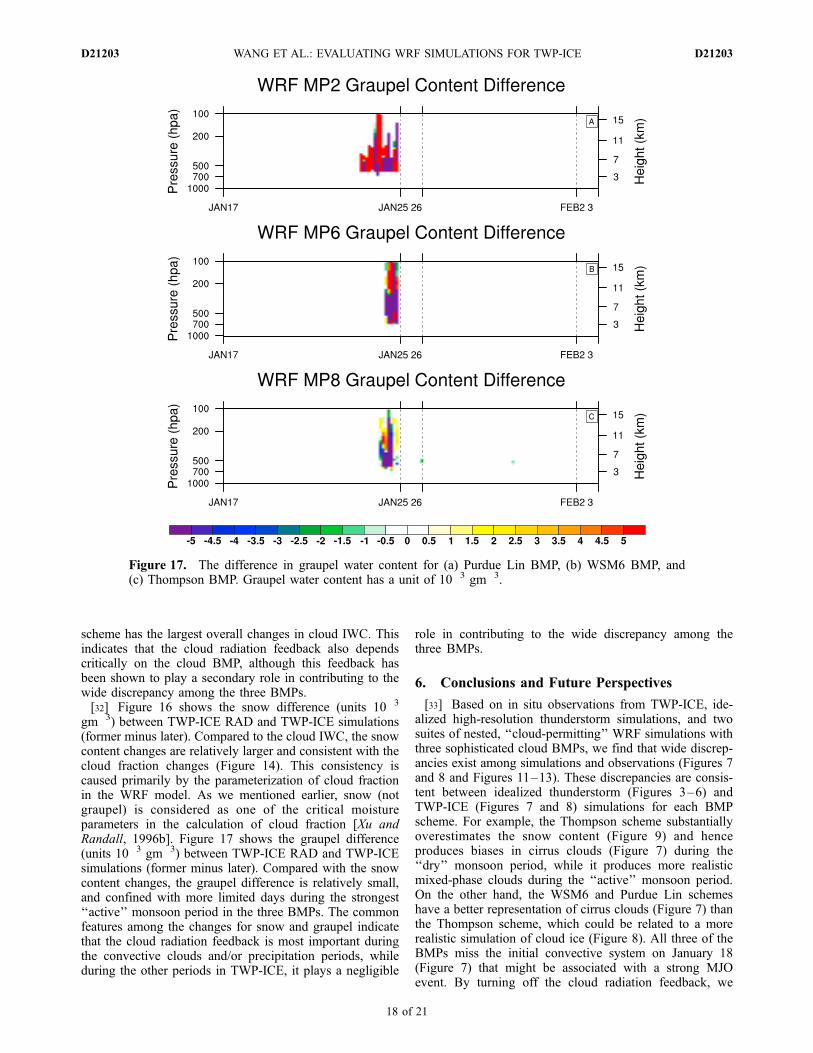
scheme has the largest overall changes in cloud IWC. Thisindicates that the cloud radiation feedback also dependscritically on the cloud BMP, although this feedback hasbeen shown to play a secondary role in contributing to thewide discrepancy among the three BMPs.[32] Figure 16 shows the snow difference (units 10�3

gm�3) between TWP-ICE RAD and TWP-ICE simulations(former minus later). Compared to the cloud IWC, the snowcontent changes are relatively larger and consistent with thecloud fraction changes (Figure 14). This consistency iscaused primarily by the parameterization of cloud fractionin the WRF model. As we mentioned earlier, snow (notgraupel) is considered as one of the critical moistureparameters in the calculation of cloud fraction [Xu andRandall, 1996b]. Figure 17 shows the graupel difference(units 10�3 gm�3) between TWP-ICE RAD and TWP-ICEsimulations (former minus later). Compared with the snowcontent changes, the graupel difference is relatively small,and confined with more limited days during the strongest‘‘active’’ monsoon period in the three BMPs. The commonfeatures among the changes for snow and graupel indicatethat the cloud radiation feedback is most important duringthe convective clouds and/or precipitation periods, whileduring the other periods in TWP-ICE, it plays a negligible

role in contributing to the wide discrepancy among thethree BMPs.

6. Conclusions and Future Perspectives

[33] Based on in situ observations from TWP-ICE, ide-alized high-resolution thunderstorm simulations, and twosuites of nested, ‘‘cloud-permitting’’ WRF simulations withthree sophisticated cloud BMPs, we find that wide discrep-ancies exist among simulations and observations (Figures 7and 8 and Figures 11–13). These discrepancies are consis-tent between idealized thunderstorm (Figures 3–6) andTWP-ICE (Figures 7 and 8) simulations for each BMPscheme. For example, the Thompson scheme substantiallyoverestimates the snow content (Figure 9) and henceproduces biases in cirrus clouds (Figure 7) during the‘‘dry’’ monsoon period, while it produces more realisticmixed-phase clouds during the ‘‘active’’ monsoon period.On the other hand, the WSM6 and Purdue Lin schemeshave a better representation of cirrus clouds (Figure 7) thanthe Thompson scheme, which could be related to a morerealistic simulation of cloud ice (Figure 8). All three of theBMPs miss the initial convective system on January 18(Figure 7) that might be associated with a strong MJOevent. By turning off the cloud radiation feedback, we

Figure 17. The difference in graupel water content for (a) Purdue Lin BMP, (b) WSM6 BMP, and(c) Thompson BMP. Graupel water content has a unit of 10�3 gm�3.


18 of 21

D21203

notice that the ice-phase cloud microphysics play the mostimportant role in contributing to the wide discrepancies,while the interaction between cloud and radiation takes thesecondary, but nonnegligible role (Figures 14–17). Thecloud-radiation interaction is most important during theconvective precipitating periods of TWP-ICE for all threeBMPs (Figure 14). It is shown that the cloud radiationfeedback is quite sensitive to the ice-phase cloud micro-physical scheme as well (Figure 15).[34] We suggest the early systematic errors in model

simulations might be related to the forcing data based onlarge-scale (1 degree) NCEP real-time analysis. It is wellknown that in tropical regions, due to the lack of observa-tional data, the largest bias is expected in our forcing data.In particular we believe that the critical MJO signal may bemissing or delayed in the forcing data from NCEP so thatthe initial convective period is not well simulated by allthree of the BMPs. In the future, we will develop amultiyear combined real-time analysis data set so that themodel biases introduced by the large-scale forcing may beeliminated (J. Dudhia and L. R. Leung, personal commu-nication, 2008).[35] On the other hand, the cloud macrophysical and

microphysical retrievals from ground-based remote sensingand satellite suffer from a few caveats. First, the satellitedata have coarse temporal and spatial resolutions comparedto model and ground-based remote sensing. Second, thesatellite data have the largest bias under cloud overlappingconditions because the sensor onboard cannot penetratethicker clouds. Third, the ground-based remote sensingsuffers from the precipitating clouds due to the attenuationof radar signals. Finally, the higher, thinner cirrus cloudshave the weakest radar signals and may not be detectable.This is particularly true because the MMCR used during theTWP-ICE was damaged by a lightening strike before theexperiment. This damage caused a 10 times less sensitivityand was found only after the TWP-ICE.[36] In addition, it is also well known that the crucial

techniques to retrieve the cloud liquid and ice microphysicalproperties are still active areas of research and have a widerange of uncertainties [Comstock et al., 2007]. For a faircomparison with sophisticated cloud microphysical schemesas used in the paper, we need to test and develop advancedapproaches to characterize the detailed cloud liquid and iceproperties under conditions such as precipitating and thincirrus clouds. Furthermore, the overestimation of cirrusclouds in model simulations may be related to biases inestimated saturation vapor pressure and relative humiditydue to the cold temperature. When the temperature dropsbelow minus 40�C, the calculation of saturation vaporpressure can have a bias of more than 20% [Murray, 1967].[37] Clouds are an integral part of the climate system.

Through their influence on radiation, atmospheric heating/moistening effects, and precipitation, clouds regulate thewater and energy cycles of the climate system. Improvingthe representation of tropical clouds has been identified asthe primary uncertainty in accurately predicting the radia-tion budget in climate models [Wielicki et al., 2002].Tropical convective systems and their associated cloudscan persist for days and spread over thousands of kilo-meters, and hence have a large radiative impact in theregion. Therefore, an improved understanding of the multi-

scale structure of tropical clouds and their interactions withthe environment is critical to observational and modelingcommunities. The TWP-ICE provided, for the first time, asuite of observational data sets that can be used in modelevaluations and parameterization development.[38] Overall, TWP-ICE was focused on clouds, in partic-

ular, deep convective clouds, their life cycle and interactionswith radiation and large-scale dynamics. In particular, wefind that deep convective clouds generally are formed laterin the model (at 4 km resolution) and last longer after theirformation than observations show (Figure 7). These issuesmay be related to the threshold behavior of the explicitcloud BMP. In particular, most cloud BMPs [Chen and Sun,2002; Hong and Lim, 2006; Thompson et al., 2004, 2008]are designed to study midlatitude, continental cloud systems(more observations available), and may not have beenapplied in the tropical environment before. To realisticallysimulate convective clouds and their life cycle in thetropical environment is an active and challenging field ofresearch.

[39] Acknowledgments. This work has been supported by theClimate and Environmental Science Division of the U.S. Department ofEnergy (DOE) as part of the Atmospheric Radiation Measurement (ARM)Program. Y. Wang is supported also by K. C. Wong Education Foundationof Chinese Academy of Sciences. X. Liu is supported by the NSFCNational Excellent Young Scientists Fund (40825008). Satellite retrievalof cloud ice water content is kindly provided by G. Liu. During the courseof our research, we have benefited from discussions with S.-C. Xie, P. May,P. Minnis, S.-Y. Hong, G. Thompson, H. Morrison, and the WRF modeldeveloping team. The WRF model simulations were carried out at theNational Energy Research Scientific Computing Center and ArgonneLeadership Computing Facility of the U.S. DOE and at EMSL, a nationalscientific user facility sponsored by the U.S. DOE’s Office of Biologicaland Environmental Research located at the Pacific Northwest NationalLaboratory.

ReferencesChen, F., and J. Dudhia (2001), Coupling and advanced land surfacehydrology model with the Penn State-NCAR MM5 modeling system.Part I: Model implementation and sensitivity, Mon. Weather Rev., 129,569–585.

Chen, S. H., and W. Y. Sun (2002), A one-dimensional time dependentcloud model, J. Meteorol. Soc. Jpn., 80, 99–118.

Collins, W. D., et al. (2004), Description of the NCAR Community Atmo-sphere Model (CAM3.0), Tech. Note TN-464+STR, 226 pp., Natl. Cent.for Atmos. Res., Boulder, Colo.

Comstock, J. M., T. P. Ackerman, and G. G. Mace (2002), Ground-basedlidar and radar remote sensing of tropical cirrus clouds at Nauru Island:Cloud statistics and radiative impacts, J. Geophys. Res., 107(D23), 4714,doi:10.1029/2002JD002203.

Comstock, J. M., et al. (2007), An intercomparison of microphysical retrie-val algorithms for upper-tropospheric ice clouds, Bull. Am. Meteorol.Soc., 88, 191–204, doi:10.1175/BAMS-88-2-191.

Cressman, G. P. (1959), An operational objective analysis scheme, Mon.Weather Rev., 87, 367–374.

Fletcher, N. H. (1962), The Physics of Rain Clouds, Cambridge Univ. Press,Cambridge, U. K.

Frederick, K., and C. Schumacher (2008), Anvil characteristics as seen byC-POL during the Tropical Warm Pool International Cloud Experiment(TWP-ICE), Mon. Weather Rev., 136, 206 – 222, doi:10.1175/2007MWR2068.1.

Ghan, S., et al. (2000), A comparison of single-column model simulationsof summertime midlatitude continental convection, J. Geophys. Res.,105, 2091–2124.

Grabowski, W. W., X. Wu, M. W. Moncrieff, and W. D. Hall (1998), Cloud-resolving modeling of cloud systems during phase III of gate. Part II:Effect of resolution and the third spatial dimension, J. Atmos. Sci., 35,3264–3282.

Heymsfield, A. J., and M. Kajikawa (1987), An improved approach tocalculating terminal velocities of plate-like crystals and graupel, J. Atmos.Sci., 44, 1088–1099.


19 of 21

D21203

Hong, S.-Y., and J.-O. J. Lim (2006), The WRF single-moment 6-classmicrophysics scheme (WSM6), J. Korean Meteorol. Soc., 42, 129–151.

Hong, S.-Y., J. Dudhia, and S.-H. Chen (2004), A revised approach to icemicrophysical processes for the bulk parameterization of clouds and pre-cipitation, Mon. Weather Rev., 132, 103–120.

Hong, S. Y., K. S. Lim, J. H. Kim, and J. J. Lim (2009), Sensitivity study ofcloud-resolving convective simulations with WRF using two bulk micro-physical parameterizations: Ice-phase microphysics versus sedimentationeffects, J. Appl. Meteorol. Climatol., 48, 61–76.

Houze, R. A., P. V. Hobbs, P. H. Herzegh, and D. B. Parsons (1979), Sizedistributions of precipitation particles in frontal clouds, J. Atmos. Sci., 36,156–162.

Jakob, C., R. Pincus, C. Hannay, and K.-M. Xu (2004), Use of cloud radarobservations for model evaluation: A probabilistic approach, J. Geophys.Res., 109, D03202, doi:10.1029/2003JD003473.

Kain, J. S. (2004), The Kain-Fritsch convective parameterization: An up-date, J. Appl. Meteorol., 43, 170–181.

Kain, J. S., et al. (2008), Some practical considerations regarding horizontalresolution in the first generation of operational convection-allowingNWP, Weather Forecast., 23, 931–952.

Kessler, E. (1969), On the distribution and continuity of water substance inatmospheric circulation, Meteorol. Monogr., 32, 84 pp.

Khairoutdinov, M. F., and D. A. Randall (2003), Cloud resolving modelingof the ARM Summer 1997 IOP: Model formulation, results, uncertain-ties, and sensitivities, J. Atmos. Sci., 60, 607–625.

Leung, R. L., Y. H. Kuo, and J. Tribbia (2006), Research needs and direc-tions of regional climate modeling using WRF and CCSM, Bull. Am.Meteorol. Soc., 87, 1747–1751.

Lin, Y., R. D. Farley, and H. D. Orville (1983), Bulk parameterization of thesnowfield in a cloud model, J. Appl. Meteorol., 22, 1065–1092.

Liu, C. L., and A. J. Illingworth (2000), Toward more accurate retrievals ofice water content from radar measurements of clouds, J. Appl. Meteorol.,39, 1130–1146.

Lo, J. C., Z. Yang, and R. A. Pielke (2008), Assessment of three dynamicalclimate downscaling methods using the Weather Research and Forecast-ing (WRF) model, J. Geophys. Res., 113, D09112, doi:10.1029/2007JD009216.

Madden, R., and P. Julian (1972), Description of global-scale circulation cellsin the tropics with a 40–50 day period, J. Atmos. Sci., 29, 1109–1123.

Madden, R., and P. Julian (1994), Observations of the 40–50 day tropicaloscillation: A review, Mon. Weather Rev., 122, 814–837.

Mather, J. H., S. A. McFarlane, M. A. Miller, and K. L. Johnson (2007),Cloud properties and associated radiative heating rates in the tropicalwestern Pacific, J. Geophys. Res., 112, D05201, doi:10.1029/2006JD007555.

May, P. T., J. H. Mather, G. Vaughan, C. Jakob, G. M. McFarquhar, K. N.Bower, and G. G. Mace (2008), The Tropical Warm Pool InternationalCloud Experiment, Bull. Am. Meteorol. Soc., 89, 629–645, doi:10.1175/BAMS-89-5-629.

McFarlane, S. A., J. H. Mather, and T. P. Ackerman (2007), Analysis oftropical radiative heating profiles: A comparison of models and observa-tions, J. Geophys. Res., 112, D14218, doi:10.1029/2006JD008290.

Michalakes, J., S. Chen, J. Dudhia, L. Hartt, J. Klemp, J. Middlecoff, andW. C. Skamarock (2001), Development of a next generation regionalweather research and forecast model, in Development in Teracomputing:Proceedings of the Ninth ECMWF Workshop on the Use of High Perfor-mance Computing in Meteorology, edited by W. Zwieflhofer and N.Kreitz, pp. 269–276, World Sci., Hackensack, N. J.

Michalakes, J., J. Dudhia, D. Gill, T. Henderson, J. Klemp, W. C.Skamarock, and W. Wang (2005), The Weather Research and Forecastmodel: Software architecture and performance, in Proceedings of theEleventh ECMWF Workshop on the Use of High Performance Com-puting in Meteorology, edited by W. Zwieflhofer and G. Mozdzynski,pp. 156–168, World Sci., Hackensack, N. J.

Miura, H., M. Satoh, T. Nasuno, A. T. Noda, and K. Oouchi (2007), AMadden-Julian Oscillation event realistically simulated by a global cloudresolving model, Science, 318, 1763–1765.

Morrison, H., J. A. Curry, and V. I. Khvorostyanov (2005), A new double-moment microphysics parameterization for application in cloud and cli-mate models. Part I: Description, J. Atmos. Sci., 62, 1665–1677.

Morrison, H., G. Thompson, and V. Tatarskii (2009), Impact of cloudmicrophysics on the development of trailing stratiform precipitation ina simulated squall line: Comparison of one- and two-moment schemes,Mon. Weather Rev., 137, 991–1007, doi:10.1175/2008MWR2556.1.

Murray, F. W. (1967), On the computation of saturation vapor pressure,J. Appl. Meteorol., 6, 203–204.

Noh, Y., W. G. Cheon, S.-Y. Hong, and S. Raasch (2003), Improvement ofthe K-profile model for the planetary boundary layer based on large eddysimulation data, Boundary Layer Meteorol., 107, 401–427.

Randall, D., et al. (2007), Climate models and their evaluation, in ClimateChange 2007: The Physical Basis. Contribution of Working Group I tothe Fourth Assessment Report of the Intergovernmental Panel on ClimateChange, edited by S. Solomon et al., pp. 591–662, Cambridge Univ.Press, Cambridge, U. K.

Rutledge, S. A., and P. V. Hobbs (1984), The mesoscale and microscalestructure and organization of clouds and precipitation in midlatitude cy-clones. XII: A diagnostic modeling study of precipitation development innarrow cloud-frontal rainbands, J. Atmos. Sci., 41, 2949–2972.

Seo, E., and G. Liu (2005), Retrievals of cloud ice water path by combiningground cloud radar and satellite high-frequency microwave measure-ments near the ARM SGP site, J. Geophys. Res., 110, D14203,doi:10.1029/2004JD005727.

Seo, E., and G. Liu (2006), Determination of 3D cloud ice water content bycombining multiple data source from satellite, ground radar, and a nu-merical model, J. Appl. Meteorol. Climatol., 45, 1494 – 1504,doi:10.1175/JAM2430.1.

Skamarock, W. C., and J. B. Klemp (2008), A time-split nonhydrostaticatmospheric model for weather and forecasting applications, J. Comput.Phys., 227, 3465–3485, doi:10.1016/j.jcp.2007.01.037.

Skamarock, W. C., J. B. Klemp, J. Dudhia, D. O. Gill, D. M. Barker,W. Wang, and J. G. Powers (2005), A description of the AdvancedResearch WRF version 2, Tech. Note TN-468+STR, 88 pp., Natl. Cent.for Atmos. Res., Boulder, Colo.

Stephens, G. L. (2005), Cloud feedbacks in the climate system: A criticalreview, J. Clim., 18, 237–273.

Tao, W. K. (2007), Cloud resolving modeling, J. Meteorol. Soc. Jpn., 85B,305–330.

Tao, W. K., et al. (2003), Microphysics, radiation and surface processes in anon-hydrostatic model, Meteorol. Atmos. Phys., 82, 97–137.

Thompson, G., R. M. Rasmussen, and K. Manning (2004), Explicit fore-casts of winter precipitation using an improved bulk microphysicsscheme. Part I: Description and sensitivity analysis, Mon. Weather Rev.,132, 519–542.

Thompson, G., P. R. Field, R. M. Rasmussen, and W. D. Hall (2008),Explicit forecasts of winter precipitation using an improved bulk micro-physics scheme. Part II: Implementation of a new snow parameterization,Mon. Weather Rev., 136, 5095–5115.

Wielicki, B. A., et al. (2002), Evidence for large decadal variability in thetropical mean radiative energy budget, Science, 295, 841–844.

Xiao, Q., Y. Kuo, Z. Ma, W. Huang, X. Huang, X. Zhang, D. M. Barker,J. Michalakes, and J. Dudhia (2008), Application of an adiabatic WRFadjoint to the investigation of the May 2004 McMurdo Antarcticasevere wind event, Mon. Weather Rev., 136, 3696–3713.

Xie, S. C., et al. (2002), Intercomparison and evaluation of cumulus para-meterizations under summertime midlatitude continental conditions, Q. J.R. Meteorol. Soc., 128, 1095–1135.

Xie, S. C., et al. (2005), Simulations of midlatitude frontal clouds by SCMsand CRMs during the ARM March 2000 Cloud IOP, J. Geophys. Res.,110, D15S03, doi:10.1029/2004JD005119.

Xie, S., S. A. Klein, J. J. Yio, A. C. M. Beljaars, C. N. Long, and M. Zhang(2006), An assessment of ECMWF analyses and model forecasts over theNorth Slope of Alaska using observations from the ARM Mixed-PhaseArctic Cloud Experiment, J. Geophys. Res., 111, D05107, doi:10.1029/2005JD006509.

Xie, S., J. Boyle, S. A. Klein, X. Liu, and S. Ghan (2008), Simulations ofArctic mixed-phase clouds in forecasts with CAM3 and AM2 forM-PACE, J. Geophys. Res., 113, D04211, doi:10.1029/2007JD009225.

Xu, K. M., and S. K. Krueger (1991), Evaluation of cloudiness parame-terizations using a cumulus ensemble model, Mon. Weather Rev., 119,342–367.

Xu, K. M., and D. A. Randall (1996a), Evaluation of statistically basedcloudiness parameterization used in climate models, J. Atmos. Sci., 53,3103–3119.

Xu, K. M., and D. A. Randall (1996b), A semiempirical cloudiness para-meterization for use in climate models, J. Atmos. Sci., 53, 3084–3102.

Xu, K.-M., and D. A. Randall (1996c), Explicit simulation of cumulusensembles with the GATE Phase III data: Comparison with observations,J. Atmos. Sci., 53, 3710–3736.

Xu, K.-M., et al. (2002), An intercomparison of cloud-resolving modelswith the Atmospheric Radiation Measurement summer 1997 IntensiveObservation Period data, Q. J. R. Meteorol. Soc., 128, 593–624.

Zhang, C. (2005), Madden-Julian Oscillation, Rev. Geophys., 43, RG2003,doi:10.1029/2004RG000158.

Zhang, C., et al. (2006), Simulations of the Madden-Julian Oscillation infour pairs of coupled and uncoupled global models, Clim. Dyn., 27,573–592.

Zhang, G. J., and M. Mu (2005), Effects of modifications to the Zhang-McFarlane convection parameterization on the simulation of the tropicalprecipitation in the National Center for Atmospheric Research Commu-


20 of 21

D21203

nity Climate Model: Version 3, J. Geophys. Res., 110, D09109,doi:10.1029/2004JD005617.

Zhang, M. H., J. L. Lin, R. T. Cederwall, J. J. Yio, and S. C. Xie (2001),Objective analysis of ARM IOP data: Method and sensitivity, Mon.Weather Rev., 129, 295–311.

��J. Dudhia, Mesoscale and Microscale Meteorology Division, ESSL,

National Center for Atmospheric Research, 3450 Mitchell Lane, P.O. Box3000, Boulder, CO 80301, USA. ([email protected])

S. J. Ghan, L. R. Leung, C. N. Long, J. H. Mather, S. A. McFarlane, andY. Wang, Pacific Northwest National Laboratory, 902 Battelle Boulevard,P.O. Box 999, MSIN: K9-24, Richland, WA 99354, USA. ([email protected]; [email protected]; [email protected]; [email protected]; [email protected]; [email protected])X. Liu, SKLLQG, Institute of Earth Environment, Chinese Academy of

Sciences, Xi’an 710075, China. ([email protected])


21 of 21

D21203

Evaluating regional cloud-permitting simulations of the WRF model for the Tropical Warm Pool...

Documents

Transcript of Evaluating regional cloud-permitting simulations of the WRF model for the Tropical Warm Pool...