Etalonnage in situ de l'instrumentation bas coˆut pour la ...
205
626 NNT : 2020IPPAX075 ´ Etalonnage in situ de l’instrumentation bas co ˆ ut pour la mesure de grandeurs ambiantes : m ´ ethode d’ ´ evaluation des algorithmes et diagnostic des d ´ erives Th` ese de doctorat de l’Institut Polytechnique de Paris pr´ epar ´ ee ` a ´ Ecole Polytechnique ´ Ecole doctorale n ◦ 626 ´ Ecole Doctorale de l’Institut Polytechnique de Paris (ED IP Paris) Sp´ ecialit ´ e de doctorat : Informatique Th` ese pr ´ esent ´ ee et soutenue ` a Champs-sur-Marne, le 04/12/2020, par F LORENTIN DELAINE Composition du Jury : Gilles Roussel Professeur des Universit´ es, Universit´ e du Littoral C ˆ ote d’Opale (LISIC) Pr´ esident Jean-Luc Bertrand-Krajewski Professeur des Universit´ es, Universit´ e de Lyon, INSA Lyon (DEEP) Rapporteur Romain Rouvoy Professeur des Universit´ es, Universit´ e de Lille (Spirals) Rapporteur Nathalie Redon Maˆ ıtre de conf ´ erences, IMT Lille Douai (SAGE) Examinatrice B´ ereng ` ere Lebental Directrice de Recherche, Institut Polytechnique de Paris, ´ Ecole Polytechnique (LPICM) Directrice de th ` ese Herv´ e Rivano Professeur des Universit´ es, Universit´ e de Lyon, INSA Lyon (CITILab) Co-directeur de th ` ese ´ Eric Peirano Directeur g ´ en´ eral adjoint en charge de la R&D, Efficacity Invit´ e Matthieu Puigt Maˆ ıtre de conf ´ erences, Universit´ e du Littoral C ˆ ote d’Opale (LISIC) Invit ´ e 1
-
Upload
khangminh22 -
Category
Documents
-
view
1 -
download
0
Transcript of Etalonnage in situ de l'instrumentation bas coˆut pour la ...
626
NN
T:2
020I
PPA
X07
5
Etalonnage in situ de l’instrumentationbas cout pour la mesure de grandeursambiantes : methode d’evaluation desalgorithmes et diagnostic des derives
These de doctorat de l’Institut Polytechnique de Parispreparee a Ecole Polytechnique
Ecole doctorale n626 Ecole Doctorale de l’Institut Polytechnique de Paris (ED IPParis)
Specialite de doctorat : Informatique
These presentee et soutenue a Champs-sur-Marne, le 04/12/2020, par
FLORENTIN DELAINE
Composition du Jury :
Gilles RousselProfesseur des Universites, Universite du Littoral Cote d’Opale(LISIC) President
Jean-Luc Bertrand-KrajewskiProfesseur des Universites, Universite de Lyon, INSA Lyon (DEEP) Rapporteur
Romain RouvoyProfesseur des Universites, Universite de Lille (Spirals) Rapporteur
Nathalie RedonMaıtre de conferences, IMT Lille Douai (SAGE) Examinatrice
Berengere LebentalDirectrice de Recherche, Institut Polytechnique de Paris, EcolePolytechnique (LPICM)
Directrice de these
Herve RivanoProfesseur des Universites, Universite de Lyon, INSA Lyon(CITILab) Co-directeur de these
Eric PeiranoDirecteur general adjoint en charge de la R&D, Efficacity Invite
Matthieu PuigtMaıtre de conferences, Universite du Littoral Cote d’Opale (LISIC) Invite
1

2
Acknowledgments2
To facilitate the understanding of this part by the people it concerns, French is used here.3
Pour commencer ces remerciements, je souhaite tout d’abord m’adresser au jury qui a évalué4
ces travaux. Merci à Gilles Roussel d’avoir accepté d’examiner cette thèse et d’en présider le5
jury. Je remercie également Jean-Luc Bertrand-Krajewski et Romain Rouvoy pour avoir accepté6
de rapporter mes travaux de thèse dans le contexte sanitaire actuel qui bouleverse les activités7
des enseignants-chercheurs. Merci pour vos rapports et les questions qui y ont figuré, m’aidant à8
préparer la soutenance. Merci également à Nathalie Redon d’avoir examiné mes travaux et enfin à9
Éric Peirano et Matthieu Puigt d’avoir pris part au jury en tant qu’invités. J’ai particulièrement10
apprécié nos échanges, notamment à travers les questions que vous avez chacun pu avoir sur mes11
travaux.12
Je souhaite m’adresser ensuite à Bérengère Lebental et Hervé Rivano, respectivements13
directrice et co-directeur de thèse. Nous venons chacun de domaines différents et il y a parfois eu14
des incompréhensions entre nous liées à cela, ajouté aux difficultés rencontrées lorsque j’avais une15
idée en tête et qu’il était complexe de m’en faire dévier. Ça n’a pas toujours été simple d’avancer,16
cette thèse aurait pu ne pas aller à son terme mais nous y sommes parvenus. Aussi, vous m’avez17
accordé une grande liberté durant ces trois années et rien que pour cela, un grand merci à vous18
deux. J’en tire de nombreux enseignements pour la suite de mon parcours dans la vie.19
Mes mots vont ensuite à Sio-Song Ieng, qui m’a mis en relation avec Bérengère alors que20
je cherchais une thèse suite à l’échec du financement d’un premier projet. Grâce à toi, j’ai pu21
poursuivre mon parcours académique et devenir docteur.22
Je souhaite également m’adresser aux collègues des différentes entités qui ont gravité autour23
de cette thèse. Je pense tout d’abord à ceux d’Efficacity où j’ai passé la plus grande partie de24
mon temps, si l’on excepte cette dernière année perturbée par le COVID-19, et à ceux du LISIS,25
dont je n’étais pas très loin en étant dans le même bâtiment. Merci à vous. Il y a toujours eu26
quelqu’un avec qui discuter, en particulier pour me remonter le moral lorsque ça n’allait pas27
ou pour me laisser évacuer. J’ai une pensée particulière pour Maud et Rémi, mes co-bureaux:28
bon courage pour la fin de vos thèses respectives. Merci aux membres de l’équipe Agora du29
laboratoire CITI qui m’ont toujours bien accueilli lors de mes déplacements du côté de Lyon et30
avec qui j’aurais souhaité passer plus de temps. Trois ans ça file vite !31
Merci à tous les copains et copines qui ont permis de décompresser régulièrement durant ces32
trois années et de sortir la tête de l’eau. Je pense à vous et ne cite personne ici en particulier car33
je m’en voudrais de commettre des oublis !34
Merci à ma famille et à ma belle-famille qui sont également des éléments importants dans35
ma vie, au-delà de cette thèse, et que je ne vois que trop peu par manque de temps et nos36
éloignements géographiques. Je remercie ma Maman avec un grand M majuscule. Il faut bien37
cela pour le pilier qu’elle est pour moi dans la vie et pour tout ce qu’elle a pu m’apporter (et38
m’apporte encore parfois) comme bases dans la vie. Je pense aussi à Philippe qui est mon autre39
pilier majeur et qui a contribué à ma construction aux côtés de ma Maman.40
Merci à Clémentine qui partage ma vie depuis quelques temps maintenant. Elle m’a ac-41
i

Acknowledgments
compagné tout au long de cette thèse jour après jour, partageant mes joies et mes peines, me42
supportant tant bien que mal quand le professionnel rejaillissait sur le privé, me remettant en43
place quand il le fallait et m’apportant tout son amour pour aller au bout de cette aventure.44
Enfin, je souhaite remercier les enseignants que j’ai pu avoir tout au long de mon parcours.45
Certains et certaines ont été plus déterminants que d’autres bien évidemment mais vous faites46
toutes et tous un métier que j’admire, qui est un dont je rêve et que je ne chosis pas pour47
le moment. Au quotidien par vos enseignements, vous avez permis que j’en arrive là. Merci.48
J’admire tous ceux dans mon entourage qui ont choisi cette voie et qui permettront sans doute à49
d’autres de réaliser des parcours auxquels ils n’étaient pas prédestinés à la naissance.50
ii
Abstract51
In various fields going from agriculture to public health, ambient quantities have to be52
monitored in indoors or outdoors areas. For example, temperature, air pollutants, water53
pollutants, noise and so on have to be tracked. To better understand these various phenomena,54
an increase of the density of measuring instruments is currently necessary. For instance, this55
would help to analyse the effective exposure of people to nuisances such as air pollutants.56
The massive deployment of sensors in the environment is made possible by the decreasing57
costs of measuring systems, mainly using sensitive elements based on micro or nano technologies.58
The drawback of this type of instrumentation is a low quality of measurement, consequently59
lowering the confidence in produced data and/or a drastic increase of the instrumentation costs60
due to necessary recalibration procedures or periodical replacement of sensors.61
There are multiple algorithms in the literature offering the possibility to perform the calibration62
of measuring instruments while leaving them deployed in the field, called in situ calibration63
techniques.64
The objective of this thesis is to contribute to the research effort on the improvement of data65
quality for low-cost measuring instruments through their in situ calibration.66
In particular, we aim at 1) facilitating the identification of existing in situ calibration67
strategies applicable to a sensor network depending on its properties and the characteristics of its68
instruments; 2) helping to choose the most suitable algorithm depending on the sensor network69
and its context of deployment; 3) improving the efficiency of in situ calibration strategies through70
the diagnosis of instruments that have drifted in a sensor network.71
Three main contributions are made in this work. First, a unified terminology is proposed72
to classify the existing works on in situ calibration. The review carried out based on this73
taxonomy showed there are numerous contributions on the subject, covering a wide variety of74
cases. Nevertheless, the classification of the existing works in terms of performances was difficult75
as there is no reference case study for the evaluation of these algorithms.76
Therefore in a second step, a framework for the simulation of sensors networks is introduced.77
It is aimed at evaluating in situ calibration algorithms. A detailed case study is provided across78
the evaluation of in situ calibration algorithms for blind static sensor networks. An analysis79
of the influence of the parameters and of the metrics used to derive the results is also carried80
out. As the results are case specific, and as most of the algorithms recalibrate instruments81
without evaluating first if they actually need it, an identification tool enabling to determine the82
instruments that are actually faulty in terms of drift would be valuable.83
Consequently, the third contribution of this thesis is a diagnosis algorithm targeting drift84
faults in sensor networks without making any assumption on the kind of sensor network at stake.85
Based on the concept of rendez-vous, the algorithm allows to identify faulty instruments as86
long as one instrument at least can be assumed as non-faulty in the sensor network. Across87
the investigation of the results of a case study, we propose several means to reduce false results88
and guidelines to adjust the parameters of the algorithm. Finally, we show that the proposed89
diagnosis approach, combined with a simple calibration technique, enables to improve the quality90
of the measurement results. Thus, the diagnosis algorithm opens new perspectives on in situ91
calibration.92
iii

Abstract
iv
Résumé93
Dans de nombreux domaines allant de l’agriculture à la santé publique, des grandeurs94
ambiantes doivent être suivies dans des espaces intérieurs ou extérieurs. On peut s’intéresser par95
exemple à la température, aux polluants dans l’air ou dans l’eau, au bruit, etc. Afin de mieux96
comprendre ces divers phénomènes, il est notamment nécessaire d’augmenter la densité spatiale97
d’instruments de mesure. Cela pourrait aider par exemple à l’analyse de l’exposition réelle des98
populations aux nuisances comme les polluants atmosphériques.99
Le déploiement massif de capteurs dans l’environnement est rendu possible par la baisse des100
coûts des systèmes de mesure, qui utilisent notamment des éléments sensibles à base de micro ou101
nano technologies. L’inconvénient de ce type de dispositifs est une qualité de mesure insuffisante.102
Il en résulte un manque de confiance dans les données produites et/ou une hausse drastique des103
coûts de l’instrumentation causée par les opérations nécessaires d’étalonnage des instruments ou104
de remplacement périodique des capteurs.105
Il existe dans la littérature de nombreux algorithmes qui offrent la possibilité de réaliser106
l’étalonnage des instruments en les laissant déployés sur le terrain, que l’on nomme techniques107
d’étalonnage in situ.108
L’objectif de cette thèse est de contribuer à l’effort de recherche visant à améliorer la qualité109
des données des instruments de mesure bas coût à travers leur étalonnage in situ.110
En particulier, on vise à 1) faciliter l’identification des techniques existantes d’étalonnage in111
situ applicables à un réseau de capteurs selon ses propriétés et les caractéristiques des instruments112
qui le composent ; 2) aider au choix de l’algorithme le plus adapté selon le réseau de capteurs et113
son contexte de déploiement ; 3) améliorer l’efficacité des stratégies d’étalonnage in situ grâce au114
diagnostic des instruments qui ont dérivé dans un réseau de capteurs.115
Trois contributions principales sont faites dans ces travaux. Tout d’abord, une terminologie116
globale est proposée pour classer les travaux existants sur l’étalonnage in situ. L’état de l’art117
effectué selon cette taxonomie a montré qu’il y a de nombreuses contributions sur le sujet,118
couvrant un large spectre de cas. Néanmoins, le classement des travaux existants selon leurs119
performances a été difficile puisqu’il n’y a pas d’étude de cas de référence pour l’évaluation de120
ces algorithmes.121
C’est pourquoi dans un second temps, un cadre pour la simulation de réseaux de capteurs122
est introduit. Il vise à guider l’évaluation d’algorithmes d’étalonnage in situ. Une étude de cas123
détaillée est fournie à travers l’évaluation d’algorithmes pour l’étalonnage in situ de réseaux124
de capteurs statiques et aveugles. Une analyse de l’influence des paramètres et des métriques125
utilisées pour extraire les résultats est également menée. Les résultats dépendant de l’étude126
de cas, et la plupart des algorithmes réétalonnant les instruments sans évaluer au préalable si127
cela est nécessaire, un outil d’identification permettant de déterminer les instruments qui sont128
effectivement fautifs en termes de dérive serait précieux.129
Dès lors, la troisième contribution de cette thèse est un algorithme de diagnostic ciblant les130
fautes de dérive dans les réseaux de capteurs sans faire d’hypothèse sur la nature du réseau131
de capteurs considéré. Basé sur le concept de rendez-vous, l’algorithme permet d’identifier les132
instruments fautifs tant qu’il est possible de supposer qu’un instrument n’est pas fautif dans le133
réseau de capteurs. À travers l’analyse des résultats d’une étude de cas, nous proposons différents134
v

Résumé
moyens pour diminuer les faux résultats et des recommandations pour régler les paramètres135
de l’algorithme. Enfin, nous montrons que l’algorithme de diagnostic proposé, combiné à une136
technique simple d’étalonnage, permet d’améliorer la qualité des résultats de mesure. Ainsi, cet137
algorithme de diagnostic ouvre de nouvelles perspectives quant à l’étalonnage in situ.138
vi

List of publications139
In Journals140
F. Delaine, B. Lebental and H. Rivano, "In Situ Calibration Algorithms for Environ-141
mental Sensor Networks: A Review," in IEEE Sensors Journal, vol. 19, no. 15, pp.142
5968-5978, 1 Aug.1, 2019, DOI: 10.1109/JSEN.2019.2910317.143
F. Delaine, B. Lebental and H. Rivano, "Framework for the Simulation of Sensor144
Networks Aimed at Evaluating In Situ Calibration Algorithms," in Sensors, vol. 20,145
no. 16, 2020, DOI: 10.3390/s20164577.146
In conferences without proceedings147
F. Delaine, B. Lebental and H. Rivano, "Methodical Evaluation of In Situ Calibration148
Strategies for Environmental Sensor Networks," Colloque CASPA, Paris, April 2019.149
Online repositories150
F. Delaine, B. Lebental and H. Rivano, "Example case study applying a "Framework151
for the Simulation of Sensor Networks Aimed at Evaluating In Situ Calibration152
Algorithms",", Université Gustave Eiffel, 2020, DOI: 10.25578/CJCYMZ.153
vii

List of publications
viii

Contents154
Acknowledgments i155
Abstract iii156
Résumé v157
List of publications vii158
Contents ix159
List of Figures xiii160
List of Tables xvii161
List of Acronyms and Abbreviations xix162
List of Notations xxi163
General Introduction 1164
1 Context of the thesis . . . . . . . . . . . . . . . . . . . . . . . . . . . . . . . . . . 1165
2 Contributions . . . . . . . . . . . . . . . . . . . . . . . . . . . . . . . . . . . . . . 2166
3 Organisation of the manuscript . . . . . . . . . . . . . . . . . . . . . . . . . . . . 3167
1 Low-cost Measuring Instruments for Air Quality Monitoring: Description,168
Performances and Challenges 5169
Introduction . . . . . . . . . . . . . . . . . . . . . . . . . . . . . . . . . . . . . . . . . . 6170
1 Measurement of ambient quantities with low-cost instruments . . . . . . . . . . . 6171
1.1 Definition of a measuring instrument . . . . . . . . . . . . . . . . . . . . . 6172
1.2 Measuring chain of an instrument . . . . . . . . . . . . . . . . . . . . . . . 6173
1.3 Low-cost instruments . . . . . . . . . . . . . . . . . . . . . . . . . . . . . . 8174
2 Threats to data quality for measuring instruments . . . . . . . . . . . . . . . . . 11175
2.1 Introduction . . . . . . . . . . . . . . . . . . . . . . . . . . . . . . . . . . . 11176
2.2 Faults . . . . . . . . . . . . . . . . . . . . . . . . . . . . . . . . . . . . . . 12177
2.3 Discussion . . . . . . . . . . . . . . . . . . . . . . . . . . . . . . . . . . . . 15178
3 Calibration of measuring instruments . . . . . . . . . . . . . . . . . . . . . . . . . 15179
3.1 Definition . . . . . . . . . . . . . . . . . . . . . . . . . . . . . . . . . . . . 16180
3.2 Analysis . . . . . . . . . . . . . . . . . . . . . . . . . . . . . . . . . . . . . 17181
3.3 In situ calibration . . . . . . . . . . . . . . . . . . . . . . . . . . . . . . . 17182
3.4 Discussion . . . . . . . . . . . . . . . . . . . . . . . . . . . . . . . . . . . . 18183
4 Sensor networks . . . . . . . . . . . . . . . . . . . . . . . . . . . . . . . . . . . . . 19184
4.1 Definition . . . . . . . . . . . . . . . . . . . . . . . . . . . . . . . . . . . . 19185
4.2 Characteristics of interest in this work . . . . . . . . . . . . . . . . . . . . 19186
ix
CONTENTS
4.3 Conclusion . . . . . . . . . . . . . . . . . . . . . . . . . . . . . . . . . . . 21187
5 Problem statement . . . . . . . . . . . . . . . . . . . . . . . . . . . . . . . . . . . 21188
5.1 Motivations . . . . . . . . . . . . . . . . . . . . . . . . . . . . . . . . . . . 21189
5.2 Objectives of the thesis . . . . . . . . . . . . . . . . . . . . . . . . . . . . 21190
2 In Situ Calibration Algorithms for Environmental Sensor Networks 23191
Introduction . . . . . . . . . . . . . . . . . . . . . . . . . . . . . . . . . . . . . . . . . . 24192
1 Scope of the taxonomy . . . . . . . . . . . . . . . . . . . . . . . . . . . . . . . . . 24193
2 Taxonomy for the classification of the algorithms . . . . . . . . . . . . . . . . . . 25194
2.1 Use of reference instruments . . . . . . . . . . . . . . . . . . . . . . . . . . 25195
2.2 Mobility of the instruments . . . . . . . . . . . . . . . . . . . . . . . . . . 26196
2.3 Calibration relationships . . . . . . . . . . . . . . . . . . . . . . . . . . . . 26197
2.4 Instrument grouping strategies . . . . . . . . . . . . . . . . . . . . . . . . 27198
3 Comparison to other taxonomies . . . . . . . . . . . . . . . . . . . . . . . . . . . 28199
4 Review of the literature based on this classification . . . . . . . . . . . . . . . . . 30200
4.1 Overview . . . . . . . . . . . . . . . . . . . . . . . . . . . . . . . . . . . . 30201
4.2 Mobile and static nodes . . . . . . . . . . . . . . . . . . . . . . . . . . . . 32202
4.3 Calibration relationships . . . . . . . . . . . . . . . . . . . . . . . . . . . . 33203
4.4 Pairwise strategies . . . . . . . . . . . . . . . . . . . . . . . . . . . . . . . 33204
4.5 Blind macro calibration . . . . . . . . . . . . . . . . . . . . . . . . . . . . 35205
4.6 Group strategies . . . . . . . . . . . . . . . . . . . . . . . . . . . . . . . . 36206
4.7 Comment regarding other surveys . . . . . . . . . . . . . . . . . . . . . . 37207
5 Conclusion . . . . . . . . . . . . . . . . . . . . . . . . . . . . . . . . . . . . . . . 37208
3 Framework for the Simulation of Sensor Networks Aimed at Evaluating In209
Situ Calibration Algorithms 39210
1 Challenges for the comparison of in situ calibration algorithms . . . . . . . . . . 41211
2 Description of the framework . . . . . . . . . . . . . . . . . . . . . . . . . . . . . 43212
2.1 Simulation-based strategy . . . . . . . . . . . . . . . . . . . . . . . . . . . 43213
2.2 Functional decomposition . . . . . . . . . . . . . . . . . . . . . . . . . . . 44214
3 Comparison of in situ calibration strategies for blind static sensor networks . . . 46215
3.1 Frame of the study . . . . . . . . . . . . . . . . . . . . . . . . . . . . . . . 46216
3.2 Application of the framework . . . . . . . . . . . . . . . . . . . . . . . . . 47217
3.3 Results . . . . . . . . . . . . . . . . . . . . . . . . . . . . . . . . . . . . . 51218
3.4 Conclusions . . . . . . . . . . . . . . . . . . . . . . . . . . . . . . . . . . . 53219
4 Evaluation of measurements after correction . . . . . . . . . . . . . . . . . . . . . 55220
4.1 Problem statement . . . . . . . . . . . . . . . . . . . . . . . . . . . . . . . 55221
4.2 Evaluation with an error model . . . . . . . . . . . . . . . . . . . . . . . . 56222
4.3 Means of visualisation . . . . . . . . . . . . . . . . . . . . . . . . . . . . . 60223
4.4 Conclusion . . . . . . . . . . . . . . . . . . . . . . . . . . . . . . . . . . . 61224
5 Sensitivity of the calibration algorithms to the specificities of the case study . . . 62225
5.1 Using a more realistic model of the true values . . . . . . . . . . . . . . . 62226
5.2 Density of the sensor network . . . . . . . . . . . . . . . . . . . . . . . . . 67227
5.3 Instrument modelling . . . . . . . . . . . . . . . . . . . . . . . . . . . . . 71228
5.4 Parameters of calibration strategies . . . . . . . . . . . . . . . . . . . . . . 77229
5.5 Summary of the results . . . . . . . . . . . . . . . . . . . . . . . . . . . . 79230
6 Discussion and conclusion . . . . . . . . . . . . . . . . . . . . . . . . . . . . . . . 80231
x
CONTENTS
4 Diagnosis of Drift Faults in Sensor Networks 83232
1 Motivations . . . . . . . . . . . . . . . . . . . . . . . . . . . . . . . . . . . . . . . 85233
2 State-of-the-art of fault diagnosis applied to sensor networks . . . . . . . . . . . . 86234
2.1 Overview of fault diagnosis for sensor networks through existing reviews . 86235
2.2 Existing methods of diagnosis compatible with the concept of rendez-vous236
addressing any fault . . . . . . . . . . . . . . . . . . . . . . . . . . . . . . 87237
2.3 Positioning of the contribution . . . . . . . . . . . . . . . . . . . . . . . . 89238
3 Definition of concepts for a drift diagnosis algorithm based on rendez-vous . . . . 89239
3.1 Validity of measurement results . . . . . . . . . . . . . . . . . . . . . . . . 90240
3.2 Compatibility of measurement results . . . . . . . . . . . . . . . . . . . . 90241
3.3 Rendez-vous . . . . . . . . . . . . . . . . . . . . . . . . . . . . . . . . . . . 91242
4 Algorithm for the diagnosis of calibration issues in a sensor network . . . . . . . 92243
4.1 General idea . . . . . . . . . . . . . . . . . . . . . . . . . . . . . . . . . . 92244
4.2 Procedure for the diagnosis of all the instruments in a sensor network . . 94245
4.3 Improvements and extensions of the presented algorithm . . . . . . . . . . 95246
4.4 Conclusion . . . . . . . . . . . . . . . . . . . . . . . . . . . . . . . . . . . 95247
5 Application of the algorithm to a first case study . . . . . . . . . . . . . . . . . . 97248
5.1 Definition of the case study . . . . . . . . . . . . . . . . . . . . . . . . . . 97249
5.2 Configuration of the diagnosis algorithm . . . . . . . . . . . . . . . . . . . 99250
5.3 Definition of the true status of an instrument . . . . . . . . . . . . . . . . 99251
5.4 Metrics for the evaluation of performances of the diagnosis algorithm . . . 99252
5.5 Results . . . . . . . . . . . . . . . . . . . . . . . . . . . . . . . . . . . . . 101253
5.6 Explanations of false results . . . . . . . . . . . . . . . . . . . . . . . . . . 107254
5.7 On the parameters of the diagnosis algorithm . . . . . . . . . . . . . . . . 108255
5.8 Conclusion . . . . . . . . . . . . . . . . . . . . . . . . . . . . . . . . . . . 110256
6 On the assumption regarding the top-class instruments being always predicted as257
non-faulty . . . . . . . . . . . . . . . . . . . . . . . . . . . . . . . . . . . . . . . . 111258
6.1 Theoretical discussion . . . . . . . . . . . . . . . . . . . . . . . . . . . . . 111259
6.2 Case study with the instrument of class cmax drifting . . . . . . . . . . . . 111260
6.3 Conclusion . . . . . . . . . . . . . . . . . . . . . . . . . . . . . . . . . . . 113261
7 Means to reduce false results . . . . . . . . . . . . . . . . . . . . . . . . . . . . . 113262
7.1 Keep the predicted status of instruments unchanged once they are predicted263
as faulty . . . . . . . . . . . . . . . . . . . . . . . . . . . . . . . . . . . . . 113264
7.2 Alternate definition for rates used to decide of the status of the instruments113265
7.3 Adjustment of the maximal tolerated values for the different rates used to266
determine the statuses of the instruments . . . . . . . . . . . . . . . . . . 115267
7.4 Conclusion . . . . . . . . . . . . . . . . . . . . . . . . . . . . . . . . . . . 116268
8 Adjustment of the minimal size required for a set of valid rendez-vous to allow a269
prediction between the statuses faulty and non-faulty . . . . . . . . . . . . . . . . 117270
8.1 Algorithm determining an upper boundary for |Φv|min . . . . . . . . . . . 117271
8.2 Application to the case study . . . . . . . . . . . . . . . . . . . . . . . . . 120272
8.3 Conclusion . . . . . . . . . . . . . . . . . . . . . . . . . . . . . . . . . . . 122273
9 Sensitivity of the algorithm to changes in the case study . . . . . . . . . . . . . . 122274
9.1 Influence of the values of drift . . . . . . . . . . . . . . . . . . . . . . . . . 122275
9.2 Influence of the true values . . . . . . . . . . . . . . . . . . . . . . . . . . 123276
9.3 Influence of the model used for the true values . . . . . . . . . . . . . . . 124277
9.4 Influence of the density of instruments . . . . . . . . . . . . . . . . . . . . 125278
9.5 Influence of other faults . . . . . . . . . . . . . . . . . . . . . . . . . . . . 131279
9.6 Conclusion . . . . . . . . . . . . . . . . . . . . . . . . . . . . . . . . . . . 131280
10 Combination with a simple calibration approach . . . . . . . . . . . . . . . . . . 133281
xi
CONTENTS
11 Conclusion . . . . . . . . . . . . . . . . . . . . . . . . . . . . . . . . . . . . . . . 138282
Conclusion and perspectives 141283
1 Conclusion . . . . . . . . . . . . . . . . . . . . . . . . . . . . . . . . . . . . . . . 141284
2 Perspectives . . . . . . . . . . . . . . . . . . . . . . . . . . . . . . . . . . . . . . . 142285
A Diagnosis Algorithm for Drift Faults in Sensor Networks: Extensions 145286
1 Formulation reducing the number of iterations of the algorithm . . . . . . . . . . 145287
2 Diagnosis with the prediction as non-faulty based on the highest sufficient class . 146288
3 From a centralised to a decentralised computation . . . . . . . . . . . . . . . . . 149289
4 Multiple measurands . . . . . . . . . . . . . . . . . . . . . . . . . . . . . . . . . . 152290
4.1 General idea . . . . . . . . . . . . . . . . . . . . . . . . . . . . . . . . . . 152291
4.2 Diagnosis of drift faults in a sub-network with instruments having influence292
quantities . . . . . . . . . . . . . . . . . . . . . . . . . . . . . . . . . . . . 152293
4.3 Conclusion . . . . . . . . . . . . . . . . . . . . . . . . . . . . . . . . . . . 153294
5 Diagnosis algorithm for drift faults in sensor networks with an event-based formulation153295
6 Real-time diagnosis algorithm of drift faults in sensor networks . . . . . . . . . . 154296
6.1 Choice of an event-based approach . . . . . . . . . . . . . . . . . . . . . . 155297
6.2 General idea . . . . . . . . . . . . . . . . . . . . . . . . . . . . . . . . . . 155298
6.3 Initialisation of the algorithm . . . . . . . . . . . . . . . . . . . . . . . . . 156299
6.4 Allowed changes of status . . . . . . . . . . . . . . . . . . . . . . . . . . . 156300
6.5 Conclusion . . . . . . . . . . . . . . . . . . . . . . . . . . . . . . . . . . . 156301
B On the Reason Why Assuming the Instruments of Class cmax are not Drift-302
ing is Acceptable 157303
C Sensitivity of the Diagnosis Algorithm: Case Study with Values Related304
Over Time for the Parameters of the True Values’ Model 159305
1 Introduction . . . . . . . . . . . . . . . . . . . . . . . . . . . . . . . . . . . . . . . 159306
2 Model used . . . . . . . . . . . . . . . . . . . . . . . . . . . . . . . . . . . . . . . 159307
3 Results . . . . . . . . . . . . . . . . . . . . . . . . . . . . . . . . . . . . . . . . . . 159308
4 Conclusion . . . . . . . . . . . . . . . . . . . . . . . . . . . . . . . . . . . . . . . 160309
xii
List of Figures310
1.1.1 Description of a mercury-in-glass thermometer . . . . . . . . . . . . . . . . . . . . 7311
1.1.2 Schematic description of the measuring chain of a measuring instrument . . . . . 8312
1.2.1 Example of situation where a fault from a system-centric point of view generates a313
fault and then a failure from a data-centric perspective. . . . . . . . . . . . . . . . 12314
1.2.2 Considered faults for measuring instruments in the manuscript (continued) . . . . 13315
1.3.1 Schematic description of the steps of a calibration operation . . . . . . . . . . . . 16316
1.4.1 Examples of sensor networks with a different number of reference instruments and317
different relationships between the instruments. . . . . . . . . . . . . . . . . . . . 19318
1.4.2 Illustration of the principle of static, static and mobile, and mobile sensor networks. 20319
2.2.1 Proposed taxonomy for the classification of in situ calibration algorithms . . . . . 25320
2.2.2 Examples of cases for grouping strategies from the point of view of an instrument321
to calibrate . . . . . . . . . . . . . . . . . . . . . . . . . . . . . . . . . . . . . . . . 28322
2.2.3 Taxonomy for the classification of self-calibration algorithms according Barcelo-323
Ordinas et al. [8] . . . . . . . . . . . . . . . . . . . . . . . . . . . . . . . . . . . . 29324
3.1.1 Usual evaluation process performed across papers . . . . . . . . . . . . . . . . . . 42325
3.2.1 Schematic diagram of the methodology proposed for in situ calibration strategies326
evaluation . . . . . . . . . . . . . . . . . . . . . . . . . . . . . . . . . . . . . . . . 44327
3.3.1 Examples of maps of concentration C used . . . . . . . . . . . . . . . . . . . . . . 48328
3.3.2 Evolution of A and FWHM for the modelling of the concentration of pollutant . 49329
3.3.3 Positions of the 16 measuring instruments considered in the case study, deployed330
uniformly in the field . . . . . . . . . . . . . . . . . . . . . . . . . . . . . . . . . . 49331
3.3.4 True values, measured values and corrected values with the strategies considered332
for a particular instrument s1 = 2 between t = 5424h and t = 5471h . . . . . . . . 52333
3.3.5 Evolution of the MAE computed for each week of the drift period between the334
drifted values and the true values, and between the corrected values for each335
strategy and the true values for a particular instrument, after the start of drift . . 54336
3.4.1 Evolution of the slope, intercept and score of the error model of s1, computed on337
each week of the drift period . . . . . . . . . . . . . . . . . . . . . . . . . . . . . . 59338
3.4.2 Box plots of the MAE, computed on the entire time interval of drift, of the 16339
nodes of the network without calibration and with SM-SVD . . . . . . . . . . . 60340
3.4.3 Matrix of the MAE, computed on the entire time interval of drift, of the 16 nodes341
of the network without calibration and with SM-SVD . . . . . . . . . . . . . . . 60342
3.4.4 Target plot of the 16 nodes as a function of their slope and intercept in the error343
model for each calibration strategy . . . . . . . . . . . . . . . . . . . . . . . . . . 61344
3.5.1 Example of concentration map used and based on the Gaussian plume model . . . 63345
3.5.2 True values, measured values and corrected values with the strategies considered346
for a particular instrument between t = 5424h and t = 5471h with the Gaussian347
plume model . . . . . . . . . . . . . . . . . . . . . . . . . . . . . . . . . . . . . . . 63348
xiii
LIST OF FIGURES
3.5.3 Target plot of the 16 nodes as a function of their slope and intercept in the error349
model, computed on the entire time interval of drift, for each calibration strategy350
and with the Gaussian plume model . . . . . . . . . . . . . . . . . . . . . . . . . . 65351
3.5.4 Evolution of the mean of the MAE, computed on the entire time interval of study,352
of all the nodes of the network, as a function of the number of nodes |S|, for the353
2D Gauss model . . . . . . . . . . . . . . . . . . . . . . . . . . . . . . . . . . . . . 67354
3.5.5 Target plot of the 16 nodes as a function of their slope and intercept in the error355
model, computed on the entire time interval of study, for each calibration strategy356
and with the Gaussian plume model . . . . . . . . . . . . . . . . . . . . . . . . . . 70357
3.5.6 Evolution of the mean of MAE, computed on the entire time interval of study, over358
the network for the strategies SM-SVD, SM-LS and SM-TLS as a function of w . 78359
3.5.7 Evolution of the mean of MAE, computed on the entire time interval of study, over360
the network for the strategies SM-SVD, SM-LS and SM-TLS as a function of w361
with a different signal subspace than in Figure 3.5.6 . . . . . . . . . . . . . . . . . 78362
3.5.8 Summary of the results observed by changing the parameters of the baseline case363
study which was built with a 2D Gaussian function to model the measurand, with364
the WGLI drift model applied to the measured values of the instruments, with 16365
nodes in the network and the values indicated in Section 3 for the parameters of366
the in situ calibration algorithms . . . . . . . . . . . . . . . . . . . . . . . . . . . 79367
4.4.1 Example where the measurement results m(si, t) and m(sj , t′) are compatible with368
each other but where m(si, t) is not compatible with its true value . . . . . . . . . 93369
4.5.1 Map of the 100 positions available for the instruments in the case study. . . . . . 97370
4.5.2 Evolution of the true status and of the predicted status for several instruments . . 102371
4.5.3 Evolution of the metrics computed for each diagnosis procedure as a function of372
the current diagnosis procedure id . . . . . . . . . . . . . . . . . . . . . . . . . . . 104373
4.5.4 Representation of an example set of measurement results M(si, (td,∆t)) . . . . . 106374
4.5.5 Evolution of the rates rtrue and r≈Φv for s1 in the case study of Section 5 . . . . . 108375
4.6.1 Evolution of the true status and of the predicted status of s9, the instrument of376
class 1, when it is drifting . . . . . . . . . . . . . . . . . . . . . . . . . . . . . . . 112377
4.7.1 Evolution of the true status and of the predicted status of s1 while keeping378
Ω(s1, t) = F for t ≥ td such as Ω(s1, td) = F for the first time. . . . . . . . . . . . 114379
4.7.2 Evolution for s1 in the case study of Section 5 (a) of the rates rtrue and r≈Φv (both380
definitions) ; (b) of its true status and of its predicted status with the alternate381
definition for r≈Φv ; while keeping Ω(s1, t) = F for t ≥ td such as Ω(s1, td) = F for382
the first time. . . . . . . . . . . . . . . . . . . . . . . . . . . . . . . . . . . . . . . 115383
4.8.1 Evolution of max |Φv|min as a function of the number of faulty instruments λ in384
the network, based on the matrix MatΦ(D,∆t) derived from the database used385
for the case study of Section 5 . . . . . . . . . . . . . . . . . . . . . . . . . . . . . 120386
4.9.1 Evolution of the metrics computed over all the diagnosis procedures as a function387
of the number of accessible positions with |Φv|min = 10 . . . . . . . . . . . . . . . 127388
4.9.2 Evolution of the metrics computed over all the diagnosis procedures as a function389
of the number of accessible positions with |Φv|min = 6 . . . . . . . . . . . . . . . . 129390
4.10.1 Evolution of true and predicted status for instrument s1 for different choices of391
calibration . . . . . . . . . . . . . . . . . . . . . . . . . . . . . . . . . . . . . . . . 134392
4.10.2 Evolution of the true values, of the values without recalibration and with recalibra-393
tion with a linear regression for s1 . . . . . . . . . . . . . . . . . . . . . . . . . . . 135394
4.10.3 Target plot of the 9 nodes of class 0 of the network as a function of their slope395
and intercept following the error model of Chapter 3, computed on the entire time396
interval of study, for each calibration strategy. . . . . . . . . . . . . . . . . . . . . 136397
xiv

LIST OF FIGURES
B.0.1 Evolution of the true status of s9, computed with the relative uncertainty ∆rv on398
the results of the instruments of class 0 instead of its own ∆rv, and its predicted399
status when it is drifting . . . . . . . . . . . . . . . . . . . . . . . . . . . . . . . . 158400
xv

LIST OF FIGURES
xvi

List of Tables401
1.1.1 Minimum and maximal values of the coefficient of determination R2 reported in402
the cited publications for PM10, PM2.5, PM1, O3, NO2, NO , CO and SO2 . . . 10403
2.4.1 In situ calibration strategies for sensor networks . . . . . . . . . . . . . . . . . . . 31404
3.3.1 Mean and standard deviation of each metric, computed on the entire time interval405
of drift, over the 16 nodes of the network. . . . . . . . . . . . . . . . . . . . . . . . 52406
3.3.2 Values of the metrics, computed on the entire time interval of drift, for two407
particular instruments of the network s1 = 2 and s2 = 10. . . . . . . . . . . . . . 53408
3.3.3 Mean and standard deviation of the weekly mean of each metric for s1 during the409
drift period . . . . . . . . . . . . . . . . . . . . . . . . . . . . . . . . . . . . . . . . 54410
3.4.1 Mean and standard deviation of the parameters of the error model and the regression411
score, computed on the entire time interval of drift, over the 16 nodes of the network 57412
3.4.2 Values of the parameters of the error model and the regression score, computed413
on the entire time interval of drift, for two particular instruments of the network414
s1 = 2 and s2 = 10 . . . . . . . . . . . . . . . . . . . . . . . . . . . . . . . . . . . 57415
3.4.3 Mean and standard deviation of the parameters of the error model and the regression416
score for s1, computed on each week of the drift period . . . . . . . . . . . . . . . 58417
3.5.1 Mean and standard deviation of each metric, computed on the entire time interval418
of drift, over the 16 nodes of the network with the Gaussian plume model . . . . . 64419
3.5.2 Values of the metrics, computed on the entire time interval of drift, for two420
particular instruments of the network s1 = 2 and s2 = 10, with the Gaussian plume421
model . . . . . . . . . . . . . . . . . . . . . . . . . . . . . . . . . . . . . . . . . . . 66422
3.5.3 Mean and standard deviation of each metric, computed on the entire time interval423
of study, over the 100 nodes of the network with the Gaussian plume model . . . 68424
3.5.4 Values of the metrics, computed on the entire time interval of study, for two425
particular instruments of the network s1 = 2 and s2 = 10, with the Gaussian plume426
model . . . . . . . . . . . . . . . . . . . . . . . . . . . . . . . . . . . . . . . . . . . 69427
3.5.5 Mean and standard deviation of each metric, computed on the entire time interval428
of study, over the 16 nodes of the network with the RGOI drift model . . . . . . . 73429
3.5.6 Mean and standard deviation of each metric, computed on the entire time interval430
of study, over the 16 nodes of the network with the CGOI drift model . . . . . . . 74431
3.5.7 Mean and standard deviation of each metric, computed on the entire time interval432
of study, over the 16 nodes of the network with the WGLI drift model, spikes and433
noise . . . . . . . . . . . . . . . . . . . . . . . . . . . . . . . . . . . . . . . . . . . 76434
4.5.1 Values of the parameters of the case study . . . . . . . . . . . . . . . . . . . . . . 98435
4.5.2 Contingency table of the different primary metrics . . . . . . . . . . . . . . . . . . 100436
4.5.3 Metrics derived from the metrics P , N , TP , TN , FP , FN , NDP and NDN . . 100437
4.5.4 Confusion matrix of the case study . . . . . . . . . . . . . . . . . . . . . . . . . . 103438
4.5.5 Statistics of the delay of positive detection ∆D for the case study . . . . . . . . . 103439
xvii
LIST OF TABLES
4.6.1 Confusion matrix of the case study when the instrument of class 1 is drifting . . . 112440
4.6.2 Statistics of the delay of positive detection ∆D for the case study when the441
instrument of class 1 is drifting . . . . . . . . . . . . . . . . . . . . . . . . . . . . 113442
4.7.1 Confusion matrix of the case study with the predicted statuses kept as faulty from443
one diagnosis procedure to another once the status of an instrument is predicted444
as faulty for the first time . . . . . . . . . . . . . . . . . . . . . . . . . . . . . . . 114445
4.7.2 Statistics of the delay of positive detection ∆D for the case study with the predicted446
statuses kept as faulty from one diagnosis procedure to another once the status of447
an instrument is predicted as faulty for the first time . . . . . . . . . . . . . . . . 115448
4.7.3 Confusion matrix of the case study with the predicted statuses kept as faulty from449
one diagnosis procedure to another once the status of an instrument is predicted450
as faulty for the first time and with the alternate definition for r≈Φv . . . . . . . . 116451
4.8.1 Confusion matrix of the case study with the predicted statuses kept as faulty from452
one diagnosis procedure to another once the status of an instrument is predicted453
as faulty for the first time and |Φv|min = 10 . . . . . . . . . . . . . . . . . . . . . 121454
4.8.2 Statistics of the delay of positive detection ∆D for the case study with the predicted455
statuses kept as faulty from one diagnosis procedure to another once the status of456
an instrument is predicted as faulty for the first time, |Φv|min = 10 . . . . . . . . 121457
4.9.1 Confusion matrix for 100 simulations of the case study with drift values drawn458
again for each one . . . . . . . . . . . . . . . . . . . . . . . . . . . . . . . . . . . . 123459
4.9.2 Confusion matrix for 100 simulations of the case study with true values following a460
2D Gaussian model which parameters are randomly drawn for each simulation . . 124461
4.9.3 Confusion matrix for 100 simulations of the case study with true values randomly462
drawn following a uniform law . . . . . . . . . . . . . . . . . . . . . . . . . . . . . 125463
4.9.4 Confusion matrix of the case study with the predicted statuses kept as faulty from464
one diagnosis procedure to another once the status of an instrument is predicted as465
faulty for the first time, |Φv|min = 10 and spikes and noise added to the measured466
values . . . . . . . . . . . . . . . . . . . . . . . . . . . . . . . . . . . . . . . . . . . 132467
4.9.5 Statistics of the delay of positive detection ∆D for the case study with the predicted468
statuses kept as faulty from one diagnosis procedure to another once the status of469
an instrument is predicted as faulty for the first time, |Φv|min = 10 and spikes and470
noise added to the measured values . . . . . . . . . . . . . . . . . . . . . . . . . . 132471
4.10.1 Confusion matrix of the case study on calibration without recalibration . . . . . . 135472
4.10.2 Confusion matrix of the case study on calibration with an oracle-based calibration 136473
4.10.3 Confusion matrix of the case study on calibration with calibration based on linear474
regression . . . . . . . . . . . . . . . . . . . . . . . . . . . . . . . . . . . . . . . . . 137475
4.10.4 Statistics of the slope, intercept and score of the error model of Chapter 3 computed476
for the nodes of class 0 of the network on the entire time interval of study and for477
each calibration strategy. . . . . . . . . . . . . . . . . . . . . . . . . . . . . . . . . 137478
4.11.1 Recommendations for the different parameters of the diagnosis algorithm . . . . . 139479
A.6.1 Possible cases when a new rendez-vous occurs between si and sj for a real-time480
diagnosis . . . . . . . . . . . . . . . . . . . . . . . . . . . . . . . . . . . . . . . . . 155481
C.3.1 Confusion matrix of the case study with true values based on the 2D Gauss model482
with values of its parameters derived from a real dataset . . . . . . . . . . . . . . 160483
xviii

List of Acronyms and Abbreviations484
VIM International Vocabulary of Metrology485
ARMA Autoregressive moving average486
SM-SVD Subspace model + Singular value decomposition (calibration strategy used in Chapter487
3)488
SM-LS Subspace model + Least squares (calibration strategy used in Chapter 3)489
SM-TLS Subspace model + Total least squares (calibration strategy used in Chapter 3)490
AB-DT Average Based + Difference trigger (calibration strategy used in Chapter 3)491
AB-KF Average Based + Kalman filter (calibration strategy used in Chapter 3)492
SVR-KF Support Vector Regression + Kalman filter (calibration strategy used in Chapter 3)493
K-KF Kriging + Kalman filter (calibration strategy used in Chapter 3)494
PCA Principal components analysis495
WGLI Weekly gain linear increase (drift model defined in Chapter 3 Section 3)496
RGOI Random gain and offset increase (drift model defined in Chapter 3 Section 5.3.1)497
CGOI Continuous gain and offset increase (drift model defined in Chapter 3 Section 5.3.1)498
xix

List of Acronyms and Abbreviations
xx
Notations499
The notations are organised into several categories to quickly identify a set of notations used500
in a particular context.501
Note from the author: Conflicts exist due to identical notations that are used for different502
objects depending on the context. It concerns notably the measurand models (2D Gaussian Model503
and Gaussian Plume model) and the parameters of the calibration algorithms to remain consistent504
with the usual notations in the literature.505
Common objects506
t Instant of time507
∆t Time duration508
ω Angular frequency509
E Expectation510
N (α, β) Normal law of mean α and standard deviation β.511
U(α, β) Uniform law on the range [α;β]512
µ Average513
σ Standard deviation514
Measuring instruments515
si, sj Measuring instruments (or systems if it is mentioned)516
c(si) Accuracy class of si517
S Set of measuring instruments. Sk, Sk+ and Sk− are respectively the sets of518
measuring instruments where c(si) = k, c(si) ≥ k and c(si) ≤ k519
m(si, t) Measurement result of si at t520
M(si, (t,∆t)) Set of measurement results for si, over the time range [t−∆t; t]521
v(si, t) Measured value of si at t522
V (si, (t,∆t)) Set of measured values for si, over the time range [t−∆t; t]523
vtrue(si, t) True value that should be measured by si at t if it were ideal524
∆v(si, t) Measurement uncertainty of the value measured by si at t. It can be a525
constant or not526
xxi

Notations
∆vr(si, t) Relative measurement uncertainty of the value measured by si at t.527
vmin(k) is the detection limit of instruments of class k528
ζ(si, t) Indication of si at t529
F Function representing the measuring chain of an instrument530
F Estimate of the measuring chain of an instrument531
F−1 Inverse of the estimate of the measuring chain of an instrument532
q(t) Vector of values of influence quantities533
q(t) Estimate of the vector of values of influence quantities534
H Relationship built during an in situ calibration535
H−1 Calibration relationship derived from an in situ calibration536
Fault models537
G Gain drift538
O Offset drift539
ε Noise540
ψ Spike value541
pψ Spike probability542
2D Gaussian model543
C Concentration544
x, y, z Coordinates545
A Amplitude546
σ Standard deviation547
FWHM Full width at half maximum548
Gaussian Plume model549
Q Emission rate at the source550
Vw Wind speed551
σy, σz Horizontal and vertical dispersions552
H Pollutant effective release
H = hs + ∆h(t)
with hs, the pollutant source height, and ∆h:
∆h(t) = 1.6F 13x
23
Vw
xxii
Notations
with F such asF = g
πD
(θs − θ(t)
θ
)g gravity constant553
D volumetric flow554
θ ambient temperature555
θs source temperature556
Parameters of the calibration algorithms557
ν Number of components of the PCA for the algorithms SM-X558
w Parameter for the algorithms SM-X559
R,Q Parameter for the algorithms X-KF560
C Penalty parameterfor the algorithm SVR-KF561
a, c0, c1 Kriging parameters for the algorithm K-KF562
Usual metrics563
MAE Mean absolute error564
MAPE Mean absolute percentage error565
RMSE Root-mean-square error566
ρ Pearson correlation coefficient567
R2 Coefficient of determination568
Error model569
F Function570
a Slope571
b Intercept572
ε Additive error573
Metrics for the evaluation of the performances of the diagnosis algorithm574
TN True negative575
FN False negative576
NDN Non-determined negative577
FP False positive578
TP True positive579
NDP Non-determined positive580
P Number of positives581
xxiii
Notations
N Number of negatives582
Prev Prevalence583
TPR True positive rate584
TNR True negative rate585
FPR False positive rate586
FNR False negative rate587
NDPR Non-determined positive rate588
NDNR Non-determined negative rate589
NDR Non-determined rate590
PPV Positive predictive value591
FDR False discovery rate592
NPV Negative predictive value593
FOR False omission rate594
ACC Accuracy595
∆D(si) Delay of first positive detection for an instrument si596
Diagnosis algorithm597
D Set of diagnosis procedures598
d Diagnosis procedure599
td Instant of the diagnosis procedure d600
∆cDmin(k) Minimal relative difference of class required for instruments of class k with601
their diagnoser instruments602
cDmin(si) Minimal class of sensors allowed to diagnose si.603
Ω(si, t) True status of si at t, equal either to NF (non-faulty) or F (faulty)604
Ω(si, t) Predicted status of si at t, equal either to NF (non-faulty), F (faulty) or A605
(ambiguous)606
Ω(si, t) Actualised status of si at t, equal either to NF (non-faulty), F (faulty) or607
A (ambiguous)608
SD Set of sensors to diagnose609
SNF (t) Set of sensors where Ω(si, t) = NF610
SF (t) Set of sensors where Ω(si, t) = F611
CF (S, λ) Set of combination of λ sensors in S that can be diagnosed as faulty612
xxiv
Notations
M≈(si, (t,∆t)) Set of measurement results coherent with true values for si, over the time613
range [t−∆t; t]614
M+(si, (t,∆t)) Set of measurement results upper non-coherent with true values for si, over615
the time range [t−∆t; t]616
M−(si, (t,∆t)) Set of measurement results lower non-coherent with true values for si, over617
the time range [t−∆t; t]618
M∗(si, (t,∆t)) Set of measurement results for si, over the time range [t −∆t; t] that are619
metrologically valid620
ϕ(si → sj , t) Rendez-vous between si and sj at t621
Φ(si → sj , (t,∆t)) Set of rendez-vous between si and sj over the time range [t−∆t; t]. Φ(si →622
S, (t,∆t)) is the set of rendez-vous between si and any other instrument of623
S over the time range [t−∆t; t]. It is also denoted Φ(si, (t,∆t))624
Φ≈(si → sj , (t,∆t)) Set of coherents rendez-vous between si and sj over the time range [t−∆t; t]625
Φ+(si → sj , (t,∆t)) Set of upper non-coherents rendez-vous between si and sj over the time626
range [t−∆t; t]627
Φ−(si → sj , (t,∆t)) Set of lower non-coherents rendez-vous between si and sj over the time628
range [t−∆t; t]629
Φ(si → S, (t,∆t)) k Set of rendez-vous between si and all sj ∈ S such as c(sj) ≥ k over the time630
range [t−∆t; t]631
MatΦ(D,∆t) Matrix of the minimal number of rendez-vous between two instruments on a632
duration ∆t and over a set of diagnosis procedures D633
Φv(si → S, (t,∆t)) Set of rendez-vous between si and sj ∈ S over the time range [t−∆t; t] that634
are valid635
|Φv|min Minimal number of valid rendez-vous required to conduct successfully a636
diagnosis637
r≈ϕv(si, (t,∆t)) Rate of coherent rendez-vous in the set of valid rendez-vous of si over the638
time range [t−∆t; t]639
r+ϕv(si, (t,∆t)) Rate of upper non-coherent rendez-vous in the set of valid rendez-vous of si640
over the time range [t−∆t; t]641
r−ϕv(si, (t,∆t)) Rate of lower non-coherent rendez-vous in the set of valid rendez-vous of si642
over the time range [t−∆t; t]643
(r+ϕv)max Maximal tolerated value for r+
ϕv(si, (t,∆t)) for any t644
(r−ϕv)max Maximal tolerated value for r−ϕv(si, (t,∆t)) for any t645
(r+ϕv + r−ϕv)max Maximal tolerated value for (r+
ϕv + r−ϕv)(si, (t,∆t)) = 1− r≈ϕv(si, (t,∆t)) for646
any t647
rtrue(si, (t,∆t)) Rate of measurement results coherent with true values of si over the time648
range [t−∆t; t]649
xxv
Notations
rtrue(si, (t,∆t)) Φ Rate of measurement results coherent with true values in the set of rendez-650
vous of si over the time range [t−∆t; t]651
rtrue(si, (t,∆t)) Φv Rate of measurement results coherent with true values in the set of valid652
rendez-vous of si over the time range [t−∆t; t]653
w Weight operator for rendez-vous such as:
w(ϕ(si → sj , t)) = 1|Φ(si, t)|
with Φ(si, t) = Φ((si, S), t|0)654
Practical definition of rendez-vous655
l(si, t) Position of si at t656
∆lϕ Maximal distance between two instruments to consider them in rendez-vous657
(spatial condition)658
∆tϕ Maximal difference between the timestamps of the measurement results of659
two instruments to consider them in rendez-vous (temporal condition)660
a(si, t) Representativity area of the instrument si at t661
xxvi
General Introduction662
1 Context of the thesis663
The monitoring of ambient quantities is a fundamental operation for the digitisation of our664
environment [59]. From the level of precipitation [32] to the concentration of pollutants in the air665
[111], more and more quantities need to be monitored. The information brought by measurements666
is used in various fields from agriculture [117] to public health [46] for instance. Such a monitoring667
may have a major impact because these quantities can have significant effects on human lives.668
For instance, heatwaves, corresponding to high temperatures at both day and night, induce an669
abnormal mortality rate that can be extremely high [81]. Combined with drought, they can also670
be disastrous for agriculture and generate water stress [159]. Thus, the comprehension of these671
phenomena is particularly important to explain and predict their evolution over time but also to672
react to them.673
This activity of monitoring has evolved over time, following the progress in science and674
technologies. Nowadays, the observation of ambient quantities is carried out with high quality675
measuring systems, at least for strategic or regulatory applications like meteorology [174] or air676
quality monitoring [158]. They can be deployed on the ground, in the sea, in the air or even in677
space via satellites. Regulatory-grade instruments are usually expensive. Regarding those on the678
ground, they are often deployed at fixed positions. Depending on the target area to monitor, on679
the spatial variability of the measurand and on the spatio-temporal resolution desired, hundreds680
of devices may be required, as shown for instance by [21] and [101] in the field of air quality681
monitoring. Thus, it may not be possible to have a high spatial resolution with such instruments682
as few of them are deployed together most of the time due to their cost [78]. For instance, about683
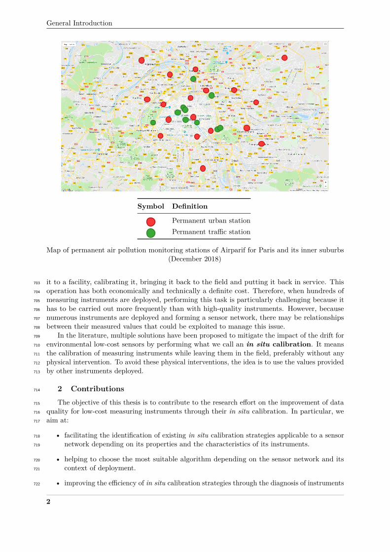
30 measuring stations are deployed across Paris and its inner suburbs to monitor air pollution [2]684
as shown in the figure page 2. Moreover, all of them are not monitoring the same quantities. For685
instance, only a third of these stations are monitoring O3. Consequently, the spatial resolution is686
even smaller for some measurands.687
Following up the scientific advances in micro and nano-electronics [90, 135], it is now possible688
to imagine a dense monitoring of ambient quantities with a fine granularity, both temporally689
and spatially, notably for air quality monitoring [110, 135] which is the practical context chosen690
for this thesis. Indeed, small low-cost measuring instruments have been designed in recent691
years. Fostered by the emergence of the Internet of Things, the interest for such devices has692
been growing significantly because they open up new possibilities for environmental sensing693
[62]. Without actually replacing regulatory grade instruments, it is hoped they can complement694
existing networks of measuring instruments. As they are affordable, they can also be owned by695
everybody. In this way, low-cost sensors are tools that could be used for individual awareness696
and education, particularly concerning both indoor and outdoor air quality [27].697
Nevertheless, these low-cost sensing technologies are still young, and several challenges are yet698
to be tackled [62, 127]. One of them concerns the quality of the measurement results they produce.699
The particular issue degrading the results addressed in this thesis is the instrumental drift which700
these instruments are prone to. The classical approach to solve this problem is to recalibrate the701
instruments in a calibration facility. This requires taking the instrument out of service, bringing702
1
General Introduction
Symbol Definition
Permanent urban stationPermanent traffic station
Map of permanent air pollution monitoring stations of Airparif for Paris and its inner suburbs(December 2018)
it to a facility, calibrating it, bringing it back to the field and putting it back in service. This703
operation has both economically and technically a definite cost. Therefore, when hundreds of704
measuring instruments are deployed, performing this task is particularly challenging because it705
has to be carried out more frequently than with high-quality instruments. However, because706
numerous instruments are deployed and forming a sensor network, there may be relationships707
between their measured values that could be exploited to manage this issue.708
In the literature, multiple solutions have been proposed to mitigate the impact of the drift for709
environmental low-cost sensors by performing what we call an in situ calibration. It means710
the calibration of measuring instruments while leaving them in the field, preferably without any711
physical intervention. To avoid these physical interventions, the idea is to use the values provided712
by other instruments deployed.713
2 Contributions714
The objective of this thesis is to contribute to the research effort on the improvement of data715
quality for low-cost measuring instruments through their in situ calibration. In particular, we716
aim at:717
• facilitating the identification of existing in situ calibration strategies applicable to a sensor718
network depending on its properties and the characteristics of its instruments.719
• helping to choose the most suitable algorithm depending on the sensor network and its720
context of deployment.721
• improving the efficiency of in situ calibration strategies through the diagnosis of instruments722
2
3. Organisation of the manuscript
that have drifted in a sensor network.723
Toward this goal, three main contributions are made in this work. First, a unified terminology724
is proposed to classify the existing works on in situ calibration. Indeed there is no shared725
vocabulary in the scientific community enabling a precise description of the main characteristics726
of the algorithms. The review carried out based on this taxonomy showed there are numerous727
contributions on the subject, covering a wide variety of cases. Due to the type of sensor network728
deployed, in terms of properties of the measuring instruments or how these devices can interact729
between them, different approaches may be considered. Nevertheless, the classification of the730
existing works in terms of performances was difficult as there is no reference case study for the731
evaluation of these algorithms.732
Therefore in a second step, a framework for the simulation of sensor networks is introduced.733
It is aimed at evaluating in situ calibration algorithms. It details all the aspects to take into734
account when designing a case study. A detailed case study is provided across the evaluation of735
in situ calibration algorithms for blind static sensor networks. An analysis of the influence of736
the parameters and of the metrics used to derive the results is also carried out. As the results737
are case specific, and as most of the algorithms recalibrate instruments without evaluating first738
if they actually need it, an identification tool enabling to determine the instruments that are739
actually faulty in terms of drift would be valuable.740
Thus, the third contribution of this thesis is the design of a diagnosis algorithm targeting741
drift faults in sensor networks without making any assumption on the kind of sensor network at742
stake. Based on the concept of rendez-vous, the algorithm allows identifying faulty instruments743
as long as one instrument at least can be assumed as non-faulty in the sensor network. Across744
the investigation of the results of a case study, we propose several means to reduce false results745
and guidelines to adjust the parameters of the algorithm. Finally, we show that the proposed746
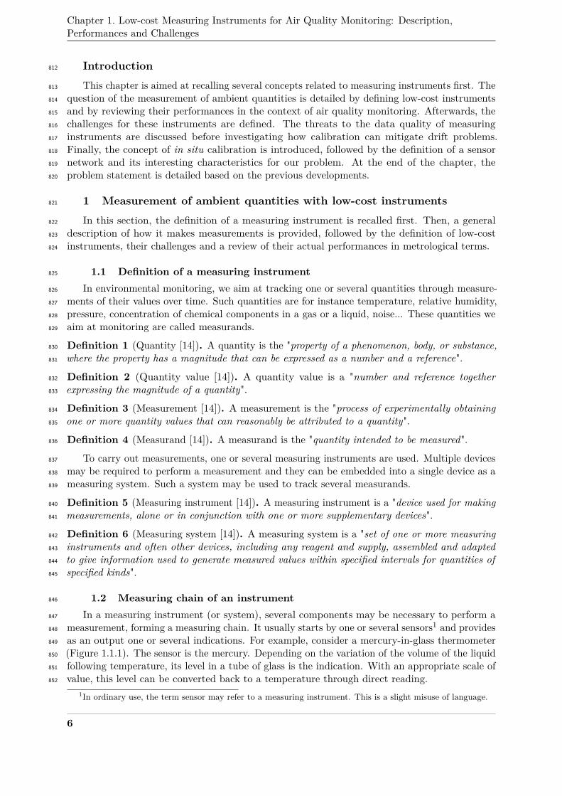
diagnosis approach, combined with a simple calibration technique, enables to improve the quality747
of the measurement results.748
3 Organisation of the manuscript749
The manuscript is organised as follows.750
In Chapter 1, concepts related to measuring instruments are defined and the performances751
of low-cost measuring instruments in the context of air quality monitoring are reviewed. Then,752
the issue of data quality for these devices and how calibration can mitigate drift problems are753
discussed. The concept of in situ calibration is introduced, followed by the interesting properties754
of sensor networks for this application. At the end of the chapter, the problem statement is755
recalled and detailed.756
In Chapter 2, the taxonomy for the classification of in situ calibration strategies is introduced,757
followed by the review of existing works.758
Chapter 3 introduces the framework for the simulation of sensor networks designed for the759
evaluation of in situ calibration algorithms. A case study concerning blind static sensor networks760
is developed, and multiple derived cases are investigated to determine the influence of parameters761
and of the metrics used on the interpretations of the results.762
Afterwards, the diagnosis algorithm for drift faults in sensor networks is introduced in Chapter763
4. A case study is developed and means to improve its results are discussed. The sensitivity of764
the diagnosis algorithm to the choices made during the design of the case study is investigated.765
It is followed by the combination of the diagnosis algorithm with a simple calibration approach766
that exploits information build during the diagnosis, applied to the preceding case study.767
Finally, the contributions are summarised in the last chapter and a general conclusion is768
provided, along with perspectives regarding this work.769
3

General Introduction
Several appendices are also provided in this manuscript. Appendix A provides variations and770
extensions of the diagnosis algorithm presented in Chapter 4. They require further studies but771
the basis are introduced towards future work. Appendix B extends the discussion on the main772
assumption made for the diagnosis algorithm. Lastly, Appendix C presents an additional case773
study related to the sensitivity of the diagnosis algorithm.774
4

Chapter775
1776
Low-cost Measuring Instruments for777
Air Quality Monitoring: Description,778
Performances and Challenges779
Contents780
781 Introduction . . . . . . . . . . . . . . . . . . . . . . . . . . . . . . . . . . . . . . . . 6782
1 Measurement of ambient quantities with low-cost instruments . . . . . . . . . 6783
1.1 Definition of a measuring instrument . . . . . . . . . . . . . . . . . . . 6784
1.2 Measuring chain of an instrument . . . . . . . . . . . . . . . . . . . . . 6785
1.3 Low-cost instruments . . . . . . . . . . . . . . . . . . . . . . . . . . . . 8786
1.3.1 Definition . . . . . . . . . . . . . . . . . . . . . . . . . . . . . . . 8787
1.3.2 Challenges of environmental monitoring . . . . . . . . . . . . . . 9788
1.3.3 Performances of low-cost instruments in the literature for air789
quality monitoring . . . . . . . . . . . . . . . . . . . . . . . . . . 9790
2 Threats to data quality for measuring instruments . . . . . . . . . . . . . . . . 11791
2.1 Introduction . . . . . . . . . . . . . . . . . . . . . . . . . . . . . . . . . 11792
2.2 Faults . . . . . . . . . . . . . . . . . . . . . . . . . . . . . . . . . . . . 12793
2.3 Discussion . . . . . . . . . . . . . . . . . . . . . . . . . . . . . . . . . . 15794
3 Calibration of measuring instruments . . . . . . . . . . . . . . . . . . . . . . . 15795
3.1 Definition . . . . . . . . . . . . . . . . . . . . . . . . . . . . . . . . . . 16796
3.2 Analysis . . . . . . . . . . . . . . . . . . . . . . . . . . . . . . . . . . . 17797
3.3 In situ calibration . . . . . . . . . . . . . . . . . . . . . . . . . . . . . 17798
3.4 Discussion . . . . . . . . . . . . . . . . . . . . . . . . . . . . . . . . . . 18799
4 Sensor networks . . . . . . . . . . . . . . . . . . . . . . . . . . . . . . . . . . . 19800
4.1 Definition . . . . . . . . . . . . . . . . . . . . . . . . . . . . . . . . . . 19801
4.2 Characteristics of interest in this work . . . . . . . . . . . . . . . . . . 19802
4.2.1 Presence of references . . . . . . . . . . . . . . . . . . . . . . . . 20803
4.2.2 Mobility . . . . . . . . . . . . . . . . . . . . . . . . . . . . . . . . 20804
4.3 Conclusion . . . . . . . . . . . . . . . . . . . . . . . . . . . . . . . . . . 21805
5 Problem statement . . . . . . . . . . . . . . . . . . . . . . . . . . . . . . . . . 21806
5.1 Motivations . . . . . . . . . . . . . . . . . . . . . . . . . . . . . . . . . 21807
5.2 Objectives of the thesis . . . . . . . . . . . . . . . . . . . . . . . . . . . 21808809810811
5
Chapter 1. Low-cost Measuring Instruments for Air Quality Monitoring: Description,Performances and Challenges
Introduction812
This chapter is aimed at recalling several concepts related to measuring instruments first. The813
question of the measurement of ambient quantities is detailed by defining low-cost instruments814
and by reviewing their performances in the context of air quality monitoring. Afterwards, the815
challenges for these instruments are defined. The threats to the data quality of measuring816
instruments are discussed before investigating how calibration can mitigate drift problems.817
Finally, the concept of in situ calibration is introduced, followed by the definition of a sensor818
network and its interesting characteristics for our problem. At the end of the chapter, the819
problem statement is detailed based on the previous developments.820
1 Measurement of ambient quantities with low-cost instruments821
In this section, the definition of a measuring instrument is recalled first. Then, a general822
description of how it makes measurements is provided, followed by the definition of low-cost823
instruments, their challenges and a review of their actual performances in metrological terms.824
1.1 Definition of a measuring instrument825
In environmental monitoring, we aim at tracking one or several quantities through measure-826
ments of their values over time. Such quantities are for instance temperature, relative humidity,827
pressure, concentration of chemical components in a gas or a liquid, noise... These quantities we828
aim at monitoring are called measurands.829
Definition 1 (Quantity [14]). A quantity is the "property of a phenomenon, body, or substance,830
where the property has a magnitude that can be expressed as a number and a reference".831
Definition 2 (Quantity value [14]). A quantity value is a "number and reference together832
expressing the magnitude of a quantity".833
Definition 3 (Measurement [14]). A measurement is the "process of experimentally obtaining834
one or more quantity values that can reasonably be attributed to a quantity".835
Definition 4 (Measurand [14]). A measurand is the "quantity intended to be measured".836
To carry out measurements, one or several measuring instruments are used. Multiple devices837
may be required to perform a measurement and they can be embedded into a single device as a838
measuring system. Such a system may be used to track several measurands.839
Definition 5 (Measuring instrument [14]). A measuring instrument is a "device used for making840
measurements, alone or in conjunction with one or more supplementary devices".841
Definition 6 (Measuring system [14]). A measuring system is a "set of one or more measuring842
instruments and often other devices, including any reagent and supply, assembled and adapted843
to give information used to generate measured values within specified intervals for quantities of844
specified kinds".845
1.2 Measuring chain of an instrument846
In a measuring instrument (or system), several components may be necessary to perform a847
measurement, forming a measuring chain. It usually starts by one or several sensors1 and provides848
as an output one or several indications. For example, consider a mercury-in-glass thermometer849
(Figure 1.1.1). The sensor is the mercury. Depending on the variation of the volume of the liquid850
following temperature, its level in a tube of glass is the indication. With an appropriate scale of851
value, this level can be converted back to a temperature through direct reading.852
1In ordinary use, the term sensor may refer to a measuring instrument. This is a slight misuse of language.
6
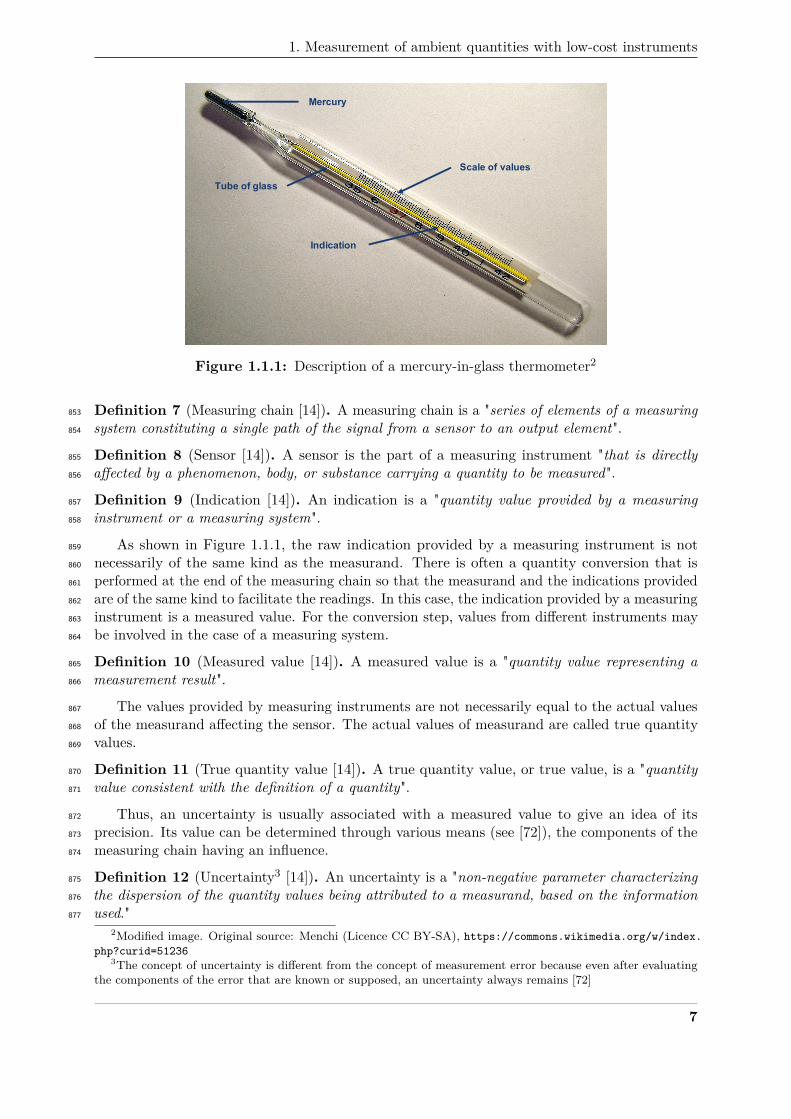
1. Measurement of ambient quantities with low-cost instruments
Mercury
Scale of values
Indication
Tube of glass
Figure 1.1.1: Description of a mercury-in-glass thermometer2
Definition 7 (Measuring chain [14]). A measuring chain is a "series of elements of a measuring853
system constituting a single path of the signal from a sensor to an output element".854
Definition 8 (Sensor [14]). A sensor is the part of a measuring instrument "that is directly855
affected by a phenomenon, body, or substance carrying a quantity to be measured".856
Definition 9 (Indication [14]). An indication is a "quantity value provided by a measuring857
instrument or a measuring system".858
As shown in Figure 1.1.1, the raw indication provided by a measuring instrument is not859
necessarily of the same kind as the measurand. There is often a quantity conversion that is860
performed at the end of the measuring chain so that the measurand and the indications provided861
are of the same kind to facilitate the readings. In this case, the indication provided by a measuring862
instrument is a measured value. For the conversion step, values from different instruments may863
be involved in the case of a measuring system.864
Definition 10 (Measured value [14]). A measured value is a "quantity value representing a865
measurement result".866
The values provided by measuring instruments are not necessarily equal to the actual values867
of the measurand affecting the sensor. The actual values of measurand are called true quantity868
values.869
Definition 11 (True quantity value [14]). A true quantity value, or true value, is a "quantity870
value consistent with the definition of a quantity".871
Thus, an uncertainty is usually associated with a measured value to give an idea of its872
precision. Its value can be determined through various means (see [72]), the components of the873
measuring chain having an influence.874
Definition 12 (Uncertainty3 [14]). An uncertainty is a "non-negative parameter characterizing875
the dispersion of the quantity values being attributed to a measurand, based on the information876
used."877
2Modified image. Original source: Menchi (Licence CC BY-SA), https://commons.wikimedia.org/w/index.php?curid=51236
3The concept of uncertainty is different from the concept of measurement error because even after evaluatingthe components of the error that are known or supposed, an uncertainty always remains [72]
7

Chapter 1. Low-cost Measuring Instruments for Air Quality Monitoring: Description,Performances and Challenges
This is notably why a measured value is a value representing a measurement result but not a878
measurement result itself. Usually, a measurement result is expressed by a measured value and an879
uncertainty. A measurement result composed of only a measured value does not allow to estimate880
how close it is to the true value. In fact, any important information for the interpretation of881
a measurement result should be added to it. It can concern the operating conditions, or data882
helping to identify when or where a result was obtained, like a timestamp or GPS coordinates.883
Definition 13 (Measurement result [14]). A measurement result is a "set of quantity values884
being attributed to a measurand together with any other available relevant information".885
All along the measuring chain, influence quantities may act on the output of the instrument.886
Definition 14 (Influence quantity [14]). An influence quantity is a "quantity that, in a direct887
measurement, does not affect the quantity that is actually measured, but affects the relation888
between the indication and the measurement result".889
The measuring chain of an instrument can be more or less long depending on the measurement890
method. For a digital thermometer, based on a thermocouple for instance, the sensor provides891
a voltage, as an indication of the temperature. Several processings are usually carried out892
afterwards like amplification and filtering, which adds steps in the measuring chain compared to893
the case of a mercury-in-glass thermometer.894
The description of the measuring chain of an instrument is summarised in Figure 1.1.2.895
Measuring chain
Measured valuesSensor(Sensitive element,
transducer…)
Processing(s)Quantity
conversionIndication(s)
…True quantity
values
Measuring instrument
Influence quantity values
Figure 1.1.2: Schematic description of the measuring chain of a measuring instrument
1.3 Low-cost instruments896
1.3.1 Definition897
For any measurand, there is a wide range of measuring instruments notably in terms of cost.898
Their price is related to the capabilities of instruments in terms of measurement range, sensitivity,899
uncertainty and so on. In the General Introduction, we exposed that reference instruments were900
sometimes too expensive to enable a dense environmental monitoring of different quantities,901
taking as an example the context of air quality monitoring. Consequently, low-cost instruments902
are necessary to help carry out this task.903
Definition 15 (Reference measuring instrument). A reference (or regulatory-grade) measuring904
instrument is a measuring instrument implementing a reference measurement procedure or905
equivalent. Such an instrument is usually expensive.906
Definition 16 (Low-cost measuring instrument). A low-cost measuring instrument is a measuring907
instrument significantly affordable compared to reference instruments.908
8
1. Measurement of ambient quantities with low-cost instruments
Depending on the application, what a low-cost measuring instrument is may be very different909
[27, 110, 138]. In the context of air pollution monitoring, we speak of devices that cost US$ 100910
or less to few US$ 1,000 [71, 85, 110] at most, considering that reference instruments can be911
worth from US$ 10,000 to more than US$ 100,000.912
Low-cost instruments are often characterised by a small size, thanks to the use of micro913
and nano technologies [183]. They are also frequently autonomous in terms of energy: they are914
powered by batteries or small solar panels. Most of the time they have wireless communications915
capabilities. They can be deployed at fixed positions or be mobile and even wearable [66].916
1.3.2 Challenges of environmental monitoring917
Few years ago, Hart et al. [62] and Rundel et al. [127] exposed various challenges for918
measuring devices used in environmental monitoring:919
Energy supply and management This subject concerns mainly autonomous devices. In this920
case, it aims notably at minimising the energy consumption so that size of the system of921
energy storage and charge can be reduced. In addition, the lifespan of the energy supply922
components has to be the longest as possible to limit the maintenance operations and its923
environmental impact.924
Hardware standardisation To have upgradeable systems, interoperability of the hardware925
must be met, with user-friendly manageability.926
Software standardisation In the same way that hardware has to be standardised, the software927
of measuring instruments should also be normalised to facilitate the usage of devices from928
different manufacturers in the same deployment.929
Data standardisation To help data management and the use of values, data formats must be930
standardised.931
Data quality improvement This challenge concerns different aspects. First, in conjunction932
with data standardisation, the data quality has to be ensured by providing for each mea-933
surement all the necessary and meaningful information regarding its realisation. Secondly,934
the accuracy of the measurements has to be improved through the upgrade of the hardware935
but also with the help of data processing algorithms.936
Data usage reinforcement To make sure the most is taken out of the acquired data, it is937
necessary to facilitate its management and use. It would also be valuable to exploit the938
measurements in the largest number of possible applications.939
Security reinforcement As systems are more and more connected, they become vulnerable to940
attacks that can affect data integrity. Protocols must be established to prevent tampering941
and protect privacy.942
Among all these challenges, data quality is an important one for low-cost instruments in943
particular and is still a major issue [119]. Indeed, if a satisfying data quality cannot be achieved,944
the responses to any of the other challenges cited will have a limited impact.945
1.3.3 Performances of low-cost instruments in the literature for air quality946
monitoring947
While the concepts introduced and methods developed in this work are generic, the examples948
and illustrations provided are taken from the field of air quality monitoring. Indeed, regulatory-949
grade instruments as used by air quality surveillance agencies are extremely expensive. Therefore,950
9
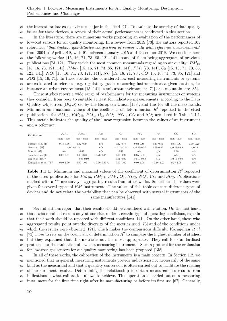
Chapter 1. Low-cost Measuring Instruments for Air Quality Monitoring: Description,Performances and Challenges
the interest for low-cost devices is major in this field [27]. To evaluate the severity of data quality951
issues for these devices, a review of their actual performances is conducted in this section.952
In the literature, there are numerous works proposing an evaluation of the performances of953
low-cost sensors for air quality monitoring. In a review from 2019 [73], the authors reported 105954
references "that include quantitative comparison of sensor data with reference measurements"955
from 2004 to April 2019, with 91 between January 2015 and December 2018. We consider here956
the following works: [15, 16, 71, 73, 85, 121, 141], some of them being aggregates of previous957
publications [73, 121]. They tackle the most common measurands regarding to air quality: PM10958
[15, 16, 73, 121, 141], PM2.5 [15, 16, 71, 73, 85, 121, 141], PM1 [73, 141], O3 [15, 16, 71, 73, 85,959
121, 141], NO2 [15, 16, 71, 73, 121, 141], NO [15, 16, 71, 73], CO [15, 16, 71, 73, 85, 121] and960
SO2 [15, 16, 71]. In these studies, the considered low-cost measuring instruments or systems961
are co-located to reference, e.g. regulatory-grade, measuring instruments at a given location, for962
instance an urban environment [15, 141], a suburban environment [71] or a mountain site [85].963
These studies report a wide range of performances for the measuring instruments or systems964
they consider: from poor to suitable at least for indicative measurements, according to the Data965
Quality Objectives (DQO) set by the European Union [158], and this for all the measurands.966
Minimum and maximal values of the coefficient of determination R2 reported in the cited967
publications for PM10, PM2.5, PM1, O3, NO2, NO , CO and SO2 are listed in Table 1.1.1.968
This metric indicates the quality of the linear regression between the values of an instrument969
and a reference.970
PublicationPM10 PM2.5 PM1 O3 NO2 NO CO SO2
min – max min – max min – max min – max min – max min – max min – max min – max
Borrego et al. [15] 0.13–0.36 0.07–0.27 n/a 0.12–0.77 0.02–0.89 0.34–0.80 0.53–0.87 0.09–0.20Jiao et al. [71] < 0.25–0.45 n/a < 0.25–0.94 < 0.25–0.57 0.77–0.87 < 0.25–0.68 < 0.25Li et al. [85] n/a 0.82 n/a 0.62 n/a n/a 0.68 n/aSpinelle et al. [141] 0.01–0.81 0.00–0.86 0.26–0.95 0.04–0.96 0.35–0.88 n/a n/a n/aRai et al. [121]* 0.07–0.99 0.01–0.99 < 0.10–0.89 n/a < 0.10–0.99 n/aKaragulian et al. [73]* 0.00–1.00 0.00–1.00 < 0.60–0.95 < 0.00–1.00 0.00–1.00 < 0.10–1.00 0.25–1.00 n/a
Table 1.1.1: Minimum and maximal values of the coefficient of determination R2 reportedin the cited publications for PM10, PM2.5, PM1, O3, NO2, NO , CO and SO2. Publicationsmarked with a "*" are surveys aggregating results from other works. Sometimes the values weregiven for several types of PM instruments. The values of this table concern different types ofdevices and do not relate the variability that can be observed with several instruments of the
same manufacturer [141].
Several authors report that their results should be considered with caution. On the first hand,971
those who obtained results only at one site, under a certain type of operating conditions, explain972
that their work should be repeated with different conditions [141]. On the other hand, those who973
aggregated results point out the diversity of the metrics used [73] and of the conditions under974
which the results were obtained [121], which makes the comparisons difficult. Karagulian et al.975
[73] chose to rely on the coefficient of determination R2 to compare the highest number of studies,976
but they explained that this metric is not the most appropriate. They call for standardised977
protocols for the evaluation of low-cost measuring instruments. Such a protocol for the evaluation978
for low-cost gas sensors for air quality monitoring has been proposed [138].979
In all of these works, the calibration of the instruments is a main concern. In Section 1.2, we980
mentioned that in general, measuring instruments provide indications not necessarily of the same981
kind as the measurand and that a quantity conversion is often carried out to facilitate the reading982
of measurement results. Determining the relationship to obtain measurements results from983
indications is what calibration allows to achieve. This operation is carried out on a measuring984
instrument for the first time right after its manufacturing or before its first use [67]. Generally,985
10
2. Threats to data quality for measuring instruments
it is performed in a dedicated facility. However, it is only mandatory to have an individual986
calibration for regulatory-grade instruments. In most cases, several instruments are calibrated987
altogether. Sometimes it also happens that instruments are not calibrated at all.988
In the publications cited, out-of-the-box measurement results were quite inaccurate most989
of the time and some instruments had to be compensated following influence quantities like990
temperature, relative humidity or chemical components depending on the measurand and on the991
measuring principle at stake [16, 71, 73, 121]. Jiao et al. [71] showed for instance an improvement992
of the coefficient R2:993
• from 0.36 to 0.43, from 0.45 to 0.60 and from 0.43 to 0.50 for three different PM instruments994
• from 0.88 to 0.94 for an O3 instrument995
• from 0.57 to 0.82 for a NO2 instrument996
In conclusion, all the authors report that the quality of measurement results can be strongly997
improved with the use of data treatment and processing tools. To better understand how data998
processing algorithms can improve the quality of the measurement results, the issues causing999
their degradation must be identified.1000
2 Threats to data quality for measuring instruments1001
2.1 Introduction1002
In Section 1.3.2, the challenge of data quality was briefly presented from different perspectives.1003
First, it can be related to the quality of the information composing a measurement result, e.g.1004
the measured value, its uncertainty, the conditions under which the measurement was made and1005
so on.1006
In another way, it can be considered as a lack (or not) of measurement accuracy compared to1007
the one of reference instruments in terms of sensitivity or resolution for instance. Such issues1008
can be known at the design or prototyping stage of measuring instruments depending on their1009
components. Therefore, to improve the quality of the measurements, the performances of the1010
instruments have to be upgraded. This can be achieved along the advances during the conception1011
and manufacturing of its components.1012
The data quality issue can also be observed as a challenge regarding the ability of a measuring1013
instrument to deliver results consistent with its specifications during its life. In the field of1014
dependability, this can be considered as a question of reliability. It is the continuity of correct1015
service delivered by a system [5]. For an instrument, the correct service is the achievement of1016
measurements consistent with its metrological specifications. It is often observed that the quality1017
of low-cost devices decays with time, even under regular operating conditions [33]. This is the1018
general issue we focus on in this work.1019
The threats to the dependability of a system, and consequently the threats to its reliability,1020
are failures, errors and faults [5]. A failure is an event making the instrument no longer able1021
to deliver a correct service regarding its specifications or requirements. This event is triggered by1022
a deviation of the normal state of the system, called an error, and its potential cause is a fault.1023
The fault itself may be explained by the failure of another part of the system and so on. Thus,1024
there is a relationship of causality between these concepts [5].1025
In our case, the failure we are interested in for a measuring system is the event when the1026
measurement results it delivers are not correct regarding the actual values of the measurand1027
and the results that should be provided by the device. To improve the quality of data provided1028
by low-cost measuring instruments, it is necessary to determine the faults that are causing this1029
failure. The faults of a measuring system can be studied from different perspectives depending1030
on the case [115]. Consider an instrument that is in failure mode from the point of view of data1031
11
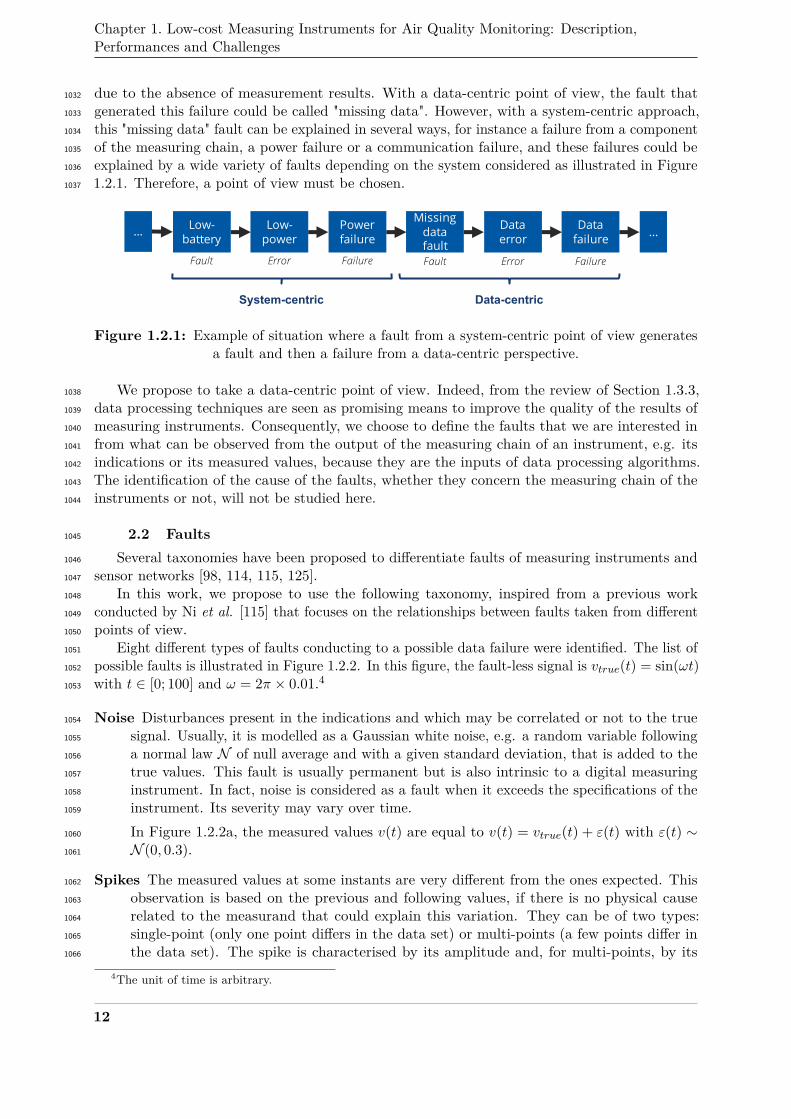
Chapter 1. Low-cost Measuring Instruments for Air Quality Monitoring: Description,Performances and Challenges
due to the absence of measurement results. With a data-centric point of view, the fault that1032
generated this failure could be called "missing data". However, with a system-centric approach,1033
this "missing data" fault can be explained in several ways, for instance a failure from a component1034
of the measuring chain, a power failure or a communication failure, and these failures could be1035
explained by a wide variety of faults depending on the system considered as illustrated in Figure1036
1.2.1. Therefore, a point of view must be chosen.1037
Low-battery
Low-power
Power failure
Missingdata fault
Data error
Data failure
Fault Error FaultFailure Error Failure
System-centric Data-centric
… …
Figure 1.2.1: Example of situation where a fault from a system-centric point of view generatesa fault and then a failure from a data-centric perspective.
We propose to take a data-centric point of view. Indeed, from the review of Section 1.3.3,1038
data processing techniques are seen as promising means to improve the quality of the results of1039
measuring instruments. Consequently, we choose to define the faults that we are interested in1040
from what can be observed from the output of the measuring chain of an instrument, e.g. its1041
indications or its measured values, because they are the inputs of data processing algorithms.1042
The identification of the cause of the faults, whether they concern the measuring chain of the1043
instruments or not, will not be studied here.1044
2.2 Faults1045
Several taxonomies have been proposed to differentiate faults of measuring instruments and1046
sensor networks [98, 114, 115, 125].1047
In this work, we propose to use the following taxonomy, inspired from a previous work1048
conducted by Ni et al. [115] that focuses on the relationships between faults taken from different1049
points of view.1050
Eight different types of faults conducting to a possible data failure were identified. The list of1051
possible faults is illustrated in Figure 1.2.2. In this figure, the fault-less signal is vtrue(t) = sin(ωt)1052
with t ∈ [0; 100] and ω = 2π × 0.01.41053
Noise Disturbances present in the indications and which may be correlated or not to the true1054
signal. Usually, it is modelled as a Gaussian white noise, e.g. a random variable following1055
a normal law N of null average and with a given standard deviation, that is added to the1056
true values. This fault is usually permanent but is also intrinsic to a digital measuring1057
instrument. In fact, noise is considered as a fault when it exceeds the specifications of the1058
instrument. Its severity may vary over time.1059
In Figure 1.2.2a, the measured values v(t) are equal to v(t) = vtrue(t) + ε(t) with ε(t) ∼1060
N (0, 0.3).1061
Spikes The measured values at some instants are very different from the ones expected. This1062
observation is based on the previous and following values, if there is no physical cause1063
related to the measurand that could explain this variation. They can be of two types:1064
single-point (only one point differs in the data set) or multi-points (a few points differ in1065
the data set). The spike is characterised by its amplitude and, for multi-points, by its1066
4The unit of time is arbitrary.
12
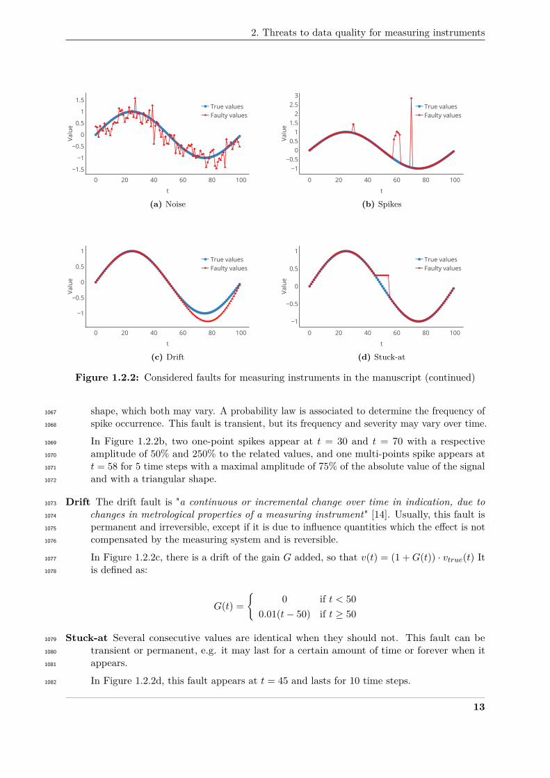
2. Threats to data quality for measuring instruments
0 20 40 60 80 100
−1.5
−1
−0.5
0
0.5
1
1.5True valuesFaulty values
t
Valu
e
(a) Noise
0 20 40 60 80 100
−1−0.5
00.5
11.5
22.5
3
True valuesFaulty values
t
Valu
e
(b) Spikes
0 20 40 60 80 100
−1
−0.5
0
0.5
1True valuesFaulty values
t
Valu
e
(c) Drift
0 20 40 60 80 100
−1
−0.5
0
0.5
1True valuesFaulty values
t
Valu
e
(d) Stuck-at
Figure 1.2.2: Considered faults for measuring instruments in the manuscript (continued)
shape, which both may vary. A probability law is associated to determine the frequency of1067
spike occurrence. This fault is transient, but its frequency and severity may vary over time.1068
In Figure 1.2.2b, two one-point spikes appear at t = 30 and t = 70 with a respective1069
amplitude of 50% and 250% to the related values, and one multi-points spike appears at1070
t = 58 for 5 time steps with a maximal amplitude of 75% of the absolute value of the signal1071
and with a triangular shape.1072
Drift The drift fault is "a continuous or incremental change over time in indication, due to1073
changes in metrological properties of a measuring instrument" [14]. Usually, this fault is1074
permanent and irreversible, except if it is due to influence quantities which the effect is not1075
compensated by the measuring system and is reversible.1076
In Figure 1.2.2c, there is a drift of the gain G added, so that v(t) = (1 +G(t)) · vtrue(t) It1077
is defined as:1078
G(t) =
0 if t < 500.01(t− 50) if t ≥ 50
Stuck-at Several consecutive values are identical when they should not. This fault can be1079
transient or permanent, e.g. it may last for a certain amount of time or forever when it1080
appears.1081
In Figure 1.2.2d, this fault appears at t = 45 and lasts for 10 time steps.1082
13

Chapter 1. Low-cost Measuring Instruments for Air Quality Monitoring: Description,Performances and Challenges
0 20 40 60 80 100
−1
−0.5
0
0.5
1True signalFaulty signal
t
Valu
e
(e) Bad timing
0 20 40 60 80 100
−1
−0.5
0
0.5
1True valuesFaulty values
t
Valu
e
(f) Missing values
0 20 40 60 80 100
−1
−0.5
0
0.5
1True valuesFaulty values
t
Valu
e
(g) Out of range
0 20 40 60 80 100−3
−2.5−2
−1.5−1
−0.50
0.51
0
20
40
60
80
100
Operating conditionLimit operating conditionTrue valuesFaulty values
t
Valu
e
Ope
ratin
g co
nditi
on
(h) Operating conditions out of range
Figure 1.2.2: Considered faults for measuring instruments in the manuscript
Bad timing A measurement result was obtained but has a timestamp differing from the one1083
expected. It can be a transient fault, for instance due to a momentary latency of the1084
instrument, or a permanent fault due to the drift of the clock of the device.1085
In Figure 1.2.2e, values expected at t ∈ [60; 100] are recorded with a delay of 8 units of1086
time.1087
Missing values Measured values have been lost. As for the stuck-at fault, it can be a transient1088
or a permanent fault. In Figure 1.2.2f, values at t ∈ [50; 80] are missing.1089
Measured values out of range The recorded measured values are out of the measurement1090
range of the sensor.1091
The instrument may behave differently depending how it was designed to manage such1092
fault. It may detect this fault and do not record the value, detect it and record it anyway,1093
or it does not have a detection system and record the values normally. If recorded, the1094
value may be equal to one of the bounds of the measurement range, simulating as it is1095
stuck-at, or to another one, more or less related to the true value of the measurand.1096
In Figure 1.2.2g, we considered the instrument having a range of [0; 0.90] and recording the1097
values, behaving as it is stuck-at when values are out-of-range.1098
Operating conditions out of range The environment of measurement is out of range of the1099
sensor’s normal operating conditions. Like for the fault of measured values out of range,1100
the possibly wrong values may be managed differently depending on the instrument. They1101
can be recorded normally, or recorded but marked as unreliable or not recorded at all.1102
14
3. Calibration of measuring instruments
In Figure 1.2.2h, the instrument is not recording values anymore when the operation1103
condition signal exceeds 40.1104
2.3 Discussion1105
This fault taxonomy is a list of the most common data faults that can be observed in sets of1106
measurement results from measuring instruments. Although several faults may be related to1107
each other5, they provide a reasonable overview of the threats to the data quality of measuring1108
instruments, in terms of accuracy of the results. The way they appear and how they manifest in1109
the data can be discussed in detail for each type of device but is out of the scope of this work.1110
These different faults can be differentiated in terms of how an instrument may be able to deal1111
with them. Indeed, low-cost environmental measuring instruments have computing capabilities,1112
though sometimes minimal. Thus, they can be self-aware of their characteristics and may be1113
able to pre-treat their measured values and potentially identify some faults.1114
For instance, concerning the "out of range" fault, a device can be able to detect when it1115
produces a value higher than its maximal possible output if it knows its measurement range. The1116
instrument may then raise an error indicating it made an incorrect measurement, either because1117
the value of its own measurand was indeed too high compared to its properties or because the1118
measuring instrument is producing an erroneous response to the value of the measurand for1119
instance. This reasoning can be extended to the faults "bad timing", "missing value" or even1120
"operating conditions out of range" if a measuring instrument can access to information on its1121
operating conditions, with the help of other devices. Note that these three faults do not concern1122
directly the measured value but more how it was obtained. On the contrary, "noise", "stuck-at",1123
"spike" and "drift" faults concern directly the measured value like the "out of range" fault. To1124
detect them with a data-centric approach, an analysis of the measured values has to be carried1125
out. "Noise", "stuck-at" and "spike" are faults having a characteristic time shorter than a "drift"1126
fault which usually affects a measuring instrument on a longer time basis. For them it is possible1127
to consider studying the variance or the gradient of the measured signal in a first step [112],1128
although more elaborated techniques have been developed [114]. Be that as it may, self correcting1129
its faults is not straightforward for measuring instruments.1130
In fact, drift is one of the most problematic faults because it is a continuous change over time1131
in the indications of the instruments. In this way, the relationship between the true values of1132
the measurand and the indications evolves. Consequently, the relationship determined through1133
a previous calibration to derive measured values from true values has to be determined again.1134
This is why calibration is an operation also conducted during the maintenance of an instrument1135
and it must be carried out periodically. To follow the traditional guidelines, it requires to take it1136
out of service and to bring it to a calibration facility. After this operation and the adjustment of1137
the instruments, it can be brought back to its deployment site and put back in service. However,1138
in the context of large deployments of measuring instruments, carrying out this maintenance1139
operation in this manner can have a significant cost, both economically and technically. It is all1140
the more important that low-cost devices are particularly prone to declining performances, often1141
sooner than expected [33].1142
3 Calibration of measuring instruments1143
In Section 1.3.3, we briefly introduced the concept of calibration. It was reported as a main1144
concern in studies on the performances of low-cost instruments. Thus, we provide here its formal1145
definition and develop why it is a challenging procedure for large deployments of measuring1146
5For instance, a "spike" fault may trigger a "measured value out of range" fault which itself may be representedby a "stuck-at". However, this is not always the case: a "measured value out of range" fault can happen due to thenormal evolution of a measurand.
15
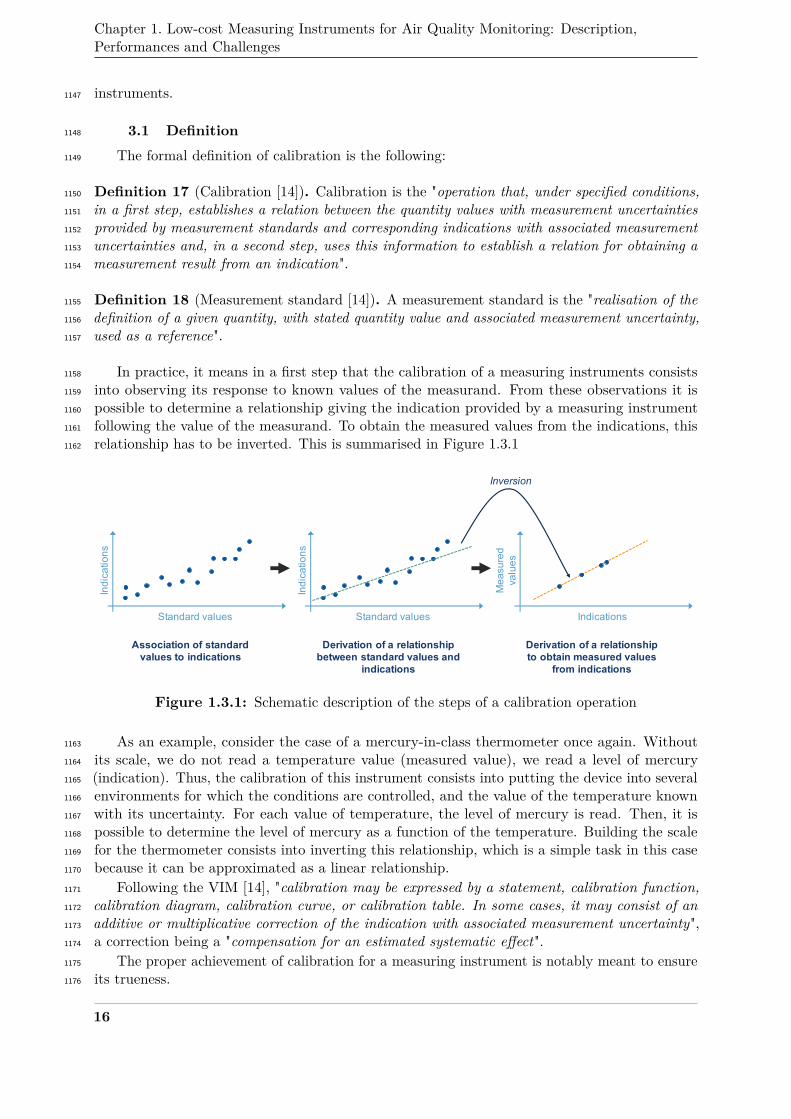
Chapter 1. Low-cost Measuring Instruments for Air Quality Monitoring: Description,Performances and Challenges
instruments.1147
3.1 Definition1148
The formal definition of calibration is the following:1149
Definition 17 (Calibration [14]). Calibration is the "operation that, under specified conditions,1150
in a first step, establishes a relation between the quantity values with measurement uncertainties1151
provided by measurement standards and corresponding indications with associated measurement1152
uncertainties and, in a second step, uses this information to establish a relation for obtaining a1153
measurement result from an indication".1154
Definition 18 (Measurement standard [14]). A measurement standard is the "realisation of the1155
definition of a given quantity, with stated quantity value and associated measurement uncertainty,1156
used as a reference".1157
In practice, it means in a first step that the calibration of a measuring instruments consists1158
into observing its response to known values of the measurand. From these observations it is1159
possible to determine a relationship giving the indication provided by a measuring instrument1160
following the value of the measurand. To obtain the measured values from the indications, this1161
relationship has to be inverted. This is summarised in Figure 1.3.11162
Standard values
Indi
catio
ns
Standard values
Indi
catio
ns
Indications
Mea
sure
d va
lues
Inversion
Association of standard values to indications
Derivation of a relationshipbetween standard values and
indications
Derivation of a relationshipto obtain measured values
from indications
Figure 1.3.1: Schematic description of the steps of a calibration operation
As an example, consider the case of a mercury-in-class thermometer once again. Without1163
its scale, we do not read a temperature value (measured value), we read a level of mercury1164
(indication). Thus, the calibration of this instrument consists into putting the device into several1165
environments for which the conditions are controlled, and the value of the temperature known1166
with its uncertainty. For each value of temperature, the level of mercury is read. Then, it is1167
possible to determine the level of mercury as a function of the temperature. Building the scale1168
for the thermometer consists into inverting this relationship, which is a simple task in this case1169
because it can be approximated as a linear relationship.1170
Following the VIM [14], "calibration may be expressed by a statement, calibration function,1171
calibration diagram, calibration curve, or calibration table. In some cases, it may consist of an1172
additive or multiplicative correction of the indication with associated measurement uncertainty",1173
a correction being a "compensation for an estimated systematic effect".1174
The proper achievement of calibration for a measuring instrument is notably meant to ensure1175
its trueness.1176
16
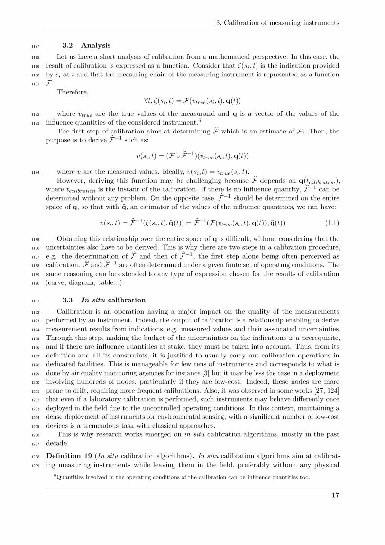
3. Calibration of measuring instruments
3.2 Analysis1177
Let us have a short analysis of calibration from a mathematical perspective. In this case, the1178
result of calibration is expressed as a function. Consider that ζ(si, t) is the indication provided1179
by si at t and that the measuring chain of the measuring instrument is represented as a function1180
F .1181
Therefore,∀t, ζ(si, t) = F(vtrue(si, t),q(t))
where vtrue are the true values of the measurand and q is a vector of the values of the1182
influence quantities of the considered instrument.61183
The first step of calibration aims at determining F which is an estimate of F . Then, thepurpose is to derive F−1 such as:
v(si, t) = (F F−1)(vtrue(si, t),q(t))
where v are the measured values. Ideally, v(si, t) = vtrue(si, t).1184
However, deriving this function may be challenging because F depends on q(tcalibration),where tcalibration is the instant of the calibration. If there is no influence quantity, F−1 can bedetermined without any problem. On the opposite case, F−1 should be determined on the entirespace of q, so that with q, an estimator of the values of the influence quantities, we can have:
v(si, t) = F−1(ζ(si, t), q(t)) = F−1(F(vtrue(si, t),q(t)), q(t)) (1.1)
Obtaining this relationship over the entire space of q is difficult, without considering that the1185
uncertainties also have to be derived. This is why there are two steps in a calibration procedure,1186
e.g. the determination of F and then of F−1, the first step alone being often perceived as1187
calibration. F and F−1 are often determined under a given finite set of operating conditions. The1188
same reasoning can be extended to any type of expression chosen for the results of calibration1189
(curve, diagram, table...).1190
3.3 In situ calibration1191
Calibration is an operation having a major impact on the quality of the measurements1192
performed by an instrument. Indeed, the output of calibration is a relationship enabling to derive1193
measurement results from indications, e.g. measured values and their associated uncertainties.1194
Through this step, making the budget of the uncertainties on the indications is a prerequisite,1195
and if there are influence quantities at stake, they must be taken into account. Thus, from its1196
definition and all its constraints, it is justified to usually carry out calibration operations in1197
dedicated facilities. This is manageable for few tens of instruments and corresponds to what is1198
done by air quality monitoring agencies for instance [3] but it may be less the case in a deployment1199
involving hundreds of nodes, particularly if they are low-cost. Indeed, these nodes are more1200
prone to drift, requiring more frequent calibrations. Also, it was observed in some works [27, 124]1201
that even if a laboratory calibration is performed, such instruments may behave differently once1202
deployed in the field due to the uncontrolled operating conditions. In this context, maintaining a1203
dense deployment of instruments for environmental sensing, with a significant number of low-cost1204
devices is a tremendous task with classical approaches.1205
This is why research works emerged on in situ calibration algorithms, mostly in the past1206
decade.1207
Definition 19 (In situ calibration algorithms). In situ calibration algorithms aim at calibrat-1208
ing measuring instruments while leaving them in the field, preferably without any physical1209
6Quantities involved in the operating conditions of the calibration can be influence quantities too.
17
Chapter 1. Low-cost Measuring Instruments for Air Quality Monitoring: Description,Performances and Challenges
intervention.1210
They are also called field [64], in place [24] or online [150] calibration algorithms.71211
The literature on the subject studies under which hypotheses, in which manner and with1212
which performances the measurement accuracy of one or several instruments can be improved1213
with such algorithms. Notably in the context of a dense deployment of measuring instruments,1214
comparisons of the measurement results of different instruments could be carried out for instance1215
to perform this task and this is exactly what these algorithms aims at exploiting in practice.1216
Most of the time, in situ calibration strategies do not take indications as an input butmeasured values. Mathematically speaking, considering the developments presented in Section3.2, it means it is not the function F that is derived but a function H mapping what areconsidered as standard values and potentially influence quantity values to measured values sothat:
H : (vstandard(si, t),q(t))→ v(si, t)
Then H−1 is derived and, in the same way that we expressed concerns regarding the determinationof F−18, the corrected values vcorr(si, t) that we obtain after an in situ calibration can be expressedas:
vcorr(si, t) = H−1(v(si, t), q(t)) (1.2)
If the in situ calibration is perfect, then vcorr(si, t) = vtrue(si, t).1217
In summary, in situ calibration strategies aim at giving relationships to obtain corrected1218
measured values from measured values. To do so, it uses standards defined with the measured1219
results of other measuring instruments. The measurement uncertainties associated with the1220
measured value measured both by the instruments to calibrate and the ones used to provide1221
standard values can be used to derive the uncertainties of the corrected values. Finally, the1222
operating conditions may be known through instruments measuring other quantities. Thus, in1223
situ calibration is a procedure conceptually close to the formal definition of calibration.1224
3.4 Discussion1225
Deploying a large number of instruments in an environment may offer opportunities to1226
overcome the problem of calibration for low-cost measuring instruments and more generally the1227
issue of data quality. Indeed, the devices deployed can be related in a network, allowing them to1228
share information like their measurement results.1229
However, regarding the formal definition of calibration and depending on the point of view,1230
using results from instruments obtained in an uncontrolled environment to calibrate other devices1231
may not be considered as equivalent to employing measurement standards or to being under1232
controlled conditions. This is particularly true if results from an instrument of an equivalent1233
accuracy class than another is used to calibrate another device.1234
Definition 20 (Accuracy class [14]). The accuracy class (or class) is the "class of measuring1235
instruments or measuring systems that meet stated metrological requirements that are intended to1236
keep measurement errors or instrumental measurement uncertainties within specified limits under1237
specified operating conditions".1238
Indeed, values in which a high confidence can be put are used to calibrate measuring1239
instruments. Thus, the sources of the measurement standards and the conditions under which1240
an algorithm is applied are critical for in situ calibration strategies.1241
7Calibration without any adjective is also used but it may be confusing regarding the definition of calibrationin the VIM [14].
8e.g. it should be carried out on the entire space of q, with an estimator q of the values of the potentialinfluence quantities.
18
4. Sensor networks
4 Sensor networks1242
We define in this section what a sensor network is. Note that we do not discuss (wireless1243
or not) sensor networks in general here. We focus on its characteristics of interest from the1244
perspective of in situ calibration of measuring instruments.1245
4.1 Definition1246
Definition 21 (Sensor network [62]). A sensor network9 is a set of measuring systems spatially1247
deployed in order to periodically measure one or more quantities in an environment and that1248
are exchanging information between them through a communication layer that can be wired or1249
wireless.1250
The measuring systems of the network are also called nodes. A node may be static or mobile.1251
The network can be either meshed, with device to device communications, or a collection of stars1252
centred on gateways for instance. A sensor network may target a single or multiple measurands.1253
For a given measurand, instruments in a same network are not necessarily of the same1254
accuracy class. In this work, those which are known to be more accurate than the others of the1255
network are called reference instruments.1256
It is also supposed that the nodes have sufficient computing and communication capabilities to1257
carry out the operations proposed by algorithms to overcome the issue of their in situ calibration.1258
(a) Each instrument can be relateddirectly to a reference
(b) Each instrument can be relatedindirectly to a reference
(c) No reference instrument in thenetwok
Symbol Definition
Reference nodeNon-reference node
Figure 1.4.1: Examples of sensor networks with a different number of reference instrumentsand different relationships between the instruments.
4.2 Characteristics of interest in this work1259
Regarding the issue of data quality for low-cost instruments, there are two characteristics of1260
sensor networks particularly interesting to tackle this issue: the presence of reference instruments1261
9Like sensor being used to refer to a measuring instrument, there is also a slight misuse of language here.However, this expression is widely used.
19
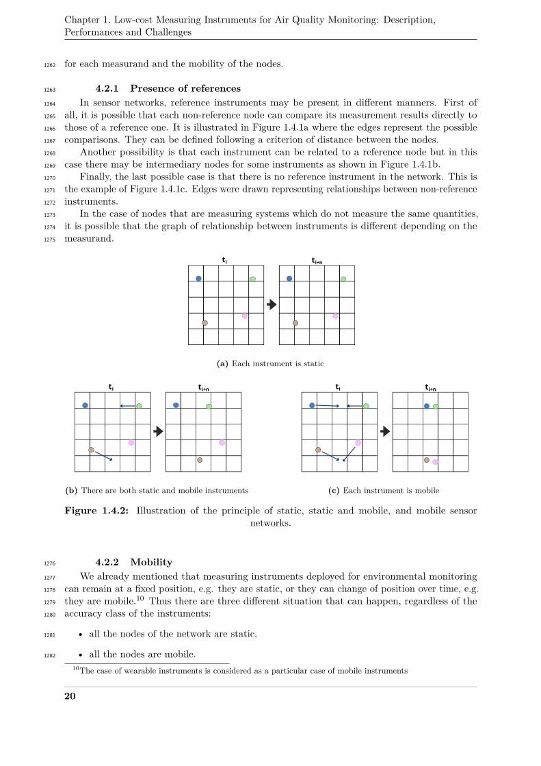
Chapter 1. Low-cost Measuring Instruments for Air Quality Monitoring: Description,Performances and Challenges
for each measurand and the mobility of the nodes.1262
4.2.1 Presence of references1263
In sensor networks, reference instruments may be present in different manners. First of1264
all, it is possible that each non-reference node can compare its measurement results directly to1265
those of a reference one. It is illustrated in Figure 1.4.1a where the edges represent the possible1266
comparisons. They can be defined following a criterion of distance between the nodes.1267
Another possibility is that each instrument can be related to a reference node but in this1268
case there may be intermediary nodes for some instruments as shown in Figure 1.4.1b.1269
Finally, the last possible case is that there is no reference instrument in the network. This is1270
the example of Figure 1.4.1c. Edges were drawn representing relationships between non-reference1271
instruments.1272
In the case of nodes that are measuring systems which do not measure the same quantities,1273
it is possible that the graph of relationship between instruments is different depending on the1274
measurand.1275
ti ti+n
(a) Each instrument is static
ti ti+n
(b) There are both static and mobile instruments
ti ti+n
(c) Each instrument is mobile
Figure 1.4.2: Illustration of the principle of static, static and mobile, and mobile sensornetworks.
4.2.2 Mobility1276
We already mentioned that measuring instruments deployed for environmental monitoring1277
can remain at a fixed position, e.g. they are static, or they can change of position over time, e.g.1278
they are mobile.10 Thus there are three different situation that can happen, regardless of the1279
accuracy class of the instruments:1280
• all the nodes of the network are static.1281
• all the nodes are mobile.1282
10The case of wearable instruments is considered as a particular case of mobile instruments
20
5. Problem statement
• there are both static and mobile nodes in the network.1283
This is illustrated in Figure 1.4.2.1284
Note that in the presence of mobile nodes, the relationships between reference and non-1285
reference instruments as exposed in the previous section may change overtime.1286
4.3 Conclusion1287
In this section, we defined what a sensor network is in a general manner. Two characteristics1288
of sensor network were presented respectively regarding the presence of reference instruments in1289
the network and the mobility of the nodes. The different possible cases for each property were1290
exposed. They are interesting for the problem we want to address because the configuration of1291
the sensor network can be exploited to drive the design of in situ calibration algorithms.1292
5 Problem statement1293
Based on the previous sections, we now detail the problem statement of this thesis briefly1294
exposed above in the General Introduction.1295
5.1 Motivations1296
To perform a dense measurement of ambient quantities in the context of environmental1297
monitoring activities such as air quality, the use of low-cost instruments is necessary to achieve1298
it at a reasonable cost economically speaking.1299
Among all the challenges for the measurement of ambient quantities in the context of1300
environmental monitoring, the need for an improvement of data quality appears to be major,1301
particularly for low-cost devices. Indeed, they are prone to faults, one of them being the1302
instrumental drift.1303
The traditional solution to mitigate this fault is to regularly perform calibration, as part1304
of maintenance operations. However, the cost of these tasks may limit the feasibility of dense1305
deployments of measuring instruments in practice. Indeed, it usually requires taking out the1306
node of the service, bringing it to a calibration facility, calibrating it and putting it back in1307
service. Therefore, there is a need for tools that allow recalibrating measuring instruments while1308
leaving them on the field.1309
Because the aim of environmental monitoring with low-cost instruments is notably to have1310
a high density of instruments in the monitored area, it is tempting to use the measurement1311
results of other instruments to detect and potentially correct drift faults. The sensor network1312
thus constituted may offer opportunities to overcome this issue of data quality. In addition, the1313
presence of reference instruments in the network, or the mobility of the nodes are characteristics1314
that can facilitate the in situ calibration of measuring instruments.1315
Fortunately, researchers have begun to tackle this issue and there are already methodologies1316
exploiting the properties of sensor networks to enable an in situ calibration of measuring1317
instruments.1318
5.2 Objectives of the thesis1319
As stated in the General Introduction, the objective of this thesis is to contribute to the1320
research effort on the improvement of data quality for low-cost measuring instruments through1321
their in situ calibration.1322
In the first place, the goal is to identify the existing techniques in the literature enabling such1323
a calibration. In Section 4, we reported there are sensor networks with different characteristics in1324
terms of presence of reference instruments and of mobility of the nodes. Thus, the same in situ1325
calibration algorithm may not be applicable to each type of sensor network for instance. This is1326
21

Chapter 1. Low-cost Measuring Instruments for Air Quality Monitoring: Description,Performances and Challenges
why a taxonomy is developed for the description of such algorithms, facilitating the identification1327
of the strategies that could be applied to a given sensor network depending on its properties and1328
the characteristics of its instruments.1329
In the case where several in situ calibration algorithms are adapted to a sensor network, it1330
is possible that each strategy does not yield the same performances. In other words, they may1331
not all allow correcting instruments as well as possible. Being able to evaluate the performances1332
of different in situ calibration strategies on the same use case would be valuable. The second1333
objective of this thesis is to provide a means to achieve this task.1334
Finally, before calibrating measuring instruments, it is necessary to determine if an instrument1335
needs to undergo such an operation. In publications introducing in situ calibration algorithms,1336
they mainly focus on how to perform the calibration itself and less on how to identify the faulty1337
instruments in a sensor network. Identifying these instruments is the last objective of this thesis.1338
22
Chapter1339
21340
In Situ Calibration Algorithms for1341
Environmental Sensor Networks1342
Contents1343
1344 Introduction . . . . . . . . . . . . . . . . . . . . . . . . . . . . . . . . . . . . . . . . 241345
1 Scope of the taxonomy . . . . . . . . . . . . . . . . . . . . . . . . . . . . . . . 241346
2 Taxonomy for the classification of the algorithms . . . . . . . . . . . . . . . . . 251347
2.1 Use of reference instruments . . . . . . . . . . . . . . . . . . . . . . . . 251348
2.2 Mobility of the instruments . . . . . . . . . . . . . . . . . . . . . . . . 261349
2.3 Calibration relationships . . . . . . . . . . . . . . . . . . . . . . . . . . 261350
2.4 Instrument grouping strategies . . . . . . . . . . . . . . . . . . . . . . 271351
3 Comparison to other taxonomies . . . . . . . . . . . . . . . . . . . . . . . . . . 281352
4 Review of the literature based on this classification . . . . . . . . . . . . . . . 301353
4.1 Overview . . . . . . . . . . . . . . . . . . . . . . . . . . . . . . . . . . 301354
4.2 Mobile and static nodes . . . . . . . . . . . . . . . . . . . . . . . . . . 321355
4.3 Calibration relationships . . . . . . . . . . . . . . . . . . . . . . . . . . 331356
4.4 Pairwise strategies . . . . . . . . . . . . . . . . . . . . . . . . . . . . . 331357
4.5 Blind macro calibration . . . . . . . . . . . . . . . . . . . . . . . . . . 351358
4.6 Group strategies . . . . . . . . . . . . . . . . . . . . . . . . . . . . . . 361359
4.7 Comment regarding other surveys . . . . . . . . . . . . . . . . . . . . . 371360
5 Conclusion . . . . . . . . . . . . . . . . . . . . . . . . . . . . . . . . . . . . . . 371361136213631364
23
Chapter 2. In Situ Calibration Algorithms for Environmental Sensor Networks
Introduction1365
In Chapter 1, we recalled that calibration is a procedure which is part of the maintenance1366
operations that must be carried out periodically on measuring instruments. To follow the1367
traditional guidelines for a device deployed in the field, it requires to take it out of service and1368
to bring it to a calibration facility. After this operation and the adjustment of the instruments,1369
it can be brought back to its deployment site and put in service again. This is manageable for1370
few tens of instruments and corresponds to what is done by air quality monitoring agencies for1371
instance [3]. However, notably in the particular case of environmental sensing, the increase of the1372
number of measuring instruments deployed to ensure a higher spatial coverage may not be feasible1373
due to the cost of regulatory-grade instruments. This is why low-cost instruments are necessary1374
to achieve this goal. In the literature, it is reported they are suffering from multiple issues, one of1375
them being a faster drift than usual instruments. Regarding calibration, it forces to increase the1376
frequency of this maintenance operation and thus its cost, economically and technically. Also, it1377
was observed in some works [27, 124] that even if a laboratory calibration is performed, once1378
deployed in the field, the instruments may behave differently due to the uncontrolled operating1379
conditions. In this context, maintaining a sensor network for environmental sensing and composed1380
of a significant number of low-cost instruments with classical approaches is a tremendous task.1381
This is why research works emerged on in situ calibration algorithms, mostly in the past1382
decade. The literature on the subject is abundant. This is expected as the topic of sensor1383
networks is a very hot research subject due to the trend for Smart Cities and the Internet of1384
Things. More practically, it is also predictable due to the variety of sensor networks as described1385
in Chapter 1, Section 4. Indeed, one can easily suspect that an algorithm may not be applicable1386
to any type of sensor network, on top of the assumptions surrounding it.1387
A major gap is the absence of a unified terminology to describe the field of application of in1388
situ calibration algorithms, regardless of the quantities measured by the sensor network. The1389
large variety of different techniques are reported under different terms in the literature, such1390
as "blind calibration", "multi-hop calibration", "macro calibration" and so on. The expression1391
describing an algorithm, notably in the title or the abstract of publications, is sometimes not1392
unique and is often incomplete. For instance, Balzano et al. [7] or Wang et al. [168] present their1393
strategies as "blind calibration" algorithms but it does not indicate if it is applicable to static1394
sensor networks, mobile ones or both. Consequently, it is not crystal-clear for an end user from1395
the first lines of an article if its content matches his/her needs.1396
Thus, through the literature review carried out on in situ calibration algorithms in this thesis,1397
a synthetic taxonomy for their classification is proposed in the following sections.1398
1 Scope of the taxonomy1399
To build the taxonomy, several guidelines were adopted. First of all, it should help to identify1400
relevant algorithms for any type of sensor network.1401
Also, the terms must be independent from the kind of measurand of the sensor networks: the1402
groups of categories described are relevant for any environmental phenomenon.1403
The attributes should also be limited to the properties involved in the definition of in situ1404
calibration, e.g. the definition of the measurement standards, how the relationship between1405
measured values and standard values is established and the relationship correcting the measured1406
values.1407
There are other considerations that could matter and interact with calibration, such as data1408
integrity, security or even privacy, in particular when crowdsensing platforms involving citizens1409
are developed [102]. The way the calibration relationship is computed, e.g. in a centralised or1410
decentralised manner is also a major subject. As a matter of fact, the care for the management1411
of these questions at an early step of the design of the sensor networks is crucial. The way these1412
24
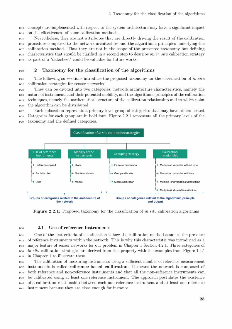
2. Taxonomy for the classification of the algorithms
concepts are implemented with respect to the system architecture may have a significant impact1413
on the effectiveness of some calibration methods.1414
Nevertheless, they are not attributes that are directly driving the result of the calibration1415
procedure compared to the network architecture and the algorithmic principles underlying the1416
calibration method. Thus they are not in the scope of the presented taxonomy but defining1417
characteristics that should be clarified in a second step to describe an in situ calibration strategy1418
as part of a "datasheet" could be valuable for future works.1419
2 Taxonomy for the classification of the algorithms1420
The following subsections introduce the proposed taxonomy for the classification of in situ1421
calibration strategies for sensor networks.1422
They can be divided into two categories: network architecture characteristics, namely the1423
nature of instruments and their potential mobility, and the algorithmic principles of the calibration1424
techniques, namely the mathematical structure of the calibration relationship and to which point1425
the algorithm can be distributed.1426
Each subsection represents a primary level group of categories that may have others nested.1427
Categories for each group are in bold font. Figure 2.2.1 represents all the primary levels of the1428
taxonomy and the defined categories.1429
Classification of in situ calibration strategies
Use of reference instruments
Calibration relationshipGrouping strategyMobility of the
instruments
Reference-based
Partially blind
Blind
Static
Mobile and static
Mobile
Pairwise calibration
Group calibration
Macro calibration
Mono-kind variables without time
Mono-kind variables with time
Multiple-kind variables with time
Multiple-kind variables without time
Groups of categories related to the algorithmic principleand output
Groups of categories related to the architecture of the network
Figure 2.2.1: Proposed taxonomy for the classification of in situ calibration algorithms
2.1 Use of reference instruments1430
One of the first criteria of classification is how the calibration method assumes the presence1431
of reference instruments within the network. This is why this characteristic was introduced as a1432
major feature of sensor networks for our problem in Chapter 1 Section 4.2.1. Three categories of1433
in situ calibration strategies are derived from this property with the examples from Figure 1.4.11434
in Chapter 1 to illustrate them.1435
The calibration of measuring instruments using a sufficient number of reference measurement1436
instruments is called reference-based calibration. It means the network is composed of1437
both reference and non-reference instruments and that all the non-reference instruments can1438
be calibrated using at least one reference instrument. The approach postulates the existence1439
of a calibration relationship between each non-reference instrument and at least one reference1440
instrument because they are close enough for instance.1441
25
Chapter 2. In Situ Calibration Algorithms for Environmental Sensor Networks
The calibration of measuring instruments in the absence of reference values is called blind1442
calibration. It means the network is composed of only non-reference instruments. These various1443
methods may or may not assume the existence of a correlation between the instrument outputs.1444
The hybrid situation is called partially blind calibration. In this setting, the network1445
may gather both reference and non-reference instruments, but a reference-based calibration is1446
not achievable, e.g. when some of the non-reference instruments can never be compared to a1447
reference instrument. It also captures the cases where a cluster of non-reference instruments is1448
considered as good enough to approximate a reference instrument.1449
2.2 Mobility of the instruments1450
The second significant aspect of the network architecture is the potential mobility of nodes.1451
As for the presence of references, this characteristic was also introduced as a major feature1452
of sensor networks in Chapter 1 Section 4.2.2. In the same way, three categories of in situ1453
calibration strategies are considered to illustrate how the methods exploit this feature. Figure1454
1.4.2 in Chapter 1 provides examples also illustrating these categories.1455
A first category of methods addresses networks with exclusively static nodes. A second1456
one addresses networks with exclusively mobile nodes. The corresponding methods rely often1457
strongly on the mobility of the nodes to achieve calibration. A last group of methods addresses1458
heterogeneous networks with both mobile and static nodes. In such cases the mobility of the1459
nodes is not systematically exploited in the calibration strategy.1460
2.3 Calibration relationships1461
In Chapter 1 Section 3, the purpose of calibration was defined as the establishment of a1462
mathematical relationship between the indications of the instrument and the standard values of1463
the measurand and then the derivation of a relationship for obtaining measurement results from1464
indications. Based on the mathematical developments in Chapter 1 Section 3.2, it is possible to1465
have different types of relationships, for instance if there are influence quantities or not.1466
The categories identified in this section are first based on the number of kinds of quantities as1467
input variables in the relationship: the measurand, the indications, the influence quantities, and1468
so on. In terms of algorithmic principles of the calibration methods, it implies the variety and1469
quantity of data to exchange as well as the computational effort necessary to achieve a target1470
accuracy.1471
The most straightforward relationships are called mono-kind variables without time.1472
They only take a single quantity as input variable and do not depend on time.1473
The second category of relationships gathers the ones that have mono-kind variables with1474
time. It accounts for a relationship with mono-kind variables which is influenced by time, for1475
instance in case of an instrument drifting due to ageing [160]. This is the reason why time is1476
considered as a particular influence quantity.1477
The relationships with multiple-kind variables without time account for two or more1478
quantities as variables but remain independent from time. These models are mainly used1479
to include the effect of influence quantities (except time) in the calibration relationship. In1480
these cases, the networks include instruments measuring the influence quantities. They are not1481
systematically reference instruments and therefore their calibration may also be included in the1482
calibration strategy.1483
Finally, this last approach may be extended into relationships with multiple-kind variables1484
with time when appropriate.1485
For each of these categories, subcategories can be defined based on the kind of mathematical1486
expression used for the calibration relationship. Popular examples are polynomials with constant1487
coefficients [7], gain-phase [13], variable offset [168], neural networks [36].1488
26
2. Taxonomy for the classification of the algorithms
These categories are particularly important regarding in situ calibration strategies. Indeed,considering Equations 1.1 and 1.2 in Chapter 1 Section 3, we have then:
vcorr(si, t) = H−1(F−1(ζ(si, t), q(t)), q(t))= H−1(F−1((F(vtrue(si, t),q(t)), q(t)), q(t))
(2.1)
For example, and recalling that in fine the purpose of in situ calibration is to determine the1489
relationship H−1, assume that the calibration relationship F−1 of an instrument is defined so1490
that:1491
v(si, t) = G · ζ(si, t) +O + κ · θ(t)
where G, O and κ are constant and G is a correction of the gain of the instrument, O a1492
correction of the offset, and κ · θ(t) a temperature compensation standing for q(t) in the general1493
expression of F−1.1494
If the behaviour of the measuring instrument changes over time, F−1 cannot ensure thatv(si, t) = vtrue(si, t). If the calibration relationship F−1 cannot be adjusted, the relationshipH−1 obtained with an in situ calibration strategy may compensate the change of behaviour.Consider H−1 such as:
vcorr(si, t) = Gcorr · v(si, t) +Ocorr + κcorr · θ(t)
Therefore:
vcorr(si, t) = GcorrG · ζ(si, t) + (GcorrO +Ocorr) + (Gcorrκ+ κcorr) · θ(t)
Here, H−1 allows determining a calibration relationship equivalent to the type of F−1.1495
However, if H−1 is such as:
vcorr(si, t) = Gcorr · v(si, t) +Ocorr
Then:vcorr(si, t) = GcorrG · ζ(si, t) + (GcorrO +Ocorr) +Gcorrκ · θ(t)
In this case, it may not be possible to correctly compensate the drift of the instrument si1496
because GcorrG and Gcorrκ are coupled: it is not possible to correct them independently.1497
This is why the type of relationship, both considering the quantities at stake and the kind of1498
relationship between them, is a key parameter of in situ calibration algorithms.1499
2.4 Instrument grouping strategies1500
While the previous categories are mostly driven by operational constraints (deployment1501
strategy, properties of the measurand and of the selected instruments), the present paragraph1502
considers the number of nodes involved in each calibration step and to which point the algorithm1503
can be distributed.1504
A first approach is pairwise calibration. Two instruments are used, one providing standard1505
values for the other. It is classically applied between a reference instrument (or an approximation1506
of reference) and each of the nodes related to it. It can be a distributed or even localised1507
algorithm. This case is illustrated in Figure 2.2.2a.1508
A macro calibration strategy consists in calibrating the network as a whole, e.g. the1509
values of all the instruments are used to calibrate each node of the network. Even if they exist,1510
node-to-node relationships may not be exploited directly. A centralised algorithm might be1511
necessary with this grouping strategy. This case is illustrated in Figure 2.2.2c.1512
27
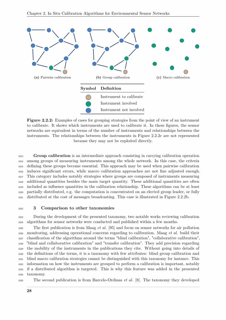
Chapter 2. In Situ Calibration Algorithms for Environmental Sensor Networks
(a) Pairwise calibration (b) Group calibration (c) Macro calibration
Symbol Definition
Instrument to calibrateInstrument involvedInstrument not involved
Figure 2.2.2: Examples of cases for grouping strategies from the point of view of an instrumentto calibrate. It shows which instruments are used to calibrate it. In these figures, the sensornetworks are equivalent in terms of the number of instruments and relationships between theinstruments. The relationships between the instruments in Figure 2.2.2c are not represented
because they may not be exploited directly.
Group calibration is an intermediate approach consisting in carrying calibration operation1513
among groups of measuring instruments among the whole network. In this case, the criteria1514
defining these groups become essential. This approach may be used when pairwise calibration1515
induces significant errors, while macro calibration approaches are not fine adjusted enough.1516
This category includes notably strategies where groups are composed of instruments measuring1517
additional quantities besides the main target quantity. These additional quantities are often1518
included as influence quantities in the calibration relationship. These algorithms can be at least1519
partially distributed, e.g. the computation is concentrated on an elected group leader, or fully1520
distributed at the cost of messages broadcasting. This case is illustrated in Figure 2.2.2b.1521
3 Comparison to other taxonomies1522
During the development of the presented taxonomy, two notable works reviewing calibration1523
algorithms for sensor networks were conducted and published within a few months.1524
The first publication is from Maag et al. [95] and focus on sensor networks for air pollution1525
monitoring, addressing operational concerns regarding to calibration. Maag et al. build their1526
classification of the algorithms around the terms "blind calibration", "collaborative calibration",1527
"blind and collaborative calibration" and "transfer calibration". They add precision regarding1528
the mobility of the instruments in the publications they cite. Without going into details of1529
the definitions of the terms, it is a taxonomy with few attributes: blind group calibration and1530
blind macro calibration strategies cannot be distinguished with this taxonomy for instance. This1531
information on how the instruments are grouped to perform a calibration is important, notably1532
if a distributed algorithm is targeted. This is why this feature was added in the presented1533
taxonomy.1534
The second publication is from Barcelo-Ordinas et al. [8]. The taxonomy they developed1535
28
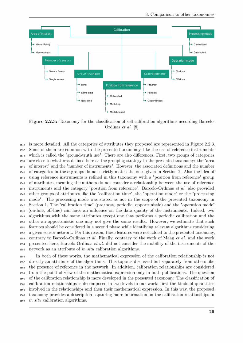
3. Comparison to other taxonomies
CalibrationArea of interest Processing mode
Position from reference
Groun- truth use
Micro (Point)
Macro (Area)
Blind
Semi-blind
Non-blind
Collocated
Multi-hop
Model-based
Centralized
Distributed
Number of sensors
Sensor Fusion
Single sensor
Calibration time
Pre/Post
Periodic
Opportunistic
Operation mode
On-Line
Off-Line
Figure 2.2.3: Taxonomy for the classification of self-calibration algorithms according Barcelo-Ordinas et al. [8]
is more detailed. All the categories of attributes they proposed are represented in Figure 2.2.3.1536
Some of them are common with the presented taxonomy, like the use of reference instruments1537
which is called the "ground-truth use". There are also differences. First, two groups of categories1538
are close to what was defined here as the grouping strategy in the presented taxonomy: the "area1539
of interest" and the "number of instruments". However, the associated definitions and the number1540
of categories in these groups do not strictly match the ones given in Section 2. Also the idea of1541
using reference instruments is refined in this taxonomy with a "position from reference" group1542
of attributes, meaning the authors do not consider a relationship between the use of reference1543
instruments and the category "position from reference". Barcelo-Ordinas et al. also provided1544
other groups of attributes like the "calibration time", the "operation mode" or the "processing1545
mode". The processing mode was stated as not in the scope of the presented taxonomy in1546
Section 1. The "calibration time" (pre/post, periodic, opportunistic) and the "operation mode"1547
(on-line, off-line) can have an influence on the data quality of the instruments. Indeed, two1548
algorithms with the same attributes except one that performs a periodic calibration and the1549
other an opportunistic one may not give the same results. However, we estimate that such1550
features should be considered in a second phase while identifying relevant algorithms considering1551
a given sensor network. For this reason, these features were not added to the presented taxonomy,1552
contrary to Barcelo-Ordinas et al. Finally, contrary to the work of Maag et al. and the work1553
presented here, Barcelo-Ordinas et al. did not consider the mobility of the instruments of the1554
network as an attribute of in situ calibration algorithms.1555
In both of these works, the mathematical expression of the calibration relationship is not1556
directly an attribute of the algorithms. This topic is discussed but separately from others like1557
the presence of reference in the network. In addition, calibration relationships are considered1558
from the point of view of the mathematical expression only in both publications. The question1559
of the calibration relationship is more developed in the presented taxonomy. The classification of1560
calibration relationships is decomposed in two levels in our work: first the kinds of quantities1561
involved in the relationships and then their mathematical expression. In this way, the proposed1562
taxonomy provides a description capturing more information on the calibration relationships in1563
in situ calibration algorithms.1564
29
Chapter 2. In Situ Calibration Algorithms for Environmental Sensor Networks
To conclude, the presented taxonomy is halfway between the one of Maag et al. which is1565
based on few groups of attributes, and the one of Barcelo-Ordinas et al. that is more extensive1566
but with information excluded from the scope of this work. Our taxonomy is limited to what1567
is seen as the essential attributes of an in situ calibration algorithm and designed with an1568
effort to avoid any redundancy or misunderstanding from the terms used, the taxonomy of1569
Barcelo-Ordinas et al. being sometimes confusing due to some groups of categories that are1570
semantically close. Nevertheless, all these works are interesting basis towards the definition and1571
use a shared terminology.1572
4 Review of the literature based on this classification1573
An application of the classification is provided here with highlights on the existing literature.1574
A large number of in situ calibration studies according to this classification are sorted in Table1575
2.4.1. Some rows refer to multiple papers as they are related somehow (same technique or same1576
authors) and consist in developments of the same initial paper. The current section focuses on a1577
description of the methods. The topic of performance comparison between methods is addressed1578
in the next section. The addressed measurands cover a wide range of environmental quantities:1579
temperature [7], pressure [182], noise [129], air pollutants [63], light [163]... Most of the reported1580
studies have generic approaches that can be transposed to other measurands.1581
4.1 Overview1582
Regarding pairwise strategies, relatively few papers address methodological issues related to1583
reference-based pairwise strategies, as this approach is the closest to a "traditional" calibration1584
approach with measurement standards and features fewer challenges. Partially blind and blind1585
pairwise calibration methods (often focusing on mobile nodes) are more complex as they require1586
to define calibration relationships not only between reference and non-reference nodes, but also1587
between non-reference nodes only. This translates into error propagation issues.1588
Macro calibration approaches were initially developed to address the absence of reference1589
instruments in a network and thus are mostly blind or partially blind. In the absence of reference,1590
there is a strong challenge in defining valid calibration relationships based on values from1591
non-reference instruments, which explains the major consideration for these methods.1592
Group strategies have been generating strong interests as they appear to outperform both1593
pairwise and macro strategies with or without reference instruments.1594
Most methods are based on relationships with mono-kind variables without time and with1595
a linear expression, but more complex models are progressively appearing to better address1596
the complexity of environmental sensing. Moreover, a particular attention is given in most1597
publications to the calibration relationship used compared to the other attributes of in situ1598
calibration that we identified. This can be explained by the significance of this information for1599
readers, e.g. it allows determining if the algorithm is able to provide a correction corresponding1600
to the way an instrument drifts.1601
Likewise, while most works initially focused on static networks, there are now many interests1602
for mobile nodes as they allow for physical rendez-vous between nodes. Henceforth, calibration1603
methods are less impacted by the physical variability of the phenomena.1604
Finally, an underlying question addressed is the ability to distribute the computation of1605
calibration relationships [23, 55, 107, 129, 143, 144, 177]. The topic is of strong interest when1606
considering privacy preservation issues [102]. The capability to decentralise is linked to the1607
grouping strategy: pairwise and group strategies foster more naturally decentralised computation,1608
under the condition that the nodes are capable of individual procession and of bidirectional1609
communication. On the contrary, macro-calibration strategies tend to be centralised, except1610
when the characteristics of the parameter identification methods allow for partially or fully1611
30
4. Review of the literature based on this classification
Table 2.4.1: In situ calibration strategies for sensor networksR: Reference-based, PB: Partially blind, B: Blind, P: Pairwise, Gr: Group, Ma: Macro,1V: Mono-kind variables without time, 1VT: Mono-kind variables with time, MV: Multiple-kindvariables without time, MVT: Multiple-kind variables with time, M: Exclusively mobile, S:
Exclusively static, MS: Mobile and static
Papers
Availabilityof referenceinstruments
Instrumentsgroupingstrategies
Kinds of variablesin calibrationrelationships
Mobilityof the
instruments
R PB B P Gr Ma 1V 1VT MV MVT M S MS
Ramanathan et al. [123] X - - X - - X - - - - X -Miluzzo et al. [107] X - - - X - X - - - X - X
Deshmukh et al. [39] X - - X - - X - - - - X -Spinelle et al. [139, 140] X - - X X - X - X - - X -Moltchanov et al. [109] X - - X - - X - - - - X -Gao et al. [58] X - - X - - X - X - - X -Lin et al. [88] X - - X - - X - - - - X -Fang et al. [50, 51] X - - - X - - - X - - X -Martin et al. [103] X X - - X - - - X - - X -Sun et al. [147] X - - - X - - - X - - X -Zimmerman et al. [186] X - - - X - - - X - - X -Weissert et al. [108, 171] X - - - X - X - - - - X -Yu et al. [184] X - - - X - - - X - - X -Topalovic et al. [155] X - - X X - X - X - - - -Wei et al. [169, 170] X - - - X - - - X - - X -Mahajan et al. [96] X - - X X - X - X - - X -Malings et al. [100] X - - - X - - - X - - X -Qin et al. [120] X - - - X - - - X - - - X
Barcelo-Ordinas et al. [9, 10,53] X - - - X - - - X - - X -
Wang et al. [165] X - - - X - - - X - - X -Loh et al. [91] X - - X - - X - X - - X -Badura et al. [6] X - - X X - X - X - - X -Cordero et al. [34] X - - - X - - - X - - X -Tsujita et al. [156] - X X X - - X - - - X - X
Tsujita et al. [157] - X X X X - - - X - - X -Y. Xiang et al. [177] - X X X - - X - - - X - X
Hasenfratz et al. [63], Saukhet al. [131, 132] - X X X - - X - - - X - X
Fu et al. [57] - X X X - - X - - - X - X
Maag et al. [93, 94] - X X - X - - - X - X - X
Arfire et al. [4] - X X - X - X X X X X - X
Markert et al. [102] - X X X X - X - - - X - X
Kizel et al. [75] - X - X - - X - - - - X -Sailhan et al. [129] - - X X X - X - - - X - -Fonollosa et al. [56] - X X X - - X - - - - X -Whitehouse et al. [172] - - X - - X X - - - - X -Ihler et al. [65] - X X - X - X - - - - X -Taylor et al. [152] - - X - - X X - - - - X -
continued on next page
31
Chapter 2. In Situ Calibration Algorithms for Environmental Sensor Networks
continued from previous page
Papers
Availabilityof referenceinstruments
Instrumentsgroupingstrategies
Kinds of variablesin calibrationrelationships
Mobilityof the
instruments
R PB B P Gr Ma 1V 1VT MV MVT M S MS
Tan et al. [151] - - X - X - X - - - - X -Bychkovskiy et al. [24] - X X X - - X - - - - X -Balzano et al. [7], Lipor etal. [89], Dorffer et al. [44] - X X - - X X - - - - X -
Takruri et al. [148–150] - - X - - X X - - - - X -Kumar et al. [76, 77] - - X - X - X - - - - X -Ramakrishnan et al. [122] - - X - - X X - - - - X -Buadhachain et al. [23] - - X - X X X - - - X - X
Bilen et al. [13] - - X - - X X - - - - X -Cambareri et al. [25] - - X - - X X - - - - X -C. Wang et al. [161–163] - - X - - X X - - - X - -C. Xiang et al. [176] - - X - - X X - - - X - -Dorffer et al. [41–43, 45] - X X - - X X - - - X - -Y. Wang et al. [166–168] Li[87] - - X - - X - X - - - X -
Ye et al. [182] - - X X - - X - - - X - -De Vito et al. [36, 47] - - X - X - - - X - - X -Son et al. [137], Lee [82] - - X - - X X - - - X - -Stankovic et al. [143, 144] - - X - - X X - - - - X -Fishbain et al. [55] - X X - X - X - - - - X -Popoola et al. [118] - - X X - - - - X - - X -Yan et al. [180] - - X - X - - - X - - X -Yang et al. [181] - - X - - X X - - - - X -Mueller et al. [113] - - X - X - - - X - - X -Kim et al. [74] - - X - X - - - X - - X -Chen et al. [30] - - X - - X - - X - - X -Wu et al. [175] - - X - X - X - - - - X -Becnel et al. [11] - X - X X - X - - - - X -Cheng et al. [31] - X - X - - X - - - - X -Sun et al. [146] - X - - X - - - X - X - -
decentralised computation. However, while distributed computing impacts the computational1612
performance of algorithms, there is no report on how it affects calibration performances so far.1613
4.2 Mobile and static nodes1614
Static networks are more frequently studied than mobile ones. A wide range of solutions1615
is now available to calibrate them. However, these calibration methods usually require a high1616
spatial density of nodes to overcome the spatial variability of the phenomena, which is not always1617
viable technically or economically. The availability of mobile nodes could alleviate this constraint,1618
as calibration operations exploit physical rendez-vous between nodes. In turn, the methods based1619
on this principle are challenged when the rendez-vous frequency is too low compared to the speed1620
of degradation of the measurement accuracy [132]. In such cases, the addition of a few reference1621
nodes seems to yield satisfying results [45, 63, 146]. Moreover, a challenge of mobile instruments1622
is that they face rapid transients. To address this, methods initially developed for static networks1623
appear promising, such as the work of De Vito et al. [36, 47] which uses dynamic and nonlinear1624
32
4. Review of the literature based on this classification
supervised machine learning tools.1625
4.3 Calibration relationships1626
Most reported relationships are of mono-kind variables without time type and based on1627
linear expressions. Nevertheless, there is a rising interest for models with multiple-kind variables,1628
which stems from the observation that there are indeed significant influence quantities for various1629
environmental measurands, notably air pollutant concentrations or temperature and humidity.1630
It often depends on the technology of the instruments used [50, 68, 71, 136, 169, 170]. Such1631
relationships gave very interesting results compared to simpler relationship models:1632
• for reference-based group calibration in [6, 9, 10, 34, 53, 120, 139, 140, 147, 155]1633
• for partially blind group calibration strategies in [4, 50, 93, 103], including with time-1634
sensitive models in [4, 23]1635
• for blind strategies, either pairwise or group based, in [47, 113, 118, 180].1636
On the contrary, relationships with multiple-kind variables were shown to be unnecessary in1637
[22, 64] where the control of the operating temperature of the device was sufficient to perform a1638
pairwise calibration without being influenced by this quantity. Malings et al. [100] reached a1639
similar conclusion while also indicating that generalised models, e.g. calibration relationships1640
built on all the values of the different measurands of a measuring system for all the instruments of1641
the device, have several advantages: they reduce the effort required to calibrate the instruments1642
because only one generalised relationship is derived instead of individual ones.1643
In general, time-dependent approaches are used to address drift issues. Drift is often modelled1644
as an additive random variable with a given probability distribution [167, 177], so that drift-1645
compensation translates as an offset correction.1646
4.4 Pairwise strategies1647
Reference-based pairwise1648
Relatively few papers address methodological issues related to reference-based pairwise1649
strategies, as this approach is the closest to a "traditional" calibration approach with measurement1650
standards. Primarily, reference instruments may be directly co-located in the field with non-1651
reference instruments to achieve their calibration [6, 50, 88, 96, 123, 139, 140, 155].1652
However, more automated strategies are expected, requiring less the co-location of instruments.1653
Nevertheless, even in the simple case of a relatively dense sensor network, the measurand may1654
spatially vary too much in general to relate a reference instrument at a given location to an1655
instrument at another location for calibration purposes. As an elementary solution to this,1656
Moltchanov et al. [109] proposed to carry out calibration against the reference node using only1657
the data collected during a specific time span based on the postulate that the phenomenon varies1658
less during this time span. This was an idea previously developed by Tsujita et al. [157] including1659
weather conditions used to correct the measured values but not with a reference-based approach.1660
In the context of the Internet of Things, Loh et al. proposed a web-query based framework using1661
machine learning to calibrate portable particulate matter measuring instruments. They reference1662
values are obtained from governmental monitoring stations.1663
Partially blind pairwise1664
Partially blind pairwise calibration focuses mostly on mobile nodes. Tsujita et al. [156]1665
tackled it first for mobile nodes by proposing that the device to calibrate should display either the1666
value of a reference node that is close enough, or the average measurements between co-located1667
33
Chapter 2. In Situ Calibration Algorithms for Environmental Sensor Networks
nodes if no reference node is available. A calibration parameter is adjusted with these values to1668
correct measurements between rendez-vous.1669
Y. Xiang et al. [177] later proposed another method. They also distinguish calibration1670
based on the values of a reference instrument and on the values of a non-reference instrument.1671
Their originality relies in the correction of the values that is performed with an estimator of the1672
drift error of the node. This error is recalculated at each calibration by minimising its variance1673
according to a linear combination of the values of the instruments involved in the calibration1674
process.1675
Hasenfratz et al. [63] addressed by various methods the case of calibration for mobile devices1676
against reference instruments or not. They notably provided dedicated extensions for the case1677
where some devices rarely encounter reference instruments. They also demonstrated a linear1678
dependency between the measurement error and the number of intermediary calibrations between1679
a given node and the reference node it is calibrated against. In [132] and [131], Saukh et al.1680
proposed solutions to this issue of error accumulation by working on the occurrence of rendez-vous1681
between nodes, in view of maximising the opportunities of calibration. An alternative idea1682
was developed by Fu et al. [57] who proposed the optimisation of the deployment of reference1683
instruments to ensure that all nodes can be calibrated against one of the references with a path1684
no longer than k hops. Then Maag et al. [93, 94] and Arfire et al. [4] extended this work to1685
models with multiple-kind variables, with and without time dependency. They showed that the1686
complexity of the model should be adjusted based on the frequency of rendez-vous.1687
In a similar way, Markert et al. [102] introduced a calibration strategy based on rendez-vous1688
but with a particular focus on privacy aspects for the exchange of data.1689
Kizel et al. [75] also proposed a multi-hop calibration method consisting into co-locating two1690
devices for a certain time, one being the reference to the other, and then moving the freshly1691
calibrated device close to another non-calibrated, a reference instrument being introduced in the1692
loop to reset the error that accumulates. The advantage is the error is related to the number of1693
hops that took place like in [63].1694
Sailhan et al. [129] developed a multi-hop, multiparty calibration scheme with the addition1695
of an assessment protocol for the relevancy of the calibration, based on a weighted directed1696
hypergraph of the network, the weights indicating the quality of the calibration. The presented1697
strategy was applied to blind networks but as in [63], it could be extended to partially blind1698
networks.1699
In the case where the instruments cannot be mobile, Weissert et al. [108, 171] proposed to1700
use a proxy model in their framework for the calibration of sensor networks. It consists into1701
using the mean and standard deviation of the data obtained at a given location that is equivalent1702
in terms of land use compared to the location of the instrument to calibrate.1703
Fonollosa et al. [56] used various models for calibration of chemical measuring instruments1704
with an approach called "calibration transfer" which is a kind of multi-hop calibration. Indeed,1705
the principle is to calibrate one of the instruments and then apply the same model on other1706
instruments to calibrate, eventually with a transformation to properly map the measurement1707
spaces. This approach was also used by Laref et al. [80]. Such strategies are widely used in1708
the field of spectroscopy [173]. It, however, requires the measuring instruments are more or1709
less behaving the same under identical varying conditions, which is not always the case when1710
dealing with low-cost instruments. Moreover, in the context of environmental sensing with1711
static instruments over a large area, it is very unlikely that the instruments measure the same1712
quantities at the same time. Thus, deriving the correct transformation to transfer the calibration1713
relationship is challenging. Cheng et al. [31] proposed an in-field calibration transfer method to1714
learn this transformation when the distributions of the reference values at the source and target1715
locations are similar, and when this transformation can be assumed as linear.1716
34

4. Review of the literature based on this classification
4.5 Blind macro calibration1717
Blind calibration strategies for sensor networks were first developed as a way to locate spatially1718
the nodes in a static network. Whitehouse et al. [172] proposed to solve an optimisation problem1719
ensuring that consistency and geometrical constraints were respected. Ihler et al. [65] proposed1720
nonparametric belief propagation instead. Taylor et al. [152] developed an inference technique1721
using a Bayesian filter. However, as they targeted spatial localisation, most of these methods1722
based their algorithms on electromagnetic or acoustic [151] propagation (time delay, intensity1723
loss...), and cannot be applied directly to other calibration problems.1724
Bychkovskiy et al. [24] proposed a first solution that could be used for any measurand,1725
provided that the existence of relations between instruments of the network is known. It demands1726
first to estimate the parameters of each existing relationship between instruments in the network.1727
Then, the consistency of the derived relationships must be maximised to be resilient to circular1728
dependencies. This technique was applied to a dense static sensor network and has not been yet1729
extended to a mobile sensor network. In theory, it could also be applied to a sensor network1730
with reference nodes but there is no report on the topic.1731
Later, Balzano et al. [7] developed a blind and partially blind calibration strategy for static1732
sensor network suitable for any measurands, without any prior knowledge on existing relationships1733
between the values of instruments. They tested it notably on temperature, light intensity or1734
CO2 level measurements. The key postulate is the sensor network is dense enough to oversample1735
the signal of interest. They proposed that the true signal lies in a subspace of the space formed1736
by the measured values. Considering the prior choice of the subspace, the parameters of the1737
calibration relationships for all nodes are then estimated using singular value decomposition or1738
by solving a system of equations using a least square estimator. This method was extended later1739
in [89] to provide a total least square formulation and also in [44] to take into account outliers1740
and separate them from the measurement matrix.1741
Alternately, Takruri et al. [148–150] addressed calibration as a drift compensation problem.1742
They proposed to proceed recursively: measured values at step n are first corrected with predicted1743
drifts obtained at step n-1, then the next measurements are predicted using support vector1744
regression (SVR). Finally, the predicted values are used to estimate the drifts using a Kalman1745
filter. Kumar et al. [76, 77] replaced SVR by kriging, which is a method of interpolation originally1746
from geostatistics, as a prediction method for next values. In the same vein of using spatial1747
relationship between the measured values, Chen et al. [31] introduced a spatial correlation model1748
for drift correction targeting sensor networks deployed in buildings.1749
Ramakrishnan et al. [122] proposed another blind calibration strategy based on a gossip-based1750
distributed consensus strategy, with SAGE algorithm used for parameter estimation. Later1751
Buadhachain et al. [23] used an expectation-maximisation algorithm instead. The consensus-1752
based approach is interesting as it can reduce the communication bandwidth.1753
Bilen et al. [13] extended the problem of blind calibration to the case of sparse input signals,1754
which are measurements with missing/useless information, and exploited compressive sensing to1755
estimate the instruments’ corrective gains.1756
Cambareri et al. [25] proposed a non-convex formulation of the problem and gave a formal1757
criterion of convergence of the calibration method enabling to estimate corrective gains for the1758
values.1759
For mobile nodes, C. Wang et al. [162] proposed a method which exploits the moments of the1760
measurements, here the average and the variance. They formulate calibration as an optimisation1761
problem minimising the difference between the moments of the true signal and the measured1762
one. The method was extended in [161] and [163] for different expressions of the calibration1763
relationship. The approach was later adjusted by C. Xiang et al. [176] to address specifically1764
mobile crowdsensing, with instruments embedded in mobile phones for instance. Dorffer et al.1765
35

Chapter 2. In Situ Calibration Algorithms for Environmental Sensor Networks
[41, 42, 45] considered mobile sensor network calibration with mono-kind variables and linear1766
relationships for spatially sparse signals by using matrix factoring, with an extension regarding1767
non-linear calibration [43].1768
Wang et al. [168] proposed an extension of [7] relaxing some hypothesis and based their1769
estimation on a Kalman filter with the help of a drift detection strategy. The approach was1770
improved in [87] in terms of drift detection, number of instruments allowed to drift at the same1771
time and pre-processing of the input signal with wavelet denoising. Wu et al. [175] applied the1772
same idea recently but in the case of clustered sensor networks, e.g. when the instruments of1773
the networks can be grouped into several clusters. In this case, it is more a group calibration1774
strategy than a macro calibration.1775
Wang et al. then extended their work for sparse signals with either a Bayesian approach1776
[167] or a deep learning approach [166].1777
Yang et al. [181] also based their work on the idea of [7]. They prove that, if the underlying1778
signals follow a first-order auto-regressive process, then the parameters of the linear calibration1779
model are recoverable. They use a nonparametric Bayesian model to do so.1780
Overall, macro calibration methods do not suffer from error propagation issues unlike pairwise1781
approaches. However, because of the absence of references, they usually require large amount of1782
data, which is typically available in the case of highly dense static networks or mobile networks1783
with high frequency of rendez-vous.1784
4.6 Group strategies1785
On the first hand, group calibration strategies are used to calibrate multiple instruments1786
located at the same place and measuring different quantities that could influence the calibration1787
relationship. It was shown that their corrected values were more accurate when exploiting1788
multiple-kind variables in calibration relationships [9, 10, 47, 53, 100, 120, 139, 140]. Therefore,1789
strategies [63] that were developed for pairwise and mono-kind variables calibration in the first1790
place were extended to group calibration [4, 93, 94]. New methods were also developed.1791
Based on results like [71, 139, 140], Zimmerman et al. [186] introduced a calibration strategy1792
using random forests with multiple-kind variable relationships for measuring systems when the1793
latter are co-located to reference instruments.1794
Kim et al. [74] recently presented an approach of blind group calibration with prior information1795
on the cross-sensitivities of instruments, known from laboratory experiments, to build calibration1796
relationships with multiple-kind variables.1797
On the other hand, other works proposed group calibration strategies to reinforce the1798
confidence in the values used as standards.1799
Miluzzo et al. [107] proposed a calibration technique with multiple reference nodes in a sensor1800
network by formulating a distributed average consensus problem estimating the offset of each1801
non-reference node. The concept of sensing factor was introduced. It refers to the area within1802
which the measurand value can be assumed to be identical for the reference instruments and the1803
instruments to calibrate.1804
Lee et al. [82, 137] proposed a blind group approach for mobile nodes. The area of deployment1805
is divided into several non-overlapping regions. It is assumed that calibration relationships exist1806
in each of these areas. This is used to formulate the parameter estimation problem as a Laplacian1807
linear equation relating the drift, the measured values and noise.1808
Stankovic et al. [144] developed a novel methodology based on exploiting the neighbours1809
of each node. Relations in the network are expressed in a matrix and, as there are groups of1810
neighbours, the matrix can be decomposed into blocks. Each block represents a group of relations1811
with parameters to estimate, reducing the problem compared to a macro blind calibration. This1812
approach was extended in [143] to better deal with the case of additive measurement noise.1813
36

5. Conclusion
Fishbain et al. [55] proposed a method of aggregation for non-calibrated sensor network1814
relying on a group-consensus strategy.1815
Fang et al. [50] later introduced reference instruments that are measuring different quantities,1816
in view of analysing the influence quantities in the calibration relationship. More recently [51],1817
they also added an outlier detection and removal strategy before the calibration stage to improve1818
the quality of the input data.1819
Yu et al. [184] also proposed to derive features from the time series of the measurands to1820
reduce the effect of cross-interference phenomenon between two quantities and then to use a deep1821
calibration model to correct the measuring instruments. The same idea of feature extraction was1822
also developed by Wang et al. [165] in a work extending the idea of piecewise linear calibration of1823
[163] to a group calibration with different types of calibration relationship computed piecewise.1824
Becnel et al. [11] used the concepts developed in [63, 131, 132] notably to propose a group1825
calibration strategy with a weighted neighbourhood approach. On a same dataset, their approach1826
seems to improve the results by 20 % compared to the previous works they considered.1827
4.7 Comment regarding other surveys1828
By comparing the common references in Table 2.4.1 to the references listed in Table 5 of1829
the survey of Barcelo-Ordinas et al. [8], we can observe that some works are not classified in1830
the same way like for instance the work of Balzano et al. [7] that is classified as "micro" for the1831
attribute "area of interest" and "single sensor" for the attribute "number of sensors" whereas it was1832
classified as a macro calibration technique here. This was expected as differences were pointed1833
out between the two taxonomies in Section 2. As the groups "area of interest" and "number of1834
sensors" of Barcelo-Ordinas et al. are similar to the grouping strategy in the presented taxonomy,1835
it appears we did not understand the algorithms in the same way. This underlines the use of a1836
shared terminology is critical to ensure a good comprehension of the algorithms.1837
5 Conclusion1838
In this chapter, a taxonomy for the classification of in situ calibration algorithms for sensor1839
networks has been proposed. It is based on four groups of categories capturing both the different1840
network architectures and algorithmic principles: the availability of reference instruments in1841
the network, the mobility of the instruments, the kind of input variables in the calibration1842
relationships, and the instruments grouping strategy (pairwise, macro or by group) used for a1843
calibration procedure.1844
The review shows that relatively few papers address methodological issues related to reference-1845
based pairwise strategies, as this approach is the closest to a "traditional" calibration approach1846
and features relatively little challenges. Partially blind and blind pairwise calibration methods,1847
which often focus on mobile nodes, are more complex as they require to define calibration1848
relationships between non-reference nodes, which translates into error propagation issues. Macro1849
calibration approaches are mostly used to deal with reference-less situation. Their challenge lies1850
in defining valid calibration relationships between non-reference instruments. Group strategies1851
appear to improve on performance of both pairwise and macro strategies with or without reference1852
instruments. Most methods are based on calibration relationships with mono-kind variables1853
and a linear expression, but more complex models are progressively appearing to better address1854
the complexity of environmental sensing. Likewise, while most work initially focused on static1855
networks, there is now a strong interest for mobile nodes as they allow for physical rendez-vous1856
between nodes, which reduces the impact of the physical variability of the phenomena between1857
static distant nodes.1858
In a general manner, the main situations and issues for the in situ calibration of environmental1859
sensor networks have been addressed multiple times in the literature. To identify the improvements1860
37
Chapter 2. In Situ Calibration Algorithms for Environmental Sensor Networks
that could be brought, the question of the performances of the existing algorithms must be1861
tackled, which is the subject of the next chapter.1862
The content of this chapter is based on the following publication:1863
F. Delaine, B. Lebental and H. Rivano, "In Situ Calibration Algorithms for Environ-1864
mental Sensor Networks: A Review," in IEEE Sensors Journal, vol. 19, no. 15, pp.1865
5968-5978, 1 Aug.1, 2019, DOI: 10.1109/JSEN.2019.2910317.1866
The review presented in this thesis was extended to the papers published after this survey.1867
38
Chapter1868
31869
Framework for the Simulation of1870
Sensor Networks Aimed at Evaluating1871
In Situ Calibration Algorithms1872
Contents1873
1874 1 Challenges for the comparison of in situ calibration algorithms . . . . . . . . . 411875
2 Description of the framework . . . . . . . . . . . . . . . . . . . . . . . . . . . . 431876
2.1 Simulation-based strategy . . . . . . . . . . . . . . . . . . . . . . . . . 431877
2.2 Functional decomposition . . . . . . . . . . . . . . . . . . . . . . . . . 441878
2.2.1 Build ideal measured values . . . . . . . . . . . . . . . . . . . . . 451879
2.2.2 Build measured values from the ideal measured values . . . . . . 461880
2.2.3 Perform calibration and build corrected values . . . . . . . . . . . 461881
2.2.4 Evaluate . . . . . . . . . . . . . . . . . . . . . . . . . . . . . . . . 461882
3 Comparison of in situ calibration strategies for blind static sensor networks . . 461883
3.1 Frame of the study . . . . . . . . . . . . . . . . . . . . . . . . . . . . . 461884
3.2 Application of the framework . . . . . . . . . . . . . . . . . . . . . . . 471885
3.2.1 Simulation of the ideal measured values . . . . . . . . . . . . . . 471886
3.2.2 Building of the measured values . . . . . . . . . . . . . . . . . . . 501887
3.2.3 Configuration of the strategies . . . . . . . . . . . . . . . . . . . . 501888
3.2.4 Evaluation . . . . . . . . . . . . . . . . . . . . . . . . . . . . . . . 511889
3.3 Results . . . . . . . . . . . . . . . . . . . . . . . . . . . . . . . . . . . . 511890
3.4 Conclusions . . . . . . . . . . . . . . . . . . . . . . . . . . . . . . . . . 531891
4 Evaluation of measurements after correction . . . . . . . . . . . . . . . . . . . 551892
4.1 Problem statement . . . . . . . . . . . . . . . . . . . . . . . . . . . . . 551893
4.2 Evaluation with an error model . . . . . . . . . . . . . . . . . . . . . . 561894
4.3 Means of visualisation . . . . . . . . . . . . . . . . . . . . . . . . . . . 601895
4.4 Conclusion . . . . . . . . . . . . . . . . . . . . . . . . . . . . . . . . . . 611896
5 Sensitivity of the calibration algorithms to the specificities of the case study . 621897
5.1 Using a more realistic model of the true values . . . . . . . . . . . . . 621898
5.2 Density of the sensor network . . . . . . . . . . . . . . . . . . . . . . . 671899
5.3 Instrument modelling . . . . . . . . . . . . . . . . . . . . . . . . . . . . 711900
5.3.1 Drift model . . . . . . . . . . . . . . . . . . . . . . . . . . . . . . 711901
39

Chapter 3. Framework for the Simulation of Sensor Networks Aimed at Evaluating In SituCalibration Algorithms
5.3.2 Other faults . . . . . . . . . . . . . . . . . . . . . . . . . . . . . . 751902
5.4 Parameters of calibration strategies . . . . . . . . . . . . . . . . . . . . 771903
5.5 Summary of the results . . . . . . . . . . . . . . . . . . . . . . . . . . . 791904
6 Discussion and conclusion . . . . . . . . . . . . . . . . . . . . . . . . . . . . . . 801905190619071908
40
1. Challenges for the comparison of in situ calibration algorithms
1 Challenges for the comparison of in situ calibration algorithms1909
In Chapter 2, after proposing a taxonomy for the classification of in situ calibration algorithms,1910
a review of the existing works was conducted. The literature on the subject is abundant1911
and numerous contributions were reported, covering all the possible types of sensor networks.1912
Nevertheless, no comparison of the in situ calibration strategies in terms of performances was1913
proposed in this survey. Indeed, though the presented algorithms in publications are operational1914
from a mathematical perspective, a formal quantification of the improvement is never provided.1915
Instead, one or several case studies are systematically provided to demonstrate how the algorithm1916
is put in practice and its efficiency on these specific cases. This step is either performed through1917
simulations [45], laboratory experiments or field experiments [109], or both [7].1918
The principle of such studies consists in comparing the measured values, both before and after1919
calibration, to the values that should have been measured by the instruments if they were ideal.1920
The latter values are obtained with the help of simulations or with higher quality instruments1921
co-located to the instruments to recalibrate.1922
Regarding approaches by simulation, different ones are proposed to compute numerically1923
the values of the measurand. It can be based on 2D Gaussian fields [41] or ARMA processes1924
[166] for instance. Disturbances like noise or drifts are added to the reference values in order1925
to generate the measured values. However, the models can be more or less realistic. Thus, the1926
model used may raise the question of the relevance of the results obtained, notably with respect1927
to experiments.1928
Concerning experimental approaches, there are lots of datasets produced and used in various1929
studies (for instance the Intel Lab Data [79], a deployment at James Reserve used in [7], the1930
OpenSense Zurich Dataset [86]). They may be representative of particular types of deployments,1931
for instance indoor (Intel Lab Data) or outdoor (James Reserve, OpenSense) measurements, with1932
static and dense sensor networks (Intel Lab Data, James Reserve) or mobile sensor networks1933
(OpenSense). Moreover, whereas repeating a simulation with different network settings (number1934
of instruments, types of instruments, positions...) but identical phenomenon is feasible, it is1935
almost impossible with experiments except under laboratory conditions. Although there are1936
existing facilities that could allow it [38], they are not adapted for the study of sensor networks1937
over large areas. A solution could be the deployment of as many instruments as necessary to1938
produce the desired configurations, but this would drastically increase the cost of the experiment.1939
Moreover, this would have to be reproduced in multiple environments in order to study its1940
influence on the performance of in situ calibration strategies.1941
More generally, whether we focus on simulation-based or experimental approaches, there is no1942
single case study that is reused a significant number of times in multiple publications by different1943
groups of authors according to the review conducted in Chapter 2. It prevents the comparison of1944
existing works. Such a study is conducted in [35] but as for the work of Karagulian et al. [73]1945
reported in Chapter 1 Section 1.3.3, the conclusions must be considered with precautions. In this1946
case, the performances after calibration of measuring systems using instruments from the same1947
manufacturer are compared based on the results published by different groups of researchers.1948
However, the results were not obtained on the same case study. In this way, conclusions may be1949
incorrect.1950
As an explanation to the absence of one or several main case studies in the community, they1951
are not always easily reproducible. For simulation-based ones, some of their parameters may1952
have not been provided or even mentioned. This is why an identical approach may be used in1953
multiple papers but rarely from different authors. Regarding experiments, datasets are often1954
shared with the community, though they sometimes become unavailable over time or require1955
post-processing that is left to the user. Nevertheless, as for simulation, a dataset is rarely used1956
in publications from authors who did not produce it. This may be due again to the fact that1957
41
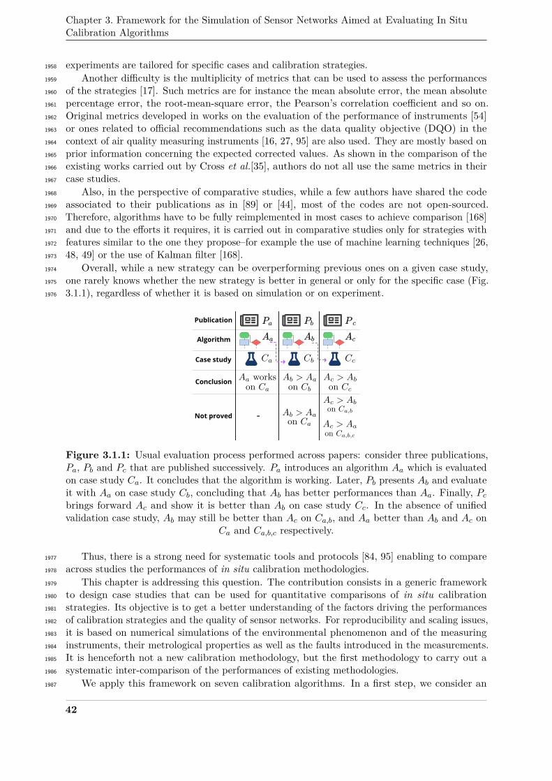
Chapter 3. Framework for the Simulation of Sensor Networks Aimed at Evaluating In SituCalibration Algorithms
experiments are tailored for specific cases and calibration strategies.1958
Another difficulty is the multiplicity of metrics that can be used to assess the performances1959
of the strategies [17]. Such metrics are for instance the mean absolute error, the mean absolute1960
percentage error, the root-mean-square error, the Pearson’s correlation coefficient and so on.1961
Original metrics developed in works on the evaluation of the performance of instruments [54]1962
or ones related to official recommendations such as the data quality objective (DQO) in the1963
context of air quality measuring instruments [16, 27, 95] are also used. They are mostly based on1964
prior information concerning the expected corrected values. As shown in the comparison of the1965
existing works carried out by Cross et al.[35], authors do not all use the same metrics in their1966
case studies.1967
Also, in the perspective of comparative studies, while a few authors have shared the code1968
associated to their publications as in [89] or [44], most of the codes are not open-sourced.1969
Therefore, algorithms have to be fully reimplemented in most cases to achieve comparison [168]1970
and due to the efforts it requires, it is carried out in comparative studies only for strategies with1971
features similar to the one they propose–for example the use of machine learning techniques [26,1972
48, 49] or the use of Kalman filter [168].1973
Overall, while a new strategy can be overperforming previous ones on a given case study,1974
one rarely knows whether the new strategy is better in general or only for the specific case (Fig.1975
3.1.1), regardless of whether it is based on simulation or on experiment.1976
Publication
Algorithm
Conclusion
Case study
Not proved -
Figure 3.1.1: Usual evaluation process performed across papers: consider three publications,Pa, Pb and Pc that are published successively. Pa introduces an algorithm Aa which is evaluatedon case study Ca. It concludes that the algorithm is working. Later, Pb presents Ab and evaluateit with Aa on case study Cb, concluding that Ab has better performances than Aa. Finally, Pcbrings forward Ac and show it is better than Ab on case study Cc. In the absence of unifiedvalidation case study, Ab may still be better than Ac on Ca,b, and Aa better than Ab and Ac on
Ca and Ca,b,c respectively.
Thus, there is a strong need for systematic tools and protocols [84, 95] enabling to compare1977
across studies the performances of in situ calibration methodologies.1978
This chapter is addressing this question. The contribution consists in a generic framework1979
to design case studies that can be used for quantitative comparisons of in situ calibration1980
strategies. Its objective is to get a better understanding of the factors driving the performances1981
of calibration strategies and the quality of sensor networks. For reproducibility and scaling issues,1982
it is based on numerical simulations of the environmental phenomenon and of the measuring1983
instruments, their metrological properties as well as the faults introduced in the measurements.1984
It is henceforth not a new calibration methodology, but the first methodology to carry out a1985
systematic inter-comparison of the performances of existing methodologies.1986
We apply this framework on seven calibration algorithms. In a first step, we consider an1987
42
2. Description of the framework
elementary case study on a blind static network that is sufficient to get first insights by analysing1988
the performances with commonly used metrics at different scales. Then, we evaluate the impact1989
of the realism of the model of pollution emission and dispersion, the density of the deployment1990
of the measuring instruments, and the error model of the devices. Finally, several engineering1991
insights are deduced from the investigations carried out, validating the relevance of such a1992
framework in the design phase of a practical network of low-cost environmental sensors.1993
2 Description of the framework1994
A generic framework to design case studies is proposed in this section for quantitative1995
comparisons of in situ calibration strategies. It aims at yielding a better understanding of the1996
factors driving the performances of calibration strategies, and at providing a protocol as rigorous1997
as possible to conduct such studies. The different steps are described in a generic way to ensure1998
their applicability for most cases.1999
Like for faults in Chapter 1 Section 2, we adopt a data-centric point of view. We do not target2000
the modelling of the entire measuring chain of an instrument described in Chapter 1 Section 1.22001
and illustrated in Figure 1.1.2 in the same chapter. We assume that instruments are grey boxes2002
which provide measured values based on true values of a measurand and possibly also on true2003
values of influence quantities. The grey boxes representing instruments consist into algorithms2004
mimicking the features of real instruments.2005
In this work, we focus on the metrological performances of in situ calibration strategies.2006
Other subjects such as the communication costs, the energy consumption or the computational2007
efforts for instance are not in the frame of this study.2008
2.1 Simulation-based strategy2009
The methodology is based on simulation because it enables the following properties that are2010
difficult to get with field or lab experiments2011
• Ability to perform a study with different operating conditions for a same sensor network.2012
• Reproducibility: same operating conditions on different sensor networks.2013
• Knowledge of true values: in experimental operating conditions, true values are not2014
known perfectly–there is always an uncertainty– and having very accurate values requires2015
high-quality instruments which are usually expensive.2016
• Scalability: the only limit to the density, number and diversity of measuring instruments is2017
the computing time.2018
To conduct the evaluation of in situ calibration strategies, the framework combines the2019
simulations of the environmental phenomena to produce the true values of the measurand, and2020
of the potential influence quantities, at any position and time, the simulations of the mobility –if2021
any– of the nodes of the network to know where and when measurements are performed, and2022
the simulations of the measuring chain of the instruments to produce the measured values. The2023
realism of the results will depend on the complexity and accuracy of each simulation model. On2024
the other hand, being able to analyse results on a simplistic model can also help to highlight2025
fundamental properties before confronting them to more complex situations. In particular, even2026
if we consider networks of sensors, we neglect to simulate the system and networking aspects.2027
We consider they have a lesser influence on the metrological performances of in situ calibration2028
strategies. One could, however, argue that system and network issues could challenge the2029
robustness of a given implementation of a calibration protocol because of packet loss. It could2030
also be interesting to evaluate the energetic cost or time to converge of such implementation. It2031
43
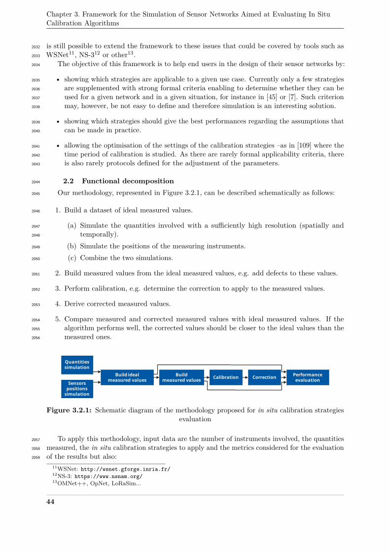
Chapter 3. Framework for the Simulation of Sensor Networks Aimed at Evaluating In SituCalibration Algorithms
is still possible to extend the framework to these issues that could be covered by tools such as2032
WSNet11, NS-312 or other13.2033
The objective of this framework is to help end users in the design of their sensor networks by:2034
• showing which strategies are applicable to a given use case. Currently only a few strategies2035
are supplemented with strong formal criteria enabling to determine whether they can be2036
used for a given network and in a given situation, for instance in [45] or [7]. Such criterion2037
may, however, be not easy to define and therefore simulation is an interesting solution.2038
• showing which strategies should give the best performances regarding the assumptions that2039
can be made in practice.2040
• allowing the optimisation of the settings of the calibration strategies –as in [109] where the2041
time period of calibration is studied. As there are rarely formal applicability criteria, there2042
is also rarely protocols defined for the adjustment of the parameters.2043
2.2 Functional decomposition2044
Our methodology, represented in Figure 3.2.1, can be described schematically as follows:2045
1. Build a dataset of ideal measured values.2046
(a) Simulate the quantities involved with a sufficiently high resolution (spatially and2047
temporally).2048
(b) Simulate the positions of the measuring instruments.2049
(c) Combine the two simulations.2050
2. Build measured values from the ideal measured values, e.g. add defects to these values.2051
3. Perform calibration, e.g. determine the correction to apply to the measured values.2052
4. Derive corrected measured values.2053
5. Compare measured and corrected measured values with ideal measured values. If the2054
algorithm performs well, the corrected values should be closer to the ideal values than the2055
measured ones.2056
Quantitiessimulation
Sensorspositions
simulation
Build idealmeasured values
Buildmeasured values Calibration Correction Performance
evaluation
Figure 3.2.1: Schematic diagram of the methodology proposed for in situ calibration strategiesevaluation
To apply this methodology, input data are the number of instruments involved, the quantities2057
measured, the in situ calibration strategies to apply and the metrics considered for the evaluation2058
of the results but also:2059
11WSNet: http://wsnet.gforge.inria.fr/12NS-3: https://www.nsnam.org/13OMNet++, OpNet, LoRaSim...
44
2. Description of the framework
• Information to simulate the quantities involved. Depending on the model, it can be as2060
simple as some parameters of an equation (e.g. a Gaussian model) or a complex description2061
of an urban scene (e.g. http://air.ec-lyon.fr/SIRANE/)2062
• Specifications on the deployment and possible mobility of the instruments. Since the2063
positions of the instruments is critical for the performances of the sensor network, the2064
number of instruments deployed, and their positions may be optimised [19].2065
• Descriptions of the measuring chain of the instruments involved, in terms of drift and of2066
their potential influence quantities.2067
• Configuration of the considered in situ calibration strategies.2068
As outputs, the framework provides time series of the true values, of the measured values2069
and of the corrected values for each instrument. Values of metrics computed for the comparison2070
of these times series may also be given.2071
The following subsections give details on each step.2072
2.2.1 Build ideal measured values2073
Ideal measured values are measured values that should be measured by instruments if2074
they were perfect. It means for an instrument si that its measured values v(si, t) are equal to2075
the true value of the measurand, noted vtrue(si, t), for all t.2076
Generating these ideal measured values for all the instruments of a sensor network can be2077
carried out as follows.2078
To build ideal measured values, true values of the measurand must be computed. True values2079
of other quantities may also be derived for the simulation such as influence quantities if the2080
instruments to model undergo such effects.2081
To be able to repeat the study with different sensor networks, the quantities can be simulated2082
independently of the positions of the instruments so that one may build different sets of ideal2083
measured values from a same simulation of the quantities depending on the sensor network.2084
Therefore, the simulation is performed on the targeted domain of study, e.g. a specific2085
geometry, at a sufficient spatial and temporal resolution, regarding the potential positions of the2086
instruments and their frequency of measurement. The model used for the simulation depends on2087
the application and on the targeted accuracy. Ideally, the simulation should perfectly represent2088
the studied environmental phenomena and the quantities affecting instruments operating under2089
real conditions. This is not always possible and thus the models used may not reflect the real2090
temporal and spatial variability of environmental phenomena. This is particularly true for air2091
pollution monitoring. While high model accuracy can be achieved with advanced computational2092
fluid dynamics models [12], such models require time and resources that are not always acceptable2093
or available for users. In multiple works, case studies were conducted with abstract models [7],2094
enabling to demonstrate that the proposed calibration strategy is functional. However, such2095
models do not enable determining if an algorithm is applicable on real cases.2096
In addition to the true values of the considered quantities, the sets of the positions where2097
measurements are performed must be built with respect to the position and possible mobility of2098
each instrument. Based on the positions of the instruments over time, true values are extracted2099
and stored from the simulation of the studied quantities at the locations of each instrument at2100
each time step according to their sampling periods.2101
Afterwards, a time series of ideal measured values is available for each measuring instrument.142102
14In this section, we considered that the simulation of the quantities and the simulation of the positions of theinstruments are carried out separately and then combined. However, it might be possible to determine first thepositions of the instruments and then to derive the ideal measured values only at the positions for instance.
45
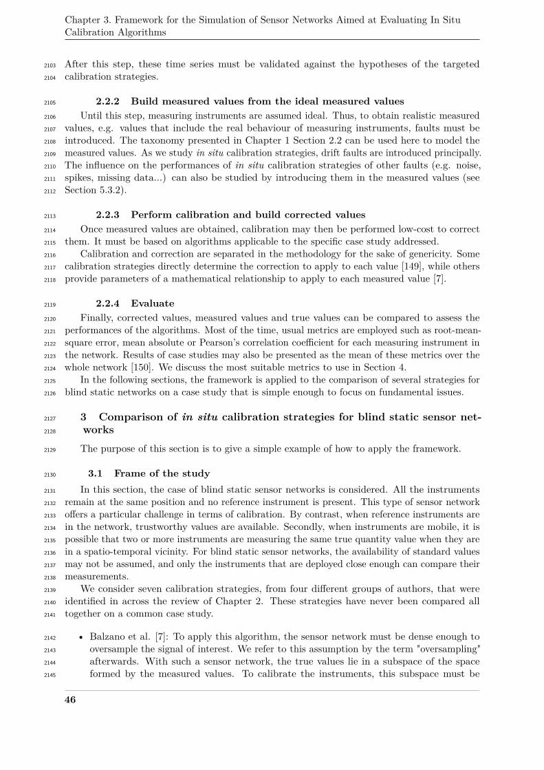
Chapter 3. Framework for the Simulation of Sensor Networks Aimed at Evaluating In SituCalibration Algorithms
After this step, these time series must be validated against the hypotheses of the targeted2103
calibration strategies.2104
2.2.2 Build measured values from the ideal measured values2105
Until this step, measuring instruments are assumed ideal. Thus, to obtain realistic measured2106
values, e.g. values that include the real behaviour of measuring instruments, faults must be2107
introduced. The taxonomy presented in Chapter 1 Section 2.2 can be used here to model the2108
measured values. As we study in situ calibration strategies, drift faults are introduced principally.2109
The influence on the performances of in situ calibration strategies of other faults (e.g. noise,2110
spikes, missing data...) can also be studied by introducing them in the measured values (see2111
Section 5.3.2).2112
2.2.3 Perform calibration and build corrected values2113
Once measured values are obtained, calibration may then be performed low-cost to correct2114
them. It must be based on algorithms applicable to the specific case study addressed.2115
Calibration and correction are separated in the methodology for the sake of genericity. Some2116
calibration strategies directly determine the correction to apply to each value [149], while others2117
provide parameters of a mathematical relationship to apply to each measured value [7].2118
2.2.4 Evaluate2119
Finally, corrected values, measured values and true values can be compared to assess the2120
performances of the algorithms. Most of the time, usual metrics are employed such as root-mean-2121
square error, mean absolute or Pearson’s correlation coefficient for each measuring instrument in2122
the network. Results of case studies may also be presented as the mean of these metrics over the2123
whole network [150]. We discuss the most suitable metrics to use in Section 4.2124
In the following sections, the framework is applied to the comparison of several strategies for2125
blind static networks on a case study that is simple enough to focus on fundamental issues.2126
3 Comparison of in situ calibration strategies for blind static sensor net-2127
works2128
The purpose of this section is to give a simple example of how to apply the framework.2129
3.1 Frame of the study2130
In this section, the case of blind static sensor networks is considered. All the instruments2131
remain at the same position and no reference instrument is present. This type of sensor network2132
offers a particular challenge in terms of calibration. By contrast, when reference instruments are2133
in the network, trustworthy values are available. Secondly, when instruments are mobile, it is2134
possible that two or more instruments are measuring the same true quantity value when they are2135
in a spatio-temporal vicinity. For blind static sensor networks, the availability of standard values2136
may not be assumed, and only the instruments that are deployed close enough can compare their2137
measurements.2138
We consider seven calibration strategies, from four different groups of authors, that were2139
identified in across the review of Chapter 2. These strategies have never been compared all2140
together on a common case study.2141
• Balzano et al. [7]: To apply this algorithm, the sensor network must be dense enough to2142
oversample the signal of interest. We refer to this assumption by the term "oversampling"2143
afterwards. With such a sensor network, the true values lie in a subspace of the space2144
formed by the measured values. To calibrate the instruments, this subspace must be2145
46

3. Comparison of in situ calibration strategies for blind static sensor networks
known. The gains and offsets for all nodes are then estimated with the chosen subspace2146
and the measured values using singular value decomposition (SVD) or by solving a system2147
of equations using a least square (LS) estimator. These strategies are respectively called2148
SM-SVD and SM-LS, SM standing for subspace matching. Note that gains are estimated2149
up to a multiplicative coefficient. Consequently, the gain of one instrument should be2150
known to complete the calibration. Likewise, the offset computation requires either to2151
know some of the offsets, or that an additional hypothesis on the signal is valid.15 As such,2152
the network is not perfectly blind in truth.2153
• Lipor et al. [89]: This work is an extent of [7]. It shows first that the solution obtained with2154
SM-SVD is equivalent to the one obtained by solving the system of equations expressed as2155
a total least squares problem (TLS). The latter strategy is called SM-TLS.162156
• Takruri et al. [148–150]: Three contributions from these authors are considered. The2157
first one is based on the idea that the average of the values of neighbouring measuring2158
instruments gives a good estimation of the correct value of an instrument to calibrate. If2159
the absolute difference between the measured value and the average is greater than a given2160
threshold, this difference is added to the instrument’s value. We call this strategy AB-DT2161
(average-based estimation for difference-based threshold). Two variations are also proposed,2162
a first one in which the difference-based threshold mechanism is replaced by a Kalman2163
filter that estimates the error affecting the instruments (AB-KF), and a second one where2164
the average-based part is replaced by support vector regression (SVR-KF).2165
• Kumar et al. [76, 77]: This work, inspired from the previous one, also proposes the use of a2166
Kalman filter to estimate the error of each instrument but instead of performing an average2167
over neighbouring nodes or using SVR for true value estimation, kriging is used (K-KF).2168
Note that not every strategy that could have been applied to our case study is considered2169
here. For instance, the work of Dorffer et al. [44] extends [7] and [89] for sparse signals, but this2170
is not in the scope of the study.2171
3.2 Application of the framework2172
3.2.1 Simulation of the ideal measured values2173
A space of 1000× 1000m is considered. It is discretised with a step of 10m. At the centreof this area, a NO2 source is considered. The concentration of NO2, C, at the instant t andposition (x, y), is modelled as:
C(x, y, t) = A(t) exp(− x2 + y2
σ(t)2
)It is a 2D Gaussian function with an equal spread σ for x and y. This model is not very2174
realistic but has been used in other papers [45] for its simplicity of implementation. Examples of2175
pollution maps are represented in Figure 3.3.1.2176
To facilitate the interpretation of σ, it is expressed as a function of the full width at halfmaximum (FWHM) of the Gaussian curve:
σ = FWHM
2 ln(2)15A usual assumption is that "the signal has a null (or known) average".16Note that additional formulations given in the publication, in the case where some gains are known for a
subset of instruments, are not considered here as it would be equivalent to have a partially blind sensor network.
47
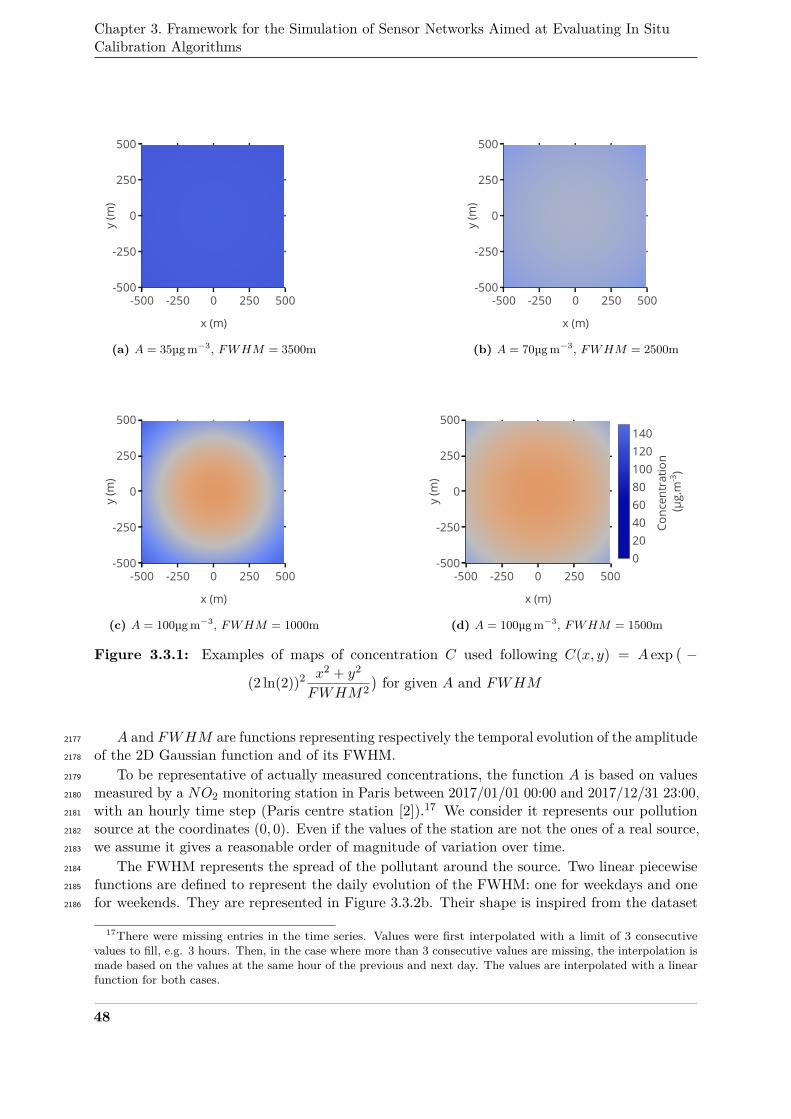
Chapter 3. Framework for the Simulation of Sensor Networks Aimed at Evaluating In SituCalibration Algorithms
-500 -250 0 250 500-500
-250
0
250
500
x (m)
y (m
)
(a) A = 35µg m−3, FWHM = 3500m
-500 -250 0 250 500-500
-250
0
250
500
x (m)
y (m
)
(b) A = 70µg m−3, FWHM = 2500m
-500 -250 0 250 500-500
-250
0
250
500
x (m)
y (m
)
(c) A = 100µg m−3, FWHM = 1000m
-500 -250 0 250 500-500
-250
0
250
500
020406080100120140
Conc
entr
atio
n (μ
g.m
-3)
x (m)
y (m
)
(d) A = 100µg m−3, FWHM = 1500m
Figure 3.3.1: Examples of maps of concentration C used following C(x, y) = A exp(−
(2 ln(2))2 x2 + y2
FWHM2)for given A and FWHM
A and FWHM are functions representing respectively the temporal evolution of the amplitude2177
of the 2D Gaussian function and of its FWHM.2178
To be representative of actually measured concentrations, the function A is based on values2179
measured by a NO2 monitoring station in Paris between 2017/01/01 00:00 and 2017/12/31 23:00,2180
with an hourly time step (Paris centre station [2]).17 We consider it represents our pollution2181
source at the coordinates (0, 0). Even if the values of the station are not the ones of a real source,2182
we assume it gives a reasonable order of magnitude of variation over time.2183
The FWHM represents the spread of the pollutant around the source. Two linear piecewise2184
functions are defined to represent the daily evolution of the FWHM: one for weekdays and one2185
for weekends. They are represented in Figure 3.3.2b. Their shape is inspired from the dataset2186
17There were missing entries in the time series. Values were first interpolated with a limit of 3 consecutivevalues to fill, e.g. 3 hours. Then, in the case where more than 3 consecutive values are missing, the interpolation ismade based on the values at the same hour of the previous and next day. The values are interpolated with a linearfunction for both cases.
48
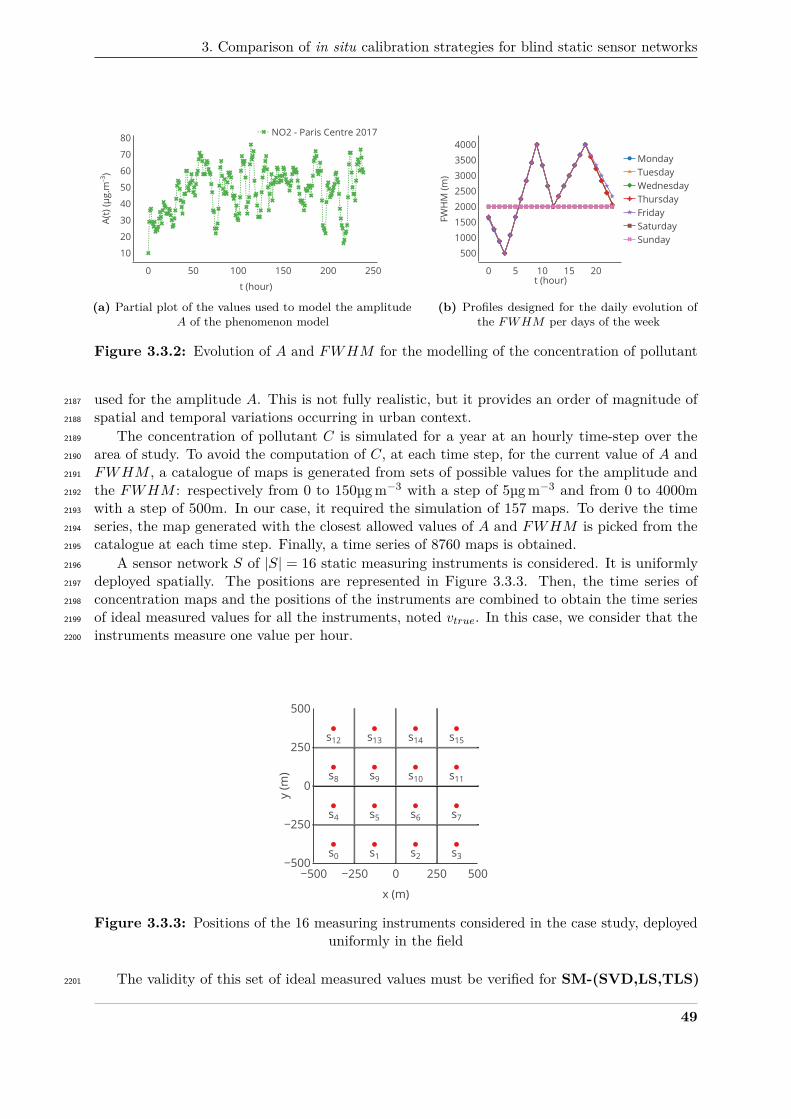
3. Comparison of in situ calibration strategies for blind static sensor networks
0 50 100 150 200 250
10
20
30
40
50
60
70
80 NO2 - Paris Centre 2017
t (hour)
A(t)
(μg.
m -3 )
(a) Partial plot of the values used to model the amplitudeA of the phenomenon model
0 5 10 15 20
5001000150020002500300035004000
MondayTuesdayWednesdayThursdayFridaySaturdaySunday
t (hour)
FWH
M (m
)
(b) Profiles designed for the daily evolution ofthe FWHM per days of the week
Figure 3.3.2: Evolution of A and FWHM for the modelling of the concentration of pollutant
used for the amplitude A. This is not fully realistic, but it provides an order of magnitude of2187
spatial and temporal variations occurring in urban context.2188
The concentration of pollutant C is simulated for a year at an hourly time-step over the2189
area of study. To avoid the computation of C, at each time step, for the current value of A and2190
FWHM , a catalogue of maps is generated from sets of possible values for the amplitude and2191
the FWHM : respectively from 0 to 150µg m−3 with a step of 5µg m−3 and from 0 to 4000m2192
with a step of 500m. In our case, it required the simulation of 157 maps. To derive the time2193
series, the map generated with the closest allowed values of A and FWHM is picked from the2194
catalogue at each time step. Finally, a time series of 8760 maps is obtained.2195
A sensor network S of |S| = 16 static measuring instruments is considered. It is uniformly2196
deployed spatially. The positions are represented in Figure 3.3.3. Then, the time series of2197
concentration maps and the positions of the instruments are combined to obtain the time series2198
of ideal measured values for all the instruments, noted vtrue. In this case, we consider that the2199
instruments measure one value per hour.2200
s 0 s 1 s 2 s 3
s 4 s 5 s 6 s 7
s 8 s 9 s 10 s 11
s 12 s 13 s 14 s 15
−500 −250 0 250 500−500
−250
0
250
500
x (m)
y (m
)
Figure 3.3.3: Positions of the 16 measuring instruments considered in the case study, deployeduniformly in the field
The validity of this set of ideal measured values must be verified for SM-(SVD,LS,TLS)2201
49

Chapter 3. Framework for the Simulation of Sensor Networks Aimed at Evaluating In SituCalibration Algorithms
strategies. The network should satisfy the hypothesis of "oversampling". To verify it, a principal2202
component analysis (PCA) of the matrix formed by the concatenation of the ideal measured2203
values time series of each node is carried out. We assume that the sensor network is satisfying the2204
oversampling hypothesis if the explained variance ratio of the ν first components is greater than2205
0.999 and ν < |S|. In our case, the condition is met for ν = 2 < |S|. Therefore, the oversampling2206
hypothesis is satisfied.2207
3.2.2 Building of the measured values2208
The network is defined as "blind", which can also be expressed by "all the instruments have the2209
same sensing reliability". In a first step, instruments are only drifting. Drift of each instrument is2210
only function of time. We assume all the instruments undergo a linear drift increasing up to 5%2211
of the gain every 7 days. The actual drift is randomly drawn following a uniform law. The value2212
of 5% is set according to what is reported in typical measuring instrument datasheets [105].2213
The instruments are assumed to be initially calibrated and to remain faultless for eight weeks,2214
which gives a training dataset for the strategies needing it, notably to learn the subspace of the2215
signal with PCA for SM-(SVD,LS,TLS). For four additional weeks, the instruments are kept2216
without drift to study how calibrations strategies behave if the devices are not drifting. Finally,2217
the instruments start drifting after twelve weeks. This instant is noted tstart drift.2218
Therefore, the gain G(si, t) of the instrument si at t is :2219
G(si, t) =
1 if t < tstart drift
G(si, t− 1) if t ≥ tstart drift and (t− tstart drift) mod 7 days 6= 0G(si, t− 1) + δG(si, t) if t ≥ tstart drift and (t− tstart drift) mod 7 days = 0
with ∀t, δG(si, t) ∼ U(0, 0.05)
This drift model is called "Weekly Gain Linear Increase"(WGLI).2220
The measured value v(si, t) of the instrument si at t is expressed from the true value vtrue(si, t)using the relationship:
v(si, t) = G(si, t) · vtrue(si, t)
3.2.3 Configuration of the strategies2221
Each strategy has parameters to set up. They are defined as follows:2222
• SM-(SVD,LS,TLS): All these strategies share the same parameters, namely the period-2223
icity of calibration and the time interval on which the linear system is solved. Note that2224
the adjustment of the parameters was not discussed by the original authors. We chose to2225
apply the strategy each week and to solve the linear system over the past w = 7 days.2226
• Kalman filter of (AB, SVR, K)-KF: Variables R and Q are set to 0.0001 and 1 respec-2227
tively.2228
• Definition of neighbours for AB-(DT,KF): Instruments are defined as neighbours if they2229
are distant of less than 250m.2230
• Parameters of the SVR for SVR-KF: Kernel used is ’rbf’, the kernel coefficient gamma is2231
set to 10−8 and the penalty parameter C is set to 103.2232
• Parameters for the weighting for K-KF: a, c0 and c1 were defined as in [77], therefore2233
a = 12, c0 = 0.25, c1 = 0.85.2234
50
3. Comparison of in situ calibration strategies for blind static sensor networks
We invite the reader to refer to the original publications for a more in-depth understanding2235
of the parameters of these calibration strategies.2236
3.2.4 Evaluation2237
To compare the corrected values of an instrument, obtained with each strategy, and its2238
measured values against its ideal measured values, metrics are needed. We consider the most2239
commonly used metrics in the publications reported in Chapter 2 and described as follows. They2240
can be computed for each instrument or averaged over the network. We discuss the relevance2241
of these statistics in Section 4. In the following, the set x stands for the k measured values2242
of an instrument si over [t −∆t; t], V (si, (t,∆t)) or the corresponding set of corrected values2243
Vcorr(si, (t,∆t)) and the set y is the associated k true values Vtrue(si, (t,∆t)).2244
• Mean absolute error (MAE):
MAE(x, y) = 1k
k∑i=0|xi − yi|
• Root-mean-square error (RMSE):
RMSE(x, y) =
√√√√1k
k∑i=0
(xi − yi)2
• Mean absolute percentage error (MAPE):
MAPE(x, y) = 100k
k∑i=0
|xi − yi||yi|
Remark: the values of y must all be different from zero.2245
• Pearson correlation coefficient (ρ):
ρ(x, y) = E[(x− E[x])(y − E[y])]√E[(x− E[x])2]E[(y − E[y])2]
with E[.] being the expectation.2246
For perfect instruments before correction (or after with vcorr instead of v):2247
• MAE(V (si, (t,∆t)), Vtrue(si, (t,∆t))) = 0.2248
• RMSE(V (si, (t,∆t)), Vtrue(si, (t,∆t))) = 0.2249
• MAPE(V (si, (t,∆t)), Vtrue(si, (t,∆t))) = 0%.2250
• ρ(V (si, (t,∆t)), Vtrue(si, (t,∆t))) = 1.2251
3.3 Results2252
In Figure 3.3.4, a partial plot of true values, measured values and corrected values obtained2253
with each strategy is displayed for a particular instrument. For the considered device, a visual2254
observation indicates that strategies SM-(SVD, LS, TLS) and SVR-KF provide better results2255
than AB-DT, AB-KF and K-KF.2256
51
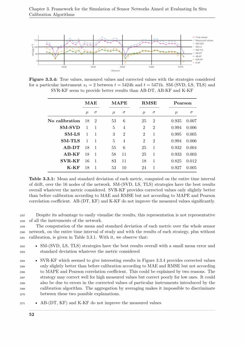
Chapter 3. Framework for the Simulation of Sensor Networks Aimed at Evaluating In SituCalibration Algorithms
5430 5440 5450 5460 5470
0
50
100
150True valuesMeasured valuesSM-SVDSM-LSSM-TLSAB-DTAB-KFSVR-KFK-KF
t (hours)
v(t)
(μg.
m -3 )
Figure 3.3.4: True values, measured values and corrected values with the strategies consideredfor a particular instrument s1 = 2 between t = 5424h and t = 5471h. SM-(SVD, LS, TLS) and
SVR-KF seem to provide better results than AB-DT, AB-KF and K-KF
MAE MAPE RMSE Pearson
µ σ µ σ µ σ µ σ
No calibration 18 2 53 6 25 2 0.935 0.007SM-SVD 1 1 5 4 2 2 0.994 0.006SM-LS 1 1 3 2 2 1 0.995 0.005
SM-TLS 1 1 5 4 2 2 0.994 0.006AB-DT 18 1 55 6 25 1 0.932 0.004AB-KF 18 1 58 11 25 1 0.933 0.003
SVR-KF 16 1 83 11 18 1 0.825 0.012K-KF 18 1 53 10 24 1 0.927 0.005
Table 3.3.1: Mean and standard deviation of each metric, computed on the entire time intervalof drift, over the 16 nodes of the network. SM-(SVD, LS, TLS) strategies have the best resultsoverall whatever the metric considered. SVR-KF provides corrected values only slightly betterthan before calibration according to MAE and RMSE but not according to MAPE and Pearsoncorrelation coefficient. AB-(DT, KF) and K-KF do not improve the measured values significantly.
Despite its advantage to easily visualise the results, this representation is not representative2257
of all the instruments of the network.2258
The computation of the mean and standard deviation of each metric over the whole sensor2259
network, on the entire time interval of study and with the results of each strategy, plus without2260
calibration, is given in Table 3.3.1. With it, we observe that:2261
• SM-(SVD, LS, TLS) strategies have the best results overall with a small mean error and2262
standard deviation whatever the metric considered2263
• SVR-KF which seemed to give interesting results in Figure 3.3.4 provides corrected values2264
only slightly better than before calibration according to MAE and RMSE but not according2265
to MAPE and Pearson correlation coefficient. This could be explained by two reasons. The2266
strategy may correct well for high measured values but correct poorly for low ones. It could2267
also be due to errors in the corrected values of particular instruments introduced by the2268
calibration algorithm. The aggregation by averaging makes it impossible to discriminate2269
between these two possible explanations.2270
• AB-(DT, KF) and K-KF do not improve the measured values2271
52
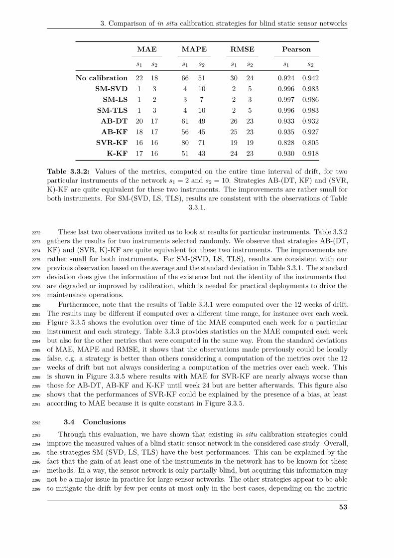
3. Comparison of in situ calibration strategies for blind static sensor networks
MAE MAPE RMSE Pearson
s1 s2 s1 s2 s1 s2 s1 s2
No calibration 22 18 66 51 30 24 0.924 0.942SM-SVD 1 3 4 10 2 5 0.996 0.983SM-LS 1 2 3 7 2 3 0.997 0.986
SM-TLS 1 3 4 10 2 5 0.996 0.983AB-DT 20 17 61 49 26 23 0.933 0.932AB-KF 18 17 56 45 25 23 0.935 0.927
SVR-KF 16 16 80 71 19 19 0.828 0.805K-KF 17 16 51 43 24 23 0.930 0.918
Table 3.3.2: Values of the metrics, computed on the entire time interval of drift, for twoparticular instruments of the network s1 = 2 and s2 = 10. Strategies AB-(DT, KF) and (SVR,K)-KF are quite equivalent for these two instruments. The improvements are rather small forboth instruments. For SM-(SVD, LS, TLS), results are consistent with the observations of Table
3.3.1.
These last two observations invited us to look at results for particular instruments. Table 3.3.22272
gathers the results for two instruments selected randomly. We observe that strategies AB-(DT,2273
KF) and (SVR, K)-KF are quite equivalent for these two instruments. The improvements are2274
rather small for both instruments. For SM-(SVD, LS, TLS), results are consistent with our2275
previous observation based on the average and the standard deviation in Table 3.3.1. The standard2276
deviation does give the information of the existence but not the identity of the instruments that2277
are degraded or improved by calibration, which is needed for practical deployments to drive the2278
maintenance operations.2279
Furthermore, note that the results of Table 3.3.1 were computed over the 12 weeks of drift.2280
The results may be different if computed over a different time range, for instance over each week.2281
Figure 3.3.5 shows the evolution over time of the MAE computed each week for a particular2282
instrument and each strategy. Table 3.3.3 provides statistics on the MAE computed each week2283
but also for the other metrics that were computed in the same way. From the standard deviations2284
of MAE, MAPE and RMSE, it shows that the observations made previously could be locally2285
false, e.g. a strategy is better than others considering a computation of the metrics over the 122286
weeks of drift but not always considering a computation of the metrics over each week. This2287
is shown in Figure 3.3.5 where results with MAE for SVR-KF are nearly always worse than2288
those for AB-DT, AB-KF and K-KF until week 24 but are better afterwards. This figure also2289
shows that the performances of SVR-KF could be explained by the presence of a bias, at least2290
according to MAE because it is quite constant in Figure 3.3.5.2291
3.4 Conclusions2292
Through this evaluation, we have shown that existing in situ calibration strategies could2293
improve the measured values of a blind static sensor network in the considered case study. Overall,2294
the strategies SM-(SVD, LS, TLS) have the best performances. This can be explained by the2295
fact that the gain of at least one of the instruments in the network has to be known for these2296
methods. In a way, the sensor network is only partially blind, but acquiring this information may2297
not be a major issue in practice for large sensor networks. The other strategies appear to be able2298
to mitigate the drift by few per cents at most only in the best cases, depending on the metric2299
53
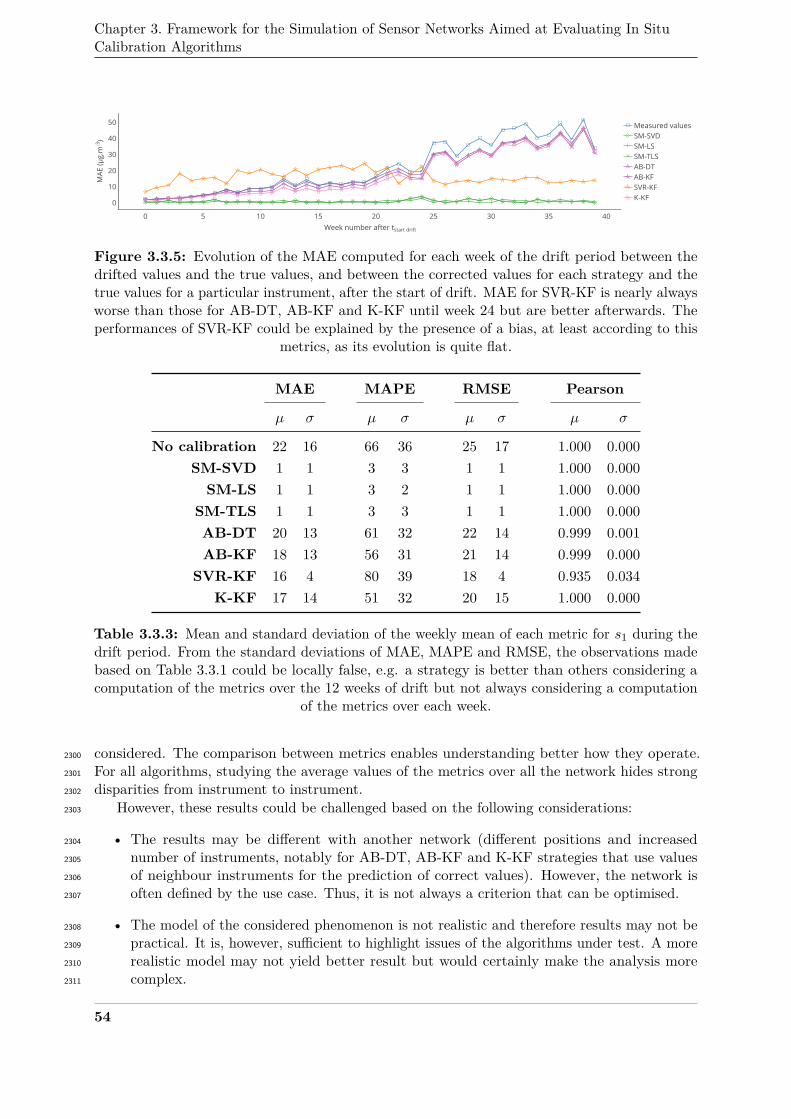
Chapter 3. Framework for the Simulation of Sensor Networks Aimed at Evaluating In SituCalibration Algorithms
0 5 10 15 20 25 30 35 40
0
10
20
30
40
50 Measured valuesSM-SVDSM-LSSM-TLSAB-DTAB-KFSVR-KFK-KF
Week number after t start drift
MAE
(μg.
m -3
)
Figure 3.3.5: Evolution of the MAE computed for each week of the drift period between thedrifted values and the true values, and between the corrected values for each strategy and thetrue values for a particular instrument, after the start of drift. MAE for SVR-KF is nearly alwaysworse than those for AB-DT, AB-KF and K-KF until week 24 but are better afterwards. Theperformances of SVR-KF could be explained by the presence of a bias, at least according to this
metrics, as its evolution is quite flat.
MAE MAPE RMSE Pearson
µ σ µ σ µ σ µ σ
No calibration 22 16 66 36 25 17 1.000 0.000SM-SVD 1 1 3 3 1 1 1.000 0.000SM-LS 1 1 3 2 1 1 1.000 0.000
SM-TLS 1 1 3 3 1 1 1.000 0.000AB-DT 20 13 61 32 22 14 0.999 0.001AB-KF 18 13 56 31 21 14 0.999 0.000
SVR-KF 16 4 80 39 18 4 0.935 0.034K-KF 17 14 51 32 20 15 1.000 0.000
Table 3.3.3: Mean and standard deviation of the weekly mean of each metric for s1 during thedrift period. From the standard deviations of MAE, MAPE and RMSE, the observations madebased on Table 3.3.1 could be locally false, e.g. a strategy is better than others considering acomputation of the metrics over the 12 weeks of drift but not always considering a computation
of the metrics over each week.
considered. The comparison between metrics enables understanding better how they operate.2300
For all algorithms, studying the average values of the metrics over all the network hides strong2301
disparities from instrument to instrument.2302
However, these results could be challenged based on the following considerations:2303
• The results may be different with another network (different positions and increased2304
number of instruments, notably for AB-DT, AB-KF and K-KF strategies that use values2305
of neighbour instruments for the prediction of correct values). However, the network is2306
often defined by the use case. Thus, it is not always a criterion that can be optimised.2307
• The model of the considered phenomenon is not realistic and therefore results may not be2308
practical. It is, however, sufficient to highlight issues of the algorithms under test. A more2309
realistic model may not yield better result but would certainly make the analysis more2310
complex.2311
54
4. Evaluation of measurements after correction
• Only a drift of the gain was added which does not fully relate the behaviour of a real2312
instrument. Adopting a finer-grained model of the behaviour also increases the complexity2313
of the case study.2314
• Other parameters of the calibration strategies may change the results. We empirically2315
explored the parameters of the algorithms, keeping in this study the values that give the2316
best results for each strategy. There is, however, no claim for optimality here, but the2317
framework can be used to optimise the parameters of a given strategy.2318
In Section 5, the impact of these four separate aspects on the algorithms is tested. Before2319
moving on to this, we discuss in the next section the metrics used and how additional ones, or2320
other ways to visualise results, can give an enhanced comprehension of the behaviour of the2321
calibration algorithms on a sensor network.2322
4 Evaluation of measurements after correction2323
4.1 Problem statement2324
To evaluate the performances of in situ calibration strategies, various metrics are commonly2325
used like MAE, MAPE, RMSE and Pearson’s correlation coefficient notably. We presented the2326
results as statistics of these metrics over the entire network or values for particular instruments.2327
The metrics were computed on the entire time interval of study or on subintervals. Results were2328
displayed as tables and plots. These choices enabled carrying out an analysis at multiple scales2329
(entire network versus individual instruments). This approach underlines disparities of efficiency2330
of the algorithms on particular instruments for instance.2331
Multiple surveys exist on metrics [17]. They aim at providing a clear reading on the differences2332
and similarities among the wide spectra of metrics used. While metrics are numerous, groups of2333
them are based on the same idea (difference, absolute difference, square difference...). In some2334
works, such as in [54], an integrated performance index was developed to combine the values2335
of several metrics into a single one. However, some metrics are interdependent [154], which2336
can exaggerate or hide information when they are combined. In the literature regarding in situ2337
calibration strategies, the choice of metrics is not always clearly justified, nor is the choice of2338
the values presented and how they are computed (values for particular instruments, statistics2339
of the metric over the network and so on). Moreover, Tian et al. [154] showed it is possible to2340
have equal values of multiple metrics for two sets of values very different from each other. They2341
justified it by the interdependence, underdetermination and incompleteness of usual metrics, in2342
addition to the fact that they assume the error to be linear. This issue is major as metrics are2343
used in official recommendations such as the data quality objectives (DQO) in the context of air2344
quality measuring instruments [16, 27, 95]. In this way, we suggest in the next section to use an2345
error model as introduced by Tian et al. [154]. It is considered as a satisfying means to deal2346
with these issues.2347
Another question lies in the way a metric is computed or in how statistics are derived from2348
it. As shown in the previous section, looking at values of metrics computed over the full-time2349
interval of drift or computed over each week may yield different interpretations. The choice of2350
the time interval on which it is derived can be guided by requirements on the minimal duration2351
for which the mean error of an instrument must be under a given threshold for instance.2352
Regarding the use of statistics, it concerns particularly networks with hundreds of nodes,2353
for which interpreting the values of metrics for each node may not be easily feasible. However,2354
statistics derived over the entire network do not enable discriminating easily between instruments2355
differently affected by an algorithm. The use of statistics is perfectly appropriate if the quality2356
of the calibration of the instruments belonging to a sensor network should be evaluated at the2357
level of the network, e.g. when it is the collective performance that matter. Otherwise, if each2358
55
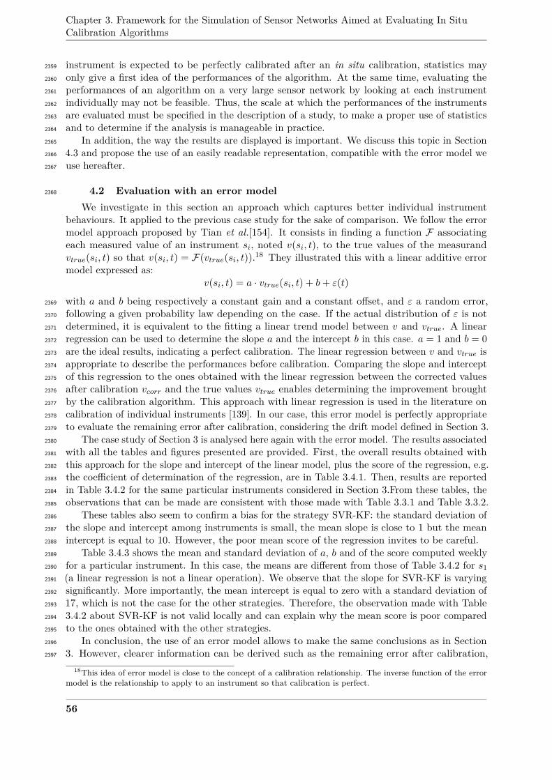
Chapter 3. Framework for the Simulation of Sensor Networks Aimed at Evaluating In SituCalibration Algorithms
instrument is expected to be perfectly calibrated after an in situ calibration, statistics may2359
only give a first idea of the performances of the algorithm. At the same time, evaluating the2360
performances of an algorithm on a very large sensor network by looking at each instrument2361
individually may not be feasible. Thus, the scale at which the performances of the instruments2362
are evaluated must be specified in the description of a study, to make a proper use of statistics2363
and to determine if the analysis is manageable in practice.2364
In addition, the way the results are displayed is important. We discuss this topic in Section2365
4.3 and propose the use of an easily readable representation, compatible with the error model we2366
use hereafter.2367
4.2 Evaluation with an error model2368
We investigate in this section an approach which captures better individual instrumentbehaviours. It applied to the previous case study for the sake of comparison. We follow the errormodel approach proposed by Tian et al.[154]. It consists in finding a function F associatingeach measured value of an instrument si, noted v(si, t), to the true values of the measurandvtrue(si, t) so that v(si, t) = F(vtrue(si, t)).18 They illustrated this with a linear additive errormodel expressed as:
v(si, t) = a · vtrue(si, t) + b+ ε(t)
with a and b being respectively a constant gain and a constant offset, and ε a random error,2369
following a given probability law depending on the case. If the actual distribution of ε is not2370
determined, it is equivalent to the fitting a linear trend model between v and vtrue. A linear2371
regression can be used to determine the slope a and the intercept b in this case. a = 1 and b = 02372
are the ideal results, indicating a perfect calibration. The linear regression between v and vtrue is2373
appropriate to describe the performances before calibration. Comparing the slope and intercept2374
of this regression to the ones obtained with the linear regression between the corrected values2375
after calibration vcorr and the true values vtrue enables determining the improvement brought2376
by the calibration algorithm. This approach with linear regression is used in the literature on2377
calibration of individual instruments [139]. In our case, this error model is perfectly appropriate2378
to evaluate the remaining error after calibration, considering the drift model defined in Section 3.2379
The case study of Section 3 is analysed here again with the error model. The results associated2380
with all the tables and figures presented are provided. First, the overall results obtained with2381
this approach for the slope and intercept of the linear model, plus the score of the regression, e.g.2382
the coefficient of determination of the regression, are in Table 3.4.1. Then, results are reported2383
in Table 3.4.2 for the same particular instruments considered in Section 3.From these tables, the2384
observations that can be made are consistent with those made with Table 3.3.1 and Table 3.3.2.2385
These tables also seem to confirm a bias for the strategy SVR-KF: the standard deviation of2386
the slope and intercept among instruments is small, the mean slope is close to 1 but the mean2387
intercept is equal to 10. However, the poor mean score of the regression invites to be careful.2388
Table 3.4.3 shows the mean and standard deviation of a, b and of the score computed weekly2389
for a particular instrument. In this case, the means are different from those of Table 3.4.2 for s12390
(a linear regression is not a linear operation). We observe that the slope for SVR-KF is varying2391
significantly. More importantly, the mean intercept is equal to zero with a standard deviation of2392
17, which is not the case for the other strategies. Therefore, the observation made with Table2393
3.4.2 about SVR-KF is not valid locally and can explain why the mean score is poor compared2394
to the ones obtained with the other strategies.2395
In conclusion, the use of an error model allows to make the same conclusions as in Section2396
3. However, clearer information can be derived such as the remaining error after calibration,2397
18This idea of error model is close to the concept of a calibration relationship. The inverse function of the errormodel is the relationship to apply to an instrument so that calibration is perfect.
56
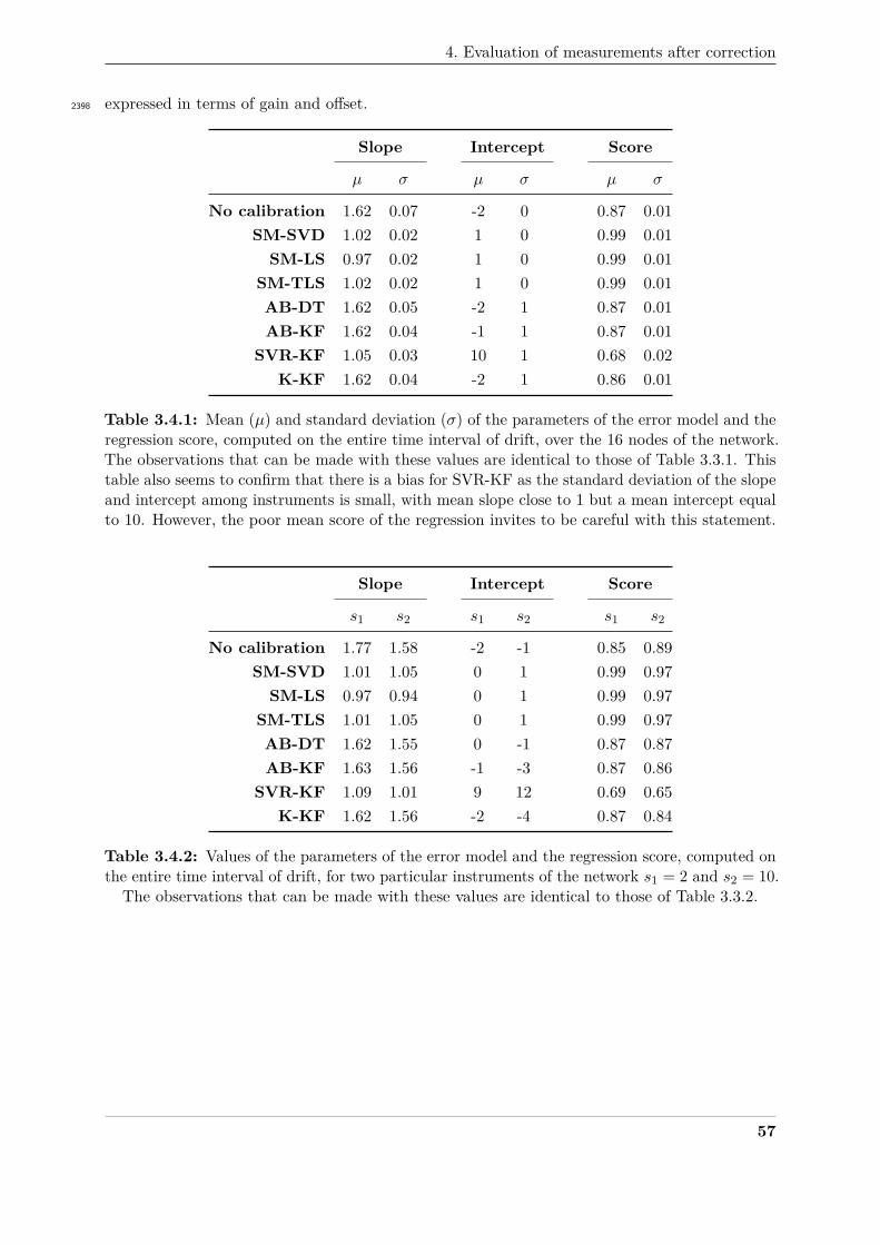
4. Evaluation of measurements after correction
expressed in terms of gain and offset.2398
Slope Intercept Score
µ σ µ σ µ σ
No calibration 1.62 0.07 -2 0 0.87 0.01SM-SVD 1.02 0.02 1 0 0.99 0.01SM-LS 0.97 0.02 1 0 0.99 0.01
SM-TLS 1.02 0.02 1 0 0.99 0.01AB-DT 1.62 0.05 -2 1 0.87 0.01AB-KF 1.62 0.04 -1 1 0.87 0.01
SVR-KF 1.05 0.03 10 1 0.68 0.02K-KF 1.62 0.04 -2 1 0.86 0.01
Table 3.4.1: Mean (µ) and standard deviation (σ) of the parameters of the error model and theregression score, computed on the entire time interval of drift, over the 16 nodes of the network.The observations that can be made with these values are identical to those of Table 3.3.1. Thistable also seems to confirm that there is a bias for SVR-KF as the standard deviation of the slopeand intercept among instruments is small, with mean slope close to 1 but a mean intercept equalto 10. However, the poor mean score of the regression invites to be careful with this statement.
Slope Intercept Score
s1 s2 s1 s2 s1 s2
No calibration 1.77 1.58 -2 -1 0.85 0.89SM-SVD 1.01 1.05 0 1 0.99 0.97SM-LS 0.97 0.94 0 1 0.99 0.97
SM-TLS 1.01 1.05 0 1 0.99 0.97AB-DT 1.62 1.55 0 -1 0.87 0.87AB-KF 1.63 1.56 -1 -3 0.87 0.86
SVR-KF 1.09 1.01 9 12 0.69 0.65K-KF 1.62 1.56 -2 -4 0.87 0.84
Table 3.4.2: Values of the parameters of the error model and the regression score, computed onthe entire time interval of drift, for two particular instruments of the network s1 = 2 and s2 = 10.
The observations that can be made with these values are identical to those of Table 3.3.2.
57
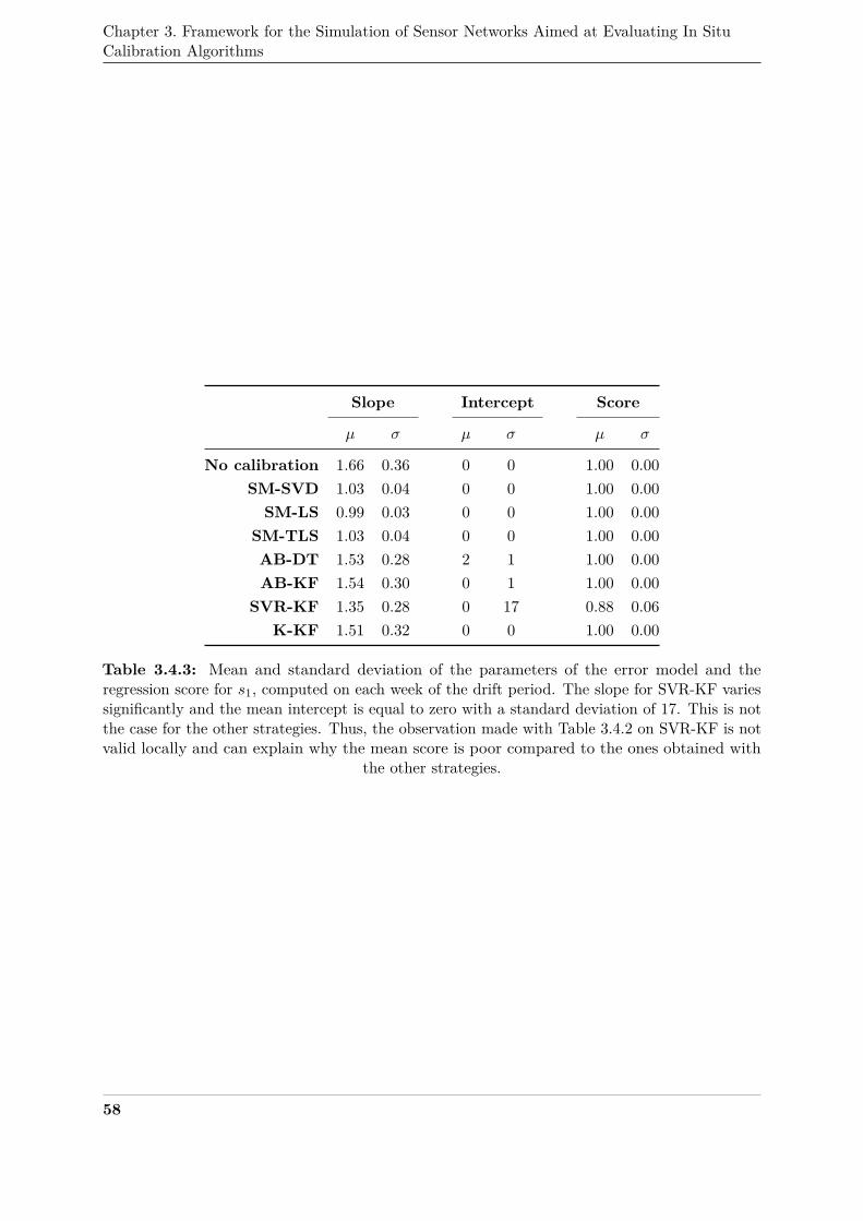
Chapter 3. Framework for the Simulation of Sensor Networks Aimed at Evaluating In SituCalibration Algorithms
Slope Intercept Score
µ σ µ σ µ σ
No calibration 1.66 0.36 0 0 1.00 0.00SM-SVD 1.03 0.04 0 0 1.00 0.00SM-LS 0.99 0.03 0 0 1.00 0.00
SM-TLS 1.03 0.04 0 0 1.00 0.00AB-DT 1.53 0.28 2 1 1.00 0.00AB-KF 1.54 0.30 0 1 1.00 0.00
SVR-KF 1.35 0.28 0 17 0.88 0.06K-KF 1.51 0.32 0 0 1.00 0.00
Table 3.4.3: Mean and standard deviation of the parameters of the error model and theregression score for s1, computed on each week of the drift period. The slope for SVR-KF variessignificantly and the mean intercept is equal to zero with a standard deviation of 17. This is notthe case for the other strategies. Thus, the observation made with Table 3.4.2 on SVR-KF is notvalid locally and can explain why the mean score is poor compared to the ones obtained with
the other strategies.
58
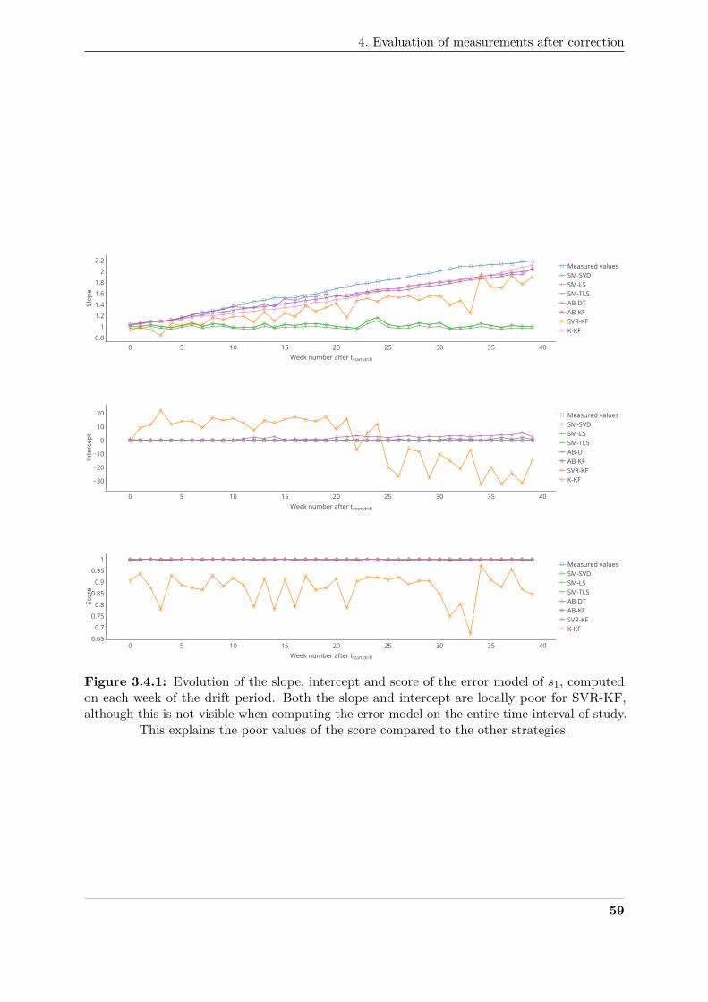
4. Evaluation of measurements after correction
0 5 10 15 20 25 30 35 400.8
1
1.2
1.4
1.6
1.8
2
2.2Measured valuesSM-SVDSM-LSSM-TLSAB-DTAB-KFSVR-KFK-KF
Week number after t start drift
Slop
e
0 5 10 15 20 25 30 35 40
−30
−20
−10
0
10
20 Measured valuesSM-SVDSM-LSSM-TLSAB-DTAB-KFSVR-KFK-KF
Week number after t start drift
Inte
rcep
t
0 5 10 15 20 25 30 35 400.65
0.7
0.75
0.8
0.85
0.9
0.95
1Measured valuesSM-SVDSM-LSSM-TLSAB-DTAB-KFSVR-KFK-KF
Week number after t start drift
Scor
e
Figure 3.4.1: Evolution of the slope, intercept and score of the error model of s1, computedon each week of the drift period. Both the slope and intercept are locally poor for SVR-KF,although this is not visible when computing the error model on the entire time interval of study.
This explains the poor values of the score compared to the other strategies.
59
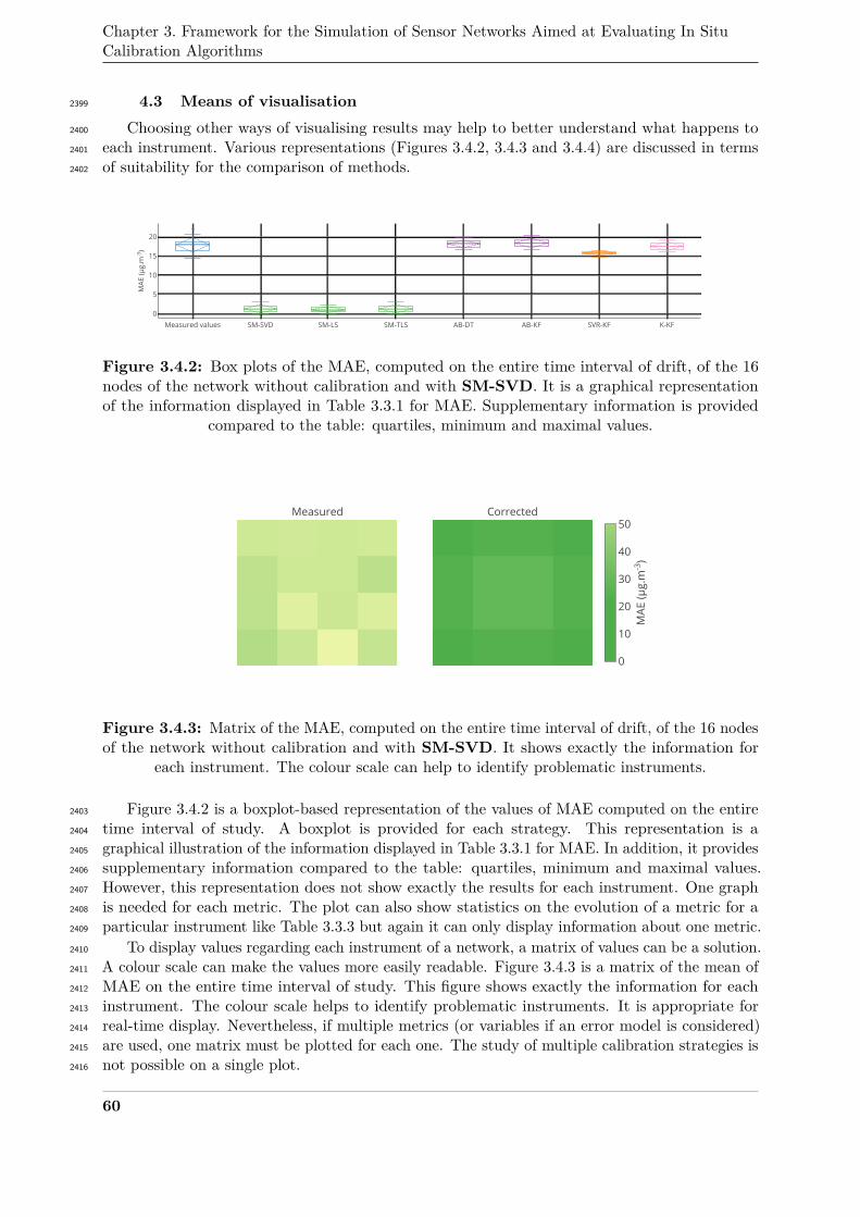
Chapter 3. Framework for the Simulation of Sensor Networks Aimed at Evaluating In SituCalibration Algorithms
4.3 Means of visualisation2399
Choosing other ways of visualising results may help to better understand what happens to2400
each instrument. Various representations (Figures 3.4.2, 3.4.3 and 3.4.4) are discussed in terms2401
of suitability for the comparison of methods.2402
Measured values SM-SVD SM-LS SM-TLS AB-DT AB-KF SVR-KF K-KF0
5
10
15
20
MAE
(μg.
m -3 )
Figure 3.4.2: Box plots of the MAE, computed on the entire time interval of drift, of the 16nodes of the network without calibration and with SM-SVD. It is a graphical representationof the information displayed in Table 3.3.1 for MAE. Supplementary information is provided
compared to the table: quartiles, minimum and maximal values.
0
10
20
30
40
50
MAE
(μg.
m -3 )
Measured Corrected
Figure 3.4.3: Matrix of the MAE, computed on the entire time interval of drift, of the 16 nodesof the network without calibration and with SM-SVD. It shows exactly the information for
each instrument. The colour scale can help to identify problematic instruments.
Figure 3.4.2 is a boxplot-based representation of the values of MAE computed on the entire2403
time interval of study. A boxplot is provided for each strategy. This representation is a2404
graphical illustration of the information displayed in Table 3.3.1 for MAE. In addition, it provides2405
supplementary information compared to the table: quartiles, minimum and maximal values.2406
However, this representation does not show exactly the results for each instrument. One graph2407
is needed for each metric. The plot can also show statistics on the evolution of a metric for a2408
particular instrument like Table 3.3.3 but again it can only display information about one metric.2409
To display values regarding each instrument of a network, a matrix of values can be a solution.2410
A colour scale can make the values more easily readable. Figure 3.4.3 is a matrix of the mean of2411
MAE on the entire time interval of study. This figure shows exactly the information for each2412
instrument. The colour scale helps to identify problematic instruments. It is appropriate for2413
real-time display. Nevertheless, if multiple metrics (or variables if an error model is considered)2414
are used, one matrix must be plotted for each one. The study of multiple calibration strategies is2415
not possible on a single plot.2416
60
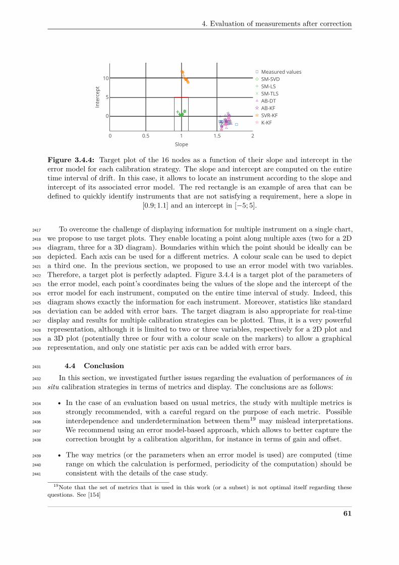
4. Evaluation of measurements after correction
0 0.5 1 1.5 2
0
5
10Measured valuesSM-SVDSM-LSSM-TLSAB-DTAB-KFSVR-KFK-KF
Slope
Inte
rcep
t
Figure 3.4.4: Target plot of the 16 nodes as a function of their slope and intercept in theerror model for each calibration strategy. The slope and intercept are computed on the entiretime interval of drift. In this case, it allows to locate an instrument according to the slope andintercept of its associated error model. The red rectangle is an example of area that can bedefined to quickly identify instruments that are not satisfying a requirement, here a slope in
[0.9; 1.1] and an intercept in [−5; 5].
To overcome the challenge of displaying information for multiple instrument on a single chart,2417
we propose to use target plots. They enable locating a point along multiple axes (two for a 2D2418
diagram, three for a 3D diagram). Boundaries within which the point should be ideally can be2419
depicted. Each axis can be used for a different metrics. A colour scale can be used to depict2420
a third one. In the previous section, we proposed to use an error model with two variables.2421
Therefore, a target plot is perfectly adapted. Figure 3.4.4 is a target plot of the parameters of2422
the error model, each point’s coordinates being the values of the slope and the intercept of the2423
error model for each instrument, computed on the entire time interval of study. Indeed, this2424
diagram shows exactly the information for each instrument. Moreover, statistics like standard2425
deviation can be added with error bars. The target diagram is also appropriate for real-time2426
display and results for multiple calibration strategies can be plotted. Thus, it is a very powerful2427
representation, although it is limited to two or three variables, respectively for a 2D plot and2428
a 3D plot (potentially three or four with a colour scale on the markers) to allow a graphical2429
representation, and only one statistic per axis can be added with error bars.2430
4.4 Conclusion2431
In this section, we investigated further issues regarding the evaluation of performances of in2432
situ calibration strategies in terms of metrics and display. The conclusions are as follows:2433
• In the case of an evaluation based on usual metrics, the study with multiple metrics is2434
strongly recommended, with a careful regard on the purpose of each metric. Possible2435
interdependence and underdetermination between them19 may mislead interpretations.2436
We recommend using an error model-based approach, which allows to better capture the2437
correction brought by a calibration algorithm, for instance in terms of gain and offset.2438
• The way metrics (or the parameters when an error model is used) are computed (time2439
range on which the calculation is performed, periodicity of the computation) should be2440
consistent with the details of the case study.2441
19Note that the set of metrics that is used in this work (or a subset) is not optimal itself regarding thesequestions. See [154]
61
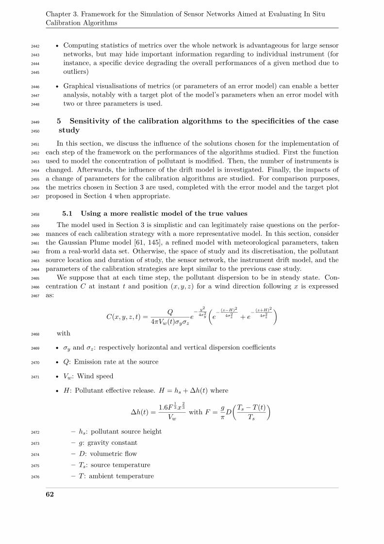
Chapter 3. Framework for the Simulation of Sensor Networks Aimed at Evaluating In SituCalibration Algorithms
• Computing statistics of metrics over the whole network is advantageous for large sensor2442
networks, but may hide important information regarding to individual instrument (for2443
instance, a specific device degrading the overall performances of a given method due to2444
outliers)2445
• Graphical visualisations of metrics (or parameters of an error model) can enable a better2446
analysis, notably with a target plot of the model’s parameters when an error model with2447
two or three parameters is used.2448
5 Sensitivity of the calibration algorithms to the specificities of the case2449
study2450
In this section, we discuss the influence of the solutions chosen for the implementation of2451
each step of the framework on the performances of the algorithms studied. First the function2452
used to model the concentration of pollutant is modified. Then, the number of instruments is2453
changed. Afterwards, the influence of the drift model is investigated. Finally, the impacts of2454
a change of parameters for the calibration algorithms are studied. For comparison purposes,2455
the metrics chosen in Section 3 are used, completed with the error model and the target plot2456
proposed in Section 4 when appropriate.2457
5.1 Using a more realistic model of the true values2458
The model used in Section 3 is simplistic and can legitimately raise questions on the perfor-2459
mances of each calibration strategy with a more representative model. In this section, consider2460
the Gaussian Plume model [61, 145], a refined model with meteorological parameters, taken2461
from a real-world data set. Otherwise, the space of study and its discretisation, the pollutant2462
source location and duration of study, the sensor network, the instrument drift model, and the2463
parameters of the calibration strategies are kept similar to the previous case study.2464
We suppose that at each time step, the pollutant dispersion to be in steady state. Con-2465
centration C at instant t and position (x, y, z) for a wind direction following x is expressed2466
as:2467
C(x, y, z, t) = Q
4πVw(t)σyσze− y2
4σ2y
(e− (z−H)2
4σ2z + e
− (z+H)2
4σ2z
)with2468
• σy and σz: respectively horizontal and vertical dispersion coefficients2469
• Q: Emission rate at the source2470
• Vw: Wind speed2471
• H: Pollutant effective release. H = hs + ∆h(t) where
∆h(t) = 1.6F 13x
23
Vwwith F = g
πD
(Ts − T (t)
Ts
)– hs: pollutant source height2472
– g: gravity constant2473
– D: volumetric flow2474
– Ts: source temperature2475
– T : ambient temperature2476
62
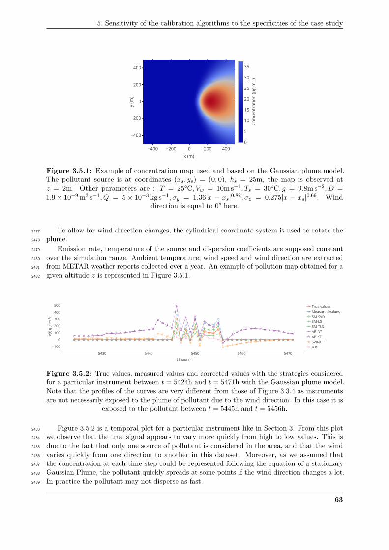
5. Sensitivity of the calibration algorithms to the specificities of the case study
−400 −200 0 200 400
−400
−200
0
200
400
0
5
10
15
20
25
30
35
Conc
entr
atio
n (μ
g.m
-3 )
x (m)
y (m
)
Figure 3.5.1: Example of concentration map used and based on the Gaussian plume model.The pollutant source is at coordinates (xs, ys) = (0, 0), hs = 25m, the map is observed atz = 2m. Other parameters are : T = 25C, Vw = 10m s−1, Ts = 30C, g = 9.8m s−2, D =1.9× 10⁻⁹ m3 s−1, Q = 5× 10⁻³ kg s−1, σy = 1.36|x − xs|0.82, σz = 0.275|x − xs|0.69. Wind
direction is equal to 0° here.
To allow for wind direction changes, the cylindrical coordinate system is used to rotate the2477
plume.2478
Emission rate, temperature of the source and dispersion coefficients are supposed constant2479
over the simulation range. Ambient temperature, wind speed and wind direction are extracted2480
from METAR weather reports collected over a year. An example of pollution map obtained for a2481
given altitude z is represented in Figure 3.5.1.2482
5430 5440 5450 5460 5470
−100
0
100
200
300
400
500 True valuesMeasured valuesSM-SVDSM-LSSM-TLSAB-DTAB-KFSVR-KFK-KF
t (hours)
v(t)
(μg.
m -3 )
Figure 3.5.2: True values, measured values and corrected values with the strategies consideredfor a particular instrument between t = 5424h and t = 5471h with the Gaussian plume model.Note that the profiles of the curves are very different from those of Figure 3.3.4 as instrumentsare not necessarily exposed to the plume of pollutant due to the wind direction. In this case it is
exposed to the pollutant between t = 5445h and t = 5456h.
Figure 3.5.2 is a temporal plot for a particular instrument like in Section 3. From this plot2483
we observe that the true signal appears to vary more quickly from high to low values. This is2484
due to the fact that only one source of pollutant is considered in the area, and that the wind2485
varies quickly from one direction to another in this dataset. Moreover, as we assumed that2486
the concentration at each time step could be represented following the equation of a stationary2487
Gaussian Plume, the pollutant quickly spreads at some points if the wind direction changes a lot.2488
In practice the pollutant may not disperse as fast.2489
63
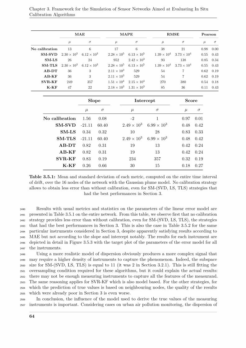
Chapter 3. Framework for the Simulation of Sensor Networks Aimed at Evaluating In SituCalibration Algorithms
MAE MAPE RMSE Pearson
µ σ µ σ µ σ µ σ
No calibration 13 6 17 6 38 21 0.98 0.00SM-SVD 2.30× 10³ 6.12× 10³ 2.28× 10⁵ 6.13× 10⁵ 1.39× 10⁴ 3.73× 10⁴ 0.55 0.43SM-LS 26 24 952 2.42× 10³ 93 138 0.85 0.34
SM-TLS 2.30× 10³ 6.12× 10³ 2.28× 10⁵ 6.13× 10⁵ 1.39× 10⁴ 3.73× 10⁴ 0.55 0.43AB-DT 36 3 2.11× 10³ 529 54 7 0.62 0.19AB-KF 36 3 2.11× 10³ 529 54 7 0.62 0.19
SVR-KF 249 357 1.51× 10⁴ 2.15× 10⁴ 270 380 0.54 0.18K-KF 47 22 2.18× 10³ 1.31× 10³ 85 36 0.11 0.43
Slope Intercept Score
µ σ µ σ µ σ
No calibration 1.56 0.08 -2 1 0.97 0.01SM-SVD -21.11 60.40 2.49× 10³ 6.99× 10³ 0.48 0.42SM-LS 0.34 0.32 10 28 0.83 0.33
SM-TLS -21.11 60.40 2.49× 10³ 6.99× 10³ 0.48 0.42AB-DT 0.82 0.31 19 13 0.42 0.24AB-KF 0.82 0.31 19 13 0.42 0.24
SVR-KF 0.83 0.19 234 357 0.32 0.19K-KF 0.26 0.66 30 15 0.18 0.27
Table 3.5.1: Mean and standard deviation of each metric, computed on the entire time intervalof drift, over the 16 nodes of the network with the Gaussian plume model. No calibration strategyallows to obtain less error than without calibration, even for SM-(SVD, LS, TLS) strategies that
had the best performances in Section 3.
Results with usual metrics and statistics on the parameters of the linear error model are2490
presented in Table 3.5.1 on the entire network. From this table, we observe first that no calibration2491
strategy provides less error than without calibration, even for SM-(SVD, LS, TLS), the strategies2492
that had the best performances in Section 3. This is also the case in Table 3.5.2 for the same2493
particular instruments considered in Section 3, despite apparently satisfying results according to2494
MAE but not according to the slope and intercept notably. The results for each instrument are2495
depicted in detail in Figure 3.5.3 with the target plot of the parameters of the error model for all2496
the instruments.2497
Using a more realistic model of dispersion obviously produces a more complex signal that2498
may require a higher density of instruments to capture the phenomenon. Indeed, the subspace2499
size for SM-(SVD, LS, TLS) is equal to 11 (it was 2 in Section 3.2.1). This is still fitting the2500
oversampling condition required for these algorithms, but it could explain the actual results:2501
there may not be enough measuring instruments to capture all the features of the measurand.2502
The same reasoning applies for SVR-KF which is also model based. For the other strategies, for2503
which the prediction of true values is based on neighbouring nodes, the quality of the results2504
which were already poor in Section 3 is even worse.2505
In conclusion, the influence of the model used to derive the true values of the measuring2506
instruments is important. Considering cases on urban air pollution monitoring, the dispersion of2507
64
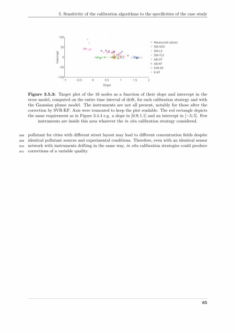
5. Sensitivity of the calibration algorithms to the specificities of the case study
−1 −0.5 0 0.5 1 1.5 2−100
−50
0
50
100
Measured valuesSM-SVDSM-LSSM-TLSAB-DTAB-KFSVR-KFK-KF
Slope
Inte
rcep
t
Figure 3.5.3: Target plot of the 16 nodes as a function of their slope and intercept in theerror model, computed on the entire time interval of drift, for each calibration strategy and withthe Gaussian plume model. The instruments are not all present, notably for those after thecorrection by SVR-KF. Axis were truncated to keep the plot readable. The red rectangle depictsthe same requirement as in Figure 3.4.4 e.g. a slope in [0.9; 1.1] and an intercept in [−5; 5]. Few
instruments are inside this area whatever the in situ calibration strategy considered.
pollutant for cities with different street layout may lead to different concentration fields despite2508
identical pollutant sources and experimental conditions. Therefore, even with an identical sensor2509
network with instruments drifting in the same way, in situ calibration strategies could produce2510
corrections of a variable quality.2511
65
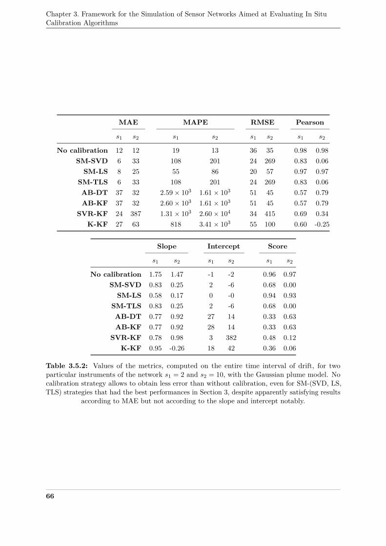
Chapter 3. Framework for the Simulation of Sensor Networks Aimed at Evaluating In SituCalibration Algorithms
MAE MAPE RMSE Pearson
s1 s2 s1 s2 s1 s2 s1 s2
No calibration 12 12 19 13 36 35 0.98 0.98SM-SVD 6 33 108 201 24 269 0.83 0.06SM-LS 8 25 55 86 20 57 0.97 0.97
SM-TLS 6 33 108 201 24 269 0.83 0.06AB-DT 37 32 2.59× 10³ 1.61× 10³ 51 45 0.57 0.79AB-KF 37 32 2.60× 10³ 1.61× 10³ 51 45 0.57 0.79
SVR-KF 24 387 1.31× 10³ 2.60× 10⁴ 34 415 0.69 0.34K-KF 27 63 818 3.41× 10³ 55 100 0.60 -0.25
Slope Intercept Score
s1 s2 s1 s2 s1 s2
No calibration 1.75 1.47 -1 -2 0.96 0.97SM-SVD 0.83 0.25 2 -6 0.68 0.00SM-LS 0.58 0.17 0 -0 0.94 0.93
SM-TLS 0.83 0.25 2 -6 0.68 0.00AB-DT 0.77 0.92 27 14 0.33 0.63AB-KF 0.77 0.92 28 14 0.33 0.63
SVR-KF 0.78 0.98 3 382 0.48 0.12K-KF 0.95 -0.26 18 42 0.36 0.06
Table 3.5.2: Values of the metrics, computed on the entire time interval of drift, for twoparticular instruments of the network s1 = 2 and s2 = 10, with the Gaussian plume model. Nocalibration strategy allows to obtain less error than without calibration, even for SM-(SVD, LS,TLS) strategies that had the best performances in Section 3, despite apparently satisfying results
according to MAE but not according to the slope and intercept notably.
66
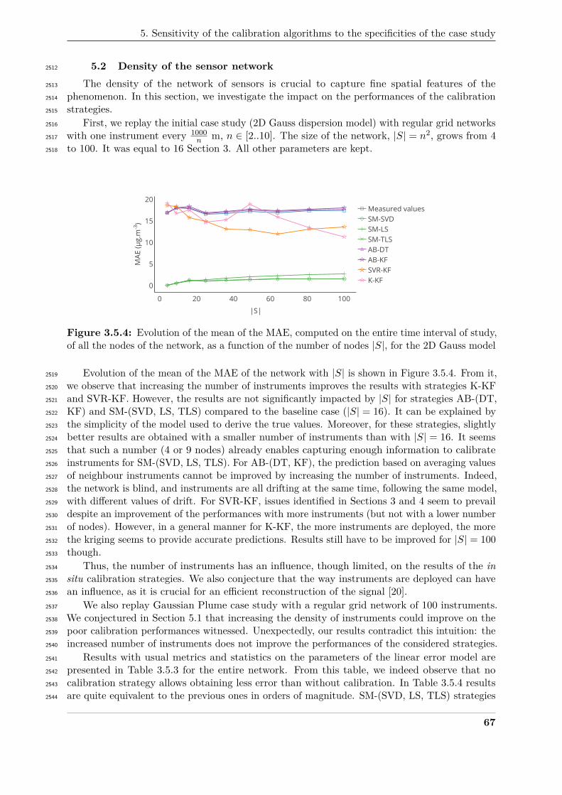
5. Sensitivity of the calibration algorithms to the specificities of the case study
5.2 Density of the sensor network2512
The density of the network of sensors is crucial to capture fine spatial features of the2513
phenomenon. In this section, we investigate the impact on the performances of the calibration2514
strategies.2515
First, we replay the initial case study (2D Gauss dispersion model) with regular grid networks2516
with one instrument every 1000n m, n ∈ [2..10]. The size of the network, |S| = n2, grows from 42517
to 100. It was equal to 16 Section 3. All other parameters are kept.2518
0 20 40 60 80 100
0
5
10
15
20Measured valuesSM-SVDSM-LSSM-TLSAB-DTAB-KFSVR-KFK-KF
|S|
MAE
(μg.
m -3 )
Figure 3.5.4: Evolution of the mean of the MAE, computed on the entire time interval of study,of all the nodes of the network, as a function of the number of nodes |S|, for the 2D Gauss model
Evolution of the mean of the MAE of the network with |S| is shown in Figure 3.5.4. From it,2519
we observe that increasing the number of instruments improves the results with strategies K-KF2520
and SVR-KF. However, the results are not significantly impacted by |S| for strategies AB-(DT,2521
KF) and SM-(SVD, LS, TLS) compared to the baseline case (|S| = 16). It can be explained by2522
the simplicity of the model used to derive the true values. Moreover, for these strategies, slightly2523
better results are obtained with a smaller number of instruments than with |S| = 16. It seems2524
that such a number (4 or 9 nodes) already enables capturing enough information to calibrate2525
instruments for SM-(SVD, LS, TLS). For AB-(DT, KF), the prediction based on averaging values2526
of neighbour instruments cannot be improved by increasing the number of instruments. Indeed,2527
the network is blind, and instruments are all drifting at the same time, following the same model,2528
with different values of drift. For SVR-KF, issues identified in Sections 3 and 4 seem to prevail2529
despite an improvement of the performances with more instruments (but not with a lower number2530
of nodes). However, in a general manner for K-KF, the more instruments are deployed, the more2531
the kriging seems to provide accurate predictions. Results still have to be improved for |S| = 1002532
though.2533
Thus, the number of instruments has an influence, though limited, on the results of the in2534
situ calibration strategies. We also conjecture that the way instruments are deployed can have2535
an influence, as it is crucial for an efficient reconstruction of the signal [20].2536
We also replay Gaussian Plume case study with a regular grid network of 100 instruments.2537
We conjectured in Section 5.1 that increasing the density of instruments could improve on the2538
poor calibration performances witnessed. Unexpectedly, our results contradict this intuition: the2539
increased number of instruments does not improve the performances of the considered strategies.2540
Results with usual metrics and statistics on the parameters of the linear error model are2541
presented in Table 3.5.3 for the entire network. From this table, we indeed observe that no2542
calibration strategy allows obtaining less error than without calibration. In Table 3.5.4 results2543
are quite equivalent to the previous ones in orders of magnitude. SM-(SVD, LS, TLS) strategies2544
67
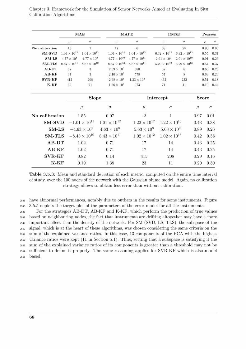
Chapter 3. Framework for the Simulation of Sensor Networks Aimed at Evaluating In SituCalibration Algorithms
MAE MAPE RMSE Pearson
µ σ µ σ µ σ µ σ
No calibration 13 7 17 6 38 25 0.98 0.00SM-SVD 1.04× 10¹² 1.04× 10¹³ 1.04× 10¹⁴ 1.04× 10¹⁵ 6.32× 10¹² 6.32× 10¹³ 0.55 0.37SM-LS 4.77× 10⁸ 4.77× 10⁹ 4.77× 10¹⁰ 4.77× 10¹¹ 2.91× 10⁹ 2.91× 10¹⁰ 0.91 0.26
SM-TLS 8.67× 10¹¹ 8.67× 10¹² 8.67× 10¹³ 8.67× 10¹⁴ 5.29× 10¹² 5.29× 10¹³ 0.54 0.37AB-DT 37 3 2.09× 10³ 580 57 8 0.63 0.20AB-KF 37 3 2.10× 10³ 578 57 8 0.63 0.20
SVR-KF 412 208 2.68× 10⁴ 1.33× 10⁴ 432 232 0.51 0.18K-KF 39 21 1.66× 10³ 973 71 41 0.10 0.44
Slope Intercept Score
µ σ µ σ µ σ
No calibration 1.55 0.07 -2 1 0.97 0.01SM-SVD −1.01× 10¹¹ 1.01× 10¹² 1.22× 10¹² 1.22× 10¹³ 0.43 0.38SM-LS −4.63× 10⁷ 4.63× 10⁸ 5.63× 10⁸ 5.63× 10⁹ 0.89 0.26
SM-TLS −8.43× 10¹⁰ 8.43× 10¹¹ 1.02× 10¹² 1.02× 10¹³ 0.42 0.38AB-DT 1.02 0.71 17 14 0.43 0.25AB-KF 1.02 0.71 17 14 0.43 0.25
SVR-KF 0.82 0.14 415 208 0.29 0.16K-KF 0.19 1.38 23 11 0.20 0.30
Table 3.5.3: Mean and standard deviation of each metric, computed on the entire time intervalof study, over the 100 nodes of the network with the Gaussian plume model. Again, no calibration
strategy allows to obtain less error than without calibration.
have abnormal performances, notably due to outliers in the results for some instruments. Figure2545
3.5.5 depicts the target plot of the parameters of the error model for all the instruments.2546
For the strategies AB-DT, AB-KF and K-KF, which perform the prediction of true values2547
based on neighbouring nodes, the fact that instruments are drifting altogether may have a more2548
important effect than the density of the network. For SM-(SVD, LS, TLS), the subspace of the2549
signal, which is at the heart of these algorithms, was chosen considering the same criteria on the2550
sum of the explained variance ratios. In this case, 13 components of the PCA with the highest2551
variance ratios were kept (11 in Section 5.1). Thus, setting that a subspace is satisfying if the2552
sum of the explained variance ratios of its components is greater than a threshold may not be2553
sufficient to define it properly. The same reasoning applies for SVR-KF which is also model2554
based.2555
68
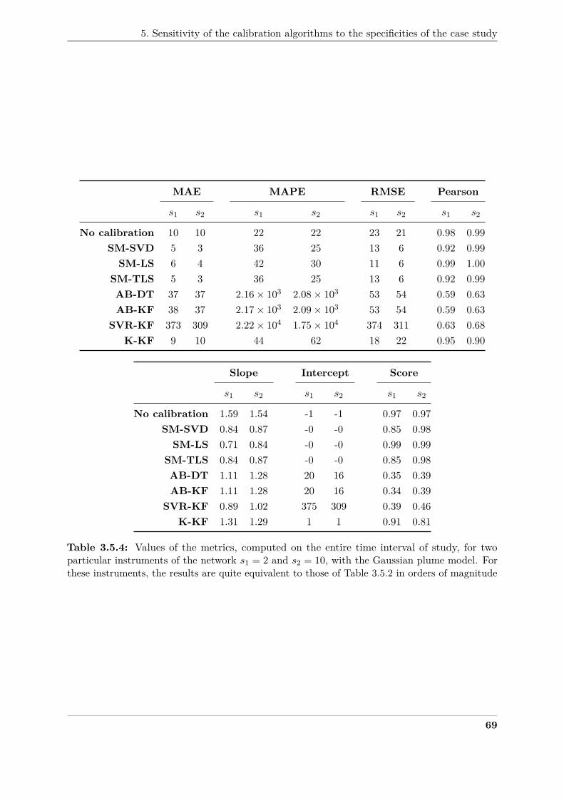
5. Sensitivity of the calibration algorithms to the specificities of the case study
MAE MAPE RMSE Pearson
s1 s2 s1 s2 s1 s2 s1 s2
No calibration 10 10 22 22 23 21 0.98 0.99SM-SVD 5 3 36 25 13 6 0.92 0.99SM-LS 6 4 42 30 11 6 0.99 1.00
SM-TLS 5 3 36 25 13 6 0.92 0.99AB-DT 37 37 2.16× 10³ 2.08× 10³ 53 54 0.59 0.63AB-KF 38 37 2.17× 10³ 2.09× 10³ 53 54 0.59 0.63
SVR-KF 373 309 2.22× 10⁴ 1.75× 10⁴ 374 311 0.63 0.68K-KF 9 10 44 62 18 22 0.95 0.90
Slope Intercept Score
s1 s2 s1 s2 s1 s2
No calibration 1.59 1.54 -1 -1 0.97 0.97SM-SVD 0.84 0.87 -0 -0 0.85 0.98SM-LS 0.71 0.84 -0 -0 0.99 0.99
SM-TLS 0.84 0.87 -0 -0 0.85 0.98AB-DT 1.11 1.28 20 16 0.35 0.39AB-KF 1.11 1.28 20 16 0.34 0.39
SVR-KF 0.89 1.02 375 309 0.39 0.46K-KF 1.31 1.29 1 1 0.91 0.81
Table 3.5.4: Values of the metrics, computed on the entire time interval of study, for twoparticular instruments of the network s1 = 2 and s2 = 10, with the Gaussian plume model. Forthese instruments, the results are quite equivalent to those of Table 3.5.2 in orders of magnitude
69
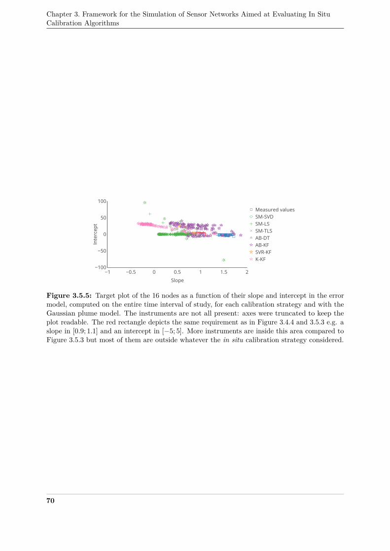
Chapter 3. Framework for the Simulation of Sensor Networks Aimed at Evaluating In SituCalibration Algorithms
−1 −0.5 0 0.5 1 1.5 2−100
−50
0
50
100
Measured valuesSM-SVDSM-LSSM-TLSAB-DTAB-KFSVR-KFK-KF
Slope
Inte
rcep
t
Figure 3.5.5: Target plot of the 16 nodes as a function of their slope and intercept in the errormodel, computed on the entire time interval of study, for each calibration strategy and with theGaussian plume model. The instruments are not all present: axes were truncated to keep theplot readable. The red rectangle depicts the same requirement as in Figure 3.4.4 and 3.5.3 e.g. aslope in [0.9; 1.1] and an intercept in [−5; 5]. More instruments are inside this area compared toFigure 3.5.3 but most of them are outside whatever the in situ calibration strategy considered.
70
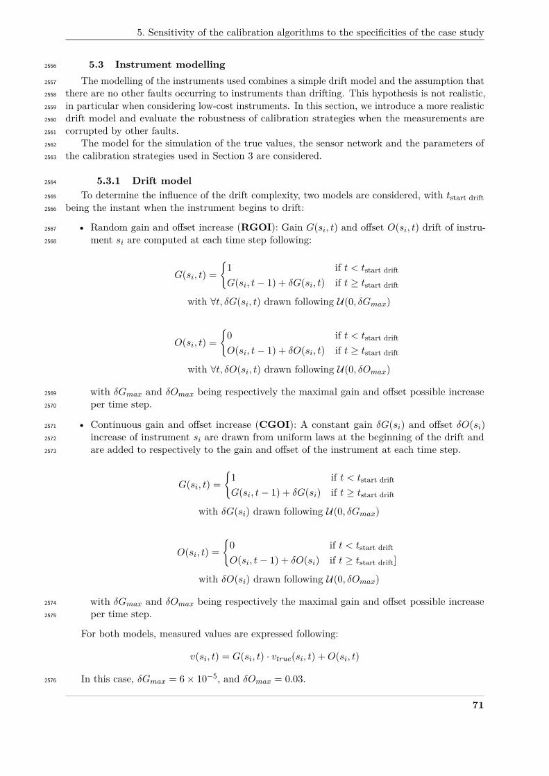
5. Sensitivity of the calibration algorithms to the specificities of the case study
5.3 Instrument modelling2556
The modelling of the instruments used combines a simple drift model and the assumption that2557
there are no other faults occurring to instruments than drifting. This hypothesis is not realistic,2558
in particular when considering low-cost instruments. In this section, we introduce a more realistic2559
drift model and evaluate the robustness of calibration strategies when the measurements are2560
corrupted by other faults.2561
The model for the simulation of the true values, the sensor network and the parameters of2562
the calibration strategies used in Section 3 are considered.2563
5.3.1 Drift model2564
To determine the influence of the drift complexity, two models are considered, with tstart drift2565
being the instant when the instrument begins to drift:2566
• Random gain and offset increase (RGOI): Gain G(si, t) and offset O(si, t) drift of instru-2567
ment si are computed at each time step following:2568
G(si, t) =
1 if t < tstart drift
G(si, t− 1) + δG(si, t) if t ≥ tstart drift
with ∀t, δG(si, t) drawn following U(0, δGmax)
O(si, t) =
0 if t < tstart drift
O(si, t− 1) + δO(si, t) if t ≥ tstart drift
with ∀t, δO(si, t) drawn following U(0, δOmax)
with δGmax and δOmax being respectively the maximal gain and offset possible increase2569
per time step.2570
• Continuous gain and offset increase (CGOI): A constant gain δG(si) and offset δO(si)2571
increase of instrument si are drawn from uniform laws at the beginning of the drift and2572
are added to respectively to the gain and offset of the instrument at each time step.2573
G(si, t) =
1 if t < tstart drift
G(si, t− 1) + δG(si) if t ≥ tstart drift
with δG(si) drawn following U(0, δGmax)
O(si, t) =
0 if t < tstart drift
O(si, t− 1) + δO(si) if t ≥ tstart drift]
with δO(si) drawn following U(0, δOmax)
with δGmax and δOmax being respectively the maximal gain and offset possible increase2574
per time step.2575
For both models, measured values are expressed following:
v(si, t) = G(si, t) · vtrue(si, t) +O(si, t)
In this case, δGmax = 6× 10⁻⁵, and δOmax = 0.03.2576
71
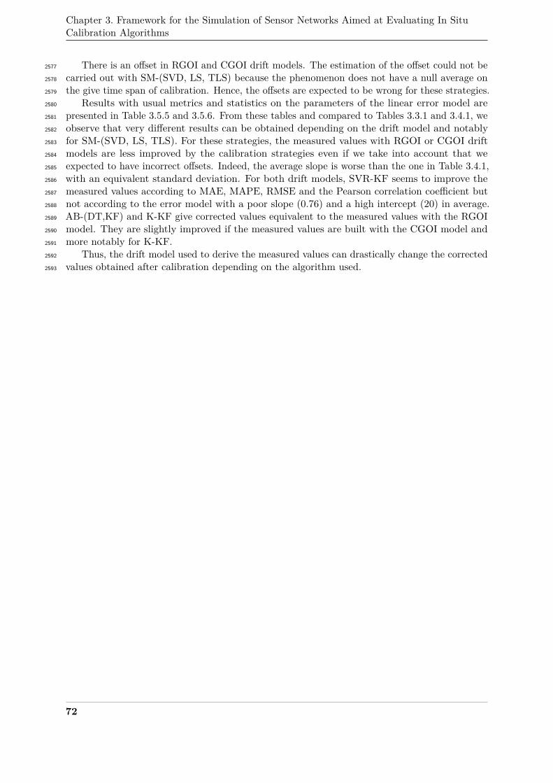
Chapter 3. Framework for the Simulation of Sensor Networks Aimed at Evaluating In SituCalibration Algorithms
There is an offset in RGOI and CGOI drift models. The estimation of the offset could not be2577
carried out with SM-(SVD, LS, TLS) because the phenomenon does not have a null average on2578
the give time span of calibration. Hence, the offsets are expected to be wrong for these strategies.2579
Results with usual metrics and statistics on the parameters of the linear error model are2580
presented in Table 3.5.5 and 3.5.6. From these tables and compared to Tables 3.3.1 and 3.4.1, we2581
observe that very different results can be obtained depending on the drift model and notably2582
for SM-(SVD, LS, TLS). For these strategies, the measured values with RGOI or CGOI drift2583
models are less improved by the calibration strategies even if we take into account that we2584
expected to have incorrect offsets. Indeed, the average slope is worse than the one in Table 3.4.1,2585
with an equivalent standard deviation. For both drift models, SVR-KF seems to improve the2586
measured values according to MAE, MAPE, RMSE and the Pearson correlation coefficient but2587
not according to the error model with a poor slope (0.76) and a high intercept (20) in average.2588
AB-(DT,KF) and K-KF give corrected values equivalent to the measured values with the RGOI2589
model. They are slightly improved if the measured values are built with the CGOI model and2590
more notably for K-KF.2591
Thus, the drift model used to derive the measured values can drastically change the corrected2592
values obtained after calibration depending on the algorithm used.2593
72
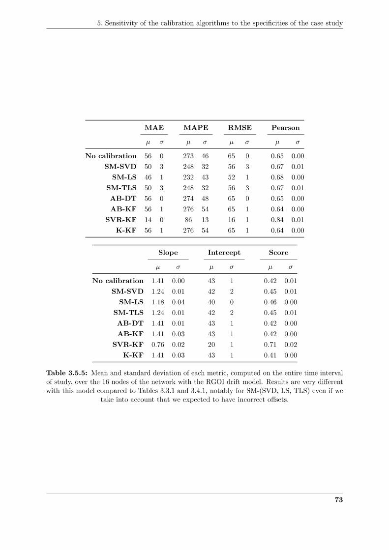
5. Sensitivity of the calibration algorithms to the specificities of the case study
MAE MAPE RMSE Pearson
µ σ µ σ µ σ µ σ
No calibration 56 0 273 46 65 0 0.65 0.00SM-SVD 50 3 248 32 56 3 0.67 0.01SM-LS 46 1 232 43 52 1 0.68 0.00
SM-TLS 50 3 248 32 56 3 0.67 0.01AB-DT 56 0 274 48 65 0 0.65 0.00AB-KF 56 1 276 54 65 1 0.64 0.00
SVR-KF 14 0 86 13 16 1 0.84 0.01K-KF 56 1 276 54 65 1 0.64 0.00
Slope Intercept Score
µ σ µ σ µ σ
No calibration 1.41 0.00 43 1 0.42 0.01SM-SVD 1.24 0.01 42 2 0.45 0.01SM-LS 1.18 0.04 40 0 0.46 0.00
SM-TLS 1.24 0.01 42 2 0.45 0.01AB-DT 1.41 0.01 43 1 0.42 0.00AB-KF 1.41 0.03 43 1 0.42 0.00
SVR-KF 0.76 0.02 20 1 0.71 0.02K-KF 1.41 0.03 43 1 0.41 0.00
Table 3.5.5: Mean and standard deviation of each metric, computed on the entire time intervalof study, over the 16 nodes of the network with the RGOI drift model. Results are very differentwith this model compared to Tables 3.3.1 and 3.4.1, notably for SM-(SVD, LS, TLS) even if we
take into account that we expected to have incorrect offsets.
73
Chapter 3. Framework for the Simulation of Sensor Networks Aimed at Evaluating In SituCalibration Algorithms
MAE MAPE RMSE Pearson
µ σ µ σ µ σ µ σ
No calibration 44 29 210 131 51 34 0.75 0.15SM-SVD 33 21 162 99 38 24 0.78 0.14SM-LS 26 16 133 89 31 19 0.77 0.13
SM-TLS 33 21 162 99 38 24 0.78 0.14AB-DT 46 1 227 44 54 1 0.70 0.01AB-KF 47 1 228 46 54 1 0.70 0.00
SVR-KF 14 0 85 13 16 0 0.84 0.01K-KF 20 1 95 22 23 1 0.89 0.00
Slope Intercept Score
µ σ µ σ µ σ
No calibration 1.34 0.20 33 23 0.58 0.23SM-SVD 1.18 0.12 27 17 0.63 0.21SM-LS 1.07 0.13 21 14 0.61 0.20
SM-TLS 1.18 0.12 27 17 0.63 0.21AB-DT 1.35 0.03 35 1 0.49 0.01AB-KF 1.35 0.03 36 1 0.49 0.00
SVR-KF 0.76 0.02 20 1 0.71 0.02K-KF 1.18 0.02 14 1 0.79 0.01
Table 3.5.6: Mean and standard deviation of each metric, computed on the entire time intervalof study, over the 16 nodes of the network with the CGOI drift model. Results are very differentwith this model compared to Tables 3.3.1 and 3.4.1, notably for SM-(SVD, LS, TLS) even if we
take into account that we expected to have incorrect offsets.
74
5. Sensitivity of the calibration algorithms to the specificities of the case study
5.3.2 Other faults2594
As stated in Chapter 1 Section 2.2, measuring instruments are subject to other faults but2595
drift. Even if calibration algorithms are not capturing these faults, the quality of input data2596
impacts the performances of calibration. In [50], it was shown that the outliers contained in the2597
time series of measured values have a more important influence on the calibration results than2598
the average quality of the data. As an early work on the topic, Ramanathan et al. [123] observed2599
that the measured values were sometimes corrupted, even with an individual field calibration for2600
each instrument performed with a mobile chemistry laboratory at the time of deployment. In2601
this section, we investigate the influence of other faults on the calibration results.2602
Let us assume that in addition to a WGLI drift, all the instruments are undergoing after2603
tstart drift:2604
Noise We model it as a random variable following a normal law. For each instrument si, the2605
value of the noise ε(si, t) is drawn from N (0, εmax) at each time step, with εmax = 20 here2606
Spikes In this study, a spike occurs depending on the random variable pψ(si, t) that follows2607
U(0, 1). If pψ(si, t) < 0.05, a spike is added to the measured value v(si, t). The value of2608
the spike is equal to (ψ · v)(si, t), with ψ(si, t) following U(−1, 1).2609
Thus, the measured values of an instrument si are equal to:2610
v(si, t) =
G(si, t) · vtrue(si, t) if t < tstart drift
G(si, t) · vtrue(si, t) + ε(si, t) if t ≥ tstart drift and pψ(si, t) ≥ 0.05(G(si, t) + ψ(si, t)) · vtrue(si, t) + ε(si, t) if t ≥ tstart drift and pψ(si, t) < 0.05
Results with usual metrics and statistics on the parameters of the linear error model are2611
presented in Table 3.5.7. While SM-(SVD, LS, TLS) strategies worked very well for instruments2612
suffering from drift only, their performances degrade significantly after introducing these faults2613
in the measured values. For the other strategies, noise and spikes do not seem to degrade the2614
results although the performances were fairly unsatisfying from the start like in Section 3. It is2615
expected since this kind of fault is not considered by the calibration strategies. It is henceforth2616
less a matter of performance than an issue of robustness of each method against abnormal values.2617
In practice, one should try to identify and correct as many faults as possible, e.g. by filtering2618
spikes and averaging noise, before applying an in situ calibration algorithm.2619
75
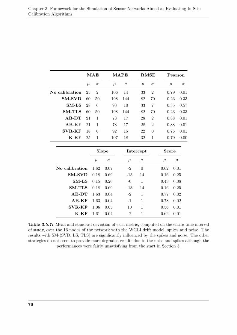
Chapter 3. Framework for the Simulation of Sensor Networks Aimed at Evaluating In SituCalibration Algorithms
MAE MAPE RMSE Pearson
µ σ µ σ µ σ µ σ
No calibration 25 2 106 14 33 2 0.79 0.01SM-SVD 60 50 198 144 82 70 0.23 0.33SM-LS 28 6 93 10 33 7 0.35 0.57
SM-TLS 60 50 198 144 82 70 0.23 0.33AB-DT 21 1 78 17 28 2 0.88 0.01AB-KF 21 1 78 17 28 2 0.88 0.01
SVR-KF 18 0 92 15 22 0 0.75 0.01K-KF 25 1 107 18 32 1 0.79 0.00
Slope Intercept Score
µ σ µ σ µ σ
No calibration 1.62 0.07 -2 0 0.62 0.01SM-SVD 0.18 0.69 -13 14 0.16 0.25SM-LS 0.15 0.26 -0 1 0.43 0.08
SM-TLS 0.18 0.69 -13 14 0.16 0.25AB-DT 1.63 0.04 -2 1 0.77 0.02AB-KF 1.63 0.04 -1 1 0.78 0.02
SVR-KF 1.06 0.03 10 1 0.56 0.01K-KF 1.61 0.04 -2 1 0.62 0.01
Table 3.5.7: Mean and standard deviation of each metric, computed on the entire time intervalof study, over the 16 nodes of the network with the WGLI drift model, spikes and noise. Theresults with SM-(SVD, LS, TLS) are significantly influenced by the spikes and noise. The otherstrategies do not seem to provide more degraded results due to the noise and spikes although the
performances were fairly unsatisfying from the start in Section 3.
76
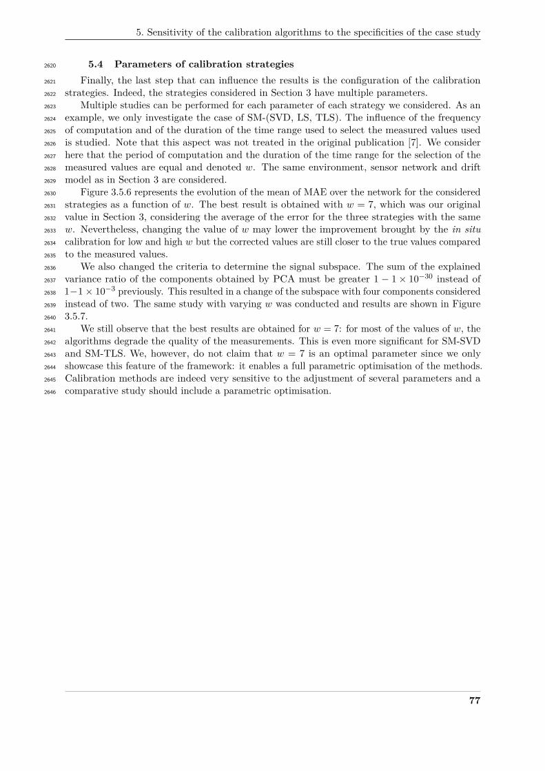
5. Sensitivity of the calibration algorithms to the specificities of the case study
5.4 Parameters of calibration strategies2620
Finally, the last step that can influence the results is the configuration of the calibration2621
strategies. Indeed, the strategies considered in Section 3 have multiple parameters.2622
Multiple studies can be performed for each parameter of each strategy we considered. As an2623
example, we only investigate the case of SM-(SVD, LS, TLS). The influence of the frequency2624
of computation and of the duration of the time range used to select the measured values used2625
is studied. Note that this aspect was not treated in the original publication [7]. We consider2626
here that the period of computation and the duration of the time range for the selection of the2627
measured values are equal and denoted w. The same environment, sensor network and drift2628
model as in Section 3 are considered.2629
Figure 3.5.6 represents the evolution of the mean of MAE over the network for the considered2630
strategies as a function of w. The best result is obtained with w = 7, which was our original2631
value in Section 3, considering the average of the error for the three strategies with the same2632
w. Nevertheless, changing the value of w may lower the improvement brought by the in situ2633
calibration for low and high w but the corrected values are still closer to the true values compared2634
to the measured values.2635
We also changed the criteria to determine the signal subspace. The sum of the explained2636
variance ratio of the components obtained by PCA must be greater 1 − 1× 10⁻³⁰ instead of2637
1−1× 10⁻³ previously. This resulted in a change of the subspace with four components considered2638
instead of two. The same study with varying w was conducted and results are shown in Figure2639
3.5.7.2640
We still observe that the best results are obtained for w = 7: for most of the values of w, the2641
algorithms degrade the quality of the measurements. This is even more significant for SM-SVD2642
and SM-TLS. We, however, do not claim that w = 7 is an optimal parameter since we only2643
showcase this feature of the framework: it enables a full parametric optimisation of the methods.2644
Calibration methods are indeed very sensitive to the adjustment of several parameters and a2645
comparative study should include a parametric optimisation.2646
77
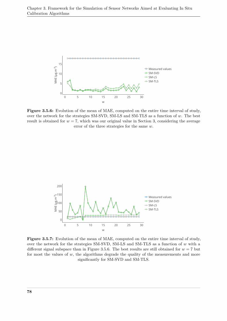
Chapter 3. Framework for the Simulation of Sensor Networks Aimed at Evaluating In SituCalibration Algorithms
0 5 10 15 20 25 300
5
10
15
Measured valuesSM-SVDSM-LSSM-TLS
w
MAE
(μg.
m -3 )
Figure 3.5.6: Evolution of the mean of MAE, computed on the entire time interval of study,over the network for the strategies SM-SVD, SM-LS and SM-TLS as a function of w. The bestresult is obtained for w = 7, which was our original value in Section 3, considering the average
error of the three strategies for the same w.
0 5 10 15 20 25 30
0
50
100
150
200
Measured valuesSM-SVDSM-LSSM-TLS
w
MAE
(μg.
m -3 )
Figure 3.5.7: Evolution of the mean of MAE, computed on the entire time interval of study,over the network for the strategies SM-SVD, SM-LS and SM-TLS as a function of w with adifferent signal subspace than in Figure 3.5.6. The best results are still obtained for w = 7 butfor most the values of w, the algorithms degrade the quality of the measurements and more
significantly for SM-SVD and SM-TLS.
78
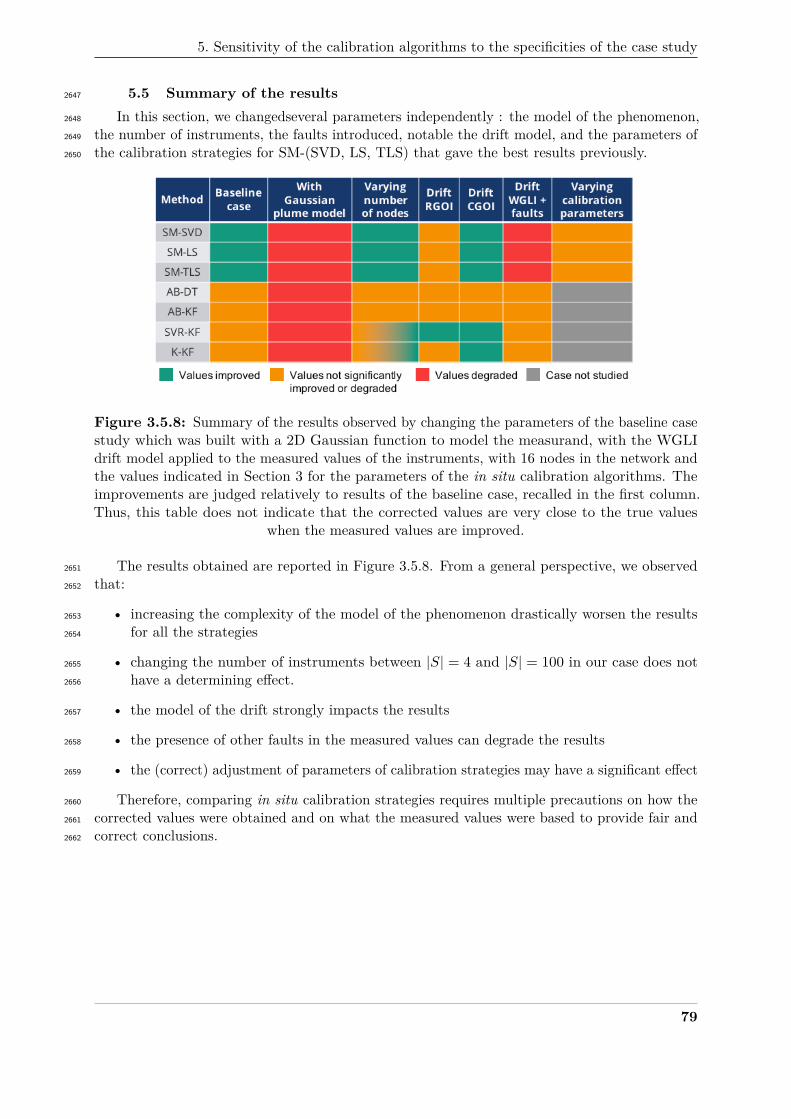
5. Sensitivity of the calibration algorithms to the specificities of the case study
5.5 Summary of the results2647
In this section, we changedseveral parameters independently : the model of the phenomenon,2648
the number of instruments, the faults introduced, notable the drift model, and the parameters of2649
the calibration strategies for SM-(SVD, LS, TLS) that gave the best results previously.2650
Figure 3.5.8: Summary of the results observed by changing the parameters of the baseline casestudy which was built with a 2D Gaussian function to model the measurand, with the WGLIdrift model applied to the measured values of the instruments, with 16 nodes in the network andthe values indicated in Section 3 for the parameters of the in situ calibration algorithms. Theimprovements are judged relatively to results of the baseline case, recalled in the first column.Thus, this table does not indicate that the corrected values are very close to the true values
when the measured values are improved.
The results obtained are reported in Figure 3.5.8. From a general perspective, we observed2651
that:2652
• increasing the complexity of the model of the phenomenon drastically worsen the results2653
for all the strategies2654
• changing the number of instruments between |S| = 4 and |S| = 100 in our case does not2655
have a determining effect.2656
• the model of the drift strongly impacts the results2657
• the presence of other faults in the measured values can degrade the results2658
• the (correct) adjustment of parameters of calibration strategies may have a significant effect2659
Therefore, comparing in situ calibration strategies requires multiple precautions on how the2660
corrected values were obtained and on what the measured values were based to provide fair and2661
correct conclusions.2662
79
Chapter 3. Framework for the Simulation of Sensor Networks Aimed at Evaluating In SituCalibration Algorithms
6 Discussion and conclusion2663
In this chapter, a framework for the simulation of sensor networks, which enables a systematic2664
comparison of in situ calibration strategies with reproducibility, and scalability, was presented.2665
We have showcased this methodology by comparing several calibration strategies for blind and2666
static sensor networks. Our results provide several engineering insights on the design of a sensor2667
network.2668
Based on the methodology described in Section 2, we have proposed a case study in Section2669
3 concerning blind and static sensor networks. Although we have shown that several strategies2670
have better performances than the others, these results have to be tempered as the conclusions2671
depends on how the evaluation is conducted. We have proposed solutions to conduct a balanced2672
assessment of the performances in terms of metrics used in Section 4. It is still challenging2673
for sensor networks with a high number of instruments that require multiple scale analysis. In2674
addition, we have shown in Section 5 that results may not be the same depending on choices2675
made during the design of the case study regardless of how the evaluation is carried out. We2676
have developed variations of our initial case study by changing the model computing the true2677
values of the measurand, the number of instruments, the fault model of the instruments and2678
parameters of calibration strategies.2679
Our results highlight the dependence of the performances of in situ calibration algorithms2680
to the case study. Besides, these performances seem to be often limited, even on the relatively2681
simple environmental models discussed here. The latter explains why more complex and accurate2682
environmental models were not tested here. Finding the good trade-off between simplicity and2683
realism of the simulation models is important. At first sight, the goal could be to consider models2684
as realistic as possible everywhere. However, the accuracy of simulation-based environmental2685
models remains challenging to establish, and costly to run, while simplified models such as those2686
used in the paper may be sufficient when the goal is to compare methods to single out the most2687
promising ones among several for a predefined case study. This is also true for the models to2688
simulate the measuring chain and the deployment of the instruments.2689
It allows to point out an additional advantage to the framework proposed in this paper:2690
its suitability as a design tool for sensor networks. For instance, after having determined the2691
number of instruments (and their positions) required to cover a given area with a static sensor2692
network, the best in situ calibration strategy and its parameters could be identified among2693
a set of algorithms applicable to this particular network. In such cases, however, a stronger2694
focus on the accuracy of the environmental model should be put whenever possible. Beyond2695
the quality of the models, the adjustment of the strategies is crucial for an objective evaluation.2696
The reproducibility provided by the framework is an asset to conduct a thorough parametric2697
optimisation and compare the best results of each calibration.2698
To conclude, we can point out the following engineering insights on the design of a sensor2699
network and the evaluation of in situ calibration strategies.2700
• There is actually no method that is universally outperforming the other. The best calibration2701
strategy to apply depends on the deployment of the instruments and the exploitation of2702
the measurements.2703
• Even on the same scenario, two strategies can outperform each other depending on which2704
metrics of performance is considered and the way they are computed. The metrics and2705
their means of visualisation have to be chosen accordingly to the target exploitation of the2706
sensor network, to focus on the relevant features. We also advise using an error model in2707
order to get meaningful details on the performances.2708
• Increasing the density of the deployment of instruments does not always lead to better2709
performances of a calibration strategy.2710
80
6. Discussion and conclusion
• In some case, the quality of data can be degraded by a calibration strategy. Besides, other2711
faults than drift will happen, in particular when considering low-cost instruments with2712
low-quality electronics. To cope with robustness issues of the calibration strategy, it seems2713
relevant to process these errors upstream.2714
The content of this chapter is based on the following publication:2715
F. Delaine, B. Lebental and H. Rivano, "Framework for the Simulation of Sensor2716
Networks Aimed at Evaluating In Situ Calibration Algorithms," in Sensors, vol. 20,2717
no. 16, 2020, DOI: 10.3390/s20164577.2718
Codes and data files used to produce the results of Sections 3, 4 and 5 are available online2719
under licence AGPL 3.0 and ODbL 1.0 respectively in [37]2720
81

Chapter 3. Framework for the Simulation of Sensor Networks Aimed at Evaluating In SituCalibration Algorithms
82
Chapter2721
42722
Diagnosis of Drift Faults in Sensor2723
Networks2724
Contents2725
2726 1 Motivations . . . . . . . . . . . . . . . . . . . . . . . . . . . . . . . . . . . . . . 852727
2 State-of-the-art of fault diagnosis applied to sensor networks . . . . . . . . . . 862728
2.1 Overview of fault diagnosis for sensor networks through existing reviews 862729
2.2 Existing methods of diagnosis compatible with the concept of rendez-2730
vous addressing any fault . . . . . . . . . . . . . . . . . . . . . . . . . 872731
2.2.1 Introduction . . . . . . . . . . . . . . . . . . . . . . . . . . . . . . 872732
2.2.2 Related works . . . . . . . . . . . . . . . . . . . . . . . . . . . . . 872733
2.2.3 Remarks . . . . . . . . . . . . . . . . . . . . . . . . . . . . . . . . 892734
2.3 Positioning of the contribution . . . . . . . . . . . . . . . . . . . . . . 892735
3 Definition of concepts for a drift diagnosis algorithm based on rendez-vous . . 892736
3.1 Validity of measurement results . . . . . . . . . . . . . . . . . . . . . . 902737
3.2 Compatibility of measurement results . . . . . . . . . . . . . . . . . . . 902738
3.3 Rendez-vous . . . . . . . . . . . . . . . . . . . . . . . . . . . . . . . . . 912739
3.3.1 Formal and practical definitions . . . . . . . . . . . . . . . . . . . 912740
3.3.2 Compatible rendez-vous . . . . . . . . . . . . . . . . . . . . . . . 922741
4 Algorithm for the diagnosis of calibration issues in a sensor network . . . . . . 922742
4.1 General idea . . . . . . . . . . . . . . . . . . . . . . . . . . . . . . . . . 922743
4.2 Procedure for the diagnosis of all the instruments in a sensor network 942744
4.3 Improvements and extensions of the presented algorithm . . . . . . . . 952745
4.4 Conclusion . . . . . . . . . . . . . . . . . . . . . . . . . . . . . . . . . . 952746
5 Application of the algorithm to a first case study . . . . . . . . . . . . . . . . . 972747
5.1 Definition of the case study . . . . . . . . . . . . . . . . . . . . . . . . 972748
5.1.1 Sensor network . . . . . . . . . . . . . . . . . . . . . . . . . . . . 972749
5.1.2 Instruments . . . . . . . . . . . . . . . . . . . . . . . . . . . . . . 972750
5.1.3 True values . . . . . . . . . . . . . . . . . . . . . . . . . . . . . . 982751
5.2 Configuration of the diagnosis algorithm . . . . . . . . . . . . . . . . . 992752
5.3 Definition of the true status of an instrument . . . . . . . . . . . . . . 992753
5.4 Metrics for the evaluation of performances of the diagnosis algorithm . 992754
5.5 Results . . . . . . . . . . . . . . . . . . . . . . . . . . . . . . . . . . . . 1012755
83
Chapter 4. Diagnosis of Drift Faults in Sensor Networks
5.5.1 Observations from the results of different instruments . . . . . . 1012756
5.5.2 Overall appreciation . . . . . . . . . . . . . . . . . . . . . . . . . 1012757
5.5.3 Evolution over time of the metrics . . . . . . . . . . . . . . . . . 1022758
5.6 Explanations of false results . . . . . . . . . . . . . . . . . . . . . . . . 1072759
5.7 On the parameters of the diagnosis algorithm . . . . . . . . . . . . . . 1082760
5.8 Conclusion . . . . . . . . . . . . . . . . . . . . . . . . . . . . . . . . . . 1102761
6 On the assumption regarding the top-class instruments being always predicted2762
as non-faulty . . . . . . . . . . . . . . . . . . . . . . . . . . . . . . . . . . . . . 1112763
6.1 Theoretical discussion . . . . . . . . . . . . . . . . . . . . . . . . . . . 1112764
6.2 Case study with the instrument of class cmax drifting . . . . . . . . . . 1112765
6.3 Conclusion . . . . . . . . . . . . . . . . . . . . . . . . . . . . . . . . . . 1132766
7 Means to reduce false results . . . . . . . . . . . . . . . . . . . . . . . . . . . . 1132767
7.1 Keep the predicted status of instruments unchanged once they are2768
predicted as faulty . . . . . . . . . . . . . . . . . . . . . . . . . . . . . 1132769
7.2 Alternate definition for rates used to decide of the status of the instruments1132770
7.3 Adjustment of the maximal tolerated values for the different rates used2771
to determine the statuses of the instruments . . . . . . . . . . . . . . . 1152772
7.4 Conclusion . . . . . . . . . . . . . . . . . . . . . . . . . . . . . . . . . . 1162773
8 Adjustment of the minimal size required for a set of valid rendez-vous to allow2774
a prediction between the statuses faulty and non-faulty . . . . . . . . . . . . . 1172775
8.1 Algorithm determining an upper boundary for |Φv|min . . . . . . . . . 1172776
8.2 Application to the case study . . . . . . . . . . . . . . . . . . . . . . . 1202777
8.3 Conclusion . . . . . . . . . . . . . . . . . . . . . . . . . . . . . . . . . . 1222778
9 Sensitivity of the algorithm to changes in the case study . . . . . . . . . . . . 1222779
9.1 Influence of the values of drift . . . . . . . . . . . . . . . . . . . . . . . 1222780
9.2 Influence of the true values . . . . . . . . . . . . . . . . . . . . . . . . 1232781
9.3 Influence of the model used for the true values . . . . . . . . . . . . . . 1242782
9.4 Influence of the density of instruments . . . . . . . . . . . . . . . . . . 1252783
9.5 Influence of other faults . . . . . . . . . . . . . . . . . . . . . . . . . . 1312784
9.6 Conclusion . . . . . . . . . . . . . . . . . . . . . . . . . . . . . . . . . . 1312785
10 Combination with a simple calibration approach . . . . . . . . . . . . . . . . . 1332786
11 Conclusion . . . . . . . . . . . . . . . . . . . . . . . . . . . . . . . . . . . . . . 1382787278827892790
84
1. Motivations
1 Motivations2791
Across the study of all the in situ calibration strategies in Chapter 2, and particularly regarding2792
those considered in Chapter 3, most strategies perform the calibration of all instruments without2793
evaluating first whether they actually need it. Moreover, we observed the algorithms may2794
not improve, or may even degrade, the quality of the measurements. Two guidelines for in2795
situ calibration algorithms can be established based on that. First, instruments providing2796
measurement results agreeing with their specifications, should not be affected by an in situ2797
calibration strategy. Secondly, the need for a calibration operation must be explicitly determined.2798
This is particularly important if the execution of the algorithm is expensive, e.g. in terms of2799
energy consumption in the case of autonomous nodes. It would add more confidence in the2800
algorithms, namely it could inform it recalibrated an instrument because a criterion on its2801
measurement results was met.2802
Some calibration algorithms are actually providing the identification of instruments needing2803
a calibration, notably in [87, 168]. In these two publications, the algorithm determines first2804
whether an instrument has drifted since the last time step. If it is the case, it gives the identity2805
of the instrument that has drifted and correct it with the help of all the other instruments.2806
However, if more than one instrument is drifting at a time, the algorithm raises an error. This is2807
problematic as such a case is very likely in practice.2808
In the same vein of assumptions that are difficult to meet in practice, multiple strategies2809
are designed based on the hypothesis that the sensor network is "dense". It means that each2810
instrument is within few tens of meters to one or several nodes of the network. The need for2811
this assumption to be verified can be explained as follows. To correct drifting instruments, their2812
correct values–or the values of the drift–must be estimated. To do so, mainly two approaches are2813
considered: the estimation from values measured by neighbouring instruments or the estimation2814
from a model of the measurand. This is the case whether the network is static or not and blind2815
or not.2816
Regarding the first approach, instruments should be physically close enough to have com-2817
parable values between them. This is something that can be easily achieved in practice and2818
the reason why the assumption of a dense sensor network is often proposed. However, if the2819
distance between the instrument to recalibrate and the instruments used to estimate its value is2820
too important compared to the characteristic spatial length of variation of the measurand, and if2821
it cannot be reduced, it may not be possible to have an accurate estimation with the desired2822
uncertainty. Thus, as complex quantities are targeted in environmental monitoring, comparisons2823
may be feasible for mobile sensor networks, but it is less likely to be the case for static sensor2824
networks. Indeed, with mobile instruments can sometimes meet whatever the number of nodes in2825
the network. For static ones, the number of instruments may have to be significantly increased2826
depending on the application so that values of different devices may be compared but with an2827
associated cost that may be significant.202828
Therefore, a model-based approach for estimating the correct values of instruments may2829
be preferred when meeting the required density of instruments is not possible, e.g. with static2830
instruments close enough or with mobile nodes meeting often. With a model-based approach, it2831
is assumed possible to model satisfyingly the measurand to estimate its value at several locations,2832
with the help of a priori information and sometimes with measured values, preferably from2833
20The case where neighbouring instruments are used to evaluate the values of an instrument could be extendedto the case where the nodes of the network embed several instruments with the same characteristics and measuringthe same quantity. In this case, the set of instruments of a node measuring the same quantity can be seen as ameasuring system, which would be equivalent to having a single instrument of a higher quality. Indeed, it canbe legitimately expected that the average of the values of these instruments is more accurate than their valuesconsidered individually. This comes down to the case described in this paragraph. For the sake of clarity, thisparticular situation is not discussed in detail in this manuscript.
85
Chapter 4. Diagnosis of Drift Faults in Sensor Networks
reference instruments. Acquiring such information may not be easy or may require a long training2834
period to capture enough features of the phenomena. The latter may not be compatible with the2835
lifespan of the instruments, especially if they are low cost. The deployment of expensive reference2836
instruments during the deployment phase is a solution but has a major cost impact, notably if a2837
high number of instruments is required. Additionally, using a model for the measurand raises2838
the question of the interest of deploying the sensor network itself. If the model is able to derive2839
at the required spatiotemporal resolution the values of the considered phenomenon, even with2840
the help of a few high-quality instruments, this may be sufficient for most applications.2841
Overall, these elements point out that most approaches for in situ calibration can be challenged2842
by the fact that the reference values used for calibration, e.g. standard values, need to meet2843
certain conditions. They are not necessarily met in in situ calibration algorithms. The same2844
precautions should be taken regarding the identification of instruments that have drifted, whatever2845
the approach chosen to determine them.2846
In this chapter, we investigate the feasibility of drift detection for measuring instruments2847
with the help of measurement results from other devices. The concept of rendez-vous is used2848
to achieve this goal and is formally defined in Section 3, based on existing works on the subject2849
[40, 132]. The study of these rendez-vous is expected to help to determine if an instrument2850
needs to be recalibrated as long as one of the instruments involved in the rendez-vous can be2851
considered as a standard, e.g. an instrument of which results can legitimately be trusted. To2852
remain the most generic as possible, no assumption is made for this algorithm on the2853
type of sensor network, on the density of instruments and on the measurand such as2854
a priori known information regarding it.212855
Thus, a formal definition of the concept of rendez-vous is proposed first based on existing2856
works. Which values of instruments may be compared to each other in practice is briefly discussed.2857
Then, a diagnosis algorithm, that is a way to identify the instruments that need a correction of2858
their calibration relationship, is provided. The approach is based on rendez-vous. Afterwards,2859
a case study is presented to illustrate the application of the diagnosis algorithm. The means2860
to improve the results, in terms of false results, are discussed followed by guidelines on the2861
adjustment of the parameters of the algorithm. The sensitivity of the algorithm to the parameters2862
of the case study is studied. Finally, the algorithm is combined to a simple calibration strategy2863
showing promising results. Before moving to these contributions, a literature review is conducted2864
regarding fault diagnosis applied to sensor networks and in particular regarding the detection of2865
drift.2866
2 State-of-the-art of fault diagnosis applied to sensor networks2867
2.1 Overview of fault diagnosis for sensor networks through existing reviews2868
In the last decade, while sensor networks gained in popularity, the question of their de-2869
pendability became a major subject. In particular, multiple contributions were made on fault2870
diagnosis as reported in various surveys [98, 106, 114, 185].2871
In these publications, the research works are classified by the way the diagnosis is performed.2872
First, the place where the decision is computed, e.g. if it is a centralised, decentralised or hybrid2873
approach, is considered. Then, the general mathematical approach used for the diagnosis (testing,2874
comparisons, majority voting, statistics, probabilities, machine learning algorithms, fuzzy logic,2875
clustering...) is studied.2876
Faults are generally characterised by "hard" or "soft" and as "permanent", "transient" or2877
"temporary"[98, 106, 185]. Only Muhammed et al. [114] used a taxonomy similar to the one of2878
Ni et al. [115] that inspired the one used in this manuscript. In particular, these authors report2879
21It could be for instance an actual correlation between the true values at two very distant points that could beexploited in a specific situation.
86
2. State-of-the-art of fault diagnosis applied to sensor networks
that the existing diagnosis algorithms are often targeting multiple faults. For those addressing2880
the drift fault22, stuck-at or out-of-range faults are also detected by the same algorithm in the2881
15 associated references they cited.2882
In the following surveys [98, 114, 185], the diagnosis approaches reported concern mainly2883
static sensor networks. Mahapatro et al. [98] listed eight algorithms that could be applied2884
to static and mobile sensor networks.23 Zhang et al. [185] reported two references explicitly2885
dealing with mobile sensor networks [1, 28]. They also stated that approaches designed for static2886
networks behave poorly when applied to mobile ones. This indicates that algorithms exploiting2887
specificities related to networks with mobile nodes in the diagnosis approach have not been2888
deeply investigated so far.2889
In addition, other subjects such as energy consumption, communication range needed,2890
communication failures, or the amount of required neighbour nodes are taken into account in the2891
surveys on fault diagnosis for sensor networks [98, 106, 114, 185]. Zhang et al. [185] underline2892
it is challenging to design a diagnosis approach having satisfying performances or properties2893
regarding all the features of interest for such an algorithm, e.g. for instance diagnosing faults2894
well with low energy consumption, few communications between nodes and so on.2895
2.2 Existing methods of diagnosis compatible with the concept of rendez-vous2896
addressing any fault2897
2.2.1 Introduction2898
The methods used to carry out the diagnosis of any fault in sensor networks are diverse in2899
terms of concepts and tools on which they are based on. According to the surveys cited [98,2900
106, 114, 185], different main ideas come out like the use of comparisons between instruments,2901
the use of statistics and probabilities, as well as the use of machine learning models (regressors,2902
classifiers...). As the goal in this chapter is to propose a diagnosis algorithm for sensor networks2903
based on rendez-vous between the nodes, we focus here on approaches compatible with this idea,2904
e.g. it consists at least in comparison of values measured by different instruments.2905
2.2.2 Related works2906
Chen et al. [29] introduced a faulty sensor detection algorithm consisting of four steps of2907
evaluation. First, each instrument compares its measured value at the instant of the diagnosis2908
with the measured values of its neighbours. If the difference between two instruments is higher2909
than a first threshold, the deviation of the difference since the last comparison is computed. If it2910
is higher than a second threshold, the test between the two instruments is marked as positive.2911
In a second step, each instrument determines if it is likely good or faulty depending on the2912
number of positive tests and its number of neighbours. This information is shared between the2913
instruments so that based on its neighbours that are likely good, an instrument determines if2914
it is actually good and share this result. Then, for the remaining undetermined instruments,2915
their statuses are decided if all their neighbours are non-faulty and if all the initial tests gave2916
the same results. If ambiguities remains, they are removed based on the likely statuses of the2917
instruments. Xu et al. [179] proposed an extension of this work dealing with the particular case2918
of tree-like networks to reduce the number of communications. To avoid intermittent faults, they2919
also proposed to compute the initial test result based on multiple comparisons of values between2920
two instruments, instead of a unique comparison. In the same way, Saha et al. [128] developed2921
a similar algorithm but with comparisons for multiple quantities (measurand and remaining2922
22In the publication of Muhammed et al. [114], calibration, gain, and offset faults correspond to what is notablya drift fault in this thesis.
23Note that the subject of mobile sensor networks was new at the time when Mahapatro et al. [98] publishedtheir survey.
87
Chapter 4. Diagnosis of Drift Faults in Sensor Networks
energy).2923
Ssu et al. [142] proposed an approach to diagnosis faults between sources and sinks. The2924
main idea is to send a request through two paths and to compare the results obtained at the2925
sink node. If the results are different, then at least one faulty path exists. The algorithm tries to2926
identify it with the help of a third path and a majority voting procedure, but the faulty paths2927
cannot always be identified. Such a method is particularly relevant to diagnose communication2928
or hardware-related faults.2929
Lee et al. [83] presented a distributed algorithm to isolate faulty nodes. Initially, the nodes2930
are all assumed as faulty. A comparison is made between the measured values of neighbour nodes2931
and if the result is higher than a threshold, then the test is positive. If less than a predefined2932
number of positive tests has been obtained, or if the test with a non-faulty node is negative, then2933
the diagnosed instrument is non-faulty. The algorithm works either based on single comparisons2934
between neighbours or with comparisons repeated multiple times.2935
Mahapatro et al. [97, 99] introduced a clustering-based diagnosis algorithm. The clustering2936
part is used for the definition of the neighbours around cluster heads, the cluster heads being2937
the instruments with the highest residual energy levels. They also compare the measured values2938
between instruments of a cluster and a majority voting strategy is used to determine the state of2939
the nodes.2940
Chanak et al. [28] developed a comparison-based scheme using a reference mobile sink node2941
moving between the static nodes of the network. When it is close to a node, several diagnoses are2942
performed to detect hardware and software faults. This also enables a low consumption of energy2943
for the transmission of the measurement results as it is no longer necessary to communication2944
with a distant gateway. The core of this contribution lies in the determination of an optimal2945
path to meet with each node.2946
Luo et al. [92] proposed an approach using the concept of average consensus. Each instrument2947
estimates first its status regarding the average consensus measured value build with the values of2948
its neighbours. Each instrument also estimates the statuses of its neighbours. Then, the decisions2949
of all the instruments are merged to make the final decision.2950
In reaction to contributions computing the average value of the neighbours of an instrument2951
by weighting their values with the inverse of the distance between them, Xiao et al. [178] argued2952
that the distance does not control alone the relationship between the values of two instruments,2953
notably if a closer one is actually faulty. Thus, they propose to take into account an indicator of2954
trustworthiness computed for each node of the network. This confidence value is used in voting2955
procedures that are used to determine the status of instruments.2956
Ji et al. [69] also developed their algorithm around a weighted average of the values measured2957
by an instrument. The weights are representing a confidence level associated to each instrument.2958
The difference between the measured value of an instrument and the average is compared to a2959
threshold. If it is greater than the threshold, the confidence level of the instrument is decreased2960
and once it reaches zero, the instrument is reported as faulty.2961
This idea of trust between instruments has been extensively studied and extended, as did2962
for instance Jiang et al. [70]. Their robust trust model is based on direct comparisons but also2963
on third parties and recommendations, with concerns about the security of the communications2964
between the instruments. Their trust framework is also adapted for mobile sensor networks.2965
Wang et al. [164] exploited Petri nets to introduce a trust-based formal model aimed at detecting2966
faults in sensor networks.2967
Sharma et al. [134] also exploited the idea of confidence in a method similar to the one of2968
Chen et al. [29]. The main difference with Chen et al. is that in a first step each instrument2969
analyses its own behaviour and that a confidence level is associated to the determined statuses.2970
Feiyue et al. [52] proposed to combine the information resulting of a self-evaluation and2971
of comparisons with the neighbours of each instrument. In a first step, the reliable nodes are2972
88
3. Definition of concepts for a drift diagnosis algorithm based on rendez-vous
determined through a majority voting procedure. Then, various metrics are computed and2973
combined to make the decisions for the instruments that were not considered reliable in the first2974
step.2975
2.2.3 Remarks2976
In this section, the way the computation is conducted (centralised, decentralised, hybrid) was2977
not discussed on purpose. Indeed, this topic impacts the number of communications required and2978
the energy consumption of the method more than the actual result of the diagnosis procedure.2979
Another aspect is how the faults are managed after detection in a diagnosis algorithm. There2980
are different visions. Considering the diagnosis of outliers for instance, Ottosen et al. [116]2981
adopted a gap-filling strategy. Fang et al. [51] preferred a fault removal approach because this2982
procedure is a data processing carried out before the calibration of the instruments of the network.2983
As shown for the calibration of measuring instruments in Chapter 3, it may also be preferable to2984
correct measurement results prior to the diagnosis of drift if any other fault may be present.2985
Finally, in the works presented here, the diagnosis is performed in most cases based on single2986
values from a given set of instruments measured at the same time. Taking a decision on a short2987
time range may not be correct, especially if drift is targeted. Indeed, drift is a fault increasing2988
little by little and thus a diagnosis on a long sequence of measured values over time could be2989
more appropriate.2990
2.3 Positioning of the contribution2991
From this review, we observed that the literature on fault diagnosis for sensor networks is rich2992
and abundant. Static sensor networks have been widely studied while mobile sensor networks2993
have been partially covered. Multiple types of faults are addressed, concerning various aspects2994
of measuring systems, but drift is not specifically targeted in existing works. Various methods2995
have been used to tackle the challenge of fault diagnosis, notably based on comparisons between2996
instruments.2997
However, the validity of the comparisons is rarely discussed from a metrological perspective.2998
It would be valuable to develop a new approach with considerations on the quality of the2999
measurement results. Moreover, exploiting the concept of rendez-vous allows to take into account3000
that it happens in a spatiotemporal vicinity. This concept is more sophisticated than the simple3001
idea of comparison of measurement results.3002
In addition, a diagnosis algorithm not requiring any assumptions on the type of sensor network3003
and its structure would be interesting. Indeed, the existing approaches are often targeting static3004
sensor networks, which may imply a dense network in the case of a comparison-based strategy,3005
and rarely networks with mobile nodes. Regarding rendez-vous, mobility is an important feature3006
that can facilitate their occurrence. Because mobile nodes can meet spatially with other mobile3007
or static nodes, a diagnosis approach based on these meeting points would allow more meaningful3008
comparisons of values if a very high density of measuring instruments is not feasible. In this3009
way, if the algorithm works whether the sensor network is static or has mobile node leaves to the3010
users the choice of the most appropriate type of sensor network for their application.3011
3 Definition of concepts for a drift diagnosis algorithm based on rendez-3012
vous3013
Before the presentation of an algorithm for the diagnosis of drift in sensor networks, this section3014
introduces the definitions of the concepts of validity and compatibility of measurement results,3015
and of rendez-vous. A sensor network composed of a set of instruments S is considered here and3016
in the following sections without any other assumption on its type and on the characteristics of3017
its nodes.3018
89
Chapter 4. Diagnosis of Drift Faults in Sensor Networks
3.1 Validity of measurement results3019
In Chapter 1 Section 1.2, we recalled that measuring instruments cannot exactly provide true3020
values. In addition, we indicated they may be different accuracy class, e.g. of different qualities,3021
in Chapter 1 Section 3.3022
On top of these ideas, we introduce here the notion of the validity of measurement results.3023
For instance, a measuring instrument cannot measure all the values of a quantity. It has a3024
bounded measuring interval which is the set of values of a quantity "that can be measured by3025
a given measuring instrument or measuring system with specified instrumental measurement3026
uncertainty, under defined conditions" [14]. In addition, it cannot work properly under any3027
operating conditions. Therefore, a measurement result with a value outside an instrument’s3028
measuring interval or which has been obtained outside of the normal conditions of operation of a3029
device, may not be valid.3030
The conditions under which measurement results are valid are specific to each type of3031
instrument. In practice, they are usually provided in the technical documentation or it is possible3032
to determine them experimentally. In this chapter, the conditions under which results are3033
considered as valid are explained in the case study.3034
The notation M∗(si, (t,∆t)) refers to the set of measurement results for si, over the time3035
range [t−∆t; t] that are metrologically valid, e.g. v(si, t) in the measuring interval and so on3036
depending on the definition of what a valid result is metrologically speaking.3037
3.2 Compatibility of measurement results3038
Definition 22. Consider si ∈ S. A measurement result m(si, t) is compatible with true3039
value if vtrue(si, t) ∈ [v(si, t)−∆v(si, t); v(si, t) + ∆v(si, t)].3040
Definition 23. Consider si ∈ S. A measurement result m(si, t) is upper non-compatible3041
with true value if vtrue(si, t) < v(si, t)−∆v(si, t).3042
Definition 24. Consider si ∈ S.A measurement result m(si, t) is lower non-compatible with3043
true value if vtrue(si, t) > v(si, t) + ∆v(si, t).3044
The set of measurement results compatible with true values of si obtained during [t−∆t; t]is noted M≈(si, (t,∆t)). M+(si, (t,∆t)) and M−(si, (t,∆t)) are defined for upper and lowernon-compatible measurement results respectively. It can be noticed that
M(si, (t,∆t)) = M≈(si, (t,∆t)) ∪M+(si, (t,∆t)) ∪M−(si, (t,∆t))
These definitions can be extended for the comparison of measurement results between different3045
instruments.3046
Definition 25. Consider si and sj ∈ S. m(si, t) is compatible with m(sj , t′) if v(sj , t′) −3047
∆v(sj , t′) ≤ v(si, t)−∆v(si, t) ≤ v(sj , t′)+∆v(sj , t′) or v(sj , t′)−∆v(sj , t′) ≤ v(si, t)+∆v(si, t) ≤3048
v(sj , t′) + ∆v(sj , t′). It is noted m(si, t) ≈ m(sj , t′).3049
Definition 26. Consider si and sj ∈ S. m(si, t) is upper non-compatible with m(sj , t′) if3050
v(si, t)−∆v(si, t) ≥ v(sj , t′) + ∆v(sj , t′). It is noted m(si, t) > m(sj , t′).3051
Definition 27. Consider si and sj ∈ S. m(si, t) is lower non-compatible with m(sj , t′) if3052
v(si, t) + ∆v(si, t) ≤ v(sj , t′)−∆v(sj , t′). It is noted m(si, t) < m(sj , t′).3053
The sets of measurement results of si obtained during [t−∆t; t] associated to these definitions3054
are respectively noted M≈(si → sj , (t,∆t)), M+(si → sj , (t,∆t)) and M−(si → sj , (t,∆t)).3055
More restrictive criteria can be set to determine if measurement results are compatible3056
either with their associated true values or with results of other instruments. For instance, it3057
90
3. Definition of concepts for a drift diagnosis algorithm based on rendez-vous
could be a minimal level of overlapping between [v(si, t) − ∆v(si, t); v(si, t) + ∆v(si, t)] and3058
[v(sj , t′) −∆v(sj , t′); v(sj , t′) + ∆v(sj , t′)]. However, the influence of these definitions are not3059
studied afterwards as it is more a matter of specification for the quality of measurements than a3060
matter of diagnosis.3061
3.3 Rendez-vous3062
3.3.1 Formal and practical definitions3063
A rendez-vous between two instruments is defined as follows.3064
Definition 28 (Rendez-vous). Two instruments si and sj ∈ S are considered in rendez-vous3065
when they are in a spatiotemporal vicinity so that their measurement results can be compared. In3066
practice, it means for both their measurement results m(si, t) and m(sj , t′) that the instruments3067
were spatially close enough and the difference between the instants of measurement t and t′ was3068
small enough to actually measure the same quantity value.3069
si being in a rendez-vous at t with sj is noted ϕ(si → sj , t). Respectively sj being in a3070
rendez-vous at t′ with si is noted ϕ(sj → si, t′).3071
The concept of "close enough" instruments will be explained later in the present section.3072
Regarding the instants of measurement, two different ones are defined, t and t′, because si3073
and sj may not have the same measurement frequency or may not have synchronous clocks.3074
Consequently, in general, the measurement results of two instruments in rendez-vous are not3075
obtained exactly at the same time.3076
The set of the rendez-vous encountered by si with sj during [t − ∆t; t] is noted Φ(si →3077
sj , (t,∆t)). By extension, Φ(si → S, (t,∆t)) is the set of rendez-vous between si and any other3078
instrument of S during [t−∆t; t].3079
First of all, with this definition of a rendez-vous, there is no reason that any of the instrument3080
should be mobile or static. As long as the conditions regarding the spatiotemporal vicinity are3081
respected, rendez-vous can happen.24 Thus, the use of the concept of rendez-vous in practice3082
requires the definition of what an acceptable spatiotemporal vicinity is for a rendez-vous.3083
A first possible definition can be based on a maximal distance ∆lϕ allowed between theinstruments and on a maximal acceptable time difference ∆tϕ between the measurement resultsof the two instruments. Therefore, si is in rendez-vous with sj at t if
∃t′ ∈ R+ such as ∃m(sj , t′) and |t− t′| ≤ ∆tϕ and |l(si, t)− l(sj , t′)| ≤ ∆lϕ
with l(si, t) and l(sj , t′) being the positions of si at t and sj at t′. The temporal condition3084
allows multiple rendez-vous with a single instrument for a same measurement result if t′ is3085
not unique. In this case, t′ can be chosen as the value reaching the minimum of |t − t′| or of3086
|l(si, t)− l(sj , t′)|. This choice of a unique measurement result for sj is necessary to ensure that3087
the measurement result of si is compared to the result the most probable to have been obtained3088
from the same quantity value.3089
In practice, ∆tϕ can be related to the characteristic time of variation of the measurand3090
whereas ∆lϕ may be related to the spatial homogeneity of this quantity.3091
Another definition of the spatial closeness can be designed based on the concept of repre-sentative area of measurement results [126], noted a(si, t) for si at t. It is the area around thelocation of a measurement result in which the measurement result is representative of any otherresult that would have been obtained at another position within the area. This definition maybe more usable in practice than the one based on a norm as it considers the geometry of the
24If no instrument is mobile, it may be necessary to have less restrictive requirements on the spatiotemporalvicinity to observe rendez-vous.
91
Chapter 4. Diagnosis of Drift Faults in Sensor Networks
area in which the instruments are. There are buildings and crossings for instance in an urbanenvironment. Thus, with this definition, si is in rendez-vous with sj at t if for instance:
∃t′ ∈ R+ such as ∃m(sj , t′) and |t− t′| ≤ ∆tϕ and a(si, t) ∩ a(sj , t′) 6= ∅
An alternate expression could be the following:
∃t′ ∈ R+ such as ∃m(sj , t′) and |t− t′| ≤ ∆tϕ and |a(si, t) ∩ a(sj , t′)| ≥ ∆aϕ
where ∆aϕ is the minimal size of the intersection of the representativity area of both measurement3092
results.3093
In conclusion, the concept of rendez-vous can be applied according to different definitions in3094
practice. In the following sections, the diagnosis algorithm is designed without any assumption3095
on the practical definition of a rendez-vous.3096
3.3.2 Compatible rendez-vous3097
Consider a rendez-vous ϕ(si → sj , t). By associating the definitions of compatible measure-3098
ment results, a rendez-vous of si with sj at t is stated as compatible if m(si, t) ≈ m(sj , t′). Oth-3099
erwise it is stated as upper non-compatible if m(si, t) > m(sj , t′) or lower non-compatible3100
if m(si, t) < m(sj , t′).25 Consequently, Φ≈(si → sj , (t,∆t)), Φ+(si → sj , (t,∆t)) and Φ−(si →3101
sj , (t,∆t)) are the respective associated sets of such rendez-vous.3102
4 Algorithm for the diagnosis of calibration issues in a sensor network3103
4.1 General idea3104
The general purpose of a diagnosis algorithm is to determine whether if a system is faulty3105
(F) or non-faulty (NF). In the present case, the predicted status of an instrument si at t is3106
noted Ω(si, t). Ideally, Ω(si, t) is equal to the true status of the instrument, Ω(si, t), which is3107
unknown in practice.3108
To determine if instruments are correctly calibrated, the proposed approach consists in using3109
the concept of rendez-vous introduced in Section 3.3. When two instruments si and sj are3110
in rendez-vous, it means that, according to chosen spatiotemporal conditions, they were both3111
measuring the same quantity value at the same time and the same place. Suppose that one of the3112
instruments, sj for instance, was diagnosed as non-faulty and consider m(si, t) and m(sj , t′), the3113
measurement results involved in a rendez-vous ϕ(si → sj , t).26 If both results are metrologically3114
valid, it means that m(sj , t′) can be seen as a standard value for si: it is a known value with an3115
associated uncertainty. Thus, if m(si, t) ≈ m(sj , t′), it denotes that si is correctly calibrated, at3116
least according to sj , and its status can be predicted as non-faulty. Otherwise, it is predicted as3117
faulty. As sj helps to predict the status of si, it is called a diagnoser of si.3118
Predicting the status of an instrument based on only one value may easily lead to falsepredictions because drift is a fault usually having a longer characteristic time than others likespike faults. For instance, if spikes are not correctly removed before carrying out a diagnosis,it is possible that m(si, t) > m(sj , t′) or that m(si, t) < m(sj , t′), e.g. the measurement resultsm(si, t) and m(sj , t′) are not compatible, whereas the true status of si, Ω(si, t) is actually equalto non-faulty from a calibration perspective. Hence, the use of multiple rendez-vous with sj andalso with other instruments to predict the status of si can reduce the impact of these particular
25We recall that more restrictive criterion can be set to determine if measurement results are compatible withthe results of other instruments but it is not studied in this work. See Section 3.2 for more details.
26We recall that the measurement resultsm(si, t) andm(sj , t′) have two different timestamps t and t′ respectivelybecause they may not have been obtained exactly at the same time (see Section 3.3).
92
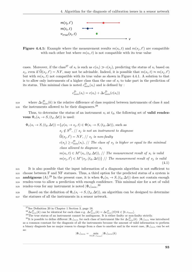
4. Algorithm for the diagnosis of calibration issues in a sensor network
v𝑣!"#$(𝑠% , 𝑡)𝑚(𝑠% , 𝑡)𝑚(𝑠&, 𝑡′)
Figure 4.4.1: Example where the measurement results m(si, t) and m(sj , t′) are compatiblewith each other but where m(si, t) is not compatible with its true value
cases. Moreover, if the class27 of si is such as c(si) c(sj), predicting the status of si based onsj , even if Ω(sj , t′) = NF , may not be advisable. Indeed, it is possible that m(si, t) ≈ m(sj , t′)but with m(si, t) not compatible with its true value as shown in Figure 4.4.1. A solution to thatis to allow only instruments of a higher class than the one of si to take part in the prediction ofits status. This minimal class is noted cDmin(si) and is defined by :
cDmin(si) = c(si) + ∆cDmin(c(si))
where ∆cDmin(k) is the relative difference of class required between instruments of class k and3119
the instruments allowed to be their diagnosers.283120
Thus, to determine the status of an instrument si at td, the following set of valid rendez-vous Φv(si → S, (td,∆t)) is used:
Φv(si → S, (td,∆t)) =ϕ(si → sj , t) ∈ Φ(si → S, (td,∆t)), such assj /∈ SD, // sj is not an instrument to diagnoseΩ(sj , t′) = NF , // sj is non-faultyc(sj) ≥ cDmin(si), // The class of sj is higher or equal to the minimalclass allowed to diagnose sim(si, t) ∈M∗(si, (td,∆t)), // The measurement result of si is validm(sj , t′) ∈M∗(sj , (td,∆t)) // The measurement result of sj is valid
(4.1)It is also possible that the input information of a diagnosis algorithm is not sufficient to3121
choose between F and NF statuses. Thus, a third option for the predicted status of a system is3122
ambiguous (A).29 In the present case, it is when Φv(si → S, (td,∆t)) does not contain enough3123
rendez-vous to allow a prediction with enough confidence. This minimal size for a set of valid3124
rendez-vous for any instrument is noted |Φv|min.303125
Based on the definition of Φv(si → S, (td,∆t)), an algorithm can be designed to determine3126
the statuses of all the instruments in a sensor network.3127
27See Definition 20 in Chapter 1 Section 3, page 18.28∆cDmin(k) can be identical for each class e.g. ∆cDmin(k) = ∆cDmin(S)∀k ∈ [0..cmax].29The true status of an instrument cannot be ambiguous. It is either faulty or non-faulty strictly.30It is possible to define different |Φv|min for each class of instrument like for ∆cDmin(k). |Φv|min was introduced
as a common constant for the diagnosis of all the instruments because the amount of valid information to performa binary diagnosis has no major reason to change from a class to another and in the worst case, |Φv|min can be setas:
|Φv|min = mink∈[0..cmax]
|Φv|min(k)
93
Chapter 4. Diagnosis of Drift Faults in Sensor Networks
4.2 Procedure for the diagnosis of all the instruments in a sensor network3128
Consider a diagnosis procedure d that occurs at td, and ∆t such as [td −∆t; td] is the time3129
range on which the diagnosis procedure is carried out. The measurement results obtained and3130
the rendez-vous that occurred during [td −∆t; td] are the data that will be used to predict the3131
statuses of the instruments of S. This forms a scene as defined by [40].3132
All the instruments in Scmax are assumed as non-faulty. 31 Thus, at the beginning of a3133
diagnosis procedure, the set of instruments to diagnose SD is equal to S \ Scmax where3134
Scmax is the set of instruments of class cmax.3135
Then, the predicted statuses Ω(si, td) for each si ∈ S are initialised. The predicted statuses3136
of the instruments in Scmax are set to non-faulty and those of the instruments in SD are initially3137
set to ambiguous.3138
Afterwards the predicted statuses of all the instruments, noted Ω(S, td), are actualised. These3139
actualised statuses are noted Ω(S, td).3140
They are determined as follows for each instrument si ∈ SD. First, if |Φ(si → S, (td,∆t))| <3141
|Φv|min, it means that during [td −∆t; td], si did not meet other instruments enough times to be3142
able to diagnose its status, whatever the predicted statuses of the other instruments. Therefore,3143
it is not possible to actualise its predicted status with another value than ambiguous, which is3144
already the value of Ω(si, td), and si is removed from SD.3145
Otherwise, Φv(si → S, (td,∆t)) is determined. If its size is lower than |Φv|min, the actualised3146
predicted status of si stays equal to ambiguous and si remains in SD as the size of Φv(si →3147
S, (td,∆t)) may change in a future iteration.3148
If |Φv(si → S, (td,∆t))| ≥ |Φv|min, the actualised predicted status can be determined between3149
non-faulty and faulty.3150
To do so, the rates r≈Φv(si → S, (td,∆t)), r+Φv(si → S, (td,∆t)) and r−Φv(si → S, (td,∆t)) are3151
computed. They are defined as follows :3152
r≈Φv(si, (td,∆t)) is the rate of compatible rendez-vous in the set of valid rendez-vous of si overthe time range [td −∆t; td]. It is equal to
r≈Φv(si, (td,∆t)) = |Φ≈v (si, (td,∆t))||Φv(si, (td,∆t))|
r+Φv(si, (td,∆t)) is the rate of upper non-compatible rendez-vous in the set of valid rendez-vous
of si over the time range [td −∆t; td]. It is equal to
r+Φv(si, (td,∆t)) = |Φ
+v (si, (td,∆t))||Φv(si, (td,∆t))|
r−Φv(si, (td,∆t)) is the rate of lower non-compatible rendez-vous in the set of valid rendez-vousof si over the time range [td −∆t; td]. It is equal to
r−Φv(si, (td,∆t)) = |Φ−v (si, (td,∆t))||Φv(si, (td,∆t))|
Based on (r+Φv)max, (r−Φv)max and (r+
Φv + r−Φv)max, which are the maximal tolerated values3153
associated to the rates r≈Φv(si, (td,∆t)), r+Φv(si, (td,∆t)) and r−Φv(si, (td,∆t)), if one of the following3154
conditions is true :3155
• r+Φv(si → S, (td,∆t)) > (r+
Φv)max3156
31This assumption is discussed in Section 6.
94
4. Algorithm for the diagnosis of calibration issues in a sensor network
• r−Φv(si → S, (td,∆t)) > (r−Φv)max3157
• (1− r≈Φv(si → S, (td,∆t))) > (r+Φv + r−Φv)max3158
then Ω(S, td) is equal to faulty. Otherwise Ω(si, td) is set to non-faulty. In the end, si is3159
removed from SD.323160
The use of three different rates, r≈Φv(si → S, (td,∆t)), r+Φv(si → S, (td,∆t)) and r−Φv(si →3161
S, (td,∆t)), is useful because it brings an additional information on the status of the instrument if3162
it is diagnosed as faulty. If this prediction was triggered by the condition on r+Φv(si → S, (td,∆t)),3163
it indicates that the instrument is overestimating its measured values for instance.3164
After all the instruments in SD are treated, if Ω(S, td) = Ω(S, td), it means that no statuses3165
of the instruments in SD changed. Consequently, the statuses of the instruments of the network3166
at td, Ω(S, td), are determined and the diagnosis procedure ends. Otherwise Ω(S, td) takes the3167
values of Ω(S, td) and the actualised statuses are determined again for each instrument si ∈ SD.3168
The pseudo-code of this algorithm is provided in Algorithm 1.3169
4.3 Improvements and extensions of the presented algorithm3170
The considered algorithm can be easily improved in terms of efficiency. Appendix A Section3171
1 provides a version with several changes that may reduce the number of iterations of the main3172
loop of Algorithm 1.3173
Moreover, it is possible to add more confidence into the predicted statuses of the instruments3174
by restricting the set of the diagnosers of an instrument si to the one of the diagnosers of3175
class k > cDmin(si), with k being the highest class such as the predicted status Ω(si, td) can be3176
determined as non-faulty. This formulation is provided in Appendix A Section 2.3177
In addition, the formulation of Algorithm 1 invites to compute it in a centralised manner.3178
Appendix A Section 3 introduces elements allowing an application of the principles of the3179
diagnosis algorithm in a decentralised manner.3180
Finally, Appendix A Section 4 gives insights on how the diagnosis procedure could be extended3181
to the case of a sensor network measuring different quantities and for which some of its measurands3182
are influence quantities for several instruments in the network.3183
For the sake of clarity, Algorithm 1 is the version used in the following sections of this chapter.3184
4.4 Conclusion3185
In this section, the principle of a diagnosis algorithm for sensor networks aiming at detecting3186
drift faults of measuring instruments was introduced. It is strongly based on the concepts of3187
rendez-vous between measuring instruments and of class of a measuring instrument. As a major3188
assumption, the instruments with the highest class must be assumed as non-faulty. Several3189
parameters drive the algorithm and are studied in the following sections. In a first step, the next3190
section gives an example of case study applying the presented algorithm.3191
32Alternate manners to determine the predicted status of an instrument according to compatible and non-compatible valid rendez-vous could be chosen. For instance, the value of the predicted status could be chosenaccording to the number of compatible and non-compatible valid rendez-vous. Thus (r+
Φv)max, (r−Φv
)max and(r+
Φv+ r−Φv
)max would be replaced by maximal numbers of tolerated non-compatible rendez-vous regarding|Φ+v (si → S, (td,∆t))|, |Φ−v (si → S, (td,∆t))| and their sum.
95
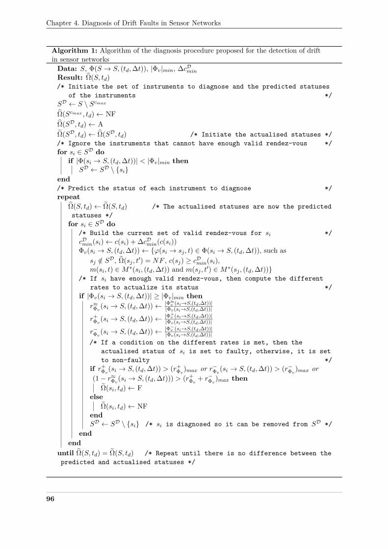
Chapter 4. Diagnosis of Drift Faults in Sensor Networks
Algorithm 1: Algorithm of the diagnosis procedure proposed for the detection of driftin sensor networksData: S, Φ(S → S, (td,∆t)), |Φv|min, ∆cDminResult: Ω(S, td)/* Initiate the set of instruments to diagnose and the predicted statuses
of the instruments */SD ← S \ ScmaxΩ(Scmax , td)← NFΩ(SD, td)← AΩ(SD, td)← Ω(SD, td) /* Initiate the actualised statuses *//* Ignore the instruments that cannot have enough valid rendez-vous */for si ∈ SD do
if |Φ(si → S, (td,∆t))| < |Φv|min thenSD ← SD \ si
end/* Predict the status of each instrument to diagnose */repeat
Ω(S, td)← Ω(S, td) /* The actualised statuses are now the predictedstatuses */for si ∈ SD do
/* Build the current set of valid rendez-vous for si */cDmin(si)← c(si) + ∆cDmin(c(si))Φv(si → S, (td,∆t))← ϕ(si → sj , t) ∈ Φ(si → S, (td,∆t)), such as
sj /∈ SD, Ω(sj , t′) = NF , c(sj) ≥ cDmin(si),m(si, t) ∈M∗(si, (td,∆t)) and m(sj , t′) ∈M∗(sj , (td,∆t))
/* If si have enough valid rendez-vous, then compute the differentrates to actualize its status */
if |Φv(si → S, (td,∆t))| ≥ |Φv|min thenr≈Φv(si → S, (td,∆t))← |Φ≈v (si→S,(td,∆t))|
|Φv(si→S,(td,∆t))|
r+Φv(si → S, (td,∆t))← |Φ+
v (si→S,(td,∆t))||Φv(si→S,(td,∆t))|
r−Φv(si → S, (td,∆t))← |Φ−v (si→S,(td,∆t))||Φv(si→S,(td,∆t))|
/* If a condition on the different rates is met, then theactualised status of si is set to faulty, otherwise, it is setto non-faulty */
if r+Φv(si → S, (td,∆t)) > (r+
Φv)max or r−Φv(si → S, (td,∆t)) > (r−Φv)max or(1− r≈Φv(si → S, (td,∆t))) > (r+
Φv + r−Φv)max thenΩ(si, td)← F
elseΩ(si, td)← NF
endSD ← SD \ si /* si is diagnosed so it can be removed from SD */
endend
until Ω(S, td) = Ω(S, td) /* Repeat until there is no difference between thepredicted and actualised statuses */
96
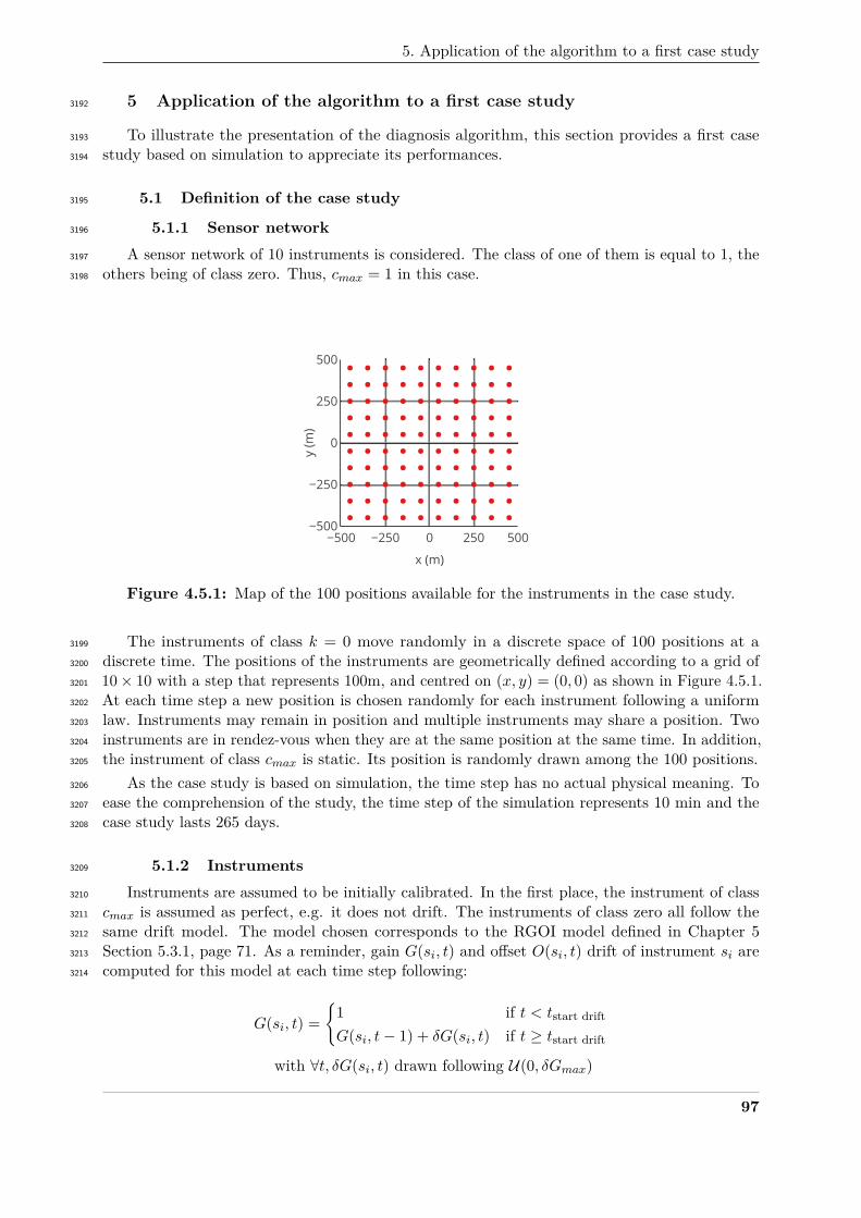
5. Application of the algorithm to a first case study
5 Application of the algorithm to a first case study3192
To illustrate the presentation of the diagnosis algorithm, this section provides a first case3193
study based on simulation to appreciate its performances.3194
5.1 Definition of the case study3195
5.1.1 Sensor network3196
A sensor network of 10 instruments is considered. The class of one of them is equal to 1, the3197
others being of class zero. Thus, cmax = 1 in this case.3198
−500 −250 0 250 500−500
−250
0
250
500
x (m)
y (m
)
Figure 4.5.1: Map of the 100 positions available for the instruments in the case study.
The instruments of class k = 0 move randomly in a discrete space of 100 positions at a3199
discrete time. The positions of the instruments are geometrically defined according to a grid of3200
10× 10 with a step that represents 100m, and centred on (x, y) = (0, 0) as shown in Figure 4.5.1.3201
At each time step a new position is chosen randomly for each instrument following a uniform3202
law. Instruments may remain in position and multiple instruments may share a position. Two3203
instruments are in rendez-vous when they are at the same position at the same time. In addition,3204
the instrument of class cmax is static. Its position is randomly drawn among the 100 positions.3205
As the case study is based on simulation, the time step has no actual physical meaning. To3206
ease the comprehension of the study, the time step of the simulation represents 10 min and the3207
case study lasts 265 days.3208
5.1.2 Instruments3209
Instruments are assumed to be initially calibrated. In the first place, the instrument of class3210
cmax is assumed as perfect, e.g. it does not drift. The instruments of class zero all follow the3211
same drift model. The model chosen corresponds to the RGOI model defined in Chapter 53212
Section 5.3.1, page 71. As a reminder, gain G(si, t) and offset O(si, t) drift of instrument si are3213
computed for this model at each time step following:3214
G(si, t) =
1 if t < tstart drift
G(si, t− 1) + δG(si, t) if t ≥ tstart drift
with ∀t, δG(si, t) drawn following U(0, δGmax)
97

Chapter 4. Diagnosis of Drift Faults in Sensor Networks
O(si, t) =
0 if t < tstart drift
O(si, t− 1) + δO(si, t) if t ≥ tstart drift
with ∀t, δO(si, t) drawn following U(0, δOmax)
with δGmax and δOmax being respectively the maximal gain and offset possible increase per3215
time step.3216
Measured values are expressed following:
v(si, t) = G(si, t) · vtrue(si, t) +O(si, t)
The instruments start to drift at t = 03217
Each measured value v(si, t) is associated to a constant relative uncertainty ∆rv(ci) dependingon the class of the instrument such as
∆v(si, t)v(si, t)
= ∆rv(ci)
A detection limit33 vmin(ci) is also defined to balance the effect of high uncertainties for low3218
measured values. This detection limit is used to determine if a measurement result m(si, t) is3219
metrologically valid, e.g. all the values below this detection limit are not considered valid.3220
All the values of the parameters are listed in Table 4.5.1.3221
Parameter Value Unit
Class 1∆rv 1 %vmin 0.752 µg m−3
Class 0δGmax 2/(24*6*30) %/10minδOmax 18.8/(24*6*30) µg/m3/10min∆rv 30 %vmin 37.6 µg m−3
True values modelAmax 200 µg m−3
σmax 3826 m
Table 4.5.1: Values of the parameters of the case study. The values of δGmax and δOmax aredisplayed as a fraction of (24 ∗ 6 ∗ 30) min for the sake of clarity, e.g. the numerator is the
maximal drift of the gain and of the offset per 30 days.
5.1.3 True values3222
To model the true values of the instruments, the model used in Chapter 3 Section 3.2.1 is3223
considered. However in this case, instead of using the data that was considered to determine3224
the values of A(t) and σ(t), A(t) and σ(t) are drawn randomly at each time step following the3225
33The detection limit is the value "obtained by a given measurement procedure, for which the probability of falselyclaiming the absence of a component is β, given a probability α of falsely claiming its presence" [14]. In practice, itis recommended that β = α = 0.05 for information.
98
5. Application of the algorithm to a first case study
uniform laws U(0, Amax) and U(0, σmax) respectively. The values of Amax and σmax are reported3226
in Table 4.5.1.3227
The impact of this choice on the results is discussed in Section 5.6 and 9.3.3228
5.2 Configuration of the diagnosis algorithm3229
We aim at performing a diagnosis every 15 days. Thus, for d ∈ D, td = (d+ 1)× 15 days,3230
with D = [0..16].3231
The goal of this diagnosis is to detect when an instrument has provided at least 25% of3232
measurement results non-compatible with their true values over the past 15 days.3233
According to this specification, we choose ∆t = 15 days and the rate thresholds (r+Φv)max,3234
(r−Φv)max and (r+Φv + r−Φv)max are all set to 25%.3235
The minimal number of valid rendez-vous to conclude with a predicted status different from3236
ambiguous |Φv|min is set initially to 15.3237
5.3 Definition of the true status of an instrument3238
As it is a simulation, it is possible to know the true status of an instrument. Indeed its3239
measured values and the true values are accessible, and therefore, it can be determined if 25% of3240
measurement results non-compatible with their true values were obtained or not during a period3241
of 15 days.3242
rtrue(si, (t,∆t)) is the rate of measurement results compatible with true values of si over[t−∆t; t]. It is equal to
rtrue(si, (t,∆t)) = |M≈(si, (t,∆t))|
|M(si, (t,∆t))|In this case, if rtrue(si, (t,∆t)) < 0.75, then Ω(si, t) = F . Otherwise, Ω(si, t) = NF .3243
Note that the true status of an instrument is based on all its measurement results against3244
the true values on the considered time range whereas its predicted status is based on the3245
measurement results of its valid rendez-vous with other devices. Thus, it is expected3246
that instruments which are actually non-faulty may be predicted as faulty and vice versa because3247
the sets of measurement results used to compute the true and predicted status of an instrument3248
are different.3249
5.4 Metrics for the evaluation of performances of the diagnosis algorithm3250
To estimate the performance of the algorithm, vocabulary and metrics that are used to3251
evaluate binary classifiers [130, 153] are appropriate but must be adapted as the predicted3252
statuses can take three values instead of two.3253
Regarding the possible true statuses and predicted statuses, there are six cases:3254
• A non-faulty status predicted for an instrument which true status is non-faulty is a true3255
negative (TN)3256
• A faulty status predicted for an instrument which true status is non-faulty is a false3257
negative (FN)3258
• An ambiguous status predicted for an instrument which true status is non-faulty is a3259
non-determined negative (NDN)3260
• A non-faulty status predicted for an instrument which true status is faulty is a false3261
positive (FP)3262
• A faulty status predicted for an instrument which true status is faulty is a true positive3263
(TP)3264
99
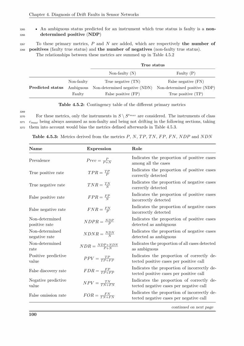
Chapter 4. Diagnosis of Drift Faults in Sensor Networks
• An ambiguous status predicted for an instrument which true status is faulty is a non-3265
determined positive (NDP)3266
To these primary metrics, P and N are added, which are respectively the number of3267
positives (faulty true status) and the number of negatives (non-faulty true status).3268
The relationships between these metrics are summed up in Table 4.5.2
True status
Non-faulty (N) Faulty (P)
Predicted statusNon-faulty True negative (TN) False negative (FN)Ambiguous Non-determined negative (NDN) Non-determined positive (NDP)
Faulty False positive (FP) True positive (TP)
Table 4.5.2: Contingency table of the different primary metrics3269
For these metrics, only the instruments in S \ Scmax are considered. The instruments of class3270
cmax being always assumed as non-faulty and being not drifting in the following sections, taking3271
them into account would bias the metrics defined afterwards in Table 4.5.3.3272
Table 4.5.3: Metrics derived from the metrics P , N , TP , TN , FP , FN , NDP and NDN
Name Expression Role
Prevalence Prev = PP+N
Indicates the proportion of positive casesamong all the cases
True positive rate TPR = TPP
Indicates the proportion of positive casescorrectly detected
True negative rate TNR = TNN
Indicates the proportion of negative casescorrectly detected
False positive rate FPR = FPN
Indicates the proportion of positive casesincorrectly detected
False negative rate FNR = FNP
Indicates the proportion of negative casesincorrectly detected
Non-determinedpositive rate NDPR = NDP
P
Indicates the proportion of positive casesdetected as ambiguous
Non-determinednegative rate NDNR = NDN
N
Indicates the proportion of negative casesdetected as ambiguous
Non-determinedrate NDR = NDP+NDN
P+NIndicates the proportion of all cases detectedas ambiguous
Positive predictivevalue PPV = TP
TP+FPIndicates the proportion of correctly de-tected positive cases per positive call
False discovery rate FDR = FPTP+FP
Indicates the proportion of incorrectly de-tected positive cases per positive call
Negative predictivevalue NPV = TN
TN+FNIndicates the proportion of correctly de-tected negative cases per negative call
False omission rate FOR = FNTN+FN
Indicates the proportion of incorrectly de-tected negative cases per negative call
continued on next page
100
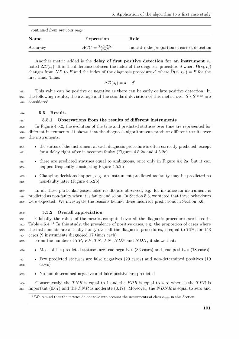
5. Application of the algorithm to a first case study
continued from previous page
Name Expression Role
Accuracy ACC = TP+TNP+N Indicates the proportion of correct detection
Another metric added is the delay of first positive detection for an instrument si,noted ∆D(si). It is the difference between the index of the diagnosis procedure d where Ω(si, td)changes from NF to F and the index of the diagnosis procedure d′ where Ω(si, td′) = F for thefirst time. Thus:
∆D(si) = d− d′
This value can be positive or negative as there can be early or late positive detection. In3273
the following results, the average and the standard deviation of this metric over S \ Scmax are3274
considered.3275
5.5 Results3276
5.5.1 Observations from the results of different instruments3277
In Figure 4.5.2, the evolution of the true and predicted statuses over time are represented for3278
different instruments. It shows that the diagnosis algorithm can produce different results over3279
the instruments:3280
• the status of the instrument at each diagnosis procedure is often correctly predicted, except3281
for a delay right after it becomes faulty (Figures 4.5.2a and 4.5.2c)3282
• there are predicted statuses equal to ambiguous, once only in Figure 4.5.2a, but it can3283
happen frequently considering Figure 4.5.2b3284
• Changing decisions happen, e.g. an instrument predicted as faulty may be predicted as3285
non-faulty later (Figure 4.5.2b)3286
In all these particular cases, false results are observed, e.g. for instance an instrument is3287
predicted as non-faulty when it is faulty and so on. In Section 5.3, we stated that these behaviours3288
were expected. We investigate the reasons behind these incorrect predictions in Section 5.6.3289
5.5.2 Overall appreciation3290
Globally, the values of the metrics computed over all the diagnosis procedures are listed in3291
Table 4.5.4.34 In this study, the prevalence of positive cases, e.g. the proportion of cases where3292
the instruments are actually faulty over all the diagnosis procedures, is equal to 76%, for 1533293
cases (9 instruments diagnosed 17 times each).3294
From the number of TP , FP , TN , FN , NDP and NDN , it shows that:3295
• Most of the predicted statuses are true negatives (36 cases) and true positives (78 cases)3296
• Few predicted statuses are false negatives (20 cases) and non-determined positives (193297
cases)3298
• No non-determined negative and false positive are predicted3299
Consequently, the TNR is equal to 1 and the FPR is equal to zero whereas the TPR is3300
important (0.67) and the FNR is moderate (0.17). Moreover, the NDNR is equal to zero and3301
34We remind that the metrics do not take into account the instruments of class cmax in this Section.
101
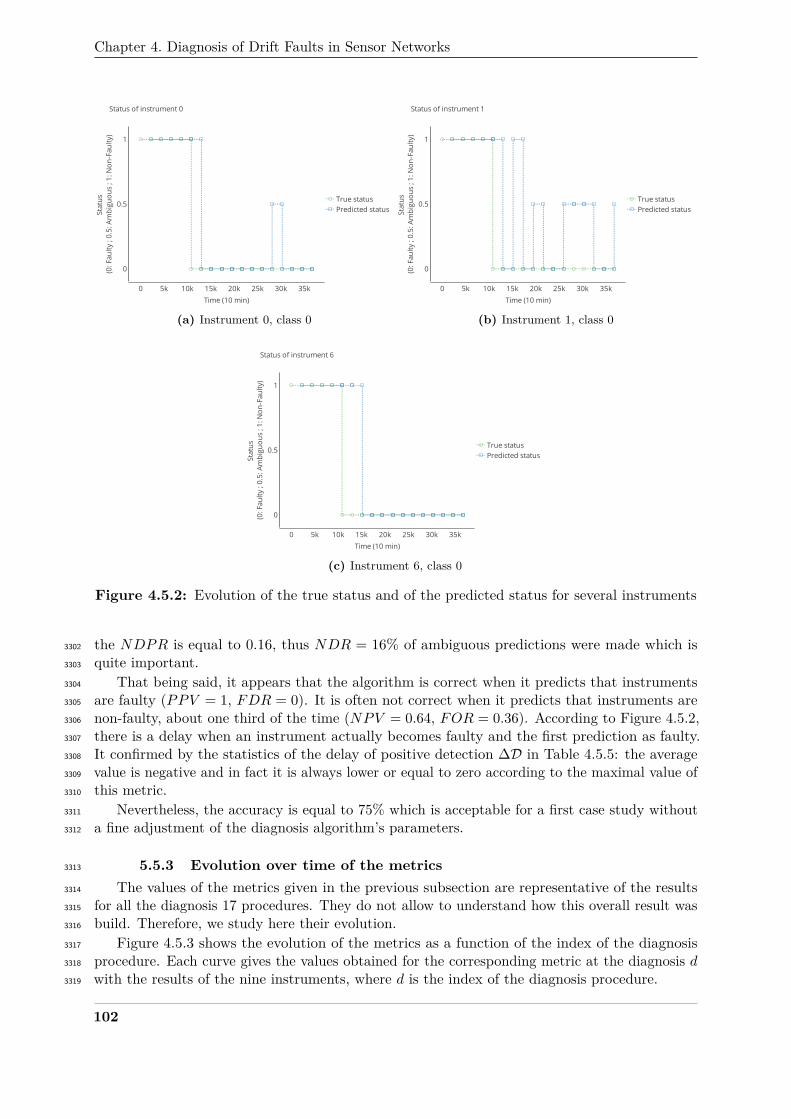
Chapter 4. Diagnosis of Drift Faults in Sensor Networks
0 5k 10k 15k 20k 25k 30k 35k
0
0.5
1
True statusPredicted status
Status of instrument 0
Time (10 min)
Stat
us
(0: F
aulty
; 0.
5: A
mbi
guou
s ; 1
: Non
-Fau
lty)
(a) Instrument 0, class 0
0 5k 10k 15k 20k 25k 30k 35k
0
0.5
1
True statusPredicted status
Status of instrument 1
Time (10 min)
Stat
us
(0: F
aulty
; 0.
5: A
mbi
guou
s ; 1
: Non
-Fau
lty)
(b) Instrument 1, class 0
0 5k 10k 15k 20k 25k 30k 35k
0
0.5
1
True statusPredicted status
Status of instrument 6
Time (10 min)
Stat
us
(0: F
aulty
; 0.
5: A
mbi
guou
s ; 1
: Non
-Fau
lty)
(c) Instrument 6, class 0
Figure 4.5.2: Evolution of the true status and of the predicted status for several instruments
the NDPR is equal to 0.16, thus NDR = 16% of ambiguous predictions were made which is3302
quite important.3303
That being said, it appears that the algorithm is correct when it predicts that instruments3304
are faulty (PPV = 1, FDR = 0). It is often not correct when it predicts that instruments are3305
non-faulty, about one third of the time (NPV = 0.64, FOR = 0.36). According to Figure 4.5.2,3306
there is a delay when an instrument actually becomes faulty and the first prediction as faulty.3307
It confirmed by the statistics of the delay of positive detection ∆D in Table 4.5.5: the average3308
value is negative and in fact it is always lower or equal to zero according to the maximal value of3309
this metric.3310
Nevertheless, the accuracy is equal to 75% which is acceptable for a first case study without3311
a fine adjustment of the diagnosis algorithm’s parameters.3312
5.5.3 Evolution over time of the metrics3313
The values of the metrics given in the previous subsection are representative of the results3314
for all the diagnosis 17 procedures. They do not allow to understand how this overall result was3315
build. Therefore, we study here their evolution.3316
Figure 4.5.3 shows the evolution of the metrics as a function of the index of the diagnosis3317
procedure. Each curve gives the values obtained for the corresponding metric at the diagnosis d3318
with the results of the nine instruments, where d is the index of the diagnosis procedure.3319
102
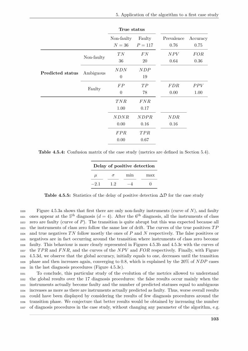
5. Application of the algorithm to a first case study
True status
Non-faulty Faulty Prevalence AccuracyN = 36 P = 117 0.76 0.75
Non-faulty TN FN NPV FOR
36 20 0.64 0.36
Predicted status Ambiguous NDN NDP
0 19
Faulty FP TP FDR PPV
0 78 0.00 1.00
TNR FNR
1.00 0.17
NDNR NDPR NDR
0.00 0.16 0.16
FPR TPR
0.00 0.67
Table 4.5.4: Confusion matrix of the case study (metrics are defined in Section 5.4).
Delay of positive detection
µ σ min max
−2.1 1.2 −4 0
Table 4.5.5: Statistics of the delay of positive detection ∆D for the case study
Figure 4.5.3a shows that first there are only non-faulty instruments (curve of N), and faulty3320
ones appear at the 5th diagnosis (d = 4). After the 6th diagnosis, all the instruments of class3321
zero are faulty (curve of P ). The transition is quite abrupt but this was expected because all3322
the instruments of class zero follow the same law of drift. The curves of the true positives TP3323
and true negatives TN follow mostly the ones of P and N respectively. The false positives or3324
negatives are in fact occurring around the transition where instruments of class zero become3325
faulty. This behaviour is more clearly represented in Figures 4.5.3b and 4.5.3c with the curves of3326
the TPR and FNR, and the curves of the NPV and FOR respectively. Finally, with Figure3327
4.5.3d, we observe that the global accuracy, initially equals to one, decreases until the transition3328
phase and then increases again, converging to 0.8, which is explained by the 20% of NDP cases3329
in the last diagnosis procedures (Figure 4.5.3c).3330
To conclude, this particular study of the evolution of the metrics allowed to understand3331
the global results over the 17 diagnosis procedures: the false results occur mainly when the3332
instruments actually become faulty and the number of predicted statuses equal to ambiguous3333
increases as more as there are instruments actually predicted as faulty. Thus, worse overall results3334
could have been displayed by considering the results of few diagnosis procedures around the3335
transition phase. We conjecture that better results would be obtained by increasing the number3336
of diagnosis procedures in the case study, without changing any parameter of the algorithm, e.g.3337
103
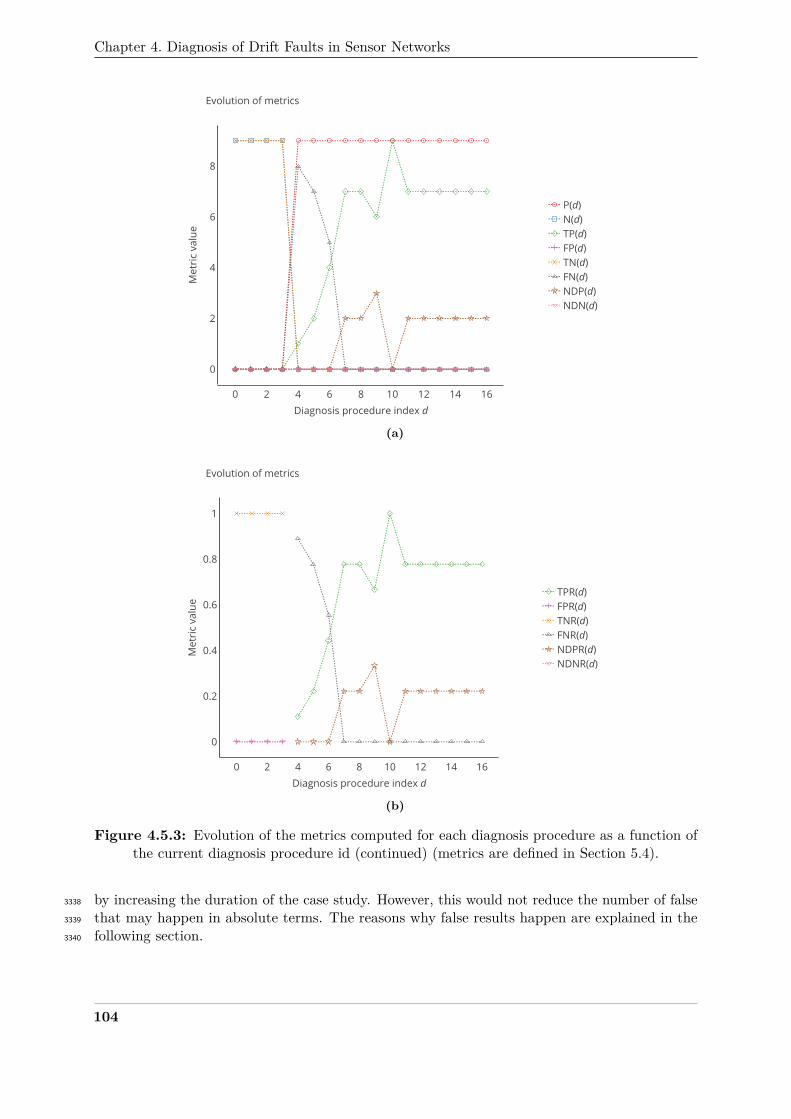
Chapter 4. Diagnosis of Drift Faults in Sensor Networks
0 2 4 6 8 10 12 14 16
0
2
4
6
8
P(d)N(d)TP(d)FP(d)TN(d)FN(d)NDP(d)NDN(d)
Evolution of metrics
Diagnosis procedure index d
Met
ric
valu
e
(a)
0 2 4 6 8 10 12 14 16
0
0.2
0.4
0.6
0.8
1
TPR(d)FPR(d)TNR(d)FNR(d)NDPR(d)NDNR(d)
Evolution of metrics
Diagnosis procedure index d
Met
ric
valu
e
(b)
Figure 4.5.3: Evolution of the metrics computed for each diagnosis procedure as a function ofthe current diagnosis procedure id (continued) (metrics are defined in Section 5.4).
by increasing the duration of the case study. However, this would not reduce the number of false3338
that may happen in absolute terms. The reasons why false results happen are explained in the3339
following section.3340
104
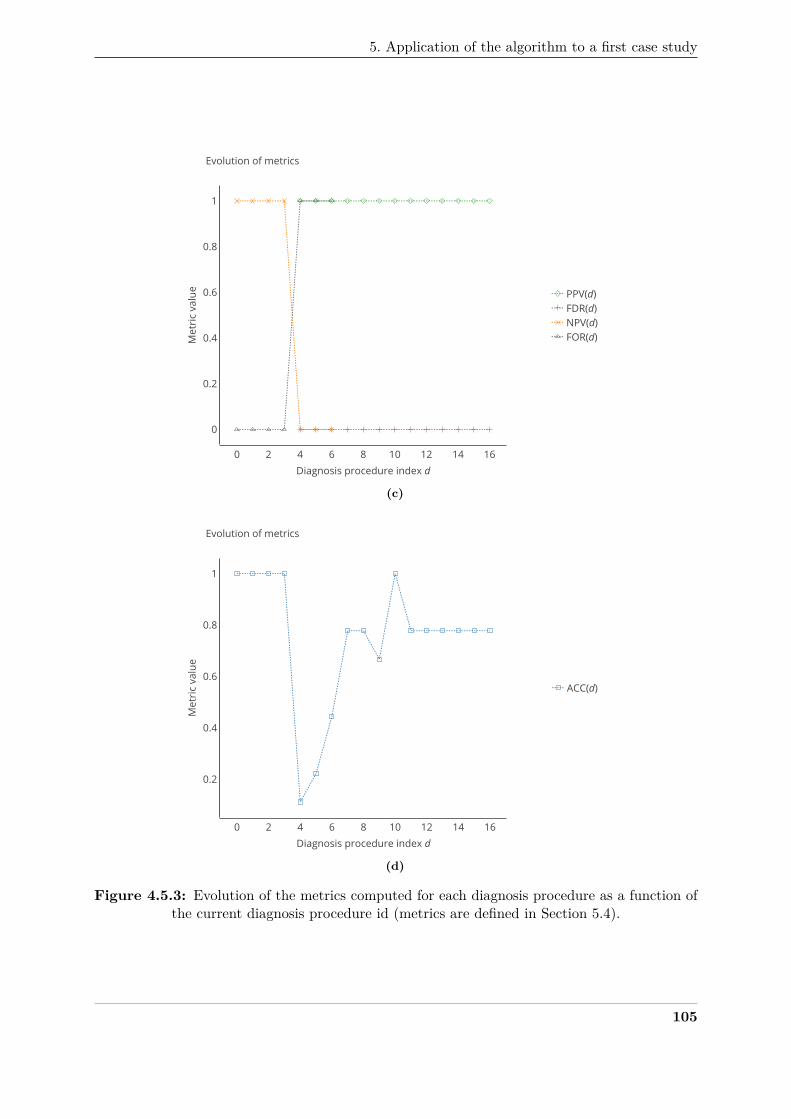
5. Application of the algorithm to a first case study
0 2 4 6 8 10 12 14 16
0
0.2
0.4
0.6
0.8
1
PPV(d)FDR(d)NPV(d)FOR(d)
Evolution of metrics
Diagnosis procedure index d
Met
ric
valu
e
(c)
0 2 4 6 8 10 12 14 16
0.2
0.4
0.6
0.8
1
ACC(d)
Evolution of metrics
Diagnosis procedure index d
Met
ric
valu
e
(d)
Figure 4.5.3: Evolution of the metrics computed for each diagnosis procedure as a function ofthe current diagnosis procedure id (metrics are defined in Section 5.4).
105
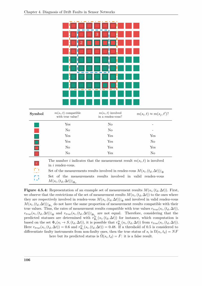
Chapter 4. Diagnosis of Drift Faults in Sensor Networks
3
2
Symbol m(si, t) compatiblewith true value?
m(si, t) involvedin a rendez-vous?
m(si, t) ≈ m(sj , t′)?
Yes No -No No -Yes Yes YesYes Yes NoNo Yes YesNo Yes No
iThe number i indicates that the measurement result m(si, t) is involvedin i rendez-vous.Set of the measurements results involved in rendez-vousM(si, (td,∆t)) ΦSet of the measurements results involved in valid rendez-vousM(si, (td,∆t)) Φv
Figure 4.5.4: Representation of an example set of measurement results M(si, (td,∆t)). First,we observe that the restrictions of the set of measurement resultsM(si, (td,∆t)) to the ones wherethey are respectively involved in rendez-vous M(si, (td,∆t)) Φ and involved in valid rendez-vousM(si, (td,∆t)) Φv do not have the same proportion of measurement results compatible with theirtrue values. Thus, the rates of measurement results compatible with true values rtrue(si, (td,∆t)),rtrue(si, (td,∆t)) Φ and rtrue(si, (td,∆t)) Φv are not equal. Therefore, considering that thepredicted statuses are determined with r≈Φv(si, (td,∆t)) for instance, which computation isbased on the set Φv(si → S, (td,∆t)), it is possible that r≈Φv(si, (td,∆t)) from rtrue(si, (td,∆t)).Here rtrue(si, (td,∆t)) = 0.6 and r≈Φv(si, (td,∆t)) = 0.48. If a threshold of 0.5 is considered todifferentiate faulty instruments from non-faulty ones, then the true status of si is Ω(si, td) = NF
here but its predicted status is Ω(si, td) = F : it is a false result.
106
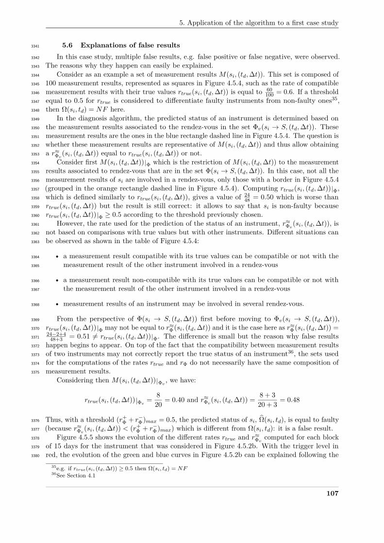
5. Application of the algorithm to a first case study
5.6 Explanations of false results3341
In this case study, multiple false results, e.g. false positive or false negative, were observed.3342
The reasons why they happen can easily be explained.3343
Consider as an example a set of measurement results M(si, (td,∆t)). This set is composed of3344
100 measurement results, represented as squares in Figure 4.5.4, such as the rate of compatible3345
measurement results with their true values rtrue(si, (td,∆t)) is equal to 60100 = 0.6. If a threshold3346
equal to 0.5 for rtrue is considered to differentiate faulty instruments from non-faulty ones35,3347
then Ω(si, td) = NF here.3348
In the diagnosis algorithm, the predicted status of an instrument is determined based on3349
the measurement results associated to the rendez-vous in the set Φv(si → S, (td,∆t)). These3350
measurement results are the ones in the blue rectangle dashed line in Figure 4.5.4. The question is3351
whether these measurement results are representative of M(si, (td,∆t)) and thus allow obtaining3352
a r≈Φv(si, (td,∆t)) equal to rtrue(si, (td,∆t)) or not.3353
Consider first M(si, (td,∆t)) Φ which is the restriction of M(si, (td,∆t)) to the measurement3354
results associated to rendez-vous that are in the set Φ(si → S, (td,∆t)). In this case, not all the3355
measurement results of si are involved in a rendez-vous, only those with a border in Figure 4.5.43356
(grouped in the orange rectangle dashed line in Figure 4.5.4). Computing rtrue(si, (td,∆t)) Φ,3357
which is defined similarly to rtrue(si, (td,∆t)), gives a value of 2448 = 0.50 which is worse than3358
rtrue(si, (td,∆t)) but the result is still correct: it allows to say that si is non-faulty because3359
rtrue(si, (td,∆t)) Φ ≥ 0.5 according to the threshold previously chosen.3360
However, the rate used for the prediction of the status of an instrument, r≈Φv(si, (td,∆t)), is3361
not based on comparisons with true values but with other instruments. Different situations can3362
be observed as shown in the table of Figure 4.5.4:3363
• a measurement result compatible with its true values can be compatible or not with the3364
measurement result of the other instrument involved in a rendez-vous3365
• a measurement result non-compatible with its true values can be compatible or not with3366
the measurement result of the other instrument involved in a rendez-vous3367
• measurement results of an instrument may be involved in several rendez-vous.3368
From the perspective of Φ(si → S, (td,∆t)) first before moving to Φv(si → S, (td,∆t)),3369
rtrue(si, (td,∆t)) Φ may not be equal to r≈Φ (si, (td,∆t)) and it is the case here as r≈Φ (si, (td,∆t)) =337024−2+4
48+3 = 0.51 6= rtrue(si, (td,∆t)) Φ. The difference is small but the reason why false results3371
happen begins to appear. On top of the fact that the compatibility between measurement results3372
of two instruments may not correctly report the true status of an instrument36, the sets used3373
for the computations of the rates rtrue and rΦ do not necessarily have the same composition of3374
measurement results.3375
Considering then M(si, (td,∆t)) Φv , we have:
rtrue(si, (td,∆t)) Φv = 820 = 0.40 and r≈Φv(si, (td,∆t)) = 8 + 3
20 + 3 = 0.48
Thus, with a threshold (r+Φ + r−Φ )max = 0.5, the predicted status of si, Ω(si, td), is equal to faulty3376
(because r≈Φv(si, (td,∆t)) < (r+Φ + r−Φ)max) which is different from Ω(si, td): it is a false result.3377
Figure 4.5.5 shows the evolution of the different rates rtrue and r≈Φv computed for each block3378
of 15 days for the instrument that was considered in Figure 4.5.2b. With the trigger level in3379
red, the evolution of the green and blue curves in Figure 4.5.2b can be explained following the3380
35e.g. if rtrue(si, (td,∆t)) ≥ 0.5 then Ω(si, td) = NF36See Section 4.1
107
Chapter 4. Diagnosis of Drift Faults in Sensor Networks
0 5k 10k 15k 20k 25k 30k 35k
0
0.2
0.4
0.6
0.8
1
r true(s i,(t d, Δt))r Φ v
≈(s i,(t d, Δt))(r + + r -) max
Rates of instrument 1
Time (10 min)
Rate
val
ue
Figure 4.5.5: Evolution of the rates rtrue and r≈Φv for s1 in the case study of Section 5. Themissing points for r≈Φv are due to the ambiguous cases where r≈Φv could not be computed.
reasoning developed for the presented theoretical example. In this Figure, the diagnosis curve is3381
particularly interesting as the instrument is alternatively diagnosed as faulty and non-faulty, and3382
several times.3383
Through this development, the reason why false results appear has been explained. It is3384
because the properties of sets of measurement results like M(si, (td,∆t)) are not necessarily3385
conserved while building Φv(si → S, (td,∆t)) and it is this latter set that is used to compute the3386
rates rΦv . In fact, there is a sort of "sampling" of M(si, (td,∆t)) that is performed through the3387
rendez-vous and resulting in M(si, (td,∆t)) Φv in the end. This explains mainly the false results3388
of the diagnosis algorithm. Solving this issue is quite challenging. It might be possible in some3389
situations where the characteristics of the sets of measurement results could be conserved by the3390
"sampling" at stake for the restriction of the sets of measurement results but it would generally3391
require strong assumptions on the measurement results and on the occurrence of rendez-vous,3392
without taking into account the notion of validity of the rendez-vous. However, by adjusting3393
the parameters of the diagnosis algorithm, it may also be possible to reduce the number of false3394
results. Therefore, they are reviewed in the following section.3395
5.7 On the parameters of the diagnosis algorithm3396
There are several parameters that drive the proposed algorithm:3397
• the instant of diagnosis td and its periodicity3398
• the time difference ∆t defining the length of the time range on which measurement results3399
selected for the input data of the algorithm3400
• the minimal relative differences of class required for instruments of class k with their3401
diagnoser instruments ∆cDmin(k)3402
• the minimal required number of valid rendez-vous |Φv|min3403
• the conditions for a measurement result to be considered as valid3404
• the conditions of spatiotemporal vicinity for two instruments to be in rendez-vous3405
108
5. Application of the algorithm to a first case study
• the maximal tolerated values (r+Φv)max, (r−Φv)max and (r+
Φv + r−Φv)max for the rates of upper3406
and lower non-compatible rendez-vous in sets of valid rendez-vous.3407
It may be possible to improve the results of case study with different rules or values for them.3408
Indeed, values were chosen but may not be the ones allowing obtaining the best results. They3409
may explain the reason why there are many false results in particular. The following paragraphs3410
provide a discussion regarding the choice of the parameters.3411
Instant of diagnosis and its periodicity3412
td is the instant of the dth diagnosis. In this case study, we chose to have a periodic diagnosis,3413
e.g. diagnosis procedures are carried out on a regular basis (every 15 days).37 With a different3414
frequency of diagnosis, for instance every week or even every day in the case study, it may3415
be possible to detect sooner that an instrument has become faulty in exchange of a higher3416
computational cost. Consequently, the overall results would be different but this would not3417
change the general behaviour of the algorithm. The choice of the instant of diagnosis and its3418
periodicity is not discussed in detail in this work despite the fact that it may have a significance3419
in practice because it strongly depends on the instruments used and on the context of deployment.3420
Indeed, all the instruments do not have the same characteristic time of drift for instance. This3421
information is often provided as an order of magnitude of drift of the gain and offset over a week3422
or a month in percentage in datasheets [104]. In this way, it would influence the periodicity3423
of the diagnosis. Moreover, the context of deployment can justify to perform the diagnosis at3424
specific times of the day.38 Thus, the characteristics of the instruments used and the context of3425
deployment can help in the choice of the moment of diagnosis and its periodicity. 393426
Length of the time range on which the algorithm is applied3427
The length of the time range ∆t has an important influence on the results. Indeed, the higher3428
∆t is, the more rendez-vous may be in Φ(si → S, (td,∆t)) and consequently in Φv(si → S, (td,∆t)),3429
and vice versa. Thus, it influences the contents of M(si, (td,∆t)) Φ and M(si, (td,∆t)) Φv .3430
However, a high value of ∆t implies that measurement results obtained at very different instants3431
would be used by the diagnosis algorithm. Considering that old measurement results are more3432
accurate than recent ones in the case of an irreversible drift, the higher ∆t is, the less the3433
measurement results at the actual level of the drift will be preponderant in M(si, (td,∆t)) Φv .3434
Therefore, choosing a different value for ∆t while trying to bring closer the distributions of3435
measured values in M(si, (td,∆t)) and M(si, (td,∆t)) Φv could also induce false results for3436
another reason because as shown in Section 5.6, the content of the sets M(si, (td,∆t)) and3437
M(si, (td,∆t)) Φv are not necessarily equivalent, regardless of ∆t. Moreover, reducing ∆t in3438
particular could also have another drawback: on a short time range there may likely be less3439
rendez-vous than on a longer one. Depending on the minimal required number of valid rendez-3440
vous |Φv|min, the value of ∆t can make the algorithm not functional, e.g. all the instruments3441
37An actual day and hour is not associated to td because it does not have a real signification here.38As an example, in [109] for an in situ calibration strategy, Moltchanov et al. chose to apply their in situ
calibration algorithm every day after 4:00a.m. and to use the measured values between 1:00a.m. and 4:00a.m..They proceeded like this because the measuring instruments to calibrate were distant from the reference and at thismoment, the measurand was supposed to be homogenous in the measurement area, enabling to compare betweenthem the values measured by the instruments. Therefore, in the same context with our diagnosis algorithm, itmay be relevant to apply it at a similar time of the day that was used in [109].
39Note that too high a frequency of diagnosis may be pointless if no rendez-vous occurs between two instants ofdiagnosis. It would be more relevant to have in this case a formulation of the algorithm so that the diagnosisprocedure is carried out when new rendez-vous happen. In this way, Appendix A Section 5 provides a discussionregarding first how to reformulate the algorithm so that it is possible to trigger a diagnosis procedure on an event,e.g. a rendez-vous, and how to use an event-based range on which the algorithm is applied. Then, elementsregarding a real-time version of the diagnosis algorithm are given in Appendix A Section 6.
109
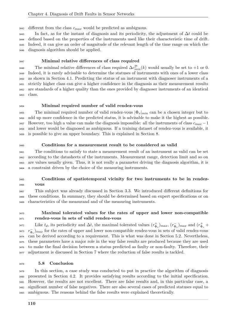
Chapter 4. Diagnosis of Drift Faults in Sensor Networks
different from the class cmax would be predicted as ambiguous.3442
In fact, as for the instant of diagnosis and its periodicity, the adjustment of ∆t could be3443
defined based on the properties of the instruments used like their characteristic time of drift.3444
Indeed, it can give an order of magnitude of the relevant length of the time range on which the3445
diagnosis algorithm should be applied.3446
Minimal relative differences of class required3447
The minimal relative differences of class required ∆cDmin(k) would usually be set to +1 or 0.3448
Indeed, it is rarely advisable to determine the statuses of instruments with ones of a lower class3449
as shown in Section 4.1. Predicting the status of an instrument with diagnoser instruments of a3450
strictly higher class can give a higher confidence in the diagnosis as their measurement results3451
are standards of a higher quality than the ones provided by diagnoser instruments of an identical3452
class.3453
Minimal required number of valid rendez-vous3454
The minimal required number of valid rendez-vous |Φv|min can be a chosen integer but to3455
add up more confidence in the predicted status, it is advisable to make it the highest as possible.3456
However, too high a value can make the diagnosis impossible: all the instruments of class cmax−13457
and lower would be diagnosed as ambiguous. If a training dataset of rendez-vous is available, it3458
is possible to give an upper boundary. This is explained in Section 8.3459
Conditions for a measurement result to be considered as valid3460
The conditions to satisfy to state a measurement result of an instrument as valid can be set3461
according to the datasheets of the instruments. Measurement range, detection limit and so on3462
are values usually given. Thus, it is not really a parameter driving the diagnosis algorithm, it is3463
a constraint driven by the choice of the measuring instruments.3464
Conditions of spatiotemporal vicinity for two instruments to be in rendez-3465
vous3466
This subject was already discussed in Section 3.3. We introduced different definitions for3467
these conditions. In summary, they should be determined based on expert specifications or on3468
characteristics of the measurand and of the measuring instruments.3469
Maximal tolerated values for the rates of upper and lower non-compatible3470
rendez-vous in sets of valid rendez-vous3471
Like td, its periodicity and ∆t, the maximal tolerated values (r+Φv)max, (r−Φv)max and (r+
Φv +3472
r−Φv)max for the rates of upper and lower non-compatible rendez-vous in sets of valid rendez-vous3473
can be derived according to a requirement. This is what was done in Section 5.2. Nevertheless,3474
these parameters have a major role in the way false results are produced because they are used3475
to make the final decision between a status predicted as faulty or non-faulty. Therefore, their3476
adjustment is discussed in Section 7 where the reduction of false results is tackled.3477
5.8 Conclusion3478
In this section, a case study was conducted to put in practice the algorithm of diagnosis3479
presented in Section 4.2. It provides satisfying results according to the initial specification.3480
However, the results are not excellent. There are false results and, in this particular case, a3481
significant number of false negatives. There are also several cases of predicted statuses equal to3482
ambiguous. The reasons behind the false results were explained theoretically.3483
110
6. On the assumption regarding the top-class instruments being always predicted as non-faulty
To improve the results, the adjustment of the parameters of the algorithm was discussed.3484
The brief overview of each one highlighted that the adjustment of some of them can be driven3485
by expert specifications and the characteristics of the measuring instruments composing the3486
sensor network. For |Φv|min, (r+Φv)max, (r−Φv)max and (r+
Φv + r−Φv)max, guidelines are provided in3487
Sections 7 and 8 to set their values.3488
Before that, we discuss in the following section the assumption for the instruments of class3489
cmax that are considered as non-faulty–they were even not drifting in the present case study.3490
6 On the assumption regarding the top-class instruments being always3491
predicted as non-faulty3492
6.1 Theoretical discussion3493
The assumption that instruments of class cmax are always predicted as non-faulty is a strong3494
one. It is, however, necessary for the proper operation of the presented algorithm. If there is no3495
assumption regarding the status of any instrument of class cmax, they are initially considered as3496
ambiguous and thus the sets Φv(si → S, (td,∆t)) are always empty. In this case, the algorithm3497
predicts a status equal to ambiguous for each instrument, which makes it useless.3498
Actually, the assumption on the instruments of class cmax can be relaxed: one single3499
instrument of class cmax supposed as non-faulty may be sufficient. More practically,3500
depending on the value of |Φv|min and on the configuration of the sensor network, only a subset3501
of Scmax may be sufficient to ensure the lowest number of instruments systematically diagnosed3502
as ambiguous.40 Note that this formulation is also more appropriate in the case of a blind sensor3503
network. Indeed, for this type of sensor network, all the instruments are considered as equivalent3504
from a metrological perspective. Consequently, there is no subset of instruments of a higher class3505
than others.413506
Following on from this new formulation of the assumption regarding the statuses of the3507
instruments of class cmax, we might be tempted to try to relax it to point where the status of3508
only one instrument of any class has to be known. Consider such an instrument si. Again, all3509
the instruments sj ∈ S such as cDmin(sj) > c(si) cannot be diagnosed differently than ambiguous3510
if the minimal relative differences of class required ∆cDmin(k) is set to +1 or 0 as recommended3511
in Section 5.7. In particular, if the class of si is the lowest class in the network, noted cmin,3512
and if ∆cDmin(cmin) = +1, then all the instruments of the network, except si are systematically3513
diagnosed as ambiguous. In fact, the lower the class of si is, the more instruments will always be3514
predicted as ambiguous. Thus, it may be simpler to come back to assuming some instruments of3515
class cmax as non-faulty. It is acceptable to guarantee such a hypothesis in real situations.3516
6.2 Case study with the instrument of class cmax drifting3517
In the case study of Section 5, the instrument of class cmax, noted here s9, was first assumed3518
as perfect, e.g. not drifting, for the sake of clarity.3519
Consider here that this instrument is also undergoing drift following the RGOI model but3520
with δGmax(s9) = 0.5/(24 ∗ 6 ∗ 30)%/10min and δOmax(s9) = 1.88/(24 ∗ 6 ∗ 30)µg/m3/10min.423521
With the previous definition of rtrue and the same criteria to determine the true status of the3522
instrument Ω(s9, t) like the other instruments, the evolution of the true and predicted statuses3523
40Note that if ∆cDmin(cmax) > 0, the instruments of class cmax which statuses are not assumed as non-faulty,cannot be diagnosed differently than ambiguous. Hence, it may be more relevant to define a sub-network withoutthese instruments on which the diagnosis algorithm is applied so that the results are not biased by the behaviourof the algorithm with these instruments.
41In the case of a blind sensor network, necessarily ∆cDmin = 0 for all the instruments, otherwise the algorithmcannot work.
42See Table 4.5.1 for the explanation regarding Gmax(s9) and Omax(s9) expressed as fractions.
111

Chapter 4. Diagnosis of Drift Faults in Sensor Networks
0 5k 10k 15k 20k 25k 30k 35k
0
0.5
1
True statusPredicted status
Status of instrument 9
Time (10 min)
Stat
us
(0: F
aulty
; 0.
5: A
mbi
guou
s ; 1
: Non
-Fau
lty)
Figure 4.6.1: Evolution of the true status and of the predicted status of s9, the instrument ofclass 1, when it is drifting
True status
Non-faulty Faulty Prevalence AccuracyN = 36 P = 117 0.76 0.72
Non-faulty TN FN NPV FOR
36 28 0.56 0.44
Predicted status Ambiguous NDN NDP
0 15
Faulty FP TP FDR PPV
0 74 0.00 1.00
TNR FNR
1.00 0.24
NDNR NDPR NDR
0.00 0.13 0.10
FPR TPR
0.00 0.63
Table 4.6.1: Confusion matrix of the case study when the instrument of class 1 is drifting(metrics are defined in Section 5.4).
over time for this particular instrument is given in Figure 4.6.1, the predicted status being again3524
assumed as always non-faulty. We observe that there are consequently false negative if the3525
assumption is kept. However, still without taking into account s9 in the metrics to evaluate the3526
results, the diagnosis algorithm gives the results of Tables 4.6.1 and 4.6.2. We observe that the3527
values of the metrics do not change significantly from Tables 4.5.4 and 4.5.5. They are slightly3528
worse sometimes: more false negatives (28 instead of 20), less true positives (74 instead of 78),3529
thus NPV is lower and the FOR is higher but the PPV is higher.3530
Therefore, it appears that even with s9 drifting, the diagnosis algorithm still provides satisfying3531
results. In this way, assuming that the instruments of class cmax are not drifting is acceptable.3532
112
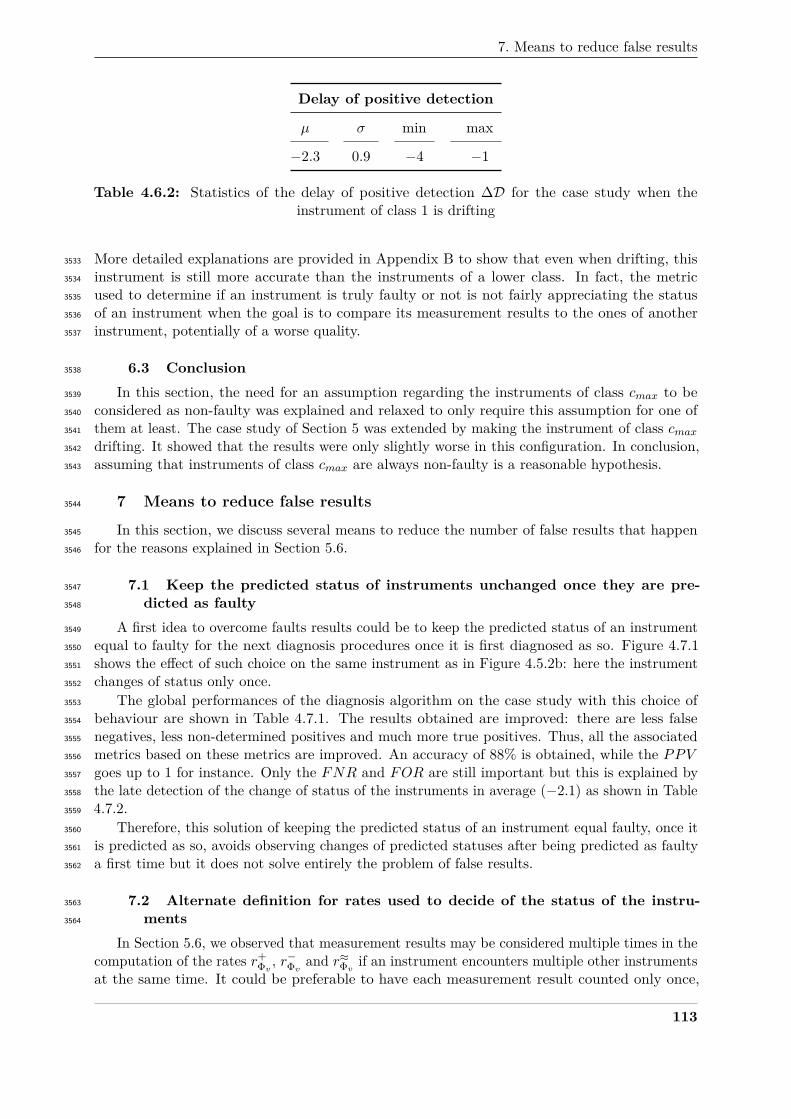
7. Means to reduce false results
Delay of positive detection
µ σ min max
−2.3 0.9 −4 −1
Table 4.6.2: Statistics of the delay of positive detection ∆D for the case study when theinstrument of class 1 is drifting
More detailed explanations are provided in Appendix B to show that even when drifting, this3533
instrument is still more accurate than the instruments of a lower class. In fact, the metric3534
used to determine if an instrument is truly faulty or not is not fairly appreciating the status3535
of an instrument when the goal is to compare its measurement results to the ones of another3536
instrument, potentially of a worse quality.3537
6.3 Conclusion3538
In this section, the need for an assumption regarding the instruments of class cmax to be3539
considered as non-faulty was explained and relaxed to only require this assumption for one of3540
them at least. The case study of Section 5 was extended by making the instrument of class cmax3541
drifting. It showed that the results were only slightly worse in this configuration. In conclusion,3542
assuming that instruments of class cmax are always non-faulty is a reasonable hypothesis.3543
7 Means to reduce false results3544
In this section, we discuss several means to reduce the number of false results that happen3545
for the reasons explained in Section 5.6.3546
7.1 Keep the predicted status of instruments unchanged once they are pre-3547
dicted as faulty3548
A first idea to overcome faults results could be to keep the predicted status of an instrument3549
equal to faulty for the next diagnosis procedures once it is first diagnosed as so. Figure 4.7.13550
shows the effect of such choice on the same instrument as in Figure 4.5.2b: here the instrument3551
changes of status only once.3552
The global performances of the diagnosis algorithm on the case study with this choice of3553
behaviour are shown in Table 4.7.1. The results obtained are improved: there are less false3554
negatives, less non-determined positives and much more true positives. Thus, all the associated3555
metrics based on these metrics are improved. An accuracy of 88% is obtained, while the PPV3556
goes up to 1 for instance. Only the FNR and FOR are still important but this is explained by3557
the late detection of the change of status of the instruments in average (−2.1) as shown in Table3558
4.7.2.3559
Therefore, this solution of keeping the predicted status of an instrument equal faulty, once it3560
is predicted as so, avoids observing changes of predicted statuses after being predicted as faulty3561
a first time but it does not solve entirely the problem of false results.3562
7.2 Alternate definition for rates used to decide of the status of the instru-3563
ments3564
In Section 5.6, we observed that measurement results may be considered multiple times in thecomputation of the rates r+
Φv , r−Φv and r≈Φv if an instrument encounters multiple other instruments
at the same time. It could be preferable to have each measurement result counted only once,
113
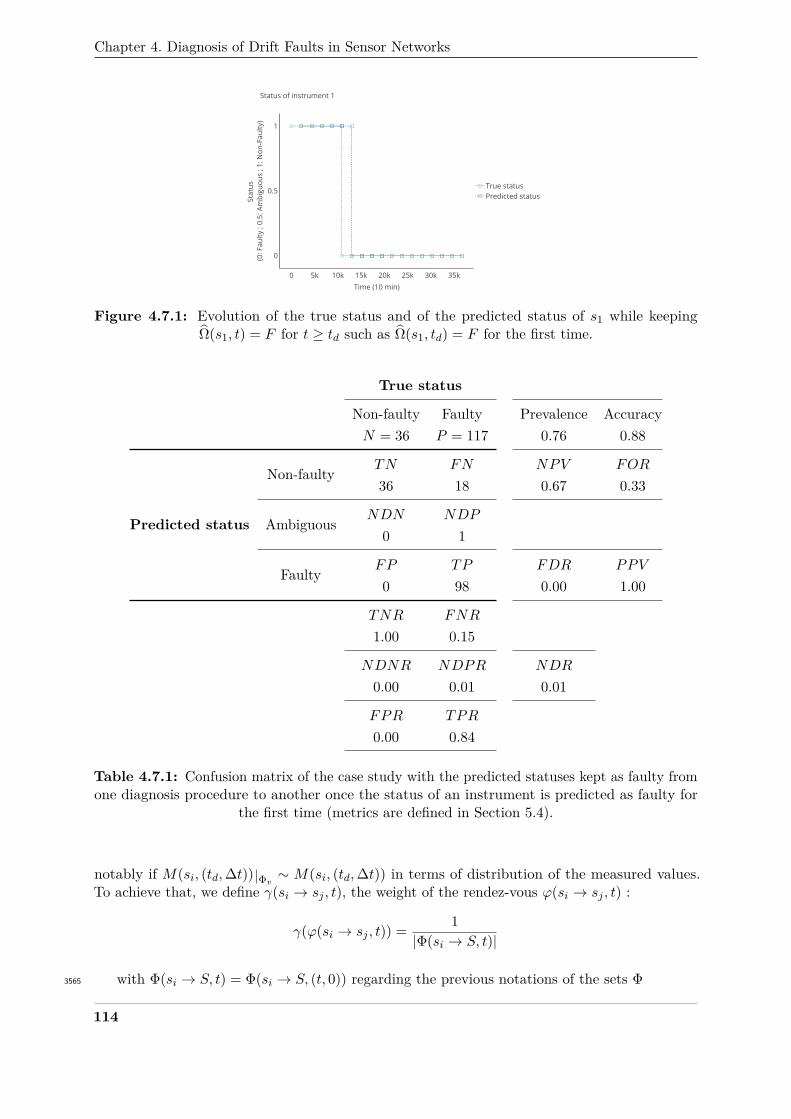
Chapter 4. Diagnosis of Drift Faults in Sensor Networks
0 5k 10k 15k 20k 25k 30k 35k
0
0.5
1
True statusPredicted status
Status of instrument 1
Time (10 min)
Stat
us
(0: F
aulty
; 0.
5: A
mbi
guou
s ; 1
: Non
-Fau
lty)
Figure 4.7.1: Evolution of the true status and of the predicted status of s1 while keepingΩ(s1, t) = F for t ≥ td such as Ω(s1, td) = F for the first time.
True status
Non-faulty Faulty Prevalence AccuracyN = 36 P = 117 0.76 0.88
Non-faulty TN FN NPV FOR
36 18 0.67 0.33
Predicted status Ambiguous NDN NDP
0 1
Faulty FP TP FDR PPV
0 98 0.00 1.00
TNR FNR
1.00 0.15
NDNR NDPR NDR
0.00 0.01 0.01
FPR TPR
0.00 0.84
Table 4.7.1: Confusion matrix of the case study with the predicted statuses kept as faulty fromone diagnosis procedure to another once the status of an instrument is predicted as faulty for
the first time (metrics are defined in Section 5.4).
notably if M(si, (td,∆t)) Φv ∼ M(si, (td,∆t)) in terms of distribution of the measured values.To achieve that, we define γ(si → sj , t), the weight of the rendez-vous ϕ(si → sj , t) :
γ(ϕ(si → sj , t)) = 1|Φ(si → S, t)|
with Φ(si → S, t) = Φ(si → S, (t, 0)) regarding the previous notations of the sets Φ3565
114

7. Means to reduce false results
Delay of positive detection
µ σ min max
−2.1 1.2 −4 0
Table 4.7.2: Statistics of the delay of positive detection ∆D for the case study with the predictedstatuses kept as faulty from one diagnosis procedure to another once the status of an instrument
is predicted as faulty for the first time
0 10k 20k 30k
0
0.2
0.4
0.6
0.8
1
r true (s i ,(t d , Δt))r ≈ Φ v (s i ,(t d , Δt)) (first definition) r ≈ Φ v (s i ,(t d , Δt)) (based on γ)1-(r + Φ v + r - Φ v ) max
Rates of instrument 1
Time (10 min)
Rate
val
ue
(a)
0 5k 10k 15k 20k 25k 30k 35k
0
0.5
1
True statusPredicted status
Status of instrument 1
Time (10 min)
Stat
us
(0: F
aulty
; 0.
5: A
mbi
guou
s ; 1
: Non
-Fau
lty)
(b)
Figure 4.7.2: Evolution for s1 in the case study of Section 5 (a) of the rates rtrue and r≈Φv (bothdefinitions) ; (b) of its true status and of its predicted status with the alternate definition for r≈Φv
; while keeping Ω(s1, t) = F for t ≥ td such as Ω(s1, td) = F for the first time.
γv can be defined for Φv too. With this weight, we have notably:∑ϕ(si→sj ,t′)∈Φv(si,(t,∆t))
γv(ϕ(si → sj , t′)) = |M(si, (t,∆t)) Φv |
Thus, an alternate definition of r≈Φv(si, (t,∆t)) is for instance:
r≈Φv(si, (t,∆t)) =
∑ϕ(si→sj ,t′)∈Φ≈v (si,(t,∆t))
γv(ϕ(si → sj , t′))
∑ϕ(si→sj ,t′)∈Φv(si,(t,∆t))
γv(ϕ(si → sj , t′))
However, Figure 4.7.2a shows that using this definition in this case study does not change the3566
values of r≈Φv(s1, (t,∆t)) compared to the results obtained with the previous definition. Hence,3567
there is no change in the predicted status of the instrument that was considered in Figure 4.7.13568
as shown in Figure 4.7.2b. This is also globally the case according to Table 4.7.3 compared to3569
Table 4.7.1.3570
7.3 Adjustment of the maximal tolerated values for the different rates used3571
to determine the statuses of the instruments3572
The issue of false results can be seen from another perspective. In fact, the most problematic3573
false results are the false negatives. Indeed, false positives will only trigger an early maintenance3574
115
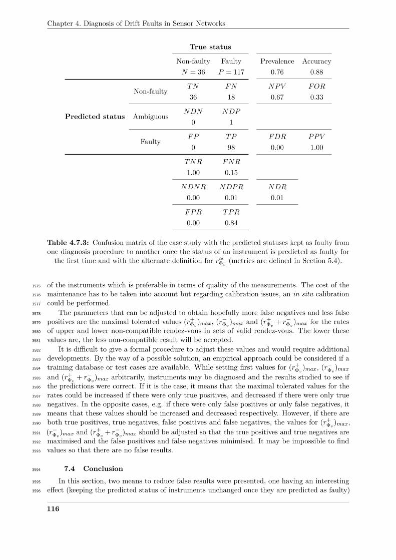
Chapter 4. Diagnosis of Drift Faults in Sensor Networks
True status
Non-faulty Faulty Prevalence AccuracyN = 36 P = 117 0.76 0.88
Non-faulty TN FN NPV FOR
36 18 0.67 0.33
Predicted status Ambiguous NDN NDP
0 1
Faulty FP TP FDR PPV
0 98 0.00 1.00
TNR FNR
1.00 0.15
NDNR NDPR NDR
0.00 0.01 0.01
FPR TPR
0.00 0.84
Table 4.7.3: Confusion matrix of the case study with the predicted statuses kept as faulty fromone diagnosis procedure to another once the status of an instrument is predicted as faulty forthe first time and with the alternate definition for r≈Φv (metrics are defined in Section 5.4).
of the instruments which is preferable in terms of quality of the measurements. The cost of the3575
maintenance has to be taken into account but regarding calibration issues, an in situ calibration3576
could be performed.3577
The parameters that can be adjusted to obtain hopefully more false negatives and less false3578
positives are the maximal tolerated values (r+Φv)max, (r−Φv)max and (r+
Φv + r−Φv)max for the rates3579
of upper and lower non-compatible rendez-vous in sets of valid rendez-vous. The lower these3580
values are, the less non-compatible result will be accepted.3581
It is difficult to give a formal procedure to adjust these values and would require additional3582
developments. By the way of a possible solution, an empirical approach could be considered if a3583
training database or test cases are available. While setting first values for (r+Φv)max, (r−Φv)max3584
and (r+Φv + r−Φv)max arbitrarily, instruments may be diagnosed and the results studied to see if3585
the predictions were correct. If it is the case, it means that the maximal tolerated values for the3586
rates could be increased if there were only true positives, and decreased if there were only true3587
negatives. In the opposite cases, e.g. if there were only false positives or only false negatives, it3588
means that these values should be increased and decreased respectively. However, if there are3589
both true positives, true negatives, false positives and false negatives, the values for (r+Φv)max,3590
(r−Φv)max and (r+Φv + r−Φv)max should be adjusted so that the true positives and true negatives are3591
maximised and the false positives and false negatives minimised. It may be impossible to find3592
values so that there are no false results.3593
7.4 Conclusion3594
In this section, two means to reduce false results were presented, one having an interesting3595
effect (keeping the predicted status of instruments unchanged once they are predicted as faulty)3596
116
8. Adjustment of the minimal size required for a set of valid rendez-vous to allow a predictionbetween the statuses faulty and non-faulty
and the other one having no influence on the results (an alternate definition for rates used to3597
decide of the status of the instruments). Then, we discussed the adjustment of the maximal3598
tolerated values for the different rates used to determine the statuses of the instruments because3599
it can help to have more false positives and less false negatives. We explained notably why false3600
positives were less predjudiciable than false negatives.3601
In conclusion, we can say that despite a careful design of the sensor network and adjustment3602
of the parameters of the diagnosis algorithm, false results may still happen. Therefore, a careful3603
investigation must be carried out if a high rate of false results is observed to understand their3604
causes.3605
8 Adjustment of the minimal size required for a set of valid rendez-vous3606
to allow a prediction between the statuses faulty and non-faulty3607
The choice of the value of |Φv|min can make the algorithm non-functional: in the worst3608
situation, all the instruments, except those of class cmax, are always diagnosed as ambiguous if3609
the condition |Φv(si, (t,∆t)| ≥ |Φv|min is never satisfied for any si to diagnose. Thus, having3610
a method to determine first if the value of |Φv|min is compatible with the considered sensor3611
network and then to give an upper boundary for its value would be interesting.3612
Note that in the case where the condition |Φv(si, (t,∆t)| ≥ |Φv|min is never satisfied, it is3613
also possible to increase ∆t so that more rendez-vous could be included in the set Φv(si, (t,∆t).3614
We assume here that ∆t was defined first to determine a relevant set of rendez-vous based on3615
expert knowledge (Section 5.7) and cannot be changed.3616
8.1 Algorithm determining an upper boundary for |Φv|min3617
Consider a training database giving the possible rendez-vous between the instruments of a3618
sensor network over a given time range, such as a set D of diagnosis procedures could be carried3619
out on it.3620
For each d ∈ D, it is possible to determine for each instrument the set of its rendez-vous3621
|Φ(si → sj , (td,∆t))|.3622
Consider the matrix MatΦ(D,∆t) ∈ N|S|×|S| where its values are defined by:
φi,j = mind∈D|Φ(si → sj , (td,∆t))|
Each line of this matrix gives the worst-case scenario of rendez-vous occurring on a range of3623
diagnosis according to the training database.3624
We will now apply a procedure similar to the diagnosis algorithm to obtain a maximum value3625
for |Φv|min such as all the instruments are diagnosable as non-faulty, noted max |Φv|min, under a3626
number of assumptions.3627
Consider first the set SNF = Scmax because the instruments of class cmax are assumed as3628
non-faulty by the diagnosis algorithm.43 and the set of instruments to diagnose SD = S \ Scmax .3629
For each si ∈ SD, it is possible to compute:
|Φv|min(si) =|S|∑j=1
c(sj)≥cDmin(si)sj∈SNF
φi,j
The maximum of these |Φv|min(si) gives a first value for the upper boundary max |Φv|min. If3630
43In the case where only a subset of Scmax is assumed as non-faulty (see Section 6), only the instruments of thissubset should be in SNF .
117
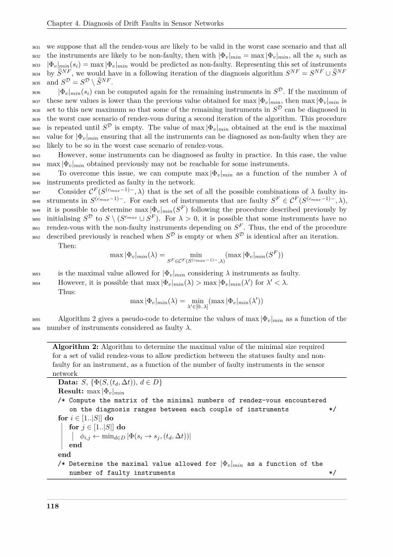
Chapter 4. Diagnosis of Drift Faults in Sensor Networks
we suppose that all the rendez-vous are likely to be valid in the worst case scenario and that all3631
the instruments are likely to be non-faulty, then with |Φv|min = max |Φv|min, all the si such as3632
|Φv|min(si) = max |Φv|min would be predicted as non-faulty. Representing this set of instruments3633
by SNF , we would have in a following iteration of the diagnosis algorithm SNF = SNF ∪ SNF3634
and SD = SD \ SNF .3635
|Φv|min(si) can be computed again for the remaining instruments in SD. If the maximum of3636
these new values is lower than the previous value obtained for max |Φv|min, then max |Φv|min is3637
set to this new maximum so that some of the remaining instruments in SD can be diagnosed in3638
the worst case scenario of rendez-vous during a second iteration of the algorithm. This procedure3639
is repeated until SD is empty. The value of max |Φv|min obtained at the end is the maximal3640
value for |Φv|min ensuring that all the instruments can be diagnosed as non-faulty when they are3641
likely to be so in the worst case scenario of rendez-vous.3642
However, some instruments can be diagnosed as faulty in practice. In this case, the value3643
max |Φv|min obtained previously may not be reachable for some instruments.3644
To overcome this issue, we can compute max |Φv|min as a function of the number λ of3645
instruments predicted as faulty in the network.3646
Consider CF (S(cmax−1)−, λ) that is the set of all the possible combinations of λ faulty in-3647
struments in S(cmax−1)−. For each set of instruments that are faulty SF ∈ CF (S(cmax−1)−, λ),3648
it is possible to determine max |Φv|min(SF ) following the procedure described previously by3649
initialising SD to S \ (Scmax ∪ SF ). For λ > 0, it is possible that some instruments have no3650
rendez-vous with the non-faulty instruments depending on SF . Thus, the end of the procedure3651
described previously is reached when SD is empty or when SD is identical after an iteration.3652
Then:max |Φv|min(λ) = min
SF∈CF (S(cmax−1)−,λ)(max |Φv|min(SF ))
is the maximal value allowed for |Φv|min considering λ instruments as faulty.3653
However, it is possible that max |Φv|min(λ) > max |Φv|min(λ′) for λ′ < λ.3654
Thus:max |Φv|min(λ) = min
λ′∈[0..λ](max |Φv|min(λ′))
Algorithm 2 gives a pseudo-code to determine the values of max |Φv|min as a function of the3655
number of instruments considered as faulty λ.3656
Algorithm 2: Algorithm to determine the maximal value of the minimal size requiredfor a set of valid rendez-vous to allow prediction between the statuses faulty and non-faulty for an instrument, as a function of the number of faulty instruments in the sensornetworkData: S, Φ(S, (td,∆t)), d ∈ DResult: max |Φv|min/* Compute the matrix of the minimal numbers of rendez-vous encountered
on the diagnosis ranges between each couple of instruments */for i ∈ [1..|S|] do
for j ∈ [1..|S|] doφi,j ← mind∈D |Φ(si → sj , (td,∆t))|
endend/* Determine the maximal value allowed for |Φv|min as a function of the
number of faulty instruments */
118
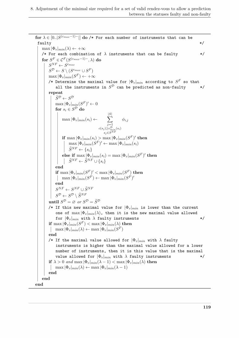
8. Adjustment of the minimal size required for a set of valid rendez-vous to allow a predictionbetween the statuses faulty and non-faulty
for λ ∈ [0..|S(cmax−1)−|] do /* For each number of instruments that can befaulty */
max |Φv|min(λ)← +∞/* For each combination of λ instruments that can be faulty */for SF ∈ CF (S(cmax−1)−, λ) do
SNF ← Scmax
SD ← S \ (Scmax ∪ SF )max |Φv|min(SF )← +∞/* Determine the maximal value for |Φv|min according to SF so that
all the instruments in SD can be predicted as non-faulty */repeat
SD ← SD
max |Φv|min(SF )′ ← 0for si ∈ SD do
max |Φv|min(si)←|S|∑j=1
c(sj)≥cDmin(si)sj∈SNF
φi,j
if max |Φv|min(si) > max |Φv|min(SF )′ thenmax |Φv|min(SF )′ ← max |Φv|min(si)SNF ← si
else if max |Φv|min(si) = max |Φv|min(SF )′ thenSNF ← SNF ∪ si
endif max |Φv|min(SF )′ < max |Φv|min(SF ) then
max |Φv|min(SF )← max |Φv|min(SF )′endSNF ← SNF ∪ SNF
SD ← SD \ SNF
until SD = ∅ or SD = SD
/* If this new maximal value for |Φv|min is lower than the currentone of max |Φv|min(λ), then it is the new maximal value allowedfor |Φv|min with λ faulty instruments */
if max |Φv|min(SF ) < max |Φv|min(λ) thenmax |Φv|min(λ)← max |Φv|min(SF )
end/* If the maximal value allowed for |Φv|min with λ faulty
instruments is higher than the maximal value allowed for a lowernumber of instruments, then it is this value that is the maximalvalue allowed for |Φv|min with λ faulty instruments */
if λ > 0 and max |Φv|min(λ− 1) < max |Φv|min(λ) thenmax |Φv|min(λ)← max |Φv|min(λ− 1)
endend
end
119
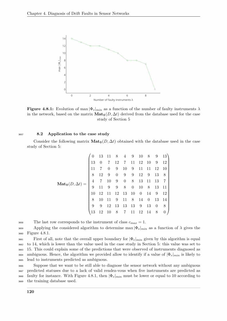
Chapter 4. Diagnosis of Drift Faults in Sensor Networks
0 2 4 6 8
0
2
4
6
8
10
12
14
Number of faulty instruments λ
max
|Φ
v| mi
n
Figure 4.8.1: Evolution of max |Φv|min as a function of the number of faulty instruments λin the network, based on the matrix MatΦ(D,∆t) derived from the database used for the case
study of Section 5
8.2 Application to the case study3657
Consider the following matrix MatΦ(D,∆t) obtained with the database used in the casestudy of Section 5:
MatΦ(D,∆t) =
0 13 11 8 4 9 10 8 9 1313 0 7 12 7 11 12 10 9 1211 7 0 9 10 9 11 11 12 108 12 9 0 9 9 12 9 13 84 7 10 9 0 8 13 11 13 79 11 9 9 8 0 10 8 13 1110 12 11 12 13 10 0 14 9 128 10 11 9 11 8 14 0 13 149 9 12 13 13 13 9 13 0 813 12 10 8 7 11 12 14 8 0
The last row corresponds to the instrument of class cmax = 1.3658
Applying the considered algorithm to determine max |Φv|min as a function of λ gives the3659
Figure 4.8.1.3660
First of all, note that the overall upper boundary for |Φv|min given by this algorithm is equal3661
to 14, which is lower than the value used in the case study in Section 5: this value was set to3662
15. This could explain some of the predictions that were observed of instruments diagnosed as3663
ambiguous. Hence, the algorithm we provided allow to identify if a value of |Φv|min is likely to3664
lead to instruments predicted as ambiguous.3665
Suppose that we want to be still able to diagnose the sensor network without any ambiguous3666
predicted statuses due to a lack of valid rendez-vous when five instruments are predicted as3667
faulty for instance. With Figure 4.8.1, then |Φv|min must be lower or equal to 10 according to3668
the training database used.3669
120
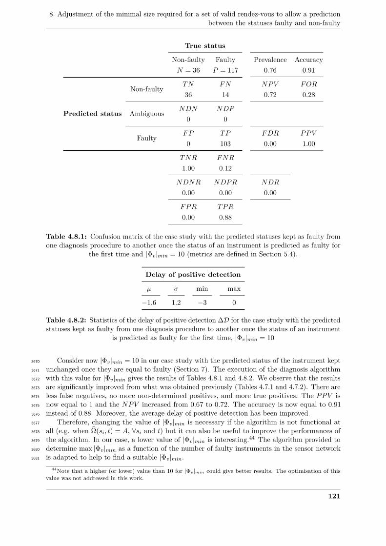
8. Adjustment of the minimal size required for a set of valid rendez-vous to allow a predictionbetween the statuses faulty and non-faulty
True status
Non-faulty Faulty Prevalence AccuracyN = 36 P = 117 0.76 0.91
Non-faulty TN FN NPV FOR
36 14 0.72 0.28
Predicted status Ambiguous NDN NDP
0 0
Faulty FP TP FDR PPV
0 103 0.00 1.00
TNR FNR
1.00 0.12
NDNR NDPR NDR
0.00 0.00 0.00
FPR TPR
0.00 0.88
Table 4.8.1: Confusion matrix of the case study with the predicted statuses kept as faulty fromone diagnosis procedure to another once the status of an instrument is predicted as faulty for
the first time and |Φv|min = 10 (metrics are defined in Section 5.4).
Delay of positive detection
µ σ min max
−1.6 1.2 −3 0
Table 4.8.2: Statistics of the delay of positive detection ∆D for the case study with the predictedstatuses kept as faulty from one diagnosis procedure to another once the status of an instrument
is predicted as faulty for the first time, |Φv|min = 10
Consider now |Φv|min = 10 in our case study with the predicted status of the instrument kept3670
unchanged once they are equal to faulty (Section 7). The execution of the diagnosis algorithm3671
with this value for |Φv|min gives the results of Tables 4.8.1 and 4.8.2. We observe that the results3672
are significantly improved from what was obtained previously (Tables 4.7.1 and 4.7.2). There are3673
less false negatives, no more non-determined positives, and more true positives. The PPV is3674
now equal to 1 and the NPV increased from 0.67 to 0.72. The accuracy is now equal to 0.913675
instead of 0.88. Moreover, the average delay of positive detection has been improved.3676
Therefore, changing the value of |Φv|min is necessary if the algorithm is not functional at3677
all (e.g. when Ω(si, t) = A, ∀si and t) but it can also be useful to improve the performances of3678
the algorithm. In our case, a lower value of |Φv|min is interesting.44 The algorithm provided to3679
determine max |Φv|min as a function of the number of faulty instruments in the sensor network3680
is adapted to help to find a suitable |Φv|min.3681
44Note that a higher (or lower) value than 10 for |Φv|min could give better results. The optimisation of thisvalue was not addressed in this work.
121
Chapter 4. Diagnosis of Drift Faults in Sensor Networks
8.3 Conclusion3682
In this section, an algorithm was provided to give an upper boundary to |Φv|min, the minimal3683
size for a set of valid rendez-vous to allow a prediction between the statuses faulty and non-faulty.3684
We defined this upper boundary max |Φv|min as a function of the number of instruments already3685
diagnosed as faulty in the sensor network to adjust |Φv|min with concerns for the robustness of3686
the diagnosis algorithm when instruments are diagnosed as faulty.3687
Afterwards, this algorithm was applied on the dataset used in the case studies presented in3688
this chapter. It allowed first to identify that the value of |Φv|min initially chosen was higher3689
than the overall upper boundary given by the algorithm. This could explain the predictions of3690
instruments as ambiguous in previous results. Then, by choosing a lower value for |Φv|min to3691
tolerate five instruments predicted as faulty in previous diagnosis procedures, the results of the3692
case study were improved, showing the interest of the algorithm developed in this section.3693
9 Sensitivity of the algorithm to changes in the case study3694
In the previous sections, the diagnosis algorithm was introduced and a case study was3695
presented to illustrate the application of the algorithm. The means to reduce false results were3696
discussed just like the assumption regarding the instruments of class cmax. In Chapter 3, the3697
influence on the results of various aspects of the case study was studied for the evaluation of in3698
situ calibration strategies. In this section, the same type of studies are conducted regarding the3699
case study that was presented in Section 5. Indeed, results are likely to be case specific according3700
to the results of the two previous sections where we saw that the choice of the values of the3701
parameters |Φv|min, (r+Φv)max, (r−Φv)max, (r+
Φv + r−Φv)max and so on could change results obtained.3702
In this section, the influence of the drift values, of the true values and of the model used to3703
build the true values is investigated. The role of the density of instruments is also questioned3704
and a discussion regarding the robustness of the algorithm against other faults is provided.3705
In the following studies, the parameters of the algorithm that allowed obtaining the3706
best results in Section 8 are used, e.g. with the predicted statuses kept as faulty from one3707
diagnosis procedure to another, once the status of an instrument is predicted as faulty, and with3708
|Φv|min = 10. It is explained when the value of a parameter is changed.3709
9.1 Influence of the values of drift3710
As the results of Section 8 and the following were obtained for one draw of drift values, the3711
case study was repeated for 100 draws. Table 4.9.1 presents the mean and standard deviation of3712
each metric.45 This table shows that:3713
• the mean values are equal to the values obtained in Table 4.8.1. This indicates that on3714
average, the observations and conclusions do not depend on the variability of the drift.3715
• the standard deviations of all the metrics are close to zero. This is small considering the3716
mean values and the relative standard deviation varying from zero to at most 16% of the3717
mean value, reached for FN .3718
Thus, in this case study, the results of the diagnosis algorithm are not dependent on the3719
values of the drift46, with this drift model at least, and with this configuration of the algorithm.3720
45The values for the delay of positive detection ∆D are not provided here for the sake of clarity.46Note that the range of magnitude of drift does not change here, only the variability is studied. A different
range would be equivalent to operating with different measuring instruments in practice.
122
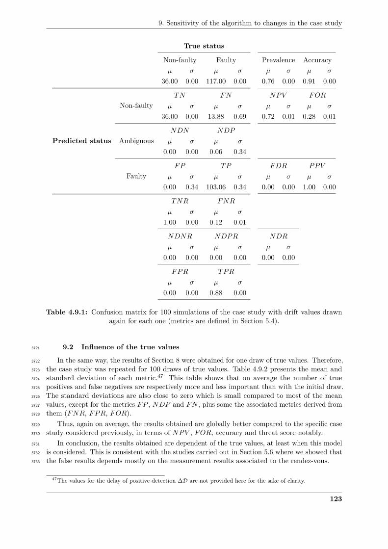
9. Sensitivity of the algorithm to changes in the case study
True status
Non-faulty Faulty Prevalence Accuracyµ σ µ σ µ σ µ σ
36.00 0.00 117.00 0.00 0.76 0.00 0.91 0.00
Non-faultyTN FN NPV FOR
µ σ µ σ µ σ µ σ
36.00 0.00 13.88 0.69 0.72 0.01 0.28 0.01
Predicted status AmbiguousNDN NDP
µ σ µ σ
0.00 0.00 0.06 0.34
FaultyFP TP FDR PPV
µ σ µ σ µ σ µ σ
0.00 0.34 103.06 0.34 0.00 0.00 1.00 0.00
TNR FNR
µ σ µ σ
1.00 0.00 0.12 0.01
NDNR NDPR NDR
µ σ µ σ µ σ
0.00 0.00 0.00 0.00 0.00 0.00
FPR TPR
µ σ µ σ
0.00 0.00 0.88 0.00
Table 4.9.1: Confusion matrix for 100 simulations of the case study with drift values drawnagain for each one (metrics are defined in Section 5.4).
9.2 Influence of the true values3721
In the same way, the results of Section 8 were obtained for one draw of true values. Therefore,3722
the case study was repeated for 100 draws of true values. Table 4.9.2 presents the mean and3723
standard deviation of each metric.47 This table shows that on average the number of true3724
positives and false negatives are respectively more and less important than with the initial draw.3725
The standard deviations are also close to zero which is small compared to most of the mean3726
values, except for the metrics FP , NDP and FN , plus some the associated metrics derived from3727
them (FNR, FPR, FOR).3728
Thus, again on average, the results obtained are globally better compared to the specific case3729
study considered previously, in terms of NPV , FOR, accuracy and threat score notably.3730
In conclusion, the results obtained are dependent of the true values, at least when this model3731
is considered. This is consistent with the studies carried out in Section 5.6 where we showed that3732
the false results depends mostly on the measurement results associated to the rendez-vous.3733
47The values for the delay of positive detection ∆D are not provided here for the sake of clarity.
123
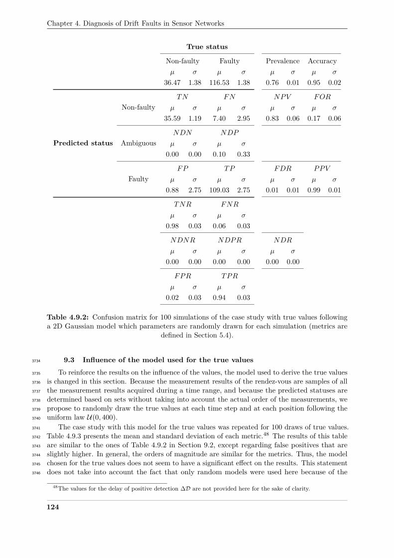
Chapter 4. Diagnosis of Drift Faults in Sensor Networks
True status
Non-faulty Faulty Prevalence Accuracyµ σ µ σ µ σ µ σ
36.47 1.38 116.53 1.38 0.76 0.01 0.95 0.02
Non-faultyTN FN NPV FOR
µ σ µ σ µ σ µ σ
35.59 1.19 7.40 2.95 0.83 0.06 0.17 0.06
Predicted status AmbiguousNDN NDP
µ σ µ σ
0.00 0.00 0.10 0.33
FaultyFP TP FDR PPV
µ σ µ σ µ σ µ σ
0.88 2.75 109.03 2.75 0.01 0.01 0.99 0.01
TNR FNR
µ σ µ σ
0.98 0.03 0.06 0.03
NDNR NDPR NDR
µ σ µ σ µ σ
0.00 0.00 0.00 0.00 0.00 0.00
FPR TPR
µ σ µ σ
0.02 0.03 0.94 0.03
Table 4.9.2: Confusion matrix for 100 simulations of the case study with true values followinga 2D Gaussian model which parameters are randomly drawn for each simulation (metrics are
defined in Section 5.4).
9.3 Influence of the model used for the true values3734
To reinforce the results on the influence of the values, the model used to derive the true values3735
is changed in this section. Because the measurement results of the rendez-vous are samples of all3736
the measurement results acquired during a time range, and because the predicted statuses are3737
determined based on sets without taking into account the actual order of the measurements, we3738
propose to randomly draw the true values at each time step and at each position following the3739
uniform law U(0, 400).3740
The case study with this model for the true values was repeated for 100 draws of true values.3741
Table 4.9.3 presents the mean and standard deviation of each metric.48 The results of this table3742
are similar to the ones of Table 4.9.2 in Section 9.2, except regarding false positives that are3743
slightly higher. In general, the orders of magnitude are similar for the metrics. Thus, the model3744
chosen for the true values does not seem to have a significant effect on the results. This statement3745
does not take into account the fact that only random models were used here because of the3746
48The values for the delay of positive detection ∆D are not provided here for the sake of clarity.
124
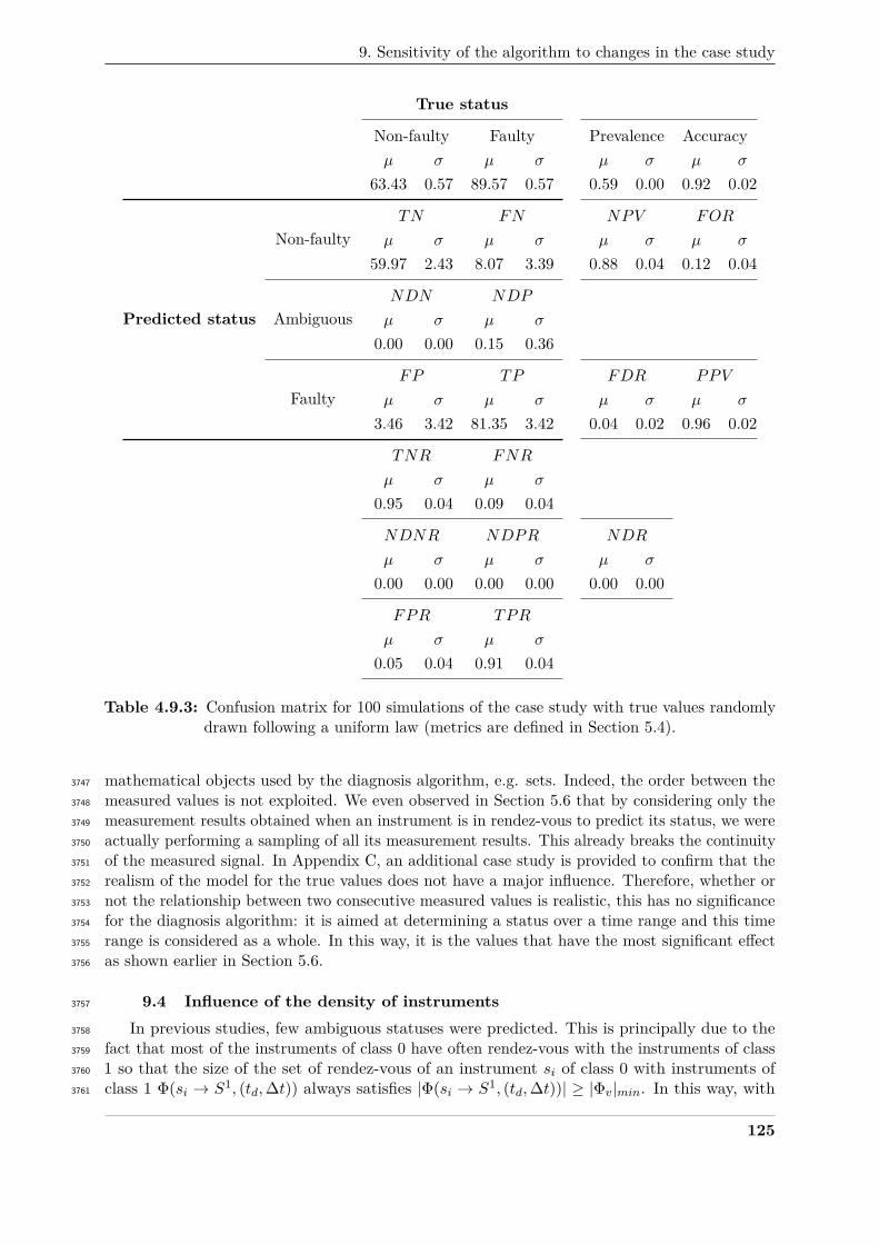
9. Sensitivity of the algorithm to changes in the case study
True status
Non-faulty Faulty Prevalence Accuracyµ σ µ σ µ σ µ σ
63.43 0.57 89.57 0.57 0.59 0.00 0.92 0.02
Non-faultyTN FN NPV FOR
µ σ µ σ µ σ µ σ
59.97 2.43 8.07 3.39 0.88 0.04 0.12 0.04
Predicted status AmbiguousNDN NDP
µ σ µ σ
0.00 0.00 0.15 0.36
FaultyFP TP FDR PPV
µ σ µ σ µ σ µ σ
3.46 3.42 81.35 3.42 0.04 0.02 0.96 0.02
TNR FNR
µ σ µ σ
0.95 0.04 0.09 0.04
NDNR NDPR NDR
µ σ µ σ µ σ
0.00 0.00 0.00 0.00 0.00 0.00
FPR TPR
µ σ µ σ
0.05 0.04 0.91 0.04
Table 4.9.3: Confusion matrix for 100 simulations of the case study with true values randomlydrawn following a uniform law (metrics are defined in Section 5.4).
mathematical objects used by the diagnosis algorithm, e.g. sets. Indeed, the order between the3747
measured values is not exploited. We even observed in Section 5.6 that by considering only the3748
measurement results obtained when an instrument is in rendez-vous to predict its status, we were3749
actually performing a sampling of all its measurement results. This already breaks the continuity3750
of the measured signal. In Appendix C, an additional case study is provided to confirm that the3751
realism of the model for the true values does not have a major influence. Therefore, whether or3752
not the relationship between two consecutive measured values is realistic, this has no significance3753
for the diagnosis algorithm: it is aimed at determining a status over a time range and this time3754
range is considered as a whole. In this way, it is the values that have the most significant effect3755
as shown earlier in Section 5.6.3756
9.4 Influence of the density of instruments3757
In previous studies, few ambiguous statuses were predicted. This is principally due to the3758
fact that most of the instruments of class 0 have often rendez-vous with the instruments of class3759
1 so that the size of the set of rendez-vous of an instrument si of class 0 with instruments of3760
class 1 Φ(si → S1, (td,∆t)) always satisfies |Φ(si → S1, (td,∆t))| ≥ |Φv|min. In this way, with3761
125
Chapter 4. Diagnosis of Drift Faults in Sensor Networks
at most one or two executions of the main loop of the algorithm, all the instruments can be3762
diagnosed faulty or non-faulty. However, if instruments were meeting less often, we expect that3763
more ambiguous statuses would be produced.3764
Consequently, to simulate the same sensor network of 10 instruments having less rendez-vous,3765
the number of accessible positions was increased from 100 to 202549. From Figure 4.9.1, we3766
can observe that with 225 positions the values of the metrics deteriorate compared to the case3767
with 100 positions and are even poorer for 400 positions and more. This can be observed just3768
from the ACC going from more than 0.7 for 225 positions to less than 0.2 afterwards but the3769
other metrics give interesting insights. Indeed, from Figure 4.9.1a, we observe that for more than3770
400 positions, there are only NDP and NDN . This explains why the TPR, FPR, TNR and3771
FPR are equal to zero, and the PPV , FDR, NPV and FOR are not defined for more than3772
400 positions, in Figures 4.9.1b and 4.9.1c respectively. This does not only indicate that the3773
diagnosis algorithm provides poor results but also that there is something making the algorithm3774
unable to predict a different status than ambiguous for the measuring instruments.3775
Therefore, the number of positions has an influence on the performances. This indicates3776
that the number of rendez-vous is at the heart of the diagnosis algorithm. If the number of3777
rendez-vous taking place cannot be increased by performing changes in the sensor network for3778
instance, the parameter that must be adjusted to have better performances is |Φv|min. Indeed, if3779
a lower value of |Φv|min can be acceptable, a sensor network with less rendez-vous occurring may3780
be diagnosable.3781
In our case, while still varying the number of positions from 100 to 2025, |Φv|min is set to3782
6 instead of 10. Figure 4.9.2 shows that even better results of diagnosis are obtained with 2253783
positions than with 100 (more TP , less FN , thus a higher TPR and PPV and a lower FNR3784
and FOR, resulting in a higher ACC value notably).3785
While the diagnosis algorithm still provides acceptable results with 400 positions, although3786
non-determined positives and negatives begin to occur, the performances remain still very3787
poor for a higher number of positions as the number of ambiguous predictions drastically3788
increases according to the evolution of NDP and NDN and the NDR. Thus, the value of ACC3789
deteriorates more slowly than in Figure 4.9.1 but still very quickly.3790
Therefore, the diagnosis algorithm depends significantly of the density of instruments but3791
more in terms of rendez-vous than of a physical density of instrument. Indeed, in Section 5, we3792
defined the positions of the instruments in an area of 1× 1km. However, we could have chosen3793
any other unit or subunit of length: this would have not changed the results we obtained. In3794
practice, it means the sensor network can cover any area as long as the nodes meet regularly for3795
diagnosis purposes.3796
49The formula used to define these numbers of positions was the following: ((1 + 0.5 · i)× 10)2 with i ∈ [0..7].
126
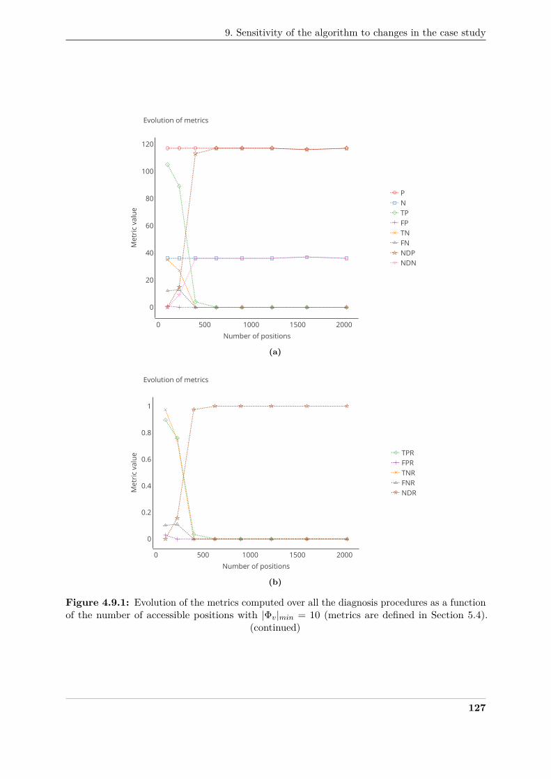
9. Sensitivity of the algorithm to changes in the case study
0 500 1000 1500 2000
0
20
40
60
80
100
120
PNTPFPTNFNNDPNDN
Evolution of metrics
Number of positions
Met
ric
valu
e
(a)
0 500 1000 1500 2000
0
0.2
0.4
0.6
0.8
1
TPRFPRTNRFNRNDR
Evolution of metrics
Number of positions
Met
ric
valu
e
(b)
Figure 4.9.1: Evolution of the metrics computed over all the diagnosis procedures as a functionof the number of accessible positions with |Φv|min = 10 (metrics are defined in Section 5.4).
(continued)
127
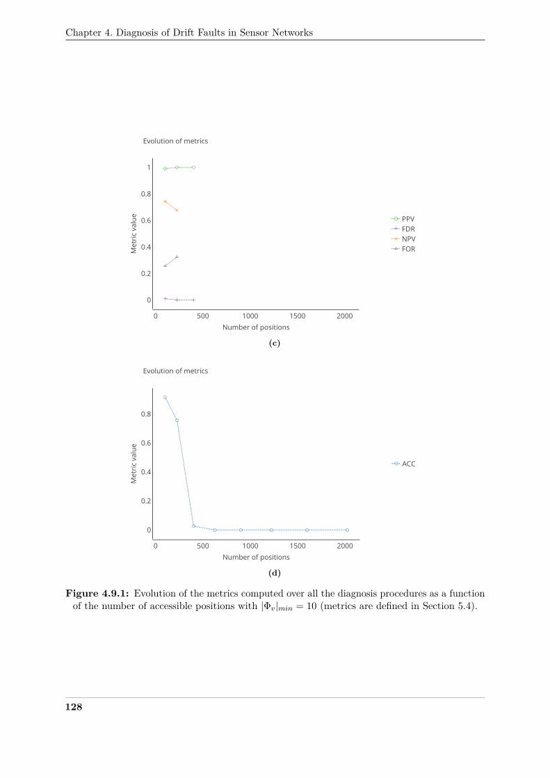
Chapter 4. Diagnosis of Drift Faults in Sensor Networks
0 500 1000 1500 2000
0
0.2
0.4
0.6
0.8
1
PPVFDRNPVFOR
Evolution of metrics
Number of positions
Met
ric
valu
e
(c)
0 500 1000 1500 2000
0
0.2
0.4
0.6
0.8
ACC
Evolution of metrics
Number of positions
Met
ric
valu
e
(d)
Figure 4.9.1: Evolution of the metrics computed over all the diagnosis procedures as a functionof the number of accessible positions with |Φv|min = 10 (metrics are defined in Section 5.4).
128
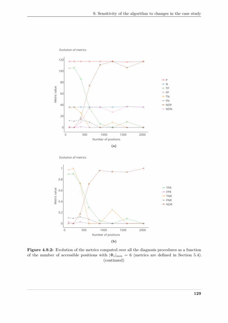
9. Sensitivity of the algorithm to changes in the case study
0 500 1000 1500 2000
0
20
40
60
80
100
120
PNTPFPTNFNNDPNDN
Evolution of metrics
Number of positions
Met
ric
valu
e
(a)
0 500 1000 1500 2000
0
0.2
0.4
0.6
0.8
1
TPRFPRTNRFNRNDR
Evolution of metrics
Number of positions
Met
ric
valu
e
(b)
Figure 4.9.2: Evolution of the metrics computed over all the diagnosis procedures as a functionof the number of accessible positions with |Φv|min = 6 (metrics are defined in Section 5.4).
(continued)
129
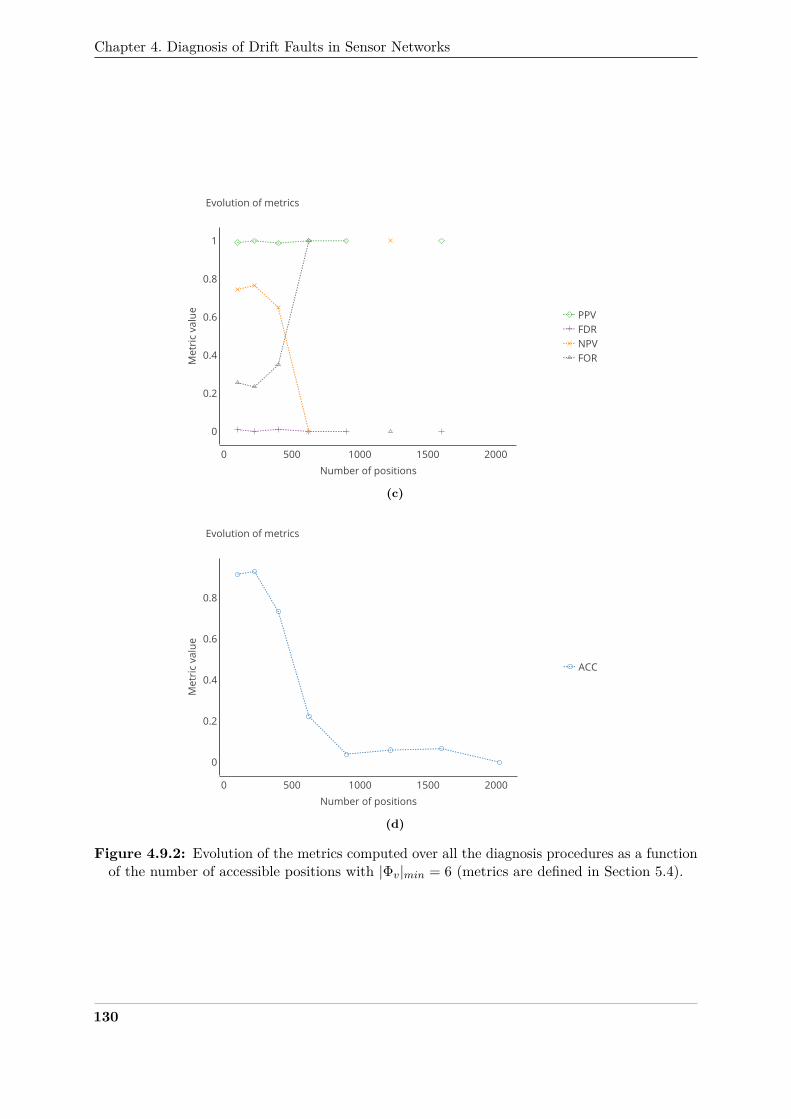
Chapter 4. Diagnosis of Drift Faults in Sensor Networks
0 500 1000 1500 2000
0
0.2
0.4
0.6
0.8
1
PPVFDRNPVFOR
Evolution of metrics
Number of positions
Met
ric
valu
e
(c)
0 500 1000 1500 2000
0
0.2
0.4
0.6
0.8
ACC
Evolution of metrics
Number of positions
Met
ric
valu
e
(d)
Figure 4.9.2: Evolution of the metrics computed over all the diagnosis procedures as a functionof the number of accessible positions with |Φv|min = 6 (metrics are defined in Section 5.4).
130
9. Sensitivity of the algorithm to changes in the case study
9.5 Influence of other faults3797
Concerning the influence of other faults on the results of diagnosis procedures, a reasoning3798
similar to the one carried out in Section 5.6 for the study of false results can be made. Indeed,3799
measurement results affected by other faults are likely to generate non-compatible measurement3800
results with their true values. We can expect it is also the case regarding other instruments3801
when such measurement results are associated to rendez-vous. Thus, it is very likely that, when3802
they are valid, the rendez-vous of an instrument si associated to such measurement results3803
affected by other faults are not belonging to the set of compatible valid rendez-vous of si,3804
Φ≈v (si, (td,∆t)). Therefore, regarding the rates r≈Φv(si → S, (td,∆t)), r+Φv(si → S, (td,∆t)) and3805
r−Φv(si → S, (td,∆t)) and their maximal associated values, the presence of measurement results3806
affected by other faults in valid rendez-vous for an instrument will tend to generate positive3807
results if they are not treated in advance, e.g. the instruments should be predicted as faulty3808
earlier.3809
To illustrate this, spikes and noise were added to the measured values following the same3810
drift model and with the same parameters that were used in Chapter 3 Section 5.3.1. The results3811
of the diagnosis are given in Tables 4.9.4 and 4.9.5. From them, we observe that N is lower3812
and P is higher than in Table 4.8.1. Therefore, the instruments should be considered as faulty3813
earlier. Regarding all the other metrics, their values are still good and similar to the results of3814
Table 4.8.1. Thus, it appears that the supplementary faulty measured values are not affecting3815
significantly the results of the diagnosis algorithm. More importantly, despite a slightly higher3816
standard deviation than in Table 4.8.2, the average delay of positive detection is close to zero and3817
even positive. Its maximal value is also positive. It indicates that the prediction of instruments3818
as faulty happens earlier than in Section 8.3819
To conclude, the proposed diagnosis algorithm targeting initially drift faults is robust to other3820
faults. Although instruments are predicted as faulty more times, regardless if such a prediction3821
is true or false, they are less harmful than false negative results in the context of drift diagnosis.3822
Indeed, it calls for an earlier maintenance of the devices in this case instead of a late one.3823
9.6 Conclusion3824
In this section, several studies were conducted to investigate the sensitivity of the diagnosis3825
algorithm to different effects. The following insights were brought:3826
• the results are not dependent on the values of the drift3827
• the true values, and thus the measurement results involved in the rendez-vous, have an3828
influence on the results. This is consistent with previous results of Section 5.63829
• the model used to derive the true values have less influence on the results than the values3830
themselves3831
• the density of instruments is critical in terms of frequency of rendez-vous with other3832
instruments3833
• the algorithm is robust to other faults. Their only effect if they are not managed prior to a3834
drift diagnosis procedure is to make the predictions of instruments as faulty happening3835
earlier. This could generate false positive results, which are less prejudicial than false3836
negatives3837
131
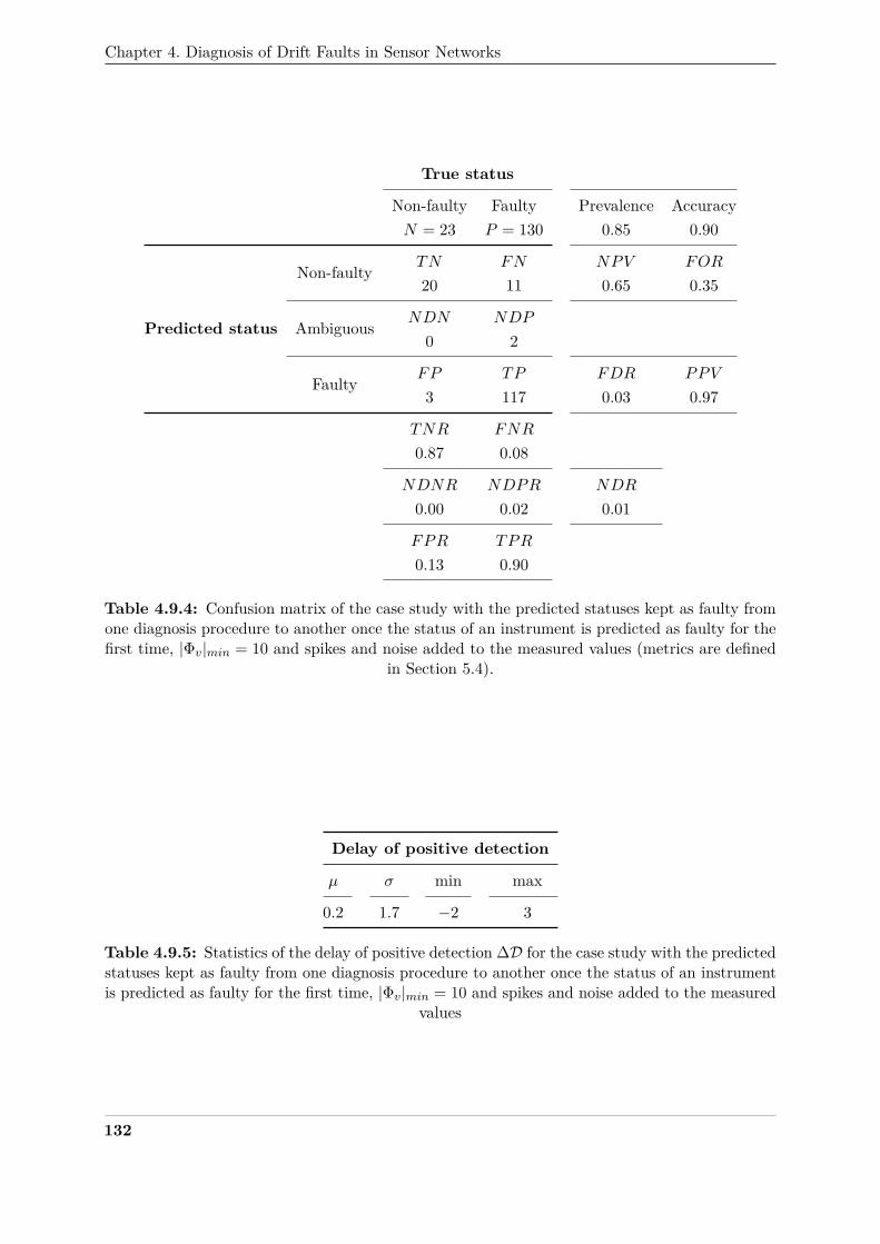
Chapter 4. Diagnosis of Drift Faults in Sensor Networks
True status
Non-faulty Faulty Prevalence AccuracyN = 23 P = 130 0.85 0.90
Non-faulty TN FN NPV FOR
20 11 0.65 0.35
Predicted status Ambiguous NDN NDP
0 2
Faulty FP TP FDR PPV
3 117 0.03 0.97
TNR FNR
0.87 0.08
NDNR NDPR NDR
0.00 0.02 0.01
FPR TPR
0.13 0.90
Table 4.9.4: Confusion matrix of the case study with the predicted statuses kept as faulty fromone diagnosis procedure to another once the status of an instrument is predicted as faulty for thefirst time, |Φv|min = 10 and spikes and noise added to the measured values (metrics are defined
in Section 5.4).
Delay of positive detection
µ σ min max
0.2 1.7 −2 3
Table 4.9.5: Statistics of the delay of positive detection ∆D for the case study with the predictedstatuses kept as faulty from one diagnosis procedure to another once the status of an instrumentis predicted as faulty for the first time, |Φv|min = 10 and spikes and noise added to the measured
values
132
10. Combination with a simple calibration approach
10 Combination with a simple calibration approach3838
The diagnosis algorithm is primarily oriented at detecting when instruments require calibration.3839
We investigate now how this algorithm behaves when calibration is carried out on an instrument3840
after it was predicted as faulty. The diagnosis algorithm is configured as in Section 5, except for3841
|Φv|min which is set to 10 as a consequence of the study in Section 8. Therefore, the status of3842
an instrument that is predicted as faulty can change as it is the trigger of a calibration3843
procedure.3844
Three cases are considered when an instrument is detected as faulty:3845
• No calibration is carried out (equivalent to what was done in Section 5)3846
• Once an instrument is predicted as faulty, its gain and offset are respectively reinitialised3847
to 1 and 0. It is equivalent to having an oracle that knows the gain and offset of each3848
instrument at each instant. That is considered as a perfect calibration.3849
• A linear regression is carried out based on the couples of measured values of the faulty3850
instruments and its diagnosers that are in the set of valid rendez-vous used for the diagnosis.3851
This technique is usually one of the firsts to be tested for the calibration of measuring3852
instruments [139].3853
Results for a single instrument are displayed in Figure 4.10.1. The instrument is recalibrated3854
right after being diagnosed as faulty for both recalibration methods. Nevertheless, it is only3855
visible at the next diagnosis procedure. Also from these curves we cannot assess the quality3856
of the calibration, it only shows that it was efficient enough to be again above the threshold3857
mentioned in the specification of the case study.3858
Table 4.10.1 represents the results for the case without calibration. Tables 4.10.2 and 4.10.33859
display the values of the metrics computed on the case study with the oracle-based and linear3860
regression-base calibration approaches respectively. Results are disturbing as the tables give3861
slightly better results without calibration. However this is normal. In the cases where there is3862
actually recalibration performed, instruments are changing of true status several times (this is3863
shown by the values of N , P and the prevalence in each table). In Section 5.5, we observed3864
that most of the false results happen around the moment where an instrument actually becomes3865
faulty. When instruments are recalibrated, they still continue to drift and they may change of3866
status again over time. Therefore, more false results are likely to be obtained when a calibration3867
strategy is applied. For this reason, the performances between the case study for which no3868
calibration is carried out and the ones where it is, based on an oracle or on linear regression here,3869
cannot be compared in terms of metrics without taking into account this fact.3870
That being said, the behaviour of the instruments is the same in terms of values and drift3871
whether the calibration is performed with an oracle or with linear regression: it is only a different3872
correction that is applied to the instruments. Thus, the results of the diagnosis algorithm can be3873
compared between Tables 4.10.2 and 4.10.3. From these tables, it appears that the calibration3874
based on linear regression provides better results in terms of improvement of the quality of the3875
instruments’ measurements: N is greater (consequently P is lower) and there are four less false3876
negative for three more true positive and negative and one more false positive. Therefore, the3877
accuracy with this method of calibration is slightly better. Although that the values of all the3878
metrics are of the same order of magnitude, it is disturbing that the oracle-based method gives3879
less accurate results, yet it corresponds to an ideal recalibration. In fact, like Figure 4.10.1, these3880
tables do not assess the actual quality of the calibration but only the quality of the diagnosis.3881
It only shows that indeed some instruments are corrected so that they are truly non-faulty3882
again–and can be detected legitimately as so.3883
133
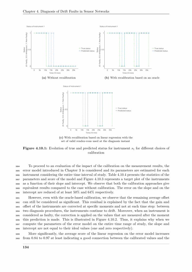
Chapter 4. Diagnosis of Drift Faults in Sensor Networks
0 5k 10k 15k 20k 25k 30k 35k
0
0.5
1
True statusPredicted status
Status of instrument 1
Time (10 min)
Stat
us
(0: F
aulty
; 0.
5: A
mbi
guou
s ; 1
: Non
-Fau
lty)
(a) Without recalibration
0 5k 10k 15k 20k 25k 30k 35k
0
0.5
1
True statusPredicted status
Status of instrument 1
Time (10 min)
Stat
us
(0: F
aulty
; 0.
5: A
mbi
guou
s ; 1
: Non
-Fau
lty)
(b) With recalibration based on an oracle
0 5k 10k 15k 20k 25k 30k 35k
0
0.5
1
True statusPredicted status
Status of instrument 1
Time (10 min)
Stat
us
(0: F
aulty
; 0.
5: A
mbi
guou
s ; 1
: Non
-Fau
lty)
(c) With recalibration based on linear regression with theset of valid rendez-vous used at the diagnosis instant
Figure 4.10.1: Evolution of true and predicted status for instrument s1 for different choices ofcalibration
To proceed to an evaluation of the impact of the calibration on the measurement results, the3884
error model introduced in Chapter 3 is considered and its parameters are estimated for each3885
instrument considering the entire time interval of study. Table 4.10.4 presents the statistics of the3886
parameters and score of the model and Figure 4.10.3 represents a target plot of the instruments3887
as a function of their slope and intercept. We observe that both the calibration approaches give3888
equivalent results compared to the case without calibration. The error on the slope and on the3889
intercept are reduced of at least 50% and 64% respectively.3890
However, even with the oracle-based calibration, we observe that the remaining average offset3891
can still be considered as significant. This residual is explained by the fact that the gain and3892
offset of the instruments are corrected at specific moments and not at each time step: between3893
two diagnosis procedures, the instruments continue to drift. Moreover, when an instrument is3894
considered as faulty, the correction is applied on the values that are measured after the moment3895
this prediction is made. This is illustrated in Figure 4.10.2. Thus, it explains why when we3896
compute the parameters of the error model on the entire time range of study, the slope and3897
intercept are not equal to their ideal values (one and zero respectively).3898
More significantly, the average score of the linear regression on the error model increases3899
from 0.84 to 0.97 at least indicating a good connection between the calibrated values and the3900
134
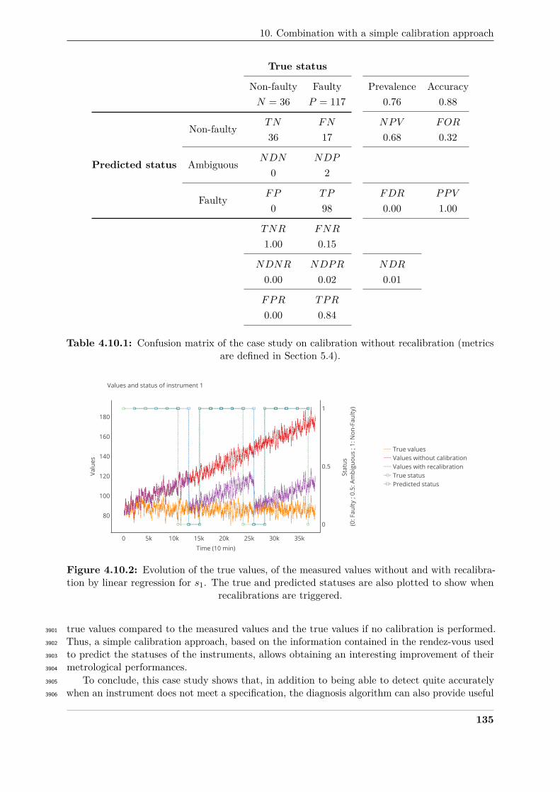
10. Combination with a simple calibration approach
True status
Non-faulty Faulty Prevalence AccuracyN = 36 P = 117 0.76 0.88
Non-faulty TN FN NPV FOR
36 17 0.68 0.32
Predicted status Ambiguous NDN NDP
0 2
Faulty FP TP FDR PPV
0 98 0.00 1.00
TNR FNR
1.00 0.15
NDNR NDPR NDR
0.00 0.02 0.01
FPR TPR
0.00 0.84
Table 4.10.1: Confusion matrix of the case study on calibration without recalibration (metricsare defined in Section 5.4).
0 5k 10k 15k 20k 25k 30k 35k
80
100
120
140
160
180
0
0.5
1
True valuesValues without calibrationValues with recalibrationTrue statusPredicted status
Values and status of instrument 1
Time (10 min)
Valu
es
Stat
us
(0: F
aulty
; 0.
5: A
mbi
guou
s ; 1
: Non
-Fau
lty)
Figure 4.10.2: Evolution of the true values, of the measured values without and with recalibra-tion by linear regression for s1. The true and predicted statuses are also plotted to show when
recalibrations are triggered.
true values compared to the measured values and the true values if no calibration is performed.3901
Thus, a simple calibration approach, based on the information contained in the rendez-vous used3902
to predict the statuses of the instruments, allows obtaining an interesting improvement of their3903
metrological performances.3904
To conclude, this case study shows that, in addition to being able to detect quite accurately3905
when an instrument does not meet a specification, the diagnosis algorithm can also provide useful3906
135
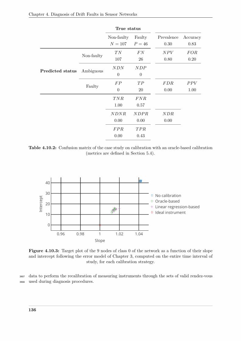
Chapter 4. Diagnosis of Drift Faults in Sensor Networks
True status
Non-faulty Faulty Prevalence AccuracyN = 107 P = 46 0.30 0.83
Non-faulty TN FN NPV FOR
107 26 0.80 0.20
Predicted status Ambiguous NDN NDP
0 0
Faulty FP TP FDR PPV
0 20 0.00 1.00
TNR FNR
1.00 0.57
NDNR NDPR NDR
0.00 0.00 0.00
FPR TPR
0.00 0.43
Table 4.10.2: Confusion matrix of the case study on calibration with an oracle-based calibration(metrics are defined in Section 5.4).
0.96 0.98 1 1.02 1.04
0
10
20
30
40
No calibrationOracle-basedLinear regression-basedIdeal instrument
Slope
Inte
rcep
t
Figure 4.10.3: Target plot of the 9 nodes of class 0 of the network as a function of their slopeand intercept following the error model of Chapter 3, computed on the entire time interval of
study, for each calibration strategy.
data to perform the recalibration of measuring instruments through the sets of valid rendez-vous3907
used during diagnosis procedures.3908
136
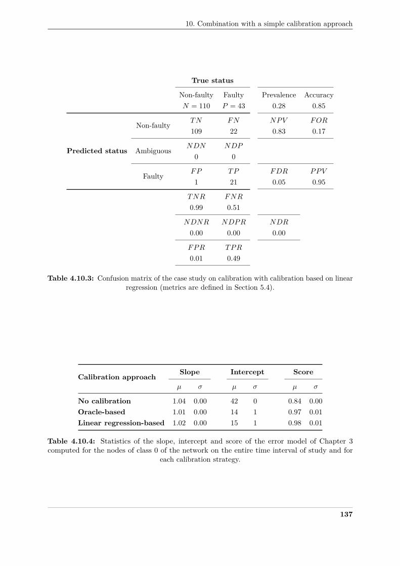
10. Combination with a simple calibration approach
True status
Non-faulty Faulty Prevalence AccuracyN = 110 P = 43 0.28 0.85
Non-faulty TN FN NPV FOR
109 22 0.83 0.17
Predicted status Ambiguous NDN NDP
0 0
Faulty FP TP FDR PPV
1 21 0.05 0.95
TNR FNR
0.99 0.51
NDNR NDPR NDR
0.00 0.00 0.00
FPR TPR
0.01 0.49
Table 4.10.3: Confusion matrix of the case study on calibration with calibration based on linearregression (metrics are defined in Section 5.4).
Calibration approachSlope Intercept Score
µ σ µ σ µ σ
No calibration 1.04 0.00 42 0 0.84 0.00Oracle-based 1.01 0.00 14 1 0.97 0.01Linear regression-based 1.02 0.00 15 1 0.98 0.01
Table 4.10.4: Statistics of the slope, intercept and score of the error model of Chapter 3computed for the nodes of class 0 of the network on the entire time interval of study and for
each calibration strategy.
137
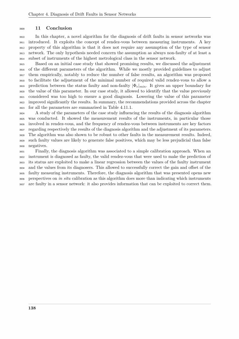
Chapter 4. Diagnosis of Drift Faults in Sensor Networks
11 Conclusion3909
In this chapter, a novel algorithm for the diagnosis of drift faults in sensor networks was3910
introduced. It exploits the concept of rendez-vous between measuring instruments. A key3911
property of this algorithm is that it does not require any assumption of the type of sensor3912
network. The only hypothesis needed concern the assumption as always non-faulty of at least a3913
subset of instruments of the highest metrological class in the sensor network.3914
Based on an initial case study that showed promising results, we discussed the adjustment3915
of the different parameters of the algorithm. While we mostly provided guidelines to adjust3916
them empirically, notably to reduce the number of false results, an algorithm was proposed3917
to facilitate the adjustment of the minimal number of required valid rendez-vous to allow a3918
prediction between the status faulty and non-faulty |Φv|min. It gives an upper boundary for3919
the value of this parameter. In our case study, it allowed to identify that the value previously3920
considered was too high to ensure a good diagnosis. Lowering the value of this parameter3921
improved significantly the results. In summary, the recommendations provided across the chapter3922
for all the parameters are summarised in Table 4.11.1.3923
A study of the parameters of the case study influencing the results of the diagnosis algorithm3924
was conducted. It showed the measurement results of the instruments, in particular those3925
involved in rendez-vous, and the frequency of rendez-vous between instruments are key factors3926
regarding respectively the results of the diagnosis algorithm and the adjustment of its parameters.3927
The algorithm was also shown to be robust to other faults in the measurement results. Indeed,3928
such faulty values are likely to generate false positives, which may be less prejudicial than false3929
negatives.3930
Finally, the diagnosis algorithm was associated to a simple calibration approach. When an3931
instrument is diagnosed as faulty, the valid rendez-vous that were used to make the prediction of3932
its status are exploited to make a linear regression between the values of the faulty instrument3933
and the values from its diagnosers. This allowed to successfully correct the gain and offset of the3934
faulty measuring instruments. Therefore, the diagnosis algorithm that was presented opens new3935
perspectives on in situ calibration as this algorithm does more than indicating which instruments3936
are faulty in a sensor network: it also provides information that can be exploited to correct them.3937
138
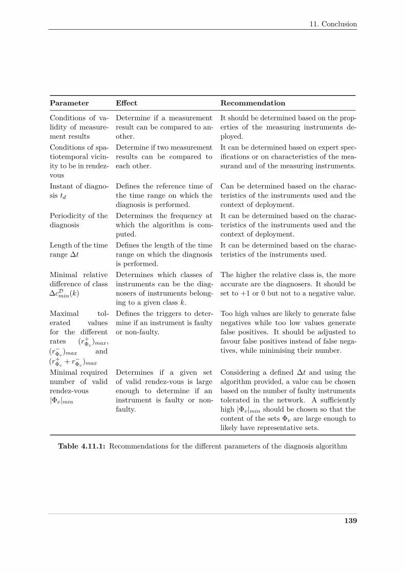
11. Conclusion
Parameter Effect Recommendation
Conditions of va-lidity of measure-ment results
Determine if a measurementresult can be compared to an-other.
It should be determined based on the prop-erties of the measuring instruments de-ployed.
Conditions of spa-tiotemporal vicin-ity to be in rendez-vous
Determine if two measurementresults can be compared toeach other.
It can be determined based on expert spec-ifications or on characteristics of the mea-surand and of the measuring instruments.
Instant of diagno-sis td
Defines the reference time ofthe time range on which thediagnosis is performed.
Can be determined based on the charac-teristics of the instruments used and thecontext of deployment.
Periodicity of thediagnosis
Determines the frequency atwhich the algorithm is com-puted.
It can be determined based on the charac-teristics of the instruments used and thecontext of deployment.
Length of the timerange ∆t
Defines the length of the timerange on which the diagnosisis performed.
It can be determined based on the charac-teristics of the instruments used.
Minimal relativedifference of class∆cDmin(k)
Determines which classes ofinstruments can be the diag-nosers of instruments belong-ing to a given class k.
The higher the relative class is, the moreaccurate are the diagnosers. It should beset to +1 or 0 but not to a negative value.
Maximal tol-erated valuesfor the differentrates (r+
Φv)max,(r−Φv)max and(r+
Φv + r−Φv)max
Defines the triggers to deter-mine if an instrument is faultyor non-faulty.
Too high values are likely to generate falsenegatives while too low values generatefalse positives. It should be adjusted tofavour false positives instead of false nega-tives, while minimising their number.
Minimal requirednumber of validrendez-vous|Φv|min
Determines if a given setof valid rendez-vous is largeenough to determine if aninstrument is faulty or non-faulty.
Considering a defined ∆t and using thealgorithm provided, a value can be chosenbased on the number of faulty instrumentstolerated in the network. A sufficientlyhigh |Φv|min should be chosen so that thecontent of the sets Φv are large enough tolikely have representative sets.
Table 4.11.1: Recommendations for the different parameters of the diagnosis algorithm
139

Chapter 4. Diagnosis of Drift Faults in Sensor Networks
140
Conclusion and perspectives3938
1 Conclusion3939
In this thesis, we tackled the issue of calibration for sensor networks, a question that is3940
particularly critical when low-cost instruments are deployed.3941
In the first part of this thesis, we reviewed the existing works concerning in situ calibration3942
which are techniques aiming at calibrating measuring instruments while leaving them in the3943
field, preferably without any physical intervention on them. Across this survey, we proposed a3944
concise taxonomy enabling the classification of the algorithms. Four main groups of categories3945
were defined, two of them following properties of the sensor networks that may be exploited,3946
namely the presence of reference instruments in the network and the mobility of the nodes,3947
and the other two concerning respectively the grouping strategy at stake in the algorithm and3948
the kind of mathematical relationship that can be derived. This extensive survey showed that3949
there are numerous contributions on the subject, covering a large spectrum of the cases that3950
can be encountered when deploying sensor networks. However, a quantitative comparison of the3951
performances of the algorithm was shown to be difficult because algorithms are often applied3952
on specific case studies in their original publication. Indeed, there is no standard use cases or3953
protocols to allow such comparisons.3954
Therefore, a framework for the simulation of sensor networks aimed at evaluating the3955
performances of in situ calibration algorithms was proposed in the second part of this thesis.3956
It was applied to the comparison of seven in situ calibration algorithms for blind and static3957
sensor networks. We independently changed the model used to derive the true values of the3958
measurand, the drift and fault model, the number of instruments and parameters of some3959
calibration algorithms. We showed that even with a particular care to conduct a balanced3960
comparison, different conclusions can be drawn by slightly changing the case study. Thus,3961
in addition to being a protocol enabling the effective comparison of strategies, the proposed3962
framework could be used to choose the most appropriate in situ calibration algorithm during the3963
design of a sensor network.3964
However, we also observed that some calibration algorithms may correct measuring instruments3965
regardless of their actual performances, particularly concerning those for blind sensor networks.3966
Therefore, it is possible that instruments which measurement results are still correct regarding the3967
metrological specifications of the instruments, have their values corrected. In the worst case, they3968
may have their values degraded. Thus, a diagnosis algorithm for drift faults in sensor networks3969
was proposed in the last part of this thesis. This algorithm is particularly interesting because it3970
is based on rendez-vous between measuring instruments. This concept is more complex than a3971
simple comparison of measured values as it encapsulates the idea of a necessary spatio-temporal3972
vicinity so that measurement results can be relevantly compared. In addition, the algorithm3973
demands no assumption on the type of sensor network used, requiring only that some of the3974
best instruments in the network can be assumed as non-faulty. Across a case study, we showed3975
that the algorithm allowed to successfully identify drifting instruments. In a second step, a3976
better adjustment of the different parameters of the algorithm enabled to improve the results,3977
although our guidelines are mainly empirical. Then, by investigating the influence of the design3978
141
Conclusion and perspectives
choices of our case study, we showed the measurement results involved in rendez-vous and the3979
frequency of rendez-vous between instruments, are key factors regarding respectively the results3980
of the diagnosis algorithm and the adjustment of its parameters. In addition, the algorithm3981
is robust to other faults: faulty values are likely to generate false positives, which may be less3982
prejudicial than false negatives in the context of environmental sensing. Finally, while combining3983
the diagnosis algorithm to a naive calibration approach, it was possible to successfully correct3984
the gain and offset of the faulty measuring instruments based on the measurement results of3985
rendez-vous between instruments, while leaving the measurement results of non-faulty ones3986
unchanged. Indeed, the diagnosis algorithm also provides information that can be exploited to3987
correct measuring instruments.3988
2 Perspectives3989
Several perspectives can be considered for the direct pursuit of this work but also for the3990
scientific community and the general public from a larger scope.3991
Direct perspectives3992
Extensions of the diagnosis algorithm3993
In the appendices, several extensions of the diagnosis algorithm are related. They aim3994
at being able to apply the diagnosis algorithm we proposed in any situation and with the3995
same performances. However, their development is not complete and demands supplementary3996
investigations. Moreover, the adjustment of some parameters of the algorithm is empirical and3997
may not be conducted through an automated optimisation procedure. Eventually, being able to3998
ensure that the specification stating when instruments should be considered as faulty or not, is3999
verified, or at least correctly implemented, would be valuable. Therefore, investigating if means4000
could be brought to improve the adjustment of the parameters of the algorithm and the formal4001
qualification of its performances would be of a major interest.4002
Design of sensor networks4003
In this work, we proposed a framework that could be used to identify the relevant algorithms4004
for the in situ calibration of a sensor network in its environment of deployment. To facilitate the4005
development of sensor networks, there is a need for engineering tools to identify at the design4006
stage what the data processing algorithms are from which a sensor network would benefit, on top4007
of tools already optimising their deployment in the case of static sensor networks for instance [18].4008
This demands to aggregate the various results obtained by the scientific community from various4009
fields in a dedicated product. Such an integrated tool is not currently available in the literature.4010
Perspectives for the scientific community and the general public4011
Standardisation of the vocabulary for the description of in situ calibration4012
algorithms4013
In this work, we proposed a taxonomy for the classification of in situ calibration algorithms.4014
We observed that there were also other taxonomies. An intensive work of standardisation of this4015
vocabulary and on the practices to describe and evaluate these algorithms would be valuable4016
in order to structure the work of the scientific community on this subject. Calls were recently4017
published along the same lines [60, 133].4018
Data processing standardisation4019
In scientific publications exploiting measurement results from low-cost sensor networks, data4020
processing that are carried out to have a clean dataset are not always fully described. For4021
142
2. Perspectives
measuring instruments on the market, even for certified ones, the way the measurements are4022
processed is rarely mentioned or only as a black box. Concerning sensors as components of4023
measuring instruments, technical datasheets are often scarce and imprecise on how they behave4024
over time and depending on their operating conditions. In the scientific community, there are calls4025
for a standardisation of the data processing algorithms in order to determine how far processed4026
measurement results are from raw ones [60, 133]. We extend this call to the need for a clear4027
information on how measuring instruments and their components behave from a metrological4028
perspective, to facilitate the identification and use of adapted data processing algorithms.4029
Qualification of instruments and their processing4030
Although experiments under laboratory or field condition conducted during this thesis were4031
not reported in this manuscript, actual measuring instruments and systems were studied in the4032
early months of this thesis through the Sense-City platform [38] as it was done in the studies4033
reported in Chapter 1 Section 1.3.3. Regarding low-cost instruments and considering the cost4034
range we considered in this work (US $100 to US $10,000), there is a wide variety of quality4035
among these measuring instruments and systems. In the scientific community, there are reports4036
on the performances of measuring instruments but it is not mandatory for a manufacturer to4037
provide the results of such works with its devices. In fact, it is currently difficult for an end user4038
to identify clearly which instrument suits its needs and at which cost because the information4039
provided is quite poor. Therefore, an effort of qualification of the performances of measuring4040
instruments, with the data processing algorithms they use, and a transparent information of the4041
general public about it when instruments are put on the market would be valuable.4042
Environmental footprint of low-cost environmental sensor network4043
Currently, there is little information on the environmental footprint of low-cost measuring4044
instruments [78]. While their interest can be legitimately justified whatever the measurand4045
considered, it has to be counterbalanced by their impact on the environment. We are dealing4046
here most of the time with electronic devices that may be difficult to recycle and may require rare4047
materials. In addition, they also require a computer and telecommunication infrastructure, those4048
being known to have more and more impact on the greenhouse gases emissions around the world.4049
Being able to evaluate the global impact of the entire measuring chain, from the instruments4050
to the datacentres in which measurement results are stored and exploited, would be of a major4051
interest in order to determine the actual benefits of dense low-cost sensor networks compared4052
to what is currently achieved with the information brought by more traditional environmental4053
measuring systems.4054
143

Conclusion and perspectives
144
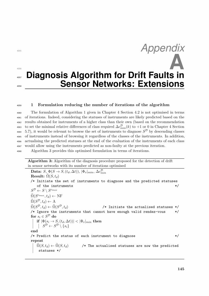
Appendix4055
A4056
Diagnosis Algorithm for Drift Faults in4057
Sensor Networks: Extensions4058
1 Formulation reducing the number of iterations of the algorithm4059
The formulation of Algorithm 1 given in Chapter 4 Section 4.2 is not optimised in terms4060
of iterations. Indeed, considering the statuses of instruments are likely predicted based on the4061
results obtained for instruments of a higher class than their own (based on the recommendation4062
to set the minimal relative differences of class required ∆cDmin(k) to +1 or 0 in Chapter 4 Section4063
5.7), it would be relevant to browse the set of instruments to diagnose SD by descending classes4064
of instruments instead of browsing it regardless of the classes of the instruments. In addition,4065
actualising the predicted statuses at the end of the evaluation of the instruments of each class4066
would allow using the instruments predicted as non-faulty at the previous iteration.4067
Algorithm 3 provides this optimised formulation in terms of iterations.4068
Algorithm 3: Algorithm of the diagnosis procedure proposed for the detection of driftin sensor networks with its number of iterations optimisedData: S, Φ(S → S, (td,∆t)), |Φv|min, ∆cDminResult: Ω(S, td)/* Initiate the set of instruments to diagnose and the predicted statuses
of the instruments */SD ← S \ ScmaxΩ(Scmax , td)← NFΩ(SD, td)← AΩ(SD, td)← Ω(SD, td) /* Initiate the actualised statuses *//* Ignore the instruments that cannot have enough valid rendez-vous */for si ∈ SD do
if |Φ(si → S, (td,∆t))| < |Φv|min thenSD ← SD \ si
end/* Predict the status of each instrument to diagnose */repeat
Ω(S, td)← Ω(S, td) /* The actualised statuses are now the predictedstatuses */
145
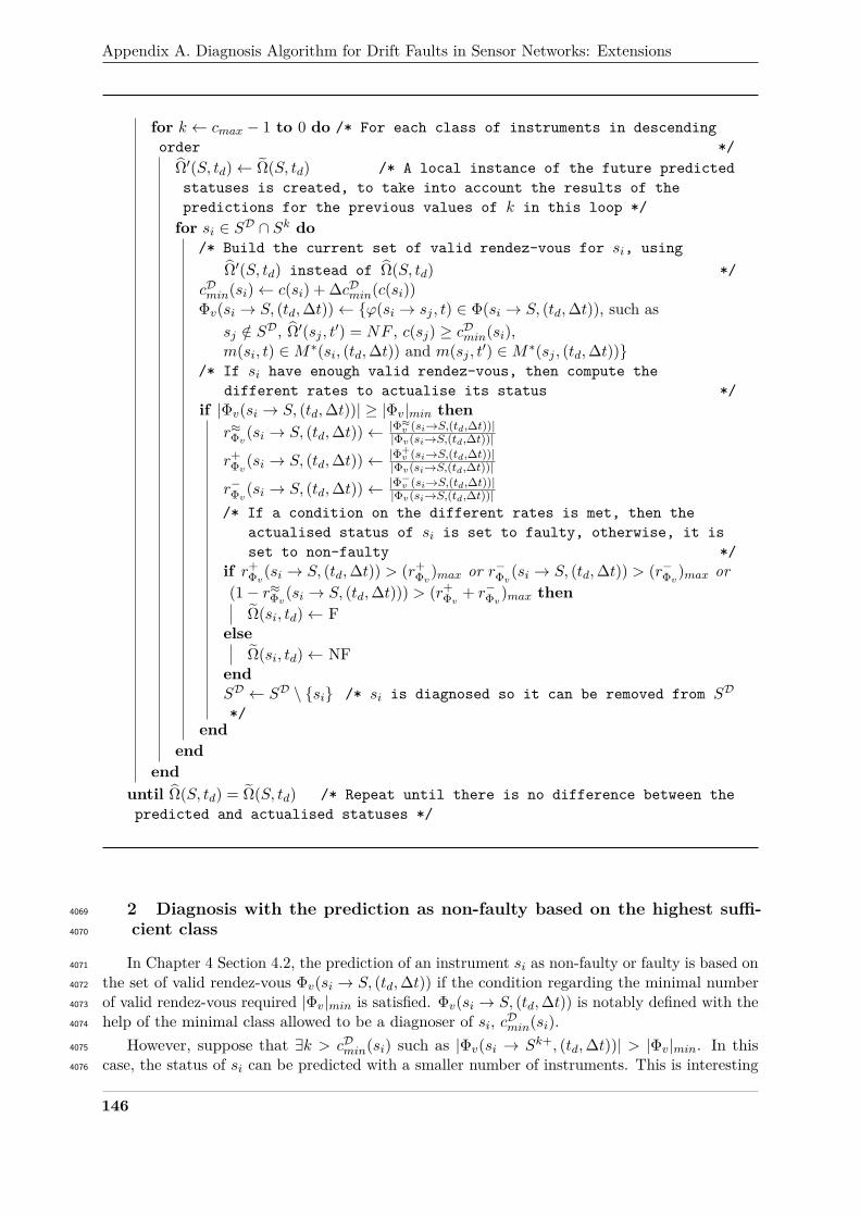
Appendix A. Diagnosis Algorithm for Drift Faults in Sensor Networks: Extensions
for k ← cmax − 1 to 0 do /* For each class of instruments in descendingorder */
Ω′(S, td)← Ω(S, td) /* A local instance of the future predictedstatuses is created, to take into account the results of thepredictions for the previous values of k in this loop */for si ∈ SD ∩ Sk do
/* Build the current set of valid rendez-vous for si, usingΩ′(S, td) instead of Ω(S, td) */
cDmin(si)← c(si) + ∆cDmin(c(si))Φv(si → S, (td,∆t))← ϕ(si → sj , t) ∈ Φ(si → S, (td,∆t)), such as
sj /∈ SD, Ω′(sj , t′) = NF , c(sj) ≥ cDmin(si),m(si, t) ∈M∗(si, (td,∆t)) and m(sj , t′) ∈M∗(sj , (td,∆t))
/* If si have enough valid rendez-vous, then compute thedifferent rates to actualise its status */
if |Φv(si → S, (td,∆t))| ≥ |Φv|min thenr≈Φv(si → S, (td,∆t))← |Φ≈v (si→S,(td,∆t))|
|Φv(si→S,(td,∆t))|
r+Φv(si → S, (td,∆t))← |Φ+
v (si→S,(td,∆t))||Φv(si→S,(td,∆t))|
r−Φv(si → S, (td,∆t))← |Φ−v (si→S,(td,∆t))||Φv(si→S,(td,∆t))|
/* If a condition on the different rates is met, then theactualised status of si is set to faulty, otherwise, it isset to non-faulty */
if r+Φv(si → S, (td,∆t)) > (r+
Φv)max or r−Φv(si → S, (td,∆t)) > (r−Φv)max or(1− r≈Φv(si → S, (td,∆t))) > (r+
Φv + r−Φv)max thenΩ(si, td)← F
elseΩ(si, td)← NF
endSD ← SD \ si /* si is diagnosed so it can be removed from SD
*/end
endend
until Ω(S, td) = Ω(S, td) /* Repeat until there is no difference between thepredicted and actualised statuses */
2 Diagnosis with the prediction as non-faulty based on the highest suffi-4069
cient class4070
In Chapter 4 Section 4.2, the prediction of an instrument si as non-faulty or faulty is based on4071
the set of valid rendez-vous Φv(si → S, (td,∆t)) if the condition regarding the minimal number4072
of valid rendez-vous required |Φv|min is satisfied. Φv(si → S, (td,∆t)) is notably defined with the4073
help of the minimal class allowed to be a diagnoser of si, cDmin(si).4074
However, suppose that ∃k > cDmin(si) such as |Φv(si → Sk+, (td,∆t))| > |Φv|min. In this4075
case, the status of si can be predicted with a smaller number of instruments. This is interesting4076
146
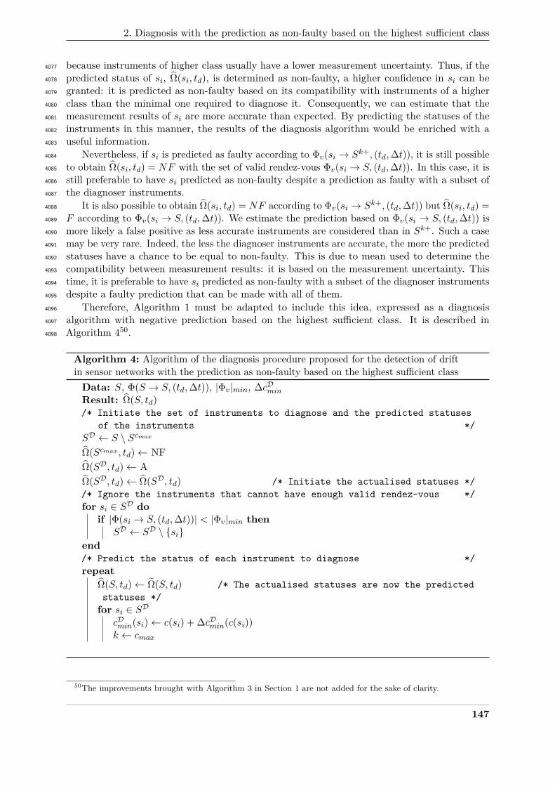
2. Diagnosis with the prediction as non-faulty based on the highest sufficient class
because instruments of higher class usually have a lower measurement uncertainty. Thus, if the4077
predicted status of si, Ω(si, td), is determined as non-faulty, a higher confidence in si can be4078
granted: it is predicted as non-faulty based on its compatibility with instruments of a higher4079
class than the minimal one required to diagnose it. Consequently, we can estimate that the4080
measurement results of si are more accurate than expected. By predicting the statuses of the4081
instruments in this manner, the results of the diagnosis algorithm would be enriched with a4082
useful information.4083
Nevertheless, if si is predicted as faulty according to Φv(si → Sk+, (td,∆t)), it is still possible4084
to obtain Ω(si, td) = NF with the set of valid rendez-vous Φv(si → S, (td,∆t)). In this case, it is4085
still preferable to have si predicted as non-faulty despite a prediction as faulty with a subset of4086
the diagnoser instruments.4087
It is also possible to obtain Ω(si, td) = NF according to Φv(si → Sk+, (td,∆t)) but Ω(si, td) =4088
F according to Φv(si → S, (td,∆t)). We estimate the prediction based on Φv(si → S, (td,∆t)) is4089
more likely a false positive as less accurate instruments are considered than in Sk+. Such a case4090
may be very rare. Indeed, the less the diagnoser instruments are accurate, the more the predicted4091
statuses have a chance to be equal to non-faulty. This is due to mean used to determine the4092
compatibility between measurement results: it is based on the measurement uncertainty. This4093
time, it is preferable to have si predicted as non-faulty with a subset of the diagnoser instruments4094
despite a faulty prediction that can be made with all of them.4095
Therefore, Algorithm 1 must be adapted to include this idea, expressed as a diagnosis4096
algorithm with negative prediction based on the highest sufficient class. It is described in4097
Algorithm 450.4098
Algorithm 4: Algorithm of the diagnosis procedure proposed for the detection of driftin sensor networks with the prediction as non-faulty based on the highest sufficient classData: S, Φ(S → S, (td,∆t)), |Φv|min, ∆cDminResult: Ω(S, td)/* Initiate the set of instruments to diagnose and the predicted statuses
of the instruments */SD ← S \ ScmaxΩ(Scmax , td)← NFΩ(SD, td)← AΩ(SD, td)← Ω(SD, td) /* Initiate the actualised statuses *//* Ignore the instruments that cannot have enough valid rendez-vous */for si ∈ SD do
if |Φ(si → S, (td,∆t))| < |Φv|min thenSD ← SD \ si
end/* Predict the status of each instrument to diagnose */repeat
Ω(S, td)← Ω(S, td) /* The actualised statuses are now the predictedstatuses */for si ∈ SD
cDmin(si)← c(si) + ∆cDmin(c(si))k ← cmax
50The improvements brought with Algorithm 3 in Section 1 are not added for the sake of clarity.
147
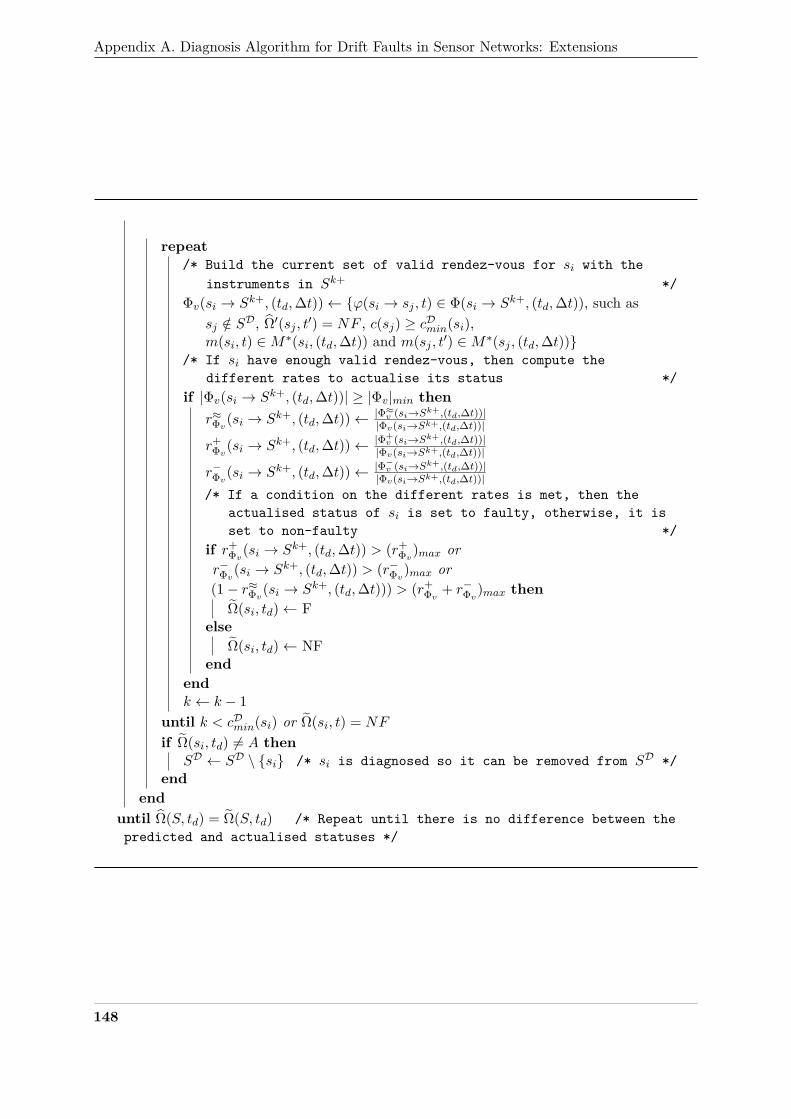
Appendix A. Diagnosis Algorithm for Drift Faults in Sensor Networks: Extensions
repeat/* Build the current set of valid rendez-vous for si with the
instruments in Sk+ */Φv(si → Sk+, (td,∆t))← ϕ(si → sj , t) ∈ Φ(si → Sk+, (td,∆t)), such as
sj /∈ SD, Ω′(sj , t′) = NF , c(sj) ≥ cDmin(si),m(si, t) ∈M∗(si, (td,∆t)) and m(sj , t′) ∈M∗(sj , (td,∆t))
/* If si have enough valid rendez-vous, then compute thedifferent rates to actualise its status */
if |Φv(si → Sk+, (td,∆t))| ≥ |Φv|min thenr≈Φv(si → Sk+, (td,∆t))← |Φ≈v (si→Sk+,(td,∆t))|
|Φv(si→Sk+,(td,∆t))|
r+Φv(si → Sk+, (td,∆t))← |Φ+
v (si→Sk+,(td,∆t))||Φv(si→Sk+,(td,∆t))|
r−Φv(si → Sk+, (td,∆t))← |Φ−v (si→Sk+,(td,∆t))||Φv(si→Sk+,(td,∆t))|
/* If a condition on the different rates is met, then theactualised status of si is set to faulty, otherwise, it isset to non-faulty */
if r+Φv(si → Sk+, (td,∆t)) > (r+
Φv)max orr−Φv(si → Sk+, (td,∆t)) > (r−Φv)max or(1− r≈Φv(si → Sk+, (td,∆t))) > (r+
Φv + r−Φv)max thenΩ(si, td)← F
elseΩ(si, td)← NF
endendk ← k − 1
until k < cDmin(si) or Ω(si, t) = NF
if Ω(si, td) 6= A thenSD ← SD \ si /* si is diagnosed so it can be removed from SD */
endend
until Ω(S, td) = Ω(S, td) /* Repeat until there is no difference between thepredicted and actualised statuses */
148
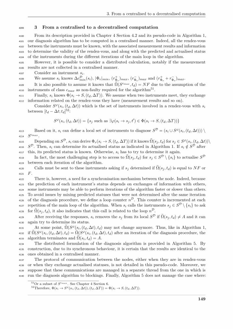
3. From a centralised to a decentralised computation
3 From a centralised to a decentralised computation4099
From its description provided in Chapter 4 Section 4.2 and its pseudo-code in Algorithm 1,4100
our diagnosis algorithm has to be computed in a centralised manner. Indeed, all the rendez-vous4101
between the instruments must be known, with the associated measurement results and information4102
to determine the validity of the rendez-vous, and along with the predicted and actualised status4103
of the instruments during the different iterations of the main loop in the algorithm.4104
However, it is possible to consider a distributed calculation, notably if the measurement4105
results are not collected in a centralised manner.4106
Consider an instrument si.4107
We assume si knows ∆cDmin(si), |Φv|min, (r+Φv)max, (r−Φv)max and (r+
Φv + r−Φv)max.4108
It is also possible to assume it knows that Ω(Scmax , td) = NF due to the assumption of the4109
instruments of class cmax as non-faulty required for the algorithm51.4110
Finally, si knows Φ(si → S, (td,∆T )). We assume when two instruments meet, they exchange4111
information related on the rendez-vous they have (measurement results and so on).4112
Consider Sϕ(si, (td,∆t)) which is the set of instruments involved in a rendez-vous with sibetween [td −∆t; td]52:
Sϕ(si, (td,∆t)) = sj such as ∃ϕ(si → sj , t′) ∈ Φ(si → S, (td,∆T ))
Based on it, si can define a local set of instruments to diagnose SD = (si ∪ Sϕ(si, (td,∆t))) \4113
Scmax .4114
Depending on SD, si can derive Φv(si → S, (td,∆T )) if it knows Ω(sj , td) for sj ∈ Sϕ(si, (td,∆t))\4115
SD. Then, si can determine its actualised status as indicated in Algorithm 1. If si /∈ SD after4116
this, its predicted status is known. Otherwise, si has to try to determine it again.4117
In fact, the most challenging step is to access to Ω(sj , td) for sj ∈ SD \ si to actualise SD4118
between each iteration of the algorithm.4119
Calls must be sent to these instruments asking if sj determined if Ω(sj , td) is equal to NF or4120
F .4121
There is, however, a need for a synchronisation mechanism between the node. Indeed, because4122
the prediction of each instrument’s status depends on exchanges of information with others,4123
some instruments may be able to perform iterations of the algorithm faster or slower than others.4124
To avoid issues by mixing predicted statuses that were not determined after the same iteration4125
of the diagnosis procedure, we define a loop counter nD. This counter is incremented at each4126
repetition of the main loop of the algorithm. When si calls the instruments sj ∈ SD \ si to ask4127
for Ω(sj , td), it also indicates that this call is related to the loop nD.4128
After receiving the responses, si removes the sj from its local SD if Ω(sj , td) 6= A and it can4129
again try to determine its status.4130
At some point, Ω(Sϕ(si, (td,∆t), td) may not change anymore. Thus, like in Algorithm 1,4131
if Ω(Sϕ(si, (td,∆t), td) = Ω(Sϕ(si, (td,∆t), td) after an iteration of the diagnosis procedure, the4132
algorithm terminates and Ω(si, td) = A.4133
The distributed formulation of the diagnosis algorithm is provided in Algorithm 5. By4134
construction, due to its synchronous behaviour, it is certain that the results are identical to the4135
ones obtained in a centralised manner.4136
The protocol of communication between the nodes, either when they are in rendez-vous4137
or when they exchange actualised statuses, is not detailed in this pseudo-code. Moreover, we4138
suppose that these communications are managed in a separate thread from the one in which is4139
run the diagnosis algorithm to blockings. Finally, Algorithm 5 does not manage the case where:4140
51Or a subset of Scmax . See Chapter 4 Section 6.52Therefore, Φ(si → Sϕ(si, (td,∆t)), (td,∆T )) = Φ(si → S, (td,∆T )).
149
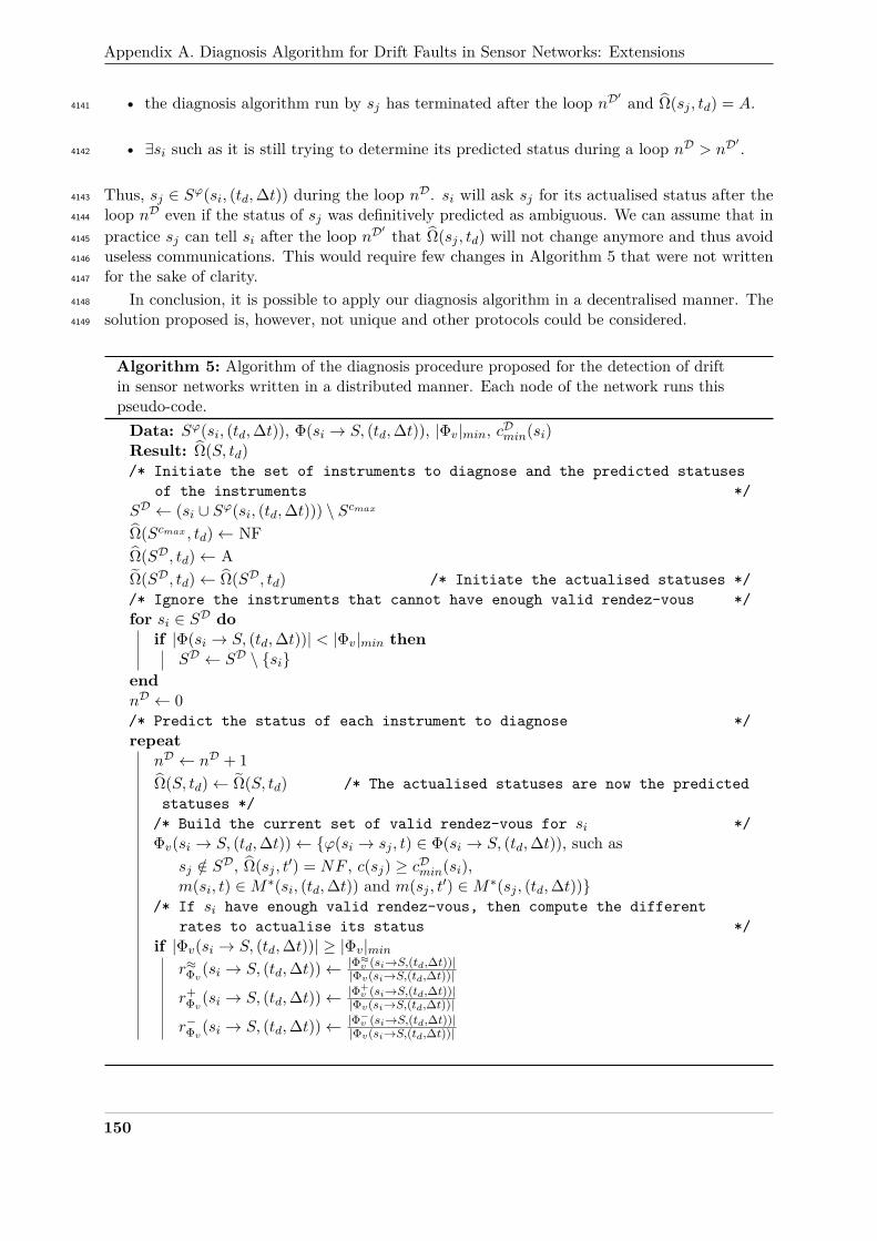
Appendix A. Diagnosis Algorithm for Drift Faults in Sensor Networks: Extensions
• the diagnosis algorithm run by sj has terminated after the loop nD′ and Ω(sj , td) = A.4141
• ∃si such as it is still trying to determine its predicted status during a loop nD > nD′ .4142
Thus, sj ∈ Sϕ(si, (td,∆t)) during the loop nD. si will ask sj for its actualised status after the4143
loop nD even if the status of sj was definitively predicted as ambiguous. We can assume that in4144
practice sj can tell si after the loop nD′ that Ω(sj , td) will not change anymore and thus avoid4145
useless communications. This would require few changes in Algorithm 5 that were not written4146
for the sake of clarity.4147
In conclusion, it is possible to apply our diagnosis algorithm in a decentralised manner. The4148
solution proposed is, however, not unique and other protocols could be considered.4149
Algorithm 5: Algorithm of the diagnosis procedure proposed for the detection of driftin sensor networks written in a distributed manner. Each node of the network runs thispseudo-code.Data: Sϕ(si, (td,∆t)), Φ(si → S, (td,∆t)), |Φv|min, cDmin(si)Result: Ω(S, td)/* Initiate the set of instruments to diagnose and the predicted statuses
of the instruments */SD ← (si ∪ Sϕ(si, (td,∆t))) \ ScmaxΩ(Scmax , td)← NFΩ(SD, td)← AΩ(SD, td)← Ω(SD, td) /* Initiate the actualised statuses *//* Ignore the instruments that cannot have enough valid rendez-vous */for si ∈ SD do
if |Φ(si → S, (td,∆t))| < |Φv|min thenSD ← SD \ si
endnD ← 0/* Predict the status of each instrument to diagnose */repeat
nD ← nD + 1Ω(S, td)← Ω(S, td) /* The actualised statuses are now the predictedstatuses */
/* Build the current set of valid rendez-vous for si */Φv(si → S, (td,∆t))← ϕ(si → sj , t) ∈ Φ(si → S, (td,∆t)), such as
sj /∈ SD, Ω(sj , t′) = NF , c(sj) ≥ cDmin(si),m(si, t) ∈M∗(si, (td,∆t)) and m(sj , t′) ∈M∗(sj , (td,∆t))
/* If si have enough valid rendez-vous, then compute the differentrates to actualise its status */
if |Φv(si → S, (td,∆t))| ≥ |Φv|minr≈Φv(si → S, (td,∆t))← |Φ≈v (si→S,(td,∆t))|
|Φv(si→S,(td,∆t))|
r+Φv(si → S, (td,∆t))← |Φ+
v (si→S,(td,∆t))||Φv(si→S,(td,∆t))|
r−Φv(si → S, (td,∆t))← |Φ−v (si→S,(td,∆t))||Φv(si→S,(td,∆t))|
150
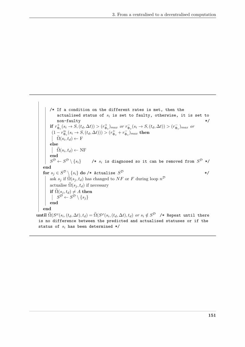
3. From a centralised to a decentralised computation
/* If a condition on the different rates is met, then theactualised status of si is set to faulty, otherwise, it is set tonon-faulty */
if r+Φv(si → S, (td,∆t)) > (r+
Φv)max or r−Φv(si → S, (td,∆t)) > (r−Φv)max or(1− r≈Φv(si → S, (td,∆t))) > (r+
Φv + r−Φv)max thenΩ(si, td)← F
elseΩ(si, td)← NF
endSD ← SD \ si /* si is diagnosed so it can be removed from SD */
endfor sj ∈ SD \ si do /* Actualise SD */
ask sj if Ω(sj , td) has changed to NF or F during loop nD
actualise Ω(sj , td) if necessaryif Ω(sj , td) 6= A then
SD ← SD \ sjend
enduntil Ω(Sϕ(si, (td,∆t), td) = Ω(Sϕ(si, (td,∆t), td) or si /∈ SD /* Repeat until thereis no difference between the predicted and actualised statuses or if thestatus of si has been determined */
151
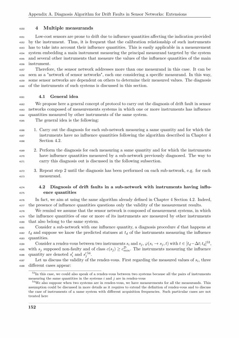
Appendix A. Diagnosis Algorithm for Drift Faults in Sensor Networks: Extensions
4 Multiple measurands4150
Low-cost sensors are prone to drift due to influence quantities affecting the indication provided4151
by the instrument. Thus, it is frequent that the calibration relationship of such instruments4152
has to take into account their influence quantities. This is easily applicable in a measurement4153
system embedding a main instrument measuring the principal measurand targeted by the system4154
and several other instruments that measure the values of the influence quantities of the main4155
instrument.4156
Therefore, the sensor network addresses more than one measurand in this case. It can be4157
seen as a "network of sensor networks", each one considering a specific measurand. In this way,4158
some sensor networks are dependent on others to determine their measured values. The diagnosis4159
of the instruments of such systems is discussed in this section.4160
4.1 General idea4161
We propose here a general concept of protocol to carry out the diagnosis of drift fault in sensor4162
networks composed of measurements systems in which one or more instruments has influence4163
quantities measured by other instruments of the same system.4164
The general idea is the following:4165
1. Carry out the diagnosis for each sub-network measuring a same quantity and for which the4166
instruments have no influence quantities following the algorithm described in Chapter 44167
Section 4.2.4168
2. Perform the diagnosis for each measuring a same quantity and for which the instruments4169
have influence quantities measured by a sub-network previously diagnosed. The way to4170
carry this diagnosis out is discussed in the following subsection.4171
3. Repeat step 2 until the diagnosis has been performed on each sub-network, e.g. for each4172
measurand.4173
4.2 Diagnosis of drift faults in a sub-network with instruments having influ-4174
ence quantities4175
In fact, we aim at using the same algorithm already defined in Chapter 4 Section 4.2. Indeed,4176
the presence of influence quantities questions only the validity of the measurement results.4177
We remind we assume that the sensor network is composed of measurement systems, in which4178
the influence quantities of one or more of its instruments are measured by other instruments4179
that also belong to the same system.4180
Consider a sub-network with one influence quantity, a diagnosis procedure d that happens at4181
td and suppose we know the predicted statuses at td of the instruments measuring the influence4182
quantities.4183
Consider a rendez-vous between two instruments si and sj , ϕ(si → sj , t) with t ∈ [td−∆t; td]53,4184
with sj supposed non-faulty and of class c(sj) ≥ cDmin. The instruments measuring the influence4185
quantity are denoted s′i and s′j54.4186
Let us discuss the validity of the rendez-vous. First regarding the measured values of si, three4187
different cases appear:4188
53In this case, we could also speak of a rendez-vous between two systems because all the pairs of instrumentsmeasuring the same quantities in the systems i and j are in rendez-vous
54We also suppose when two systems are in rendez-vous, we have measurements for all the measurands. Thisassumption could be discussed in more details as it requires to extend the definition of rendez-vous and to discussthe case of instruments of a same system with different acquisition frequencies. Such particular cases are nottreated here
152
5. Diagnosis algorithm for drift faults in sensor networks with an event-based formulation
• s′i is non-faulty: the measured value of s′i can be used to determine the one of si with4189
its calibration relationship. In this case, the measurement result m(si, t) is valid and the4190
rendez-vous may be valid too55.4191
• s′i is faulty but s′j is non-faulty: the measured value of s′j can be used to determine the one4192
of si with its calibration relationship. In this case, m(si, t) is again valid the rendez-vous4193
may be valid too 56.4194
• s′i and s′j are faulty: the measured value of si cannot be determined as no value of its4195
influence quantity can be reliably used with the calibration relationship. In this case,4196
m(si, t) is not valid. Therefore, ϕ(si → sj , t) is not valid.4197
The same reasoning can be applied to sj .57584198
In fact, the presence of influence quantities has only an influence on the validity of the4199
measurement results. Thus, the Equation 4.1 from Chapter 4 Section 4.1 used to determine4200
Φv(si → S, (td,∆t)) is still valid. We recall this equation:4201
Φv(si → S, (td,∆t)) =ϕ(si → sj , t) ∈ Φ(si → S, (td,∆t)), such assj /∈ SD, // sj is not an instrument to diagnoseΩ(sj , t′) = NF , // sj is non-faultyc(sj) ≥ cDmin(si), // The class of sj is higher or equal to the minimalclass allowed to diagnose sim(si, t) ∈M∗(si, (td,∆t)), // The measurement result of si is validm(sj , t′) ∈M∗(sj , (td,∆t)) // The measurement result of sj is valid
(A.1)This is why, apart from the conditions on the validity of the measurement results that may4202
change, the diagnosis algorithm remains applicable in the context of measuring instruments with4203
influence quantities.4204
4.3 Conclusion4205
In this section, we presented a manner to extend our diagnosis algorithm for drift faults in4206
sensor networks to the case where4207
However, a formulation enriching the results provided by the diagnosis algorithm could be4208
developed in future work. Indeed, the fact that values of measuring instruments from other4209
systems can be used to determine the status of an instrument in a given system could allow us4210
to determine a status at the level of the measuring system for instance or at least to qualify the4211
predicted statuses in light of how the validity of measurement results is determined.4212
5 Diagnosis algorithm for drift faults in sensor networks with an event-4213
based formulation4214
In the first place, the diagnosis algorithm was presented as being applied at an instant td over4215
[td −∆t; td]. It means that it is time which triggered the diagnosis and that the determination of4216
55Depending on the other conditions defined for the validity of the measurement results.56See note 5557This development can be extended to the case where there are multiple influences quantities but also to the
case where more than two instruments meet at the same time, e.g. the values of the influence quantity measuredby a third system could be used when s′i and s′j are faulty in our case.
58The definitions related the compatibility between two measurement results could be extended based on thesethree cases.
153
Appendix A. Diagnosis Algorithm for Drift Faults in Sensor Networks: Extensions
the sets of rendez-vous is notably based on a time range.4217
However, notably in the perspective of a real-time application, it could be valuable to trigger4218
the diagnosis when rendez-vous occurs. A rendez-vous can be assimilated to an event able to4219
trigger a diagnosis procedure. Such rendez-vous is noted ϕ(...), "..." standing for the instruments4220
actually involved in the rendez-vous and the time instant at which it occurred.4221
In the same way, the contents of the sets of rendez-vous could be determined based on a4222
number of rendez-vous, noted |Φ|D, that occurred before ϕ(...). It can be useful if the number of4223
rendez-vous on [td −∆t; td] varies a lot between the instruments. For instance, some of them4224
may not be diagnosable with not enough (valid) rendez-vous on this time range. A solution is4225
to increase ∆t. However in this case, other instruments may have their statuses not correctly4226
predicted with a greater ∆t (see Chapter 4 Section 7). Thus, replacing ∆t by |Φ|D can help to4227
overcome this situation: all the instruments will be diagnosed based on sets of rendez-vous that4228
are equivalent in terms of size.4229
In addition to the couple (td,∆t) defining the moment of the diagnosis and the time period4230
on which it is made, there are other combinations possible to set these characteristics of the4231
algorithm with the help of ϕ(...) and |Φ|D:4232
• (td, |Φ|D): the diagnosis occurs at td and the last |Φ|D rendez-vous are considered for each4233
instrument to predict its status.4234
• (td,∆t, |Φ|D): the diagnosis occurs at td and the rendez-vous that happened in [td −∆t; td]4235
are considered, up to the |Φ|D last ones.4236
• (ϕ(...),∆t): the diagnosis occurs on ϕ(...) and the rendez-vous that happened in [td−∆t; td]4237
are considered, with td being the instant at which ϕ(...) was generated.4238
• (ϕ(...), |Φ|D): the diagnosis occurs on ϕ(...) and the last |Φ|D rendez-vous are considered4239
for each instrument to predict its status.4240
• (ϕ(...),∆t, |Φ|D): the diagnosis occurs at ϕ(...) and the rendez-vous that happened in4241
[td −∆t; td] are considered, up to the |Φ|D last ones59.4242
The diagnosis algorithm can be easily adapted to consider these alternate definitions of the4243
instant α ∈ td, ϕ(...) at which is executed and of the duration β ∈ ∆t, |Φ|D, (∆t, |Φ|D) used4244
to define the sets used by the algorithm. Indeed, the expression "(td,∆t)" can be replaced by4245
"(α, β)" straightforward in Algorithm 160.4246
To conclude, the proposed diagnosis algorithm can also be applied with an event-based4247
definition of the instant at which it is executed and of the duration used to define the sets of4248
rendez-vous it uses.4249
6 Real-time diagnosis algorithm of drift faults in sensor networks4250
Until then, the diagnosis was considered as a procedure carried out periodically or, with the4251
definitions of Section 5, on events. If it is performed at each time step or on each event, the4252
59When ∆t and |Φ|D are combined it is possible that a set of rendez-vous:– contains less than |Φ|D rendez-vous if less than that occurred during [td −∆t; td].– does not contain all the rendez-vous that occurred during [td −∆t; td] if there were more rendez-vous than|Φ|D.
60In fact, behind "..." in ϕ(...) lies a "td" which is the instant at which the rendez-vous occurred. This td is usedin practice to determine the sets involved in a diagnosis procedure. Also behind "|Φ|D" lies a "t′d" which is theinstant when the first of the |Φ|D rendez-vous occurred. This t′d is different for each instrument. The definitionsgiven in Chapter 4 Section 3 have to be adapted depending on the choice of α and β.
154
6. Real-time diagnosis algorithm of drift faults in sensor networks
algorithm is not very efficient: it computes rates based on sets that are not often changing (and4253
probably not a lot) between two time steps. This section aims at providing elements for the4254
design of a more efficient way to perform in real-time the diagnosis of drift faults in a sensor4255
network.4256
6.1 Choice of an event-based approach4257
To provide a real-time formulation of the diagnosis algorithm, we choose to rely on an4258
event-based approach, at least regarding α following the notations of Section 5.4259
This choice is guided by the fact that the sets of rendez-vous Φ(si → S, (α, β)) for each si ∈ S4260
do not have to be actualised at each time step but only when a new rendez-vous happens.4261
However, if β = ∆t, it invites to determine the statuses of the instruments based on a sliding4262
window of rendez-vous that changes at each time step. This case is discussed afterwards.4263
6.2 General idea4264
Consider two instruments si and sj . When a rendez-vous happens between them, at t for4265
instance, Φ(si → S, (α, β)) and Φ(sj → S, (α, β)) are changed. Thus, the predicted statuses of si4266
and sj have to be actualised.4267
To determine the statuses of the instruments after this rendez-vous, the principles introduced4268
in Chapter 4 Section 4.1 have to be extended.4269
Indeed, we must determine which instrument between si and sj is the diagnoser instrument4270
for the other. The set of diagnosers of si at t is noted Sdiagnosers(si, t).4271
At t, in a real-time approach, we have values for Ω(si, t) and Ω(sj , t). Depending on the case,4272
the rendez-vous ϕ(si → sj , t) will be considered either in Φv(si → S, (α, β)) or Φv(sj → S, (α, β))4273
(sets of valid rendez-vous).4274
The following cases are possible:4275
Ω(si, t) Ω(sj , t) Decision
NF NF The diagnoser must be chosen between si and sj .NF A si is a diagnoser for sj .NF F si is a diagnoser for sj .A NF sj is a diagnoser for si.A A The rendez-vous cannot be considered as valid by any of the instruments.A F The rendez-vous cannot be considered as valid by any of the instruments.F NF sj is a diagnoser for si.F A The rendez-vous cannot be considered as valid by any of the instruments.F F The rendez-vous cannot be considered as valid by any of the instruments.
Table A.6.1: Possible cases when a new rendez-vous occurs between si and sj for a real-timediagnosis
In fact, there is only one particular case: when Ω(si, t) = Ω(sj , t) = NF . To choose the one4276
to use as a diagnoser, we propose to rely on the class and on the duration since the instruments4277
were predicted as non-faulty. The diagnoser is the one that has first the highest class and then4278
the one that has been predicted as non-faulty first.4279
Once this information is determined, e.g. sj is a diagnoser for si for instance, the set of valid4280
rendez-vous Φv(si → S, (α, β)) is actualised following a derived version of Equation 4.1 from4281
155
Appendix A. Diagnosis Algorithm for Drift Faults in Sensor Networks: Extensions
Chapter 4 Section 4.1:4282
Φv(si → S, (α, β)) =ϕ(si → sj , t) ∈ Φ(si → S, (α, β)), such assj ∈ Sdiagnosers(si, t), // sj is a diagnoser of siΩ(sj , t′) = NF , // sj is non-faultyc(sj) ≥ cDmin(si), // The class of sj is higher or equal to the minimalclass allowed to diagnose sim(si, t) ∈M∗(si, (α, β)), // The measurement result of si is validm(sj , t′) ∈M∗(sj , (α, β)) // The measurement result of sj is valid
(A.2)Then, the predicted status of si can be actualised following the same principles described in4283
Chapter 4 Section 4.2 (rates, criteria...). Because the predicted status of only of the instruments4284
involved in the rendez-vous is actualised, it would be valuable to use a decentralised approach.4285
6.3 Initialisation of the algorithm4286
Like in Chapter 4 Section 4.2, all the instruments in Scmax are assumed as non-faulty, the4287
set of instruments to diagnose SD is equal to S \ Scmax and the predicted statuses Ω(si, td) are4288
initialised to non-faulty for si ∈ Scmax and to ambiguous for si ∈ SD.4289
At t = 0, for each si ∈ S, Φ(si → S, (t, β)) = ∅. Overtime, these sets will be filled with4290
rendez-vous. Only when Φv(si → S, (α, β)) ≥ |Φv|min for si ∈ SD, the predicted statuses can4291
begin to change.4292
6.4 Allowed changes of status4293
With the principles presented, the predicted statuses of the instruments can change from4294
one rendez-vous to another like in Chapter 4 Section 4.2. It may be preferable to consider an4295
approach where the predicted status of an instrument is kept equal to faulty once it is first4296
diagnosed as so as suggested in Chapter 4 Section 7 to avoid false results.4297
6.5 Conclusion4298
In this section, we provided avenues toward the definition of a real-time formulation of4299
our diagnosis algorithm. We suggested using an event-based approach following the concepts4300
introduced in Section 5. We introduced a general idea to actualise the predicted status of the4301
instruments when a new rendez-vous occurs and discussed the particular cases. We presented the4302
criteria of initialisation which are equivalent to those of Chapter 4 and we recommended using4303
the approach of Chapter 4 Section 7 where the predicted status of an instrument is kept equal4304
to faulty once it is first diagnosed. To validate the ideas presented, it would be necessary to4305
fully develop the algorithm and compared its execution on a same case study where our original4306
diagnosis algorithm61 would be applied at each time step.4307
Afterwards, the algorithm giving an upper boundary to |Φv|min, the minimal size for a set4308
of valid rendez-vous to allow a prediction between the status faulty and non-faulty could be4309
extended for the cases where the diagnosis is performed in real-time.4310
61With the predicted status of the instruments kept equal to faulty once first diagnosed as so.
156
Appendix4311
B4312
On the Reason Why Assuming the4313
Instruments of Class cmax are not4314
Drifting is Acceptable4315
In this appendix, more details are briefly given to understand why assuming the instruments4316
of class cmax are not drifting is acceptable.4317
In Chapter 4 Section 6.2, it appeared that even with s9 drifting, the diagnosis algorithm still4318
provides satisfying results when assuming this instrument as always non-faulty.4319
Suppose that there was a means to correctly predict the status of s9. Following the reasoning4320
that was used to design the algorithm in Chapter 4 Section 4, this instrument should not be4321
considered at some point for the prediction of the statuses of other instruments. Nevertheless,4322
based on the results obtained in the study we conducted, the information provided by this4323
instrument with its measurement results is of a sufficient quality to help the prediction of the4324
other instruments.4325
In fact, this can be explained by the definition used for rtrue in Chapter 4 Section 5.3.4326
rtrue uses the set of measurements results compatible with the true values M≈(si, (t,∆)). The4327
compatibility of a measurement with its true value is appreciated regarding the uncertainty on4328
the measured value and the true value. For the instruments of class cmax here, the uncertainty,4329
absolute or relative, is significantly smaller than the uncertainty of the instruments of lower class,4330
particularly in this case study (see Table 4.5.1 in Chapter 4 Section 5 where ∆rv(s9) ∆rv(sj)4331
for all the other instruments sj). Thus, with this definition of rtrue, when two instruments of4332
different classes have their true statuses equal to faulty for the first time, it does not mean that4333
their drift is equivalent. It is possible that an instrument of a given class is still performing well4334
relatively to an instrument of a lower class, which is the case here with s9 drifting more slowly:4335
δGmax(s9) δGmax(sj) and δOmax(s9) δOmax(sj). This is the most important feature and4336
such relationships would likely be valid in practice with instruments of different metrological4337
class.4338
Therefore, to better appreciate the true status of a given instrument regarding one of a4339
lower class (or not), the compatibility of its measurement results with its true values should be4340
evaluated considering the highest measurement uncertainty between these two devices. In our4341
case, the true status of s9 is always non-faulty if M≈(si, (t,∆)) is determined with the relative4342
uncertainty ∆rv of the instruments of class zero than with its own ∆rv as shown in Figure B.0.1.4343
In conclusion, assuming that s9 is not drifting and is always non-faulty is valid from the4344
point of view of all the other instruments of lower class in the network because even when4345
drifting, this instrument is still more accurate than the instruments of a lower class. The metric4346
157
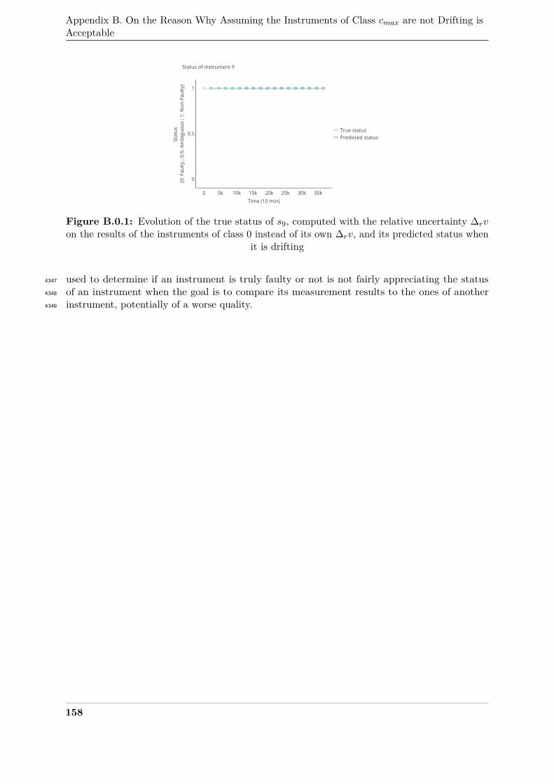
Appendix B. On the Reason Why Assuming the Instruments of Class cmax are not Drifting isAcceptable
0 5k 10k 15k 20k 25k 30k 35k
0
0.5
1
True statusPredicted status
Status of instrument 9
Time (10 min)
Stat
us
(0: F
aulty
; 0.
5: A
mbi
guou
s ; 1
: Non
-Fau
lty)
Figure B.0.1: Evolution of the true status of s9, computed with the relative uncertainty ∆rvon the results of the instruments of class 0 instead of its own ∆rv, and its predicted status when
it is drifting
used to determine if an instrument is truly faulty or not is not fairly appreciating the status4347
of an instrument when the goal is to compare its measurement results to the ones of another4348
instrument, potentially of a worse quality.4349
158
Appendix4350
C4351
Sensitivity of the Diagnosis4352
Algorithm: Case Study with Values4353
Related Over Time for the Parameters4354
of the True Values’ Model4355
1 Introduction4356
We extend here the results of Chapter 4 Section 9.3 on the influence of the model used for4357
the true values in the case study developed in Section 5 of the same chapter. More precisely, an4358
additional case study is provided to confirm that the realism of the model for the true values4359
does not have a major influence.4360
2 Model used4361
We propose to use for the true values the same model as in Chapter 4 Section 3 but instead4362
of using values drawn randomly for the amplitude and FWHM of the Gaussian curve at each4363
time step, the dataset that was exploited in Chapter 3 Section 3 is considered here to derive4364
these values. Thus, the values of the amplitude and FWHM of the Gaussian curve are related4365
from one time step to another.4366
In this dataset, the values are given hourly. As we used a time step equivalent to 10min4367
in Chapter 4 Section 3, the dataset has to be resampled. The missing values are interpolated4368
linearly.4369
Apart from the model for the true values, the case study is identical to the one of Chapter 44370
Section 8 (case study of Section 3 with improvements regarding false results and the adjustment4371
of |Φv|min|).4372
3 Results4373
Table C.3.1 gives the values of each metric. Compared to the results of Table 4.8.1 and4374
considering there is a slightly higher prevalence here (0.88 instead of 0.76), e.g. more faulty cases4375
that non-faulty ones, we observe there are less false negative results (10 instead of 14). The4376
number of true negatives TN is equal to the number of negative cases N (18). Thus, there are4377
no false positives. There are also no predicted statuses equal to ambiguous.4378
Therefore, the TNR and TPR are high (1.00 and 0.93) and so is the PPV (1.00). Only4379
the NPV and FOR are worse than with a random draw of the parameters of the model of the4380
true values (0.64 and 0.36 respectively instead of 0.72 and 0.28) . Although, considering the low4381
159
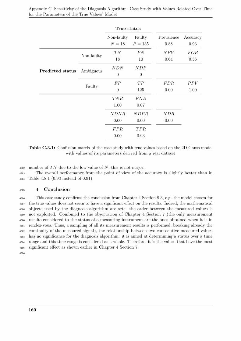
Appendix C. Sensitivity of the Diagnosis Algorithm: Case Study with Values Related Over Timefor the Parameters of the True Values’ Model
True status
Non-faulty Faulty Prevalence AccuracyN = 18 P = 135 0.88 0.93
Non-faulty TN FN NPV FOR
18 10 0.64 0.36
Predicted status Ambiguous NDN NDP
0 0
Faulty FP TP FDR PPV
0 125 0.00 1.00
TNR FNR
1.00 0.07
NDNR NDPR NDR
0.00 0.00 0.00
FPR TPR
0.00 0.93
Table C.3.1: Confusion matrix of the case study with true values based on the 2D Gauss modelwith values of its parameters derived from a real dataset
number of TN due to the low value of N , this is not major.4382
The overall performance from the point of view of the accuracy is slightly better than in4383
Table 4.8.1 (0.93 instead of 0.91)4384
4 Conclusion4385
This case study confirms the conclusion from Chapter 4 Section 9.3, e.g. the model chosen for4386
the true values does not seem to have a significant effect on the results. Indeed, the mathematical4387
objects used by the diagnosis algorithm are sets: the order between the measured values is4388
not exploited. Combined to the observation of Chapter 4 Section 7 (the only measurement4389
results considered to the status of a measuring instrument are the ones obtained when it is in4390
rendez-vous. Thus, a sampling of all its measurement results is performed, breaking already the4391
continuity of the measured signal), the relationship between two consecutive measured values4392
has no significance for the diagnosis algorithm: it is aimed at determining a status over a time4393
range and this time range is considered as a whole. Therefore, it is the values that have the most4394
significant effect as shown earlier in Chapter 4 Section 7.4395
4396
160

Bibliography4397
[1] Mohammed Abo-Zahhad, Sabah M. Ahmed, Nabil Sabor, and Shigenobu Sasaki. “Mobile4398
Sink-Based Adaptive Immune Energy-Efficient Clustering Protocol for Improving the4399
Lifetime and Stability Period of Wireless Sensor Networks”. In: IEEE Sensors Journal4400
15.8 (2015), pp. 4576–4586. doi: 10.1109/JSEN.2015.2424296.4401
[2] Airparif. Airparif website. 2020. url: https://www.airparif.asso.fr (visited on4402
01/29/2019).4403
[3] Airparif. Laboratoire de métrologie. 2020. url: https : / / www . airparif . asso . fr /4404
methodes-surveillance/laboratoire-metrologie (visited on 01/29/2019).4405
[4] Adrian Arfire, Ali Marjovi, and Alcherio Martinoli. “Model-based rendezvous calibration4406
of mobile sensor networks for monitoring air quality”. In: 2015 IEEE SENSORS. 2015,4407
pp. 1–4. doi: 10.1109/ICSENS.2015.7370258.4408
[5] Algirdas Avižienis, Jean-Claude Laprie, Brian Randell, and Carl Landwehr. “Basic Con-4409
cepts and Taxonomy of Dependable and Secure Computing”. In: IEEE Transactions on4410
Dependable and Secure Computing 1.1 (2004), pp. 11–33. doi: 10.1109/TDSC.2004.2.4411
[6] Marek Badura, Piotr Batog, Anetta Drzeniecka-Osiadacz, and Piotr Modzel. “Regression4412
methods in the calibration of low-cost sensors for ambient particulate matter measure-4413
ments”. In: SN Applied Sciences 1.6 (2019). doi: 10.1007/s42452-019-0630-1.4414
[7] Laura Balzano and Robert Nowak. “Blind Calibration of Sensor Networks”. In: 2007 6th4415
International Symposium on Information Processing in Sensor Networks (2007), pp. 79–88.4416
doi: 10.1109/IPSN.2007.4379667.4417
[8] Jose M. Barcelo-Ordinas, Messaoud Doudou, Jorge Garcia-Vidal, and Nadjib Badache.4418
“Self-calibration methods for uncontrolled environments in sensor networks: A reference4419
survey”. In: Ad Hoc Networks 88 (2019), pp. 142–159. doi: 10.1016/j.adhoc.2019.01.4420
008.4421
[9] Jose M. Barcelo-Ordinas, Pau Ferrer-Cid, Jorge Garcia-Vidal, Anna Ripoll, and Mar4422
Viana. “Distributed multi-scale calibration of low-cost ozone sensors in wireless sensor4423
networks”. In: Sensors (Switzerland) 19.11 (2019), pp. 1–25. doi: 10.3390/s19112503.4424
[10] Jose M. Barcelo-Ordinas, Jorge Garcia-Vidal, Messaoud Doudou, Santiago Rodrigo-Munoz,4425
and Albert Cerezo-Llavero. “Calibrating low-cost air quality sensors using multiple arrays4426
of sensors”. In: IEEE Wireless Communications and Networking Conference, WCNC.4427
2018, pp. 1–6. doi: 10.1109/WCNC.2018.8377051.4428
[11] Thomas Becnel, Tofigh Sayahi, Kerry Kelly, and Pierre Emmanuel Gaillardon. “A recursive4429
approach to partially blind calibration of a pollution sensor network”. In: 2019 IEEE4430
International Conference on Embedded Software and Systems, ICESS 2019. 2019. doi:4431
10.1109/ICESS.2019.8782523.4432
161
BIBLIOGRAPHY
[12] Antoine Berchet, Katrin Zink, Clive Muller, Dietmar Oettl, Juerg Brunner, Lukas4433
Emmenegger, and Dominik Brunner. “A cost-effective method for simulating city-wide air4434
flow and pollutant dispersion at building resolving scale”. In: Atmospheric Environment4435
158 (2017), pp. 181–196. doi: 10.1016/j.atmosenv.2017.03.030.4436
[13] Cagdas Bilen, Gilles Puy, Rémi Gribonval, and Laurent Daudet. “Convex Optimization4437
Approaches for Blind Sensor Calibration using Sparsity”. In: IEEE Transactions on Signal4438
Processing (2013), pp. 1–11. doi: 10.1109/TSP.2014.2342651.4439
[14] BIPM, IEC, IFCC, ILAC, IUPAC, IUPAP, ISO, and OIML. International vocabulary4440
of metrology - Basic and general concepts and associated terms (VIM). 3rd edn. JCGM4441
200:2012, 2012.4442
[15] C. Borrego, A. M. Costa, J. Ginja, M. Amorim, M. Coutinho, K. Karatzas, Th Sioumis, N.4443
Katsifarakis, K. Konstantinidis, S. De Vito, et al. “Assessment of air quality microsensors4444
versus reference methods: The EuNetAir joint exercise”. In: Atmospheric Environment4445
147.2 (2016), pp. 246–263. doi: 10.1016/j.atmosenv.2016.09.050.4446
[16] C. Borrego, J. Ginja, M. Coutinho, C. Ribeiro, K. Karatzas, Th Sioumis, N. Katsifarakis,4447
K. Konstantinidis, Saverio De Vito, Elena Esposito, et al. “Assessment of air quality4448
microsensors versus reference methods: The EuNetAir Joint Exercise – Part II”. In:4449
Atmospheric Environment 193 (2018), pp. 127–142. doi: 10.1016/j.atmosenv.2018.08.4450
028.4451
[17] A. Botchkarev. “A New Typology Design of Performance Metrics to Measure Errors in4452
Machine Learning Regression Algorithms”. In: Interdisciplinary Journal of Information,4453
Knowledge, and Management 14 (2019), pp. 045–076. doi: 10.28945/4184.4454
[18] Ahmed Boubrima, Walid Bechkit, and Herve Rivano. “A new WSN deployment approach4455
for air pollution monitoring”. In: 2017 14th IEEE Annual Consumer Communications4456
and Networking Conference, CCNC 2017. 2017, pp. 455–460. doi: 10.1109/CCNC.2017.4457
7983151.4458
[19] Ahmed Boubrima, Walid Bechkit, and Herve Rivano. “Optimal WSN Deployment Models4459
for Air Pollution Monitoring”. In: IEEE Transactions on Wireless Communications 16.54460
(2017), pp. 2723–2735. doi: 10.1109/TWC.2017.2658601.4461
[20] Ahmed Boubrima, Walid Bechkit, and Hervé Rivano. “On the Deployment of Wireless4462
Sensor Networks for Air Quality Mapping: Optimization Models and Algorithms”. In:4463
IEEE/ACM Transactions on Networking 27.4 (Aug. 2019), pp. 1629–1642. doi: 10.1109/4464
TNET.2019.2923737.4465
[21] Ahmed Boubrima, Walid Bechkit, Hervé Rivano, and Lionel Soulhac. “Leveraging the4466
Potential of WSN for an Efficient Correction of Air Pollution Fine-Grained Simulations”.4467
In: The 27th International Conference on Computer Communications and Networks4468
(ICCCN 2018). Hangzou, China, 2018, pp. 1–9. doi: 10.1109/ICCCN.2018.8487343.4469
[22] Marcel Bruins, Jan Willem, Wendy W. J. Van De Sande, Alex Van Belkum, and Albert4470
Bos. “Enabling a transferable calibration model for metal-oxide type electronic noses”.4471
In: Sensors and Actuators: B. Chemical 188 (2013), pp. 1187–1195. doi: 10.1016/j.snb.4472
2013.08.006.4473
[23] Seamus Buadhachain and Gregory Provan. “A model-based control method for decen-4474
tralized calibration of wireless sensor networks”. In: 2013 American Control Conference.4475
2013, pp. 6571–6576. doi: 10.1109/ACC.2013.6580870.4476
162
BIBLIOGRAPHY
[24] Vladimir Bychkovskiy, Seapahn Megerian, Deborah Estrin, and Miodrag Potkonjak.4477
“A collaborative approach to in-place sensor calibration”. In: Proceedings of the 2nd4478
International Conference on Information Processing in Sensor Networks. 2003, pp. 301–4479
316. doi: 10.1007/3-540-36978-3_20.4480
[25] Valerio Cambareri and Laurent Jacques. “A Non-Convex Blind Calibration Method for4481
Randomised Sensing Strategies”. In: 2016 4th International Workshop on Compressed4482
Sensing Theory and its Applications to Radar, Sonar and Remote Sensing (CoSeRa). 2016,4483
pp. 16–20. doi: 10.1109/CoSeRa.2016.7745690.4484
[26] Joanna Gordon Casey and Michael P. Hannigan. “Testing the performance of field4485
calibration techniques for low-cost gas sensors in new deployment locations: across a4486
county line and across Colorado”. In: Atmospheric Measurement Techniques 11.11 (2018),4487
pp. 6351–6378. doi: 10.5194/amt-11-6351-2018.4488
[27] Nuria Castell, Franck R. Dauge, Philipp Schneider, Matthias Vogt, Uri Lerner, Barak4489
Fishbain, David M. Broday, and Alena Bartonova. “Can commercial low-cost sensor4490
platforms contribute to air quality monitoring and exposure estimates?” In: Environment4491
International 99 (2017), pp. 293–302. doi: 10.1016/j.envint.2016.12.007.4492
[28] Prasenjit Chanak, Indrajit Banerjee, and R. Simon Sherratt. “Mobile sink based fault4493
diagnosis scheme for wireless sensor networks”. In: Journal of Systems and Software 1194494
(2016), pp. 45–57. doi: 10.1016/j.jss.2016.05.041.4495
[29] Jinran Chen, Shubha Kher, and Arun Somani. “Distributed fault detection of wireless4496
sensor networks”. In: Proceedings of the 2006 workshop on Dependability issues in wireless4497
ad hoc networks and sensor networks - DIWANS ’06. 2006, p. 65. doi: 10.1145/1160972.4498
1160985.4499
[30] Tinghuan Chen, Bingqing Lin, Hao Geng, and Bei Yu. “Sensor drift calibration via spatial4500
correlation model in smart building”. In: Proceedings - Design Automation Conference.4501
2019. doi: 10.1145/3316781.3317909.4502
[31] Yun Cheng, Xiaoxi He, Zimu Zhou, and Lothar Thiele. “ICT: In-field Calibration Transfer4503
for Air Quality Sensor Deployments”. In: Proceedings of the ACM on Interactive, Mobile,4504
Wearable and Ubiquitous Technologies 3.1 (2019), pp. 1–19. doi: 10.1145/3314393.4505
[32] Yong-Seung Chung, Tae-Koon Kim, and Ki-Hyun Kim. “Temporal variation and cause of4506
acidic precipitation from a monitoring network in Korea”. In: Atmospheric Environment4507
30.13 (1996), pp. 2429–2435. doi: 10.1016/1352-2310(95)00186-7.4508
[33] Andrea L. Clements, William G. Griswold, Abhijit Rs, Jill E. Johnston, Megan M. Herting,4509
Jacob Thorson, Ashley Collier-Oxandale, and Michael Hannigan. “Low-Cost Air Quality4510
Monitoring Tools : From Research to Practice (A Workshop Summary)”. In: Sensors 17.114511
(2017). doi: 10.3390/s17112478.4512
[34] José María Cordero, Rafael Borge, and Adolfo Narros. “Using statistical methods to carry4513
out in field calibrations of low cost air quality sensors”. In: Sensors and Actuators, B:4514
Chemical 267.2 (2018), pp. 245–254. doi: 10.1016/j.snb.2018.04.021.4515
[35] Eben S. Cross, Leah R. Williams, David K. Lewis, Gregory R. Magoon, Timothy B. Onasch,4516
Michael L. Kaminsky, Douglas R. Worsnop, and John T. Jayne. “Use of electrochemical4517
sensors for measurement of air pollution: Correcting interference response and validating4518
measurements”. In: Atmospheric Measurement Techniques 10.9 (2017), pp. 3575–3588.4519
doi: 10.5194/amt-10-3575-2017.4520
163
BIBLIOGRAPHY
[36] Saverio De Vito, P Delli Veneri, Elena Esposito, Maria Salvato, W. Bright, R. L. Jones,4521
and Olalekan A.M. Popoola. “Dynamic Multivariate Regression For On-Field Calibration4522
Of High Speed Air Quality Chemical Multi-Sensor Systems”. In: 2015 XVIII AISEM4523
Annual Conference. 2015, pp. 1–3. doi: 10.1109/AISEM.2015.7066794.4524
[37] Florentin Delaine, Bérengère Lebental, and Hervé Rivano. Example case study applying a4525
"Framework for the Simulation of Sensor Networks Aimed at Evaluating In Situ Calibration4526
Algorithms". Version V1. 2020. doi: 10.25578/CJCYMZ.4527
[38] François Derkx, Bérengère Lebental, Tarik Bourouina, Frédéric Bourquin, Costel-Sorin4528
Cojocaru, Enric Robine, and Henri Van Damme. “The Sense-City project”. In: XVIIIth4529
Symposium on Vibrations, Shocks and Noise. 2012.4530
[39] Sharvari Deshmukh, Kalyani Kamde, Arun Jana, Sanjivani Korde, Rajib Bandyopadhyay,4531
Ravi Sankar, Nabarun Bhattacharyya, and R A Pandey. “Calibration transfer between4532
electronic nose systems for rapid In situ measurement of pulp and paper industry emissions”.4533
In: Analytica Chimica Acta 841 (2014), pp. 58–67. doi: 10.1016/j.aca.2014.05.054.4534
[40] Clément Dorffer. “Méthodes informées de factorisation matricielle pour l’étalonnage de4535
réseaux de capteurs mobiles et la cartographie de champs de pollution”. PhD thesis.4536
Université du Littoral Côte d’Opale, France, 2017.4537
[41] Clément Dorffer, Matthieu Puigt, Gilles Delmaire, and Gilles Roussel. “Blind Calibration of4538
Mobile Sensors Using Informed Nonnegative Matrix Factorization”. In: 12th International4539
Conference on Latent Variable Analysis and Signal Separation (LVA/ICA 2015). 2015,4540
pp. 497–505. doi: 10.1109/ICASSP.2016.7472216.4541
[42] Clément Dorffer, Matthieu Puigt, Gilles Delmaire, and Gilles Roussel. “Blind mobile4542
sensor calibration using an informed nonnegative matrix factorization with a relaxed4543
rendezvous model”. In: 2016 IEEE International Conference on Acoustics, Speech and4544
Signal Processing (ICASSP). 2016, pp. 2941–2945. doi: 10.1109/ICASSP.2016.7472216.4545
[43] Clément Dorffer, Matthieu Puigt, Gilles Delmaire, and Gilles Roussel. “Nonlinear mobile4546
sensor calibration using informed semi-nonnegative matrix factorization with a Vander-4547
monde factor”. In: 2016 IEEE Sensor Array and Multichannel Signal Processing Workshop4548
(SAM). 2016. doi: 10.1109/SAM.2016.7569735.4549
[44] Clément Dorffer, Matthieu Puigt, Gilles Delmaire, and Gilles Roussel. “Outlier-robust4550
calibration method for sensor networks”. In: Proceedings of the 2017 IEEE Interna-4551
tional Workshop of Electronics, Control, Measurement, Signals and their Application to4552
Mechatronics, ECMSM 2017. 2017. doi: 10.1109/ECMSM.2017.7945907.4553
[45] Clément Dorffer, Matthieu Puigt, Gilles Delmaire, and Gilles Roussel. “Informed Nonneg-4554
ative Matrix Factorization Methods for Mobile Sensor Network Calibration”. In: IEEE4555
Transactions on Signal and Information Processing over Networks 4.4 (2018), pp. 667–682.4556
doi: 10.1109/TSIPN.2018.2811962.4557
[46] Bénédicte Dousset, Françoise Gourmelon, Karine Laaidi, Abdelkrim Zeghnoun, Emmanuel4558
Giraudet, Philippe Bretin, Elena Mauri, and Stéphanie Vandentorren. “Satellite monitoring4559
of summer heat waves in the Paris metropolitan area”. In: International Journal of4560
Climatology 31.2 (2011), pp. 313–323. doi: 10.1002/joc.2222.4561
[47] Elena Esposito, Saverio De Vito, Maria Salvato, V. Bright, R. L. Jones, and O. Popoola.4562
“Dynamic neural network architectures for on field stochastic calibration of indicative low4563
cost air quality sensing systems”. In: Sensors and Actuators, B: Chemical 231 (2016),4564
pp. 701–713. doi: 10.1016/j.snb.2016.03.038.4565
164

BIBLIOGRAPHY
[48] Elena Esposito, Saverio De Vito, Maria Salvato, Grazia Fattoruso, V Bright, R L Jones,4566
Dte-fsn-dineneap E Fermi, and Portici Na. “Stochastic Comparison of Machine Learning4567
Approaches to Calibration of Mobile Air Quality Monitors”. In: Sensors: Proceedings of4568
the Third National Conference on Sensors. 2018. doi: 10.1007/978-3-319-55077-0_38.4569
[49] Elena Esposito, Saverio De Vito, Maria Salvato, Grazia Fattoruso, and Girolamo Di4570
Francia. “Computational Intelligence for Smart Air Quality Monitors Calibration”. In:4571
Computational Science and Its Applications - ICCSA 2017. 2017, pp. 443–454. doi:4572
10.1007/978-3-319-62398-6_31.4573
[50] Xinwei Fang and Iain Bate. “Using Multi-parameters for Calibration of Low-cost Sensors in4574
Urban Environment”. In: Proceedings of the 2017 International Conference on Embedded4575
Wireless Systems and Networks. 2017, pp. 1–11.4576
[51] Xinwei Fang and Iain Bate. “An Improved Sensor Calibration with Anomaly Detection and4577
Removal”. In: Sensors and Actuators, B: Chemical 307.November 2019 (2020), p. 127428.4578
doi: 10.1016/j.snb.2019.127428.4579
[52] Yang Feiyue, Tao Yang, Zhang Siqing, Dai Jianjian, Xu Juan, and Hou Yao. “A Faulty node4580
detection algorithm based on spatial-temporal cooperation in wireless sensor networks”.4581
In: Procedia Computer Science. Vol. 131. Elsevier B.V., 2018, pp. 1089–1094. doi: 10.4582
1016/j.procs.2018.04.266.4583
[53] Pau Ferrer-Cid, Jose M. Barcelo-Ordinas, Jorge Garcia-Vidal, Anna Ripoll, and Mar4584
Viana. “A comparative Study of Calibration Methods for Low-Cost Ozone Sensors in IoT4585
Platforms”. In: IEEE Internet of Things Journal PP.X (2019), pp. 1–1. doi: 10.1109/4586
jiot.2019.2929594.4587
[54] Barak Fishbain, Uri Lerner, Nuria Castell, Tom Cole-Hunter, Olalekan A.M. Popoola,4588
David M. Broday, Tania Martinez-Iñiguez, Mark Nieuwenhuijsen, Milena Jovašević-4589
Stojanović, Dušan Topalović, et al. “An evaluation tool kit of air quality micro-sensing4590
units”. In: Science of the Total Environment 575 (2017), pp. 639–648. doi: 10.1016/j.4591
scitotenv.2016.09.061.4592
[55] Barak Fishbain and Erick Moreno-Centeno. “Self Calibrated Wireless Distributed Envi-4593
ronmental Sensory Networks”. In: Scientific Reports 6 (2016), pp. 1–10. doi: 10.1038/4594
srep24382.4595
[56] J. Fonollosa, L. Fernandez, A. Gutierrez-Galvez, R. Huerta, and S. Marco. “Calibration4596
transfer and drift counteraction in chemical sensor arrays using Direct Standardization”.4597
In: Sensors and Actuators, B: Chemical 236 (2016), pp. 1044–1053. doi: 10.1016/j.snb.4598
2016.05.089.4599
[57] Kaibo Fu, Wei Ren, and Wei Dong. “Multihop Calibration for Mobile Sensing : k-hop4600
Calibratability and Reference Sensor Deployment”. In: IEEE INFOCOM 2017 - IEEE4601
Conference on Computer Communications. 2017, pp. 1–9. doi: 10.1109/INFOCOM.2017.4602
8056962.4603
[58] Meiling Gao, Junji Cao, and Edmund Seto. “A distributed network of low-cost continuous4604
reading sensors to measure spatiotemporal variations of PM2.5 in Xi’an, China”. In:4605
Environmental Pollution 199 (2015), pp. 56–65. doi: 10.1016/j.envpol.2015.01.013.4606
[59] Hugh S. Gorman and Erik M. Conway. “Monitoring the environment: Taking a historical4607
perspective”. In: Environmental Monitoring and Assessment 106.1-3 (2005), pp. 1–10.4608
doi: 10.1007/s10661-005-0755-0.4609
165
BIBLIOGRAPHY
[60] Gayle S.W. Hagler, Ronald Williams, Vasileios Papapostolou, and Andrea Polidori. “Air4610
Quality Sensors and Data Adjustment Algorithms: When Is It No Longer a Measurement?”4611
In: Environmental Science and Technology 52.10 (2018), pp. 5530–5531. doi: 10.1021/4612
acs.est.8b01826.4613
[61] S.R. Hanna, G.A. Briggs, and R.P. Jr. Hosker. Handbook on atmospheric diffusion. Tech.4614
rep. National Oceanic, Atmospheric Administration, Oak Ridge, TN (USA). Atmospheric4615
Turbulence, and Diffusion Lab., Jan. 1982. doi: 10.2172/5591108.4616
[62] Jane K. Hart and Kirk Martinez. “Environmental Sensor Networks: A revolution in4617
the earth system science?” In: Earth-Science Reviews 78.3-4 (2006), pp. 177–191. doi:4618
10.1016/j.earscirev.2006.05.001.4619
[63] David Hasenfratz, Olga Saukh, and Lothar Thiele. “On-the-fly calibration of low-cost gas4620
sensors”. In: Proceedings of the 9th European Conference on Wireless Sensor Networks.4621
Ed. by Gian Pietro Picco and Wendi Heinzelman. Springer Berlin Heidelberg, 2012,4622
pp. 228–244. doi: 10.1007/978-3-642-28169-3_15.4623
[64] D. M. Holstius, A. Pillarisetti, K. R. Smith, and E. Seto. “Field calibrations of a low-cost4624
aerosol sensor at a regulatory monitoring site in California”. In: Atmospheric Measurement4625
Techniques 7.4 (2014), pp. 1121–1131. doi: 10.5194/amt-7-1121-2014.4626
[65] Alexander T. Ihler, J W Fisher III, Randolph L. Moses, and Alan S. Willsky. “Nonpara-4627
metric belief propagation for self-calibration in sensor networks”. In: Third International4628
Symposium on Information Processing in Sensor Networks, 2004. IPSN 2004. 2004,4629
pp. 225–233. doi: 10.1145/984622.984656.4630
[66] Marian Emanuel Ionascu, Iasmina Gruicin, and Marius Marcu. “Towards Wearable Air4631
Quality Monitoring Systems - Initial Assessments on Newly Developed Sensors”. In: 20184632
26th Telecommunications Forum, TELFOR 2018 - Proceedings. IEEE, 2018, pp. 1–4. doi:4633
10.1109/TELFOR.2018.8611832.4634
[67] International Organization for Standardization. ISO 9001:2015(E), Quality management4635
systems - Requirements. Tech. rep. Geneva, CH: International Organization for Standard-4636
ization, Oct. 2015.4637
[68] Rohan Jayaratne, Xiaoting Liu, Phong Thai, Matthew Dunbabin, and Lidia Morawska.4638
“The influence of humidity on the performance of a low-cost air particle mass sensor and4639
the effect of atmospheric fog”. In: Atmospheric Measurement Techniques 11.8 (2018),4640
pp. 4883–4890. doi: 10.5194/amt-11-4883-2018.4641
[69] Sai Ji, Shen Fang Yuan, Ting Huai Ma, and Chang Tan. “Distributed fault detection for4642
wireless sensor based on weighted average”. In: NSWCTC 2010 - The 2nd International4643
Conference on Networks Security, Wireless Communications and Trusted Computing.4644
Vol. 1. 2010, pp. 57–60. doi: 10.1109/NSWCTC.2010.21.4645
[70] Jinfang Jiang, Guangjie Han, Feng Wang, Lei Shu, and Mohsen Guizani. “An Efficient4646
Distributed Trust Model for Wireless Sensor Networks”. In: IEEE Transactions on Parallel4647
and Distributed Systems 26.5 (2015), pp. 1228–1237. doi: 10.1109/TPDS.2014.2320505.4648
[71] Wan Jiao, Gayle Hagler, Ronald Williams, Robert Sharpe, Ryan Brown, Daniel Garver,4649
Robert Judge, Motria Caudill, Joshua Rickard, Michael Davis, et al. “Community Air4650
Sensor Network (CAIRSENSE) project : evaluation of low-cost sensor performance in a4651
suburban environment in the southeastern United States”. In: Atmospheric Measurement4652
Techniques 9 (2016), pp. 5281–5292. doi: 10.5194/amt-9-5281-2016.4653
[72] Joint Committee For Guides In Metrology. Evaluation of measurement data — Guide to4654
the expression of uncertainty in measurement. Vol. 50. September. 2008, p. 134.4655
166
BIBLIOGRAPHY
[73] Federico Karagulian, Maurizio Barbiere, Alexander Kotsev, Laurent Spinelle, Michel4656
Gerboles, Friedrich Lagler, Nathalie Redon, Sabine Crunaire, and Annette Borowiak.4657
“Review of the performance of low-cost sensors for air quality monitoring”. In: Atmosphere4658
10.9 (2019). doi: 10.3390/atmos10090506.4659
[74] Jinsol Kim, Alexis A. Shusterman, Kaitlyn J. Lieschke, Catherine Newman, and Ronald C.4660
Cohen. “The Berkeley Atmospheric CO2 Observation Network: Field calibration and4661
evaluation of low-cost air quality sensors”. In: Atmospheric Measurement Techniques 11.44662
(2018), pp. 1937–1946. doi: 10.5194/amt-11-1937-2018.4663
[75] Fadi Kizel, Yael Etzion, Rakefet Shafran-Nathan, Ilan Levy, Barak Fishbain, Alena4664
Bartonova, and David M. Broday. “Node-to-node field calibration of wireless distributed4665
air pollution sensor network”. In: Environmental Pollution 233 (2018), pp. 900–909. doi:4666
10.1016/j.envpol.2017.09.042.4667
[76] Dheeraj Kumar, Sutharshan Rajasegarar, and Marimuthu Palaniswami. “Automatic sensor4668
drift detection and correction using spatial kriging and kalman filtering”. In: 2013 IEEE4669
International Conference on Distributed Computing in Sensor Systems. 2013, pp. 183–190.4670
doi: 10.1109/DCOSS.2013.52.4671
[77] Dheeraj Kumar, Sutharshan Rajasegarar, and Marimuthu Palaniswami. “Geospatial4672
Estimation-Based Auto Drift Correction in Wireless Sensor Networks”. In: ACM Transac-4673
tions on Sensor Networks 11.3 (2015), 50:1–50:39. doi: 10.1145/2736697.4674
[78] Prashant Kumar, Lidia Morawska, Claudio Martani, George Biskos, Marina Neophytou,4675
Silvana Di Sabatino, Margaret Bell, Leslie Norford, and Rex Britter. “The rise of low-cost4676
sensing for managing air pollution in cities”. In: Environment International 75 (2015),4677
pp. 199–205. doi: 10.1016/j.envint.2014.11.019.4678
[79] Intel Berkeley Research lab. Intel Lab Data. 2004. url: http://db.lcs.mit.edu/4679
labdata/labdata.html (visited on 10/22/2019).4680
[80] Rachid Laref, Etienne Losson, Alexandre Sava, and Maryam Siadat. “Support vector4681
machine regression for calibration transfer between electronic noses dedicated to air4682
pollution monitoring”. In: Sensors 18.11 (2018). doi: 10.3390/s18113716.4683
[81] Alain Le Tertre, Agnès Lefranc, Daniel Eilstein, Christophe Declercq, Sylvia Medina,4684
Myriam Blanchard, Benoît Chardon, Pascal Fabre, Laurent Filleul, Jean-françois Jusot,4685
et al. “Impact of the 2003 Heatwave on All-Cause Mortality in 9 French Cities”. In:4686
Epidemiology 17.1 (2014), pp. 75–79. doi: 10.1097/01.ede.0000187650.36636.1f.4687
[82] Byung Tak Lee, Seung Chul Son, and Kyungran Kang. “A blind calibration scheme4688
exploiting mutual calibration relationships for a dense mobile sensor network”. In: IEEE4689
Sensors Journal 14.5 (2014), pp. 1518–1526. doi: 10.1109/JSEN.2013.2297714.4690
[83] Myeong-Hyeon Lee and Yoon-Hwa Choi. “Distributed diagnosis of wireless sensor net-4691
works”. In: TENCON 2007 - 2007 IEEE Region 10 Conference. 2007, pp. 2159–3450. doi:4692
10.1109/TENCON.2007.4429026.4693
[84] Alastair C. Lewis, Erika Von Schneidemesser, and Richard E. Peltier. Low-cost sensors for4694
the measurement of atmospheric composition: overview of topic and future applications.4695
Tech. rep. May. World Meteorological Organization (WMO), 2018.4696
[85] Hongyong Li, Yujiao Zhu, Yong Zhao, Tianshu Chen, Ying Jiang, Ye Shan, Yuhong Liu,4697
Jiangshan Mu, Xiangkun Yin, Di Wu, et al. “Evaluation of the performance of low-cost4698
air quality sensors at a high mountain station with complex meteorological conditions”.4699
In: Atmosphere 11.2 (2020), pp. 1–16. doi: 10.3390/atmos11020212.4700
167
BIBLIOGRAPHY
[86] Jason Jingshi Li, Boi Faltings, Olga Saukh, David Hasenfratz, and Jan Beutel. “Sensing4701
the Air We Breathe-The OpenSense Zurich Dataset.” In: Proceedings of the Twenty-Sixth4702
AAAI Conference on Artificial Intelligence. 2012, pp. 323–325.4703
[87] Zhan Li, Yuzhi Wang, Anqi Yang, and Huazhong Yang. “Drift detection and calibration4704
of sensor networks”. In: 2015 International Conference on Wireless Communications and4705
Signal Processing, WCSP 2015. 2015, pp. 1–6. doi: 10.1109/WCSP.2015.7341138.4706
[88] Chun Lin, Nicola Masey, Hao Wu, Mark Jackson, David J Carruthers, Stefan Reis, Ruth M4707
Doherty, Iain J Beverland, and Mathew R Heal. “Practical Field Calibration of Portable4708
Monitors for Mobile Measurements of Multiple Air Pollutants”. In: Atmosphere 8.124709
(2017). doi: 10.3390/atmos8120231.4710
[89] John Lipor and Laura Balzano. “Robust blind calibration via total least squares”. In: 20144711
IEEE International Conference on Acoustics, Speech and Signal Processing (ICASSP).4712
2014, pp. 4244–4248. doi: 10.1109/ICASSP.2014.6854402.4713
[90] Xiao Liu, Sitian Cheng, Hong Liu, Sha Hu, Daqiang Zhang, and Huansheng Ning. “A4714
survey on gas sensing technology”. In: Sensors 12.7 (2012), pp. 9635–9665. doi: 10.3390/4715
s120709635.4716
[91] Byoung Gook Loh and Gi Heung Choi. “Calibration of Portable Particulate Matter–Monitoring4717
Device using Web Query and Machine Learning”. In: Safety and Health at Work 10.44718
(2019), pp. 452–460. doi: 10.1016/j.shaw.2019.08.002.4719
[92] Xuanwen Luo and Ming Dong. “Distributed Faulty Sensor Detection in Sensor Networks”.4720
In: Artificial Neural Networks – ICANN 2009. 2009, pp. 964–975. doi: 10.1007/978-3-4721
642-04277-5_97.4722
[93] Balz Maag, Olga Saukh, David Hasenfratz, and Lothar Thiele. “Pre-Deployment Testing,4723
Augmentation and Calibration of Cross-Sensitive Sensors”. In: Proceedings of the 20164724
International Conference on Embedded Wireless Systems and Networks. 2016, pp. 169–180.4725
[94] Balz Maag, Zimu Zhou, Olga Saukh, and Lothar Thiele. “SCAN: Multi-Hop Calibration4726
for Mobile Sensor Arrays”. In: Proc. ACM Interact. Mob. Wearable Ubiquitous Technol.4727
1.2 (2017), 19:1–19:21. doi: 10.1145/3090084.4728
[95] Balz Maag, Zimu Zhou, and Lothar Thiele. “A Survey on Sensor Calibration in Air4729
Pollution Monitoring Deployments”. In: IEEE Internet of Things Journal 5.6 (2018),4730
pp. 4857–4870. doi: 10.1109/JIOT.2018.2853660.4731
[96] Sachit Mahajan and Prashant Kumar. “Evaluation of low-cost sensors for quantitative4732
personal exposure monitoring”. In: Sustainable Cities and Society 57.January (2020),4733
p. 102076. doi: 10.1016/j.scs.2020.102076.4734
[97] Arunanshu Mahapatro and Pabitra Mohan Khilar. “Online distributed fault diagnosis in4735
wireless sensor networks”. In: Wireless Personal Communications 71.3 (2013), pp. 1931–4736
1960. doi: 10.1007/s11277-012-0916-8.4737
[98] Arunanshu Mahapatro and Ajit Kumar Panda. “Fault Diagnosis in Wireless Sensor4738
Networks: A Survey”. In: IEEE Communications Surveys Tutorials Early Acce (2013),4739
pp. 1–27. doi: 10.1109/SURV.2013.030713.00062.4740
[99] Arunanshu Mahapatro and Ajit Kumar Panda. “Choice of detection parameters on4741
fault detection in wireless sensor networks: A multiobjective optimization approach”. In:4742
Wireless Personal Communications 78.1 (2014), pp. 649–669. doi: 10.1007/s11277-014-4743
1776-1.4744
168
BIBLIOGRAPHY
[100] Carl Malings, Rebecca Tanzer, Aliaksei Hauryliuk, Sriniwasa P. N. Kumar, Naomi Zim-4745
merman, Levent B. Kara, Albert A. Presto, and R. Subramanian. “Development of a4746
General Calibration Model and Long-Term Performance Evaluation of Low-Cost Sensors4747
for Air Pollutant Gas Monitoring”. In: Atmospheric Measurement Techniques Discussions4748
(2018), pp. 1–30. doi: 10.5194/amt-2018-216.4749
[101] Ali Marjovi, Adrian Arfire, and Alcherio Martinoli. “High Resolution Air Pollution Maps4750
in Urban Environments Using Mobile Sensor Networks”. In: 2015 International Conference4751
on Distributed Computing in Sensor Systems (2015), pp. 11–20. doi: 10.1109/DCOSS.4752
2015.32.4753
[102] Jan-Frederic Markert, Matthias Budde, Gregor Schindler, Markus Klug, and Michael Beigl.4754
“Privacy-Preserving Collaborative Blind Macro-Calibration of Environmental Sensors4755
in Participatory Sensing”. In: EAI Endorsed Transactions on Internet of Things 18.104756
(2018), pp. 1–8. doi: 10.4108/eai.15-1-2018.153564.4757
[103] Cory R. Martin, Ning Zeng, Anna Karion, Russell R. Dickerson, Xinrong Ren, Bari N.4758
Turpie, and Kristy J. Weber. “Evaluation and environmental correction of ambient CO24759
measurements from a low-cost NDIR sensor”. In: Atmospheric Measurement Techniques4760
10.7 (2017), pp. 2383–2395. doi: 10.5194/amt-10-2383-2017.4761
[104] Measurement specialities. HS1101LF – Relative Humidity Sensor Datasheet. 2012. url:4762
https://docs-emea.rs-online.com/webdocs/142c/0900766b8142cdcd.pdf (visited4763
on 09/26/2018).4764
[105] Measurement specialities. NO2-B43F – Nitrogen Dioxide Sensor Datasheet. 2019. url:4765
http://www.alphasense.com/WEB1213/wp-content/uploads/2019/09/NO2-B43F.pdf4766
(visited on 10/22/2019).4767
[106] Amjad Mehmood, Nabil Alrajeh, Mithun Mukherjee, Salwani Abdullah, and Houbing Song.4768
“A survey on proactive, active and passive fault diagnosis protocols for WSNs: Network4769
operation perspective”. In: Sensors (Switzerland) 18.6 (2018). doi: 10.3390/s18061787.4770
[107] Emiliano Miluzzo, Nicholas D. Lane, Andrew T. Campbell, and Reza Olfati-Saber. “Cali-4771
Bree: A self-calibration system for mobile sensor networks”. In: Distributed Computing in4772
Sensor Systems. 2008, pp. 314–331. doi: 10.1007/978-3-540-69170-9_21.4773
[108] Georgia Miskell, Jennifer A. Salmond, and David E. Williams. “Solution to the Problem of4774
Calibration of Low-Cost Air Quality Measurement Sensors in Networks”. In: ACS Sensors4775
3.4 (2018), pp. 832–843. doi: 10.1021/acssensors.8b00074.4776
[109] Sharon Moltchanov, Ilan Levy, Yael Etzion, Uri Lerner, David M. Broday, and Barak4777
Fishbain. “On the feasibility of measuring urban air pollution by wireless distributed4778
sensor networks”. In: Science of the Total Environment 502 (2015), pp. 537–547. doi:4779
10.1016/j.scitotenv.2014.09.059.4780
[110] Lidia Morawska, Phong K Thai, Xiaoting Liu, Akwasi Asumadu-sakyi, Godwin Ayoko,4781
Alena Bartonova, Andrea Bedini, Fahe Chai, Bryce Christensen, Matthew Dunbabin, et al.4782
“Applications of low-cost sensing technologies for air quality monitoring and exposure4783
assessment : How far have they gone ?” In: Environment International 116 (2018), pp. 286–4784
299. doi: 10.1016/j.envint.2018.04.018.4785
[111] Naser Hossein Motlagh, Eemil Lagerspetz, Petteri Nurmi, Xin Li, Samu Varjonen, Julien4786
Mineraud, Matti Siekkinen, Andrew Rebeiro-Hargrave, Tareq Hussein, Tuukka Petäjä, et4787
al. “Toward Massive Scale Air Quality Monitoring”. In: IEEE Communications Magazine4788
58.2 (2020), pp. 54–59. doi: 10.1109/MCOM.001.1900515.4789
169
BIBLIOGRAPHY
[112] M. Mourad and J.-L. Bertrand-Krajewski. “A method for automatic validation of long4790
time series of data in urban hydrology”. In: Water Science and Technology 45.4-5 (2002),4791
pp. 263–270. doi: 10.2166/wst.2002.0601.4792
[113] Michael Mueller, Jonas Meyer, and Christoph Hueglin. “Design of an ozone and nitrogen4793
dioxide sensor unit and its long-term operation within a sensor network in the city of4794
Zurich”. In: Atmospheric Measurement Techniques 10.10 (2017), pp. 3783–3799. doi:4795
10.5194/amt-10-3783-2017.4796
[114] Thaha Muhammed and Riaz Ahmed Shaikh. “An analysis of fault detection strategies in4797
wireless sensor networks”. In: Journal of Network and Computer Applications 78 (2017),4798
pp. 267–287. doi: 10.1016/j.jnca.2016.10.019.4799
[115] Kevin Ni, Mani Srivastava, Nithya Ramanathan, Mohamed Nabil Hajj Chehade, Laura4800
Balzano, Sheela Nair, Sadaf Zahedi, Eddie Kohler, Greg Pottie, and Mark Hansen. “Sensor4801
network data fault types”. In: ACM Transactions on Sensor Networks 5.3 (2009), pp. 1–29.4802
doi: 10.1145/1525856.1525863.4803
[116] Thor Bjørn Ottosen and Prashant Kumar. “Outlier detection and gap filling methodologies4804
for low-cost air quality measurements”. In: Environmental Science: Processes and Impacts4805
21.4 (2019), pp. 701–713. doi: 10.1039/c8em00593a.4806
[117] F. J. Pierce and T. V. Elliott. “Regional and on-farm wireless sensor networks for4807
agricultural systems in Eastern Washington”. In: Computers and Electronics in Agriculture4808
61.1 (2008), pp. 32–43. doi: 10.1016/j.compag.2007.05.007.4809
[118] Olalekan A.M. Popoola, Gregor B. Stewart, Mohammed I. Mead, and Roderic L. Jones.4810
“Development of a baseline-temperature correction methodology for electrochemical sensors4811
and its implications for long-term stability”. In: Atmospheric Environment 147 (2016),4812
pp. 330–343. doi: 10.1016/j.atmosenv.2016.10.024.4813
[119] Matthieu Puigt, Gilles Delmaire, Gilles Roussel, Matthieu Puigt, Gilles Delmaire, and4814
Gilles Roussel. “Environmental signal processing : new trends and applications”. In:4815
European Symposium on Artificial Neural Networks, Computational Intelligence and4816
Machine Learning (ESANN). 2017.4817
[120] Xiaoliang Qin, Lujian Hou, Jian Gao, and Shuchun Si. “The evaluation and optimization4818
of calibration methods for low-cost particulate matter sensors: Inter-comparison between4819
fixed and mobile methods”. In: Science of the Total Environment 715 (2020), p. 136791.4820
doi: 10.1016/j.scitotenv.2020.136791.4821
[121] Aakash C. Rai, Prashant Kumar, Francesco Pilla, Andreas N. Skouloudis, Silvana Di,4822
Carlo Ratti, Ansar Yasar, and David Rickerby. “End-user perspective of low-cost sensors4823
for outdoor air pollution monitoring”. In: Science of the Total Environment 607-6084824
(2017), pp. 691–705. doi: 10.1016/j.scitotenv.2017.06.266.4825
[122] Naveen Ramakrishnan, Emre Ertin, and Randolph L. Moses. “Distributed signature4826
learning and calibration for large-scale sensor networks”. In: 2010 Conference Record of4827
the Forty Fourth Asilomar Conference on Signals, Systems and Computers. 2010, pp. 1545–4828
1549. doi: 10.1109/ACSSC.2010.5757796.4829
[123] Nithya Ramanathan, Laura Balzano, Marci Burt, Deborah Estrin, Thomas C. Harmon,4830
Charlie Harvey, Jenny Jay, Eddie Kohler, Sarah Rothenberg, and Mani Srivastava. Rapid4831
Deployment with Confidence: Calibration and Fault Detection in Environmental Sensor4832
Networks. Tech. rep. UCLA, 2006.4833
170

BIBLIOGRAPHY
[124] Nithya Ramanathan, Laura Balzano, Deborah Estrin, Mark Hansen, Thomas C. Harmon,4834
Jenny Jay, William Kaiser, and Gaurav Sukhatme. “Designing wireless sensor networks4835
as a shared resource for sustainable development”. In: 2006 International Conference on4836
Information and Communication Technology and Development, ICTD2006. 2006, pp. 256–4837
265. doi: 10.1109/ICTD.2006.301863.4838
[125] Duarte Raposo, André Rodrigues, Jorge Sá Silva, and Fernando Boavida. “A Taxonomy4839
of Faults for Wireless Sensor Networks”. In: Journal of Network and Systems Management4840
25.3 (2017), pp. 591–611. doi: 10.1007/s10922-017-9403-6.4841
[126] Delphy Rodriguez, Myrto Valari, Sébastien Payan, and Laurence Eymard. “On the spatial4842
representativeness of NOX and PM10 monitoring-sites in Paris, France”. In: Atmospheric4843
Environment: X 1 (2019), p. 100010. doi: 10.1016/j.aeaoa.2019.100010.4844
[127] Philip W. Rundel, Eric A. Graham, Michael F. Allen, Jason C. Fisher, and Thomas C.4845
Harmon. “Environmental sensor networks in ecological research”. In: New Phytologist4846
182.3 (2009), pp. 589–607. doi: 10.1111/j.1469-8137.2009.02811.x.4847
[128] Tamal Saha and Sudipta Mahapatra. “Distributed Fault diagnosis in wireless sensor net-4848
works”. In: 2011 International Conference on Process Automation, Control and Computing.4849
2011. doi: 10.1109/PACC.2011.5978857.4850
[129] Françoise Sailhan, Valérie Issarny, and Otto Tavares-Nascimiento. “Opportunistic Mul-4851
tiparty Calibration for Robust Participatory Sensing”. In: Proceedings - 14th IEEE4852
International Conference on Mobile Ad Hoc and Sensor Systems, MASS 2017. 2017,4853
pp. 435–443. doi: 10.1109/MASS.2017.56.4854
[130] Claude Sammut and Geoffrey I. Webb. Encyclopedia of Machine Learning. 1st. Springer4855
Publishing Company, Incorporated, 2011. doi: 10.1007/978-0-387-30164-8.4856
[131] Olga Saukh, David Hasenfratz, and Lothar Thiele. “Reducing multi-hop calibration errors4857
in large-scale mobile sensor networks”. In: Proceedings of the 14th International Conference4858
on Information Processing in Sensor Networks. 2015, pp. 274–285. doi: 10.1145/2737095.4859
2737113.4860
[132] Olga Saukh, David Hasenfratz, Christoph Walser, and Lothar Thiele. “On rendezvous in4861
mobile sensing networks”. In: In Springer RealWSN. 2013, pp. 29–42. doi: 10.1007/978-4862
3-319-03071-5_3.4863
[133] Philipp Schneider, Alena Bartonova, Nuria Castell, Franck R. Dauge, Michel Gerboles,4864
Gayle S.W. Hagler, Christoph Hüglin, Roderic L. Jones, Sean Khan, Alastair C. Lewis,4865
et al. “Toward a unified terminology of processing levels for low-cost air-quality sensors”.4866
In: Environmental Science and Technology 53.15 (2019), pp. 8485–8487. doi: 10.1021/4867
acs.est.9b03950.4868
[134] Krishna P. Sharma and T. P. Sharma. “rDFD: reactive distributed fault detection in4869
wireless sensor networks”. In: Wireless Networks 23.4 (2017), pp. 1145–1160. doi: 10.4870
1007/s11276-016-1207-1.4871
[135] Emily G. Snyder, Timothy H. Watkins, Paul A. Solomon, Eben D. Thoma, Ronald W.4872
Williams, Gayle S.W. Hagler, David Shelow, David A. Hindin, Vasu J. Kilaru, and Peter W.4873
Preuss. “The changing paradigm of air pollution monitoring”. In: Environmental Science4874
and Technology 47.20 (2013), pp. 11369–11377. doi: 10.1021/es4022602.4875
[136] Jae Ho Sohn, Michael Atzeni, Les Zeller, and Giovanni Pioggia. “Characterisation of4876
humidity dependence of a metal oxide semiconductor sensor array using partial least4877
squares”. In: Sensors and Actuators, B: Chemical 131.1 (2008), pp. 230–235. doi: 10.4878
1016/j.snb.2007.11.009.4879
171
BIBLIOGRAPHY
[137] Seung-chul Son and Byung-tak Lee. “A Blind Calibration Scheme using a Graph Model4880
for Optical Mobile Sensor Network”. In: 2014 12th International Conference on Optical4881
Internet 2014 (COIN). 2014, pp. 1–2. doi: 10.1109/COIN.2014.6950632.4882
[138] Laurent Spinelle, Manuel Aleixandre, and Michel Gerboles. Protocol of evaluation and4883
calibration of low-cost gas sensors for the monitoring of air pollution. Tech. rep. European4884
Commission, 2013.4885
[139] Laurent Spinelle, Michel Gerboles, Maria Gabriella Villani, Manuel Aleixandre, and Fausto4886
Bonavitacola. “Field calibration of a cluster of low-cost available sensors for air quality4887
monitoring. Part A: Ozone and nitrogen dioxide”. In: Sensors and Actuators, B: Chemical4888
215 (2015), pp. 249–257. doi: 10.1016/j.snb.2015.03.031.4889
[140] Laurent Spinelle, Michel Gerboles, Maria Gabriella Villani, Manuel Aleixandre, and Fausto4890
Bonavitacola. “Field calibration of a cluster of low-cost commercially available sensors4891
for air quality monitoring. Part B: NO, CO and CO2”. In: Sensors and Actuators, B:4892
Chemical 238 (2017), pp. 706–715. doi: 10.1016/j.snb.2016.07.036.4893
[141] Laurent Spinelle, Clothilde Mantelle, Caroline Marchand, Benoît Herbin, Sabine Crunaire,4894
and Nathalie Redon. Résultats du premier Essai national d’Aptitude des micro-Capteurs4895
pour la surveillance de la qualité de l’air. 2020. url: https://www.lcsqa.org/fr/4896
rapport/resultats-du-premier-essai-national-daptitude-des-micro-capteurs-4897
eamc-pour-la-surveillance.4898
[142] Kuo Feng Ssu, Chih Hsun Chou, Hewijin Christine Jiau, and Wei Te Hu. “Detection4899
and diagnosis of data inconsistency failures in wireless sensor networks”. In: Computer4900
Networks 50.9 (2006), pp. 1247–1260. doi: 10.1016/j.comnet.2005.05.034.4901
[143] Miloš S. Stanković, Srdjan S. Stanković, and Karl H. Johansson. “Asynchronous Distributed4902
Blind Calibration of Sensor Networks under Noisy Measurements”. In: IEEE Transactions4903
on Control of Network Systems 5.1 (2018), pp. 571–582. doi: 10.1109/TCNS.2016.4904
2633788.4905
[144] Miloš S. Stanković, Srdjan S. Stanković, and Karl Henrik Johansson. “Distributed Blind4906
Calibration in Lossy Sensor Networks via Output Synchronization”. In: IEEE Transactions4907
on Automatic Control 60.12 (2015), pp. 3257–3262. doi: 10.1109/TAC.2015.2426272.4908
[145] John M. Stockie. “The mathematics of atmospheric dispersion modeling”. In: SIAM4909
Review 53.2 (2011), pp. 349–372. doi: 10.1137/10080991X.4910
[146] Li-Juan Sun, Yang-Qing Su, Shu Shen, Ru-Chuan Wang, and Wen-Juan Li. “Cooperative4911
Calibration Scheme for Mobile Wireless Sensor Network”. In: 2019 15th International4912
Conference on Mobile Ad-Hoc and Sensor Networks (MSN). IEEE, 2020, pp. 143–150.4913
doi: 10.1109/msn48538.2019.00038.4914
[147] Li Sun, Dane Westerdahl, and Zhi Ning. “Development and Evaluation of A Novel and4915
Cost-Effective Approach for Low-Cost NO2 Sensor Drift Correction”. In: Sensors 17.84916
(2017). doi: 10.3390/s17081916.4917
[148] Maen Takruri, Khalid Aboura, and Subhash Challa. “Distributed recursive algorithm for4918
auto calibration in drift aware wireless sensor networks”. In: Innovations and Advanced4919
Techniques in Systems, Computing Sciences and Software Engineering (2008), pp. 21–25.4920
doi: 10.1007/978-1-4020-8735-6_5.4921
[149] Maen Takruri and Subhash Challa. “Drift aware wireless sensor networks”. In: 2007 10th4922
International Conference on Information Fusion. 2007, pp. 1–7. doi: 10.1109/ICIF.2007.4923
4408091.4924
172
BIBLIOGRAPHY
[150] Maen Takruri, Sutharshan Rajasegarar, Subhash Challa, Christopher Leckie, and Marimuthu4925
Palaniswami. “Online Drift Correction in Wireless Sensor Networks Using Spatio-Temporal4926
Modeling”. In: 2008 11th International Conference on Information Fusion. 2008, pp. 1–8.4927
[151] Rui Tan, Guoliang Xing, Zhaohui Yuan, Xue Liu, and Jianguo Yao. “System-level Cali-4928
bration for Data Fusion in Wireless Sensor Networks”. In: ACM Transactions on Sensor4929
Networks 9.3 (2013), 28:1–28:27. doi: 10.1145/2480730.2480731.4930
[152] Christopher Taylor, Ali Rahimi, Jonathan Bachrach, Howard Shrobe, and Anthony Grue.4931
“Simultaneous localization, calibration, and tracking in an ad hoc sensor network”. In:4932
2006 5th International Conference on Information Processing in Sensor Networks. 2006,4933
pp. 27–33. doi: 10.1145/1127777.1127785.4934
[153] Alaa Tharwat. “Classification assessment methods”. In: Applied Computing and Informat-4935
ics (2018). doi: https://doi.org/10.1016/j.aci.2018.08.003.4936
[154] Yudong Tian, Grey S. Nearing, Christa D. Peters-Lidard, Kenneth W. Harrison, and4937
Ling Tang. “Performance Metrics, Error Modeling, and Uncertainty Quantification”. In:4938
Monthly Weather Review 144.2 (2016), pp. 607–613. doi: 10.1175/MWR-D-15-0087.1.4939
[155] Dušan B. Topalović, Miloš D. Davidović, Maja Jovanović, A. Bartonova, Z. Ristovski,4940
and Milena Jovašević-Stojanović. “In search of an optimal in-field calibration method of4941
low-cost gas sensors for ambient air pollutants: Comparison of linear, multilinear and4942
artificial neural network approaches”. In: Atmospheric Environment 213.May (2019),4943
pp. 640–658. doi: 10.1016/j.atmosenv.2019.06.028.4944
[156] Wataru Tsujita, H. Ishida, and Toyosaka Moriizumi. “Dynamic gas sensor network for air4945
pollution monitoring and its auto-calibration”. In: SENSORS, 2004 IEEE. Vienna, 2004,4946
pp. 56–59. doi: 10.1109/ICSENS.2004.1426098.4947
[157] Wataru Tsujita, Akihito Yoshino, Hiroshi Ishida, and Toyosaka Moriizumi. “Gas sensor4948
network for air-pollution monitoring”. In: Sensors and Actuators, B: Chemical 110.24949
(2005), pp. 304–311. doi: 10.1016/j.snb.2005.02.008.4950
[158] European Union. Directive 2008/50/EC of the European Parliament and of the Council4951
of 21 May 2008 on ambient air quality and cleaner air for Europe. 2008.4952
[159] Marijn van der Velde, Gunter Wriedt, and Fayçal Bouraoui. “Estimating irrigation use and4953
effects on maize yield during the 2003 heatwave in France”. In: Agriculture, Ecosystems4954
and Environment 135.1-2 (2010), pp. 90–97. doi: 10.1016/j.agee.2009.08.017.4955
[160] Alexander Vergara, Shankar Vembu, Tuba Ayhan, Margaret A. Ryan, Margie L. Homer,4956
and Ramón Huerta. “Chemical gas sensor drift compensation using classifier ensembles”.4957
In: Sensors and Actuators, B: Chemical 166-167 (2012), pp. 320–329. doi: 10.1016/j.4958
snb.2012.01.074.4959
[161] Chao Wang, Parameswaran Ramanathan, and Kewal K. Saluja. “Calibrating nonlinear4960
mobile sensors”. In: 2008 5th Annual IEEE Communications Society Conference on Sensor,4961
Mesh and Ad Hoc Communications and Networks. 2008, pp. 533–541. doi: 10.1109/4962
SAHCN.2008.70.4963
[162] Chao Wang, Parameswaran Ramanathan, and Kewal K. Saluja. “Moments based blind4964
calibration in mobile sensor networks”. In: 2008 IEEE International Conference on4965
Communications. 2008, pp. 896–900. doi: 10.1109/ICC.2008.176.4966
[163] Chao Wang, Parameswaran Ramanathan, and Kewal K. Saluja. “Blindly Calibrating4967
Mobile Sensors Using Piecewise Linear Functions”. In: 2009 6th Annual IEEE Communi-4968
cations Society Conference on Sensor, Mesh and Ad Hoc Communications and Networks.4969
2009, pp. 1–9. doi: 10.1109/SAHCN.2009.5168912.4970
173

BIBLIOGRAPHY
[164] Na Wang, Jiacun Wang, and Xuemin Chen. “A trust-based formal model for fault4971
detection in wireless sensor networks”. In: Sensors (Switzerland) 19.8 (2019), pp. 1–20.4972
doi: 10.3390/s19081916.4973
[165] Rao Wang, Qingyong Li, Haomin Yu, Zechuan Chen, Yingjun Zhang, Ling Zhang, Houxin4974
Cui, and Ke Zhang. “A Category-Based Calibration Approach with Fault Tolerance4975
for Air Monitoring Sensors”. In: IEEE Sensors Journal 1748.c (2020), pp. 1–1. doi:4976
10.1109/jsen.2020.2994645.4977
[166] Yuzhi Wang, Anqi Yang, Xiaoming Chen, Pengjun Wang, Yu Wang, and Huazhong Yang.4978
“A Deep Learning Approach for Blind Drift Calibration of Sensor Networks”. In: IEEE4979
Sensors Journal 17.13 (2017), pp. 4158–4171. doi: 10.1109/JSEN.2017.2703885.4980
[167] Yuzhi Wang, Anqi Yang, Zhan Li, Xiaoming Chen, Pengjun Wang, and Huazhong Yang.4981
“Blind drift calibration of sensor networks using sparse Bayesian learning”. In: IEEE4982
Sensors Journal 16.16 (2016), pp. 6249–6260. doi: 10.1109/JSEN.2016.2582539.4983
[168] Yuzhi Wang, Anqi Yang, Zhan Li, Pengjun Wang, and Huazhong Yang. “Blind drift4984
calibration of sensor networks using signal space projection and Kalman filter”. In:4985
2015 IEEE Tenth International Conference on Intelligent Sensors, Sensor Networks and4986
Information Processing (ISSNIP). 2015, pp. 1–6. doi: 10.1109/ISSNIP.2015.7106904.4987
[169] Peng Wei, Zhi Ning, Sheng Ye, Li Sun, Fenhuan Yang, Ka Chun Wong, Dane Westerdahl,4988
and Peter K.K. Louie. “Impact analysis of temperature and humidity conditions on4989
electrochemical sensor response in ambient air quality monitoring”. In: Sensors 18.24990
(2018). doi: 10.3390/s18020059.4991
[170] Peng Wei, Li Sun, Anand Abhishek, Qing Zhang, Zong Huixin, Zhiqiang Deng, Ying Wang,4992
and Zhi Ning. “Development and evaluation of a robust temperature sensitive algorithm4993
for long term NO2 gas sensor network data correction”. In: Atmospheric Environment4994
230.April (2020), p. 117509. doi: 10.1016/j.atmosenv.2020.117509.4995
[171] Lena Weissert, Elaine Miles, Georgia Miskell, Kyle Alberti, Brandon Feenstra, Geoff S.4996
Henshaw, Vasileios Papapostolou, Hamesh Patel, Andrea Polidori, Jennifer A. Salmond, et4997
al. “Hierarchical network design for nitrogen dioxide measurement in urban environments”.4998
In: Atmospheric Environment 228.2 (2020). doi: 10.1016/j.atmosenv.2020.117428.4999
[172] Kamin Whitehouse and David Culler. “Calibration as parameter estimation in sensor5000
networks”. In: Proceedings of the 1st ACM International Workshop on Wireless Sensor5001
Networks and Applications. ACM, 2002, pp. 59–67. doi: 10.1145/570743.570747.5002
[173] Jerome J Workman Jr. “A Review of Calibration Transfer Practices and Instrument5003
Differences in Spectroscopy”. In: Applied Spectroscopy 72.3 (2018), pp. 340–365. doi:5004
10.1177/0003702817736064.5005
[174] World Meteorological Organization. Technical regulations. Volume II, Meteorological5006
service for international air navigation. 2008.5007
[175] Jiawen Wu and Guanghui Li. “Drift Calibration Using Constrained Extreme Learning5008
Machine and Kalman Filter in Clustered Wireless Sensor Networks”. In: IEEE Access 85009
(2020), pp. 13078–13085. doi: 10.1109/ACCESS.2019.2949878.5010
[176] Chaocan Xiang and Panlong Yang. “An Iterative Method of Sensor Calibration in Par-5011
ticipatory Sensing Network”. In: 2013 IEEE 10th International Conference on Mobile5012
Ad-Hoc and Sensor Systems. 2013, pp. 431–432. doi: 10.1109/MASS.2013.19.5013
174
BIBLIOGRAPHY
[177] Yun Xiang, Lan Bai, Ricardo Piedrahita, Robert P. Dick, Qin Lv, Michael Hannigan, and5014
Li Shang. “Collaborative calibration and sensor placement for mobile sensor networks”.5015
In: 2012 ACM/IEEE 11th International Conference on Information Processing in Sensor5016
Networks (IPSN). 2012, pp. 73–83. doi: 10.1145/2185677.2185687.5017
[178] Xiang Yan Xiao, Wen Chih Peng, Chih Chieh Hung, and Wang Chien Lee. “Using5018
sensorranks for in-network detection of faulty readings in wireless sensor networks”. In:5019
International Workshop on Data Engineering for Wireless and Mobile Access. 2007, pp. 1–5020
8. doi: 10.1145/1254850.1254852.5021
[179] Xianghua Xu, Wanyong Chen, Jian Wan, and Ritai Yu. “Distributed fault diagnosis of5022
wireless sensor networks”. In: International Conference on Communication Technology5023
Proceedings, ICCT. 2008, pp. 148–151. doi: 10.1109/ICCT.2008.4716155.5024
[180] Ke Yan and David Zhang. “Calibration transfer and drift compensation of e-noses via5025
coupled task learning”. In: Sensors and Actuators: B. Chemical 225 (2016), pp. 288–297.5026
doi: 10.1016/j.snb.2015.11.058.5027
[181] Jielong Yang, Wee Peng Tay, and Xionghu Zhong. “A dynamic Bayesian nonparametric5028
model for blind calibration of sensor networks”. In: 2017 IEEE International Conference5029
on Acoustics, Speech and Signal Processing (ICASSP). 2017, pp. 4207–4211. doi: 10.5030
1109/ICASSP.2017.7952949.5031
[182] Haibo Ye, Tao Gu, Xianping Tao, and Jian Lu. “SBC : Scalable Smartphone Barometer5032
Calibration through Crowdsourcing”. In: 11th International Conference on Mobile and5033
Ubiquitous Systems: Computing, Networking and Services. 2014. doi: 10.1002/wcm.2706.5034
[183] Wei Ying Yi, Kin Ming Lo, Terrence Mak, Kwong Sak Leung, Yee Leung, and Mei Ling5035
Meng. “A Survey of Wireless Sensor Network Based Air Pollution Monitoring Systems”.5036
In: Sensors 15.12 (2015), pp. 31392–31427. doi: 10.3390/s151229859.5037
[184] Haomin Yu, Qingyong Li, Rao Wang, Zechuan Chen, Yingjun Zhang, Yangli-ao Geng,5038
Ling Zhang, Houxin Cui, and Ke Zhang. “A Deep Calibration Method for Low-Cost5039
Air Monitoring Sensors with Multi-Level Sequence Modeling”. In: IEEE Transactions5040
on Instrumentation and Measurement 9456.c (2020), pp. 1–1. doi: 10.1109/tim.2020.5041
2978596.5042
[185] Zeyu Zhang, Amjad Mehmood, Lei Shu, Zhiqiang Huo, Yu Zhang, and Mithun Mukherjee.5043
“A survey on fault diagnosis in wireless sensor networks”. In: IEEE Access 6 (2018),5044
pp. 11349–11364. doi: 10.1109/ACCESS.2018.2794519.5045
[186] Naomi Zimmerman, Albert A. Presto, Sriniwasa P.N. Kumar, Jason Gu, Aliaksei Hauryliuk,5046
Ellis S. Robinson, Allen L. Robinson, and R. Subramanian. “A machine learning calibration5047
model using random forests to improve sensor performance for lower-cost air quality5048
monitoring”. In: Atmospheric Measurement Techniques 11.1 (2018), pp. 291–313. doi:5049
10.5194/amt-11-291-2018.5050
175

Titre : Etalonnage in situ de l’instrumentation bas cout pour la mesure de grandeurs ambiantes : methoded’evaluation des algorithmes et diagnostic des derives
Mots cles : Reseaux de capteurs, Qualite de mesure, Etalonnage, Evaluation, Diagnostic, Mesures ambiantes
Resume : Dans de nombreux domaines allant del’agriculture a la sante publique, des grandeursambiantes doivent etre suivies dans des espacesinterieurs ou exterieurs. On peut s’interesser parexemple a la temperature, aux polluants dans l’air oudans l’eau, au bruit, etc. Afin de mieux comprendreces divers phenomenes, il est notamment necessaired’augmenter la densite spatiale d’instruments de me-sure. Cela pourrait aider par exemple a l’analysede l’exposition reelle des populations aux nuisancescomme les polluants atmospheriques.Le deploiement massif de capteurs dans l’environ-nement est rendu possible par la baisse des coutsdes systemes de mesure, qui utilisent notammentdes elements sensibles a base de micro ou nanotechnologies. L’inconvenient de ce type de dispositifsest une qualite de mesure insuffisante. Il en resulteun manque de confiance dans les donnees pro-duites et/ou une hausse drastique des couts de l’ins-trumentation causee par les operations necessairesd’etalonnage des instruments ou de remplacementperiodique des capteurs.Il existe dans la litterature de nombreux algorithmesqui offrent la possibilite de realiser l’etalonnage desinstruments en les laissant deployes sur le terrain,que l’on nomme techniques d’etalonnage in situ.L’objectif de cette these est de contribuer a l’effort derecherche visant a ameliorer la qualite des donneesdes instruments de mesure bas cout a travers leuretalonnage in situ.En particulier, on vise a 1) faciliter l’identification destechniques existantes d’etalonnage in situ applicablesa un reseau de capteurs selon ses proprietes et lescaracteristiques des instruments qui le composent ;2) aider au choix de l’algorithme le plus adapte selonle reseau de capteurs et son contexte de deploiement; 3) ameliorer l’efficacite des strategies d’etalonnagein situ grace au diagnostic des instruments qui ontderive dans un reseau de capteurs.Trois contributions principales sont faites dans ces
travaux. Tout d’abord, une terminologie globale estproposee pour classer les travaux existants surl’etalonnage in situ. L’etat de l’art effectue selon cettetaxonomie a montre qu’il y a de nombreuses contri-butions sur le sujet, couvrant un large spectre de cas.Neanmoins, le classement des travaux existants se-lon leurs performances a ete difficile puisqu’il n’y apas d’etude de cas de reference pour l’evaluation deces algorithmes.C’est pourquoi dans un second temps, un cadre pourla simulation de reseaux de capteurs est introduit. Ilvise a guider l’evaluation d’algorithmes d’etalonnagein situ. Une etude de cas detaillee est fournie a tra-vers l’evaluation d’algorithmes pour l’etalonnage insitu de reseaux de capteurs statiques et aveugles.Une analyse de l’influence des parametres et desmetriques utilisees pour extraire les resultats estegalement menee. Les resultats dependant de l’etudede cas, et la plupart des algorithmes reetalonnantles instruments sans evaluer au prealable si celaest necessaire, un outil d’identification permettant dedeterminer les instruments qui sont effectivement fau-tifs en termes de derive serait precieux.Des lors, la troisieme contribution de cette theseest un algorithme de diagnostic ciblant les fautesde derive dans les reseaux de capteurs sans faired’hypothese sur la nature du reseau de capteursconsidere. Base sur le concept de rendez-vous, l’al-gorithme permet d’identifier les instruments fautifstant qu’il est possible de supposer qu’un instrumentn’est pas fautif dans le reseau de capteurs. A tra-vers l’analyse des resultats d’une etude de cas, nousproposons differents moyens pour diminuer les fauxresultats et des recommandations pour regler les pa-rametres de l’algorithme. Enfin, nous montrons quel’algorithme de diagnostic propose, combine a unetechnique simple d’etalonnage, permet d’ameliorer laqualite des resultats de mesure. Ainsi, cet algorithmede diagnostic ouvre de nouvelles perspectives quanta l’etalonnage in situ.
5051
Title : In situ calibration of low-cost instrumentation for the measurement of ambient quantities: evaluationmethodology of the algorithms and diagnosis of drifts
Keywords : Sensor networks, Measurement quality, Calibration, Evaluation, Diagnosis, Environmental sen-sing
Abstract : In various fields going from agriculture topublic health, ambient quantities have to be monitoredin indoors or outdoors areas. For example, tempera-ture, air pollutants, water pollutants, noise and so onhave to be tracked. To better understand these variousphenomena, an increase of the density of measuringinstruments is currently necessary. For instance, thiswould help to analyse the effective exposure of peopleto nuisances such as air pollutants.The massive deployment of sensors in the environ-ment is made possible by the decreasing costs ofmeasuring systems, mainly using sensitive elementsbased on micro or nano technologies. The drawbackof this type of instrumentation is a low quality of mea-surement, consequently lowering the confidence inproduced data and/or a drastic increase of the instru-mentation costs due to necessary recalibration proce-dures or periodical replacement of sensors.There are multiple algorithms in the literature offeringthe possibility to perform the calibration of measuringinstruments while leaving them deployed in the field,called in situ calibration techniques.The objective of this thesis is to contribute to the re-search effort on the improvement of data quality forlow-cost measuring instruments through their in situcalibration.In particular, we aim at 1) facilitating the identificationof existing in situ calibration strategies applicable toa sensor network depending on its properties and thecharacteristics of its instruments; 2) helping to choosethe most suitable algorithm depending on the sensornetwork and its context of deployment; 3) improvingthe efficiency of in situ calibration strategies throughthe diagnosis of instruments that have drifted in a sen-sor network.Three main contributions are made in this work. First,
a unified terminology is proposed to classify the exis-ting works on in situ calibration. The review carried outbased on this taxonomy showed there are numerouscontributions on the subject, covering a wide variety ofcases. Nevertheless, the classification of the existingworks in terms of performances was difficult as thereis no reference case study for the evaluation of thesealgorithms.Therefore in a second step, a framework for the simu-lation of sensors networks is introduced. It is aimedat evaluating in situ calibration algorithms. A detai-led case study is provided across the evaluation of insitu calibration algorithms for blind static sensor net-works. An analysis of the influence of the parametersand of the metrics used to derive the results is alsocarried out. As the results are case specific, and asmost of the algorithms recalibrate instruments withoutevaluating first if they actually need it, an identificationtool enabling to determine the instruments that are ac-tually faulty in terms of drift would be valuable.Consequently, the third contribution of this thesis isa diagnosis algorithm targeting drift faults in sensornetworks without making any assumption on the kindof sensor network at stake. Based on the concept ofrendez-vous, the algorithm allows to identify faulty ins-truments as long as one instrument at least can beassumed as non-faulty in the sensor network. Acrossthe investigation of the results of a case study, we pro-pose several means to reduce false results and guide-lines to adjust the parameters of the algorithm. Finally,we show that the proposed diagnosis approach, com-bined with a simple calibration technique, enables toimprove the quality of the measurement results. Thus,the diagnosis algorithm opens new perspectives on insitu calibration.
Institut Polytechnique de Paris91120 Palaiseau, France
5052