Estuarine, Coastal and Shelf Science
58
Estuarine, Coastal and Shelf Science Manuscript Draft Manuscript Number: ECSS-D-13-00115 Title: Abrupt transitions between benthic faunal assemblages across seagrass bed margins Article Type: Research Paper Keywords: Benthos; biodiversity; ecotone; edge effects; sandflat; seagrass Abstract: Benthic macrofaunal assemblages in the 0.75 m wide marginal zones on either side of stable interfaces between intertidal seagrass and unvegetated sand were compared at three shore heights in the subtropical Moreton Bay Marine Park, eastern Australia. Macrofaunal abundance, species density (both observed and estimated total) and faunal composition were uniform within the marginal bands of each habitat type. Neither were there significant differences in assemblage features between the marginal and non-edge regions of the habitats concerned. There were, however, very marked differences between the two contiguous marginal zones, the two interacting assemblages reacting symmetrically to the interface. Effectively all these differences in composition, abundance and biodiversity from the seagrass state (dominated by rissooidean gastropods, macrophthalmid brachyurans, phoxocephalid amphipods, and tanaoideans) to that in the unvegetated sand (dominated by a urohaustoriid amphipod, a mictyrid brachyuran, scaliolid gastropods, venerid and galeommatoid bivalves, and goniadid and spionidan polychaetes) took place over an ecotone distance of only 0.5 m at most. Sill points derived from semivariogram analysis indicated a scale of only 30-125 mm as that across which point samples of assemblages appeared to influence each other. It also appeared that edge effects on individual species within the seagrass were more a variable local response than a general consistent effect of closeness to the sandflat.
-
Upload
independent -
Category
Documents
-
view
2 -
download
0
Transcript of Estuarine, Coastal and Shelf Science
Estuarine, Coastal and Shelf
Science
Manuscript Draft
Manuscript Number: ECSS-D-13-00115
Title: Abrupt transitions between benthic faunal assemblages across
seagrass bed margins
Article Type: Research Paper
Keywords: Benthos; biodiversity; ecotone; edge effects; sandflat;
seagrass
Abstract: Benthic macrofaunal assemblages in the 0.75 m wide marginal
zones on either side of stable interfaces between intertidal seagrass and
unvegetated sand were compared at three shore heights in the subtropical
Moreton Bay Marine Park, eastern Australia. Macrofaunal abundance,
species density (both observed and estimated total) and faunal
composition were uniform within the marginal bands of each habitat type.
Neither were there significant differences in assemblage features between
the marginal and non-edge regions of the habitats concerned. There were,
however, very marked differences between the two contiguous marginal
zones, the two interacting assemblages reacting symmetrically to the
interface. Effectively all these differences in composition, abundance
and biodiversity from the seagrass state (dominated by rissooidean
gastropods, macrophthalmid brachyurans, phoxocephalid amphipods, and
tanaoideans) to that in the unvegetated sand (dominated by a
urohaustoriid amphipod, a mictyrid brachyuran, scaliolid gastropods,
venerid and galeommatoid bivalves, and goniadid and spionidan
polychaetes) took place over an ecotone distance of only 0.5 m at most.
Sill points derived from semivariogram analysis indicated a scale of only
30-125 mm as that across which point samples of assemblages appeared to
influence each other. It also appeared that edge effects on individual
species within the seagrass were more a variable local response than a
general consistent effect of closeness to the sandflat.

1 2 3 4 5 6 7 8 9 10 11 12 13 14 15 16 17 18 19 20 21 22 23 24 25 26 27 28 29 30 31 32 33 34 35 36 37 38 39 40 41 42 43 44 45 46 47 48 49 50 51 52 53 54 55 56 57 58 59 60 61 62 63 64 65
1
Abrupt transitions between benthic faunal assemblages across seagrass 1
bed margins 2
3
R.S.K. Barnes1,2 and S.M. Hamylton3 4
5
1School of Biological Sciences, University of Queensland, Brisbane, 6
Queensland 4072, Australia 7
2Biodiversity Program, Queensland Museum (South Bank), Brisbane, 8
Queensland 4101, Australia 9
3School of Earth & Environmental Sciences, University of Wollongong, 10
Wollongong, New South Wales 2522, Australia 11
Corresponding author's email: [email protected] 12
13
ABSTRACT 14
Benthic macrofaunal assemblages in the 0.75 m wide marginal zones on 15
either side of stable interfaces between intertidal seagrass and unvegetated 16
sand were compared at three shore heights in the subtropical Moreton Bay 17
Marine Park, eastern Australia. Macrofaunal abundance, species density 18
(both observed and estimated total) and faunal composition were uniform 19
within the marginal bands of each habitat type. Neither were there 20
significant differences in assemblage features between the marginal and non-21
*ManuscriptClick here to download Manuscript: Barnes & Hamylton text.doc Click here to view linked References

1 2 3 4 5 6 7 8 9 10 11 12 13 14 15 16 17 18 19 20 21 22 23 24 25 26 27 28 29 30 31 32 33 34 35 36 37 38 39 40 41 42 43 44 45 46 47 48 49 50 51 52 53 54 55 56 57 58 59 60 61 62 63 64 65
2
edge regions of the habitats concerned. There were, however, very marked 1
differences between the two contiguous marginal zones, the two interacting 2
assemblages reacting symmetrically to the interface. Effectively all these 3
differences in composition, abundance and biodiversity from the seagrass 4
state (dominated by rissooidean gastropods, macrophthalmid brachyurans, 5
phoxocephalid amphipods, and tanaoideans) to that in the unvegetated sand 6
(dominated by a urohaustoriid amphipod, a mictyrid brachyuran, scaliolid 7
gastropods, venerid and galeommatoid bivalves, and goniadid and spionidan 8
polychaetes) took place over an ecotone distance of only 0.5 m at most. Sill 9
points derived from semivariogram analysis indicated a scale of only 30-125 10
mm as that across which point samples of assemblages appeared to 11
influence each other. It also appeared that edge effects on individual species 12
within the seagrass were more a variable local response than a general 13
consistent effect of closeness to the sandflat. 14
15
Key words 16
Benthos, biodiversity, ecotone, edge effects, sandflat, seagrass 17
18
1. INTRODUCTION 19
Most natural environments, including coastal marine ones (Eyre et al., 20
2011), are mosaics of different habitat patches and the transitional zones 21
between these patches are increasingly being recognised as ecologically 22
important, not least because landscape structure affects habitat quality (Levin 23
1 2 3 4 5 6 7 8 9 10 11 12 13 14 15 16 17 18 19 20 21 22 23 24 25 26 27 28 29 30 31 32 33 34 35 36 37 38 39 40 41 42 43 44 45 46 47 48 49 50 51 52 53 54 55 56 57 58 59 60 61 62 63 64 65
3
et al., 2001; Zajac et al., 2003; Ries et al., 2004; etc.). The quality of seagrass 1
habitats is of particular current concern because of their recent worldwide 2
decline (Lotze et al., 2006; Waycott et al., 2009; Fourqurean et al., 2012), 3
because of concerns that the resultant denuded habitat may support lesser 4
animal abundance and biodiversity (e.g. Pillay et al., 2010), and because 5
seagrass beds provide economically important ecosystem services, including 6
not only physically protective habitat for the juveniles of commercially-7
significant fish and crustaceans but also food for those juveniles in the form 8
of the smaller benthic macrofauna that seagrasses support in abundance 9
(Duarte, 2000; Unsworth and Cullen, 2010; Coles et al., 2011; Barbier et al., 10
2011). 11
Throughout much of the world, sheltered intertidal and shallow subtidal 12
sandflats occur in one of two characteristically alternative patch states: one 13
being seagrass beds, the other unvegetated sediment. These two alternatives 14
are dynamic and interchangeable, with each member of the pair expanding 15
into territory held by the other in one region or another of any shared sandflat 16
(e.g. Berkenbusch et al., 2007). Although not always the case in vegetated 17
versus unvegetated comparisons, especially in high latitude areas subject only 18
to Arenicola bioturbation (see e.g. Asmus and Asmus, 2000; Polte et al., 19
2005), wherever the bare sediment is structured by the bioturbation of 20
burrowing thalassinidean crustaceans (Pillay and Branch, 2011) benthic 21
faunal assemblages supported by the two alternative habitat types may be 22
very different, as, for example, in the Nanozostera capensis versus Callichirus 23
kraussi system in Langebaan, South Africa (Siebert and Branch, 2007) and in 24

1 2 3 4 5 6 7 8 9 10 11 12 13 14 15 16 17 18 19 20 21 22 23 24 25 26 27 28 29 30 31 32 33 34 35 36 37 38 39 40 41 42 43 44 45 46 47 48 49 50 51 52 53 54 55 56 57 58 59 60 61 62 63 64 65
4
the Nanozostera muelleri versus Trypaea australiensis system in Moreton Bay, 1
Australia (Barnes and Barnes, 2012). At these localities, as well as at others 2
(Boström and Bonsdorff, 1997), change from one patch type to the other may 3
essentially involve a fauna almost entirely of burrowers replacing or being 4
replaced by a largely epifaunal one. Few former species appear to remain in 5
situ after the transition, if for no other reason because of the marked change 6
in nature and stability of the substratum induced by the contrasting 7
ecosystem bioengineers (Berkenbusch and Rowden, 2007; Siebert and 8
Branch, 2007; etc.). 9
On the same shores in low latitudes, a second type of patch system, 10
lower-level seagrass beds versus upper-level mangroves, may also occur at 11
some point between HWN and MSL (Nagelkerken and van der Velde, 2004; 12
Alfaro, 2006; Unsworth et al., 2009). Such study as has been devoted to the 13
interface between these habitats has mostly concerned movement of fish 14
between the two (e.g. Unsworth et al., 2008; Luo et al., 2009), and 15
quantitative information on mangrove-associated benthos remains scanty 16
(Lee, 2008; Nagelkerken et al., 2012). Sheridan (1997) and Alfaro (2006), 17
however, have compared the faunal assemblages in these two system 18
compartments in Rookery Bay (Florida) and the Matapouri Estuary (New 19
Zealand), respectively, finding significant differences in species composition, 20
species density and faunal abundance. Alfaro (2006) has also suggested that 21
seaward expanses of Avicennia marina pneumatophores are an important 22
ecological transitional environment between the mangrove zone proper and 23
seagrass. 24
1 2 3 4 5 6 7 8 9 10 11 12 13 14 15 16 17 18 19 20 21 22 23 24 25 26 27 28 29 30 31 32 33 34 35 36 37 38 39 40 41 42 43 44 45 46 47 48 49 50 51 52 53 54 55 56 57 58 59 60 61 62 63 64 65
5
Some aspects of the actual transition between seagrass and adjacent 1
habitat types have received detailed attention. In particular, edge effects 2
within blocks of seagrass have been extensively studied in both the Atlantic 3
and the Pacific (Bologna and Heck, 2002; Tanner, 2005, 2006; Warry et al., 4
2009; Murphy et al., 2010; etc), with, somewhat paradoxically, it often being 5
reported that densities of seagrass-associated animals were higher on the 6
margins of the bed than nearer its centre. Equivalent work on edge effects in 7
unvegetated sediment or around the fringes of mangroves are much rarer, 8
however. The studies by van Houte-Howes et al. (2004) and Tanner (2005) 9
are two of the very few that have extended right across an interface to 10
examine the whole transitional zone between two patch types. Van Houte-11
Howes et al. (2004) explored the boundary between mid-intertidal unvegetated 12
sand and Nanozostera muelleri in North Island, New Zealand, and they 13
reported evidence that distinctive assemblages were present at the edges of 14
the seagrass (at least under conditions of abundant seagrass shoots). These 15
authors investigated the transitional zone via a series of sampling points 16
relatively far apart and spanning the relatively large total distance of 100 m 17
(at -50, -10, -1, +1 and +50 m, where zero is the interface itself). Tanner 18
(2005), from the perspective of the abundance of certain seagrass-associated 19
species in fragmented systems, narrowed the zone of investigation to the 2 m 20
on either side of the sand/seagrass boundary and showed marked changes in 21
population density of various seagrass polychaetes, crustaceans and bivalves 22
across this zone in a N. muelleri meadow at LWS in South Australia. 23
1 2 3 4 5 6 7 8 9 10 11 12 13 14 15 16 17 18 19 20 21 22 23 24 25 26 27 28 29 30 31 32 33 34 35 36 37 38 39 40 41 42 43 44 45 46 47 48 49 50 51 52 53 54 55 56 57 58 59 60 61 62 63 64 65
6
In order to examine the responses of the whole macrofaunal assemblages 1
concerned to spatial change in nature of their habitat from seagrass to 2
unvegetated sediment and vice versa, including adjacent to mangrove 3
pneumatophore-fields, the present study was designed to investigate in detail 4
the actual boundary (0.75 m on either side of the observed interface) at a 5
locality for which recent information on the contrasting faunal assemblages of 6
the seagrass and unvegetated sediment away from the transitional zones was 7
also available (Barnes and Barnes, 2011, 2012; Barnes and Ellwood, 2011, 8
2012). It was thereby hoped to determine: whether faunal transitions 9
between seagrass and sand patches take the form of sharp ecotones or more 10
gradual ecoclines (Attrill and Rundle, 2002; Yarrow and Marín, 2007); 11
whether the two interacting faunal assemblages across the interface react 12
symmetrically to habitat change; and the location and magnitude of any effect 13
of the interface on the overall abundance and biodiversity of benthic 14
assemblages. Besides analysis of individual assemblage metrics, spatial 15
statistical techniques were employed at multiple scales to overcome some of 16
the inherent challenges associated with studying benthic assemblage metrics, 17
especially the occurrence of spatial autocorrelation. 18
19
2. METHODS 20
2.1. STUDY AREA, SAMPLE COLLECTION AND PROCESSING 21
Macrofaunal sampling was conducted over a period of 11 weeks during 22
the 2012 austral spring along the sheltered Rainbow Channel western coast 23

1 2 3 4 5 6 7 8 9 10 11 12 13 14 15 16 17 18 19 20 21 22 23 24 25 26 27 28 29 30 31 32 33 34 35 36 37 38 39 40 41 42 43 44 45 46 47 48 49 50 51 52 53 54 55 56 57 58 59 60 61 62 63 64 65
7
of North Stradbroke, a large (27,400 ha) sand-dune barrier island in the 1
relatively pristine Eastern Banks region of the oligohaline, sub-tropical 2
Moreton Bay Marine Park, Queensland (Dennison and Abal, 1999). The 3
Eastern Banks contain the majority of the Bay’s 190 km2 of seagrass 4
(Roelfsema et al., 2009) and support its greatest numbers of animal species, 5
including many that are southern outliers of a tropical Great Barrier Reef 6
assemblage (Davie and Hooper, 1998). Here, for example, the seagrass is the 7
refuge and feeding ground for juveniles of many species of penaeid prawns 8
and fish as well as for green turtle and dugong (Weng, 1990; Davie et al., 9
2011). In the specific area sampled, the beds are predominantly of the 10
dwarf-eelgrass Nanozostera muelleri capricorni (= Zostera capricorni = 11
Zosterella capricorni) with some Halodule uninervis (especially at lower shore 12
levels) and Halophila ovalis, and the seagrass extends from the sublittoral 13
right up into the mangrove zone amongst the seaward pneumatophores of 14
Avicennia marina var. australasica, i.e. over an intertidal vertical height 15
range of >1 m and a distance of up to 600 m. Typically, the seagrass plants 16
are of the smaller morphological forms characteristic of shallow areas (Young 17
and Kirkman, 1975). Within the seagrass zone are also unvegetated areas of 18
the fine- to medium-grained quartz sand that comprises the island (Laycock, 19
1978), often occurring as a series of large patches from about LWN to MSL. 20
Such areas are structured by two bioturbating decapods, the thalassinidean 21
Trypaea australiensis and soldier crab Mictyris longicarpus, both dependent 22
on sedimentary diatoms (Spilmont et al., 2009). The same sand, with or 23
without a surface coating of mud, underlies the upper-shore mangroves. 24

1 2 3 4 5 6 7 8 9 10 11 12 13 14 15 16 17 18 19 20 21 22 23 24 25 26 27 28 29 30 31 32 33 34 35 36 37 38 39 40 41 42 43 44 45 46 47 48 49 50 51 52 53 54 55 56 57 58 59 60 61 62 63 64 65
8
Data on the macrobenthic assemblages were collected from three sites 1
over a distance of 2.5 km centred on the Moreton Bay Research Station at 2
Dunwich — (a) Deanbilla, (b) Polka, and (c) Yerrol (Fig. 1) — roughly in the 3
middle of a virtually uninterrupted 25+ km long belt of seagrass. Precise 4
sampling sites were located where the margins of the seagrass beds 5
appeared neither to be advancing nor retreating to avoid possible 6
complications resulting from temporally transitional states. Advancing 7
seagrass was identified by lines of young plants extending out from the bed 8
and retreating seagrass margins by the occurrence of dead root-rhizome 9
mats beneath the surface of the bare sand. In all cases data were collected 10
from lattices of 60 cores across and along the seagrass/sand interface (see 11
Fig. 1). Each lattice comprised 6 transects (‘rows’) worked parallel to the 12
interface, at +0.75, +0.5, +0.25, -0.25, -0.5 and -0.75 m from it (where '+' 13
indicates seagrass and '–' indicates unvegetated sand) and 10 core samples 14
(‘columns’) taken at 1 m intervals along each transect; this interval allowed 15
for the high level of small-scale spatial variability previously seen in such 16
systems (Winberg et al., 2007; Barnes and Ellwood, 2012). Interfaces were 17
sampled at three intertidal heights, near LWS, LWN and MSL, each 18
replicated at two different sites, so that transitional zones at each tidal 19
height were represented by a total of 120 core samples. At LWS and LWN 20
the interfaces were between seagrass and unvegetated open sandflat, and 21
near MSL they were between seagrass and the sand adjacent to the seaward 22
zone of Avicennia pneumatophores. As noted at other localities (e.g. Bryan et 23
al., 2007), the boundary between N. m. capricorni beds and blocks of 24
unvegetated sand can be very sharp, and the sites near LWS and LWN had 25
1 2 3 4 5 6 7 8 9 10 11 12 13 14 15 16 17 18 19 20 21 22 23 24 25 26 27 28 29 30 31 32 33 34 35 36 37 38 39 40 41 42 43 44 45 46 47 48 49 50 51 52 53 54 55 56 57 58 59 60 61 62 63 64 65
9
such sharp boundaries (Fig. 2). The seagrass/ pneumatophore-field 1
interface near MSL, however, was mostly very diffuse, broken up into small 2
patches, and with an extensive overlap of up to 20 m, although in places the 3
seagrass had its upper limit immediately below the pneumatophore-zone 4
edge and it was in these areas that the two upper-shore lattices were located. 5
With one exception, all lattices were located in areas where large continuous 6
blocks (>0.5 ha) of the two patch types met to avoid the potentially 7
confounding variable of patch size (Bowden et al., 2001; Mills and 8
Berkenbusch, 2009). However, as previously (Barnes and Barnes, 2012), the 9
core samples near MSL at Yerrol had to be located on the margin of a patch 10
of seagrass isolated from the lower shore bed by an intervening stretch of 11
sand. Coordinates of each lattice were taken by means of a hand-held 12
GPS+GLONASS unit (with a stated accuracy of 3 m). 13
To compare transitional zone assemblages and those from within the 14
main blocks of the relevant habitat types, equivalent data on the nature of 15
faunal assemblages at each locality >4 m away from any boundary zone were 16
extracted from the earlier database of Barnes and Barnes (2012). These 17
data were from samples taken 12 months previously, also from transects of 18
10 replicate cores. Information from two additional equivalent transects was 19
also collected within the upper-shore seaward belt of Avicennia 20
pneumatophores, with again core samples at 1 m intervals, in order to 21
provide comparable baseline data to those previously obtained for the other 22
non-marginal habitat types. 23
1 2 3 4 5 6 7 8 9 10 11 12 13 14 15 16 17 18 19 20 21 22 23 24 25 26 27 28 29 30 31 32 33 34 35 36 37 38 39 40 41 42 43 44 45 46 47 48 49 50 51 52 53 54 55 56 57 58 59 60 61 62 63 64 65
10
All core samples were of 54 cm2 area and 10 cm depth on the basis that 1
(a) most benthic macrofauna is known to occur in the top few mm of 2
sediment in seagrass meadows (e.g. 98% in the top 5 mm in the study by 3
Klumpp and Kwak, 2005), and (b) earlier work (Barnes and Ellwood, 2012) 4
had suggested that 10 replicates 1 m apart would yield an acceptable 5
standard error <17.5% of the arithmetic mean in estimation of local 6
macrofaunal abundance. This sampling procedure collects the smaller and 7
most numerous members of the macrofauna that constitute the large 8
majority both of the biodiversity (Albano et al., 2011) and of the food of the 9
commercially-significant juvenile nekton (O’Brien, 1994), but not the scarcer 10
megafauna or the deeply-burrowing species that include the ecosystem 11
bioengineers Trypaea (that burrows down to depths of 1m) and Mictyris (that 12
vacates its burrow during the first part of low tide), although their juveniles 13
were frequently obtained. 14
Collection and treatment of these core samples were essentially the 15
same as in earlier studies of macrofaunal assemblages within the North 16
Stradbroke intertidal (e.g. Barnes and Barnes, 2011, 2012). Cores were 17
collected at low tide, soon after tidal ebb from the sites, and these were 18
gently sieved through 710 µm mesh on site. All sieved samples were 19
immediately transported to a local laboratory, where each was placed in a 30 20
x 25 cm white tray in which the living fauna was located by visual inspection 21
and was counted, this continuing until no further animal could be seen 22
during a 3-minute period. Animals were identified to species level wherever 23
possible, with nomenclature as listed in the World Register of Marine Species 24
1 2 3 4 5 6 7 8 9 10 11 12 13 14 15 16 17 18 19 20 21 22 23 24 25 26 27 28 29 30 31 32 33 34 35 36 37 38 39 40 41 42 43 44 45 46 47 48 49 50 51 52 53 54 55 56 57 58 59 60 61 62 63 64 65
11
(WoRMS, www.marinespecies.org). Several taxa, however, although 1
relatively important in Moreton Bay, have not yet been investigated 2
systematically in this general region (Davie and Phillips, 2008) and there are 3
‘enormous problems’ in the identification of their species (Davie et al., 2011, 4
p. 8). If such animals could not be named with confidence, they were treated 5
as morphospecies — an operationally appropriate procedure to detect spatial 6
patterns of numbers of species and their differential abundance (Dethier and 7
Schoch, 2006; Albano et al., 2011). The number of seagrass shoots in each 8
sample was also recorded, but sessile macrofauna attached to the seagrass 9
leaves was not. 10
2.2. STATISTICAL ANALYSES 11
Assessment of univariate changes in biodiversity across the interfaces 12
was carried out via EstimateS 8.2.0 (Colwell, 2011; Colwell et al., 2012). 13
Given the high proportion of rare species in the local seagrass fauna [29% of 14
the 184 species obtained from the boundary zone were represented by single 15
individuals, and a further 14% by doubletons], estimates of total numbers of 16
species (Smax) per unit area (i.e. of species density sensu Gotelli and Colwell, 17
2001) were derived from the observed numbers of species (Sobs) and their 18
differential abundance. Different estimators of true species density yield 19
different results, hence each value of Smax was obtained by taking the mean 20
of three disparate measures: Chao-2 (Chao, 1987), Michaelis Menten (Colwell 21
et al., 2004), and Abundance-based Coverage (Chazdon et al., 1998), using, 22
where appropriate, the bias-correction formula for Chao-2 and an upper 23
abundance limit of 5 for infrequent species for the Abundance-based 24
1 2 3 4 5 6 7 8 9 10 11 12 13 14 15 16 17 18 19 20 21 22 23 24 25 26 27 28 29 30 31 32 33 34 35 36 37 38 39 40 41 42 43 44 45 46 47 48 49 50 51 52 53 54 55 56 57 58 59 60 61 62 63 64 65
12
Coverage Estimator. Species diversities, both and , were assessed as the 1
linear 'effective number of species' by the reciprocal of the Hill (1973) N2 to 2
permit quantitative comparison (Jost, 2006). Also because of the high 3
probability of absence of species present at low population density from any 4
given sample, changes in -diversity across adjacent transitional horizons 5
were estimated by the Chao et al. (2005; 2006) abundance-based Sørensen 6
(dis)similarity statistic, as modified to correct for undersampling bias, again 7
with a set upper abundance limit per sample for rare species of 5. This 8
modification substantially reduces the negative bias of traditional similarity 9
indices, especially when samples from species-rich assemblages are likely to 10
be incomplete (Chao et al., 2005). Estimated numbers of shared species 11
between different assemblages were likewise obtained from Chao et al.’s 12
(2000) coverage-based estimator. Comparison of these assemblage metrics 13
at various distances from the interface, i.e. species density, total faunal 14
abundance and dissimilarity, used one-way ANOVA after ln[x+1] 15
transformation of data, followed by post-hoc Tukey HSD tests where 16
applicable. 17
Spatial analyses were executed using a combination of GeoDa software 18
and the Geostatistical Analyst tools within ArcGIS10. Spatial statistical 19
techniques employed were cross-scale trend analysis, calculation of the 20
global Moran’s I statistic at the local and regional scales, and calculation of a 21
semivariogram and associated semivariogram surface for the core lattices. 22
Trend analysis was undertaken to ascertain whether transitions in the 23
measured assemblage metrics could accurately and consistently be captured 24
1 2 3 4 5 6 7 8 9 10 11 12 13 14 15 16 17 18 19 20 21 22 23 24 25 26 27 28 29 30 31 32 33 34 35 36 37 38 39 40 41 42 43 44 45 46 47 48 49 50 51 52 53 54 55 56 57 58 59 60 61 62 63 64 65
13
in a simple spatial model. Trends were explored at both the local (lattice) and 1
regional (all sites) scales by plotting values of the four metrics along an axis 2
representing distance from the seagrass/sand interface. The local scale 3
analysis examined mean values from all sites along the benthic transition 4
axis, whilst the regional scale analysis retained the relative geographical 5
positions of each site. A series of models was developed (linear, first, second 6
and third order polynomial) to express the observed changes in each metric 7
at both the regional and local scales. The accuracy of each model was 8
expressed as the percentage of variation of the observed distribution 9
explained by the model (R2). To assess cross-scale consistency in models, the 10
most accurate model type was recorded at both the local and regional scale. 11
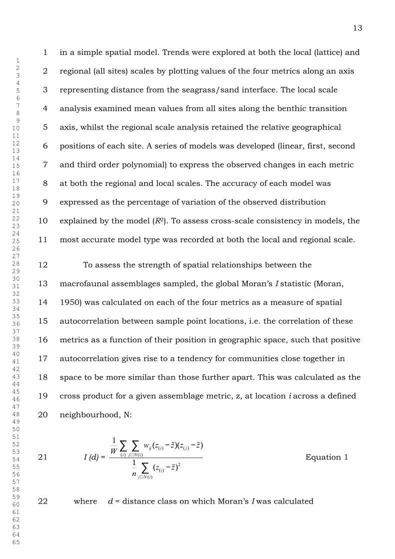
To assess the strength of spatial relationships between the 12
macrofaunal assemblages sampled, the global Moran’s I statistic (Moran, 13
1950) was calculated on each of the four metrics as a measure of spatial 14
autocorrelation between sample point locations, i.e. the correlation of these 15
metrics as a function of their position in geographic space, such that positive 16
autocorrelation gives rise to a tendency for communities close together in 17
space to be more similar than those further apart. This was calculated as the 18
cross product for a given assemblage metric, z, at location i across a defined 19
neighbourhood, N: 20
I (d) =
1
Wwij (z(i) - z)(z( j ) - z)
jÎN (i)
å(i)
å
1
n(z(i) - z)2
jÎN (i)
å Equation 1 21
where d = distance class on which Moran’s I was calculated 22

1 2 3 4 5 6 7 8 9 10 11 12 13 14 15 16 17 18 19 20 21 22 23 24 25 26 27 28 29 30 31 32 33 34 35 36 37 38 39 40 41 42 43 44 45 46 47 48 49 50 51 52 53 54 55 56 57 58 59 60 61 62 63 64 65
14
zi = macrofaunal assemblage metric at location i 1
N = neighbourhood within which the assemblage metrics were 2
sampled 3
˜ z = mean of the z values 4
W = sum of the weights wij for the given distance class. 5
W takes the value of 1 when sites i and j are at or within a distance d, and 0 6
otherwise. In this way, only the pairs of sites (i,j) within the stated distance 7
class (d) of each point location were taken into account. This yielded a large 8
and positive statistic in the presence of positive spatial dependence, a large 9
and negative statistic in the presence of negative spatial dependence and 10
was close to zero with a random assemblage distribution. 11
Spatial autocorrelation was also assessed at the local scale by 12
generating a semivariogram for each lattice. This calculated Geary’s C 13
statistic (Geary, 1954) on the total number of individuals sampled to assess 14
similarity for every possible combination of sample point pairs across each 15
lattice grid. Geary’s C measured correspondence for a given distance class d, 16
on the basis of the squared difference of a particular characteristic between 17
two point locations zi and zj: 18
c(d) =
1
2Wwij (z(i) - z( j ))
2
jÎN (i)
å(i)
å
1
n -1(z(i) - z( j ))
2
jÎN (i)
å Equation 2 19
This measure ranged from 0 to some unspecified value larger than 1. Values 20
of Geary’s C were then plotted against the distance between points to 21
1 2 3 4 5 6 7 8 9 10 11 12 13 14 15 16 17 18 19 20 21 22 23 24 25 26 27 28 29 30 31 32 33 34 35 36 37 38 39 40 41 42 43 44 45 46 47 48 49 50 51 52 53 54 55 56 57 58 59 60 61 62 63 64 65
15
generate a semivariogram exploring the magnitude and spatial configuration 1
of locally-measured autocorrelation plotted across the map. The sill point, 2
the distance at which Geary’s C levelled off and no further increase in the 3
statistic was observed as the distance between point pairs increased, was 4
recorded for each semivariogram. This corresponded to a given distance 5
range beyond which benthic invertebrate assemblages no longer influenced 6
each other. Finally, a semivariogram surface was generated to map the 7
value of the Geary’s C across each lattice as a localized measure of 8
assemblage similarity in geographical space. To account for the anisotropic 9
effect across the tidal axis, a search direction of 90 degrees was used to 10
define the neighbourhood of each point. The surface was generated using an 11
interpolation technique that combined values in the semivariogram plot into 12
bins based on the direction and distance between pairs of point sample 13
locations. Binned values were then averaged and smoothed to produce the 14
semivariogram surface. 15
16
3. RESULTS 17
Faunal assemblages of the adjacent 0.75 m wide boundary zones on 18
either side of the interface between seagrass and unvegetated sand showed 19
markedly different abundance and species density (all one-way ANOVA F1,34 20
>60; P <<0.0001). Overall, the marginal strip of seagrass supported an 21
observed total of 168 species (estimated true total 220) at an overall 22
abundance of 2,430 ind. m-2 and a -diversity of 16.0. The contiguous 23
marginal strip of sand, in contrast, supported only 61 observed species 24
1 2 3 4 5 6 7 8 9 10 11 12 13 14 15 16 17 18 19 20 21 22 23 24 25 26 27 28 29 30 31 32 33 34 35 36 37 38 39 40 41 42 43 44 45 46 47 48 49 50 51 52 53 54 55 56 57 58 59 60 61 62 63 64 65
16
(estimated true total 78), 750 ind. m-2, and a -diversity of 11.6. Even 1
though abutting, the two assemblages shared only 24% of their observed 2
total fauna and only 44% of their higher-level taxa. The relative richness of 3
the seagrass assemblage was not a consequence of its greater abundance 4
(Gotelli and Colwell, 2001), the number of species per macrobenthic 5
individual within the seagrass being always considerably larger than that in 6
the unvegetated sand at a ratio of 1 : >1.5; per unit area the ratio was close 7
to 1 : 2.7 (Fig. 3). The seagrass-edge assemblage was dominated by Calopia 8
imitata, Enigmaplax littoralis, Limnoporeia sp., Nassarius burchardi and 9
Longiflagrum caeruleus (in descending order of abundance), which were the 10
only species to contribute ≥4% of the total individuals, whilst in the 11
unvegetated sand the same percentage was contributed by each of 12
Urohaustorius mertungi, Mictyris longicarpus, Mysella vitrea, Finella fabrica, 13
Eumarcia fumigata, Goniada ?tripartita, Leitoscoloplos ?normalis, Nephtys 14
spp, Doowia dexterae and Spio pacifica (likewise in descending order of 15
abundance). ANOVA comparisons of the abundance of these dominant 16
species in the marginal and in the main areas of their respective habitats did 17
not show any significant differences in unvegetated areas of sand, except in 18
respect of the gastropod Finella which was more abundant in the marginal 19
zone than in the main sandflat (ANOVA F1,22 = 4.9; P = 0.04) (and than in the 20
marginal or main areas of seagrass, P <0.03). In the seagrass beds, several 21
animals (including Calopia, Limnoporeia, Longiflagrum and Leptochelia) were 22
more abundant at the seagrass edge at some sites but were less abundant 23
marginally at others. Only in respect of Pseudoliotia was there a significant 24
1 2 3 4 5 6 7 8 9 10 11 12 13 14 15 16 17 18 19 20 21 22 23 24 25 26 27 28 29 30 31 32 33 34 35 36 37 38 39 40 41 42 43 44 45 46 47 48 49 50 51 52 53 54 55 56 57 58 59 60 61 62 63 64 65
17
difference overall (ANOVA F1,22 = 13.1; P = 0.001), this microgastropod being 1
less abundant near edges. 2
Variation across the boundary zone in mean faunal abundance, 3
observed and estimated true species density, and levels of -diversity are 4
shown in Figure 4a-c, and -diversity changes between adjacent sampling 5
horizons are given in Table 1. Two-way ANOVA tests of these features in the 6
seagrass marginal horizons and in the unvegetated sand margins (Table 2) 7
indicates no significant effect of distance of the sampling horizon from the 8
interface on any assemblage feature, and no significant interaction between 9
this distance and position on the shore. In each case, this includes 10
comparisons between the marginal zone and the main body of the habitat 11
concerned. The faunal assemblage within the mangrove pneumatophore-12
field, however, which was dominated by Salinator fragilis, was completely 13
different from those in both the adjacent unvegetated-sand and in the 14
seagrass (in each case with a dissimilarity of >90%). It was not used in any 15
further comparisons. As previously noted at these sites (Barnes and Barnes, 16
2012), values of -diversity were again very variable (see Fig. 4c) and 17
displayed no correlation with values of species density (Seagrass: Spearman 18
R = 0.17; P >0.4. Sandflat: Spearman R = 0.18; P >0.4). 19
In marked contrast to the uniformity within each of the marginal 20
habitat zones, however, there were highly significant changes in faunal 21
abundance, observed and estimated true species density, and in 22
dissimilarity between adjacent horizons, across the 25 cm wide strip on 23
either side of the actual interface (Tables 1 and 3) over which the sharp 24
1 2 3 4 5 6 7 8 9 10 11 12 13 14 15 16 17 18 19 20 21 22 23 24 25 26 27 28 29 30 31 32 33 34 35 36 37 38 39 40 41 42 43 44 45 46 47 48 49 50 51 52 53 54 55 56 57 58 59 60 61 62 63 64 65
18
change in seagrass abundance occurred (Fig. 4d). Each of the four seagrass 1
horizons was significantly different from each of the four unvegetated sand 2
horizons in faunal abundance and species density (all Tukey HSD test 3
statistics ≥ 6; P ≤0.003). Therefore, effectively all the dramatic change in 4
composition, abundance and biodiversity between the faunal assemblages of 5
seagrass and of adjacent unvegetated sand took place over the very small 6
distance of 0.5 m at most. Categorising the various species as either 7
‘seagrass specialist’, ‘unvegetated-sand specialist’ or ‘generalist’, on the basis 8
of whether their abundance in the two habitat types was greater or less than 9
a ratio of 1 : 2.5, and removing all rare species (those with ≤5 individuals in 10
total) from the analysis, the two assemblages appear to react symmetrically 11
to the interface (Fig. 5). Total abundance of the generalist category 12
(principally Nephtys, Goniada, Spio and Mysella) was unaffected by the 13
transition. As a result of the difference in overall abundance, however, these 14
four taxa were significant elements in the fauna of the unvegetated sand (see 15
above) but not in that of the seagrass. 16
Figure 6 illustrates a plot of the four assemblage metrics at the local 17
and regional scales. Spatial trends in the metrics were captured accurately 18
at both scales (local R2 = 0.87 to 0.93; regional R2 = 0.71 to 0.74) using 19
second and third order polynomial regression models, although local scale 20
models consistently performed better than regional scale models. In terms of 21
cross-scale comparisons, the highest performing model type remained 22
consistent transitioning from the local to the regional scale. Alpha species 23
diversity was modelled with the highest accuracy at both scales. 24

1 2 3 4 5 6 7 8 9 10 11 12 13 14 15 16 17 18 19 20 21 22 23 24 25 26 27 28 29 30 31 32 33 34 35 36 37 38 39 40 41 42 43 44 45 46 47 48 49 50 51 52 53 54 55 56 57 58 59 60 61 62 63 64 65
19
The global Moran’s I statistic calculated for all sites together and for 1
the lattice at each individual site is shown in Table 4. Three of the metrics 2
(faunal abundance and both species density measures) exhibited positive 3
spatial autocorrelation of moderate strength (I = 0.16 to 0.44). Alpha species 4
diversity showed weaker levels of autocorrelation that approximated a 5
randomly distributed community (I = -0.18 to 0.11). 6
The semivariogram plot and surface generated for pairs of sample sites 7
in each lattice are shown in Figure 7. The sill points indicated that distances 8
over which invertebrate communities displayed spatial dependence were in 9
the range 30-125 mm. At all sites the semivariogram surfaces indicated a 10
symmetrical pattern of autocorrelation about the seagrass/sand interface. 11
With the exception of the Polka LWS site, all lattices displayed lower 12
measures of autocorrelation closer to the interface (i.e. assemblages sampled 13
across the boundary appeared to be less similar within the defined 14
neighbourhood) and higher measures of autocorrelation within the main 15
bodies of the respective habitat types. 16
17
4. DISCUSSION 18
Three features of the differential assemblage composition, abundance 19
and species density of seagrass and unvegetated sand stand out. First, the 20
marginal zones of both seagrass and unvegetated sand not only do not vary 21
with closeness to the actual interface but are not significantly different from 22
the main bodies of the respective habitat types. Secondly, the two 23

1 2 3 4 5 6 7 8 9 10 11 12 13 14 15 16 17 18 19 20 21 22 23 24 25 26 27 28 29 30 31 32 33 34 35 36 37 38 39 40 41 42 43 44 45 46 47 48 49 50 51 52 53 54 55 56 57 58 59 60 61 62 63 64 65
20
contiguous faunal assemblages are very different, with only a few generalist 1
species having a more than insignificant presence. All marginal seagrass 2
horizons were significantly different from all marginal sandflat ones in 3
composition, faunal abundance and species density, and hence there must 4
be a very rapid change from one assemblage type to the other across the 5
interface. Thirdly, that this is accomplished over a distance of only 0.5 m at 6
most is unexpected, although Warry et al. (2009) have shown that 0.5 m is a 7
large distance for seagrass harpacticoids and other meiofauna. Local 8
ecological changes over small distances are commonplace in seagrass 9
systems (Thrush et al., 2001; Barnes and Ellwood, 2012) but the changes 10
taking place over 0.5 m here are far from local, occurring at all shore heights 11
investigated and at all localities. Attrill and Rundle (2002, p. 929) define an 12
ecotone (as distinct from an ecocline) as ‘an area of relatively rapid change, 13
producing a narrow ecological zone between two different and relatively 14
homogeneous community types’: the boundary zone and assemblage types 15
studied here exactly fit this definition. Although Hansen and di Castri 16
(1992) consider that ecotones can range in width from distances measured 17
in centimetres to those measured in kilometres, the dimension of this 18
ecotone must be one of the smallest ever recorded in association with a 19
major change from one ecosystem bioengineer to another. Nevertheless, 20
there are a number of potential reasons why the Stradbroke 21
seagrass/sandflat ecotone might be of such small width. The interfaces 22
chosen for study were deliberately those that appeared stable, and therefore 23
the situation may be rather different in actively advancing or retreating 24
boundaries. Much may also depend on the precise habitat provided by the 25
1 2 3 4 5 6 7 8 9 10 11 12 13 14 15 16 17 18 19 20 21 22 23 24 25 26 27 28 29 30 31 32 33 34 35 36 37 38 39 40 41 42 43 44 45 46 47 48 49 50 51 52 53 54 55 56 57 58 59 60 61 62 63 64 65
21
marginal seagrass areas (Tuya et al., 2011). At the sites investigated, there 1
was no diminution in the number of seagrass shoots per unit area as the 2
interface was approached (see Figure 4d), and maintenance of a relatively 3
constant habitat framework — water velocities excepted (see below) — right 4
up to the interface itself may well aid the continuation of relatively constant 5
assemblage characteristics until that point. Thirdly, the two assemblages 6
are dominated by organisms of contrasting biology: the seagrass fauna being 7
largely epifaunal and that of the unvegetated sand being mainly infaunal 8
(Barnes and Barnes, 2012). It is well established (Orth et al., 1984; van 9
Houte-Howes et al., 2004; etc) that seagrass root/rhizome systems inhibit 10
burrowing, whilst the lack of a plant cover can expose surface-dwelling 11
species to heavy predation. In any event, unlike several other transitional 12
zones (Rand et al., 2006), that between seagrass and unvegetated sand on 13
Stradbroke certainly does not appear to support mixed faunal assemblages 14
enriched by elements from both juxtaposed habitat types. Neither did the 15
faunal assemblage within the seaward pneumatophore-field appear in any 16
way to support an assemblage with elements from both the mangrove and 17
the lower unvegetated sand or seagrass (c.f. Alfaro, 2006). 18
It is also noteworthy that the results of this study do not display large 19
straight-forward and consistent edge effects in respect to species 20
distributions. In fact, the response of benthic animals to the edges of 21
seagrass beds appears in earlier studies to vary from group to group 22
(Murphy et al., 2010) and from study to study (Tuya et al., 2011). Thus 23
some have shown densities of peracaridan crustaceans, including tanaids 24
1 2 3 4 5 6 7 8 9 10 11 12 13 14 15 16 17 18 19 20 21 22 23 24 25 26 27 28 29 30 31 32 33 34 35 36 37 38 39 40 41 42 43 44 45 46 47 48 49 50 51 52 53 54 55 56 57 58 59 60 61 62 63 64 65
22
(Tanner, 2005), to be higher at edges than nearer the centre (e.g. Boström et 1
al., 2006), whereas in others (e.g. Murphy et al., 2010) tanaids increased in 2
abundance away from the edge, and the effect in other peracaridans was 3
dependent on size of patch investigated. In the Stradbroke intertidal, only 4
one species (the microgastropod Pseudoliotia) showed a consistent reaction. 5
At some sites tanaids, for example, were five times more abundant near the 6
edge but at other sites they were only half as dense. Overall, the 25 7
peracaridan species were more abundant at the edge at half the sites but 8
less abundant at the other half. The most abundant seagrass inhabitant, 9
the microgastropod Calopia, was also almost twice as abundant near edges 10
at two sites, but was ten times less abundant at two others. On average, 11
however, the 33 microgastropod species present were less abundant at the 12
edge at two-thirds of the sites and overall were only half as abundant at 13
edges, although the effect was not statistically significant. Little previous 14
work has concerned small, fragile, epibenthic microgastropods such as 15
Calopia and Pseudoliotia — forms that dominate the Stradbroke seagrass 16
patches away from the edges (Barnes and Barnes, 2011, 2012; Barnes and 17
Ellwood, 2012). But as water velocities are known to be higher near 18
seagrass margins (Peterson et al., 2004; Murphy et al., 2010), it is perhaps 19
not surprising that some species, such as Pseudoliotia, should be less 20
abundant and widespread under the more turbulent conditions near the 21
interface, maybe via effects on their recruitment (Bologna and Heck, 2002) or 22
because of dislodgement (Tuya et al., 2011). Alternatively, small, fragile 23
animals may be at greater risk from predators when relatively exposed (Kark 24
and van Rensburg, 2006; Barnes, 2010). Other than these microgastropods, 25
1 2 3 4 5 6 7 8 9 10 11 12 13 14 15 16 17 18 19 20 21 22 23 24 25 26 27 28 29 30 31 32 33 34 35 36 37 38 39 40 41 42 43 44 45 46 47 48 49 50 51 52 53 54 55 56 57 58 59 60 61 62 63 64 65
23
however, it would appear that edge effects may be more a variable local 1
response to specific habitat conditions within patch margins than a general 2
consistent effect of closeness to an interface with a different habitat type. 3
It is significant that trend analysis suggests that the emergent 4
assemblage features captured in each of the four metrics could accurately 5
and consistently be characterised across scales as second and third order 6
polynomial regression models. Such models have not only proved useful in 7
furthering our understanding of how assemblages are organised in space 8
(Peres-Neto and Legendre, 2010) but allow, for example, prediction of 9
assemblage composition at unsampled locations and interpolation 10
techniques such as kriging. 11
Thrush (1991) noted that spatial autocorrelation in variables that 12
capture the biodiversity of macrobenthic assemblages can confound 13
experimental designs and affect the reliability of inferential statistics that 14
may be used to assess distribution patterns. For example, the presence of 15
spatial dependence often results in a violation of the statistical assumption 16
of independence of observations. Tobler’s (1970) First Law of Geography, 17
that objects closer together tend to be more similar than those further apart, 18
has repeatedly been found to apply to point sample datasets of ecological 19
communities (Fortin and Dale, 205). Hence it is no surprise that moderate 20
autocorrelation was detected in three of the four metrics sampled in the 21
present study (i.e. faunal abundance and both species density measures). In 22
the present case, however, this does not affect conclusions as to the nature 23
and size of the boundary between the two patch types. In contrast to the 24

1 2 3 4 5 6 7 8 9 10 11 12 13 14 15 16 17 18 19 20 21 22 23 24 25 26 27 28 29 30 31 32 33 34 35 36 37 38 39 40 41 42 43 44 45 46 47 48 49 50 51 52 53 54 55 56 57 58 59 60 61 62 63 64 65
24
other metrics, the fourth, species diversity, showed remarkable and 1
consistent resistance to autocorrelation at each site. This might be taken to 2
suggest that -diversity could potentially be a good resistant measure of 3
biodiversity for benthic intertidal faunal assemblages. That this is not so, 4
however, is indicated by the lack of correlation of -diversity with species 5
density (often regarded as the most important measure of biodiversity; e.g. 6
by Wang et al., 2008) and by the very large degree of scatter in this metric 7
shown in Figure 4c. Both these features were also seen in the earlier study 8
of the sites by Barnes and Barnes (2012), who also showed that values of -9
diversity there were almost solely a result of the evenness component and 10
were also very closely correlated to the reciprocal of the degree of Berger-11
Parker dominance by the single most abundant species. 12
The semivariogram surfaces generated for each sample lattice provide 13
useful insight into the magnitude and spatial configuration of locally-14
measured autocorrelation, which itself may vary in response to habitat 15
change. The coincidence of the low measures of autocorrelation with the 16
interface between the two patch types corroborates the finding that highly 17
significant and abrupt changes occur across this boundary. While most of 18
the autocorrelation surfaces approximate a symmetrical pattern on either 19
side of the interface, these are not necessarily due to changes in habitat. 20
Neighbourhood context interactions of ecological relevance might also 21
underpin the observed semivariogram surface patterns. These could include 22
predation by waders or juvenile fish (Meire and Kuyken, 1984) or 23
modifications of predator-prey interactions due to the presence of a key 24

1 2 3 4 5 6 7 8 9 10 11 12 13 14 15 16 17 18 19 20 21 22 23 24 25 26 27 28 29 30 31 32 33 34 35 36 37 38 39 40 41 42 43 44 45 46 47 48 49 50 51 52 53 54 55 56 57 58 59 60 61 62 63 64 65
25
species, as for example in the profound influence that the presence of 1
burrowing crustaceans and their associated bioturbation has on sediment 2
structure, quality and dynamics (Martinetto et al., 2005) (and see below). 3
Nevertheless, the consistent tendency for the higher levels of invertebrate 4
assemblage autocorrelation to be nested within the main bodies of the 5
respective habitat types suggests a strong association between the 6
configuration of assemblage spatial dependency and habitat. Further 7
inferential testing, for example, through the development of spatially lagged 8
autoregressive models would provide insight on this point. 9
Winberg et al. (2007) highlight the value of examining multiple 10
measures of macrobenthic biodiversity across a variety of scales. The present 11
study has examined spatial patterning in four assemblage metrics at the 12
local (lattice) and regional (all sites) scales, traversing spatial dimensions 13
ranging over 5 orders of magnitude from 0.25 m to 2.5 km. One of its most 14
remarkable findings, highlighted in the elevated significance of β-diversity 15
horizon comparisons across the interface (i.e. between the +0.25 and -0.25 16
m increments, Table 1), is the small spatial scales over which intertidal 17
benthic faunal assemblages can display marked variation. The sill points 18
extracted from the semivariograms identify scales of 30 to 125 mm as the 19
distances across which point samples of assemblages appear to be 20
influencing each other. This finding lies in contrast to calls for statistical 21
work on soft sediment macrobenthos to be undertaken at large scales (i.e. >1 22
km) to ascertain the relative importance of different habitats to populations 23
(Constable, 1999). Such large scales have been highlighted because they are 24

1 2 3 4 5 6 7 8 9 10 11 12 13 14 15 16 17 18 19 20 21 22 23 24 25 26 27 28 29 30 31 32 33 34 35 36 37 38 39 40 41 42 43 44 45 46 47 48 49 50 51 52 53 54 55 56 57 58 59 60 61 62 63 64 65
26
associated with reduced uncertainty in the quantitative predictions derived 1
from ecological systems models; however, they would appear to be at odds 2
with the spatial scales of variation in processes driving the assemblage 3
patterns in the present study, regardless of what these processes are. 4
Overall, we therefore conclude that in Moreton Bay faunal transitions 5
across stable seagrass/sand interfaces take the form of very sharp ecotones 6
indeed, across which the two assemblages react symmetrically, with the 7
interface itself being the location of the marked change in faunal abundance 8
and biodiversity observed between the contrasting patch types. At a global 9
level, however, this seems likely to be more a specific effect of the two low-10
latitude, low-abundance but high-biodiversity faunal assemblages that are 11
interacting (or of the key members of those assemblages) than of any change 12
in prevailing habitat characteristic per se, in that such contrasting 13
assemblages are not universal. Differences between seagrass and adjacent 14
sand assemblages, and hence changes across seagrass/sand boundaries, in 15
high-latitude, high-abundance but low biodiversity regions such as the 16
north-west Atlantic, for example, are relatively insignificant (Asmus and 17
Asmus, 2000; Polte et al., 2005; Barnes, 2010; 2013). 18
19
ACKNOWLEDGEMENTS 20
RSKB wishes to thank the staff of the Moreton Bay Research Station, 21
especially Kevin Townsend and Martin Wynne, for invaluable assistance. 22
Sampling within the Moreton Bay Marine Park was carried out under The 23
1 2 3 4 5 6 7 8 9 10 11 12 13 14 15 16 17 18 19 20 21 22 23 24 25 26 27 28 29 30 31 32 33 34 35 36 37 38 39 40 41 42 43 44 45 46 47 48 49 50 51 52 53 54 55 56 57 58 59 60 61 62 63 64 65
27
Queensland Museum's permits (Department of Environment and Resource 1
Management Permit No. QS2011/CVL588 and General Fisheries Permit No. 2
91454). 3
4
REFERENCES 5
Albano, P.G., Sabelli, B., Bouchet, P., 2011. The challenge of small and rare 6
species in marine biodiversity surveys: microgastropod diversity in a 7
complex tropical coastal environment. Biodiversity and Conservation 20, 8
3233-3237. 9
Alfaro, A.C., 2006. Benthic macro-invertebrate community composition 10
within a mangrove/seagrass estuary in northern New Zealand. 11
Estuarine, Coastal and Shelf Science 66, 97-110. 12
Asmus, H., Asmus, R., 2000. Material exchange and food webs of seagrass 13
beds in the Sylt-Rømø Bight: how significant are community changes at 14
the ecosystem level? Helgoland Marine Research 54, 137-150. 15
Attrill, M.J., Rundle, S.D., 2002. Ecotone or ecocline: ecological boundaries in 16
estuaries. Estuarine, Coastal and Shelf Science 55, 929-936. 17
Barbier, E.B., Hacker, S.D., Kennedy, C., Koch, E.W., Stier, A.C., Silliman, 18
R.R., 2011. The value of estuarine and coastal ecosystem services. 19
Ecological Monographs 81, 169-193. 20
Barnes, R.S.K., 2010. Regional and latitudinal variation in the diversity, 21
1 2 3 4 5 6 7 8 9 10 11 12 13 14 15 16 17 18 19 20 21 22 23 24 25 26 27 28 29 30 31 32 33 34 35 36 37 38 39 40 41 42 43 44 45 46 47 48 49 50 51 52 53 54 55 56 57 58 59 60 61 62 63 64 65
28
dominance and abundance of microphagous microgastropods and other 1
benthos in intertidal beds of dwarf eelgrass, Nanozostera spp. Marine 2
Biodiversity 40, 95-106. 3
Barnes, R.S.K., 2013. Distribution patterns of macrobenthic biodiversity in 4
the intertidal seagrass beds of an estuarine system and their conservation 5
significance. Biodiversity and Conservation 22, 357-372. 6
Barnes, R.S.K., Barnes, M.K.S., 2011. Hierarchical scales of spatial variation 7
in the smaller surface and near-surface macrobenthos of a subtropical 8
intertidal seagrass system in Moreton Bay, Queensland. Hydrobiologia 9
673, 169-178. 10
Barnes, R.S.K., Barnes, M.K.S., 2012. Shore height and differentials 11
between macrobenthic assemblages in vegetated and unvegetated areas 12
of an intertidal sandflat. Estuarine, Coastal and Shelf Science 106, 112-13
120. 14
Barnes, R.S.K., Ellwood, M.D.F., 2011. Macrobenthic assemblage structure 15
in a cool-temperate intertidal dwarf eelgrass bed in comparison with those 16
from lower latitudes. Biological Journal of the Linnean Society 104, 527-17
540. 18
Barnes, R.S.K., Ellwood, M.D.F., 2012. The critical scale of small-scale 19
spatial variation in ecological patterns and processes in intertidal 20
macrobenthic seagrass assemblages. Estuarine, Coastal and Shelf Science 21
98, 119-125. 22

1 2 3 4 5 6 7 8 9 10 11 12 13 14 15 16 17 18 19 20 21 22 23 24 25 26 27 28 29 30 31 32 33 34 35 36 37 38 39 40 41 42 43 44 45 46 47 48 49 50 51 52 53 54 55 56 57 58 59 60 61 62 63 64 65
29
Berkenbusch, K., Rowden, A.A., 2007. An examination of the spatial and 1
temporal generality of the influence of ecosystem engineers on the 2
composition of associated assemblages. Aquatic Ecology 41, 129-147. 3
Berkenbusch, K., Rowden, A.A., Myers, T.E., 2007. Interaction between 4
seagrasses and burrowing ghost shrimps and their influence on faunal 5
assemblages. Journal of Experimental Marine Biology and Ecology 341, 6
70-84. 7
Bologna, P.A.X., Heck, K.L.Jr, 2002. Impact of habitat edges on density and 8
secondary production of seagrass-associated fauna. Estuaries 25, 1033-9
1044. 10
Boström, C., Bonsdorff, E., 1997. Community structure and spatial variation 11
of benthic invertebrates associated with Zostera marina (L.) beds in the 12
northern Baltic Sea. Journal of Sea Research 37, 153-166. 13
Boström, C., Jackson, E.L., Simenstad, C.A., 2006. Seagrass landscapes and 14
their effects on associated faunas: a review. Estuarine, Coastal and Shelf 15
Science 68, 383-403. 16
Bowden, D.A., Rowden, A.A., Attrill, M.J., 2001. Effect of patch size and in-17
patch location on the infaunal macroinvertebrate assemblages of Zostera 18
marina seagrass beds. Journal of Experimental Marine Biology and 19
Ecology 259, 133-154. 20
Bryan, K.R., Tay, H.W., Pildich, C.A., Lundquist, C.J., Hunt, H.L., 2007. The 21
effects of seagrass (Zostera muelleri) on boundary-layer hydrodynamics in 22
1 2 3 4 5 6 7 8 9 10 11 12 13 14 15 16 17 18 19 20 21 22 23 24 25 26 27 28 29 30 31 32 33 34 35 36 37 38 39 40 41 42 43 44 45 46 47 48 49 50 51 52 53 54 55 56 57 58 59 60 61 62 63 64 65
30
Whangapoua Estuary, New Zealand. Journal of Coastal Research Special 1
Issue 50, 668-672. 2
Chao, A., 1987. Estimating the population size for capture-recapture data 3
with unequal catchability. Biometrics 43, 783-791. 4
Chao, A., Chazdon, R.L., Colwell, R.K., Shen, T-J., 2005. A new statistical 5
approach for assessing compositional similarity based on incidence and 6
abundance data. Ecology Letters 8, 148-159. 7
Chao, A., Chazdon, R.L., Colwell, R.K., Shen, T-J., 2006. Abundance-based 8
similarity indices and their estimation when there are unseen species in 9
samples. Biometrics 62, 361-371. 10
Chao, A., Hwang, W-H., Chen, Y-C., Kuo, C-Y., 2000. Estimating the number 11
of shared species in two communities. Statistica Sinica 10, 227-246. 12
Chazdon, R.L., Colwell, R.K., Denslow, J.S., Guariguata, M.R., 1998. 13
Statistical methods for estimating species richness of woody regeneration 14
in primary and secondary rain forests of NE Costa Rica. In: Dallmeier, F., 15
Comiskey, J.A. (Eds) Forest biodiversity research, monitoring and 16
modelling: conceptual background and Old World case studies. Pathenon, 17
Paris, 285-309. 18
Coles, R., Grech, A., Rasheed, M., McKenzie, L., Unsworth, R., Short, F., 19
2011. Seagrass ecology and threats in the tropical Indo-Pacific region. In: 20
Pirog, R.S. (Ed.), Seagrass: ecology, uses and threats. Nova Science, N.Y., 21
225-239. 22
1 2 3 4 5 6 7 8 9 10 11 12 13 14 15 16 17 18 19 20 21 22 23 24 25 26 27 28 29 30 31 32 33 34 35 36 37 38 39 40 41 42 43 44 45 46 47 48 49 50 51 52 53 54 55 56 57 58 59 60 61 62 63 64 65
31
Colwell, R.K., 2011. EstimateS: Statistical estimation of species richness 1
and shared species from samples, version 8.2.0Mac. Users guide and 2
application available at http://purl.oclc.org/estimates 3
Colwell, R.K., Chao, A., Gotelli, N.J., Lin, S-Y., Mao, C.X., Chazdon, R.L., 4
Longino, J.T., 2012. Models and estimators linking individual-based and 5
sample-based rarefaction, extrapolation, and comparison of assemblages. 6
Journal of Plant Ecology 5, 3-21. 7
Colwell, R.K., Mao, C.X., Chang, J., 2004. Interpolating, extrapolating and 8
comparing incidence-based species accumulation curves. Ecology 85, 9
2717-2727. 10
Constable, A.J., 1999. Ecology of benthic macro-invertebrates in soft-11
sediment environments: a review of progress towards quantitative models 12
and predictions. Australian Journal of Ecology 24, 452-476. 13
Davie, P.J.F. and 45 other authors, 2011. Wild Guide to Moreton Bay, 2nd 14
Edn. Queensland Museum, Brisbane. 15
Davie, P.J.F., Hooper, J.N.A., 1998. Patterns of biodiversity in marine 16
invertebrate and fish communities of Moreton Bay. In: Tibbetts, I.R., 17
Hall, N.J., Dennison, W.C. (Eds), Moreton Bay and Catchment. School of 18
Marine Science, University of Queensland, Brisbane, pp 331-346. 19
Davie, P.J.F., Phillips, J.A., 2008. The Marine Fauna and Flora of Moreton 20
Bay Workshop: a focus on species. In: Davie, P.J.F., J.A. Phillips (Eds), 21
Proceedings of the Thirteenth International Marine Biological Workshop. 22
1 2 3 4 5 6 7 8 9 10 11 12 13 14 15 16 17 18 19 20 21 22 23 24 25 26 27 28 29 30 31 32 33 34 35 36 37 38 39 40 41 42 43 44 45 46 47 48 49 50 51 52 53 54 55 56 57 58 59 60 61 62 63 64 65
32
The Marine Fauna and Flora of Moreton Bay, Queensland. Memoirs of the 1
Queensland Museum – Nature 54(1), xi-xvii. 2
Dennison, W.C., Abal, E.G., 1999. Moreton Bay Study: A Scientific Basis for 3
the Healthy Waterways Campaign. SE Queensland Regional Water Quality 4
Management Strategy, Brisbane. 5
Dethier, M.N., Schoch, G.C., 2006. Taxonomic sufficiency in distinguishing 6
natural spatial patterns on an estuarine shoreline. Marine Ecology 7
Progress Series 306, 41-49. 8
Duarte, C.M., 2000. Marine biodiversity and ecosystem services: an elusive 9
link. Journal of Experimental Marine Biology and Ecology 250, 117-131. 10
Eyre, B.D., Ferguson, A.J.P., Webb, A., Maher, D., Oakes, J.M., 2011. 11
Metabolism of different benthic habitats and their contribution to the 12
carbon budget of a shallow oligotrophic sub-tropical coastal system 13
(southern Moreton Bay, Australia). Biogeochemistry 102, 87-110. 14
Fortin, M-J., Dale, M.R.T, 2005. Spatial Analysis. A guide for ecologists. 15
Cambridge University Press, Cambridge. 16
Fourqurean, J.W., and 10 other authors, 2012. Seagrass ecosystems as a 17
globally significant carbon stock. Nature Geosciences 5, 505-509. 18
Geary, R.C., 1954. The contiguity ratio and statistical mapping. The 19
Incorporated Statistician 5(3), 115-145. 20
Gotelli, N.J., Colwell, R.K., 2001. Quantifying biodiversity: procedures and 21
1 2 3 4 5 6 7 8 9 10 11 12 13 14 15 16 17 18 19 20 21 22 23 24 25 26 27 28 29 30 31 32 33 34 35 36 37 38 39 40 41 42 43 44 45 46 47 48 49 50 51 52 53 54 55 56 57 58 59 60 61 62 63 64 65
33
pitfalls in the measurement and comparison of species richness. Ecology 1
Letters 4, 379-391. 2
Hansen, A., di Castri, F., 1992. Landscape boundaries: consequences for 3
biotic diversity and ecological flows. Springer, Berlin. 4
Hill, M.O., 1973. Diversity and evenness: a unifying notation and its 5
consequences. Ecology 54, 427-432. 6
Jost, L., 2006. Entropy and diversity. Oikos 113, 363-375. 7
Kark, S., van Rensburg, B.J., 2006. Ecotones: Marginal or central areas of 8
transition. Israel Journal of Ecology and Evolution 52, 29-53. 9
Klumpp, D.W., Kwak, S.N., 2005. Composition and abundance of benthic 10
macrofauna of a tropical sea-grass bed in north Queensland, Australia. 11
Pacific Science 59, 541-560. 12
Laycock, J.W., 1978. North Stradbroke Island. Papers from the Department 13
of Geology, University of Queensland 8, 89-96. 14
Lee, S.Y., 2008. Mangrove macrobenthos: assemblages, services and linkages. 15
Journal of Sea Research 59, 16-29. 16
Levin, L.A. and 11 other authors, 2001. The function of marine critical 17
transition zones and the importance of sediment biodiversity. Ecosystems 18
4, 430-451. 19
Lotze, H.K., Lenihan, H.S., Bourque, B.J., Bradbury, R.H., Cooke, R.G., Kay, 20
M.C., Kidwell, S.M., Kirby, M.X., Peterson, C.H., Jackson, J.B.C., 2006. 21
1 2 3 4 5 6 7 8 9 10 11 12 13 14 15 16 17 18 19 20 21 22 23 24 25 26 27 28 29 30 31 32 33 34 35 36 37 38 39 40 41 42 43 44 45 46 47 48 49 50 51 52 53 54 55 56 57 58 59 60 61 62 63 64 65
34
Depletion, degradation and recovery potential of estuaries and coastal seas. 1
Science 312, 1806-1809. 2
Luo, J., Serafy, J.E., Sponaugle, S., Teare, P.B., Kleckbusch, D., 2009. 3
Movement of gray snapper Lutjanus griseus among subtropical seagrass, 4
mangrove, and coral reef habitats. Marine Ecology Progress Series 380, 5
255-269. 6
Martinetto, P., Iribarne, O., Palomo, G., 2005. Effect of fish predation on 7
intertidal benthic fauna is modified by crab bioturbation. Journal of 8
Experimental Marine Biology and Ecology 318, 71-84. 9
Meire, P., Kuyken, E., 1984. Relationships between the distribution of 10
waders and the intertidal benthic fauna of the Oosterschelde, Netherlands. 11
In: Evans, P.R., Goss-Custard, J.D., Hale, W.G. (Eds), Coastal waders and 12
wildfowl in winter. Cambridge University Press, Cambridge, 57-68. 13
Mills, V.S., Berkenbusch, K., 2009. Seagrass (Zostera muelleri) patch size and 14
spatial location influence infaunal macroinvertebrate assemblages. 15
Estuarine, Coastal and Shelf Science 81, 123-129. 16
Moran, P.A.P., 1950. Notes on continuous stochastic phenomena. Biometrika 17
37, 17-23. 18
Murphy, H.M., Jenkins, G.P., Hindell, J.S., Connolly, R.M., 2010. Response of 19
fauna in seagrass to habitat edges, patch attributes and hydrodynamics. 20
Austral Ecology 35, 535-543. 21
1 2 3 4 5 6 7 8 9 10 11 12 13 14 15 16 17 18 19 20 21 22 23 24 25 26 27 28 29 30 31 32 33 34 35 36 37 38 39 40 41 42 43 44 45 46 47 48 49 50 51 52 53 54 55 56 57 58 59 60 61 62 63 64 65
35
Nagelkerken, I. and 10 other authors, 2012. The habitat function of 1
mangroves for terrestrial and marine fauna: a review. Aquatic Botany 89, 2
155-185. 3
Nagelkerken, I., van der Velde, G., 2004. Are Caribbean mangroves important 4
feeding grounds for juvenile reef fish from adjacent seagrass beds? Marine 5
Ecology Progress Series 274, 143-151. 6
O’Brien, C.J., 1994. Ontogenetic changes in the diet of juvenile brown tiger 7
prawns Penaeus esculentus. Marine Ecology Progress Series 112, 195-200. 8
Orth, R.J., Heck, K.L.Jr, van Montfrans, J., 1984. Faunal communities in 9
seagrass beds: a review of the influence of plant structure and prey 10
characteristics on predator-prey relationships. Estuaries 7, 339-350. 11
Perez-Neto, P.R., Legendre, P., 2010. Estimating and controlling for spatial 12
structure in the study of ecological communities. Global Ecology and 13
Biogeography 19, 174-184. 14
Peterson, C.H., Luettich, R.A.Jr, Micheli, F., Skilleter, G.A., 2004. 15
Attenuation of water flow inside seagrass canopies of differing structure. 16
Marine Ecology Progress Series 268, 81-92. 17
Pillay, D., Branch, G.M., 2011. Bioengineering effects of burrowing 18
thalassiniodean shrimps on marine soft-bottom ecosystems. 19
Oceanography and Marine Biology: An Annual Review 49, 137-192. 20
Pillay, D., Branch, G.M., Griffiths, C.L., Williams, C., Prinsloo, A., 2010. 21
Ecosystem change in a South African marine reserve (1960-2009): role of 22
1 2 3 4 5 6 7 8 9 10 11 12 13 14 15 16 17 18 19 20 21 22 23 24 25 26 27 28 29 30 31 32 33 34 35 36 37 38 39 40 41 42 43 44 45 46 47 48 49 50 51 52 53 54 55 56 57 58 59 60 61 62 63 64 65
36
seagrass loss and anthropogenic disturbance. Marine Ecology Progress 1
Series 415, 35-48. 2
Polte, P., Schanz, A., Asmus, H., 2005. The contribution of seagrass beds 3
(Zostera noltii) to the function of tidal flats as juvenile habitat for dominant 4
epibenthos in the Wadden Sea. Marine Biology 147, 813-822. 5
Rand, T.A., Tylianakis, J.M., Tsacharntke, T., 2006. Spillover edge effects: 6
the dispersal of agriculturally subsidized insect natural enemies into 7
adjacent natural habitats. Ecology Letters 9, 603-614. 8
Ries, L., Fletcher, R.J.Jr, Battin.J., Sisk, T.D., 2004. Ecological responses to 9
habitat edges: mechanisms, models, and variability explained. Annual 10
Review of Ecology and Systematics 35, 491-522. 11
Roelfsema, C.M., Phinn, S.R., Udy, N., Maxwell, P., 2009. An integrated field 12
and remote sensing approach for mapping seagrass cover, Moreton Bay, 13
Australia. Spatial Science 54, 45-62. 14
Sheridan, P., 1997. Benthos of adjacent mangrove, seagrass and non-15
vegetated habitats in Rookery Bay, Florida. Estuarine, Coastal and Shelf 16
Science 44, 455-469. 17
Siebert, T., Branch, G.M., 2007. Influences of biological interactions on 18
community structure within seagrass beds and sandprawn-dominated 19
sandflats. Journal of Experimental Marine Biology and Ecology 340, 11-20
24. 21
1 2 3 4 5 6 7 8 9 10 11 12 13 14 15 16 17 18 19 20 21 22 23 24 25 26 27 28 29 30 31 32 33 34 35 36 37 38 39 40 41 42 43 44 45 46 47 48 49 50 51 52 53 54 55 56 57 58 59 60 61 62 63 64 65
37
Spilmont, N., Meziane, T., Seuront, L., Welsh, D.T., 2009. Identification of 1
the food sources of sympatric ghost shrimp (Trypaea austraiensis) and 2
soldier crab (Mictyris longicarpus) populations using a lipid biomarker, 3
dual stable isotope approach. Austral Ecology 34, 878-888. 4
Tanner, J.E., 2005. Edge effects on fauna in fragmented seagrass meadows. 5
Austral Ecology 30, 210-218. 6
Tanner, J.E., 2006. Landscape ecology of interactions between seagrass and 7
mobile epifauna: the matrix matters. Estuarine, Coastal and Shelf Science 8
68, 404-412. 9
Thrush, S.F., 1991. Spatial patterns in soft-bottom communities. Trends in 10
Ecology and Evolution 6, 75-79. 11
Thrush, S.F., Hewitt, J.E., Funnell, G.A., Cummings, V.J., Ellis, J., Schultz, 12
D., Talley, D., Norkko, A., 2001. Fishing disturbance and marine 13
biodiversity: the role of habitat structure in simple soft-sediment systems. 14
Marine Ecology Progress Series 223, 277-286. 15
Tobler, W., 1970. A computer movie simulating urban growth in the Detroit 16
region. Economic Geography 46, 234-240. 17
Tuya, F., Vanderklift, M.A., Wernberg, T., Thomsen, M.S., 2011. Gradients in 18
the number of species at reef-seagrass ecotones explained by gradients in 19
abundance. PLoS ONE 6(5), e20190. 20

1 2 3 4 5 6 7 8 9 10 11 12 13 14 15 16 17 18 19 20 21 22 23 24 25 26 27 28 29 30 31 32 33 34 35 36 37 38 39 40 41 42 43 44 45 46 47 48 49 50 51 52 53 54 55 56 57 58 59 60 61 62 63 64 65
38
Unsworth, R.K.F., Cullen, L.C., 2010. Recognising the necessity for Indo-1
Pacific seagrass conservation. Conservation Letters 3, 63-73. 2
Unsworth, R.K.F., de León, P.S., Garrard, S.L., Jompa, J., Smith, D.J., Bell, 3
J.J., 2008. High connectivity of Indo-Pacific seagrass fish assemblages with 4
mangrove and coral reef habitats. Marine Ecology Progress Series 353, 213-5
224. 6
Unsworth, R.K.F., Garrard, S.L., de León, P.S., Cullen, L.C., Smith, D.J., 7
Sloman, K.A., Bell, J.J., 2009. Structuring of Indo-Pacific fish assemblages 8
along the mangrove-seagrass continuum. Aquatic Biology 5, 85-95. 9
Van Houte-Howes, K.S.S., Turner, S.J., Pilditch, C.A., 2004. Spatial 10
differences in macroinvertebrate communities in intertidal seagrass 11
habitats and unvegetated sediment in three New Zealand estuaries. 12
Estuaries 27, 945-957. 13
Wang, X., Hao, Z., Ye, J., Zhang, J., Li, B., Yao, X., 2008. Spatial variation of 14
species diversity across scales in an old-growth temperate forest of China. 15
Ecological Research 23, 709-717. 16
Warry, F.Y., Hindell, J.S., Macreadie, P.I., Jenkins, G.P., Connolly, R.M., 17
2009. Integrating edge effects into studies of habitat fragmentation: a test 18
using meiofauna in seagrass. Oecologia 159, 883-892. 19
Waycott, M. and 13 other authors, 2009. Accelerating loss of seagrasses 20
across the globe threatens coastal ecosystems. Proceedings of the National 21
Academy of Sciences of the USA 106, 12377-12381. 22
1 2 3 4 5 6 7 8 9 10 11 12 13 14 15 16 17 18 19 20 21 22 23 24 25 26 27 28 29 30 31 32 33 34 35 36 37 38 39 40 41 42 43 44 45 46 47 48 49 50 51 52 53 54 55 56 57 58 59 60 61 62 63 64 65
39
Weng, H.T., 1990. Fish in shallow areas in Moreton Bay, Queensland, and 1
factors affecting their distribution. Estuarine, Coastal and Shelf Science 2
30, 569-578. 3
Winberg, P.C., Lynch, T.P., Murray, A., Jones, A.R., Davis, A.R., 2007. The 4
importance of spatial scale for the conservation of tidal flat macrobenthos: 5
an example from New South Wales, Australia. Biological Conservation 134, 6
310-320. 7
Yarrow, M.M., Marín, V.H., 2007. Toward conceptual cohesiveness: a 8
historical analysis of the theory and utility of ecological boundaries and 9
transition zones. Ecosystems 10, 462-476. 10
Young P.C., Kirkman, H., 1975. The seagrass communities of Moreton Bay, 11
Queensland. Aquatic Botany 1, 191-202. 12
Zajac, R.N., Lewis, R.S., Poppe, L.J., Twichell, D.C., Vozarik, J., DiGiacomo-13
Cohen, M.L., 2003. Responses of infaunal populations to benthoscape 14
structure and the potential importance of transitional zones. Limnology 15
and Oceanography 48, 829-842. 16
17
1 2 3 4 5 6 7 8 9 10 11 12 13 14 15 16 17 18 19 20 21 22 23 24 25 26 27 28 29 30 31 32 33 34 35 36 37 38 39 40 41 42 43 44 45 46 47 48 49 50 51 52 53 54 55 56 57 58 59 60 61 62 63 64 65
40
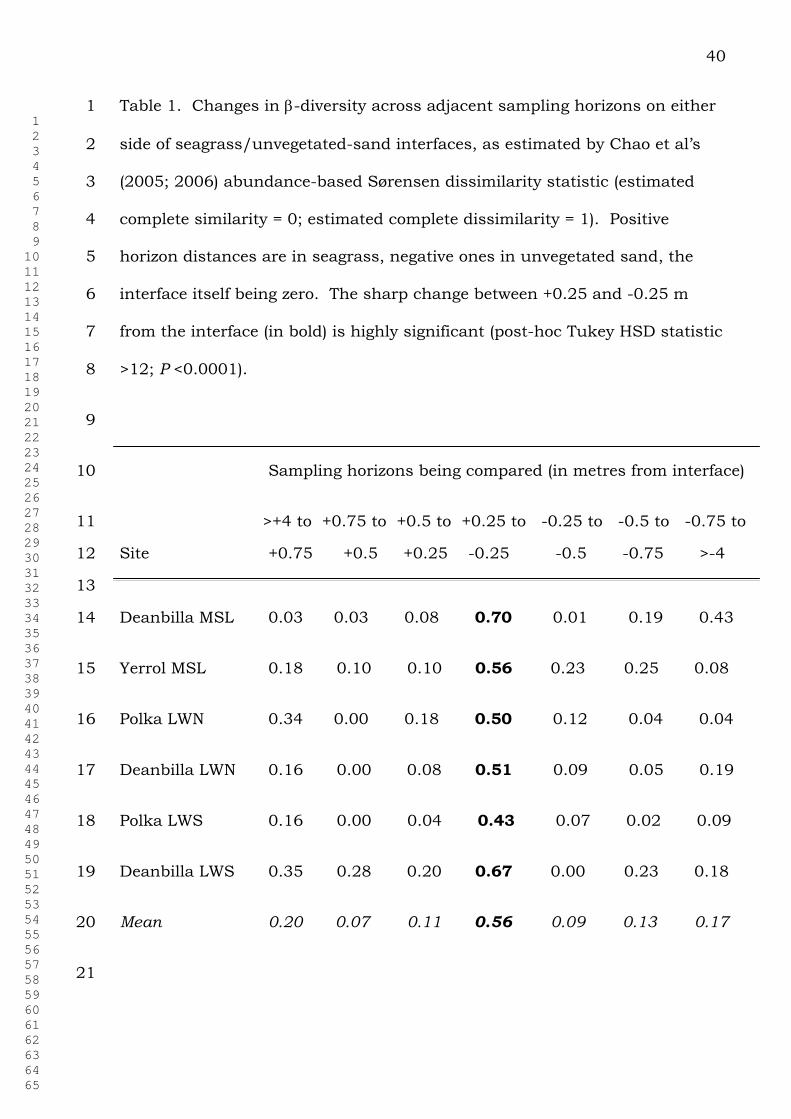
Table 1. Changes in -diversity across adjacent sampling horizons on either 1
side of seagrass/unvegetated-sand interfaces, as estimated by Chao et al’s 2
(2005; 2006) abundance-based Sørensen dissimilarity statistic (estimated 3
complete similarity = 0; estimated complete dissimilarity = 1). Positive 4
horizon distances are in seagrass, negative ones in unvegetated sand, the 5
interface itself being zero. The sharp change between +0.25 and -0.25 m 6
from the interface (in bold) is highly significant (post-hoc Tukey HSD statistic 7
>12; P <0.0001). 8
9
Sampling horizons being compared (in metres from interface) 10
>+4 to +0.75 to +0.5 to +0.25 to -0.25 to -0.5 to -0.75 to 11
Site +0.75 +0.5 +0.25 -0.25 -0.5 -0.75 >-4 12
13
Deanbilla MSL 0.03 0.03 0.08 0.70 0.01 0.19 0.43 14
Yerrol MSL 0.18 0.10 0.10 0.56 0.23 0.25 0.08 15
Polka LWN 0.34 0.00 0.18 0.50 0.12 0.04 0.04 16
Deanbilla LWN 0.16 0.00 0.08 0.51 0.09 0.05 0.19 17
Polka LWS 0.16 0.00 0.04 0.43 0.07 0.02 0.09 18
Deanbilla LWS 0.35 0.28 0.20 0.67 0.00 0.23 0.18 19
Mean 0.20 0.07 0.11 0.56 0.09 0.13 0.17 20
21

1 2 3 4 5 6 7 8 9 10 11 12 13 14 15 16 17 18 19 20 21 22 23 24 25 26 27 28 29 30 31 32 33 34 35 36 37 38 39 40 41 42 43 44 45 46 47 48 49 50 51 52 53 54 55 56 57 58 59 60 61 62 63 64 65
41
Table 2. Summary of results of two-way ANOVA on various macrofaunal 1
assemblage metrics across distance horizons away from the interface 2
between seagrass and unvegetated sand, including the main bodies of the 3
habitats concerned. Significant effects are indicated in bold. 4
5
Source of variation df MS F P 6
7
A: ASSEMBLAGES WITHIN MARGINAL SEAGRASS 8
9
1. Faunal abundance 10
Distance from interface 3 0.11 0.96 0.44 11
Position on shore 2 0.31 2.59 0.12 12
Interaction 6 0.05 0.39 0.87 13
Error 12 0.12 14
2. Observed species density 15
Distance from interface 3 0.02 1.18 0.36 16
Position on shore 2 0.33 19.72 <0.001‡ 17
Interaction 6 0.01 0.63 0.71 18
Error 12 0.02 19
3. Estimated true species density 20
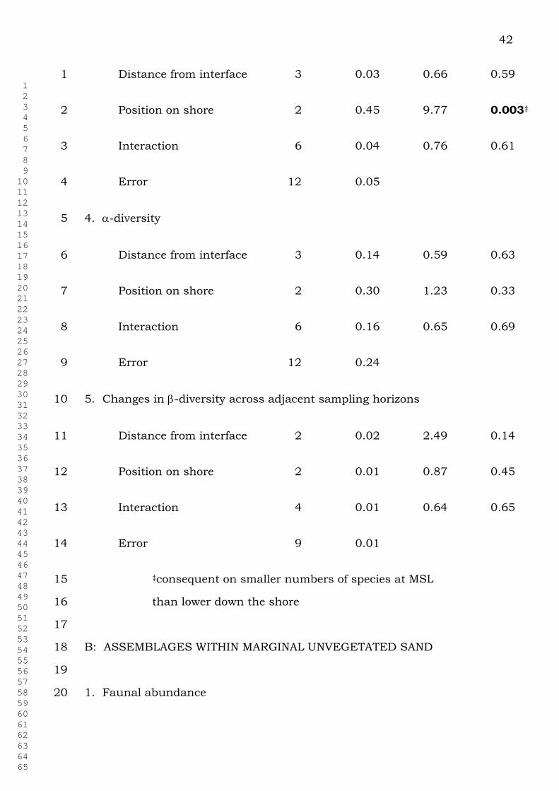
1 2 3 4 5 6 7 8 9 10 11 12 13 14 15 16 17 18 19 20 21 22 23 24 25 26 27 28 29 30 31 32 33 34 35 36 37 38 39 40 41 42 43 44 45 46 47 48 49 50 51 52 53 54 55 56 57 58 59 60 61 62 63 64 65
42
Distance from interface 3 0.03 0.66 0.59 1
Position on shore 2 0.45 9.77 0.003‡ 2
Interaction 6 0.04 0.76 0.61 3
Error 12 0.05 4
4. -diversity 5
Distance from interface 3 0.14 0.59 0.63 6
Position on shore 2 0.30 1.23 0.33 7
Interaction 6 0.16 0.65 0.69 8
Error 12 0.24 9
5. Changes in -diversity across adjacent sampling horizons 10
Distance from interface 2 0.02 2.49 0.14 11
Position on shore 2 0.01 0.87 0.45 12
Interaction 4 0.01 0.64 0.65 13
Error 9 0.01 14
‡consequent on smaller numbers of species at MSL 15
than lower down the shore 16
17
B: ASSEMBLAGES WITHIN MARGINAL UNVEGETATED SAND 18
19
1. Faunal abundance 20
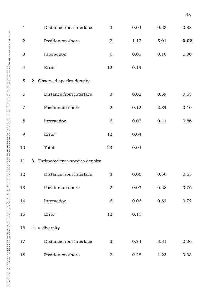
1 2 3 4 5 6 7 8 9 10 11 12 13 14 15 16 17 18 19 20 21 22 23 24 25 26 27 28 29 30 31 32 33 34 35 36 37 38 39 40 41 42 43 44 45 46 47 48 49 50 51 52 53 54 55 56 57 58 59 60 61 62 63 64 65
43
Distance from interface 3 0.04 0.23 0.88 1
Position on shore 2 1.13 5.91 0.02‡ 2
Interaction 6 0.02 0.10 1.00 3
Error 12 0.19 4
2. Observed species density 5
Distance from interface 3 0.02 0.59 0.63 6
Position on shore 2 0.12 2.84 0.10 7
Interaction 6 0.02 0.41 0.86 8
Error 12 0.04 9
Total 23 0.04 10
3. Estimated true species density 11
Distance from interface 3 0.06 0.56 0.65 12
Position on shore 2 0.03 0.28 0.76 13
Interaction 6 0.06 0.61 0.72 14
Error 12 0.10 15
4. -diversity 16
Distance from interface 3 0.74 3.31 0.06 17
Position on shore 2 0.28 1.23 0.33 18
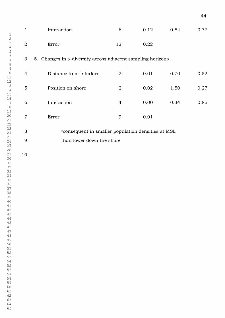
1 2 3 4 5 6 7 8 9 10 11 12 13 14 15 16 17 18 19 20 21 22 23 24 25 26 27 28 29 30 31 32 33 34 35 36 37 38 39 40 41 42 43 44 45 46 47 48 49 50 51 52 53 54 55 56 57 58 59 60 61 62 63 64 65
44
Interaction 6 0.12 0.54 0.77 1
Error 12 0.22 2
5. Changes in -diversity across adjacent sampling horizons 3
Distance from interface 2 0.01 0.70 0.52 4
Position on shore 2 0.02 1.50 0.27 5
Interaction 4 0.00 0.34 0.85 6
Error 9 0.01 7
‡consequent in smaller population densities at MSL 8
than lower down the shore 9
10
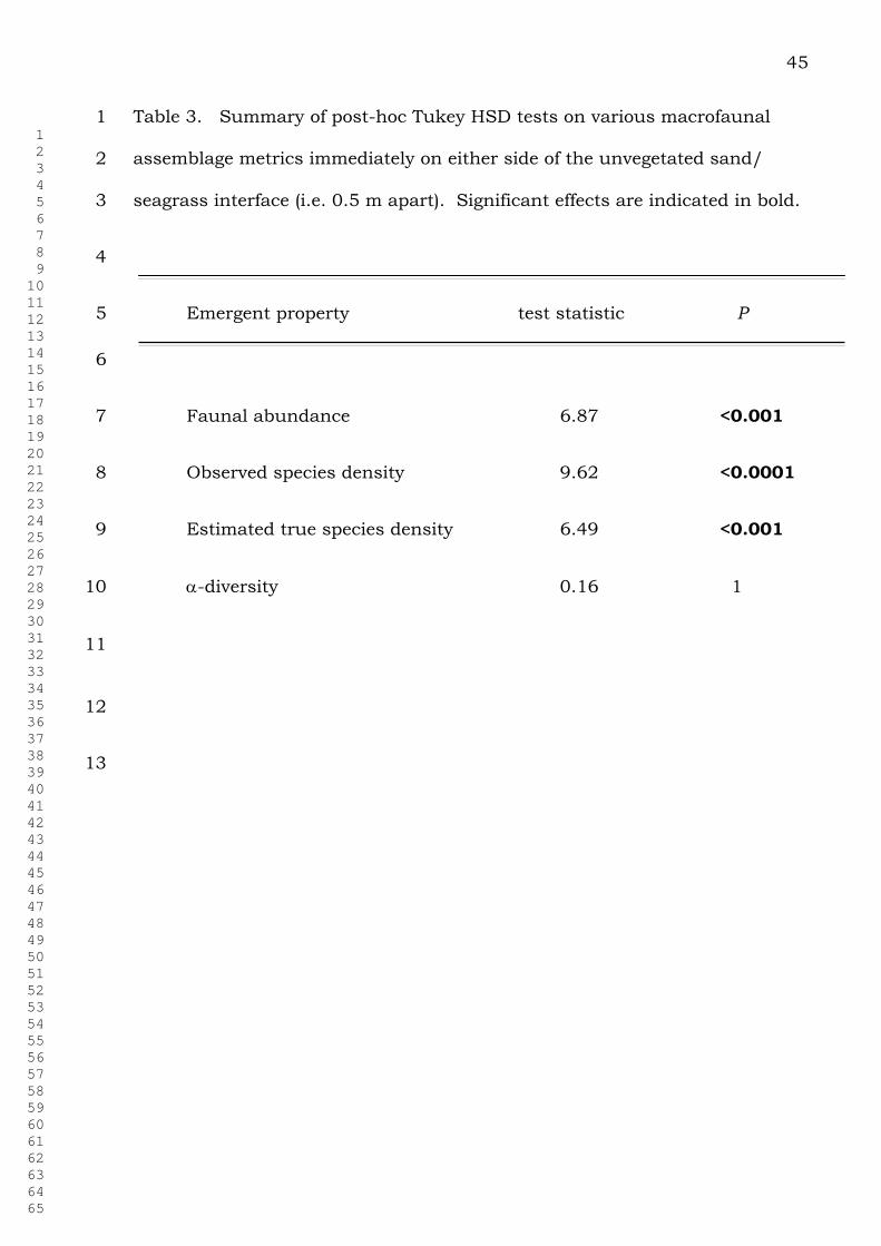
1 2 3 4 5 6 7 8 9 10 11 12 13 14 15 16 17 18 19 20 21 22 23 24 25 26 27 28 29 30 31 32 33 34 35 36 37 38 39 40 41 42 43 44 45 46 47 48 49 50 51 52 53 54 55 56 57 58 59 60 61 62 63 64 65
45
Table 3. Summary of post-hoc Tukey HSD tests on various macrofaunal 1
assemblage metrics immediately on either side of the unvegetated sand/ 2
seagrass interface (i.e. 0.5 m apart). Significant effects are indicated in bold. 3
4
Emergent property test statistic P 5
6
Faunal abundance 6.87 <0.001 7
Observed species density 9.62 <0.0001 8
Estimated true species density 6.49 <0.001 9
-diversity 0.16 1 10
11
12
13
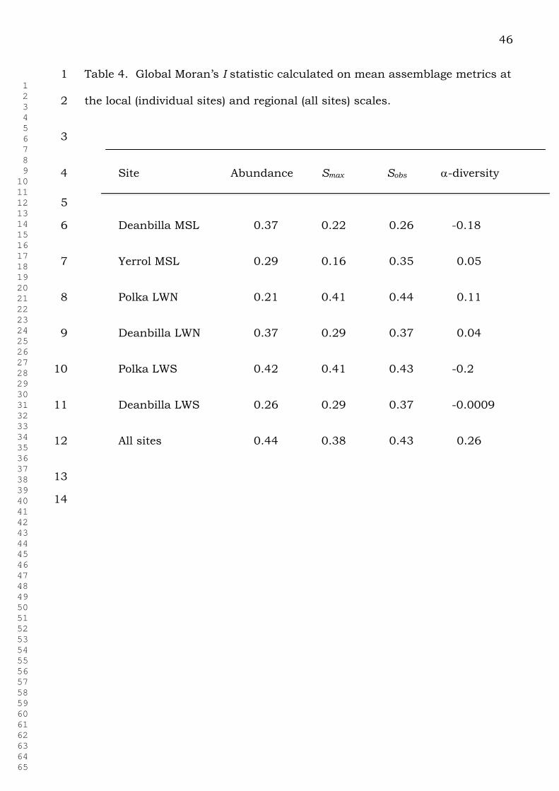
1 2 3 4 5 6 7 8 9 10 11 12 13 14 15 16 17 18 19 20 21 22 23 24 25 26 27 28 29 30 31 32 33 34 35 36 37 38 39 40 41 42 43 44 45 46 47 48 49 50 51 52 53 54 55 56 57 58 59 60 61 62 63 64 65
46
Table 4. Global Moran’s I statistic calculated on mean assemblage metrics at 1
the local (individual sites) and regional (all sites) scales. 2
3
Site Abundance Smax Sobs -diversity 4
5
Deanbilla MSL 0.37 0.22 0.26 -0.18 6
Yerrol MSL 0.29 0.16 0.35 0.05 7
Polka LWN 0.21 0.41 0.44 0.11 8
Deanbilla LWN 0.37 0.29 0.37 0.04 9
Polka LWS 0.42 0.41 0.43 -0.2 10
Deanbilla LWS 0.26 0.29 0.37 -0.0009 11
All sites 0.44 0.38 0.43 0.26 12
13
14

1 2 3 4 5 6 7 8 9 10 11 12 13 14 15 16 17 18 19 20 21 22 23 24 25 26 27 28 29 30 31 32 33 34 35 36 37 38 39 40 41 42 43 44 45 46 47 48 49 50 51 52 53 54 55 56 57 58 59 60 61 62 63 64 65
47
Legends for Figures 1
1. Sampling locations, with inset showing the structure of the individual 2
core lattices. 3
2. Interface between intertidal seagrass and unvegetated sandflat at Polka. 4
3. Numbers of macrofaunal species in marginal areas of seagrass and of 5
unvegetated sandflat in relation to (a) cumulative number of individuals 6
sampled (squares) [i.e. species richness] and (b) cumulative area sampled, as 7
number of cores (circles) [i.e. species density]. (Sample accumulation orders 8
randomised 50 times.) 9
4. The distribution of assemblage metrics across the sampling horizons on 10
either side of the interface between unvegetated sand (-) and seagrass (+): (A) 11
mean macrofaunal abundance . m-2 (± SE; n = 6); (B) mean observed (Sobs) 12
and estimated true (Smax) species density (± SE; n = 6); (C) macrofaunal -13
diversity values; and (D) mean number of seagrass shoots per core sample (± 14
SE; n = 60). 15
5. Percentage of maximum total abundance of seagrass specialist (n = 55), 16
bare-sand specialist (n = 10) and generalist (n = 8) macrofaunal species (as 17
judged from their local distributions) in each sampling horizon on either side 18
of the intertidal interface between unvegetated sand (-) and seagrass (+). 19
6. Spatial trend analysis plot of the assemblage metrics at the local (lattice) 20
and regional (all sites) scales. Mean values for each lattice are shown on the 21
left hand side and values are plotted in their geographical (x,y) locations on 22
the right hand side with the z axis depicting the value of the metric. The x 23
1 2 3 4 5 6 7 8 9 10 11 12 13 14 15 16 17 18 19 20 21 22 23 24 25 26 27 28 29 30 31 32 33 34 35 36 37 38 39 40 41 42 43 44 45 46 47 48 49 50 51 52 53 54 55 56 57 58 59 60 61 62 63 64 65
48
axis on both the local and regional plot is a proxy for distance from the 1
seagrass/sand interface. 2
7. Semivariogram plots and surfaces constructed for the lattices at each site. 3

Figure 1Click here to download high resolution image
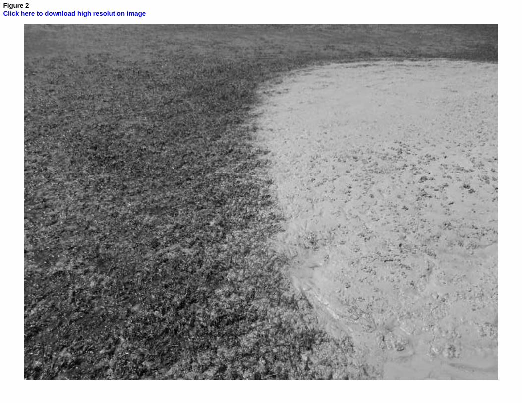
Figure 2Click here to download high resolution image
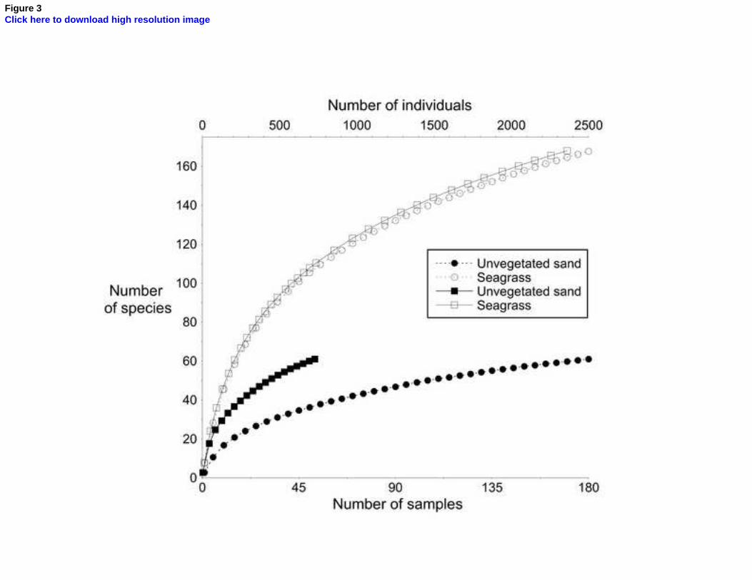
Figure 3Click here to download high resolution image
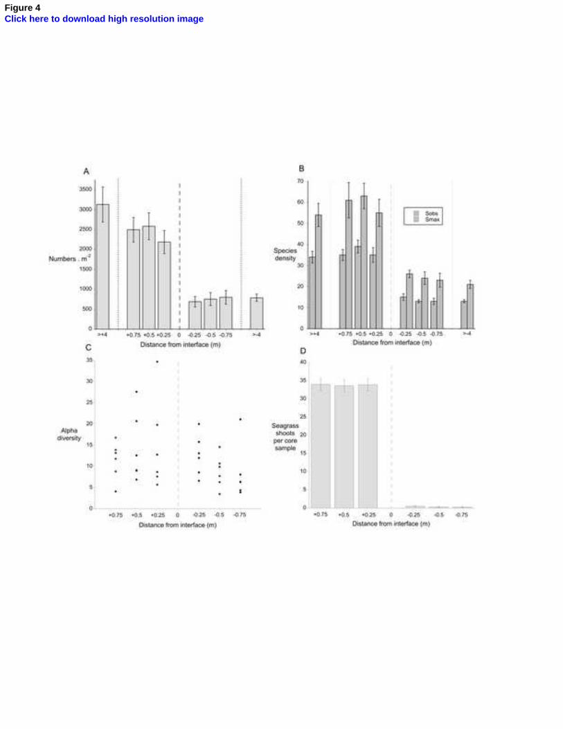
Figure 4Click here to download high resolution image
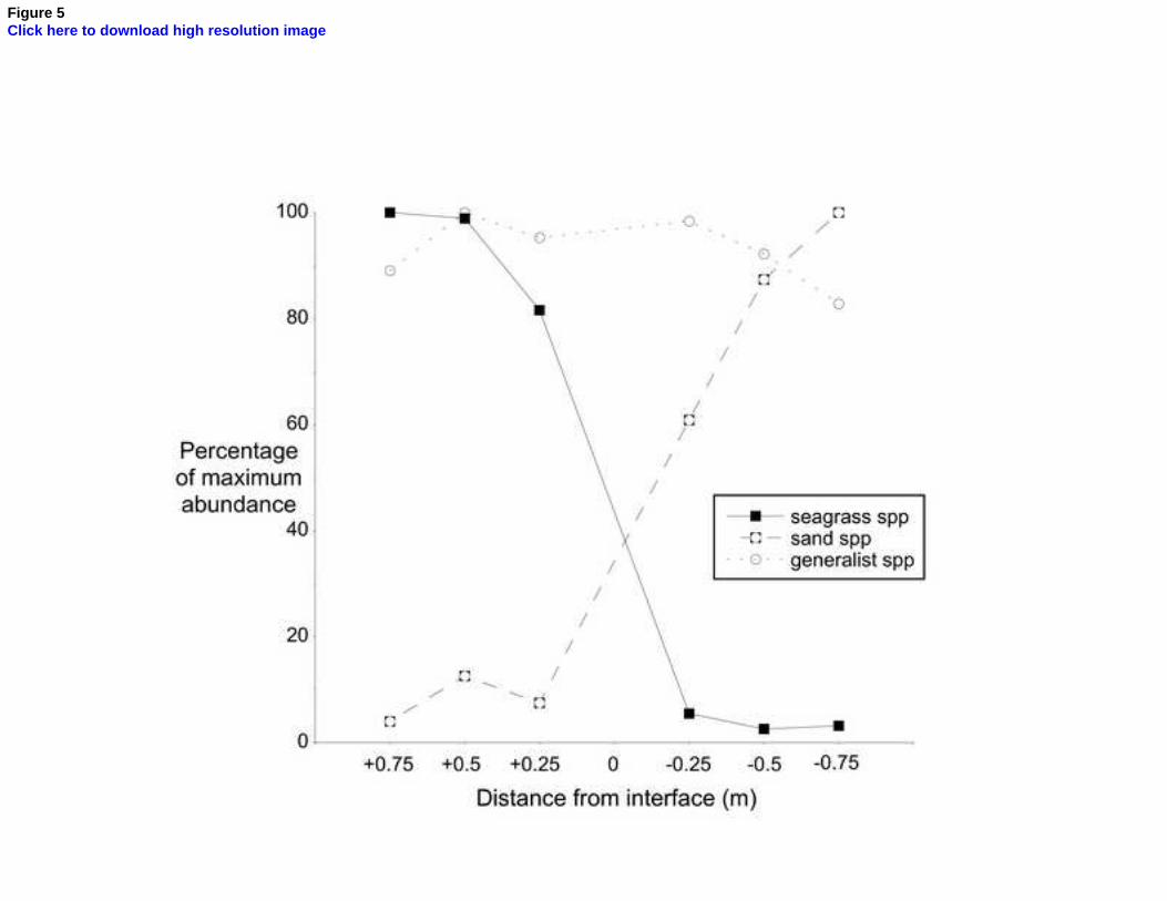
Figure 5Click here to download high resolution image

Figure 6Click here to download high resolution image
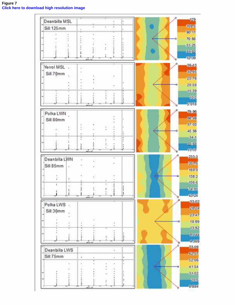
Figure 7Click here to download high resolution image
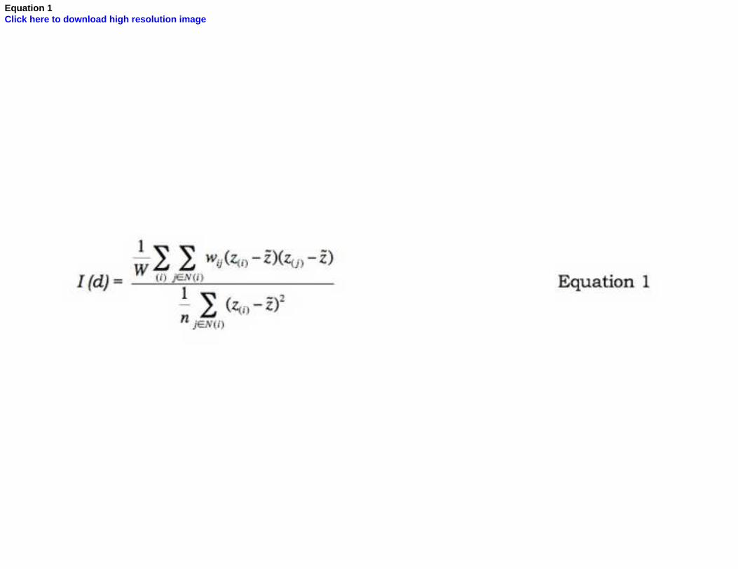
Equation 1Click here to download high resolution image
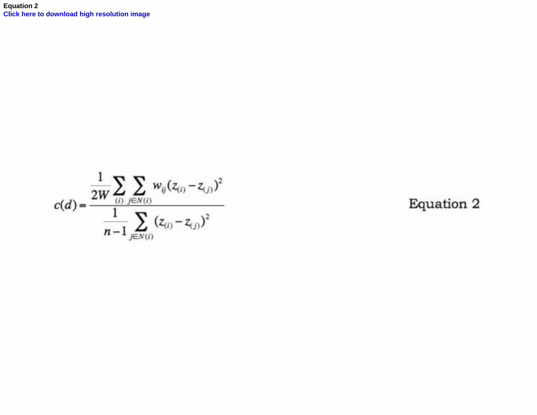
Equation 2Click here to download high resolution image