
Water quality in estuarine impoundments - Durham E-Theses
573
• • •
-
Upload
khangminh22 -
Category
Documents
-
view
3 -
download
0
Transcript of Water quality in estuarine impoundments - Durham E-Theses

Durham E-Theses
Water quality in estuarine impoundments
Wright, Julian Paul
How to cite:
Wright, Julian Paul (2002) Water quality in estuarine impoundments, Durham theses, Durham University.Available at Durham E-Theses Online: http://etheses.dur.ac.uk/4027/
Use policy
The full-text may be used and/or reproduced, and given to third parties in any format or medium, without prior permission orcharge, for personal research or study, educational, or not-for-pro�t purposes provided that:
• a full bibliographic reference is made to the original source
• a link is made to the metadata record in Durham E-Theses
• the full-text is not changed in any way
The full-text must not be sold in any format or medium without the formal permission of the copyright holders.
Please consult the full Durham E-Theses policy for further details.
Academic Support O�ce, Durham University, University O�ce, Old Elvet, Durham DH1 3HPe-mail: [email protected] Tel: +44 0191 334 6107
http://etheses.dur.ac.uk

A K ; eq xov avxov TCOTafiov OVK dv 8|j.pairiq.
(You can't step twice into the same river.)
Heraclitus, in Plato "Cratylus".

Water Quality in Estuarine Impoundments
Julian Paul Wright
The copyright of this thesis rests with the author.
No quotation from it should be published without
his prior written consent and information derived
from it should be acknowledged.
I 8 JUH 2003
Thesis submitted in accordance with
the regulations for the degree of Doctor of Philosophy
in the University of Durham,
Department of Geological Sciences, 2002.

Abstract
Water Quality in Estuarine Impoundments
Julian Paul Wright
The impounding of estuaries is currently a popular approach to urban regeneration in
the UK, with barrages constructed (Tees, Wansbeck, Tawe, Cardiff Bay, Lagan and
Clyde) or proposed (Usk, Loughor, Neath, Hayle, Avonmouth and Ipswich) nationwide.
Impounding fundamentally alters the dynamics of estuaries with consequences in terms
of sedimentation patterns and rates, ecology, flooding, groundwater, etc. This thesis
presents the findings from research into the effects of impounding on estuarine water
quality.
A series of surveys of a range of physical and chemical parameters were carried out
within four estuaries representing the complete range of tidal modification by barrage
construction. Internal versus external controls on water quality are distinguished.
General water quality in estuarine impoundments is good, but significant problems
occur where water bodies show entrenched density stratification, with anoxia and
associated increases in ammonia and metal concentrations developing. Stratification
related problems are worse in partial than total tidal exclusion impoundments (although
a higher rate of tidal overtopping shortens the isolation periods of deep anoxic waters),
and low water quality at depth is observed over the majority of the year. The potential
for eutrophication is increased by barrage construction, although phosphorus (generally
the limiting nutrient) is shown to be catchment sourced, with internal cycling from
sediment insignificant. Sediment thickness is shown not to be a control on water quality,
although sediment build-up over time eventually leads to a loss of amenity value. Sterol
fingerprints are used to identify sewage inputs to the impoundments. Advice for
barrage planners and designers is given, including the exclusion and removal of saline
water, provision of destratification/aeration devices, control of nutrient inputs, and
modelling of sediment loads and deposition. This study has shown that catchment
management is fundamental in the sustainability of estuarine impoundments.

Acknowledgements
I would like to thank my supervisor, Fred Worrall, for his tireless support throughout
this research. Fieldwork would not have been possible without the assistance of Jens
Lamping, Bernard McEleavey, Steve Richardson, Ruth Stadnik, Anna Reed, Mareike
Leiss, John Collins, Heather Handley and Alex Gardiner, all of whom endured variable
weather and erratic boat driving with stoicism. Thanks go to Norman Howitt of the
Cambois Rowing Club for allowing storage of the RV, Terry Gamick of Wansbeck
District Council for discussions on management of the Wansbeck impoundment, and
John Dickson of British Waterways for information on management of the Tees Barrage.
I would like to thank all those who made my stay in Swansea so enjoyable and
productive, particularly Hugh Morgan and Sam Taylor of Swansea City Council.
The principles and operation of the ICP machines were taught with patience by Chris
Ottley of the Department of Geological Sciences, University of Durham. Frank Davies
and Derek Coates of the Department of Geography assisted with the particle size
analyses, and many thanks go to Brian Whitton, Robert Baxter and the members of
laboratory 9 of the Department of Biological Sciences for allowing use of the nutrient
autoanalyser. Alison Reeve of the University of Dundee, Martin Jones of the University
of Newcastle and particularly Marie Russell of the Department of Geography,
University of Durham, helped with the analyses of sterol biomarkers.
Many from the Environment Agency of England and Wales provided useful data,
comment and discussion, including Michael Stokes, Richard Vaughan, Jeff Hoddy,
Eddie Douglas and Roger Inverarity. Excellent and varied logistical support was given
by the staff of the Department of Geological Sciences, University of Durham. This
work was supported financially by EPSRC Grant GR/M 42299.
Finally I would like to thank all those who have provided friendship and support during
my time in Durham. Particular mention must go to my family, Rebecca, Mrs. Grant, Dr.
Mark, Dave and Hannah, the BC Boys, the Graduate Society Hockey Club and the
postgraduate members of St. John's College and the Department of Geological Sciences.
H I

I confirm that no part of the material presented in this thesis has previously been
submitted by me or any other person for a degree in this or any other university. In all
cases material from the work of others has been acknowledged.
The copyright of this thesis rests with the author. No quotation from it should be
published without prior written consent and information derived from it should be
acknowledged.
Signed:
Date: O] /o:s /o:
I V

Contents
Title page i
Abstract i i
Acknowledgements i i i
Declaration iv
Contents v
1 Introduction l 1.1 Outline of the problem 1
1.2 Research objectives and structure of the thesis 1
1.3 Introduction to the study areas 3
1.3.1 Estuaries studied 3
1.3.2 The Tees Estuary 4
1.3.2.1 Tees River 4
1.3.2.2 Tees Barrage 6
1.3.3 The Wansbeck Estuary 8
1.3.3.1 Wansbeck River 8
1.3.3.2 Wansbeck Barrage 8
1.3.4 The Tawe Estuary 10
1.3.4.1 Tawe River 10
1.3.4.2 Tawe Barrage 10
1.3.5 The Blyth Estuary 12
1.3.5.1 Blyth River 12
1.3.5.2 Blyth Estuary 13
1.4 Water quality in estuarine impoundments; definitions and review 13
of research
1.4.1 Types of barrage 13
1.4.1.1 Tidal power barrages 14
1.4.1.2 Flood protection barrages 14
1.4.1.3 Water storage barrages 15
1.4.1.4 Urban redevelopment and amenity barrages 15
1.4.2 Water quality issues 16
1.4.2.1 Stratification 16
1.4.2.2 Dissolved oxygen 16

1.4.2.3 Sedimentation 17
1.4.2.4 Eutrophication 17
1.4.2.5 Remediation schemes 18
1.4.3 Summary of related issues 19
1.4.3.1 Ecology 19
1.4.3.2 Fisheries and fish passes 20
1.4.3.3 Groundwater 20
1.4.3.4 Flooding 21
1.4.3.5 Amenity use 22
1.4.3.6 Costs and benefits 22
Water Quality Surveys 24 2.1 Survey desien 24
2.1.1 Experimental design 24
2.1.2 Estuaries studied 24
2.1.3 Sampling stations 25
2.1.4 Depths sampled 29
2.1.5 Replicates 30
2.1.6 Dates sampled and hypothesis testing 30
2.2 Sampling procedure 32
2.2.1 Safety precautions 32
2.2.2 Procedure 32
2.3 Water quality parameters measured 34
2.3.1 Introduction 34
2.3.2 Physical/chemical 35
2.3.2.1 Dissolved oxygen 35
2.3.2.2 Biochemical oxygen demand 35
2.3.2.3 pH 36
2.3.2.4 Alkalinity 36
2.3.2.5 Eh 37
2.3.2.6 Conductivity 37
2.3.2.7 Temperature 38
2.3.2.8 Transparency 38
2.3.2.9 Total Suspended Solids 38
2.3.3 Nutrients 38
vi

2.3.3.1 Nitrogen 39
2.3.3.2 Phosphorus 40
2.3.3.3 Silicon 41
2.3.4 Major elements 41
2.3.4.1 Sodium 41
2.3.4.2 Potassium 42
2.3.4.3 Magnesium 42
2.3.4.4 Calcium 42
2.3.4.5 Sulphur 42
2.3.5 Minor and trace metals 43
2.3.6 Flow 44
2.4 Analytical methods 46
2.4.1 Dissolved oxygen 46
2.4.2 pH 47
2.4.3 Eh 48
2.4.4 Conductivity 49
2.4.5 Temperature 50
2.4.6 Transparency 51
2.4.6 Alkalinity 52
2.4.7 Total suspended solids 52
2.4.8 Biochemical oxygen demand 53
2.4.9 Nitrate, ammonia and phosphate 54
2.4.9.1 Nitrate 55
2.4.9.2 Ammonia 55
2.4.9.3 Phosphate 56
2.4.10 Metals and non-metals by ICP-OES 56
2.5 Overview of data collected during the water quality surveys 61
2.5.1 Data handling and quality assurance 61
2.5.2 Fulfilment of experimental design 61
2.5.2.1 Rivers/estuaries studied 62
2.5.2.2 Dates sampled 62
2.5.2.3 Sites and distances sampled 62
2.5.2.4 Depths sampled 62
2.5.3 Data summary 63
2.5.3.1 One-way ANOVA between estuaries 63
vii

2.5.3.2 Graphical presentation of data as boxplots 65
2.5.3.3 Tidal height and overtopping 66
2.5.3.4 River flow 66
2.5.3.5 Temperature 68
2.5.3.6 Dissolved oxygen 69
2.5.3.7 BOD 72
2.5.3.8 pH 73
2.5.3.9 Alkalinity 74
2.5.3.10 Conductivity 74
2.5.3.11 Eh 77
2.5.3.12 Transparency 78
2.5.3.13 TSS 79
2.5.3.14 Nutrients 80
2.5.3.15 Major elements 83
2.5.3.16 Minor and trace metals 86
Seasonal Effects on Water Quality 89
3.1 Introduction 89
3.2 Tees 89
3.2.1 Temperature 90
3.2.2 Dissolved oxygen 91
3.2.3 BOD 96
3.2.4 pH 100
3.2.5 Alkalinity 103
3.2.6 Conductivity 105
3.2.7 Transparency 108
3.2.8 Nutrients 112
3.2.8.1 Nitrate 112
3.2.8.2 Ammonia 116
3.2.8.3 Phosphate 119
3.2.8.4 Silica 121
3.2.9 Major elements 124
3.2.10 Fe and Mn 136
3.2.11 Summary and conclusions 142
vin
3.3 Wansbeck 146
3.3.1 Dissolved oxygen 146
3.3.2 pH 153
3.3.3 Nitrate 159
3.3.4 Ammonia 165
3.3.5 Fe 170
3.3.6 Mn 178
3.3.7 Summary and conclusions 185
Barrage Design and Water Quality 187
4.1 Introduction 187
4.2 Identification of controlling factors through PCA 187
4.3 Behavioural differences between impoundments 195
4.3.1 Dissolved oxygen 196
4.3.2 BOD 209
4.3.3 pH 210
4.3.4 Alkalinity 216
4.3.5 Conductivity 220
4.3.6 Transparency 226
4.3.7 TSS 229
4.3.8 Nutrients 233
4.3.8.1 Nitrate 223
4.3.8.2 Ammonia 243
4.3.8.3 Phosphate 252
4.3.8.4 Silica 257
4.3.9 Major elements 262
4.3.10 Fe and Mn 266
4.3.11 Fe and P 277
4.4 Summary and conclusions 279
4.4.1 Catchment controls 282
4.4.2 Freshwater flow controls 282
4.4.3 Mixing controls 283
4.4.4 Stratification controls 283
I X

3.3 Wansbeck 146
3.3.1 Dissolved oxygen 146
3.3.2 pH 153
3.3.3 Nitrate 159
3.3.4 Ammonia 165
3.3.5 Fe 170
3.3.6 Mn 178
3.3.7 Summary and conclusions 185
Barrage Design and Water Quality 187
4.1 Introduction 187
4.2 Identiflcation of controlling factors through PCA 187
4.3 Behavioural differences between impoundments 195
4.3.1 Dissolved oxygen 196
4.3.2 BOD 209
4.3.3 pH 210
4.3.4 Alkalinity 216
4.3.5 Conductivity 220
4.3.6 Transparency 226
4.3.7 TSS 229
4.3.8 Nutrients 233
4.3.8.1 Nitrate 223
4.3.8.2 Ammonia 243
4.3.8.3 Phosphate 252
4.3.8.4 Silica 257
4.3.9 Major elements 262
4.3.10 Fe and Mn 266
4.3.11 Fe and P 277
4.4 Summary and conclusions 279
4.4.1 Catchment controls 282
4.4.2 Freshwater flow controls 282
4.4.3 Mixing controls 283
4.4.4 Stratification controls 283
I X
Barrage Presence and Water Quality 285 5.1 Introduction 285
5.2 Results and discussion 286
5.2.1 Dissolved oxygen 286
5.2.2 pH 291
5.2.3 TSS 296
5.2.4 Nitrate 302
5.2.5 Ammonia 308
5.2.6 Phosphate 313
5.2.7 Na 320
5.2.8 Fe 323
5.2.9 Mn 328
5.3 Summary and conclusions 335
Sediment Quality and Speciation 337 6.1 Introduction 337
6.2 Sediment survey design 337
6.2.1 Estuaries studied 337
6.2.2 Sampling sites and dates 338
6.2.3 Replicates 338
6.3 Sediment sampling procedure 338
6.3.1 Safety precautions 338
6.3.2 Procedures 339
6.3.3 Coring 339
6.3.3.1 Dutch auger 339
6.3.3.2 Mackereth corer 339
6.4 Sediment parameters measured 340
6.4.1 Sequential extraction 341
6.4.2 Moisture content 342
6.4.3 Organic matter 342
6.4.4 Particle size distribution 343
6.5 Sediment analytical methods 343
6.5.1 Moisture content 343
6.5.2 Loss on ignition 344

6.5.3 Organic carbon 345
6.5.4 Particle size distribution 345
6.6 Sequential extractions 347
6.6.1 Sequential extraction method (after Tessier et al., 1979) 348
6.6.2 S E D E X method (after Ruttenburg, 1992) 350
6.6.3 ICP-OES analysis of extracts 353
6.7 Results and discussion 354
6.7.1 Errors 354
6.7.2 Particle size distribution 355
6.7.3 Organic matter 363
6.7.4 Metals and non-metals concentration and speciation 368
6.7.4.1 Al 368
6.7.4.2 Ca 372
6.7.4.3 Co 378
6.7.4.4 Cr 383
6.7.4.5 Cu 387
6.7.4.6 Fe 391
6.7.4.7 K 395
6.7.4.8 Mg 399
6.7.4.9 Mn 405
6.7.4.10 Ni 411
6.7.4.11 P 416
6.7.4.12 Sc 420
6.7.4.13 Si 424
6.7.4.14 Ti 429
6.7.4.15 Zn 433
6.8 Controls on sediment chemistry 438
6.9 Summary and conclusions 448
6.9.1 PCA 448
6.9.2 Geochemistry 449
6.9.2.1 Redox controls 451
6.9.2.2 Input controls 453
6.9.2.3 Overlying water composition and ion-exchange 455
controls
6.9.2.4 Particle-size controls 456
XI

6.9.3 Sediment quality 457
6.9.4 Sediment fingerprinting 459
Sediment Pore Water Sampling 462
7.1 Introduction 462
7.2 Survey design 462
7.2.1 Estuaries studied 462
7.2.2 Sampling sites and dates 462
7.2.3 Replicates 463
7.3 Sampling procedure 463
7.3.1 Sediment coring 463
7.3.2 Gel probe description 463
7.3.3 Gel probe deployment and front equilibration 465
7.3.4 Gel probe retrieval and slicing 465
7.3.5 Back equilibration of gel slices 466
7.3.6 Elemental analysis 466
7.3.7 Method development experiments and LODs 468
7.4 Results and discussion 470
7.4.1 Al 472
7.4.2 As 473
7.4.3 Ca 475
7.4.4 Co 476
7.4.5 Cr 477
7.4.6 Cu 479
7.4.7 Fe 480
7.4.8 Hg 481
7.4.9 K and Mg 482
7.4.10 Mn 484
7.4.11 P 485
7.4.12 Pb 487
7.4.13 Sc 488
7.4.14 Si 489
7.4.15 Ti 491
7.4.16 V 492
Xll

7.5 Summary and conclusions 494
7.5.1 Biogeochemistry/diagenetic controls 494
7.5.1.1 Fe, Mn, Al, Co, Cr, P, Si and Ti 494
7.5.1.2 Ca, K and Mg 495
7.5.1.3 As, Hg, Sc and V 495
7.5.1.4 Cu and Pb 496
7.5.2 Fluxes across the SWI 496
7.5.2./ Relative contribution of sediment P to the 499
impounded water bodies
7.5.2.2 Relative contribution of sediment Mn to the 500
impounded water bodies
8 Sterol Biomarkers in Estuarine Impoundments 502 8.1 Introduction 502
8.2 Survey design 504
8.2.1 Estuaries studied 504
8.2.2 Sampling sites and dates 504
8.3 Methodologies 505
8.3.1 Sediment sampling 505
8.3.2 Sterol extraction 505
8.3.3 Sterol analysis 506
8.4 Results and discussion 507
8.4.1 Ratios and sources of sterols 508
8.4.2 Coprostanol concentrations and faecal inputs over time 511
8.5 Summary and conclusions 512
9 Conclusions 514 9.1 Review of research objectives 514
9.2 Major findings 514
9.2.1 Current water quality 514
9.2.2 Seasonal variation in water quality 515
9.2.3 Barrage design and water quality 515
9.2.4 The effects of impounding on water quality 516
xm

9.2.5 Sediment quality 516
9.2.6 Sediment geochemistry 517
9.2.7 Pore water quality 517
9.2.8 Biogeochemical processes at the SWI 518
9.2.9 Fluxes across the SWI 518
9.2.10 Sewage inputs to the impoundments 518
9.3 Implications 519
9.4 Suggestions for further work 521
9.5 Concluding remarks 523
References 524
Appendices 551
1. Statistical methods used 551
XI v

Chapter 1: Introduction
Chapter 1
Introduction
1.1 Outline of the problem
The impounding of estuaries is currently a popular approach to urban regeneration in
the UK (Wright and Worrall, 2001). By creation of an aesthetically pleasing amenity
impoundment, including the drowning of "unsightly" tidal mud flats, it is hoped that
prestige development will be encouraged in the estuarine area (Burt and Cruickshank,
1996). Such barrage developments include the Tawe and Cardiff Bay in South Wales,
the Lagan in Northern Ireland and the Tees in Northeast England. The concepts of
impounding estuaries are also of international significance, with projects proposed or
built worldwide (e.g. the Venice Lagoon Project (Cecconi, 1996)).
Negative impacts on water quality associated with impounding of estuaries have been
reported (e.g. Worrall et al., 1998; Reynolds, 1996), including unacceptably low
concentrations of dissolved oxygen and increased likelihood of algal blooms. Research
has concentrated on either case studies of water quality in single impoundments (e.g.
Evans and Rogers, 1996) or process-based water quality modelling (e.g. Maskell and
Barraclough, 1996). Very little empirical modelling, and no comprehensive studies
including comparison of a several estuarine impoundments, have been carried out.
Broadly this research aims to address this shortfall in order to assess the impacts of
impounding estuaries and allow suggestion of how negative water quality impacts may
be mitigated.
1.2 Research objectives and structure of the thesis
The general aim of this research is to understand water quality in estuarine
impoundments. The main objectives of the research may be summarised:
1. Assess the current state of water and sediment quality in estuarine
impoundments.
2. Measure the importance of the factors of season, barrage design and
impounding on estuarine water quality.
3. Understand the processes controlling water quality that are affected by
impoundment (particularly in terms of sediment-water interactions).

Chapter 1: Introduction
The work carried out in order to achieve these research objectives and reported within this thesis includes:
1. Water quality surveys of a broad range of physical and chemical water quality
paranmeters within a set of four estuaries showing differences in impoundment
status (impounded or non-impounded; amount of tidal intrusion).
2. Bed sediment surveys of elemental concentrations and speciations from two
estuaries of contrasting impoundment design (partial vs. total tidal exclusion).
3. Pore water surveys of elemental concentrations within the bed sediments close
to the sediment-water column interfaces of two estuaries of contrasting
impoundment design (partial vs. total tidal exclusion).
4. Sewage input surveys based on the extraction of sterol biomarkers from the
sediments of two impoundments.
A series of water quality surveys were carried out on a range of periods between 1999
and 2001 for the Tees, Wansbeck, Blyth and Tawe estuaries. Chapter 2 presents the
background to these water quality surveys including the survey designs, choice of water
quality parameters included, sampling procedures and analytical methodologies,
together with an overview of the data collected during the surveys. Chapter 3 presents
statistical assessments of the seasonal differences in water quality within both the Tees
and the Wansbeck impounded estuaries. Chapter 4 looks at the differences in water
quality behaviour between designs of estuarine impoundment (the Tees, Wansbeck and
Tawe impoundments). The effects of impoundment are discussed in chapter 5 through
the comparison of an impounded with an equivalent un-impounded estuary (the
Wansbeck and the Blyth respectively).
Cores of bed sediment were taken from the Tees and Wansbeck impounded estuaries in
July 2001 and underwent sequential extraction and elemental analysis by ICP-OES.
Chapter 6 presents the results from these experiments and discussion in terms of
sediment quality, elemental speciation and environmental mobility within the sediments
of estuarine impoundments.
The biogeochemistry of elements in the pore water phase of the sediments of estuarine
impoundments was researched through tne use of DET gel-probe technology pore water
sampling within the Tees and the Wansbeck impoundments and is discussed in chapter

Chapter 1: Introduction
7. Within this chapter estimations of exchanges across the sediment-water column
interface and the impacts on water quahty are also presented.
Chapter 8 presents work carried out using sterol biomarker analysis from samples from
the bed sediments of the Tees and Wansbeck to assess the inputs of sewage to these
impoundments.
A summary of the major findings from chapters 2 to 8 together with a discussion of the
implications of this research are presented in the final chapter of this thesis.
Suggestions for further work in the subject of water quality in estuarine impoundments
are also given.
1.3 Introduction to the study areas
1.3.1 Estuaries studied
Four UK estuaries were included in this study. The estuaries chosen represent the
complete range of impacts of barrage construction on tidal intrusion to estuaries (figure
1.1). The location of the estuaries is shown in figure 1.2.
Non-impounded
("natural" estuary)
Total tidal
exclusion
(freshwater
impoundment)
Blyth
(estuary)
100%
Tawe
(impoundment)
70%
Wansbeck
(impoundment)
30%
Tees
(impoundment)
0%
Figure 1.1. The estuaries included in this research showing the % of tides being able to
enter the impoundments or estuary.

t-4 ' j
»
Tawe
Chapter 1: Introduction
Wansbeck
Blyth
Tees
4 J
Figure 1.2. Approximate locations in the UK of the four estuaries included in this
research (more detailed site maps are included in chapter 2).
1.3.2 The Tees Estuary
13.2.1 Tees River
The River Tees is located in NE England, and rises at Tees Head on the eastern slopes
of Cross Fell in the Cumbrian Pennines at 893 m AOD. The river flows from west to
east with an approximate length of 160 kilometres and a drainage area of 1930 km^.
Tributaries to the Tees include the Rivers Greta, Balder, Skeme, Leven, Lune and
Billingham Beck. The upland Tees flows over open moorland to Cow Green Reservoir
(built in 1970 to store 40 million m^ of water for the then predicted heavy industrial
growth on Teeside) which, together with the Selset and Grassholme Reservoirs on the
Lune and Balderhead, Blakton and Hury Reservoirs on the Balder, acts to moderate
flood flows and sustain a minimum flow during dry periods. Nevertheless, the Tees
remains a 'flashy' river with water rising by as much as 1 m in 15 minutes during the
summer (Archer, 1992). The Tees then flows ESE through Teesdale to Barnard Castle
then turns E to Darlington, at which point the valley widens, the slope decreases and

Chapter 1: Introduction
flow meanders over a wide flood plain. The lowland tributaries contribute little to the
stormflow of the Tees, the majority of which is generated by rainfall on the Pennines.
The upland Tees flows over solid geology of mainly limestones and sandstones of the
Carboniferous Limestone Series (Dinantian) plus parts of the Whin Sill (doleritic
igneous intrusion) and extensive areas of blanket peat. Within the lowland river and
estuary the solid geology is overlain by drift deposits of clay, peat, alluvium, river
gravels and blown sands.
The major industrial discharges to the Tees take place in the lower estuary (i.e.
downstream of the barrage). The industrialisation of Teesside commenced with the
opening of the Stockton - Darlington railway in 1825 and development of steel works.
In 1926 Imperial Chemical Industries (ICI) was formed, this produced large-scale
investment in chemical complex at Billingham. ICI produce fertilisers, heavy organic
chemicals and chlorine. In 1934 British Titan Products (now BTP Tioxide) conmienced
production of titanium dioxide pigments at Billingham. More recently Monsanto,
Rohm and Hahns (UK), Shell Oil and Phillips Petroleum came to Teesside. The Tees
estuary has -10% of total UK oil refining capacity. The river Tees before the
industrialisation of Teesside had supported a flourishing fishing industry and was noted
for its catches of salmon, sea trout, flounders and eels. By 1937 salmon had virtually
been eliminated. In 1970 the river Tees was considered to be one of the most heavily
polluted estuaries in the UK. The daily BOD load (>500 tonnes) from chemical,
petrochemical, steel making industries and untreated domestic sewage left the estuary
devoid of oxygen. Conmion Law control mechanisms had failed to prevent gross
pollution of the river Tees. In 1972 Teesside Borough Council drew up a proposal to
decrease pollution by domestic sewage. Large interceptor sewers were built to channel
discharges from Stockton, Norton and Billingham in the north, and from Aklan,
Linthorpe and Thomaby in the south, to a newly constructed treatment works at
Portrack. A major pollution initiative in 1980 reduced the BOD discharge load to a
quarter of the 1970s load. In 2001 estuarine water quality in the lower estuary was
defined as generally fair according to EA General Quality Assessment methodologies,
and good above the barrage. Improvements in levels of DO have meant that the Tees is
now able to support runs of migratory fish, with 7000 salmon and 13000 sea trout
estimated to have migrated through the Tees in 2000 (www.environment-
agency.gov.uk).

Chapter 1; Introduction
1.3.2.2 Tees Barrage
The Teesside Development Corporation (TDC) was established in 1987 to encourage
redevelopment of the Teesside area. Economic analysis suggested that construction of a
barrage would have a positive impact on land and property values in the vicinity of the
impoundment, and therefore the TDC submitted a Private Bill proposing such to
Parliament in 1988. Royal Assent was given in 1990 and construction (by Tarmac
Construction) started in November 1991. The Tees barrage came into operation in
January 1995, with all construction work completed by April 1995.
The Tees Barrage (NZ 4616 1905) rests on a 5 m thick 70 m by 32 m reinforced
concrete foundation, above which stand 5 concrete piers with 4 fish belly flap gates
between them. Each gate is 13.5 m long and 8.1 m deep and hinged at the base with
height controlled by hydraulic rams (figure 1.3), with crest height permanently
maintained at between 2.4 and 2.8 m AOD. The piers incorporate low-level sluices
designed to discharge any accumulated low level pollution or saline intrusion. There
are pavilion buildings at each end of the barrage and a road linking to the A66 running
along the top (figure 1.4). Ancillary works incorporated in the scheme include a white
water course (for canoeing and white-water rafting), a 6 m wide navigation lock, fish
pass and caravan and camping park and outdoor amphitheatre. The impoundment itself
allows a range of water sports including rowing, sailing, jet-skiing and water-skiing.
Prior to construction of the barrage the tidal limit was at Low Moor (NZ 3655 1050) 44
km from the mouth of the Tees estuary, with saline intrusion penetrating approximately
28 km upstream from the mouth (Environment Agency, 1999). The strength of tidal
currents was insufficient to produce complete mixing of fresh and saline water over the
whole length of the estuary and the system was classified as partially stratified
according to the classification scheme of Pritchard (1955). The Tees Barrage is a total
tidal exclusion barrage, i.e. the crest height of the barrage is permanently kept higher
than all high tides. The barrage therefore marks the upstream limit of saline intrusion
with a completely freshwater impoundment maintained above this. The length of the
Tees from the former tidal limit at Low Moor to the Tees Barrage is 26 km. The
historic poor water quality of the lower Tees Estuary was a sipjiificant factor in the
decision to construct the barrage as a total tidal exclusion system.

Chapter 1: Introduction
Figure 1.3. The hydraulically controlled flap-gates of the Tees Barrage.
Figure 1.4. The Tees Barrage viewed from the upstream (impounded) section.

Chapter 1: Introduction
1.3.3 The Wansbeck Estuary
1.3.3.1 Wansbeck River
The Wansbeck is a lowland river also in NE England. It flows from west to east for a
distance of 39 km, with the highest point at 440 m AOD, draining a catchment of 339
km^. Tributaries include the River Font, including the Font Reservoir, and Hart Bum.
The geology of the Wansbeck catchment is of Carboniferous age, with the Fell
Sandstone of the Carboniferous Limestone Series in the headwaters, Millstone Grit in
the middle reaches, and Coal Measures in the lower reaches. Land-use on the
catchment is predominantly agricultural, with an increase in intensity from the
headwaters to the downstream stretches of the river as the river flows through the town
of Morpeth. Flows in the Wansbeck average 2.85 m /s, with very low levels during dry
summers (0.12 m /s reported in 1989 (Archer, 1992) having caused public water supply
at Mitford to cease for 4 months (Archer, 1992)).
The Wansbeck is classified as eutrophic, and in June 2002 the River Wansbeck and the
Amenity Lake (estuarine impoundment) were added to the list of Sensitive Areas under
Urban Waste Water Treatment Regulations (DEFRA, 2002). These regulations,
transposed from European Council Directive (91/271/EEC), require tertiary treatment
(i.e. removal of phosphorus and/or nitrogen) within sewage treatment works (STWs)
serving communities of greater than 10,000 discharging to the water course. The
Wansbeck is subject to inputs from acid mine drainage from abandoned coal mines in
the catchment.
1.3.3.2 Wansbeck Barrage
In 1972, the then Ashington Urban Council contracted Babtie, Shaw and Morton
Consulting and Civil Engineers to carry out a feasibility study for construction of a
barrage across the Wansbeck Estuary. The aim of barrage construction on the
Wansbeck was the creation of an amenity area for the local population in the form of a
riverside park, and thus to attract replacement industries to the area following the
decline of the north-east coalfield. This contrasts with the major aims of urban
redevelopment on the margins of the Tees and Tawe impoundments. Construction of a
barrage commenced in January 1974 and the estuary was impounded in May 1975, thus
making the Wansbeck Barrage the oldest amenity estuarine impoundment scheme in the
UK.
8

Chapter 1: Introduction
The Wansbeck Barrage (NZ 2935 8536; figure 1.5) is a fixed crest concrete structure resting on a 0.5 m thick 9 m by 100 m concrete foundation. The crest height is 2.14 m AOD. A footbridge supported by piers at 8 m intervals runs over the barrage at a height of 2.7 m above the crest. Ancillary works include a navigation lock, fish pass, sluice gate to allow draining of the impoundment, and caravan park. The impoundment is used by Cambois Rowing Club, and to a minor degree by jet-skiers, although the shallow depth and trapping of tree branches carried by high flows can interfere with these uses. At present the lock is in a poor state of repair and cannot function to allow navigation, although it is used by Wansbeck District Council in attempts to drain the impounded area since the sluice gate lifting mechanisms are missing.
Figure 1.5. The Wansbeck Barrage viewed from the upstream (impounded) section.
The tidal limit of the Wansbeck estuary is 4 km upstream of the barrage at the weir at
Sheepwash (NZ 2565 8587), with a maximum saline intrusion both pre and post-barrage
construction through the majority of this distance. Prior to barrage construction, low
freshwater discharges of the River Wansbeck caused exposure of large areas of tidal
mud flats at low tides, and the covering of this 'black desolation' was a major motive

Chapter 1: Introduction
for impoundment (Worrall and Mclntyre, 1998). The crest height of 2.14 m allows high
tides of 4.7 m and greater (30 % of high tides) to enter the impounded area. The
decision on the height of the barrage crest was made on the basis of a desire to provide a
sufficient water depth in the impoundment to allow navigation of boats of 1.6 m draft,
and the false assumption that optimum water quality would be maintained by increasing
turnaround of the impounded water under conditions of low freshwater flow by the
intrusion of seawater. The volume of water stored in the Wansbeck impoundment is
approximately 725000 m^.
1.3.4 The Tawe Estuary
1.3.4.1 Tawe River
The River Tawe is located in South Wales. It rises in the Black Mountains at
approximately 590 m AOD and flows in a south-westerly direction over a length of 48
km to meet the Bristol Channel at Swansea. The Tawe catchment is 272 km^ and is
heavily urbanised in its lower reaches with the towns of Ystradgynlais, Ystalyfera,
Pontrdawe, Clydach and Swansea. The major tributary to the Tawe is the Afon Twrch.
The River Tawe flows mainly over Carboniferous Coal Measures, with the
Carboniferous Limestone Series and Millstone Grit series plus Old Red Sandstone
(Devonian) exposed in upstream reaches. Flows in the Tawe averaged 12.7 m /s at the
tidal limit between 1982 and 1992 (Russell et al., 1998).
The Lower Swansea Valley has a 240 year (1720-1960) history as a world centre for
industrial metal smelting, which has left large areas of land contaminated with Cu, Zn,
Pb, Cd and Ni. Metal pollution to the Tawe from these sources has declined since the
1960s as a result of cessation of smelting and remediation work carried out, but metal
inputs are still significant during stormflow conditions (Bird, 1987). The Tawe is also
subject to inputs of acid mine drainage from abandoned coal mines in the catchment.
1.3.4.2 Tawe Barrage
Following the decline of the heavy industrial use (metal smelting) of the lower Swansea
Valley, Swansea City Council proposed construction of an amenity barrage as part of a
redevelopment plan for the urban area. Feasibility studies, carried out by W S Atkins
(Atkins, 1983), indicated that there were unUkely to be adverse effects from the
proposed scheme, although the final structure ditfered significantly from the initial
plans for which the impact assessment was carried out by being partial as opposed to
10

Chapter 1: Introduction
total tidal exclusion. Permission for barrage construction was granted in the Swansea
City Council (Tawe Barrage) Act in 1986, construction of the barrage began in 1990
and the estuary was impounded in July 1992.
Figure 1.6. The Tawe Barrage viewed from the downstream side.
Figure 1.7. The navigation lock of the Tawe scheme showing the redevelopment of the
marina area.
11
Chapter 1: Introduction
The Tawe Barrage (SS 6640 9260; figure 1.6) is a fixed crest concrete structure with a total length of 140 m, with a primary weir of 19 m length and a secondary weir of 45 m length. The crest height of the primary weir is 3.05 m AOD with the secondary weir at 3.35 m AOD. Low level sluices are included in the design to allow drawdown of the impoundment. Ancillary features of the Tawe Barrage include a navigation lock and a fish pass. The impounded area includes a popular marina development meaning that the navigation lock is in regular use (figure 1.7), and that the financial implications of drawdown of the impoundment are prohibitively large.
The tidal range at the Tawe estuary is large, and the crest height of the primary weir of
8.05 m AOD allows approximately 70 % of high tides to overtop the barrage, with
influx of seawater occurring over 16 % of the time (Mee et al., 1996). Prior to
impoundment there was little vertical variation in salinity, except for short periods
around slack water (Shackley and Dyrynda, 1996), and the estuary was classified as
partially mixed. The limit of saline intrusion was recorded to approximately 3.6 km
upstream of the current barrage site, and the tidal limit is at Landore (SS 6660 9620) 5.6
km upstream from the barrage. Post-impoundment, saline stratification of the water
body has been recorded up to 5 km upstream of the barrage (Russell et al., 1998).
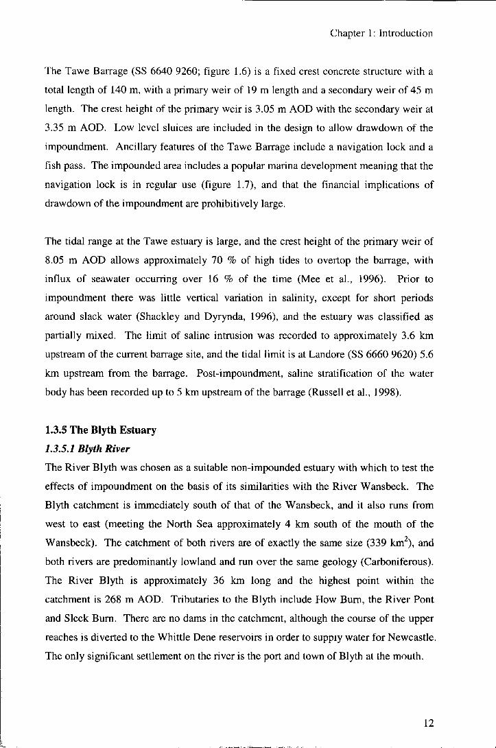
1.3.5 The Blyth Estuary
1.3.5.1 Blyth River
The River Blyth was chosen as a suitable non-impounded estuary with which to test the
effects of impoundment on the basis of its similarities with the River Wansbeck. The
Blyth catchment is immediately south of that of the Wansbeck, and it also runs from
west to east (meeting the North Sea approximately 4 km south of the mouth of the
Wansbeck). The catchment of both rivers are of exactly the same size (339 km^), and
both rivers are predominantly lowland and run over the same geology (Carboniferous).
The River Blyth is approximately 36 km long and the highest point within the
catchment is 268 m AOD. Tributaries to the Blyth include How Bum, the River Pont
and Sleek Bum. There are no dams in the catchment, although the course of the upper
reaches is diverted to the Whittle Dene reservoirs in order to supply water for Newcastle.
The only significant settlement on the river is the port and town of Blyth at the mouth.
12

Chapter 1: Introduction
1.3.5.2 Blyth Estuary
The Cramlington and Blyth STWs have a combined discharge to the estuary (NZ 2950
8249), with a maximum discharge of secondary treated sewage (with 70 % BOD
removal according to the Urban Waste Water Treatment Directive) of 19880 m^/day
from Cramlington and 11664 m^/day from Blyth. In terms of estuary classification, the
tidal currents within the Blyth create an estuary with a partially mixed salinity structure.
Tees Wansbeck Tawe Blyth
River length 160 km 39 km 48 km 36 km
Catchment area 1930 km^ 339 km^ 272 km^ 339 km^
Highest point 893 m 440 m 590 m 268 m
Geology Carb. Ists. and Carb. ssts.. Carb. ssts.. Carb. ssts.,
ssts. grits and coal Ists., grits and grits and coal
Dolerite. measures. coal measures. measures.
Extensive drift ORS
(mainly peat (Devonian)
and alluvial).
Table 1.1. Catchment characteristics for the rivers included in this research.
1.4 Water quality in estuarine impoundments; definitions and review of research
1.4.1 Types of barrage
An estuary is a semi-enclosed coastal body of water which has free connection to the
open sea and within which sea water is measurably diluted with fresh water derived
from land drainage (Cameron and Pritchard, 1963). An estuarine barrage is a structure
which, for various reasons, is designed to modify or totally prevent the progression of
the tide up an estuary or inlet (Burt and Rees, 2001). Major reasons for barrage
construction include:
• Tidal power generation.
• Tidal surge flood protection.
• Water storage.
• Urban regeneration.
• Amenity use.
13

Chapter 1: Introduction
1.4.1.1 Tidal power barrages
Barrages for tidal power generation are periodically considered in regions with large (5-
15 m) tidal ranges. Within the UK, schemes have been proposed for several estuaries of
the west coast including the Severn, Dee, Ribble, Solway and Mersey estuaries. The
economics of the costs of barrage construction vs. the revenues from the electricity
produced have meant that few tidal power generation schemes have been built.
Significant power is produced at the Ranee Barrage in France and the Annapolis Royal
Power Station in Canada. The Ranee Barrage was completed in 1967, and with twenty
four 10 MW turbines is the largest tidal energy scheme in the world (Burt and
Cruickshank, 1996; Shaw, 1995). Operating and environmental problems encountered
in the Ranee include marine growth in the generators, sedimentation and accumulation
of organic matter in the basin, reduction in littoral area, and loss of species diversity.
The isolation of the estuary during the construction phase is given as particularly
environmentally damaging, eradicating marine flora and fauna (Retiere, 1994). The
Annapolis Barrage, successfully operating since 1984, is a 20 MW pilot project with the
aim of assessing the potential for a large scale tidal power project in the Bay of Fundy.
Increased primary production (due to both stratification of and reduced turbidity in the
(non-nutrient limited) impounded water) is suggested as a consequence of such a
scheme (Gordon, 1994; Tidmarsh, 1984). Parker (1993) suggests that the water quality
implications of tidal power barrages are likely to be site specific, and strongly
dependent on inputs to the impounded area.
1.4.1.2 Flood protection barrages
As opposed to power generation barrages, tidal surge protection barrages are relatively
common. Surge protection is generally achieved by means of a movable barrier, which
is only positioned to impede tidal ingress under periods of flood risk. Examples of such
schemes include the Thames and Hull Barriers in the UK, and the Delta Works of SW
Holland and the Venice Lagoon Project in Italy. The Thames Barrier is the largest
navigable flood barrier in the world and was constructed to protect London from
flooding during storm surge conditions in the North Sea. It consists of a series of rising
sector ggtes set in sills at bed level such that the obstruction to normal tidal flows is
minimal. The gates are raised only during tidal surges up the Thames fWilkes, 1996).
A similar scheme is proposed for the Venice Lagoon to avoid the increasingly frequent
(average 45 times per year) acqua alta (floodings) of Venice (Bandarin, 1994; Cecconi,
14

Chapter 1: Introduction
1996). Flood protection estuarine barrages are generally designed to minimise the
disruption of natural estuarine behaviour and thus have minimal impact on water quality,
and are therefore not included this research. The Venice Lagoon may however undergo
longer periods of tidal disruption and, as with tidal power barrages, pollution loads to
the impounded area are suggested as critical in controlling water quality (Bernstein and
Cecconi, 1996).
1.4.1.3 Water storage barrages
Estuarine impoundments may function as freshwater storage impoundments in regions
with limited groundwater or space for inland reservoirs. Such embayments are built in
Hong Kong (Don, 1973), but have been rejected as economically unviable in the UK
(Water Resources Board, 1966).
1.4.1.4 Urban redevelopment and amenity barrages
The research described within this thesis concentrates on barrages constructed in
relation to urban redevelopment and amenity use in the UK. The barrages on which
sampling was carried out (the Tees, Wansbeck and Tawe) are described above. A large
number of additional estuarine barrages have either been constructed or have been
proposed throughout the UK. Barrages which have been constructed include the Lagan
in Northern Ireland, the Clyde in Scotland and Cardiff Bay in South Wales. Barrages
have been proposed for the Usk, Loughor and Neath in S Wales and at Hayle,
Avonmouth and Ipswich in England (Burt and Rees, 2001). The Lagan Weir was
completed in January 1994 as part of a regeneration programme for Belfast managed by
the Laganside Corporation. The structure is a partial tidal exclusion design, and
consists of five fish-belly flap gates creating a 5 km long impoundment (Mackey, 1994;
Millington, 1997). A similar planning process by the Cardiff Bay Development
Corporation led to the construction of the largest UK barrage scheme, with closure of
the sluice gates in November 1999 creating a freshwater impoundment of 200 ha
(Crompton, 2002). The proposed Usk Barrage project in Newport, S Wales, has not
been constructed on the basis of economic and environmental grounds (Burt and Rees,
2001). The water quality and related issues relevant to the construction of urban
redevelopment and amenity barrages are discussed below.
15

Chapter 1: Introduction
1.4.2 Water quality issues
The research carried out thus far on water quality in estuarine impoundments has tended
to concentrate on sampling of post-impoundment water quality in specific systems (e.g.
Worrall and Mclntyre (1998) and Worrall et al. (1998) for the Wansbeck, Evans and
Rogers (1996) and Taylor et al. (2002) for the Tawe, and Wright and Worrall (2001) for
the Tees). Additional work has been carried out modelling the effects on water quality
of proposed estuarine barrages (Broyd et al. (1984) for the Tawe, Bach and Jensen
(1994) for the Usk, Watts and Smith (1994) for the Lagan, Nottage et al. (1991) for the
Tees, and HR Wallingford (1987) for Cardiff Bay). These studies have highlighted a
selection of water quality issues associated with impoundment of estuaries:
1.4.2.1 Stratification
Natural estuaries may be classified according to the extent of density stratification
within them (Cameron and Pritchard, 1963). Estuaries with a high river flow relative to
tidal flow (e.g. Mississippi) tend to be highly stratified, with httle mixing between the
overlying freshwater and saline water beneath. Fjords, which tend to be deep but with a
shallower sill at their mouths, are also often highly stratified. Where tidal flows are
large and river flows small estuaries are vertically homogenous (e.g. Deleware). Most
natural UK estuaries are of intermediate partially mixed type, showing some mixing of
fresh and saline water through turbulent eddies. The constmction of a barrage
fundamentally alters the tidal flow within an estuary and strong stratification of the
water column has been reported for the Tawe, Wansbeck and Lagan estuarine
impoundments (Shackley and Dyrynda, 1996; Worrall and Mclntyre, 1998; Burt and
Rees, 2001).
1.4.2.2 Dissolved oxygen
Reductions in dissolved oxygen (DO) to unacceptable levels have been associated with
this saline stratification. The Environmental Protection Department of Northem Ireland
originally set a water quality target of 30 % DO as a 95 percentile for the Lagan
impoundment, but has since had to reduce this to a more realistic target according to the
Estuarine and Coastal Waters Classitication Scheme. The Environment Agency of
England and Wales has set standards of 5 mg/1 DO (at a percentile as yet undecided) for
the Tawe and 5 mg/1 (100 percentile) for Cardiff Bay (Taylor et al., 2002). Actual
values of DO reported within partial tidal exclusion estuarine impoundments are >1
16

Chapter 1: Introduction
mg/1 in the Tawe (Jones et al., 1996), 0 mg/1 in the Wansbeck (Worrall and Mclntyre,
1998) and 5 % saturation in the Lagan (Burt and Rees, 2001). Within the freshwater
Cardiff Bay impoundment DO has also been encountered at reduced levels, and
reoxygeneation of the water body has been required using bubbler boats (Phillips and
Wilhams., 2000). Recycling of metals and nutrients from sediments and elevated
ammonia concentrations have been suggested as additional effects of stratification and
development of anoxia in impounded water bodies (Evans and Rogers, 1996; Worrall et
al., 1998). These conditions have prompted the suggestion and use of a selection of
remedial measures as described in section 1.4.2.5 below.
1.4.2.3 Sedimentation
The reductions in DO and recycling of metals and nutrients have been suggested to be
closely linked to build-up of organic rich sediment (Dyrynda, 1994; Henry, 1992;
Worrall and Mclntyre, 1998), although prior to the work presented in this thesis no
research had been carried out to quantify the sediment-water column exchanges
occurring in impounded estuaries. Organic deposits in the Lagan were dredged prior to
barrage construction. Sediment build-up is also significant in determining the lifespan
of a barrage scheme, and a large amount of modelling work has been carried out to
predict patterns and increases in rates of sediment deposition following impoundment.
Burt and Littlewood (2002) and Burt (2002) report that modelling gave approximately
60 cm of sedimentation within the Cardiff Bay impoundment in 30 years and that
dredging would be necessary every few years to avoid the risk of fluvial flooding as the
bed level builds up. Modelling preceding construction of the Tees Barrage gave a
maximum potential sedimentation rate of 300 mm/annum upstream of the barrage, with
75-80 % of siltation removed by the annual 100 m /s flood giving a net deposition of
between 10 and 30 mm/annum, with this sedimentation rate having no negative impacts
on the river (Fawcett et al., 1995). Sedimentation downstream of the barrage (where 90
% of the sediment deposited enters Tees Bay during easterly storms) was predicted to
decrease due to a reduced tidal prism.
1.4.2.4 Eutrophication
Many UK rivers carry high nutrient loads but algal and cyanobacterial blooms are
avoided through suspended material in the water column. I f impounded, aggressiveness
of flow is reduced, suspended material is deposited, light can penetrate further into the
water column, and the residence time of the water is increased. These factors have the
17

Chapter 1: Introduction
potential to increase the probability of nuisance and potentially toxic algal and
cyanobacterial blooms (Reynolds, 1996). In addition the decrease in mixing between
fresh and saline water give greater stability of salinity in the water body meaning that
conditions are favourable for a greater range of species. Blooms have been observed in
the Wansbeck impoundment (Worrall et a l , 1998), and positive heterograde DO
profiles are encountered in the Tawe and the Lagan impoundments due to
concentrations of marine phytoplankton at the halocline (Burt and Rees, 2001). Prior to
the construction of the Cardiff Bay Barrage predictive modelling of phytoplankton
growth showed that average to above average flows would mean replacement of the
water in the impoundment in < 8 days, allowing phytoplankton concentrations to
increase to 3-4 times input values (no negative effects). Under low flow conditions the
nutrient inputs of the rivers entering the impoundment would allow crops of > 200 mg
chlorophyll/m^ and a species dominance by cyanobacteria (Reynolds, 1989).
1.4.2.5 Remediation schemes
In several estuarine impoundments low water quality, particularly in terms of hypoxia
as described above, has led to the introduction of apparatus and work to improve water
quality. The most commonly used technique is aeration, with devices used in the Tawe,
Lagan and Cardiff Bay impoundments (Taylor et al., 2002; Millington, 1997; Phillips
and Williams, 2000). These consist of ceramic diffusers fitted to pumps inputting either
air or oxygen to the water column and thus increasing levels of DO. Based on
comparison of 1997 and 1999 data (pre and post diffuser instalment), the devices in the
Tawe impoundment are reported to be generally effective in maintaining DO
concentrations above the 5 mg/1 level but a increase in the number of devices is
recommended (Taylor et al., 2002). The Tawe impoundment also contains a mixing
propeller immediately upstream of the barrage designed to expel saline water at depth.
The success of these devices is further explored by Lamping (2003). Other remediation
measures reported include relocation of outfalls, collection of algal material and
selective draining of the impounded water bodies. Prior to the construction of the Tees
Barrage, the Yarm and Clockwood Sewage Treatment Works (STW) were abandoned
and their inputs diverted to Portrack STW downstream of the barrage, and sluice pipes
are used to remove saline water at depth and avoid debris accumulation under the gates
(Hall et al., 1995a). For the Cardiff Bay Project 16 major sewers were diverted to
discharge points beyond the barrage prior to impoundment, and surface accumulating
and filamentous algae will be collected and disposed to landfill or S T ^ (Crompton,
18

Chapter 1: Introduction
2002). The Wansbeck is periodically drained by opening the navigation lock in an
attempt to remove accumulated sediment (Wansbeck District Council, pers. com.).
1.4.3 Summary of related issues
In the planning and construction of estuarine barrages a broad range of inter-related
environmental and socio-economic issues, in addition to those of water quality, must be
considered. A brief summary of some of the most significant issues relating to estuarine
impoundments follows:
1.4.3.1 Ecology
Estuaries are unique ecological environments and in their natural state support species
poor but highly productive ecosystems. The construction of a barrage fundamentally
changes the hydrodynamics and salinity structure of an estuary, and wil l thus alter the
assemblage of species to which the estuary is favourable. These changes brought about
by barrage construction may lead to the water quality problems described above and
have negative impacts on biota. Inter-tidal mud flats commonly provide feeding
grounds in winter for migratory wading birds and wildfowl. A major motive for barrage
projects is that they will drown 'unsightly' mudflats. In addition, the physical presence
of a barrage may form a barrier to migratory species of fish using passing through the
estuary during various stages of their life cycles. The specific problems and solutions of
fish migration are discussed below. Ecological concerns have recently become major
causes of opposition to large civil engineering projects including estuarine barrages, and
opposition to the Cardiff Bay Project was particularly strong (e.g. "Friends of the Earth
is determined the Barrage will be stopped and we are consulting our lawyers with a
view to block it in the courts." (Friends of the Earth, 1997)). Prior to impoundment
Cardiff Bay contained the Taff-Ely Site of Special Scientific Interest (SSSI), so
designated due to its importance to significant populations of wetland birds (Hill, 1996).
In an average winter approximately 6000 birds, particularly dunlin and redshank used
the mud-flats as feeding grounds. The Cardiff Bay Project included the compensatory
measures of creation of wet reed beds, wet flooded grassland and shallow saline lagoons
at alternative sites at a cost of £10.4 million (Crompton, 2002), and act described by
FoE director Tony Juniper as "like knocking down the Tower of Pisa and building a
cinema and calling it compensation.". The majority of studies of the ecological impacts
of barrage construction have been predictive (e.g. Gough, 1996; Shaw, 1995), with little
19

Chapter 1: Introduction
data gathered as yet for completed barrage projects, with the exception of the Tawe
(Dyrynda, 1996).
1.4.3.2 Fisheries and fish passes
A universal ancillary feature in barrage designs is the inclusion of a fish pass for
migratory species of fish. Migratory species such as shad, sea trout and Atlantic salmon
need to pass through estuaries at least twice in order to complete their life cycles. In
natural estuaries diadromous fish use tides to assist in their migrations (Dodson et al.,
1972). Barrages affect tidal flows and form a physical barrier to these migrations, and
fish passes are included as the principle attempt to minimise impact on migratory fish
(Gough, 1996). Currently a large amount of research is taking place to monitor the
success of fish passes in estuarine barrages, particularly in terms of the migration of
salmonids (Atlantic salmon and sea trout), with provision made in the Tees and Cardiff
Bay schemes for monitoring. For the Tawe it has been found that, although
approximately half of the adult salmonids are attracted to the freshwater plume
emanating from the fish pass, few fish ascend by the fish pass, most moving upstream
on tidal overtopping of the barrage (Russell et al., 1998).
1.4.3.3 Groundwater
Rivers and estuaries are hydraulically connected to aquifers, and raising the water level
by construction of a barrage may cause groundwater levels to rise in the vicinity of the
impoundment. Rising groundwater levels have a number of potential impacts, including
pollution of aquifers, impacts on property, and reduction in slope stability along the
banks of the impoundment. Aquifers may be polluted by saline intrusion from the
impoundment and, since many barrages are built on estuaries with a major industrial
heritage, rising groundwater levels may mobilise pollutants within contaminated land.
Effects on property include dampness and associated structural damage. Raising
groundwater levels has the potential to increase pore water pressures and thus lead to
slope instability (see e.g. Wright, 1996). Provision for monitoring of groundwater
levels, preventative measures, and physical and legal protection may need to be
included in barrage projects (Burt and Rees, 2001). In the planning stages of the Cardiff
Bay Barrage computer modelling of groundwater predicted a maximum rise in water
levels of 3 m in the gravel aquifer and 1.2 m in the made ground surrounding the
impoundment. Up to 1600 properties were at risk in terms of dampness, but no
structural damage was anticipated. Pre-impoundment surveying was carried out, with
20
Chapter 1: Introduction
post-impoundment surveys 2 years after closure, and a legal responsibility of the Cardiff
Bay Development Corporation or its successor to rectify damage that occurs.
Dewatering wells and drains are installed in areas around the impoundment, and
pumping wil l continue in perpetuity (Crompton, 2002). Within the Tees development,
slope stability in the upper reaches of the impoundment was a major concern, and an
extensive programme of site investigation and geomorphological mapping was carried
out. Piezometers were installed in standpipes and parametric stability analyses were
carried out. Widespread slope instability was discovered and monitoring is continuing
to determine to what extent this is due to rising groundwater levels associated with
impoundment (Hall et al., 1995b).
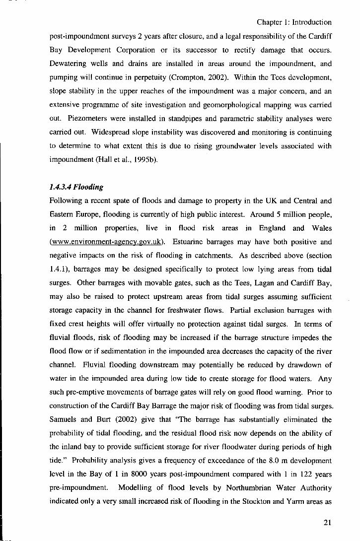
1.4.3.4 Flooding
Following a recent spate of floods and damage to property in the UK and Central and
Eastern Europe, flooding is currently of high public interest. Around 5 million people,
in 2 million properties, live in flood risk areas in England and Wales
(www.environment-agencv.gov.uk). Estuarine barrages may have both positive and
negative impacts on the risk of flooding in catchments. As described above (section
1.4.1), barrages may be designed specifically to protect low lying areas from tidal
surges. Other barrages with movable gates, such as the Tees, Lagan and Cardiff Bay,
may also be raised to protect upstream areas from tidal surges assuming sufficient
storage capacity in the channel for freshwater flows. Partial exclusion barrages with
fixed crest heights wil l offer virtually no protection against tidal surges. In terms of
fluvial floods, risk of flooding may be increased i f the barrage structure impedes the
flood flow or i f sedimentation in the impounded area decreases the capacity of the river
channel. Ruvial flooding downstream may potentially be reduced by drawdown of
water in the impounded area during low tide to create storage for flood waters. Any
such pre-emptive movements of barrage gates will rely on good flood warning. Prior to
construction of the Cardiff Bay Barrage the major risk of flooding was from tidal surges.
Samuels and Burt (2002) give that "The barrage has substantially eliminated the
probability of tidal flooding, and the residual flood risk now depends on the ability of
the inland bay to provide sufficient storage for river floodwater during periods of high
tide." Probability analysis gives a frequency of exceedance of the 8.0 m development
level in the Bay of 1 in 8000 years post-impoundment compared with 1 in 122 years
pre-impoundment. Modelling of flood levels by Northumbrian Water Authority
indicated only a very small increased risk of flooding in the Stockton and Yarm areas as
21

Chapter 1: Introduction
a result of the Tees Barrage (Hall et al., 1995a). Management of the Tees Barrage
during river flood conditions involves lowering the gates to maintain an upstream level
of below 2.65 m AOD.
1.4.3.5 Amenity use
Barrages constructed to encourage urban redevelopment are often described as amenity
barrages due to the incorporation of facilities for recreational use in their designs.
Impoundments may provide facilities for a large range of water contact activities
including rowing, white water rafting and canoeing, sailing, water skiing and jet-skiing.
Surrounding areas may be landscaped to provide a pleasant environment for walking,
caravanning and camping and outdoor concerts. Navigational rights may apply to
estuaries to be impounded, thus necessitating the inclusion of navigation locks, and
recreational boating in the area may be encouraged through provision of marina
facilities. The ancillary features of the barrages included in this research are listed
above. Use of the Wansbeck impoundment for water sports is restricted and less than
that originally envisaged due to the shallow water depth and semi-submerged obstacles.
Successful use of the impoundment by Cambois Rowing Club is limited during low
river flows and following transport of debris into the impoundment by river floods. The
poor state of repair precludes the use of the navigation lock by craft at present. An
amenity survey carried out in 1996 showed that, in terms of activities carried out, the
Wansbeck Riverside Park has a visitor profile similar to that of many urban parks
(Worrall and Mclntyre, 1998). In contrast, the use of the Tees Barrage impoundment
for water contact activities is very successful, and the white water course is particularly
popular. The Chief Executive of the Teesside Development Corporation quotes the
editor of Canoeist magazine describing the inaugural slalom event as attracting "what
may well have been the biggest crowd ever for a British canoeing event" (Hall, 1996).
The use of estuarine impoundments for water contact activities is reliant on the
maintenance of high water quality, particularly in terms of water-borne pathogens.
1.4.3.6 Costs and benefits
Recent barrage constructions in the UK have been a response to the decline in heavy
industries along the margins of estuaries. By creation of a pleasant waterfront
environment and associated infrastructure it is hoped that these areas may be
redeveloped and economic growth of the region achieved. The primary decision to
build an estuarine barrage is therefore cuireiitly economic, and the construction and
22

Chapter 1: Introduction
environmental costs of construction must be outweighed by the predicted financial
benefits. It must be determined whether a barrage is the best way to stimulate economic
growth, or whether a similar amount of investment through other channels would give
equal or better returns. Financial incentives offered to businesses locating in the area
associated with development schemes may have the same effects independent of the
presence or absence of a barrage. Anecdotal evidence suggests that regeneration on the
Avon commenced as soon as the Bristol Development Corporation showed an interest
in the area, prior to any proposal for barrage construction.
The Tees Barrage scheme is reported as an economic success (e.g. Hall, 1996).
Economic evaluation of the Teesside Development Corporation's strategy suggested
that it would create new employment opportunities (an estimated 8000 jobs) and
financial investment (approximately £500 million), and provide new homes for the
existing population and incoming employers (Price Waterhouse, 1988), and it is
reported to be close to meeting these targets (Hall et al., 1995a). The Cardiff Bay
Barrage is the centrepiece of a £24 billion regeneration scheme for Cardiff, and is also
reported as having met its economic targets (Crompton, 2002). The Cardiff Bay
Development Corporation's strategy was even more ambitious, and aimed to create
30000 new jobs and attract 2 million visitors/annum to Cardiff s waterfront. The cost
of barrage construction per hectare of regenerated land equates to £180,000, with an
average post development market value for this previously undesirable land of £500,000,
and the Development Corporation has estimated that an estimated £170 million a year is
returned to the public purse through taxation directly attributable to developments.
Redevelopment of the Swansea Valley in association with the Tawe Barrage is
acclaimed by the Council of Europe as an international example of Urban Renaissance
(Phillips and Williams, 2000).
/3

Chapter 2: Water Quality Surveys
Chapter 2
Water Quality Surveys
2.1 Survey design
2.1.1 Experimental design
The water quality surveys undertaken were factorial in design (Miller and Miller, 1994;
Wright and Worrall, 2001; Hillebrand, 2003; Jacquemyn et al., 2003). The general
principle of the design of the surveys was that they should be able to produce datasets
that allow statistical testing of the significance of a number of factors in controlling
water quality in the impoundments. These factors include barrage design, position
(longitudinal and depth) within impoundments, and external controls on water quality
such as temperature, river flow, time of year and tidal state. Factorial design measures
the response to combinations of factor levels, whereas in classical (one-at-a-time)
experimental design each factor to be tested is run in an experiment in which all other
factors are held constant. Obviously in a natural system such as an impoundment, factor
levels will vary simultaneously and a classical approach would be impossible.
However, factorial design also shows distinct advantages over classical design in that
interactions between factors can be determined, and fewer sets of results are needed to
gain the same precision as in a one-at-a-time design. Interactions are where the
response to a combination of factors is greater or smaller than would be expected i f the
effects were solely additive.
2.1.2 Estuaries studied
Water quality surveys were carried out on a total of four estuaries, chosen to allow
comparison between different ages and designs of impoundment (partial and total tidal
exclusion and amount of tidal overtopping), and to include a non-impounded "control"
estuary. These are the River Tawe in South Wales and the Rivers Tees, Wansbeck and
Blyth in Northeast England (figure 1.2, chapter 1). UK estuaries were chosen for
convenience and to minimise differences in climatic and land-use factors.
The River Tees, impounded in 1994, is a total tidal exclusion (freshwater) system. The
River Wansbeck, impounded in 1975, is a partial tidal exclusion system which allows
approximately 30% of tides to overtop the barrage. The River Tawe, impounded in
1992, is a partial tidal exclusion system which allows approximately 70% of tides to
overtop the barrage. The River Blyth is of a similar size and runs roughly parallel to
24

Chapter 2: Water Quality Surveys
and to the south of the River Wansbeck, and is not impounded.
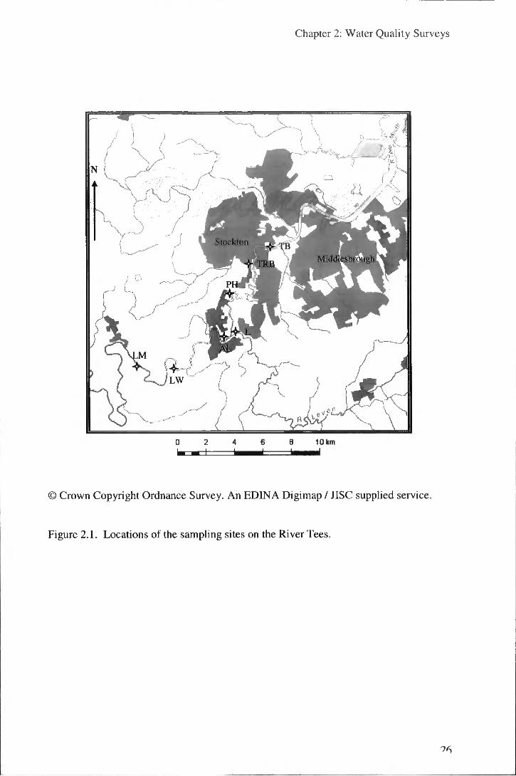
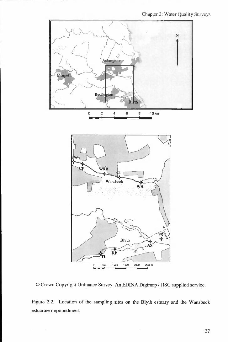
2.1.3 Sampling stations
The river sections studied for the three impoundments extend upstream from the
barrages to the normal tidal limits representing the downstream limits of unidirectional
flow (or pre-barrage normal tidal limit for the River Tees), taken from Ordnance Survey
maps. These can be thought of as the sections of river which have undergone
impoundment by the construction of the barrages. This project does not attempt to
consider the effects of barrage construction on the sections of estuary downstream from
the barrages. The section of the River Blyth studied extended downstream from the
normal tidal Umit to the dredged and pile-walled shipping channel of the Port of Blyth
(i.e. a section representing the "natural" condition of the estuary was selected).
General practice was applied in choosing sampling sites (ISO, 1990; Bartram and
Balance, 1996). A number of sampling stations (4 on Blyth, 7 on Tees, 5 on Wansbeck
and 6 on Tawe) were established approximately equidistantly along the sections studied,
and at the deepest point of the river cross-section at each of these distances. Stations
were chosen at clearly identifiable points (i.e. at obvious landmarks such as bridges,
buildings, weirs and river confluences) to ensure repeatability of sampling at the same
points and, where data are gathered by the Environment Agency (EA), to correspond
with EA sampling sites. For each river a site was chosen at the tidal limit with the
objective of identifying the baseline conditions of water quality as it entered the systems
under study. For the Tees, surveys sites were established immediately upstream of the
confluence with, and within, the major tributary of Leven to allow its effect on water
quality to be taken into account. Figures 2.1, 2.2 and 2.3 and table 2.1 show the
locations of the sampling sites within each of the estuaries.
25
Chapter 2: Water Quality Surveys
10 km
© Crown Copyright Ordnance Survey. An EDENA Digimap / JISC supplied service.
Figure 2.1. Locations of the sampling sites on the River Tees.
96
Chapter 2: Water Quality Surveys
Ashinaton
Bedlin 2 ton
10 km
N
Wansbeck
0 SOO lODO 1S00 2000 2500 m
© Crown Copyright Ordnance Survey. An EDINA Digimap / JISC supplied service.
Figure 2.2. Location of the sampling sites on the Blyth estuary and the Wansbeck
estuarine impoundment.
27

Chapter 2: Water Quality Surveys
SKvansea
e 10 km
© Crown Copyright Ordnance Survey. An EDINA Digima^ / JISC supplied service.
Figure 2.3. Locatior. of the sampling sites on the Tawe estuarine impoundment.
28
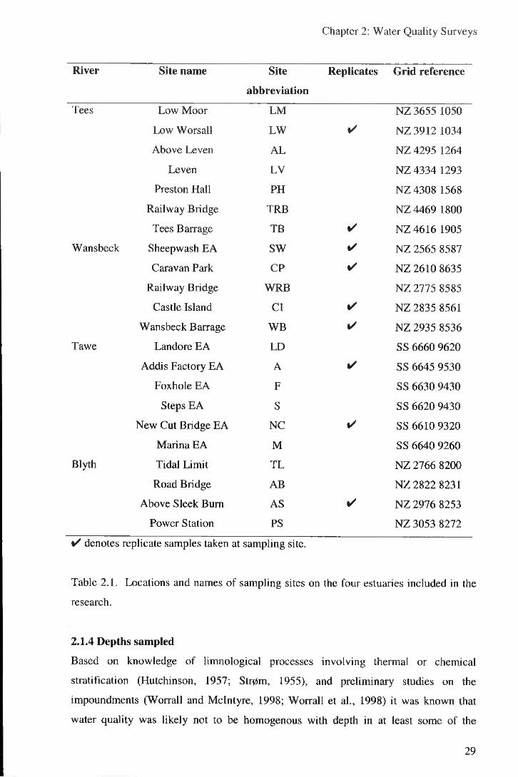
Chapter 2: Water Quality Surveys
River Site name Site
abbreviation
Replicates Grid reference
Tees Low Moor L M NZ 3655 1050
Low Worsall LW • NZ 3912 1034
Above Leven A L NZ4295 1264
Leven LV NZ4334 1293
Preston Hall PH NZ4308 1568
Railway Bridge TRB NZ4469 1800
Tees Barrage TB • NZ4616 1905
Wansbeck Sheepwash EA SW • NZ 2565 8587
Caravan Park CP • NZ 2610 8635
Railway Bridge WRB NZ 2775 8585
Castle Island CI • NZ 2835 8561
Wansbeck Barrage WB • NZ 2935 8536
Tawe Landore EA LD SS 6660 9620
Addis Factory EA A • SS 6645 9530
Foxhole EA F SS 6630 9430
Steps EA S SS 6620 9430
New Cut Bridge EA NC • SS 6610 9320
Marina EA M SS 6640 9260
Blyth Tidal Limit TL NZ 2766 8200
Road Bridge AB NZ2822 8231
Above Sleek Bum AS • NZ 2976 8253
Power Station PS NZ 3053 8272
• denotes replicate samples taken at sampling site.
Table 2.1. Locations and names of sampling sites on the four estuaries included in the
research.
2.1.4 Depths sampled
Based on knowledge of limnological processes involving thermal or chemical
stratification (Hutchinson, 1957; Str0m, 1955), and preliminary studies on the
impoundments (Worrall and Mclntyre, 1998; Worrall et al., 1998) it was known that
water quality was likely not to be homogenous with depth in at least some of the
29

Chapter 2: Water Quality Surveys
systems. As such, it was decided to take samples for analysis at three depths at each
site. These were at the surface, just (circa 10cm) above the sediment water interface,
and at the mid-depth between these points. Depth was measured using an echo sounder
on the RV. At shallow sites where it had been ensured that the water was well mixed
enough to be homogenous (by taking DO, T and conductivity measurements), only
surface samples were taken. This was always the case at sites TL on the Blyth, and SW
and CI on the Wansbeck, where weirs or riffles provided turbulence to mix the water
body. At L M on the Tees samples are recorded at 3 depths but can effectively be
thought of as replicates since a weir provides complete mixing here. The water quality
parameters measured in the field (DO, T, conductivity, pH and, when taken. Eh) were
also taken at surface, mid and deep points in the water column. On several occasions
profiles of these parameters were taken at a resolution of 30.5cm throughout the water
column to help define vertical variations in water quality on a finer scale.
2.L5 Replicates
As a check on random errors introduced in either sampling or analysis, duplicate
samples were taken at all depths (shallow, mid and deep) at a variety of sites. The sites
at which duplicates were taken are recorded in table 2.1.
2.1.6 Dates sampled and hypothesis testing
The water quality surveys were carried out with the aim of statistically testing the
significance of a selection of factors as controls on water quality (hypothesis testing).
The major comparisons carried out within this research using the results of the water
quality surveys may be summarised:
1. Testing of the significance of season (summer vs. winter) and river stage on
water quality within a total tidal exclusion impoundment (the Tees).
2. Testing of the significance of season (spring, summer, autumn (fall) and winter)
and river stage on water quality within a partial tidal exclusion impoundment
(the Wansbeck).
3. Testing of the significance of barrage design (partial vs. total tidal exclusion;
high vs. low proportions of tides overtopping) on water quality (Tees, Tawe and
Wansbeck summer surveys).
4. Testing of the significance of presence vs. absence of a banage on water quality
(Wansbeck and Blyth summer surveys).
^0

Chapter 2: Water Quality Surveys
Name of Dates sampled Days Tests
survey sampled
Tees summer 21/07/99, 04/08/99, 11/08/99, 25/08/99, 08/09/99, 6 1 and
1999 22/09/99 3
Tees winter 02/02/00, 08/02/00, 16/02/00, 23/02/00, 29/02/00 5 1 and
2000 3
Wansbeck 04/03/00, 05/03/00, 07/03/00, 09/03/00, 11/03/00, 10 2
spring 2000 12/03/00, 13/03/00, 14/03/00, 15/03/00, 16/03/00
Wansbeck 25/09/00, 26/09/00, 27/09/00, 28/09/00, 29/09/00, 16 2
autumn 2000 30/09/00, 01/10/00, 02/10/00, 03/10/00, 04/10/00,
05/10/00, 06/10/00, 07/10/00, 08/10/00, 09/10/00,
10/10/00
Wansbeck 03/02/01, 05/02/01, 06/02/01, 07/02/01, 08/02/01, 6 2
winter 2001 09/02/01
Wansbeck 04/06/01, 05/06/01, 06/06/01, 07/06/01, 08/06/01, 21 2,3
summer 09/06/01, 10/06/01, 11/06/01, 12/06/01, 13/06/01, and 4
2001 14/06/01, 15/06/01, 16/06/01, 17/06/01, 18/06/01,
19/06/01, 20/06/01, 21/06/01, 22/06/01, 23/06/01,
24/06/01
Blyth 04/06/01, 05/06/01,06/06/01, 07/06/01, 08/06/01, 9 4
summer 09/06/01, 10/06/01, 11/06/01, 12/06/01
2001
Tawe 10/06/00,11/06/00, 12/06/00, 13/06/00,14/06/00, 12 3
summer 15/06/00, 16/06/00, 17/06/00, 18/06/00,19/06/00,
2000 20/06/00, 21/06/00
Total: 85
Table 2.2. Dates sampled for each of the estuaries studied during the water quality
surveys.
Seasonal effects on water quality are discussed within chapter 3, barrage design effects
within chapter 4 and impoundment effects within chapter 5 of this thesis. The dates
water quality sampling was carried out within the estuaries in order to carry out the tests
above are shown in table 2.2. A total of 85 days of water quality surveying was
31

Chapter 2: Water Quality Surveys
completed, with sampling during summer earned out on the Tawe, Blyth, Tees and
Wansbeck, winter sampling carried out for the Tees and Wansbeck, and autumn and
spring sampling carried out for the Wansbeck alone.
2.2 Sampling procedure
2.2.1 Safety precautions
Precautions were taken to limit the risk to those involved during water quality sampling.
Fieldwork was always completed with at least 2 people in the RV and at least one on
shore, all carrying mobile telephones, on all occasions. Lifejackets and high visibility
clothing were worn when on the water or when working from river banks. A first-aid
kit was carried in the RV. Gloves were worn when collecting samples to avoid risk of
infection, in addition to avoiding contamination of samples. Al l field and laboratory
work carried out as part of this PhD was done so without any injury to any party.
2.2.2 Procedure
Sampling was attempted to be carried out as close as possible to midday during all of
the surveys to avoid diurnal changes in water quality (e.g. changes in DO due to algal
respiration with time of day (Lingeman et al., 1975)) confounding results. This was not
possible for the survey of the River Blyth due to sampling needing to be carried out at
high tide when depth of water was at its maximum. In this case, sampling was carried
out from around 3pm at the start of the survey to around 8pm at the end of the survey.
The length of time taken for each date's sampling run was on average circa 3 hours
(slightly longer on the Tees and slightly shorter on the Blyth). The sequence of data and
sample collection from each of the sites varied between rivers depending on the relative
position at which the RV was launched. However, it is assumed that parameters did not
vary significantly during the length of time taken to complete a date's sampling run.
All work was carried out from the RV (figure 2.4) except at sites SW on the Wansbeck
and L M on the Tees where, at low flows, sampling was carried out by wading. Care
was taken to carry out field analysis and water sampling on the upstream side of the RV
and gloves were worn to minimise the risk of contamination. At each site the time,
water depth and number of samples successfully taken, and the water quahty pai ^ neters
measured in the field (using the methods outlined in Field Analytical Methods) and the
depth of their measurement, were recorded in a notebook. At the start of each run the
weather conditions were noted.
32

Chapter 2: Water Quality Surveys
Figure 2.4. The research vessel used during the water quality surveys.
Water sampling was carried out using a stainless steel depth (grab) sampler. This
consists of a tube of 10cm diameter and 30cm length held in a horizontal position,
oriented parallel to the flow by a fin. Two sprung-loaded flaps can be closed over the
ends of the tube by dropping a messenger weight down the graduated lowering rope to
enclose a sample of water from a defined depth. It was felt unlikely that the steel of the
depth sampler would act as a source of metal contamination at the range of pHs
encountered. Samples were transferred to the laboratory in 0.1 M nitric acid-washed 1
litre polyethylene sample bottles. These were rinsed 3 times with portions of the
samples with which they were to be filled. Samples were transported to the laboratory
in the dark in cool boxes at 4°C, and the time between collection and preliminary
laboratory analysis and treatment was kept to less than 2 hours (ISO 1990).
Samples were taken in order of increasing depth (surface, then mid, then deep
sampling). The depth sampler was lowered gently into position to avoid disturbance of
any stratification, and held in position for 10 seconds prior to releasing the messenger.
Care was taken when lowering the sampler to depth not to disturb the bed sediment.
33

Chapter 2: Water Quality Surveys
Where it was noticed that sediment had been disturbed, samphng was repeated.
Inclusion of non-homogenous particulates such as wood and leaves in samples was
avoided.
2.3 Water quality parameters measured
2.3.1 Introduction
Water quality may be defined by a huge variety of parameters. Until relatively recently
the range and type of parameters used to assess water quality has varied between
countries and even regionally (Kristensen and B0gestrand, 1996). The trend now is
towards the harmonisation of water quality monitoring and assessment programmes
(e.g. European Union River Network, United Nations Environment Programme
(UNEP), OECD). The UNEP Global Environmental Monitoring System Freshwater
Quality Programme (Meybeck et al., 1989; WHO, 1991) divides water quahty
parameters by the following classification:
o Physical/Chemical: Conductance, Suspended Solids, pH, BOD and COD.
o Major Ions: Alkalinity, Sodium, Magnesium, Sulphate, Chloride, Potassium,
and Calcium.
o Metals: Aluminum, Chromium, Manganese, Iron, Nickel, Copper, Zinc,
Arsenic, Selenium, Cadmium, Mercury, and Lead,
o Nutrients: Nitrogen, Ammonia, and Phosphorus.
o Organic: P,P-DDT, DDT, 0,P-DDT, P,P-DDD, 0,P-DDD, P,P-DDE, 0,P-
DDE, Lindane, Alpha - BHC, Mirex, Aldrin, Endrin, Dieldrin, PCBs, Atrazine,
Methiocarb, Aldicarb, 2,4-D, P,P-DDD Olefin, and BHC.
e Microbiology: Total Coliforms, Faecal Coliforms, and Faecal Streptococci.
The choice of water quality parameters to measure in this research was based on the
GEMSAVater programme, with the range of analytes being kept to a manageable level
by excluding the organic and radcrobiological parameters. Thus, the focus was on the
general physical and chemical parameters, major ions, metals, and nutrients. This
scheme allows a suitably broad assessment of water quality, whose results may be
compared internationally. To aid in comparability, standard methods of analysis were
used wherever possible (American Public Health Association (Clpsceri et al., 1998) or
International Organisation for Standardisation (ISO, 1990)).
34

Chapter 2: Water Quality Surveys
Due to availability of equipment, the parameters measured differed slightly from those
listed above. Since the majority of metal analysis was carried out using ICP-OES/AES,
the range of analytes measured in most samples excluded heavy metals (Cd, Hg, Pb)
and As and Se, but included a greater range of less heavy elements (Co, Sc, Si, Sn, Ti ,
V). Chloride was not measured, but it was felt that in an estuarine environment chloride
would almost certainly be proportional to sodium, and that sodium could be used as an
alternative conservative index of mixing. Time constraints during the immediate
processing of samples following sampling runs meant that BOD alone, without COD,
was taken as an indicator of oxygen demand. Throughout this work, according to
convention (e.g. APHA, 1998), dissolved refers to all components passing through a
filter of 0.45 ^m pore size.
2.3.2 Physical/chemical
2.3.2.1 Dissolved oxygen
Dissolved oxygen (DO) is probably the most fundamental parameter in the study of
water quality. Chapman (1996) explains that, "...oxygen is involved in, or influences,
nearly all chemical and biological processes within water bodies." Oxygen dissolves in
water from the atmosphere, which contains around 21% oxygen. The solubility of
oxygen in water increases non-linearly with decreasing temperature, and linearly with
increasing atmospheric partial pressure (Mortimer, 1981). Salinity reduces the
solubility of oxygen, and oxygen contents of seawater are around 80% relative to
freshwaters under the same conditions (Green and Carritt, 1967; Weiss, 1970). The
differences between observed values of DO and those expected from purely physical
controls (given as a % saturation) are a reflection of the biological processes
(photosynthesis and respiration) in a water body. The aerobic decomposition of organic
matter in the water column or at the sediment-water interface is particularly significant
in leading to dangerously low DO levels (Breuer et al., 1977). Most fish cannot survive
below levels of 2 mg/1 DO (Chapman, 1996), and anaerobic conditions can lead to
releases of methane (CH4), ammonium (NH3), hydrogen sulphide (H2S), phosphorus
(P), and iron (Fe) and manganese (Mn) and associated metals, to the water column.
2.3.2.2 Biochemical oxygen demand
Since aerobic decomposition of organic matter is a major depleter of DO in water
bodies, it is useful to have a measure of how much oxygen the decomposition of any
organic matter wil l consume. The biochemical oxygen demand (BOD) gives an
35

Chapter 2: Water Quality Surveys
approximate determination of the amount of DO required by aerobic micro-organisms
to break down the organic material contained within a water or wastewater sample
(Velz, 1984). BOD values range from under 1 mg/l in some unpolluted waters, to
around 600 mg/l for raw sewage and 25000 mg/l for paper pulping waste (Reeve, 1994).
Chemical oxygen demand (COD) measures the oxygen equivalent of organic material
broken down by a strong chemical oxidant, and is often used together with or instead of
BOD measurements. In this project, due to time constraints during the water quality
surveys, it was decided to measure BOD alone. BOD better reflects the environmental
behaviour of organic material than COD. Due to the limited number of BOD bottles
available and that fact that each BOD determination takes a period of 5 days, BOD
values were only taken on a portion of the days of water quality sampling, and therefore
the power of significance tests involving BOD are lower than for other parameters
analysed (see appendix 1 for a description of power in statistical analyses).
2.3.2.3 pH
pH is defined as the negative of the logarithm to the base 10 of the hydrogen ion activity
(generally the same as concentration) in a solution. Pure water dissociates weakly to
and OH" ions to give a pH of 7 defined as neutrality. In natural UK lowland waters the
pH tends to be mainly controlled by the balance between carbon dioxide, carbonate and
bicarbonate ions, and tends to lie between 6.0 and 8.5 (Chapman, 1996). This balance
can be altered by the addition of pollutants (e.g. acid rain), by natural organic acids (e.g.
in Sphagnum bogs) or inorganic acids (mainly in volcanic regions), and autochthonous
production of carbon dioxide and bicarbonate on a various time-scales. Fish
populations are strongly affected by low pH values, salmon decreasing below pH 6.5,
perch below 6.0 and eels below 5.5, with little Hfe below pH 5 (Reeve, 1994). pH also
affects the speciation and solubility of metals in water bodies.
2.3.2.4 Alkalinity
Whilst pH is the measurement of the hydrogen ion activity in a water body, the
alkalinity is the measurement of the resistance to change of the pH. Low alkalinities
indicate that a water body is susceptible to a reduction of pH on the addition of an acid.
Alkalinity is taken to represent the amounts of carbonate oicarbonate and hydroxide in
the water body, and tends to be given in units of mg/l CaCOs '"'-uivalent (the
hypothetical value assuming all alkalinity were due to CaCOa).
36

Chapter 2: Water Quality Surveys
2.3.2.5 Eh
Eh or redox potential gives a qualitative idea of whether a water is in reducing or
oxidising state. In a similar way to pH representing the behaviour of acids and bases as
proton (hydrogen ion) donors and acceptors, Eh represents the behaviour of reductants
and oxidants as electron donors and acceptors in a solution. Unlike protons, however,
there are no free electrons: every oxidation is accompanied by a reduction (Stumm and
Morgan, 1981). Eh is given as a potential, and its range in natural waters is around -
500 mV to +700 mV (Chapman, 1996). It is dependent on the equilibria of all the redox
systems in the water (i.e. the number of oxidised and reduced species), and is
particularly influenced by the redox states of oxygen, iron and sulphur. The presence of
dissolved oxygen normally gives Eh values of between +100 and +500 mV, and highly
reducing conditions, characterised by the presence of hydrogen sulphide, have Eh
values down to -100 mV. Under stratified conditions in the impoundments studied a
fall in Eh values might be expected from the oxygenated freshwater layer to the
deoxygenated saline water at depth.
2.3.2.6 Conductivity
Conductivity is the measure of the ability of water to carry an electrical current. It is
dependent on the concentration and type of dissolved solids in the water. Inorganic
solutes tend to be good conductors, whereas organic solutes tend not to dissociate as
easily and are poor conductors. Conductivity is given in units of microsiemens per
centimetre (^iS/cm) in freshwaters, or millisiemens per centimetre (mS/cm) in brackish
and saline waters where conductivity is several orders of magnitude higher.
Conductivity can give an idea of the total dissolved solids content (mg/1) of a water
sample i f the ionic makeup is known. For waters in which sodium and chloride
dominate:
mg/l ^O.eixjuS/cm
gives an approximation of total dissolved solids (mg/1). In freshwaters, pollutants or a
high proportion of land run-off tend to increase the conductivity. Conductivity was
considered to be an important determinand in this study since it can indicate the amount
of mixing between fresh and saline waters.
37
Chapter 2: Water Quality Surveys
2.3.2.7 Temperature
Temperature in a water body will vary seasonally and often diumally. In general the
larger the water body the lower are its fluctuations in temperature. Changes in
temperature are dependent on the amount of solar insolation, transfers of heat from
sediments and the air, and condensation and evaporation of water at the water surface.
The rates of physical, chemical and biological processes in water are dependent on the
temperature. The solubility of gases, including oxygen and carbon dioxide, decrease
with increasing temperature. In general rates of reactions increase with temperature
increases. Metabolic rates, and hence rates of decomposition of organic material
leading to deoxygenation, growth rates of algae, etc., increase with increased
temperature.
2.3.2.8 Transparency
The transparency of a water body is a combined function of its colour and turbidity.
Turbidity is controlled by the amount and concentration of suspended particulate matter
in the water column. Particulates can be mineral (e.g. clay and silt) or biological (e.g.
algae and cyanobacteria) in origin. Colour is imparted by dissolved components such as
minerals and organic acids. Transparency will vary under a variety of conditions
including flow and the growth rates of suspended organisms, and is a simple and
convenient method of giving a rough comparison of these factors.
2.3.2.9 Total Suspended Solids
Total suspended solids (TSS) is the measurement of particulate matter (mineral or
organic) which is suspended in the water column. Convention is to define total
suspended solids as the matter which will not pass through a filter of 0.45|xm pore size.
TSS will affect the amount of Hght available for photosynthesis entering the water.
Significantly for this study, fluxes in TSS may indicate the state of sedimentation or
erosion in an impoundment.
2.3.3 Nutrients
The Environment Agency defines eutrophication as:
'The enrichment of waters by inorganic plant nutrients which result in the stimulation
of an array of symptomatic changes. These include the increased pioduction of algae
38

Chapter 2: Water Quality Surveys
and/or other aquatic plants, affecting the quality of the water and disturbing the balance
of organisms present within it. Such changes may be undesirable and interfere with
water uses." (Environment Agency, 1998; OECD, 1982).
Eutrophication is a problem in many parts of the world including the UK, and so the
study of the nutrient status is key in any study of water quality. The biological
productivity in a water body tends to be limited by the concentration of either nitrogen
(N) or phosphorus (P) (Vollenweider, 1968). Silica can be important where diatoms are
a significant part of algal production (Lund, 1954).
2.3.3.1 Nitrogen
Nitrogen is essential to organisms in the formation of proteins and DNA, and is
converted by algae and aquatic plants from inorganic to organic forms. Inorganic forms
of nitrogen occur in waters as nitrate (NO3"), nitrite (NO2'), ammonium (NKj"^) and
molecular nitrogen (N2), and various processes act to convert N between its oxidation
states. These can be summarised as:
a) Assimilation of inorganic forms by organisms to produce organic N, such as amino
acids.
b) Nitrogen fixation: reduction by micro-organisms of N2 —> NHt"^ and organic N.
c) Heterotrophic conversions.
d) Nitrification: oxidation of NH^"^ -> NO2' NO3".
e) Ammonification: production of NH4* by decomposition of organic matter.
f ) Denitrification: reduction of NO3' -> NO2' N2O N2 (which may be lost from
the system) under anoxic conditions.
Physical transfers of N occur due to the processes of sorption and sedimentation.
Ammonia
The main sources of ammonia in water bodies are from the breakdown of organic
material, and industrial and sewage waste and agricultural run-off. In addition to its
contribution to eutrophication, at high concentrations and higher pH conditions
ammonia is highly toxic to many organisms, especially fish. At high pH the equilibrium
between ammonium (NH4*) and toxic undissociated ammonia (NH3) (the two dominant
forms of ammonia) moves towards ammonia. Total ammonia concentrations tend to be
39

Chapter 2: Water Quality Surveys
low in natural waters (<0.1 mg/1). Higher values occur in polluted waters or where
anoxic decomposition of organic material is significant.
Nitrate
Nitrate (NO3') is normally the dominant form of N occurring in natural waters.
Determination of nitrate tends to include nitrite (NO2"), but since nitrite is rapidly
oxidised to nitrate its contribution is usually minor. The concentrations of nitrate in
natural waters are low (<0.1 mg/1), but concentrations are usually higher due to
contributions from industrial and sewage wastes, and particularly run-off of inorganic
nitrate fertilisers. The Environment Agency (1996) give that the UK use of nitrogenous
fertihsers increased by around 50% from 1970 to 1990, although has since remained
relatively constant. Nitrate is the major form of N available to algae and aquatic plants,
and therefore a significant factor in understanding eutrophication. Very high
concentrations (>200 mg/1) of nitrate in drinking water have led to "blue baby
syndrome" in the past, although these levels are never approached in the UK today
(Porteous, 2000).
2.3.3.2 Phosphorus
Relative to N and other elements essential to biota, P is normally the least abundant in
natural waters, and most commonly limits biological productivity (Sakamoto, 1966;
Dillon and Rigler, 1974; Schindler, 1977), although estuaries may show N limitation at
their seaward ends. P is essential to organisms as a component of nucleic acids and in
intracellular molecular synthesis and transport. The majority of P is therefore contained
within organic forms, the majority of this being in particulate material. Dissolved
orthophosphate (phosphate) is less than 5% of total P in natural waters (Prepas and
Rigler, 1982). However it is this form which is most bioavailable, with most other
forms scarcely available at all (Reynolds and Davies, 2001). Levels of phosphate in
water bodies are normally very low (<0.02 mg/1) since uptake of phosphate by
organisms is very rapid. Significant inputs of phosphate come from sewage
(particularly containing polyphosphate-based detergents), industrial effluents and
agricultural run-off. Binding to sediment can act as a sink for phosphorus, but
phosphorus may be recycled irom sediments under anoxic conditions. L- inis study,
both dissolved orthophosphate (SRP) and total dissolved P (TDP) were measured.
^0

Chapter 2: Water Quality Surveys
2.3.3.3 Silicon
Silicon occurs in natural waters as dissolved, colloidal or suspended forms of silica
(Si02). Dissolved forms occur as silicilic acid and its dissociation and association
products, and organic silicon compounds. In this study, total dissolved silica was
measured. The majority of silica is derived from the weathering of siliceous minerals.
Silica is relatively unreactive, but is essential to diatomaceous algae and may limit
blooms of diatoms in spring. Seasonal variations my occur due to uptake by diatoms
during cell growth, and release during decomposition. Concentrations of silica tend to
be fairly high relative to other nutrients (1-30 mg/1 in freshwaters (Chapman, 1996)),
and higher in freshwaters than seawaters.
2.3.4 Major elements
There is a marked difference in both total concentrations and relative abundances of
major elemental constituents between freshwater and seawater. The major cations in
freshwater generally follow an order of abundance of Ca " > Na* > Mg^* > K" , whilst in
seawater the order is Na " > Mg " > Ca " > (Ward, 1996). Whereas the concentration
in freshwaters can vary widely between catchments, the concentration of major ions in
seawater is remarkably constant around the world. The ionic strength of seawater is
such that mixing of only 1% by volume with freshwaters in an estuary will give a ratio
of ions which is almost identical to that in the seawater (Andrews et al., 1996). This
difference has a major affect on the transport of particulate and dissolved material
through estuaries, through the processes of flocculation and ion exchange. Thus,
measurement of the concentration of major ions in seawater can constrain mixing and
its associated processes in estuaries.
2.3.4.1 Sodium
Sodium (Na " ) is the dominant cation in seawater (World mean concentration of around
10800 mg/1) and also occurs in significant concentration in freshwaters (World mean
concentration in stream water of 6.1 mg/1) (Reimann and Caritat, 1998). It is highly
soluble and mainly sourced from rainwater and dissolution of Na bearing minerals.
Human inputs of sodium to freshwaters include sewage and industrial discharges, and
run-off from road salting. High levels of sodium can cause freshwaters to be unsuitable
for use for drinking or for irrigation. Sodium behaves conservatively on mixing of fresh
and saline waters in an estuary, and can hence be used as an index of mixing when
looking at the conservative/non-conservative behaviour of other elements (Liss, 1976).
41

Chapter 2: Water Quality Surveys
2.3.4.2 Potassium
Potassium (K*) is sourced from dissolution of rocks plus cation exchange but, since
potassium containing minerals are generally of low solubility, concentrations are lower
than for sodium in both fresh (2.3 mg/1 World mean) and saline (399 mg/1 World mean)
waters (Reimann and Caritat, 1998). Potassium is an essential nutrient, and is applied in
large quantities as a plant fertiliser. Fertiliser run-off, together with industrial
discharges provide the main anthropogenic inputs of potassium. Potassium also
behaves conservatively on mixing in estuaries.
2.3.4.3 Magnesium
Magnesium (Mg^*) is sourced from ferromagnesium and carbonate minerals.
Anthropogenic inputs are usually relatively insignificant. World average concentrations
are 1290 mg/1 in seawater and 4.1 mg/1 in freshwater (Reimann and Caritat, 1998).
Magnesium behaves conservatively on mixing in estuaries.
2.3.4.4 Calcium
Calcium (Ca "* ) dissolves easily from carbonate or sulphate rocks. Calcium is essential
for most organisms (particularly for shells and bones), but concentrations are normally
higher than would limit biological productivity. Calcium and magnesium salts cause
hardness. World average concentrations are 412 mg/1 in seawater and 18 mg/1 in
freshwater (Reimann and Caritat, 1998). Calcium behaves conservatively on mixing in
estuaries.
2.3.4.5 Sulphur
Sulphur (S) exists in several oxidation states in natural waters. Under oxidising
conditions sulphate (S04^') is the dominant form. Sulphate can be used as an oxygen
source by bacteria, which convert it to hydrogen sulphide (H2S, HS") under anaerobic
conditions. Total dissolved sulphur was measured. Sulphur is essential for all
organisms but deficiencies are rare. High concentrations of hydrogen sulphide are toxic
to aquatic life and make water unsuitable for drinking. Sulphur in freshwaters is
sourced from sulphur containing minerals (sulphates or sulphides), atmospheric
deposition of oceanic aerosols, and significant anthropogenic atmospheric inputs from
the burning of fossil fuels. World average concentrations are 905 mg/1 in seawater and 4
mg/1 in freshwater (Reimann and Caritat, 1998). Sulphur behaves conservatively on
42

Chapter 2: Water Quahty Surveys
mixing in estuaries, although anoxia can lead to some loss of sulphur as insoluble metal
sulphides and as hydrogen sulphide gas.
2.3.5 Minor and trace metals
Element Mean Mean Environmental Impacts or Behaviour
World World
Seawater Stream
Cone. Water
(mg/l) Cone.
(mg/l)
Al 0.002 0.3 Toxic to fish at low pH. Linked to Alzheimer's disease.
Co 0.00002 0.0002 Deficiencies more widespread than toxicity problems.
Cr 0.0003 0.0007 Cr (VI) highly toxic.
Cu 0.00025 0.003 Toxic at high doses.
Fe 0.002 0.04 Redox governed. Acid mine drainage can precipitate
ferric hydroxide.
Mn 0.0002 0.004 Redox governed. Similar behaviour to Fe.
Ni 0.00056 0.0003 Some compounds toxic.
Sc 0.0000006 0.000004 Thought to be non-toxic.
Sn 0.000004 0.00001 Organic forms toxic to lower organisms.
Ti 0.001 0.003 Non-toxic.
V 0.0025 0.0009 Toxic at some oxidation states.
Zn 0.0049 0.015 Low toxicity.
Table 2.3. Mean world ocean water trace metal concentrations from Lide (1996)
compiled data and mean world stream water trace metal concentrations from Koljonen
(1992) compiled data, reported in Reimann and Caritat (1998).
The concentration of a variety of minor and trace elements is critical to the biological
health of a water body. Several metals, such as Mn, Zn, V, Cu and Co, are essential
micronutrients, but at raised concentrations may exhibit toxic effects. Trace metals are
released from the weathering of minerals, and anthropogenic inputs come from sources
such as mining and industrial effluents. The form in which an element occurs often
controls its toxicity. Ionic forms of metals are generally the most toxic, and both
43

Chapter 2: Water Quality Surveys
mobility and toxicity may be controlled by oxidation state. Some organic metal
compounds (e.g. methylmercury or tributyltin) have very high toxicities. Many metals
show adsorption onto suspended sediment, and partitioning to sediment can act as a sink
for metals. In this study, dissolved forms of metals were measured as part of the water
quality surveys and adsorbed forms were measured in sediment surveys (see chapter 6).
The range of metals analysed was in main defined by what could be analysed for
accurately with the machines available. For the majority of water samples for which
analysis was by ICP-OES, a total of 12 minor and trace metals were measured. For
those samples which were also analysed using ICP-MS an additional 48 (mainly ultra-
trace) elements were looked at. These elements are likely not to be at high enough
levels to exhibit environmental impacts, but can be used to help fingerprint water and
sediment inputs to the systems. Table 2.3 summarises the average abundances, and
environmental impacts and behaviour, of the 12 minor and trace elements measured in
all water samples.
2.3.6 Flow
Flow in estuaries is controlled by river flow and tidal flow, and will vary dependent on
the relative state of each.
River flow or discharge is generally an essential measurement in all river water quality
studies as it allows:
o measurement of the amount of volume available for use
o calculation of fluxes of materials carried by the flow (e.g. suspended sediment or
nutrients)
o characterisation of the origin of many water quality parameters by their relationship
to flow.
Discharge regimes are controlled by, the size of catchment, climate, topography and
land-use, and hydrology. Larger flows are more able to cope with inputs of effluents
and wastewaters, and low water quality conditions may occur under drought conditions
where flows are insufficient to dilute pollutant inputs.
44

Chapter 2: Water Quality Surveys
A river's hydrograph (a graphical presentation of variations of flow over time) is made
up of two components: baseflow and runoff (Wilson, 1990). Baseflow is the water
entering a river from groundwater, which tends to be relatively constant compared to
runoff, which is the portion of rainfall which flows overland to the river. Many
variations in water quality can be explained by the relative influence of these two
sources. Runoff will contain high TSS, organic carbon and N and P, whilst
groundwater provides elements derived from rock weathering (Si02, Ca^*, Na*, Mg^" ,
K" ) (Chapman, 1996). Substances entering a river at a constant rate (from groundwater
or an anthropogenic point source) will be negatively correlated with discharge.
Particulates and bound species such as P and some metals, and organic material, which
increase with increased runoff will be positively correlated in some manner with
discharge.
Data for river discharges during the sampling runs was obtained from the EA. The EA
gauging stations at which discharges were measured are:
River Name of Gauging Station Catchment Area
(square km)
Grid Reference
Tees
Tawe
Wansbeck
Blyth
Low Moor
Ynystanglws
Mitford
Hartford Bridge
1264.0
287.3
227.7
269.4
NZ 365 105
SS 685 998
NZ 175 858
NZ 243 800
Table 2.4. Gauging stations used for flow data within the research.
Discharges are reported at the approximate time of sampling (12:00). Since the
freshwater contained within the impoundments may represent flow conditions prior to
the time of sampling, the maximum and mean discharges over the prior 24 hour period
are also included in the dataset. Discharges are given in m^/s.
Seawater discharges were not measured directly, but rather the height of the high tide
prior to sampling relative to the crest height of the barrage is given. This overtopping
(measured in m) gives a relative idea of how much seawater is entering the impounded
areas, although the volume wil l vary with the amount of freshwater discharge opposing
this input. Tidal data was obtained from the UK Hydrographic Office (2000, 2001).
45
Chapter 2: Water Quality Surveys
Seawater is of a far more constant composition than freshwater, and will not vary significantly with tidal flow at the point of entrance to mouths of estuaries, although within the estuaries the strength of tidal flow is important in the transport of sediment and bound species. Within estuaries there is a continual exchange of sediment between the suspended and bed phases due to tidal flows (Mehta and Dyer, 1990).
2.4 Analytical methods
The parameters of DO, pH, Eh, conductivity, temperature and transparency were
measured in situ in the field. The parameters of alkalinity, TSS, BOD, nutrients, major
elements and minor and trace metals and non-metals were measured in laboratories of
the University of Durham and set up within Swansea City Council offices on samples
transported and stored as described above.
Analytical grade reagents and Milli-Q® 18 Mii .cm water were used in all the laboratory
work described. Glassware and plasticware was acid and Decon 90® (non-ionic
surfactant) washed (soaked overnight in 1% HNO3, followed by overnight in 5% Decon
90® and rinsed in de-ionised water). Where reported, limits of detection LOD are given
as:
LOD = Sb + 3a
where:
Sb = the mean measured value of a series of sample blanks, and
CT = the standard deviation of the series of sample blanks
(Long and Winefordner, 1983).
2.4.1 Dissolved oxygen
Principle:
Membrane electrometric methods of DO measurement were used in all water quality
surveys including the determinations of BOD. Membrane electrode methods have
advantages over iodometric (Winkler) techniques due to their resistance to interferences
in natural waters (McKeown et al., 1967) and ability to measure in situ, md are suitable
46

Chapter 2: Water Quality Surveys
for measuring DO in polluted, highly coloured and saline waters (Mancy and Okun,
1960).
Apparatus:
A Hanna Instruments H I 9143 Portable Waterproof Microprocessor Dissolved Oxygen
Meter was used for all fieldwork. The probe consists of a silver chloride anode, a
platinum cathode (sensor) and an oxygen permeable Teflon membrane cap. Care was
taken to keep the platinum cathode untarnished and the electrolyte solution (KCl) free
from bubbles of air, and the membrane was replaced if dirt or algal growth was
observed. The manufacturer's specifications are:
Range: 0.00 to 19.99 mg/1 O2
0.0 to 100.0 % O2
Resolution: 0.01 mg/1 O2
0.1 %02
Accuracy (@25°C): ±1.5% Full Scale
Calibration: Automatic in saturated air.
Temperature compensation: Automatic from 0 to 50°C.
The meter was easy to calibrate (at 100% saturation) in air, and was checked in
solutions of 100% and 0% saturation. The response time was relatively rapid and a
water movement of at least 0.3m/sec was ensured during measurements by either the
flow of the rivers or manual agitation where flow was insufficient.
For laboratory measurements of DO during BOD analyses a WTW Oxi92 Dissolved
Oxygen Meter of very similar design and operation to the Hanna meter was used.
2.4.2 pH
Principle:
Electrometric methods of pH measurement were used in all water quality surveys.
Electrometric measurement determines the activity of the hydrogen ions within a
solution by measuring the potential between a glass electrode and a reference electrode.
The potential between the electrodes is in linear relation to the pH, and the meter is
calibrated using standard pH buffer solutions to enable readouts directly in units of pH
(Bates, 1973). pH measurements are affected by temperature (both mechanically and
47

Chapter 2: Water Quality Surveys
chemically) and meters usually include temperature probes and automatic temperature
compensation features. Glass electrodes are not significantly affected by salinity
(except at pH>10), or colour, turbidity or redox state (Clesceri et al., 1998).
Apparatus:
For the water quality surveys on the Tees and the Tawe, and for the Wansbeck March
2000 survey, pH was measured using a Hanna Instruments HANNA Water Tester with
specifications of:
Range: 0.0 to 14.0
Resolution: 0.1
Accuracy: ±0.2
Calibration: Double point calibration in neutral (pH 7.00±0.02 at 20°C
phosphate) buffer solution plus an acid (pH 4.00±0.02 at 20°C phthalate) buffer
solution.
This meter requires a small sample of the water for analysis to be poured into a sample
compartment, and as such limited pH measurement to samples collected in the water
trap and brought to the surface. It was decided, to enable pH measurement at a higher
resolution over the depth of the impoundments, to use a Hanna Instruments 9023C pH
meter with a length of cable between the probe and the meter for the majority of the
surveys. The 9023C has the added advantage of higher resolution and accuracy:
Range: 0.00 to 14.00
Resolution: 0.01
Accuracy: ±0.01
Calibration: Automatic with 3 memorised standard buffers (4.01, 7.01 and
10.01).
2.4.3 E h
Principle:
Eh (or oxidation-ieduction potential (ORP)) is also measured electrometrically, by
measurement of the potential between an inert electrode (e.g. platinum) and an i i . 'icator
electrode which ideally donates or accepts electrons from oxidised and reduced species
in the water being analysed. The measurement of Eh is complicated by several factors
48

Chapter 2: Water Quality Surveys
including inert redox couples, electrode poisoning, very small exchange currents,
irreversible reactions and rapid changes in redox conditions on storage (Clesceri et al.,
1998).
Apparatus:
Eh measurements were also made using a Hanna Instruments HANNA Water Tester in
the same manner as pH. The manufacturer's specifications are:
Range: -1000 to +1000mV
Resolution: ImV
Accuracy: ±5mV
The HANNA instrument is non-calibratable for Eh. It was found during the surveys
that Eh measurements for the same samples varied between the HANNA Water Testers
used (probably due to differences in the conditions of the electrodes), and thus the
accuracy of the Eh data are likely to be poor. Appelo and Postma (1994) explain that,
"Eh measurements are only qualitative indicators for redox comditions and should be
made as sloppy as possible, so that you will not be tempted to relate them to anything
quantitative afterwards." It was decided that, on dropping the HANNA Water Tester
for the measurement of pH (see above), Eh measurement would not continue.
2.4.4 Conductivity
Principle:
Conductivity in a solution is measured between 2 inert electrodes applying an
alternating current and measuring resistance using a Wheatstone bridge, and should be
made in situ or in the field immediately after sample collection. Meters are calibrated
against standard solutions of KCl to determine cell constants for the meter.
Conductivity is temperature dependent (increases with increasing temperature due to
increasing ionic motion) and readings are usually standardised at 25°C. Conductivity
probes are fairly robust, although poor readings may be obtained from fouled electrodes
or inadequate water circulation.
Apparatus:
As for pH and Eh, initial water quality surveys' conductivity readings were made using
a Hanna Instruments HANNA Water Tester of specifications:
49

Chapter 2: Water Quality Surveys
Range: 0 to 1999 |:iS/cm Resolution: 1 nS/cm Accuracy: 2% Full Scale
Calibration: Single point conductivity solution (1413 |i,S/cm @ 25°C)
As indicated above, the HANNA Water Tester's range is only up to 1999 |a,S/cm and
therefore saline and brackish waters were diluted volumetrically with de-ionised water
(of assumed 0 conductivity) for measurement. To avoid the errors and inconvenience
introduced by these dilutions, and the general problems with the HANNA Water Tester
outlined in the pH methodology, the majority of the surveys' conductivity
measurements were made using a Hanna Instruments H I 9635 Portable Waterproof
Multi-Range Conductivity/TDS Meter:
Range: 0.0 to 150.0 ^S/cm
150 to 1500^S/cm
1.50 to 15.00 mS/cm
15.0 to 199.9 mS/cm
Resolution: 0.1 [iS/cm
1 ixS/cm
0.01 mS/cm
0.1 mS/cm
Accuracy: ±2% Full Scale @ 20°C
Calibration: Automatic 1, 2 or 3 point calibration at 84, 1413 or 12880 |i,S/cm
Temperature compensation: Automatic from 0 to 60°C
This allowed measurement of conductivity in situ and over the whole range of values
encountered in the estuaries.
2.4.5 Temperature
Principle:
Thermistor electrical thermometers were used for all water temperature measurement?.
Thermistors allow determinations of temperature from the principle of electriv-al
resistance decreasing with increasing temperature, and have the advantages of rapid
50

Chapter 2: Water Quality Surveys
response and ease of in situ measurement. Apparatus:
Temperatures were measured in situ as part of the water quality surveys using the
temperature sensor of the Hanna Instruments HI9143 Dissolved Oxygen Meter (see DO
method):
Range: 0.0to50.0°C
Resolution: O .rC
Accuracy: ±0.5°C
Readings were occasionally checked against those from the pH meters and taken using a
mercury thermometer and were found to be in good agreement.
2.4.6 Transparency
Principle:
Transparency of the water column is measured as the depth at which a Secchi disc (first
used in the Mediterranean in 1865 by Secchi) lowered into the water column disappears
from view. Secchi discs are made of metal or rigid plastic, but may vary in design in
terms of colour, pattern and size (Bartram and Balance, 1996).
Apparatus:
The Secchi disk used in all transparency measurements was a 30cm wide metal disc
pEiinted with black and white quadrants, suspended from a graduated rope
(manufactured in the workshop of the Department of Geological Sciences, Durham
University). The disk was lowered into the water from the shaded side of the RV, and
the depth noted at which it disappeared from view. It was then raised and the depth at
which it reappeared was noted. The average of these 2 depths (given to the nearest 5cm
in this research) was recorded as the Secchi depth. The method is subject to several
problems including, variations in light conditions between dates, times and sites, its
inability to measure during high flow conditions, and inherent subjectivity, but gives a
rough idea of variations in colour and turbidity.
51

Chapter 2: Water Quality Surveys
2.4.6 Alkalinity
Principle:
Carbonate/bicarbonate alkalinity of a water sample is determined by titration with a
strong mineral acid to a defined pH end point. The change in pH can be followed over
the titration either by colour indicator solutions (phenolphthalein (pH 8.3 end point) or
methyl orange (pH 4.5 end point)) or electrometrically. Colour indicators are
appropriate in most cases, but electrometric methods must be used where high accuracy
is essential or where high colour, turbidity or suspended solids would obscure the
indicator colour change. Indicator solutions were used in this study after ensuring that
there was good agreement with electrometric tests.
Method:
Samples were transported in cool boxes and stored at 4°C prior to analyses. Titrations
were carried out a maximum of 3 hours after sample collection for all water quality
surveys. Samples were titrated in conical flasks using 0.005 M HCl to a pH 4.5 end
point using methyl orange solution as the indicator, and alkalinity T as CaCOs
equivalent mg/1 calculated by:
^ _ SOOOOxAxM V
where:
A = volume of HCl (ml) used to reach the methyl orange end point,
M = concentration of HCl (M), and
V = volume of sample (ml).
Blanks of deionised water were analysed for quality control and found to give results of
effectively zero. Clesceri et al. (1998) report that precision is likely to be much higher
than uncertainties introduced in sampling and sample handling before the analysis.
2.4.7 Total suspended solids
Principle:
Total suspended solids (TSS) (also referred to as suspended particulate matter (SPM)) is
determined by vacuum filtering a well mixed water sample through a weighed tiller of

Chapter 2: Water Quality Surveys
defined pore size, which is then dried under specified conditions to a constant weight
(Degen and Nussberger, 1956). The increase in weight of the filter over the volume of
sample filtered is the TSS. Filtration volumes are adjusted according to the amount of
TSS in the samples to give residues of approximately 100-200mg on each filter (to
avoid clogging of the filters, leading to excessive filtration times and removal of
colloidal material). Large floating particles (e.g. leaf and other vegetation material) are
removed prior to filtration.
Method:
Samples were transported in cool boxes and stored at 4°C prior to analyses. Filtrations
were carried out a maximum of 3 hours after sample collection for all water quality
surveys. Standard Whatman® Cellulose Nitrate Membrane Filters of 0.45nm pore
diameter were used in all determinations of TSS and filtering of samples for further
analysis for nutrients and metals. These were stored in a desiccator prior to pre-
weighing, and filters and residues were dried at 105°C overnight followed by cooling in
a desiccator prior to weighing to 4 decimal places on a Mettler AJlOO electronic
balance. TSS values in mg/1 were calculated by:
_ ( A - ^ ) x 1000000
where:
A = weight of filter + retained solids (g),
B = weight of filter (g), and
V = volume of sample filtered.
Blank (de-ionised water) samples were run to check that the weight of filters did not
alter significantly on use.
2.4.8 Biochemical oxygen demand
Principle:
Biochemical oxygen demand (BOD) measures the amount of oxygen consumed during
the biochemical breakdown of matter in a water or wastewater sample. It is determined
by measuring the DO of a sample (either iodometrically or potentiometrically) before
53

Chapter 2: Water Quality Surveys
and after incubation in the dark in airtight bottles under defined conditions and for a
specified duration. Several standard methods exist with various variations in these
conditions and incubation periods (Young et al., 1981; National Council of the Paper
Industry, 1982; ISO, 1990), but the most commonly used methods are run over 5 days
(BOD5) and are based on the original United Kingdom Royal Commission on Sewage
Disposal method. pH of samples should be between 6.5 and 8.5, and sterile samples
need to be seeded with an appropriate microbial culture. The method can be subject to
errors from the additional use of oxygen by nitrifying bacteria to oxidise ammonia to
nitrite and nitrate, and nitrification inhibitors (e.g. allylthiourea (ATU) or 2-chloro-6-
(trichloro methyl) pyridine (TCMP)) may be added to samples containing ammonia
(e.g. riverwaters).
Method:
The standard method from Methods for the Examination of Waters and Associated
Materials: 5 Day Biochemical Oxygen Demand (BOD5) (HMSO 1998) was used for all
BOD analyses. Samples were transported in cool boxes and stored at 4°C prior to
analyses. BOD incubations were initiated a maximum of 3 hours after sample
collection during all water quality surveys, and analyses were carried out on well mixed
unfiltered samples. DO readings were taken potentiometrically using a WTW Oxi92
Dissolved Oxygen Meter, and ATU was used as a nitrification inhibitor. Blanks of
Milli-Q® 18 Mi2.cm water were run in parallel with sample BOD5 determinations.
Bottles were incubated in a temperature controlled room (20°C ± 10%, temperature
checked with a maximum/minimum thermometer) in the dark. No sample pre-treatment
for the presence of algae, chlorine, ferrous iron, hydrogen sulphide or sulphur dioxide,
or high TSS were deemed necessary for any of the samples.
2.4.9 Nitrate, ammonia and phosphate
Principle:
Nitrate, ammonia and phosphate were analysed by segmented continuous flow
autoanalytical techniques. For continuous flow methods sample is continuously taken
up together with appropriate reagents, flows through a manifold (to undergo treatment
such as mixing, heating or dialysis) into a flow cell to be detected, and is ejected to
waste. In segmented continuous flow techniques gas (normally air) bubbles seprr Ue the
liquid stream into discrete compartments to aid sample and reagent mixing and avoid
54
Chapter 2: Water Quality Surveys
carry-over between samples. Samples are introduced to the flow using an autosampler,
and responses from the detector are recorded and processed by a computer.
Methods:
2.4.9.1 Nitrate
Nitrate (or more strictly nitrate plus nitrite) analysis was carried out on a SanP'"'
Segmented Flow Analyser from Skalar Analytical B.V. set-up with a Skalar Sampler
1000 autosampler. The procedure is based on the cadmium reduction method (Navone,
1964). The water sample is passed through an activated copper-cadmium column to
reduce nitrate to nitrite. The nitrite then reacts with sulphanilamide and a-
naphthylethylenediamine dihydrochloride to form a highly coloured diazo dye. Colour
is measured at 540nm in a spectrophotometer. Sample turbidity may interfere, and so
samples should be filtered before analysis (Clesceri et al., 1998).
Samples were transported in cool boxes and stored at 4°C prior to filtration within 3
hours on 0.45nm Whatman® Cellulose Nitrate Membrane Filters, before being stored
frozen at -20°C in 60ml Azlon polyethylene bottles for a maximum of one month prior
to analysis. Standard calibration curves were created using sodium nitrate standards at
2, 4, 6, 8 and lOmg/1 N-NO3 or 1, 2, 3, 4 and 5mg/l N-NO3 depending on the
concentration in the samples. Correlations were all r = 0.99 or better. The LOD from
the analyses of 6 blanks (Milli-Q® 18 MQ.cm water), is 0.02mg/l N-NO3.
2.4.9.2 Ammonia
Ammonia (ammonium) determination is based on the modified Berthelot reaction
(Verdouw et al., 1977). This entails the chlorination of ammonia to monochloramine,
which reacts with salicylate to 5-aminosalicylate. This is oxidised to produce a green
coloured complex with absorbance measured at 660nm. Ammonia analyses were
carried out on the same system as nitrate and phosphate (San '"^ Segmented Flow
Analyser from Skalar Analytical B.V. set-up with a Skalar Sampler 1000 autosampler),
set up to allow simultaneous determination of all three parameters from the same water
sample. Sample pre-treatment and storage conditions are therefore identical for nitrate,
ammonia and phosphate analyses.
Standard calibration curves were created using ammonium chloride standards at 0.2,
0.4, 0.6, 0.8 and l.Omg/1 N-NH3 or 0.1, 0.2, 0.3, 0.4 and 0.5mg/l N-NH3. Correlations
55

Chapter 2: Water Quality Surveys
were all r = 0.99 or better. The LOD from the analyses of 6 blanks (Milli-Q® 18
MQ.cm water), is 0.04mg/l N-NH3.
2.4.9.3 Phosphate
Phosphate analyses were carried out in parallel with nitrate and ammonia analyses on a
San'''"^ Segmented Flow Analyser from Skalar Analytical B.V. set-up with a Skalar
Sampler 1000 autosampler. Phosphate (i.e. orthophosphate or dissolved reactive
phosphate) analysis is based on the reaction of acidified ammonium molybdate
catalysed by potassium antimony tartrate with phosphate to form a phospho-molybdic
acid complex (Boltz and Mellon, 1948). When reduced by ascorbic acid this forms an
intense blue colour with absorbance measured at 880nm. The reaction is quite tolerant
to interferences (salt concentrations up to 20% (w/v) cause an error of less than 1%
(Clesceri et al., 1998)), but turbidity should be removed by filtration.
Standard calibration curves were created using potassium dihydrogen o-phosphate
standards at 0.2, 0.4, 0.6, 0.8 and l.Omg/1 P-P04 ' or 0.1, 0.2, 0.3, 0.4 and 0.5mg/l P-
P04 '. Correlations were all r = 0.99 or better. The LOD from the analyses of 6 blanks
(MiUi-Q® 18 Ua.cm water), is less than O.OOmg/1 P-P04 ".
2.4.10 Metals and non-metals by ICP-OES
Principle:
Inductively coupled plasma - optical emission spectrometry (ICP-OES), or as it is also
known inductively coupled plasma - atomic emission spectrometry (ICP-AES), initially
developed in the 1960s (Greenfield et al., 1964), is now established as one of the most
widely used techniques of elemental analysis (Walsh, 1997). It has great advantages
due to the high temperature of the plasma (breaking all chemical bonds), low
background interferences, ability to create linear calibration lines over a wide range of
concentrations and ability to measure a range of elements in a sample almost
simultaneously.
A plasma is a high temperature (6000 to 8000°K) partially ionised gas which is a good
conductor of electricity. Inductively coupled plasma (ICP) methods use a plasma
source to evaporate and dissociate samples into free atoms and ionc, and to excite the
free atoms and ions into higher energy states. The high temperature of the plasma and
the dissociation and excitation of analytes is caused by collision with free electrons.
56

Chapter 2: Water Quality Surveys
An inductively coupled plasma is created through argon gas flowing through a quartz torch surrounded by an induction coil through which radio frequency (RF) radiation is applied. The RF field creates an intense oscillating magnetic field, which in turn induces an electric field in the gas. The plasma is "ignited" by a Tesla discharge which provides seed electrons and ions that oscillate within the electric field to form the plasma. The torch and induction coil are water cooled.
Optical emission spectrometry (OES) (also often termed atomic emission spectrometry
(AES)) makes use of the fact that the excited state of the atoms and ions in the plasma is
unstable. The particles lose their energy either by colliding with other particles, or by a
reduction in energy level of their electrons. This reduction in energy level emits
electromagnetic radiation in the optical range (an ionic emission spectra). The
wavelengths of the light emitted are characteristic of the elements which are excited in
the plasma flame. In the spectrometer the light is separated into discrete spectral lines
by a diffraction grating, and the intensity of these lines is measured to give a
quantitative measurement of analyte concentration. Spectrometers are designed to
either measure several spectral lines simultaneously (polychromator) or one line at a
time (monochromator). Sample is introduced to the plasma as an aerosol created by a
nebuliser via a carrier gas flow (generally argon) into the centre of the flame.
Method:
A Perkin Elmer Optima 3000 Family Optima 3300RL ICP Emission Spectrometer was
used for all ICP-OES work (Perkin Elmer, 1997). Calibration and reprocessing of
signals was carried out using Perkin Elmer ICP WinLab^" software (Perkin Elmer,
1997). This is a dual detector system: a UV detector covers an ultraviolet wavelength
range from 165 to 403nm and a VIS detector covers a visible wavelength range from
404 to 782nm. The plasma is viewed radially: i.e. the torch is positioned vertically and
viewed form the side. An echelle grating is used to separate wavelengths and detection
is by a polychromator. Samples were run using a Perkin Elmer AS90 autosampler.
Samples were transported in cool boxes and stored at 4°C prior to filtration within 3
hours on 0.45nm Whatman® Cellulose Nitrate Membrane Filters. Samples were then
acidified to <pH 2 by adding 0.1ml of HNO3 per 20ml of sample, and stored in 30ml
polystyrene specimen containers at 4°C for a maximum of 2 months prior to analysis.
57

Chapter 2: Water Quality Surveys
Al l water samples taken were analysed for the following analytes using the wavelengths indicated below (all values in nm). Intensities were also measured for at least one other wavelength for each element as a check against interferences.
Aluminium (Al 396.153)
Calcium (Ca 315.887)
Cobalt (Co 230.786)
Chromium (Cr 205.560)
Copper (Cu 324.752)
Iron (Fe 234.349)
Potassium (K 766.490)
Magnesium (Mg 279.077)
Manganese (Mn 293.305)
Sodium (Na 330.237)
Nickel (Ni 227.022)
Phosphorus (P 214.914)
Sulphur (S 181.975)
Scandium (Sc 361.383)
Silicon (Si 251.611)
Tin (Sn 235.485)
Titanium (Ti 336.121)
Vanadium (V 270.093)
Zinc (Zn 213.857)
Standard linear calibration curves were produced using standard solutions made up from
analytical grade standard stock solutions of the following concentrations:
For freshwater (Tees) samples:
Standard: Analytes: Concentration:
Minors Al , Co, Cu, Cr, Mn, Ni, P, 0.5, 1.0and2.0mg/l
S, Sc Si, Sn, Ti , V and Zn
Majors Ca, Fe, K, Mg and Na 5, 10 and 25mg/l

Chapter 2: Water Quality Surveys
For Tawe, Wansbeck and Blyth samples:
Standard: Analytes: Concentration:
Iron
Minor metals
Minor non-metals
"Seawater" standard
Fe
A l , Co, Cr, Cu, Mn, Ni , Sc,
Sn, Ti , V and Zn
P and Si
Na
Mg and S
Ca and K
2.5, 5.0 and lO.Omg/1
0.05,0.10 and 0.20mg/l
0.5,1.0 and 2.0mg/l
5000, 10000 and 20000mg/l
250, 500 and lOOOmg/1
125, 250 and 500mg/l
Tables 2.5 and 2.6. Analytical standards used during metal and non-metal analysis by
ICP-OES.
Different standards were used for the wholly freshwater survey samples (Tees) to the
truly "estuarine" survey samples which included fresh to saline waters (Tawe,
Wansbeck and Blyth) due to the different concentration ranges for the analytes
involved. In addition, in latter analyses, standards for metals and non-metals (Si and P)
were separated to avoid any possible complexation and precipitation of elements on
storage of standard solutions.
0.1ml of lOOmg/1 yttrium (Y) solution was added per 10ml of sample as an internal
standard (spike). High ionic strength (brackish and seawater) samples were found to
have measured intensities about 20% lower than in freshwater samples (and calibration
and process blanks) for Y (measured at 360.073nm). This suppression was probably
due to high salt loading in the plasma decreasing the power delivered to the argon ions
which maintain the plasma (Walsh, 1997). It was assumed that all wavelength
intensities were suppressed by the same factor as that for the Y internal standard, and
values were adjusted accordingly. Spiking also allows correction for any drift in
machine sensitivity.
The viewing height within the plasma flame was 7mm. Machine sensitivity tests were
carried out before each sample run using a standard lOmg/1 Mn solution. Quality
control included periodically analysing standard solutions as unknowns during sample
runs as a check on accuracy. LOD (3s) calculated from a set of 6 blanks (Milli-Q® 18
59

Chapter 2: Water Quality Surveys
Mfi .cm water) run as part of this study (within analysis of Blyth samples), and working
detection limits (6s) data from Potts (1987) are as follows:
Analyte: 3s detection limit (data from 6s detection limit (data from
this study) mg/1: Potts, 1987) mg/1:
Al 0.055 0.005-0.05
Ca 0.587 0.005-0.05
Co 0.002 0.005-0.05
Cr 0.004 0.005-0.05
Cu 0.003 0.005-0.05
Fe 0.004 0.005-0.05
K 1.085 >0.05
Mg 1.832 >0.05
Mn 0.004 <0.005
Na 8.252 >0.05
Ni 0.005 0.005-0.05
P 0.007 >0.05
S 1.348 Not normally measurable
Sc 0.000 0.005-0.05
Si 0.013 0.005-0.05
Sn 0.033 0.005-0.05
Ti 0.002 0.005-0.05
V 0.011 0.005-0.05
Zn 0.003 0.005-0.05
Table 2.7. Analytical limits of detection for ICP-OES analyses.
60

Chapter 2: Water Quality Surveys
2.5 Overview of data collected during the water quality surveys
2.5.1 Data handling and quality assurance
Data collected during the surveys were initially recorded in 3 ways:
1. Parameters measured in the field (depth, T, DO, pH, conductivity and Secchi
depth) were recorded systematically field notebooks.
2. Parameters measured manually in the laboratory (BOD where measured,
alkalinity and TSS) were recorded systematically on custom laboratory results
sheets.
3. Parameters measured on automated systems in the laboratory (nutrients and
metals), and flow data obtained from the EA, were recorded in personal
computer (PC) data files.
Data were subsequently transferred to spreadsheets for each sampling period, in which
water quality variables appear in columns and data for each sample are recorded in the
rows. Care was taken to avoid transcription errors when carrying out the (somewhat
arduous!) task of transferring data from paper to PC, and outlying values were double
checked for any such mistakes. The automatically recorded (nutrient and metal) data
had the advantage that transcription errors were avoided, but checks were carried out to
ensure there were no systematic (and potentially more serious) errors in recording these
data in the spreadsheets. This included checking that data fell within the ranges
expected and that major ion ratios were similar for each river.
The spreadsheets for the individual sampling periods were subsequently combined to
form a spreadsheet containing all data collected during the water quality surveys, which
could easily be transferred between statistical and analytical software packages (from
Excel to Minitab).
2.5.2 Fulfilment of experimental design
It is almost inevitable during a large water quality assessment programme that not all
data planned to be collected in the experimental design will be. This can be for a
variety of reasons such as spilt or missing samples, failure of equipment, or lack of
access to sampling site (in the case of this study due to dangerously high flow and storm
conditions). Overall, however, the vast majority of data intended to be collected were
61

Chapter 2: Water Quality Surveys
able to be, and the water quality surveying work can be considered successful (with
many thanks due to those listed in the acknowledgements).
2.5.2.1 Rivers/estuaries studied
Water quality parameters in four rivers were sampled: the Tees, Wansbeck, Tawe and
Blyth. For further information see section 2.1 Survey design.
2.5.2.2 Dates sampled
Water quality was sampled on a total of 11 dates on the Tees, 53 on the Wansbeck, 12
on the Tawe, and 9 on the Blyth (a combined total of 85 sample dates). Sampling was
carried out during the seasons of: summer and winter for the Tees; spring, summer,
autumn (fall) and winter for the Wansbeck; and summer alone for both the Tawe and
Blyth. Al l periods intended to be sampled in the experimental designs were able to be.
For further information see section 2.1.
2.5.2.3 Sites and distances sampled
Sampling was carried out at 6 sites (plus 1 site in the Leven tributary) within the Tees, 5
sites within the Wansbeck, 6 sites within the Tawe, and 4 sites within the Blyth. These
sites are located with approximately equidistant spacing longitudinally within the water
bodies. The length of the profiles sampled are 25.9 km within the Tees, 4.3 km within
the Wansbeck, 5.6 km within the Tawe, and 3.4 km within the Blyth. Al l sites intended
to be sampled were able to be so, with the exception of sites at which water depth was
too shallow to allow access by the RV during draining of the Wansbeck impoundment.
For further information see section 2.1.
2.5.2.4 Depths sampled
Water quality was sampled at 3 depths at each site (except at sites where the water depth
was shallow enough for complete turbulent mixing to be observed), shallow (s), mid-
depth (m) and deep (d). Actual depths varied between sites, and with river level. The
maximum depths sampled were 11.6 m in the Tees, 5.5 m in the Wansbeck, 8.5 m in the
Tawe, and 4.6 m in the Blyth. For further information see section 2.1 Survey design.
62

Chapter 2: Water Quality Surveys
2.5.3 Data summary
2.5.3.1 One-way ANOVA between estuaries
Simple one-way ANOVA was carried out to test the significance of differences in the
water quality variables measured between the estuaries for the periods studied.
Normality of distribution of the datasets for each estuary was assumed. Graphical
presentation showed this generally to be the case, although several parameters show
skewed or bimodal distributions, particularly where two distinct water bodies (fresh and
seawater) are involved (figures 2.5 and 2.6). There is strong argument about how
suitable ANOVA and other parametric tests are when the distribution assumptions are
not fully met (e.g. Bradley, 1968), although generally such tests are "remarkably
unaffected by violations in distribution assumptions" (Howell, 1997). Of particular
importance to this study is that ANOVA can work with multiple normal distributions
within a dataset.
20000 40000 conductivity
60000 80000
Figure 2.5. Histogram of conductivity (in ^iS/cm) with normal curve for all water
quality surveys on the Wansbeck, showing positively skewed dataset due to the large
difference in conductivity between freshwater (the larger volume of water in the
impoundment) and seawater.
63

Chapter 2: Water Quality Surveys
looH
c
50-
3 4
log conductivity
Figure 2.6. Histogram of data with from the Wansbeck estuary as figure 2.5 after log
transformation of the conductivities, showing the bimodal distribution due to
incompletely mixed freshwater and seawater end members.
The P-values obtained from one-way ANOVA show that during the periods of sampling
there were significant (at > 99 % confidence interval) differences in all the water quality
parameters measured between the 4 estuaries studied. (P-values are 0.000 for all
parameters, with the exception of absolute DO concentration which gives 0.002). The
differences observed between the estuaries are likely to be caused by both:
o fundamental differences between the systems (e.g. catchment sizes and
characteristics, or barrage design), and
o differences in conditions during sampling periods (e.g. in temperature, flow or
seasonal effects).
Subsequent comparison of the systems must take into account the multiple sources of
variance within the data to enable isolation of the factors of interest (e.g. by
normalisation to input values to remove catchment effects on water quality differences).
To ensure that non-normal distributions do not invalidate the use of parametric testing,
Kruskal-Wallis tests (the non-parametric analogue for one-way ANOV A) were carried
64

Chapter 2: Water Quality Surveys
out in addition to ANOVA. Resulting P-values for Kruskal-Wallis tests of differences
between estuaries were all 0.000 (> 99 % probability of a significant difference).
2.5.3.2 Graphical presentation of data as boxplots
The boxplots used in the subsequent data presentation were produced using the Minitab
13 statistical package, and use the following (figure 2.7) conventions:
6^ O Q
140
120
100
80
60
40
20 H
0
Q3-
Q1-
-outliers
I ft
-adjacent value
-median
-<—adjacent value
— I — Tees river
Figure 2.7. Example boxplot showing distribution characteristics shown in all boxplots
presented.
Q l = first quartile,
Q3 = third quartile, and
whiskers extend from the top and bottom of the box to the highest and lowest adjacent
values within upper and lower limits defined by:
Lower Limit: Q l -1.5 (Q3 - Q l )
Upper Limit: Q3 + 1.5 (Q3 - Ql ) .
Outlying values where they occur are shown by asterisks and the mean values where
shown by solid circles.
65
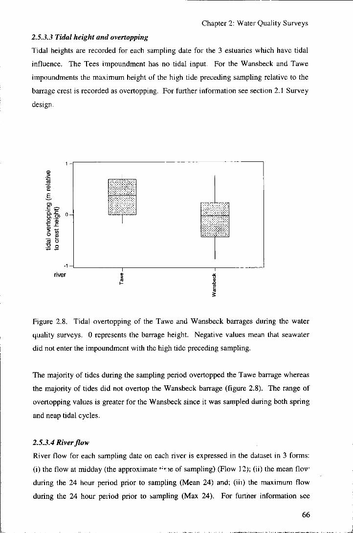
Chapter 2: Water Quality Surveys
2.5.3.3 Tidal height and overtopping
Tidal heights are recorded for each sampling date for the 3 estuaries which have tidal
influence. The Tees impoundment has no tidal input. For the Wansbeck and Tawe
impoundments the maximum height of the high tide preceding sampling relative to the
barrage crest is recorded as overtopping. For further information see section 2.1 Survey
design.
O)
Q. D>
/IS
(0 o :2 o
river
Figure 2.8. Tidal overtopping of the Tawe and Wansbeck barrages during the water
quality surveys. 0 represents the barrage height. Negative values mean that seawater
did not enter the impoundment with the high tide preceding sampling.
The majority of tides during the sampling period overtopped the Tawe barrage whereas
the majority of tides did not overtop the Wansbeck barrage (figure 2.8). The range of
overtopping values is greater for the Wansbeck since it was sampled during both spring
and neap tidal cycles.
2.5.3.4 River flow
River flow for each sampling date on each river is expressed in the dataset in 3 forms:
(i) the flow at midday (the approximate ^-rie of sampling) (Flow 12); (ii) the mean f lov
during the 24 hour period prior to sampling (Mean 24) and; (iii) the maximum flow
during the 24 hour peiiod prior to sampling (Max 24). For further infonnaiion see
66

Chapter 2: Water Quality Surveys
section 2.1 Survey design. During the periods sampled these terms were strongly
correlated for the whole dataset:
Mean 24 = 1.49 + 0.859 Flow 12 (P = 0.000, S = 6.846, R-Sq = 75.3%)
and.
Max 24 = 2.42 + 1.35 Flow 12 (P = 0.000, S = 9.922, R-Sq = 78.1%).
Obviously the relationship between these values wil l depend on when sampling takes
place in relation to any high flow events (whether on the rising or the falling limb of the
hydrograph). However the relatively strong linear relationships during the sampling
periods of this study mean that in subsequent data analyses a single parameter may be
used to represent flow.
(means are indicated by solid cirdes)
river
Figure 2.9. River flow in the estuaries studied during the water quality surveys.
67

Chapter 2: Water Quality Surveys
The mean river flow varies between estuaries on the basis of the different sizes of the
catchments, and seasonal and meteorological effects. The range in values of flow for
the rivers during the water quality surveys represent the range of flow conditions
sampled for each river (figure 2.9). Both the Tees and the Wansbeck were sampled
during multiple periods, including both summer and winter flow conditions and the
ranges in river flow are high. The Tawe and Blyth were only sampled for a single
summer period each and have lower ranges. No flood events were sampled on the
Blyth and hence its flow remained relatively constant during the sampling period.
2.5.5.5 Temperature
The water temperature was taken in situ at the three depths sampled at each site on each
date sampled for each river. Temperature is likely to be dependent on meteorological
conditions on the dates of sampling. The Tawe and the Blyth have higher mean
temperatures since they were only sampled during summer periods. The range in
temperatures is higher for the Tees and the Wansbeck, which were sampled over a range
of seasons, compared with the Tawe and Blyth, which were only sampled during
summers (figure 2.10). The mean temperatures (and standard deviations) measured
during the sampling periods are 12.4, 14.4, 11.8 and 10.5°C (SD = 1.5, 1.7, 6.5 and
3.8°C) for the Blyth, Tawe, Tees and Wansbeck respectively.
Temperature data collection was relatively simple due to the straightforwardness of the
equipment used. Almost all data intended to be collected in the experimental design
was able to be. A sudden violent storm during sampling at the Tees barrage caused
measurement of temperature (and DO) to be abandoned (2 datum missing). During the
period in which the Wansbeck impoundment was drained, water depths were too
shallow to allow the RV to access the sampling sites, and therefore some data is missing
(55 datum in total for T) for these dates.
68

Chapter 2: Water Quality Surveys
(means are Indicated by solid circles)
river
Figure 2.10. Water temperature (in °C) in the estuaries studied during the water quality
surveys.
2.5.3.6 Dissolved oxygen
The dissolved oxygen concentration of the water was taken in situ at the three depths
sampled at each site on each date sampled for each river. Data are reported as both
absolute concentrations (mg/1) and as percentage saturations (%). The meter used
included automatic temperature compensation so that the values in mg/1 are not fixed to
values in % saturation (solubility increases with decreasing temperature). Values were
not compensated for salinity however, and % saturations in saline waters are therefore
reported at lower than their true values. Hence the relationship between DO in mg/1 and
DO as % saturation, although good (figure 2.11, DO = - 0.169 + 0.113 DO%, S =
0.9807, R-Sq = 88.3%), shows some scatter from a straight line for the periods
surveyed.
69

Chapter 2: Water Quality Surveys
20 H
DOmg/l
10
50 100
DO % saturation
150
Figure 2.11. The relationship between DO concentration and % saturation for the water
quality surveys.
(means are irxlicated by solid cirdes)
150H
c o
1 100-
2 50 H
OH
nver
Figure 2.12. DO % saturations in the estu.iries studied during the water quality survey?
70

Chapter 2: Water Quality Surveys
(means are indicated by solid circles)
20-f
E
8 10-
river
Figure 2.13. DO absolute concentrations (mg/1) in the estuaries studied during the water
quality surveys.
Mean values (and SDs) for DO in the estuaries during the periods studied are 8.4, 9.1,
9.4 and 9.7 mg/1 (SD = 2.1, 1.1, 2.7 and 3.3 mg/1) for the Blyth, Tawe, Tees and
Wansbeck respectively (figure 2.13). In terms of saturation levels values are 75.8, 89.1,
84.1 % and 77.1 (SD = 20.0, 10.0, 16.3 and 27.9 %) respectively (figure 2.12).
The behaviour of DO in water bodies is complicated, and the variations which are seen
to occur could be due to a variety of factors. The behaviour of DO is further
investigated in subsequent chapters. At this stage it is worth noting however that
several values are recorded at below 5 mg/1, which is the threshold Statutory Water
Quality Objective (SWQO) value set by the then NRA (National Rivers Authority,
1991) for salmonid species of fishery, and on occasions the DO was below the 3 mg/1
necessary for cyprinid and migratory fisheries. These low oxygen conditions were
encountered at depth, and detailed depth profiles carried out on several occasions
showed stratification of DO levels associated with density stratification of the water
column (often as positive heterograde curves, figure 2.14).
71

Chapter 2: Water Quality Surveys
200
•CP
DO % saturation
nd Figure 2.14. Dissolved oxygen profile from site CP from the Wansbeck from the 2
September 2000, showing sharp decrease in DO with progression from fresh water at
surface to brackish and saline water at depth. Supersaturation is observed in the surface
waters due to the effects of high primary production (cyanobacterial blooms).
2.5.3.7 BOD
(means are indicated t)y solid circles)
E,
s o ca
river
Figure 2.15. BOD values for the rivTrs during the water quality i i r/eys.
72
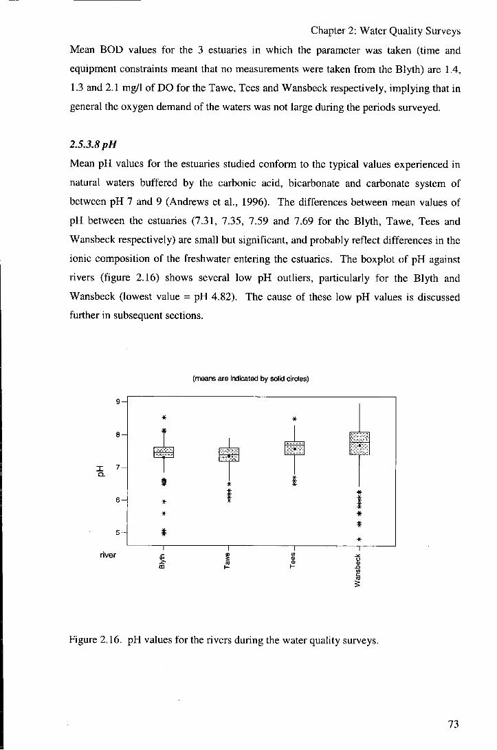
Chapter 2: Water Quality Surveys
Mean BOD values for the 3 estuaries in which the parameter was taken (time and
equipment constraints meant that no measurements were taken from the Blyth) are 1.4,
1.3 and 2.1 mg/1 of DO for the Tawe, Tees and Wansbeck respectively, implying that in
general the oxygen demand of the waters was not large during the periods surveyed.
2.5.3.8 pH
Mean pH values for the estuaries studied conform to the typical values experienced in
natural waters buffered by the carbonic acid, bicarbonate and carbonate system of
between pH 7 and 9 (Andrews et al., 1996). The differences between mean values of
pH between the estuaries (7.31, 7.35, 7.59 and 7.69 for the Blyth, Tawe, Tees and
Wansbeck respectively) are small but significant, and probably reflect differences in the
ionic composition of the freshwater entering the estuaries. The boxplot of pH against
rivers (figure 2.16) shows several low pH outliers, particularly for the Blyth and
Wansbeck (lowest value = pH 4.82). The cause of these low pH values is discussed
further in subsequent sections.
(rneans are indicated by solid circles)
8H
X 7-Q.
nver
Figure 2.16. pH values for the rivers during the water quality surveys.
73

Chapter 2: Water Quality Surveys
2.5.3.9 Alkalinity
Alkalinity mainly arises from the presence of the carbonate buffer system described
above. These ions come from the atmosphere and biological respiration, plus
dissolution of carbonate rocks where these occur in the watershed. The values
encountered in the estuaries studied suggest that they are well buffered. All of the rivers
run through solid geologies containing some carbonate (Carboniferous) and this
contributes to their alkalinities. The alkalinity of the Blyth, which as discussed for
conductivity below consists mainly of seawater for the dates and section sampled, has a
lower average alkalinity. This is contrary to the general estuarine situation in which
seawater alkalinity is higher than that of riverwater (Dyrssen and Wedborg, 1980).
(means are indicated by solid circles)
300 H
CO
1 c 15
200 H
100 H
river
Figure 2.17. Alkalinity values for the rivers during the water quality surveys.
2.5.3.10 Conductivity
There are large differences between the conductivities of the 4 rivers (figure 2.18). The
mean conductivities are related to the amount of seawater to freshwater in the systems,
and reflect the differences in barra2:; heights to the tidal frame. The highest m^an
cond-ctivity is therefore found in the Blyth '"'':.ere there is no impoundment
(conductivities were augmented due to low freshwater flows during the sampling period
on the Blyth), and lowest on the fees where no seawater can enter the impoundment.
74

Chapter 2: Water Quality Surveys
The median values for conductivity for the Tees, Wansbeck and Tawe (figure 2.18) are
similar lower values (251, 943 and 940 |i,S/cm respectively), and show that most of the
water sampled is fresh in these impoundments, whereas the Blyth median value of
41200 \xS/cm is higher than the mean and shows that most of the water in this estuary is
saHne.
conductivity
80000-
70000 H
60000
50000H
40000
30000H
20000
10000H
0
river
(means are indicated by solid circles)
m
Figure 2.18. Conductivity values (in |j,S/cm) for the rivers during the water quality
surveys, showing the difference between total exclusion (Tees), partial exclusion (Tawe
and Wansbeck), and unimpounded (Blyth) estuaftes.
Detailed depth profiles carried out on several occasions showed there to be a strong
salinity (density) stratification in the partial tidal exclusion impoundments (e.g. figure
2.19).
75

Chapter 2: Water Quality Surveys
0 10000 20000 30000 40000 50000 60000
•CP -WB
conductivity (uS/cm)
Figure 2.19. Conductivity changes with depth in the water column from two sampling
sites from the Wansbeck from 2"'' September 2000, showing stratification between fresh
and brackish and saline waters. Site WB is immediately behind the barrage whilst CP is
further upstream at the deepest point in the impoundment.
80000
^ 70000
1 60000
3 50000
^ 40000
1 30000
O 20000 o
10000
0 H
e o %
o o
0 5000
Na (mg/l)
— I — 10000
Figure 2.20. The relationship between conductivity and Na for samples taken during all
water quality surveys, showmg significant scatter from straight line.
76

Chapter 2: Water Quality Surveys
In theory conductivity should be proportional to Na for the samples, assuming that
seawater dominates conductivity in the systems, but a large amount of scatter from a
straight line relationship is seen (figure 2.20). This implies that, although care was
taken to take water samples for laboratory analysis at the same point at which in-situ
parameters were measured, values from field and laboratory measurements may not
represent exactly the same portion of water. This is particularly the case for samples
and readings taken close to the sharp and strong halocline (the interface between
seawater and freshwater stratified due to density differences) which was observed in the
Tawe and Wansbeck impoundments. Small vertical variations about this interface are
likely to have meant that distinct (freshwater or seawater) packages of water were
sampled at the "same" point (giving outlying values on figure 2.20). Care should thus
be taken when comparing field and laboratory measured parameters.
2.5.3.11 Eh
(means are indicated by solid circles)
500 H
200 H
river
Figure 2.21. Eh values for the rivers during the water quality surveys.
Eh measurements were taken during just under half of the water quality surveys (based
on equipment availability: see section on Field Analytical Methods). No Eh
measurements were made on the Blyth estuary.
77

Chapter 2: Water Quality Surveys
Strongly reducing conditions were not observed during the Eh sampling periods, although some values (below = 100 mV) suggest that anoxic conditions are developed (cf. DO data). Semi-quantitive interpretation gives that reducing conditions are more likely in the Wansbeck and the Tawe than in the Tees impoundment.
2.5.3.12 Transparency
Transparency ranges from 0.05 m (following high flow in the Wansbeck) to 3.55 m
(Tawe), and there are significant differences in transparencies (measured as Secchi
depths) between the estuaries (figure 2.22).
(means are indicated by solid circles)
c
ca tn c to
4 H
3 H
OH nver
Figure 2.22. Transparency values (as Secchi depths) for the rivers during the water
quality surveys.
Transparency is a combined function of colour and turbidity. The Tawe is relatively far
more transparent than the estuaries in the Northeast of England. This is probably
related to the low TSS of the freshwater entering the impoundment dunng the period
sampled (related to low flow and relativeW low drift deposits in the catchment). The
Tees has a strong colour imparted by humic and fulvic acids (Wright and Worrall, 2001)
and hence exhibits a relatively low transparency.
78

2.5.3.13 TSS
Chapter 2: Water Quality Surveys
(means are indicated by solid circles)
600 H
CO 300
100-
river
Figure 2.23. TSS values for the rivers during the water quality surveys.
TSS also varies significantly between estuaries, with the Wansbeck and Blyth showing
much higher average values (50 and 72 mg/1 respectively) than the Tees and Tawe (20
and 13 mg/1 respectively). The Tawe was sampled under low flow conditions, and has a
distinct catchment as described above. It is probable that the Tees is less turbid and has
lower TSS (although, as mentioned, a low transparency due to its strong colouration)
due to a lack of tidal currents acting to re-suspend settling particulates. Re-suspension
of material by turbulent shearing from strong tidal currents acts to give high TSS values
for the Blyth even when TSS inputs from the freshwater source (samples taken from the
tidal limit) are low. Continual and rapid exchange of sediment between the bed and
suspended phase due to tidal currents is described by Dyer (1995). Such tidal currents
wil l be suppressed by the construction of a barrage. The allochthonous supply of TSS
in freshwater is likely to relate to freshwater flow for each catchment.
Outlying high values observed for TSS relate to either high flow periods or samples
from depth at sampling sites. Although care was taken to avoid disturbing the
sediment-water interface when taking water samples at depth, it is possible that in some
79

Chapter 2: Water Quality Surveys
cases high TSS were measured due to disturbed bed sediment. Unfortunately it is
impossible to assess whether this is the case, or whether "true" sediment concentrations
were being recorded (e.g. sampling a fluff layer at the sediment-water column
interface).
Some negative values for TSS were recorded for the initial laboratory work (mainly
from the Tees) in which the cellulose nitrate filter papers used were not perfectly dry
before use (and thus lost weight on subsequent oven drying and dessication). In later
work care was taken that dry papers were used by storing them in a dessicator, and pre-
weighing at a distance from any water samples. Additional problems occurred in
several cases because filter material was lost on transfer to and from filter apparatus and
the balance, due to the fragile nature of the filter papers. Negative values of TSS are
excluded from data analyses.
2.5.3.14 Nutrients
Nitrate
(means are Indicated by solid circles)
9 -
8 -
7 -
6 -E,
^ — o
4 -
3 -
2 -
1 -
0 -
river
* •X-
m
Figure 2.24. Nitrate values for the rivers during the water quality surveys.
80

Chapter 2: Water Quality Surveys
Mean nitrate values for the periods studied are 0.53, 0.61, 2.58 and 2.64 mg/1 N for the Blyth, Tawe, Tees and Wansbeck respectively (figure 2.24). The outlying values for the Blyth represent the freshwater input to the estuary, which show significantly higher nitrate than the seawater end member. The positive outliers for the Wansbeck are from sampling on the 16"' June 2001. The 2 Tees outlying values are from deep sampling points and may represent sampling which disturbed the bed sediment.
Variations in nitrate concentrations occur with different land management within
catchments (e.g. amount of ploughing or fertiliser application (Roberts and Marsh,
1987; Johnes and Burt, 1993)), quantities of point source inputs, and with season (peak
nitrate tending to occur in spring (Heathwaite and Johnes, 1996)). The greatest range in
nitrate concentrations is seen in the Wansbeck, which was sampled over the greatest
range of seasons. The Blyth and Tawe were only sampled during summer periods,
during which run-off and nitrogen export are likely to be at their lowest.
Ammonia
(means are indicated by solid circles)
1.5H
O) 1 0 -E. CO
' c o E E ro
0.5 H
0.0-
river
Figure 2.25. Ammonia values for the rivers during the water quality surveys.
81

Chapter 2: Water Quality Surveys
The pattem for the relative mean values of ammonia between the estuaries is the reverse
of that for nitrate. The values for the Blyth and Tawe (0.27 and 0.26 mg/1 N
respectively) are higher than those for the Tees and Wansbeck (0.13 and 0.20 mg/1 N
respectively). Ammonia is normally at low levels in unpolluted waters due to
biologically mediated reactions to more oxidised states (nitrification). The values in the
estuaries studies are generally low and suggest that conditions are relatively unpolluted
by ammonia and are oxic. However, several outlying high values (figure 2.25)
corresponding to deep samples indicate that anoxic conditions and possible release from
sediments may exist in places.
Phosphate
(means are indicated by solid circles)
O)
Q. W O
1.5-
1.0H
0.5-
0.0-
river
Figure 2.26. Phosphate values for the rivers during the water quality surveys.
Dissolved orthophosphate concentrations tend to be very low in natural waters since it is
rapidly taken up by biota. Maybeck (1982) gives the global average river water
concentration of dissolved phosphorus as 0.028 mg/1 P - PO4. The OECD threshold
level rcr lake eutrophy is 0.035 mg/1 P - PO4 (Reynolds and Davies, 2000). The mean
values encountered in *,he estuaries during th'" water quality survp"- are above these
levels (;0.057, 0.041, 0.225 and 0.109 mg/1 P for the Blyth, Tawe, Tees and Wansbeck
respectively), the Tees and Wansbeck in particular having high phosphate
82

Chapter 2: Water Quality Surveys
concentrations, indicating that there are anthropogenic inputs to the systems which may
lead to eutrophic behaviour. The positive outlying values for phosphate for the Tees
and Wansbeck (figure 2.26) are from summer sampling dates (low flows) on the rivers.
Silica
(means are indicated by solid circles)
4 H
01
O H
nver
Figure 2.27. Si values for the rivers during the water quality surveys.
Mean silica values for the estuaries are 0.35, 1.30, 0.99 and 1.68 mg/1 for the Blyth,
Tawe, Tees and Wansbeck respectively. Silica variations between freshwater inputs are
likely to be due to variations in the geologies of the catchments, and flows.
Concentrations on specific dates wil l vary with the relative amounts of baseflow and
stormflow contributing to the freshwater flow. The concentrations in freshwater are
higher than those in seawater.
2.5.3.15 Major elements
The mean values for the (dissolved) major elements of Na, Mg, Ca, K and S in the
impoundments show the same pattern as conductivity, being dominated by the relative
amount of seawater in the system (figure 2.28 and table 2.8).
83

Chapter 2: Water Quality Surveys
(mg^) Blyth Tawe Tees Wansbeck
Ca 324 74 29 114
K 314 59 3 61
Mg 991 181 6 213
Na 7918 1523 24 1578
S 757 384 16 179
Table 2.8. Mean concentrations for major elements during water quality surveys.
(means are indicated by solid circles)
10000H
E (0
5000-
O H
river
Figure 2.28. Na values for the rivers during the water quality surveys.
84

Chapter 2: Water Quality Surveys
O
990
330
305
101
327
109
Na Mg C a
Figure 2.29. Co-linearity between major metals with conservative mixing of freshwater
and seawater for the water quality surveys.
Major elements are of far higher concentration in seawater than river water and behave
conservatively (Liss, 1976), and therefore represent the relative amount of seawater in
an estuary. The Blyth contains the maximum amount of seawater and the Tees contains
no seawater, with the Tawe and Wansbeck in intermediate positions.
Conservative mixing of the major elements can be seen in the strong co-linearity of Ca,
Mg, K and Na for all data (figure 2.29):
• Ca = 42.4-I-0.0361 Na (P = 0.000, S = 20.97, R-Sq = 96.5%)
• K = 0.773 + 0.0378 Na (P = 0.000, S = 9.548, R-Sq = 99.3%)
• Mg = 3.24-h 0.125 Na (P = 0.000, S = 13.55, R-Sq = 99.9%)
S is less well correlated with Na (figure 2.30) due to analytical problems in the
determination of S.
85

Chapter 2: Water Quality Surveys
2000
CO 1000
5000
Na (mg/l)
10000
Figure 2.30 The relationship of S to Na during the water quality surveys. The scatter of
points above the conservative mixing line is due to analytical error.
Whilst for the majority of analytical runs on the ICP-OES S measurement showed low
error and could be seen to show conservative mixing within the impoundments, for a
few runs S determination showed large random (although always positive) errors.
These were identified as errors (rather than true measurements) by the observation of
large fluctuations in the S values reported for the "seawater" standard included
periodically in the sampling runs. These errors were unique to S and no underlying
cause was able to be identified. Care is taken in interpretation of results for S which
include these errors.
2.5.3.16 Minor and trace metals
Trace metal levels and LOD
A large number of the trace metal values lie close to or below the 3s limit of detections
(LOD). These elements tend to have very low concentrations in dissolved forms and
partition strongly to particulate phases at normal pH values, and so the low values
encountered in the water quality surveys are typical. Ine 3s LOD represents the value
at which there is 99% probability of the response being a true vpiue (rather than
analytical error). Considering values below this level entails a greater risk of responses
being due to random error rather than the concentration in the sample. Hence, for many
86

Chapter 2: Water Quahty Surveys
of the dissolved trace elements analysed for in the water quality surveys, interpretation
may only be semi-quantitative.
mg/1 LOD Blyth Tawe Tees Wansbeck
Al 0.055 0.013 0.013 0.048 0.031
Co 0.587 0.0011 0.0013 -0.0020 -0.0001
Cr 0.004 0.0015 0.0046 -0.0026 0.0012
Cu 0.003 -0.0093 -0.0016 -0.0026 -0.0016
Fe 0.004 0.082 0.078 0.167 0.168
Mn 0.004 0.058 0.109 0.017 0.166
Ni 0.005 0.0036 0.0015 -0.0035 -0.0005
Sc 0.000 -0.0014 0.0006 0.0027 -0.0001
Sn 0.033 0.0059 -0.0382 0.0055 0.0054
Ti 0.002 -0.0015 0.0004 -0.0035 0.0003
V 0.011 0.0087 0.0615 -0.0086 0.0423
Zn 0.003 -0.0163 0.0590 0.0180 0.0017
Table 2.9. Mean concentrations and LODs (see section 2.4.10) for minor and trace
elements during water quality surveys.
Fe and Mn
Both Fe and Mn occur at levels well above the 3s LOD values for the ICP-OES analysis
(Fe = 0.004 mg/1, Mn = 0.004 mg/1), and show significant mean concentration
differences between the estuaries. The concentration of Fe and Mn are likely to be
controlled both external to (freshwater and seawater inputs to the estuaries) and within
the estuaries. The behaviour of both elements is strongly controlled by redox
conditions. In oxygenated water, Fe occurs as insoluble ferric hydroxide and as
complexes with dissolved and colloidal organic (particularly humic) and inorganic
substances. Mn behaves similarly but has a higher solubility. Under low oxygen
conditions Fe and Mn are released from sediment in dissolved form to the water
colunm. The high values of Mn observed for some of the samples taken at depth within
the Wansbeck, Tawe and Tees (positive outliers on figure 2.31) suggest some release
from sediments occurs in these systems. The redox conditions within the systems are
discussed further in subsequent sections.
87
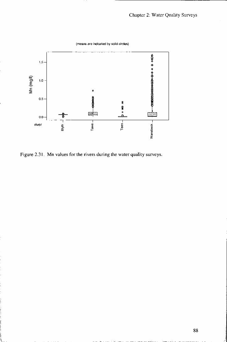
Chapter 2: Water Quality Surveys
(nieans are indicated by solid circles)
river
Figure 2.31. Mn values for the rivers during the water quality surveys.
88

Chapter 3: Seasonal Effects on Water Quality
Chapter 3
Seasonal Effects on Water Quality
3.1 Introduction
Differences in water quality in estuarine impoundments between seasons were
examined using data collected from water quality surveys of the Tees and the Wansbeck
impoundments. Firstly, differences between the summer and winter seasons in a total
tidal exclusion impoundment (the Tees) were assessed using the complete range of
water quality parameters measured. Secondly, the variation between spring, summer,
autumn and winter in a partial tidal exclusion impoundment (the Wansbeck) were
assessed using a selection of water quality parameters. General Linear Model (GLM)
ANOVA was used to assess the significance of season as a factor in water quality
variation.
3.2 Tees
Seasonal differences in water quality were examined using (GLM) ANOVA. For the
Tees, sampling periods were summer (dates sampled: 04/08/99, 11/08/99, 25/08/99,
08/09/99 and 22/09/99), and winter (dates sampled: 02/02/00, 08/02/00, 16/02/00,
23/02/00 and 29/02/00). To create a balanced dataset (one in which factor levels (e.g.
number of dates sampled or sample sites) are the same for each treatment (season, etc.),
one of the dates sampled as part of the summer survey (21/07/99) was not included in
the analyses.
The significant controls on the water quality parameters in the Tees impoundment were
assessed using ANOVA with the factor levels of season (summer or winter), distance
within the impoundment from the former tidal limit (in terms of the 6 approximately
equidistant sites sampled, represented by numbers 1 to 6 with increasing distance from
the upstream limit at Low Moor), and depth (shallow (s), middle (m) and deep (d))
sampled in the water column at each sampling site. The interactions between these
factors (season*distance, etc.) were assessed. Analyses were carried out both with and
without the inclusion of flow and temperature as covariates in the models, with the
results from these analyses presented where relevant.
89

Chapter 3: Seasonal Effects on Water Quality
3.2.1 Temperature
Results
Source F P a" Size of
Effect (0) )
Season 2191.19 0.000 247.9 1.00
Distance 0.16 0.977 na na
Depth 1.01 0.366 na na
Season* distance 0.20 0.964 na na
Season*depth 0.68 0.509 na na
Depth* distance 0.04 1.000 na na
S eason * di stance* depth 0.07 1.000 na na
Error 4.1 0.00
Table 3.1. Results from GLM ANOVA for seasonal effects on temperature within the
Tees impoundment (na = not applicable since factor insignificant (P>0.05)).
season distance depth
Figure 3.1. Main effects plot for temperature (in °C) in the lees impoundment Hea t
square (LS) means for factor levels), showing season as the only significant factor.
90

Chapter 3: Seasonal Effects on Water Quality
The results (table 3.1) show that all of the variation in temperature observed in the
sampling periods can be explained by season (size of effect for season (o)' ) = 1.00).
Water temperature does not vary with either distance or depth within the impoundment.
Discussion
The results show that, as might be expected, the temperature of the Tees impoundment
varies significantly dependent on climatic factors (expressed as season in the model).
No internal variation within the water body is seen to develop. Significantly, the system
may be assumed to have sufficient mixing throughout the year that thermal stratification
(as occurs in the majority of temperate lakes of > approximately 10 m depth (Wetzel
1983)) does not occur.
3.2.2 Dissolved oxygen
Results
The difference in behaviour of DO within the impoundment was analysed in terms of
DO % saturation to remove the effects of solubility differences due to temperature on
the concentrations. The raw DO % values were used, with no normalisation to input
values (the water entering the impoundment at the upstream limit of the impoundment)
being apphed. Results are shown in table 3.2.
Source F P a" Size of
Effect (0)^)
Season 188.75 0.000 532.0 0.41
Distance 16.82 0.000 224.2 0.17
Depth 13.49 0.000 70.8 0.05
Season*distance 16.10 0.000 213.9 0.17
Season*depth 15.05 0.000 79.6 0.06
Depth*distance 2.10 0.025 31.3 0.02
Season*distance*depth 2.20 0.019 33.9 0.03
Error 102.0 0.08
Table 3.2. Results for GLM ANOVA for DO % with season within the Tees.
91
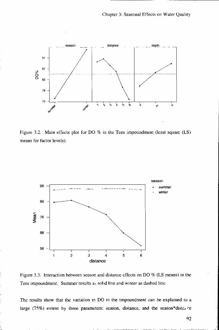
Chapter 3: Seasonal Effects on Water Quality
distance depth
O Q
91 H
87 H
83 -{
79 H
75 - I
Figure 3.2. Main effects plot for DO % in the Tees impoundment (least square (LS)
means for factor levels).
96 - (
86
1 76
66 H
56
distance
season ° summer • winter
Figure 3.3. Interaction between season and distance effects on DO % (LS means) in the
Tees impoundment. Summer results a solid line and winter as dashed line.
The results show that the variation in DO in the impoundment can be explained to a
large (75%) extent by three parameters: season, distance, and the season*distci/^e
02

Chapter 3: Seasonal Effects on Water Quality
interaction. The largest effect in the model is that of season, which explains 41% of the
variation in levels of DO in the Tees impoundment. Distance accounts for 17% of the
variation, and shows a substantial (17%) interaction with season (figure 3.3). During
summer, DO saturations are significantly (P = 0.000) lower (table 3.2 and figure 3.2),
with a mean value of 75.4 %. The range of values of DO is also far greater than in
winter (SD = 19.7 %, maximum = 135.6 % and minimum = 15.1 % ) . The effects of
distance and depth in the impoundment only become significant during summer (figures
3.3 and 3.4). Statistically this is demonstrated by the size of experimental effects being
almost identical for both distance and the distance*season interaction (to^ = 0.17 and
0.17 respectively), and depth and the depth*season interaction (co = 0.05 and 0.06
respectively). DO decreases with distance downstream in the impoundment and with
depth at sampling sites. The depth effects, in terms of reduced DO concentrations with
increasing depth in the system, also becomes slightly more pronounced with distance
downstream (figure 3.5, interaction (o = 0.02).
season 95 -4
85 H c
75
65 H
summer winter
depth
Figure 3.4. Interaction between season and depth effects on DO % (LS mean) in the
Tees impoundment. Summer results as solid line and winter as dashed line.
93

Chapter 3: Seasonal Effects on Water Quality
c (0
92 -o — — "o
82 - ^ - - ^ ' ^ ^ .^-"^
72 -
y
y
62 -
d 1
m depth
1 s
distance
1 2 3
o •
4 5 6
Figure 3.5. Interaction between distance and depth effects on DO % (LS mean) in the
Tees impoundment.
Discussion
The Tees carries a large (particularly dissolved) organic load (Worrall et al. in press)
due to its source in peat covered uplands, which is likely to exert a natural BOD to the
river. The impact of this BOD will be greater during the summer period due to the
higher temperatures of the water and hence the Tees, as would be expected, shows
significant seasonal differences in DO %. The impacts of colour due to humic
substances with seasonality on DO levels are discussed in Belanger et al. (1987) and
Crisman et al. (1998). The variation in dissolved organic carbon levels with season and
flow is discussed in the section on BOD below.
As mentioned temperature controls the solubility of oxygen in water (and therefore
modelling was carried out using % saturations), so that absolute values (in which terms
SWQOs for DO tend to be set) at a particular % saturation will be lower in warmer
summer water. The mean summer water temperature during the surveys was 17.2°C
and that in winter 4.9°C, both with low variation (SD = 2.5°C and 1.0°C respective'v),
and the temperature control on absoli e DO concentrptior can be seen in the se ^ - \ 'm
of summer and winter data when DO % and DO m<?J\ values are plotted (figure 3.6).
94
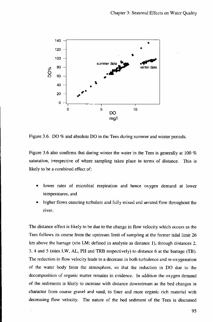
Chapter 3: Seasonal Effects on Water Quality
140
120 -
100 -
80 -
o Q 60
40 -
20 -
0 -
summer data n d a t ^ ^ ^ winter data
DO mg/l
10
Figure 3.6. DO % and absolute DO in the Tees during summer and winter periods.
Figure 3.6 also confirms that during winter the water in the Tees is generally at 100 %
saturation, irrespective of where sampling takes place in terms of distance. This is
likely to be a combined effect of:
• lower rates of microbial respiration and hence oxygen demand at lower
temperatures, and
• higher flows ensuring turbulent and fully mixed and aerated flow throughout the
river.
The distance effect is likely to be due to the change in flow velocity which occurs as the
Tees follows its course from the upstream limit of sampling at the former tidal limit 26
km above the barrage (site L M ; defined in analysis as distance 1), through distances 2,
3, 4 and 5 (sites LW, AL, PH and TRB respectively) to distance 6 at the barrage (TB).
The reduction in flow velocity leads to a decrease in both turbulence and re-ox ygenation
of the water body from the atmosphere, so that the reduction in DO due to the
decomposition of organic matter remains in evidence. In addition the oxygen demand
of the sediments is likely to increase with distance downstream as the bed changes in
character from coarse gravel and sand, to finer and more organic rich material with
decreasing flow velocity. The nature of the bed sediment of the Tees is discussed
95

Chapter 3: Seasonal Effects on Water Quality
further elsewhere in the thesis. It is also possible that the there is an increased oxygen
demand within the water column with the course of the river from diffuse (agricultural)
or point (CSO and other wastewater) source inputs, although no evidence for this was
seen in the BOD results, which remain relatively constant throughout the impoundment.
The decrease in DO levels with depth is only significant during summer periods, when
flows are lower and incomplete mixing of the water column occurs. This leads to a
slight stratification in DO levels which becomes more pronounced as depth in the
impoundment increases and river gradient decreases (and hence flow velocity and
turbulence decrease) with distance downstream. Re-oxygenation of the waters isolated
from the water column-atmosphere interface cannot occur and reduced DO saturation
occurs.
The error term in the ANOVA for DO % saturation has a value of 0)^ of 0.08, meaning
that 8 % of the variation in DO cannot be explained by the factors included in the
model. This error may include differences in external loading of oxygen demand to the
water body not accounted for by seasonality, or variations in flow which are
independent of season. Repeat analysis carried out with the inclusion of flow as a
covariate showed this term to be insignificant, however.
An additional impact of seasonality is on primary production in the water body.
Phytoplankton primary production is evident in the Tees in summer from observations
of supersaturation of DO. At shallow and mid depths on the 4* August (during which
water temperature was high (s22°) and river flow low (=3.5 m2/sec)) at sites A L and
PH, oversaturation (<137 %) was measured. Assuming the normal diel effects of
primary production and respiration, these values would have fallen to undersaturation
during the night.
3.2.3 BOD
Results
The model used to assess DO behaviour above (with season, distance and depth as
factors) was run for BOD, with both exclusion and inclusion '^f flow as a covariate.
Although flow is generally higher :n the winter than in summer, it shows a large a nount
of variation in and some overlap between these seasons during the Tees sampling.
Without flow as a covariate, none of the 3 factor levels or their interactions showed any
96

Chapter 3: Seasonal Effects on Water Quality
significant effects (at 95 % confidence interval) on BOD. Including flow (as the mean
flow in the 24 hour period preceding sampling (Mean 24)) gave the following results:
Source F P a" Size of
Effect (0)^)
Flow 83.3 0.000 2.15 0.45
Season 67.6 0.000 1.74 0.36
Distance 1.1 0.368 na 0.00
Depth 1.2 0.299 na 0.00
Season*distance 1.0 0.405 na 0.00
Season*depth 0.6 0.527 na 0.00
Depth*distance 0.4 0.950 na 0.00
Season*distance*depth 0.6 0.806 na 0.00
Error 0.94 0.19
Table 3.3. Results from GLM ANOVA for seasonal effects on BOD within the Tees
impoundment including flow as a covariate (na = not applicable since factor
insignificant (P>0.05)).
During summer BOD levels are significantly higher than in winter during the periods
sampled in the Tees (table 3.3, figure 3.7). BOD does not vary significantly within the
impoundment with either distance or depth during either summer or winter. The
seasonal effect is independent of flow, which also shows a significant control on BOD.
Together flow and season account for the majority of the variation in values of BOD
measured during the sampling periods (o) = 0.45 and 0.36 respectively), with an error
term in the model of 19 %.
97
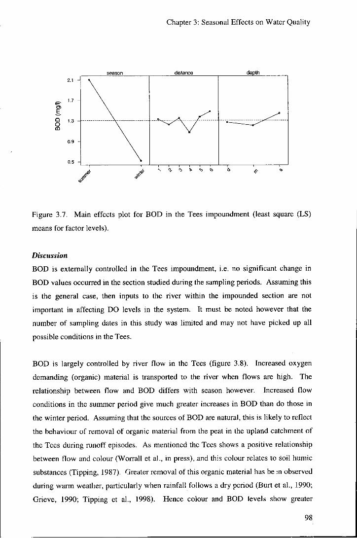
Chapter 3: Seasonal Effects on Water Quality
season distance depth
Figure 3.7. Main effects plot for BOD in the Tees impoundment (least square (LS)
means for factor levels).
Discussion
BOD is externally controlled in the Tees impoundment, i.e. no significant change in
BOD values occurred in the section studied during the sampling periods. Assuming this
is the general case, then inputs to the river within the impounded section are not
important in affecting DO levels in the system. It must be noted however that the
number of sampling dates in this study was limited and may not have picked up all
possible conditions in the Tees.
BOD is largely controlled by river flow in the Tees (figure 3.8). Increased oxygen
demanding (organic) material is transported to the river when flows are high. The
relationship between flow and BOD differs with season however. Increased flow
conditions in the summer period give much greater increases in BOD than do those in
the winter period. Assuming that the sources of BOD are natural, this is likely to reflect
the behaviour of removal of organic material from the peat in the upland catchment of
the Tees during runoff episodes. As mentioned the Tees shows a positive relationship
between flow and colour (Worrall et al., in press), and this colour relates to soil humic
substances (Tipping, 1987). Greater removal of this organic material has be ;n observed
during warm weather, particularly when rainfall follows a dry period (Burt et al., 1990;
Grieve, 1990; Tipping et al., 1998). Hence colour and BOD levels show greater
98
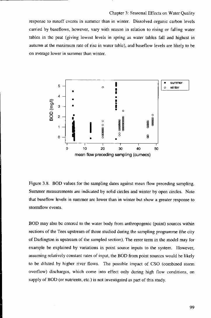
Chapter 3: Seasonal Effects on Water Quality
response to runoff events in summer than in winter. Dissolved organic carbon levels
carried by baseflows, however, vary with season in relation to rising or falling water
tables in the peat (giving lowest levels in spring as water tables fall and highest in
autumn at the maximum rate of rise in water table), and baseflow levels are likely to be
on average lower in summer than winter.
• summer o winter
mean flow preceding sampling (cumecs)
Figure 3.8. BOD values for the sampling dates against mean flow preceding sampling.
Summer measurements are indicated by solid circles and winter by open circles. Note
that baseflow levels in summer are lower than in winter but show a greater response to
stormflow events.
BOD may also be entered to the water body from anthropogenic (point) sources within
sections of the Tees upstream of those studied during the sampling programme (the city
of Darlington is upstream of the sampled section). The error term in the model may for
example be explained by variations in point source inputs to the system. However,
assuming relatively constant rates of input, the BOD from point sources would be likely
to be diluted by higher river flows. The possible impact of CSO (combined storm
overflow) discharges, which come into effect only during high flow conditions, on
supply of BOD (or nutrients, etc.) is not investigated as part of this study.
99

Chapter 3: Seasonal Effects on Water Quality
3.2.4 pH
Results
Source F P a" Size of
Effect (0)^)
Season 104.98 0.000 0.182 0.54
Distance 4.52 0.001 0.031 0.09
Depth 1.18 0.307 na 0.00
Season*distance 8.10 0.000 0.062 0.18
Season *depth 1.20 0.302 na 0.00
Depth* distance 0.88 0.557 na 0.00
Season*distance*depth 0.48 0.903 na 0.00
Error 0.063 0.19
Table 3.4. Results from GLM ANOVA for seasonal effects on pH within the Tees
impoundment (na = not applicable since factor insignificant (P>0.05)).
season distance depth
7.72
7.64 H
° - 7.56
7.48
7.40 - I
Figure 3.9. Main effects plot for pH in the Tees impoundment (least square means for
factor levels).
100

Chapter 3: Seasonal Effects on Water Quality
The same model applied above to DO was used to examine the seasonal behaviour of
pH within the Tees impoundment. The results are shown in table 3.4. The majority of
the variance in the data (54 %) is due to the effect of season. Distance within the
impoundment is also significant at the 99 % level, but accounts for only 9 % of the
differences between pH values. There is a significant interaction between season and
distance (figure 3.10, co = 0.18), and distance is seen to be a more significant factor
during the sunmier period. Depth is not shown to be a significant control on pH in the
Tees impoundment.
season
distance
summer winter
Figure 3.10. Interaction between season and distance effects on pH (LS mean) in the
Tees impoundment. Summer results as solid line and winter as dashed line.
Discussion
The variations in pH observed in the Tees, although significant, are not large and,
assuming the sampling periods are representative of the general situation in the river,
the range of values is such that pH is not likely to be a cause any major water quality
problems (such as solubilisation of metals). Low variability in pH would be expected
given the well buffered nature of the water body due to carbonate dissolution (mean
alkalinity during the sampling of 121 mg/1 CaCOs equivalent).
101

Chapter 3: Seasonal Effects on Water Quality
pH values observed were slightly lower in summer than in winter. Within a water body primary production tends to increase pH and alkalinity by photosynthetic fixation of dissolved CO2 together with H* according to:
IO6CO2 + I6NO3" + HP04^" + I22H2O + 18H^ o {C106H263O110N16P1} + 13802
(Andrews et al., 1996). Respiration acts in the reverse direction and reduces pH.
Changes in the relative amounts of photosynthesis and respiration with light availability
can lead to diel cycles in pH and DO. In this study the effects of any such variations on
the reporting of water quality were minimised by sampling at approximately the same
time of day for each sampling date and site. Oxidation of organic matter either in the
water column or the sediments also acts to reduce pH. The lower pH values
encountered during the summer period could be explained by increased rates of
oxidation with higher temperature.
It is also possible that change in the water source with season may have an effect on pH.
Summer flows may contain a higher proportion of baseflow coming from lower pH
Permo-Trias sandstones of the catchment, compared with the winter condition of flow
from the upland catchment (composed of Carboniferous sediments).
The River Leven tributary, which has its major groundwater source in the Permo-
Triassic geologies and enters the Tees between sites 3 and 4, may explain some of the
decrease in pH seen between these points in summer, although the pattern is opposite in
winter and the contribution of the Leven cannot be well quantified due to lack of flow
data. It may be assumed therefore that the majority of the distance effects on pH
observed are due to the relative rates of photosynthesis, respiration and oxidation. As is
evident in DO values, the impact of oxidation increases with distance downstream
during the summer period, and pH values also decrease in summer towards the barrage.
Increasing pH with distance in the whole system in winter, and at upstream sites in
summer, could correspond to increased primary production at these sites associated with
decreasing flow velocities in the river. That pH values do not decrease r.gnificantly
with depth (as occurs in the hypolimnion of eutrophic lakes), in addition to the low size
of depth effect on DO, suggests that entrenched stratification of the water column of tht
Tees does not occur.
102

Chapter 3: Seasonal Effects on Water Quality
The error term in the model is relatively large (19 % ) , meaning that the terms included (season, distance and depth) cannot account for all of the variance in pH values seen. Including flow (as the mean flow in the 24 hours previous to sampling) as a covariate in the model reduces the error term to 13 %. Including temperature as a covariate in the model does not reduce the error term, and it can be assumed that temperature effects are adequately explained within season. It is possible that variations in the contribution to pH levels from the Leven tributatry may explain a portion of the error.
3.2.5 Alkalinity
Results
•en .£ O
a O
150 -r
130 H
110 4
season distance depth
90
70 H
Figure 3.11. Main effects plot for alkalinity in the Tees impoundment (least square
means for factor levels). Distance and depth effects are insignificant at 95 % CI.
Alkalinity is significantly lower (99 % level) in winter than in summer. Applying the
ANOVA model used for DO, BOD and pH to alkalinity shows that there are no
significant differences with either distance or depth in the impoundment (figure 3.11),
implying that alkalinity is externally controlled. One-way ANOVA shows a magnitude
of effect for season of 88 %.
103

Chapter 3: Seasonal Effects on Water Quality
Discussion
The Tees is well buffered due to dissolution of carbonate minerals in the geology of its
catchment. Flow is higher in winter than summer and, given relatively constant rates
of carbonate dissolution, alkalinity is diluted by these higher flows (figure 3.12,
Kirschner et al. 1993) such that:
alkalinity = 270 - 135 log(Mean 24) (P = 0.000, S = 23.7413, R-Sq
86.0 %)
where alkalinity is measured in mg/1 CaCOs equivalent, and Mean 24 is the mean flow
during the 24 hours prior to sampling measured in m /s (cumecs).
300 H
200
I 100 H
0
a 0 •
1
D S
0
n
a 1
3.0 4.0 6.0 8.0 10 15 20 30 40
mean flow preceding sampling (cumecs)
Figure 3.12. The relationship between alkalinity and flow in the Tees, showing the
dilution effect with increasing flow (logarithmic scale). P = 0.000, R-Sq = 86.0 %.
104

Chapter 3: Seasonal Effects on Water Quality
3.2.6 Conductivity
Results
Source F P a" Size of
Effect (0)^)
Flow 66.28 0.000 29886 0.40
Season 1.24 0.267 na 0.00
Distance 7.82 0.000 15616 0.21
Depth 3.76 0.025 2524 0.03
Season*distance 4.57 0.001 8164 0.11
Season*depth 3.86 0.027 2455 0.03
Depth* distance 1.80 0.062 na 0.00
Season*distance*depth 1.72 0.077 na 0.00
Error 16481 0.22
Table 3.5. Results from GLM ANOVA for seasonal effects on conductivity within the
Tees impoundment (na = not applicable since factor insignificant (P>0.05)).
Using a model containing the factors of season, distance and depth shows that
conductivity varies significantly with season and distance. Factoring in flow as a
covariate removes any significant effects of season and gives the results shown in table
3.5 and figure 3.13. Flow and distance within the impoundment can explain the
majority of variation (o)^ = 0.40 and 0.21 respectively) in values of conductivity in the
Tees. There is also a significant interaction between the distance effect and season
(figure 3.14), with a general increase in conductivity values with distance downstream
in the impoundment. There is also a small (to^ = 0.03) depth effect during the summer
period, with higher conductivity values at depth (figure 3.15). Approximately 22 % of
the behaviour of conductivity is not explained by terms in the model.
105

Chapter 3: Seasonal Effects on Water Quality
distance depth
340
310
£
•B. 280 A
O o 250
220
Figure 3.13. Main effects plot for conductivity in the Tees impoundment (least square
means for factor levels).
season
E CO
3 T> C o o
500 - 1
400
300
200 H
distance
summer winter
106

Chapter 3: Seasonal Effects on Water Quality
Figure 3.14. Interaction between distance and season effects on conductivity (LS mean)
in the Tees impoundment. Summer results as solid line and winter as dashed line.
season
E o
ZJ 400 H
o =1 300 C
8
200
sunnmer winter
depth
Figure 3.15. Interaction between depth and season effects on conductivity (LS mean) in
the Tees impoundment. Summer results as solid line and winter as dashed line.
Discussion
As for alkalinity, conductivity is also controlled by the relative amounts of baseflow and
stormflow making up the discharge of the Tees, and therefore shows a dilution effect
with increased flow (figure 3.16).
conductivity = 586 - 247 log(Mean24) (P = 0.000, S = 153.305, R-Sq = 32.9 %)
where conductivity is measured in |xS/cm, and Mean 24 is the mean flow during the
24 hours prior to sampling measured in mVs (cumecs).
However the relationship is less strong than that for alkalinity due to several other
factors showing significant control, particularly during the summer period. Whereas
alkalinity is controlled almost wholly by species dissolved from the geologies of the
catchment, conductivity is controlled by a variety of species of different sources
showing a variety of responses to variations in discharge. For example, as mentioned,
the dissolved organic input to the Tees increases with increasing flow.
107

Chapter 3: Seasonal Effects on Water Quality
1000 H
E o CO 3
o 3 -a c 8
500 H
0 - I -| 1—r 6.0 8.0 10
mean flow preceding sampling (cumecs)
Figure 3.16. The relationship between conductivity and flow in the Tees, showing the
dilution effect with increasing flow (logarithmic scale). P = 0.000, R-Sq = 32.9 %.
Additional inputs to conductivity occur with distance downstream in the river (distance
effect), and possibly to a small extent from releases from bed sediment (depth effect).
As mentioned for major elements below, some of the distance and depth effects on
conductivity are due to the intrusion of small amounts of seawater close to the barrage,
probably through the navigation lock. It is likely that there is a variable effect
dependent on the relative flow of the Leven tributary which enters the Tees between
distances 3 and 4 and generally has a higher conductivity (a mean value of 508 |uiS/cm
compared to 293 fAS/cm for the Tees), although in general its effects appear to be
insignificant. During the winter period when flows are higher and more turbulent, the
water body throughout the impounded area is more homogenous, and these "internal"
inputs have less impact than during the lower flows of summer.
3.2.7 Transparency
Results
Transparency (as Secchi depth) was measured once at each site on each date sampled on
the Tees, hence the ANOVA model run included the factors of season and distance. As
108

Chapter 3: Seasonal Effects on Water Quality
mentioned, the amount of colour in the Tees increases with flow, as generally does
turbidity in rivers, and so flow (as the mean flow in the 24 hour period prior to
sampling) was included as a covariate.
Source F P Size of
Effect ((0^)
Flow 245 0.000 1.4 0.62
Season 73 0.000 0.4 0.18
Distance 16 0.000 0.3 0.15
Season*distance 3 0.024 0.0 0.02
Error 0.05 0.03
Table 3.6. Results for GLM ANOVA for transparency with season within the Tees.
season distance
1,28
1.16
1.04
2 0.92
0.80 H
Figure 3.17. Main effects plot for transparency (as Secchi depth) in the Tees
impoundment (least square means for factor levels).
The results (table 3.6, figure 3.17) show that transparency varies significantly with flow,
season and distance within the impounded area. The majority of the variance in data
(62 %) can be related to flow in the river. 18 % of the behaviour is explained by season,
and distance accounts for 15 % of the variance. There is very little interaction between
the season and distance effects (figure 3.18). Since the depth at site L M (distance 1)
109

Chapter 3: Seasonal Effects on Water Quality
was too shallow to allow measurement of Secchi depth, the distance effect on
transparency is only tested at 5 distances. The error term is small (3 % ) , and the terms
included are adequate to model the behaviour of transparency in the Tees.
b 1.05
S 0.95
c 0.85
distance
season • summer • winter
Figure 3.18. Interaction between distance and season effects on transparency (LS mean)
in the Tees impoundment. Summer results as solid line and winter as dashed line.
Discussion
The effect of flow on transparency (figure 3.19) is assumed to be a combined effect of
increased colour (humic organic compounds) and increased turbidity with increased
flow. With the covariance with flow factored out, the seasonal effect is to reduce
transparency in winter compared with summer. It is likely that this is an effect of
increased turbidity in winter since the colour response to flow events is temperature
dependent (Worrall et al., in press), and thus likely to be inversely greater during
summer. The likely mechanism giving increased turbidity in winter is greater overland
runoff due to greater saturation of the soil of the catchment. It is also possible that
lesser vegetation cover of agricultural land also allows greater removal of particulate
material in winter. Unfortunately ANOVA could not be run on fSS (suspended solids)
data due lo rank deficiency (insufficient data) associated with the problems in
measurement mentioned previously.
110

Chapter 3: Seasonal Effects on Water Quality
1.9 - f
1.4 H
c
CO
c CO
0.4
• • • • 0
• 0 0 0
• • t • 8
• o 0 o
• 0 • • 0 o • •
o 8 8
"T 10 20 30 40 50
mean flow preceding sampling (cumecs)
Figure 3.19. The relationship between transparency and flow in the Tees. Summer
measurements are indicated by solid circles and winter by open circles. P = 0.000, R-Sq
= 35.2 %.
to 1.0
CO 0 9 -
\ I 10 20
distance downstream (km)
Figure 3.20. The relationship between transparency and distance downstream within
the impounded area of the Tees. S = 0.0490, R-Sq(adj) = 94.6 %.
I l l

Chapter 3: Seasonal Effects on Water Quality
Re-suspension of bed and bank material is proposed as the mechanism by which
transparency decreases with distance downstream (figure 3.20). Transparency
decreases with distance downstream within the impoundment according to:
transparency = 1.47 - 0.0269 Mean24 (S = 0.0490, R-Sq(adj) = 94.6 %)
where transparency is measured as Secchi disk visibility (m) and Mean24 is the mean
flow in the 24 hours preceding sampling measured in cumecs.
The lack of interaction between distance and season implies that biological productivity
in the water column (assumed to be seasonal) does not impact significantly on
transparencies.
3.2.8 Nutrients
3.2.8.1 Nitrate
Results
Source F P a" Size of
Effect (0)^)
Flow 217.86 0.000 4.32 0.45
Season 213.72 0.000 4.24 0.44
Distance 1.78 0.119 na 0.00
Depth 0.56 0.571 na 0.00
Season*distance 3.84 0.002 0.28 0.03
Season*depth 0.74 0.479 na 0.00
Depth*distance 0.25 0.991 na 0.00
Season *di stance* depth 0.41 0.940 na 0.00
Error 0.72 0.08
Table 3.7. Results from GLM ANOVA for seasonal effects on nitrate within the Tees
impoundment (na = not applicable since factor insignificant (P>0.05)).
11^

Chapter 3: Seasonal Effects on Water Quality
season distance depth
3.5
3,0
2.5
2.0
1.5
Figure 3.21. Main effects plot for nitrate in the Tees impoundment (least square means
for factor levels).
season
distance
summer winter
Figure 3.22. Interaction between distance and season effects on nitrate (LS mean) in the
Tees impoundment. Summer results as solid line and winter as dashed line.
113

Chapter 3: Seasonal Effects on Water Quality
The majority of variance (= 89 %) values for nitrate in the Tees impoundment during
the periods studied can be explained by flow (= 45 %) and by season 44 %) (table
3.7). Nitrate levels are significantly (P = 0.000) higher in winter than in summer (figure
3.21). There is a significant interaction between season and distance, with contrasting
patterns of behaviour for the 2 seasons studied (figure 3.22) (hence distance on its own
is not a significant factor), although the size of the effect is small (s 3 %) . Nitrate does
not vary significantly with depth in the Tees. The error term in the model is relatively
small (= 8 % ) .
Discussion
E, 0) CO
10 20 30 40 50
mean flow preceding sampling (cumecs)
Figure 3.23. The relationship between nitrate and flow in the Tees. Summer
measurements are indicated by solid circles and winter by open circles. P = 0.001, R-Sq
= 3.8 %.
The increased levels of nitrate experienced in winter are assumed to relate to greater
removal of nitrate from soil due to higher saturation and hence subsurface flow
(Heathwaite and Johnes 1996), plus a greater amount of nitrate available in soil due to a
lack of vegetation on ploughed land of the catchment and lower vegetation growtn rates
elsewhere. Nitrate tends to decrease with increasing flow both in summer and in winter
(figure 3.23). Jarvie et al. (1998) suggest that a negative relationship between nitrate
and flow occurs in urban and industrial rivers in which point sources of N doT.inate,
114

Chapter 3: Seasonal Effects on Water Quality
and which undergo dilution with increased flow. It seems logical to suggest therefore
that nitrate sources in the Tees are both diffuse (and seasonally controlled) and point
(and flow controlled). The limited number of dates and flow conditions sampled
however mean that more work needs to be done to confirm the sources and behaviour of
nitrate in the system.
The small distance*season interaction in the model is interpreted as being due to greater
assimilation of nitrate by organisms during the summer period leading to a decrease in
nitrate levels on progression downstream within the less turbulent sections of the river.
During winter, due to lower temperatures and insolation and P limitation, the biological
impact on nitrate levels is insignificant relative to inputs to the system with distance
downstream.
To
9
8
7
6
5
4
3
2
1
0
N/P = 26.5 •
/ • L i N/P = 6.7
o . . . . ^
• summer o winter
0.0 0.1 0.2 0.3 0.4 0.5 0.6 0.7 0.8 0.9
phosphate
Figure 3.24. N/P in the Tees impoundment during the periods sampled showing the
difference in nutrient limitation between winter and summer.
It is worth noting also that there is a distinct difference in the nutrient limitation in terms
of the 'Redfield ratio' for limitation of biological primary production by either N
(bioavailable nitrogen) or by P (bioavailable P) between winter and summer in the Tees.
Stoichiometrically a ratio of N/P greater than 16 means that growth in a water body is
limited by P, and a ratio of less than 16 means that the system is limited by N. By mass
115

Chapter 3: Seasonal Effects on Water Quality
this ratio is 7.3 (Jarvie et al. 1998). Assuming that the Redfield ratio (which was
developed for marine phytoplankton) can be applied to the freshwater Tees, and that
total bioavailable N and total bioavailable P can be represented by nitrate and
orthophosphate, respectively (Reynolds and Davies 2001), then in winter the river is
generally phosphate limited (ratio of the mean values from the winter season = 26.5 by
mass) and in summer it is nitrate limited (ratio of the mean values from the summer
season = 6.7) (figure 3.24). It is difficult to say to what extent this change in the N/P
ratio is due to a change in inputs to the river or to variation in growth rates (higher
during summer) of algae, etc. with season. That the scatter of N/P values tends to be
higher under low flow conditions in summer (figure 3.24) during which biological
production is likely to be at its highest (as opposed to much less variable N/P ratios
during winter) suggest that growth rates are significant.
3.2.8.2 Ammonia
Results
Source F P a" Size of
Effect (o) )
Season 5.75 0.017 0.002 0.07
Distance 3.69 0.003 0.004 0.20
Depth 3.27 0.040 0.001 0.07
Season*distance 2.63 0.025 0.003 0.12
Season*depth 2.68 0.071 0.00
Depth* distance 1.32 0.222 0.00
Season*distance*depth 0.77 0.653 0.00
Error 0.012 0.54
Table 3.8. Results from GLM ANOVA for seasonal effects on ammonia within the
Tees impoundment (na = not applicable since factor insignificant (P>0.05)).
Using a model containing the terms of season, distance and depth plus their interactions
can account for less than half of the variance in ammonia values observed in the Tees
impoundment (o)^ for error of 0.54, table 3.8). To attempt to explain more wf the
variance in ammonia behaviour the same model was applied witn the inclusion in turn
of the covariates of flow, temperature and dissolved oxygen concentration. How and
116

Chapter 3: Seasonal Effects on Water Quality
temperature proved to have an insignificant effect on anunonia levels, but DO % was
found to remove the effects of all terms in the model except for season. The data were
reanalysed with only season as a factor level, and DO % as a covariate was able to
account for over 90 % of the behaviour of ammonia observed (table 3.9).
Source F P Size of
Effect (co )
D O % 110.50 0.000 0.50 0.91
Season 10.38 0.001 0.04 0.08
Error 0.01 0.02
Table 3.9. Results from GLM ANOVA for seasonal effects on ammonia within the
Tees impoundment with the inclusion of DO % as a covariate.
There is also a significant difference between levels of ammonia between seasons, with
winter levels of anmionia generally slightly higher than summer levels (figure 3.25).
CO 0.13
winter
season
Figure 3.25. Main effects plot for ammonia by season in the Tees impoundment (least
square means for factor levels), with the inclusion of DO % as a covariate.
117

Chapter 3: Seasonal Effects on Water Quality
Discussion
Relative to the effect of DO levels on ammonia in the Tees, the effects of flow, distance
and depth within the impoundment are insignificant, and the impact of season is minor.
The small (w^ = 0.08) seasonal difference giving greater ammonia levels in winter are
interpreted as due to greater removal (possible adsorbed onto particulates) from the
catchment during the period of minimum crop cover (Heathwaite et al. 1989,
Heathwaite and Johnes 1996).
E 0.2
0.0
D0%
Figure 3.26. The relationship between ammonia and DO % levels (logarithmic scale) in
the Tees impoundment, showing ammonification under low DO conditions. Summer
measurements are indicated by solid circles and winter by open circles.
The major influence on ammonia levels in the water of the Tees impoundment is the
amount of DO dissolved in the water (figure 3.26). DO % is in turn controlled by the
factors of season, distance and depth described above (low DO % and high ammonia
points on figure 3.26 are from sites 5 and 6 from a range of summer sampling dates).
Ammonia is generated as the primary end product of the breakdown of organic material.
Under low oxygen conditions the process of nitrification (NHt"^ NO2 NO3'),
which normally acts to convert ammonia to nitrate, f.eases and allows ammonia levels to
build up. In addition the loss of an oxidised layer at the upper surface of the sediments
interfacing with the water column decreases the particulate adsorptive capacity and
release of ammonia may occur (Kamiyama et al. 1977).
118

Chapter 3: Seasonal Effects on Water Quality
3.2.8.3 Phosphate
Results
Source F P a" Size of
Effect (0)^)
Season 142.82 0.000 0.09 0.65
Distance 6.21 0.000 0.02 0.12
Depth 0.04 0.965 na 0.00
Season*distance 3.60 0.004 0.01 0.06
Season*depth 0.03 0.973 na 0.00
Depth*distance 0.23 0.993 na 0.00
Season*distance*depth 0.18 0.998 na 0.00
Error 0.02 0.17
Table 3.10. Results from GLM ANOVA for seasonal effects on phosphate within the
Tees impoundment (na = not applicable since factor insignificant (P>0.05)).
distance deptti
Q .
5 Q.
I a.
0.34
0.28 -\
0.22
0.16
0.10
Figure 3.27. Main effects plot for phosphate in the Tees impoundment (least square
means for factor levels).
119

Chapter 3: Seasonal Effects on Water Quality
season
E,
a.
0.4
0.3
0.2 H
0.1 H
distance
summer winter
Figure 3.28. Interaction between distance and season effects on phosphate (LS mean) in
the Tees impoundment. Summer results as solid line and winter as dashed line.
The results (table 3.10, figure 3.27) show that there is a distinct difference between
phosphate levels in the Tees between summer and winter, which accounts for
approximately 65 % of the variance of the dataset, with phosphate levels generally
higher in summer than in winter. Phosphate also varies with distance, with decreasing
values with distance downstream within the impounded area particularly during the
summer season (figure 3.28).
Discussion
The higher levels of phosphate observed in summer than in winter are interpreted as due
to point sources dominafing dissolved orthophosphate (a.k.a. SRP, see Heathwaite and
Johnes 1996, Jarvie et al. 1998 or Reynolds and Davies 2001 for discussion of P
speciafion and bioavailability) inputs to the system which undergo dilution under higher
winter flows (figure 3.29). Diffuse sources of dissolved P (due to fertiliser applicafion)
are likely to be minimal due to strong adsorption to particulate material (Neal c. al.
1996b). Adsorpfion to particulates drastically reduces the bioavailability of P
(Reynolds and Davies 2001).
120

Chapter 3: Seasonal Effects on Water Quality
55 0.6
• summer o winter
10 100 mean flow preceding sampling (cumecs)
Figure 3.29. The relationship between phosphate and flow in the Tees. P = 0.000, R-Sq
= 43.2 %.
There is a distinct decrease in levels of phosphate with progression downstream in the
impoundment during the summer season, and a minor decrease during the winter
season. The difference in behaviour between the seasons implies that this is likely to be
due to utilisation in primary production in the water column (conversion from dissolved
P to particulate organic P) with progression downstream to the less turbulent sections of
the river. This assumption could be tested in future work including determinations of
chlorophyll a. That phosphate levels do not generally decrease to zero during the
growing season confirms that growth tends not to be phosphate limited in the
impounded area of the Tees.
3.2.8.4 Silica
Results
Silica variation is explained to a large (o)^ = 0.78) extent by season in the Tees (table
3.11, figure 3.30), with levels generally being higher in winter than in summer (the
inverse of the situation for phosphate). Silica values also increase significantly with
distance downstream within the impounded section, and this effect does not show any
significant difference (P = 0.325 for season*distance interaction) between winter and
summer. Introducing flow as a covariate to the model (P = 0.000) shows part of the
121

Chapter 3: Seasonal Effects on Water Quality
seasonal effect being due to the general difference in flow between the seasons, but
season remains a significant factor and the size of the error term is not reduced.
Source F P a" Size of
Effect (co )
Season 153.46 0.000 0.45 0.78
Distance 2.41 0.037 0.02 0.04
Depth 1.52 0.222 na 0.00
Season*distance 1.17 0.325 na 0.00
Season* depth 2.27 0.106 na 0.00
Depth*distance 0.68 0.741 na 0.00
Season*distance*depth 0.57 0.839 na 0.00
Error 0.11 0.18
Table 3.11. Results from GLM ANOVA for seasonal effects on silica within the Tees
impoundment (na = not applicable since factor insignificant (P>0.05)).
season distance depth
0.80 H
Figure 3.30. Main effects plot for silica in the Tees impoundment (least square means
for factor levels).
122

Chapter 3: Seasonal Effects on Water Quality
Discussion
3 - f
^ 2
E
CO 1 H
i
• summer o winter
10 100
mean flow preceding sampling (cumecs)
Figure 3.31. The relationship between silica and flow in the Tees (logarithmic scale for
flow). P = 0.000, R-Sq = 17.6 %.
The increase in Si levels with flow (figure 3.31) is likely to be due to a diffuse
catchment source for the element, with levels in baseflow lower than in surface and
shallow runoff (stormflow), contrasting with for example alkalinity or Ca which show
dilution with increased stormflow. There is an additional difference between sunmier
and winter Si levels. The generally higher values in winter are interpreted as due to
greater removal of Si from soils in the catchment due to lack of vegetation and generally
higher levels of soil saturation. This near surface diffuse source for Si is also suggested
by the increase in levels of Si with distance downstream in the river during both
summer and winter. The lack of difference between the distance effects between the
seasons suggests that, at least during the periods sampled, biological mediation of Si
levels is insignificant (either because levels are far in excess of those required or
because diatoms form a minor part of the biota during these periods (Pinder et al.
(1997a) found diatom growth rates to be highest in the River Great Ouse, southeast UK,
to be greatest during April)).
123

Chapter 3: Seasonal Effects on Water Quality
3.2.9 Major elements Results
The behaviour of the major elements (Ca, Na, Mg, K and S) in the Tees was examined
using an ANOVA model containing season, and distance and depth within the
impoundment (and interactions between these factors), together with flow as a covariate
(since assuming that rock weathering is the source of the major elements (Chapman
1996) then values are likely to be lower under high flow conditions when groundwater
flow is diluted). The results are as follows:
Ca
Source F P a" Size of
Effect (0)^)
Flow 357.96 0.000 361.10 0.77
Season 59.33 0.000 59.01 0.13
Distance 3.17 0.009 10.95 0.02
Depth 0.92 0.402 na 0.00
Season*distance 0.93 0.460 na 0.00
Season* depth 1.08 0.340 na 0.00
Depth*distance 0.61 0.806 na 0.00
Season*distance*depth 0.50 0.889 na 0.00
Error 36.42 0.08
Table 3.12. Results from GLM ANOVA for seasonal effects on Ca within the Tees
impoundment (na = not applicable since factor insignificant (P>0.05)).
The majority of variation in Ca (77 %) is explained by variation in flow during the
periods sampled on the Tees. Season also shows a significant effect (at >99 % level),
with approximately 13 % of the variance being explained by reduced summer values of
Ca (table 3.12, figure 3.32). There is a minor increase in Ca values with distance
downstream in the impounded area, but depth is not a significant factor.
124

Chapter 3: Seasonal Effects on Water Quality
season distance deptti
Figure 3.32. Main effects plot for Ca in the Tees impoundment (least square means for
factor levels).
Source F P Size of
Effect (0)^)
Flow 20.57 0.000 193.81 0.16
Season 0.56 0.455 na 0.00
Distance 8.03 0.000 348.08 0.29
Depth 3.47 0.033 48.88 0.04
Season*distance 4.77 0.000 186.86 0.16
Season*depth 3.57 0.030 50.84 0.04
Depth*distance 1.59 0.109 na 0.00
Season*distance*depth 1.65 0.095 na 0.00
Error 356.50 0.30
Table 3.13. Results from GLM ANOVA for seasonal effects on Na within the Tees
impoundment (na = not applicable since factor insignificant (P>0.05)).
125

Chapter 3: Seasonal Effects on Water Quality
distance deptli
31
27
23 4
19 H
15
Figure 3.33. Main effects plot for Na in the Tees impoundment (least square means for
factor levels).
season
to
40 -\
30
20
10 H
distance
summer winter
Figure 3.34. Interaction between distance and season effects on Na (LS mean) in th<.
Tees impoundment. Summer results as solid line and winter as dashed hne.
Iz6

Chapter 3: Seasonal Effects on Water Quality
season
30
« 25
20 H
summer winter
Figure 3.35. Interaction between depth and season effects on Na (LS mean) in the Tees
impoundment. Summer results as solid line and winter as dashed line.
Flow is also a significant factor in controlling Na values in the Tees, although the size
of effect is smaller than for Ca (table 3.13, figure 3.33). Distance explains a greater
portion of the variance in Na levels (o) = 0.29 as opposed to 0.02), with levels
increasing during both summer and winter, although to a greater extent during summer
(distance*season interacfion (O = 0.16, figure 3.34). Na levels also increase slightly
with depth, but this effect is only significant during the summer season (figure 3.35). A
relatively large proportion of the variance in Na levels (approximately 30 %) cannot be
explained by the terms in the model.
Mg
The behaviour of Mg is very similar to that of Ca in the Tees, although with a slightly
smaller effect of season, a slightly larger effect of distance (figure 3.36), and a larger
error term (o) = 0.18 compared to 0.08, table 3.14).
127

Chapter 3: Seasonal Effects on Water Quality
Source F P Size of
Effect (0)^)
Flow 136.25 0.000 20.11 0.69
Season 12.48 0.000 1.71 0.06
Distance 3.57 0.004 1.91 0.07
Depth 2.51 0.084 na 0.00
Season*distance 0.98 0.432 na 0.00
Season*depth 3.01 0.051 na 0.00
Depth* distance 1.24 0.264 na 0.00
Season*distance*depth 1.58 0.112 na 0.00
Error 5.35 0.18
Table 3.14. Results from GLM ANOVA for seasonal effects on Mg within the Tees
impoundment (na = not applicable since factor insignificant (P>0.05)).
e.
7.1
6.7
6.3 H
5.9
5.5
season distance depth
Figure 3.36. Main effects plot for Mg in the Tees impoundment (least square means for
factor levels).
K
128

Chapter 3: Seasonal Effects on Water Quality
Source F P Size of
Effect (0)^)
Flow 59.99 0.000 1.40 0.26
Season 117.98 0.000 2.77 0.51
Distance 3.21 0.008 0.26 0.05
Depth 3.98 0.020 0.14 0.03
Season*distance 0.58 0.713 na 0.00
Season*depth 2.29 0.104 na 0.00
Depth*distance 0.88 0.553 na 0.00
Season*distance*depth 1.33 0.215 na 0.00
Error 0.85 0.16
Table 3.15. Results from GLM ANOVA for seasonal effects on K within the Tees
impoundment (na = not applicable since factor insignificant (P>0.05)).
4.5
4.0 H
"§> 3.5
3.0
2.5 H
season distance
-1 1 1 1 1 1— \ % 'b ^ ^ <b
depth
Figure 3.37. Main effects plot for K in the Tees impoundment (least square means for
factor levels).
129
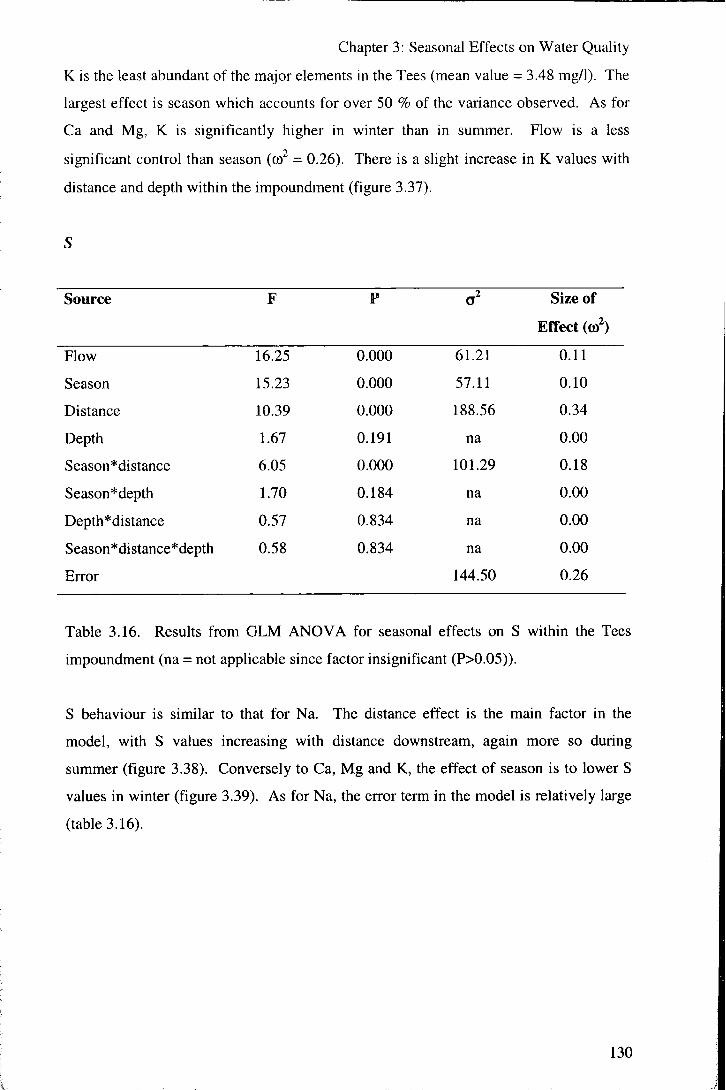
Chapter 3: Seasonal Effects on Water Quality
K is the least abundant of the major elements in the Tees (mean value = 3.48 mg/1). The
largest effect is season which accounts for over 50 % of the variance observed. As for
Ca and Mg, K is significantly higher in winter than in summer. Flow is a less
significant control than season (co = 0.26). There is a slight increase in K values with
distance and depth within the impoundment (figure 3.37).
Source F P a" Size of
Effect (0)^)
Row 16.25 0.000 61.21 0.11
Season 15.23 0.000 57.11 0.10
Distance 10.39 0.000 188.56 0.34
Depth 1.67 0.191 na 0.00
Season*distance 6.05 0.000 101.29 0.18
Season*depth 1.70 0.184 na 0.00
Depth* distance 0.57 0.834 na 0.00
Season*distance*depth 0.58 0.834 na 0.00
Error 144.50 0.26
Table 3.16. Resuhs from GLM ANOVA for seasonal effects on S within the Tees
impoundment (na = not applicable since factor insignificant (P>0.05)).
S behaviour is similar to that for Na. The distance effect is the main factor in the
model, with S values increasing with distance downstream, again more so during
summer (figure 3.38). Conversely to Ca, Mg and K, the effect of season is to lower S
values in winter (figure 3.39). As for Na, the error term in the model is relatively large
(table 3.16).
130

Chapter 3: Seasonal Effects on Water Quality
CO
22 -r
19 H
16 -4
distance depth
13
10
Figure 3.38. Main effects plot for S in the Tees impoundment (least square means for
factor levels).
season
distance
summer winter
Figure 3.39. Interaction between distance and season effects on S (LS mean) in the
Tees impoundment. Summer results as solid line and winter as dashed line.
131

Chapter 3: Seasonal Effects on Water Quality
Discussion
The behaviour of the major elements in the Tees shows a variety of controls including
river flow (discharge), season, distance and depth. The behaviour of the individual
elements differs, as might be expected given that their relationships between one
another are not perfectly linear (figure 3.40).
Ca
7.89751 -
3.49592 -
0 0 O n
0 0 K
22.5764 -
8.9272 -
e B O 0
d
Mg
150.523 -
53.439 -
• K e
0
°°
B
° 8 • Ma
108.856 -
38.608 -
a e O
Figure 3.40. The relationships between the major elements in the Tees during the
sampling periods. Values in mg/1.
The effect of flow, which is significant for all the major elements, is to give decreased
concentrations with increasing river disci. Mges (figure 3.41). For example for Ca,
which shows *he strongest flow effect, the relationship is:
Ca = 40 - 0.488 Mean24 (P = 0.000, 3 -• O.30424, R-Sq = 59.8 %)
132^

Chapter 3: Seasonal Effects on Water Quality
where,
Ca = concentration of Ca in the river (mg/1), and
Mean24 = the mean flow in the 24 hour period preceding sampling.
This implies that groundwater supphes a large proportion of the major elements, via
dissolution from the geologies, to the Tees. As discharge increases following rainfall,
the contribution of groundwater or base flow to the river relative to surface runoff or
stormflow decreases. When groundwater levels are higher, baseflows in the river are
higher, and so for the same level of (summer) discharge the values for the major
elements encountered in winter are likely to be higher. Neal et al. (2000) suggest that
agricultural disturbance of land increases the amount of weathering at the surface, and
the increase in ploughed area in winter may also impact to give reduced dilution effects.
60
50
o) to E CO
O 30 H
20 H
10 H 0 10 20 30 40 50
mean flow preceding sampling (cumecs)
Figure 3.41. The relationship between Ca and flow on the Tees, showing dilution as the
relative amount of baseflow decreases. P = 0.000, R-Sq = 59.8 %.
133

Chapter 3: Seasonal Effects on Water Quality
There is also a general increase in concentrations with distance downstream in Tees,
which is also likely to relate to the relative amounts of baseflow and stormflow in the
water body. Water is likely to enter the river from groundwater throughout its course,
but the majority of overland flow for the Tees enters the river in the upland catchment
above the section surveyed, thus there is an increase in baseflow to stormflow
component with distance.
The impact of the River Leven entering the Tees between distances 3 and 4 (sites A L
and PH) is seen normally to be minimal. The concentration of major elements is
approximately twice as high in the Leven (a lowland river) than the Tees (table 3.17),
although the discharge is generally much smaller than that in the Tees. However on the
8* September 1999 the relative and absolute levels of Na and S in the Leven are much
greater (151 and 129 mg/1 respectively) for unknown reasons, and the values in the Tees
inmiediately upstream and downstream of the confluence are affected.
Major element Leven Tees
Ca 55 28
K 4.6 3.5
Mg 13 6.2
Na 36 23
S 30 15
Table 3.17. Mean concentration of the major elements (in mg/1) for the water quality
surveys for the River Tees and its tributary the River Leven.
The third impact on levels of major element concentrations in the Tees impoundment
appears to be the incursion of small amounts of seawater close to the barrage (at the
downstream limit of the section surveyed) during the summer period (or specifically on
the dates of 25"" August and 8"" September 1999). The Tees barrage height is above the
level of the highest tide encountered and thus no tides overtop the barrage, and although
the upstream (freshwater) section is linked to the downstream (tidal) section by a
navigation lock the design does not allow seawater incursion. It is therefore assumed
that small amounts of seawater were able to enter the impoundment via groundwater
during this period. The large difference in ionic composition and strength seawater
means that small amounts can totally dominate the composition of the mixed v/ater.
134

Chapter 3: Seasonal Effects on Water Quality
The effects of this are seen in the depth effects for Na, K and S described above, and in
the relatively high error terms within the model.
The major element concentrations in the Tees impoundment are in summary controlled
by (figure 3.42):
• the relative proportions of baseflow to stormflow making up the discharge,
• the relative discharge and composition of the Leven tributary, or
• the amount of incursion of brackish or saline water from downstream of the
barrage.
CO
150
100
50
0 -A 100
Na (mg/l) 200
Figure 3.42. The relationship between S and Na in the Tees impoundment showing the
mixing of water sources in the system. Line 1 represents the effects of flow on
concentration (flow decreasing in direction of arrow) in the Tees, line 2 represents the
mixing of Leven water of higher ionic strength but similar S/Na ratio with the water
from 1, and line 3 represents the mixing of seawater (of higher ionic strength and
different ionic composition) with the water from 1.
135

Chapter 3: Seasonal Effects on Water Quality
3.2.10 Fe and Mn
Results
Fe
Source F P a" Size of
Effect (0)^)
Flow 212.19 0.000 0.027 0.49
Season 187.25 0.000 0.024 0.43
Distance 0.96 0.441 na 0.00
Depth 0.18 0.834 na 0.00
Season*distance 0.89 0.487 na 0.00
Season*depth 0.13 0.874 na 0.00
Depth*distance 0.30 0.982 na 0.00
Season*distance*depth 0.27 0.987 na 0.00
Error 0.005 0.08
Table 3.18. Results from GLM ANOVA for seasonal effects on Fe within the Tees
impoundment (na = not applicable since factor insignificant (P>0.05)).
season distance depth
0.26 H
0.22 H
0.18 H
0.14
0.10
Figure 3.43. Main effects plot for Fe in the Tees impoundment (least square means for
factor levels).
136

Chapter 3: Seasonal Effects on Water Quality
Approximately 92 % of the variance observed in Fe levels in the Tees during the water quality surveys is explained by flow (w^ = 0.49) and seasonal (o) = 0.43) effects (table 3.18). The effect of season is to give increased Fe concentrations during summer compared to winter (at the same levels of flow). No other factors are significant, and the error term is relatively small (table 3.18, figure 3.43).
Mn
The behaviour of Mn contrasts with that of Fe. Flow as a covariate is insignificant, and
seasonal effects on their own are small (table 3.19). As opposed to Fe there are
significant differences in Mn levels with distance (w^ = 0.19) and depth (w^ = 0.07)
within the impoundment, and several higher order interactions between the factors in
the model (table 3.19, figure 3.44). Mn tends to increase with distance downstream, but
more significantly during summer and at depth (figures 3.45, 3.46 and 3.47).
Source F P a" Size of
Effect (m )
Season 16.57 0.000 0.0005 0.05
Distance 12.13 0.000 0.0017 0.19
Depth 11.32 0.000 0.0006 0.07
Season*distance 4.64 0.000 0.0005 0.06
Season*depth 10.79 0.000 0.0006 0.07
Depth*distance 7.60 0.000 0.0020 0.23
Season*distance*depth 7.16 0.000 0.0019 0.21
Error 0.0011 0.12
Table 3.19. Results from GLM ANOVA for seasonal effects on Mn within the Tees
impoundment (na = not applicable since factor insignificant (P>0.05)).
137

Chapter 3; Seasonal Effects on Water Quality
distance depth
0.045 H
0.035 H
0.025
0.015
0.005 H
Figure 3.44. Main effects plot for Mn in the Tees impoundment (least square means for
factor levels).
season
D) E , c
0.07 H
0.06
0.05
0.04 H
0.03
0.02
0.01
0.00 n r 3 4
distance
sunrmer winter
Figure 3.45. Interaction between distance and s&ason effects on Mn (LS mean) in the
Tees impoundment. Summer results as solid line and winter as damned line.
138

Chapter 3: Seasonal Effects on Water Quality
0.05 H
E £ 0.03
0.01
season
• summer • winter
Figure 3.46. Interaction between depth and season effects on Mn (LS mean) in the Tees
impoundment. Summer results as solid line and winter as dashed line.
depth
0.10
^ E c ' 0.05
0.00
distance
d m s
Figure 3.47. Interaction between depth and distance effects on Mn (LS mean) in the
Tees impoundment.
139

Chapter 3: Seasonal Effects on Water Quality
Discussion
There is a distinct contrast between the controls on Fe and Mn in the Tees
impoundment. It is likely that Fe is mainly sourced from the upland part of the Tees
catchment within dissolved humic substances removed from the extensive areas of peat.
As mentioned above (for BOD and colour), the removal of dissolved organic material
increases with flow, but is greatest under storm events following warm and dry periods
due to increased humification in the upper layers of peat (Evans et al. 1999). Therefore
Fe concentrations are strongly related to both season and to discharge in the Tees (figure
3.48). During the periods sampled there appeared to be very little internal cycling of Fe
relative to the external inputs.
o sumnner o winter
flow at time of sampling (cumecs)
Figure 3.48. The relationship between Fe and discharge in the Tees impoundment,
showing an increase in Fe concentration with increasing flow in addition to a marked
seasonal difference.
In contrast the behaviour of Mn appears to be controlled totally internally within the
impoundment. The concentration of Mn increases with distance downstream,
particularly during summer and at aepth within the impoundment. This is interpreted as
an effect of diffusion of Mn from sediment, and is ^een to be strongly redox controlled.
Significant increases in dissolved Mn concentrations are strongly related to l o w ( <
approximately 40 %) DO conditions encountered in the impoundment (figure j ^v9). lio
140

Chapter 3: Seasonal Effects on Water Quality
similar pattern is seen for Fe implying that either the reducing conditions which develop
are insufficient to allow mobilisation of Fe from the sediment, or that the effects of
mobilisation are insignificant compared to the flow and seasonal controls on
concentrations.
0.4 H
0.3
E , 0.2
0.1
0.0 H
• summer o winter
140
Figure 3.49. The relationship between Mn and DO in the Tees impoundment, showing
release of Mn from sediment under reducing conditions. Increased Mn values at low
DO % are from depth at sites 5 (RB) and 6 (TB) from 4* August, 25* August and 8""
September 1999.
141

Chapter 3: Seasonal Effects on Water Quality
3.2.11 Summary and conclusions
Parameter to for season Covariates Controlling processes
Temperature
DO
1.00
0.41
BOD 0.36
PH 0.54
Alkalinity 0.88
Conductivity Not significant
with flow as a
covariate
Transparency 0.18
Climate.
Temperature controlled microbial
respiration.
Flow controlled stratification vs.
mixing and aeration.
Seasonal primary production.
Flow Flow controlled removal of humic
substances from peat.
Temperature and saturation levels in
peat of catchment.
Temperature controlled microbial
respiration.
Primary production.
Seasonally controlled geological
sources.
Row controlled dilution (stormflow
vs. baseflow).
Flow Flow controlled dilution (stormflow
vs. baseflow).
Relative contribution of Leven
tributary.
Small amounts of seawater intrusion
close to barrage.
Flow Flow controlled colour and
turbidity.
Increased overland flow and less
vegetation cover in winter giving
greater particulate removal.
Resuspension c t bed and bank
material with distance downstrean .
142

Chapter 3: Seasonal Effects on Water Quality
Parameter (0 for season Covariates Controlling processes
Nitrate
Ammonia
Phosphate
Si
Ca
Na
Mg
K
S
Fe
Mn
0.44
0.08
0.65
0.78
0.13
Not significant
with flow as a
covariate
0.06
0.51
0.10
0.43
0.05
Flow
DO
Flow
Flow
Flow
How
Flow
Flow
Increased soil nitrate export in
winter.
Flow controlled dilution of point
sources of nitrate.
Seasonal primary production.
Increased soil ammonia export in
winter.
Seasonal lack of nitrification under
low DO conditions.
Flow controlled dilution of point
sources of phosphate.
Seasonal primary production.
Increased soil Si export in winter
and with increased flow.
Flow controlled dilution (stormflow
vs. baseflow).
Relative contribution of Leven
tributary.
Small amounts of seawater intrusion
close to barrage.
As Ca.
As Ca.
As Ca.
As Ca.
Flow and seasonally controlled
removal with humic substances
from peat (cf. BOD).
Redox controlled diffusion from
sediments.
Tables 3.20 and 3.21. Summaries of seasonal effects and proposed controlling
processes on water quality parameters in the Tees impoundment.
143

Chapter 3: Seasonal Effects on Water Quality
Seasonal variation in water quality behaviour is important in the Tees impoundment, and through determination of the controlling processes it can be generalised that this is likely to apply to all estuarine impoundments. Season has a significant impact on the behaviour of all of the water quality parameters measured (at above LODs) except for Na (for which any effect is overshadowed by the impact of small amounts of seawater intrusion to the impoundment), although the size of the seasonal effect varies widely between parameters (co for significant seasonal effect varies from 0.05 (for Mn) to 1.00 (for temperature)). Summaries of the results from ANOVA testing of the significance of seasonal effects, and proposed controlling processes for each of the water quality parameters are shown in tables 3.20 and 3.21.
A large amount of the seasonal variation is related to flow (river discharge), either as a
dilution effect of constant point source or baseflow inputs (e.g. major metals, alkalinity
and phosphate), or increased flow leading to greater export from diffuse sources (e.g.
BOD, Si and Fe). Levels of saturation of the soil and peat of the catchment also vary
with season, and control the amount of surface and near-surface runoff (transparency, N
and Si) and the amount of humification in peat (BOD, transparency and Fe). The
seasonal differences in flow have a third effect on the homogeneity of the water body,
with a generally more homogenous water body being observed during the higher flows
of winter, and greater variation with distance and depth during the lower flows of
summer (particularly noticeable for DO). The relative impact of the River Leven
tributary cannot easily be constrained, but is generally considered to be minor.
Seasonal variation is also related to temperature differences, and in particular their
effects on the rates of biological processes within the catchment and water body. Rates
of microbial respiration (oxidation of organic material) are higher during the summer
reducing DO and pH (and in turn increasing ammonia and Mn), and increasing
humification of peat in the catchment. Biological primary production relates to both
temperature and light and nutrient availability, all of which show seasonal variation.
Photosynthetic production affects pH, DO and the amounts of nitrate and phosphate in
the w i^^r body.
In conclusion, the close links between the processci controlling water quality in the
Tees to river flow and temperature mean that there are significant seasonal differences
144

Chapter 3: Seasonal Effects on Water Quality
in the values of parameters. In general low water quality conditions are more likely to
be encountered during the summer, and DO conditions below the SWQO for both
salmonids and cyprinids (NRA 1991) and increased levels of ammonia (although below
the 0.78 mg/1 SWQO for salmonids) are observed in the Tees impoundment during the
sampling periods. The majority of the processes discussed are involved in all of the
impoundments investigated, and significant differences in water quality between
seasons are likely to be universal. The strong influence that the extensive areas of
blanket peat in the upper catchment have on the Tees is probably not applicable to the
other (more lowland) systems studied however.
In terms of subsequent modelling and comparison between the systems, it is important
that the effects of seasonality (particularly temperature and river flow) are considered.
At the simplest level this involves comparing datasets collected during the same season.
To enable comparison of processes occurring within the areas of study, catchment
differences may be factored out by normalising to input values for the parameters of
interest.
145

Chapter 3: Seasonal Effects on Water Quality
3.3 Wansbeck
Examination of seasonal differences in the behaviour of selected water quality variables
was carried out for total tidal exclusion (freshwater) impoundments in section 3.2, and
is discussed here for partial tidal exclusion systems using the Wansbeck as an example.
Analysis concentrated on those variables which were seen to show significant internal
(within impounded area) variance in the Tees impoundment. Those parameters are DO,
pH, nitrate, ammonia, Fe and Mn.
A general linear model (ANOVA) including the terms of season, distance within the
impounded area and depth within the impounded area plus the interactions between
season and distance and season and depth was used. Interactions between distance and
depth could not be assessed since at two sites (SW and CI (distances I and 4)) only
surface samples were taken since the water depths were low (normally < 0.5 m). The
Wansbeck was sampled during four periods designated as spring, summer, autumn and
winter in the model. The spring sampling period includes the dates of 4" , 5*, 7*, 9*
and l l " " to 14* March 2000, the summer period was from the 4* to IS* June 2001,
autumn sampling was from 25*** September to 10* October 2000, and winter sampling
was 3^'^ and 5* to 9* February 2001. Periods were chosen within spring tidal cycles
giving a similar number of days without seawater influx for all seasons in order to factor
out tidal effects and sample during the periods of lowest likely water quality. Distance
downstream/sampling site were represented by numbers 1 to 5 from the former tidal
limit (SW) to the barrage (WB). Depth is represented by sampling at shallow (S), mid-
depth (m) and deep (d) at each sampling site. The significances of differences in water
quality between seasons were tested using Tukey simultaneous tests. Analyses were
carried out using both raw data and data normalised to the freshwater inputs to the
impoundment to allow assessment of the differences between seasons based on
catchment effects and those due to differences in behaviour within the impounded area.
3.3.1 Dissolved oxygen
Results
Due to connection problems with the DO meter during the winter sampling period the
data used in the analysis are limited to the 3 '', 6* and 7* February 2001. Mean DO
levels are significantly lower in summer and higher in winter than in spring and autumn
(figure 3.50, table 3.22). However the most significant effect on DO % levels in the
Wansbeck is depth. The decreases in DO with depth explain approximately 50 % of the
146

Chapter 3: Seasonal Effects on Water Quality
variance in the dataset. The distance effect is strongly related to the depths of the
sampling sites, with lowest mean values for DO at the deepest site (distance 2/site CP)
(figure 3.51). The depth effects were the same for summer, spring and autumn but
much smaller (and probably related solely to salinity) during the winter sampling period
(figure 3.52). Approximately 16 % of the variance in DO % in the dataset cannot be
explained by the terms in the model.
Source F P a2 Size of Effect
(0)2)
Season 15.06 0.000 335 0.12
Distance 6.67 0.000 180 0.06
Depth 92.67 0.000 1455 0.50
Season*distance 5.27 0.000 271 0.09
Season*depth 6.43 0.000 173 0.06
Error 476 0.16
Table 3.22. Results from GLM ANOVA for DO % (raw data) between seasons in the
Wansbeck impoundment.
season distance depth
92
84
O Q 76
68 H
60 ^
Figure 3.50. Main effects plot for the factors of season, distance and depth on DO %
(raw data) in the Wansbeck impoundment (LS means for factor levels).
147

Chapter 3: Seasonal Effects on Water Quality
g
season O autumn • spring O summer A winter
distance
Figure 3.51. Interaction between season and distance effects on DO % (raw data)
within the Wansbeck impoundment (LS means).
100
90 _
80 -
o 70 -
60 -
50 -
40 -
season
O autunnn • spring O sunmer A winter
Figure 3.52. Interaction between season and depth effects on DO % (raw data) within
the Wansbeck impoundment (LS means).
148

Chapter 3: Seasonal Effects on Water Quality
Factor Pairwise comparison Adjusted P-value
Season Spring - Autumn 0.999
Summer - Autumn 0.000
Winter - Autumn 0.000
Suncimer - Spring 0.000
Winter -Spring 0.000
Summer - Winter 0.000
Table 3.23. Results from Tukey simultaneous tests on the significance of differences
between the means of factor levels used in the ANOVA for DO % (raw data) within the
Wansbeck impoundment.
Since DO % levels are broadly similar within the freshwater inputs to the systems, the
general pattern of results for data normalised to the freshwater inputs is similar to that
for raw data (figure 3.53). The distance behaviour is very similar for spring, summer
and autumn but contrasting in winter (figure 3.54). Depth remains the most significant
factor and even more clearly shows that the decrease in DO with depth is similar for
spring, summer and autumn but lower in winter (figure 3.55). Relative to input levels
DO is lower by approximately 8 % in winter and by approximately 20 % in the
impounded area in spring, summer and autumn.
Source F P a2 Size of Effect
(co2)
Season 50.58 0.000 0.17 0.33
Distance 6.02 0.000 0.02 0.05
Depth 77.95 0.000 0.17 0.35
Season*distance 5.14 0.000 0.04 0.07
Season*depth 8.32 0.000 0.03 0.07
Error 0.07 0.13
Table 3.24. Results from GLM ANOVA for DO (normalised data) between seasons in
the Wansbeck impoundment.
149

Chapter 3: Seasonal Effects on Water Quality
season distance depth
O 09
Figure 3.53. Main effects plot for the factors of season, distance and depth on DO
(normalised data) in the Wansbeck impoundment (LS means for factor levels).
^ 0.8
season
0 autumn • spring O surmier A winter
distance
Figure 3.54. Interaction between season and distance effects on DO (normalised data)
within the Wansbeck impoundment (LS means).
150

Chapter 3: Seasonal Effects on Water Quality
1.02 -
0.92 O Q 0.82
I 0.72
O 0.62 c
0.52
0.42
A -
-^^^^
/ '
T m
season
9 autumn B spring 4 summer A winter
depth
Figure 3.55. Interaction between season and depth effects on DO (normalised data)
within the Wansbeck impoundment (LS means).
Factor Pairwise comparison Adjusted P-value
Season Spring - Autumn 0.470
Summer - Autumn 0.747
Winter - Autumn 0.001
Summer - Spring 0.101
Winter -Spring 0.044
Summer - Winter 0.000
Table 3.25. Results from Tukey simultaneous tests on the significance of differences
between the means of factor levels used in the ANOVA for DO (normalised data)
within the Wansbeck impoundment.
Discussion
The most significant control on oxygen levels in the impoundments is density
stratification. Stratification isolates portions of water from sources of re-oxygenation
whilst respirative processes act to consume dissolved oxygen. In comparison of barrage
151

Chapter 3: Seasonal Effects on Water Quality
designs (chapter 4) it is seen that this effect is most significant in the Wansbeck
impoundment.
The results above show that for the Wansbeck impoundment the effect of stratification
is significant throughout the year, but to a greater extent during spring, summer and
autumn periods, and only slightly greater during summer when mean temperatures are
highest (mean T during the sampling periods are 11.8, 7.2, 13.1 and 3.0°C for autumn,
spring, summer and winter respectively). That the lowest levels of DO are encountered
during the summer period relates more to the lower DO concentrations in the water
entering the impoundment than to greater impacts of stratification. During all seasons
the freshwater input progresses downstream along the surface of the impoundment and
is unaffected by internal processes in terms of DO concentration.
150
^ 100
g 50
0 autumn o spring e summer
winter
~i 1 i 1 1 I I i i r
0 10 20 30 40 50 60 70 80 90 100
mean flow preceding sampling (cumecs)
Figure 3.56. DO vs. flow for the Wansbeck impoundment showing the lack of low DO
values under high flow conditions due to the removal of saline stratification of the water
body.
The differences in behaviour betwc. n the seasons sampled is likely to be due to ..oth
differences in temperature and differences in freshwuicr discharge. During the winter
period sampled flow was generally high enough to remove the majority of saline water,
and particularly to remove any stratification at the deepest point (distance 2 / site CP) at
152

Chapter 3: Seasonal Effects on Water Quality
which lowest DO conditions were encountered at other periods of the year (figure 3.56).
Comparing the decreases in DO at depth over periods of isolation of deep saline water
at site CP during the other seasons shows that the rate of de-oxygenation is virtually
identical for spring and autumn (figure 3.57), but that DO is consistently at almost 0 %
during summer (implying that low DO may exist over longer periods in the summer).
P 30
° 20
-•—spnng
-•—autumn
-A—summer
d a y
Figure 3.57. The decrease in DO concentration in deep (stratified) water from site CP
on the Wansbeck during 3 sampling periods. Spring data are from 12* to 16* March
2000, autumn data are from l " to 7* October 2000, and summer data are from 8* to 15*
June 2001.
3.3.2 pH
Results
For raw pH data the majority of variance is between seasons (table 3.26). Lowest pH
values occur in summer and the highest in spring and autumn, with significant
differences between all pairs of season except spring and autumn (figure 3.58 and table
3.27). The distance pattern relates to the water depths at each sampling distance, such
that deeper sites (especially site CP at distance 2) show lower mean pHs (figure 3.59).
pH decreases with depth to a similar degree during all seasons. Approximately 14 % of
the variance in the dataset cannot be explained by the terms in the model.
153
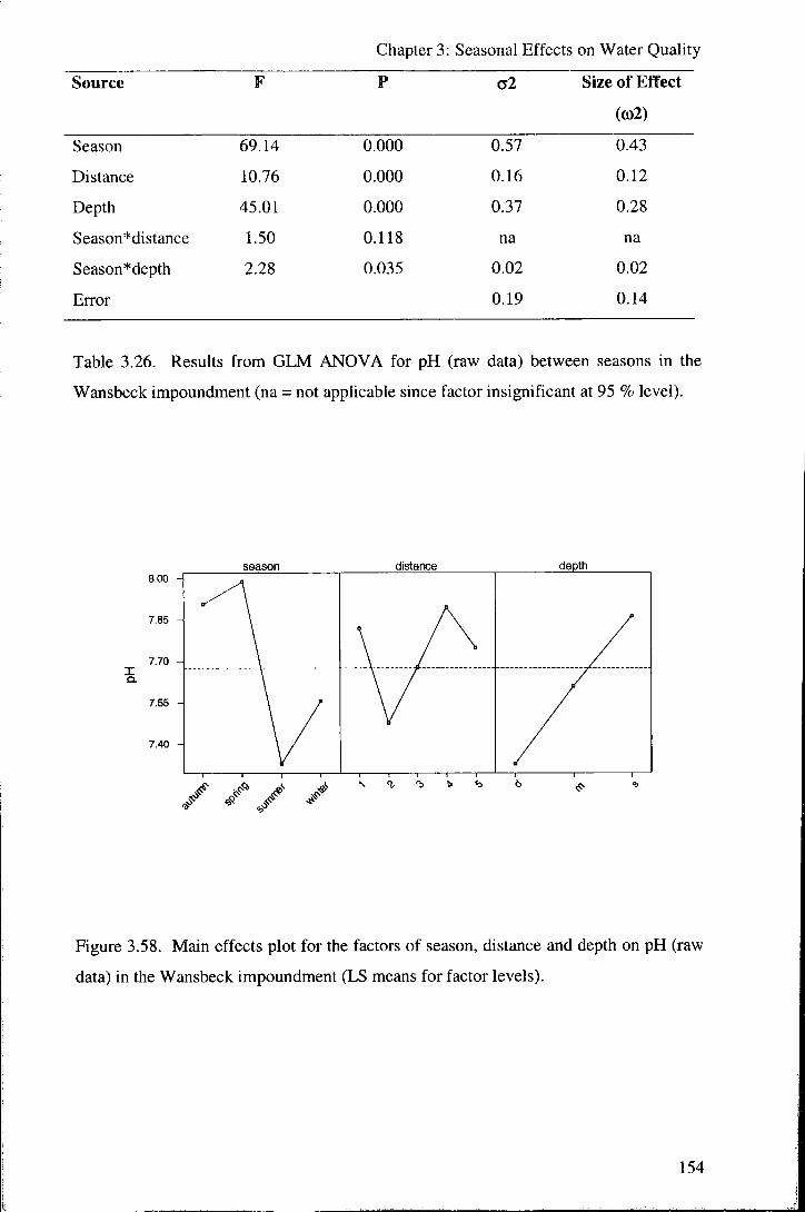
Chapter 3: Seasonal Effects on Water Quality
Source F P a2 Size of Effect
(0)2)
Season 69.14 0.000 0.57 0.43
Distance 10.76 0.000 0.16 0.12
Depth 45.01 0.000 0.37 0.28
Season*distance 1.50 0.118 na na
Season*depth 2.28 0.035 0.02 0.02
Error 0.19 0.14
Table 3.26. Results from GLM ANOVA for pH (raw data) between seasons in the
Wansbeck impoundment (na = not applicable since factor insignificant at 95 % level).
season distance
I Q.
8.00
7.85
7.70 H
7.55 H
7.40 H
depth
Figure 3.58. Main effects plot for the factors of season, distance and depth on pH (raw
data) in the Wansbeck impoundment (LS means for factor levels).
154

Chapter 3: Seasonal Effects on Water Quality
8.0
7.5
7.0
season
9 autunrm B spring 4 summer A winter
depth
Figure 3.59. Interaction between season and depth effects on pH (raw data) within the
Wansbeck impoundment (LS means).
Factor Pairwise comparison Adjusted P-value
Season Spring - Autumn 0.375
Summer - Autumn 0.000
Winter - Autumn 0.000
Summer - Spring 0.000
Winter -Spring 0.000
Summer - Winter 0.001
Table 3.27. Results from Tukey simultaneous tests on the significance of differences
between the means of factor levels used in the ANOVA for pH (raw data) within the
Wansbeck impoundment.
Normalising the data to the freshwater input values for each of the days sampling
almost totally removes the effect of season, implying that within impoundment variation
in values of pH is relatively constant throughout the year (table 3.28, figure 3.60).
Approximately 74 % of the variance within the impounded area is with depth or
distance, pH values being approximately 5 % lower at depth than in surface waters and
the distance pattern relating to the actual water depths at each sampling site (with lowest
155

Chapter 3: Seasonal Effects on Water Quality
pH being found at the deepest site (CP) at distance 2) (figure 3.61). The reduction in
pH with depth is slightly higher in summer than in the other seasons (figure 3.62).
Source F P o2 Size of Effect
(to2)
Season 5.43 0.001 0.00 0.03
Distance 20.88 0.000 0.00 0.24
Depth 83.57 0.000 0.01 0.50
Season *distance 2.88 0.001 0.00 0.05
Season*depth 4.50 0.000 0.00 0.04
Error 0.00 0.14
Table 3.28. Results from GLM ANOVA for pH (normalised data) between seasons in
the Wansbeck impoundment.
season distance depth
1.010
X 0.995 T3 o in
0.980
8 0.965
0.950 H
/ /•* , / /
Figure 3.60. Main effects plot for the factors of season, distance and depth on pH
(normalised data) in the Wansbeck impoundment (LS means for factor levels).
156

Chapter 3: Seasonal Effects on Water Quality
1.025
^ 1.000
•s w E 0.975 O c
0.950
1 3
distance 4
season
9 autumn • spring ^ summer A winter
Figure 3.61. Interaction between season and distance effects on pH (normalised data)
within the Wansbeck impoundment (LS means).
1.015 -I
Q. 0.990 TD <D CO
"cD E 0.965 O c
0.940
season # autumn • spring ^ summer A winter
Figure 3.62. Interaction between season and depth effects on pH (normalised data)
within the Wansbeck impoundment (LS means).
157

Chapter 3: Seasonal Effects on Water Quality
Factor Pairwise comparison Adjusted P-value
Season Spring - Autumn 0.948
Summer - Autumn 0.026
Winter - Autumn 0.894
Summer - Spring 0.007
Winter -Spring 0.996
Summer - Winter 0.012
Table 3.29. Results from Tukey simultaneous tests on the significance of differences
between the means of factor levels used in the ANOVA for pH (normalised data) within
the Wansbeck impoundment.
Discussion
n i 1 1 1 1 1 1 1 1 r
0 10 20 30 40 50 60 70 80 90 100 mean flow preceding sampling (cumecs)
Figure 3.63. pH vs. flow in the Wansbeck impoundment, showing greater variation in
pH under low flow conditions due to stratification and production/respiration effects.
Under high flows stratification of the water body is removed and pH values are more
homogenous.
The majority of the variation in pH between seasons is explained by the differences in
the freshwater entering the impounded areas at their upstream limits. Variation in the
pH of the freshwater inputs is independent of flow (although, as for DO, at nitrher flows
158

Chapter 3: Seasonal Effects on Water Quality
pH shows less variance due to a lack of stratification (figure 3.63)), and therefore is
likely to relate to biological effects. On this basis primary production relative to
respiration in the water column is greatest in the spring and autumn periods of sampling.
Within the impounded areas the variation in pH is with depth in the water column and
relates to both the lower pH in seawater than river water and the greater amount of
respiration in deep water in a stratified water column. The decreases in pH with depth
are similar throughout the year implying that lower pHs in seawater are more important
than biological processing, although the slightly greater decreases in summer (in
addition to a slight increase in alkalinity (figure 3.64) suggest that respiration effects on
pH are more significant in this season.
1.25
16 ^ 1.15 CO
o c
1.05 - 4
0.95 -4 a-
A -
d 1
m depth
1 s
season
• autumn • spring 4 summer A winter
Figure 3.64. Interaction between season and depth effects on alkalinity (normalised
data) within the Wansbeck impoundment (LS means).
3.3.3 Nitrate
Results
The seasonal effects on nitrate are small relative to internal variation within the
Wansbeck impoundment (table 3.30, figure 3.65). Actual nitrate concentrations are
significantly lower in autumn than during the other seasons. Variation with depth
accounts for 61 % of the behaviour of nitrate. Nitrate values decrease significantly with
159
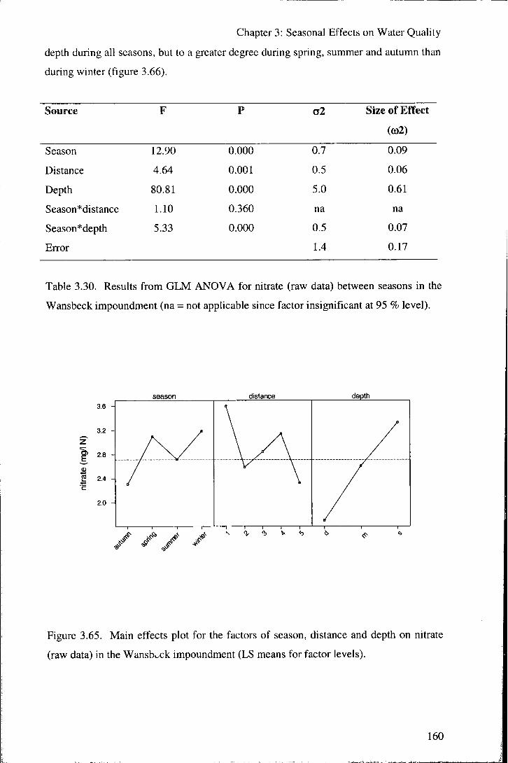
Chapter 3: Seasonal Effects on Water Quality
depth during all seasons, but to a greater degree during spring, summer and autumn than
during winter (figure 3.66).
Source F P o2 Size of Effect
(0)2)
Season 12.90 0.000 0.7 0.09
Distance 4.64 0.001 0.5 0.06
Depth 80.81 0.000 5.0 0.61
Season*distance 1.10 0.360 na na
Season*depth 5.33 0.000 0.5 0.07
Error 1.4 0.17
Table 3.30. Results from GLM ANOVA for nitrate (raw data) between seasons in the
Wansbeck impoundment (na = not applicable since factor insignificant at 95 % level).
distance depth
Figure 3.65. Main effects plot for the factors of season, distance and depth on nitrate
(raw data) in the Wansb^ck impoundment (LS means for factor levels).
160
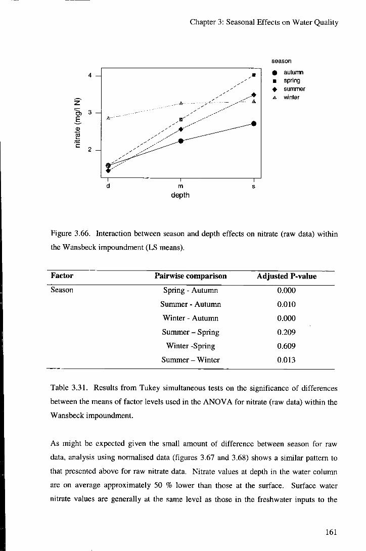
Chapter 3: Seasonal Effects on Water Quality
E. <v 15
A
^ ^
y ..s^—
T m
season
9 autumn • spring ^ summer 4 winter
depth
Figure 3.66. Interaction between season and depth effects on nitrate (raw data) within
the Wansbeck impoundment (LS means).
Factor Pairwise comparison Adjusted P-value
Season Spring - Autumn 0.000
Summer - Autumn 0.010
Winter - Autumn 0.000
Summer-Spring 0.209
Winter -Spring 0.609
Summer - Winter 0.013
Table 3.31. Results from Tukey simultaneous tests on the significance of differences
between the means of factor levels used in the ANOVA for nitrate (raw data) within the
Wansbeck impoundment.
As might be expected given the small amount of difference between season for raw
data, analysis using normalised data (figures 3.67 and 3.68) shows a similar pattern to
that presented above for raw nitrate data. Nitrate values at depth in the water column
are on average approximately 50 % lower than those at the surface. Surface water
nitrate values are generally at the same level as those in the freshwater inputs to the
161
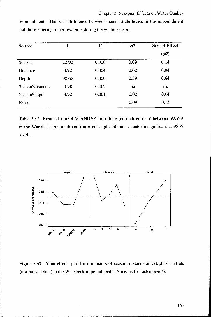
Chapter 3: Seasonal Effects on Water Quality
impoundment. The least difference between mean nitrate levels in the impoundment
and those entering in freshwater is during the winter season.
Source F P CT2 Size of Effect
(0)2)
Season 22.90 0.000 0.09 0.14
Distance 3.92 0.004 0.02 0.04
Depth 98.68 0.000 0.39 0.64
Season*distance 0.98 0.462 na na
Season*depth 3.92 0.001 0.02 0.04
Error 0.09 0.15
Table 3.32. Results from GLM ANOVA for nitrate (normalised data) between seasons
in the Wansbeck impoundment (na = not applicable since factor insignificant at 95 %
level).
0.50 A
season distance depth
2 0.74
Figure 3.67. Main effects plot for the factors of season, distance and depth on nitrate
(normalised data) in the Wansbeck impoundment (LS means for factor levels).
162

Chapter 3: Seasonal Effects on Water Quality
0.95 H
13 0.85
^ 0.75
0.65 to § 0.55 O
^ 0.45
0.35
- A
A-- """'
1 d
1 m
1 S
depth
season
# autumn @ spring ^ summer ,4 winter
Figure 3.68. Interaction between season and depth effects on nitrate (normalised data)
within the Wansbeck impoundment (LS means).
Factor Pairwise comparison Adjusted P-value
Season Spring - Autumn 0.001
Summer - Autumn 0.000
Winter - Autumn 0.000
Summer - Spring 1.000
Winter -Spring 0.000
Summer - Winter 0.000
Table 3.33. Results from Tukey simultaneous tests on the significance of differences
between the means of factor levels used in the ANOVA for nitrate (normalised data)
within the Wansbeck impoundment.
Discussion
It was shown during comparison of barrage designs that the largest control on internal
(within impounded area) variation of nitrate concentrations in partial tidal exclusion
impoundments is the difference in nitrate concentrations between fresh and seawater in
the systems. For the whole of the data from the Wansbeck included in the analyses
presented above the mean nitrate value in freshwater (conductivity < 500 ^.S/cm) was
163

Chapter 3: Seasonal Effects on Water Quality
3.56 mg/1 N and in saline water (conductivity < 500 ^iS/cm) it was 2.20 mg/1 N (a
difference of approximately 40 %) . The mean difference between (generally saline)
water at depth and (generally fresh) water at the surface during the periods studied was
50 % implying that the majority of variation with depth throughout the year is due to
this difference.
1.4 -I
1.2
z 1
0.8 -
0) "S
0.6 -2 c 0.4 -
0.2
0
spring -o— autumn -A— summer
day
Figure 3.69. The decrease in nitrate concentration in deep (stratified) water from site
CP on the Wansbeck during 3 sampling periods. Spring data is from 12" to 16'" March
2000, autumn data is from to 1^ October 2000, and summer data is from 8"' to 15"'
June 2001.
It was also seen that nitrate generally behaved conservatively on mixing of fresh and
seawater. Some loss of nitrate through denitrification and reduction to ammonia was
observed at depth (particularly at site CP) during autumn in the Wansbeck. For the
periods over which decreasing DO concentrations are presented above, the patterns of
nitrate decrease are similar for spring and autumn (as was DO % decrease) but had
already reduced to a minimum level at the start of sampling in summer (figure 3.69),
meaning that no comparison of rates can be carried out. It is likely that rates of all of
the biologically mediated processes are increased at higher temperatures, but since
164

Chapter 3: Seasonal Effects on Water Quality
conditions in terms of flow (and hence amount of time in which the water column is
stratified) vary markedly between periods this is difficult to assess.
3.3.4 Ammonia
Results
Source F P a2 Size of Effect
(0)2)
Season 13.17 0.000 0.015 0.11
Distance 0.97 0.421 na na
Depth 63.17 0.000 0.075 0.58
Season*distance 2.09 0.015 0.005 0.04
Season*depth 3.56 0.002 0.006 0.05
Error 0.027 0.21
Table 3.34. Results from GLM ANOVA for ammonia (raw data) between seasons in
the Wansbeck impoundment (na = not applicable since factor insignificant at 95 %
level).
0.32 season distance depth
Figure 3.70. Main effects plot for the factors of season, distance and depth on ammonia
(raw data) in the Wansbeck impoundment (LS means for factor levels).
165

Chapter 3: Seasonal Effects on Water Quality
0.3 -4
O) E,
.CO 0.2 c o E E CO
0.1
/ /
/ /
/ / / o
/ fjv——_ / ^\
\ \
C) ^ / /
/ A 1 / I
1 / I ' / /
/ / / / / ,'
V '
^\ \ \ \ ,
\ \ /
\ / ' ,'
....-A
season
O autumn a spring O summer A wtnXer
distance
Figure 3.71. Interaction between season and distance effects on ammonia (raw data)
within the Wansbeck impoundment (LS means).
0.4 -I
0.3 -A t3) E,
E 0.2 E CO
0.1 -A
season 0 autumn • spring <> summer A winter
Figure 3.72. Interaction between season and depth effects on ammonia (raw data)
within the Wansbeck impoundment (LS means).
166

Chapter 3: Seasonal Effects on Water Quality
Factor Pairwise comparison Adjusted P-value
Season Spring - Autumn 0.998
Summer - Autumn 0.046
Winter - Autumn 0.000
Summer - Spring 0.164
Winter -Spring 0.000
Summer - Winter 0.001
Table 3.35. Results from Tukey simultaneous tests on the significance of differences
between the means of factor levels used in the ANOVA for ammonia (raw data) within
the Wansbeck impoundment.
The seasonal differences in anmionia levels are minor (table 3.34, figure 3.70) and
relate almost totally to the differences between seasons in the distance and depth
behaviour (figures 3.71 and 3.72). The depth effect explains over half of the variance in
the dataset, with anmionia values increasing with depth in the water column in all
seasons except winter. The distance effect, as for DO, relates to the actual water depth
at each sampling site with maximum ammonia levels at the deepest site (CP). The
relatively large error is likely to be due to random analytical error (and hence error is
magnified when data is normalised).
Source F P a2 Size of Effect
(0)2)
Season 8.67 0.000 5.4 0.16
Distance 0.78 0.535 na na
Depth 15.66 0.000 10.3 0.30
Season*distance 0.97 0.472 na na
Season*depth 2.75 0.012 2.5 0.07
Error 15.8 0.47
Table 3.36. Results from GLM ANOVA for ammonia (normalised data) between
seasons in the Wansbeck impoundment (na = not applicable since factor insignificant at
95 % level).
167

Chapter 3: Seasonal Effects on Water Quality
season distance depth
m 'c
(0
(0
8
3.4
2.8
2.2
1.6
1.0 H
Figure 3.73. Main effects plot for the factors of season, distance and depth on ammonia
(normalised data) in the Wansbeck impoundment (LS means for factor levels).
6 -
.55 5 -o
i 4 -
.52
i C
1 — " A .~ • -T r r J
1 d
1 m
depth
1 8
season
O autumn • spring <> summer A winter
Figure 3.74. Interaction between season and depth effects on ammonia (normalised
data) within the Wansbeck impoundment (LS means).
168
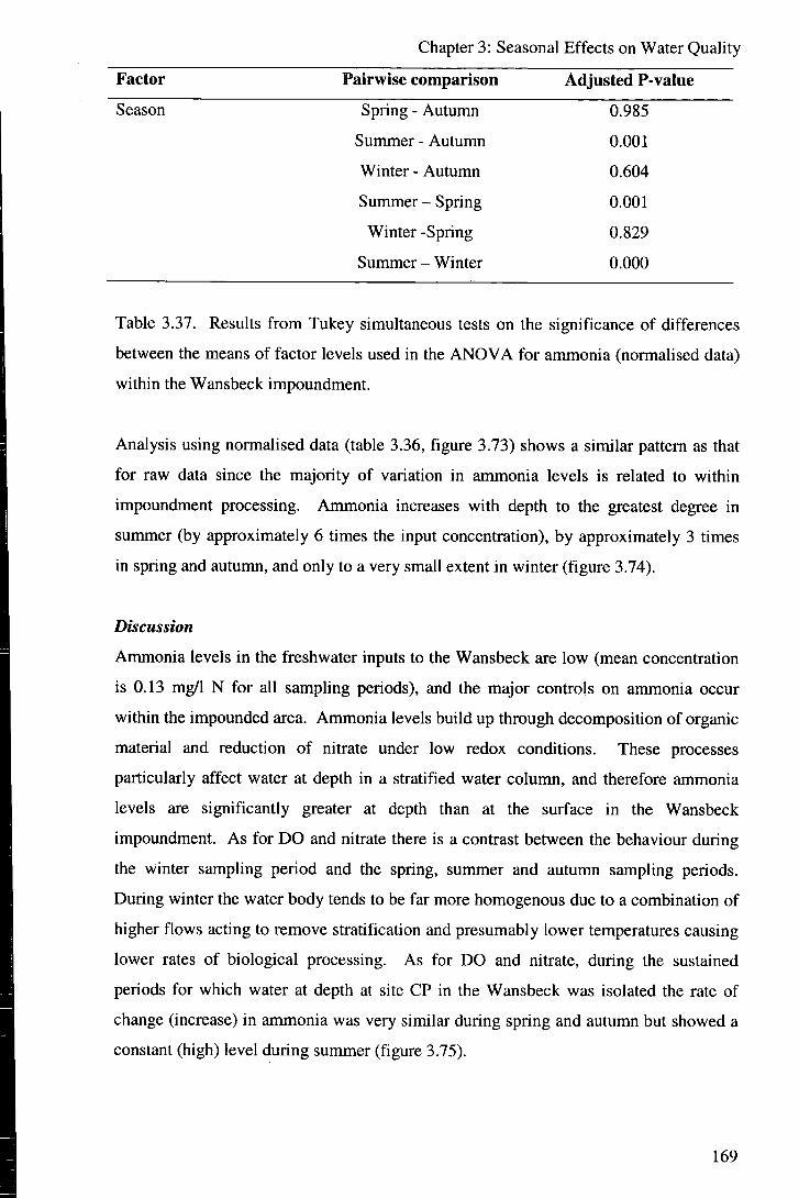
Chapter 3: Seasonal Effects on Water Quality
Factor Pairwise comparison Adjusted P-value
Season Spring - Autumn 0.985
Summer - Autumn 0.001
Winter - Autumn 0.604
Summer - Spring 0.001
Winter -Spring 0.829
Summer - Winter 0.000
Table 3.37. Results from Tukey simultaneous tests on the significance of differences
between the means of factor levels used in the ANOVA for ammonia (normalised data)
within the Wansbeck impoundment.
Analysis using normalised data (table 3.36, figure 3.73) shows a similar pattern as that
for raw data since the majority of variation in ammonia levels is related to within
impoundment processing. Ammonia increases with depth to the greatest degree in
summer (by approximately 6 times the input concentration), by approximately 3 times
in spring and autumn, and only to a very small extent in winter (figure 3.74).
Discussion
Ammonia levels in the freshwater inputs to the Wansbeck are low (mean concentration
is 0.13 mg/1 N for all sampling periods), and the major controls on ammonia occur
within the impounded area. Ammonia levels build up through decomposition of organic
material and reduction of nitrate under low redox conditions. These processes
particularly affect water at depth in a stratified water column, and therefore ammonia
levels are significantly greater at depth than at the surface in the Wansbeck
impoundment. As for DO and nitrate there is a contrast between the behaviour during
the winter sampling period and the spring, summer and autumn sampling periods.
During winter the water body tends to be far more homogenous due to a combination of
higher flows acting to remove stratification and presumably lower temperatures causing
lower rates of biological processing. As for DO and nitrate, during the sustained
periods for which water at depth at site CP in the Wansbeck was isolated the rate of
change (increase) in ammonia was very similar during spring and autumn but showed a
constant (high) level during summer (figure 3.75).
169

Chapter 3: Seasonal Effects on Water Quality
•spnng • autumn -summer
Figure 3.75. The increase in ammonia concentration in deep (stratified) water from site
CP on the Wansbeck during 3 sampling periods. Spring data is from 12"' to 16'" March
2000, autumn data is from l " to 7"" October 2000, and summer data is from 8* to 15""
June 2001.
: t h
3.3.5 Fe
Results
Source F P a2 Size of Effect
(0)2)
Season 103.61 0.000 0.054 0.66
Distance 9.66 0.000 0.009 0.11
Depth 1.97 0.140 na na
Season*distance 1.78 0.047 0.002 0.02
Season*depth 6.01 0.000 0.005 0.06
Error 0.012 0.14
Table 3.38. Results from GLM ANOVA for Fe (raw data) between seasons in the
Wansbeck impoundment (na = not appli able since factor insignificant at 95 % level).
1/0

Chapter 3: Seasonal Effects on Water Quality
season distance depth 0.27 H
0.22 -A
0) 0.17 -4
0.12 H
0.07 A
Figure 3.76. Main effects plot for the factors of season, distance and depth on Fe (raw
data) in the Wansbeck impoundment (LS means for factor levels).
season
# autunm a spring 4 summer A winter
distance
Figure 3.77. Interaction between season and distance effects on Fe (raw data) within the
Wansbeck impoundment (LS means).
171

Chapter 3: Seasonal Effects on Water Quality
E
0.3
0,2 ,A--
0,1 _
1 d
1 m
depth
1 s
season
O autumn • spring O summer A winter
Figure 3.78. Interaction between season and depth effects on Fe (raw data) within the
Wansbeck impoundment (LS means).
Factor Pairwise comparison Adjusted P-value
Season Spring - Autumn 0.000
Summer - Autumn 0.000
Winter - Autumn 0.026
Summer - Spring 0.343
Winter -Spring 0.000
Summer - Winter 0.000
Table 3.39. Results from Tukey simultaneous tests on the significance of differences
between the means of factor levels used in the ANOVA for Fe (raw data) within the
Wansbeck impoundment.
Fe shows a large variation between seasons with significant differences between all
pairs of season except summer and spring (tables 3.38 and 3.39). Mean Fe levels within
the Wansbeck were highest during the autumn sampling period, slightly low-r during
winter, and lowest during spring and summe. (figure 3.76). Distance is also a
significant factor, with Fe decreasing slighdy downstream particularly during autumn
(figure 3.77). Contrasting deoth effects are shown between seasons {u^'ire 3.76).
172

Chapter 3: Seasonal Effects on Water Quality
During summer Fe concentrations at depth are higher than those in surface water, but
during the other seasons Fe shows no variation or a slight decrease with depth.
Source F P CT2 Size of Effect
(0)2)
Season 23.33 0.000 0.73 0.29
Distance 8.56 0.000 0.50 0.20
Depth 2.08 0.126 na na
Season*distance 1.90 0.031 0.12 0.05
Season*depth 7.44 0.000 0.42 0.17
Error 0.739 0.29
Table 3.40. Results from GLM ANOVA for Fe (normalised data) between seasons in
the Wansbeck impoundment (na = not applicable since factor insignificant at 95 %
level).
season distance depth
o c
Figure 3.79. Main effects plot for the factors of season, distance and depth on Fe
(normalised data) in the Wansbeck impoundment (LS means for factor levels).
173
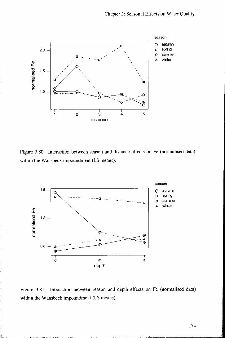
Chapter 3: Seasonal Effects on Water Quality
season
O autumn • spring O summer A winter
distance
Figure 3.80. Interaction between season and distance effects on Fe (normalised data)
within the Wansbeck impoundment (LS means).
1.8
0) U-
w
o c
1.3 -A
0.8 - ]
season
O autumn • spring O summer A winter
depth
Figure 3.81. Interaction between season and depth effects on Fe (normalised data)
within the Wansbeck impoundment (LS means).
174

Chapter 3: Seasonal Effects on Water Quality
Factor Pairwise comparison Adjusted P-value
Season Spring - Autumn 0.000
Summer - Autumn 0.000
Winter - Autumn 0.976
Summer - Spring 0.000
Winter -Spring 0.000
Summer - Winter 0.034
Table 3.41. Results from Tukey simultaneous tests on the significance of differences
between the means of factor levels used in the ANOVA for Fe (normalised data) within
the Wansbeck impoundment.
Season is a less significant factor for analysis using data normalised to the freshwater
inputs compared to analysis with raw data (approximately 29 % as opposed to 66 % of
the variance in the dataset). This implies that much of the variation in Fe concentrations
in the Wansbeck with season are due to effects external to the impounded area. Relative
to input values Fe levels are higher in spring and summer and lower in winter and
autumn in the impounded area (figure 3.79). There is a general decrease in Fe with
distance, although during spring and summer the distance pattern relates to the depth of
the water column (i.e. is elevated at distance 2) (figure 3.80). As for raw data the
pattern for depth effects is contrasting between the seasons (figure 3.81). During winter
and autumn Fe decreases with depth, during summer Fe increases with depth and during
spring it remains constant with depth.
Discussion
A large amount of the variation in concentrations of Fe is related to freshwater flow in
the Wansbeck. There is a positive correlation between Fe concentration and flow, but
the exact nature of this correlation differs between the seasons (figure 3.82). The
greater rate of increase in Fe concentrations with flow during spring, summer and
autumn relative to winter (as was observed for the Tees) suggests that temperature is
important in controlling the near-surface availability of Fe (through humification and
weathering processes). The higher flows experienced during autumn and winter
sampling explain the higher average Fe concentrations in the Wansbeck impoundment
during these periods. The maximum rate of increase of Fe concentration with flow in
175

Chapter 3: Seasonal Effects on Water Quality
autumn probably relates to the flushing of dissolved organic carbon following the
summer period (Evans et al., 1999).
0.7
0.6
0.5
I' 0.4
V 0.3
0.2
0.1
0.0
o o 2/autumn
winter
-1 r 1—I—r I I I I -1 1—I I I I I I
o autumn
* winter
1 10 100 mean flow preceding sampling (cumecs)
Figure 3.82. The differing relationships between Fe and flow in the Wansbeck
impoundment between seasons.
D5
0)
0.7
0.6
0.5
0.4
0.3
0.2
0.1
0.0
conservative nixing
5000
Na (mg/l)
— r 10000
Figure 3.83. Conservative mixing behaviour of Fe in the Wansbeck impoundment
during the autumn sampling period.
176
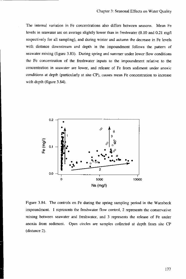
Chapter 3: Seasonal Effects on Water Quality
The internal variation in Fe concentrations also differs between seasons. Mean Fe levels in seawater are on average slightly lower than in freshwater (0.10 and 0.21 mg/1 respectively for all sampling), and during winter and autumn the decrease in Fe levels with distance downstream and depth in the impoundment follows the pattern of seawater mixing (figure 3.83). During spring and summer under lower flow conditions the Fe concentration of the freshwater inputs to the impoundment relative to the concentration in seawater are lower, and release of Fe from sediment under anoxic conditions at depth (particularly at site CP), causes mean Fe concentration to increase with depth (figure 3.84).
0.2 - r
£ 0.1 U.
0.0
• •
i Q 1 1 3
» o 0
• O
• • • . • ••••
• • *
• i • . o * ° S c * f ••^ — 1 • • 2
5000
Na (mg/l) 10000
Figure 3.84. The controls on Fe during the spring sampling period in the Wansbeck
impoundment. 1 represents the freshwater flow control, 2 represents the conservative
mixing between seawater and freshwater, and 3 represents the release of Fe under
anoxia from sediment. Open circles are samples collected at depth from site CP
(distance 2).
177

Chapter 3: Seasonal Effects on Water Quality
3.3.6 Mn
Results
Source F P o2 Size of Effect
(0)2)
Season 23.20 0.000 0.06 0.12
Distance 11.88 0.000 0.06 0.11
Depth 77.28 0.000 0.22 0.40
Season*distance 6.83 0.000 0.07 0.12
Season*depth 14.39 0.000 0.08 0.14
Error 0.06 0.12
Table 3.42. Results from GLM ANOVA for Mn (raw data) between seasons in the
Wansbeck impoundment.
season distance depth
0.4
0.3
2 02
0.1
0.0
Figure 3.84. Main effects plot for the factors of season, distance and depth on Mn (raw
data) in the Wansbeck impoundment (LS means for factor levels).
17b

Chapter 3: Seasonal Effects on Water Quality
E
season 9 autumn B spring ^ summer A winter
distance
Figure 3.85. Interaction between season and distance effects on Mn (raw data) within
the Wansbeck impoundment (LS means).
season e autumn • spring 4 summer A winter
E
0.7
0,6 _
0.5 -
0.4
0.3 \
0.2
0.1 ^ "^-^ ^ ^ ^ ^ ^ ^ ^
0.0 _ A .. „ ^ "~ia— — _ ^
A - ~ ~ ~ ~ ~ ~ ^--^^
m depth
Figure 3.86. Interaction between season and depth effects on Mn (raw data) within the
Wansbeck impoundment (LS means).
179
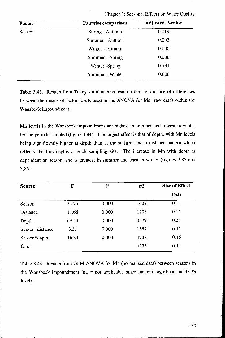
Chapter 3: Seasonal Effects on Water Quality
Factor Pairwise comparison Adjusted P-value
Season Spring - Autumn 0.019
Summer - Autumn 0.003
Winter - Autumn 0.000
Summer - Spring 0.000
Winter -Spring 0.131
Summer - Winter 0.000
Table 3.43. Results from Tukey simultaneous tests on the significance of differences
between the means of factor levels used in the ANOVA for Mn (raw data) within the
Wansbeck impoundment.
Mn levels in the Wansbeck impoundment are highest in summer and lowest in winter
for the periods sampled (figure 3.84). The largest effect is that of depth, with Mn levels
being significantly higher at depth than at the surface, and a distance pattern which
reflects the true depths at each sampling site. The increase in Mn with depth is
dependent on season, and is greatest in summer and least in winter (figures 3.85 and
3.86).
Source F P o2 Size of Effect
(0)2)
Season 25.75 0.000 1402 0.13
Distance 11.66 0.000 1208 0.11
Depth 69.44 0.000 3879 0.35
Season*distance 8.31 0.000 1657 0.15
Season*depth 16.33 0.000 1738 0.16
Error 1275 0.11
Table 3.44. Results from GLM ANOVA for Mn (normalised data) between seasons in
the Wansbeck impoundment (na = not applicable since factor insignificant at 95 %
level).
180
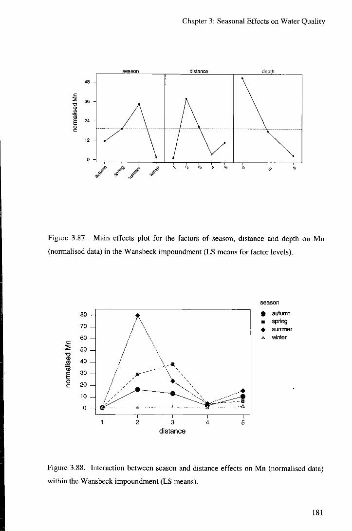
Chapter 3: Seasonal Effects on Water Quality
season distance depth
(U to
8
48
36
24 H
12 H
0 H
Figure 3.87. Main effects plot for the factors of season, distance and depth on Mn
(normalised data) in the Wansbeck impoundment (LS means for factor levels).
.52 15
o c
80 70 60 50 40 30 20 10 0
/
/
/ /
i !
\ \
/ M / / / ^ ^ ^
X ^ " © \ ^ / ^
A " - •
1 1 1 2
1 1 3 4
distance
1 5
season • autumn • spring ^ summer A winter
Figure 3.88. Interaction between season and distance effects on Mn (normalised data)
within the Wansbeck impoundment (LS means).
181

Chapter 3: Seasonal Effects on Water Quality
CO "cO
o c
season O autumn • spring O summer A winter
Figure 3.89. Interaction between season and depth effects on Mn (normalised data)
within the Wansbeck impoundment (LS means).
Factor Pairwise comparison Adjusted P-value
Season Spring - Autumn 0.051
Summer - Autumn 0.000
Winter - Autumn 0.096
Summer - Spring 0.003
Winter -Spring 0.000
Summer - Winter 0.000
Table 3.45. Results from Tukey simultaneous tests on the significance of differences
between the means of factor levels used in the ANOVA for Mn (normalised data)
within the Wansbeck impoundment.
Since the freshwater input Mn values are consistently low the relative increases within
the impounded area are large. The pattern of results using normalised data is similar to
that using raw data (figures 3.87 and 3.88). Dc^ih is the most significant factor and
shows interaction with season (figure 3.89). Mn shows the maximum increase with
depth in the summer sampling period, less in the spring, even less in the autumn, and
virtually no increase with depth during the winter campling oeriod.
182

Discussion
Chapter 3: Seasonal Effects on Water Quality
1.0
E 0.5
0.0 H n 1 1 1 1 1 1 1 1 r
10 20 30 40 50 60 70 80 90 100 • 0 %
Figure 3.90. Mn vs. DO % from the spring sampling period on the Wansbeck.
E
• 1.0 -
• > k
release from sediment
0.5 - • « • e
0.0 -
• • . ^! ^ ^ " ^ ^ conservative mixing
• •
5000
Na (mg/l) 10000
Figure 3.91. Mn vs. Na from the spring sampling period on the Wansbeck, showing the
far greater impact of release of Mn from sediment on Mn concentrations than seawater
183

Chapter 3: Seasonal Effects on Water Quality
mixing. The points above the conservative mixing line are from depth at sites CP, RB
and WB (distances 2, 3 and 5 in general linear model).
It is seen during comparison of barrage designs (chapter 4) that Mn release from
sediment takes place during summer under redox conditions corresponding to
approximately 50 % DO concentration in the water body (figure 3.90). Mn is also
related to DO concentration during the other seasons, although Mn release is seen to
take place at higher (< 90 %) DO % saturations. The Mn concentration in seawater is
higher than in freshwater, but it can be seen that the difference is small relative to that of
sediment releases (figure 3.91). Corresponding to the degree of oxygen depletion
observed during the sampling periods, Mn releases are greatest during summer, lower in
spring and autumn, and almost zero during winter (figure 3.92) when high flows act to
remove the density stratification which allows low oxygen conditions to develop.
0.2 H
E 0.1 H
0.0
conservative mixing
1 I I 1 I I I r 0 1000 2000 3000 4000 5000 6000 7000 8000
Na (nng/l)
Figure 3.92. Mn vs. Na from the winter sampling period on the Wansbeck, showing
that the majority of water sampled was fresh (and of very low Mn concentration) and
that mixing between freshwater and seawater is generally conservative. A small amount
of release of Mn from sediment occ"\s at sites RB and WB (points above th,'
conservativ.. mixing line).
184

Chapter 3: Seasonal Effects on Water Quality
3.3.7 Summary and conclusions
For all of the parameters assessed there are significant differences between seasons in
the Wansbeck impoundment (table 3.46). Through comparison of the significance of
seasonal differences for analysis carried out with raw data and data normalised to the
freshwater inputs these differences were determined to be either mainly due to
processing taking place internal or external to the impounded area (i.e. seasonal
differences which may be affected by the construction of an estuarine barrage and those
which are independent of the presence of a barrage). As discussed previously
parameters which show variation internal to the impounded area are strongly related to
density stratification of the water body. The impact of impoundment on saline
stratification and the subsequent processing of water quality are explored in the
following section of this chapter.
Parameter Varies Major seasonal
with control
season (internal/external)
Major internal process
DO
PH
Nitrate
Ammonia
Fe
Mn
V
V
V
V
V
Internal
External
Internal
Internal
External
Internal
Respiration relative to re-
oxygenation
Seawater/freshwater mixing
Decomposition of organic material
and nitrate reduction
Redox controlled release from
sediment
Table 3.46. Summary of seasonal variation and controlling processes in the Wansbeck
impoundment.
For the Wansbeck impoundment it is found that lowest water quality conditions (lowest
DO, highest ammonia, maximum redox controlled release of Fe and Mn (and associated
metals) from sediment, etc.) occur in summer, during which temperatures (and hence
rates of reactions) tend to be highest and freshwater discharges (which may act to
185

Chapter 3: Seasonal Effects on Water Quality
remove stratification of the water column) lowest. However, sampling shows that low
water quality conditions may be encountered during the majority of the year in the
Wansbeck impoundment (observed during both the March (spring) and
September/October (autumn) sampling periods in addition to summer). This has
important implications for management and remediation of partial tidal exclusion
systems. Significantly any use of aerators (such as are installed in the Tawe
impoundment) would need to function over most of the year. Only during winter are
good water quaUty conditions generally maintained throughout the impounded area of
the Wansbeck (in main due to high freshwater discharges acting to remove density
stratification, although also temperature related).
In section 3.2 it was shown that for the (freshwater) Tees lower water quality conditions
are also likely to be encountered during summer. Comparison of barrage design
however showed there to be contrast between the behaviour of water quality within the
impounded areas which did not relate to type of impoundment (in terms of partial or
total tidal exclusion). It is likely therefore that the seasonal effects on water quality are
also differ between individual impoundments, and it is recommended that assessments
of the probable periods of low water quality are made on a case by case basis.
186

Chapter 4: Barrage Design and Water Quality
Chapter 4
Barrage Design and Water Quality
4.1 Introduction
An important question in the design and management of impounded estuaries is what
differences in behaviour there are between systems which totally exclude any tidal
intrusion and maintain a freshwater impounded area, and those which allow a
proportion of high tides to overtop the barrage crest and whose impounded areas contain
both fresh and saline water. The crucial question is which design maintains higher
impounded water quality.
4.2 Identification of controlling factors throu2h PCA
Initial determination that differences exist in the behaviour between total and partial
exclusion impoundments, and preliminary identification of major controls on water
quality, was carried out using principal components analysis (PCA).
Results
Initial PCA was carried out using a correlation matrix (as opposed to a covariance
matrix) since parameters were measured on different scales, and included the water
quality parameters of DO % saturation, pH, conductivity, alkalinity, nitrate, anmionia,
phosphate, Ca, Fe, Mn, TSS and temperature. The strong covariance between Na, Ca,
Mg, K and S (related to conservative mixing of fresh and seawater) meant that a single
major ion (Ca) was used to represent the 5 ions. The minor and trace metals which were
measured close to or below their LODs were excluded from the analysis. To ensure that
a lack of data on TSS for some of the samples (due to the problems outlined in the
section Overview of Data Collected) did not significantly affect the results, analysis was
also carried out using transparency instead of TSS and found to give a similar pattern.
The results are summarised in table 4.1 and 4.2 and figure 4.1.
187

Chapter 4: Ban-age Design and Water Quality
Principal Eigenvalue Proportion of Cumulative component variance proportion of
variance 1 3.8125 0.318 0.318 2 1.7115 0.143 0.460 3 1.4186 0.118 0.579 4 1.1471 0.096 0.674 5 0.9136 0.076 0.750 6 0.7531 0.063 0.813 7 0.6268 0.052 0.865 8 0.5217 0.043 0.909 9 0.4109 0.034 0.943 10 0.3496 0.029 0.972 11 0.2649 0.022 0.994 12 0.0696 0.006 1.000
Table 4.1. Eigenvalues and proportions of variance for the principal components
calculated for PCA carried out for all data collected from the impounded estuaries
studied.
Component Number
Figure 4.1. Scree plot of eigenvaluj"^ for principal components calculated for PC.
carried ou. for all data collected from the impounded estuaries studied, showing a large
amount of variance explained by the 1 ' principal component relative to subsequent
components.
188
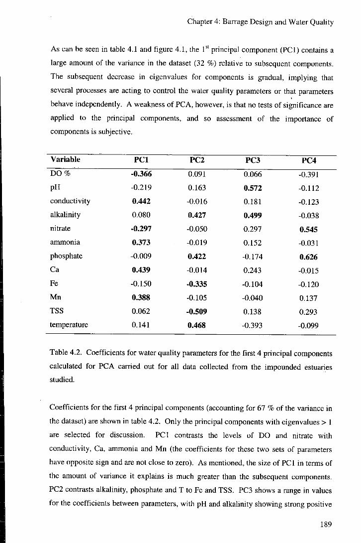
Chapter 4: Barrage Design and Water Quality
As can be seen in table 4.1 and figure 4.1, the I'* ' principal component (PCI) contains a large amount of the variance in the dataset (32 %) relative to subsequent components. The subsequent decrease in eigenvalues for components is gradual, implying that several processes are acting to control the water quality parameters or that parameters behave independently. A weakness of PCA, however, is that no tests of significance are applied to the principal components, and so assessment of the importance of components is subjective.
Variable P C I PC2 PC3 PC4
D O % -0.366 0.091 0.066 -0.391
pH -0.219 0.163 0.572 -0.112
conductivity 0.442 -0.016 0.181 -0.123
alkalinity 0.080 0.427 0.499 -0.038
nitrate -0.297 -0.050 0.297 0.545
ammonia 0.373 -0.019 0.152 -0.031
phosphate -0.009 0.422 -0.174 0.626
Ca 0.439 -0.014 0.243 -0.015
Fe -0.150 -0.335 -0.104 -0.120
Mn 0.388 -0.105 -0.040 0.137
TSS 0.062 -0.509 0.138 0.293
temperature 0. I4I 0.468 -0.393 -0.099
Table 4.2. Coefficients for water quality parameters for the first 4 principal components
calculated for PCA carried out for all data collected from the impounded estuaries
studied.
Coefficients for the first 4 principal components (accounting for 67 % of the variance in
the dataset) are shown in table 4.2. Only the principal components with eigenvalues > 1
are selected for discussion. PCI contrasts the levels of DO and nitrate with
conductivity, Ca, ammonia and Mn (the coefficients for these two sets of parameters
have opposite sign and are not close to zero). As mentioned, the size of PCI in terms of
the amount of variance it explains is much greater than the subsequent components.
PC2 contrasts alkalinity, phosphate and T to Fe and TSS. PC3 shows a range in values
for the coefficients between parameters, with pH and alkalinity showing strong positive
189

Chapter 4: Barrage Design and Water Quality
relation to this component. PC4 also shows a range of coefficients, with nitrate and
phosphate showing the strongest correlation. The smaller amount of variance
(eigenvalues < 1) explained by subsequent components means that consideration of
their relationships and interpretation is not carried out.
Discussion
Salinity
o Q.
-5 H
• TawB
• Tees • Wansbeck
River disciiarge
Figure 4.2. Principal component scores for l " and 2°'' principal components showing
contrasting control of saline stratification and river discharge on the Tees, Tawe and
Wansbeck impoundments.
Plotting scores for PC2 against PCI (figure 4.2) shows that the 3 impoundments studied
show both similar and contrasting behaviours. PCI contrasts the levels of DO and
nitrate with conductivity, Ca, ammonia and Mn, and can be interpreted as representing
both the amount of and the processes associated with saline intrusion to the impounded
area. Conductj^ty and Ca are fairiy well correlated (Ca = 42.5784 + 0.0054213
conductivity; S = 38.3142, R-Sq = 82.7 %) and, due to the large difference in the ionic
strength between fresh and seawater, can be taken aS a measuiie of salinity -of the water
sample. The salinity of the water shows a subsequent control (thrdugb^tfatification) on
190

Chapter 4: Barrage Design and Water Quality
DO and ammonia/nitrate as discussed below. Hence data from the Tawe and Wansbeck
(partial exclusion) impoundments show a spread of values along this axis due to the
saline water entering the system, whilst Tees data generally plots at below zero and does
not trend along PCI. Since PCI relates to the input of seawater to the systems it
understandably explains a much larger amount of the variance in the whole dataset than
the subsequent components. The Tawe and Wansbeck data also group slighdy into
positive and negative scores along this axis, which may be interpreted as distinct saline
and freshwater bodies respectively. Detailed conductivity depth profiles carried out on
several occasions showed there to be strong salinity (density) stratification in the partial
exclusion water bodies.
In addition to showing relative amounts of seawater in the impoundments, PCI includes
variance in parameters due to processes associated with seawater intrusion. For
example DO was observed to be generally at near 100 % saturation in the fresh/surface
waters of the Wansbeck impoundment, but was often depleted at depth in saline water
(down to 0.0 % ) , associated with isolation from the atmosphere (the source of re-
oxygenation) and contact with oxygen demanding sediments of the bed. Low DO
concentrations in turn control the amount of ammonia vs. nitrate in the water, and the
release of Mn from the sediment, as noted for summer in the Tees in the section on
Seasonal Effects. The high coefficients for these parameters on PCI are likely to
represent this series of relationships. Indeed the scatter of points from the Tees
impoundment (which contains virtually no seawater) above 0 on the PCI axis is of
values of low (< 30 %) DO, and increased ammonia (> approximately 0.30 mg/l) and
Mn (> approximately 0.10 mg/l).
PC2 contrasts alkalinity, phosphate and T with Fe and TSS, such that increasing values
of PC2 relate to increased alkalinity, phosphate and T, and decreased Fe and TSS. As
can be seen on figure 4.2, there is a large amount of scatter in the scores for the water
samples on this component, particularly in freshwater samples (low scores on PCI).
The spread of data along PC2 is seen to relate quite closely to freshwater flow
(discharge) for each of the impoundments, such that higher discharges give lower scores
on this component. PC2 is therefore interpreted as relating to the freshwater flow
controlled water quality parameters in the impoundments. For example, alkalinity is
seen to decrease with increasing freshwater flow into the impoundments (figure 4.3),
and Fe is seen to increase (figure 4.4).
191

Chapter 4: Baixage Design and Water Quality
I 150 CT 0)
CO O o CO O 100
E,
I CO =i 50 H
cd
5 10 15 20 mean flow preceding sampling (cumecs)
Figure 4.3. Decreasing alkalinity with increasing freshwater flow for the Tawe
impoundment, related to dilution of baseflow component by increasing stormflow.
0.2 - I
0.1
0.0
0 i e
H ei ^ 1 ID
f> ( £1 as *
i g 0
Vv 5 10 15 20
mean flow preceding sampling (cumecs)
Figure 4.4. The positive relationship between Fe concentrations and freshwater ^lo^/ in
the Tawe impoundment. Fe is assumed to have a diffuse/surface or near-surface source
(perhaps organic ::ssociated)
192

Chapter 4: Barrage Design and Water Quality
The two main controls on the water quality parameters included in the PCA can thus be interpreted as the amount of saline water and/or stratification and internal processing in the systems (by a long way the largest control), and the flow-controlled freshwater (external or catchment controlled) inputs to the systems. The Tees shows lower variation in scores on PCI than the two other impoundments since it is an entirely freshwater impoundment, and the Tawe shows lower variation on PC2 since it was sampled under a lower range of flow conditions (for a 12 day period in summer only).
Scores for the 3 '' and 4* principal components are shown in figure 4.5. The 3 ''
principal component shows high coefficients for pH and alkalinity (0.572 and 0.499
respectively). Water samples from all of the impoundments show a general relationship
between higher scores on this component and higher pH or alkalinity. This is an
interesting pattern to observe, since the pH and alkalinity variation are assumed to be
independently sourced. Regression analysis for the relationship between pH and
alkalinity for the whole dataset included in the PCA reveals that these two parameters
are not strongly related (R-Sq = 7.1 %) , implying independent relationships to PC3 (i.e.
PC3 is related to either pH variations at similar levels of alkalinity, or alkalinity
variations at similar pHs). On specific dates and at specific sites in which significant
amounts of organic decomposition are taking place, alkalinity and pH are seen to be
negatively correlated (figure 4.6). pH is largely controlled by the partial pressure of
carbon dioxide in the water, such that an increase in C O 2 concentration due to
respiration leads to an increase in hydrogen ion concentration and hence decreased pH
(Mortimer, 1971; Maberly, 1996; Neal et al., 2002). As noted previously, the majority
of variance in alkalinity is related to variation in freshwater flow. Additional variance
may be sourced from, in addition to biological effects, difference between the alkalinity
of freshwater and seawater inputs to the impoundments, and variations in freshwater
source based on distribution and pattern of rainfall within the catchment, variations in
contribution from groundwater based on height of the piezometric surface, etc.
193

Chapter 4: Barrage Design and Water Quality
pH and alkalinity
Q.
4
Tawe Tees Wansbeck
nitrate and phosphate
Figure 4.5. Principal component scores for 3"* and 4* principal components, showing
internal (respirative) control on pH and alkalinity within all the impoundments, and a
contrast between nutrient levels and behaviours between the impoundments.
O 110 -A
Figure 4.6. pH and alkalinity at site CP (deepest point) in the Wansbeck impoundment
from ll**" June 2001. The relative amounts of production vs. respiration in the water
column, and sediment-water exchanges, at different depths within the stratified water
column lead to variations in the pH and alkalinity of the water samples, s = shallow, m
194

Chapter 4: Barrage Design and Water Quality
= mid-depth, and d = deep water sampling (coiresponding to depths of 0.00, 2.44 and
4.88 m depth in the water column). Replicates were taken and are plotted at each depth.
(R-Sq = 99.4 %, R-Sq(adj) = 99.3 % ) .
The 4' principal component has strong coefficients for nitrate and phosphate.
Generally an increase in score on this component relates to an increase in levels of these
nutrients in the water sample. This component is interpreted as representing the general
level of nutrient input to the systems. Nutrient values show a large amount of variation
due to a combination of factors which probably include freshwater flow, seawater vs.
freshwater concentrations, seasonal variations in catchment vegetation and fertiliser
application, variation in point source inputs including CSOs, and a range of differences
between the rivers. Whilst PCA can give a general grouping of variables and imply
similar underlying controls, it does not lend itself to the identification of or the
breakdown of the significance of controls. As for PC2 the Tawe, which was sampled
over a lower range of conditions, shows less variation in its scores on this component
than do the Tees and Wansbeck impoundments.
4.3 Behavioural differences between impoundments
The PCA carried out above suggests a number of factors act to control water quality in
the impoundments, including the influence of seawater and stratification in the water
body, flow related freshwater inputs, internal biological controls, etc. In addition PCA
has allowed qualitative comparison of the extent of these factors in each of the
impoundments, and enabled suggestion of the groups of underlying processes acting to
control water quality parameters. More detailed investigation of the differences in
behaviour between the impoundments, and quantitative testing of the significance of
factors is carried out through ANOVA.
The significance of the factors of river (used interchangeably with the term
impoundment), distance (as sampling sites at 5 distances in each of the impounded
areas), and depth in the water column sampled (shallow (s), mid-depth (m) and deep
(d)) were determined for a selection of water quality variables using general linear
modelling (GLM) ANOVA. Note that both distance (1 to 5) and depth (s, m and d)
vary in real (km and m) terms between the impoundments (e.g. the Tees is a bigger river
in terms of length and depth of impounded area than the Tawe and Wansbeck). For the
Tees and the Tawe data from one of the sampling sites from each (site L M and S
195

Chapter 4: Barrage Design and Water Quality
respectively, see chapter 2) was excluded from the analyses to give an equal number of
sample distances (5 distances) for all impoundments. The interactions between river
and depth and river and distance were also examined to determine whether distance and
depth effects varied between impoundments. Season was not included as a factor since
the seasons sampled differed between impoundments (the Wansbeck was sampled in
spring, summer, autumn and winter, the Tees in summer and winter, and the Tawe in
summer alone). Only data from the summer periods of sampling on each river were
included in the analyses. For the Tees the dates included were 21" July, 4* 11* and 25'*"
August and 8* and 22"'' September 1999, for the Wansbeck the dates included were the
4" to 18" June 2001, and for the Tawe the lO"" to 21' ' June 2000. Although a longer
period was sampled in summer in the Wansbeck (up to 24"* June), during the latter part
of this period the impoundment was drained by opening the navigation lock gates in the
barrage in an attempt to remove bed sediment and so this data is not included in the
modelling. The effects of draining and refilling on water quality are discussed
elsewhere (Lamping, PhD Thesis). The seasonal variations in water quality in total and
partial tidal exclusion impoundments are discussed in chapter 3. A crossed model was
specified. Size of effects are calculated and reported, and the significance of differences
between means (hypothesis testing) for the factor level of was carried out using the
Tukey method of multiple comparisons.
To enable comparison of the importance of external (catchment) controls and internal
(within the impounded areas) processing on water quality, several analyses were carried
out using both raw data and data normalised to the values entering the impounded areas
at the upstream limits. For those parameters showing markedly different values for
fresh and seawater (conductivity, Na, Si, etc.) analysis was with raw data only.
4.3.1 Dissolved oxygen
Results
Initial ANOVA was carried out on raw data for levels of DO % saturation in the
impoundments during the periods of water quality survey. % saturations as opposed to
mg/1 values were used to normalise against the effects of temperature changes within
the sampling periods. The results show that all factors included in the model have a
significant effect on DO % levels (tabl° 4.3). The effect of river explains approximal'^ly
31 % of the variation in DO levels, with significant differences between all 3
impoundments. Mean levels are highest in the Tawe and lowest in the Wansbeck
196

Chapter 4: Barrage Design and Water Quality
(figure 4.7). There are significant differences in DO with depth in the impoundments
accounting for 28 % of the variance, with levels generally decreasing with depth.
However the depth effect varies between impoundments (river*depth interaction ((o^ =
0.17)), with greater depth effects in the Wansbeck than in the Tawe or Tees (figure 4.8).
Distance shows a small but significant effect and shows contrasting behaviour between
the impoundments, with a consistent decrease with distance in the Tees (figure 4.9).
Source F P Size of Effect
(0)')
River 89.69 0.000 1250 0.31
Distance 4.66 0.001 103 0.03
Depth 81.61 0.000 1136 0.28
River*distance 11.24 0.000 577 0.14
River* depth 25.59 0.000 693 0.17
Error 317 0.08
Table 4.3. Results from GLM ANOVA for DO % (raw data) in partial and total tidal
exclusion impoundments.
river distance depth
5? O Q
89
83
77
71
65
Figure 4.7. Main effects plot for the factors of impoundment (river), distance and depth
on DO % (raw data) (LS means for factor levels).
197

Chapter 4: Barrage Design and Water Quality
river O Tawe • Tees O Wansbeck
depth
Figure 4.8. Interaction between river and depth effects on DO % (LS means).
river
O
90 - JS> — © 0 • O
Tawe Tees Wansbeck
80 -\
\
\ / x 70 -
\
/
60 - \ /
50 — V'' 1 1
1 2
1 3
1 4
1 5
distance
Figure 4.9. Interaction between river and distance effects on DO % (LS means).
198

Chapter 4: Barrage Design and Water Quality
Factor Pairwise comparison Adjusted P-value
River Tees - Tawe 0.000
Wansbeck - Tawe 0.000
Wansbeck - Tees 0.000
Table 4.4. Results from Tukey simultaneous tests on the significance of differences
between the means of factor levels used in the ANOVA for DO % (raw data) in partial
and total tidal exclusion impoundments.
The results reported above for ANOVA carried out on the raw DO % values show that
the largest effect is that of river. They do not however distinguish between the impact
that is related to, for example, differences in catchment and those which relate to
internal (within the impounded area) processing of DO. In order to aid in this
distinction, ANOVA was repeated for DO % values normalised to the values of DO %
in the freshwater samples entering the impounded areas at the upstream ends for each of
the sampling dates (i.e. results were divided by the upstream input value for that days
sampling). Thus, DO is given as a proportion of these input values (such that a value
greater than 1 represents an increase in DO and a value of less than 1 represents a
decrease).
Source F P a' Size of Effect
(0)')
River 48.55 0.000 0.078 0.16
Distance 5.17 0.000 0.014 0.03
Depth 103.00 0.000 0.168 0.34
River* distance 13.10 0.000 0.080 0.16
River*depth 36.78 0.000 0.118 0.24
Error 0.037 0.07
Table 4.5. Results from GLM ANOVA for DO % (data normalised to freshwater
inputs) in partial and total tidal exclusion impoundments.
199

Chapter 4: Barrage Design and Water Quality
distance depth
O 0-92 i
O 0.80 H
Figure 4.10. Main effects plot for the factors of impoundment (river), distance and
depth on DO % (data normalised to freshwater inputs) (LS means for factor levels).
nver 1.02
0.92 - j
0.82
0.72 -I
8 CO
15
g 0.62
0.52 -4
0.42 -4
d m
® Tawe • Tees ^ Wansbeck
depth
Figure 4.11. Interaction between river and depth effects on DO % (data normalised to
input values) (LS means).
200
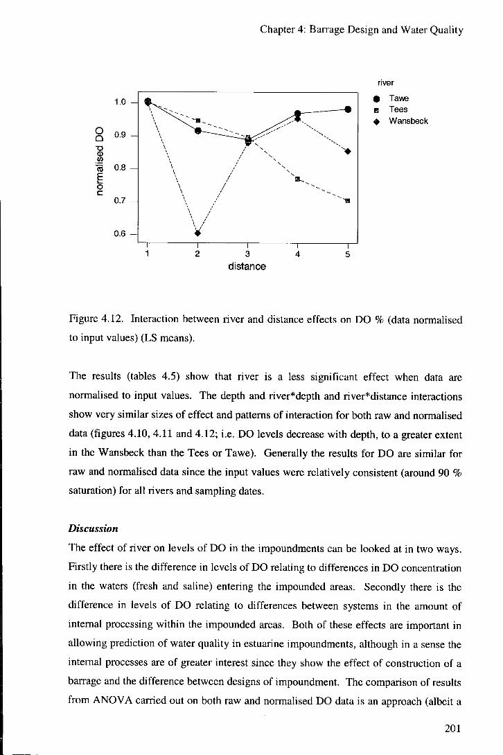
Chapter 4: Barrage Design and Water Quality
1.0
0.9
•ffl 0.8 E o
0.7 -A
0.6 - \
river • Tawe • Tees ^ Wansbeck
distance
Figure 4.12. Interaction between river and distance effects on DO % (data normalised
to input values) (LS means).
The results (tables 4.5) show that river is a less significant effect when data are
normalised to input values. The depth and river*depth and river*distance interactions
show very similar sizes of effect and patterns of interaction for both raw and normalised
data (figures 4.10, 4.11 and 4.12; i.e. DO levels decrease with depth, to a greater extent
in the Wansbeck than the Tees or Tawe). Generally the results for DO are similar for
raw and normalised data since the input values were relatively consistent (around 90 %
saturation) for all rivers and sampling dates.
Discussion
The effect of river on levels of DO in the impoundments can be looked at in two ways.
Firstly there is the difference in levels of DO relating to differences in DO concentration
in the waters (fresh and saline) entering the impounded areas. Secondly there is the
difference in levels of DO relating to differences between systems in the amount of
internal processing within the impounded areas. Both of these effects are important in
allowing prediction of water quality in estuarine impoundments, although in a sense the
internal processes are of greater interest since they show the effect of construction of a
barrage and the difference between designs of impoundment. The comparison of results
from ANOVA carried out on both raw and normalised DO data is an approach (albeit a
201
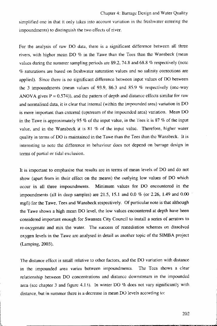
Chapter 4: Barrage Design and Water Quality
simplified one in that it only takes into account variation in the freshwater entering the
impoundments) to distinguish the two effects of river.
For the analysis of raw DO data, there is a significant difference between all three
rivers, with higher mean DO % in the Tawe than the Tees than the Wansbeck (mean
values during the summer sampling periods are 89.2, 74.8 and 68.8 % respectively (note
% saturations are based on freshwater saturation values and no salinity corrections are
applied). Since there is no significant difference between input values of DO between
the 3 impoundments (mean values of 93.9, 86.3 and 85.9 % respectively (one-way
ANOVA gives P = 0.574)), and the pattern of depth and distance effects similar for raw
and normalised data, it is clear that internal (within the impounded area) variation in DO
is more important than external (upstream of the impounded area) variation. Mean DO
in the Tawe is approximately 95 % of the input value, in the Tees it is 87 % of the input
value, and in the Wansbeck it is 81 % of the input value. Therefore, higher water
quality in terms of DO is maintained in the Tawe than the Tees than the Wansbeck. It is
interesting to note the difference in behaviour does not depend on barrage design in
terms of partial or tidal exclusion.
It is important to emphasise that results are in terms of mean levels of DO and do not
show (apart from in their effect on the means) the outlying low values of DO which
occur in all three impoundments. Minimum values for DO encountered in the
impoundments (all in deep samples) are 21.5, 15.1 and 0.0 % (or 2.26, 1.49 and 0.00
mg/1) for the Tawe, Tees and Wansbeck respectively. Of particular note is that although
the Tawe shows a high mean DO level, the low values encountered at depth have been
considered important enough for Swansea City Council to install a series of aerators to
re-oxygenate and mix the water. The success of remediation schemes on dissolved
oxygen levels in the Tawe are analysed in detail as another topic of the SIMBA project
(Lamping, 2003).
The distance effect is small relative to other factors, and the DO variation with distance
in the impounded area varies between impoundments. The Tees shows a clear
relationship between DO concentrations and distance downstream in the impounded
area (see chapter 3 and figure 4.13). In winter DO % does not vary significant!) with
distance, but in summer there is a decrease in mean DO levels according to:
202

Chapter 4: Barrage Design and Water Quality
Mean DO % = 85.9 + 0.508 distance - 0.0573 distance^
(S = 0.422017 R-Sq = 99.9 % R-Sq(adj) = 99.8 % ) .
This decrease in DO during summer is related to the amount of de-oxygenation by
decomposition of organic matter exceeding the amount of re-oxygenation from the
atmosphere, associated with a decrease in flow velocities and possibly the change in
nature of the bed sediments to more organic rich material with distance downstream.
As mentioned previously, no evidence is seen of an increase in the levels of BOD with
distance downstream. No oxygen depletion occurs in winter since rates of biological
respiration are lower and higher flows ensure turbulence and re-oxygenation of the
water column. Neither the Wansbeck nor the Tawe shows any significant correlation
between DO and distance (figure 4.14, R-Sq(adj) = 0.0 % ) , although it must be noted
that the length of river sampled (the impounded section) is much shorter than for the
Tees, and the differences in mean DO levels with distance relate to the depth effects
discussed below.
O Q c
E
90
80 H
70
60
0 10 20
distance downstream from former tidal limit (km)
Figure 4.13. Fitted line plot for the quadratic relationship between DO % and distance
downstream in the Tees impoundment (summer data only).
203

Chapter 4: Barrage Design and Water Quality
8 c
E
90 - f
80 -A
70
60
50
1 2
distance downstreann from former tidal limit (km)
Figure 4.14. DO % and distance downstream in summer in the Wansbeck
impoundment. Variation in mean DO % levels with distance relates to differences in
depth between sampling sites.
There are significant differences in DO between the three depths sampled in each of the
impoundments. It was noted during the PCA and within the section on seasonal effects
that DO internal processing is depth related. This internal processing is related to
thermal or salinity stratification of the water bodies, leading to isolation from the
atmosphere and prolonged contact with oxygen demanding bed sediments. The
presence of stratification and low DO conditions over the majority of the year is
demonstrated statistically in this project for the Wansbeck, and has also been recorded
in the Tawe (Swansea City Council, pers. com.), more research is needed to determine
the proportion of time the Tees is subject to stratification. It is felt that since
stratification in the Tees is solely due to thermal density differences then the periods of
stratification are likely to be shorter and the energy (freshwater flow) required to mix
the water body lower. The density of pure water is at a maximum of 1.000 g/ml at
approximately 4°C and decreases non-linearly with increasing temperature to 0.998
g/ml at approximately 20°C (Vallentyne, 1957), whilst density increases lir^carly with
increasing salt content to a mean seawater (35 %o) value of 1.028 g/ml at 4°C (Ruttner
1963).
204
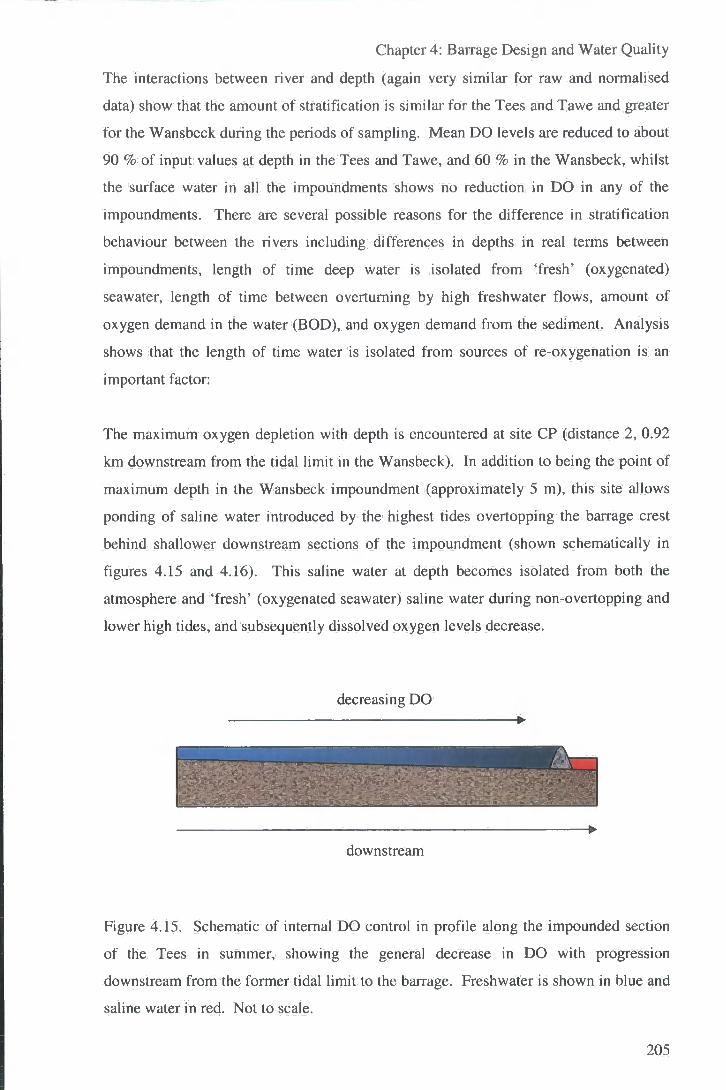
Chapter 4: Barrage Design and Water Quality
The interactions between river and depth (again very similar for raw and normalised
data) show that the amount of stratification is similar for the Tees and Tawe and greater
for the Wansbeck during the periods of sampling. Mean DO levels are reduced to about
90 % of input values at depth in the Tees and Tawe, and 60 % in the Wansbeck, whilst
the surface water in all the impoundments shows no reduction in DO in any of the
impoundments. There are several possible reasons for the difference in stratification
behaviour between the rivers including differences in depths in real terms between
impoundments, length of time deep water is isolated from 'fresh' (oxygenated)
seawater, length of time between overturning by high freshwater flows, amount of
oxygen demand in the water (BOD), and oxygen demand from the sediment. Analysis
shows that the length of time water is isolated from sources of re-oxygenation is an
important factor:
The maximum oxygen depletion with depth is encountered at site CP (distance 2, 0.92
km downstream from the tidal limit in the Wansbeck). In addition to being the point of
maximum depth in the Wansbeck impoundment (approximately 5 m), this site allows
ponding of saline water introduced by the highest tides overtopping the barrage crest
behind shallower downstream sections of the impoundment (shown schematically in
figures 4.15 and 4.16). This saline water at depth becomes isolated from both the
atmosphere and 'fresh' (oxygenated seawater) saline water during non-overtopping and
lower high tides, and subsequentiy dissolved oxygen levels decrease.
decreasing DO •
downstream
Figure 4.15. Schematic of internal DO control in profile along the impounded section
of the Tees in summer, showing the general decrease in DO with progression
downstream from the former tidal limit to the barrage. Freshwater is shown in blue and
saline water in red. Not to scale.
205
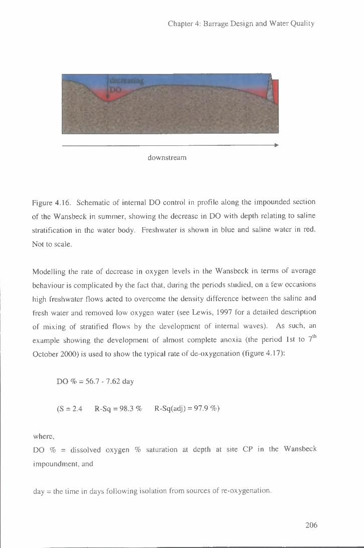
Chapter 4: Barrage Design and Water Quality
downstream
Figure 4.16. Schematic of internal DO control in profile along the impounded section
of the Wansbeck in summer, showing the decrease in DO with depth relating to saline
stratification in the water body. Freshwater is shown in blue and saline water in red.
Not to scale.
Modelling the rate of decrease in oxygen levels in the Wansbeck in terms of average
behaviour is complicated by the fact that, during the periods studied, on a few occasions
high freshwater flows acted to overcome the density difference between the saline and
fresh water and removed low oxygen water (see Lewis, 1997 for a detailed description
of mixing of stratified flows by the development of internal waves). As such, an
example showing the development of almost complete anoxia (the period 1st to 7*
October 2000) is used to show the typical rate of de-oxygenation (figure 4.17):
DO % = 56.7 - 7.62 day
(S = 2.4 R-Sq = 98.3 % R-Sq(adj) = 97.9 %)
where,
DO % = dissolved oxygen % saturation at depth at site CP in the Wansbeck
impoundment, and
day = the time in days following isolation from sources of re-oxygenation.
206

Chapter 4: Barrage Design and Water Quality
40
30 H
20 H
10
o Q
Figure 4.17. The decrease in DO concentration in deep (stratified) water from the
Wansbeck impoundment between the dates of 1st and 7* October 2000.
• D O % -Na
120 J
100 --
80 -
o 60 -Q
40 --
20
0 --
7000.00
6000.00 5000.00
4000.00 3000.00 2000.00 1000.00 0.00
-1000.00
i
5
day
Figure 4.18. DO and Na concentrations over 10* to IS"' June 2000 in deep water at site
F in the Tawe.
207

Chapter 4: Barrage Design and Water Quality
-flow • overtopping
o 10.0
« 5.0
5
day
Figure 4.19. Mean freshwater discharge and tidal overtopping preceding sampling over
the same period as figure 4.18 above (overtopping = tidal height - barrage height).
It is noteworthy that DO absolute concentrations at depth decreased in the Wansbeck to
below the SWQO of 5 mg/1 for salmonid species on approximately the 2"** day and the 3
mg/1 for cyprinid species on the 4'*' day. The tidal height at which seawater was able to
progress upstream to site CP was approximately 5 m (30 cm higher than the crest height
of the Wansbeck barrage).
That DO concentrations at depth in the Tawe are not generally as low as in the
Wansbeck during the periods studied is not due to the rate of de-oxygenation being any
less in the Tawe than in the Wansbeck, but due to the shorter periods of isolation
encountered by waters in the Tawe. Over a 9 day period of sampling from a site (F) in
the Tawe where ponding of saline water is often encountered (Swansea City Council,
pers. comm.) a complex relationship between DO concentration and salinity and
freshwater discharge and tidal overtopping height is seen (figures 4.18 and 4.19). DO is
generally maintained at close to 100 % over the majority of the period either by 'fresh'
seawater progressing upstream to this point or by sufficient freshwater discharge to
provide mixing and removal of saline stratification, but falls rapidly (from 91.7 to 21.5
% over 1 day) on isolation of brackish water (between day 1 and 2 on igure 4.18). The
relationship between overtopping, freshwater discharge ana DO in the Tawe
impoundment is explored further using a larger dataset by Lamping (2003).
208

Chapter 4: Barrage Design and Water Quality
4.3.2 BOD
Results
Applying the model used above for DO % for ANOVA on BOD gave no significant
effects for any of the factors included, although no comparisons can be made for the
Wansbeck since due to time constraints no BOD measurements were taken during the
summer sampling period.
During examination of seasonal effects on the Tees it was identified that BOD in this
river is mainly from natural sources and shows a strong control by freshwater flow. It
was also shown that for the Tees there were no significant internal (with depth or
distance) variations in BOD during the periods studied. Initial examination of the
Wansbeck and Tawe shows that BOD is also flow related in these rivers (figure 4.20):
n r 0.50 1.00 2.00
mean flow preceding sampling (cumecs)
Figure 4.20. The relationship between BOD and flow for the Wansbeck (data from
spring, autumn and winter sampling periods).
For the Wansbeck:
BOD = 0.969 + 1.64 log(Mean24) (P = 0.000, S = 0.809, R-Sq = 37.8 %)
209

Chapter 4: Barrage Design and Water Quality
For the Tawe:
BOD = -0.721 + 2.42 log(Mean24) (P = 0.000, S = 0.450, R-Sq = 48,1 %)
where BOD is measured in mg/1 and Mean24 is the mean flow in the 24 hours
preceding samphng measured in cumecs.
Discussion
BOD increases with increasing flow implying a diffuse source in all 3 rivers studied.
The mean BOD measured was higher in the Wansbeck than the Tees or Tawe (2.1, 1.3
and 1.4 mg/1 respectively) for all sampling, although BOD in the water column is fairly
low in all 3 impoundments. The higher value of BOD for the Wansbeck is likely to
relate to the lowland and more heavily farmed nature of its catchment. There is a
relatively large amount of unexplained variation in the dataset for BOD. The
measurement of BOD is a fairly imprecise technique, and often 2 mg/1 is given as the
LOD (Clesceri et al., 1998). For future work the use of COD as a measure of oxygen
demand is recommended due to its greater precision and repeatability. The random
variance due to the analytical technique makes it difficult to draw any conclusions about
any within impoundment control on BOD, although for the data collected no significant
effects can be shown. This implies that much of the oxygen demand within the systems
causing the reductions in DO described above is from the organic rich bed sediments.
4.3.3 pH
Results
Source F P a' Size of Effect
(to')
River 5.07 0.007 0.041 0.06
Distance 1.14 0.334 na na
Depth 23.17 0.000 0.223 0.31
River* distance 4.97 0.000 0.159 0.22
River*depth 4.26 0.002 0.066 0.09
Error 0.226 0.32
Table 4.6. Results from GLM ANOVA for pH (raw data) in partial and total tidal
exclusion impoundments (na = not applicable since factor insignificant at 95 % level).
210

Chapter 4: Barrage Design and Water Quality
distance depth
7.52 H
7.44 H
Q. 7.36
7.28
7.20 H
Figure 4.21. Main effects plot for the factors of impoundment (river), distance and
depth on pH (raw data) (LS means for factor levels).
Source F P a' Size of Effect
(0)')
River 32.85 0.000 0.003 0.24
Distance 1.80 0.127 na na
Depth 38.47 0.000 0.004 0.28
River*distance 8.18 0.000 0.003 0.22
River* depth 6.93 0.000 0.001 0.09
Error 0.002 0.17
Table 4.7. Results from GLM ANOVA for pH (data normalised to freshwater input
values) in partial and total tidal exclusion impoundments (na = not applicable since
factor insignificant at 95 % level).
211

Chapter 4: Barrage Design and Water Quality
distance depth
1.01
1.00 H
Q. 0.99
0.98 H
0.97
Figure 4.22. Main effects plot for the factors of impoundment (river), distance and
depth on pH (data normalised to freshwater inputs) (LS means for factor levels).
1.04
X Q.
I 0.99 CO
o c
0.94
Q ^ . ^ ^
0.^
\
/
\ / '
river
O Tawe • Tees O Wansbeck
distance
Figure 4.23. Interaction between river and distance effects on pH (data normalised to
input values) (LS means).
212

Chapter 4: Barrage Design and Water Quality
1.03 —
X Q.
&
norm
alis
ed
o to
1
0.93 -
1 d
1 m
depth
1 S
river 9 Tawe m Tees ^ Wansbeck
Figure 4.24. Interaction between river and depth effects on pH (data normalised to
input values) (LS means).
Factor Pairwise comparison Adjusted P-value
River Tees - Tawe 0.000
Wansbeck - Tawe 0.000
Wansbeck - Tees 0.000
Table 4.8. Results from Tukey simultaneous tests on the significance of differences
between the means of factor levels used in the ANOVA for pH (data normalised to
freshwater inputs) in partial and total tidal exclusion impoundments.
Analysis of pH was done using values normalised to the pH values of the freshwater
inputs to the systems for each days sampling in order to assess the processes affecting
pH within the impounded areas. Analysis carried out using raw data (table 4.6 and
figure 4.21) showed a very similar pattern although with lesser variance due to river
(implying that differences between rivers are more due to internal than external
variation). One-way ANOVA gave no significant difference between the input values
of pH between rivers during the summer samphng period (P = 0.602). The factors
included in the model were as used with DO above.
213

Chapter 4: Barrage Design and Water Quality
24 % of the intemal variation in pH in the dataset is due to differences between the impoundments (table 4.7). The three systems show significantly different levels of pH change between them, with the Tees showing a small increase in pH, the Tawe a small decrease in pH and mean pH in the Wansbeck decreasing by a slightly larger amount (figure 4.22). Variation in pH with distance is very different between impoundments (figure 4.23) with only the Tees showing an obvious trend. Depth effects account for approximately 37 % of the variance, and pH decreases with depth in all impoundments but to a greater extent in the Wansbeck than the Tees or Tawe (figure 4.24). Approximately 17 % of the variation in pH intemal change cannot be explained by the terms included in the model.
Discussion
In general changes in pH are small, and pH remains within a range that is not
detrimental to aquatic life. Changes in pH in the impoundments are likely to be
biologically mediated. Primary production leads to increased pH, and respiration
reactions decrease pH. In this light, in the Wansbeck and Tawe impoundments
respiration is in excess of production, and in the Tees production is in excess of
respiration. Interpretation of pH changes are complicated however by the differences in
pH between freshwater and seawater inputs to the impoundments. Burton (1976)
suggests that river water is often of lower pH than seawater. In the estuaries included in
this study the opposite appears to be true. In the Blyth estuary the mean value for
freshwater inputs is pH 7.6 and for the rest of the estuary (which is interpreted as
seawater relatively unaffected by biological processes) the mean pH is 7.2. Samples in
the other estuaries which are composed of saline water also tend to have lower pHs than
the freshwater inputs although, as will be discussed, the pHs of these waters may have
been affected by respiration processes.
The decreases in pH are greater in deep water due to contact with the organic rich bed
sediments. The depth effects are greater in the Wansbeck implying that, as for DO
processing, more stable stratification (due to salinity as opposed to temperature
differences) gives greater periods in which respiration may take place, although some of
this difference is probably due to the initial difference in pH values between seawater
and freshwater inputs.
214

Chapter 4: Barrage Design and Water Quality
• DO % • alkalinity •pH
10 11 12 13 14 15
Figure 4.25. DO, pH and alkalinity over the period 4' to 18*** June 2001 in deep water
at site CP in the Wansbeck impoundment.
The lowest values of both DO and pH are encountered in the Wansbeck impoundment.
As described for DO above, the difference between the Wansbeck and Tawe
impoundments in the development of low pH conditions at depth in stratified water is
likely to be due more to the greater length of time that water is 'ponded' in the
Wansbeck rather than differences in the rates of DO and pH decrease. Unfortunately
for the period analysed above to determine the rate of DO % decrease in deep stratified
water no pH data was collected due to the cable supplied by the manufacturer for the pH
probe being to short to reach the depth of sampling. The cable was lengthened for
subsequent sampling periods on the Wansbeck, but unfortunately a similar period
showing the progression from 'fresh' to 'stagnant' (reduced DO and pH, etc.) water was
not sampled. Figure 4.25 shows pH, alkalinity and DO at depth over the longest period
of anoxia sampled on the Wansbeck, and the subsequent removal of the saline water
between day 12 and 13 of sampling by high freshwater discharge. It can be seen that
pH remains relatively constant (buffered) between days 1 and 7 whilst alkalinity
increases slightly. No reason can be determined for the drop in pH and increase in
alkalinity on day 8, although perhaps sampling on this day disturbed the bed sediment.
On mixing with freshwater (day 13) DO increases, pH increases slightly, and alkalinity
drops markedly. The subsequent decrease in pH and increase in alkalinity may relate to
215

Chapter 4: Barrage Design and Water Quality
the breakdown in suspended organic material transported to the impoundment with the
high (maximum 50.2 m^/s) discharge. TSS for day 13 is 310 mg/l compared with <100
mg/1 for all other days.
The maximum rate of pH decrease at site F in the Tawe over the period for which DO is
discussed above is from 7.7 to 6.5 over 1 day (figure 4.26). Alkalinity over this period
follows the proportion of seawater (Na concentration) in the deep water quite closely
(R-Sq = 69.2 % ) . For both the Tawe and the Wansbeck the biological effects on
alkalinity appear to be minor relative to the proportion of seawater (higher alkalinity) to
river water (lower alkalinity).
• D 0 % —^alkalinity —o—pH
^ |> 80 n
Figure 4.26. DO, pH and alkalinity over the period 10* to 18* June 2000 in deep water
at site F in the Tawe impoundment.
4.3.4 Alkalinity
Results
PCA showed that alkalinity was strongly aligned with a principal component interpreted
as a freshwater discharge factor, and that alkalinity shows a dilution effect with
increasing flow. For the periods studied (data from all seasons sampled) on the 3
impoundments the relationships are:
216

Chapter 4: Barrage Design and Water Quality
For the Tees:
alkalinity = 270 - 135 log(Mean 24) (S = 23.7, R-Sq = 86.0 %)
For the Tawe:
alkalinity = 180 - 86.3 log(Mean24) (S = 14.1, R-Sq = 60.3 %)
For the Wansbeck:
alkalinity = 92.1 - 26.1 log(Mean24) (S = 13.5, R-Sq = 53.4 %)
where alkalinity is measured in mg/1 CaCOa equivalent and Mean24 is the mean flow in
the 24 hours preceding sampling measured in cumecs. P = 0.000 for each relationship.
ANOVA carried out on raw alkalinity data gives significant differences between rivers,
but no significant variation in alkalinity with distance and only a very small effect of
depth (table 4.9). The Tees has significantly higher alkalinity than the Tawe, and the
Tawe has significantly higher alkalinity than the Wansbeck (P = 0.000 for Tukey
simultaneous tests). 12 % of the variance in alkalinity cannot be explained by the
factors in the model, and probably relates to within river variation in alkalinity with
variation in freshwater flow.
Source F P a' Size of Effect
(to") River 159.63 0.000 10704 0.86
Distance 2.26 0.061 na na
Depth 3.38 0.034 161 0.01
River* distance 0.62 0.763 na na
River* depth 0.42 0.797 na na
Error 1518 0.12
Table 4.9. Results from GLM ANOVA for alkalinity (raw data) in partial and total tidal
exclusion impoundments (na = not applicable since factor insignificant (P>0.05)).
To determine the within impoundment controls on alkalinity the ANOVA applied above
to raw data was repeated with data normalised to the values of alkalinity in the
217

Chapter 4: Barrage Design and Water Quality
freshwater inputs to the impoundments for each of the sampling dates. The importance
of river as a factor is much smaller when looking at internal changes compared with the
overall variation in alkalinity (i.e. comparing input normalised and raw data results).
Alkalinity is higher within the impounded areas than in the freshwater inputs in all the
systems, but to a greater extent in the Tawe and Wansbeck (which show no statistical
difference between them). Alkalinity increases with distance downstream and with
depth in all 3 impoundments to a similar degree. The error term when using normalised
data is relatively large (44 %) and probably relates in part to random analytical enw
relating to the precise identification of the end-point (methyl orange indicator colour
change) in the alkalinity titrations, and in part to variation in the amount of seawater
entering the systems.
Source F P a' Size of Effect
(0)')
River 7.48 0.001 0.018 0.13
Distance 6.88 0.000 0.032 0.23
Depth 11.39 0.000 0.028 0.20
River* distance 1.28 0.248 na na
River*depth 0.93 0.445 na na
Error 0.062 0.44
Table 4.10. Results from GLM ANOVA for alkalinity (data normalised to freshwater
input values) in partial and total tidal exclusion impoundments (na = not applicable
since factor insignificant (P>0.05)).
Factor Pairwise comparison Adjusted P-value
River Tees - Tawe 0.001
Wansbeck - Tawe 0.875
Wansbeck - Tees 0.006
Table 4.11. Results from Tukey simultaneous tests on the significance of differences
between the means of factor levels used in the ANOVA for alkalinity (data normalised
to input values) in partial and total tidal exclusion impoundments.
218

Chapter 4: Barrage Design and Water Quality
river distance depth
1.21
1.17 ^
1.13 -A
1 •o <D = i 1.09
1.05
Figure 4.27. Main effects plot for the factors of impoundment (river), distance and
depth on alkalinity (data normalised to freshwater inputs) (LS means for factor levels).
Discussion
The majority of variation in levels of alkalinity is due to differences in freshwater inputs
which relate to differences between the catchments of the rivers (geological effects) and
with the relative proportion of baseflow to stormflow components of river discharge. In
relation to these variations, the variation within the impounded areas of the estuaries is
small, and therefore the effect on alkalinity of barrage construction minor.
The difference between rivers when examining data normalised to the freshwater inputs
to the systems is in part an effect of the difference in volumes of seawater entering the
systems. In general the alkalinity of seawater is higher than that of freshwater (Dryssen
and Wedborg, 1980), and alkalinity behaves conservatively on mixing (figure 4.28).
For the three impoundments studied the mean value for alkalinity in brackish and saline
water (arbitrarily defined as Na > 100 mg/1) is 99 mg/1 CaCOa equivalent compared
with 88 mg/1 CaCOj equivalent in fresh (Na < 100 mg/1) water (mean pHs are 7.53 and
7.66 respectively). The Tawe and Wansbeck have similar amounts of tidal overtopping
of the barrage crest and seawater entering the impoundment, and so in general show a
greater increase in alkalinity from freshwater inputs than the Tees.
219

Chapter 4: Barrage Design and Water Quality
150 H i §"
CO O O CO
O
c
5 CO
100
2000 3000 Na (mg/1)
5000
Figure 4.28. Conservative behaviour of alkalinity on mixing between fresh and saline
water. Data shown from the Tawe impoundment. Variation in freshwater samples
relates to river flow.
Since the behaviour is similar for all impoundments (i.e. no interactions are significant)
the distance and depth effects on alkalinity within the impoundments are likely to be
due in part to the biological controls of production (acting to decrease alkalinity by
removing CO2) and respiration (acting to increase alkalinity by releasing CO2). The
relationship between alkalinity and pH with depth was identified during PCA above. At
depth there is a significant increase in alkalinity due to respiration in excess of
production (mirroring the behaviour of pH as described above). The general increase in
alkalinity with distance downstream may relate to biological effects, inputs of
groundwater, dissolution of CO2 from the atmosphere or, for the partial exclusion
systems, greater seawater contribution closer to the barrages.
4.3.5 Conductivity
Results
Conductivity relates to the amount of seawater entering the impounded areas. The
pattern of its distribution in time and space relates to density stratification a..d the
mixing and removal of saline water by freshwater flow. ANOVA carried out on all
conductivity data collected during the water quality surveys of the impoundments shows
220

Chapter 4: Barrage Design and Water Quality
that there is (as would be expected) significantly higher conductivity in the partial tidal
exclusion impoundments (Tawe and Wansbeck) than the total exclusion impoundment
(Tees). There is no significant difference between the Tawe and Wansbeck for the
periods sampled. Conductivity increases with distance downstream (proximity to the
barrage) in the partial exclusion systems (figure 4.29). A larger effect (34 %) is shown
by depth, with conductivity increasing with depth in the partial exclusion systems.
Source F P Size of Effect
(0)')
River 49.96 0.000 248151315 0.23
Distance 9.53 0.000 86486241 0.08
Depth 71.98 0.000 359760731 0.34
River*distance 5.94 0.000 100172092 0.09
River*depth 16.82 0.000 160346308 0.15
Error 114046936 0.11
Table 4.12. Results from GLM ANOVA for conductivity (raw data) in partial and total
tidal exclusion impoundments.
distance depth
12000
9000
E
••g 6000
c o O 3000
0 ^
Figure 4.29. Main effects plot for the factors of impoundment (river), distance and
depth on conductivity (raw data) (LS means for factor levels).
221

Chapter 4: Barrage Design and Water Quality
E
o T3 C
8
20000 -
10000 -
/ /
0 -/
0 -
1 1
1 2
1 3
distance
1 4
1 5
river O Tawe • Tees O Wansbeck
Figure 4.30. Interaction between river and distance effects on conductivity (raw data)
(LS means).
20000
o
:1 10000
3 -a c o o
river
Q TawB • Tees <3> Wansbeck
Figure 4.31. Interaction between river and depth effects on conductivity (raw data) (LS
means).
222
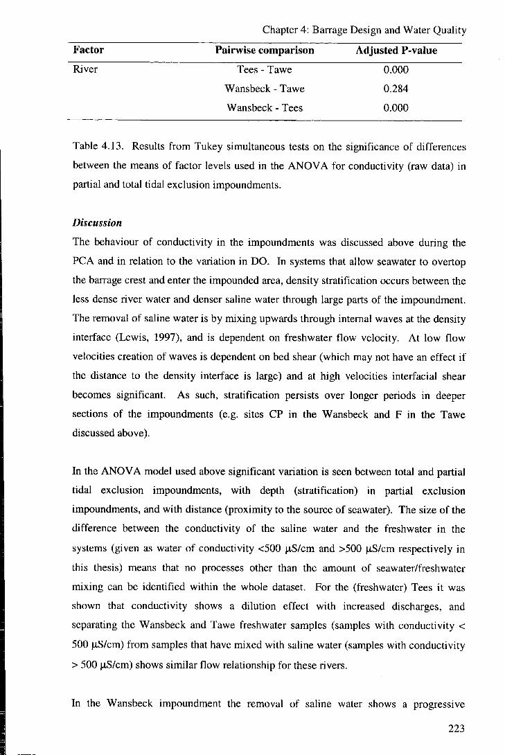
Chapter 4: Barrage Design and Water Quality
Factor Pairvyise comparison Adjusted P-value
River Tees - Tawe 0.000
Wansbeck - Tawe 0.284
Wansbeck - Tees 0.000
Table 4.13. Results from Tukey simultaneous tests on the significance of differences
between the means of factor levels used in the ANOVA for conductivity (raw data) in
partial and total tidal exclusion impoundments.
Discussion
The behaviour of conductivity in the impoundments was discussed above during the
PCA and in relation to the variation in DO. In systems that allow seawater to overtop
the barrage crest and enter the impounded area, density stratification occurs between the
less dense river water and denser saline water through large parts of the impoundment.
The removal of saline water is by mixing upwards through intemal waves at the density
interface (Lewis, 1997), and is dependent on freshwater flow velocity. At low flow
velocities creation of waves is dependent on bed shear (which may not have an effect if
the distance to the density interface is large) and at high velocities interfacial shear
becomes significant. As such, stratification persists over longer periods in deeper
sections of the impoundments (e.g. sites CP in the Wansbeck and F in the Tawe
discussed above).
In the ANOVA model used above significant variation is seen between total and partial
tidal exclusion impoundments, with depth (stratification) in partial exclusion
impoundments, and with distance (proximity to the source of seawater). The size of the
difference between the conductivity of the saline water and the freshwater in the
systems (given as water of conductivity <500 |a,S/cm and >500 |iS/cm respectively in
this thesis) means that no processes other than the amount of seawater/freshwater
mixing can be identified within the whole dataset. For the (freshwater) Tees it was
shown that conductivity shows a dilution effect with increased discharges, and
separating the Wansbeck and Tawe freshwater samples (samples with conductivity <
500 ^S/cm) from samples that have mixed with saline water (samples with conductivity
> 500 (xS/cm) shows similar flow relationship for these rivers.
In the Wansbeck impoundment the removal of saline water shows a progressive
223

Chapter 4: Barrage Design and Water Quality
increase with increased flow, and the mixing upwards effect is shown by the relatively
constant conductivity of the deep saline water through all ranges of flow at which it is
encountered (figure 4.32). The removal of saline water is demonstrated by the decrease
in the number of points at which it is encountered, and commences at flows greater than
approximately 5 cumecs (m^/s). Total removal of saline water does not occur until
somewhere between 40 and 100 cumecs, with saline water being found at depth behind
the barrage up to this point.
100000
E o CO 10000 3
o •D c 8
1000 H
100 H
saline
mixing
1 10 100 mean flow preceding sampling (cumecs)
Figure 4.32. Conductivity and freshwater flow in the Wansbeck impoundment. Saline
water conductivity is independent of flow but the number of sampling sites at which
saline water is encountered decreases with increasing flow. High conductivity samples
are almost all from depth. Freshwater conductivity decreases with increasing flow.
The behaviour of density stratification with flow is similar for the Tawe impoundment
(figure 4.33). The removal of saline water (shown by the decrease in number of
samples of high conductivity) commences at approximately 7 cumecs. The slightly
higher discharge for the Tawe compared with the Wansbeck is probably due to the
greater water depth (mean depths 2.15 and 1.39 m respectively) meaning that bed shear
has less impact in the creation of internal waves and hence mixing for the same
discharge.
224

Chapter 4: Barrage Design and Water Quality
o -a c
8
100000
E o W 10000
>
1000
100
saline
mxing
mean flow preceding sampling (cumecs)
Figure 4.33. Conductivity and freshwater flow in the Tawe impoundment. The
behaviour is very similar to the Wansbeck (above). Removal of saline water
commences at approximately 7 cumecs.
For both rivers, the freshwater samples (taken as those with conductivities lower than
500 |LiS/cm) show a decrease in conductivity with increasing freshwater flow,
interpreted as due to dilution of baseflow component by increasing stormflow (figure
4.34). The relationships between freshwater conductivities and freshwater flow within
the impoundments are:
For the Wansbeck:
conductivity = 621 - 231 log(Mean24) (S = 124, R-Sq = 51.8 %)
For the Tawe:
conductivity = 515 - 272 log(Mean24) (S = 51.5, R-Sq = 55.2 %)
For the Tees: conductivity = 586 - 247 log(Mean24) (S = 153, R-Sq = 32.9 %)
225

Chapter 4: Barrage Design and Water Quality
where conductivity is measured in |aS/cm, and Mean24 is the mean flow in the 24 hours
preceding samphng measured in cumecs. P = 0.000 for each relationship.
500
400 H E CO
* - 300 —i
o
8
100 —I
5 10 15 20
mean flow preceding sampling (cumecs)
Figure 4.34. The relationship between freshwater (taken as conductivity < 500 iS/cm)
and flow in the River Tawe. The scatter of points above the regression line are due to
the mixing of freshwater with seawater.
4.3.6 Transparency
Results
Since transparency (measured using a Secchi disk) was measured once at each site on
each date sampled, the ANOVA model used excluded depth as a factor. On several
occasions the water depth at the former tidal limit sites (which were used to represent
the freshwater inputs to the systems for data normalisation) was too shallow to allow
transparency measurements to be taken, and so analysis is carried out on raw data only.
The results show that there are large differences in transparency between the
impoundments, explaining 91 % of the variance in raw transparency values.
Transparency is greater in the Tawe than the Tees, and in the Tees than the Wansbeck
(table 4.14). Transparencies show a small but significant amount of decrease with
226
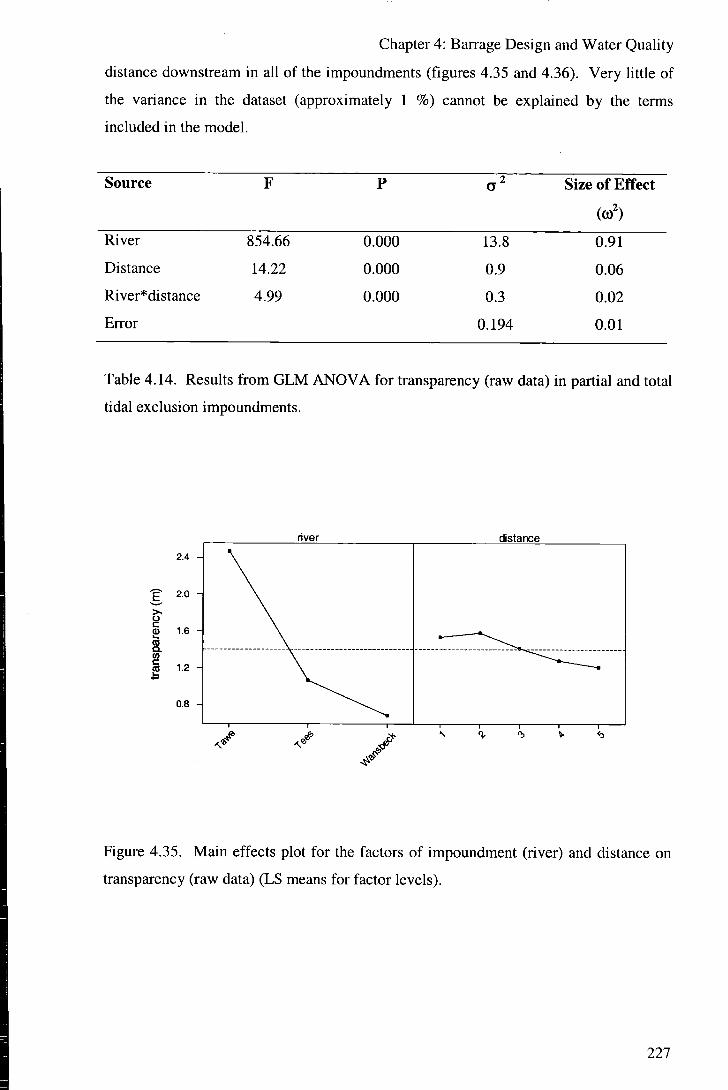
Chapter 4: Barrage Design and Water Quality
distance downstream in all of the impoundments (figures 4.35 and 4.36). Very little of
the variance in the dataset (approximately 1 %) cannot be explained by the terms
included in the model.
Source Size of Effect
River 854.66
Distance 14.22
River*distance 4.99
Error
0.000
0.000
0.000
13.8
0.9
0.3
0.194
0.91
0.06
0.02
0.01
Table 4.14. Results from GLM ANOVA for transparency (raw data) in partial and total
tidal exclusion impoundments.
distance
Figure 4.35. Main effects plot for the factors of impoundment (river) and distance on
transparency (raw data) (LS means for factor levels).
227

Chapter 4: Barrage Design and Water Quality
2.5 ^
>. o c
CO Q . CO c CO
1.5 -A
0.5 -A
river O Tawe • Tees O Wansbeck
distance
Figure 4.36. Interaction between river and distance effects on transparency (raw data)
(LS means).
Discussion
Within the River Tees it was seen that a large amount of variation in transparency was
due to increased turbidity with increased discharge. However, the small amount of
variance unexplained in the model above when comparing the 3 impoundments studied
suggests that flow is a minor effect compared to the size of the differences in
transparency between the rivers. If it is assumed that transparencies relate to turbidity
in all the systems, then this large difference has implications in terms of the relative
amounts of sediment and possible sediment build-up in the impounded areas. The Tees
and the Wansbeck have the potential for more rapid sedimentation than does the Tawe.
Sedimentation, and in particular sediment quality, are discussed in chapter 6.
The decrease in transparency with distance downstream was interpreted as due to the re-
suspension of bed material in the Tees, and this is also likely to be the case in the partial
exclusion systems although in these tidal currents may also act to re-suspend material.
Note that for the Wansbeck the transparency at distance 1 is unrepresentatively low
since the low water depth at this point meant that measurement could only take place
under low transparency conditions. Un-impounded estuaries often show turbidity
maxima due to tidal pumping (Dyer, 1988), but no maxima appear to be present (in
228

Chapter 4: Barrage Design and Water Quality
terms of transparency peaks) in the impounded estuaries studied, although tidal inputs
and currents may explain some of the downstream decrease in transparencies in the
Tawe and Wansbeck.
4.3.7 TSS
Results
The data for TSS collected in summer 1999 on the Tees is suspect due to variation in
the amount of moisture in the filter papers used in the measurements, and therefore only
the Tawe and Wansbeck impoundments are compared in the ANOVA. Analysis is
initially carried out using raw TSS data to examine the overall differences between the
rivers, and then using data normalised to the freshwater input values to assess the
internal variation in TSS.
Analysis using raw data shows that (as for transparency) differences between rivers
account for the majority of the variance in the dataset (table 4.15), with suspended
solids approximately 5 times higher in the Wansbeck than the Tawe during the sampling
periods (figure 4.37). Compared to this variance the effect of distance and the
river*distance interaction is insignificant. There are significant differences between the
3 factor levels of depth in the impoundments, and depth accounts for approximately 16
% of the variance. TSS increase with depth, and to a greater extent (in absolute terms)
in the Wansbeck than the Tawe. It is likely that much of the unexplained variance in
TSS is related to variation in freshwater flow.
Source F P a' Size of Effect
(0)') River 96.40 0.000 7412 0.58 Distance 0.12 0.974 na na Depth 27.81 0.000 2083 0.16 River* distance 1.04 0.385 na na River*depth 10.36 0.000 1455 0.11 Error 1748 0.14
Table 4.15. Results from GLM ANOVA for TSS (raw data) in partial and total tidal
exclusion impoundments (na = not applicable since factor insignificant).
229

Chapter 4: Barrage Design and Water Quality
river distance depth
^ 30 A
Figure 4.37. Main effects plot for the factors of impoundment (river), distance and
depth on TSS (raw data) (LS means for factor levels).
E, CO 05
river
O Tawe • Wansbeck
depth
Figure 4.38. Interaction between river and depth effects on TSS (raw data) (LS means).
230

Chapter 4: Barrage Design and Water Quality
Source F P Size of Effect
River 2.08 0.150 na na Distance 8.54 0.000 14.1 0.16 Depth 49.96 0.000 45.8 0.51 River*distance 3.43 0.009 9.1 0.10 River*depth 0.84 0.433 na na Error 21.0 0.23
Table 4.16. Results from GLM ANOVA for TSS (data normalised to freshwater input
values) in partial and total tidal exclusion impoundments (na = not applicable since
factor insignificant).
river distance depth
CO
Figure 4.39. Main effects plot for the factors of impoundment (river), distance and
depth on TSS (data normalised to freshwater inputs) (LS means for factor levels).
Repeating the ANOVA using normalised data (results in table 4.16) shows no
significant effect for river, therefore differences between the rivers are generally due to
differences in the amount of TSS entering the systems rather than any differences in the
behaviours within the impounded areas. Removing the variance in TSS entering the
impounded areas allows distance to show a significant effect with values of TSS
231

Chapter 4: Barrage Design and Water Quality
increasing with distance downstream (figure 4.39), and by a greater degree in the Tawe
than the Wansbeck (figure 4.40). The biggest within impoundment variation in TSS is
with depth (a) = 0.51), with TSS increasing with depth by exactly the same degree in
both impoundments.
E CO
8 -
7 -
6 -
5 -/
4 - / /
3 - / y / /• B . ^
/ / / / ^ / /
2 -^ / •
1 -
river % Tawe • Wansbeck
distance
Figure 4.40. Interaction between river and distance effects on TSS (raw data) (LS
means).
Discussion The major controls on the amount of suspended material in the impoundments' water
columns are external to (i.e. upstream of) the impounded areas. These controls on
sediment load relate to the catchments (e.g. land use) and river discharge. Modelling of
sediment transport (Beavers, 2003) and an attempt at fingerprinting sediment sources to
the impoundment (Neilson, 2003) are carried out as specific tasks of the SIMBA
Project.
Relative to these external effects, internal variance in the concentration of suspended
particulate material is low, but demonstrates some important behaviour. Firstly, both
the Tawe and the Wansbeck show the same relative increase in TSS with depth in the
impounded area, with deep samples containing approximately 3 times the concentration
of suspended material as surface samples. This suggests that sediment may be settling
232

Chapter 4: Barrage Design and Water Quahty
through the water column from the surface water down to the bed at similar rates in
both systems. It may also be that the saline water at depth shows higher TSS
concentrations due to inputs from downstream of the barrages, or re-suspension of
unconsolidated bed material by tidal currents (as is common in estuaries of unrestricted
tidal circulation (Dyer, 1988). The greater relative increase in TSS concentrations
downstream in the Tawe, which is subject to higher tidal overtopping, may also be due
to the effect of tidal currents resuspending bed material. The TSS results, as might be
expected, mirror the transparency results for the Tawe and Wansbeck suggesting that
the assumption that transparency relates to turbidity in these rivers is correct. The
pattern of sediment transport and build-up within the impounded areas is discussed
further in chapter 6.
4.3.8 Nutrients
4.3.8.1 Nitrate
Results
The majority of the variance (67 %) in nitrate in the systems studied is between the
rivers. The Tees and the Wansbeck have significantly higher mean nitrate levels than
the Tawe (figure 4.41 and table 4.17). Nitrate levels decrease slightly with distance
downstream in all 3 impoundments, but there are contrasting depth effects. The Tees
and the Tawe show no depth effects but the Wansbeck shows a significant decrease in
levels of nitrate with increasing depth (figure 4.42).
Source F P a' Size of Effect
River 162.94 0.000 9.86 0.67 Distance 7.32 0.000 0.77 0.05 Depth 13.82 0.000 0.78 0.05 River*distance 1.40 0.195 na na River*depth 16.55 0.000 1.89 0.13 Error 1.37 0.09
Table 4.17. Results from GLM ANOVA for nitrate (raw data) in partial and total tidal
exclusion impoundments (na = not applicable since factor insignificant).
233

Chapter 4: Bairage Design and Water Quality
river distance depth 2.6
2.1
03 1.1
1.1
0.6 H
Figure 4.41. Main effects plot for the factors of impoundment (river), distance and
depth on nitrate (raw data) (LS means for factor levels).
3.5
2,5 -
1.5
_ _ _ — — € ) 0 5 - . ^— ^
1 d
1
m depth
1 s
river
O TawB • Tees O Wansbeck
Figure 4.42. Interaction between river and depth effects on nitrate (raw data) (LS
means).
234

Chapter 4: Barrage Design and Water Quality
Factor Pairwise comparison Adjusted P-value River Tees - Tawe 0.000
Wansbeck - Tawe 0.000
Wansbeck - Tees 0.065
Table 4.18. Results from Tukey simultaneous tests on the significance of differences
between the means of factor levels used in the ANOVA for nitrate (raw data) in partial
and total tidal exclusion impoundments.
Applying the same model to data normalised to the upstream freshwater input values for
nitrate gives the following results (table 4.19). Difference between the rivers remains
the most important effect (explaining 58 % of the variance), however the pattern differs
from that shown by raw data. Mean levels of nitrate in the Tees are approximately 30 %
higher than those entering the impoundment at the upstream limit. The distinct increase
in nitrate concentrations takes place between site LM and site LW in the Tees. In the
Tawe and the Wansbeck mean levels of nitrate are lower than in the freshwater input
values, and to a significantly greater extent in the Wansbeck. The size and pattern for
the distance and depth effects is similar for both raw and normalised data. Nitrate levels
increase slightly with distance downstream in all 3 impoundments, but show contrasting
depth effects. Nitrate decreases with depth in the partial tidal exclusion systems and
increases slightly in the Tees.
Source F P a' Size of Effect
(to') River 83.13 0.000 0.70 0.58 Distance 4.41 0.002 0.06 0.05 Depth 13.97 0.000 0.11 0.09 River* distance 0.88 0.529 na na River*depth 9.95 0.000 0.15 0.13 Error 0.19 0.16
Table 4.19. Results from GLM ANOVA for nitrate (data normalised to freshwater
input values) in partial and total tidal exclusion impoundments (na = not applicable
since factor insignificant).
235

Chapter 4: Barrage Design and Water Quality
river distance depth
1.30
1.15
1.00
0.85
0.70
Figure 4.43. Main effects plot for the factors of impoundment (river), distance and
depth on nitrate (data normalised to input values) (LS means for factor levels).
1.4
13 0.9
0.4
river
O Tawe • Tees O Wansbeck
depth
Figure 4.44. Interaction between river and depth effects on nitrate (data normalised to
input values) (LS means).
236

Chapter 4: Barrage Design and Water Quality
Factor Pairwise comparison Adjusted P-value
River Tees - Tawe 0.000
Wansbeck - Tawe 0.020
Wansbeck - Tees 0.000
Table 4.20. Results from Tukey simultaneous tests on the significance of differences
between the means of factor levels used in the ANOVA for nitrate (data normalised to
input values) in partial and total tidal exclusion impoundments.
Discussion
A large amount of the difference in levels of nitrate within the impoundments can be
explained by differences between the amount of nitrate input to the systems from the
rivers. During the periods included in the analysis above, mean nitrate levels in the
freshwater inputs to the systems were 3.85, 2.16 and 0.79 mg/1 N for the Wansbeck,
Tees and Tawe, respectively, and this is reflected in the relative mean values for the
whole impoundments. Differences in nitrate levels in the rivers are due to a
combination of catchment (land-use), flow and point-source effects. As mentioned,
nitrate in the Tees shows an approximate dilution with increasing flows (R-Sq = 39.1 %
for summer data; R-Sq = 56.8 % for winter data) and is therefore possibly point-source
(urban) dominated in this river, with seasonal differences controlled by diffuse sources.
However, high flow events in the Tees are generally due to rainfall on the upland
(Pennines) part of the catchment which is a poorer nitrate source than the more
intensively farmed lowlands, and it is difficult to separate this contribution to the
dilution effect. Carrying out regression analysis on nitrate vs. flow for the freshwater
nitrate values in the Wansbeck and Tawe during the summer periods shows nitrate to be
inversely related to flow (and therefore predominantly of point source) in the Tawe (R-
Sq = 62.2 %, figure 4.45), but that nitrate is proportional to flow (and therefore of
diffuse source) in the Wansbeck (R-Sq = 23.8 %, figure 4.46).
237

Chapter 4: Barrage Design and Water Quality
1.0
CO
0.5
0.0
5 10 15 20
mean flow preceding sampling (cumecs)
Figure 4.45. The relationship between nitrate concentration in freshwater (conductivity
< 500 |aS/cm) samples and river flow in the Tawe.
I
mean flow preceding sampling (cumecs)
Figure 4.46. The relationship between nitrate concentration in freshwater (conductivity
< 500 nS/cm) samples and river flow in the Wansbeck.
238
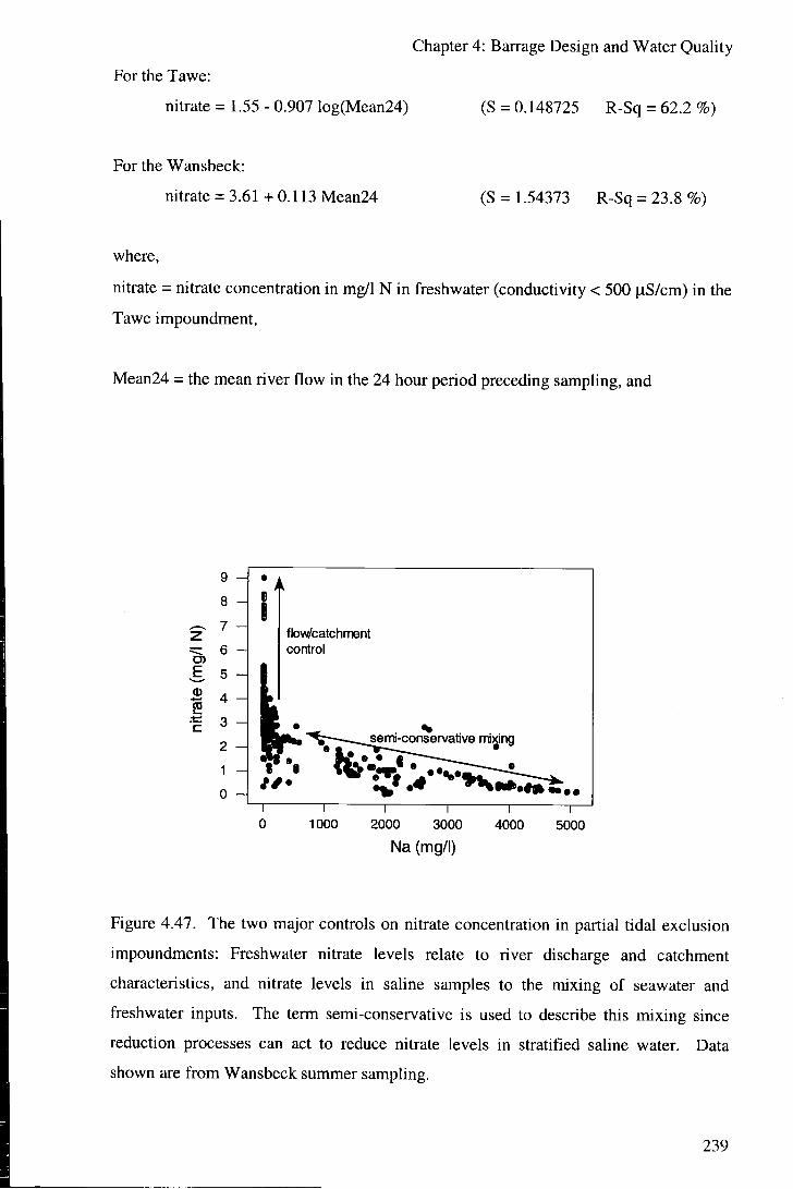
Chapter 4: Barrage Design and Water Quality
For the Tawe: nitrate = 1.55 - 0.907 log(Mean24) (S = 0.148725 R-Sq = 62.2 %)
For the Wansbeck:
nitrate = 3.61 + 0.113 Mean24 (8 = 1.54373 R-Sq = 23.8%)
where,
nitrate = nitrate concentration in mg/1 N in freshwater (conductivity < 500 nS/cm) in the
Tawe impoundment,
Mean24 = the mean river flow in the 24 hour period preceding sampling, and
15
9
8
7
6
5
4
3
2
1
0
flow/catchnrent control
semi-conservative mixing
•••• 1000 2000 3000
Na (mg/l) 4000 5000
Figure 4.47. The two major controls on nitrate concentration in partial tidal exclusion
impoundments: Freshwater nitrate levels relate to river discharge and catchment
characteristics, and nitrate levels in saline samples to the mixing of seawater and
freshwater inputs. The term semi-conservative is used to describe this mixing since
reduction processes can act to reduce nitrate levels in stratified saline water. Data
shown are from Wansbeck summer sampling.
239

Chapter 4: Barrage Design and Water Quality
E,
CO
E
4.0
3.5
3.0 H
2.5
O0.915
o 0.000
2.630 o 3.300
o
4.320 o
100 200
mean Na (mg/l)
Figure 4.48. Mean nitrate levels vs. mean Na levels in surface water samples at each
sampling site in the Wansbeck (summer data), showing mixing of fresh and saline water
with progression downstream. Data labels are distance (km) from the tidal limit for the
sampling sites.
The second difference between systems is related to the relative amounts of seawater
and freshwater within the impounded areas. Nitrate levels in river water tend to be
higher than those in seawater. For example, for the Tawe during the summer sampling
period the mean level in freshwater samples (conductivity < 500 |iS/cm) was 0.68 mg/l
N whereas in saline (conductivity > 500 |J,S/cm) water it was 0.56 mg/l N. For the
Wansbeck the difference is even greater at 4.75 and 2.10 mg/l N for fresh and saline
water respectively. The decrease in nitrate levels due to seawater inputs is seen in the
ANOVA for normahsed data as the lower mean nitrate values in the partial exclusion
systems relative to the freshwater inputs, and in the decrease in nitrate with depth and
distance in these impoundments. The relative decreases in nitrate concentration with
mixing are lower for the Tawe than the Wansbeck since the freshwater inputs for this
system are of lower nitrate concentration, but the amount of seawater mixing is (based
on conductivity and Na data) assumed to be similar for both impoundments.
240

Chapter 4: Barrage Design and Water Quality
The mixing of fresh and seawater is generally conservative in relation to nitrate levels
(figures 4.47 and 4.48), although in stratified saline water a gradual decrease in nitrate is
seen as anoxic conditions develop and nitrate reduction processes (denitrification and
reduction to ammonia) take place (figures 4.49 and 4.50). For the Wansbeck the same
period over which DO levels were seen to decrease in the deep water at site CP is used
to determine a rate of nitrate reduction. As mentioned above for DO, a similar period of
deep saline water isolation is not seen during the sampling period on the Tawe due to
replacement by new saline water or removal by high freshwater flow. For the same
period at site F over which DO was described above, nitrate follows DO levels in the
water (which are in turn related to length of time of isolation from sources of DO) quite
closely (figure 4.51). Relative to the variance in nitrate levels associated with changes
in the freshwater inputs to the system or the amount of seawater mixing, the effect of
nitrate reduction is small, but may be important in removal of N from the systems
and/or in the build-up of anmionia levels in the water column. The behaviour of
ammonia is explored further below.
2.5 H
E
15 1.5 H
0.5
fresh
saline •
0 1
reduction
Figure 4.49. The changes in nitrate concentration through change from fresh to saline
water followed by reductive processes in deep (stratified) water from the Wansbeck
impoundment between the dates of 30"* September and 7* October 2000.
241

Chapter 4: Barrage Design and Water Quality
1.2
r o
0.9
d) E, 0)
2 •+-•
0.8
07
0.6
Figure 4.50. The decrease in nitrate concentration through reductive processes in deep
(stratified) water from the Wansbeck impoundment between the dates of 1st and 7*
October 2000.
Apart from the small decrease in nitrate levels with distance downstream in the Tees,
which is interpreted as due to biological uptake, no other processes could be identified
as important in controlling nitrate levels in the impounded areas. The importance of
sediment as a possible nutrient source and sink is examined further in the sediment
chapters of this thesis.
242
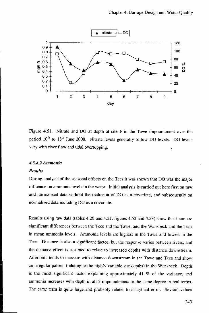
Chapter 4: Barrage Design and Water Quality
- nitrate •DO
+ 100
60 o
Figure 4.51. Nitrate and DO at depth at site F in the Tawe impoundment over the
period 10* to 18* June 2000. Nitrate levels generally follow DO levels. DO levels
vary with river flow and tidal overtopping.
4.3.8.2 Ammonia
Results
During analysis of the seasonal effects on the Tees it was shown that DO was the major
influence on ammonia levels in the water. Initial analysis is carried out here first on raw
and normalised data without the inclusion of DO as a covariate, and subsequently on
normalised data including DO as a covariate.
Results using raw data (tables 4.20 and 4.21, figures 4.52 and 4.53) show that there are
significant differences between the Tees and the Tawe, and the Wansbeck and the Tees
in mean ammonia levels. Ammonia levels are highest in the Tawe and lowest in the
Tees. Distance is also a significant factor, but the response varies between rivers, and
the distance effect is assumed to relate to increased depths with distance downstream.
Ammonia tends to increase with distance downstream in the Tawe and Tees and show
an irregular pattern (relating to the highly variable site depths) in the Wansbeck. Depth
is the most significant factor explaining approximately 41 % of the variance, and
ammonia increases with depth in all 3 impoundments to the same degree in real terms.
The error term is quite large and probably relates to analytical error. Several values
243

Chapter 4: Barrage Design and Water Quality
(particularly from the Tees) are measured at close to the 3s LOD (0.04 mg/1 N), and in
general the baseline during the colorimetric determination of ammonia was subject to
noise (and drift, although a drift standards were used to correct for this).
Source F P a' Size of Effect
River 11.47 0.000 0.015 0.13
Distance 4.63 0.001 0.011 0.09
Depth 34.27 0.000 0.048 0.41
River*distance 2.75 0.005 0.010 0.09
River*depth 1.67 0.155 na na
Error 0.033 0.28
Table 4.20. Results from GLM ANOVA for ammonia (raw data) in partial and total
tidal exclusion impoundments (na = not applicable since factor insignificant).
0.30 river distance depth
E 0.18
Figure 4.52. Main effects plot for the factors of impoundment (river), distance and
depth on ammonia (raw data) (LS means for factor levels).
244

Chapter 4: Barrage Design and Water Quality
0 5 E , a 'c o E E to
0.3
0 2
0.1 -
y
1 1
1 2
1 3
1 4
1 5
river
9 Tawe B Tees ^ Wansbeck
distance
Figure 4.53. Interaction between river and distance effects on ammonia (raw data) (LS
means).
Factor Pairwise comparison Adjusted P-value
River Tees - Tawe 0.000
Wansbeck - Tawe 0.090
Wansbeck - Tees 0.013
Table 4.21. Results from Tukey simultaneous tests on the significance of differences
between the means of factor levels used in the ANOVA for ammonia (raw data) in
partial and total tidal exclusion impoundments.
Results for analysis using data normalised to freshwater inputs to the impoundments
(tables 4.22 and 4.23, figures 4.54 and 4.55) show that ammonia levels in all 3
impoundments are significantly higher than in the water entering at the upstream limits.
The increase in the Wansbeck is higher than in the Tees and Tawe. The Tees and Tawe
show no statistical difference between them in the overall level of increase in ammonia.
The size of effect for the factor of river is greater using normalised data (18 %) than for
raw data (13 %) implying that the majority of variation in ammonia levels is within the
impounded areas. Whilst in real terms the increase in ammonia with depth is the same
in all 3 impoundments, as a proportion of the input values the increase is greater in the
245

Chapter 4: Barrage Design and Water Quality
Wansbeck (levels approximately 6 times greater than input values in deep samples) than
in the Tees or Tawe (2 to 3 times greater).
Source F P Size of Effect
(Q)')
River 9.47 0.000 7.93 0.18
Distance 1.13 0.340 na na
Depth 13.93 0.000 12.10 0.27
River* distance 1.69 1.69 na na
River*depth 3.24 3.24 4.20 0.09
Error 21.05 0.46
Table 4.22. Results from GLM ANOVA for ammonia (data normalised to freshwater
inputs) in partial and total tidal exclusion impoundments (na = not applicable since
factor insignificant).
distance depth
3.5 -as 'c o E 3.0 -E (0
TJ a>
2.5 -
^ 2.0 -o c
1.5 -
Figure 4.54. Main effects plot for the factors of impoundment (river), distance and
depth on ammonia (data normalised to freshwater inputs) (LS means for factor levels).
246

Chapter 4: Barrage Design and Water Quality
CO
o c
6 -4
«5 c o E E
CO
CO « 3
2 -4
river
e Tawe B Tees 4 Wanstjeck
Figure 4.55. Interaction between river and depth effects on ammonia (data normalised
to freshwater inputs) (LS means).
Factor Pairwise comparison Adjusted P-value
River Tees - Tawe 0.742
Wansbeck - Tawe 0.000
Wansbeck - Tees 0.015
Table 4.23. Results from Tukey simultaneous tests on the significance of differences
between the means of factor levels used in the ANOVA for ammonia (data normalised
to freshwater inputs) in partial and total tidal exclusion impoundments.
Including normalised DO as a covariate in the model shows that a large amount of the
depth effects relate to oxygen levels being lower in deeper water. Even accounting for
the effects of oxygen depletion on ammonia build-up, the increase relative to input
values is greater in the Wansbeck, and there is an increase downstream in all
impoundments. Inclusion of DO as a covariate does not help to reduce the amount of
unexplained variance in the model, which is in contrast to the behaviour of the Tees,
implying that the relationship between DO and ammonia levels differs between the
impoundments.
247

Chapter 4: Barrage Design and Water Quality
Source F P a' Size of Effect
(0)')
Normalised 20.88 0.000 3.23 0.22 DO River 4.26 0.014 1.06 0.07
Distance 3.37 0.010 1.54 0.11
Depth 5.31 0.005 1.40 0.10
River*distance 0.76 0.639 na na
River*depth 1.43 0.223 na na
Enor 7.31 0.50
Table 4.24. Results from GLM ANOVA for ammonia (data normalised to freshwater
inputs) in partial and total tidal exclusion impoundments (na = not applicable since
factor insignificant). Model including DO as a covariate.
river distance depth
Figure 4.56. Main effects plot for the factors of impoundment (river), distance and
depth, and DO as a covariate, on ammonia (data normalised to freshwater inputs) (LS
means for factor levels).
248

Chapter 4: Barrage Design and Water Quality
Factor Pairwise comparison Adjusted P-value
River Tees - Tawe 0.856
Wansbeck - Tawe 0.012
Wansbeck - Tees 0.104
Table 4.25. Results from Tukey simultaneous tests on the significance of differences
between the means of factor levels used in the ANOVA for ammonia (data normalised
to freshwater inputs) in partial and total tidal exclusion impoundments. Model
including DO as a covariate.
Discussion
The mean values of ammonia in the freshwater entering the impoundments is low (mean
values of 0.16, 0.11 and 0.09 mg/1 N for the Tawe, Tees and Wansbeck respectively)
and shows relatively little variation (standard deviations are 0.04, 0.13 and 0.08 mg/1
N). The mean values for the whole impoundments are higher (0.25, 0.15 and 0.19 mg/1
N for the Tawe, Tees and Wansbeck respectively) with greater variation (standard
deviations are 0.15, 0.14 and 0.25 mg/1 N). In all except the Wansbeck levels are below
the SWQO for salmonid and cyprinid species. In the Wansbeck the SWQO for
salmonids (0.78 mg/1 N) is exceeded in 12 samples (all from deep water at site WB or
CP) from 6 dates, and that for cyprinids (1.5 mg/1 N) is exceeded on the 13* and 14* of
June at site CP.
The ratios of mean ammonia/mean nitrate in the freshwater inputs to the impoundments
help constrain the dominant sources of N in the rivers (Royal Society, 1983). For the
Tawe the ratio was 0.206 ammonia/nitrate suggesting, together with the dilution effect
for nitrate noted above, that point-sources (sewage) are dominant in this river. For the
Wansbeck the ratio is 0.024, and it was seen that nitrate levels are proportional with
flow, therefore diffuse (agricultural) sources dominate this river. For the Tees it was
suggested that since a negative relationship exists between flow and nitrate
concentrations, but that nitrate levels are generally higher in winter than summer, N is
both point and diffuse sourced. The ammonia/nitrate ratio is therefore intermediate at
0.050. The differences between the riverine inputs are however small relative to the
differences in ammonia levels within the impounded areas, and the differences in
behaviour between the impoundments.
249

Chapter 4: Barrage Design and Water Quality
Ammonia levels build up in the deep water of all three impoundments studied due to the
decomposition of organic material particularly in the sediments (figure 4.57).
Concentrations of ammonia are also related to DO levels since under low redox
conditions the process of nitrification ceases and dissimilatory nitrate reduction to
ammonia can take place at (particularly at summer (>17°C) temperatures (Kelly-
Gerreynet al., 2001)).
E ,
55 'c o E E CO
Figure 4.57. The increase in ammonia concentration in deep (stratified) water from the
Wansbeck impoundment between the dates of 1st and 7* October 2000.
ammonia = 0.37 + 0.035 day (S = 0.039 R-Sq = 81.8% R-Sq(adj) = 78.2 %)
where,
ammonia = ammonia concentration (mg/1 N) at site CP in the Wansbeck impoundment,
and
day = the time in days following isolation from sources of re-oxygenation.
The rate for nitrate reduction over the same period was determined as 0.0807 mg/1
N/day and so, assuming that all ammonia is derived from nitrate reduction, applying a
simple mass balance in terms of N suggests that N is being removed from the saline
250

Chapter 4: Barrage Design and Water Quality
water, either by reduction to gaseous forms or by exchange with the overlying
freshwater element:
decrease in nitrate N - increase in ammonia N = N loss from system
0.081 - 0.035 = 0.46 mg/1 N/day lost.
Nitrate, ammonia and DO all show zero-order rate equations within isolated deep water
(i.e. the rates of change of these parameters are independent of their concentrations).
-A—ammonia DO
60 o
5
day
Figure 4.58. Ammonia and DO at depth at site F in the Tawe impoundment over the
period lO"" to 18* June 2000. Ammonia levels generally mirror DO levels. DO levels
vary with river flow and tidal overtopping.
For the Tawe the rate of increase in ammonia concentrations is higher than in the
Wansbeck at an equivalent 'ponded' site (figure 4.58) at approximately 0.2 mg/1 N per
day of isolation of deep water. Care must be taken however since the majority of this
increase is due to the change in water composition from lower ammonia (mean = 0.15
mg/1 N over sampling period) freshwater (conductivity < 500 ^S/cm) to higher
ammonia (mean = 0.35 mg/1 N over sampling period) saline water (conductivity > 500
|xS/cm). The mixing of fresh and seawater is generally conservative, although additions
251

Chapter 4: Barrage Design and Water Quality
of ammonia to the mixing water body (from respiratory processes) can be seen (figure
4.59). A dataset that captured a longer period of isolation of deep stratified water would
be necessary to determine the rate of change in ammonia (and DO and nitrate)
excluding the effects of mixing in the Tawe. Since the mixing of seawater is also
important in determining ammonia levels, the inclusion of DO as a covariate in the
general linear model described above shows a worse fit for all impoundments than was
seen for the Tees which has only one water source.
E ,
'c o E E CO
5000 Na (mg/l)
10000
Figure 4.59. Ammonia vs. Na in the Tawe impoundment. Ammonia levels are raised
above the conservative mixing line by additions from organic decomposition within
sediments. The positive outlying values for ammonia are from the l l " ' , 12" and B"'
June 2000 from site S.
4.3.8.3 Phosphate
Results
Most (74 %) of the variance in phosphate levels in the dataset can be explained by the
differences between the rivers. Phosphate levels are significantly higher in the Tees
than the Wansbeck than the Tawe. Internal variation in levels of phosphate in the
impoundments is minor, with only small decreases with distance in the Wansbeck and
Tees being important. Repeat analysis using data normalised to the freshwater input
252

. Chapter 4: Barrage Design and Water Quality
values showed that there are no significant differences (hence results are not presented)
between the impoundments other than in terms of their freshwater input values and the
small contrast in behaviour with distance.
Source F P Size of Effect
(co") River 140.57 0.000 0.141 0.74
Distance 8.65 0.000 0.015 0.08
Depth 1.38 0.252 na na
River* distance 3.92 0.000 0.012 0.06
River* depth 1.78 0.132 na na
Error 0.023 0.12
Table 4.26. Results from GLM ANOVA for phosphate (raw data) in partial and total
tidal exclusion impoundments (na = not applicable since factor insignificant).
river d istarx» depth
0.05 ^
Figure 4.60. Main effects plot for the factors of impoundment (river), distance and
depth on phosphate (raw data) (LS means for factor levels).
253

Chapter 4: Barrage Design and Water Quality
0.45
=^ 0,35 Q. —
0.25 -4 Q . CO O
JZ Q . 0.15
0.05
river
O Tawe D Tees O Wansbeck
distance
Figure 4.61. Interaction between river and distance effects on phosphate (raw data) (LS
means).
Factor Pairwise comparison Adjusted P-value
River Tees - Tawe 0.000
Wansbeck - Tawe 0.000
Wansbeck - Tees 0.000
Table 4.27. Results from Tukey simultaneous tests on the significance of differences
between the means of factor levels used in the ANOVA for phosphate (raw data) in
partial and total tidal exclusion impoundments.
Discussion
Dissolved P shows a dilution by increasing freshwater flows (figures 4.62 and 4.63) and
therefore the majority of phosphate entering the rivers is likely to be from point-
sources.
254

Chapter 4: Barrage Design and Water Quality
mean flow preceding sampling (cumecs)
Figure 4.62. The relationship between phosphate and flow in freshwater (conductivity
< 500 |xS/cm) samples in the Tawe.
Q .
0.5 - r
0.4 — J
0.3 H •
0.2 —]
0.1 -A
0.0
mean flow preceding sampling (cumecs)
Figure 4.63. The relationship between phosphate and flow in freshwater (conductivity
< 500 ^iS/cm) samples in the Wansbeck.
255

Chapter 4: Barrage Design and Water Quality
For the Tawe;
phosphate = 0.12-0.076 log(Mean24) (S = 0.012 R-Sq = 62.5%)
For the Wansbeck:
phosphate = 0.22 - 0.17 log(Mean24) (S = 0.063 R-Sq = 68.4 %)
where,
phosphate = dissolved orthophosphate concentration (mg/l P) in freshwater
(conductivity < 500 |xS/cm) samples, and
Mean24 = the mean freshwater flow in the 24 hours preceding sampling.
0.10 H
d) E, a. 0.05
0.00
9
conservative mixing
o
1 5000
Na (mg/l) 10000
Figure 4.64. Conservative mixing behaviour of P. Data from the Tawe impoundment.
P as total dissolved P.
Within the dataset no internal variation in phosphate levels could be identified apart
from a small decrease in levels with distance downstream in the Tees and Wansbeck
impoundments. During the periods studied no depth effects were encountered, i.e. there
were no significant exchanges of phosphate between .he sediment and the water
columns. P behaved conservatively on mixing between fresh and seawater (figure 4,64).
The distance effect is interpreted as due to the utilisation of phosphate in primary

Chapter 4: Barrage Design and Water Quality
production within the water bodies. On several occasions at site SW on the Wansbeck
(distance 1) large developments of Enteromorpha intestinalis were observed, causing
the drop in phosphate levels between distances 1 and 2. Similar blooms were not seen
further downstream in the saline parts of the impoundment. In terms of nutrient
limitation, as was noted in the discussion of seasonal effects, the Tees has an N/P ratio
below the Redfield ratio and thus biological productivity is limited by the availability of
bioavailable (dissolved) N. For the Wansbeck and the Tawe the by mass ratios of the
mean nitrate to mean phosphate levels are 12.5 and 14.7 respectively. By mass the
Redfield ratio is 7.3 and therefore primary production in both the Wansbeck and the
Tawe is in general limited by P during the summer periods.
4.3.8.4 Silica
Results
Analysis was carried out on raw Si data only since the levels in seawater are distinctly
lower than in freshwater. The majority of the variance (61 %) in the dataset is
explained by differences between the 3 rivers. Tukey simultaneous testing gives
significant differences between each of the impoundments, with levels in general
highest in the Tawe and lowest in the Tees (figure 4.65). There is a small but
significant decrease in Si levels with distance downstream in the systems (the
interaction, although not significant at the 95 % confidence interval, shows Si levels
increasing with distance in the Tees however). The Tawe shows a small decrease in Si
with depth in the water column, the Tees a small increase, and the Wansbeck a small
decrease then increase.
Source F P Size of Effect
(0)')
River 49.84 0.000 0.57 0.61
Distance 3.00 0.018 0.05 0.05
Depth 2.32 0.099 na na
River* distance 1.83 0.068 na na
River*depth 3.41 0.009 0.06 0.06
Error 0.26 0.28
Table 4.28. Results from GLM ANOVA for silica (raw data) in partial and total tidal
exclusion impoundments (na = not applicable since factor insignificant).
257

Chapter 4: Barrage Design and Water Quality
river distance depth 1.28
1.16
1' 1.04
0.92
0.80 -4
Figure 4.65. Main effects plot for the factors of impoundment (river), distance and
depth on Si (raw data) (LS means for factor levels).
1.45 -
^ 1.20 -
(mg/
0.95 — ^ - - - -
0.70 —
I d
1
m depth
1 s
river © TawB • Tees O Wansbeck
Figure 4.66. Interaction between river and depth effects on Si (raw data) (LS means).
258

Chapter 4: Barrage Design and Water Quality
Factor Pairwise comparison Adjusted P-value
River Tees - Tawe 0.000
Wansbeck - Tawe 0.000
Wansbeck - Tees 0.010
Table 4.29. Results from Tukey simultaneous tests on the significance of differences
between the means of factor levels used in the ANOVA for Si (raw data) in partial and
total tidal exclusion impoundments.
Discussion
E, CO
2 H
8
flow
ffrestii«er >- seawateit " 1 I 1 1 1 1 1 1 1 r 0 1000 2000 3000 4000 5000 6000 7000 8000 9000
Na (mg/l)
Figure 4.67. The behaviour of Si in the Wansbeck impoundment (summer data).
Freshwater Si concentration is controlled by freshwater flow, and concentration in
saline water is generally controlled by conservative mixing with seawater. Points
within 1 are from the 16'*", 17"' and 18* June when high freshwater flows removed all
saline water from the impounded area. Points within 2 are from deep water at site CP
and show increased Si concentrations due to release from sediment.
The majority of the variation in Si levels relates to differences between the rivers
entering the impounded areas. Si levels vary between rivers in relation to the geologies
and land-uses of the catchments. It was noted for the Tees that Si levels increase with
259

Chapter 4: Barrage Design and Water Quality
increased river discharge, implying a near-surface diffuse source for the element. This
also appears to be the case for the Wansbeck although the relationship is not strong (R-
squared = 21.7 % for linear regression between Si and flow in freshwater (conductivity
< 500 |aS/cm) samples). For the Tawe the opposite appears to be the case (figure 4.68),
implying that the Si source is groundwater/baseflow dominated (probably relating to the
greater amount of silicate (Triassic sandstones) and less intensive agriculture in the
catchment).
D)
1.0 H
0.5
mean flow preceding sampling (cumecs)
Figure 4.68. The relationship between Si and freshwater flow in the Tawe (R-squared =
32.2 % ) .
The mixing between fresh and seawater is of lesser importance in controlling Si levels
than the riverine controls. Mixing is generally conservative in the Tawe and Wansbeck
impoundments (figures 4.67 and 4.69). Figure 4.69 shows three component mixing
between low flow freshwater (top left), high flow freshwater (bottom left) and seawater
(bottom right) end-members. Levels of Si are lower in seawater than in the river waters
(removal of Si in the marine environment is thought to take place through both
biological and non-biological processes (e.g. DeMaster, 1981)).
260

Chapter 4: Barrage Design and Water Quality
2 H
E :rr i CO
0 -4
8*
5000 Na (mg/l)
10000
Figure 4.69. Si and Na concentrations in the Tawe, showing three component
(triangular) mixing between low flow freshwater, high flow freshwater and seawater.
E, 00
Figure 4.70. The changes in Si concentration through change from fresh to saline water
followed by release from sediment in deep (stratified) water from the Wansbeck
impoundment between the dates of 30"* September and 7* October 2000.
261

Chapter 4: Barrage Design and Water Quality
Some increased values of Si were seen in deep isolated saline samples (site CP in the
Wansbeck and sites F and S in the Tawe) due to release from sediment or possible
remineralisation of diatomic algae. For the Wansbeck the rate of increase in Si levels in
deep water is determined for the period l " to 7"" October 2000 (figures 4.70):
Si = 1.99-1- 0.0392 day (S = 0.0406 R-Sq = 83.9 % R-Sq(adj) = 80.7 %)
where,
Si = Si concentration in mg/1 at depth at site CP in the Wansbeck, and
day = number of days following isolation of deep water.
In general, for all the nutrients studied (N, P and Si) impounded estuaries behave in the
same manner as un-impounded estuaries (Kaul and Froelich, 1984; Edmond et al., 1981
and 1985) in terms of general conservative behaviours and export of the majority of the
riverine inputs to the coastal shelf (with the exception of some loss of N through
denitrification). A small amount of removal of P was identified for the partial exclusion
systems which may relate to primary biological production or interaction with
particulate material (which is at increased concentrations in the impounded areas
relative to the upstream sections). The possible interactions between sediment and
water are explored elsewhere in this thesis (chapter 7). The differences between
impounded and un-impounded estuaries are explored further in chapter 5 through
comparison of the Wansbeck and the Blyth.
4.3.9 Major elements
Results
Since the major elements (Ca, Mg, K and Na) show co-linearity due to conservative
mixing between fresh and seawater, results are presented for Na only. The results for
Na (major elements) are, as might be expected, very similar to those for conductivity
given above. Conductivity and Na are interpreted as proportional to the ratio of
seawater/freshwater in a sample. Na is significantly higher in the partial than the total
exclusion impoundment. There is no significant difference in Na levels (the amount of
seawater) between the two partial tidal exclusion impoundments during the periods
studied. The distance and depth effects relate, as has been noted, to saline stratification
in the systems, and the patterns of distribution vary with the topography of the partial
262

Chapter 4: Barrage Design and Water Quality
exclusion impoundment beds (e.g. distance 2 (site CP) from the Wansbeck is a deep site
and 'ponds' saline water, whereas distance 4 (site CI) is very shallow (< 1 m) and
stratification does not develop).
Source F P Size of Effect
(0)')
River 47.78 0.000 1240283 0.21
Distance 7.55 0.000 347357 0.06
Depth 82.80 0.000 2168751 0.37
River*distance 4.43 0.000 363595 0.06
River*depth 22.27 0.000 1127764 0.19
Error 596527 0.10
Table 4.30. Results from GLM ANOVA for Na (major metals) (raw data) in partial and
total tidal exclusion impoundments.
river distarx» depth
2000
1500
1000
500 H
0 -i
Figure 4.71. Main effects plot for the factors of impoundment (river), distance and
depth on Na (raw data) (LS means for factor levels).
263

Chapter 4: Barrage Design and Water Quality
2000
E, W 1000 - I
river O Tawe • Tees O Wansbeck
distance
Figure 4.72. Interaction between river and distance effects on Na (raw data) (LS
means).
river 4000
3000
^ 2000 CO
z 1000
1 d
1 m
1 s
depth
® Tawe • Tees O Wansbeck
Figure 4.73. Interaction between river and depth effects on Na (raw data) (LS means).
264

Chapter 4: Barrage Design and Water Quality
Factor Pairwise comparison Adjusted P-value
River Tees - Tawe 0.000
Wansbeck - Tawe 0.207
Wansbeck - Tees 0.000
Table 4.31. Results from Tukey simultaneous tests on the significance of differences
between the means of factor levels used in the ANOVA for Na (raw data) in partial and
total tidal exclusion impoundments.
Discussion
The distribution and concentration of major elements is (as for conductivity) dominated
in the partial tidal exclusion systems by the amount of seawater mixing. The
impoundments are subject to saline (density) stratification which is only broken down
under conditions of high freshwater flow. The major elements behave conservatively
on mixing (c.f. Liss, 1976). Ratios of major elements in world mean seawater and those
in the impoundments show good comparison, and the range of major element
concentrations in the impoundments extends almost up to seawater concentrations (table
4.32). For S data from the Tawe (which showed significant analytical error) is
excluded.
Estuarine impoundments World mean seawater
Mg/Na 0.124 0.119
K/Na 0.0366 0.0369
Ca/Na 0.0375 0.0381
S/Na 0.0859 0.0838
Na (mg/1) 9271 10800
Mg (mg/1) 1124 1290
K(mg/1) 357 399
Ca (mg/1) 358 412
S (mg/1) 787 905
Table 4.32. Ratios and maximum concentrations of major elements in the
impoundments (during the summer sampling periods) and Worid mean seawater (data
from Reimann and Caritat, 1998).
265
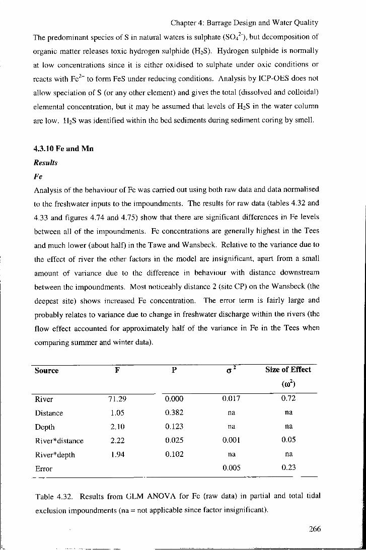
Chapter 4: Barrage Design and Water Quality
The predominant species of S in natural waters is sulphate (S04^'), but decomposition of
organic matter releases toxic hydrogen sulphide ( H 2 S ) . Hydrogen sulphide is normally
at low concentrations since it is either oxidised to sulphate under oxic conditions or
reacts with Fe""* to form FeS under reducing conditions. Analysis by ICP-OES does not
allow speciation of S (or any other element) and gives the total (dissolved and colloidal)
elemental concentration, but it may be assumed that levels of H 2 S in the water column
are low. H 2 S was identified within the bed sediments during sediment coring by smell.
4.3.10 Fe and Mn
Results
Fe
Analysis of the behaviour of Fe was carried out using both raw data and data normalised
to the freshwater inputs to the impoundments. The results for raw data (tables 4.32 and
4.33 and figures 4.74 and 4.75) show that there are significant differences in Fe levels
between all of the impoundments. Fe concentrations are generally highest in the Tees
and much lower (about half) in the Tawe and Wansbeck. Relative to the variance due to
the effect of river the other factors in the model are insignificant, apart from a small
amount of variance due to the difference in behaviour with distance downstream
between the impoundments. Most noticeably distance 2 (site CP) on the Wansbeck (the
deepest site) shows increased Fe concentration. The error term is fairly large and
probably relates to variance due to change in freshwater discharge within the rivers (the
flow effect accounted for approximately half of the variance in Fe in the Tees when
comparing summer and winter data).
Source F P a' Size of Effect
River 71.29 0.000 0.017 0.72
Distance 1.05 0.382 na na
Depth 2.10 0.123 na na
River*distance 2.22 0.025 0.001 0.05
River*depth 1.94 0.102 na na
Error 0.005 0.23
Table 4.32. Results from GLM ANOVA for Fe (raw data) in partial and total tidal
exclusion impoundments (na = not applicable since factor insignificant).
266

Chapter 4: Barrage Design and Water Quality
distance depth
0.16 H
0.14
0.12 -\
0.10
0.08
Figure 4.74. Main effects plot for the factors of impoundment (river), distance and
depth on Fe (raw data) (LS means for factor levels).
0.19 - I
0.17
0.15
5) 0.13 E,
O 0.11
0.09
0.07
0.05 2
I 3
distance
river 9 Tawe a Tees 4 Wansbeck
Figure 4.75. Interaction between river and distance effects on Fe (raw data) (LS
means).
267

Chapter 4: Barrage Design and Water Quality
Factor Pairwise comparison Adjusted P-value
River Tees - Tawe 0.000
Wansbeck - Tawe 0.012
Wansbeck - Tees 0.000
Table 4.33. Results from Tukey simultaneous tests on the significance of differences
between the means of factor levels used in the ANOVA for Fe (raw data) in partial and
total tidal exclusion impoundments.
Repeating the analysis using data normalised to input values (i.e. removing the variation
in inputs to the systems) shows contrasting results to those from analysis of raw data.
Al l factors in the model show significant effects. The Tees and the Tawe behave in the
same manner and show no overall increase in Fe concentrations relative to the
freshwater input levels, whereas within the Wansbeck mean Fe concentration is
increased (by approximately 22 %) relative to that entering in the freshwater input.
Also within the Wansbeck Fe levels are approximately 80 % higher in deep water than
in surface water. The river*distance interaction suggests that (ignoring the depth effects
for the Wansbeck) Fe decreases downstream in the partial exclusion systems (seawater
Fe levels are lower than those in freshwater), and increases slighdy with distance
downstream in the Tees.
Source F P Size of Effect
(0)')
River 6.50 0.002 0.138 0.08
Distance 1.79 0.129 na na
Depth 9.50 0.000 0.213 0.12
River* distance 4.74 0.000 0.375 0.22
River*depth 9.90 0.000 0.447 0.26
Error 0.564 0.32
Table 4.34. Results from GLM ANOVA for Fe (data normalised to input values) in
partial and total tidal exclusion impoundments (na = not applicable since factor
insignificant).
268

Chapter 4: Barrage Design and Water Quality
1.26 distance depth
Figure 4.76. Main effects plot for the factors of impoundment (river), distance and
depth on Fe (data normalised to input values) (LS means for factor levels).
1.4
^ 1.3
|> 1.2
1.1
1.0
0.9
0.8
0.7
/
i~
/ ">
\ / » /
\ y \ /
^ m @ —
B - ' ' "
>"
river # Tawe • Tees ^ Wansbeck
3 distance
Figure 4.77. Interaction between river and distance effects on Fe (data normalised to
input values) (LS means).
269

Chapter 4: Barrage Design and Water Quality
1.8 - A
1.6
I ' 1.4
U-1.2 -A
1.0 O-
1 d
1 m
1 s
river
O Tawe • Tees O Wansbeck
depth
Figure 4.78. Interaction between river and depth effects on Fe (data normalised to input
values) (LS means).
Factor Pairwise comparison Adjusted P-value
River Tees - Tawe 0.859
Wansbeck - Tawe 0.001
Wansbeck - Tees 0.031
Table 4.35. Results from Tukey simultaneous tests on the significance of differences
between the means of factor levels used in the ANOVA for Fe (data normalised to input
values) in partial and total tidal exclusion impoundments.
Mn
Results for Mn using both raw and normalised data are very similar since levels in the
inputs are close to zero (< O.I mg/1) in all three impoundments. Results for raw data are
presented. Mean Mn levels are highest in the Wansbeck and lowest in the Tees. The
distance pattern shows a small increase in Mn in the Tees (as was identified during
examination of seasonal effects in the Tees), and depth related patterns in the other
impoundments. Depth is the most significant factoi and there are small increases in Mn
with depth in the Tees and Tawe, and much larger increases in the Wansbeck.
270
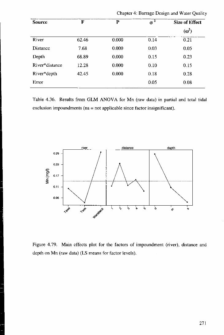
Chapter 4: Barrage Design and Water Quality
Source F P Size of Effect
(0)')
River 62.46 0.000 0.14 0.21
Distance 7.68 0.000 0.03 0.05
Depth 68.89 0.000 0.15 0.23
River*distance 12.28 0.000 0.10 0.15
River*depth 42.45 0.000 0.18 0.28
Error 0.05 0.08
Table 4.36. Results from GLM ANOVA for Mn (raw data) in partial and total tidal
exclusion impoundments (na = not applicable since factor insignificant).
river distance depth
0.05 H
Figure 4.79. Main effects plot for the factors of impoundment (river), distance and
depth on Mn (raw data) (LS means for factor levels).
271

Chapter 4: Barrage Design and Water Quality
E
river O Tawe Q Tees <> Wansbeck
distance
Figure 4.80. Interaction between river and distance effects on Mn (raw data) (LS
means).
E
0.7 -
0.6
0.5
0,4
0.3
0 2 -
0.1 —
0.0 -Q-
Q
1 d
1
m depth
1 s
river O Tawe D Tees O Wansbeck
Figure 4.81. Interaction between river and depth effects on Mn (raw data) (LS means).
272

Chapter 4: Barrage Design and Water Quality
Factor Pairwise comparison Adjusted P-vaiue
River Tees - Tawe 0.006
Wansbeck - Tawe 0.000
Wansbeck - Tees 0.000
Table 4.37. Results from Tukey simultaneous tests on the significance of differences
between the means of factor levels used in the ANOVA for Mn (raw data) in partial and
total tidal exclusion impoundments.
Discussion
For the Tees it was noted that Fe increased with flow (to a greater degree in summer
than winter), and a humic source (peat uplands) and transport mechanism were
suggested. Assuming this to be the case, then the extensive areas of peat present in the
Tees catchment (but not in the catchments of the Tawe or Wansbeck) explains the
difference between the impoundments in their overall Fe concentrations. For the partial
exclusion systems flow is also a major control on Fe concentrations in freshwater
(figure 4.82), and both the Tawe and the Wansbeck show positive correlations between
Fe concentration and freshwater discharge (R-Sq = 52.6 % and 68.3 % respectively).
02
0.1
0.0
5 10 15 20
mean flow preceding sampling (cumecs)
Figure 4.82. The semi-log relationship between Fe in freshwater (Na < 300mg/l) and
flow in the Tawe impoundment (R-Sq = 52.6 %) .
273

Chapter 4: Barrage Design and Water Quality
o _ O cP
o o o ^ o "conservative mixing
5000
Na (mg/l)
— r
10000
Figure 4.83. The freshwater flow and conservative mixing controls of Fe in the Tawe
impoundment. Open circles represent sampling which disturbed bed sediment.
0.3 - f
^ 0.2 - \
0.1
0.0 - I
flow CP (distance 2) deep sanples
conservative mixing n 1 1 1 1 1 1 1 I
0 1000 2000 3000 4000 5000 6000 7000 8000 9000
Na (mg/l)
Figure 4.84. The freshwater flow and conservative mixing controls of Fe in the
Wansbeck impoundment. Increased Fe concentrations are measureu in deep samples
from site CP due to sedimentary release under reducing conditions.
274

Chapter 4: Barrage Design and Water Quality
The mixing between fresh and seawater in both the Tawe and Wansbeck impoundments
is conservative (figures 4.83 and 4.84) and, since over the sampHng periods the mean
level in the seawater end-member was lower than the mean freshwater levels, the
distance effect in the ANOVA is of decreasing Fe with distance downstream (increasing
seawater mixing). A significant depth effect is shown for the Wansbeck impoundment
however, and increased Fe concentrations are measured at depth at site CP (distance 2)
within the impounded area (figure 4.84).
1.5
D) 1.0 E
0.5
0.0
0.0 0.1 0.2 0.3 Fe (mg/l)
Figure 4.85. The main controls on Fe and Mn in the impoundments (data from
Wansbeck sunmier sampling). Fe concentration in shallow water is controlled by
freshwater discharge (1). Fe concentration in deep (saline) water and Mn concentration
are controlled by release from sediment under low DO conditions (2).
The solubility of Fe is redox dependent. Under normal oxygenated conditions dissolved
Fe is normally found mainly associated with organic colloids. Under reducing
conditions (< 250 mV) Fe^^ (ferrous iron) diffuses from sediments to increase dissolved
Fe concentrations. Whereas for the Tees and Tawe these reducing conditions were not
reached, entrenched stratification of the water body in the Wansbeck impoundment at
site CP allows Fe^* to build-up in deep water. As mentioned above, under very low
redox conditions (< 100 mV) H 2 S is produced and reacts with Fe " to precipitate FeS.
Observational sedimentary evidence from sediment coring on the Wansbeck (i.e. the
275

Chapter 4: Banage Design and Water Quality
presence of a pale oxidised microzone above black (sulphide rich) sediment) suggests
that these conditions are not reached in the water column but are just below the surface
of the bed sediments.
The behaviour of Mn is similar to that of Fe in terms of redox control. Mn is mobile at
slightly higher redox potentials (less reducing conditions) than Fe, and Mn will remain
soluble in waters in which DO < approximately 50 % (Bums and Nriagu, 1976; figure
4.86). The external controls on Mn are seen to be minor compared to the redox controls
taking place within the impounded areas.
1.5 H
O) 1.0
0.5
0.0 H
D 0 % 150
Figure 4.86. Mn vs. DO % in the Wansbeck impoundment (summer data). Mn is
insoluble at DO greater than approximately 50 %. The scatter of points of increased Mn
at higher DO concentrations and low Mn at low DO concentrations are from sampling
at mid-depths and are interpreted as due to the problems of sampling close to a sharp
density interface.
As might be expected given the release of Fe from the sediment to the water column at
depth noted above, the Wansbeck shows increased levels of Mn in deep water samples.
Mn concentration in freshwater and in "new" seawater are close to zero and increase to
a maximum of approximately 1.5 mg/1 at depth at site CP (at which significant release
of Fe is observed). The rate of release of Mn can be determined over the same period
(T' to 7* October 2000) for which DO, etc. were modelled above (figure 4.87):
276

Chapter 4: Barrage Design and Water Quality
E
Figure 4.87. Rate of release of Mn from sediment under anoxic (DO < 50 %)
conditions at depth at site CP in the Wansbeck.
Mn =0.467 + 0.131 day (S = 0.0335 R-Sq = 98.8 % R-Sq(adj) = 98.6 %)
where,
Mn = concentration of Mn in mg/l, and
day = number of days following reduction of DO to below approximately 50 %.
The amounts of release of Mn in the Tawe and Tees impoundments are significant but
lower than in the Wansbeck due to the less frequent occurrence of low oxygen (< 50 %)
conditions at depth (see comparison of DO behaviour above).
4.3.11 Fe and P
It is well established that there is a strong affinity between P and particulate Fe(OH)3 in
sediments in water bodies, and thus that P mobility may be redox mediated (Mortimer,
1941 and 1942). For the Wansbeck it has been shown that anoxic conditions can
develop in the water column which allow the reduction of Fe " to Fe " , and it is possible
that release of P is associated with this (figure 4.88), although relative to the variation in
277

Chapter 4: Baixage Design and Water Quality
P in the riverine inputs to the impoundments the impact is minor. In addition, any
increase in the amount of dissolved (bio-avaiiable) P will occur under reducing
conditions at depth and is therefore not likely to contribute to an increase in primary
production in the systems. Upon mixing with surface waters Fe(0H)3 wil l re-precipitate
and scavenge dissolved P, thus removing any effects of redox controlled sedimentary P
release on biota.
•Fe •Mn
1.00 ^ E 0.15
0.80 E = 0.10
0.05 +
0.00 4
d a y
Figure 4.88. Mn, Fe and P over the period l " to 7* October 2000 in deep water at site
CP in the Wansbeck impoundment during the development of anoxia, showing the
possible relationship between release of Fe and release of P from sediment to the water
column.
278

Chapter 4: Barrage Design and Water Quality
4.4 Summary and conclusions
Within this chapter the three impounded estuaries included in this research have been
compared in terms of the summer behaviour of a range of 18 water quality variables.
Initially principal components analysis (PCA) was used to identify the correlation
structure of the multivariate dataset, and through this to identify likely controlling
processes on these groups of variables. Subsequently, general linear modelling was
used to statistically assess the differences between the impoundments and the
importance of processing within the impounded areas relative to the external controls on
water quality. During discussion of the results obtained regression was carried out
between a variety of the water quality variables and their underlying controls.
The first 2 principal components produced by PCA were interpreted as representing
significant controls on a variety of variables, whilst the 3' '' and 4* principal components
showed less clear relationships to any single controlling process:
• PCI = salinity control (variables showing different levels in saline and fresh
water in the impoundments: conductivity, Ca, nitrate, ammonia, Mn and DO).
• PC2 = freshwater flow control (variables showing variation with discharge in the
freshwater inputs to the impoundments: alkalinity, phosphate, T, Fe and TSS).
• PCS = pH and alkalinity score strongly (probably representing a baseflow or
geological control rather than a biological control on these parameters since
coefficients are of the same sign).
• PC4 = nitrate and phosphate score strongly (representing a similar overall source
for these nutrients).
PCA allowed only simple and qualitative comparison of the three impoundments, and
so more detailed investigation was carried out using general linear modelling
(ANOVA).
Significant differences of varying degrees were shown between the impoundments for
all of the water quality parameters assessed, with the exception of BOD (for which
limited data was available). By comparing analyses carried out using raw data and
carried out using data normalised to the freshwater inputs to the impounded areas, the
amount of variation external to the impounded areas relative to the variation within the
impounded areas was assessed. The external variation can be thought of as independent
279

Chapter 4: Barrage Design and Water Quality
of the construction of a barrage, whereas the internal variation may be affected by
impoundment. The processes identified as important in the control of the water quality
parameters are listed in table 4.38 in approximate order of significance.
Parameter (0 for river (if
significant)
Controlling processes
DO
BOD
PH
Alkalinity
0.31 (raw)
0.16 (norm)
Not significant
(data for Tees and
Tawe only)
0.06 (raw)
0.24 (norm)
0.86 (raw)
0.13 (norm)
Conductivity
TSS
0.23 (raw)
Transparency 0.91 (raw)
0.58 (raw)
Not significant
(norm)
Microbial respirative utilisation of DO relative to
re-oxygenation (strongly related to density
stratification).
Flow controlled removal of organic material in
catchments.
Amount of seawater mixing (conservative).
Microbial respiration (strongly related to density
stratification).
Catchment geology.
Flow controlled dilution of baseflow.
Amount of seawater mixing (conservative).
Microbial respiration (strongly related to density
stratification).
Density stratification (breakdown in stratification
and conservative mixing between seawater and
freshwater related to freshwater flow).
Flow controlled dilution of baseflow (freshwater
conductivities).
Catchment controls on particulate availability.
Flow controlled turbidity.
Re-suspension of bed material within the
impounded areas.
Catchment controls on particulate availability.
Flow controlled turbidity.
Re-suspension of bed material within the
impoundec' ireas.
280

Chapter 4: Barrage Design and Water Quality
Phosphate
Major
elements
Fe
0.13 (raw)
0.18 (norm)
0.22 (norm + DO
as covariate)
0.74 (raw)
Nitrate 0.67 (raw) Catchment, point-source and flow effects on
0.58 (norm) river inputs.
Amount of seawater mixing (conservative).
Denitrification and reduction to ammonia
(strongly related to density stratification).
Ammonia 0.13 (raw) Point source inputs to the rivers.
Amount of seawater mixing (conservative).
Microbial respiration and reduction of nitrate
(strongly related to density stratification).
Point-source and flow effects on river inputs.
Biological utilisation.
Possible release from sediment (strongly related
to density stratification) in Wansbeck only.
Si 0.61 (raw) Catchment geology, land-use and flow effects on
river inputs.
Amount of seawater mixing (conservative).
Release from sediment (strongly related to
density stratification) in Wansbeck only.
0.21 (raw) Amount of seawater mixing (conservative).
0.72 (raw) Catchment (amount of peat) and flow effects on
0.08 (norm) river inputs.
Amount of seawater mixing (conservative).
Redox controlled release from sediment (strongly
related to density stratification) in Wansbeck
only.
Mn 0.21 (raw) Redox controlled release from sediment (strongly
related to density stratification), maximum in
Wansbeck but significant in all impoundments.
Table 4.38. Summary of the effects of river (impoundment) and proposed important
controlling processes on water quality within the Tees, Tawe and Wansbeck
impoundments, raw = results from analysis of raw data, norm = results from analysis
of data normalised to freshwater inputs.
281

Chapter 4: Barrage Design and Water Quality
Four types of control on water quality are identified. These can be summarised as:
1. Catchment controls on external inputs.
2. Flow controls on external inputs.
3. Internal mixing of seawater and freshwater.
4. Internal processing related to density stratification.
4.4.1 Catchment controls
Difference between the rivers entering the impoundments is the most important factor in
controlling the levels of alkalinity, transparency and TSS, phosphate. Si and Fe in the
impoundments, and is a significant factor for several other variables. The catchments
vary in terms of size, geology, relief and precipitation, land-use, etc. and in the point-
source inputs within them. Whilst some suggestion has been made of how catchment
relates to water quality parameters, the study of catchment processes is generally
beyond the scope of this thesis. However, it is important to note that for all
impoundments, for several of the parameters, catchment management is the key to
controlling water quality. This is particularly significant for phosphate and for
suspended solids (TSS), both of which are identified as of major importance in
impounded water quality. Both the Tawe and the Wansbeck have been identified as P
limited in terms of primary productivity, and therefore any control of the eutrophic
behaviour of these impoundments must be by reduced P inputs to the rivers entering the
impoundments. Equally control of sedimentation within the impoundments should
focus on the sediment sources to the rivers. Identification of sediment sources and
transport form specific themes of the SIMBA project (Nelson, 2003; Beavers, 2003).
4.4.2 Freshwater flow controls
Several parameters show strong relationships to levels in freshwater and river discharge.
The sign and nature of the correlations varies according to the sources within the
catchments of the parameters:
1. Negative correlation = dilution effect (alkalinity, conductivity, nitrate (Tawe and
Tees), phosphate and major elements).
2. Positive correlation = diffuse source (BOD, TSS, nitrate (Wansbeck) am Fe).
The exact relationships vary between the catchments, and are dependent on the
282

Chapter 4: Barrage Design and Water Quality
catchment factors discussed above (e.g. geology, land-use, quantity of sewage inflows).
Generally higher flows also act to remove stratification and so reduce the probability of
the development of low water quality conditions at depth. However, the majority of
sediment transport within systems takes place during conditions of peak flow,
particularly in the Tees where bank erosion provides a major source of fine material (S.
Anderton, pers. com.). For Devon rivers, Webb and Walling (1982a) give that 90 % of
the TSS transport takes place in 10 % or less of the time. High flow conditions, and the
associated sediment transport and deposition within the impounded areas, are therefore
important in assessing the long term sustainability of estuarine barrage systems.
4.4.3 Mixing controls
Several parameters show markedly different levels between the two main water sources
(i.e. seawater and freshwater) which enter partial tidal exclusion impoundments:
1. Higher in seawater: Alkalinity, conductivity, major elements (Na, Mg, Ca, K
and S), ammonia and P.
2. Higher in freshwater: DO (absolute concentration), pH, Si and nitrate.
The mixing of major elements and conductivity is conservative between fresh and
seawater. The mixing of the majority of other parameters is generally conservative, but
may show alteration within the impoundments through a variety of processes related to
density stratification.
4.4.4 Stratiflcation controls
Impounded water bodies may become stratified due to density differences in the water
column based on salinity or temperature differences. This stratification can lead to
water at depth which is isolated from the atmosphere and in contact with oxygen
demanding organic rich bed sediments. Respiration (organic decomposition) in excess
of re-oxygenation cause a reduction in DO, and a simultaneous decrease in pH and
increase in alkalinity. Under these reducing conditions a lack of denitrification and
nitrate reduction leads to a decrease in nitrate and increase in ammonia concentrations
in the deep water. Under sustained isolation of the deep water redox conditions
decrease to levels at which Mn and subsequently Fe and associated P are released from
the sediment to the water column.
283

Chapter 4: Barrage Design and Water Quality
Stratification is stronger in partial than total tidal exclusion impoundments since the
density differences based on salinity differences are much greater than those due to
temperature differences alone. The effects of the processes associated with stratification
are particulariy significant at deep locations within the impoundments upstream of more
shallow sections since only the highest tides are able to replace the "stagnant" deep
waters with "fresh" (oxygenated) seawater. The length of the periods of isolation of
these "ponded" waters is therefore greatest at these points. The Tawe barrage allows a
larger proportion of tides to enter the impoundment and therefore has shorter periods of
isolation of deep water and better water quality than the Wansbeck. Stratification may
also be removed under conditions of high freshwater discharge through the development
of internal waves and mixing upwards of the saline water.
284

Chapter 5: Barrage Presence and Water Quality
Chapter 5
Barrage Presence and Water Quality
5.1 Introduction
The study of the effects of barrage construction on estuaries is limited by the lack of
good water quality data pre-dating impoundment. However, understanding the
difference between estuaries in their natural state and those that are impounded is
fundamental in planning and policy for estuarine barrage construction. To aim to
answer this question, comparison of two equivalent estuaries - one impounded and one
un-impounded - was carried out.
The Wansbeck impounded estuary has already been examined for seasonal differences
in water quality and in comparison with the Tees and Tawe impounded estuaries
(chapter 3 and chapter 4). Here results for comparison of the Wansbeck with the River
Blyth un-impounded estuary are presented. As described in chapter 1, the Blyth runs
parallel to the Wansbeck to enter the North Sea approximately 5 km to the south of the
mouth of the Wansbeck, and is of almost identical size (both 339.4 km^), geology, relief
and land-use of catchment (Archer 1992). Both estuaries were sampled daily during the
period 4* to 12* June 2001, with sampling on the Blyth following that on the Wansbeck
by not more than 2 hours.
A general linear model (ANOVA) including the terms of river, distance downstream
within the estuary and depth within the estuary plus the interactions between river and
distance and river and depth was used. Distance/sampling site were represented by
numbers 1 to 4 from the former tidal limit (SW) on the Wansbeck or the tidal limit (TL)
on the Blyth, downstream to the barrage (WB) for the Wansbeck or a similarly
distanced site (PS) on the Blyth. In order to give the same number of distances for both
estuaries, data from site CI on the Wansbeck is excluded from the analyses. Depth is
represented by sampling at shallow (S), mid-depth (m) and deep (d) at each sampling
site (with the exception of the tidal limit or former tidal limit at which only surface
samples were taken). For practical reasons sampling was carried out approximately 2
hours before high tide on the Wansbeck and at high tide on the Blyth. The tidal heights
during the sampling period were such that the barrage on the Wansbeck was overtopped
by seawater on the majority of sampling dates compared, with only the first day (4"
June 2001) following a period of 8 days of non-overtopping and the final 3 days (lO'*",
285

Chapter 5: Barrage Presence and Water Quality
U " ' and 12" June 2001) sampling days 1, 2 and 3 of the subsequent non-overtopping
period. Analyses were carried out using both raw data and data normalised to the
freshwater inputs to the estuaries to allow assessment of the differences between
estuaries based on catchment effects and those due to differences in behaviour due to
the presence of a bairage. Results are presented for those parameters that show
significant internal (within estuary) variation (DO, pH, TSS, nitrate, ammonia,
phosphate, Na/major elements, Fe and Mn).
5.2 Results and discussion
5.2.1 Dissolved oxygen
Results
There is very little difference between the results for raw data and the results for
normalised data since freshwater input DO concentrations are similar between days and
between rivers (implying that the choice of the Blyth as a comparable estuary to the
Wansbeck was justified). DO concentrations are significantly lower in the Wansbeck
than the Blyth (table 5.1 and figure 5.1), and this difference is due to variation within
the impounded area of the Wansbeck (table 5.2). Depth has a significant effect and
shows significant interaction with river. DO concentrations decrease with depth in both
estuaries but to a far greater extent in the Wansbeck (figure 5.3). There is a similar
slight decrease in DO with distance downstream in both estuaries but this is
compounded by a large reduction in DO at distance 2 (site CP) at the deepest point of
the Wansbeck (figure 5.2).
Source F P a" Size of Effect
(to')
River 20.97 0.000 257 0.09
Distance 7.63 0.000 255 0.09
Depth 41.70 0.000 1046 0.36
River* distance 12.99 0.000 462 0.16
River*depth 23.08 0.000 568 0.20
Error 308 0.11
Table 5.1. Results from GLM ANOVA for DO % (raw cluta) between the Blyth estuary
and the Wansbeck impounded estuary.
286

Chapter 5: Barrage Presence and Water Quality
O Q
95
85
75 A
65 H
55
river distarx» depth
Figure 5.1. Main effects plot for the factors of river, distance and depth on DO % (raw
data) in the Blyth and Wansbeck estuaries (LS means for factor levels).
nver 96
86 - \
76
o Q 66
56 -4
46
• Blyth B Wansbeck
distance
Figure 5.2. Interaction between river and distance effects on DO % (raw data) for the
Blyth and Wansbeck estuaries (LS means).
287
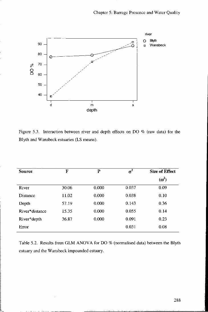
Chapter 5: Barrage Presence and Water Quality
90 - \
80
70
o <=> 60
50
40
river O BIyth • Wansbeck
depth
Figure 5.3. Interaction between river and depth effects on DO % (raw data) for the
Blyth and Wansbeck estuaries (LS means).
Source F P a" Size of Effect
River 30.06 0.000 0.037 0.09
Distance 11.02 0.000 0.038 0.10
Depth 57.19 0.000 0.143 0.36
River* distance 15.35 0.000 0.055 0.14
River*depth 36.87 0.000 0.091 0.23
Error 0.031 0.08
Table 5.2. Results from GLM ANOVA for DO % (normalised data) between the Blyth
estuary and the Wansbeck impounded estuary.
288

Chapter 5: Barrage Presence and Water Quality
river distance depth
Figure 5.4. Main effects plot for the factors of river, distance and depth on DO %
(normalised data) in the Blyth and Wansbeck estuaries (LS means for factor levels).
1.02
0.92 -A O Q •g 0.82 m la E 0.72 b c
0.62 -A
0.52 -A
river
• Blyth • Wansbeck
distance
Figure 5.5. Interaction between river and distance effects on DO % (normalised data)
for the Blyth and Wansbeck estuaries (LS means).
289

Chapter 5: Barrage Presence and Water Quality
0.9 -A
O Q 0.8 •a 0}
0.7 CO b 0.6
0.5
0.4
o -Qr^ "7^^ y y y y y
y ^y
y y /
/ y y y y /
U
1 d
1 m
1 s
depth
river
O BIyth • Wansbeck
Figure 5.6. Interaction between river and depth effects on DO % (normalised data) for
the Blyth and Wansbeck estuaries (LS means).
Discussion
The Blyth and the Wansbeck estuaries behaved significantly differently in terms of DO
during the periods sampled. The major difference was the greater degree of oxygen
depletion at depth within the Wansbeck, and this was in particular affected by the low
DO conditions encountered almost throughout the sampling period at depth at site CP.
As has been discussed site CP is the deepest point of the Wansbeck and shows long
periods of isolation of saline water, which is only removed under conditions of high
freshwater discharge or replaced when the highest (> 4.9 m) tides force new saline
water upstream to this point. For the Blyth no similar sites of dramatically reduced DO
at depth were encountered, and it is suggested that the unrestricted tidal circulation,
along with the generally shallower depth, means that such "ponding" of saline water at
depth does not occur. The minimum DO concentration encountered in the Blyth was
53.5 % compared with 0.00 % over a sustained period in the Wansbeck.
290

Chapter 5: Barrage Presence and Water Quality
5.2.2 p H
Results
Freshwater input values fo r the two rivers are similar and hence, as with DO, results are
similar for both raw and normalised data. There are no significant differences between
the two estuaries overall (tables 5.3 and 5.4) (power of detecting a significant difference
using data collected calculated as 1.000 for one-way A N O V A ) . Both systems are well
buffered and show low p H variation. Both depth and distance are significant effects
however, and both show interaction with river. pH decreases with depth and to a
greater extent in the Wansbeck, and shows a decrease followed by an increase with
distance downstream in both estuaries, and a large drop in value at distance 2 (site CP)
in the Wansbeck. For both analyses a relatively large amount of variance is
unexplained and may relate to varying amounts of biological productivity and
respiration spatially and temporally.
Source F P a" Size of Effect
( « ' )
River 2.82 0.094 na na
Distance 3.58 0.015 0.16 0.14
Depth 6.88 0.001 0.25 0.21
River* distance 3.33 0.020 0.15 0.12
River*depth 4.21 0.016 0.14 0.11
Error 0.51 0.42
Table 5.3. Results f rom G L M A N O V A for p H (raw data) between the Blyth estuary
and the Wansbeck impounded estuary (na = not applicable since factor insignificant at
95 % level).
291

Chapter 5: Barrage Presence and Water Quality
river distance depth
I Q.
7,48
7.36 H
7.24
7.12
7.00
Figure 5.7. Main effects plot for the factors of river, distance and depth on pH (raw
data) in the Blyth and Wansbeck estuaries (LS means for factor levels).
X Q.
river
© Blyth • Wansbeck
distance
Figure 5.8. Interaction between river and distance effects on pH (raw data) for the
Blyth and Wansbeck estuaries (LS means).
292

Chapter 5: Barrage Presence and Water Quality
river
I Q.
Blyth Wansbeck
depth
Figure 5.9. Interaction between river and depth effects on p H (raw data) for the Blyth
and Wansbeck estuaries (LS means).
Source F P Size o f Effect
(0)')
River 0.62 0.431 na na
Distance 8.24 0.000 0.0035 0.19
Depth 16.10 0.000 0.0049 0.27
River*distance 7.64 0.000 0.0032 0.18
River*depth 9.74 0.000 0.0028 0.15
Error 0.0039 0.21
Table 5.4. Results f rom G L M A N O V A for pH (normalised data) between the Blyth
estuary and the Wansbeck impounded estuary (na = not applicable since factor
insignificant at 95 % level).
293

Chapter 5: Barrage Presence and Water Quality
I Q.
T3 <B I f )
O C
1.00559
0.98519
0.96479 -Jr
0.94439
0.92399
distarxje depth
Figure 5.10. Main effects plot for the factors of river, distance and depth on pH
(normalised data) in the Blyth and Wansbeck estuaries (LS means for factor levels).
.00 - A
0.99 - \
CL 0.98 0 0.97
S 0.96
^ 0.95
river
® Blyth o Wansbeck
distance
Figure 5.11. Interaction between river and distance effects on pH (normalised data) for
the Blyth and Wansbeck estuaries (LS means).
294
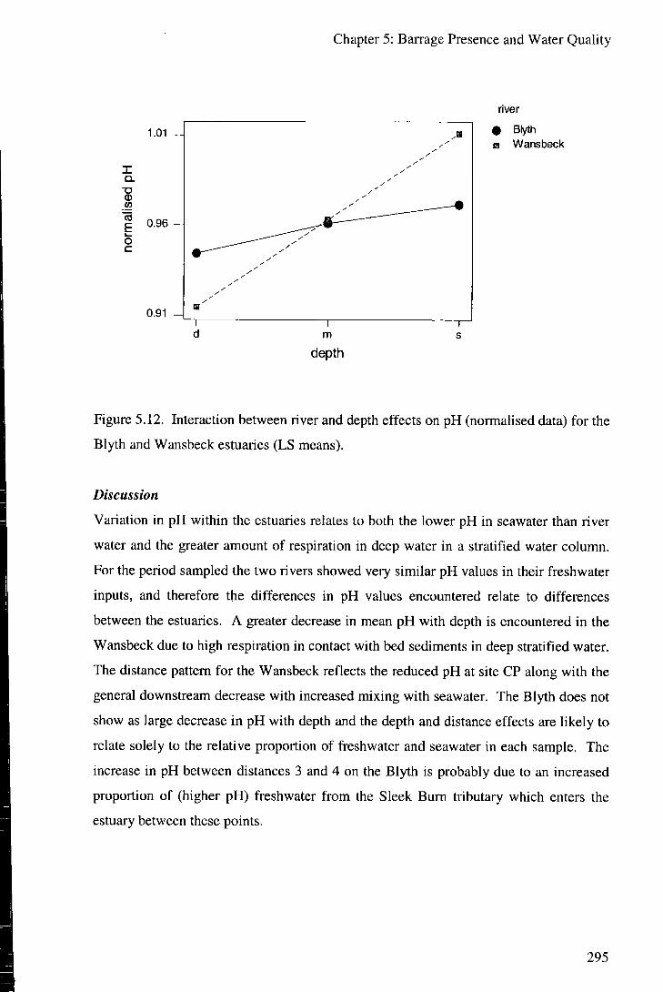
Chapter 5: Barrage Presence and Water Quality
1.01
X
Q.
«
E o c
0.96 -A
0.91
river
• Blyth • Wansbeck
depth
Figure 5.12. Interaction between river and depth effects on p H (normalised data) for the
Blyth and Wansbeck estuaries (LS means).
Discussion
Variation in p H within the estuaries relates to both the lower pH in seawater than river
water and the greater amount of respiration in deep water in a stratified water column.
For the period sampled the two rivers showed very similar p H values in their freshwater
inputs, and therefore the differences in pH values encountered relate to differences
between the estuaries. A greater decrease in mean p H with depth is encountered in the
Wansbeck due to high respiration in contact with bed sediments in deep stratified water.
The distance pattern for the Wansbeck reflects the reduced p H at site CP along wi th the
general downstream decrease with increased mixing wi th seawater. The Blyth does not
show as large decrease in pH with depth and the depth and distance effects are l ikely to
relate solely to the relative proportion of freshwater and seawater in each sample. The
increase in pH between distances 3 and 4 on the Blyth is probably due to an increased
proportion of (higher pH) freshwater f rom the Sleek Bum tributary which enters the
estuary between these points.
295

Chapter 5: Barrage Presence and Water Quality
5.2.3 TSS
Results
Again, as for DO and pH, results are very similar for analyses using raw and normalised
data since the freshwater input values are similar and the majority of variance in the
dataset is within the estuaries. Mean concentration of TSS is significantly higher in the
Blyth than in the Wansbeck. TSS increases with distance downstream and depth in both
estuaries (figure 5.13). The increase in TSS with distance is greater in the Blyth than
the Wansbeck (figure 5.14). The depth effect also varies between the estuaries, with the
Blyth showing maximum increase in TSS between shallow and mid-depths and the
Wansbeck showing maximum increase between mid-depth and deep samples (figure
5.15). Overall TSS levels are approximately 4 times higher in the estuary than in the
river input in the Wansbeck during the sampling period and 9 times greater in the Blyth
estuary (figure 5.16).
Source F P a" Size of Effect
(0)')
River 109.85 0.000 1509 0.21
Distance 32.78 0.000 1322 0.18
Depth 81.35 0.000 2228 0.31
River* distance 26.29 0.000 1052 0.15
River*depth 29.86 0.000 800 0.11
Error 333 0.05
Table 5.5. Results f rom G L M A N O V A for TSS (raw data) between the Blyth estuary
and the Wansbeck impounded estuary.
296

Chapter 5: Barrage Presence and Water Quality
distance depth
Figure 5.13. Main effects plot for the factors of river, distance and depth on TSS (raw
data) in the Blyth and Wansbeck estuaries (LS means for factor levels).
E, CO CO
river
• Blyth m Wansbeck
distance
Figure 5.14. Interaction between river and distance effects on TSS (raw data) for the
Blyth and Wansbeck estuaries (LS means).
297

Chapter 5: Barrage Presence and Water Quality
CO
river
O Blyth Q Wansbeck
depth
Figure 5.15. Interaction between river and depth effects on TSS (raw data) for the Blyth
and Wansbeck estuaries (LS means).
Source F P a" Size o f Effect
River 34.20 0.000 27.3 0.24
Distance 10.41 0.000 23.2 0.20
Depth 16.41 0.000 25.3 0.22
River*distance 6.15 0.000 12.7 0.11
River*depth 4.80 0.009 6.2 0.05
Error 19.7 0.17
Table 5.6. Results f rom G L M A N O V A for TSS (normalised data) between the Blyth
estuary and the Wansbeck impounded estuary.
298

Chapter 5: Barrage Presence and Water Quality
distance
8
9 H
CO 7
•D (1)
3 A
depth
Figure 5.16. Main effects plot for the factors of river, distance and depth on TSS
(normalised data) in the Blyth and Wansbeck estuaries (LS means for factor levels).
CO
E i— o c
river
11
1 -A
• Blyth B Wansbeck
distance
Figure 5.17. Interaction between river and distance effects on TSS (normalised data)
for the Blyth and Wansbeck estuaries (LS means).
299

Chapter 5: Barrage Presence and Water Quality
CO
w
E o c
river
O Blyth • Wansbeck
depth
Figure 5.18. Interaction between river and depth effects on TSS (normalised data) for
the Blyth and Wansbeck estuaries (LS means).
Discussion
The freshwater sediment inputs to the Blyth and the Wansbeck estuaries were similar
during the period studied, which is in contrast with the comparison of impoundments in
which it was shown that the major variation is due to differences between the
concentrations of TSS carried by the rivers. For the Blyth and the Wansbeck the major
difference in TSS behaviour is due to differences within the estuaries. These differences
are interpreted as due to the effect of barrage construction on tidal circulation and
mixing in the systems.
For the Wansbeck, sampling of the seawater entering the impounded area during
overtopping showed that the majority of sediment within the impounded area is
delivered in the freshwater inputs. Potsma (1980) gives that most TSS in strongly
stratified estuaries is of f luvial source and is transported downstream in the freshwater
layer. No estimation can be made of the contribution f rom the sea by tidal pumping for
the Blyth, and it is suggested that further sediment fingerprinting work is carried out to
determine the relative contributions i i . impounded compared with un-impounded
systems. However, assuming that the sediment contribution f rom the sea is also low in
the Blyth, then the greater TSS concentrations encountered in this estuary are due to
300

Chapter 5: Barrage Presence and Water Quality
greater tidal flows and higher bed shear stresses acting to cycle bed sediment and create
a "turbidity maxima" (Dyer 1997). For the Wansbeck tidal circulation is reduced and
re-suspension of bed sediment is lower, and its effects limited to deeper water. The
effect of the combined discharge f rom the Blyth and Cramlington Sewage Treatment
Works (STW) into the middle of the Blyth estuary (NZ 2950 8249; 11,664 mVday of 30
mg/1 solids dry weather maximum and 9,600 mVday of 80 mg/1 solids respectively)
appears to have no effect on the distribution of TSS.
150
^ 100
E, CO ^ 50
0 H
o •
5000
Na (mg/1)
10000
o Blyth • Wansbeck
Figure 5.19. TSS vs. Na concentrations in the Blyth and Wansbeck estuaries. The
greater TSS values in the Blyth which has higher seawater influence are interpreted as
due to greater tidal currents and cycling of bed material rather than a seaward source of
material.
Observational evidence (often in relation to contact between the RV outboard motor and
the sediment!) suggests that the bed sediment is far coarser grained in the Blyth than the
Wansbeck, supporting the suggestion that tidal currents are lower and hence
sedimentation rates higher in the Wansbeck. The effectiveness of impounded estuaries
as sediment traps in relation to current velocities is modelled as a specific task of the
SIMBA project (Beavers, 2003).
301

Chapter 5: Barrage Presence and Water Quality
5.2.4 Nitrate
Results
The freshwater input values for nitrate vary between the Rivers Blyth and Wansbeck,
and hence the effect of river is larger for raw data than for normalised data
(approximately 37 % compared with approximately 14 % ) . Nitrate levels in both the
freshwater inputs to the Wansbeck and the estuary are higher than those in the Blyth
(figure 5.20). Results for normalised data show that it is not the difference in freshwater
input concentrations alone that explains the difference in nitrate levels and that internal
effects are significant. Nitrate decreases with distance downstream and depth in both
estuaries. The decrease with distance is larger in the Blyth than the Wansbeck (figure
5.21) although the depth effect in the Blyth is smaller (figure 5.22).
Source F P Size of Effect
River 179.10 0.000 3.9 0.37
Distance 24.52 0.000 1.6 0.15
Depth 56.96 0.000 2.5 0.23
River* distance 7.10 0.000 0.4 0.04
River*depth 38.60 0.000 1.7 0.16
Error 0.5 0.05
Table 5.7. Results f rom G L M A N O V A for nitrate (raw data) between the Blyth estuary
and the Wansbeck impounded estuary.
302

Chapter 5: Barrage Presence and Water Quality
river distance depth
1, 2.0 H
Figure 5.20. Main effects plot for the factors of river, distance and depth on nitrate (raw
data) in the Blyth and Wansbeck estuaries (LS means for factor levels).
13
river
• Blyth B Wansbeck
distance
Figure 5.21. Interaction between river and distance effects on nitrate (raw data) for the
Blyth and Wansbeck estuaries (LS means).
303

Chapter 5: Barrage Presence and Water Quality
river
O Blyth o Wansbeck
depth
Figure 5.22. Interaction between river and depth effects on nitrate (raw data) for the
Blyth and Wansbeck estuaries (LS means).
Source F P a" Size of Effect
(0)')
River 39.07 0.000 0.15 0.14
Distance 21.21 0.000 0.24 0.23
Depth 35.07 0.000 0.28 0.26
River* distance 12.10 0.000 0.13 0.13
River* depth 20.77 0.000 0.16 0.15
Error 0.10 0.09
Table 5.8. Results f rom G L M A N O V A for nitrate (normalised data) between the Blyth
estuary and the Wansbeck impounded estuary.
304

Chapter 5: Barrage Presence and Water Quality
distance depth
1.0
2 0.8
O 0.4 c
0.2
Figure 5.23. Main effects plot for the factors of river, distance and depth on nitrate
(normalised data) in the Blyth and Wansbeck estuaries (LS means for factor levels).
•D 0) CO la
o c
1.1 -A
0.6
0.1 ^
river • Blyth K Wansbeck
distance
Figure 5.24. Interaction between river and distance effects on nitrate (normalised data)
for the Blyth and Wansbeck estuaries (LS means).
305

Chapter 5: Baixage Presence and Water Quality
river
CD
m
E o c
1.0 -0.9 -0.8 -0.7 -
0.6 -0.5 -
0.4 0 3 _
0.2 -0.1 — #
1 d m
depth
1 s
© BIyth B Wansbeck
Figure 5.25. Interaction between river and depth effects on nitrate (normahsed data) for
the Blyth and Wansbeck estuaries (LS means).
Discussion
Nitrate within the estuaries generally behaves conservatively on mixing of freshwater
and seawater (figure 5.27). (A consistent pattern of lower nitrate values at depth at site
CP suggests that reducing conditions lead to some denitrification at this point, although
it is difficult to assess the amount of N lost from the system.) The pattern of nitrate
concentrations in the estuaries therefore reflects the relative amounts of freshwater to
seawater in the water samples analysed. Nitrate is generally lower in the Blyth since
this estuary is seawater dominated (see analysis for Na). The lower depth effect for
nitrate in the Blyth reflects the greater degree of vertical mixing than in the Wansbeck.
Within the Wansbeck surface water samples show little change in nitrate concentrations
from those in the freshwater inputs since this water moves along the surface of the
impoundment with little interaction with the underlying saline water. In terms of
denitrification the behaviour of the estuaries studied is somewhat counter-intuitive, i.e.
the system showing the development of reducing conditions and potential for
denitrification shows the greatest nitrate levels since these processes only take place in
saline water which is of low initial nitrate concentration, with the freshwater (high
initial nitrate concentrations) not exposed to denitrifying (reducing) conditions.
306

Chapter 5: Barrage Presence and Water Quality
Figure 5.26. Schematic of denitrification in impounded estuaries subject to strong
stratification. Reducing conditions and denitrification processes only affect saline water
(of low initial nitrate concentration) at depth in the impoundment (1), whilst freshwater
(of high initial nitrate concentration) progresses downstream at shallow depth and is not
exposed to denitrifying conditions (2).
o ooo
o BIyth • Wansbeck
5000
Na (mg/l) 10000
Figure 5.27. Nitrate vs. Na for the Blyth and Wansbeck estuaries. 1 represents the
freshwater flow control, 2 represents conservative mixing of nitrate between freshwater
and seawater, and 3 represents denitrification under low redox conditions at depth (only
significant at site CP on the Wansbeck).
307

Chapter 5: Barrage Presence and Water Quality
5.2.5 Ammonia
Results
Overall ammonia levels are higher in the Blyth than in the Wansbeck (figure 5.28).
Relative to freshwater input values the changes in ammonia levels are the same within
both estuaries (no significant effect for river using normalised data, table 5.10). For
both estuaries the main effect (approximately 37 % of variance) is distance, which
shows a pattern of sharp increase between distances 1 and 2 on both impoundments
followed by a decrease with distance downstream. This effect is less pronounced in the
Wansbeck (figure 5.29), although almost identical i f data are normalised to the
freshwater input values. The depth effects contrast between the estuaries (i.e. the depth
effect alone is not significant but the river*depth interaction is), with an increase in
ammonia levels with depth in the Wansbeck but far less variation with depth in the
Blyth (figures 5.30 and 5.32).
Source F P a" Size of Effect
(0)')
River 9.40 0.002 0.015 0.09
Distance 11.78 0.000 0.059 0.37
Depth 2.08 0.127 na na
River* distance 5.21 0.002 0.023 0.14
River*depth 5.49 0.005 0.016 0.10
Error 0.044 0.27
Table 5.9. Results from GLM ANOVA for ammonia (raw data) between the Blyth
estuary and the Wansbeck impounded estuary (na = not applicable since factor
insignificant at 95 % level).
308

Chapter 5: Barrage Presence and Water Quality
1.
<5
0.30
0.25 -\
0.20
river distance deptti
i 0.1E £ (0
0.10
Figure 5.28. Main effects plot for the factors of river, distance and depth on ammonia
(raw data) in the Blyth and Wansbeck estuaries (LS means for factor levels).
river
0.45 -J
0.05
CO 0.15
2
e Blyth • Wansbeck
distance
Figure 5.29. Interaction between river and distance effects on ammonia (raw data) for
the Blyth and Wansbeck estuaries (LS means).
309

Chapter 5: Barrage Presence and Water Quality
river
'c o E E CO
0.3
0.2 - ]
0.1 -A
O Blyth B Wansbeck
Figure 5.30. Interaction between river and depth effects on ammonia (raw data) for the
Blyth and Wansbeck estuaries (LS means).
Source F P a" Size of Effect
River 0.30 0.587 na na
Distance 5.99 0.001 32 0.29
Depth 3.31 0.035 10 0.09
River*distance 0.78 0.506 na na
River* depth 4.51 0.012 15 0.14
Error 51 0.47
Table 5.10. Results from GLM ANOVA for ammonia (normalised data) between the
Blyth estuary and the Wansbeck impounded estuary (na = not applicable since factor
insignificant at 95 % level).
310

Chapter 5: Barrage Presence and Water Quality
distance depth
Figure 5.31. Main effects plot for the factors of river, distance and depth on ammonia
(normalised data) in the Blyth and Wansbeck estuaries (LS means for factor levels).
8.2
CO 7.2
6.2 c o E E "J 5.2 0)
4.2 I 3.2 c
2.2
1.2
river • Blyth B Wansbeck
depth
Figure 5.32. Interaction between river and depth effects on ammonia (normalised data)
for the Blyth and Wansbeck estuaries (LS means).
311
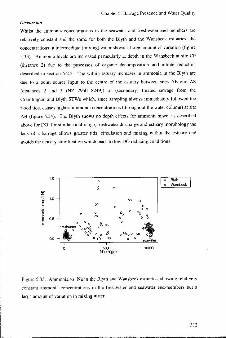
Chapter 5: Bairage Presence and Water Quality
Discussion
Whilst the ammonia concentrations in the seawater and freshwater end-members are
relatively constant and the same for both the Blyth and the Wansbeck estuaries, the
concentrations in intermediate (mixing) water shows a large amount of variation (figure
5.33). Ammonia levels are increased particularly at depth in the Wansbeck at site CP
(distance 2) due to the processes of organic decomposition and nitrate reduction
described in section 5.2.5. The within estuary increases in ammonia in the Blyth are
due to a point source input to the centre of the estuary between sites AB and AS
(distances 2 and 3 (NZ 2950 8249)) of (secondary) treated sewage from the
Cramlington and Blyth STWs which, since sampling always immediately followed the
flood tide, causes highest ammonia concentrations (throughout the water column) at site
AB (figure 5.34). The Blyth shows no depth effects for ammonia since, as described
above for DO, for similar tidal range, freshwater discharge and estuary morphology the
lack of a barrage allows greater tidal circulation and mixing within the estuary and
avoids the density stratification which leads to low DO reducing conditions.
1.5 - f
(0
E (0
0.5
0.0 H
0 0 0 o
«3 o
o
CP
0 CD
o o ° o
° o ° ° ° o 0 0 o
o ° o freshwater % ^oO
0 0 °
0 0
0
0 "^o o oo O 2P Co ° ° seawater
1 0
1 5000
Na(mg/I)
1 10000
o Blyth o Wanstieck
Figure 5.33. Ammonia vs. Na in the Blyth and Wansbeck estuaries, showing relatively
constant ammonia concentrations in the freshwater and seawater end-members but a
larg amount of variation in mixing water.
312
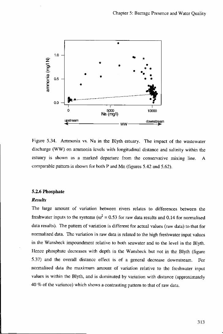
Chapter 5: Barrage Presence and Water Quality
5000 Na(mg/I)
u^ream ww-
10000
downstr^m
Figure 5.34. Ammonia vs. Na in the Blyth estuary. The impact of the wastewater
discharge (WW) on ammonia levels with longitudinal distance and salinity within the
estuary is shown as a marked departure from the conservative mixing line. A
comparable pattern is shown for both P and Mn (figures 5.42 and 5.62).
5.2.6 Phosphate
Results
The large amount of variation between rivers relates to differences between the
freshwater inputs to the systems (co = 0.53 for raw data results and 0.14 for normalised
data results). The pattern of variation is different for actual values (raw data) to that for
normalised data. The variation in raw data is related to the high freshwater input values
in the Wansbeck impoundment relative to both seawater and to the level in the Blyth.
Hence phosphate decreases with depth in the Wansbeck but not in the Blyth (figure
5.37) and the overall distance effect is of a general decrease downstream. For
normalised data the maximum amount of variation relative to the freshwater input
values is within the Blyth, and is dominated by variation with distance (approximately
40 % of the variance) which shows a contrasting pattern to that of raw data.
313

Chapter 5: Barrage Presence and Water Quality
Source F P Size of Effect
(0)')
River 135.50 0.000 0.090 0.53
Distance 2.76 0.042 0.025 0.15
Depth 13.68 0.000 0.017 0.10
River*distance 4.95 0.002 0.008 0.05
River* depth 10.95 0.000 0.013 0.08
Error 0.016 0.09
Table 5.11. Results from GLM ANOVA for phosphate (raw data) between the Blyth
estuary and the Wansbeck impounded estuary.
distance depth
5. 0.10
Figure 5.35. Main effects plot for the factors of river, distance and depth on phosphate
(raw data) in the Blyth and Wansbeck estuaries (LS means for factor levels).
314

Chapter 5: Barrage Presence and Water Quality
0.44
0- 0.34 - \
E, 0) 0.24 CO
JO a. OT O 0.14
0.04 -I
river • Blyth B Wansbeck
distance
Figure 5.36. Interaction between river and distance effects on phosphate (raw data) for
the Blyth and Wansbeck estuaries (LS means).
river
0.35 -4
0.25
§• 0.15
Q.
0.05
• Blyth • Wansbeck
depth
Figure 5.37. Interaction between river and depth effects on phosphate (raw data) for the
Blyth and Wansbeck estuaries (LS means).
315

Chapter 5: Barrage Presence and Water Quality
Source F P Size of Effect
(0)')
River 10.77 0.001 1.91 0.14
Distance 3.98 0.005 1.74 0.13
Depth 1.03 0.357 na na
River* distance 10.32 0.000 5.46 0.40
River*depth 0.31 0.733 na na
Error 4.69 0.34
Table 5.12. Results from GLM ANOVA for phosphate (normalised data) between the
Blyth estuary and the Wansbeck impounded estuary (na = not applicable since factor
insignificant at 95 % level).
a.
t •o
o c
2.20
1.95 H
1.70 H
distance depth
1.45
1.20
Figure 5.38. Main effects plot for the factors of river, distance and depth on phosphate
(normalised data) in the Blyth and Wansbeck estuaries (LS means for factor levels).
316

Chapter 5: Barrage Presence and Water Quality
river
CD
Q .
CO
3 -A
CO 2
o c 1 ^
• Blyth B Wansbeck
distance
Figure 5.39. Interaction between river and distance effects on phosphate (normalised
data) for the Blyth and Wansbeck estuaries (LS means).
Discussion
D) E,
0.7
0.6
0.5
0.4
0.3
0.2
0.1
• e
i 1
• •
1 •
1 " 1 1 1 1 r
0 1000 2000 3000 4000 5000 6000 7000 8000 9000
Na (mg/l)
Figure 5.40. P (as dissolved orthophospate) vs. Na in the Wansbeck impoundment
showing control by freshwater flow (1) and conservative mixing between freshwater
and seawater (2).
317

Chapter 5: Barrage Presence and Water Quality
Phosphate levels in the Wansbeck are higher than in the Blyth due to higher mean
inputs from the freshwater entering the estuary. As stated in chapter 3, management of
phosphate within the impoundments studied needs to be focussed on the inputs to the
rivers. The variation in freshwater inputs is discharge related. Phosphate behaves
conservatively on mixing of seawater and freshwater in the Wansbeck (figure 5.40) and
hence, as for nitrate, shows a pattern of distribution related to mixing (or rather lack of)
within the impoundment (i.e. a general decrease with distance downstream and a
contrast between surface and deep water). For the Blyth the variation in phosphate
(which represents virtually all of the dissolved phosphorus in this estuary (figure 5.41))
is, as for ammonia, related to the point source input of treated sewage between distances
2 and 3 (figure 5.42). The ratio of ammonia to phosphorous in the discharge was
constant throughout the sampling period at N (as ammonia):P of approximately 5:1 by
mass (figure 5.43).
CL
CO
x: Q. « O
0.3 H
0.2
0.1
0.0 - I
OS o
0.2 0.3 total dissolved P (mg/l)
0.4
Figure 5.41. The relationship between dissolved orthophosphate (phosphate) and total
dissolved P in the Blyth estuary. Virtually all P is as phosphate from wastewater within
the Blyth.
The presence of the wastewater discharge to the Blyth, and its impacts on ammonia and
phosphate levels in the estuary mean that it is difficult to inake a direct comparison with
the Wansbeck. On the basis of a lack of depth effect and the constant ratio of
ammonia/P through mixing it is assumed however that no processes other than physical
318

Chapter 5: Barrage Presence and Water Quality
mixing of the water sources are significant. In particular in contrast to the Wansbeck
impoundment the lack of stratification means that no reducing conditions and ammonia
build-up can take place within the Blyth estuary.
0.4 - f
0.3 H
E 0.2
0.1
0.0
r 5000
Na (mg/l) 10000
Figure 5.42. P vs. Na in the Blyth estuary, showing the impact of the wastewater
discharge to the estuary (cf. figure 5.34).
E, 55 'c o E
1.0
0.5 H
0.0
P (mg/l)
Figure 5.43. Co-linearity between ammonia and P in the Blyth estuary due to the
wastewater source for these nutrients.
319

Chapter 5: Barrage Presence and Water Quality
5.2.7 Na
Results
Source F P a" Size of Effect
(Q ) ' )
River 602.32 0.000 49161207 0.43
Distance 96.96 0.000 23537037 0.21
Depth 91.17 0.000 14744540 0.13
River* distance 87.04 0.000 21102772 0.18
River* depth 27.15 0.000 4275517 0.04
Error 1962144 0.02
Table 5.13. Results from GLM ANOVA for Na (raw data) between the Blyth estuary
and the Wansbeck impounded estuary.
distance depth
6800 H
i . 4400 -
3200 H
Figure 5.44. Main effects plot for the factors of river, distance and depth on Na (raw
data) in the Blyth and Wansbeck estuaries (LS means for factor levels).
320

Chapter 5: Barrage Presence and Water Quality
river
10000
CO 5000 ~A
• BIyth m Wansbeck
distance
Figure 5.45. Interaction between river and distance effects on Na (raw data) for the
Blyth and Wansbeck estuaries (LS means).
10000 -I
5000 CO
0 -A
river
• Blyth m Wansbeck
depth
Figure 5.46. Interaction between river and depth effects on Na (raw data) for the Blyth
and Wansbeck estuaries (LS means).
321

Chapter 5: Barrage Presence and Water Quality
Na concentrations show a large difference between the two estuaries, with mean level
being over three times greater in the Blyth (mean Na = 7924 mg/1) than the Wansbeck
(mean Na = 2094 mg/1 during the same sampling period). Na shows a general increase
with distance downstream, but this is more pronounced and regular in the Blyth estuary
(figure 5.45). Na increases with depth in the water column, but concentrations tend to
be the same for mid-depths and deep sampling in the Blyth whereas they show
difference between all depths of sampling in the Wansbeck (figure 5.46). Very little of
the variance (approximately 2 %) is unexplained by terms in the model.
Discussion
350 H
^ 250 H O)
O 150
50 H -] \ 1 1 r ~ — I 1 1 1 r 0 1000 2000 3000 4000 5000 6000 7000 8000 9000
Na (mg/1)
Figure 5.47. Ca vs. Na for summer sampling in the Wansbeck impoundment, showing
release of Ca from sediment to deep water samples. Samples from depth at sites RB
and CP and mid-depth at site CP are indicated by asterisks. Al l other sites are
represented by solid circles.
Na is a conservative tracer of seawater/freshwater physical mixing in estuaries and as
such shows a distinct contrast between the impounded and the un-impounded estuary.
Seawater access is unrestricted to and therefore dominates in the Blyth whereas the
majority of the water in the Wansbeck is fresh due to the reduced hydrad.c heads of
tidal water by impoundment. The reduction in tidal circulation, as has been observed
for several parameters that are largely controlled by physical mixing, a i s o allows long-
322

Chapter 5: Barrage Presence and Water Quality
term density stratification to develop in the Wansbeck. Within the Blyth estuary
freshwater is rapidly mixed with seawater to produce a more homogenous and freely
circulating water body. Na, Mg, K and S are co-linear within both the Blyth and the
Wansbeck estuaries during the summer periods. Ca however shows some evidence of
non-conservative behaviour during summer within the Wansbeck, where Ca
concentrations above the conservative mixing line are observed in samples from depth
at sites CP and RB (figure 5.47). These increases may relate to increased sedimentary
carbonate solubility under the reduced pH conditions described above, and may allow
mobilisation of other elements held in the carbonate phase. The elemental speciation
within the sediments of the Wansbeck is discussed in chapter 6.
5.2.8 Fe
Results
The size of the variation in mean Fe between the estuaries is small (size of effect for
raw data is approximately 1 %) . Fe concentrations in the freshwater inputs to the two
systems are similar and so the results from analyses using both raw and normalised data
show similar patterns. The largest effect in both cases is that of the river*distance
interaction (figures 5.49 and 5.52). The Blyth shows a continuous increase in Fe
concentration with distance downstream whilst the Wansbeck show a peak in
concentration at distance 2. The general effect of depth is of an increase in Fe with
sampling depth. In the Blyth the mid-depth and deep samples tend to show the same Fe
concentration whereas in the Wansbeck concentrations are greatest in deep water and
water at the surface remains little changed from the freshwater input concentration.
Source F P Size of Effect
(co') River 5.30 0.022 0.0001 0.01
Distance 8.42 0.000 0.0005 0.07
Depth 42.74 0.000 0.0019 0.26
River* distance 44.79 0.000 0.0030 0.40
River*depth 30.72 0.000 0.0013 0.18
Error 0.0005 0.07
Table 5.14. Results from GLM ANOVA for Fe (raw data) between the Blyth estuary
and the Wansbeck impounded estuary.
323

Chapter 5: Baixage Presence and Water Quality
distance depth
if
0.09
0.08
0.07 H
0.06
0.05
Figure 5.48. Main effects plot for the factors of river, distance and depth on Fe (raw
data) in the Blyth and Wansbeck estuaries (LS means for factor levels).
river
0.095
0.085
0.075
0.065
0.055
0.045
0.035
O Blyth a Wansbeck
distance
Figure 5.49. Interaction between river and distance effecib on Fe (raw data) for the
Blyth and Wansbeck estuaries (LS means).
324
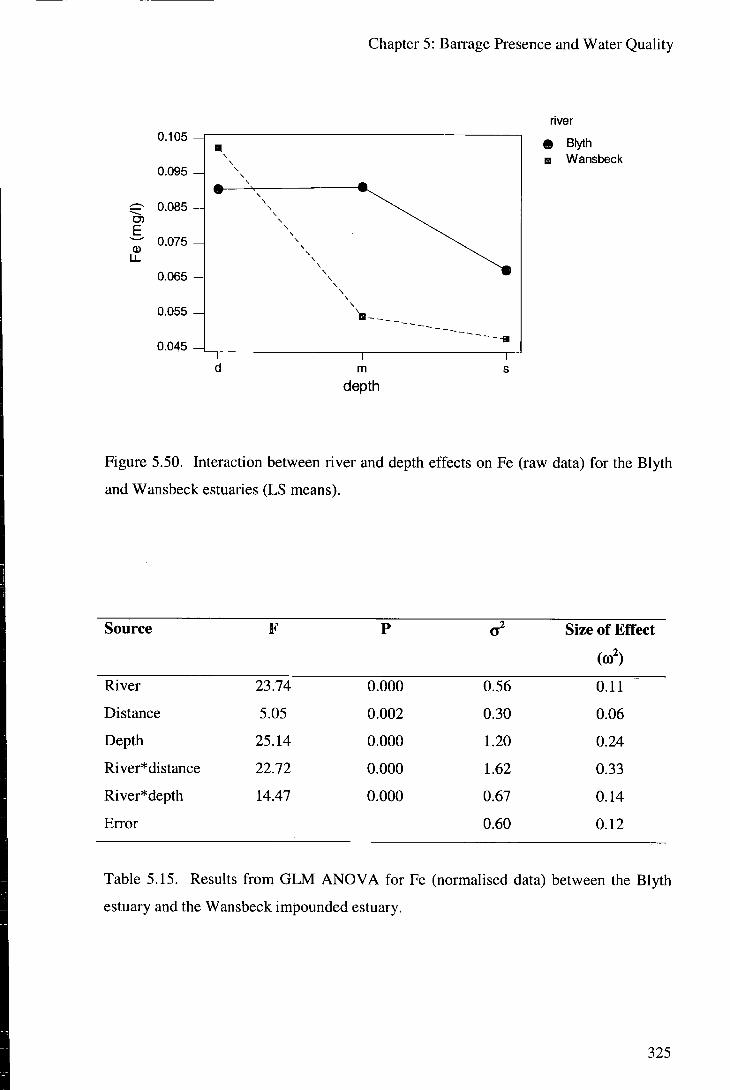
Chapter 5: Barrage Presence and Water Quality
river 0.105
0.095 - I
^ 0.085
0.065
0.055 -
0.045 -
m depth
Blyth Wansbeck
Figure 5.50. Interaction between river and depth effects on Fe (raw data) for the Blyth
and Wansbeck estuaries (LS means).
Source F P Size of Effect
River 23.74 0.000 0.56 0.11
Distance 5.05 0.002 0.30 0.06
Depth 25.14 0.000 1.20 0.24
River* distance 22.72 0.000 1.62 0.33
River*depth 14.47 0.000 0.67 0.14
Error 0.60 0.12
Table 5.15. Results from GLM ANOVA for Fe (normalised data) between the Blyth
estuary and the Wansbeck impounded estuary.
325

Chapter 5: Barrage Presence and Water Quality
distance deptli
Figure 5.51. Main effects plot for the factors of river, distance and depth on Fe
(normalised data) in the Blyth and Wansbeck estuaries (LS means for factor levels).
0)
.52
o c
2.5
2.0 - \
1.5
1.0 -A
river
O Blyth • Wansbeck
distance
Figure 5.52. Interaction between river and distance effects on Fe (normalised data) for
tiie Blyth and Wansbeck estuaries (LS means).
326
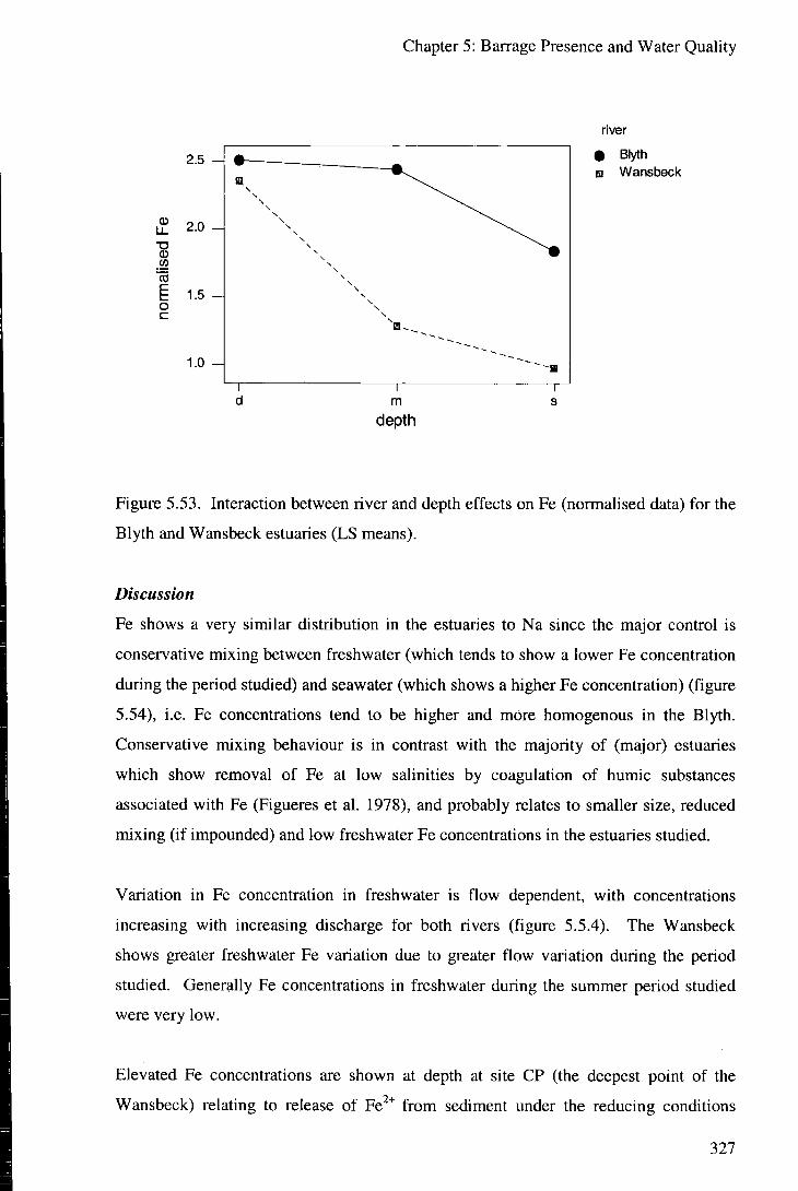
Chapter 5: Barrage Presence and Water Quality
river
• Blyth m Wansbeck
depth
Figure 5.53. Interaction between river and depth effects on Fe (normalised data) for the
Blyth and Wansbeck estuaries (LS means).
Discussion
Fe shows a very similar distribution in the estuaries to Na since the major control is
conservative mixing between freshwater (which tends to show a lower Fe concentration
during the period studied) and seawater (which shows a higher Fe concentration) (figure
5.54), i.e. Fe concentrations tend to be higher and more homogenous in the Blyth.
Conservative mixing behaviour is in contrast with the majority of (major) estuaries
which show removal of Fe at low salinities by coagulation of humic substances
associated with Fe (Figueres et al. 1978), and probably relates to smaller size, reduced
mixing (if impounded) and low freshwater Fe concentrations in the estuaries studied.
Variation in Fe concentration in freshwater is flow dependent, with concentrations
increasing with increasing discharge for both rivers (figure 5.5.4). The Wansbeck
shows greater freshwater Fe variation due to greater flow variation during the period
studied. Generally Fe concentrations in freshwater during the summer period studied
were very low.
Elevated Fe concentrations are shown at depth at site CP (the deepest point of the
Wansbeck) relating to release of Fe^* from sediment under the reducing conditions
327

Chapter 5: Barrage Presence and Water Quality
which develop in the isolated saline water (figure 5.54). Within the Blyth no redox
controlled mobihsation of Fe is seen since, as described for DO, etc., greater tidal
circulation causes greater mixing of the water body.
0.2
E .05
0.1
0.0 - [ 5000
Na (mg/l)
10000
o Blyth o Wansbeck
Figure 5.54. Fe vs. Na for the Blyth and Wansbeck estuaries. 1 represents the
freshwater flow control, 2 represents conservative mixing of Fe between freshwater and
seawater, and 3 represents the release of Fe under low redox conditions at depth (only
significant for the Wansbeck).
5.2.9 Mn
Results
Since Mn values in freshwater inputs to both systems are so low relative to the values
within the estuaries, results for analyses using both raw and normalised data are very
similar. Mean levels of Mn are higher in the Wansbeck than the Blyth estuary. The
distance effect differs between estuaries, with a small increase with distance
downstream in the Blyth and a large peak in Mn concentrations at distance 2 (site CP)
in the Wansbeck (figures 5.56 and 5.59). The depth effect also shows interaction with
estuary. Relative to shallow water Mn concentrations those at depth within the
Wansbeck are almost two orders of magnitude higher. Within the Blyth estuary Mn
shows no significant difference between depths in the water column.
328

Chapter 5: Barrage Presence and Water Quality
Source F P a" Size of Effect
(0)')
River 77.07 0.000 0.17 0.17
Distance 24.40 0.000 0.16 0.15
Depth 57.08 0.000 0.25 0.25
River*distance 22.47 0.000 0.14 0.14
River* depth 55.96 0.000 0.25 0.24
Error 0.05 0.05
Table 5.16. Results from GLM ANOVA for Mn (raw data) between the Blyth estuary
and the Wansbeck impounded estuary.
distance depth
0.48 H
0.36 H
C 0.24
0.12
0.00 H
Figure 5.55. Main effects plot for the factors of river, distance and depth on Mn (raw
data) in the Blyth and Wansbeck estuaries (LS means for factor levels).
329

Chapter 5: Barrage Presence and Water Quality
river
O) 0.4
distance
O Blyth m Wansbeck
Figure 5.56. Interaction between river and distance effects on Mn (raw data) for the
Blyth and Wansbeck estuaries (LS means).
05 E
river
O Blyth • Wansbeck
depth
Figure 5.57. Interaction between river and depth effects on Mn (raw data) for the Blyth
and Wansbeck estuaries (LS means).
330

Chapter 5: Barrage Presence and Water Quality
Source F P Size of Effect
(0)')
River 58.98 0.000 3657 0.15
Distance 20.62 0.000 3713 0.15
Depth 48.42 0.000 5982 0.25
River* distance 18.34 0.000 3281 0.14
River*depth 47.39 0.000 5852 0.24
Error 1514 0.06
Table 5.17. Results from GLM ANOVA for Mn (normalised data) between the Blyth
estuary and the Wansbeck impounded estuary.
T3
80
60
40
20 H
0 H
river distance depth
Figure 5.58. Main effects plot for the factors of river, distance and depth on Mn
(normalised data) in the Blyth and Wansbeck estuaries (LS means for factor levels).
331

Chapter 5: Barrage Presence and Water Quality
river
100
w "cc 50
b c
0 -A
O Blyth B Wansbeck
distance
Figure 5.59. Interaction between river and distance effects on Mn (normalised data) for
the Blyth and Wansbeck estuaries (LS means).
river
100 -A
"co
b c
50 - ]
0 -4
© Blyth • Wansbeck
depth
Figure 5.60. Interaction between river and depth effects on Mn (normalised data) for
the biyth and Wansbeck estuaries (LS means).
332

Chapter 5: Barrage Presence and Water Quality
Discussion
In contrast to Fe which shows conservative behaviour in the estuaries for the periods
studied, Mn show distinctly non-conservative patterns (figures 5.61 and 5.62). As
described in chapter 4, Mn^^ may be released from bottom sediment to the water
column under low redox conditions. Within the Wansbeck this process is the major
control on Mn concentrations, and the distribution of Mn relates to the distribution of
reducing conditions in the density stratified water column. The increase in Mn
concentrations within the mixing zone of the Blyth estuary is much smaller than that
shown from bed sediment release in the Wansbeck, and is due to wastewater input to
the estuary (figure 5.62). Due to higher oxygen levels, release of Mn^^ from bed
sediment does not occur within the Blyth estuary.
05
1.5 H
1.0
0.5 H
0.0
f •• •
• • * • • • • • • . .
<• * 003 8 o ^ ^ 3 * 9mn^fn^gm^
o Blyth • Wansbeck
5000
Na (mg/1)
10000
Figure 5.61. Mn vs. Na in the Blyth and Wansbeck estuaries (summer sampling),
showing large release of Mn from sediment under low redox conditions within the
Wansbeck.
333

0.10 -
E 0.05
0.00
Chapter 5: Bairage Presence and Water Quality
& 0
< ^
0 0
o e
0 1 0 5000 10000
Na (mg/l)
Figure 5.62. Mn vs. Na in the Blyth estuary (summer sampling). The departure from
the conservative mixing line between the freshwater and seawater end members is due
to wastewater input to the estuary (cf. figures 5.34 and 5.42).
334

Chapter 5: Barrage Presence and Water Quality
5.3 Summary and conclusions
The presence or absence of a barrage has a significant effect on all of the parameters
assessed (table 5.18). For all parameters which may cause or relate to detrimental
effects in water bodies, the effect of barrage construction is to potentially reduce water
quality. The changes in behaviour relate to three main effects of barrage construction.
All three effects aie due to the decrease in tidal intrusion to impounded compared with
equivalent un-impounded estuaries:
1. Changes in the relative amount and distribution of freshwater and seawater in
the estuary.
2. Increased stratification leading to isolation of portions of the water column.
3. Decreased tidal currents and mobilisation of bottom sediment.
Parameter Affected by
impoundment
Water quality
reduced by
impoundment
Main affecting process
DO V Increased stratification of water
column
pH V y/ Increased stratification of water
column
TSS X Reduced tidal circulation and re-
suspension of bed sediment
Nitrate V Reduced seawater to freshwater ratio
(physical mixing control)
Ammonia V V Increased stratification of water
column
Phosphate V Reduced seawater to freshwater ratio
(physical mixing control)
Na X Reduced seawater to freshwater ratio
(physical mixing control)
Fe V Increased stratification of water
column
Mn V V Increased stratification of water
column
Table 5.18. Summary of the impact of barrage construction on water quality.
335

Chapter 5: Barrage Presence and Water Quality
Nitrate, phosphate and the major elements (modelled using Na) show concentrations and distributions which relate mainly to the difference in concentration between seawater and freshwater and the effects of barrage construction on the relative volumes of these two end-members. This physical mixing control is also a significant factor for several other parameters analysed, and has implications for any pollutants which are transported in either the fluvial or tidal component. The concentrations of nitrate and phosphate tend to be higher in the freshwater inputs than in seawater, and therefore, since barrage construction reduces the proportion of seawater, impounded estuaries are likely to show greater concentrations of these nutrients. Nitrate and phosphate are marked as having a potential detrimental effect on water quality in the impoundment in terms of their potential impacts on eutrophication, although whether a biological response is encountered will depend on a variety of factors (e.g. N/P limitation, turbidity, turbulence, etc.). As mentioned, eutrophic behaviour is encountered within the Wansbeck impoundment.
Reduced tidal influence on impoundment also allows changes the nature of the estuary
towards a more stratified water body. In the Wansbeck the effects of this stratification
are particularly dramatic due to the irregular topography of the estuarine profile which
allows saline water to "pond" within deeper sections. This deep "ponded" water
undergoes a series of changes following isolation from the atmosphere and contact with
organic rich bottom sediments including reduction in DO and pH, and increase in
ammonia and Fe and Mn (and associated metals). Although most pronounced in the
Wansbeck, these effects are observed in all of the impoundments studied and may be
assumed to be a major negative impact of barrage construction.
Finally, the reduction of tidal circulation has an impact on the behaviour of sediment
within the estuaries. Estuaries are effective sediment traps in their formative stages but
reach an equilibrium between sediment deposition and scour by currents over time
(Dyer 1997). Construction of a barrage reduces the scour by currents and sedimentation
will take place within the impounded area until a new equilibrium is reached. In the
Blyth estuary higher tidal currents were evident in the development of a turbidity
maxima due to re-sus' ension of bottom sediments and the genera „oarser grained
nature of the bed.
336

Chapter 6: Sediment Quality and Speciation
Chapter 6
Sediment Quality and Speciation
6.1 Introduction
The objectives of the sediment surveys were multifold;
1. To assess the current state of the sediment quality in the impoundments and
enable appropriate design of more detailed surveying.
2. To determine the possibility of, and conditions under which, internal cycHng
may lead to release of elements from the sediment to the water column of the
impoundments.
3. To determine the trends in sediment quality following impoundment.
4. Together with data supplied from sedimentological studies of the SIMBA
Project, to determine the flux of sediment and associated elements to the
impoundments, to enable prediction of the long-term sustainability of the
systems.
In order to perform these objectives bed sediment coring on the Wansbeck and Tees
impoundments was carried out.
6.2 Sediment survey design
Sediment coring was carried out to give vertical profiles of sediment quality, with the
aim of assessing trends in deposition and sediment quality over the lifetime of the
impoundments. The coring experiments were also designed to assess the differences in
sediment quality and deposition between types and ages of impoundments. The scope
of this project allowed the comparison of sediment between 2 estuaries.
6.2.1 Estuaries studied
The estuaries chosen for sediment coring surveys were the Wansbeck and the Tees. The
Wansbeck was impounded in 1975 and is a partial tidal exclusion system. The Tees
was impounded in 1994 and is a total tidal exclusion (freshwater) system. Both
estuaries are located in the Northeast of England within 1 hours drive of the University
of Durham. Whilst additional sampling from the Tawe would have allowed more
rigorous testing of the factors of age and design on the sediment quality, time and
equipment constraints meant that this was not possible within this project.
337

Chapter 6: Sediment Quality and Speciation
6.2.2 Sampling sites and dates
2 sites from each impoundment were chosen as representing the most stable
sedimentary environments, which had undergone the least physical mixing of sediment
and were likely to give the least disturbed sediment profiles (table 6.1). These sites
were chosen based on preliminary longitudinal grab-sample profiles of the
impoundments, with field examination of the particle size and colour (as a rough proxy
for organic content) of the sediment being used to estimate the lowest energy
environments (finest particle size and highest organic content). These surveys also gave
an indication of when the nature of the sedimentary behaviour changed from riverine to
lacustrine typology. An additional sample was taken from the emerging island next to
site RB (site SM), to assess the significant sedimentation observed to be occurring at the
margins of the Wansbeck impoundment. Sampling was carried out on the 23/07/01 for
the Wansbeck and 24/07/01 for the Tees.
River Site name Site abbreviation Grid reference
Tees Opposite Kvaemer KV NZ 4570 1905
Building
Tees Tees Barrage TB NZ 4616 1905
Wansbeck Railway Bridge RB NZ 2775 8585
Wansbeck Barrage WB NZ 2935 8536
Wansbeck Railway Bridge SM NZ 2935 8536
Island
Table 6.1. Sediment coring sampling sites.
6.2.3 Replicates
In order to assess local variations in sediment quality, and allow statistical testing of the
significance in differences with depth in the profiles relative to random variation,
duplicate cores were taken within 1 m of each other at sites WB and TB.
6.3 Sediment sampling procedure
6.3.1 Safety precautions
Precautions were taken to limit the risk to those involved during sediment sampling.
Fieldwork was always completed with at least 2 people in the RV and at least one on
338

Chapter 6: Sediment Quality and Speciation
shore, all carrying mobile telephones, on all occasions. Lifejackets and high visibility
clothing were worn when on the water or when working from river banks. A first-aid
kit was carried in the RV. Gloves were worn when collecting samples to avoid risk of
infection, in addition to avoiding contamination of samples. Al l field and laboratory
work carried out as part of this PhD was done so without any injury to any party.
6.3.2 Procedures
All work (except Dutch auger coring) was carried out from the RV, normally with a
crew of 3 people. Sampling was carried out where possible with plastic or stainless
steel equipment, and gloves were worn at all times, to minimise the risk of
contamination. The date, location and time of sampling, plus any additional relevant
information were recorded in a notebook for each sample taken.
6.3.3 Coring
Sediment cores were taken using either a Dutch auger coring device for the sample
taken from the newly formed island at RB, or a pneumatically driven Mackereth coring
device for all other sediment coring work.
6.3.3.1 Dutch auger
The Dutch auger consists of 1 m length of metal split tube, which is manually turned
and driven into the sediment before being retrieved vertically with the sediment sample.
The section retrieved may then be subsampled at defined depths from the sediment.
The Dutch auger is effective for relatively well consolidated (low moisture content) silts
and clays, such as are found on the emerged ground at RB in the Wansbeck
impoundment. The 1 m core taken from the island at RB was subsampled in the field at
5 cm intervals with a stainless steel palette knife, and transferred to labelled polythene
sample bags. Samples were transported to the laboratory in the dark in cool boxes at
4°C, before being stored frozen for a maximum of 1 month at -20°C prior to drying and
sequential extraction, and other analyses.
6.3.3.2 Mackereth corer
The pneumatically driven Mackereth corer consists of a 1 m by 10 cm diameter perspex
sampling tube which is driven vertically into the bed sediment by compressed air. The
sampler and core are then brought back to the water surface, with the sediment being
held in place by a plunger at the top of the perspex sample tube creating a "suction"
339

Chapter 6: Sediment Quality and Speciation
force on the sediment. The base of the sampling tube is then capped before removal
from the water, and the tube and sample removed from the sampling device on the RV
and capped at the top end. Mackereth corers are appropriate for obtaining undisturbed
cores from relatively unconsolidated (high moisture content) sediments such as are
found in the beds of lakes and estuaries. 3 cores were taken from the RV from the bed
of the Wansbeck impoundment (1 from site RB and 2 (replicates) from WB), and 3
cores from the Tees impoundment (1 from site KV and 2 (replicates) from TB). Visibly
disturbed cores were discarded and sampling repeated. The length of core retrieved
ranged from 40 to 70 cm, with shorter cores being retrieved from the Tees due to sandy
material (which was not retained in the sample tubes) being encountered at
approximately 60 cm sediment depth. The cores were transported with minimum
disturbance in the dark to the laboratory, and within 1 hour were placed in a freezer.
Once frozen, the sediment cores were extruded from the perspex sampling tubes using a
steel plunger, and subsampled at 3 cm intervals using a stainless steel palette knife.
Sample that had been in contact with the steel plunger was discarded. These discs of
frozen sediment were then split into two semi-circles of material using a palette knife, to
give one portion for sequential extraction experiments and one portion for trace organic
analysis. Subsamples were transferred to labelled polythene bags (or wrapped in fired
aluminium foil for samples to be used for trace organic analysis), and stored frozen for a
maximum of 1 month at -20°C prior to drying and sequential extraction, and other
analyses.
6.4 Sediment parameters measured
The focus of the sediment quality surveys was on the metal and nutrient contents and
speciation in this phase. Parameters were measured using, as far as possible, similar
techniques to those carried out in the water quality surveys to allow comparison of the
metal and nutrient contents between the water and sediment phases.
6.4.1 Sequential extraction
Since the design of the sediment survey was to assess sediment quality in the
impoundments in terms of possible environmental impact, determination of elemental
speciation was considered important. Information about the physiochemical forms of
elements is required to understand their environmental mobility, pathways and
bioavailability (Tack and Verloo 1993). The Commission of the European
Communities, Community Bureau of Reference (BCR), defines speciation as either (a)
340*

Chapter 6: Sediment Quality and Speciation
the process of identification and quantification of defined species, forms or phases in a
material or (b) the description of the amounts of these species, forms or phases present
(Ure et al. 1993a). Many speciation techniques have been developed with varying
degrees of success and acceptance (McBride 1989). For the solid phase these include
single reagent leaching, sequential extractions and ion exchange resins. Although
controversial due mainly to arguments over its operationally defined and non-selective
nature, sequential extraction is the most conmionly applied.
Tessier et al.
(1979)
Ruttenberg
(1992)
Step Extractant Extracted Step Extractant Extracted
1 NaOAc Exchangeable 1 MgCla Exchangeable
(pH 8.2), or (pH8)
MgCb
(pH7)
2 NaOAc (pH 5) Acid-soluble 2 Na-citrate, Na- Reducible (Fe
(carbonate HCO3, Na- and Mn oxide
bound) dithionite (pH bound)
7.6)
3 Na-dithionite, Reducible (Fe 3 NaOAc Acid soluble at
Na-citrate and and Mn oxide (pH4) moderately low
H-citrate, or bound) pH (carbonate
NH2OH.HCI bound plus
and HO Ac authigenic and
biogenic apatite)
4 H2O2, HNO3 Oxidisable 4 1 M H C l Acid soluble
(organically (detrital apatite
bound) plus other
inorganic P)
5 HF-HCIO4 Residual 5 Ash at 550°C Oxidisable
(silicate bound) followed by 1 (organically
M H C l bound)
Table 6.2. The sequential extraction procedures of Tessier et al. (1979) and Ruttenberg
(1992).
341

Chapter 6: Sediment Quality and Speciation
There are a large number of wet chemical sequential extraction techniques applied to the problem of determining elemental speciation in sediments (Pickering 1995). The general procedure involves applying the least aggressive reagents first, with subsequent extraction steps using progressively more aggressive and lower pH solutions. Examples of commonly used sequential extraction techniques include those of Tessier et al. (1979), Salomons and Forstner (1984), and Ure et al. (1993b) for metal extraction, and Williams et al. (1976) and Ruttenberg (1992) for phosphorus. Techniques differ in terms of their number of extraction stages (species determined), the order of extraction, and the exact reagents used. Generally most techniques are based on the protocol of Tessier et al. (1979) and differ only in minor operational detail (Kersten and Forstner 1995). Although there is a movement towards harmonisation of sequential extraction procedures to allow comparability of results based on a simple three step extraction procedure (Whalley and Grant 1994, Quevauviller et al. 1996 and Quevauviller 1998), the Tessier scheme is still widely used. In this project it was felt that the environmental conditions likely to be encountered in the impoundments could most closely be modelled by the extraction steps of the Tessier sequential extraction procedure. To determine whether the Tessier scheme could also be used to quantify the speciation and hence likely release of phosphorus in the sediments, a selection of samples also underwent extraction by the procedure of Ruttenberg (1992). A summary of the two procedures is given in table 6.2.
6.4.2 Moisture content
Drying of sediments is necessary since analyses are based on dry weight of samples.
Deposited sediments contain high water contents (30 to 95 %) (Loring and Rantala
1992), depending on the depositional environment, mineralogy and depth within the
sedimentary sequence. A measurement of moisture content allows the effect of
interstitial water composition (salinity) on the geochemical analyses to be accounted for.
6.4.3 Organic matter
Particulate organic matter has a very high specific area and therefore a very high
adsorption capacity. Contaminants entering water bodies are very often adsorbed onto
organic particulates (Chapman and Wang 2001), and so the determination of organic
matter content of sediment is therefore necessary to assess the environmental behaviour
of elements.
^42

Chapter 6: Sediment Quality and Speciation
6.4.4 Particle size distribution
Contaminants are often associated with the fine particles of sediments due to an
exponential increase in specific surface area with decreasing grain size and an increase
in surface charge (Forstner et al. 1982 and Birch and Taylor 2000). As mentioned,
organic matter is also often associated with contaminants, and tends to be associated
with fine grained particles. This "grain size effect" must be eliminated to allow inter-
comparison of results between different sampling sites or with depth within cores. This
can be done either by: (a) separation and analysis of only the fine grained (generally
taken as silt and clay (<64 \im)) fraction of the sediment or, (b) by analysis of bulk
samples followed by the normalisation of results to the either grain size or a chemical
proxy for grain size or mineralogy (e.g. A l , Si, Cs, Sc, Li) . The first approach does not
account for variations in grain size within the fine fraction (i.e. relative amounts of silt
and clay), and so normalisation is the recommended approach. Hence, particle size
analysis was necessary as part of the sediment quality surveys of the impoundments.
6.5 Sediment analytical methods
6.5.1 Moisture content
Principle:
Moisture content or water content is determined by conventional oven-drying (BS 1377
1990) or microwave oven-drying (Bentley and Carter 1987) of a sample of soil or
sediment. The sample is carefully weighed before and after drying, and the difference
in weights in relation to the original weight of sample is the moisture content. The
microwave oven-drying is unsuitable for sediments containing a high proportion of
organic material.
Method:
Percentage moisture content of approximately 50 g wet weight sediment samples was
determined by oven-drying at 105°C for 24 hours and cooling in a desiccator, according
to BS 1377 (1990). Percentage moisture content (M) was calculated by:
W1-W2 M = x l00%
• Wx-Wb
where:
343

Chapter 6: Sediment Quality and Speciation
Wi = weight of beaker and wet sediment sample (g),
W2 = weight of beaker and dried sediment sample (g), and
Wb = weight of beaker (g).
Dried samples were then gently crushed and homogenised in an agate mortar for use in
subsequent analyses and sequential extraction experiments.
6.5.2 Loss on ignition
Principle:
Loss on ignition (LOI%) is determined by heating a sample of soil or sediment (that has
previously been dried at 105°C) in a furnace to bum off any organic matter. The sample
is carefully weighed before and after ignition, and the difference in weights in relation
to the original weight of sample is the LOI. The temperature and timing of ignition can
vary (Ball 1964). LOI% is not necessarily a true representation of the organic C content
of a soil since weight loss can also occur due to loss of CO2 from carbonates, and loss of
structural water from clays.
Method:
Percentage loss on ignition was determined from preweighed 2-3 g subsamples of
sediment, which had previously been dried at 105°C and homogenised. Samples were
held at 900°C for at least 10 hours (overnight), before cooling in a dessicator and
weighing to 4 decimal places on a Mettler AJlOO electronic balance. LOI% was
calculated by:
Wi-Wz LOI% = x l00%
Wi-Wc
where:
Wi = weight of crucible and sediment sample prior to ignition (g),
W2 = weight of crucible and sediment sample following ignition (g), and
Wc = weight of crucible (g).
344

Chapter 6: Sediment Quality and Speciation
6.5.3 Organic carbon
Principle:
Organic carbon can be estimated by LOI% or determined by methods involving wet or
dry oxidation of organic matter. Dry oxidation techniques generally involve
measurement of liberated CO2 by infrared CO2 spectrometry or gas chromatography.
Modem CHNS analysers allow simultaneous determination of C, H, N and S in organic
material. Wet oxidation techniques determine by titration the amount of dichromate
which reacts with organic matter in a strongly acid solution.
Method:
Organic carbon content of the sediments was determined by the modified Walkley-
Black (1934) titration method of Gaudette et al (1974). This is based on oxidation of
organic material in the sediment by 1 N (0.167 M) K2Cr207 and concentrated H2SO4,
and the titration of excess K2Cr207 with 0.5 N (0.5 M) Fe(NH4)2(S04)2 with
diphenylamine indicator to a sharp 1 drop end-point.
Approximately 0.25 g sediment samples which had previously been dried at 105°C and
homogenised were used, together with 10 ml of K2Cr207. A standardisation blank was
run with each new batch of samples. % organic carbon (C) was calculated by:
C = 0.03x X 100 w ,
where:
W = weight of sediment sample (g),
T = sample titration volume (ml 0.5 M Fe(NH4)2(S04)2), and
S = blank titration volume (ml 0.5 M Fe(NH4)2(S04)2).
6.5.4 Particle size distribution
Principle:
Particle size distributions (PSD) can be determined by sieving, by sedimentation or by
laser diffraction. PSD information is usually given as the % by weight or volume of
345

Chapter 6: Sediment Quality and Speciation
material finer than defined diameters. Initial PSD determinations in this study were
carried out by a combination sieving and sedimentation analysis. The majority of PSD
analyses were carried out by laser diffraction.
Sieving may be used to determine the PSD down to fine sand size, and is carried out by
passing sediment through a stack of sieves of descending size order, and weighing the
material retained at each diameter. Dry sieving may be used for coarse grained
material, but wet sieving (with a dispersant) is more accurate for materials containing
any clay fraction. Sedimentation analysis is carried out on particles finer than 63 |xm
(i.e. the silt and clay fraction of a sediment), and is based on the velocity of settling of
spherical particles in a suspension (Stokes' law): larger particles settle more rapidly.
Samples from a settling suspension of material removed by pipette at a defined depth
and time represent a specific particle size fraction, with the PSD being determined by
the weight of the residues. Alternatively, the sedimentation can be followed by
measuring the change in specific gravity of the suspension over time using a
hydrometer.
The traditional methods of PSD determination of sieving and suspension are time-
consuming. Modem instrumentation uses diffraction to allow much more rapid PSD
analysis. When a particle is placed in a laser beam, light is diffracted by the particle
over a pattern of angles and intensities (Fraunhofer diffraction pattern) which is specific
to the particle size. The scattering pattern due to the diffraction from an ensemble of
particles can be measured by an array of detectors and interpreted to a PSD (given in
terms of volume of material). Diffraction data can determine PSD from around 2000
|a.m to 0.4 |J,m. Analysis of particles smaller than 0.4 ^m is carried out by some
machines based on the interaction of very small particles with polarised light of
wavelength greater than the diameter of the particles.
Sieving method:
The dry sieving test described in BS 1377 (1990) was used. Test sieves were of 1800,
1200, 710, 420, 300, 150 and 63 nm. Approximately 500 g of oven dried and gently
crushed and homogenised sediment were poured into the largest size sieve, and
mechanically shaken fo.- at least 10 minutes. Retained masses were ,.eighed in g to 1
decimal place. The material passing the 63 |xm sieve was retained for subsequent
sedimentation analysis.
346

Chapter 6: Sediment Quality and Speciation
Sedimentation method:
The standard method described in BS 1377 (1990) was used. Samples had previously
been oven dried and crushed and homogenised, and were pretreated with hydrogen
peroxide according to BS 1377 to digest organic material. Removal of portions of
suspension by pipette at 10cm depth were carried out at 4 minutes 10 seconds, 47
minutes 30 seconds, and 7 hours 7 minutes after the start of the sedimentations,
equivalent to particle diameters of 20, 6 and 2 ^m. Sodium hexametaphosphate (2%)
solution was used as a dispersant.
Laser diffraction method:
The majority of PSD analyses were carried out using a Coulter® LS 230 laser
granulometer. This uses both diffraction and PIDS (Polarisation Intensity Differential
of Scattered light) to give a 116 channel PSD from 0.04 ^im to 2000 ^m. Calgon
(sodium hexametaphosphate with sodium bicarbonate) solution was used as the
dispersant. Approximately 0.3 - 0.5 g of sample was used dependent on the clay
fraction of the sediment (in order to maintain a PIDS obscuration of 40-60%).
Obscuration of the diffraction optics was generally around 20%. Sediment samples had
previously undergone drying at 105°C and crushing and homogenisation, but no other
pretreatment (i.e. no removal of organic material). Samples were left in 20 ml of Mi l l i -
Q® 18 MQ..cm water plus 2 ml dispersant solution overnight, followed by sonification
in a sonic bath for 15 minutes prior to introduction to the sampling module. A variable
speed fluid module was used (Coulter® 1994).
6.6 Sequential extractions
Analytical grade reagents and 18 MQ.cm ultra-high purity water were used in all the
laboratory work described. Equipment was acid and Decon 90® (non-ionic surfactant)
washed (soaked overnight in 1% HNO3, followed by overnight soaking in 5% Decon
90® and rinsed in de-ionised water). Prior to chemical extraction, loss on ignition
(LOI), and particle size distribution (PSD) analysis, sediment samples were dried at
105°C overnight, and carefully crushed and homogenised in an agate mortar. Since all
sediment samples analysed contained no particulate fraction >2mm in diameter (i.e. all
particles were sand sized or finer (Craig 1992)) no sieving was deemed necessary.
Dried and crushed samples were stored at room temperature in polythene bags for a
maximum of 2 weeks prior to analyses or extractions.
347

Chapter 6: Sediment Quality and Speciation
6.6.1 Sequential extraction method (after Tessier et al., 1979)
Sediment extractions were carried out using a methodology based on the sequential
extraction procedure of Tessier et al. (1979). Due to safety and equipment issues, the
methodology used excluded the final (5*) step of the Tessier scheme, which uses 5:1
HF:HC104 to digest the silicate lattices in the residual minerals remaining after the
previous 4 extraction stages. Under normal environmental conditions this breakdown of
minerals never occurs, and the metals contained within lattice positions are not
bioavailable or released to the water column. The second significant modification to the
Tessier procedure was that the supematants from the wash steps between extraction
stages were retained for analysis in this study, whereas in the original procedure they
are discarded. It was felt that discarding the wash solution could result in an
underestimation of the metal concentrations. For the initial (exchangeables) extraction
step the Tessier method gives the choice of using either NaOAc or MgCb as the
reagent. For this work it was decided to use NaOAc to allow analysis of Mg from the
sediments.
Initial extractions were carried out in borosilicate glassware, and with vacuum filtration
on standard Whatman® Cellulose Nitrate Membrane Filters of 0.45 |J,m pore diameter
between extraction stages and washes. The retained material on the filters was rinsed
off for use in the subsequent stage following each filtration, with the weight change in
the filters being used to calculate the weight of sediment used at the start of each step.
Due to concerns about the preferential loss of fine sediment on the filters, and to
improve time efficiency, the majority of sequential extractions were carried out using
centrifuging between each extraction and wash stage. These sequential extractions were
carried out in polyethylene sample bottles, which posed less risk of loss of elements
(particularly P) by adsorption to container surfaces than glassware.
The sequence used for the Tessier centrifugation method follows (the sequence for the
initial (filtration) method was exactly the same but with vacuum filtration at the steps
where centrifuging is noted):
348

Chapter 6: Sediment Quality and Speciation
Stage 1 (exchangeable or loosely sorted)
1. 2.500 ± 0.001 g dry weight of sediment was transferred using a stainless steel
spatula into a 60 ml polyethylene sample bottle.
2. 20ml I M NaOAc was added to the sample.
3. The sample was agitated for 1 hour at room temperature on a shaker table.
4. The sample was centrifuged at 4000 rpm for 30 min.
5. The supernatant was decanted to a 30 ml polystyrene specimen container (all
extracts and washes were acidified to < pH 2 by adding 0.1 ml of HNO3, and
stored in at 4°C for a maximum of 2 months prior to analysis by ICP-OES or
ICP-MS).
6. 20 ml H2O was added as a wash to the residual sample and agitated briefly.
7. The sample was centrifuged at 4000 rpm for 30 min.
8. The wash supernatant was decanted to a 30 ml polystyrene specimen container.
Stage 2 (carbonate bound)
1. 20 ml 1 M NaOAc buffered to pH 5 with acetic acid was added to the residual
sample from Stage 1.
2. The sample was agitated for 5 hours at room temperature on a shaker table.
3. The sample was centrifuged at 4000 rpm for 30 min.
4. The supernatant was decanted to a 30 ml polystyrene specimen container.
5. 20 ml H2O was added as a wash to the residual sample and agitated briefly.
6. The sample was centrifuged at 4000 rpm for 30 min.
7. The wash supernatant was decanted to a 30 ml polystyrene specimen container.
Stage 3 (Fe and Mn bound)
1. 20 ml of a solution of 0.3 M Na2S204, 0.175 M Na-citrate and 0.025 M citric
acid was added to the residual sample from Stage 2.
2. The sample was agitated for 8 hours at room temperature on a shaker table.
3. The sample was centrifuged at 4000 rpm for 30 min.
4. The supernatant was decanted to a 30 ml polystyrene specimen container.
5. 20 ml H2O was added as a wash to the residual sample and agitated briefly.
6. The sample was centrifuged at 4000 rpm for 30 min.
7. The wash supernatant was decanted to a 30 ml polystyrene specimen container.
349

Chapter 6: Sediment Quality and Speciation
Stage 4 (organically bound)
1. 7.5 ml 0.02 M HNO3 then 12.5 ml 30% H2O2 (adjusted to pH 2 with HNO3) was
added to the residual sample from Stage 3.
2. The sample was left for 2 hours at 85°C with occasional agitation.
3. A further 7.5 ml aliquot of H2O2 (pH 2) was added.
4. The sample was left for a further 3 hours at 85°C with occasional agitation.
5. The sample was centrifuged at 4000 rpm for 30 min.
6. The supernatant was decanted to a 30 ml polystyrene specimen container.
9. 20 ml H2O was added as a wash to the residual sample and agitated briefly.
10. The sample was centrifuged at 4000 rpm for 30 min.
11. The wash supernatant was decanted to a 30 ml polystyrene specimen container.
Reagent blanks were taken in duplicate from each batch of each reagent, with the group
of extractions corresponding to each batch being noted. The mean concentration values
of the appropriate blanks were subtracted from the corresponding extractants' values.
Elemental concentrations are reported as mg/kg of dry sediment.
6.6.2 SEDEX metliod (after Ruttenburg, 1992)
A selection of sediment samples underwent sequential extraction by the SEDEX method
of Ruttenberg (1992) in addition to the Tessier method, to allow comparision of the
selectivity for the elemental phases (particularly P) of each. The SEDEX work was
completed prior to the purchase of a centrifuge, and was therefore carried out in acid
washed borosilicate glassware with vacuum filtration on standard Whatman® Cellulose
Nitrate Membrane Filters of 0.45 \xm pore diameter between extraction phases and
washes.
0.500 ± 0.001 g dry weight of sediment was used. Extractant volumes were 50 ml
except in stage 2 where it was 45 ml citrate bicarbonate + 1.125 g of Na2S204.
Extraction by the principal extractants is followed by successive MgCh washes which
desorb any secondarily adsorbed elements. Agitation was provided at each step by a
shaker table. Extraction steps were carried out at British room temperature (20°C) in a
temperature controlled laboratory, as opposed to the American room temperature (25°C)
defined by Ruttenberg.
350

Chapter 6: Sediment Quality and Speciation
The sequence used for the S E D E X extraction method follows:
Stage 1 (exchangeable or loosely sorted)
1. 0.500 ± 0.001 g dry weight of sediment was transferred using a stainless steel
spatula to a 100 ml conical flask.
2. 50 ml 1 M MgCl2 was added to the sample.
3. The sample was agitated for 2 hours at room temperature on a shaker table.
4. The sample was vacuum filtered.
5. The filtrate was transferred to a 30 ml polystyrene specimen container (all
extracts and washes were acidified to < pH 2 by adding 0.1 ml of HNO3, and
stored in at 4°C for a maximum of 2 months prior to analysis by I C P - O E S or
ICP-MS).
6. The residue was washed from the filter with 50 ml 1 M MgCh into a 100 ml
conical flask.
7. The sample was agitated for 2 hours at room temperature on a shaker table.
8. The sample was vacuum filtered.
9. The filtrate was transferred to a 30 ml polystyrene specimen container.
10. The residue was washed from the filter with 50 ml H2O into a 100 ml conical
flask.
11. The sample was agitated for 2 hours at room temperature on a shaker table.
12. The sample was vacuum filtered.
13. The filtrate was transferred to a 30 ml polystyrene specimen container.
14. The residue was washed from the filter with 50 ml H2O into a 100 ml conical
flask.
15. The sample was agitated for 2 hours at room temperature on a shaker table.
16. The sample was vacuum filtered.
17. The filtrate was transferred to a 30 ml polystyrene specimen container.
Stage 2 (Fe and Mn bound)
1. The residue from Stage 1 was washed from the filter with 45 ml (0.30 M Nas-
citrate 1.0 M NaHCOs) into a 100 ml conical flask and 1.125g Na2S204 was
added.
2. The sample was agitated for 8 hours at room temperature on a shaker table.
3. The sample was vacuum filtered.
4. The filtrate was transferred to a 30 ml polystyrene specimen container.
351

Chapter 6: Sediment Quality and Speciation
5. The residue was washed from the filter with 50 ml 1 M MgCh into a 100 ml
conical flask.
6. The sample was agitated for 2 hours at room temperature on a shaker table.
7. The sample was vacuum filtered.
8. The filtrate was transferred to a 30 ml polystyrene specimen container.
9. The residue was washed from the filter with 50 ml H2O into a 100 ml conical
flask.
10. The sample was agitated for 2 hours at room temperature on a shaker table.
11. The sample was vacuum filtered.
12. The filtrate was transferred to a 30 ml polystyrene specimen container.
Stage 3 (carbonate bound (+Pin authigenic and biogenic apatite))
1. The residue from Stage 2 was washed from the filter with 50 ml 1 M NaOAc
buffered to pH 4 with acetic acid into a 100 ml conical flask.
2. The sample was agitated for 6 hours at room temperature on a shaker table.
3. The sample was vacuum filtered.
4. The filtrate was transferred to a 30 ml polystyrene specimen container.
5. The residue was washed from the filter with 50 ml 1 M MgCh into a 100 ml
conical flask.
6. The sample was agitated for 2 hours at room temperature on a shaker table.
7. The sample was vacuum filtered.
8. The filtrate was transferred to a 30 ml polystyrene specimen container.
9. The residue was washed from the filter with 50 ml 1 M MgCb into a 100 ml
conical flask.
10. The sample was agitated for 2 hours at room temperature on a shaker table.
11. The sample was vacuum filtered.
12. The filtrate was transferred to a 30 ml polystyrene specimen container.
13. The residue was washed from the filter with 50 ml H2O into a 100 ml conical
flask.
14. The sample was agitated for 2 hours at room temperature on a shaker table.
15. The sample was vacuum filtered.
16. The filtrate was transferred to a 30 ml polystyrene specimen container.
352

Chapter 6: Sediment Quality and Speciation
Stage 4 (Pas detrital apatite)
1. The residue from Stage 3 was washed from the filter with 50 ml 1 M HCl into a
100 ml conical flask.
2. The sample was agitated for 16 hours at room temperature on a shaker table.
3. The sample was vacuum filtered.
4. The filtrate was transferred to a 30 ml polystyrene specimen container.
Stage 5 (organically bound)
1. The residue from Stage 4 was transferred to a crucible.
2. The sample was ashed at 550°C.
3. The residue was washed from the crucible with 50 ml 1 M HCl into a 100 ml
conical flask.
4. The sample was agitated for 16 hours at room temperature on a shaker table.
5. The sample was vacuum filtered.
6. The filtrate was transferred to a 30 ml polystyrene specimen container.
Process blanks were carried out in duplicate for each stage. The mean concentration
values of the appropriate blanks were subtracted from the corresponding extractants'
values. Elemental concentrations are reported as mg/kg of dry sediment.
6.6.3 ICP-OES analysis of extracts
The extracts produced by each of the stages of both the sequential extraction procedures
were analysed by inductively coupled plasma - optical emission spectrometry (ICP-
OES). The same methodology and standards were used as described in chapter 2 for
analysis of metals within brackish and saline water samples (section 2.4.10). Y was
used as an internal standard to correct for suppression of signal due to the high ionic
strength of the extracts. A total of 17 elements were analysed for. Data were collected
for A l , Ca, Co, Cr, Cu, Fe, K, Mg, Mn, Ni, P, Sc, Si, Ti and Zn. Sn and V were at levels
below the analytical LOD. P was unable to be measured in stage 4 extracts due to
analytical problems.
353

Chapter 6: Sediment Quality and Speciation
6.7 Results and discussion
Sediment quality data are presented for the sediment coring surveys and analyses
carried out for the Tees and Wansbeck impoundments. As described in section 6.2,
seven cores in total were collected during the sediment sampling. From the Tees one
core was collected from site KV and two cores from within 1 m of each other from site
TB (cores TBI and TB2). From the Wansbeck one core was collected from site RB and
two cores from within 1 m of each other from site WB (cores W B l and WB2), with an
additional core taken (for which data is not reported in detail) from the emerging island
alongside the bridge pier next to RB (site SM).
6.7.1 Errors
Replicate extractions and analyses were carried out for samples taken at 15 cm intervals
within each core (i.e. at 1.5, 16.5, 31.5, etc. cm depth in the sediment). Sources of
variation in the measurements obtained from these pairs of samples are analytical error,
variation in extraction and pre-treatment conditions, and heterogeneity within the
samples used. Al l analytes except Sn and V were recorded at significantly higher levels
than their analytical LODs (reported in chapter 2), and analytical errors are considered
minor. Appropriate care was taken in carrying out the extraction procedures to ensure
repeatability of the processes (procedure outlined in section 6.5). A significant
proportion of variation may be due to actual differences between the replicate sediment
based on sub-sampling at each depth, and reflect local heterogeneity within the
sediment.
The differences between measurements for replicate pairs were calculated as
percentages of the mean value for each pair. The means of these percentage differences
(from all replicate pairs from all bottom sediment cores) are reported as the error for
each analysis (table 6.3). Within profiles the initial replicate analysed is plotted at those
depths at which replicates were taken.
354

Chapter 6: Sediment Quality and Speciation
Parameter Extraction Extraction Extraction Extraction
stage 1 stage 2 stage 3 stage 4
Sand 11.4 11.4 11.4 11.4
Silt 2.0 2.0 2.0 2.0
Clay 10.7 10.7 10.7 10.7
Organic 0.8 0.8 0.8 0.8
matter
Al 44.8 (16) 3.3 (44) 4.0 (791) 21.5 (577)
Ca 1.7 (3323) 1.2 (454Sj 2.0 (1166) 10.2 (756)
Co 13.8 (0) 2.2 (1.4) 3.5 (2) 44.8 (7)
Cr 34.3 (0) 4.5 f i ; 3.7 (8) 3.7 (27)
Cu 9.1 (1) 3.5 (1) 47.3 (72j 21.4 (70)
Fe 25.0 (37) 2.5 (406) 4.5 (77976) 25.4 (5765)
K 2.1 (873) 1.8 ( i56j 7.1 (55) 6.1 (64)
Mg 2.1 (1645) 2.4 (556) 3.9 (564) 7.5 (843)
Mn 2.3 (61) 1.4 (181) 3.8 (705) 12.7 (59)
Ni 11.0 (0) 3.8 (1.6) 3.1 (4.8) 18.1 (5)
P 4.0 (21) 3.2 (20.7) 2.0 (64(?) -
Sc 183.0 (Oj 5.4 CO) 5.0 (4) 49.8 (0)
Si 19.4 (57j 1.7 (195) 3.7 (407) 7.4 (540)
Ti 164.8 (0) 100.3 (0.7) 4.7 (74.4) 37.8 (7)
Zn 11.0 f j j 1.6 (61.4) 3.6 (77) 27.5 (75)
Table 6.3. Mean % variation between replicate samples for each of the sequential
extraction stages. Mean concentrations (mg/kg) for all samples from each extraction
stage are given in italics.
6.7.2 Particle size distribution
Tees
The grain size distributions in terms of % volume of sand, silt and clay with depth for
each of the cores collected in the Tees impoundment are presented in figures 6.1, 6.2
and 6.3. All three cores collected in the Tees impoundment show relatively consistent
grain size distribution with depth in the sediment, and similar mean proportions of sand
(63 - 2000 u r n ) , silt (2 - 63 urn) and clay (< 2 ^m) fractions (table 6.4).
355

Chapter 6: Sediment Quality and Speciation
Particle size Core Mean Median StDev
% sand KV 26 24 10
% sand TBI 24 12 26
% sand TB2 23 25 7
% silt KV 66 68 9
% silt TBI 61 70 21
% silt TB2 68 68 6
% clay KV 8 8 1
% clay TBI 15 15 6
% clay TB2 9 8 3
Table 6.4. Basic statistics for particle size in cores collected within the Tees
impoundment. Similar mean particle sizes for the cores suggests a similar pattern of
deposition within the lower impoundment. The greater standard deviation for all
particle size fractions TBI relates to sampling of pre-impoundment sediment in this
core.
0 10 20 30 40 50 60 70 80 90 100
o -30
Q- -40
-o--- %sand -»--%silt -ni— % clay
% volume
Figure 6.1. Particle size distribution with depth in the sediment for core T B I .
356

Chapter 6: Sediment Quality and Speciation
10 20 30 40 50 60 70 80 90 100 0 -5
-10 -15
I -20 £ -25 8" -30
-35 -40 -45 -50
A ' ' <> '
\ "o. \ \ r
T ?
V *
1
•• •<>••• %sand - - ^ - % s i l t —*— % clay
% volume
Figure 6.2. Particle size distribution with depth in the sediment for core TB2.
10 20 30 40 50 60 70 80 90 100
• ••<>---% sand - - » - - % silt —*— % clay
% volume
Figure 6.3. Particle size distribution with depth in the sediment for core KV.
357

Chapter 6: Sediment Quality and Speciation
The sediment in the lower impoundment of the Tees is dominated by silt-sized particles,
with all three cores composed mainly of silt throughout their lengths. Sand-sized
material makes up approximately a quarter of the volume of the sediment, and the clay
fraction generally less than 10 %. No material of grain size coarser than sand (> 2 mm)
was collected in any of the core samples taken. The sediment is somewhat coarser than
that reported downstream of the Tees barrage (median silt and clay content of 62 and 24
% respectively (Jones and Turki 1997) or > 95 % clay + silt (Shillabeer and Tapp
1990)), which probably relates to a lack of salinity induced flocculation and subsequent
settling of clay-sized particles within the impoundment.
D) C w !8 60 Q.
• 0-3 cm • 30-33 cm •55.5-58.5 cm
0.01 1 100 10000 particle diameter (micron)
Figure 6.4. Particle size distribution curves for selected depths of sediment from core
T B I , showing contrast in sedimentation between pre and post-impoundment of the Tees
estuary.
No trend in fining or coarsening upwards can be seen in the bottom sediment of the
lower Tees impoundment, but sequences of coarser and finer material are present. It is
likely that these relate to periods of high and low river flow (and coarser and finer
sediment supply), and may follow an approximately annual cycle, although without
sediment dating this is difficult to confirm. Without dating of sediment it is also
difficult to determine rates of sedimentation within the impoundment, however the
sharp contrast between sand dominated sediment below and silt and clay dominated
sediment above 50 cm depth is interpreted as representing the change in
sedimentological regime on impoundment of the estuary. On this basis net sediment
358

Chapter 6: Sediment Quality and Speciation
deposition at this site in the impoundment has been approximately 7 cm/annum (50 cm
in 7 years). Detailed determination of sediment supply and flux, and modelling of
patterns of deposition are specific tasks of the SIMBA project (Beavers, 2003).
Wansbeck
The grain size distributions in terms of % volume of sand, silt and clay with depth for
each of the cores collected in the Wansbeck impoundment are presented in figures 6.5,
6.6, 6.7 and 6.8. The two bottom sediment cores collected at site WB in the Wansbeck
impoundment show relatively consistent grain size distribution with depth in the
sediment, and similar mean proportions of sand, silt and clay fractions (table 6.5). Core
RB is of similar particle size distribution to sediment from WB but shows a possible
coarsening upwards. The core taken from the emergent sand bar (core SM) also shows
a possible coarsening upwards, and is generally of coarser material than the bottom
sediment.
Particle size Core Mean Median StDev
% sand RB 37 38 8
% sand W B l 38 38 7
% sand WB2 30 29 7
% sand SM 66 66 8
% silt RB 56 55 6
% silt W B l 57 57 6
% silt WB2 62 62 6
% silt SM 31 31 7
% clay RB 7 6 3
% clay W B l 5 5 2
% clay WB2 8 8 2
% clay SM 4 3 1
Table 6.5. Basic statistics for particle size in cores collected within the Wansbeck
impoundment. Cores RB, W B l and WB2 are from bottom sediment and core SM is
from an exposed sand bar.
359

Chapter 6: Sediment Quality and Speciation
10 20 30 40 50 60 70 80 90 100 0
-10
-20
l -30
I -40 •o
-50
-60
-70
1 ' i '
A O' A o 4 A *' ^ o.,
\ <s' 9 r P
-.to.-:.' 1^ <>',"' 4 "",•<> A v.'..
\ o-
-•<>---% sand - - o - - % S i l t
—ft— % clay
% volume
Figure 6.5. Particle size distribution with depth in the sediment for core W B l .
10 20 30 40 50 60 70 80 90 100
Q. •a
0
-10
-20
-30
-40
-50
-60
",•0 <>•.
-I r or""
.<> a. c ' 'o. P
•»,
•p t r 0, p .."0 <^
<K"' 'o.
,":o
o q
%sancl % silt % clay
% volume
Figure 6.6. Particle size distribution with depth in the sediment for core WB2.
360

Chapter 6: Sediment Quality and Speciation
0 10 20 30 40 50 60 70 80 90 100
••>•• %sand - ^ - % s l l t - A — % clay
% volume
Figure 6.7. Particle size distribution with depth in the sediment for core RB.
10 20 30 40 50 60 70 80 90 100
- •-<>-•- %sand -•*--% silt — A — % clay
-120
% volume
Figure 6.8. Particle size distribution with depth in the sediment for core SM.
361
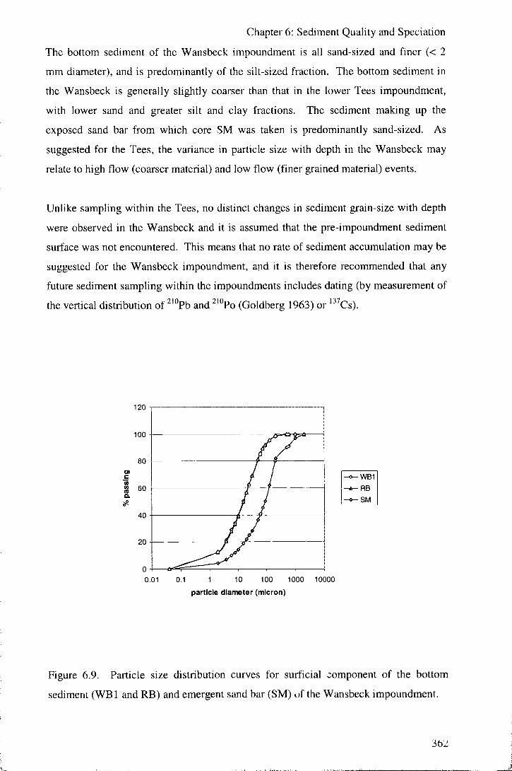
Chapter 6: Sediment Quality and Speciation
The bottom sediment of the Wansbeck impoundment is all sand-sized and finer (< 2
mm diameter), and is predominantly of the silt-sized fraction. The bottom sediment in
the Wansbeck is generally slightly coarser than that in the lower Tees impoundment,
with lower sand and greater silt and clay fractions. The sediment making up the
exposed sand bar from which core SM was taken is predominantly sand-sized. As
suggested for the Tees, the variance in particle size with depth in the Wansbeck may
relate to high flow (coarser material) and low flow (finer grained material) events.
Unlike sampling within the Tees, no distinct changes in sediment grain-size with depth
were observed in the Wansbeck and it is assumed that the pre-impoundment sediment
surface was not encountered. This means that no rate of sediment accumulation may be
suggested for the Wansbeck impoundment, and it is therefore recommended that any
future sediment sampling within the impoundments includes dating (by measurement of
the vertical distribution of 2'Vb and ^'°Po (Goldberg 1963) or '"Cs).
120
" 60
- 0 - WB1 -tr- RB
- 9 - SM
0.1 1 10 100 1000
particle diameter (micron)
10000
Figure 6.9. Particle size distribution curves for surficial component of the bottom
sediment (WBl and RB) and emergent sand bar (SM) of the Wansbeck impoundment.
3bZ

Chapter 6: Sediment Quality and Speciation
The difference in particle size distributions between the impoundments may relate to
both the nature of the sediment supply and the depositional environment. The length of
river affected by impoundment is shorter in the Wansbeck meaning that the sampling
sites are more proximal to the riverine sediment inputs. In addition, the Wansbeck
impoundment is shallower (in part due to more mature sediment f i l l ) and, hence, the
scouring effects of river flow is greater. Both these effects are likely to be significant in
causing the sediment of the Wansbeck to be coarser grained than that of the Tees. The
coarsening upwards in cores RB and SM may be due to a decrease in deposition of finer
sediment as water depth decreased at these sites, although the lack of a general
coarsening upwards sequence implies that there remains capacity for sediment
deposition within the Wansbeck to date.
Impoundment % sand % silt % clay % organic
Tees 24 65 11 17
Wansbeck 35 58 7 22
Table 6.6. Mean % grain-size fractions and % organic matter for bottom sediment cores
from the Tees and Wansbeck impoundments.
6.7.3 Organic matter
Organic matter contents of the sediment were determined as loss on ignitions (LOI) for
all samples. Organic carbon was determined through dichromate oxidations for 32
samples to check that LOI could be taken as an appropriate measure of organic content.
As shown in figure 6.10, there is a strong relationship (r^ = 89.4 %, n = 32) between the
two methods of organic determination:
LOI % = 3.78 organic carbon
This conversion value between organic carbon and organic matter content is higher than
that of 1.72 typically used (SSSA 1996), although several studies (e.g. Broadbent 1953)
have suggested that this conversion factor is too low for high organic sediments since
dichromate oxidation does not breakdown all organic components. In addition LOI
techniques tend to overestimate organic matter contents through loss of structural water
from hydrated aluminosilicates (particularly from clay lattices) and breakdown of
carbonates (a significant component of the Tees and Wansbeck sediments). The organic
363

Chapter 6: Sediment Quality and Speciation
matter contents reported are therefore likely to give good, i f somewhat slightly too high,
representations of the organic material in the sediment samples.
30 H
20
10
o ©-0
% organic carbon
Figure 6.10. The relationship between % loss on ignition at 900°C and % organic
carbon deteiTnined by dichromate oxidation for a selection of samples representing all
cores collected. Organic matter contents determined by LOI are approximately 3.8
times those determined by wet oxidation.
Tees
The mean organic matter content within the lower Tees impoundment sediment is 17.5
%. The mean organic carbon content is 4.5 %. This value is comparable with the
median value of 5.36 % organic carbon given by Jones and Turki (1997) for Tees
estuary sediment downstream of the barrage. Organic content shows no trends with
depth but a large scatter (figure 6.11), assumed to relate to variation in input of organic
particulates (either allochthonous or autochthonous). Organic matter is associated with
the silt-sized fraction of the sediment in the Tees (figure 6.12), and shows an inverse
relationship with sand content. The proportion of organic matter (as with the silt-sized
fraction) in the sediment increased dramatically on the impoundment of the estuary
(from < 5 to > 15 % ) .
3b4
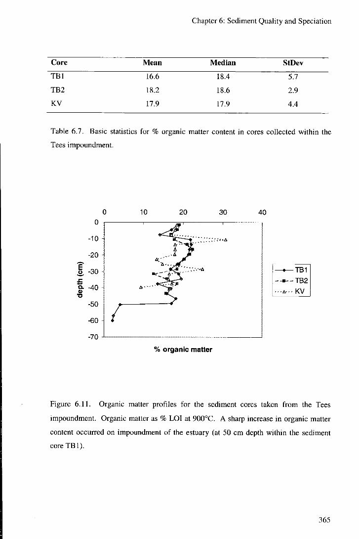
Chapter 6: Sediment Quality and Speciation
Core Mean Median StDev
TBI 16.6 18.4 5.7
TB2 18.2 18.6 2.9
KV 17.9 17.9 4.4
Table 6.7. Basic statistics for % organic matter content in cores collected within the
Tees impoundment.
10 20 30 40
5 -30
p. -40
TB1 - -» - -TB2 - - A - . - KV
% organic matter
Figure 6.11. Organic matter profiles for the sediment cores taken from the Tees
impoundment. Organic matter as % LOT at 900°C. A sharp increase in organic matter
content occurred on impoundment of the estuary (at 50 cm depth within the sediment
core TBI) .
365

Chapter 6: Sediment Quality and Speciation
E o 'c CO O) \—
o
30
20
10
0
o
0
0 0
10 20 30 40
% Silt
50 T 60 70 80
Figure 6.12. The relationship between organic matter and silt content in bottom
sediment of the lower Tees impoundment.
Wansbeck
The bottom sediment (all sites cored except SM) of the Wansbeck impoundment is
significantly richer in organic material than the lower Tees impoundment (22.3 %
compared with 17.5 % organic matter; P = 0.000). This difference may in part be due to
greater flocculation of organic material in the saline Wansbeck compared with the
freshwater Tees (Sholkovitz 1978), and may in part be due to tidal input of coal waste
material from the former mining operations around Ashington (noticeable coal particles
of a range of sizes were identified in all cores collected from the Wansbeck). Proximity
to the source of this material may explain the higher organic contents of the cores taken
immediately behind the barrage compared with those taken further upstream (table 6,8).
In addition less oxic conditions in the sediment of the Wansbeck than the Tees are likely
to allow better preservation of organic material in this impoundment. No relationship
between organic matter content and any particle size parameter is shown for the
Wansbeck impoundment sediments. Organic content shows a relatively large amount
of scatter but no noticeable trends with depth (figure 6.13).
366

Chapter 6: Sediment Quality and Speciation
Core Mean Median StDev
W B l
WB2
RB
SM
24.9
25.6
17.4
11.7
24.7
25.6
16.7
11.1
1.7
2.2
2.5
4.4
Table 6.8. Basic statistics for % organic matter content in cores collected within the
Wansbeck impoundment. Cores RB, W B l and WB2 are from bottom sediment and
core SM is from an exposed sand bar.
0
-10
-20
'E -30 u £ -40 Q. •g -50
-60
-70
-80
10 20 30 40 1 A 1
- - A Y A . - ' i . "A
" A > ,ts. A " •
A'. <L ' A , J
"A < •
A . ' «t ' ;A
-A' A . . .
V - A • <
" : : ' A
A : " - A
WBl -•*--WB2
- A - - - RB
% organic matter
Figure 6.13. Organic matter profiles for the sediment cores taken from the Wansbeck
impoundment. Organic matter as % LOI at 900°C.
367
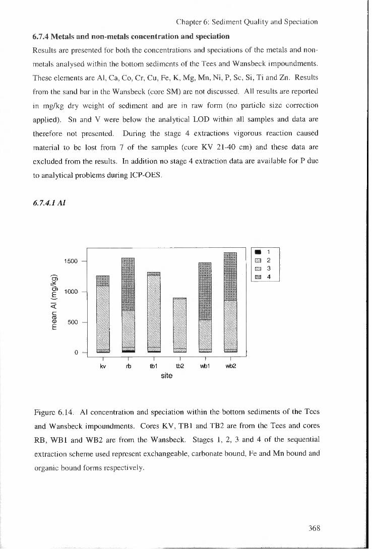
Chapter 6: Sediment Quality and Speciation
6.7.4 Metals and non-metals concentration and speciation
Results are presented for both the concentrations and speciations of the metals and non-
metals analysed within the bottom sediments of the Tees and Wansbeck impoundments.
These elements are Al , Ca, Co, Cr, Cu, Fe, K, Mg, Mn, Ni, P, Sc, Si, Ti and Zn. Results
from the sand bar in the Wansbeck (core SM) are not discussed. Al l results are reported
in mg/kg dry weight of sediment and are in raw form (no particle size correction
applied). Sn and V were below the analytical LOD within all samples and data are
therefore not presented. During the stage 4 extractions vigorous reaction caused
material to be lost from 7 of the samples (core KV 21-40 cm) and these data are
excluded from the results. In addition no stage 4 extraction data are available for P due
to analytical problems during ICP-OES.
6.7.4.1 Al
E
c 03 (U E
1500
1000
500
r ^
Figure 6.14. Al concentration and speciation within the bottom sediments of the Tees
and Wansbeck impoundments. Cores KV, T B I and TB2 are from the Tees and cores
RB, W B l and WB2 are from the Wansbeck. Stages 1, 2, 3 and 4 of the sequential
extraction scheme used represent exchangeable, carbonate bound, Fe and Mn bound and
organic bound forms respectively.
368

Chapter 6: Sediment Quality and Speciation
Sediment Stage
1
Stage
2
Stage
3
Stage
4
Total
available
Tees impoundment 13 53 1031 76 1173
Wansbeck impoundment 18 43 624 861 1547
Organic stream sediment 11400
(Finland)
Table 6.9. Average Al concentrations in sediment (mg/kg) from the Tees and
Wansbeck impoundments (stage 1 to 4 plus sum of stages of Tessier extraction scheme)
and organic stream sediment (concentrated HNO3 extraction; data from Lahermo et al.
1996).
Total potentially mobile Al levels are similar in the two impoundments but the phases in
which it is held differ (table 6.9, figure 6.14). Al is associated with the stage 3
extraction step within the Tees sediments. Within the Wansbeck sediment Al is
associated with both the stage 3 and the stage 4 extraction steps. (Stage 3 of the
extraction scheme is designated as corresponding with Fe and Mn oxide associated
elements, and stage 4 removes organic and sulphide bound elements (Tessier et al.
1979, Kersten and Forstner 1989)). Astrdm (1998) gives that available (released on
oxidation) A l is from 0.2 to 0.8 % of the total Al concentration in sulphide rich
sediments.
Profiles for stage 3 and stage 4 extractable Al within the sediments of the Tees and
Wansbeck impoundments show no clear trends but a large amount of fluctuation with
depth (figures 6.15, 6.16, 6.17 and 6.18). Stage 4 extractable Al shows a possible slight
decrease towards the surface of the sediment in the Wansbeck (figure 6.18), and a clear
change between pre and post-impoundment sediment in the Tees barrage cores (figure
6.17).
369

Chapter 6: Sediment Quality and Speciation
500 1000 1500
9- -40
-60 H
-TB2 - A - - - KV
Al (mg/kg)
Figure 6.15. Stage 3 extractable Al with depth in cores T B I , TB2 and KV from the
Tees impoundment.
500 1000 1500
-WB2
Al (mg/kg)
Figure 6.16. Stage 3 extractable Al with depth in cores W B l , WB2 and RB from the
Wansbeck impoundment.
370

Chapter 6: Sediment Quality and Speciation
500 1000 1500 2000
20 ^
o -30
a. -40 *
1 — ^ T B I __»._TB2
- A - - - KV
Al (mg/kg)
Figure 6.17. Stage 4 extractable Al with depth in cores T B I , TB2 and KV from the
Tees impoundment.
500 1000 1500 2000
•6 -50
WB1 --*--WB2 . - A -- RB
Al (mg/kg)
Figure 6.18. Stage 4 extractable Al with depth in cores W B l , WB2 and RB from the
Wansbeck impoundment.
371

6.7.4.2 Ca
Chapter 6: Sediment Quality and Speciation
D )
CO
O c 0
10000 H
5000 H
T 1 1 r
kv rb tb1 tb2 wb1 \At)2 site
Figure 6.19. Ca concentration and speciation within the bottom sediments of the Tees
and Wansbeck impoundments. Cores KV, TBI and TB2 are from the Tees and cores
RB, W B l and WB2 are from the Wansbeck. Stages 1, 2, 3 and 4 of the sequential
extraction scheme used represent exchangeable, carbonate bound, Fe and Mn bound and
organic bound forms respectively.
Sediment Stage
1
Stage Stage Stage Total
2 3 4 available
3975 1476 555 10170
4886 1085 936 9444
5600
Tees impoundment 4164
Wansbeck impoundment 2537
Organic stream sediment
(Finland)
Table 6.10. Average Ca concentrations in sediment (mg/kg) from the Tees and
Wansbeck impoundments (stage 1 to 4 plus sum of stages of Tessier extraction scheme)
and organic stream sediment (concentrated HNO3 extraction; data from Lahermo et al.
1996).
372

Chapter 6: Sediment Quality and Speciation
Significant amounts of Ca are held in all phases modelled by the extraction procedure
and total available concentrations are comparable for the two impoundments (table 6.10
and figure 6.19). Perhaps surprisingly, considering that the Tees is a freshwater
impoundment (and no pore water corrections are applied), exchangeable (stage 1
extractable) Ca levels are higher in Tees sediment than in the Wansbeck (which
periodically contains seawater). It is possible that ion exchange with the seawater input
to the Wansbeck impoundment has removed Ca from exchangeable sites in the
sediment. However, stage 1 is likely to be partially dissolving carbonates present, and
thus estimations of cation exchange capacities for the sediments are impossible. Not
surprisingly, given that the catchments of both rivers are composed in part of carbonate
geologies, the carbonate bound phase (stage 2 extraction) is a major source of Ca within
the sediments of both impoundments. Stage 3 extractable Ca is on average higher and
stage 4 extractable Ca lower in the Tees than in the Wansbeck sediments.
Profiles for exchangeable Ca (figures 6.20 and 6.21) show that for the Tees the
concentration within the sand dominated pre-impoundment sediment is much lower
than in the silt dominated (and higher pore-water content) post-impoundment sediment.
Within the post-impoundment sediment at the barrage sampling site there is a slight
increase in exchangeable Ca with depth in the sediment. Within the Wansbeck
sediment exchangeable Ca is relatively constant with depth in the sediment. Carbonate
input to the sediment went up significantly for a period following impoundment of the
Tees (figure 6.22), and may be due to increased inputs of carbonate material from the
catchment during the high flow periods of 1995. Within the Wansbeck sediment
carbonate bound Ca shows a large amount of variation and a possible slight increase
with depth (figure 6.23). The amount of Ca associated with stage 3 of the extraction
procedure is relatively constant with depth for both impoundments (figures 6.24 and
6.25) with the only significant feature being much greater concentrations within the pre-
impoundment sediment, possibly associated with Fe oxide coating on the sand-sized
particles. Stage 4 extractable Ca also shows a distinct decrease between pre and post-
impoundment sediment (figure 6.26). As with A l , stage 4 extractable Ca shows no
identifiable pattern but is of higher concentration in Wansbeck than Tees sediment
(figure 6.27).
373

Chapter 6: Sediment Quality and Speciation
2000 4000 6000
5 -30
g- -40
-TB2
Ca (mg/kg)
Figure 6.20. Stage 1 extractable Ca with depth in cores T B I , TB2 and KV from the
Tees impoundment.
2000 4000 6000
E o
0
-10
-20
-30
£ -40
5 -50
-60
-70
-80
' A . ' A .
Pry ' A ' A ; * ; .
> "J?
•A ^
.-A A , ' ' <
••A m / A «
x' • A . A .
. ; A A ; " <y
• A
-WB2 - A -- RB
Ca (mg/kg)
Figure 6.21. Stage 1 extractable Ca with depth in cores W B l , WB2 and RB from the Wansbeck impoundment.
374

Chapter 6: Sediment Quality and Speciation
2000 4000 6000 8000
o -30
Q - -40
-50 H
— ^ T B 1 -•*--TB2
- A - - - KV
Ca (mg/kg)
Figure 6.22. Stage 2 extractable Ca with depth in cores T B I , TB2 and KV from the
Tees impoundment.
8000
WB1 '-•-'VJB2 - - A . . . RB
Ca (mg/kg)
Figure 6.23. Stage 2 extractable Ca with depth in cores W B l , WB2 and RB from the Wansbeck impoundment.
375

Chapter 6: Sediment Quality and Speciation
0 2000 4000 6000
5- -40 -TB2
- - - A - - - KV
Ca (mg/kg)
Figure 6.24. Stage 3 extractable Ca with depth in cores T B I , TB2 and KV from the
Tees impoundment.
2000 4000 6000
•S -50
-WB2 - - A - - RB
Ca (mg/kg)
Figure 6.25. Stage 3 extractable Ca with depth in cores W B l , WB2 and RB from the
Wansbeck iinpoundment.
370

Chapter 6: Sediment Quality and Speciation
1000 2000 3000
o -30
Q - -40
•TB1 - - ^ - T B 2
- A - - - KV
Ca (mg/kg)
Figure 6.26. Stage 4 extractable Ca with depth in cores T B I , TB2 and KV from the
Tees impoundment.
0 1000 2000 3000
E u
a •a
1 •WB1
- -*- -WB2 - - A - - . RB
Ca (mg/kg)
Figure 6.27. Stage 4 extractable Ca with depth in cores W B l , WB2 and RB from the Wansbeck impoundment.
377

6.7.4.3 Co
Chapter 6: Sediment Quality and Speciation
O) 4 J*:
^ 3 O O c CO o E
2 H
Figure 6.28. Co concentration and speciation within the bottom sediments of the Tees
and Wansbeck impoundments. Cores KV, T B I and TB2 are from the Tees and cores
RB, W B l and WB2 are from the Wansbeck. Stages 1, 2, 3 and 4 of the sequential
extraction scheme used represent exchangeable, carbonate bound, Fe and Mn bound and
organic bound forms respectively.
Sediment Stage 1 Stage 2 Stage 3 Stage 4 Total
Tees impoundment 0.12 1.65 3.04 0.13 4.94
Wansbeck impoundment 0.12 1.23 1.66 2.30 5.31
Organic stream sediment (Finland) 10.5
Tees estuary downstream of barrage 34
Humber estuary 16
Table 6.11. Average Co concentrations in sediment (mg/kg) from the Tees and
Wansbeck impoundments (stage 1 to 4 plus sum of stages of Tessier extraction
scheme), organic stream sediment (< 2 mm fraction, concentrated HNO3 extraction;
data from Lahermo et al. 1996), Tees estuary sediment from downstream of barrage
(total extraction; data from Jones and Turki 1997), and Humber estuary (< 100 |.im
fraction, concentrated HNO3 extraction: data from Bryan and Langston 1992).
378

Chapter 6: Sediment Quality and Speciation
Levels of Co reported in this study are much lower than those determined for bottom
sediment downstream of the Tees barrage (Jones and Turki, 1997; table 6.11), although
the data are not directly comparable due to the difference between extraction techniques
employed (potentially environmentally mobile vs. total concentrations). Jones and
Turki state that the Co is dominantly held in the residual minerals (siUcates), and most
Co is therefore not available for exchange with the water column or biota.
Total available Co levels are similar for sediment from the Tees and the Wansbeck
impoundments but their pattern of speciation differs. Very little Co is held
exchangeably within sediments from either of the impoundments. Carbonate bound Co
is slightly higher in the Tees than the Wansbeck sediment. The major difference
between the impoundments is in terms of stage 3 and stage 4 extractable phases for Co,
and the pattern shown is similar to that of Al . Within the Tees sediment the majority of
Co is held in the reducible phase (stage 3), with very little Co in the oxidisable phase
(stage 4). In Wansbeck sediment Co is held in both phases, with the greatest proportion
removed during extraction 4 (table 6.11, figure 6.28).
Stage 2 extractable Co shows, as for Ca, a significant peak within the sedimentation
following impoundment of the Tees estuary (figure 6.29). Stage 3 extractable Co
concentration fluctuates with depth in the Tees but shows no determinable trend (figure
6.31). Stage 2 and 3 extractable Co is relatively constant with depth within the
Wansbeck (figures 6.30 and 6.32). As is seen repeatedly for a variety of elements
within the Tees sediment, the pattern for stage 4 extraction is of very low concentrations
at all depths, with slightly higher levels in pre-impoundment sediment (figure 6.33).
Sediment in the Wansbeck shows a significant decrease towards the sediment surface
from circa 4 mg/kg at 70 cm depth to circa 1 mg/kg at the surface (figure 6.34).
379

Chapter 6: Sediment Quality and Speciation
o -30 -TB2
D. -40 . - - A -. KV
Co (mg/kg)
Figure 6.29. Stage 2 extractable Co with depth in cores T B I , TB2 and KV from the
Tees impoundment.
-WB2 - A - - - RB
Co (mg/kg)
Figure 6.30. Stage 2 extractable Co with depth in cores W B l , WB2 and RB from the
Wansbeck impoundment.
380

Chapter 6: Sediment Quality and Speciation
0 -1
-10 -
-20 -
(cm
)
-30
Q .
a> -40 -
-50 -
-60 -
-70 -
— • — T B I - - - - T B 2 - . - A - - - KV
Co (mg/kg)
Figure 6.31. Stage 3 extractable Co with depth in cores T B I , TB2 and KV from the
Tees impoundment.
— • — W B l - - - - - W B 2
- A - - - RB
Co (mg/kg)
Figure 6.32. Stage 3 extractable Co with depth in cores W B l , WB2 and RB from the
Wansbeck impoundment.
381

Chapter 6: Sediment Quality and Speciation
•a
0 -i
-10 1
>'A
t '" W
-20 -
-30 1
-40 1
-50 -
-60 -
-70 -
-TB2 A -- KV
Co (mg/kg)
Figure 6.33. Stage 4 extractable Co with depth in cores T B I , TB2 and KV from the
Tees impoundment.
E
t a> •a
0 n
-10 -
-20 -
A . 1 ^ ^ ' 1
-30 -
-40 -
^ i i - A — 1 ^ " A
* A 7 ; > O
-50 -
-60 -- A .
-70 - ^ A
-80 -
-WB2 A RB
Co (mg/kg)
Figure 6.34. Stage 4 extractable Co with depth in cores W B l , WB2 and RB from the Wansbeck impoundment.
382

Chapter 6: Sediment Quality and Speciation
6.7.4.4 Cr
O)
O c s E
wb2 site
Figure 6.35. Cr concentration and speciation within the bottom sediments of the Tees
and Wansbeck impoundments. Cores KV, TB1 and TB2 are from the Tees and cores
RB, W B l and WB2 are from the Wansbeck. Stages 1, 2, 3 and 4 of the sequential
extraction scheme used represent exchangeable, carbonate bound, Fe and Mn bound and
organic bound forms respectively.
Sediment Stage 1 Stage 2 Stage 3 Stage 4 Total
Tees impoundment 0.14 1.78 22.78 46.46 71.16
Wansbeck impoundment 0.08 0.61 4.34 4.50 9.53
Organic stream sediment (Finland) 31.3
Tees estuary downstream of barrage 224
River Tees upstream of impoundment 64
Humber estuary 77
Table 6.12. Average Cr concentrations in sediment (mg/kg) from the Tees and
Wansbeck impoundments (stage 1 to 4 plus sum of stages of Tessier extraction
scheme), organic stream sediment (< 2 mm fraction, concentrated HNO3 extraction;
data from Lahermo et al. 1996), Tees estuary sediment from downstream of barrage
(total extraction; data from Jones and Turki 1997), River Tees sediment upstream of
383

Chapter 6: Sediment Quality and Speciation
impoundment (< 63 pim fraction, total extraction; data from EA), and Humber estuary
(< 100 |J,m fraction, concentrated HNO3 extraction; data from Bryan and Langston
1992).
Cr occurs in distinctly different concentration in the two impoundments, with levels
higher in the Tees through all speciations (figure 6.35 and table 6.12) likely to be due to
industrial input from Cr works at Eaglescliffe (upstream of barrage). Levels in the Tees
impoundment are lower however than those encountered downstream of the barrage
(where available forms generally exceed 150 mg/kg (Jones and Turki 1997)), which
reflects greater sewage and industrial inputs in the downstream section of the estuary.
Bryan and Langston (1992) report available Cr levels reaching a maximum in UK
estuaries studied of 800 mg/kg in the Loughor estuary (South Wales) which is subject to
pollution from tinplate production.
The speciation pattern is similar within sediment from both impoundments. Very little
Cr is held exchangeably of bound to carbonates, and the stage 3 and stage 4 extractable
species are the main available forms (figure 6.35).
The pattern of stage 3 extractable (Fe and Mn oxide bound) Cr with depth in the Tees is
of relatively constant concentration with depth within the post-impoundment sediment,
but significantly higher Cr within the pre-impoundment sediment (> 50 cm depth)
(figure 6.36). Within the Wansbeck Cr increases slightly with depth in the sediment,
although there is much scatter (figure 6.37). The pattern of stage 4 extractable (sulphide
and organic bound) Cr is similar to that for stage 3 extractable Cr for both
impoundments, with higher concentrations in pre-impoundment sediment in the Tees
(figure 6.38) and much lower concentrations but a small increase with depth in the
Wansbeck (figure 6.39).
384

Chapter 6: Sediment Quality and Speciation
50 100 150 200
o -30
Q- -40
TBI --*--TB2
. - A - . . KV
Cr (mg/kg)
Figure 6.36. Stage 3 extractable Cr with depth in cores T B I , TB2 and KV from the
Tees impoundment.
E o WB1 - -» - -WB2
- A - - - RB
Cr (mg/kg)
Figure 6.37. Stage 3 extractable Cr with depth in cores W B l , WB2 and RB from the
Wansbeck impoundment (note different concentration scale to figure 6.36 above).
385

Chapter 6: Sediment Quality and Speciation
50 100 150 0
-10
-20
1 -30
I -40
-50
-60
-70
3 '
A '
-TB2
Cr (mg/kg)
Figure 6.38. Stage 4 extractable Cr with depth in cores T B I , TB2 and KV from the
Tees impoundment.
-WB2 A - . - RB
Cr (mg/kg)
Figure 6.39. Stage 4 extractable Cr with depth in cores W B l , WB2 and RB from the
Wansbeck impoundment (note different concentration scale to figure 6.38 above).
386

6.7.4.5 Cu
Chapter 6: Sediment Quality and Speciation
E,
o c S E
30
20
10 H
0 H
Figure 6.40. Cu concentration and speciation within the bottom sediments of the Tees
and Wansbeck impoundments. Cores KV, T B I and TB2 are from the Tees and cores
RB, W B l and WB2 are from the Wansbeck. Stages 1, 2, 3 and 4 of the sequential
extraction scheme used represent exchangeable, carbonate bound, Fe and Mn bound and
organic bound forms respectively.
Sediment Stage 1 Stage 2 Stage 3 Stage 4 Total
Tees impoundment 0.41 0.44 11.54 0.92 13.31
Wansbeck impoundment 0.62 0.69 11.80 15.57 26.68
Organic stream sediment (Finland) 12.4
Tees estuary downstream of barrage 103
River Tees upstream of impoundment 56
Humber estuary 54
Table 6.13. Average Cu concentrations in sediment (mg/kg) from the Tees and
Wansbeck impoundments (stage 1 to 4 plus sum of stages of Tessier extraction
scheme), organic stream sediment (< 2 mm fraction, concentrated HNO3 extraction;
data from Lahermo et al. 1996), Tees estuary sediment from downstream of barrage
387

Chapter 6: Sediment Quality and Speciation
(total extraction; data from Jones and Turki 1997), River Tees sediment upstream of
impoundment (< 63 \im fraction, total extraction; data from EA), and Humber estuary
(< 100 \im fraction, concentrated HNO3 extraction; data from Bryan and Langston
1992).
Cu levels in sediment in the Wansbeck are approximately double those in the Tees
impoundment (table 6.13). Levels are slightly higher than in organic stream sediment,
but lower than those reported for sediment collected in the Tees estuary downstream of
the barrage.
A similar pattern of speciation to that of Al , Fe, Ni, Sc, Zn, and to an extent Co and Mn,
is shown in the sediment of the impoundments by Cu: i.e. the majority of Cu is held in
stage 3 extractable form (Fe and Mn oxides). Hydrous oxides of Fe and Mn are major
trace metal hosts in several estuaries (Calmano and Forstner 1983; Luoma and Davies
1983; Peterson et al. 1995). In the Tees virtually no Cu is held in the oxidisable/stage 4
phase, but in the Wansbeck this phase is significant (figure 6.40). Very little Cu is held
exchangeably or bound with carbonates.
Extraction stage 3 is subject to very large errors for Cu (47 %) for unknown reasons,
and the irregular profiles for both impoundments reflect this error, with no patterns
discernible (figures 6.41 and 6.42). The profile for stage 4 extractable Cu in the Tees
shows very low levels through the post-impoundment sediment and higher levels in pre-
impoundment sediment (figure 6.43), and in the Wansbeck there is a relatively steady
increase with depth in the sediment column (figure 6,44).
388

Chapter 6: Sediment Quality and Speciation
10 20 30
o -30
o- -40
TBI - -*--TB2 - . - A - . - KV
Cu (mg/kg)
Figure 6.41. Stage 3 extractable Cu with depth in cores T B I , TB2 and KV from the
Tees impoundment.
WB1 - -» - -WB2 . - - A - - - RB
Cu (mg/kg)
Figure 6.42. Stage 3 extractable Cu with depth in cores W B l , WB2 and RB from the
Wansbeck impoundment.
389

Chapter 6: Sediment Quality and Speciation
10 20 30 40 50
o -30
a -40 -TB2
- A K V
Cu (mg/kg)
Figure 6.43. Stage 4 extractable Cu with depth in cores T B I , TB2 and KV from the
Tees impoundment.
10 20 30 40 50
-WB2 A - - - RB 6 -50
Cu (mg/kg)
Figure 6.44. Stage 4 extractable Cu with depth in cores W B l , WB2 and RB from the
Wansbeck impoundment.
390
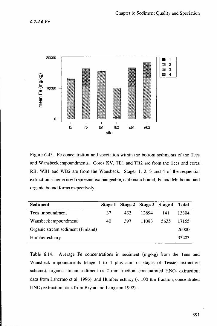
6.7.4.6 Fe
Chapter 6: Sediment Quality and Speciation
20000
D )
o
% E
10000 H
Figure 6.45. Fe concentration and speciation within the bottom sediments of the Tees
and Wansbeck impoundments. Cores KV, TBI and TB2 are from the Tees and cores
RB, W B l and WB2 are from the Wansbeck. Stages 1, 2, 3 and 4 of the sequential
extraction scheme used represent exchangeable, carbonate bound, Fe and Mn bound and
organic bound forms respectively.
Sediment Stage 1 Stage 2 Stage 3 Stage 4 Total
Tees impoundment
Wansbeck impoundment
Organic stream sediment (Finland)
Humber estuary
37
40
432
397
12694
11083
141
5635
13304
17155
26000
35203
Table 6.14. Average Fe concentrations in sediment (mg/kg) from the Tees and
Wansbeck impoundments (stage 1 to 4 plus sum of stages of Tessier extraction
scheme), organic stream sediment (< 2 mm fraction, concentrated HNO3 extraction;
data from Lahermo et al. 1996), and Humber estuary (< 100 \xm fraction, concentrated
HNO3 extraction; data from Bryan and Langston 1992).
391

Chapter 6: Sediment Quality and Speciation
Total available Fe levels are slightly higher in the sediments of the Wansbeck than the
Tees impoundment (table 6.14). That levels are lower than those reported for organic
stream sediment or for the Humber estuary probably relates to difference in the
extraction technique and grain-size fraction analysed rather than large differences in Fe
behaviour.
The speciation of Fe shows the same pattern as a number of heavy metals (Cu, Ni , Zn,
etc.) in the sediments of the impoundments. Very little Fe is held in either
exchangeable (stage 1 extractable) or carbonate bound (stage 2 extractable) in either
estuary. Within the Tees almost all Fe is held in the reducible (Fe oxide) phase. In the
Wansbeck sediments Fe is held in both the reducible and oxidisable (Fe sulphides and
organic bound) phases (figure 6.45).
Fe in oxides (stage 3 extractable) shows variation but no identifiable trends with depth
in the sediment of the Tees (figure 6.46), and shows a slight increase (but with much
scatter) in the Wansbeck (figure 6.47). There is effectively no stage 4 extractable Fe in
the Tees impoundment, apart from within the deep (pre-impoundment) sediment
encountered within core TBI (figure 6.48). Fe within sulphide (and organic bound)
shows an increase with depth in sediment within the Wansbeck with concentrations at
approximately 2000 mg/kg at the sediment-water column interface and almost 10000 at
a depth of 60 cm (figure 6.49).
392

Chapter 6: Sediment Quality and Speciation
5000 10000 15000 20000 25000
o -30
g- -40
•TBI - - » - - T B 2
- A - - - KV
Fe (mg/kg)
Figure 6.46. Stage 3 extractable Fe with depth in cores T B I , TB2 and KV from the
Tees impoundment.
5000 10000 15000 20000 25000
— ^ W B I - -*- -WB2
- A - - - RB
Fe (mg/kg)
Figure 6.47. Stage 3 extractable Fe with depth in cores W B l , WB2 and RB from the
Wansbeck impoundment.
393

Chapter 6: Sediment Quality and Speciation
5000 10000 15000 0
-10
-20
J , -30
Q. -40 v •D
-50
-60
-70
^ s — T B I --Q---TB2
- A - - - KV
Fe (mg/kg)
Figure 6.48. Stage 4 extractable Fe with depth in cores T B I , TB2 and KV from the
Tees impoundment.
5000 10000 15000
WBl _ ^ - W B 2 - - A -- RB
Fe (mg/kg)
Figure 6.49. Stage 4 extractable Fe with depth in cores W B l , WBl and RB from the
Wansbeck impoundment.
394

6.7.4J K
Chapter 6: Sediment Quality and Speciation
2000
0 5
E
c % E
1000
0 A rb tb1 tb2
site wb1 wb2
Figure 6.50. K concentration and speciation within the bottom sediments of the Tees
and Wansbeck impoundments. Cores KV, TBI and TB2 are from the Tees and cores
RB, W B l and WB2 are from the Wansbeck. Stages 1, 2, 3 and 4 of the sequential
extraction scheme used represent exchangeable, carbonate bound, Fe and Mn bound and
organic bound forms respectively.
Sediment Stage 1 Stage 2 Stage 3 Stage 4 Total
Tees impoundment 341 81 38 47 507
Wansbeck impoundment 1193 202 69 77 1541
Organic stream sediment (Finland) 1600
Table 6.15. Average K concentrations in sediment (mg/kg) from the Tees and
Wansbeck impoundments (stage 1 to 4 plus sum of stages of Tessier extraction
scheme), and organic stream sediment (< 2 mm fraction, concentrated HNO3 extraction;
data from Lahermo et al. 1996).
Available K concentrations are higher in the sediment of the Wansbeck than the Tees
impoundment, with the main difference being in the concentrations between
exchangeable and carbonate bound phases (table 6.15 and figure 6.50). The difference
395

Chapter 6: Sediment Quality and Speciation
is assumed to be due to the difference in K content of the overlying water columns in
the impoundments (freshwater in the Tees as opposed to seawater in the Wansbeck).
The higher K contents within the cores taken immediately upstream of the barrages in
both impoundments is likely to be due to greater seawater influence at these points
(even the "freshwater" Tees is observed to occasionally undergo seawater intrusion (see
chapter 3)).
Within the sediments of both estuaries K is mainly held in the exchangeable phase, but
the stage 2, and to a degree 3 and 4, extractable forms are also significant (figure 6.50).
Core KV from the Tees shows a relatively constant level of exchangeable K with depth
in the sediment, whereas site TB shows an almost linear increase with depth down to
the depth at which sand-dominated (and both lower moisture and clay content) pre-
impoundment sediments are encountered where exchangeable K drops sharply (figure
6.51). This may be either a diffusion of mobile K at depth in the sediment towards the
low (mean 3 mg/1) K water column or an ion exchange effect (see Mg below). Within
the Wansbeck sediments a similar but smaller diffusion gradient is seen, but since
sampling was during a period in which the seawater was overlying the sediment, a
distinct increase in exchangeable K is seen close to the sediment surface (figure 6.52).
Carbonate bound K in the Tees shows a very similar pattern to that of Ca and is likely to
relate to the relative proportion of (flow controlled) carbonate inputs from the catchment
to the sediment (figure 6.53). The profile for carbonate bound K in the Wansbeck
shows a large amount of scatter but no significant trends with depth in the sediment
(figure 6.54).
396

Chapter 6: Sediment Quality and Speciation
500 1000 1500 2000 2500
Q- -40
TBI --*--TB2
- A - - - KV
K (mg/kg)
Figure 6.51. Stage 1 extractable K with depth in cores T B I , TB2 and KV from the Tees
impoundment.
500 1000 1500 2000 2500
6 -50
•WB1 -- i»--WB2
- A - - - RB
K (mg/kg)
Figure 6.52. Stage 1 extractable K with depth in cores W B l , WB2 and RB from the Wansbeck impoundment.
397

Chapter 6: Sediment Quality and Speciation
100 200 300 400
5 -30
CL -40 A - . . KV
K (mg/kg)
Figure 6.53. Stage 2 extractable K with depth in cores T B I , TB2 and KV from the Tees
impoundment.
100 200 300 400
-WB2 A -- RB
K (mg/kg)
Figure 6.54. Stage 2 extractable K with depth in cores W B l , WB2 and RB from the
Wansbeck impoundment.
398
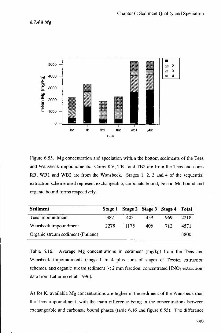
6.7.4.8 Mg
Chapter 6: Sediment Quality and Speciation
5000 H
4000
E 3000 C3)
c % E
2000
1000
0 -A 1 r wbl wb2
Figure 6.55. Mg concentration and speciation within the bottom sediments of the Tees
and Wansbeck impoundments. Cores KV, T B I and TB2 are from the Tees and cores
RB, W B l and WB2 are from the Wansbeck. Stages 1, 2, 3 and 4 of the sequential
extraction scheme used represent exchangeable, carbonate bound, Fe and Mn bound and
organic bound forms respectively.
Sediment Stage 1 Stage 2 Stage 3 Stage 4 Total
Tees impoundment 387 403 459 969 2218
Wansbeck impoundment 2278 1175 406 712 4571
Organic stream sediment (Finland) 3800
Table 6.16. Average Mg concentrations in sediment (mg/kg) from the Tees and
Wansbeck impoundments (stage 1 to 4 plus sum of stages of Tessier extraction
scheme), and organic stream sediment (< 2 mm fraction, concentrated HNO3 extraction;
data from Lahermo et al. 1996).
As for K, available Mg concentrations are higher in the sediment of the Wansbeck than
the Tees impoundment, with the main difference being in the concentrations between
exchangeable and carbonate bound phases (table 6.16 and figure 6.55). The difference
399
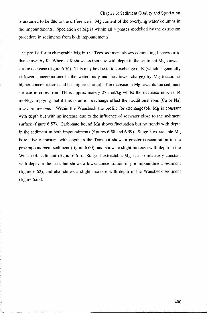
Chapter 6: Sediment Quality and Speciation
is assumed to be due to the difference in Mg content of the overlying water columns in
the impoundments. Speciation of Mg is within all 4 phases modelled by the extraction
procedure in sediments from both impoundments.
The profile for exchangeable Mg in the Tees sediment shows contrasting behaviour to
that shown by K. Whereas K shows an increase with depth in the sediment Mg shows a
strong decrease (figure 6.56). This may be due to ion exchange of K (which is generally
at lower concentrations in the water body and has lower charge) by Mg (occurs at
higher concentrations and has higher charge). The increase in Mg towards the sediment
surface in cores from TB is approximately 27 mol/kg whilst the decrease in K is 14
mol/kg, implying that if this is an ion exchange effect then additional ions (Ca or Na)
must be involved. Within the Wansbeck the profile for exchangeable Mg is constant
with depth but with an increase due to the influence of seawater close to the sediment
surface (figure 6.57). Carbonate bound Mg shows fluctuation but no trends with depth
in the sediment in both impoundments (figures 6.58 and 6.59). Stage 3 extractable Mg
is relatively constant with depth in the Tees but shows a greater concentration in the
pre-impoundment sediment (figure 6.60), and shows a slight increase with depth in the
Wansbeck sediment (figure 6.61). Stage 4 extractable Mg is also relatively constant
with depth in the Tees but shows a lower concentration in pre-impoundment sediment
(figure 6.62), and also shows a slight increase with depth in the Wansbeck sediment
(figure 6.63).
400

Chapter 6: Sediment Quality and Speciation
200 400 600 800
£ u
a. <u
TBI - •* - -TB2
- A - - - KV
Mg (mg/kg)
Figure 6.56. Stage 1 extractable Mg with depth in cores T B I , TB2 and KV from the
Tees impoundment.
0 2000 4000 6000
-30 H
£ -40 H •WB1
- - - - -WB2 • -•A--. RB
Mg (mg/kg)
Figure 6.57. Stage 1 extractable Mg with depth in cores W B l , WB2 and RB from the Wansbeck impoundment (note different concentration scale to figure 6.56 above).
401

Chapter 6: Sediment Quality and Speciation
500 1000 1500 2000
o -30
Q. -40 'TB2
Wig (mg/kg)
Figure 6.58. Stage 2 extractable Mg with depth in cores T B I , TB2 and KV from the
Tees impoundment.
500 1000 1500 2000
-WB2 • - A - - - RB
Mg (mg/kg)
Figure 6.59. Stage 2 extractable Mg with depth in cores W B l , WB2 and RB from the
Wansbeck impoundment.
402

Chapter 6: Sediment Quality and Speciation
500 1000 1500
o -30
a -40
TBI - -* - -TB2
- A - - - KV
Mg (mg/kg)
Figure 6.60. Stage 3 extractable Mg with depth in cores T B I , TB2 and KV from the
Tees impoundment.
500 1000 1500
E u
a. a> •a
•WB1 - - ^ - W B 2
- A R B
Mg (mg/kg)
Figure 6.61. Stage 3 extractable Mg with depth in cores W B l , WB2 and RB from the
Wansbeck impoundment.
403

Chapter 6: Sediment Quality and Speciation
500 1000 1500 2000
o -30
Q- -40
— e ^ T B I
---A---KV
Mg (mg/kg)
Figure 6.62. Stage 4 extractable Mg with depth in cores T B I , TB2 and KV from the
Tees impoundment.
500 1000 1500 2000
•6 -50
•WB1
- A -- RB
Mg (mg/kg)
Figure 6.63. Stage 4 extractable Mg with aepth in cores W B l , WB2 and RB from the
Wansbeck impoundment.
404

6.7.4.9 Mn
Chapter 6: Sediment Quality and Speciation
600
^ 500
O) 400 E
300 -A
% 200
100 H
Figure 6.64. Mn concentration and speciation within the bottom sediments of the Tees
and Wansbeck impoundments. Cores KV, T B I and TB2 are from the Tees and cores
RB, W B l and WB2 are from the Wansbeck. Stages 1, 2, 3 and 4 of the sequential
extraction scheme used represent exchangeable, carbonate bound, Fe and Mn bound and
organic bound forms respectively.
Sediment Stage 1 Stage 2 Stage 3 Stage 4 Total
Tees impoundment
Wansbeck impoundment
Organic stream sediment (Finland)
Humber estuary
115
13
284
93
168
52
10
ICQ
577
258
546
1015
Table 6.17. Average Mn concentrations in sediment (mg/kg) from the Tees and
Wansbeck impoundments (stage 1 to 4 plus sum of stages of Tessier extraction
scheme), organic stream sediment (< 2 mm fraction, concentrated HNO3 extraction;
data from Lahermo et al. 1996), and Humber estuary (< 100 ^im fraction, concentrated
HNO3 extraction; data from Bryan and Langston 1992).
405

Chapter 6: Sediment Quality and Speciation
Available Mn concentrations are higher in the sediment in the Tees than the Wansbeck
impoundment (table 6.17). Mean Mn levels vary widely between UK estuaries, with
concentrations in the Humber relatively high (mean Mn in the Tyne is 395 mg/kg for
example; Bryan and Langston 1992).
The patterns of speciation for Mn differ between the impoundments (figure 6.64).
Within the sediments of the Tees Mn is held exchangeably, bound with carbonates and
bound in reducible form, with very little released in the oxidisable phase. Within the
sediment of the Wansbeck Mn is held bound with carbonates, bound in reducible foim
and bound in the oxidisable phase, with very little held exchangeably.
Assuming that conditions are not significantly altered during sampling and pre-
treatment, then the exchangeable Mn fraction represents the amount of (dissolved) Mn "
in the sediment. Mn solubility is redox controlled, such that Mn^* is released when Mn-
oxides are used as secondary oxidants for the breakdown of organic matter as dissolved
oxygen levels fall (see chapter 4). The profiles for exchangeable Mn thus represent the
redox conditions within the sediment, with maxima approximating the depth at which
maximum use of Mn as an electron acceptor is occurring. Within the Tees this is at
approximately 15 cm at both sites sampled, and within the Wansbeck it is
approximately 7 cm at the barrage site and almost at the surface at site RB (figures 6.65
and 6.66). The profiles are typical of organic rich anoxic nearshore sediments (Heggie
et al., 1987; Upstill-Goddard et al., 1989). The depths of Mn maxima represent the
relative anoxia in the sediments of the impoundments, with oxygen reaching greater
depths in the sediment profile in the Tees, and anoxic conditions at the sediment-water
column interface at site RB within the Wansbeck. The profiles for both carbonate and
oxide bound Mn show a similar pattern to that of exchangeable Mn (figures 6.67, 6.68,
6.69 and 6.70), implying that either Mn is depleted at depth where Mn has already been
released from the sediment or that on pre-treatment of the samples exposure of
oxidising conditions caused precipitation of solid phases (particularly oxides) of Mn.
Very little Mn is held in the oxidisable phase in the Tees (figure 6.71), but in the
Wansbeck Mn in the oxidisable phase (assumed to be associated with organic material)
shows an increase with depth (figure 6.72).
406
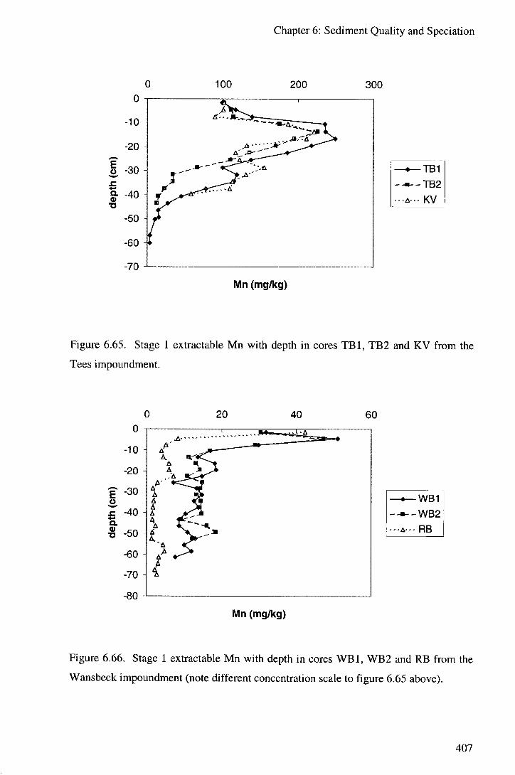
Chapter 6: Sediment Quality and Speciation
100 200 300 0
-10
-20
(cm
)
-30 £
Q. 0)
-40 TJ
-50
-60
-70
—•—TB1 --••--TB2
- A - . - KV
Mn (mg/kg)
Figure 6.65. Stage 1 extractable Mn with depth in cores T B I , TB2 and KV from the
Tees impoundment.
0 20 40 60
E o
a. 0) T3
0
-10
-20
-30
-40
-50
-60
-70
-80
!
A ^ ' •
-'^''^
A J* / A
A S»
A JtC^ A ft-jT
A <
A ^ ^
A S»
A JtC^ A ft-jT
A <
A ^ ^ A
1
WBl --*--WB2
- A - - - RB
Mn (mg/kg)
Figure 6.66. Stage 1 extractable Mn with depth in cores W B l , WB2 and RB from the
Wansbeck impoundment (note different concentration scale to figure 6.65 above).
407

Chapter 6: Sediment Quality and Speciation
100 200 300 400 500 0
-10
-20
1, -30
I -40
-50
-60
-70
--TB2 . - - A - . - KV
Mn (mg/kg)
Figure 6.67. Stage 2 extractable Mn with depth in cores T B I , TB2 and K V from the
Tees impoundment.
100 200 300 400 500
-WB2
Mn (mg/kg)
Figure 6.68. Stage 2 extractable Mn with depth in cores W B l , WB2 and RB from the Wansbeck impoundment.
408

Chapter 6: Sediment Quality and Speciation
100 200 300
o -30
g- -40
•TBI - -* - -TB2 - - - A - - . KV
Mn (mg/kg)
Figure 6.69. Stage 3 extractable Mn with depth in cores T B I , TB2 and KV from the
Tees impoundment.
100 200 300
•WBl - - ^ - W B 2
- A - - - RB
Mn (mg/kg)
Figure 6.70. Stage 3 extractable Mn with depth in cores W B l , WB2 and RB from the
Wansbeck impoundment.
409

Chapter 6: Sediment Quality and Speciation
100 200 300
o -30 -TB2
Q- -40 - A - - - KV
Mn (mg/kg)
Figure 6.71. Stage 4 extractable Mn with depth in cores T B I , TB2 and KV from the
Tees impoundment.
100 200 300
E o
Q. 0) •a
0 -1
-10 -
A 9 P h ^ y
1 1
-20 -
-30 -It!- • A
.-A
-40 -
-50 -c
^-^ ^ ^ ^ ^ ^ • A y>
-oU - A - -
-70 -
-80 -
-WB2
Mn (mg/kg)
Figure 6.72, Stage 4 extractable Mn with depth in cores W B l , WB2 and RB from the
Wansbeck impoundment.
410

6.7.4.10 Ni
Chapter 6: Sediment Quality and Speciation
E
1 E
10
0 H 1 r
rb tb1 tb2 wb1 wb2 site
Figure 6.73. Ni concentration and speciation within the bottom sediments of the Tees
and Wansbeck impoundments. Cores KV, T B I and TB2 are from the Tees and cores
RB, W B l and WB2 are from the Wansbeck. Stages 1, 2, 3 and 4 of the sequential
extraction scheme used represent exchangeable, carbonate bound, Fe and Mn bound and
organic bound forms respectively.
Sediment Stage 1 Stage! Stage 3 Stage 4 Total
Tees impoundment 0.22 1.65 5.54 0.46 7.87
Wansbeck impoundment 0.30 1.61 4.29 5.30 11.50
Organic stream sediment (Finland) 13.9
Tees estuary downstream of barrage 41
River Tees upstream of impoundment 36
Humber estuary 39
Table 6.18. Average Ni concentrations in sediment (mg/kg) from the Tees and
Wansbeck impoundments (stage 1 to 4 plus sum of stages of Tessier extraction
scheme), organic stream sediment (< 2 mm fraction, concentrated HNO3 extraction;
data from Lahermo et al. 1996), Tees estuary sediment from downstream of barrage
411

Chapter 6: Sediment Quality and Speciation
(total extraction; data from Jones and Turki 1997), River Tees sediment upstream of
impoundment (< 63 |xm fraction, total extraction; data from EA), and Humber estuary
(< 100 ^m fraction, concentrated H N O 3 extraction; data from Bryan and Langston
1992).
Available Ni concentrations are slightly higher in the Wansbeck than the Tees
impoundment, mainly due to the fraction held in the oxidisable fraction (table 6.18 and
figure 6.73). Concentrations are much lower than those reported for downstream of the
barrage in the Tees estuary for total Ni, although approximately half the concentration
of available (stage 1 to 4 of Tessier et al. (1979) extraction scheme) found downstream
since the majority of Ni is held in residual (non-available) forms (Jones and Turki
1997).
Very little Ni is held exchangeably within the sediment of either impoundment, similar
quantities of Ni are removed by extraction stages 2 and 3 in both impoundments, and
stage 4 extractable Ni is only a significant fraction in the Wansbeck impoundment
(figure 6.73).
The profile for carbonate bound Ni in the sediment of the Tees impoundment shows a
similar pattern to that shown for Ca, with a peak in the sedimentation following
impoundment, interpreted as due to high flow related high carbonate input (figure 6.74).
The carbonate bound Ni profile in the Wansbeck is more constant with depth (figure
6.75). The profiles for stage 3 and stage 4 extractable Ni within the impoundments
show the same pattern as that shown by Fe (and several other heavy metals), with the
clearest trend being an increase in the stage 4 extractable portion with depth in the
Wansbeck (figures 6.76, 6.77, 6.78 and 6.79).
412

Chapter 6: Sediment Quality and Speciation
0
o -30
o- -40
•TBI --^i--TB2 . - A - - - KV
Ni (mg/kg)
Figure 6.74. Stage 2 extractable Ni with depth in cores T B I , TB2 and KV from the
Tees impoundment.
0
-10
-20
-30 o
£ -40
t -50
-60
-70
-80
A J B i L 1 1
I n . W ' - . A
A . ' '•P A
4 i _ ^ A
, - " A \ A . - . - ;
11U_2^A^ - A
WBl - - • - -WB2
- A - - - RB
Ni (mg/kg)
Figure 6.75. Stage 2 extractable Ni with depth in cores W B l , WB2 and RB from the
Wansbeck impoundment.
413

Chapter 6: Sediment Quality and Speciation
Ni (mg/kg)
10
o -30 -TB2
Q- -40 A -- KV
Figure 6.76. Stage 3 extractable Ni with depth in cores T B I , TB2 and KV from the
Tees impoundment.
10
- -« - -WB2
Ni (mg/kg)
Figure 6.77. Stage 3 extractable Ni with depth in cores W B l , WB2 and RB from the
Wansbeck impoundment.
414

Chapter 6: Sediment Quality and Speciation
10
o -30
Q. -40
— T B I - - • - - T B 2
- A - . - KV
Ni (mg/kg)
Figure 6.78. Stage 4 extractable Ni with depth in cores T B I , TB2 and KV from the
Tees impoundment.
— ^ W B I - - ^ - W B 2 - - - A -- RB
Ni (mg/kg)
Figure 6.79. Stage 4 extractable Ni with depth in cores W B l , WB2 and RB from the
Wansbeck impoundment.
415
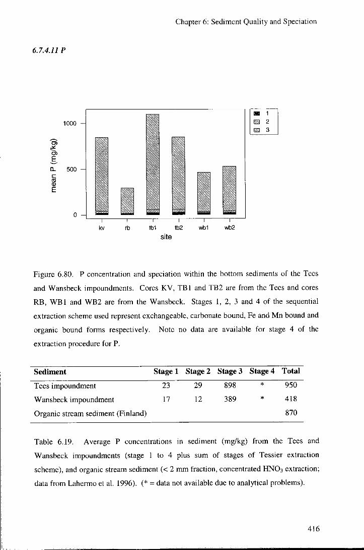
6.7.4.11 P
Chapter 6: Sediment Quality and Speciation
1000 H
E, Q. 500 c CO Q) E
0 ^ " T " kv rb
~n T" tbi tb2
site wbl wb2
Figure 6.80. P concentration and speciation within the bottom sediments of the Tees
and Wansbeck impoundments. Cores KV, TBI and TB2 are from the Tees and cores
RB, W B l and WB2 are from the Wansbeck. Stages 1, 2, 3 and 4 of the sequential
extraction scheme used represent exchangeable, carbonate bound, Fe and Mn bound and
organic bound forms respectively. Note no data are available for stage 4 of the
extraction procedure for P.
Sediment Stage 1 Stage 2 Stages Stage 4 Total
Tees impoundment 23 29 898 * 950
Wansbeck impoundment 17 12 389 * 418
Organic stream sediment (Finland) 870
Table 6.19. Average P concentrations in sediment (mg/kg) from the Tees and
Wansbeck impoundments (stage 1 to 4 plus sum of stages of Tessier extraction
scheme), and organic stream sediment (< 2 mm fraction, concentrated HNO3 extraction;
data from Lahermo et al. 1996). (* = data not available due to analytical problems).
416

Chapter 6: Sediment Quality and Speciation
P levels are higher in the sediment of the Tees than the Wansbeck impoundment (table
6.19), with mean concentration of P approaching 1 %o by mass in the sediments in this
river.
700 - f 600
^ 500
E 400
c 300
E 200 - I
100
0
m 4
W a n s b e c k
Figure 6.81. P concentration and speciation within the surficial sediments of the
Wansbeck impoundment. Stages 1, 2, 3, 4 and 5 represent the exchangeable or loosely
sorbed, Fe-bound, authigenic apatite plus carbonate bound plus biogenic apatite, detrital
apatite plus other organic P and organic P phases of Ruttenberg's (1992) SEDEX
sequential extraction procedure for P.
Little P is held exchangeably or stage 2 extractably in the sediments of either
impoundment. The majority of P appears to be held in the stage 3 extractable phase
(figure 6.80), although due to analytical problems unfortunately no results are available
for the stage 4 extract for the Tessier et al. (1979) extraction experiments. Surficial
sediments from the Wansbeck underwent sequential extraction using the SEDEX
scheme of Ruttenberg (1992) (developed specifically for P) to ensure that results from
the Tessier et al. (1979) procedure (which was developed for trace metals) accurately
represented P speciation. The results (figure 6.81) confirm that the main species of P
within the sediments is Fe-bound and that the main extraction procedure used
adequately models P speciation, and in addition that a small amount of P is held in the
oxidisable/organic phase. Davies (1997) reports that ferric-bound P is the major
fraction in most lake sediments, accounting for over 50 % of the total mass of P.
417

Chapter 6: Sediment Quality and Speciation
Both stage 3 extractable Fe and P show an increase towards the sediment-water column interface from approximately 15 cm depth in core RB, which may imply that less reducing conditions at this point allow precipitation of Fe hydroxide and immobilisation of P (figure 6.82). The profiles for Fe and Mn oxide bound P within the sediments show relatively high variation with depth in both impoundments and approximately follow the profiles for stage 3 extractable Fe (figures 6.83 and 6.84). P concentrations are significantly lower in the pre-impoundment sediment of the Tees.
600 H
500
400
CL
200
100
0
>-1.5
sediment / sur face / ^ . 4 5
0-7 .5 %i
0^% ^
o o
5000 1
10000 —r 15000
Fe (mg/kg)
Figure 6.82. The relationship between P and Fe in sediment from site RB in the
Wansbeck impoundment, showing enrichment of sediment in Fe-oxide and associated P
at the surface of the sediments. Data labels show depth (cm) within sediment core.
418

Chapter 6: Sediment Quality and Speciation
500 1000 1500 2000
g- -40
•TB1 -•*--TB2
• A - - . KV
P (mg/kg)
Figure 6.83. Stage 3 extractable P with depth in cores T B I , TB2 and KV from the Tees
impoundment.
500 1000 1500 2000
WB1 - - ^ - W B 2 - . - A -- RB
P (mg/kg)
Figure 6.84. Stage 3 extractable P with depth in cores W B l , WB2 and RB from the Wansbeck impoundment.
419

6.7.4.12 Sc
Chapter 6: Sediment Quality and Speciation
CD -iC
o C/) c CO
E
Figure 6.85. Sc concentration and speciation within the bottom sediments of the Tees
and Wansbeck impoundments. Cores KV, TBI and TB2 are from the Tees and cores
RB, W B l and WB2 are from the Wansbeck. Stages 1, 2, 3 and 4 of the sequential
extraction scheme used represent exchangeable, carbonate bound, Fe and Mn bound and
organic bound forms respectively.
Sediment Stage 1 Stage 2 Stages Stage 4 Total
Tees impoundment 0.00 0.05 3.78 0.03 3.86
Wansbeck impoundment 0.00 0.07 3.73 0.80 4.60
Organic stream sediment (Finland) 4.6
Table 6.20. Average Sc concentrations in sediment (mg/kg) from the Tees and
Wansbeck impoundments (stage 1 to 4 plus sum of stages of Tessier extraction
scheme), and organic stream sediment (< 2 mm fraction, concentrated HNO3 extraction;
data from Lahermo et al. 1996).
Unlike other transition metals Sc has a single oxidation state (Sc "") and shows similar
behaviour in the environment to Al (Reimann and Caritat, 1998). Levels of available Sc
420

Chapter 6: Sediment Quality and Speciation
are slightly higher in the sediment of the Wansbeck than the Tees impoundment, and
comparable to the mean concentration in organic rich sediment (table 6.20 and figure
6.85).
The pattern of speciation for Sc is similar to that of Fe and Al , etc. Very little Sc is held
exchangeably or carbonate bound, the stage 3 extractable phase is the dominant species
for Sc in both impoundments, and a portion of Sc is held in the stage 4 extractable phase
in the Wansbeck but not in the Tees.
The profiles for stage 3 and stage 4 extractable Sc are similar to those for Fe, with the
distinctive patterns being a lower stage 3 extractable, but higher stage 4 extractable,
content in the pre-impoundment sediment in the Tees, and a general increase in stage 4
extractable Sc with depth in the Wansbeck (figures 6.86, 6.87, 6.88 and 6.89).
421

Chapter 6: Sediment Quality and Speciation
o -30 -TB2
Q- -40
Sc (mg/kg)
Figure 6.86. Stage 3 extractable Sc with depth in cores T B I , TB2 and KV from the
Tees impoundment.
— ^ W B I --«^-WB2
- A -- RB
Sc (mg/kg)
Figure 6.87 Stage 3 extractable Sc with depth in cores W B l , WB2 and RB from the
Wansbeck impoundment.
422

Chapter 6: Sediment Quality and Speciation
o -30 i
o. -40
- ^ T B 1
- -A-- - KV
Sc (mg/kg)
Figure 6.88. Stage 4 extractable Sc with depth in cores T B I , TB2 and KV from the
Tees impoundment.
E o
Q. •D
0
-10
-20
-30
-40
-50
-60
-70
-80
1
"'-A
A - ' " "^jT " A . . .
•;A • ,A' «
A.',' - A «> , A
A-.'.'
A '•'-A
-WB2
Sc (mg/kg)
Figure 6.89. Stage 4 extractable Sc with depth in cores W B l , WB2 and RB from the
Wansbeck impoundment.
423

6.7.4.13 Si
Chapter 6: Sediment Quality and Speciation
1500 H
O) 1000
e CO c 5? <D E
500
0 -A
Figure 6.90. Si concentration and speciation within the bottom sediments of the Tees
and Wansbeck impoundments. Cores KV, T B I and TB2 are from the Tees and cores
RB, W B l and WB2 are from the Wansbeck. Stages 1, 2, 3 and 4 of the sequential
extraction scheme used represent exchangeable, carbonate bound, Fe and Mn bound and
organic bound forms respectively.
Sediment Stage 1 Stage 2 Stage 3 Stage 4 Total
Tees
impoundment
Wansbeck
impoundment
55
53
193
208
534
386
278
732
1060
1379
Table 6.21. Average Si concentrations in sediment (mg/kg) from the Tees and
Wansbeck impoundments (stage 1 to 4 plus sum of stages of Tessier extraction
scheme).
Available Si concentrations are slightly higher in the sediments of the Wansbeck than
the Tees impoundment (table 6.21 and figure 6.90). Only a small amount of Si is founa
424
Chapter 6: Sediment Quality and Speciation
exchangeably in the sediments of either impoundment. Significant quantities of Si are
released during stage 2, 3 and 4 of the sequential extraction procedure.
The profiles for the carbonate bound phase show that Si is relatively constant to about
40 cm depth in the sediment in the Tees impoundment, but shows higher concentrations
below this level (figure 6.91). This is interpreted as a combined grain-size and
carbonate input effect, with higher levels in the coarser grained pre-impoundment
sediment followed by high carbonate input to the overlying sediment due to high flow
conditions during 1995. Within the Wansbeck stage 2 extractable Si (as with particle
size) remains relatively constant with depth (figure 6.92). Stage 3 extractable Si is
constant with depth in both impoundments but shows dramatically higher concentration
in the pre-impoundment sediment encountered in the Tees, likely to be due to some
dissolution of Si from marine quartz sand in these sediments (figures 6.93 and 6.94).
The pattern is repeated for Si within the stage 4 extractions for both impoundments
(figures 6.95 and 6.96), with Si closely following the organic matter concentration in
the Wansbeck (figure 6.97) and therefore coal particles are suggested as the Si source in
this phase.
425

Chapter 6: Sediment Quality and Speciation
200 400 600
o -30 - T B 2
D. -40 - A- - - KV
Si (mg/kg)
Figure 6.91. Stage 2 extractable Si with depth in cores T B I , TB2 and K V from the
Tees impoundment.
200 400 600
-WB2
Si (mg/kg)
Figure 6.92. Stage 2 extractable Si with depth in cores W B l , WB2 and R3 from the
Wansbeck impoundment.
426

Chapter 6: Sediment Quality and Speciation
1000 2000 3000
o -30
Q- -40
•TB1 - - • - - T B 2 . - A - . - KV
Si (mg/kg)
Figure 6.93. Stage 3 extractable Si with depth in cores T B I , TB2 and KV from the
Tees impoundment.
1000 2000 3000
•WBl - - i i - -WB2
- A . - . RB
Si (mg/kg)
Figure 6.94. Stage 3 extractable Si with depth in cores W B l , WB2 and RB from the Wansbeck impoundment.
427

Chapter 6: Sediment Quality and Speciation
500 1000 1500
o -30
p. -40 A - - KV
Si (mg/kg)
Figure 6.95. Stage 4 extractable Si with depth in cores T B I , TB2 and KV from the
Tees impoundment.
500 1000 1500
--«_-WB2
Si (mg/kg)
Figure 6.96. Stage 4 extractable Si with depth in cores W B l , WB2 and RB from the
Wansbeck impoundment.
428

Chapter 6: Sediment Quality and Speciation
E 600 -A
400 H
15 20
% organic matter
Figure 6.97. The relationship between Si in the stage 4 extraction and organic matter in
sediment from site RB in the Wansbeck impoundment.
6.7.4.14 Ti
Sediment Stage 1 Stage 2 Stage 3 Stage 4 Total
Tees impoundment 0.2 0.1 18.2 1.6 20.1
Wansbeck impoundment 0.4 0.1 12.6 1.3 14.4
Organic stream sediment (Finland) 1270
Table 6.22. Average Ti concentrations in sediment (mg/kg) from the Tees and
Wansbeck impoundments (stage 1 to 4 plus sum of stages of Tessier extraction
scheme), and organic stream sediment (< 2 mm fraction, concentrated HNO3 extraction;
data from Lahermo et al. 1996).
Potentially available Ti is in low concentrations in the sediments of the impoundments
with the majority assumed to be contained within refractory (silicate) minerals. Ti is
generally considered non-toxic. The majority of Ti is held in the stage 3 extractable
429

Chapter 6: Sediment Quality and Speciation
phase, with small amounts extracted in stage 4, in the sediments of both impoundments
(table 6.22 and figure 6.98).
25 -4
20 H
15
c 10 H s E
5
kv rb "H r ~ tbi tb2
site wbl wb2
Figure 6.98. Ti concentration and speciation within the bottom sediments of the Tees
and Wansbeck impoundments. Cores KV, TBI and TB2 are from the Tees and cores
RB, W B l and WB2 are from the Wansbeck. Stages 1, 2, 3 and 4 of the sequential
extraction scheme used represent exchangeable, carbonate bound, Fe and Mn bound and
organic bound forms respectively.
The profiles for both stage 3 and stage 4 extractable Ti in the sediments of both
impoundments show no clear trends with depth (figures 6.99, 6.100, 6.101 and 6.102).
The only feature of note is that concentrations of Ti are higher in both stage 3 and 4
extractions in the pre-impoundment sediment of the Tees. This is likely to be due to
industrial inputs to the estuary downstream of the position of the barrage from the Ti-
oxide plant (Tioxide UK Ltd.) at Seal Sands. The peak in Ti (and Ni, etc.) levels at
approximately 10 cm depth within the core from site KV is thought to be due to
reduction of reagent volume during the vigorous reaction of stage 4 of the extraction
procedure in these sediments (which, as mentioned, also led to boiling over and loss of
sediment material from some samples in this core). The reason for the greater reactivity
of the sediment from site KV could not be identified (the organic matter content is
similar to other cores from the Tees).
430

Chapter 6: Sediment Quality and Speciation
0 10 20 30 40
o -30
9- -40
7
TB1 - - ^ - T B 2
- A-- - KV
Ti (mg/kg)
Figure 6.99. Stage 3 extractable Ti with depth in cores T B I , TB2 and KV from the
Tees impoundment.
10 20 30 40
E
•*-» a. •D
•WBl - - ^ - W B 2 - - - A - - - RB
Ti (mg/kg)
Figure 6.100. Stage 3 extractable Ti with depth in cores W B l , WB2 and RB from the
Wansbeck impoundment.
431

Chapter 6: Sediment Quality and Speciation
8 10 0
-10
-20
1 -30
I -40
-50
-60
-70
1 1
A
, . A
6 •
< -A--- KV
Ti (mg/kg)
Figure 6.101. Stage 4 extractable Ti with depth in cores T B I , TB2 and KV from the
Tees impoundment.
10 0
-10
-20
-30 u r -40
t -50
-60
-70
-80
1 1 1
'--•-A
A yi
4
WB1 _-B---WB2 - - A - - . RB
Ti (mg/kg)
Figure 6.102. Stage 4 extractable Ti with depth in cores W B l , WB2 and RB from the
Wansbeck impoundment.
432

6.7.4.15 Zn
Chapter 6: Sediment Quality and Speciation
200
c N c s E
100 -A
Figure 6.103. Zn concentration and speciation within the bottom sediments of the Tees
and Wansbeck impoundments. Cores KV, T B I and TB2 are from the Tees and cores
RB, W B l and WB2 are from the Wansbeck. Stages 1, 2, 3 and 4 of the sequential
extraction scheme used represent exchangeable, carbonate bound, Fe and Mn bound and
organic bound forms respectively.
Sediment Stage 1 Stage 2 Stage 3 Stage 4 Total
Tees impoundment 4.4 80.0 99.5 1.0 184.9
Wansbeck impoundment 1.3 46.8 47.4 25.9 121.4
Organic stream sediment (Finland) 45.9
Tees estuary downstream of barrage 392
River Tees upstream of impoundment 518
Humber estuary 252
Table 6.23. Average Zn concentrations in sediment (mg/kg) from the Tees and
Wansbeck impoundments (stage 1 to 4 plus sum of stages of Tessier extraction
scheme), organic stream sediment (< 2 mm fraction, concentrated HNO3 extraction;
data from Lahermo et al. 1996), Tees estuary sediment from downstream of barrage
433
Chapter 6: Sediment Quality and Speciation
(total extraction; data from Jones and Turki 1997), River Tees sediment upstream of
impoundment (< 63 |xm fraction, total extraction; data from EA), and Humber estuary
(< 100 jxm fraction, concentrated HNO3 extraction; data from Bryan and Langston
1992),
Zn concentrations are higher in the sediments of the Tees than the Wansbeck
impoundment. Jones and Turki (1997) found that approximately 75 % of Zn held in the
sediments of the Tees estuary downstream of the barrage is held in available forms
(stages 1 to 4 of Tessier et al. (1979) extraction procedure). Zn is extracted almost
equally in stages 2 (carbonate bound) and 3 (Fe oxide bound) of the extraction
procedure from sediment from the Tees impoundment. For the Wansbeck sediment the
amount of stage 2 and stage 3 extractable Zn is also similar, but additional Zn is held in
the stage 4 (oxidisable) extraction phase (table 6.23 and figure 6.103).
Stage 2 extractable Zn within the Tees cores shows a similar pattern to that of Ca apart
from an additional peak in concentrations in all cores between 10 and 20 cm depth
(figure 6.104). It is likely that, as for Ca and K, the profile of stage 2 extractable Zn is
strongly controlled by carbonate inputs to the sediment. For the Wansbeck, stage 2
extractable Zn shows a slight increase (as does Ca) with depth (figure 6.105). Both
stage 2 and stage 3 extractable Zn increase in the sediment following impoundment of
the Tees estuary, which fits with the higher reported values for sediment upstream of the
impoundment compared with the estuary downstream, and is likely to be a dilution
effect by coarse grained marine derived sediment. The profile for stage 3 extractable Zn
is irregular in the Tees sediment, but as for stage 2 shows a clear peak at between 10
and 20 cm depth (figure 6.106). In the Wansbeck there is a steady decrease in stage 3
extractable Zn towards the sediment surface (figure 6.107). There is very little stage 4
extractable (sulphide and organic bound) Zn in the sediment of the Tees impoundment
(figure 6.108), and an obvious increase with depth of this phase in the Wansbeck (figure
6.109).
434

Chapter 6: Sediment Quality and Speciation
50 100 150
o -30
Q- -40
•TBI --*--TB2
- A -. KV
Zn (mg/kg)
Figure 6.104. Stage 2 extractable Zn with depth in cores T B I , TB2 and KV from the
Tees impoundment.
50 100 150
E
T3
-WB1 - - ^ - W B 2
- A - . - RB
Zn (mg/kg)
Figure 6.105. Stage 2 extractable Zn with depth in cores W B l , WB2 and RB from the
Wansbeck impoundment.
435

Chapter 6: Sediment Quality and Speciation
50 100 150 200
o -30 'TB2
g- -40 - A - . - KV
Zn (mg/kg)
Figure 6.106. Stage 3 extractable Zn with depth in cores T B I , TB2 and KV from the
Tees impoundment.
50 100 150 200
E o •c -Q.
•a
-WB2
Zn (mg/kg)
Figure 6.107. Stage 3 extractable Zn with depth in cures W B l , WB2 and RB from the Wansbeck impoundment.
436

Chapter 6: Sediment Quality and Speciation
20 40 60
10 * A
o -30
g . -40 *
7
—»—TB1 - - * - -TB2 - - A - . KV
Zn (mg/kg)
Figure 6.108. Stage 4 extractable Zn with depth in cores T B I , TB2 and KV from the
Tees impoundment.
20 40 60
WB1 - - - - W B 2
- A - - - RB
Zn (mg/kg)
Figure 6.109. Stage 4 extractable Zn with depth in cores W B l , WB2 and RB from the Wansbeck impoundment.
437

Chapter 6: Sediment Quality and Speciation
6.8 Controls on sediment chemistry
Principal components analysis (PCA) (see appendix 1) was used to identify the controls
on sediment chemistry in estuarine impoundments using data from the bed sediment
cores taken from the Tees and Wansbeck impoundments. PCA was carried out using a
correlation matrix (since parameters were measured on different scales) including the
parameters of % organic matter content, % clay, silt and sand content, and
concentrations of Al , Ca, Co, Cr, Cu, Fe, K, Mg, Mn, Ni, Sc, Si, Ti and Zn. As
described above Sn and V were generally below the analytical LCD, sample was lost
during stage 4 extraction of deep sample from core KV and analysis of P was
problematic, and therefore these data were excluded from the PCA. The results in terms
of eigenvalues and coefficients to the major principal components are summarised in
tables 6.24 and 6.25 and figure 6.110.
Principal Eigenvalue Proportion of Cumulative
component variance proportion of
variance
1 7.0425 0.391 0.391
2 3.0333 0.169 0.560
3 1.9872 0.110 0.670
4 1.7485 0.097 0.767
5 1.0722 0.060 0.827
6 0.9319 0.052 0.879
Table 6.24. Eigenvalues and proportions of variance for the first 6 principal
components calculated for PCA of data from sediment cores from the Tees and
Wansbeck impoundments.
438

Chapter 6: Sediment Quality and Speciation
Component Number
Figure 6.110. Scree plot of eigenvalues for principal components calculated for PCA of
data from sediment cores from the Tees and Wansbeck impoundments.
A large amount of variance in the dataset (39 %) is contained by the 1 ' principal
component calculated (PCI) (table 6.24 and figure 6.110). Together the first 5 principal
components contain 83 % of the variance in the dataset and eigenvalues fall below 1
from PC6 onwards. Only the principal components with eigenvalues > 1 are selected
for discussion, and the coefficients for each of the parameters included in the analysis to
each of these components are shown in table 6.25.
PCI shows strong loadings (all in the same direction) for Al , Co, Cu, Fe, Ni , Sc, Si, T i
and Zn, with weaker correlations of the opposite sign for K and Mg. Particle size and
organic matter content are not correlated with PCI. PC2 contrasts the levels of clay and
silt in the sediment with that of sand, with elemental correlations being lower. PC3 has
strong loadings of the same sign for organic matter, Mg and K. PC4 includes the
majority of variables not included in the preceding components, with clay and Cr
showing positive correlations and Ca and Mn showing negative correlations. PCS
shows the strongest correlation with Ti.
439
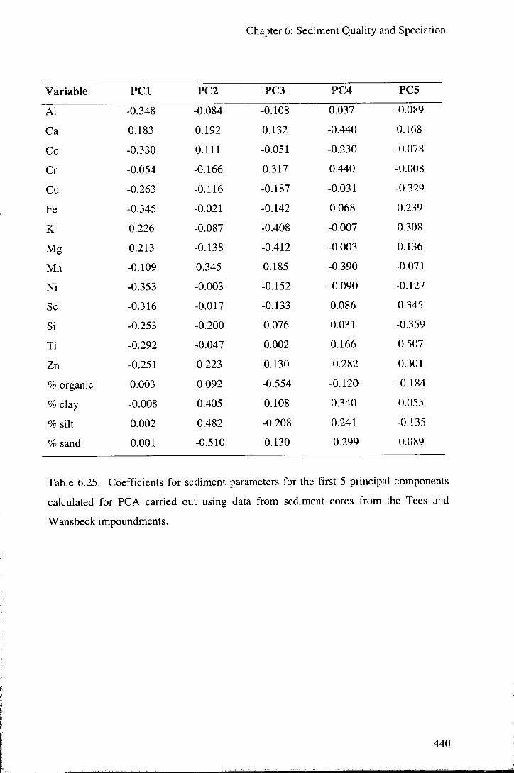
Chapter 6: Sediment Quality and Speciation
Variable PCI PC2 PC3 PC4 PCS
Al -0.348 -0.084 -0.108 0.037 -0.089
Ca 0.183 0.192 0.132 -0.440 0.168
Co -0.330 0.111 -0.051 -0.230 -0.078
Cr -0.054 -0.166 0.317 0.440 -0.008
Cu -0.263 -0.116 -0.187 -0.031 -0.329
Fe -0.345 -0.021 -0.142 0.068 0.239
K 0.226 -0.087 -0.408 -0.007 0.308
Mg 0.213 -0.138 -0.412 -0.003 0.136
Mn -0.109 0.345 0.185 -0.390 -0.071
Ni -0.353 -0.003 -0.152 -0.090 -0.127
Sc -0.316 -0.017 -0.133 0.086 0.345
Si -0.253 -0.200 0.076 0.031 -0.359
Ti -0.292 -0.047 0.002 0.166 0.507
Zn -0.251 0.223 0.130 -0.282 0.301
% organic 0.003 0.092 -0.554 -0.120 -0.184
% clay -0.008 0.405 0.108 0.340 0.055
% silt 0.002 0.482 -0.208 0.241 -0.135
% sand 0.001 -0.510 0.130 -0.299 0.089
Table 6.25. Coefficients for sediment parameters for the first 5 principal components
calculated for PCA carried out using data from sediment cores from the Tees and
Wansbeck impoundments.
440

Chapter 6: Sediment Quality and Speciation
Fe and associated metals
0 H
o.
-5 H
PC1
5 - {
O.
-5
post-impoundment
pre-impoundment
PC1
• Tees • Wansbecl<
particle size
Figures 6.111 and 6.112. Principal component scores for 1'' and 2"'^ principal
components for data from sediment cores from the Tees and Wansbeck impoundments.
PCI represents the speciation of Fe and associated metals within the sediment hence
distinguishes between extraction stages (1 to 4 of Tessier et al (1979) sequential
extraction procedure). PC2 represents the grain-size distribution in the sediments and
hence distinguishes between the generally coarser grained Wansbeck and finer grained
441

Chapter 6: Sediment Quality and Speciation
Tees sediment, and between the pre and post-impoundment sedimentation within the
Tees.
PCI represents the association of a large number of the elements analysed with Fe.
These metals show the same "speciation" as Fe, and as such plotting scores for PCI
distinguishes the stages of the sequential extraction procedure (figure 6.111). Stages 1
and 2, and stage 4 from the Tees, extract minor amounts of these metals (Al, Co, Cu,
Fe, Ni, Sc, Ti and Zn) and show positive scores for PCI. Stage 3, and stage 4 from the
Wansbeck, extractions contain the majority of the "available" portion of these metals
and show negative scores for PCI. The relationships between Al and Sc and Fe, and Ni
and Co are shown as examples of this association of elements within the sediments
(figures 6.113, 6.114 and 6.115).
E
1500 - \
1000
500 H
5000
Fe (mg/kg) 10000
Figure 6.113. The relationship between Al and Fe within the stage 4 extraction (organic
and sulphide bound fraction) in the sediments of the Tees and Wansbeck
impoundments.
442

Chapter 6: Sediment Quality and Speciation
E, o CO
4 H
«
10000
Fe (mg/kg)
20000
Figure 6.114. The relationship between Sc and Fe for all extraction stages within the
sediment of the Tees impoundment.
E
o Tees • Wansbeck
Co (mg/kg)
Figure 6.115. The relationship between Ni and Co for all extraction stages for the
sediment from the Tees and Wansbeck impoundments. Group i is from extraction stage
1 from both impoundments and extraction stage 4 from the Tees, group i i is from
443

Chapter 6: Sediment Quality and Speciation
extraction stage 2 from both impoundments, and group i i i is from extraction stage 3
from both impoundments and extraction stage 4 from the Wansbeck.
PC2 is related to particle size distribution, which surprisingly shows little relationship to
elemental concentrations indicating that speciation effects (PCI) are larger than grain-
size effects. Since particle size differences play a secondary role in controlling
elemental concentrations all sediment sequential extraction data presented and
discussed within this study is in a raw form, as opposed to grain-size normalised (see
for example Loring and Rantala 1992). Since sediment within the Wansbeck
impoundment is slightly coarser grained than that in the Tees, PC2 distinguishes
between the two impoundments (figure 6.112). In addition scores for the sand-
dominated pre-impoundment sediment from the Tees are much lower than those for the
silt-dominated post-impoundment sedimentation.
K, Mg and organic matter
o Tees o Wansbeck
Ca and Cr Mn and
clay
i
PC3
Figure 6.116. Principal component scores for 3"* and 4* principal components for data
from sediment cores from the Tees and Wansbeck impoundments. PC3 relates to Mg
and K (particularly within the exchangeable fraction) and organic matter, and groupings
of scores for PC4 relate mainly to Cr concentration in stage 4 extractions from the Tees.
444

Chapter 6: Sediment Quality and Speciation
2000
O)
CD E 1000
0 H
o
*
10
o o
o o - o - ~ ^ o '
o
" a o " o o
+
I 20
% organic matter 30
o 1 + 2 X 3 X 4
Figure 6.117. K vs. organic matter by speciation (stages 1 to 4 of Tessier et al. (1979)
sequential extraction procedure) for bottom sediment from the Wansbeck impoundment,
showing strong association of exchangeable K with organic material.
100
90 c © c 80 o 80 o 0)
70 CO
70 o E
60
50
20 % organic matter
30
Figure 6.118. The relationship between moisture content and organic matter within
sediment from the Wansbeck impoundment.
445

Chapter 6: Sediment Quality and Speciation
PC3 relates to the concentrations of Mg, K and organic matter within the sediment and,
as with PC2, also generally distinguishes between the impoundments (however, smce
PCA forces components to be orthogonal the variables within PC2 are unlikely to be
correlated with those in PC3). The Wansbeck is a partial tidal intrusion impoundment
and periodically (including at the time of sediment coring) has seawater in contact with
the sediment. Concentrations of Mg and K within the pore-water of the sediment are
therefore higher than in the Tees, and much of this is associated with organic matter
(also higher in the Wansbeck) so that scores on PC3 for the Wansbeck tend to be
negative (figure 6.116). The relationships between K and organic matter, and between
moisture content and organic matter within the sediment of the Wansbeck are shown in
figures 6.117 and 6.118.
E
O
Tees Wansbeck
"1 1 1 1 1 1 r 200 400 600 800 1000 1200 1400 1600 1800
Ca (mg/kg)
Figure 6.119. Cr vs. Ca within stage 4 extractions from sediment from the Tees and
Wansbeck impoundments. The high Cr high Ca samples are from pre-impoundment
sediment.
PC4 relates to the majority of elements which do not show covariance with Fe (PCI) or
to organic matter (PC3), with the strongest loading for Cr which contrasts with the other
elements studied in showing a far greater concentration in the stage 4 extractions for the
Tees than the Wansbeck impoundment. As mentioned high Cr concentrations within
446

Chapter 6: Sediment Quality and Speciation
the Tees are likely to be due to a chromium works in the upstream sections of this river.
Within stage 4 extractions from the Tees Ca shows an approximate negative
relationship to Cr (figure 6.119) and thus shows a similar coefficient (but of opposite
sign) to Cr on PC4. Of note is that Mn shows greater correlation to PC4 than to PCI
(Fe and associated elements) implying that the behaviour of Mn differs from that of Fe.
Briefly it can be stated that Mn/Fe shows a similar concentration in hydroxides and Mn
concentration is therefore proportional to Fe concentration within stage 3 extractions,
but that Mn shows greater relative concentrations within other species than do Fe or
associated elements due to greater environmental mobiUty (figure 6.120).
PC5 explains approximately 6 % of the variance in the dataset and relates to variation in
Ti levels between the extraction stages and cores, with this and subsequent components
likely to be related to analytical and other errors to a large extent.
400 H
300
^ 200 c
100
0 H
+
i
^ ^ X X
X 1 x ^ a*.
10000
Fe (mg/kg)
o 1 + 2 X 3 * 4
20000
Figure 6.120. Mn vs. Fe by speciation (stages 1 to 4 of Tessier et al. (1979) sequential
extraction procedure) for bottom sediment from the Tees impoundment, showing
correlation between Mn and Fe within oxides (stage 3 extraction), but greater variation
of Mn (due to greater environmental mobility) than Fe within other phases.
447

Chapter 6: Sediment Quality and Speciation
6.9 Summary and conclusions
Within this section the data collected from a total of 6 bottom sediment cores of
approximately 50 cm length taken from the Tees and Wansbeck impoundments have
been presented and discussed. Data from an additional core taken from an emergent
sand-bar in the Wansbeck impoundment is discussed briefly. For each sub-sample
taken at 3 cm intervals the parameters of particle size, organic matter, and the
concentration and speciation of Al , Ca, Co, Cr, Cu, Fe, K, Mg, Mn, Ni , P, Sc, Si, Ti and
Zn based on a modified sequential extraction procedure as developed by Tessier et al.
(1979), have been determined. Elemental results are presented in terms of mean
concentrations within each operationally defined "species" (exchangeable, carbonate
bound, Fe and Mn oxide bound, and organic or sulphide bound) and profiles of
concentration of each species with depth in each of the sediment cores. Comparison of
the concentrations determined in this study is made where possible with data from
comparable surveys (e.g. the Tees upstream and downstream of the impounded area and
the Humber estuary). Similarities between the behaviours of groups of elements, and
possible controlling mechanisms on the speciation, concentration and distribution of
elements is suggested and are summarised below. PCA was carried out to aid
identification of the controls on elemental behaviour.
6.9.1 PCA
The principal components having Eigenvalues > 1 are considered. The 1 ' principal
component calculated accounts for 39 % of the variance in the dataset, with the first 4
components together including 77 % of the variance. Subsequent components are
interpreted as relating to a large extent to random variation (error and local
heterogeneity) in the data collected. The major principal components represent:
® PCI = covariance between Fe and a suite of elements (Al, Co, Cu, Fe, Ni, Sc, Ti
and Zn) particularly related to association with Fe hydroxide.
o PC2 = particle-size variation (significantly this is relatively independent of the
major controls on elemental concentrations implying that grain-size
normalisation (e.g. Loring and Rantalla, 1992) is inappropriate for this kind of
speciation study).
o PC3 = pore-water component showing variation of exchangeable cations
between impoundment types (freshwater and mixed seawater/freshwater), and
relating to organic matter within each of these systems.
448

Chapter 6: Sediment Quality and Speciation
• PC4 = strongly related to anthropogenic Cr inputs to the sediments.
6.9.2 Geochemistry
Species Controls
Al 3
4
Held in sulphides and oxides of Fe with contrast
impoundments based on prevailing oxygen conditions in
water.
between
overlying
Ca 1 Ion exchange removes Ca from exchangeable phase.
2 Variation in allochthonous (catchment) carbonate inputs.
3 Some Ca associated with sulphides and oxides of Fe.
4
Co 2 Variation in allochthonous (catchment) carbonate inputs.
3 Held in sulphides and oxides of Fe with contrast between
4 impoundments based on prevailing oxygen conditions in overlying
water.
Cr 3 Concentration controlled by industrial input of Cr. Speciation
4 controlled by sulphides and oxides of Fe.
Cu 3 Held in sulphides and oxides of Fe with contrast between
4 impoundments based on prevailing oxygen conditions in overlying
water.
Fe 3 Held in sulphides and oxides with contrast between impoundments
4 based on prevailing oxygen conditions in overlying water.
K I K content of overlying water plus organic/moisture content of sediments
2 controls exchangeable phase.
Variation in allochthonous (catchment) carbonate inputs.
Mg 1 Mg content of overlying water plus ion exchange (increasing Mg) for
2 exchangeable phase.
3 Variation in allochthonous (catchment) carbonate inputs.
4 Some Mg associated with sulphides and oxides of Fe.
Mn 1 Redox controlled mobility/speciation, varies between impoundments
2 based on prevailing oxygen conditions in overlying water.
3
4
449

Chapter 6: Sediment Quality and Speciation
Ni 2 Variation in allochthonous (catchment) carbonate inputs.
3 Held in sulphides and oxides of Fe with contrast between
4 impoundments based on prevailing oxygen conditions in overlying
water.
P 3 Anthropogenic inputs of P, strongly associates with oxides of Fe in
sediment.
Sc 3 Held in sulphides and oxides of Fe with contrast between
4 impoundments based on prevailing oxygen conditions in overlying
water.
Si 2 Variation in allochthonous (catchment) carbonate inputs.
3 Grain-size effect relating to change from pre to post-impoundment
4 sedimentation in the Tees.
Associated with organic matter (coal) in the Wansbeck.
Ti 3 Held in sulphides and oxides of Fe with contrast between
4 impoundments based on prevailing oxygen conditions in overlying
water.
Zn 2 Variation in allochthonous (catchment) carbonate inputs.
3 Held in sulphides and oxides of Fe with contrast between
4 impoundments based on prevailing oxygen conditions in overlying
water.
Table 6.26. Summary of the operationally defined species in which the elements
analysed are held, and suggested controls on speciation and concentration, within the
bottom sediment of the Tees and Wansbeck estuarine impoundments. Within the
species column 1 to 4 represent the first 4 stages of the sequential extraction procedure
(Tessier et al. 1979). The principal phases removed by each of these extractions are:
1 = Exchangeable
2 = Carbonates
3 = Fe and Mn oxides
4 = Organic matter and sulphides
Together with PCA, graphical presentation of the sediment geochemistry data has
allowed several controls on patterns of speciation and concentration of elements within
the bottom sediments of the Tees and Wansbeck impoundments:
450

Chapter 6: Sediment Quality and Speciation
1. Redox controls.
2. Input controls.
3. Overlying water composition and ion-exchange controls.
4. Particle-size controls.
6.9.2.1 Redox controls
A large number of the elements analysed (Al, Co, Cu, Ni, So, Ti and Zn) show similar
behaviour due to association with Fe in the sediment. Insoluble Fe^* hydroxides (and
Mn'*' oxides) are the major species of Fe in oxic conditions in both the water column
and bottom sediments of many water bodies, and due to high adsorptive capacities and
low degrees of crystallinity are of major importance in adsorbing or occluding trace
metals (Turner, 2(X)0). These metals are potentially bioavailable to filter-feeding and
burrowing organisms since acidic, reducing conditions are present within their digestive
systems (Bryan and Langston, 1992; Langston and Spence, 1995). As described in
chapter 4, under reducing conditions Fe hydroxides are reduced and release soluble Fe ^
ions (along with any associated heavy metals). With increased anoxia with depth in
sediments the onset of sulphate reduction to sulphide (as an electron source in the
decomposition of organic matter) rapidly converts remaining Fe hydroxides to insoluble
Fe sulphides. Metals associated with Fe hydroxides also tend to undergo transfer to
sulphides, although Huerta-Diaz and Morse (1992) found that Cr and Zn partition less
strongly to sulphides than Co, Cu and Ni. Under sustained reducing conditions these
metal sulphides represent a sink for metal pollutants, but may be resolubilised under a
change in redox conditions (such as upon dredging or erosion of sediment).
Assuming that the change in speciation upon sampling and pre-treatment of sediment
was minimal (descriptions of the effects of preservation on metal speciation are given in
Kersten and Forstner (1987) and Rapin et al. (1986)), then the distributions of species
for Fe and associated metals within and between the impoundments represent the
distribution of redox conditions in the sediments. In reahty a proportion of the
sulphides are likely to be oxidized on drying of the sediment samples and so speciation
is misrepresented (gel-probe sampling (chapter 7) overcomes the redox change
problems of sample preparation during the study of elemental mobility by "in-situ"
sampling). Nevertheless, comparison of these speciations suggests that sediment within
the Tees impoundment is less reducing than that of the Wansbeck since far less sulphide
451

Chapter 6: Sediment Quality and Speciation
bound fraction is seen for any of the metals given above. Within the Wansbeck
sediment significant proportions of the metals are found within the "sulphide"
extraction, and the sediment can be interpreted as being more reducing through a
combination of greater organic matter content and a generally lower DO concentration
in the overlying water column (see chapter 4). This interpretation is supported by visual
and olfactory examination of the sediment cores, with those from the Wanbeck being
black throughout their length apart from a small (2 mm) oxidised zone at the surface
and a distinct smell of hydrogen sulphide, and those from the Tees paler in colour with
less odour. It is also possible that part of this difference between the stage 4
extractables in Tees and the Wansbeck sediment is due to the presence of sulphides
within coal particles in the Wansbeck, although there is no clear relationship between
concentration of sulphide bound metals (which show a general increase with depth in
the sediment) and organic matter content (which shows no trend with depth in the
sediment). The trend of greater sulphide bound metals with increasing depth in the
sediment of the Wansbeck is due to increasing stability of reducing conditions with
depth, with diffusion into the overlying water column of Fe ^ periodically taking place
from the surface of the sediment.
The water quality surveys showed that increased dissolved Fe and Mn concentrations
due to release from sediment periodically occur in the Wansbeck impoundment, but that
only elevated Mn was observed in the Tees due to the differences in the redox
conditions in the water columns between the impoundments. Reduction of Mn'*^ oxides
to release soluble Mn " takes place under less reducing conditions than Fe. Within the
sediments sampled the dissolved Mn maxima (i.e. the development of < approximately
50 % DO) were within the sediment at approximately 15 cm depth in the Tees, but at
approximately 7 cm depth (at the WB site) and at the surface (site RB) in the Wansbeck,
confirming that more reducing conditions are encountered both in the sediment and the
water column of the Wansbeck impoundment. Metals associated with Mn in the
sediment may also be released to the water column, although concentrations were
generally found to be below the analytical LOD during the water quality surveys and no
similar patterns could be observed in the sediment for trace metals. Since the
concentrations of Fe are fai- greater than those for Mn, Fe speciation exerts a greater
control on speciation and availability than does Mn in the sediments studied.
452
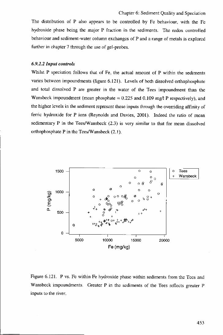
Chapter 6: Sediment Quality and Speciation
The distribution of P also appears to be controlled by Fe behaviour, with the Fe
hydroxide phase being the major P fraction in the sediments. The redox controlled
behaviour and sediment-water column exchanges of P and a range of metals is explored
further in chapter 7 through the use of gel-probes.
6.9.2.2 Input controls
Whilst P speciation follows that of Fe, the actual amount of P within the sediments
varies between impoundments (figure 6.121). Levels of both dissolved orthophosphate
and total dissolved P are greater in the water of the Tees impoundment than the
Wansbeck impoundment (mean phosphate = 0.225 and 0.109 mg/1 P respectively), and
the higher levels in the sediment represent these inputs through the overriding affinity of
ferric hydroxide for P ions (Reynolds and Davies, 2001). Indeed the ratio of mean
sedimentary P in the TeesAVansbeck (2.3) is very similar to that for mean dissolved
orthophosphate P in the TeesAVansbeck (2.1).
E
1500
1000 -A
500 -A
5000
o o
o O
o o
o o e o
o O O O o O 0(© O o +
o R P n
+ o + o
+++ + +
10000 15000
Fe (mg/kg)
o Tees + Wansbeck
20000
Figure 6.121. P vs. Fe within Fe hydroxide phase within sediments from the Tees and
Wansbeck impoundments. Greater P in the sediments of the Tees reflects greater P
inputs to the river.
453

Chapter 6: Sediment Quality and Speciation
200 H
^ 100
o 0
s o
o 0
o 0 e
o Oo 0
oo Of. CO
o ° ° 0
0 o
2000 3000 4000 5000 6000
Ca (mg/kg)
7000
Figure 6.122. The relationship between K and Ca in the carbonate phase of sediments
from the Tees impoundment.
3 H
O) E
0 -A
Co (mg/l)
Figure 6.123. The relationship between Ni and Co in the carbonate phase of the Tees
sediments.
454

Chapter 6: Sediment Quality and Speciation
Transport of carbonate material to the sediments of the impoundments is also
significantly input controlled. The elements associated with the carbonate phase of the
sediments (Ca, Co, K, Mg, Ni, Si and Zn; figures 6.122 and 6.123), and therefore the
inputs of carbonates to the systems, have shown variation over time (with depth in the
sediment cores). The input of allochthonous carbonates to the sediment from the
geologies of the catchments is likely to increase with increasing river discharge, and the
peak in stage 2 extractable (carbonate bound) Ca, etc. following impoundment of the
Tees estuary is interpreted as due to the high flow conditions encountered in 1995.
Cr concentration in the sediments is also interpreted as significantly input controlled,
and industrial discharges from a Cr works is suggested as causing the far higher levels
within the sediments of the Tees than the Wansbeck. The pattern of speciation of Cr
differs to other metals, with the largest fraction from the Tees sediment being extracted
in stage 4 (oxidisable phase). Since generally little sulphide is encountered in the
sediment samples Cr is therefore likely to be associating with organic material within
the river. A similar association of Cr with organic matter was also found in the
sediments of the Tees estuary downstream of the barrage (Jones and Turki, 1997).
6.9.2.3 Overlying water composition and ion-exchange controls
The group 1 and 2 elements analysed (K, Mg and Ca) show significant fractions in the
exchangeable phase within the sediments of both the Tees and the Wansbeck, but the
concentrations and distributions of these metals differs between the impoundments due
to differences in the composition of the overlying water bodies and ion-exchange
behaviour. Clay minerals, Fe and Mn hydroxides and humic acids are all well known to
demonstrate adsorption of metals (Tessier et al., 1979), and changes in the ionic
composition of overlying waters affects sorption and desorption processes. It is
suggested that in the Wansbeck adsorption of major ions from seawater to particulate
material takes place, giving higher exchangeable concentrations of Mg and K within the
sediments of this impoundment than the Tees. Within the Wansbeck it is seen that the
proportion of Mg and K within the exchangeable fraction of the sediment is closely
related to organic matter. The profiles of Ca and K within the exchangeable fraction of
the Tees sediment show the opposite trend to that for Mg, and it is suggested that this
may be due to an ion-exchange by Mg (figure 6.124).
455

Chapter 6: Sediment Quality and Speciation
E
800
700 H
600
500 H
400
300
200
100 H
>k + . + +
+0 Q) o
et-
o kv + tb1 X tb2
1 i i 1 1 1 1 1 0 100 200 300 400 500 600 700 800
Mg (mg/kg)
Figure 6.124. K vs. Mg in the exchangeable phase within the sediments of the Tees
impoundment, showing possible replacement of K by Mg towards the sediment surface.
6.9.2.4 Particle-size controls
Generally it is found that particle size is not a major factor in controlling elemental
concentrations, and particle-size distributions are relatively constant with depth in the
sediments of the two impoundments. For these reasons it was felt unnecessary to apply
grain-size corrections to the data such as are suggested where metal data from distinct
sedimentary environments are to be compared (Loring and Rantalla, 1992).
The only large difference in particle-size distribution occurs in the sediment of the Tees
where there is a distinct difference between sand dominated pre-impoundment
sedimentation and silt dominated post-impoundment sedimentation. The majority of
elements analysed show distinct concentrations through some or all of the speciations in
which they occur across this boundary. It is impossible to tell to what extent these
differences are due to a grain-size effect, and to what extent they are due to distinct
concentrations within the water body and within the sediments deposited during the pre
and post-impoundment periods. For Fe and associated metals concentrations tend to be
lower in the pre-impoundment sediment for the Fe hydroxide bound fraction, but higher
for the sulphide and organic bound fraction. Si concentrations are higher in pre-
impoundment sediment for all species and a quartz sand source is suggested (a true
456

Chapter 6: Sediment Quality and Speciation
grain-size effect). The contrasting behaviour for different elements and even different
species to grain-size differences confirms that particle-size normalisation techniques
(which typically assume a dilution effect by sand-sized material) are inappropriate for
this kind of multi-elemental speciation study.
6.9.3 Sediment quality
Within the UK no Environmental Quality Standards (EQSs) for levels of pollutants in
sediment in rivers, lakes and estuaries have been set. For 'List I ' pollutants of the
European Dangerous Substances Directive (1976, 76/464/EEC) the official position of
the EA is that levels should remain at 'standstill', i.e. no increase from current levels is
permissible. Unofficially sediment quality guideUnes produced by the Canadian
Council of Ministers of the Environment (CCME, 1999 and 2001) are used as an aid in
assessing levels of contamination within freshwater sediments. These consist of lower
Interim Freshwater Sediment Quality Guidelines (ISQGs) and higher Probable Effects
Levels (PELs) at which adverse biological effects become likely, derived according to
CCME (1995). Table 6.27 compares the mean levels of potentially toxic metals found
in the sediments of the Tees and Wansbeck impoundments (as the sum of means for
stages 1 to 4 of the extraction procedure) with the CCME guideline values and the
Maximum Permissible Concentrations (MPC) of the Dutch National Institute of Public
Health and the Environment (RIVM, 1997):
Metal ISQG P E L MPC Tees Wansbeck
Co - - 10 4.9 5.3
Cr 37.3 90.0 1620 71.6 9.5
Cu 35.7 197 37 13.0 28.7
Ni - - 9.4 7.7 11.5
Sn - - 22000 - -V - - 14 - -
Zn 123 315 480 185 121
Table 6.27. A comparison of mean metal levels in the sediments of the Tees and
Wansbeck impoundments with Canadian (ISQG and PEL) and Dutch (MPC) sediment
EQSs. Concentrations are in mg/kg dry weight, and for EQSs refer to total extractions
and for the Tees and Wansbeck to the sum of partial extractions (excluding the
residual/silicate bound phase).
457

Chapter 6: Sediment Quality and Speciation
The concentrations given in table 6.27 for the Tees and Wansbeck refer to the potentially environmentally available fraction within the sediment, and thus are likely to underestimate the total concentrations within the sediments. Jones and Turki (1997) found that the residual (not environmentally available) fraction was significant in the sediments in the Tees estuary downstream of the barrage for a range of heavy metals, particularly Co and Ni for which the largest fractions are in this phase.
The sediments of the two impoundments are generally relatively high in metals, due to a
combination of anthropogenic inputs to the water bodies and the fine grained and
organic rich nature of the sediment. Whilst Co levels are reported as below the Dutch
standards, it is likely that total values are close to or in excess of the MPC since the
majority of Co is found to be associated with the residual phase (Jones and Turki,
1997). By the same argument, Ni is likely to be significantly above the MPC in the
sediments of both impoundments. Zn is well below the Dutch standard within both
impoundments, but exceeds the more stringent Canadian ISQG standard in the Tees
sediment. CCME (2001) give 32 % adverse biological effects in the Zn range between
the ISQG and PEL concentrations. Comparison of Cu concentrations suggest that the
sediments in both impoundments are unpolluted with this metal. Sediment in the
Wansbeck is unpolluted with respect to Cr but the Tees, on which Cr industry is based,
shows levels approaching the PEL standard. CCME (2001) suggest an incidence of
adverse biological effects of approximately 19 % within this range of Cr concentrations,
although actual environmental impact is likely to depend on the oxidation state (Cr''^ is
considered relatively harmless whereas Cr " is highly toxic with some compounds
carcinogenic).
An important reason for studying the speciation of metals within the sediment of the
estuarine impoundments was to assess the likely impact of dredging on water quality. It
has been shown that impoundments are infilling with sediment. Within the Tees an
approximate rate of sediment infi l l of 7 cm/annum is seen. In the Wansbeck
sedimentation has caused extensive areas of shallow (< 50 cm depth) water in which
debris (mainly parts of trees) carried by high flows can become stuck, interfering with
leisure activities (rowing and jet-skiing) on ttic impoundment. Dredging is a possible
solution to this sediment infilling, but may have negative water quality impacts relating
to resuspension of polluted sediment (Peterson et al., 1997). The largest remobiiisation
458
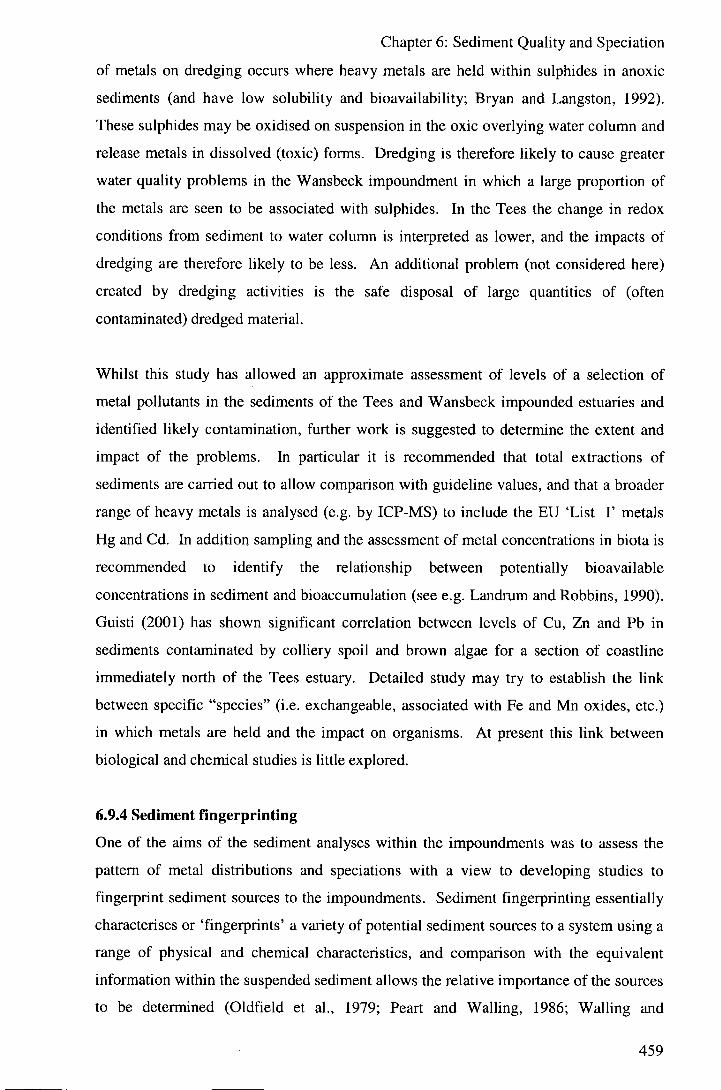
Chapter 6: Sediment Quality and Speciation
of metals on dredging occurs where heavy metals are held within sulphides in anoxic
sediments (and have low solubility and bioavailability; Bryan and Langston, 1992).
These sulphides may be oxidised on suspension in the oxic overlying water column and
release metals in dissolved (toxic) forms. Dredging is therefore likely to cause greater
water quality problems in the Wansbeck impoundment in which a large proportion of
the metals are seen to be associated with sulphides. In the Tees the change in redox
conditions from sediment to water column is interpreted as lower, and the impacts of
dredging are therefore likely to be less. An additional problem (not considered here)
created by dredging activities is the safe disposal of large quantities of (often
contaminated) dredged material.
Whilst this study has allowed an approximate assessment of levels of a selection of
metal pollutants in the sediments of the Tees and Wansbeck impounded estuaries and
identified likely contamination, further work is suggested to determine the extent and
impact of the problems. In particular it is recommended that total extractions of
sediments are carried out to allow comparison with guideline values, and that a broader
range of heavy metals is analysed (e.g. by ICP-MS) to include the EU 'List I ' metals
Hg and Cd. In addition sampling and the assessment of metal concentrations in biota is
recommended to identify the relationship between potentially bioavailable
concentrations in sediment and bioaccumulation (see e.g. Landrum and Robbins, 1990).
Guisti (2001) has shown significant correlation between levels of Cu, Zn and Pb in
sediments contaminated by colliery spoil and brown algae for a section of coastline
immediately north of the Tees estuary. Detailed study may try to establish the link
between specific "species" (i.e. exchangeable, associated with Fe and Mn oxides, etc.)
in which metals are held and the impact on organisms. At present this link between
biological and chemical studies is little explored.
6.9.4 Sediment Hngerprinting
One of the aims of the sediment analyses within the impoundments was to assess the
pattern of metal distributions and speciations with a view to developing studies to
fingerprint sediment sources to the impoundments. Sediment fingerprinting essentially
characterises or 'fingerprints' a variety of potential sediment sources to a system using a
range of physical and chemical characteristics, and comparison with the equivalent
information within the suspended sediment allows the relative importance of the sources
to be determined (Oldfield et al., 1979; Peart and Walling, 1986; Walling and
459

Chapter 6: Sediment Quality and Speciation
Woodward, 1992). Sediment fingerprinting studies generally assess the contribution of
sediment sources to the suspended sediment within a system. Within this study the
physical and chemical characteristics showing the maximum amount of variance in the
sediment cores are determined, with the aim of assessing the potential for using bed
sediment as the downstream end member of a multivariate mixing model. As described
above, variance in the multivariate dataset collected relates to several groups of factors.
These include covariance in Fe and associated elements, particle size variations,
variations relating to ionic composition of the overlying water column, and a range of
external inputs (of which Cr variation is the most significant).
Rtver Distance 12000 H
9000
£ 6000 -]
3000
Stage
Figure 6.125. Main effects plot for GLM of the factors of river, distance and extraction
stage on Fe in the sediment of the impoundments (LS means for factor levels).
The majority of variation in Fe and associated metals is related to their speciation
(figure 6.125), with the majority of these metals associated with Fe and Mn oxides and
organic material and sulphides. These phases have been shown to be subject to redox
controlled mobilisation within the sediments (including potential exchanges across the
sediment-water interface), and because of this are likely not to represent the patterns of
metals within source sediment. In addition group 1 and 2 metals are shown to show
variation within the exchangeable fractions dependent on the ionic strength and
composition of the overlying water column (i.e. concentration of these metals changes
460

Chapter 6: Sediment Quality and Speciation
on contact with seawater in impoundments). Use of metals within sediment
fingerprinting studies for bed sediment is therefore suggested to concentrate on the
residual mineral phase of sediment since this has no potential for alteration following
sediment deposition.
The particle size of suspended material is likely to vary with distance downstream in a
river system with changes in flow velocities. The impoundments are generally stable
environments in which a reduction of flow velocities relative to the rivers entering them
allows deposition of fine particulate material. Particle size distributions in the bed
sediments of the impoundments wil l bear little relationship to those in the sediment
sources, and can therefore not be used in fingerprinting.
Cr shows large amounts of variation both between and within the two impoundments,
and is interpreted as relating to anthropogenic inputs to the systems. Within the Tees it
was seen that there is a significant difference between the sediment deposited pre-
impoundment and that deposited post-impoundment through all extraction stages.
Elements showing distinct concentrations in sediment entering the impoundments from
the seaward and the landward directions has the potential to be used to assess the
relative contribution of these fractions to the bed sediment in partial tidal exclusion
systems. The carbonate bound phase was also interpreted as showing variation based
on sediment source, with changing sediment source during prolonged high flow periods
suggested. Of the parameters studied within this work elements associated with this
phase show the greatest potential for discriminating between catchment sediment
sources to the bed sediments of the impoundments.
461

Chapter 7: Sediment Pore Water Sampling
Chapter 7
Sediment Pore Water Sampling
7.1 Introduction
In situ sampling of pore waters within the sediment of estuarine impoundments was
carried out, together with speciation experiments (chapter 6), to:
1. assess the biogeochemical processes occurring in the systems, and,
2. estimate exchanges between sediment and water-columns.
The diffusive equilibration in thin f i lm (DET) technique (a.k.a. gel probes) (e.g.
Davison W and Zhang H 1994; Zhang H et al. 1995; Krom et al. 1994; Davison W et al.
1994) was used to sample pore waters from sediment cores taken from two impounded
estuaries from within the SIMBA project (see section 7.3 for further details of analytical
techniques).
7.2 Survey design
7.2.1 Estuaries studied
To allow comparison with the results collected during both water quality surveys
(chapters 3 and 4) and sequential extraction experiments (chapter 6), the Tees and
Wansbeck impounded estuaries were chosen for pore water sampling. This choice
allowed comparison of pore waters in a total tidal exclusion (freshwater) impoundment
(the Tees) with a partial tidal exclusion (mixed freshwater and seawater) impoundment
(the Wansbeck).
7.2.2 Sampling sites and dates
For consistency the same sites at which cores were taken for the sequential extraction
sediment sampling were chosen for sediment pore water sampling. These were
immediately upstream of the barrages in both impoundments, and further upstream at
site KV in the Tees (table 7.1). Unfortunately, due to equipment constraints, only 5
cores could be examined, and site RB from the Wansbeck (NZ 2775 8585) was
excluded from the sediment pore water sampling experiments.
Coring was carried out on 26"' October 2001 for sites in the Wansbeck impoundment.
On this date the water body of the Wansbeck impoundment was predominantly
462

Chapter 7: Sediment Pore Water Sampling
freshwater. For the Tees impoundment, coring for pore water sampling was carried out
on the 16* November 2001.
River Site name Site
abbreviation
Number cores
taken
Grid reference
Tees Opposite Kvaemer
Building
KV 1 NZ4570 1905
Tees Tees Barrage TB 2 NZ4616 1905
Wansbeck Wansbeck Barrage WB 2 NZ 2935 8536
Table 7.1. Sediment pore water sampling sites.
7.2.3 Replicates
As with the sediment quaUty surveys (chapter 6) replicate pore water sampling was
carried out using replicate cores taken from within 1 m of each other at sites TB and
WB to allow assessment of local variation in conditions (table 7.1).
7.3 Sampling procedure
7.3.1 Sediment coring
The five cores used for in situ pore water sampling were collected from the project RV
using a Mackereth corer in the same manner as described in chapter 6. Undisturbed
cores of approximately 50 cm length and which included at least 10 cm of the overlying
water column were selected. Comparison of deployment made by divers and that in
cores of 7 cm diameter indicates that the structure of surface 1 cm of sediment may be
lost when DET probes are used in cores (Davison et al. 1994).
Cores were transported in the dark with the minimum of disturbance, and were chilled
to 4°C within 1 hour of sampling. The gel probes were deployed in the sediment cores
after a setding period of approximately 2 hours.
7.3.2 Gel probe description
The gel probes used in the pore water sampling experiments were prepared by DGT
Research Ltd., Lancaster (email: [email protected]). These consist of a
polyacrylamide sheet of gel of approximately 1 mm thickness and 96 % water content
prepared according to Krom et al. (1994), housed in a Perspex casing giving a 15 cm by
463

Chapter 7: Sediment Pore Water Sampling
1.8 cm window of gel along one side of the probe (figure 7.1). The polyacrylamide gel
surface is covered by a 0.45 |im (pore size) cellulose nitrate membrane filter to avoid
damage to the gel during insertion and authigenic deposition of oxyhydroxides on the
gel during deployment (Davison et al. 2000). The probe casings have a sharpened end
to aid in insertion.
1.8 cm <8-
15 cm
Casing
Gel
w
4 cm
Figure 7.1. Diagram and dimensions of the DET gel probes used, s-w marks the level
of the sediment-water column interface during deployment of the probe.
464

Chapter 7: Sediment Pore Water Sampling
7.3.3 Gel probe deployment and front equilibration
Probes were mcirked with a fine line at either 4 or 5 cm (exactly) below the top of the
gel window and deoxygenated prior to deployment in the sediment cores. Probe
deoxygenation was carried out by bubbling oxygen free nitrogen through 18 M^i.cm
water containing the probes for 24 hours immediately preceding deployment. Clean
gloves were worn at all times when handling probes to minimise the possibility of
contamination.
Probes were inserted gently and slowly by hand into the sediment, until the marks at 4
or 5 cm below the top of the gel window were in line with the sediment-water interface.
Care was taken to keep the probes as vertical as possible during deployment. One probe
was inserted to each sediment core collected.
Probes were left in the sediment cores for a period of 72 hours to ensure complete
equihbration with the pore waters and overlying water column. Mortimer et al. (1998)
determined that anions in marine and estuarine pore waters require up to 48 hours for
complete front equilibration, and that Ca and alkalinity require up to 8 hours. The
sediment cores were stored in the dark at 4°C during this equilibration period to
minimise alterations from the in situ conditions (particularly in terms of redox
conditions).
7.3.4 Gel probe retrieval and slicing
On retrieval following front equilibration with pore waters in the sediment there is a
relaxation of concentration differences within the gel probes due to diffusional
equilibration (Harper et al. 1997), and gels must be rapidly sliced or chemically fixed to
avoid loss of fine scale (< 2 mm) features in the profiles. Within this project the former
option was chosen, and the whole process of probe removal, slicing and placement in
specimen containers was carried out in under 10 minutes for each probe.
After 72 hours of front equilibration probes were removed from the sediment cores and
rinsed briefly with a minimum of deionised water, and adhering sediment wiped away
with a tissue. A cut was made across the gel at the sediment-water interface mark and
around the edge of the gel window using a Teflon coated razor blade, and the gel and
covering membrane were removed and placed on an acid washed Perspex cutting board
using plastic tweezers. The filter membrane was then removed, and the gel sliced into 1
465

Chapter 7: Sediment Pore Water Sampling
cm sections and placed into 5 ml polystyrene specimen containers. This process was
carried out within a laminar flow hood to avoid the possibility of contamination of the
gels by airborne particulates. The weights of the slices were determined to allow
calculation of the original gel concentrations following back equilibration and analysis.
7.3.5 Back equilibration of gel slices
Analysis by ICP-MS required the elements contained within the gels to be in solution
(gels can also be dried for analysis by PIXE or ICP-laser ablation techniques (Fones et
al. 1998), and so gel slices were back equilibrated into 4 ml of 3.5 % HNO3. Gel slices
were left for at least 1 week to back equilibrate prior to analysis.
7.3.6 Elemental analysis
The elution solutions obtained from back equilibration of the gel probe slices were
analysed using ICP-MS.
Principle:
Inductively coupled plasma was first successfully used as an ion source for a mass
spectrometer in 1981 at the University of Surrey (Gray 1986a). It can be used on a wide
variety of samples (waters, or solids after suitable digestion) (Montaser and Golightly
1992, Date and Gray 1989), and allows rapid analysis of most elements in the periodic
table over wide concentration ranges down to levels of 10 ng/1 (Houk and Thompson
1988). The ICP provides essentially the same function in MS as in OES/AES analysis
(Jarvis et al. 1992), i.e. to evaporate and dissociate samples into free atoms and ions,
and to excite the free atoms and ions into higher energy states. Ions are extracted from
the plasma due to a decrease in pressure into the mass spectrometer. Mass
spectrometers operate under high vacuum, and the pressure differential between the
plasma (at atmospheric pressure) and spectrometer is maintained by two conical nickel
apertures (sampling cone and skimmer) which allow ions to pass into the spectrometer
but deflect away the majority of uncharged particles (Jarvis 1997).
After passing through the skimmer, ions are focused to a beam by a set of electrostatic
lenses before passing in to the mass analyser. Mass spectrometry works by
distinguishing particles on the basis of their mass-to-charge ratio un/z). The most
common form 01 mass analyser used in ICP-MS is a quadrapole mass filter (Jarvis
1997). A quadrapole consists of four parallel stainless steel or molybdenum rods across
466

Chapter 7: Sediment Pore Water Sampling
which a potential is applied in such a way to only allow particles of one m/z ratio to
pass through to the (electron-multiplier) detector, with lighter or heavier particles being
deflected into the rods and neutralised. By sweeping the combination of potentials, the
detector will scan across the m/z ratios. The responses of several scans are normally
combined, and the composite peaks produced are processed by computer to give
elemental concentrations in the sample analysed.
Method:
A Perkin Elmer Sciex Elan 6000 ICP- Mass Spectrometer was used for all ICP-MS
work (Perkin Elmer 1996). Signal processing was carried out using Elan NT software
(Perkin Elmer 1996). Samples were run either manually or using a Perkin Elmer AS90
autosampler.
A semi-quantitative "TotalQuant" methodology was used. This provides a good
(±10%) estimate of the concentration of 65 elements across the total mass range
(excluding halogens and lighter elements which cannot normally be effectively
measured on ICP-MS, and those that showed significant interferences) in each sample.
It has the advantages of rapid analysis and no requirement of prior knowledge of
sample.
Response factors for the machine were determined by the running of a lOppb external
standard containing a suite of elements from across the mass range (Mg, Cu, Cd, Pb, Sc,
Rh, Tl, Ce, Tb, Ba, Ge, P and Si.
To account for any possible suppression and/or drift in machine sensitivity 20 ,1 of
lmg/1 indium (In) was added per 10ml of sample as an internal standard (spike). It was
assumed that the response across the whole mass range was the same as that for the
internal standard.
Quality control included periodically analysing the standard solution as an unknown
sample during sample runs as a check on accuracy. LOD values determined in this
study are generally low, the majority of elements detectable to below lOng/1 (table 7.2):
467

Chapter 7: Sediment Pore Water Sampling
LOD<10ng/l LOD<100ng/l LOD>0.1ng/l (value in
\xg/\ in brackets)
Si, Sc, V, Co, Ga, Ge, Se, Mn Mg (3.347)
Rb, Y, Zr, Nb, Mo, Ru, Rh, Ni Al (0.110)
Pd, Ag, Cd, Sn, Sb, Te, I , Cu P (0.402)
Cs, La, Ce, Pr, Nd, Sm, Eu, Zn K (13.328)
Gd, Tb, Dy, Ho, Er, Tm, As Ca (23.375)
Yb, Lu, Hf, Ta, W, Re, Os Ti (0.112)
,Ir, Pt, Au, Hg, Tl , Pb, Bi, Cr (0.132)
Th ,U Fe (8.921)
Sr(0.129)
Ba (0.108)
Table 7.2. Analytical LOD values for the ICP-MS pore water analyses.
LOD values tend to be higher for lighter elements where interferences from polyatomic
ions are significant (e.g. P has a mass number (m/z) of 31 which is equal to the
polyatomic species of ' ^ N ^ ' O and ' ' *N" '0 'H) . High CI concentrations in samples form
argon chlorides and oxides which interfere significantly in the determination of V, Se
and As, however as only freshwater samples were analysed it is assumed that this was
not a problem.
The operating software used assumed normal isotopic ratios existed in all samples, and
corrected for isobaric interferences (isotopes of a different elements having the same
m/z as the element being determined) on this basis.
The flush time between samples was set at 90 seconds and was assumed to be sufficient
to avoid any memory effects in the equipment. Suppression of signal and machine
sensitivity drift were minimal during all sample runs.
7.3.7 Method development experiments and LODs
Method limits of detection were determined by carrying out the slicing and back
equilibration procedures on a blank DET gel probe. 3s LODs in for each element
analysed are given in table 7.3. The majority of elements measured in the pore waters
of the sediment are above the LODs for the procedure.
468

Chapter 7: Sediment Pore Water Sampling
Element L O D Element L O D Element L O D Element LOD
Mg 166 Zn 574 Sn 0.955 Tm 0.000 AI 58 Ga 0.07 Sb 0.115 Yb 0.000 Si 0.00 Ge 0.05 Te 0.000 L u 0.000 P 7.08 As 0.02 I 0.000 Hf 0.000 S na Se 0.00 Cs 0.000 Ta 0.032
CI na Rb 0.54 Ba 90 W 0.000 K 609 Sr 2.97 L a 0.021 Re 0.033
Ca 436 Y 0.00 Ce 0.016 Os 0.074 Sc 0.02 Zr 0.09 Pr 0.016 Ir 0.000 Ti 2.76 Nb 0.02 Nd 0.016 Pt 0.000 V 0.14 Mo 0.17 Sm 0.000 Au 0.000
Cr 4.26 Ru 0.00 E u 0.016 Hg 0.000 Mn 6.59 Rh 0.00 Gd 0.016 Tl 0.000 Fe 250 Pd 0.00 Tb 0.000 Pb 0.205 Co 0.47 Ag 0.10 Dy 0.000 Bi 0.028 Ni 11.6 Cd 0.03 Ho 0.000 Th 0.000
Cu 5.11 In spike E r 0.000 U 0.035
Table 7.3. Process LODs (3s) in ^ig/l (ppb) for the DET gel probe pore water analysis
technique, na = not measured for technical reasons. In was added to all samples as an
internal standard (spike) during ICP-MS.
Several workers have shown that gels equilibrated in the laboratory with solutions of
known analyte concentrations contain the same concentration as in the solution (Krom
et al. 1994; Davison et al. 1994; Mortimer et al. 1998; Zhang et al. 1999). In this study
an experiment was carried out to test the recovery of various elements from gels. A
series of 5 gel slices were left to forward equilibrate in standard solutions containing
200 mg/1 Ca, 20 Cu and 20 \ig/\ Pb (to test through a large mass range of metals)
for 72 hours, before being back equilibrated and analysed using the procedures outlined
above. The mean recovery factors for these experiments were:
• Ca = 89.4 ± 1.2%,
• Cu = 96.5 ± 4.9 %, and
• Pb = 93.4 ± 3.5 %.
The reported values for concentrations of analytes are therefore likely to represent well,
but slightly underestimate, true pore water values across the whole mass range
measured.
469

Chapter 7: Sediment Pore Water Sampling
7.4 Results and discussion
Results are presented for the sediment pore water sampling carried out using DET gel
probes as described above. Comparison of the pore water behaviour between types of
impoundments is carried out by comparing results from cores collected from sites WB
and TB (immediately upstream of the Wansbeck and Tees barrages respectively). Data
from site KV in the Tees impoundment are not discussed in detail.
Whilst the ICP-MS analysis allowed the collection of data for 65 elements within pore
waters, discussion concentrates on those elements which were also examined during
study of the sediment quality (chapter 6), and on elements included in both 'List F and
'List IT of the European Dangerous Substances Directive (1976, 76/464/EEC). These
elements are Al , As, Ca, Cd, Co, Cr, Cu, Fe, Hg, K, Mg, Mn, Ni, P, Pb, Sc, Si, Sn, Ti , V
and Zn, Cd and Hg are within 'List 1' and have Environmental Quality Standards
(EQSs) assigned by the EU, and As, Cr, Cu, Fe, Ni, Pb, Sn, V and Zn (and B which
cannot be measured by ICP-MS) are within 'List 2' and setting of appropriate EQSs is
left to individual Member States (table 7.4).
List Element Annual average (pig/1) I Cd 2.5
Hg 0.3 I I As 25
Cr 15 Cu 5 Fe 1000 Ni 30 Pb 25
Sn (as tributlytin/triphenyltin) 0.002/0.008 V 100 Zn 40
Table 7.4. Saline EQSs for elements included in the EU Dangerous Substances
Directive. Values refer to dissolved forms except for V and organotin compounds
which are for total.
Cd was undetectable in almost all gel slices and Ni, Sn and Zn concentrations were
generally below the LOD for the method and these results are not presented. In addition
gel probe WBl was interpreted as contaminated with A l , and there were analytical
problems measuring Cr in gel probe TB2, and therefore these data are also not
470

Chapter 7: Sediment Pore Water Sampling
presented. Please note that whilst data within the chapters on water and sediment
quality is generally given in ppm (mg/1 or mg/kg), data for pore waters is presented in
units of [ig/\ (ppb). A summary of the mean levels found within pore water and water
immediately overlying the sediment is given in table 7.5.
Element Mean World Mean level Mean level Mean Mean level Streamwater in in level in in Tees
Wansbeck Wansbeck Tees pore water water pore water water
Al 300 30 71 107 283 As 4 5 ( V ) 3 2 ( x ) 0.5 (V) 3.9 iV) Ca 18000 67000 226000 62000 150000 Co 0.2 1.7 3.5 2.0 5.0 Cr 0.7 17 ( X ) 26 ( X ) 13 (V) 15 ( X )
Cu 3.0 76 ( X ) 33 ( X ) 63 ( X ) 9 ( x )
Fe 40 2500 ( X ) 29100 (X) 2940 ( X ) 72700 ( X )
Hg 0.05 0.00 (V) 0.06 (V) 0.00 (V) 0.00 (V) K 2300 34000 208000 7600 15000 Mg 4100 66000 612000 17000 51000 Mn 4.0 2200 5900 2100 10700 P 20 340 10560 408 10950 Pb 3.0 21 (V) 3.5 iV) 21 (V) 4.4 (V) Sc 0.004 0.7 4.4 0.0 0.0 Si 6000 2300 7500 3600 10600 Ti 3.0 8 54 4 41 V 0.9 6iV) 29 iV) 0(V)
Table 7.5. Summary of elemental concentrations (ng/1) within pore water and water
overlying sediment from the Tees and Wansbeck estuarine impoundments and
estimated World mean streamwater concentration (data from Koljonen, 1992).
Comparison with UK Environmental Quality Standards for water quality (not specific to
pore waters): x = level exceeds EQS; V = level does not excede EQS.
471
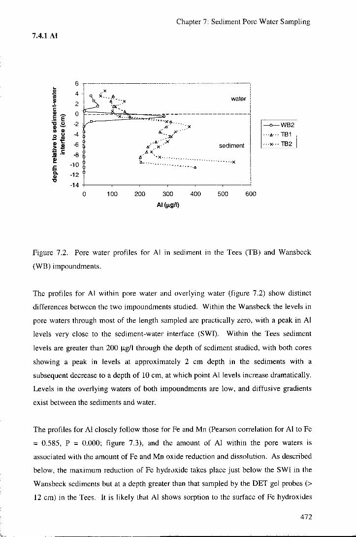
7.4.1 Al
Chapter 7: Sediment Pore Water Sampling
f c
. i ? •o o
11 a
. A ' ' • • X A.' X - "
. . A ' y A-" , X ' "
4 " - X A
water
sediment
200 300 400
Ai(ng/i)
500 600
Figure 7.2. Pore water profiles for Al in sediment in the Tees (TB) and Wansbeck
(WB) impoundments.
The profiles for Al within pore water and overlying water (figure 7.2) show distinct
differences between the two impoundments studied. Within the Wansbeck the levels in
pore waters through most of the length sampled are practically zero, with a peak in Al
levels very close to the sediment-water interface (SWI). Within the Tees sediment
levels are greater than 200 |xg/l through the depth of sediment studied, with both cores
showing a peak in levels at approximately 2 cm depth in the sediments with a
subsequent decrease to a depth of 10 cm, at which point Al levels increase dramatically.
Levels in the overlying waters of both impoundments are low, and diffusive gradients
exist between the sediments and water.
The profiles for Al closely follow those for Fe and Mn (Pearson correlation for Al to Fe
= 0.585, P = 0.000; figure 7.3), and the amount of Al within the pore waters is
associated with the amount of Fe and Mn oxide reduction and dissolution. As described
below, the maximum reduction of Fe hydroxide takes place just below the SWI in the
Wansbeck sediments but at a depth greater than that sampled by the DET gel probes (>
12 cm) in the Tees. It is likely that Al shows sorption to the surface of Fe hydroxides
472
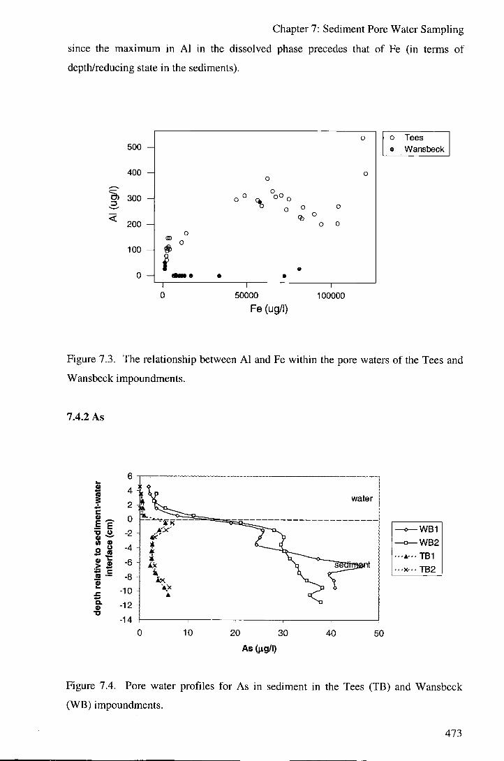
Chapter 7: Sediment Pore Water Sampling
since the maximum in Al in the dissolved phase precedes that of Fe (in terms of
depth/reducing state in the sediments).
<
o 500
400 -o
o
300 -
200 -
^ O 0 0
O 0
100 -
o
# Q
0 -•
• • 50000
Fe (ug/l)
1 " 100000
o Tees « Wansbeck
Figure 7.3. The relationship between Al and Fe within the pore waters of the Tees and
Wansbeck impoundments.
7.4.2 As
water
CO a>
10 20 30
As (ng/l) 40 50
Figure 7.4. Pore water profiles for As in sediment in the Tees (TB) and Wansbeck
(WB) impoundments.
473

Chapter 7: Sediment Pore Water Sampling
As is below the EQS in the waters of both impoundments and in the sediment pore water of the Tees impoundment, but the mean level in the sediment pore water of the Wansbeck exceeds the EQS (table 7.5). High concentrations of pollutants in sediment pore waters may have an impact on benthic biota in the impoundments (As^* is particularly toxic and teratogenic). As shows a distinct peak immediately below the SWT in the Tees with an apparent diffusion from (anoxic) sediment at depth up to this point. Within the Wansbeck there is some localised variation in As levels which may relate to heterogeneity in As concentration in the particulate material. The general trend is of a diffusion upwards in the sediment. As input to the Wansbeck sediment is probably associated with coal mining in the area. In both impoundments a diffusion gradient for As exists between the levels in pore water and the lower levels in the overlying water across the SWI.
Association of As with Fe in the solid phase of sediments has been observed (DeVitre et
al., 1991), and Davison et al. (1997) suggest simultaneous (and localised) remobilisation
of these metals, but no evidence for a Fe association is seen in this project (Pearson
correlation = -0.204, P = 0.115). Within the cores studied As appears to be released
from anoxic sediments even at depths at which Fe is assumed to be immobilised as
sulphides (see section 7.4.7 below), and decomposition of organic material at depth is
proposed as the source of As to the pore water.
474

7.4.3 Ca
Chapter 7: Sediment Pore Water Sampling
water
W 0)
sediment
100000 200000
Ca (fig/l) 300000 400000
Figure 7.5. Pore water profiles for Ca in sediment in the Tees (TB) and Wansbeck
(WB) impoundments.
Ca shows similar diffusion controlled profiles for both the Tees and the Wansbeck
sediments, with concentrations higher at depth than within the overlying water. Note
that coring on the Wansbeck was carried out during a period following high river flow
and therefore the water overlying the sediments was fresh. This is in contrast with the
coring for sequential extraction experiments (chapter 6) during which sediments in the
Wansbeck were overlain by saline water. The Tees impoundment is designed to totally
exclude tidal waters and is almost exclusively freshwater. The source of Ca within the
pore waters of the Tees sediment could either be from carbonate dissolution or from
seawater. The World mean seawater Ca concentration is approximately 412000 /xg/1
(Reimann and Caritat, 1998). That the relationship between K or Mg and Ca (Pearson
correlation = 0.793 and 0.815 respectively; P = 0.000) is lower than that between K and
Mg (Pearson correlation = 0.996; P = 0.000), and that the ratio of Mg/Ca differs to that
in seawater (Mg/Ca in pore water = 1.79; Mg/Ca in world mean seawater (Lide, 1996) =
3.13) suggests that some carbonate dissolution is taking place. The gradient of Ca (and
K and Mg) with depth in the Wansbeck pore waters changes at approximately 5 cm
depth. The same change in gradient (but in the opposite direction since sampling was
during a period in which the overlying water was saline) is observed in the
exchangeable fraction of the sediment cores (figure 7.5), and represents the depth to
4 7 5

Chapter 7: Sediment Pore Water Sampling
which short term changes in overlying water composition with tidal input and
freshwater flow (fresh vs. seawater) impact on these ions in the sediments.
7.4.4 Co
c
. i ?
l | I I « —
Q. T3
4
2
0
-2
-4
-6
-8
-10
-12
-14
water
/ > X K
/ X - i |
/ > X K
/ X - i |
sediment
4 6
Co(^g/l)
10
Figure 7.6. Pore water profiles for Co in sediment in the Tees (TB) and Wansbeck
(WB) impoundments.
Co shows low concentrations in the water column with peaks in concentration just
below the SWl in both impoundments, with lower levels in pore waters deeper within
the sediments. The peak in Co is slightly closer to the SWl in the Wansbeck than the
Tees sediment (figure 7.6).
In chapter 6 it was shown that Co is held in the solid phase of sediments in association
with carbonate, oxides of Fe and Mn and in sulphides or organic matter. The pattern
within pore waters is similar to that for Mn and Fe (Pearson correlation = 0.707 and
0.712 (P = 0.000) respectively; figure 7.7) and Co is interpreted as redox controlled,
undergoing release to pore waters with reduction of Fe and Mn hydroxides.
Release of Co is seen to precede Mn and Fe release in the reduction sequence (with
depth) in the sediment, implying that Co may be associated with hydroxide particle
surfaces and therefore be disproportionately released at the onset of hydroxide
reduction.
476

Chapter 7: Sediment Pore Water Sampling
o O
9 - • 8 -
/ • C D \ 0
7 - I ° 1 1 • 6 - V ° * y 5 -
4 -
3 -
B o° • o
• « o •
o o
0
0 o
2 -
1 -
0 -1
10000
Mn (ug/l)
r 20000
o Tees • Wansbeck
Figure 7.7. Co vs. Mn within the pore waters of the Tees and Wansbeck
impoundments, showing release of Co preceding Mn release (1) in the reduction
sequence.
7.4.5 Cr
.1 ?
l | (0 —
Q. O •a
6
4
2
0
-2
-4
-6
-8
-10
-12
-14 10
1 water
i f ' aC_ ' a
sediment
20
Cr(|ig/I) 30 40
Figure 7.8. Pore water profiles for Cr in sediment in the Tees (TB) and Wansbeck
(WB) impoundments.
477
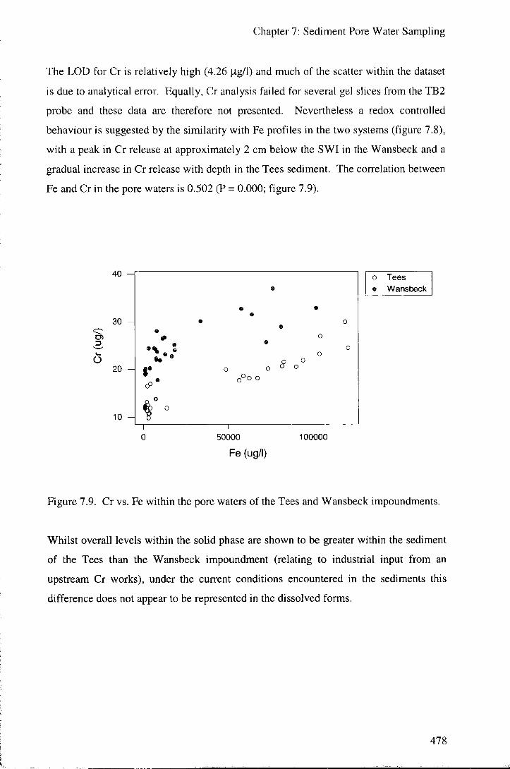
Chapter 7: Sediment Pore Water Sampling
The LOD for Cr is relatively high (4.26 [ig/l) and much of the scatter within the dataset is due to analytical error. Equally, Cr analysis failed for several gel slices from the TB2 probe and these data are therefore not presented. Nevertheless a redox controlled behaviour is suggested by the similarity with Fe profiles in the two systems (figure 7.8), with a peak in Cr release at approximately 2 cm below the SWI in the Wansbeck and a gradual increase in Cr release with depth in the Tees sediment. The correlation between Fe and Cr in the pore waters is 0.502 (P = 0.000; figure 7.9).
40
30
3
20 H
10
50000
Fe (ug/l) 100000
o Tees • Wansbeck
Figure 7.9. Cr vs. Fe within the pore waters of the Tees and Wansbeck impoundments.
Whilst overall levels within the solid phase are shown to be greater within the sediment
of the Tees than the Wansbeck impoundment (relating to industrial input from an
upstream Cr works), under the current conditions encountered in the sediments this
difference does not appear to be represented in the dissolved forms.
478

7.4.6 Cu
Chapter 7: Sediment Pore Water Sampling
. i ?
o. 0) "D
6 4 2 0
-2 -4 -6 -8
-10 -12 -14
X > a K.
" S ! ! ^ a
^-'^"^^"^ water
i ^^^^^
~ ^
: =t?
sediment
1
50 100 Cu (ng/l)
150
Figure 7.10. Pore water profiles for Cu in sediment in the Tees (TB) and Wansbeck
(WB) impoundments.
Cu concentrations are on average higher in the overlying water than in the sediment
pore waters within both impoundments, and exceeds the EQS in both the water and pore
water of both the Tees and Wansbeck. These dissolved Cu levels are higher in the
Wansbeck than the Tees reflecting the pattern within the solid phase of the sediments
(chapter 6). Although it was seen that Cu is largely associated with Fe and Mn oxides
through sequential extraction experiments, Cu does not closely follow the pattern in
pore water shown by Fe and for example Co. Within the Tees sediment pore water Cu
is relatively constant with depth, but in the Wansbeck there exist distinct horizons
showing peaks in Cu (figure 7.10).
These peaks may relate to variable inputs of Cu to the sediments, although no effective
comparison could be made with the sediment extractions due to the different scale of
sampling (sediment cores were sampled at 3 cm intervals compared with 1 cm slices for
pore water sampling). The strongest relationship of Cu with the elements discussed is
with Pb (Pearson correlation = 0.749, P = 0.000) suggesting a similar source for these
two metals.
479

7.4.7 Fe
Chapter 7: Sediment Pore Water Sampling
water
M «
sediment . . A - . - TBI
50000 100000
Fe(^g/I)
150000
Figure 7.11. Pore water profiles for Fe in sediment in the Tees (TB) and Wansbeck
(WB) impoundments.
Levels of Fe in the overlying water and pore waters of both impoundments studied are
greater than the recommended EQS. Although the EQS is exceeded within the
overiying water of the sediment cores during the DET equilibrations, this does not
necessarily translate to the situation in the impoundments in which a much larger
volume of water is available to dilute any Fe release from sediment. Water quality
surveying showed mean values of 167 and 168 ^ig/l - well below the EQS of 1000 |ig/l
- in the Tees and Wansbeck respectively.
The distribution of Fe reflects the redox profile within the sediments. The sequence of
redox reactions in surface sediments follows the order of use of:
oxygen nitrate Mn(IV) Fe(in) sulphate
as thermodynamically favourable electron acceptors for the breakdown of organic
material (Stumm and Morgan, 1996; Santschi et al., 1990). Within the overlying water
of both impoundments some oxygen is present and the majority of Fe is in the insoluble
state Fe(lll) and hence concentrations sampled by the DET gel probes were low (figure
480

Chapter 7: Sediment Pore Water Sampling
7,11). With progression into the sediment the above sequence of reductions takes place,
with the depth at which each occurs dependent on the relative concentration of each
electron acceptor and the amount of organic material present. Within the sediments of
the Wansbeck, which are organic rich and have a periodically anoxic overlying water
column (see chapter 4), oxygen and nitrate are rapidly depleted and Fe(ni) hydroxides
are reduced to release dissolved Fe^* ions at a depth of 2 to 3 cm in the sediment.
Below this depth redox potentials fall further and the presence of sulphide from the
reduction of sulphate forms insoluble FeS, and the level of dissolved Fe in the pore
waters is low. This pattern is typical of that of anoxic nearshore sediments (e.g. Aller,
1980; Elderfield et al., 1981; Heggie et al., 1987). Within the Tees the sediments are
less reducing and the maximum release of Fe ^ is not encountered in the depth of
sediment sampled (i.e. it is assumed to be at > 12 cm depth in the sediment). Sequential
extraction experiments (chapter 6) showed that the sediments of the Tees contain very
little sulphide within the circa 50 cm cores taken, supporting the conclusion that
conditions are less reducing. The reason for this is likely to be higher DO levels in the
overlying water column (normally close to saturation) than in the Wansbeck, with lower
organic matter content of the sediments possibly also important (although this could
relate to better preservation of organic material in the sediments of the Wansbeck rather
than differences in organic inputs).
7.4.8 Hg
c
.1 "E
l l 0) .> ™ a — 9>
a. •a
6 4 2 0
-2 -4 -6 -8
-10 -12 -14
0.0
water
JL
- O
• sediment
1 > - 0
1
0.1 0.2
Hg (ng/i)
0.3 0.4
Figure 7.12. Pore water profiles for Hg in sediment in the Tees (TB) and Wansbeck
(WB) impoundments.
481
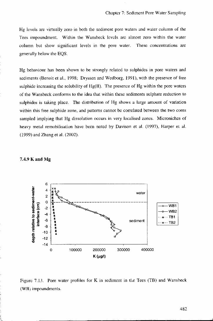
Chapter 7: Sediment Pore Water Sampling
Hg levels are virtually zero in both the sediment pore waters and water column of the Tees impoundment. Within the Wansbeck levels are almost zero within the water column but show significant levels in the pore water. These concentrations are generally below the EQS.
Hg behaviour has been shown to be strongly related to sulphides in pore waters and
sediments (Benoit et al., 1998; Dryssen and Wedborg, 1991), with the presence of free
sulphide increasing the solubility of Hg(n). The presence of Hg within the pore waters
of the Wansbeck conforms to the idea that within these sediments sulphate reduction to
sulphides is taking place. The distribution of Hg shows a large amount of variation
within this free sulphide zone, and patterns cannot be correlated between the two cores
sampled implying that Hg dissolution occurs in very localised zones. Microniches of
heavy metal remobilisation have been noted by Davison et al. (1997), Harper et al.
(1999) and Zhang et al. (2002).
7.4.9 K and Mg
water
U 0)
sediment ...x -. TB2
100000 200000
K(^g/l)
300000 400000
Figure 7.13. Pore water profiles for K in sediment in the Tees (TB) and Wansbeck
(WB; impoundments.
482

Chapter 7: Sediment Pore Water Sampling
S i
•a (», » a 2 |
I I Q . «
6 4 2 0
-2 -4 -6 -8
-10 -12 -14
water ^ ^ ^ ^
k k k i if k
1 1
sediment
0 200000 400000 600000 Mg (ng/l)
800000 1000000
Figure 7.14. Pore water profiles for Mg in sediment in the Tees (TB) and Wansbeck
(WB) impoundments.
K and Mg are strongly correlated in the pore waters of the impoundments (Pearson
correlation = 0.996). Both K and Mg, as for Ca, show diffusive behaviour in pore water
related to the salinity of the overlying water column. Whilst the diffusion profile is
likely to remain relatively constant over time in the Tees impoundment, in the
Wansbeck the salinity of the overlying water varies dependent on the tidal state and
river discharge and the direction of diffusion wil l vary. The ratio of Mg to K in the pore
waters of the impoundments is 2.96 compared with a ratio of 3.23 in seawater. In
chapter 6 some replacement of K by Mg on ion exchange sites in the sediment was
suggested, and it is possible that the reduction of this ratio relative to seawater relates to
this exchange.
483

7.4.10 Mn
Chapter 7: Sediment Pore Water Sampling
f c 0) E ••5 Si o 0)
- I «
E
8
D. a>
water
sediment •A- - TBI
5000 10000 15000 20000 Mn (ng/l)
25000
Figure 7.15. Pore water profiles for Mn in sediment in the Tees (TB) and Wansbeck
(WB) impoundments.
Mn shows similar redox controlled behaviour to Fe in sediments, although its reduction
and release to pore waters slightly precedes that of Fe in the series of reductions which
takes place during organic decomposition. The profile for Mn at the SWI in the two
impoundments (figure 7.15) is very similar to that for Fe (figure 7.11), and the two
elements show strong correlation (Pearson correlation = 0.887; figure 7.16). The
maximum release of Mn^* ions to the pore water within the Wansbeck sediment takes
place at a slightly shallower depth than the Fe " release (between 1 and 2 cm compared
with between 2 and 3 cm), conforming with the expected sequence of reductions. As
for Fe, the maximum release of Mn^* to the pore water of the Tees is interpreted as
occurring at greater depth in the sediment than was sampled.
484

Chapter 7: Sediment Pore Water Sampling
20000
3
10000 -A
50000
Fe (ug/l) 100000
o Tees • Wansbeck
Figure 7.16. The relationship between Mn and Fe in the pore waters of the sediments of
the Tees and Wansbeck impoundments.
7.4.11 P
. 1 ?
11 !1> Q . a>
T3
6 4 2 0
-2 -4 -6 -8
-10 -12 -14
i water
A
- T x' x' sediment
p y
\ "'-A
X- - TB2
0 5000 10000 15000 20000 25000 30000
p (jig/i)
Figure 7.17. Pore water profiles for P in sediment in the Tees (TB) and Wansbeck (WB) impoundments.
485

Chapter 7: Sediment Pore Water Sampling
FeO , 0 >:
FeO OH
Figure 7.18. P association with Fe hydroxides in oxic sediments (from Golterman et al.,
1983).
Sequential extraction experiments (chapter 6) showed P to be strongly associated with
Fe in the sediments of both impoundments, and the affinity of P with Fe and Mn oxides
is well reported (e.g. Davies, 1997; Jensen et al., 1992; figure 7.18). The distribution of
P in the pore waters and overlying waters of the sediments of the Tees and Wansbeck
impoundments are quite closely related to the patterns of behaviour of Fe and Mn
(figure 7.19). P release to pore waters is proportional to Fe release from hydroxides at
the onset of reduction but is lower than Fe as reduction progresses, especially in the
Tees sediments, implying that P may be associated with the surface of oxide particles.
20000
3
10000 H
0 H
O O
o O
ce o o % o .
50000
Fe (ug/l)
— I 100000
o
o
o Tees o Wansbeck
Figure 7.19. P vs. Fe in the pore waters of sediments of the Tees and Wansbeck
impoundments.
486

7.4.12 Pb
Chapter 7: Sediment Pore Water Sampling
c
. i ?
p Q . V
XI
6 4 2 0
-2 -4 -6 -8
-10 -12 -14
,^ X a
X "x-.tgrnTTrr
• water
ffit"
sediment
X
10 20
Pb(^g/l)
30 40
Figure 7.20. Pore water profiles for Pb in sediment in the Tees (TB) and Wansbeck
(WB) impoundments.
Mean Pb concentrations are lower than the HQS in the sediment pore waters but
approach the HQS (25 |Lig/l) in the overlying waters of both impoundments (figure 7.20).
The pattern for Pb distribution shows no relationship to the Fe and Mn profiles,
indicating that within these sediments Pb is not scavenged by oxides. That
concentrations are much higher in the overlying water column than the pore waters of
the sediments implies that Pb is in stable dissolved forms (perhaps associated with
organic colloids) in the water columns and does not partition into the solid phase. As
for Cu the profiles for Pb suggest that the direction of diffusion is from the water
column to the sediment pore water.
487

7.4.13 Sc
Chapter 7: Sediment Pore Water Sampling
water
10 »
sediment
Sc (ug/l)
- ^ ^ W B I —o—WB2
• A - - - TBI - x - . - TB2
Figure 7.21. Pore water profiles for Sc in sediment in the Tees (TB) and Wansbeck
(WB) impoundments.
Overall Sc concentrations within the solid phase were shown to be similar for the
sediments of the two impoundments, with Sc speciation following that of Fe (chapter 6).
Within the solid phase of the Tees sediments Sc is associated with Fe and Mn oxides
and within the Wansbeck with both Fe and Mn oxides and sulphides/organic matter. Sc
concentrations within both the pore water and overlying water of the Tees sediment are
effectively zero. In the Wansbeck Sc concentrations in pore water are higher than those
in overlying water, with a diffusion gradient across the SWI.
Sc and As (and V) show good correlation within the pore waters (Pearson correlation =
0.929; P = 0.000; figure 7.22), but show no relationship to the behaviour of Fe (Pearson
correlation = -0.162; P = 0.213). As for As, release on decomposition of organic matter
is the likely source of Sc within the Wansbeck impoundment. The pattern of Sc
concentration in the pore waters fits with the finding that a fraction of the Sc in the solid
phase is associated with organic matter/sulphide within the Wansbeck but not in the
Tees.
488

cn
o
Chapter 7: Sediment Pore Water Sampling
7
6
5 H
4
3
2
1
0
• " •
• 9
10 20 30 40
o Tees • Wansbeck
50 As (ug/l)
Figure 7.22. The relationship between Sc and As in the pore water of sediments of the
Tees and Wansbeck impoundments.
7.4.14 Si
water
sediment
^ ^ W B I —o—WB2
- A - - . TB1 - x - . - TB2
5000 10000
Si(ng/l)
15000 20000
Figure 7.23. Pore water profiles for Si in sediment in the Tees (TB) and Wansbeck
(WB) impoundments.
489

Chapter 7: Sediment Pore Water Sampling
Within the Tees Si dissolution from the solid phase to the pore waters is interpreted as
relatively constant with depth, with concentrations in pore water being controlled by
diffusion to the overlying water column (figure 7.23). The profile within the Wansbeck
is less regular, with localised variation in dissolved Si levels with depth. This variation
may relate to differences in particle size, although no PSD analysis was carried out at
the same resolution as DET pore water sampling and this cannot be tested.
Si concentration within the pore water shows relatively strong correlation with Fe
(Pearson correlation = 0.814, P = 0.000; figure 7.24), and may be controlled by
dissolution of (authigenic) Fe-Al silicates (formed by reaction of Si from diatoms with
Fe hydroxides; Wetzel, 1983).
20000 - f
CD
10000
0 - \
o
0
%
o O Q
Cb oo o
o
o
i» O 0 o 0 o © o
0
0 °
1 0
1 50000
Fe (ug/l)
1 100000
o Tees o Wansbeck
Figure 7.24. The relationship between Si and Fe in the pore water of sediments of the
Tees and Wansbeck impoundments.
490

7.4.15 Ti
Chapter 7: Sediment Pore Water Sampling
20 40 60
Ti(ng/i)
water
sediment
^ ^ W B I —o—WB2 • --A.--TB1 . - - X . - - TB2
80 100
Figure 7.25. Pore water profiles for Ti in sediment in the Tees (TB) and Wansbeck
(WB) impoundments.
Ti concentrations are low in the overlying waters of both impoundments and
significantly higher in the pore waters of the sediments, with a diffusion gradient across
the SWI (figure 7.25).
Ti is significantly correlated with Fe (Pearson correlation = 0.607, P = 0.000; figure
7.26) and, as for A l , Co, Cr and P, release to pore waters is related to the dissolution by
reduction of Fe hydroxides in the sediment. Whilst levels in the solid phase of the
sediment are higher in the Tees than the Wansbeck (chapter 6), there is no clear
reflection of this in the relative concentrations in the pore water between the two
impoundments.
491

Chapter 7: Sediment Pore Water Sampling
0 5 3
90 -80 -
70 -
60 -
50 -
O 0
° 0 ° 0
40 -
30 - % 20 - 0
10 - o
0 -
0
° ° ° o o < o
50000 Fe (ug/l)
— \ — 100000
o Tees o Wansbeck
Figure 7.26. The relationship between Ti and Fe in the pore water of sediments of the
Tees and Wansbeck impoundments.
7.4.16 V
water
(0 »
sediment
—<^WB1 —1>—WB2
- A - - - TBI - - - X - - TB2
10 20 30
V (jig/i)
40 50
Figure 7.27. Pore water profiles for V in sediment in the Tees (TB) and Wansbeck
(WB) impoundments.
492

Chapter 7: Sediment Pore Water Sampling
V concentrations within both the pore waters and water columns of both impoundments are well below the EQS (table 7.5). Concentrations in both impoundments are lower within the overlying waters than in the pore waters and diffusion gradients exist across the SWI. V concentrations are higher in the pore waters of the Wansbeck than in the Tees.
V shows no significant correlation at 99 % probability level with Fe within the systems
(Pearson correlation = -0.255, P = 0.047), but is strongly correlated with As (Pearson
correlation = 0.983, P = 0.000; figure 7.28). As for As and Sc, V release to pore waters
is likely to be associated with organic matter/sulphides in the sediment, with the
difference between the Tees and the Wansbeck due to the difference in the quantities of
metals held within this phase within the sediment.
V (ug/l)
o Tees o Wansbecl<
Figure 7.28. The relationship between As and V in the pore water of sediments of the
Tees and Wansbeck impoundments.
493

Chapter 7: Sediment Pore Water Sampling
7.5 Summary and conclusions
7.5.1 Biogeochemistry/diagenetic controls
DET gel probe sampling has allowed detailed profiles of elemental concentrations about
the SWI (to approximately 12 cm depth in the sediment and 3 cm of the overlying water
column) to be plotted. The results suggest that a variety of physical, chemical and
biochemical processes are important in controlling the distribution and concentration of
elements within the pore waters of the sediments. These controls and the elements
associated with them are outlined in table 7.6.
Element Distribution Control
Fe, Mn, A l , Lower in overlying water than in pore Associated with sequence of
Co, Cr, P, Si water. Fe reduction processes
andTi Maximum at 2-3 cm below SWI in (particularly release of Fe^*
Wansbeck. ions on reduction of Fe ^
Maximum deeper in Tees. hydroxide).
Ca, K and Lower in overlying water than in pore Diffusion relating to salinity
Mg water. of overlying water column
Approximate linear increase with (no biological mediation).
depth in sediment.
As, Hg, Sc Lower in overlying water than in pore Related to organic
and V water. matter/sulphides within
Concentrations low in pore waters in sediment.
Tees but increase with depth in
Wansbeck.
Irregular profile for Hg in Wansbeck.
Cu and Pb Greater in overlying water than in pore Dissolved inputs greater
water. than sediment bound inputs.
Table 7.6. Summary of suggested controls on distributions of elements in pore waters
in the Tees and Wansbeck estuarine impoundments.
7.5.1.1 Fe, Mn, Al, Co, Cr, P, Si and Ti
Fe, Mn, Al , Co, Cr, P, Si and Ti are associated with Fe hydroxides in the solid phase of
the sediment, ana show pore water profiles relating to the reduction of these oxides to
release free ions. In the Wansbeck the overlying water column is periodically anoxic
494

Chapter 7: Sediment Pore Water Sampling
and the sediment is organic rich, and so oxygen is rapidly depleted on progression into
the sediment column. The onset of use of Fe and Mn oxides as electron acceptors in the
breakdown of organic matter is marked by peaks in the concentrations of the above
elements. With greater depth in the sediment of the Wansbeck (4 cm below the SWI
and deeper) organic matter decomposition is by sulphate reduction, and the presence of
free sulphide allows precipitation of FeS together with the above metals to varying
degrees. In the Tees less reducing conditions are encountered in the sediment due to
greater oxygen content in the water column and lower organic content in the sediment.
In the Tees sediment the maximum release of free ions by reduction of Fe and Mn
oxides is deeper than the depth sampled (12 cm), and no sulphate reduction is
encountered.
7.5.1.2 Ca,K and Mg
Ca, K and Mg show diffusion from the sediment to the water column in both
impoundments. In the Wansbeck the direction of diffusion of these ions will reverse
during periods in which the overlying water column is saline, whereas in the
(freshwater) Tees the diffusion is permanently unidirectional. The source of saline
water at depth in the sediment in the Tees is either from the pre-impoundment sediment
(deposited under saline conditions) or from current saline intrusion beneath the barrage.
Whilst K and Mg are directly proportional in the pore waters and in the same ratio as in
seawater, Ca shows a lower correlation and dissolution of carbonates is suggested as
providing an additional source for this ion.
7.5.1.3 As, Hg, Sc and V
As, Hg, Sc and V show poor correlation with Fe in the pore waters and show maximum
concentrations at the depth at which sulphides are present (i.e. concentrations are low in
the overlying water and upper sediment in the Wansbeck and throughout the depth
sampled in the Tees). These elements are associated with sulphate reduction to
sulphides in the sediment, or release from organic material in the presence of sulphides.
It is possible that these metals are present in stable dissolved forms as organometal
compounds. The methylisation of As and Hg have been studied in detail (Andreae,
1986; Mason et al., 1993) due to the toxicological properties of these organometals. It
is likely that methane production occurs at depth in the Wansbeck sediment as the next
stage in the sequence of redox processes following sulphate reduction. The distribution
495

Chapter 7: Sediment Pore Water Sampling
of Hg in the pore waters of the Wansbeck is very irregular suggesting that sulphate
reduction and mobilisation of this metal occurs in localised zones within the sediment.
7.5.1.4 Cu and Pb
Cu and Pb show greater concentrations in the overlying water column than in the
sediment pore water implying that, unlike the other elements studied, these metals are
present in stable dissolved forms and do not partition into the sediment. Cu is strongly
chelated by organic matter in natural waters, particularly in biologically productive
systems (such as the impoundments), giving stable dissolved forms, and Pb is mainly
present as dissolved Pb^* at pH > 7 (Stumm and Morgan, 1996). Sediments (suspended
or bed) do not therefore act as sinks for these metals in the impoundments.
7.5.2 Fluxes across the SWI
In addition to helping to understand diagenetic processes taking place within the
sediments, DET gel probe sampling was carried out to allow estimation of the
exchanges taking place across the SWI. The movement of dissolved materials from the
sediment pore water to the water column may be simply modelled as a diffusion
(ignoring the effects of hydrostatic pressure gradients and sediment and water mixing at
the SWI by bioturbation and water turbulence) according to Fick's first law (Gill et al.,
1999):
where F is the diffusive flux of a solute with concentration C at depth x, 0 is the
tortuosity (dimensionless), (p is the sediment porosity, and Dw is the diffusion
coefficient of the solute of interest in water without the presence of a sediment matrix.
Tortuosity is generally related to porosity according to:
The diffusion coefficients for most aqueous species, including organics, are similar
differing by, at most, a factor of two from the self-diffusion coefficient of water whxh
is 2.4 X 10" cm /s at 25°C (www.uf3ventures.com). Diffusion coefficients in porous
media that are less than 10" cm /s result from m.?chanisms or conditions other than the
496

Chapter 7: Sediment Pore Water Sampling
inherent mobility differences between the species themselves. These mechanisms
include path length differences due to water content differences and retardation due to
sorption and transient chemical effects.
The fluxes of a selection of ions (P04^", Ca^ , Mg^^, Fe^+, Mn^^, Cr04^" and CHsHgCl")
across the SWI interface were estimated using the above expression of Fickian diffusion
and diffusion coefficients for the charged ions calculated according to Boudreau (1997),
assuming a temperature of 15°C, atmospheric pressure and saHnity of 0.5 %c (table 7.7).
I o n Diffusion coefficient (cmVs x 10'*) in freshwater (0.5 %o
salinity)
P04^" 048
Ca + 0.63
Mg^^ 0.56
Fe ^ 0.56
Mn^^ 0.55
Cr04^" 1.1
CHsHgCl'^ 1.3
Table 7.7. Diffusion coefficients used for calculation of diffusive fluxes across the
SWI.
Note that P04^' was chosen as the major phosphate species present and the effects of the
presence of H2PO'*' and HP04^" (which have greater diffusion coefficients) were
ignored. The estimate for phosphate flux is therefore at the lower boundary. CHsHgCl"
was chosen as the species of Hg present since the majority of dissolved Hg in natural
waters has been shown to exist in colloidal forms, with the diffusion coefficient given in
Gill et al. (1999) being used. Based on the moisture content determinations from the
sediment coring a value of porosity of 70 % was used. The concentration gradients
across the SWI were taken from the pore water profiles sampled by the DET gel probes.
The results are summarised in tables 7.8 and 7.9.
497

Chapter 7: Sediment Pore Water Sampling
Ion Flux in Wansbeck Flux in Tees Flux in Tamar
(Hg/m /day) (Hg/mVday) ()Xg/m /day)
P-PO4' 1420 570 1360
Ca ^ 29500 23000
Mg^^ 118000 4900
Fe ^ 37800 23000 5030
Mn'-^ 4240 2400 4200
Cr-Cr04^" 27.8 12.1
Table 7.8. Diffusive fluxes for a selection of ions across the SWI at sites WB and TB in
the Wansbeck and Tees impoundments respectively (data from this project) and mean
fluxes in the Tamar Estuary (data from Upstill-Goddard et al., 1989).
Ion Flux in Wansbeck Flux in Tees Flux in Lavaca Bay
(^ig/mVday) (Hg/mVday) (Hg/mVday)
Hg- 0.138 0.000 0.139
CHsHgCl"
Table 7.9. Diffusive fluxes for Hg of across the SWI at sites WB and TB in the
Wansbeck and Tees impoundments respectively (data from this project) and mean flux
in Lavaca Bay, Texas (data from Gill et al., 1999).
Under higher salinities, such as are periodically encountered in the Wansbeck, diffusion
coefficients (and hence fluxes) are reduced. For example in the Wansbeck under 15 %o
salinity the flux of Mn is 4240 ng/m^/day compared to 4400 |a,g/m /day under
freshwater. For phosphate the respective values are 1420 and 1480 [ig/m^/day P.
The fluxes across the SWI determined through DET gel probe pore water sampling in
the Tees and Wansbeck impoundments are similar to data reported for un-impounded
estuarine and nearshore environments (e.g. Upstill-Goddard et al., 1989; Rowe et al.,
1975; Klump and Martens, 1981; Gill et al., 1999). Mean data are presented above for
studies carried out in spring 1983 on the Tamar Estuary, UK (largely unpolluted organic
rich sediments) and in spring 1996 in Lavaca Bay, Texas (an estuary historirplly
impacted by Hg discharges). The calculation of flux of Hg within the Wansbeck
assumed that all of the Hg present was in monomethyl form and is therefore likely to
498

Chapter 7: Sediment Pore Water Sampling
overestimate Hg-CHsHgCl'^ flux. Gill et al. (1999) found that monomethyl Hg
represented on average 35 % of total Hg present in the sediments of Lavaca Bay.
Assuming a similar ratio in sediments in the Wansbeck gives a flux of Hg-CHsHgCl" of
approximately 0.048 \xg/m^/day, i.e. significantly lower than that reported in the
historically contaminated sediments of Lavaca Bay.
7.5.2.1 Relative contribution of sediment P to the impounded water bodies
In chapter 3 it was suggested that the major controls on P concentrations in the
impoundments are catchment related, and that internal cycling of P from sediment is
small relative to these external inputs. The size of the contribution of P to the water
body by release from the sediment may be approximately quantified using the estimates
of fluxes reported above.
The surface areas of the sediment showing P release in the two impoundments were
estimated as the surface areas of the impoundments underlain by predominantly silt and
clay sized bed material (and therefore showing anoxia within the sediment column).
Within the Wansbeck impoundment this area was taken as the area of the length of river
between the barrage (NZ 2935 8536) and Stakeford Bridge (NZ 2715 8595) and within
the Tees impoundment the area of the length of river between the barrage (NZ 4616
1905) and the railway bridge (NZ 4469 1800). The estimated surface areas are 0.38
km^for the Wansbeck and 0.28 km^ for the Tees. No account of the morphology of the
beds was taken and a flat bed was assumed for both impoundments. These surface areas
of the sediments in the impoundments are therefore likely to be slight underestimates.
Knowing the flux per surface area of sediment and the surface area of the sediment the
mass of P released per unit of time may be calculated:
Wansbeck = 540 g/day
Tees =160 g/day
Assuming steady state conditions, the impact of these mean inputs of P on the
concentration of P in the water column may be estimated on the basis of mean
discharges of the two rivers. The mean discharges (taken as the mean discharges at the
nearest upstream gauging stations: see chapter 2) over the periods of this study were 3.4
m /s in the Wansbeck and 10.5 m /s in the Tees. Since DET sampling was carried out
499
Chapter 7: Sediment Pore Water Sampling
under a period of non-overtopping on the Wansbeck the effect of tidal input of water
may be ignored. The mean increases in P concentration in the water of the two
impoundments are therefore:
Wansbeck = 0.00184 mg/1
Tees = 0.00018 mg/1
Mean P concentrations measured in the water of the impoundments during the sampling
periods were 0.27 and 0.80 mg/1 for the Wansbeck and the Tees respectively (median
concentrations were 0.24 and 0.76 mg/1). The overall impact of release of P from
sediment to the water columns on phosphate concentrations in the impounded water is
therefore negligible (< 1 % in each system).
7.5.2.2 Relative contribution of sediment Mn to the impounded water bodies
Whereas it has been shown that the major controls on P concentration in the water
bodies are external to the impounded areas, a large proportion of dissolved Mn is
sourced internal to the impounded areas and release of Mn from sediment under
conditions of low DO is suggested. Using the same methodology as used above for P,
the mean increases in Mn concentration in the water column due to diffusion across the
SWI may be estimated:
Wansbeck = 0.00548 mg/1
Tees = 0.00074 mg/1
During the period studied the median Mn concentrations measured in the water of the
two impoundments were 0.043 and 0.012 mg/1 for the Wansbeck and Tees respectively.
The flux calculations based on the DET pore water sampling therefore confirm that
release from sediment under low DO conditions is a significant source of Mn (and
associated metals) to the water body (approximately 13 and 6 % of the average values).
As mentioned these approximations are based on the assumption of steady state flow
conditions (i.e. output = input plus complete mixing of the water body). As is described
in chapter 4, in reality the impounded water bodies are often stratified such that the
riverine input progresses along the surface of the impoundment and undergoes no
interaction with the bed sediments. The residence time of deeper water is therefore
much longer than it would be in a non-stratified water body, and given steady diffusion
500

Chapter 7: Sediment Pore Water Sampling
from the sediments, concentrations of Mn at depth continue to rise for as long as the
water bodies remain unmixed.
An approximate estimation of the effect of the release of Mn on a stratified water body
may be carried out. Assuming a mean thickness of a stratified layer at depth of 1 m
receiving constant Mn input from the sediments according to the diffusive fluxes given
above, the rates of increase in Mn concentration at depth will be:
Wansbeck = 0.00424 mg/Vday
Tees = 0.00240 mg/l/day
Water quality surveying (chapter 2) revealed a maximum rate of Mn increase in the
water column in the Wansbeck impoundment (at site CP) of 0.131 mg/l/day, i.e. it
would appear that DET estimations of fluxes may seriously underestimate true fluxes
for Mn. As described in chapter 2, rapid Mn release from sediment occurs with the
onset of conditions of below 50 % DO, and it is likely that the low diffusion observed in
the gel probes is due to DO saturations in the water column above the sediment cores
being above this level. Sampling under a range of DO conditions should therefore be
key to any future work examining diffusive fluxes of redox controlled elements across
the SWI.
501

Chapter 8: Sterol Biomarkers in Estuarine Impoundments
Chapter 8
Sterol Biomarkers in Estuariine Impoundments
8.1 Introduction
Measurement of sterols in the sediments of estuarine impoundments was carried out in
order to:
© Assess the potential use of sterol biomarkers in identification of sewage inputs
to estuarine impoundments,
o Make a preliminary estimate of the nature and quantity of sewage inputs to the
sediments of the impoundments studied.
Sterol compounds are powerful tracers of organic matter in aquatic systems due to their
good preservation in recent sediments and specificity of biosynthesis (Saliot et al.,
1991). When faecal matter is introduced to a water body, the sterol compounds strongly
partition to particulate material and, once deposited into sediments, show little
degradation (Bartlett, 1987; Leeming et al., 1996). The source specificity of faecal
sterols is due to differences in both the diets, and biosynthesis and bacterial
biohydrogenation of sterols in the gut, between different warm-blooded animals. The
ratios of these sterols may therefore be used to determine the sources of organic material,
and the absolute value of coprostanol (the major faecal sterol present in human waste
(Brown and Wade, 1984)) may be used to assess relative amounts of sewage input.
Preliminary identification of sewage inputs to the impoundments in this study was
carried out by determination of the concentrations of cholesterol (cholest-5-en-3P-ol),
and the primary products of biohydrogenation of cholesterol in the guts of warm
blooded animals and in the environment (coprostanol (5P-cholestan-3P-ol),
epicoprostanol (5P-cholestan-3a-ol), and cholestanol (5a-cholestan-3p-ol)) (e.g.
LeBlanc et al., 1992; Mudge and Norris, 1996; Patton and Reeves, 1999; Elhmmali et
al., 2000). The systematic names and structures of these sterols are given in table 8.1
and figure 8.1 respectively.
502

Chapter 8: Sterol Biomarkers in Estuarine Impoundments
Trivial name Systematic name
Cholesterol
Coprostanol
Cholestanol
Epicoprostanol
cholest-5-en-3|3-ol
5P-cholestan-3P-ol
5a-cholestan-3P-ol
5P-cholestan-3a-ol
Table 8.1. Trivial and systematic names for the sterol compounds measured in this
study.
cholesterol
coprostanol
cholestanol
503
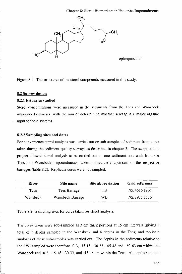
Chapter 8: Sterol Biomarkers in Estuarine Impoundments
CH,
epicoprostanol
Figure 8.1. The structures of the sterol compounds measured in this study.
8.2 Survey desi£n
8.2.1 Estuaries studied
Sterol concentrations were measured in the sediments from the Tees and Wansbeck
impounded estuaries, with the aim of determining whether sewage is a major organic
input to these systems.
8.2.2 Sampling sites and dates
For convenience sterol analysis was carried out on sub-samples of sediment from cores
taken during the sediment quality surveys as described in chapter 3. The scope of this
project allowed sterol analysis to be carried out on one sediment core each from the
Tees and Wansbeck impoundments, taken immediately upstream of the respective
barrages (table 8.2). Replicate cores were not sampled.
River Site name Site abbreviation Grid reference
Tees Tees Barrage TB NZ 4616 1905
Wansbeck Wansbeck Barrage WB NZ 2935 8536
Table 8.2. Sampling sites for cores taken for sterol analysis.
The cores taken were sub-sampled as 3 cm thick portions at 15 cm intervals (giving a
total of 5 depths sampled in the Wansbeck and 4 depths in the Tees) and replicate
analyses of these sub-samples was carried out. The depths in the sediments relative to
the SWI sampled were therefore -0-3, -15-18, -30-33, -45-48 and -60-63 cm within the
Wansbeck and -0-3, -15-18, -30-33, and -45-48 om within the Tees. Al l depths samplea
504

Chapter 8: Sterol Biomarkers in Estuarine Impoundments
represent post-impoundment sedimentation. Sampling was carried out on the 23/07/01
for the Wansbeck and 24/07/01 for the Tees.
8.3 Methodologies
8.3.1 Sediment sampling
Sediment cores were collected using a Mackereth corer, frozen, and sub-sampled at 15
cm intervals using stainless steel equipment as described in chapter 6. These sub-
samples were wrapped in fired aluminium foil and stored frozen for a maximum of one
month before thawing and sterol extraction.
8.3.2 Sterol extraction
Analytical grade reagents were used in all the laboratory work described, and all
appropriate care was taken to avoid organic contamination. Equipment was acid and
Decon 90® (non-ionic surfactant) washed (soaked overnight in 1% HNO3, followed by
overnight in 5% Decon 90® and rinsed in de-ionised water), and fired overnight at
500°C. Sterol extraction from the sediment samples was carried out using the
procedure of Mudge and Norris (1997):
1. Known wet weight circa 30 g of samples refluxed for 4 h in 50 ml of boiling 6
% w/v potassium hydroxide in methanol.
2. Samples centrifuged in glass centrifuge tubes.
3. Supernatant decanted to separating funnels and shaken with 5 ml of organic free
water.
4. Free non-polar lipids extracted into hexane (three 25 ml hexane washes) from
the supernatant by liquid/liquid extraction.
5. Samples concentrated by rotary evaporation to circa 2 ml.
6. Any remaining water removed from samples by pipetting through cleaned
anhydrous sodium sulphate.
7. 5 |xg 5a-cholestane added as an internal standard.
8. Samples evaporated to dryness under oxygen free nitrogen and stored at -20°C
for a maximum of 2 weeks prior to analysis.
9. Samples derivatised by the addition of 100 f i l of bis-(trimethylsilyl)
trifluoroacetamide (BSTFA) and heating to 60°C for one hour.
10. Samples evaporated to dryness under oxygen free nitrogen and redissolved in 1
ml of hexane for injection to the GC column.
505

Chapter 8: Sterol Biomarkers in Estuarine Impoundments
Analysis for sterols was carried out within 24 h of derivatisation of samples.
8.3.3 Sterol analysis
Principle:
Sterols were analysed by flame ionisation gas chromatography (GC-FID). In gas
chromatography a mobile phase (a carrier gas) and a stationary phase (nowadays usually
a capillary column coating) are used to separate individual organic compounds. The
column is held in a temperature controlled oven with one end connected to a
temperature controlled injector block and the other to some foiTn of detector. On
injection to the column samples are vaporised and transported through the column by
the carrier gas, with the rate of movement (and hence the time of appearance at the
detector) dependent on the partitioning between the mobile and stationary phases of the
individual compounds. Using the appropriate temperature program, column (in terms of
stationary phase material, length and diameter) and carrier gas flow gives retention
times in the column unique to each of the analytes of interest.
A variety of detectors are used in gas chromatography, including electrolytic
conductivity detectors, electron capture detectors, photo ionisation detectors, flame
ionisation detectors and mass spectrometers. The most widely used detector is the
flame ionisation detector due to its high sensitivity to a large range of organic carbon-
containing compounds and general analytical ease of use and robustness to impurities
(APHA, 1998). A flame ionisation detector consists of a small hydrogen flame across
which a voltage is applied at the end of the GC column. As organic compounds enter
the flame, electrically charged intermediates are formed which transport a current across
the flame. The size of the current produced is proportional to the mass of compound
entering the detector and therefore, by use of standards for the analytes of interest,
quantification may be carried out.
Method:
Sterol analysis was carried out using a Fisons GC 8065 GC-FED using splitless injection
with a hot needle technique. To give maximum repeatability, injections were made
using a Fisons AS 8u0 autosampler. The carrier gas was helium w ith a column flow
rate of 3 ml/min. A conditioned non-polar (5 % phenyl polysi'.uxane) capillary column
(Phenomenex® Zcbron ZB-5) of 30 m length, 0.32 mm internal diameter and 0.25 [im
506

Chapter 8: Sterol Biomarkers in Estuarine Impoundments
film thickness was used for all sterol analyses. The temperature program started at
60°C (held for I minute) followed by a ramp of 20°C/min up to 200°C, then at 6°C/min
to a maximum of 310°C (isothermal for 23 minutes). Data handling was carried out
using Chromeleon Dionex software.
Retention times of the sterols were determined using standards, and quantification was
determined by comparison with the peak area of the internal standard (5a-cholestane)
for each analysis. Sterol concentrations are expressed in ng/g by dry weight of
sediment as the mean of the replicate extractions for each sample. The conversion from
wet weights to dry weights was made on the basis of % moisture contents determined
during the sediment quality surveys (chapter 3).
8.4 Results and discussion
Results are presented for the sampling of sterols (lipid biomarkers) from the sediments
of the Tees and Wansbeck impoundments. Physical properties and metal speciations for
these sediments are described in chapter 6. The mean concentrations of sterols found in
[ig/g dry weight of sediment are presented in table 8.3. As mentioned in chapter 6, the
sediments from these locations are silt dominated and with only minor variation in
particle size distribution with depth in the sediment column, and therefore no particle
size corrections are applied to the data.
Tees Wansbeck
Coprostanol 1.650 0.699
Epicoprostanol 0.289 0.156
Cholesterol 0.912 0.882
Cholestanol 0.612 0.427
Table 8.3. Mean concentrations in jug/g dry weight of sediment of the lipid biomarkers
sampled in the Tees and Wansbeck impoundments.
Levels of coprostanol (the major faecal sterol present in human waste) are comparable
to concentrations reported at other locations (table 8.4). Brown and Wade (1984) give
the coprostanol concentration in raw sewage as being approximately 160 jug/g. Levels
in the Tees and Wansbeck sediments are significantly lower than this, indicating
dilution or loss of sterols from the systems. Based on the relative coprostanol levels in
507

Chapter 8: Sterol Biomarkers in Estuarine Impoundments
the impoundments and in raw sewage it may be roughly estimated that approximately 1
% of the sediment in the Tees is from sewage sources compared with <0.5 % in the
Wansbeck.
Location Concentration (ngjg) Reference
Antarctica <0.001-1.282 Green and Nichols (1995)
Hong Kong 0.34-5.09 Chan et al. (1998)
Venice Lagoon, Italy 0.04-4.41 Fattoreet al. (1996)
Coasts of Florida, USA <1 Sherblom et al. (1997)
Firth of Clyde, Scotland 152.2 Kelly (1995)
Firth of Tay, Scotland 0.603-1.534 Patton and Reeves (1999)
Table 8.4. Recently reported levels of the lipid biomarker coprostanol in near-shore and
estuarine sediments.
8.4.1 Ratios and sources of sterols
Ratios between the lipid biomarkers may be used to determine provenance of the sterols
(Patton and Reeves, 1999). The ratio of coprostanol/cholesterol may be used to
distinguish between mainly biogenic (autochthonous) sources or mainly sewage sources
for the sterols (raw sewage being the primary source of coprostanol and zooplankton
being a major source of cholesterol (Mudge and Norris, 1997)). It is suggested that
ratios <1 indicate biogenic sources and ratios >1 indicate sewage sources (Nichols et al.,
1996). The ratio of coprostanol/epicoprostanol may be used to identify the primary
faecal source as human as opposed to sources such as agricultural slurry or marine
mammals (LeBlanc et al., 1992), by contrasting the dominant excreted metabolite of
cholesterol (coprostanol) from the human gut with that of the majority of herbivores
(epicoprostanol) (Leeming et al., 1996). A ratio of >1.5 indicates a human faecal source
(Fattore et al., 1996). Finally the ratio of cholesterol/(cholesterol -i- cholestanol) may be
used as a check that the concentrations of sterols have not undergone any significant
changes over time due to diagenetic effects (i.e. as an indicator of sterol preservation).
A constant ratio indicates that there are no significant changes in diagenetic alteration
with either time or location. In summary:
o Coprostanol/cholesterol: <1 = biogenic source; >1 = sewage source,
o Coprostanol/epicoprostanol: >1.5 = human faecal source.
508

Chapter 8: Sterol Biomarkers in Estuarine Impoundments
e Cholesterol/(cholesterol + cholestanol): constant ratio = no change in diagenesis.
The mean values for these ratios in sediments of the Tees impoundment (table 8.5 and
figures 8.2 and 8.3) indicate that sewage is the dominant major source of sterols within
the Tees and that this sewage is strongly dominated by human sources, with little
change in the nature of the inputs of sterols with depth in the sediment. As stated in
chapter 3, the depth of sediment sampled represents the sedimentation over the 7 years
since the Tees estuary was impounded, and therefore the sterol signature indicates that
there has been little change in the nature of discharges of sewage to the river over this
period.
Depth Coprostanol/ Coprostanol/ Cholesterol/
(cm) cholesterol epicoprostanol (cholesterol+cholestanol)
0-3 1.67 6.41 0.71
15-18 1.81 4.83 0.57
30-33 2.18 6.25 0.56
45-48 1.53 4.89 0.48
Table 8.5. Sterol ratios with depth in the sediment of the Tees impoundment.
Depth Coprostanol/ Coprostanol/ Cholesterol/
(cm) cholesterol epicoprostanol (cholesterol+cholestanol)
0-3 0.60 9.42 0.80
15-18 1.01 3.83 0.59
30-33 0.88 1.93 0.58
45-48 0.93 3.41 0.59
60-63 0.96 3.29 0.57
Table 8.6. Sterol ratios with depth in the sediment of the Wansbeck impoundment.
509

Chapter 8: Sterol Biomarkers in Estuarine Impoundments
6 8 10
2 -20 - Coprostanol/Cholesterol
-Coprostanol/Epicoprostanol
- Cholesterol/(Cholesterol+Chol estanol
mean ratio
Figure 8.2. Sterol ratios with depth in the sediment of the Tees impoundment.
0 0 -
-10 -
-20 ~ c <u E -30 -'•B 0) (0 -40 -c Q. -50 -a> •o
-60 -
-70 -
10
. Coprostanol/Cholesterol
• Coprostanol/Epicoprostanol
.Cholesterol/(Cholesterol+Chol estanol
mean ratio
Figure 8.3. Sterol ratios with depth in the sediment of the Wansbeck impoundment.
The ratios in the sediments of the Wansbeck indicate that the sterols are of a combined
biogenic (autochthonous) and sewage source, with the coprostanol/cholesterol ratio at
<1 through much of the depth of sediment sampled. The coprostanol/epiroprosfanol
510

Chapter 8: Sterol Biomarkers in Estuarine Impoundments
ratio indicates however that the fraction of the sterols that are sewage sourced is
dominated by human faecal sources throughout the sediment depth sampled. As
mentioned in chapter 3, in contrast to the Tees, no pre-impoundment sedimentation was
sampled during the Wansbeck coring, and hence the sedimentation rates and the periods
represented by the sediment cores sampled is not constrained. The
coprostanol/epicoprostanol ratio does appear to indicate however that the ratio of
human/agricultural faecal input has shown greater variation over time than that in the
river Tees.
5a-cholestanol is the thermodynamically most stable microbial product from the
reductive hydrogenation of cholesterol in the environment and is therefore produced
during diagenesis (Patton and Reeves, 1999). Within the sediments of both
impoundments the cholesterol/(cholesterol -i- cholestanol) ratio is relatively constant
with depth in the impoundment indicating that little diagenetic alteration of the sterol
signatures has taken place, and that hence the concentrations measured in the sediment
reflect the relative concentrations in the inputs to the rivers. The minor decrease in this
ratio with depth in the sediments of both impoundments fits with the corresponding
presence of increasingly reducing conditions. That this decrease is more rapid in the
Wansbeck may reflect the more rapid progression in the reductive series with depth in
this system.
8.4.2 Coprostanol concentrations and faecal inputs over time
The absolute values of coprostanol give an approximate indication of the relative
changes in human faecal input to the systems over time at a sampling site. However,
without any calibration to known volumes of sewage input, coprostanol levels in the
sediment cannot be used to determine actual amounts of faecal contamination to the
water bodies. In addition, comparison of relative amounts of sewage input assumes that
sedimentation conditions (for example sedimentation rates and particle size distributions)
and sterol preservation have remained constant over the period of sediment deposition
sampled. Whilst the cholesterol/(cholesterol + cholestanol) has been used to show that
sterol preservation is relatively constant with depth in the sediment cores taken from the
Tees and the Wansbeck, it has been suggested (chapter 3) that rates of sediment
deposition in the impoundments have varied over time dependent on river discharges,
and hence the sterol signature is likely to have shown variation in dilution over the
periods studied.
511

Chapter 8: Sterol Biomarkers in Estuarine Impoundments
0.0 0,5 1.0 1.5 2.0 2.5
-Tees
• Wansbeck
coprostanol (ug/g)
Figure 8.4. Coprostanol concentrations with depth in the sediment of the Tees and the
Wansbeck impoundments.
The results for coprostanol concentrations (figure 8.4) do however suggest that inputs of
human sewage organic material to the sediment show significant variation over time.
This may relate to variation in inputs from CSOs to the rivers, or alternatively to
variation in dilution of constant inputs with changes in flow and hence sediment
transport. When discussing the impacts of sewage in the water of the impoundments
(chapter 4) it was seen that phosphate, for example, shows strong negative correlation
with flow in the rivers, and therefore CSO inputs (which only operate under high flow
conditions) are likely to be insignificant relative to constant rates of input and their
dilution effects.
8.5 Summary and conclusions
The salient points of this chapter are that:
1. Sewage inputs can be identified using lipid biomarkers in the sediments of both
the Tees and Wansbeck impoundments with approximately 1 % of sediment in
the Tees and <0.5 % of sediment in the Wansbeck being suggested as sewage
sourced.
512

Chapter 8: Sterol Biomarkers in Estuarine Impoundments
2. Sterol ratios show that faecal inputs to both the Tees and the Wansbeck are
dominantly human.
3. Sterol signatures show good preservation in the sediments of both the Tees and
the Wansbeck.
4. Coprostanol concentrations in the sediments of both the Tees and the Wansbeck
have varied over time, but it cannot be determined whether this is due to
variation in sewage inputs of variation in rates of sedimentation.
The preliminary work described in this chapter has shown that measurement of lipid
biomarkers may be used effectively to determine the presence or absence, and the
importance relative to other organic sources, of human sewage inputs to the sediments
of estuarine impoundments. It is, however, clear that significant further work would
need to be carried out to assess actual amounts of sewage inputs to water columns of the
systems, and that faecal sterol identification in the sediments is not a particularly useful
tool for this purpose.
513

Chapter 9; Conclusions
Chapter 9
Conclusions
9.1 Review of research objectives
The aim of this research has been to progress the knowledge and understanding of water
quality in the specific environment of estuarine impoundments. The main objectives of
the research may be summarised:
1. Assess the current state of water and sediment quality in estuarine
impoundments.
2. Measure the importance of the factors of season, barrage design and
impounding on estuarine water quality.
3. Understand the processes controlling water quality that are affected by
impoundment (particularly in terms of sediment-water interactions), and thus
enable prediction of poor water quality events and the long-term sustainability of
managed barrages.
9.2 Major findings
9.2.1 Current water quality
Within the estuarine impoundments studied water quality generally shows few problems
in terms of the water quality parameters measured during most periods and at most
locations within the water bodies. However, the water quality surveys carried out
within this research have highlighted water quality issues in a number of areas. As
described in detail, the most dramatic water quality problems relate to the depletion of
DO, and associated reduction of pH and increases in ammonia and Mn (and associated
metals), in stratified water bodies. DO concentrations of below the UK SWQOs for
salmonid species (5 mg/1) and cyprinid and migratory species (3 mg/1) of fishery are
periodically encountered at depth within the impoundments, particularly during the
summer periods. The second water quality issue identified in this research, although
one which has been conclusively shown to be sourced external to the impoundments, is
of nutrient enrichment of the water bodies and the potential for eutrophic effects.
Phosphate levels are greater than the OECD threshold level for lake eutrophy in all the
systems studied, particularly within the rivers Tees and Wansbeck. Algal
(cyanobacterial) blooms are periodically present during the growing season in the
514

Chapter 9: Conclusions
Wansbeck impoundment, and algal problems are reported for the Tawe and Tees. In
general (with the exception of the Tees in summer) phosphate is found to be the nutrient
limiting primary production within the water bodies. Phosphate is shown to be
dominantly derived from point sources in the rivers entering the three impoundments
studied, and therefore management of these inputs is suggested as key in controlling
eutrophication.
9.2.2 Seasonal variation in water quality
Analysis of the seasonal variation in water quality has been carried out for both an
example of a total tidal exclusion impoundment (Tees) and an example of a partial tidal
exclusion impoundment (Wansbeck). For the Tees it was shown that differences
between summer and winter in water quality are mainly related to variation in river flow
or temperature. Flow is important in terms of either dilution effects (major metals,
alkalinity and phosphate), export effects (BOD, Si and Fe), or in relation to the
homogeneity of the water body (stratification of the water body only occurring under
low flow conditions). Temperature is important in terms of its influence on the rates of
the biological processes of respiration and primary production. High rates of microbial
respiration during the summer lead to reduced DO and pH, and increased ammonia and
Mn and associated metals. It is shown in the Wansbeck that whilst lowest water quality
is encountered during summer, low water quality conditions (particularly in terms of
DO) are encountered throughout the majority of the year, with only winter freshwater
discharges generally being sufficient to break down stratification of the water body and
avoid poor water quality at depth. The same processes leading to low water quality are
identified in both impoundments, but the degree and response to the seasonal effects are
seen to differ. It is recommended that determination of the likely periods of low water
quality be carried out on a case by case basis for individual impoundments.
9.2.3 Barrage design and water quality
There are significant differences in water quality between the Tees, Tawe and
Wansbeck impoundments. These differences are a combination of differences between
the rivers entering the impounded areas (external effects) and differences in processes
occurring within the impounded areas (internal effects). External effects are
independent of the construction of a barrage, whereas the internal variation may be
affected by impoundment. For example, mean DO saturation varies by approximately
30 % between impoundments, with approximately half of this variation due to processes
515

Chapter 9: Conclusions
occurring within the impounded areas and the other half due to differences between
rivers entering the impoundments. The worst water quality (in terms of DO and related
parameters) is encountered in the Wansbeck impoundment due to strong (saline) density
stratification existing for sustained periods (regularly 8 days or more) and isolating
portions of the water column from sources of reoxygenation. Stratification exists for
shorter periods in the Tees and Tawe impoundments due to a lack of saline water and a
greater rate of tidal overtopping respectively, and hence the water quality impacts of the
presence of a barrage are lower.
9.2.4 The effects of impounding on water quality
Impounding of estuaries is likely to have a negative impact on water quality. Decreases
in tidal intrusion upon construction of a barrage lead to:
© changes in the relative amount and distribution of freshwater and seawater in the
estuary,
© increased stratification leading to isolation of portions of the water column; and,
® decreased tidal currents and mobilisation of bottom sediments.
Nutrient levels (N and P) are generally higher in freshwater than seawater in the
estuaries studied, and therefore increases in the relative proportion of freshwater cause
an increase in the potential for eutrophication in impoundments. Increased residence
times and decreased turbidities will also increase the likelihood of algal blooms.
Reduced tidal influence leads to increased stratification of the water column and an
increase in the periods of low water quality at depth described above. Finally, barrage
construction causes a decrease in tidal scour and a marked increase in sedimentation in
estuaries.
9.2.5 Sediment quality
Mean sediment quality within the Tees and the Wansbeck impoundments in terms of
potentially toxic metals has been assessed. The sediments of the two impoundments are
generally relatively high in metals due to a combination of anthropogenic inputs to the
water bodies and the fine grained and organic-rich nature of the sediment.
Concentrations of Co and Ni are above guideline values in the sediments of both
impoundments. Both impoundments are unpolluted by Cu. The Tees sediment is
polluted with Zn and Cr, with mean concentrations between the Canadian ISQG and
PEL guidelines, although the oxidation state (and hence toxicity) of the Cr was not
determined. Dredging is a possible solution to the sediment infilling observed in the
516

Chapter 9: Conclusions
impoundments. The largest remobilisation of metals on dredging occurs where heavy
metals are held within sulphides in anoxic sediment, and hence water quality impacts on
dredging are likely to be greater in the Wansbeck impoundment than the Tees.
9.2.6 Sediment geochemistry
Four controls on patterns of speciation and concentration of elements within the bottom
sediments of the Tees and Wansbeck estuaries were identified. A large number of
elements show behaviour controlled by the redox behaviour of Fe, with changes in their
speciation from hydroxide to sulphide-bound forms with increased anoxia (depth) in the
sediment column. The lower concentrations of sulphide-bound elements in the Tees
reflect the less reducing conditions within these sediments. The Fe hydroxide phase is
the major P fraction in the sediments, and although this has the potential for release to
the water column under reducing conditions, data from the water quality surveys and
pore water sampling show that sedimentary release is not a significant source of P in the
water bodies. Secondly, the concentrations of several elements vary with changes in
inputs to the sediments spatially and temporally. P concentrations in the sediments of
the Tees and Wansbeck reflect differences in the P concentrations of the overlying
water columns of these impoundments. Carbonate material and associated elements
have shown significant variation in inputs over time due to variations in erosion of the
geologies of the catchments. The large difference in Cr levels in the sediments between
the two impoundments reflects the anthropogenic input of Cr to the River Tees. Thirdly,
group 1 and 2 elements show significant fractions in the exchangeable phase of the
sediments, with concentrations greater in the sediments of the Wansbeck due to the
periodic presence of saline water within the impoundment. Finally, grain size effects on
elemental concentrations in the sediments are seen to be minor compared to the factors
described above, with the exception of Si (from quartz sand); the particle-size
normalisation techniques usually employed in sediment quality surveys are
inappropriate for multi-elemental speciation studies.
9.2.7 Pore water quality
The pore waters from sediments within the Tees and Wansbeck impoundments are
below the UK EQSs for Hg, Pb and V. Levels of Cr, Cu and Fe, however, exceed the
EQSs in both the sediment pore waters and in the water immediately overlying the
sediment water interface (SWI) in both impoundments. As is in excess of the EQS
within the pore water, although not in the overlying water column, of the Wansbeck
517

Chapter 9: Conclusions
impoundment. The dissolved form of these elements means that they are highly
bioavailable to benthic organisms.
9.2.8 Biogeoclieniical processes at the sediment-water interface
Fe, Mn, Al , Co, Cr, P, Si and Ti are associated with Fe hydroxides in the solid phase of
the sediment, and show pore water profiles relating to the reduction of these oxides to
release free ions. The onset of oxide reduction and maximum pore water concentrations
of these elements occurs at 2-3 cm below the SWI in the Wansbeck and at >12 cm
below the SWI in the Tees, with the more rapid progression to reducing conditions
being encountered in the Wansbeck sediments due to lower mean DO concentrations in
the overlying water column and higher organic content of the sediments. Ca, K and Mg
show simple diffusion profiles in the sediment pore waters dependent on the relative
ionic strengths of the waters above and below the SWI. The direction of this diffusion
periodically changes in the Wansbeck with tidal overtopping cycles. As, Hg, Sc and V
are stable in dissolved forms at depths at which sulphides are present, possibly as
organometal compounds (e.g. methylised As or Hg). Cu and Pb do not partition into
sediments since they occur in stable dissolved forms in the water column overlying the
SWI (chelated to organic matter and as a free ion for Cu and Pb respectively).
9.2.9 Fluxes across the sediment-water interface
Based on DET sampling results, fluxes for a selection of ions across the SWI were
calculated based on Fick's law. Fluxes of P from the sediment contribute less than 1 %
to the total dissolved P concentration in the water columns of the impoundments.
Calculations of the proportion of Mn contributed to the water column through release
from sediment are larger, but cannot account for the maximum concentrations observed
during water quality sampling since pore water sampling was carried out under
conditions of higher DO.
9.2.10 Sewage inputs to the impoundments
Sewage inputs can be identified in the sediments of the Tees and Wansbeck
impoundments, and approximately 1 % of the sediment in the Tees and <0.5 % of the
sediment in the Wansbeck is sewage sourced. Sterol ratios show that the faecal inputs
to both the Tees and the Wansbeck are dominantly human. Whilst sterol concentrations
may be used to assess the contribution of sewage to sedimentary material, they are
unable to quantify volumes of sewage input to the water bodies.
5J8

Chapter 9: Conclusions
9.3 Implications
The SEVLBA (sustainability in managed barrages) project group, of which this research
into water quality forms part, was set up to consider the long-term sustainability of
impounded estuaries. Various aspects of the results from this study shed light on the
future for impoundments in water quality terms.
The impoundments studied are infilling with sediment. Significantly, sedimentation
rate and sediment quality have remained relatively constant over time since barrage
construction. None of the current measures taken to avoid sediment build-up (flushing
the impoundments by opening the lock gates (Wansbeck) or rapidly lowering the
barrage crest (Tees)) are effective. Interactions between the sediment and the water
column are generally small, and focussed in the top few centimetres (e.g. < 5 cm in the
Wansbeck) of the sediment. No difference is seen in the rate of deoxygenation of water
columns with different post-impoundment sediment thicknesses either within or
between impoundments. The impact of sediment infilling of the impoundments is
therefore not likely to cause large changes in water quality over time once barrages are
constructed and initial sediment infil l has taken place.
Sediment infi l l may be an issue for a variety of reasons. Firstly, all of the permanently
operational estuarine barrages in the UK (i.e. excluding flood protection systems) are
constructed to create amenity impoundments. Sediment infilling eventually leads to a
loss in amenity value. The oldest UK estuarine impoundment (the Wansbeck;
impounded in 1975) is less than 50 cm deep over large parts of the impoundment, and
sediment build-up, and particularly the trapping of large tree branches carried under
flood conditions, cause significant problems in the use of the impoundment for water
sports. The Tees impoundment (impounded in 1995) had a greater initial water depth
on impoundment and hence has a greater lifespan before sediment infil l interferes with
amenity use. The current depth of the impoundment next to the barrage is 7.3 m and a
sedimentation rate of approximately 7 cm/annum has occurred since barrage
construction, suggesting a lifespan for the Tees of close to 100 years. Secondly,
sediment infil l may necessitate dredging to be carried out as a remediation measure.
The sediments have high metal concentrations, and are contaminated with Co and Ni
(plus Cr and Zn in the Tees). Where these metals are held in sulphide bound forms (e.g.
in the sediments of the Wansbeck) significant and potentially toxic concentrations will
519

Chapter 9: Conclusions
be released to the water column on dredging. Finally, sedimentation may change to
topography of the bed of an impoundment over time. Pre-impoundment, freshwater
flow through the estuary at low tide is along a thalweg which acts to drain upstream
sections of the estuary of saline water. On impoundment, sediment build-up at the point
at which the estuary widens from riverine to estuarine morphology means that the
thalweg is infilled and upstream sections may show greater depth than downstream
sections of the impoundment. The effect of this, as is seen clearly in the Wansbeck and
Tawe, is that saline water may pond at depth in sections of the impoundment leading to
the poor water quality conditions (low DO, high ammonia, etc.) described above.
The presence of sections of low water quality at depth may necessitate remediation
measures (currently installed in the Tawe and proposed for the Wansbeck). Such
remediation devices may include aerators, designed to reoxygenate low DO water, or
mixing devices such as propellers or boom-skirts, designed to remove saline water at
depth (Lamping, 2003). This research shows that the problems addressed by the
remediation measures installed in the Tawe are common to all estuarine impoundments
(including, although to a lesser extent, total tidal exclusion (freshwater) systems), with
low water quality at depth encountered over the majority of the year. The cost of
installation and running these likely remediation systems should therefore be included
in any estuarine barrage proposals.
Importantly, this research shows that a large part of the water quality functioning of
estuarine impoundments is dependent on processes occurring on the catchment scale.
This is particularly the case for nutrients and the problems of eutrophication observed,
with phosphate being point (urban wastewater inputs) sourced, and nitrate being point
sourced in the Tees and the Tawe but predominantly diffuse (agriculturally) sourced in
the Wansbeck. A very small proportion of nutrients are sourced from recycling from
the sediments within the impounded areas. The implication of this for management of
water quality in estuarine impoundments in the long-term is that reduction in
eutrophication in the impoundments may only be carried out by reducing the inputs of
nutrients to the rivers entering the impoundments.
The application of the knowledge gained in this research for the future construction of
estuaiine barrages needs final consideration in this thesis. Whilst it has been shown that
barrage construction has negative impacts on water quality, these effects are not
520

Chapter 9: Conclusions
pervasive and the majority of the water within the impoundments is of good quality
(according to UK EA criteria). Indeed, average water quality in the upstream
(impounded) section of the Tees has increased following construction of a barrage due
to the exclusion of poor quality tidal waters. The construction of barrages must also be
considered in a broader environmental and social context, of which water quality is only
a part. The essence of estuarine barrage construction is to improve quality of life for
communities living and working in the regions of the estuaries. In this sense the
developments and facilities provided in association with impoundment may be
considered to outweigh the small decreases in water quality. Barrage construction may
be hence a good thing. In terms of the type of barrage to build, this research
conclusively shows that fewer water quality problems are encountered in total exclusion
impoundments. Within these designs, to maintain maximum water quality, facilities
should be included to allow removal of any saline water that might enter the
impoundment (through groundwater flow or through locks), and to destratify and/or
aerate the water column should stratification occur. Nutrient and other pollutant rich
wastewater inputs to the impounded area should, i f possible, be either terminated or
diverted to enter estuaries downstream of the barrages. Detailed measurement of
sediment loads carried by the rivers and modeUing of sediment deposition are essential
to determine the likely lifespan of a proposed barrage scheme. If dredging is to be
considered an option, the concentration (and likely speciation once incorporated in bed
sediments) of contaminants carried in the sediment load must be determined.
9.4 Suggestions for further work
During this project several areas of study have been identified as worthy of further work.
These relate to both topics considered at the outset of this research and excluded due to
time limitations and to issues raised as the research progressed. The areas can be
summarised as:
1. Water quality surveying of organic pollutants, microbiological pollutants
and bio-indicator species.
2. Further sediment studies including laboratory based modelling of the
impacts of dredging, pore water sampling under a greater range of
environmental conditions, and sediment quality and speciation surveys of
the Tawe impoundment.
521

Chapter 9: Conclusions
3. Time series water quality surveys over a number of years following
impoundment, or from pre to post-impoundment conditions following
construction of a new impoundment.
4. Catchment based studies focussing on sourcing inputs to the rivers entering
estuarine impoundments.
At the outset of the project it was decided that the water quality surveys would
concentrate on physical and chemical water quality parameters, and the discussion of
water quality in this research refers to these aspects. More general comment on water
quality could be made by the inclusion of organic compounds (pesticides, PCBs, etc.),
microbiology (total coliforms, faecal coliforms and faecal Streptococci), and indicator
species (macroinvertebrates and algae). In particular, sampling of bacteria would allow
assessment of sewage inputs to the water bodies (whereas the sterol analysis carried out
in this study only allows assessment of inputs to the sediment). In addition, the
eutrophication of impoundments (whilst visually observed and noted in terms of effects
on DO in this study) and the relationships to nutrient status of the water bodies should
be explored through measurement of chlorophyll a.
The impacts of dredging on water quality are estimated in this research through
determinations of the concentrations and speciations of metals within the bed sediments
of the impoundments. Laboratory-based studies on the release of metals to the water
column on re-suspension of sediments would allow better judgement of the impacts of
dredging as a potential remediation process. Within the pore water sampling chapter
discrepancies between the impact of exchanges across the sediment-water interface
(SWI) on concentrations in the water column and the actual concentrations measured in
the water column during water quality surveys were noted. It was suggested that this
was due to sampling being limited to one set of environmental conditions, and that
sampling over a greater range of conditions (salinities and levels of DO) would reveal
large variation in exchanges across the SWI, and validate the DET gel-probe technique.
It is also suggested that the sediment work carried out (sediment quality, speciation and
pore water studies) be transferred to the Tawe impoundment. The industrial heritage of
the Tawe (Cu, Fe, Sn and Zn smelting) means that these sediments are highly
contaminated (Shackley, 1986; Dyrynda, 1994), a.id studies would allow assessment of
the impacts of this on water quality.
522

Chapter 9: Conclusions
Much of the assessment of the impacts of barrage construction in this research is made
on the basis of the processes occurring within the impoundments and comparison of
similar impounded and un-impounded estuaries. The models could be validated by the
long term study of an impounded estuary over a number of years, preferably including a
period preceding barrage construction. Obviously this approach showed limitations for
PhD research!
One of the major findings of this research is that water quality in estuarine
impoundments shows strong control by processes occurring external to the impounded
areas. The water quality surveys carried out in this research have allowed tentative
suggestion of the sources of these riverine inputs to the impoundments, generally based
on relationships to river flow. Further research into the behaviour of these catchment
scale inputs is strongly recommended and is considered key in allowing the long-term
management of water quality in estuarine impoundments.
9.5 Concluding remarks
Impoundments (estuarine or otherwise) are a contentious issue. Ideas concerning the
environmental costs and economic and social benefits of barrage construction are often
in conflict. It is hoped that the research presented in this thesis goes some way towards
aiding in objective decision making in the planning and management of impounded
estuaries.
523

References
References
Aller R C, 1980. Diagenetic processes near the sediment-water interface of Long Island
Sound. I I , Fe and Mn. Adv. Geophysics, 22:351-414.
Anderson T W, 1984. An Introduction to Multivariate Statistical Analysis. 2°" ed. John
Wiley and Sons, New York.
Andreae M O, 1986. Organoarsenic compounds in the environment. In Organometallic
Compounds in the Environment. Longmans, Harlow.
Andrews J E, Brimblecombe P, Jickells T D and Liss P S, 1996. An Introduction to
Environmental Chemistry. Blackwell Science, Oxford.
APHA, 1998. Standard methods for the examination of water and wastewater, 20* ed.
American Public Health Association, American Water Works Association and Water
Environment Federation.
Appelo C A J and Postma D, 1994. Geochemistry, groundwater and pollution. A A
Balkema, Rotterdam/Brookfield.
Archer D, 1992. Land of Singing Waters: Rivers and Great Floods of Northumbria.
Spredden Press, Stocksfield.
Astrom M, 1998. Mobility of Al , Co, Cr, Cu, Fe, Mn, Ni and V in sulphide-bearing fine
grained sediments exposed to atmospheric O2: an experimental study. Environmental
Geology, 36(3/4):219-226.
Atkins W S, 1983. Tawe Barrage feasibility study. Atkins Research and Development.
Bach H K and Jensen J K, 1994. Modelling of the water quality of a proposed impounded
lake of a tidally influenced river. Ecological Modelling, 74:77-90.
524
References
Ball D F, 1964. Loss-on-ignition as an estimate of organic matter and organic carbon in
non-calcareous soils. Journal of Soil Science, 15(l):84-92.
Bandarin F, 1994. The Venice project: a challenge for modem engineering. Proc. Inst.
Civ. Eng. Civ. Eng., 102:163-174.
Bartlett P D, 1987. Degradation of coprostanol in an experimental system. Marine
Pollution Bulletin, 18:27-29.
Bartram J and Balance R, 1996. Water Quality Monitoring: A practical guide to the design
and implementation of freshwater quality studies and monitoring programmes. E & F N
Spon: An imprint of Chapman & Hall, London.
Bates RG, 1973. Determination of pH, Theory and Practice, 2"** ed. John Wiley & Sons,
New York.
Beavers L, 2003. PhD thesis. Herriot-Watt University.
Belanger T V, Dierberg F E and Roberts J, 1985. Dissolved oxygen concentrations in
Florida's humic-colored waters and water quality standard implications. Florida Scientist,
48:107-119.
Benoit J M, Gilmour C C, Mason R P, Riedel G S and Riedel G F, 1998. Behavior of
mercury in the Patuxent River estuary. Biogeochemistry, 40(2-3):249-265.
Bendey S P and Carter M, 1987. A microwave drying time chart. Journal of the
Institution of Highways and Transportation and HTTA, 34(3):36-37.
Bernstein A G and Cecconi G, 1996. The impacts on water quality of the Venice tidal
barriers. In Barrages: Engineering Design and Environmental Impacts. John Wiley and
Sons, Chichester.
525

References
Birch G F and Taylor S E, 2000. The use of size-normalised procedures in the analysis of
organic contaminants in estuarine sediments. Hydrobiologia, 431:129-133.
Bird S C, 1987. The effect of hydrological factors on trace metal contamination in the
River Tawe, South Wales. Environmental Pollution, 45:87-124.
Boltz D F and Mellon M G, 1948. Spectrophotometric determination of phosphorus as
molydiphosphoric acid. Analytical Chemistry, vol. 20(8):749-751.
BoudreauB, 1997. Diagenetic models and their implementation. Springer, Berlin.
Bradley J V, 1968. Distribution-free statistical tests. Prentice-Hall, New Jersey.
Breuer W S, Abemathy A R and Paynter M J B, 1977. Oxygen consumption by freshwater
sediments. Water Research, 11:471-473.
Broadbent F E, 1953. The soil organic fraction. Adv. Agron, 5:153-183.
Brown R C and Wade T L, 1984. Sedimentary coprostanol and hydrocarbon distribution
adjacent to a sewage outfall. Water Research, 18:621-632.
Broyd T W, Hooper A G and Kingsbury R S W M, 1984. The effects of constructing a
barrage across the Tawe estuary. Wat. Sci. Tech., 16:463-475.
Bryan G W and Langston W J, 1992. Bioavailability, accumulation and effects of heavy
metals in sediments with special reference to UK estuaries: a review. Environmental
Pollution, 76:89-131.
BS 1377, 1990. Methods of tests for soils for civil engineering purposes. British Standards
Institution, London.
Bums N M and Nriagu J O, 1976. Forms of iron and manganese in L<.ke Erie waters. J.
Fish. Res. Bd. Cor . 33:463-470.
526

References
Burt N and Cruickshank I C, 1996. Tidal barrages - learning from experience. In
Barrages: Engineering Design and Environmental Impacts. John Wiley and Sons,
Chichester.
Burt N, 2001. Cardiff Bay Barrage: overview of hydraulic studies. Proc. Inst. Civ. Eng.
Water and Maritime Eng., 2:93-102.
Burt N and Littlewood M, 2001. Cardiff Bay Barrage: sedimentation aspects. Proc. Inst.
Civ. Eng. Water and Maritime Eng., 2:103-107.
Burt N and Rees A, 2001. Guidelines for the assessment and planning of estuarine
barrages. Thomas Telford Publishing, London.
Burt T P, Heathwaite A L and Labadz J C, 1990. Runoff production in peat-covered
catchments. In Process Studies in Hillslope Hydrology. John Wiley and Sons, Chichester.
Burton J D, 1976. Basic properties and processes in estuarine chemistry. In Estuarine
Chemistry. Academic Press, London.
Calmano W and Forstner U, 1983. Chemical extraction of heavy metals in polluted river
sediments in central Europe. The Science of the Total Environment, 28:77-90.
Cameron W M and Pritchard D W, 1963. Estuaries. In: The Sea, Vol. 2. Wiley, New
York.
CCME, 1995. Protocol for the derivation of Canadian sediment quality guidelines for the
protection of aquatic life. CCME EPC-98E. Environment Canada, Ottowa.
CCME, 2001(updated from 1999). Canadian sediment quality guidelines for the protection
of aquatic life: Summary tables. CCME, Winnipeg.
527

References
Cecconi G, 1996. The tidal barriers for the Venice Lagoon. In Barrages: Engineering
Design and Environmental Impacts. John Wiley and Sons, Chichester.
Chan K H, Lam M H, Poon K F, Yeung H Y and Chiu T K T, 1998. Application of
sedimentary faecal stanols and sterols in tracing sewage pollution in coastal waters. Water
Resources, 32:225-235.
Chapman D, 1996. Water Quality Assessments: A Guide to the Use of Biota, Sediments
and Water in I
Hall, London.
and Water in Environmental Monitoring, 2" * ed. E & F N Spon: An imprint of Chapman &
Chapman P M and Wang F, 2001. Assessing sediment contamination in estuaries.
Environmental Toxicology and Chemistry, 20(l):3-22.
Clesceri S C, Greenberg A E and Eaton D E, 1998. Standard methods for the examination
of water and wastewater, 20" ed. American Public Health Association, American Water
Works Association and Water Environment Federation.
Coulter®, 1994. LS Series Product Manual. Coulter Corporation, Miami.
Craig R F, 1992. Soil Mechanics. 5* edition. Chapman & Hall, London.
Crisman T L, Chapman L J and Chapman C A, 1998. Predictors of seasonal oxygen levels
in small Florida lakes: the importance of colour. Hydrobiologia, 368:149-155.
Crompton D, 2002. Cardiff Bay Barrage. Proc. Inst. Civ. Eng. Water and Maritime Eng.,
2:81-88.
Date A R and Gray A L, 1989. Applications of Inductively Coupled Plasma Mass
Spectrometry. Blackie Academic & Professional, Glasgow.
Davies P S, 1997. Fluxes of phosphorous relevant to phytoplankton ecology. PhD thesis.
University of Leeds.
528

References
Davison W and Zhang H, 1994. In situ speciation measurements of trace components in natural waters using thin-film gels. Nature, 367:545.
Davison W, Zhang H and Grime G W, 1994. Performance characteristics of gel probe used
for measuring pore waters. Environ. Sci. Tech, 28:1623.
Davison W, Fones G R and Grime G W, 1997. Dissolved metals in surface sediment and a
microbial mat at 100 |J,m resolution. Nature, 387:885-888.
Davison W, Fones G, Harper M, Teasdale P and Zhang H, 2000. Dialysis, DET and DGT:
In situ diffusional techniques for studying water, sediments and soils. In: In Situ
Monitoring of Aquatic Systems: Chemical Analysis and Speciation. John Wiley and Sons,
Chichester.
Degen J and Nussberger F E, 1956. Notes on the determination of suspended solids.
Sewage Ind. Wastes, 30:1062.
DeMaster D J, 1981. The supply and accumulation of silica in the marine environment.
Geochim. Cosmochim. Acta, 45:1715-1732.
DeVitre R, Belzile R and Tessier A, 1991. Speciation and adsorption of arsenic on
diagenetic iron oxyhydroxides. Limnology and Oceanography, 36:1480-1485.
Dillon P J and Rigler F H, 1974. The phosphorus chlorophyll relationship in lakes.
Limnology and Oceanography, 19:767-773.
Dodson J J, Leggett W C and Jones R A, 1972. The behaviour of adult American shad
during migration from salt to fresh water as observed by ultrasonic tracking techniques. J.
Fish. Res. Bd. Canada, 29:1445-1449.
Don J S, 1973. Some design considerations of the High Island Water Scheme. /. Eng.
Soc, 39-46.
529

References
Dyer K R, 1988. Fine sediment particle transport in estuaries. In Physical Processes in Estuaries. Springer-Verlag, Berlin.
Dyer K R, 1995. Sediment transport processes in estuaries. In Geomorphology and
Sedimentology of Estuaries. Elsevier, Amsterdam.
Dyer KR, 1997. Estuaries: A Physical Introduction. 2nd Ed. Wiley, Chichester.
Dyrssen D and Wedborg M, 1980. Chemical speciation in estuarine waters. In Chemistry
and Biogeochemistry of Estuaries. John Wiley and Sons, Chichester.
Dyrssen D and Wedborg M, 1991. The sulphur-mercury(II) system in natural waters.
Water Air Soil Pollution, 56:507-519.
Dyrynda P E J, 1994. Environmental impacts of an operational amenity barrage: Tawe
estuary (South Wales). University College Swansea Report.
Dyrynda P E J, 1996. Construction of a tidal amenity barrage within the Tawe Estuary
(South Wales, UK): Impacts on aquatic wildlife. In Barrages: Engineering Design and
Environmental Impacts. John Wiley and Sons, Chichester.
Edmond J M, Boyle E A, Grant B and Stallard R F, 1981. Chemical mass balance in the
Amazon plume I : the nutrients. Deep-Sea Research, 28:1339-1374.
Edmond J M, Spivack A, Grant B, Ming-Hui H, Zexiam C, Sung C and Xiushau Z, 1985.
Chemical dynamics of the Changjiang estuary. Cont. Shelf Research, 4:17-36.
Elderfield H, McCaffrey R J, Luedtke N, Bender M and Truesdale V W, 1981. Chemical
diagenesis in Narragansett Bay sediments. Am. Journal of Science, 281:1021-1055.
530

References
Elhmmali M M, Roberts D J and Evershed R P, 2000. Combined analysis of bile acids and
sterols/stanols from riverine particulates to assess sewage discharges and other fecal
sources. Environmental Science and Technology, 34:39-46.
Environment Agency, 1996. The Environment of England and Wales: A Snapshot.
Environment Agency, Bristol.
Environment Agency, 1998. Aquatic eutrophication in England and Wales: A proposed
management strategy. Environment Agency, Bristol.
Environment Agency, 1999. Tees Estuary Present and Future: State of the Tees Estuary
environment, and strategy into the millennium. Environment Agency, Leeds.
Evans D M and Rogers A P, 1996. The effect of the Tawe Barrage on estuarine water
quality. In Barrages: Engineering Design and Environmental Impacts. John Wiley and
Sons, Chichester.
Evans M G, Burt T P, Holden J and Adamson J K, 1999. Runoff generation and water
table fluctuations in blanket peat: evidence from UK data spanning the dry summer of
1995. Journal of Hydrology, 221:141-160.
Fattore E, Benfenati E, Marelli R, Cools E and Fanelli R, 1996. Sterols in sediments from
the Venice Lagoon, Italy. Chemosphere, 33:2383-2393.
Fawcett S E, Hewling M and Burt N, 1995. Tees Barrage - Part 2: Design of the barrage.
Proc. Inst. Civ. Eng. Mun. Eng., 109:153-167.
Figueres G, Martin J M and Maybeck M, 1978. Iron behaviour in the Zaire estuary. Neth.
J. Sea Res., 12:329-337.
Fones G R, Davison W and Grime G W, 1998. Development of constrained DET for
measurements of dissolved iron in surface sediments at sub-mm resolution. Science of the
Total Environment, 221:127.
531

References
Forstner U, Calmano W and Schoer J, 1982. Metals in sediments from the Elbe, Wesser and Ems Estuaries and from the German Bight: grain size effects and chemical forms. Thalassia Jugosi., 12:30-38.
Friends of the Earth, 1997. Labour hypocrites over Cardiff Bay Barrage says FoE. Press
Release. Friends of the Earth, London.
Gaudette H E, Flight W R, Toner L and Folger D W, 1974. An inexpensive titration
method for the detemiination of organic carbon in recent sediments. Journal of Sed.
Petrology, 44:1 -.249-253.
Gill G A, Bloom N S, Cappellino S, Driscoll C T, Dobbs C, McShea L, Mason R and Rudd
J W M, 1999. Sediment-water fluxes of mercury in Lavaca Bay, Texas. Environmental
Science and Technology, 33:663-669.
Goldberg E D, 1963. Geochronology with 21 OPb in radioactive dating. IAEA, Vienna.
Golterman H L, Sly P G and Thomas R L, 1983. Study of the relationship between water
quality and sediment transport: A guide for the collection and interpretation of sediment
quality data. Unesco, Paris.
Gordon D C, 1994. Intertidal ecology and potential power impacts. Bay of Fundy, Canada.
Biological Journal of the Linnean Society, 51:17-23.
Gough P J, 1996. Potential impact of estuarine barrages on migratory fish in England and
Wales. In Barrages: Engineering Design and Environmental Impacts. John Wiley and
Sons, Chichester.
Gray A L, 1986a. The evolution of the ICP as an ion source for mass spectrometry. J.
Anal. Atom. Spectrom. 1: 403-405.
532
References
Green E J and Carritt D E, 1967. New tables for oxygen saturation of seawater. J. Mar.
Res., 25:140-147.
Green G and Nichols P D, 1995. Hydrocarbons and sterols in marine sediments and soils at
Davies Station, Antarctica: a survey for human-derived contaminants. Antarctic Science,
7:137-144.
Greenfield S, Jones I L and Berry C T, 1964. High-pressure plasma-spectroscopic emission
sources. Analyst, 89:713.
Grieve I C, 1990. Seasonal, hydrological, and land management factors controlling
dissolved organic carbon concentrations in the Loch Fleet catchments, southwest Scotland.
Hydrological Processes, 4:231-239.
Guisti L, 2001. Heavy metal contamination of brown seaweed and sediments from the UK
coastline between the Wear river and the Tees river. Environment International, 26:275-
286.
Hall D, 1996. Tees Barrage - A success story. In Barrages: Engineering Design and
Environmental Impacts. John Wiley and Sons, Chichester.
Hall D, Frith S J and Odd N V M, 1995a. Tees Barrage - Part 1: Planning. Proc. Inst. Civ.
Eng. Mun. Eng., 109:131-152.
Hall D, Saunders W and Money M S, 1995b. Tees Barrage - Part 6: Operation of the
barrage and management of the upstream river. Proc. Inst. Civ. Eng. Mun. Eng., 109:212-
232.
Harper M P, Davison W and Tych W, 1997. Temporal, spatial, and resolution constraints
for in situ sampling devices using diffusional equilibration: dialysis and DET.
Environmental Science and Technology, 31:3110.
533

References
Harper M P, Davison W and Tych, 1999. One-dimensional views of three-dimensional
sediments. Environmental Science and Technology, 33:2611-2616.
Heathwaite A L, Burt T P and Trudgill S T, 1989. Runoff, sediment and solute delivery in
agricultural drainage basins - a scale dependent approach. In Regional Characterisation of
Water Quality. lAHS Publication, 182:175-191.
Heathwaite A L and Johnes P J, 1996. Contribution of nitrogen species and phosphorus
fractions to stream water quality in agricultural catchments. Hydrological Processes,
10:971-983.
Heggie D, Klinkhammer G and Cullen D, 1987. Manganese and copper fluxes from
continental margin sediments. Geochim. Cosmochim. Acta, 51:1059-1070.
Henry H C, 1992. Sediment oxygen detnand in the tidal River Lagan. Belfast Industrial
Research and Technology Unit Report.
Hill M I , 1996. Impacts of barrages on saltmarshes and other wetlands. In Barrages:
Engineering Design and Environmental Impacts. John Wiley and Sons, Chichester.
Hillebrand H, 2003. Opposing effects of grazing and nutrients on diversity. Oikos,
100:3:592-600.
HMSO, 1988. 5 day biochemical oxygen demand (BODS). 2"" Ed. Methods for the
Examination of Waters and Associated Materials. HMSO, London.
Houk R S and Thompson J J, 1988. Inductively coupled plasma - mass spectrometry. In
Mass Spectrometry Reviews, 7:425-461.
Howard P J A, 1991. An Introduction to Environmental Pattern Analysis. Parthenon
Publishing Group.
Howe!! D C, 1997. Statistical Methods for Psychology. 4'*'Ed. Duxbury Press, BeLnout.
534

References
HR Wallingford, 1987. Cardijf Bay Barrage feasibility study. Part D: Water Quality Studies.
Hutchinson G E, 1957. A Treatise on Limnology. I. Geography, Physics, and Chemistry.
John Wiley & Sons, New York.
Hydes D J and Liss P S, 1977. The behaviour of dissolved Al in estuarine and coastal
waters. Estuarine and Coastal Shelf Science, 5:755-769.
ISO, 1990. Water Quality Sampling. Part 1: Guidelines on the Design of Sampling
Programmes. International Standard ISO 5667-1, International Organisation for
Standardisation, Geneva.
ISO, 1990. Water Quality Sampling. Part 2: Guidelines on Sampling Techniques.
International Standard ISO 5667-2, International Organisation for Standardisation, Geneva.
ISO, 1990. Water Quality Sampling. Part 3: Guidelines on the Preservation and
Handling of Samples. International Standard ISO 5667-3, International Organisation for
Standardisation, Geneva.
ISO, 1990. Water Quality - Determination of biochemical oxygen demand after 5 days
(BODS), dilution and seeding method. International Standard ISO 5815, International
Organisation for Standardisation, Geneva.
Jacquemyn H, Brys R, Hermy M, 2003. Short-term effects of different management
regimes on the response of calcareous grassland vegetation to increased nitrogen. Biol.
Conservation, 111:2:137-147.
Jarvie H P, Whitton B A and Neal C, 1998. Nitrogen and phosphorus in east coast British
rivers: Speciation, sources and biological significance. Science of the Total Environment,
210/211:79-109.
535
References
Jai'vis K E, Gray A L and Houk R S, 1992. Handbook of Inductively Coupled Plasma -
Mass Spectrometry. Blackie Academic & Professional, Glasgow.
Jarvis K E, 1997. Inductively coupled plasma - mass spectrometry (ICP-MS). In Modem
Analytical Geochemistry. Addison Wesley Longman Limited, Harlow.
Jensen J P, Kristensen P, Jeppesen E and Skytthe A, 1992. Iron-phosphorous ratio in
surface sediment as an indicator of release from aerobic sediments. Hydrobiologia,
235/236:731-743.
Jobson J D, 1992. Applied Multivariate Data Analysis. Vol. I I : Categorical and
Multivariate Methods. Springer, New York.
Johnes P J and Burt T P, 1993. Nitrate in surface waters. In Nitrate: Processes, Patterns
and Control. Wiley, Chichester.
Jones B and Turki A, 1997. Distribution and speciation of heavy metals in surficial
sediments from the Tees Estuary, North-east England. Marine Pollution Bulletin,
34:10:768-779.
Jones F H, Gough P J and Axford S, 1996. Banage developments in England and Wales -
the role of the Environment Agency in protecting the aquatic environment. In Barrages:
Engineering Design and Environmental Impacts. John Wiley and Sons, Chichester.
Kamiyama K , Okuda S and Kawai A, 1977. Studies on the release of ammonium nitrogen
from the bottom sediments in freshwater regions. Japan Journal of Limnology, 38:100-
106.
Kaul L W and Froelich P N, 1984. Modelling estuarine nutrient chemistry in a simple
system. Geochim. Cosmochim. Acta, 4S:1411-1433.
536
References
Kelly A G, 1995. Accumulation and persistence of chlorobiphenyls, organochlorine
pesticides and faecal sterols at the Garroch Head sewage sludge disposal site. Firth of
Clyde. Environmental Pollution, 88:207-217.
Kelly-Gerreyn B A, Trimmer M and Hydes D J, 2001. A diagenetic model discriminating
denitrification and dissimilatory nitrate reduction to ammonium in a temperate estuarine
sediment. Marine Ecology Progress Series, 220:33-46.
Kersten M and Forstner U, 1987. Effect of sample pretreatment on the reliability of solid
speciation data of heavy metals - implications for the study of early diagenetic processes.
Marine Chemistry, 22:299.
Kersten M and Forstner U, 1989. Chemical fractionation of heavy metals in anoxic
estuarine and coastal sediments. Water Science and Technology, 18:121-130.
Kersten M and Forstner U, 1995. Speciation of trace metals in sediments and combustion
waste. In Chemical Speciation in the Environment. Blackie Academic & Professional,
Glasgow.
Kirschner J W, Dillon P J and Lazerte B D. Separating hydrological and geochemical
influences in spatially heterogeneous catchments. Water Resource Research, 29:3903-
3916.
Klump J V and Martens C S, 1981. Biogeochemical cycling in an organic-rich coastal
marine basin. Nutrient sediment-water exchange processes. Geochim. Cosmochim. Acta,
45:101-121.
Koljonen T, 1992. Geochemical Atlas of Finland, Part 2: Till. Geological Survey of
Finland, Espoo.
Kristensen P and B0gestrand J, 1996. Surface Water Quality Monitoring. European
Envirorunent Agency, Copenhagen.
537

References
Krom M D, Davison P, Zhang H and Davison W, 1994. High resolution pore water
sampling with a gel sampler. Limnology and Oceanography, 39:1967.
Lahermo P, Vaananen P, Tarvainen T and Salminen R, 1996. Geochemical Atlas of
Finland. Part 3: Environmental Geochemistry, Stream Waters and Sediments. Geological
Survey of Finland, Espoo.
Lamping J, 2003. PhD thesis. University of Durham.
Landrum P F and Robbins J A, 1990. Bioavailability of sediment associated contaminants
to benthic invertebrates. In Sediments: Chemistry and Toxicity of In-place Pollutants.
Lewis, Michigan.
Langston W J and Spence S K, 1995. Biological factors involved in metal concentrations
observed in aquatic organisms. In Metal Speciation and Bioavailability in Aquatic Systems.
Wiley, Chichester.
LeBlanc L A, Latimer J S, Ellis J T and Quinn J G, 1992. The geochemistry in waters and
sediments from Narragansett Bay. Estuarine, Coastal and Shelf Science, 34:439-358.
Leeming R, Ball A, Ashbolt N and Nichols P, 1996. Using faecal sterols from humans and
animals to distinguish faecal pollution in receiving waters. Water Resources, 30:12:2893-
2900.
Lewis R, 1997. Dispersion in Estuaries and Coastal Waters. Wiley, Chichester.
LideDR, 1996. CRC Handbook of Chemistry and Physics. 77 ^ edition. CRC Press, Boca
Raton.
Lingeman R, Flik B J G and Ringelberg J, 1975. Stability of the oxygen stratification in a
eutrophic lake. Verh. Int. Verein. Limnol., 19:1193-1201.
538

References
Liss P S, 1976. Conservative and non-conservative behaviour of dissolved constituents
during estuarine mixing. In Estuarine Chemistry. Academic Press, London.
Long G L and Winefordner J D, 1983. Analytical Chemistry, 55:112A.
Loving D H and Rantala R T T, 1992. Manual for the geochemical analysis of marine
sediments and suspended particulate matter. Earth-Science Reviews, 32:235-283.
Lund J W G, 1954. The seasonal cycle of the plankton diatom, Melosira italica (Ehr.)
Kutz. Subsp subarctica O. Mull. J. Ecol, 42:151-179.
Luoma S N and Davis J A, 1983. Requirements for modelling trace metal partitioning in
oxidised estuarine sediments. Marine Chemistry, 12:159-181.
Maberly S C, 1996. Diel, episodic and seasonal changes in pH and concentrations of
inorganic carbon in a productive lake. Freshwater Biology, 35(3):579-598.
Mackey G, 1994. Urban regeneration in Belfast. Proc. Inst. Civ. Eng. Mun. Eng., 103:225-
232.
Mancy K H and Okun D A, 1960. Automatic recording of dissolved oxygen in aqueous
systems containing surface active agents. Analytical Chemistry, 32:108.
Mason R P, Fitzgerald W F, Hurley J, Hanson A K, Donaghay P L and Sieburth J M, 1993.
Mercury biogeochemical cycling in a stratified estuary. Limnology and Oceanography,
38:1227-1241.
McBrideMB, 1989. Advances in Soil Science. 10:1-56.
McLaren J W, Lam J W H, Berman S S, Akatsuka K and Azerado M A, 1993. On-line
method for the analysis of seawater for trace elements by inductively coupled plasma mass
spectrometry. J. Anal. At. Spectrom. 8:279-286.
539

References
McKeown J J, Brown L C and Gove G W, 1967. Comparative studies of dissolved oxygen
analysis methods. J. Water Pollution Control Fed., 39:1323.
Mee D M, Kirkpatrick A J and Stonehewer R O, 1996. Post-impoundment fishery
investigations on the Tawe Barrage, South Wales. In Barrages: Engineering Design and
Environmental Impacts. John Wiley and Sons, Chichester.
Mehta A J and Dyer K R, 1990. Cohesive sediment transport in estuarine and coastal
waters. In The Sea, vol. 9. Wiley Interscience, New York.
Meybeck M, Chapman D V and Helmer R, 1989. Global freshwater quality - a first
assessment. GEMS. UNEP and WHO. Blackwell, Oxford.
Miller J C and Miller J N, 1994. Statistics for Analytical Chemistry. Ellis Horwood.
Millington G S, 1997. Development of the River Lagan in Belfast. Proc. Inst. Civ. Eng.
Civ. Eng., 120:165-176.
Montaser A and Golightly D W (eds.), 1992. Inductively coupled plasmas in analytical
atomic spectrometry, 2"'' edition. VCH Publishers, New York.
Mortimer C H, 1941. The exchange of dissolved substances between mud and water in
lakes I . Journal of Ecology, 29:280-329.
Mortimer C H, 1941. The exchange of dissolved substances between mud and water in
lakes I I . Journal of Ecology, 30:147-201.
Mortimer C H, 1971. Chemical exchanges between sediments and water in the Great Lakes
- speculations on probable regulatory mechanisms. Limnol. Oceanogr., 16:387-404.
Mortimer C H, 1981. The oxygen content of air-saturated fresh waters over ranges of
temperature and atmospheric pressure of limnological interest. Mitt. Int. Ver. Limnol., 22.
540

References
Mortimer R J G, Krom M D, Hall P O J, Hulth S and Stahl H, 1998. Use of gel probes for
the determination of high resolution solute distributions in marine and estuarine pore
waters. Marine Chemistry, 63:119-129.
Mudge S M and Norris C E, 1997. Lipid biomarkers in the Conwy Estuary (North Wales,
UK): a comparison between fatty alcohols and sterols. Marine Chemistry, 57:61-84.
National Council of the Paper Industry for Air and Stream Improvement, Inc. 1982. A
review of ultimate BOD and its kinetic formulation for pulp and paper mill effluents. Tech.
Bull. No. 382, New York.
National Rivers Authority, 1991. Proposals for Statutory Water Quality Objectives. Water
Quality Series, 5. NRA, Bristol.
Navone R, 1964. Proposed method for nitrate in potable waters. J. American Water Works
Ass., 56: 781.
Neal C, Robson A J, Wass P, et al., 1998b. Major, minor, trace element and suspended
sediment variations in the River Derwent: results from the LOIS core monitoring
programme. Science of the Total Environment, 210/211:163-172.
Neal C, House W A, Leeks G J L, Whitton B A and Williams R J, 2000. Conclusions to
the special issue of Science of the Total Environment concerning 'The water quality of UK
rivers entering the North Sea'. Science of the Total Environment, 251/252:557-573.
Neal C, Watts C, Williams R J, Neal M, Hill L and Wickham H, 2002. Diurnal and longer
term patterns in carbon dioxide and calcite saturation for the River Kennet, south-eastern
England. Science of the Total Environment, 282-283:205-231.
Neilson T, 2002. PhD thesis. University of Durham.
Nichols P D, Leeming R, Rayner M S and Latham V, 1996. Use of capillary gas
chromatography for measuring faecal derived sterols. Application to stormwater, the sea
541

References
surface microlayer, beach greases, regional studies and distinguishing algal blooms and
human and non-human sources of sewage pollution. Journal of Chromatography, 733:497-
509.
Nottage A S, Birkbeck T H and Mackie C, 1991. The distribution, extent and significance
of nitrification in the Tees Estuary, N E England. In Water Pollution: Modelling,
Measuring and Prediction. Computational Mechanics Publications, Bristol.
OECD, 1982. Eutrophication of waters: monitoring and assessment. OECD, Paris.
Oldfield F, Rummery T A, Thompson R and Walling D E, 1979. Identification of
suspended sediment sources by means of magnetic measurements: some preliminary
results. Water Resources Research, 15:211-219.
Parker D M, 1993. Environmental implications of tidal power generation. lEE
Proceedings-A, 140:71-75.
Patton D and Reeves A D, 1999. Sterol concentrations and temporal variations on the north
shore mudflats of the Firth of Tay, Scotland. Marine Pollution Bulletin, 38:7:613-618.
Peart M R and Walling D E, 1986. Fingerprinting sediment source: the example of a
drainage basin in Devon, UK. In Drainage Basin Sediment Delivery. lAHS Publ. 159.
Perkin Elmer, 1996. Elan 6000 ICP/MS Systems Software Guide. Perkin Elmer
Corporation.
Perkin Elmer, 1996. Elan 6000 ICP/MS Systems Hardware Guide. Perkin Elmer
Corporation.
Perkin Elmer, 1997. Optima 3000 Family Hardware Guide. Perkin Elmer Corporation.
Perkin Elmer, 1997. ICP WinLab ™Software Guide. Perkin Elmer Corporation.
542

References
Peterson W, Wallmann K, Li P L, Schroeder F and Knauth H D, 1995. Exchange of trace
elements at the sediement-water interface during early diagenesis processes. Marine and
Freshwater Research, 46:19-26.
Peterson W, Wilier E and Willamowski C, 1997. Remobilisation of trace elements from
polluted anoxic sediments after resuspension in oxic water. Water, Air and Soil Pollution,
99:515-522.
Phillips M R and Williams A T, 2000. Barrages: amenities or environmental disasters -
case studies from the South Wales coastline, UK. Period. Biol., 102:355-363.
Pickering W F, 1995. General strategies for speciation. In Chemical Speciation in the
Environment. Blackie Academic & Professional, Glasgow.
Pinder L C V, Marker A H, Mann R H K, Bass J A B and Copp G H, 1997a. The River
Great Ouse, a highly eutrophic, slow flowing lowland river in eastern England. Regulated
Rivers: Resource Management, 13:203-218.
Porteous A, 2000. Dictionary of Environmental Science and Technology. John Wiley and
Sons, Chichester.
Potsma H, 1980. Sediment transport and sedimentation. In Chemistry and Biochemistry of
Estuaries. Wiley, New York.
Potts P J, 1987. A Handbook of Silicate Rock Analysis. Blackie, Glasgow.
Prepas E E and Rigler F H, 1982. Improvements in quantifying the phosphorus
concentration in lake water. Canadian J. Fish. Aquat. Sci., 39:882-829.
Price Waterhouse, 1988. Economic evaluation of the proposed Teesdale development.
Price Waterhouse.
Pritchard D W, 1955. Estuarine circulation patterns. Proc. Am. Soc. Civ. Eng., 81:717.
543

References
Quevauviller P, van der Sloot H A, Ure A, Muntau H, Gomez A and Rauret G, 1996. Conclusions of the workshop: harmonisation of leaching/extraction tests for environmental risk assessment. Science of the Total Environment, 178:133-139.
Quevauviller P, 1998. Operationally defined extraction procedures for soil and sediment
analysis 1: Standardisation. Trends in Analytical Chemistry, 17(5):289-298.
Rapin F, Tessier A, Campbell P G C and Carignan R, 1986. Potential artefacts in the
determination of metal partitioning in sediments by a sequential extraction procedure.
Environmental Science and Technology, 20:836.
Reeve R N, 1994. Environmental Analysis. John Wiley and Sons, Chichester.
Reimann C and Caritat P, 1998. Chemical Elements in the Environment: Factsheets for the
Geochemist and Environmental Scientist. Springer, Berlin.
Retiere C, 1994. Tidal power and the aquatic environment of La Ranee. Biological
Journal of the Linnean Society, 51:25-36.
Reynolds C S, 1989. The FBA ~ Welsh Water simulation model of phytoplankton dynamics
in flushed systems. Authentication in a coastal lagoon. Freshwater Biological Association,
Ambleside.
Reynolds C S, 1996. The threat of algal blooms in proposed estuarine barrages: models,
predictions, risks. In Barrages: Engineering Design and Environmental Impacts. John
Wiley and Sons, Chichester.
Reynolds C S and Davies P S, 2001. Sources and bioavailability of phosphorus fractions in
freshwaters: a British perspective. Biol. Rev., 76:27-64.
RIVM, 1997, Maximum permissible concentrations and negligible concentrations for
metals, taking background concentrations into account. RIVM Report Number
544

References
601501001. National Institute of Public Health and the Environment, Bilthoven, The
Netherlands.
Roberts G and Marsh T, 1987. The effects of agricultural practices on the nitrate
concentrations in the surface water domestic supply sources of western Europe. In Water
for the Future: Hydrology and Perspective, lAHS 164:365-380.
Rowe G T, Clifford C H, Smith K L and Hamilton P L, 1975. Benthic nutrient
regeneration and its coupling to primary productivity in coastal waters. Nature, 255:215-
217.
Royal Society, 1983. The nitrogen cycle of the UK. Report of the Royal Society, London.
Russell I C, Moore A, Kell L T, Ives M J and Stonehewer R O, 1998. The migratory
behaviour of juvenile and adult salmonids in relation to an estuarine barrage.
Hydrobiologia, 371/372:321-333.
Ruttenberg K C, 1992. Development of a sequential extraction method for different forms
of phosphorus in marine sediments. Limnol. Oceanogr., 37:7:1460-1482.
RuttnerF, 1963. Fundamentals of Limnology. University of Toronto Press.
Sakamoto M, 1966. Primary production by phytoplankton community in some Japanese
lakes and its dependence on lake depth. Archiv fUr Hydrobiologie, 62:1-28.
Saliot A, Laurelliard J, Scribe P and Sicre M A, 1991. Evolutionary trends in the lipid
biomarker approach for investigating the biogeochemistry of organic matter in the marine
environment. Marine Chemistry, 36:233-248.
Salomons W and Forstner U, 1984. Metals in the Hydrocycle. Springer, Berlin.
Samuels P G and Burt N, 2002. A new joint probability appraisal of flood risk. Proc. Inst.
Civ. Eng. Water and Maritime Eng., 2:109-115.
545

References
Santtschi P, Hohener P, Benoit G and Buchholtz-ten Brink M, 1990. Chemical processes at
the sediment-water interface. Marine Chemistry, 30:269-315.
Schindler D W, 1977. Evolution of phosphorus limitation in lakes. Science, 196:260-262.
Shackley S and Dyrynda P, 1996. Construction of a tidal amenity barrage within the Tawe
Estuary (South Wales, UK): Impacts on the physical environment. In Barrages:
Engineering Design and Environmental Impacts. John Wiley and Sons, Chichester.
Shaw T L, 1995. Environmental effects of estuary barrages. Proc. Inst. Civ. Eng. Water,
Maritime and Energy, 112:48-59.
Sherblom P M, Henry M S and Kelly D, 1997. Questions remain in the use of coprostanol
and epicoprostanol as domestic waste markers: examples from coastal Florida. AC5
Symposium Series, 671:320-331.
Shillabeer N and Tapp J F, 1990. Long-term studies of the benthic biology of the Tees Bay
and Tees Estuary. Hydrobiologia, 195:63-78.
Sholkovitz E R, 1978. The flocculation of dissolved Fe, Mn, Al , Cu, Ni, Co and Cd during
estuarine mixing. Earth Planet Science Letters, 41:77-86.
SSSA, 1996. Methods of Soil Analysis Part 3: Chemical Methods. Soil Science Society of
America, Wisconsin.
Str0m K M, 1955. Waters and sediments in the deep of lakes. Mem. Ist. Ital. Idrobiol.,
8:345-356.
Stumm W and Morgan J J, 1981. Aquatic Chemistry: An Introduction Emphasizing
Chemical Equilibria in Natural Waters. 2"'' ed. John Wiley and Sons, New York.
546
References
Stumm W and Morgan J J, 1996. Aquatic Chemistry: Chemical Equilibria and Rates in
Natural Waters. 3^^ ed. John Wiley and Sons, New York.
Tack F M G and Verloo M G, 1993. Chemical speciation and fractionation in soil and
sediment heavy metal analysis: a review. International Journal of Environmental
Analytical Chemistry, 59:225-238.
Taylor S L, Morgan H, O'Hara K, Rutstein A and Thomas K, 2002. The influence of water
column mixing on dissolved oxygen concentrations and saline stratification in the River
Tawe Barrage, Wales, UK. J. CIWEM, 16:79-84.
Tessier A, Campbell P G C and Bisson M, 1979. Sequential extraction procedure for the
speciation of particulate trace metals. Analytical Chemistry, 51:7:844-851.
Tidmarsh W G, 1984. Assessing the environmental impact of the Annapolis tidal power
project. Water Science Technology, 16:307-317.
Tipping R E, 1987. Solid-solution interactions in acid organic soils and their effect on the
colour of the soil solution. In Colour in Upland Waters. Yorkshire Water and Water
Research.
Tipping R E, Woof C, Scott M J and Jones M N, 1998. Concentration and fluxes of
dissolved organic carbon in drainage water from an upland peat system. Environment
International, 24:5/6:537-546.
Turner A, 2000. Trace metal contamination in sediments from UK estuaries: An empirical
evaluation of the role of hydrous iron and manganese oxides. Estuarine, Coastal and Shelf
Science, 50:355-371.
UK Hydrographic Office, 2000. Admiralty tide tables. Vol.1: United Kingdom and Ireland
including European Channel ports. Taunton.
547
References
UK Hydrographic Office, 2001. Admiralty tide tables. Vol.]: United Kingdom and Ireland
including European Channel ports. Taunton.
Upstill-Goddard R C, Alexander W R, Elderfield H and Whitfield M, 1989. Chemical
Diagenesis in the Tamar Estuary. Contributions to Sedimentology, 16. E.
Schweizerbart'sche Verlagsbuchhandlung, Stuttgart.
Ure A M, Quevauviller P H, Muntau H and Griepink B, 1993a. Speciation of heavy nmetals
in soils and sediments. An account of the improvement and harmonisation of extraction
techniques under the auspices of the BCR of the Commission of the European
Communities. International Journal of Environmental Analytical Chemistry, 51:135-151.
Ure A M, Quevauviller P H, Muntau H and Griepink B, 1993b. Improvements in the
determination of extractable contents of trace metals in soil atid sediment prior to
certification (EUR Report 14763 EN). Commission of the European Communities,
Luxembourg.
Vallentyne J R, 1957. Principles of modern limnology. Amer. Sci., 45:218-244.
Vaughan G M and Corballis M C, 1969. Beyorui tests of significance: Estimating strength
of effects in selected ANOVA designs. Psychological Bulletin, 72:204-223.
VelzCJ, 1984. Applied Stream Sanitation. 2"''ed. John Wiley and Sons, New York.
Verdouw H, van Echteld C J A and Dekkers E M J, 1977. Ammonia determination based
on indophenol formation with sodium salicylate. Water Research, 12, 339-402.
Vollenweider R A, 1968. Scientific fundamentals of the eutrophication of lakes and
flowing waters, with particular reference to nitrogen and phosphorus as factors in
eutrophication. OECD, Paris.
548

References
Walkley A and Black I A, 1934. An examination of the Degthareff method for determining
soil organic matter and a proposed modification of the chromic acid titration method. Soil
Science, 27:29-38.
Walling D E and Woodward J C, 1992. Use of radiometric fingerprints to derive
information on suspended sediment sources. In Erosion and Sediment Transport
Monitoring Programmes in River Basins. lAHS Publ. 210.
Walsh J N, 1997. Inductively coupled plasma - atomic emission spectrometry (ICP-AES).
In Modern Analytical Geochemistry. Addison Wesley Longman Limited, Harlow.
Ward N I , 1996. Trace Elements. In Environmental Analytical Chemistry. Blackie
Academic & Professional, Glasgow.
Water Resources Board, 1966. Morecambe Bay and Solway Barrages: Report on Desk
Studies. HMSO, London.
Watts S E J and Smith B J, 1994. The contribution of highway run-off to river sediments
and implications for the impounding of urban estuaries: a case study of Belfast. Science of
the Total Environment, 146/147:507-514.
Weiss R F, 1970. The solubility of nitrogen, oxygen and argon in water and seawater.
Deep-Sea Res., 17:721-751.
Whalley C and Grant A, 1994. Assessment of the phase selectivity of the European
Conununity Bureau of Reference (BCR) sequential extraction procedure for metals in
sediment. Analytica ChimicaActa, 291:287-295.
WHO, 1991. GEMSAVater 1990-2000 The Challenge Ahead. World Health Organisation,
Geneva.
Wilkes D J, 1996. Analysis and management of risk at the Thames Barrier. In Barrages:
Engineering Design and Environmental Impacts. John Wiley and Sons, Chichester.
549

References
Williams J D H, Jaquet J M and Thomas R L, 1976. Forms of phosphorus in the surficial
sediments of Lake Erie. J. Fish. Res. Bd. Can., 33:413-429.
Wilson E M , 1990. Engineering Hydrology, 4^ edition. Macmillan, Basingstoke.
Wilson and Wilson's, 1999. Comprehensive Analytical Chemistry. Vol. XXXII,
Environmental Analytical Chemistry. Elsevier Science, Amsterdam.
Worrall F and Mclntyre P M, 1998. The Wansbeck Barrage Scheme: 21 years of
environmental impact. Water Env. Management Journal, 12:144-149.
Worrall F, Wooff D A and Mclntyre P, 1998. A simple modelling approach for water
quality: the example of an estuarine impoundment. Science of the Total Environment,
219:41-51.
Wright J P, 1996. Slope stability studies from the Rua de Aviero, Coimbra, Portugal. MSc
thesis. University of Durham.
Wright J P and Worrall F, 2001. The effects of river flow on water quality m estuarine
impoundments. Phys. Chem. Earth (B), 26(9):741-746.
Young J C, McDermott G N and Jenkins D, 1981. Alterations in the BOD procedure for
the 15" edition of Standard Methods for the Examination of Water and Wastewater. J.
Water Pollution Control Fed., 53:1253.
Zhang H, Davison W and Grime G W, 1995. New in situ procedures for measuring trace
metals in pore waters. In Dredging, Remediation and Containment of Contaminated
Sediments. American Society for Testing and Materials, Philadelphia.
Zhang H, Davison W and Ottley C, 1999. Remobilisation of major ions in freshly
deposited lacustrine sediment at overturn. Aquatic Science, 61:354-361.
550

Appendix 1: Statistical Methods Used
Appendix 1
Statistical Methods Used
A brief outline of the statistical methods used in data analysis within this research
follows. More detailed description of the methods may be found in standard statistical
texts (e.g. Anderson, 1984; Howard, 1991).
A 1.1 One-way tests
Al.1.1 ANOVA
One-way analysis of variance (ANOVA) tests the hypothesis that the means of several
populations are equal. It requires a response variable (e.g. water quality parameter)
measured for different levels of a factor (e.g. estuary). The null hypothesis is that no
difference exists between the means of factor levels. ANOVA compares the variance
within factors with the variance between factors. Estimates of variance are calculated as
mean squares (MS; i.e. the sum of squared differences from the mean divided by the
degrees of freedom). If the null hypothesis is correct then these two variances will be
equal. I f the null hypothesis is incorrect then the between factor variance will be greater
than the mean of the within factor variance. To test whether it is significantly greater, a
one-tailed F-test is used, and the result compared with critical values of F at the chosen
significance level (generally P = 0.05, i.e. 95 % confidence). General assumptions of
ANOVA calculations are that variance is homogenous (i.e. each factor has the same
variance), data is normally distributed (although, as discussed in chapter 2, ANOVA is
fairly robust against departures from normality), and that observations are independent
of one another.
Al.1.2 Kruskal-Wallis
Kruskal-Wallis analysis is a non-parametric or distribution-free equivalent of one-way
ANOVA, and does not rely on assumptions of normality in the dataset used. Kruskal-
Wallis analysis uses ranking of data and compares the medians as opposed to the means
of factor levels. In chapter 2, Kruskal-Wallis tests were applied as a check that
departure from normality of the water quality data did not invalidate the results from
parametric (ANOVA) tests. The advantage of parametric tests over equivalent
distribution-free tests is that they have greater power (see section A1.3 below).
551

Appendix 1: Statistical Methods Used
A 1.2 General linear model
A 1.2.1 Multivariate ANOVA
General linear model (GLM) ANOVA uses a least-squares (LS) multiple-regression
framework to carry out comparisons of the means of multiple factors (e.g. estuary,
distance and depth). A design matrix is formed from the factors (and covariates) in the
model and response variables are regressed on the columns of the design matrix. The
significance of both a selection of main effects (e.g. estuary, distance and depth) and
interactions between these main effects (e.g. estuary*distance) may be tested. As with
one-way ANOVA, the null hypothesis that the means from several populations are
equal is tested using F-tests based on the MS for each factor. Tables of results for GLM
ANOVA within this thesis show values of F and P for each factor used (table A 1.1).
Source F P Size of
Effect (0)^)
Season 188.75 0.000 532.0 0.41
Distance 16.82 0.000 224.2 0.17
Depth 13.49 0.000 70.8 0.05
Season*distance 16.10 0.000 213.9 0.17
Season*depth 15.05 0.000 79.6 0.06
Depth* distance 2.10 0.025 31.3 0.02
Season*distance*depth 2.20 0.019 33.9 0.03
Error 102.0 0.08
Table A L L Example of a table of results for GLM ANOVA (results for DO % with
season within the Tees).
Size of effects may be calculated as the variances accounted for by each of the factors or
interactions included in the model (o^), with these variances as a proportion of the total
variance of the dataset being the size of effect (co ).
A 1.2.2 Main effects plots
The LS means calculated for factor levels in GLM ANOVA may be plotted as main
effects plots to give a visual indication of the difference in response of the variable of
interest between factor levels and comparison of the size of effects between factors (e.g.
figure 3.1). The overall mean for the factor is shown as a horizontal dashed hne.
5^2

Appendix 1: Statistical Methods Used
Al.2.3 Interactions plots
In addition, interaction plots may be plotted (e.g. figure 3.3) as a visual indication of
whether a change in factor level (e.g. season) gives the same response within two or
more other factors (e.g. estuary). I f the lines on the interaction plot are parallel then
there is no interaction. The greater the lines depart from being parallel, the greater the
interaction.
A 1.2.4 Tukey method of multiple comparisons
Whilst multivariate ANOVA can determine whether or not significant differences exist
between factor levels, it does not assess whether all of the factor levels show significant
differences between them. The Tukey method compares all possible pairs of level
means for the specified factors. Within this research Tukey pairwise comparisons were
carried out where the main factor of interest (season or estuary) had greater than two
factor levels. For example within chapter 2, for comparisons of the summer and winter
seasons for the Tees Tukey comparisons were not necessary, whereas for comparison of
spring, summer, autumn and winter for the Wansbeck the significance of the difference
between each pair of seasons was tested (e.g. table 3.23). WTiere adjusted P values are
greater than the chosen significance level (generally 0.05 within this work), then no
difference between the pair of factor levels is assumed.
A 1.3 Power analysis
Power analysis was performed retrospectively for the one-way ANOVA analyses
carried out in chapter 2 as a check on the validity of the experimental design. Power is
the probability of detecting a significant difference where one exists (Howell 1997).
In statistical testing, the validity of a null hypothesis (Ho) (which states that no
significant difference exists) is tested. When carrying out an experiment to test a null
hypothesis two types of error may occur. A type I error (probability = a) occurs when
the Ho is true but is rejected. The probability a represents the significance (P) for the
test. The second possibility is that the Ho is accepted when it is in fact false. This is
defined as a type I I error (probability = P). Power is the probability of not making a
type n error (P = 1 - p).
553

Appendix 1: Statistical Methods Used
Used retrospectively power shows whether the experimental design used was good
enough to be able to detect any statistically significant results. The power of an
experimental design is influenced by four factors:
o The significance of a test: high significances give high powers,
o The variability in the data: higher variability gives low powers,
o The size of the significant difference between treatment (e.g. river): the larger
the difference the higher the power,
o The sample size: larger sample sizes give higher powers.
Parameter Minimum sample size Power
River flow 125 1.0000
Temperature 125 1.0000
DO 84 0.4910
PH 125 0.9988
Conductivity 125 1.0000
Alkalinity 125 0.9925
Secchi depth 51 1.0000
TSS 125 1.0000
Nitrate 125 1.0000
Ammonia 125 0.9998
Phosphate 125 1.0000
Silica 125 1.0000
Major Elements (Na, K, 125 1.0000
Mg, Ca, S)
Fe 125 0.9970
Mn 125 0.7854
Table A1.2. One-way ANOVA Powers at a = 0.05 (95% level), Number of Levels = 4
(Tees, Tawe, Blyth and Wansbeck).
A check on the power of the experimental design used in the water quality surveys was
carried out. The lowest powers will occur for the smallest sample size. It is therefore
only necessary to carry out power analysis for the smallest sample size used in the test.
For the one-way ANOVA to test for between river differences (chapter 2) the smallest
554

Appendix 1: Statistical Methods Used
sample size was that of the Blyth, in which 125 samples were taken for the majority of
parameters. This sample size decreases for DO due to a fault in the meter used in the
water quality surveys meaning that these parameters were not measured on 3 of the days
of sampling. The sample size for Secchi depth is also smaller since it was only taken
once at each site for each sample date.
The results shown in table A1.2 indicate that the experimental design was powerful
enough to pick up any statistically significant differences in the majority of water
quality variables measured between rivers. Only 2 variables do not meet the 99 %
probability level (i.e. had less than a 99 % likelihood of detecting differences between
the rivers). For Mn this is mainly due to the large amount of variability in the dataset
relative to the size of the differences between rivers. For DO it is due to the reduced
minimum sample size due to missing data due to problems with the DO meter, in
addition to large within treatment (river) variance within the dataset. Using the next
smallest sample size (that for the Tees: 197 samples) increases the power to the greater
level of 0.8795.
A 1.4 Principal components analysis
Principal components analysis (PCA) is a multivariate statistical technique developed to
reduce complexity in a dataset by transforming a large number of variables into a
smaller set of new variables (principal components) which contain most of the
information held in the original data matrix. As such PCA can be used to either
determine the covariance structure of a dataset and/or to create a smaller number of
independent variables for subsequent analysis. In this research PCA is used to
determine the covariance structure of the water quality dataset and hence identify
possible controlling factors of water quality.
Mathematically, principal components are normalised linear combinations
(eigenvectors) of the variables based on matrix diagonalisation. The components
produced are orthogonal (uncorrected) to one another and are organised in order of
decreasing variance, i.e. the 1 ' principal component (PCI) explains most of the variance
in the dataset and has the maximum eigenvalue, with successive components having
decreasing variances. The maximum number of components calculated is equal to the
number of variables included in the analysis, but usually only the first few components
are considered since they normally explain the majority of the variance in the dataset
555

Appendix 1: Statistical Methods Used
(subsequent components are often strongly influenced by analytical errors). A
convention is to only examine the principal components with eigenvalues > 1. Scree
plots of the eigenvalues may be used to graphically represent the relative amounts of
variance explained by each of the principal components.
Within environmental multivariate datasets, variables are often measured using different
scales (e.g. for the water quality dataset parameters are measured in mg/1, |xS/cm, %
saturation, etc.), and so PCA is carried out using a correlation matrix. For data
measured in the same units a covariance matrix may be used.
The coefficients of the variables to the principal components are used to determine
groupings of variables, and to calculate scores for each of the rows (water samples) in
the dataset. These principal component scores can be plotted on scatterplots using the
principal components of interest as axes, and often show groupings of data based on
underlying controlling processes, although care must be taken not to subjectively over-
interpret results (further numerical analysis such as regression should be carried out).
Detailed discussion of the principles, use and advantages and disadvantages of PCA are
included in Jobson (1992), Howard (1991) and Wilson and Wilson (1999).
556