materials

Article

Estimation of the Plastic Zone in Fatigue via Micro-Indentation

Cristina Lopez-Crespo 1,2, Alejandro S. Cruces 1 , Stanislav Seitl 3,4 , Belen Moreno 1 andPablo Lopez-Crespo 1,*

�����������������

Citation: Lopez-Crespo, C.; Cruces,

A.S.; Seitl, S.; Moreno, B.;

Lopez-Crespo, P. Estimation of the

Plastic Zone in Fatigue via

Micro-Indentation. Materials 2021, 14,

5885. https://doi.org/10.3390/

ma14195885

Academic Editors:

Francesco Iacoviello and

Christian Motz

Received: 13 August 2021

Accepted: 5 October 2021

Published: 8 October 2021

Publisher’s Note: MDPI stays neutral

with regard to jurisdictional claims in

published maps and institutional affil-

iations.

Copyright: © 2021 by the authors.

Licensee MDPI, Basel, Switzerland.

This article is an open access article

distributed under the terms and

conditions of the Creative Commons

Attribution (CC BY) license (https://

creativecommons.org/licenses/by/

4.0/).

1 Department of Civil and Materials Engineering, University of Malaga, C/Dr Ortiz Ramos s/n,29071 Malaga, Spain; crilop60@uma.es (C.L.-C.); ascruces@uma.es (A.S.C.); bmoreno@uma.es (B.M.)

2 Department, I. E. S. Politecnico Jesus Marin, C/Politecnico, 1, 29007 Malaga, Spain3 Institute of Physics of Materials, Czech Academy of Science, Žižkova 22, 61662 Brno, Czech Republic;

seitl@ipm.cz4 Faculty of Civil Engineering, Brno University of Technology, Veverí 331/95, 60200 Brno, Czech Republic* Correspondence: plopezcrespo@uma.es

Abstract: Accurate knowledge of the plastic zone of fatigue cracks is a very direct and effectiveway to quantify the damage of components subjected to cyclic loads. In this work, we proposean ultra-fine experimental characterisation of the plastic zone based on Vickers micro-indentations.The methodology is applied to different compact tension (CT) specimens made of aluminium alloy2024-T351 subjected to increasing stress intensity factors. The experimental work and sensitivityanalysis showed that polishing the surface to #3 µm surface finish and applying a 25 g-force loadfor 15 s produced the best results in terms of resolution and quality of the data. The methodologyallowed the size and shape of both the cyclic and the monotonic plastic zones to be visualised through2D contour maps. Comparison with Westergaard’s analytical model indicates that the methodology,in general, overestimates the plastic zone. Comparison with S355 low carbon steel suggests that themethodology works best for alloys exhibiting a high strain hardening ratio.

Keywords: plastic zone in fatigue cracks; fatigue of materials; micro-indentation

1. Introduction

The plastic zone refers to the distance over which the material is plastically deformedat the tip of a growing crack subject to cyclic load. The size and shape of such a zone is adirect measure of the damage taking place at the tip of the crack. Accordingly, accurateknowledge of the evolution of the plastic zone might be extremely useful to quantify thedamage in materials. For example, the size of the plastic zone might be used as a way toestimate the fracture toughness of materials [1]. In addition, the size of the plastic zoneis also a powerful tool to understand the unexpected failure of components. For instance,it might throw some light over the magnitude of stresses before fracture based on theplastic zone. Moreover, the plastic zone might be used to understand micromechanismsthat control the deformation at the tip and ultimately the fracture process and has beenfound to be proportional to the work required in generating new crack surfaces [2]. Inaddition, the plastic zone can be used to predict fracture instability, e.g., through the criticalelastic energy release rate concept [3]. To obtain the K-R curve for a material (resistanceto crack extension), the plastic zone size is often added to the physical crack length inorder to compute the effective crack length [4]. Given the key role of the plastic zone forunderstanding the damage ahead of a fatigue crack, it seems logical to use the size andshape of the plastic zone as a gold standard to validate different types of numerical modelsbased on 2D and 3D finite element methods [5–7], extended finite element methods [8,9] orcrystal plasticity finite element modelling [10,11]. Such validation would clearly be moredirect and hence more robust than using other fatigue and fracture parameters that canonly be calculated after post-processing stress, strain or displacement data.

Materials 2021, 14, 5885. https://doi.org/10.3390/ma14195885 https://www.mdpi.com/journal/materials

Materials 2021, 14, 5885 2 of 14

There exists a number of fatigue approaches aimed at predicting the failure underSmall Scale Yielding (SSY) or Large Scale Yielding (LSY) conditions. For example, theParis [12], Walker [13] or Forman [14] equations are in general more suitable for SSYconditions while the J-integral [15], J-Q theory [16], the J-A2 three-term approach [17] orthe modified J-Q solution [18] were devised for LSY or fully plastic conditions. Accurateexperimental characterisation of the plastic zone allows the transition between SSY andLSY to be identified and hence helps understanding why one or another method should beused under certain conditions.

One method to characterise experimentally the plastic zone is to measure the hard-ness at different locations around the crack tip [19]. The volume of material within theplastic zone has been plastically deformed and thus has hardened. Such increment inhardness can be detected with indentations [20]. Such a method has been used in the pastbecause it is straightforward and is based on direct measurements of a material property.Early works measured the hardness along a straight line, typically coinciding with thecrack growing direction [21,22]. Such works employed around 20 measurement points tocharacterise the crack tip. Subsequent works focused on a number of issues both relatedto the material and the techniques, such as the effect of using a very low load, the effectof the microstructure [19], the effect of high temperatures on the plastic zone [23] or theinfluence of the specimen geometry on the plastic zone [24]. Nevertheless, their plastic zonecharacterisation was based on measuring the hardness along single directions. Subsequentworks extended the methodology to four different directions [25,26]. Their measurementsconsisted of measuring the hardness radially from the crack tip. This allowed relativelylarge plastic zones to be studied but the data did not allow 2D maps to be generated. To theauthors’ knowledge, a bi-dimensional study of the plastic zone has only been performed byBhattacharyya and co-authors [27]. They generated 2D maps of the plastic zone on an M-50NiL bearing steel. Unlike in the current work, such a plastic zone was not generated by astandard crack tip field and instead was referred to as the rolling contact fatigue affectedplastic zone.

All of the above-mentioned works are based on few hardness measurements anddo not allow to properly characterise the plastic zone. In addition, none of the aboveworks give enough experimental details so that the method can be reproduced in othermaterials and conditions. In this work, an improvement over the previous works isproposed. We perform an ultra-fine experimental characterisation of the plastic zone basedon micro-indentations and propose a criterion for identifying the boundary between plasticand elastic behaviour. Moreover, plenty of experimental detail is given here so that themethod can be reproduced in other laboratories provided they have any type of hardnessmethod. First, the material is described, both in terms of main mechanical properties andmicrostructure. Then the experiments and the micro-indentation procedure are explained.This explanation is enhanced with a sensitivity analysis of the key experimental parametersthat have an effect on the micro-indentation measurements for estimating the plastic zone.Finally, the micro-indentation results are mapped for the different specimens and these arecompared with analytical models and discussed.

2. Materials and Methods2.1. Aluminium Alloy 2024-T351

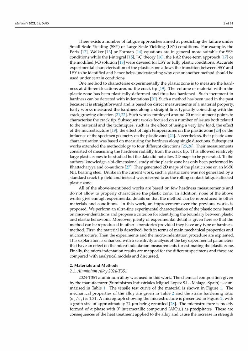
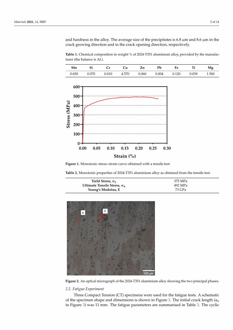
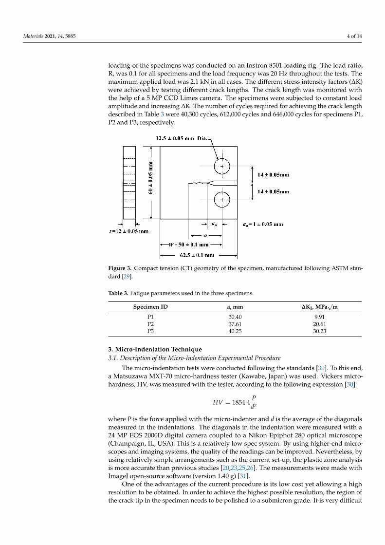
2024-T351 aluminium alloy was used in this work. The chemical composition givenby the manufacturer (Suministros Industriales Miguel Lopez S.L., Malaga, Spain) is sum-marised in Table 1. The tensile test curve of the material is shown in Figure 1. Themechanical properties of the alloy are given in Table 2 and the strain hardening ratio(σu/σy) is 1.31. A micrograph showing the microstructure is presented in Figure 2, witha grain size of approximately 74 µm being recorded [28]. The microstructure is mostlyformed of α phase with θ’ intermetallic compound (AlCu2) as precipitates. These areconsequences of the heat treatment applied to the alloy and cause the increase in strength

Materials 2021, 14, 5885 3 of 14

and hardness in the alloy. The average size of the precipitates is 6.8 µm and 8.6 µm in thecrack growing direction and in the crack opening direction, respectively.

Table 1. Chemical composition in weight % of 2024-T351 aluminium alloy, provided by the manufac-turer (the balance is Al.).

Mn Si Cr Cu Zn Pb Fe Ti Mg

0.650 0.070 0.010 4.570 0.060 0.004 0.120 0.039 1.500

Materials 2021, 11, x FOR PEER REVIEW 3 of 15

in the alloy. The average size of the precipitates is 6.8 μm and 8.6 μm in the crack growing

direction and in the crack opening direction, respectively.

Table 1. Chemical composition in weight % of 2024-T351 aluminium alloy, provided by the manu-

facturer (the balance is Al.).

Mn Si Cr Cu Zn Pb Fe Ti Mg

0.650 0.070 0.010 4.570 0.060 0.004 0.120 0.039 1.500

0.00 0.05 0.10 0.15 0.20 0.25 0.300

100

200

300

400

500

600

Strain (%)

Str

ess

(M

Pa

)

Figure 1. Monotonic stress–strain curve obtained with a tensile test.

Table 2. Monotonic properties of 2024-T351 aluminium alloy as obtained from the tensile test.

Yield Stress, σy 375 MPa

Ultimate Tensile Stress, σu 492 MPa

Young’s Modulus, E 73 GPa

Figure 2. An optical micrograph of the 2024-T351 aluminium alloy showing the two principal

phases.

2.2. Fatigue Experiment

Three Compact Tension (CT) specimens were used for the fatigue tests. A schematic

of the specimen shape and dimensions is shown in Figure 3. The initial crack length (an in

Figure 3) was 11 mm. The fatigue parameters are summarised in Table 3. The cyclic loading

Figure 1. Monotonic stress–strain curve obtained with a tensile test.

Table 2. Monotonic properties of 2024-T351 aluminium alloy as obtained from the tensile test.

Yield Stress, σy 375 MPaUltimate Tensile Stress, σu 492 MPa

Young’s Modulus, E 73 GPa

Materials 2021, 11, x FOR PEER REVIEW 3 of 15

in the alloy. The average size of the precipitates is 6.8 μm and 8.6 μm in the crack growing

direction and in the crack opening direction, respectively.

Table 1. Chemical composition in weight % of 2024-T351 aluminium alloy, provided by the manu-

facturer (the balance is Al.).

Mn Si Cr Cu Zn Pb Fe Ti Mg

0.650 0.070 0.010 4.570 0.060 0.004 0.120 0.039 1.500

0.00 0.05 0.10 0.15 0.20 0.25 0.300

100

200

300

400

500

600

Strain (%)

Str

ess

(M

Pa

)

Figure 1. Monotonic stress–strain curve obtained with a tensile test.

Table 2. Monotonic properties of 2024-T351 aluminium alloy as obtained from the tensile test.

Yield Stress, σy 375 MPa

Ultimate Tensile Stress, σu 492 MPa

Young’s Modulus, E 73 GPa

Figure 2. An optical micrograph of the 2024-T351 aluminium alloy showing the two principal

phases.

2.2. Fatigue Experiment

Three Compact Tension (CT) specimens were used for the fatigue tests. A schematic

of the specimen shape and dimensions is shown in Figure 3. The initial crack length (an in

Figure 3) was 11 mm. The fatigue parameters are summarised in Table 3. The cyclic loading

Figure 2. An optical micrograph of the 2024-T351 aluminium alloy showing the two principal phases.

2.2. Fatigue Experiment

Three Compact Tension (CT) specimens were used for the fatigue tests. A schematicof the specimen shape and dimensions is shown in Figure 3. The initial crack length (anin Figure 3) was 11 mm. The fatigue parameters are summarised in Table 3. The cyclic

Materials 2021, 14, 5885 4 of 14

loading of the specimens was conducted on an Instron 8501 loading rig. The load ratio,R, was 0.1 for all specimens and the load frequency was 20 Hz throughout the tests. Themaximum applied load was 2.1 kN in all cases. The different stress intensity factors (∆K)were achieved by testing different crack lengths. The crack length was monitored withthe help of a 5 MP CCD Limes camera. The specimens were subjected to constant loadamplitude and increasing ∆K. The number of cycles required for achieving the crack lengthdescribed in Table 3 were 40,300 cycles, 612,000 cycles and 646,000 cycles for specimens P1,P2 and P3, respectively.

Materials 2021, 11, x FOR PEER REVIEW 4 of 15

of the specimens was conducted on an Instron 8501 loading rig. The load ratio, R, was 0.1

for all specimens and the load frequency was 20 Hz throughout the tests. The maximum

applied load was 2.1 kN in all cases. The different stress intensity factors (ΔK) were

achieved by testing different crack lengths. The crack length was monitored with the help

of a 5MP CCD Limes camera. The specimens were subjected to constant load amplitude

and increasing ΔK. The number of cycles required for achieving the crack length described

in Table 3 were 40,300 cycles, 612,000 cycles and 646,000 cycles for specimens P1, P2 and

P3, respectively.

Figure 3. Compact tension (CT) geometry of the specimen, manufactured following ASTM standard

[29].

Table 3. Fatigue parameters used in the three specimens.

Specimen ID a, mm ΔKI, MPa√m

P1 30.40 9.91

P2 37.61 20.61

P3 40.25 30.23

3. Micro-indentation Technique

3.1. Description of the Micro-Indentation Experimental Procedure

The micro-indentation tests were conducted following the standards [30]. To this

end, a Matsuzawa MXT-70 micro-hardness tester (Kawabe, Japan) was used. Vickers mi-

cro-hardness, HV, was measured with the tester, according to the following expression

[30]:

𝐻𝑉 = 1854.4𝑃

𝑑2

where P is the force applied with the micro-indenter and d is the average of the diagonals

measured in the indentations. The diagonals in the indentation were measured with a

24MP EOS 2000D digital camera coupled to a Nikon Epiphot 280 optical microscope

(Champaign, Illinois, USA.) . This is a relatively low spec system. By using higher-end

microscopes and imaging systems, the quality of the readings can be improved. Never-

theless, by using relatively simple arrangements such as the current set-up, the plastic

zone analysis is more accurate than previous studies [20,23,25,26]. The measurements

were made with ImageJ open-source software (version 1.40g) [31].

One of the advantages of the current procedure is its low cost yet allowing a high

resolution to be obtained. In order to achieve the highest possible resolution, the region of

Figure 3. Compact tension (CT) geometry of the specimen, manufactured following ASTM stan-dard [29].

Table 3. Fatigue parameters used in the three specimens.

Specimen ID a, mm ∆KI, MPa√

m

P1 30.40 9.91P2 37.61 20.61P3 40.25 30.23

3. Micro-Indentation Technique3.1. Description of the Micro-Indentation Experimental Procedure

The micro-indentation tests were conducted following the standards [30]. To this end,a Matsuzawa MXT-70 micro-hardness tester (Kawabe, Japan) was used. Vickers micro-hardness, HV, was measured with the tester, according to the following expression [30]:

HV = 1854.4Pd2

where P is the force applied with the micro-indenter and d is the average of the diagonalsmeasured in the indentations. The diagonals in the indentation were measured with a24 MP EOS 2000D digital camera coupled to a Nikon Epiphot 280 optical microscope(Champaign, IL, USA). This is a relatively low spec system. By using higher-end micro-scopes and imaging systems, the quality of the readings can be improved. Nevertheless, byusing relatively simple arrangements such as the current set-up, the plastic zone analysisis more accurate than previous studies [20,23,25,26]. The measurements were made withImageJ open-source software (version 1.40 g) [31].

One of the advantages of the current procedure is its low cost yet allowing a highresolution to be obtained. In order to achieve the highest possible resolution, the region ofthe crack tip in the specimen needs to be polished to a submicron grade. It is very difficult

Materials 2021, 14, 5885 5 of 14

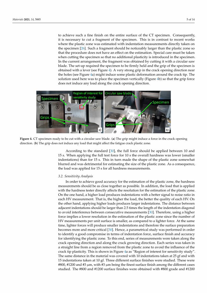
to achieve such a fine finish on the entire surface of the CT specimen. Consequently,it is necessary to cut a fragment of the specimen. This is in contrast to recent workswhere the plastic zone was estimated with indentation measurements directly taken onthe specimen [26]. Such a fragment should be noticeably larger than the plastic zone sothat the procedure does not have an effect on the estimation. Special care must be takenwhen cutting the specimen so that no additional plasticity is introduced in the specimen.In the current arrangement, the fragment was obtained by cutting it with a circular sawblade. The set-up required the specimen to be firmly held and the grip of the specimen isobtained with a lever (see Figure 4). A very strong grip in the crack opening direction nearthe holes (see Figure 4a) might induce some plastic deformation around the crack tip. Thesolution used here was to place the specimen vertically (Figure 4b) so that the grip forcedoes not induce any load along the crack opening direction.

Materials 2021, 11, x FOR PEER REVIEW 5 of 15

the crack tip in the specimen needs to be polished to a submicron grade. It is very difficult

to achieve such a fine finish on the entire surface of the CT specimen. Consequently, it is

necessary to cut a fragment of the specimen. This is in contrast to recent works where the

plastic zone was estimated with indentation measurements directly taken on the specimen

[26]. Such a fragment should be noticeably larger than the plastic zone so that the proce-

dure does not have an effect on the estimation. Special care must be taken when cutting

the specimen so that no additional plasticity is introduced in the specimen. In the current

arrangement, the fragment was obtained by cutting it with a circular saw blade. The set-

up required the specimen to be firmly held and the grip of the specimen is obtained with

a lever (see Figure 4). A very strong grip in the crack opening direction near the holes (see

Figure 4a) might induce some plastic deformation around the crack tip. The solution used

here was to place the specimen vertically (Figure 4b) so that the grip force does not induce

any load along the crack opening direction.

Figure 4. CT specimen ready to be cut with a circular saw blade. (a) The grip might induce a force

in the crack opening direction. (b) The grip does not induce any load that might affect the fatigue

crack plastic zone.

According to the standard [30], the full force should be applied between 10 and 15

seconds. When applying the full test force for 10 seconds the overall hardness was lower

(smaller indentations) than for 15 seconds. This in turn made the shape of the plastic zone

somewhat blurred and was detrimental for estimating the size of the plastic zone. As a

consequence, the load was applied for 15 seconds for all hardness measurements.

3.2. Sensitivity Analysis

In order to achieve good accuracy for the estimation of the plastic zone, the hardness

measurements should be as close together as possible. In addition, the load that is applied

with the hardness tester directly affects the resolution for the estimation of the plastic

zone. On the one hand, a higher load produces indentations with a better signal to noise

ratio in each HV measurement. That is, the higher the load, the better the quality of each

HV. On the other hand, applying higher loads produces larger indentations. The distance

between adjacent indentations should be larger than 2.5 times the length of the indenta-

tion diagonal to avoid interference between consecutive measurements [30]. Therefore,

using a higher force implies a lower resolution in the estimation of the plastic zone since

the number of HV measurements per unit surface is smaller, as compared to a lighter

force. At the same time, lighter forces will produce smaller indentations and therefore the

surface preparation becomes more and more critical [30]. Hence, a parametrical study was

performed in order to identify a good compromise in terms of indentation force, surface

finish and accuracy for identifying the plastic zone. To this end, series of measurements

were taken along the crack opening direction and along the crack growing direction. Each

series was taken in a straight line from a region removed from the plastic zone to avoid

the influence of the crack tip plasticity. This is shown in Figure 4a as “Region of interest

for sensitivity study”. The same distance in the material was covered with 10 indentations

taken at 25 gf and with 15 indentations taken at 10 gf. Three different surface finishes were

Figure 4. CT specimen ready to be cut with a circular saw blade. (a) The grip might induce a force in the crack openingdirection. (b) The grip does not induce any load that might affect the fatigue crack plastic zone.

According to the standard [30], the full force should be applied between 10 and15 s. When applying the full test force for 10 s the overall hardness was lower (smallerindentations) than for 15 s. This in turn made the shape of the plastic zone somewhatblurred and was detrimental for estimating the size of the plastic zone. As a consequence,the load was applied for 15 s for all hardness measurements.

3.2. Sensitivity Analysis

In order to achieve good accuracy for the estimation of the plastic zone, the hardnessmeasurements should be as close together as possible. In addition, the load that is appliedwith the hardness tester directly affects the resolution for the estimation of the plastic zone.On the one hand, a higher load produces indentations with a better signal to noise ratio ineach HV measurement. That is, the higher the load, the better the quality of each HV. Onthe other hand, applying higher loads produces larger indentations. The distance betweenadjacent indentations should be larger than 2.5 times the length of the indentation diagonalto avoid interference between consecutive measurements [30]. Therefore, using a higherforce implies a lower resolution in the estimation of the plastic zone since the number ofHV measurements per unit surface is smaller, as compared to a lighter force. At the sametime, lighter forces will produce smaller indentations and therefore the surface preparationbecomes more and more critical [30]. Hence, a parametrical study was performed in orderto identify a good compromise in terms of indentation force, surface finish and accuracyfor identifying the plastic zone. To this end, series of measurements were taken along thecrack opening direction and along the crack growing direction. Each series was taken ina straight line from a region removed from the plastic zone to avoid the influence of thecrack tip plasticity. This is shown in Figure 4a as “Region of interest for sensitivity study”.The same distance in the material was covered with 10 indentations taken at 25 gf and with15 indentations taken at 10 gf. Three different surface finishes were studied. These were#800, #1200 and #3 µm, with #3 µm being the finest surface finish among the different casesstudied. The #800 and #1200 surface finishes were obtained with #800 grade and #1200

Materials 2021, 14, 5885 6 of 14

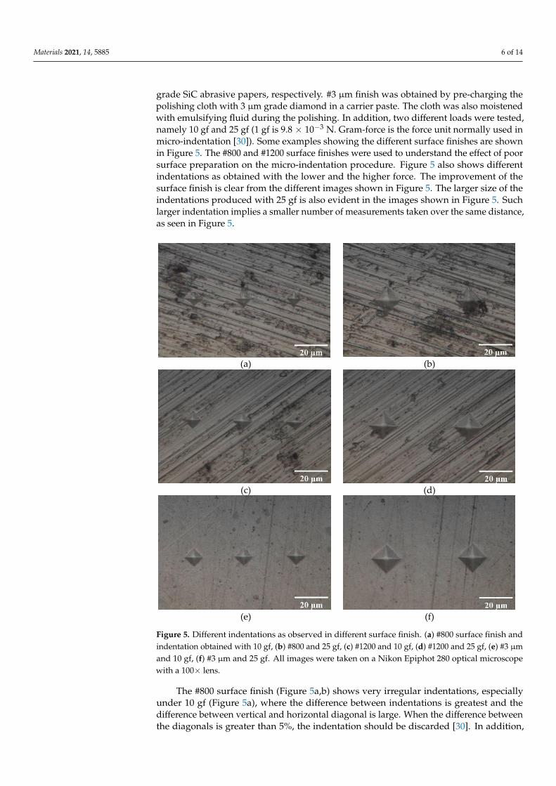
grade SiC abrasive papers, respectively. #3 µm finish was obtained by pre-charging thepolishing cloth with 3 µm grade diamond in a carrier paste. The cloth was also moistenedwith emulsifying fluid during the polishing. In addition, two different loads were tested,namely 10 gf and 25 gf (1 gf is 9.8 × 10−3 N. Gram-force is the force unit normally used inmicro-indentation [30]). Some examples showing the different surface finishes are shownin Figure 5. The #800 and #1200 surface finishes were used to understand the effect of poorsurface preparation on the micro-indentation procedure. Figure 5 also shows differentindentations as obtained with the lower and the higher force. The improvement of thesurface finish is clear from the different images shown in Figure 5. The larger size of theindentations produced with 25 gf is also evident in the images shown in Figure 5. Suchlarger indentation implies a smaller number of measurements taken over the same distance,as seen in Figure 5.

Materials 2021, 11, x FOR PEER REVIEW 6 of 15

studied. These were #800, #1200 and #3 μm, with #3 μm being the finest surface finish

among the different cases studied. The #800 and #1200 surface finishes were obtained with

#800 grade and #1200 grade SiC abrasive papers, respectively. #3 μm finish was obtained

by pre-charging the polishing cloth with 3 μm grade diamond in a carrier paste. The cloth

was also moistened with emulsifying fluid during the polishing. In addition, two different

loads were tested, namely 10 gf and 25 gf (1 gf is 9.8×10−3 N. Gram-force is the force unit

normally used in micro-indentation [30]). Some examples showing the different surface

finishes are shown in Figure 5. The #800 and #1200 surface finishes were used to under-

stand the effect of poor surface preparation on the micro-indentation procedure. Figure 5

also shows different indentations as obtained with the lower and the higher force. The

improvement of the surface finish is clear from the different images shown in Figure 5.

The larger size of the indentations produced with 25 gf is also evident in the images shown

in Figure 5. Such larger indentation implies a smaller number of measurements taken over

the same distance, as seen in Figure 5.

(a) (b)

(c) (d)

(e) (f)

Figure 5. Different indentations as observed in different surface finish. (a) #800 surface finish and

indentation obtained with 10 gf, (b) #800 and 25 gf, (c) #1200 and 10 gf, (d) #1200 and 25 gf, (e) #3

μm and 10 gf, (f) #3 μm and 25 gf. All images were taken on a Nikon Epiphot 280 optical microscope

with a 100X lens.

The #800 surface finish (Figure 5a,b) shows very irregular indentations, especially

under 10 gf (Figure 5a), where the difference between indentations is greatest and the

Figure 5. Different indentations as observed in different surface finish. (a) #800 surface finish andindentation obtained with 10 gf, (b) #800 and 25 gf, (c) #1200 and 10 gf, (d) #1200 and 25 gf, (e) #3 µmand 10 gf, (f) #3 µm and 25 gf. All images were taken on a Nikon Epiphot 280 optical microscopewith a 100× lens.

The #800 surface finish (Figure 5a,b) shows very irregular indentations, especiallyunder 10 gf (Figure 5a), where the difference between indentations is greatest and thedifference between vertical and horizontal diagonal is large. When the difference betweenthe diagonals is greater than 5%, the indentation should be discarded [30]. In addition,

Materials 2021, 14, 5885 7 of 14

the poor surface finish creates dark regions that make it difficult to measure the diagonalsand, therefore, decreases the quality of the hardness measurements. In some cases, thesedark regions obscure the indentation to the point that the measurement of the diagonalis not possible. Comparison between images taken at 10 gf (Figure 5a,c,e) and imagestaken at 25 gf (Figure 5b,d,f) clearly shows more deformed indentations with decreasingload. Moving from #800 to #1200 clearly improves the quality of the indentations, eventhough they are still quite irregular, particularly under 10 gf (Figure 5c). The distortion ofthe indentations is clearly reduced by polishing to the next grade (#3 µm), as observed inFigure 5e,f. Moreover, the polishing direction is drastically reduced by using 3 µm gradediamond in a carrier paste (see Figure 5e,f). The finest polish (Figure 5e,f) produces themost regular indentations and the most uniform background, free of features, thus makingit easier to measure the indentations diagonals.

The reproducibility of the measurements is studied by plotting the mean and the stan-dard deviation for the different experimental conditions. The results of the measurementsalong the crack growing direction and along the crack opening direction in a region awayfrom the crack tip are shown in Figures 6 and 7, respectively.

Materials 2021, 11, x FOR PEER REVIEW 7 of 15

difference between vertical and horizontal diagonal is large. When the difference between

the diagonals is greater than 5%, the indentation should be discarded [30]. In addition, the

poor surface finish creates dark regions that make it difficult to measure the diagonals

and, therefore, decreases the quality of the hardness measurements. In some cases, these

dark regions obscure the indentation to the point that the measurement of the diagonal is

not possible. Comparison between images taken at 10 gf (Figure 5a,c,e) and images taken

at 25 gf (Figure 5b,d,f) clearly shows more deformed indentations with decreasing load.

Moving from #800 to #1200 clearly improves the quality of the indentations, even though

they are still quite irregular, particularly under 10 gf (Figure 5c). The distortion of the

indentations is clearly reduced by polishing to the next grade (#3 μm), as observed in Fig-

ures 5.e and 5.f. Moreover, the polishing direction is drastically reduced by using 3 μm

grade diamond in a carrier paste (see Figures 5e,f). The finest polish (Figure 5e,f) produces

the most regular indentations and the most uniform background, free of features, thus

making it easier to measure the indentations diagonals.

The reproducibility of the measurements is studied by plotting the mean and the

standard deviation for the different experimental conditions. The results of the measure-

ments along the crack growing direction and along the crack opening direction in a region

away from the crack tip are shown in Figures 6 and 7, respectively.

#800

#120

0

#3m

140

150

160

170

180

190

200

210

A

HV

#800

#1200

#3m

#800

#120

0

#3m

140

150

160

170

180

190

200

210

BH

V

#800

#1200

#3m

Figure 6. Mean hardness measurements obtained with Vickers micro-hardness testing along the

crack growing direction for different surface finish and (A) 25 gf and (B) 10 gf. The standard devia-

tion is shown as error bars.

#800

#120

0

#3m

140

150

160

170

180

190

200

210

A

HV

#800

#1200

#3m

#800

#120

0

#3m

130

140

150

160

170

180

190

200

210

B

HV

#800

#1200

#3m

Figure 7. Mean hardness measurements obtained with Vickers micro-hardness testing along the

crack opening direction for different surface finish and (A) 25 gf and (B) 10 gf. The standard devia-

tion is shown as error bars.

Figure 6. Mean hardness measurements obtained with Vickers micro-hardness testing along the crackgrowing direction for different surface finish and (A) 25 gf and (B) 10 gf. The standard deviation isshown as error bars.

Materials 2021, 11, x FOR PEER REVIEW 7 of 15

difference between vertical and horizontal diagonal is large. When the difference between

the diagonals is greater than 5%, the indentation should be discarded [30]. In addition, the

poor surface finish creates dark regions that make it difficult to measure the diagonals

and, therefore, decreases the quality of the hardness measurements. In some cases, these

dark regions obscure the indentation to the point that the measurement of the diagonal is

not possible. Comparison between images taken at 10 gf (Figure 5a,c,e) and images taken

at 25 gf (Figure 5b,d,f) clearly shows more deformed indentations with decreasing load.

Moving from #800 to #1200 clearly improves the quality of the indentations, even though

they are still quite irregular, particularly under 10 gf (Figure 5c). The distortion of the

indentations is clearly reduced by polishing to the next grade (#3 μm), as observed in Fig-

ures 5.e and 5.f. Moreover, the polishing direction is drastically reduced by using 3 μm

grade diamond in a carrier paste (see Figures 5e,f). The finest polish (Figure 5e,f) produces

the most regular indentations and the most uniform background, free of features, thus

making it easier to measure the indentations diagonals.

The reproducibility of the measurements is studied by plotting the mean and the

standard deviation for the different experimental conditions. The results of the measure-

ments along the crack growing direction and along the crack opening direction in a region

away from the crack tip are shown in Figures 6 and 7, respectively.

#800

#120

0

#3m

140

150

160

170

180

190

200

210

A

HV

#800

#1200

#3m

#800

#120

0

#3m

140

150

160

170

180

190

200

210

B

HV

#800

#1200

#3m

Figure 6. Mean hardness measurements obtained with Vickers micro-hardness testing along the

crack growing direction for different surface finish and (A) 25 gf and (B) 10 gf. The standard devia-

tion is shown as error bars.

#800

#120

0

#3m

140

150

160

170

180

190

200

210

A

HV

#800

#1200

#3m

#800

#120

0

#3m

130

140

150

160

170

180

190

200

210

B

HV

#800

#1200

#3m

Figure 7. Mean hardness measurements obtained with Vickers micro-hardness testing along the

crack opening direction for different surface finish and (A) 25 gf and (B) 10 gf. The standard devia-

tion is shown as error bars.

Figure 7. Mean hardness measurements obtained with Vickers micro-hardness testing along thecrack opening direction for different surface finish and (A) 25 gf and (B) 10 gf. The standard deviationis shown as error bars.

Figures 6 and 7 show that both the mean values as well as the scattering (measured asstandard deviation) in the measurements decrease as the surface finish is improved. Thisis due to the easier surface penetration of the indenter due to less surface irregularitiesexisting in the surface. Such behaviour is in agreement with previous works where higherscattering was recorded for smaller loads of the indenter [19]. The fact that larger indenterloads produce overall lower HV values has also been observed in previous repeatability

Materials 2021, 14, 5885 8 of 14

studies [30]. Such effect is observed here in the different surface finishes under study.Accordingly, the best results both in the crack growing direction (Figure 6) and in the crackopening direction (Figure 7) are obtained with 25 gf load and #3 µm surface finish.

4. Results and Discussion4.1. Plastic Zone Estimation

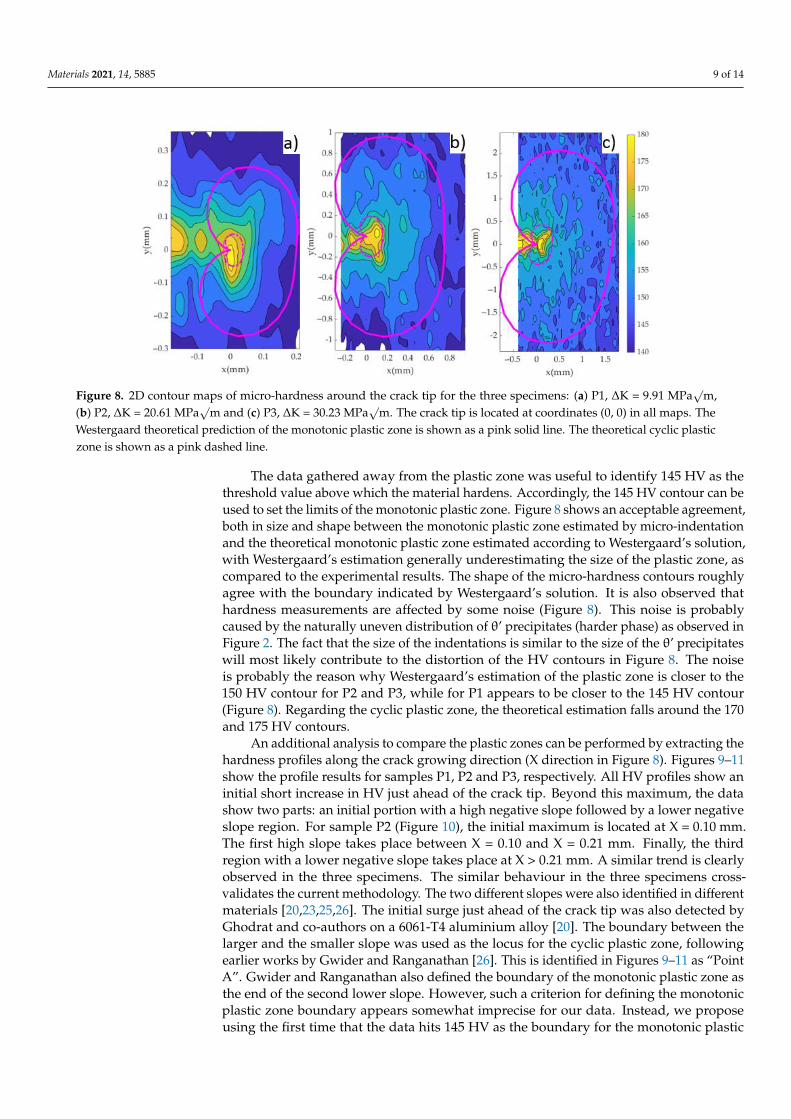
Figure 8 shows the 2D contour maps of micro-hardness measurements taken aroundthe crack tip for the three specimens. Following the results of the previous section, allindentations were performed with 25 gf load and #3 µm surface finish. The number of datapoints collected was 322, 1075 and 4365 for samples P1, P2 and P3, respectively. Such anamount of data points appears to be sufficient to properly characterise the Vickers hardnessevolution around the crack tip. Hence, the resolution achieved is up to 57 times higher thanin previous works [20,23,25,26]. The data were linearly interpolated to generate the contourplots. In addition, the data were smoothed with a Gaussian filter operator. This is a 2Dconvolution operator that provides gentler smoothing than other operators and preservesfeatures better than other operators [32]. Figure 8a–c show the results for samples P1, P2and P3, respectively. For validation purposes, the theoretical monotonic plastic zone wasalso computed in a similar fashion to previous works [33]. This theoretical estimation wasbased on the Westergaard stress field around the crack tip (Equations (1)–(4)) [34] combinedwith the Von Mises criterion [35]. Such a solution is well established to understand theshape and size of the plastic zone [33,35,36]. Plane stress conditions were assumed sincethe analysis is performed at the surface.

σxx = A0·r−12 · cos

(θ

2

)·(

1− sin(

θ

2

)· sin

(3θ

2

))(1)

σyy = A0·r−12 · cos

(θ

2

)·(

1 + sin(

θ

2

)· sin

(3θ

2

))(2)

τxy = A0·r−12 · cos

(θ

2

)· sin

(θ

2

)· cos

(3θ

2

)(3)

A0 =KI√2·π

(4)

where r and θ are the polar coordinates with respect to the crack tip and KI is the appliedstress intensity factor.

The cyclic plastic zone was also computed analytically and used as a reference forcomparison. The theoretical cyclic plastic zone was also calculated, according to [37]:

rc(θ) =1

4π

(∆KI

2σy

)2[1 + cos θ +

32

sin2 θ

](5)

where rc and θ are the polar coordinates values of the cyclic plastic zone boundary, ∆KI isthe stress intensity factor range in mode I and σy is the yield stress.

These theoretical plastic zones are also plotted in Figure 8 as a pink solid line (mono-tonic) and pink dashed line (cyclic). The crack tip is located at the origin of coordinates(coordinates (0, 0) in Figure 8). The plastic zones were tilted slightly in Figure 8a,c tocompensate for the crack angle observed experimentally in samples P1 and P3. For sampleP2 the crack appeared perfectly horizontal at the time of analysis, so no angle correctionwas required in this case. As observed in Figure 8, the HV scale starts at 140 HV andends at 180 HV, with 5 HV steps. Based on the sensitivity analysis (Figures 6 and 7),hardness values at 145 HV or below could be considered as non-affected by the crack tiphardening [38].

Materials 2021, 14, 5885 9 of 14Materials 2021, 11, x FOR PEER REVIEW 9 of 15

Figure 8. 2D contour maps of micro-hardness around the crack tip for the three specimens: (a) P1,

ΔK = 9.91 MPa√m, (b) P2, ΔK = 20.61 MPa√m and (c) P3, ΔK = 30.23 MPa√m. The crack tip is lo-

cated at coordinates (0, 0) in all maps. The Westergaard theoretical prediction of the monotonic

plastic zone is shown as a pink solid line. The theoretical cyclic plastic zone is shown as a pink

dashed line.

These theoretical plastic zones are also plotted in Figure 8 as a pink solid line (mon-

otonic) and pink dashed line (cyclic). The crack tip is located at the origin of coordinates

(coordinates (0, 0) in Figure 8). The plastic zones were tilted slightly in Figure 8a,c to com-

pensate for the crack angle observed experimentally in samples P1 and P3. For sample P2

the crack appeared perfectly horizontal at the time of analysis, so no angle correction was

required in this case. As observed in Figure 8, the HV scale starts at 140HV and ends at

180HV, with 5HV steps. Based on the sensitivity analysis (Figures 6 and 7), hardness values

at 145HV or below could be considered as non-affected by the crack tip hardening [38].

The data gathered away from the plastic zone was useful to identify 145HV as the

threshold value above which the material hardens. Accordingly, the 145HV contour can

be used to set the limits of the monotonic plastic zone. Figure 8 shows an acceptable agree-

ment, both in size and shape between the monotonic plastic zone estimated by micro-

indentation and the theoretical monotonic plastic zone estimated according to

Westergaard’s solution, with Westergaard’s estimation generally underestimating the

size of the plastic zone, as compared to the experimental results. The shape of the micro-

hardness contours roughly agree with the boundary indicated by Westergaard’s solution.

It is also observed that hardness measurements are affected by some noise (Figure 8). This

noise is probably caused by the naturally uneven distribution of θ’ precipitates (harder

phase) as observed in Figure 2. The fact that the size of the indentations is similar to the

size of the θ’ precipitates will most likely contribute to the distortion of the HV contours

in Figure 8. The noise is probably the reason why Westergaard’s estimation of the plastic

zone is closer to the 150 HV contour for P2 and P3, while for P1 appears to be closer to the

145 HV contour (Figure 8). Regarding the cyclic plastic zone, the theoretical estimation

falls around the 170 and 175 HV contours.

An additional analysis to compare the plastic zones can be performed by extracting

the hardness profiles along the crack growing direction (X direction in Figure 8). Figures

9, 10 and 11 show the profile results for samples P1, P2 and P3, respectively. All HV pro-

files show an initial short increase in HV just ahead of the crack tip. Beyond this maxi-

mum, the data show two parts: an initial portion with a high negative slope followed by

a lower negative slope region. For sample P2 (Figure 10), the initial maximum is located

at X = 0.10 mm. The first high slope takes place between X = 0.10 and X = 0.21 mm. Finally,

the third region with a lower negative slope takes place at X > 0.21 mm. A similar trend is

Figure 8. 2D contour maps of micro-hardness around the crack tip for the three specimens: (a) P1, ∆K = 9.91 MPa√

m,(b) P2, ∆K = 20.61 MPa

√m and (c) P3, ∆K = 30.23 MPa

√m. The crack tip is located at coordinates (0, 0) in all maps. The

Westergaard theoretical prediction of the monotonic plastic zone is shown as a pink solid line. The theoretical cyclic plasticzone is shown as a pink dashed line.

The data gathered away from the plastic zone was useful to identify 145 HV as thethreshold value above which the material hardens. Accordingly, the 145 HV contour can beused to set the limits of the monotonic plastic zone. Figure 8 shows an acceptable agreement,both in size and shape between the monotonic plastic zone estimated by micro-indentationand the theoretical monotonic plastic zone estimated according to Westergaard’s solution,with Westergaard’s estimation generally underestimating the size of the plastic zone, ascompared to the experimental results. The shape of the micro-hardness contours roughlyagree with the boundary indicated by Westergaard’s solution. It is also observed thathardness measurements are affected by some noise (Figure 8). This noise is probablycaused by the naturally uneven distribution of θ’ precipitates (harder phase) as observed inFigure 2. The fact that the size of the indentations is similar to the size of the θ’ precipitateswill most likely contribute to the distortion of the HV contours in Figure 8. The noiseis probably the reason why Westergaard’s estimation of the plastic zone is closer to the150 HV contour for P2 and P3, while for P1 appears to be closer to the 145 HV contour(Figure 8). Regarding the cyclic plastic zone, the theoretical estimation falls around the 170and 175 HV contours.

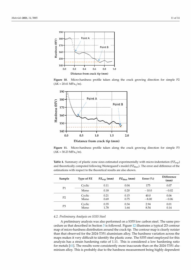
An additional analysis to compare the plastic zones can be performed by extracting thehardness profiles along the crack growing direction (X direction in Figure 8). Figures 9–11show the profile results for samples P1, P2 and P3, respectively. All HV profiles show aninitial short increase in HV just ahead of the crack tip. Beyond this maximum, the datashow two parts: an initial portion with a high negative slope followed by a lower negativeslope region. For sample P2 (Figure 10), the initial maximum is located at X = 0.10 mm.The first high slope takes place between X = 0.10 and X = 0.21 mm. Finally, the thirdregion with a lower negative slope takes place at X > 0.21 mm. A similar trend is clearlyobserved in the three specimens. The similar behaviour in the three specimens cross-validates the current methodology. The two different slopes were also identified in differentmaterials [20,23,25,26]. The initial surge just ahead of the crack tip was also detected byGhodrat and co-authors on a 6061-T4 aluminium alloy [20]. The boundary between thelarger and the smaller slope was used as the locus for the cyclic plastic zone, followingearlier works by Gwider and Ranganathan [26]. This is identified in Figures 9–11 as “PointA”. Gwider and Ranganathan also defined the boundary of the monotonic plastic zone asthe end of the second lower slope. However, such a criterion for defining the monotonicplastic zone boundary appears somewhat imprecise for our data. Instead, we proposeusing the first time that the data hits 145 HV as the boundary for the monotonic plastic

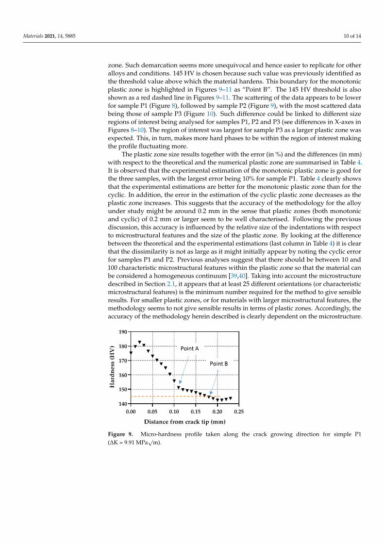
Materials 2021, 14, 5885 10 of 14

zone. Such demarcation seems more unequivocal and hence easier to replicate for otheralloys and conditions. 145 HV is chosen because such value was previously identified asthe threshold value above which the material hardens. This boundary for the monotonicplastic zone is highlighted in Figures 9–11 as “Point B”. The 145 HV threshold is alsoshown as a red dashed line in Figures 9–11. The scattering of the data appears to be lowerfor sample P1 (Figure 8), followed by sample P2 (Figure 9), with the most scattered databeing those of sample P3 (Figure 10). Such difference could be linked to different sizeregions of interest being analysed for samples P1, P2 and P3 (see differences in X-axes inFigures 8–10). The region of interest was largest for sample P3 as a larger plastic zone wasexpected. This, in turn, makes more hard phases to be within the region of interest makingthe profile fluctuating more.

The plastic zone size results together with the error (in %) and the differences (in mm)with respect to the theoretical and the numerical plastic zone are summarised in Table 4.It is observed that the experimental estimation of the monotonic plastic zone is good forthe three samples, with the largest error being 10% for sample P1. Table 4 clearly showsthat the experimental estimations are better for the monotonic plastic zone than for thecyclic. In addition, the error in the estimation of the cyclic plastic zone decreases as theplastic zone increases. This suggests that the accuracy of the methodology for the alloyunder study might be around 0.2 mm in the sense that plastic zones (both monotonicand cyclic) of 0.2 mm or larger seem to be well characterised. Following the previousdiscussion, this accuracy is influenced by the relative size of the indentations with respectto microstructural features and the size of the plastic zone. By looking at the differencebetween the theoretical and the experimental estimations (last column in Table 4) it is clearthat the dissimilarity is not as large as it might initially appear by noting the cyclic errorfor samples P1 and P2. Previous analyses suggest that there should be between 10 and100 characteristic microstructural features within the plastic zone so that the material canbe considered a homogeneous continuum [39,40]. Taking into account the microstructuredescribed in Section 2.1, it appears that at least 25 different orientations (or characteristicmicrostructural features) is the minimum number required for the method to give sensibleresults. For smaller plastic zones, or for materials with larger microstructural features, themethodology seems to not give sensible results in terms of plastic zones. Accordingly, theaccuracy of the methodology herein described is clearly dependent on the microstructure.

Materials 2021, 11, x FOR PEER REVIEW 10 of 15

clearly observed in the three specimens. The similar behaviour in the three specimens

cross-validates the current methodology. The two different slopes were also identified in

different materials [20,23,25,26]. The initial surge just ahead of the crack tip was also de-

tected by Ghodrat and co-authors on a 6061-T4 aluminium alloy [20]. The boundary be-

tween the larger and the smaller slope was used as the locus for the cyclic plastic zone,

following earlier works by Gwider and Ranganathan [26]. This is identified in Figures 9–

11 as “Point A”. Gwider and Ranganathan also defined the boundary of the monotonic

plastic zone as the end of the second lower slope. However, such a criterion for defining

the monotonic plastic zone boundary appears somewhat imprecise for our data. Instead,

we propose using the first time that the data hits 145 HV as the boundary for the mono-

tonic plastic zone. Such demarcation seems more unequivocal and hence easier to repli-

cate for other alloys and conditions. 145 HV is chosen because such value was previously

identified as the threshold value above which the material hardens. This boundary for the

monotonic plastic zone is highlighted in Figures 9–11 as “Point B”. The 145 HV threshold

is also shown as a red dashed line in Figures 9–11. The scattering of the data appears to be

lower for sample P1 (Figure 8), followed by sample P2 (Figure 9), with the most scattered

data being those of sample P3 (Figure 10). Such difference could be linked to different size

regions of interest being analysed for samples P1, P2 and P3 (see differences in X-axes in

Figures 8–10). The region of interest was largest for sample P3 as a larger plastic zone was

expected. This, in turn, makes more hard phases to be within the region of interest making

the profile fluctuating more.

Figure 9. Micro-hardness profile taken along the crack growing direction for simple P1 (ΔK = 9.91

MPa√m).

Figure 10. Micro-hardness profile taken along the crack growing direction for simple P2 (ΔK = 20.61

MPa√m).

Figure 9. Micro-hardness profile taken along the crack growing direction for simple P1(∆K = 9.91 MPa

√m).

Materials 2021, 14, 5885 11 of 14

Materials 2021, 11, x FOR PEER REVIEW 10 of 15

clearly observed in the three specimens. The similar behaviour in the three specimens

cross-validates the current methodology. The two different slopes were also identified in

different materials [20,23,25,26]. The initial surge just ahead of the crack tip was also de-

tected by Ghodrat and co-authors on a 6061-T4 aluminium alloy [20]. The boundary be-

tween the larger and the smaller slope was used as the locus for the cyclic plastic zone,

following earlier works by Gwider and Ranganathan [26]. This is identified in Figures 9–

11 as “Point A”. Gwider and Ranganathan also defined the boundary of the monotonic

plastic zone as the end of the second lower slope. However, such a criterion for defining

the monotonic plastic zone boundary appears somewhat imprecise for our data. Instead,

we propose using the first time that the data hits 145 HV as the boundary for the mono-

tonic plastic zone. Such demarcation seems more unequivocal and hence easier to repli-

cate for other alloys and conditions. 145 HV is chosen because such value was previously

identified as the threshold value above which the material hardens. This boundary for the

monotonic plastic zone is highlighted in Figures 9–11 as “Point B”. The 145 HV threshold

is also shown as a red dashed line in Figures 9–11. The scattering of the data appears to be

lower for sample P1 (Figure 8), followed by sample P2 (Figure 9), with the most scattered

data being those of sample P3 (Figure 10). Such difference could be linked to different size

regions of interest being analysed for samples P1, P2 and P3 (see differences in X-axes in

Figures 8–10). The region of interest was largest for sample P3 as a larger plastic zone was

expected. This, in turn, makes more hard phases to be within the region of interest making

the profile fluctuating more.

Figure 9. Micro-hardness profile taken along the crack growing direction for simple P1 (ΔK = 9.91

MPa√m).

Figure 10. Micro-hardness profile taken along the crack growing direction for simple P2 (ΔK = 20.61

MPa√m).

Figure 10. Micro-hardness profile taken along the crack growing direction for simple P2(∆K = 20.61 MPa

√m).

Materials 2021, 11, x FOR PEER REVIEW 11 of 15

Figure 11. Micro-hardness profile taken along the crack growing direction for simple P3 (ΔK = 30.23

MPa√m).

The plastic zone size results together with the error (in %) and the differences (in mm)

with respect to the theoretical and the numerical plastic zone are summarised in Table 4.

It is observed that the experimental estimation of the monotonic plastic zone is good for

the three samples, with the largest error being 10% for sample P1. Table 4 clearly shows

that the experimental estimations are better for the monotonic plastic zone than for the

cyclic. In addition, the error in the estimation of the cyclic plastic zone decreases as the

plastic zone increases. This suggests that the accuracy of the methodology for the alloy

under study might be around 0.2 mm in the sense that plastic zones (both monotonic and

cyclic) of 0.2 mm or larger seem to be well characterised. Following the previous discus-

sion, this accuracy is influenced by the relative size of the indentations with respect to

microstructural features and the size of the plastic zone. By looking at the difference be-

tween the theoretical and the experimental estimations (last column in Table 4) it is clear

that the dissimilarity is not as large as it might initially appear by noting the cyclic error

for samples P1 and P2. Previous analyses suggest that there should be between 10 and 100

characteristic microstructural features within the plastic zone so that the material can be

considered a homogeneous continuum [39,40]. Taking into account the microstructure de-

scribed in Section 2.1, it appears that at least 25 different orientations (or characteristic

microstructural features) is the minimum number required for the method to give sensible

results. For smaller plastic zones, or for materials with larger microstructural features, the

methodology seems to not give sensible results in terms of plastic zones. Accordingly, the

accuracy of the methodology herein described is clearly dependent on the microstructure.

Table 4. Summary of plastic zone sizes estimated experimentally with micro-indentation (PZexp) and

theoretically computed following Westergaard’s model (PZtheo). The error and difference of the es-

timations with respect to the theoretical results are also shown.

Sample Type of PZ PZexp (mm) PZtheo (mm) Error (%) Difference (mm)

P1 Cyclic 0.11 0.04 175 0.07

Mono 0.18 0.20 −10.0 −0.02

P2 Cyclic 0.21 0.15 40.0 0.06

Mono 0.69 0.75 −8.00 −0.06

P3 Cyclic 0.35 0.34 2.94 0.01

Mono 1.78 1.64 8.54 0.14

4.2. Preliminary Analysis on S355 Steel

A preliminary analysis was also performed on a S355 low carbon steel. The same

procedure as that described in Section 3 is followed. Figure 12 illustrates a typical 2D con-

tour map of micro-hardness distribution around the crack tip. The contour map is clearly

Figure 11. Micro-hardness profile taken along the crack growing direction for simple P3(∆K = 30.23 MPa

√m).

Table 4. Summary of plastic zone sizes estimated experimentally with micro-indentation (PZexp)and theoretically computed following Westergaard’s model (PZtheo). The error and difference of theestimations with respect to the theoretical results are also shown.

Sample Type of PZ PZexp (mm) PZtheo (mm) Error (%) Difference(mm)

P1Cyclic 0.11 0.04 175 0.07

Mono 0.18 0.20 −10.0 −0.02

P2Cyclic 0.21 0.15 40.0 0.06Mono 0.69 0.75 −8.00 −0.06

P3Cyclic 0.35 0.34 2.94 0.01Mono 1.78 1.64 8.54 0.14

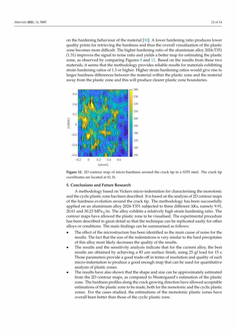
4.2. Preliminary Analysis on S355 Steel

A preliminary analysis was also performed on a S355 low carbon steel. The same pro-cedure as that described in Section 3 is followed. Figure 12 illustrates a typical 2D contourmap of micro-hardness distribution around the crack tip. The contour map is clearly noisierthan that observed for the 2024-T351 aluminium alloy. The hardness variation across themaps makes it very difficult to identify the plastic zone. The S355 steel employed for thisanalysis has a strain hardening ratio of 1.11. This is considered a low hardening ratiofor metals [41]. The results were consistently more inaccurate than on the 2024-T351 alu-minium alloy. This is probably due to the hardness measurement being highly dependent

Materials 2021, 14, 5885 12 of 14

on the hardening behaviour of the material [30]. A lower hardening ratio produces lowerquality prints for retrieving the hardness and thus the overall visualisation of the plasticzone becomes more difficult. The higher hardening ratio of the aluminium alloy 2024-T351(1.31) improves the signal to noise ratio and yields a better map for estimating the plasticzone, as observed by comparing Figures 8 and 12. Based on the results from these twomaterials, it seems that the methodology provides reliable results for materials exhibitingstrain hardening ratios of 1.3 or higher. Higher strain hardening ratios would give rise tolarger hardness differences between the material within the plastic zone and the materialaway from the plastic zone and this will produce clearer plastic zone boundaries.

Materials 2021, 11, x FOR PEER REVIEW 12 of 15

noisier than that observed for the 2024-T351 aluminium alloy. The hardness variation

across the maps makes it very difficult to identify the plastic zone. The S355 steel em-

ployed for this analysis has a strain hardening ratio of 1.11. This is considered a low hard-

ening ratio for metals [41]. The results were consistently more inaccurate than on the 2024-

T351 aluminium alloy. This is probably due to the hardness measurement being highly

dependent on the hardening behaviour of the material [30]. A lower hardening ratio pro-

duces lower quality prints for retrieving the hardness and thus the overall visualisation

of the plastic zone becomes more difficult. The higher hardening ratio of the aluminium

alloy 2024-T351 (1.31) improves the signal to noise ratio and yields a better map for esti-

mating the plastic zone, as observed by comparing Figure 8 and Figure 12. Based on the

results from these two materials, it seems that the methodology provides reliable results

for materials exhibiting strain hardening ratios of 1.3 or higher. Higher strain hardening

ratios would give rise to larger hardness differences between the material within the plas-

tic zone and the material away from the plastic zone and this will produce clearer plastic

zone boundaries.

Figure 12. 2D contour map of micro-hardness around the crack tip in a S355 steel. The crack tip

coordinates are located at (0, 0).

5. Conclusions and Future Research

A methodology based on Vickers micro-indentation for characterising the monotonic

and the cyclic plastic zone has been described. It is based on the analysis of 2D contour

maps of the hardness evolution around the crack tip. The methodology has been success-

fully applied on an aluminium alloy 2024-T351 subjected to three different ΔKs, namely

9.91, 20.61 and 30.23 MPa√m. The alloy exhibits a relatively high strain hardening ratio.

The contour maps have allowed the plastic zone to be visualised. The experimental pro-

cedure has been described in great detail so that the technique can be replicated easily for

other alloys or conditions. The main findings can be summarised as follows:

• The effect of the microstructure has been identified as the main cause of noise for the

results. The fact that the size of the indentations is very similar to the hard precipi-

tates of this alloy most likely decreases the quality of the results.

• The results and the sensitivity analysis indicate that for the current alloy, the best

results are obtained by achieving a #3 μm surface finish, using 25 gf load for 15 sec-

onds. Those parameters provide a good trade-off in terms of resolution and quality

of each micro-indentation to produce a good enough map that can be used for quan-

titative analysis of plastic zones.

Figure 12. 2D contour map of micro-hardness around the crack tip in a S355 steel. The crack tipcoordinates are located at (0, 0).

5. Conclusions and Future Research

A methodology based on Vickers micro-indentation for characterising the monotonicand the cyclic plastic zone has been described. It is based on the analysis of 2D contour mapsof the hardness evolution around the crack tip. The methodology has been successfullyapplied on an aluminium alloy 2024-T351 subjected to three different ∆Ks, namely 9.91,20.61 and 30.23 MPa

√m. The alloy exhibits a relatively high strain hardening ratio. The

contour maps have allowed the plastic zone to be visualised. The experimental procedurehas been described in great detail so that the technique can be replicated easily for otheralloys or conditions. The main findings can be summarised as follows:

• The effect of the microstructure has been identified as the main cause of noise for theresults. The fact that the size of the indentations is very similar to the hard precipitatesof this alloy most likely decreases the quality of the results.

• The results and the sensitivity analysis indicate that for the current alloy, the bestresults are obtained by achieving a #3 µm surface finish, using 25 gf load for 15 s.Those parameters provide a good trade-off in terms of resolution and quality of eachmicro-indentation to produce a good enough map that can be used for quantitativeanalysis of plastic zones.

• The results have also shown that the shape and size can be approximately estimatedfrom the 2D contour maps, as compared to Westergaard’s estimation of the plasticzone. The hardness profiles along the crack growing direction have allowed acceptableestimations of the plastic zone to be made, both for the monotonic and the cyclic plasticzones. For the cases studied, the estimations of the monotonic plastic zones haveoverall been better than those of the cyclic plastic zone.

Materials 2021, 14, 5885 13 of 14

• The results indicate that 0.2 mm appears to be the approximate size of the plastic zonethat this methodology captures reliably. Plastic zones well below this figure can bespotted but visualisation of size and shape can be difficult.

• Based on previous works, a new criterion is proposed to separate the elastic fromthe plastic contribution from the micro-hardness measurements which enables us toretrieve the monotonic and the cyclic plastic zone. The current procedure for inferringthe plastic zone around a fatigue crack tip is based on the hardening of the materialbeing tested. Accordingly, applying this procedure to materials experiencing lowstrain hardening will yield less accurate results.

Part of the novelty of the current methodology lies in the combination of experimentaldata taken at the micro-scale for generating global parameters (plastic zone size). Webelieve this work contributes to bridging the gap between microstructural and continuummechanics approaches for design against fatigue.

The results described in this work can be used to incorporate microstructural featuresinto numerical simulations via micromechanical modelling [10,11,42]. Such a type of analy-sis can enhance the microstructural side of the current study regarding the plastic zone.

Author Contributions: Conceptualization, P.L.-C., A.S.C. and S.S.; methodology, C.L.-C. and A.S.C.;validation, C.L.-C.; formal analysis, C.L.-C. and A.S.C.; investigation, C.L.-C.; resources, C.L.-C.,A.S.C., S.S. and B.M.; data curation, C.L.-C.; writing—original draft preparation, C.L.-C.; writing—review and editing, C.L.-C., A.S.C., S.S., B.M. and P.L.-C.; visualization, C.L.-C. and B.M.; supervision,A.S.C., S.S. and P.L.-C.; project administration, P.L.-C.; funding acquisition, P.L.-C. and S.S. All authorshave read and agreed to the published version of the manuscript.

Funding: This research was funded by Programa Operativo FEDER from the Junta de Andaluciathrough grant reference UMA18-FEDERJA-250. The APC was funded by Programa Operativo FEDERfrom the Junta de Andalucia through grant reference UMA18-FEDERJA-250. The Czech part of thisproject was supported by the Czech Science Foundation through the project No. 20-00761S.

Institutional Review Board Statement: Not applicable.

Informed Consent Statement: Not applicable.

Data Availability Statement: Authors are happy to share the data with anyone interested in furtherpost-processing the data.

Conflicts of Interest: The authors declare no conflict of interest.

References1. Banerjee, S. Influence of specimen size and configuration on the plastic zone size, toughness and crack growth. Engineering Fract.

Mech. 1981, 15, 343–390. [CrossRef]2. Davidson, D.L.; Lankford, J. Fatigue crack tip plastic tip strain in high-strength aluminum alloys. Fatigue Fract. Eng. Mater. Struct.

1980, 3, 289–303. [CrossRef]3. ASTM International. Fracture Toughness Testing and its Applications; ASTM International: West Conshohocken, PA, USA, 1965.4. Lu, L.; Wang, S. Relationship between crack growth resistance curves and critical CTOA. Eng. Fract. Mech. 2017, 173, 146–156.

[CrossRef]5. Dougherty, J.D.; Srivatsan, T.S.; Padovan, J. Fatigue crack propagation and closure behavior of modified 1070 steel: Experimental

results. Eng. Fract. Mech. 1997, 56, 189–212. [CrossRef]6. Branco, R.; Antunes, F.V.; Costa, J.D. A review on 3D-FE adaptive remeshing techniques for crack growth modelling. Eng. Fract.

Mech. 2015, 141, 170–195. [CrossRef]7. Lopez-Crespo, P.; Camas, D.; Antunes, F.V.; Yates, J.R. A study of the evolution of crack tip plasticity along a crack front. Theor.

Appl. Fract. Mech. 2018, 98, 59–66. [CrossRef]8. Sukumar, N.; Moës, N.; Moran, B.; Belytschko, T. Extended finite element method for three-dimensional crack modelling. Int. J.

Numer. Methods Eng. 2000, 48, 1549–1570. [CrossRef]9. Bergara, A.; Dorado, J.I.; Martin-Meizoso, A.; Martínez-Esnaola, J.M. Fatigue crack propagation in complex stress fields:

Experiments and numerical simulations using the Extended Finite Element Method (XFEM). Int. J. Fatigue 2017, 103, 112–121.[CrossRef]

10. Cheong, K.-S.; Smillie, M.J.; Knowles, D.M. Predicting fatigue crack initiation through image-based micromechanical modeling.Acta Mater. 2007, 55, 1757–1768. [CrossRef]

Materials 2021, 14, 5885 14 of 14

11. McDowell, D.L.; Dunne, F.P.E. Microstructure-sensitive computational modeling of fatigue crack formation. Int. J. Fatigue 2010,32, 1521–1542. [CrossRef]

12. Paris, P.C.; Gomez, C.; Anderson, W.P. A rational analytic theory of fatigue. Trend Eng. 1961, 13, 9–14.13. Walker, K. The effect of stress ratio during crack propagation and fatigue for 2024-T3 and 7075-T6 aluminum. In Effects of

Environment and Complex Load History for Fatigue Life, STP 462; American Society for Testing and Materials: Philadelphia, PA, USA,1970; pp. 1–14.

14. Forman, R.G.; Kearney, V.E.; Engle, R.M. Numerical analysis of crack propagation in cyclic-loaded structures. J. Basic Eng. 1967,89, 459–464. [CrossRef]

15. Rice, J.R. A Path Independent Integral and the Approximate Analysis of Strain Concentration by Notches and Cracks. J. Appl.Mech. 1968, 35, 379. [CrossRef]

16. Dowd, O.N.; Shih, C.F. Two-Parameter Fracture Mechanics: Theory and Applications. In Fracture Mechanics. ASTM STP 1207, 24;American Society for Testing and Materials: West Conshohocken, PA, USA, 1994; pp. 21–47.

17. Chao, Y.J.; Yang, S.; Sutton, M.A. On the fracture of solids characterized by one or two parameters: Theory and practice. J. Mech.Phys. Solids 1994, 42, 629–647. [CrossRef]

18. Zhu, X.-K.; Leis, B.N. Bending modified J–Q theory and crack-tip constraint quantification. Int. J. Fract. 2006, 141, 115–134.[CrossRef]

19. Nyström, M.; Soderlund, E.; Karlsson, B. Plastic zones around fatigue cracks studied by ultra-low-load indentation technique. Int.J. Fatigue 1995, 17, 141–147. [CrossRef]

20. Ghodrat, S.; Riemslag, A.C.; Kestens, L.A.I. Measuring Plasticity with Orientation Contrast Microscopy in Aluminium 6061-T4.Metals 2017, 7, 108. [CrossRef]

21. Pineau, A.G.; Pelloux, R.M. Influence of Strain-Induced Martensitic Transformations on Fatigue Crack Growth Rates in StainlessSteels. Metall. Trans. 1974, 5, 1103–1112. [CrossRef]

22. Kwun, S.I.; Park, S.H. Plastic zone size measurement by critical grain growth method. Scr. Metall. 1987, 21, 797–800. [CrossRef]23. Maeng, M.-Y.; Kim, M.-H. Comparative study on the fatigue crack growth behavior of 316L and 316LN stainless steels: Effect of

microstructure of cyclic plastic strain zone at crack tip. J. Nucl. Mater. 2000, 282, 32–39. [CrossRef]24. Kudari, S.K.; Maiti, B.; Ray, K.K. Experimental investigation on possible dependence of plastic zone size on specimen geometry.

Frattura ed Integrita Strutturale2 2009, 7, 57–64. [CrossRef]25. Do, T.-D.; Chalon, F.; Duong, P.-T.-M. Determination of the Plastic Zone Size by Using Nanotest for Aluminum Alloy 2024T351:

Proceedings of the International Conference, ICERA 2018. In Advances in Engineering Research and Application; Lecture Notes inNetworks and Systems Series; Springer: Berlin/Heidelberg, Germany, 2018; pp. 236–245.

26. Gwider, A.; Ranganathan, N. Plastic Zones at a Fatigue Crack Tip. J. Fail. Anal. Prev. 2019, 19, 673–681. [CrossRef]27. Bhattacharyya, A.; Subhash, G.; Arakere, N. Evolution of subsurface plastic zone due to rolling contact fatigue of M-50 NiL case

hardened bearing steel. Int. J. Fatigue 2014, 59, 102–113. [CrossRef]28. ASTM International. ASTM E112-10, Standard Test Methods for Determining Average Grain Size; ASTM International: West

Conshohocken, PA, USA, 2010; pp. 1–27.29. ASTM International. ASTM E647, Standard Test Method for Measurement of Fatigue Crack Growth Rates; ASTM International: West

Conshohocken, PA, USA, 2001.30. ASTM International. ASTM E384-08, Microindentation Hardness of Materials; ASTM International: West Conshohocken, PA, USA,

2008; pp. 1–24.31. Image J. Available online: https://imagej.nih.gov/ij/ (accessed on 2 May 2020).32. Gonzalez, R.C.; Woods, R.E. Digital Image Processing; Pearson Prentice Hall: Hoboken, NJ, USA, 2008.33. Vasco-Olmo, J.M.; James, M.N.; Christopher, C.J.; Patterson, E.A.; Díaz, F.A. Assessment of crack tip plastic zone size and shape

and its influence on crack tip shielding. Fatigue Fract. Eng. Mater. Struct. 2016, 39, 969–989. [CrossRef]34. Westergaard, H.M. Bearing pressures and cracks. J. Appl. Mech. 1939, 61, A49–A53. [CrossRef]35. Broek, D. Elementary Engineering Fracture Mechanics, 4th ed.; Kluwer Academic Publishers: Boston, MA, USA, 1986.36. Janssen, M.; Zuidema, J.; Wanhill, R.J.H. Fracture Mechanics, 2nd ed.; Spon Press: Abingdon, UK, 2006.37. Suresh, S. Fatigue of Materials, 2nd ed.; Cambridge University Press: Cambridge, UK, 1998.38. Purcell, A.H.; Weertman, J. Crack Tip Area in Fatigued Copper Single Crystals. Metall. Trans. 1974, 5, 1805–1809. [CrossRef]39. Suresh, S.; Ritchie, R.O. Propagation of short fatigue cracks. Int. Mater. Rev. 1984, 29, 445–475. [CrossRef]40. Miller, K.J. Materials science perspective of metal fatigue resistance. Mater. Sci. Technol. 1993, 9, 453–462. [CrossRef]41. Dowling, N.E. Mechanical Behavior of Materials. Engineering Methods for Deformation, Fracture, and Fatigue, 4th ed.; Pearson

Education Limited: London, UK, 2012.42. Shenoy, M.; Zhang, J.; McDowell, D.L. Estimating fatigue sensitivity to polycrystalline Ni-base superalloy microstructures using

a computational approach. Fatigue Fract. Eng. Mater. Struct. 2007, 30, 889–904. [CrossRef]