Estimation of depth from motion using an anthropomorphic visual sensor

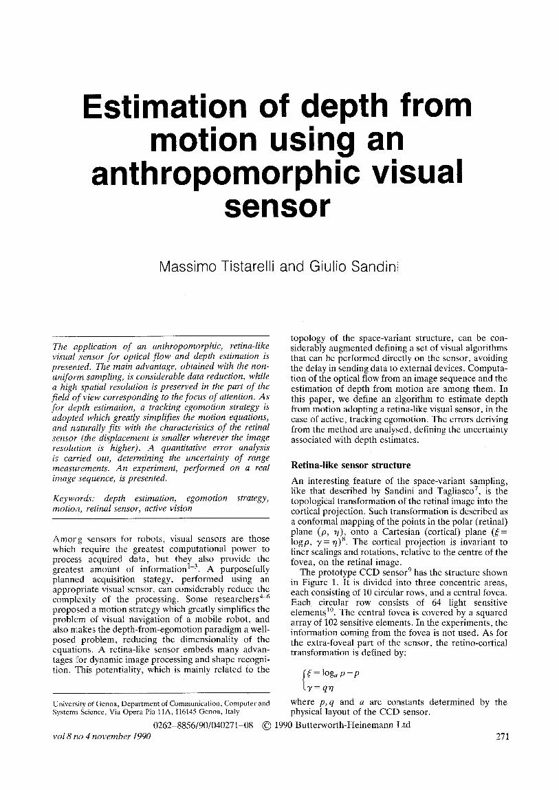
Estimation of depth from motion using an

anthropomorphic visual sensor

Massimo Tistarelli and Giulio Sandini

The application of an anthropomorphic, retina-like visual sensor for optical flow and depth estimation is presented. The main advantage, obtained with the non- uniform sampling, is considerable data reduction, while a higl~ spatial resolution is preserved in the part of the field of view corresponding to the focus of attention. As for depth estimation, a tracking egomotion strategy is adopwd which greatly simplifies the motion equations, and naturally fits with the characteristics of the retinal sensor (the displacement is smaller wherever the image resolution is higher). A quantitative error analysis is carried out, determining the uncertainty of range measurements. An experiment, performed on a real image sequence, is presented.

Keywords: depth estimation, egomotion strategy, motion, retinal sensor, active vision

Amortg sensors for robots, visual sensors are those which require the greatest computational power to process acquired data, but they also provide the greatest amount of information 1-3. A purposefully planned acquisition stategy, performed using an appropriate visual sensor, can considerably reduce the complexity of the processing. Some researchers 4-6 proposed a motion strategy which greatly simplifies the problem of visual navigation of a mobile robot, and also makes the depth-from-egomotion paradigm a well- posed problem, reducing the dimensionality of the equations. A retina-like sensor embeds many advantages for dynamic image processing and shape recogni- tion. This potentiality, which is mainly related to the

University of Genoa, Department of Communication, Computer and Systems Science, Via Opera Pia llA, I16145 Genoa, Italy

vol 8 no 4 november 1990

topology of the space-variant structure, can be considerably augmented defining a set of visual algorithms that can be performed directly on the sensor, avoiding the delay in sending data to external devices. Computa- tion of the optical flow from an image sequence and the estimation of depth from motion are among them. In this paper, we define an algorithm to estimate depth from motion adopting a retina-like visual sensor, in the case of active, tracking egomotion. The errors deriving from the method are analysed, defining the uncertainty associated with depth estimates.

Ret ina - l ike sensor s tructure

An interesting feature of the space-variant sampling, like that described by Sandini and Tagtiasco 7, is the topological transformation of the retinal image into the cortical projection. Such transformation is described as a conformal mapping of the points in the polar (retinal) plane (p, ~), onto a Cartesian (cortical) plane (~= logp, y = r/) 8. The cortical projection is invariant to liner scalings and rotations, relative to the centre of the fovea, on the retinal image.

The prototype CCD sensor 9 has the structure shown in Figure 1. It is divided into three concentric areas, each consisting of 10 circular rows, and a central fovea. Each circular row consists of 64 light sensitive elements l°. The central fovea is covered by a squared array of 102 sensitive elements. In the experiments, the information coming from the fovea is not used. As for the extra-foveal part of the sensor, the retino-cortical transformation is defined by:

{ ( = log~ p - p

y= q~7

where p,q and a are constants determined by the physical layout of the CCD sensor.

0262-8856/90/040271-08 © 1990 Butterworth-Heinemann Ltd 271

I } ! t

a

b Figure 1, (a) Outline and (b) picture of the retinal CCD sensor

DEPTH FROM OPTICAL FLOW

As for the acquisition of range data, active movements can induce much structural information in the flow of images acquired by a moving observer. Performing a tracking egomotion only five parameters are involved in determining camera velocity instead of six. We consider the distances of the camera from the fixation point D~ and D2 in two successive time instants, and the rotations of the camera &, 0 and ~p, referred to its coordinate axes, as shown in Figure 2. The translational velocity of the camera is then:

W x = - D 2 COSq~ s in 0

W r = D2sin~b

Wz = Da - D2 cos{b cos 0

(1)

F{xatioll Pt~in!

Figure 2. Camera coordinate system The optical flow can be expressed as a function of the camera parameters, and decomposed into two terms depending on the rotational and translational components of camera velocity respectively6:

V~.= [ Xy~5 - [x 2 + F 2] 0 + Fy~p

F

[y2 + F z] q~ - xyO - Fx(J

F (2)

-~ Z ~

V~= y[D1- D2 cosq5 cos 0] - FD2 sin (9

Z

where Z is the distance of the world point from the image plane. The rotational part of the flow field ~ can be computed from the camera rotational angles and the focal length, while ~ also requires the knowledge of environmental depth. Once the global optic flow V is computed, ~ and ~nsequently Z, is determined by subtracting V~ from V.

As explained above, the images acquired with the retina-like sensor are the result of the retino-cortical topological transformation. The image velocity is then computed by applying an algorithm for the estimation of the optical flow to a sequence of cortical images. In Figure 3 the first and last images of a sequence of 11 are shown. The images have been acquired with a conven- tional CCD camera and digitized with 256 x 256 pixels and 8 bits per pixel. The sequence represents three planar surfaces, actually three books; it was acquired during the translation of the camera along a linear trajectory. The rail on which the camera was mounted can be seen in the foreground. A point on the surface of the book in the middle was tracked during movement. The motion of the sensor was a translation plus a rotation {b around its horizontal axis X. In Figure 4, the result of the retinal sampling applied to the images in Figure 3 is shown. These images have been obtained simulating the non-uniform sampling operated by the

272 image and vision computing

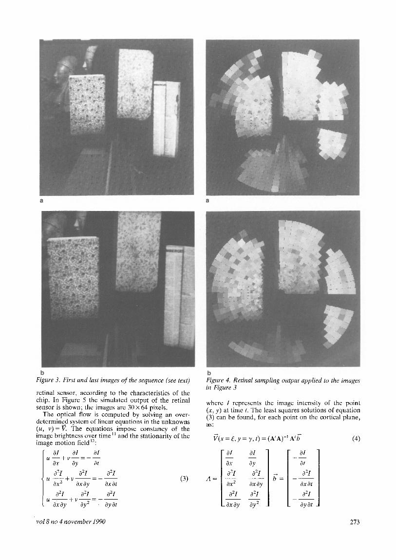
b Figure 3. First and last images of the sequence (see text)

retinal sensor, according to the characteristics of the chip. In Figure 5 the simulated output of the retinal sensor is shown; the images are 30 x 64 pixels,

The optical flow is computed by solving an over- determined system of linear equations in the unknowns (u, v )= V. The equations impose constancy of the image brightness over time 11 and the stationarity of the image motion field12: I OI OI OI

u - - + v Ox Oy Ot

021 021 021 u ~ v - - - (3)

OX 2 -4- OxOy OxOt

021 021 021 U +V = - - - -

Ox Oy Oy 2 Oy at

b Figure 4. Retinal sampling output applied to the images in Figure 3

where I represents the image intensity of the point (x, y) at time t. The least squares solutions of equation (3) can be found, for each point on the cortical plane, as~

A =

V(x = ~:, y = y, t) = (AtA) "1 Atb

OI OI

Ox Oy

021 02I

Ox 2 OxOy

021 021

OxOy Oy 2

OI

G=

(4)

Ot

021

Ox Ot

021

Oy Ot

vol 8 no 4 november 1990 273

a

0I OI 021 021 021 021 Ot Ox 20xOt OyOt O-~-y/

V=

--(~x 0I+ o2I 021 k - - 021 021] 2 Oy Ox 2 OxOy Oy 2 OxOy/

(0I OI 02I 02I 02I 021 1

- ~ x - - + - - - - + - - O - - ~ y / Oy Ox 20xOy Oy 2 OI OI 021 021 021 02I ~+

Ox Ot 4 - - - - + - - Ox 20xOt OyOt OxOy/ 012 0212 ( 02I ~2~

,912 0212 ( 02112 '} Oy + 0 7 + \ ~ ) ) +

_ ( 012 0212+( 02//2] 0---~ + Ox ---g \ OxOy/ /

( OI OI o2I + - -+- -021 021~ Oy ot Oy 20yOt OxOt O-£--Oj/

OI OI+ O=I 02I 02I 021~2

-( o-; o, o oy + 7 o7,

. .'2.f" " - i (

~._~_.__:~ --~'~ =.

a

b

Figure 5. Simulated output of the retinal sensor for the images in Figure 3

U =

( OI OI 021 021 021 02I] + 2 + \Ox Oy Ox OxOy Oy2 OxOy/

(OI OI ~ 02I 021 + 02I 02I ~.jf_ \ Oy Ot Oy 20y Ot Ox Ot O--~y'/

012 0212 ( 02I ~2~

Ox + Ox -----~ + \ Ox Oy/ / (OI 2 0212 (02112]

+ + \ Oy ~ + \ Ox Oy/ /

_( +( Oy + ~y2 \ Ox Oyl /

n ^

5 . " ;

¢* 7 " 4 •

|

Figure 6, (a) Optical flow of the sequence in Figure 5, (b) variance of the optical flow


where (x = ~:, y = y) represent the point coordinates on the cortical plane.

In Figure 6a the optical flow of the sequence of Figure 5 is shown, together with the error in Figure 6b, computed as stated above, it is worth noting that in the area of the image near the fovea, which maps on the left side of the cortical plane, the velocity field is almost zero. This is due to the fact that the centre of the image is stabilized during the tracking egomotion. As can be seen, velocity has been computed only at the image contours; the other image areas are almost uniform, lacking the structural information needed to obtain significant values from the derivatives of image brightness.

In equation (2) we defined the relation between camera velocity and optical flow; now we develop the same equations for the velocity field induced onto the cortical plane.

First we derive the motion equations on the cortical plane:

s c '= /5 logae P

3' = q~} (5)

where e is the natural logarithmic base, and a, q are constants, related to the eccentricity and the density of the receptive fields of the retinal sensor. The retinal velocity (P, ~}) can be expressed as a function of the retinal coordinates relative to a Cartesian reference system (as p = x V ~ y 2 and r/= atan(y/x)):

~ y 2

x ) - yA x2+y 2

(6)

(A, ~) is the retinal velocity of the image point, referred to a Cartesian reference system centred on the fovea. Substituting equation (6) into equation (5) and explicit- ing the retinal velocity V= (u, v):

{ x~logea Y}

1~ _ --~ -~ q - v , + v , = x~ y~ logea +

q

(7)

@, ~,) is the velocity field computed from the seq_uence of cortical images. Substituting the expression of Vr from equation(2) into equation (7), we obtain the translational flow V~ referred to the retinal plane:

x i logea Y--~Y xYq~-[x2+F2]O+FyO q F

Vt= x'~ [y2 + F2]c~-xyO-Fxfft y{: log e a +

q F

(8)

It is worth noting that, expressing the Cartesian coordinates, centred on the fovea, of a retinal point in micros, the focal length and the retinal velocity are also expressed in the same units.

The depth of all the image points on the retinal plane, is computed as:

Z M Wz [I7,] (9)

M is the displacement of the considered point from the focus of the translational field on the image plane, and Wz is the translational component of the sensor velocity along the optical (Z) axis. We can easily be determined from equation (1) if the distance of the fixation point from the camera is known at two successive time instants. The measurement unit of Z depends on the unit of We. If Wz is set equal to 1, the time to collision of the sensor with respect to the world point is computed. The location of the FOE is estimated by computing the least squares fit of the pseudo intersection of the set of straight lines determined by the velocity vectors ~.

Figure 7a shows the depth map of the scene in Figure 4, and Figure 7b shows the associated uncertainty. It

a

Figure 7. (a) Depth map on the cortical plane, (b) depth map on the retinal plane


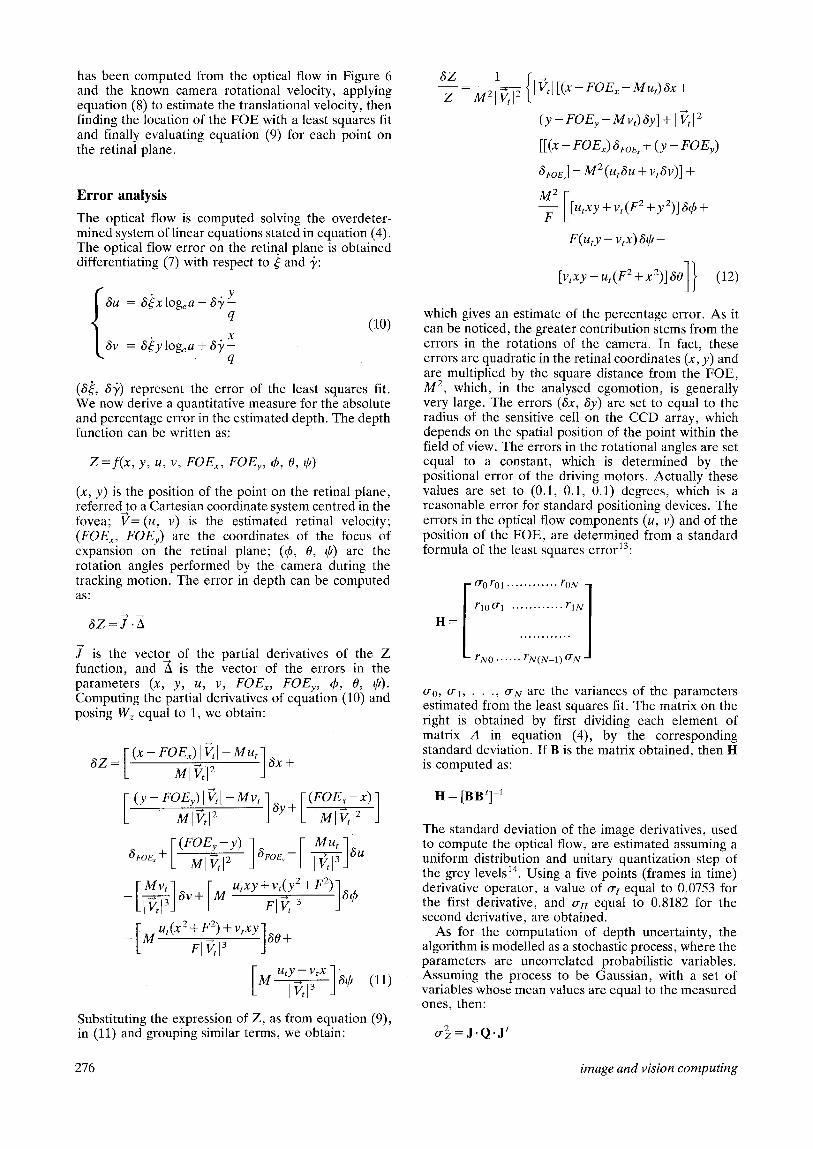
has been computed from the optical flow in Figure 6 and the known camera rotational velocity, applying equation (8) to estimate the translational velocity, then finding the location of the FOE with a least squares fit and finally evaluating equation (9) for each point on the retinal plane.

E r r o r a n a l y s i s

The optical flow is computed solving the overdeter- mined system of linear equations stated in equation (4). The optical flow error on the retinal plane is obtained differentiating (7) with respect to ~ and ~:

6u = 6~-xlogea- 8"y y q

8v = 8~-ylogea + 6y x-- q

(lo)

(6~, 6~,) represent the error of the least squares fit. We now derive a quantitative measure for the absolute and percentage error in the estimated depth. The depth function can be written as:

Z =f(x, y, u, v, FOEx, FOEy, 4), O, ~)

(x, y) is the position of the point on the retinal plane, referred to a Cartesian coordinate system centred in the fovea; ~'= (u, v) is the estimated retinal velocity; (FOEx, FOEy) are the coordinates of the focus of expansion on the retinal plane; (4), 0, 0) are the rotation angles performed by the camera during the tracking motion. The error in depth can be computed as:

az=i.X

i is the vector of the partial derivatives of the Z function, and ~ is the vector of the errors in the parameters (x, y, u, v, FOEx, FOEy, 4), O, 0). Computing the partial derivatives of equation (10) and posing Wz equal to 1, we obtain:

6Z= [ (x-FOEx) I~I-Mu~ MI ,I2

[(y-FOEy)I'P'I-Mv'IaY+ [ MIV, I2 j

6poe +[(F2~,izY) ]6FOe--[ Mut-1

-- 1_1 ~ 1 3 j ~V-I- M rl ,13

- [ M u'(x2+F2)+v'xY]60+Fl~,? M u t y - - v t x 1 ,13 ]aj, (11)

Substituting the expression of Z, as from equation (9), in (11) and grouping similar terms, we obtain:

8Z

Z

1{ M2[ ~tl 2 Iv t l[(x- fOEx-Mu,)~x+

( y - f O g y - Mv~)~Yl + l V~F 2

[[(x - FOEx) 6FOe~ + (y -- rOEy)

~FOEy] - - M2(ut ~u + vt6v)] +

F [utxy+vt(F2+y2)]64)

F(uty - vtx) 6 0 -

[vtxy + ut(F2 + x2)]~Ol}

+

(12)

which gives an estimate of the percentage error. As it can be noticed, the greater contribution stems from the errors in the rotations of the camera. In fact, these errors are quadratic in the retinal coordinates (x, y) and are multiplied by the square distance from the FOE, M 2, which, in the analysed egomotion, is generally very large. The errors (6x, 6y) are set to equal to the radius of the sensitive cell on the CCD array, which depends on the spatial position of the point within the field of view. The errors in the rotational angles are set equal to a constant, which is determined by the positional error of the driving motors. Actually these values are set to (0.1, 0.1, 0.1) degrees, which is a reasonable error for standard positioning devices. The errors in the optical flow components (u, v) and of the position of the FOE, are determined from a standard formula of the least squares error13:

H =

(To F01 . . . . . . . . . . . . ?'ON ]

I F10 o'1 . . . . . . . . . . . . F1N /

O-0, O-I, - • ' , O-N a re the variances of the parameters estimated from the least squares fit. The matrix on the right is obtained by first dividing each element of matrix A in equation (4), by the corresponding standard deviation. If B is the matrix obtained, then H is computed as:

H = [BB t] 1

The standard deviation of the image derivatives, used to compute the optical flow, are estimated assuming a uniform distribution and unitary quantization step of the grey levels ~4. Using a five points (frames in time) derivative operator, a value of o'i equal to 0.0753 for the first derivative, and o"ti equal to 0.8182 for the second derivative, are obtained.

As for the computation of depth uncertainty, the algorithm is modelled as a stochastic process, where the parameters are uncorrelated probabilistic variables. Assuming the process to be Gaussian, with a set of variables whose mean values are equal to the measured ones, then:

o - ~ = j . Q . j t


J is the Jacobian of the depth function and Q is the diagonal matrix of the variances of the independent

. . . . 2 0.2 2 variables. The variances m matrix Q, (o-x, y, o.~, 0-0 2, K~) are considered equal to the squared errors, while the variances in the optical flow and the position

2 2 2 of the FOE (o -2, o'v, O.FOEx, O.FOEy) are determined as for the variances of the optical flow. Writing explicitly the variance in depth, we obtain:

\MtVtl L (FOEy - y)20.2oEy ~

+ [(fOEx-x) lV l +Mut]20- +

22} + [(fOEy - y) I ~¢~1 + Mv,] O'y

[ W z M \ 2 f 2 2

l- 13 ) + [utxy + v t (F 2 + y 2 ) ] 2

F 2 0-~ +

[vtxy + ut(V z + xe)] e o-2+

F 2

[uty-vtx]eo.~l (13)

The last two rows represent the higher term, as it is multiplied by M. Consequently, the higher errors are those due to the computation of image velocity and the estimation of the rotational angles of the cameras (or conversely, the positioning error of the driving motors).

The terms containing the errors in the rotational angles are also quadratic in the image coordinates, hence the periphery of the visual field will be more effected than the fovea. Nevertheless, all these terms are divided by the cubic module of velocity, therefore if the amplitude of image displacement is sufficiently large, the error drops very quickly. As a matter of fact the amplitude of the optical flow is of crucial importance reducing the uncertainty in depth estimation. This can be achieved using a long motion baseline, for example, subsampling the sequence over time, or alternatively, cumulating the optical flows over multiple frames. As for the last option, the disadvan- tages of tracking image features have been shown 15A6, because errors are cumulated over time. Nevertheless, these errors can be considerably reduced if, for each computed optical flow, the previous measurements are also taken into account to establish pointwise corres- pondence. A method to perform this temporal integra- tion has already been presented16; another method, based on a local spatio-temporal interpolation of image velocities, is being developed.

C O N C L U S I O N

The application of a retina-like, anthropomorphic visual sensor for dynamic image analysis has been investigated. In particular, the case of a moving observer, undertaking active movements, has been considered to estimate environmental depth. The main advantages obtained with the retina-like sensor, are

b Figure 8. (a) Depth uncertainty on the cortical plane, (b) depth uncertainty on the retinal plane

related to the space-variant sampling structure, which features image scaling and rotation invariance and a variable resolution. Due to this topology, the amount of incoming data is considerably reduced, but a high resolution is preserved in the part of the image corresponding to the focus of attention.

Adopting a tracking egomotion strategy, the computation of the optical flow and depth-from-motion, is simplified. Moreover, as the amplitude of image displacements increases from the fovea to the periphery of the retinal image, almost the same computational accuracy is achieved throughout the visual field, minimizing the number of pixels to be processed.

In human beings, most 'low-level' visual processes are directly performed on the retina or in the early stages of the visual system. Simple image processes like filtering, edge and motion detection must be performed quickly and with minimal delay from the acquisition stage, because of vital importance for survival (for example, to detect static and moving obstacles). These


processes could be implemented directly on the sensor, as local (even analogic, using the electrical charge output of the sensitive elements) parallel operations, avoiding the delay for decoding and transmitting data to external devices.

ACKNOWLEDGEMENTS

This research was supported by the special project on robotics of the Italian National Council of Research.

REFERENCES

1 Marr, D Vision Freeman and Co, San Francisco, USA (1982)

2 Ballard, D H and Brown, C M Computer Vision Prentice-Hall, NJ, USA (1982)

3 I-Iildreth, E C The Measurement of Visual Motion MIT Press, MA, USA (1983)

4 Bandopadhay, A, Chandra, B and Ballard, D H 'Active navigation: tracking an environmental point considered beneficial' Proc Workshop on Motion: Representation & Analysis Kaiwah Island Resort, USA (May 7-9 1986)

5 Sandini, G, Tagliasco, V and Tistarelli, M 'Analy- sis of object motion and camera motion in real scenes' Proc IEEE Int. Conf. Robot & Automat. San Francisco, CA, USA (April 7-10 1986)

6 Sandini, G and Tistarelli, M 'Active tracking strategy for monocular depth inference over multiple frames' IEEE Trans. PAMIVol 11 No 12 (December 1989)

7 Sandini, G and Tagliaseo, V 'An anthropomorphic retina-like structure for scene analysis' Comput. Graph, Vision & Image Process Vol 14 No 3 (1980) pp 181-194

8 Schwartz, E L 'Spatial mapping in the primate sensory projection: analytic structure and rele- vance to perception' Biol. Cybern. Vol 25 (1977) pp 365-372

9 Van der Spiegel, J, Kreider, G, Claeys, C, Debuss- chere, I, Sandini, G, Dario, P, Fantini, F, Bellutti, P and Soncini, G in Analog VLSI and Neural Network Implementations Mead, C and De Kluwer, M I (eds) (1989) •

10 Debusschere, I, Bronekaers, E, Claeys, C, Kreider, G, Van der Spiegel, J, BeUutti, P, Soncini, G, Dario, P, Fantini, F and Sandini, G 'A 2D retinal CCD sensor for fast 2D shape reconition and tracking' Proc 5th Int. Solid-State Sensor and Transducers Montreux, France (June 25-30 1989)

11 Horn, B K P and Schunck, B G 'Determining optical flow' Artif. Intell. Vot i7 Nos 1-3 (1981) pp I85-204

12 Uras, S, Girosi, F, Verri, A and Torre, V 'Computational approach to motion perception' Biol. Cybern. (1988)

i3 Bevington, P R Data Reduction and Error Analysis McGraw-Hill, NY, USA (1969)

14 Kamgar.Parsi, B and Kamgar-Parsi, B 'Evaluation of quantization error in computer vision' Proc. DARPA Workshop on Image Understanding (1988)

I4 Bharwani, S, Riseman, E and Hanson, A 'Refine- ment of envirionmentaI depth maps over multiple frames' Proc. Workshop on Motion: Representa- tion and Analysis Kaiwah Island Resort, USA (May 7-9 1986)

16 Tistarelli, M and Sandini, G 'Uncertainty analysis in visual motion and depth estimation from active egomotion' Proc~ IEEE/SPIE Int. Conf. Appl. of Artif. Intell. VII Orlando, FL, USA (March 28-30 1989)


Estimation of depth from motion using an anthropomorphic visual sensor

Documents

Transcript of Estimation of depth from motion using an anthropomorphic visual sensor