Estimation and Modelling of PCBs Bioaccumulation inthe Adriatic Sea Ecosystem

Marianna Taffia,e, Nicola Paolettib, Pietro Lioc, Luca Teseid, SandraPucciarellia, Mauro Marinie

aSchool of Biosciences and Veterinary Medicine, University of Camerino, Via Gentile IIIDa Varano 62032, Camerino, Italy

bDepartment of Computer Science, University of Oxford, Parks road, Oxford OX1 3QD,United Kingdom

cComputer Laboratory, University of Cambridge, 15 JJ Thomson Ave, Cambridge CB30FD, United Kingdom

dSchool of Science and Technology, Computer Science division, via Del Bastione 1, 62032Camerino, Italy

eNational Research Council, Institute of Marine Science (ISMAR), Largo Fiera della Pesca2, 60125 Ancona, Italy

Abstract

Persistent Organic Pollutants represent a global ecological concern due to theirability to accumulate in organisms and to spread species-by-species via feedingconnections. In this work we focus on the estimation and simulation of thebioaccumulation dynamics of persistent pollutants in the marine ecosystem,and we apply the approach for reconstructing a model of PCBs bioaccumulationin the Adriatic sea, estimated after an extensive review of trophic and PCBsconcentration data on Adriatic species. Our estimations evidence the occurrenceof PCBs biomagnification in the Adriatic food web, together with a strongdependence of bioaccumulation on trophic dynamics and external factors likefishing activity.

Keywords: Adriatic Sea, Polychlorinated Biphenyls, bioaccumulationmodelling, Linear Inverse Modelling

1. Introduction

Chemical contamination is one of the strongest and most complex abioticperturbations threatening the stability of marine ecosystems. Constantly, anunrestrained flow of pollutants is released into the seas triggering unpredictableecological consequences in marine biota, having also cascade effects in the entireecosystem. The aquatic environment is characterized by multiple contaminationpathways making marine organisms particularly prone to bioaccumulation andbiomagnification phenomena (defined in Table 1), of which Persistent OrganicPollutants (POPs) are globally recognised as one of the main and worst causes.

Chemically belonging to the same class of POPs, Polychlorinated biphenyl(PCBs) have been for a long time matter of ecotoxicological interest for theirproperty of binding with the fatty tissue of animals and, thus, of spreadingthrough feeding connections amplifying their toxic perturbations species-by-species. As a consequence, feeding links become a critical medium of chemi-cal transport across trophic levels up to the human being (Kelly et al., 2007,

arX

iv:1

405.

6384

v1 [

q-bi

o.PE

] 2

5 M

ay 2

014

Lohmann et al., 2007), which makes the entire marine ecosystem both sink andsource of hazardous substances.

Bioaccumulation represents a complex and exhaustive ecotoxicological indi-cator to evaluate the toxic exposure of living organisms. Its definition (Mackayand Fraser, 2000) includes abiotic and biotic factors (see Table 1), therefore itcan vary for the same species surveyed in different environments. Variations maydepend on the multiple patterns of uptake and their related concentrations, onthe nature of xenobiotics, and on species-specific biological characteristics (lipidcontent, size, age and etc). The combination of all these aspects with the vari-ety of local environmental and ecological scenarios makes difficult to obtain anall-encompassing model.

In the field of environmental toxicology, prediction-oriented works are stillrelatively recent. However, over the last decades this area has considerablyevolved with advances in models, approaches and indices to assess chemicalsfate and effects on species and communities (Van der Oost et al., 2003, Mackayand Fraser, 2000, Arnot and Gobas, 2006, Devillers, 2009, Jørgensen and Ben-doricchio, 2001). What makes a model exploitable for predictive purposes is itspractical utility and, above all, its ability to reproduce bioaccumulation dynam-ics in a robust way (Luoma and Rainbow, 2005).

As opposed to regression-based approaches for predicting species biocon-centration or bioaccumulation, mechanistic models (Mackay and Fraser, 2000,Nichols et al., 2009) require specifying and quantifying the different pathwaysof contaminant uptake and loss. Thus, they provide a more detailed charac-terization of the bioaccumulation dynamics and can accommodate the use ofempirical data so that estimations and predictions are able to reflect measuredconditions. In addition, toxicokinetic-toxicodynamic (TKTD) models study theeffects of specific molecules at finer scales, including the diffusion within inter-nal compartments (fat tissue, liver, muscle and etc) and the responses at thegenetic and cellular levels. It is clear that a large amount of high quality, species-specific, toxicity data are needed to parametrize TKTD models. Therefore, dataavailability mainly drives the choice of a particular model and its degree of de-tail. Besides this, simpler models could provide, with less effort, a fair accuracyor predictive power and having more specific models do not necessarily implybetter results (Wainwright and Mulligan, 2013, Wania and Mackay, 1999).

In this work, we derive a bioaccumulation model of PCBs in the Adriatic sea,based on one of the most complete trophic studies in this area (Coll et al., 2007).Since PCBs necessarily follow feeding links, we take a mechanistic approachwhere pathways of contaminant uptake and loss correspond to trophic flowsamong species and environmental compartments. What makes the Adriaticarea of crucial interest from an ecotoxicological point of view is the combinationof high environmental variability and biodiversity with several anthropogenicfactors, and a peculiar geography and orography.

A number of studies on PCBs concentration in Adriatic species have beencarried out during the last decades. Using this literature we have reconstructed adatabase that includes toxicity data for each considered species (see Table A.4).However, due to the lack of data for some compartments and their temporaland spatial patchiness, the resulting collection is still incomplete. Hence, weuse Linear Inverse Modelling (LIM), a technique typically employed in trophicestimation, to calculate the missing information. In particular, we obtain, as afirst result, a static bioaccumulation network model from which we parametrize

2

Table 1: Glossary of ecotoxicological concepts.

Bioconcentration is the net process of chemical adsorption only from wa-ter through respiration and dermal surfaces minus eliminations routes (res-piration, egestion, growth dilution and metabolic tranformation).Bioaccumulation refers to the contamination process of an organism re-sulting from all possible paths of uptake: waterborne (bioconcentration)and dietary sources, net of chemical elimination routes.Biomagnification is the phenomenon by which predators have higher con-centrations than their prey, leading to increasing accumulation of pollutantsalong increasing trophic levels.Polychlorinated Biphenyls are synthetic chemical compounds, chemi-cally defined as chlorinated hydrocarbons. They are highly stable moleculeswith general formula C12H(10−n)Cln (n = 1, . . . , 10 number of chlorineatoms), consisting in a group of 209 different congeners. Congeners varyin the degree of chlorination and chlorine position (para, meta and ortho).Higher chlorine contents correspond to higher environmental persistenceand lower biodegradability (photolytic, biological and chemical). PCBs arecharacterized by semi-volatility, low water solubility, low vapour pressureand long-range transport. PCBs have been used in hundreds of commercialand industrial application until their ban in the 80’s, but are still ubiquitousand have been traced even much farther than their application point, like inArctic regions (Norstrom et al., 1988). Biologically, they are highly noxiousfor aquatic living organisms for their lipophilicity, i.e. the ability to dissolvein fats and lipids (including oils and non-polar solvents). This gives riseto the phenomena of bioaccumulation and biomagnification in marine foodwebs, up to the human being (Dewailly et al., 1989).

a Lotka-Volterra ODE system used to analyse the contaminant long-term dy-namics through the food web.

With our methodological framework, we show the occurrence of biomagnifi-cation in Adriatic species and that bioaccumulation mainly depends on trophicaspects (e.g. diet and fishing).

2. Materials and Methods

2.1. The Adriatic Sea Ecosystem

This study focuses on the Adriatic Sea, a relatively shallow sub-basin ofthe Mediaterranean Sea (max depth 1250 m) with limited extension (800 kmmajor axis - 200 km minor axis) but characterized by high ecological relevanceand environmental variability (Cushman-Roisin et al., 2001), wide diversity ofmarine species and microbial communities (Coll et al., 2010).

This area is exposed to multiple external forcing mechanisms that combined,lead to adverse effects in the pollution load spilled into the Adriatic ecosystem.The Adriatic region is characterized by high anthropogenic activities (De Lazzariet al., 2004) and river discharge fluctuations.

Geographically, the complex orography of the gulf of Trieste and the Venicelagoon causes a significant penetration and exchange of coastal water into theurban environment. In particular the Po river by crossing a wide industrial and

3

agricultural area, represents the major buoyancy input with an annual meandischarge rate of 1500 m3 · s−1 accounting for the third of the total riverinefreshwater input into the Adriatic Sea Sea (Campanelli et al., 2011). Moreover,the Southern Eastern Adriatic rivers are equally an important potential sourceof pollutants, being the mainly entrance to the Southern part of the AdriaticSea (Marini et al., 2010). In relation to this aspects, several surveys conductedin different Adriatic regions report significant concentrations of different xeno-biotics detected both in species and environmental compartment (Marini et al.,2012, Bellucci et al., 2002, Horvat et al., 1999, Kannan et al., 2002)

2.2. Input data

In order to define the PCBs bioaccumulation model, we firstly need to esti-mate the trophic network of Adriatic species. We start from data reported in(Coll et al., 2007), one of the most complete quantitative study of the Northernand Central Adriatic food web in which forty functional groups have been iden-tified to investigate the ecological impact of fishing activity during the decade1990-2000. In their work the Adriatic trophic model is developed with ECO-PATH (Christensen and Walters, 2004), and estimated through a mass balancedapproach by using literature and survey data on species abundance. In ourmodel, we follow the same functional group classification as in (Coll et al., 2007),taking the same input data (reported in Table Appendix A) regarding biomass(B, measured in t ·km−2 wet weight organic matter); production/biomass ratio(P , i.e. rate of biomass generation, yr−1) and consumption/biomass ratio (Q,i.e. rate of biomass losses, yr−1). Data on fishing activity has also been takeninto account, but not reported here. Diet composition is illustrated in Fig. A.4(a) of the supplementary material. Biomass flows are expressed in t·km−2 ·yr−1.

We reviewed a large amount of literature dealing with field analysis of PCBsbioconcentration in marine species of the Adriatic Sea conducted over the lastdecades. In order to maintain homogeneity with trophic data, we follow somecriteria in the selection of the available PCB concentration data. In particular,we collected data sampled in species in North, Central and South Adriatic areaduring the period 1994-2002, where PCBs concentrations in marine organismshave been determined in edible parts and muscle tissue; and, as usually done infield surveys, we considered the sum of PCBs congeners expressed in ng · g−1wet weight-based. When PCBs values are not available for the same speciesidentified in (Coll et al., 2007), we select concentration data of Adriatic specieswith the same taxonomic classification. Table A.4 summarizes the PCBs con-centration data used in the estimation of the bioaccumulation model for eachfunctional group, together with the corresponding sampled species and litera-ture reference. Details on the sampling period, geographic area, tissue analysedand PCBs congeners detected are summarized in Tab. Appendix A of thesupplement.

2.3. Food web estimation with Linear Inverse Modelling

Following (Ulanowicz, 2004), to describe an ecological network we needits topology (qualitative information), i.e. the nodes representing the relevantgroups and the directed edges representing the feeding links; and its flow rates(quantitative information), i.e. for each edge, the rate at which a medium (inour case, biomass or contaminant) is transferred from the source (the prey) to

4

the target (the predator). Generally, flow rates are estimated at some equilib-rium conditions, according to which functional groups are mass-balanced, i.e.the inflows must equal the outflows. In addition, each group possesses an inter-nal storage of biomass/bioconcentration affecting the value of flow rates. Foodweb models need to include also external compartments, used to implementexogenous imports and exports. Externals are not mass-balanced, thus theyrepresent potentially unlimited sources and sinks of medium.

In the following, we denote with bi−→j and ci−→j the flow rate of biomassand contaminant, respectively, from compartment i (the prey) to j (the preda-tor); and the storages Bi and Ci are used to indicate the biomass and PCBsconcentration of i, respectively.

One of the most extensively used techniques in reconstructing feeding con-nections from empirical data is Linear Inverse Modelling (LIM), through whichthe food web is described as a linear function of its unknown flows. The terminverse indicates that such unknown flows are determined from empirical data,put in the model by means of linear equalities and inequalities (van Oevelenet al., 2010). A LIM problem can be formulated as

min |A · x− b|2 (2.1)

subject to A · x ' b (2.2)

E · x = f (2.3)

G · x ≥ h, (2.4)

where x is the vector of unknown flows; Eq. 2.2 indicates an optional set ofequalities that are approximately met (as closest as possible); the strict equal-ities in Eq. 2.3 are used to model hard constraints, typically to incorporatemass balances and high quality data; and inequalities in 2.4 are used to modelssoft constraints (e.g. when dealing with low quality data). Among the differ-ent methods available for solving a LIM problem, in this work we use the leastsquare method that attempts to minimize the squared difference between theestimates and the data in the approximate equations (see Eq. 2.1), and solutionsare accepted up to a fixed tolerance value.

When approximate equalities are excluded and the solution space is not-empty (i.e. when dealing with an under-determined model), a single solution canbe picked up that minimizes the sum of squared flows or other global ecosystemproperties expressible as linear functions. Alternatively, the solution space canbe explored through Monte-Carlo sampling for finding the flows that are mostlikely under a statistical viewpoint. Then, the mean of the sampled solutionscan be taken as a single (valid) solution, as shown in (van Oevelen et al., 2010).

2.4. Adriatic PCBs bioaccumulation model

2.4.1. Conceptual model

Figure 1 illustrates the conceptual model describing the biomass and thePCBs flows between the groups of our network. Given a generic (mass-balanced)group i, we consider:

• consumption (bj−→i) or contaminant uptake (cj−→i) from a prey j;

• predation (bi−→k) or contaminant losses (ci−→k) due to consumption by apredator k;

5

GROUP iIMPORT FISHING

LANDINGDISCARD

EXPORT

CO2WATER

DETRITUS

PREDATOR k

PREY j

Figure 1: Conceptual model of the Adriatic PCBs bioaccumulation network.Mass-balanced groups are enclosed in the gray box; externals are depicted out-side of the box. Generic compartments i, j, k correspond to any of the mass-balanced groups. Solid arrows indicate combined biomass and contaminant flowsbetween groups. The dashed arrow from the water compartment represents theonly contaminant uptake flow which is not mediated by biomass.

• external inputs of biomass and PCBs from Import (bImport−→i and cImport−→i),used to model generic inflows like immigration;

• flows describing contaminant uptake from water (cWater−→i), which clearlydo not involve a corresponding biomass transfer;

• external outputs to Export (bi−→Export and ci−→Export), describing genericoutflows like emigration;

• outflows to the CO2 compartment (bi−→CO2 and ci−→CO2), modelling res-piration flows and that together with the flows to detritus account for theunassimilated portion of “ingested” food; and

• outflows due to fishing activity, which can be directed to the landings(bi−→Landing and ci−→Landing) or to the discards (bi−→Discard and ci−→Discard).The latter enters back the biomass cycle and is modelled as a mass-balanced group.

2.4.2. Trophic Network

Table 2 summarizes the linear equalities and inequalities defined for theestimation of biomass flows. The results of the quantification are discussed inSection 3.1 (Fig. 2 (a) gives a graphical illustration of the estimated networkand Table Appendix A reports the numerical results).

2.4.3. Bioaccumulation Network

Following (Hendriks et al., 2001, Laender et al., 2009), our bioaccumulationmodel distinguishes between two kinds of functional groups:

i ∈ INST : compartments modelling small particles that are assumed to be ininstant equilibrium with the water phase, like detritus and planktonic

6

Table 2: Linear Inverse Model for the estimation of trophic flows. bi→j denotesthe biomass flow from group i to group j.

Mass balances: dbidt

=∑

j bj→i −∑

j bi→j = 0

The difference between inflows and outflows is zero for each functional group i; jranges among groups and externals.

Ingestion1: Ii =∑

j bj→i = Bi ·Qi

The total ingestion Ii of a group i, i.e. the sum of all the consumption flows, equalsthe product between biomass Bi and consumption rate Qi; i and j are functionalgroups; for i, we exclude detritus and primary producers (phytoplankton).

Unassimilated Food: bi→CO2 + bi→Detritus = Ii · (1− gi)Respiration flows bi→CO2 and flows to detritus bi→Detritus constitute together afraction of the total ingestion and accounts for the proportion of food that is notconverted into biomass. gi = Pi

Qiis the gross food conversion efficiency (Chris-

tensen and Walters, 2004).

Respiration-assimilation: bi→CO2 ≤ Ii · giAs pointed out in (Coll et al., 2007), the ratio respiration/assimilation has to belower than one, in order to have realistic estimates.

Diet1: bi→j = Ij ·DCij .

The biomass flow from prey i to predator j is given by the proportion of the totalingestion of j coming from i. DC is the diet composition matrix (Fig. A.4 (a)).

Non-negativity of flows: b ≥ 01For species with uncertain input biomass and diet data, appropriate inequalities are set.

Table 3: Linear Inverse Model for the estimation of PCB concentrations. ci→j

denotes the contaminant flow from group i to group j.

Mass balances: dcidt

=∑

j cj→i −∑

j ci→j = 0

For each group i ∈ KINE, bioconcentrations are estimated under the mass-balance assumption; j ranges among groups and externals.

Concentration data: Ci = PCBi

These equations incorporate PCB input data (PCBi) into the model. Inequalitiesare used in correspondence of groups with uncertain input PCB concentrations.i ∈ KINE ∪ INST .

Uptake from food/losses: cj→i = bj→i · Cj

The contaminant flow from j ∈ KINE ∪ INST to i is the product of the corre-sponding biomass flow bj→i and the PCB concentration in j. If i ∈ KINE, theequation describes the uptake from food by predator i. If instead i is an external,cj→i represents a contaminant loss by j.

Uptake from generic imports: cimport→i = bimport→i · Ci

The concentration of the biomass imported into group i ∈ KINE) is assumed tobe the same as in i.

Uptake from environment: cwater→i = wi · Cwater

wi is the rate of contaminant uptake from water by group i ∈ KINE and Cwater

is the concentration in water1.

Non-negativity of concentrations: Ci ≥ 01wi cannot directly estimated, since it depends on a non-linear constraint (wi and Cwater

are both unknowns). cwater→i is instead computed and wi calculated subsequently.

7

groups. For such groups, contaminant concentration is computed as:

Ci = Cwater ·OCi ·KOC

where Ci is the concentration of i and OCi is its organic carbon frac-tion; Cwater (µg/L) is the unknown concentration in water and KOC =kOC/OW ·KOW is the organic carbon-water partition ratio, calculated asa function of KOW , the octanol-water partition ratio of the contaminant.KOW is a measure of how a compound is hydrophilic or hydrophobic, andin this case its value depends on the particular PCB congener considered.Since we consider the sum of congeners, we set KOW = 106, given thatthe LogKOW of PCBs varies between 5 and 7, as reported in (Walterset al., 2011). The other parameters have been taken from (Laender et al.,2009): OCi = 0.028 and kOC/OW = 0.41.

i ∈ KINE: compartments whose concentration depends on the amount of con-taminant exchanged through biomass flows, and are estimated as in Table3. This option applies to groups where contaminant uptake and losses re-sulting from absorption, ingestion, egestion, excretion and growth cannotbe neglected (Hendriks et al., 2001).

We formulate a linear inverse model (Table 3) where PCB concentrationsCi are the unknowns to estimate, differently from the trophic model wherebiomass flows are the unknown variables. Contaminant flows are expressedin ng · g−1 · t · km−2 · y−1. In Section 3.1 we illustrate the estimated PCBbioaccumulation network and we evaluate biomagnification phenomena on thespecies of the Adriatic ecosystem. Numerical results are reported in Table A.6.

2.5. Derivation of ODE Model

Recalling that PCB diffusion follows the same paths as biomass flows de-termined by prey-predator relationships, we define a dynamic bioaccumulationmodel on top of a multi-species Lotka-Volterra system used to describe the tem-poral changes in species biomass. In its general form, the system is formulatedas:

Bi(t) = Bi(t)

gi −∑j

AijBj(t)

(2.5)

where Bi(t) is the biomass of species i at time t; gi is the intrinsic growth rate ofi; and A is the interaction matrix describing inter-specific effects. In particularAij describes the predation effect of species j on species i. Although there areseveral possible ways to derive population-dynamics parameters from a foodweb model (Palamara et al., 2011), here we follow quite a standard approach:

• Bi(0) = Bi, initial biomass values are those in the static food web esti-mated with LIM;

• gi =

∑j bj→i −

∑j bi→j

Bi(0), with j ranging among the external groups: the

growth rate of i is the sum of exogenous inflows and outflow, over theestimated biomass of i;

8

• Aij =bi→j − bj→i

Bi(0) ·Bj(0), the interaction rate between prey i and predator j

is calculated as the net flow going from i to j divided by the estimatedbiomasses of i and j.

Additionally, we can define the biomass flow rate from group i to j at time t,bi→j(t), which is non-linear with respect to the biomasses of i and j, as:

bi→j(t) =bi→j

Bi(0) ·Bj(0)·Bi(t) ·Bj(t)

in a way that Eq. 2.5 can be rewritten as:

Bi(t) = gi ·Bi(t) +∑j

bj→i(t)−∑j

bi→j(t)

Therefore, the dynamics of the contaminant concentration in species i, Ci(t), isgiven by the net sum of contaminant flows, over the biomass of i:

Ci(t) = wi · Cwater+

gi ·Bi(t) · Ci(t) +∑

j bj→i(t) · Cj(t)−∑

j bi→j(t) · Ci(t)

Bi(t)(2.6)

where Cwater is the concentration in water (assumed constant) and wi is theuptake rate from water by group i. As done for the biomass equations, the ini-tial concentrations correspond to those estimated in the static bioaccumulationnetwork: Ci(0) = Ci, for each group i.

Finally, expanding the interaction terms, Eq. 2.6 is equivalent to the follow-ing:

Ci(t) = wi · Cwater + gi · Ci(t) +∑j

(bj→i

Bi(0) ·Bj(0)·Bj(t) · Cj(t)

)

−∑j

(bi→j

Bi(0) ·Bj(0)·Bj(t) · Ci(t)

)(2.7)

In the remainder of the paper, we will focus on the temporal changes in bio-concentrations independently of the biomass variations, thus assuming constantspecies biomass (Bi(t) = Bi(0),∀t), which gives the following system of lineardifferential equations:

Ci(t) = wi · Cwater + gi · Ci(t) +∑j

(bj→i · Cj(t)− bi→j · Ci(t)

Bi(0)

)(2.8)

Note that this simplification does not change the quantitative dynamics of themodel, because biomasses have been estimated under mass-balance conditions.

3. Results and Discussion

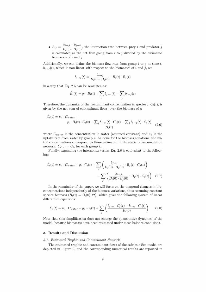
3.1. Estimated Trophic and Contaminant Network

The estimated trophic and contaminant flows of the Adriatic Sea model aredepicted in Figure 2, and the corresponding numerical results are reported in

9

Table Appendix A for the biomass network, and in Table A.6 for the PCBsbioaccumulation network. Estimating the trophic network with LIM requiredto take an approximate solution (with error tolerance ≤ 10−8) because thelarge amount of input trophic data taken from (Coll et al., 2007) (reported inTable Appendix A) generates a high number of constraints and in turn anempty solution space. On the other hand, the partial availability of PCBs bio-concentration data produces an under-determined problem (i.e. many possiblesolutions), solved in this case through Markov Chain Monte Carlo (MCMC)sampling (5000 iterations) of the solution space.

Trophic Network Analysis. The analysis of the biomass network shows thatspecies at lower trophic levels are the most prominent in terms of internal andexchanged biomass and that biomass content and trophic level are negativelycorrelated, as visible in Fig. 2 (a). The only exception is the Discard group,which accounts for the discarded catches that enter back the biomass cycle. Dis-card is considered in this model as a detritus, and thus has associated a trophiclevel (TL) of 1. However, it clearly possesses a much lower biomass than thenatural detritus (group Detritus) and primary producers (group Phytoplank-ton). We report that our quantitative estimations agree with the original workby Coll et al., which allows us to validate our trophic model.

PCBs Bioaccumulation Analysis. On the other hand, PCBs bioaccumulationvalues tend to increase at higher trophic levels, thus a phenomenon of biomag-nification is clearly detectable, as one can observe in the network plot (Fig. 2(b)).We also evince that functional groups with high concentrations have asso-ciated low biomass values.

We indeed register the most prominent PCBs values in top predators: LargePelagic Fish (TL = 4.343, PCB = 70.491), Demersal skates (TL = 4.154, PCB= 54.833), Turbot and brill (TL = 4.152, PCB = 54.746), Dolphins (TL=4.302,PCB=54.048), Anglerfish (TL = 4.553, PCB = 53.808), and Atlantic bonito (TL= 4.087, PCB = 52.704). In particular, Large Pelagic Fish (Tuna and Swordfish)shows by far the highest PCBs bioaccumulation, which can be explained bythe concentration in groups composing its diet (mainly European Anchovy andSquids).

Anyway, by the nature of the LIM approach, we note that input concentra-tion data strongly influence estimated values. Specifically, low upper boundson PCBs values limit the output concentrations in some top predators (Squids,Hake 2 and Demersal Sharks). On the contrary, setting high or infinite upperbounds results in large bioaccumulation values also for groups at TL=3, likein Demersal fish 2, Flatfish, Bentopelagic fish and Mackarel. Naturally, hav-ing employed a stochastic search algorithm, the concentration variables withless constraints typically have a higher variability (see standard deviation σ inTable A.6).

Fishing activity and overexploitation represent a biomass loss, and thereforecan also affect the patterns of PCBs diffusion in the ecosystem. Bioaccumu-lation results from the continuous uptake of pollutants over the years. Thus,fishing activity can ideally interrupt the bioaccumulation process by increasingthe mortality rate of a species, even if overexploitation is not clearly an ecologi-cally sustainable solution (Coll et al., 2008). In our model, relatively low PCBsvalues can be detected in correspondence of exploited species (i.e. with fishing

10

(a) Biomass network

(b) Bioaccumulation network

Figure 2: Estimated Adriatic trophic (a) and PCB bioaccumulation (b) net-works. Nodes represent functional groups whose size is proportional to thebiomass content (a) or PCB bioconcentration (b). Edges represent feeding con-nection and their thickness indicates the contribution of the source node in thediet of the target node (a), or in the uptake of contaminant from food in thecase of bioaccumulation network (b). Flows to detritus and to fishing discardsare not shown.

11

rates exceeding biomass). For instance, Crabs, Other gadiformes and Red mul-lets show concentrations substantially lower (< 1 ng · g−1) than those in speciesbelonging to the same TL, but not affected by fishing pressure. A similar phe-nomenon is observable in Conger eel where, albeit with a wide PCBs inputrange, the estimated bioaccumulation value stands close to the lower bound.This is even more evident by looking at the variations in PCBs bioaccumula-tion between groups describing the same species but subject to different fishingpressures, like between Hake 1 (< 40 cm, vulnerable to fishing, PCB=3.852)and Hake 2 (> 40 cm, not vulnerable, PCB=21.658); or between Demersal fish1 (overexploited, PCB=8.159) and Demersal fish 2 (PCB=55.424).

Differently from natural detritus, fishing discards are characterized by asignificant PCBs concentration. This has to be attributed mainly to its lowtotal biomass, combined with its species composition, that contributes to aconsiderable total inflow of contaminant as detailed in Table A.6 (column Dis).

Finally, with our bioaccumulation model we are also able to estimate PCBsconcentration in the landing fraction of biomass exported by fishing. This issimply computed as the sum of contaminant outflows to the landings over the

sum of biomass exported to the same compartment:

∑i ci→Land∑i bi→Land

. The mean

concentration value in landings equals to 18.17 ng · g−1. This kind of analy-sis could provide an effective indicator of the chemical pollution in species ofcommercial interest.

3.2. ODE bioaccumulation model

We evaluate the long-term bioaccumulation dynamics in the Adriatic foodweb by simulating the ODE model at Eq. 2.8 for a period of 4 years with a timestep of 1 month. We just report the sum of PCBs concentrations (Figure 3)under default initial conditions (derived from network estimations) and underrandom perturbations of the input concentrations (100 uniformly distributedvalues for each species).

We notice that the qualitative dynamics of the system are robust with re-spect to changes in the initial conditions. At the same time, the model is ableto reproduce the quantitative impact of perturbations in PCBs concentrations,which tends to be amplified over the time. The initial steep increase in totalbioaccumulation is attributable to the fact that groups in rapid equilibrium withthe water compartment (INST class) are not mass-balanced in the bioaccumu-lation network. This implies that the initial ODE state is far from equilibriumconditions, that are in any case practically reached within the first 2 years, anddespite of random perturbations.

3.3. Implementation

Our bioaccumulation model has been implemented in R. The LIM package(van Oevelen et al., 2010) was used to estimate trophic and bioaccumulation net-works. This package has been preferred to the ECOPATH software (Christensenand Walters, 2004), a de facto standard in trophic estimation and analysis, be-cause LIM supports custom models and equations and is general enough todescribe multiple flow currencies (both biomass and PCBs), a crucial feature inour study.

The calculation of trophic levels (TL and OI) has been performed withthe R package NetIndices (Kones et al., 2009), and we used the package FME

12

800

900

1000

1100

0 1 2 3 4Time [y]

Tota

l con

cent

ratio

n [n

g/g

ww

]

Figure 3: Temporal evolution of total PCBs concentrations, simulated throughthe dynamic ODE model over a period of 4 years and time step of 1 month (redline). Shaded dots indicate the results obtained after 100 random perturbationsof the initial concentration, for each species.

(Soetaert and Petzoldt, 2010) for ODE simulations. Network plots have beengenerated with Graphviz (Ellson et al., 2002). Source code is available uponrequest to authors.

4. Conclusions

The main contribution of this study is the combination of computationaland network analysis tools in order to investigate the bioaccumulation of Per-sistent Organic Pollutants in marine food webs. We consider the case study ofPCBs bioaccumulation in the Adriatic sea, providing a state of the art review onPCBs concentration data for the Adriatic food web and the first network levelreconstruction, which allows us to evaluate the occurrence of biomagnificationthrough trophic levels. In this context, Linear Inverse Modelling provides ef-fective means to formulate our estimation problem and to deal with incompleteand uncertain data, which we quantified also with a stochastic search of theadmissible contaminant flow values.

The derived dynamic ODEs simulated under random perturbation of theinitial PCBs concentrations, show robust qualitative dynamics which sets theground for a deeper study on the temporal bioaccumulation dynamics in theAdriatic ecosystem.

References

Arnot, J.A., Gobas, F.A.. A review of bioconcentration factor (BCF) andbioaccumulation factor (BAF) assessments for organic chemicals in aquaticorganisms. Environmental Reviews 2006;14(4):257–297.

Bayarri, S., Baldassarri, L.T., Iacovella, N., Ferrara, F., Domenico, A.d..PCDDs, PCDFs, PCBs and DDE in edible marine species from the AdriaticSea. Chemosphere 2001;43(4):601–610.

13

Bellucci, L.G., Frignani, M., Paolucci, D., Ravanelli, M.. Distribution ofheavy metals in sediments of the Venice Lagoon: the role of the industrialarea. Science of the Total Environment 2002;295(1):35–49.

Campanelli, A., Grilli, F., Paschini, E., Marini, M.. The influence of an excep-tional Po River flood on the physical and chemical oceanographic properties ofthe Adriatic Sea. Dynamics of Atmospheres and Oceans 2011;52(1):284–297.

Christensen, V., Walters, C.. Ecopath with Ecosim: methods, capabilities andlimitations. Ecological modelling 2004;172(2):109–139.

Coll, M., Libralato, S., Tudela, S., Palomera, I., Pranovi, F.. Ecosystemoverfishing in the ocean. PLoS one 2008;3(12):e3881.

Coll, M., Piroddi, C., Steenbeek, J., Kaschner, K., Lasram, F.B.R., Aguzzi,J., Ballesteros, E., Bianchi, C.N., Corbera, J., Dailianis, T., et al. Thebiodiversity of the Mediterranean Sea: estimates, patterns, and threats. PloSone 2010;5(8):e11842.

Coll, M., Santojanni, A., Palomera, I., Tudela, S., Arneri, E.. An ecolog-ical model of the Northern and Central Adriatic Sea: analysis of ecosystemstructure and fishing impacts. Journal of Marine Systems 2007;67(1):119–154.

Corsolini, S., Aurigi, S., Focardi, S.. Presence of Polychlorobiphenyls (PCBs)and Coplanar Congeners in the Tissues of the Mediterranean LoggerheadTurtle Caretta caretta. Marine Pollution Bulletin 2000;40(11):952–960.

Cushman-Roisin, B., Gacic, M., Poulain, P.M., Artegiani, A.. Physicaloceanography of the Adriatic Sea. Kluwer Academic Publishers, 2001.

De Lazzari, A., Rampazzo, G., Pavoni, B.. Geochemistry of sediments inthe Northern and Central Adriatic Sea. Estuarine, Coastal and Shelf Science2004;59(3):429–440.

Devillers, J.. Ecotoxicology modeling. volume 2. Springer, 2009.

Dewailly, E., Nantel, A., Weber, J.P., Meyer, F.. High levels of PCBs inbreast milk of Inuit women from Arctic Quebec. Bulletin of EnvironmentalContamination and Toxicology 1989;43(5):641–646.

Ellson, J., Gansner, E., Koutsofios, L., North, S.C., Woodhull, G.. Graphvi-zopen source graph drawing tools. In: Graph Drawing. Springer; 2002. p.483–484.

Hendriks, A.J., van der Linde, A., Cornelissen, G., Sijm, D.T.. The powerof size. 1. Rate constants and equilibrium ratios for accumulation of organicsubstances related to octanol-water partition ratio and species weight. Envi-ronmental toxicology and chemistry 2001;20(7):1399–1420.

Horvat, M., Covelli, S., Faganeli, J., Logar, M., Mandic, V., Rajar, R.,Sirca, A., Zagar, D.. Mercury in contaminated coastal environments; a casestudy: the Gulf of Trieste. Science of the Total Environment 1999;237:43–56.

Jørgensen, S.E., Bendoricchio, G.. Fundamentals of ecological modelling.volume 21. Elsevier, 2001.

14

Kannan, K., Corsolini, S., Falandysz, J., Oehme, G., Focardi, S., Giesy,J.P.. Perfluorooctanesulfonate and related fluorinated hydrocarbons in marinemammals, fishes, and birds from coasts of the Baltic and the MediterraneanSeas. Environmental Science & Technology 2002;36(15):3210–3216.

Kelly, B.C., Ikonomou, M.G., Blair, J.D., Morin, A.E., Gobas, F.A..Food web–specific biomagnification of persistent organic pollutants. science2007;317(5835):236–239.

Kones, J.K., Soetaert, K., van Oevelen, D., Owino, J.O.. Are networkindices robust indicators of food web functioning? a monte carlo approach.Ecological Modelling 2009;220(3):370–382.

Laender, F.D., Oevelen, D.V., Middelburg, J.J., Soetaert, K.. Incorporat-ing ecological data and associated uncertainty in bioaccumulation modeling:methodology development and case study. Environmental science & technol-ogy 2009;43(7):2620–2626.

Lohmann, R., Breivik, K., Dachs, J., Muir, D.. Global fate of POPs: currentand future research directions. Environmental Pollution 2007;150(1):150–165.

Luoma, S.N., Rainbow, P.S.. Why is metal bioaccumulation so variable?Biodynamics as a unifying concept. Environmental Science & Technology2005;39(7):1921–1931.

Mackay, D., Fraser, A.. Bioaccumulation of persistent organic chemicals:mechanisms and models. Environmental Pollution 2000;110(3):375–391.

Marcotrigiano, G., Storelli, M.. Heavy metal, polychlorinated biphenyl andorganochlorine pesticide residues in marine organisms: risk evaluation forconsumers. Veterinary research communications 2003;27(1):183–195.

Marini, M., Betti, M., Grati, F., Marconi, V., Mastrogiacomo, A.R., Polidori,P., Sanxhaku, M.. Evaluation of lindane diffusion along the southeasternAdriatic coastal strip (Mediterranean Sea): A case study in an Albanianindustrial area. Marine pollution bulletin 2012;64(3):472–478.

Marini, M., Grilli, F., Guarnieri, A., Jones, B.H., Klajic, Z., Pinardi, N.,Sanxhaku, M.. Is the southeastern Adriatic Sea coastal strip an eutrophicarea? Estuarine, Coastal and Shelf Science 2010;88(3):395–406.

Nichols, J.W., Bonnell, M., Dimitrov, S.D., Escher, B.I., Han, X., Kramer,N.I.. Bioaccumulation assessment using predictive approaches. Integratedenvironmental assessment and management 2009;5(4):577–597.

Norstrom, R.J., Simon, M., Muir, D.C., Schweinsburg, R.E.. Organochlo-rine contaminants in Arctic marine food chains: identification, geographicaldistribution and temporal trends in polar bears. Environmental science &technology 1988;22(9):1063–1071.

van Oevelen, D., Van den Meersche, K., Meysman, F., Soetaert, K., Middel-burg, J., Vezina, A.. Quantifying food web flows using linear inverse models.Ecosystems 2010;13(1):32–45.

15

Van der Oost, R., Beyer, J., Vermeulen, N.P.. Fish bioaccumulation andbiomarkers in environmental risk assessment: a review. Environmental toxi-cology and pharmacology 2003;13(2):57–149.

Palamara, G.M., Zlatic, V., Scala, A., Caldarelli, G.. Population dynamicson complex food webs. Advances in Complex Systems 2011;14(04):635–647.

Perugini, M., Cavaliere, M., Giammarino, A., Mazzone, P., Olivieri, V.,Amorena, M.. Levels of polychlorinated biphenyls and organochlorine pesti-cides in some edible marine organisms from the Central Adriatic Sea. Chemo-sphere 2004;57(5):391–400.

Soetaert, K., Petzoldt, T.. Inverse modelling, sensitivity and monte carloanalysis in R using package FME. Journal of Statistical Software 2010;33.

Storelli, M., Barone, G., Garofalo, R., Marcotrigiano, G.. Metals andorganochlorine compounds in eel (Anguilla anguilla) from the Lesina lagoon,Adriatic Sea (Italy). Food Chemistry 2007a;100(4):1337–1341.

Storelli, M., Barone, G., Marcotrigiano, G.. Polychlorinated biphenylsand other chlorinated organic contaminants in the tissues of Mediter-ranean loggerhead turtle Caretta caretta. Science of the Total Environment2007b;373(2):456–463.

Storelli, M., Giacominelli-Stuffler, R., Storelli, A., Marcotrigiano, G.. Poly-chlorinated biphenyls in seafood: contamination levels and human dietaryexposure. Food chemistry 2003;82(3):491–496.

Storelli, M., Marcotrigiano, G.. Persistent organochlorine residues and toxicevaluation of polychlorinated biphenyls in sharks from the Mediterranean Sea(Italy). Marine pollution bulletin 2001;42(12):1323–1329.

Ulanowicz, R.E.. Quantitative methods for ecological network analysis. Com-putational Biology and Chemistry 2004;28(5):321–339.

Wainwright, J., Mulligan, M.. Environmental modelling: finding simplicity incomplexity. John Wiley & Sons, 2013.

Walters, D.M., Mills, M.A., Cade, B.S., Burkard, L.P.. Trophic Magnificationof PCBs and Its Relationship to the Octanol- Water Partition Coefficient.Environmental science & technology 2011;45(9):3917–3924.

Wania, F., Mackay, D.. The evolution of mass balance models of persis-tent organic pollutant fate in the environment. Environmental Pollution1999;100(1):223–240.

16

Appendix A. Supplementary Material

Table A.4: Input PCBs bioconcentration data (ng · g−1) by functional groupand corresponding references. In order to account for multiple data, we deriveconcentration ranges instead of single values.

Id Group∑

PCB min∑

PCB max Species and References

1 Phytoplankton2 Micro and mesozoop.3 Macrozooplankton4 Jellyfish5 Suprabenthos6 Polychaetes7 Commercial bivalves 1.24 20.29 M. galloprovincialis (Perugini et al.,

2004); M. galloprovincialis, C. gal-lina (Bayarri et al., 2001); C.gallina, A. tubercolata, E. siliqua,M. galloprovincialis (Marcotrigianoand Storelli, 2003)

8 Benthic Invertebrates9 Shrimps 0.346 11.61 P. longirostris, A. antennatus (Mar-

cotrigiano and Storelli, 2003); A. an-tennatus, P. longirostris, P. martia(Storelli et al., 2003)

10 Norway lobster 0.2 10.63 N. norvegicus (Bayarri et al., 2001,Perugini et al., 2004, Storelli et al.,2003)

11 Mantis shrimp 2.64 11.61 S. mantis (Marcotrigiano andStorelli, 2003)

12 Crabs13 Benthic cephalopods 0.31 6.7 T. sagittatus, S. officinalis (Perug-

ini et al., 2004); O. salutii (Marcot-rigiano and Storelli, 2003)

14 Squids 9.53 37.7 L. vulgaris (bayarri2001pcdds);I. coindetii (Marcotrigiano andStorelli, 2003)

15 Hake 13.183 31.93

M. merluccius (Storelli et al., 2003,Marcotrigiano and Storelli, 2003)16 Hake 2

17 Other gadiformes18 Red mullets19 Conger eel 22.424 104 C. conger (Storelli et al., 2003,

2007a)20 Anglerfish 0.2 L. boudegassa (Storelli et al., 2003)21 Flatfish22 Turbot and brill23 Demersal sharks 2 42 C. granolousus, S. blainvillei

(Storelli and Marcotrigiano, 2001);24 Demersal skates 0.45 R. miraletus, R. clavata, R.

oxyrhincus (Storelli et al., 2003);25 Demersal fish 1 6.687

S. flexuosa, H. dactyloptereus(Storelli et al., 2003)

26 Demersal fish 2 6.68727 Bentopelagic fish 6.68728 European Anchovy 1.22 62.7 E. encrasicolus (Perugini et al.,

2004, Bayarri et al., 2001)

17

29 European Pilchard 5.327 26.25 S. pilchardus (Perugini et al., 2004,Storelli et al., 2003)

30 Small Pelagic Fish 4.54 31.9 S. aurita (Marcotrigiano andStorelli, 2003); S. maris, A. rochei(Storelli et al., 2003)

31 Horse Mackarel 6.761 T. trachurus (Storelli et al., 2003)32 Mackarel 0.95 80.6 S. scombrus (Perugini et al., 2004,

Bayarri et al., 2001)33 Atlantic bonito34 Large Pelagic Fish35 Dolphins36 Loggerhead turtle 0.63 23.49 C. caretta (Storelli et al., 2007b,

Corsolini et al., 2000)37 Sea birds38 Discard39 Detritus

18

Prey

Pre

dato

r

1.PHYTOPLANKTON2.MICRO_AND_MESOZOOPLANKTON

3.MACROZOOPLANKTON4.JELLYFISH

5.SUPRABENTHOS6.POLYCHAETES

7.COMMERCIAL_BIVALVES_AND_GASTROP8.BENTHIC_INVERTEBRATES

9.SHRIMPS10.NORWAY_LOBSTER

11.MANTIS_SHRIMP12.CRABS

13.BENTHIC_CEPHALOPODS14.SQUIDS15.HAKE_116.HAKE_2

17.OTHER_GADIFORMES18.RED_MULLETS19.CONGER_EEL20.ANGLERFISH

21.FLATFISH22.TURBOT_AND_BRILL23.DEMERSAL_SHARKS24.DEMERSAL_SKATES25.DEMERSAL_FISH_126.DEMERSAL_FISH_2

27.BENTOPELAGIC_FISH28.EUROPEAN_ANCHOVY29.EUROPEAN_PILCHARD

30.OTHER_SMALL_PELAGIC_FISH31.HORSE_MACKAREL

32.MACKAREL33.ATLANTIC_BONITO

34.LARGE_PELAGIC_FISH35.DOLPHINS

36.LOGGERHEAD_TURTLE37.SEA_BIRDS

38.DISCARD39.DETRITUS

1 2 3 4 5 6 7 8 9 101112131415161718192021222324252627282930313233343536373839

0.0

0.2

0.4

0.6

0.8

1.0

(a) Diet composition matrix

Prey

Pre

dato

r

1.PHYTOPLANKTON2.MICRO_AND_MESOZOOPLANKTON

3.MACROZOOPLANKTON4.JELLYFISH

5.SUPRABENTHOS6.POLYCHAETES

7.COMMERCIAL_BIVALVES_AND_GASTROP8.BENTHIC_INVERTEBRATES

9.SHRIMPS10.NORWAY_LOBSTER

11.MANTIS_SHRIMP12.CRABS

13.BENTHIC_CEPHALOPODS14.SQUIDS15.HAKE_116.HAKE_2

17.OTHER_GADIFORMES18.RED_MULLETS19.CONGER_EEL20.ANGLERFISH

21.FLATFISH22.TURBOT_AND_BRILL23.DEMERSAL_SHARKS24.DEMERSAL_SKATES25.DEMERSAL_FISH_126.DEMERSAL_FISH_2

27.BENTOPELAGIC_FISH28.EUROPEAN_ANCHOVY29.EUROPEAN_PILCHARD

30.OTHER_SMALL_PELAGIC_FISH31.HORSE_MACKAREL

32.MACKAREL33.ATLANTIC_BONITO

34.LARGE_PELAGIC_FISH35.DOLPHINS

36.LOGGERHEAD_TURTLE37.SEA_BIRDS

38.DISCARD39.DETRITUS

1 2 3 4 5 6 7 8 9 101112131415161718192021222324252627282930313233343536373839

0.0

0.2

0.4

0.6

0.8

1.0

(b) Contaminant uptake from diet matrix

Figure A.4: Level plots of the diet composition matrix in the trophic network(a) and of the contaminant uptake rate from diet relative to the PCB bioaccu-mulation network. Darker cells indicate feeding links where the contribution ofthe prey in the diet/PCBs concentration of the predator is higher. Diet compo-sition has been taken from Coll et al. (2007), while the uptake rate of a predatorj from a prey i, Uij , is the contaminant flow from i to j scaled by the sum ofthe inflows of j.

19

Tab

leA

.5:

Inp

ut

and

esti

mat

edd

ata

for

the

trop

hic

new

tork

.In

pu

td

ata

are

:B

in,

inp

ut

bio

mass

(t·km−2);P

,p

rod

uct

ion

rate

(yr−

1);

Q,

con

sum

pti

onra

te(yr−

1).B

out

(t·km−2)

isth

ees

tim

ate

db

iom

ass

;F

isth

eb

iom

ass

exp

ort

sd

ue

tofi

shin

g(t·km−2·yr−

1),

an

dDis

the

frac

tion

dis

card

ed.

Tro

ph

icle

vel

anal

ysi

sis

sum

mari

zed

inOI,

om

niv

ory

ind

ex;

an

dTL

,tr

op

hic

leve

l.

IdG

roup

Bin

PQ

Bout

FDis

OI

TL

1P

hyto

pla

nkto

n16.6

58

69.0

316.6

58

00

01

2M

icro

and

mes

ozo

opla

nkto

n9.5

12

30.4

349.8

79.5

12

00

0.0

53

2.0

53

3M

acr

ozo

opla

nkto

n0.5

421.2

853.1

40.5

40

00.2

10

3.0

47

4Jel

lyfish

414.6

50.4

84

00

0.2

28

2.8

84

5Supra

ben

thos

1.0

18.4

54.3

61.0

10

00.1

00

2.1

05

6P

oly

chaet

es9.9

84

1.9

11.5

39.9

84

00

02

7C

om

mer

cial

biv

alv

esand

gast

rop

0.0

43

1.0

63.1

30.0

43

0.0

35

00

28

Ben

thic

Inver

tebra

tes

79.7

63

1.0

63.1

379.7

63

0.3

28

0.3

28

02

9Shri

mps

3.2

17.2

0.6

80.0

33

0.0

17

0.0

22

3.0

18

10

Norw

aylo

bst

er0.0

18

1.2

54.5

60.0

18

0.0

37

00.2

12

3.7

71

11

Manti

ssh

rim

p0.0

15

1.5

4.5

60.0

15

0.0

72

00.2

26

3.3

07

12

Cra

bs

0.0

09

2.4

44.7

30.0

09

0.1

79

0.1

77

0.3

52

2.9

98

13

Ben

thic

cephalo

pods

0.0

68

2.9

65.3

0.0

68

0.1

56

0.0

02

0.2

81

3.3

07

14

Squid

s0.0

23.1

126.4

70.0

20.0

41

00.0

40

4.1

40

15

Hake

10.0

61

4.2

40.0

60.1

83

0.0

70.1

32

3.9

96

16

Hake

20.5

1.8

50.5

60

00.0

27

4.1

14

17

Oth

ergadif

orm

es0.0

29

1.5

94.3

70.0

29

0.1

08

0.0

83

0.2

02

3.3

69

18

Red

mullet

s0.0

25

1.9

8.0

20.0

25

0.1

12

00.1

53

3.1

90

19

Conger

eel

0.0

05

1.9

26.4

50.0

05

0.0

08

0.0

08

0.0

78

4.1

56

20

Angle

rfish

0.0

06

1.0

44.5

80.0

06

0.0

07

00.0

95

4.5

53

21

Fla

tfish

0.0

09

1.4

39.8

30.0

09

0.0

40

0.4

51

3.8

86

22

Turb

ot

and

bri

ll1.4

35.3

40.0

40.0

16

00.0

46

4.1

52

23

Dem

ersa

lsh

ark

s0.0

18

0.6

34.4

70.0

18

0.0

08

00.2

60

4.0

86

24

Dem

ersa

lsk

ate

s0.0

03

1.1

17.0

80.0

03

0.0

02

00.2

52

4.1

54

25

Dem

ersa

lfish

10.0

56

2.4

7.6

80.0

56

0.1

06

0.0

51

0.2

38

3.3

15

26

Dem

ersa

lfish

22.4

5.6

80.2

40.0

17

0.0

01

0.4

95

3.6

19

20

27

Ben

top

elagic

fish

1.0

77.9

91.2

0.0

02

00.2

12

3.7

31

28

Euro

pea

nA

nch

ovy

1.0

19

-6.6

11

0.8

711.0

21.4

97

0.5

01

0.0

05

03.0

53

29

Euro

pea

nP

ilch

ard

2.9

85

-7.8

03

0.7

59.1

92.9

85

0.4

06

0.0

42

0.0

82

2.9

68

30

Oth

ersm

all

Pel

agic

Fis

h0.4

13

-1.5

17

1.1

11.2

91.5

17

0.0

13

0.0

01

0.1

58

3.2

51

31

Hors

eM

ack

are

l0.6

59

-2.4

55

0.9

97.5

72.4

55

0.0

22

0.0

02

0.2

43

3.4

93

32

Mack

are

l0.4

52

-1.6

83

0.9

96.0

91.6

83

0.0

25

0.0

08

0.2

17

3.3

19

33

Atl

anti

cb

onit

o0.3

0.3

94.5

40.3

0.0

18

00.0

21

4.0

87

34

Larg

eP

elagic

Fis

h0.1

38

0.3

71.9

90.1

38

0.0

26

00.2

19

4.3

43

35

Dolp

hin

s0.0

12

0.0

811.0

10.0

12

0.0

001

0.0

001

0.0

76

4.3

02

36

Logger

hea

dtu

rtle

0.0

32

0.1

72.5

40.0

32

0.0

04

0.0

04

0.0

10

3.0

10

37

Sea

bir

ds

0.0

01

4.6

169.3

40.0

01

00

0.5

97

3.8

99

38

Dis

card

0.7

33

0.7

33

00

01

39

Det

ritu

s200

200

00

01

21

Table A.6: PCBs concentrations (∑

PCBest, ng · g−1) and standard deviations(σ, ng · g−1) obtained with MCMC-based sampling. F (t · ng · y−1 · km−2)indicates PCBs outflows due to fishing, and Dis the fraction discarded.

Id Group∑

PCBest σ F Dis

1 Phytoplankton 2.247 0.955 0 02 Micro and mesozooplankton 2.247 0.955 0 03 Macrozooplankton 2.247 0.955 0 04 Jellyfish 0.843 0.353 0 05 Suprabenthos 5.952 3.247 0 06 Polychaetes 0.348 0.200 0 07 Commercial bivalves and gastrop 10.502 5.369 0.368 08 Benthic Invertebrates 2.120 0.846 0.696 0.6969 Shrimps 4.746 2.752 0.157 0.08110 Norway lobster 5.542 3.115 0.205 011 Mantis shrimp 6.103 3.228 0.439 012 Crabs 0.058 0.039 0.010 0.01013 Benthic cephalopods 3.198 1.770 0.499 0.00614 Squids 23.289 8.172 0.955 015 Hake 1 3.852 0.617 0.705 0.27016 Hake 2 21.658 5.950 0 017 Other gadiformes 0.567 0.285 0.061 0.04718 Red mullets 0.385 0.262 0.043 019 Conger eel 22.879 0.443 0.183 0.18320 Anglerfish 53.808 29.234 0.377 021 Flatfish 51.436 30.137 2.057 022 Turbot and brill 54.746 28.303 0.876 023 Demersal sharks 21.840 11.571 0.175 024 Demersal skates 54.833 29.337 0.110 025 Demersal fish 1 8.159 1.132 0.865 0.41626 Demersal fish 2 55.424 28.667 0.942 0.05527 Bentopelagic fish 51.324 28.892 0.103 028 European Anchovy 27.104 18.170 13.579 0.13629 European Pilchard 14.969 6.234 6.077 0.62930 Other small Pelagic Fish 16.533 8.180 0.215 0.01731 Horse Mackarel 12.496 1.171 0.275 0.02532 Mackarel 47.960 21.422 1.199 0.38433 Atlantic bonito 52.704 29.504 0.949 034 Large Pelagic Fish 70.491 20.461 1.833 035 Dolphins 54.048 29.286 0.005 0.00536 Loggerhead turtle 5.478 4.412 0.022 0.02237 Sea birds 0.161 0.058 0 038 Discard 49.005 0.840 0 039 Detritus 2.247 0.955 0 0

22

Tab

leA

.7:

Su

mm

ary

ofth

est

ud

ies

con

sid

ered

for

the

para

met

riza

tion

of

the

PC

Bs

bio

acc

um

ula

tion

mod

el.

We

rep

ort

refe

ren

ce;

per

iod

and

area

ofan

alysi

s;sp

ecie

sco

nsi

der

ed;

kin

dof

tiss

ue

sam

ple

d;

un

its

of

mea

sure

men

t;an

dP

CB

sco

ngen

ers

det

ecte

d.

Ref

eren

ceP

erio

dA

rea

Sp

ecie

sT

issu

eU

nit

sP

CB

sco

ngen

ers

(Per

ugin

iet

al.,

2004)

2002

Cen

ter

M.

gall

op

rovi

nci

ali

s,N

.n

orv

egic

us,

M.

bar-

batu

s,S

.o

ffici

na

lis,

E.

flyi

ng

squ

id,

E.

en-

cra

sich

olu

s,S

.p

ilch

ard

us,

S.r

sco

mbr

us

edib

leng/g

ww

28,

52,

101,

118,

138,

153,

180

(Marc

otr

igia

no

and

Sto

relli,

2003)

Adri

ati

c,Io

nia

nSea

M.

Mer

lucc

ius,

M.

pou

tass

ou

,P

.bl

enn

oid

es,

S.

sma

ris,

S.

pil

cha

rdu

s,E

.en

cra

sich

olu

s,L

.ca

ud

atu

s,H

.d

act

ylo

pte

rus,

L.

bud

ega

ssa

,T

.tr

ach

uru

s,A

.ro

chei

,R

aje

spp

,P

.gl

au

ca,

S.

aca

nth

ias,

S.

bla

invi

llei

,S

.ca

nic

ula

,G

.m

ela

sto

mu

s,C

.ga

llin

a,

A.

tube

rco

lata

,E

.si

liqu

a,

M.

gall

op

rovi

nci

ali

s,O

.sa

luti

i,I.

coin

det

i,S

.m

an

tis,

P.

lon

giro

stri

s,A

.a

n-

ten

na

tus

musc

leng/g

ww

8,

20,

28,

35,

52,

60,

77,

101,

105,

118,

126,

138,

153,

156,

169,

180,

209

(Bay

arr

iet

al.,

2001)

1997-1

998

Nort

h,C

en-

ter,

South

L.

vulg

ari

s,M

.ga

llo

pro

vin

cia

lis,

N.

no

rveg

i-cu

s,M

.ba

rba

tus,

C.

gall

ina

edib

leng/g

ww

28,

52,

101,

118,

138,

153,

180,

138,

163

(Sto

relli

etal.,

2003)

2001

South

C.

con

ger,

H.

da

ctyl

op

teru

s,L

.bo

ud

ega

ssa

,M

.ba

rba

tus,

S.

flex

uo

sa,

P.

blen

no

ides

,P

.er

yth

rin

us,

R.

cla

vata

,R

.o

xyri

nch

us,

R.

mi-

rale

tus,

S.

pil

cha

rdu

s,M

.m

erlu

cciu

s,S

.a

u-

rita

,S

.sc

om

bru

s,T

.tr

ach

uru

s,A

.a

nte

nn

a-

tus,

N.

no

rveg

icu

s,P

.lo

ngi

rost

ris,

P.

ma

rtia

musc

lepg/g

ww

60,

77,

101,

105,

118,

126,

138,

153,

156,

169,

180,

209

(Sto

relli

etal.,

2007a)

South

A.

an

guil

lam

usc

leng/g

ww

52,

70,

77,

101,

105,

118,126,138,153,180

(Sto

relli

and

Marc

otr

igia

no,

2001)

1999

South

C.

gra

nu

losu

s,S

.bl

ain

vill

eim

usc

leng/g

ww

8,

20,

28,

35,

52,

60,

77,

101,

105,

118,

126,

138,

153,

156,

169,

180,

209

23

(Sto

relli

etal.,

2007b)

Adri

ati

c,Io

nia

nSea

C.

care

tta

musc

leng/g

ww

8,

20,

28,

35,

52,

60,

77,

101,

105,

118,

126,

138,

153,

156,

169,

180,

209

(Cors

olini

etal.,

2000)

1994

Adri

ati

c,B

alt

ic,

Nort

her

nSea

C.

care

tta

musc

leng/g

ww

153,

137,

138,

180,

170,

194,

60,

118,

105,

156,

189,

77,

126,

169

24