ESTIMATING THE ECONOMIC IMPACTS OF AGRICULTURAL YIELD RELATED

CHANGES FOR CALIFORNIA

A Paper From: California Climate Change Center Prepared By: Richard Howitt, Josué Medellín-Azuara and Duncan MacEwan

DISCLAIMER This paper was prepared as the result of work sponsored by the California Energy Commission (Energy Commission) and the California Environmental Protection Agency (Cal/EPA). It does not necessarily represent the views of the Energy Commission, Cal/EPA, their employees, or the State of California. The Energy Commission, Cal/EPA, the State of California, their employees, contractors, and subcontractors make no warrant, express or implied, and assume no legal liability for the information in this paper; nor does any party represent that the uses of this information will not infringe upon privately owned rights. This paper has not been approved or disapproved by the California Energy Commission or Cal/EPA, nor has the California Energy Commission or Cal/EPA passed upon the accuracy or adequacy of the information in this paper.

D

RA

FT P

APE

R

Arnold Schwarzenegger, Governor

March 2009

CEC-500-2009-042-D

i

Acknowledgments

The authors are thankful to Kurt Richter for providing data and Chenguang Lee for her research support. The authors also acknowledge valuable inputs received from Professor Jay R. Lund at the University of California, Davis. The funding of the California Energy Commission’s Public Interest Energy Research (PIER) is greatly appreciated.

ii

ii

Preface

The California Energy Commission’s Public Interest Energy Research (PIER) Program supports public interest energy research and development that will help improve the quality of life in California by bringing environmentally safe, affordable and reliable energy services and products to the marketplace.

The PIER Program conducts public interest research, development and demonstration (RD&D) projects to benefit California’s electricity and natural gas ratepayers. The PIER Program strives to conduct the most promising public interest energy research by partnering with RD&D entities including individuals, businesses, utilities and public or private research institutions.

PIER funding efforts focus on the following RD&D program areas:

• Buildings End-Use Energy Efficiency • Energy-Related Environmental Research • Energy Systems Integration • Environmentally Preferred Advanced Generation • Industrial/Agricultural/Water End-Use Energy Efficiency • Renewable Energy Technologies • Transportation

In 2003, the California Energy Commission’s PIER Program established the California Climate Change Center to document climate change research relevant to the states. This center is a virtual organization with core research activities at Scripps Institution of Oceanography and the University of California, Berkeley, complemented by efforts at other research institutions. Priority research areas defined in PIER’s five-year Climate Change Research Plan are: monitoring, analysis and modeling of climate; analysis of options to reduce greenhouse gas emissions; assessment of physical impacts and of adaptation strategies; and analysis of the economic consequences of both climate change impacts and the efforts designed to reduce emissions.

The California Climate Change Center Report Series details ongoing center-sponsored research. As interim project results, the information contained in these reports may change; authors should be contacted for the most recent project results. By providing ready access to this timely research, the center seeks to inform the public and expand dissemination of climate change information, thereby leveraging collaborative efforts and increasing the benefits of this research to California’s citizens, environment and economy.

For more information on the PIER Program, please visit the Energy Commission’s website www.energy.ca.gov/pier/ or contract the Energy Commission at (916) 654-5164.

iii

iv

Table of Contents

Preface......................................................................................................................................................... ii Abstract ......................................................................................................................................................vii 1.0 Introduction..................................................................................................................................1 2.0 Model Description and Methods ............................................................................................ 1

2.1. The Statewide Agricultural Production Model, SWAP ................................................. 1 2.1.1. Model Regions and Crop Groups ..............................................................................2 2.1.2. SWAP Model Architecture.......................................................................................... 3

2.2. Model Innovations for Year 2050 ....................................................................................... 5 2.2.1. Changes in Land Use....................................................................................................5 2.2.2. Technological Change ...................................................................................................6 2.2.3. Shifts in Crop Demands for California ....................................................................7 2.2.4. Model Innovations from Climate Change ................................................................ 10 2.2.5. Regional Crop Data in SWAP .................................................................................... 11

2.3. Policy Simulations .................................................................................................................. 12 3.0 Results ...........................................................................................................................................12

3.1. Results for the Pilot Region ..................................................................................................13 3.2. Statewide Results ................................................................................................................... 14 3.3. Model Limitations and Extensions .................................................................................... 25

4.0 Conclusions ..................................................................................................................................27 5.0 References .....................................................................................................................................28 6.0 Glossary ........................................................................................................................................30

List of Figures

Figure 1. Map of coverage of the Statewide Agricultural Production Model (SWAP) .....................3

Figure 2. Land Use in CVPM region 19 ................................................................................................... 12

Figure 3. Total cultivated land per crop under climate scenarios in the Sacramento region ........ 21

Figure 4. Total cultivated land per crop under climate scenarios in the San Joaquin Basin ......... 22

Figure 5. Total cultivated land per crop under climate scenarios in the Tulare Basin ................... 23

Figure 6. Total cultivated land per crop under climate scenarios in Southern California ............. 24

Figure 7. Percent change in land use under climate scenarios for all crops and regions ................ 26

List of Tables

Table 1. Expected changes in land area between 2020 and 2050 (adapted from Landis and Reilly 2002) and CALVIN-SWAP region crop areas .......................................................................6

v

Table 2. Technological change projection summary..................................................................................7

Table 3. Real (2005 dollars) percent changes in price, base 2005 .........................................................8

Table 4. Elasticities by SWAP crop group..................................................................................................9

Table 5. Demand shifts ................................................................................................................................ 10

Table 6. Expected percent change in yields as a result of a warm-dry climate scenario............. 10

Table 7. Expected percentage reduction in available water................................................................. 11

Table 8. Agricultural land use per crop groups at CVPM 19 .............................................................. 11

Table 9. Crop acreage in CVPM region 19 ............................................................................................... 14

Table 10. Changes by 2050 at the intensive margin (water use per acre) CVPM 19...................... 14

Table 11. Base land use (in thousands of acres) per region................................................................. 15

Table 12. Price changes under standard and climate change scenarios ............................................ 16

Table 13. Total agricultural revenues by region and scenario (in millions of 2005 dollars).......... 16

Table 14. Water use by region (in TAF/yr) ............................................................................................. 16

Table 15. Percentage change price, production, revenue (historical vs. warm-dry climate scenarios) for year 2050....................................................................................................................... 18

Table 16. Land use (in acres) per crop and region under 2050 historical climate .......................... 19

Table 17. Land use (in acres) per crop and region under 2050 climate change............................... 19

Table 18. Total land use (in acres) by crop under climate scenarios ................................................. 20

vi

vii

Abstract

This research measured the economic effects of climate-related yield change in California crops. Agricultural yields may be adversely affected by climate warming, resulting in increased production costs per unit. These effects may be partially offset by higher crop prices if California can maintain its position as the dominant supplier. Yield reductions vary by crop and region, but initial results show significant revenue losses for farming activity in California. A statewide mathematical programming model, the Statewide Agricultural Production Model (SWAP), was used to generate the estimations of revenue impacts. Advantage of explicitly modeling crop production is that one can formally link the results from hydrologic models, or climate-related agronomic the model directly into the economic model. The base regional cropping pattern was established using geo-referenced data of land use for twenty-one regions in California’s Central Valley and five regions in Southern California including Palo Verde, Imperial, Coachella, Ventura and San Diego. As such, a total twenty-six (26) regions were included. Results show significant reductions in irrigated acres that range regionally from 28 percent to 17 percent, and 10.5 percent to 16.3 percent reductions in revenues due to partial offsets from price and crop changes. Changes in prices and productivity contribute to changes in total revenue. Revenues across all regions are reduced under climate change, as is water usage. Since the 26 regions that were considered have comparative advantages in different crops and different endowments and prices of inputs, all of these effects vary by region. The overall conclusion from model runs is that, while the effect of climate change is manifest through yield changes, after economic adaptation, the results on irrigated crop production are predominately shown in economic terms and changes in aggregate land and water use.

Keywords: climate change, mathematical programming, crop yield, production functions, SWAP

viii

1

1.0 Introduction In California, agriculture is a significant contributor to the state’s gross state product, employment and development. Agriculture in the state’s Central Valley, the largest production region in California, may be severely affected by climate warming. Previous studies on yield change due to global warming indicate that most crops suffer from reduced yields in California’s Central Valley (Adams et al. 2003; Lobell et al. 2007; Schlenker et al 2005). Furthermore, it has been found that the fertilizing effect of higher carbon dioxide (CO2) concentrations may also inhibit photorespiration in C3 species such as tomato, wheat and barley (Bloom 2006). An advantage of explicitly modeling crop production is that one can formally link the results from the above hydrologic, or climate related, agronomic models directly into the economic model. It is no exaggeration to say that these current model results are a direct function of the results from other climate related studies in this project.

A modified version of the Statewide Agricultural Production Model, (SWAP, after Howitt et al. 2001) is used to generate the results that follow. Data from a geo-referenced land use survey from the California Department of Water Resources (DWR) is combined with information from United States Department of Agriculture (USDA) surveys and corroborated by county agricultural commissioner’s reports. Cost information was obtained from crop production budgets from the University of California (UC) Davis cooperative extension and the Agricultural Issues Center (AIC). The results show differences between projections to 2050 under a historical climate and a warm-dry climate change scenario.

2.0 Model Description and Methods This section details the SWAP model and data used in the analysis. Several innovations have been added to the SWAP model to generate more accurate results; these are discussed as well.

2.1. The Statewide Agricultural Production Model, SWAP The Statewide Agricultural Production Model (SWAP) was developed by Howitt and collaborators (2001) and continues to be improved upon. The original use for this model was to provide the economic scarcity cost of water for agriculture to CALVIN (Jenkins et al. 2001), a statewide economic engineering optimization model for water management in California.1 More recently, SWAP has been used to estimate economic losses due to salinity in the Central Valley (Howitt et al. 2008), economic losses to agriculture in the San Joaquin Delta (Appendix to Lund et al. 2007) and economic losses for agriculture and confined animal operations in California’s Central Valley (Appendix to Lund et al. 2008).

SWAP, at its root, is a mathematical programming model for major crops and regions in California and uses Positive Mathematical Programming (or PMP, after Howitt 1995). Implicit in this model is the assumption that farmers optimize their production input use to maximize their own profit.

1 http://cee.engr.ucdavis.edu/CALVIN.

2

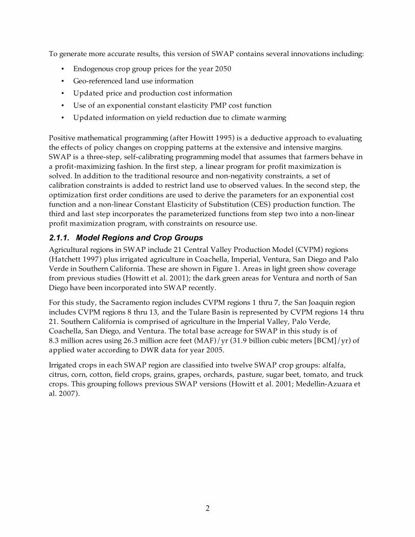
To generate more accurate results, this version of SWAP contains several innovations including:

• Endogenous crop group prices for the year 2050 • Geo-referenced land use information • Updated price and production cost information • Use of an exponential constant elasticity PMP cost function • Updated information on yield reduction due to climate warming

Positive mathematical programming (after Howitt 1995) is a deductive approach to evaluating the effects of policy changes on cropping patterns at the extensive and intensive margins. SWAP is a three-step, self-calibrating programming model that assumes that farmers behave in a profit-maximizing fashion. In the first step, a linear program for profit maximization is solved. In addition to the traditional resource and non-negativity constraints, a set of calibration constraints is added to restrict land use to observed values. In the second step, the optimization first order conditions are used to derive the parameters for an exponential cost function and a non-linear Constant Elasticity of Substitution (CES) production function. The third and last step incorporates the parameterized functions from step two into a non-linear profit maximization program, with constraints on resource use.

2.1.1. Model Regions and Crop Groups Agricultural regions in SWAP include 21 Central Valley Production Model (CVPM) regions (Hatchett 1997) plus irrigated agriculture in Coachella, Imperial, Ventura, San Diego and Palo Verde in Southern California. These are shown in Figure 1. Areas in light green show coverage from previous studies (Howitt et al. 2001); the dark green areas for Ventura and north of San Diego have been incorporated into SWAP recently.

For this study, the Sacramento region includes CVPM regions 1 thru 7, the San Joaquin region includes CVPM regions 8 thru 13, and the Tulare Basin is represented by CVPM regions 14 thru 21. Southern California is comprised of agriculture in the Imperial Valley, Palo Verde, Coachella, San Diego, and Ventura. The total base acreage for SWAP in this study is of 8.3 million acres using 26.3 million acre feet (MAF)/yr (31.9 billion cubic meters [BCM]/yr) of applied water according to DWR data for year 2005.

Irrigated crops in each SWAP region are classified into twelve SWAP crop groups: alfalfa, citrus, corn, cotton, field crops, grains, grapes, orchards, pasture, sugar beet, tomato, and truck crops. This grouping follows previous SWAP versions (Howitt et al. 2001; Medellin-Azuara et al. 2007).

3

Figure 1. Map of coverage of the Statewide Agricultural Production Model (SWAP)

2.1.2. SWAP Model Architecture The following section lays out the technical details of the SWAP model. For a more comprehensive treatment, see the references cited below.

A CES production function is defined and parameterized as in Howitt (2006). The elasticity of substitution between inputs is assumed to vary by crop but not by region. The specification of the generalized CES production function is:

/ ii

gi gi gij gijjY X

! ""# $% &=

' () (1)

Sub-index g corresponds to the CVPM region, i refers to crops and j to production factors or inputs. The model in this study has four inputs: land, labor, water, and supplies. Ygi represents the output for crop i in region or group g. The scale parameter of the CES production function is referred as � gi, whereas the share parameters for the resources for each crop are represented by

gij! . Xgij denotes usage of factor j in production of crop i in region g. The elasticity of

substitution for crop i is defined as � i and � i=( � i-1)/ � i. The returns to scale coefficient is given by � .

The first step in PMP is to obtain marginal values for the calibration constraints to enable the derivation of the cost function parameters in the second step. The linear program with calibration constraints is as follows:

landgigijgij

g i

gigix xayldvMax ,

j

0 )(! """ #=$ % (2)

4

jgbxa gj

i

landgigij ,,

!"# (3)

, , g,igi land gi landx x !" + #% (4)

Equation 2 is the objective function (profits) of the linear program. Decision variables are defined as follows: xgi,land are the total acres planted for region or group g and crop i. The marginal revenue per ton of crop i in region g is given by vgi and average yields are given by yldgj. Average variable costs, � gji, are used in the linear objective function 2. The Leontieff coefficients, agji, are given by the ratio of total factor usage to land.

Equations 3 and 4 represent the constraint set. Parameter bij is the regional limit on resource j. Constraint four (4) is for the upper bound calibration constraints,

,gi landx% is the observed value of resources usage, and � is small perturbation that decouples the resource and calibration constraints.

The second step in PMP estimation is to calculate parameters needed by the exponential cost function and the CES production function. The constant elasticity cost function is given by Equation 5 below:

igexTC landgigi x

gilandgilandgi , )( ,

,, !="

# (5)

� gi and � gi are the intercept and the elasticity parameter for the exponential acreage response function, respectively. These parameters are obtained from an ordinary least squares regression, with restrictions, on the PMP formulation and elasticity of supply for each crop group.

The last step in PMP is to solve a non-linear constrained profit maximization program. The objective function is defined as:

! "" """""#

$ %%= )(g ,

0,

i landjj

gijigj

g i

x

gi

g i

gigigix xeYvyredMax landgigi &'( (6)

subject to:

jgbx gj

i

gij ,!"# (7)

g,mxmetxmi

watergigimgm!"#

, (8)

gbavailwaterxm gwater

m

mg ,,

!"#$ (9)

In Equation 6, � gi is defined by the production function in Equation 1 above and the derivation of parameters � gi and � gij of the production function is detailed in Medellin-Azuara (2006). The second term in the equation is the PMP cost function, calibrated in the previous step. Constraint 7 is as in 3 above, except that all resources are included not just those limited by fixed quantities. In Equation 6, the parameter yredgi is a scaling factor for yield changes due to climate and technological change.

5

A new constraint on monthly water use has been included. Variable xmgm in Equation (8) is monthly water use in region g in month m. Three underlying assumptions need to be discussed. First, water is assumed to be interchangeable among crops within a region. Second, a farm group (or region) maximizes profits on a yearly basis, equalizing marginal revenue of water to its marginal cost every month. Third, a region or farm group selects the crop mix that maximizes profits within the region. In other words, the shadow value of water will be the same for all months and for all crops i in a region or farm group g. This assumes sufficient levels of water storage and internal water distribution capacity and flexibility. To accurately model the effects of snowpack and water storage reductions under warmer and drier climate scenarios CALVIN was used to generate water availability and shortage levels (Medellin-Azuara et al. 2008) in SWAP regions.

The last constraint set in Equation 9 is for regional water in which bwater,g corresponds to that in the right-hand side of Equation 7 for water. The parameter “availwater” is used later to obtain shadow values of water by constraining water regionally, such that 0 < availwater < 1. The constraint set assumes that yearly water is available in a limited amount for every region or group. Less realistically, it also implies that water is not re-traded across groups or regions under the basic calibration assumptions.

2.2. Model Innovations for Year 2050 In this study, modifications and assumptions for projections until 2050 follow Medellin-Azuara et al. (2007). Specifically, we consider land use projections (Landis and Reilly 2002), crop demand projections and yield changes as a result of technological improvement (Brunke et al. 2004) and climate change (Adams et al. 2003; Lee et al. 2008; Lobell et al. 2007). These innovations are applied to both models: 2050 under historical climate and 2050 under climate change.

2.2.1. Changes in Land Use Urbanization and agricultural land conversion in this study follow estimates from Landis and Reilly (2002) for prime farming land, locally important farms, unique farms, and grazing lands.

Table 1 shows statewide and regional land use patterns by the year 2050. Most of the land conversion from agriculture occurs south of the Sacramento Valley, where population growth is rapid. A statewide reduction in agricultural land use close to 5.0% is expected between years 2020 and 2050 (and of about 8.5% between 2005 and 2050. Changes in land use were applied to both 2050 standard (historical) and 2050 climate change (warm-dry) climate scenarios.

6

Table 1. Expected changes in land area between 2020 and 2050 (adapted from Landis and Reilly 2002) and CALVIN-SWAP region crop areas Urbanized Land Agricultural Land*

Regional Total Area, Acre (ha)

% Change

CALVIN Regional Total Area, Acre (ha)

% Change

2020 2050 2020 2050 Northern California and Sacramento

1,337,465 (540,737)

1,663,876 (660,576)

22.2 1,713,900 (693,590)

1,656,771 (670,495)

-3.3

San Joaquin Valley and Tulare

646,381 (261,587)

1,044,333 (422,224)

61.4 5,083,100 (2,057,057)

4,797,749 (1,941,649)

-5.6

Southern California 2,550,040 (1,030,981)

3,442,696 (1,391,882)

35.0 964,360 (390,262)

905,394 (366,413)

-6.1

Statewide 4,534,516 (1,833,305)

6,120,905 (2,474,682)

35.0

7,761,360 (3,140,911)

7,363,711 (2,980,094)

-5.1

*Note: For agriculture, Northern California includes Central Valley Production Model (CVPM) regions 1 to 7. The San Joaquin Valley and Tulare represents CVPM regions 8 to 21. Southern California considers projections of Landis and Reilly (2002) for agricultural areas in the counties that include Coachella, Imperial Valley, Palo Verde, and the counties of Ventura and San Diego.

2.2.2. Technological Change Technological change by year 2050 is represented as increasing crop yields. This is calculated based on extrapolating current trends as detailed in “Future Food Consumption and Production in California Under Alternative Scenarios” (Brunke et al. 2004). Current trends are detailed in Table 2, below. Growth rates marked with an asterisk (*) are unavailable and, consequently, are set equal to the average log-linear growth rate of 1.2. We assume that the rate of yield increases will level out in the future and we cap the extrapolations and use a slower rate of technical change from 2020–2050. Yield related technological growth is capped at 2020 since there is an inherent limit to the rate of carbon fixation through photosynthesis. Thus technology likely will not improve yields at the same rate indefinitely over time. Specifically, we assume a log-linear growth rate of 0.25 for 2020–2050. Based on the assumptions above the total rate of growth is extrapolated out and reported in Table 2.

7

Table 2. Technological change projection summary Technological Change by 2050

Crop Log-Linear Annual Growth Rate 2050 Total % Yield Increase Alfalfa 1.2* 29.05 Citrus 1.17 28.47 Corn 1.01 25.42 Cotton 1.2* 29.05 Field 1.2* 29.05 Grains 1.2* 29.05 Grapes 0.9 23.37 Orchards 1.57 36.41 Pasture 1.2* 29.05 Rice 1.35 31.98 Tomato 1.75 40.14 Truck 1.01 25.42

2.2.3. Shifts in Crop Demands for California Over time, the demand for California crops, with the exception of global commodities in the Grain, Rice, and Corn groups, is expected to increase with increasing population and incomes. As such, demands for crops in 2050 are changed to reflect population growth and income projections. This effect on crop demand is captured through the income elasticity of demand for California crops, income, and population growth. In the absence of alternative information on long-term trends in world crop production, the proportion of California crops exported is assumed to remain constant through 2050. Details of this method are laid out below.

First, we list the demand assumptions for Grain, Rice and Corn. The demand for California Grain, Rice and Corn is essentially perfectly elastic. This assumption is justified because there is no separate demand for these crop groups from California since they are global commodities, and California production is a small proportion of national production. As such, California can be seen as a price taker implying that demand is equal to price, and shifts in demand can be directly related to changes in world prices. As such, the only necessary information is long run projections of real prices. Forecasting long run prices for these crops is difficult with current conflicting evidence on the trends in agricultural prices. Over the last few years real prices have increased, which is in stark contrast to the historical downward trend. To reconcile these differences for use in our analysis we assume that prices will continue to trend up for several years into the future and will eventually resume the downward trend. The details of this analysis are as follows. We assume that prices will increase in accordance with the results of the World Bank’s report, Double Jeopardy: Responding to High Fuel and Food Prices (World Bank 2008) which projects price increases (in real terms) out to 2015. At 2015 we assume that real prices will resume the historic downward trend. We quantify this effect using UC Davis Agricultural Issues Center data, which shows the real prices of Corn, Grain, and Rice over the last 100 years. Using this data an exponential time trend regression is fit and used to project prices from 2015–2050. Results are summarized in (Table 3).

8

Table 3. Real (2005 dollars) percent changes in price, base 2005

Crop Group

% Change in Price by 2015 (Total)

% Change in Price 2015-2050 (per year)

% Shift in Demand Intercept (Total)

Rice 60 -1.45 -4.05 Corn 48 -0.67 17.00 Grain 40 -1.58 -19.88

The demand shift for all other crop groups is calculated using the following methodology. The U.S. population is expected to grow into the foreseeable future, and this will generate increased food demands. We assume that 1% increases in population will lead to 1% increases in food demand; in essence assuming a “population elasticity” of unity. According to the 2000 Census2 the U.S. population is projected to increase by approximately 5% every five years until 2030. These projections are based on the 2000 census and include five-year interval population projections until 2030. We use U.S. population growth as a proxy for total population-generated sources of increased California crop demand. Using the census results, we assume 5% growth every five years from present to 2020. From 2020–2050 we reduce the rate of population growth to 2.5%, half of current projections. At these growth rates, the U.S. population is expected to increase from approximately 290 million (base of 2005) to 415 million by 2050.

In addition to increasing population, real incomes are expected to increase. According to the Bureau of Labor Statistics3 average incomes in the United States have increased 6.9% annually between 1982–1992, 5.6% annually between 1992–2002, and are projected to increase 5.4% annually until 2012, nominally. Using this projection and extrapolating out to 2050 we assume incomes increase 5.4% on average annually. With 3.4% average historical inflation this is approximately 2% real annual income growth. Following the method for population expansion, we assume the real income growth rate is halved in 2020 to 1% real annual growth. Extrapolating out, average U.S. annual income is expected to increase from approximately $36,000 to $90,000 annually in real terms.

We assume that shifts in demand are solely a result of increasing incomes and population and that California’s export share grows in proportion to the domestic market. Income and population increases can be directly mapped to increases in quantity through respective elasticity estimates. Furthermore, for simplicity in calculations, we assume a perfectly elastic long run supply of each crop. As such, our estimates represent an upper bound on the demand shifts. Crop demands are linear, and we are interested in parallel shifts of demand, thus it is assumed that the increase in quantity produces a change in price that is constant at every quantity along the demand schedule.

Our calculations follow the methodology of Muth (1964), a seminal paper in equilibrium displacement models. Specifically, we calculate that the percentage shift in the intercept of the demand curve as a result of increasing incomes as: � =- � i/ � dln(I), where ! represents the percentage shift along the price axis,

i! is income elasticity of crop demand, ! is the own price

2 www.census.gov/population/www/projections/projectionsagesex.html. 3 www.bls.gov/opub/mlr/2007/11/art2full.pdf.

9

elasticity of demand, and ln( )d I is the change in log income over the relevant range (2005–2050 in our analysis). This equation is calculated separately for each crop and the procedure is repeated for changing population. As a proxy for “population elasticity” we assume unity, 1% increase in population leads to a proportional percentage increase in demand. The shifts from income changes and population are combined to determine the overall shift in demand. The details and derivation of this result can be found in Muth (1964), elasticity estimates and data are summarized in Table 4 below. It should be noted that the literature on income elasticity estimates is sparse and many, including authors of some studies used here, caution that these estimates often capture other unintended effects. As such, when reliable income elasticity estimates are unavailable, 0.2 is assumed for low value crops and 0.5 is assumed for high value crops; in Table 4 these are denoted by asterisks (*). Most of these estimates and references to others used can be found in the paper “Estimation of Supply and Demand Elasticities of California Commodities” (Green, Howitt, and Russo 2006).

Table 4. Elasticities by SWAP crop group Crop Group Income Elasticity Price Elasticity (D) Alfalfa 0.2* -0.107 Citrus 0.5* -1.25 Corn 0.2* -0.5 Cotton 0.05 -0.95 Field 0.2* -0.86 Grain 0.2 -0.38 Grapes 0.51 -0.28 Orchards 0.51 -1.2 Sugar beet 0.254 -0.042 Tomato 0.89 -0.25 Truck 0.99 -0.16

Using the Muth results and the elasticity estimates outlined above, the respective demand shifts are calculated. Based on the assumptions detailed above, calculated demand shifts are presented in Table 5, and two exceptions are denoted by asterisks (*). First, alfalfa is not calculated independently. Because alfalfa demand is largely tied to the expansion of livestock and substitution between grain and alfalfa, instead it is pegged to the field crop group which is estimated at 3.34. Similarly, due to the reduction in sugar beet processing facilities and other exogenous factors, we expect the level of California sugar beet production to be zero by 2050. All results are detailed in Table 5, below.

10

Table 5. Demand shifts Crop Group

% Shift in Demand Intercept

Alfalfa* 3.34 Citrus 3.63 Corn 5.74 Cotton 2.14 Field 3.34 Grain 7.56 Orchards 3.83 Grapes 16.42 Tomato 26.86 Truck 45.45

2.2.4. Model Innovations from Climate Change Changes in yields due to climate change follow Adams et al. (2003), as well as ongoing research by Lobell et al (2007) and Lee at al. (2008). Table 6 shows expected percent change in yields as a result of climatic change in GFDL2 for the Sacramento Basin, San Joaquin Delta. Citrus and orchard are projected to be the most affected crop groups under a warm-dry form of climate change. These shifts are one of the driving factors in the crop reaction to climate change.

Table 6. Expected percent change in yields as a result of a warm-dry climate scenario

Crop Groups Sacramento San

Joaquin Alfalfa 4.9 7.5 Citrus 1.77 -18.4 Corn -2.7 -2.5 Cotton 0.0 -5.5 Field -1.9 -3.7 Grain -4.8 -1.4 Orchards -9.0 -9.0 Pasture 5.0 5.0 Grape -6.0 -6.0 Rice 0.8 -2.8 Tomato 2.4 1.1 Truck Crops -11.0 -11.0 Sources: Adams et al. 2003; Lee et al. 2008; Lobell et a l . 2007

In addition to yield changes as a result of climate changes, the model results are driven by changes in available water under climate change. Available regional water supplies are determined from CALVIN model runs that optimize the statewide economic returns to all water uses under climate change. As such, the climate change model, relative to the historical model, incorporates water reductions by considering an optimal percentage decrease in water by region determined by simulating profitable water trades that could be realized with the existing water infrastructure. Table 7 summarizes this input, below. The regional allocations in the table reflect

11

water trades from agricultural to urban regions. Thus while the total average reduction in water deliveries is 14% the average reduction for agricultural regions is 21%, indicating that a statewide optimal market solution would induce voluntary sales of an additional 7% of agricultural water supplies to the urban sector to largely offset supply reductions. In the absence of such a market, the social costs of climate change would be significantly higher.

Table 7. Expected percentage reduction in available water

Region Agriculture Urban Total

Sacramento 24.3 0.1 19.1

San Joaquin 22.5 0.0 17.6

Tulare 15.9 0.0 13.5

Southern California 25.9 1.12 8.9

Total 21.0 0.7 14..0

2.2.5. Regional Crop Data in SWAP An example of a region in SWAP is shown in Table 8, which corresponds to CVPM region 19 (Figure 1). This region is distinct because it is within a single county (Kern) and has been used as a pilot for ongoing research on salinity south of the San Joaquin Delta (Howitt et al. 2008). Kern is within the service area of the State Water Project. Agricultural land use, recorded by parcel by DWR is at www.sjd.water.ca.gov; Table 8 shows agricultural land use at CVPM 19.

Table 8. Agricultural land use per crop groups at CVPM 19 Crop Acres Alfalfa 60,916 Citrus 2,399 Corn 16,469 Cotton 50,998 Field Crops 75,584 Grains 15,685 Grapes 6,199 Orchards 51,890 Pasture 2,474 Tomato 2,198 Truck Crops 57,361 Total 342,173

Source: DWR Land use surveys.

12

Figure 2. Land Use in CVPM region 19 Source: DWR Land use surveys.

2.3. Policy Simulations The use of inputs is based on Medellin-Azuara et al. (2007). Inputs to the production function in the model include water, labor, land and supplies. The last group of inputs was normalized to use per acre and comprises farm budgets on fertilizer pesticides and all other inputs. A constraint on corn silage was imposed on the optimization program to account for the feeding needs of dairy farm operations. The total California dairy herd is assumed to decline slightly from 1.503 million cows in 2005 to 1.25 million in 2050. This reduction in dairy cows in the Central Valley is based on restrictions that result from current dairy waste disposal technology, costs, and projected regulation (Howitt et al 2008). Corn used for silage tends to displace marginal field crops and cotton.

Analysis of agricultural activity for the year 2050 in SWAP is based on a set of algorithms that incorporate the 2050 adjustments discussed in the model description section. First, the land use from a linear programming program was constrained to the observed values of land use from DWR land use surveys and average production input use in the base years. Second, a PMP exponential cost function was calibrated so that, in the base case, input use from a non-linear optimization problem calibrates to observed values. The parameters for the CES production function are derived from the first order profit maximization conditions for each crop and region. Given these parameters, the calibrated non-linear program is used to simulate the economic effects of changes in crop yield parameters and policies.

3.0 Results This section details the results of the SWAP model runs. First, a pilot region, CVPM 19, is considered in detail to highlight the workings of SWAP and breadth of results. Next the state-

13

wide results are summarized. Since it is unwieldy to consider results from 26 separate regions results are aggregated into four “meso-regions” including Tulare Basin, Sacramento, San Joaquin and Southern California. Region-specific findings are highlighted and discussed in addition to universal findings. All results are discussed with the results from the 2050 historical climate conditions compared to results in 2050 under climate change.

3.1. Results for the Pilot Region The pilot region is CVPM 19, which was discussed in detail in Section 2.2.5. Table 9 summarizes changes in irrigated crop acres for CVPM 19 under historical climate and 2050 climate change (warm-dry) scenario. Comparing the projection under standard conditions to that under climate change conditions we note there are both positive and negative crop acreage changes. This is to be expected, as some crops suffer serious reductions under climate change and others are relatively resilient. As such, comparative advantage dictates adjustments by profit-maximizing farmers. This also takes into account the counteracting price effect on crops. However, it is important to note that this comparison is based on the direct effect of climate change.

Overall, results show that there is a significant reduction in water-intensive crops and moderate shifts in others. One important finding is that corn acreage is relatively constant under both climate scenarios. This is a direct result of the dairy industry, which necessitates a lower bound constraint on silage corn. Specifically, as discussed above, we assume that the California dairy industry will not be directly affected under climate scenarios, thus there will be a minimum amount of feed that is necessary. The model runs attain this lower bound, thus acreage is unaltered under climate change. Corn grown for sale as grain is essentially driven to zero by 2050.

Changes in water use per acre (intensive margin adjustments in economic parlance) are mixed under climate change and are shown in Table 10. It is important to note that these reflect contributions from CALVIN and assume socially optimal water markets in California, to be discussed more in Section 3.2. Results show that in CVPM 19 (Kern County) water use per acre of farmland is going to increase for most crops. This is a result of substitution between inputs and reduced farming acres. Since there are markets for water, CVPM 19 is able to buy supplies from northern regions. Model results indicate that the changes in applied water occur within reasonable ranges.

14

Table 9. Crop acreage in CVPM region 19 Crop Name 2050 Historical 2050 Climate Change % Change

Alfalfa 53,940 58,580 8.60

Citrus 2,448 2,408 -1.62

Corn 16,469 16,469 0.00

Cotton 46,433 45,778 -1.41

Field Crops 53,629 50,290 -6.23

Grains 14,222 14,302 0.57

Grapes 6,455 6,416 -0.60

Orchards 52,293 52,217 -0.15

Tomato 2,377 2,385 0.30

Truck Crops 61,085 60,505 -0.95

Total 309,352 309,352 8.60

Table 10. Changes by 2050 at the intensive margin (water use per acre) CVPM 19 Crop 2050 Historical

Applied Water per Acre

2050 Climate Change Applied Water per Acre

% Change

Alfalfa 4.38 4.41 0.58 Citrus 3.40 3.26 -4.08 Corn 3.59 3.42 -4.73 Cotton 2.88 2.76 -4.15 Field Crops 2.48 2.38 -3.90 Grains 1.62 1.58 -2.49 Grapes 2.97 2.89 -2.93 Orchards 3.22 3.21 -0.26 Tomato 3.61 3.54 -1.76 Truck Crops 2.11 2.02 -4.20

3.2. Statewide Results This section provides results for California under historical and climate change trends. For clarity, we group the 26 SWAP regions into four larger regions, namely Sacramento, San Joaquin, the Tulare Basin and Southern California. The Sacramento region includes CVPM regions 1 to 7, San Joaquin includes CVPM regions 8 to 13, Tulare Basin includes CVPM regions 14 to 21, and Southern California comprises agriculture in Coachella, Palo Verde, Imperial, Los Angeles, San Bernardino, San Diego, and Ventura.

Table 11 shows the land use under the standard 2050 climate and the 2050 climate change scenarios. The results under climate change reflect insights from the CALVIN water model. This assumes that by 2050 California has developed a reliable and economical method of transferring water between northern and southern regions, such as a peripheral canal.

15

Additionally, CALVIN posits that socially optimal water markets exist and function between regions in California. As such, this model presents an optimistic view of future water markets and infrastructure in California by 2050. Implications of CALVIN are further discussed below.

There is an overall land use reduction of 20.15% under climate change compared to standard climate scenarios. Results show that Sacramento and San Joaquin are the hardest-hit regions in terms of land use reductions. Since warm-dry (climate change) land use takes into account CALVIN water shortages for a warm-dry climate (Medellin-Azuara et al. 2008) and allows for water transfers through functioning water markets, we expect these regions to be water exporters as production shifts to higher-value crops in regions like Tulare. As such, there is a reduction in irrigated land in Sacramento as many farmers opt to sell water to southern regions. Similarly, Southern California land use reductions are dampened by the ability to import water. Land use changes are broken down by crop and summarized in more detail below.

Table 11. Base land use (in thousands of acres) per region

Scenario Sacramento San Joaquin Tulare Southern California Total

2050 Standard

1,920,878 1,886,535 953,569 2,966,229 7,727,211

2050 Climate Change

1,461,989 1,463,179 745,236 2,499,987 6,170,391

% Change

-23.89 -22.44 -21.85 -15.72 -20.15

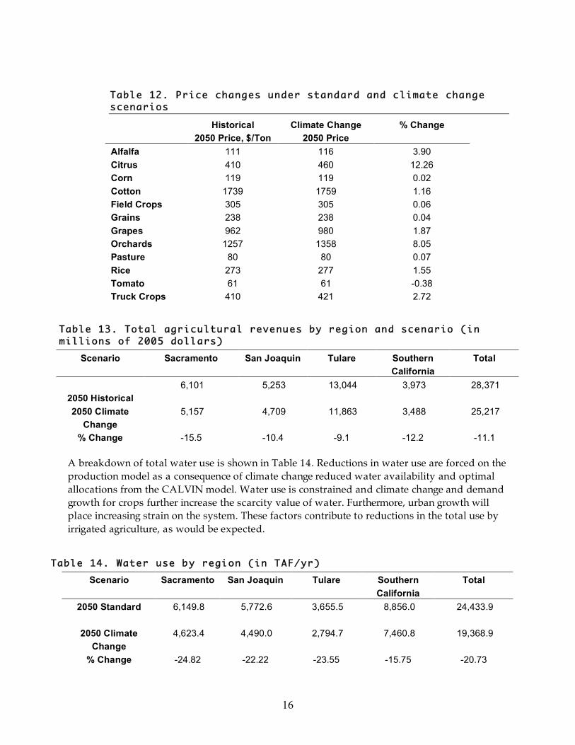
Tables Error! Reference source not found. and Error! Reference source not found. show respectively a decrease in land and various changes in prices. Error! Reference source not found. shows projected 2050 crop group prices (in 2005 dollars) under both scenarios. Most crop prices are expected to increase with climate change, although most changes are moderate. The only exception is tomato, due to a slight increase in production as it will be show below (Table ) resulting in increased acreage pushing down the price of the crop under climate change (Table 12).

Table 13 shows total agricultural revenues by region with and without climate change. Results show a varying ability of agricultural regions to adapt to climate change, which is to be expected. San Joaquin is the most affected with a 10.4% reduction in revenues. Clearly, over the time horizon considered, both the impact of climate change and the ability to adapt to it are most constrained in the Southern California region, which, however, shows the lowest impacts on revenue and land. The two effects of price increases and shifts in the mix of crops toward higher valued crops provide a partial offset to yield and acreage reductions from climate change. Note that a comparison of Tables 11 and 14 shows that the statewide reduction in irrigated land and water use are 20.15% and 20.73%, respectively; but the reduction in revenues is 11.1% (Table 13).

16

Table 12. Price changes under standard and climate change scenarios

Historical 2050 Price, $/Ton

Climate Change 2050 Price

% Change

Alfalfa 111 116 3.90 Citrus 410 460 12.26 Corn 119 119 0.02 Cotton 1739 1759 1.16 Field Crops 305 305 0.06 Grains 238 238 0.04 Grapes 962 980 1.87 Orchards 1257 1358 8.05 Pasture 80 80 0.07 Rice 273 277 1.55 Tomato 61 61 -0.38 Truck Crops 410 421 2.72

Table 13. Total agricultural revenues by region and scenario (in millions of 2005 dollars)

Scenario Sacramento San Joaquin Tulare Southern California

Total

2050 Historical

6,101 5,253 13,044 3,973 28,371

2050 Climate Change

5,157 4,709 11,863 3,488 25,217

% Change -15.5 -10.4 -9.1 -12.2 -11.1 A breakdown of total water use is shown in Table 14. Reductions in water use are forced on the production model as a consequence of climate change reduced water availability and optimal allocations from the CALVIN model. Water use is constrained and climate change and demand growth for crops further increase the scarcity value of water. Furthermore, urban growth will place increasing strain on the system. These factors contribute to reductions in the total use by irrigated agriculture, as would be expected.

Table 14. Water use by region (in TAF/yr)

Scenario Sacramento San Joaquin Tulare Southern California

Total

2050 Standard

6,149.8 5,772.6 3,655.5 8,856.0 24,433.9

2050 Climate Change

4,623.4 4,490.0 2,794.7 7,460.8 19,368.9

% Change -24.82 -22.22 -23.55 -15.75 -20.73

17

18

SWAP model results show that climate changes induces changes in price, reduced yields, reduced land use and reduced revenue under climate change relative to historical climate. Table 15 shows change in price, production, and revenue for each crop group, broken down across all regions. Revenue losses stem from changes in price, production, or both. For example, tomato is expected to experience a decrease close to 0.4% in its price per ton; however, an increase in production yields leads to a net positive change in total revenues (the product of yields, acreage, and crop price). Other crops, like orchards, may face a large increase in price but a large decrease in production yields, which ultimately result in an overall loss in revenues. This seemingly counterintuitive result is likely a result of shifting regional production and the availability of water markets.

Table 15. Percentage change price, production, revenue (historical vs. warm-dry climate scenarios) for year 2050

Crop Group

% Change Price % Change Production % Change Revenues

Alfalfa 3.90 -6.2 -3.20

Citrus 12.26 -18.7 -8.36 Corn 0.02 -22.9 -22.61 Cotton 1.16 -23.6 -20.59 Field 0.06 -48.9 -48.40 Grains 0.04 -31.3 -30.05 Grapes 1.87 -7.3 -5.60 Orchards 8.05 -10.2 -2.94 Pasture 0.07 -95.7 -95.70 Rice 1.55 -22.4 -21.22 Tomato -0.38 1.4 0.96 Truck 2.72 -13.3 -10.88 A more comprehensive table of disaggregated land use by region is shown below in tables 16 and 17. Total land use for all crops under both climate scenarios is shown in Table 18. To better illustrate adaptation, the last column of Table 18 shows how the proportion of each crops changes with respect to the total crop mix. Land use share decreases for some water-intensive crop groups such as field crops and grains. This is mostly caused by water shortages on the order of 20% estimated in CALVIN under a warm-dry climate. Therefore under a warm-dry climate the crop mix becomes higher valued and less water intensive, despite the likely loss in climate-related agricultural yields.

19

Table 16. Land use (in acres) per crop and region under 2050 historical climate

Historical 2050 Climate Scenario Crop Name Sacramento San Joaquin Tulare Southern

California Total

Alfalfa 74,124 242,178 325,766 186,327 828,394

Citrus 28,719 7,148 215,332 121,240 372,440

Corn 26,066 267,556 208,385 9,366 511,374

Cotton 1,244 105,676 499,435 25,887 632,242

Field Crops 377,633 476,446 424,512 68,325 1,346,916

Grains 41,724 64,115 158,571 225,106 489,517

Grapes 13,755 253,176 351,088 15,362 633,381

Orchards 23,618 209,671 512,260 1,514 747,062

Pasture 63,882 102,743 3,764 81,067 251,456

Rice 541,104 14,244 555,348

Tomato 79,510 113,094 125,621 89 318,313

Truck Crops 649,499 30,487 141,496 219,286 1,040,768

Total 1,920,878 1,886,535 2,966,229 953,569 7,727,211

Table 17. Land use (in acres) per crop and region under 2050 climate change

Warm-Dry 2050 Climate Scenario Crop Name Sacramento San Joaquin Tulare Southern

California Total

Alfalfa 57,087 238,463 270,885 158,942 725,377

Citrus 28,689 7,148 209,536 120,980 366,353

Corn 10,567 207,421 187,954 405,942

Cotton 76,151 425,219 8,363 509,732

Field Crops 208,018 272,338 160,928 60,097 701,381

Grains 0 41,794 126,860 163,458 332,113

Grapes 13,553 251,128 345,595 15,215 625,491

Orchards 22,453 207,743 505,850 1,644 737,691

Pasture 7,101 2,811 9,912

Rice 416,583 11,104 427,687

Tomato 78,306 112,819 125,466 92 316,685

Truck Crops 626,734 29,970 138,881 216,443 1,012,028

Total 1,461,989 1,463,179 2,499,987 745,236 6,170,391

20

Table 18. Total land use (in acres) by crop under climate scenarios

Crop Name Historical Climate Change Total

% Change Acres

%Change in Crop share

Alfalfa 828,394 725,377 -12.4 9.66

Citrus 372,440 366,353 -1.6 23.18 Corn 511,374 405,942 -20.6 -0.59 Cotton 632,242 509,732 -19.4 0.96 Field Crops 1,346,916 701,381 -47.9 -34.79 Grains 489,517 332,113 -32.2 -15.04 Grapes 633,381 625,491 -1.2 23.67 Orchards 747,062 737,691 -1.3 23.66 Pasture 251,456 9,912 -96.1 -95.06 Rice 555,348 427,687 -23.0 -3.56 Tomato 318,313 316,685 -0.5 24.59 Truck Crops 1,040,768 1,012,028 -2.8 21.77 Total 828,394 725,377 -20.1 As shown, total land use changes and crop substitution occurs in response to climate change. Large reductions occur in pasture, field crops, grains, and rice; water intensive activities that have seen recent declines in California. Note that the crops most heavily affected are water-intensive or low-value crops; more resilient crops include, higher-value, price responsive crops such as grapes and tomatoes.

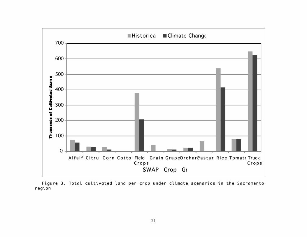
For more clarity Figures 3-6 show agricultural land use graphically. The figures that follow compare 2050 Historical and 2050 warm-dry (climate change) scenarios.

21

0

100

200

300

400

500

600

700

A l f a l f aC i t r u s C o r n Co t tonField

C r o p s

G r a i n sG r a p e sO r c h a r d sP a s t u r eR i c e TomatoTruck

C r o p s

SWAP Crop Group

Historical Climate Change

Figure 3. Total cultivated land per crop under climate scenarios in the Sacramento

region

22

0

50

100

150

200

250

300

350

400

450

500

A l f a l f aC i t r u s C o r n Co t tonField

C r o p s

G r a i n sG r a p e sO r c h a r d sP a s t u r eR i c e TomatoTruck

C r o p s

SWAP Crop Group

Historical Climate Change

Figure 4. Total cultivated land per crop under climate scenarios in the San Joaquin

Basin

23

0

200

400

600

800

1,000

1,200

A l f a l f aC i t r u s C o r n Co t tonField

C r o p s

G r a i n sG r a p e sO r c h a r d sP a s t u r eR i c e TomatoTruck

C r o p s

SWAP Crop Group

Historical Climate Change

Figure 5. Total cultivated land per crop under climate scenarios in the Tulare Basin

24

0

50

100

150

200

250

A l f a l f aC i t r u s C o r n Co t ton Field

C r o p s

G r a i n sG r a p e sO r c h a r d sP a s t u r eTomato Truck

C r o p s

SWAP Crop Group

Historical Climate Change

Figure 6. Total cultivated land per crop under climate scenarios in Southern California

25

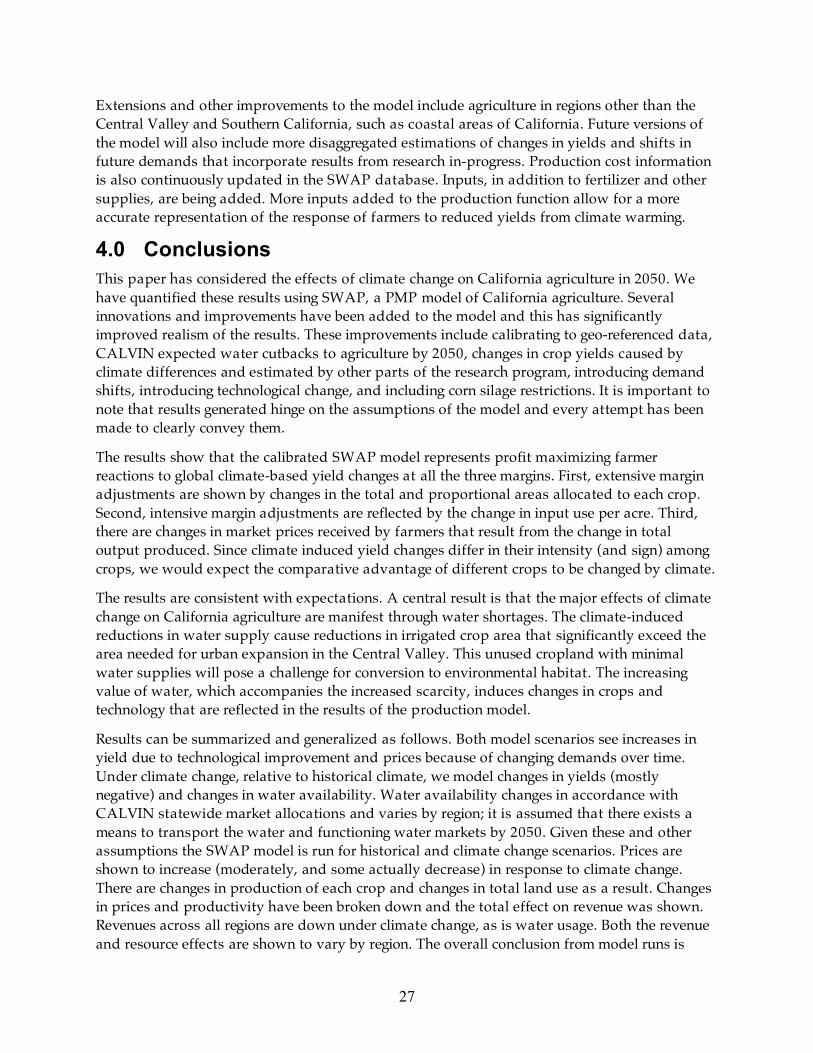
Figure 7 shows percent differences between Historical and Climate Change Scenarios in 2050 for all regions and crops in the study. As discussed above, both the total land use and relative cropping patterns are shown to change between the regions.

Sacramento sees the largest reductions in both water-intensive and low-value crops. This is because CALVIN, used to generate optimal regional water allocations under climate change, assumes there are markets for water and a means to transport the water. Consequently, it becomes more profitable for farmers in the Sacramento region to sell water to southern regions. Those crops that are still profitable to continue growing tend to be the high-value crops with significant increases in both yield and demand in California.

San Joaquin shows significant reductions in crop acreage as well. Referring to Table 7 and noting that average water reductions are 17%, we see that San Joaquin is a large exporter of water. This is a result of comparative advantages in other California regions and high-value crop production shifts to regions like Tulare. Tulare follows a similar pattern of land reductions, although effects are less dramatic as they import water from other regions, Sacramento and San Joaquin, to provide water for high value crops.

Southern California is shown to have relatively small percent changes in acres between the climate scenarios. It is important to note that while there is less change in percentage terms, the Southern California regions have fewer planted acres under both scenarios. The availability of water markets allow for the reduced impact on total acres.

We should emphasize that these shifts in land use are in contrast to the substantial economic effects of climate change on total revenue, as discussed above. Results indicate that revenues are expected to go down by less than the land and water reductions, which is consistent with economic theory.

3.3. Model Limitations and Extensions The model results for 2050 should be viewed as a plausible scenario that results from the most probable assumptions. Given the very long time horizon required in this study, the results should not be considered a projection or forecast, but as a probable outcome of the interaction of several uncertain driving forces. California agriculture has always been driven by the interactions between technology, resources, and market demands, and future production can be viewed as a balance between the rates of change in these three variables. Accordingly, we have attempted to make the assumptions, mathematics, and the parameter values used in this study as transparent as possible to enable the reader to assess the basis for the results.

Limitations of this model have been discussed in Medellin-Azuara (2007) and in Howitt et al. 2001). SWAP is in the process of major updates to address most of these limitations. Worthwhile discussing here is that estimated changes in yields from other studies vary widely depending on the set of considerations. These considerations include CO2 fertilization, location, and crop variety. Another limitation is that some SWAP crop categories are coarse, and yields may vary within each category. Risk preferences are implicit in the calibrated production model of SWAP,

26

-100

-90

-80

-70

-60

-50

-40

-30

-20

-10

0

10

Sacramento San Joaquin Tu l a r e Southern California

Figure 7. Percent change in land use under climate scenarios for all crops and regions

27

Extensions and other improvements to the model include agriculture in regions other than the Central Valley and Southern California, such as coastal areas of California. Future versions of the model will also include more disaggregated estimations of changes in yields and shifts in future demands that incorporate results from research in-progress. Production cost information is also continuously updated in the SWAP database. Inputs, in addition to fertilizer and other supplies, are being added. More inputs added to the production function allow for a more accurate representation of the response of farmers to reduced yields from climate warming.

4.0 Conclusions This paper has considered the effects of climate change on California agriculture in 2050. We have quantified these results using SWAP, a PMP model of California agriculture. Several innovations and improvements have been added to the model and this has significantly improved realism of the results. These improvements include calibrating to geo-referenced data, CALVIN expected water cutbacks to agriculture by 2050, changes in crop yields caused by climate differences and estimated by other parts of the research program, introducing demand shifts, introducing technological change, and including corn silage restrictions. It is important to note that results generated hinge on the assumptions of the model and every attempt has been made to clearly convey them.

The results show that the calibrated SWAP model represents profit maximizing farmer reactions to global climate-based yield changes at all the three margins. First, extensive margin adjustments are shown by changes in the total and proportional areas allocated to each crop. Second, intensive margin adjustments are reflected by the change in input use per acre. Third, there are changes in market prices received by farmers that result from the change in total output produced. Since climate induced yield changes differ in their intensity (and sign) among crops, we would expect the comparative advantage of different crops to be changed by climate.

The results are consistent with expectations. A central result is that the major effects of climate change on California agriculture are manifest through water shortages. The climate-induced reductions in water supply cause reductions in irrigated crop area that significantly exceed the area needed for urban expansion in the Central Valley. This unused cropland with minimal water supplies will pose a challenge for conversion to environmental habitat. The increasing value of water, which accompanies the increased scarcity, induces changes in crops and technology that are reflected in the results of the production model.

Results can be summarized and generalized as follows. Both model scenarios see increases in yield due to technological improvement and prices because of changing demands over time. Under climate change, relative to historical climate, we model changes in yields (mostly negative) and changes in water availability. Water availability changes in accordance with CALVIN statewide market allocations and varies by region; it is assumed that there exists a means to transport the water and functioning water markets by 2050. Given these and other assumptions the SWAP model is run for historical and climate change scenarios. Prices are shown to increase (moderately, and some actually decrease) in response to climate change. There are changes in production of each crop and changes in total land use as a result. Changes in prices and productivity have been broken down and the total effect on revenue was shown. Revenues across all regions are down under climate change, as is water usage. Both the revenue and resource effects are shown to vary by region. The overall conclusion from model runs is

28

that, while the effect of climate change is manifest through yield changes, after economic adaptation, the results on irrigated crop production are predominately shown in economic terms and changes in aggregate land and water use. There are very significant reductions in irrigated acres that range regionally from 16% to 24%, and 9% to 16% reductions in revenues due to partial offsets from price and crop changes.

5.0 References Adams, R. M., J. Wu, and L. L. Houston. 2003. Climate Change and California, Appendix IX: The

effects of climate change on yields and water use of major California crops. California Energy Commission, Public Interest Energy Research (PIER), Sacramento, California.

Bloom, A. J., M. Burger, L. B. Randall, A. Cousins, and S. Rachmilevitch. "Nitrate Assimilation and Photorespiration." University of California, Davis.

Brunke, H., D. Sumner, and R. E. Howitt. 2004. "Future Food Production and Consumption in California Under Alternative Scenarios." Agricultural Issues Center, University of California, Davis, California.

Green, R., R. Howitt, and C. Russo. 2006. "Estimaion of Supply and Demand Elastiticies of California Commodities." Working Paper. Department of Agricultural and Resource Economics. Universtity of California, Davis. Davis, California.

Hatchett, S. 1997. Draft methodology/modelling technical appendix: CVPM. Central Valley Project Improvement Act. Programmatic Environmental Impact Statement. U.S. Bureau of Reclamation, Technical Appendix volume 8, Sacramento, California.

Howitt, Richard E. 1995. “Positive Mathematical Programming.” American Journal of Agricultural Economics 77: 329–342.

Howitt, R., J. Kaplan, D. Larson, D. MacEwan, J. Medellin-Azuara, N. Lee, and G. Horner. 2008. Central Valley Salinity Report. Report for the State Water Resources Control Board. University of California, Davis, California.

Howitt, R. E., K. B. Ward, and S. Msangi. 2001. "Statewide Agricultural Production Model." University of California, Davis. Davis, California.

Jenkins, M. W., A. J. Draper, J. R. Lund, R. E. Howitt, S. K. Tanaka, R. Ritzema, G. F. Marques, S. M. Msangi, B. D. Newlin, B. J. Van Lienden, M. D. Davis, and K. B. Ward. 2001. Improving California Water Management: Optimizing Value and Flexibility. University of California Davis. Davis, California.

Landis, J. D., and M. Reilly. 2002. How We Will Grow: Baseline Projections of California’s Urban Footprint Through the Year 2100. Project Completion Report, Department of City and Regional Planning, Institute of Urban and Regional Development, University of California, Berkeley. Berkeley, California.

Lee, J., S. De Gryze, and J. Six. 2008. Effect of Climate Change on Field Crop Production in the Central Valley of California. California Energy Commission, Public Interest Energy Research (PIER), Sacramento, California.

29

Lobell, D. B., K. N. Cahill, and C. B. Field. 2007. "Historical effects of temperature and precipitation on California crop yields." Climatic Change 81(2): 187–203.

Lund, J. R., E. Hanak, W. Fleenor, W. Bennett, R. Howitt, and P. Moyle. 2008. Comparing Futures for the Sacramento-San Joaquin Delta. Public Policy Institute of California.

Lund, J. R., E. Hanak, W. Fleenor, R. Howitt, J. Mount, and P. Moyle. 2007. Envisioning Futures for the Sacramento-San Joaquin River Delta. Public Policy Institute of California, San Francisco, California.

Medellín-Azuara, J., C. R. Connell, K. Madani, J. R. Lund, and R. E. Howitt. 2008. Water Management Adaptation with Climate Change. California Energy Commission, Public Interest Energy Research (PIER). Sacramento, California.

Medellín-Azuara, J., R. E. Howitt, and J. R. Lund. 2007. California agricultural water demands for year 2050 under historic and warming climates. California Energy Commission. Public Interest Energy Research (PIER). Sacramento, California.

Medellín-Azuara, J. 2006. Economic-Engineering Analysis of Water Management for Restoring the Colorado River Delta, Dissertation, University of California, Davis, 146 pp.

Muth, R. F. 1964. "The Derived Demand Curve for a Productive Factor and the Industry Supply Curve." Oxford Economic Papers New Series, 16(2): 221–234.

Schlenker, W., W. Michael Hanemann, and Anthony C. Fisher. 2005. "Will U.S. Agriculture Really Benefit from Global Warming? Accounting for Irrigation in the Hedonic Approach." American Economic Review, 95(1)395-406.

World Bank. 2008. Double Jeopardy: Responding to High Fuel and Food Prices. G8 Hokkaido-Toyako Summit. July 2.Adams, R. M., Wu, J., and Houston, L. L. 2003. "Climate Change and California, Appendix IX: The effects of climate change on yields and water use of major California crops." California Energy Commission, Public Interest Energy Research (PIER), Sacramento, California.

30

6.0 Glossary af acre-foot

AIC University of California Agricultural Issues Center

BCM Billion cubic meters

CALVIN University of California, Davis Economic-Engineering Water Model

CES constant elasticity of substitution

CVPM Central Valley Production Model

DWR California Department of Water Resources

MAF million acre feet

PMP positive mathematical programming

SWAP Statewide Agricultural Production Model

TAF thousand acre-foot

UC Davis University of California, Davis

USDA United States Department of Agriculture