This article was downloaded by: [Monica Bocco]On: 22 November 2011, At: 09:47Publisher: Taylor & FrancisInforma Ltd Registered in England and Wales Registered Number: 1072954 Registeredoffice: Mortimer House, 37-41 Mortimer Street, London W1T 3JH, UK

International Journal of RemoteSensingPublication details, including instructions for authors andsubscription information:http://www.tandfonline.com/loi/tres20

Estimating soybean ground cover fromsatellite images using neural-networksmodelsMonica Bocco a , Gustavo Ovando a , Silvina Sayago a , EnriqueWillington a & Susana Heredia aa Facultad de Ciencias Agropecuarias, Universidad Nacional deCórdoba, Córdoba, 5000, Argentina

Available online: 22 Aug 2011

To cite this article: Monica Bocco, Gustavo Ovando, Silvina Sayago, Enrique Willington & SusanaHeredia (2012): Estimating soybean ground cover from satellite images using neural-networksmodels, International Journal of Remote Sensing, 33:6, 1717-1728

To link to this article: http://dx.doi.org/10.1080/01431161.2011.600347

PLEASE SCROLL DOWN FOR ARTICLE

Full terms and conditions of use: http://www.tandfonline.com/page/terms-and-conditions

This article may be used for research, teaching, and private study purposes. Anysubstantial or systematic reproduction, redistribution, reselling, loan, sub-licensing,systematic supply, or distribution in any form to anyone is expressly forbidden.

The publisher does not give any warranty express or implied or make any representationthat the contents will be complete or accurate or up to date. The accuracy of anyinstructions, formulae, and drug doses should be independently verified with primarysources. The publisher shall not be liable for any loss, actions, claims, proceedings,demand, or costs or damages whatsoever or howsoever caused arising directly orindirectly in connection with or arising out of the use of this material.

International Journal of Remote SensingVol. 33, No. 6, 20 March 2012, 1717–1728

Estimating soybean ground cover from satellite images usingneural-networks models

MONICA BOCCO*, GUSTAVO OVANDO, SILVINA SAYAGO, ENRIQUEWILLINGTON and SUSANA HEREDIA

Facultad de Ciencias Agropecuarias, Universidad Nacional de Córdoba, Córdoba 5000,Argentina

(Received 7 June 2010; in final form 1 June 2011)

The ground cover is a necessary parameter for agronomic and environmental appli-cations. In Argentina, soybean (Glycine max (L.) Merill) is the most importantcrop; therefore it is necessary to determine its amount and configuration. In thiswork, neural-network (NN) models were developed to calculate soybean percent-age ground cover (fractional vegetation cover, fCover) and to compare the accuracyof the estimate from Moderate-Resolution Imaging Spectroradiometer (MODIS)and Landsat satellites data. The NN design included spectral values of the redand near-infrared (NIR) bands as input variables and one neuron output, whichexpressed the estimated coverage. Data of fCover were acquired throughout thegrowing season in the central plains of Córdoba (Argentina); they were used fortraining and validating the networks. The results show that the NNs are an appro-priate methodology for estimating the temporal evolution of soybean coveragefraction from MODIS and Landsat images, with coefficients of determination (R2)equal to 0.90 and 0.91, respectively.

1. Introduction

Plant canopy regulates exchanges of mass and energy and controls the operation ofhydrological processes through modification of the infiltration, runoff and evapotran-spiration (Cayrol et al. 2000). The density of foliage is used in crop growth and energybalance models and as a mean of quantifying the crop variability in precision agri-culture (Walthall et al. 2004). So, also, the importance of including vegetation coverin climatic and hydrological models as a dynamic component is widely recognized(Montaldo et al. 2005, Donohue et al. 2007, Guerschman et al. 2009). The amountand duration of leaf area available for photosynthesis influence the crop’s growth andyield (Daughtry et al. 1984).

The amount of vegetation can be described, among others, from the leaf area index(LAI) and the fractional vegetation cover (fCover). The LAI refers to photosynthet-ically active leaf area per soil unit area and the fCover is the fraction of groundcovered by vegetation (Fensholt et al. 2004). Mauget and Upchurch (2000) used acoverage measurement method based on the classification through maximum likeli-hood of high-resolution digital photographs, discriminating illuminated and shadedvegetation areas and illuminated and shaded bare soil areas.

*Corresponding author. Email: mbocco@agro.unc.edu.ar

International Journal of Remote SensingISSN 0143-1161 print/ISSN 1366-5901 online © 2012 Taylor & Francis

http://www.tandf.co.uk/journalshttp://dx.doi.org/10.1080/01431161.2011.600347

Dow

nloa

ded

by [

Mon

ica

Boc

co]

at 0

9:47

22

Nov

embe

r 20

11

1718 M. Bocco et al.

Accurate measurement of the amount and configuration of crops is tedious andtime consuming due to the spatial variability inherent to them. Satellite data providea spatially and periodic comprehensive view of the actual state of the crops (Daughtryet al. 1984, Jiang et al. 2006, Numata et al. 2007).

Over the past few decades, several spectral vegetation indices (VIs) have been devel-oped and used to estimate a vegetation canopy’s biophysical properties at a rangeof spatial scales (Danson et al. 2003, Jiang et al. 2006). These indices combinespectral reflectance from two or more wavebands (generally red and near-infrared(NIR)) to improve sensitivity to plant vegetation. The basis of this relationship isthe strong absorption (low reflectance) of red light by chlorophyll and low absorp-tion (high reflectance and transmittance) in the NIR by green leaves (Shanahan et al.2001). Hatfield et al. (2008) stated that many of the current VIs are based on broadwavebands closely associated with Landsat Thematic Mapper (Landsat-TM) satellitewavebands. At the canopy level, the changes of reflectance are the largest in the NIRwavelengths throughout the growing season, due to increase in biomass.

The high spatial resolution (30 m) from Landsat would be more suitable in areaswhere the field sizes are small, but the temporal frequency (16 days) and, eventu-ally, cloud cover limit the retrieval of crop biophysical parameters that are rapidlychanging during the season (Chen et al. 2005, Doraiswamy et al. 2005). The spatialresolution (250 m) and temporal (daily) coverage of Moderate-Resolution ImagingSpectroradiometer (MODIS) sensor data offer potential for retrieval of biophysi-cal parameters of extensive crops (Doraiswamy et al. 2004). However, the relativelycoarse spatial resolution may subsume significant heterogeneity in vegetation and,hence, introduce error. Potapov et al. (2008) validated correlation results when esti-mating forest cover in 18.5 km side size blocks obtained from MODIS and Landsatdata.

There are two types of methods to estimate biophysical variables from reflectancedata (Weiss et al. 2002, Walthall et al. 2004). Empirical approaches based on a rela-tion between land surface reflectance data or VI and some biophysical variables, forexample, linear and non-linear regression, look-up tables and neural networks (NNs);and physical approaches based on inversion of canopy reflectance models.

NNs appear to be quite powerful and easy to operationally implement because theyhave the ability to compute, process, predict and classify data (Bocco et al. 2007,Verger et al. 2008); they also allow adjustment of a response even with a complexand non-linear problem, input–output mapping, adaptivity, generalization and faulttolerance (Panda et al. 2010).

NNs consist of a system of interconnected neurons, or nodes, that transmitinformation among themselves, which give a result through mathematical functions(Trombetti et al. 2008). An important feature of non-parametric models, whichinclude NNs, is that they do not require a prior assumption about the statisticalbehaviour or about any specific relationship between variables. These models usethe data itself to extract the relationship between the inputs and their correspondingoutputs (Lakhankar et al. 2009).

Baret et al. (1995), estimating canopy gap fraction in sugar beet, compared theperformance of classical VI and backpropagation NNs. They expressed that both tech-niques can estimate accurately the desired variable using red and NIR reflectances,although they expressed that the applicability of the empirical approach is generallyrestricted to the conditions that prevailed during the experiments. Using the samemethodology, Baret et al. (2007) estimated fCover from Satellite Pour l’Observationde la Terre – Vegetation (SPOT VEGETATION) information, training the networks

Dow

nloa

ded

by [

Mon

ica

Boc

co]

at 0

9:47

22

Nov

embe

r 20

11

Models for estimations from satellite images 1719

with output from the Prospect Model + Scattering from Arbitrarily Inclined LeavesModel (PROSPECT+SAIL) (Jacquemoud et al. 2009).

Soybean (Glycine max (L.) Merrill) is the most important crop in Argentina,considering the economic yield obtained by farmers and the sown surface (16 × 106 hain 2007–2008; Ministerio de Agricultura, Ganadería y Pesca de la Nación (MAGyP)2009). The province of Córdoba is the first producer of soybean in Argentina withapproximately 4 527 200 ha cultivated in 2007–2008 according to estimations made byMAGyP (2009).

The objective of this work was to develop NN models to calculate soybean groundcover and to compare the accuracy of the estimate from the reflectance values fromthe MODIS and Landsat satellites.

2. Data and methods

2.1 Study area

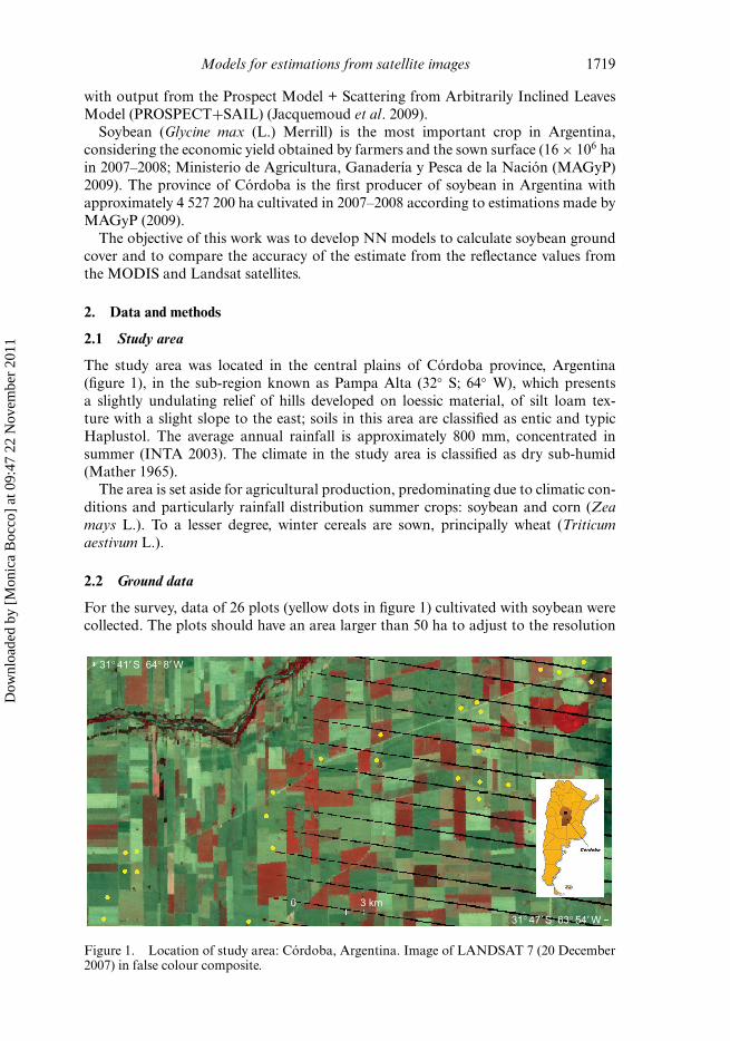
The study area was located in the central plains of Córdoba province, Argentina(figure 1), in the sub-region known as Pampa Alta (32◦ S; 64◦ W), which presentsa slightly undulating relief of hills developed on loessic material, of silt loam tex-ture with a slight slope to the east; soils in this area are classified as entic and typicHaplustol. The average annual rainfall is approximately 800 mm, concentrated insummer (INTA 2003). The climate in the study area is classified as dry sub-humid(Mather 1965).

The area is set aside for agricultural production, predominating due to climatic con-ditions and particularly rainfall distribution summer crops: soybean and corn (Zeamays L.). To a lesser degree, winter cereals are sown, principally wheat (Triticumaestivum L.).

2.2 Ground data

For the survey, data of 26 plots (yellow dots in figure 1) cultivated with soybean werecollected. The plots should have an area larger than 50 ha to adjust to the resolution

31° 41′ S 64° 8′ W

31° 47′ S 63° 54′ W

0 3 km

Figure 1. Location of study area: Córdoba, Argentina. Image of LANDSAT 7 (20 December2007) in false colour composite.

Dow

nloa

ded

by [

Mon

ica

Boc

co]

at 0

9:47

22

Nov

embe

r 20

11

1720 M. Bocco et al.

of the MODIS sensor. The sampling was carried out in the middle of Landsat imagewhere the missing data due to Scan Line Corrector off (SLC-off) were minimal.

Soybean cultivation in this region is done by direct sowing of transgenic varietiesresistant to glyphosate, with maturity groups between 3 and 4, and spacing of 32 cmbetween rows, without fertilizer application (Piatti and Ferreyra 2009).

Field data were acquired continuously throughout the growing season (16November 2007–14 April 2008), from V1 (soybean first trifoliate leaf stage) to R7(soybean beginning maturity) (Fehr et al. 1971). Although on some dates and plots,the acquisition of field data was not possible due to sowing, irrigation and harvestingoperations.

In this region, soybean shows a uniform distribution, so only three digital pho-tographs from 1.5 m height in each plot was used for estimating the percentage ofgreen coverage (fCover). These digital photographs were classified into two classes:green vegetation (soybean) and soil, using the maximum likelihood methodology. Forall plots and samples, fCover ranged between 0% and 98% with a standard deviationfor each plot and acquisition date below 5%, for more than 75% of the samples.

2.3 Satellite data

2.3.1 MODIS. Eleven images from AQUA satellite were used for the growing sea-son; these came from the MODIS–MYD13Q1/Aqua 16-Day integrated L3 Global250 m spatial resolution as a gridded level-3 product in the sinusoidal projection(SIN Grid), and were obtained by the Land Processes Distributed Active ArchiveCenter (LPDAAC)–US Geological Center (USGS) for Earth Resources Observationand Science (EROS) Data Center, located in Sioux Falls, SD, USA.

Daily images in a continuous time series do not always precisely describe thecondition of vegetation during the growing season, since contamination by cloudsdecreases the VI value. Consequently, the solution is to retain a high temporal res-olution uncovering and removing cloudy pixels from daily images, thus creatingnormalized difference vegetation index (NDVI) composite images of 10–15 days onlywith data taken during the smallest cloud contamination days (Báez-González et al.2002). The MYD13Q1 reflectance values in red (RED_MOD, 620–670 nm) and NIR(NIR_MOD, 841–876 nm) were used as input for the central pixel in each of the 26plots.

2.3.2 Landsat-TM and Enhanced Thematic Mapper Plus. Five images from Landsatsatellites, obtained on clear days were used for the same period, four of these belongto the Landsat 7 Enhanced Thematic Mapper Plus (ETM+) and the remaining toLandsat 5 TM (1 March 2008, table 1). The Landsat 7 keeps the spatial (30 m), tem-poral (16 days) and radiometric resolution from Landsat 5, and also maintains thebands’ spectral resolution in visible and infrared parts (bands 1, 2, 3, 4, 5 and 7).

For this work, the bands of Landsat scenes in red (RED_TM, 630–690 nm, band 3)and NIR (NIR_TM, 760–900 nm, band 4) were used. To avoid taking null value dueto SLC-off, for example without the image effects caused by the SLC failure aboardLandsat 7), data from the innermost pixel with valid information was recorded in eachof these same 26 plots. Digital counts were converted to spectral radiance prior toanalysis according to the methodology proposed by Chavez (1989) and implementedby Gürtler et al. (2005).

Dow

nloa

ded

by [

Mon

ica

Boc

co]

at 0

9:47

22

Nov

embe

r 20

11

Models for estimations from satellite images 1721

Table 1. Dates of acquisition of field samples and satellite data.

Field data MODIS Landsat

16 November 2007 9 November 200712 December 2007 25 November 2007 20 December 2007

11 December 20078 January 2008 27 December 2007 5 January 2008

9 January 20081 February 2008 25 January 2008 6 February 20085 March 2008 26 February 2008 1 March 200814 April 2008 29 March 2008 10 April 2008

14 April 2008

2.4 Date of field and satellite data

For MODIS images, as 16 days series were used, the reflectance value was linearlyinterpolated, so that it corresponded to the photograph acquisition date. In contrast,for Landsat, as only five images were available, values of fCover were linearly interpo-lated to the date of image acquisition. The dates of field samples and satellite imagesdata acquisition are shown in table 1.

2.5 Neural networks

NN architecture, in general, consists of three layers: the input, the hidden and theoutput; input and output layers contain neurons that correspond to input and outputvariables, respectively (Bocco et al. 2007). NNs learn from the existing informationthrough a training process by which their parameters (weights) are adjusted so as toprovide an approximate output close to the desired one. During the learning phase,a transfer function is applied through series of iterations, so that predicted values arecompared with the observed ones. Training finishes when an acceptably low error forall the learning patterns is reached. Finally, the trained network is then tested with anindependent data set.

Two sets of NN models of the multilayer feed-forward perceptron type weredesigned in this work, one set for MODIS data and another set for Landsat data. Allmodels included three neuron layers: input, hidden and output, and all of them werebuilt with two neurons in the input layer. The models were developed with MicrosoftFortran F90/95 programming language.

Models with MODIS data used RED_MOD and NIR_MOD values correspond-ing to the field sampling date as input layer; the second set (Landsat data) employedRED_TM and NIR_TM data.

One way to avoid network overfitting is to design a small neural net (Armstrong2001), so we tested several models with different numbers of hidden neurons (two, fourand eight) to determine the optimal number of neurons in the hidden layer. Finally,the output layer, with one neuron, estimated the percentage of green coverage.

During training, the learning algorithm used was backpropagation. The weights ofthe connections between layers were determined iteratively using hyperbolic tangentas transfer and activation functions. Initial weight values were randomly assigned.

In the learning phase of the designed nets, NNs were trained for a maximumnumber of epochs (3000), or until the mean square error was lower than a desired

Dow

nloa

ded

by [

Mon

ica

Boc

co]

at 0

9:47

22

Nov

embe

r 20

11

1722 M. Bocco et al.

value (error <0.001). To accelerate the learning process, learning rates 0.5 or 1.0 wereincluded, and to correct the direction of the error, a moment term equal to 0.7 for allconnections between layers was considered. For each model, in this phase, 69 patternsof data were used for MODIS and 66 for Landsat. The steps that demonstrate thetraining algorithm of the proposed networks were described in detail by Bocco et al.(2006).

Once the training was completed and the best weights were obtained, validationwas performed to verify the efficiency of the network and determine error models.This phase employed an independent set (69 patterns for MODIS and 55 patterns forLandsat).

The NN performances were evaluated using standard statistics: coefficient of deter-mination (R2) and root mean square error (RMSE); also, scatter plots betweenmeasured and estimated values were considered. The equation for RMSE is given by

RMSE = √(MSE) =

√(SSE)

n − p, (1)

where n is the number of data, p is the number of parameter to be estimated, SSE isthe sum of squared error, and MSE is the mean square error.

3. Results and discussion

The performances obtained in the training and validation phases, varying differentparameters for the developed NN, are presented in table 2.

The performances of all models were very good. Considering that networks withtwo hidden units contain more degrees of freedom than others, for the result analy-sis the models MOD1 (NN_MOD) and TM1 (NN_TM) were chosen. Increasing thenumber of neurons in the hidden layer does not produce a better network result; anefficient network structure is one which contains the minimum number of hidden-layer neurons needed to achieve a level of modelling accuracy that is appropriate to agiven application. Large networks take a long time to learn, and tend to give accurate

Table 2. Parameters and statistics of NN models.

Image from Model

Number ofhiddenneurons

Learningrate R2

TrainingRMSE

(%)

ValidationRMSE

(%)

MODIS MOD1 2 1 0.904 18.02 11.18MOD2 4 1 0.903 17.84 11.12MOD3 8 1 0.902 17.69 11.17MOD4 2 0.5 0.904 18.03 11.19MOD5 4 0.5 0.903 18.01 11.18MOD6 8 0.5 0.904 17.96 11.11

LANDSAT TM1 2 1 0.909 14.03 10.03TM 2 4 1 0.900 15.26 11.44TM 3 8 1 0.898 15.58 11.54TM 4 2 0.5 0.903 16.11 11.26TM 5 4 0.5 0.903 15.84 11.29TM 6 8 0.5 0.899 15.73 11.55

Dow

nloa

ded

by [

Mon

ica

Boc

co]

at 0

9:47

22

Nov

embe

r 20

11

Models for estimations from satellite images 1723

classification results for training data but not for unknown test data (Kavzoglu andMather 2003).

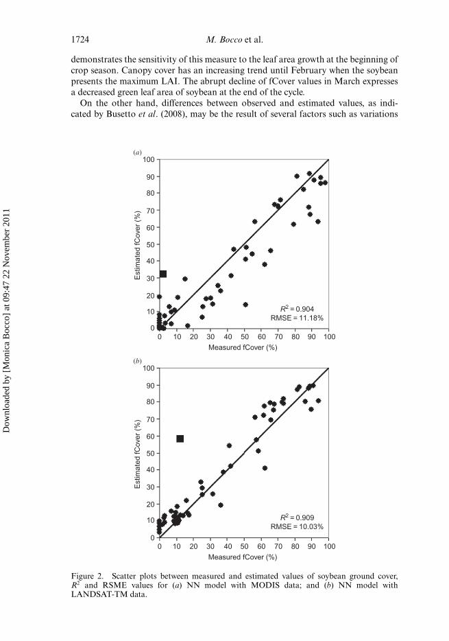
The relationship between coverage values estimated by NN_MOD and NN_TMmodels, and coverage values measured in the field are presented in figure 2(a) and (b).Similar statistical indicators were obtained when NNs were applied to both MODISand Landsat images.

The measured data of fCover used for the validation phase varied along the cropcycle between 0% and 98%, while the NNs estimated this variable in a narrower rangefrom 0% to 92% for both NN_MOD and NN_TM models. In general, plots withunderestimation of the fCover are observed for the model based on MODIS data(figure 2(a)), while overestimation is noted in the NN_TM model (figure 2(b)).

For low fCover values, both models overestimate fCover (figure 2(a) and (b)). Inthis situation, the bare soil dominates the crop; in particular, Xiao and Moody (2005)observed that NDVI-based methods are sensitive to soil background reflectance andHuete et al. (1985) found that greenness measures of vegetation canopies were sig-nificantly affected by soil background reflectance. Bachmann et al. (2007) found, forpastures in dry land environments, overestimation if the land is rough and the coverageis incomplete, stating that the degree of overestimation was due to the satellite–sun–land surface geometry. Moreover, Cyr et al. (1995) stated that indices overestimatethe ground coverage at the beginning of the growing season and underestimate it atthe end. Generally, a hysteresis type phase difference can be noted for all the indicesin relation to the vegetation cover. In the case of soybean, there are overestimationsby the indices for low vegetation covers at the beginning of the growing phase andunderestimation in senescence.

Both models show a special behaviour for one plot, regardless of the satellite (statedby a square symbol in figure 2(a) and (b)), due to differences between the interpolationresults for input and field data on 14 April 2008. These data correspond to the finalcrop stage when there are fast changes in fCover (harvest or senescence) and cropappearance (colour change). These data were also used for calculating all reportedstatistics.

The spatial resolution of Landsat allows a very good estimation of the soybean cov-erage evolution, on the other hand, in plots as the used (area greater than 50 ha) hightemporal resolution of MODIS compensates its low spatial coverage. Doraiswamyet al. (2004) state that the MODIS sensor is already appropriate when plots largerthan 25 ha are monitored. Lamparelli et al. (2008) indicated that the high tempo-ral resolution of the MODIS satellite makes it suitable as the TM sensor to mapsoybean.

The error values obtained in this work (table 2), for both NN models are simi-lar to those presented by Maas and Rajan (2008) who, using Landsat 5 images anda least squares linear regression line, estimated fCover with an R2 equal to 0.89 fora combination of cotton (Gossypium hirsutum L.), corn, sorghum (Sorghum bicolor(L.) Moench), alfalfa (Medicago sativa L.) and bare soil fields. Zhang et al. (2009)using NN models for predicting dates of soybean vegetative growth stages (V stages),obtained RMSE values between 10% and 42%.

Figure 3 shows for plot 24, as an example, spline smooth curves which describethe performance of both models throughout the observation period, for each sam-pling date. This figure shows that NN_MOD and NN_TM predict adequately thesoybean crop coverage evolution, with the exception of the errors mentioned above.According to Rizzi and Rudorff (2007), the fast increase in fCover values in December

Dow

nloa

ded

by [

Mon

ica

Boc

co]

at 0

9:47

22

Nov

embe

r 20

11

1724 M. Bocco et al.

demonstrates the sensitivity of this measure to the leaf area growth at the beginning ofcrop season. Canopy cover has an increasing trend until February when the soybeanpresents the maximum LAI. The abrupt decline of fCover values in March expressesa decreased green leaf area of soybean at the end of the cycle.

On the other hand, differences between observed and estimated values, as indi-cated by Busetto et al. (2008), may be the result of several factors such as variations

100(a)

90

80

70

60

50

40

30

20

10

00 10 20 30

R2 = 0.904RMSE = 11.18%

40Measured fCover (%)

Est

imat

ed fC

over

(%

)

50 60 70 80 90 100

100(b)

90

80

70

60

50

40

30

20

10

00 10 20 30

R2 = 0.909RMSE = 10.03%

40Measured fCover (%)

Est

imat

ed fC

over

(%

)

50 60 70 80 90 100

Figure 2. Scatter plots between measured and estimated values of soybean ground cover,R2 and RSME values for (a) NN model with MODIS data; and (b) NN model withLANDSAT-TM data.

Dow

nloa

ded

by [

Mon

ica

Boc

co]

at 0

9:47

22

Nov

embe

r 20

11

Models for estimations from satellite images 1725

100Measured

NN_MOD

NN_TM

1 2

5 64

3

90

80

70

60

50

fCov

er (

%)

40

30

20

10

015 Nov

1 2

3

4

5

6

5 Dec 25 Dec 14 Jan 3 FebDate

23 Feb 14 Mar 3 Apr 23 Apr

Figure 3. Evolution of ground cover during the growing season for plot 24, measured andestimated with NN models. The numbers inside the squares are associated with the photographsand numbers in circles. Each number corresponds to an observation from which an fCover valuewas obtained (Dates in 2007/2008).

between the characteristics of the spectral bands of MODIS and Landsat, dissim-ilar weather conditions on the date of sampling of each satellite and the differentcorrection methods used by satellites, among others.

4. Conclusions

This study demonstrated that the fraction cover of soybean canopies is a variable thatcan be accurately estimated using only red and NIR reflectances from medium- andhigh-resolution multispectral satellite imagery.

NNs are an appropriate methodology for estimating the temporal evolution ofsoybean coverage fraction from satellite information.

Modelled estimations were suitable for different spatial and temporal resolutions ofsensors, although both underestimate high values of soybean ground cover.

Dow

nloa

ded

by [

Mon

ica

Boc

co]

at 0

9:47

22

Nov

embe

r 20

11

1726 M. Bocco et al.

Estimation of soybean fCover is important for predicting crop yield, and modelssuch as the proposed would be extremely useful. The main contribution of this workfor precision agriculture was to show that Landsat satellite images can help improvethe crop ground cover prediction. This research also verified the utility of NN applica-tion as tools for fCover estimation, with high accuracies. In particular, the examinationof the obtained results should be continued for different soybean varieties and cropseasons in order to provide estimates for long periods and different areas.

AcknowledgementThe authors express their sincere thanks to Secretaría de Ciencia yTécnica – Universidad Nacional de Córdoba–Argentina (Secyt-UNC) for financialsupport of this study.

ReferencesARMSTRONG, J. (Ed.), 2001, Principles of Forecasting: A Handbook for Researchers and

Practitioners Summarizes Knowledge from Experts and from Empirical Studies, p. 849(Boston, MA: Kluwer Academic Publishers).

BACHMANN, M., HOLZWARTH, S. and MÜLLER, A., 2007, Influence of local incidenceangle effects on ground cover estimates. In 10th International Symposium of PhysicalMeasurements and Signatures in Remote Sensing, 12–14 March 2007, M.E. Schaepman,S. Liang, N.E. Groot and M. Kneubühler (Eds.), Davos, Switzerland, pp. 393–397.

BÁEZ-GONZÁLEZ, A.D., CHEN, P.Y., TISCARENO-LOPEZ, M. and SRINIVASAN, R., 2002, Usingsatellite and field data with crop growth modeling to monitor and estimate corn yield inMexico. Crop Science, 42, pp. 1943–1949.

BARET, F., CLEVERS, J.G. and STEVEN, M.D., 1995, The robustness of canopy gap fractionestimates from red and near-infrared reflectances: a comparison of approaches. RemoteSensing of Environment, 54, pp. 141–151.

BARET, F., HAGOLLE, O., GEIGER, B., BICHERON, P., MIRAS, B., HUC, M., BERTHELOT,B., NIÑO, F., WEISS, M., SAMAIN, O., ROUJEAN, J.L. and LEROY, M., 2007, LAI,fAPAR and fCover CYCLOPES global products derived from VEGETATION Part1: principles of the algorithm. Remote Sensing of Environment, 110, pp. 275–286.

BOCCO, M., OVANDO, G. and SAYAGO, S., 2006, Development and evaluation of neural networkmodels to estimate daily solar radiation at Córdoba, Argentina. Pesquisa AgropecuariaBrasileira, 41, pp. 179–184.

BOCCO, M., OVANDO, G., SAYAGO, S. and WILLINGTON, E., 2007, Neural network models forland cover classification from satellite images. Agricultura Técnica, 67, pp. 414–421.

BUSETTO, L., MERONI, M. and COLOMBO, R., 2008, Combining medium and coarse spatial res-olution satellite data to improve the estimation of sub-pixel NDVI time series. RemoteSensing of Environment, 112, pp. 118–131.

CAYROL, P., CHEHBOUNI, A., KERGOAT, L., DEDIEU, G., MORDELET, P. and NOUVELLON, Y.,2000, Grassland modeling and monitoring with SPOT-4 VEGETATION instrumentduring the 1997–1999 SALSA experiment. Agricultural and Forest Meteorology, 105,pp. 91–115.

CHAVEZ JR., P.S., 1989, Radiometric calibration of Landsat Thematic Mapper multispectralimages. Photogrammetric Engineering and Remote Sensing, 55, pp. 1285–1294.

CHEN, D., HUANG, J. and JACKSON, T.J., 2005, Vegetation water content estimation for cornand soybeans using spectral indices derived from MODIS near- and short-wave infraredbands. Remote Sensing of Environment, 98, pp. 225–236.

CYR, L., BONN, F. and PESANT, A., 1995, Vegetation indices derived from remote sensing foran estimation of soil protection against water erosion. Ecological Modelling, 79, pp.277–285.

Dow

nloa

ded

by [

Mon

ica

Boc

co]

at 0

9:47

22

Nov

embe

r 20

11

Models for estimations from satellite images 1727

DANSON, F.M., ROWLAND, C.S. and BARET, F., 2003, Training a neural network to estimatecrop leaf area index. International Journal of Remote Sensing, 24, pp. 4891–4905.

DAUGHTRY, C., GALLO, K., BIEHL, L., KANEMASU, E., ASRAR, G., BLAD, B., NORMAN, J. andGARDNER, B., 1984, Spectral estimates of agronomic characteristics of crops. In 10thInternational Symposium: Machine Processing of Remotely Sensed Data Symposium,12–14 June 1984, M.M. Klepfer and D.B. Morrison (Eds.), Purdue University, WestLafayette, IN, pp. 348–356.

DONOHUE, R.J., RODERICK, M.L. and MCVICAR, T.R., 2007, On the importance of includ-ing vegetation dynamics, in Budyko’s hydrological model. Hydrology and Earth SystemSciences, 11, pp. 983–995.

DORAISWAMY, P., HATFIELD, J., JACKSON, T., AKHMEDOV, B., PRUEGER, J. and STERN, A.,2004, Crop condition and yield simulation using Landsat and MODIS. Remote Sensingof Environment, 91, pp. 548–559.

DORAISWAMY, P., SINCLAIR, T., HOLLINGER, S., AKHMEDOV, B., STERN, A. and PRUEGER, J.,2005, Application of MODIS derived parameters for regional yield assessment. RemoteSensing of Environment, 97, pp. 192–202.

FEHR, W., CAVINESS, C., BURMOOD, D. and PENNINGTON, J., 1971, Stage of developmentdescriptions for soybeans, Glycine max (L.) Merrill. Crop Science, 11, pp. 929–931.

FENSHOLT, R., SANDHOLT, I. and RASMUSSEN, M.S., 2004, Evaluation of MODIS LAI, fAPARand the relation between fAPAR and NDVI in a semi-arid environment using in situmeasurements. Remote Sensing of Environment, 91, pp. 490–507.

GUERSCHMAN, J.P., HILL, M.J., RENZULLO, L.J., BARRETT, D.J., MARKS, A.S. and BOTHA, E.J.,2009, Estimating fractional cover of photosynthetic vegetation, non-photosyntheticvegetation and bare soil in the Australian tropical savanna region upscaling the EO-1Hyperion and MODIS sensors. Remote Sensing of Environment, 113, pp. 928–945.

GÜRTLER, S., EPIPHANIO, J., LUIZ, A. and FORMAGGIO, A., 2005, Planilha eletrônica parao cálculo da reflectância em imagens TM e ETM+ Landsat. Revista Brasileira DeCartografia, 57, pp. 162–167.

HATFIELD, J., GITELSON, A., SCHEPERS, J. and WALTHALL, C., 2008, Application of spectralremote sensing for agronomic decisions. Agronomy Journal, 100, pp. 117–131.

HUETE, A., JACKSON, R. and POST, D., 1985, Spectral response of a plant canopy with differentsoil backgrounds. Remote Sensing of Environment, 17, pp. 37–53.

INTA (Ed.), 2003, Recursos Naturales De La Provincia De Córdoba: Los Suelos, p. 567(Córdoba: Agencia Córdoba D.A.C. y T. SEM - Instituto Nacional de TecnologíaAgropecuaria).

JACQUEMOUD, S., VERHOEF, W., BARET, F., BACOUR, D., ZARCO-TEJADA, P.J., ASNER, G.P.,FRANÇOIS, C. and USTIN, S.L., 2009, PROSPECT+SAIL models: a review of use forvegetation characterization. Remote Sensing of Environment, 113, pp. 56–66.

JIANG, Z., HUETE, A., CHEN, J., CHEN, Y., LI, J., YAN, G. and ZHANG, X., 2006, Analysis ofNDVI and scaled difference vegetation index retrievals of vegetation fraction. RemoteSensing of Environment, 101, pp. 366–378.

KAVZOGLU, T. and MATHER, M., 2003, The use of backpropagating artificial neural networksin land cover classification. International Journal of Remote Sensing, 24, pp. 4907–4938.

LAKHANKAR, T., GHEDIRA, H., TEMIMI, M., AZAR, A. and KHANBILVARDI, R., 2009, Effectof land cover heterogeneity on soil moisture retrieval using active microwave remotesensing data. Remote Sensing, 1, pp. 80–91.

LAMPARELLI, R., DE CARVALHO, W. and MERCANTE, E., 2008, Mapeamento de semeadurasde soja (Glycine max (L.) Merr.) mediante dados MODIS/Terra e TM/Landsat 5: umcomparativo. Engenharia Agrícola, 28, pp. 334–344.

MAAS, S. and RAJAN, N., 2008, Estimating ground cover of field crops using medium-resolutionmultispectral satellite imagery. Agronomy Journal, 100, pp. 320–327.

MAGyP, 2009, Ministerio de Agricultura, Ganadería y Pesca de la Nación. Available online at:www.minagri.gov.ar (accessed 3 June 2010).

Dow

nloa

ded

by [

Mon

ica

Boc

co]

at 0

9:47

22

Nov

embe

r 20

11

1728 M. Bocco et al.

MATHER, J.R., 1965, Average climatic water balance data of the continents, part viii: SouthAmerica. Publications in Climatology, 18.

MAUGET, S.A. and UPCHURCH, D.R., 2000, Vegetation index response to leaf area indexand fractional vegetated area over cotton. In IEEE 2000 International Geoscienceand Remote Sensing Sympos, Taking the Pulse of the Planet: The Role of RemoteSensing in Managing the Environment, 24–28 July 2000, T.I. Stein (Ed.), Honolulu, HI,pp. 372–374.

MONTALDO, N., RONDENA, R., ALBERTSON, J.D. and MANCINI, M., 2005, Parsimonious mod-eling of vegetation dynamics for ecohydrologic studies of water-limited ecosystems.Water Resources Research, 41, W10416, doi:10.1029/2005WR004094.

NUMATA, I., ROBERTS, D.A., CHADWICK, O.A., SCHIMEL, J., SAMPAIO, F.R., LEONIDAS, F.C.and SOARES, J.V., 2007, Characterization of pasture biophysical properties and theimpact of grazing intensity using remotely sensed data. Remote Sensing of Environment,109, pp. 314−327.

PANDA, S.S., AMES, D.P. and PANIGRAHI, S., 2010, Application of vegetation indices for agri-cultural crop yield prediction using neural network techniques. Remote Sensing, 2, pp.673–696.

PIATTI, F. and FERREYRA, L., 2009, Evaluación de cultivares comerciales de soja. Campaña2008/09. Cartilla Digital Manfredi-INTA EEA Manfredi, 5, pp. 1–20.

POTAPOV, P., MATTHEW, A., HANSEN, C., STEPHEN, A., STEHMAN, V., THOMAS, B., LOVELAND,R. and KYLE, A., 2008, Combining MODIS and Landsat imagery to estimate and mapboreal forest cover loss. Remote Sensing of Environment, 112, pp. 3708–3719.

RIZZI, R. and RUDORFF, B., 2007, Imagens do sensor MODIS associadas a um modeloagronômico para estimar a productividade de soja. Pesquisa Agropecuaria Brasileira,42, pp. 73–80.

SHANAHAN, J., SCHEPERS, J., FRANCIS, D., VARVEL, G., WILHELM, W., TRINGE, J.,SCHLEMMER, M. and MAJOR, D., 2001, Use of remote sensing imagery to estimate corngrain yield. Agronomy Journal, 93, pp. 583–589.

TROMBETTI, M., RIAÑO, D., RUBIO, M.A., CHENG, Y.B. and USTIN, S.L., 2008, Multi-temporalvegetation canopy water content retrieval and interpretation using artificial neuralnetworks for the continental USA. Remote Sensing of Environment, 112, pp. 203−215.

VERGER, A., BARET, F. and WEISS, M., 2008, Performances of neural networks for derivingLAI estimates from existing CYCLOPES and MODIS products. Remote Sensing ofEnvironment, 112, pp. 2789–2803.

WALTHALL, C., DULANEY, W., ANDERSON, M., NORMAN, J., FANG, H. and LIANG, S., 2004,A comparison of empirical and neural network approaches for estimating corn andsoybean leaf area index from Landsat ETM+ imagery. Remote Sensing of Environment,92, pp. 465–474.

WEISS, M., BARET, F., LEROY, M., HAUTECOEUR, O., BACOUR, C., PRÉVOT, L. and BRUGUIER,N., 2002, Validation of neural net techniques to estimate canopy biophysical variablesfrom remote sensing data. Agronomie, 22, pp. 547–553.

XIAO, J. and MOODY, A., 2005, A comparison of methods for estimating fractional green veg-etation cover within a desert-to-upland transition zone in central New Mexico, USA.Remote Sensing of Environment, 98, pp. 237–250.

ZHANG, J., ZHANG, L., ZHANG, M. and WATSON, C., 2009, Prediction of soybean growth anddevelopment using artificial neural network and statistical models. Acta AgronomicaSinica, 35, pp. 341–347.

Dow

nloa

ded

by [

Mon

ica

Boc

co]

at 0

9:47

22

Nov

embe

r 20

11