arX

iv:0

910.

2848

v2 [

astr

o-ph

.CO

] 15

Nov

200

9

To appear inThe Astrophysical Journal

Estimating Black Hole Masses in Active Galactic Nuclei Using theMg II λ2800 Emission Line

Jian-Guo Wang1,2,5,6, Xiao-Bo Dong2,4, Ting-Gui Wang2,4, Luis C. Ho3, Weimin Yuan1,Huiyuan Wang2,4, Kai Zhang2,4, Shaohua Zhang2,4, and Hongyan Zhou2,4

ABSTRACT

We investigate the relationship between the linewidths of broad MgII λ2800 andHβ in active galactic nuclei (AGNs) to refine them as tools to estimate black hole (BH)masses. We perform a detailed spectral analysis of a large sample of AGNs at inter-mediate redshifts selected from the Sloan Digital Sky Survey, along with a smallersample of archival ultraviolet spectra for nearby sources monitored with reverberationmapping (RM). Careful attention is devoted to accurate spectral decomposition, espe-cially in the treatment of narrow-line blending and FeII contamination. We show that,contrary to popular belief, the velocity width of MgII tends to be smaller than thatof Hβ, suggesting that the two species are not cospatial in the broad-line region. Us-ing these findings and recently updated BH mass measurementsfrom RM, we presenta new calibration of the empirical prescriptions for estimating virial BH masses forAGNs using the broad MgII and Hβ lines. We show that the BH masses derived fromour new formalisms show subtle but important differences compared to some of themass estimators currently used in the literature.

Subject headings: black hole physics — galaxies: active — quasars: emission lines— quasars: general

1National Astronomical Observatories/Yunnan Observatory, Chinese Academy of Sciences, P.O. Box 110, Kun-ming, Yunnan 650011, China; wangjg, wmy@ynao.ac.cn

2Key Laboratory for Research in Galaxies and Cosmology, The University of Sciences and Technology of China,Chinese Academy of Sciences, Hefei, Anhui 230026, China; xbdong, twang@ustc.edu.cn

3The Observatories of the Carnegie Institution for Science,813 Santa Barbara Street, Pasadena, CA 91101,USA; lho@obs.carnegiescience.edu

4Center for Astrophysics, University of Science and Technology of China, Hefei, Anhui 230026, China

5Department of Physics, Yunnan University, Kunming, Yunnan650031, China

6Graduate School of the Chinese Academy of Sciences, 19A Yuquan Road, P.O. Box 3908, Beijing 100039, China

– 2 –

1. Introduction

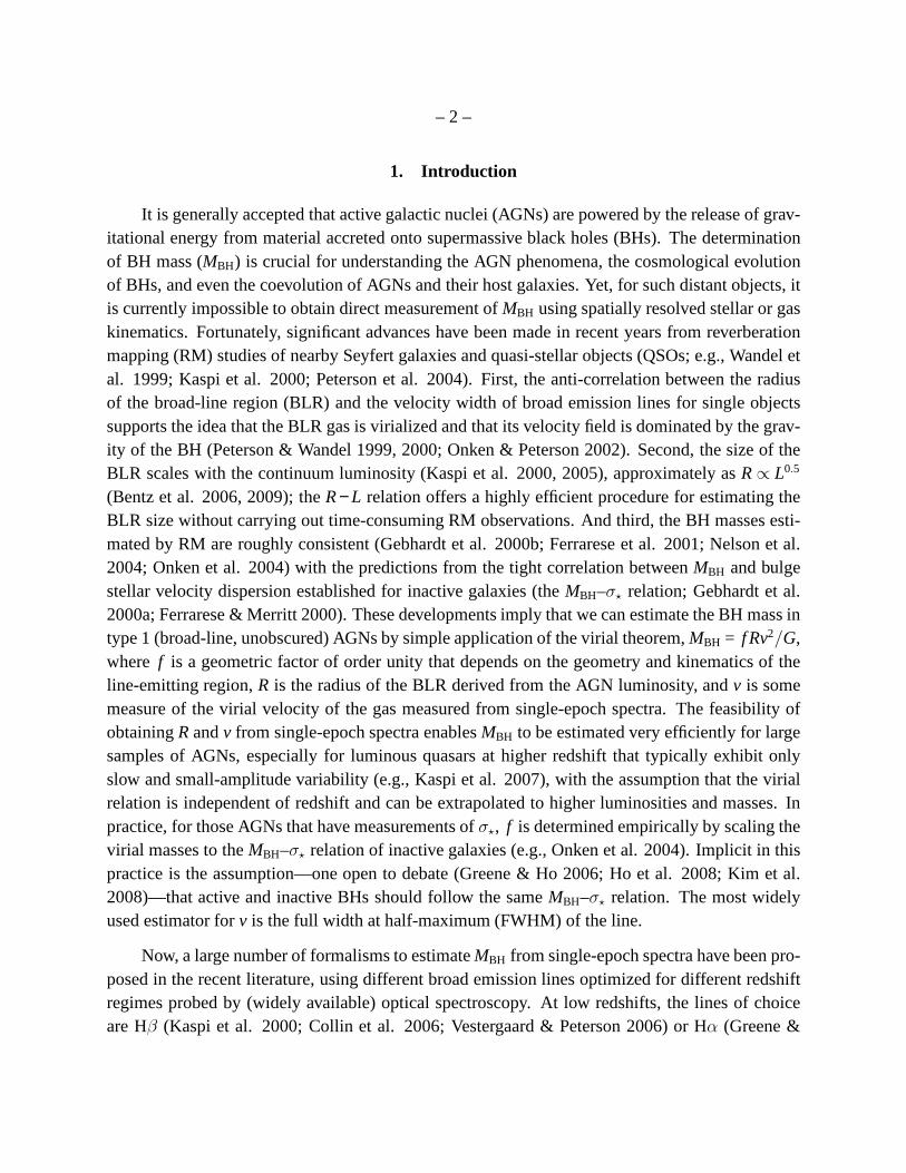
It is generally accepted that active galactic nuclei (AGNs)are powered by the release of grav-itational energy from material accreted onto supermassiveblack holes (BHs). The determinationof BH mass (MBH) is crucial for understanding the AGN phenomena, the cosmological evolutionof BHs, and even the coevolution of AGNs and their host galaxies. Yet, for such distant objects, itis currently impossible to obtain direct measurement ofMBH using spatially resolved stellar or gaskinematics. Fortunately, significant advances have been made in recent years from reverberationmapping (RM) studies of nearby Seyfert galaxies and quasi-stellar objects (QSOs; e.g., Wandel etal. 1999; Kaspi et al. 2000; Peterson et al. 2004). First, theanti-correlation between the radiusof the broad-line region (BLR) and the velocity width of broad emission lines for single objectssupports the idea that the BLR gas is virialized and that its velocity field is dominated by the grav-ity of the BH (Peterson & Wandel 1999, 2000; Onken & Peterson 2002). Second, the size of theBLR scales with the continuum luminosity (Kaspi et al. 2000,2005), approximately asR ∝ L0.5

(Bentz et al. 2006, 2009); theR − L relation offers a highly efficient procedure for estimatingtheBLR size without carrying out time-consuming RM observations. And third, the BH masses esti-mated by RM are roughly consistent (Gebhardt et al. 2000b; Ferrarese et al. 2001; Nelson et al.2004; Onken et al. 2004) with the predictions from the tight correlation betweenMBH and bulgestellar velocity dispersion established for inactive galaxies (theMBH–σ⋆ relation; Gebhardt et al.2000a; Ferrarese & Merritt 2000). These developments implythat we can estimate the BH mass intype 1 (broad-line, unobscured) AGNs by simple applicationof the virial theorem,MBH = f Rv2/G,where f is a geometric factor of order unity that depends on the geometry and kinematics of theline-emitting region,R is the radius of the BLR derived from the AGN luminosity, andv is somemeasure of the virial velocity of the gas measured from single-epoch spectra. The feasibility ofobtainingR andv from single-epoch spectra enablesMBH to be estimated very efficiently for largesamples of AGNs, especially for luminous quasars at higher redshift that typically exhibit onlyslow and small-amplitude variability (e.g., Kaspi et al. 2007), with the assumption that the virialrelation is independent of redshift and can be extrapolatedto higher luminosities and masses. Inpractice, for those AGNs that have measurements ofσ⋆, f is determined empirically by scaling thevirial masses to theMBH–σ⋆ relation of inactive galaxies (e.g., Onken et al. 2004). Implicit in thispractice is the assumption—one open to debate (Greene & Ho 2006; Ho et al. 2008; Kim et al.2008)—that active and inactive BHs should follow the sameMBH–σ⋆ relation. The most widelyused estimator forv is the full width at half-maximum (FWHM) of the line.

Now, a large number of formalisms to estimateMBH from single-epoch spectra have been pro-posed in the recent literature, using different broad emission lines optimized for different redshiftregimes probed by (widely available) optical spectroscopy. At low redshifts, the lines of choiceare Hβ (Kaspi et al. 2000; Collin et al. 2006; Vestergaard & Peterson 2006) or Hα (Greene &

– 3 –

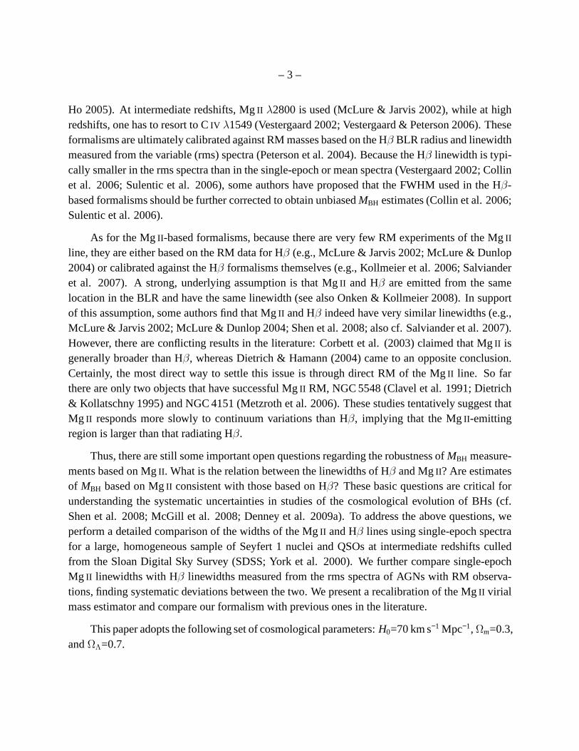
Ho 2005). At intermediate redshifts, MgII λ2800 is used (McLure & Jarvis 2002), while at highredshifts, one has to resort to CIV λ1549 (Vestergaard 2002; Vestergaard & Peterson 2006). Theseformalisms are ultimately calibrated against RM masses based on the Hβ BLR radius and linewidthmeasured from the variable (rms) spectra (Peterson et al. 2004). Because the Hβ linewidth is typi-cally smaller in the rms spectra than in the single-epoch or mean spectra (Vestergaard 2002; Collinet al. 2006; Sulentic et al. 2006), some authors have proposed that the FWHM used in the Hβ-based formalisms should be further corrected to obtain unbiasedMBH estimates (Collin et al. 2006;Sulentic et al. 2006).

As for the MgII-based formalisms, because there are very few RM experiments of the MgII

line, they are either based on the RM data for Hβ (e.g., McLure & Jarvis 2002; McLure & Dunlop2004) or calibrated against the Hβ formalisms themselves (e.g., Kollmeier et al. 2006; Salvianderet al. 2007). A strong, underlying assumption is that MgII and Hβ are emitted from the samelocation in the BLR and have the same linewidth (see also Onken & Kollmeier 2008). In supportof this assumption, some authors find that MgII and Hβ indeed have very similar linewidths (e.g.,McLure & Jarvis 2002; McLure & Dunlop 2004; Shen et al. 2008; also cf. Salviander et al. 2007).However, there are conflicting results in the literature: Corbett et al. (2003) claimed that MgII isgenerally broader than Hβ, whereas Dietrich & Hamann (2004) came to an opposite conclusion.Certainly, the most direct way to settle this issue is through direct RM of the MgII line. So farthere are only two objects that have successful MgII RM, NGC 5548 (Clavel et al. 1991; Dietrich& Kollatschny 1995) and NGC 4151 (Metzroth et al. 2006). These studies tentatively suggest thatMg II responds more slowly to continuum variations than Hβ, implying that the MgII-emittingregion is larger than that radiating Hβ.

Thus, there are still some important open questions regarding the robustness ofMBH measure-ments based on MgII . What is the relation between the linewidths of Hβ and MgII? Are estimatesof MBH based on MgII consistent with those based on Hβ? These basic questions are critical forunderstanding the systematic uncertainties in studies of the cosmological evolution of BHs (cf.Shen et al. 2008; McGill et al. 2008; Denney et al. 2009a). To address the above questions, weperform a detailed comparison of the widths of the MgII and Hβ lines using single-epoch spectrafor a large, homogeneous sample of Seyfert 1 nuclei and QSOs at intermediate redshifts culledfrom the Sloan Digital Sky Survey (SDSS; York et al. 2000). Wefurther compare single-epochMg II linewidths with Hβ linewidths measured from the rms spectra of AGNs with RM observa-tions, finding systematic deviations between the two. We present a recalibration of the MgII virialmass estimator and compare our formalism with previous onesin the literature.

This paper adopts the following set of cosmological parameters:H0=70 km s−1 Mpc−1, Ωm=0.3,andΩΛ=0.7.

– 4 –

2. Sample and Data Analysis

2.1. The Samples

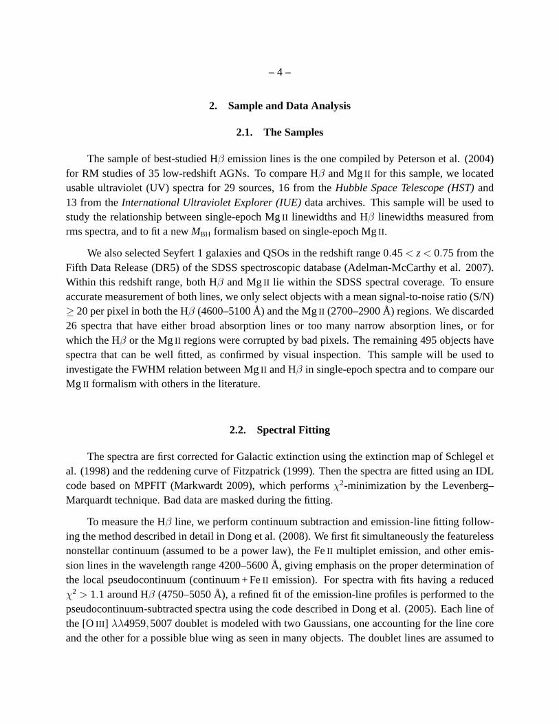
The sample of best-studied Hβ emission lines is the one compiled by Peterson et al. (2004)for RM studies of 35 low-redshift AGNs. To compare Hβ and MgII for this sample, we locatedusable ultraviolet (UV) spectra for 29 sources, 16 from theHubble Space Telescope (HST) and13 from theInternational Ultraviolet Explorer (IUE) data archives. This sample will be used tostudy the relationship between single-epoch MgII linewidths and Hβ linewidths measured fromrms spectra, and to fit a newMBH formalism based on single-epoch MgII .

We also selected Seyfert 1 galaxies and QSOs in the redshift range 0.45< z < 0.75 from theFifth Data Release (DR5) of the SDSS spectroscopic database(Adelman-McCarthy et al. 2007).Within this redshift range, both Hβ and MgII lie within the SDSS spectral coverage. To ensureaccurate measurement of both lines, we only select objects with a mean signal-to-noise ratio (S/N)≥ 20 per pixel in both the Hβ (4600–5100 Å) and the MgII (2700–2900 Å) regions. We discarded26 spectra that have either broad absorption lines or too many narrow absorption lines, or forwhich the Hβ or the MgII regions were corrupted by bad pixels. The remaining 495 objects havespectra that can be well fitted, as confirmed by visual inspection. This sample will be used toinvestigate the FWHM relation between MgII and Hβ in single-epoch spectra and to compare ourMg II formalism with others in the literature.

2.2. Spectral Fitting

The spectra are first corrected for Galactic extinction using the extinction map of Schlegel etal. (1998) and the reddening curve of Fitzpatrick (1999). Then the spectra are fitted using an IDLcode based on MPFIT (Markwardt 2009), which performsχ2-minimization by the Levenberg–Marquardt technique. Bad data are masked during the fitting.

To measure the Hβ line, we perform continuum subtraction and emission-line fitting follow-ing the method described in detail in Dong et al. (2008). We first fit simultaneously the featurelessnonstellar continuum (assumed to be a power law), the FeII multiplet emission, and other emis-sion lines in the wavelength range 4200–5600 Å, giving emphasis on the proper determination ofthe local pseudocontinuum (continuum + FeII emission). For spectra with fits having a reducedχ2 > 1.1 around Hβ (4750–5050 Å), a refined fit of the emission-line profiles is performed to thepseudocontinuum-subtracted spectra using the code described in Dong et al. (2005). Each line ofthe [OIII ] λλ4959,5007 doublet is modeled with two Gaussians, one accounting for the line coreand the other for a possible blue wing as seen in many objects.The doublet lines are assumed to

– 5 –

have the same redshifts and profiles, and the flux ratioλ5007/λ4959 is fixed to the theoretical valueof 3. The narrow component of Hβ is fitted with one Gaussian, assumed to have the same widthas the line core of [OIII ] λ5007. The broad component of Hβ is fitted with as many Gaussians asstatistically justified (see Dong et al. 2008 for details).

To measure the MgII line, we adopt the following procedure. We first obtain an initial estimateof the nonstellar featureless continuum by fitting a simple power law,

f PL(λ; a,β) = a

(

λ

2200

)β

, (1)

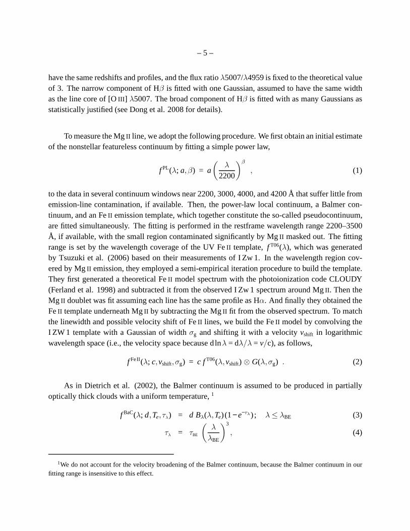
to the data in several continuum windows near 2200, 3000, 4000, and 4200 Å that suffer little fromemission-line contamination, if available. Then, the power-law local continuum, a Balmer con-tinuum, and an FeII emission template, which together constitute the so-called pseudocontinuum,are fitted simultaneously. The fitting is performed in the restframe wavelength range 2200–3500Å, if available, with the small region contaminated significantly by MgII masked out. The fittingrange is set by the wavelength coverage of the UV FeII template,f T06(λ), which was generatedby Tsuzuki et al. (2006) based on their measurements of I Zw 1.In the wavelength region cov-ered by MgII emission, they employed a semi-empirical iteration procedure to build the template.They first generated a theoretical FeII model spectrum with the photoionization code CLOUDY(Ferland et al. 1998) and subtracted it from the observed I Zw1 spectrum around MgII . Then theMg II doublet was fit assuming each line has the same profile as Hα. And finally they obtained theFeII template underneath MgII by subtracting the MgII fit from the observed spectrum. To matchthe linewidth and possible velocity shift of FeII lines, we build the FeII model by convolving theI ZW 1 template with a Gaussian of widthσg and shifting it with a velocityvshift in logarithmicwavelength space (i.e., the velocity space because dlnλ = dλ/λ = v/c), as follows,

f FeII(λ; c,vshift,σg) = c f T06(λ,vshift) ⊗ G(λ,σg) . (2)

As in Dietrich et al. (2002), the Balmer continuum is assumedto be produced in partiallyoptically thick clouds with a uniform temperature,1

f BaC(λ; d,Te,τλ) = d Bλ(λ,Te) (1− e−τλ) ; λ ≤ λBE (3)

τλ = τBE

(

λ

λBE

)3

, (4)

1We do not account for the velocity broadening of the Balmer continuum, because the Balmer continuum in ourfitting range is insensitive to this effect.

– 6 –

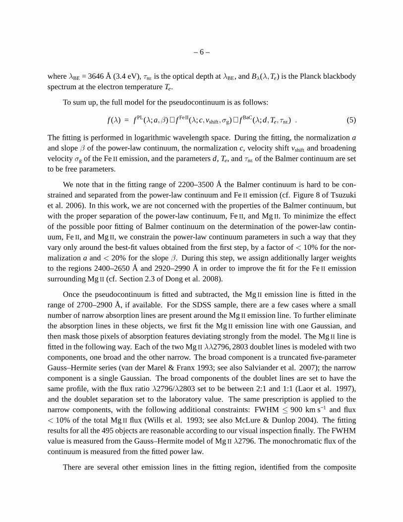
whereλBE = 3646 Å (3.4 eV),τBE is the optical depth atλBE, andBλ(λ,Te) is the Planck blackbodyspectrum at the electron temperatureTe.

To sum up, the full model for the pseudocontinuum is as follows:

f (λ) = f PL(λ;a,β) + f FeII(λ;c,vshift,σg) + f BaC(λ;d,Te,τBE) . (5)

The fitting is performed in logarithmic wavelength space. During the fitting, the normalizationaand slopeβ of the power-law continuum, the normalizationc, velocity shiftvshift and broadeningvelocityσg of the FeII emission, and the parametersd, Te, andτBE of the Balmer continuum are setto be free parameters.

We note that in the fitting range of 2200–3500 Å the Balmer continuum is hard to be con-strained and separated from the power-law continuum and FeII emission (cf. Figure 8 of Tsuzukiet al. 2006). In this work, we are not concerned with the properties of the Balmer continuum, butwith the proper separation of the power-law continuum, FeII , and MgII . To minimize the effectof the possible poor fitting of Balmer continuum on the determination of the power-law contin-uum, FeII , and MgII , we constrain the power-law continuum parameters in such a way that theyvary only around the best-fit values obtained from the first step, by a factor of< 10% for the nor-malizationa and< 20% for the slopeβ. During this step, we assign additionally larger weightsto the regions 2400–2650 Å and 2920–2990 Å in order to improvethe fit for the FeII emissionsurrounding MgII (cf. Section 2.3 of Dong et al. 2008).

Once the pseudocontinuum is fitted and subtracted, the MgII emission line is fitted in therange of 2700–2900 Å, if available. For the SDSS sample, there are a few cases where a smallnumber of narrow absorption lines are present around the MgII emission line. To further eliminatethe absorption lines in these objects, we first fit the MgII emission line with one Gaussian, andthen mask those pixels of absorption features deviating strongly from the model. The MgII line isfitted in the following way. Each of the two MgII λλ2796, 2803 doublet lines is modeled with twocomponents, one broad and the other narrow. The broad component is a truncated five-parameterGauss–Hermite series (van der Marel & Franx 1993; see also Salviander et al. 2007); the narrowcomponent is a single Gaussian. The broad components of the doublet lines are set to have thesame profile, with the flux ratioλ2796/λ2803 set to be between 2:1 and 1:1 (Laor et al. 1997),and the doublet separation set to the laboratory value. The same prescription is applied to thenarrow components, with the following additional constraints: FWHM ≤ 900 km s−1 and flux< 10% of the total MgII flux (Wills et al. 1993; see also McLure & Dunlop 2004). The fittingresults for all the 495 objects are reasonable according to our visual inspection finally. The FWHMvalue is measured from the Gauss–Hermite model of MgII λ2796. The monochromatic flux of thecontinuum is measured from the fitted power law.

There are several other emission lines in the fitting region,identified from the composite

– 7 –

SDSS QSO spectrum (see Table 2 of Vanden Berk et al. 2001); yet, because of their weakness, wesimply masked them out in the fit. Because of the limited wavelength coverage of the RM sample,we cannot separate the Balmer continuum from the power-law continuum. Thus, the Balmer con-tinuum was not included in the fits for this sample. Additionally, there are deep narrow absorptionfeatures around MgII in the spectra of NGC 3227, NGC 3516, NGC 3783, and NGC 4151 in theRM sample. Each of the absorption features is fitted simultaneously with a Gaussian when fittingthe MgII emission line.

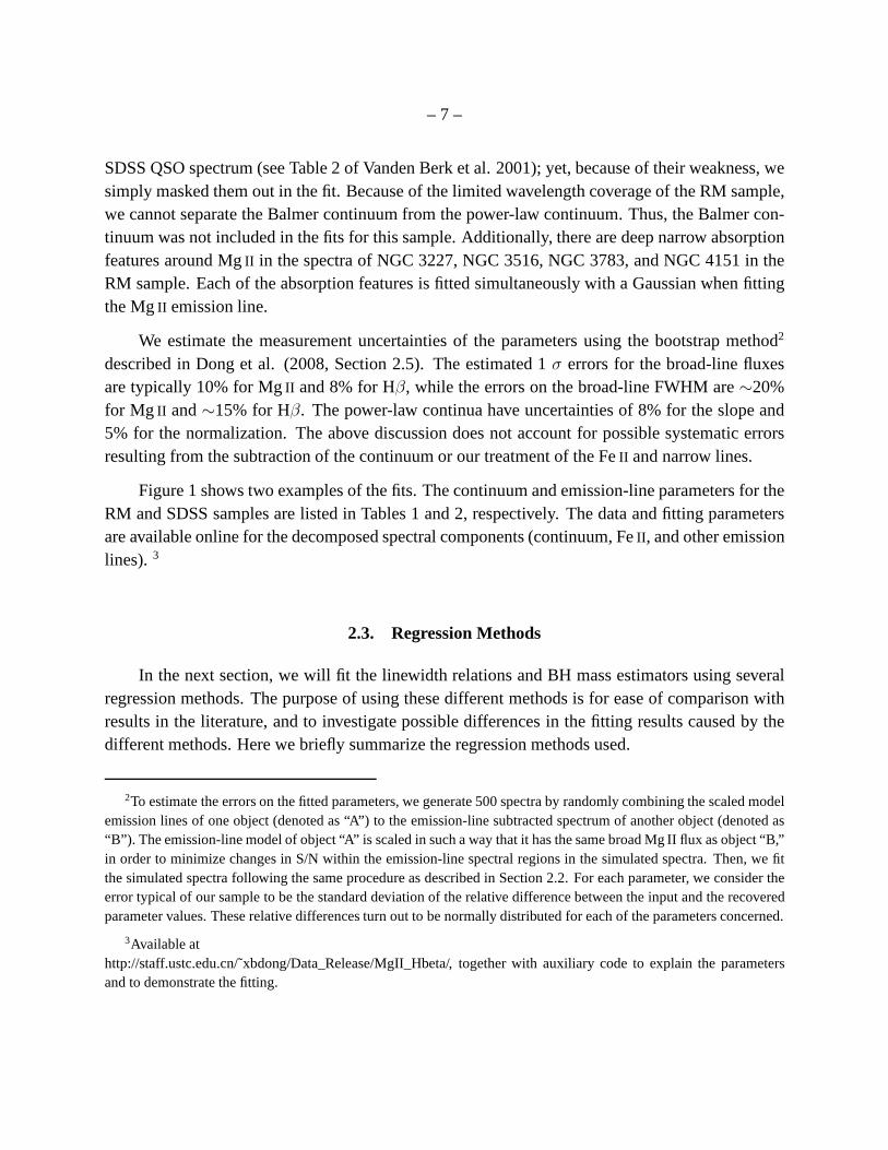
We estimate the measurement uncertainties of the parameters using the bootstrap method2

described in Dong et al. (2008, Section 2.5). The estimated 1σ errors for the broad-line fluxesare typically 10% for MgII and 8% for Hβ, while the errors on the broad-line FWHM are∼20%for Mg II and∼15% for Hβ. The power-law continua have uncertainties of 8% for the slope and5% for the normalization. The above discussion does not account for possible systematic errorsresulting from the subtraction of the continuum or our treatment of the FeII and narrow lines.

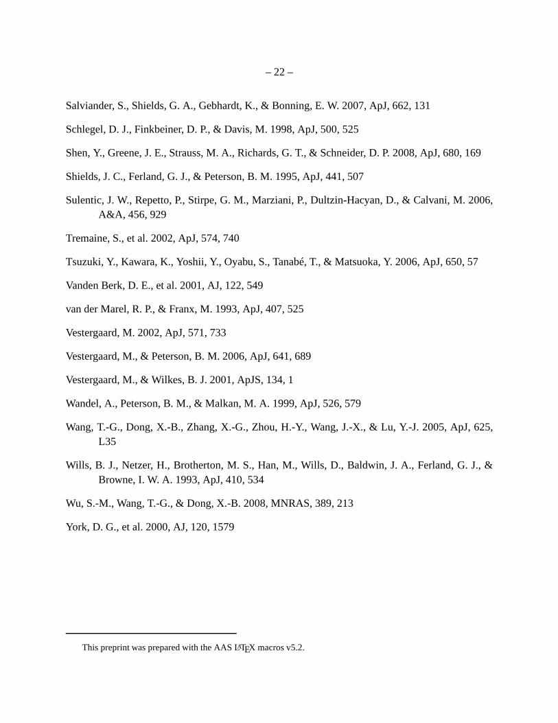
Figure 1 shows two examples of the fits. The continuum and emission-line parameters for theRM and SDSS samples are listed in Tables 1 and 2, respectively. The data and fitting parametersare available online for the decomposed spectral components (continuum, FeII , and other emissionlines).3

2.3. Regression Methods

In the next section, we will fit the linewidth relations and BHmass estimators using severalregression methods. The purpose of using these different methods is for ease of comparison withresults in the literature, and to investigate possible differences in the fitting results caused by thedifferent methods. Here we briefly summarize the regressionmethods used.

2To estimate the errors on the fitted parameters, we generate 500 spectra by randomly combining the scaled modelemission lines of one object (denoted as “A”) to the emission-line subtracted spectrum of another object (denoted as“B”). The emission-line model of object “A” is scaled in sucha way that it has the same broad Mg II flux as object “B,”in order to minimize changes in S/N within the emission-linespectral regions in the simulated spectra. Then, we fitthe simulated spectra following the same procedure as described in Section 2.2. For each parameter, we consider theerror typical of our sample to be the standard deviation of the relative difference between the input and the recoveredparameter values. These relative differences turn out to benormally distributed for each of the parameters concerned.

3Available athttp://staff.ustc.edu.cn/˜xbdong/Data_Release/MgII_Hbeta/, together with auxiliary code to explain the parametersand to demonstrate the fitting.

– 8 –

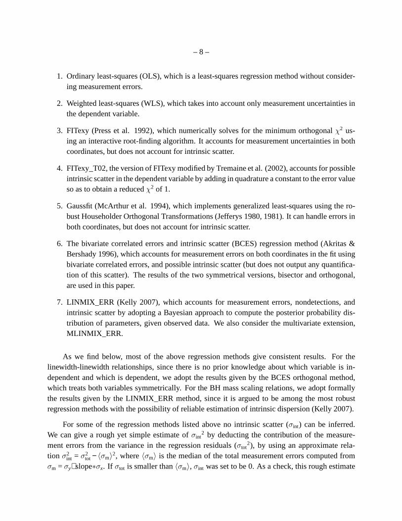
1. Ordinary least-squares (OLS), which is a least-squares regression method without consider-ing measurement errors.

2. Weighted least-squares (WLS), which takes into account only measurement uncertainties inthe dependent variable.

3. FITexy (Press et al. 1992), which numerically solves for the minimum orthogonalχ2 us-ing an interactive root-finding algorithm. It accounts for measurement uncertainties in bothcoordinates, but does not account for intrinsic scatter.

4. FITexy_T02, the version of FITexy modified by Tremaine et al. (2002), accounts for possibleintrinsic scatter in the dependent variable by adding in quadrature a constant to the error valueso as to obtain a reducedχ2 of 1.

5. Gaussfit (McArthur et al. 1994), which implements generalized least-squares using the ro-bust Householder Orthogonal Transformations (Jefferys 1980, 1981). It can handle errors inboth coordinates, but does not account for intrinsic scatter.

6. The bivariate correlated errors and intrinsic scatter (BCES) regression method (Akritas &Bershady 1996), which accounts for measurement errors on both coordinates in the fit usingbivariate correlated errors, and possible intrinsic scatter (but does not output any quantifica-tion of this scatter). The results of the two symmetrical versions, bisector and orthogonal,are used in this paper.

7. LINMIX_ERR (Kelly 2007), which accounts for measurementerrors, nondetections, andintrinsic scatter by adopting a Bayesian approach to compute the posterior probability dis-tribution of parameters, given observed data. We also consider the multivariate extension,MLINMIX_ERR.

As we find below, most of the above regression methods give consistent results. For thelinewidth-linewidth relationships, since there is no prior knowledge about which variable is in-dependent and which is dependent, we adopt the results givenby the BCES orthogonal method,which treats both variables symmetrically. For the BH mass scaling relations, we adopt formallythe results given by the LINMIX_ERR method, since it is argued to be among the most robustregression methods with the possibility of reliable estimation of intrinsic dispersion (Kelly 2007).

For some of the regression methods listed above no intrinsicscatter (σint) can be inferred.We can give a rough yet simple estimate ofσint

2 by deducting the contribution of the measure-ment errors from the variance in the regression residuals (σtot

2), by using an approximate rela-tion σ2

int = σ2tot − 〈σm〉

2, where〈σm〉 is the median of the total measurement errors computed fromσm = σy+slope∗σx. If σtot is smaller than〈σm〉, σint was set to be 0. As a check, this rough estimate

– 9 –

can be compared with the intrinsic scatter given by some of the regression methods that providesuch a measure.

3. Results

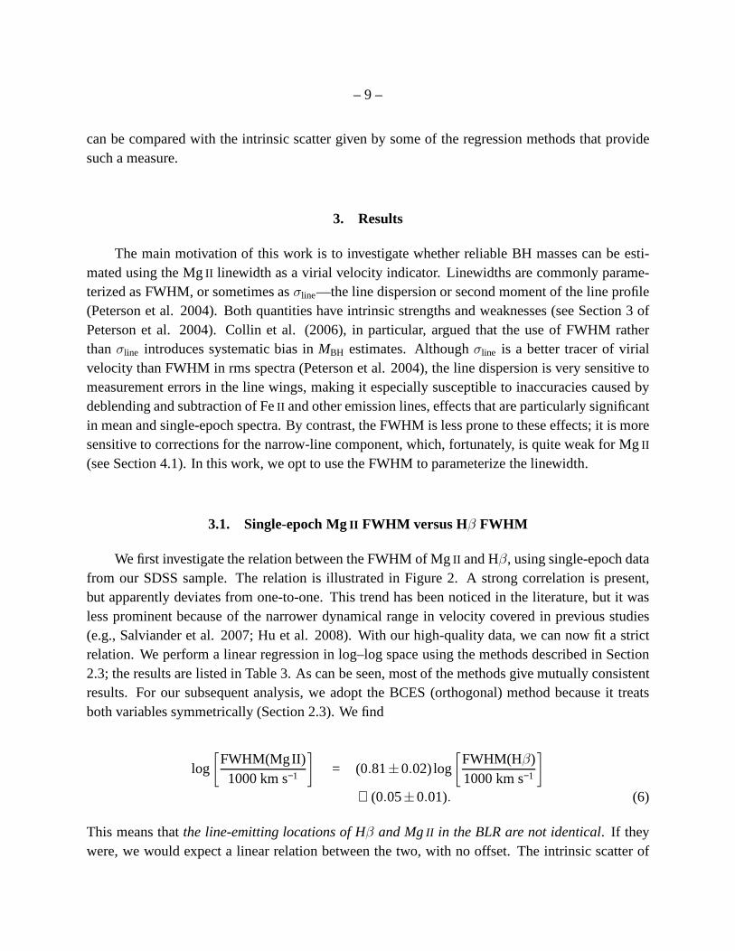
The main motivation of this work is to investigate whether reliable BH masses can be esti-mated using the MgII linewidth as a virial velocity indicator. Linewidths are commonly parame-terized as FWHM, or sometimes asσline—the line dispersion or second moment of the line profile(Peterson et al. 2004). Both quantities have intrinsic strengths and weaknesses (see Section 3 ofPeterson et al. 2004). Collin et al. (2006), in particular, argued that the use of FWHM ratherthanσline introduces systematic bias inMBH estimates. Althoughσline is a better tracer of virialvelocity than FWHM in rms spectra (Peterson et al. 2004), theline dispersion is very sensitive tomeasurement errors in the line wings, making it especially susceptible to inaccuracies caused bydeblending and subtraction of FeII and other emission lines, effects that are particularly significantin mean and single-epoch spectra. By contrast, the FWHM is less prone to these effects; it is moresensitive to corrections for the narrow-line component, which, fortunately, is quite weak for MgII(see Section 4.1). In this work, we opt to use the FWHM to parameterize the linewidth.

3.1. Single-epoch Mg II FWHM versus Hβ FWHM

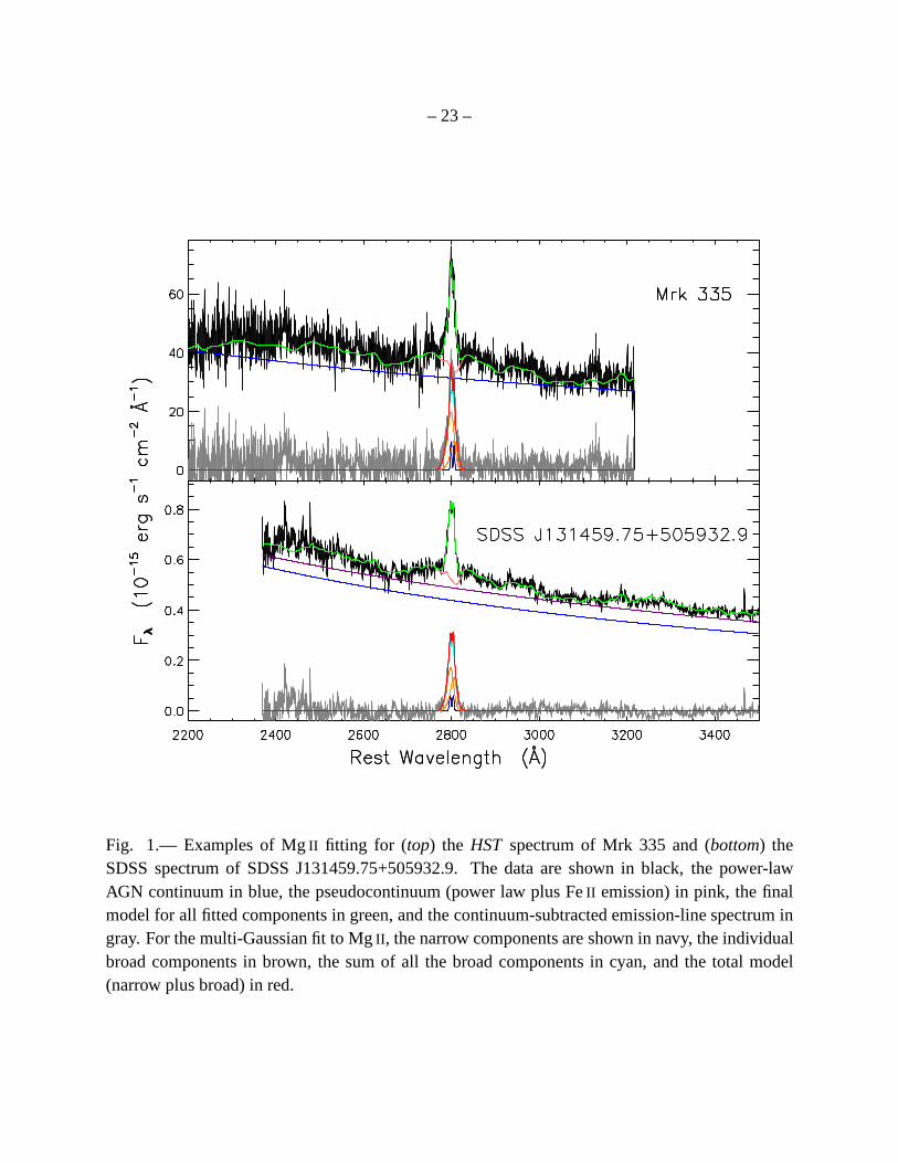
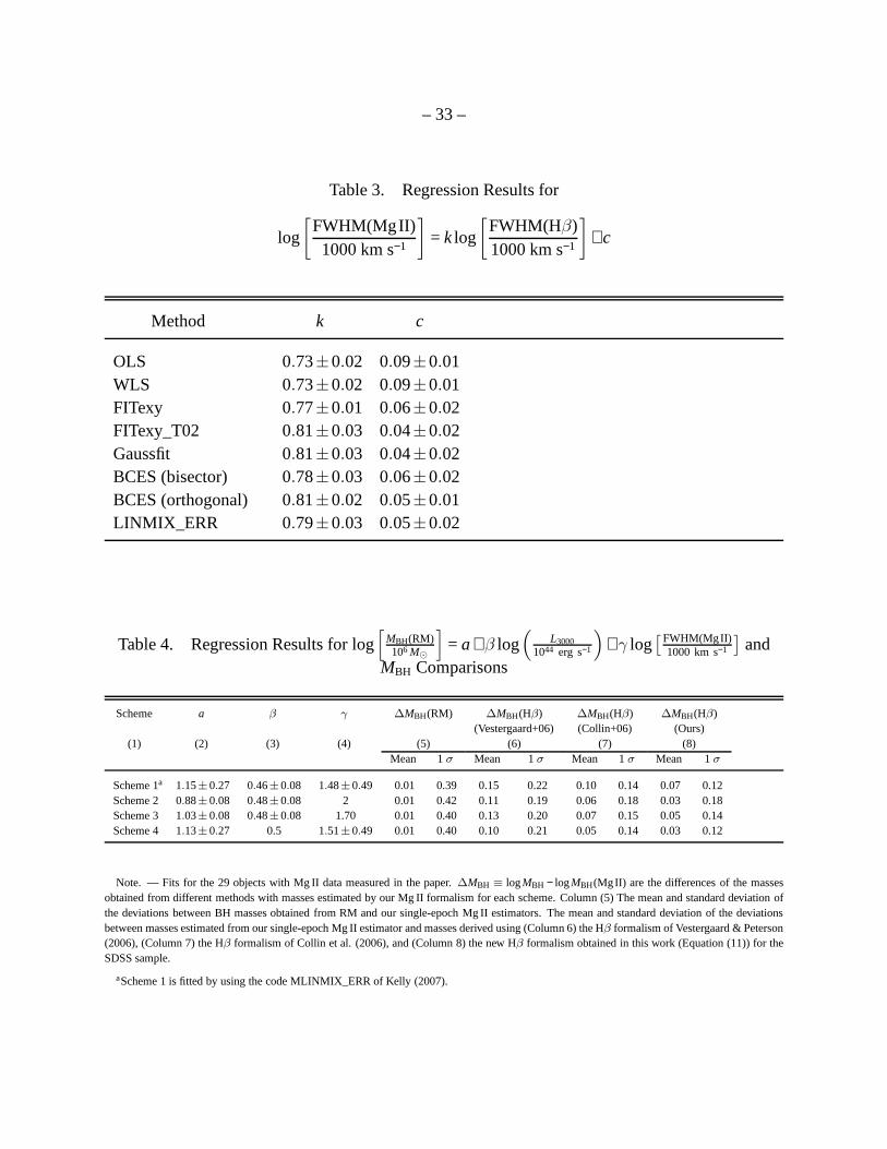
We first investigate the relation between the FWHM of MgII and Hβ, using single-epoch datafrom our SDSS sample. The relation is illustrated in Figure 2. A strong correlation is present,but apparently deviates from one-to-one. This trend has been noticed in the literature, but it wasless prominent because of the narrower dynamical range in velocity covered in previous studies(e.g., Salviander et al. 2007; Hu et al. 2008). With our high-quality data, we can now fit a strictrelation. We perform a linear regression in log–log space using the methods described in Section2.3; the results are listed in Table 3. As can be seen, most of the methods give mutually consistentresults. For our subsequent analysis, we adopt the BCES (orthogonal) method because it treatsboth variables symmetrically (Section 2.3). We find

log

[

FWHM(MgII)1000 km s−1

]

= (0.81±0.02) log

[

FWHM(Hβ)1000 km s−1

]

+ (0.05±0.01). (6)

This means thatthe line-emitting locations of Hβ and Mg II in the BLR are not identical. If theywere, we would expect a linear relation between the two, withno offset. The intrinsic scatter of

– 10 –

this relation, as given by the regression methods listed above, is extremely small and negligiblecompared to the measurement errors. The latter is actually comparable to thetotal scatter (σtot) ofthe relationship, which is found to be 0.08 dex.

3.2. Single-epoch Mg II FWHM versus rms Hβ σline

Since the assumption that MgII FWHM is identical to Hβ FWHM does not hold, we explorethe relation between MgII FWHM and rms Hβ σline, which has been argued to be a good tracer ofthe virial velocity of the BLR clouds emitting (variable) Hβ (see references in Section 1). We usedata for the 29 objects in the RM sample that have UV spectra toperform this exploration. MgIIFWHM is measured from the single-epochHST/IUE spectra, as listed in Table 1. The data forrms Hβ σline are mainly taken from Peterson et al. (2004). In addition, weuse updated RM datafor NGC 4051 (Denney et al. 2009b), NGC 4151 (Metzroth et al. 2006), NGC 4593 (Denney etal. 2006), NGC 5548 (Bentz et al. 2007), and PG 2130+099 (Grier et al. 2008). For objects withmultiple measurements, the geometric mean (i.e., the mean in the log scale) was used.

We find that the slope of the relation between MgII FWHM and rms Hβ σline deviates fromunity, with a best fit of

log

[

σline(Hβ, rms)1000 km s−1

]

= (0.85±0.21) log

[

FWHM(MgII)1000 km s−1

]

− (0.21±0.12) . (7)

The formal relation is nonlinear although the significance level is only about 1σ. A nonlinearrelation between MgII FWHM and rms Hβ σline is not very surprising, in light of a similar situationobserved for Hβ FWHM (Collin et al. 2006; also Sulentic et al. 2006, Section 1). For verification,we also fit the relation between Hβ FWHM in the mean spectra and rms Hβ σline using data for35 objects in the RM sample; the FWHM data are taken from Collin et al. (2006) and from theupdated sources mentioned above. The best-fit relation deviates from unity even more seriouslythan the case of MgII FWHM:

log

[

σline(Hβ, rms)1000 km s−1

]

= (0.54±0.08) log

[

FWHM(Hβ,mean)1000 km s−1

]

− (0.09±0.05) . (8)

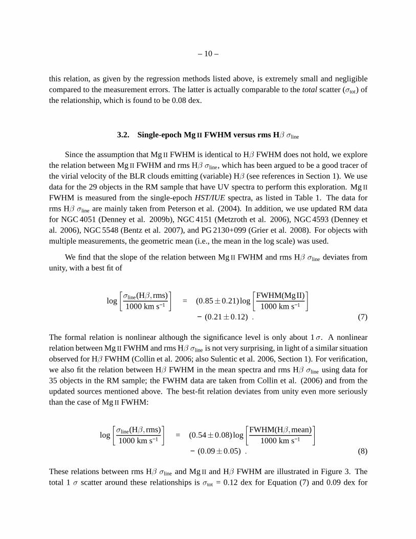
These relations between rms Hβ σline and MgII and Hβ FWHM are illustrated in Figure 3. Thetotal 1 σ scatter around these relationships isσtot = 0.12 dex for Equation (7) and 0.09 dex for

– 11 –

Equation (8). Given the relatively small measurement errors of the linewidths, there likely existsintrinsic scatter in these relationships. Using the simplemethod of deducting the measurementerrors from the total scatter, as described in Section 2.3, we findσint≈ 0.09 dex and≈ 0.08 dex forthe relationships of Equations (7) and (8), respectively. The underlying reason for the nonlinearityof these relationships may be, at least partially, that theσline of rms spectra traces the velocity ofthe line-emitting region that responds to continuum variation, while the FWHM of single-epochspectra may be contributed by various components (see Section 4.2 for a discussion).

3.3. Practical Formalism for New Mg II-based MBH Estimator

As described above, MgII FWHM is not identical to, but rather generally smaller than,Hβ

FWHM; for Mg II FWHM & 6000 km s−1, the difference is& 0.2 dex. This means that one of thefundamental premises of the previous MgII-based formalisms—that MgII and Hβ trace similarkinematics—does not hold. Moreover, similar to the behavior of Hβ FWHM, Mg II FWHM seemsnot to be linearly proportional to rms Hβ σline . If rms σline is more directly linked to the virialvelocity, this implies that we cannot build a virialMBH formalism by simply assumingMBH ∝

FWHM2. Furthermore, theMBH data of the RM AGNs used in McLure & Jarvis (2002) andMcLure & Dunlop (2004) have since been recalibrated or updated (Peterson et al. 2004; Denneyet al. 2006, 2009b; Metzroth et al. 2006; Bentz et al. 2007; Grier et al. 2008). Thus, it is necessaryto reformulate the virialMBH formalism based on single-epoch MgII FWHM.

We proceed by assuming that there is a tight relation betweenthe BLR radius of the MgII-emitting region and the AGN continuum luminosity, in the form RMgII ∝ Lβ , and another betweenthe virial velocity of MgII and the FWHM of the line, in the formv2

virial ∝ FWHMγ. Then, usingthe 29 objects with theMBH values based on RM and the MgII data measured here (Table 1), wecalculate the free parameters by fitting

log

[

MBH(RM)106 M⊙

]

= a +β log

(

L3000

1044 erg s−1

)

+ γ log

[

FWHM(MgII)1000 km s−1

]

, (9)

whereL3000≡ λLλ(3000 Å). The RM-basedMBH data are mainly taken from Peterson et al. (2004),who calibrated thef -factor by normalizing to theMBH–σ⋆ relation of Onken et al. (2004);MBH forthe updated objects comes from the references given in Section 3.2.

We fit Equation (9) following four schemes, using the (LINMIX_ERR/MLINMIX_ERR)method of Kelly (2007):

– 12 –

1. a, β, andγ are treated as free parameters.

2. a andβ are treated as free parameters, but, as in all previous formalisms, we fixγ = 2.

3. a andβ are treated as free parameters, but we setγ = 1.70, as suggested by Equation (7).

4. a andγ are treated as free parameters, but we fixβ = 0.5, as suggested by the latestR − Lrelation (Bentz et al. 2006, 2009).

Table 4 lists the best-fit regression for each scheme (Columns 1–4), as well as comparisonsbetween theMBH estimates based on each scheme and the RM-based masses (Column 5). It isapparent that the best-fit values forβ for all the schemes are consistent with 0.5 within 1σ error.Interestingly,γ appears to be marginally smaller than 2, since the standard deviation of the BHmass for Scheme 2 is slightly larger than that for the other three schemes. If we setβ = 0.5 (i.e.,adopt Scheme 4), the best-fit MgII-based formalism is

log

(

MBH

106 M⊙

)

= (1.13±0.27)+ 0.5log

(

L3000

1044 erg s−1

)

+ (1.51±0.49) log

[

FWHM(MgII)1000 km s−1

]

. (10)

Fitting the Hβ FWHM data for the 35 RM objects under the same assumptions (β = 0.5), theHβ-based formalism becomes

log

(

MBH

106 M⊙

)

= (1.39±0.14)+ 0.5log

(

L5100

1044 erg s−1

)

+ (1.09±0.23) log

[

FWHM(Hβ)1000 km s−1

]

. (11)

The best-fittingγ = 1.09±0.23 agrees well with theσline(Hβ, rms)− FWHM(Hβ) relation derivedin Equation (8).

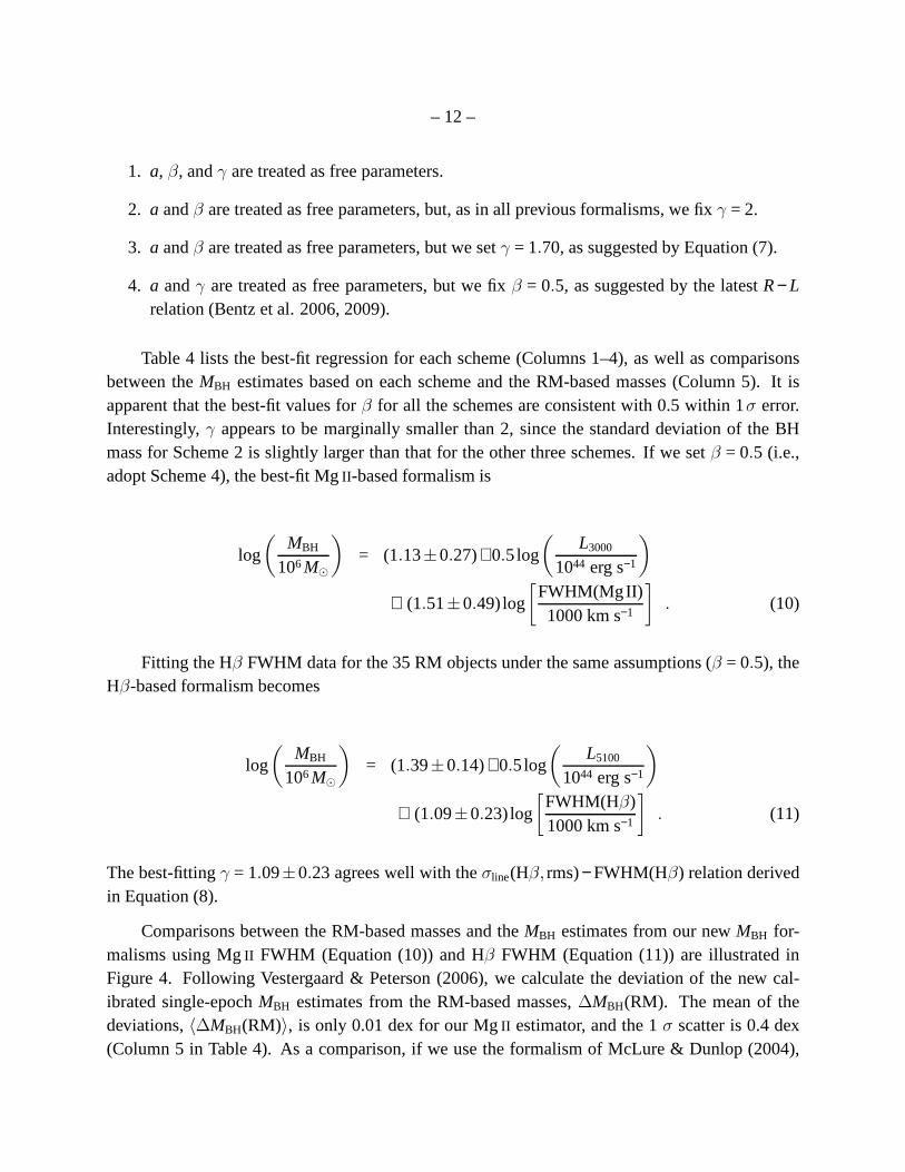
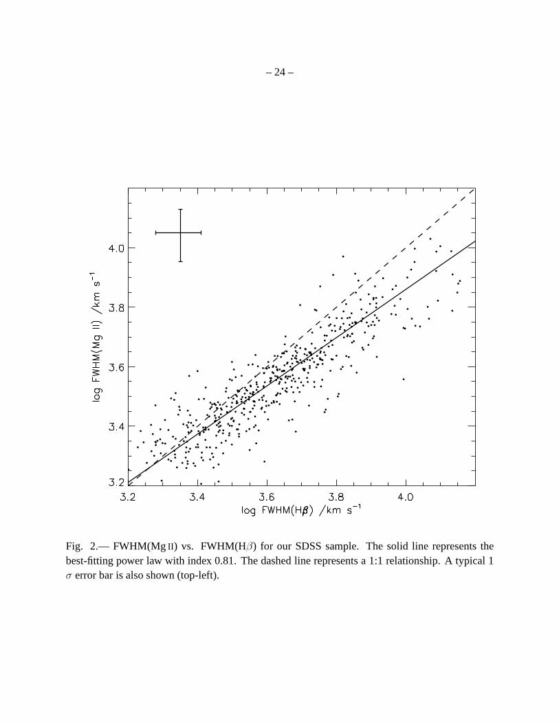
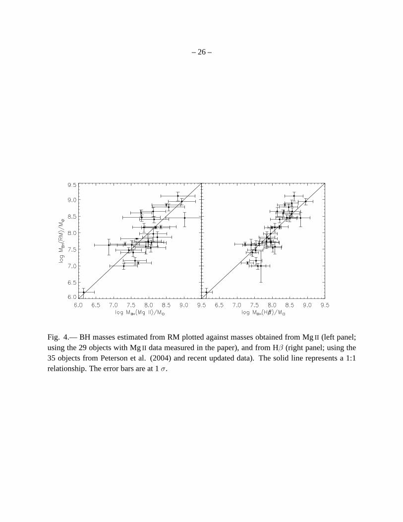
Comparisons between the RM-based masses and theMBH estimates from our newMBH for-malisms using MgII FWHM (Equation (10)) and Hβ FWHM (Equation (11)) are illustrated inFigure 4. Following Vestergaard & Peterson (2006), we calculate the deviation of the new cal-ibrated single-epochMBH estimates from the RM-based masses,∆MBH(RM). The mean of thedeviations,〈∆MBH(RM)〉, is only 0.01 dex for our MgII estimator, and the 1σ scatter is 0.4 dex(Column 5 in Table 4). As a comparison, if we use the formalismof McLure & Dunlop (2004),

– 13 –

the deviations from the same RM-based masses have a mean of 0.38 dex and a 1σ scatter of 0.45dex. For our Hβ estimator,〈∆MBH(RM)〉 is 0.01 dex and the 1σ scatter is 0.3 dex, comparedto 〈∆MBH(RM)〉 = 0.05 dex andσ = 0.4 dex if the formalism of Vestergaard & Peterson (2006)is used.4 It should be noted that these scatters of the scaling relations, which give a measure ofthe uncertainty in estimatingMBH from the single-epoch spectroscopic data, is relative to the RM-based masses only. Since, as pointed out by Vestergaard & Peterson (2006), the RM-based massesthemselves are uncertain typically by a factor of∼ 2.9 (as calibrated against theMBH–σ⋆ relation;Onken et al. 2004), the absolute uncertainty of the masses thus estimated is even higher. For theHβ formalism, we find this absolute uncertainty to be a factor of∼ 3.5, to be compared with afactor of∼ 4 given in Vestergaard & Peterson (2006); for MgII , we estimate that the absoluteuncertainty is a factor of∼ 4.

As shown above, our new formalisms improve somewhat the scatter in the single-epochMBH

estimates compared to previous Hβ and MgII estimators, by 0.1 dex and 0.05 dex, respectively.Given the same linewidth and luminosity data used in this work and in Vestergaard & Peterson(2006), the reduction in the scatter of theMBH estimates should result from a decrease in theintrin-sic dispersion of our improved single-epochMBH formalisms. Using the LINMIX_ERR method,the intrinsic scatter inherent in ourMBH formalism can be inferred to be 0.08 dex (1σ) for the Hβ

and 0.14 dex for MgII .

Figure 5 compares our new MgII-based formalism (we show only Schemes 2 and 4) with theprevious Hβ-based formalisms of Vestergaard & Peterson (2006; panel a)and Collin et al. (2006;panel b), as well as our newly derived version using the SDSS sample of 495 Seyfert 1s and QSOs(Equation (11); panel c). TheMBH residuals between our MgII formalism and the Hβ formalismsare listed in Table 4 (Columns 6–8). While our MgII-based formalism, especially for Scheme 4(Equation (10)), agrees well with our Hβ-based formalism (Equation (11)), note that it deviatesmarkedly from the Hβ formalism of Vestergaard & Peterson. This confirms previoussuspicions(Collin et al. 2006; Sulentic et al. 2006) that the use of Hβ FWHM from mean and single-epochspectra with the assumptionγ = 2 introduces systematic bias intoMBH estimates.

We further compare our new MgII-based formalism (Equation (10)) with other MgII for-malisms widely used in the literature. Figure 5 illustratesthat theMBH estimates following theformalisms of McLure & Dunlop (2004; panel d), Kollmeier et al. (2006; panel e), and Salvianderet al. (2007; panel f) show large systematic deviations, mostly in the sense of being smaller thanours. The deviations stem primarily from the recalibrationof the RM masses; other factors are

4 It should be noted that here we use the averaged spectrum for an object with more than one observation, unlikein Vestergaard & Peterson (2006) where the individual single-epoch Hβ spectral data were used in the regression.If we take the latter approach, our Hβ estimator gives a〈∆MBH(RM)〉 = −0.07 dex and a scatter of 0.33 dex, whileVestergaard & Peterson (2006) gave〈∆MBH(RM)〉 = −0.12 dex and a scatter of 0.45 dex.

– 14 –

discussed in Section 4.3. We note that a yet-unpublished MgII-based formalism by M. Vestergaardet al. (in preparation) used in the recent literature (e.g.,Kelly et al. 2009) is almost identical to ourScheme 2 (withγ fixed to 2).

4. Discussion

4.1. Testing the Effect of Narrow-line Subtraction

The narrow component of MgII is generally weak in luminous type 1 AGNs (e.g., Wills etal. 1993; Laor et al. 1994), and so its contribution to the total line flux can be safely neglected.However, its presence might have a more pronounced impact onthe FWHM measurement of broadMg II . In the literature, narrow MgII was accounted for in the line fitting by some authors (e.g.,McLure & Dunlop 2004), but not by others (e.g., Salviander etal. 2007). As there is usually noclear inflection in the MgII profile, separating narrow MgII from the broad component is oftenchallenging. Fortunately, for the spectra in our SDSS sample, [OIII ] λ5007 is present, and thuswe can use [OIII ] to try to constrain narrow MgII , to test the effect of narrow MgII on the FWHMmeasurement of broad MgII , and also to test the reliability of our MgII fitting strategy.

In addition to the default fitting strategy described in Section 2.2, in which narrow MgIIis modeled as a single free Gaussian, we tried two alternative strategies in which narrow MgIIis (A) not fit at all, and (B) is fit using a single-Gaussian model constrained to that of the linecore of [OIII ]. Broad MgII is modeled as described in Section 2.2. We find that, for the 495objects in our SDSS sample, the distributions of the reducedχ2 of the MgII emission line fit ofthe three approaches can be approximated reasonably well with a log-normal function. The peakand standard deviation of the reducedχ2 are very similar for all three, being (0.97, 0.10 dex) forthe default strategy, (1.01, 0.10 dex) for Strategy A, and (0.99, 0.10 dex) for Strategy B. Regardingthe FWHM of broad MgII , the mean and standard deviation are (−0.04, 0.05) for log[ FWHM(A)

FWHM(default)]

and (0.00, 0.05) for log[ FWHM(B)FWHM(default)]. For Strategy B, the fitted flux of narrow MgII is less than

10% of the total line flux for almost all the objects. Our testsshow that omitting the subtraction ofnarrow MgII has a negligible effect on the FWHM of broad MgII , typically decreasing it only bya tiny factor of 0.04 dex. We further confirm that our default procedure for modeling narrow MgIIis consistent with that using the [OIII ] core as a template.

The above Strategy A is exactly the same as the MgII-fitting method adopted by Salviander etal. (2007). We also compared our method with that of McLure & Dunlop (2004). When fitting thespectra in our SDSS sample by the method of McLure & Dunlop (2004), on average the FWHMof broad MgII is larger than that of our method by 0.1 dex.

– 15 –

4.2. MBH Estimators with Single-epoch Hβ and Mg II

As analyzed in detail by Sulentic et al. (2006), the overall profile of the Hβ emission line,as viewed in single-epoch spectra, likely comprises multiple components emitted from differentsites. First, as a recombination line, Hβ can arise from BLR gas that is very close to the centralengine. Then Hβ can be gravitationally redshifted, as (part of) the component of the “very BLR”(Marziani & Sulentic 1993). Such clouds may be optically thin to the ionizing continuum, suchthat Hβ is no longer responsive to continuum variation (Shields et al. 1995). Second, like CIVλ1549, Hβ can be produced partly in high-ionization winds, as some observations suggest (seeMarziani et al. 2008, and references therein). This wind component would not be virial. Third, Hβcan also be produced on the surface of the accretion disk, both by recombination and collisionalexcitation (Chen & Halpern 1989; Wang et al. 2005; Wu et al. 2008); this component would behighly anisotropic (cf. Collin et al. 2006). Considering the above factors, it is not surprising thatsingle-epoch FWHM is not linearly proportional toσline for rms Hβ (Equation (8)).

Mg II , as a low-ionization, collisionally excited emission line, cannot be produced in cloudsvery close to the central engine. Furthermore, because MgII originates only from optically thickclouds, radiation pressure force cannot act on them very significantly (cf. Marconi et al. 2008,2009; Dong et al. 2009a,b), and thus MgII suffers little from nonvirial motion. Hence, comparedto Hβ, the FWHM of single-epoch MgII should, in principle, deviate less, if at all, from the truevirial velocity of the line-emitting clouds. This is suggested by the best-fit value forγ in Equation(10), which indicatesv2

virial ∝ FWHM(MgII)1.51±0.49.

Previously, researchers have feared that the substantial contamination of the MgII region byFeII multiplets might introduce significant uncertainties in its linewidth measurements, such thatMg II-basedMBH estimates may not be as accurate as those based on Hβ. With the recent avail-ability of a more refined UV FeII template (Tsuzuki et al. 2006; cf. Vestergaard & Wilkes 2001),we have higher confidence that the linewidth measurements ofMg II are reasonably robust. Ourwork suggests that we can measure MgII FWHM typically to within an uncertainty of∼20%.Nevertheless, it would be highly desirable to attempt to further improve the methodology for FeII

subtraction, not only in the UV but also at optical wavelengths.

4.3. Comparison with Previous Studies

As shown in Section 3 (see Figure 5), our MgII- and Hβ-basedMBH formalisms show, inaddition to somewhat improved internal scatter, subtle butsystematic deviations from some ofthe commonly usedMBH estimators in the literature. In general, the formalism prescribed byour Scheme 4 (Equation (10);MBH ∝ FWHM1.51±0.49) gives progressively higher and lowerMBH

– 16 –

values toward the low- and high-mass ends, respectively. The only exception is the Hβ-basedformalism of Collin et al. (2006), which gives roughly consistent results as ours over a relativelylarge mass range. The discrepancies between previous mass estimators and ours arise from one,or a combination, of the following factors incorporated into our analysis. (1) We use the mostrecently recalibrated and updated RMMBH measurements from the literature (Peterson et al. 2004;Denney et al. 2006, 2009b; Metzroth et al. 2006; Bentz et al. 2007; Grier et al. 2008). (2) Ournew formalism (Scheme 4, Equation (10)) uses the best-fitting value ofγ instead of the canonicalvalue ofγ = 2. (3) For MgII , we determine the scaling factor (incorporated into the coefficienta of Equation (9)) and the power-law index (β) of the RMgII –L relation by fitting Equation (9) tothe data, instead of simply using the existingRHβ–L relation as a surrogate. (4) Differences in theline-fitting and determination of the FWHM. We discuss each of these factors in detail below.

Specifically, assuming the canonical value ofγ = 2 in Equation (9) would, compared to ourScheme 4, underestimateMBH at the low-end and overestimateMBH at the high-end, for bothMg II and Hβ. This accounts for most of the deviations from Vestergaard &Peterson (2006) andKollmeier et al. (2006), and partially from others in Figure5. In order to account for systematicbiases with respect to RM-basedMBH, Collin et al. (2006) introduced a correction factor, whichisdependent on Hβ FWHM, into their Hβ-based formalism assumingγ = 2. This correction has asimilar effect as fittingγ as a free parameter, as we do here, and thus the rough consistency betweenour results and theirs is not surprising. Factor (3) is also partially responsible for producing thedeviations from some of the previous MgII-basedMBH estimators, such as those of McLure &Dunlop (2004) and Salviander et al. (2007), who assumed thatboth MgII and Hβ obey the sameR–L relation, and of Kollmeier et al. (2006), who used a very steep relation ofRMgII ∝ L0.88.

There have been previous reports of discrepancies between Mg II- and Hβ-based estimators,which are sometimes claimed to correlate with luminosity orEddington ratio (e.g., Kollmeier et al.2006; Onken & Kollmeier 2008). These effects can be traced, at least partially, to the one-to-onerelation assumed between FWHM(MgII) and FWHM(Hβ), which is contradictory to the nonlinearrelation found in this work. In fact, by adopting a nonlinearFWHM(Mg II)–FWHM(Hβ) relationandRMgII ∝ L0.5, our new MgII- and Hβ-based estimators yield mutually consistent results forthe SDSS sample (Figure 5, panel c). We verified that the previously claimed correlations of theresiduals of the MgII- and Hβ-based estimators with luminosity or Eddington ratio largely vanish;a Spearman rank analysis indicates a chance probability of 0.09 for the former and 0.05 for thelatter.

It is generally accepted that the width of the variable part of the line, the line dispersionσline measured in the rms spectrum, is by far the best tracer of the virial velocity of the BLR gasresponsible for the variable portion of the emission line (e.g., Onken & Peterson 2002), such thatMBH ∝ σ2

line according to the virial theorem. If the virial velocity is estimated using FWHM (or

– 17 –

any other measure of the linewidth) in single-epoch spectra, as long as its relation withσline isnonlinear,γ in Equation (9) is expected to deviate fromγ = 2. This is exactly what we find in thiswork for FWHM(Mg II) at 1σ significance level, as well as for FWHM(Hβ) at 6σ significancelevel. In fact, the fitted value ofγ = 1.51±0.49 for MgII (Equation (10)) and 1.09±0.23 for Hβ

(Equation (11)) are almost identical to those derived from the fittedσline–FWHM(Mg II) andσline–FWHM(Hβ) relations, which have slopes of 1.70±0.42 and 1.08±0.16, respectively. Factor (3)is justified by the compelling evidence presented in this work that the line-emitting locations ofHβ and MgII in the BLR are not identical. Possible physical processes underlying factors (2) and(3) are discussed in Section 4.2.

As an additional consideration, we have performed in this work refined and careful line fittingand determination of the FWHM, which may have subtle differences from previous results. Thesedifferences may also give rise to, to some extent, the systematic discrepancies between the massrelations in Figure 5 since we use our measured FWHM and luminosity data when producing thefigure. For example, Salviander et al. (2007) did not subtract the narrow component of MgII ,leading to MgII FWHM statistically smaller than ours; so the true deviations in Figure 5 (panel f)would be larger if their FWHM data were used. On the contrary,McLure & Dunlop (2004) over-subtracted the narrow component compared to ours (they considered a possible narrow componentas having an upper limit of FWHM = 2000 km s−1, much larger than the 900 km s−1 used in ourwork), and their MgII FWHM are statistically larger than ours; thus, the true deviations in Figure5 (panel e) would be somewhat smaller if their FWHM data were used.

Finally, the appropriateness of our approach is further justified by the fact that our formalismsgive MBH values consistent with the RM measurements with the least systematic bias, as well asa reduced (intrinsic) scatter compared to previous formalisms (Section 3.3). Moreover, we findconsistent masses between the MgII- and Hβ-based estimators. We thus conclude that ourMBH

estimators introduce less systematic bias compared to previous formalisms. Obviously, more RMmeasurements (for both Hβ and MgII) are needed in order to improve the determination of theσline–FWHM relation, theR–L relation, and the indexγ in theMBH ∝ FWHMγ relation.

5. Summary and Conclusions

We investigate the relation between the velocity widths forthe broad MgII and Hβ emissionlines, derived from FWHM measurements of single-epoch spectra from a homogeneous sample of495 SDSS Seyfert 1s and QSOs at 0.45< z < 0.75. Careful attention is devoted to accurate spec-tral decomposition, especially in the treatment of narrow-line blending and FeII contamination. Wefind that MgII FWHM is systematic smaller than Hβ FWHM, such that FWHM(MgII)∝FWHM(Hβ)0.81±0.02.Using 29 AGNs that have optical RM data and usable archival UVspectra, we then investigate

– 18 –

the relation between single-epoch MgII FWHM and rms Hβ σline (line dispersion), a quantityregarded as a good tracer of the virial velocity of the BLR clouds emitting the variable Hβ com-ponent. We find that, similar to the situation for the FWHM of single-epoch Hβ, single-epochMg II FWHM is unlikely to be linearly proportional to rms Hβ σline . The above two findingssuggest that a major assumption of previous MgII-based virial BH mass formalisms—that theMg II-emitting region is identical to that ofHβ—is problematic. This finding and the recent up-dates of the reverberation-mapped BH masses (Peterson et al. 2004; Denney et al. 2006, 2009b;Metzroth et al. 2006; Bentz et al. 2007; Grier et al. 2008) motivated us to recalibrate theMBH

estimator based on single-epoch MgII spectra.

Starting with the empirically well-motivated BLR radius–luminosity relation and the virialtheorem,MBH ∝ LβFWHMγ , we fit the reverberation-mapped objects in a variety of different waysto constrainβ andγ. For all the strategies we have considered,β has a well-defined value of∼0.5,in excellent agreement with the latest BLR radius–luminosity relation (Bentz et al. 2006, 2009),whereasγ ≈1.5±0.5, which is marginally in conflict with the canonical value ofγ = 2 normally as-sumed in past studies. Performing a similar exercise for Hβ yieldsMBH ∝ L0.5FWHM(Hβ)1.09±0.22,which again significantly departs from the functional formsused in the literature. The 1σ uncer-tainty (scatter) is of the order of 0.3 dex relative to the RM-based masses for the Hβ estimator,and∼0.4 dex for the MgII estimator. Using the same data set, the scatter of our Hβ mass scalingrelation is reduced by 0.1 dex over that of Vestergaard & Peterson (2006), indicating improvementin the internal scatter.

We use the SDSS database to compare our newMBH estimators with various existing for-malisms based on single-epoch Hβ and MgII spectra. BH masses derived from our MgII-basedmass estimator show subtle but important deviations from many of the commonly usedMBH esti-mators in the literature. Most of the differences stem from the recent recalibration of the massesderived from RM. Researchers should exercise caution in selecting the most up-to-dateMBH esti-mators, which are presented here.

We thank the referee, Michael Strauss, for his careful comments and helpful suggestions thatimproved the paper. This work is supported by Chinese NSF grants NSF-10533050 and NSF-10703006, National Basic Research Program of China (973 Program 2009CB824800) and a CASKnowledge Innovation Program (grant no. KJCX2-YW-T05). The research of L.C.H. is supportedby the Carnegie Institution for Science. Funding for the SDSS and SDSS-II has been providedby the Alfred P. Sloan Foundation, the Participating Institutions, the National Science Foundation,the U.S. Department of Energy, the National Aeronautics andSpace Administration, the JapaneseMonbukagakusho, the Max Planck Society, and the Higher Education Funding Council for Eng-land. The SDSS Web Site is http://www.sdss.org/.

– 19 –

REFERENCES

Adelman-McCarthy, J. K., et al. 2007, ApJS, 172, 634

Akritas, M. G., & Bershady, M. A. 1996, ApJ, 470, 706

Bentz, M. C., Peterson, B. M., Netzer, H., Pogge, R. W., & Vestergaard, M. 2009, ApJ, 697, 160

Bentz, M. C., Peterson, B. M., Pogge, R. W., Vestergaard, M.,& Onken, C. A. 2006, ApJ, 644,133

Bentz, M. C., et al. 2007, ApJ, 662, 205

Chen, K., & Halpern, J. P. 1989, ApJ, 344, 115

Clavel, J., et al. 1991, ApJ, 366, 64

Collin, S., Kawaguchi, T., Peterson, B. M., & Vestergaard, M. 2006, A&A, 456, 75

Corbett, E. A., et al. 2003, MNRAS, 343, 705

Denney, K. D., Peterson, B. M., Dietrich, M., Vestergaard, M., & Bentz, M. C. 2009a, ApJ, 692,246

Denney, K. D., et al. 2006, ApJ, 653, 152

Denney, K. D., et al. 2009b, ApJ, 702, 1353

Dietrich, M., Appenzeller, I., Vestergaard, M., & Wagner, S. J. 2002, ApJ, 564, 581

Dietrich, M., & Hamann, F. 2004, ApJ, 611, 761

Dietrich, M., & Kollatschny, W. 1995, A&A, 303, 405

Dong, X.-B., Wang, T.-G., Wang, J.-G., Fan, X., Wang, H., Zhou, H., & Yuan, W. 2009a, ApJ,703, L1

Dong, X.-B., Wang, J.-G., Wang, T.-G., Wang, H., Fan, X., Zhou, H., & Yuan, W. 2009b, ApJsubmitted (arXiv:0903.5020)

Dong, X.-B., Wang, T.-G., Wang, J.-G., Yuan, W., Zhou, H., Dai, H., & Zhang, K. 2008, MNRAS,383, 581

Dong, X.-B., Zhou, H.-Y., Wang, T.-G., Wang, J.-X., Li, C., &Zhou, Y.-Y. 2005, ApJ, 620, 629

– 20 –

Ferland, G. J., Korista, K. T., Verner, D. A., Ferguson, J. W., Kingdon, J. B., & Verner, E. M. 1998,PASP, 110, 761

Ferrarese, L., & Merritt, D. 2000, ApJ, 539, L9

Ferrarese, L., Pogge, R. W., Peterson, B. M., Merritt, D., Wandel, A., & Joseph, C. L. 2001, ApJ,555, L79

Fitzpatrick, E. L. 1999, PASP, 111, 63

Gebhardt, K., et al. 2000a, ApJ, 539, L13

Gebhardt, K., et al. 2000b, ApJ, 543, L5

Greene, J. E., & Ho, L. C. 2005, ApJ, 630, 122

Greene, J. E., & Ho, L. C. 2006, ApJ, 641, L21

Grier, C. J., et al. 2008, ApJ, 688, 837

Ho, L. C., Darling, J., & Greene, J. E. 2008, ApJ, 681, 128

Hu, C., Wang, J.-M., Ho, L. C., Chen, Y.-M., Zhang, H.-T., Bian, W.-H., & Xue, S.-J. 2008, ApJ,687, 78

Jefferys, W. H. 1980, AJ, 85, 177

Jefferys, W. H. 1981, AJ, 86, 149

Kaspi, S., Brandt, W. N., Maoz, D., Netzer, H., Schneider, D.P., & Shemmer, O. 2007, ApJ, 659,997

Kaspi, S., Maoz, D., Netzer, H., Peterson, B. M., Vestergaard, M., & Jannuzi, B. T. 2005, ApJ,629, 61

Kaspi, S., Smith, P. S., Netzer, H., Maoz, D., Jannuzi, B. T.,& Giveon, U. 2000, ApJ, 533, 631

Kelly, B. C. 2007, ApJ, 665, 1489

Kelly, B. C., Vestergaard, M., & Fan, X. 2009, ApJ, 692, 1388

Kim, M., Ho, L. C., Peng, C. Y., Barth, A. J., Im, M., Martini, P., & Nelson, C. H. 2008, ApJ, 687,767

Kollmeier, J. A., et al. 2006, ApJ, 648, 128

– 21 –

Laor, A., Bahcall, J. N., Jannuzi, B. T., Schneider, D. P., Green, R. F., & Hartig, G. F. 1994, ApJ,420, 110

Laor, A., Jannuzi, B. T., Green, R. F., & Boroson, T. A. 1997, ApJ, 489, 656

Marconi, A., Axon, D. J., Maiolino, R., Nagao, T., Pastorini, G., Pietrini, P., Robinson, A., &Torricelli, G. 2008, ApJ, 678, 693

Marconi, A., Axon, D. J., Maiolino, R., Nagao, T., Pietrini,P., Risaliti, G., Robinson, A., &Torricelli, G. 2009, ApJ, 698, L103

Markwardt, C. B. 2009, in ASP Conf. Ser. 411, Astronomical Data Analysis Software and SystemsXVIII, ed. D. A. Bohlender, Daniel Durand, and Patrick Dowler (San Francisco, CA: ASP),251

Marziani, P., & Sulentic, J. W. 1993, ApJ, 409, 612

Marziani, P., Sulentic, J. W., & Dultzin, D. 2008, RevMexAA,32, 69

McArthur, B., Jefferys, W., & McCartney, J. 1994, BAAS, 26, 900

McGill, K. L., Woo, J.-H., Treu, T., & Malkan, M. A. 2008, ApJ,673, 703

McLure, R. J., & Dunlop, J. S. 2004, MNRAS, 352, 1390

McLure, R. J., & Jarvis, M. J. 2002, MNRAS, 337, 109

Metzroth, K. G., Onken, C. A., & Peterson, B. M. 2006, ApJ, 647, 901

Nelson, C. H., Green, R. F., Bower, G., Gebhardt, K., & Weistrop, D. 2004, ApJ, 615, 652

Onken, C. A., Ferrarese, L., Merritt, D., Peterson, B. M., Pogge, R. W., Vestergaard, M., & Wandel,A. 2004, ApJ, 615, 645

Onken, C. A., & Kollmeier, J. A. 2008, ApJ, 689, L13

Onken, C. A., & Peterson, B. M. 2002, ApJ, 572, 746

Peterson, B. M., & Wandel, A. 1999, ApJ, 521, L95

Peterson, B. M., & Wandel, A. 2000, ApJ, 540, L13

Peterson, B. M., et al. 2004, ApJ, 613, 682

Press, W. H., Teukolsky, S. A., Vetterling, W. T., & Flannery, B. P. 1992, Numerical Recipes inFORTRAN. The Art of Scientific Computing (Cambridge: Cambridge Univ. Press)

– 22 –

Salviander, S., Shields, G. A., Gebhardt, K., & Bonning, E. W. 2007, ApJ, 662, 131

Schlegel, D. J., Finkbeiner, D. P., & Davis, M. 1998, ApJ, 500, 525

Shen, Y., Greene, J. E., Strauss, M. A., Richards, G. T., & Schneider, D. P. 2008, ApJ, 680, 169

Shields, J. C., Ferland, G. J., & Peterson, B. M. 1995, ApJ, 441, 507

Sulentic, J. W., Repetto, P., Stirpe, G. M., Marziani, P., Dultzin-Hacyan, D., & Calvani, M. 2006,A&A, 456, 929

Tremaine, S., et al. 2002, ApJ, 574, 740

Tsuzuki, Y., Kawara, K., Yoshii, Y., Oyabu, S., Tanabé, T., &Matsuoka, Y. 2006, ApJ, 650, 57

Vanden Berk, D. E., et al. 2001, AJ, 122, 549

van der Marel, R. P., & Franx, M. 1993, ApJ, 407, 525

Vestergaard, M. 2002, ApJ, 571, 733

Vestergaard, M., & Peterson, B. M. 2006, ApJ, 641, 689

Vestergaard, M., & Wilkes, B. J. 2001, ApJS, 134, 1

Wandel, A., Peterson, B. M., & Malkan, M. A. 1999, ApJ, 526, 579

Wang, T.-G., Dong, X.-B., Zhang, X.-G., Zhou, H.-Y., Wang, J.-X., & Lu, Y.-J. 2005, ApJ, 625,L35

Wills, B. J., Netzer, H., Brotherton, M. S., Han, M., Wills, D., Baldwin, J. A., Ferland, G. J., &Browne, I. W. A. 1993, ApJ, 410, 534

Wu, S.-M., Wang, T.-G., & Dong, X.-B. 2008, MNRAS, 389, 213

York, D. G., et al. 2000, AJ, 120, 1579

This preprint was prepared with the AAS LATEX macros v5.2.

– 23 –

Fig. 1.— Examples of MgII fitting for (top) the HST spectrum of Mrk 335 and (bottom) theSDSS spectrum of SDSS J131459.75+505932.9. The data are shown in black, the power-lawAGN continuum in blue, the pseudocontinuum (power law plus FeII emission) in pink, the finalmodel for all fitted components in green, and the continuum-subtracted emission-line spectrum ingray. For the multi-Gaussian fit to MgII , the narrow components are shown in navy, the individualbroad components in brown, the sum of all the broad components in cyan, and the total model(narrow plus broad) in red.

– 24 –

Fig. 2.— FWHM(MgII) vs. FWHM(Hβ) for our SDSS sample. The solid line represents thebest-fitting power law with index 0.81. The dashed line represents a 1:1 relationship. A typical 1σ error bar is also shown (top-left).

– 25 –

Fig. 3.— σline(Hβ, rms) vs. FWHM(MgII) of the 29 objects with MgII FWHM measured in thepaper (left panel) and FWHM(Hβ, mean) of the 35 objects from Collin et al. (2006) and recentupdated data (right panel). The solid lines show the best-fitting relations. The error bars are at 1σ.

– 26 –

Fig. 4.— BH masses estimated from RM plotted against masses obtained from MgII (left panel;using the 29 objects with MgII data measured in the paper), and from Hβ (right panel; using the35 objects from Peterson et al. (2004) and recent updated data). The solid line represents a 1:1relationship. The error bars are at 1σ.

– 27 –

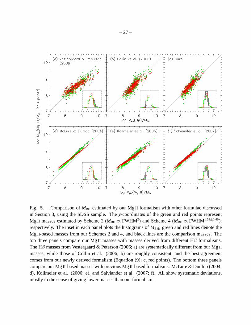
Fig. 5.— Comparison ofMBH estimated by our MgII formalism with other formulae discussedin Section 3, using the SDSS sample. They-coordinates of the green and red points representMg II masses estimated by Scheme 2 (MBH ∝ FWHM2) and Scheme 4 (MBH ∝ FWHM1.51±0.49),respectively. The inset in each panel plots the histograms of MBH; green and red lines denote theMg II-based masses from our Schemes 2 and 4, and black lines are thecomparison masses. Thetop three panels compare our MgII masses with masses derived from different Hβ formalisms.The Hβ masses from Vestergaard & Peterson (2006; a) are systematically different from our MgII

masses, while those of Collin et al. (2006; b) are roughly consistent, and the best agreementcomes from our newly derived formalism (Equation (9); c, redpoints). The bottom three panelscompare our MgII-based masses with previous MgII-based formalisms: McLure & Dunlop (2004;d), Kollmeier et al. (2006; e), and Salviander et al. (2007; f). All show systematic deviations,mostly in the sense of giving lower masses than our formalism.

– 28 –

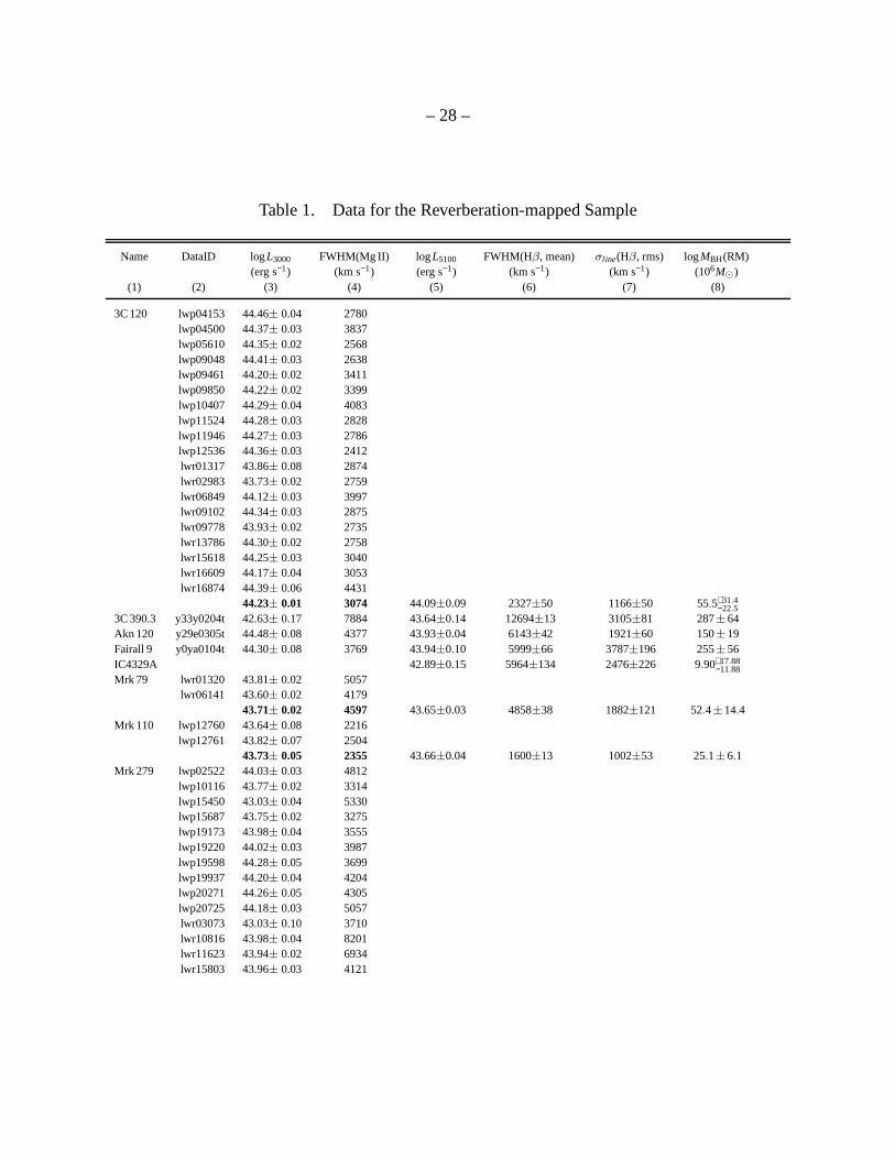
Table 1. Data for the Reverberation-mapped Sample

Name DataID logL3000 FWHM(Mg II) log L5100 FWHM(Hβ, mean) σline(Hβ, rms) logMBH(RM)(erg s−1) (km s−1) (erg s−1) (km s−1) (km s−1) (106M⊙)

(1) (2) (3) (4) (5) (6) (7) (8)

3C 120 lwp04153 44.46± 0.04 2780lwp04500 44.37± 0.03 3837lwp05610 44.35± 0.02 2568lwp09048 44.41± 0.03 2638lwp09461 44.20± 0.02 3411lwp09850 44.22± 0.02 3399lwp10407 44.29± 0.04 4083lwp11524 44.28± 0.03 2828lwp11946 44.27± 0.03 2786lwp12536 44.36± 0.03 2412lwr01317 43.86± 0.08 2874lwr02983 43.73± 0.02 2759lwr06849 44.12± 0.03 3997lwr09102 44.34± 0.03 2875lwr09778 43.93± 0.02 2735lwr13786 44.30± 0.02 2758lwr15618 44.25± 0.03 3040lwr16609 44.17± 0.04 3053lwr16874 44.39± 0.06 4431

44.23± 0.01 3074 44.09±0.09 2327±50 1166±50 55.5+31.4−22.5

3C 390.3 y33y0204t 42.63± 0.17 7884 43.64±0.14 12694±13 3105±81 287±64Akn 120 y29e0305t 44.48± 0.08 4377 43.93±0.04 6143±42 1921±60 150±19Fairall 9 y0ya0104t 44.30± 0.08 3769 43.94±0.10 5999±66 3787±196 255±56IC4329A 42.89±0.15 5964±134 2476±226 9.90+17.88

−11.88Mrk 79 lwr01320 43.81± 0.02 5057

lwr06141 43.60± 0.02 417943.71± 0.02 4597 43.65±0.03 4858±38 1882±121 52.4±14.4

Mrk 110 lwp12760 43.64± 0.08 2216lwp12761 43.82± 0.07 2504

43.73± 0.05 2355 43.66±0.04 1600±13 1002±53 25.1±6.1Mrk 279 lwp02522 44.03± 0.03 4812

lwp10116 43.77± 0.02 3314lwp15450 43.03± 0.04 5330lwp15687 43.75± 0.02 3275lwp19173 43.98± 0.04 3555lwp19220 44.02± 0.03 3987lwp19598 44.28± 0.05 3699lwp19937 44.20± 0.04 4204lwp20271 44.26± 0.05 4305lwp20725 44.18± 0.03 5057lwr03073 43.03± 0.10 3710lwr10816 43.98± 0.04 8201lwr11623 43.94± 0.02 6934lwr15803 43.96± 0.03 4121

– 29 –

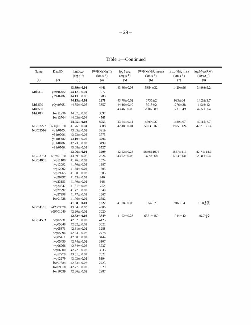
Table 1—Continued

Name DataID logL3000 FWHM(Mg II) log L5100 FWHM(Hβ, mean) σline(Hβ, rms) logMBH(RM)(erg s−1) (km s−1) (erg s−1) (km s−1) (km s−1) (106M⊙)

(1) (2) (3) (4) (5) (6) (7) (8)

43.89± 0.01 4441 43.66±0.08 5354±32 1420±96 34.9±9.2Mrk 335 y29e0205t 44.12± 0.04 1977

y29e0206t 44.13± 0.05 178344.13± 0.03 1878 43.78±0.02 1735±2 933±64 14.2±3.7

Mrk 509 y0ya0305t 44.55± 0.05 3357 44.16±0.10 3015±2 1276±28 143±12Mrk 590 43.46±0.05 2906±89 1231±49 47.5±7.4Mrk 817 lwr11936 44.07± 0.03 3597

lwr13704 44.03± 0.04 456544.05± 0.03 4053 43.64±0.14 4899±37 1680±67 49.4±7.7

NGC 3227 o5kp01010 41.76± 0.04 3688 42.48±0.04 5103±160 1925±124 42.2±21.4NGC 3516 y31r0105t 43.05± 0.02 3919

y31r0206t 43.23± 0.02 3775y31r0306t 43.19± 0.02 3796y31r0406t 42.73± 0.02 3499y31r0506t 43.08± 0.02 3527

43.06± 0.01 3699 42.62±0.28 5840±1976 1837±115 42.7±14.6NGC 3783 o57b01010 43.39± 0.06 2524 43.02±0.06 3770±68 1753±141 29.8±5.4NGC 4051 lwp11100 41.76± 0.02 1574

lwp12092 41.70± 0.02 1387lwp12092 41.68± 0.02 1503lwp19265 41.58± 0.02 1305lwp20497 41.53± 0.02 946lwp23153 41.70± 0.02 918lwp24347 41.81± 0.02 752lwp27297 41.77± 0.02 1349lwp27298 41.77± 0.02 1667lwr01728 41.76± 0.02 2582

41.68± 0.01 1322 41.88±0.08 654±2 916±64 1.58+0.50−0.65

NGC 4151 o42303070 43.04± 0.03 4905o59701040 42.20± 0.02 3020

42.62± 0.02 3849 41.92±0.23 6371±150 1914±42 45.7+5.7−4.7

NGC 4593 lwp02731 42.82± 0.02 4123lwp05348 42.82± 0.02 3022lwp05371 42.81± 0.02 3288lwp05394 42.83± 0.02 2778lwp05411 42.80± 0.02 3444lwp05430 42.74± 0.02 3107lwp06266 42.64± 0.02 3237lwp06300 42.72± 0.02 3033lwp12278 43.01± 0.02 2822lwp12279 43.03± 0.02 5194lwr07884 42.83± 0.02 2723lwr09818 42.77± 0.02 1929lwr10539 42.86± 0.02 2987

– 30 –

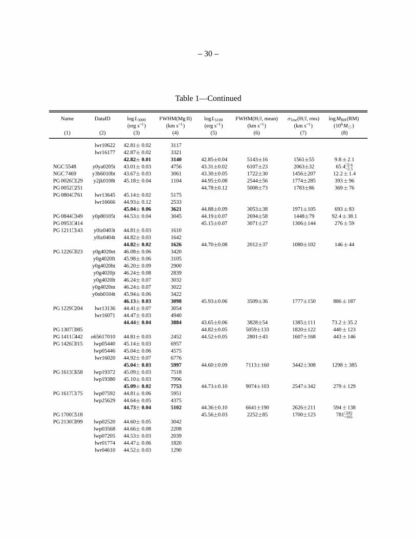
Table 1—Continued

Name DataID logL3000 FWHM(Mg II) log L5100 FWHM(Hβ, mean) σline(Hβ, rms) logMBH(RM)(erg s−1) (km s−1) (erg s−1) (km s−1) (km s−1) (106M⊙)

(1) (2) (3) (4) (5) (6) (7) (8)

lwr10622 42.81± 0.02 3117lwr16177 42.87± 0.02 3321

42.82± 0.01 3140 42.85±0.04 5143±16 1561±55 9.8±2.1NGC 5548 y0ya0205t 43.01± 0.03 4756 43.31±0.02 6107±23 2063±32 65.4+2.6

−2.5NGC 7469 y3b6010bt 43.67± 0.03 3061 43.30±0.05 1722±30 1456±207 12.2±1.4PG 0026+129 y2jk0108t 45.18± 0.04 1104 44.95±0.08 2544±56 1774±285 393±96PG 0052+251 44.78±0.12 5008±73 1783±86 369±76PG 0804+761 lwr13645 45.14± 0.02 5175

lwr16666 44.93± 0.12 253345.04± 0.06 3621 44.88±0.09 3053±38 1971±105 693±83

PG 0844+349 y0p80105t 44.53± 0.04 3045 44.19±0.07 2694±58 1448±79 92.4±38.1PG 0953+414 45.15±0.07 3071±27 1306±144 276±59PG 1211+143 y0iz0403t 44.81± 0.03 1610

y0iz0404t 44.82± 0.03 164244.82± 0.02 1626 44.70±0.08 2012±37 1080±102 146±44

PG 1226+023 y0g4020et 46.08± 0.06 3420y0g4020ft 45.98± 0.06 3105y0g4020ht 46.20± 0.09 2900y0g4020jt 46.24± 0.08 2839y0g4020lt 46.24± 0.07 3032y0g4020nt 46.24± 0.07 3022y0nb0104t 45.94± 0.06 3422

46.13± 0.03 3098 45.93±0.06 3509±36 1777±150 886±187PG 1229+204 lwr13136 44.41± 0.07 3054

lwr16071 44.47± 0.03 494044.44± 0.04 3884 43.65±0.06 3828±54 1385±111 73.2±35.2

PG 1307+085 44.82±0.05 5059±133 1820±122 440±123PG 1411+442 o65617010 44.81± 0.03 2452 44.52±0.05 2801±43 1607±168 443±146PG 1426+015 lwp05440 45.14± 0.03 6957

lwp05446 45.04± 0.06 4575lwr16020 44.92± 0.07 6776

45.04± 0.03 5997 44.60±0.09 7113±160 3442±308 1298±385PG 1613+658 lwp19372 45.09± 0.03 7518

lwp19380 45.10± 0.03 799645.09± 0.02 7753 44.73±0.10 9074±103 2547±342 279±129

PG 1617+175 lwp07592 44.81± 0.06 5951lwp25629 44.64± 0.05 4375

44.73± 0.04 5102 44.36±0.10 6641±190 2626±211 594±138PG 1700+518 45.56±0.03 2252±85 1700±123 781+182

−165PG 2130+099 lwp02520 44.60± 0.05 3042

lwp03568 44.66± 0.08 2208lwp07205 44.53± 0.03 2039lwr01774 44.47± 0.06 1820lwr04610 44.52± 0.03 1290

– 31 –

Table 1—Continued

Name DataID logL3000 FWHM(Mg II) log L5100 FWHM(Hβ, mean) σline(Hβ, rms) logMBH(RM)(erg s−1) (km s−1) (erg s−1) (km s−1) (km s−1) (106M⊙)

(1) (2) (3) (4) (5) (6) (7) (8)

lwr04628 44.58± 0.06 2479lwr15802 44.51± 0.03 2885

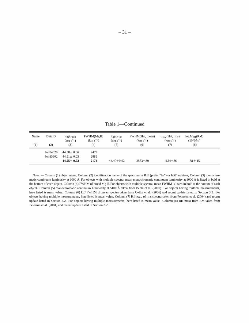
44.55± 0.02 2174 44.40±0.02 2853±39 1624±86 38±15

Note. — Column (1) object name; Column (2) identification name of the spectrum inIUE (prefix “lw”) or HST archives; Column (3) monochro-matic continuum luminosity at 3000 Å. For objects with multiple spectra, mean monochromatic continuum luminosity at 3000 Å is listed in bold atthe bottom of each object. Column (4) FWHM of broad Mg II. For objects with multiple spectra, mean FWHM is listed in bold at the bottom of eachobject. Column (5) monochromatic continuum luminosity at 5100 Å taken from Bentz et al. (2009). For objects having multiple measurements,here listed is mean value. Column (6) Hβ FWHM of mean spectra taken from Collin et al. (2006) and recent update listed in Section 3.2. Forobjects having multiple measurements, here listed is mean value. Column (7) Hβ σline of rms spectra taken from Peterson et al. (2004) and recentupdate listed in Section 3.2. For objects having multiple measurements, here listed is mean value. Column (8) BH mass from RM taken fromPeterson et al. (2004) and recent update listed in Section 3.2.

– 32 –

Table 2. Continuum and Emission-line Parameters of the SDSSSample

SDSS Name z logL5100 FWHM(Hβb) logF(Hβb) logF(Hβn) logL3000 FWHM(Mg IIb) logF(Mg IIb) logF(Mg IIn)(1) (2) (3) (4) (5) (6) (7) (8) (9) (10)

J000011.96+000225.3 0.478 44.69 3037 −13.89 −15.68 44.99 3284 −13.84 −14.89J000110.97−105247.5 0.529 44.98 6807 −13.73 −15.53 45.18 5797 −13.85 −15.15J001725.36+141132.6 0.514 45.23 5676 −13.49 −15.52 45.49 4432 −13.64 −14.71J002019.22−110609.2 0.492 44.85 2832 −13.74 · · · 45.00 2677 −13.91 −16.16J005121.25+004521.5 0.727 45.04 2572 −14.09 −15.07 45.14 1606 −14.42 −15.41J005441.19+000110.7 0.646 45.08 2220 −14.24 · · · 45.13 2172 −14.20 −15.29J010448.57−091013.0 0.469 44.77 4610 −13.81 −15.33 44.88 2627 −14.11 −15.86J010644.16−103410.6 0.468 44.72 3873 −13.83 −15.35 44.85 3074 −13.80 −15.43J011132.34+133519.0 0.576 45.13 8060 −13.66 −15.72 45.39 5495 −13.73 −14.87J012016.73−092028.8 0.495 44.71 3284 −13.72 −16.02 45.05 3312 −13.58 −16.07

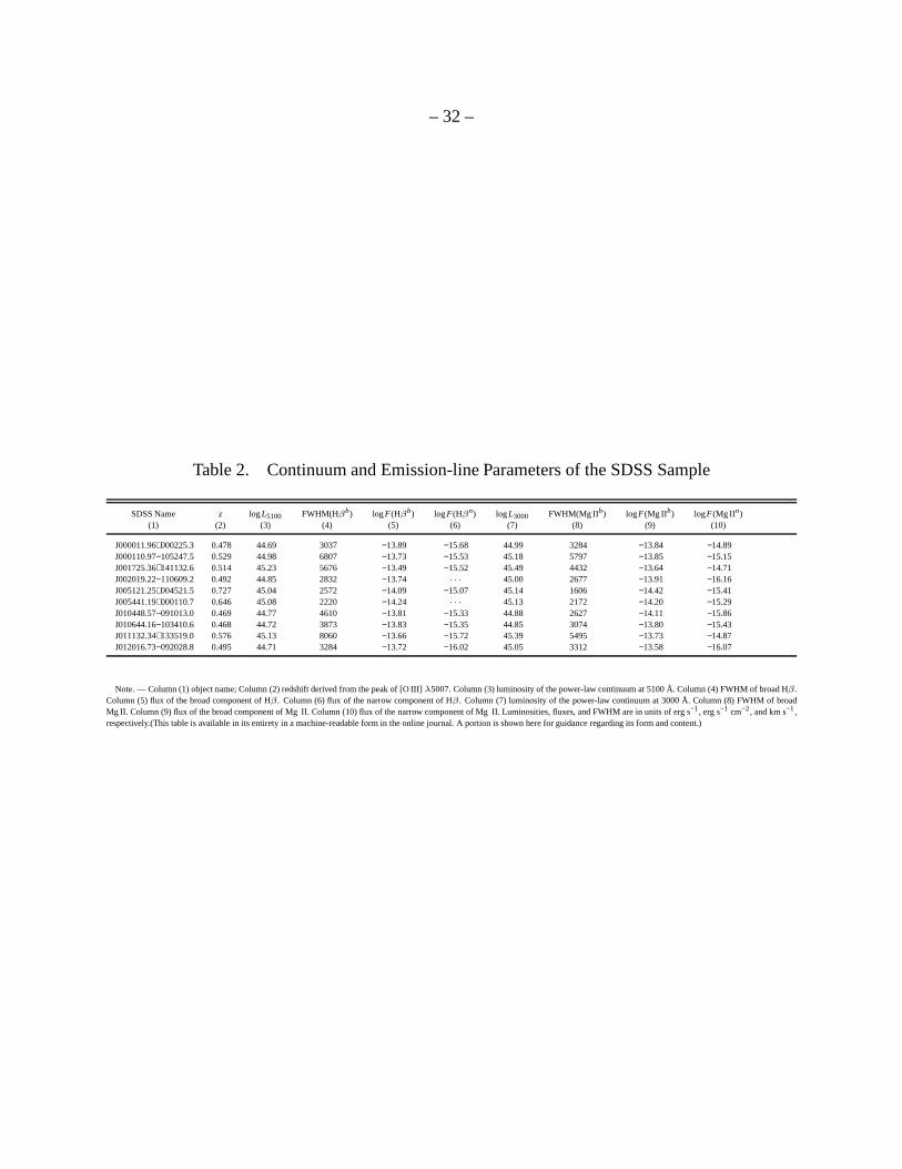
Note. — Column (1) object name; Column (2) redshift derived from the peak of [O III]λ5007. Column (3) luminosity of the power-law continuum at 5100 Å. Column (4) FWHM of broad Hβ.Column (5) flux of the broad component of Hβ. Column (6) flux of the narrow component of Hβ. Column (7) luminosity of the power-law continuum at 3000 Å.Column (8) FWHM of broadMg II. Column (9) flux of the broad component of Mg II. Column (10) flux of the narrow component of Mg II. Luminosities, fluxes,and FWHM are in units of erg s−1, erg s−1 cm−2, and km s−1,respectively.(This table is available in its entirety in a machine-readable form in the online journal. A portion is shown here for guidance regarding its form and content.)

– 33 –

Table 3. Regression Results for

log

[

FWHM(MgII)1000 km s−1

]

= k log

[

FWHM(Hβ)1000 km s−1

]

+ c

Method k c

OLS 0.73±0.02 0.09±0.01WLS 0.73±0.02 0.09±0.01FITexy 0.77±0.01 0.06±0.02FITexy_T02 0.81±0.03 0.04±0.02Gaussfit 0.81±0.03 0.04±0.02BCES (bisector) 0.78±0.03 0.06±0.02BCES (orthogonal) 0.81±0.02 0.05±0.01LINMIX_ERR 0.79±0.03 0.05±0.02

Table 4. Regression Results for log[

MBH(RM)106 M⊙

]

= a +β log(

L30001044 erg s−1

)

+γ log[FWHM(MgII)

1000 km s−1

]

andMBH Comparisons

Scheme a β γ ∆MBH(RM) ∆MBH(Hβ) ∆MBH(Hβ) ∆MBH(Hβ)(Vestergaard+06) (Collin+06) (Ours)

(1) (2) (3) (4) (5) (6) (7) (8)Mean 1σ Mean 1σ Mean 1σ Mean 1σ

Scheme 1a 1.15±0.27 0.46±0.08 1.48±0.49 0.01 0.39 0.15 0.22 0.10 0.14 0.07 0.12Scheme 2 0.88±0.08 0.48±0.08 2 0.01 0.42 0.11 0.19 0.06 0.18 0.03 0.18Scheme 3 1.03±0.08 0.48±0.08 1.70 0.01 0.40 0.13 0.20 0.07 0.15 0.05 0.14Scheme 4 1.13±0.27 0.5 1.51±0.49 0.01 0.40 0.10 0.21 0.05 0.14 0.03 0.12

Note. — Fits for the 29 objects with Mg II data measured in the paper. ∆MBH ≡ logMBH − logMBH(MgII) are the differences of the massesobtained from different methods with masses estimated by our Mg II formalism for each scheme. Column (5) The mean and standard deviation ofthe deviations between BH masses obtained from RM and our single-epoch Mg II estimators. The mean and standard deviationof the deviationsbetween masses estimated from our single-epoch Mg II estimator and masses derived using (Column 6) the Hβ formalism of Vestergaard & Peterson(2006), (Column 7) the Hβ formalism of Collin et al. (2006), and (Column 8) the new Hβ formalism obtained in this work (Equation (11)) for theSDSS sample.

aScheme 1 is fitted by using the code MLINMIX_ERR of Kelly (2007).