Estimating and testing haplotype–trait associations in non-diploid populations

Journal compilation © 2009 Royal Statistical Society 0035–9254/09/58663

Appl. Statist. (2009)58, Part 5, pp. 663–678

Estimating and testing haplotype–trait associationsin non-diploid populations

X. Li,

University of Massachusetts, Amherst, USA

B. N. Thomas,

Rochester Institute of Technology, USA

S. M. Rich and D. Ecker,


J. K. Tumwine

Makerere University, Kampala, Uganda

and A. S. Foulkes


[Received June 2008. Final revision January 2009]

Summary. Malaria is an infectious disease that is caused by a group of parasites of the genusPlasmodium. Characterizing the association between polymorphisms in the parasite genomeand measured traits in an infected human host may provide insight into disease aetiology and ul-timately inform new strategies for improved treatment and prevention. This, however, presentsan analytic challenge since individuals are often multiply infected with a variable and unknownnumber of genetically diverse parasitic strains. In addition, data on the alignment of nucleotideson a single chromosome, which is commonly referred to as haplotypic phase, is not generallyobserved. An expectation–maximization algorithm for estimating and testing associationsbetween haplotypes and quantitative traits has been described for diploid (human) populations.We extend this method to account for both the uncertainty in haplotypic phase and the vari-able and unknown number of infections in the malaria setting. Further extensions are describedfor the human immunodeficiency virus quasi-species setting. A simulation study is presentedto characterize performance of the method. Application of this approach to data arising from across-sectional study of n D 126 multiply infected children in Uganda reveals some interestingassociations requiring further investigation.

Keywords: Expectation–maximization algorithm; Genotype; Haplotype; Humanimmunodeficiency virus; Linear model; Malaria; Phenotype; Quasi-species; Strain

1. Introduction

Our investigation is motivated by a study of the human pathogenic species Plasmodium falci-

Address for correspondence: A. S. Foulkes, School of Public Health and Health Sciences, University ofMassachusetts, 404 Arnold House, 715 North Pleasant Street, Amherst, MA 01003, USA.E-mail: [email protected]

Re-use of this article is permitted in accordance with the Creative Commons Deed, Attribution 2.5, which doesnot permit commercial exploitation.

664 X. Li, B. N. Thomas, S. M. Rich, D. Ecker, J. K. Tumwine and A. S. Foulkes

parum, the group of parasites that cause malaria. Here, interest lies in characterizing associa-tions between genetic polymorphisms in the haploid parasite and clinical measures of severity ofdisease, such as red blood cell (RBC) count or the amount of parasite in plasma. In this setting,multiple infections can arise as a result of two or more singly infected mosquitoes taking bloodmeals from the same individual, an infected mosquito taking blood meals over several days or asingle multiply infected mosquito taking a blood meal from an individual. These three settingsare indistinguishable from a data analytic perspective and all result in multiple strains withina single human host. In general, the observed genotype data consist of the set of nucleotidesat each location of the genome across the entire population of organisms within a single host.Thus, as in the human genetics setting, the specific alignment of these nucleotides on a singlechromosome, which is called the haplotype, is generally unobservable. This constitutes the firstanalytic challenge.

The second challenge, rendering the infectious disease setting unique from human investiga-tions, is that the number of infections is unknown and this number can vary across individuals.Combined, these two challenges serve as the motivation for our present research. Consider, forexample, an individual who is infected by multiple parasites. Further suppose that the observedgenotype for this individual is Aa at one site and Bb at a second site on the genome, whereA, a, B and b are used to represent the observed nucleotide. In this simple case, there are fourpossible haplotypes: h1 = .A, B/, h2 = .A, b/, h3 = .a, B/ and h4 = .a, b/. The precise combina-tion of these haplotypes within this individual is not observable. In a human population, thenumber of homologous chromosomes is fixed at 2 and therefore the truth could be .h1, h4/

or .h2, h3/. However, in the malaria setting, since the number of strains within each personis also unobserved, the number of copies of each haplotype is unknown. In this case, the truehaplotype combination could be .h1, h4/, .h2, h3/, .h1, h4, h4/ or .h1, h1, h4, h4/, etc. and dependson whether the individual has two, three or four infections. Note that two distinct strains mayhave the same haplotype for the gene under consideration and thus we include, for example,.h1, h4/ and .h1, h4, h4/ as two distinct possibilities.

Several methods for characterizing population level haplotype frequencies and haplotype–trait associations in human populations have been described (Excoffier and Slatkin, 1995;Stephens et al., 2001; Zaykin et al., 2002; Stephens and Donnelly, 2003; Schaid et al., 2002; Lakeet al., 2003; Lin and Zeng, 2006; Foulkes et al., 2008). In this paper, we propose an extensionof the EM approach for haplotype–trait association studies (Lake et al., 2003; Lin and Zeng,2006) for infectious disease settings. Here interest lies similarly in characterizing the relationshipbetween genetic information and a trait; however, in the infectious disease context, the geneticinformation is typically measured on the infectious agent (such as a parasite or virus) ratherthan the human. In both cases, we assume that the trait is a host (human) level measurement.

In previous work, we described an expectation–maximization (EM) type of algorithm forestimating haplotype frequencies in the malaria setting that uses only the observed genotypedata (Li et al., 2007). This prior work, while extending the methods of Excoffier and Slatkin(1995) and Hill and Babiker (1995), does not take into account phenotypic or clinical informa-tion about the host. In this paper, we propose an EM-type algorithm that additionally takesinto account information on a measured trait. This provides a comprehensive framework forsimultaneous estimation of population haplotype frequencies and haplotype–trait associations.Thus the method that is presented represents an extension of Li et al. (2007) to incorporatetrait information as well as an extension of Lake et al. (2003) and Lin and Zeng (2006) to thenon-diploid setting.

An underlying premise motivating our research is that haplotypes may explain variability ina measured trait that is not fully captured by consideration of genotype data alone. In human

Haplotype–Trait Associations in Non-diploid Populations 665

genetic settings, haplotype-based investigations are important if the polymorphisms underconsideration are in linkage disequilibrium with the true disease-causing variant but are notthemselves causal. In the malaria settings, the specific combinations of nucleotides on a singlestrain may be relevant to protein production and, ultimately, to parasite fitness. The methodthat is presented herein provides the framework for evaluating these potential associations.

In Section 2, we describe an extension of the EM framework for estimation and inferenceunder several models for the distribution of the number of infections. In Section 3, this approachis applied in a simulation study as well as to data arising from a cohort of n=126 multiply infectedchildren from Uganda. Section 4 describes extensions for the human immunodeficiency virus(HIV) quasi-species setting in which multiple strains can arise from repeat infections though,more generally, this is a result of external pressures, such as treatment exposures. Finally, inSection 5 we provide a discussion of our findings.

2. Methods

We begin in this section by outlining our notation and the structure of the data. We then describethree approaches to estimation of the effect of haplotypes on a quantitative trait that each involvedifferent assumptions about the distribution of the number of infections:

(a) we assume that the number of infections within a host is fixed at a constant C> 0;(b) we assume that this number follows a conditional Poisson distribution where we condition

on the presence of at least one infection;(c) we make no assumption about the distribution of the number of infections and esti-

mate separately the probabilities of having exactly c infections where c=1, 2, . . . , C for Csufficiently large.

Finally, a formal testing procedure is described.

2.1. NotationLet G = .G1, . . . , Gn/ where Gi is the unphased (observed) multisite genotype for individuali. Further suppose that H= .H1, . . . , Hn/ where Hi represents the combination of haplotypeswithin individual i. In general, Hi is not known and multiple values of Hi are consistent withGi. The set of all haplotype combinations that are consistent with Gi is denoted by S.Gi/.Let h1, . . . , hK denote the K possible haplotypes over all observed individuals and define θ =.θ1, . . . , θK/ where θk is the population frequency of hk. Now let Y = .Y1, . . . , Yn/ where Yi is thetrait for i=1, . . . , n. We model Y by using the generalized linear model such that the expectedvalue of Yi is related to the linear predictor . XT

i HTi /β through a link function g:

g.E[Yi]/= . XTi HT

i /β .1/

where Xi is a vector of environmental or demographic covariates, including the intercept as thefirst element, Hi is a vector of numerical codes for Hi and β is the corresponding parametervector. For a quantitative trait, g.·/ reduces to the identity link. Since the haplotype combinationfor individual i is potentially unobserved, we consider all possible Hi that are consistent withthe observed genotype data, as described in Section 2.2. Hi can take many forms depending onthe specific genetic model. For example, we may define Hi as a K × 1 vector of indicators forthe presence of a specific dominant haplotype in individual i. Alternatively, we can set the kthelement of Hi equal to the number of copies of hk in individual i, corresponding to an additivegenetic model. Further discussion of formulations for this design matrix are given in Lin andZeng (2006).


2.2. EstimationIn this section we describe the general EM framework for estimation, assuming a givendistribution for the number of infections. We then elaborate on this algorithm for each ofthree distributional assumptions. First note that, for the generalized linear model framework,we assume that the probability density of Y is from an exponential family, given by

Pr.Y|X, H, β/=L.β|Y, X, H/=n∏

i=1exp

[Yi. XT

i HTi /β−b{. XT

i HTi /β}

a.ψ/+ c.Yi,ψ/

].2/

where a, b and c are known functions, ψ is a scale parameter and in our setting H is unknown.The ambiguity in H renders the haplotype-trait association study a missing data problem andthus an EM-type algorithm is a natural choice for this setting. The EM algorithm, which wasformalized by Dempster et al. (1977), involves first taking the conditional expectation of thecomplete-data log-likelihood (E-step), maximizing this with respect to the parameters of interest(M-step) and then iterating between these two steps until a convergence criterion has been met.In our setting, the observed data consist of Y, X and G and are denoted X.obs/, whereas thecomplete data consist of Y, X, G and H and are denoted X.com/. Let Φ be the parameters ofinterest, as described in each of the following sections. The complete-data likelihood for Φ isthus given by

L.Φ|X.com//=n∏

i=1Pr.Yi|Xi, Hi, β/ Pr.Hi|θ/ .3/

where Pr.Hi|θ/ is the corresponding haplotype set probabilities for the ith individual. Notably,this likelihood assumes that the haplotype frequencies are independent of environmental ordemographic information. In general, if departures from this assumption are tenable, a stratifiedanalysis may be appropriate. As seen below, Pr.Hi|θ/ depends on the particular assumptionsthat are made with respect to the number of infections.

Let Φ.t/

be the estimate of Φ derived from the tth iteration of the EM algorithm. Formally,we have that the expectation of the complete-data log-likelihood conditional on the observeddata and the current parameter estimates is given by

E[log{L.Φ|X.com//}|X.obs/, Φ.t/

]=n∑

i=1

∑Hi∈S.Gi/

piHi.Φ.t/

/[log{Pr.Yi|Xi, Hi, β/}+ log{Pr.Hi|θ/}]

.4/

where

piHi.Φ.t/

/=p{Hi|Hi ∈S.Gi/, Yi, Xi, Φ.t/}= Pr.Yi|Xi, Hi, β

.t//Pr.Hi|θ.t/

/∑Hi∈S.Gi/

Pr.Yi|Xi, Hi, β.t/

/Pr .Hi|θ.t//: .5/

Next, we maximize the conditional expectation of the complete-data log-likelihood given inequation (4). It is straightforward to show that the (t + 1)th estimate of Φ can be obtained byfinding the root for the equations

@E[log{L.Φ|X.com//}|X.obs/, Φ.t/

]@β

=n∑

i=1

∑Hi∈S.Gi/

piHi.Φ.t/

/@ log{L.β|Yi, Xi, Hi/}

@β

=n∑

i=1

∑Hi∈S.Gi/

piHi.Φ.t/

/.Yi −E[Yi|Xi, Hi, β]/ . XT

i HTi /T

a.ψ/

=0 .6/


and


]@θk

=n∑

i=1

∑Hi∈S.Gi/

piHi.Φ.t/

/@ log{Pr.Hi|θ/}

@θk=0: .7/

As noted in Lake et al. (2003) for the diploid setting, equation (6) reveals that the regressionparameter β can be estimated via weighted regression, where the weights are the posteriorprobabilities of the haplotype sets for each individual, allowing us to use standard statisticalsoftware packages at this step. In the following subsections we describe estimation underspecific assumptions for Pr.Hi|θ/. We assume convergence of the algorithm when max.|Φ.t/ −Φ

.t+1/|=Φ.t// < 1:0×10−5. Alternatively, a convergence criterion can be based on the observed

data likelihood, which is given byn∏

i=1

∑Hi∈S.Gi/

Pr.Yi|Xi, Hi, β/ Pr.Hi|θ/:

2.2.1. Fixed number of infectionsLet δik denote the number of copies of haplotype hk in the haplotype combination Hi. Firstsuppose that there are exactly C strains in each individual where C > 0, i.e. assume that eachindividual has exactly C infections, where C is some known positive integer. This implies thatΣK

k=1δik =C, where δik ranges from 1 to C. Pr.Hi|θ/ of equation (3) is thus given by

Pr.Hi|θ/= C!δi1!. . . δiK!

K∏k=1

θδikk : .8/

In this case, Φ= .β, θ/. Plugging equation (8) into equation (7), we have


]@θk

=n∑

i=1

∑Hi∈S.Gi/

piHi.Φ.t/

/

(δik

θk− δiK

θK

)=0: .9/

Resulting closed form solutions for θk (see Appendix A.1) are given by

θ.t+1/

k =

n∑i=1

∑Hi∈S.Gi/

piHi.Φ.t/

/δik

nC: .10/

2.2.2. Poisson assumption on the numbers of infectionsIn Section 2.2.1 we assumed that the number of infections is fixed; however, in general this num-ber may be variable for each individual. In this section we relax this assumption and insteadassume a Poisson distribution on the number of infections per individual, as described in Hilland Babiker (1995). Since data sets are generally comprised only of individuals with at leastone detectable infection, the conditional Poisson model is considered. Let the Poisson modelconditioning on at least one infection be given by

φc.λ/={

λc=c!exp.λ/−1

c> 0,

0 c=0.11/

where φc.λ/ is the probability of having c infections. In this case, Φ= .β, θ,λ/. Since the numberof strains ci can be determined from Hi, equation (8) for the haplotype combination probabilitiesis now replaced by


Pr.Hi|θ,λ/=Pr.Hi, ci|θ,λ/=φci .λ/ci!

δi1!. . . δiK!

K∏k=1

θδikk .12/

where ci is the number of infections for the ith individual. Estimation of θ proceeds similarly tothe setting in which C is fixed. Straightforward calculation (see Appendix A.2) leads to closedform solutions for θk given by

θ.t+1/

k =

n∑i=1

∑Hi∈S.Gi/

piHi.Φ.t/

/δik

n∑i=1

∑Hi∈S.Gi/

piHi.Φ.t/

/ci

: .13/

Estimation of λ is achieved by solving


]@λ

=n∑

i=1

∑Hi∈S.Gi/

piHi.Φ.t/

/@ log{Pr.Hi|θ,λ/}

@λ

=n∑

i=1

∑Hi∈S.Gi/

piHi.Φ.t/

/

{ci

λ− exp.λ/

exp.λ/−1

}=0: .14/

There is no closed form for λ and a Newton–Raphson procedure can be employed. In this set-ting, the number of possible strains in an individual is not limited, which leads to an infinite sumin the E-step of the EM algorithm. In practice, we consider the number of strains to be limitedby a large number (C) such that the probability of having more than C infections is small.

2.2.3. Semiparametric approachFinally, we consider the approach in which no assumptions are made about the distribution ofthe number of infections. In this approach, we estimate separately the probabilities of havingexactly c infections where c = 1, 2, . . . , C for C sufficiently large. Let qc be the probability ofhaving c infections and define q = .q1, . . . , qC/ and Φ= .β, θ, q/. Equation (8) for the haplotypeset probabilities is now replaced by

Pr.Hi|θ, q/= ci!δi1!. . . δiK!

K∏k=1

θδikk

C∏c=1

qI.ci=c/c .15/

where I.ci = c/ equals 1 if ci = c and 0 otherwise. Estimation of q proceeds by solving


]@qc

=n∑

i=1

∑Hi∈S.Gi/

piHi.Φ.t/

/@ log{Pr.Hi|θ, q/}

@qc

=n∑

i=1

∑Hi∈S.Gi/

piHi.Φ.t/

/

{I.ci = c/

qc− I.ci =C/

qC

}=0 .16/

and resulting closed form solutions (see Appendix A.3) for qc are given by

q.t+1/c = 1

n

n∑i=1

∑Hi∈S.Gi/

piHi.Φ.t/

/I.ci = c/: .17/

2.3. InferenceWald tests are used to test hypotheses of haplotype–trait associations. To do this, estimates of themodel parameters and the corresponding variance–covariance matrix are needed. Estimation


of the variance–covariance matrix proceeds by inverting the observed information matrix,which is computed via Louis’s method within the EM framework (Louis, 1982). An alternativeapproach is to approximate the observed information matrix with the empirical observed infor-mation matrix which can be computed by (Meilijson, 1989)

Ie.Φ; X/=n∑

i=1si.Φ/sT

i .Φ/|Φ=Φ .18/

where Φ is the estimate of the parameters in the last EM iteration and si.Φ/ is the score functionfrom the observed data likelihood for the ith individual. The score is given by (McLachlan andKrishnan, 1997)

si.Φ/=EΦ

[@ log{Li.Φ|X.com/

i /}@Φ

∣∣∣∣X.obs/i , Φ

]: .19/

For example, under the fixed number of infections assumption, we have

si.Φ/= ∑Hi∈S.Gi/

piHi.Φ/

⎛⎜⎜⎝.Yi −E[Yi|Xi, Hi, β]/ . XT

i HTi /T =a.ψ/

δi1=θ1 − δiK=θK:::

δik−1=θk−1 − δiK=θK

⎞⎟⎟⎠: .20/

3. Data examples

In the following simulation study and real data example we focus on a quantitative trait for easeof presentation. In this case, g.·/ of equation (1) is set equal to the identity link and we have thelinear regression model

Yi = . XTi HT

i /β+ "i: .21/

We further assume the "i are independent and normally distributed with mean 0 and variancegiven by σ2. Notably, this model assumes homoscedasticity and is therefore applicable when thestandard deviation of the trait is constant over the values of X and H. In the real data examplethat is provided below, we have no biological reason to believe that there is a violation ofthis assumption though, in general, evaluation of the appropriateness of the homoscedasticityassumption can be achieved through close examination of residual plots.

3.1. Simulation studyTo evaluate the performance of the methods that were described in Section 2, we conduct asimulation study and report the type 1 error rates (ERs) and power under each of the threemodels for the number of infections: fixed, Poisson and semiparametic. The simulation startsby generating the number of infections c for each individual. Under the fixed number model,the number of infections is set equal to a constant C. Under the Poisson assumption, c is gener-ated randomly from a conditional Poisson distribution with assumed rate parameters λ=2 andλ=3. Finally, under the semiparametric approach, we assume that the number of infections cranges from 1 to 4 with corresponding probabilities q = .0:3, 0:3, 0:2, 0:2/.

Next we simulate the haplotype combination for each individual on the basis of themultinomial distribution. Four haplotypes, which are given by h1 = .A1, B1/, h2 = .A1, B2/,h3 = .A2, B1/ and h4 = .A2, B2/, with corresponding population frequencies of θ= .0:25, 0:35,0:20, 0:20/, are assumed. The trait Y is generated by using random sampling with the error


generated from a normal distribution. A single haplotype effect is assumed with an effect sizeranging from 0.2 to 0.8. For simplicity of presentation, we let σ2 =1 and vary β. In addition, weconsider a model in which there is no haplotype effect, in which case the response is generatedsimply from a normal distribution with mean and variance equal to 1. In all cases, a dominantgenetic model is assumed. For each configuration, B=200 data sets with sample sizes of n=500are generated. Analysis is performed using genotype data and trait information only, i.e. weassume that the haplotypic phase and the number of infections are unknown and apply themethods that were described in Section 2.

Simulation results are provided in Table 1. Bias, coverage rates, power and ER are reported.Bias is defined as the absolute difference between the mean parameter estimates over thesimulations and the true value. The estimated standard error of the parameter estimates basedon the simulations is given by se. The parameter β1, the haplotype effect for the first haplotypeh1 = .A1, B1/, is varied across the simulations. Power is defined as the proportion of simulationsin which we detect the true haplotype effect. The ER is the proportion of simulations for whichan incorrect haplotype is detected, averaged over the haplotypes that are assumed to have noeffect.

Under each of the three model assumptions and a range of haplotype effect sizes, the biasranges from less than 0.001 to 0.086 and the coverage rates are between 0.92 and 0.97. Thissuggests that our algorithm results in reasonably well-calibrated interval estimates. As expected,the power for detecting the haplotype effect increases as the effect size increases from 0.0 to 0.8.In general, for samples of size of n=500, we achieve greater than 80% power to detect moderateeffect sizes of greater than 0.40. Notably, however, we see a reduction in power and an increasein the bias for β1 as the number of infections (parasite strains) is increased from 2 to 4 underthe fixed number assumption. This is likely to be the result of increased ambiguity associatedwith more possible haplotype combinations within an individual as the number of infections(C) increases.

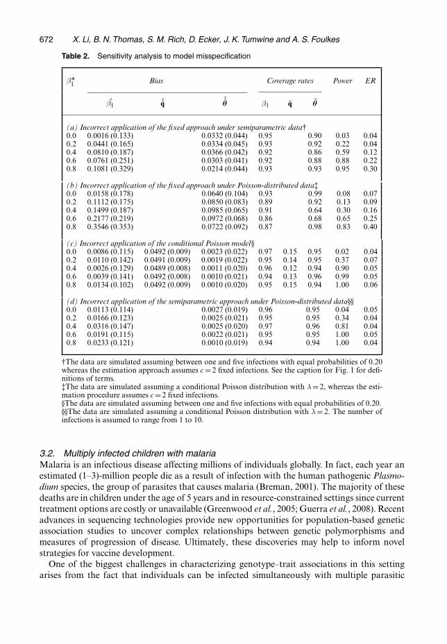
To evaluate the performance of the proposed method when the number of infections violatesmodel assumptions, we conduct several sensitivity analyses. First, we perform estimation byusing the fixed approach, assuming that the number of infections is equal to 2, when in factthe probabilities of having c infections for c = 1, . . . , 5 are all equal to 0.2. The results arepresented in Table 2, part (a). Comparing this with correct application of the semiparametricmethod (Table 1), we see a dramatic loss of power and a less severe, but noteworthy, decreasein coverage rates for both β and θ. In addition, the type 1 ER is substantially larger for β1 �0:4.Secondly, we perform estimation by using the fixed number approach, again assuming thatthe number of infections is equal to 2, when in fact the number of infections arises from aconditional Poisson distribution with λ= 2. The results are presented in Table 2, part (b).Comparing these results with correct application of the Poisson approach with λ=2 (Table 1),we see a more dramatic decrease in coverage rates for both β and θ. In addition, a significantdecrease in power and increase in the type 1 ER are observed for β�0:2. These findings supportthe use of the more sophisticated modelling approaches in these settings.

Next, we perform estimation by using the Poisson approach when in fact the probabilitiesof having c infections for c = 1, . . . , 5 are all equal to 0.2 and we present the results in Table 2,part (c). Here the modelling approach provides estimates of λ and, from this, we calculate qc

as .λc=c!/={exp.λ/ − 1}. As expected under this type of model misspecification, the coverage

rates for qc are very low (0.12–0.15). Interestingly, the coverage rates for both β and θ remainat approximately 95% and the power and ER are reasonable, though slightly worse than usingthe correct model (Table 1). Finally, we evaluate performance in applying the semiparametricapproach when the number of infections actually arises from a Poisson distribution with λ=2.


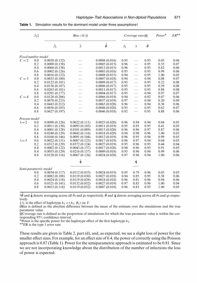
Table 1. Simulation results for the dominant model under three assumptions†

β1‡ Bias (se)§ Coverage rates§§ PowerÅ ERÅÅ

β1 λ ¯θ β1 λ θ

Fixed number modelC = 2 0.0 0.0038 (0.132) — 0.0008 (0.016) 0.95 — 0.95 0.05 0.06

0.2 0.0009 (0.138) — 0.0005 (0.015) 0.96 — 0.95 0.35 0.070.4 0.0060 (0.138) — 0.0013 (0.015) 0.96 — 0.95 0.82 0.060.6 0.0002 (0.126) — 0.0003 (0.016) 0.95 — 0.95 0.99 0.060.8 0.0016 (0.122) — 0.0008 (0.015) 0.94 — 0.95 1.00 0.05

C = 3 0.0 0.0035 (0.180) — 0.0007 (0.018) 0.94 — 0.94 0.08 0.070.2 0.0122 (0.181) — 0.0009 (0.017) 0.95 — 0.95 0.22 0.080.4 0.0136 (0.187) — 0.0006 (0.017) 0.95 — 0.95 0.59 0.080.6 0.0265 (0.181) — 0.0011 (0.017) 0.95 — 0.95 0.88 0.080.8 0.0291 (0.177) — 0.0004 (0.017) 0.95 — 0.94 0.97 0.07

C = 4 0.0 0.0128 (0.206) — 0.0066 (0.019) 0.94 — 0.92 0.07 0.060.2 0.0078 (0.223) — 0.0037 (0.019) 0.97 — 0.94 0.20 0.090.4 0.0443 (0.212) — 0.0065 (0.020) 0.96 — 0.94 0.38 0.060.6 0.0856 (0.185) — 0.0048 (0.020) 0.93 — 0.95 0.62 0.070.8 0.0627 (0.197) — 0.0046 (0.018) 0.92 — 0.95 0.88 0.06

Poisson modelλ=2 0.0 0.0098 (0.126) 0.0022 (0.111) 0.0025 (0.020) 0.96 0.94 0.94 0.04 0.05

0.2 0.0011 (0.150) 0.0093 (0.105) 0.0011 (0.019) 0.95 0.95 0.95 0.41 0.050.4 0.0001 (0.128) 0.0101 (0.089) 0.0013 (0.020) 0.96 0.96 0.97 0.87 0.060.6 0.0240 (0.129) 0.0042 (0.116) 0.0018 (0.020) 0.94 0.98 0.96 1.00 0.030.8 0.0160 (0.146) 0.0091 (0.104) 0.0012 (0.019) 0.96 0.95 0.94 0.99 0.05

λ=3 0.0 0.0022 (0.131) 0.0087 (0.123) 0.0017 (0.019) 0.96 0.97 0.94 0.04 0.030.2 0.0312 (0.129) 0.0372 (0.124) 0.0027 (0.019) 0.95 0.96 0.95 0.44 0.040.4 0.0002 (0.122) 0.0043 (0.137) 0.0017 (0.020) 0.94 0.96 0.95 0.91 0.050.4 0.0055 (0.129) 0.0216 (0.137) 0.0009 (0.018) 0.93 0.96 0.94 0.99 0.060.8 0.0120 (0.116) 0.0067 (0.126) 0.0024 (0.020) 0.97 0.96 0.94 1.00 0.06

¯q q

Semi-parametric model0.0 0.0034 (0.117) 0.0112 (0.033) 0.0024 (0.019) 0.95 0.79 0.96 0.05 0.030.2 0.0082 (0.108) 0.0119 (0.030) 0.0027 (0.018) 0.94 0.85 0.95 0.38 0.060.4 0.0024 (0.118) 0.0119 (0.029) 0.0018 (0.018) 0.96 0.81 0.96 0.94 0.060.6 0.0321 (0.141) 0.0132 (0.032) 0.0027 (0.019) 0.97 0.83 0.96 1.00 0.040.8 0.0015 (0.116) 0.0119 (0.032) 0.0007 (0.018) 0.96 0.83 0.95 1.00 0.05

† ¯θ and ¯q denote averaging across all θs and qs respectively. θ and q denote averaging across all θs and qs respec-tively.‡β1 is the effect of haplotype h1 = .A1, B1/ on Y.§Bias is defined as the absolute difference between the mean of the estimate over the simulations and the trueparameter value.§§Coverage rate is defined as the proportion of simulations for which the true parameter value is within the cor-responding 95% confidence interval.ÅPower is the specific power for the haplotype effect of the first haplotype h1.ÅÅER is the type 1 error rate.

These results are given in Table 2, part (d), and, as expected, we see a slight loss of power for thesmaller effect sizes. For example, for an effect size of 0.4, the power of correctly using the Poissonapproach is 0.87 (Table 1). Power for the semiparametric approach is estimated to be 0.81. Sincewe are not incorporating knowledge about the distribution of the number of infections the lossof power is expected.


Table 2. Sensitivity analysis to model misspecification

βÅ1 Bias Coverage rates Power ER

β1 ¯q ¯θ β1 q θ

(a) Incorrect application of the fixed approach under semiparametric data†0.0 0.0016 (0.133) 0.0332 (0.044) 0.95 0.90 0.03 0.040.2 0.0441 (0.165) 0.0334 (0.045) 0.93 0.92 0.22 0.040.4 0.0810 (0.187) 0.0366 (0.042) 0.92 0.86 0.59 0.120.6 0.0761 (0.251) 0.0303 (0.041) 0.92 0.88 0.88 0.220.8 0.1081 (0.329) 0.0214 (0.044) 0.93 0.93 0.95 0.30

(b) Incorrect application of the fixed approach under Poisson-distributed data‡0.0 0.0158 (0.178) 0.0640 (0.104) 0.93 0.99 0.08 0.070.2 0.1112 (0.175) 0.0850 (0.083) 0.89 0.92 0.13 0.090.4 0.1499 (0.187) 0.0985 (0.065) 0.91 0.64 0.30 0.160.6 0.2177 (0.219) 0.0972 (0.068) 0.86 0.68 0.65 0.250.8 0.3546 (0.353) 0.0722 (0.092) 0.87 0.98 0.83 0.40

(c) Incorrect application of the conditional Poisson model§0.0 0.0086 (0.115) 0.0492 (0.009) 0.0023 (0.022) 0.97 0.15 0.95 0.02 0.040.2 0.0110 (0.142) 0.0491 (0.009) 0.0019 (0.022) 0.95 0.14 0.95 0.37 0.070.4 0.0026 (0.129) 0.0489 (0.008) 0.0011 (0.020) 0.96 0.12 0.94 0.90 0.050.6 0.0039 (0.141) 0.0492 (0.008) 0.0010 (0.021) 0.94 0.13 0.96 0.99 0.050.8 0.0134 (0.102) 0.0492 (0.009) 0.0010 (0.020) 0.95 0.15 0.94 1.00 0.06

(d) Incorrect application of the semiparametric approach under Poisson-distributed data§§0.0 0.0113 (0.114) 0.0027 (0.019) 0.96 0.95 0.04 0.050.2 0.0166 (0.123) 0.0025 (0.021) 0.95 0.95 0.34 0.040.4 0.0316 (0.147) 0.0025 (0.020) 0.97 0.96 0.81 0.040.6 0.0191 (0.115) 0.0022 (0.021) 0.95 0.95 1.00 0.050.8 0.0233 (0.121) 0.0010 (0.019) 0.94 0.94 1.00 0.04

†The data are simulated assuming between one and five infections with equal probabilities of 0.20whereas the estimation approach assumes c = 2 fixed infections. See the caption for Fig. 1 for defi-nitions of terms.‡The data are simulated assuming a conditional Poisson distribution with λ= 2, whereas the esti-mation procedure assumes c=2 fixed infections.§The data are simulated assuming between one and five infections with equal probabilities of 0.20.§§The data are simulated assuming a conditional Poisson distribution with λ= 2. The number ofinfections is assumed to range from 1 to 10.

3.2. Multiply infected children with malariaMalaria is an infectious disease affecting millions of individuals globally. In fact, each year anestimated (1–3)-million people die as a result of infection with the human pathogenic Plasmo-dium species, the group of parasites that causes malaria (Breman, 2001). The majority of thesedeaths are in children under the age of 5 years and in resource-constrained settings since currenttreatment options are costly or unavailable (Greenwood et al., 2005; Guerra et al., 2008). Recentadvances in sequencing technologies provide new opportunities for population-based geneticassociation studies to uncover complex relationships between genetic polymorphisms andmeasures of progression of disease. Ultimately, these discoveries may help to inform novelstrategies for vaccine development.

One of the biggest challenges in characterizing genotype–trait associations in this settingarises from the fact that individuals can be infected simultaneously with multiple parasitic


strains. In the present investigation, we apply an EM approach (see Section 2) to data arisingfrom a cross-sectional study of n = 126 malaria-infected children from Uganda. We focuson haplotypes in one polymorphic circumsporozoite protein (CSP) region (CSP-TH3) of thegene that encodes for a cellular adhesion domain of the CSP. The CSP facilitates adhesionof the parasite to liver cells, which is a critical initial step in its replication process in a hu-man host (Zavala et al., 1983; Hollingdale et al., 1984). The goal of our analysis is to uncoverhaplotype associations with RBC count (log-transformed). The RBC count is a well-knowndiagnostic tool for detecting anaemia, which is a common and often lethal manifestation ofmalaria.

Data on 12 sites, 10 of which are polymorphic in our sample, are considered. Notably, sites thatare constant across our data do not inform the analysis but are included for completeness. Acrossall individuals, we see up to three different nucleotides at a site and, within a single individual,one or two nucleotides are present at any given site. A total of 35 unique genotypes are observedin our data and a sample of the data is provided in Li et al. (2007). For computational purposes,the set of possible haplotypes is limited to those with estimated frequencies of greater than 0.01where frequency estimates are obtained by using the approach of Li et al. (2007). We assumea Poisson distribution and apply the approach of Section 2.2.2. A dominant genetic model isassumed, as in the simulation study.

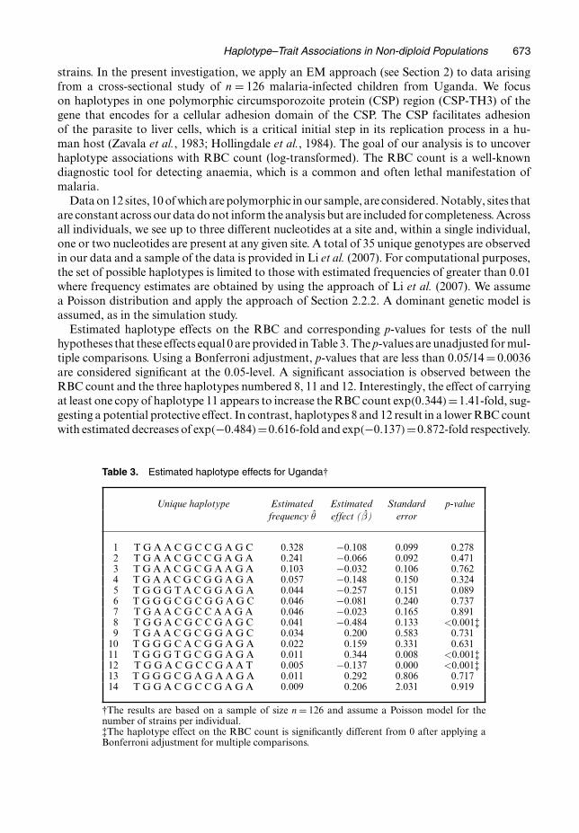
Estimated haplotype effects on the RBC and corresponding p-values for tests of the nullhypotheses that these effects equal 0 are provided in Table 3. The p-values are unadjusted for mul-tiple comparisons. Using a Bonferroni adjustment, p-values that are less than 0.05/14 = 0.0036are considered significant at the 0.05-level. A significant association is observed between theRBC count and the three haplotypes numbered 8, 11 and 12. Interestingly, the effect of carryingat least one copy of haplotype 11 appears to increase the RBC count exp.0:344/=1:41-fold, sug-gesting a potential protective effect. In contrast, haplotypes 8 and 12 result in a lower RBC countwith estimated decreases of exp.−0:484/=0:616-fold and exp.−0:137/=0:872-fold respectively.

Table 3. Estimated haplotype effects for Uganda†

Unique haplotype Estimated Estimated Standard p-valuefrequency θ effect (β) error

1 T G A A C G C C G A G C 0.328 −0.108 0.099 0.2782 T G A A C G C C G A G A 0.241 −0.066 0.092 0.4713 T G A A C G C G A A G A 0.103 −0.032 0.106 0.7624 T G A A C G C G G A G A 0.057 −0.148 0.150 0.3245 T G G G T A C G G A G A 0.044 −0.257 0.151 0.0896 T G G G C G C G G A G C 0.046 −0.081 0.240 0.7377 T G A A C G C C A A G A 0.046 −0.023 0.165 0.8918 T G G A C G C C G A G C 0.041 −0.484 0.133 <0.001‡9 T G A A C G C G G A G C 0.034 0.200 0.583 0.731

10 T G G G C A C G G A G A 0.022 0.159 0.331 0.63111 T G G G T G C G G A G A 0.011 0.344 0.008 <0.001‡12 T G G A C G C C G A A T 0.005 −0.137 0.000 <0.001‡13 T G G G C G A G A A G A 0.011 0.292 0.806 0.71714 T G G A C G C C G A G A 0.009 0.206 2.031 0.919

†The results are based on a sample of size n = 126 and assume a Poisson model for thenumber of strains per individual.‡The haplotype effect on the RBC count is significantly different from 0 after applying aBonferroni adjustment for multiple comparisons.


Notably, the estimated number of individuals with each of these haplotypes (which is given by126θk) is small and further confirmatory research is required to make firm conclusions.

4. Further extensions for the quasi-species setting

In the methods that were described above for estimation of haplotype effects on a trait, weincorporate population level haplotype frequencies. These frequencies can be thought of as theamount of each parasite strain circulating in the mosquito population that infects humans.Importantly, we assume that the frequencies within individuals reflect these population levelparameters. In other words, the probability of being infected with a given strain does not dependon prior infections and is equal to the proportion of this strain in the general population.Patients who are infected with HIV similarly host a population of viruses; however, the pres-ence of such a quasi-species generally results from external pressures, such as drug exposures,rather than multiple repeat infections. As a result, the frequencies of each haplotype within anindividual may not reflect the true population level frequencies. This is evidenced, for example,by the existence of latent reservoirs of resistant variants that rapidly emerge in the presence ofa drug.

For this reason, rather than using population level haplotype frequencies in the HIV setting,we consider the probabilities that an individual in the target population carries a given haplo-type. Although this distinction is subtle, it does require modification of the estimation approachthat was described in Section 2. Again let Gi be the unphased (observed) multisite genotypefor the ith individual where i = 1, . . . , n. Further suppose that Hi represents the combinationof unique haplotypes within individual i where Hi is generally unobservable and multiple val-ues of Hi are consistent with Gi. We emphasize unique here since, in the previously describedapproach, such a minimal set was not required, i.e. we are now interested in whether an individualcarries a specific haplotype and not in the number of copies. Again, the set of all combinationsthat are consistent with Gi is denoted S.Gi/ and h1, . . . , hK denotes the K possible haplotypesover all observed individuals. Let α= .α1, . . . ,αK/ whereαk is the probability that an individualcarries at least one copy of hk and define

δik ={

1 if hk is present in the ith individual,0 if hk is not present in the ith individual.

.22/

Under the model that is given in equation (1), the complete likelihood function can again bewritten as in equation (3) where Pr.Hi|θ/ is replaced with

Pr.Hi|α/=K∏

k=1αδikk .1−αk/1−δik : .23/

In this case, estimation of the regression parameter β proceeds as described above and an esti-mate of α is obtained by finding the root of the equation

@E[log{L.Φ/|X.com/}|X.obs/, Φ.t/

]@αk

=n∑

i=1

∑Hi∈S.Gi/

piHi.Φ.t/

/@ log{Pr.Hi|α/}

@αk

=n∑

i=1

∑Hi∈S.Gi/

piHi.Φ.t/

/

(δik

αk− 1− δik

1−αk

)=0: .24/

Resulting closed form solutions (see Appendix A.4) for αk are given by


α.t+1/k =

n∑i=1

∑Hi∈S.Gi/

piHi.Φ.t/

/δik

n: .25/

5. Discussion

In this paper, we describe an approach to estimate and test haplotype–trait associations betweenindividuals with multiple strains of an infectious agent. Three approaches to modelling thenumber of infections were described in Section 2. The first, which involves fixing the number ofinfections to be a constant C, is presented since it represents a natural extension of the diploidsetting, within which C =2 and our approach reduces to the EM method of Lake et al. (2003).Since in the infectious disease setting the number of infections is rarely known with certainty,this first approach may be more relevant to investigations of polyploidy organisms in which thenumber of homologous chromosomes is greater than 2, such as flatworms, goldfish, salmon anda variety of ferns and flowering plants. Note that the assumption of independent segregationthat is made in equation (8) needs to be addressed specifically for each of these settings.

Our simulation study suggests that application of the Poisson approach, when in fact thenumbers of infections are c =1, . . . , 5 with equal probabilities, results in reasonable power andtype 1 ERs but substantial bias in these probability estimates. The semiparametric approachperforms reasonably well under the Poisson model with a slight loss of power. Incorrectapplication of the fixed number approach leads to more substantial losses of power, reductionsin coverage rates and increases in type 1 ERs. Applications of the correct models lead toreasonable power and control of type 1 ERs.

Coupled with this investigation is the need for appropriate methods for controlling type 1ERs in the context of multiple comparisons. In Section 3.2, we applied a Bonferroni correctionto assess significance. Alternative single-step and step-down methods that are based on the falsediscovery rate and that account for the correlated nature of these tests (Benjamini and Hochberg,1995; Benjamini and Yekutieli, 2001; Storey and Tibshirani, 2003) are also tenable. In addition,further consideration of resampling-based approaches and related extensions (Westfall andYoung, 1993; Pollard and van der Laan, 2004; Foulkes and DeGruttola, 2007) may be appro-priate. Extensions of the mixed effects modelling approaches that were developed originally forthe diploid setting (Foulkes et al., 2007, 2008) would offer a single degree of freedom omnibustest for association across all haplotypes.

Notably, our analysis is limited to data arising from individuals who visited one of thedesignated clinics. This may lead to ascertainment bias for several reasons, including that theindividuals under study exhibited symptoms that were sufficiently severe to warrant at leastone visit to the doctor. This is a potential limitation of the method that is described herein.Specifically, a population level prevalence greater than 0 of infection by a strain that results inmild symptoms may result in overestimation of the frequencies of haplotypes that lead to moresevere symptoms.

Application of this EM approach to a small cohort of children in Uganda revealed threepotentially informative haplotypes within the CSP region of the parasite genome. In general,characterizing the association between polymorphisms in the parasite genome and measuredtraits in an infected human host may provide greater insight into disease aetiology and helpto inform new strategies for treatment and vaccine development efforts. Drawing meaningfulbiological and clinical conclusions, however, will require further analysis. Specifically consid-eration of host level factors, such as host genetic profile and clinical or demographic features,may be warrented. The methods that are described herein provide a general framework and the


analytic tools to investigate such associations under several models of association and modelsfor the numbers of infections.

Acknowledgements

Support for this research was provided by the National Institute of Allergy and InfectiousDiseases research award R01AI056983. Funding for data collection was provided by the NationalInstitute of General Medicine (R01GM070077) and the World Health Organization (TDR-A10375).

Appendix A

A.1. Estimation under fixed number of infectionsNote that the sum of the population level haplotype frequencies must equal 1, so we have θK =1−ΣK−1

k=1 θk.Equation (9) is then given by


]@θk

=n∑

i=1

∑Hi∈S.Gi/

piHi.Φ

.t//

⎛⎝ δik

θk

− δiK

1−K−1∑k=1

θk

⎞⎠=0

for k =1, . . . , K −1 or, equivalently,

⎛⎜⎜⎜⎜⎜⎜⎜⎜⎜⎝

n∑i=1

∑Hi∈S.Gi/

piHi.Φ

.t//δi1=θ1

n∑i=1

∑Hi∈S.Gi/

piHi.Φ

.t//δi2=θ2

:::n∑

i=1

∑Hi∈S.Gi/

piHi.Φ

.t//δiK−1 =θK−1

⎞⎟⎟⎟⎟⎟⎟⎟⎟⎟⎠

=

⎛⎜⎜⎜⎜⎜⎜⎜⎜⎜⎜⎜⎝

n∑i=1

∑Hi∈S.Gi/

piHi.Φ

.t//δiK

/(1−

K−1∑k=1

θk

)

n∑i=1

∑Hi∈S.Gi/

piHi.Φ

.t//δiK

/(1−

K−1∑k=1

θk

)

:::n∑

i=1

∑Hi∈S.Gi/

piHi.Φ

.t//δiK

/(1−

K−1∑k=1

θk

)

⎞⎟⎟⎟⎟⎟⎟⎟⎟⎟⎟⎟⎠

: .26/

Note that all the elements of the vector on the right-hand side of equation (26) are equal. Therefore, wecan set the first element of the vector on the left-hand side of equation (26) equal to each of the remainingelements of this vector, which yields

θk =

n∑i=1

∑Hi∈S.Gi/

piHi.Φ

.t//δik

n∑i=1

∑Hi∈S.Gi/

piHi.Φ

.t//δi1

θ1: .27/

Thus we can derive an estimate of θ1 and use equation (27) to find estimates of θk for k = 2, . . . , K − 1.From the first element of equation (26) we have

θ1

n∑i=1

∑Hi∈S.Gi/

piHi.Φ

.t//δiK =

n∑i=1

∑Hi∈S.Gi/

piHi.Φ

.t//δi1

⎧⎪⎪⎨⎪⎪⎩1−θ1 −θ1

K−1∑k=2

n∑i=1

∑Hi∈S.Gi/

piHi.Φ

.t//δik

n∑i=1

∑Hi∈S.Gi/

piHi.Φ

.t//δi1

⎫⎪⎪⎬⎪⎪⎭

=n∑

i=1

∑Hi∈S.Gi/

piHi.Φ

.t//δi1 −θ1

K−1∑k=1

n∑i=1

∑Hi∈S.Gi/

piHi.Φ

.t//δik


or equivalently

θ1

n∑i=1

∑Hi∈S.Gi/

piHi.Φ

.t//

K∑k=1

δik =n∑

i=1

∑Hi∈S.Gi/

piHi.Φ

.t//δi1: .28/

Finally, since ΣKk=1δik =C and ΣHi∈S.Gi/ piHi

=1, equation (28) yields

θ.t+1/

1 =

n∑i=1

∑Hi∈S.Gi/

piHi.Φ

.t//δi1

nC:

A.2. Estimation under Poisson assumptionUnder the Poisson assumption, we have ΣK

k=1 δik = ci and therefore equation (28) is written

θ1

n∑i=1

∑Hi∈S.Gi/

piHi.Φ

.t//ci =

n∑i=1

∑Hi∈S.Gi/

piHi.Φ

.t//δi1

resulting in

θ.t+1/

1 =

n∑i=1

∑Hi∈S.Gi/

piHi.Φ

.t//δi1

n∑i=1

∑Hi∈S.Gi/

piHi.Φ

.t//ci

:

A.3. Estimation for semiparametric approachNote that the sum of the qc must equal 1, so we have qC =1−ΣC−1

c=1 qc and equation (16) is given by


]@qc

=n∑

i=1

∑Hi∈S.Gi/

piHi.Φ

.t//

{I.ci = c/

qc

− I.ci =C/

1−C∑

c=1qc

}=0

for c=1, . . . , C −1. Using the same approach as described in Appendix A.1, we have

q.t+1/c = 1

n

n∑i=1

∑Hi∈S.Gi/

piHi.Φ

.t// I.ci = c/: .29/

A.4. Estimation for quasi-species settingFrom equation (24), we have

n∑i=1

∑Hi∈S.Gi/

piHi.Φ

.t//δik

αk

=

n∑i=1

∑Hi∈S.Gi/

piHi.Φ

.t//.1− δik/

1−αk

or equivalently

αk

n∑i=1

∑Hi∈S.Gi/

piHi.Φ

.t//=

n∑i=1

∑Hi∈S.Gi/

piHi.Φ

.t//δik: .30/

Since Σni=1 ΣHi∈S.Gi/piHi

.Φ.t/

/=n, equation (30) yields

α.t+1/k =

n∑i=1

∑Hi∈S.Gi/

piHi.Φ

.t//δik

n:


References

Benjamini, Y. and Hochberg, Y. (1995) Controlling the false discovery rate: a practical and powerful approach tomultiple testing. J. R. Statist. Soc. B, 57, 289–300.

Benjamini, Y. and Yekutieli, D. (2001) The control of the false discovery rate in multiple testing under dependency.Ann. Statist., 29, 1165–1188.

Breman, J. G. (2001) The ears of the hippopotamus: manifestations, determinants, and estimates of the malariaburden. Am. J. Trop. Med. Hyg., 64, suppl. 1–2, 1–11.

Dempster, A. P., Laird, N. M. and Rubin, D. B. (1977) Maximum likelihood from incomplete data via the EMalgorithm (with discussion). J. R. Statist. Soc. B, 39, 1–38.

Excoffier, L. and Slatkin, M. (1995) Maximum-likelihood estimation of molecular haplotype frequencies in adiploid population. Molec. Biol. Evoln, 12, 921–927.

Foulkes, A. and DeGruttola, V. (2007) A resampling-based approach to multiple testing with uncertainty in phase.Int. J. Biostatist., 3, article 2.

Foulkes, A., Yucel, R. and Li, X. (2008) A likelihood based approach to mixed modeling with ambiguity in clusteridentifiers. Biostatistics, 9, 635–657.

Foulkes, A., Yucel, R. and Reilly, M. (2007) Mixed modeling and multiple imputation for unobservable genotypeclusters. Statist. Med., 27, 2784–2801.

Greenwood, B. M., Bojang, K., Whitty, C. J. and Targett, G. A. (2005) Malaria. Lancet, 365, 1487–1498.Guerra, C., Gikandi, P., Tatem, A., Noor, A., Smith, D., Hay, S. and Snow, R. (2008) The limits and intensity

of plasmodium falciparum transmission: implications for malaria control and elimination worldwide. PLoSMed., 5, no. 2, e38.

Hill, W. G. and Babiker, H. A. (1995) Estimation of number of malaria clones in blood samples. Proc. R. Soc.Lond., 262, 249–257.

Hollingdale, M., Nardin, E., Tharavanij, S., Schwartz, A. and Nussenzweig, R. (1984) Inhibition of entry ofPlasmodium falciparum and P. vivax sporozoites into cultured cells; an in vitro assay of protective antibodies.J. Immunol., 132, 909–913.

Lake, S. L., Lyon, H., Tantisira, K., Silverman, E. K., Weiss, S. T., Laird, N. M. and Schaid, D. J. (2003)Estimation and testing of haplotype-environment interaction when linkage phase is ambiguous. Hum. Hered.,55, 56–65.

Li, X., Foulkes, A., Yucel, R. and Rich, S. (2007) An expectation maximization approach to estimate malariahaplotype frequencies in multiply infected children. Statist. Applic. Genet. Molec. Biol., 6, article 33.

Lin, D. and Zeng, D. (2006) Likelihood-based inference on haplotype effects in genetic association studies. J. Am.Statist. Ass., 101, 89–104.

Louis, T. A. (1982) Finding the observed information matrix when using the EM algorithm. J. R. Statist. Soc. B,44, 226–233.

McLachlan, G. J. and Krishnan, T. (1997) The EM Algorithm and Extensions. New York: Wiley.Meilijson, I. (1989) A fast improvement to the EM algorithm on its own terms. J. R. Statist. Soc. B, 51, 127–138.Pollard, K. and van der Laan, M. (2004) Choice of a null distribution in resampling-based multiple testing. J.

Statist. Planng Inf., 125, 85–100.Schaid, D., Rowland, C., Tines, D., Jacobson, R. and Poland, G. (2002) Score tests for association between traits

and haplotypes when linkage phase is ambiguous. Am. J. Hum. Genet., 70, 425–434.Stephens, M. and Donnelly, P. (2003) A comparison of bayesian methods for haplotype reconstruction from

population genotype data. Am. J. Hum. Genet., 73, 1162–1169.Stephens, M., Smith, N. J. and Donnelly, P. (2001) A new statistical method for haplotype reconstruction from

population data. Am. J. Hum. Genet., 68, 978–989.Storey, J. and Tibshirani, R. (2003) Statistical significance for genomewide studies. Proc. Natn. Acad. Sci. USA,

100, 9440–9445.Westfall, P. and Young, S. (1993) Resampling-based Multiple Testing. New York: Wiley.Zavala, F., Cochrane, A. H., Nardin, E. H., Nussenzweig, R. S. and Nussenzweig, V. (1983) Circumsporozoite

proteins of malaria parasites contain a single immunodominant region with two or more identical epitopes. J.Exptl Med., 157, 1947–1957.

Zaykin, D., Westfall, P., Young, S., Karnoub, M., Wagner, M. and Ehm, M. (2002) Testing association of statisti-cally inferred haplotypes with discrete and continuous traits in samples of unrelated individuals. Hum. Hered.,53, 79–91.

Estimating and testing haplotype–trait associations in non-diploid populations

Documents

Transcript of Estimating and testing haplotype–trait associations in non-diploid populations