ESSAYS ON PRICE OVERREACTION AND PRICE LIMITS IN

EMERGING MARKETS: THE CASE OF THE EGYPTIAN STOCK

EXCHANGE

by

HISHAM FARAG OMAR

A thesis submitted to The University of Birmingham

For the degree of Doctor of Philosophy in Accounting and Finance

Department of Accounting and Finance

Business School

The University of Birmingham

June 2012

University of Birmingham Research Archive

e-theses repository This unpublished thesis/dissertation is copyright of the author and/or third parties. The intellectual property rights of the author or third parties in respect of this work are as defined by The Copyright Designs and Patents Act 1988 or as modified by any successor legislation. Any use made of information contained in this thesis/dissertation must be in accordance with that legislation and must be properly acknowledged. Further distribution or reproduction in any format is prohibited without the permission of the copyright holder.

i

Abstract

The main objective of this thesis is to investigate the short and long–term overreaction

phenomenon in the Egyptian stock market. In addition, the thesis investigates links between

stock market regulatory policies (price limits and circuit breakers) and the profitability of

contrarian strategies. Finally, the study examines the effect of regime switch – from strict price

limits to circuit breakers – on the volatility spillover, delayed price discovery and trading

interference hypotheses.

Using data from the Egyptian stock exchange, I find that a panel data approach adds a new

dimension to the existing models, offers interesting additional insights and reveals the

importance of the role of unobservable firm-specific factors in addition to observable factors

in the analysis of the overreaction phenomenon. Moreover, portfolios based on unobserved

factors i.e. management quality, corporate governance and political connections of board

members, significantly outperform traditional portfolios based on size. Results also show

evidence of genuine long-term overreaction phenomenon in the Egyptian stock market as the

contrarian profits of the arbitrage portfolio cannot be attributed to the small firm effect,

formation period length, and stability of time varying factor or seasonality effect. Finally,

switching from a strict price limit to a circuit breakers regime increases stock price volatility

and disrupts the price discovery mechanism in the Egyptian stock market.

ii

Dedication

To my wife, my children (Salma, Youssef and Mostafa), my mother and the soul of my father.

iii

Acknowledgement

This thesis could not have been accomplished without the invaluable supervision of my

honourable supervisor and the great scholar Professor Robert Cressy. I would like to express

my sincere deep respect and appreciation to him. His guidance, comments, patience, time and

directions have been influential in achieving this thesis. Professor Cressy has encouraged and

motivated me over the past few years, as a result of which we have published four papers out

of this thesis. I would like also to thank the University of Birmingham for the financial support

for my PhD. Finally, I am grateful to all the members of staff in the Accounting and Finance

department for their support.

I alone take full responsibility for any errors and inaccuracies found in this thesis.

iv

Table of contents

Chapter 1 Introduction and Motivation ............................................................................................ 1

1.1 Introduction and background ................................................................................................... 1

1.2 Research objectives and motivation ......................................................................................... 7

1.3 Research contributions ............................................................................................................. 9

1.4 Background about the Egyptian economy .............................................................................. 11

1.4.1 Introduction ........................................................................................................................... 11

1.4.2 Egypt’s main economic indicators ........................................................................................ 12

1.5 Overview about the Egyptian Exchange (EGX) .................................................................... 16

1.5.1 The history of the Egyptian Exchanges ................................................................................. 16

1.5.2 Main Stock Market Indices ................................................................................................... 17

1.5.3 Stock market regulations ....................................................................................................... 18

1.5.4 The performance of the Egyptian stock market .................................................................... 20

1.6 The structure of the thesis ...................................................................................................... 22

Chapter 2 : Literature Review ......................................................................................................... 25

2.1 Introduction ............................................................................................................................ 25

2.2 Short –term overreaction ........................................................................................................ 27

2.2.1 Developed Markets ............................................................................................................... 27

2.2.2 Emerging Markets ................................................................................................................. 33

2.3 Long–term overreaction ......................................................................................................... 34

2.3.1 Developed markets ................................................................................................................ 35

2.3.2. Emerging markets ................................................................................................................ 44

2.4 Possible explanations to the overreaction hypothesis ............................................................ 46

2.4.1 Variation in beta .................................................................................................................... 46

2.4.2 Seasonality effect .................................................................................................................. 46

2.4.3 Size effect .............................................................................................................................. 47

2.4.4 Bid-ask spread ....................................................................................................................... 48

2.4.5 Tax loss hypothesis ............................................................................................................... 50

v

2.5 Overreaction to specific events .............................................................................................. 51

2.6 Opponents of the contrarian strategy...................................................................................... 56

2.6.1 Computation errors ......................................................................................................... 57

2.6.2 Contrarian or momentum ............................................................................................... 59

2.7 Summary ................................................................................................................................ 64

Chapter 3 : Short-term overreaction: Unobservable portfolios? .................................................. 83

3.1 Introduction .................................................................................................................................. 83

3.2 Theoretical background ................................................................................................................ 84

3.2.1 Traditional theories ............................................................................................................... 84

3.2.2 A new model: Unobservable effects ..................................................................................... 85

3.3 Data .............................................................................................................................................. 87

3.4 Econometric modeling and empirical results ............................................................................... 88

3.4.1 Daily Returns......................................................................................................................... 88

3.4.2 Stock abnormal returns (ARs) ............................................................................................... 89

3.4.3 Cumulative abnormal returns (CARs) ................................................................................... 89

3.4.4 Descriptive statistics .............................................................................................................. 90

3.4.5 Correlation matrix ................................................................................................................. 92

3.4.6 The overreaction hypothesis .................................................................................................. 92

3.4.7 The optimal holding period .................................................................................................. 96

3.4.8 Cross-sectional regression ................................................................................................... 101

3.4.9 Panel data econometrics ...................................................................................................... 105

3.4.10 Fixed effects (FE) or Random effects (RE)? ..................................................................... 107

3.4.11 Unobservable or size portfolios? ....................................................................................... 113

3.4.12 System GMM dynamic panel data model ....................................................................... 119

3.4.13 What are these unobservable factors? ............................................................................... 126

3.5 Summary and conclusions .......................................................................................................... 132

Chapter 4 : Long-term performance: momentum or overreaction? .......................................... 135

4.1 Introduction ................................................................................................................................ 135

4.2 Empirical literature debate: Long-term performance CARs or BH? .......................................... 137

4.2.1 Cumulative average residual returns CARs ........................................................................ 137

vi

4.2.2 Buy and Hold Abnormal Returns (BHARs) ........................................................................ 139

4.3 Alternative sources of the contrarian and momentum abnormal returns. .................................. 141

4.3.1 Biases and measurement errors in contrarian strategies. ..................................................... 141

4.3.2 Portfolio construction and evaluation methodology............................................................ 143

4.3.3 Long-term performance with risk and size adjustments. ..................................................... 143

4.3.4 Overreaction to firm-specific information and lead-lag structure. ...................................... 144

4.4 Data ............................................................................................................................................ 145

4.5 Methodology and empirical results ............................................................................................ 147

4.5.1 Daily Returns....................................................................................................................... 147

4.5.2 Security abnormal returns (ARs) ......................................................................................... 148

4.5.3 Cumulative residual return over the rank period (CARs) ................................................... 148

4.5.4 Cumulative abnormal residual returns over the test period (CARs) ................................... 149

4.5.5 Long-term overreaction Hypotheses ................................................................................... 151

4.5.6 Long-term overreaction: the sensitivity to formation period length.................................... 157

4.5.7 Long-term overreaction: the sensitivity to size effect. ........................................................ 164

4.5.8 Long-term performance with risk adjustment (robustness to time-varying market risk) .... 170

4.5.9 The variation of risk performance between rank and test periods ....................................... 173

4.5.10 Long-term overreaction with adjustment for the seasonality effect. ................................. 177

4.5.11 Is the contrarian factor priced? The Fama and French three-factor model. ..................... 180

4.5.12 Augmented Fama and French and Carhart models. ......................................................... 183

4.6 Summary and conclusion ........................................................................................................... 188

Chapter 5 Price limits and the overreaction phenomenon .......................................................... 193

5.1 Introduction ................................................................................................................................ 193

5.1.1 Price limits........................................................................................................................... 194

5.1.2 Firm –specific trading halts ................................................................................................. 194

5.1.3 Market-wide circuit-breakers .............................................................................................. 196

5.2 The impact of circuit breakers and price limits .......................................................................... 199

5.2.1 Information Hypothesis (Delayed price discovery) ............................................................ 200

5.2.2 Overreaction Hypothesis ..................................................................................................... 200

5.2.3 Information asymmetry ....................................................................................................... 201

vii

5.2.4 Order imbalance .................................................................................................................. 201

5.2.5 Volatility spillover ............................................................................................................... 202

5.2.6 Trading (liquidity) interference hypothesis ......................................................................... 202

5.2.7 Magnet effect....................................................................................................................... 202

5.2.8 Closing price manipulation ................................................................................................. 203

5.2.9 Information arrival modes ................................................................................................... 203

5.3 Literature Review ....................................................................................................................... 204

5.3.1 Developed markets. ............................................................................................................. 205

5.3.2 Emerging markets ............................................................................................................... 211

5.3.3 Price limits in Futures Markets ........................................................................................... 222

5.4 The data ...................................................................................................................................... 226

5.5 Econometrics Modeling and empirical results ........................................................................... 227

5.5.1 Overreaction hypothesis ...................................................................................................... 228

5.5.2 Volatility Spillover hypothesis ............................................................................................ 243

5.5.3 The delayed price discovery hypothesis .............................................................................. 250

5.5.4 The Trading Interference hypothesis. .................................................................................. 255

5.5.5 Regulatory policies and volume-volatility relationship. ..................................................... 259

5.5.6 Long term volatility and regime switch .............................................................................. 264

5.6 Summary and conclusion ........................................................................................................... 268

Chapter 6 : Conclusions .................................................................................................................. 287

6.1 Introduction ................................................................................................................................ 287

6.2 Summary of the main findings ................................................................................................... 289

6.3 Contribution of the study............................................................................................................ 300

6.4 Research limitations ................................................................................................................... 302

6.5 Policy implication of the findings .............................................................................................. 302

6.6 Suggestions for future research .................................................................................................. 304

viii

List of tables

Table page

number

Table 1.1: Privatisation Programme 2000/2001-2009/2010 .................................................................. 13

Table 1.2: Selected Economic and Financial Indicators ....................................................................... 15

Table 1.3: Trading hours at the EGX ..................................................................................................... 20

Table 1.4: Main Market Indicators for the Egyptian stock exchange (EGX) 2001-2010 ...................... 22

Table 2.1: Summary of the literature on the Short-term overreaction ................................................... 66

Table 2.2: Summary of the literature on the Long-term overreaction .................................................... 73

Table 3.1: Descriptive Statistics ............................................................................................................. 91

Table 3.2: Correlation Matrix ................................................................................................................. 92

Table 3.3: Average abnormal returns (AARs) for Losers and Winners ................................................. 93

Table 3.4: Cumulative average abnormal returns for Losers and Winners over event window ............ 98

Table 3.5: Cross Sectional Regressions ............................................................................................... 104

Table 3.6: Static Panel Data Models .................................................................................................... 110

Table 3.7: Panel Data Diagnostic tests ................................................................................................. 112

Table 3.8: System GMM estimates ...................................................................................................... 124

Table 3.9: Cross Sectional Regressions explaining unobservable factors ........................................... 131

Table 4.1: Cumulative average market-adjusted abnormal returns for the five two–year test periods

2000-2009 .......................................................................................................................... 154

Table 4.2: Average monthly cumulative average abnormal return (CAR) over the 24 months of the test

period.................................................................................................................................. 156

Table 4.3: Average cumulative average market-adjusted abnormal returns for two four–year test

periods 2002-2009 .............................................................................................................. 158

Table 4.4: Average monthly cumulative average abnormal return over the 48 months of the test period

2002-2005 .......................................................................................................................... 160

Table 4.5: Average monthly cumulative average abnormal return over 48 months into the test period

2006-2009 .......................................................................................................................... 163

Table 4.6: Average monthly cumulative average abnormal return over 24 months into the test period

for small firms .................................................................................................................... 166

Table 4.7: Average monthly cumulative average abnormal return over 24 months into the test period

for big firms ........................................................................................................................ 168

ix

Table 4.8: Long- term performance with risk adjustment (Robustness to time – varying risk) ........... 172

Table 4.9: Abnormal returns and the Stability of risk throughout rank and test periods ..................... 176

Table 4.10: Long–term overreaction with adjustment to seasonality effect ........................................ 179

Table 4.11: The Fama and French three-factor model and the augmented model for returns over the

period 2000-2009 ............................................................................................................... 187

Table 5.1: Price limit rules for a sample of world stock exchanges. .................................................... 195

Table 5.2: The history of market-wide circuit breaker regulations ...................................................... 197

Table 5.3: Summary statistics for the total number of events .............................................................. 230

Table 5.4: Average abnormal returns for upper and lower limit hits within the Strict Price Limits

regime ................................................................................................................................. 232

Table 5.5: ARs and CARS for Upper and Lower limit hits within the CB regime .............................. 234

Table 5.6: Average abnormal returns for the upper limit hits for Big and Small portfolios within SPL

regime ................................................................................................................................. 238

Table 5.7: Average abnormal returns for the lower limit hits for Big and Small portfolios within SPL

regime ................................................................................................................................. 239

Table 5.8: Average abnormal returns for the upper limit hits for Big and Small portfolios within CB

regime ................................................................................................................................. 241

Table 5.9: Average abnormal returns for the upper and lower limit hits for Big and Small portfolios

within CB regime ............................................................................................................... 242

Table 5.10: Volatility Spillover Hypothesis ......................................................................................... 246

Table 5.11 Frequencies of price continuation and price reversal for the two regimes ......................... 251

Table 5.12: Delayed price discovery: price continuation and reversal ................................................ 254

Table 5.13: Trading interference hypothesis: Turnover ratio ............................................................... 258

Table 5.14: Volume volatility relationship for the Upper limit hits ..................................................... 262

Table 5.15: Volume volatility relationship for the Lower limit hits .................................................... 263

Table 5.16: Augmented EGARCH Estimation .................................................................................... 266

Table 5.17: Summary of the literature on price limits and circuit breakers ......................................... 274

x

List of Figures

Figure 3-1: Post-event CARs determined by market cap and unobservable effects .............................. 86

Figure 3-2: Cumulative average abnormal returns for Losers................................................................ 94

Figure 3-3: Cumulative average abnormal returns for Winners ............................................................. 95

Figure 3-4: Cumulative average abnormal returns for Winners and Losers .......................................... 96

Figure 3-5: Cumulative average abnormal returns for Losers over event window ................................ 99

Figure 3-6: Cumulative average abnormal returns for Winners over event window ........................... 100

Figure 3-7: Cumulative average abnormal returns for Winners and Losers ....................................... 100

Figure 3-8: Unobservable portfolios for event A ................................................................................. 115

Figure 3-9: Unobservable portfolios for event B ................................................................................. 115

Figure 3-10: Size portfolios for event A .............................................................................................. 116

Figure 3-11: Unobservable portfolios for event C ............................................................................... 117

Figure 3-12: Unobservable portfolios for event D ............................................................................... 117

Figure 3-13: Size portfolios for event C ............................................................................................... 118

Figure 3-14: Size portfolios for event D .............................................................................................. 118

Figure 4-1 Average cumulative average abnormal return over 24 months .......................................... 157

Figure 4.2 Average cumulative average abnormal returnACARs ........................................................ 159

Figure 4.3 Average cumulative average abnormal return for 48 months over 2006-2009. ................. 161

Figure 4.4 Average cumulative average abnormal return over 24 months into the test period 2000-2009

for small firms .................................................................................................................... 167

Figure 4.5 Average cumulative average abnormal return over 24 months into the test period 2000-2009

for big firms. ....................................................................................................................... 169

Figure 5-1: Total number of events over the period 1999-2009 .......................................................... 231

Figure 5-2: Cumulative average abnormal returns for the upper limit hit for the two regimes ........... 235

Figure 5-3: Cumulative average abnormal returns for the lower limit hit for the two regimes ........... 235

Figure 5-4: Cumulative average abnormal returns (CAARs) for the upper and lower price limit hits

over the event window for the two regimes ....................................................................... 236

Figure 5-5: Cumulative averages abnormal returns for Big and Small portfolios for the upper and lower

limit hits within SPL regime .............................................................................................. 240

Figure 5-6: cumulative averages abnormal returns over the event window for the Big and Small

portfolios within the CB regime ......................................................................................... 243

Figure 5-7: Daily price volatility for the Upper limit hits for the two regimes around event day ....... 248

Figure 5-8: Daily price volatility for the Lower limit hits for the two regimes around event day ....... 249

xi

Figure 5-9: Cumulative average volatility (CAV) for the Upper limits hits for the two regimes ........ 249

Figure 5-10: Cumulative average volatility (CAV) for the Lower limits hits for the two regimes ...... 250

Figure 5-11: Frequencies for price continuation and price reversal for the Upper limit hits within both

regimes. .............................................................................................................................. 254

Figure 5-12: Frequencies for price continuation and price reversal for the Lower limit hits within both

regimes. .............................................................................................................................. 255

Figure 5-13: Trading activity ratio (TAR) for the Upper limit hits ...................................................... 259

Figure 5-14: Trading activity ratio (TAR) for the Lower limit hits ..................................................... 259

1

Chapter 1 Introduction and Motivation

1.1 Introduction and background

The research on Behavioural Finance (BF) is concerned with the psychological interpretations

of investor behaviour in stock markets. BF focuses on the cognitive psychology that links

financial economics with the human decision making process. The main research findings of

the BF show that investors interpret information differently and irrationally, and this leads to

uninformed decisions. Therefore investors sometimes behave in an unpredictable and biased

manner. Behavioural Finance puts much weight on the behaviour of investors that leads to

stock market anomalies, Subrahmanyam (2007).

In other words, BF tries to introduce a better interpretation for the existing financial

econometrics models by taking into account human emotions and cognitive errors. Research

findings on BF find that human flaws are predictable and consistent; therefore analysing

investor psychology might offer superior investment opportunities Stracca (2004).

The overreaction phenomenon is one of the consequences of taking human emotions in

consideration when analysing investors’ behaviour in stock markets. In addition, the

overreaction phenomenon is considered the most recent market anomaly added to the long list

of traditional market anomalies, i.e. day of the week, January effect and low P/E ratio. It is

worth mentioning that many non-traditional financial anomalies have been added to the

literature over time, e.g.the excessive volatility of stock prices (Shiller 1981), long-term price

2

reversal (De Bondt and Thaler, 1985), and short-term trends (momentum) Jegadeesh and

Titman (1993).

Keynes (1936) is considered the first to observe the overreaction phenomenon. Keynes argues

that daily variability of profits does influence markets and causes excessive reaction. The

appropriate reaction to information can be defined in the light of Bayes’ rule (1980). However,

Tversky and Kahneman (1974) (TK) introduced the representativeness heuristic theory (RHT)

in which people tend to underweight more distant past information and overweight recent

information. In addition, TK argue that they usually judge the probabilities of an event

compared with a well known probability distribution of other events or previous experiences

or beliefs.

Arrow (1982) finds results consistent with the RHT and concludes that all securities and

futures markets can be characterised by excessive reaction to the recent information. Dreman

(1982) and Basu (1977) also find evidence of the P/E anomaly as they find that stocks with

low P/E ratio outperform those of high P/E ratio and earn abnormal risk-adjusted returns. In

addition, Dreman (1982) provided a behavioural interpretation of PE/ratio hypothesis; he

argued that stocks with low P/E ratios are underpriced due to investor pessimism as the result

of announcements of poor earnings or other bad news.

Barberies, Schleifer and Vishny (1998) introduce the model of investment sentiment in which

they provide an alternative interpretation to the under and overreaction phenomena. They

differentiate between the size of the shocks or signals and their weights (importance). They

3

argue that underreaction occurs if investors focus too much on the importance (weight) of the

signal while the overreaction occurs when investors focus too much on the size (strength) of

the shocks. On the other hand, (Daniel, Hirschleifer and Subrahmanyam (1998) introduced

amodel of biased self-attribution in which they argue that individual investors are over

confident and subject to self-attribution bias when public information is found in line with

prior information. This leads to rapid overreaction to the predicted signals.

George and Hwang (2007) argue that the systematic mistakes of irrational investors in

responding to new information are the main determinant of the overreaction hypothesis. These

mistakes may result from the biased self-attribution theory of Daniel et al. (1998) or investors’

beliefs about the expected price behaviour in response to good or bad news (George and

Hwang, 2007). Therefore investors may interpret and react to the new information arriving in

the market differently; this leads to two contradictory investment behaviours, namely, price

continuation or price reversals.

On the other hand, the efficient market hypothesis (Fama, 1976) assumes that stock prices

reflect all information available instantly, and prices follow a random walk with no trend and

therefore abnormal profits are impossible; however in reality, investors tend to overreact to

new information, in particular to positive and negative shocks. This suggests that stock price

trends are predictable and investors can achieve abnormal returns.

The dilemma, therefore, is whether stock prices are predictable and valuation errors are

systematic or not. If this is so we have therefore a potential conflict between the Market

4

Efficiency and the Behavioural Finance views. The former assumes that stock prices follow

random walk and equilibrium will be restored in the longer run in the event of temporary

fluctuations in stock prices. Therefore the true price is the present value of the future dividends

stream associated with it. However, the latter assumes that prices are highly influenced by

investors’ psychological makeup (optimistic or pessimistic). This pushes prices to unexpected

levels in both directions. Therefore the true stock price is the expected price based on the

psychological makeup of investors.

De Bondt and Thaler (1985) were the first to empirically examine the overreaction hypothesis

in the finance literature. They built on the reasoning of Dreman (1982) and discovered a new

stock market anomaly based on the Tversky and Kahneman’s representativeness theory

(1974).

De Bondt and Thaler (1985) argue that price reversals can be predicted in the US using only

past return data (3-5 years) in case of systematic price overshoot. Therefore stock returns are

predictable and this implies violation of the weak-form market efficiency. They formulate two

main testable hypotheses; the first hypothesis, “large stock price movements will be followed

by price reversals in the opposite direction” (the directional effect of Brown and Harlow,

1988) and the second hypothesis, “the larger the initial price movements the greater the

subsequent reversals” (the magnitude effect). This means that stock returns exhibit negative

serial correlation over the longer horizon and therefore investors may earn abnormal returns

by exploiting this long-term mispricing. This suggests a clear violation of market efficiency.

Fama (1976) formulated the efficient market condition as in equation 1

5

0)|~()|)|~

(~

( 111 titt

m

titmit FuEFFRERE (1)

Where itR~

is the return on security i, 1tF is the complete set of information at time t-1 and

)|)|~

( 11 t

m

titm FFRE is the expected return on stock (i) based on the complete set of information

arriving in the market m

tF 1. )|~( 1tit FuE is the estimated residual portfolio returns given a

complete set of information arriving in the market. The efficiency condition is therefore that

the expected returns on Winners equals the expected returns on Losers and equal to zero;

therefore investors cannot beat the market by constructing a portfolio based on the past return;

arbitrage profits are zero. De Bondt and Thaler (1985) (DT) formulate this condition as in

equation (2)

0)|~()|~( 11 tLttWt FuEFuE (2)

By contrast, the Overreaction hypothesis of DT is “Loser portfolios constructed using past

information (stock returns) outperform those of Winners”. In particular, they expect residuals

to satisfy the following relationship1:

0)|~(0)|~( 11 tLttWt FuEandFuE (3)

1 Losers are defined as stocks with poor performance (negative stock returns) in the previous period earn positive

risk-adjusted abnormal returns in the subsequent period in US. However Winners are defined as stocks that

perform better (positive stock returns) in the previous period earn negative risk-adjusted abnormal returns in the

subsequent period. (DeBondt and Thaler (1985 and 1987).

6

In other words, abnormal returns to Winners are expected to be negative and those to Losers,

positive. If the market is efficient, trading strategies based on Loser-Winner anomaly cannot

achieve abnormal returns (after transaction costs) given the available set of information m

tF 1

between market participants (Jensen 1978). Therefore, if the efficient market hypothesis holds,

the difference between excess returns on Winners and Losers is zero as in equation 4.

However, if the overreaction hypothesis holds, we would expect positive excess returns based

on the Losers–Winners anomaly as in equation 5 (see Dissanaike, 1997).

0,, TWTL RR (4)

0,, TWTL RR (5)

Where R is the cumulative average excess return during test period T. TLR , and TWR , are the

average returns on the loser and winner’s portfolios respectively.

De Bondt and Thaler (1985) find that past Losers outperform past Winners by 24.6% in the

US, and therefore they recommend selling Winners short and buying Losers as a profitable

strategy. They argue that the overreaction phenomenon causes past Losers to be underpriced

and past Winners to be overpriced. In addition, they find evidence that the overreaction effect

is asymmetric and most of the cumulative average abnormal residuals (16.6%) are realised in

January. De Bondt and Thaler (1985) concluded that the market prices are predictable and

deviate from their fundamental due to investors’ overreactive behaviour and this suggests a

clear violation of the Weak Form market efficiency (stock prices reflect past information).

7

Fama (1998), on the other hand, argues that long-term overreaction phenomenon is quite

sensitive to the methodology of modelling excess returns (i.e. Cumulative Abnormal Returs-

CARs or Buy and Hold-BAH). In addition, the abnormal returns sometimes disappear when

using particular models (CAPM, market model and market-adjusted return) or when using a

particular statistical approach Fama (1998)2. This suggests that the existence of the long–term

overreaction might be attributable to chance; this argument is consistent with the EMH Fama

(1998).

1.2 Research objectives and motivation

Emerging stock markets –by contrast with developed markets –– are characterised by excess

volatility and lower efficiency (Fama, 1998). Therefore investors and fund managers in

particular have been trying to exploit market imperfection to achieve abnormal returns by

creating trading rules or exploiting market anomalies. The overreaction phenomenon is

regarded as one of the newly added anomalies to the existing list of stock market anomalies

(De Bondt and Thaler, 1985). The existing body of the literature has extensively investigated

the overreaction phenomenon and how to achieve abnormal returns in developed markets;

however, few studies have been conducted on emerging markets.

The main objective of this thesis is to investigate the short and long–term overreaction

phenomenon in the Egyptian stock market. The Egyptian stock market is one of the leading

2 Fama (1998) defend the efficient market hypothesis and claims that the long-term return anomalies are fragile.

In addition, he claims that the computation errors of the cumulative average abnormal returns using different

methodologies (CARs, Buy and Hold, Rebalancing methods) are the main cause of the overreaction and

underreaction anomalies in stock markets.

8

emerging markets in the Middle East and North Africa region (MENA) based on the statistics

of the World Federation of Exchanges (WFE, 2010). In addition, the thesis links between the

long- term overreaction phenomenon and the regulatory policies (price limits and circuit

breakers). Finally, the study examines the effect of regime switch – from strict price limits to

circuit breakers – on the volatility spillover, delayed price discovery and trading interference

hypotheses3.

The existing body of literature has investigated the overreaction phenomenon using traditional

methodologies; either cross-sectional or time series analyses. However, none of the existing

studies has combined the two dimensions using panel data models involving cross section-

time series analysis (CSTS). Ignoring time dimension may lay the estimation open to bias

(Cressy and Farag, 2011). Moreover, none of the existing studies has investigated the

overreaction phenomenon dynamics using a dynamic panel data model and system GMM in

3 Price limits are regulatory tools in both equity and futures markets in which further trading is prevented for a

period of time with the intention of cooling market traders’ emotions and reducing price volatility. Within circuit

breakers regime, trading may be stopped - for a pre-specified duration – across the whole market or for a

particular stock if stock prices or market index hit a pre-determined level (Kim and Yang (2008)).

Volatility spillover hypothesis states that price limits cause stock price volatility to spread out over a few days

subsequent to the event (limit hit) (Kim and Rhee (1997)). Delayed price discovery hypothesis states that the

price discovery mechanism is delayed due to the suspension of trading for a period of time (Kim and Rhee

(1997)). Therefore, it is argued, price limits prevent security prices from reaching their intrinsic values and

equilibrium levels. According to the trading interference hypothesis, Fama (1989), Telser (1989), Lauterbach and

Ben-Zion (1993) and Kim and Rhee (1997) claim that if trading is prevented by price limits, then shares become

less liquid and this leads to intensive trading activity during the following trading days. Detailed discussions of

the above mentioned hypothesis are provided in chapter 5.

9

particular. In addition, none of the existing literature has identified the main unobservable

factors that may be used to construct the so-called Unobservable portfolios4.

Finally, regulatory policies (price limits and circuit breakers) play an important role in cooling

down stock market volatility in both developed (trading halts) and emerging markets.

However, none of the existing body of the overreaction literature has investigated the link

between regulatory policies and overreaction hypothesis. The above-mentioned gaps in the

literature are the main motivation for this thesis.

1.3 Research contributions

One of the most important contributions of this thesis is the novel methodology. A panel data

model is used for the first time in the finance literature to examine the overreaction hypothesis.

There are many benefits of using panel data models (Hsiao 2004:p3). Firstly, panel data

models take individual stock heterogeneity into consideration; ignoring individual

heterogeneity may lay the estimation open to bias and inconsistent estimates (Baltagi, 2010).

Secondly, panel data models are less vulnerable to collinearity among variables, are more

informative, offer more degrees of freedom and less variation (Baltagi, 2010: p7). Thus panel

data models are more efficient and provide reliable parameter estimation compared with either

cross section or time series models ((Baltagi, 2010: p7). Thirdly, more complicated models

can be estimated i.e. dynamic models. Fourthly and most importantly, panel data models are

4 I use companies fixed effects as a new portfolio formation approach. Fixed effects are defined as the

unobservable factors that cause the regression line to shift up or down across companies. Further discussion is

provided in chapter 4.

10

better at identifying the so called unobservable effects (either fixed or random), which cannot

be detected through both pure time series and cross section analyses

The main contribution of chapter three is the use of the dynamic panel data model in

investigating the overreaction phenomenon. Unobservable factors (fixed effects) are then used

as a new methodology to construct portfolios by contrast the traditional size-based portfolios.

Finally, the chapter attempts to identify unobservable factors. It concludes that management

quality, corporate governance and political connections of the board of directors are the main

observable correlates to the unobservables, thus adding new insights to the existing panel data

models. It is worth mentioning that this chapter is the first in the literature to investigate the

relationship between firms’ corporate governance compliance, the political connections of the

board of directors and the overreaction phenomenon.

Chapter four is the first to link the long-term overreaction phenomenon with the change in

regulatory policies, namely the switch from strict price limits to circuit breakers. In addition,

this study is the first to augment the Fama and French three-factor and the Carhart (1997) four-

factor models by including contrarian and unobservable factors based on the company

heterogeneity.

The main contribution of chapter five is that it is the first to investigate the effect of regime

switch (from strict price limits to circuit breakers) on overreaction, volatility spillover, delayed

price discovery and trading interference hypotheses.

11

Finally, this study is the first to investigate empirically the short and long–term overreaction

phenomenon, the relationship between regulatory policies and the volatility spillover, delayed

price discovery and the trading interference hypotheses in the Egyptian stock market, one of

the leading markets in the Middle East and North Africa region (MENA).

1.4 Background about the Egyptian economy

1.4.1 Introduction

The world economy witnessed in 2008 the worst global financial crisis since the great

depression of the 1930s. This had substantial implications for the world financial system.

Subsequent growth rates in leading developed economies were therefore expected to be zero

or negative. The crises instantly spread out and were transmitted to the leading global

economies with the result that investment and consumption have been frozen in the UK and

Europe and economic growth has started to slow down in many countries since 2009, three

years after the crisis erupted.

President Obama signed in February 2009 the biggest bailout plan in the history as the US

Congress passed the Recovery and Reinvestment Act. Under this Act the US administration

provided US $787 billion package to stimulate the economy and create 3.5 million jobs.

Similarly, the external competitiveness of the second biggest world economy, namely Japan,

deteriorated as the Yen rose dramatically against the Euro and the US$.

The impact of the global financial crisis has spread to the vast majority of emerging

economies, particularly those having direct links with the leading economies. The liquidity

12

position of countries has been remarkably affected as foreign direct investments, external

demand and the exports of emerging markets have been dramatically diminished.

The effect of the global financial crisis on the Egyptian economy has been cushioned as the

Egyptian economy, and particularly the Egyptian banks, are less integrated into the

international financial system. Despite the remarkable growth in the value of the foreign direct

investment (FDI) and the portfolio investment funds, they have been proportionately small

compared with other emerging economies. However, the Egyptian economy has been exposed

to indirect external shocks such as the decline in tourism, fluctuations in international natural

gas prices, and a potential shift in foreign direct investment (FDI) flows.

1.4.2 Egypt’s main economic indicators

The Egyptian economy for decades was highly centralised. However, the economic reform

process was greatly accelerated during the era of the former President Hosni Mubarak (1981-

2011). International institutions increasingly supported the Egyptian government to take

actions towards the liberalisation of trade and stock market; as a result the GDP growth rate

reached 7.2% in 2007 and 4.2% in 2008 during the global financial crisis, while the vast

majority of the leading economies languished with negative or zero growth.

Because the Egyptian economy had made such effective steps towards economic reform and

enhancement of the investment climate, the Economic Reform Forum of the World Bank in

2008 chose Egypt among the seven best-performing countries in the world. The growth rate

since then has fallen and in 2011 is estimated at a lower 1.5% - 3.5% due primarily to the

political tension in the Middle East region following the Arab Spring and the Egyptian

13

revolution. However, in 2012, once the parliamentary and the presidential elections have been

run, the economy is expected to recover once more and to grow at a modest 5% annual rate.

The Egyptian economic reform programme started in 1994 when the Egyptian government

announced a major privatisation programme covering large swathe of publicly owned

companies. 411 companies were sold since 1994 for Egyptian pounds (LE) 57 billion. The

remarkable success in the programme has positively affected the development of Egyptian

capital markets as the vast majority of the companies were sold to the public and anchor

investors (ownership greater than 50%) via IPOs through the stock market.

Table 1.1 summarises the main results of the privatisation programme over the period 2000-

2011. We can see that in numerical and value terms privatisations peaked in the period 2005-

2007, and rose again in 2008-9 after a major dip during the financial crisis.

Table 1.1: Privatisation Programme 2000/2001-2009/2010

Total Sales

Companies/Assets

(100% state-owned)

Other Public Sector

Sales

Joint Venture

Sales Total Sales GDP

%of

Total

Sales to

GDP

No. Value

in LE

Millions

No.

Value

in LE

Millions

No.

Value in

LE

Millions

No.

Value in

LE

Millions

Value

in LE

Billions

2000/2001 11 252 -- -- 7 118 18 370 391 0.09

2001/2002 7 73 -- -- 3 879 10 952 379 0.25

2002/2003 6 49 -- -- 1 64 7 113 418 0.03

2003/2004 9 428 -- -- 4 115 13 543 485 0.11

2004/2005 16 824 -- -- 12 4,819 28 5,643 539 1.05

2005/2006 47 1,843 1 5,122 18 7,647 66 14,612 618 2.37

2006/2007 45 2,774 1 9,274 7 1,559 53 13,607 745 1.83

2007/2008 20 745 0 0 16 3,238 36 3,983 896 0.44

2008/2009 16 1,590 0 0 1 63 17 1,653 1,039 0.16

Dec-09 -- -- -- -- 1 4 1 4 1,181 0.00

Grand Total 338 24,440 2 14,396 70 18,516 411 57,366

Source: The Egyptian Ministry of Investment

14

Table 1.2 presents selected economic and financial indicators for the Egyptian economy over

the period 2005 – 2010. The figures presented in table 1.2 show that foreign direct investment

(FDI) amounted to US$ 4.3 billion in 2010 compared to US$ 5.2 in 2009. The net FDI

investments of the oil sector represent over 50% of the total FDI during the last two years. The

private sector in the Egyptian economy is now regarded as the engine of economic growth.

The private sector contributed around two-thirds of the total GDP over the period 2003/04-

2007/08. The official statistics of the fiscal year 2008/09 also show that the growth rate in the

private sector is 3.31% compared to 1.35% growth rate in the public sector. Foreign reserves

increased from US$ 34.2 billion in 2008/09 to US$ 36 billion in 2009/10, meanwhile the

inflation rate decreased from 13.2% in Dec 2009 to 10.3% in December 2010.

The inflation rate in Egypt has been remarkably high over the past few years; it reached 11%

in 2010 and was expected to increase during 2011 to 15% due to the political tension. This

caused a devaluation of the Egyptian pound against the US$ by 5% during the first quarter of

2011. The value of the external Egyptian debt was US$ 34.5 billion in 2010 of which 23%

represented short-term debt.

The external debt balance represented 14.5% of the GDP in 2010. On the other hand, the

foreign exchange currency exceeded this debt liability over the past few years. Finally, since

2008 Egypt has been regarded as one of the world’s main exporters of natural gas

(representing 50% of all merchandise exports). The trade deficit is moreover usually

15

compensated by the revenue from service sector, in particular by Suez Canal transit fees and

revenue from tourism.

Table 1.2: Selected Economic and Financial Indicators

Jun-05 Jun-06 Jun-07 Jun-08 Jun-09 Mar-09 Mar-10

GDP at Market Prices (LE

Billions) 538.5 617.7 744.8 895.5 1,038.6 771.6 893.5

GNP (LE Billions) 563.3 649.4 787.4 949.2 1,081.7 805.5 915.4

Real GDP (% Growth Rate ) 4.5 6.8 7.1 7.2 4.6 4.7 5.1

Real Per Capita GDP (% Growth

Rate) 2.5 4.9 4.9 5.1 2.5 NA NA

Average Per Capita Income 7,693.2 8,657.6 10,211.1 12,030.0 13,654.8 13,526.0 15,332.1

Share of Private Sector in GDP

(%) 61.7 60.3 62.4 61.6 62.8 62.5 63.6

Overall Fiscal Balance (% GDP) (9.6) (8.2) (7.3) (6.8) (6.9) (5.4) (7.3)

Net FDI in Egypt (%GDP) 4.4 5.7 8.5 8.1 4.3 0.7 0.8

Public Domestic Debt (% GDP)

Net Domestic Budget Sector Debt 72.5 72.0 64.2 53.5 54.1 53.3 55.7

Net Domestic General

Government Debt 51.5 53.8 49.6 42.7 45.0 43.5 47.8

Net Domestic Public Debt 52.3 53.9 48.8 43.2 45.8 44.4 48.6

Inflation Rates

CPI (% Growth Rate) 11.4 4.2 11.0 11.7 16.2 13.3 12.9

WPI (% Growth Rate) 9.9 4.1 11.8 -- -- -- --

PP (% Growth Rate) -- 4.1 11.8 17.7 2.5 (7.0) 13.2

Exchange Rates

Official Exchange Rate (LE/ US$) 6.006 5.747 5.710 5.500 5.510 5.570 5.460

Interest Rates

Interest Rate on T-Bills (91 days) 10.1 8.8 8.7 7.0 11.3 10.2 10.1

Broad Money (% Growth Rate) 13.6 13.5 18.3 15.7 8.4 6.9 9.8

External Debt

External Debt (% GDP) 31.1 27.6 22.8 20.1 17.0 16.7 14.8

External Debt (% Exports of

G&S) 100.3 82.4 70.4 59.9 64.4 293.6 295.5

Debt Service (% Current

Receipts) 7.9 7.3 5.9 3.9 5.3 4.8 4.8

Debt Service (% Exports of G&S) 9.4 8.5 6.9 4.6 6.2 5.7 5.8

Population (% Growth Rate ) 1.97 1.93 2.23 2.06 2.18 NA NA

Domestic Savings (LE Billions) 84.6 105.7 121.2 150.4 129.1 101.4 130.4

National Savings (LE Billions) 109.4 137.4 163.8 204.1 172.2 135.3 152.3 Source: Ministry of Economic Development, Ministry of Finance, and Central Bank of Egypt.

16

1.5 Overview about the Egyptian Exchange (EGX)5

1.5.1 The history of the Egyptian Exchanges

The Egyptian exchange is the oldest stock market in the MENA (Middle East and North

Africa) region. The Alexandria stock exchange was founded in 1883 followed by the Cairo

stock exchange in 1903. It is worth mentioning that the Alexandria exchange is one of the

oldest futures markets in the world, particularly in cotton forward contracts. The vast majority

of trading volume in the Alexandria futures market was done with the Liverpool Cotton

Exchange until 1950.

The Egyptian economy had grown significantly and before 1950 the Cairo and Alexandria

stock exchanges were regarded as one of the top five stock exchanges in the world. The

number of listed companies had reached 228 with a total market capitalisation of 91m

Egyptian pounds. By the early 1960s, however, the vast majority of private firms had been

nationalised by the socialist government. Therefore the role of the Cairo and Alexandria stock

exchanges was dramatically diminished; the number of listed firms declined to a nine after

thirty years.

By contrast, in the 1990s the former president Mubarak adopted a comprehensive economic

reform strategy. The Cairo and Alexandria stock exchanges were re- activated with large scale

flotations. 656 companies were listed by 1992. The two stock exchanges were linked with one

automated trading system; this facilitated the implementation of the privatisation programme

5 The main source of information in this section is the EGX annual reports (1996-2010)

17

starting from 1992, in which a number of IPOs of state-owned companies were executed

through the Cairo and Alexandria stock exchanges.

1.5.2 Main Stock Market Indices6

The EGX 30 index is the main Egyptian stock market index and the most widely used as an

market benchmark and barometer. EGX performance could be tracked through the S&P-IFC

Global and Investable Indices from 1996 and 1997 respectively.

The EGX30 was initially launched in 2003 as a free-floated market capitalization weighted

index and was retroactively computed as of 1 January 1998 with a base value of 1000 points.

The major international financial institutions provide information and analysis of the

performance of the Egyptian exchange based on the EGX30. The EGX30 is, like most world

indices, weighted by the market capitalisation of its constituent stocks. It avoids cross holdings

and industry concentration and excludes bankrupt companies and any companies ‘consumed’

in merger and acquisition deals. To reflect market activity, the index is rebalanced and updated

every six months.

In 2006 the Egyptian exchange launched a new market index, namely the Dow Jones EGX

Egypt Titans 20 Index (DJ20) jointly with the leading global index provider Dow Jones

indexes. The DJ20 tracks the 20 blue chips of the Egyptian stock market in terms of free-float

adjusted market capitalisation, sales and net income.

6 EGX annual reports (1996-2010)

18

In March 2009 the EGX then introduced two new price index products, namely EGX70 and

EGX100, to track the performance of the most active 70 and 100 companies excluding the

constituents of the EGX30. More recently, in 2010, the EGX launched the EGX20 capped

index (allowing only a 10% maximum weight to any of its constituent stocks) with the aim of

capturing the performance of the most active 20 companies in terms of market capitalisation

and liquidity.

1.5.3 Stock market regulations

1.5.3.1 Price Limits

Since 1996 EGX trading regulations imposed strict price limits (SPL) for all the listed shares,

amounting to absolute changes of more than 5% of the current stock price. The limit is

activated for a particular stock only when stock return hits the upper or lower limit; then the

trading on the share is suspended for the rest of the trading session. The SPL is only removed

in case of any corporate action. The SPL was first launched by the regulator with the intention

of cooling down the market and avoiding excess volatility. In 2002 the regulator commenced a

new price ceiling system, namely circuit breakers (CB) in which the price limits were widened

to +-20% for the most actively traded shares in the EGX. Within the new CB regime, trading

would be halted for 30 minutes should the stock price change for a particular stock hit +-10%.

During the 30 minute trading halt, brokers must inform their clients of the temporary

suspension of the trading session. In addition brokers are allowed to cancel or adjust traders’

orders to adjust their portfolio positions. When the trading session is resumed and if the stock

19

return for a given share has hit the upper or lower limit (now +-20%), trading is suspended

until the end of the trading session.

1.5.3.2 Intra-day trading mechanism:

The Intra-day trading mechanism was launched in 2004 by the regulator for the listed shares in

the main and the OTC markets for the most actively traded companies on the market.

1.5.3.3 Settlement:

The settlement mechanism in the EGX is as follows:

T (trading day) + 0 for securities traded by the Intra-day trading system.

T (trading day) +1 for government bonds.

T (trading day) +2 for all other securities.

1.5.3.4 Tax system

According to the capital market law No.95/1992 no taxes are imposed on both dividends and

capital gain in addition to coupon payments for individuals.

1.5.3.5 Foreign investments

There are no regulatory restrictions on foreign investment or profit repatriation in the Egyptian

stock market.

1.5.3.6 Trading hours

The trading hours of the market are shown in the table below.

20

Table 1.3: Trading hours at the EGX

Main Market Trading hours

Trading session 10:30am – 2:30pm

Bonds Market (Primary Dealers) 10:30am – 2:30pm

NILEX (SMEs Market) 11am-12pm

Over-the-Counter Market 9:45am- 11:15am Source:www.egyptse.com

1.5.3.7 Short selling

To support stock market liquidity the EGX has permitted margin trading and set up regulations

for short selling of the most actively trading stocks.

1.5.4 The performance of the Egyptian stock market

The Egyptian stock market was classified by the Economist in 2010 as one of the best six

emerging markets (CIVETS)7 offering significant potential growth over the next decade. In

addition, the World Federation of Exchanges’ (WFE) statistics in 2010 reported that the

Egyptian exchange achieved average gain of 15% during 2010, ahead of many leading world

emerging stock exchanges i.e. China, Brazil, and Czech Republic, and ahead of all Arab stock

markets excepting those of Qatar (25%) and Casablanca (21%) . The Morgan Stanley

International index MSCI and S&P IFCI reported that the annual growth rates for the EGX

during 2010 were 9% and 13% in US$ respectively. By comparison, the average growth rate

for emerging markets was 12% in US$.

7 Colombia, Indonesia, Vietnam, Egypt, Turkey and South Africa

21

The Egyptian stock market achieved reasonable performance indicators during 2008-2010

even though the negative impact of the global financial crisis affected the vast majority of the

stock markets throughout the world. The main market indicators diminished only slightly in

2010 as compared to 2009. The total value traded during 2010 was LE 321 billion compared

to LE 448 billion in 2009, meanwhile the total trading volume was 33 billion securities in

2010 compared to 37 billion securities in 2009. The market capitalisation of the main market

was LE 488 billion (40% of the GDP) during 2010 compared to LE 500 billion in 2009.

During 2010 the EGX achieved attractive P/E of 14.7 compared to 13 in 2009; however, based

on the statistics of the S&P/IFC composite index for emerging markets the average P/E is

13.5. On the other hand, the dividend yield increased from 6.5% in 2009 to 7.1% in 2010 and

the emerging market average dividend yield was 1.8%.

Trading volume, dominated by financial institutions, rose from 37% in 2009 to 52% in 2010,

while individual investors share fell to 48% of trading volume in 2010 compared to 63% in

2009. Foreign investments accounted for 22% of the total trading volume in 2010 and total

foreign capital inflow fell from LE8.4 billion in 2010 compared to LE5 billion in 2009.

Foreign investments in EGX were dominated by Europe (43%), the US (27%) and Arab

investments (24%).

The UK investors were the first in the Egyptian stock market and accounted for 37% of the

total foreign investments in 2010. Finally, the OTC trading volume sharply declined from LE

115 billion in 2009 to LE billion in 2010. Table 1.4 presents the main market indicators for the

Egyptian stock exchange (EGX) over the period 2001-2010.

22

Table 1.4: Main Market Indicators for the Egyptian stock exchange (EGX) 2001-2010

1.6 The structure of the thesis

The thesis comprises six main chapters; chapter one consists of six main sections; in section

one I discuss the theoretical and conceptual background of the topic. Section two presents the

main objectives and motivation of the study. Section three focuses on the main contribution of

the thesis. Sections four and five present background about the Egyptian economy and an

2001 2002 2003 2004 2005 2006 2007 2008 2009 2010

Total Volume (bn shares) 1.3 0.9 1.4 2.4 5.3 9.1 15.5 25.5 36.6 33

Volume of Listed Securities 1.2 0.7 1.2 1.8 4.2 7.8 11.4 21.9 28.6 28

Volume of Unlisted Securities 0.1 0.2 0.2 0.6 1.1 1.3 3.7 3.6 8 5 Total Value Traded (LE bn) 31.8 34.2 27.8 42.3 160.6 287.0 363 529.6 448.2 321

Value Traded (Listed Sec) 24.7 25.8 23.0 36.1 150.9 271.1 321.5 475.9 333.5 273

Value Traded (Unlisted Sec) 7.1 8.4 4.8 6.2 9.7 15.9 41.5 53.7 114.7 48 Number of Transactions (m) 1.1 0.8 1.2 1.7 4.2 6.8 9 13.5 14.6 10

Number of Transactions

(Listed Securities) 1.1 0.7 1.2 1.7 4.0 6.6 8.7 12.8 13.5 10

Number of Transactions

(Unlisted Securities) 0.01 0.1 0.02 0.1 0.2 0.2 0.3 0.7 1.1 0.4

Average Monthly Value

Traded (LE billion) 2.7 2.9 2.3 3.5 13.4 23.9 1488 1656 1822 1300

Average Monthly Value

Traded (Listed Securities) 2.1 2.2 1.9 3.0 12.6 22.6 1318 1436 1356 1105

Average Monthly Value

Traded (Unlisted Securities) 0.6 0.7 0.4 0.5 0.8 1.3 170 220 466 194

Turnover Ratio (%) 14.1 9.5 11.5 14.2 31.1 48.7 38.7 70.3 49.9 42.9 Foreign Participation as a %

of Total Value Traded 13.3 17.3 12.7 20.5 16.4 16.6 19.2 20 12.7 16.5

Arab Participation as a % of

Total Value of Traded 2.9 1.8 7.8 7.0 13.9 13.6 12.5 10 6.3 6.1

Number of Trading Days 246 249 244 249 249 244 244 244 249 247

Average Company Size (LE

million) 101 106 176 294 613 897 1766 1259 1633 2302

Number of Traded Companies 251 261 260 233 241 227 237 222 229 211

Market Capitalisation (LE bn) 112 122 172 234 456 534 768 474 500 488

Market Capitalisation % GDP 30 29 35 43 74 80 86 45 41 40

Source: The Egyptian Exchange , annual reports 2001-2010

23

overview of the Egyptian stock exchange respectively. Finally, section six presents the

structure of the thesis.

Chapter two introduces a comprehensive literature survey of the overreaction phenomenon.

The chapter mainly is divided into seven main sections. Section 1 includes introduction and

motivation. Section two presents summary of the short-term overreaction in developed and

emerging markets. In section 3 I present the development of the long term overreaction in both

developed and emerging markets. In section 4 I present the possible interpretation to the

overreaction phenomenon, namely the variation of risk (beta), seasonality and size effects,

bid-ask spread and the tax hypothesis. Section five analyses the overreaction to specific events

such as the overreaction to corporate actions (merger, acquisition and earnings and dividends

announcements), to rumours and to the international sport championships results. Section six

refutes the main arguments of the opponents of the overreaction phenomenon. Finally, section

seven summarises and concludes.

Chapter three investigates the short–term overreaction using a novel methodology, namely,

dynamic panel data model using system GMM. Chapter three consists of five main sections.

Section one includes the main objectives and motivation of the chapter. Section two presents

the theoretical background about the traditional models and the proposed new model to

explain the short-term overreaction. Section three describes the dataset used in the analysis.

Section 4 presents the econometric modeling and the empirical results. Finally, section five

summarises and concludes.

24

Chapter four, on the other hand, investigates the long–term overreaction phenomenon for all

listed shares in the Egyptian stock exchange. Chapter four consists of six main sections. I

present in section one the main objectives and motivations of the chapter. Section two

discusses the theoretical arguments and the alternative measures of the long–term

performance. Section three presents the alternative sources of the contrarian and momentum

abnormal returns. Section four describes the dataset used in the analysis. Section 5 describes

the econometric modeling and the empirical results. Finally, section six summarises and

concludes.

Chapter five investigates the effects of regime switch on the overreaction phenomenon.

Chapter five consists of six main sections. Section one includes the main motivation and

objectives of the chapter in addition to the theoretical background about the evolution of the

different types of regulatory policies. In section two I analyse the academic debate about the

impact of the circuit breakers and price limits. Section three presents a comprehensive

literature review of the different types of regulatory policies. Sections four describes the

dataset used in the analysis. Section five presents the econometric modeling and the empirical

results. Finally, section six summarises and concludes.

Chapter six presents a summary of the main findings of the thesis. Chapter six consists of six

main sections. Sections one and two present the research objectives and main results of the

thesis respectively. Sections three and four analyse the main contributions and research

limitations respectively, while section five analyses the policy implication. Finally, section six

provides suggestions for future research.

25

Chapter 2 : Literature Review

2.1 Introduction

The literature on the overreaction phenomenon is separated into long–term and short-term

behaviour. The existing literature has extensively explored the overreaction phenomenon in

developed markets. However, few studies have investigated the overreaction effect in

emerging markets, generally recognised to be less informationally efficient and therefore more

likely to be subject to market anomalies. Recent strands of research have concluded that - to

the contrary of the efficient market hypothesis - using past prices, stock returns are predictable

both over short and long horizons. See for example Shiller (1981) and De Bondt and Thaler

(1985).

This constitutes a newly added market anomaly8 in which changes in investor information

result in an initial reaction (buying or selling), a price trend (down or up) and finally a partial

reversal of the trend as investors revise their estimate of the impact of this new information.

This phenomenon is called the overreaction effect and implies that stock returns are negatively

serially correlated. Therefore stocks that performed poorly (Loser portfolios) during a

portfolio formation period (the period over which the model is estimated) may outperform the

market during the test period (the period over which the model is tested).

On the other hand, the good performers (Winner portfolios) on this theory are expected to

underperform the average market return in the test period. Therefore, based on the market

8 Others include the January and Monday effects in addition to small firm effect and low PE ratio.

26

shocks and whether they represent good or bad news, stock returns may be predictable and a

‘contrarian’ strategy may earn abnormal return by selling Winners short and buying Losers.

De Bondt and Thaler (1985) thus devised a zero investment portfolio in which cash from short

sales of Winners is used to finance investment in Losers. The overreaction hypothesis provides

clear evidence of invalidity of Weak Form market efficiency (Fama, 1976) as investors can

predict stock returns using past stock prices (Conrad, et al. (1997) and Baytas and Cakici

(1999)).

The main objective of this chapter is to conduct a comprehensive literature survey of the

overreaction phenomenon. The chapter mainly is divided into seven main sections. Section

one includes introduction and motivation. Section two presents summary of the short-term

overreaction in developed and emerging markets. In section three I present the development of

the long term overreaction in both developed and emerging markets.

In section four I present the possible interpretation to the overreaction phenomenon, namely

the variation of risk (beta), seasonality and size effects, bid-ask spread and the tax hypothesis.

Section five analyses the overreaction to specific events such as the overreaction to corporate

actions (merger, acquisition and earnings and dividends announcements), rumours and the

international sport championships results. Section six refutes the main arguments of the

opponents of the overreaction phenomenon. Finally, section seven summarises and concludes.

27

2.2 Short –term overreaction

In this section, I present the literature on the short-term overreaction hypothesis in both

developed and emerging markets.

2.2.1 Developed Markets

Zarowin, (1989) investigates the short–term overreaction phenomenon and whether or not size

and seasonality effects can explain this phenomenon. Monthly returns data are collected over

the period 1927-1985 for the listed shares in the NYSE. Zarowin formed equally size

portfolios based on past returns performance and calculated the risk-adjusted abnormal

performance of the two extreme portfolios, namely Winners and Losers following De Bondt

and Thaler (1987). Results support the short-term overreaction in the NYSE as Losers

significantly outperformed Winners by 2%-2.5% per month regardless their size. In addition,

Zarowin argues that short-term overreaction is considered a clear violation of the efficient

market hypothesis and regarded as a new market anomaly.

Atkins and Dyl (1990) investigate the short–term overreaction in the US. They define the

event as stock prices that experienced a large price change (based on the Wall Street Journal)

in a single trading day. In addition, they examine the proposed relationship between the short-

term reversals and the bid-ask spread. Daily return data are collected for all listed shares in the

NYSE over the period 1975-1984. Using the mean-adjusted, market and risk-adjusted returns

to calculate the abnormal returns, they find strong evidence of short –term overreaction in case

of bad news and weak evidence in case of good news. When they control for the bid-ask

spread, they found that price reversals are minimised and traders could not profit from the

28

overreaction anomaly. This implies market efficiency. They conclude that the bid-ask spread

is not the main source of the overreaction phenomenon in the NYSE.

Bremer and Sweeney (1991) examine the short-term price reversal phenomenon in the US.

They define the event as stocks that experienced at least -10% price drops in a single trading

day. Daily stock return data are collected for all listed shares in the Fortune 500 over the

period 1962-1986. Using the mean adjusted returns, results show evidence of price reversal in

the US; positive cumulative excess returns (2.2%) tend to be following the large negative price

drop over two days following the event. The price reversal phenomenon is unrelated to

weekend and turn-of-the-year effects.

Liang and Mullineaux (1994) investigate the short-term overreaction in NYSE and ASE over

the period 1963-1988. They define the event based on the residuals of the market model, and

then the three largest positive and negative events have been selected for each firm/year. Daily

return data are collected over 401 days pre (200) and post (200) event. Using the event study

methodology following Brown and Warner (1985), they find significant price reversal post

negative and positive events. They also find that stock prices tend to decrease pre positive

events (shocks) and increase pre negative shocks. Their results support the short-term

overreaction hypothesis.

Park (1995) argues that the predicted stock returns following large one-day price dramatic

changes are biased due to both sample selection bias and bid-ask spread. Therefore Park

(1995) investigates the effect of the bid-ask spread on the estimated stock returns following

29

one-day large price changes and the potential market microstructure explanation to this

phenomenon.

Daily price data of all listed shares of NASDAQ/NMS are collected over the period 1984-

1987. They calculate the stock returns based on the average bid-ask prices compared with the

traditional returns based on closing prices and define the event if the absolute value of the

market-adjusted abnormal returns exceeded 10% change in a particular day. Using the

compounded cumulative abnormal returns (CARs), they find that bid-ask spread did not fully

explain price reversals following the large one day price drop. In addition, they find evidence

of the short–term market overreaction; however, the contrarian profits are not large enough to

be exploited due to transaction costs.

Cooper (1999) investigates the short-term overreaction phenomenon and the impact of

alternative filter rules on contrarian profits of large capitalisation in the NYSE and AMEX.

Weekly return and trading volumes data are collected for the 300 large firms in the NYES and

AMEX - to minimise the bid-ask spread bias - over the period 1962-1993. Cooper uses the

filter rule methodology by specifying Losers and Winners based on minimum amount of

lagged weekly returns and trading volume growth. Cooper finds evidence of the overreaction

phenomenon in the NYSE. In addition, he finds that the lower the trading activity the higher

the price reversals. Results show that the filter rule strategies outperformed the buy and hold

counterparts.

30

Nam et al. (2001) find evidence of mean reversion in NYSE using the asymmetric non-linear

transition generalized autoregressive conditional model ANSTGARCH. They also find that

the reversal from negative to positive returns is quicker than the reversal from positive to

negative returns; in addition their findings support the overreaction hypothesis.

Schnusenberg and Madura (2001) examine the short–term overreaction and underreaction of

six main market indices in the US to avoid the potential bid-ask spread bias. They define the

event based on the best (Winners) and worst (Losers) index historical performance. Daily

price data are collected for major six stock indices in the US equity market since inception and

until 1997, namely; DJIA, NYSE, NASDAQ, S&P500, Russel 3000, and Wilshire 5000. They

use the mean–adjusted return and ARIMA models to estimate the expected returns.

They find evidence of market underreaction in the following day subsequent to the event for

the six market indices. In addition, they find significant short-term overreaction for the Losers

and underreactions for the Winners over the 60 days following the event, these results are

consistent with Fama (1998). They find that the less constituents (i.e. NASDAQ) in the index

the greater degree of underreaction for the Winners.

Larson and Madura (2003) investigate the relationship between overreaction/underreaction

and the information disseminated to the market in the short-term based on the classification of

the Wall Street Journal (informed/uninformed event). They define the event as stocks that

experience at least +-10% daily price change over a three-day event window. Daily returns

data are collected for the listed shares in the NYSE over the period 1988-1995. They estimate

31

the market model using the methodology of Brown et al. (1988) with the estimation window is

(-260,-41), the examination window (-3, +20) and the event window (+81-+300). They find

evidence of the overreaction phenomenon in cases of uninformed events. Their results support

the overconfidence and self-attribution bias by Daniel, Hirshleifer and Subrahmanyam (1998).

Ma et al. (2005) investigate the short-term overreaction in the US. They define the event as

stocks that experienced the largest price change reported in the Wall Street Journal. Daily

price data of a sample of (852) Winners and Losers listed in NYSE and NASDAQ are

collected over the period 1996-1997. They find little evidence of price overreaction in the

NYSE for both Winners and Losers; however, they find significant price reversal and evidence

of the overreaction phenomenon in the NASDAQ market. They conclude that investors may

interpret the new information differently in the NYSE and NASDAQ.

Michayluk and Neuhauser (2006) investigate the overreaction hypothesis in the NYSE in

response to the Asian financial crises in 1997. Daily price data are collected for 6276 stocks

over 60 days following the crash. They find significant evidence of market overreaction to the

Asian financial crises over one week following the Asian market crash. In addition, they find

that both size and CAPM-beta did not explain the initial price decline following the crash.

Finally they present evidence of short-term return predictability during the Asian stock market

crash.

Lo and Coggins (2006) investigate the daily and hourly overreaction phenomenon in the

Australian stock market and whether or not trading volume and stock liquidity explain price

reversals. Daily and hourly price data are collected for the top 200 companies listed in the

32

Australian stock exchange ASX from 2000 to 2002. Following the methodology of Lo and

MacKinlay (1990), they find strong evidence of short–term contrarian profits; however these

strategies are no longer profitable after controlling for transaction costs. They find a positive

relationship between price reversals and order imbalance and that the overreaction

phenomenon can be explained by temporary liquidity imbalance.

Spyrou et al. (2007) examine the short term overreaction and underreaction to market shocks

in the UK. Daily closing price data are collected for four stock market indices, namely, the

FT30, FTSE100, FTSE250 and FTSE Small Cap over the period 1988 to 2004. They define

the event (positive or negative shocks) when return on the market index is above or below two

standard deviations over (-60,-11) day estimation window. They find no evidence of

overreaction to market shocks for big firms, as no significant abnormal returns are found on

the following days subsequent to the shock. On the other hand, they find evidence of market

underreaction for small and medium size firms. Price reversals occur during 12-20 days

following the event. They find no effect of the seasonality, bid-ask spread, and time varying

risk in their results.

Recently, Lobe and Rieks (2011) investigated the out of sample estimation of the short-term

overreaction hypothesis in the German stock market. They define the event as stocks

experienced price change at least 10% as a proxy of positive and negative shocks. Daily data

are collected for four main German stock market indices since inception, namely, DAX30,

MDAX, SDAX, technology. Using the market and size–adjusted abnormal returns over a five-

day post-event, they find significant evidence of short-term overreaction in the German stock

33

market and this overreaction is not due to size or bid-ask spread. In addition, they find

asymmetric price reaction to positive and negative shocks. When they controlled for the

transaction costs, the contrarian profits were negligible. Their results support the efficient

market hypothesis in the German stock market.

2.2.2 Emerging Markets

Few studies have investigated the short-term overreaction phenomenon in emerging stock

markets. Bowman and Iverson (1998) investigate the short-term overreaction hypothesis in the

New Zealand stock exchange. Weekly return data for all listed shares are collected over the

period 1967-1986. They define the event as stock that experienced at least 10% weekly price

change. They find strong evidence of the overreaction phenomenon in the New Zealand stock

market as abnormal returns for Losers one week post-event (2.4%) outperform Winners (-

1.5%). The overreaction phenomenon was not due to bid ask bounce, non-synchronous trading

or size effect.

Otchere and Chan (2003) investigate the short–term overreaction in the Hong Kong stock

exchange (HKSE). They argue that the Hong Kong stock market is unique for international

investors as neither capital gains nor dividends are taxed. Daily data are collected over two

periods around the Asian financial crises pre (1996-1997) and post crisis (1997-1998). They

use three different methods to calculate the abnormal returns, namely, mean-adjusted, market

model and the CAPM. They find little but significant evidence of price overreaction in the

HKSE pre the Asian financial crises. They also find that price reversals are more pronounced

34

for Winner than for Losers. In addition, when they controlled for transaction costs, there was

no evidence of contrarian profits. The overreaction phenomenon is diminished during the

crises period and cannot be explained by either bid-ask spread or the day of the week effect.

Farag and Cressy (2010) investigate the short-term overreaction and the disposition effect in

the Egyptian stock exchange (EGX) over the period 2005-2008. Daily data are collected for 20

companies listed in the EGX and experience one-day dramatic change in stock return (defined

as a change greater in absolute value than 10% of the current intraday price). They argue that

the existing body of the literature ignores the time dimension in the analysis and this may lay

the estimation open to bias due to company heterogeneity. Using a panel data model, they find

that the fixed effect model best suits the EGX data and the unobservable factors play an

important role in explaining the overreaction phenomenon. Their results support the

disposition effect as past Losers outperform past Winners. Table 2.2 presents a summary of

the literature on the short-term overreaction.

2.3 Long–term overreaction

The existing body of research on the long-term overreaction is impressive, although we shall

find that the interpretation of this phenomenon is controversial (Gunaratne and Yonesawa

(1997), Shiller (1981), De Bondt and Thaler (1985) and Conrad, et al. (1997). In this section, I

present the literature on the long-term overreaction hypothesis in both developed and

emerging markets.

35

2.3.1 Developed markets

De Bondt and Thaler (1985) are considered the first to elaborate the overreaction hypothesis

which, as we have seen, claims that, contrary to the EMH, stock prices are predictable. They

argue that the overreaction phenomenon should attract the attention of finance researchers as it

represents a behavioural principle that can be applied in many other contexts. Motivated by

work in cognitive psychology on intuitive prediction, monthly returns data are collected from

NYSE. They form a three-year non-overlapping portfolio ranking based on the top and bottom

50 cumulative excess returns in the formation period 1926-1982.

De Bondt and Thaler calculate the cumulative average abnormal residuals and find that Loser

portfolios – on average – outperform the market by 19.6% during the three-year formation

period. However, the Winners achieve 5% less than the market. This suggests that the

cumulative average abnormal residual of the arbitrage portfolio (Losers-Winners) equals

24.6%. This implies that the overreaction effect is asymmetric as it is much larger for the

Losers. In addition they find evidence of the seasonality effect as most of the abnormal returns

occur in January, consistent with the turn-of-the-year effect anomaly. Finally, they find results

consistent with Graham's arguments that the overreaction hypothesis becomes very clear

within the first 24-36 months of the test period.

Howe (1986) investigates the long–term overreaction in the NYSE. Weekly data are collected

over the period 1963-1981. The event is defined as stocks that experienced arbitrary large (+-

50%) weekly return and the estimation and events windows are defined as 52 weeks pre and

post large price change. Using the OLS and Scholes-Williams (S-W) technique to measure the

36

systematic risk in case of good (+50%) and bad news (-50%), results reveal that Losers have

greater systematic risk than those of Winners. Howe (1986) finds evidence to support the

overreaction hypothesis; Winners perform poorly during the event window (30% less than the

market). However, Losers achieve positive and significant cumulative abnormal returns of

14% during the first five weeks of the event window. Finally, Howe (1986) concludes that the

overreaction phenomenon in the NYSE cannot be attributed to January effect.

De Bondt and Thaler (1987) in a follow-up paper, re-investigate the overreaction hypothesis

with more focus on size and seasonality effects. In addition, they examine the relationship

between time-varying risk premia and market efficiency and whether the variation in CAPM-

beta can explain the Loser-Winner anomaly. Using the same dataset and methodology of De

Bondt and Thaler (1985), they find that Losers’ January returns are negatively related to the

returns of the formation period. In addition, the excess returns of January of the Winners are

negatively related to December excess returns due to the tax–loss hypothesis. They also find

that the variation in CAPM-beta cannot explain the Winner–Loser anomaly. Finally, they

claim that the Winner–Loser anomaly is not attributed to the size effect (small firms have

greater growth opportunity and more volatile compared to big firms effect). On the other hand,

De Bondt and Thaler (1990) conclude that professional financial analysts overreact (the

tendency to make extreme forecasts) in the same pattern as naive undergraduates. Therefore

they argue that the behavioural interpretation should be taken into consideration when

explaining stock market anomalies. Moreover, Amir and Ganzach (1998) conclude that there

37

is a direct relationship between the forecast horizon and the prediction bias, as they find

greater overreaction and underreaction to analysts’ forecasts in the long term.

Brown and Harlow (1988) examine the overreaction hypothesis as well as the intensity effect

in the NYSE over the period 1946-1983. They define the intensity effect as “the shorter the

duration the initial price change the greater price reversal”. Their results are consistent with

De Bondt and Thaler (1985) who find evidence of the overreaction and intensity effects in the

NYSE of America particularly for the Losers. Alonso and Rubio (1990) investigate the

overreaction phenomenon in the Spanish stock market. Monthly return data are collected for

all the listed shares over the period 1965-1984. They use the market model to calculate the

cumulative excess returns for the three-year non-overlapping portfolios as well as two size

portfolios, namely ‘big’ and ‘small’, following the methodology of De Bondt and Thaler

(1985). Their results support the existence of the overreaction phenomenon in the Spanish

stock market, as Losers outperform Winners by 24.5% over the 12 months following the

formation period.

Chopra et al. (1992) investigate long-term performance using an innovative methodology to

re-evaluate the overreaction phenomenon for all listed shares in the NYSE over the period

1936-1986. They use the the estimated market compensation per unit of beta risk instead of

CAPM–beta, with adjustments for size and time variation in beta. They adopt the Buy-and

Hold returns measure to rank portfolios during a five-year ranking period; in addition, the

formation period is defined as a set of overlapping five-year intervals.

38

Their results support the overreaction phenomenon in the NYSE as Losers are found to

outperform Winners by 9.5% per year; in addition the overreaction phenomenon cannot be

attributed to size effect. However, the overreaction is found to be much stronger for small

firms. Chopra et al. (1992) argue that past returns, beta and size are highly correlated;

therefore ignoring any of them will lay the estimation open to the omitted variable bias. They

also find strong evidence of the January effect.

Brailsford (1992) examines the mean reversion return behaviour and the Winner-Loser

anomaly in the Australian stock market over the period 1958 to 1987. Following the

methodology of De Bondt and Thaler (1985), cumulative abnormal returns (CARs) are

calculated over three-year non-overlapping portfolios using the zero-one market model.

Brailsford (1992) finds no evidence of a Winner-Loser anomaly in the Australian stock

market: the difference in CARs for the Loser-Winner arbitrage portfolios is found

insignificant.

Chen and Sauer (1997) investigate the stability of the overreaction hypothesis in the NYSE in

the light of the results of Chopra et al. (1992). Monthly return data are collected over the

period 1926-1992. Using the methodology of Chopra et al. (1992), they find that returns on the

contrarian strategies are not stable over time, and that the overreaction hypothesis operates

during the pre-World War II period. In addition, they find that extreme portfolios are less

likely to remain extreme portfolios in subsequent periods as the standard deviation as a

function of time in the rank period is U-shaped. Finally, they find a highly significant

relationship between market risk premium and arbitrage portfolio returns.

39

Clare and Thomas (1995) investigate the long-run overreaction hypothesis in the UK. Monthly

data are collected from the London Business School Share Price Database (LSPD) for 1000

companies over the period 1955-1990. Following the methodology of De Bondt and Thaler

(1985), they find that past Losers outperform Winners by 1.7% per year. They argue that this

limited overreaction effect is attributed to size effect. Similarly, Dissanaike (1997) investigates

the overreaction hypothesis in the UK.

Monthly returns data are collected for 925 large companies from the LSE over the period

1975-1991. Using the buy and hold portfolios and rebalancing methods9, he finds evidence of

the overreaction hypothesis in the UK large firms. In addition, they find that Losers tend to be

riskier than Winners and this causes Losers’ superior returns. The variation in CAPM beta

does not seem to explain the Loser-Winner anomaly in the UK. Campbell and Limmack

(1997) provide additional support for the existence of the long-term overreaction phenomenon

in the UK.

Dissanaike (2002) extends his previous work in this paper to investigate whether the size

effect may explain the stock price reversal in the FT500. Using the same dataset and the

methodology of Dissanaike (1997), his results show that there is no evidence that the Winner-

Losers anomaly is explained by size. This result is consistent with the overreaction literature

in the UK (see Levis 1989a). Dissanaike (2002) argues that, during the past few years, there is

a positive relationship between firm size and stock return, (Dimson and Marsh, 1998). Finally,

9 The Buy and Hold and the Rebalancing methods are explained in more detailed in chapter 4.

40

Dissanaike claimed that the sample of FT500 is biased towards big size firms and his results

are not in favour the efficient market hypotheses.

Gunaratne and Yonesawa (1997) examine the mean reversion and overreaction phenomena in

the Japanese stock market. Monthly return data are collected from the Japanese stock market

over the period 1955-1990. Using the market-adjusted model, they form 20 non- overlapping

four-year portfolios; they find evidence of overreaction phenomenon in the Japanese stock

market as past Losers outperform Winners by 11% per annum. In addition, the variation of

CAPM-beta partially explains the mean reversion phenomenon between rank and test periods.

The overreaction hypothesis cannot be attributed to the seasonality effect anomalies.

Odean (1998) examines the disposition effect of Shefrin and Stattman (1985) – the tendency

of selling Winners short and buying Losers – in the NYSE. To examine the disposition effect,

Odean analyses 10000 accounts and the trading records of a large brokerage house over the

period 1987-1993. Results show that on average investors realise their gains faster than their

losses and the vast majority of them are involved in tax motivated selling pressure in

December. In addition, investors show their preferences to hold Losers and to sell Winners.

Richards (1997) investigates the overreaction phenomenon for the country level using monthly

data of 16 national market indices over the period 1969–1995. Using the methodology of De

Bondt and Thaler (1985), results show evidence of price reversals in smaller markets, and this

might be explained by the small country effect. Richards argues that the cross border equity

flow is not sufficient to remove the mispricing in equity prices.

41

Baytas and Cakici (1999) investigate the performance of the arbitrage portfolios based on size

and past performance in seven stock markets, namely the US, UK, Canada, Japan, Germany,

France and Italy. In addition, they examine whether firm size can explain the holding period

returns of Losers and Winners. Five-year annual return data are collected over the period

1982-1991. Following Conrad and Kaul’s (1993) methodology, they find evidence of

overreaction phenomenon in all countries except the US. Their results are consistent with the

literature on price overreaction and particularly Conrad and Kaul’s (1993). They also find that

long term investment strategies based on size outperform those of based on long-term past

performance. Finally, they find that long-term price reversals might be explained by firm size.

Mun et al. (2000) use non-parametric methodology to investigate the overreaction hypothesis

in the US and Canada. They find significant risk–adjusted residual returns in the short and

intermediate horizon in the US sample; however they find evidence of contrarian profits in the

intermediate term in the Canadian stock market. In addition, the variation of CAPM-beta does

not explain the contrarian profits in both markets.

Balvers et al. (2000) find significant evidence of mean reversion phenomenon in market

indices across 16 developed countries. They suggest a new trading strategy, the “parametric

contrarian strategy”, based on exploiting the mean reversion (share prices revert to their

fundamental values over time) to better predict stock returns. This follows the work of

Richards (1997). They conclude that the parametric contrarian strategy outperforms the

traditional Buy and Hold method.

42

Gaunt (2000) investigates long-term overreaction phenomenon and the role of size in the

Australian market. Monthly returns and market capitalisation data are collected over the

period 1974-1997. Following the methodologies of De Bondt and Thaler (1985) and

Brailsford (1992), Gaunt constructs three-year non-overlapping portfolios using the zero-one

market model to rank the portfolios into Losers and Winners. Using both cumulative

rebalancing methods and buy and hold excess returns, Gaunt finds evidence of price reversal

in both Winners and Losers. In addition, the Loser-Winner anomaly disappeared when the buy

and hold method is used. Gaunt (2000) finds evidence of the small firm effect as Losers tend

to be smaller and less liquid than Winners; therefore, the profitability of the Loser-Winner

arbitrage portfolio is not exploitable in the Australian Market.

Benou and Richie (2003) investigate the long-term overreaction phenomenon for large firms

that experienced dramatic monthly price drop (at least 20%) in the US over the period 1990-

2000. Monthly return data are collected over one, two and three–year test periods. Following

Fama (1998), they estimated the cumulative abnormal returns CARs and found positive and

significant abnormal returns one year following the event. In addition, they found highly

significant price reversals for technology stocks. However, results show evidence of

underreaction for service stocks. Their results support the overreaction hypothesis in the US.

They argue that buying large firms that experienced a large price drop is a profitable

investment strategy. Similarly, Hirschey (2003) finds evidence of the overreaction hypothesis

in both S&P500 and NASDAQ firms.

43

Chiao et al. (2005) examine the role of size and book-to-market ratios in explaining the

overreaction hypothesis in the Japanese stock market. Monthly price data are collected for the

listed shares in the Tokyo stock exchange (TSE) over the period 1975-1999. They construct

size-BM portfolios based and prior returns and find strong evidence of persistent overreaction

phenomenon in the Japanese market. In addition, they find that size and book-to-market ratios

are correlated with the price reversals.

Mazouz and Li (2007) investigate the overreaction hypothesis and whether or not size and

time varying risk factors may explain this phenomenon in the UK. Monthly price data of the

constituent of the FTSE all shares market index are collected over the period 1972-2002.

Using both cumulative abnormal returns and buy and hold methods, and following the

methodology of De Bondt and Thaler (1985), they find strong evidence of price overreaction

in the London stock exchange. In addition, they find that Losers outperform Winners by

16.4% and 18.3% using CARS and BAH methods respectively. They find no evidence of the

January effect on the contrarian profits; however, size effect cannot fully explain the

overreaction phenomenon.

Dissanaike and Lim (2010) investigate whether contrarian strategies based on advanced

accounting valuation measures such as residual earnings and Ohlson models outperform the

traditional measures such as book-to-market, earnings–to–price and cash flow-to-price ratios.

Price and accounting data are collected from LSE for all the listed shares (excluding

investment and unit trusts) over the period 1987-2001. They find that both the residual

earnings and the Ohlson models outperform the traditional strategies based on B/M and E/P.

44

In addition, they find that traditional cash flow-to-price ratios outperform the advanced

accounting measures. They recommend that investors’ size and the technical knowledge of

more advanced models are the main determinant of the optimal portfolio formation.

2.3.2. Emerging markets

Da Costa (1994) investigates the overreaction hypothesis in the Brazilian stock market.

Monthly data are collected from the Sao Paulo stock exchange (BOVESPA) over the period

1970-1989. Da Costa constructs eight non-overlapping portfolios (the test and formation

period are two years) following the methodology of De Bondt and Thaler (1985). Results

support the overreaction hypothesis in the Brazilian stock market. In addition, the variation in

CAPM-beta cannot explain Winner-Loser anomaly.

Fung (1999) investigates the overreaction hypothesis in the Hong Kong stock market. Monthly

return data of the constituents (33 companies) of the HSI market index are collected over the

period 1980-1993. Fung adopts the buy and hold method following Conrad and Kaul (1993) to

reduce the bid-ask spread bias. Results supported the overreaction phenomenon in the Hong

Kong stock market as Losers outperform Winners by 10% one year after portfolio formation.

Ahmad and Hussain (2001) investigate the long-term overreaction and seasonality in returns in

the Kuala Lumpur Stock exchange (KLSE). Daily price data are collected for 166 listed shares

in KLSE over the period 1986-1996. They use the daily market-adjusted excess returns to rank

and construct three-year non-overlapping portfolios. Using the traditional arithmetic

(cumulative) excess return and the buy and hold methods, they find evidence of price

45

overreaction in the KLSE as both Losers and Winners experienced significant reversals over

the three-year test period. In addition, results show that the overreaction phenomenon is not

dominated by size effect. They find evidence of the seasonality effect (Chinese New Year) in

the KLSE.

Chin et al. (2002) find evidence of overreaction in the New Zealand stock exchange. They also

find that all contrarian strategies based on the accounting valuation ratios earned superior

cumulative abnormal returns over the period 1988-1995. Wang et al. (2004) investigate the

overreaction phenomenon in the Shanghai and Shenzhen stock market over the period 1994-

2000. Weekly return data are collected for 244 A shares 57 B shares (A-share market is

opened for local Chinese investors while B- share market is for foreign investors). They use

the market-adjusted model to calculate the abnormal returns and to construct Winner and

Losers portfolios. They find that “A” shares have the tendency to overreact more than “B”

shares.

Saleh (2007) finds evidence of the overreaction hypothesis in the Amman stock exchange on

the long-term (i.e. 48 month test periods). However, during the short- run, he finds evidence of

momentum as Losers tend to be Losers during 3, 12, 16 and 36 month test periods. In addition,

no evidence of size or January effect is found to explain the overreaction phenomenon. Table

2.1 presents a summary of the literature on the long-term overreaction.

46

2.4 Possible explanations to the overreaction hypothesis

In this section I discuss possible underlying explanations for what has been attributed to the

overreaction of investors to new information. These include uncontrolled-for variations in

beta, seasonality effects, size effect, bid-ask spread and tax loss hypothesis.

2.4.1 Variation in beta

Chan (1988) introduces an alternative interpretation to the traditional psychological one for the

overreaction phenomenon. He argues that the risk of the Winners and Losers is not constant

over time. Therefore the estimation of the abnormal returns is likely to be sensitive to CAPM-

beta and the variation in risk between estimation and test periods. Using the same data and the

methodology of De Bondt and Thaler (1985), Chan finds that Losers tend to be bigger in size

at the beginning of the rank period and betas for the Losers are smaller and safer than those of

Winners within the rank period. Chan also finds large shift in the value of betas from

formation to test periods. Loser stocks changed from being safer – as compared with Winners

– at the beginning of the formation period to riskier within the test period. He concludes that

the overreaction phenomenon and the Loser - Winner anomaly can be attributable to the

variation in risk; controlling for the variation in CAPM-betas, the contrarian strategy achieves

only a small abnormal return.

2.4.2 Seasonality effect

The seasonality effect is defined as repetitive stock price movements around trend

line.Davidson and Dutia (1989) investigate the overreaction hypothesis for all the listed shares

in the NYSE and AMEX over the period 1963-1985 to determine if a seasonality effect is the

47

underlying explanation of effects attributable to overreaction. They calculate the predicted and

cumulative predicted errors based on the market model. They construct two portfolios,

namely, highest and lowest cumulative predictive errors. Their results contradict the

overreaction hypothesis as Winners (Losers) continued to be Winners (Losers) as abnormal

returns earned in year (t-1) are positively related to the abnormal returns earned in year (t).

They also find evidence of a January anomaly as 25% of the Winners occur in January,

whereas Losers are no longer Losers in January.

2.4.3 Size effect

Zarowin (1990) replicates the methodology of De Bondt and Thaler (1985) and reexamines

the overreaction hypothesis in the NYSE over the period 1926-1982. Contrary to De Bondt

and Thaler (1985), Winners and Losers are defined as the highest and lowest quintiles of the

cumulative excess returns over the formation period. Zarowin (1990) finds that the variation in

size is the main cause of the superior performance of Loser portfolios over those of Winners.

Zarowin (1990) also finds that the excess abnormal returns disappeared – except for those on

January - when controlling for size and this supports the role of tax loss selling hypothesis in

explaining the January effect. He also finds evidence of short–term overreaction over one

month and this anomaly cannot be explained by size effect.

Lo and MacKinlay (1990) investigate the proposed association between the overreaction

phenomenon and the profitability of contrarian strategies. Using weekly autocorrelation data

of the equal and value-weighted indices over the period 1962-1987, they find evidence of

48

positive auto-correlation in the stock market index. However, individual stock returns are

found to be negatively serially correlated. They argue that this suggests that overreaction is not

necessarily the only interpretation of the contrarian profits as less than 50% of the contrarian’s

expected profits may be attributed to the overreaction phenomenon.

2.4.4 Bid-ask spread

The bid-ask spread originating in the work of Roll (1983) may potentially explain the

overreaction phenomenon. The bid-ask spread consists of the difference between the buying

and selling price of a stock. The idea behind it is that at the end of the day (when prices are

measured) one may randomly end on a buy or a sell order. Since these two prices differ by the

bid-ask spread a negative autocorrelation of stock prices is obtained. Atkins and Dyl (1990)

find that the shift between bid and ask prices may cause a temporal patterns in stock returns

and this shift may explain the overreaction hypothesis.

Kaul and Nimalendran, (1990) investigate whether bid-ask spread or overreaction

phenomenon determines the short-term properties of stock returns on the NASAQ. Two series

of returns are collected, namely, stock returns both including and excluding the bid-ask spread

over the period 1983-1987. Using the variance ratio (variance ratio is used to measure the

relative magnitudes of daily stock returns errors as the result of overreaction or bid-ask spread,

Kaul and Nimalendran, (1990)), they find that bid-ask spread is the main source of stock price

reversals. Kaul and Nimalendran (1990) show that over 23% and 50% of stock return

variances for big and small firms respectively can be explained by bid-ask errors. As a result

they find little evidence of the overreaction phenomenon in NASDAQ firms.

49

Cox and Peterson (1994) investigate the role of the bid-ask spread and stock liquidity in

explaining stock price reversals following a large one-day return drop (at least 10% following

Bremer and Sweeney (1991)). Daily price data are collected for all listed shares in NYSE,

AMEX, and NMS over the period 1963–1991. They calculate the stock abnormal returns as

mean-adjusted, market model and the market-adjusted returns respectively. The estimation

window is from 105 through six days pre-event and the post-event window is from 21 to 120

days post-event. However, the event window is from 1-20 days post-event. They find strong

evidence of price post-event reversals post-event, but the degree of reversal diminishes over

time. In addition, they find evidence of small firm effect as small firms reverse more than

large. Finally, they find that the price reversal phenomenon can be attributed to the bid-ask

spread. Therefore their findings do not support the short-term overreaction.

Akhigbe et al. (1998) investigate the short-term overreaction in the NYSE during 1992. The

dataset consists of stocks that experienced a large percentage change over one day during 1992

as published in the Wall Street Journal. The estimation window is from (-220, -20) days pre-

event and the event window is (-5, +4) days post-event. Using the market model to calculate

the abnormal returns, they compare the expected abnormal return with the average percentage

of bid-ask spread. Results show evidence of the overreaction hypothesis as Losers experienced

greater reversals than the average percentage bid-ask spread during the next two days

subsequent to the event. They conclude that the bid-ask spread (after controlling for the day of

the week and the initial price change in event day) has significant explanatory power of the

price reversal phenomenon during 1992.

50

Conrad, et al. (1997) investigate the main characteristics of the short-term overreaction in the

US and whether or not the bid-ask spread is the main source of the profits for a contrarian

strategies. They use weekly data from both NASDAQ from 1985-1989 and NYSE/AMEX

from 1990-1991. Using the bid returns data, their results show that the measurement errors and

the bid-ask spreads (negative serial co-variances) are the main source of the contrarian profits.

Therefore there is no evidence of the overreaction hypothesis in both NASDAQ and

NYSE/AMEX in the short-term. In addition, the inclusion of the transaction costs eliminates

the contrarian profits. The authors highlight that the measurement errors may lead to

misinterpretation to the weak-form market efficiency.

2.4.5 Tax loss hypothesis

The tax hypothesis attempts to explain the overreaction phenomenon by reference to the role

of tax in determining investor behaviour. George and Hwang (2007) investigate whether or not

long-term price reversal for the Winners can be explained by this hypothesis. They argue that

investors are reluctant to sell high locked- in capital gain securities (Winners) to postpone tax

payments. This suggests that high locked- in capital gain stocks are expected to have higher

prices and lower expected returns compared to non-locked-in capital gain stocks10

.

Monthly data are collected for NYSE, AMEX, and NASDAQ over the period 1963-2001 in

addition to Hong Kong monthly data from 1980-2000. They use three alternative measures of

returns to test the overreaction hypothesis, namely, the traditional return, five-year high and

10

Capital gain stocks are said to be locked in if investors are unable or unwilling to sell their shares due to high

capital gain taxes.

51

five-year low measures, as well as two additional measures to test the lock-in hypothesis,

namely, equal-weighted gain and loss and equal-weighted gain only measures. They find

strong evidence of the tax hypothesis as Winners reversal diminished because the traditional

reversal measures are subsumed in the locked-in measures. In addition, no price reversals are

found for non January Loser portfolios. They also find no evidence of price reversals for both

Winners and Losers in the Hong Kong stock exchange where no capital gain or dividends

taxes are imposed. Their results are inconsistent with the overreaction hypothesis.

Hoitash and Krishnan (2008) find evidence that high speculative intensity11

or herding

behaviour may explain long-term investor overreaction in the US over the period 1985–2004.

This may occur because of the expected serial autocorrelation caused by noise traders. Yalcin

(2008) by contrast investigates the gradual information diffusion model of Hong and Stein

(1999) which argues that as long as different traders hold different sets of information,

investors only respond to the information they know and thus the expected stock prices might

be biased. Yalcin (2008) finds that the contrarian profits diminish gradually by the increase of

the rate of information dissemination in the NYSE from July 1980 to December 2004.

2.5 Overreaction to specific events

In this section I discuss studies that relate stock market overreaction to a number of different

events including the so-called earnings phenomenon, the trading behaviour of insiders,

11

defined as the adjusted autocorrelation in daily trading volumes based on the amount of information arrived in

the market)

52

takeover rumours, and adjustments in foreign exchange markets and going concern audit

opinion announcements.

Zarowin, (1989) investigates the overreaction to the earnings phenomenon in the US. He

creates a trading rule based on firms that experience good earnings (Winners) and bad

earnings (Losers). All listed firms with seven consecutive years of earnings (six years pre the

event and the current earning year) are included in a sample from NYSE over the period 1971-

1981. Zarowin forms two portfolios, namely, the worst performer and best performer based on

the earning performance measure. He calculated average excess return over the 36 months

subsequent to the extreme earnings year following De Bondt and Thaler (1985). Results show

that the poorest earning portfolio outperforms the best earning portfolio by 16.6% over the test

period due to the differences in firm size. Therefore the overreaction to earning hypothesis is

not supported.

Seyhun (1990) investigates the trading behaviour of insiders in NYSE, ASE and NASDAQ

around the October 1987 stock market crash. Daily stock data are collected over the period

from January 1975 to November 1988. Seyhun finds evidence of the overreaction hypothesis

during the crash as insiders became heavy buyers after the crash so that extreme Losers

became Winners over the three years subsequent to the crash.

Abarbanell and Bernard (1992) examine the overreaction/underreaction of financial analysts

to earnings announcements. EPS and price forecasts quarterly data are collected for 178 firms

over the period 1976-1986. They find evidence of analysts’ underreaction to earnings

53

announcements rather than overreaction. In addition, and contrary to the results of De Bondt

and Thaler (1990), they conclude that extreme earnings forecasts by analysts cannot be

explained by the overreaction hypothesis.

Jegadeesh and Titman (1995) investigate the reaction of stock prices to common factors and

firm-specific information in the US. Weekly data are collected from the ASE and the NYSE

over the period 1963-1990. They find evidence of underreaction to the stock market common

factors and significant evidence of market overreaction to firm-specific information. In

addition, they find that the main source of the contrarian profits in the short horizon is the

overreaction to firm specific information. They argue that price pressure of liquidity motivated

traders is the main cause of price reversal.

Michaely et al. (1995) examine the immediate and long-term reaction to two main dividend

policies, namely, cash dividends initiation and omission. The sample includes all listed

companies in both the NYSE and AMEX that initiated or omitted cash dividends over the

period 1964-1988. Stocks abnormal returns are calculated based on the Buy and Hold strategy

for three days pre and post-events. They find that the short-run price effect of dividends

omission is negative; however the price impact on dividends initiation is positive. In addition,

the market reaction for both dividends initiation and omission are equal. They also find highly

significant long-term drift subsequent to dividend omissions. Their results are not consistent

with De Bondt and Thaler (1985).

54

Zivney et al. (1996) investigate the market overreaction to takeover rumours in the US. They

examine over 2000 takeover rumours articles published in the “Heard on the Street” (HOTS)

and “Abreast of the Market” (AOTM) columns in the Wall Street Journal. The sample

represents all listed shares subject to takeover in the NYSE and AMEX over the period 1985-

1988. Using the market-adjusted residual return following the methodology of Brown and

Warner (1985), they find negative abnormal returns one year post takeover rumours. Therefore

they conclude that the buy on rumours strategy is not profitable. However, the authors

recommend that selling short subsequent to rumours (published on AOTM) 100 days after the

rumour day, earns 20% cumulative annual abnormal returns.

Larson and Madura (2001) investigate the short-term overreaction to adjustments in the

foreign exchange market. They analyse the effect of extreme one-day exchange rate

adjustments on a sample of developed and emerging markets. Daily data of 15 (five emerging

and 10 industrial currencies) exchange rates are collected over the period 1988-1995. Using

the event study methodology following Brown et al. (1988), results fail to support the efficient

market hypothesis. Interestingly, they find evidence of investor underreaction in the industrial

economies, and overreaction in the emerging economies.

Chelley-Steeley (2001) uses the Kalman filter methodology to estimate price adjustments for

the daily opening and closing prices of the Dow Jones market index. They find that

overreaction at the opening prices involves both higher volatility and negative autocorrelation.

55

In addition, they find greater tendency of overreactive behaviour of the stock market index at

the opening prices than those of closing prices.

Kadiyala and Rau (2004) investigate the overreaction/underreaction towards four main

corporate events in the US, namely, cash and equity financed acquisition, share buyback and

equity offerings. They find that the announcements of corporate events after good news (i.e.

positive earnings surprise) outperforms those events after bad news announcements (negative

earnings surprise) apart from the information convoyed in the corporate event. They also find

no evidence of market overreaction to the corporate events.

Schaub (2006) finds evidence of overreaction to the going concern audit opinion

announcements in the US. They analyse 79 announcements published in the Wall Street

Journal over the period 1984-1996. Using the risk adjusted model to calculate the abnormal

returns, they find significant negative abnormal returns (-15.31%) subsequent to the

announcements followed by positive and significant cumulative abnormal returns (10.33%) 10

days post the announcement day.

Edmans et al. (2007) investigate the relationship between investor’s mode and stock returns.

They find significant negative abnormal returns (-7% monthly) as the result of market reaction

to losses by national football teams especially in the western European countries. In addition,

they find weak evidence of market reaction to international cricket, rugby, and basketball

international competitions. They argue that investors may earn abnormal returns by selling

56

short the futures on market indices before major sports events in the western European

countries. On the other hand, Vergin (2001) finds evidence of price overreaction to the

outstanding performance in the National Football League (NFL) games compared to the

previous 2-5 games in the US between 1981 and 1995.

2.6 Opponents of the contrarian strategy

A large strand of the literature argues that the overreaction phenomenon can be attributed

simply to the computation errors in abnormal returns. Another large body of the literature

however believes that momentum is the most profitable trading strategy. In this section I

present the alternative views of the opponents of the contrarian trading strategy.

Jegadeesh and Titman (1993) examine the relative strength strategies over 3-12 month

periods. Daily stock returns data are collected around earnings announcement dates from

NYES and AMEX over the period 1965-1989. They consider 16 different relative strength

strategies (selecting stocks based on past 1-4 quarters returns and hold them for the same

period). They find that the strategy based on buying past Winners (six months) and holding

them for another six months earns 12.01% compounded excess returns on average. In addition,

they find that Winner portfolios earn higher excess returns during seven months and 36

months of the formation period. They conclude that the profitability of the relative strength

strategies cannot be attributed to size or systematic risk.

57

Jegadeesh and Titman (2001) re-examined the alternative interpretations of momentum profits

documented in their earlier paper in 1993. They provide evidence that the momentum profits

during the 1990s is genuine and is not due to data mining or data snooping biases. In addition,

they find evidence that the positive momentum profit in the test periods is sometimes

associated with price reversals. Therefore they argue that the behavioural models such as the

representative heuristic of Tversky and Kahneman (1974) and self-attribution of Daniel et al.

(1998) and Hong and Stein (1999) provide a partial interpretation of the momentum anomaly.

2.6.1 Computation errors

Conrad and Kaul (1993) claim that the long-term cumulative average abnormal return is

upwardly biased. They argue that (CARs) accumulate monthly measurement errors (bid-ask

spread and non-synchronous trading12

) as well as the true abnormal return over a long period

and this leads to spurious returns. Conrad and Kaul (1993) claim that the Buy and Hold

method is the most relevant technique to measure the long-term performance13

.Monthly data

are collected from the NYSE over the period 1926-1988 and using the methodology of De

Bondt and Thaler (1985), they find no evidence of market overreaction as CARs are found to

be upwardly biased. For instance the non-January cumulative abnormal returns are 12.2%

under the CARs, however it is actually -1.7% under the BAH technique. They show that

Losers outperform Winners only in January and this is not due to the overreaction

phenomenon.

12

Non- synchronous trading is defined as infrequent trading. 13

Chapter 4 includes detailed discussion of the alternative measures of the abnormal returns.

58

On the other hand, Loughran and Ritter (1996) show (using monthly data form NYSE over the

period 1929-1988) that the results of Conrad and Kaul (1993) are driven by survivorship bias

and long-term mean reversion. They find that the strong explanatory power of price in the

pooled regression of Conrad and Kaul (1993) is due to the tendency for low (high) stock prices

to be followed by high (low) returns. They claim that the discrepancies in results between De

Bondt and Thaler (1985) and Conrad and Kaul (1993) are due to the inclusion of AMEX firms

in the sample. Loughran and Ritter (1996) argue that the results of De Bondt and Thaler

(1985) are not driven by the bias in CARs, but by the bid-ask spread bias. They further argue

that bid-ask spreads affect monthly CARs of low–priced stocks. They conclude that the bid-

ask spread bias is found to be the main cause of the long-term overreaction when forming

portfolios based on CARs.

Dissanaike (1994) compares the alternative techniques of measuring long-term cumulative

abnormal returns, namely, arithmetic method CARs, rebalancing method RB and buy and hold

method BAH. Dissanaike argues that the rank period returns using the arithmetic method is

biased and leads to inaccurate ranks for both Winners and Loser portfolios. Monthly returns

data are collected for the FT500 over the period 1981-1991. The results show the sensitivity of

the rank and test period returns to the different approaches of computing the cumulative

abnormal returns and hence it may alter the conclusion of the overreaction hypothesis.

Dissanaike finds that the rebalancing method RB is more accurate than the arithmetic method.

Ball et al. (1995) investigate the measurement error in raw abnormal returns of contrarian

portfolios. Monthly returns data are collected from NYSE and AMEX. Using the buy and hold

59

method to calculate the abnormal returns over non-overlapping five years, they find that the

profitability of contrarian strategy is substantially driven by low-priced Losers in the

portfolios. They find little evidence of the January anomaly, however negative abnormal

returns are found in the June-end portfolios. Kim (2009) used the Morgan Stanley Capital

Index (MSCI) data for 16 developed countries from 1969 to 2007 to examine the profitability

of the contrarian strategies. Results provide evidence against the contrarian strategy as the

mean reversion rate of stock prices is very slow across the sample. This suggests that the

contrarian strategies might be profitable but only in the very long term.

2.6.2 Contrarian or momentum

Conrad and Kaul (1998) investigate 120 different trading strategies over the period 1923-1989

in the NYSE. They find that less than 50% of the trading strategies earn significant abnormal

returns. The contrarian strategies are found to be profitable in the long term during 1926-1947;

however the authors find that the momentum strategies are profitable in the short term (3-12

months).

Rouwenhorst (1998) investigated the Winner–Loser anomaly in 12 European stock markets,

namely, Austria, Belgium, Denmark, France, Germany, Italy, The Netherlands, Norway,

Spain, Sweden, Switzerland, and the United Kingdom. Monthly return data are collected over

the period 1978-1995. Portfolios are constructed following the methodology of Jegadeesh and

Titman (1993). They find evidence of momentum profits in the internationally diversified

portfolios as past Winners outperform past Losers by 1.5% per month. In addition, the return

continuations are detected for small and big firms in all the 12 countries, however small firms

60

exhibit more return continuation. Their results support the findings of Jegadeesh and Titman

(1993).

Schiereck et al. (1999) investigate the contrarian and momentum strategies in the German

stock market. They find consistent results with behavioural finance literature as momentum

strategies are found to be profitable in the short term, however contrarian strategies are found

to be profitable in the long term.

Kang et al. (2002) investigate the short-term overreaction and the intermediate–term

momentum strategies and the main source of the contrarian/momentum profits in the Chinese

stock market 1994-2000. Weekly stock price data are collected for 163 companies in 1994 and

286 companies over the period 1995-2000. Using the methodologies of Lo and MacKinlay

(1990) and Jegadeesh and Titman (1995), they find evidence of the short-term overreaction

and intermediate–term momentum profits. They also find that the overreaction profits are

dominating in case of equal-weighted portfolio strategies, however momentum profits are

prevailing when they use the value-weighted portfolio strategies. They conclude that the high

proportion of individual investors and the unreliable information (rumors) are the main source

of the contrarian profits.

Demir et al. (2004) examine the short and intermediate momentum strategies in the Australian

market. Daily volume weighted average price data are collected for all the approved stocks

(462 stocks) over the period 1990-2001 and all shares (772 stocks) included in the All

61

Ordinaries Index of the Australian Stock Exchange (ASX) over the period 1996-2001. They

construct momentum portfolios based on 30, 60, 90, 180 day estimation and test periods.

Using the buy and hold excess returns method, they find that taking long positions on Winners

for 30, 60, 90 and 180 days and selling short Losers yields significant abnormal returns

ranging from 5.34% to 0.46% per month. In addition, they find that momentum profits are

prevailing for both big and small companies. The momentum profits are significantly higher

than those of the US and European markets.

Xiang et al. (2002) find that cross-sectional returns are predictable by insider trading activities

in US over the period 1985 to 1996. In addition, book-to-market and size cannot explain

momentum profits. They conclude that the overreaction phenomenon can be seen as the main

reason for the intermediate momentum profits. On the other hand, Hon and Tonks (2003) find

evidence of momentum profits in the UK. However, they conclude that this momentum is not

prevailing over the whole period 1955-1996; therefore it is not considered as a main feature of

the UK stock market.

Forner and Marhuenda (2003) extend the study of Alonso and Rubio (1990) and reexamine the

overreaction hypothesis in the Spanish stock markets. They use different methodology and test

periods (6, 12, 60 month windows in addition to the 36 month window previously analysed by

Alonso and Rubio (1990)). Using the CAPM model they construct two portfolios, namely,

Losers and Winners based on the extreme residual returns using CARs following De Bondt

and Thaler (1985) and BAH following Conrad and Kaul (1993). Monthly return data are

collected over the period 1963-1997.

62

They find that one-year and five-year momentum and contrarian strategies earn significant

abnormal returns. Contrary to Alonso and Rubio (1990), no significant abnormal returns are

detected within the 36 month test period. Their results support the existence of the momentum

profits in the short term and the contrarian profits in the longer term, even after accounting for

time varying risk. They argue that their results cannot be attributed to data snooping bias.

George and Hwang (2004), using the methodology of Jegadeesh and Titman (1993), find that

the profitability of momentum strategies can be explained by the previously published 52-

week high price data rather than the traditional past return rank period. They also find no

evidence of long-term price reversal based on the 52-week high price rule over the period

1963–2001. They conclude that there is no relationship between short-term momentum and

long-term reversals; they are likely to be two separate phenomena.

Antoniou et al. (2005) argue that studying the contrarian strategies in emerging markets is

more profitable due to market inefficiency and the possibility of returns predictability. They

examine the out-of-sample evidence of the overreaction profitability and the main sources of

the contrarian profits in the Athens stock market. Weekly price data are collected for all listed

shares and the ASE General Price Index over the period 1990-2000. The portfolio investment

strategy is based on short sell previous Winners and take long position on the Losers following

the methodology of Lo and MacKinlay (1990) and Jegadeesh and Titman (1995).

63

They find that negative serial correlations leads to statistically significant short-term

contrarian profits in the ASE. They find that this profit is not fully attributed to market

frictions or risk. The Fama French three-factor model explains the contrarian profit

considerably better than the CAPM. Siganos (2007) finds evidence of the momentum profits

in the UK over the period 1975-2001 and concludes that – contrary to the literature – investors

can maximise their momentum profits by including small firms of both Losers and Winners in

their portfolios.

Gutierrez and Pirinsky (2007) define two different types of momentum strategies, namely,

firm-specific abnormal returns and relative returns momentum. The former shows continuing

long-term return performance consistent with the underreaction hypothesis. However, the

latter shows a reversal in one year consistent with the overreaction hypothesis. In addition,

they find that institutional investors tend to buy securities based on past high returns and avoid

past poor securities.

McInish et al. (2008) examine the profitability of both contrarian and momentum strategies in

seven Pacific-Basin stock markets. Weekly returns data are collected from Japan, Taiwan,

Korea, Hong Kong, Malaysia, Thailand and Singapore over the period 1990-2000. Using the

methodology of Lo and Mackinlay's (1990) and Jegadeesh and Titman (1995), they find

evidence of contrarian profits in five out of seven countries. Contrarian profits are reported in

Japan while momentum profits are found in both Japan and Hong Kong. In addition, they find

that Losers display momentum and Winners display reversals. Combining Winners and Losers

in a trading strategy earns abnormal returns for one week.

64

Wu (2011) investigates the dynamic relationship between mean reversion and momentum

strategies in the Chinese stock market using the methodology of Balvers and Wu (2006). Daily

returns data are collected for the “A” shares listed in the Shanghai Stock Exchange (SHSE)

over the period 1990-2001. Wu finds no significant abnormal returns for the pure short-term

(3-12months) momentum strategy of Jegadeesh and Titman (1993). However he finds highly

significant abnormal returns for the pure contrarian strategy for all holding periods. Wu also

finds that the combined strategy (momentum + contrarian, 12 month formation and test

periods) results in a significant excess return of 22.2%. His results support the overreaction

hypothesis in the Chinese market.

2.7 Summary

The main objective of this chapter has been to conduct a comprehensive literature survey of

the overreaction phenomenon and to address issues raised by its critics. I have presented the

literature on both short and long-term overreaction and in both developed and emerging

markets. Moreover, I have analysed the competing explanations for events attributed to

overreaction, namely, the variation of risk (beta), seasonality and size effects, bid-ask spread

and the tax hypothesis. In addition, I have analysed the overreaction to specific events, such as

the overreaction to corporate actions (merger, acquisition and earnings and dividends

announcements), to rumours and to international sport championship results. Finally, I have

critically discussed the main arguments of the opponents of the overreaction phenomenon.

65

The main findings of this chapter are that both short and long-term overreaction phenomenon

have been extensively investigated in developed markets in the 1980s and 1990s using both

the cumulative average abnormal return (arithmetic and rebalancing method) and the buy and

hold methods. However, a new strand of literature has recently begun to investigate the

overreaction phenomenon in emerging markets. The literature survey illustrated the ongoing

debate about the existence of the overreaction phenomenon itself and whether or not other

factors (the change in risk (beta), firm size, seasonality, and bid-ask spread) are really the main

source of contrarian profits.

I showed that one deficiency of the existing body of the literature is that it has investigated the

overreaction phenomenon using either cross section or time series data alone. None of the

existing studies has combined these two dimensions by using a panel data model. Ignoring the

time- or the cross-sectional dimensions may however lay the estimation open to questions of

bias (Cressy and Farag (2011)). Moreover, existing studies have largely ignored the dynamics

of the process of overreaction. To do this requires the use of a dynamic panel data model and

of system GMM in particular.

Finally, the existing body of the literature on overreaction has not investigated the link

between regulatory policies and overreaction hypothesis. Regulatory policies (price limits and

circuit breakers) adopted by policy makers to reduce volatility, may play an important role in

explaining what we observe in these markets. This requires a particular kind of data that this

study, unlike those in the literature, is able to provide. The above mentioned gaps in the

literature are therefore main motivation for this thesis and we shall attempt to fill these gaps in

the empirical chapters that follow.

66

Table 2.1: Summary of the literature on the Short-term overreaction

Authors, date and title Market Estimation and

Event windows

Sample &

study period Methodology Summary of empirical findings

Atkins, A. & Dyl, E. (1990)

Price Reversals, Bid-Ask

Spreads, and Market

Efficiency.

NYSE

US

Estimation

window (-70 , -

11 days)

Event window

(-10, +10 days)

Daily return data

for all listed shares

over the period

1975-1984.

Three Losers and

three Winners

Mean-adjusted,

Market-adjusted

returns

Risk-adjusted returns

Strong evidence of short–term

overreaction for bad news.

Weak evidence of short –term

overreaction in case of good news.

Bid-ask spread is not the main

source of the overreaction

phenomenon.

Consistent results with De Bondt

and Thaler.

Bremer, M. & Sweeney, R.

(1991). The Reversal of

Large Stock-Price

Decreases.

NYSE

US

Event window

(-20, +20 days)

Daily stock returns

for all listed shares

in the Fortune 500

over the period

1962-1986.

Mean adjusted

returns

Evidence of price reversal

phenomenon in the US.

Price reversal phenomenon is

unrelated to both the weekend and

turn-of-the-year effects.

Cox, D. & Peterson, D.

(1994) Stock Returns

Following Large One-Day

Declines: Evidence on

Short-Term Reversals and

Longer-Term Performance.

NYSE,

AMEX,

and NMS

US

The estimation

window is (-105

to +6) days pre-

event and the

post-event

window is (+21

to +120) days

post-event. The

event window is

(+1 +20) days

post-event.

Daily price data for

all listed shares in

NYSE, AMEX,

and NMS over the

period 1963 –

1991.

Mean-adjusted

returns. Market

model.

Market- adjusted

returns.

Strong evidence of price reversals

post-event.

The degree of reversals is

diminished over time.

Evidence of small firm effect as

small firms was found to reverse

more than large firms.

The price reversal phenomenon

can be attributed to the bid -ask

spread. Therefore their findings do

not support the short term

overreaction.

Liang, Y. & Mullineaux, D.

(1994) Overreaction and

Reverse Anticipation: Two

Related Puzzles?

NYSE &

ASE

US

Event window

(-200 , +200

days)

Daily stock returns

for all listed shares

1963-1988

Event type

methodology of

Brown and Warner

(1985).

Form four base

Significant price reversal post

negative and positive events.

Stock prices tend to decrease pre

positive events (shocks) and

increase pre negative shocks.

67

portfolios and 16

control portfolios.

Support the overreaction

hypothesis.

Zivney, T., Bertin, W. &

Torabzadeh, K. (1996)

Overreaction to Takeover

Speculation.

NYSE

&AMEX

US

Event window

(-20 ,+252

days)

All listed shares

subject to takeover

in the NYSE and

AMEX 1985-1988.

Market-adjusted

residual return

following the

methodology of

Brown and Warner

(1985)

Negative abnormal returns one

year post takeover rumours.

The buy on rumours strategy is not

profitable.

Selling short the subsequent

rumours 100 days after the

rumours day, earns 20%

cumulative annual abnormal

returns.

Akhigbe, A., Gosnell, T. &

Harikumar, T. (1998)

Winners and Losers on

NYSE: A Re-Examination

Using Daily Closing Bid-

Ask Spreads.

NYSE

US

Estimation

window (-220

,+20 days

Event window

(-5,+4)

Stocks that

experienced large

percentage change

over one day

during 1992 as

published in Wall

Street Journal

The market model to

calculate the

abnormal returns.

Compare the

expected abnormal

return with the

average percentage

of bid-ask spread.

Results showed evidence of the

overreaction hypothesis.

Losers experienced greater

reversals than the average

percentage bid-ask spread during

the next two days subsequent to

the event.

The bid- ask spread has significant

explanatory power of the price

reversal phenomenon.

Bowman, R. & Iverson, D.

(1998) Short-run

overreaction in the New

Zealand stock market.

New

Zealand

Estimation

window (+21

, +80 weeks

Event window

(-5,+10 weeks)

Weekly return data

for all listed shares

were collected over

the period 1967 -

1986

Market model

Risk adjusted model.

Weekly CARs.

Bowman and Iverson (1998)

investigated the short-term

overreaction hypothesis in the

New Zealand stock exchange.

They found strong evidence of the

overreaction in the New Zealand

stock market as abnormal returns

for Losers one week post-event

(2.4%) outperform Winners (-

1.5%). The overreaction

phenomenon was not due to bid

ask bounce, non-synchronous

trading or size effect.

68

Cooper, M. (1999) Filter

Rules Based on Price and

Volume in Individual

Security Overreaction.

NYSE

&

AMEX

US

Alternative

filter rules based

on weekly

returns and

trading

volumes.

300 large firms to

minimise the bid-

ask spread bias

over the period

1962-1993.

Filter rule methods

by specifying Losers

and Winners based

on minimum amount

of lagged weekly

returns and growth

in trading volume

Compare filter rules

to Buy and hold

abnormal returns.

Supporting evidence of the

overreaction phenomenon in the

NYSE.

The lower the trading activity the

higher the price reversals.

The filter rules strategies

outperformed the buy and hold

counterparts.

Schnusenberg, O. &

Madura, J. (2001) Does

U.S. Stock Market Indexes

Over– or Underreact?

US

DJIA,

NYSE,

Nasdaq,

S&P500,

Russel

3000, and

Wilshire

5000

Estimation

window (-1,-60)

and the event

windows (+1,

+2, +5, +10,

+30, +60)

Daily price data

were collected for

major six stock

indices in the US

equity market since

inception and

until1997

They defined the

event based on the

best (Winners) and

worst (Losers) index

historical

performance.

They used the mean

–adjusted return and

ARIMA models to

estimate the

expected returns.

Evidence of the market

underreaction in the following day

subsequent to the event for the six

market indices.

Significant short-term overreaction

for the Losers and underreactions

for the Winners over the 60 days

following the event, the fewer

constituents (i.e. Nasdaq) in the

index the greater degree of

underreaction for the Winners.

Otchere, I. & Chan, J.

(2003) Short-Term

Overreaction in the Hong

Kong Stock Market: Can a

Contrarian Trading

Strategy Beat the Market?

HKSE

Hong

Kong

Estimation

window (-70,-

10) and the

event windows

(-7, +7).

Daily data over two

periods pre (1996-

1997) and post

(1997-1998) Asian

financial crises

1996-1998.

Three different

methods to calculate

the abnormal returns,

mean-adjusted,

market model and

the CAPM.

Buy–and-Hold

abnormal returns.

Little but significant evidence of

price overreaction pre the Asian

financial crises.

Price reversals were more

pronounced for Winner.

The overreaction phenomenon is

diminished during the crises

period and cannot be explained by

either bid –ask spread or the day of

the week effect.

Larson, S. & Madura, J.

(2003) What drives stock

price behaviour following

NYSE

US

Estimation,

examination and

windows are (-

Listed shares 1988-

1995

They defined the

event as at least +-

10% daily price

They found significant evidence of

the overreaction phenomenon in

case of uninformed events.

69

extreme one-day returns. 260, -41), the

examination

window (-3,

+20) and the

event window

(+81-+300)).

change over three-

day event window.

They estimated the

market model using

the methodology of

Brown et al. (1988)

No evidence of overreaction in

case of informed events.

Their results supported the

overconfidence and self-

attribution bias by Hirshleifer and

Subrahmanyam (1998).

Demir, I., Muthuswamy, J.

& Walter, T. (2004)

Momentum returns in

Australian equities: The

influences of size, risk,

liquidity and return

computation.

ASX

Australia

30, 60, 90, 180

day estimation

and test periods

Daily volume

weighted average

price data for all

the approved

stocks 1990-2001

and all shares

included in the in

the All Ordinaries

Index 1996-2001.

They constructed

momentum

portfolios based on

the buy and hold

excess returns

method.

They found that taking long

positions on Winners and selling

short Losers yields significant

abnormal returns range from

5.34% to 0.46% per month.

Momentum profits were prevailing

for both big and small companies.

Momentum profits are

significantly higher than those of

the US and European markets

Ma, Y. Beach, L. & Hasan,

T. (2005)

The Stock Price

Overreaction Effect:

Evidence on Nasdaq Stocks

Nasdaq

NYSE

US

Estimation

Window (-120,

-21) and event

windows (-5,

+5,

(+1, +2) (+3,

+10) (+11,

+20)

(+21, +50).

Daily price data of

a sample (852) of

Winners and

Losers listed in

NYSE and

NASDAQ over the

period 1996-1997.

The market model to

calculate the

abnormal returns,

CARs.

Little evidence of price

overreaction in the NYSE for both

Winners and Losers.

Significant price reversal as

evidence of the overreaction

phenomenon in Nasdaq market.

Investors may interpret and

analyse the new information

differently in the NYSE and

NASDAQ.

Antoniou, A. & Galariotis,

E. (2005) Contrarian

Profits and the

Overreaction Hypothesis:

the Case of the Athens

Stock Exchange.

ASE

Athens

Buy and Hold

for

1-4 quarters

returns period.

Weekly price data

for all listed shares

over the period

1990-2000.

The investment

strategy based on

short sell previous

Winners and go long

on the Losers

following the

methodology of Lo

and MacKinlay

Negative serial correlations leads

to statistically significant short-

term contrarian profits in the ASE.

These profits are not fully

attributed to market frictions or

risk.

Fama French three- factor model

explained the contrarian proffers

70

(1990) and

Jegadeesh and

Titman (1995).

well better than the CAPM.

Schaub, M. (2006) Investor

overreaction to going

concern audit opinion

announcements.

US Estimation

window

(-299,-50) and

the event

windows

(+1, +10)

Analysed 79

announcements

published in the

Wall Street Journal

Daily price data

over the period

1984-1996

Using the risk

adjusted model to

calculate the

abnormal returns.

Event study

methodology.

Significant negative abnormal

returns (-15.31%) subsequent to all

the 79 announcements followed by

positive and significant cumulative

abnormal returns (10.33%) 10

days post the announcement day.

Evidence of overreaction to the

going concern audit report.

Michayluk, D. &

Neuhauser, K. (2006)

Investor Overreaction

During Market Declines:

Evidence from the 1997

Asian Financial Crisis.

NYSE,

AMEX,

Nasdaq

US

Event windows

+1, +5, +30,

+60 days

Daily price data for

6276 stocks over

60 days around the

crash

Cumulative

abnormal returns and

return correlations.

Significant evidence of market

overreaction to the Asian financial

crises over one week following the

market crash.

Both size effect and CAPM beta

did not explain the initial return

decline following the crash.

Evidence of short-term return

predictability during Asian stock

market crash.

Lo, K. & Coggins, R.

(2006) Effects of order

flow imbalance on short

horizon contrarian

strategies in the Australian

equity market.

ASX

Australia

Five lags of

autocorrelation

for hourly and

daily returns on

individual

securities.

Daily and hourly

price for the top

200 companies

from 2000 to 2002.

Following the

methodology of Lo

and MacKinlay

(1990)

Strong evidence of short –term

contrarian profits.

Contrarian strategies were no

longer profitable after controlling

or transaction costs.

Positive relationship between price

reversals and order imbalance.

The overreaction phenomenon can

be explained by temporary

liquidity imbalance.

Spyrou, S. Kassimatis, K.

& Galariotis, E. (2007)

Short-term overreaction,

LSE

UK

Positive or

negative shocks

when the market

Daily closing price

FT30, FTSE100,

FTSE250 and

Calculate AR and

CARs using a mean-

adjusted.

No evidence of overreaction to

market shocks for big firms.

No significant abnormal returns

71

underreaction and efficient

reaction: evidence from the

London Stock Exchange.

return is above

or below two

SD over -60,-11

day estimation

window

FTSE Small Cap

over the period

1988 to 2004.

were found on the following days

subsequent to the shock.

Evidence of market underreaction

for small and medium size firms.

Price reversals occurred during 12-

20 days following the event. No

effect of the seasonality bid-ask

spread, and time varying risk on

their results.

McInish, T., Ding, D. &

Pyun, C. (2008) Short

horizon contrarian and

momentum strategies in

Asian markets: An

integrated analysis.

Japan,

Taiwan,

Korea,

Hong

Kong,

Malaysia,

Thailand,

and

Singapore

Rank period

one, two and

four weeks.

Weekly returns

data were collected

over the period

1990-2000

Using the

methodology of Lo

and MacKinlay's

(1990) and

Jegadeesh and

Titman (1995).

Weighted relative

strength portfolios.

long/short position in

Positive/negative

excess return stocks.

Evidence of contrarian profits in

five out of seven countries.

Contrarian profits were reported in

Japan while, momentum profies

were found in both Japan and

Hong Kong.

Losers on display momentum and

Winners display reversals.

Combining Winners and Losers in

a trading strategy earn abnormal

return that last for one week.

Farag, H & Cressy, R.

(2010)

Do unobservable factors

explain the disposition

effect in emerging stock

markets?

EGX30

Egypt

Estimation

period (-6 to -

106) and event

window (+1 to

+120)

Daily data are

collected over the

period 2005-2008

Panel data methods

and the event study

following the

methodology of Cox

and Peterson (1994)

Fixed effect model best suits the

EGX data.

The unobservable factors play an

important role in explaining the

overreaction phenomenon.

Their results support the

disposition effect as past Losers

outperform past Winners.

Lobe, S. & Rieks, J. (2011)

Short-term market

overreaction the Frankfurt

stock exchange.

DAX30,

MDAX,

SDAX,

technology

Germany

1-5 day window

post-event

Daily data were

collected for four

main market

indices since

inception namely,

DAX30, MDAX,

Calculate AR using

the market and size –

adjusted abnormal

returns over five-day

post-event,

Significant evidence of short-term

overreaction in the German stock

market.

Price overreaction is not due to

size or bid-ask-spread.

They found asymmetric price

72

SDAX, technology reaction to positive and negative

shocks.

When they controlled for the

transaction costs, the contrarian

profits were negligible.

Their results supported the

efficient market hypothesis in the

German stock market.

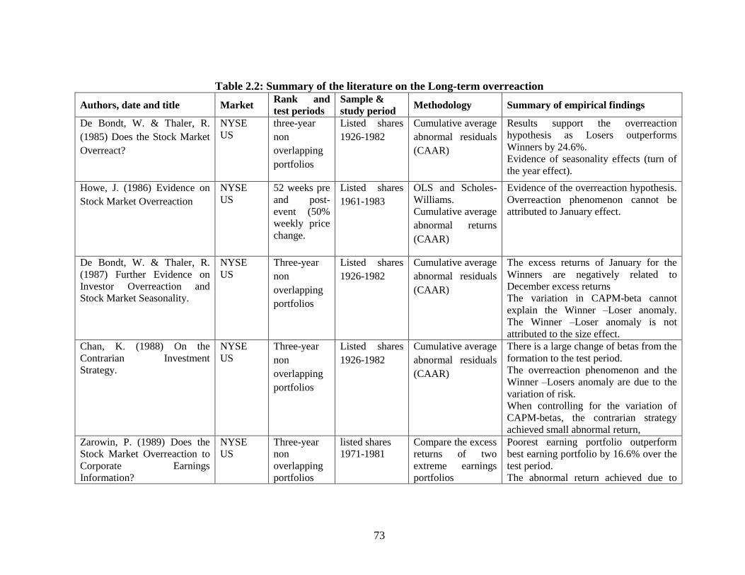
73

Table 2.2: Summary of the literature on the Long-term overreaction

Authors, date and title Market Rank and

test periods

Sample &

study period Methodology Summary of empirical findings

De Bondt, W. & Thaler, R.

(1985) Does the Stock Market

Overreact?

NYSE

US

three-year

non

overlapping

portfolios

Listed shares

1926-1982

Cumulative average

abnormal residuals

(CAAR)

Results support the overreaction

hypothesis as Losers outperforms

Winners by 24.6%.

Evidence of seasonality effects (turn of

the year effect).

Howe, J. (1986) Evidence on

Stock Market Overreaction

NYSE

US

52 weeks pre

and post-

event (50%

weekly price

change.

Listed shares

1961-1983

OLS and Scholes-

Williams.

Cumulative average

abnormal returns

(CAAR)

Evidence of the overreaction hypothesis.

Overreaction phenomenon cannot be

attributed to January effect.

De Bondt, W. & Thaler, R.

(1987) Further Evidence on

Investor Overreaction and

Stock Market Seasonality.

NYSE

US

Three-year

non

overlapping

portfolios

Listed shares

1926-1982

Cumulative average

abnormal residuals

(CAAR)

The excess returns of January for the

Winners are negatively related to

December excess returns

The variation in CAPM-beta cannot

explain the Winner –Loser anomaly.

The Winner –Loser anomaly is not

attributed to the size effect.

Chan, K. (1988) On the

Contrarian Investment

Strategy.

NYSE

US

Three-year

non

overlapping

portfolios

Listed shares

1926-1982

Cumulative average

abnormal residuals

(CAAR)

There is a large change of betas from the

formation to the test period.

The overreaction phenomenon and the

Winner –Losers anomaly are due to the

variation of risk.

When controlling for the variation of

CAPM-betas, the contrarian strategy

achieved small abnormal return,

Zarowin, P. (1989) Does the

Stock Market Overreaction to

Corporate Earnings

Information?

NYSE

US

Three-year

non

overlapping

portfolios

listed shares

1971-1981 Compare the excess

returns of two

extreme earnings

portfolios

Poorest earning portfolio outperform

best earning portfolio by 16.6% over the

test period.

The abnormal return achieved due to

74

differences in size.

The overreaction to earning hypothesis

is not supported Davidson, W. & Dutia, D.

(1989) A Note on the

Behaviour of Security Returns:

A Test of Stock Market

Overreaction and Efficiency.

NYSE

and

AMEX

US

One year non

overlapping

portfolios

listed shares

1963-1985

Calculated the

cumulative

predicted errors

based on the market

model for two

extreme portfolios.

contradicted to the overreaction

hypothesis

Winners (Losers) continued to be

Winners (Losers)

Evidence of January anomaly as 25% of

the Winners occur in January, and

Losers were no longer Losers in

subsequent January. Alonso, A. & Rubio, G. (1990)

Overreaction in the Spanish

Equity Market.

Spain Three-year

non

overlapping

portfolios

listed shares

1967-1984

Following the

methodology of De

Bondt and Thaler

(1985)

Results supported the overreaction

phenomenon in the Spanish stock

market.

Losers outperform Winners by 24.5% 12

months after formation period.

Zarowin, P. (1990) Size,

Seasonality, and Stock Market

Overreaction.

NYSE

US

Three year

non

overlapping

portfolios

Listed shares

1926-1982

Following the

methodology of De

Bondt and Thaler

(1985).

The variation in size is the main cause of

the superior performance of Loser

portfolios over those of Winners.

The excess abnormal returns

disappeared – except for those on

January- when controlling for size.

Evidence of the January effect.

Chopra, N., Lakonishok, J. &

Ritter, J. (1992) Measuring

abnormal performance: Do

stocks overreact?

NYSE

US

Five-year

ranking

period.

Five-year

overlapping

formation

period.

Listed shares

1936-1986

Calculated the

abnormal returns

with adjustments

for size and time

variation in beta.

Used the Buy-and

Hold returns to

rank portfolios.

Results supported the overreaction

phenomenon Consistent results with De

Bondt and Thaler (1985)

Losers were found to outperform

Winners by 9.5% per year.

The overreaction phenomenon cannot be

attributed to size effect.

Strong evidence of January effect.

75

Brailsford, T. (1992) A Test

for the Winner-Loser Anomaly

in the Australian Equity

Market: 1958-87

Australia Three-year

non

overlapping

portfolios

Listed shares

1958-1987

Cumulative average

abnormal residuals

using zero-one

market model

following De Bondt

and Thaler

No evidence of the Winner-Loser

anomaly in the Australian stock market

The difference in CARs for the Losers-

Winner portfolios is insignificant.

Jegadeesh, N. & Titman, S.

(1993)

Returns to Buying Winners

and Selling Losers:

Implications for Stock Market

Efficiency.

NYES

and

AMEX

Buy and

Hold for

1-4 quarters

returns

period.

Listed shares

1965-1989

16 different relative

strength strategies

over 3-12 month

horizons.

Buying past Winners (6 months) and

holding them for another 6 months earns

12.01% compounded excess returns on

average.

the profitability of the relative strength

strategies cannot be attributed to size or

systematic risk

Conrad, J. & Kaul, G. (1993)

Long-Term Market

Overreaction or Biases in

Computed Returns?

NYSE

US

Three-year

non

overlapping

portfolios

Listed shares

1926-1982

Cumulative average

abnormal residuals

(CAAR) and BAH.

Zero-one market

model following

De Bondt and

Thaler

No evidence of market overreaction.

Long-term abnormal returns of the

contrarian strategies are upwardly biased

due to measurement errors.

Buy and Hold method is the most

relevant techniques to measure the long-

term performance

January CARs were 12.2% under the

CARs and - 1.7% under the BAH

Da Costa, N. (1994)

Overreaction in the Brazilian

stock market.

BOVESPA

Brazil Two-year

non

overlapping

portfolios

Listed shares

1970-1989

Cumulative average

abnormal residuals

(CAAR) and BAH.

Zero-one market

model following

De Bondt and

Thaler

Results supported the overreaction

hypothesis.

The variation in CAPM-beta could not

explain Winner-Loser anomaly.

The overreaction effect is asymmetric.

Clare, A. & Thomas, S. (1995)

The Overreaction Hypothesis

FTA All

Share

Index

Three-year

non

overlapping

Listed shares

1955-1990

Cumulative average

abnormal residuals

(CAAR).

Past Losers outperform Winners by

1.7% per year.

This limited overreaction effect is

76

and the UK Stock market. UK portfolios Zero-one market

model following

De Bondt and

Thaler.

attributed to the size effect

Overreaction hypothesis is not supported

by using annual data.

Ball, R., Kothan, S. &

Shanken, J. (1995) Problems

in measuring portfolio

performance An application to

contrarian investment

strategies.

NYSE

and

AMEX.

US

Three-year

non

overlapping

portfolios

Listed shares

1925-1984

For NYES

1962-1984

For AMEX

Buy- and Hold

abnormal returns

Jensen alpha

The contrarian strategy profitability is

much driven by low-priced Losers.

Limited evidence of the January

abnormal returns anomaly.

Negative abnormal returns were found

in the June-end portfolios.

Loughran, T. & Ritter, J.

(1996) Long-Term Market

Overreaction: The Effect of

Low-Priced Stocks.

NYSE

US

Three-year

non

overlapping

portfolios

Listed shares

1929-1988

Cumulative average

abnormal residuals

(CAAR).

Buy- and Hold

The results of Conrad and Kaul (1993)

were driven by the survivor bias.

The discrepancies in results between De

Bondt and Thaler (1985) and Conrad

and Kaul (1993) were due to the

inclusion of AMEX firms.

Bid –ask-spread bias was found to be the

main cause of the long-term

overreaction when forming portfolios

based on CARs

Losers outperform Winners more using

buy and hold method compared to

CARs.

Chen, C. & Sauer, D. (1997) Is

Stock Market Overreaction

Persistent Over Time?

NYSE

US

Five-year

ranking

period.

Five-year

overlapping

formation

period.

Listed shares

1926-1992

Calculated the

abnormal returns

with adjustments

for size and time

variation in beta.

Following the

methodology of

Chopra et al.

(1992).

The returns on the contrarian strategies

are not stable over time,

The overreaction hypothesis is

prevailing during the pre-war period.

The extreme portfolios are less likely to

remain extreme portfolios during the

subsequent periods.

Highly significant relationship between

market risk premium and arbitrage

portfolio returns.

77

Dissanaike, G. (1997) Do

Stock Market Investors

Overreact?

FT500

UK Two-year

ranking

period.

Two-year

non

overlapping

formation

period.

925 Large

companies

1975-1991

Buy and hold and

rebalancing

methods.

Past Losers portfolios outperform

Winners.

Losers tend to be riskier than Winners.

The variation in CAPM beta does not

seem to explain the Loser- Winner

anomaly in the UK. Results supported the overreaction

hypothesis in the UK

Gunaratne, P. & Yonesawa, Y.

(1997) Return reversals in the

Tokyo Stock Exchange: A test

of stock market overreaction.

TSE

Japan

20 non

overlapping

portfolios.

Four –year

rank and test

periods.

Listed shares

1955-1990

Risk adjusted

model.

CARs Following

De Bondt and

Thaler (1985).

Time varying beta

of Chan (1988)

Evidence of the overreaction

phenomenon in the Japanese market.

Past Losers outperformed Winners by

11% per annum.

The variation of CAPM-beta partially

explains the mean reversion between

rank and test periods.

The overreaction hypothesis cannot be

attributed to the seasonality effect

anomalies. Rouwenhorst, K. (1998)

International Momentum

Strategies.

12

European

stock

markets

Buy and

Hold for

1-4 quarters

returns

period.

Listed shares

1978-1995

16 different relative

strength strategies

over 3-12 month

horizons.

Following the

methodology of

Jegadeesh and

Titman (1993).

They found evidence of momentum

profits in the internationally diversified

portfolios.

Past Winners outperform past Losers by

1.5% per month.

Return continuations found for Small-

Medium-Big firms in all the 12

countries

Results supported the findings of

Jegadeesh and Titman (1993).

Fung, A. (1999) Overreaction

in the Hong Kong stock

market.

HIS

Hong

Kong

Two-year

rank period.

Two-year

non

overlapping

formation

33 stocks

constituents of

the HSI

market index

1980-1993

estimated the

cumulative excess

returns using the

buy and hold

method of Conrad

and Kaul (1993) to

Results supported the overreaction

phenomenon in the Hong Kong stock

market. Losers outperform Winners by

10% in year one after portfolio

formation.

78

period. reduce the bid-ask

spread bias

Schiereck, D., De Bondt, W. &

Weber, M. (1999) Contrarian

and Momentum in Strategies

in Germany.

DAX

FSE

Frankfurt

Rank periods

1, 3, and 6

months and

12 month test

period.

375 major

listed shares

1961-1991

CARs and Buy and

Hold to calculate

the excess

cumulative returns.

Consistent results with the behavioural

finance literature.

Momentum strategies were found to be

profitable in the short run.

Contrarian strategies were found to be

profitable in the long horizon.

Baytas, A. & Cakici, N. (1999)

Do markets overreact:

International evidence.

Seven

stock

markets

namely ,

US, UK,

Canada,

Japan,

Germany,

France

and Italy

Five-year

rank and test

period based

on the

holding

period

returns

(HPR)

Five-year

annual return

data over the

period 1982-

1991

Holding period

returns are used to

sort and classify

stocks into Losers

and Winners,

following Conrad

and Kaul’s (1993)

Evidence of overreaction phenomenon

in all countries but the US.

Consistent results with the literature on

price overreaction and particularly

Conrad and Kaul’s (1993).

Long term investment strategies based

on size and price outperforms those of

based on long-term past performance.

Long–term price reversals might be

explained by firm size.

Gaunt, C. (2000) Overreaction

in the Australian equity

market: 1974–1997.

Australia Three-year

non

overlapping

portfolios

Listed shares

1974-1997

Following the

methodologies of

De Bondt and

Thaler (1985) and

Brailsford (1992)

cumulative

rebalancing

methods and buy

and hold excess

returns

Evidence of price reversal phenomenon

in both Winners and Losers.

Loser-Winner anomaly disappeared

when buy and hold method is used.

Evidence of small firm effect as Losers

tends to be smaller and less liquidity

than Winners.

The profitability of the Loser-Winner

arbitrage portfolio is not exploitable in

the Australian Market.

Ahmad, Z. & Hussain, S.

(2001) KLSE Long Run

Overreaction and the Chinese

New Year Effect.

Malaysia,

Kuala

Lumpur

Stock

exchange

Three-year

non

overlapping

portfolios

166 listed

shares over the

period 1986-

1996.

Market-adjusted

excess returns to

rank and construct

portfolios.

Cumulative excess

Evidence of price overreaction in the

KLSE.

Both Losers and Winners experienced

significant reversals over the test period.

The overreaction phenomenon is not

79

(KLSE return and the buy

and hold methods,

dominated by size effect.

Evidence of the seasonality effect

(Chinese New Year) in the KLSE.

Kang, J., Liu, M.-H. & Ni, S.

(2002) Contrarian and

momentum strategies in the

China stock market: 1993–

2000.

China Eight different

horizons (i.e.,

1, 2, 4, 8, 12,

16, 20 and 26

weeks) for

both formation

and holding

periods.

163 shares in

1994 and 286

companies

over the period

1995-2000

Using the portfolio

formation

methodologies of

Lo and MacKinlay

(1990) and

Jegadeesh and

Titman (1995),

Evidence of the short- term overreaction

and intermediate –term momentum

profits.

The overreaction profits were

dominating in case of equal-weighted

portfolio strategies.

The high proportion of individual investors

and the unreliable information (rumors) are

the main source of the contrarian profits.

Momentum profits were prevailing when

they used the value-weighted portfolio

strategies

Dissanaike, G. (2002) Does

the Size Effect Explain the UK

Winner-Loser Effect?

FT500

UK Four-year

ranking

period.

Four -year

non

overlapping

formation

period.

925 Large

companies

1975-1991

Buy and hold and

rebalancing

methods.

Same methodology

of Dissanaike

(1997)

Results showed that there is no evidence

to suggest that the Winner-Losers

anomaly might be explained by size.

This result is consistent with the

overreaction literature in the UK (see

Levis 1989a).

Dissanaike claimed that the sample of

FT500 is biased towards big size firms.

Results were not in favour the efficient

market hypotheses.

Benou, G. & Richie, N. (2003)

The reversal of large stock

price declines: The case of

large firms.

US Three

different test

periods.

One, two and

three – year

test periods.

Monthly return

data for Large

firms

experienced

dramatic price

drop (at least

20%) 1990-

2000.

The market-

adjusted model.

The risk-adjusted

model using

GARCH 11).

CARs following

Fama (1998)

Positive and significant abnormal

returns over one year following the

event.

Highly significant price reversal for

technology stocks.

Evidence of underreaction for the

service stocks.

Their results support the overreaction

hypothesis in the US.

Buying large firms that experienced

80

large price drop is a profitable

investment strategy.

Forner, C. & Marhuenda, J.

(2003) Contrarian and

Momentum Strategies in the

Spanish Stock Market.

Spain 6, 12, 36, 60

month-

formation

and test

periods

Monthly return

data 1963-

1997.

Losers and Winners

portfolios extreme

based on the

extreme residual

returns using CARs

following of De

Bondt and Thaler

(1985) and BAH

following Conrad

and Kaul (1993)

The one-year and five-year momentum

and contrarian strategies earn significant

abnormal return.

Their results supported the existence of

the momentum profits in the short run

and the contrarian profits in the longer

horizons even after controlling for time

varying risk.

Finally, they argued that their results

were not due to the data snooping bias.

Chiao, C., Cheng, D. & Hung,

W. (2005) Overreaction after

Controlling for Size and Book-

to-Market Effects and its

Mimicking Portfolio in Japan.

TSE

Japan

Five-year

formation

and test

periods

Monthly return

data for the

listed shares

1975-1999.

Two main

portfolios namely;

size-BM based and

prior returns based

portfolios.

FF3-factor model.

Strong evidence of persistent

overreaction phenomenon in the

Japanese market.

Size and book-to-market ration were

correlated with the overreaction.

Fama French three-factor model

explained portfolios excess returns. Siganos, A. (2007) Momentum

returns and size of Winner and

Loser portfolios.

LSE

UK

Winner and

Loser

portfolios,

includes the

best and the

worst 10, 20,

30, and 300

shares.

Monthly return

data for the

listed shares

1975-2001

Calculate

momentum profits

by ranking all the

company based

past six months

market

performance

months.

Three size

portfolios were

constructed based

on mcap.

Evidence of the momentum profits in

the UK.

Investors can maximise their momentum

profits by including small firms of both

Losers and Winners in their portfolios.

It is not necessarily for the investors to

sell-short Losers as the momentum

returns for the large portfolios remain

constant.

Mazouz, K. & Li, X. (2007)

The overreaction hypothesis in

LSE

UK

Three-year

non

The

constituent of

CARS and BAH,

and following the

Strong evidence of price overreaction in

the London stock exchange

81

the UK market: empirical

analysis.

overlapping

portfolios

the FTSE All

shares market

index over the

period 1972-

2002

methodology of De

Bondt and Thaler

(1985) in portfolio

formation

Losers outperform Winners by 16.4%

and 18.3% using CARS and BAH

methods respectively.

No evidence of January effect on the

contrarian profits; however size effect

cannot fully explain the overreaction

phenomenon.

George, T. & Hwang, C.-Y.

(2007) Long-Term Return

Reversals: Overreaction or

Taxes?

NYSE,

AMEX,

and

Nasdaq

US and

Hong

Kong

Five-year-

formation

and test

periods

All listed

shares

1963-2001

(US)

1980-2000

(HK)

three alternative

measures to test the

OH; traditional

return, Five-year

high and five-year

low measures,

Two additional

measures to test the

lock-in hypothesis

equal-weighted

gain and loss and

equal-weighted

gain only measures

They found strong evidence of the tax

hypothesis.

Winner reversal diminished as the

traditional reversal measures were

subsumed in the locked-in measures.

No price reversals were found for non

January Loser portfolios.

No price reversals for both Winners and

Losers in Hong Kong where no capital

gain or dividends tax.

Their results are inconsistent with the

overreaction hypothesis.

Dissanaike, G. & Lim, K.-H.

(2010) The Sophisticated and

the Simple: the Profitability of

Contrarian Strategies.

LSE

UK

Three-year

formation

and test

periods

All the listed

shares

(excluding

investment and

unit trusts)

over the period

1987-2001

Portfolio formation

methodologies:

book value,

earnings, cash flow

or operating cash

flow or residual

income model and

Ohlson model. Buy-and-hold

returns

The residual earnings and the Ohlson

models outperform the traditional

strategies based on B/M and E/P.

The traditional cash flow to price ratio

outperforms the advanced accounting

measures. They recommended that

investors’ size and the technical

knowledge of more advanced models are

the main determinants of the optimal

portfolio formation.

Wu, Y. (2011) Momentum

Trading, Mean Reversal and

Overreaction in Chinese Stock

Shanghai

Stock

Exchange

Six and 12

months

formation

Daily data for

the “A” listed

shares 1990-

2001

methodology of

Fama and French

(1988) and Balvers

and Wu (2006)

No significant abnormal returns for the

pure short-term (3 - 12 months)

momentum strategy of Jegadeesh and

Titman (1993).

82

Market. (SHSE) and test

periods

Highly significant abnormal returns for

the pure contrarian strategy for all

holding periods.

The combined strategy (momentum +

contrarian) results in a significant excess

return 22.2%.

their results supported the overreaction

hypothesis in the Chinese market.

83

Chapter 3 : Short-term overreaction: Unobservable portfolios?

3.1 Introduction

The existing body of literature on the overreaction phenomenon has extensively used time

series analysis. This can be found in the papers of De Bondt and Thaler, (1985), Conrad and

Kaul (1993), Jegadeesh and Titman (1995), Da Costa, (1994), Loughran and Ritter (1996) and

Dissanaike (1997). Another much smaller strand of the literature has used cross-sectional

analysis to investigate the phenomenon. The work of Bremer and Sweeney (1991), Cox and

Petersen (1994), Otchere and Chan (2003), Larson and Madura (2003), Ma, Beach, and Hasan

(2005) is illustrative. If these two dimensions have not been combined, the analysis is subject

to criticism. Hsiao (2004) and Baltagi (2010), for example, argue that ignoring the time

dimension raises the question of bias due to group (company) heterogeneity. Ignoring the

dynamics of the process also raises questions of bias in the estimation (Arellano and Bond

(1991).

Therefore, in this chapter I present a new methodology to investigate the overreaction

phenomenon, the two-way fixed effects panel data model (see Farag and Cressy (2010)14

), and

in addressing the dynamics of the process I employ the Blundell and Bond (1998) two-step

Difference GMM estimator which adds dynamics into the process. Finally, I attempt to

explain the measured unobservable effects by means of observable variables. These include

14

This paper has been published based on my earlier work in this chapter and based on small sample of 20

companies.

84

corporate governance compliance, political connection of board members, and management

quality.

The main contribution of this chapter then is, firstly, the use of static and dynamic panel data

models to investigate the overreaction phenomenon; secondly, to use the results from this

analysis to form ‘unobservable’ portfolios based on the fixed effects model. Interestingly, we

shall see that the Unobservable portfolios outperform the traditional size portfolios. Thirdly, I

investigate the relationship between firms’ corporate governance compliance, the political

connections of the board of directors and the overreaction phenomenon.

I use data from the Egyptian stock market. This adds an additional dimension since my study

is the first to empirically investigate the overreaction phenomenon in this market, one of the

leading markets in the Middle East and North Africa region (MENA).

This chapter is organised as follows: section 2 presents the theoretical background about the

traditional models and the proposed new model to explain the short – term overreaction.

Sections 3 describes the dataset used in the analysis. Section 4 presents the econometric

modeling and the empirical results. Finally, section 5 summarises and concludes.

3.2 Theoretical background

3.2.1 Traditional theories

According to the overreaction hypothesis, the greater the initial shock proportional price

change at time 0 the greater the subsequent price reversals (De Bondt and Thaler (1985)).

85

Cressy and Farag (2011) argue that small companies are riskier and more informationally

opaque compared with large companies. Therefore, the inverse relationship between

cumulative abnormal returns CARst and the initial abnormal return ARs0 is expected to be

stronger for small firms. This relationship is econometrically represented by a negative slope

of the regression line with respect to a measure of firm size (Cox and Peterson (1994)).

3.2.2 A new model: Unobservable effects

Fixed, unobservable effects in two dimensions, I argue, can potentially provide a better

explanation of the behavior of cumulative abnormal returns compared with the traditional one-

dimensional models. The panel data model, in particular the fixed effects model, allows that in

addition to observable factors i.e. typically size and trading volume, can explain the

overreaction to dramatic price changes between companies, there are also unobservable effects

(group and period) that may play a potentially important role (Farag and Cressy (2010)).

Cressy and Farag (2011) argue that company effects can be described as ‘permanent’

(independent of time in the reversal window) or ’temporary’ (one period duration). They

suggest that these effects might be explained as a proxy of firm quality; however they were not

able to empirically identify observable correlates for these effects.

Figure 3.1 presents a graphical illustration of the relationship between initial price reaction

(AR(i,0)) and subsequent cumulative abnormal returns (CARs). In the traditional model the

CARs are the same ( for high and low quality firms. However, and in the light of the

unobservable effects model, these CARs shift up or down based on company heterogeneity

86

(quality) ( 2 for higher quality firms, for average quality firms and 1 for low

quality firms) where 12 0 . If alpha is positive, the effect of (permanent) firm quality on

a price fall (e.g.) is to counteract the fall; if negative, to reinforce it (Cressy and Farag (2011).

Thus for high quality firms, dramatic price fall is subsequently corrected (reversed) to some

degree. For low quality firms, it is subsequently accentuated.

On the other hand, temporary factors (period effects) common to all companies may shift the

intercepts 1 and 2 up (positive effects) or down (negative effects) in any given

period (Cressy and Farag (2011)).

AR(i,0)

CAR(i,t+s)

0

2

1

12 0

Low quality firm

High quality firm

Average quality firm

Figure 3-1: Post-event CARs determined by market cap and unobservable effects

87

3.3 Data

To examine the short-term overreaction hypothesis in the Egyptian stock market, daily data for

stock prices, free float market capitalisation and the EGX 30 market index are utilised for 100

listed stocks with no price limits on the exchange (EGX) over the period 2003-2009. I define

the event for a given stock as the experience of a one-day price rise (Winners) or price fall

(Losers) of at least 10% as the result of one of the following events:

Event (A): Sharm El Sheikh Terrorist Attacks (24 July 2005).

Event (B): The Lebanon War, (12 Jul 2006) as a proxy for the tension in the Middle

East region.

Event (C): The Announcement of the Constitutional Change, (25-Dec 2006) as a proxy

for a political reform.

Event (D): The formation of the new government, (27-Dec 2005).

I initially defined the events in the line of the literature (shares that experienced at least 10%

one day price change). I then clarified the main causes of these events. Therefore these events

are the most influential events in the Egyptian stock exchange during the period of study.

I use the EGX 30 index, a free-floated market capitalisation weighted index to represent the

Egyptian stock market benchmark Farag and Cressy (2010). Data were collected from the,

Egyptian stock exchange in addition to Egypt for Information Dissemination Company

(EGID).

88

It is worth mentioning that the 100 companies included in the sample are the most actively

traded companies in the Egyptian stock exchange (EGX). Therefore, the sample seems to be

homogeneous and highly unlikely to be affected by the less frequently traded shares or outlier

bias.

Following Cox and Peterson (1994), Cressy and Farag (2011) and Farag and Cressy (2010)

methodologies, the estimation period for betas is (-105, -6) and test period is (+1, +120) days.

I use the market model as a benchmark to measure the abnormal returns with betas estimated

for each security over the 100 days prior to the event. Other measures are also tried, namely,

the CAPM model and market-adjusted abnormal return, but qualitatively the results remain the

same. This is also in line with the literature (Cox and Peterson, 1994).

3.4 Econometric modeling and empirical results

I use the Event Study methodology to estimate the abnormal returns during the test period.

Following the methodology of Bremer and Sweeney (1991) and Cox and Peterson (1994), I

begin by defining daily returns.

3.4.1 Daily Returns

The return variable tR is defined as the first difference in the natural logarithm of the closing

price over two consecutive trading days:

1 ttt PLogPLogR (1)

Where tp is the closing price of the stock in day (t) adjusted for dividends, rights issue, stock

dividends, and stock split.

89

3.4.2 Stock abnormal returns (ARs)

Stocks’ abnormal returns in the test period are defined as the residuals of the market model

following Cox and Peterson, (1994) and Farag and Cressy (2010).

TtRRAR mtiiitit .....,2,1,0, (2)

where

itmtjjit RR (3)

where, i and i are the results of the market model, itR is the stock return on day (t), mtR is

the daily market returns of the EGX market index and T = 120 days. The parameters of the

market model are estimated over the estimation window (-105—6). I used both symmetric

GARCH and asymmetric TARCH models to estimate the abnormal returns and to control for

any potential serial correlation in the return time series. I obtained similar results for the two

methods (Benou and Richie (2003).

3.4.3 Cumulative abnormal returns (CARs)

Cumulative abnormal returns (CARs) and cumulative average abnormal returns (CAARs) are

calculated as follows following Cox and Peterson, (1994) and Farag and Cressy (2010):

t

iit ARCAR1

(4)

ICARCAARI

i

itt /1

(5)

90

where I = 100 is the number of stocks in the sample

I use t-test statistic to examine whether or not there is a significant difference in CARs

between Winners and Losers for a given day within the event window. The statistic is defined

as follows:

n

at

t

tt

nAARARARS

ARSARstatt

1/)()(

)(/

2

(6)

Where S is the standard deviation of securities’ abnormal returns.

3.4.4 Descriptive statistics

The descriptive statistics for the four events (A-D) are presented in Table 3.1. The sample size

is 100 companies over 120 days as test periods. The initial one-day abnormal return on event

day ( 0iAR ) for the Loser events (A and B) are -5.60% and -3.17% respectively. However, the

initial abnormal return on event day for the Winner events (C and D) is 7.11% and 6.52%

respectively. Cumulative abnormal returns ( itCar ) over event window (120 days) for the

Losers are 14.59% and 7.46 % for events A and B respectively and for the Winners are -

20.52% and -35.19% for events C and D respectively.

This suggests that buying Losers on average not only earn positive abnormal returns over the

period following the event but also (as in DeBondt and Thaler, 1985) these portfolios

outperform the Winner portfolios. Specifically, cumulative average abnormal returns three

days before the event - as a proxy for the leakage of information (Leak) - for the Losers are

1.07% and -0.12 % respectively and for the Winners are 0.66% and -0.56% respectively.

91

Table 3.1: Descriptive Statistics

Mean S.D Skewness Kurtosis

Panel A: Loser Event A

itCar 0.1459 0.5331 0.8378 3.5184

0iAR -0.0560 0.0305 -0.9938 5.4384

Lnmcap 19.557 2.1201 -0.2359 3.4275

Leak 0.0107 0.0364 0.3326 3.9305

Private 0.5000 0.5051 0.0000 1.0000

Panel B: Loser Event B

itCar 0.0746 0.4560 0.8879 4.2309

0iAR -0.0317 0.0515 2.4385 5.3944

Lnmcap 19.684 1.6846 0.1821 2.4302

Leak -0.0012 0.0619 -3.9771 2.3192

Private 0.5000 0.5051 0.0000 1.0000

Panel C: Winner Event C

itCar -0.2052 0.6675 0.2085 6.1621

0iAR 0.0711 0.0389 1.3019 4.4327

Lnmcap 19.731 1.8593 -0.3922 3.6710

Leak 0.0066 0.0422 0.9448 4.0901

Private 0.5000 0.5051 0.0000 1.0000

Panel D: Winner Event D

itCar -0.3519 0.5917 -0.3775 2.7186

0iAR 0.0652 0.0312 1.86134 6.0601

Lnmcap 19.604 1.3670 0.1102 2.3783

Leak -0.0056 0.0417 -2.1486 3.1620

Private 0.5000 0.5051 0.0000 1.0000

Number of observations is 12000 observations (100 companies * 120 days).

Average firm size proxied by market capitalisation of the Losers are 312 million and 354

million Egyptian pounds respectively, whereas the average firm size for the Winners are 370

million and 326 million Egyptian pounds. Finally, 50% of the sample was formerly state-

owned companies.

92

3.4.5 Correlation matrix

Table 3.2 presents the correlation matrix for the Winners and Losers covariates.

Table 3.2: Correlation Matrix

Lnmcap ARio Leak Private Panel A: Loser Event A

Lnmcap 1.0000

ARio -0.0388 1.0000

Leak 0.0040 -0.1455 1.0000

Private 0.1262 -0.2257 -0.2555 1.0000

Panel B: Loser Event B

Lnmcap 1.0000

ARio 0.0146 1.0000

Leak 0.1174 -0.0589 1.0000

Private 0.4507 0.2362 -0.0816 1.0000

Panel C: Winner Event C

Lnmcap 1.0000

ARio -0.1087 1.0000

Leak 0.2641 0.3422 1.0000

Private 0.2989 -0.0848 -0.0007 1.0000

Panel D: Winner Event D

Lnmcap 1.0000

ARio 0.0014 1.0000

Leak 0.0562 -0.1267 1.0000

Private -0.1532 -0.0597 0.1030 1.0000

***, **,* indicate significance at the 1%, 5% and 10% levels.

Number of observations is 12000 observations (100 companies * 120 days).

The reported correlations show that there is no potential multicollinearity as none of these

correlations is above 0.50 or statistically significant, even at 10%.

3.4.6 The overreaction hypothesis

I investigate the overreaction phenomenon firstly by examining the significance of the

abnormal returns pre- and post- each of the four events. Table 3.3 presents the average

abnormal returns and t- statistics for the Losers and Winners over event window (–5 to +5). It

93

is clear that both Losers and Winners - as expected - have highly significant abnormal returns

on event day (p value < 0.001).

For event A (Terrorist Attacks), we notice positive abnormal returns pre-event (-4 to -1 days)

which may indicate investors' optimism and herding behaviour. The average abnormal return

on event day is negative -5.61% and highly significant at 0.001. We also notice that the effect

of event (A) continues (the so-called price continuation phenomenon, (Kim and Rhree (1997))

for the subsequent three days post-event, as the average abnormal return is negative and highly

significant (at 5%). Price reversal occurs on the fourth day, as positive abnormal returns are

found on day 4 as well as a positive and significant (at 10%) abnormal return on day 5.

Table 3.3: Average abnormal returns (AARs) for Losers and Winners

Losers Winners

Event A Event B Event C Event D

AR t. value AR t. value AR t. value AR t. value -5 0.0076 1.5545 0.0164 3.6968

*** -0.0082 -1.6781

* -0.0139 -3.8321

***

-4 0.0132 3.2188***

0.0036 0.9181 -0.0076 -1.6032 -0.0021 -0.5180

-3 0.0057 1.6057**

-0.0021 -0.4622 -0.0015 -0.2217 -0.0065 -1.8253*

-2 0.0071 1.8626* 0.0013 0.2268 0.0016 0.3584 -0.0038 -0.6696

-1 0.0107 2.0852**

-0.0012 -0.1316 0.0165 2.0974**

-0.0155 -0.9416

0 -0.0561 -12.9808***

-0.0317 -4.351***

0.0711 12.9446***

0.0652 14.7585***

1 -0.0102 -2.0736**

0.0135 2.3198**

-0.0019 -0.2682 -0.0045 -0.7875

2 -0.0027 -2.0399**

0.0071 1.4715 -0.0042 -0.6728 -0.0141 -2.4994**

3 -0.0029 -2.0098**

0.0027 0.6223 -0.0023 -0.4373 -0.0027 -0.6476

4 0.0009 0.2347 0.0004 0.1173 0.0015 0.2596 0.0029 0.6588

5 0.0076 1.8693* 0.0019 0.4245 0.0044 0.7254 0.0024 0.4093

***, **,* indicate significance at the 1%, 5% and 10% levels.

Number of observations is 12000 observations (100 companies * 120 days).

With regard to event B (the Lebanon War), the average abnormal return on event day is

negative -3.17% and highly significant at 0.001. However, price reversal occurs on day one

94

post-event as we notice positive (1.35%) and highly significant (at 5%) abnormal returns on

day one post-event. There is no leakage of information, as insignificant abnormal returns are

found over the five days pre-event B.

Figure 3-2 shows the results of plotting cumulative average abnormal returns (CAARs) over

time, for the Losers over one week pre and post-events. The asymmetric overreaction is clear

from figure 3-2 as stock price reversal of event (B) occurs on day one while the price reversal

of event (A) occurs in the fourth day post-event.

Figure 3-2: Cumulative average abnormal returns for Losers

Winners have highly significant (p value < 0.001) abnormal returns (7.11% and 6.52%) on

event day for events C (the announcement of the constitutional change) and D (the formation

of the new government) respectively. In addition, price reversal occurs on day one post-event

for both events. We also notice positive and significant (at 5%) abnormal returns for event C

on day one pre-event; this implies the leakage of information effect.

-0.03

-0.02

-0.01

0

0.01

0.02

0.03

0.04

0.05

-5 -4 -3 -2 -1 0 1 2 3 4 5

CA

AR

One week event window Event A Event B

95

It is worth mentioning that the overreaction phenomenon and the subsequent price reversals

are clear for the Losers rather than those of the Winners. Chan (1988) argues that Losers are

more risky during the estimation window compared with Winners. This suggests that Losers

are on average bigger in size, therefore they are expected to react to the new information more

efficiently that those of Winners (Chan (1988)). These results are consistent with the literature

on overreaction hypothesis as Losers on the short- term are expected to outperform Winners

(Cox and Peterson (1994) and Bremer and Sweeney (1991)).

Figure 3-3 shows the results of plotting Cumulative Average Abnormal Returns (CAARs) over

time, for the Winners over one week pre and post-events.

Figure 3-3: Cumulative average abnormal returns for Winners

I conclude that the terrorist attacks have significant effects on stock price movements for three

days post event. However, the Lebanon war as a proxy for the tension in the Middle East

region had no effect on the average abnormal returns in the Egyptian stock exchange.

-0.04

-0.02

0

0.02

0.04

0.06

0.08

-5 -4 -3 -2 -1 0 1 2 3 4 5

CA

AR

One week event window Event C Event D

96

Furthermore, there was no significant average abnormal return as the result of the

announcement of constitutional change and the formation of a new government.

Figure 3-4 shows the results of plotting Cumulative Average Abnormal Returns (CAARs) over

time, for the Winners and Losers over one week pre- and post-events.

Figure 3-4: Cumulative average abnormal returns for Winners and Losers

To summarise, findings are consistent with the literature on overreaction. Past Losers

outperform past Winners so that investors may achieve abnormal returns by selling Winners

and buying Losers.

3.4.7 The optimal holding period

I now discuss the optimal holding period for Winners and Losers. Table 3.4 reports the

cumulative average abnormal returns for Losers and Winners over the following periods

CAAR(-5, -1), CAAR (+1, +3), CAAR (+4, +10), CAAR (+21, +50), CAAR (+51, +120), and

CAAR (+1, +120).

With regard to event (A), the cumulative average abnormal return pre-event window (-5, -1) is

negative and highly significant; this suggests – as discussed above – both herding behaviour

-0.04

-0.02

0

0.02

0.04

0.06

0.08

-5 -4 -3 -2 -1 0 1 2 3 4 5

CA

AR

Event A

Event B

Event C

Event D

97

and investor optimism. Highly significant negative abnormal returns are reported on the

following day due to the terrorist attacks. CAAR (+21, +50), and (+51, +120) windows have

positive and abnormal return at a level of 5%. The optimal holding periods are (+21, +30),

(+51, +60), and (+41, +50) as the cumulative average abnormal returns are 4.40%, 3.89% and

3.72% respectively. However, the optimal holding period for event (B) is (+31, +40), as the

cumulative average abnormal returns is 5.36%. The optimal selling period for the Winners

events (C) and (D) are (+41, +50), and (+71, +80) respectively as we notice positive

cumulative average abnormal returns over these periods (1.75% and 0.01% respectively).

These findings support the argument that past Losers outperform past Winners.

The results presented in table 3.4 suggest that stock prices in the short term for both Losers

and Winners are not predictable as the cumulative average abnormal returns five days pre

event (as a proxy for the leakage of information) are positive and highly significant for event

A and negative and highly significant for event D. This may imply the effect of investor

optimism and herding behavior in the Egyptian stock market.

On the other hand, Losers may achieve cumulative average abnormal returns quicker than

those of Winners as the optimal holding periods for the Losers are (+21, +30) and (+31, +40)

days for events A and B respectively. However, the optimal holding period returns for the

Winners are (+41, +50) and (+71, +80) days for events C and D respectively. This suggests

that Losers on average outperform Winners and investors may achieve abnormal return by

adopting the contrarian strategy by selling Winners and Buying Losers.

98

Table 3.4: Cumulative average abnormal returns for Losers and Winners over event window

Loser Winner

Event A Event B Event C Event D

CAAR t. value CAAR t. value CAAR t. value CAAR t. value

CAAR(-5, -1) 0.0442 4.3367***

0.0182 1.0320 -0.0091 -0.6260 -0.0318 -2.2355**

CAAR (+1,+3) -0.0103 -1.3035 0.0232 2.4000**

-0.0084 -0.8859 -0.0213 -2.5359**

CAAR (+4, +10) -0.0202 -1.5722 0.0096 0.6974 -0.0207 -1.2872 -0.0130 -0.8731

CAAR (+11,+20) -0.0258 -1.5302 0.0286 1.7410* -0.0364 -1.8625

* -0.0744 -4.8753

***

CAAR (+21,+30) 0.0440 2.6806**

-0.0214 -1.7046* -0.0284 -1.6095 -0.0297 -2.8938

***

CAAR (+31,+40) 0.0129 0.8168 0.0536 3.3828***

-0.0044 -0.2696 -0.0119 -0.8013

CAAR (+41,+50) 0.0372 2.1367**

-0.0003 -0.0159 0.0175 1.0686 -0.0105 -0.7185

CAAR (+51,+60) 0.0389 2.2478**

0.0037 0.3419 -0.0277 -2.7228**

-0.0282 -2.0974**

CAAR (+61,+70) 0.0181 1.1175 -0.0015 -0.1280 -0.0138 -0.7880 -0.0333 -2.5463**

CAAR (+71,+80) 0.0258 1.5835 -0.0121 -0.9497 -0.0222 -1.5291 0.0001 0.0027

CAAR (+81,+90) 0.0191 1.1156 0.0156 0.8437 -0.0168 -0.9501 -0.0173 -1.0317

CAAR (+91,+100) 0.0085 0.5045 -0.0073 -0.5856 -0.0216 -1.8115**

-0.0242 -1.2570

CAAR (+101,+110) -0.0140 -0.6897 -0.0072 -0.5663 -0.0336 -3.0108***

-0.0348 -2.3560**

CAAR (+111,+120) 0.0089 0.4647 -0.0090 -0.7796 0.0116 1.2655 -0.0567 -4.9903***

CAAR (+21,+50) 0.0941 3.1020***

0.0319 1.0002 -0.0153 -0.4314 -0.0521 -1.9923*

CAAR (+51,+120) 0.1053 2.1986**

-0.0178 -0.4985 -0.1240 -2.6274**

-0.1945 -3.2825***

CAAR (+1,+120) 0.1455 1.9336* 0.0737 1.1440 -0.2022 -2.1365

** -0.3736 -4.2565

***

***, **,* indicate significance at the 1%, 5% and 10% levels.

Number of observations is 12000 observations (100 companies * 120 days).

99

Figures 3-5, 3-6 and 3-7 show the results of plotting Cumulative Average Abnormal Returns

(CAARs), for Winners and Losers over 120 days post-event. It is clear from the figures that

past losers outperform past winners, so that investors can achieve abnormal returns by selling

winners and buying losers (the disposition effect). These results are consistent with the

literature on price reversal (De Bondt and Thaler1985). Similar results were found by Cox and

Petersen, (1994); Larson & Madura, (2003); Ma, Tang and Hasan, (2005) and Farag and

Cressy (2011).

Figure 3-5: Cumulative average abnormal returns for Losers over event window

-0.1

-0.05

0

0.05

0.1

0.15

0.2

-5 0 5 10 15 20 25 30 35 40 45 50 55 60 65 70 75 80 85 90 95 100 105 110 115 120

CA

AR

Event window Event A Event B

100

Figure 3-6: Cumulative average abnormal returns for Winners over event window

Figure 3-7: Cumulative average abnormal returns for Winners and Losers

-0.35

-0.3

-0.25

-0.2

-0.15

-0.1

-0.05

0

0.05

0.1

CA

AR

Event window Event C Event D

-0.4

-0.3

-0.2

-0.1

0

0.1

0.2

CA

AR

Event window Event A Event B Event C Event D

101

3.4.8 Cross-sectional regression

Following Cox and Petersen, (1994), Farag and Cressy (2010), Cressy and Farag (2011),

Larson and Madura, (2003); Ma, Tang and Hasan, (2005), I obtain average returns on each

firm’s stock over the whole time period. I then estimate the following cross-sectional

regression by regressing cumulative average abnormal returns iCAR against initial abnormal

returns in event day i0AR , along with firm size (natural log of the free float mcap one day

before the event to avoid the endogeniety problem), and a dummy variable representing the

company ownership which will be defined below.

In addition, I include a iLeak variable representing the cumulative average abnormal returns

for three days before the event date to capture the leakage of information into the market and

the effects of insider information. These can be considered proxies for market inefficiency (see

Larson and Madura 2003).

The dummy variable (Private) is a proxy of firm ownership and is equal to one if the company

was privately held before IPO. This is consistent with the Egyptian economic reform

programme started in 1997; as we have seen in chapter (1) a number of -state-owned

companies were floated on the Egyptian stock exchange in the period. I model CAR(i), then,

as follows:

102

100,...1,privateLeaklnmcap AR 4i3i2i01 iCAR iii (7)

where

100/120

1

t

iti CAARCAR

0iAR = Initial abnormal return in event day t = 0.

iprivate is a dummy variable = 1 if the company was privately held before

IPO; = 0 otherwise

imcapln is the natural log of the free floated market cap of company (i) one day

before the event.

iLeak is cumulative average abnormal returns for three days before event date as a

proxy for the leakage of information.

i = a white noise error term for stock (i)

Cox and Peterson (1994) argue that there is a negative relationship between firm size and the

cumulative average abnormal returns (small firm effect). If so small firms have higher price

reversals compared to large firms; this is due to higher degree of risk. If size effect holds in the

Egyptian stock market we are expecting negative sign for lnmcap variable.

Moreover, Cox and Peterson (1994) and Larson and Madura (2003) argue that there is a

positive relationship between abnormal returns on event day ( 0iAR ) and the cumulative

average abnormal returns. This suggests the magnitude effects of the overreaction hypothesis

(the higher the initial price changes the higher the subsequent price reversals). Therefore we

103

expect positive sign for 0iAR . Larson and Madura (2003) on the other hand argue that the

leakage of information may play an important role in explaining the overreaction hypothesis

due to the role of noise trading and information inefficiency in emerging markets. Therefore

iLeak is expected to have positive and significant coefficient. Finally, I incorporate iprivate

variable into the analysis to investigate the performance of private and state owned companies;

this is due to the recent economic reform programme adopted by the Egyptian government.

Table 3.5 presents the results of the cross-sectional OLS regression of equation 7. It is clear

that the models are reasonably well specified (F statistics are highly significant for Winners

and Losers). The average adjusted R-squared is 23.29% and 22.63% for the Losers and

Winners respectively.

The negative sign of lnmcap as a proxy for firm size suggests the presence of a small firm

effect, as small firms tend to have greater reversals compared with large firms in the post-

event period. This result is consistent with the literature on the overreaction phenomenon (e.g.,

Cox and Peterson (1994) and Farag and Cressy (2010).

Interestingly, the leakage of information variable (Leak(i)) is positive and highly significant

for events A and D respectively. This suggests the role of insider trading and information

inefficiency in the Egyptian stock market for particular types of events namely terrorist attacks

(some international agencies issue warning about potential terrorist acts in some regions) and

the formation of the new government.

104

Table 3.5: Cross Sectional Regressions

Losers Winners

Event A Event B Event C Event D

C 1.2342**

(0.5963)

1.7719**

(0.7581)

1.9500*

(1.0102)

1.1827

(1.1555)

Lnmcap -0.0665**

(0.0319)

-0.1042***

(0.0410)

-0.0988*

(0.0501)

-0.0174

(0.0575)

Leak 0.4020***

(0.0721)

-0.9480

(1.1972)

-2.9608

(2.2338)

4.5557**

(1.8844)

ARio 2.6280

(2.3067)

-2.9834**

(1.4622)

-5.2833**

(2.3474)

0.7006

(2.5030)

Private 0.4371***

(0.1438)

0.3391**

(0.1453)

0.3517*

(0.1747)

-0.4660***

(0.1568)

R2 0.2896 0.2704 0.2942 0.2596

Adj R2 0.2265 0.2394 0.2315 0.2211

F.stat 4.5868***

(0.0034)

3.8202***

(0.0059)

4.6895***

(0.0030)

3.3522**

(0.0174)

White test for heteroskedasticity 0.9545 0.1837 0.4293 0.6241

*, **,*** indicates significance at the 1%, 5% and 10% levels.

Number of observations is 100 observations.

The initial abnormal returns on event day (ARi0) on the other hand are insignificant for both

events A and D. This result is consistent with Cox and Peterson (1994) as incorporating size

effect in the regression does remove the effect of the initial abnormal returns. However, initial

abnormal returns on event day (ARi0) are highly significant for events B and C.

Furthermore, private firms have greater CARs than state-owned firms for both Losers and

Winners (except in the case of Event D). The management quality of private firms usually

outperforms the management quality of state owned firms in the Egyptian context. This may

explain the positive and significant relationship of private variable in table 3.5. However event

D has the least significant results in table 3.5 (i.e. firm size and initial abnormal returns on

event day). This may explain the weak investor reaction to this event. In addition, Private

variable will be dropped from the analysis due to the assumptions of panel data model.

105

As mentioned above, it is necessary to drop the dummy variable (Private) from the fixed

effects regression due to collinearity problems it introduces. Therefore I re-estimated the cross

section regression of equation 7, dropping the dummy variable (Private). The results were

virtually unchanged.

3.4.9 Panel data econometrics

In this section I explain the structure of the two-way panel data econometrics I use

subsequently.

There are two main competing models of panel data econometrics, namely, fixed and random

effect as in equations 8 and 9.

ittiitity

(Two way fixed effect model) (8)

ittiiitit uhy )()(

(Two way random effect model) (9)

where: i is unobserved firm-specific (time-constant) effect for company i, t is time-specific

effect for period t, iu is group-specific random effect, ih is a random vector that induces the

variability of the parameters across individuals, it is a white noise error term.

Unobservable factors in stock price reversal may thus be either random or fixed (Farag and

Cressy 2010). The fundamental distinction between the FE and RE model is whether the

unobservable effects embodies elements that are correlated with the regressors. A fixed effects

model allows that the effects may be correlated with the regressors (covariates) whilst a

random effects model does not: random effects are part of the error term and hence any

correlation with the covariates implies an endogeneity problem. (Greene 2012).

106

Farag and Cressy (2010) and Cressy and Farag (2011) argue that observable factors

(variables) e.g. size, trading volume and the leakage of information are not the only variables

that explain the price reversal phenomenon15

.In equation 8, unlike equation 7, the relationship

may shift up or down based on the sign of the firm fixed effect coefficient P (positive) or

N (negative). It may also shift up or down as a results of factors common to firms in a given

time period, via the time-specific effect t . I argue that these effects may explain the

company heterogeneity in response the dramatic change in stock prices.

I estimate the two-way first order autoregressive fixed/random effect (FE/RE) models to

obviate the serial correlation in itCAR , as in the following equation:

ittiit

ittiitit

itittiit

retiuxCAR

fetixCAR

1,

0

0

120,....1;100,...1, )('

120,....1;100,...1,'

(10)

Where 0 =common intercept for all i,t

itx = independent variables

i = company-specific effect for company i

t = time-specific effect for period t

it = white noise error term.

Note that for the random effects model I use the GLS-estimator, a weighted average of

between-firm and within-firm effects. 1 and it is independent and identically distributed

15

This paper has been published based on my earlier work in this chapter and based on small sample of 20

companies.

107

(i.i.d.) with zero mean and variance =2

. Baltagi and Wu (1999) derive a transformation of

the data that removes the AR (1) component. Their )(iC can be written as:

1

11

1)1(

1)1(

2/1

,,(2

,(2

,

2/1

,(2,

2/12

2/12

*

1

1

1,1ijtijti

titij

tititijti

ijit

it

tifyy

tify

y

j

j

jijij

ij

ij

(11)

Using the analogous transform on the independent variables generates transformed data

without the AR (1) component.

3.4.10 Fixed effects (FE) or Random effects (RE)?

An advantage of the RE model is that we can include time-invariant variables (e.g. Private and

AR(i,0), to obviate the problem of errors being correlated with independent variables. This

allows time-invariant variables to play a role as explanatory variables. However, in the fixed

effect model these variables are absorbed in the intercept.

To decide whether a fixed or random effect model should be used in the estimation, I use the

Hausman test with the Null "individual effects are uncorrelated with the other regressors". The

Hausman test statistic is distributed as )(2 K . Rejecting the Null is in favour of the fixed

effect model.

108

There are two methodological problems in using the Hausman test: Firstly, the test requires

strict exogeneity of the error term. Hence correlation between regressors and the error term

causes both the FE and RE estimators to be inconsistent. Secondly, the test is usually

implemented assuming that both the idiosyncratic error term and the unobserved effect have

constant variances. If this assumption fails to hold, the Hausman test has a non-standard

limiting distribution implying that the resulting test could have an asymptotic size smaller or

larger than the nominal size of the test. Therefore I estimate the Wooldridge (2002) robust

version of Hausman test. Finally, the Hausman test is an asymptotic one, implying that the

sample size should be large for it to be valid.

In addition to Hausman, I use the Lagrange Multiplier statistic of Breusch and Pagan (1980)

to investigate the existence of the random effect. Following Farag and Cressy (2010) this is

defined as.

)1(~1)1(2

2

22

2

i t

it

i t

it

e

e

T

nTLM

(12)

Where ite is the OLS pooled regression residual, LM statistic is distributed as )1(2 for

company and period effects (Baltagi (2008)).

As a robustness check, I also generate the RE estimator by applying pooled OLS after the

following transformation (Wooldridge 2002):

120,....1;100,...1)},()1{()1()(')(

'

tixCARCAR

CAR

iitiiitiit

itiitit

(13)

109

where 22

2

1

T

Note that i are assumed to be random variables (i.i.d. random effect) and that

0),( iitCov . Then we are able to obtain consistent estimates using pooled OLS.

ranges from 0 and1and if 1 then the estimation of both FE and RE is identical; if 0 then

the RE estimators is identical with the pooled OLS. The degree of biasness of the RE

estimator depends on the magnitude of . If 22

then will be close to 1and the RE

estimator will be least biased.

In addition to these tests, I run the main panel data diagnostic tests to examine autocorrelation,

heteroskedasticity as well as the stationarity of residuals specifically I use the Wooldridge and

Modified Wald test for group-wise heteroskedasticity, LM test and Baltagi-Wu LBI tests for

serial correlation. However, to test the stationarity of residuals I use the Levin–Lin–Chu

(LLC) stationarity test.

Table 3.6 presents the results of the two-way random and fixed effect models of equation 10.

All time-invariant variables, namely, Private and ARio are removed from the fixed effect

estimation for reasons of collinearity.

Table 3.6 reports similar coefficients and signs for both random and fixed effect models.

Interestingly, and in contrast with the cross-sectional regressions, the sign of lnmcap (our

110

proxy for firm size) is positive for both Losers and Winners. This suggests underlying

company heterogeneity in the data and the biased estimation of the OLS regressions.

In addition, size coefficients in the two-way model are highly significant for both Losers and

Winners. The leakage of information variable is positive in sign and highly significant for all

the events except C. This reflects the increasing role of insider information in the Egyptian

stock market and thus market inefficiency.

Table 3.6: Static Panel Data Models

Loser Winner

Event A Event B Event C Event D

RE FE RE FE RE FE RE FE

C -2.6871***

(0.1517)

-2.6741***

(0.0012)

-3.633***

(0.1312)

-3.7991***

(0.0016)

-4.5833***

(0.1896)

-4.7388***

(0.0011)

-9.1548***

(0.2268)

-9.7601***

(0.0009)

Lnmcap 0.1487***

(0.0046)

0.1494***

(0.0047)

0.1947***

(0.0052)

0.3830***

(0.0213)

0.2298***

(0.0051)

0.2262***

(0.0051)

0.4538***

(0.0065)

0.4613***

(0.0063)

Leak 0.0396***

(0.0092)

0.0388***

(0.0091)

0.0357***

(0.0085)

0.0351***

(0.0083)

-0.0017

(0.0080)

-0.0034

(0.0078)

0.0355***

(0.0072)

0.0328***

(0.0068)

ARio 0.1443

(0.7930) ---

0.6973

(0.9868) ---

-.0.3260

(0.9072) ---

-0.5599

(0.6307) ---

Private -0.0203

(0.1083) ---

-0.2149**

(0.1015) ---

0.0434

(0.1415) ---

0.1075

(0.1626) ---

Adj R2

0.2849 0.2707 0.3673 0.4199 0.3979 0.3156 0.2704 0.5736

Wald

test chi2

130.46***

--- 118.61***

--- 223.20***

--- 248.51***

---

F.stat --- 12.77***

--- 18.28***

--- 16.55***

--- 334.97***

***, **,* indicate significance at the 1%, 5% and 10% levels.

Number of observations is 12000 observations (100 companies * 120 days).

The initial abnormal return in event day variable (ARio) is insignificant for all events,

however its sign changes from positive (Losers) to negative (Winners). This result is

consistent with Cox and Peterson (1994) as size does remove the effect of initial returns on

subsequent price behavior. The time-invariant variable Private is insignificant except for B,

however its sign changes from negative (Losers) to positive (Winners).

111

Results reported in table 3.6 show that we can reject the null that all independent variables are

zero (at well below 1 percent for both Winners and Losers). Finally, the average adjusted R-

squared is 34% and 39% for the Losers and Winners respectively16

.

Table 3.7 presents the diagnostic tests for the static panel data models. To establish the

existence of fixed effects, I run the redundant fixed effect tests (company and time effects) of

equation 10. This rejects the null hypothesis that all fixed effects are zero. In addition, we also

reject the nulls that specifically company and periods fixed effects are zero for both Winners

and Losers.

To determine which of the random or fixed effects model a better description of the data is I

perform the Breusch & Pagan LM random effect test using the residuals of the OLS

regression. The Chi-squared values for company and period effects for events B and D are

marginally significant. However for events A and C they are insignificant, so that we cannot

confidently reject the null of no random effects.

However, we can reject the null hypothesis of the Hausman test that "individual effects are

uncorrelated with the regressors". This suggests that the random effect estimators are biased

and that therefore the fixed effects model is preferred. I also estimate the Wooldridge (2002)

robust version of Hausman test and got the same conclusion.

16

I deal with time-invariant variables, the potential endogeniety between market capitalisation and

CARs and the problem of slope instability by using the system GMM model of equation 19.

112

Testing for the presence of heteroscedasticity, I run the modified Wald test for group-wise

heteroskedasticity in the fixed effects model. The test rejects the null of homosksdasicity

implying that the estimated standard errors of the coefficients of the model are biased. I shall

shortly deal more effectively with this problem using the system GMM estimator.

Table 3.7: Panel Data Diagnostic tests

Losers Winners

Event A Event B Event C Event D

Redundant fixed effects

By group 3.1641***

3.3458***

5.0966***

3.5145***

By time 1.5459***

1.6517***

1.3238**

1.1990*

By group & time 1.9898***

2.1962***

2.4661***

1.8869***

Breusch & Pagan LM random effect test 2.1421 2.076* 2.012 2.1119*

Hausman test 12.359***

10.958***

14.646***

9.278***

Modified Wald test for group-wise

heteroskedasticity in fixed effects

models.

42.781***

39.854***

49.511***

32.874***

Modified Bhargave et al DW test 1.9981 1.9778 1.9697 1.9785

Baltagi-Wu LBI serial correlation 2.0057 2.0001 1.9921 1.9822

Theta 0.8781 0.8685 0.8268 0.8297

Levin–Lin–Chu (LLC) -33.057***

-31.758***

-41.257***

-15.861***

***, **,* indicate significance at the 1%, 5% and 10% levels.

Number of observations is 12000 observations (100 companies * 120 days).

We note, however, that the random effect model is estimated using GLS which relaxes the

assumption of heteroskedasticity, so that bias in this model from this source at least is

obviated. Modified Bhargave et al DW and Baltagi-Wu LBI serial correlation tests are also

applied and indicate that the estimated residuals are serially uncorrelated.

Regarding the choice between random and fixed effects models, theta-estimates range from

82% to 86%, suggesting no significant difference between fixed and random effect approaches

113

in our dataset17

. Finally, examining stationarity of the time series, the Levin–Lin–Chu (LLC)

test for the existence of a unit root rejects the null that the panels contain unit root and hence

the underlying time series can be assumed to be stationary.

3.4.11 Unobservable or size portfolios?

In this section I introduce Unobservable portfolios and examine their performance compared

with the traditional portfolios. Unobservable portfolios are formed on the basis of fixed effects

estimated on the pre-event data. If the FEs are important predictors of post-event returns such

portfolios should outperform those constructed according to traditional criteria.

To further develop the analysis I therefore test the hypothesis that Unobservable portfolios

outperform traditional size portfolios. Therefore I form two main portfolios, namely, size and

Unobservable portfolios. Company size quintiles are ranked into an ascending order based on

the company’s market capitalisation within the estimation window. I use both market

capitalisation and free float market capitalisation as a proxy of size.

However, to form the Unobservable portfolios I re-estimate equation 10 within the estimation

window, and then sort the companies’ fixed effects into an ascending order. All sample firms

are grouped into five quintiles based on company fixed effects and market capitalisation. I

then estimate the cumulative average abnormal returns CARs for two size portfolios, namely,

Big and Small portfolios as well as High and Low Fixed effects based on the first and the fifth

quintile of each portfolio.

17

Theta - by definition - ranges from 0 and 1 and if theta =1 then the estimation of both FE and RE is

identical (equation 13).

114

It is worth mentioning that these portfolios are expected to satisfy the poolability conditions of

the panel data model. Poolability tests are designed to examine group (company) and time

slopes stability (Farag and Cressy (2010). The Null hypothesis of poolability by company

kikH :0 the test F statistic is:

))(,)1((~)](/['

])1/[(''(KTnKnF

KTnee

KneeeeF

ii

ii

Obs

(14)

And the F test of the poolability test by time is:

))(,)1((~)](/['

])1/[(''(KnTKTF

KnTee

KTeeeeF

tt

tt

Obs

(15)

Where ee' is the sum squared errors of the pooled OLS, ii ee ' and tt ee ' are the sum squared

errors of the OLS regression for company (i) and period (t) respectively. Rejection of the Null

means that the panel data are not poolable (Cressy and Farag 2011).

Figures 3-8, 3-9, 3-10, and 3-11 present the cumulative average abnormal returns CARs for

both size and unobservable (fixed effects) portfolios for the Losers (events A and B). It is clear

that in case of bad news (Losers) low fixed effects portfolios not only outperform high fixed

effects ones, but they also outperform small and big size portfolios. In addition, the arbitrage

portfolios LMH outperform SMB portfolios on average.

115

Figure 3-8: Unobservable portfolios for event A

Figure 3-9: Unobservable portfolios for event B18

18

HQ and LQ stand for high and low fixed effects respectively, however LMH stands for the arbitrage portfolio

low – high fixed effects.

-0.2

-0.15

-0.1

-0.05

0

0.05

0.1

0.15

0.2

0.25

0.3

1

8

15

22

29

36

43

50

57

64

71

78

85

92

99

10

6

11

3

12

0

CA

RR

s

Days after event

LQ

HQ

LMH

-0.2

-0.1

0

0.1

0.2

0.3

0.4

1

8

15

22

29

36

43

50

57

64

71

78

85

92

99

10

6

11

3

12

0

CA

AR

s

Days after event

HQ

LQ

LMH

116

Figure 3-10: Size portfolios for event A

Figure 3-11 Size portfolios for event B

On the other hand, figures 3-12, 3-13, 3-14, and 3-15 present the cumulative average

abnormal returns CARs for both size and unobservable (fixed effects) portfolios for the

-0.15

-0.1

-0.05

0

0.05

0.1

0.15

0.2

0.25

0.3

1

9

17

25

33

41

49

57

65

73

81

89

97

10

5

11

3

C

A

A

R

s

Days After event

Small size

Big Size

SMB

-0.05

0

0.05

0.1

0.15

0.2

0.25

1

8

15

22

29

36

43

50

57

64

71

78

85

92

99

10

6

11

3

12

0

Big size

Small size

SMB

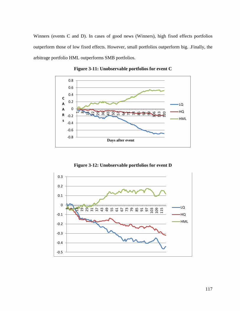
117

Winners (events C and D). In cases of good news (Winners), high fixed effects portfolios

outperform those of low fixed effects. However, small portfolios outperform big. .Finally, the

arbitrage portfolio HML outperforms SMB portfolios.

Figure 3-11: Unobservable portfolios for event C

Figure 3-12: Unobservable portfolios for event D

-0.8

-0.6

-0.4

-0.2

0

0.2

0.4

0.6

0.8 1

8

15

22

29

36

43

50

57

64

71

78

85

92

99

10

6

11

3

12

0

C

A

A

R

s

Days after event

LQ

HQ

HML

-0.5

-0.4

-0.3

-0.2

-0.1

0

0.1

0.2

0.3

1

7

13

19

25

31

37

43

49

55

61

67

73

79

85

91

97

10

3

10

9

11

5 LQ

HQ

HML

118

Figure 3-13: Size portfolios for event C

Figure 3-14: Size portfolios for event D

-0.3

-0.2

-0.1

0

0.1

0.2

0.3

0.4

1

9

17

25

33

41

49

57

65

73

81

89

97

10

5

11

3

C

A

A

R

s

Days after event

Big Size

Small size

SMB

-0.1

-0.05

0

0.05

0.1

0.15

0.2

1

8

15

22

29

36

43

50

57

64

71

78

85

92

99

10

6

11

3

12

0

Big Size

Small size

SMB

119

3.4.12 System GMM dynamic panel data model

Many econometrics problems may arise in the estimation of equation 10. Firstly, firm size

may be endogenous and correlated with residuals. Secondly, the fixed effect model assumes

that errors are correlated with company fixed effects. Thirdly, due to the assumptions of these

models, in order to get estimates of the fixed effects we need to remove all covariates that do

not vary with time or company (Farag and Cressy 2010). Therefore, by definition, time-

invariant variables cannot be included in FE models (i.e. in our case, AR(i0), Private). Finally,

serial correlation and heteroskedasicity may bias the estimation.

In this chapter I initially estimate the Arellano and Bond (1991), Arrellano and Bover (1995)

and Blundell and Bond (1998) two-step Difference GMM estimator to obviate the above

problems. The main assumption of the first step in the estimation is that the errors are

independent and homoskedastic across companies and over time (Beck and Levine 2004). In

the second step, we construct a consistent variance- covariance matrix using the residuals

derived from the first step (Beck and Levine2004).

As linear GMM estimators, the Arellano-Bond and Blundell-Bond estimators have one- and

two-step variants, though the two-step method is asymptotically more efficient, and the

standard errors are less biased (Arellano and Bond 1991; Blundell and Bond 1998).

The general form of the Difference-GMM is (Roodman 2009):

0)()()(

'10

itiiti

itiit

itititit

vEvEE

v

xCARCAR

(16)

120

The disturbance term thus has two orthogonal components, namely, the fixed effects i and

the idiosyncratic shocks itv (Roodman (2009). The GMM estimator uses the first differences to

transform equation 16 into:

itiit

itititit

v

xCARCAR

')1( 1 (17)

Lagged levels are used as instruments for the regression in differences. By transforming the

regressors by first differencing, the fixed company-specific effects are removed as they are –

by definition – time-invariant. However, the new error term 1 itit which is correlated with

the lagged dependent variable 21 itit CARCAR , now represents a source of potential bias

(Beck and Levine2004).

Arellano and Bond (1991) introduce the following moment conditions to deal with this

problem, assuming that the error term is not serially correlated and the independent

variables are uncorrelated with error term.:

TtsforXE

TtsforyE

titisti

titisti

,,.........3;20).(

,,.........3;20).(

1,,,

1,,,

(18)

On the other hand, Blundell and Bond (1998) claim that there are major conceptual and

statistical shortcomings of the first difference GMM i.e. when the explanatory variables are

persistent over time, lagged levels of these variables are weak instruments. This may lead to

biased coefficients especially in case of small samples.

121

To overcome these conceptual and statistical drawbacks, Blundell and Bond (1998) introduce

the system GMM estimator. The new estimator of GMM combines in a system the first

differenced equation with the same equation expressed in levels.

Lagged levels are used as instruments for the regression in differences; however I used the

lagged (three lags) differences of Mcap as instruments in the equation in level. Arellano and

Bover (1995 argue that using additional lagged differences would result in redundant moment

conditions. Therefore Blundell and Bond (1998) propose additional moment conditions for the

regression in levels (the second equation in the system) as in equation 19.

(19)

Thus, I use the moment conditions presented in equations 18 and 19 to overcome the

drawbacks of the first difference GMM and to obtain consistent and efficient parameter

estimates.

The system GMM has main assumptions i.e. fixed individual effects, endogenous regressors,

the idiosyncratic error terms (not fixed effects) are of hetroskedastic and serially correlated,

the idiosyncratic error terms are uncorrelated across companies (groups) and, finally, a smaller

number of time periods (T) compared with the number of groups (N) (small T and large N)

Roodman (2009).

TtsforvXXE

TtsforvyyE

tiististi

tiististi

,,.........3;10)).(

,,.........3,10)).(

,1,,

,1,,

122

To satisfy the assumptions of the system GMM and in order to alleviate the severe serial

correlation identified in CARs for the Egyptian stock price data (Cressy and Farag (2010)), I

chose five-day (weekly) rather than daily returns. This results in 20 pre-event and 24 post-

event observations per firm.

I also include in this analysis a new dummy variable “DumQ” as a proxy for the direction of

firm reaction to the events or companies’ unobservable effects. It is based on the rankings of

fixed effects within the estimation window and takes the value of 1 in the case of positive

unobservable effects and 0 for negative effects.

itiit

itititit

v

tixCARCAR

24,...1;100,...1,'11 (20)

Where ),,,,(' 54321 and )DumQ,Private,Leak,Lnmcap,(' ii0 ititiit ARx

To examine the residuals of the system GMM, I report the Arellano-Bond test, AR (1) and AR

(2), for serial correlation with null hypothesis of “No serial correlation”. We are particularly

interested in AR (2) as the test of AR (1) usually rejects the null hypothesis) (see Roodman,

2009). I also report the Hanson and Sargan tests of exogeniety of instruments and the over-

identifying restrictions in the two-step GMM criterion function. The Null hypothesis of Sargan

and Hanson tests is that “the instruments are exogenious” Therefore the insignificant value of

both tests indicates that the estimation is well specified.

123

I also examine the residuals of the system GMM for a unit root using Levin, Lin–Chu (2002),

as in equation 20. The null hypothesis is then 0:0 iH for all i versus the alternative

0: iaH

p

j

ittiijiittiit yZyy1

1,1, (21)

where ity is the variable being tested; and it is a stationary error term. The itZ term can

represent panel-specific means and a time trend, finally, p is the number of lags. I also use

Harris–Tzavalis (1999), Breitung (2000; Breitung and Das 2005), unit root tests under the null

hypothesis that all the panels contain a unit root.

Table 3.8 presents the outputs for the system GMM model defined of equation 20. The system

GMM results reject the hypothesis that the lagged CAR coefficient is zero. I interpret this as a

rejection of a static model in favour of a dynamic model. Interestingly, and consistent with the

estimation of the two-way fixed effects model, and in contrast with the cross-sectional

regressions, the sign of lnmcap (our proxy for firm size) is positive for both Losers and

Winners.

This suggests concealed company heterogeneity and clearly indicates the bias introduced by

simple OLS estimation involving only one dimension and no fixed effects (Baltagi (2008)).

The size coefficients are highly significant for Losers but insignificant for the Winners. This

may reflect the greater effect of size on the cumulative average abnormal return in cases of

124

negative shocks (the so-called ‘leverage’ effect). However, the leakage of information variable

is positive in sign and highly significant for all the events. This, we believe, reflects the

important role of insider information and thus the existence of significant market inefficiency

in the Egyptian stock exchange.

Table 3.8: System GMM estimates

Losers Winners

Event A Event B Event C Event D

L.Carit 0.0398

***

(0.0083)

0.0338***

(0.0064)

0.0375***

(0.0063)

0.0500***

(0.0038)

Lnmcap 0.0060

***

(0.0016)

0.0075**

(0.0029)

0.0036

(0.0024)

0.0051

(0.0042)

Leak 0.9110

**

(0.3825)

0.9518***

(0.1129)

1.9778***

(0.3992)

1.4372***

(0.0800)

ARio 0.0180

(0.0179)

0.1152***

(0.0362)

-0.1795

(0.0981)

-0.0506

(0.0429)

Private -0.0162

**

(0.0074)

-0.0153***

(0.0038)

-0.0085

(0.0092)

-0.0080***

(0.0032)

DumQ -0.0194

***

(0.0065)

-0.0133***

(0.0044)

-0.0050*

(0.0079)

-0.0046*

(0.0026)

Wald test chi2

111.92***

403.33***

167.24***

213.6***

Arellano Bond test for AR (1) -3.91***

-2.60***

-4.03***

-4.77***

Arellano Bond test for AR (2) -0.93 0.51 1.20 -1.33

Sargan test 2.884 2.012 2.164 5.156*

P value (0.196) (0.146) (0.179) (0.107)

Hansen test 20.14 32.58 12.93 35.36

P value (0.267) (0.341) (0.298) (0.592)

Difference in Hansen Tests

for Exogeniety:

GMM instruments for

levels:

Hansen test excluding group 8.69 23.49 8.46 30.24

Difference 11.45 9.09 4.47 5.12

Instrumental variables

Hansen test excluding group 17.14 29.46 10.35 28.58

Difference 3.00 3.12 2.58 6.79

Levin-Lin- Chu unit root test -9.2090***

-10.699***

-13.432***

-9.4198***

***, **,* indicate significance at the 1%, 5% and 10% levels.

Number of observations is 2400 observations (100 companies * 24 weeks).

125

The coefficients for initial returns on event day are insignificant for Losers and Winners

except for event B. This result is consistent with Cox and Peterson (1994) as including size

removes the effect of initial returns on subsequent price behavior. ARio coefficients are

positive in sign for Losers, however, and interestingly, they are negative for Winners. This

suggests the existence of a leverage effect in the Egyptian stock market.

More importantly, the DumQ variable (our proxy for companies’ unobservable factors) is

negative and highly significant for Winners and Losers. This suggests that low unobservable

effects portfolios outperform high unobservable effects portfolios. It is worth mentioning that

both Losers and Winners Unobservable portfolios significantly outperform the traditional size

portfolios.

This result is new to the literature on price overreaction. Finally, and in contrast with the OLS

regression results, amongst the Losers and Winners formerly private firms have lower CAARs

than formerly state-owned firms. This again may suggest potential bias in the estimation

arising from the absence of the time dimension in the cross-sectional regression.

We also notice that the economic significance of the variables is less than those of the fixed

and random effects estimation presented in table 3.6. However we are interested in the

consistency of the signs across different panel data models rather than the economic

significance to investigate the effect of company heterogeneity on the overreaction hypothesis.

126

We note that the specification tests are satisfactory. The tests regarding serial correlation reject

the absence of first order, but not second order serial correlation, and the Hansen tests do not

reject the over-identifying restrictions. The models are well specified as Wald test statistics are

highly significant.

3.4.13 What are these unobservable factors?

Cressy and Farag (2011) pointed out that the unobservable firm factors might be interpretable

as measures of firm quality. However, they were not able to show evidence to support this

interpretation. To remedy this deficiency in this chapter I shall investigate possible empirical

correlates for these unobserved factors.

To this end I choose Market Value Added (MVA) as a proxy for management quality and

performance. MVA is defined as the management value added and is measured by the

difference between the market value of the company and the value of its capital (equity)

supplied by ordinary shareholders. Based on the model presented in Cressy and Farag (2011),

the sign of the management quality variable is expected to be negative as the higher the firm

quality the lower the company heterogeneity.

The existing body of the literature emphasises the increasing role of corporate governance

(CG) as a means of improving company performance. See for example Millstein and

MacAvoy (1998), Core et al. (1999), Mallin (2001), Brown and Caylor (2004), Core et al.

(2006), Bhagat and Bolton (2008) and Mallin (2010). CG characteristics such as the separation

of the roles of the CEO and Chairman, board independence and various types of committees

127

(e.g. remuneration and audit) are identified in the literature as keys to 'good' governance. But

the main practical question is, does better CG improve company performance? Therefore, the

sign of the corporate governance compliance variable is expected to be negative; this suggests

that the better corporate governance characteristic the lower the firm heterogeneity and lower

overreaction to market shocks.

The Egyptian Corporate Governance code (2003-2006) recommended firms to disclose in

their annual reports whether or not they comply (fully or partially) with the code. There were

few provisions for the Egyptian Corporate Governance code; however they were not

obligatory. During the period of study, some companies have partially complied (none has

fully complied) with the code while the others have not19

. I define the corporate governance

compliance variable as a dummy variable takes the value of 1 for company i if it (fully or

partially) complies with the Egyptian Corporate Governance Code, and is 0 otherwise.

Despite this, there is a debate in the literature about the relationship between corporate

governance and agency cost with some authors arguing that CG improvement increases

agency costs in the company. For example, McKnight and Weir (2009) found that the number

of non-executive directors and duality had little effect on agency cost and Vafeas and

Theodorou (1998), and Weir, Laing, and McKnight (2002) found that the duality (the

separation of the roles of CEO and Chairman) has no effect of company performance. Finally,

McKnight and Weir (2009) using UK data found that the existence of a nomination committee

19

I collected this information from the companies’ annual reports.

128

did in fact increase agency costs (measured by sales to assets ratio). However, greater board

ownership was associated with lower agency costs in the company.

Regarding proxies for agency costs, Ang et al. (2000) and Singh and Davidson (2003) use the

Sales Assets Ratio (SAR) to measure this variable. SAR can be regarded as a measure of

management’s efficiency in using assets to generate sales revenue. Ang et al. (2000) thus

argue that a higher SAR ratio implies lower agency costs as it reflects greater management

efficiency in doing this. Therefore the sign of the agency cost variable is expected to be

positive as the higher the agency cost the higher the company heterogeneity and the higher

overreaction to market shocks.

Finally, I include as an empirical proxy for unobservables the role of political connections of

the company. In Egypt, political connections have an important direct impact on company

performance. I argue that the greater the political connections on the board the better a

company’s performance and the more it is subject to insider information. This suggests a

higher degree of market inefficiency for stocks of companies with political connections, and

greater permanent company-specific effects accordingly. Therefore the sign of this variable is

expected to be positive. I measure political connections by the presence of a Minister, a

Member of Parliament, and by ruling party members on the board of directors.

It is worth mentioning that the existing body of the literature has not investigated the nature of

the fixed effects (unobservable factors). These unobservable may lay the estimation open to

the omitted variable and misspecification biases. One of the contributions of this chapter is to

try to explain what these factors are. Although the political connection of the board members

129

might be observable factor (it may minimise the omitted variable bias), however for some

companies this is unobservable factors to the existing shareholders due to the information

inefficiency and the weak corporate governance practices in the Egyptian stock market. In

addition, none of the existing studies has investigated the effect of the political connection of

the board members on the overreaction phenomenon.

To empirically examine the effect of the above variables on company fixed effects, I carry out

a cross-sectional regression using ordinary least squares (OLS) with the company-specific

effects (fixed effects) as dependent variable and the lagged value of market value added

(MVA), the corporate governance dummy and the political connections (dummy) as in the

following equation. The company fixed effects (company heterogeneity) have been estimated

based on the residuals of equation 10 (the first order autoregressive fixed effects).

iiiiiii SARPolconCGMVAFe 4321 (22)

where: iFe is company fixed (specific) effects,

iMVA is the lagged company market value added measured by the difference between

the market and book value of equity/book value of equity.

iCG is dummy variable takes the value of 1 for company i if it (fully or partially)

complies with the Egyptian Corporate Governance Code, and is 0 otherwise.

iPolcon is dummy variable takes the value of 1 if there is a Minister, Member of

Parliament member, or Ruling Party member on the board of directors, and is 0

otherwise.

iSAR is the lagged sales to assets ratio as a proxy for agency costs.

130

To empirically identify the unobservable factors, table 3.9 presents the outputs of equation 22.

The corporate governance dummy (CG) is negative in sign and highly significant for the

Losers but only marginally significant for Winners. This suggests an inverse relationship

between corporate governance characteristics and the company heterogeneity (fixed effects).

The negative sign may be interpreted as meaning that better corporate governance

characteristic indicates lower firm heterogeneity and lower overreaction to market shocks. The

sustainability in the management policies and company’s strategic objectives are possible

interpretations for this inverse relationship. This in turn reduces the conflict between

shareholders and management.

Management value added (MVA, our proxy of the management quality) is also negatively and

significantly related to permanent differences in the market’s overreaction to news, for all

events (except for event D). This might be explained as meaning that better management

quality is associated with smaller permanent differences in investor reaction to news that

affects its performance. Higher management quality suggests higher efficiency in the firm and

this in turn is reflected in stock price reactions. Therefore, the better the quality of

management the more efficiently is the stock priced and the less permanent investors’

overreaction accordingly. This result is consistent with Cressy and Farag (2011). Sales to

assets ratio SAR (our proxy for agency cost) is positive and insignificant for both Winners and

Losers. This suggests that agency cost has a null effect on company heterogeneity.

131

Table 3.9: Cross Sectional Regressions explaining unobservable factors

Losers Winners

Event A Event B Event C Event D

C 0.0002

(0.0121)

-0.0063

(0.0052)

0.0413***

(0.0069)

0.0912***

(0.0121)

Pol 0.0034**

(0.0014)

0.0048**

(0.0021)

0.0066**

(0.0031)

0.0051

(0.0041)

CG -0.0034**

(0.0015)

-0.0261***

(0.0062)

-0.0191*

(0.0099)

-0.0322*

(0.0181)

MVA -0.0004**

(0.0002)

-0.0008***

(0.0002)

-0.0004*

(0.0002)

-0.0014**

(0.0007)

SAR 0.0036

(0.0032)

0.0003

(0.0003)

0.0002

(0.0004)

0.0001

(0.0006)

R2 0.2112 0.3734 0.2162 0.2144

Adj R2 0.2897 0.3177 0.2465 0.2145

F.stat 3.0112*** 6.7054*** 3.1036*** 3.0706***

White test for heteroskedasticity 0.7414 0.3518 0.5392 0.5148 *, **,*** indicates significance at the 1%, 5% and 10% levels.

Number of observations is 100 observations.

The descriptive statistics for the company heterogeneity (fixed effects) are 0.052%, 7.056%, -

0.015 %, and 0.054% for the mean, maximum, minimum and standard deviation respectively.

The political connection variable is found positive and highly significant for both Winners and

Losers (except for event D). This suggests that the higher degree of political connections the

firm has, the higher the company’s heterogeneity and the less efficiency of its price.

The models are well specified as F statistics are highly significant. The adjusted R squared

range from 21% and 32%. In addition, the residuals seem homoskedastic as the results of

White tests are insignificant. It is worth mentioning that the correlation matrix reports that

there is no potential correlation between the independent variables. I examine the potential

endogeniety between a company’s fixed effect (company heterogeneity) and the independent

variables. The Hausman test cannot reject the null that the regressor is exogenous; therefore

there is no potential endogeniety problem in the estimation, in particular between firm size and

the company’s heterogeneity

132

3.5 Summary and conclusions

Existing empirical studies of stock price reversal have used either cross section or time series

regressions. I argued that this wastes information and may lead to potential biases in the

results. Combining group and time dimensions may therefore result in better estimates of the

coefficients. Such studies also ignore the dynamic aspects of overreaction; namely the

tendency for past abnormal returns to influence future returns. In this chapter I have used

Egyptian stock market data and both traditional and dynamic panel data methods to deal with

these problems. Unobservable factors reflecting heterogeneity in the data emerge

automatically from this estimation process and I have investigated their potential role as

criteria for portfolio formation.

Using daily price data from the Egyptian stock market on a sample of 100 companies which

experienced dramatic one-day price change as the result of four main events over the period

2003 to 2009, I found negative and significant abnormal returns for one of these, namely the

terrorist attacks. These lasted for three days after the event. However, the Lebanon war as a

proxy for the tension in the Middle East region had no effect on the average abnormal returns

in the Egyptian stock exchange. Furthermore, there was no significant average abnormal

return from either the announcement of the constitutional change or the formation of the new

Egyptian government.

The traditional fixed and random effects models showed that – in contrast with the cross-

sectional regressions – the sign of our proxy for firm size (lnmcap)) was positive for both

133

Losers and Winners. This suggested the presence of underlying company heterogeneity in the

data and confirmed our suspicions regarding biases introduced by simple OLS estimation. The

dynamic model estimated using system GMM produced estimates consistent with those of the

two-way fixed effects model and contrasted with those of the cross-sectional regressions. In

particular the sign of the firm size variable) was again positive for both Losers and Winners.

This once more suggests concealed company heterogeneity and indicates biases produced by

estimation using simple OLS. The size coefficients were highly significant for Losers but

insignificant for Winners. This may reflect, in case of negative shocks, the greater effect of

size on the cumulative average abnormal return (the so-called ‘leverage’ effect).

I found also that the leakage of information variable (Leak) was positive in sign and highly

significant for all the events. This, I believe, reflects the important role of insider information

and thus market inefficiency in the Egyptian stock exchange. The coefficients for initial

returns on event day are insignificant for Losers and Winners except for event C. This result is

consistent with Cox and Peterson (1994) as size removes the effect of initial returns on

subsequent price behavior.

More importantly, including the DumQ variable (the proxy for company unobservables) in the

system GMM suggests that low unobservable effects portfolios outperform high unobservable

effects portfolios. Both Losers and Winners Unobservable portfolios significantly

outperformed the traditional size portfolios. This result is new to the literature on price

overreaction.

Interestingly, I found that low fixed effects portfolios for Losers not only outperformed those

of high fixed effects, but also outperformed small and big size portfolios. In addition, the

134

arbitrage portfolio LMH )fixed effects) outperforms SMB portfolios on average. High fixed

effects Winners outperform low fixed effects portfolios on average, however small size

portfolios outperform those of big size on average. This result is new to the literature as I

argue that the portfolio formation based on fixed effects may be used as a new profitable

construction strategy to achieve higher abnormal return than the traditional size portfolios.

To identify the potential unobservable factors, I regressed the company’s fixed effects against

potential unobservable variables i.e. corporate governance compliance, political connections,

agency costs and the management quality. I found a positive and significant relationship

between the political connections of the board members and the company heterogeneity in

addition and interestingly, I found an inverse relationship between both management quality

and corporate governance compliance the company heterogeneity. This suggests that the better

the management quality the lower the company heterogeneity and the more efficiency the

share price.

I conclude that investors can exploit the Egyptian market imperfection and achieve abnormal

returns as the results of major events. Past Losers significantly outperform past Winners post-

events over the event window. In addition, the panel data approach adds a new dimension to

the existing models and offers interesting insights and reveals the importance role of

unobservable firm-specific factors in addition to the observable size in the analysis of the

overreaction phenomenon. Finally, constructing portfolios based on some unobserved factors

i.e. management quality, corporate governance and political connections of board members

significantly outperform traditional portfolios based on size.

135

Chapter 4 : Long-term performance: momentum or overreaction?

4.1 Introduction

The main objective of this chapter is to investigate the long-term overreaction phenomenon for

all listed shares in the Egyptian stock exchange over the period 1998-2009. The chapter also

investigates the role of size, the stability of beta and the seasonality effect on the overreaction

hypothesis in the Egyptian stock market. Finally, I investigate whether the contrarian and the

unobservable (fixed effect) factors are already incorporated in pricesby using the Fama and

French three-factor model and the Carhart (1997) four-factor model.

The main contribution of this chapter is that it is– to the best of my knowledge – the first work

to link the overreaction hypothesis with a change in regulatory policies, namely, the switch

from strict price limits to circuit breakers. In addition, I augment the traditional Fama and

French three-factor model and the Carhart (1997) four-factor model by including a contrarian

factor and an unobservable factor based on company heterogeneity. Finally, this is the first

empirical study of the long-term overreaction phenomenon in the Egyptian stock market – one

of the leading stock exchanges in the Middle East and Mena reign (MENA).

De Bondt and Thaler (1985) using monthly return data investigated the so called long-term

overreaction and found that past Losers significantly outperform past Winners by 24.6% of

positive risk-adjusted abnormal returns in the subsequent period on average. De Bondt and

Thaler (1985) argue that the main cause of this market anomaly is due to the overreaction to

the new information. Huang (1998) argues that in the event of good news stock prices initially

136

overstate the equilibrium prices then price reversals occur in the subsequent periods to move

them back nearer to equilibrium levels. However, in cases of bad news, stock prices initially

understate their equilibrium levels followed by reversals in the later period.

The overreaction hypothesis posits that an extreme movement in stock prices will be followed

by subsequent price reversal (movement in the opposite direction), noting that the bigger the

initial price movement the greater subsequent price reversal that is expected. This is

considered a violation of the Weak Form market efficiency (De Bondt and Thaler 1985).

The existing body of literature argues that the claimed overreaction phenomenon of De Bondt

and Thaler (1985) is mainly due to computation errors in beta between the estimation and the

event window (Chan, 1988), or to the small firm and seasonality effects (January effect)

(Zarowin, 1990).

This chapter is organised as follows: section 2 presents the academic debate about the

measurements of the long-term performance using two competing methods, namely,

cumulative abnormal returns and buy and hold. In section 3, I discuss the alternative sources

of the contrarian and momentum abnormal returns. Section 4 describes the dataset used in the

analysis. Section 5 presents the methodology and the empirical results. Finally, section 6

summarises and concludes.

137

4.2 Empirical literature debate: Long-term performance CARs or BH?

There is a remarkable debate in the existing body of the finance literature regarding the use of

different measures of returns in empirical work. The two main rival candidates are Cumulative

Average Residual returns (CARs) and the Buy and Hold abnormal return (BH). Dissanaike

(1994) argues that the rebalancing method (RB) provides a more accurate measure for excess

returns over CARs. He found that the CAR method underestimated the actual excess returns

36 months after portfolio formation by 28.3%. Dissanaike (1994) also found that the portfolio

performance is sensitive to the method of test and rank period calculations. In this section I

present the pros and cons for each methodology. In addition I highlight the different types of

biases and measurement errors for contrarian and momentum strategies in the empirical

literature.

4.2.1 Cumulative average residual returns CARs

The cumulative average residual return is the most and widely used method in the existing

body of the finance literature. Many researchers used the cumulative average residuals, e.g. De

Bondt and Thaler, (1985), (1987), Chen, (1988), and Alonso and Rubio, (1990). However,

Dissanaike (1994) argues that the arithmetic cumulative average residuals as in equation 1

may result in spurious abnormal returns as the calculated returns are not the same as the actual

returns that investors experience.

T

i

T

i

mt

N

i

itCAR R

N

RR

0 0 (1)

138

Where CAR is the cumulative average residuals, N is the number of shares, T is the number of

time periods. itR and mtR are the monthly (t) stock and market returns respectively for share i.

The more realistic technique for measuring long-term abnormal returns is the rebalancing

method (RB) - which provides more convincing return metric. Within the RB methods

dividends are assumed to be reinvested in a given portfolio using equal weights as in equation

2.

N

i

mt

T

i

N

i

itRB R

N

RR

00 (2)

where N is the total number of securities in the portfolio, T is the total number of months (t) in

the test period. The RB approach assumes that each portfolio is rebalanced on a monthly basis.

This implies equal amounts are assumed to be invested in the individual stocks each month

during the test period. This suggests significant transaction costs may be associated with the

rebalancing method. Blume and Stambaugh (1983) argue that the results from the RB

approach are subject to the bid-ask spread bias due to the existing divergence between the

closing prices observed and the actual prices. This leads returns to be upwardly biased as a

result. However, the bias may be reduced when the BH approach is adopted. In addition, the

RB method could negatively affect the contrarian strategy if only a few stocks were to reverse

and the others do not. In that case the allocation of funds between Losers and Winners may be

diverted away Dissanaike (1994 and 1997).

139

4.2.2 Buy and Hold Abnormal Returns (BHARs)

The BH method assumes that equal investments are invested. There is no monthly rebalancing

process in the BH method as opposed to the RB and CAR methods. In addition, it assumes

that all dividends are reinvested for each stock as in the following equation

N

i

T

t

T

t

mtitBH RRN

R0 0

1

(3)

Conrad and Kaul (1993) argue that in comparison with CARs, the abnormal return of the

contrarian strategy is spuriously exaggerated when calculating long-term performance.

Furthermore, Conrad and Kaul (1993) and Ball et al. (1995) find that underpriced stocks have

greater upward bias. Consequently, if Losers have lower returns than the Winners, there will

be an obvious upward bias to the results and this will generate spurious contrarian profits (see

also Forner and Marhuenda, 2003).

In contrast with the CARs, the BH method involves lower transaction costs and is less tending

to the infrequent trading problems, Dissanaike (1994). Dissanaike (1994) argues that the BH

method is preferred over the RB method when testing the overreaction hypothesis. He claims

that the rebalancing process may affect the contrarian strategy (negatively or positively).

The overreaction hypothesis states that by buying Losers and selling Winners, investors can

achieve abnormal returns as Winners are assumed to be overpriced and Losers are assumed to

be underpriced at the portfolio formation date. The contrarian profits for Loser portfolios are

likely to be much more significant if price reversals do not occur at the same time for

140

individual shares. Therefore investors would sell shares whose prices have increased and buy

shares whose prices have not yet reversed, Dissanaike (1994). This suggests that it would be

more realistic to follow the contrarian strategy without adding the monthly rebalancing effect.

One of the drawbacks of the BH method is that Winners over time carry more weight in the

portfolio than Losers when a particular stock is delisted or dropped out during the test period;

this may lead to a reduction in diversification. According to the assumptions of the BH, all

stocks bought at the beginning of the test period should be held until the end of test period

(e.g. 24 or 36 months) (Gaunt 2000). This is in fact unrealistic assumption of the BHARs and

may bias the estimates of abnormal returns. Gaunt (2000) presents three different alternatives

to overcome this complication. Firstly, to reinvest the proceeds of the delisted stock equally

amongst the remaining stocks. Secondly, to reinvest the proceeds according to the market

capitalisation of the remaining stocks. Thirdly, to invest the proceeds in the market index

(Gaunt 2000).

To conclude, Fama (1998) claims that the RB CARs approach outperforms the Buy and Hold

BH approach as the later implies fewer theoretical and statistical problems than long-term BH.

In addition, Roll (1983) argues that using monthly returns is less likely to be affected by the

choice of CARs or BH. Dissanake (1994) argues that the BH approach may lead to less benefit

from diversification in the longer run. Finally, Loughran and Ritter (1996) claim that there is a

little difference between BH and CARs in test period returns calculations, and they argue that

the results of Conrad and Kaul (1993) are affected by the survivorship bias.

141

4.3 Alternative sources of the contrarian and momentum abnormal returns.

Chan (1988), Lehman (1990), Park (1995), Dissanaike (1997), and Conrad et al. (1997)

concluded that the contrarian or momentum abnormal returns have four main sources, namely,

measurement errors and biases, portfolio construction and evaluation methodology, time-

varying market risk between rank and test windows and, finally, the overreaction to the firm

specific information (Kang et al. 2002). In this section I shed the light on these four alternative

sources of overreaction and momentum abnormal returns.

4.3.1 Biases and measurement errors in contrarian strategies.

Contrarian profits may be spurious due to the bid-ask spread. Stocks may be wrongly

classified as Winners or Losers when bid-ask prices are used in portfolios’ returns calculation.

This leads to magnifying the short-term contrarian profits, Lehmann (1990), Park (1995),

Conrad et al (1997) and Kang et al (2002). The bid-ask spread bias arises when the initial

transaction of selling Winners and/or buying Losers is done at the bid and ask prices

respectively. However, the corresponding transaction is done based on ask and bid prices

respectively Lehmann (1990), Conrad et al (1997) and Kang et al (2002).

A survivorship bias arises when the data base excludes the companies that have ceased to exist

due to liquidation, delisting, and fail to comply with the stock exchange regulations. As the

survivor companies look better and have higher performance (returns) than those that no

longer exist, this leads to overestimation of portfolios’ average return.

142

A data-snooping bias arises when the empirical results of a particular research are driven and

highly influenced by the results of other empirical researches especially if large number of

empirical studies is carried on based on same datasets Conrad et al (1997) and Kang et al

(2002). A data-snooping bias may lead to a data mining bias which is defined as when a

researcher is drilling into the same dataset to reach to a particular result.

A look-ahead bias occurs especially in testing market efficiency when a researcher assumes

that all the relevant information is reflected in the share prices while it is not. For example,

forming portfolios based on June (fiscal year) accounting data, whilst the data will not be

available for investors due to the information lag in financial reports in addition to the lagged

response of the market, Conrad et al (1997) and Kang et al (2002).

Roll (1983), Conrad and Kaul (1993) and Lyon et al. (1999) defined the rebalancing bias as

fixed weights that are commonly used in portfolios’ monthly returns calculations. These

results in both high and low returns as stocks are sold by the end of the formation period and

then the proceeds are reinvested at the original (fixed) weights. However, in the rank period,

high return stocks for instance have increased their weight in the portfolio and the opposite is

correct for low return stocks. The rebalancing bias results in underweighting the previously

high return stocks and overweighting the previously low return stocks in the rank period.

Finally, non-synchronous trading may result in cross correlation between returns on traded

(liquid) and non-traded (illiquid) stocks. This leads to spurious contrarian profits as liquid

shares tend to react contemporaneously to the new information, however, illiquid shares

143

respond to the new information with lag once the next trading occurs. Therefore, portfolio

returns are likely to suffer from lead-lag reaction in addition to serial correlation, Lo and

MacKinlay (1990), Cohen (1979) and Miller et al. (1994).

4.3.2 Portfolio construction and evaluation methodology.

There is a debate about the use of the non-overlapping test periods (three to five years) and

then estimate one overall statistical test on the aggregate data Dissanaike (1997). In fact, using

non-overlapping test periods (3-5) results in unavoidable loss of information. In addition, there

is always the likelihood that the outcome of the contrarian strategy is influenced by economy-

wide cyclical factors, Dissanaike (1997).

Bali and Kothari (1989), Dissanaike (1997) introduce an alternative methodology which

allows overlapping within the formation and test periods. However, the main drawback to this

methodology is the inevitable inter-temporal structure in return distribution as well as in the

betas, Forner and Marhuenda (2003).

4.3.3 Long-term performance with risk and size adjustments.

Chan (1988) argued that there are many critics to the contrarian strategy in the academic

literature. He introduced an alternative interpretation to the contrarian profits. Chan (1988)

argued that the risk of Winners and Losers varies over time between formation and test

periods. Therefore the achieved abnormal return may be due to the approach used in

measuring risk and/or measurement errors in beta estimations during the formation and test

periods of Winners and Losers. Thus the estimation of beta in the formation period will be

144

biased if we used it as a risk factor in the test period. For instance, betas will be

underestimated in the test periods for Loser portfolios as Losers tend to be riskier in the

formation period. Conversely, the betas will be overestimated in the test periods for Winner

portfolios as Winners tend to be less risky in the formation period (Chan, 1988).

On the other hand, the market values of both Winners and Losers vary during the rank period

(small firm effect). De Bondt and Thaler (1985) found significant large variances between the

market capitalisation of Losers (-45%) and Winners (365%), however, they found that the

median of Losers were greater than of those of Winners at the beginning of the rank periods.

Surprisingly, the median of market capitalisation of the Losers became smaller than those of

Winners in the subsequent test periods. This suggests that – if market value is a good proxy for

risk – Losers are safer at the beginning of the rank periods and switch into higher risk class by

the end of the formation period (Chan 1988).

4.3.4 Overreaction to firm-specific information and lead-lag structure.

Lo and MacKinlay (1990) claim that not only the overreaction to firm-specific information is

the main source of contrarian profits but also the lead-lag structure in stock returns. The lead-

lag structure is considered as one of the main sources of contrarian profits, which is related to

the market efficiency as some stocks may react more quickly to the information than others

(Kang et. al 2002). Lo and MacKinlay (1990) found significant and large positive cross-serial

covariance between small stocks and lagged large stocks returns. However, they found weak

cross-serial covariance between large stocks and lagged small stocks returns. They claim that

the main source of short-term contrarian profits is the positive cross-serial covariance (the

145

size-related lead-lag structure) rather than the overreaction to firm-specific information (Kang

et. al 2002).

Contrastingly, Jegadeesh and Titman (1995) claim that the lead-lag structure is not a

fundamental source of momentum profits in the US. However, (Kang et. al 2002) found that

the lead-lag structure is the main source of momentum but not the contrarian profits in the

Chinese stock market.

4.4 Data

I used the EGX30 index, a free floated market capitalisation weighted index (Galariotis (2004)

shows that the selection of a value weighted or an equally weighted index does not alter the

main findings. However, I used the EFG equally weighted index and obtained similar results.

Daily stock returns were adjusted for stock dividends, stock split and dividend yields over the

period January 1998-December 2009 (144 months). The number of stock in the sample ranges

from 180-251 companies according to the number of listed and traded shares in the Egyptian

stock exchange. The main source of data is the Egyptian stock exchange. For each stock to be

included in the sample, I made sure that each stock has continuous trading behaviour during

the formation period and traded at least once during the test period) Forner and Marhuenda

(2003).

The vast majority (84%) of the Egyptian companies have June as the end of their fiscal year.

Therefore all portfolios are formed starting from January to allow all financial information and

146

financial statements to be disseminated and to be reflected on stock prices in addition, to be

available for all investors. This will overcome the look-ahead bias.

I excluded all financial sectors and property investment companies from the sample as the

recorded values of assets in financial sectors’ companies for instance are actually market

rather than book values. In addition, property investment companies usually reevaluate their

book value of assets. Therefore the book to market equity ratio may not have same

interpretation as those of other types. Fama and French (1992) argue that financial sector

companies have higher leverage than those of other sectors; this may lead to higher degree of

financial distress. Twelve financial and property investments firms were excluded from the

initial sample (3% of the total number of firms). The mean values of returns excluding

financial and investment property firms do not change significantly.

I investigate the effect of delisting following De Bondt and Thaler (1985 and 1987) and

Brailsford (1992), so that companies that are delisted or dropped out before the formation date

are not included in the analysis. However, if a firm is delisted or dropped out during the test

period, it is excluded from the analysis and set its last return to minus one in order to minimise

the difference between Losers and Winners portfolios, De Bondt and Thaler (1985 and 1987)

and Brailsford (1992). In the Egyptian stock exchange the number of delisted firms is 11

during the period of study due to failing to comply with the Egyptian stock exchange

regulations or upon the company’s request. Therefore the survivorship bias is highly unlikely

to arise.

147

The portfolio formation process starts from December each year to avoid the so called look-

ahead bias. Therefore there is enough time for the financial statements and reports to be

available to all participants and to be reflected in stock prices. It worth mentioning that all

listed shares in the Egyptian stock exchange are required to publish their annual reports within

90 days of the end of the financial year.

As no other studies in the literature investigated the long-term overreaction phenomenon in the

Egyptian stock market, there is no potential data-snooping or data mining bias (Sullivan et al.

1999, 2001). Finally, and following Lehmann (1990) and Kang et al (2002), I skipped one

trading day between portfolio formation and portfolio holding periods to overcome the bid-ask

spread bias.

4.5 Methodology and empirical results

In this section I present the methodology and the main findings of the empirical models. The

methodology adopted in this chapter is based on identifying non-overlapping 24-month

periods during 1998-2009.

4.5.1 Daily Returns

The monthly return variable tR is defined as the first difference in the natural logarithm of the

closing price over one month. The monthly returns are adjusted for dividends, rights issue,

stock dividends, and stock split.

1 ttt pLogpLogR (4)

where tp is the closing price of the stock in month (t).

148

4.5.2 Security abnormal returns (ARs)

There are three widely used methods to calculate the residual returns in the existing financial

literature, namely, market model, CAPM, and market-adjusted excess returns. The later is a

special case of CAPM with zero and 1 .

Da Costa (1994) found that both CAPM and market-adjusted excess returns have similar

results. Following De Bondt and Thaler (1985, 1987), Brailsford (1992), Da Costa (1994),

Gaunt (2000) and Forner and Marhuenda (2003) I will adopt the market-adjusted excess

returns method.

mtitit RR (5)

where it : is the market-adjusted abnormal return for stock i in month t .

itR : is the monthly return on company i over the period t

mtR : is the return on an value weighted EGX30 index in month t

4.5.3 Cumulative residual return over the rank period (CARs)

All companies are ranked into ascending order based on the cumulative abnormal (CAR)

returns over the rank period. Then top (best performing) and bottom (worst performing)

deciles are identified and selected to form the Winner and the Loser portfolios (Brailsford,

1992) and (Gaunt, 2000).

149

0

24t

iiCU (6)

where iCU : is the cumulative market-adjusted abnormal return for stock i over the period from

24 months prior to the start of the test period.

4.5.4 Cumulative abnormal residual returns over the test period (CARs)

I then compute the cumulative average residual returns for all securities in the Losers and

Winners portfolios for the next 24 months (the test period), they are denoted tzLCAR ,,

and

tzWCAR ,,respectively.

T

t

N

i

titnp NCAR1 1

,,, )/1(

(7)

wheretnpCAR ,, is cumulative average market-adjusted abnormal residual returns for month t

of test period n for Winners and Losers portfolios p and N are the number of stocks in each

portfolio. If a security’s return is missing in a particular month following portfolio formation

then this stock will be dropped permanently from the portfolio and the CAR is calculated as a

mean of remaining residual returns, De Bondt and Thaler (1985). This involves an implicit

rebalancing process (Fama 1998).

The above estimated tnpCAR ,, based on equation (7) assumes implicit monthly rebalancing and

is not actually consistent with the explicit rebalancing strategy RB (Brailsford (1992).

150

Roll (1983) describes equation (7) as the arithmetic method in which returns are aggregated

across all stocks and over time. This involves implicit monthly rebalancing using monthly

equal weights. Although Roll (1983) argues that the empirical research using monthly returns

is less affected by the choice of the returns calculation methodology, Dissanaike (1994) argues

that the arithmetic approach yields unrealistic results as the monthly returns are aggregated not

multiplied.

To clarify the above debate, if the monthly prices for a particular stock were 50, 25 and 40 for

a particular three months respectively, the arithmetic returns yields +10% if the relevant

returns are aggregated while the rebalancing approach (compounding) yields -20%

(Dissanaike 1994). The heterogeneity in these two results may be greater in case of higher

volatility in the return time series (Dissanaike, 1994).

For the above reasons, and following Roll (1983), Dissanaike (1994), Loughran and Ritter

(1996), Fama (1998), I adopt in this chapter the more realistic approach in return calculations,

namely, the rebalancing approach (RB) in which dividends are assumed to be reinvested in the

portfolio using equal weights, as in equation 8:

N

i

mt

T

i

N

i

itTNP R

N

RCAR

00

., (8)

In this equation N is the total number of securities in the portfolio, T is the total number of

months in the test period. The cumulative abnormal return (CAR) during the rank period for

each firm i is then

151

0

24

0

24 i

mt

i

iti RRCAR (9)

This methodology is repeated for each non-overlapping two-year period so that the rank

periods are 1998-1999, 2000-2001, 2002-2003, 2004-2005, and 2006-2007 and the matching

test periods are 2000-2001, 2002-2003, 2004-2005, 2006-2007, and 2008-2009.

Average CARs are calculated for both portfolios and each month between t =1 and t =24 for

all 5 test periods. They are denoted tWACAR , and

tLACAR ,

N

CAR

ACAR

N

z

tnp

tp

1

,,

, (10)

wheretpACAR , is the average CAR across the test periods (N=5) for each Winner and Loser

portfolios p for each month between t =1 and t =24 for all the 5 test periods. It is worth

mentioning that the choice of the formation and test periods is made arbitrarily in the existing

literature. In addition, due to data limitation I use two-year non-overlapping tests and

formation periods. Moreover, and to measure the sensitivity to the formation period length, I

repeated the above methodology using four-year (48 months) non-overlapping formation and

test periods.

4.5.5 Long-term overreaction Hypotheses

The overreaction hypothesis suggests that 0, tWACAR and 0, tLACAR for ( 0t ), this

implies that 0)( ,, tWtL ACARACAR . The contrarian strategy is tested via the following null

hypotheses:

152

0: ,1 tLACARH , 0: ,2 tWACARH , 0)(: ,,3 tWtL ACARACARH , where 24.......1t

To test whether or not the average residual returns is significantly different from zero for

Winners and Losers, I estimate the standard t- test on the means of tWACAR , and

tLACAR , as

follows:

NS

ACARt

p

tp

tp

,

, (11)

1

)(1

2

,,,2

N

ARAR

S

N

n

tptnp

p (12)

wherepS is the sample standard deviation for Losers and Winners portfolio p .

pS is mainly

estimated to test H1 and H2 respectively.

Then I pooled the estimate of the population variance in iCAR to assess whether or not there is

a significant difference in investment performance at any time t

)1(2

)()(1 1

2

,,,:

2

,,,2

N

ACARCARACARCAR

S

N

n

N

n

tLtnLtWtnW

t (13)

where 2

tS is the population standard deviation, and the t-statistic for H3 as in equation 14:

NS

ACARACARt

t

tWtL

tWL

/2 2

,,

,

(14)

153

Table 4.1 presents the results of the cumulative average abnormal returns for the five test

periods over the period 2000-2009. The results presented in table 4.1 show that in two out of

five test periods we can reject the null that the average residual returns are significantly

different from zero.

In addition, Losers outperform Winners as we notice positive and highly significant market-

adjusted abnormal returns for the arbitrage portfolios (Losers – Winners) in 2006-2007 and

2009-2009 respectively. This suggests significant contrarian profit in the Egyptian stock

market starting from 2006. This result is inconsistent with the efficient market hypothesis and

indicates a clear violation of the Weak Form of the Efficient Market Hypothesis. De Long et.al

(1991) argues that the noise trading is the main source of the contrarian profits as irrational

expectations destabilise the stock market.

A closer look at the analysis and the results presented in table 4.1 reveals highly significant

market-adjusted abnormal returns in the test periods 2006-2007 and 2008-2009. This may be

due to the change in regulations from strict symmetric (+ / - 5%) price limit to the circuit

breaker regime. The regulator switched the price limit regime from strict price limits (+/-5) to

wider limits (+/-20%) associated with trading halts for 30 minutes to cool down the market

(Circuit Breakers) in the period 2006 to 2009.

154

Table 4.1: Cumulative average market-adjusted abnormal returns for the five two–year

test periods 2000-2009

Rank Period Test Period Mean CAR

Loser Winner Loser - Winner t- value

1998-99 2000-01 0.2121 0.1439 0.0682 1.5042

2000-01 2002-03 -0.1561 0.0780 -0.2341 -1.7221*

2002-03 2004-05 -0.1211 0.1029 -0.2241 -1.7913*

2004-05 2006-07 0.1637 -0.2459 0.4097 4.2470***

2006-07 2008-09 0.2312 -0.1906 0.4218 4.9838***

The overreaction hypothesis suggests that 0, tWACAR and 0, tLACAR for ( 0t ). This implies

that 0)( ,, tWtL ACARACAR . The contrarian strategy is tested via the following null hypotheses:

0: ,1 tLACARH , 0: ,2 tWACARH , 0)(: ,,3 tWtL ACARACARH , where 24.......1t . To test

whether or not the average residual returns are significantly different from zero for both Winners

and Losers, I use a standard t- test on the means of tWACAR , and

tLACAR ,.

***, **,* indicate significance at the 1%, 5% and 10% levels.

The number of observations varies across time. It ranges from 180-251 companies.

The results presented in table 4.1 suggest that the abnormal return subsequent to 2006 might

be due to the effect of regulatory policies or price limits regime change20

. However, it is clear

from table 4.1 that the overreaction phenomenon is prevailed in the post price-limit period of

the Egyptian stock market.

Table 4.2 presents the average monthly cumulative average abnormal return ACAR over 24

months into the test period. The results presented in table 4.2 show that both Losers and

Winners have significantly reversed after the formation period. We notice that Losers have

reversed starting from the third month of the test period.

20

I investigate this claim in more detail in chapter 5

155

Table 4.2 reports positive and highly significant cumulative average abnormal returns for the

losers over the remaining 22 months of the test period. The longer the test period is, the

greater the average cumulative average market-adjusted abnormal return, and by the 24th

month Losers have achieved a 20% market-adjusted abnormal return.

The Winner portfolios, on the other hand, have also significantly reversed immediately after

the formation period. Nonetheless, table 4.2 shows that by forming the arbitrage portfolio

(selling Winners and buying Losers) we can achieve significant and positive abnormal return

during 3-6 months and 12-24 months after the formation period.

The above results are consistent with the literature on the overreaction phenomenon e.g. De

Bondt and Thaler (1985), Brailsford (1992), Da Costa (1994), Gaunt (2000) and Forner and

Marhuenda (2003).

I thus argue that investors can achieve significant and positive abnormal return by adopting a

contrarian strategy (zero-investment portfolio) in the Egyptian stock market taken over a two-

year investment horizon.

156

Table 4.2: Average monthly cumulative average abnormal return (CAR) over the

24 months of the test period Month into

Test period Loser Winner Loser-Winner ACAR t-stat ACAR t-stat ACAR t-stat

1 -0.0743 -1.9984**

-0.0790 -2.4351**

0.0047 0.0379

2 -0.0262 -0.7046 -0.0577 -1.5789 0.0315 0.2523

3 0.0050 0.1349 -0.0830 -2.5570**

0.0880 0.7038

4 0.0899 2.4178**

-0.0838 -2.5818***

0.1737 1.9189**

5 0.1430 3.8458***

-0.0705 -2.1722**

0.2135 2.7071***

6 0.1591 4.2789***

-0.0572 -1.5610 0.2162 2.7291***

7 0.0906 2.4364**

-0.1009 -3.1085***

0.1915 1.9311*

8 0.0676 1.8173* -0.0489 -1.1765 0.1164 1.3310

9 0.0705 1.8969* -0.0459 -1.1551 0.1664 1.3309

10 0.0545 1.4649 -0.1117 -3.4412***

0.1662 1.3286

11 0.0697 1.5807 -0.0889 -2.7400***

0.1586 1.5081

12 0.0809 2.1747**

-0.1339 -4.1254***

0.2148 2.7173***

13 0.1207 3.2467***

-0.0553 -1.5158 0.1760 2.2266**

14 0.1622 4.3637***

-0.1859 -5.7287***

0.3482 3.7842***

15 0.1929 5.1898***

-0.1868 -5.7548***

0.3797 3.0365***

16 0.1471 3.9564***

-0.2213 -6.8191***

0.3684 3.4461***

17 0.0717 1.9298**

-0.2402 -7.4013***

0.3120 3.1947***

18 0.0379 1.0201 -0.2460 -7.5802***

0.2840 2.2707**

19 0.0546 1.2745 -0.2160 -6.6537***

0.2705 2.4031**

20 0.1860 5.0033***

-0.2036 -6.2738***

0.3896 3.1158***

21 0.2188 5.8853***

-0.1941 -5.9789***

0.4129 3.7014***

22 0.1578 4.2440***

-0.2162 -6.6596***

0.3739 3.0302***

23 0.1798 4.8358***

-0.2035 -5.9684***

0.3832 3.0646***

24 0.2065 5.5547***

-0.2014 -6.2049***

0.4079 4.2618***

***, **,* indicate significance at the 1%, 5% and 10% levels.

The number of observations varies across time. It ranges from 180-251 companies.

Figure 4.1 presents the graphics of these findings. The average cumulative average

market-adjusted abnormal returns, or ACARs, for the Losers, Winners and the arbitrage

(Loser–Winner) portfolio are charted. It is clear from figure 4.1 that the Losers’ portfolio

outperforms the Winners’ and that cumulative average market-adjusted abnormal returns can

be achieved by constructing the zero-investment or arbitrage portfolio of De Bondt and Thaler

(1985).

157

Figure 4-1 Average cumulative average abnormal return over 24 months

4.5.6 Long-term overreaction: the sensitivity to formation period length.

To measure the sensitivity of our results to the formation (rank) period length, I repeated the

same methodology using different formation and test periods, namely, four-year (48 months)

non-overlapping formation and test periods. I calculated the monthly average cumulative

average abnormal returns (ACARs) for two individual test periods, namely, 2002-2005 and

2006-2009.

Table 4.3 presents the average cumulative average market-adjusted abnormal returns for the

two four-year test periods in 2002-2009. The results show positive and highly significant

abnormal returns for the arbitrage portfolio (Losers–Winners) in the post-Limit period (2006-

2009). These results are consistent with results of the ACAR over 24 months of the test period

presented in table 4.1. It suggests also that the overreaction phenomenon is only significant

during the period 2006-2009. Therefore, I conclude that there is no effect of the change in the

formation period length on the results.

-0.3

-0.2

-0.1

0

0.1

0.2

0.3

0.4

0.5

1 2 3 4 5 6 7 8 9 10 11 12 13 14 15 16 17 18 19 20 21 22 23 24

AC

AR

s

Month into test period

ACARitL

ACARitW

ACARL-ACARW

158

Table 4.3: Average cumulative average market-adjusted abnormal returns for two four–year test

periods 2002-2009

Rank Period Test Period Mean CAR

Loser Winner Loser – Winner t- value

1998-01 2002-05 - 0.7579 - 0.8967 0.3387 1.1603

2002-05 2006-09 0.4346 - 0.2403 0.6750 2.8990***

The overreaction hypothesis suggests that 0, tWACAR and 0, tLACAR for ( 0t ), this implies that

0)( ,, tWtL ACARACAR . The contrarian strategy is tested via the following null hypotheses:

0: ,1 tLACARH , 0: ,2 tWACARH , 0)(: ,,3 tWtL ACARACARH , where 48.......1t . To test

whether or not the average residual returns are significantly different from zero for both Winners and

Losers, I use the standard t- teat on the means of tWACAR , and

tLACAR ,.

***, **,* indicate significance at the 1%, 5% and 10% levels.

The number of observations varies across time. It ranges from 180-251 companies.

Figure 4.2 presents the average cumulative average abnormal returns for the Losers, Winners

and the arbitrage (Loser–Winner) portfolio over the 48 months of the test period 2002-2005.

The results are shown graphically in Figure 4.2 where I have defined ACARL, ACARW as the

ACARs for Losers and Winners respectively, and ACARL-W as the ACAR for the arbitrage

portfolio.

It is clear from figure that initially both Losers and Winners continue to be Losers and

Winners continue to be Winners (the momentum effect); however, Winners, and more

dramatically, Losers, reverse near the end of the test period21

. In addition, the arbitrage

portfolio achieves positive abnormal returns after 37 months following the formation period

though never reaching above 20%.

21

It might be argued that this final reversal may reflect other factors uncontrolled for in our model. This criticism

is potentially correct, and is dealt with in Chapter 3 of the thesis where we allow for unobservable firm- and time-

specific fixed effects (in addition to observable variables). We find that these factors do indeed possess

explanatory power for the overreaction phenomenon. However, they do not in any way dispose of it.

159

Figure 4.2 Average cumulative average abnormal returnACARs

for the 48 month period 2002-2005.

Table 4.4 presents the average cumulative average abnormal returns ACAR for the Losers,

Winners and the arbitrage (Loser–Winner) portfolio over 48 months into the test period 2002-

2005. It is clear from table 4.4 that Losers reversed immediately after the formation period for

six months following the formation period. However, losers reversed again and continue to be

losers (momentum behaviour) until the end of the test period (7-48 months).

Winners, on the other hand, reversed starting from the second month following the formation

period up till the end of the test period (except for the period 13-16 months following the

formation period). In addition, the arbitrage portfolio achieves positive (but not significant)

market-adjusted abnormal returns after 37 months following the formation period. I argue that

the overreaction behavior is not detected in the Egyptian stock market during the test period

2002-2006.

-1.4

-1.2

-1

-0.8

-0.6

-0.4

-0.2

0

0.2

0.4

1 3 5 7 9 11 13 15 17 19 21 23 25 27 29 31 33 35 37 39 41 43 45 47

AC

AR

s

Month into test period

ACARL

ACARW

ACARL-W

160

Table 4.4: Average monthly cumulative average abnormal return over the 48 months of

the test period 2002-2005 Month into

Test period

Loser Winner Loser-Winner

ACAR t-stat ACAR t-stat ACAR t-stat 1 0.0303 0.2016 0.0069 0.0393 0.0234 0.0441

2 0.0060 0.0402 -0.0203 -0.1160 0.0143 0.0268

3 0.0017 0.0112 -0.0233 -0.1332 0.0250 0.0470

4 0.0166 0.1102 -0.0153 -0.0871 0.0318 0.0598

5 0.0186 0.1238 -0.0104 -0.0594 0.0290 0.0546

6 0.0277 0.1844 -0.0092 -0.0525 0.0369 0.0694

7 -0.0579 -0.3852 -0.0078 -0.0446 -0.0501 -0.0942

8 -0.0708 -0.4704 -0.0023 -0.0132 -0.0685 -0.1287

9 -0.0960 -0.6382 -0.0096 -0.0546 -0.0864 -0.1625

10 -0.1017 -0.6762 -0.0225 -0.1283 -0.0792 -0.1490

11 -0.1124 -0.7470 -0.0292 -0.1667 -0.0832 -0.1563

12 -0.1400 -0.9307 -0.0286 -0.1634 -0.1113 -0.2093

13 -0.1223 -0.8132 0.0371 0.2118 -0.1594 -0.2997

14 -0.1397 -0.9289 0.0485 0.2769 -0.1882 -0.3539

15 -0.1026 -0.6819 0.0586 0.3344 -0.1612 -0.3029

16 -0.1386 -0.9216 0.0396 0.2261 -0.1782 -0.3350

17 -0.1305 -0.8678 -0.0300 -0.1715 -0.1005 -0.1889

18 -0.1313 -0.8730 -0.0508 -0.2902 -0.0805 -0.1513

19 -0.0793 -0.5273 -0.0154 -0.0879 -0.0639 -0.1201

20 -0.1243 -0.8266 -0.0537 -0.3063 -0.0707 -0.1329

21 -0.1926 -1.2805 -0.1149 -0.6560 -0.0777 -0.1460

22 -0.2614 -1.7376* -0.1694 -0.9666 -0.0920 -0.1729

23 -0.2753 -1.8304* -0.1769 -1.0096 -0.0984 -0.1850

24 -0.3132 -2.0824* -0.2140 -1.2215 -0.0992 -0.1865

25 -0.3838 -2.5513**

-0.2757 -1.5737 -0.1080 -0.2030

26 -0.3686 -2.4509**

-0.2669 -1.5234 -0.1017 -0.1912

27 -0.3350 -2.2271**

-0.2579 -1.4721 -0.0770 -0.1448

28 -0.3083 -2.0496**

-0.2797 -1.5963 -0.0286 -0.0537

29 -0.2755 -1.8320* -0.2620 -1.4954 -0.0135 -0.0254

30 -0.2870 -1.9078**

-0.2734 -1.5603 -0.0136 -0.0255

31 -0.3121 -2.0747**

-0.2867 -1.6365* -0.0253 -0.0476

32 -0.3747 -2.4910**

-0.3143 -1.7939* -0.0603 -0.1134

33 -0.4578 -3.0433***

-0.3730 -2.1287**

-0.0848 -0.1593

34 -0.5209 -3.4632***

-0.4128 -2.3557**

-0.1081 -0.2033

35 -0.4970 -3.3045***

-0.4047 -2.3098**

-0.0923 -0.1735

36 -0.5146 -3.4210***

-0.4373 -2.4956**

-0.0773 -0.1453

37 -0.5672 -3.7712***

-0.5598 -3.1949***

-0.0074 -0.0140

38 -0.4979 -3.3105***

-0.5757 -3.2857***

0.0778 0.1462

39 -0.5269 -3.5029***

-0.5672 -3.2370***

0.0403 0.0758

40 -0.5669 -3.7687***

-0.6040 -3.4470***

0.0371 0.0698

41 -0.6296 -4.1860***

-0.6246 -3.5647***

-0.0050 -0.0095

42 -0.6618 -4.4002***

-0.6524 -3.7233***

-0.0094 -0.0178

43 -0.6362 -4.2300***

-0.6476 -3.6957***

0.0113 0.0213

44 -0.6111 -4.0627***

-0.6277 -3.5821***

0.0166 0.0312

45 -0.5475 -3.6400***

-0.6148 -3.5086***

0.0673 0.1265

46 -0.5405 -3.5932***

-0.6078 -3.4688***

0.0673 0.1266

47 -0.4659 -3.0974***

-0.6138 -3.5032***

0.1479 0.2781

48 -0.3790 -2.5196**

-0.5984 -3.4149***

0.2194 0.4124

***, **,* indicate significance at the 1%, 5% and 10% levels.

The number of observations varies across time. It ranges from 180-251 companies.

161

Figure 4.3 presents the average cumulative average abnormal returns ACAR for the Losers,

Winners and the arbitrage portfolio over 48 months into the test period 2006-2009. It is clear

from figure 4.3 that Losers outperform Winners’ portfolio and cumulative average market-

adjusted abnormal returns can be achieved by constructing the arbitrage portfolio.

Figure 4.3 Average cumulative average abnormal return for 48 months over 2006-2009.

Table 4.5 presents the monthly cumulative average market-adjusted abnormal return ACAR

over 48 months into the test period 2006-2009. It is clear from table 4.5 that Winners have

significantly reversed immediately after the formation period. However, Losers have reversed

starting from the ninth month as we notice positive market–adjusted abnormal returns during

the remaining 40 months of the test period (9-48). This suggests that the overreaction

phenomenon has been detected in the Egyptian stock market over the test period 2006-2009.

-0.6

-0.4

-0.2

0

0.2

0.4

0.6

0.8

1

1 3 5 7 9 11 13 15 17 19 21 23 25 27 29 31 33 35 37 39 41 43 45 47

AC

AR

s

Month into test period

ACARL

ACARW

ACARL-W

162

The arbitrage portfolio earns positive abnormal returns starting from the fifth month after the

formation period, however, highly significant and positive market-adjusted abnormal returns

can be detected starting from month 36 (3 years) as the average cumulative abnormal return on

the arbitrage portfolio is 74%. It is worth mentioning also that by time the arbitrage portfolio

achieves greater market-adjusted abnormal returns. The maximum abnormal returns of 90%

can be achieved 39 months into the test period. This suggests that the long-term investors have

the opportunity to achieve significant and positive abnormal returns by adopting the contrarian

strategy of selling Winners and buying Losers.

To summarise, the above analysis and findings suggest that the overreaction phenomenon in

the Egyptian stock market is not sensitive to the length of the formation period. In addition

and within the two and four non-overlapping formation periods, overreaction phenomenon has

not been detected for the period governed by the strict price limit regime. Results show that

there is no significant market-adjusted abnormal return from the contrarian strategy. Losers

continue to be Losers and Winners are reversed and thus there are no positive and significant

abnormal returns for the arbitrage portfolio during the strict price limit period.

On the other hand, the overreaction phenomenon is clear during the circuit breaker regime

(2006-2009) for both the short (two years) and longer (four years) formation periods. Results

show positive and highly significant market-adjusted abnormal returns for the arbitrage

portfolio. The main interpretation to this is the delayed price discovery hypothesis (Kim and

Rhee, 1997).

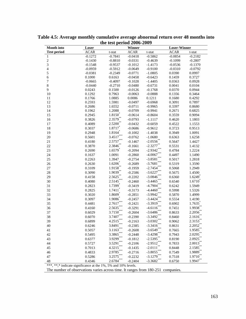
163

Table 4.5: Average monthly cumulative average abnormal return over 48 months into

the test period 2006-2009 Month into

Test period

Loser Winner Loser-Winner

ACAR t-stat ACAR t-stat ACAR t-stat

1 -0.1272 -0.7841 -0.0418 -0.5862 -0.0854 -0.2182

2 -0.1430 -0.8810 -0.0331 -0.4639 -0.1099 -0.2807

3 -0.1548 -0.9537 -0.1012 -1.4173 -0.0536 -0.1370

4 -0.0959 -0.5912 -0.0649 -0.9100 -0.0310 -0.0792

5 -0.0381 -0.2349 -0.0771 -1.0805 0.0390 0.0997

6 0.1000 0.6163 -0.0458 -0.6423 0.1459 0.3727

7 -0.0665 -0.4097 -0.1028 -1.4405 0.0363 0.0928

8 -0.0440 -0.2710 -0.0480 -0.6731 0.0041 0.0104

9 0.0243 0.1500 -0.0126 -0.1768 0.0370 0.0944

10 0.1292 0.7963 -0.0063 -0.0888 0.1356 0.3464

11 0.1766 1.0885 0.0086 0.1211 0.1680 0.4292

12 0.2593 1.5981 -0.0497 -0.6968 0.3091 0.7897

13 0.2686 1.6552 -0.0711 -0.9965 0.3397 0.8680

14 0.1962 1.2088 -0.0709 -0.9941 0.2671 0.6825

15 0.2945 1.8150* -0.0614 -0.8604 0.3559 0.9094

16 0.3826 2.3579**

-0.0793 -1.1117 0.4620 1.1803

17 0.4089 2.5200**

-0.0432 -0.6059 0.4522 1.1553

18 0.3037 1.8717* -0.0686 -0.9612 0.3723 0.9513

19 0.2948 1.8164* -0.1002 -1.4038 0.3949 1.0091

20 0.5601 3.4517***

-0.0762 -1.0680 0.6363 1.6258

21 0.4180 2.5757***

-0.1467 -2.0556**

0.5647 1.4427

22 0.3870 2.3846**

-0.1661 -2.3277**

0.5531 1.4132

23 0.2690 1.6579* -0.2094 -2.9342

*** 0.4784 1.2224

24 0.1637 1.0091 -0.2860 -4.0067***

0.4497 1.1490

25 0.2263 1.3947 -0.2754 -3.8581***

0.5017 1.2818

26 0.2630 1.6206* -0.2689 -3.7681

*** 0.5319 1.3590

27 0.3109 1.9158**

-0.1959 -2.7454***

0.5068 1.2949

28 0.3090 1.9039**

-0.2586 -3.6227***

0.5675 1.4500

29 0.4158 2.5625**

-0.2202 -3.0846***

0.6360 1.6249*

30 0.4080 2.5145***

-0.2460 -3.4465***

0.6540 1.6710*

31 0.2823 1.7399* -0.3419 -4.7904

*** 0.6242 1.5949

32 0.2825 1.7411* -0.3173 -4.4460

*** 0.5998 1.5326

33 0.3020 1.8609* -0.2851 -3.9942

*** 0.5870 1.4999

34 0.3097 1.9086* -0.2457 -3.4424

*** 0.5554 1.4190

35 0.4481 2.7617***

-0.2421 -3.3919***

0.6902 1.7635*

36 0.4160 2.5635***

-0.3291 -4.6116***

0.7451 1.9938**

37 0.6029 3.7150***

-0.2604 -3.6486***

0.8633 2.2056**

38 0.6070 3.7407***

-0.2390 -3.3492***

0.8460 2.1616**

39 0.6899 4.2515***

-0.2163 -3.0302***

0.9062 2.3153**

40 0.6246 3.8491***

-0.2385 -3.3416***

0.8631 2.2052**

41 0.5057 3.1163***

-0.2608 -3.6549***

0.7665 1.9585**

42 0.5495 3.3865***

-0.2448 -3.4298***

0.7943 2.0295**

43 0.6377 3.9299***

-0.1812 -2.5395**

0.8190 2.0925**

44 0.5727 3.5291***

-0.2106 -2.9512***

0.7833 2.0013**

45 0.7013 4.3215***

-0.1435 -2.0111**

0.8448 2.1585**

46 0.4833 2.9785***

-0.2716 -3.8055***

0.7549 1.9889**

47 0.5286 3.2575***

-0.2232 -3.1279***

0.7518 1.9710**

48 0.4346 2.6784***

-0.2404 -3.3682***

0.6750 1.9947**

***, **,* indicate significance at the 1%, 5% and 10% levels.

The number of observations varies across time. It ranges from 180-251 companies.

164

Fama (1989), Lehmann (1989), and Lee, Ready, and Seguin (1994) argued that price limits

interfere with the price discovery mechanism as trading usually ceased (when prices hit the

limit) until the limits were revised. Therefore, at the limit hit day these constraints (limits)

prevent stock prices from reaching their equilibrium levels until the following trading day

(session) (Kim and Rhee, 1997). On the other hand, within the circuit breaker regime (wider

price limits) investors have more time (during the trading halts) to adjust their portfolios. This

may lead to overreactive behavior by some speculative traders due to the lack of informational

efficiency and the noise trading in emerging markets.

The existing body of the literature argues that the reported overreaction phenomenon by De

Bondt and Thaler (1985) is mainly due to computation errors in beta between the estimation

and the event window (Chan, 1988), or due to small firm effect (size effect) and seasonality

effects (January effect) (Zarowin, 1990). In this section of the chapter, I investigate firstly the

role of the size effect and whether or not the overreaction phenomenon is mainly due to small

firm effects. I also investigate the stability of beta within the formation and test periods.

Finally, I present the results of the effects of the seasonality effect on the overreaction

phenomenon.

4.5.7 Long-term overreaction: the sensitivity to size effect.

The above methodology is repeated using Small and Big size portfolios based on the

companies’ market capitalisation to investigate whether or not the overreaction phenomenon

can be explained by the size effect. In December of each year all listed shares (excluding

financial sector and property investment companies) are ranked - based on market

165

capitalisation (firm size) - in an ascending order. This is done over the period 1998-2009 and

for each of the formation and test periods. The median value of firm size is then used to split

the stocks into two main categories, namely, Small and Big (S and B) 22

.

To investigate the size effect on the long-term overreaction, I estimate the average monthly

cumulative average market-adjusted abnormal return over 24 months into the test period for

small and big firms based on market capitalisation.

Table 4.6 presents the results of the monthly cumulative average market-adjusted abnormal

return over 24 months for small firms.

The results presented in table 4.6 shows that price reversal for the Losers occurs starting from

the fourth month until the sixth month and then reverse again and continue to be Losers

(momentum effect) until month 12. However, starting from month 15 until the end of the test

period, Losers earn positive and significant market-adjusted abnormal returns.

The price reversals of the small Winners, on the other hand, occur immediately after the

formation period as we notice highly significant and negative abnormal returns on the first

month of the test period and then starting from the eighth month.

22

Following the literature on price limits, I use market capitalisation as a proxy for firm size as all the firms

included in the sample are listed in the EGX. None of the literature used other measures i.e. total assets due to the

drawback of accounting measures.

166

The results of the arbitrage portfolio report highly significant and positive abnormal returns

starting from month 13; this suggests that the overreaction behavior is prevailing in small

firms’ portfolios.

Table 4.6: Average monthly cumulative average abnormal return over 24 months into the test

period for small firms

Month into

Test period Loser Winner Loser-Winner ACAR t-stat ACAR t-stat ACAR t-stat

1 -0.1096 -3.5021***

-0.0897 -2.1113***

-0.0199 -0.1977

2 -0.0931 -2.9727***

-0.0392 -0.9231 -0.0538 -0.5351

3 -0.0535 -1.7080* -0.0460 -1.0821 -0.0075 -0.0743

4 0.0215 0.6872 -0.0294 -0.6912 0.0509 0.5059

5 0.0186 0.5943 -0.0015 -0.0355 0.0201 0.2000

6 0.0322 1.0296 0.0134 0.3151 0.0188 0.1873

7 -0.0360 -1.1494 -0.0758 -1.7834* 0.0398 0.3959

8 -0.0584 -1.8655**

-0.0892 -2.0991***

0.0308 0.3064

9 -0.0714 -2.2821***

-0.0915 -2.1524***

0.0200 0.1993

10 -0.0823 -2.6279***

-0.1419 -3.3392***

0.0597 0.5932

11 -0.0063 -0.2026 -0.1110 -2.6105***

0.1173 1.1661

12 -0.0138 -0.4396 -0.1588 -3.7367***

0.1451 1.4421

13 0.0039 0.1252 -0.2147 -5.0515***

0.2186 2.1734***

14 0.0480 1.5331 -0.2245 -5.2822***

0.2725 2.7091***

15 0.0953 3.0455***

-0.1994 -4.6926***

0.2948 2.9306***

16 0.0668 2.1352***

-0.2442 -5.7451***

0.3110 3.0920***

17 0.0247 0.7881 -0.2785 -6.5532***

0.2539 2.5237***

18 0.0342 1.0917 -0.2805 -6.6009***

0.3147 2.4494***

19 0.0133 0.4241 -0.2388 -5.6187***

0.2521 2.5061***

20 0.0625 1.9970***

-0.2358 -5.5488***

0.2983 2.9660***

21 0.0951 3.0369***

-0.2091 -4.9193***

0.3041 3.0237***

22 0.0721 2.3049***

-0.2524 -5.9376***

0.3245 3.2262***

23 0.1078 3.4428***

-0.2343 -5.5134***

0.3421 3.4011***

24 0.1582 5.0524***

-0.2652 -6.2406***

0.4234 4.2092***

***, **,* indicate significance at the 1%, 5% and 10% levels.

The number of observations varies across time. It ranges from 180-251 companies.

Figure 4.4 presents the average cumulative average abnormal returns ACARs for the Losers,

Winners and the arbitrage (Loser–Winner) portfolio over 24 months into the test period 2006-

2009 for small firms.

167

Figure 4.4 Average cumulative average abnormal return over 24 months into the test

period 2000-2009 for small firms

It is clear from figure 4.4 that small Losers outperform small Winners’ portfolio and

cumulative average market-adjusted abnormal returns can be achieved by constructing the

arbitrage portfolio. Table 4.7 presents the results of the average monthly cumulative average

abnormal return over 24 months for big firms.

The results presented in table 4.7 show that price reversal for the big Losers occurs

immediately after the second month following the formation period. In addition, highly

significant and negative abnormal returns for the Losers are found in months five and six and

from month 10-16 and finally from month 20-24.

The price reversal for the big Winners occurs immediately after the formation period as we

notice highly significant and negative abnormal returns over the 24 months following the

-0.4

-0.3

-0.2

-0.1

0

0.1

0.2

0.3

0.4

0.5

1 3 5 7 9 11 13 15 17 19 21 23

AC

AR

s

Month into test period

ACARitL

ACARitW

ACARL-ACARW

168

formation period. In addition, the arbitrage portfolio earns highly significant and positive

abnormal returns over the period 11-24 month. It is clear from the table that big Losers

outperform big Winners and investors can achieve abnormal returns by forming the arbitrage

portfolio (Losers–Winners).

Table 4.7: Average monthly cumulative average abnormal return over 24 months into the test

period for big firms Month into

Test period Loser Winner Loser-Winner ACAR t-stat ACAR t-stat ACAR t-stat

1 -0.0115 -0.5541 -0.0591 -2.0687**

0.0476 0.3810

2 0.0148 0.7134 -0.0881 -3.0863***

0.1029 0.8238

3 0.0282 1.3630 -0.1185 -4.1505***

0.1467 1.1747

4 0.0358 1.7283* -0.1414 -4.9529

*** 0.1772 1.4187

5 0.0403 1.9463**

-0.1641 -5.7466***

0.2044 1.6363

6 0.0535 2.5829***

-0.1749 -2.1248**

0.2283 1.8282*

7 0.0040 0.1940 -0.2065 -2.2337***

0.2105 1.6857*

8 -0.0131 -0.6345 -0.2175 -2.6183***

0.2044 1.6363

9 0.0105 0.5049 -0.2593 -3.0822***

0.2698 2.1598**

10 -0.0122 -0.5898 -0.2209 -2.7385***

0.2087 1.6712*

11 0.1004 4.8503***

-0.1846 -2.4645**

0.2850 2.2818**

12 0.0624 3.0131***

-0.2003 -2.0148**

0.2627 2.1030**

13 0.0569 2.7503***

-0.2571 -3.0037***

0.3140 2.5141**

14 0.1035 4.9986***

-0.2390 -3.3696***

0.3425 2.7419***

15 0.1092 5.2747***

-0.2556 -3.9531***

0.3648 2.9210***

16 0.0506 2.4438**

-0.2736 -4.5832***

0.3242 2.5958***

17 0.0192 0.9277 -0.2893 -5.1321***

0.3085 2.4699**

18 0.0117 0.5660 -0.2920 -5.2267***

0.3037 2.4316**

19 0.0159 0.7681 -0.2780 -4.7363***

0.2939 2.3530**

20 0.0660 3.1881***

-0.2579 -4.0345***

0.3240 2.5937***

21 0.1077 5.2021***

-0.2533 -3.8714***

0.3610 2.8903***

22 0.0755 3.6455***

-0.2668 -4.3457***

0.3423 2.7407***

23 0.1247 6.0241***

-0.2564 -3.9822***

0.3812 3.0519***

24 0.1472 7.1108

*** -0.2410 -3.4397

*** 0.3882 3.1080

***

***, **,* indicate significance at the 1%, 5% and 10% levels.

The number of observations varies across time. It ranges from 180-251 companies.

Figure 4.5 presents the average cumulative average abnormal returns ACARs for the Losers,

Winners and the arbitrage (Loser–Winner) portfolio over 24 months into the test period 2006-

2009 for big firms. It is clear from figure 4.5 that big Losers outperform big Winners’

169

portfolio and cumulative average market-adjusted abnormal returns can be achieved by

constructing the arbitrage portfolio.

Figure 4.5 Average cumulative average abnormal return over 24 months into the test

period 2000-2009 for big firms.

To conclude, the findings presented in the above tables and figures show evidence of a

genuine investors’ overreactive behavior in the Egyptian stock market and it is not due to

small firm effect. Losers are found to outperform Winners for big and small firms and

abnormal returns can be achieved by forming the arbitrage portfolios. Therefore contrarian

strategy by buying Losers and selling Winners is likely to be a profitable strategy by the

investors in the Egyptian stock market.

-0.4

-0.3

-0.2

-0.1

0

0.1

0.2

0.3

0.4

0.5

1 3 5 7 9 11 13 15 17 19 21 23

AC

AR

s

Month into test period

ACARitL

ACARitW

ACARL-ACARW

170

4.5.8 Long-term performance with risk adjustment (robustness to time-varying market

risk)

In order to investigate the overreaction/momentum hypothesis, Claire and Thomas (1995) run

the following regression:

ntRRR iiiPWPLPLMW .........1 Overreaction hypothesis (15)

where PLMWR is the difference between the returns on the Loser and Winner portfolios i is

the constant term and it is the white noise error term. The simple t- statistic of i suggests

whether or not there is a significant positive or negative difference in means for the Losers and

Winners. Significant and positive i supports the overreaction hypothesis; however

significant and negative i supports the momentum hypothesis.

In addition, Zarowin (1990) controls for time-varying risk. Therefore to take this into account

I run two additional regressions (after controlling for autocorrelation) as follows:

),()( LWPrrrr itftmtiiftPt (16)

ntrrR itftmtiiPLMW .........1)( (17)

where i is the Jensen performance index, are the CAPM betas as a difference between the

respective market risk of the two portfolios (Winner and Losers) andftr

is the risk free rate

(one month Treasury Bill at the beginning of each month (Zarowin,(1990)) .

Significant and positive i implies the overreaction hypothesis while significant and negative

i suggests the momentum hypothesis.

171

Significant and positive suggests that Losers may embody higher systematic risk than

Winners. In addition, Winners may imply higher degree of systematic risk in case of

significant and negative is found.

To investigate the overreaction hypothesis, and following Zarowin (1990), Claire and Thomas

(1995) and Kang et.al (2002), table 4.8 shows the long-term performance with risk adjustment

(robustness to time-varying market risks) as in equations 16 and 17 (estimated using Ordinary

Least Squares). The results presented in table 4.8 show that the coefficients of systematic risk

are positive in all periods and highly significant in the aggregate period of the arbitrage

portfolio. In addition, the coefficients of beta for the Losers are greater than those of Winners;

this suggests that Losers tend to be riskier than Winners and the difference in returns can be

explained by the differences in the systematic risk.

The positive and significant i of the arbitrage portfolio supports the overreaction hypothesis

in the test periods during the circuit breakers regime (2006-2007 and 2008-2009). However,

the negative i supports the momentum hypothesis during the strict price limit regime (2001-

2002 and 2002-2003).

172

Table 4.8: Long- term performance with risk adjustment (Robustness to time – varying risk) Test Loser Winner Loser - Winner

Period α β F-test ADJ R2 α β F-test ADJ R2 α β F-test ADJ R2

2000-01 0.0049

(0.0092)

0.3626***

(0.1131) 10.277*** 0.0190

-0.0210***

(0.0079)

0.3461***

(0.0979) 12.509*** 0.0235

-0.0259

(0.0218) 0.0165

(0.1459) 0.0128 0.0021

2002–03 0.0115

(0.0106)

0.3807**

(0.1584) 5.781** 0.0099

-0.0012

(0.0072)

0.2799***

(0.1069) 6.8557*** 0.0121

-0.0128

(0.0125)

0.1009

(0.1866) 0.2922 0.0015

2004–05 0.0190*

(0.0109)

0.6062***

(0.0967) 39.278*** 0.0740

-0.0135*

(0.0072)

0.4141***

(0.0643) 41.423*** 0.0778

0.0325

(0.0224)

0.1921*

(0.1106) 3.0171* 0.0042

2006-07 0.0210**

(0.0088)

0.4826***

(0.0916) 17.460*** 0.0332

-0.0086

(0.0058)

0.2572***

(0.0604) 21.64*** 0.2952

0.0296***

(0.0102)

0.2254***

(0.0964) 19.911*** 0.0380

2008-09 0.0079

(0.0087)

0.8156***

(0.0626) 19.68*** 0.2604

-0.0036

(0.0064)

0.5169***

(0.0462) 23.79*** 0.4506

0.0115***

(0.0006)

0.2987***

(0.0764) 1.7550 0.0016

Aggregate 0.0055

(0.0039)

0.6197***

(0.0379) 26.70*** 0.0997

-0.0068**

(0.0028)

0.5004***

(0.0274) 25.16*** 0.2143

0.0123***

(0.0048)

0.1193***

(0.0471) 28.24*** 0.0830

To control for risk I run these additional regression models (after controlling for auto correlation) following Zarowin (1990), Claire and Thomas (1995) and Kang

et.al (2002),

).()( LWPrrrr itftmtiiftPt

ntrrR itftmtiiPLMW .........1)(

where PLMWR is the difference between the returns on the Loser and Winner portfolios i (the constant term) is the Jensen performance index, are the

CAPM betas as a difference between the respective market risk of the two portfolios (Winner and Losers), ftr is the risk free rate (one month Treasury Bill at the

beginning of each month and it is the white noise error term. Significant positive i confirms the overreaction hypothesis while significant negative

i

confirms the momentum hypothesis. ***, **,* indicate significance at the 1%, 5% and 10% levels.

The number of observations varies across time. It ranges from 180-251 companies.

173

4.5.9 The variation of risk performance between rank and test periods

Brailsford (1992) argues that risk adjusted returns are biased due to the bias in the market-

adjusted model parameters estimated in the rank period. Following Chan (1988), and Gaunt,

(2000), abnormal returns can be tested by examining the value of in the following Sharp –

Linter CAPM equation:

itftmtiiftit rrrr )( (18)

Where the value weighed EGX30 market index is the market portfolio mtr . I initially estimate

equation 18 over the test period in which beta is assumed to be constant. The null hypothesis is

0i this suggests that asset (i) has no abnormal return. This implies that size effect is

ignored in the above equation. However, at the beginning of the test period Loser stocks are

usually smaller in size than Winners – if the size effect if significant – this suggests that our

null hypothesis is biased by the size effect (Chan 1988). I then estimate the betas and the

abnormal returns simultaneously in the test period.

To examine risk performance and whether or not betas are stable over the rank period and test

periods, I modify equation 18 following Chan (1988) for the Losers, Winners and the arbitrage

portfolio (Losers –Winners) as follows:

ittftmtiDftmtititiftit DrrrrDDrr )()()1( 21 (19)

where t= 1 to 48 months, itr is continuously compounded return on portfolio i at time t, mtr is

the return on an value weighted EGX30 index in month t , ftr is the risk-free rate. Importantly,

tD is a dummy variable equal to zero in the rank period (t< 25) and is equal to one in the test

174

period (t > 24). it is assumed to be normally distributed with two variances 2

1i and 2

2i for

the rank and test periods respectively. Chan (1988) argues that there should not be significant

difference in ’s between equation 18 and 19 in the rank and test periods separately.

The outcomes of the above regression allow us to estimate different ii and for the rank

and test periods. i1 and i2 are the average abnormal returns for the rank and test periods

respectively, however, i and )ˆˆ( iDi are the estimated betas for the rank and test periods

respectively. If iD is not significantly different from zero, then betas are assumed to be

constant throughout the rank and test periods.

Finally, I run the aggregate t test statistics for the entire period (1998-2009) under the null

hypothesis and using the Central Limit theorem (Chan 1988). The test statistics is given as

follows:

)1,0()1/()3(1

1

NTTtN

UN

i

iii

(20)

Table 4.9 presents the findings of testing the existence of the abnormal returns and the

Stability of risk factor (beta) throughout rank and test periods. The results presented in table

4.9 show that the abnormal return during the rank periods i1 is negative for Losers for all

rank periods and highly significant for the aggregate period. However, the average abnormal

return for the Winners is positive for all the rank periods and highly significant in the

aggregate period. The abnormal return for the arbitrage portfolio (Losers-Winners (LMW)) is

negative and highly significant in all rank periods in addition to the aggregate rank period.

175

Price reversal behaviour can be detected as the abnormal return coefficient i2 is positive for

the Losers and negative for the Winners in all test periods. In addition, the arbitrage portfolio

(LMW) supports the overreaction behaviour as we notice a change in the sign of i2 from

negative in the rank period to positive in the test period. Moreover, highly significant

abnormal return is detected in the aggregate test period.

Table 4.9 also shows that test period betas iDi for the Losers are greater than those of

rank periods i except for the following test periods: 2000–2001 and 2002-2003. In addition,

the aggregate beta for the test period for Loser portfolios is highly significant and outperforms

beta in the rank period. This suggests that Losers are more risky during the test period. This

result is consistent with Chan (1988). Chan argues that the risk of Loser portfolios is higher

during the test period and moreover, Losers are on average bigger in size than those of

Winners.

Betas of the Winner portfolios in the rank periods significantly exceed those of test periods

(except for the 2008- 2009 test period). The coefficient of iD (the change in beta from rank to

test period) is negative and highly significant in the aggregate test period for the winners. We

also notice that betas of the Losers are greater than those of Winners in the aggregate test

period; iD is positive and highly significant. This suggests that beta is not constant over time

throughout the rank and the test periods. These results are consistent with Chan (1988) and

Gaunt (2000).

176

Table 4.9: Abnormal returns and the Stability of risk throughout rank and test periods

Rank Test Loser Winner Loser - Winner Period Period

i1 i2 i iD i1 i2 i iD i1 i2 i iD

1998-

1999

2000-

2001

-0.0823***

(0.0122)

0.0049

(0.0146)

0.4445***

(0.1202)

-0.1901

(0.2168)

0.0031

(0.0057)

-0.0210***

(0.0068) 0.4110***

(0.0591) -0.0649

(0.1029) -0.0854***

(0.0133) 0.0259

(0.0160) 0.0335

(0.1383) -0.1252

(0.2409) 2000-

2001

2002-

2003

-0.0148

(0.0120)

0.0115

(0.0092)

0.5948***

(0.1493)

-0.2140

(0.2033)

0.0168*

(0.0089)

-0.0012

(0.0070)

0.4594***

(0.1128)

-0.1795

(0.1535)

-0.0316**

(0.0143)

0.0128

(0.0112)

0.1345

(0.1815)

-0.0345

(0.2470)

2002–

2003

2004-

2005

-0.0292**

(0.0119)

0.0190

(0.0140)

0.1818

(0.1817)

0.4244*

(0.2202)

0.0205***

(0.0061)

-0.0135*

(0.0071)

0.6182***

(0.0932)

-0.2041*

(0.1129)

-0.0498***

(0.0133)

0.0325***

(0.0155)

-0.4363**

(0.2023)

0.6285**

(0.2451)

2004–

2005

2006-

2007

- 0.0029

(0.0103)

0.0210***

(0.0080)

0.4113***

(0.0935)

0.0287

(0.1249)

0.0322***

(0.0087)

-0.0086

(0.0068)

0.5673***

(0.0808)

-0.2899***

(0.1075)

-0.0351**

(0.0129)

0.0296***

(0.0100)

-0.1560

(0.1174)

-0.3186**

(0.1569)

2006-

2007

2008-

2009

-0.0084

(0.0076)

0.0086

(0.0074)

0.5988***

(0.0690)

0.2405***

(0.0807)

0.0087

(0.0067)

-0.0036

(0.0065)

0.8078***

(0.0771)

0.1091

(0.0904)

-0.0171*

(0.0099)

0.0123

(0.0097)

-0.2090**

(0.1150)

0.1314

(0.1347)

Aggregate -0.0302***

(0.0044)

0.0054

(0.0042)

0.4911***

(0.0458)

0.1324**

(0.0603)

0.0176***

(0.0029)

-0.0068**

(0.0027)

0.4103***

(0.0328)

-0.1013**

(0.0426)

-0.0478***

(0.0051)

0.0123**

(0.0049)

-0.0808***

(0.0585)

0.2337***

(0.0460)

Table 8 presents the results of Chan’s (1988) model estimated using ordinary least squares. ittftmtiDftmtititiftit DrrrrDDrr )()()1( 21

where t= 1 to 48 months, itr is continuously compounded return on portfolio I at time t, mtr is the return on an value weighted EGX30 index in month t , ftr is the

risk- free rate , tD is a dummy variable equal to zero in the rank period (t<25) and is equal to one in the test period (t >24). it is assumed to be normally distributed

with two variances 2

1i and 2

2i for the rank and test periods respectively. ***, **,* indicate significance at the 1%, 5% and 10% levels.

The number of observations varies across time. It ranges from 180-251 companies.

177

4.5.10 Long-term overreaction with adjustment for the seasonality effect.

The existing body of the literature documented that the overreaction phenomenon is highly

likely to occur in January (the January Effect). See for example, De Bondt and Thaler (1985,

1987), Zarowin (1990), and Clare and Thomas (1995).

In this section I investigate the seasonality effect in the Egyptian stock exchange by regressing

the average monthly abnormal returns for the Losers, Winners and the arbitrage portfolio

(Losers–Winners) on a set of dummy variables which take the value of one in the respective

month and zero otherwise. I exclude the intercept to avoid the dummy variable trap., t is a

stochastic IID error term as in the following regression.

itDectMartFebtJantitLMW MMMMAR 12321 ............ (21)

In addition I use the Cochrane-Orcutt two-step iterative technique to overcome the potential

autocorrelation in equation 21. In the first step I estimate the following regression based on the

residuals of the equation 21, i.e. tt 1ˆˆ . Then in the second step I run the Cochrane-

Orcutt method using the following generalized least squares (GLS) equation. This equation is

repeated in cases of higher order of autocorrelation.

)ˆ()ˆ()ˆ1(ˆ11101 tttttt XXyy (22)

178

Table 4.10 presents the findings of long-term overreaction with adjustment to seasonality

effect. The findings presented in table 4.10 show evidence of the January effect in the

arbitrage portfolio, as we notice positive and highly significant abnormal returns in January,

whereas December reports negative and highly significant abnormal returns for the contrarian

portfolio.

This result is consistent with the literature on the calendar effect and the tax–loss hypothesis as

investors tend to sell Losers by the end of December to increase the capital losses and to

reduce the tax burden at the end of the financial year followed by buying Winners in January.

We also notice significant and positive abnormal returns in July as the vast majority of the

listed companies in the Egyptian stock exchange have June as end of their financial year.

We notice positive and marginal significant abnormal returns in June (the end of financial

year). This suggests that the significant abnormal return resulting from the overreaction

phenomenon in the Egyptian stock market is not primarily due to the seasonality effect.

179

Table 4.10: Long–term overreaction with adjustment to seasonality effect

Test Period Jan Feb March April May June July Aug Sept Oct Nov Dec ADJ

R2

DW

Aggregate

Loser 0.0038

(0.0132)

0.0600***

(0.0132)

0.0014

(0.0132)

0.0138

(0.0132)

-0.0219*

(0.0132)

0.0171

(0.0132)

-0.0163

(0.0132)

0.0253**

(0.0132)

0.0024

(0.0132)

-0.0469***

(0.0132)

0.0125

(0.0132)

-0.0027

(0.0132)

0.014 2.14

Winner -0.0120

(0.0105)

-0.0290*

(0.0148)

0.0691***

(0.0148)

-0.0063

(0.0148)

0.0138

(0.0148)

-0.0159

(0.0148)

0.0310**

(0.0148)

0.0161

(0.0148)

0.0142

(0.0148)

0.0096

(0.0148)

-0.0211

(0.0148)

0.0192

(0.0148)

0.024 2.14

Loser-Winner 0.0394***

(0.0177)

0.0231

(0.0250)

0.0665***

(0.0250)

0.0726***

(0.0250)

0.0184

(0.0250)

0.0435*

(0.0250)

0.0629**

(0.0250)

0.0083

(0.0250)

0.0292

(0.0250)

0.0142

(0.0250)

0.0284

(0.0250)

-0.0730***

(0.0250)

0.005 1.92

The table included the outputs of the equation 21 estimated using ordinary least squares. DecJan MM .... are set of dummy variables which take the value of one

in the respective month and zero otherwise. I excluded the intercept to avoid the dummy variable trap, t is a stochastic IID error term as in the following

regression.

itDectMartFebtJantitLMW MMMMAR 12321 ............

***, **,* indicate significance at the 1%, 5% and 10% levels.

The number of observations varies across time. It ranges from 180-251 companies.

180

4.5.11 Is the contrarian factor priced? The Fama and French three-factor model.

In this section I investigate whether or not the overreaction factor is priced in the Egyptian

stock market. Initially I estimate the traditional Fama and French three-factor model. I expect

that Fama French three-factor model provides better explanation in risk-return relationship in

the Egyptian stock market. Fama and French’s three-factor model not only overcomes the

major drawbacks of CAPM (a one –factor model) but it also does well in explaining the risk-

return relationship in emerging markets. Cheung et al. (1993) found a weak risk-return

relationship in both Korean and Taiwanese stock exchanges using the CAPM whilst, Huang

(1998) found a negative risk–return relationship in the Taiwanese stock exchange.

ittititiiftit HMLhSMBsMKTrr (23)

Following Fama and French (1993) the dependent variable in equations 23 is the excess

returns (monthly returns minus the one month Treasury bill rate of return). ir is the return on

asset (i), fr is the risk- free return, i is the abnormal returns that cannot be explained by the

factors in the models, MKT is the value-weighted average market return (ftmt rr ) as in

CAPM; mr is the return on the market portfolio, i is the systematic risk of asset (i) relative to

the market portfolio beta 2/),( Mmii rrCov and 2

M is the variance of market portfolio.

SMB is the difference between the return on a portfolio of small stocks and the return on a

portfolio of big stocks. HML is the difference between the return on a portfolio of high book-

181

to-market stocks and the return on a portfolio of low book-to-market stocks. i is the

sensitivity of the asset returns to market portfolio, is is the sensitivity of the asset returns to

return of SMB, ih is the sensitivity of the asset returns to return of HML.

Considering now the mechanics of the estimation, in December of each year all listed shares

(excluding financial sector and property investment companies) are ranked - based on market

capitalisation (firm size) - in an ascending order over the period 1998-2009. The median value

of firm size is then used to split the stocks into two main categories, namely, Small and Big

size (S and B). All the listed firms are grouped into three main categories - based on book to

market equity BE/ME - namely, Low BE/ME (bottom 30%), Medium BE/ME (middle 40%)

and High BE/ME (high 30%).

Following Fama and French (1993), the book value of common equity = book value of

shareholders’ equity + deferred tax (balance sheet) + investment tax credit – book value of

preferred stock.

Fama and French (1992b) arbitrarily grouped firm size and BE/ME into two and three

categories as they found that BE/ME plays a much more important role in explaining the

variation in stock returns. In addition they argued that there is no reason for the test results to

vary according to these grouping choices.

182

Based on the intersection of the above two classifications (two size portfolios and three

BE/ME portfolios), I construct six different portfolios namely, (S/L, S/M, S/H, B/L, B/M and

B/H).

I match the BE/ME ratio for firms with fiscal year ending in June t-1 with monthly stock

returns from January of year t to December of year t+1 (Fama and French 1993). I exclude all

negative equity book values. BE/ME is then book common equity for the fiscal year ending in

June t-1 divided by market equity at the end of December of t-1 (Fama and French 1993). (For

example, the B/H portfolio contains the stocks in the Big size group and the High -BE/ME

group as well.)

I calculate the monthly-weighted average returns on the six portfolios from January of year t

to December of year t and the portfolios are reformed in January of the year t+1.

SMB portfolio returns are the monthly differences between the simple average of the returns

on the three small size portfolios, namely, (S/L, S/M and S/H), and the big size portfolios,

namely, (B/S, B/M and B/H).

)]///()///[(3/1 HBMBLBHSMSLSSMB (24)

While the HML portfolios are the monthly difference between the simple average of the

returns on the two high- BE/ME portfolios, namely, S/H and B/H and the two low- BE/ME

portfolios, namely, S/L and B/L.

)]//()//[(2/1 LBLSHBHSHML (25)

183

4.5.12 Augmented Fama and French and Carhart models.

Carhart (1997) augmented Fama and French three-factor model by adding a momentum factor.

The main intuition of Carhart’s model is to investigate whether the momentum factor is priced

or not. Carhart‘s model is known in the financial literature as the Carhart four-factor model. In

this section I augment further the Carhart (1997) four-factor model by including two

additional variables, namely, LMW and HMLFE representing loser minus winner and high

minus low fixed effects respectively. I include both LMW and HMLFE to examine whether or

not the overreaction factor as well as the unobservable factors have been priced into returns.

The model is then written:

itititititiiftit HMLFELMWHMLhSMBsMKTrr

(26)

In a well specified asset pricing model i should not be statistically different from zero.

Therefore i is considered a simple excess-return measure. In the Fama and French three-

factor model, the market factor, in addition to size and book-to-market equity factors, seems to

explain better variations in stock returns. Equation on 26 then, provides an augmented Fama

and French three-factor model by including an overreaction/momentum factor as well as the

difference between low and high fixed effects portfolios. The main objective of including

theses two additional factors is to examine whether or not the overreaction/momentum and/or

other unobservable factors are already priced in to returns.

In terms of the mechanics of estimation, LMW is constructed as the difference between the

returns on the Losers portfolio and the returns on the Winners portfolio for a given time

184

period. To construct contrarian (overreaction) portfolios, six value-weighted portfolios are

formed as follows; in December of each year all listed shares (excluding financial sector and

property investment companies) are ranked - based on market capitalisation (firm size) - in an

ascending order over the period 1998-2009. The median value of firm size is then used to split

the stocks into two main categories, namely, Small(S) and Big (B).

All listed firms are grouped into three main categories based on cumulative abnormal return in

year t-1, namely, Low CARs (bottom 30%), Medium CARs (middle 40%) and High CARs

(high 30%). Based on the intersection of the above two classifications (two size portfolios and

three CARs portfolios), I construct six different portfolios, namely, (S/LCARs, S/MCARs,

S/HCARs, B/LCARs, B/MCARS and B/HCARs).

LMW portfolios are the monthly difference between the simple average of the returns on the

two low CARs portfolios (Losers), namely, (LCARs/S, LCARs/B) and the two high CARs

portfolios (Winners) namely; (HCARs/S, HCARs/B).

)//()//(2/1 BHCARsSHCARsBLCARsSLCARsLMW (27)

To construct the unobservable (fixed effects) portfolios I estimated equation 23 for all

formation and the aggregate windows using panel data model. To construct the six

unobservable value-weighted portfolios, in December of each year all listed shares (excluding

financial sector and property investment companies) are ranked - based on market

185

capitalisation (firm size) - in an ascending order over the period 1998-2009. The median value

of firm size is then used to split the stocks into two main categories, namely, Small and Big

size (S and B).

All the listed firms are then grouped into three main categories based on company fixed

effects in year t-1, namely, Low FEs (bottom 30%), Medium FEs (middle 40%) and High FEs

(high 30%). Based on the intersection of the above two classifications (two size portfolios and

three FEs portfolios), I construct six different portfolios, namely, (S/LFEs, S/MFEs, S/HFEs,

B/LFEs, B/MFEs and B/HFEs).

HMLFE portfolios are the monthly difference between the simple average of the returns on the

two high FEs (unobservable) portfolios namely (HFEs/S, HFEs/B) and the low FEs portfolios

(Winners), namely, (LFEs/S, LFEs/B).

)//()//(2/1 BLFEsSLFEsBHFEsSHFEsHMLFE (28)

Table 4.11 reports the Fama and French three-factor model and the augmented versions four

and five-factor models over the period 2000-2009. The results show that the model is well

specified as we cannot reject the null that all i ’s are insignificantly different from zero for all

the models and for both Losers and Winners. Therefore the Fama and French three-factor

model and the augmented models do well in explaining the returns on Losers, Winners and

aggregate portfolios. MKT, HML LMW, and HMLFE are highly significant at 1% and 5% for

186

the Winners and Losers. The MKT factor dominates all the other factors in the model and

explains much of the variation in the portfolio returns.

HML loadings are positive in sign for the Losers and negative for the Winners; this implies

that HML is positively correlated with the return on Loser portfolios and negatively correlated

with the return on Winners. This suggests that value stocks (high book-to-market ratio)

outperform growth stocks (low book-to-market ratio) for the Losers and the opposite is correct

for the Winners.

The contrarian factor LMW on the other hand is positive for the Losers and negative for the

Winners. This supports the previous results as Losers outperform Winners. Interestingly,

HMLFE (High minus Low fixed effects) is negative in sign for both Winners and Losers; this

suggests that lower fixed effects portfolios are not only positively correlated with the

portfolios return but also outperform higher fixed effects portfolios. This result is consistent

with main findings of the system GMM of chapter 3. The loadings of SMB are insignificant

and quite small compared with other loadings; this suggests that size effect has a minor role in

explaining portfolio returns in the Egyptian stock exchange.

187

Table 4.11: The Fama and French three-factor model and the augmented model for returns over the period 2000-2009

Loser Winner Aggregate

Model 1 Model 2 Model 3 Model 1 Model 2 Model 3 Model 1 Model 2 Model 3

C -0.0002

(0.0071)

-0.0041

(0.0046)

-0.0050

(0.0050)

-0.0070

(0.0048)

-0.0053

(0.0044)

-0.0066

(0.0050)

-0.0003

(0.0041)

-0.0021

(0.0037)

-0.0028

(0.0050)

HML 0.2661**

(0.1325)

0.2922***

(0.1089)

0.1907**

(0.0992)

-0.1282**

(0.0673)

-0.1577***

(0.0540)

-0.1866**

(0.0742)

0.1751**

(0.0844)

0.2188**

(0.1098)

0.1907**

(0.0911)

SMB 0.0415

(0.1222)

-0.0080

(0.0728)

-0.0179

(0.0750)

0.0598

(0.0597)

0.0705

(0.0550)

0.0796

(0.0575)

0.0229

(0.0736)

0.0009

(0.0674)

0.0011

(0.0677)

MKT 0.6829***

(0.0694)

0.7842***

(0.0435)

0.7800***

(0.0443)

0.8157***

(0.0482)

0.7898***

(0.0447)

0.7994***

(0.0481)

0.6439***

(0.0397)

0.6676***

(0.0366)

0.6668***

(0.0370)

LMW --- 0.7825***

(0.0541)

0.7795***

(0.0544)

--- -0.2553***

(0.0548)

-0.2588***

(0.0553)

--- 0.2261***

(0.0465)

0.2236***

(0.0486)

HMLFE --- --- -0.2146***

(0.0284)

--- --- -0.1744***

-(0.0258)

--- --- -0.2506***

(0.0547)

ADJ R2 0.4672 0.8053 0.8040 0.7217 0.7639 0.7625 0.6953 0.7451 0.7429

F.TEST 33.092***

98.597***

81.671***

103.86***

97.265***

77.410***

91.510***

87.940***

69.770***

The table presents the outputs of augmented Fama and French three- factor and the Carhart four- factor models as in equation 26

itititititiiftit HMLFELMWHMLhSMBsMKTrr

SMB is the difference between the return on a portfolio of small stocks and the return on a portfolio of big stocks. HML is the difference between

the return on a portfolio of high book-to-market stocks and the return on a portfolio of low book-to-market stocks. i is the sensitivity of the

asset returns to market portfolio, is is the sensitivity of the asset returns to return of SMB, ih is the sensitivity of the asset returns to return of

HML. LMW is constructed as the difference between the returns on the Losers portfolio and the returns on the Winners portfolio for a given time

period. HMLFE portfolios are the monthly difference between the simple average of the returns on the two high FEs (unobservable) portfolios

and the low FEs portfolios (Winners). ***, **,* indicate significance at the 1%, 5% and 10% levels.

The number of observations varies across time. It ranges from 180-251 companies.

188

Finally, all the models are well specified as F statistics are highly significant and the

adjusted R squared range from 46%-80% for the Losers and from 69% to 76% for the

Winners. I concluded that both the contrarian factor (LMW) and the fixed effects factor

(HMLFE) are priced in the augmented 4 and 5 - factor models. This result is new to the

literature on overreaction phenomenon.

4.6 Summary and conclusion

The main objective of this chapter has been to examine the long-term overreaction for all

listed shares in the Egyptian Stock exchange over the period 1998-2009. In addition, I have

investigated the validity of competing hypotheses to explain the phenomenon observed.

These include the so-called size effect, the effects of time-varying risk, the stability of beta

over the rank and test periods and the seasonality (calendar effect), Huang (1998). Finally,

I investigate whether the contrarian and the unobservable (fixed effect) factors are priced

in to returns by augmenting the Fama and French three-factor model and the Carhart

(1997) four-factor model to include the contrarian and fixed effects factors.

The chapter has also helped to resolve the academic debate over alternative measures of

long-term stock performance. The debate concerns the relative merits of cumulative

abnormal returns (CARs) over the rebalancing method (RB) and buy and hold returns

(BAHARs). Following Roll (1983), Dissanaike (1994), Loughran and Ritter (1996), and

Fama (1998), in this chapter I adopted the more realistic approach in return calculations,

namely, the rebalancing approach (RB).

189

I have argued that – following Fama (1998) – the RB CARs approach outperforms the buy

and hold BH approach as the latter implies fewer theoretical and statistical problems than

long-term BH. Roll (1983) argues that using monthly returns is less likely to be affected by

the choice of CARs or BH. Dissanake (1994) argues that the BH approach may lead to less

benefit from diversification in the longer term. Moreover, Loughran and Ritter (1996)

claim that there is a little difference between BH and CARs in test period returns

calculations, and they argue that the results of Conrad and Kaul (1993) are affected by the

survivorship bias.

The chapter has also investigated the different types of biases and measurement errors that

may explain the overreaction phenomenon i.e. bid-ask spread, survivorship bias, data-

snooping bias, data mining bias, look-ahead bias, rebalancing bias and the non-

synchronous trading bias. I adopted in the econometrics analysis methods to avoid and

minimise the effect of the above mentioned biases.

The main contribution of this chapter is that it is – the first attempt to link the overreaction

hypothesis with a change in regulatory policies, namely, the switch from strict price limits

to circuit breakers. I augmented the traditional Fama and French three-factor model and the

Carhart (1997) four-factor model by including the contrarian and the unobservable factors

based on the company heterogeneity.

This is the first empirical study of the long-term overreaction phenomenon in the Egyptian

stock market – one of the leading stock exchanges in the Middle East and Mena region

(MENA).

190

The main findings presented in the chapter are evidence of a genuine overreaction

phenomenon in the Egyptian stock market. The overreactive behaviour is not due to the

small firm effect. Losers are found to outperform Winners for big and small firms and

abnormal returns can be achieved by forming the arbitrage portfolio. Therefore a

contrarian strategy of buying Losers and selling Winners is likely to be a profitable for

investors in the Egyptian stock market. Combining with the short run results, the findings

suggest that the overreaction phenomenon in the Egyptian stock market is not sensitive to

the length of the formation period.

Interestingly, I found a link between changes in regulatory policies and the overreaction

phenomenon in the Egyptian stock market. Results show that within the two and four non-

overlapping formation periods, overreaction was not detected within the strict price limit

regime. There is no significant market-adjusted abnormal return to adopting the contrarian

strategy within the strict price limits regime as Losers continue to be Losers and Winners

continue to be Winners; and thus there are no positive and significant abnormal returns for

the arbitrage portfolio during the strict price limit period.

On the other hand, the overreaction phenomenon is present in the circuit breaker regime

for both short (two years) and longer (four years) formation periods. Results here show

positive and highly significant market-adjusted abnormal returns for the arbitrage portfolio.

The main explanation of this seems to be the delayed price discovery hypothesis (Kim and

Rhee, 1997).

191

The tests of the stability of beta coefficients show that beta for Loser portfolios in the

aggregate test period is highly significant and outperforms beta in the rank period. This

suggests that Losers are more risky during the test period. This result is consistent with

Chan (1988) who argues that the risk of Loser portfolios is higher during the test period,

with Losers are on average being bigger in size than those of Winners.

Conversely, betas of the Winner portfolios in the rank periods significantly exceeded those

of the test periods (except for the 2008-2009 test period). In addition, the change in beta

from rank to test period was negative and highly significant in the aggregate test period for

the Winners. We also noticed that betas of the Losers are greater than those of Winners in

the aggregate test period. This suggests that beta is not constant over time throughout the

rank and the test periods. These results are consistent with Chan (1988) and Gaunt (2000).

The findings presented in the chapter also show evidence of the January effect in the

arbitrage portfolio, as we notice positive and highly significant abnormal returns in

January, whereas December reports negative and highly significant abnormal returns for

the contrarian portfolio. This result is consistent with the literature on the calendar effect

and the tax–loss hypothesis. Investors tend to sell Losers by the end of December to

increase the capital losses and to reduce the tax burden at the end of the financial year

followed by buying Winners in January.

We also noticed significant and positive abnormal returns in June and July of the year as

the vast majority (84%) of the listed companies in the Egyptian stock exchange have June

as the end of their financial year. This suggests that the significant abnormal returns

192

resulting from the overreaction phenomenon in the Egyptian stock market is not mainly

due to the seasonality effect.

The results of the augmented Fama and French and the Carhart (1997) models showed that

the HML loadings were positive in sign for the Losers and negative for the Winners; this

implies that HML is positively correlated with the return on Loser portfolios and

negatively correlated with the return on Winners. This suggests that value stocks (high

book-to-market ratio) outperformed growth stocks (low book-to-market ratio) for the

Losers and the opposite is true for the Winners.

The contrarian factor LMW was found to be positive for the Losers and negative for the

Winners. This suggests that Losers outperform Winners. Interestingly, HMLFE (High

minus Low fixed effects) is negative in sign for both Winners and Losers; this suggests

that lower fixed effects portfolios are positively correlated with the portfolios return and is

consistent with main findings of the system GMM of chapter 3. Finally, the size effect has

a minor role in explaining portfolio returns in the Egyptian stock exchange.

193

Chapter 5 Price limits and the overreaction phenomenon

5.1 Introduction

The term ‘circuit breaker’ originates in electrical engineering. In electrical engineering,

circuit breakers are automated electrical shut downs of electrical activity designed to

protect an electrical circuit from damage when the system’s capacity is exceeded. The

circuit breakers – in the context of Finance – were first launched in the NYSE in 1988

(Brady, 1988) following the stock market crash in 1987. During the market crash the Dow

Jones Industrial Average (DJIA) decreased by 7.2% (554) points on 27th October 1987

(see Ackert et al., 2001). The main reason for launching this regulatory policy was to

protect investors from the excessive stock price volatility by cooling down the market.

Circuit breakers became very popular and widely used by different stock exchanges over

the world; however, the rules of the circuit breakers vary amongst the world’s stock

exchanges. Despite the popularity of the circuit breakers, there is a remarkable debate in

the academic literature regarding the effectiveness of such regulatory tools, and whether or

not circuit breakers actually reduce price volatility as intended.

According to the efficient market hypotheses (EMH), stock prices should reflect all

information disseminated in the market, so that circuit breakers or any other regulatory

policies may have a negative impact on stock markets (trading interference and volatility

spillover hypotheses). In addition, imposing these regulatory polices itself implies a degree

of market inefficiency and a clear violation of the semi-strong efficient market hypothesis,

as circuit breakers prevent stock prices from reaching their equilibrium levels (Kim and

194

Rhee, 1997). According to Kim and Yang (2004), there are three main categories of circuit

breakers, namely, price limits, firm-specific trading halts and market-wide circuit breakers.

5.1.1 Price limits

Price limits are regulatory tools in both equity and futures markets in which further trading

is prevented for a period of time with the intention of cooling market traders’ emotions and

reducing price volatility. The trigger for such limits is when prices hit particular pre-

specified price boundaries23

. Table 5.1 presents price limits rules for a sample of

international stock exchanges.

The proponents of price limits argue that they are efficient in reducing price volatility and

providing time for both brokers and investors to adjust their portfolio positions. However,

the opponents claim that these regulatory tools are useless as they lead to spreading out

price volatility over a longer time, delaying price discovery, and interfering with trading

activity.

5.1.2 Firm –specific trading halts

With firm-specific trading halts, trading is ceased for a given period of time within the

session, or until the end of the trading session, for a particular stock(s) if prices hit the

predetermined limit. The history of the firm-specific trading halts started in 1934 when

Securities and Exchange Commission (SEC) was granted the power to suspend trading on

23 Price limits have a long history and were first implemented in the Japanese rice futures market (the Dojima

exchange) in the eighteenth century (see Chung and Gan, 2005). In 1917, price limits on cotton futures

contracts were used in the US. The Chicago Board of Trade (CBOT) adopted this regulatory tool in 1925

(Kim and Yang, 2004).

195

particular shares in the organised market (Kim and Yang (2004). The SEC extended this to

the over-the-counter market in 1964 (Kim and Yang (2004).

The most popular example of firm-specific trading halts is that operated in the NYSE

where there are two main types of trading halts, namely, news and order imbalance trading

halts (Kim and Yang (2004). The former comes into operation when the regulator expects

that disseminated news will have an impact on prices, whereas the latter comes into

operation when there are large discrepancies between buy and sell orders (Kim and Yang

(2004).

Table 5.1: Price limit rules for a sample of world stock exchanges.

Country Stock exchange Price limit

Austria Wiener Borse AG 5%

Bangladesh Dhaka SE 7.5–20%

Belgium Brussels SE 5–10%

China ** 10%

Czech Republic Prague SE 5%

Ecuador Guayaquil SE 10–20%

Egypt Egyptian SE 5–20%

Finland Helsinki Exchange 15%

France Paris SE 10–20%

Israel Tel Aviv SE 15% (during opening)

Italy Italian SE 10–20%

Japan Tokyo SE 10–60%

Korea Korea SE 15%

Latvia Riga SE 15%

Lithuania NSE of Lithuania 5–10%

Luxembourg Luxembourg SE 5%

Malaysia Kuala Lumpur SE 30%

Mauritius SE of Mauritius 6%

Mexico Mexican SE 10%

Peru Lima SE 15%

Philippines PSE 50% up, 40% down

Portugal Lisbon and Oporto E 15%

Romania Bucharest SE 15%

Spain ** 10%

Taiwan Taiwan SE 7%

Thailand Thailand SE 30%

Turkey Istanbul SE 5%

Thailand Thailand SE 30% Source: Chung, J and Li Gan (2005), Estimating the Effect of Price Limit Hitting Days. Econometric Journal, Vol. 8,

81-82. **These countries have multiple exchanges where the same price limit rules apply.

196

Kyle (1988) argues that trading halts reduce price volatility and cool the markets down as

they allow investors to adjust their portfolios or to cancel their orders. Therefore – from the

perspective of regulators – trading halts may protect investors from incurring heavy losses.

However, Kim and Rhee (1997) argue that trading halts also may delay price discovery

mechanism. Trading halts, it is suggested, imply welfare loss for traders as they are unable

to trade during the halts (Kim and Yang (2004).

Greenwald and Stein (1988) and Greenwald and Stein (1991) are regarded the main

proponents of trading halts as they argue that trading halts provide a suitable time for the

dissemination of information between brokers and traders, so that large price movements

are expected post trading halts. Greenwald and Stein (1988) claim that these large price

movements are not a cause for concern as long as there are no asymmetries of information

between the traders and specialists. The appropriate objective of trading halts is to re-

provide the timely information to all market participants.

Fama (1989) argues that trading halts historically failed to cool markets down and to

decrease price volatility. In contrast, volatility is found to be higher under such halts (Lee,

Ready, and Seguin (1994). Fama believes that all investors implement their own trading

halts if they wish to analyse the disseminated information; these are called “homemade’’

trading halts, Fama (1989).

5.1.3 Market-wide circuit-breakers

Finally, with market-wide circuit breakers, trading may be stopped - for a pre-specified

duration – across the whole market if the market index hits a pre-determined level. The

197

NYSE experience demonstrates that this is the most popular market-wide circuit breaker.

Table 5.2 reports the regulations of market-wide circuit breakers in the NYSE since the

market crash in 1987.

Table 5.2: The history of market-wide circuit breaker regulations

October 1988: the first implementation for circuit breaker

250 point drop in DJIA 60 minutes trading halt

400 point drop in DJIA 120 minutes trading halt if additional 150 point drop

in DJIA after trading resumes

January 1997: Circuit breakers have widener limits

350 points drop in DJIA 30 minutes trading halt

550 points drop in DJIA 60 minutes trading halt if additional 200 point drop in

DJIA after trading resumes

February 1998- present

10% drop 60 minutes trading halt if before 2:00 p.m.

30 minutes trading halt if between 2:00 and 2:30 p.m.

No trading halt if after 2:30 p.m.

20% drop 120 minutes trading halt if before 1:00 p.m.

60 minutes trading halt if between 1:00 and 2:00 p.m.

Stop trading until the following trading day if after

2:00 p.m.

30% drop Close the market for the day

Source: Ackert, L., Church, B. & Jayaraman, N. (2001) An experimental study of circuit breakers:

The effects of mandated market closures and temporary halts on market behaviour. Journal of

Future Markets 4, 182-208.

NYSE website

The theoretical and empirical models of trading halts can be extended and applied to

market-wide circuit breakers (Kim and Yang, 2004). However, there are few papers

analysing market-wide circuit breakers due to data availability. The NYSE, for instance,

has applied market-wide circuit breakers only once since 1988 (see for example,

Subrahmanyam (1994 &1997), Gerety and Mulherin (1992), Lauterbach and Ben-Zion

(1993), and Goldstein and Kavajecz (2000)).

198

The existing body of literature on price limits studies narrow price limits in many stock

exchanges i.e. Taiwan, Tokyo and Athens Stock Exchanges, Chen (1997), Kim and Rhee

(1997), Phylaktis et al. (1999). The empirical findings of these papers are mixed, therefore

we cannot really decide whether strict and narrow price limits decrease stock returns

volatility and cool down the market.

The main objective of this chapter is to investigate, in the context of the Egyptian stock

market, the effect of regulatory policies (price limits, circuit breakers) on four main

hypotheses, namely, (i) the overreaction hypothesis, (ii) volatility spillover hypothesis, (iii)

the delayed price discovery hypothesis and (iv) the trading interference hypothesis. In

addition, the chapter investigates the impact of regulatory policies on the dynamic

relationship between volume volatility relationships. Finally, it examines the effect of the

regime switch (from strict price limits to circuit breakers) on the long-term volatility. In

achieving these objectives the chapter provides a comprehensive literature review of price

limits and the theoretical motivation for the evolution of regulatory policies.

One of the compelling reasons for studying price limits in the context of the Egyptian stock

exchange is that it uniquely provides an example of the switch from strict price limits to

circuit breakers The switch is accompanied by a move to much wider price limits (+/-20%)

(see table 5.1).

The main contribution of this chapter is that it is the first study to investigate the

overreaction hypothesis, volatility spillover hypothesis, the delayed price discovery

hypothesis and the trading interference hypothesis simultaneously in the Egyptian stock

199

market. Most importantly, it examines theses hypotheses across two different regimes,

namely, strict price limits and circuit breakers. The existing body of the literature has

investigated the effect of price limits or circuit breakers by examining the above mentioned

hypothesis. However, due to the unique regulatory policies in the Egyptian stock market

we can investigate and compare the effect of regime switch on the overreaction, volatility

spillover, the delayed price discovery and the trading interference hypotheses.

There are a few stock exchanges throughout the world that have switched to a wider price

limits, i.e. Thailand from 10% to 30%, and the Korean Stock Exchange from 6% to 15%.

Therefore, there is an obvious policy implication in this chapter as we can identify the right

band of price limits.

This chapter is organised as follows: section 2 presents the academic debate about the

impact of the circuit breakers and price limits. In section 3 I present a detailed literature

survey of price limits and circuit breakers in both emerging and developed markets.

Section 4 describes the dataset used in the analysis. Section 5 presents the econometric

modeling and the empirical results. Finally, section 6 summarises and concludes.

5.2 The impact of circuit breakers and price limits

In this section I present the theory of main effects of circuit breakers and price limits on

volatility derived from the literature.

200

5.2.1 Information Hypothesis (Delayed price discovery)

The information hypothesis and the delayed price discovery hypothesis are used

interchangeably in the Finance literature. According to this hypothesis, the price discovery

mechanism is delayed due to the suspension of trading for a period of time. Therefore, it is

argued, price limits prevent security prices from immediately reaching their intrinsic values

and equilibrium levels (Phylaktis et al.(1999) and Kim and Rhee(1997)). Fama (1989),

Lehmann (1989), and Lee, Ready, and Seguin (1994) argue that price limits interfere with

the price discovery mechanism as trading usually ceases (when prices hit the limit) until

the limits are revised. Therefore, at the limit-hit day these constraints (limits) prevent stock

prices from reaching their equilibrium levels until the following trading day (session) (Kim

and Rhee, 1997).

5.2.2 Overreaction Hypothesis

According to the overreaction hypothesis, price limits play an important role in cooling

down stock price volatility. In efficient markets, investors usually react to new information

arriving in the market, as a result of which, stock prices reach their equilibrium levels

instantly. However, in less efficient markets i.e. emerging markets, information does not

get disseminated to all investors at the same time. Therefore when new information arrives

to the market, investors tend to overreact or underreact; share prices then move (up or

down) towards their equilibrium levels.

Imposing price limits, on this theory, prevents speculative traders from overreacting to the

information and allows more time for investors to analyse this new information and to

adjust their portfolios, particularly during the trading halt period until the next trading

201

session. Therefore price limits– in theory –should cool down market sentiment and reduce

stock price volatility (Phylaktis et al. (1999), Chen (1997), Kim and Rhee (1997) and Chan

et al. (2005).

5.2.3 Information asymmetry

The literature on price limits suggests that price limits provide time for information

dissemination. Price limits are designed to minimise uncertainty and information

asymmetry. Thus the improvement in information asymmetry depends on the effectiveness

of the price limits (Chan et al. (2005), Madhavan and Smidt (1991) and Choi and

Subrahmanyam (1994).

5.2.4 Order imbalance

The proponents of price limits argue that price limits provide enough time for the stock

markets to correct order imbalance and to absorb large one-sided volume (supply or

demand) (Chen et al., 2005). Contrary to that, Chan et al (2005) argued that price limits

may be the main reason of order imbalance. They claim that as informed traders know in

advance that trading will be ceased once prices hit the Upper or Lower limits, they will

then buy or sell massively before trading is halted. Therefore the volume will be one-sided

creating the problem of order imbalance, which in turn leads to speeding up the prices

towards limits hits (magnet effect of price limits) (Cho et al. (2003) and Chen et al.,

(2005).

During the post limit period investors can adjust their orders based on their fundamental

prices. This suggests that the trading will no longer be a one-sided volume and thus no

202

order imbalance phenomenon will be observed during post limits period (Cho et al.

(2003) and Chen et al., (2005).

5.2.5 Volatility spillover

Kyle (1988) and Kuhn et al. (1991) among others find that price limits are an inefficient

tool in reducing volatility in the US. In addition, they find that price limits cause stock

price volatility to spread out over a few days subsequent to the event (limit hit). Kuhn et al.

(1991) argue that price limits prevent price changes above the target limit, therefore

preventing immediate corrections in order imbalance. Lee et al. (1994) argue that when

trading halts are announced, the news is disseminated by the media coverage, leading to

dispersion of investors’ belief about the equilibrium prices and thus some irrational traders

are drawn to the market under the effect of excessive media coverage. This leads to an

increase in both trading volume and volatility (Farag and Cressy (2011)).

5.2.6 Trading (liquidity) interference hypothesis

Fama (1989), Telser (1989), Lauterbach and Ben-Zion (1993) and Kim and Rhee (1997)

claim that if trading is prevented by price limits, then shares become less liquid and this

leads to intensive trading activity during the following trading days. Lehmann (1989)

argued that order imbalances are corrected in the following days as informed traders will

wait until the prices reach their equilibrium levels.

5.2.7 Magnet effect

Price limits may have a magnet effect in which stock prices are pulled closer to the upper

or lower band. This leads to higher levels of volatility and trading volumes, see for

203

example Subrahmanyam (1994) and Cho et al. (2003). The main reason for this

phenomenon is the aggressive trading strategy by some investors (high trading volumes),

who try to avoid position lock and illiquidity caused by imminent price limits hit.

In such cases traders may rush to submit orders that sometimes do not match with their

trading objectives, which may lead to destabilising of the stock price behaviour (Goldstein

and Kavajecz, 2004; Chanet al. 2005; Fernandes and Rocha, 2007; Wong, Chang & Tu,

2009, Hsieh et al. 2009).

5.2.8 Closing price manipulation

McDonald and Michayluk (2003) define the so called ‘suspicious’ trading halts when stock

price movement during the trading session is in an opposite direction of a trading halt.

Some noise traders (opportunistic) submit orders outside the limits and they know that

these orders are unexecutable, so that they can terminate the trading session and preserve

the most recent trade as the day’s closing price. Therefore closing prices may be subject to

manipulation by noise trading investors or by fund managers, McDonald and Michayluk

(2003), Felixson and Pelli (1999) and Carhart et al. (2002).

5.2.9 Information arrival modes

Farag and Cressy (2011)24

show that there is a link between regulatory policies and the

information arrival modes in emerging markets. They examine the effect of the switch

from a strict price limit regime to a wider band limit regime with trading halts (circuit

breakers) on the dissemination of information in the Egyptian stock exchange over the

period 1998-2008. Farag and Cressy used the Mixture of Distributions Hypothesis (MDH)

24

This paper has been published based on my earlier work in this chapter.

204

and the Sequential of Information Arrival Hypothesis (SIAH) as a proxy of the information

arrival modes to the market. The former hypothesis assumes that information is reflected

into the share price instantly; however the latter assumes that information arrives to the

market in a sequential order and hence not all investors are informed and able to react upon

this information. Therefore there is a delayed price reaction based on this hypothesis.

Farag and Cressy (2011) find that the mixture of distributions hypothesis (MDH) is

prevailing within the Strict Price Limits. However, the sequential of information arrival

hypothesis is prevailing within the circuit breakers regime. They claim that price volatility

is higher within the circuit breakers regime due to the role of insider information and noise

trading in emerging markets. They argue that during the trading halts period, investors

have the chance to adjust their portfolios based on the new information arriving in the

market. However, not all investors are informed; therefore price volatility might be greater

within the circuit breakers regime.

5.3 Literature Review

In this section I summarise the literature on circuit breakers in both developed and

emerging markets. Primarily I summarise the effect of imposing different types of circuit

breakers on five main areas, namely, volatility and overreaction, price discovery and

trading (liquidity) interference, magnet effect, market efficiency and equilibrium prices.

Finally, I present the summary of the literature on the price limits in futures markets.

205

The effect of price limits on stock markets has been investigated in emerging markets

rather than developed markets (except for futures markets). Firm-specific trading halts and

market-wide circuit breakers are widely used in the developed markets.

5.3.1 Developed markets.

5.3.1.1 Volatility and overreaction

Gerety and Mulherin (1992) investigate the performance of daily trading volume when

trading is halted in a particular trading session. They use hourly trading volume data of

three market indices - the New York Stock Exchange (NYSE) from 1933-1988, the Dow

Jones (DJ) 30 industrial index from 1933-1940 and the Dow Jones 65 Composite Index

over the period 1941-1988. They estimate the expected and unexpected volatility following

Brock and Kleidon (1992), and Davidian and Carroll (1987). Gerety and Mulherin (1992)

find that the circuit breaker regime leads to an overreactive behaviour rather than cooling

the market down as was intended. In addition they find that trading volume at the closing

hour is highly related to the previous day’s trading volume at the opening hour.

Lee et al. (1994) investigate the effect of trading halts on stock price volatility and trading

volume. They adopt the price-matched case control methodology to isolate the volume -

volatility effects on the share prices. Lee et al. (1994) control for firm-specific effects, the

amount of information released and the relationship between media coverage and post

trading halt activity. Using a sample of 852 trading halts of 449 firms on the NYSE during

1988, they find that trading halts increase both trading volume and stock price volatility by

230% higher than the following non halt control. In addition they find little evidence that

the flow of information is not facilitated by the trading halts.

206

They argue that the media coverage plays an important role in explaining the post halt

price behaviour due to the increase in heterogeneity of investors’ beliefs.

Subrahmanyam (1994) examines the effect of circuit breakers on stock price volatility.

Using the daily date of the New York Stock Exchange (NYSE) and Dow Jones Industrial

Average (DJIA), the main finding of this paper is that imposing circuit breakers increases

stock price volatility rather than cooling the volatility down as was intended. Furthermore,

Subrahmanyam (1994) argues that circuit breakers regime has negative impact on stock

market liquidity.

Santoni and Liu (1994) look at the volatility of the NYSE under circuit breakers and

whether or not price limits reduce stock price volatility. Daily data are collected for the

S&P 500 over the period July 1962 to May 1991. Using the ARCH model they find that

imposing circuit breakers do not reduce the stock price volatility in the US. Edelen and

Gervais (2003) investigate the effect of trading halts in the NYSE and find significant

increases in volatility and information asymmetry following trading halts.

George and Hwang (1995) investigate stock price volatility over 24 hours for the most

actively traded against the least traded shares listed in Tokyo stock exchange (TSE) over

the period from January 1975 to December 1989. Using the Generalized Method of

Moments (GMM), they find that price limits prevent share prices from reaching their

equilibrium level when changes in share price are associated with order imbalance.

Therefore, the most actively traded shares exhibit price continuation with high trading

volumes.

207

Kim et al. (2008) look at the trading activity, liquidity, stock price volatility in addition to

price discovery mechanism in the Spanish stock exchange around trading halts and price

limit (Upper or Lower) hits. The Spanish stock market has a unique price limit regime

which combines Strict Price Limits (+/- 15%) with discretionary trading halts based on

news announcements for individual firms.

The data set consists of daily stock returns, trading volume for the listed shares in the

Spanish Stock Exchange over the period January 1, 1998, to April 30, 2001. Kim et al.

(2008) find that both trading volume and volatility increase immediately after trading halts.

However, liquidity tends to be higher within trading halts regime compared to Strict Price

Limits. They argue that investors are willing to provide liquidity as the degree of

information asymmetry is reduced by the release of the new information during the trading

halts.

5.3.1.2 Price discovery and trading (liquidity) interference

Greenwald and Stein (1991) investigate the relationship between the imperfection

transactional mechanisms and the stock market crash in the NYSE. They find that circuit

breakers play an important role in absorbing stock markets’ large volume shocks and

enhance the information inefficiency problems.

Kim and Rhee (1997) use daily stock price date from Tokyo Stock Exchange (TSE) over

the period 1989-1992 to examine the price limits mechanism. Kim and Rhee (1997)

investigate three main hypotheses, namely, volatility spillover, delayed price discovery,

and trading Interference hypotheses. In TSE there are no Strict Price Limits as individual

shares have different limit sizes based on the closing price in the previous day. They use

208

the squared stock returns as a measure of stock returns volatility for all the listed shares in

the TSE over a 21-day window for three different events, namely, stock hitting the limit,

stocks hitting 0.90 and 0.80 of the limits.

The main finding of this paper is that imposing price limits leads to volatility spillover

effects, as price limits prevent larger price changes. Therefore price limits do not cool

down volatility but just spread the volatility over the subsequent days following hitting the

Upper or the Lower limit. In addition they find evidence of price continuation and trading

inference hypotheses as trading activity was found to increase following the limit-hit

day(s).

Booth and Broussard (1998) investigate the probability that the predetermined circuit

breakers will lead to trading halts in the US. Using daily data from the Dow Jones

Industrial Average (DJIA) over the period 1928-1995, they find that fixed point circuit

breakers in the DJIA are inefficient and inflexible, and would be more flexible by setting

the trigger in relative measures.

Kryzanowski and Nemiroff (1998) examine whether the relationship between price

discovery and the regulatory polices (trading halts) are stable over time. They analyse 823

trading halts from the Montreal stock exchange over three six-month sub periods arbitrarily

chosen during the period 1988-1989. Kryzanowski and Nemiroff (1998) use the mean-

adjusted model to measure the abnormal returns for stocks that experienced trading halts.

They find that both volatility and trading volume tend to increase significantly around

trading halts over two days subsequent to trading halts.

209

Corwin and Lipson (2000) investigate daily trading behaviour and shares liquidity around

trading halts in the NYSE. The data set consists of 469 intraday trading halts for all listed

shares over the period 1995-1996. They compare the normal trading activity (non halts

sessions) with those of trading halts for 10 days before and after the halt. The NYSE

individual shares may be subject to trading halts when a large order imbalance exists or

when significant news is released and expected to affect the market value of shares. They

find consistent results with Lee et al. (1994) as volatility tends to be higher following

trading halts due to the decrease in liquidity around trading halts. In addition, they find

higher volume of order submission and cancellation around trading halts; this suggests that

investors are trying to adjust their portfolios during the halt period.

Christie et al. (2002) investigate the relationship between trading halts and the

dissemination of information during the halts. In the NASDAQ there are two types of price

discovery mechanisms associated with trading halts. One is the five-minute quotation

period pre the resumption of trading. The second type is if a trading halt occurs after 4pm.

In this case, trading will reopen the following day (trading session) with 90 minutes trading

quotation. Christie et al. (2002) examine the effect of these two different reopening

mechanisms on stock price movements, transaction costs, and trading activity. Data consist

of 714 news-related trading halts in the NASDAQ over the period 1997- 1998.

They find that liquidity can be enhanced during the market closure as trading halts allow

the dissemination of information and enable investors to adjust their portfolios. They also

find highly significant increases in trading volume and stock price volatility during the 90

minutes quotation period in the following day (trading session).

210

McDonald and Michayluk (2003), on the other hand, examine such a type of trading halts

that stimulate investors to take advantage due to the imperfection of the Paris Bourse.

They do not argue about the effectiveness of the trading halts mechanism; however they

define the suspicious trading halts as when stock price movement during the trading

session is in an opposite direction of a trading halt.

Some noise traders submit orders outside the limits and they know that these orders are

unexecutable, so that they can terminate the trading session and preserve the most recent

trade as the day’s closing price. Therefore closing prices may be manipulated by noise

trading investors or by fund managers. The data set consists of daily transactions, quotes

and orders of all continuously traded shares listed in the Paris Bourse during 1997-1998.

Using the Wilcoxon rank sums test and ANOVA F-test they find that the closing price in

the Paris Bourse can be manipulated by some noise traders using trading halt mechanism

and this leads to a dramatic decrease in market liquidity for the rest of the trading session.

Madura et al. (2006) investigate the consequences of trading halts for 656 trading halts in

the NASDAQ in 1998. They compare the price behaviour pre, and post trading halts in

order to examine investors’ reaction to the halts. They find significant abnormal returns pre

trading halts period in the NASDAQ however, they find no significant abnormal returns

post trading halts.

Jiang et al. (2009) investigate the effect of trading halts on the informationally related

shares in the NYSE. They define the informationally related shares based on the

correlation between stock returns, trading volume and volatility within the same four digits

of the SIC (industry classification). The data set consists of daily stock returns for the

211

halted shares in the NYSE over the period 2003-2005. Using the methodology of Spiegel

and Subrahmanyam (2000), they find a direct impact of liquidity on the correlation

between halted and reference (non-halted) stocks. They also find that the effect of the

liquidity is more significant for small firms.

5.3.1.3 Magnet effect

Abad and Pascual (2007) investigate the so called magnet effect of price limits (the

acceleration of stock price movements towards their Upper/Lower limits) in the Spanish

stock exchange (SSE) over the period from 2001-2003 for 114 listed shares. The Spanish

stock exchange has a unique price limits mechanism in which trading session is

temporarily ceased and switched to a volatility auction regime for five minutes when stock

prices hit the limit. Following Madhavan (1992), they compare trading sessions with the

limit hits with other normal trading sessions (no limit hits). Using FGLS they find that

switching the limit regime does not create a magnet effect in the Spanish stock exchange.

5.3.2 Emerging markets

5.3.2.1 Volatility and overreaction

Huang (1998) investigates the overreaction hypothesis following up and down limit moves

for all the listed shares in the Taiwan stock exchange during the period 1971-1993. Using

the market model in the context of the event study methodology, he finds highly significant

price reversals following up and down limit moves; these reversals are not due to size

effects. Therefore the overreaction hypothesis is dominated in the Taiwanese stock market

under a price limit regime. Diacogiannis et al. (2005) using the same methodology find

similar results in the Athens Stock Exchange (ASE).

212

Phylaktis et al. (1999) investigate the effect of price limits on stock price volatility in the

Athens Stock Exchange (ASE). They also examine the information and overreaction

hypotheses. The dataset consists of daily and monthly closing prices for the most active 10

stocks in the ASE over the period from January 1990 to June 1996. Using the serial

correlations of the daily returns and the time varying model (Generalized Autoregressive

Conditional Heteroscedasticity - GARCH), they find that price limits have no effects on

stock price volatility. Their results support the information and the overreaction hypotheses

in the ASE.

Shen and Wang (1998) examine the effect of price limits on stock return autocorrelation

and trading volume. Using daily date from the Taiwan stock exchange over the period

from November 1988 to December 1995, and using the Generalized Autoregressive

Conditional Heteroscedasticity (GARCH) and the Generalized Method of Moment

(GMM), they find evidence of the impact of price limits on stock returns autocorrelation.

They also find that the Upper limits have a positive and stronger impact than the Lower

limits.

Kim and Limpaphayom (2000) look at the characteristics of shares that frequently hit the

limit in Taiwan and Thailand stock exchanges. The dataset consists of daily and monthly

returns over four years 1990-1993. They find that it is highly likely for the share to hit the

limits if it has small market capitalisation (small firm effect), high volatility, and high

trading volume.

213

Huang et al. (2001) investigate the information and overreaction hypothesis in the Taiwan

stock market. The dataset consists of all Upper and Lower limit hits for three consecutive

days for all listed shares in the Taiwan stock exchange over the period 1990-1996. The

study extends the analysis to further investigate the intraday limit moves and near-limit

cases. They use the market model in the context of the event study methodology to

examine the overnight and trading time abnormal returns. The main findings of the paper

support both the information and the overreaction hypotheses as a continuation pattern is

found in the overnight period following limit moves and price reversal behaviour is

reported in the subsequent trading days due to noise trading.

Lee and Chou (2004) investigate the characteristics of stock returns around intra-day price

limits in Taiwan stock exchange and conclude that there is no significant relationship

between intra-day price limits and stock return dynamics. The sign of the pre-event (limit)

price movement and the market capitalisation play an important role in explaining the

intraday return dynamics.

Nath (2005) investigates the effect of price limits on different groups of stocks listed in the

National Stock Exchange (NSE) in India over the period 1999-2000. Nath concludes that

price limits are found to be a useful tool in captivating volatility for some individual shares

but not for the entire Indian stock market.

Kim and Yang (2008) examine the relationship between price limits and both information

asymmetry and intra-day price volatility by investigating the information and the

overreaction hypotheses in the Taiwanese Stock Exchange (TWSE). They identify three

214

main types of limit hits, namely, closing, single, and consecutive. They use transaction data

for all listed shares in the TWSE during 2000. They compare stock returns and variances

during five-minutes in either 30 or 15 minutes before and after limits hit. Results show that

there is a dramatic decrease in price volatility following consecutive limit hits; in addition,

price limits are found unable to reduce information asymmetry in the TWSE.

5.3.2.2 Price discovery and trading (liquidity) interference

Lauterbach and Ben-Zion (1993) analyse stock price movements of small firms after

imposing circuit breakers during the stock market crash of 1987 in the Tel Aviv Stock

Exchange (TASE). They use a short window (form 13th

to 28th

October) of daily stock

prices, firm characteristic and order imbalances data around the stock market crash (1987).

Regressing order imbalances on firm specific characteristics, they find no evidence that

circuit breakers affect the magnitude of the market decline. In addition, they find that

during the crash (1987) the selling pressure were concentrated on both higher beta and

bigger companies. They conclude that circuit breakers might have smoothed the

fluctuations in share prices, i.e. reduced volatility.

Chen et al. (2004) following the methodology of Bossaerts and Hillion (2001), investigate

the learning behaviour of rational investors and the role of past information within the

strict (7%) price limits regime in Taiwan. Using daily data of 362 IPOs over the period

1991-1998, they find significant and positive abnormal returns in the four months post

IPO. This suggests underreaction behaviour due to the delayed information hypothesis

under price limits regime.

215

Chen et al. (2005) use daily data of 83 firms over the period from July 1999 to December

2002 form the Chinese stock exchange to investigate whether illiquid stocks are highly

affected by price limits and are more vulnerable to hitting the limit more frequently than

liquid shares. The regulator in the Chinese stock exchange set Strict Price Limits +-10% on

the daily prices. Chen et al. (2005) analyse a sample of both A-shares (shares that are

owned and traded by the Chinese investors) and B-shares (shares that are owned and traded

by the non-Chinese investors).

Their main argument is that B-shares are less liquid than those of A-shares due to the

discrepancies in ownership structure. If this is the case then there should be wider price

limits for B-shares compared to A-shares. They find that B-shares are less liquid and have

a wider bid-ask spread than those of A-shares. This suggests that B-shares hit the limits

more frequently than those of A-shares. They also find a positive and systematic

relationship between the bids - ask spread and the tendency to hit the limits.

Chan et al. (2005) investigate the effect of imposing wider price limits (+/- 30%) on price

discovery mechanism, information asymmetry and order imbalance in the Kuala Lumpur

Stock Exchange (KLSE) of Malaysia. They use order flow data and real-time transaction

data over the period from January 1995 to December 1996. They identify two main groups,

namely, the limit-hit and non limit-hit groups. Using the methodology of Madhavan and

Smidt (1991) and Choi and Subrahmanyam (1994) and by comparing pre- and post-hit

periods, they find no evidence that price limit enhances information asymmetry. They also

find that price limits delay the information flow and lead to order imbalance. Kim (2001)

216

finds similar results on the Taiwanese Stock Exchange and argues that the more restricted

bands of price limits the higher the volatility of stock returns.

Bildik and Gulay (2006) investigate the effects of price limits on the volatility spillover,

delayed price discovery, and trading interference hypotheses using the methodology of

Kim and Rhee (1997). The data are collected from Istanbul stock market over the period

1998–2002. They find that volume weighted average prices (VWAP) provide stronger

evidence for the volatility spillover, delayed price discovery, and trading interference

hypotheses.

Chou et al. (2006) estimate the Value at Risk (VaR) using the two-limit type Tobit models.

Following the methodology of Scholes and Williams (1977), they investigate the potential

bias at VaR estimation due to the infrequent trading and price limits. Using daily stock

returns of all listed shares in the Taiwan Stock Exchange (TWSE) together with the over

the counter market data over the period 1998-2003, they find that the simulation models

are reasonably well specified in the TWSE except for the OLS even in cases of higher

volatility when prices hit the limits.

Chen et al. (2005) used the methodology of Kim and Rhee (1997) to investigate the

volatility spillover and the trading interference hypotheses in the Shanghai Stock Exchange

(SHSE) and the Shenzhen Stock Exchange (SZSE). Their results support the two

hypotheses; in addition they find that the higher the book-to-market ratio the greater

tendency to hit the limit.

217

5.3.2.3 Magnet effect

Cho et al. (2003), investigate the so-called ‘magnet’ effect of price limits. This effect

implies the acceleration of stock price movements towards their Upper/Lower limits when

limits are imposed. They use high-frequency data, namely, intra-day data from Taiwan

stock exchange TWSE (5-minute return series on all the listed shares from January 3, 1998

to March 20, 1999). Cho et al. (2003) tackle the deterministic volatility pattern by

standardising the 5-minute returns by its standard deviations. They find evidence of the so

called ceiling magnet effect (price acceleration towards upper limits); however they find

only weak evidence of floor magnet effect (price acceleration towards lower limits). They

argue that the magnet effect is considered strong evidence against the overreaction

hypothesis so that price limits fail as a tool to control price overreaction.

Hsieh et al. (2009) use transactional data from the TWSE to investigate the magnet effect.

Using the Logit model their findings support the magnet effect in the Taiwanese stock

exchange; they also find significant increase in the conditional probability when prices

reach their upper limits and the opposite is correct when prices approach the lower limits.

Wong et al. (2009) investigate the intra-day dynamics of magnet effect (ceiling and floor)

of the price limits in the Shanghai Stock Exchange (SHSE) using intra-day data (5-minute

price returns half an hour prior to the limit hits) over the period January 2002 to December

2002. They use the methodology of Du et al. (2005) and find evidence of an acceleration of

both trading activity and stock price volatility when prices approach limits hit. In addition

they find an asymmetric price limit effect between ceiling and floor limits as trading

volume tends to be lower when stock prices approach the lower limits.

218

5.3.2.4 Market efficiency

Lee and Chung (1996) investigate the effect of price limits on market efficiency in the

Korean Stock Exchange KSE. The dataset consists of thirty active individual stocks over

the period from January 1990 to December 1993. They use the conditional

heteroscedasticity to test for efficient market hypotheses in the Korean Stock Exchange

(KSE). They find evidence that the KSE seems to be inefficient due to price limit regime.

They argue that opening prices reflect all the information that is not fully reflected during

the previous trading session (day) due to price limits.

Lee and Kim (1995) investigate the effect of price limits on the parameters of the market

model particularly on beta in the Korean stock exchange. They use the methodology of

restricted regression analysis together with the two-pass regression to investigate whether

or not the estimation of beta is biased. The dataset consists of all listed shares in the

Korean Stock Exchange over the period 1990-1993. They find that the stochastic process

of the returns and the parameters of market models are significantly affected by the price

limits regime. They also find that the estimation of beta is biased and unstable over the

time.

Rayoo and Smith (2002) investigate the random walk hypothesis in the Korean stock

exchange (KSE) under different regimes of price limits during the period 1988-1998. They

conclude that stock prices in the Korean stock exchange under wider bands of price limits

(+-15%) follow the random walk hypothesis; however within thinner bands of limits the

random walk process is not detected. Berkman and Lee (2002) conclude that the wider the

219

price limits band the greater the long-term volatility and the lower the trading activities in

the Korean stock exchange.

Naughton and Veeraraghavan (2004) investigate whether or not price limits are priced. The

dataset consists of monthly stock returns over the period 1975-1996 in the Taiwanese stock

exchange (TWSE). They augment the Fama and French three-factor model by adding the

price limit factor. Naughton and Veeraraghavan (2004) find that size and price limits

factors significantly explain the cross section of stock returns in Taiwan. They find that

shares that hit the limit less frequently have significant returns and risk premium.

Kim and Park (2010) interestingly find a high direct relationship between the level of

corruption together with low-quality public enforcement and the likelihood of adopting

price limit regimes using a sample of international stock exchanges. They find no

significant relationship between the information asymmetry and price limits regimes.

Recently, Farag and Cressy (2011) investigate the relationship between regulatory policies

and the information arrival modes in the Egyptian stock market. They examine the effect

of the switch from strict price limit regime to a wider band limit regime with trading halts

(circuit breakers) on the dissemination of information in the Egyptian stock exchange over

the period 1998-2008. Farag and Cressy (2011) use the Mixture of Distributions

Hypothesis (MDH) and the Sequential of Information Arrival Hypothesis (SIAH) as a

proxy of the information arrival modes. The former hypothesis assumes that information

arriving in the market is reflected into the share price instantly; however the latter assumes

that information arrives in a sequential order and hence not all investors are informed and

220

able to react upon this information. Therefore there is a delayed price reaction based on

this hypothesis.

Farag and Cressy (2011) find that the mixture of distributions hypothesis (MDH) is

prevailing within the Strict Price Limits. However, the sequential of information arrival

hypothesis is prevailing within the circuit breakers regime. They claim that price volatility

is higher within the circuit breakers regime due to the role of insider information and noise

trading in emerging markets. They argue that during the trading halts period, investors

have the chance to adjust their portfolios based on the new information arriving in the

market, however not all investors are informed; therefore, price volatility might be greater

within circuit breakers regime.

5.3.2.5 Equilibrium prices

Chung and Gan (2005) investigate the relationship between price limits and the underlying

equilibrium prices on limit-hitting days. In addition they examine the ceiling and cooling

effects. The sample consists of 69 continuously traded stocks over the period 1987-1997.

They use a mixture normal density and the Mixture of Distributions Hypothesis (MDH) -

introduced by Clark (1973) and then developed by Epps and Epps (1976) and Tauchen and

Pitts (1983) - as a proxy of the latent information content of the price limits. Using the

maximum likelihood estimation of the effect of price limits on all listed shares in the

Taiwanese stock exchange, they find evidence of the cooling effect as imposing price

limits leads to cooling down the average stock returns. In addition, they find a significant

effect of price limits on stock return volatility assuming that stock returns follow a simple

221

normal density function. However, these effects disappear if the mixture normal density

function is used.

Hsieh and Yang (2009) argue that equilibrium prices are unobservable when share prices

hit the limit. Therefore they use the censored stochastic volatility model (SCV) to examine

shares return process under price limits. The dataset consists of a sample of two actively

traded shares in the Taiwanese stock exchange (TWSE) in addition to two futures contracts

in the Chicago Board of Trade CBOT. They find that the SCV model offers better

interpretation to risk–return relationships under price limits. In addition, they suggest that

portfolio managers may use the censored stochastic volatility model (SCV) in order to

obtain better estimates for risk under price limits.

Wei (2002) uses the censored generalised autoregressive conditional heteroskedasticity –

GARCH – to model returns process under price limits. Wei (2002) concludes that price

limits should be taken in consideration when modelling securities returns. He argues that

price limits distort the behaviour of the return distribution causing negative kurtosis.

Hauser et al. (2006) investigate the effect of trading halts on the price discovery

mechanism and the speed of adjustments to the new information. The dataset consists of all

company announcements during 2001 in the Tel Aviv Stock Exchange (TASE). They find

that during trading halts information dissemination of the announcements is faster. In

addition they find that investors use trading halts periods to adjust their portfolios and that

both volatility and trading volume increased subsequent to trading halts.

222

The literature on price limits is much diversified including many policy implications

topics, i.e. leverage and stock market stability under price limits (Chowdahry and Nanda,

1998), market quotes and spread components between cross listed shares, (Kryzanowski

and Nemiroff, (2001), describing the behaviour of asset pricing under price limits (Chou,

1999), the impact on the lead-lag portfolio returns (Chiao et al. (2004), trading strategies

during circuit breakers Goldstein and Kavajecz (2004).

5.3.3 Price limits in Futures Markets

Due to the unique characteristics of futures markets the empirical results of the literature

on price limits in equity markets cannot be generalised to futures markets. I present in this

section the main findings of the effect of imposing price limits in futures market.

Ma et al. (1989) find that price limits decrease stock price volatility immediately after limit

moves in the Treasury Bond futures market. They use Treasury Bond futures prices to test

both the overreaction and the information hypotheses over the period 1980-1983 in the

Chicago Board of Trade (CBOT). Ma et al. (1989) also examine the effect of imposing

price limits on the behaviour of the commodities futures market. They find evidence of

price reversal one day following limits hit associated with high trading volume. In addition

they find that price limits lower volatility and do not disrupt the price discovery

mechanism.

Arak and Cook (1997) investigate the effect of imposing daily price limits on the Treasury

Bonds in the US stock market. The main objective is to investigate whether or not price

limits destabilise price behaviour or act as a magnet in the U.S. Treasury Bond futures

223

market. Daily price data are collected for the US Treasury Bonds over the period from

1980 to April 29 1987. In order to include a day into the dataset, the absolute value of the

overnight price change should be twice as the standard deviation. Two empirical models

are used to examine the effect of the price limits or news on the change in price. They find

that price limits lead to little price reversal behaviour; this supports that the role of price

limits as a stabiliser in the US futures market.

Ackert et al. (1997) investigate the impact of the changes in price limits regulations on

investors’ expectations. Using the of S&P 500 futures contracts, they find that circuit

breakers fail to minimise both futures market volatility and investors expectations.

Chen (1998) investigates the overreaction hypothesis and the effect of price resolution in

futures markets. The dataset consists of daily prices for 19 futures contracts. The main

results of the paper relatively support the efficiency of futures market in the US with

regard to information dissemination. In addition, he finds little evidence of the overreaction

hypothesis in the US futures markets.

Chou et al. (2005) also investigate the relationship between price limits and default risk

and whether or not price limits can reduce the effective margin requirements and to

minimise default risk in the Taiwanese futures market. They find evidence that price limits

can actually reduce the cost of contracts and the margin requirements only for low risk

aversion investors. They also find that price limit is not an efficient tool to cool down the

futures price volatility for risk averse investors.

224

Ackert et al. (2001) investigate the relationship between circuit breakers and both trading

volume and price dynamics in the NYSE futures markets. They use experimental methods

on nine different markets to analyse and compare the behaviour of prices under three

regulatory policies, namely, temporary halt, no limit effects and market closure. They find

that circuit breakers significantly affect trading volume as trading activities tend to be

higher when prices are closer to limits hit. They also find no impact of temporary trading

halts on trading behaviour.

Similarly, Holder et al. (2002) collect data of Treasury Bond futures prices from the

Chicago Board of Trade (CBOT) over the period 1980-1988. They conclude that price

limit moves can be predicted three hours prior to the first limit move as they argue that the

true futures prices deviate from the actual prices. In addition they find evidence that the

overreaction hypothesis may offer a better explanation to the behaviour of stock prices

around limits than the information hypothesis in the US futures market.

There is a growing body of literature investigating the effect of price limits in futures

markets, mainly the returns predictability under circuit breakers, price discovery

mechanism and volatility of futures contracts, see for example, Kao and Ma (1992),

Kuserk and Locke (1996), Berkman and Steenbeek (1998), Broussard (2001), Hall and

Kofman (2001), Martens and Steenbeek (2001), Chen (2002), and Egelkraut et al. (2007),

To conclude, the effect of the different types of circuit breakers has been excessively

investigated in both developed and emerging markets in addition to futures markets. The

main finding of the empirical literature is that price limits increase volatility in the short

225

run rather than cool the market down as was intended. However, there is no clear effect or

evidence of price limits and/or circuit breakers in the longer-term due to the time-varying

price volatility.

Kim and Yang (2004) argue that the time-varying price volatility makes it difficult to

investigate the effect of regulatory policies on stock price movements. In this chapter I

investigate the effect of both short and long-term effects of regulatory policies (price limits

and/or circuit breakers) on stock price movements; this is one of the main contributions of

this chapter25

.

On the other hand, the main findings of the empirical literature support the argument that

imposing price limits results in delaying the price discovery mechanism and the so called

magnet effect. The literature survey concludes also that the effects of price limits on price

overreaction are mixed, Kim and Yang (2004). Moreover, the results of the empirical

literature on trading halts are consistent for both developed and emerging markets as

volatility and trading volume are found to be higher around trading halts. Trading halts

support the process of information dissemination during the halt period as intended.

Finally, the main conclusion of the empirical studies is that price limits have no value

added to the stock markets; on the contrary these policies should have been reconsidered

by the regulators, Kim and Yang (2004). Table 5.17 presents a summary of main findings

of the literature on price limits and circuit breakers in equity markets.

25

This result has been published in Farag and Cressy (2011) based on the earlier version of this chapter.

226

5.4 The data

The Egyptian Stock Exchange (EGX) has become one of the biggest and most promising

emerging markets in Middle East and North Africa region, having grown substantially

since the beginning of the Egyptian economic reform and privatisation program in mid-

1990s.

The Egyptian stock exchange (EGX) has unique history of price limit regimes; this makes

studying the EGX - amongst few other stock exchanges i.e. Korean stock exchange -

interesting. Since 1996 EGX trading regulations have imposed strict (+-5%) price limits

(SPL) for all the listed shares. The limit is activated for a particular stock only when stock

returns hit the Upper or Lower limit, then the trading on these shares is suspended to the

end of the trading session. The SPL is only removed in case of any corporate action. The

SPL was first launched by the regulator to cool down the market and to avoid excess

volatility.

In 2002 the regulator commenced a new price ceiling system, namely, circuit breakers

(CB) in which the price limits have winded to (+-20%) for the most actively traded shares

in the EGX. Within the new CB regime, trading is halted for 30 minutes when stock return

for a particular stock hits (+-10%).

During the 30-minute trading halt, brokers should inform their clients about the temporary

suspension of the trading session. In addition they are allowed to cancel or adjust traders’

orders to adjust their portfolio positions. When the trading session is resumed and if stock

227

return for a given share hits the Upper or Lower limit (20%), trading is suspended until the

end of trading session.

The dataset consists of daily open, high, low and closing prices for all listed shares in the

Egyptian stock exchange over the period 1999-2009, in addition to trading volumes as a

proxy for trading activity and market capitalisation as a proxy for size. I use the EGX30 -

a free-float market capitalisation-weighted index - as a benchmark.

5.5 Econometrics Modeling and empirical results

In this section, I present the econometric modeling used in this chapter to investigate the

effect of the changes in regulatory policies on the overreaction hypothesis, volatility

spillover hypothesis, delayed price discovery hypothesis, the trading interference

hypotheses and the volume volatility relationship. In addition, I present the empirical

results and the main findings.

The econometric modeling of this chapter depends on the methodologies of both Huang

(1998), Kim and Rhee (1997) and Farag and Cressy (2011). The main difference between

the methodology of this chapter compared to the papers of Huang (1998) and Kim and

Rhee (1997) is that it is – to the best of my knowledge – the first to examine and compare

the effect of regime switch (from Strict Price Limits to circuit breakers) on the

overreaction, volatility spillover, the delayed price discovery and the trading interference

hypotheses.

228

5.5.1 Overreaction hypothesis

To investigate the overreaction hypothesis under price limits and/or circuit breakers, I

adopt the event study methodology of Brown and Warner (1980) and Huang (1998). I start

in section 5.5.1.1 defining the returns measures I shall use.

5.5.1.1 Daily Returns

The return variable tR is defined as the first difference in the natural logarithm of the

closing price over two consecutive trading days:

1 ttt pLogpLogR

(1)

where tp is the adjusted (dividends, stock split and stock dividends) closing price of the

stock in day (t).

5.5.1.2 Stock Abnormal Returns (ARs)

I estimate the market model parameters i and i over estimation window 125 days (-

140,-16) as in equation 2. Stocks’ Abnormal Returns in the test period are defined as

follows:

TtRR mtiiit .....,2,1,0,

(2)

I define the event (t=0) as when stock prices hit the Upper or the Lower limit in both

regimes (SPL +/-5%) and (CB +-10%). The Egyptian stock market is regarded as a thinly

trading market so that and in order to avoid the infrequent trading bias, and following

Huang (1998), I exclude those shares that are not traded at least 80% of trading days

during the estimation window. Following Huang (1998), the event window is (-15, +15)

229

and the security abnormal return in the post-event period has been estimated as in equation

3:

TtRRAR mtiiitit .....,2,1,0, (3)

where T = 31days around event (-15, +15), i and i are the parameters of the market

model for each company over the estimation window using the OLS. In addition to the

OLS, I use the GARCH and TARCH models to estimate security abnormal returns and

obtained similar results as the OLS. itR and mtR are the returns on company (i) and the

value weighted market index EGX30 respectively.

To further develop the analysis, I examine the effect of firm size on the overreaction

hypothesis in the style of Huang (1998). Market capitalisation (as a proxy for size) is

calculated for each share based on the average daily market capitalisation in the previous

month (t-1). Firms included in the sample are ranked in an ascending order and grouped

into five quintiles based on market capitalisation of the previous month. This process is

updated according to the monthly market capitalisation rankings of the firms included in a

sample. Therefore, daily average abnormal returns have been calculated for two groups,

namely, Small-Big based on the first and fifth quintile.

5.5.1.3 Average and Cumulative Abnormal Returns (CARs)

The daily average abnormal return (AAR) for a given day for (n) events and the cumulative

average abnormal returns for the event window (-15, +15) are calculated as in equations 4

and 5.

230

t

iit ARn

AAR1

1

(4)

t

iit ARCAR1

(5)

The test statistic for a given day within event window is

)(/ tt ARSARt

(6)

And the standard deviation of the Abnormal Returns is:

n

at

t nAARARARS 1/)()( 2

(7)

5.5.1.4 Event definition

I define the Event in our analysis as when a stock hits its Upper or Lower limit within the

two regimes (SPL and CB). The total number of events is 4221 over the period 1999-2009.

1655 and 771 events are associated with +5% and +10% Upper limit hits respectively;

1174 and 621 events are associated with -5% and -10% Lower limit hits respectively.

Table 5.3 and figure 5.1 summarise the total number of events over the period 1999-2009.

Table 5.3: Summary statistics for the total number of events

year

Upper limit

Hits

Lower limit

Hits

Total

no. of

events +5% +10% -5% -10%

Total no. of events 5555 775 5574 525 4225

1999 553 0 85 0 244

2000 570 0 44 0 254

2001 574 0 555 0 240

2002 587 25 527 58 353

2003 544 34 534 25 388

2004 208 44 143 32 427

2005 283 52 223 43 505

2006 182 127 167 133 504

2007 38 146 35 106 325

2008 35 558 24 524 352

2009 24 574 25 544 358

231

Figure 5-1: Total number of events over the period 1999-2009

Table 5.3 shows that the total number of events associated with Upper limit hits (2426) is

greater than those associated with Lower limits hits (1795) for the two regimes. The total

number of the Upper limit hits is greater than those of the Lower limit hits by 41% and

24% for the (SPL) Strict Price Limits and CB regimes respectively. This suggests that

either price limits or circuit breakers are more likely to prevent stock price increases rather

than price decreases.

Table 5.4 presents the average abnormal returns and the cumulative average abnormal

returns for the Strict Price Limits (SPL) Upper and Lower limit hits (+-5%). Table 5.4

shows that the average abnormal returns for the Upper limit hits on event day is positive

(3.95%) and highly significant, meanwhile the average abnormal returns for the Lower

limit hits on event day is negative (4.45%) and highly significant as well. Price reversals

occur in the third day subsequent to Upper limit hits and on the second day for the Lower

limit hits.

0

100

200

300

400

500

600

700

1999 2000 2001 2002 2003 2004 2005 2006 2007 2008 2009

5%

10%

-5%

-10%

total

232

Table 5.4: Average abnormal returns for upper and lower limit hits within the Strict

Price Limits regime

Upper limit hits Lower limit hits

Days +5% -5%

AR(%) CAR(%) t(AR) t(CAR) AR(%) CAR(%) t(AR) t(CAR)

-15 -0.1337 -0.1337 -0.7053 -0.7053 -0.1466 -0.1466 -0.7416 -0.7416

-14 0.4708 0.3371 2.3759** 1.1345 0.0436 -0.1030 0.2238 -0.3215

-13 -0.0091 0.3280 -0.0476 0.9721 0.0247 -0.0783 0.1620 -0.2275

-12 -0.0403 0.2877 -0.2522 0.6879 0.1019 0.0236 0.5391 0.0626

-11 -0.2779 0.0098 -1.5355 0.0199 0.1778 0.2014 1.0985 0.4825

-10 0.4274 0.4371 2.0443** 0.7266 0.2186 0.4200 1.1556 0.8003

-9 0.3331 0.7702 2.0270** 1.1084 0.1235 0.5435 0.6470 0.9827

-8 -0.1745 0.5957 -1.0198 0.7933 0.4712 1.0147 2.5957*** 1.5929

-7 0.2254 0.8212 0.9448 1.0718 0.1224 1.1371 0.7364 1.6877*

-6 0.1820 1.0031 0.8574 1.1912 0.1869 1.3240 0.9184 1.7804

-5 0.1699 1.1730 0.6652 1.2834 0.3655 1.6895 1.6938* 2.0334**

-4 0.1105 1.2835 0.5700 1.3923 0.4626 2.1521 2.0669** 2.4037**

-3 0.1105 1.3941 0.5700 1.2337 0.4626 2.6147 2.0669** 2.4243**

-2 -0.1225 1.2716 -0.4642 0.9835 0.5427 3.1574 2.3646** 2.6531***

-1 0.2801 1.5517 1.8423* 1.7903* 0.1087 3.2661 2.4301** 2.4896**

0 3.9534 5.5051 16.0287*** 4.2220*** -4.4529 -1.1868 -26.737*** -2.7332***

1 0.1362 5.6413 0.3454 4.052*** -0.3606 -1.5474 -0.5246 -0.7338

2 0.6337 6.275 1.7307* 3.3583*** 0.1696 -1.3778 0.6839 -0.8564

3 -0.2785 5.9965 -0.9321 3.4481*** 0.5106 -0.8672 0.7667 -0.5402

4 0.4493 6.4458 1.3325 3.6264*** 0.8104 -0.0568 1.7195 -0.0612

5 0.4683 6.9141 1.7822* 3.718*** -0.4758 -0.5326 -2.0772 -0.2555

6 0.0938 7.0079 0.315 3.619*** -0.014 -0.5466 -0.0754 -0.2593

7 -0.2552 6.7527 -0.9973 3.326*** 0.7228 0.1762 1.1274 0.1783

8 0.1858 6.9385 0.7209 3.3392*** -0.1532 0.023 -0.8588 0.0934

9 0.1855 7.124 0.7789 3.3875*** -0.2755 -0.2525 -1.252 -0.0574

10 0.1091 7.2331 0.318 3.2987*** -0.4219 -0.6744 -2.0937** -0.2886

11 0.0062 7.2393 0.0217 3.2778*** 0.1079 -0.5665 0.5671 -0.2285

12 0.4204 7.6597 1.7641* 3.4827*** -0.0441 -0.6106 -0.2445 -0.2573

13 0.2426 7.9023 0.8959 3.5581 -0.2921 -0.9027 -1.3307 -0.4106

14 0.3764 8.2787 1.4538 3.5337*** 0.0475 -0.8552 0.2305 -0.3778

15 0.551 8.8297 2.5838*** 3.6886*** -0.2898 -1.145 -1.3161 -0.5264 ***, **,* indicate significance at the 1%, 5% and 10% levels. The number of observations varies across time. It

ranges from 180-251 companies and the total number of events is 4221 events.

A possible explanation for this phenomenon is the Delayed Price Discovery hypothesis.

According to this hypothesis Strict Price Limits delay or prevent stock prices from

reaching their equilibrium levels for a few days after the event as trading is suspended until

233

the end of trading session when prices hit the limits. Therefore the effect of limit hit

continues in the following day(s) subsequent to up and down limit activation.

In addition, we notice the leakage of information effect one day pre the Upper event (AR=

+ 0.28% and marginally significant). This suggests that Upper limit hits might be

predictable one day pre the event. As for the Lower limit hits, table 5.5 reports highly

significant and positive abnormal returns five days pre the event. This suggests that the

Lower limit hits may not be predictable under the strict (-+5%) price limit regime. The

positive and significant abnormal returns five days pre vent may imply investor optimism

towards stock prices and herding bahaviour26

.

Table 5.5 presents the average abnormal returns and the cumulative average abnormal

returns for the +-10% Upper and Lower limit hits.

Table 5.5 shows that the average Abnormal Returns for the Upper and Lower limit hits on

event day are (+11.32%) and (-8.63%) respectively and both are highly significant. Price

reversal occurs on day one following the Upper and Lower limit hits; however, the latter is

highly significant.

We notice the leakage of information effect for the Upper limit hits, as the abnormal

returns on day one pre-event are highly significant, (although positive abnormal returns are

found four days pre-event). This suggests that Upper limit hits might be predictable one

day pre the event within the circuit breakers (CB) regime.

26

If there is a leakage of information effect we would expect negative and significant abnormal returns pre

event.

234

As for the Lower limit hits, table 5.5 reports positive abnormal returns six days pre the

event, which suggests that the Lower limit might not be predictable under the CB regime.

Table 5.5: ARs and CARS for Upper and Lower limit hits within the CB regime

Upper limit hits Lower limit hits

Days +10% -10%

AR(%) CAR(%) t(AR) t(CAR) AR(%) CAR(%) t(AR) t(CAR)

-15 -0.0352 -0.0352 -0.1146 -0.1146 0.7467 0.7467 1.9948** 1.9948**

-14 -0.1875 -0.2227 -0.7146 -0.8474 1.2343 1.9810 3.8296*** 4.2844***

-13 -0.7487 -0.9714 -2.4672** -1.3135 0.2616 2.2426 0.6871 3.3353***

-12 -0.0655 -1.0369 -0.2752 -1.2489 0.0250 2.2676 0.0923 3.2370***

-11 -0.5312 -1.5681 -1.7723* -1.5640 0.6578 2.9254 1.5807 2.7832***

-10 -0.3646 -1.9327 -1.1692 -1.6915* 0.5777 3.5031 1.3842 2.3340***

-9 0.4298 -1.5029 1.5179 -1.0597 0.4586 3.9617 1.2985 2.6023***

-8 0.0697 -1.4332 0.3258 -1.1228 -0.0195 3.9422 -0.0672 2.4284**

-7 0.3477 -1.0855 1.0907 -0.6605 -0.4015 3.5407 -1.3467 2.0850**

-6 -0.1090 -1.1945 -0.4382 -0.4560 0.0780 3.6187 0.2473 2.0273**

-5 -0.1169 -1.3114 -0.3555 -0.3608 0.7022 4.3209 2.0623 1.9820**

-4 0.3177 -0.9937 0.9916 0.2769 0.4225 4.7434 1.1711 2.0687**

-3 0.3177 -0.676 0.9916 0.5384 0.4225 5.1659 1.1711 2.2486**

-2 0.0627 -0.6133 0.1490 0.9301 0.1050 5.2709 0.2430 2.5619**

-1 0.6043 -0.009 1.9668** 1.1639 0.3731 5.644 1.0595 2.6258***

0 11.3280 11.319 30.6179*** 7.3844*** -8.6362 -2.9922 -21.384*** -2.9432***

1 -0.5768 10.7422 -0.9159 7.0178*** 1.6122 -1.38 2.9928*** -1.9197*

2 -0.1945 10.5477 -0.3465 6.2229*** -0.6983 -2.0783 -1.9257* -1.0556

3 0.6262 11.1739 1.4070 6.0432*** -0.0692 -2.1475 -0.1643 -1.1549

4 -0.0290 11.1449 -0.0701 5.7334*** -0.9047 -3.0522 -1.3984 -1.4125

5 0.0026 11.1475 0.0053 5.1626*** 0.6204 -2.4318 1.0971 -0.6703

6 -0.1624 10.9851 -0.3823 5.0544*** 0.0002 -2.4316 0.0007 -0.4215

7 0.2800 11.2651 0.5203 4.6873*** -0.5460 -2.9776 -1.7603* -0.7332

8 0.2905 11.5556 0.6901 4.6616*** -1.3613 -4.3389 -1.7523* -1.1866

9 1.0686 12.6242 1.9663** 4.5480*** -0.4132 -4.7521 -0.6104 -1.2211

10 -0.2191 12.4051 -0.5495 4.3324*** 0.0724 -4.6797 0.1247 -1.3032

11 -0.1317 12.2734 -0.3226 4.1756*** -0.0407 -4.7204 -0.0837 -1.3312

12 0.1090 12.3824 0.2530 4.7106*** -0.2387 -4.9591 -0.5701 -1.1091

13 0.2646 12.647 0.6042 4.9524*** -0.2259 -5.685 -0.5191 -1.2902

14 -0.2947 12.3523 -0.7927 4.7403*** -0.4727 -6.1577 -1.3298 -1.3675

15 0.0048 12.3571 0.0135 4.7940*** -0.0682 -6.2259 -0.1595 -1.3481 ***, **,* indicate significance at the 1%, 5% and 10% levels. The number of observations varies across time. It

ranges from 180-251 companies and the total number of events is 4221 events.

Figures 5.2, 5.3 and 5.4 show the cumulative average abnormal returns for the Upper and

Lower price limit hits over the event window for the two regimes.

235

Figure 5-2: Cumulative average abnormal returns for the upper limit hit for the two

regimes

Figure 5-3: Cumulative average abnormal returns for the lower limit hit for the two

regimes

-0.04

-0.02

0

0.02

0.04

0.06

0.08

0.1

0.12

0.14

-15

-13

-11

-9

-7

-5

-3

-1

1

3

5

7

9

11

13

15

CA

Rs

Event window

CARs ( +5%)

CARs (+10%)

-0.08

-0.06

-0.04

-0.02

0

0.02

0.04

0.06

-15 -13 -11 -9 -7 -5 -3 -1 1 3 5 7 9 11 13 15

CA

Rs

Event window

CAR (-5%)

CAR (-10%)

236

Figure 5-4: Cumulative average abnormal returns (CAARs) for the upper and lower

price limit hits over the event window for the two regimes

Figure 5.2 shows that there are no significant price reversal patterns either for the Strict

Price Limits or for the more relaxed Circuit Breaker regimes in the case of the Upper limit

hits (although we notice negative and insignificant abnormal returns one and three days

subsequent circuit breakers and strict price limits regimes respectively). This suggests that

price continuation patterns are expected post-Upper limit hits. The jump in the cumulative

average abnormal returns on Event date within circuit breakers regime is wider – as

expected – post-event compared with those of pre-events.

On the other hand, for the Lower limit hits, figure 5.3 shows that there is a significant price

reversal pattern for the CB regime on day one following limit hits. However, there is an

insignificant price reversal pattern for the SPL regime. The event day drop in the CAARs

between the two regimes is again wider for the CB regime.

-0.1

-0.05

0

0.05

0.1

0.15

-15 -13 -11 -9 -7 -5 -3 -1 1 3 5 7 9 11 13 15

CA

Rs

Event window

CAR (+5%)

CAR (+10%)

CAR (-5%)

CAR (-10%)

237

To sum up, the above figures show that there is price reversal pattern for the Lower limit

hits (bad news) within the two regimes. In addition, there is price continuation pattern

(momentum behavior) for the Upper limit hits (good news) within the two regimes.

In conclusion, these results support the overreaction hypothesis in the case of bad news

(Lower limit hits) and suggest the presence of a leverage effect in the Egyptian stock

market within the two regimes.

5.5.1.5 Overreaction hypothesis: the size effect

To investigate the effect of firm size27

on the overreaction hypothesis under different

regulatory policies, Table 5.6 presents the average abnormal returns and the cumulative

average abnormal returns for the strict (+5%) Upper limit hits (good news) for Small and

Big portfolios.

The results presented in table 5.6 (Upper limit hits) show that there is price continuation

behaviour for small portfolios for two days following event day (limit hit). Price reversals

occur on day three following the event. These results are consistent with Huang (1998) as

we are interested in the sign (direction) rather than the significance of the abnormal

returns; however we notice positive and marginally significant abnormal returns one day

following the event.

Table 5.6 also reports that price reversal for big portfolios occurs on the second day

following the event for the Upper limit hit. The leakage of information is clear for big

portfolios in cases of Upper limit hits (good news) as highly significant and positive

cumulative abnormal returns are detected for two days pre limit hits. A possible

27

Following the literature of the overreaction hypothesis and price limits, I use market capitalisation as a

proxy for firm size as all the firms included in the sample are listed in the EGX. None of the literature used

other measures i.e. total assets due to the drawback of accounting measures.

238

interpretation of this result is the vast majority of investors are actively involved in

analysing the news of big firms.

Table 5.6: Average abnormal returns for the upper limit hits for Big and Small

portfolios within SPL regime

Upper limit hits +5%

Days Small portfolio Big portfolio

AR(%) CAR(%) t(AR) t(CAR) AR(%) CAR(%) t(AR) t(CAR)

-15 -0.3628 -0.3628 -0.9109 -0.9109 0.1285 0.1285 0.4165 0.4165

-14 1.1477 0.7849 2.6569*** 1.5510 0.3629 0.4914 1.4986 1.8737*

-13 -0.7191 0.0658 -1.6397* 0.1611 0.2636 0.755 1.4876 2.3366**

-12 0.5414 0.6072 1.9375* 1.1319 -0.2198 0.5352 -1.0585 1.2286

-11 -0.7107 -0.1035 -1.4020 -0.1628 0.0365 0.5717 0.1285 1.0401

-10 0.8820 0.7785 1.9968** 0.9402 0.3271 0.8988 1.0941 1.4539

-9 0.6619 1.4404 1.7361* 1.3823 0.2668 1.1656 1.0184 1.5516

-8 -0.2919 1.1485 -0.8285 1.0858 0.1483 1.3139 0.8344 1.5656

-7 0.2745 1.423 0.4719 1.2900 0.4210 1.7349 1.5200 1.3301

-6 -0.7047 0.7183 -1.9739** 0.6218 0.0268 1.7617 0.1200 1.3558

-5 0.1271 0.8454 0.1583 0.4836 0.0858 1.8475 0.2709 2.3573**

-4 0.2510 1.0964 0.6533 0.5566 -0.1743 1.6732 -0.9536 1.9856**

-3 0.2510 1.3474 0.6533 0.4151 -0.1743 1.4989 -0.9536 2.2870**

-2 -0.3751 0.9723 -0.5475 0.2103 0.2724 1.7713 1.9596** 2.0891**

-1 0.0678 1.0401 0.0978 0.1977 0.3615 2.1328 1.9604** 2.2447**

0 3.8801 4.9202 6.1000*** 2.9372*** 3.7326 5.8654 13.3678*** 5.3084***

1 0.0778 4.998 0.0583* 1.2906 0.1048 5.9702 0.1755 4.434***

2 0.7752 5.7732 0.7695 1.0854 -1.2117 4.7585 -2.4622** 3.2049***

3 -0.3761 5.3971 -0.4428 1.1963 0.4813 5.2398 0.894 3.7437***

4 0.3922 5.7893 0.4325 1.3891 0.2277 5.4675 0.4061 3.3547***

5 1.0838 6.8731 1.9944** 1.5849 -0.0854 5.3821 -0.1715 3.1556***

6 1.4037 8.2768 2.0287** 1.8153* -0.4670 4.9151 -1.1205 2.7652***

7 -0.4326 7.8442 -0.7240 1.6311 -0.5090 4.4061 -1.3056 2.5228**

8 -0.6800 7.1642 -0.8938 1.5577 -0.2555 4.1506 -0.7500 2.4402**

9 0.1946 7.3588 0.2943 1.6454* 0.9579 5.1085 2.8107*** 2.7367***

10 0.6032 7.962 0.9669 1.8512* 0.3398 5.4483 0.6603 3.0451***

11 0.8317 8.7937 1.0101 1.8084* -0.1059 5.3424 -0.2685 3.3089***

12 -0.2078 8.5859 -0.3158 1.6886* 0.6081 5.9505 1.7028 3.6141***

13 0.9613 9.5472 1.5074 1.8712* -0.0209 5.9296 -0.0863 3.6537***

14 0.8263 10.3735 1.5167 1.8924* -0.0017 5.9279 -0.005 3.9516***

15 0.6163 10.9898 1.2618 1.9369* 0.3798 6.3077 0.8430 4.2100*** ***, **,* indicate significance at the 1%, 5% and 10% levels. The number of observations varies across time.

It ranges from 180-251 companies and the total number of events is 4221 events.

Table 5.7 presents the average abnormal returns and the cumulative average abnormal

returns for the strict (-5%) Lower limit hits (bad news) for Small and Big portfolios.

239

Table 5.7 reports that price reversal for small portfolios occurs on the third day following

the event (Lower limit hits). We notice positive and highly significant abnormal returns for

small portfolios on days three and four following the event. However, price reversal for big

portfolios occurs on the second day following the event. The leakage of information is not

clear for both Small and Big portfolios.

Table 5.7: Average abnormal returns for the lower limit hits for Big and Small

portfolios within SPL regime

Lower linit hits -5%

Days Small portfolio Big portfolio

AR(%) CAR(%) t(AR) t(CAR) AR(%) CAR(%) t(AR) t(CAR)

-15 0.3520 0.3520 0.6964 0.6964 -0.2510 -0.2510 -0.6794 -0.6794

-14 -0.0243 0.3278 -0.0600 0.4210 0.1595 -0.0915 0.4657 -0.1547

-13 0.1485 0.4763 0.5712 0.6308 -0.3701 -0.4616 -1.1573 -0.8320

-12 -0.1330 0.3432 -0.4052 0.3833 -0.0729 -0.5345 -0.1947 -0.6543

-11 0.1058 0.4491 0.5046 0.4441 0.1909 -0.3436 1.0285 -0.3812

-10 0.9216 1.3706 2.1811** 1.0331 -0.0899 -0.4335 -0.2389 -0.4252

-9 -0.2312 1.1394 -0.4048 0.7610 0.2933 -0.1402 1.0392 -0.1205

-8 0.6140 1.7533 1.1886 0.9167 0.2425 0.1023 0.6663 0.0870

-7 0.2348 1.9882 0.7034 1.0167 0.0601 0.1624 0.1439 0.1110

-6 0.1290 2.1172 0.2511 0.9107 -0.1922 -0.0298 -0.5011 -0.0234

-5 -0.0703 2.0469 -0.1680 0.8068 0.1234 0.0936 0.2269 0.0754

-4 0.1268 2.1737 0.2704 0.8246 0.4688 0.5624 1.0389 0.4067

-3 0.1268 2.5031 0.2704 0.8908 0.4688 0.0379 1.0389 0.0257

-2 0.9282 3.4314 2.0186** 1.0771 0.2310 0.2690 0.3852 0.1848

-1 0.4986 3.9300 0.9355 1.1235 -0.1157 0.1533 -0.2225 0.0933

0 -4.3080 -0.3780 -10.2560*** -0.1036 -4.9465 -4.7932 -22.048*** -2.7439***

1 -0.7945 -1.1725 -1.6235* -0.3095 -0.7171 -5.5103 1.1773 -2.2732**

2 -0.9835 -2.1560 -2.2162** -0.5835 0.0376 -5.4727 -0.0614 -2.4389**

3 2.6901 0.5341 1.9817** 0.2217 -0.5376 -6.0103 -1.3276 -2.8949***

4 2.8364 3.3705 1.9825** 0.9592 -0.2411 -6.2514 -0.8844 -2.8865***

5 -0.9755 2.3951 -1.9136* 0.7427 0.4912 -5.7602 1.1370 -2.6105***

6 0.2461 2.6412 0.6696 0.8276 -0.0559 -5.8161 -0.1248 -2.4556**

7 2.1338 4.7750 0.8127 0.9084 0.0070 -5.8091 0.0193 -2.5287

8 -0.2399 4.5351 -0.5887 0.8640 0.1656 -5.6435 0.4210 -2.4596**

9 -0.8771 3.6580 -1.5489 0.7450 0.0178 -5.6257 0.0500 -2.4672**

10 -0.4041 3.2539 -0.9203 0.6715 -0.2660 -5.8917 -0.6671 -2.7143***

11 0.1545 3.4084 0.4715 0.7001 -0.8966 -6.7883 -2.6559*** -3.5623***

12 0.0002 3.4087 0.0005 0.7375 0.3842 -6.4041 0.9133 -2.7968***

13 0.3077 3.7164 0.7227 0.7928 -0.0889 -6.493 -0.1721 -2.3969**

14 0.2926 4.0090 0.5418 0.8557 0.0313 -6.4617 0.0614 -2.4342**

15 -0.8617 3.1473 -2.5813*** 0.6938 -0.4662 -6.9279 -1.4975 -2.7522*** ***, **,* indicate significance at the 1%, 5% and 10% levels. The number of observations varies across time. It

ranges from 180-251 companies and the total number of events is 4221 events.

240

The results presented in tables 5.6 and 5.7 support the effect of firm size on the

overreaction hypothesis for the Lower limit hits for small firms in particular. This can be

explained in the light of the literature as volatility is more likely to be higher for small

firms (Huang (1998).

Figure 5.5 plots the cumulative averages abnormal returns for Big and Small portfolios

within the Strict Price Limits +-5% Upper and Lower limit hits. It is clear from figure 5.5

that price reversals are prevailing for small firms in case of strict (-5%) price limit.

Figure 5-5: Cumulative averages abnormal returns for Big and Small portfolios for

the upper and lower limit hits within SPL regime

Tables 5.8 and 5.9 present the average abnormal returns and the cumulative average

abnormal returns for Small and Big portfolios within the CB Upper and downward (10%)

limit hits respectively. It is clear from the tables that within the Upper and Lower 10%

limit hits, price reversals occur one day following the event (limit hits day) for both Big

and Small portfolios. However, these reversals are highly significant for small firms for the

-8

-6

-4

-2

0

2

4

6

8

10

12

-15 -13 -11 -9 -7 -5 -3 -1 1 3 5 7 9 11 13 15

CARs Small(5%)

CARs Big (5%)

CARs Small(-5%)

CARs Big (-5%)

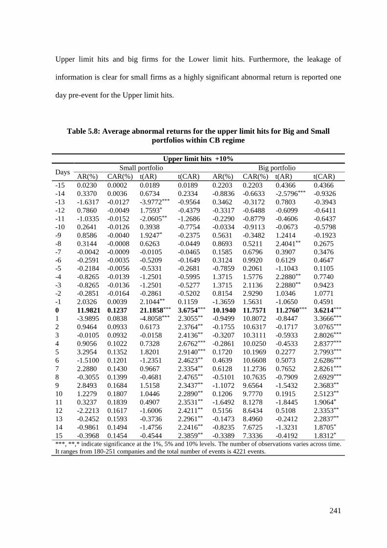
241

Upper limit hits and big firms for the Lower limit hits. Furthermore, the leakage of

information is clear for small firms as a highly significant abnormal return is reported one

day pre-event for the Upper limit hits.

Table 5.8: Average abnormal returns for the upper limit hits for Big and Small

portfolios within CB regime

Upper limit hits +10%

Days Small portfolio Big portfolio

AR(%) CAR(%) t(AR) t(CAR) AR(%) CAR(%) t(AR) t(CAR)

-15 0.0230 0.0002 0.0189 0.0189 0.2203 0.2203 0.4366 0.4366

-14 0.3370 0.0036 0.6734 0.2334 -0.8836 -0.6633 -2.5796*** -0.9326

-13 -1.6317 -0.0127 -3.9772*** -0.9564 0.3462 -0.3172 0.7803 -0.3943

-12 0.7860 -0.0049 1.7593* -0.4379 -0.3317 -0.6488 -0.6099 -0.6411

-11 -1.0335 -0.0152 -2.0605** -1.2686 -0.2290 -0.8779 -0.4606 -0.6437

-10 0.2641 -0.0126 0.3938 -0.7754 -0.0334 -0.9113 -0.0673 -0.5798

-9 0.8586 -0.0040 1.9247* -0.2375 0.5631 -0.3482 1.2414 -0.1923

-8 0.3144 -0.0008 0.6263 -0.0449 0.8693 0.5211 2.4041** 0.2675

-7 -0.0042 -0.0009 -0.0105 -0.0465 0.1585 0.6796 0.3907 0.3476

-6 -0.2591 -0.0035 -0.5209 -0.1649 0.3124 0.9920 0.6129 0.4647

-5 -0.2184 -0.0056 -0.5331 -0.2681 -0.7859 0.2061 -1.1043 0.1105

-4 -0.8265 -0.0139 -1.2501 -0.5995 1.3715 1.5776 2.2880** 0.7740

-3 -0.8265 -0.0136 -1.2501 -0.5277 1.3715 2.1136 2.2880** 0.9423

-2 -0.2851 -0.0164 -0.2861 -0.5202 0.8154 2.9290 1.0346 1.0771

-1 2.0326 0.0039 2.1044** 0.1159 -1.3659 1.5631 -1.0650 0.4591

0 11.9821 0.1237 21.1858*** 3.6754*** 10.1940 11.7571 11.2760*** 3.6214***

1 -3.9895 0.0838 -4.8058*** 2.3055** -0.9499 10.8072 -0.8447 3.3666***

2 0.9464 0.0933 0.6173 2.3764** -0.1755 10.6317 -0.1717 3.0765***

3 -0.0105 0.0932 -0.0158 2.4136** -0.3207 10.3111 -0.5933 2.8026***

4 0.9056 0.1022 0.7328 2.6762*** -0.2861 10.0250 -0.4533 2.8377***

5 3.2954 0.1352 1.8201 2.9140*** 0.1720 10.1969 0.2277 2.7993***

6 -1.5100 0.1201 -1.2351 2.4623** 0.4639 10.6608 0.5073 2.6286***

7 2.2880 0.1430 0.9667 2.3354** 0.6128 11.2736 0.7652 2.8261***

8 -0.3055 0.1399 -0.4681 2.4765** -0.5101 10.7635 -0.7909 2.6929***

9 2.8493 0.1684 1.5158 2.3437** -1.1072 9.6564 -1.5432 2.3683**

10 1.2279 0.1807 1.0446 2.2890** 0.1206 9.7770 0.1915 2.5123**

11 0.3237 0.1839 0.4907 2.3531** -1.6492 8.1278 -1.8445 1.9064*

12 -2.2213 0.1617 -1.6006 2.4211** 0.5156 8.6434 0.5108 2.3353**

13 -0.2452 0.1593 -0.3736 2.2961** -0.1473 8.4960 -0.2412 2.2837**

14 -0.9861 0.1494 -1.4756 2.2416** -0.8235 7.6725 -1.3231 1.8705*

15 -0.3968 0.1454 -0.4544 2.3859** -0.3389 7.3336 -0.4192 1.8312* ***, **,* indicate significance at the 1%, 5% and 10% levels. The number of observations varies across time.

It ranges from 180-251 companies and the total number of events is 4221 events.

242

Table 5.9: Average abnormal returns for the upper and lower limit hits for Big and

Small portfolios within CB regime

Lower limit hits -10%

Days Small sized portfolio Big sized portfolio

AR(%) CAR(%) t(AR) t(CAR) AR(%) CAR(%) t(AR) t(CAR)

-15 2.3637 2.3637 1.3984 1.3984 0.4387 0.4387 0.8998 0.8998

-14 0.2721 2.6357 0.4462 1.3198 0.1276 0.5663 0.3126 1.0189

-13 -0.3024 2.3334 -0.4000 1.3910 0.2504 0.8166 0.3876 0.7924

-12 -1.0080 1.3254 -1.4911 0.6828 0.8922 1.7089 1.9430* 1.4483

-11 -0.8538 0.4717 -1.0516 0.2010 0.9058 2.6147 1.8833* 2.1399**

-10 0.7254 1.1971 0.4910 0.3944 -0.4132 2.2015 -1.5097 1.9101*

-9 -0.0102 1.1868 -0.0085 0.3256 -0.0339 2.1676 -0.0804 1.9666**

-8 0.8040 1.9909 0.9015 0.5127 -0.4043 1.7633 -1.5907 1.4895

-7 0.0789 2.0697 0.0674 0.5385 0.1785 1.9418 0.4517 1.4396

-6 -0.7880 1.2817 -0.6720 0.3260 -0.6130 1.3288 -1.0243 0.8624

-5 -0.0874 1.1943 -0.1089 0.2878 -0.4531 0.8757 -1.0928 0.5774

-4 -0.2045 0.9898 -0.2792 0.2227 -0.0153 0.8604 -0.0280 0.5701

-3 -0.2045 1.5429 -0.2792 0.3253 -0.0153 0.2956 -0.0280 0.1797

-2 -1.0182 0.5247 -0.9959 0.1102 -0.9721 -0.6765 -1.4695 -0.3702

-1 0.5944 1.1191 0.3527 0.2299 1.6311 0.9547 2.7069*** 0.4790

0 -11.2329 -10.1138 -8.9462*** -2.1427** -7.6231 -6.6684 -6.3750*** -2.8245***

1 0.2354 -9.8785 0.2371 -1.8729* 4.4624 -2.2060 3.8610*** -0.7539

2 1.3024 -8.5761 0.8968 -1.6109 -1.3305 -3.5365 -1.7616* -1.3486

3 -1.0993 -9.6754 -1.2649 -1.9779** -1.0512 -4.5877 -1.3126 -1.7083*

4 -1.9053 -11.5808 -1.5797 -2.1336** 0.8758 -3.7119 1.4234 -1.4249

5 1.0256 -10.5552 1.0104 -2.0436** 1.8371 -1.8748 2.9406*** -0.6304

6 0.2712 -10.2840 0.3895 -2.1216** -0.1722 -2.0471 -0.4245 -0.7125

7 0.2394 -10.0446 0.4581 -2.0873** -1.0398 -3.0868 -1.9040* -1.0431

8 -2.1925 -12.2371 -1.2813 -2.1864** -0.6933 -3.7801 -0.7307 -1.2956

9 -0.8417 -13.0787 -0.9092 -2.2535** -1.1947 -4.9748 -1.9592** -1.7038*

10 -1.6071 -14.6859 -1.8575* -2.5001** 0.8214 -4.1534 1.0468 -1.2910

11 -1.4261 -16.1120 -1.8654* -2.8093*** 0.9363 -3.2171 1.1676 -0.9404

12 -1.3349 -17.4468 -1.1400 -3.0846*** 1.0451 -2.1720 1.5368 -0.6068

13 0.6416 -16.8053 0.4889 -2.8946*** 1.0910 -1.0810 1.4690 -0.2913

14 0.9747 -15.8305 1.2816 -2.6729*** 0.0852 -0.9958 0.1975 -0.2620

15 -1.0714 -16.9019 -1.2455 -2.7000*** -1.2359 -2.2317 -1.3426 -0.6072 ***, **,* indicate significance at the 1%, 5% and 10% levels. The number of observations varies across time. It

ranges from 180-251 companies and the total number of events is 4221 events.

Results presented in tables 5.8 and 5.9 do not support the effect of firm size on the

overreaction hypothesis within the circuit breakers regime as price reversals occur one day

following the event. Therefore there is no evidence of the volatility spillover hypothesis

within circuit breakers regime; this result is consistent with Kim and Rhee (1997) .

243

Figure 5.6 plots the cumulative averages abnormal returns over the event window for the

Big and Small portfolios within the CB (10%) Upper and Lower limit hits.

Figure 5-6: cumulative averages abnormal returns over the event window for the Big

and Small portfolios within the CB regime

5.5.2 Volatility Spillover hypothesis

To investigate the Volatility Spillover (VS) hypothesis, for each event (price hits the Upper

or the Lower limit), I identify days (events) where the high price during the trading session

matches its previous day's closing price plus the symmetric price limit (-/+5%) or (-/+

10%) (Kim and Rhee 1997).

For Upper limits I assume:

)1(1 ttt SPLCH (8)

And for lower limits I assume:

)1(1 ttt SPLCL (9)

-0.2

-0.15

-0.1

-0.05

0

0.05

0.1

0.15

0.2

0.25

-15 -12 -9 -6 -3 0 3 6 9 12 15

CA

Rs

Event window

CAR Big+10%

CAR Small+10%

CAR Big-10%

CAR Small -10%

244

where:

tH is day's high price.

tL is day's low price.

1tC is previous day's closing price.

tSPL is the symmetric price limit for day (t) (+/-5% or +/-10%) according to the

regime in operation (SPL or CB).

To test the volatility spillover hypothesis and following Kim and Rhee (1997), I examine

volatility during 21 days (-10, +10) around event day. The event for a particular stock

occurs when its price hits its Upper or lower price limit (+/-5% or +/-10%) in a particular

day. In event time, this day is t=0.

I define daily price volatility in the fashion of Kim and Rhee (1997) as in equation 10:

2

tjtj RV (10)

where: tjV is the volatility of stock (j) on day (t).

tjR is the close-to-close return for stock j on day t, measured by the log of the

firm’s price ratio i.e.

1/ln ttt PPR where tP is the closing price of the stock on day (t).

In order to examine the volatility spillover hypothesis in post limit days for each regime

(SPL +/-5% or CB +/-10%) within the two categories (upward and downward movements),

245

I calculate the daily price volatility 2

tjR for each stock in the four categories (upward and

downward +/-5% or +/-10%) and then take the daily averages.

To overcome potential bias in volatility estimation I include only non-overlapping event

windows; the inclusion of consecutive events would bias the post-event window. To

compare volatility levels for upward and downward price movements, I use the

nonparametric Wilcoxon signed–rank test (Kim and Rhee, 1997). I assume that the sample

distribution of the difference between the matched pairs is symmetric. The null hypothesis

is ''The distribution is centered on zero difference''.

To investigate the volatility spillover hypothesis, table 5.10 presents stock returns volatility

around the event (limit hit day) for the Upper and Lower limit hits within the two regimes.

I exclude from the analysis the multiple overlapping events to minimise the pre-limit day

volatility bias arising from the inclusion of the consecutive events as independent events

(Kim and Rhee 1997). This reduces the sample size for the stocks that hits their limits by

19.20% (from 4221 to 3542).

It is clear from the table 5.10 that the highest volatility is reported on event day for both

Upper and lower price movements for the two regimes. For the Upper limit hits for

instance, we notice a large drop in volatility on day one from 2.5 to 5.57 for the strict (+

5%) price limit regime and from 10 to 0.81 for the (+ 10%) circuit breakers regime.

However, for the lower price limits we also notice a large drop in volatility on event day

from 2.5 to 1.28 and from 10 to 0.89 within Strict Price Limits (SPL) and circuit breakers

(CB) regimes respectively. Ma et al. (1989) explain this as the cooling effect of price

246

limits, however Kim and Rhee (1997) and Lee et al. (1994) conclude that volatility

measures will naturally decline when stocks hit their limits. To support this result, I re-

estimated the volatility spillover hypothesis for other categories of stocks that nearly hit

their limit 90% and 80% of Upper and Lower limit, and found similar results.

Table 5.10: Volatility Spillover Hypothesis

Days Upper price movements Lower price movements

+5% +10% -5% -10%

-10 0.1768 0.1291 0.2200 0.2241

-9 0.1653 0.2984 0.2190 0.2216

-8 0.0827 0.2414 0.2813 0.2450

-7 0.1095 0.2422 0.1933 0.2936

-6 0.0957 0.2490 0.2071 0.3542

-5 0.1349 0.2239 0.2373 0.2214

-4 0.1110 0.2568 0.2398 0.2440

-3 0.1333 < 0.2644 0.2430 0.3259

-2 0.2667 0.3379 0.2541 < 0.4071

-1 0.4072 0.5560 0.3674 << 0.6695

0 2.5000 << 10.0000 2.5000 << 10.0000

1 1.5723 >> 0.8088 1.2797 >> 0.8947

2 1.2739 >> 0.7680 0.3649 < 0.4448

3 0.2427 << 0.3895 0.2962 << 0.4770

4 0.1107 < 0.2857 0.1309 0.2409

5 0.1277 0.2572 0.1727 0.2115

6 0.1586 0.2876 0.2138 0.2883

7 0.1432 0.3813 0.1735 0.4051

8 0.1745 0.3598 0.1752 0.2809

9 0.1326 0.3249 0.1400 0.3169

10 0.1343 0.2779 0.2005 0.2590 >> and > implies that the left hand figure is significantly greater than the right hand figure at 0.01 and 0.05

significance levels respectively using Wilcoxon signed-ranked test.

Volatility is measured by squared stock returns multiplied by 1000.

The number of observations varies across time. It ranges from 180-251 companies and the total number

of events is 4221 events.

By comparing the volatility within the two regimes, we notice that for the Upper and

Lower events, the volatility within the CB regime is greater than those of the SPL regime

247

over the entire event window except for the first two days subsequent to the Upper limit

hits and for the first day post-event for the Lower limit hits.

Volatility of the Upper (+ 5%) SPL for the first two days post-event (limit hits) is greater

than those of CB by 93%, and 65% respectively. However, volatility of the Lower SPL (-

5%) is greater than those of the CB regime by 43.82% only during the first day post-event.

This suggests that within the SPL regime, stocks that hit their Upper and Lower limit

continue to experience greater volatility during the first 1-2 days post-event compared with

the CB regime.

These results are consistent with the volatility spillover hypothesis as price discovery

mechanism is disrupted when stocks experience greater volatility for a few days post limit

hits, therefore stock prices are prevented from reaching their equilibrium levels for the

following few days post-event. These deviations from the true prices are expected to

prevail within the SPL (+-5%) regime as trading session is suspended until the following

day (trading session) when the prices hit their Upper or lower limits. However, within

wider bands of limits (- +10%) followed by trading halts investors have chance to adjust

their portfolio positions within the same trading session. Therefore, the volatility spillover

is expected to be higher within the SPL regime.

To support the analysis I compare between volatility levels pre and post each regime. We

notice that within the Upper and Lower price limit regimes, volatility post limits is greater

than those of pre limits for two and three days for Lower and Upper price limits

respectively, for example, within +5% SPL, post limit volatility is greater than those of pre

248

limit volatility for the first three days post limits by 286%, 377% and 82%. Similarly,

within +10% CB regime, post limit volatility for the first three days is greater than those of

pre-limit hit by 45%, 127% and 47%. This result supports the volatility spillover

hypothesis. Finally, the Wilcoxon signed–rank test shows that the differences between the

two regimes are significantly different from zero at the 0.01 and 0.05 levels on event day

and over the three days post-event.

To conclude, results show that price limits do not decrease volatility as intended in both

regimes (SPL and CB). However, volatility is found to be higher within the CB regime. On

the other hand, within the SPL regime, volatility is spread out over the following two days

subsequent to limit hit day. These results support the volatility spillover hypothesis in the

Egyptian stock exchange consistent with findings of Kim and Rhee, (1997) and Lee et al

(1994). Figures 5.7 and 5.8 present the daily price volatility around event day.

Figure 5-7: Daily price volatility for the Upper limit hits for the two regimes around

event day

0

2

4

6

8

10

12

-10 -8 -6 -4 -2 0 2 4 6 8 10

Vo

lati

lity

Event window

SPL

CB

249

Figure 5-8: Daily price volatility for the Lower limit hits for the two regimes around

event day

Figures 5.9 and 5.10 present the cumulative average volayility (CAV) for the Upper and

Lower limit hits for the two regimes.

Figure 5-9: Cumulative average volatility (CAV) for the Upper limits hits for the two

regimes

0

2

4

6

8

10

12

-10 -8 -6 -4 -2 0 2 4 6 8 10

Vo

lati

lity

Event window

SPL

CB

0

2

4

6

8

10

12

14

16

18

-10

-9

-8

-7

-6

-5

-4

-3

-2

-1

0

1

2

3

4

5

6

7

8

9

10

SPL

CB

250

Figure 5-10: Cumulative average volatility (CAV) for the Lower limits hits for the

two regimes

5.5.3 The delayed price discovery hypothesis

According to the Delayed Price Discovery (DPD) hypothesis there will be positive

overnight returns for stocks which hit their Upper limits and negative overnight returns for

stocks which hit their Lower limits (Kim and Rhee 1997).

To investigate these claims I estimate the following two returns series: open-to-close

returns on the limit day, namely )/ln()( 0000 OCCOR and close-to-open returns between

the event day and the following day, namely )/ln()( 0110 COOCR , where 0C is the

closing price on day (t) and 1O is the opening price on day (t+1). As stock returns can be

positive, negative or zero, we have nine return series (+, +), (+, 0), (0, +), (0, -), (0. 0), (+, -

), (-, +), (-, -) and (-, 0) as shown in table 5.11 below.

0

2

4

6

8

10

12

14

16

18 -1

0

-9

-8

-7

-6

-5

-4

-3

-2

-1

0

1

2

3

4

5

6

7

8

9

10

SPL

CB

251

The first return symbol represents the open-to-close returns on the limit day

)/ln()( 0000 OCCOR and the second return symbol represents the close (in event day)-to-

open (in event day +1) )/ln()( 0110 COOCR .

Stocks often experience either price continuation or price reversal based on overnight

returns. I compare the price behaviour of the two regimes (SPL and CB) so that if price

continuation behaviour within SPL is greater than those of the CB regime then, we can

infer that the efficient price discovery mechanism is much delayed within the strict price

limit regime and the opposite is correct.

In other words, I argue that price continuation behaviour prevents stock price from

reaching their equilibrium levels (Kim and Rhee, 1997), since otherwise we should observe

price reversals or overreactive behaviour (Roll, 1983). I examine the immediate stock price

movement subsequent to price-limit hit on event day for both regimes (SPL and CB) by

estimating the frequencies of price continuation, price reversal and no changes, as in the

following table 5.11.

Table 5.11 Frequencies of price continuation and price reversal for the two regimes

Upper limit Lower limit

Price continuation (+, +) and (0, +) (-, -) and (0, -)

Price reversal (+, -), (0, -), (-, +), (-, 0) and (-, -) (-, +), (0, +), (+, -), (+, 0) and (+, +)

No change (+,0) and (0,0) (-, 0) and (0, 0) Note: The first return symbol represents the open-to-close returns on the limit day )/ln()( 0000 OCCOR and the

second return symbol represents the close-to-open )/ln()( 0110 COOCR

The number of observations varies across time. It ranges from 180-251 companies and the total number of events is

4221 events.

252

Following Kim and Rhee (1997) and Bildik, and Gulay (2006), consecutive event days are

not excluded from the analysis as they will underestimate the frequencies of price

continuation and price reversals. As can be seen from Table 5.11 I classify both (+, +) and

(0, +) categories as price continuation for the Upper Limit hits. The (0, +) category is

classified as price continuation because these stocks experience an overnight price increase

(stocks open at the Upper limit and remain unchanged over the event day). The same

concept applies to the lower limits as I classify (-, -) and (0, -) categories as price

continuation for the Lower limit, Kim and Rhee (1997) and Bildik, and Gulay (2006).

On the other hand, I classify – following Kim and Rhee (1997) (+, -), (0, -), (-, +), (-, 0)

and (- , -) as price reversal for the Upper limits. I include (-, +), (-, 0) and (-, -) categories

as price reversal as the first negative sign (open-to-close returns) implies price reversal

before the end of trading session in event day (Kim and Rhee (1997) and Bildik, and Gulay

(2006)). The same concept applies on the lower limits as I classify (-, +), (0, +), (+, -), (+,

0) and (+, +) categories as price reversals for the Lower limit. Finally, I consider (+, 0) and

(0, 0) as no-change categories for the Upper limit hits and the (-, 0) and (0, 0) as no-change

categories for the Lower limit hits (Kim and Rhee (1997) and Bildik, and Gulay (2006)).

I use the following standard nonparametric binomial Z-test to examine for significant

differences between the two regimes with respect to price continuations and price reversals

(Kim and Rhee (1997) and Bildik, and Gulay (2006)).

)*)1(

)*(

hithitCBhitCB

hithitCBhitsSPL

Npxpx

Npxxz

(11)

253

where:

hitsSPLx : Number of price continuations or price reversals events that stocks

experience within SPL regime.

hitCBpx : Percentage of price continuations or price reversals events that stocks

experience within CB regime hitCBhitCB Nx / .

hitN : sample size for stocks hit the limit within the SPL and CB regimes.

As the sample is large the Z-statistic is normally distributed (Olkin, Gleser, and Dermam,

1980 pp. 244-253).

I now discuss the empirical results of the delayed price discovery hypothesis. Table 5.12

presents the frequencies of price continuations, price reversals and no change events for

stocks that hit their Upper and/or lower price limits for the two regimes over the period

1999-2009.

For the Upper price limit hits, table 5.12 shows that price continuation occurs 74.7% and

51.04% immediately following the event (limit hit day) for SPL and CB regimes

respectively. However, price reversals occur 24.88% and 47.15% immediately following

the event for SPL and CB regimes respectively over the same period. The no change events

occurs 0.42% and 0.81% immediately following the event for SPL and CB regimes

respectively. For the Lower price limit hits, price continuation occurs 69.15% and 47.58%

immediately following the event for SPL and CB regimes respectively.

However, price reversals occur 30.15% and 52.40% immediately following the event for

the SPL and CB regimes respectively.

254

We notice that price continuation occurs more frequently within the SPL regime; however,

price reversals occur more frequently within the CB regime immediately following the

event. This result is consistent with the delayed price discovery hypothesis as price limits

prevents stock prices from reaching their equilibrium levels, in particular within a strict

price limit regime. The nonparametric binomial Z test show that there are significant

differences between the two regimes regarding price continuations and price reversals.

Table 5.12: Delayed price discovery: price continuation and reversal

Price Behaviour Upper price movements Lower price movements

SPL (%) CB (%) SPL-CB

(z- stat)

SPL (%) CB (%) SPL-CB

(z-stat)

Price Continuation 74.70 51.04 5.7737*** 69.15 47.58 7.9097***

Price Reversal 24.88 47.15 -8.9936*** 30.15 52.40 -5.3111***

No. change 0.42 0.81 -1.2568 0.70 0.02 1.5987 The table presents the limit hit frequencies for the two regimes. The number of observations varies across time.

It ranges from 180-251 companies and the total number of events is 4221 events.

Figures 5.11 and 5.12 illustrate the frequencies for price continuation and price reversal

within the two regimes.

Figure 5-11: Frequencies for price continuation and price reversal for the

Upper limit hits within both regimes.

0

10

20

30

40

50

60

70

80

Price Continuation Price Reversal No. change

Fre

qu

en

cy (

%)

SPL

CB

255

Figure 5-12: Frequencies for price continuation and price reversal for the Lower limit

hits within both regimes.

To summarise, price continuation behaviour occurs more frequently within the SPL regime

immediately following the event (limit hit day). This implies that price discovery

mechanism is delayed by the Strict Price Limits. This result supports the delayed price

discovery hypothesis. Price reversal behaviour seems to occur more frequently within the

CB regime compared to the SPL regime immediately following the event. This implies that

Strict Price Limits delay or prevent - to some extent - the overreactive behaviour,

compared to the circuit breakers regime.

5.5.4 The Trading Interference hypothesis.

The Trading Interference (TI) hypothesis claims that trading volume (as a proxy for trading

activity) will be higher for stocks that hit their Upper or Lower limits for a few days post-

event (Bildik, and Gulay (2006)). As we expect that price limits will prevent rational

trading on the event day, therefore trading volume is expected to continue increasing over

the post-event days (Kim and Rhee (1997).

0

10

20

30

40

50

60

70

80

Price Continuation Price Reversal No. change

Fre

qu

en

cy (

%)

SPL

CB

256

To investigate the trading interference TI hypothesis around limit-days, following Kim and

Rhee, (1997) and Cressy and Farag (2011), I calculate the percentage change in the

turnover ratio as a proxy for trading activity in the window (-10 to +10 days): as follows:

)/ln(% 1 jtjtjt TATATA

(12)

sharesofNoVolTA tjt ./

(13)

where:

jtTA is the turnover ratio as a proxy for trading activity of stock (j) at time (t).

jtVol is a daily trading volume for stock (j) at time (t).

I calculate the percentage change in the turnover ratio for each stock in the two regimes (±

5% SPL) and (± 10% CB) and then take averages for each day for each window (-10, +10);

I exclude the consecutive events during the limit window (-10, +10) to be consistent with

volatility spillover (VS) hypothesis analysis (Kim and Rhee, (1997). We are interested in

the daily percentage change in turnover ratio because liquidity (trading) interference

hypothesis is mainly concerned with the daily change in trading activity (Bildik, and Gulay

(2006)).

Table 5.12 presents daily percentage change in turnover ratio as a proxy for trading activity

over a 25-day window (-10 to +10) around the event (limits hit ± 5% and ± 10%) for both

SPL and CB regimes.

It is clear from the table that there is sharp increase in trading activity on event day (limit

hit day) for both the SPL and CB regime. For the upward price movement, table 5.13

reports that the percentage increases in trading activity on event day are 51.26% and

257

77.03% for SPL and CB respectively. In addition, the trading activity on event day (limit

hit day) is significantly greater than those within the first 8 days of trading window.

The increase in trading activity lasts for two days (45.15% and 36.69%) subsequent to the

event within the SPL and lasts only for one day (40.50%) following the event within the

CB regime. Trading activity within the CB regime is higher than those of the SPL four

days pre-event.

For the Lower price movements, the highest trading activity – as expected – is reported on

event day; 42.84% and 67.15% for the SPL and CB respectively. We also notice that the

increase in trading activity lasts only for one day (24.89%) following the event within the

SPL regime. In addition, we find a significant decrease in trading activity one day

following the event within CB regime. Trading activity within the CB regime – on average

– is higher than those of the SPL for four days pre-event.

I interpret these results as follows: within the SPL regime, traders are unable to obtain their

desired positions on event day. In addition, traders are unable to adjust their portfolios’

positions – when prices hit the limit – and are forced to wait until the following day.

Therefore Strict Price Limits interfere with trading activity.

On the other hand, within circuit breakers regime, trading activity on average is

significantly higher than those of Strict Price Limits as price limits are widened to ± 10%.

Investors within the CB regime have the chance to adjust their portfolios positions during

the same trading session. However, not all investors are informed about the suspension of

258

trading due to the lack of informational efficiency in the emerging markets. Therefore,

only one day following the event (in case of Lower limit hits) may be required to adjust

portfolios’ position.

Table 5.13: Trading interference hypothesis: Turnover ratio

Days Upper price movements Lower price movements

+5% +10% -5% -10% -10 -0.0498 0.0227 -0.0380 0.0012

-9 -0.0462 0.0249 -0.0354 -0.1074

-8 -0.0716 -0.1658 0.2126 > 0.1201

-7 0.1791 > 0.0855 0.0274 -0.0336

-6 -0.0151 0.1044 -0.1268 0.1127

-5 -0.1385 -0.1485 0.1669 -0.0172

-4 0.0569 0.1480 -0.0857 -0.0704

-3 0.0511 0.1052 -0.0368 0.0583

-2 -0.0475 0.0958 0.1470 < 0.1701

-1 0.2578 < 0.4053 -0.1330 -0.0453

0 0.5126 << 0.7703 0.4284 << 0.6715

1 0.4515 >> 0.4050 0.2489 >> -0.3751

2 0.3669 >> -0.2302 -0.1296 0.0618

3 -0.1578 0.1976 0.0929 0.1522

4 -0.0168 -0.0079 0.0722 << 0.1550

5 -0.1162 -0.0345 -0.0526 -0.0355

6 -0.1133 -0.0236 -0.0563 << 0.1122

7 -0.0534 >> -0.1374 0.0607 0.0935

8 -0.1176 0.0078 -0.0568 -0.0183

9 -0.0256 << 0.1283 0.1099 -0.0457

10 0.0179 0.0686 -0.1377 << -0.0461 >> and > implies that the left hand figure is greater than the right hand figure at 0.01 and 0.05 significance

respectively using Wilcoxon signed-ranked test. The number of observations varies across time. It

ranges from 180-251 companies and the total number of events is 4221 events.

This result suggests that price limits interfere with trading activity and negatively affect

the investors’ liquidity positions within the two regimes. Moreover, these results are

consistent with Lehmann, (1989) and Kim and Rhee (1997). Figures 5.13 and 5.14 present

the trading activity ratio (TAR) for the Upper and Lower limit hits respectively.

259

Figure 5-13: Trading activity ratio (TAR) for the Upper limit hits

Figure 5-14: Trading activity ratio (TAR) for the Lower limit hits

5.5.5 Regulatory policies and volume-volatility relationship.

In this section I investigate the relationship between regulatory policies and volume-

volatility dynamics. It is well documented that there is a positive relationship between

-0.4

-0.2

0

0.2

0.4

0.6

0.8

1

-10

-9

-8

-7

-6

-5

-4

-3

-2

-1 0

1

2

3

4

5

6

7

8

9

10

SPL

CB

-0.6

-0.4

-0.2

0

0.2

0.4

0.6

0.8

-10

-9

-8

-7

-6

-5

-4

-3

-2

-1 0

1

2

3

4

5

6

7

8

9

10

SPL

CB

260

trading volume and stock price volatility which is often explained by the Mixture of

Distributions Hypothesis of Clark (1973) subsequently developed by Epps and Epps

(1976) and Tauchen and Pitts (1983). An alternative explanation is provided by the

Sequential of Information Arrival hypothesis (SIAH) of Copeland (1976Farag and Cressy

(2011).

To explore further the Trading Interference hypothesis, I run a regression (following Kim

and Rhee, 1997) for the 21-day window for both the Upper and Lower limits within the

two limit regimes as in equation 14. I exclude the consecutive events for the sake of

consistency with the volatility spillover analysis.

jjjj CBTAV 21 )( (14)

where:

jV : Squared stock returns as a measure of price volatility.

jTA : The percentage change of turnover ratio as a proxy of trading activity.

jCB : A dummy variable that equals 1 for stocks that reach Upper or Lower limit

within CB regime, and equals 0 within SPL regime.

I use the turnover ratio as a proxy for trading activity instead of trading volume per se as

Farag and Cressy (2011) found that there is an endogeneity problem between trading

volume and stock price volatility (each determines the other). I estimate the above equation

for each day of the 21-day window for both Upper and Lower limit hits.

261

According to the literature, I expect a positive relationship between trading activity and

stock price volatility during the 21-day window. However, in day 0, I do not expect this

relationship to continue, as price limits interfere with trading activity according to the

trading interference (TI) hypothesis. The sign of the CB – dummy is expected to be

positive and significant around event day. This implies an increase in stock price volatility

due to regime switch from Strict Price Limits to circuit breakers.

To investigate the relationship between regulatory policies and the volume volatility

relationship, tables 5.14 and 5.15 report the results of the OLS regressions for the Upper

and Lower price movements as in equation 14. The two models are well specified as the F

stat is highly significant and the adjusted R squared is reasonably high on event day.

As expected, tables 5.14 and 5.15 report a positive relationship between turnover ratio (as a

proxy for trading activity) and stock price volatility over the 21-day window for the Upper

and Lower price movements. This suggests a positive relationship between trading volume

and stock price volatility. However, this volume–volatility relationship is much stronger

and highly significant around event day for the Lower and Upper price movements

respectively28

.

Interestingly, I find an insignificant volume–volatility relationship on event day (limit hits

day) and on the first day subsequent to the event or both Upper and Lower limit hits. This

suggests that regulatory policies (Strict Price Limits and circuit breakers) disrupt trading

activity according to the trading interference hypothesis.

28

Although the adjusted R squared is quite low in table 5.14, however, this is consistent with Kim and Rhee

(1997) as we are interested in the direction (sign) of the volume-volatility relationships not in the explanatory

power of the model. However we notice that F-statistics are highly significant.

262

Table 5.14: Volume volatility relationship for the Upper limit hits

Day Intercept CB TR Adj R2 F.value

-10 0.0013

***

(0.0002)

0.0004**

(0.0002)

0.00004

(0.0001) 0.0074 2.6455

*

-9 0.0014

***

(0.0002)

0.0007***

(0.0003)

0.0002*

(0.0001) 0.0208 5.7050

***

-8 0.0015

***

(0.0001)

0.0010***

(0.0002)

0.0003***

(0.0001) 0.0773 19.544

***

-7 0.0012

***

(0.0001)

0.0006***

(0.0002)

0.0002**

(0.0001) 0.0341 8.8236

***

-6 0.0017

***

(0.0002)

0.0011***

(0.0003)

0.0003

(0.0002) 0.0560 14.146

***

-5 0.0013

***

(0.0001)

0.0006***

(0.0002)

0.0004***

(0.0001) 0.0239 6.4277

***

-4 0.0014

***

(0.0002)

0.0008***

(0.0002)

0.0003**

(0.0003) 0.0379 9.7202

***

-3 0.0140

(0.0843)

0.0834

(0.1092)

0.1182***

(0.0417) 0.0150 4.3669

**

-2 0.0012

***

(0.0001)

0.0006***

(0.0002)

0.0004**

(0.0004) 0.0403 10.290

***

-1 0.0030

***

(0.0003)

0.0025***

(0.0003)

0.0006***

(0.0001) 0.1669 45.363

***

0 0.0177***

(0.0004)

0.0152***

(0.0005)

0.0002

(0.0002) 0.6544 78.36

***

1 0.0037

***

(0.0002)

0.0024***

(0.0003)

0.0004

(0.0003) 0.1531 41.030

***

2 0.0014

***

(0.0002)

0.0006***

(0.0002)

0.0003***

(0.0001) 0.0163 4.6628

***

3 0.0012

***

(0.0001)

0.0004***

(0.0002)

0.0002***

(0.0001) 0.0279 7.3632

***

4 0.0016

***

(0.0002)

0.0008***

(0.0002)

0.0002***

(0.0001) 0.0369 9.4785

***

5 0.0014

***

(0.0001)

0.0005***

(0.0002)

0.0002***

(0.0001) 0.0323 8.3821

***

6 0.0018

***

(0.0002)

0.0010***

(0.0003)

0.0002**

(0.0001) 0.0377 9.6817

***

7 0.0011

***

(0.0001)

0.0004**

(0.0002)

0.0001*

(0.0001) 0.0153 4.4516

**

8 0.0017

***

(0.0002)

0.0011***

(0.0003)

0.00002

(0.0001) 0.0324 8.4281

***

9 0.0014

***

(0.0001)

0.0008***

(0.0002)

0.0003***

(0.0001) 0.0640 16.153

***

10 0.0012

***

(0.0001)

0.0004***

(0.0002)

0.0001*

(0.0001) 0.0213 5.8159

***

The table presents the results of equation 14 for the Upper limit hits.

jjjj CBTAV 21 )(

where, jV : Squared stock returns as a measure of price volatility,

jTA : The

percentage change of turnover ratio as a proxy of trading activity, jCB : dummy

variable equals 1 for stocks that reach Upper or Lower limit within CB regime, and 0

within SPL regime. ***, **,* indicate significance at the 1%, 5% and 10% levels.

The number of observations varies across time. It ranges from 180-251 companies

and the total number of events is 4221 events.

263

Table 5.15: Volume volatility relationship for the Lower limit hits

Day Intercept CB TR Adj R2 F.value

-10 0.0010

***

(0.0001)

0.0003*

(0.0001)

0.00003

(0.0001) 0.0045 1.7904

-9 0.0012

***

(0.0001)

0.0005***

(0.0002)

0.00001

(0.0001) 0.0140 3.4804

**

-8 0.0010

***

(0.0001)

0.0003**

(0.0001)

0.0001*

(0.0001) 0.0229 5.1069

***

-7 0.0017

***

(0.0002)

0.0010***

(0.0003)

0.0003*

(0.0001) 0.0327 6.9245

***

-6 0.0019

***

(0.0003)

0.0013***

(0.0004)

0.0001

(0.0002) 0.0283 6.0977

***

-5 0.0014

***

(0.0002)

0.0008**

(0.0003)

0.00003

(0.0001) 0.0109 2.9250

*

-4 0.0011

***

(0.0001)

0.0006***

(0.0002)

0.0001

(0.0001) 0.0291 6.2441

***

-3 0.0038

***

(0.0008)

0.0032***

(0.0011)

0.00004**

(0.0002) 0.0174 4.1070

**

-2 0.0020

***

(0.0003)

0.0012***

(0.0004)

0.0005**

(0.0002) 0.0289 6.2000

***

-1 0.0054

***

(0.0008)

0.0046***

(0.0011)

0.0004**

(0.0002) 0.0410 8.4796

***

0 0.0180

***

(0.0005)

0.0151***

(0.0007)

-0.0002

(0.0003) 0.5732 36.00

***

1 0.0021

***

(0.0002)

0.0010***

(0.0003)

0.0002

(0.0002) 0.0411 8.5066

***

2 0.0023

***

(0.0002)

0.0016***

(0.0003)

0.0002**

(0.0001) 0.0717 14.519

***

3 0.0018

***

(0.0002)

0.0010***

(0.0002)

0.000**

(0.0001) 0.0417 8.6144

***

4 0.0013

***

(0.0001)

0.0006***

(0.0002)

-0.0001*

(0.0001) 0.0425 8.7626

***

5 0.0012

***

(0.0001)

0.0005**

(0.0002)

0.0001

(0.0001) 0.0137 3.4380

**

6 0.0018

***

(0.0002)

0.0010***

(0.0003)

0.0001

(0.0001) 0.0275 5.9499

***

7 0.0015

***

(0.0002)

0.0009***

(0.0003)

0.0002

(0.0002) 0.0175 4.1251

**

8 0.0008

***

(0.0001)

0.0001

(0.0001)

0.0001

(0.0001) -0.0016 0.7234

9 0.0012

***

(0.0002)

0.0004**

(0.0002)

0.0002*

(0.0001) 0.0134 3.3710

**

10 0.0013

***

(0.0002)

0.0006*

(0.0003)

0.0002

(0.0001) 0.01165 3.0476

**

The table presents the results of equation 14 for the Lower limit hits.

jjjj CBTAV 21 )(

where, jV : Squared stock returns as a measure of price volatility,

jTA : The

percentage change of turnover ratio as a proxy of trading activity, jCB : dummy

variable equals 1 for stocks that reach Upper or Lower limit within CB regime, and 0

within SPL regime. ***, **,* indicate significance at the 1%, 5% and 10% levels. ***,

**,* indicate significance at the 1%, 5% and 10% levels. The number of observations

varies across time. It ranges from 180-251 companies and the total number of events is

4221 events.

264

On the other hand, I also find a positive and significant relationship between the dummy

variable (CB) and stock price volatility within the Upper and Lower limit hits. This

suggests that switching from Strict Price Limits to circuit breakers does increase short-term

stock price volatility rather than cooling down the market as was intended by the regulator.

These findings are consistent with the volatility spillover hypothesis as regulatory policies

(not trading activity) cause volatility to spread out few days subsequent to limits hit.

5.5.6 Long term volatility and regime switch

To further investigate the long-term effect of regime switch on stock price volatility, I

estimate the Exponential Asymmetry GARCH model (EGARCH of Nelson (1991)) for the

EGX30 market index over the period 1999-2009 (5 years within SPL regime and 5 years

within CB regime) and augment it by adding a price limit dummy variable as in equation

15. The EGARCH model has many advantages over the symmetric GARCH as the

estimation has no negative parameters ( )(log 2

t is positive), and so, no non-negativity

constraints need be imposed on the model parameters as in TARCH-GJR model. The

EGARCH formula is presented in equation 15 below.

Leverage effect (the effect of positive and negative shocks on the future conditional

volatility) is allowed and the parameter is expected to be negative in sign if the

relationship between return and volatility is negative. The leverage effect in the EGARCH

model is exponential rather than quadratic and can be tested by the hypothesis that 0 .

The impact is asymmetric if 0 . The volatility persistence is measured by to examine

whether big (small) shocks are followed by bigger (smaller) shocks.

265

t

t

t

t

ttt CB

2)ln()ln(

2

1

1

2

1

12

1

2 (15)

where:

)ln( 2

t is the conditional variance of return at time (t)

)ln( 2

1t : is the conditional variance at time (t-1)

2

2

1

1

t

t is the effect of the shock (i.e. new information arrival) on

conditional volatility.

2

1

1

t

t

is the effect of positive and negative shocks on conditional volatility

(leverage effect).

tCB is a dummy variable takes the value of 1 if the CB regime is in operation on

day t; and zero if the SPL regime is in operation.

Importantly for our empirical analysis, the sign of will be positive or negative as

switching regimes increase or decrease volatility. Nelson (1991) assumed that the error

term follows the Generalized Error Distribution (GED). This is defined by

)ln(5.01

ln)2ln(1

12

1ln)( 2

t

v

t

tt h

vvh

vI

(16)

where )))/3(ln())2/1()/1(ln()2/1()2ln()/1exp(( vvv , and v is a tail thickness

parameter. When v = 2, tu has a Standard ormal distribution. Finally, I use the Berndt-

Hall-Hall-Hausman (BHHH) technique to maximize the log likelihood function of the

GED.

266

To investigate the effect of long-term volatility on regulatory policies, table 5.16 presents

the results of the augmented EGARCH model. The model is well specified as the log

likelihood estimation is big compared to the symmetric GARCH model. This suggests that

the EGARH model fits the daily returns time series of the EGX30 and the temporal

dependence of return volatility can be captured by the model.

The volatility persistence coefficients and are highly significant, however is

greater in magnitude than ; this implies that the bigger the market shocks the relatively

smaller revision expected volatility.

Table 5.16: Augmented EGARCH Estimation

EGX30 -0.4949***

(0.0704)

0.9686***

(0.0068)

-0.0281*

(0.0167)

0.0371***

(0.0135) 0.0296

**

(0.0142)

Log likelihood 5680

Ljung-Box Q(20) 35.831

Ljung-Box Q2(20) 18.634

LMARCH 1.1435

The table presents the results of the augmented Exponential Generalized autoregressive GARCH

model as in equation 15. ***, **,* indicate significance at the 1%, 5% and 10% levels.

t

t

t

t

ttt CB

2)ln()ln(

2

1

1

2

1

12

1

2

The number of observations varies based on the number of trading days in the EGX across years.

The leverage effect is negative as expected; this suggests that negative shocks have greater

effect on conditional volatility in the EGX. Most importantly, the CB coefficient is positive

in sign and highly significant; this suggests that the switch from SPL to CB increases

future volatility. This result is consistent with the previous analysis. Furthermore, we can

reject the null that the residuals are serially uncorrelated and homoskedastic. The results of

267

the Ljung-Box Q(20) and Ljung-Box Q2(20) for serial correlation and the LMARCH for

heteroskedastisity are insignificant.

The results of the volatility spillover and delayed price discovery hypotheses in addition to

the asymmetry EGARCH models show that switching from the SPL to the CB did increase

stock price volatility in the Egyptian stock market. A potential interpretation to this result

is as follows: based on the volatility spillover hypothesis, price limits prevent speculative

traders from responding to the new information and to adjust their portfolios. This implies

a remarkable delay in price discovery mechanism as current prices are away from their

equilibrium levels (Farag and Cressy (2011).

I claim that the price discovery mechanism in the Egyptian stock market varies between

SPL and CB. Within the SPL as prices hit the limit, trading is suspended until the end of

the trading session, therefore volatility is expected to spread out over the following day(s),

Meanwhile, investors have more time (until the following day) to analyse and to react to

the new information and then adjust their portfolios accordingly. On the other hand, within

the CB regime, when prices hit the limit, trading is suspended for 30 minutes. During this

relatively short time investors have to adjust their portfolios based on the new information

arriving in the market (Farag and Cressy (2011).

I argue that since herding behaviour and noise trading are dominant behaviours in

emerging markets, intense trading activity is continued by some speculative traders when a

trading session is resumed. In addition, the media coverage plays an important role in

affecting investors’ belies within a trading halt period (Lee et al. 1994) and (Farag and

Cressy (2011).

268

However, due to the lack of informational efficiency in the Egyptian stock market not all

investors are being informed with the new information. Therefore investors are unable to

reveal their demand during the halt period. This suggests that stock prices are expected to

be much noisier post halt period and significantly different from their equilibrium levels.

As a result, higher volume and volatility are expected when trading is resumed (Lee et al.

(1994) and Farag and Cressy (2011)29

.

5.6 Summary and conclusion

The main objective of this chapter is to investigate the effect of regulatory policies (price

limits, circuit breakers) on four main hypotheses, namely, the overreaction hypothesis,

volatility spillover hypothesis, the delayed price discovery hypothesis and the trading

interference hypothesis in the Egyptian stock market. In addition, the chapter examines the

effect of the regime switch (from Strict Price Limits to circuit breakers) on the long-term

volatility. Moreover, the chapter introduces a comprehensive literature review of price

limits as well as the theoretical background about the evolution of the different types of

regulatory policies.

The dataset consists of daily open, high, low and closing prices for all listed shares in the

Egyptian stock exchange during the period 1999-2009, in addition to trading volumes as a

proxy for trading activity and market capitalisation as a proxy for size. Moreover, I use the

EGX30 - a free-float market capitalisation-weighted index - as a benchmark.

29

These results have been published in the European Journal of Finance (forthcoming) based on my earlier

work in this chapter.

269

The Egyptian stock exchange (EGX) has unique price limit regimes; this makes studying

the EGX - amongst a few other stock exchanges i.e. Korean stock exchange - interesting.

The regulator in the EGX has imposed strict (+-5%) price limits (SPL) for all the listed

shares since 1996. The limit is activated for a particular stock only when stock return hits

the Upper or Lower limit, then the trading on this share is suspended to the end of the

trading session. In 2002 the regulator commenced a new price ceiling system, namely,

circuit breakers (CB) in which the price limits have winded to (+-20%) for the most

actively traded shares in the EGX. Within the new CB regime, trading is halted for 30

minutes when stock return for a particular stock hits (+-10%).

The results of the overreaction hypothesis show that there is price reversal pattern for the

Lower limit hits (bad news) one and two days following the event within the two regimes

SPL and CB respectively. In addition, there is a price continuation pattern for the Upper

limit hits (good news) within the SPL regime over the event window. This result supports

the overreaction hypothesis in case of bad news (Lower limit hits) while also suggesting

the leverage effect in the Egyptian stock market within the two regimes.

Moreover, the results support the effect of firm size on the overreaction hypothesis for the

Lower limit hits for small firms in particular. This can be explained in the light of the

literature as volatility is more likely to be higher for small firms (Huang (1997 and (1998)).

The results do not support the effect of firm size on the overreaction hypothesis within the

circuit breakers regimes.

The findings of the volatility spillover hypothesis conclude that price limits do not

decrease volatility as intended in both regimes (SPL and CB). However, volatility is found

270

to be higher within the CB regime whereas, within the SPL regime, volatility is spread out

over the following two days subsequent to limit hit day.

These results are consistent with the volatility spillover hypothesis as the price discovery

mechanism is disrupted when stocks experience greater volatility for a few days post limit

hits, therefore stock prices are prevented from reaching their equilibrium levels for the

following few days post-event. These deviations from the true prices are expected to

prevail within the SPL (+-5%) regime as a trading session is suspended until the following

day (trading session) when the prices hit their Upper or lower limits. However, within

wider bands of limits (- +10%) followed by trading halts, investors have chance to adjust

their portfolios position within the same trading session. Therefore the delay in the price

discovery process is expected to be higher within the SPL regime. These results are

consistent with Kim and Rhee, (1997) and Lee et al (1994).

The results of the delayed price discovery hypothesis show that price continuations

behaviour occurs more frequently within the SPL regime immediately following the event

(limit hit day). This implies that the price discovery mechanism is delayed by the Strict

Price Limits. This result is consistent with the delayed price discovery hypothesis. Price

reversal behaviour seems to occur more frequently within the CB regime compared to the

SPL regime immediately following the event, thus implying that Strict Price Limits delay

or prevent the overreactive behaviour, compared to the circuit breakers regime.

The results of the trading interference hypothesis show that there is a sharp increase in

trading activity on event day (limit hit day) for both SPL and CB regimes for the Upper

and Lower price movement. In addition, the trading activity on event day (limit hit day) is

271

significantly greater than those within the rest of trading window. This increase in trading

activity lasts for 1-2 days subsequent to the event.

I interpret these results as follows: within the SPL regime, traders are unable to obtain their

desired positions on event day. In addition, traders are unable to adjust their portfolios’

positions - when prices hit the limit - and are forced to wait until the following day.

Therefore Strict Price Limits interfere with trading activity.

On the other hand, within circuit breakers regime, trading activity on average is

significantly higher than those of Strict Price Limits. Investors within the CB regime have

the chance to adjust their portfolio positions during the same trading session. However, not

all investors are informed about the suspension of trading due to the lack of informational

efficiency in emerging markets. Therefore only one day following the event may be

required to adjust their portfolios’ position. This result suggests that price limits interfere

with trading activity and negatively affect the investors’ liquidity positions within the two

regimes. Moreover, these results are consistent with Lehmann, (1989) and Kim and Rhee

(1997).

The results of the volume volatility relationship show that there is a positive relationship

between turnover ratio (as a proxy for trading activity) and stock price volatility over the

21-day window for the Upper and Lower price movements. However, this positive

volume–volatility relationship is much stronger and highly significant around event day for

the Lower and Upper price movements respectively.

272

Interestingly, I find insignificant volume–volatility relationship on event day (limit hits

day) and on the first day subsequent to the event for both Upper and Lower limit hits. This

suggests that regulatory policies (Strict Price Limits and circuit breakers) disrupt trading

activity according to the trading interference hypothesis.

On the other hand, I also find a positive and significant relationship between the dummy

variable (CB) and stock price volatility within the Upper and Lower limit hits in the short

run. In addition, I investigate the effect of regulatory policies on the long-term conditional

volatility, using the augmented EGARCH model. I find that the CB coefficient (dummy

variable in the conditional variance of the EGARCH model) is positive in sign and highly

significant, thus suggesting that the switch from SPL to CB increases future volatility.

To conclude, the above results of the volatility spillover and delayed price discovery

hypotheses in addition to the asymmetric EGARCH model show that switching from the

SPL to the CB did increase stock price volatility in the Egyptian stock market. A potential

interpretation to this result is as follows: based on the volatility spillover hypothesis, price

limits prevent speculative traders from responding to the new information and to adjust

their portfolios. This implies a remarkable delay in price discovery mechanism as current

prices are away from their equilibrium levels (Farag and Cressy (2011).

I claim that the price discovery mechanism in the Egyptian stock market varies between

SPL and CB. Within the SPL as prices hit the limit, trading is suspended until the end of

the trading session, therefore volatility is expected to spread out over the following day(s).

Meanwhile, investors have more time (until the following day) to analyse and to react to

273

the new information and then adjust their portfolios accordingly. Within the CB regime,

when prices hit the limit, trading is suspended for 30 minutes. During this relatively short

time investors have to adjust their portfolios based on the new information arriving in the

market (Farag and Cressy (2011).

I argue that since herding behaviour and noise trading are dominant behaviours in

emerging markets, intense trading activity is continued by some speculative traders when

trading session is resumed. In addition, the media coverage plays an important role in

affecting investors’ belies within trading halt period (Lee et al. 1994) and (Farag and

Cressy (2011).

Due to the lack of informational efficiency in the Egyptian stock market not all investors

are being informed with the new information. Therefore investors are unable to reveal their

demand during the halt period. This suggests that stock prices are expected to be much

noisier post halt period and significantly different from their equilibrium levels; as a result

higher volume and volatility are expected when trading is resumed (Lee et al. (1994) and

Farag and Cressy (2011).

274

Table 5.17: Summary of the literature on price limits and circuit breakers

Authors, date and title Study objective(s) Sample description, study period

and methodology

Summary of empirical finding

and conclusion

Gerety, M. & Mulherin,

J. (1992) Trading Halts

and Market Activity: An

Analysis of Volume at

the Open and the Close.

Investigate the performance of the

daily trading volume under trading

halts at the open and the close of

the trading day.

They used hourly trading volume data

of three market indices - the New York

Stock Exchange (NYSE) from 1933-

1988, the Down Jones (DJ) 30

industrial index from 1933-1940 and

the Dow Jones 65 Composite Index

over the period 1941- 1988. They

estimated of expected and unexpected

volatility following Brock and Kleidon

(1992), and Davidian and Carroll

(1987).

They found that circuit breaker

leads to an overreaction

phenomenon rather than cooling the

market down as was intended. In

addition they found that the trading

volume at a closing hour is highly

related to the previous day’s trading

volume at the opening hour.

Santoni, G. & Liu, T.

(1993) Circuit Breakers

and Stock Market

Volatility.

Looked at the volatility of the

NYSE under circuit breakers and

whether or not price limits reduced

stock price volatility.

Daily data were collected for the S&P

500 over the period July 1962 - May

1991 and using the ARCH model.

They found that imposing circuit

breakers did not reduce the stock

price volatility in the US.

Lauterbach, B and Ben-

Zion (1993) Stock

Market Crashes and the

Performance of Circuit

Breakers: Empirical

Evidence.

To analyze the behaviour of stock

prices for small firms after the

imposition of circuit breakers for a

selected number of stocks during

the stock market crash of 1987.

They used a short window (form 13th

to 28th October) of daily stock prices,

firm characteristic and order

imbalances data around the stock

market crash (1987) from the Tel Aviv

Stock Exchange (TASE). They regress

the order imbalances on firm specific

characteristics.

They found no evidence that circuit

breakers affected the magnitude of

the decline but concluded that they

might have smoothed fluctuations

in prices, i.e. reduced volatility. In

addition, they found that during the

crash (1987) the selling pressure

were concentrated on both higher

beta and larger companies.

275

Lee, C, Ready, M, and

Seguin, P. (1994)

Volume, Volatility, and

New York Stock

Exchange Trading Halts.

To investigate the effect of trading

halts on stock price volatility and

trading volume.

They used a sample of 852 trading

halts of 449 firms on NYSE during

1988 and followed the price-matched

case control methodology to isolate the

volume volatility effects of the price

impact. In addition, they controlled for

firm-specific time-of-day effects, the

amount of information released and the

relationship between media coverage

and posthalt activity.

They found that trading halts

increase both trading volume and

stock price volatility by 230%

higher than following nonhalt

control. In addition they found

little evidence that the flow of

information is not facilitated by the

trading halts. Finally they argued

that media coverage played an

important role in explaining the

posthalt price behavior due to the

increase heterogeneity of investors’

beliefs.

Subrahmanyam, A.

(1994) Circuit Breakers

and Market Volatility: A

Theoretical Perspective.

Examined the effect of circuit

breakers (price limit + trading halts)

on stock return volatility in New

York Stock Exchange (NYSE) and

Dow Jones Industrial Average.

Daily date of New York Stock

Exchange (NYSE) and Dow Jones

Industrial Average (DJIA).

Linear equilibrium and optimization in

addition to market models.

Imposing circuit breakers increases

stock return volatility rather than

cooling the volatility as intended. In

addition these regulatory policies

are not consistent with maximising

market liquidity objectives.

George, T. & Hwang, C.-

Y. (1995) Transitory

Price Changes and Price-

Limit Rules: Evidence

from the Tokyo Stock

Exchange.

Investigated the stock returns

volatility during 24 hours for the

most actively traded against the

least traded shares listed in Tokyo

stock exchange (TSE).

Open and close price data were

collected over the period from January

1975 to December 1989. They used the

Generalized Method of Moments

(GMM).

They found the price limits prevent

share prices from reaching to the

equilibrium level when changes in

share value is associated with order

imbalance. Therefore, the most

actively traded shares are exhibited

price continuation with high trading

volumes.

276

Lee, S. & Chung, J.

(1996) Price limits and

stock market efficiency.

Investigated the effect of price limit

on the market efficiency in the

Korean Stock Exchange KSE.

They used a sample of thirty active

individual stocks over the period from

January 1990 to December 1993, and

the conditional heteroscedasticity to

test the efficient market hypotheses.

The main findings of this paper is

that the KSE seems to be inefficient

due to the price limit regime as

opening prices reflects all the

information that was not fully

reflected during the previous

session due to the limits.

Kim, K. & Rhee, S.

(1997) Price Limit

Performance: Evidence

from the Tokyo Stock

Exchange.

To examine the price limit

mechanism and to investigate three

main hypotheses namely volatility

spillover, delayed price discovery,

and trading Interference

hypotheses.

Daily stock prices date from Tokyo

Stock Exchange (TSE) over the period

1989-1992. They used the squared

stock returns as a measure of volatility

for all the listed shares in the TSE for a

21-day window for three different

events namely; stock hitting the limit,

stocks hitting 0.90 and 0.80 of the

limits.

The main finding of this paper is

that imposing price limits leads to

volatility spillover, as price limits

prevent larger price changes.

Therefore price limits do not cool

off volatility but just spread the

volatility over the subsequent days.

In addition they found evidence for

the price continuation hypothesis as

well as trading inference

hypothesis.

Lee, S. & Kim, D. (1997)

Price Limits and Beta.

Investigated the effect of price

limits on the parameters of the

market model particularly on beta

in the Koran stock exchange.

They used the methodology of

restricted regression analysis together

with the two-pass regression analysis

(suggested by Cohen et al. 1983) to

investigate whether the estimation of

bets is bias or not. The data set consists

of all listed shares in the Korean Stock

Exchange over the period 1990-1993.

The found that the stochastic

process of the returns and the

parameters of market models are

significantly affected by the price

limits. In addition, they found that

the estimation of beta is biased and

unstable over the time.

277

Arak, M. & Cook, R.

(1997) Do Daily Price

Limits Act as Magnets?

The Case of

Treasury Bond Futures.

The main objective is to investigate

whether price limits destabilise

price behaviour or act as a magnet

in the U.S. Treasury bond futures

market.

Daily price data were collected for the

US treasury Bonds over the period

from 1980 to April 29 1987. In order

to include a day into the data set, the

absolute value of the overnight price

change should be twice as the standard

deviation. Two empirical models were

used to examine the effect of the price

limits or news on the change in price.

They found that price limits lead to

small price reversal behaviour; this

suggests the role of price limits as a

stabilizer in the US futures market.

Kryzanowski, L. &

Nemiroff, H. (1998)

Price Discovery around

Trading halts on the

Montreal Exchange using

trade –by- trade data.

To examine whether the

relationship between price

discovery and the regulatory

polices (trading halts) are stable

over time.

Using 823 trading halts from the

Montreal stock exchange over three-

six month sub periods arbitrarily

chosen over the period 1988-1989.

They used the mean –adjusted

generating model to measure the

Abnormal Returns for stocks that

experienced trading halts.

They found that both volatility and

trading volume tend to increase

significantly around trading halts

over the two days subsequent to

trading halts.

Shen, C.-H. & Wang, L.-

R. (1998) Daily serial

correlation, trading

volume and price limits:

Evidence from the

Taiwan stock market.

To examine the effect of price

limits on the stock return

autocorrelation, and trading

volume.

Daily date from Taiwan stock

exchange over the period from

November 1988 to December 1995,

and using generalized autoregressive

conditional heteroscedasticity

(GARCH) and the (GMM).

They found evidence of the impact

of price limits on stock

autocorrelation; however the

UpperUpper limit has positive and

stronger impact than o Lower limit.

Chen, H. (1998) Price

Limits, Overreaction, and

Price Resolution in

Investigated the overreaction

hypothesis and the effect of price

resolution in the futures markets.

The data set consists of daily prices for

19 futures contracts. They used the

event study methodology following

Ma et al. (1989, 1990) and Gay et al.

The main results of this paper

relatively support the futures

market efficiency with regard the

information dissemination. In

278

Futures Markets. (1994). addition, little evidence of

overreaction hypothesis is found in

the US futures markets.

Huang (1998), Stock

Price Reaction to Daily

Limit moves: Evidence

from the Taiwan Stock

Exchange.

Investigated the overreaction

hypothesis following up and down

limit moves.

The data set consists of all listed shares

in the Taiwan stock exchange over the

period 1971-1993. They used the

market model in the context of the

event study methodology.

They found highly significant price

reversals following up and down

limit moves; in addition, these

reversals are not due to size effects.

Therefore the overreaction

hypothesis is dominated in the

Taiwan Stock Market under the

price limit regime.

Phylaktis, K.,

Kavussanos, M. &

Manalis, G. (1999)

Price limits and stock

market volatility in the

Athens Stock Exchange.

Investigated effect of price limits of

stock price volatility in the Athens

Stock Exchange (ASE). In addition

the paper examined the information

and overreaction hypotheses.

The dataset consists of daily and

monthly closing prices for the most

active 10 stocks in the ASE over the

period from January 1990 to June

1996. They used the serial correlation

of the daily returns and the time

varying models (GARCH).

They found that no effects of price

limits on stock price volatility, in

addition their results supported the

information and the overreaction

hypotheses in the ASE.

Kim, K. &

Limpaphayom, P. (2000)

Characteristics of stocks

that frequently hit price

limits: Empirical

evidence from Taiwan

and Thailand.

Looked at the characteristics of

shares that frequently hit the limit

in Taiwan and Thailand stock

exchanges.

The data set consists of daily and

monthly returns over four years 1990-

1993. They used the generalized

method of moments (GMM) following

Gallant (1987) and Ogaki (1993).

They found that it is highly likely

for the share to hit the limits if it

has small market capitalisation

(small firm effect), high volatility,

and high trading volume.

279

Corwin, S. & Lipson, M.

(2000)

Order Flow and Liquidity

around NYSE Trading

Halts.

Looked at the trading behaviour,

stock price volatility and shares

liquidity around halts in the NYSE.

The data set consists of 469 intraday

trading halts for the listed shares over

the period 1995-1996. They compared

the normal trading activity (non halts

sessions) with those of trading halts for

10 days before and after the halt.

They found consistent results with

Lee et al. (1994) as volatility tends

to be higher following trading halts

as liquidity is decreased around

trading halts. In addition they found

higher volume of order submission

and cancellation around trading

halts; this suggests that investors

are trying to adjust their portfolios

during the halt period.

Ackert, L., Church, B. &

Jayaraman, N. (2001) An

experimental study of

circuit breakers: The

effects of mandated

market closures and

temporary halts on

market behaviour.

Investigated the relationship

between circuit breakers and both

trading volume and price dynamics

in the NYSE futures markets.

They used experimental methods on

nine different markets to analyse and

compare the behaviour of prices under

three regulatory policies namely;

temporary halt, no limit effects and

market closure.

The main finding of this paper is

that circuit breakers significantly

affect trading volume as trading

activities tend to be higher the

closer the limit hits. In addition

they found no impact of temporary

trading halts on trading profits.

Huang, Y., Fu, T.-W. &

Ke, M.-C. (2001) Daily

price limits and Stock

price behaviour:

evidence from the

Taiwan stock exchange.

To investigate the information and

overreaction hypothesis in the

Taiwan stock market.

The data set consists of all Upper and

downward limits for consecutive three

days for all listed shares in the Taiwan

stock exchange over the period 1990-

1996. In addition the study extended

the analysis to further investigate the

intraday limit moves and near-limit

cases. They used the market model in

the context of the event study

The main findings of the paper

supported both the information and

the overreaction hypotheses as

continuation pattern is found in the

overnight period following the limit

moves and price reversal behavior

is reported in the subsequent

trading days due to noise trading.

280

methodology to examine the overnight

and trading time Abnormal Returns.

Holder, M, Ma, C.

and Mallet, J. (2002)

Future price limits moves

as option.

To investigate the information and

the overreaction Treasury bond

future prices in the US futures

market.

Simulation models were used on the

Treasury bond futures prices data were

collected from the Chicago Board of

Trade (CBOT) over the period 1980-

1988.

They concluded that the price limit

moves can be predicted three hours

prior to the first limit move as the

true futures prices deviate from the

actual prices In addition they found

evidence that the overreaction

hypothesis better explain stock

prices around price limits than the

information hypothesis in the US

future market.

Christie, W., Corwin, S.

& Harris, J. (2002)

Nasdaq Trading Halts:

The Impact of Market

Mechanisms on Prices,

Trading Activity, and

Execution Costs.

The main objective of the paper is

to examine the effect of two

different reopening mechanisms on

stock prices, transaction costs, and

trading activity.

Data set consists of a sample of 714

news –related halts in Nasdaq over the

period 1997- 1998 and using a

matched sample of trading halts and

non trading halts days.

They found that the market

liquidity can be enhanced during

market closure as trading halts

allows the dissemination of

information. They also found

highly significant increase in the

trading volume and stock price

volatility during the 90 minutes

following halts reopened in the

following morning.

Cho, D., Russell, J.,

Tiao, G. & Tsay, R.

(2003) The magnet effect

of price limits: evidence

Investigated the ‘magnet’ effect of

imposing price limits in Taiwan

stock exchange.

Intraday data from Taiwan stock

exchange (5-min return series on all

the listed companies from January 3,

1998 to March 20, 1999). They tackle

They found evidence of ceiling

magnet effect but only a weak

evidence of floor magnet effect.

They argue that magnet effect is

281

from high-frequency data

on Taiwan Stock

Exchange.

the deterministic volatility pattern by

standardising the 5-min returns by its

standard deviations.

strong evidence against

overreaction hypothesis so that

price limits fail as a tool for the

control of price overreaction.

McDonald, C &

Michayluk, D. (2003),

Suspicious trading halts

To Examine the type of trading

halts that stimulates investors to

take advantage due to Paris Bourse

imperfection.

The data set consists of daily

transactions, quotes and orders of all

continuously traded shares listed on

the Paris Bourse during 1997-1998.

They used Wilcoxon rank sums test

and ANOVA F-test.

They found that closing price in the

Paris Bourse can be manipulated by

some noise traders using trading

halt mechanism and this leads to

dramatic decrease in the market

liquidity for the rest of the trading

session.

Chen, A, Chiou, S and

Wu, C (2004),

Efficient learning under

price limits: evidence

from IPOs in Taiwan

Investigated the learning behaviour

by rational investors and the role of

past information within price limits

regime (7%) in Taiwan.

Daily data of 362 IPOs were collected

over the period 1991-1998. They

adopted the methodology of Bossaerts

and Hillion (2001) and using Fama and

French 3 factor model to estimate the

IPO’s benchmark return.

They found significant and positive

abnormal return four months after

IPO. This suggests underreaction

behaviour due to the delayed

information hypothesis under price

limits.

Naughton, T. &

Veeraraghavan, M.

(2004) Stock Exchange

Are Price Limits Priced?

Evidence from the

Taiwan.

Investigated whether or not price

limits are priced in the Taiwan

stock exchange (TSE).

The data set consists of monthly stock

returns over the period 1975-1996 and

using the Fama and French three-factor

model and augmented it by the price

limit factor.

They found that size and price

limits factors significantly explain

cross section of stock returns in

Taiwan. In addition, they found that

shares that hit the limit less

frequently have significant returns

and risk premium as well.

Chung, J. & Gan, L.

(2005) Estimating the

Investigated the relationship

between price limits and the

The sample consists of 69

continuously traded stocks over the

They found evidence that imposing

price limits leads to cooling effect

282

effect of price limits on

limit-hitting days.

underlying equilibrium prices on

limit-hitting days. In addition the

paper examined the two main

effects namely; Ceiling and

Cooling off (Heating up) effects.

period 1987-1997. They used the

maximum likelihood estimation of the

effect of price limits on five randomly

selected shares as well as for all listed

shares in the Taiwan stock exchange.

In addition to the mixture normal

density and the Mixture of

Distributions Hypothesis (MDH).

on average stock returns. In

addition they found significant

effect of price limits on stock return

volatility assuming that stock

returns follow simple normal

density function. However these

effects disappear if the mixture

normal density function is used.

Chan, S, Kim, K and

Rhee, J. (2005). Price

limit performance:

evidence from

transactions data and the

limit order book

Investigated the effect of imposing

wider price limits on price

discovery mechanism, information

asymmetry and order imbalance in

Kuala Lumpur Stock Exchange

(KLSE) of Malaysia.

They used order flow data and real-

time transaction data over the period

from Jan. 1995 to Dec.1996. Using the

methodology of Madhavan and Smidt

(1991) and Choi and Subrahmanyam

(1994), they identified two main

groups namely limit-hit group and

non-hit group and comparing the pre-

and post-hit periods.

They found no evidence that price

limit enhance information

asymmetry, in addition they found

that price limits delay the

information flow and lead to order

imbalance.

Chen, G.-M., Kim, K. &

Rui, O. (2005) A note on

price limit performance:

The case of illiquid

stocks.

To investigate whether illiquid

stocks are highly affected by price

limits and more vulnerable to

hitting the limit more frequently

than liquid shares.

Daily data of 83 firms (A-shares and

B-shares) over the period from July

1999 to December 2002 from the

Chinese stock exchange.

Following the methodology of Kim

and Limpaphayom (2000), they run a

regression to examine the relationship

between the wider bid-ask spread and

the frequency of limit hitting for liquid

and illiquid stocks.

They found that B-shares are less

liquid and have wider bid-ask

spread than those of A-shares this

may lead to hitting the price limit

more frequently than those of A-

shares. They also found positive

and systematic relationship between

bid-ask spread and tendency to hit

the limits.

283

Chou, P.-H., Lin, M.-C.

& Yu, M.-T. (2005) Risk

aversion and price limits

in futures markets.

Investigated the relationship

between price limits and default

risk and whether price limits can

reduce the effective margin

requirements and to minimise

default risk in the Taiwan futures

market.

Using optimization problem and the

extended Brennan (1986) model on a

numerical example from Taiwan stock

exchange.

They found evidence that price

limits can actually reduce the cost

of contracts and the margin

requirements only for low risk

aversion investors. In addition they

found that price limit is not an

efficient tool to cool down the

futures market price volatility for

risk averse investors.

Chou, P.-H., Li, W.-S.

Lin, J.-B. &Wang, J.-S.

(2006) Estimating the

VaR of a portfolio

subject to price limits

and non-synchronous

trading.

To investigate the potential bias at

the VaR estimation due to the

infrequent trading and price limits.

Using daily stock returns of all listed

shares in the Taiwan Stock Exchange

(TSE) together with the Over the

counter market over the period 1998-

2003 they estimated the Value at Risk

(VaR) using the two-limit type Tobit

model and following the methodology

of Scholes and Williams (1977).

They found that the simulation

models were reasonably well

specified in TSE except for the

OLS even in case of higher

volatility when prices hit the limits.

Madura, J., Richie, N. &

Tucker, A. (2006)

Trading Halts and Price

Discovery.

Investigated the consequences of

the trading halts and investors’

reaction pre, during and post

trading halts in NASDAQ.

Data of 656 trading halts were

collected in NASDAQ in 1998. They

compared the price behaviour pre,

during and post trading halts in order

to examine investors’ reaction to the

halts.

They found significant Abnormal

Returns pre and during the halts

period in NASDAQ, in addition

they found no significant Abnormal

Returns post trading halts.

Bildik, R. & Gulay, G.

(2006) Are Price Limits

Effective? Evidence from

the Istanbul Stock

Iinvestigated the effects of price

limits on the volatility spillover,

delayed price discovery, and

The data were collected from Istanbul

stock market over the period 1998 –

2002. They used the methodology of

They found that volume weighted

average prices (VWAP) provide

stronger evidence for the volatility

spillover, delayed price discovery,

284

Exchange. trading interference hypotheses. Kim and Rhee (1997).

and trading interference hypotheses

compared with limit moves.

Abad, D & Pascual, R.

(2007)

On the Magnet Effect of

Price Limits.

Investigated the magnet effect of

the price limits in the Spanish stock

exchange (SSE).

Data were collected for 114 listed

shares over the period from 2001-

2003. They compared trading sessions

with limits hit with other normal

trading sessions (no limit hits).

Using FGLS they found that regime

switch does not create magnet

effect of price limits in the Spanish

stock exchange.

Kim, H, Yague, J. &

Yang, J. (2008).

Relative performance of

trading halts and price

limits: Evidence from the

Spanish Stock Exchange.

Looked at the trading activity,

liquidity, stock price volatility in

addition to price discovery

mechanism in the Spanish stock

exchange around trading halts and

price limit hits.

The dataset consists of daily returns,

trading volume for the listed shares in

the Spanish Stock Exchange over the

period January 1, 1998, and April 30,

2001. They analysed the Abnormal

Returns over 10 days around trading

halts.

They found that both trading

volume and volatility increases

immediately after trading halts.

However, liquidity tends to be

higher within trading halts.

Kim, Y. & Yang, J.

(2008) The effect of

price limits on intraday

volatility and information

asymmetry.

Investigated the relationship

between price limits and both

information asymmetry and

intraday price volatility by

investigating the information and

the overreaction hypotheses in the

Taiwan Stock Exchange (TWSE).

They used transaction data for all listed

shares in the TWSE during 2000 to

calculate stock returns and variances

during 5-minute in either 30 or 15 min

before and after the limit hits.

They found that there is a dramatic

decrease in price volatility

following consecutive limit hits; in

addition they found that price limits

are unable to reduce information

asymmetry in the TWSE.

Wong, W., Liu, B. &

Zeng, Y. (2009) Can

price limits help when

the price is falling?

Investigated the intraday dynamics

of magnet effect (ceiling and floor)

of the price limits in the Shanghai

Intraday (5-min price returns half an

hour prior to the limit hits) data were

collected over the period January 2002

to December 2002. They used the

They found evidence of trading

activity acceleration and higher

volatility when prices approach to

limit hit, in addition they found

285

Evidence from

transactions data on the

Shanghai Stock

Exchange.

Stock Exchange (SHSE). methodology of Du et al. (2005). asymmetric price limit effect

between ceiling and floor limit hits

as trading volume tends to be lower

when stock prices approach the

floor limits.

Hsieh, P.-H. & Yang, J.

(2009) A censored

stochastic volatility

approach to the

estimation of price limit

moves.

They examined stock returns under

price limits as equilibrium prices

are unobservable when share prices

hit the limit.

Data were collected form a sample of

two actively traded shares in the

Taiwan stock exchange TSE in

addition to two futures contracts in the

Chicago Board of Trade CBOT. They

used the censored stochastic volatility

model.

They suggested that portfolio

managers may use the CSV model

to model return time series under

price limits to obtain better

estimates for risk.

Jiang, C, Mclnish, T. &

Upson, J. (2009).

The information content

of trading halts.

Investigated the effect of trading

halts on the informationally related

shares in the NYSE.

The dataset consists of daily stock

returns for the halted shares in the

NYSE over the period 2003-2005.

They used the methodology of Spiegel

and Subrahmanyam (2000).

They found direct impact of

liquidity and high correlation

between halted and reference

stocks. In addition the effect of the

liquidity is found to be more

significant for small firms.

Hsieh, P. & Kim, J. &

Yang, J. (2009).

The magnet effect of

price limits: A logit

approach.

Investigated the magnet effect

using new approach, namely, the

logit approach to control for the

macroeconomic variables in the

Taiwan stock market.

Transactional data are collected for all

listed shares in the Taiwan stock

exchange TWSE. They used the logit

model to control for the microstructure

variables and stock price behaviour.

The main findings of this paper

supported the magnet effect in the

Taiwan stock exchange as they

found significant increase of the

conditional probability of stock

prices when the prices reach their

Upper limits and the opposite is

correct when prices approach the

286

lower limits.

Kim, K. & Park, J.

(2010) Why Do Price

Limits Exist in Stock

Markets? A

Manipulation-Based

Explanation.

Investigated the relationship

between the levels of corruption

together with the quality of public

enforcement of the likelihood of

adopting price limits regime.

Corruption data were collected as a

proxy of market manipulation a sample

of stock exchange all over the world.

They found high direct relationship

between the level of corruption

together with low-quality public

enforcement and the likelihood of

adopting price limits. In addition

they found no significant

relationship between the

information asymmetry and price

limits regime.

Farag, H. and Cressy, R.

(2011) Stock Market

Regulation and News

Dissemination: Evidence

from an Emerging

Market.

Investigated the relationship

between the changes in regulatory

policies namely the switch from

Strict Price Limits to circuit

breakers on stock price volatility. In

addition, they investigate the

relationship between regulatory

policies and the information arrival

modes using two competing

hypotheses, namely, the Mixture of

Distributions Hypothesis (MDH)

and the Sequential of Information

Arrival Hypothesis (SIAH).

Data for the market index EGX30 and

trading volumes were collected from

the Egyptian stock exchange over the

period 1999-2009.

They found that the mixture of

distributions hypothesis is

prevailing within the Strict Price

Limits; however the sequential of

information arrival hypothesis is

prevailing within the circuit

breakers regime. In addition, the

switch from the SPL to CB leads to

an increase in volatility due to the

information inefficiency and noise

trading in the Egyptian stock

market.

287

Chapter 6 : Conclusions

6.1 Introduction

This chapter includes summary and main conclusions of the study. In addition, I present

the main policy implications of the findings as well as suggestions for future research.

This study investigates both short and long-term overreaction phenomenon. Moreover, the

study examines the role and the effect of regulatory policies (price limits/circuit breakers)

on the overreaction hypothesis in the Egyptian stock market. The Egyptian Stock market is

considered one of the leading emerging markets in the Middle East and North Africa

region (MENA) according to the statistics of the WFE (World Federation of Exchanges).

The literature survey revealed that the overreaction phenomenon is regarded one of the

newly added stock market anomalies. De Bondt and Thaler (1985) are the first to

empirically examine the overreaction hypothesis in the finance literature. De Bondt and

Thaler argue that price reversals can be predicted using only past return data. Therefore

stock returns are predictable and this implies a clear violation of the weak-form market

efficiency. Therefore the overreaction hypothesis is “Loser portfolios constructed using

past information (stock returns) outperform those of Winners”.

De Bondt and Thaler (1985) argue that large stock price movements will be followed by

price reversals in the opposite direction. This suggests that stock returns exhibit negative

serial correlation over longer horizon, therefore investors may earn abnormal return by

exploiting this long-term mispricing.

288

Chapter two of this thesis presents a comprehensive literature survey of the overreaction

phenomenon in both developed and emerging stock markets. The literature survey shows

that the overreaction hypothesis has been extensively investigated in developed markets.

However, few studies have been carried out on emerging markets. Emerging stock markets

are regarded as less efficient, and therefore there is a possibility to achieve abnormal

returns by exploiting market imperfection.

Chapter three investigates the short-term overreaction using a novel methodology, namely,

the dynamic panel data model using system GMM. Moreover, the chapter introduces a

comparison between the traditional size portfolios and the so called fixed effects portfolios.

In addition, chapter three investigates the unobservable factors which cause the company

heterogeneity.

Chapter four on the other hand, investigates the long-term overreaction phenomenon for all

listed shares in the Egyptian Stock exchange. I present in chapter four the theoretical

arguments of the abnormal returns measurements in addition to the alternative explanations

of the long-term overreaction phenomenon. Moreover, chapter four investigates the

relationship between regulatory policies and long-term overreaction. I augment the

traditional Fama and French three-factor model by including the contrarian factor and the

unobservable (fixed effect) factor based on the company heterogeneity.

Chapter five introduces a comprehensive literature review of the different types of

regulatory policies (price limits and circuit breakers) as well as the theoretical background

about the evolution of the different types of regulatory policies. The chapter also examines

289

the effect of regime switch (from Strict Price Limits to circuit breakers) on the four main

hypotheses, namely, overreaction, volatility spillover, the delayed price discovery and the

trading interference hypotheses in the Egyptian stock market. The chapter also investigates

the impact of regulatory policies on the dynamic relationship between volume volatility

relationships. Finally, the chapter examines the effect of the regime switch on the long-

term conditional volatility.

6.2 Summary of the main findings

Chapter two of the thesis includes a comprehensive literature survey of the overreaction

phenomenon. I present the literature on the short- and long-term overreaction in both

developed and emerging markets. Moreover, I analyse the possible interpretation to the

overreaction phenomenon, namely, the variation of risk (beta), seasonally and size effects,

bid-ask spread and the tax hypothesis. In addition, I analyse the overreaction to specific

events such as the overreaction to corporate actions (merger, acquisition and earnings and

dividends announcements), overreaction to rumors and overreaction to the international

sport championships results. Finally, I critically discuss the main arguments of the

opponents of the overreaction phenomenon.

I find that both short- and long-term overreaction phenomenon have been extensively

investigated in developed markets in the 1980s and 1990s using both cumulative average

abnormal return (arithmetic and rebalancing method) and the buy and hold method.

However, a new strand of literature has recently investigated the overreaction phenomenon

in emerging markets. The literature survey shows that there is a debate about the existence

290

of the overreaction phenomenon itself and whether or not the change in risk factor (beta),

firm size, seasonality, and bid-ask spread are the main sources of contrarian profits.

The existing body of the literature has investigated the overreaction phenomenon using

either cross section or time series dimension. However, none of the existing studies has

combined the two dimensions using panel data model cross section time series (CSTS).

Ignoring time dimension may lay the estimation open to bias (Cressy and Farag (2011).

Moreover, none of the existing studies has investigated the overreaction phenomenon using

the dynamic panel data model and system GMM in particular.

Regulatory policies (price limits and circuit breakers) play an important role in cooling

down stock market volatility in both developed (trading halts) and emerging markets.

However, none of the existing body of the literature on the overreaction has investigated

the link between regulatory policies and overreaction hypothesis. The above mentioned

gaps in the literature are the main motivation for this thesis.

Chapter three empirically investigates the short-term overreaction hypothesis using a novel

methodology, namely, dynamic panel data. In this chapter I compare the traditional and

dynamic panel data models to investigate the short-term overreaction and price reversal

phenomena in the Egyptian stock market. Using daily price data from the Egyptian stock

market on a sample of 100 companies which experienced dramatic one-day price change as

the result of main four events over the period 2003 to 2009, I find negative and significant

abnormal returns as the result of terrorist attacks for the subsequent three days post-event.

However, the Lebanon war as a proxy for the tension in the Middle East region has no

effect on the average abnormal returns in the Egyptian stock exchange.

291

There is no significant average abnormal return as the result of the announcement of the

constitutional change and the formation of the new government. In addition, I find that past

Losers significantly outperform past Winners over 120 days post-events. Therefore

investors can beat the market and exploit market imperfection to achieve abnormal return.

The traditional fixed and random effects models show that the sign of lnmcap (our proxy

for firm size) is positive for both Losers and Winners. This suggests the underlying

company heterogeneity in the data and a biased estimation of the OLS regressions.

The system GMM results are consistent with the estimation of the two-way fixed effects

model and in contrast with the cross-sectional regressions; this confirms the concealed

company heterogeneity and the biased estimation of the OLS. I find also evidence of the

leverage effect as size coefficients are highly significant for Losers (negative shocks) but

insignificant for the Winners (positive shocks). Moreover, I find evidence of insider

information and market inefficiency as the leakage of information variable is found

positive in sign and highly significant for all the events.

Most importantly, I find that low fixed effects portfolios outperform high fixed effects

portfolios as the dummy variable DumQ (our proxy of company heterogeneity) is found

negative for all events and highly significant for the Losers.

One of the main contributions of this chapter is to construct the so called fixed effects

(unobservable) portfolios. I find that low fixed effects portfolios for Losers not only

outperform those of high fixed effects, but also outperform small and big size portfolios. In

addition, the arbitrage portfolio LMH )fixed effects) outperforms the SMB portfolios on

292

average. High fixed effects Winners outperform low fixed effects portfolios on average,

however small size portfolios outperform those of big size on average. This result is new to

the literature as I argue that the portfolio formation based on fixed effects may be used as a

new profitable construction strategy to achieve higher abnormal return than the traditional

size portfolios.

To identify the potential unobservable factors, I found a positive and significant

relationship between the political connections of the board members and the company

heterogeneity in addition and, interestingly, I found an inverse relationship between both

management quality and corporate governance compliance with the company

heterogeneity. This suggests that the better the management quality the lower the company

heterogeneity and the more efficient the share price.

To conclude, investors can exploit the Egyptian market imperfection and achieve abnormal

returns as a result of major events. Past Losers significantly outperform past Winners post-

events over the event window. The panel data approach adds a new dimension to the

existing models and offers interesting insights and reveals the importance role of

unobservable firm-specific factors in addition to the observable size in the analysis of the

overreaction phenomenon. Finally, constructing portfolios based on some unobserved

factors i.e. management quality, corporate governance and political connections of board

members significantly outperform traditional portfolios based on size.

Chapter four investigates the long-term overreaction for all listed shares in the Egyptian

Stock exchange and whether or not the overreaction phenomenon can be attributed to size,

293

length of formation period, time varying risk and seasonality effects. Based on the results

of chapter three that the fixed effects portfolios outperform traditional size portfolios, I

investigate whether the contrarian and the unobservable (fixed effect) factors are priced or

not by using the augmented Fama and French three-factor model and the Carhart (1997)

four-factor model.

The chapter also investigates the academic debate regarding the measures of the long-term

performance (CARs vs BAH) in addition to the different types of biases and measurement

errors in contrarian strategies i.e. bid-ask spread, Survivorship bias, data- snooping bias,

data mining bias, look-ahead bias, rebalancing bias and the non-synchronous trading bias.

Following Fama (1998) I adopted the rebalancing RB CARs approach as it implies fewer

theoretical and statistical problems than long-term Buy and Hold. In addition, Roll (1983)

argues that using monthly returns is less likely to be affected by the choice of CARs or BH.

Dissanake (1994) argues that the BH approach may lead to less benefit from diversification

in the longer term. Moreover, Loughran and Ritter (1996) claim that there is a little

difference between BH and CARs in test period returns calculations, and they argue that

the results of Conrad and Kaul (1993) are affected by the survivorship bias.

I find evidence of genuine long-term overreaction in the Egyptian stock market and this

phenomenon is not attributed to size effect. Past Losers outperform past Winners for Big

and Small firms. Therefore investors can earn significant abnormal returns by buying

Losers and selling Winners. In addition, the findings suggest that the overreaction

phenomenon in the Egyptian stock market is not sensitive to the length of the formation

period.

294

One of the main contributions of this chapter is the first to link the overreaction

phenomenon with regulatory policies. Results show that within the strict price limit

regime, there is no significant market-adjusted abnormal return by adopting the contrarian

strategy (for the two non-overlapping portfolios) as Losers continue to be Losers and

Winners continue to be Winners and thus there is no positive abnormal return for the

arbitrage portfolio.

On the other hand, the overreaction phenomenon is clear during the circuit breaker regime

for both short (two years) and longer (four years) test periods. Results show positive and

highly significant market-adjusted abnormal returns for the arbitrage portfolio. The main

interpretation for this is the delayed price discovery hypothesis as imposing price limits

prevent stock prices from reaching their equilibrium levels (Kim and Rhee, 1997).

The stability of beta results shows that beta for Loser portfolios – in the aggregate test

period- are highly significant and outperform those in the rank period. This suggests that

Losers are more risky during the test period. On the other hand, betas of the Winner

portfolios in the rank periods significantly exceed those of test periods. The change in beta

from rank to test period is negative and highly significant. We also notice that betas of the

Losers are greater than those of Winners in the aggregate test period. This suggests that

beta is not constant over time throughout the rank and the test periods. These results are

consistent with Chan (1988) and Gaunt (2000).

I also find evidence of the January effect in the arbitrage portfolio, as we notice positive

and highly significant abnormal return in January and negative and highly significant

295

abnormal returns in December. This result is consistent with the literature on the calendar

effect and the tax–loss hypothesis as investors tend to sell Losers by the end of December

to increase the capital losses and to reduce the tax burden at the end of the financial year

followed by buying Winners in January. I also find significant and positive abnormal

return in June and July as the vast majority (84%) of the listed companies in the Egyptian

stock exchange have June as the end of their financial year. This suggests that the

significant abnormal return resulting from the overreaction phenomenon in the Egyptian

stock market is not mainly due to the seasonality effect.

The results of the augmented Fama and French and the Carhart (1997) models show that

the HML loadings are positive in sign for the Losers and negative for the Winners. This

suggests that value stocks (high book-to-market ratio) outperform growth stocks (low

book- to-market ratio) for the Losers and the opposite is correct for the Winners. In

addition, the contrarian factor LMW is positive for the Losers and negative for the

Winners. This implies that Losers outperform Winners. Interestingly, HMLFE (High

minus Low fixed effects) is negative in sign for both Winners and Losers; this suggests

that lower fixed effects portfolios are positively correlated with portfolios return. This

result is consistent with main findings of the system GMM of chapter three. Finally, size

effect has a minor role in explaining portfolio returns in the Egyptian stock exchange.

To conclude, results show evidence of genuine long-term overreaction phenomenon in the

Egyptian stock market. The contrarian profits of the arbitrage portfolio cannot be attributed

to the small firm effect, formation period length, or seasonality effect. In addition, the

study highlighted the strong relationship between regulatory policies and the long-term

296

contrarian profits. Results show no evidence of contrarian profits within the Strict Price

Limits, however there are clear contrarian profits within circuit breakers regime. I find that

the contrarian factor LMW is positive for the Losers and negative for the Winners. This

suggests that Losers outperform Winners. Moreover, HMLFE is negative for both Winners

and Losers and this suggests that lower fixed effects portfolios outperform higher fixed

effect portfolios and are positively correlated with the portfolios return.

Chapter five investigates the effect of the regime switch (from Strict Price Limits to circuit

breakers) on the overreaction, volatility spillover, the delayed price discovery and the

trading interference hypotheses in the Egyptian stock market. The chapter also examines

the effect of the regime switch on the long-term conditional volatility.

The results of the overreaction hypothesis show that there is price reversal pattern for the

Lower limit hits (bad news) one and two days following the event within SPL and CB

regimes respectively. However, there is a price continuation pattern for the Upper limit hits

(good news) within the SPL regime over the event window. This result supports the

overreaction hypothesis in cases of bad news (Lower limit hits). Moreover, the results

support the effect of firm size on the overreaction hypothesis for the Lower limit hits for

small firms in particular. This can be explained in the light of the literature as volatility is

more likely to be higher for small firms (Huang (1998). However, results do not support

the effect of firm size on the overreaction hypothesis within the circuit breakers regimes.

The results of the volatility spillover hypothesis show that price limits do not decrease

volatility as was intended in both regimes. However, volatility is found to be higher within

297

the CB regime. Within the SPL regime, volatility is spread out over the following two days

subsequent to limit hit day. These results are consistent with the volatility spillover

hypothesis as price discovery mechanism is disrupted when stocks experience greater

volatility few days post limit hits, therefore stock prices are prevented from reaching their

equilibrium levels for the following few days post-event.

These deviations from the true prices are expected to prevail within SPL (+-5%) regime as

the trading session is suspended until the following day (trading session) when the prices

hit their upper or lower limits. However, within wider bands of limits (- +10%) followed

by trading halts investors have chance to adjust their portfolios position within the same

trading session. Therefore the delay in price discovery process is expected to be higher

within the SPL regime. These results are consistent with Kim and Rhee, (1997) and Lee et

al (1994).

The results of the delayed price discovery hypothesis show that price continuations

behaviour occurs more frequently within the SPL regime. This implies that price discovery

mechanism is delayed by the Strict Price Limits. This result is consistent with the delayed

price discovery hypothesis. Price reversal behaviour seems to occur more frequently within

the CB regime compared to the SPL regime, which suggests that strict price limit delays or

prevents the overreactive behaviour, compared to the circuit breakers regime.

The results of the trading interference hypothesis show that there is sharp increase in

trading activity on event day (limit hit day) for both the SPL and CB regimes for the Upper

and Lower price movement. In addition, the trading activity on event day (limit hit day) is

298

significantly greater than those within the rest of trading window. This increase in trading

activity lasts for one-two days subsequent to the event.

I interpret these results as follows: within the SPL regime, traders are unable to obtain their

desired positions on event day. In addition, traders are unable to adjust their portfolios’

positions - when prices hit the limit - and are forced to wait until the following day.

Therefore Strict Price Limits interfere with trading activity.

On the other hand, within the circuit breakers regime, trading activity on average is

significantly higher than those of Strict Price Limits. Investors within the CB regime have

the chance to adjust their portfolio positions during the same trading session. However, not

all investors are informed about the suspension of trading due to the lack of informational

efficiency in emerging markets. Therefore only one day following the event may be

required to adjust portfolios’ position. This result suggests that price limits interfere with

trading activity and negatively affect the investors’ liquidity positions within the two

regimes. Moreover these results are consistent with Lehmann, (1989) and Kim and Rhee

(1997).

The results of the volume volatility relationship show that there is positive relationship

between turnover ratio (as a proxy for trading activity) and stock price volatility over the

21- day window for the Upper and Lower price movements. However, this positive volume

volatility relationship is much stronger and highly significant around event day for the

Lower and Upper price movements respectively. Interestingly, I find an insignificant

volume–volatility relationship on event day (limit hits day) and on the first day subsequent

299

to the event for both Upper and Lower limit hits. This suggests that regulatory policies

disrupt trading activity according to the trading interference hypothesis.

On the other hand, I find a positive and significant relationship between the dummy

variable (CB) and stock price volatility within the Upper and Lower limit hits in the short

term. This suggests that volatility is found to be higher within the CB regime. In addition, I

investigate the effect of regulatory policies on the long-term conditional volatility, using

the augmented EGARCH model. I find that CB coefficient (dummy variable in the

conditional variance of the EGARCH model) is positive in sign and highly significant, thus

suggesting that the switch from SPL to CB increases conditional volatility.

To conclude, the above results of the volatility spillover and delayed price discovery

hypotheses in addition to the asymmetric EGARCH model show that switching from the

SPL to the CB did increase stock price volatility in the Egyptian stock market. A potential

interpretation to this result is as follows: based on the volatility spillover hypothesis, price

limits prevent speculative traders from responding to the new information and to adjust

their portfolios. This implies a remarkable delay in price discovery mechanism as current

prices are away from their equilibrium levels (Farag and Cressy (2011).

I claim that the price discovery mechanism in the Egyptian stock market varies between

SPL and CB. Within the SPL as prices hit the limit, trading is suspended until the end of

the trading session, therefore volatility is expected to spread out over the following day(s),

Meanwhile investors have more time (until the following day) to analyse and to react to

the new information and then adjust their portfolios accordingly. Within the CB regime,

300

when prices hit the limit, trading is suspended for 30 minutes. During this relatively short

time investors have to adjust their portfolios based on the new information arriving in the

market (Farag and Cressy (2011).

I argue that since herding behaviour and noise trading are dominant behaviour in emerging

markets, intense trading activity is continued by some speculative traders when trading

session is resumed. In addition, the media coverage plays an important role in affecting

investors’ beliefs within the trading halt period (Lee et al. 1994) and (Farag and Cressy

(2011).

However, due to the lack of informational efficiency in the Egyptian stock market not all

investors being informed with the new information. Therefore investors are unable to

reveal their demand during the halt period. This suggests that stock prices are expected to

be much noisier post halt period and significantly different from their equilibrium levels

and as a result higher volume and volatility are expected when trading is resumed (Lee et

al. (1994) and Farag and Cressy (2011).

6.3 Contribution of the study

The study contains many methodological contributions. The main contribution of chapter

three is the use of the dynamic panel data model in investigating the overreaction

phenomenon. Panel data approach adds a new dimension to the existing models and offers

interesting insights and reveals the importance role of unobservable firm-specific factors in

addition to the observable size in the analysis of the overreaction phenomenon (Cressy and

Farag 2011). I use the unobservable factors (fixed effects) as a new methodology to

construct portfolios compared with the traditional size portfolios. The chapter investigates

301

the potential unobservable factors and concludes that management quality, corporate

governance and political connections of the board of directors are the main unobservable

factors which may add new insight to the existing panel data models. This chapter is the

first in the literature to investigate the relationship between firms’ corporate governance

compliance as well as the political connections of the board of directors and the

overreaction phenomenon.

The main contribution of chapter four is that it is the first to link the long-term overreaction

phenomenon with the change in regulatory policies, namely, the switch from Strict Price

Limits to circuit breakers. In addition, this study is the first to augment the Fama and

French three-factor model and the Carhart (1997) four-factor model by including the

contrarian factor and the unobservable factor based on the company heterogeneity.

The main contribution of chapter five is that it is the first to investigate the effect of regime

switch (from Strict Price Limits to circuit breakers) on the overreaction, volatility spillover,

the delayed price discovery and the trading interference hypotheses.

Finally, this study is the first to empirically investigate both the short- and long-term

overreaction phenomenon and the relationship between regulatory policies and the

volatility spillover, the delayed price discovery and the trading interference hypotheses in

the Egyptian stock market as one of the leading market in the Middle East and North

Africa region (MENA).

302

6.4 Research limitations

The vast majority of the well-documented and most influential studies of the overreaction

phenomenon are focused in developed markets (US and UK). This is due to the availability

and the reliability of the data from different sources and data bases. Emerging markets are

considered less informationally efficient and transparent. This feature makes conducting

research on emerging markets rather difficult. The sources of the data in this thesis are

from a range of sources, namely the Egyptian stock exchange, Egypt for Information

Dissemination Company (EGID) and the Capital Market Authority in addition to the

companies’ annual reports. There is no published intraday (hourly) trading data available

to the researcher; this kind of data would have enabled one to investigate intraday volatility

and its relationship with regulatory policies. In addition, there is no published data on both

bid and ask prices in addition to margin buying data. Finally, the Egyptian stock market is

considered a thinly traded market and less liquid compared with developed markets, and

this limits valid comparison of results to other markets.

6.5 Policy implication of the findings

The thesis has clear policy implications; firstly, from the viewpoint of investors, it provides

clear evidence of stock market imperfection, namely, stock market overreaction. Investors

and fund managers in particular are trying to explore a potential violation of efficient

market hypothesis and to exploit emerging market imperfection to achieve abnormal

returns on their portfolios. The opportunities are limited in well developed markets.

Therefore, emerging markets are essential for the international portfolio investments. The

long- and short-term overreaction phenomenon in the Egyptian stock markets encourages

both local and international investors and fund managers to well diversify their portfolio

303

risk and to achieve abnormal returns. The Egyptian stock market provides a suitable

investment environment to investors all over the world as there is no tax on either

dividends or capital gains, in addition to the strong legal and regulatory institutional

settings compared with other emerging markets.

Since the short selling strategy, which is not widely used in the Egyptian stock market,

investors may adopt one of the following two trading strategies base on the overreaction

hypothesis. Firstly, at the end of each trading day, investors may buy shares that

experience a particular event and to sell it at the end of the following trading session,

Brown et al. (1988) and Lob and Rieks, (2011). Secondly, investors may buy Losers based

on stocks past performance or unobservable factors and sell Winners at the end of

particular investment holding period.

From the perspective of regulators, exploring market imperfections and a potential market

anomaly works as an early warning system to the regulator. Emerging stock markets are

known to be more volatile and less efficient than well established markets. In particular,

thinly trading markets are likely to be more risky and therefore the effect of shocks is

greater than in larger, established markets.

The regulatory authorities in all markets are trying their best to raise the level of market

efficiency and to make sure that stock prices do not depart from their true economic values.

The vast majority of emerging markets are thinly traded markets; therefore raising the level

of market efficiency encourages share buying and increases the market liquidity. Most

304

importantly, market efficiency facilitates the process of resource allocation in the

economy, and it gives a message to the current management (Fama, 1976).

On the other hand, due to the greater volatility of emerging markets, the regulator adopts

price limits and circuit breakers to cool markets down during times of panic and to reduce

excessive price volatility. However, despite the potential benefits of price limits and circuit

breakers, much recent empirical research in this area finds that they are not fit for purpose:

they do not reduce volatility. This is found to be true for both developed and developing

markets. See for example, Santoni, and Liu (1993), Subrahmanyam (1994), Kim and Rhee

(1997), Phylaktis et al. (1999), Lee and Chung (1996), Ryoo and Smith (2002) and Kohers

et al. (2004).

Following Lee and Chung (1996) and Ryoo and Smith (2002) I argue that the Weak Form

market efficiency hypothesis is violated in the Egyptian stock exchange due to the effect of

price limits. The thesis finds consistent results with Lee and Chung (1996) as closing

prices do not fully reflect all the information arriving in the market when prices hit the

limits. Therefore price limits prevent prices from reaching their equilibrium levels. There is

an obvious policy implication beyond this as we can firstly, identify the right band of price

limits. Secondly and most importantly, the regulator should consider the potential tradeoff

between market efficiency and the excessive volatility.

6.6 Suggestions for future research

Several suggestions for future research can be identified. Firstly, examine empirically the

profitability of different trading strategies such as selling Winners short and buying Losers

(the disposition effect). This could be done by collecting data on the short selling

305

transactions on the Egyptian stock exchange. Secondly, more attention could be given to

comparing the profitability of both contrarian and momentum strategies. Momentum

strategy – by contrast of overreaction hypothesis- assumes that Losers continue to be

Losers and Winners continue to be Winners and thus the disposition effect does not exist.

Thirdly, to investigate the generalisability of the results of the dynamic panel data model

by using data from other emerging and developed markets; in particular those emerging

markets which have similar characteristics of regulatory policies i.e. the Korean stock

exchange.

Fourthly, the potential definitions of the unobservable factors (management quality,

corporate governance compliance and political connections of the board members) might

be taken into consideration when estimating the GMM model. Controlling for these factors

may lead to better explanation to the overreaction phenomenon and to overcome the

potential omitted variables problem.

Fifthly, as there are few stock markets that have the regime switch features, i.e. Korean

stock market, future research might compare the effect of regime switch on the volatility

spillover, delayed price reaction and the trading interference hypotheses. Furthermore,

more attention should be given to those stock markets which operate from Sunday-

Thursday while the vast majority of the well developed markets are closed. This creates the

notion of the 24/7 trading phenomenon. Finally, investigating the relationship between

regulatory policies and the intraday volatility is another future research suggestion.

306

Bibliography

Abad, D. and Pascual, R. (2007) On the magnet effect of price limits. European Financial

Management, 13 (5): 833-852.

Abarbanell, J.S. and Bernard, V.L. (1992) Tests of Analysts' Overreaction/Underreaction to

Earnings Information as an Explanation for Anomalous Stock Price Behavior. The

Journal of Finance, 47 (3): 1181-1207.

Ackert, L.F., Church, B. and Jayaraman, N. (2001) An Experimental Study of Circuit

Breakers: The Effects of Mandated Market Closures and Temporary Halts on Market

Behavior. Journal of Financial Markets, 4 (2): 185-208.

Ackert, L.F., Hao, J. and Hunter, W.C. (1997) The Effect of Circuit Breakers on Expected

Volatility: Tests Using Implied Volatilities. Atlantic Economic Journal, 25 (2): 117-

127.

Ahmad, Z. and Hussain, S. (2001) KLSE Long Run Overreaction and the Chinese New Year

Effect. Journal of Business Finance & Accounting, 28 (1) & (2): 63-105.

Akhigbe, A., Gosnell, T. and Harikumar, T. (1998) Winners and Losers on NYSE: A re-

examination using daily closing bid-ask spreads. Journal of Financial Research, 21

(1): 53–64.

Alonso, A. and Rubio, G. (1990). Overreaction in the Spanish Equity Market. Journal of

Banking and Finance, 14 (2-3): 469-481.

Amir, E. and Ganzach, Y. (1998) Overreaction and Underreaction in Analysts' Forecasts.

Journal of Economic Behavior and Organization, 37 (3): 333-347.

Ang, J., Cole, R. and Lin, J. (2000) Agency costs and ownership structure. The Journal of

Finance, 55 (1): 81–106.

Antoniou, A., Galariotis, E.C. and Spyrou, S.I. (2005) Contrarian Profits and the Overreaction

Hypothesis: The Case of the Athens Stock Exchange. European Financial

Management, 11 (1): 71–98.

Arak, M. and Cook, R.E. (1997) Do Daily Price Limits Act as Magnets? The Case of Treasury

Bond Futures. Journal of Financial Services Research, 12 (1): 5-20.

Arellano, M. and Bond, S. (1991) Some tests of specification for panel data: Monte Carlo

evidence and an application to employment equations. The Review of Economic

Studies, 58 (2): 277-297.

Arellano, M. and Bover. O. (1995) Another look at the instrumental variable estimation of

error-components models. Journal of Econometrics, 68 (1): 29-51.

Arrow, K.J. (1982) Risk Perception in Psychology and Economics. Economic Inquiry, 20

(1):1-9.

307

Atkins, A.B. and Dyl, E.A. (1990) Price Reversals, Bid-Ask Spreads, and Market Efficiency.

The Journal of Financial and Quantitative Analysis, 25 (4): 535-547.

Bali, R. and Kothari, S.P. (1989) Non-stationary expected returns: Implications for tests of

market efficiency and serial correlation in returns. Journal of Financial Economics,

25 (1): 51–74.

Ball, R., Kothari, S.P. and Shanken, J. (1995) Problems in Measuring Portfolio Performance:

An Application to Contrarian Investment Strategies. Journal of Financial Economics,

38 (1): 79-107.

Baltagi, B.H. (2008) The Econometric analysis of panel data, 4th ed. New York: Wiley.

Baltagi, B.H. (2010) Econometric analysis of panel data,4th Edition, Wiley.

Baltagi, B.H. and Wu, P.X. (1999) Unequally Spaced Panel Data Regressions With Ar(1)

Disturbances. Econometric Theory, Cambridge University Press, 15, 814-823.

Balvers, R. and Wu, Y. (2006) Momentum and mean reversion across national equity markets.

Journal of Empirical Finance, 13(1): 24–48.

Balvers, R., Wu, Y. and Gilliland, E. (2000) Mean Reversion across National Stock Markets

and Parametric Contrarian Investment Strategies. Journal of Finance, 55 (2): 745-772.

Barberis, N., Shleifer, A. and Vishny, R. (1998) A Model of Investor Sentiment. Journal of

Financial Economics, 49 (3): 307–343.

Basu, S. (1977) Investment Performance of Common Stocks in Relation to Their Price-

Earnings Ratios: A Test of the Efficient Market Hypothesis. Journal of Finance, 32

(3): 663–682.

Baytas, A. and Cakici, N. (1999) Do markets overreact: International evidence. Journal of

Banking & Finance, 23(7): 1121-1144.

Beck, T. and Levine, R. (2004) Stock markets, banks, and growth: Panel evidence. Journal of

Banking & Finance, 28 (3): 1121–1144.

Benou, G. and Richie, N. (2003) The Reversal of Large Stock Price declines: the case of large

firms. Journal of Economics and Finance, 27 (1): 19-38.

Berkman, H. and Lee, J.B.T. (2002) The Effectiveness of Price Limits in an Emerging Market:

Evidence from the Korean Stock Exchange. Pacific-Basin Finance Journal, 10 (5):

517-530.

Berkman, H. and Steenbeek, O.W. (1998) The Influence of Daily Price Limits on Trading in

Nikkei Futures. Journal of Futures Markets, 18 (3): 265-279.

308

Bhagat, S. And Bolton, B. (2008) Corporate governance and firm performance. Journal of

Corporate Finance, 14 (3): 257–273.

Bildik, R. and Gulay, G. (2006) Are Price Limits Effective? Evidence From the Istanbul Stock

Exchange. The Journal of Financial Research, 29 (3): 383–403.

Blume, M. and Stambaugh, R. (1983) Biases in computed returns: An application to the size

effect. Journal of Financial Economics, 12 (3): 387–404.

Blundell, R. and Bond, S. (1998) Initial conditions and moment restrictions in dynamic panel

data models. Journal of Econometrics, 87 (1): 115-43.

Booth, G.G. and Broussard, J.P. (1998) Setting NYSE Circuit Breaker Triggers. Journal of

Financial Services Research, 13 (3): 187–204.

Bossaerts, P. and Hillion, P. (2001) IPO post-issue markets: questionable predilections but

diligent learners? Review of Economics and Statistics, 83(2): 333–347.

Bowman, R.G. and Iverson, D. (1998) Short-run overreaction in the New Zealand stock

Market. Pacific-Basin Finance Journal, 6 (5): 475-491.

Brady, N.F., et al. (1988) Report of the Presidential Task Force on Market Mechanisms.

Washington, DC, U.S. Government Printing Office.

Brailsford, T. (1992) A Test for the Winner-Loser Anomaly in the Australian Equity Market:

1958-87. Journal of Business Finance & Accounting, 19 (2): 225-241.

Breitung, J. (2000) The Local Power of Some Unit Root Tests for Panel Data. in: B. Baltagi

(ed.), Nonstationary Panels, Panel Cointegration, and Dynamic Panels, Advances in

Econometrics, 15, JAI: Amsterdam, 161-178.

Breitung, J. and Das, S. (2005) Panel unit root tests under cross-sectional dependence.

Statistica Neerlandica, 59 (4): 414–433.

Bremer, M. and Sweeney, R.J. (1991) The Reversal of Large Stock-Price Decreases. The

Journal of Finance, 46 (2): 747-754.

Breusch, T. and Pagan, A. (1980) The Lagrange multiplier test and its applications to model

specification in econometrics. Review of Economic Studies, 47 (1): 239–253.

Brock, W.A. and Kleidon, A.W. (1992) Periodic Market Closure and Trading Volume: A

Model of Intraday Bids and Asks. Journal of Economic Dynamics and Control, 16

(3): 451–489.

Broussard, J.P. (2001) Extreme-Value and Margin Setting with and without Price Limits.

Quarterly Review of Economics and Finance, 41 (3): 365-385.

309

Brown, K.C. and Harlow, W.V. (1988) Market Overreaction: Magnitude and Intensity.

Journal of Portfolio Management, 14 (2): 6-13.

Brown, K.C., Harlow, W.V. and Tinic, S.M. (1988) Risk aversion, uncertain information, and

market efficiency. Journal of Financial Economics, 22 (2): 355–385.

Brown, L.D. and Caylor, M.L. (2004) Corporate governance and firm performance.

Georgia State University working paper

Brown, S. and Warner, J. (1980) Measuring security price performance. Journal of Financial

Economics, 8 (3): 205-258.

Brown, S.J. and Warner, J.B. (1985) Using Daily Stock Returns: The Case of Event Studies.

Journal of Financial Economics, 14 (1): 3–31.

Campbell, K. and Limmack, R.J. (1997) Long-term over-reaction in the UK stock market and

size adjustments. Applied Financial Economics, 7 (5):537–48.

Carhart, M., Kaniel, R., Musto, D. and Reed, A. (2002) Leaning for the tape: Evidence of

gaming behavior in equity mutual funds. Journal of Finance, 57 (2): 661–693.

Carhart, M.M. (1997) On Persistence in Mutual Fund Performance. Journal of Finance,

52(1): 57- 82.

Chan, K.C. (1988) On the contrarian investment strategy. Journal of Business, 61(2): 147–64.

Chan, S.H., Kim, K. and Rhee, S.G. (2005) Price limit performance: evidence from

transactions data and the limit order book. Journal of Empirical Finance, 12 (2): 269–

290.

Chelley-Steeley, P.L. (2001) Noise, Overreaction and the Trading Mechanism. Journal of

Financial Research, 24 (4): 513–521.

Chen, A., Chiou, S.L. and Wu, C. (2004) Efficient learning under price limits: evidence from

IPOs in Taiwan. Economics Letters, 85 (3): 373–378.

Chen, C.R. and Sauer, D.A. (1997) Is Stock Market Overreaction Persistent over Time?.

Journal of Business Finance & Accounting, 24 (1): 51-66.

Chen, G.-M., Kim, K.A. and Rui, O.M. (2005) A Note on Price Limit Performance: The Case

of Illiquid Stocks. Pacific-Basin Finance Journal, 13 (1): 81-92.

Chen, G.-M., Rui, O.M. and Wang, S.S. (2005) The Effectiveness of Price Limits and Stock

Characteristics: Evidence from the Shanghai and Shenzhen Stock Exchanges. Review

of Quantitative Finance and Accounting, 25 (2): 159–182.

Chen, H. (1998) Price Limits, Overreaction, and Price Resolution in Futures Markets. Journal

of Futures Markets, 18 (3): 243-263.

310

Chen, H. (2002) Price Limits and Margin Requirements in Futures Markets. The Financial

Review, 37 (1): 105-121

Chen, Y.-M. (1997) Price limits and liquidity: A five-minute data analysis. Journal of Financial

Studies, 4 (1): 45–65.

Cheung, Y.L., Wong, K.A. and Ho, Y.K. (1993) The pricing of risky assets in two emerging

Asian markets – Korea and Taiwan. Applied Financial Economics, 3 (4): 315–324.

Chiao, C., Cheng, D.C. and Hung, W. (2005) Overreaction after Controlling for Size and

Book-to-Market Effects and its Mimicking Portfolio in Japan. Review of Quantitative

Finance and Accounting, 24 (1): 65-91.

Chiao, C., Hung, K. and Srivastava, S. (2004) Testing Lead-Lag Relations between Portfolio

Returns under Price-Limits. Applied Economics Letters, 11 (5): 313-317.

Chin, J.Y.F., Prevost, A.K. and Gottesman, A.A. (2002) Contrarian Investing in a Small

Capitalization Market: Evidence from New Zealand. Financial Review, 37 (3): 421-446.

Cho, D.D., Russell, J., Tiao, G.C. and Tsay, R. (2003) The Magnet Effect of Price Limits:

Evidence from High-Frequency Data on Taiwan Stock Exchange. Journal of

Empirical Finance, 10 (1-2): 133-168.

Choi, H. and Subrahmanyam, A. (1994) Using intraday data to test the effects of index futures

on the underlying stock markets. Journal of Futures Markets, 14 (3): 293–322.

Chopra, N., Lakonishok, J. and Ritter J.R. (1992) Measuring Abnormal Performance: Do

Stocks Overreact?. Journal of Financial Economics, 31 (2): 235–268.

Chou, P.-H. (1999) Modeling Daily Price Limits. International Review of Financial

Analysis, 8 (3): 283-301.

Chou, P.-H., Li, W.-S., Lin, J.-B. and Wang, J.-S. (2006) Estimating the VaR of a Portfolio

Subject to Price Limits and Nonsynchronous Trading. International Review of

Financial Analysis, 15 (4-5): 363-376.

Chou, P.-H., Lin, M.-C. & Yu, M.-T. (2005) Risk aversion and price limits in futures markets.

Finance Research Letters, 2 (3): 173–184.

Chowdhry, B. and Nanda, V. (1998) Leverage and Market Stability: The Role of Margin Rules

and Price Limits. Journal of Business, 71 (2): 179-210.

Christie, W.G., Corwin, S.A. and Harris, J.H. (2002) Nasdaq Trading Halts: The Impact of

Market Mechanism on Prices, Trading Activity, and Execution Costs. Journal of

Finance, 57 (3): 1443-1478.

Chung, J. and Gan, L. (2005) Estimating the Effect of Price Limits on Limit-Hitting Days.

Econometrics Journal, 8 (1): 79–96.

311

Clare, A. and Thomas, S. (1995) The Overreaction Hypothesis and the UK stock market.

Journal of Business Finance & Accounting, 22 (7): 961-973.

Clark, P.K. (1973) A subordinated stochastic process model with finite variance for speculative

prices. Econometrica, 41(1): 135-156.

Clark, P.K. (1973) A subordinated stochastic process model with finite variance for speculative

prices. Econometrica, 41(1): 135–156.

Clive Gaunt, C. (2000) Overreaction in the Australian equity market: 1974-1997. Pacific-

Basin Finance Journal, 8 (3-4): 375-398.

Cohen, K.J. (1979) On the Existence of Serial Correlation in an Efficient Securities Market,

TIMS. Studies in the Management Sciences, 11 (1): 151–168.

Conrad, J. and Kaul, G. (1993) Long-Term Market Overreaction or Biases in Computed

Returns? The Journal of Finance, 48 (1): 39-63.

Conrad, J. and Kaul, G. (1998) An anatomy of trading strategies. Review of Financial

Studies, 11 (3): 489–519.

Conrad, J., Gultekin, M.N. and Kaul, G. (1997) Profitability of Short-Term Contrarian

Strategies: Implications for Market Efficiency. Journal of Business and Economic

Statistics, 15 (3): 379-386.

Cooper, M. (1999) Filter Rules Based on Price and Volume in Individual Security

Overreaction. The Review of Financial Studies, 12 (4): 901-935.

Copeland, T.E. (1976) A model for asset trading under the assumption of sequential

information arrival. Journal of Finance, 31 (4): 1149-1168.

Core, J., Guay, W. and Rusticus, T. (2006) Does weak governance cause weak stock returns?

An examination of firm operating performance and investors' expectations. Journal of

Finance, 61 (2): 655–687.

Core, J.E., Holthausen, R.W. and Larcker, D.F. (1999) Corporate governance, chief executive

officer compensation, and firm performance. Journal of Financial Economics, 51 (3):

371–406.

Corwin, S.A. and Lipson, M.L. (2000) Order flow and liquidity around NYSE trading halts.

Journal of Finance, 55 (4): 1771-1801.

Cox, D.R. and Peterson, D.P. (1994) Stock Returns Following Large One-Day Declines:

Evidence on Short-Term Reversals and Longer-Term Performance. The Journal of

Finance, 49 (1): 255-267.

Cressy, R. and Farag, H. (2011) Do size and unobservable company factors explain stock price

reversals? Journal of Economics and Finance, 35 (1): 1-21.

312

Da Costa, N.C.A., Jr. (1994) Overreaction in the Brazilian Stock Market. Journal of Banking

and Finance, 18 (4): 633-642.

Daniel, K., Hirshleifer, D. and Subrahmanyam, A. (1998) Investor Psychology and Security

Market under- and Overreactions. The Journal of Finance, 53 (6): 1839-1885.

Davidian, M. and Carroll, R.J. (1987) Variance function estimation. Journal of the American

Statistical Association, 82 (400): 1079–1091.

Davidson, W.N. and Dutia, D. (1989) A Note on the Behavior of Security Returns: A Test of

Stock Market Overreaction and Efficiency. Journal of Financial Research, 12 (3):

245-252.

Dahya, J., McConnell, J. And Travlos, N. (2003) The Cadbury Committee, corporate

performance and top management, turnover. Journal of Finance, 57 (1): 451–483.

De Bondt, W. and Thaler, R. (1985) Does the Stock market overreact? Journal of Finance, 40

(3): 793–805.

De Bondt, W.F.M. and Thaler, R.H. (1987) Further Evidence on Investor Overreaction and

Stock Market Seasonality. Journal of Finance, 42 (3): 557-581.

De Bondt, W.F.M. and Thaler, R.H. (1990) Do Security Analysts Overreact? The American

Economic Review, 80 (2): 52-57.

De Long, J.B., Shleifer, A., Summers, L.H. and Waldmann, R.J. (1991) The Survival of Noise

Traders in Financial Markets. Journal of Business, 64 (1): 1–19.

Demir, I., Muthuswamy, J. and Walter, T. (2004) Momentum returns in Australian equities:

The influences of size, risk, liquidity and return computation. Pacific-Basin Finance

Journal, 12 (2): 143–158.

Diacogiannis, G.P., Patsalis, N., Tsangarakis, N.V. and Tsiritakis, E.D. (2005) Price limits and

overreaction in the Athens Stock Exchange. Applied Financial Economics, 15 (1):

53–62.

Dimson, E. and Marsh P. (1998) Murphy's Law and Market Anomalies: The Sad Story of

the Size Effect. Unpublished manuscript.

Dissanaike, G. (1994) On the Computation of Returns in Tests of the Stock Market

Overreaction Hypothesis. Journal of Banking and Finance, 18 (6): 1083-1094.

Dissanaike, G. (1997) Do Stock Market Investors Overreact? Journal of Business Finance &

Accounting, 24 (1): 27-49.

Dissanaike, G. (2002) Does the Size Effect Explain the UK Winner-Loser Effect?. Journal of

Business Finance & Accounting, 29 (1) & (2): 139-154.

313

Dissanaike, G. and Lim, K.-H. (2010) The Sophisticated and the Simple: The Profitability of

Contrarian Strategies. European Financial Management, 16 (2): 229-255.

Dreman, N. (1982) The New Contrarian Investment Strategy. New York: Random House.

Du, Y., Liu, Q., & Rhee, S. G. (2005). An anatomy of the magnet effect: Evidence from the

Korea Stock Exchange high frequency data. Center for Economic Institutions Working

Paper Series CEI Working Paper Series, No. 2005-17 Available from

http://ideas.repec.org/ p/hit/hitcei/2005-17.html

Edelen, R. and Gervais, S. (2003) The Role of Trading Halts in Monitoring a Specialist

Market. Review of Financial Studies, 16 (1): 263-300.

Edmans, A., Garcia, D. and Norli, O. (2007) Sports Sentiment and Stock Returns. The

Journal of Finance, 62 (4): 1967-1998.

Egelkraut, T.M., Garcia, P. and Sherrick, B.J. (2007) Options-based forecasts of futures prices

in the presence of limit moves. Applied Economics, 39 (1-3): 145-152.

Epps, T.W. and Epps, M.L. (1976) The stochastic dependence of security price changes and

transaction volumes: Implications for the mixture-of-distributions hypothesis.

Econometrica, 44(2): 305–321.

Fama, E. and French, K. (1992) The cross-section of expected stock returns. Journal of

Finance, 47 (2): 427-465.

Fama, E. and French, K. (1993) Common risk factors in the returns on stocks and bonds.

Journal of Financial Economics, 33 (1): 3–56.

Fama, E.F. (1976) Foundations of Finance. New York: Basic Books, Inc.

Fama, E.F. (1989) Perspectives on October 1987, Or, What Did We Learn from the Crash?

Black Monday and the Future of Financial Markets, R.W. Kamphuis, Jr. et al,

eds., New York: Irwin.

Fama, E.F. (1998) Market efficiency, long-term returns, and behavioral finance. Journal of

Financial Economics, 49 (3): 283-306.

Farag, H. and Cressy, R. (2010) Do unobservable factors explain the disposition effect in

emerging stock markets? Applied Financial Economics, 20 (15): 1173–1183.

Farag, H. and Cressy, R. (2011) forthcoming. Stock market regulation and news dissemination:

evidence from an emerging market. The European Journal of Finance,

DOI:10.1080/1351847X.2011.579740 published online: 06 Jun 2011

Felixson, K. and Pelli, A. (1999) Day-end returns – stock price manipulation. Journal of

Multinational Financial Management, 9 (2): 95–127.

314

Fernandes, M. and Rocha, M. (2007) Are Price Limits on Futures Markets That Cool?

Evidence from the Brazilian Mercantile and Futures Exchange. Journal of Financial

Econometrics, 5 (2): 219-242.

Forner, C. and Marhuenda, J. (2003) Contrarian and Momentum Strategies in the Spanish

Stock Market. European Financial Management, 9 (1): 67–88.

Fung, A.K.-W. (1999) Overreaction in the Hong Kong stock market. Global Finance Journal,

10 (2): 223-230.

Galariotis, E.G. (2004) Sources of contrarian profits and return predictability in emerging

markets. Applied Financial Economics, 14 (14): 1027–34.

George, T.J. and Hwang, C.Y. (1995) Transitory Price Changes and Price-Limit Rules -

Evidence from the Tokyo Stock-Exchange. Journal of Financial and Quantitative

Analysis, 30 (2): 313-327.

George, T.J. and Hwang, C.-Y. (2004) The 52-week high and momentum investing. The

Journal of Finance, 54 (5): 2145– 2176.

George, T.J. and Hwang, C.Y. (2007) Long-Term Return Reversals: Overreaction or Taxes?

The Journal of Finance, 62 (6): 2865-2896.

Gerety, M.S. and Mulherin, J.H. (1992) Trading Halts and Market Activity: An Analysis of

Volume at the Open and the Close. Journal of Finance, 47 (5): 1765-784.

Goldstein, M.A. and Kavajecz, K.A. (2000) Eighths, Sixteenths and Market Depth: Changes in

Tick Size and Liquidity Provision the NYSE. Journal of Financial Economics, 56 (1):

125–149.

Goldstein, M.A. and Kavajecz, K.A. (2004) Trading Strategies during Circuit Breakers and

Extreme Market Movements. Journal of Financial Markets, 7(3): 301–333.

Greene, W. (2012) Econometrics analysis, 7th Edition, Person education.

Greenwald, B.C. and Stein, J.C. (1988) The Task Force Report: The Reasoning Behind the

Recommendations. Journal of Economic Perspectives, 2 (3): 3-23.

Greenwald, B.C. and Stein, J. (1991) Transactional risk, market crashes and the role of circuit

breakers. Journal of Business, 64 (4): 443-462.

Grether, D.M. (1980) Bayes Rule as a Descriptive Model: The Representativeness Heuristic.

Quarterly Journal of Economics, 95 (1): 1537–1557.

Gunaratne, P.S.M. and Yonesawa, Y. (1997) Return Reversals in the Tokyo Stock Exchange:

A Test of Stock Market Overreaction. Japan and the World Economy, 9 (3): 363-

384.

Gutierrez, Jr., R.C., and Pirinsky, C.A. (2007) Momentum, reversal, and the trading behaviors

of institutions. Journal of Financial Markets, 10(2): 48–75.

315

Hall, A.D. and Kofman, P. (2001) Limits to Linear Price Behavior: Futures Prices Regulated

by Limits. Journal of Futures Markets, 21 (5): 463-488.

Harris, R.D.F. and Tzavalis, E. (1999) Inference for unit roots in dynamic panels where the

time dimension is fixed. Journal of Econometrics, 91 (2): 201–226.

Hauser, S., Kedar-Levy, H., Pilo, B. and Shurki, I. (2006) The Effect of Trading Halts on the

Speed of Price Discovery. Journal of Financial Services Research, 29 (1): 83-99.

Hirschey, M. (2003) Extreme Return Reversal in the Stock Market: Strong support for

insightful fundamental analysis. The Journal of Portfolio Management, 29 (3): 78-

90.

Hoitash, R. and Krishnan, M. (2008) Herding, momentum and investor over-reaction. Review

of Quantitative Finance and Accounting, 30 (1): 25-47.

Holder, M.E., Ma, C.K. and Mallett, J.E. (2002) Futures price limit moves as option. 22 (9):

901–913.

Hon, M.T. and Tonks, I. (2003) Momentum in the UK stock market. Journal of

Multinational Financial Management, 13 (1): 43–70.

Hong, H. and Stein, J.C. (1999) A unified theory of underreaction, momentum trading, and

overreaction in asset markets. The Journal of Finance, 54 (6): 2143-2184.

Howe, J.S. (1986) Evidence on Stock Overreaction. Financial Analysts Journal, 42 (4): 74-

77.

Hsiao, C. (2004) The analysis of panel data (2nd Edition). Cambridge University Press.

Hsieh, P.-H. and Yang, J.J. (2009) A Censored Stochastic Volatility Approach to the

Estimation of Price Limit Moves. Journal of Empirical Finance, 16 (2): 337-351.

Hsieh, P.-H., Kim, Y.H. and Yang, J.J. (2009) The Magnet Effect of Price Limits: A Logit

Approach. Journal of Empirical Finance, 16 (5): 830-837.

Huang, Y., Fu, T. and Ke, M. (2001) Daily price limits and stock price behavior: Evidence

from the Taiwan Stock Exchange. International Review of Economics and Finance,

10 (3): 263–288.

Huang, Y.S. (1998) Stock Price Reaction to Daily Limit Moves: Evidence from the Taiwan

Stock Exchange. Journal of Business finance and Accounting, 25 (3): 469–483.

Jegadeesh, N. and Titman, S. (1993) Returns to Buying Winners and Selling Losers:

Implications for Stock Market Efficiency. Journal of Finance, 48 (1): 65-91.

Jegadeesh, N. and Titman, S. (1995) Overreaction, Delayed Reaction, and Contrarian Profits.

The Review of Financial Studies, 8 (4): 973-993.

316

Jegadeesh, N., and Titman, S. (2001) Profitability of momentum strategies: an evaluation of

alternative explanations. The Journal of Finance, 56 (2): 699–720.

Jensen, M. (1978) Some Anomalous Evidence Regarding Market Efficiency. Journal of

Financial Economics, 6 (3): 95-102.

Jiang, C., McInish, T. and Upson, J. (2009) The information content of trading halts. Journal

of Financial Markets, 12 (4): 703–726.

Kadiyala, P. and Rau, P.R. (2004) Investor reaction to corporate event announcements:

Underreaction or overreaction? Journal of Business, 77 (2): 357-386.

Kang, J., Liu, M.-H. and Ni, S. (2002) Contrarian and Momentum Strategies in the China

Stock Market: 1993-2000. Pacific-Basin Finance Journal, 10 (3): 243–265.

Kao, G.W. and Ma, C.K. (1992) Memories, Heteroscedasticity, and Price Limit in Currency

Futures Markets. Journal of Futures Markets, 12 (6): 679-692.

Kaul, G. and Nimalendran, M. (1990) Price Reversals: Bid-Ask Errors or Market

Overreaction? Journal of Financial Economics, 28 (1-2): 67-93.

Keynes, J.M. (1936) The General Theory of Employment, Interest, and Money. London:

Harcourt Brace Jovanovich.

Kim, H. (2009) On the Usefulness of the Contrarian Strategy across National Stock Markets: A

Grid Bootstrap Analysis. Journal of Empirical Finance, 16 (5): 734-744.

Kim, K. and Park, J. (2010) Why Do Price Limits Exist in Stock Markets? A Manipulation-

Based Explanation. European Financial Management, 16 (2): 296–318.

Kim, K.A. (2001) Price Limits and Stock Market Volatility. Economics Letters, 71 (1): 131-

136.

Kim, K.A. and Limpaphayom, P. (2000) Characteristics of Stocks that Frequently Hit Price

Limits: Empirical Evidence from Taiwan and Thailand. Journal of Financial

Markets, 3 (3): 315-332.

Kim, K.A. and Rhee, S.G. (1997) Price limit performance: Evidence from the Tokyo Stock

Exchange. Journal of Finance, 52 (2): 885-901.

Kim, Y.H. and Yang, J.J. (2004) What Makes Circuit Breakers Attractive to Financial

Markets? A Survey. Financial Markets, Institutions and Instruments, 13 (3): 109-146.

Kim, Y.H. and Yang, J.J. (2008) The effect of price limits on intraday volatility and

information asymmetry. Pacific-Basin Finance Journal, 16 (5): 522–538.

317

Kim, Y.H., Yague, J. and Yang, J.J. (2008) Relative performance of trading halts and price

limits: Evidence from the Spanish Stock Exchange. International Review of

Economics & Finance, 17 (2): 197-215.

Kryzanowski, L. and Nemiroff, H. (1998) Price Discovery around Trading Halts on the

Montreal Exchange Using Trade-by-Trade Data. Financial Review, 33 (2): 195-212.

Kryzanowski, L. and Nemiroff, H. (2001) Market Quote and Spread Component Cost

Behavior around Trading Halts for Stocks Interlisted on the Montreal and Toronto

Stock Exchanges. Financial Review, 36 (2): 115-138.

Kuhn, B.A., Kuserk, G.J. and Locke, P. (1991) Do Circuit Breakers Moderate Volatility?

Evidence from October 1989. The Review of Futures Markets, 10 (1): 136-175.

Kuserk, G.J. and Locke, P.R. (1996) Market Making with Price Limits. Journal of Futures

Markets, 16 (6): 677-696.

Kyle, A.S. (1988) Trading Halts and Price Limits. The Review of Futures Markets, 7 (3):

426-434.

Larson, S.J. and Madura, J. (2001) Overreaction and Underreaction in the Foreign Exchange

Market. Global Finance Journal, 12 (2): 153-177.

Larson, S.J. and Madura, J. (2003) What drives stock price behavior following extreme one-

day returns. The Journal of Financial Research, 26 (1): 113-127.

Lauterbach, B. and Ben-Zion, U. (1993) Stock Market Crashes and the Performance of Circuit

Breakers: Empirical Evidence. Journal of Finance, 48 (5): 1909-1925.

Lee, C.M.C., Ready, M.J. and Seguin, P.J. (1994) Volume, Volatility, and New York Stock

Exchange Trading Halts. Journal of Finance, 49 (1): 183-214.

Lee, J.-H. and Chou, R.K. (2004) The intraday stock return characteristics surrounding price

limit hits. Journal of Multinational Financial Management, 14 (4): 485–501.

Lee, S.B. and Chung, J.S. (1996) Price limits and stock market efficiency. Journal of Business

Finance and Accounting, 23(4), 585–601.

Lee, S.B. and Kim, K.J. (1995) The Effect of Price Limits on Stock Price Volatility: Empirical

Evidence in Korea. Journal of Business Finance & Accounting, 22 (2): 257–267.

Lehmann, B.N. (1989) Commentary: Volatility, Price Resolution, and the Effectiveness of

Price Limits. Journal of Financial Services Research, 3 (2-3): 205-209.

Lehmann, B.N. (1990) Fads, Martingales, and Market Efficiency. Quarterly Journal of

Economics, 105 (1): 1–28.

Levin, A., Lin, C.-F. and Chu, C.-S.J. (2002) Unit root tests in panel data: Asymptotic and

finite-sample properties. Journal of Econometrics, 108 (1): 1–24.

318

Levis, M. (1989) Market Size, PE Ratios, Dividend Yield and Share Prices: The UK Evidence',

in Guimaraes et al. (eds.), A Re-appraisal of the Efficiency of Financial Markets

(NATO ISI series, Springer Verlag).

Liang, Y.G. and Mullineaux, D.J. (1994) Overreaction and Reverse Anticipation: Two Related

Puzzles. Journal of Financial Research, 17 (1): 31-43.

Lo, A.W. and MacKinlay, A.C. (1990) When are Contrarian Profits Due to Stock Market

Overreaction? The Review of Financial Studies, 3 (2): 175-205.

Lo, K. and Coggins, R. (2006) Effects of Order Flow Imbalance on Short-Horizon Contrarian

Strategies in the Australian Equity Market. Pacific-Basin Finance Journal, 14 (3):

291-310.

Lobe, S. and Rieks, J. (2011) Short-term market overreaction the Frankfurt stock exchange.

The Quarterly Review of Economics and Finance, 51 (3): 113–123.

Loughran, T. and Ritter, J.R. (1996) Long-Term Market Overreaction: The Effect of Low-

Priced Stocks. The Journal of Finance, 51 (5): 1959-1970.

Lyon, J.D., Barber, B.M. and Tsai, C. (1999) Improved methods for tests of long-run abnormal

stock returns. Journal of Finance, 54 (1): 165–201.

Ma, C.K., Rao, R.P. and Sears, R.S. (1989) Volatility, Price Resolution, and the Effectiveness

of Price Limits. Journal of Financial Services Research, 3(3):165-199.

Ma, C.K., Rao, R.P. and Sears, R.S. (1989) Limit moves and price resolution: The case of the

Treasury Bond futures market. Journal of Futures Market, 9 (4): 321-335.

Ma, Y., Tang, A.P. and Hasan, T. (2005) The Stock Price Overreaction Effect: Evidence on

Nasdaq Stocks. Quarterly Journal of Business and Economics, 44 (3-4): 113-127.

Madhavan, A. (1992) Trading mechanisms in security markets. Journal of Finance, 47 (2):

607–642.

Madhavan, A. and Smidt, S. (1991) A Bayesian model of intraday specialist pricing. Journal

of Financial Economics, 30 (1): 99–134.

Madura, J., Richie, N. and Tucker, A. (2006) Trading Halts and Price Discovery. Journal of

Financial Services Research, 30 (3): 311–328.

Mallin, C. (2001) Corporate governance and the bottom line. Corporate Governance: An

International Review, 9 (2):77–78.

Mallin, C.A. (2010) Corporate Governance. Oxford University Press, 3rd edition.

Martens, M. and Steenbeek, O.W. (2001) Intraday Trading Halts in the Nikkei Futures Market.

Pacific-Basin Finance Journal, 9 (5): 535-561.

319

Mazouz, K. and Li, X. (2007) The Overreaction Hypothesis in the UK Market: Empirical

Analysis. Applied Financial Economics, 17 (13-15): 1101-1111.

McDonald, C.G. and Michayluk, D. (2003) Suspicious Trading Halts. Journal of

Multinational Financial Management, 13 (3): 251-263.

McInish, T.H., Ding, D.K., Pyun, C.S. and Wongchoti, U. (2008) Short-Horizon Contrarian

and Momentum Strategies in Asian Markets: An Integrated Analysis. International

Review of Financial Analysis, 17 (2): 312-329.

McKnight, P.J. and Weir, C. (2009) Agency costs, corporate governance mechanisms and

ownership structure in large UK publicly quoted companies: A panel data analysis.

The Quarterly Review of Economics and Finance, 49 (4): 139–158

Michaely, R., Thaler, R.H. and Womack, K.L. (1995) Price Reactions to Dividend Initiations

and Omissions: Overreaction or Drift? Journal of Finance, 50 (2): 573-608.

Michayluk, D. and Neuhauser, K.L. (2006) Investor Overreaction during Market Declines:

Evidence from the 1997 Asian Financial Crisis. The Journal of Financial

Research, 29 (2): 217-234.

Miller, M., Muthuswamy, J. and Whaley, R. (1994) Mean reversion of Standard and Poor’s

500 index basis changes: Arbitrage-induced or statistical illusion. Journal of

Finance, 49 (2): 479–513.

Millstein, I.M. and MacAvoy, P.W. (1998) The Active Board of Directors and

Performance of the Large Publicly Traded Corporation. Columbia Law Review,

98 (5): 1283-1322.

Mun, J.C., Vasconcellos, G.M. and Kish, R. (2000) The Contrarian/Overreaction

Hypothesis: An Analysis of the US and Canadian Stock Markets. Global Finance

Journal, 11 (1-2): 53-72.

Nam, K., Pyun, C.S. and Avard, S.L. (2001) Asymmetric Reverting Behavior of Short-

Horizon Stock Returns: An Evidence of Stock Market Overreaction. Journal of

Banking and Finance, 25 (4): 807-824.

Nath, P. (2005) Are price limits always bad? Journal of Emerging Market Finance, 4

(3): 281-313.

Naughton, T. and Veeraraghavan, M. (2004) Are Price Limits Priced? Evidence from the

Taiwan Stock Exchange. Journal of Emerging Market Finance, 3 (3): 249–267.

Nelson, D.B. (1991) Conditional Heteroskedasticity in Asset Returns: A New Approach.

Econometrica, 59 (2): 347-370.

Odean, T. (1998) Are Investors Reluctant to Realize Their Losses? The Journal of

Finance, 53 (5): 1775-1798.

320

Olkin, I., Gleser, L.J. and Derman, C. (1980) Probability Models and Applications.

MacMillan: New York.

Otchere, I. and Chan, J. (2003) Short-Term Overreaction in the Hong Kong Stock Market:

can a contrarian Trading Strategy Beat the Market? The Journal of Behavioral

Finance, 4 (3): 157-171.

Park, J. (1995) A Market Microstructure Explanation for Predictable Variations in Stock

Returns following Large Price Changes. The Journal of Financial and

Quantitative Analysis, 30 (2): 241–256.

Phylaktis, K., Kavussanos, M. and Manalis, G. (1999) Price Limits and Stock Market

Volatility in the Athens Stock Exchange. European Financial Management, 5

(1): 69-84.

Richards, A.J. (1997) Winner-Loser reversals in national stock market indices: can they be

explained. Journal of Finance, 52 (5): 2129–2144.

Roll, R. (1983) Vas ist das? Journal of portfolio management, 9 (2): 18–28.

Roodman, D. (2009) How to do xtabond2: An introduction to difference and system GMM

in Stata. Stata Journal, 9 (1): 86-136.

Rouwenhorst, K.G. (1998) International Momentum Strategies. The Journal of Finance,

53 (1): 267-284.

Ryoo, H.J. and Smith, G. (2002) Korean Stock Prices under Price Limits: Variance Ratio

Tests of Random Walks. Applied Financial Economics, 12 (8): 545-553.

Saleh, W. (2007) Overreaction: The Sensitivity of Defining the Duration of the Formation

Period. Applied Financial Economics, 17 (1-3): 45-61.

Santoni, G.J. and Liu, T. (1993) Circuit Breakers and Stock Market Volatility. Journal of

Futures Markets, 13 (3): 261–278.

Schaub, M. (2006) Investor Overreaction to Going Concern Audit Opinion

Announcements. Applied Financial Economics, 16 (16): 1163-1170.

Schiereck, D., De Bondt, W. and Weber, M. (1999), Contrarian and Momentum Strategies

in Germany. Financial Analysts Journal, 55 (6): 104–116.

Schnusenberg, O. and Madura, J. (2001) Do US Stock Market Indexes Over or

Underreact? The Journal of Financial Research, 24 (2): 179-204.

Scholes, M. and Williams, J. (1977) Estimating betas from nonsynchronous data. Journal

of Financial Economics, 5 (3): 309–327.

Seyhun, H.N. (1990) Overreaction or Fundamentals: Some Lessons from Insiders'

Response to the Market Crash of 1987. Journal of Finance, 45 (5): 1363-1388.

321

Shefrin, H. and Statman, M. (1985) The Disposition to Sell Winners Too Early and Ride

Losers Too Long: Theory and Evidence. The Journal of Finance, 40 (3): 777-790.

Shen, C.H. and Wang, L.R. (1998) Daily Serial Correlation, Trading Volume and Price

Limits: Evidence from the Taiwan Stock Market. Pacific–Basin Finance

Journal, 6 (3-4): 251-273.

Shiller, R.J. (1981) Do Stock Prices Move Too Much to be Justified by Subsequent

Changes in Dividends? American Economic Review, 71 (3): 421-36.

Siganos, A. (2007) Momentum Returns and Size of Winner and Loser Portfolios. Applied

Financial Economics, 17 (7-9): 701-708.

Singh, M. and Davidson, W.A. (2003) Agency costs, ownership structures and corporate

governance mechanisms. Journal of Banking and Finance, 27 (5): 793–816.

Spiegel, M. and Subrahmanyam A. (2000) Asymmetric Information and News Disclosure

Rules. Journal of Financial Intermediation, 9 (4): 363–403.

Spyrou, S., Kassimatis, K. and Galariotis, E. (2007) Short-Term Overreaction,

Underreaction and Efficient Reaction: Evidence from the London Stock Exchange.

Applied Financial Economics, 17 (1-3): 221-235.

Stracca, L. (2004) Behavioral finance and asset prices: Where do we stand? Journal of

Economic Psychology, 25 (3): 373–405.

Subrahmanyam, A. (1994) Circuit Breakers and Market Volatility: A Theoretical

Perspective. Journal of Finance, 49 (1): 237-254.

Subrahmanyam, A. (1997) The Ex Ante Effects of Trade Halting Rules on Informed Trading

Strategies and Market Liquidity. Review of Financial Economics, 6 (1): 1-14.

Subrahmanyam, A. (2007) Behavioural Finance: A Review and Synthesis. European

Financial Management, 14 (1):12–29.

Sullivan, R., Timmermann, A. and White, H. (1999) Data-mining, technical trading rule

performance, and the bootstrap. Journal of Finance, 54 (5): 1647–1691.

Sullivan, R., Timmermann, A. and White, H. (2001) Dangers of data-mining: The case of

calendar effects in stock returns. Journal of Econometrics, 105 (1): 249–286.

Tauchen, G. and Pitts, M. (1983) The price variability-volume relationship on speculative

markets. Econometrica, 51 (2): 485-505.

Telser, I.G. (1989) October 1987 and the structure of financial markets. In Black Monday

and the Future of Financial Markets Kampuis, R, R Kormendi and J Watson (eds.),

Homewood, IL: Irwin.

Tversky, A. and Kahneman, D. (1974) Judgment under Uncertainty: Heuristics and Biases.

Science, New Series, 185 (4157): 1124-1131.

322

Vafeas, N. and Theodorou, E. (1998) The relationship between board structure and firm

performance in the UK. British Accounting Review, 30 (4): 383–407.

Vergin, R.C. (2001) Overreaction in the NFL Point Spread Market. Applied Financial

Economics, 11 (5): 497-509.

Wang, J., Burton, B.M. and Power, D.M. (2004) Analysis of the overreaction effect in the

Chinese stock market. Applied Economics Letters, 11 (7): 437-442.

Wei, S.X. (2002) A Censored -GARCH Model of Asset Returns with Price Limits.

Journal of Empirical Finance, 9 (2): 197-223.

Weir, C., Laing, D. and McKnight, P. (2002) Internal and external governance

mechanisms: Their impact on the performance of large UK public companies.

Journal of Business Finance and Accounting, 29(5&6): 579–611.

Wong, W., Liu, B. & Zeng, Y. (2009) Can price limits help when the price is falling?

Evidence from transactions data on the Shanghai Stock Exchange. China

Economic Review, 20 (1): 91–102.

Wong, W.K., Chang, M.C. and Tu, A.H. (2009) Are magnet effects caused by uninformed

traders? Evidence from Taiwan Stock Exchange. Pacific-Basin Finance Journal,

17 (1): 28–40.

Wooldridge, J.M. (2002) Econometric Analysis of Cross Section and Panel Data.1st

Edition, MIT Press, Cambridge:

Wu, Y. (2011) Momentum trading, mean reversal and overreaction in Chinese stock

market. Review of Quantitative Finance and Accounting, 37 (3): 301–323.

Xiang, J., He, J. and Cao, M. (2002) Continuous Overreaction, Insiders Trading Activities

and Momentum Strategies. Journal of Multinational Financial Management, 12

(4-5): 429-449.

Yalcin, A. (2008) Gradual Information Diffusion and Contrarian Strategies. Quarterly

Review of Economics and Finance, 48 (3): 579-604.

Zarowin, P. (1989) Does the Stock Market Overreact to Corporate Earnings Information?

The Journal of Finance, 44 (5): 1385-1399.

Zarowin, P. (1989) Short-run Market Overreaction: Size and Seasonality Effects. Journal

of Portfolio Management, 15 (3): 26-29.

Zarowin, P. (1990) Size, Seasonality, and Stock Market Overreaction. Journal of

Financial and Quantitative Analysis, 25 (1): 113-125.

Zivney, T.L., Bertin, W.J. and Torabzadeh, K.M. (1996) Overreaction to Takeover

Speculation. Quarterly Review of Economics and Finance, 36 (1): 89-115.