
Essays on Market Reaction and Cryptocurrency - Opus4
106
Toan Luu Duc Huynh Essays on Market Reaction and Cryptocurrency Disseration for obtaining the degree of Doctor of Business and Economics (Doctor rerum politicarum - Dr. rer. pol.) at WHU – Otto Beisheim School of Management January 25, 2022 First Advisor: Prof. Dr. Mei Wang Second Advisor: Prof. Dr. Ralf Fendel
-
Upload
khangminh22 -
Category
Documents
-
view
0 -
download
0
Transcript of Essays on Market Reaction and Cryptocurrency - Opus4

Toan Luu Duc Huynh
Essays on Market Reaction and Cryptocurrency
Disserationfor obtaining the degree of Doctor of Business and Economics
(Doctor rerum politicarum - Dr. rer. pol.)at WHU – Otto Beisheim School of Management
January 25, 2022
First Advisor: Prof. Dr. Mei WangSecond Advisor: Prof. Dr. Ralf Fendel

i
“It does not matter how slowly you go as long as you do not stop.”
- Confucius

ii
WHU – OTTO BEISHEIM SCHOOL OF MANAGEMENT
AbstractChair of Behavioral Finance
Doctor of Philosophy
Essays on Market Reaction and Cryptocurrency
by Toan Luu Duc Huynh
In the decade following the 2008 financial crisis, the coronavirus viral disease 2019(COVID-19) pandemic and United States (US) President Trump’s Twitter account be-came representations of market uncertainty, attracting the financial research of (Good-ell, 2020; Benton and Philips, 2020). Due to the popularity of these events and theirimpact on financial markets, many unanswered questions still persist, particularly, howthe financial structure has changed during this unique time. The popularity of Bitcoin,one of the main cryptocurrencies, has caused a controversial topic to arise in recentacademic research, namely, whether its function compares to that of conventional pre-cious metals such as gold and platinum. This doctoral thesis aims to fill this researchgap in two ways: (i) by addressing market reactions to the COVID-19 pandemic andpolitical news by answering the question of how US legislators traded at an industrylevel during the ongoing COVID-19 pandemic, and how Trump’s Twitter account couldshake the equity market during a trade war, and (ii) by examining the power of thegold and platinum ratio, which was first studied by (Huang and Kilic, 2019) ), in pre-dicting Bitcoin as well as how political sentiment could drive the returns, volatility,and volume of this cryptocurrency. This thesis contributes to the empirical evidencein the areas mentioned above due to the growing attention on the financial functionof cryptocurrency, the debatable effects of political news regarding the use of socialmedia, and the eventual and unprecedented scale of the COVID-19 pandemic.

iii
AcknowledgmentsThe Ph.D. journey offered me a chance to enjoy the academic life with many pieces ofjoy, but it was not easy. This thesis would not have been possible without the endlesssupport and help of many great people who deserve my highest gratitude.
First and foremost, I would like to thank my first supervisor, Mei Wang, for actingas an academic advisor and mentor in life. Not only did she provide me the excellentopportunity to conduct some fascinating studies at the Chair of Behavioral Finance,cultivating an interest in science, but she also encourages me to espouse liberalismand highly influences me to become an economist as well as a social scientist. I amgreatly grateful for our fruitful and insightful discussion over the years, helping me con-sider carefully my future research. Our meetings in her office, restaurants, train (fromKoblenz to Trier), and even on the way to the bus station to discuss my research andtalk about my motherhood, family life, and my future career have made my doctoraljourney enjoyable. Her tolerant, sincere, and supportive manner has been intellectuallystimulating and inspiring to interact with her on academic and personal topics. I alsothank her for encouraging me to be confident and bold, although I am typically timid.Finally, I owe her a debt of gratitude for patiently guiding me through the academicprocess and unconditionally providing care as a member of her family. Also, sincerethanks to Marc Oliver Rieger for introducing me to Mei and sharing a voluminousexperience to my doctoral journey.
I sincerely thank my second advisor, Ralf Fendel, for his extensive advice and guidance.Especially, I would like to express my appreciation to thank him for encouraging me toask ‘big questions’ in both the research field and even on my job market. Moreover, ouroccasional online meetings (between Germany and Vietnam) and lively discussions onall sorts of topics have considerably influenced the formation of my academic thoughts.I have been lucky to benefit from his experienced advice and insights into academiclife, which has been extremely valuable and inspiring in setting my research agenda.His dedication to students is the most valuable attribute I hope to take with me in myfuture endeavors in academia.
I am also grateful to Daniel Schunk, Steffen Altmann, Alexander Sebald, RobertoFumagalli, Christina Gravert, and Peter-J. Jost for their enthusiastic and insightfullectures during my doctoral courses. In addition, the Finance and Accounting Groupof the WHU - Otto Beisheim School of Management has been a place filled with fullof nice and supportive colleagues. I thank Anja Ziegler for her excellent help and sup-port in a variety of requests over the last three years. Thank you, Anja, for beingan inseparable companion and sharing with me through the many ups and downs ofmy doctoral life. I could have probably not understood and felt the German culturewithout you and your hospitality. You have enriched my world outside of research.Several colleagues and friends at the WHU community have helped to make the years

iv
in Vallendar such special ones. I especially thank Michael Frenkel, Rainer MichaelRilke, Jiachun Lu for many inspirational discussions. I feel fortunate to have spentendless hours chatting next to my fellow doctoral students and friends, Mustafa Kil-inc, Armin Klomfass, Quynh Pham, Maximilian Ambros, Haiko Stefan, Tuyet Ngo,Diep Tran, Nabil Alkafri, Sina Timm, Reza Fathollahi, and Sebastian Seidens. The 1st
floor (D-building) is an awesome office home thanks to Niklas Meyer, Basma Heidar,Robert Vossebürger, and Thorben Wulff with occasional lunches and the times of funtogether. Special thanks to Can Deniz Dogan for being my emotional anchor. I alsothank Gongjue Tian and Qinghang Wu for playing the role of a sister in the doctoralprogram by chatting, sharing, and learning together. Last but not least, I would like tothank all doctoral office colleagues, particularly Claudia Heymann, Diana Britscho, aswell as the IT Department for helping me during my the doctoral study. They reallymake this such a smooth process.
I am so lucky to have formed coauthorship with John W. Goodell and Tobias Burggraf.I especially thank John W. Goodell, who helped me significantly to grow as a researcherfrom your valuable experience. Likewise, I would like to thank my dear friend, TobiasBurggraf, for your excellent work, generous provision of comments, and always beingreadily available for working on our manuscripts even late evening or early morning.With you, my journey has been an incredible amount of joy. Then, we have growntogether throughout every step of this challenging journey. I always look forward tomany more years of friendship and coauthors.
Likewise, I would like to thank my friends Duy Tra, Minh-Hau Bui, Huong Tram,Thi-Nhan Nguyen, Hien-Thu Nguyen, Hai-Minh Ngo, Tam-Thanh Tran, Thuy-ChungPhan, Huy (Eric) Phan, Ha Nguyen, Ngan Nguyen, Muhammad Ali Nasir, ThongTrung, Bao-Anh Phan, Duy Duong, Thach-Ngoc Ly, Huyen Nguyen, Nam Bui, TuanPhan, Tan-Thong Nguyen, Kim-Ngoc Phan, Nhat-Quang Trinh, and Duyen-Ngoc Laifor making me feel closer to home when I was in Germany. We are bearing with eachother through laughter and through tears after many friendship years. I also thankHoai-Trong Nguyen, Minh-Huyen Dao, Peng-Fei Dai, Huy-Viet Hoang, Phuoc-Huu Le,and Anh Huynh for their generous support to complete this thesis.
Words cannot describe how grateful I am to my mom for her endless love and encour-agement. She has always provided the necessary support and encouraged me to pursuewhatever made me happy. She sacrificed everything for me and I am blessed to haveher. This work is dedicated to her. To my grandparents for instilling in me to becomea valuable person - I wish you could be here to read this work with me.

v
Contents
Abstract ii
Acknowledgments iii
1 Introduction 1
2 Political news and stock prices 52.1 Introduction . . . . . . . . . . . . . . . . . . . . . . . . . . . . . . . . . . 52.2 Data and Methodology . . . . . . . . . . . . . . . . . . . . . . . . . . . . 62.3 Results . . . . . . . . . . . . . . . . . . . . . . . . . . . . . . . . . . . . . 62.4 Conclusion . . . . . . . . . . . . . . . . . . . . . . . . . . . . . . . . . . 9
3 Did Congress trade ahead? 103.1 Introduction . . . . . . . . . . . . . . . . . . . . . . . . . . . . . . . . . . 103.2 Data and methodology . . . . . . . . . . . . . . . . . . . . . . . . . . . . 12
3.2.1 Data . . . . . . . . . . . . . . . . . . . . . . . . . . . . . . . . . . 123.2.2 Methodology . . . . . . . . . . . . . . . . . . . . . . . . . . . . . 12
Google searches and industry returns . . . . . . . . . . . . . . . . 12Event study . . . . . . . . . . . . . . . . . . . . . . . . . . . . . . 14
3.3 Results . . . . . . . . . . . . . . . . . . . . . . . . . . . . . . . . . . . . . 153.3.1 When did investor interest in COVID begin? . . . . . . . . . . . 153.3.2 Impact of COVID-related investor attention . . . . . . . . . . . . 163.3.3 Abnormal returns . . . . . . . . . . . . . . . . . . . . . . . . . . 16
3.4 Conclusion . . . . . . . . . . . . . . . . . . . . . . . . . . . . . . . . . . 18
4 Gold, platinum, and expected Bitcoin returns 214.1 Introduction . . . . . . . . . . . . . . . . . . . . . . . . . . . . . . . . . . 21
4.1.1 Background . . . . . . . . . . . . . . . . . . . . . . . . . . . . . . 214.1.2 Motivation . . . . . . . . . . . . . . . . . . . . . . . . . . . . . . 22
4.2 Literature Review . . . . . . . . . . . . . . . . . . . . . . . . . . . . . . 234.3 Methodology . . . . . . . . . . . . . . . . . . . . . . . . . . . . . . . . . 26
4.3.1 Wavelet multiple correlation . . . . . . . . . . . . . . . . . . . . . 264.3.2 Quantile regression . . . . . . . . . . . . . . . . . . . . . . . . . . 274.3.3 General model specification . . . . . . . . . . . . . . . . . . . . . 274.3.4 Forecast Error Variance Decompositions from VAR . . . . . . . . 28
4.4 Results . . . . . . . . . . . . . . . . . . . . . . . . . . . . . . . . . . . . . 294.4.1 Data description . . . . . . . . . . . . . . . . . . . . . . . . . . . 29

vi
4.4.2 Wavelet Multiple Correlation Results . . . . . . . . . . . . . . . . 314.4.3 Bitcoin return predictability . . . . . . . . . . . . . . . . . . . . . 334.4.4 Robustness check . . . . . . . . . . . . . . . . . . . . . . . . . . . 37
4.5 Conclusion . . . . . . . . . . . . . . . . . . . . . . . . . . . . . . . . . . 40
5 Does Bitcoin react to Trump’s Tweets? 415.1 Introduction . . . . . . . . . . . . . . . . . . . . . . . . . . . . . . . . . . 415.2 Theoretical framework . . . . . . . . . . . . . . . . . . . . . . . . . . . . 435.3 Methodology . . . . . . . . . . . . . . . . . . . . . . . . . . . . . . . . . 44
5.3.1 Textual analysis . . . . . . . . . . . . . . . . . . . . . . . . . . . 445.3.2 Spillover effects . . . . . . . . . . . . . . . . . . . . . . . . . . . . 44
5.4 Data . . . . . . . . . . . . . . . . . . . . . . . . . . . . . . . . . . . . . . 455.5 Main findings . . . . . . . . . . . . . . . . . . . . . . . . . . . . . . . . . 49
5.5.1 Regression and Causal relationship . . . . . . . . . . . . . . . . . 495.5.2 Spillover effects of Trump’s sentiment on Bitcoin market . . . . . 535.5.3 Trump attitudes towards COVID-19 pandemic and Bitcoin . . . 555.5.4 Do Trump’s Tweets trigger the Bitcoin jumps? . . . . . . . . . . 575.5.5 Robustness check . . . . . . . . . . . . . . . . . . . . . . . . . . . 57
5.6 Conclusion . . . . . . . . . . . . . . . . . . . . . . . . . . . . . . . . . . 59
6 Conclusion 60
A Political news and stock prices: Evidence from Trump’s trade war 64
B Did Congress trade ahead? Considering the reaction of US industriesto COVID-19 68
C Gold, Platinum, and expected Bitcoin returns 70
D Does Bitcoin react to Trump’s Tweets? 72
E Textual analysis code 78
Bibliography 83

vii
List of Figures
2.1 Average S&P 500 return with and without ‘Trump tweet’ by industries. 8
3.1 The time varying of Corona and COVID-19 searching terms in the US. . 15
4.1 LogGP ratio and Log Bitcoin price . . . . . . . . . . . . . . . . . . . . . 304.2 Wavelet multiple correlation for GP Ratio and Excessive Bitcoin Return 324.3 LogGP ratio and Excess Bitcoin Return . . . . . . . . . . . . . . . . . . 344.4 Spillovers from volatility by using 12-month window rolling . . . . . . . 37
5.1 Time-varying between negative and positive from textual analysis. . . . 465.2 Time-varying between Bitcoin prices and negative sentiment. . . . . . . 475.3 Average return and trading volume under two regimes . . . . . . . . . . 485.4 Time-varying spillover effects using a different-days rolling window . . . 545.5 Net spillover effects by each component . . . . . . . . . . . . . . . . . . 55
B.1 Correlation matrix (Full sample). . . . . . . . . . . . . . . . . . . . . . . 68B.2 Correlation matrix (After January 21, 2021). . . . . . . . . . . . . . . . 69B.3 Correlation matrix (Before January 21, 2021). . . . . . . . . . . . . . . . 69
C.1 LogGP ratio and Excess Ethereum Return . . . . . . . . . . . . . . . . . 71
D.1 Bitcoin volatility was estimated by the GARCH-in-mean (M-GARCH) . 72D.2 Bitcoin volatility was estimated by the Threshold-GARCH (T-GARCH) 77

viii
List of Tables
2.1 Descriptive statistics of political news and stock prices . . . . . . . . . . 72.2 The impact of Trump tweets on S&P 500 and VIX . . . . . . . . . . . . 7
3.1 Descriptive statistics of 49 industries, market, and Corona attention . . 133.2 Summary of event, estimation window and excluded days . . . . . . . . 143.3 The impact of public focus on ‘corona’ on industry returns . . . . . . . . 173.4 The ARs and CARs across industries on February 26, 2020 . . . . . . . 19
4.1 Descriptive statistics of Gold-Platinum and excessive Bitcoin return . . 314.2 Stationary test . . . . . . . . . . . . . . . . . . . . . . . . . . . . . . . . 314.3 Bitcoin return predictability by Ordinary Least Squares . . . . . . . . . 334.4 Bitcoin return predictability by Vector Auto Regressive (VAR) . . . . . 354.5 Volatility spillover table rows (to), columns (from) . . . . . . . . . . . . 354.6 Bitcoin return predictability by quantile regression . . . . . . . . . . . . 384.7 Bitcoin return predictability with January effect sub-sample . . . . . . . 384.8 Descriptive statistics for daily data . . . . . . . . . . . . . . . . . . . . . 394.9 Bitcoin predictability by Ordinary Least Squares with data from Bitstamp 39
5.1 Descriptive statistics of Bitcoin and Trump’s sentiment . . . . . . . . . . 465.2 Impact of Trump’s sentiment on contemporaneous Bitcoin returns . . . 495.3 Impact of Trump’s sentiment on daily contemporaneous Bitcoin volume 505.4 Impact of Trump’s sentiment on monthly contemporaneous BTC volatility 515.5 Vector Autoregressive Granger causality . . . . . . . . . . . . . . . . . . 525.6 Trump sentiment and long-term spillovers on volatility . . . . . . . . . . 535.7 Impact of Trump’s sentiment regarding COVID-19 on Bitcoin market . 565.8 The predictive power of Trump’s Tweets on the Bitcoin’s jumps . . . . . 58
A.1 Robustness Test: Vector autoregressions with Placebo Tweet . . . . . . 64A.2 Robustness Test: Granger causality tests with Placebo Tweet . . . . . . 65A.3 Robustness Test: Vector autoregressions with the Dow Jones . . . . . . 65A.4 Robustness Test: Granger causality tests with the Dow Jones . . . . . . 65A.5 Industry test: Summary of VAR tests for industry . . . . . . . . . . . . 66A.6 Industry test: Summary of SVAR tests for industry . . . . . . . . . . . . 66A.7 Industry test: Differences in return across industries . . . . . . . . . . . 67
C.1 Descriptive statistics for Ethereum and logGP . . . . . . . . . . . . . . . 70C.2 Ethereum predictability by OLS with data from Bitstamp . . . . . . . . 70

ix
D.1 Impact of Trump’s sentiment on Bitcoin volatility, captured by M-GARCH 73D.2 Impact of Trump’s sentiment on Bitcoin volatility, captured by T-GARCH 74D.3 Impact of Trump’s sentiment on contemporaneous ETH returns . . . . . 75D.4 The predictive power of Trump sentiment on the ratio Gold-Platinum . 76

x
List of Abbreviations
ADF Augmented Dickey–FullerAIC Akaike Information CriterionAMEX AMerican Stock EXchangeAPI Application Programming InterfaceAR Abnormal ReturnARDL Auto Regressive Distributed LagBRICS Brazil, Russia, India, China, and South AfricaBTC BiTCoinCAPM Capital Asset Pricing ModelCAR Cumulative Abnormal ReturnCBOE Chicago Board Options ExchangeCDC Centers for Disease Control and PreventionCDS Credit Default SwapCOVID COronaVIrus DiseaseCRSP Center for Research in Security PricesDAX Deutscher AktienindeXEBR Excessive Bitcoin ReturnEPU Economic Policy UncertaintyETH ETHereumEURO EUROpean Monetary UnitFEARS Financial and Economic Attitudes Revealed by SearchFOMC Federal Open Market CommitteeGARCH Generalized Autoregressive Conditional HeteroscedasticityGDP Gross Domestic ProductGP Gold PlatinumGPU Graphics Processing UnitsHAC Heteroskedasticity, Autocorrelation ConsistentJB Jarque-BeraJP Morgan John Pierpont MorganKAABA Korean Academic Association of Business AdministrationMERS Middle East Respiratory Syndrome coronavirusMODWT Maximal Overlap Discrete Wavelet TransformMSCI Morgan Stanley Capital InternationalNASDAQ National Association of Securities Dealers Automated QuotationNYSE New York Stock ExchangeOLS Ordinary Least Square

xi
PHEIC Public Health Emergency of International ConcernPP Phillips–PerronSARS Severe Acute Respiratory SyndromeSD Standard DeviationSIC Schwarz Information CriterionSVAR Structural Vector Auto RegressionUK United KingdomUS United StatesVAR Vector Auto RegressionVECM Vector Error Correction ModelVIF Variance Inflation FactorVIX Volatility IndeXWHO World Health OrganizationWMCC Wavelet Multiple CrossCorrelationWTI West Texas Intermediate

1
Chapter 1
Introduction
Since the financial crisis ended in 2009, the world has witnessed two unexpected eventsthat have had a substantial influence on financial markets. The first is the victory ofDonald J. Trump as the 45th president of the United States (US) on November 8, 2016.The second is the outbreak of the novel coronavirus disease 2019 (COVID-19), whichwas declared as Public Health Risk Emergency of International Concern on January30, 2020 by the World Health Organization (WHO).
Ranco and Mozetič (2015) claimed that institutional investors have kept track of a vastamount of political, social, and economic information, which intentionally or uninten-tionally induces investor sentiment. Interestingly, Donald Trump’s Twitter account iscontroversial because this is the first US president to use social media to express his ideaswith the utmost indifference to his predecessors. In this context, JP Morgan Chase alsocreated a novel index called the ‘Volfefe Index’ to quantify how President Trump’s Twit-ter account influences financial markets. Recently, Klaus and Koser (2020) employed arolling-window regression model to examine the relationship between Trump’s tweetsand the European stock market’s performance after controlling for the relevant factors.In the same vein, Wagner, Zeckhauser, and Ziegler (2018) concluded that Trump’s elec-tion shifted investors’ expectations due to the unexpected changes in taxation, trade,and tariff policies. One of the most influential policies is the Trump administration’sUS–China trade war, which had been looming since January 2018. While the situationhas calmed down, it was previously an unprecedented event in contemporary history.This conflict context poses the following question: could Trump’s sentiment towardsthe trade war destabilize financial markets? Because this event represents not only na-tional conflict but also a disruption of the global supply chain (Mao and Görg, 2020).Examining this question is the first motivation of this thesis.
The ongoing COVID-19 pandemic has garnered significant attention from not only me-dia outlets but also public broadcasters such as Haroon and Rizvi (2020). Althoughan argument exists that COVID-19 poses a fearsome and novel risk, this pandemiccould be considered an ideal environment for exploiting asymmetrical information bytrading ahead of financial markets and generating positive returns. At present, thereare many studies that have examined how the COVID-19 pandemic influenced financialmarkets from a variety of perspectives (Zhang, Hu, and Ji, 2020; Goodell, 2020; Baker

Chapter 1. Introduction 2
et al., 2020; Schell, Wang, and Huynh, 2020). However, there is still a research gap interms of investigating the stock market’s reaction to COVID-19 news announcementsby several US legislators as well as Google searches and financial markets. This is thesecond motivation for this thesis.
The market value of cryptocurrency now exceeds the gross domestic product (GDP)of 130 countries (Selmi, Tiwari, Hammoudeh, et al., 2018). While investors and re-searchers ask, ‘What drives Bitcoin returns?’, contemporaneous studies answer by ref-erencing supply and demand (Ciaian, Rajcaniova, and Kancs, 2016), macroeconomicnews (or the US Federal Funds interest rate and quantitative easing announcements)(Corbet et al., 2020b; Corbet et al., 2020a), and economic policy uncertainty (Demiret al., 2018). The current literature confirms the effects of social media and publicbroadcasters on Bitcoin returns (Urquhart, 2016; Urquhart, 2018; Shen, Urquhart, andWang, 2019). Beyond that, Trump’s Twitter account conveys political information andpolicies that might drive Bitcoin’s returns, volatility, and trading volume. While Bit-coin has been controversially known as ‘Digital Gold’1, the characteristics of Bitcoin asdigital gold is still an ongoing debate. Some previous studies have claimed that Bitcoinexhibits superior resilience during periods of financial distress (Popper, 2015; Bouriet al., 2017). While there is mounting evidence confirming the predictive power of thegold–platinum (GP) ratio to equity markets (Huang and Kilic, 2019), bond risk premia(Bouri et al., 2020), the Chinese stock market (Han, Ruan, and Tan, 2020), and so on,the predictive power of this ratio is not applied in the pricing of cryptocurrency assets.The economic rationale for using this ratio to predict Bitcoin returns is the opportunitycost of alternative investments with an increase in aggregate market risk, representingvariations in the natural logarithm of the GP ratio. For the aforementioned reasons,investigating the predictive power of this ratio and Trump’s Twitter account is the thirdmain motivation for examining cryptocurrency investments.
While the world experiences unexpected losses from the newly emerging pandemic andthe resultant political uncertainty, the Bitcoin price reached a new peak of $13,519.772
as expectations rose for its function as a safe haven during this tumultuous time. Cryp-tocurrencies might become an alternative investment to hedge against the potentialrisks of future uncertainty. This concern has not yet been addressed. Therefore, ex-amining cryptocurrency investment is not only a fascinating topic, but also provides agreater understanding of financial stability. Concomitantly, during this age of Twitterpopularity, the study of President Trump’s Twitter account might explain the financialmechanisms underlying returns movements in classical investments (e.g., the US eq-uity indices and industry-level analysis) and in digital currencies (e.g., Bitcoin). Moreimportantly, the initial losses of financial markets caused by the COVID-19 pandemic
1This point does not only result from academic research, but also from industry perspectives.The term ‘digital gold’ refers to Bitcoin’s detachment from centralized government mechanisms, whichenables people and investors to preserve wealth in a secure way.
2See https://coinmarketcap.com/currencies/bitcoin/ at 3rd November 2020

Chapter 1. Introduction 3
are still being assessed as the second wave is currently underway. Obviously, the recentspread of the COVID-19 pandemic is a distinctive natural experiment for conductingfinancial research. This effect certainly offers an opportunity to assess the dynamics offinancial markets, including stock and Bitcoin, in this thesis.
This thesis is structured as follows. There are two main parts—the market reactionsand the cryptocurrency study. Chapter 2 provides empirical evidence that politicalnews could impact financial markets from Trump’s trade war. Chapter 3 covers indus-try market reactions to three notable news releases and investors’ trading behavior atthe onset of the COVID-19 pandemic. Chapter 2 and 3 are both classified as marketreaction. The remaining part consists of another two projects. Chapter 4 investigatesthe predictive power of the GP ratio for Bitcoin returns. Finally, my thesis concludeswith chapter 5, which explains how Trump’s Twitter account functions as a proxy forpresidential sentiment and could therefore influence the Bitcoin market.
Chapter 2 provides an empirical evidence about the impact of political news on stockprice movements. Analysing more than 3,200 tweets from US President Donald Trump’sTwitter account, the study finds that tweets related to the US-China trade war neg-atively predict S&P 500 returns and positively predict CBOE Volatility Index (VIX).Granger causality estimates indicate that the causal relationship is one-directional –from Trump tweets to returns and VIX. Finally, the results vary across industries de-pending on their degree of trade intensity with China (Burggraf, Fendel, and Huynh,2019). Chapter 3 sets out to explore the market reactions on the onset of COVID-19pandemic. During the ongoing COVID-19 pandemic in the US, there has been con-siderable media attention regarding several US legislators who traded stocks from lateJanuary through February 2020. The concern is that these legislators traded in antic-ipation of COVID-19 having a major impact on the financial markets, while publiclysuggesting otherwise. This study considers whether these legislator trades were in atime window, and of a nature, that would be consistent with trading ahead of themarket. Towards this end, the reactions of US industries to sudden COVID-relatednews announcements are examined, concomitantly with an analysis of levels of investorattention to COVID. Results suggest that, at an industry-level, for legislator tradingto be “ahead of the market” it needed to have been done prior to February 26, andinvolved the 15 industries we identify as having abnormal returns, especially medicaland pharmaceutical products (positive); restaurants, hotels, and motels (negative); aswell as services and utilities. These criteria are met by many of the legislator trades.The results help to both parameterize concerns about this case of legislator trading; aswell as provide insight into the reactions and expectations of investors toward COVID-19 (Goodell and Huynh, 2020). The next chapter (Chapter 4) examines the predictionpower of the ratio of gold to platinum prices (GP) on Bitcoin. By using different mod-els and data sources for Bitcoin, this chapter finds that GP predicts future Bitcoinreturn. When the price of gold relative to platinum increases, Bitcoin return also goes

Chapter 1. Introduction 4
up. This finding is consistent with previous studies and contributes to the ongoingdiscussion whether GP can be used as an indicator for aggregate market risk. Usingvariance decomposition, the study also explores that volatility in the gold and platinummarket can influence Bitcoin volatility and that this relationship shows time-varyingdependency. Finally, the results are robust to including new year effects and data ofdifferent frequencies. Hence, this paper contributes to the current literature of Bit-coin by showing that GP provides an important proxy of risk in the economy (Huynh,Burggraf, and Wang, 2020). Finally, chapter 5 having textual analysis with spillovereffects examines whether the sentiment expressed in the US President Donald Trump’stweets correlates to price and volume activity in the Bitcoin market. After examin-ing 13,918 tweets from January 2017 to January 2020, this chapter finds that negativesentiment is a predictive factor for Bitcoin returns, trading volumes, realized volatility,and jumps. In addition, only negative sentiment has a Granger-causal relation withvolatility. This final chapter also finds that Trump’s Twitter sentiment can influencethe Bitcoin market in the form of time-varying dependence. This paper also extendedthe COVID-19 period and found that Trump’s sentiment can be a predictive tool tothe Bitcoin market during the pandemic. The results hold robust for alternative cryp-tocurrencies and offer insights into this market (Huynh, 2021).

5
Chapter 2
Political news and stock prices:Evidence from Trump’s trade war†
2.1 Introduction
Donald Trump’s use of social media is controversial. Having used Twitter more than16,000 times1 since his official declaration of candidacy in June 2015, his tweets are oftenbrash, petulant and unpredictable. Yet, they capture the attention of a wide audience,for better or worse. By anecdotic evidence, on the 5th of May 2019, he announcedvia Twitter to place additional tariffs on $200 billion of imported Chinese goods – Twotweets and 102 words that wiped off about $1.36 trillion of global stocks2. The renewedhostilities between the two economic giants raise the question of how many tweets fromDonald Trump can swing stock markets.
Academic research on the effects of political news on stock returns has not been conclu-sive. Cutler, Poterba, and Summers (1989) find a ‘surprisingly small effect’ of electionsand international conflicts, Riley and Luksetich (1980) and Herbst and Slinkman (1984)find significant negative price changes before presidential elections. Harms (2002) eval-uates the importance of political risk on equity returns and, more recently, RaimundoJúnior et al. (2019) confirm the role of political risk by analyzing beta herding effects. Inthis study, we investigate whether political news leaked by tweets from Donald Trumpnegatively influence stock markets. While previous studies such as Zhang, Fuehres,and Gloor (2011) and Azar and Lo (2016) focus on aggregated public mood measuredby Twitter sentiment, this is the first study to examine the impact of an individual’sTwitter activities. There are two major factors that prompt us to link Trump’s Twitteraccount to stock market returns. First, President Trump is among the most contro-versial users of the platform. He uses Twitter extensively and captures the attentionof a wide audience. Second, every political move is documented in his Twitter accountand is often ‘leaked’ on Twitter before the official announcement. Even the WhiteHouse recently clarified that his tweets represent presidential statements, carrying the
†This chapter is based on Burggraf, T., Fendel, R., Huynh, T. L. D. (2020). Political newsand stock prices: evidence from Trump’s trade war. Applied Economics Letters, 27(18), 1485-1488,https://doi.org/10.1080/13504851.2019.1690626.
1Trump tweeted 16,752 times from June 2015 to June 2019, according to the his Twitter Archive website.2‘Each Word of Trump’s Tariff Tweets Wiped $13 Billion Off Stocks’ (Bloomberg article) on May 8, 2019.

Chapter 2. Political news and stock prices 6
same imprimatur as a comment issued by his press office3. The rest of this paper isstructured as follows. Section 2.2 introduces the data and methodologies. Section 2.3summarizes our empirical results. We conclude in section 2.4.
2.2 Data and Methodology
Tweets from Donald Trump’s Twitter account@realDonaldTrump including timestampsin minutes are scrapped from Twitter. Because the Twitter API only allows to returnup to 3,200 of a user’s most recent tweets, we limit our sample to the period 14.09.2018– 28.05.2019. In the next step, we filter the sample using the following keywords:‘China’, ‘trade’, ‘trade war’ and ‘tariffs’. This leaves us with 224 tweets. Subsequently,retweets and tweets not related to the trade war between the US and China are elimi-nated. Tweets on the weekend are treated as Friday tweets, i.e. Saturday and Sundaytweets are (t− 1) tweets for subsequent Monday returns. Our final sample includes 77tweets. Daily closing indices for the S&P 500, VIX (our main test) are retrieved fromRefinitiv. We use different equity indices4 and macroeconomic factors5 to control theregressions. To test the influence of ‘Trump Tweets’ on various industry returns, we usethe Fama-French portfolio industry by assigning each stock listed on the US exchangewith industry code in the same time period.
To examine the impact of Trump tweets on financial markets, we use a Vector Autore-gressive (VAR) model which fits a multivariate time-series regression of each dependentvariable on lags of itself and on lags of all the other independent variables. Further-more, to investigate the effects of Trump tweets on contemporanous (t=0) S&P 500return and VIX, we employ a Structural Vector Autoregressive (SVAR) model. Af-ter fitting our VAR model, we also investigate whether one variable ‘Granger-causes’another variable by applying Granger (1969) causality test.
2.3 Results
Table 2.1 reports descriptive statistics. Average S&P 500 return is -0.00005 and thechange in VIX is -0.01. The Jarque-Bera test of normality is rejected for all variables.To get a first impression of the impact of Trump tweets, we split our data into twosubsamples: ‘with tweet’ and ‘without tweet’. There is a significant difference betweenaverage return ‘with tweet’ (–0.46%) and ‘without tweet’ (0.06%) (t-test, ρ-value <0.01). In addition, we find a significant difference between average VIX ’with tweet’(–1.12%) and ’without tweet’ (2.44%) (t-test, ρ < 0.05).
3On June 6, 2017, White House press-secretary Sean Spicer declared that Mr. Trump’s tweets are ‘officialstatements’.
4We use MSCI China, Nikkei, DAX, FTSE100, and EURO STOXX 50.5We use the 3-month Treasury Bill rate, Economic Policy Uncertainty index, Industrial Production Index,
and WTI crude-oil.

Chapter 2. Political news and stock prices 7
Table 2.1: Descriptive statistics of political news and stock prices
Variable Mean SD Skewness Kurtosis Jarque-BeraS&P 500 -0.00005 0.01 -0.04 5.73 82.4***VIX -0.01 0.08 0.82 5.03 75.17***Tweet 0.13 0.33 2.27 6.14 334.9***
Note: *** p < 0.01; ** p < 0.05; * p < 0.10.
Table 2.2 reports estimates of our VAR model. Trump tweets predict returns at morethan one lag. While lag one tweets negatively predict returns, lag two tweets positivelypredict returns, but with lower magnitude. Therefore, we find evidence that the mar-ket reacts to Trump tweets but mean reverses in subsequent periods. However, thiscorrecting effect cannot fully offset the shock from period (t− 1). Both coefficients arestatistically significant. In addition, we find that lag one Trump tweets significantlypredict an increase in investor fear measured by VIX. Lag (t− 2) tweets reduce riskagain, but with lower magnitude. Finally, both lag one returns and lag one VIX posi-tively predict returns.
Table 2.2: The impact of Trump tweets on S&P 500 and VIX
Variable S&P 500(t) VIX(t)
S&P 500(t−1)0.376*** -0.654(-0.11) (-0.903)
S&P 500(t−2)0.009 0.241(-0.106) (-0.872)
VIX(t−1)0.030** 0.201(-0.001) (-0.105)
VIX(t−2)-0.01 0.009(-0.013) (-0.108)
Tweet(t−1)-0.006*** 0.039**(-0.002) (-0.016)
Tweet(t−2)0.004** -0.032**(-0.002) (-0.016)
Note: *** p < 0.01; ** p < 0.05; * p < 0.10.Control variables are used. Robust standard errors in parentheses.
To investigate the causal relationship between our three main variables, we apply aGranger causality test. We construct two hypotheses. H01: Trump tweets do notGranger cause S&P 500 return, and H02: Trump tweets do not Granger cause VIX.The first hypothesis is rejected (F-statistics: 10.664, ρ−value < 0.01). Therefore, weconclude that stocks fall when Donald Trump tweets about the trade war. The secondhypothesis is also rejected (F-statistics: 8.138, ρ−value < 0.05). Hence, we can con-clude that tweets from Donald Trump cause investor uncertainty measured by the ‘fearindex’ VIX. When employing SVAR estimation, we find that tweets also impact contem-poraneous S&P 500 return – when Donald Trump tweets (β = -0.308, ρ−value < 0.01),

Chapter 2. Political news and stock prices 8
the S&P 500 falls on the same day (t = 0). His tweets also trigger an increase incontemporaneous volatility (β = 0.393, ρ−value < 0.01) measured by the VIX.
Figure 2.1: Average S&P 500 return with and without ‘Trump tweet’ by industries.Error bars are standard errors of the mean and industries are ranked by descending trade intensity.
One would assume that Trump’s tweets related to the US-China trade war should havea stronger impact on those firms that rely heavily on international trade, especiallytrade with China. In order to validate this point, we check with the U.S. Interna-tional Trade Commission that the top three industries of US-China trading intensity(imports plus exports over total trade) in 2017 are electronic products (40.33%), ma-chinery (11.47%) and transportation equipment (10.45%). As displayed in Figure 4.1,the reversed returns with ‘Trump tweet’ significantly appear in those sectors. Addition-ally, when running the same econometric analysis as before, but on an industry level,we find that ‘Trump tweets’ also predict negative contemporaneous industry return(by using SVAR) and one-lagged period return (by using VAR). Finally, we find that9 out of 10 industries have a Granger causal relationship with ‘Trump tweet’6. Thecorrelation between trade intensity and Trump tweets is 0.29. Therefore, both move inthe same direction.
To assess the robustness of our results, we create a ‘placebo’ tweet variable includingtweets from Donald Trump that mention China but which are not related to the US-China trade war. Performing the same VAR-Granger causality analysis, we do not findany evidence that placebo tweets significantly influence S&P 500 or VIX. We apply ourmodel to the Dow Jones Industrial Average index. We find consistent results acrossboth indices7.
6The results are available in Tables A.5 – A.7.7The results are available in Tables A.1 – A.4

Chapter 2. Political news and stock prices 9
2.4 Conclusion
How many words do you need to shake up markets? We find evidence that one tweetor 280 characters are enough. Results from our VAR model indicate that tweets fromDonald Trump have significant negative effects on stock prices and positive effects onVIX. The results vary over industries depending on their degree of trade opennesswith China. Granger causality estimates find one-directional causal relationships fromTrump tweets to S&P 500 return and VIX. Finally, our results are robust using ourplacebo tweet variable and for the Dow Jones index as well.
10
Chapter 3
Did Congress trade ahead?Considering the reaction of USindustries to COVID-19‡
3.1 Introduction
During the ongoing COVID-19 pandemic in the US, there has been considerable pub-lic and media attention regarding several US legislators who traded stocks from lateJanuary through February 2020. The concern is that these legislators traded in antic-ipation of COVID-19 having a major impact on the financial markets, while publiclysuggesting otherwise. Roughly, the scenario is that two US senators, Richard Burr andKelly Loeffler both sold large amounts of stock in late January through mid Febru-ary. This was when US markets were at peak values. Both Burr and Loeffler receivednon-public information about the global spread of coronavirus from White House of-ficials, who had been briefing Senators regularly for some weeks. The concern is notthat either Burr or Loeffler received specific, material, non-public information and thenused it to trade specific stock (qualifications for insider trading), but rather that theirconcomitant public assertions of market optimism violated the public trust. On Feb.13, one week before U.S. stocks began sliding, Burr executed 33 trades, selling morethan half a million dollars of shares (Aaron, 2020). Burr and Loeffler may have exe-cuted the largest magnitude of trading but they are by no means the only legislatorsunder scrutiny. For instance, representative Susan Davis sold several thousand dollarsof shares in Alaska Air and Royal Caribbean Cruise Lines on February 11 (Maggie andKaty, 2020). In some ways, the COVID-19 crisis presented an ideal environment forasymmetric information between government officials and the general public. Electedofficials in the US were mindful of the political importance of economic and market op-timism, while COVID-19 seemingly surprised many, particularly western, economies.Initially, many people evaluated the risk of COVID-19 as like a typical flu. Others,perhaps, may have regarded COVID-19 as an infectious disease, like SARS or MERS,would be mainly limited to some domestic outbreaks, especially in China (Fan et al.,2019).
‡This chapter is based on Goodell, J. W., Huynh, T. L. D. (2020). Did Congress trade ahead?Considering the reaction of US industries to COVID-19. Finance Research Letters, 36, 101578,https://doi.org/10.1016/j.frl.2020.101578.

Chapter 3. Did Congress trade ahead? 11
It remains to be seen what changes COVID-19 will eventually bring to individuals,societies, and, to industries. There is already a flurry of academic interest in all as-pects and implications of the COVID crisis (Richard and Beatrice, 2020; Goodell,2020). Academics are already addressing possible ways of mitigating economic dam-age1 (Gopinath, 2020); how markets will react and how markets have already suggestedimpacts2 (Ramelli and Wagner, 2020). One early step in this process is to investigatemarket expectations of COVID-19’s impact across industries. As has long been noted(Schwert, 1981), stock markets can offer insights into investor expectations. Thereis now particular attention on how recent market reactions may reflect economic ex-pectations (Ramelli and Wagner, 2020). There is a great deal of literature on shocksimpacting economies and markets. Particularly, oil shocks (Aggarwal, Akhigbe, andMohanty, 2012; Elyasiani, Mansur, and Odusami, 2011; Nandha and Faff, 2008; Sakaki,2019; Zavadska, Morales, and Coughlan, 2020; Wang, Wu, and Yang, 2013; You et al.,2017); monetary transmissions (Ammer, Vega, and Wongswan, 2010; Bredin et al.,2009); and industrial accidents (Corbet et al., 2020b)3.
As noted by Goodell (2020), COVID-19 presents a new normal for investors. The ex-tent of global impact, along with the likelihood of future occurrences; as well as thelikelihood of survivability (compared to other catastrophe scenarios) suggests the nexttime there is a sudden appearance of a contagious respiratory illness, or a new flaring ofCOVID-19, there will concomitantly be substantial financial market reaction. COVID-19 will shape future investigations of financial markets. It is important to understandhow the unprecedented social distancing that has ensued from this enormous globalevent has impacted industries and the financial market.
We consider whether the legislator trades in question were in a time window that wouldbe consistent with trading ahead of the market. Did the trades occur before abnor-mal returns in particular industries that were identifiable with COVID? Toward thisend, we assess the reactions of US industries to sudden COVID-related news announce-ments, concomitantly with an analysis of levels of investor attention to COVID. Weanalyze the abnormal returns of 49 industrial sectors from December 9, 2019–February28, 2020, examining the market reactions of US industries to several key US-relevantCOVID news announcements through an event study methodology (MacKinlay, 1997).Alternatively, we also examine the impact on industry returns of investor attention, viaexamining levels of COVID-related Google search term activity (Da, Engelberg, andGao, 2011).
We find that, post January 21, 2020, there was considerable public attention in the USon COVID-19. Further, for January 21–February 28 levels of this attention are asso-ciated with returns in several industries that are also later associated with abnormal
1See Abu-Ghunmi, Corbet, and Larkin (2020), Adda (2016), and Zhu, Gao, and Sherman (2020).2Including the impacts of subjective reactions (see Flori (2019)).3See also (Evans and Elphick, 2005; Wu, 2019) for systemic risks in general.

Chapter 3. Did Congress trade ahead? 12
returns around a February 26 COVID-related news announcement. Second, we analyzemore specifically the market reactions to three notable news releases: 1) the first USconfirmed cases (January 20, 2020); 2), the Public Health Emergency of InternationalConcern announcement (January 30, 2020); and 3) the first local transmission case(February 26, 2020)4. Overall, we find little evidence of abnormal returns until Febru-ary 26, 2020. Results suggest that, at an industry-level, for legislator trading to be“ahead of the market” it needed to have been done prior to February 26, and involv-ing the 15 industries we identify as having abnormal returns, especially medical andpharmaceutical products (positive); restaurants, hotels, and motels (negative); as wellas services and utilities. These criteria are met by many of the legislator trades. Ourresults help to both parameterize concerns about this case of legislator trading; as wellas provide insight into the reactions and expectations of investors toward COVID-19.
3.2 Data and methodology
3.2.1 Data
This study covers the daily stock return of 49 industries in the United States, followingthe Ken French portfolio taxonomy. Industry portfolios are constructed by assigningeach NYSE, AMEX and NASDAQ stock to an industry portfolio at the end of Juneof year t based on its four-digit SIC code at that time. COMPUSTAT SIC codesare used, with alternative CRSP SIC codes when necessary. To gauge general marketperformance, we utilize the S&P 500 Composite Index because it includes the largestmarket capitalization on the NYSE and NASDAQ. We calculate as the natural loga-rithmic first difference of the daily closing prices for the market index. Table 3.1 listssummary statistics for US industry for our period of study.
3.2.2 Methodology
Google searches and industry returns
We use the Google search term “corona” as a proxy to examine the impact of investorattention on industry stock return5. Following Edmans, Garcia, and Norli (2007), weexamine the impact of investor attention on the abnormal returns, measured by the“raw residual” in the conventional CAPM model. We estimate:
Rit = αi + βiRmt + εit (3.1)4“CDC Confirms Possible Instance of Community Spread of COVID-19 in U.S”.5We do not use the term “COVID-19” because the World Health Organization changed the name
of “SARS-CoV-2” to “COVID-19” after February 12, 2020, while our investigation includes the longerperiod from December 9, 2019 to February 28, 2020. Additionally, we find, over the period of ourinvestigation, a much greater prevalence of search-term hits on “corona” than on “COVID-19.” TheAppendix highlights that while “corona” tended to capture clearer evidence about investor attentionthan “COVID-19.”

Chapter 3. Did Congress trade ahead? 13
Table 3.1: Descriptive statistics of 49 industries, market, and Corona attention
No Variable Mean Std. Dev. Skewness Kurtosis
1 Agriculture 0.08 1.93 -0.49 4.482 Food Products –0.16 0.88 -0.74 5.343 Candy and Soda –0.02 1.03 -1.43 8.814 Beer and Liquor –0.07 1.01 -1.91 8.025 Tobacco Products –0.14 1.16 -1.41 6.756 Creation –0.35 1.54 -0.46 2.997 Entertainment 0.06 1.55 -0.48 3.118 Printing and Publishing –0.16 1.42 -0.08 4.659 Consumer Goods –0.12 0.95 -2.29 10.7210 Apparel –0.18 1.23 -1.32 5.7111 Healthcare –0.06 1.13 -0.71 3.9512 Medical Equipment –0.14 1.05 -0.91 3.6813 Pharmaceutical Products –0.07 0.91 -1.16 5.4514 Chemicals –0.30 1.34 -1.13 5.0515 Rubber and Plastic Products –0.16 1.08 -0.85 4.1316 Textiles –0.28 1.66 -0.17 2.7117 Construction Materials –0.15 1.14 -1.05 4.2818 Construction –0.07 1.29 -1.01 4.7719 Steel Works Etc –0.52 1.42 -0.67 3.6520 Fabricated Products –0.13 1.89 -0.55 3.2821 Machinery –0.11 1.36 -0.63 4.0422 Electrical Equipment –0.13 1.26 -0.79 5.2623 Automobiles and Trucks 0.20 2.53 -0.30 6.2524 Aircraft –0.29 1.36 -1.20 5.7125 Shipbuilding, Railroad Equipment –0.23 1.43 -0.39 3.1526 Defense –0.04 1.34 -0.89 5.4127 Precious Metals 0.16 1.72 -0.95 5.4328 Non-Metallic and Industrial Metal Mining –0.28 1.55 -0.52 3.0929 Coal –0.60 2.95 1.18 6.2930 Petroleum and Natural Gas –0.44 1.69 -0.73 4.9331 Utilities –0.03 1.01 -2.40 10.3132 Communication –0.13 0.92 -1.32 5.4933 Personal Services –0.12 1.04 -1.47 5.5834 Business Services –0.06 1.10 -1.56 6.1835 Computers –0.14 1.49 -0.92 4.0736 Computer Software 0.04 1.28 -1.62 6.7537 Electronic Equipment 0.01 1.64 -1.44 5.438 Measuring and Control Equipment –0.16 1.17 -1.29 4.7539 Business Supplies –0.22 1.01 -0.46 4.5140 Shipping Containers –0.12 1.34 -0.93 5.4241 Transportation –0.17 1.30 -1.56 5.7442 Wholesale –0.20 1.05 -1.55 6.1543 Retail –0.04 1.01 -1.75 8.0244 Restaurants, Hotels, Motels –0.11 1.06 -1.46 5.5145 Banking –0.23 1.28 -1.49 5.9646 Insurance –0.16 1.30 -1.22 6.7847 Real Estate –0.15 1.13 -1.24 5.5948 Trading –0.14 1.16 -1.18 4.7649 Almost Nothing –0.11 1.03 -1.44 6.3950 Market return –0.11 1.07 -2.16 8.6551 ∆Corona 0.06 0.24 0.69 4.57
Note: Our sample covers the period from December 9, 2019 to February 28, 2020.Values are in % for US Industries.

Chapter 3. Did Congress trade ahead? 14
where Rit represents the return of a specific industry i on day t which belongs to theestimation window, Rmt is the market return of the United States market on day tbelonging to the same period, and εit is an abnormal raw return, which is not capturedby the Capital Asset Pricing Model (CAPM). We subsequently employ Ordinary LeastSquares (OLS) to estimate βA from:
εit = β0 + βAAttention+ βDDummy+ µit (3.2)
where µit is an error term that can be heteroskedastic and contemporaneously correlatedacross industries. The delta of attention represents the change in the standardizedGoogle search term in the specific period from December 9, 2019 to February 28, 2020.In addition, “dummy” is a binary variable receiving ‘0’ if return is before January 21,2020th—the first confirmed case in the United States and ‘1’ otherwise 6.
Event study
We subsequently employ an event-study methodology to identify abnormal returns.We choose an estimation window of 250 trading days, excluding the 14 days precedingthe event. Table 3.2 summarizes our event timeline for three events. We estimate theexpected return for each industry with a market model.
Table 3.2: Summary of event, estimation window and excluded days
No Event Estimation window
1 The first confirmed case (1/20/2020) January 02, 2019 - December 27, 20202 PHEIC (1/30/2020) January 11, 2019 - January 08, 20203 The first domestic local transmission February 26, 2020 February 07, 2019 - February 04, 2020
Note: Following (MacKinlay, 1997). All events excluded 14 days.PHEIC represents the Public Health Emergency of International Concern.
Rit = αi + βiRmt + εit (3.3)
In Equation 3.3, Rit represents the return of a specific industry i on day t which belongsto the estimation window, Rmt is the market return of the United States market onday t belonging to the same period. αi and βi are parameters in the regression forconstant terms and coefficients, respectively. The expected return E(Rit) is calculatedas follows:
E(Rit) = αi + βiRmt (3.4)
Abnormal returns are estimated as follows:
ARit = Rit −E(Rit) (3.5)6See Appendix figure B.1 - B.3 for illustration of correlations of industries and Google searches over
several sampling periods.

Chapter 3. Did Congress trade ahead? 15
In Equation 3.5, ARit denotes the abnormal return of one industry return on dayt, which belongs to event window. To measure the total impact of an event over aparticular period, we sequentially add up the individual abnormal returns to createa cumulative abnormal return (CAR) for each of the event windows. Due to dataavailability, we perform [-2, 2] and [0, 2] for the first domestic local transmission onFebruary 26, 2020. The other events are followed by longer event windows [3,3], [0,3]to examine persistent effects.
CARit =t2∑t=t1
ARit (3.6)
In Equation 3.6, t1 and t2 represent the start and end of event window. After con-structing ARit and CAR, we perform t-tests to examine whether the ARs and CARsare different from zero.
3.3 Results
3.3.1 When did investor interest in COVID begin?
Figure 3.1 highlights the levels of investor attention (proxied by levels of Google searcheson ‘corona’ by date). On January 21, there occurs the first strong indication of investorattention, as illustrated by the figure.
Figure 3.1: The time varying of Corona and COVID-19 searching terms in the US.

Chapter 3. Did Congress trade ahead? 16
3.3.2 Impact of COVID-related investor attention
We consider the impact of investors’ attention on specific industries by three mainsub-categories: (i) full sample, (ii) before January 21, 2020, and (iii) after January 21,2020. Table 3.3 summarizes OLS regressions for the impact of the Google search term‘corona’ on 49 US industries7. Several key features of the role of investors’ attentionare worth highlighting. First, only four industries had significant coefficients beforethe day when the US had the first confirmed case8. Interestingly, the returns of thecommunication industry had a positive association (significant at 5%) with an increasein Google searches about corona prior to January 21, 2020. Perhaps investors werepredicting social-distancing related growth in the communication industry?
Returns to entertainment, heavy industry (including steel, chemical, construction mate-rials, machinery, electrical equipment, industrial metal mining, and coal), and services(including restaurants, hotels, motels; and insurance) are negatively associated withinvestors were paying more attention to the coronavirus. These results are intuitivelyconsistent with these industries likely to face difficulties with importing and exportingthe materials from China.
While evidence of past research is mixed with whether Google search terms can predictabnormal returns (e.g., Donadelli and Gerotto (2019), Kim et al. (2019), and Swamy,Dharani, and Takeda (2019)), we evidence that levels of searches on “corona” had an as-sociation with industry-level returns9. The results of this section help confirm that ourresults outlined in the next section for the abnormal returns associated with three keyCOVID-related news announcements are indeed reactions to concern about COVID-19.
3.3.3 Abnormal returns
Table 3.4 demonstrates the abnormal return in the first column on February 26, 2020,representing the first domestic case confirmed in California with no travel history. Weevidence 15 US industries’ returns reacting to this news. Except for tobacco, all indus-tries exhibited a negative abnormal return on this day10. We also find three primaryindustries, namely precious metals, utilities; and restaurants, hotels, motels, experi-enced both abnormal return from the first domestic COVID-19 confirmed case, butalso cumulative average abnormal returns in the event window [0, 2], consistent with
7Because of the notable change in investor attention on January 21, Table 3.3 presents results forthree different samples: 1) the full-sample period; 2) before January 21; and 3) after January 21.
8Construction materials and computer software industries exhibited a weak decline in abnormalreturn when investors paid more attention to coronavirus. Perhaps COVID-related disruption in tradingactivities of these materials led to a decrease in stock return due to the potential loss in the expectedfuture cash flow. Electronic and construction materials are top trading sectors between the US andChina (Burggraf, Fendel, and Huynh, 2020).
9See also Broadstock and Zhang (2019); as well as Philippas et al. (2019).10We only observe the positive abnormal return for tobacco on one day. February 26, 2020 was the
first day that several tobacco companies in the US, implemented price increases, possibly engenderingexpectations of higher future cash flows.

Chapter 3. Did Congress trade ahead? 17
Table 3.3: The impact of public focus on ‘corona’ on industry returns
Industry
∆ Corona
Industry
∆ Corona
Full After Before Full After Beforesample 21-Jan 21-Jan sample 21-Jan 21-Jan
Agriculture-0.707 -1.394 0.857
Defense0.737 1.445** -0.814
[-0.748] [-1.47] [0.391] [1.36] [2.874] [-0.722]
Food Products 0.414 0.338 1.086 Precious Metals 0.249 0.268 0.342[1.466] [1.266] [1.248] [0.319] [0.295] [0.166]
Candy & Soda 0.524* 0.607** 0.323 Non-Metallic Mining -1.196 -1.446** -0.089[1.917] [2.45] [0.394] [-2.381] [-2.599] [-0.08]
Beer & Liquor 0.561* 0.692*** 0.2 Coal -2.973** -3.329* -1.565[1.856] [3.486] [0.164] [-2.076] [-1.745] [-0.616]
Tobacco Products 0.07 0.436 -0.529 Petroleum and Gas -0.315 -0.573 1.115[0.128] [0.717] [-0.647] [-0.425] [-0.58] [0.94]
Creation 0.329 0.482 0.525 Utilities 0.555 0.571 0.955[0.503] [0.53] [0.493] [1.569] [1.539] [0.962]
Entertainment -0.932 -1.363** 0.063 Communication 0.258 0.099 0.858**[-1.649] [-2.236] [0.079] [1.115] [0.309] [3.052]
Printing and Publishing -0.656 -0.947 0.411 Personal Services -0.831* -0.844 -0.513[-1.363] [-1.541] [0.494] [-1.975] [-1.581] [-0.973]
Consumer Goods 0.124 0.076 0.336 Business Services -0.204 -0.149 -0.562[0.402] [0.253] [0.404] [-0.735] [-0.423] [-1.677]
Apparel -0.472* -0.667 0.515 Computers -0.592* -0.332 -1.021[-1.703] [-1.69] [1.176] [-1.884] [-0.908] [-1.434]
Healthcare -0.182 -0.343 0.252 Computer Software -0.297 -0.258 -0.752*[-0.542] [-0.862] [0.374] [-1.028] [-0.643] [-1.727]
Medical Equipment 0.026 0.079 -0.053 Electronic Equipment 0.406 0.616 -0.185[0.08] [0.178] [-0.196] [0.971] [1.21] [-0.249]
Pharmaceutical Products -0.198 -0.265 0.145 Measuring control tool -0.24 -0.412* 0.533[-0.547] [-0.615] [0.185] [-1.147] [-1.727] [1.265]
Chemicals -0.315 -0.787* 1.169 Business Supplies -0.239 -0.277 0.64[-0.772] [-1.95] [1.349] [-0.688] [-0.692] [0.907]
Rubber, Plastic Products -0.393 -0.515 0.43 Shipping Containers 0.033 -0.13 0.356[-0.917] [-1.037] [0.545] [0.053] [-0.169] [0.352]
Textiles -0.274 -0.51 0.455 Transportation -0.48 -0.683* 0.381[-0.396] [-0.702] [0.208] [-1.406] [-1.717] [0.582]
Construction Materials -0.651** -0.702* -0.592* Wholesale 0.137 0.139 0.279[-2.257] [-1.901] [-2.028] [0.499] [0.415] [0.417]
Construction 0.267 0.038 1.122 Retail 0.136 0.006 0.131[0.446] [0.052] [1.027] [0.478] [0.015] [0.281]
Steel Works Etc. -0.756 -1.659** 1.917* Restaurants, Hotels -0.644** -0.665* -0.438[-1.154] [-2.404] [1.928] [-2.277] [-1.89] [-0.979]
Fabricated Products -1.164 -0.851 -1.351 Banking -0.241 -0.292 -0.163[-1.34] [-0.765] [-1.085] [-1.081] [-1.234] [-0.327]
Machinery -0.391 -0.662* 0.273 Insurance -0.353 -0.371* -0.487[-1.41] [-1.852] [0.605] [-1.278] [-1.002] [-0.86]
Electrical Equipment -0.393 -0.698** -0.018 Real Estate -0.492 -0.711 0.173[-1.58] [-2.27] [-0.044] [-1.308] [-1.749] [0.232]
Automobiles and Trucks -0.569 -1.286 0.421 Trading -0.027 0.15 -0.527[-0.367] [-0.571] [0.328] [-0.135] [0.627] [-1.191]
Aircraft 0.184 0.149 -0.093 Almost Nothing -0.069 -0.038 -0.273[0.375] [0.265] [-0.084] [-0.24] [-0.094] [-0.681]
Shipbuilding, Railroad-0.658 -0.753 -0.128[-1.587] [-1.571] [-0.121]
Note: * < 0.1, ** < 0.05, *** < 0.01. T-statistics are in the bracket. There are 49 industries in three period such as the fullsample (December 9, 2019 to February 28, 2020), before the first case (December 9, 2019 to January 21, 2020), after the first case(January 21, 2020 to February 28, 2020).

Chapter 3. Did Congress trade ahead? 18
a delayed market reaction. However, the event window [-2, 2] of these sectors has adownward trend, consistent with the market processing previous information aboutCOVID-19 before the first domestic confirmation. We also weakly evidence for medicalequipment and pharmaceutical products a positive abnormal return in the event win-dow [-2, 2], consistent with evolving investor expectations about the potential profitfrom these industries in the pandemic.
There are three main conclusions regarding US industries’ reaction in the first domesticcase confirmed. First, effects happened quite strongly on this event date, with thirtypercent of all industries having a negative abnormal return. Notably, services and utili-ties had the most sensitive reaction, while a particularly positive outlook was in medicaland pharmaceutical products. Restaurants, hotels, and motels; as well as utilities, ex-perienced negative reactions. Of particular interest for this paper, the transportationindustry, which includes airlines and cruise lines, had a significantly negative abnor-mal return on February 26. However, this effect was not persistent, with the CARsnot significant. We also calculated abnormal returns and cumulative abnormal returnson two other dates: 1) the first US confirmed cases (January 20, 2020); and 2), thePublic Health Emergency of International Concern announcement (January 30, 2020).However, perhaps surprisingly, the market was without any reaction on these dates.Overall, results strongly suggest that the market did not react to the COVID-19 crisisuntil February 26, 2020. Therefore, the trades made by legislators prior to February26 are consistent with being ahead of the market.
3.4 Conclusion
During the ongoing COVID-19 pandemic in the US, there has been considerable pub-lic and media attention regarding several US legislators who traded stocks from lateJanuary through February 2020. The concern is that these legislators traded in antic-ipation of COVID-19 having a major impact on the financial markets, while publiclysuggesting otherwise. We consider whether these legislator trades were in a time win-dow that would be consistent with trading ahead of the market. Towards this end, weassess the reactions of US industries to sudden COVID-related news announcements,concomitantly with an analysis of levels of investor attention to COVID. We analyze theabnormal returns of 49 industrial sectors from December 9, 2019 to February 28, 2020,examining the market reactions of US industries to several key US-relevant COVIDnews announcements through an event study methodology (MacKinlay, 1997). Alter-natively, we also examine the impact on industry returns of investor attention, viaexamining levels of COVID-related Google search term activity (Da, Engelberg, andGao, 2011).

Chapter 3. Did Congress trade ahead? 19
Table 3.4: The ARs and CARs across industries on February 26, 2020
No IndustryWindow [0] Window [-2, 2] Window [0, 2]
AR T-stats CAR T-stats CAR T-stats
1 Agriculture -0.007 -0.875 0.038 1.126 0.004 0.1172 Food Products -0.011 -1.999** -0.027 -1.142 -0.028 -1.2083 Candy & Soda -0.012 -0.721 -0.040 -0.579 -0.021 -0.3024 Beer & Liquor -0.015 -1.098 -0.007 -0.124 -0.024 -0.4195 Tobacco Products 0.045 2.983*** 0.037 0.591 0.059 0.9586 Creation -0.020 -2.001** 0.021 0.504 0.000 0.0107 Entertainment -0.030 -4.097*** -0.054 -1.7742* -0.017 -0.5538 Printing and Publishing -0.017 -1.107 -0.010 -0.162 0.003 0.0569 Consumer Goods -0.010 -1.717* 0.002 0.064 0.010 0.38910 Apparel -0.007 -0.804 0.025 0.720 0.024 0.68411 Healthcare -0.010 -1.027 -0.002 -0.064 0.000 -0.00612 Medical Equipment -0.004 -0.484 0.061 1.708* 0.046 1.30213 Pharmaceutical Products -0.001 -0.112 0.067 1.651* 0.050 1.24514 Chemicals -0.008 -0.969 0.007 0.218 0.011 0.35015 Rubber and Plastic Products 0.003 0.248 0.057 1.060 0.054 1.00016 Textiles -0.005 -0.345 -0.023 -0.403 -0.022 -0.37517 Construction Materials -0.014 -1.862* 0.005 0.177 -0.002 -0.05718 Construction -0.027 -3.162*** -0.039 -1.085 -0.028 -0.77819 Steel Works Etc -0.008 -0.698 0.062 1.402 0.033 0.75020 Fabricated Products -0.012 -0.948 0.057 1.107 0.044 0.86121 Machinery -0.005 -0.677 0.040 1.267 0.025 0.81322 Electrical Equipment -0.009 -1.008 0.004 0.118 -0.004 -0.09923 Automobiles and Trucks -0.009 -0.860 0.014 0.312 0.015 0.33824 Aircraft -0.018 -2.347** -0.049 -1.554 -0.019 -0.60825 Shipbuilding, Railroad Equipment -0.007 -0.546 0.049 0.953 0.035 0.68126 Defense -0.005 -0.477 -0.008 -0.181 0.003 0.05627 Precious Metals 0.017 0.753 -0.349 -3.696*** -0.203 -2.152**28 Non-Metallic and Industrial Metal Mining -0.004 -0.333 -0.016 -0.306 -0.001 -0.02529 Coal -0.046 -2.471** 0.174 2.2907** 0.124 1.63630 Petroleum and Natural Gas -0.031 -1.591 0.022 0.269 0.016 0.19631 Utilities -0.014 -2.368** -0.084 -3.540*** -0.069 -2.926***32 Communication -0.013 -1.528 0.014 0.394 0.001 0.04033 Personal Services -0.019 -2.549** -0.001 -0.037 0.001 0.03334 Business Services -0.010 -2.139** -0.004 -0.235 -0.004 -0.20935 Computers -0.021 -2.679*** -0.007 -0.218 -0.006 -0.19236 Computer Software -0.002 -0.399 0.031 1.344 0.021 0.90637 Electronic Equipment -0.012 -1.885* 0.031 1.135 0.014 0.51938 Measuring and Control Equipment 0.001 0.180 0.023 0.942 0.028 1.14439 Business Supplies -0.009 -0.920 0.011 0.297 0.009 0.24740 Shipping Containers 0.009 0.982 -0.009 -0.240 0.011 0.29041 Transportation -0.020 -2.460** -0.008 -0.246 0.003 0.07842 Wholesale 0.002 0.365 0.033 1.248 0.029 1.11643 Retail -0.015 -1.614 0.009 0.235 0.005 0.13744 Restaurants, Hotels, Motels -0.033 -6.097*** -0.062 -2.772*** -0.051 -2.279**45 Banking -0.003 -0.484 -0.003 -0.121 -0.012 -0.49946 Insurance -0.007 -1.608 -0.024 -1.438 -0.026 -1.51147 Real Estate -0.018 -2.437** -0.024 -0.806 -0.031 -1.02248 Trading -0.005 -0.985 0.015 0.659 -0.004 -0.16549 Almost Nothing -0.005 -0.725 -0.002 -0.081 -0.003 -0.095
Note: This table represents the cumulative average abnormal returns for 49 industries in the American market. CARdemonstrates the cross-sectional average of CAR returns over industry indices obtained for different event windows.We test the null hypothesis of H0: CAR = 0 with the t-statistics and *, **, *** denote for the significance level at10%, 5%, and 1%, respectively.

Chapter 3. Did Congress trade ahead? 20
We find that, post January 21, there was considerable public attention in the US onCOVID-19. Further, for January 21–February 28 levels of this attention are associ-ated with returns in several industries that are also later associated with abnormalreturns around a February 26 COVID-related news announcement. Second, we ana-lyze more specifically the market reactions to three notable news releases: 1) the firstUS confirmed cases (January 20, 2020); 2), the Public Health Emergency of Interna-tional Concern announcement (January 30, 2020); and 3) the first local transmissioncase (February 26, 2020). Overall, we find little evidence of abnormal returns untilFebruary 26, 2020. Results suggest that, at an industry-level, for legislator tradingto be “ahead of the market” it needed to have been done prior to February 26, andinvolving the 15 industries we identify as having abnormal returns, especially medicaland pharmaceutical products (positive); restaurants, hotels, and motels (negative); aswell as services and utilities. These criteria are met by many of the legislator trades.
Regarding the movement of industries with Google search activity, we find that anincrease of one percentage point in the search term would predict a 0.651% decreasein construction material returns over the period from December 9, 2019 to February28, 2020. As Google searches on corona in the US were increasing rapidly, this is con-sistent with there being a significant economic benefit of trading prior to February 26(our abnormal return announcement date) in this industry.
In summary, our results help to parameterize concerns about this case of legislator trad-ing; as well as provide insight into the reactions and expectations of investors towardCOVID-19. We assist policymakers to identify industries that had COVID-related ab-normal returns. We identify that trading ahead of the market in these industries wouldbe economically meaningful. We also identify particularly February 26, 2020 as a keydate with regards to general US market reaction to COVID-19. This is the date thatthe US Centers for Disease Control and Prevention (CDC) announced a possible firstcommunity transmission of COVID-19 in the US11. This information will be of inter-est to policymakers interested in the reactions and trading of various market actors toCOVID-19.
There has been already much ongoing interest in the impact of global economic shockson industries. The COVID-19 crisis, with its perhaps unprecedented global reach andscale will no doubt prompt a great deal of future research in this area (Goodell, 2020).This paper presents one of the first analyses of how investors react to the news an-nouncement regarding the COVID-19 at the industry level.
11CDC Confirms Possible Instance of Community Spread of COVID-19 in U.S.

21
Chapter 4
Gold, platinum,and expected Bitcoin returns§
4.1 Introduction
4.1.1 Background
Gold and Platinum are precious metals1 that share many unique qualities – they aredense, soft, and malleable metals, perfect for shaping, handling, smelting, and fabri-cating. However, there is one important thing that differentiates them from each otherthat has important economic implications. While gold is considered a consumptiongood, which is mainly used in dentistry, in the aerospace industry, and, most com-monly, in jewelry and other artistic applications, it is also seen as an investment and astore of value2 during economic downturns (Bernstein, 2012). Platinum, on the otherhand, has important industrial applications, such as catalytic converters for cars andturbine engines for planes, but is rarely considered a store of value. Therefore, the ratioof gold to platinum should cancel out the consumption component and should workas an economic state variable by isolating variation in risk and economic confidence.Bitcoin has been controversially known as the ‘Digital Gold’3 since many studies in-dicated Bitcoin features as superior resilience during the period of financial distress.When it comes to ‘Digital Gold’, this viewpoint is controversial that many papers haveargued about it. Precisely, Popper (2015) argues that Bitcoin is likely to be plausi-bly component in the optimal portfolio to avoid the economic crisis or the graduallylosing currencies’ values. In contrast, Chibane and Janson (2020) and Klein, Thu,and Walther (2018) criticized that Bitcoin does not reflect any distinctive properties ofgold. In particular, investors flock to Bitcoin market to as safe-haven but the level ofgeopolitical risk is quite low. Thus, these behaviors are just speculation. To sum up,
§This chapter is based on Huynh, T. L. D., Burggraf, T., Wang, M. (2020). Gold, plat-inum, and expected Bitcoin returns. Journal of Multinational Financial Management, 56, 100628,https://doi.org/10.1016/j.mulfin.2020.100628.
1A precious metal is a rare, naturally occurring metallic chemical element of high economic value.2Brennan (1976) and Fama and French (1988) also concluded that gold has different storage costs
for precious metals because gold seems unresponsive.3This point does not only result from academia research but also industry perspectives. The term
of digital gold refers to the detachment from centralized mechanism of government, which allows peopleand investors to preserve wealth in a secure way.

Chapter 4. Gold, platinum, and expected Bitcoin returns 22
the property of using Bitcoin as Digital gold is still ongoing debatable. Although Bit-coin has a controversial function in terms of the global financial crisis 2008, Dyhrberg(2016b) draws attention that Bitcoin gained the popularity in investing world as well asstrengthened its value although Baur, Dimpfl, and Kuck (2018) found that Bitcoin hasdistinctive characteristics in terms of return, volatility and correlation with gold andUS dollar.It also implies the controversial features of Bitcoin, which is still attractingscholars’ attention. In the same vein, Bouri et al. (2017) use the dynamic conditionalcorrelations to draw a conclusion that Bitcoin is likely to be good shelter for the uncer-tain shakes in banking and financial system. Unexpectedly, Luther and Salter (2017)witnesses the shifting movement from deposit balances to Bitcoin by depositors duringthe Cyprus bailout. This effect is also consistent with the previous study of Luther andOlson (2013) that investors tend to move to Bitcoin when there is uncertainty in theEuro-area. Meanwhile, Bouoiyour and Selmi (2017) argue that Bitcoin is considered asone of appealing options to hold cash when several governments (Venezuela and India)imposed the law regarding the restriction of capital outside. Therefore, Bitcoin couldbe an alternative tool for people to hold. Gradually, this results in the comparisonbetween Bitcoin and gold. Thus, Bitcoin is possibly considered as the safe-haven likegold during the economic bailout or financial distress. However, ‘is Bitcoin safe-haven?’is still an open question because of its complex characteristics while the use of gold intimes of severe distress was mentioned many times ago.
4.1.2 Motivation
While there is mounting literature to confirm the predictive power of Gold-Platinumratio (GP) to equity markets (Huang and Kilic, 2019), bond prices (Bouri, Wohar, etal., 2019), this paper examines the ratio of two precious metals in forecasting Bitcoinreturns. The fundamental concept of these two metals as a predictive tool is based onthe countercyclical of business. However, we believe that investors use precious metalsas alternative hedging instruments in their portfolio due to the lower correlation (Re-boredo and Rivera-Castro, 2014; Shahzad et al., 2019a; Baur and McDermott, 2010).Although Bitcoin has just been established in late 2009, one of its distinguishing featuresis its resilience during financial turmoil, underlining Bitcoin as a hedging or safe-haveninstrument during financial distress (Bouri and Dyhrberg, 2016; Bouri et al., 2017;Bouri, Wohar, et al., 2019; Corbet et al., 2018; Bouoiyour, Selmi, and Wohar, 2018;Selmi et al., 2018). Hence, apart from its investing and hedging function, this paperexamines the role of gold as a predictive tool. This paper contributes to the literatureon Bitcoin return predictability. While previous studies examine the causal relationbetween Bitcoin and supply and demand (Ciaian, Rajcaniova, and Kancs, 2016), re-turn and volatility (Balcilar and Roubaud, 2017), or investor sentiment (Burggraf etal., 2019; Kristoufek, 2013) to the best of our knowledge, this is the first study tolink precious metals and GP to cryptocurrencies. By demonstrating that the ratio ofgold to platinum prices (GP) has predictive power, our work also extends the growingliterature on the role of GP in predict financial assets. Moreover, the current literature

Chapter 4. Gold, platinum, and expected Bitcoin returns 23
examines the relationship between gold and Bitcoin by using advanced autoregressivedistributed lag (ARDL) models (Bouri, Lahiani, and Shahbaz, 2018; Klein, Thu, andWalther, 2018), or wavelet analysis (Kang, McIver, and Hernandez, 2019). However,this paper revisits the relationship between Bitcoin and gold returns by taking intoaccount that the movement of two assets involves heterogeneous agents and differenttime horizons, as well as operates in different time scales. More importantly, this studyalso considers the predictability of GP on Bitcoin excess return, which reflects the op-portunity cost in investing the alternative investments with the increase in aggregatemarket risk, representing the variation of log GP.
This paper will contribute to the existing literature by three main ways. First, ourwork draws the literature examining the correlation between Gold-Platinum and Bit-coin returns by using Wavelet multiple correlation method, which indicates the differenttime-scale as well as cyclical movements. The main advantage by using Wavelet Multi-ple Correlation method is to consider multivariate time series, which allows us considerthe randomness of time-series. In addition, this method can handle any sample sizewith small scale, which represents in our data as monthly from 2013 to 2019. Second,using the simple regression and rolling in one-three-six months, this paper investigatesthe role of Gold-Platinum on predicting Bitcoin return. Third, checking robustness bytwo methods such as quantile regression and sub-sample with the new year, we findthat the ratio of Gold-Platinum is still robust when it predicts the Bitcoin return. Inthe following part, we will summarize our main methodology, applied in our empiricalpart. The rest of this study is structured as follows. Section 4.2 reviews the exist-ing literature regarding Bitcoin and gold. Section 4.3 provides the data used in thisstudy and introduces wavelet multiple correlation and quantile regression. Section 4.4discusses the results. Section 4.5 concludes.
4.2 Literature Review
The growing bodies of literature regarding gold and Bitcoin open many different per-spectives rather than their functions. What are the similarities and differences betweenGold and Bitcoin? Bhaskar, Linacre, and Machin (2017) argue that Bitcoin should beintangible asset with many ambiguity regarding legal issues while gold offer the clearpicture of tangibility, historical and intrinsic value as well as acceptance for global mon-etary reserve. By doing so, Kristoufek (2015) and Ciaian, Rajcaniova, and Kancs (2016)confirm that Bitcoin possesses the unique characteristic which qualifies the standardsof financial and speculative assets. Latter, Kristoufek (2018) claims that Bitcoin is stillconsidered as the shallow market, which is not attractive for big institutional investorswhile Xu and Zhang (2019) support the hypothesis that institutional players are occu-pied by the majority in gold market. Interestingly, both of these assets are classifiedas commodity asset by the US Commodity Futures Trading Commission (Shahzad etal., 2019b) although the process of gold mining and Bitcoin mining is totally different

Chapter 4. Gold, platinum, and expected Bitcoin returns 24
(Bouri et al., 2017; Tufano, 1996). While gold is based on physical mining production,Bitcoin is linked to Graphics Processing Units (GPU) for mining new unit of Bitcoin.Thus, both gold and Bitcoin are not easily produced, which immediately pressures onthe supply source. Furthermore, Shahzad et al. (2019b) emphasize that these assets areless sensitive to positive and negative news and they do not have any ability to generatethe future cash-flows like the conventional financial assets such as stock or fixed-incomeinstrument. Thus, Shahzad et al. (2019b) suggest that both of them are good at hedg-ing inflation as well as stock market risk due to these aforementioned characteristics.This study also points out one of interesting features regarding inflation. It meansBitcoin has circulating supply, known as coherent algorithm; therefore, the number ofBitcoin unit could not be increased by inflationary ‘money printing’. Following thisargument, Kristoufek (2015) indicates that the combination of Bitcoin and gold will bevery effective for diversification. However, there is no previous study mentioned thatthe ratio of Gold and Platinum is also a tool for predicting Bitcoin return. Hence, thispaper will bridge this gap by using the previous study of Huang and Kilic (2019) toconstruct Bitcoin pricing model with gold as the main component.
The study of Gomes, Kogan, and Yogo (2009) implies that the shocks in the preciousmetals market might not influence the stock’s risk premium. Afterwards, Huang andKilic (2019) built the theoretical framework to prove that both gold and platinum de-cline when the probability of financial turmoil increases. This study also confirms thatgold prices decrease less relative than platinum. Therefore, this ratio Gold-Platinumcould predict the stock return due to the co-integration of Gold prices and Platinumprices in terms of the dynamic movement (Huang and Kilic, 2019)4. Recently, SyedZwick and Syed (2019) use Gold as the predictive tool to forecast Bitcoin return byusing the threshold regression model. This study also indicates that an increase in goldprice might positively predict the Bitcoin price, which triggers the higher demand forBitcoin under uncertainties. This study also implies the radical movement as a gooddiversification and a hedging tool. In the early stage, Das and Kannadhasan (2018)explain the investing choices from investors’ behaviors. Accordingly, the risk-averseinvestors tend to choose the gold while the speculative taste prefer investing in Bitcoin,which shows the significant but weak evidence.
Why should we consider the ratio of natural logarithm of Gold and Platinum (log GP)as predictive tool for Bitcoin? Because the study of Huang and Kilic (2019) indicatesthat this proxy represents the countercyclical behavior. Therefore, this ratio could pre-dict the equity return not only in the United States but also in the international stockmarket. Currently, this factor is outperforming nearly all extant return predictors.More importantly, Huang and Kilic (2019) built the theoretical model to prove that
4This paper employs the test of Engle and Granger (1987). In this paper, we also performedthree types of Copula including Gaussian, Clayton and Gumbel to test the whole, left-tail, right-taildistribution, respectively. Our result indicate that Gold and Platinum during the research period arenormally dependent on the whole distribution (With maximized loglikelihood for Gaussian Copulas is1940 - highest to choose the most appropriate Copulas - Clayton: 1746 and Gumbel: 1893).

Chapter 4. Gold, platinum, and expected Bitcoin returns 25
this proxy (log GP) offers the information on variation in the aggregate market risk.In doing so, log GP can be used as variable to reflect the economic state. Latterly, thestudy of Bouri, Wohar, et al. (2019) drew a conclusion that log GP captures valuablepredictive information over the evolution of future interest rates by predicting excessreturns on the U.S. Government Bonds. This study implies that the ratio of log GPincreases the future short-term interest rate, which requires investors to increase theirexpected premium in another investing channel. Recently, Wolff and Neugebauer (2019)used Machine learning for the proxy (log GP) in predicting equity return. The eco-nomic intuitive explanation results from the reflection on systematic risk (Gao, 2016).Although the characteristics of Bitcoin are still controversial, several studies found thatBitcoin should be considered as the alternative investment since it generates substantialhigher risk-adjusted returns (Platanakis and Urquhart, 2019; Matkovskyy et al., 2019;Briere, Oosterlinck, and Szafarz, 2015). Concomitantly, some papers considered thatBitcoin can be classified into asset class in the mature stage (Cheah and Fry, 2015;Koutmos, 2018a; Nadarajah and Chu, 2017). Contradictory, Kajtazi and Moro (2019)confirmed that Bitcoin should be treated as speculative assets rather than as means ofpayment because Bitcoin is not qualified as the investment grade status (Cheah andFry, 2015; Urquhart, 2016). In scope of this paper, our hypothesis is that Bitcoin isan investment, which has time-varying ‘discount rates’ (‘risk premium’, and ‘expectedreturn’ also reflect the same meaning)5 (Cochrane, 2011). Thus, our hypothesis is thatlog GP, reflecting the uncertain macroeconomic situation, would capture the Bitcoinexpected return. In summary, the linkage between log GP and expected Bitcoin returnscould be explained through the expected risk premium, which will be discussed in theour main predictability findings.
After reviewing the current literature, this paper sheds a new light on the Bitcoinpredictability model. To our knowledge, there are several factors which show predic-tive power to Bitcoin return such as evolving return (Khuntia and Pattanayak, 2018;Catania, Grassi, and Ravazzolo, 2019), liquidity (Brauneis and Mestel, 2018), investorsentiment (Eom et al., 2019; Nasir et al., 2019), trading volume (Balcilar and Roubaud,2017), Bitcoin itself price (Salisu, Isah, and Akanni, 2019), twitter (Shen, Urquhart, andWang, 2019), risk factor (Trucíos, 2019), etc. This paper contributes a new predictivefactor to forecast Bitcoin. Although the paper of Welch and Goyal (2007) shows thatsome predictor is unstable (or having inferior forecasting performance in sub-sample),we do find that the ratio of Gold-Platinum is robust under sub-sample of January ef-fects. The main reason for us to choose the January effect is due to the gold demand inthe new year, which is mentioned in the prior literature as a wealth protection device(Street et al., 2016). Therefore, in the January new year, there is an increase in gold
5At the same vein, there are three main perspectives to explain why discount rates are varying suchas macroeconomic perspective in the future consumption (Fama and French, 1996), biased behavioraltheories from ‘expectation’ and ‘risk’ from biases (Barberis and Thaler, 2003), segmented and interme-diated markets from risk sharing among the pool of investors (Gabaix, Krishnamurthy, and Vigneron,2007), liquidity with asymmetric information reflection (Vayanos and Wang, 2012), efficiency market(Milgrom and Stokey, 1982), etc.

Chapter 4. Gold, platinum, and expected Bitcoin returns 26
prices, which might make our findings not robust (Qi and Wang, 2013). This paperproves that the ratio of Gold-Platinum is stable for in-sample (new-year month) andout-sample (non-new-year month) because of the change in gold demand during theseperiods. In addition, this paper also confirms the validity of data sources by usinganother different data from Bitcoin prices, which are retrieved from Thomson Reuterson Bitstamp as suggest in the study of Alexander and Dakos (2020). Consequently,the predictive characteristic of log GP is robust for different data sources and datafrequency.
4.3 Methodology
4.3.1 Wavelet multiple correlation
This method produces multiscale multiple correlation of 3 variables (Gold-Platinum ra-tio, excess Bitcoin return and multivariate normal random variate6) with approximateconfidence intervals.
Let Xt = (x1t,x2t,...,xnt) be a multivariate stochastic process and Wjt = (w1jt, w2jt,...,wnt) the wavelet coefficients (denoted as λj) retrieved using the maximal overlap dis-crete wavelet transform (MODWT)7 to each respective xit process. (Percival andWalden, 2000; Gençay, Selçuk, and Whitcher, 2001).
Wavelet multiple correlation ϕX (λj) is a single set of multi-scale correlations, obtainedfromXt. λj is the wavelet scale, having the square root of regression coefficient of deter-mination. Fernández-Macho (2012) also indicates that the coefficient of determinationfor linear combination of variables wijt, i = 1,...,n is a maximum. Then, ϕX (λj) canestimated as:
ϕX(λj) =
√1− 1
maxdiagP−1j
(4.1)
where Pj is the n× n correlation matrix of size of Wj and the max diag(.) operatorselects the highest element in the diagonal of the matrix, extracted from R2
i = 1− 1ρii
where ρii is the ith diagonal element of the inverse of the complete correlation matrix.More precisely, Wavelet multiple correlation can be written as:
ϕX(λj) = Corr(wijt, wijt) =Cov(wijtwijt)√
V ar(wijt)V ar(wijt)(4.2)
where wijt are the fitted values in the regression of wijt on the rest of the waveletcoefficients at scale λj . More importantly, wijt will be chosen to maximize ϕX (λj).
6This variable is randomly generated by the software.7MODWT is a linear algorithm to filter and transform a series into the coefficient related to variation
over a set of scales.

Chapter 4. Gold, platinum, and expected Bitcoin returns 27
After that, when we add the lag → into (Equation 4.2), we have the wavelet multiplecross-correlation (WMCC)8:
ϕX(λj) = Corr(wijt, wijt+τ ) =Cov(wijtwijt+τ )√
V ar(wijt)V ar(wijt+τ )(4.3)
There are several benefits when applying wavelet multiple correlation to detect corre-lation (Fernández-Macho, 2012). First, this method provides more robust results andavoids spurious correlation when using normal wavelet within multivariate set. Sec-ond, it limits the possibility of type I errors in terms of comparing to the multivariatedataset. Lastly, the interpreted results can be used to predict and examine heteroge-neous involvement between the Gold-Platinum ratio and excess Bitcoin return underdifferent time horizons and time scales with random changes.
4.3.2 Quantile regression
The second part of this paper employs quantile regression, based on Koenker and Bas-sett Jr (1978). The main purpose is to examine the marginal effect of the explanatoryasset pricing (Gold-Platinum ratio) across the dependent variable’s distribution (theexcess Bitcoin return). We briefly describe the methodology of quantile regression.
The conditional quantile regression of dependent variable (Y) in terms of X at quantileτ ∈ (0; 1) is a defined function Qτ (Yi) = Xiβτ . In which, the parameter βτ ought tobe estimated so that we obtain the minimum value of total deviation at quantile τ .
βτ = argmin〈τ∑
yi≥Xiβτ
(yi −Xiβτ ) + (1− τ )∑
yi<Xiβτ
(yi −Xiβτ )〉 (4.4)
4.3.3 General model specification
In the previous literature, we acknowledge the role of Gold-Platinum in terms of pre-dicting excessive Bitcoin return. Therefore, we refer to the predictability model ofHuang and Kilic (2019) as follows:
12hh∑i=1
logRt+i − logRft+i = β0 + β1logGPt + εt+h (4.5)
where the left-hand variable denotes excess log return of Bitcoin in regard to the 3-month US Treasury bill, representing risk-free rate as logRft , annualized by the horizonh, while the right hand predictor is logGP. In addition, β0 is the constant coefficient, β1
is coefficient of log GP, and εt+h is the error terms. To follow the convention regardingthe natural logarithm in stock return predictability in (Hodrick, 1992), logRt+1 ≡log(Rt+1/Rt) with Pt is the end-of-month Bitcoin price. In addition, the log GP ratiois measured as the natural logarithm of the ratio of gold to platinum prices.
8Therefore, if n = 2, we obtain the standard wavelet correlation and cross-correlation, which coin-cides when solving.
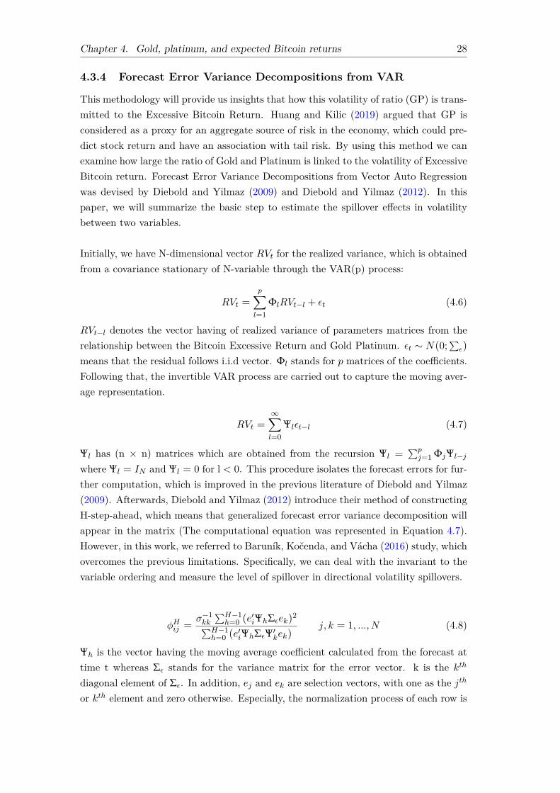
Chapter 4. Gold, platinum, and expected Bitcoin returns 28
4.3.4 Forecast Error Variance Decompositions from VAR
This methodology will provide us insights that how this volatility of ratio (GP) is trans-mitted to the Excessive Bitcoin Return. Huang and Kilic (2019) argued that GP isconsidered as a proxy for an aggregate source of risk in the economy, which could pre-dict stock return and have an association with tail risk. By using this method we canexamine how large the ratio of Gold and Platinum is linked to the volatility of ExcessiveBitcoin return. Forecast Error Variance Decompositions from Vector Auto Regressionwas devised by Diebold and Yilmaz (2009) and Diebold and Yilmaz (2012). In thispaper, we will summarize the basic step to estimate the spillover effects in volatilitybetween two variables.
Initially, we have N-dimensional vector RVt for the realized variance, which is obtainedfrom a covariance stationary of N-variable through the VAR(p) process:
RVt =p∑l=1
ΦlRVt−l + εt (4.6)
RVt−l denotes the vector having of realized variance of parameters matrices from therelationship between the Bitcoin Excessive Return and Gold Platinum. εt ∼ N(0;
∑ε)
means that the residual follows i.i.d vector. Φl stands for p matrices of the coefficients.Following that, the invertible VAR process are carried out to capture the moving aver-age representation.
RVt =∞∑l=0
Ψlεt−l (4.7)
Ψl has (n × n) matrices which are obtained from the recursion Ψl =∑pj=1 ΦjΨl−j
where Ψl = IN and Ψl = 0 for l < 0. This procedure isolates the forecast errors for fur-ther computation, which is improved in the previous literature of Diebold and Yilmaz(2009). Afterwards, Diebold and Yilmaz (2012) introduce their method of constructingH-step-ahead, which means that generalized forecast error variance decomposition willappear in the matrix (The computational equation was represented in Equation 4.7).However, in this work, we referred to Baruník, Kočenda, and Vácha (2016) study, whichovercomes the previous limitations. Specifically, we can deal with the invariant to thevariable ordering and measure the level of spillover in directional volatility spillovers.
φHij =σ−1kk
∑H−1h=0 (e
′iΨhΣεek)2∑H−1
h=0 (e′iΨhΣεΨ′kek)
j, k = 1, ...,N (4.8)
Ψh is the vector having the moving average coefficient calculated from the forecast attime t whereas Σε stands for the variance matrix for the error vector. k is the kth
diagonal element of Σε. In addition, ej and ek are selection vectors, with one as the jth
or kth element and zero otherwise. Especially, the normalization process of each row is

Chapter 4. Gold, platinum, and expected Bitcoin returns 29
calculated as θHjk =θHjk∑N
k=1 θHjk
. Thus, the total interconnectedness from volatility shocks
in the estimation to total forecast error variance:
SH = 100× 1N
N∑j,k=1;j 6=k
θHjk (4.9)
It is worth noting that∑Nk=1 θ
Hjk = 1 and
∑Nj,k=1 θ
Hjk = N . In this paper, we replicated
the 12-month rolling window as one year from (t - 11) to point t. In addition, we choosethe VAR lag length based on AIC criteria.
4.4 Results
4.4.1 Data description
Our data are retrieved from two main sources: (i) coinmarketcap.com for daily Bitcoinprice from 1st May 2013 to 28th October 2019 and (ii) Thomson Reuters for Gold andPlatinum prices. We calculated the natural logarithm daily return based on Bitcoinprices. Afterwards, we constructed the average monthly return9 for Bitcoin from theaverage daily return instead of using the beginning and ending data, which implies theforgettable memories in this period. Our main reason is used for monthly data becausewe consider Bitcoin as the alternative investment (not speculative asset with daily trad-ing data). In addition, the conventional investment model prefers using monthly data todaily data due to the avoidance of noise trading and the unrealistic of investing strate-gies in restructuring portfolio by each month (Huang and Kilic, 2019; Yang, Zhang,and Zhang, 2020). In the Bitcoin studies, the use of monthly data could be referred toDwyer (2015), Eom et al. (2019), and Chevapatrakul and Mascia (2019) for the realizedvolatility and returns. More importantly, we employed two types of robustness checkto examine whether log GP is a persistent factor in investing strategies (monthly data)and speculative strategies (daily data) or not. In addition, the test of the January ef-fect, which significantly increases the gold consumption in the world, will be examined.Because the controversial debate regarding data sources in cryptocurrency research ismentioned in Alexander and Dakos (2020), we also used alternative sources of Bitcoinprices from Thomson Reuters, which was collected from Bitstamp for robustness checkour validity of data sources.
Figure 4.1 plots logGP ratio and Bitcoin prices. We observe that the average monthlyBitcoin price goes up during the period from 2013 to 2019. Noticeably, after the crashof Bitcoin in January 2018, Bitcoin prices went down but the GP ratio increased. Itis very interesting to conclude this characteristic of these two assets (counter-cyclicaland interconnected relationship in crisis period), which is an element to predict theasset pricing model of (Huang and Kilic, 2019). Table 4.1 shows descriptive statistics
9The average monthly is calculated as R = 1n∑n
i=2 ln(PiPi−1). We refer to the calculation fromthe study of Huynh, Wang, and Vo (2021) for monthly average Bitcoin returns.

Chapter 4. Gold, platinum, and expected Bitcoin returns 30
of our variables. Similar to the equity valuation ratio of Huang and Kilic (2019), thecorrelation between EBR and logGP is high (ρ Pearson = -0.5501 and p-value < 0.01).Our AR(1) coefficient for log GP is 0.99, which means inside the unit circle.
Notes: This figure shows the natural logarithm of the Gold-Platinum prices Ratio and Bitcoin pricesfrom 2013 to 2019. Our data is monthly frequency.
Figure 4.1: LogGP ratio and Log Bitcoin price
The excessive Bitcoin return over the risk-free rate is negative. It means that the invest-ment in Bitcoin does not earn the positive return in comparison with the 3-month USTreasury bill. Although the average excess return is negative, the variable is positivelyskewed and fat-tailed. This implies that investors gain large Bitcoin return duringthe period from May 2013 to October 2019; however, it is also reasonable to concludethat investors suffer due to unexpected losses. The EBR rejects the null hypothesisof normality of the distribution at the 1% significance level. Thus, the variable doesnot follow a normal distribution. On the other hand, log GP tends to have normaldistributions with the Jarque-Bera test rejected at the 10% significance level.
In order to avoid spurious results of our estimates, we need to perform stationary tests.Formally, we performed different tests of stationary to assure that our variables arestationary. The results are presented in Table 4.2.
We find that the EBR is stationary at any level while logGP is only stationary with aweak condition when controlling for trend effects using the Augmented Dickey Fuller(ADF) and Phillip-Perron (PP) test, respectively. Therefore, the results suggest to

Chapter 4. Gold, platinum, and expected Bitcoin returns 31
Table 4.1: Descriptive statistics of Gold-Platinum and excessive Bitcoin return
Variable Mean Std. Dev. Min Max Skewness Kurtosis JBEBR -0.0060 0.0132 -0.0383 0.0564 0.8901 8.1243 95.64***logGP 0.1918 0.2008 -0.1333 0.5558 -0.1912 1.8441 4.817*
Notes: The symbols ***, **, and * indicate significance at the 1%, 5%, and 10% levels, respectively. JBdenontes Jarque-Bera test for normality. Monthly data from May 2013 to October 2019. EBR is ExcessBitcoin Return, calculated by the discrepancy between real Bitcoin return and risk-free rate return of 3-month US Treasury bill. Gold fixing prices are collected from the London Bullion Market Association whileplatinum fixing prices are retrieved from London Platinum and Palladium Market. These data are dailyand recalculated by average daily price to monthly prices. logGP was calculated by the natural logarithmof the ratio between Gold and Platinum prices by monthly frequency.
Table 4.2: Stationary test
Variable ADF (No-trend) ADF (Trend) PP PP (Trend)EBR -5.079*** -7.075*** -5.119*** -7.167***logGP -0.239 -3.276* -0.044 -3.236*
Notes: The symbols ***, **, and * indicate significance at the 1%, 5%, and 10% levels, re-spectively. ADF denotes Augmented Dickey-Fuller test, which strictly follows a unit-root pro-cess with additional lags of the first-differenced variable while PP stands for Phillip Perron test(1988), using Newey-West standard errors to account for serial correlation.
also put time-effects in the predicted return regression. In addition, when we testedthe first-difference of log GP, we found that this variable is stationary (ADF: p <
0.001 and PP: p < 0.001). Because our data has the weak stationary at the originallevel I(0) and the strong stationary at the first-difference I(1), which is similar to theprevious study of Huang and Kilic (2019). Hence, apart from OLS and VAR in ourempirical section, we will examine the co-integration test and use the Vector error-correction models (VECM) to examine the relationship between log GP and ExcessBitcoin Return.
4.4.2 Wavelet Multiple Correlation Results
Before starting with expected return prediction, this part examines correlations be-tween Gold-Platinum and Excessive Bitcoin Return under the changes of cyclical scale.As the previous part mentioned that the interconnectedness of these variables varyingwith the countercyclical. Therefore, using the wavelet multiple correlation, devised byFernández-Macho (2012) to bring better statistical interpretation due to the partici-pant of random variables, representing random changes in return. Figure 4.2 shows thewavelet multiple correlation of triple variables (Gold-Platinum ratio, Excessive BitcoinReturn, and Normal random distribution variables) with the chosen of the maximaloverlap discrete wavelet transform (MODWT) as length of 8 (Liow et al., 2019; Re-boredo and Rivera-Castro, 2014).
Our result indicates that the multiple correlation lies in average level. However, thiscorrelation value starts at nearly a half of 0.5 and rises at the increasing time scale. In

Chapter 4. Gold, platinum, and expected Bitcoin returns 32
This graph demonstrates the wave multiple correlation for GP Ratio and Excessive Bitcoin Return.The U-line and L-line correspond to the upper and lower bounds of the 95% confidence interval.
Figure 4.2: Wavelet multiple correlation for GP Ratio and Excessive Bitcoin Return
addition, the cross-correlation among log GP, Excess Bitcoin return and randomnessappears significance at time-scale 2. In contrast, the time-scale 4 and 8 tend to beinsignificant. It means that the relationship between Gold-Platinum Ratio and ExcessBitcoin Return ruled out by longer time-horizon. Saying in another way, each twotime-scale, the movement of the ratio of Gold and Platinum and Excess Bitcoin Returnis likely to have the same movement (going up or going down). As seen in the firstscale (random changes), this correlation is lower than having Gold-Platinum existencein terms of correlated comparison. Then, under longer time horizons, the dependence ofGold-Platinum Ratio on Excessive Bitcoin Return is decreasing while itself correlation,EBR, increases. This means that Excessive Bitcoin return could be relied on randomchanges, itself and GP at different time horizons.
The Wave multiple correlation result reveals the existence of randomness between Bit-coin return and logGP for the periods of time longer than one month. This methodconsists of a set of multi-scale correlations, calculated by the square root of the re-gression coefficient from the linear model of wavelet coefficients so that this coefficientof determination has the maximum value. By doing so, we can see the dependencebetween two continuous variables with the existence of randomness over the differenttimescales. Although this method is applied in financial and cryptocurrency world aswell as the precious metals world (Omane-Adjepong, Ababio, and Alagidede, 2019;Omane-Adjepong and Alagidede, 2019; Hkiri et al., 2018; Boubaker and Raza, 2017;Das et al., 2018; Tweneboah and Alagidede, 2018), to the best of our knowledge, thispaper is the first application between the ratio of gold and platinum to examine the

Chapter 4. Gold, platinum, and expected Bitcoin returns 33
dependence with Bitcoin return under randomness. Apart from the statistical evidencethat Gold and Platinum have a dependence on Bitcoin by two different time-scale, thispaper focuses on the predictability of these precious metals on ‘Digital Gold’, mentionedin the following parts.
4.4.3 Bitcoin return predictability
There are two main reasons for us to implement OLS, VAR, and quantile regression asBitcoin return predictability instead of quantile autoregression. First, the conventionalof asset pricing model usually considers the exogenous factors than itself in terms of ex-plaining asset returns (Huang and Kilic, 2019; Fama and French, 2015; Hodrick, 1992).Second, Quantile autoregression (including the lagged terms of the dependent variable)has possible misspecification (refer to the comment part of studies of Koenker and Xiao(2006)). Therefore, we implemented two methods to examine the role of Gold-Platinumin terms of Bitcoin return predictability (OLS, VAR, and quantile regression, for ro-bustness), which only focus on exogenous determinants. Table 4.3 shows the results ofBitcoin return predictability with different long-horizon time by using OLS.
Table 4.3: Bitcoin return predictability by Ordinary Least Squares
Bitcoin excess return 1 month 3 months 6 months 1 yearlogGP(t) 0.0481** 0.0539*** 0.0541* 0.0345**
R2 adjusted (%) 40.21 43.26 41.25 48.84
Time-effect control Yes Yes Yes YesNotes: The symbols ***, **, and * indicate significance at the 1%, 5%, and 10% levels,respectively. Bitcoin returns are calculated from overlapping monthly data and the robustOLS regressions are applied. The further estimations based on Newey and Kenneth (1987)with correcting the heteroskedasticity, autocorrelation consistent (HAC) and robust stan-dard errors are consistent to our results. Long-horizon returns are constructed from over-lapping monthly returns. Figure 4.3 demonstrates the relationship between the ratio ofGold-Platinum prices and Excess Bitcoin Return.
As seen in Table 4.3, the Gold-Platinum ratio is a very good predictor to forecast theBitcoin return. All coefficients are positive and significant. This means that when Goldprices increase relatively to an increase of Platinum prices, the expected Bitcoin returnalso increases. It means that the logGP high when the Bitcoin prices are low; therefore,the Bitcoin risk premium is high, giving the ratio of GP the predictive power to theBitcoin future return. Thus, if investing into this market, investors need to require thehigher premium to subsidy for the risk they might bear in the future. Our findingsare in-line with the previous literature (Huang and Kilic, 2019). The predictability ofthe model varies from 40.21% to 48.84%. In addition, our estimated co-efficient onlogGP for one-month horizon is 0.0481 and the standard deviation of logGP is 0.2008.It implies that one standard deviation increase in logGP has in association with 0.96%increase in Bitcoin excess return in the following month. We can easily interpret theremainder of significant coefficients in our estimated models for the changes in logGP,

Chapter 4. Gold, platinum, and expected Bitcoin returns 34
This figure shows the natural logarithm of the Gold-Platinum prices Ratio and Excess Bitcoin Returnfrom 2013 to 2019. Our data is monthly frequency.
Figure 4.3: LogGP ratio and Excess Bitcoin Return
which associates with the positive increase in the Bitcoin excess return. To avoid thespurious results raised from weak stationary time-series, we also employed the Vectorerror-correction models (VECM) for Excess Bitcoin Return and log GP with at leastone cointegrating equations (Johansen tests for cointegration). Our results are still ro-bust. In addition, we also extracted the residual from our regression to test whether theresidual is stationary at I(0) or not. Consequently, all of our residual from regressionare I(0)10.
Table 4.4 demonstrates the predictability of the ratio of Gold-Platinum on the ExcessiveBitcoin Return (EBR) by using Vector Auto Regressive model (VAR). The previousliterature of Hodrick (1992) uses Vector Autoregression (VAR) framework to predictthe overlapping returns. As the same pattern to the OLS estimation, the ratio of goldand platinum is still a good predictor of the Excessive Bitcoin Return from all horizonsfrom one month to one year.
In this part, our results indicate that the ratio of logGP is predictive tool to forecast theExcessive Bitcoin return in the upcoming months (with our estimated windows as 1,3, 6 and 12 months). We find that the ratio (log GP) provides explanatory significance
10T-statistics values of our residual estimates for each horizon (1 month, 3 months, 6 months and12 months) are -7.85, -7.79, -8.83 and -5.48, respectively.

Chapter 4. Gold, platinum, and expected Bitcoin returns 35
Table 4.4: Bitcoin return predictability by Vector Auto Regressive (VAR)
Bitcoin excess return 1 month 3 months 6 months 1 yearlogGP(t) 0.0419* 0.0516** 0.0458** 0.035*
R2 adjusted (%) 41.59 43.44 43.42 48.85
Time-effect control Yes Yes Yes YesNotes: The symbols ***, **, and * indicate significance at the 1%, 5%, and 10% lev-els, respectively. VAR method is employed as the study of Hodrick (1992) for financialasset predictability, which imposes parametric assumption. Long-horizon returns are con-structed from overlapping monthly returns. Figure 4.3 demonstrates the relationship be-tween the ratio of Gold-Platinum prices and Excess Bitcoin Return.
around 40% change in the Bitcoin excess return. In addition, all coefficients are signifi-cantly positive, which implies the persistent and strong association with future Bitcoinreturn while the ratio of Gold-Platinum was considered as the proxy for the potentialaggregate source of risk in the economy in the near future. In addition, when using theVAR Granger to examine the causal relationship between this ratio and the ExcessiveBitcoin return, we found that the changes in Gold/Platinum ratio cause the changes inBitcoin return with Granger causality Wald tests (χ2 = 5.104, p < 0.05). However, wedo not find the further evidence in the opposite direction (Bitcoin 6→ Gold/Platinumratio, χ2 = 0.0003, p = 0.98). It implies that there is not only predictability of Bitcoinreturn, this ratio also causes the changes. Clearly, the Bitcoin return is driven by thebehavior in trading the precious metals.
As mentioned in the literature, the ratio of natural logarithm between Gold and Plat-inum prices has the systematic risk information. Therefore, we examine how this ratiocorrelates with the Economic Policy Uncertainty from Baker, Bloom, and Davis (2016).We find that log GP has strong correlation (ρ = 0.7823, p < 0.01); βEPU = 0.00029with explanatory R2 as 94% to log GP ratio. Therefore, we confirmed that the increasein log GP at time t conveys the variation in aggregation market risk, which would in-crease the expected Bitcoin return in the future as the risk premium or discount ratesfor the alternative investment.
Table 4.5: Volatility spillover table rows (to), columns (from)
One to four days Five to inf daysEBR lnGP EBR lnGP
→ EBR 36.71 0.78 40.11 22.4→ lnGP 0.11 0.53 11.16 88.2
Notes: Table 4.5 decomposes the volatility spillover indices fromone variable to another variable. The net spillover effects betweennet-contributors and net-recipients of volatility spillovers across twomarkets are 2.34% and 20.74% for the short-term and long-term pe-riods, respectively.
Table 4.5 represents that the contribution of lnGP to the Excessive Bitcoin return in

Chapter 4. Gold, platinum, and expected Bitcoin returns 36
short term is only 0.78% while this effect is stronger in the long run, up to 22.4%. Itmeans that the changes in the volatility of Bitcoin are not associated with the contem-poraneous shocks but there exists the dynamic and time-varying link. Although thestudy of Dyhrberg (2016a) confirms that Gold and Bitcoin share similarities in hedgingcapabilities and the symmetrical reaction, our results support the findings from Baur,Dimpfl, and Kuck (2018) that Bitcoin has exhibits distinctively different volatility andreturn features compared to gold. If Bitcoin and gold share the similar characteris-tics as Dyhrberg (2016a) suggestion, their volatility transmission through frequencyconnectedness should be low. From another perspective, we do find that the ratio ofnatural logarithm in Gold and Platinum prices have the higher volatility connectedness.Thus, this study also contributes to the existing literature by examining the spillovereffects between two kinds of assets. In addition, the role of ‘flight-to-quality’ of goldhas been confirmed by many previous studies (see from Erb and Harvey (2013) andBarro and Misra (2016)), the volatility spillover could be a potential channel for thefurther explanation of an increase in the expected return of Bitcoin. As seen in Figure4.4, on average, the time-varying spillover index exhibits a great degree of fluctuationaround the volatility spillover indices, ranging from about 10% to 50%. Especially,in the period of Bitcoin crash, the link of volatility between Bitcoin and this ratiois quite low while the booming period is witnessed the stronger volatility contagion.Our results imply that shocks from Gold and Platinum markets do not necessarily andsubstantially impact the volatility of Bitcoin market over the whole sample period,but the degree of volatility spillover varies over time. In addition, it also confirms thepredictability power of this ratio to the Bitcoin return, which might be misunderstoodby the high dependence volatility resulting in the return. Hence, we can confirm thegold and platinum prices can largely be explained by the same risk factors causing thecryptocurrency market.
Our findings manifest positive coefficients of log GP in terms of predicting the expectedBitcoin return. Using the economic intuition from (Huang and Kilic, 2019; Bouri,Wohar, et al., 2019; Wolff and Neugebauer, 2019; Gao, 2016), we attempt to explain theexpected premium in investing in Bitcoin. The increase in log GP at time t implies thatthe ratio of log GPt is relatively higher than log GPt−1. Meanwhile, log GP is insulatedfrom shocks to consumption. More importantly, gold prices fall by less than platinumprices in these shocks because gold has two functions, namely consumption and storage(as many financial institutions are using as collateral). In contrast, Platinum has mainpurpose of jewelry. Thus, the increase of log GP reflects the rising storage behaviorsfrom systematic risk. This factor significantly increases the expected Bitcoin returnsin time (t+ 1), which means that expected price E(Pt+1) should be relatively higherthan the current price Pt+1. It implies the higher required risk premium for investorsto invest in Bitcoin.

Chapter 4. Gold, platinum, and expected Bitcoin returns 37
Notes: We also plot the total volatility Spillover index using a 365-day rolling window estimation,equivalent 12 months because Bitcoin does not have trading gap time as well as non-working days.
Figure 4.4: Spillovers from volatility by using 12-month window rolling
4.4.4 Robustness check
The quantile regression results for robustness in Table 4.6 suggests that the ratio ofGP would be good at predicting Bitcoin return if investors choose to hold less thanone-year maturity. Precisely, the GP predictor is well sensible to predict the Bitcoinreturn in the short-term period.
Interestingly, the one-year excessive return does not experience any statistical coeffi-cients, which implies that the ratio of Gold-Platinum is the weakly predictive tool forthe long horizon investment (equally and above one-year). In addition, the R-squareindicator also shows that one-month (with the highest values) is likely to be an appro-priate time that this ratio plays its predictive role in Bitcoin excessive return. The useof quantile regression in asset pricing is employed by several papers (Pedersen, 2015;Huynh, Nguyen, and Duong, 2018). Apart from the OLS with Newey and Kenneth(1987) correction and Vector Auto Regression with matrix construction, this paper alsoconfirms the robustness of Gold-Platinum ratio in terms of forecasting the Bitcoin ex-cessive return.
Table 4.7 also confirms that the effect of new year does not influence the predictabilityof this ratio (Gold-Platinum). Although the previous studies indicate that gold pricesmight increase in New Year due to several reasons, Gold-Platinum remains its charac-teristic to predict Bitcoin excessive return in the following month. Finally, we confirmthe characteristic of Gold-Platinum to predict the future Bitcoin return through ourmodel during the period from 2013 to 2019.

Chapter 4. Gold, platinum, and expected Bitcoin returns 38
Table 4.6: Bitcoin return predictability by quantile regression
Bitcoin excess return 1 month 3 months 6 months 1 yearQuantile (q=10)
logGP(t) 0.7594*** 0.4651** 0.5215*** -0.1864R2 adjusted (%) 83.91 76.71 79.76 76.74
Quantile (q=25)logGP(t) 0.8077*** 0.3695* 0.5151*** -0.1819
R2 adjusted (%) 86.85 80.01 80.39 75.79
Quantile (q=50)logGP(t) 0.8056*** 0.3101*** 0.2369*** -0.2259
R2 adjusted (%) 85.88 79.42 77.54 72.05
Quantile (q=75)logGP(t) 0.8028*** 0.5284*** 0.5084*** -0.1307
R2 adjusted (%) 84.57 76.99 74.74 69.23
Quantile (q=90)logGP(t) 0.7193*** 0.6851*** 0.6490*** -0.3593*
R2 adjusted (%) 83.59 77.9 71.7 68.43
Time-effect control Yes Yes Yes YesNotes: The symbols ***, **, and * indicate significance at the 1%, 5%, and 10% levels,respectively. Bitcoin returns are calculated from overlapping monthly data and the ro-bust OLS regressions are applied. Long-horizon returns are constructed from overlappingmonthly returns.
Table 4.7: Bitcoin return predictability with January effect sub-sample
Bitcoin excess return With January effect Without January effectlogGP(t) 0.0868* 0.0434*
R2 adjusted (%) 43.36 41.83
Time-effect control Yes Yes
Robust effect Yes YesNotes: The symbols ***, **, and * indicate significance at the 1%, 5%, and 10% levels, re-spectively. The further estimations based on Newey and Kenneth (1987) with correcting the het-eroskedasticity, autocorrelation consistent (HAC) and robust standard errors are consistent to ourresults.

Chapter 4. Gold, platinum, and expected Bitcoin returns 39
Another robust check in our paper is a change in the frequency of data. We con-structed the daily data for examined whether the predictive power of log GP still holdsor not. Table 4.8 demonstrates the daily characteristics of Excess Bitcoin Return andlog GP. There are two main worth noting things from this table. First, our variableshave non-normal distribution. Second, the stationary feature is satisfied with the trendexistence. It also implies that we should consider the time-effect as well as the Vector-Error-Corrected Model for our robust check.
Table 4.8: Descriptive statistics for daily data
Variable Mean Std. Dev. Skewness Kurtosis JB ADF ADF (trend)
Daily EBR -0.8191 0.8563 -0.6057 1.7915 216.7*** -2.209 -3.697**Daily Log GP 0.0888 0.0887 -0.2290 1.8430 114.6*** -0.162 -3.853**
Notes: The symbols ***, **, and * indicate significance at the 1%, 5%, and 10% levels, respec-tively. JB denontes Jarque-Bera test for normality. ADF stands for Dickey-Fuller stationary testwith- and without- trend. Daily data from 1st May 2013 to 31st October 2019. EBR is ExcessBitcoin Return, calculated by the discrepancy between real Bitcoin return and risk-free rate returnof 3-month US Treasury bill. Gold fixing prices are collected from the London Bullion Market As-sociation while platinum fixing prices are retrieved from London Platinum and Palladium Market.These data are daily. logGP was calculated by the natural logarithm of the ratio between Gold andPlatinum prices by daily frequency.
Table 4.9 demonstrates the predictability of log GP on Bitcoin daily return with time-horizon from 1 day to 7 days from another data source (Bitstamp). Our robust resultsare also in line with the previous findings that when the ratio of Gold and Platinumincreases, the expected Bitcoin return also rises. Therefore, our main results are robustwhen the frequency of our data ranges from daily to one year. In addition, the studyof Alexander and Dakos (2020) raised a concern that cryptocurrency market indexvaries significantly, depending on the data source and the index selected. Therefore, weemployed another source suggested by Alexander and Dakos (2020) and Corbet et al.(2018) to consider whether our results are robust or not. Overall, log GP still holds itspredictive power on the Bitcoin excess return.
Table 4.9: Bitcoin predictability by Ordinary Least Squares with data from Bitstamp
Bitcoin excess returnDaily (Bitstamp) Monthly (Bitstamp)
1 day 7 day 1 month 3 month 6 month 12 month
logGP(t) 4.1326*** 4.2376*** 0.0552* 0.0694*** 0.071 0.0439**R2 34.98 34.84 26.1 30.46 28.24 33.79
Time-effect control Yes Yes Yes Yes Yes Yes
Notes: *** p < 0.01, ** p < 0.05; * p < 0.1. Bitcoin returns are calculated from overlappingdaily data and the robust OLS regressions are applied. The further estimations based on Neweyand Kenneth (1987) with correcting the heteroskedasticity, autocorrelation consistent (HAC) androbust standard errors are consistent to our results.
To examine whether the predictive power of the ratio log GP holds or not, we substi-tuted Bitcoin data with data for Ethereum. Again, we find an association between theExcessive Ethereum returns and the natural logarithm of Gold and Platinum prices.

Chapter 4. Gold, platinum, and expected Bitcoin returns 40
The results are available in Appendix C.1, C.1, and D.3. Therefore, the validity of thisratio does not only apply to Bitcoin but also other alternative coins (altcoin) in thecryptocurrency market.
4.5 Conclusion
In this study, we examined the prediction power of Gold-Platinum as an economic statevariable on Bitcoin. By applying wavelet multiple correlation and several econometricsmodels, we find that Gold-Platinum is able to predict Bitcoin particularly well in theshort-term period (less than one year). When the price of gold relative to platinumincreases, Bitcoin return goes up as well. This is consistent to the literature andshows that Bitcoin can be indeed considered a safe haven asset and a store of valuewith similar characteristics as gold. Although Bitcoin has yet to see a major globalfinancial crisis, our findings have important implications for investors who are lookingfor alternatives for hedging their investments during economic distress, as gold hasproven less reliable in recent years. Future research might investigate whether theresults are consistent across different cryptocurrencies. Our results are also persistentwith robustness check by using different quantile levels and January effects (changesin the gold demand). By using the ratio of Gold-Platinum, we accomplish one ofthe advantages namely the counter-cyclical form suggested by Huang and Kilic (2019)from the economic background. In our model, Gold-Platinum also reflects the dynamicsand predictability of Bitcoin return during the financial turmoil. However, the role ofinstitutional players need to be more examined in both gold and Bitcoin markets. Thisis still a promising avenue for the future researches.

41
Chapter 5
Does Bitcoin React to Trump’s Tweets?§
5.1 Introduction
President Donald J. Trump’s incessant and sometimes caustic tweeting gathers a world-wide audience. Although Twitter might or might not be an official channel for US pol-icy1, Trump’s tweets are political news and escalate global uncertainty as suggested bythe nearly fourfold increase in the Index of Global Economic Policy Uncertainty from230.75 at the start of Trump’s presidency in 2017 to 907.43 in November 2019.
Financial markets digest Trump’s tweets for potential effects, and scholars have doc-umented them. Beckers (2018) found evidence to challenge the Efficient Market Hy-potheses after showing that lagged variables for social media news could predict globalequity returns the next month. Examining word clusters, Liu (2017) found that Trumptweets featuring ‘jobless’ and ‘worst’ preceded equity market declines. Trump tweetsalso preceded a decline in the S&P500 and an increase in the CBOE Volatility Indexduring trade disputes with China.
Market values of cryptocurrency now exceed the GDP of 130 countries (Selmi, Tiwari,Hammoudeh, et al., 2018). Cryptocurrency has become a platform for ‘Fintech’ and‘peer-to-peer’ lending. Huynh, Wang, and Vo (2021), Shahzad et al. (2019a), and Wanget al. (2019) have indicated cryptocurrencies could be safe-haven investments, implyingthe property characteristics (Yuneline, 2019). As investors and researchers ask, ‘Whatdrives Bitcoin returns?’, studies answer with reference to supply and demand (Cia-ian, Rajcaniova, and Kancs, 2016), investor attention (Corbet, McHugh, and Meegan,2014; Urquhart, 2018), speculative bubbles (Cheah and Fry, 2015), or economic policyuncertainty (Demir et al., 2018). Studies also confirm that social media influences cryp-tocurrency markets. Urquhart (2016) and Urquhart (2018) found that Bitcoin pricescould be predicted and joined Beckers (2018) in contributing an empirical evidence
§This chapter is based on Huynh, T. L. D. (2021). Does Bitcoin React to Trump’s Tweets?. Journalof Behavioral and Experimental Finance, 31, 100546, https://doi.org/10.1016/j.jbef.2021.100546. Inaddition, this work was presented at the online seminar participants at the Brazil Finance WebinarSeries, Finance Research Forum (organized by the Department of Finance at Monash University’sMalaysia Campus), and the Korean Academic Association of Business Administration (KAABA) JointInternational Conference (organized by the Korean Academic Association of Business Administration)
1https://edition.cnn.com/2017/06/06/politics/trump-tweets-official-statements/index.html

Chapter 5. Does Bitcoin react to Trump’s Tweets? 42
disputing the Efficient Market Hypothesis. Shen, Urquhart, and Wang (2019) used anumber of hashtags in Twitter platforms and found that the number of tweets writtenby investors could forecast Bitcoin volatility, volume, or returns.
This study investigates whether Trump’s tweets have influenced Bitcoin markets. Itdiffers from earlier studies in that we do not define whether those tweets constitutepolicy announcements or reflect investor sentiment. We presume, instead, that theyobviously constitute a statement from the US Chief Executive, and that—as afore-mentioned studies proved—they can impose uncertainties on Bitcoin markets. Morespecifically, we textually assess the sentiment of 13,918 Trump tweets covering January2017 to January 2020. We cluster text into negative words (indicating downbeat ordisapproving attitudes), positive words (indicating optimistic or approving attitudes),and total words (frequency with which Trump tweets). We then measure their spillovereffects on prices and volatility in Bitcoin markets.
This study makes five contributions to scholarly literature during ‘The Age of Twitter’(Ott, 2017). First, it adds to studies of relations between perspectives in social mediaand Bitcoin, an innovative payment network and a new kind of money. Second, it com-bines state-of-the-art textual analysis and sophisticated Vector Autoregression to assesseffects on a financial market. Third, it proposes a factor for predicting Bitcoin returns.Our findings are twofold. First, lagged terms denoting Trump’s sentiment significantlypredict positive Bitcoin returns, negative trading volume, and mixed volatility, but neg-ative sentiment has a Granger-causal relationship only with volatility. Second, spillovereffects of Trump’s tweeted sentiments on Bitcoin exhibit time-varying dependence, withlonger periods showing greater spillovers since 2019. Additionally, the volatility trans-mission exhibits large fluctuations during shorter periods. Additionally, our study alsocontributes to the ongoing studies about financial markets and COVID-19 that Trumpsentiment, particularly in the disease outbreak, could act as the predictive tool to theBitcoin markets. To be more precise, there is a relationship between attitudes towardsCOVID-19 and the Bitcoin returns as well as volume. However, volatility seems to beimmune to changes in the President’s sentiment. Finally, US President Donald Trump’stweets can possibly act as the predictive power on Bitcoin’s jumps by using the frame-work of Barndorff-Nielsen and Shephard (2006). Differing from Ahn and Kim (2019)regarding the driving factor of Sentiment disagreement, our study considers specificmessages containing valuable information from Donald Trump, known as the US Pres-ident. Therefore, his opinion has been perceived as a political risk (Burggraf, Fendel,and Huynh, 2019). By doing this, our study offers a channel on how social mediainfluencers could impact the Bitcoin market while the current literature examines therole of peer opinions driving this cryptocurrency market (Ahn and Kim, 2019; Shen,Urquhart, and Wang, 2019; Urquhart, 2018).
The paper proceeds as follows. Section 5.2 generalizes the theoretical framework to

Chapter 5. Does Bitcoin react to Trump’s Tweets? 43
investigate how Trump’s sentiment might impact cryptocurrency markets. Section 5.3discusses our method. Section 4.3 summarizes how we collect, process, and charac-terize data. Section 5.5 presents findings regarding our research question. Section 5.6concludes.
5.2 Theoretical framework
We build upon the theoretical frameworks of Schwert (1981) and Wagner, Zeckhauser,and Ziegler (2018) concerning how prices of financial assets respond to the politicalnews. Since Trump’s tweets could be considered as news (Ajjoub, Walker, and Zhao,2020; Burggraf, Fendel, and Huynh, 2019), this study extends an understanding of Bit-coin reactions to the news released from the White House. Simply put, if markets reflectthe optimal news from political outcomes, there are changes in differences between ex-pected discounted payoff between two possible states and the ex-ante probability thatthis outcome happens.
Pi is the cryptocurrency price (i) prior to the date Trump posts a tweet. Pi,N andPi,P denote the expected prices of cryptocurrency given Trump’s expression of negativeand positive sentiments. In addition, πN and 1 - πN = πP are the probabilities ofTrump’s sentiments. We make two assumptions. First, discounting over a short periodis included. Second, risk aversion is a minor consideration.
Pi = πNPi,N + πTPi,P (5.1)
The price change for Bitcoin given that Trump has tweeted negative words is given by.
∆Pi = Pi,N − Pi = (Pi,N − Pi,P )(1− πN ) (5.2)
In sum, prices change once Trump expresses a positive or negative sentiment. That is,investors who might have had no particular impression form one after Trump tweets.We scale the previous equations by the initial price. Thus, returns once a Trump tweetappears are given by.
Ri =Pi,N − Pi
Pi=
(Pi,N − Pi,P )(1− πN )Pi
(5.3)
Each form of cryptocurrency responds to Trump’s sentiment differently depending uponthe sign and magnitude of the spread between Pi,N and Pi,P . So, we hold the viewof how investors react and expect on the cryptocurrency prices. If the negative andpositive tones of Trump diverged significantly over the period, it would explain whycryptocurrency prices responded strongly. Therefore, in the following part, we would

Chapter 5. Does Bitcoin react to Trump’s Tweets? 44
like to mention how we clean up the data and calculate the Trump sentiment for furtherestimating the expected prices that investors hold in the cryptocurrency market.
5.3 Methodology
5.3.1 Textual analysis
We first counted how many words appeared in a Trump tweet. Then we consultedthe 2016 Loughran and McDonald Master Dictionary to determine how many nega-tive and positive sentiments Trump expressed. Although Ahn and Kim (2019) used adifferent sentiment dictionary to correlate disagreeable sentiments and Bitcoin prices’fluctuations, we adopted Loughran and McDonald, which is synthesized from Loughranand McDonald (2011), Bodnaruk, Loughran, and McDonald (2015), and Loughran andMcDonald (2016) because it specifies sentiment words that Tetlock (2007) used in theirfinancial context analyses—for example, loss(es), impairment, adverse(ly), etc. Wecreated a proxy for negative words as the ratio of negative to total words in each tweet:
Negativity =The number of negative words
The total words× 100 (5.4)
We replicated the procedure to create a proxy for positive words. We also examinedthe impact of total words in each Trump tweet. The natural logarithm of that total isused for the total of words.
5.3.2 Spillover effects
We examined whether negative and positive words in Trump’s tweets spilled over intoBitcoin trading. We followed Diebold and Yilmaz (2009) in measuring the volatilityof any spillover. The method employs forecast error variance decompositions fromVAR, but it has two disadvantages: it depends on the order of variables, and it mea-sures only total spillovers. We turned to Baruník, Kočenda, and Vácha (2016) andDiebold and Yilmaz (2012), who capture individual effects by considering invariant-to-variable ordering. Their method is widely applied in financial contexts (Baruník andKocenda, 2019; Baruník and Křehlík, 2018; Yarovaya, Brzeszczyński, and Lau, 2016).Recently, the study of Foglia and Dai (2021a) employed this method to examine howcryptocurrency uncertainty index could impact the cryptocurrency market. Our pro-cedure initially delivered n-dimensional vector RVt, that has stationary VAR(p) underthe following process:
RVt =p∑l=1
ΦlRVt−l + εt (5.5)
The residual follows the i.i.d vector as εt ∼ N(0;∑ε) whereas Φl denotes p matrices
having the coefficients. Following that, the invertible VAR process extracts the moving
Chapter 5. Does Bitcoin react to Trump’s Tweets? 45
average representation.
RVt =∞∑l=0
Ψlεt−l (5.6)
We obtained (n × n) matrices from the recursion Ψl =∑pj=1 ΦjΨl−j where Ψl = IN
and Ψl = 0 for l < 0. This procedure isolates forecast errors for further computation,which is improved in a previous study by Diebold and Yilmaz (2009). Diebold andYilmaz (2012) later introduced a method of constructing H-step-ahead point forecastssuch that generalized forecast error variance decomposition appears in the matrix:
φHij =σ−1kk
∑H−1h=0 (e
′iΨhΣεek)2∑H−1
h=0 (e′iΨhΣεΨ′kek)
j, k = 1, ...,N (5.7)
This vector has a moving average coefficient calculated from the forecast at time t. Σεdenotes the variance matrix for the error vector. k is the kth diagonal element of Σε.ej and ek are selection vectors, with one as the jth or kth element and zero otherwise.Especially, the normalization process of each row is calculated as θHjk =
θHjk∑N
k=1 θHjk
. Thus,
total interconnectedness from volatility shocks in the estimation of total forecast errorvariance is given by:
SH = 100× 1N
N∑j,k=1;j 6=k
θHjk (5.8)
Noted that∑Nk=1 θ
Hjk = 1 and
∑Nj,k=1 θ
Hjk = N . We identified different rolling windows
as trading days in one year from (t - 199) to point t because Bitcoin trades continu-ously. We based VAR lag lengths on Akaike Information Criteria. After calculatingtotal spillover effects, we followed Baruník and Kocenda (2019) to estimate the direc-tional spillover that Trump’s sentiments send to Bitcoin and vice versa.
5.4 Data
We collected 13,920 tweets (365,690 words) from@realDonaldTrump, each time-stampedin minutes, from January 2017 to January 2020. Trump was inaugurated on January20th, 2017, so collection starts with the first moments he used his Twitter account in theWhite House. The majority of Trump’s Tweets express consistently negative attitudesabout Mexico (Benton and Philips, 2018), US–China trade relations (Burggraf, Fendel,and Huynh, 2019) and the European Financial markets (Klaus and Koser, 2020).
Figure 5.1 shows that negative and positive sentiments moved together from 2017 to2020. However, the number of negative words slightly exceeds the positive in time-varying connections. There is no significant correlation between proxies for positiveand negative sentiments (ρ = 0.0491, and OLS regression generating the insignificant
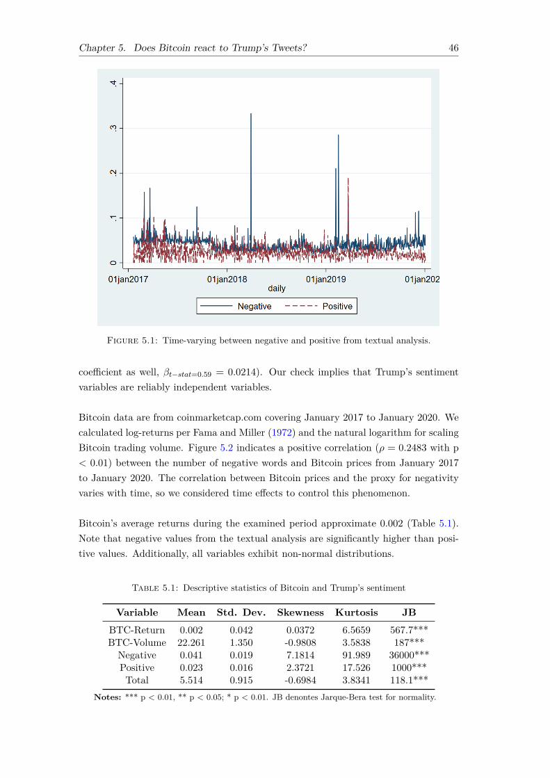
Chapter 5. Does Bitcoin react to Trump’s Tweets? 46
Figure 5.1: Time-varying between negative and positive from textual analysis.
coefficient as well, βt−stat=0.59 = 0.0214). Our check implies that Trump’s sentimentvariables are reliably independent variables.
Bitcoin data are from coinmarketcap.com covering January 2017 to January 2020. Wecalculated log-returns per Fama and Miller (1972) and the natural logarithm for scalingBitcoin trading volume. Figure 5.2 indicates a positive correlation (ρ = 0.2483 with p< 0.01) between the number of negative words and Bitcoin prices from January 2017to January 2020. The correlation between Bitcoin prices and the proxy for negativityvaries with time, so we considered time effects to control this phenomenon.
Bitcoin’s average returns during the examined period approximate 0.002 (Table 5.1).Note that negative values from the textual analysis are significantly higher than posi-tive values. Additionally, all variables exhibit non-normal distributions.
Table 5.1: Descriptive statistics of Bitcoin and Trump’s sentiment
Variable Mean Std. Dev. Skewness Kurtosis JBBTC-Return 0.002 0.042 0.0372 6.5659 567.7***BTC-Volume 22.261 1.350 -0.9808 3.5838 187***Negative 0.041 0.019 7.1814 91.989 36000***Positive 0.023 0.016 2.3721 17.526 1000***Total 5.514 0.915 -0.6984 3.8341 118.1***
Notes: *** p < 0.01, ** p < 0.05; * p < 0.01. JB denontes Jarque-Bera test for normality.

Chapter 5. Does Bitcoin react to Trump’s Tweets? 47
Figure 5.2: Time-varying between Bitcoin prices and negative sentiment.
We examined Bitcoin’s average returns and average trading volume under two regimes(low and high states compared to median values). Figure 3 shows no significant dif-ference in average Bitcoin returns between low and high regimes. It is statisticallyinsignificant that average Bitcoin returns during high negativity exceed those in thelow regime. This effect seems to be the opposite for positive states. Negative andpositive sentiments in Trump’s tweets and the number of words seem to drive Bitcointrading volumes, but effects differ significantly during periods of above-average andbelow-average occurrence of positive and negative words. Our findings endorse Kamin-ski (2014), who correlates Bitcoin trading volume and sentiments expressed by 57,727unique Twitter users. The effect of Twitter sentiment on Bitcoin trading volumes isindicated as ‘speculative’ (Kaminski, 2014; Shen, Urquhart, and Wang, 2019).
Preliminary data analysis provides three conclusions. First, there is no correlationamong variables denoting negative, positive, and total words in Trump’s tweets. Sec-ond, variables are not distributed normally. Third, given time fixed-effects, only tradingvolume reacts to regimes of above-average positivity and negativity. Fluctuations inBitcoin returns are statistically insignificant during both regimes.

Chapter 5. Does Bitcoin react to Trump’s Tweets? 48
(a) Average return
(b) Average trading volume
Figure 5.3: Average return and trading volume under two regimes

Chapter 5. Does Bitcoin react to Trump’s Tweets? 49
5.5 Main findings
5.5.1 Regression and Causal relationship
Table 5.2 shows the impact of Trump’s sentiment on contemporaneous Bitcoin returns.To our surprise, coefficients for contemporaneous sentiment are insignificant. Onlynegative sentiment correlates significantly and positively with Bitcoin returns at 5%.These findings indicate that increases in Bitcoin prices correlate to Trump’s negativesentiments with a one-day lag. A 1% increase in negative sentiment is associated witha next-day increase of 11.0% to 11.7% in Bitcoin prices, depending on the regressionconsidered. Then, Shen, Urquhart, and Wang (2019) indicated Twitter does not pre-dict Bitcoin returns, but our negative coefficients are significant at 5%. Differencesin method and research question explain the disparity in findings. Previous studiesemploy the number of times the term ‘Bitcoin’ which is tweeted (@BitinfoCharts) andcapture investor sentiment. We consider the sentiment of Trump’s tweets.
Table 5.2: Impact of Trump’s sentiment on contemporaneous Bitcoin returns
Variables (1) BTC(t) (2) BTC(t) (3) BTC(t) (4) BTC(t)
Negative(t) -0.039[-0.588]
-0.064[-0.986]
Positive(t) -0.031[-0.435]
-0.023[-0.283]
Total words(t) -0.0001[-0.053]
-0.0001[-0.237]
Negative(t−1) 0.110**[1.993]
0.117**[2.038]
Positive(t−1) -0.062[-0.819]
-0.061[-0.711]
Total words(t−1) 0.002[1.026]
0.002[1.086]
Negative(t−2) 0.054[0.606]
0.031[0.347]
Positive(t−2) 0.026[0.298]
0.022[0.250]
Total words(t−2) -0.0001[-0.030]
-0.001[-0.353]
Observation 1071 1070 1069 1053Adjusted R-square 0.004 0.005 0.003 0.007Time-effect control Yes Yes Yes Yes
Notes: This table presents OLS regression estimation results. The dependent variable iscontemporaneous Bitcoin returns. We use variance inflation factors (VIFs) to check for mul-ticollinearity. Because average mean VIF values for all variables (around 2.45) are well belowthe threshold of 10, we find no evidence for multicollinearity. t-tests reject the null hypothe-ses that Positive = Negative in all regressions. Robust standard deviations are in parenthe-ses. *** p < 0.01; ** p < 0.05; * p < 0.10. We used the time-effect to control the dynamicsof Bitcoin from the previous literature (Huynh, Burggraf, and Wang, 2020).

Chapter 5. Does Bitcoin react to Trump’s Tweets? 50
Table 5.3: Impact of Trump’s sentiment on daily contemporaneous Bitcoin volume
Variables (1) V olumet (2) V olumet (3) V olumet (4) V olumetNegative(t) -8.676***
[-2.909]-6.474***[-2.583]
Positive(t) 0.304[0.185]
-0.315[-0.184]
Total words(t) -0.020[-0.564]
-0.002[-0.057]
Negative(t−1) -9.195***[-3.207]
-7.396***[-2.998]
Positive(t−1) 0.363[0.229]
0.086[0.053]
Total words(t−1) -0.037[-1.035]
-0.025[-0.676]
Negative(t−2) -8.867***[-3.137]
-6.934***[-2.993]
Positive(t−2) 0.893[0.585]
1.697[1.201]
Total words(t−2) -0.059[-1.608]
-0.057[-1.518]
Observation 1071 1070 1069 1053Adjusted R-square 0.714 0.714 0.720 0.734Time-effect control Yes Yes Yes Yes
Notes: This table presents estimations from OLS regression . The dependent variable is contem-poraneous Bitcoin volume. We use VIFs to check for multicollinearity. Because average mean VIFvalues for all variables (1.58) are well below the threshold of 10, we find no evidence for multi-collinearity. t-tests reject the null hypotheses that Positive = Negative in all regressions. Robuststandard deviations are in parentheses. *** p < 0.01; ** p < 0.05; * p < 0.10. We used the time-effect to control the dynamics of Bitcoin from the previous literature (Huynh, Burggraf, and Wang,2020). Concomitantly, we also control the daily Bitcoin return to predict the Bitcoin volume.

Chapter 5. Does Bitcoin react to Trump’s Tweets? 51
Among surprising results in Table 5.3, trading volume declines when Trump’s tweetscontain more negative words. Moreover, the decline in trading volume contrasts withpositive returns under uncertainty regimes. This counterintuitive finding also manifestsamong conventional asset classes. However, when Bitcoin prices rise, bid-ask spreadswiden when Trump tweets more negative words. That finding indicates sellers incorpo-rate greater uncertainty premiums (lower bids, higher ask prices) into immediate trades.This behavior seems not to apply to traditional financial assets, but Aalborg, Molnár,and Vries (2019) and Koutmos (2018b) demonstrated it is commonplace for cryptocur-rency when Bitcoin trading volume declines during uncertainty. By approaching themicrostructure of Bitcoin characteristics, we explain at 1% significance why negativeTrump tweets induce positive returns as volumes decline.
Table 5.4: Impact of Trump’s sentiment on monthly contemporaneous BTC volatility
Variables (1) V olatilityt (2) V olatilityt (3) V olatilityt (4) V olatilitytNegative(t) -0.818*
[-1.859]-1.083**[-2.093]
Positive(t) -0.366[-0.383]
-0.634[-0.673]
Total words(t) -0.010[-1.479]
-0.014[-1.611]
Negative(t−1) -0.506[-1.204]
-0.556[-0.995]
Positive(t−1) 0.721[0.888]
-0.897[-1.205]
Total words(t−1) -0.005[-0.941]
Negative(t−2) 0.384[0.996]
1.383**[2.314]
Positive(t−2) 0.192[0.326]
-0.105[-0.171]
Total words(t−2) -0.006[-1.066]
Observation 37 36 35 35Adjusted R-square 0.139 0.112 0.137 0.377Time-effect control Yes Yes Yes Yes
Notes: This table presents estimations from OLS regression. The dependent variable is contemporaneousBitcoin volatility. Variance inflation factors (VIFs) confirm that the first and second lagged of total wordsexhibit multicollinearity with contemporaneous total words (VIF > 10). Therefore, we excluded those vari-ables from the regression (4). Average mean VIF values (2.88) for all variables are well below the thresholdof 10, indicating no evidence for multicollinearity. t-tests reject the null hypotheses that Positive = Negativein all regressions. Robust standard deviations are in parentheses. *** p < 0.01, ** p < 0.05, * p < 0.10.Lag length of one period is determined by the Schwarz Bayesian information criterion; we examine two daysfor further insights. We used the time-effect to control the dynamics of Bitcoin from the previous literature(Huynh, Burggraf, and Wang, 2020). Concomitantly, we also control the average Bitcoin return to predictthe Bitcoin volume.

Chapter 5. Does Bitcoin react to Trump’s Tweets? 52
Table 5.4 depicts the predictive power of Trump’s tweets on Bitcoin volatility. UnlikeShen, Urquhart, and Wang (2019) we find at 5% significance that volatility correlatespositively with a two-day lag in the variable denoting Trump’s attitudes towards neg-ative tone, and that variable with contemporaneous term correlates negatively withvolatility. In our study, we referred to the previous empirical evidence from Huynh,Wang, and Vo (2021), which estimated the realized monthly volatility by taking thedeviation from the daily price in one month. Interestingly, this study also found thata high level of global economic policy uncertainty could negatively predict Bitcoinvolatility. One of the possible explanations is the bid-ask spread, which implies theirrisk aversion. Our findings are also consistent with the sound theory by Arrow (1959)and Bernanke (1983). Accordingly, the investors tend to wait and see under a high levelof uncertainties. Concomitantly, we also used the approach of GARCH-in-mean (M-GARCH) to capture Bitcoin volatility. We also found that Trump’s negative sentiment(contemporaneous and lagged terms) could negatively predict Bitcoin volatility (See inAppendices Figure D.1 and Table D.1). The results still hold when using Threshold-GARCH (T-GARCH) (See in Appendices Figure D.2 and Table D.2)
Our findings support Aysan and Lau (2019) that changes in historical geopolitical riskdata correlate positively with Bitcoin volatility at different quantiles. Therefore, ourresults also link to the conflicts, political instability, which is through the presidentialpolitical announcements, can significantly influence Bitcoin’s realized volatility. Allin all, Bitcoin’s returns, volatility, and trading volumes respond to the sentiment ofTrump’s tweets, especially, when it is negative.
Table 5.5: Vector Autoregressive Granger causality
Granger causality χ2
Negative sentiment does not Granger cause Return 1.20Positive sentiment does not Granger cause Return 0.47Total words do not Granger cause Return 0.92Negative sentiment does not Granger cause Volume 2.35Positive sentiment does not Granger cause Volume 2.09Total words do not Granger cause Volume 0.68Negative sentiment does not Granger cause Volatility 8.95***Positive sentiment does not Granger cause Volatility 0.45Total words do not Granger cause volatility 0.62Notes: *** p < 0.01; ** p < 0.05; * p < 0.10. The lag length is determined bythe Schwarz Bayesian information criterion as one-level.
To test for causal relationships among positive sentiment, negative sentiment, and totalwords, we employ VAR Granger causality (Granger, 1969). In Table 5.5 the sentimentof Trump’s tweets influences volatility, not returns and volume. Like Shen, Urquhart,and Wang (2019), we confirm a causal relation between tweeting and Bitcoin volatility,but we find none with respect to returns and volume.

Chapter 5. Does Bitcoin react to Trump’s Tweets? 53
5.5.2 Spillover effects of Trump’s sentiment on Bitcoin market
Table 5.6 decomposes indices for the spillover effects of the sentiment in Trump’s tweetson Bitcoin. In particular, the negative sentiment contributes more to Bitcoin’s returnsthan the positive sentiment. However, OLS estimations reveal no significant coeffi-cients. In addition, a pairwise comparison of spillovers and volatility indicates thatpositive sentiments in Trump’s tweets induce greater daily volatility. The number ofwords spills over onto returns but not volatility.
Table 5.6: Trump sentiment and long-term spillovers on volatility
Return Volume Negative Positive TotalReturn 25.74 0.17 0.13 0.01 0.03Volume 7.8 89.75 0.11 0.67 0Negative 0.35 3.23 32.09 0.25 0.09Positive 0.19 0.9 0.57 27.91 0.98Total 1.05 13.07 1.41 0.86 35.14Notes: This table captures directional spillover from variable j to variablei with rows indicating spillovers on and columns indicating spillovers from.These columns contain net pairwise (i,j)-th spillover indices.
Figure 5.4 depicts the total volatility of spillover effects across three rolling windowsin the time series (three years of daily data). It shows that the effects of Trump’stweets on Bitcoin were particularly high during the 2018 crash and early 2019. Overall,spillover effects are higher during shorter periods. Spillover is dramatic, presentingfluctuations of 30 to 80, during 50-day windows and less dramatic (fluctuations of 15to 25) for longer periods. These findings indicate that the sentiment of Trump’s tweetsprecipitates wide but fleeting short-term fluctuations on Bitcoin markets.
Ours is the first study to examine the effect of Trump’s sentiment on Bitcoin marketsusing time-varying spillover effects. We find that Bitcoin digital currency is signifi-cantly affected by the political uncertainty raised by the politician. Although Bitcoinreturns rise with the negative sentiment of Trump’s tweets, this feature is challenged bythe role of non-governmental control as well as safe-haven. Our findings confirm Jiang,Nie, and Ruan (2018) that the Bitcoin market is inefficient. The market is clearly notpersistent in different rolling windows, which suggests investors should be cautious inpresuming any arbitrarily beneficial opportunity or invest with only speculative intent.Our results also suggest Bitcoin’s usefulness as a hedge due to heightened returns underTrump’s negative sentiment. Fang et al. (2019) demonstrate that Bitcoin and equitiescorrelate positively with economic policy uncertainty.
Figure 5.5 shows net spillover effects by component. Positive values indicate net con-tributors of spillovers and negative values its net recipients. The effects of Trump’s

Chapter 5. Does Bitcoin react to Trump’s Tweets? 54
(a) 200-day
(b) 100-day
(c) 50-day
Figure 5.4: Time-varying spillover effects using a different-days rolling window

Chapter 5. Does Bitcoin react to Trump’s Tweets? 55
tweeted sentiments are weaker before 2019 and stronger after. In contrast, the positivesentiment and the total words are mostly recipient with time-varying values below 0.
(a) Return, Volume and Negative
(b) Positive and Total words
Figure 5.5: Net spillover effects by each component
5.5.3 Trump attitudes towards COVID-19 pandemic and Bitcoin
Recently, Rufai and Bunce (2020) confirmed the role of Twitter’s G7 leaders in responseto the COVID-19 pandemic because it should be considered as the potential source ofinformation on the financial market. Concomitantly, the current literature indicates nolinkage between feverish news and stock return changes but volatility (Ambros et al.,2020). However, the role of fake news, as well as investors’ sentiment, play an importantrole (Huynh et al., 2021). Given the flow of Trump’s tweets having responsive policies,this study extends the Trump’s sentiment to examine whether this predictive factorholds robust during the pandemic time or not. We constructed the index of negativeand positive sentiment by calculating the fraction of the number of negative words intweets mentioning coronavirus (or COVID-19 pandemic, and so forth) over the totalnegative words on that day. It holds the same for positive sentiment. Finally, Table 5.7represents the impact of Mr. President’s attitudes towards the COVID-19 pandemic

Chapter 5. Does Bitcoin react to Trump’s Tweets? 56
on the cryptocurrency market.
Table 5.7: Impact of Trump’s sentiment regarding COVID-19 on Bitcoin market
Variables Return Volatility VolumeCOV ID Negative(t) -0.403*
[-1.871]-0.010[-0.123]
0.527[1.489]
COV ID Positive(t) 0.064*[1.929]
-0.013[-0.858]
-0.144[-0.500]
Total words(t) 0.003[1.000]
0.002[0.501]
0.044[1.318]
COV ID Negative(t−1) 0.010[0.424]
0.046[0.706]
-0.021[-0.258]
COV ID Positive(t−1) -0.011[-0.499]
-0.003[-0.084]
0.364*[1.884]
Total words(t−1) -0.002[-0.746]
-0.004[-0.701]
0.035[1.170]
COV ID Negative(t−2) 0.005[1.109]
0.000[0.010]
0.232*[1.798]
COV ID Positive(t−2) 0.031[1.432]
-0.002[-0.053]
0.213[0.885]
Total words(t−2) 0.000[0.087]
0.001[0.354]
0.078***[2.640]
Constant -0.060[-0.221]
-0.011[-0.029]
65.750***[17.980]
R-squared 0.219 0.02 0.394Time-effect control Yes Yes Yes
Notes: *** p < 0.01; ** p < 0.05; * p < 0.10. The lag length is determined by the Schwarz Bayesianinformation criterion as one-level. This table presents estimations from OLS regression. The de-pendent variable is contemporaneous Bitcoin volume. We use VIFs to check for multicollinearity.Because average mean VIF values for all variables (less than 2.0) are well below the threshold of 10,we find no evidence for multicollinearity. Robust standard deviations are in parentheses. The dailysample covers the period from December 2018 to October 2020. We used the time-effect to controlthe dynamics of Bitcoin from the previous literature (Huynh, Burggraf, and Wang, 2020). In addi-tion, we used the Bitcoin return to control the predictive regression model for volume and volatility.
While the current literature emphasizes the role of media coverage on financial marketsduring the COVID-19 time (Haroon and Rizvi, 2020), our findings also contribute tothe existing literature that the country leader’s attitudes could predict the Bitcoin mar-ket. Accordingly, the higher the pessimistic (optimistic) sentiment, the lower (higher)Bitcoin’s expected return. Differing from the previous findings, we offer an insight thatthe Bitcoin market reacts immediately (contemporaneous time) instead of a one-daylagged term. However, we also obtain weak evidence that Trump sentiment is associ-ated with the changes in Bitcoin returns at 10% significance level.
Concomitantly, we do not find any evidence that Trump’s attitudes towards pandemiccould predict the volatility while the Bitcoin volume is likely to respond to DonaldTrump’s sentiment in COVID-19 from one to two lagged days at 10% significance level.

Chapter 5. Does Bitcoin react to Trump’s Tweets? 57
Therefore, our findings confirm the extant literature that sentiment plays a role in im-proving market liquidity (Burggraf et al., 2020; Liu, 2015). To sum up, the cryptocur-rency market reacts like the financial assets when the President’s sentiment changedduring the pandemic. To be more precise, it requires more (less) risk premium whenhaving negative (positive) feelings from the leader; however, the sentiment is not thesource of risk in this period. Our findings also contribute empirical evidence to theongoing studies about financial markets and COVID-19.
5.5.4 Do Trump’s Tweets trigger the Bitcoin jumps?
In this section, we examine whether Trump’s tweets could predict the Bitcoin jumps.We employed the asymptotic distribution theory for a few non-parametric tests ofBarndorff-Nielsen and Shephard (2006) to construct the binary variables for “Positivejumps” and “Negative jumps” from the hourly return of Bitcoin. Table 5.8 representshow Trump sentiments correlate with the possibility of having a jump of Bitcoin. In-terestingly, only negative sentiments could act as the predictive factor to the Bitcoinpositive jumps. Accordingly, when Trump expressed his attitudes towards the negativetone in a contemporaneous period, it was less likely to have positive jumps at the sametime. Although we did not find any predictive power of negative sentiment at time(t) on Bitcoin returns, we extended the further empirical evidence that Trump’s pes-simistic tone negatively correlated with the likelihood of jumps having positive returns.Concomitantly, the higher (lower) return is associated with the higher (lower) possibil-ity of having positive (negative) jumps. However, a decrease in trading volume couldincrease in the chance of facing new jumps in the largest capitalization cryptocurrency.
5.5.5 Robustness check
To examine whether the sentiment of Trump’s tweets affects other cryptocurrencies,we substituted Bitcoin data with data for Ethereum (See in Appendix D.3). Again,we find an association between Ethereum’s returns and a one-day lag in sentiment.Negative sentiments relate to lower same-day trading volume and with lags of oneand two days. However, we find no Granger causality between Trump’s sentimentand Ethereum’s returns, trading volume, and volatility. Overall, our findings are stillpersisted when replacing different cryptocurrency assets. In addition, we employed thepredictive regression model to test a relationship between the Trump sentiment andpersistent variation in risk. We also found that Trump sentiments positively predictthis ratio, representing the aggregate source of risk in the economy (Huang and Kilic,2019). Hence, the possible channel of Trump’s sentiments in predicting the futureBitcoin return could be the market risk (Huynh, Burggraf, and Wang, 2020) (See inAppendix D.4).
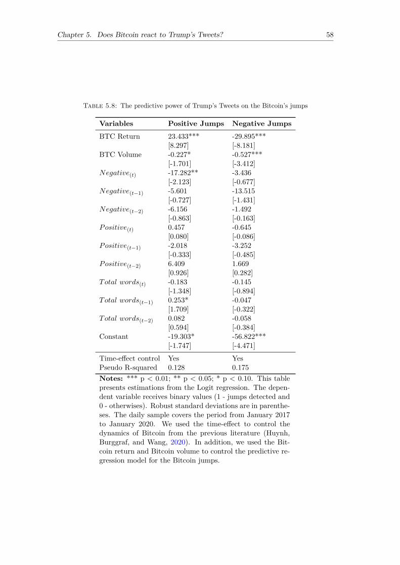
Chapter 5. Does Bitcoin react to Trump’s Tweets? 58
Table 5.8: The predictive power of Trump’s Tweets on the Bitcoin’s jumps
Variables Positive Jumps Negative JumpsBTC Return 23.433***
[8.297]-29.895***[-8.181]
BTC Volume -0.227*[-1.701]
-0.527***[-3.412]
Negative(t) -17.282**[-2.123]
-3.436[-0.677]
Negative(t−1) -5.601[-0.727]
-13.515[-1.431]
Negative(t−2) -6.156[-0.863]
-1.492[-0.163]
Positive(t) 0.457[0.080]
-0.645[-0.086]
Positive(t−1) -2.018[-0.333]
-3.252[-0.485]
Positive(t−2) 6.409[0.926]
1.669[0.282]
Total words(t) -0.183[-1.348]
-0.145[-0.894]
Total words(t−1) 0.253*[1.709]
-0.047[-0.322]
Total words(t−2) 0.082[0.594]
-0.058[-0.384]
Constant -19.303*[-1.747]
-56.822***[-4.471]
Time-effect control Yes YesPseudo R-squared 0.128 0.175Notes: *** p < 0.01; ** p < 0.05; * p < 0.10. This tablepresents estimations from the Logit regression. The depen-dent variable receives binary values (1 - jumps detected and0 - otherwises). Robust standard deviations are in parenthe-ses. The daily sample covers the period from January 2017to January 2020. We used the time-effect to control thedynamics of Bitcoin from the previous literature (Huynh,Burggraf, and Wang, 2020). In addition, we used the Bit-coin return and Bitcoin volume to control the predictive re-gression model for the Bitcoin jumps.

Chapter 5. Does Bitcoin react to Trump’s Tweets? 59
5.6 Conclusion
This paper has explored relations between Bitcoin’s returns, volatility, and trading vol-umes and the positive or negative sentiments expressed in tweets by the US PresidentDonald J. Trump. We find that the sentiment of Trump’s tweets reasonably predictsBitcoin’s returns, volatility, and trading volumes. The more negative Trump’s senti-ment, the higher returns. However, volatility diminishes when Trump tweets negativesentiments. The trading volume rises with lags of two days and declines contempora-neously. Only volatility and negativity exhibit Granger-causal relationships.
Although Donald Trump is no longer the US President, this study still has some merits.First, this is the first study to offer a relationship between textual analyses in socialmedia account of politician and cryptocurrency markets. Our study also challenges theconcept that these coins are independent of the political risk (or any uncertainties aris-ing from the specific government). After controlling the rigorous variables, we foundthat one Twitter account, particularly the US President, could drive the cryptocur-rency markets. This is the typical case of Elon Musk, the richest man in the world(Ante, 2021), who can be an influential and well-known individual on the cryptocur-rency market. In doing so, future research could explain how other politicians’ andbillionaires’ social media accounts could drive the cryptocurrency markets. Second,this paper also discusses the evolution of cryptocurrency markets’ behaviors during thepandemic crisis. To be more specific, in normal times, cryptocurrency exhibits its owncharacteristics in response to the uncertainties. However, in the crisis time, cryptocur-rency is likely to respond as the traditional financial assets. Also, future research canconsider how cryptocurrencies change during the specific period in their development.Finally, we also found that Trump’s tweets with pessimistic feelings could predict theBitcoin’s jumps; therefore, this paper contributes the predictive feature of Trump’s toneon how Bitcoin returns jump during the 2017-2020 period. Accordingly, professionaltraders could keep their eyes on the content on social media to predict when and howBitcoin exhibits large movements in its return.
We find evidence of time-varying spillover effects between Trump’s sentiments and Bit-coin prices. Longer periods showed lower spillovers in volatility than shorter periods,indicating that the short-term effects of Trump’s tweets are greater than their long-termeffects. Additionally, the negative effect is most evident during periods of above-averageand below-average occurrence of positive and negative words and the total number ofwords in Trump’s tweets. We also find Bitcoin markets seem more sensitive to Trump’snegative sentiments after 2018. This study employs daily data. Future studies mightgarner more insights using intra-day or tick-by-tick data with the existence of cryp-tocurrency uncertainty indices (Foglia and Dai, 2021b), or machine learning approach(Abdullah, 2021).

60
Chapter 6
Conclusion
This dissertation comprises four individual essays which contribute to the existing lit-erature in terms of “market reactions and cryptocurrency”. Since the detailed findingsand results have been discussed in the previous chapters, only some key features andpractical implications can be discussed in this concluding chapter. They can be sum-marized as follows.
In the first chapter, the causal relationships between political news and stock market re-actions are examined. It finds that tweets related to the US-China trade war negativelycause S&P 500 returns and positively cause VIX. The effects of political news on socialmedia are heterogeneous across industries depending on their level of trade opennesswith China. The second essay provides an industry-level analysis of the market reactionto sudden COVID-19 news announcements in the United States. The results indicatethat the market significantly reacts before February 26. More precisely, medical andpharmaceutical products have a positive reaction while restaurants, hotels, motels, andservices and utilities show the opposite finding. Furthermore, this study also exhibitsthe relationship between the searching term (‘coronavirus’), the level of investor atten-tion to COVID-19, and industry returns. The following two chapters are a collectionof a cryptocurrency study. The third chapter investigates the prediction power of theratio of gold to platinum prices (GP) on the cryptocurrency market. Since this ratiohas been used as the aggregate market risk to predict the expected stock return, bondpremium, this study provides a piece of empirical evidence that the Bitcoin (even alter-native coin - Ethereum) return goes up when having a relative increase in the price ofgold to platinum. This study also employs different methodologies, a sub-sample testfor the special period with a significant increase in gold prices, and the different datasources to validate the results. Eventually, our results hold robust. The last chapterapplies the textual analysis and spillover estimations to study whether the sentimentexpressed in the US President’s tweets is associated with the changes in price, volatil-ity, and trading volume in the cryptocurrency market. After analyzing 13,918 tweetsover 4-year starting from 2017, this work found that only negative sentiment had thepredictive power on Bitcoin returns, trading volumes, realized volatility, and jumps.By introducing a novel methodology (spillover connectedness) and constructing the so-cial media sentiment index for the market risk, it demonstrates that Trump’s Twittersentiment can impact the Bitcoin market in the form of time-varying dependence. I

Chapter 6. Conclusion 61
also carry out further analysis, particularly in the COVID-19 pandemic, and find thathis attitudes towards the coronavirus also have predictive power on the Bitcoin market.Likewise the previous chapter, our findings are persisted when replacing the alternativecoin (Ethereum).
Overall, the results documented in this dissertation contribute to the ongoing litera-ture in finance. Whether political uncertainty affecting economic activity is currentlya debatable topic. It seems stunning that politicians’ pronouncements on social me-dia could instantly create or wipe off hundreds of billions of dollars from the financialmarket. Obviously, after the global financial crisis 2007-2008, the world is more likelyto experience more uncertainties from many different aspects. This news can be fromthe withdrawal of the United Kingdom (UK) from the European Union (EU) (calledBREXIT), the conflicts in terms of trade between the United States and China, theintense criticism about immigration, and so forth. Concomitantly, the world has suf-fered from the unprecedented event, coronavirus outbreak (also known as COVID-19pandemic). These critical events partially reflect how life happens in the contempo-rary era. Significantly, this concept is also linked with technological advancement whenpolitical news can be immediately released on the Internet. In addition, life is chang-ing with quickly measuring how people pay their attention to the simple ‘click’ on theGoogle website. Taken together, the two first chapters provide evidence that givesmore complete pictures of how the market swings with political news leaked by tweetsor public health announcements confirmed by the official organization (for example,WHO). Hence, this study explains that the continuous flow of crucial news in this eraleads investors to update their beliefs in investing strategies in the future. As with otheraspects of news, time will tell whether these beliefs are justified. Therefore, this thesistries to fill this gap to study how contemporaneous events could influence the financialmarkets. Another noteworthy contribution is provided with regards to the examinationof the insights about the cryptocurrency market. The topic of cryptocurrency returnpredictability at the aggregate market risk is of great interest to both scholars and prac-titioners. Due to the incomplete literature on the intrinsic value of cryptocurrencies,this study provides empirical evidence to validate the ratio of Gold and Platinum pricesin the digital currency world. Being the first study to investigate the predictive powerof this ratio on this market, this work does not only validate the existing literaturebut also shed a new light on the prediction model in the cryptocurrency market. Theprevious evidence has been focused on equity and fixed-income markets. This studycomplements the current literature by explaining how cryptocurrencies are sensitiveto macroeconomic shocks, showing that these coins should be considered as invest-ing assets. Finally, the last academic chapter highlights the role of sentiment in thecryptocurrency market. Although traditional finance suggests that investor sentimentcan explain the stock’s price based on the divergence of price from its fundamentalvalue, there is still a space for this market. However, there is little research on thepolitician’s sentiment. This is somewhat surprising given the US President’s leakage of

Chapter 6. Conclusion 62
information or announcements as the potential risks. Then, the investors might absorbinformation with overly optimistic or pessimistic attitudes, partially leading to irra-tional investment decisions. Thus, this final study proposes a new textual disclosuretone-based politician perspective that might contain incremental sentiment informationbeyond other market participants. The result is part of a new stream of literature usingthe big text data on Twitter to capture three potential tones of Mr. Donald Trump,which significantly predict the cryptocurrency market. A realistic and straightforwardexplanation for this finding is that the role of cryptocurrencies in the financial worldhas not yet been confirmed. They can be treated as an electronic payment tool, aninvestment, a safe-haven asset, a hedging instrument, or even a diversifier. Overall, itseems extremely difficult for our empirical results to assess due to the anonymity anddecentralized trading system transparently. Among potential mechanisms, academicsand industry-sector respondents viewed that Bitcoin and other alternative cryptocur-rencies were more likely to listen to the fundamental economic news.
With regards to practical implications, the findings in this thesis are of interest todifferent stakeholders, policymakers, financial analysts, investment professionals. Jour-nalists used to describe Donald J. Trump with the strongest tone. Bigot. Racist.Trumpedy.1 The superlatives are not all bad. Trump’s presidency can be considereda natural experiment to measure the impacts of unofficial news on financial markets.This point holds to the COVID-19 pandemic. There is a great deal of fake news,conspiracy theory, and fears during these special times. Thus, resolving informationasymmetries from a wide range of information sources (social media, the White House)is the first implication for policymakers. It is worth stressing that the world will havemore unexpected news and events, widening the gap of asymmetric information. Con-comitantly, the mechanisms of supervising unexpected news should be implementedfrom the authority perspective. From the investors’ standpoint, the results contributeto the market reactions based on different sources of news. Thus, the investment profes-sionals should keep their eyes on the market, which might help identify the unexpectednews to avoid losses or make profits from the market expectations. Clearly, financialanalysts could incorporate these types of news as financial indicators to improve thecurrent models. Given the brash, petulant and unpredictable content from Donald J.Trump’s Twitter and the unprecedented and unique event from the COVID-19 pan-demic, some could probably challenge whether my results are generalizable. In thisrespect, this thesis could generate the trend and tendency of using social media aspass-through policies in the US. Furthermore, what we know about COVID-19 mightbe applicable for the future pandemic. At any rate, the results certainly provide uniqueinsight to the certain merits of financial markets in the contemporary era. As regardsthe two last chapters, research on the cryptocurrency market in finance is still in itsbeginning. Therefore, exploring two predictive indicators, such as Gold-Platinum andTrump’s sentiment, could help understand the market structure of cryptocurrency. In
1See more at Trump is an embarrassment by CNN.
Chapter 6. Conclusion 63
doing so, the algorithms and prediction model should include these elements to capturethe cryptocurrency movements. The techniques developed in this thesis can be usedin building more indices, captured the sentiment from other well-known social mediaaccounts such as Elon Musk, CZ (the founder of Binance exchange), and so forth asnew market participants are added. By shedding light on predicting Bitcoin with theaggregate market risk, this thesis hopes to explain the Bitcoin characteristic as an in-vestment tool, thereby allowing more investing decisions that weigh up the benefits andcosts under the specific market periods (growing time or distress).
Finally, this doctoral thesis moves the literature closer to answering the crucial roleof news and announcements on market reactions on the onset of pandemic and tech-nological integration. Additionally, the validity of predictive indicators, including theprecious metals or digital content, could potentially explain the cryptocurrency charac-teristics. With the more frequent data, especially tick-by-tick or each minute, anotherinteresting avenue for future research would be to model how long the market reactsafter these types of news. The future study might employ state-of-the-art hybrid deeplearning to improve the quality of textual analysis. From the standpoint of practi-tioners, these approaches could substantially improve their financial decision-makingin both the conventional and cryptocurrency markets.

64
Appendix A
Political news and stock prices:Evidence from Trump’s trade war
This section is based on Burggraf, T., Fendel, R., Huynh, T. L. D. (2020). Political news and stock prices:evidence from Trump’s trade war. Applied Economics Letters, 27(18), 1485-1488.
To assess the robustness of our results, we create a ‘placebo’ tweet variable includingtweets from Donald Trump that mention China but which are not related to the US-China trade war. Performing the same VAR-Granger causality analysis, we do not findany evidence that placebo tweets significantly influence S&P 500 return or VIX. Fi-nally, we apply our model to the Dow Jones Industrial Average index. The robustnesstests can be found in Tables A.1 – A.4.
Table A.1: Robustness Test: Vector autoregressions with Placebo Tweet
Variables Return(t) V IX(t) PlaceboTweet(t)
Return(t−1) 0.471*** -0.634 -3.716(0.11) (14.36) (2.80)
Return(t−2) -0.131 0.275 -3.379(0.10) (14.00) (2.73)
V IX(t−1) 0.002*** -0.001 0.008(0.00) (0.10) (0.02)
V IX(t−2) -0.001 -0.121 -0.044(0.00) (0.09) (0.02)
PlaceboTweet(t−1) -0.001 0.41 0.035(0.00) (0.31) (0.06)
PlaceboTweet(t−2) -0.003 0.196 0.077(0.00) (0.31) (0.06)
Note: *** p < 0.01; ** p < 0.05; * p < 0.10.Control variables are used. Robust standard errors in parentheses.

Appendix A. Political news and stock prices: Evidence from Trump’s trade war 65
Table A.2: Robustness Test: Granger causality tests with Placebo Tweet
Variable Null hypothesis 1F-statistics p-value
Return 1.7295 0.421VIX 2.1047 0.349
Note: *** p < 0.01; ** p < 0.05; * p < 0.10.
Table A.3: Robustness Test: Vector autoregressions with the Dow Jones
Variables Return(t) V IX(t) Trump Tweet(t)Dow Jones
Return(t−1) 0.394*** 6.348 -2.344(0.103) (14.216) (3.387)
Return(t−2) -0.113 -6.340 4.359(0.100) (13.888) (3.309)
V IX(t−1) 0.001*** 0.032 -0.001(0.001) (0.098) (0.023)
V IX(t−2) -0.001 -0.136 0.019(0.001) (0.092) (0.022)
Tweet(t−1) -0.005*** 0.585** 0.250***(0.002) (0.270) (0.064)
Tweet(t−2) 0.003** -0.400 0.062(0.002) (0.270) (0.064)
Note: *** p < 0.01; ** p < 0.05; * p < 0.10.Control variables are used. Robust standard errors in parentheses.
Table A.4: Robustness Test: Granger causality tests with the Dow Jones
Variable Null hypothesis 1
F-statistics p-value
Return (Dow Jones) 10.029*** 0.007VIX 5.7574* 0.056
Note: *** p < 0.01; ** p < 0.05; * p < 0.10.

Appendix
A.
Politicalnews
andstock
prices:Evidence
fromTrum
p’strade
war
66
Table A.5: Industry test: Summary of VAR tests for industry
Variables Electronic Machinery Transportation Chemicals Textiles Minerals Agricultural Forest Footwear Energy
Tweet(t−1)-0.820*** -0.953*** -0.935*** -1.050*** -0.838*** -0.345* -0.498** -0.613* -0.697** -0.618**[0.263] [0.294] [0.244] [0.297] [0.321] [0.183] [0.242] [0.346] [0.335] [0.307]
Tweet(t−2)0.34 0.418 0.225 0.207 0.359 0.438** 0.333 0.081 0.459 0.361[0.264] [0.295] [0.245] [0.298] [0.320] [0.181] [0.242] [0.344] [0.333] [0.306]
VAR Granger causality 10.092*** 11.003*** 14.706*** 12.490*** 7.112** 7.793** 5.098* 3.163 5.218* 4.611*
Other control variables Yes Yes Yes Yes Yes Yes Yes Yes Yes YesTrade openness (US-China) 220,542 62,716 57,146 49,552 45,880 41,715 28,085 17,333 14,357 9,577% Trade 40.33% 11.47% 10.45% 9.06% 8.39% 7.63% 5.14% 3.17% 2.63% 1.75%
Note: *** p < 0.01; ** p < 0.05; * p < 0.10. Robust standard errors in brackets.
Table A.6: Industry test: Summary of SVAR tests for industry
Variables Electronic Machinery Transportation Chemicals Textiles Minerals Agricultural Forest Footwear Energy
Tweet(t) - Structural VAR-0.653*** -0.677*** -0.655*** -0.552*** 0.582*** -0.916*** -0.460*** 0.437*** 0.509*** -0.394***[0.062] [0.060] [0.064] [0.056] [0.055] [0.085] [0.060] [0.051] [0.052] [0.0512]
Other control variables Yes Yes Yes Yes Yes Yes Yes Yes Yes YesTrade openness (US-China) 220,542 62,716 57,146 49,552 45,880 41,715 28,085 17,333 14,357 9,577% Trade 40.33% 11.47% 10.45% 9.06% 8.39% 7.63% 5.14% 3.17% 2.63% 1.75%
Note: *** p < 0.01; ** p < 0.05; * p < 0.10. Robust standard errors in brackets.

Appendix
A.
Politicalnews
andstock
prices:Evidence
fromTrum
p’strade
war
67
Table A.7: Industry test: Differences in return across industries
Electronic Machinery Transportation Chemicals Textiles Minerals Agricultural Forest Footwear Energy
Mean return (With Tweet) -0.6833 -0.6833 -0.6833 -0.4084 -0.7478 -0.1595 -0.0682 -0.7436 -0.5118 -0.4365Standard error 0.3431 0.3431 0.3431 0.3845 0.437 0.2147 0.0849 0.3867 0.3553 0.3377
Mean return (No Tweet) 0.0244 0.0244 0.0244 0.0474 0.0214 0.0421 -0.5206 0.2067 -0.1284 -0.0381Standard error 0.0856 0.0856 0.0856 0.0989 0.1043 0.0622 0.2887 0.1148 0.1141 0.1085
T-statistics 2.7148*** 2.7148*** 2.7148*** 1.5251 2.3951** 1.0989 1.8121* 2.8208*** 1.1602 1.2679
Note: *** p < 0.01; ** p < 0.05; * p < 0.10.

68
Appendix B
Did Congress trade ahead? Consideringthe reaction of US industries toCOVID-19
This chapter is based on Goodell, J. W., Huynh, T. L. D. (2020). Did Congress trade ahead? Considering the re-action of US industries to COVID-19. Finance Research Letters, 36, 101578, https://doi.org/10.1016/j.frl.2020.101578.
Figure B.1: Correlation matrix (Full sample).

Appendix B. Did Congress trade ahead? Considering the reaction of US industries toCOVID-19
69
Figure B.2: Correlation matrix (After January 21, 2021).
Figure B.3: Correlation matrix (Before January 21, 2021).

70
Appendix C
Gold, Platinum, and expected Bitcoinreturns
This chapter is based on Huynh, T. L. D., Burggraf, T., Wang, M. (2020). Gold, platinum, and expected Bitcoinreturns. Journal of Multinational Financial Management, 56, 100628, https://doi.org/10.1016/j.mulfin.2020.100628.
Table C.1: Descriptive statistics for Ethereum and logGP
Variable Mean Std.dev.
Min Max KPSS ADF
LogGP 0.214 0.065 0.127 0.355 0.445*** -3.881***EER -0.010 0.019 -0.052 0.029 0.316*** -1.614
Notes: The symbols ***, **, and * indicate significance at the 1%, 5%, and 10% levels, respectively.ADF stands for Dickey-Fuller stationary test. The monthly data from September 2017 to July 2021.EER is Excess Ethereum Return, calculated by the discrepancy between real Ethereum return andrisk-free rate return of 3-month US Treasury bill. Gold fixing prices are collected from the LondonBullion Market Association while platinum fixing prices are retrieved from London Platinum and Pal-ladium Market. These data are daily and aggregated to monthly to avoid missing information. logGPwas calculated by the natural logarithm of ratio between two metals’ prices by monthly frequency.
Table C.2: Ethereum predictability by OLS with data from Bitstamp
Ethereum excess returnMonthly (Bitstamp)
1 month 3 month 6 month 12 month
logGP 0.0821** 0.158*** 0.190*** 0.149***R2 8.72 28.54 46.83 33.88Time-effect control Yes Yes Yes Yes
Notes: *** p < 0.01, ** p < 0.05; * p < 0.1. Excess Ethereum Return, calculated bythe discrepancy between real Ethereum return and risk-free rate return of 3-month USTreasury bill. The robust OLS regressions are applied. The further estimations basedon Newey and Kenneth (1987) with correcting the heteroskedasticity, autocorrelationconsistent (HAC), and robust standard errors are consistent to our results.

Appendix C. Gold, Platinum, and expected Bitcoin returns 71
This figure shows the natural logarithm of the Gold-Platinum prices Ratio and Excess Etherum Returnfrom September 2017 to July 2021. Our data is monthly frequency.
Figure C.1: LogGP ratio and Excess Ethereum Return

72
Appendix D
Does Bitcoin react to Trump’s Tweets?
This section is based on Huynh, T. L. D. (2021). Does Bitcoin React to Trump’s Tweets?. Journal of Behavioraland Experimental Finance, 31, 100546, https://doi.org/10.1016/j.jbef.2021.100546
.
Notes: We employed the GARCH-in-Mean estimations to measure the Bitcoin volatility. This figureillustrates variance functions.
Figure D.1: Bitcoin volatility was estimated by the GARCH-in-mean (M-GARCH)

Appendix D. Does Bitcoin react to Trump’s Tweets? 73
Table D.1: Impact of Trump’s sentiment on Bitcoin volatility, captured by M-GARCH
Variables (1) V olatilityt (2) V olatilityt (3) V olatilityt (4) V olatilitytNegative(t) -0.009**
[-2.492]-0.007**[-2.208]
Positive(t) 0.002[0.559]
0.001[0.291]
Total words(t) -0.0001[-1.049]
-0.0001[-0.844]
Negative(t−1) -0.009***[-2.609]
-0.007**[-2.247]
Positive(t−1) 0.001[0.428]
0.001[0.403]
Total words(t−1) -0.0001[-0.783]
-0.0001[-0.438]
Negative(t−2) -0.010***[-3.085]
-0.008***[-2.917]
Positive(t−2) -0.000[-0.128]
-0.000[-0.044]
Total words(t−2) -0.0001[-1.047]
-0.0001[-0.966]
Observation 1071 1070 1069 1053Adjusted R-square 0.05 0.05 0.053 0.07Other control Yes Yes Yes Yes
Notes: This table presents estimations from OLS regression. The dependent variable is contemporaneous Bit-coin volatility, estimated by using GARCH-in-Mean (M-GARCH). Variance inflation factors (VIFs) confirm thatthe first and second lagged of total words exhibit multicollinearity with contemporaneous total words (VIF > 10).Therefore, we excluded those variables from the regression (4). Average mean VIF values (1.58) for all variablesare well below the threshold of 10, indicating no evidence for multicollinearity. Robust standard deviations arein parentheses. *** p < 0.01, ** p < 0.05, * p < 0.10. Lag length of one period is determined by the SchwarzBayesian information criterion; we examine two days for further insights. We used the time-effect to control thedynamics of Bitcoin from the previous literature (Huynh, Burggraf, and Wang, 2020).

Appendix D. Does Bitcoin react to Trump’s Tweets? 74
Table D.2: Impact of Trump’s sentiment on Bitcoin volatility, captured by T-GARCH
Variables (1) V olatilityt (2) V olatilityt (3) V olatilityt (4) V olatilitytNegative(t) -0.009**
[-2.452]-0.008**[-2.162]
Positive(t) 0.002[0.576]
0.001[0.315]
Total words(t) -0.0001[-1.028]
-0.0001[-0.823]
Negative(t−1) -0.009***[-2.589]
-0.007**[-2.221]
Positive(t−1) 0.001[0.433]
0.001[0.406]
Total words(t−1) -0.0001[-0.777]
-0.0001[-0.437]
Negative(t−2) -0.010***[-3.069]
-0.008***[-2.895]
Positive(t−2) -0.0001[-0.128]
-0.0001[-0.047]
Total words(t−2) -0.0001[-1.040]
-0.0001[-0.960]
Observation 1071 1070 1069 1053Adjusted R-square 0.04 0.05 0.053 0.07Other control Yes Yes Yes Yes
Notes: This table presents estimations from OLS regression. The dependent variable is contemporaneous Bit-coin volatility, estimated by using Threshold-GARCH (T-GARCH). Variance inflation factors (VIFs) confirm thatthe first and second lagged of total words exhibit multicollinearity with contemporaneous total words (VIF > 10).Therefore, we excluded those variables from the regression (4). Average mean VIF values (1.58) for all variablesare well below the threshold of 10, indicating no evidence for multicollinearity. Robust standard deviations arein parentheses. *** p < 0.01, ** p < 0.05, * p < 0.10. Lag length of one period is determined by the SchwarzBayesian information criterion; we examine two days for further insights. We used the time-effect to control thedynamics of Bitcoin from the previous literature (Huynh, Burggraf, and Wang, 2020).

Appendix D. Does Bitcoin react to Trump’s Tweets? 75
Table D.3: Impact of Trump’s sentiment on contemporaneous ETH returns
Variables (1) ETHt (2) ETHt (3) ETHt (4) ETHt
Negative(t) 0.034[0.403]
0.005[0.061]
Positive(t) -0.155[-1.261]
-0.144[-1.054]
Total words(t) -0.003[-0.910]
-0.002[-0.675]
Negative(t−1) 0.194**[1.972]
0.177*[1.798]
Positive(t−1) 0.095[0.782]
0.118[0.867]
Total words(t−1) 0.001[0.453]
0.002[0.722]
Negative(t−2) 0.209[1.423]
0.172[1.195]
Positive(t−2) 0.066[0.395]
0.042[0.247]
Total words(t−2) -0.003[-1.136]
-0.003[-1.167]
Observation 1071 1070 1069 1053Adjusted R-square 0.01 0.01 0.02 0.02Other control Yes Yes Yes Yes
Notes: This table presents OLS regression estimation results. The dependent variable is contem-poraneous Ethereum returns. We use variance inflation factors (VIFs) to check for multicollinearity.Because average mean VIF values for all variables (around 1.98) are well below the threshold of 10,we find no evidence for multicollinearity. t-tests reject the null hypotheses that Positive = Negativein all regressions. Robust standard deviations are in parentheses. *** p < 0.01; ** p < 0.05; * p< 0.10. We used the time-effect to control the dynamics of Ethereum from the previous literature(Huynh, Burggraf, and Wang, 2020) and the trading volume of Ethereum.

Appendix D. Does Bitcoin react to Trump’s Tweets? 76
Table D.4: The predictive power of Trump sentiment on the ratio Gold-Platinum
Variables (1) GPt (2) GPt (3) GPt (4) GPtNegative(t) -0.036
[-1.111]0.077[0.889]
Positive(t) 0.061*[1.675]
-0.073[-1.078]
Total words(t) -0.0003[-0.355]
0.012***[7.351]
Negative(t−1) -0.046[-1.030]
-0.034[-0.264]
Positive(t−1) 0.014[0.464]
-0.120*[-1.896]
Total words(t−1) -0.0001[-0.178]
0.012***[7.513]
Negative(t−2) -0.002[-0.037]
0.168*[1.871]
Positive(t−2) 0.004[0.148]
0.024[0.392]
Total words(t−2) -0.0004[-0.505]
0.013***[8.283]
Observation 767 761 760 755Adjusted R-square 0.837 0.837 0.836 0.511Other control Yes Yes Yes Yes
Notes: This table presents OLS regression estimation results. The dependent variable is contempo-raneous ratio of Gold-Platinum. We use variance inflation factors (VIFs) to check for multicollinearity.Because average mean VIF values for all variables (around 1.47) are well below the threshold of 10, wefind no evidence for multicollinearity. Robust standard deviations are in parentheses. *** p < 0.01; **p < 0.05; * p < 0.10. We used the time-effect to control the dynamics of Ethereum from the previousliterature (Huynh, Burggraf, and Wang, 2020).

Appendix D. Does Bitcoin react to Trump’s Tweets? 77
Notes: We employed the Threshold-GARCH estimations to measure the Bitcoin volatility. This figureillustrates variance functions.
Figure D.2: Bitcoin volatility was estimated by the Threshold-GARCH (T-GARCH)

78
Appendix E
Textual analysis code
This content is based on (Hutto and Gilbert, 2014).
1 import sys , string , re2 import pandas as pd3
4 lmdict = {’Negative ’: [’ ’],5 ’Positive ’: [’ ’]}6
7 hdict = {’Negative ’: [’ ’],8 ’Positive ’: [’ ’]}9
10 negate = [’ ’]11
12
13 def negated (word):14 if word.lower () in negate :15 return True16 else:17 return False18
19
20 def tone_count_with_negation_check (dict , article ):21
22 pos_count = 023 neg_count = 024
25 pos_words = []26 neg_words = []27
28 input_words = re. findall (r’\b([a-zA -Z]+n\’t|[a-zA -Z]+\ ’s|[a-zA -Z]+)\b’, article .lower ())
29
30 word_count = len( input_words )31
32 for i in range (0, word_count ):33 if input_words [i] in dict[’Negative ’]:34 neg_count += 135 neg_words . append ( input_words [i])36 if input_words [i] in dict[’Positive ’]:37 if i >= 3:

Appendix E. Textual analysis code 79
38 if negated ( input_words [i - 1]) or negated ( input_words [i- 2]) or negated ( input_words [i - 3]):
39 neg_count += 140 neg_words . append ( input_words [i] + ’ (with negation )’
)41 else:42 pos_count += 143 pos_words . append ( input_words [i])44 elif i == 2:45 if negated ( input_words [i - 1]) or negated ( input_words [i
- 2]):46 neg_count += 147 neg_words . append ( input_words [i] + ’ (with negation )’
)48 else:49 pos_count += 150 pos_words . append ( input_words [i])51 elif i == 1:52 if negated ( input_words [i - 1]):53 neg_count += 154 neg_words . append ( input_words [i] + ’ (with negation )’
)55 else:56 pos_count += 157 pos_words . append ( input_words [i])58 elif i == 0:59 pos_count += 160 pos_words . append ( input_words [i])61
62 #print(’The results with negation check:’, end =’\n\n ’)63 #print(’The # of positive words:’, pos_count )64 #print(’The # of negative words:’, neg_count )65 #print(’The list of found positive words:’, pos_words )66 #print(’The list of found negative words:’, neg_words )67 #print (’\n’, end=’’)68 #print(’Total word:’, word_count )69
70 results = [word_count , pos_count , neg_count , pos_words , neg_words ]71
72
73 return results
Listing E.1: Python code for textual analysis

Appendix E. Textual analysis code 80
Loughran and McDonald Sentiment Word Lists
Some examples for negative words:
’abandon’, ’abandoned’, ’abandoning’, ’abandonment’, ’abandonments’, ’abandons’, ’abdicated’, ’abdicates’,’abdicating’, ’abdication’, ’abdications’, ’aberrant’, ’aberration’, ’aberrational’, ’aberrations’, ’abetting’, ’ab-normal’, ’abnormalities’, ’abnormality’, ’abnormally’, ’abolish’, ’abolished’, ’abolishes’, ’abolishing’, ’abro-gate’, ’abrogated’, ’abrogates’, ’abrogating’, ’abrogation’, ’abrogations’, ’abrupt’, ’abruptly’, ’abruptness’, ’ab-sence’, ’absences’, ’absenteeism’, ’abuse’, ’abused’, ’abuses’, ’abusing’, ’abusive’, ’abusively’, ’abusiveness’,’accident’, ’accidental’, ’accidentally’, ’accidents’, ’accusation’, ’accusations’, ’accuse’, ’accused’, ’accuses’,’accusing’, ’acquiesce’, ’acquiesced’, ’acquiesces’, ’acquiescing’, ’acquit’, ’acquits’, ’acquittal’, ’acquittals’, ’ac-quitted’, ’acquitting’, ’adulterate’, ’adulterated’, ’adulterating’, ’adulteration’, ’adulterations’, ’adversarial’,’adversaries’, ’adversary’, ’adverse’, ’adversely’, ’adversities’, ’adversity’, ’aftermath’, ’aftermaths’, ’against’,’aggravate’, ’aggravated’, ’aggravates’, ’aggravating’, ’aggravation’, ’aggravations’, ’alerted’, ’alerting’, ’alien-ate’, ’alienated’, ’alienates’, ’alienating’, ’alienation’, ’alienations’, ’allegation’, ’allegations’, ’allege’, ’alleged’,’allegedly’, ’alleges’, ’alleging’, ’annoy’, ’annoyance’, ’annoyances’, ’annoyed’, ’annoying’, ’annoys’, ’annul’, ’an-nulled’, ’annulling’, ’annulment’, ’annulments’, ’annuls’, ’anomalies’, ’anomalous’, ’anomalously’, ’anomaly’,’anticompetitive’, ’antitrust’, ’argue’, ’argued’, ’arguing’, ’argument’, ’argumentative’, ’arguments’, ’arrear-age’, ’arrearages’, ’arrears’, ’arrest’, ’arrested’, ’arrests’, ’artificially’, ’assault’, ’assaulted’, ’assaulting’, ’as-saults’, ’assertions’, ’attrition’, ’aversely’, ’backdating’, ’bad’, ’bail’, ’bailout’, ’balk’, ’balked’, ’bankrupt’,’bankruptcies’, ’bankruptcy’, ’bankrupted’, ’bankrupting’, ’bankrupts’, ’bans’, ’barred’, ’barrier’, ’barriers’,’bottleneck’, ’bottlenecks’, ’boycott’, ’boycotted’, ’boycotting’, ’boycotts’, ’breach’, ’breached’, ’breaches’,’breaching’, ’break’, ’breakage’, ’breakages’, ’breakdown’, ’breakdowns’, ’breaking’, ’breaks’, ’bribe’, ’bribed’,’briberies’, ’bribery’, ’bribes’, ’bribing’, ’bridge’, ’broken’, ’burden’, ’burdened’, ’burdening’, ’burdens’, ’bur-densome’, ’burned’, ’calamities’, ’calamitous’, ’calamity’, ’cancel’, ’canceled’, ’canceling’, ’cancellation’, ’can-cellations’, ’cancelled’, ’cancelling’, ’cancels’, ’careless’, ’carelessly’, ’carelessness’, ’catastrophe’, ’catastrophes’,’catastrophic’, ’catastrophically’, ’caution’, ’cautionary’, ’cautioned’, ’cautioning’, ’cautions’, ’cease’, ’ceased’,’ceases’, ’ceasing’, ’censure’, ’censured’, ’censures’, ’censuring’, ’challenge’, ’challenged’, ’challenges’, ’challeng-ing’, ’chargeoffs’, ’circumvent’, ’circumvented’, ’circumventing’, ’circumvention’, ’circumventions’, ’circum-vents’, ’claiming’, ’claims’, ’clawback’, ’closed’, ’closeout’, ’closeouts’, ’closing’, ’closings’, ’closure’, ’closures’,’coerce’, ’coerced’, ’coerces’, ’coercing’, ’coercion’, ’coercive’, ’collapse’, ’collapsed’, ’collapses’, ’collapsing’,’collision’, ’collisions’, ’collude’, ’colluded’, ’colludes’, ’colluding’, ’collusion’, ’collusions’, ’collusive’, ’com-plain’, ’complained’, ’complaining’, ’complains’, ’complaint’, ’complaints’, ’complicate’, ’complicated’, ’compli-cates’, ’complicating’, ’complication’, ’complications’, ’compulsion’, ’concealed’, ’concealing’, ’concede’, ’con-ceded’, ’concedes’, ’conceding’, ’concern’, ’concerned’, ’concerns’, ’conciliating’, ’conciliation’, ’conciliations’,’condemn’, ’condemnation’, ’condemnations’, ’condemned’, ’condemning’, ’condemns’, ’condone’, ’condoned’,’confess’, ’confessed’, ’confesses’, ’confessing’, ’confession’, ’confine’, ’confined’, ’confinement’, ’confinements’,’confines’, ’confining’, ’confiscate’, ’confiscated’, ’confiscates’, ’confiscating’, ’confiscation’, ’confiscations’, ’con-flict’, ’conflicted’, ’conflicting’, ’conflicts’, ’confront’, ’confrontation’, ’confrontational’, ’confrontations’, ’con-fronted’, ’confronting’, ’confronts’, ’confuse’, ’confused’, ’confuses’, ’confusing’, ’confusingly’, ’confusion’, ’con-spiracies’, ’conspiracy’, ’conspirator’, ’conspiratorial’, ’conspirators’, ’conspire’, ’conspired’, ’conspires’, ’con-spiring’, ’contempt’, ’contend’, ’contended’, ’contending’, ’contends’, ’contention’, ’contentions’, ’contentious’,’contentiously’, ’contested’, ’contesting’, ’contraction’, ’contractions’, ’contradict’, ’contradicted’, ’contradict-ing’, ’contradiction’, ’contradictions’, ’contradictory’, ’contradicts’, ’contrary’, ’controversial’, ’controversies’,’controversy’, ’convict’, ’convicted’, ’convicting’, ’conviction’, ’convictions’, ’corrected’, ’correcting’, ’correc-tion’, ’corrections’, ’corrects’, ’corrupt’, ’corrupted’, ’corrupting’, ’corruption’, ’corruptions’, ’corruptly’, ’cor-ruptness’, ’costly’, ’counterclaim’, ’counterclaimed’, ’counterclaiming’, ’counterclaims’, ’counterfeit’, ’coun-terfeited’, ’counterfeiter’, ’counterfeiters’, ’counterfeiting’, ’counterfeits’, ’countermeasure’, ’countermeasures’,’crime’, ’crimes’, ’criminal’, ’criminally’, ’criminals’, ’crises’, ’crisis’, ’critical’, ’critically’, ’criticism’, ’criti-cisms’, ’criticize’, ’criticized’, ’criticizes’, ’criticizing’, ’crucial’, ’crucially’, ’culpability’, ’culpable’, ’culpably’,’cumbersome’, ’curtail’, ’curtailed’, ’curtailing’, ’curtailment’, ’curtailments’, ’curtails’, ’cut’, ’cutback’, ’cut-backs’, ’cyberattack’, ’cyberattacks’, ’cyberbullying’, ’cybercrime’, ’cybercrimes’, ’cybercriminal’, ’cybercrim-inals’ (...)

Appendix E. Textual analysis code 81
Some examples for positive words:
’able’, ’abundance’, ’abundant’, ’acclaimed’, ’accomplish’, ’accomplished’, ’accomplishes’, ’accomplishing’, ’ac-complishment’, ’accomplishments’, ’achieve’, ’achieved’, ’achievement’, ’achievements’, ’achieves’, ’achieving’,’adequately’, ’advancement’, ’advancements’, ’advances’, ’advancing’, ’advantage’, ’advantaged’, ’advanta-geous’, ’advantageously’, ’advantages’, ’alliance’, ’alliances’, ’assure’, ’assured’, ’assures’, ’assuring’, ’attain’,’attained’, ’attaining’, ’attainment’, ’attainments’, ’attains’, ’attractive’, ’attractiveness’, ’beautiful’, ’beau-tifully’, ’beneficial’, ’beneficially’, ’benefit’, ’benefited’, ’benefiting’, ’benefitted’, ’benefitting’, ’best’, ’bet-ter’, ’bolstered’, ’bolstering’, ’bolsters’, ’boom’, ’booming’, ’boost’, ’boosted’, ’breakthrough’, ’breakthroughs’,’brilliant’, ’charitable’, ’collaborate’, ’collaborated’, ’collaborates’, ’collaborating’, ’collaboration’, ’collabora-tions’, ’collaborative’, ’collaborator’, ’collaborators’, ’compliment’, ’complimentary’, ’complimented’, ’compli-menting’, ’compliments’, ’conclusive’, ’conclusively’, ’conducive’, ’confident’, ’constructive’, ’constructively’,’courteous’, ’creative’, ’creatively’, ’creativeness’, ’creativity’, ’delight’, ’delighted’, ’delightful’, ’delightfully’,’delighting’, ’delights’, ’dependability’, ’dependable’, ’desirable’, ’desired’, ’despite’, ’destined’, ’diligent’, ’dili-gently’, ’distinction’, ’distinctions’, ’distinctive’, ’distinctively’, ’distinctiveness’, ’dream’, ’easier’, ’easily’,’easy’, ’effective’, ’efficiencies’, ’efficiency’, ’efficient’, ’efficiently’, ’empower’, ’empowered’, ’empowering’, ’em-powers’, ’enable’, ’enabled’, ’enables’, ’enabling’, ’encouraged’, ’encouragement’, ’encourages’, ’encouraging’,’enhance’, ’enhanced’, ’enhancement’, ’enhancements’, ’enhances’, ’enhancing’, ’enjoy’, ’enjoyable’, ’enjoy-ably’, ’enjoyed’, ’enjoying’, ’enjoyment’, ’enjoys’, ’enthusiasm’, ’enthusiastic’, ’enthusiastically’, ’excellence’,’excellent’, ’excelling’, ’excels’, ’exceptional’, ’exceptionally’, ’excited’, ’excitement’, ’exciting’, ’exclusive’, ’ex-clusively’, ’exclusiveness’, ’exclusives’, ’exclusivity’, ’exemplary’, ’fantastic’, ’favorable’, ’favorably’, ’favored’,’favoring’, ’favorite’, ’favorites’, ’friendly’, ’gain’, ’gained’, ’gaining’, ’gains’, ’good’, ’great’, ’greater’, ’great-est’, ’greatly’, ’greatness’, ’happiest’, ’happily’, ’happiness’, ’happy’, ’highest’, ’honor’, ’honorable’, ’honored’,’honoring’, ’honors’, ’ideal’, ’impress’, ’impressed’, ’impresses’, ’impressing’, ’impressive’, ’impressively’, ’im-prove’, ’improved’, ’improvement’, ’improvements’, ’improves’, ’improving’, ’incredible’, ’incredibly’, ’influen-tial’, ’informative’, ’ingenuity’, ’innovate’, ’innovated’, ’innovates’, ’innovating’, ’innovation’, ’innovations’,’innovative’, ’innovativeness’, ’innovator’, ’innovators’, ’insightful’, ’inspiration’, ’inspirational’, ’integrity’,’invent’, ’invented’, ’inventing’, ’invention’, ’inventions’, ’inventive’, ’inventiveness’, ’inventor’, ’inventors’,’leadership’, ’leading’, ’loyal’, ’lucrative’, ’meritorious’, ’opportunities’, ’opportunity’, ’optimistic’, ’outper-form’, ’outperformed’, ’outperforming’, ’outperforms’, ’perfect’, ’perfected’, ’perfectly’, ’perfects’, ’pleasant’,’pleasantly’, ’pleased’, ’pleasure’, ’plentiful’, ’popular’, ’popularity’, ’positive’, ’positively’, ’preeminence’, ’pre-eminent’, ’premier’, ’premiere’, ’prestige’, ’prestigious’, ’proactive’, ’proactively’, ’proficiency’, ’proficient’,’proficiently’, ’profitability’, ’profitable’, ’profitably’, ’progress’, ’progressed’, ’progresses’, ’progressing’, ’pros-pered’, ’prospering’, ’prosperity’, ’prosperous’, ’prospers’, ’rebound’, ’rebounded’, ’rebounding’, ’receptive’,’regain’, ’regained’, ’regaining’, ’resolve’, ’revolutionize’, ’revolutionized’, ’revolutionizes’, ’revolutionizing’, ’re-ward’, ’rewarded’, ’rewarding’, ’rewards’, ’satisfaction’, ’satisfactorily’, ’satisfactory’, ’satisfied’, ’satisfies’, ’sat-isfy’, ’satisfying’, ’smooth’, ’smoothing’, ’smoothly’, ’smooths’, ’solves’, ’solving’, ’spectacular’, ’spectacularly’,’stability’, ’stabilization’, ’stabilizations’, ’stabilize’, ’stabilized’, ’stabilizes’, ’stabilizing’, ’stable’, ’strength’,’strengthen’, ’strengthened’, ’strengthening’, ’strengthens’, ’strengths’, ’strong’, ’stronger’, ’strongest’, ’suc-ceed’, ’succeeded’, ’succeeding’, ’succeeds’, ’success’, ’successes’, ’successful’, ’successfully’, ’superior’, ’sur-pass’, ’surpassed’, ’surpasses’, ’surpassing’, ’transparency’, ’tremendous’, ’tremendously’, ’unmatched’, ’un-paralleled’, ’unsurpassed’, ’upturn’, ’upturns’, ’valuable’, ’versatile’, ’versatility’, ’vibrancy’, ’vibrant’, ’win’,’winner’, ’winners’, ’winning’, ’worthy’

Appendix E. Textual analysis code 82
Are investors influenced by how earnings press releases are written?(Henry, 2008)
Some examples for negative words:
’negative’, ’negatives’, ’fail’, ’fails’, ’failing’, ’failure’, ’weak’, ’weakness’, ’weaknesses’, ’difficult’, ’difficulty’,’hurdle’, ’hurdles’, ’obstacle’, ’obstacles’, ’slump’, ’slumps’, ’slumping’, ’slumped’, ’uncertain’, ’uncertainty’,’unsettled’, ’unfavorable’, ’downturn’, ’depressed’, ’disappoint’, ’disappoints’, ’disappointing’, ’disappointed’,’disappointment’, ’risk’, ’risks’, ’risky’, ’threat’, ’threats’, ’penalty’, ’penalties’, ’down’, ’decrease’, ’decreases’,’decreasing’, ’decreased’, ’decline’, ’declines’, ’declining’, ’declined’, ’fall’, ’falls’, ’falling’, ’fell’, ’fallen’, ’drop’,’drops’, ’dropping’, ’dropped’, ’deteriorate’, ’deteriorates’, ’deteriorating’, ’deteriorated’, ’worsen’, ’worsens’,’worsening’, ’weaken’, ’weakens’, ’weakening’, ’weakened’, ’worse’, ’worst’, ’low’, ’lower’, ’lowest’, ’less’, ’least’,’smaller’, ’smallest’, ’shrink’, ’shrinks’, ’shrinking’, ’shrunk’, ’below’, ’under’, ’challenge’, ’challenges’, ’chal-lenging’, ’challenged’
Some examples for positive words:
’positive’, ’positives’, ’success’, ’successes’, ’successful’, ’succeed’, ’succeeds’, ’succeeding’, ’succeeded’, ’ac-complish’, ’accomplishes’, ’accomplishing’, ’accomplished’, ’accomplishment’, ’accomplishments’, ’strong’,’strength’, ’strengths’, ’certain’, ’certainty’, ’definite’, ’solid’, ’excellent’, ’good’, ’leading’, ’achieve’, ’achieves’,’achieved’, ’achieving’, ’achievement’, ’achievements’, ’progress’, ’progressing’, ’deliver’, ’delivers’, ’delivered’,’delivering’, ’leader’, ’leading’, ’pleased’, ’reward’, ’rewards’, ’rewarding’, ’rewarded’, ’opportunity’, ’opportuni-ties’, ’enjoy’, ’enjoys’, ’enjoying’, ’enjoyed’, ’encouraged’, ’encouraging’, ’up’, ’increase’, ’increases’, ’increasing’,’increased’, ’rise’, ’rises’, ’rising’, ’rose’, ’risen’, ’improve’, ’improves’, ’improving’, ’improved’, ’improvement’,’improvements’, ’strengthen’, ’strengthens’, ’strengthening’, ’strengthened’, ’stronger’, ’strongest’, ’better’,’best’, ’more’, ’most’, ’above’, ’record’, ’high’, ’higher’, ’highest’, ’greater’, ’greatest’, ’larger’, ’largest’, ’grow’,’grows’, ’growing’, ’grew’, ’grown’, ’growth’, ’expand’, ’expands’, ’expanding’, ’expanded’, ’expansion’, ’ex-ceed’, ’exceeds’, ’exceeded’, ’exceeding’, ’beat’, ’beats’, ’beating’
Some examples for negate words:
"aint", "arent", "cannot", "cant", "couldnt", "darent", "didnt", "doesnt", "ain’t", "aren’t", "can’t", "couldn’t","daren’t", "didn’t", "doesn’t", "dont", "hadnt", "hasnt", "havent", "isnt", "mightnt", "mustnt", "neither", "don’t","hadn’t", "hasn’t", "haven’t", "isn’t", "mightn’t", "mustn’t", "neednt", "needn’t", "never", "none", "nope", "nor","not", "nothing", "nowhere", "oughtnt", "shant", "shouldnt", "wasnt", "werent", "oughtn’t", "shan’t", "shouldn’t","wasn’t", "weren’t", "without", "wont", "wouldnt", "won’t", "wouldn’t", "rarely", "seldom", "despite", "no", "no-body"

83
Bibliography
Aalborg, Halvor Aarhus, Peter Molnár, and Jon Erik de Vries (2019). “What can explainthe price, volatility and trading volume of Bitcoin?” In: Finance Research Letters29, pp. 255–265.
Aaron, Blake (2020). “How damnng are Richard Burr’s and Kelly Loeffler’s coronavirusstock trades? Let’s break it down”. In: Washington Post (Washington).
Abdullah, Mohammad (2021). “The implication of machine learning for financial sol-vency prediction: an empirical analysis on public listed companies of Bangladesh”.In: Journal of Asian Business and Economic Studies ahead-of-print.ahead-of-print.issn: 2515-964X. doi: 10.1108/JABES-11-2020-0128. url: https://doi.org/
10.1108/JABES-11-2020-0128.Abu-Ghunmi, Diana, Shaen Corbet, and Charles Larkin (2020). “An international anal-
ysis of the economic cost for countries located in crisis zones”. In: Research in In-ternational Business and Finance 51, p. 101090.
Adda, Jérôme (2016). “Economic activity and the spread of viral diseases: Evidencefrom high frequency data”. In: The Quarterly Journal of Economics 131.2, pp. 891–941.
Aggarwal, Raj, Aigbe Akhigbe, and Sunil K Mohanty (2012). “Oil price shocks andtransportation firm asset prices”. In: Energy Economics 34.5, pp. 1370–1379.
Ahn, Yongkil and Dongyeon Kim (2019). “Sentiment disagreement and bitcoin pricefluctuations: a psycholinguistic approach”. In: Applied Economics Letters, pp. 1–5.
Ajjoub, Carl, Thomas Walker, and Yunfei Zhao (2020). “Social media posts and stockreturns: The Trump factor”. In: International Journal of Managerial Finance.
Alexander, Carol and Michael Dakos (2020). “A critical investigation of cryptocurrencydata and analysis”. In: Quantitative Finance 20.2, pp. 173–188.
Ambros, Maximilian et al. (2020). “COVID-19 pandemic news and stock market reac-tion during the onset of the crisis: evidence from high-frequency data”. In: AppliedEconomics Letters, pp. 1–4.
Ammer, John, Clara Vega, and Jon Wongswan (2010). “International transmission ofUS monetary policy shocks: Evidence from stock prices”. In: Journal of Money,Credit and Banking 42, pp. 179–198.
Ante, Lennart (2021). “How Elon Musk’s Twitter Activity Moves Cryptocurrency Mar-kets”. In: Available at SSRN 3778844.
Arrow, Kenneth J (1959). “Functions of a theory of behavior under uncertainty”. In:Metroeconomica 11.1-2, pp. 12–20.

Bibliography 84
Aysan Ahmet Faruk, Demir Ender Gozgor Giray and Chi Keung Marco Lau (2019).“Effects of the geopolitical risks on Bitcoin returns and volatility”. In: Research inInternational Business and Finance 47, pp. 511–518.
Azar, Pablo D and Andrew W Lo (2016). “The wisdom of Twitter crowds: Predictingstock market reactions to FOMC meetings via Twitter feeds”. In: The Journal ofPortfolio Management 42.5, pp. 123–134.
Baker, Scott R, Nicholas Bloom, and Steven J Davis (2016). “Measuring economicpolicy uncertainty”. In: The quarterly journal of economics 131.4, pp. 1593–1636.
Baker, Scott R et al. (2020). “The unprecedented stock market reaction to COVID-19”.In: The Review of Asset Pricing Studies.
Balcilar Mehmet, Bouri Elie Gupta Rangan and David Roubaud (2017). “Can volumepredict Bitcoin returns and volatility? A quantiles-based approach”. In: EconomicModelling 64, pp. 74–81.
Barberis, Nicholas and Richard Thaler (2003). “A survey of behavioral finance”. In:Handbook of the Economics of Finance 1, pp. 1053–1128.
Barndorff-Nielsen, Ole E and Neil Shephard (2006). “Econometrics of testing for jumpsin financial economics using bipower variation”. In: Journal of financial Economet-rics 4.1, pp. 1–30.
Barro, Robert J and Sanjay Misra (2016). “Gold returns”. In: The Economic Journal126.594, pp. 1293–1317.
Baruník, Jozef and Evžen Kocenda (2019). “Total, asymmetric and frequency connect-edness between oil and forex markets”. In: The Energy Journal 40.Special Issue.
Baruník, Jozef, Evžen Kočenda, and Lukáš Vácha (2016). “Asymmetric connectednesson the US stock market: Bad and good volatility spillovers”. In: Journal of FinancialMarkets 27, pp. 55–78.
Baruník, Jozef and Tomáš Křehlík (2018). “Measuring the frequency dynamics of fi-nancial connectedness and systemic risk”. In: Journal of Financial Econometrics16.2, pp. 271–296.
Baur, Dirk G, Thomas Dimpfl, and Konstantin Kuck (2018). “Bitcoin, gold and the USdollar–A replication and extension”. In: Finance Research Letters 25, pp. 103–110.
Baur, Dirk G and Thomas K McDermott (2010). “Is gold a safe haven? Internationalevidence”. In: Journal of Banking & Finance 34.8, pp. 1886–1898.
Beckers, Stan (2018). “Do Social Media Trump News? The Relative Importance ofSocial Media and News Based Sentiment for Market Timing”. In: The Journal ofPortfolio Management 45.2, pp. 58–67.
Benton, Allyson L and Andrew Q Philips (2018). “Does the@ realDonaldTrump ReallyMatter to Financial Markets?” In: American Journal of Political Science.
— (2020). “Does the@ realDonaldTrump really matter to financial markets?” In: Amer-ican Journal of Political Science 64.1, pp. 169–190.
Bernanke, Ben S (1983). “Irreversibility, uncertainty, and cyclical investment”. In: Thequarterly journal of economics 98.1, pp. 85–106.

Bibliography 85
Bernstein, Peter L (2012). The power of gold: the history of an obsession. John Wiley& Sons.
Bhaskar, V, Robin Linacre, and Stephen Machin (2017). “The economic functioning ofonline drugs markets”. In: Journal of Economic Behavior & Organization.
Bodnaruk, Andriy, Tim Loughran, and Bill McDonald (2015). “Using 10-K text togauge financial constraints”. In: Journal of Financial and Quantitative Analysis50.4, pp. 623–646.
Boubaker, Heni and Syed Ali Raza (2017). “A wavelet analysis of mean and volatilityspillovers between oil and BRICS stock markets”. In: Energy Economics 64, pp. 105–117.
Bouoiyour, Jamal and Refk Selmi (2017). “The Bitcoin price formation: Beyond thefundamental sources”. In: arXiv preprint arXiv:1707.01284.
Bouoiyour, Jamal, Refk Selmi, and Mark E Wohar (2018). “Measuring the response ofgold prices to uncertainty: An analysis beyond the mean”. In: Economic Modelling75, pp. 105–116.
Bouri Elie, Azzi Georges and Anne Haubo Dyhrberg (2016). “On the return-volatilityrelationship in the Bitcoin market around the price crash of 2013”. In: Available atSSRN 2869855.
Bouri Elie, Demirer Riza Gupta Rangan, Mark E Wohar, et al. (2019). “Gold, Platinumand the Predictability of Bond Risk Premia”. In:
Bouri, Elie et al. (2017). “Bitcoin for energy commodities before and after the December2013 crash: diversifier, hedge or safe haven?” In: Applied Economics 49.50, pp. 5063–5073.
Bouri, Elie et al. (2020). “Gold, Platinum and the Predictability of Bond Risk Premia”.In: Finance Research Letters, p. 101490.
Bouri Elie, Gupta Rangan, Amine Lahiani, and Muhammad Shahbaz (2018). “Testingfor asymmetric nonlinear short-and long-run relationships between bitcoin, aggre-gate commodity and gold prices”. In: Resources Policy 57, pp. 224–235.
Brauneis, Alexander and Roland Mestel (2018). “Price discovery of cryptocurrencies:Bitcoin and beyond”. In: Economics Letters 165, pp. 58–61.
Bredin, Don et al. (2009). “European monetary policy surprises: the aggregate andsectoral stock market response”. In: International Journal of Finance & Economics14.2, pp. 156–171.
Brennan, Michael J (1976). “The supply of storage”. In: The Economics of FuturesTrading. Springer, pp. 100–107.
Briere, Marie, Kim Oosterlinck, and Ariane Szafarz (2015). “Virtual currency, tangiblereturn: Portfolio diversification with bitcoin”. In: Journal of Asset Management16.6, pp. 365–373.
Broadstock, David C and Dayong Zhang (2019). “Social-media and intraday stockreturns: The pricing power of sentiment”. In: Finance Research Letters 30, pp. 116–123.

Bibliography 86
Burggraf, Tobias, Ralf Fendel, and Toan Luu Duc Huynh (2019). “Political news andstock prices: evidence from Trump’s trade war”. In: Applied Economics Letters,pp. 1–4.
— (2020). “Political news and stock prices: evidence from Trump’s trade war”. In:Applied Economics Letters 27.18, pp. 1485–1488.
Burggraf, Tobias et al. (2019). “Do FEARS drive Bitcoin?” In: Review of BehavioralFinance 13.3, pp. 229–258.
— (2020). “Do FEARS drive Bitcoin?” In: Review of Behavioral Finance.Catania, Leopoldo, Stefano Grassi, and Francesco Ravazzolo (2019). “Forecasting cryp-
tocurrencies under model and parameter instability”. In: International Journal ofForecasting 35.2, pp. 485–501.
Cheah, Eng-Tuck and John Fry (2015). “Speculative bubbles in Bitcoin markets? Anempirical investigation into the fundamental value of Bitcoin”. In: Economics Let-ters 130, pp. 32–36.
Chevapatrakul, Thanaset and Danilo V Mascia (2019). “Detecting overreaction in theBitcoin market: A quantile autoregression approach”. In: Finance Research Letters30, pp. 371–377.
Chibane, Messaoud and Nathalie Janson (2020). “Do Bitcoin Stylized Facts Depend onGeopolitical Risk?” In: Available at SSRN 3530020.
Ciaian, Pavel, Miroslava Rajcaniova, and d’Artis Kancs (2016). “The economics ofBitCoin price formation”. In: Applied Economics 48.19, pp. 1799–1815.
Cochrane, John H (2011). “Presidential address: Discount rates”. In: The Journal offinance 66.4, pp. 1047–1108.
Corbet, Shaen, Grace McHugh, and Andrew Meegan (2014). “The influence of cen-tral bank monetary policy announcements on cryptocurrency return volatility”. In:Investment management and financial innovations 14, Iss. 4, pp. 60–72.
Corbet, Shaen et al. (2018). “Exploring the dynamic relationships between cryptocur-rencies and other financial assets”. In: Economics Letters 165, pp. 28–34.
Corbet, Shaen et al. (2020a). “Cryptocurrency reaction to fomc announcements: Evi-dence of heterogeneity based on blockchain stack position”. In: Journal of FinancialStability 46, p. 100706.
Corbet, Shaen et al. (2020b). “The impact of macroeconomic news on bitcoin returns”.In: The European Journal of Finance, pp. 1–21.
Cutler, David M, James M Poterba, and Lawrence H Summers (1989). “What movesthe stock market”. In: Journal of Portfolio Management 15.3, pp. 4–11.
Da, Zhi, Joseph Engelberg, and Pengjie Gao (2011). “In search of attention”. In: Thejournal of finance 66.5, pp. 1461–1499.
Das, Debojyoti and M Kannadhasan (2018). “Do global factors impact bitcoin prices?Evidence from Wavelet approach”. In: Journal of Economic Research.
Das, Debojyoti et al. (2018). “Has co-movement dynamics in emerging stock marketschanged after global financial crisis? New evidence from wavelet analysis”. In: Ap-plied Economics Letters 25.20, pp. 1447–1453.

Bibliography 87
Demir, Ender et al. (2018). “Does economic policy uncertainty predict the Bitcoinreturns? An empirical investigation”. In: Finance Research Letters 26, pp. 145–149.
Diebold, Francis X and Kamil Yilmaz (2009). “Measuring financial asset return andvolatility spillovers, with application to global equity markets”. In: The EconomicJournal 119.534, pp. 158–171.
— (2012). “Better to give than to receive: Predictive directional measurement of volatil-ity spillovers”. In: International Journal of Forecasting 28.1, pp. 57–66.
Donadelli, Michael and Luca Gerotto (2019). “Non-macro-based Google searches, un-certainty, and real economic activity”. In: Research in International Business andFinance 48, pp. 111–142.
Dwyer, Gerald P (2015). “The economics of Bitcoin and similar private digital curren-cies”. In: Journal of Financial Stability 17, pp. 81–91.
Dyhrberg, Anne Haubo (2016a). “Bitcoin, gold and the dollar–A GARCH volatilityanalysis”. In: Finance Research Letters 16, pp. 85–92.
— (2016b). “Hedging capabilities of bitcoin. Is it the virtual gold?” In: Finance Re-search Letters 16, pp. 139–144.
Edmans, Alex, Diego Garcia, and Øyvind Norli (2007). “Sports sentiment and stockreturns”. In: The Journal of finance 62.4, pp. 1967–1998.
Elyasiani, Elyas, Iqbal Mansur, and Babatunde Odusami (2011). “Oil price shocks andindustry stock returns”. In: Energy Economics 33.5, pp. 966–974.
Engle, Robert F and Clive WJ Granger (1987). “Co-integration and error correction:representation, estimation, and testing”. In: Econometrica: journal of the Econo-metric Society, pp. 251–276.
Eom, Cheoljun et al. (2019). “Bitcoin and investor sentiment: Statistical characteristicsand predictability”. In: Physica A: Statistical Mechanics and its Applications 514,pp. 511–521.
Erb, Claude B and Campbell R Harvey (2013). “The golden dilemma”. In: FinancialAnalysts Journal 69.4, pp. 10–42.
Evans, Nigel and Sarah Elphick (2005). “Models of crisis management: An evaluationof their value for strategic planning in the international travel industry”. In: Inter-national journal of tourism research 7.3, pp. 135–150.
Fama, Eugene F and Kenneth R French (1988). “Business cycles and the behavior ofmetals prices”. In: The Journal of Finance 43.5, pp. 1075–1093.
— (1996). “Multifactor explanations of asset pricing anomalies”. In: The journal offinance 51.1, pp. 55–84.
— (2015). “A five-factor asset pricing model”. In: Journal of financial economics 116.1,pp. 1–22.
Fama, Eugene F and Merton H Miller (1972). The theory of finance. Holt Rinehart &Winston.
Fan, Yi et al. (2019). “Bat coronaviruses in China”. In: Viruses 11.3, p. 210.

Bibliography 88
Fang, Libing et al. (2019). “Does global economic uncertainty matter for the volatilityand hedging effectiveness of Bitcoin?” In: International Review of Financial Analysis61, pp. 29–36.
Fernández-Macho, Javier (2012). “Wavelet multiple correlation and cross-correlation: Amultiscale analysis of Eurozone stock markets”. In: Physica A: Statistical Mechanicsand its Applications 391.4, pp. 1097–1104.
Flori, Andrea (2019). “News and subjective beliefs: A Bayesian approach to Bitcoininvestments”. In: Research in International Business and Finance 50, pp. 336–356.
Foglia, Matteo and Peng-Fei Dai (2021b). ““Ubiquitous uncertainties”: spillovers acrosseconomic policy uncertainty and cryptocurrency uncertainty indices”. In: Journalof Asian Business and Economic Studies ahead-of-print.ahead-of-print. issn: 2515-964X. doi: 10.1108/JABES-05-2021-0051. url: https://doi.org/10.1108/
JABES-05-2021-0051.— (2021a). “Ubiquitous Uncertainties: Spillovers across Economic Policy Uncertainty
and Cryptocurrency Uncertainty Indices”. In: Journal of Asian Business and Eco-nomic Studies forthcoming.
Gabaix, Xavier, Arvind Krishnamurthy, and Olivier Vigneron (2007). “Limits of arbi-trage: theory and evidence from the mortgage-backed securities market”. In: TheJournal of Finance 62.2, pp. 557–595.
Gao, Lili (2016). “Applications of MachLearning and Computational Linguistics inFinancial Economics”. PhD thesis. Carnegie Mellon University.
Gençay, Ramazan, Faruk Selçuk, and Brandon J Whitcher (2001). An introduction towavelets and other filtering methods in finance and economics. Elsevier.
Gomes, Joao F, Leonid Kogan, and Motohiro Yogo (2009). “Durability of output andexpected stock returns”. In: Journal of Political Economy 117.5, pp. 941–986.
Goodell, John W (2020). “COVID-19 and finance: Agendas for future research”. In:Finance Research Letters, p. 101512.
Goodell, John W and Toan Luu Duc Huynh (2020). “Did Congress trade ahead? Con-sidering the reaction of US industries to COVID-19”. In: Finance Research Letters36, p. 101578.
Gopinath, Gita (2020). “Limiting the economic fallout of the coronavirus with large tar-geted policies”. In: Mitigating the COVID economic crisis: Act fast and do whateverit takes, pp. 41–48.
Granger, Clive WJ (1969). “Investigating causal relations by econometric models andcross-spectral methods”. In: Econometrica: Journal of the Econometric Society,pp. 424–438.
Han, Xing, Xinfeng Ruan, and Yongxian Tan (2020). “Can the relative price ratioof gold to platinum predict the Chinese stock market?” In: Pacific-Basin FinanceJournal 62, p. 101379.
Harms, Philipp (2002). “Political risk and equity investment in developing countries”.In: Applied Economics Letters 9.6, pp. 377–380.

Bibliography 89
Haroon, Omair and Syed Aun R Rizvi (2020). “COVID-19: Media coverage and financialmarkets behavior—A sectoral inquiry”. In: Journal of Behavioral and ExperimentalFinance, p. 100343.
Henry, Elaine (2008). “Are investors influenced by how earnings press releases are writ-ten?” In: The Journal of Business Communication (1973) 45.4, pp. 363–407.
Herbst, Anthony F and Craig W Slinkman (1984). “Political-economic cycles in the USstock market”. In: Financial Analysts Journal 40.2, pp. 38–44.
Hkiri, Besma et al. (2018). “The interconnections between US financial CDS spreads andcontrol variables: New evidence using partial and multivariate wavelet coherences”.In: International Review of Economics & Finance 57, pp. 237–257.
Hodrick, Robert J (1992). “Dividend yields and expected stock returns: Alternativeprocedures for inference and measurement”. In: The Review of Financial Studies5.3, pp. 357–386.
Huang, Darien and Mete Kilic (2019). “Gold, platinum, and expected stock returns”.In: Journal of Financial Economics 132.3, pp. 50–75.
Hutto, Clayton and Eric Gilbert (2014). “Vader: A parsimonious rule-based model forsentiment analysis of social media text”. In: Proceedings of the International AAAIConference on Web and Social Media. Vol. 8. 1.
Huynh, Toan Luu Duc (2021). “Does Bitcoin React to Trump’s Tweets?” In: Journalof Behavioral and Experimental Finance 31, p. 100546.
Huynh, Toan Luu Duc, Tobias Burggraf, and Mei Wang (2020). “Gold, platinum, andexpected Bitcoin returns”. In: Journal of Multinational Financial Management 56,p. 100628.
Huynh, Toan Luu Duc, Sang Phu Nguyen, and Duy Duong (2018). “Pricing assetswith higher co-moments and value-at-risk by quantile regression approach: Evidencefrom Vietnam stock market”. In: International Econometric Conference of Vietnam.Springer, pp. 953–986.
Huynh, Toan Luu Duc, Mei Wang, and Vinh Xuan Vo (2021). “Economic policy uncer-tainty and the Bitcoin market: An investigation in the COVID-19 pandemic withtransfer entropy”. In: The Singapore Economic Review, pp. 1–27.
Huynh, Toan Luu Duc et al. (2021). “Feverish sentiment and global equity marketduring COVID-19 Pandemic”. In: Journal of Economic Behavior & Organizationforthcoming.
Jiang, Yonghong, He Nie, and Weihua Ruan (2018). “Time-varying long-term memoryin Bitcoin market”. In: Finance Research Letters 25, pp. 280–284.
Kajtazi, Anton and Andrea Moro (2019). “The role of bitcoin in well diversified port-folios: A comparative global study”. In: International Review of Financial Analysis61, pp. 143–157.
Kaminski, Jermain (2014). “Nowcasting the bitcoin market with twitter signals”. In:arXiv preprint arXiv:1406.7577.

Bibliography 90
Kang, Sang Hoon, Ron P McIver, and Jose Arreola Hernandez (2019). “Co-movementsbetween Bitcoin and Gold: A wavelet coherence analysis”. In: Physica A: StatisticalMechanics and its Applications, p. 120888.
Khuntia, Sashikanta and JK Pattanayak (2018). “Adaptive market hypothesis andevolving predictability of bitcoin”. In: Economics Letters 167, pp. 26–28.
Kim, Neri et al. (2019). “Google searches and stock market activity: Evidence fromNorway”. In: Finance Research Letters 28, pp. 208–220.
Klaus, Jürgen and Christoph Koser (2020). “Measuring Trump: The Volfefe Index andits impact on European financial markets”. In: Finance Research Letters, p. 101447.
Klein, Tony, Hien Pham Thu, and Thomas Walther (2018). “Bitcoin is not the NewGold–A comparison of volatility, correlation, and portfolio performance”. In: Inter-national Review of Financial Analysis 59, pp. 105–116.
Koenker, Roger and Gilbert Bassett Jr (1978). “Regression quantiles”. In: Economet-rica: journal of the Econometric Society, pp. 33–50.
Koenker, Roger and Zhijie Xiao (2006). “Quantile autoregression”. In: Journal of theAmerican Statistical Association 101.475, pp. 980–990.
Koutmos, Dimitrios (2018a). “Bitcoin returns and transaction activity”. In: EconomicsLetters 167, pp. 81–85.
— (2018b). “Liquidity uncertainty and Bitcoin’s market microstructure”. In: Eco-nomics Letters 172, pp. 97–101.
Kristoufek, Ladislav (2013). “BitCoin meets Google Trends and Wikipedia: Quantifyingthe relationship between phenomena of the Internet era”. In: Scientific reports 3,p. 3415.
— (2015). “What are the main drivers of the Bitcoin price? Evidence from waveletcoherence analysis”. In: PloS one 10.4, e0123923.
— (2018). “On Bitcoin markets (in) efficiency and its evolution”. In: Physica A: Sta-tistical Mechanics and its Applications 503, pp. 257–262.
Liow, KimHiang et al. (2019). “Dynamic interdependence between the US and the secu-ritized real estate markets of the Asian-Pacific economies”. In: Journal of PropertyInvestment & Finance 37.1, pp. 92–117.
Liu, Clare H (2017). “Applications of twitter emotion detection for stock market pre-diction”. PhD thesis. Massachusetts Institute of Technology.
Liu, Shuming (2015). “Investor sentiment and stock market liquidity”. In: Journal ofBehavioral Finance 16.1, pp. 51–67.
Loughran, Tim and Bill McDonald (2011). “When is a liability not a liability? Textualanalysis, dictionaries, and 10-Ks”. In: The Journal of Finance 66.1, pp. 35–65.
— (2016). “Textual analysis in accounting and finance: A survey”. In: Journal of Ac-counting Research 54.4, pp. 1187–1230.
Luther, William J and Josiah Olson (2013). “Bitcoin is memory”. In: Journal of Prices& Markets 3.3, p. 2015.
Luther, William J and Alexander W Salter (2017). “Bitcoin and the bailout”. In: TheQuarterly Review of Economics and Finance 66, pp. 50–56.

Bibliography 91
MacKinlay, A Craig (1997). “Event studies in economics and finance”. In: Journal ofeconomic literature 35.1, pp. 13–39.
Maggie, Sevens and O’Donnell Katy (2020). “House members, Senate aids traded stocksin early days of coronavirus”. In: Politico (2020).
Mao, Haiou and Holger Görg (2020). “Friends like this: The impact of the US–Chinatrade war on global value chains”. In: The World Economy 43.7, pp. 1776–1791.
Matkovskyy, Roman et al. (2019). “From bottom ten to top ten: the role of cryp-tocurrencies in enhancing portfolio return of poorly performing stocks”. In: FinanceResearch Letters, p. 101405.
Milgrom, Paul and Nancy Stokey (1982). “Information, trade and common knowledge”.In: Journal of economic theory 26.1, pp. 17–27.
Nadarajah, Saralees and Jeffrey Chu (2017). “On the inefficiency of Bitcoin”. In: Eco-nomics Letters 150, pp. 6–9.
Nandha, Mohan and Robert Faff (2008). “Does oil move equity prices? A global view”.In: Energy economics 30.3, pp. 986–997.
Nasir, Muhammad Ali et al. (2019). “Forecasting cryptocurrency returns and volumeusing search engines”. In: Financial Innovation 5.1, p. 2.
Newey, Whitney K and D Kenneth (1987). “A simple, positive semi-defi and autocor-relation consistent covariance matrix”. In: Econometrica 55.3, p. 7.
Omane-Adjepong, Maurice, Kofi Agyarko Ababio, and Paul Alagidede (2019). “Time-frequency analysis of behaviourally classified financial asset markets”. In: Researchin International Business and Finance.
Omane-Adjepong, Maurice and Imhotep Paul Alagidede (2019). “Multiresolution anal-ysis and spillovers of major cryptocurrency markets”. In: Research in InternationalBusiness and Finance 49, pp. 191–206.
Ott, Brian L (2017). “The age of Twitter: Donald J. Trump and the politics of debase-ment”. In: Critical studies in media communication 34.1, pp. 59–68.
Pedersen, Thomas Q (2015). “Predictable return distributions”. In: Journal of Fore-casting 34.2, pp. 114–132.
Percival, Donald B and Andrew T Walden (2000). Wavelet methods for time seriesanalysis. Vol. 4. Cambridge university press.
Philippas, Dionisis et al. (2019). “Media attention and Bitcoin prices”. In: FinanceResearch Letters 30, pp. 37–43.
Platanakis, Emmanouil and Andrew Urquhart (2019). “Should investors include bitcoinin their portfolios? a portfolio theory approach”. In: The British Accounting Review,p. 100837.
Popper, Nathaniel (2015). Digital gold: The untold story of Bitcoin. Penguin UK.Qi, Ming and Wenyao Wang (2013). “The monthly effects in Chinese gold market”. In:
International Journal of Economics and Finance 5.10, p141.Raimundo Júnior, Gerson De Souza et al. (2019). “Political risk, fear, and herding on
the Brazilian stock exchange”. In: Applied Economics Letters, pp. 1–5.

Bibliography 92
Ramelli, Stefano and Alexander Wagner (2020). “What the stock market tells us aboutthe consequences of COVID-19”. In: Mitigating the COVID Economic Crisis: ActFast and Do Whatever 63.
Ranco Gabriele, Aleksovski Darko Caldarelli Guido Grčar Miha and Igor Mozetič(2015). “The effects of Twitter sentiment on stock price returns”. In: PloS one10.9, e0138441.
Reboredo, Juan C and Miguel A Rivera-Castro (2014). “Can gold hedge and preservevalue when the US dollar depreciates?” In: Economic Modelling 39, pp. 168–173.
Richard, Baldwin and Weder di Mauro Beatrice (2020). Mitigating the COVID Eco-nomic Crisis. Act Fast and Do Whatever It Takes. Centre for Economic PolicyResearch Press.
Riley, William B and William A Luksetich (1980). “The market prefers republicans:Myth or reality”. In: Journal of Financial and Quantitative Analysis 15.3, pp. 541–560.
Rufai, Sohaib R and Catey Bunce (2020). “World leaders’ usage of Twitter in responseto the COVID-19 pandemic: a content analysis”. In: Journal of Public Health 42.3,pp. 510–516.
Sakaki, Hamid (2019). “Oil price shocks and the equity market: Evidence for theS&P 500 sectoral indices”. In: Research in International Business and Finance 49,pp. 137–155.
Salisu, Afees A, Kazeem Isah, and Lateef O Akanni (2019). “Improving the predictabil-ity of stock returns with Bitcoin prices”. In: The North American Journal of Eco-nomics and Finance 48, pp. 857–867.
Schell, Daniel, Mei Wang, and Toan Luu Duc Huynh (2020). “This time is indeeddifferent: A study on global market reactions to public health crisis”. In: Journal ofBehavioral and Experimental Finance, p. 100349.
Schwert, G William (1981). “Using financial data to measure effects of regulation”. In:The Journal of Law and Economics 24.1, pp. 121–158.
Selmi, Refk, Aviral Kumar Tiwari, Shawkat Hammoudeh, et al. (2018). “Efficiency orspeculation? A dynamic analysis of the Bitcoin market”. In: Economics bulletin38.4, pp. 2037–2046.
Selmi, Refk et al. (2018). “Is Bitcoin a hedge, a safe haven or a diversifier for oil pricemovements? A comparison with gold”. In: Energy Economics 74, pp. 787–801.
Shahzad, Syed Jawad Hussain et al. (2019a). “Is Bitcoin a better safe-haven investmentthan gold and commodities?” In: International Review of Financial Analysis 63,pp. 322–330.
Shahzad, Syed Jawad Hussain et al. (2019b). “Safe haven, hedge and diversification forG7 stock markets: Gold versus bitcoin”. In: Economic Modelling.
Shen, Dehua, Andrew Urquhart, and Pengfei Wang (2019). “Does twitter predict Bit-coin?” In: Economics Letters 174, pp. 118–122.
Street, Louise et al. (2016). “Gold Demand Trends”. In: Technology 3, p. 4.

Bibliography 93
Swamy, Vighneswara, M Dharani, and Fumiko Takeda (2019). “Investor attention andGoogle Search Volume Index: Evidence from an emerging market using quantileregression analysis”. In: Research in International Business and Finance 50, pp. 1–17.
Syed Zwick, Hélène and Sarfaraz Ali Shah Syed (2019). “Bitcoin and gold prices: Afledging long-term relationship”. In:
Tetlock, Paul C (2007). “Giving content to investor sentiment: The role of media in thestock market”. In: The Journal of finance 62.3, pp. 1139–1168.
Trucíos, Carlos (2019). “Forecasting Bitcoin risk measures: A robust approach”. In:International Journal of Forecasting 35.3, pp. 836–847.
Tufano, Peter (1996). “Who manages risk? An empirical examination of risk man-agement practices in the gold mining industry”. In: the Journal of Finance 51.4,pp. 1097–1137.
Tweneboah, George and Paul Alagidede (2018). “Interdependence structure of preciousmetal prices: A multi-scale perspective”. In: Resources Policy 59, pp. 427–434.
Urquhart, Andrew (2016). “The inefficiency of Bitcoin”. In: Economics Letters 148,pp. 80–82.
— (2018). “What causes the attention of Bitcoin?” In: Economics Letters 166, pp. 40–44.
Vayanos, Dimitri and Jiang Wang (2012). “Liquidity and asset returns under asymmet-ric information and imperfect competition”. In: The Review of Financial Studies25.5, pp. 1339–1365.
Wagner, Alexander F, Richard J Zeckhauser, and Alexandre Ziegler (2018). “Companystock price reactions to the 2016 election shock: Trump, taxes, and trade”. In:Journal of Financial Economics 130.2, pp. 428–451.
Wang, Gang-Jin et al. (2019). “When Bitcoin meets economic policy uncertainty (EPU):Measuring risk spillover effect from EPU to Bitcoin”. In: Finance Research Letters31.
Wang, Yudong, Chongfeng Wu, and Li Yang (2013). “Oil price shocks and stock marketactivities: Evidence from oil-importing and oil-exporting countries”. In: Journal ofComparative economics 41.4, pp. 1220–1239.
Welch, Ivo and Amit Goyal (2007). “A comprehensive look at the empirical performanceof equity premium prediction”. In: The Review of Financial Studies 21.4, pp. 1455–1508.
Wolff, Dominik and Ulrich Neugebauer (2019). “Tree-based machine learning approachesfor equity market predictions”. In: Journal of Asset Management 20.4, pp. 273–288.
Wu, Fei (2019). “Sectoral contributions to systemic risk in the Chinese stock market”.In: Finance Research Letters 31.
Xu, Caihong and Dong Zhang (2019). “Market openness and market quality in goldmarkets”. In: Journal of Futures Markets 39.3, pp. 384–401.
Bibliography 94
Yang, Yung Chiang, Bohui Zhang, and Chu Zhang (2020). “Is information risk priced?Evidence from abnormal idiosyncratic volatility”. In: Journal of Financial Eco-nomics 135.2, pp. 528–554.
Yarovaya, Larisa, Janusz Brzeszczyński, and Chi Keung Marco Lau (2016). “Intra-and inter-regional return and volatility spillovers across emerging and developedmarkets: Evidence from stock indices and stock index futures”. In: InternationalReview of Financial Analysis 43, pp. 96–114.
You, Wanhai et al. (2017). “Oil price shocks, economic policy uncertainty and industrystock returns in China: Asymmetric effects with quantile regression”. In: EnergyEconomics 68, pp. 1–18.
Yuneline, Mirza Hedismarlina (2019). “Analysis of cryptocurrency’s characteristics infour perspectives”. In: Journal of Asian Business and Economic Studies.
Zavadska, Miroslava, Lucía Morales, and Joseph Coughlan (2020). “Brent crude oilprices volatility during major crises”. In: Finance Research Letters 32, p. 101078.
Zhang, Dayong, Min Hu, and Qiang Ji (2020). “Financial markets under the globalpandemic of COVID-19”. In: Finance Research Letters, p. 101528.
Zhang, Xue, Hauke Fuehres, and Peter A Gloor (2011). “Predicting stock market indi-cators through twitter “I hope it is not as bad as I fear””. In: Procedia-Social andBehavioral Sciences 26, pp. 55–62.
Zhu, Sheng, Jun Gao, and Meadhbh Sherman (2020). “The role of future economicconditions in the cross-section of stock returns: Evidence from the US and UK”. In:Research in International Business and Finance 52, p. 101193.