1

Global and regional ocean carbon uptake and climate change: 1

Sensitivity to a substantial mitigation scenario 2

M. Vichi (1,2), E. Manzini (1,2,3), P.G. Fogli (1), A. Alessandri (1), L. Patara (1,4), 3

E. Scoccimarro (2), S. Masina (1,2) and A. Navarra (1,2) 4

(1) Centro Euro-Mediterraneo per i Cambiamenti Climatici (CMCC), Bologna, Italy 5 (2) Istituto Nazionale di Geofisica e Vulcanologia, Bologna, Italy 6

(3) now at Max Planck Institute for Meteorology, Hamburg, Germany 7 (4) now at Leibniz Institute of Marine Sciences (IFM-GEOMAR), Kiel, Germany 8

9

Corresponding Author: Marcello Vichi (marcello.vichi@cmcc.it) 10

Viale Aldo Moro 44, 40127 Bologna. Italy. Tel: +39 051 3782631 Fax: +39 051 3782654 11

Abstract 12

Under future scenarios of business-as-usual emissions, the ocean storage of anthropogenic carbon is 13

anticipated to decrease because of ocean chemistry constraints and positive feedbacks in the carbon-14

climate dynamics, whereas it is still unknown how the oceanic carbon cycle will respond to more 15

substantial mitigation scenarios. To evaluate the natural system response to prescribed atmospheric 16

“target” concentrations and assess the response of the ocean carbon pool to these values, 2 centennial 17

projection simulations have been performed with an Earth System Model that includes a fully coupled 18

carbon cycle, forced in one case with a mitigation scenario and the other with the SRES A1B 19

scenario. End of century ocean uptake with the mitigation scenario is projected to return to the same 20

magnitude of carbon fluxes as simulated in 1960 in the Pacific Ocean and to lower values in the 21

Atlantic. With A1B, the major ocean basins are instead projected to decrease the capacity for carbon 22

uptake globally as found with simpler carbon cycle models, while at the regional level the response is 23

contrasting. The model indicates that the equatorial Pacific may increase the carbon uptake rates in 24

both scenarios, owing to enhancement of the biological carbon pump evidenced by an increase in Net 25

2

Community Production (NCP) following changes in the subsurface equatorial circulation and 26

enhanced iron availability from extratropical regions. NCP is a proxy of the bulk organic carbon made 27

available to the higher trophic levels and potentially exportable from the surface layers. The model 28

results indicate that, besides the localized increase in the equatorial Pacific, the NCP of lower trophic 29

levels in the northern Pacific and Atlantic oceans is projected to be halved with respect to the current 30

climate under a substantial mitigation scenario at the end of the 21st century. It is thus suggested that 31

changes due to cumulative carbon emissions up to present and the projected concentration pathways 32

of aerosol in the next decades control the evolution of surface ocean biogeochemistry in the second 33

half of this century more than the specific pathways of atmospheric CO2 concentrations. 34

35

Keywords : Climate – Projections – Stabilisation - Ocean carbon cycle – Marine biogeochemical 36

model - PELAGOS – ENSEMBLES 37

38

39

1. Introduction 40

The ocean is the largest pool of inorganic carbon in dissolved form and on time scales of centuries 41

to millennia controls the atmospheric levels of carbon dioxide (Raven and Falkowski 1999; Sabine et 42

al., 2004). The capability of the ocean to store part of the atmospheric carbon dioxide is called ocean 43

uptake, which is driven by a positive surface-to-bottom gradient of total CO2. This gradient is the 44

result of the interplay between the physical processes of diffusive (turbulent) mixing and upwelling 45

and the ocean carbon pumps. These pumps (Volk and Hoffert 1985) work to maintain a higher 46

concentration of dissolved inorganic carbon (DIC) at depth than at the surface by means of biological 47

(the soft-tissue and carbonate pumps) and chemical processes (the solubility pump). The growth of 48

atmospheric CO2 has been demonstrated to increase the ocean uptake, while at the same time the 49

additional radiative forcing increases sea surface temperatures, thus reducing the efficiency of the 50

solubility pump that is temperature dependent. The response of ocean biogeochemistry to an 51

atmospheric CO2 growth is less predictable, because a possible temperature-dependent increase in 52

3

primary productivity may be contrasted by a concurrent increase in respiratory processes. Therefore, 53

the net formation of organic carbon by biogeochemical processes may also be altered by possible 54

changes in the supply of nutrients and in the food web structure. While there are indications that the 55

biological pumps may not play a relevant role in the past and present uptake of anthropogenic carbon 56

by the ocean (Gruber and Sarmiento 2002), the response under future emission scenarios may instead 57

become relevant because of the changes in the ocean circulation underlying the functioning of 58

biogeochemical processes (e.g. Sarmiento et al. 2004; Bopp et al. 2005). 59

The observed increase in fossil fuel utilizations, cement manufacturing and land-use changes in the 60

current and previous century (Marland et al. 2008; Houghton 2008) has released substantial amounts 61

of carbon dioxide in the atmosphere, which have not been redistributed among the ocean and 62

terrestrial components as expected from geochemical considerations (Sarmiento and Gruber 2006, 63

Chap. 10). In the span of the last 60 years, when direct instrumental data are available, the ocean and 64

land have apparently been able to uptake only half of the carbon released from anthropogenic 65

activities, as it can be derived by comparing the measured annual rate of change in atmospheric CO2 66

concentration with the emission rate estimates (the so-called airborne fraction, Canadell et al. 2007; 67

Marland et al. 2008, Houghton 2008). According to recent inverse model estimates, observational 68

proxies and numerical simulations, the annual atmosphere-to-ocean global flux in the last 20 years is 69

2.2±0.4 Pg C/y (Denman et al. 2007 and references therein), about one third of the current estimates 70

of fossil fuel emissions. 71

Results from state-of-the-art Earth System Models have shown that the major ocean basins 72

feedback differently to a given business-as-usual climate change scenario (Crueger et al. 2008; 73

Frölicher and Joos 2010). Recent numerical simulations with forced ocean carbon cycle models 74

indicate that the Southern Ocean may have already reduced its capability to uptake atmospheric CO2 75

(Le Querè et al. 2007; Lovendusky et al. 2008), although the scientific debate on what will be the 76

uptake capability of the major oceans and the expected time scales is still open (e.g. Law et al. 2008; 77

Zickfield et al. 2008). In addition, the global and regional response of the future ocean carbon cycle to 78

scenarios including stabilization conditions is still uncertain. 79

4

There is the need to assess and quantify the changes in the carbon uptake capacity of the different 80

ocean basins under future scenarios including mitigation actions, specifically considering the role that 81

ocean biogeochemistry may play by using more refined models as previously done (e.g. Sarmiento et 82

al. 1998; 2004). This is of major interest because simple models cannot take into account the changes 83

in the ocean carbon buffering capacity exerted by the presence of biogeochemical processes (e.g. 84

Frankignoulle 1994). 85

The aim of this work is thus to investigate, by means of centennial simulations performed with a 86

carbon cycle model, the large scale ocean processes involved in the exchange of carbon between the 87

inorganic atmospheric reservoir and the inorganic and organic pools in the ocean. The focus is on the 88

identification and evaluation of the exchange processes for a biogeochemical ocean system under 89

strong external forcing: the increase in atmospheric CO2 of the last part of the 20th century and 90

projected future increases, including mitigation scenarios. Therefore, atmospheric CO2 concentrations 91

instead of emissions are used to drive the carbon cycle model, following the simulation strategy 92

proposed by Hibbard et al. (2007). This method partly reduces the uncertainties on the feedbacks of 93

the natural ocean and land carbon pools and is well designed for stabilization experiments, because 94

the achievement and maintenance of a target level of atmospheric CO2 is likely to require large human 95

intervention that is expected to be higher than the natural fluxes of carbon. 96

The future scenarios considered in this work are the A1B scenario and a substantial mitigation 97

scenario. The A1B scenario is a SRES medium-high emission scenario without climate mitigation 98

policy and driven by high economic growth, strong globalization, and rapid technology development 99

(Nakicenovic and Swart 2000). The mitigation scenario is named E1, developed within the 100

ENSEMBLES project with the aim of evaluating the effects of substantial mitigation actions (Den 101

Elzen and van Vuuren 2007, Lowe et al. 2009) and very close to the RCP3-PD scenario proposed for 102

CMIP5 (see Johns et al 2011 for a scenario comparison). The motivation to run the A1B scenario is to 103

compare the current results with those previously discussed in Meehl et al (2007) and to contrast it 104

with the E1 scenario. 105

5

This work focuses on the oceanic component of the carbon cycle with emphasis on the interaction 106

between biogeochemistry and ocean circulation, and it is organized around the following scientific 107

questions: 108

1. What is the role of the ocean in determining the allowed atmospheric emissions in order to 109

match CO2 target pathways in a model of the climate system that considers the feedbacks of fully 110

dynamical natural carbon cycle? 111

2. What are the ocean physical and/or biogeochemical components that are more sensitive to 112

changes in atmospheric CO2 also in the case of a substantial mitigation effort? 113

In order to interpret the results of the ocean model within the larger perspective provided by the 114

Earth System Model, prior to the presentation of the ocean model results (Sections 4 and 5), changes 115

in the allowable global carbon emissions and in the global 2 m temperature are introduced in Section 116

3. The simulations have been performed with the INGV-CMCC-CE model (see Section 2) and are 117

part of the ENSEMBLES multi-model experiment described in Johns et al (2011), where information 118

on the spread and uncertainty of the projections in meteorological parameters as well as in carbon 119

fluxes are found. Discussion (Section 6) and Summary and Conclusion (Section 7) close the 120

manuscript. 121

2. Methods 122

2.1. Model description 123

The INGV-CMCC Carbon cycle Earth system model (here after INGV-CMCC-CE) consists of an 124

atmosphere-ocean-sea ice physical core coupled to models resolving carbon cycle on land and ocean, 125

respectively. The technical description of the atmosphere-ocean coupling as well as the coupling of 126

the carbon cycle models into the physical core are described in Fogli et al. (2009). The model 127

components are: the ECHAM5 model for the atmosphere (Roeckner et al. 2006); the SILVA land 128

surface model (Alessandri 2006; Alessandri et al. in preparation); the OPA8.2 model for the ocean 129

(Madec et al. 1998); the LIM2 model for the sea ice (Timmermann et al. 2005), and the PELAGOS 130

model for the ocean biogeochemistry (Vichi et al. 2007a,b; Vichi and Masina 2009). The software 131

6

used to couple the atmosphere (including the land-vegetation model) component and the ocean 132

(including the biogeochemistry) is OASIS3 (Valcke 2006). 133

The ECHAM5 model numerically solves the primitive equations for the general circulation of the 134

atmosphere on a sphere with state of the art physical parameterizations (see Roeckner et al. 2003; 135

2006). In this application, the horizontal triangular truncation used is T31, while in the vertical 19 136

vertical levels and the top at 10 hPa are used. The OPA8.2 model is a primitive equation ocean 137

general circulation model that is numerically solved on a global ocean curvilinear grid known as 138

ORCA (Madec and Imbard 1996). In this application, we use ORCA2, with a resolution of 2 degrees 139

of longitude and a variable mesh of 0.5-2 degrees of latitudes from the equator to the poles. The 140

vertical grid has 31 levels (the 31st level is below the bottom) with variable layer depth and a constant 141

10 m step in the top 100 m. The atmosphere is coupled to the ocean and sea ice models with a 142

coupling step of one day and the exchanged fields and coupling procedures are fully detailed in Fogli 143

et al. (2009). With respect to the previous ECHAM/OPA coupled model (INGV-SXG, Gualdi et al. 144

2008), in the coupling interface with OPA8.2, here it is made use of the capability of ECHAM5 to 145

compute surface heat fluxes for both the ocean and sea ice surfaces at the same grid point and then to 146

combine them according to an ocean and sea ice fractional mask (see Fogli et al. 2009, for the detailed 147

description of the technical implementation). The coupling time step between the LIM2 sea ice model 148

and the OPA8.2 ocean model is 8 hours. The ocean state variables are accumulated and averaged at 149

every ocean-sea ice coupling time step. 150

The Surface Interactive Land VegetAtion model (SILVA, Alessandri 2006, Alessandri et al. 2007) 151

simulates land surface processes and their associated variability. The biophysical version of the 152

SILVA model, which includes also carbon and vegetation dynamics, is discussed in Alessandri et al. 153

(in preparation). The vegetation and carbon dynamics and the CO2 flux exchange are derived from the 154

core parameterizations of VEGAS (VEgetation-Global-Atmosphere-Soil, Zeng et al. 2004). 155

The PELAGOS model (PELAgic biogeochemistry for Global Ocean Simulations model, Vichi et 156

al. 2007a,b) has been further extended to incorporate a full description of the dissolved inorganic 157

carbon (DIC) dynamics and adequately simulate the ocean components of the carbon cycle. The 158

PELAGOS model consists of the global ocean version of the Biogeochemical Flux Model (BFM, 159

7

http://bfm.cmcc.it) and its coupling to the OPA OGCM. A detailed assessment of an interannual 160

forced simulation of the last 20 years of the 20th century is presented in Vichi and Masina (2009) with 161

a particular focus on the evaluation against existing datasets of carbon production and transfer through 162

the lower trophic levels of the marine food web. For the current application, the model also includes 163

dynamics of dissolved inorganic carbon and the computation of surface exchange fluxes according to 164

the carbonate chemistry equations (e.g. Zeebe and Wolf-Gladrow 2001) and air-sea gas transfer 165

interactions (Wanninkhof 1992). 166

The PELAGOS model is written in a generalized mathematical formulation that allows the 167

description of lower trophic levels and major inorganic and organic components of the marine 168

ecosystem from a unified functional perspective (Vichi et al. 2007a). The pelagic state variables of 169

PELAGOS are three unicellular planktonic autotrophs (picophytoplankton, nanophytoplankton and 170

diatoms), three zooplankton groups (nano-, micro- and meso-) and bacterioplankton. The other 171

chemical functional families are nitrate, ammonium, orthophosphate, silicate, dissolved bioavailable 172

iron, oxygen, carbon dioxide and dissolved and particulate (non-living) organic matter (DOM, POM), 173

for a total of 44 state variables. The implementation of carbonate chemistry for the closure of the 174

carbon cycle adds 2 dynamically transported variables (total alkalinity and total dissolved inorganic 175

carbon) and 5 diagnostic variables for the carbonate speciation (CO2, bicarbonate and carbonate 176

concentrations, CO2 partial pressure and pH). When coupled to the ocean model, PELAGOS is 177

computed every 4 time steps of the ocean model. 178

2.2. Experiment set up 179

The experimental set up follows the multi-model ENSEMBLES concerted experiment described in 180

Johns et al. (2011). Namely, with the INGV-CMCC-CE model the following simulations have been 181

performed and are here reported: an historical (1860-1999) run and two future scenario runs. The 182

historical simulation started from a 300 years physics-only control run at pre-industrial conditions, 183

specifically with well mixed greenhouse gases (GHG: CO2, CH4 and N2O), ozone and sulphate 184

aerosols fixed at 1860. The initialization of the pre-industrial run followed Stouffer et al (2004) and 185

was started from historical oceanic conditions representative of current temperature and salinity 186

8

distributions (Levitus et al. 1998). During the physical control run the coupled model adjusted to the 187

radiative fluxes of a preindustrial atmosphere. The control run is characterized by a weak negative 188

trend in surface temperature (about -0.2 oC per century), which was not removed from the results 189

presented in this work. 190

Land and ocean carbon pools were initialized independently using dedicated acceleration 191

techniques. Oceanic DIC and alkalinity pools have been initialized from current climate data 192

reconstructions (Key et al. 2004) and DIC has been spun up to equilibrium with the preindustrial 193

atmospheric CO2 concentration by means of an acceleration method (adapted from Alessandri 2006 194

and Alessandri et al. in preparation) consisting of increasing the air-sea CO2 outgassing flux of a 195

factor 20 and removing the corresponding DIC amount homogeneously from the oceanic pool. This 196

procedure accelerates the release of the anthropogenic oceanic carbon to the atmosphere and ensures 197

the preservation of the vertical gradients observed in the current climate. It has been found that the 198

application of the acceleration procedure for a period of 100 years was sufficient to reach dynamical 199

equilibrium. Thereafter, once the dynamical equilibrium is reached, the initial oceanic DIC pool is 200

found to be reduced of about 300 Pg C, a value that is slightly more than half the cumulative carbon 201

emissions estimated from fossil fuels and land-use change (Marland et al. 2008; Houghton 2008). The 202

terrestrial carbon pools have been initialized from scratch (empty pools), following the acceleration 203

method of Alessandri (2006) over a few hundreds years. The preindustrial run with the full carbon 204

cycle has been prolonged for another 100 years to provide a control reference. Nutrients are initialized 205

from contemporary climatological datasets (Conkright et al 2002) and the simulations were performed 206

without any restoration to the background values. A constant decreasing linear trend in total nitrogen 207

and phosphorus of 0.3% every 10 years has been removed from the results presented in this work. 208

The well-mixed GHGs and the sulphate aerosols used in the preindustrial and historical runs are 209

the annually prescribed observation-based concentrations available from the ENSEMBLES multi-210

model experiment (Johns et al. 2011; forcing data are publicly available at 211

http://www.cnrm.meteo.fr/ensembles/public/model_simulation.html). The future scenario 212

experiments respectively employed the A1B SRES (Nakicenovic and Swart 2000) and E1 213

anthropogenic scenarios for the well-mixed GHGs and the sulphate aerosols, the latter developed with 214

9

the IMAGE 2.4 Integrated Assessment Model (IAM, MNP 2006; van Vuuren et al. 2007; Lowe et al. 215

2009). The INGV-CMCC-CE simulations were performed without any variation in natural forcings 216

(solar and volcanic). 217

The time evolution of the atmospheric CO2 concentrations and total sulphur burden used are 218

shown in Fig. 1a. By 2025, the A1B and E1 scenarios have already diverged. The CO2 concentration 219

in E1 peaks around 2040 and then slowly decreases for the whole second part of the 21st century. The 220

concentration of sulphate aerosol for A1B is the same used in previous simulations (Boucher and 221

Pham, 2002) and reported in Meehl et al. (2007), while the new field concentrations for E1 were 222

specifically computed (with the same chemistry climate model) for the ENSELMBLES multi-model 223

experiment (Johns et al. 2011). The A1B SRES scenario shows a strong increase in the first quarter of 224

the 21st century with a peak in 2020 and a rapid decline afterward. E1 is characterized by an 225

immediate decline reaching a plateau after 2050. The ozone distribution from 1860 to 2100 is based 226

on Kiehl et al. (1999), and includes the tropospheric ozone increase in the recent past decades, 227

stratospheric ozone depletion and a simple projection of stratospheric ozone recovery. 228

Although the atmospheric CO2 concentration was prescribed from observations for the whole 229

historical simulation (1860-1999), previously of ~1950 the atmospheric CO2 concentrations are not 230

dominated by anthropogenic emissions, while natural variability might have played a substantial role 231

(see also Johns et al 2011). It is argued that the Hibbard et al. (2007) design is questionable for the 232

pre-1950 period, because the imposed CO2 growth rate derived from proxy estimates of the early part 233

of the historical period are likely to be affected by natural carbon cycle oscillations associated with 234

internal climate variability and therefore inconsistent with the modelled internal climate variability. 235

Most of the presented results therefore focus on the 1960-2100 period, to avoid these ambiguities in 236

the interpretation of the results. 237

By specifying the time evolution of the atmospheric CO2 concentration in a model with land and 238

ocean prognostic carbon (e.g. a carbon cycle model), it is possible, on average, to calculate the 239

anthropogenic global emissions that would be necessary to balance the modelled land-to-atmosphere 240

and ocean-to-atmosphere natural carbon, by subtracting to the specified atmospheric CO2 growth rate 241

the diagnosed natural carbon fluxes from the model. The anthropogenic emissions so estimated 242

10

(orange curve in Figure 1b) are defined “implied carbon emissions” and can be compared with the 243

results of the Integrated Assessment Models (IAM) used to produce the target concentration pathways 244

of GHGs. In Johns et al (2011) the implied emissions from a number of carbon cycle models are inter-245

compared. Here the analysis is focused on the contribution of the ocean carbon cycle model to the 246

determination of the implied carbon emissions. 247

3. Global changes: Historical simulation and projections 248

Figure 1b shows the time evolution of carbon fluxes from 1850 to 2100. Both the A1B and E1 249

projections are shown. For the 1960-2000 period, the implied emission simulated by the INGV-250

CMCC model falls close to the anthropogenic emission estimates (Marland et al. 2008). The 251

computation of implied fluxes in the 20th century represents the validation of the model capability to 252

capture the land-ocean-atmosphere feedbacks in the carbon cycle over this period. 253

For the future scenarios, model results are comparable to those made with the IMAGE IAM (van 254

Vuuren et al. 2007, Lowe et al. 2009). The imposed atmospheric CO2 growth rate for the 1960-2000 255

period is derived from the observations (Johns et al., 2011), hence the excellent agreement with the 256

observed one, while for the scenarios is derived from the specified atmospheric CO2 evolutions, A1B 257

and E1 respectively. Figure 1b shows that the A1B and E1 implied carbon emissions diverge as soon 258

as the atmospheric CO2 growth rate does so, around 2010, indicative of a relatively fast response of 259

the natural carbon fluxes to the changes in atmospheric CO2 concentration. Estimating an uncertainty 260

in the model results of 1.5 Pg C/year (from Johns et al 2011, but also here from the difference 261

between INGV-CMCC-CE and IMAGE), Fig. 1 shows that in order to achieve the E1 atmospheric 262

CO2 stabilization, by 2040-2060 the carbon emission will have to be reduced to the level of about 263

1960, i.e., those of a century before. The comparison of the INGV-CMCC-CE model with the rest of 264

the ENSEMBLES models discussed in Johns et al. (2011) shows that these results are within the 265

models’ range, and typically close to the multi-model mean. 266

In both scenario simulations, the implied flux is lower than the estimate from the IMAGE model 267

(Fig. 1b). The permissible emissions computed by the INGV-CMCC-CE model for A1B are required 268

to be about 18% lower than the simpler IMAGE model. In the E1 scenario the permissible emissions 269

11

are also lower than estimated with the IMAGE model, although this number is the net result of 270

oscillations mostly caused by the terrestrial fluxes that in this scenario are of the same order of the 271

ocean uptake (not shown). 272

Figure 2 shows the time evolution of the annual global average of the surface air temperature 273

anomaly, from 1960 to 2100. For the 1960-2000 period, the temperature anomalies simulated by the 274

INGV-CMCC-CE model compare well with those estimated by reanalysis data (ERA40, Uppala et al. 275

2005), in accord with previous works (Meehl et al. 2007). During the first half of the 21st century both 276

the A1B and E1 projected temperature steadily increases, because in the early part of the century the 277

warming is due to the ocean inertia responding to the atmospheric CO2 already present in the 278

atmosphere at 2000 (Meehl et al. 2007). In addition, the temperature projection is higher in E1 than 279

A1B during the first part of the 21st century because the sulphate aerosol burden is decreasing 280

throughout the 21st century in E1, while it is peaking in 2020 in A1B (F1g. 1a). This additional 281

radiative forcing in a cooling sense has been diagnosed in all the models used for these ENSEMBLES 282

simulations (Johns et al. 2011). Around mid 21st century, the E1 and A1B temperature projections 283

diverge; clearly, the rate of increase of the temperature anomaly is substantially decreased in the E1 284

scenario in the second part of the 21st century and the E1 temperature anomaly remains below 2 °C for 285

all the century (with respect to the 1980-1999 average). 286

The surface carbon fluxes with the ocean component are presented in Fig. 3 for the control 287

(preindustrial), historical and scenario simulations. The ocean is the largest carbon sink for 288

anthropogenic emissions in the model, as shown in Figure 12 of Johns et al. (2011) and also deducible 289

from the allowable global carbon emissions and the imposed atmospheric CO2 growth rate shown in 290

Fig. 1b. Note also that the large oscillations found during the 20th century and at the end of the 21st in 291

the allowable global carbon emissions (fig.1b) are mostly due to land exchanges, given the lack of 292

such oscillations in Fig. 3. During the preindustrial simulation the ocean CO2 fluxes adjust to a 293

negative background value of about -1 Pg C/year with. The ocean uptake becomes constant after 2060 294

in the A1B scenario whereas in the E1 scenario it slowly decreases to the values of 1960 after peaking 295

in 2020. The simulated current oceanic carbon uptake is larger than reported by other authors with 296

12

different methodologies for the last period of the 20th century (e.g. Gruber et al. 2009; Denman et al. 297

2007). 298

4. Regional validation: Historical simulation 299

4.1. SST 300

Mean annual fields of Sea Surface Temperature (SST) in the 20C simulation (1970-1999) and 301

differences with the A1B and E1 scenarios are presented in Fig. 4. The global mean SST is slightly 302

colder on average than that calculated from HadISST data (Rayner et al. 2003), specifically the 303

modelled global mean bias = -1.42 ºC), This cold bias is mostly confined to the middle high latitudes 304

(bias = -1.62 ºC), being reduced to -0.76 ºC in the tropics (30 ºS - 30 ºN) and it does not affect the 305

structure of the SST. The overall assessment of the annual climatology in modelled SST versus 306

HadISST data leads to an unbiased root mean square error of 1.78 ºC and linear correlation of 0.98, 307

which indicates a good description of the major SST patterns. The diagnosed bias in modelled SST is 308

comparable to typical biases in state-of-the art climate models (Randall et al. 2007). 309

4.2. Meridional Overturning Circulation 310

The mean streamfunction of the meridional overturning circulation (MOC) in the Atlantic Ocean is 311

presented in Fig. 5a. The streamfunction pattern agrees well with other coupled climate models (e.g. 312

Crueger et al. 2008) and model-based estimates of historical MOC (Lozier et al. 2010). The maximum 313

intensity of the simulated MOC is however on the lower end of the range of IPCC models presented 314

in Schmittner et al. (2005) and Meehl et al. (2007), which is attributable to the low resolution of the 315

atmospheric model (Marti et al. 2010 reported an increase from 11 Sv to 15 Sv using the same ocean 316

model used in this work but doubling the atmospheric resolution). 317

4.3. Anthropogenic carbon inventory 318

It has been estimated that substantial portions of the anthropogenic carbon emitted to the atmosphere 319

has been taken up by the ocean regions with higher ventilation rates (Sabine et al. 2004). The 320

distribution of the anthropogenic carbon inventory in the global ocean, defined as the difference in 321

13

DIC concentration between current climate conditions and the preindustrial ocean, is therefore one 322

possible indicator of the model ability to simulate the ocean carbon cycle dynamics. The deep storage 323

of anthropogenic carbon is closely related to the intensity of the thermohaline circulation. 324

The estimated distribution of anthropogenic carbon closely follows the pattern of the thermohaline 325

circulation in the North Atlantic (Fig. 5b). This figure agrees well with the estimates of Sabine et al. 326

(2004) and Feely et al. (2004) derived from in situ data, which shows that the highest concentrations 327

of anthropogenic CO2 are found in the surface waters. The mixing rate in the southern Atlantic gyre is 328

apparently higher than estimated by Sabine et al. (2004) since the anthropogenic carbon has 329

penetrated deeper in the water column. This may also occur due to a too intense convergence of the 330

DIC-rich subpolar waters. 331

A similar feature is also found in the southern Pacific Ocean and partly in the northern Pacific 332

(Fig. 5c). The equatorial upwelling is marked by a low concentration of anthropogenic CO2 as found 333

in data estimates, although the model also reveals that part of the anthropogenic carbon may have 334

been exported at depth thanks to the sinking of organic particles and subsequent remineralization. The 335

lack of this pattern in Sabine et al. (2004) may be attributed to the low spatial and temporal resolution 336

of the used dataset, although a similar maximum of anthropogenic carbon at depth is visible in the 337

Pacific section presented by Gruber et al. (2009, their Fig. 5). 338

4.4. CO2 partial pressure 339

The surface partial pressure of CO2 (pCO2) determines the exchange of inorganic carbon with the 340

atmosphere according to empirical parameterizations (e.g. Wanninkhof et al. 1992). It is thus one of 341

the carbon cycle variables that can be used to partly assess the simulated carbon fluxes under current 342

climate conditions. Surface pCO2 data shown in Fig. 6 have been obtained from the LDEO dataset 343

(Takahashi et al. 2009, covering the period 1968-2008) and binned onto a regular 2x2 degrees grid to 344

obtain an annual distribution to be compared with model annual means of the 20th century. Model data 345

have been interpolated onto the same grid excluding bins with missing data in the LDEO dataset. 346

Figure 6 shows that the model reproduces the pattern of high pCO2 in the large scale equatorial 347

upwelling of the Pacific Ocean and low values in the Southern Ocean. The minima in the northern 348

14

Pacific subtropical gyre are lower than observed as well as in the Kuroshio region, due to a previously 349

known bias of higher primary production and particle export as it was found in forced simulations as 350

well (Vichi and Masina 2009). 351

Major model biases are found in the equatorial Pacific where the upwelling waters are 352

characterised by lower values and in the tropical Indian and Atlantic Oceans where the regions of high 353

pCO2 are absent, indicating that these latter areas act as sinks and not as sources in the historical 354

simulation (see also Sec. 5.2). This bias is attributed to the coarse resolution of the ocean model (also 355

found in forced simulations, e.g. Vichi et al. 2007b; Vichi and Masina 2009) The upwelling simulated 356

by the physical model involves only surface waters which are progressively depleted of dissolved 357

inorganic carbon by primary production instead of being resupplied by deep DIC-rich waters. 358

5. Regional changes: Projections 359

5.1. Ocean properties 360

The projected changes in SST indicate a generalized increase in the northern hemisphere in both 361

scenarios at the end of the 21st century (Fig. 4c and d). The SST changes in the A1B are comparable 362

with the changes reported in the IPCC AR4 (Meehl et al. 2007). The highest increases are found in the 363

central north Pacific, North Atlantic and equatorial Pacific, with warming localized in the easternmost 364

and westernmost parts. The changes in the E1 scenario at the end of this century are much lower, 365

especially in the tropical Pacific Ocean, where in most of the basins they are below 2º C. For both 366

A1B and E1, the tropical Pacific warming is somewhat narrow, only limited to the equatorial band. 367

The separation between the eastern and the western parts is still visible in the E1 scenario. 368

The SST increase in the north Atlantic is instead similar in the E1 and A1B scenarios at the end of 369

the century. This may suggest that in this specific model configuration and spatial resolution, the 370

North Atlantic dynamics are mostly affected by the heating rates that occurred during the 20th century 371

and the differences in the anthropogenic radiative forcing induced by the GHG pathways do not 372

further increase the ocean surface temperature in this region (while this occurs at the global scale as 373

shown in Fig. 2). 374

15

Fig. 7a presents the time evolution of the ocean heat content computed over the uppermost 300 m 375

in the northern Atlantic and Pacific Oceans. Both regions show the initial increase in heat content in 376

the E1 scenario with respect to A1B that was found in the global surface temperature (Fig. 2) and 377

which is attributable to the difference in aerosol forcing between the scenarios at the beginning of the 378

21st century (Fig. 1a). It is shown that the ocean model is particularly sensitive to this factor and that 379

the initial heating of the northern Atlantic in E1 leads to a similar heat content at the end of the 21st 380

century as the one found in A1B. Therefore, the similarity in the mean SST state of the northern 381

Atlantic (Fig. 4) is mostly due to the choice of the end-of-century averaging windows, because it is 382

clear that E1 and A1B would diverge as in the northern Pacific Ocean if we would consider a later 30 383

year period for the comparison. 384

The CO2 fluxes with the atmosphere are controlled by the mixing state of the ocean and, especially 385

in the northern Atlantic, by the deep water formation processes. The winter mixing is also a good 386

proxy for the resupply of pre-formed nutrients to the surface ocean and the potential magnitude of the 387

biological carbon pump that will be analysed in the next sections. Figures 7b and 7c present the 388

projections of change in the March mixed layer depth (MLD) for the northern Atlantic and Pacific and 389

the intensity of the Atlantic MOC at 25°N and 48°N for the two scenarios. The MLD is projected to 390

decrease in both scenarios with a larger reduction in E1 at the beginning of this century in 391

combination with the higher heating rates (Fig. 7a). The trends at the end of the century are different 392

for the two basins, with a linear decrease in A1B relative to E1 in the northern Atlantic and 393

adjustment around values lower than 100 m in the Pacific for both scenarios. 394

The sensitivity of the model to the prescription of anthropogenic forcings at the beginning of this 395

century is particularly evident in the maximum transport of the Atlantic MOC, shown in Fig. 7c at 396

two different latitudes. The model results indicate a reduction of about 20% at the end of the century 397

in A1B that is in line with the values from other coupled simulations (Schmittner et al. 2005; Crueger 398

et al. 2008). The interesting result is that both scenarios lead to the same MOC values at the end of the 399

century, although this is obtained by a larger initial slow down of the thermohaline circulation that 400

eventually decreases in E1 and by an almost linear decrease over the 21st century in A1B. 401

16

We note that the maximum MOC transport shows a decadal variability that is also found in the 402

Atlantic MLD. This timescale of natural variability is observed in other coupled models (e.g. 403

Danabasoglu 2008) and in idealized model studies (Farneti and Vallis 2009). 404

5.2. Air-sea carbon fluxes 405

This section presents the distribution among the major ocean basins (11-years running means in 406

the Southern Ocean south of 50º S, Atlantic, Pacific and Indian oceans, Fig. 8) of the simulated global 407

ocean sink presented in Fig. 3b. The Pacific is the largest ocean sink in the model owing to its large 408

spatial extension, but also because most of its area is characterized by a higher buffering capacity for 409

CO2 uptake (Feely et al. 2004). In the A1B scenario, the Pacific Ocean responds more rapidly than 410

other basins to the changes in GHG forcings and also shows the highest decadal variability. The ocean 411

carbon uptake increases until 2040-50 for both the Atlantic and the Pacific Ocean, while the Southern 412

Ocean is still acting as a carbon sink at the end of this century. 413

The decrease in the ocean uptake is clearly visible in the E1 scenario owing to the strong reduction 414

of atmospheric CO2. The response is similar in the different basins but the timescales give indications 415

on the basin that is likely to respond faster to the mitigation actions. The Pacific Ocean shows a clear 416

change in the curve derivative prior to 2020 and decrease relatively fast, while the Atlantic is 417

characterised by an earlier onset, longer plateu and a slower uptake reduction. 418

Under the E1 scenario, the air-sea carbon fluxes in the Pacific at the end of the century are 419

projected to decrease to the levels of 1960 whereas this is not found for the Atlantic and the Southern 420

Ocean. The Atlantic is apparently faster than the Southern Ocean in releasing the anthropogenic 421

carbon to the atmosphere, as the uptake is lower than the value found in the 60’s. The time scales of 422

the Southern Ocean are longer than the other basins, as it acts as a long-term sink in the A1B scenario 423

and has the slowest tendency of uptake reduction in the E1 scenario. 424

Fig. 8 also shows the range of estimates for contemporary net CO2 fluxes from Gruber et al. 425

(2009). The overestimation of the contemporary total ocean carbon uptake (Fig. 3) is attributed to 426

biases in the Indian Ocean and partly in the Pacific Ocean, which are related to the biases in surface 427

pCO2 discussed in Sec. 4.3. 428

17

The average patterns of air-sea CO2 annual fluxes for the last three decades of the 20C and 429

differences with the scenario simulations are shown in Fig. 9. The pattern is mainly driven by changes 430

in the surface values of the ocean pCO2 (cf. the 20th century values in Fig. 6b). The reduction of ocean 431

uptake found in the A1B scenario in the Pacific ocean (Fig. 8a) is mostly due to changes in the 432

northern hemisphere where the outgassing is enhanced (Fig. 9b). The largest difference is observed in 433

the northern subtropical gyre below 30° which leads to a change of sign with respect to the 20C 434

simulation and a subsequent extension of the positive region. Ocean uptake increases in the north-435

western Atlantic and Pacific and in most of the Southern Ocean. 436

The most striking difference between the scenarios and the 20C simulation is the increase of ocean 437

uptake in the equatorial Pacific both in A1B and E1. This difference is larger than the background 438

value in 20C and therefore it leads to a reversal of the flux in A1B and to values about zero in E1. 439

This change is intuitively in accordance with the increase of SST in the equatorial region (Fig. 4), that 440

is associated to an increase of stratification and a reduced upwelling of colder and DIC-rich waters in 441

the eastern equatorial Pacific (mean vertical velocity in the surface 100 m is reduced of 20% in the 442

A1B and 10% in the E1 scenario, see also Fig. 12). However, the surface DIC value is expected to 443

equilibrate with the atmosphere in the climatological mean, therefore the presence of a mean ocean 444

uptake (i.e. a negative flux) is likely to be related to an enhancement of the physical or biological 445

pump as it will be further discussed in the next Section. 446

The areas of coastal upwelling along the Antarctic continent are characterized by a further 447

decrease of the negative air-sea CO2 flux, which is much larger in A1B than in E1. Another large 448

increase of uptake is observed in the sub-Antarctic region in correspondence with a southward shift 449

and intensification of the westerlies (a feature found in other coupled climate model results and also in 450

the last 40 years of observations, e.g. Toggweiler and Russell 2008). The E1 scenario (Fig. 9c) 451

presents the same pattern of changes but with a generalized reduction in intensity, apart from the 452

northern North Atlantic and the southern hemisphere mid-latitudes that are more similar in both 453

scenarios. 454

18

5.3. Changes in the biological carbon pump 455

The changes in the surface ocean carbon dynamics have been investigated by comparing air-sea 456

CO2 fluxes and Net Community Production rates (NCP) in three sub-regions of the Pacific and 457

Atlantic oceans (Figs. 10 and 11, respectively). 458

The ocean reverts the net positive CO2 flux in the tropical Pacific in the last 50 years of the A1B 459

simulation (Fig. 10a), while it is always negative (i.e. ocean uptake) in the northern Pacific and in the 460

southern subtropical gyre. The model indicates that in the last part of the 20th century the outgassing 461

related to the upwelling of cold, DIC-rich waters should have already decreased as a consequence of 462

the increase in SST and reduced upwelling in the eastern equatorial Pacific (Fig. 4), whereas the other 463

sub-basins in the Pacific oceans show lesser changes. From 2030 till the end of the century, the flux in 464

the equatorial Pacific is projected to become a net sink for atmospheric carbon in the A1B scenario 465

(Fig. 10a) and oscillates about zero in the E1 case. Both in the northern and southern regions the A1B 466

and E1 scenarios show an increasing trend towards positive values relative to 20C (i.e. decreased 467

ocean sink). This feature is driven by two different processes as it will be explained further on in the 468

case of the Atlantic Ocean. 469

In the tropical Pacific, air-sea CO2 fluxes were found to be inversely correlated with Net 470

Community Production in the surface euphotic zone (Fig. 10b) with a linear correlation coefficient of 471

-0.76 in A1B and -0.66 in E1. NCP is defined as the difference between primary production integrated 472

over the euphotic zone and the respiration of the planktonic community (both phytoplankton and 473

heterotrophic organisms such as bacteria and zooplankton). Positive values of NCP decrease the 474

surface concentration of DIC and can be considered a proxy for the biological “soft-tissue” pump 475

efficiency. If we assume that all NCP is converted into exportable particulate organic carbon, we have 476

a maximum figure of the potential flux from the surface to the deeper layers where organic 477

consumption processes are slower. The change in CO2 ingassing is roughly equivalent to the NCP 478

change, indicating that the NCP change in the tropical Pacific could quantitatively account for the air-479

sea CO2 flux change in the considered scenarios. 480

19

The potential biological pump in the northern Pacific (Fig. 10b) is projected to decrease more than 481

in the southern Pacific and in the Atlantic (cf. below and Fig. 11b). This is due to a decrease in 482

nutrient supply owing to an increase of vertical stratification (Fig. 7b), a trend that has been 483

documented over the last 30 years in the subarctic north Pacific (Ono et al., 2008). Ono et al. 484

estimated a shrinkage of the productive region of the subarctic Pacific of about 25% by the end of this 485

century considering the linear trend derived from the current observational data. The model estimates 486

that a 25% reduction of NCP with respect to the mean value of 20C would occur as early as year 487

2020, faster in the case of the E1 scenario than in A1B as it is found for heat content and MLD (Fig. 488

7a,b). NCP decreases by 50% in the E1 scenario at the end of the century and by 80% in A1B, in this 489

case almost suppressing net community production of lower trophic levels in the euphotic layer. It is 490

interesting to note that changes in net primary production are instead lower (14% in E1 and 20% in 491

A1B) indicating that carbon fixation would only partly be affected whereas the reduced supply of 492

nutrients would undermine the organic particle production which is at the base of the grazing food 493

web. The north Pacific is thus projected to attain a neutral trophic state or even become net 494

heterotrophic at the end of the 21st century under both a mitigation and a business-as-usual scenarios. 495

The Atlantic Ocean, particularly in the northern part of the basin (Fig. 11a), attains about half of 496

the North Pacific carbon sink but with a larger decadal variability. The tropical surface CO2 flux, 497

differently from the Pacific, is less sensitive to the climate change scenarios. Given the fact that this 498

region shows an unrealistically low surface pCO2 and a lack of CO2 outgassing in the contemporary 499

ocean (Figs. 6 and 9), it is not possible to assess if this lack of response is due to a realistic process or 500

to the bias in the mean state. 501

The uptake in the North Atlantic is reduced relative to historical period both in A1B and E1 502

scenarios but for different reasons. In A1B the decrease in the meridional overturning circulation 503

caused by the tropospheric warming (see Sec. 5.1) diminishes the ocean capability to store the 504

atmospheric carbon, thus reducing the uptake in spite of the increasing atmospheric pCO2. The air-sea 505

CO2 flux in E1 (Fig. 11b) is instead controlled by the reduction in atmospheric concentration, and 506

consequently the ocean uptake diminishes. 507

20

The reductions in NCP in the northern part of the Atlantic basin (by about 40% in both scenarios 508

relative to the contemporary period) are more similar to the Pacific Ocean and independent of the 509

atmospheric CO2 concentration pathway. This is linked to a similar change in the water column 510

stratification under the A1B and E1 scenarios evidenced by the same variation in heat content found 511

at the end of the century (Sec. 5.1 and Fig. 7a). This increase leads to a shallower mixed layer depth in 512

the North Atlantic relative to 20C (Fig. 7b) that reduces the mean surface availability of nutrients. The 513

model thus predicts that the E1 mitigation scenario is ineffective in controlling the reduction of NCP, 514

which is expected to be as large as in the Pacific Ocean. This change will however have little impact 515

on the surface carbon fluxes given the fact that in this region the exchange is mostly driven by 516

ventilation processes that are similar in the two scenarios (Fig. 7c). 517

6. Discussion 518

The atmospheric CO2 concentration is the result of the natural and anthropogenic fluxes within the 519

Earth system. The prescription of atmospheric CO2 in this model of climate change made possible to 520

assess how the ocean adjusts according to internal dynamics and biogeochemistry. Instantaneously, 521

this approach may create local imbalances because of the absence of feedbacks, but in the longer 522

terms (from years to decades) the ocean carbon fluxes are likely to represent the actual oceanic 523

contribution to the pool. This is more likely to be verified when the external forcings are stronger, as 524

it occurred in the second half of the 20th century with the rise of anthropogenic emissions from fossil-525

fuel combustion and cement manufacturing (Canadell et al. 2007). When anthropogenic carbon 526

emissions are low, natural variability is dominant and the reconstruction of implied fluxes is less 527

valid. 528

The results shown here, obtained with a full carbon cycle ESM, indicate that the presence of more 529

refined physical and biogeochemical ocean processes would lead to permissible emissions that are 530

lower than estimated with simpler IAMs, more with the A1B than with the E1 mitigation scenario. 531

This occurs because the oceanic regions respond differently to the forcings, as shown in Sec. 5 by 532

comparing changes in ocean physics with changes in the net air-sea CO2 fluxes and the biological 533

carbon pump identified by the NCP rate. 534

21

One of the most striking results of this modelling work is the change from ocean CO2 outgassing 535

to ocean uptake in A1B or near equilibrium in E1 in the equatorial Pacific (Fig. 9), which is due to 536

increased NCP (Fig. 10b). These model results suggest that the tropical Pacific is likely to be less 537

vulnerable to future climate change than previously speculated by extrapolating results from physics 538

only coupled climate models and data (e.g. Vecchi et al. 2006). 539

Generally, scenario simulations (including this work), indicate an equatorial warming in the 540

eastern Pacific and a reduced east–west SST gradient (e.g. Vecchi and Soden 2007). How can the 541

increase in biological net community production observed in the equatorial Pacific be reconciled with 542

a generalized increase of SST (as shown in Fig. 4) that is intuitively linked to more El Niño-like 543

conditions and thus to a reduction of primary production? 544

It first needs to be considered that the equatorial circulation is more complex and models do not 545

agree on the ENSO response to the GHGs increase, indicating that the reduction in the gradient does 546

not necessarily lead to the dominance of one or the other of the ENSO states (Vecchi et al. 2008; 547

Guilyardi et al. 2009). In the INGV-CMCC-CE model there is insignificant change in ENSO 548

variability (not shown) but there is a detectable change in other features of the equatorial ocean 549

circulation associated to the horizontal structure of the SST gradient (Fig. 4). The differences in mean 550

vertical velocity between the scenarios and the contemporary ocean present an increase of the 551

upwelling velocity in the central Pacific and a decrease in the easternmost part (Fig. 12) following a 552

westerly wind anomaly over this latter area (not shown). 553

This feature is proposed to be the mechanism responsible for the increase in NCP despite the 554

decrease in upwelling velocity in the other parts of the equatorial Pacific consistently with the surface 555

ocean warming. Upwelling rates in the central equatorial Pacific are connected to subsurface water 556

circulation and to the equatorial undercurrent (EUC, see for instance Weisberg and Qiao 2000). Vichi 557

et al. (2008), by using the same ocean biogeochemistry model of this work, demonstrated that the 558

EUC is the major source of iron to the central and eastern Pacific and that substantial concentrations 559

of iron are found in the core of the EUC in agreement with observations (Coale et al. 1996). Fig. 13 560

presents the timeseries of simulated EUC water mass properties at 140°W, where the EUC waters are 561

defined as the model grid points comprised between 3°S-3°N and 0-350 m depth that have an 562

22

eastward velocity component. The modelled transport of the contemporary ocean is in good 563

agreement with the estimates of 25-35 Sv reported by Lukas and Firing (1984) and Sloyan et al. 564

(2003). EUC transport increases by about 4 Sv over the 21st century, with little differences between 565

the two scenarios. The weighted transport of DIC (Fig. 13b) evidences the role of ventilation and air-566

sea CO2 fluxes in regulating the amount of carbon flowing in the EUC. The DIC concentration found 567

in the EUC increases linearly in the A1B scenario while it reaches a plateau after 2040 in the E1 case 568

following the prescribed changes in atmospheric pCO2 (Fig. 1a). The iron transport is instead similar 569

under both scenarios (Fig. 13c, differences between scenarios are not statistically distinguishable), 570

showing a net increase from the values reported in Coale et al. (1996) to concentrations that are 10% 571

higher. Phosphate (Fig. 13d), as well as nitrate (not shown), instead decreases in the EUC, indicating 572

that the EUC waters progressively become enriched in iron and depleted in nutrients. It is well known 573

that the EUC waters originate from subduction in extratropical regions with time-scales ranging from 574

5 to 100 years (e.g. Gu and Philander 1997, Goodman et al. 2005). This was also demonstrated with 575

the same ocean model and spatial resolution used in this work (Rodgers et al. 2002). Therefore, it is 576

suggested that the increase in EUC transport driven by the climate change scenarios brings more 577

waters into the equator from the subtropical regions, which are characterized by high iron and low 578

macronutrient concentrations like the ones we find in the core of the EUC. 579

Given the high macro-nutrient concentrations typical of this region, the increase in iron availability 580

through upwelling of EUC waters enhances primary production (Vichi et al. 2008) and a more 581

efficient community production (Sec. 5.3), as it is summarized in Table 1 showing model averages 582

from a region in the central equatorial Pacific from 130° to 150° W. Vertical velocity increases in 583

both scenarios, with an increase in iron inventory and production rates, while macronutrients are 584

reduced although not to limiting levels. The changes in the ratios between nutrients and carbon are not 585

linear as the biogeochemical model parameterizes variable nutrient cell quota in the food web (see 586

Vichi et al. 2007a). 587

This anomalous increase of the biological pump in the equatorial Pacific has a mechanistic 588

explanation in the framework of the INGV-CMCC-CE model. It will be of interest to see if the 589

current results can be reproduced by other modelling studies, especially comparing with models that 590

23

uses a more simplified description of biogeochemical processes. Primary production rates in this 591

model have been thoroughly assessed in forced simulations (Vichi and Masina 2009), particularly in 592

the equatorial Pacific, where it has been shown that model derived rates are equivalent to the 593

estimates from the satellite-based model estimates. The coupled ESM has a generalized lower net 594

primary production at the global scale than found in the forced simulations (NPP in INGV-CMCC-CE 595

is 31.6 Pg/y, NPP in forced run is 46.5 Pg/y), although these results compare well with other ESMs 596

(data from four different models range from 23.7 to 30.7 Pg/y, Schneider et al. 2008). The same 597

models have also been used to estimate the changes in NPP under a climate change scenario (SRES 598

A2, Steinacher et al. 2010). Only one out of four models report an increase in NPP in the equatorial 599

Pacific as found in our results, while at the global scale all model agrees that NPP is projected to 600

decrease by about 13% (8% in the E1 and 11% in A1B in our case) but a larger 20% decrease is 601

estimated for export production, which is comparable with our estimates of NCP that is projected to 602

globally decrease by 10% in E1 and 17% in A1B. 603

The reported regional analysis points out that NCP in the northern Atlantic and Pacific are 604

projected to decrease more than in other regions. The amount of organic carbon made available to the 605

higher trophic levels is projected to be halved in the next 100 years also under the mitigation scenario, 606

with a reduction up to 80% with almost zero net community production from the lower trophic levels 607

of the northern Pacific in the case of the A1B scenario. 608

In the limit of the formulation of the ocean model used in this work, the fact that these biological 609

responses are of large magnitude also in the case of a substantial mitigation scenario indicates that the 610

simulated changes occurred in the ocean circulation over the 20th century and the initial part of the 21st 611

century determine the response of biogeochemistry in the distant future. The similar response is 612

ascribed to the difference in the aerosol forcing in the two scenarios and to the slow time scales of 613

oceanic processes. The lowest sulphate burden prescribed in E1 relative to A1B before 2050 leads to 614

an initial larger warming of the surface ocean that also involves a larger slow-down of the 615

thermohaline circulation. It is clear from Sec. 5.1 that at the end of the century the time rates of 616

change of surface heat content and mixing state are much larger in A1B than in the E1 scenario, 617

which also shows a stabilization of the transport in the Atlantic MOC. In the longer term, the E1 618

24

scenario is thus projected to achieve the prescribed target, but these results point out that the changes 619

due to cumulative carbon emissions up to present and the projected concentration pathways of aerosol 620

in the very next decades are more relevant for the evolution of surface ocean biogeochemistry than the 621

end of century pathways of atmospheric CO2 concentrations. 622

7. Summary and Conclusions 623

The computation of implied fluxes with the INGV-CMCC-CE model over the 20th century have 624

shown that simulated global carbon fluxes fall within the observed anthropogenic emissions from 625

fossil sources and the estimates of land-use changes. The simulation experiments indicate that the 626

ocean uptake of anthropogenic CO2 emissions is projected to reduce during the 21st century in case of 627

the A1B scenario of socio-economic development. The projections are however different under the 628

strong constraints of an aggressive scenario of emission mitigation like the ones prescribed in the E1 629

case. In this case, ocean uptake at the end of this century is expected to return to the same magnitude 630

of air-sea carbon fluxes as simulated in 1960. 631

Model projections indicate that the presence of a dynamical carbon cycle in the coupled climate 632

system requires a reduction of the permissible anthropogenic emissions of about 20% with respect to 633

the ones assumed in the A1B scenario and in the 450 ppm stabilization scenario E1. The carbon 634

mitigation rates prescribed in the E1 scenario are likely to achieve the targeted CO2 pathway, also 635

considering the dynamical response of the natural carbon cycle implemented in the model. 636

In both cases, the ocean capacity to uptake atmospheric carbon is not uniformly distributed over 637

the global ocean. While the Southern Ocean is projected to linearly increase the storage of 638

anthropogenic carbon with A1B, the Pacific and Atlantic Ocean are anticipated to show the first signs 639

of saturation in the next 30 years, though some ocean regions such as the tropical Pacific will show an 640

increase in the air-sea CO2 uptake. The reason for this contrasting response is ascribed to 641

complementary changes in ocean vertical stratification and biological carbon pump intensity. While 642

the majority of northern hemisphere basins is expected to feedback positively to the increase of 643

atmospheric pCO2 because of the decrease in solubility and deep water ventilation, the Southern 644

Ocean and the tropical Pacific will increase the surface uptake rates. In the tropical Pacific, this 645

25

feature is attributed to the enhancement of the biological carbon pump evidenced by an increase in 646

Net Community Production following changes in the subsurface equatorial circulation and enhanced 647

iron availability in the central equatorial Pacific from sub-tropical regions through the Equatorial 648

Undercurrent. 649

However, Net Community Production of lower trophic levels in the northern Pacific and Atlantic 650

oceans is projected to decrease substantially (from 50 to 80%) at the end of the 21st century. This 651

occurs also in the case of the aggressive 450 ppm mitigation scenario that imposes marked emission 652

reduction starting from 2015-20 but also a marked reduction of sulphate burden that increase the 653

warming of the surface ocean in the first part of this century and affects the subsequent evolution of 654

surface biogeochemistry. Although the NCP decrease appears to have little impact on the ocean 655

carbon uptake capacity at the end of the century, the consequences for marine ecosystems may be 656

potentially large and needs to be assessed with complementary studies that include higher trophic 657

levels beyond the planktonic components used in this work. 658

659

Acknowledgements 660

This work was supported by the ENSEMBLES project, funded by the European Commission's 6th 661

Framework Programme through contract GOCE-CT-2003-505539 and by the Italian FISR project 662

VECTOR funded by the Ministry of University and Scientific Research.We are grateful to the three 663

Reviewers, for their thorough comments and suggestions that have improved the manuscript. 664

665

References 666

Alessandri, A. (2006). Effects of Land Surface and Vegetation Processes on the Climate Simulated 667

by an Atmospheric General Circulation Model. PhD Thesis, Bologna University Alma Mater 668

Studiorum, 114 pp. 669

Alessandri A., et al. (2010) Coupling between the land surface and the changing climate. In 670

preparation. 671

Alessandri, A., S. Gualdi, J. Polcher, and A. Navarra (2007), Effects of land surface and vegetation 672

on the boreal summer surface climate of a GCM., J. Climate, 20(2), 255–278. 673

26

Bopp, L., O. Aumont, P. Cadule, S. Alvain, and M. Gehlen (2005), Response of diatoms 674

distribution to global warming and potential implications: A global model study, Geophys. Res. Lett., 675

32, L19,606, doi:10.1029/ 2005GL023653. 676

Canadell, J. G., C. Le Quéré, M. R. Raupach, C. B. Field, E. T. Buitenhuis, P. Ciais, T. J. Conway, 677

N. P. Gillett, R. A. Houghton, and G. Marland (2007), Contributions to accelerating atmospheric CO2 678

growth from economic activity, carbon intensity, and efficiency of natural sinks., Proc Natl Acad Sci 679

USA, 104(47), 18,866–18,870, 10.1073/pnas.0702737104. 680

Coale, K. H., S. E. Fitzwater, R. M. Gordon, K. S. Johnson, and R. T. Barber (1996), Control of 681

community growth and export production by upwelled iron in the equatorial Pacific ocean, Nature, 682

379, 621–624 683

Conkright, M., H. Garcia, T. O’Brien, R. Locarnini, T. Boyer, C. Stephens, and J. Antonov (2002), 684

World Ocean Atlas 2001, Volume 4: Nutrients, vol. NOAA Atlas NESDIS 52, U.S. Government 685

Printing Office, Washington D.C., 686

Crueger, T., E. Roeckner, T. Raddatz, R. Schnur, and P. Wetzel (2008), Ocean dynamics 687

determine the response of oceanic CO2 uptake to climate change, Clim. Dynam., 31(2-3), 151–168, 688

10.1007/s00382-007-0342-x. 689

Danabasoglu (2008) On multi-decadal variability of the Atlantic meridional overturning 690

circulation in the Community Climate System Model version 3 (CCSM3). J Clim 21:5524–5544 691

Denman, K., G. Brasseur, A. Chidthaisong, P. Ciais, P. Cox, R. Dickinson, D. Hauglustaine, 692

C. Heinze, E. Holland, D. Jacob, U. Lohmann, S. Ramachandran, P. da Silva Dias, S. Wofsy, and 693

X. Zhang (2007), Couplings between changes in the climate system and biogeochemistry, in Climate 694

Change 2007: The Physical Science Basis. Contribution of Working Group I to the Fourth 695

Assessment Report of the Intergovernmental Panel on Climate Change, edited by S. Solomon, D. Qin, 696

M. Manning, Z. Chen, M. Marquis, K. Averyt, M.Tignor, and H. Miller, Cambridge University Press, 697

Cambridge, United Kingdom and New York, NY, USA. 698

Den Elzen M.G.J and D.P van Vuuren (2007) Peaking profiles for achieving long-term 699

temperature targets with more likelihood at lower costs. Proc Natl Acad Sci USA 104: 17931-17936. 700

27

Farneti R. and G. K. Vallis (2009) Mechanisms of interdecadal climate variability and the role of 701

ocean–atmosphere coupling, Clim Dynam, 10.1007/s00382-009-0674-9 702

Feely, R. A., C. L. Sabine, K. Lee, W. Berelson, J. Kleypas, V. J. Fabry, and F. J. Millero (2004), 703

Impact of anthropogenic CO2 on the CaCO3 system in the oceans, Science, 305(5682), 362–6, 704

10.1126/science.1097329. 705

Fogli, P. G., E. Manzini, M. Vichi, L. P. A. Alessandri, S. Gualdi, E. Scoccimarro, S. Masina, and 706

A. Navarra (2009), INGV-CMCC Carbon: A Carbon Cycle Earth System Model, Tech. Rep. RP0061, 707

CMCC, http://www.cmcc.it/publications-meetings/publications/research-papers/rp0061-ingv-cmcc-708

carbon-icc-a-carbon-cycle-earth-system-model 709

Friedlingstein, P., P. Cox, R. Betts, L. Bopp, W. Von Bloh, V. Brovkin, P. Cadule, S. Doney, 710

M. Eby, I. Fung, G. Bala, J. John, C. Jones, F. Joos, T. Kato, M. Kawamiya, W. Knorr, K. Lindsay, 711

H. D. Matthews, T. Raddatz, P. Rayner, C. Reick, E. Roeckner, K. G. Schnitzler, R. Schnur, 712

K. Strassmann, A. J. Weaver, C. Yoshikawa, and N. Zeng (2006), Climate-carbon cycle feedback 713

analysis: Results from the C4MIP model intercomparison, J. Climate, 19(14), 3337–3353. 714

Frölicher, T. L. and F. Joos, 2010, Reversible and irreversible impacts of greenhouse gas 715

emissions in multi-century projections with the NCAR global coupled carbon cycle-climate model. 716

Climate Dynamics, in press, doi:10.1007/s00382-009-0727-0. 717

Goodman, P. J., W. Hazeleger, P. de Vries, M. Cane, 2005: Pathways into the Pacific Equatorial 718

Undercurrent: A Trajectory Analysis. J. Phys. Oceanogr., 35, 2134–2151. 719

Gruber, N., Gloor, M., Mikaloff-Fletcher, S. E., Doney, S. C., Dutkiewicz, S., Follows, M. J., 720

Gerber, M., Jacobson, A. R., Joos, F., Lindsay, K., Menemenlis, D., Mouchet, A., Mueller, S. A., 721

Sarmiento, J. L., and Takahashi, T., (2009). Oceanic sources, sinks, and transport of atmospheric CO2. 722

Global Biogeochemical Cycles, 23, GB1005, 10.1029/2008GB003349 723

Gruber, N., and J. L. Sarmiento (2002), Biogeochemical/physical interactions in elemental cycles, 724

in Biological-Physical Interactions in the Oceans, THE SEA, vol. 12, edited by A. R. Robinson, J. J. 725

Mccarthy, and B. J. Rothschild, chap. 9, pp. 337–399, John Wiley and Sons. 726

28

Gualdi, S., E. Scoccimarro, and A. Navarra (2008), Changes in tropical cyclone activity due to 727

global warming: Results from a high-resolution coupled general circulation model, J. Climate, 21(20), 728

5204–5228 729

Gu, D., and S. Philander (1997), Interdecadal climate fluctuations that depend on exchanges 730

between the tropics and extratropics, Science, 275(5301), 805. 731

Guilyardi, E., A. Wittenberg, A. Fedorov, M. Collins, C. Wang, A. Capotondi, G. J. van 732

Oldenborgh, and T. Stockdale (2009), Understanding El Niño in ocean-atmosphere general circulation 733

models: Progress and challenges, B. Am. Meteorol. Soc., 90(3), 325–340. 734

Hibbard, K., G. Meehl, P. Cox, and P. Friedlingstein (2007), A strategy for climate change 735

stabilization experiments, EOS, 88(20), 217, 10.1029/2007EO200002. 736

Houghton, R.A. (2008). Carbon Flux to the Atmosphere from Land-Use Changes: 1850-2005. In 737

TRENDS: A Compendium of Data on Global Change. Carbon Dioxide Information Analysis Center, 738

Oak Ridge National Laboratory, U.S. Department of Energy, Oak Ridge, Tenn., U.S.A. 739

http://cdiac.ornl.gov/trends/landuse/houghton/houghton.html 740

Johns, T.C., J.-F. Royer, I. Höschel, H. Huebener, E. Roeckner, E. Manzini, W. May, J.-L. 741

Dufresne, O.H. Otterå, D.P. van Vuuren, D. Salas y Melia, M. Giorgetta, S. Denvil, S. Yang, P.G. 742

Fogli, J.Körper, C.D. Hewitt, (2011) Climate change under aggressive mitigation: The ENSEMBLES 743

multi-model experiment, accepted for publication on Climate Dynamics. 744

Key, R. M., A. Kozyr, C. L. Sabine, K. Lee, R. Wanninkhof, J. L. Bullister, R. A. Feely, F. J. 745

Millero, C. Mordy, and T. H. Peng (2004), A global ocean carbon climatology: Results from global 746

data analysis project (GLODAP), Glob. Biogeochem. Cy., 18(4), GB4031 747

Kiehl JT, Schneider TL, Portmann RW, Solomon S (1999) Climate forcing due to tropospheric 748

and stratospheric ozone. J Geophys Res - Atmos 104: 31239-31254 749

Law, R. M., R. J. Matear, and R. J. Francey (2008), Comment on "Saturation of the Southern 750

Ocean CO2 sink due to recent climate change". Science, 319(5863), 570, 10.1126/science.1149077. 751

Le Quéré, C., M. Raupach, J. Canadell, G. Marland, et al. (2009), Trends in the sources and sinks 752

of carbon dioxide, Nature Geoscience, 2, 831–836 753

29

Le Quéré, C., C. Rodenbeck, E. T. Buitenhuis, T. J. Conway, R. Langenfelds, A. Gomez, 754

C. Labuschagne, M. Ramonet, T. Nakazawa, N. Metzl, N. Gillett, and M. Heimann (2007), Saturation 755

of the Southern Ocean CO2 sink due to recent climate change., Science, 316(5832), 1735–1738, 756

10.1126/science.1136188. 757

Levitus, S., T. Boyer, M. Conkright, T. O’Brien, J. Antonov, C. Stephens, L. Stathoplos, 758

D. Johnson, and R. Gelfeld (1998), WORLD OCEAN DATABASE 1998: Vol. 1: Introduction, vol. 759

NOAA Atlas NESDIS 18, 346 pp., U.S. Gov. Printing Office, Washington D.C. 760

Lovenduski, N. S., N. Gruber, and S. C. Doney (2008), Toward a mechanistic understanding of the 761

decadal trends in the Southern Ocean carbon sink, Global Biogeochem. Cycles, 22, 762

10.1029/2007GB003139. 763

Lowe JA, Hewitt CD, van Vuuren DP, Johns TC, Stehfest E, Royer JF, van der Linden PJ (2009) 764

New study for climate modeling, analyses, and scenarios. EOS Trans AGU 90: 181-182 765

Lozier, M. S., V. Roussenov, M. S. C. Reed, and R. G. Williams (2010), Opposing decadal 766

changes for the North Atlantic meridional overturning circulation, Nature Geosci., 3(10), 728–734, 767

10.1038/ngeo947 768

Lukas, R. and E. Firing (1984), The geostrophic balance of the Pacific equatorial undercurrent, 769

Deep-Sea Research, 31, 61–66. 770

Madec, G., P. Delecluse, M. Imbard, and C. Levy (1998), OPA8.1 ocean general circulation model 771

reference manual, Notes du pole de modelisation, IPSL, France, http://www.nemo-772

ocean.eu/Media/Files/Doc_OPA8.1. 773

Madec, G., and M. Imbard (1996), A global ocean mesh to overcome the North Pole singularity, 774

Clim. Dynam., 12, 381–388. 775

Marland, G., T.A. Boden, and R.J. Andres (2008). Global, Regional, and National CO2 Emissions. 776

In TRENDS: A Compendium of Data on Global Change. Carbon Dioxide Information Analysis 777

Center, Oak Ridge National Laboratory, U.S. Department of Energy, Oak Ridge, Tenn., U.S.A. 778

http://cdiac.ornl.gov/trends/emis/tre_glob.html 779

Marti, O., P. Braconnot, J. L. Dufresne, J. Bellier, R. Benshila, S. Bony, P. Brockmann, P. Cadule, 780

A. Caubel, F. Codron, N. de Noblet, S. Denvil, L. Fairhead, T. Fichefet, M. A. Foujols, 781

30

P. Friedlingstein, H. Goosse, J. Y. Grandpeix, E. Guilyardi, F. Hourdin, A. Idelkadi, M. Kageyama, 782

G. Krinner, C. Lévy, G. Madec, J. Mignot, I. Musat, D. Swingedouw, and C. Talandier (2010), Key 783

features of the IPSL ocean atmosphere model and its sensitivity to atmospheric resolution, Clim. 784

Dynam., 34(1), 1–26, 10.1007/s00382-009-0640-6. 785

Meehl, G.A., T.F. Stocker, W.D. Collins, P. Friedlingstein, A.T. Gaye, J.M. Gregory, A. Kitoh, R. 786

Knutti, J.M. Murphy, A. Noda, S.C.B. Raper,I.G. Watterson, A.J. Weaver and Z.-C. Zhao, 2007: 787

Global Climate Projections. In: Climate Change 2007: The Physical Science Basis. Contribution of 788

Working Group I to the Fourth Assessment Report of the Intergovernmental Panel on Climate Change 789

[Solomon, S.,D. Qin, M. Manning, Z. Chen, M. Marquis, K.B. Averyt, M. Tignor and H.L. Miller 790

(eds.)]. Cambridge University Press, Cambridge, United Kingdom and New York, NY, USA. 791

Nakicenovic, N., and R. Swart (Eds.) (2000), Special Report on Emissions Scenarios. A Special 792

Report of Working Group III of the Intergovernmental Panel on Climate Change, 612 pp., Cambridge 793

University Press, Cambridge, UK, ISBN 0521804930. 794

Ono, T., A. Shiomoto, and T. Saino (2008), Recent decrease of summer nutrients concentrations 795

and future possible shrinkage of the subarctic north pacific high-nutrient low-chlorophyll region, 796

Glob. Biogeochem. Cy., 22, doi:10.1029/2007GB003092. 797

Randall, D.A., R.A. Wood, S. Bony, R. Colman, T. Fichefet, J. Fyfe, V. Kattsov, A. Pitman, J. 798

Shukla, J. Srinivasan, R.J. Stouffer, A. Sumi and K.E. Taylor, 2007: Climate Models and Their 799

Evaluation. In: Climate Change 2007: The Physical Science Basis. Contribution of Working Group I 800

to the Fourth Assessment Report of the Intergovernmental Panel on Climate Change [Solomon, S., D. 801

Qin, M. Manning, Z. Chen, M. Marquis, K.B. Averyt, M.Tignor and H.L. Miller (eds.)]. Cambridge 802

University Press, Cambridge, United Kingdom and New York, NY, USA. 803

Raven, J. A., and P. G. Falkowski (1999), Oceanic sinks for atmospheric CO2, Plant Cell And 804

Environment, 22, 741–755. 805

Rayner, N. A., D. E. Parker, E. B. Horton, C. K. Folland, L. V. Alexander, D. P. Rowell, E. C. 806

Kent, and A. Kaplan (2003), Global analyses of sea surface temperature, sea ice, and night marine air 807

temperature since the late nineteenth century, J. Geophys. Res., 108, 10.1029/2002JD002670. 808

31

Rodgers, K. B., B. Blanke, G. Madec, O. Aumont, P. Ciais, and J.-C. Dutay (2003), Extratropical 809

sources of Equatorial Pacific upwelling in an OGCM, Geophys. Res. Lett., 30(2), 1084, 810

doi:10.1029/2002GL016003 811

Roeckner, E., G. Bäuml, L. Bonaventura, R. Brokopf, M. Esch, M. Giorgetta, S. Hagemann, I. 812

Kirchner, L. Kornblueh, E. Manzini, A. Rhodin, U. Schlese, U. Schulzweida, and A. Tompkins 813

(2003): The atmospheric general circulation model ECHAM5. Part I: Model description. Rep. No. 814

349, Max-Planck-Institut für Meteorologie, Hamburg, Germany, 127 pp. 815

Roeckner, E., R. Brokopf, M. Esch, M. Giorgetta, S. Hagemann, L. Kornblueh, E. Manzini, 816

U. Schlese, , and U. Schulzweida (2006), Sensitivity of simulated climate to horizontal and vertical 817

resolution in the ECHAM5 atmosphere model, J. Climate, 19, 3771–3791. 818

Sabine, C. L., R. A. Feely, N. Gruber, R. M. Key, K. Lee, J. L. Bullister, R. Wanninkhof, C. S. 819

Wong, D. W. R. Wallace, B. Tilbrook, F. J. Millero, T.-H. Peng, A. Kozyr, T. Ono, and A. F. Rios 820

(2004), The oceanic sink for anthropogenic CO2. Science, 305 (5682), 367–371, 821

doi:10.1126/science.1097403. 822

Sarmiento, J., T. Hughes, R. Stouffer, and S. Manabe (1998), Simulated response of the ocean 823

carbon cycle to anthropogenic climate warming, Nature, 393, 245–249 824

Sarmiento, J. L., R. Slater, R. Barber, L. Bopp, S. C. Doney, A. C. Hirst, J. Kleypas, R. Matear, 825

U. Mikolajewicz, P. Monfray, V. Soldatov, S. A. Spall, and R. Stouffer (2004), Response of ocean 826

ecosystems to climate warming, Glob. Biogeochem. Cy., 18, 3003. 827

Schmittner, A., M. Latif, and B. Schneider (2005), Model projections of the North Atlantic 828

thermohaline circulation for the 21st century assessed by observations, Geophys. Res. Lett., 32(23), 829

10.1029/2005GL024368 830

Schneider, B., L. Bopp, M. Gehlen, J. Segschneider, T. L. Frölicher, P. Cadule, P. Friedlingstein, 831

S. C. Doney, M. J. Behrenfeld, , and F. Joos (2008), Climate-induced interannual variability of marine 832

primary and export production in three global coupled climate carbon cycle models, Biogeosciences, 833

5, 597–614 834

Sloyan, B., G. Johnson, and W. Kessler (2003), The Pacific Cold Tongue: A pathway for 835

interhemispheric exchange, Journal of Physical Oceanography, 33, 1027–1043. 836

32

Steinacher, M., F. Joos, T. L. Frölicher, L. Bopp, V. Cocco, P. Cadule, S. C. Doney, M. Gehlen, K. 837

Lindsay, J. K. Moore, B. Schneider and J. Segschneider, 2010, Projected 21st century decrease in 838

marine productivity: a multi-model analysis. Biogeosciences 7, 979-1005. 839

Stouffer, J. R., A. J. Weaver and M. Eby (2004) A method for obtaining pre-twentieth century 840

initial conditions for use in climate change studies, Climate Dynamics (2004) 23: 327–339 DOI 841

10.1007/s00382-004-0446-5. 842

Takahashi, T., S.C. Sutherland, and A. Kozyr (2009). Global Ocean Surface Water Partial Pressure 843

of CO2 Database: Measurements Performed During 1968–2008 (Version 2008). ORNL/CDIAC-152, 844

NDP-088r. Carbon Dioxide Information Analysis Center, Oak Ridge National Laboratory, U.S. 845

Department of Energy, Oak Ridge, Tennessee, doi: 10.3334/CDIAC/otg.ndp088r 846

Timmermann, R., H. Goosse, G. Madec, T. Fichefet, C. Etheb, and V. Duliere (2005), On the 847

representation of high latitude processes in the ORCA-LIM global coupled sea ice ocean model, 848

Ocean Modell., 8, 175–201. 849

Toggweiler, J. R., and J. Russell (2008), Ocean circulation in a warming climate, Nature, 451, 286–850

288, 10.1038/nature06590. 851

Uppala, S., P. Kallberg, A. Simmons, U. Andrae, V. da Costa Bechtold, M. Fiorino, J. Gibson, 852

J. Haseler, A. Hernandez, G. Kelly, X. Li, K. Onogi, S. Saarinen, N. Sokka, R. Allan, E. Andersson, 853

K. Arpe, M. Balmaseda, A. Beljaars, L. van de Berg, J. Bidlot, N. Bormann, S. Caires, F. Chevallier, 854

A. Dethof, M. Dragosavac, M. Fisher, M. Fuentes, S. Hagemann, E. Holm, B. Hoskins, L. Isaksen, 855

P. Janssen, R. Jenne, A. McNally, J.-F. Mahfouf, J.-J. Morcrette, N. Rayner, R. Saunders, P. Simon, 856

A. Sterl, K. Trenberth, A. Untch, D. Vasiljevic, P. Viterbo, and J. Woollen (2005), The ERA-40 re-857

analysis, Quart. J. Roy. Meteor. Soc., 131, 2961–3012, 10.1256/qj.04.17 858

Valcke, S. (2006): OASIS3 User Guide (prism_2-5), PRISM Report No 2, 6th Ed., CERFACS, 859

Tolouse, France, 64 pp. 860

van Vuuren D, den Elzen M, Lucas P, Eickhout B, Strengers B, van Ruijven B, Wonink S, van 861

Houdt R (2007) Stabilizing greenhouse gas concentrations at low levels: an assessment of reduction 862

strategies and costs. Climatic Change, doi:10.1007/s/10584-006-9172-9tim.johns� 11-12-09 16:56 863

33

Vecchi, G. A., and B. J. Soden (2007), Global warming and the weakening of the tropical circulation, 864

J. Climate, 20, 4316–4340, doi:10.1175/JCLI4258.1. 865

Vecchi, G. A., and B. J. Soden (2008), Examining the tropical pacific’s response to global warming, 866

EOS, 89(9), 81–83. 867

Vecchi, G. A., B. J. Soden, A. T. Wittenberg, I. M. Held, A. Leetmaa, and M. J. Harrison (2006), 868

Weakening of tropical pacific atmospheric circulation due to anthropogenic forcing, Nature, 441, 73–869

66, 10.1038/nature04744. 870

Vichi, M. and Masina, S. (2009) Skill assessment of the PELAGOS global ocean biogeochemistry 871

model over the period 1980–2000, Biogeosciences, 6, 3511-3562. 872

Vichi M., S. Masina and F. Nencioli (2008) A process-oriented model study of equatorial Pacific 873

phytoplankton: the role of iron supply and tropical instability waves. Progress in Oceanography 78 , 874

pp. 147-162. DOI: 10.1016/j.pocean.2008.04.003 875

Vichi, M., S. Masina, and A. Navarra (2007b), A generalized model of pelagic biogeochemistry for 876

the global ocean ecosystem. Part II: numerical simulations, J. Mar. Sys., 64, 110–134. 877

Vichi, M., N. Pinardi, and S. Masina (2007a), A generalized model of pelagic biogeochemistry for 878

the global ocean ecosystem. Part I: theory, J. Mar. Sys., 64, 89–109. 879

Wanninkhof, R. (1992), Relationship between windspeed and gas exchange over the ocean, J. 880

Geophys. Res., 97, 7373–7382. 881

Weisberg, R. H., Lin Qiao, (2000), Equatorial Upwelling in the Central Pacific Estimated from 882

Moored Velocity Profilers. J. Phys. Oceanogr., 30, 105–124 883

Zeebe, R. E., and D. A. Wolf-Gladrow (2001), CO2 in Seawater: Equilibrium, Kinetics, Isotopes, 884

Oceanography Book Series, vol. 65, 346 pp., Elsevier, Amsterdam. 885

Zeng, N., A. Mariotti, and P. Wetzel (2004), Terrestrial mechanisms of interannual CO2 886

variability, Glob. Biogeochem. Cy., 19, 2539–2558 887

888

889

890

34

890

Variable 20C A1B (%change) E1 (%change)

w [m/day] 0.84 0.93 (+11%) 0.90 (+7%)

NPP [Pg/year] 6.0 6.4 (+6%) 6.2 (+3%)

NCP [Pg/year] 2.3 3.7 (+61%) 3.3 (+43%)

diss. Fe [umol m-2] 10.9 13.7 (+26%) 13.5 (+24%)

NO3 [mmol m-2] 129.6 106.2 (-18%) 110.4 (-15%)

PO4 [mmol m-2] 8.79 7.13 (-19%) 7.60 (-14%)

891

Table 1. Mean values and changes of physical and biogeochemical variables in the central equatorial 892

Pacific (20C 1970-1999; A1B and E1 2070-2099, 120-150 W; 3S-3N). Net Primary Production and 893

Net Community Production are computed for a larger region as the one shown in Fig. 10. 894

895

35

895

1850 1900 1950 2000 2050 2100250

300

350

400

450

500

550

600

650

700

750

ppm

20CA1BE1

1850 1900 1950 2000 2050 21000

0.2

0.4

0.6

0.8

1

Tg S

(a)

1850 1900 1950 2000 2050 21002

0

2

4

6

8

10

12

14

16

18

Pg C

/yea

r

(b)

Implied Emissions, 20C & A1BE1Imposed Growth Rate, 20C & A1BE1Fossil Emissions20C obs. & A1BE1Obs. Growth Rate

Figure 1: Time evolutions of (a) prescribed atmospheric CO2 concentrations (left axis, continuous lines)

and total sulphate burden (right axis, dashed lines) and (b) observed and simulated carbon fluxes in the

20C and projections for the A1B and E1 scenarios. 21st century scenarios of fossil emissions have been

obtained with the IMAGE integrated assessment model (van Vuuren et al., 2007, Lowe et al., 2009). Data

are shown with a 11-year running mean.

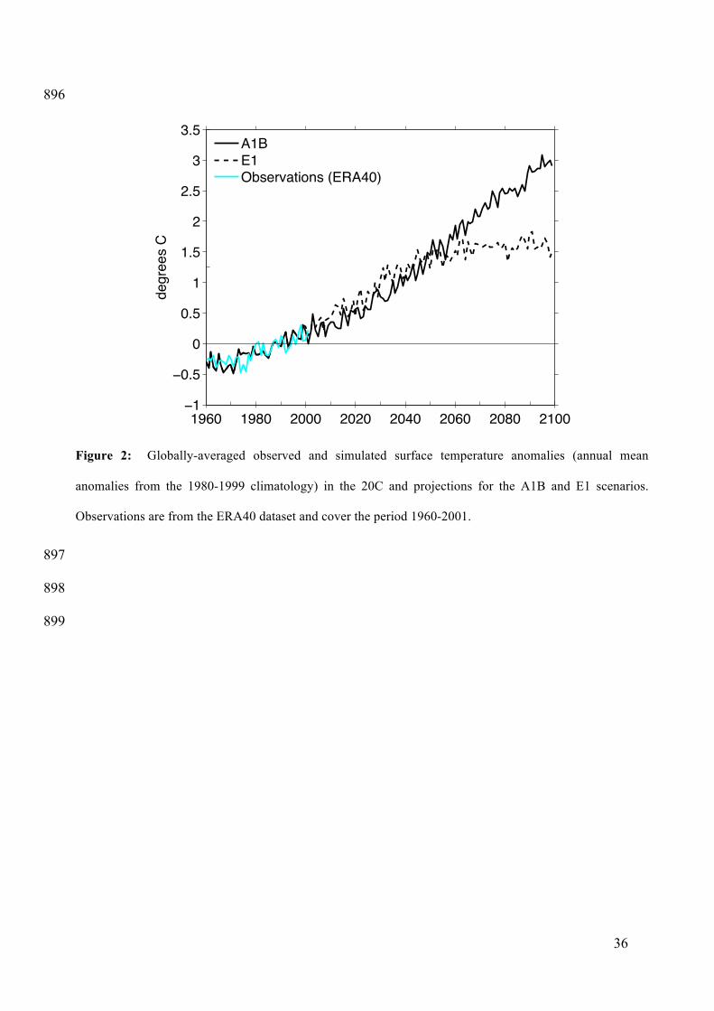
36

896

897

898

899

1960 1980 2000 2020 2040 2060 2080 21001

0.5

0

0.5

1

1.5

2

2.5

3

3.5

degr

ees

C

A1BE1Observations (ERA40)

Figure 2: Globally-averaged observed and simulated surface temperature anomalies (annual mean

anomalies from the 1980-1999 climatology) in the 20C and projections for the A1B and E1 scenarios.

Observations are from the ERA40 dataset and cover the period 1960-2001.

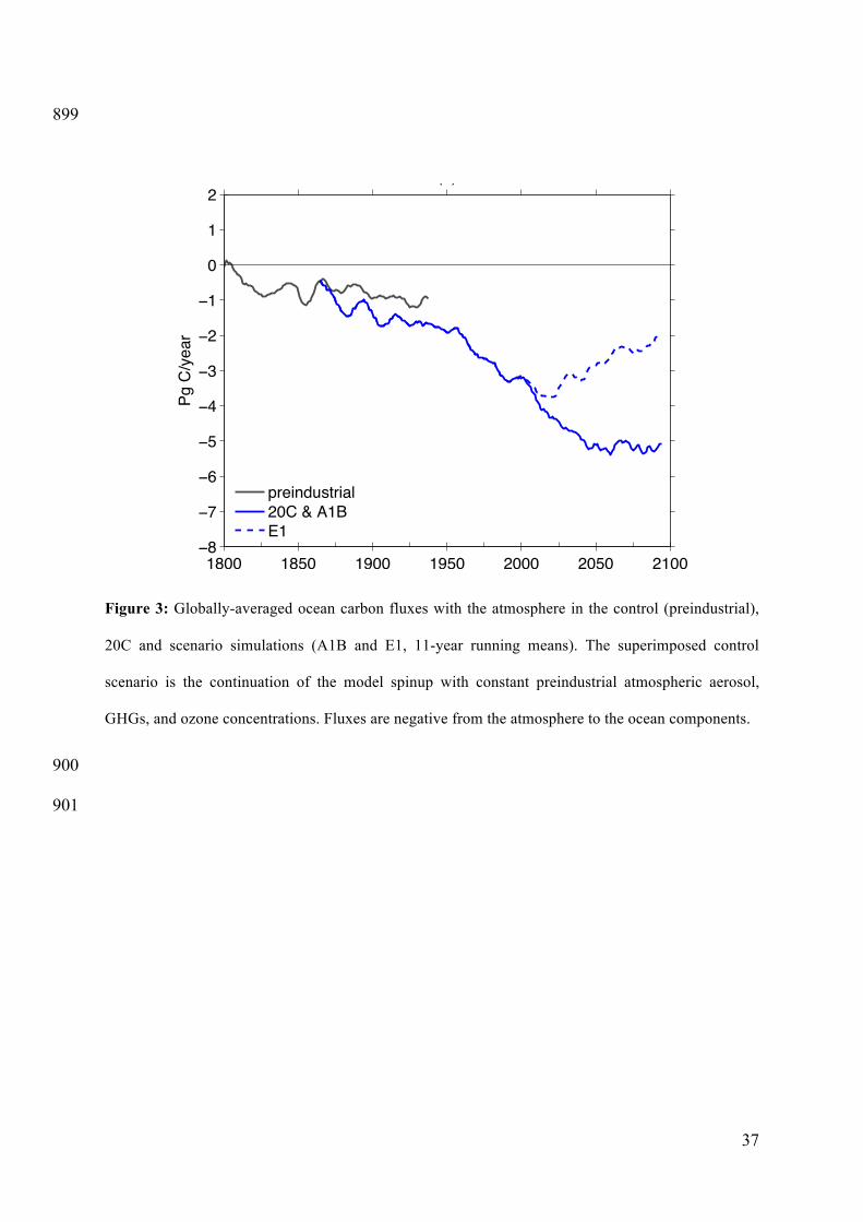
37

899

1800 1850 1900 1950 2000 2050 21008

7

6

5

4

3

2

1

0

1

2Pg

C/y

ear

(b)

preindustrial20C & A1BE1

Figure 3: Globally-averaged ocean carbon fluxes with the atmosphere in the control (preindustrial),

20C and scenario simulations (A1B and E1, 11-year running means). The superimposed control

scenario is the continuation of the model spinup with constant preindustrial atmospheric aerosol,

GHGs, and ozone concentrations. Fluxes are negative from the atmosphere to the ocean components.

900

901

38

901

2 0 2 4 6 8 10 12 14 16 18 20 22 24 26 28 30 32

60° E 120° E 180° W 120° W 60° W 0°

60° S

30° S

0°

30° N

60° N

(a) HadISST [degC]

2 0 2 4 6 8 10 12 14 16 18 20 22 24 26 28 30 32

60° E 120° E 180° W 120° W 60° W 0°

60° S

30° S

0°

30° N

60° N

(b) SST 20C [degC]

0 0.5 1 1.5 2 2.5 3 3.5 4

60° E 120° E 180° W 120° W 60° W 0°

60° S

30° S

0°

30° N

60° N

(c) SST A1B 20C [degC]

0 0.5 1 1.5 2 2.5 3 3.5 4

60° E 120° E 180° W 120° W 60° W 0°

60° S

30° S

0°

30° N

60° N

(d) SST E1 20C [degC]

Figure 4: Maps of the mean annual SST distribution during the 20th century from (a) HadISST

dataset, (b) 20C simulation (1970-1999) and differences with the scenarios: (b) A1B (2070-2099)

minus 20C (1970-1999); (c) E1 (2070-2099) minus 20C.

902

903

39

903

0

0 0 0 0

0

00 0

1 11

22

23

33

3

44

4

4

5 5 5

66 6

77 7

88

8 99

99

9

10101010

11

1

1

Latitude

(a)

20 0 20 40 60

4500400035003000250020001500

0

0

0 0 0

0

0

00

01

1

1

1

1

2

2

2

2

3

3

3

3

4

4

4

5

5

55

56

6

6

6

7

7

77

78

8

88

8

88

8 99

99

9

0

10

10

10

11126 5 433

222

1

1

1

(a) 20 0 20 40 60

1000

500

0

Figure 5: (a) Mean streamfunction of the meridional overturning circulation in the Atlantic Ocean for

the 20C simulation (1970-1999, in Sverdrup = 106 m3 s-1) and sections of the estimated anthropogenic

carbon inventory in (b) Atlantic and (c) Pacific for the same time period (in µmol C kg-1).

904

40

905

(a)

60° E 120° E 180° W 120° W 60° W 0°

60° S

30° S

0°

30° N

60° N

200 250 300 350 400 450 500

(b)

60° E 120° E 180° W 120° W 60° W 0°

60° S

30° S

0°

30° N

60° N

Figure 6: Maps of 2x2 degrees binned data of surface pCO2 (µatm) from a) LDEO dataset

(Takahashi et al., 2007), b) annual climatology of 20C model results.

906

907

41

907

1900 1940 1980 2020 2060 21004

6

8

10

12

14

Hea

t Con

tent

030

0 m

[GJ/

m2]

(a)

N Atlantic 20C & A1BE1N Pacific 20C & A1BE1

1900 1940 1980 2020 2060 2100

60

80

100

120

140

160

180

200

220

240

MLD

[m]

(b)

N Atlantic 20C & A1BE1N Pacific 20C & A1BE1

1900 1940 1980 2020 2060 21004

5

6

7

8

9

10

11

12(c)

Tran

spor

t [Sv

]

25°N 20C & A1BE148°N 20C & A1BE1

Figure 7: Annual means of (a) Heat content in the uppermost 300 m and (b) mixed layer depth in the North Atlantic and North Pacific (20°N-60°N) for the 20C and scenario simulations (note that in (b) the vertical scale is reverted). (c) Mean maximum intensity of the Atlantic MOC at 48°N and 25°N for the 20C and scenario simulations. Results are shown as 5-year running means.

908

42

909

910

1900 1940 1980 2020 2060 21002.5

2

1.5

1

0.5

0

0.5

Pg C

/yea

r

SO 20C & A1BE1Atlantic 20C & A1BE1Pacific 20C & A1BE1Indian 20C & A1BE1

Figure 8: Ocean carbon uptake in the 20C, A1B and E1 simulations divided into major basin contributions

(11 years running means, negative values mean ocean uptake). The Southern Ocean (SO) is defined as the

area southern of 50°S. The range of estimates for contemporary net CO2 fluxes from Gruber et al. (2009)

are shown as vertical bars with the relative colour for each basin.

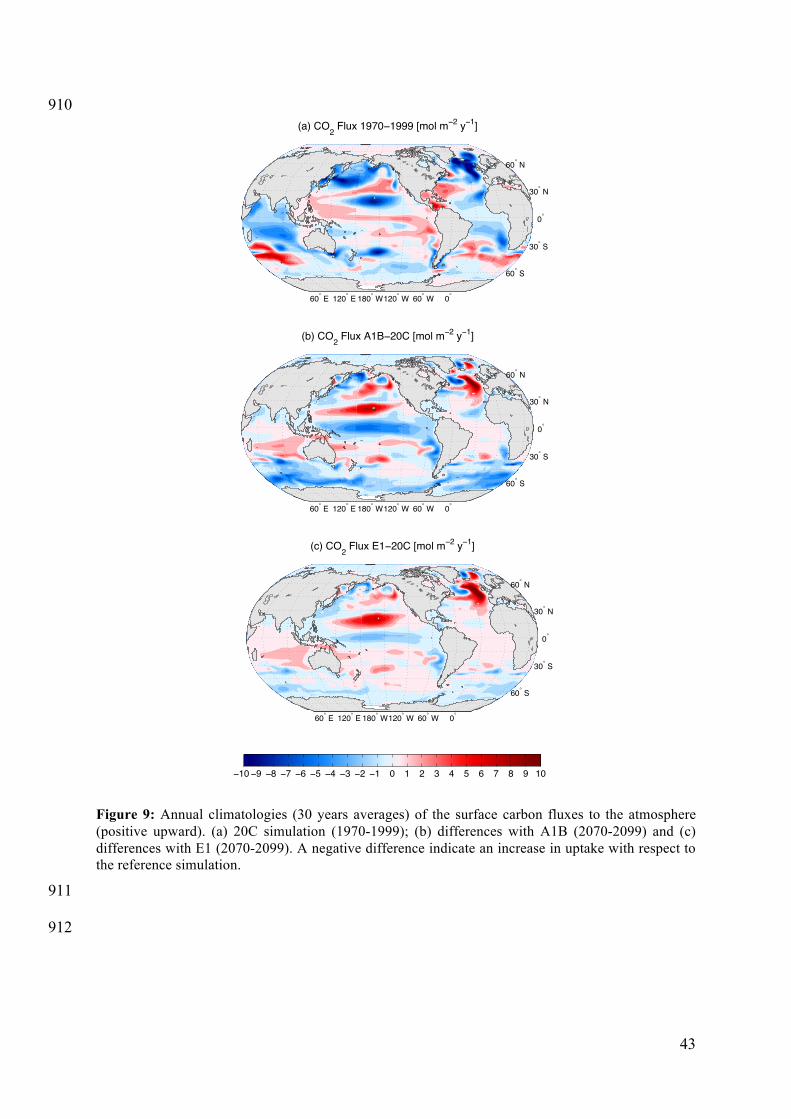
43

910

60° E 120° E 180° W 120° W 60° W 0°

60° S

30° S

0°

30° N

60° N

(a) CO2 Flux 1970 1999 [mol m 2 y 1]

60° E 120° E 180° W 120° W 60° W 0°

60° S

30° S

0°

30° N

60° N

(b) CO2 Flux A1B 20C [mol m 2 y 1]

10 9 8 7 6 5 4 3 2 1 0 1 2 3 4 5 6 7 8 9 10

60° E 120° E 180° W 120° W 60° W 0°

60° S

30° S

0°

30° N

60° N

(c) CO2 Flux E1 20C [mol m 2 y 1]

Figure 9: Annual climatologies (30 years averages) of the surface carbon fluxes to the atmosphere (positive upward). (a) 20C simulation (1970-1999); (b) differences with A1B (2070-2099) and (c) differences with E1 (2070-2099). A negative difference indicate an increase in uptake with respect to the reference simulation.

911

912

44

912

1960 1980 2000 2020 2040 2060 2080 21001.4

1.2

1

0.8

0.6

0.4

0.2

0

0.2

0.4

0.6

0.8

Pg C

/yea

r

(a)

Tropical 20C & A1BE1Northern 20C & A1BE1Southern 20C & A1BE1

1960 1980 2000 2020 2040 2060 2080 21000

0.5

1

1.5

2

2.5

3

3.5

4

4.5

5

Pg C

/yea

r

(b)

Tropical 20C & A1BE1Northern 20C & A1BE1Southern 20C & A1BE1

Figure 10: (a) Net air-sea carbon fluxes in the Pacific Ocean for 20C and scenarios and (b) Net Community Production (NCP) in the euphotic layer for the same simulations. Regions are defined as: Tropical (20°N-20°S); Northern (20°N-60°N), Southern (20°S-45°S). Results are shown with 5 years running means, and negative values in (a) correspond to ocean uptake.

913

914

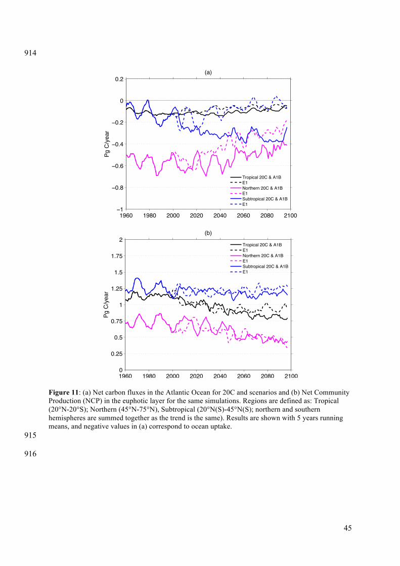
45

914

1960 1980 2000 2020 2040 2060 2080 21001

0.8

0.6

0.4

0.2

0

0.2

Pg C

/yea

r

(a)

Tropical 20C & A1BE1Northern 20C & A1BE1Subtropical 20C & A1BE1

1960 1980 2000 2020 2040 2060 2080 21000

0.25

0.5

0.75

1

1.25

1.5

1.75

2

Pg C

/yea

r

(b)

Tropical 20C & A1BE1Northern 20C & A1BE1Subtropical 20C & A1BE1

Figure 11: (a) Net carbon fluxes in the Atlantic Ocean for 20C and scenarios and (b) Net Community Production (NCP) in the euphotic layer for the same simulations. Regions are defined as: Tropical (20°N-20°S); Northern (45°N-75°N), Subtropical (20°N(S)-45°N(S); northern and southern hemispheres are summed together as the trend is the same). Results are shown with 5 years running means, and negative values in (a) correspond to ocean uptake. 915

916

46

916

W [m/d] A1B (2070 2099) 20C (1970 1999)

120° E 150° E 180° E 150° W 120° W 90° W

0°

0.5

0

0.5

W [m/d] E1 (2070 2099) 20C (1970 1999)

120° E 150° E 180° E 150° W 120° W 90° W

0°

0.5

0

0.5

Figure 12. Differences in mean vertical velocity (m/d) in the tropical Pacific (20°S-20°N) between the scenarios (A1B top and E1 bottom) and the 20C simulation. Averaging periods are given in the titles.

917

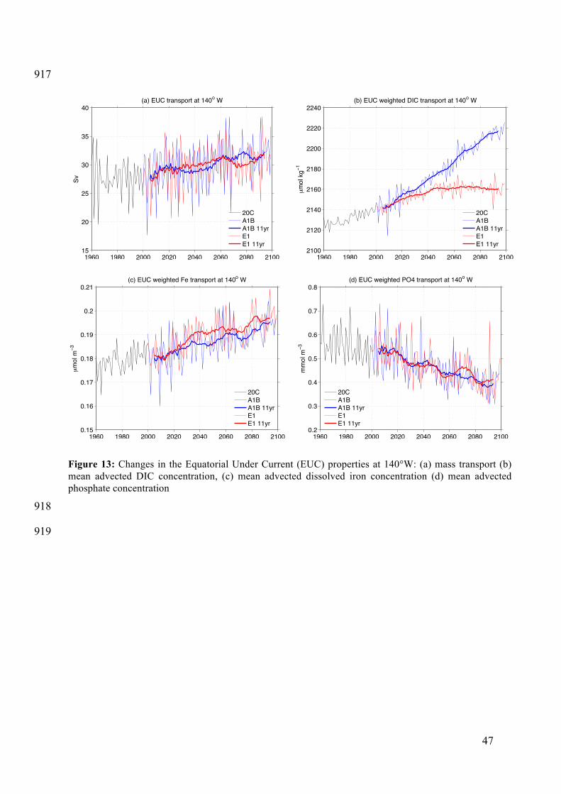
47

917

1960 1980 2000 2020 2040 2060 2080 210015

20

25

30

35

40

Sv

(a) EUC transport at 140o W

20CA1BA1B 11yrE1E1 11yr

1960 1980 2000 2020 2040 2060 2080 21002100

2120

2140

2160

2180

2200

2220

2240

µm

ol k

g1

(b) EUC weighted DIC transport at 140o W

20CA1BA1B 11yrE1E1 11yr

1960 1980 2000 2020 2040 2060 2080 21000.15

0.16

0.17

0.18

0.19

0.2

0.21

µm

ol m

3

(c) EUC weighted Fe transport at 140o W

20CA1BA1B 11yrE1E1 11yr

1960 1980 2000 2020 2040 2060 2080 21000.2

0.3

0.4

0.5

0.6

0.7

0.8

mm

ol m

3

(d) EUC weighted PO4 transport at 140o W

20CA1BA1B 11yrE1E1 11yr

Figure 13: Changes in the Equatorial Under Current (EUC) properties at 140°W: (a) mass transport (b) mean advected DIC concentration, (c) mean advected dissolved iron concentration (d) mean advected phosphate concentration

918

919