CDCCEN TERS FOR DISEASE CONTROL

NID5H

Analyzing Workplace Exposures Using Direct Reading Instruments and Video

Exposure Monitoring Techniques

U .S . DEPARTMENT OF HEALTH AND HUMAN SERVICESPublic Health Service

Centers for D isease Control National Institute for Occupational Safety and Health

ERRATA

Analyzing Workplace Exposures Using Direct Reading Instruments and Video Exposure Monitoring Techniques

Page 22--Replace the value "0.8" with "1,2" on line 12 of the first paragraph.

ANALYZING WORKPLACE EXPOSURES USING DIRECT READING INSTRUMENTS AND VIDEO EXPOSURE MONITORING TECHNIQUES

Technical Editors MICHAEL G. GRESSEL

WILLIAM A. HE1TBRINK

Contributing Authors MICHAEL G. GRESSEL

WILLIAM A. HEIT6RINK PAUL A. JENSEN

THOMAS C. COOPER DENNIS M. O'BRIEN

JAMES D. McGLOTHUN THOMAS J. FISCHBACH JENNIFER L. TOPMILLER

U.S. DEPARTMENT OF HEALTH AND HUMAN SERVICES Public Health Service

Centers for Disease Control National Institute for Occupational Safety and Health

Division of Physical Sciences and Engineering Cincinnati, Ohio 45226

August 1992

DISCLAIMER

Mention of company names or products does not constitute endorsement by the National Institute for Occupational Safety and Health.

DHHS (NIOSH) PUBLICATION NUMBER 92-104

ABSTRACT

A typical evaluation of a worker's exposure to an air contaminant requires a pump to draw air through a filter, sampling tube, or other media suitable for collecting the contaminant for a measured period of time. These "integrated" samples provide an indication of the extent of a worker's exposure. Depending on the worker's job tasks, these samples normally do not identify the specific job elements that contribute most to the worker's exposure. To help identify these critical work elements, a technique called video exposure monitoring has been developed by researchers from the National Institute for Occupational Safety and Health.

Part 1 of this document (1) outlines the techniques for conducting video exposure monitoring; (2) describes the equipment required to monitor and record worker breathing zone concentrations; (3) discusses the analysis of the real-time exposure data using video recordings; and (4) discusses the use of real-time concentration data from a direct reading instrument to determine a room's effective ventilation rate, the mixing factor, and the room concentration at a given time. Part 2 contains case studies describing a variety of circumstances where the video exposure monitoring techniques provided useful information not obtainable by integrated sampling. Each case study briefly describes the process being monitored and the methodology used to monitor the exposures and, further, discusses the findings and the recommendations derived from the case study. These case studies demonstrate the power and utility of video exposure monitoring.

ABBREVIATIONS

A Absorbance of samplel/mole/cmm

ASCII American Standard Code for m2information Interchange m2

A/D Analog to digital m3/hr0 Regression coefficient mg/m3C Concentration moles/l

Average concentration mvcfm Cubic feet per minute ncm Centimeters N20

Concentration at reduced pressure NIOSHc « Actual concentrationcm Concentration at time t NMAM°c Degrees CelsiusDC Direct current NTSC€ molar absorbtivity (1/mole/cm)€ Regression constant o 2EGA Enhanced Graphics Adapter OSHAeV Electron voltsfibers/cc Fibers per cubic centimeter Pfpm Feet per minute •̂tmft3 Cubic feetG Emission factor ppmHAM Handheld Aerosol Monitor Qhr Hours Q/VHVLV High velocity-low volume RAMHz Hertz RELin Inches rpm1 Intensity of light transmitted by sec

sample STEL>0 Intensity of incident light ST,IR InfrarediRi Time weighted average instrument t

response TWAIR(t) Instrument response at time t //mK Mixing factor UVKB Kilobytes Vkg Kilograms VkHz Kilohertz VGAL Path length VHS1 Liters Xlb Pounds Yl/min Liters per minute

Liters per mole per centimeter MetersSquare metersSquare metersCubic meters per hourMilligrams per cubic meterMoles per literMillivoltsNumberNitrous oxideNational Institute for Occupational Safety and Health NIOSH Manual of Analytical

MethodsN ationa l T e lev is ion System

Committee OxygenOccupational Health and Safety

Administration ProbabilityAtmospheric pressure Pressure drop Parts per million Volumetric flow rate Air changesReal-time Aerosol Monitor Recommended Exposure Limit Revolutions per minute SecondsShort Term Exposure Limit Time weighted average sorbent

tube concentration TimeTime weighted averageMicronsUltravioletVolumeVoltsVideo Graphics Array Video Home System Independent variable Dependant variable

CONTENTS

Part 1. Video Exposure Monitoring TechniquesI. Introduction .......................................................................................................... 1II. Video Equipment.................................................................................................... 3

A. Conventional Video Equipment............................................................... 3B. Infrared Video Equipment ....................................................................... 3

III. Monitoring Equipment........................................................................................... 5A. Aerosol Photometers .............................................................................. 7B. Photoionization Detectors ....................................................................... 8C. Infrared Analyzers ................................................................................... 9

IV. Personal Computer Software .............................................................................. 11V. Personal Computer Hardware............................................................................... 13VI. Data Acquisition..................................................................................................... 15VII. Activity Analysis..................................................................................................... 17VIII. Data Analysis................. ....................................................................................... 18

A. Transportation Lag and Autocorrelation................................................ 18B. Assembling the Data S e t......................................................................... 18C. Data Analysis Techniques....................................................................... 19

1. . . Descriptive Statistics................................................................. 202. . . Data Censoring Using a Spreadsheets ................................... 203. . . Time Series Analysis................................................................. 22

D. Summary of Data Analysis .................................................................... 23IX. Dilution Ventilation and Material Balances .......................................................... 24X. Practical Application of Video Exposure M onitoring......................................... 29XI. References...............................................................................................................31

Part 2. Case Studies.....................................................................................................................33A. Manual Material W eighout....................................................................... 33B. Ceramic Casting Cleaning ....................................................................... 37C. Dumping Bags of Powdered Materials ................................................. 39D. Furniture Stripping................................................................................... 43E. Dental Administration of Nitrous O x id e ................................................. 47F. Hand-held Sanding Operation.................................................................. 51G. Methanol Exposures in Maintenance Garages.................... - .............. 53H. Brake Servicing ........................................................................................ 56I. Bulk Loading of Railroad Cars and Trucks ............................................ 59J. Grinding Operations ................................................................................. 63

AppendicesA. Program Listings ......................................................................................67B. Bar Program Operating Instructions........................................................ 80

v

FIGURES

1. Infrarod imaging system.......................................................................................... 42. Ideal mixing tank concentration response to inlet concentration

changes: A) inlet concentration step change from 0.05 to 1.0,B) concentration pulse of 25% of the tank's time constant............................. 6

3. Schematic of aerosol photometer utilizing scattered light.................................. 84. Infrared analyzer schematic.................................................................................... 95. Overlay file format: (A) one bar (B) two bars...................................................... 126. Diagram of the personal computer system's equipment and connections

needed to overlay exposure data with work activities. . ................................. 147. An example of regression analysis on a spreadsheet......................................... 218. Room concentration decay curve.......................................................................... 269. Effects of mixing factor on room concentration decay curve............................ 2610. Room concentration buildup curve........................................................................ 2711. Effects of mixing factor on room concentration buildup curve..........................28A-1. Diagram of workstation.......................................................................................... 33A-2. Modeled dust exposure of a worker as a function of bag count for

scooping, weighing, and turning.......................................................................... 35A-3. Modeled dust exposure of worker for filling bags 51 thru 53........................... 35C-1. Relative worker exposure to lead chromate from dumping a single

bag (by activity)......................................................................................................40C-2. Sketch of low dust exposure activity (dumping bag) with overlaid

exposure measurement..........................................................................................41C-3. Sketch of high dust exposure activity (bag disposal) with overlaid

exposure measurement.......................................................................................... 41D-1. Real-time and modeled methylene chloride and methanol exposure

concentrations, by task only................................................................................. 44D-2. Real-time and modeled methylene chloride and methanol exposure

concentrations, by furniture type......................................................................... 45E-1. Diagram of a typical N20 scavenging system...................................................... 47E-2. Plot of real-time N20 concentration with activities and supply

concentrations........................................................................................................ 49G-1. Real-time plot of exposures during servicing and refueling operation...............54G-2. Real-time plot of exposures during fuel filter maintenance................................ 54H-1. Diagram of brake washing unit.............................................................................. 561-1. Types of raficar hopper openings................. ........................................................ 601-2. Retractable, ventilated loading spouts, endosed-type and open-type.............. 601-3. Types of truck hopper openings............................................................................ 61J-1. Average dust concentration for each tool type and the percent

of the time each tool was used in cleaning the castings...................................64J-2. Percentage of "dust-dose” as a function of tool type, tool location

and swarf direction when grinding castings........................................................65

vi

TABLES

1. Approaches to analyzing real-time data................................................................ 20B-1. Relative exposures and doses for the dealing of white and

green castings.........................................................................................................38C-1. Worker dust exposure by activity......................................................................... 42D-1. Methylene chloride generation rates..................................................................... 45F-1. Real-time sampling results for the sanding operators......................................... 52F-2. Average dust concentrations during sanding aid "other" activities................. 52H-1. Average relative dust concentrations by brake activity......................................571-1. Average area respirable dust concentrations (mg/m3)........................................ 611-2. Average real-time total dust concentrations at ventilated spout.......................611-3. Average real-time total dust concentrations at nonventilated spout................ 62

vii

ACKNOWLEDGMENTS

The editors wish to express their gratitude to all the contributing authors for all of their contributions of time and expertise. The editors wish to specifically thank Marion Curry, Phillip Froehlich, and Leroy Mickelsen for their assistance in reviewing this document and Ronald Hall for his assistance in preparing the art work for this report.

Part 1 . Video Exposure Monitoring Techniques

I. Introduction

Occupational exposure to air contaminants is usually monitored by means of integrated sampling of the air a worker breathes. The air is drawn through a filter or other collection medium at a known flow rate by means of a small battery powered pump for a measured period of time. The collection medium is analyzed to determine the quantity of contaminant collected, and the average exposure during the sampling period is computed. These results indicate the extent of exposure, but integrated air sampling provides little insight into the specific causes of the worker's exposure. Recommendations for controlling the air contaminant exposures are often based upon an observer's judgment and can result in implementation of control measures that do not address the major worker air contaminant exposure sources. To help overcome this problem, direct reading instruments and data recording devices can be used as a part of a system for recording events and exposures in the workplace as a function oftime. The data from such a system can be used to associate events and exposures and to promotemore effective and focussed recommendations for controlling the air contaminant exposures.

Through studies conducted in a variety of industries, researchers with the National Institute for Occupational Safety and Health (NIOSH) have developed a systematic approach to help identify the sources of worker exposures and to provide an effective means for communicating the results to workers and management.11,21 This system employs:

• direct reading instruments and data recording devices to monitor and store data characterizing worker exposures,

• video cameras and recorders to document worker activities.• task analyses to evaluate work activities,• statistical techniques to develop predictive models and to summarize the results, and• personal computers to perform analyses on the data and to combine the activity data and

the exposure data into a presentable form.

The present system evolved from a series of studies conducted either to evaluate the effectiveness of engineering controls or to identify characteristics about the worker's exposure so that controls could be implemented. Direct reading instruments were used so that exposure changes over a short time interval (on the order of seconds) could be monitored. The output from these instruments was stored in an electronic recording device rather than on a stripchart recorder, so that the data would not require re-keying for statistical analysis. Worker's activities were documented by video recording systems to determine whether exposures were the result of particular work practices. Work activity data were combined with the real-time exposure data by determining both the exposure and the activity at any given time. Time series analysis of the combined real-time and work activity data set resulted in a model to predict worker exposures. After several studies, however, it became apparent that time series analysis could become a prohibitive task because of the tremendous amount of data that can be collected in a very short period of time. To ease this problem, several simplified analysis techniques were developed. Although these techniques are not as powerful as the time series analysis, in most

1

cases they can identify those activities that contribute the most to the worker's contaminant exposures.

As some of the initial studies were being completed, a need became obvious: a way to communicate the study results to workers and to management. The consensus among the individuals working on these studies was that a video recording of the work activity combined with a display of the real-time exposure measurement would be most effective. The exposure data could be presented in two forms: numerically, with the value of the exposure measure being displayed on the video screen, or graphically, by displaying a graphical representation of the exposure on the video screen. Both options were combined by displaying both the numerical exposure concentration and a bar representing the relative magnitude of the exposure. To place the bar and number on the video screen, a computer program was written to read the exposure data file and to generate and update the bar with time. The system required the use of consumer quality video and ordinary personal computer equipment; the only specialized equipment required was a special graphics card for the personal computer. The result was a video recording that graphically showed how exposure to a particular substance was affected by the activities of the worker.

This document describes various aspects of using direct reading monitors to evaluate occupational exposures. The discussion of the different techniques includes the equipment necessary for conducting this type of exposure assessment. Finally, several case studies illustrate the use and limitations of these techniques.

2

II. Video Equipment

Two types of video equipment are described in this report: conventional video equipment, used to document the worker's activities, and infrared video equipment used to visualize specific air contaminant plumes. The discussion of conventional equipment includes the system requirements for conducting video exposure monitoring; the discussion of infrared equipment includes theory and operation, and explains how it can be used with direct reading instruments to characterize workplace contaminant concentrations.

A. Conventional Video EquipmentThe conventional video recording system consists of a video camera and a videotape recorder. For better portability, a camcorder, a video camera with built-in recorder, can be used. Mounting the video camera onto a tripod eliminates the need to hold the camera throughout the entire process. The tape format (Beta, VHS, 8-mm) is not important, and many consumer-quality video recording systems are suitable for video exposure monitoring. There are, however, two important requirements. First, the video system must have a National Television System Committee (NTSC) standard video output signal — a signal used by the video overlay system described elsewhere in this document. This standard is used by most home video equipment. Second, an on-screen clock or timer is needed — one that can be synchronized with the real-time clock of the data recording device. Synchronizing the data recording device with the video camera can be as simple as starting the timer in the camera at the same time the data logger is turned on. The clock or timer should have a resolution of at least 1 sec. The on-screen clock permits an exposure to be coordinated with an associated activity. The video recording of the work cycle or process can then be reviewed while simultaneously tracking the worker's exposure from a printout or plot of the real-time exposure data.

B. Infrared Video EquipmentEffective control of air contaminants depends on understanding of the characteristics of their release. Not only is concentration important but it is also necessary to know the source and path of the emission. Although some gasses and vapors are visible, most are not. Infrared imaging is a technique that can provide a real-time picture of some otherwise invisible emissions.

A schematic of such an infrared imaging system is presented in Figure 1. An infrared scanner (Thermovision 782)131 detects changes in absorption of infrared radiation by contaminant gases or vapors. Two versions of the scanner may be used depending on the range in which the gases absorb infrared radiation: a shortwave band (2 to 5.6 microns) and a longwave band (8 to 12 microns). The images received by the scanner are transmitted to a display unit and may be converted from the normal infrared gray scale image to a colored scale. This image is then simultaneously transmitted to a monitor and video recorder for real-time viewing and recording.

The system uses a flat, black panel as an infrared radiator. The panel is a square, 2-in. thick aluminum tank filled with water. A flat-sheet electrical heater is glued to the back surface of the tank; the front surface is painted black. An electronic temperature controller maintains the tank at a constant temperature. The water in the tank is circulated by a laboratory stirrer to inhibit the formation of a temperature gradient across the panel surface.

The radiant panel and the infrared scanner are positioned so that the emission source is between them. The scanner sees the panel as a constant temperature source, and it is displayed as a uniform image. As a contaminant gas passes between the scanner and the heat source, it absorbs some of the

3

Figure 1. Infrared imaging system.

radiated infrared energy. The scanner detects this as a lower temperature, which is then displayed as a different color or shade of gray and recorded.

The system as described here is useful for detecting certain process emissions because rt provides a real-time image that identifies both the source and path of the emissions. Medical processes, such as the release of nitrous oxide (N20) during dental surgery, as well as industrial processes can be monitored. Also, the infrared imaging system may be used in determining of flow patterns around exhaust openings with the use of a tracer gas. An advantage to this technique is that the effect of specific work activities or changes in control configuration can be determined immediately.

The most important limitation of this system is sensitivity. The absorption of the emission cloud is directly related to the concentration of the emission and the path length through the cloud. Thus, lower concentrations must be present in greater quantities to be visualized. For example, the sensitivity for N20 is on the order of 200 ppm-meter( i.e., a cloud of nitrous oxide having a concentration of 200 ppm must be 1 m across to be detected. System sensitivity can be increased by the use of narrow band pass filters that filter out radiation outside the narrow band containing the absorption peak of the monitored contaminant. The high concentrations typically found at the generation point of an emission can generally be visualized using this system. Detection of contaminant levels in the range of occupational health standards is, however, limited. Another limitation of the system is lack of portability. Because the radiant panel is a water-filled tank, it is quite heavy and not easily positioned. Although this is not a severe limitation for laboratory use, it does make field operation difficult.

Some of these limitations are addressed by recent advances in thermal imaging technology. A system that uses a laser in combination with the infrared scanner to detect changes in energy is now available. The laser scans the viewed object, thus eliminating the need for a radiant panel, greatly increasing portability and making the system much more convenient for field use. This system also has a sensitivity in the range of one order of magnitude greater than the one previously described.

4

III. Monitoring Equipment

Any air contaminant monitoring instrument that can produce an output signal of the concentration measurements can potentially be used to conduct real-time assessments of a worker's exposure to an air contaminant. The usefulness of a specific instrument will vary with the situation. To evaluate the utility of an instrument, consider:

1. the nature of the analog or serial output,2. the response time of the instrument,3. specificity for the contaminant of interest, and4. portability and size.

Output. Because real-time concentration data are generally used to evaluate the relationship between events in the workplace and air contaminant concentrations, the concentration measurements generally need to be recorded automatically. For a monitor to be useful, it should produce a digital or analog output. The analog output of many industrial hygiene instruments is a voltage that is proportional to concentration. Techniques for recording analog data are given in the "Data Acquisition” section of this document. Some instruments also provide a digital output that is periodically updated. The frequency of these concentration measurements is usually a function of the instrument and normally cannot be adjusted by the user.

Response Time. The total system response time (for the monitor and the setting being evaluated) can be defined as the sum of (a) the time required for the air contaminant to be transported to and to accumulate in the worker's breathing zone and (b) the time required for the instrument to respond to a change in concentration in the worker's breathing zone. To conduct video exposure monitoring studies of air contaminant concentrations, the total system response time must be less than that of the events of interest. As a result of the delays that make up the total system response, the instrument output lags behind work events in the workplace.

The time constant describes how an instrument responds to changes in concentration. An instrument responds to changes in concentration in the same way that the concentration in an ideal stirred mixing tank responds to changes in concentration of the incoming stream.M> The time constant of the tank is the time needed for the tank's volume to flow through the tank at a given flow rate. (The time constant equals the tank's volume [V] divided by the flow rate [Q]). The concentration in the mixing tank is the average concentration of each increment of fluid that is flowing through the tank. Some of these fluid increments flow in and out of the tank quickly, whereas others remain in the tank for some time. As a result, the average concentration in the tank does not immediately respond to changes in inlet concentration. Figure 2 illustrates the theoretical response of the concentration in an ideal stirred tank to changes in the inlet concentration. Figure 2A illustrates the effect of a step change in the inlet concentration upon the concentration in the tank. More than two time constants are needed for the concentration in the tank to complete 90% of its response to the change in concentration. Figure 2B illustrates the effect of a concentration pulse upon the concentration in the mixing tank. The width of the concentration pulse is one-fourth of the tank's time constant. Figure 2B, shows a distorted picture of the inlet concentration as measured by the concentration in the tank. The concentration in the tank reaches a maximum when the concentration pulse has completely passed into the tank. A period of several time constants is required to completely flush the concentration pulse out of the tank. Air monitoring instruments respond to changing concentrations in a manner similar to that of the stirred tank. Therefore, when changes in the inlet concentration occur faster than

5

(A)

Time / (Time Constant)

(B)

Time / (Time Constant)

Figure 2. Ideal mixing tank concentration response to inlet concentration changes: (A) inlet concentration step change from 0.05 to 1.0, (B) concentration pulse of 25% of the tank's time constant.

6

the instrument's response, the measured concentration profile will be a distorted picture of the actual concentration profile. To limit this distortion, the instrument's time constant should be shorter than the events being studied.

Specificity. The air monitoring instruments used in industrial hygiene are usually not specific for a particular substance. These instruments are usually based upon the measurement of some parameter that is proportional to concentration. For example, aerosol photometers respond to any aerosol that scatters light. This limitation of the existing equipment requires either that the monitor be calibrated for the specific air contaminant or that the results be reported as a relative concentration.

Portability. To allow for worker acceptance, the monitoring equipment should be light enough to be worn comfortably by the worker. The equipment should be battery-operated, and should weigh as little as possible. If the equipment cannot be worn by the worker, tubing can be used to transport the air contaminant from the worker's breathing zone to the instrument. This, however, adds some extra complications. The monitoring system's response time will increase because of the time needed to transport the air contaminant through the tube to the monitor. In addition, the tubing might collect the air contaminants or might contribute to the instruments's signal; aerosols can be lost to the tubing walls and later be released if the tubing is struck or vibrated; and organic vapors can be adsorbed onto the tubing walls during periods of high concentration and desorbed during periods of low concentration.

Users need to consider the limitations and capabilities of the direct reading instruments to design and conduct studies that yield useful information about exposure sources. The instruments used in the case studies described in this document all have limit capabilities. In the case studies, three types of instruments were used: aerosol photometers, photoionization detectors, and portable infrared spectrometers. Background information on these instruments can be obtained from the NIOSH Manual of Analytical Methods (NMAM) and the American Conference of Governmental Industrial Hygienists' (ACGIH) Air Sampling Instruments.” 61 The following paragraphs discuss each of these instruments from the perspective of an occupational health professional who wishes to conduct video exposure monitoring.

A. Aerosol PhotometersAerosol photometers, such as the Real-Time Aerosol Monitor (RAM*) (Mie Inc., Bedford, MA) or the Hand-held Aerosol Monitor (HAM) (PPM Inc., Knoxville, TN), provide a continuous signal (analog voltage and digital display) output that is proportional to concentration. Both instruments have user selectable time constants. As illustrated in Figure 3, such instruments are operated by continuously drawing the aerosol through an illuminated sensing volume and detecting the light scattered by all the particles in that volume. The amount of light scattered by the aerosol is a complex function of particle size, shape, and refractive index. Generally, as particle size increases above 1 //m, the mass sensitivity of these instruments decreases with increasing particle size.17,81 As a result, instrument calibration may vary dramatically between different materials and different samples of the same material. In using these instruments to conduct video exposure monitoring, the assumption is that the nature of the aerosol (particle size distribution, composition, etc.) remains constant so that the calibration of the instrument does not change while collecting data. This assumption can be verified by conducting integrated sampling to confirm that the response of the aerosol photometers correlates with the actual integrated exposure results.

For aerosol photometers to be useful for video exposure monitoring, the contaminant of interest must cause most of the scattered light. If studying the sources of exposure that are small in relation to the total background aerosol concentration, sampling with aerosol photometers may not yield useful information. The background concentration caused by ambient air pollution is about 0.03 mg/m3.

7

Aerosol

Incident Light

Light Trap

/Scattered Light

Detector

Figure 3. Schematic of aerosol photometer utilizing scattered light (from Reference 6).

Some commercially available aerosol photometers such as the HAM do not have pumps to draw air through the sensing volume. They are designed so that natural air currents transport the aerosol to the sensor. This adds to the lag between events and measured concentration. To minimize this lag, a personal sampling pump can be used to draw air through the instrument's sensing chamber.

B. Photo ionization DetectorsPhotoionization detectors operate by passing air through a sensing chamber that is illuminated by an ultraviolet (UV) lamp. The UV radiation from this lamp ionizes many of the contaminants that may be present in the air, and thus a current flows between negative and positive electrodes located in the sensing chamber. The measured current flowing between the negatively and positively charged electrodes in the sensing chamber is proportional to the concentration in the chamber. The lamps in these instruments produce photons with an energy of less than 11 eV. Therefore, these instruments respond to gases and vapors that have an ionization potential less than 11 eV. Because they do not respond well to gases and vapors that have ionization potentials much greater than the energy of the photons produced by the lamp,” 1 the common components of air such as oxygen, nitrogen, helium, carbon dioxide, and water vapor (all of which have higher ionization potentials) are not detected. Because many chemicals have an ionization potential that is less that 11 eV, photoionization detectors are not specific for a given air contaminant.

Commercially available photoionization detectors such as the HNu* model 101 (HNu Systems, Newton, MA) and TIP9 II (Photovac Inc., Thornhill, Ontario, Canada) have relatively short response times. Both instruments have a time constant of approximately 1 sec. In these instruments, a small fan is used to draw air through the sensor. As a result, a small pressure loss in any sampling train can cause a reduction in the flow rate through the sensing volume and a subsequent increase in the instrument response time.

8

C. Infrared AnalyzersUnlike the aerosol photometers and the photoionization detectors, infrared (IR) analyzers can be used to analyze for a specific compound in the presence of interferences. A pump or fan draws air through tubing into the sampling chamber of the analyzer, and IR radiation is passed through the sampling chamber. Compounds absorb infrared radiation at specific wavelengths that are characteristic of the chemical bonds between the atoms of the compound. The IR wavelength is selected to maximize the radiation absorption of the compound of interest and to minimize the absorption of interfering compounds. The amount of infrared radiation adsorbed is described by the Beer-Lambert Law, which states that the radiation absorption is proportional to the molar concentration of the compound and the distance through which the radiation travels. This relationship is stated mathematically as:1101

To have adequate sensitivity, these instruments usually have path lengths on the order of meters. The long path lengths are achieved in small volumes by using mirrors and multiple reflections. A conceptual diagram of the mixing chamber is shown in Figure 4.

= A = eCL (1)

where:

AeCL

'ointensity of light transmitted by sample intensity of incident light absorbance of sample molar absorbtivity (l/mole/cm) concentration (moles/1) path length (cm)

The response time of these portable infrared analyzers is frequently determined by the volume of the sampling chamber. The time constant usually can be calculated by dividing the volume of the sampling

^ Light SourceDetector

Figure 4. Infrared analyzer schematic.

9

chamber by the flow rate. For the MIRAN® 1A (Foxboro Instruments, Foxboro, MA), this time constant is about 17 sec based upon a mixing chamber volume of 5.6 I and a sampling rate of 20 Ipm. The response time for portable infrared spectrometers will generally be longer than those for aerosol photometers and photoionization detectors.

To minimize the time constant, the flow rate through the sampling chamber can be increased by using an external pump to move air through the sampling chamber. This can, however, cause a significant pressure drop through sampling lines and in the sampling chamber, and, as a result, there may be a noticeable decrease in the absolute pressure in the chamber and in the moles per volume of analyte in the mixing chamber. The measured concentration can be corrected for the reduced chamber pressure by the following:

where:= Actual concentration = Concentration at reduced pressure

P**, = Atmospheric PressureP ^ = Pressure drop

Although portable infrared analyzers can be carried from site to site, they are too heavy (10 to 20 kg) to be placed on a worker. A sampling line inlet can be mounted on the worker's lape! or very near the worker's breathing zone (see Case Study E), but this can present a number of complications. The total response time of the instrument is increased because of the long sampling line. Because the flow rate induced by the fan decreases rapidly with an increase in the static pressure, adding a sampling line may decrease the air sampling rate. Pressure tosses through the sampling line can be minimized by using larger diameter tubing and by minimizing the number of bends and kinks in the tubing.

(2)

10

IV. Personal Computer Software

Several types of software may be used to collect and analyze real-time exposure data. Control software is used to operate an analog-to-digital converter card, and communications software is used to down load portable data loggers. Spreadsheets are valuable for manipulating the real-time exposure data as well as for performing some simple analyses. For more sophisticated data analyses, full- function statistical analysis packages may be required. In addition, if the exposure data are to be combined with the work activity video recording, a specially written computer program can be used to generate a graphical representation of the worker's exposure.

Control software is used to operate the analog-to-digital converter that is either a card located in the computer or a stand-alone system with an interface to the computer. These software packages usually require special device drivers for the particular hardware system in use. Many of these control packages can process the real-time data as they are being collected, and some packages provide some limited data analysis capabilities. Besides collecting data from an analog source (a direct reading instrument for example), the control software can also instruct the computer to send out signals. Although the capability to function as a controller may be useful in the industrial or laboratory setting, it is not further described in this report.

Configuring the analog-to-digital system is normally done by menu-driven software. Many of the software packages will allow the readings to be displayed on the computer screen as the data are being collected. This display may be graphical or tabular. Once data collection is complete, the readings are stored in a data file. Some programs will link directly with a spreadsheet program making it possible to save the data in a spreadsheet file. For other programs, the data are stored in file formats that can be imported into the spreadsheet. There are several different control programs with many different functions and capabilities. Two specific packages are Labtech Notebook (Laboratory Technologies Corporation, Wilmington, MA) and ASYST (MacMillan Software Company, New York, NY). Both of these programs will work with a variety of analog-to-digital converter cards. Oepending on the options purchased, the prices of these packages range from $200 to $2000.

If a portable data recording device (data logger) is used to record the real-time exposure data, control software is not needed. Instead, a program to down toad the data logger to a personal computer is required. Most data loggers either come complete with down loading software or have one available for an additional cost. After down loading the data logger, some of the programs may allow simple data analysis to be performed. Many of these programs store the data in a file that can then be imported into a spreadsheet program. In addition to the programs supplied with the data loggers, communications programs such as Crosstalk (Crosstalk Communications, Roswell, GA) and Procomm (Datastorm Technologies Inc., Columbia, MO) also can down load some data loggers through the computer's asynchronous communications port. Using the communications programs may be a nonstandard procedure, since the format of the data from the data logger may vary with the device.

After the data have been collected and stored in a file, spreadsheet programs can be used for data manipulation and simple data analysis. Lotus 1-2-3 (Lotus Development Corporation, Cambridge, MA) and Microsoft Excel (Microsoft Corporation, Redmond, WA) are examples of two spreadsheet programs. If the data are to be analyzed by worker activity, a spreadsheet is useful for keying activities with the real-time exposure data: determine the time a particular reading was recorded and then observe the worker's activities for that time on the video recording of the work activity. Spreadsheets can be used not only to sort data and perform elementary statistical analysis but to

11

format data sets for analysis in a statistical analysis program or to combine the work activities and the real-time exposure data onto videotape. A detailed discussion on the use of the spreadsheet for more sophisticated data analysis is given in the Data Analysis section of this document.

To combine the real-time exposure data w ith the video recording of the worker's activities, NIOSH researchers have written a program for IBM compatible computers that generates a graphical representation of the worker's exposure. A listing of this program, written in BASIC, is given in Appendix A, and instructions for running the program are given in Appendix B. This IBM compatible program reads a real-time data file, generates a bar to represent the magnitude of the exposure, and then displays the bar on the screen. When this program is run through a video overlay system, a video recording graphically shows how a worker's exposure is influenced by the work activity. The video overlay system is discussed in the Personal Computer Hardware section of this report. The bar is updated at the same time interval as the readings in the data set. The program was written to allow either one or two bars to be displayed on the screen at one time. Two bars can be displayed if the exposures of two workers are to be compared or if one worker is monitored with two different instruments. To use the program, the real-time exposure data must be stored in a properly formatted ASCII file. For the program to display one bar, the format of the data file must have three columns of data: two columns for the time the reading was recorded (minutes and seconds) and one column for the exposure measurements. For the program to display two bars, then the data file format must have an additional column for the second exposure measurement. The first data set will be displayed on the left side of the screen while the second data set will be displayed on the right. The time interval between the readings must be constant. Figures 5A and 5B shows examples of the data file formats. The spreadsheet program can be used to arrange the data file into the proper format. The bar generated by this program is overlaid onto the work activity video recording through the use of a video overlay system.

The computer software packages discussed here are only a few examples of the programs that can be used in collecting, analyzing, and presenting real-time exposure data. The choice of the specific package depends upon the needs of the particular situation. The case studies presented in this document outline some specific uses of some of these packages.

(A) Minutes Seconds Reading (B) Minutes Seconds Reading 1 Reading 210 00 0.25 10 00 0.25 0.3510 01 0.30 10 01 0.30 0.3310 02 0.59 10 02 0.59 0.0510 03 1.20 10 03 1.20 0.6510 04 1.03 10 04 1.03 0.7910 05 0.74 10 05 0.74 1.1310 06 0.66 10 06 0.66 1.5410 07 0.88 10 07 0.88 1.4410 08 1.01 10 08 1.01 1.0910 09 0.54 10 09 0.54 0.7610 10 0.29 10 10 0.29 0.32

Figure 5. Overlay file format: (A) one bar (B) two bars. Do not include column headinas in the file.

12

V. Personal Computer Hardware

The computer hardware required for collecting and presenting real-time data, as described in this document, is fairly basic. Specialized equipment is required only for combining the graphical exposure bars with the video recordings of the work activity or if a computer-based analog-to-digital converter system is to be used. The basic computer system used by NIOSH researchers is an IBM PC compatible personal computer. The computer that is used should have at least 640 KB of memory and, preferably, a hard-disk drive. Additional memory may be desirable if unusually large data sets are to be manipulated in a spreadsheet. If the real-time exposure data are not going to be combined with the video recording of the work activity, then the type of graphics card is not critical. If data loggers are to be down loaded to the computer, an asynchronous (serial) communications port is required (most computers are sold with this port as standard equipment).

Computer based analog-to-digital converters are special cards that fit into an expansion slot of the computer. Special software drivers and control programs may be required to operate this board. Control software packages were discussed in the Personal Computer Software section of this document and the Data Acquisition section contains more detailed descriptions of the analog-to-digital converter systems.

To overlay the real-time exposure data with the video recording of the work activity, the computer will need either an Enhanced Graphics Adapter (EGA) card and a video overlay board or a Variable Graphics Array (VGA) card with the overlay features built in. A monitor appropriate for the graphics card also is needed. Both VGA and EGA are high resolution color graphics adapters, with VGA having slightly higher resolution.

If an EGA card is used, it must be combined with a video overlay system. One such system, the Video Charley® (Progressive Image Technology, Folsom, CA), consists of a single computer card. The Video Charley requires the EGA card to have a standard Features Connector (most EGA cards do). The Features Connector links the video overlay board with the computer. The video overlay board will convert the computer's graphics signal to a National Television System Committee (NTSC) signal and overlay the graphics onto the activity video recording. Besides the Features Connector, most EGA cards also have a DB9-pin connector for the EGA monitor and two RCA-type connectors. Under normal circumstances (without the Video Charley), the two RCA connectors serve no function. With the Video Charley board installed, however, one RCA connector becomes the input for the activity video signal, and the other is used to output the video signal with computer graphics overlaid.

When overlaying computer graphics using the Video Charley, signal differences require the computer display system to operate at a resolution of 640x200, rather than at the typical EGA resolution of 640x350. To combine the activity video signal with the computer graphics signal, the two signals must have the same synchronization frequencies. In the case of the video signal, an NTSC signal, the horizontal sync frequency is 15.7 kHz and the vertical sync frequency is 60 Hz. In the 640x200 mode, the horizontal and vertical sync frequencies are also 15.7 kHz and 60 Hz, respectively. In the 640x350 mode, the vertical sync frequency is 60 Hz; however, the horizontal sync frequency is 21.8 kHz. To get both signals at the same horizontal sync frequency, the computer graphics card must operate at the lower resolution mode. Depending on the type of EGA card used, either software drivers or hardware switches can be used to set the resolution.

13

If the VGA option is chosen, an appropriate VGA card is required. Two such cards are the USVideo VGA/NTSC Recordable9 graphics card with the Genlock Overlay Module (USVideo, Stamford, CT) and the Willow Peripherals VGA-TV GE/O® (Willow Peripherals, Bronx, NY). These two systems will allow computer graphics to be overlaid onto video images at a higher resolution than will the EGA system with the Video Charley. To do the overlay on VGA systems, only one setting needs to be changed to direct the card's output to the video monitor: on the USVideo card, this is done with a hardware switch; on the Willow Peripherals card, a software program is run. Both cards have two RCA~type ports, one for video in and one for video out. The cabling setup, shown in Figure 6, is the same for both the EGA/Video Charley and the VGA systems. Operation of the VGA overlay system is similar to the normal use of the computer, except that the video monitor (connected to the video out RCA- type port) is the primary monitor.

exposure data with work activities.

14

VI. Data Acquisition

Many direct reading monitors have analog output capabilities, usually in the form of a DC voltage signal, typically on the order of 1 to 10 v, full scale. Before the proliferation of the personal computer, this analog output was typically used to drive a strip chart recorder. A t that time, to perform data analysis with a computer, the data from the strip chart was keyed into the computer, a tedious process. With advances in personal computers, the analog output from these monitors can now be stored digitally, allowing the data to be transferred to the computer with just a few easy steps.

Data recording devices generally fall into two categories: portable data loggers and computer based analogto-digital (A/D) converter systems. Both types of devices have a limited resolution over their working voltage range. Depending on the type, the device will either have a fixed input voltage range {0 to 2 v for example), or the working range can be chosen with hardware switches or control software. This working range is then broken down into intervals. Resolution of a data recording device is usually given in bits. For example, an 8-bit data logger with a working range of 0 to 2 v, will break the 0 to 2 v range into 256 intervals. The number of intervals is determined as follows:

Number of Intervals = 2B**

The magnitude of these voltage intervals is calculated from

where, v, = Interval, vvy = Upper working range, v vL = Lower working range, v N = Number of intervals.

(3)1 N

For the 8-bit, 0 to 2 v working range example, the difference must be at least 0.008 v for the data recording device to detect a difference between two voltage readings. In most instances, an 8-bit device should be sufficient. Data loggers are typically 8~bit devices whereas A/D converters range from 8 to 16 bits; 12-bit boards are very common.

Computer based systems store the data directly into the computer's memory or onto a disk drive. These systems require software programs to control the parameters. Depending on the program, the exposure measurements can be displayed on the computer screen as the data are being collected. In general, computer-based A/D converter systems are more flexible than are portable data loggers. The computer based system is usually more expensive; A/D boards can cost $1000 or more and the control software can cost another $1000.

Portable data loggers store the data in a built-in bank of memory. After data collection, the data logger must be down loaded to the computer, typically through the computer's communication port. A general communications program or a program written specifically for down loading a particular data logger can control the down loading procedure. Most data loggers have parameter setting programs built in and require no additional control software. Most data loggers only display limited amounts of data while recording, since the data logger is likely to be fastened to a worker, observing the data as it is being generated is not feasible. Portable data loggers can be purchased for as little as $500 including down loading software.

15

A hybrid of the A/D systems and the portable data loggers is a telemetry system. Telemetry systems use a transmitter and receiver to transfer data from an instrument to a base unit for storage. The base unit may include a personal computer and may allow the data to be displayed as it is being generated. As with the portable data loggers, telemetry systems do not require a worker to be tethered to a computer. Unfortunately, most commercially available telemetry systems are expensive.'111 However, NIOSH researchers have developed a telemetry system that should be more cost effective for industrial hygiene applications.*12’

16

VII. Activity Analysis

Activity analysis is an important step in video exposure monitoring because such an analysis helps catalog work activities (and the elements composing the tasks) of interest. This analysis is a systematic method for breaking a complex job into its elements and subelements so they can be studied for improvements. More importantly, these elements can be sorted so those elements that contribute most to a worker's air contaminant exposure can be dealt with first.

The first phase of activity analysis can be a time and motion study. Analyzing work methods determines the work content of the job. A job is described as a set of tasks, with each task consisting of a series of steps or elements,n2> that is, the fundamental movements or acts (reaching, grasping, moving, positioning, use, etc.) required to perform a job. Gilbreth suggested that formal element definitions were arbitrary in that one could increase or decrease detail as necessary.113’ For example, "get” adequately describes the process of "reach-grasp-move,” and "put" works well on "move-position-release." By observing the job or by observing slow-motion video recordings of the job, the elements are identified. Activities (also known as tasks) are groups of elements that are usually performed in the same sequence to accomplish a common end. Examples of tasks might include: "turn on machine," "operate machine," and "clean-up." For the purpose of this section, managers, supervisors, and workers can provide job descriptions and demonstrations from which to determine tasks; time-study and production records and timed observations provide the necessary interval data.

The second phase of activity analysis is an actual review of the job for recognized occupational risk factors that may cause excess exposure to air contaminants. If a trained investigator can record the risk factors as the worker is performing the Job, this analysis can be done at the work site. A more thorough analysis can be done, however, by viewing the video recording of the worker's activities. The clock or timer in the video camera documents the time it takes the worker to perform the various activities. The clock or timer also coordinates the occurrence of activities with changes in the air contaminant exposure as measured by direct reading instruments. When evaluating air contaminant data, the job analysis need not be done with more detail than the real-time exposure data can reveal. For example, if the response time of the instrument measuring the air contaminant exposure is longer than the time required to complete the individual work activities being video recorded, then those individual activities are of little value and should be combined into a "principal" activity. This principal activity can then be associated with the air contaminant exposure. Examples of how to perform a task analysis in which work activities are matched with worker exposures are described in some of the case studies section of this document.

17

Vili. Data Analysis

To perform data analysis, worker exposure measurements and descriptions of events in the workplace are combined into a single data set. Descriptive statistics describe the contribution of workplace events to a worker's air contaminant exposure. In addition, statistical analysis evaluates whether workplace events significantly affect exposure. The findings of the data analyses can be used to focus control measures upon actual sources of worker air contaminant exposure.

A. Transportation Lag and AutocorrelationAs a prologue to data analysis, an appreciation is needed of how events in the workplace affect the concentration measured by an instrument. Consider a worker standing at a work station. Turbulence in front of the worker transports the air contaminant from a source at the work station to the worker's breathing zone. If it takes 2 sec for the air contaminants to travel from the source to the workers breathing zone, the concentration in the worker's breathing zone does not start to change until 2 seconds after the event has occurred. In statistical terms, the concentration is said to lag behind the workplace events. This can be referred to as transportation lag. The actual magnitude of this tag can be estimated by observation and measurement, or it can be addressed in the selection of a statistical model and data analysis package.

After, the air contaminant has been transported to the worker's breathing zone, the direct reading monitor begins to respond to the changing concentration. As discussed in Chapter 111, the monitor does not immediately respond to a change in concentration. A monitor with a time constant of 1 sec, would require 3 sec to complete 95% of the change in response to an abrupt change in concentration. Because of the dynamics of the monitor's response, the measured concentration at any moment in time is a function of the concentration in the preceding time intervals. This phenomena is called autocorrelation.

B. Assembling the Data SetConcentration measurements from a direct reading instrument are recorded and stored by data logging devices. Because the software written for controlling or down loading data logging devices has limited data analysis capabilities, real-time concentration data can be imported into a spreadsheet program for manipulation and data analysis. Many of the down loading or control programs include utilities for storing the real-time concentration measurements in a "print file" that can be imported into the spreadsheet. (A print file is a text file in ASCII format that can be printed directly by the operating system's print command.) The interval between the concentration measurement readings is set either before the data are recorded by the data logging device or when the data are stored in the print file.

The real-time exposure data are loaded into the spreadsheet using the "import” command. (The name of this command may vary from program to program, but the command loads a print file into the spreadsheet.) The print file loaded into the spreadsheet may contain several columns of numbers depending on the type of data logging device used. These columns may include several time columns (elapsed time, clock time, etc.), event markers, and concentration measurements. The data can be manipulated in the spreadsheet to create a data set that includes only two columns, one for the real­time concentration measurement and one for the time the readings were recorded. This time reading can be elapsed time or clock time depending on how the data logging device was synchronized with the video camera's clock or timer.

18

After the time and concentration readings have been isolated, work activity variables can be added to the spreadsheet. The video recording of the work activities can be viewed while tracking the worker's exposure in the data set. From this recording, the worker's activities can be defined in two different ways: so that only one activity can occur at any given time or so that any one of several activities can occur at any given time. For each concentration measurement, the activity can be coded into the data set in one of several ways, depending on how the activities were defined and the type of data analysis to be conducted. Two methods frequently used are: (1) entering the activity as a single variable with a different value for each activity, or 2) entering each activity as a separate variable, with one value if the activity occurs and another value if it does not occur ("1" and ” 0" for example). If the activities are defined such that only one activity can occur at a time, the single variable method would usually be more appropriate since it will result in a smaller data set than if each activity were entered as a separate variable. If, however, several activities can occur at a time or if data analysis involves using a spreadsheet program to perform multiple regression, then each activity is usually entered as a separate variable. If the activities were entered using the single variable method in these cases, a different value would be needed for every combination of activities.

As discussed earlier, the air contaminant concentration lags the causal activities because of the time required to transport the air contaminant from the source to the monitor. The magnitude of the transportation lag can be determined either through knowledge of the process (estimating the lag by observing the activities and the exposure data) or through the selection of a statistical model (the lag is incorporated into the model by the data analysis package). If the transportation lag will not be addressed by the statistical analysis package, the air contaminant concentration measurements can be "slipped" with respect to the worker activity variables, after estimating the magnitude of the lag. This matches the worker's activities with the associated air contaminant concentration measurements. A t this time, the data set (a time series) is now ready to be analyzed.

C. Data Analysis TechniquesAfter assembling the data set as a time series, it can be analyzed to determine the effect of workplace activities on the changes in worker air contaminant exposures. Autocorrelation considerably complicates any statistical analysis that is done to model worker exposures and to examine whether the worker's activities are affecting the air contaminant exposures. In general, when conducting statistical analysis, the extent of the changes in exposure attributed to worker's activities are compared with the variability of the exposure data. When the changes in exposure are large in respect to the exposure data variability, the conclusion is that the activities significantly affect the exposure. Autocorrelation can cause the variability of the exposure data to be underestimated during regression analysis and analysis of variance. Thus, autocorrelation can cause these two data analysis techniques to overstate the level of confidence for concluding that the workplace events affect the worker's exposure. Special techniques, called time-series analysis, have been devised to deal with autocorrelated data.

A variety of techniques are available to analyze real-time data and deal with autocorrelation (Table 1), but because of the time and complexity required to deal with autocorrelation, descriptive statistics are commonly used. For a quantitative evaluation of whether activities are causing air contaminant exposures, autocorrelation in the data can be addressed either by censoring the data to remove autocorrelation or by performing time-series analysis. In case study A, time-series analysis is used to remove autocorrelation from the data set without censoring. Case study F illustrates how the data set was censored to remove autocorrelation before conducting statistical analysis. The techniques given in Table 1 are discussed in the following paragraphs.

19

Table 1. Approaches to analyzing real-time data

Approach Knowledge of Statistics

Comments

Descriptive statistics;

graphing and annotating

Simple Ignores problem caused by autocorrelation. Summary statistics can present the fraction of the worker's exposure caused by different activities. User must exercise caution in evaluating the data.

Censor data to remove

autocorrelation

Regressionanalysis

In censoring the data some information may be lost. Still, this allows the investigator to use routine regression analysis and analysis of variance techniques that can be done on a spread sheet or by a standard statistical analysis package.

Time-seríesanalysis

Sophisticated This involves modeling the structure of the experimental noise.

1. Descriptive StatisticsIn some cases, worker exposure is plotted as a function of time and the activities contributing to the exposure are noted on the plot. Plotting or tabulating average worker exposure as a function of activity also may be useful. Frequently, plots and tables are prepared to illustrate the fraction of the worker's total time-weighted average exposure or dose (the product of exposure concentration and length of exposure) caused by the various activities. Such results are used to indicate which activities need to be controlled in order to reduce worker air contaminant exposures. If activities appear to be causing more than an order-of~magnrtude change in the worker's average exposure, it probably can be concluded that activity affects exposure. Statistical analysis can be used to quantitatively evaluate the uncertainty in making this conclusion.

2. Data Censoring Using a SpreadsheetSpreadsheet programs can be used to perform multiple regression to determine which workplace events are causing changes in air contaminant concentrations. Multiple regression determines if the dependent variable is a function of the explanatory variables. Typically, the dependent variable (the Y-range in a spreadsheet) is the concentration of the contaminant, but it also may be a function of concentration such as a difference. H ie explanatory or independent variables (the X-range) are the workplace activities. In regression analysis, the data are fitted to a model of the following form:

Exposure Concentration = (fi0 x 1)+(0t x Xt )+(/?2 x X2)+...+(/?„ x X„) + e (4)

where:fioA -~ A

£

constant or intercept of regression line coefficients of regression explanatory or independent variablesthe difference between the measured and predicted concentration (also called the residual); it has a mean value of zero and is assumed to be normally distributed

For example, the spreadsheet in Figure 7 illustrates the application of regression analysis to real-time data. This spreadsheet contains an abbreviated listing of exposure data for a worker who uses two different tools (A & B). The measured concentration is the dependent variable "exposure,“ and the explanatory variable is the qualitative variable "tool.* To compute the standard error for the intercept, the spreadsheet's intercept option is set at "zero" and a column of 1 's is added, labeled "intercept."

2 0

A B C D E F12 One worker uses two tools (A&B) to perform his job.3 Which tool causes the greater exposure?45 Measured Intercept Predicted6 Time Concentration Tool Constant Concentration Residual7 (Y) (X,)8 0.0 1.0 0.0 1.0 -0.19 1.0 1.0 0.0 1.0 -0.110 2.0 1.2 0.0 1.0 0.111 3.0 1.3 0.0 1.0 0.212 4.0 1.0 0.0 1.0 -0.113 5.0 4.0 1.0 1.0 3.6 0.414 6.0 4.0 1.0 1.0 3.6 0.415 7.0 3.0 1.0 1.0 3.6 -0.616 8.0 2.0 1.0 1.0 3.6 -1.617 9.0 5.0 1.0 1.0 3.6 1.41819 MODEL Y = 0 , * X, + fio2021 Regression Output22 Constant 0.0 < -Forced through 023 Std Err of Y Est 0.8124 R Squared 0.7525 No. of Observations 1026 Degrees of Freedom 82728 Tool Intercept29 Regression Coeffìcient(s) 2.5 1.130 Std Err of Coef. 0.51 0.363132 Exposure = 2.5 * TOOL + 1 .13334 Exposure when using tool "A" For "A", TOOL=Q35 EXPOSURE(A) = 2.5 * 0 + 1.136 EXPOSURE(A) = 1.13738 Exposure when using tool "B" For "B", TOOL= 139 EXPOSURE(B) = 2.5 * 1 + 1 . 140 EXPOSURE(B) = 3.64142 Coefficient 043 f i , = EXPOSURE!B) - EXPOSURES)44 0^ = 2.545

Figure 7. An example of regression analysis on a spreadsheet.

21

In the column labeled tool, a value of 0 is entered when tool A is in use and a value of 1 is entered when tool B is used. The regression function in the spreadsheet was used to fit the data to the model described in line 20 of Figure 7. As a result of the coding scheme (0 for tool A and 1 for tool B) and the form of the model, the regression coefficient for the variable tool is the difference in exposure between tools A and B. The regression coefficient 0 O is the Y-intercept. The results of the regression analysis are presented in lines 23 to 32. To evaluate whether the variable tool affected the worker's exposure, the 95% confidence limit for the regression coefficient /?, is computed. If this confidence interval does not contain 0, then the explanatory variable is said to have a significant effect upon exposure. The confidence interval for a regression coefficient is computed by multiplying the coefficient's standard error by the appropriate value of the t-statistic and adding/subtracting the result to the coefficient. To compute the 95% confidence interval for f iy, a value of 2.3 is obtained from tables of the t-statistic and the 95% confidence interval about is 2.5 ± 1.2 ,n4) Thus, the variable tool is said to significantly affect exposure.

in many cases, real-time data may be autocorrelated. To determine the degree of autocorrelation, the regression equation is u:«ed to calculate a predicted value of the dependent variable (e.g., dust exposure). The predicted value minus the observed or measured value yields the residual (£ in equation 4). If the real-time data are independent, each residual value should be independent of the others. To test for time dependence, the residuals can be copied to an empty section of the spreadsheet and then recopied to adjoining columns but offset by one, two, and three readings corresponding to delays of 1, 2, and 3 time intervals. In statistical terminology, these copied residuals are called the residuals at lags of 1, 2, and 3. Regression analyses are done to determine whether the residual is a function of the residuals at lags of 1, 2, and 3. If this analysis demonstrates that each residual is dependent only on the residual preceding it, the autocorrelation can be removed from the original data set by eliminating every other data point and then performing a regression (as described above) on the reduced, time independent data set. Similar data censoring can be done if a time dependence exists for readings separated by 2 or 3 time intervals. For 2 time intervals, every third reading is used for the regression, and for 3 time intervals, every fourth reading is used.

3. Time-Seríes AnalysisA t times, too much information is lost when the data are censored to remove autocorrelation. When this occurs, time-series analysis methods can evaluate the relationship between the worker's activities and air contaminant concentrations without censoring the data set.*1*'1* Because time-series analysis can be very complicated, the assistance of a statistician may be needed. This section provides an overview of the complexities that arise when time-series techniques are applied to real-time data.

The objective for time-series analysis in video exposure monitoring is to remove the serial dependence (autocorrelation) among concentration measurements so that the effects of a worker's activity on air contaminant exposures can be evaluated. Time-series analysis frequently involves several iterations of a two-step process:

1. Development of an explanatory model that relates exposure to the worker's activities. This model is of the form of equation (4).

2. Development of a time-series model, using the residuals obtained from step 1, to describe the relationship between sequential exposure measurements.

The time-series model transforms the original data set, eliminating autocorrelation, and regression analysis is then done on the transformed data set. Because the time-series model is developed with the use of residuals from a regression model that may not adequately f it the data, the estimate of the variability of the concentration data may be distorted, and the resulting estimate of the transformation

22

required to achieve independence may be poor. Therefore, the time-series step can be repeated, the data set transformed with the revised time-series model, and the regression analysis performed again on this new data set. This iterative cycle might be repeated several times until the changes in the models become negligible.

The explanatory model developed during the first step includes explanatory variables that describe worker activities at the time of the exposure measurement. In addition, the model can contain explanatory variables that describe worker activities in one or more earlier intervals. These explanatory variables are said to be lagged, and they are included in the model because a change in exposure, caused by some work activity, may be delayed. (As mentioned earlier, such delays occur because of instrument response, transportation delays, or the nature of the process under study.) Determining how many time intervals to lag is a difficulty that may be resolved either by knowing the process or by developing the explanatory model.

The time and expense for performing the iterative cycle described in the preceding paragraphs may not produce commensurate benefits. A less rigorous and less time-consuming alternative is to include lagged values of the worker's exposure as independent variables in the mode! and to omit the time- series analysis step completely. This may sufficiently adjust the model for the autocorrelation that can occur in the exposure data. After obtaining a model that fits the data, the results may be used cautiously to obtain insight about those variables that affect a worker's exposure to air contaminants.

D. Summary of Data AnalysisDescriptive statistics can be used to conduct exploratory data analysis. In such an analysis, the identity of workplace activities causing differences in the worker's exposure is investigated. If there are no differences or if the differences are greater than an order of magnitude, conclusions can usually be based on the findings of the descriptive statistics. However, when the observed differences in concentration are less than an order of magnitude, statistical analysis should be performed. In conducting statistical analysis, the effect of autocorrelation on the analysis must be evaluated. If too much data are lost by censoring, time-series analysis may be required.

Real-time data are frequently analyzed to evaluate whether specific workplace activities affect worker exposures. When a workplace activity occurs and the worker's exposure increases, the activity is concluded to have contributed to the exposure. Because many activities can occur simultaneously in the industrial environment, some unrecognized activity may possibly cause the change in the worker's exposure. Thus, judgment must be exercised when interpreting the results of the data analysis. After analyzing the real-time data, control measures can be focussed on actual exposure sources.

23

IX. Dilution Ventilation and Material Balances

By applying a simple material balance to real-time exposure data, the generation rate of a vapor or gas can be estimated and the room mixing factor can be determined. By using these data, a dilution ventilation system can be sized to reduce the contaminant to a level below a given occupational exposure limit or a need can be demonstrated for better control at the point of contaminant generation. The concentration of a contaminant at any time can be expressed as a differential material balance. When integrated over a sampling period, this material balance will provide a rational basis for relating ventilation rate to the generation and removal of a contaminant in a room.n75

V = volume of room or enclosure (nr*)C = concentration of contaminant at time t (mg/m3) G = rate of generation of contaminant (mg/hr) t = time (hr)Q = rate of ventilation (m3/hr)K = design distribution constant or mixing factor

Assuming that the volume of the room (V), the rate of generation of the gas or vapor (G), the rate of ventilation of the room (Q), and the mixing factor (K) are constant during the period of interest, equation (5) can be rearranged and integrated as follows:

ACCUMULATION RATE = GENERATION RATE - REMOVAL RATE

VdC = G d t - ^ d t K

(5)

where:

K

(6)

where:Ct, = concentration at time t,C'' = concentration at time t2

Solving this definite integral yields the following:

(7)

24

Equation (7) is transformed by taking the exponential of each side of the material balance.

QC.G

(8»

Solving equation (8) for c^ yields the following generalized equation:

(9)

Air changes per hour (Q/V) is the ratio of the ventilation flow rate of the room (Q) to the volume of the room (V). The exponential term in equation (9) contains not only Q/V but also the exponential of the inverse of the mixing factor (K). This mixing factor adjusts for incomplete mixing of the ventilation air in the room. Over the years, the term "air changes per hour" has been employed incorrectly more often than correctly.1181 Inspection of equation (9) reveals that Q/V has no effect on the equilibrium (when (ts-t,) > > Q/KV or when Q/KV > > 1) concentration but affects only the rate at which that concentration is reached. When applied to meeting rooms, offices, and similar spaces where the purpose of ventilation is simply the control of odor, temperature, or humidity, and the only contamination of the air is from the activity of people, the use of air changes per hour (Q/V) may be appropriate.1171 For contaminant control, however, there is no sound basis for designing dilution ventilation based on the number of air changes per hour. Like the ratio Q/V, K affects the rate at which an equilibrium concentration is reached. Unlike Q/V, K also appears in equation (9) as a multiplier, affecting the equilibrium concentration. Dilution ventilation requirements should be expressed as some absolute unit of air flow (e.g., m3/hr).

Where no gas or vapor is generated (i.e., G = 0), equation (9) reduces to an exponential decay of the initial concentration. The mixing factor (K) can be estimated by solving the following equation for K:

K is specific to the room, the location within the room, and other environmental conditions at the time of sampling.1171 If some contaminant remains in the room and none is being generated, the decay of the contaminant in the room would be similar to that shown in Figure 8. The K factor can be estimated by performing a least squares fit of the data to equation (10). Figure 9 shows the effect of varying K. If K doubles, the effective ventilation rate is decreased by a factor of two, and the decay of the contaminant is much slower. If K is halved, indicating "better" exhaust locations, the effective ventilation rate is doubled, and the decay is much faster. ACGIH illustrates examples of mixing factors for several inlet and exhaust locations (Figure 2-1, page 2-4).<1SI

25

Elapsed Time

Figura 8. Room concentration decay curve.

Elapsed Time

Figure 9. Effects of mixing factor on room concentration decay curve.

26

Another use for a material balance is to illustrate the buildup of contaminant and to estimate the equilibrium air contaminant concentration maintained by dilution ventilation. With the same assumptions used to develop equation (6), at equilibrium, equation (9) reduces to the following:

C . - — (11)' Q

If there were no changes in the generation or exhaust rates of the contaminants in the air, the concentration in the room would increase to a level equal to C^, as is shown in Figure 10. As Figure 11 shows, doubling K reduces the effective ventilation rate by 50%. The contaminant buildup within the room will initially be faster and the equilibrium concentration will be double; it will take much longer to reach the equilibrium concentration. The opposite is true if K is halved. The contaminant buildup within the room will initially be slower, the equilibrium concentration will be halved, and the equilibrium concentration will be reached in less time.

The buildup and decay of the contaminant in the room air as well as the location of the worker in relation to the source of the contaminant affect the concentration of contaminant in the breathing zone of the worker and, thus, the real-time exposure data. In two recent studies, NIOSH researchers applied this material balance approach to real-time exposure data to estimate the generation rate of the contaminant as well as the effect of the room ventilation. Details of these studies are given in Case Studies D and E.

Figure 10. Room concentration buildup curve.

27

Figure 11 . Effects of mixing factor on room concentration buildup curve.

28

X. Practical Application of Video Exposure Monitoring

All the ideas presented in the other sections are gathered here to show how video exposure monitoring can be conducted. Video exposure monitoring is effective for identifying those specific activities that most contribute to a worker's exposure to an air contaminant. Some integrated monitoring, such as sorbet tube or filter sampling, is normally conducted to determine the extent of the worker's exposure (averaged over the sampling period) before conducting video exposure monitoring. After determining the extent of the exposures, the techniques for video exposure monitoring can be applied as outlined in this document. A typical video exposure monitoring evaluation might proceed in the following manner.

1. With the process of interest and contaminant of concern identified, the appropriate direct reading monitor must be chosen (Section III). The monitor should be appropriate for the contaminant, e.g., an aerosol photometer to monitor for aerosols. The monitor should have a minimal time constant so that activities of short duration can be evaluated and should be as portable as possible. The monitor should be zeroed and calibrated according to the manufacturer's instructions.

2. In addition to the direct reading monitor, an IR video system (Section II, Part B) may prove useful, depending upon the contaminant being sampled. Such a video system, if applicable, can visualize air contaminant plumes, identify contaminant sources, and identify work practices that may contribute to a worker's exposures.

3. The output of the direct reading instrument should be recorded by a data acquisition system (Section VI). Setup of this system consists either of programming the data logger or of running the control software of the analog to digital converter system. The clock on the video camera (Section II, Part A) and the data recording device should also be synchronized at this point.

4. Data collection begins by starting the data recording device and the video camera. Data collection continues for a period judged to be representative of the process being studied. After the data collection period, the data must be stored in a data file. If a data logger was used, it must be down loaded to a computer for storage to a file.

5. After data collection and filing, the data are imported into a spreadsheet program. Work activity analysis (Section VII) is conducted, with the use of the video recording of the work activities. The activity variables are entered into the spreadsheet to accompany the air contaminant exposure data (Section VIH, Part A). Data analysis (Section VIII, Part B) can be conducted with the spreadsheet or by statistical analysis programs. The spreadsheet analyses can consist of simple descriptive statistics or of regression analysis. The statistical analysis programs are used for more sophisticated analyses, such as time-series analysis.

6. If the exposure data are to be overlaid onto the video recording of the work activities, the video overlay system (Section V) must be assembled and the exposure data stored in a specifically formatted ASCII file for use by the bar generating program (Section IV). To overlay the exposure data onto the video recording of the work activities, the bar generating program is set up (inputs entered); the work activity videotape then is played back. When the time on the video image reaches the time of the initial reading from the data file, the program's display is started. This

29

synchronizes the exposure data with the video recording. The overlaid signal can be displayed on a video monitor and recorded on a second video recorder.

7. In some situations, the real-time concentration data can be used to evaluate dilution ventilation systems and determine the contaminant generation rate for the process (Section IX). In these instances, the spreadsheet's regression function or a statistical analysis program can be used to determine the room's mixing factor. With this factor, the generation rate for the process can be estimated, and the dilution ventilation system can be further evaluated.

Video exposure monitoring is a set of flexible techniques that can be used to determine the specific sources of a worker's exposure to air contaminants. All the steps outlined above need not be used to evaluate worker's exposure. It may be possible to determine the source of a worker's exposure by simply performing summary statistics on the real-time exposure data set, without overlaying the exposure data onto the video recording of the work activities. Conversely, the overlay of the exposure data on the recording of the work activities may be the only product desired. Regardless of how many of the techniques are applied, users should find video exposure monitoring to be a valuable tool for identifying and reducing a worker's air contaminant exposure.

30

1. Gressel, M.G.; Heitbrink, W.A.; McGlothlin, J.D.; and Fischbach, T.J.: Advantages of Real-Time Data Acquisition for Exposure Assessment. Applied Industrial Hygiene 3(11):316-320 (1988).

2. Gressel, M.G.; Deye, G.J.; Heitbrink, W.A.; and McGlothlin, J.D.: Graphical Exposure Demonstration: Computers and Video Link Together. Presented at the American Industrial Hygiene Conference, St. Louis, MO, May 21-26 1989.

3. Operating Manual, Thermovision*782. AGA Infrared Systems AB. Secaucus, NJ (1984).

4. Coughanowr, D.; and Koppel, L.: Process Systems Analysis and Control. McGraw-Hill, New York (1966).

5. American Conference of Governmental Industrial Hygienist: Air Sampling Instruments for Evaluation of Atmospheric Conditions, 7th ed. ACGIH, Cincinnati, OH (1990)

6. Eller, P. (Ed.): NIOSH Manual of Analytical Methods (NMAM), 3rd Ed. USDHHS (NIOSH) Pub. No. 84-100, (1984); 85-117 (1985); 87-117 (1987); 89-127 (1989); and 90-121 (1990). NIOSH, Cincinnati, OH

7. Marple, V.; and Liu, B.: Aerosols in the Mining and Industrial Work Environments, Volume 3, Instrumentation. Ann Arbor Science, Ann Arbor, Ml (1983).

8. Marple, V.; and Rubow, K.: Respirable Dust Measurements, Report for U.S. Bureau of Mines, Contract No. J0113042. NTIS No. PB-85-245843. National Technical Information Service, Springfield VA (1984).

9. Operating Manual, MicroTIP HL-200. Photovac, Inc. Thornhill, Ontario, Canada (1990).

10. Skoog, D.; and West, D.: Principles of Instrument Analysis. Holt, Rinehart and Winston, New York (1971).

11. Price Catalog #110190D. Robotic Guard Systems Inc. Denton TX (1991).

12. Barnes, R.M.: Motion and Time Study, Design and Measurement of Work, 7th ed. John Wiley and Sons, New York (1980).

13. Gilbreth, F.B.: Motion Study. Van Nostand, Princeton, NJ (1911).

14. Draper, N.R.; and Smith, H.: Applied Regression Analysis. Wiley, New York (1981).

15. Box, G.; and Jenkins, G.: Time Series Analysis: Forecasting and Control. Holding-Day, San Francisco (1981).

16. Berenson, M.; Levine, D.; and Goldstein, M.: intermediate Statistical Methods and Applications. Prentice-Hall, Englewood Cliffs, NJ (1983).

XI. References

31

17. National Institute for Occupational Safety and Health: The Industrial Environment * Its Evaluation and Control. NIOSH, Cincinnati, OH (1973).

18. American Conference of Governmental Industrial Hygienist: Industrial Ventilation: A Manual of Recommended Practice, 20th ed. ACG1H, Cincinnati, OH (1988).

32

Part 2 . Case Studies

Case Study A. Manual Materia! Weighout

IntroductionAt this operation, powdered acrylic copolymer was weighed into batch lots at a weigh-out booth, diagrammed in Figure A-1 .tA1) A hinged segment of the work platform could be raised to allow a drum of raw material to be placed inside the booth. An exhaust plenum formed the back wall of the booth. A t the booth, the worker emptied 22.7 kg (50 lb) bags of powder into a fiber drum measuring 84 cm (33 in.) high and 55 cm (21.5 in.) in diameter. Then, using a scoop, the worker transferred the powder from the drum to a small paper bag. The bag was placed on the scale and the weight of powder in the bag adjusted. Usually, two scoops of the powder were required to achieve the proper weight. Finally, the filled bag was closed and placed in a bin behind the worker. This process was repeated until the required number of batches were filled or the fiber drum was emptied.

33

MethodologyDirect reading monitors were used to study the effect of depth of material in the drum and the elements of the job cycle on dust exposure. The worker began with a full drum and weighed the powder into paper bags. An aerosol photometer, the Hand-held Aerosol Monitor (HAM) (PPM Inc. Knoxville, TN), was used to monitor the dust concentration in the worker's breathing zone. Every2 see, the HAM's analog output was recorded by an Apple II Plus9 computer equipped with an Al 13 analog-to-digital converter (Interactive Structures Inc., Bala Cynwyd, PA). The evaluation ended when the drum was nearly empty (about 22 min).

The voltage output was statistically analyzed to determine if the amount of powder in the drum affected worker dust exposure, and if it did, which activities contributed the most to this increase. The strategy for this analysis was to fit a regression model involving the relation of the variable, "worker," (a time-dependent measure of dust exposure) to the independent variables, "bagcount," "scooping," "weighing," and "turning." Worker was the voltage output of the direct reading monitor mounted on the worker. Bagcount was the cumulative number of bags that were weighed. Scooping was the cumulative time during each cycle spent scooping material from the drum and into the bag. Weighing was the cumulative time during each cycle spent weighing the bag on the scale and adjusting the amount of powder in the bag. Turning was the cumulative time during each cycle spent placing the bag in the bin. The worker's exposure was modeled closely enough to provide a fair representation of its relationship to the variables. There was no attempt to continue to add terms to the model until the lack of fit was not statistically significant.

A key assumption in the data analysis is the independence of measurements. Successive readings from the instrument are not independent. When a dust generating event occurs, dust concentrations do not increase immediately; time is needed for the air to transport the dust cloud from the point of generation to the inlet of the instrument. Also, the HAM was operated with a time constant of 1 sec and required some time to respond to fluctuating concentrations. The total instrument response time appeared to be 2 to 5 sec, meaning the instrument responded 2 to 5 sec after a dust generating activity occurred. As a result, autoregressive terms were used in the analysis.

The results of the regression analysis are shown in Figures A-2 and A-3. Figure A-2 shows that dust exposure during the scooping activity increased as the bag count increased. Bag count was a surrogate measure for the level of powder in the drum; a bag count of 0 corresponded to a ful! drum, and a bag count of 55 corresponded to an empty drum. During weighing and turning, the worker's dust exposure either remained constant or failed to increase as fast as the exposures during scooping.

Figure A-3 illustrates the effect of job cycle upon dust exposure. During the scooping activity, the dust exposure increased. During the weighing and turning activities, the dust exposure decreased. This suggests that most of the worker's dust exposure was caused when scooping the powder from the drum. Dust exposures caused by weighing and turning were much smaller than the dust exposures caused by scooping and may have been controlled by the ventilation system. The weighing activity appeared to be associated with higher dust exposure than did the turning activity. This difference, however, may be an artifact caused by the delay of the HAM's response to the high dust exposures during scooping.

FindingsFigure A-2 shows that dust exposure increased with bag count, which is a surrogate variable for depth of scooping. The data were collected over an approximately 20 min period. This same conclusion was reached with the use of conventional short-term measurement of dust concentrations with pumps and filters. The filter data, which required three full shifts to collect, did not however, provide any insight into the relationship between job cycle and the workers' dust exposure. Knowledge of the specific task that elevated the workers' dust exposure was crucial to the redesign of the weigh-out booth.

34

Bag Count

Figure A-2. Modeled dust exposure of a worker as a function of bag count for scooping, weighing, and turning.

Time (Seconds)Figure A-3. Modeled dust exposure of worker for filling bags 51 thru 53.

35

RecommendationsA recommendation was made, based upon the results presented in Figures A-2 and A-3, to restrict the depth from which powders are scooped out of drums: use shorter drums for bulk storage. This case study clearly showed that direct reading monitors can be used to qualitatively and quantitatively study sources of dust exposure during the work cycle — exposures too short to be studied with integrated air sampling methods.

ReferenceA1. Gressel, M.; W. Hertbrink; J. McGlothlin; and T. Fischbach: Real-time, Integrated, and

Ergonomic Analysis of Dust Exposure During Manual Materials Handling. Applied Industrial Hygiene 2(3):108-113, <1987).

36

Case Study B. Ceramic Casting Cleaning

IntroductionA casting operation in a ceramics manufacturing plant was studied to characterize occupational respirable silica exposures.*1’ This particular plant made sanitary fixtures such as sinks and toilets. Worker began the cleaning process by placing a casting on a rotating platform. They "scraped” the mold marks and other rough areas with a flat blade. After smoothing the rough areas, the workers 'brushed” the dust from the casting and then ”wiped” the casting with a wet sponge for final smoothing. Workers then turned the casting over and repeated the process for the other side of the casting.

The castings cleaned in this plant were in two different states. If made on the previous day, the casting was green. If made more than one day earlier, the casting was white. Green castings contain more water than white castings. The silica exposures resulting from cleaning white castings was compared with that from green castings. In addition, all elements of the job cycle were evaluated to determine their effect on exposures.

MethodologySince no direct reading monitor is available for measuring silica, total dust was measured as a surrogate for the silica exposures. If the silica concentration in each casting remained constant, the silica exposure was assumed to be proportional to the total dust. The worker wore a portable aerosol monitor (HAM, PPM Inc., Knoxville, TN), and the output signal was recorded by a data logger (Rustrak? Ranger, Gulton, Inc., East Greenwich, Rl). A video recording system documented the activities of the worker. The clock of the data logger was synchronized with the timer in the video camera. A worker cleaned four white castings and then four green castings. The data loggers were downloaded after data collection. The data logger software converted the data set to an ASCII file for import to a spreadsheet program. The casting cleaning process was broken down into four major activities: scraping, brushing, wiping (as earlier defined) and other (such as moving the castings and other activities not directly related to the cleaning operation). From viewing the video recording, the exposure measurements were coded with the corresponding activity by using the spreadsheet program. Data in the spreadsheet were analyzed to evaluate the effect of activity and the type of casting upon exposure.

FindingsThe analysis results, summarized in Table B-1, show statistically significantly greater dust exposures when cleaning white castings. The brushing and wiping activities brought the highest instrument response. Since the brushing activity did not last for a long period of time, it did not result in a high dose (time x concentration). The brushing activity may, however, have increased the workers exposure for a period of time extending into the wiping activity, which did last for a long period of time. The wiping activity was responsible for more than half the dose during the cleaning of both white and green castings.

37

Table B-1. Relative exposures and doses for the cleaning of white and green castings.

Casting Type/Activity

Air Concentration Index*

ARelative Mean

BOperating Time

(sec)

A x B Relative Dose

Green castings overall 0.10 923 92Scraping 0.07 300 21Brushing 0.07 69 5Wiping 0.13 486 63Other 0.06 68 4

White castings overall 0.45 1115 502Scraping 0.16 380 61Brushing 0.58 99 57Wiping 0.69 530 366Other 0.11 106 12

Levels are reported as an "Index" since the instrument was not calibrated.

RecommendationsThe major recommendation of this evaluation was to clean castings while they are still green. Modified brushing and wiping activities also were recommended. The use of a vacuum system for removing the dust on the castings may eliminate the brushing activity. Wetting the dust on the casting with a spray bottle also may help reduce exposures during the wiping activity. The graphical presentation of the data demonstrating activity results was most useful. In this case, the computer overlay system was used to place the raw exposure data onto the video recording of the activities. The resulting video recording illustrated how the workers' exposures changed as a result of the various work activities.

ReferenceB1. Caplan, P.E.; Cooper, T.C.; Crouch, K.G.; Gideon, J.A.; Gressel, M.G.; and McGlothlin, J.D.:

Sentinel Event Notification System for Occupational Risks (SENSOR): Recommendations for Control of Silica Exposures at Woodbridge Sanitary Pottery Corporation, Woodbridge, New Jersey. NT1S Pub. No. PB-89-227-847. National Technical Information Service, Springfield, VA (1989).

38

Case Study C. Dumping Bags of Powdered Material

IntroductionIn this case study of a bag emptying operation,* an operator emptied 50 lb bags of lead chromate into a ventilated hopper. This labor intensive operation had eight repetitive tasks, most requiring only a few seconds to complete. Video exposure monitoring made it possible to isolate the individual tasks contributing most to the operator's total exposure. By combining these data with a video recording of the operation, it was possible to view simultaneously the operator's activity and the resultant dust exposure. This combination proved to be a useful tool in identifying good and poor work practices, as well as effective and ineffective engineering controls in relation to the operator's

MethodologyIn a 24-min period, an operator emptied sixty-five 50-lb bags of lead chromate ventilated dump station. This job was broken down into the following eight tasks:

1. Move a pallet load of bags to the dump station.2. Remove the plastic wrap from the pallet.3. Position the bag on pallet.4. Cut open the bag.5. Lift the bag to the dump shelf of the station.6. Empty the bag into hopper.7. Drop the empty bag into a barrel for disposal.8. Manually compact the empty bags by pushing the bag into the barrel.

Tasks 3 thorough 8 were repeated at a rate of over a 160 times per hour, each task requiring from less than 1 to 8 sec to complete.

Four basic components were used to collect real-time data: a direct reading monitor, a data logger, a portable computer, and a video taping system. The direct reading monitor was a Hand-held Aerosol Monitor, (HAM manufactured by PPM, Inc., Knoxville, TN). This instrument was set to respond torespirable dust; however, it did not differentiate between different types of dust. Only relativeconcentrations - estimates of the actual lead chromate dust concentration — were given. Parallel filter samples were used to determine actual concentration of the lead chromate dust.

The HAM's analog output was connected to a data logger, Rustrak* Ranger (Gulton, Inc., East Greenwich, V). When the data collection was completed, the data logger was downloaded into a portable Compaq* Portable III computer (Compaq Computer Corporation, Houston, TX) for analysis. A database of exposure measurements was constructed with a 1-sec interval between the concentration measurements. The database was imported into a spreadsheet program, which was used to plot the real-time information and to provide a graphic display of the relative dust concentrations during the worker's activities.

The video recording system was a camcorder with an on-screen clock displaying hours, minutes, and seconds. The clocks in the camcorder and the data logger were synchronized at the start of the data collection. Identifying and coding worker tasks into the data set using a spreadsheet program permitting the dust contribution for each task to be calculated. From a graphical printout of the data shown in Figure C-1, activities resulting in elevated dust levels were identified.

movements.K2>

pigment into a

39

The real-time exposure data were overlaid onto the video recording of the operator's activity to give a video recording of the worker activities and the resultant dust exposures. The exposure representation was in the form of a bar that increased or decreased with the worker's exposure. An example is shown in Figures C-2 and C-3.

FindingsThe real-time data are summarized in Table C-1 and depicted in Figure C-1. Three tasks causing elevated dust levels were identified; cutting bag open, lifting opened bag, and pushing emptied bag into the barrel. The greatest exposure occurred when the bags were pushed into the barrel: 39% of the total exposure and only 15% of the worker's time. The other two tasks accounted for 14% of the total exposure and 15% of the worker's time. By reducing the average concentration of these three activities to near background levels, the worker's average exposure would be reduced by about 30%.

RecommendationsThe existing bag emptying station should be altered to make it easier to use. As designed, it requires the worker to reach inside the hood to dispose of the empty bag, stretching at an awkward angle to compact the bags into the barrel. Most workers prefer placing the barrel outside the hooded enclosure, but when they compact the bags into the barrel, dust laden air is forced from the bags out of the barrel and directly into the worker's breathing zone. There are bag emptying machines that automatically open, empty, and compact the bags thus removing the worker from the main dust source. Another possibility is to install an air-operated ram inside the enclosure to compact the bags while the barrel remains inside the hood. The worker dust exposures could be reduced further by lifting the bag from the pallet and placing it on to the dump shelf before cutting it open.

Figure C-1. Relative worker exposure to lead chromate dust from dumping a single bag (by activity).

40

FuRBag*

Figure C-2. Sketch of low dust exposure activity (dumping bag) with overlaid exposure measurement.

Figure C-3. Sketch of high dust exposure activity (bag disposal) with overlaid exposure measurement.

41

Table C-1. Worker dust exposure by activity.

Tasks:Emptying 65 Bags

Avg. Relative Concentration

voltsAverage Time

secondsTotal

Time, %Total

Dose, %

None* 0.007 2.2 10 6Miscellaneous1 0.009 2.6 12 10Moving bag on pallet 0.008 2.4 11 8Cutting bag open 0.011 1.3 6 6Lift bag to hood 0.010 2.0 9 8Empty bag 0.007 7.8 36 22Drop bag into barrel 0.003 0.2 >1 >1Push bag into barrel 0.028 3.3 15 39

Total1 hi___ ______

0.011 21.8 100 100

t Miscellaneous - activities such as removing the stretch wrap from pallet and placing the wrap in a barrel; using the forklift to raise the pallet load to waist height; replacing full bag-disposal barrel with an empty barrel.

ReferencesCl. Cooper, T.C.; Heitbrink, W.A.; O'Brien, D.M.: Study Report: Evaluation of Dustiness Test

Methods and Recommendations for Improved Dust Control at Heubach Inc., Newark, New Jersey. NTIS Pub. No. PB-89-187-876. National Technical Information Service, Springfield, VA (1989).

C2. Gressel, M.G.; Heitbrink, W.A.; McGlothlin, J.D.; and Fischbach, TJ.: Advantages of Real-time Data Acquisition for Exposure Assessment. Applied Industrial Hygiene 3(11 ):316-320 (1988).

42

Case Study D. Furniture Stripping

IntroductionMethylene chloride and methanol are commonly found in solutions used to strip paint, vanish and other finishes from furniture. The facility surveyed in this study used a Row-Over* tank.®11 A piece of furniture was placed in this shallow tank, recycled furniture stripping solution was pumped through a brush, and the solution was applied to the furniture. After allowing the solution to react with the finish, more recycled solution was applied and the old finish was brushed off. After the finish was removed, the residual solution was rinsed off the furniture with tap water and allowed to air dry.

MethodologyDuring the entire stripping process, TWA sorbent-tube samples (SKC 226-01 & SKC 226-10, SKC, Inc., Eighty-Four, PA) were collected in the worker's breathing zone. Concurrent with the sorbent-tube samples, a Photovac TIP II* (Photovac, Inc., Thornhill, Ontario, Canada) with a 10.6 eV ultraviolet lamp continuously monitored the relative methanol and methylene chloride concentrations. The analog output of the TIP II was recorded on a Rustrak* Ranger data logger (Gulton, Inc., East Greenwich, Rl). The data logger was later downloaded to an IBM compatible computer. The following formula converts the TIP II output (volts) to contaminant concentration (mg/m3):

Cfit) = m t ) ST, ] <D-1)iR

where:C;(t) = Concentration of contaminant at time t (mg/m3)IR(t) = Instrument response at time t (volts)ST, = TWA sorbent tube concentration (mg/m3)IR = TWA instrument response (volts)

The major assumption with this estimation method was that the relative vapor concentration ratio of methylene chloride to methanol remained constant throughout the stripping process. The limited sorbent tube data collected supported this assumption.

The real-time concentration measurements were used to evaluate the difference in vapor generation rate among the tasks of stripping, rinsing, and other duties performed by the worker. While stripping the furniture, the employee works in proximity to the evaporating furniture stripping solution and sprays additional solution on the furniture throughout the stripping process. During the rinsing procedure, the employee works in proximity to the furniture; however, only the evaporation of the residual stripping solution contributes to the generation of vapors. Finally, during the "other” category, only residual stripping solution in the room or on the furniture contributes to the generation rate. Because of these three different scenarios for generation rates, a material balance was applied independently to each task, assuming that each had a different generation rate. The "other” category of tasks included leaving the stripping area to answer the phone, talk to customers, and carry furniture outside to dry. Due to the room configuration, die mixing factor (K) was assumed to be six.102’ Because each task lasted 3 to 5 minutes, the generation rate (G) for each task was estimated by

43

rearranging equation (11) in section IX. The general ventilation rate for the room was multiplied by the TWA concentration of methylene chloride for each task, and divided by K:

G = Q Cavg (D-2)K

where:G = Contaminant generation rate Q = Exhaust flow rate Cavg = TWA concentration during each task K = Room mixing factor

To explain the apparent difference in exposure among the various types of furniture stripped, the generation rates (G) were recalculated for each item stripped (i.e., chair, desk, roll top, and nothing). A least squares fit of the material balance (equation (9), section IX) to the data was performed.

FindingsAs displayed in Figure D-1, the initial model using the material balance without considering the type of furniture followed the real-time data; however, a more refined model was needed to better define the apparent difference in generation rates throughout the sampling interval. A least squares curve fit was used to determine the room mixing factor and the generation rate of each specific type of furniture. This model, as in Figure D-2, followed the real-time concentration data. The generation rateestimates from the model are listed in Table D-1. The generation rates (G) for the second model appearreasonable, but the mixing factor (K) was less than one. This led to a relatively large effective ventilation rate. The normal range for K is between 3 and 10 for a room of this configuration.021

20 30 40Elapsed Time (minute»)

Actual Data Modelled Data

Figure D-1. Real-time and modeled methylene chloride and methanol exposure concentrations, by task only. Concentrations were measured with the PPM TIP II.

44

0 10 20 30 40 60 60Elapsed Time minutes

-----Actual Data Modelled Data

Figure D-2. Real-time and modeled methylene chloride and methanol exposure concentrations, by furniture type. Concentrations measured with PPM TIP II.

Table 0-1. Methylene chloride generation rates

Task Performed Furniture CategoryMethylene Chloride

Generation Rate, Ipm

Stripping All 0.27

Chair 0.48

Desk 0.32

Roll Top 0.25

Nothing 0.19

Rinsing All 0.14

Chair 0.23

Desk 0.16

Roll Top 0.18

Nothing 0.11

Other All 0.09

45

Obviously, the room ventilation rate was greater than that of the measured general exhaust. Additional ventilation flow of approximately 10,000 m3/hr was assumed to be from a 2.2 m2 open window and two large open double doors totalling 5.4 m2. The worker was receiving far greater dilution air from to "natural ventilation” than from the installed general exhaust system of 1,500 nrvVhr.

The material balance clearfy shows that the generation rate not only varies with the specific task (i.e., stripping, rinsing, or other tasks) but also with the physical characteristics of the furniture being stripped (i.e., chair, roll top, desk, or nothing). In addition, the generation rate of methylene chloride and methanol vapors during the rinsing process was approximately 60% of that during the stripping process. Another significant observation was that the baseline for the vapor concentration data while the worker was in the stripping area was not zero. The existing ventilation, at best, maintained a level of control of several hundred parts per million.

RecommendationsSolvent exposures at both the stripping and the rinsing areas must be controlled. Chairs and other tall pieces of furniture should be placed flat in the Row-Over tank to increase the distance between the furniture and the breathing zone of the worker. The installation of a local ventilation system should be investigated to reduce solvent exposure.

ReferencesD1. Jensen, P.A.; Todd, W.F.; and Fischbach, T.J.: Walk-through Survey Report: Control of

Methylene Chloride in Furniture Striping at Ronald Alsip Furniture Refinishing, Cincinnati, OH. USDHHS(NIOSH) Report No. ECTB 170-12a. NIOSH, Cincinnati, OH (1990).

D2. American Conference of Governmental Industrial Hygienists: Industrial Ventilation: A manual of Recommended Practice, 20th ed. ACGIH, Cincinnati, OH (1988).

46

Case Study E. Dental Administration of Nitrous Oxide

IntroductionThis study was conducted to evaluate how effectively scavenging systems reduce occupational exposure to waste nitrous oxide (NjO).*11 NzO has used for more than 100 years in dentistry as a general anesthetic agent, an analgesic, and a sedative.01 Today, NzO is used primarily for psychosedation, to reduce fear and anxiety in the conscious patient.1“’ N20 scavenging systems typically have three principal components: a N20 and oxygen (02) gas delivery system, a nasal cone for the patient from which to inhale the gases, and an exhaust system that carries the respired gas from the patient out of the building. A schematic of the nasal cone is shown in Figure E-1. Although studies show that scavenging systems significantly reduce N20 concentrations, the systems do not reduce it to the NIOSH Recommended Exposure Limit (REL) of 25 ppm during the time of administration.*31 In addition to evaluating the effectiveness of scavenging systems, this study was also conducted to determine why exposures exceeded 25 ppm.

MethodologyA dental facility that uses a market-available scavenging system during dental surgery was evaluated by NIOSH researchers. Ten dental operations (i.e., filling, extracting) were monitored by using a combination of sampling strategies: personal breathing zone sampling (dentist and dental assistant), general area sampling, and real-time sampling. A Miran® 1A (Foxboro Instruments, Foxboro, MA) was used to monitor the real-time N20 concentrations. A sampling probe connected to the Miran 1A was

47

placed approximately 12 in. above the patient's head. In addition, video recordings using video and infrared scanning equipment monitored the dental practices (activities). Because N20 is infrared absorbing, it can be "visualized” by using infrared thermography. Motion and time measurement techniques were used to document activities of the dentist, the dental assistant, and the patient during the operation.*4’ These activities, listed below, were coded into a computer spreadsheet along with the associated NzO concentration data.

• local anesthetic injection• extraction of tooth• filling of tooth• use of aspirator• use of water and air syringe• use of rubber dam (small rubber sheet used to isolate the operative site)• use of curing light for restorative composite resin material• patient talking, coughing, and yawning• turning on N20• turning off N20• adjusting N20 flow rate

Statistical analysis of the N20 concentration and changes in concentration were modeled as a function of these work elements from the spreadsheet.*6’

FindingsAverage real-time N20 concentrations for the 10 operations ranged from 206 ppm to 770 ppm. The average real-time concentration over all 10 operations was 442 ppm. The average personal breathing zone (integrated sample) concentration over all 10 operations for the dentists was 487 ppm. There was no significant difference (p<0.68) between the real-time and personal breathing zone concentrations for dentists. There was, however, a significant difference (p<0.014) between the overall average real-time sampling concentration and the average personal breathing zone concentrations among dental assistants (150 ppm). The differences in dental assistant breathing zone concentrations and the real-time concentrations may have been because the sampling probe was placed closer to the patient's and the dentist's breathing zone than to the breathing zone of the dental assistant. Thus, these real-time sampling results may be more representative of the dentist's exposure than that of the dental assistants. It also was determined that the dentists, by nature of the dental surgery, worked in closer to the patient's breathing zone than did the dental assistants.

Real-time sampling results and work activities were combined to determine if changes in N20 concentrations were related to these activities. From the video recordings, several dental surgery activities were selected for analysis. To analyze the data, the real-time concentrations were matched with the identified dental activities. A plot of this relationship is shown in Figure E-2. Based on this analysis, the only activities that showed significant N20 concentration changes were: (a) when the dentist turned the N20 gas on, (b) when the dentist adjusted the N20 concentration over the course of the operation, and (c) when the dentist turned the N20 gas off at the end of the operation. Statistical analysis showed that 98% of the changes in N20 exposure could be accounted for by the N20 concentration of the gas delivered to the patient. Specific dental surgery activities had less effect on changes in N20 concentration to which the dentist and dental assistant were exposed (note the ”sawtooth” pattern in Figure E-2). Thus, the primary source of N20 exposure was not from the work practices of the dentists but from N20 delivery and the inadequacy of scavenging system exhaust.

During two of the 10 dental operations, an infrared video camera was used to qualitatively evaluate scavenging mask leakage. The infrared camera revealed N20 leakage between the mask and face seal, indicating the scavenging mask did not fit the patient's face properly. However, the off gassing of N20

48

Elapsed Time (minutes)

Figure E-2. Plot of real-time N20 concentration with activities and supply concentrations. Real-time concentrations measured by the Miran 1 A.

during patient mouth breathing also affected exposure during these two operations. The infrared video camera also revealed that a sudden increase in N20 exposure could be traced to the patient's expired breath. This increase was also observed from the real-time data. When the patient inspired, the N20 levels decreased. Synchronization of the real-time data with the infrared video camera helped to confirm that patient mouth breathing was also a source of N20 exposure.

RecommendationsScavenging mask leakage and inadequate scavenging system exhaust caused most of the N20 exposure in the dental operatory evaluated in this study. Patient mouth breathing was a secondary source of exposure. If the scavenging system were more efficient, the work practices, such as use of the aspirator, air and water syringes, and patient mouth breathing may have had a greater impact on the N20 exposures of dentists.

The infrared video camera proved to be a valuable tool for detecting N20 leakage from the patient's mask as well as from patient mouth breathing. By following the real-time data patterns, NIOSH researchers discerned when there was a mask leak, when the patient was mouth breathing, or both. This ability to determine these exposure sources helped provide recommendations for scavenging system mask design, improving work practices, and reducing overall N20 exposures.

ReferencesE1. McGlothlin, J.D.; Jensen, P.A.; Todd, W.F.; Fischbach, T. J.; and Fairfield, C.L.: Control of

Anesthetic Gases in Dental Operatories at Children's Hospital Medical Center, Dental Facility, Cincinnati, Ohio. NTIS Pub. No. PB-90-155-946. National Technical Information Service, Springfield, VA (1990).

E2. Eger, E.l. (Ed.): Nitrous 0xide/N20. Elsevier Science Publishing Co. Inc., New York (1985).

49

E3. National Institute for Occupational Safety and Health: Criteria for a Recommended Standard; Occupational Exposure to Waste Anesthetic Gases and Vapors. Pub. No. 77-140. NIOSH, Cincinnati, OH, (1977).

E4. Barnes, R.M.: Motion and Time Study, Design and Measurement of Work, 7th ed. John Wileyand Sons, New York (1980).

E5. McGlothlin, J.D.; Jensen, P.A.; Todd, W.F.; and Fischbach, T. J.: Study Protocol: Control ofAnesthetic Gases in Dental Operatories. USDHHS(NIOSH) Report No. ECTB 166-03. NIOSH, Cincinnati, OH (1989).

50

Case Study F. Hand-held Sanding Operations

IntroductionThis case study describes an evaluation of tool-mounted, high-velocity, low-volume (HVLV) exhaust hoods used on hand-held sanders.F11 Exposures to sanding dust were determined for two workers, one using a sander with a hood, the other using a sander with none. Both workers were partners in a two-person team sanding a fiber-reinforced plastic truck hood and fender assembly. The equipment employed in this study included direct reading monitors to obtain a time history of exposure during a short (e.g., 20 minutes) sampling period and a stopwatch-equipped video camera to identify work activities. Exposure measurements of workers operating sanders with and without hoods were used to estimate potential exposure reductions.

MethodologyThe dust exposure of each sander operator was measured with the use of a hand-held aerosol monitor (HAM, PPM, Inc., Knoxville, TN) connected to a data logger while his/her activities were recorded on videotape. The HAM is a device that indirectly determines the quantity of airborne dust from amount of light scattered by dust particles. To calibrate the instrument, the instrument output signal, integrated over a given period, was compared with a measurement obtained by conventional (filter) techniques over the same period. One instrument sampled a worker's dust exposure while using a hooded sander; a second sampled a worker using an uncontrolled sander. Dust exposure data from each worker were combined into a spreadsheet. Review of the video recording allowed worker activity variables (sanding, compressed air blowing, and other) to be coded with the associated real-time exposure measurements in the spreadsheet so the contribution of each activity to each worker's dose of dust could be calculated.

FindingsRegression analysis of the spreadsheet data indicated that the exposure difference between the two workers was statistically significant (probability > t = 0.95). When the activity variables were used as the sorting criteria, the contribution of the various work activities (sanding, using compressed air, and other) was easily determined. The relative importance of each activity was ascertained by calculating the dose (concentration x time). If the average dust concentration during "other” activities is subtracted from the average concentration during "sanding,” then the contribution of that worker's own "sanding” activities can be measured and the results compared for the hood equipped and uncontrolled tools. The results of these calculations are presented in Tables F-1 and F-2. The estimated reduction in dust concentration as a result of using the hooded sander was 71 %. Since the hood emission rate was not measured directly the degree of reduction may have considerable uncertainty, as it represents the ratio of numbers of great variability. "Other” sources represent about one half of the dust dose. Since none of the "other” activities involve dust generating operations, this dose must be due to cross-contamination from other workers sanding in the vicinity. Blowing dust off the truck hood assembly did not appear to result in an appreciable dust dose to the two workers studied; "blowing” represented from 2% to 8% of the total dose.

51

Table F-1. Real-time sampling results for the sanding operators. These result are based on sorted data from reduced (time independent) data set.

Uncontrolled Sander Hooded Sander

TaskTime,sec

Dose,mg/im3*s

% ofdose

Cone,mg/m3

Time,sec

Dose,mg/m3*s

% of dose

Cone,mg/m3

Sanding 381 1410 54 3.7 (3.1)* 306 551 31 1.8 (0.9)Blowing 48 58 2 1.2 (1.0) 60 138 8 2.3 (0.7)Other 912 1157 44 1.3 (1.0) 975 1073 61 1.1 (0.9)Total 1341 2625 100 1341 1762 100

*( ) indicates standard deviation

Table F-2. Average dust concentrations during sanding and "other' activities.

Concentration/Difference Uncontrolled Sander Hooded Sander

Average sanding concentration 3.7 1.8Average "other" Concentration 1.3 1.1Average difference between sanding and other 2.4 0.7

RecommendationsHVLV hoods for the sanding operations demonstrated a statistically significant exposure reduction. The real-time sampling results indicated potential reductions of about 71 %. Integrated sampling results obtained at this plant indicated reductions of the same magnitude. These numbers are crude estimates; better estimates would require installing more hoods and studying the operations on an off-shift to avoid problems of cross contamination from other dust producing operations. The results are encouraging but not definitive.

Although use of compressed air in the blowing operation did not appreciably contribute to dust exposure, review of the videotapes indicates that visible clouds of dust are blown away from the workers. Thus, although the two workers took care not to blow dust at each other, these activities probably increased the exposure of others in the work area. Use of the compressed air nozzles not only removed dust from the hood assembly but re-entrained dust that had settled to the floor.

ReferenceFI. O'Brien, D.M.; Ftschbach, TJ.; Cooper, T.C.; Todd, W.F.; Gressel, M.G.; and Martinez,

K.F.:Acquisition and Spreadsheet Analysis of Real-time Dust Exposure Data: A Case Study. Applied Industrial Hygiene. 4(9):238~243 (1989).

52

Case Study G. Methanol Exposures in Maintenance Garages

IntroductionA site visit was conducted at a public transit facility where ten methanol-powered buses were in service. The survey was done to determine the methanol vapor exposures associated with routine refueling, maintenance, and operation of methanol-powered buses.1611

MethodologyDuring each process of interest, TWA samples were collected on sorbent tubes (NIOSH Method 2000(G2>) placed in the breathing zone of a transit garage worker. Concurrent with the sorbent tube samples, the relative concentration of methanol was measured and recorded continuously, using a Photovac TIP II9 (Photovac, Inc., Thornhill, Ontario, Canada) with a 10.6 eV ultraviolet lamp. The analog output of the TIP II was recorded on a Rustrak Ranger® data logger (Gulton, Inc., East Greenwich Rl). The data logger was later downloaded to a Compaq Portable III computer (Compaq Computer Corp., Houston TX). The following formula was used to convert the output of the TIP II (volts) to concentration of contaminant (mg/m3):

c w - « w £ «3-1)

where:C(t) = concentration of methanol at time t (mg/m3)IR(t) = instrument response at time t (volts)ST — TWA sorbent tube methanol concentration (mg/m3)IR = TWA instrument response (volts)

During all operations, methanol concentrations were measured and recorded continuously with a Miran9 1B2 infrared analyzer (Foxboro Instruments, Inc., Foxboro, MA) that was calibrated for methanol. The Miran 1B2 was used to measure 'instantaneous* methanol levels. The sampling probe was placed in the vicinity of the breathing zone of the worker or was carried at a height approximating normal breathing zone height around the bus and general work area to detect other sources of methanol. The analog output of the Miran 1B2 was recorded on a Rustrak Ranger data logger, later down loaded to an IBM compatible computer, and then converted to concentration of methanol.

The transit workers performing the refueling and the maintenance tasks were videotaped to document work activities and sampling conditions.

FindingsBy simply sorting the TWA sorbent tube data by task, exposures during the maintenance of fuel filters were found to be twice those measured during refueling. The 8-hr TWA exposure of the maintenance workers (n = 6) was 3.5 ppm whereas the refueler's (n = 4) 8-hr TWA exposure was <2 ppm. The exposures during refueling (Figure G-1) can be compared with those during fuel filter maintenance (Figure G-2). The total maintenance period (the time required to replace both fuel filters on a single bus) was approximately double that of the refueling period for a single bus. One TWA sample taken during refueling was significantly higher than the other refueling TWA samples. A review of the videotape indicated that the worker spent several minutes cleaning up after a minor "over-fill" of a fuel tank. The real-time data indicated a significantly higher exposure when the worker cleaned up the

53

Elapsed Time (minutes)

Figura G-2. Real-time plot of exposures during fuel filter maintenance.

54

spiiled methanol. In addition, the real-time data indicated that a large portion of the exposure occurred directly after the refueling nozzle was disconnected.

RecommendationsExposures to methanol during refueling operations were well below current occupational exposure limits. Good work practices can maintain workers exposures below the limit of detection for NIOSH method 2000.1621 After refueling, the operator should wait a few minutes for the nozzle to drain to ensure that no fuel remains in the refueling nozzle. This will eliminate minor spills in the vicinity of the refueling nozzle. Management also must train personnel on proper response to minor and major releases of methanol to ensure the safety and health of its workers.

While changing fuel filters, workers were exposed to methanol concentration levels approaching the OSHA short term exposure limit (STEL) of 250 ppm. The 8-hr TWA exposure was well below current limits because the worker serviced only two methanol-powered buses per shift. To reduce the exposures during filter changes, the filter canister should be drained into a partially closed container. After the old fuel filters are removed, they should be placed in a closed container to reduce methanol vapors in the vicinity of the worker.

ReferencesG1. Piacitelli, G.; Fajen, J.; Jensen, P.; Roder, M.; and Smith, D.: Industrial Hygiene Survey Report

of Southern California Rapid Transit District, Division 1 Bus Garage, Los Angeles, CA. USDHHS(NIOSH) Report No. IWSB 163.2.03. NIOSH, Cincinnati, OH (1990).

G2. Eller, P. (Ed.): NIOSH Manual of Analytical Methods (NMAM), 3rd Ed. USDHHS (NIOSH) Pub. No. 84-100, (1984); 85*117 (1985); 87-117 (1987); 89-127 (1989); and 90-121 (1990). NIOSH, Cincinnati, OH

55

Case Study H. Brake Servicing

IntroductionAsbestos has been used as a component in motor vehicle brake materials and may be found in a large number of brakes. This case study was concerned with the control of asbestos exposures to workers at a maintenance shop that services brakes on over 1100 vehicles a year."11 Most of the these vehicles had 13- and 14-in. wheels, with 10-in. long brake shoes. A wet brake washer assembly, shown in Figure H-1, controlled potential asbestos exposure. The catch basin, raised to the work area, is used for holding small brake parts and catching the brake washing solution. The solution is recirculated through a nylon filter and pumped at a gentle flow through a flexible tube out through the bristles of the brush for cleaning the brake assembly.

MethodologyVideo exposure monitoring was conducted to evaluate the brake maintenance operation. Two hand-held aerosol monitors (HAM, PPM, Knoxville, TN) and a personal computer (Apple II Plus9, Apple Computer Corp., Cupertino, CA) measured and recorded dust levels. The HAM, measuring respirable total dust levels, is a light scattering device; its response is dependent on the optical characteristics of the dust being measured. Because it does not differentiate between asbestos fibers and other dusts, dust concentrations were reported as relative levels (rather than absolute levels) and were used only to compare similar operations. At the start of the operation, the computer's clock was synchronized with the timer in the video camera that recorded the entire operation on videotape. Sampling pumps were connected by tubing to each HAM, and each HAM in turn was connected by

56

a 25-ft electrical lead to the computer. The brake maintenance operator wore one HAM (personal sample) measuring dust levels in his breathing zone and the other HAM was set beneath the axle of the vehicle (source sample). The computer stored the data on a disk in a file that was later imported into a spreadsheet. The computer program recorded a maximum of 2,000 readings at a minimum of four second intervals before it had to be reset. Using a spreadsheet program (Lotus 1 -2*3®, Lotus Development Corp., Cambridge, MA), a plot of the real-time dust levels was constructed. By comparing the plots with the video, the work practices producing changes in dust levels were identified.

Personal and area air samples for asbestos analysis (NIOSH Method 7400-B(H2>) were collected on filters. Personal exposures were taken during the entire brake servicing for each vehicle. Area samples near the axle and fender determined fiber concentrations at the source; general shop area samples determined background fiber levels inside the garage, and out-of-door samples determined the environmental level of asbestos.

FindingsReal-time data were collected on nine different operators performing brake maintenance on 10 vehicles. The general brake maintenance procedure was:

• remove the wheel's lug bolts and wheel;• remove the brake drum;• thoroughly wash the drum, brake shoes, and brake support plate;• inspect the brake shoes; if they do not need replacing, reinstall the drum and wheel;• remove brake shoes needing replacement, and• install the new brake shoes and brake drum, remount the wheel, and tighten the lug bolts.

To interpret the real-time data, the instrument background level (the internal noise level of the Apple/HAM combination was 0.05 millivolts) was used as the reference level. Values above this level were used to identify dust sources and determine their magnitude. Brief elevations of dust were detected during the removal of the lug bolts and the drum, and during the reinstallation of the lug bolts.

As shown if Table H-1, the highest measured dust levels occurred during the removal of the brake drum. Since this dust contained ground-up brake shoe (which may or may not be asbestos), this activity was assumed to have the highest potential exposure for asbestos. The second and third highest measured dust levels occurred during the removal and remounting of the wheels and lug bolts. Since most of this dust came from accumulated road dirt on the wheel and probably contained little asbestos, this activity was assumed to have a low potential asbestos exposure. The measured dust levels for all other brake servicing activities were near background levels; these activities were a low potential source for asbestos exposure.

Table H-1. Average relative dust concentrations by brake activity.

Brake Activity Average Relative Concentration

Remove lug bolts and wheels 0.094Remove drums 0.173Clean brake assemblies 0.005Remove brake hardware 0.008Install brake hardware 0.007Remount wheels and lug bolts 0.040

57

Real-time data indicated that thorough washing of the brake support plate, brake shoes, and gear used to attach the brake shoes reduced dust levels. It appeared that the dust was either removed or wetted before the operator started to manually manipulate the brakes. As a result, dust levels were low or not measurable during 91 % of the brake shoe service.

Air sample results further confirmed the real-time data indicating that the brake washer assembly effectively reduced the worker's potential exposure to asbestos during brake servicing. Nineteen of twenty personal samples were below the detectable limits of 0.004 fibers/cc and well below both the current OSHA PEL of 0.2 libers/cc and the NIOSH REL of 0.1 fibers/cc. Source and area samples were less than 0.002 fibers/cc (source and area sample limit of detection was 0.002 fibers/cc). The axle source sample data showed that fibers were not being propelled by the brake washer assembly toward the other side of the vehicle. Background and ambient asbestos levels (0.002 fibers/cc) were also low, indicating that the asbestos in the personal and source samples were from brake servicing activities and not from outdoor sources or from resuspended dust in the garage.

RecommendationsDirect reading monitors used to measure dust levels, although not necessarily specific for asbestos fibers, can indicate activities where there is a potential asbestos exposure. Analysis of the video and real-time data indicates that some dust emissions may be reduced by altering work practices such as: (1) allowing the cleansing fluid to flow between the brake drum and brake support plate before the drum is removed, and (2) after removing the brake drum, thoroughly wetting contaminated surfaces before the operator starts to manually remove the old shoes. To determine actual asbestos exposures, air samples collected on the appropriate filters are still needed.

ReferencesH I. Sheehy, J.W.; Cooper, T.C.; O'Brien, D.M.; McGlothlin, J.D.; and Froehlich, P.A.: Technical

Report: Control of Asbestos Exposure During Brake Drum Service. USDHHS(NIOSH) Pub. No. 89-121. NIOSH, Cincinnati, OH (1990).

H2. Eller, P. (Ed.): NIOSH Manual of Analytical Methods (NMAM), 3rd Ed. USDHHS (NIOSH) Pub. No. 84-100, (1984); 85-117 (1985); 87-117 (1987); 89-127 (1989); and 90-121 (1990). NIOSH, Cincinnati, OH

58

Case Study I. Bulk Loading of Railroad Cars and Trucks

IntroductionLoading whole grain sand into trucks and railroad cars can be a major dust generating operation. This case study was conducted to determine if a ventilated loading spout, as compared to a nonventilated spout, could significantly reduce dust emissions. Whole grain sand was being loaded into railroad cars from a nonventilated spout and into trucks from a ventilated spout at a sand mine."1' Exposure monitoring with note-taking was used to compare dust concentrations between the two types of spouts while filling different types of vehicles. Spreadsheet analysis of the data compared dust generation from each type of spout during filling operations.

The nonventilated loading spout used to fill railroad cars was a flexible hose from the silo connected to a metal pipe fitted with a manually operated slide gate. Sand flowed by gravity at approximately 4500 Ib/min (45 ftVmin). The spout was positioned over an open hatch, the flow gate opened to fill a portion of the car. The gate was closed while the car was moved forward, and filling was resumed through the next hatch until the car was filled. The types of railcar hopper openings are illustrated in Figure 1-1.

The ventilated loading spout used to fill trucks was an enclosed-type retractable spout, operated from an isolated control room. An open-type ventilated spout, designed for filling open vehicles, is also available. These two ventilated spout designs are shown in Figure 1-2. To fill the truck hopper openings illustrated in Figure 1-3, sand flowed by gravity at approximately 10,000 Ib/min (100 frVmin) from an overhead hopper through the spout and into the truck. The spout was lowered, the flow started, and as the sand rose, the operator retracted the spout keeping it within a few inches of the top of the sand. When a portion of the truck was filled, the flow was stopped, the truck was moved forward, the spout was lowered, and loading was resumed until the truck was filled. For hopper trucks, the spout remained a few inches above the open hatch during filling. For trucks with cross ribs but no longitudinal rib, the spout was lowered between the ribs. For trucks with a longitudinal rib, the spout was lowered to the longitudinal rib and the sand flowed over the rib into the truck.

MethodologyA combination of respirable area air samples and direct reading monitors determined dust emissions from a controlled and an uncontrolled loading spout. Several of the air samples collected were analyzed for respirable dust and respirable free silica.

Real-time measurements were taken near each spout using a hand-held aerosol monitor (HAM, PPM, Knoxville, TN) connected to a data logger (Rustrak® Ranger, Gulton, Inc., East Greenwich, Rl). The response of the HAM, a light scattering device, is dependent on the optical characteristics of the dust monitored. It was used to measure respirable dust concentrations. Because the HAM cannot be calibrated to differentiate between crystalline silica and other dusts, dust levels were reported as relative levels (rather than absolute levels) and were only used to compare similar operations. When sampling was completed, the data logger was downloaded to a portable computer (Compaq9 Portable III) for analysis.

FindingsA summary of the concentrations from the respirable dust samples and real-time samples for the ventilated and nonventilated spouts is shown in Table 1-1. The real-time dust levels are summarized for the ventilated spout in Table I-2 and for the nonventilated spout, in Table I-3.

59

Coffin Ud(Rw*«Q

o o o o

4 Hatch (Most Common)

o o o oo o o o

• Hatch

Figure 1-1. Types of rail car hopper openings.

Encloeed Loading Open Loading

Figure I-2. Retractable, ventilated, loading spouts, enclosed type and open-type.

60

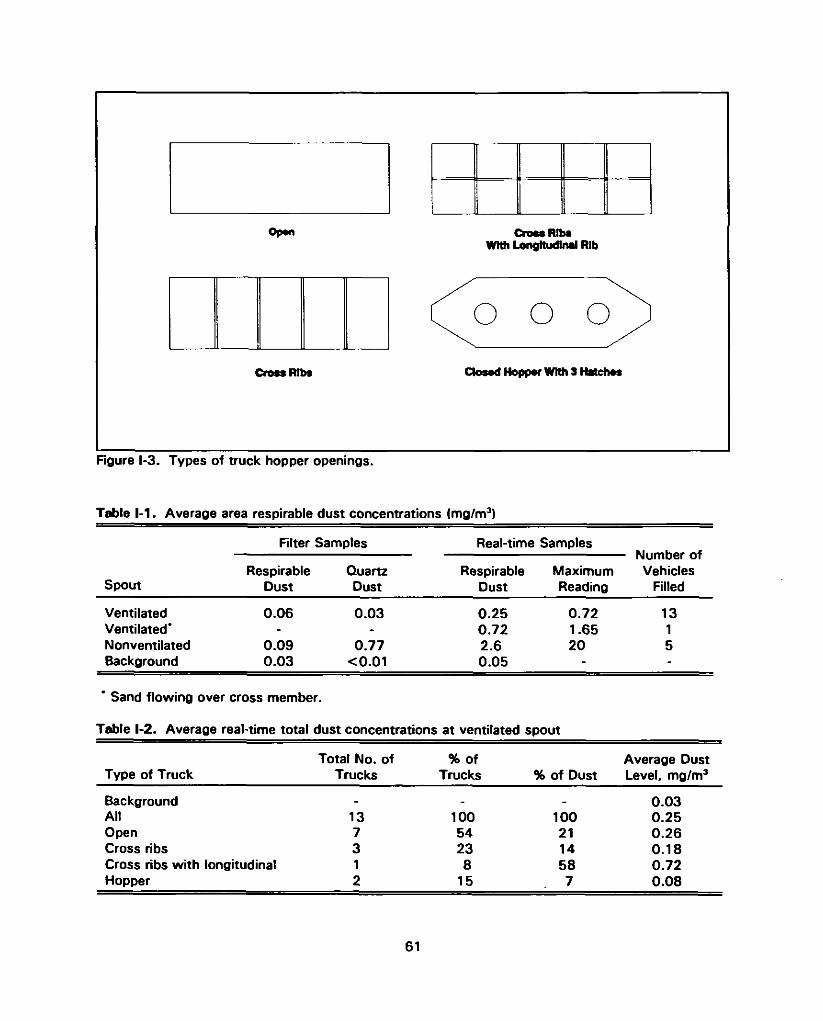
Figure 1-3. Types of truck hopper openings.

Table 1-1. Average area respirable dust concentrations (mg/m3)

Filter Samples Real-time Samples

SpoutRespirable

DustQuartzDust

RespirableDust

MaximumReading

iMUiuOGr OT Vehicles

Filled

Ventilated 0.06 0.03 0.25 0.72 13Ventilated* - - 0.72 1.65 1Nonventilated 0.09 0.77 2.6 20 5Background 0.03 <0.01 0.05 - -

* Sand flowing over cross member.

Table 1-2. Average real-time total dust concentrations at ventilated spout

Type of TruckTotal No. of

Trucks% of

Trucks % of DustAverage Dust Level, mg/m3

Background - - _ 0.03All 13 100 100 0.25Open 7 54 21 0.26Cross ribs 3 23 14 0.18Cross ribs with longitudinal 1 8 58 0.72Hopper 2 15 7 0.08

61

Table 1*3. Average real-time total dust concentrations at nonventilated spout

Type of Railroad Car

No. of Cars Cars, % Dust, %

Average Dust Level, mg/m3

All cars 5 100 100 2.64 Hatch 2 40 30 3.28 Hatch 1 20 48 5.110 Hatch 1 20 17 1.82 Coffin lid 1 20 5 0.5

Dust levels were 10 (real-time data) to 15 (air samples) times higher near the nonventilated loading spout than near the ventilated spout. When the spout was not lowered to the bottom of the truck or when sand flowed over a rib, dust levels were up to 40 times higher than when the spout was kept near the top of the sand pile. This was a problem for trucks with longitudinal ribs. By keeping the spout near the top of the sand pile, the free fall distance of the sand, the amount of airflow entrained in the falling sand, and the amount of dust generated were greatly reduced. When loading enclosed hopper trucks, free falling sand generates dust inside the enclosed container. With sufficient exhaust ventilation at the spout, the dust was effectively contained. The controlled spout used in this case study operated at the designed ventilation rate, with a face velocity of 130 ft/min (400 frVmin) for a loading capacity of 100 frVmin of sand.

RecommendationsWhen a ventilated spout used to bulk fill vehicles with a dry, free flowing sand was compared with a nonventilated spout, the former reduced dust concentrations by approximately 97%. To accomplish this reduction in dust concentrations, sufficient ventilation at the spout was needed. The proper type of ventilated spout, open or closed, could possibly further reduce these concentrations during loading operations. This was shown when the enclosed-type loading spout was used to fill an open-type truck (Table 1-2). No matter which controls are used, good work practices are needed. When using a ventilated spout, it is important to prevent the flow of sand over a rib and to keep the spout discharge near the top of the accumulating sand pile.

ReferenceII. Cooper, T.C.; O'Brien, D.M.; Sheehy, J.W.; Froehlich, P.A.; Valiante, D.; and Stephens, A.:

Sentinel Event Notification System for Occupational Risks (SENSOR): Recommendations for Control of Silica Exposures at Uniman Dividing Creek Sand Plant, Millville, New Jersey. USDHHS(NIOSH) Report No. ECTB 171-12b. NIOSH, Cincinnati, OH (1990).

62

Case Study J. Grinding Operations

IntroductionThis case study describes an evaluation of exposures to silica-containing dusts in the casting cleaning operation at a steel foundry.11,11 In the metal casting process, crystalline silica is contained in molding and coremaking sands, in clays used as bonding agents, in parting compounds, in some refractory materials, and as surface contamination on castings. Exposure can occur almost anywhere within the foundry. Castings are first cleaned by steel shot in an abrasive blasting machine or by sand blasting in a walk-in cabinet. Additional material is primarily removed from castings by various hand-held grinders on downdraft benches. Full-shift exposure measurements of the grinder operators demonstrated the potential for excessive exposure to silica.

MethodologyBecause the greatest number of workers are potentially overexposed to silica in the casting cleaning operations, this area of the foundry received special attention. Real-time dust concentrations were measured with a hand-held aerosol monitor (HAM, PPM, Inc., Knoxville, TN). The HAM is a light scattering monitor; its response is dependent on the optical characteristics of the dust being measured. The HAM responds to respirable dust but does not differentiate between crystalline silica and other dusts. Measurements were made on two workers performing chipping and grinding operations to determine the relative exposure caused by different tools and operations. Each worker selected a casting that required the use of a variety of tools. One selected a pump housing; the other selected an impeller. Each worker used a 6-in. horizontal radial wheel grinder (6000 rpm), a 4-in. cutoff wheel (15,000 rpm), and a 3/8-in. diameter burr mounted on a 16-in. extension (18,000 rpm). The worker cleaning the impeller also used a cone wheel mounted to the same type of tool as the 4-in. cutoff wheel. Each tool was pneumatically operated with the exhaust unmuffled at the tool. Dust exposure measurements and video recordings were made for a nominal 30 min on each worker, and a data logger (Rustrak® Ranger, Guitón, Inc., East Greenwich, Rl) electronically recorded dust exposures.

Dust exposure data were overlaid as a moving bar (proportional to the exposure) onto the video record and viewed to estimate activities that may affect exposure. This review indicated that the type of tool used, the direction of the grinding swarf (the stream of glowing metal particles), and the position of tool (inside or outside of the casting) caused noticeable exposure differences. To determine the extent to which these variables affected exposure, the real-time data were assembled into a commercial spreadsheet consisting of time, exposure, and activity for each 5-sec time period. The exposure measurements were "slipped” 5 sec with respect to the time and activities to allow for instrument and contaminant transportation lag. This lag was determined by viewing the video recordings of the work activities while tracking the real-time exposure measurements. The average exposure, the time, and the "dust-dose" (the product of dust concentration and time) were calculated for each of the activity variables with the use of the "database" functions of the spreadsheet.

FindingsThe average dust concentration for each tool type and the percent of the time each tool was used are presented in Figure J-1. While cleaning the pump housing, dust concentrations were highest for the 6-in. grinder and the 4-in. cutoff wheel. While cleaning the impeller, dust concentrations were highest for the 6-in. grinder and the cone grinder. Tool usage times were similar, except that the cone grinder was not used on the impeller housing. The "dust-dose" is described graphically in Figure J-2 as a function of tool type, tool location, and swarf direction. The "dust-dose” was almost an order of

63

8

6 Inch 4 Inch Con« Burr OtherGrinder Type

Pump Housing V/X Impeller

6 Inch 4 Inch Con« BurrGrinder Type

Other

Pump Housing ^ 3 Impeller

Figure J-1. Average dust concentration for each tool type and the percent of the time each toot was used in cleaning the castings.

64

Pump Housing (97 ibj/ w *- win) Tod Un

Impollor (12 mg/m *- win) Tool Um

• MiMWr

Tbol Loottion Ib d LootSon

Figure J-2. Percentage of "dust-dose" as a function of tool type, tool location, and swarf direction when grinding castings.

65

magnitude greater for the pump housing than for the impeller. The 4-in. cutoff wheel was the greatest contributor (57%) to "dust-dose" for the worker cleaning the pump housing, and the 6-in. grinder was the greatest contributor (54%) to the "dust-dose" for the worker cleaning the impeller. When the inside of the impeller casting was cleaned, the dust dose was lessened; although the worker spent about five times as long cleaning the inside of the casting as the outside, cleaning the inside resulted in only about 39% of the total "dust-dose* for this worker. This reduced dose may be because the impeller diffused the grinding swarf. Swarf direction appeared to be a major exposure factor; for the pump housing, concentrations ranged from highest to lowest in the order of "toward," "up," "away," "down," and "undetermined." For the impeller, only short periods were observed where the swarf was directed "toward," "up," or "away."

RecommendationsCleaning the large castings presents difficult problems. The size of the casting precludes working close enough to the grates of the downdraft booths for dust to be efficiently captured. Perhaps a sidedraft booth would be more effective — one with the castings set on a rotating fixture so that the grinding swarf could be directed into the hood (the real-time data indicated that the swarf direction was an important exposure factor). Worker training and continued supervision would be required to encourage proper use of such a system. A better approach for cleaning large castings would be the installation of high-velocity, low-volume (HVLV) exhaust hoods to supplement the downdraft benches. The real-time monitoring indicates that the tools that are most easily controlled, the 6-in. grinder and the 4-in. cutoff wheel, are also the tools that contribute most heavily to dust exposure.g21 The American Conference Governmental Industrial Hygienist has made detailed recommendations for HVLV hoods (VS-801 through VS-SO^.“3'

ReferencesJ1. O'Brien, D.M.; Froehlich, P.A.; Gressel, M.G.; and Hall, R.M.: Sentinel Event Notification

System for Occupational Risks (SENSOR): Recommendations for Control of Silica Exposures at Ingersol-Rand Company, Foundry Division, Phillipsburg, New Jersey. USDHHS(NIOSH) Report No. ECTB 171-17b. NIOSH, Cincinnati, OH (1990).

J2. Cusamano, G.: Personal Communication. Aer-X-Dust Co., Tennent, NJ. November 1989.

J3. American Conference of Governmental Industrial Hygienist. Industrial Ventilation: A Manualof Recommended Practice, 20th edition. ACGIH, Cincinnati, OH (1988).

66

APPENDIX A. PROGRAM LISTINGS

BASIC listing for BAR program.

This listing is intended for use with a BASIC compiler (Turbo BASIC, QuickBasic, etc.). If a compiler is not used, several modifications are required for the program to operate correctly. In BAR.BAS, line 100, BARS1A.EXE and BARS2A.EXE should be changed to BARS1 A.BAS and BARS2A.BAS. Also in BAR.BAS, line 490, "BARS2A" becomes "BASICA BARS2A.BAS," and in line 500, "BARS1A" becomes "BASICA BARS! A.BAS."

1 0 ................. * .............................................................BAR.BAS.........................................20 ................* * • •••WRITTEN BY GREGORY J. DEYE & MICHAEL G. GRESSEL*****30 '•••••••••••N A T IO N A L INSTITUTE FOR OCCUPATIONAL SAFETY AND HEALTH4 0 .................. * ............ * DIVISION OF PHYSICAL SCIENCES AND ENGINEERING............5 0 .............................................................4676 COLUMBIA PARKWAY............................ <6 0 ............................................. * ...........CINCINNATI, OHIO 45226...................................7 0 ............................................................................................................* ......................80 '90 '100 THIS PROGRAM REQUIRES 3 ADDITIONAL FILES: BARS1A.EXE, BARS2A.EXE,1 1 0 ' AND PARMS.TXT120 'LIMITATIONS OF PROGRAM: DATA FILE CAN CONTAIN UP TO 3000 DATA POINTS 130 '140 ' IF YOU ARE GENERATING TWO BARS 150 ' THE DATA FILE MUST HAVE 4 COLUMNS OF NUMBERS 160 ' COLUMN 1 - MINUTES170 ' COLUMN 2 - SECONDS180 ' COLUMN 3 - EXPOSURE VALUE #1190 ' COLUMN 4 - EXPOSURE VALUE #2200 '

210 ' IF YOU ARE GENERATING A SINGLE BAR220 ' THE DATA FILE MUST HAVE 3 COLUMNS OF NUMBERS230 ' COLUMN 1 - MINUTES240 ' COLUMN 2 - SECONDS250 ' COLUMN 3 - EXPOSURE VALUE2 6 0 '270 'IF DATA FILE IS GENERATED IN LOTUS 1*2*3, MINUTES, SECOND AND EXPOUSRES 280 ' MUST BE IN SEPARATE COLUMNS. PRINT SPREADSHEET TO A FILE.290 '300 '****T H IS PROGRAM REQUIRES AT LEAST A COLOR GRAPHICS ADAPTER (CGA)**< 310 '320 'IF THE VIDEO OVERLAY SYSTEM IS USED. COMPUTER MUST HAVE AN ENHANCED 330 'GRAPHICS ADAPTER (EGA) AND OPERATE IN EGA 640x200 RESOLUTION MODE 3 4 0 '350 ON ERROR GOTO 580 360 SCREEN 0: COLOR 10 370 CLS380 PRINT * VIDEO BAR GENERATOR": PRINT390 PRINT : PRINT " WRITTEN BY GREGORY DEYE AND MICHAEL GRESSEL"400 PRINT • NATIONAL INSTITUTE FOR OCCUPATIONAL SAFETY AND HEALTH"410 PRINT ’ 4676 COLUMBIA PARKWAY. MAILSTOP R-5*420 PRINT " CINCINNATI. OHIO 45226"

67

430 '440 LOCATE 12. 7 450 COLOR 10460 LOCATE 13, 7: PRINT "Enter Number of Bars to be Displayed (<1 > or < 2 > )."470 LOCATE 14. 7: PRINT 'Enter <Q > to Quit *482 LOCATE 19, 7: COLOR 11: PRINT "Press <F1 > for Information on Data Rie Format.“486 KEY 1, "HEL* + CHR$(13)488 LOCATE 16. 7: COLOR 12: INPUT •Enter < 1 > ,< 2 > , or <Q > \ bamum$489 KEY 1, " : KEY 10, ""490 IF bamum* = *2’ THEN SHELL "BARS2A"500 IF bamum$ * "V THEN SHELL "BARSI A"510 IF bamumS * "HEL" THEN GOTO 610520 IF bamum$ = "Q" OR bamum$ » "q" THEN CLS 525 IF bamum$ = "Q" OR bamum$ = "q" THEN END 530 IF bamum$ = "2" THEN GOTO 360 540 IF bamum$ = "1* THEN GOTO 360550 CLS : LOCATE 12. 0: COLOR 12: PRINT " INVAUD INPUTI! PRESS ENTER TO CONTINUE 560 INV$ = INKEY$: IF INV$ < > CHR$(13) THEN GOTO 560 ELSE GOTO 360 580 CLS590 LOCATE 12. 28: COLOR 12: PRINT "ERROR!! PRESS ENTER TO CONTINUE ’595 EER$ = INKEY$: IF EER$ < > CHR$(13) THEN GOTO 595 600 RESUME 360 610 CLS : COLOR 10620 PRINT " DATA FILE FORMAT INSTRUCTIONS": PRINT622 SHELL "TYPE FORMAT.TXT"630 A$ = INKEY$: IF A$ < > CHR$<13) THEN GOTO 630 ELSE GOTO 10

68

BASIC Esting for BARS1A program

10 'BARS1 A.BAS 20 CLEAR 30 KEY OFF 40 FILE2$ = " “50 CLS 60 SCREEN 870 LOCATE 1, 30: COLOR 10: PRINT "VIDEO BAR GENERATOR"80 LOCATE 21. 3: PRINT "PROMPTS AND MESSAGES"90 LINE (0. 32M639. 89), 11, B 100 COLOR 10110 LOCATE 6, 10: PRINT "MINIMUM READING"120 LOCATE 8, 10: PRINT "MAXIMUM READING*130 LOCATE 10, 7: PRINT "2-MAXIMUM TO BE DISPLAYED"140 LINE (450, 32)-(450, 89), 11 150 LINE (80, 97M559, 149), 11, B 160 LINE (420, 97M420, 149), 11 170 LINE (0, 171M639, 189), 11, B180 LOCATE 16, 14: COLOR 10: PRINT "3-MAXIMUM SCALE VALUE"190 LOCATE 14, 14: PRINT * TIME OF FIRST MEASUREMENT"200 LOCATE 18. 14: PRINT "4-TIME AND CONCENTRATION ON SCREEN7"210 LOCATE 4, 7: COLOR 10: PRINT "1 -": LOCATE 4, 10: COLOR 14: PRINT FILE$220 MAXY = 300 230 DEFINT l-L: DEFSNG Y 240 ON ERROR GOTO 1480 250 DUMMY = 0 260IMAX = 10 270 KOUNT - 0280 LX2 = 319: LY1 = 199: DELX = 16: LX1 = LX2 - DELX: KSYPREV = LY1:

KMIDX = INT((LX1 + LX2) / 2)290 DIM KX(3000), Y(3000), KX2(3000)300 GOSUB 380 'FILENAME310 GOSUB 620 'MAX READING320 SCALE = 1 :GOSUB 2140 'SCALE VALUE330 GOSUB 680 'INTERVAL340 GOSUB 730 TIME AND CONCENTRATION350 GOTO 780360 .................................. PROGRAM PARAMETER PROMPTS370 .................................. FILE NAME380 LOCATE 23, 3: COLOR 14: INPUT "1-DATA FILE NAME (< ENTER> RETURNS DEFAULT): ", FILE2$ 390 IF LEN(FILE2$) = 0 THEN FILE$ = FILE$ ELSE FILE$ = FILE2$400 GOSUB 1870 410 CLOSE420 LOCATE 23, 3: PRINT "READING FILE- 430 OPEN "I", #1, FILE$440 WHILE NOT EOF(1)450 INPUT #1, XREAD, X2READ, YREAD460 IF NOT KFIRST THEN YMIN = YREAD: KFIRST = -1470 KOUNT = KOUNT + 1480 KX(KOUNT) = XREAD: Y(KOUNT) = YREAD: KX2(K0UNT) = X2READ 490 IF YREAD > YMAX THEN YMAX = YREAD: KOUNTMAX = KOUNT 500 IF YREAD < YMIN THEN YMIN = YREAD: KOUNTMIN = KOUNT 510 WEND520 LOCATE 6, 64: COLOR 14: PRINT USING "# # # # .« "; YMIN 530 LOCATE 8, 64: PRINT USING "####.##"; YMAX

69

540 LOCATE 4, 10: PRINT FILE$550 KXTIME$ = STR$(INT(KX2(1)))560 IF LEN(KXT1ME$) = 2 THEN KXT1ME$ . "O’ + RIGHTS (KXT1ME$, 1) ELSE

KXTIME$ = RIGHT$(KXTIME$. 2)570 LOCATE 14. 59: PRINT KX(1); RIGHT$(KXTIME$, 2)580 IF LEN(STR$(KX(1))) = 2 THEN LOCATE 14, 61 ELSE LOCATE 14. 62 590 PRINT ":"600 RETURN610 '* * • * ..........................MAXIMUM READING DISPLAYED620 LOCATE 23. 3: INPUT “2-ENTER THE MAXIMUM READING (DEFAULT = MAXIMUM) ". YMAX1 630 GOSUB 1870640 IF YMAX1 = 0 THEN YMAX = YMAX ELSE YMAX = YMAX1 650 LOCATE 10. 64: COLOR 14: PRINT USING "####.##“ ; YMAX 660 RETURN670 '* * * .............. • * * * . »READING INTERVAL680 INCSEC = KX2(2) - KX2(1)690 IF INCSEC < O THEN INCSEC = KX2(3) - KX2(2)700 KBEEP = O 710 RETURN7 2 0 .........................*****T IM E AND CONCENTRATION DISPLAY730 LOCATE 23. 3: INPUT "4-TIME AND CONCENTRATION ON SCREEN? (DEFAULT=YES) ", AN$:

IF LEFT$(AN$, 1) = "N" OR LEFT$(AN$, 1) = "n" THEN K PRINT = 0 ELSE K PR I NT = -1 740 LOCATE 18, 60: IF KPRINT « -1 THEN PRINT “YES" ELSE PRINT "NO "750 GOSUB 1870 760 RETURN770 ' • • • .............. * * * * * «PARAMETER CHANGES780 LOCATE 23. 3: COLOR 14: INPUT "ARE INPUTS CORRECT? (DEFAULT = YES) ", ACORRÍ 790 GOSUB 1870: IF ACORR$ = “N" OR ACORRÍ = “n" THEN GOTO 810 800 GOTO 870810 LOCATE 23, 3: INPUT "ENTER INPUT NUMBER TO CHANGE: ", CHANGES: GOSUB 1870820 IF CHANGES = 1 THEN GOSUB 1900830 IF CHANGES = 2 THEN GOSUB 620840 IF CHANGES - 3 THEN GOSUB 2140850 IF CHANGES = 4 THEN GOSUB 730860 GOTO 780870 CLS880 LOCATE 15, 3: PRINT "WHEN VIDEO CLOCK READS KX(1); RIGHT$(KXT1ME$.2)890 LOCATE 16, 3: PRINT "PRESS S TO BEGIN OVERLAY, PRESS Q TO QUIT-900 LBARDRAWN = 0: LAP * 0: KSYPREV = LY1910 IK$ = INKEY$: IF IK$ < > *S" AND IK$ < > "s" THEN 910920 SCREEN 7930 PALETTE 8. 0940 LOCATE , . 0950 CLS960 COLOR 49 7 0 '9 8 0 ................•••••••••P R O G R A M EXECUTION990 GOSUB 1190: DAYSECONDS = TOTALSECONDS: 'get seconds in day 1000 TIME$ = “00:00:00“1010 KSECPREV = VAL(RIGHT$(T1ME$, 2)): Inrtilization of previous second 1020 1 * 1 : GOSUB 1260: 'starts out on first rearing on key press1030 WHILE I < KOUNT1040 KSEC = VAL(RIGHT$(TIME$. 2)): 'seconds from dock1050 LAP = ((KSEC - KSECPREV + 60) MOD 60): IF LAP < INCSEC THEN 1040:1060 GOSUB12601070 KSECPREV = KSEC MOD 60: 'set up new previous second equal to present

70

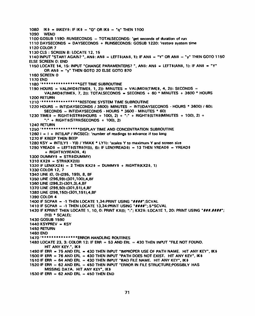
1080 IK$ = INKEY$: IF IK$ = 'Q ' OR IK$ = "q" THEN 1100 1090 WEND1100 GOSUB 1190: RUNSECONDS = TOTALSECONDS: ’get seconds of duration of run 1110 DAYSECONDS = DAYSECONDS + RUNSECONDS: GOSUB 1220: 'restore system time 1120 COLOR 71130 CLS : SCREEN 8: LOCATE 12, 151140 INPUT "START AGAIN? \ AN$: AN$ = LEFT$(AN$, 1): IF AN$ = "Y* OR AN$ = "y" THEN GOTO 1150 ELSE SCREEN 0: END1150 LOCATE 14. 15: INPUT "CHANGE PARAMENTERS? ", ANS: AN$ * LEFT$(AN$, 1): IF AN$ = "Y"

OR AN$ = -y" THEN GOTO 20 ELSE GOTO 870 1160 SCREEN 0 1170 END1180......................... *****G ETTIM E SUBROUTINE1190 HOURS - VAL(MID$(TIME$, 1, 2)): MINUTES = VAL(MID$ (TIMES, 4, 2»: SECONDS =

VAL(MID$(TIME$, 7, 2)): TOTALSECONDS = SECONDS + 60 * MINUTES + 3600 * HOURS 1200 RETURN1210 .................................... RESTORE SYSTEM TIME SUBROUTINE1220 HOURS - INT(DAYSECONDS / 3600): MINUTES = INT((DAYSECONDS - HOURS * 3600) / 60):

SECONDS = INT(DAYSECONDS - HOURS * 3600 - MINUTES * 60)1230 T1ME$ = RIGHT$(STR$(HOURS + 100), 2) + + RIGHT$(STR$(MINUTES + 100), 2) +

":" + RIGHT$(STR$(SECONDS + 100), 2)1240 RETURN1250...................... * * * * * «DISPLAY TIME AND CONCENTRATION SUBROUTINE1260 1 = 1 + INT(LAP / INCSEC): 'number of readings to advance if too long 1270 IF KBEEP THEN BEEP1280 KSY = INT(LY1 - Y(l) / YMAX • LY1): 'scales Y to maximum Y and screen size 1290 YREAD$ = LEFT$(STR$(Y(I», 6): IF LEN(YREAD$) = 13 THEN YREAD$ = YREAD$

+ RIGHT$(YREAD$, 4)1300 DUMMY$ = STR$(DUMMY)1310 KX2$ = STR$(KX2(I))1320 IF LEN(KX2$) = 2 THEN KX2$ = D U M M Y $ + RIGHT$(KX2$, 1)1330 COLOR 12, 7 1340 UNE (0. 0M295. 199), 8, BF 1350 UNE (296,99)-(301,100),4,BF 1360 UNE (296.2H301,3),4,BF 1370 UNE (296,50M301,51).4,BF 1380 UNE (296.150)-(301,151 ),4,BF 1390 COLOR 41400 IF SCPAR = -1 THEN LOCATE 1,34:PRINT USING ’ ####" ;SCVAL 1410 IF SCPAR = -1 THEN LOCATE 13,34:PRINT USING "####";.5*SCVAL1420 IF KPRINT THEN LOCATE 1. 10, 0: PRINT KX(I); KX2$: LOCATE 1, 20: PRINT USING "###.####";

(Y(l) * SCALE);1430 GOSUB 1590 1440 KSYPREV = KSY 1450 RETURN 1460 END1470 .................................. ERROR HANDLING ROUTINES1480 LOCATE 23, 3: COLOR 12: IF ERR = 53 AND ERL = 430 THEN INPUT "FILE NOT FOUND.

HIT ANY KEY.", IK$1490 IF ERR = 75 AND ERL = 430 THEN INPUT "IMPROPER USE OF PATH NAME. HIT ANY KEY". IK$ 1500 IF ERR = 76 AND ERL - 430 THEN INPUT "PATH DOES NOT EXIST. HIT ANY KEY", IK$1510 IF ERR = 64 AND ERL = 430 THEN INPUT "BAD FILE NAME. HIT ANY KEY", IK$1520 IF ERR = 62 AND ERL = 450 THEN INPUT "ERROR IN FILE STRUCTURE;POSSIBLY HAS

MISSING DATA. HIT ANY KEY". IK$1530 IF ERR = 62 AND ERL - 450 THEN END

71

1540 IF ERR * 53 OR ERR = 75 OR ERR ~ 76 OR 64 THEN RESUME 380 ELSE PRINT "Error PRINT ERR: PRINT : PRINT ’ Error Level*: PRINT ERL

1550 LOCATE 22. 1: PRINT ’ HIT ANY KEY- 1560 IK$ = INKEYS: IF IKS = ” THEN GOTO 1560 1570 END1580 ............* * * * * • • • «BAR DRAW SUBROUTINE1590 IF KSY < 0 AND NOT LBARDRAWN THEN GOSUB 17901600 'IF KSY-KSYPREV THEN RETURN1610 IF KSY > KSYPREV THEN GOSUB 16501620 IF KSY < KSYPREV THEN GOSUB 17201630 RETURN1640 ..........* ............ * ‘ BAR CLEAR SUBROUTINE1650 KY = KSYPREV1660 WHILE KY < KSY1670 UNE (LX1, KYMLX2, KY), 01680 KY - KY + 11690 WEND1700 RETURN1710 FILL SUBROUTINE1720 KY = KSYPREV1730 WHILE KY > KSY1740 UNE (LX1, KYMLX2. KY). 41750 KY - KY - 11760 WEND1770 RETURN1780 .......... LEVEL SUBROUTINE1790 KY = LY11800 WHILE KY > 01810 UNE (LX1, KYHLX2. KY), 41820 KY = KY - 11830 WEND1840 LBARDRAWN = -11850 RETURN1860 ..............* ............. * ‘ PROMPT UNE CLEAR ROUTINE1870 UNE (2. 174M630. 186). 0, BF 1880 RETURN1890 ................ . * * * * • »DATA FILE CHANGE ROUTINE1900 LOCATE 23, 31910 SHELL "DEL PARMS.BAR*1920 OPEN *0 *. 2, -PARMS.BAR*1930 WRITE #2, FILES, SCALE. KPRINT 1940 CLOSE 1950 CLEAR1960 FILES - * •: FILE2S = “ *1970 KEY OFF1980MAXY = 3001990 DEFINT l-L: DEFSNG Y2000 ON ERROR GOTO 14802010 DUMMY » 0: DUMMYS = STRS(DUMMY)2020 IMAX - 10 2030 KOUNT = O2040 LX2 = 319: LY1 - 199: DELX « 16: LX1 = LX2 - DELX: KSYPREV = LY1 :

KMIDX « INT((LX1 + LX2) / 2)2050 CLOSE2060 OPEN "I", 3, “PARMS.BAR*2070 INPUT #3. FILES, SCALE. KPRINT

72

2080 GOSUB 3802090 LOCATE 10, 64: PRINT "2100 GOSUB 620 2110 GOSUB 680 2120 GOTO 7802 1 3 0 .........* * * * « * * » # * s c A L E VALUE2140 LOCATE 23,3: INPUT "3-SCALE ON SCREEN? (DEFAULT = NO) \AN$:!F LEFT$(AN$,1) = "y"

OR LEFT$(AN$,1) = "Y" THEN SCPAR = -1 ELSE SCPAR=0 2150 IF SCPAR = 0 THEN LOCATE 16,60:PRINT ’ NONE" :RETURN 2160 GOSUB 18702170 LOCATE 23.3: INPUT "3-INPUT FULL SCALE VALUE. \SCVAL 2180 GOSUB 18702190 LOCATE 16.60: PRINT USING "####";SCVAL 2200 RETURN

73

8ASIC listing for BARS2A program

10 'BARS2A.BAS 20 FILES * " "30 FILE2S = " - 40 CLS 50 SCREEN 860 LOCATE 1, 30: COLOR 10: PRINT “VIDEO BAR GENERATOR"70 LOCATE 21. 3: PRINT "PROMPTS AND MESSAGES"80 LINE (0, 32M639, 102). 11, B 90 COLOR 10100 LOCATE 6. 10: PRINT "MINIMUM READING"110 LOCATE 8. 10: PRINT "MAXIMUM READING"120 LOCATE 10, 7: PRINT "4-MAXIMUM TO BE DISPLAYED"130 LOCATE 3. 48: COLOR 10: PRINT "BAR 1"140 LOCATE 3. 65: COLOR 10: PRINT 'BAR 2"150 UNE (500. 32M500, 102). 11 160 UNE (361, 32M361. 102). 11 170 UNE (80. 111M559. 150), 11, B 180 UNE (420. 111M420, 150), 11 190 UNE (0, 171H639, 189), 11, B200 LOCATE 16, 14: COLOR 10: PRINT " TIME OF FIRST MEASUREMENT"210 LOCATE 12, 7: COLOR 10: PRINT "5-MAXIMUM SCALE VALUE"220 LOCATE 18, 14: PRINT '6-TIM E AND CONCENTRATION ON SCREEN?"230 LOCATE 4, 48: COLOR 10: PRINT '2 - "240 LOCATE 4, 65: COLOR 10: PRINT "3 -"250 LOCATE 4, 7: COLOR 10: PRINT " I - " : LOCATE 4, 10: COLOR 14: PRINT FILES260 KEY OFF270 MAXY = 300280 DEFINT I-L: DEFSNG Y290 ON ERROR GOTO 1930300 DUMMY = 0: DUMMYS = STRS (DUMMY)310IM AX = 10320 KOUNT = 0: Y2MIN = 1000: Y1MIN = 1000: Y1MAX = 0: Y2MAX = 0 330 LBARDRAWN1 - O: LBARDRAWN2 = O 340 CLOSE350 LX11 * O: LY1 = 199: DELX = 1 6 : LX12 = LX11 + DELX: 'parameters for bar size and location 360 KSY1PREV * LY1370 LX22 * 319: LY2 = 199: DELX * 16: LX21 = LX22 - DELX 380 KSY2PREV = LY2 390 GOSUB 490'400 GOSUB 790410 GOSUB 840420 GOSUB 890430 SCALE=1: GOSUB 2900440 GOSUB 1000450 GOSUB 1040460 GOTO 1090470 ............ *» ***p ROGRAM PARAMETER PROMPTS4 8 0 ......................... NAME490 LOCATE 23, 3: COLOR 14: INPUT " 1 -DATA FILE NAME (<ENTER> RETURNS DEFAULT): \ FILE2S500 GOSUB 2580510 LOCATE 4, 10: PRINT "520 IF LEN(FILE2S) = 0 THEN FILES = FILES ELSE FILES = FILE2S530 LOCATE 23. 3: PRINT 'READING RLE......"540 GOSUB 2580

74

550 DIM KX(2000), YK2000). KX2(2000), Y2{2000)560 OPEN "I", #1, FILE$570 WHILE NOT EOF(1)580 INPUT #1, XREAD, X2READ, Y1 READ, Y2READ590 IF NOT KFIRST THEN Y1MIN = Y1READ: Y2MIN = Y2READ: KFIRST = -1: ' start minumum Y off

with first reading 600 KOUNT = KOUNT + 1610 KX(KOUNT) = XREAD: KX2(KOUNT) = X2READ: Y1 (KOUNT) = Y1READ: Y2(KOUNT) = Y2READ620 IF Y1 READ > Y1 MAX THEN Y1MAX = Y1 READ: KOUNTMAX1 = KOUNT: 'find maximum Y1 and

time for Y1630 IF Y1 READ < Y1MIN THEN Y1MIN = Y1READ: KOUNTMIN1 = KOUNT640 IF Y2READ > Y2MAX THEN Y2MAX = Y2READ: KOUNTMAX2 = KOUNT650 IF Y2READ < Y2MIN THEN Y2MIN = Y2READ: KOUNTMIN2 « KOUNT660 WEND670 LOCATE 6. 48: COLOR 14: PRINT USING "####.##"; Y1MIN 680 LOCATE 8, 48: PRINT USING "####.##"; Y1MAX 690 LOCATE 6, 65: PRINT USING "####.##"; Y2MIN 700 LOCATE 8, 65: PRINT USING "####.##"; Y2MAX 710 LOCATE 4, 10: PRINT FILE$720 KXTIME$ = STR$(INT(KX2(1)))730 IF LEN(KXTIME$} = 2 THEN KXTIME$ = "0* + RIGHT$(KXTIME$, 1) ELSE KXTIMES =

RIGHT$(KXTIME$, 2)740 LOCATE 16, 59: PRINT KX(1); RIGHT$(KXTIME$, 2)750 IF LEN(STR$(KX(1})) = 2 THEN LOCATE 16, 61 ELSE LOCATE 16, 62 760 PRINT 770 RETURN780 .................. * ............... DATASET 1 NAME790 LOCATE 23, 3: INPUT "2-ENTER FIRST DATA SET NAME: ", NAME1 $800 GOSUB 2580810 LOCATE 4, 51: PRINT NAME1 $820 RETURN8 3 0 .................................... DATASET 2 NAME840 LOCATE 23, 3: INPUT "3-ENTER SECOND DATA SET NAME: ", NAME2$850 GOSUB 2580860 LOCATE 4, 68: PRINT NAME2$870 RETURN880 .................. * ............... MAXIMUM READING890 LOCATE 23, 3: COLOR 14: INPUT "4-ENTER THE MAXIMUM READING FOR FIRST

SET (DEFAULT = MAXIMUM) ", YINMAX 900 IF YINMAX < > 0 THEN Y1MAX = YINMAX 910 LOCATE 10, 48: COLOR 14: PRINT USING "####.##"; Y1MAX 920 GOSUB 2580930 .....................* .............MAXIMUM READING 2940 LOCATE 23. 3: INPUT "4-ENTER THE MAXIMUM READING FOR SECOND SET (DEFAULT =

MAXIMUM) ", YINMAX 950 IF YINMAX < > 0 THEN Y2MAX = YINMAX 960 LOCATE 10, 65: PRINT USING "####.##"; Y2MAX 970 GOSUB 2580980 RETURN '9 9 0 ....................................... ****DETERMINE INTERVAL1000 INCSEC = KX2(2) - KX2(1):1010 IF INCSEC < 0 THEN INCSEC = KX2(3> - KX2(2)1020 RETURN1030 ............. AND CONCENTRATION DISPLAY1040 LOCATE 23, 3: INPUT "6-TIME AND CONCENTRATION ON SCREEN? (DEFAULT =YES) ", AN$:

IF LEFT$(AN$, 1) = "n" OR LEFT$(AN$, 1) = "N" THEN KPRINT = 0 ELSE KPRINT = -1

75

1050 LOCATE 18. 60: IF KPRINT = -1 THEN PRINT "YES’ ELSE PRINT "NO "1060 GOSUB 2580 1070 RETURN1080............. ....................INPUT CORRECTION1090 LOCATE 23, 3: COLOR 14: INPUT "ARE INPUTS CORRECT? (DEFAULT= YES) ", ACORR$1100 GOSUB 2580: IF ACORR$ = "n" OR ACORR$ = "N" THEN GOTO 1120 1110 GOTO 12701120 LOCATE 23. 3: INPUT "ENTER INPUT NUMBER TO CHANGE: ", CHANGES: GOSUB 2580 1130 IF CHANGES = 1 THEN GOTO 2610 1140 LOCATE 10. 48: IF CHANGES = 4 THEN PRINT "1150 LOCATE 10, 65: IF CHANGES = 4 THEN PRINT "1160 LOCATE 4, 51: IF CHANGES = 2 THEN PRINT "1170 IF CHANGES = 2 THEN GOSUB 790 1180 LOCATE 4, 68: IF CHANGES = 3 THEN PRINT "1190 IF CHANGES = 3 THEN GOSUB 840 1200 IF CHANGES = 4 THEN GOSUB 890 1210 LOCATE 16. 60: IF CHANGES = 5 THEN PRINT " "1220 IF CHANGES = 5 THEN GOSUB 29001230 LOCATE 18. 60: IF CHANGES = 6 THEN PRINT " "1240 IF CHANGES - 6 THEN GOSUB 1040 1250 GOTO 10901260 ........................... ****START P R O G R A M **********.............* ...........*1270 CLS1280 LOCATE 15. 3: PRINT "WHEN VIDEO CLOCK READS KX(1); RIGHT$(KXTIME$.2)1290 LOCATE 16, 3: PRINT "PRESS S TO BEGIN OVERLAY. PRESS Q TO QUIT-1300 LBARDRAWN *= 0: LAP =■= 0: KSYPREV = LY11310 LX11 = 0: LY1 * 199: DELX = 16: LX12 = LX11 + DELX1320 KSY1PREV = LY11330 LX22 = 319: LY2 * 199: DELX = 16: LX21 = LX22 - DELX 1340 KSY2PREV = LY21350 IK$ * INKEY$: IF IK$ < > "S" AND IK$ < > "s" THEN 13501360 LOCATE , . 01370 CLS1380 SCREEN 71390 PALETTE 8. 01400 GOSUB 24101410 COLOR 121420 '1430 '• • • •• •• •• •• •• • ••P R O G R A M EXECUTION1440 GOSUB 1640: DAYSECONDS = TOTALSECONDS: 'get seconds in day 1450 T1ME$ = "00:00:00“1460 KSECPREV = VAL(RJGHT${T1ME$, 2)): Tnitilization of previous second 1470 1 = 1: GOSUB 1710: 'starts out on firs t reacfing on key press1480 WHILE I < KOUNT1490 KSEC = VAL(R!GHT$(TIME$, 2)): 'seconds from dock1500 LAP = ((KSEC - KSECPREV + 60) MOD 60): IF LAP < INCSEC THEN 1490: 'return until dock

ticks INCSEC seconds 1510 GOSUB 1710: ' update bar on screen and, if needed, print values on screen 1520 KSECPREV = KSEC MOD 60: 'set up new previous second equal to present 1530 IK$ = INKEY$: IF IK$ - "Q" OR 1K$ = "q" THEN 1550 1540 WEND1550 GOSUB 1640: RUNSECONDS = TOTALSECONDS: 'get seconds of duration of run 1560 DAYSECONDS = DAYSECONDS + RUNSECONDS: GOSUB 1670: 'restore system time 1570 COLOR 71580 SCREEN 8: CLS : LOCATE 10. 15, 0

76

1590 INPUT 'START AGAIN? ", AN$: AN$ = LEFT$(AN$, 1): IF AN$ = "Y" OR AN$ = "y" THEN GOTO 1600 ELSE SCREEN 9: END

1600 LOCATE 12, 15: INPUT "CHANGE PARAMETERS? \ AN$: AN$ = LEFT$(AN$, 1): IF AN$ = "Y" OR AN$ « -y - THEN GOTO 10 ELSE GOTO 1270

1610 SCREEN 0 1620 END1630.................... * .............GET TIME SUBROUTINE1640 HOURS = VAL(MID$(TIMES, 1, 2)): MINUTES = VAL(MID$(TIME$. 4. 2)»: SECONDS =

VAL(MID$(TIME$, 7. 2}): TOTALSECONDS = SECONDS + 60 * MINUTES + 3600 * HOURS 1650 RETURN1660 ................................* »RESTORE SYSTEM TIME SUBROUTINE1670 HOURS = I NT (D A YSECONDS / 3600): MINUTES = INT((DAYSECONDS - HOURS * 3600) / 60):

SECONDS * INT(DAYSECONDS - HOURS * 3600 - MINUTES * 60)1680 TIME$ = RIGHT$(STR$(HOURS + 100), 2) + + RIG HT$(STR$ (MINUTES + 100), 2) +

":" + RIG HT $ (STR $ (SECONDS + 100), 2)1690 RETURN1 7 0 0 '...................................DISPLAY TIME AND CONCENTRATION SUBROUTINE1710 I = I + INT(LAP / INCSEC): 'number of readings to advance if waiting too long in other routines 1720 '1730 KSY1 = INT(LY1 - Y1(!) / Y1MAX * LY1): 'scales Y1 to maximum Y1 and screen size1740 KSY2 = INT(LY1 - Y2(l) / Y2MAX * LY1): 'scales Y2 to same maximum Y1 and screen siz1750 IF KSY1 < 0 THEN KSY1 = 0: 'prevents delay in updating bar if too high 1760 IF KSY2 < 0 THEN KSY2 = 0 1770 IF KSY1 > 199 THEN KSY1 * 199 1780 IF KSY2 > 199 THEN KSY2 - 1991790 Y1READ$ = LEFT $ (STR $(Y 1(1)), 6): IF LEN(Y1READ$) = 13 THEN Y1READ$ = Y1READ$ +

RIGHT$(Y1 READ$, 4): 'format for screen display 1800 Y2READ$ = LEFT$(STR$(Y2(D), 6): IF LEN(Y2READ$) = 13 THEN Y2READ$ = Y2READS +

RIGHT$(Y2READ$, 4): 'format for screen display 1810 KX2$ = STR$(KX2(I))1820 IF LEN(KX2$) = 2 THEN KX2$ = DUMMY$ + RIGHT$(KX2S, 1)1830 COLOR 41840 SCALE -1 :IF KPRINT THEN LOCATE 1, 17. 0: PRINT KX(I); KX2$;1850 IF KPRINT THEN LOCATE 1, 10: PRINT USING "###.##"; (Y1(l) * SCALE);1860 IF KPRINT THEN LOCATE 1, 25: PRINT USING "###.##"; (Y2(l) * SCALE);1870 GOSUB 2060: 'update bar1880 KSY1PREV = KSY1: 'new previous line mmber for bar 1890 KSY2PREV = KSY2 1900 RETURN 1910 END1920..................................................................................* ..ERROR HANDLING ROUTINES1930 LOCATE 23, 3: COLOR 12: IF ERR = 53 AND ERL = 560 THEN INPUT "FILE NOT FOUND.

HIT ANY KEY.", IK$1940 IF ERR = 75 AND ERL = 560 THEN INPUT "IMPORPER USE OF PATH NAME. HIT ANY KEY.", IK$ 1950 IF ERR = 76 AND ERL = 560 THEN INPUT "PATH DOES NOT EXIST. HIT ANY KEY.", IK$1960 IF ERR = 64 AND ERL = 560 THEN INPUT "BAD FILE NAME. HIT ANY KEY.", IK$1970 IF ERR «= 62 AND ERL = 580 THEN PRINT "ERROR IN FILE STRUCTURE; POSSIBLY HAS MISSING

DATA. HIT ANY KEY."1980 IF ERR = 5 AND ERL = 1380 THEN PRINT "WRONG GRAPHICS ADAPTER HAS BEEN CHOSEN.

RERUN SETUP."1990 IF ERR = 5 AND ERL = 1380 THEN GOTO 2020 2000 IF ERR = 62 AND ERL = 580 THEN END2010 IF ERR = 53 OR ERR = 75 OR ERR = 76 OR ERR = 64 THEN RESUME 490 ELSE PRINT "Error

PRINT ERR: PRINT : PRINT "Error Level": PRINT ERL 2020 LOCATE 22, 1, 0: PRINT "HIT ANY KEY";2030 IK$ - INKEY$: IF IK$ - " THEN 2030

77

2040 END2050 ............................. **BAR DRAW SUBROUTINE2060 IF KSY1 < 0 AND NOT LBARDRAWN1 THEN GOSUB 2350: LBARDRAWN1 = -1: ' for drawing

first bar If o ff screen 2070 CLOR « 22080 IF KSY2 < 0 AND NOT LBARDRAWN2 THEN GOSUB 2350: LB ARDRAWN 2 - -1 2090 CLOR = 42100 'IF KSY = KSYPREV THEN RETURN2110 IF KSY1 > KSY1PREV THEN KSY = KSY1: KSYPREV = KSY1PREV: LXSTART = LX11: LXEND = LX12:

GOSUB 2210 2120 CLOR = 22130 IF KSY2 > KSY2PREV THEN KSY = KSY2: KSYPREV = KSY2PREV: LXSTART = LX21: LXEND = LX22:

GOSUB 2210 2140 CLOR = 42150 IF KSY1 < KSY1PREV THEN KSY = KSY1: KSYPREV = KSY1PREV: LXSTART = LX11: LXEND = LX12:

GOSUB 2280 2160 CLOR = 22170 IF KSY2 < KSY2PREV THEN KSY = KSY2: KSYPREV = KSY2PREV: LXSTART = LX21: LXEND = LX22:

GOSUB 2280 2180 CLOR = 4 2190 RETURN2200 ........................... BAR CLEAR SUBROUTINE2210 KY = KSYPREV2220 WHILE KY < KSY2230 UNE (LXSTART, KYMLXEND. KY), 02240 KY = KY + 12250 WEND2260 RETURN2270 .........................BAR FILL SUBROUTINE2280 KY = KSYPREV2290 WHILE KY > KSY2300 UNE (LXSTART, KYMLXEND, KY), CLOR2310 KY = KY - 12320 WEND2330 RETURN2340 ................ * ............... BAR LEVEL SUBROUTINE2350 KY - LY1 2360 WHILE KY > 02370 UNE (LXSTART. KYMLXEND, KY), CLOR2380 KY - KY - 12390 WEND2400 RETURN2410 COLOR 3, 72420 UNE (24, 8M295, 199), 8. BF 2430 LOCO - 38 * (LEN(NAME2$))2440 LOCATE 24, 4:C0L0R 42450 PRINT NAME1 $: LOCATE 23. LOCO: COLOR 2:PRINT NAME2$2460 UNE (24, 184M295. 199), 8. BF2470 UNE (296.99H301,100).2.BF:UNE (18.99)-(23.100),4,BF2480 UNE (296,2H301,3),2,BF:UNE (1842M23.3),4,BF2490 UNE (296.50H301,51 ),2,BF:LINE (18,50M23,51),4.BF2500 UNE (296,150M301,151),2,BF:UNE (18.150M23,151),4,BF2510 IF SCPAR = -1 THEN COLOR 2:LOCATE 1,34:PRINT USING "####";SCVAL22520 IF SCPAR = -1 THEN LOCATE 13,34:PRINT USING "####";.5*SCVAL22530 IF SCPAR = -1 THEN COLOR 4:L0CATE 1,4:PRINT USING "####’ ;SCVAL12540 IF SCPAR = -1 THEN LOCATE 13,4:PRINT USING "####\\5*SCVAL1

78

2550 RETURN 2560 RETURN2570 '• * * • • • • • • ******PR 0M PT CLEAR ROUTINE2580 LINE (2. 174M630, 186), 0, BF 2590 RETURN2600 ................ "D A T A FILE CHANGE ROUTINE2610 LOCATE 23. 32620 SHELL "DEL PARMS.BAR’2630 OPEN * 0 \ 2. "PARMS.BAR"2640 WRITE #2, F1LE$, NAME1 $, NAME2$, SCALE. KPRINT 2650 CLOSE 2660 CLEAR2670 FILE$ = " FILE2$ = " ’2680 KEY OFF2690 MAXY = 3002700 DEFINT l-L: DEFSNG Y2710 ON ERROR GOTO 19302720 DUMMY = O: DUMMY$ = STR$(DUMMY)2730 IMAX = 102740 KOUNT = 0: Y2MIN = 1000: Y1MIN = 1000: Y1MAX = 0: Y2MAX = 0 2750 LBARDRAWN1 - 0: LBARDRAWN2 - 0 2760 CLOSE2770 LX11 = O: LY1 = 199: DELX = 16: LX12 = LX11 + DELX: 'parameters for bar size and location 2780 KSY1PREV = LY12790 LX22 = 319: LY2 = 199: DELX = 16: LX21 = LX22 - DELX2800 KSY2PREV = LY22810 OPEN "I", 3. "PARMS.BAR"2820 INPUT #3. FILE$, NAME1 $. NAME2$, SCALE. KPRINT2830 GOSUB 4902840 LOCATE 10, 48: PRINT "2850 LOCATE 10. 65: PRINT ’2860 GOSUB 890 2870 GOSUB 1000 2880 GOTO 10902890 ..................................SCALE VALUE2900 LOCATE 23.3: INPUT "5-SCALE ON SCREEN? (DEFAULT = NO) ",AN$:IF LEFT$(AN$,1) = "Y* OR

AN$ = "y" THEN SCPAR = -1 ELSE SCPAR=0 2910 IF SCPAR = 0 THEN LOCATE 12.51 :PRINT "NONE":LOCATE 12,68:PRINT "NONE":RETURN 2920 GOSUB 25802930 LOCATE 23,3: INPUT ’ 5-INPUT DATA SET 1 FULL SCALE VALUE. \SCVAL1 2940 GOSUB 25802950 LOCATE 23.3: INPUT "5-INPUT DATA SET 2 FULL SCALE VALUE. \SCVAL22960 LOCATE 12.51:PRINT USING "####"; SCVAL1 :LOCATE 12.68:PRINT USING "####";SCVAL22970 RETURN

79

APPENDIX B. BAR PROGRAM OPERATING INSTRUCTIONS

To run the bar program, change to the drive and directory where the program is located, then type "BAR" at the DOS prompt. A screen appears listing three choices of operation: display one bar, display two bars, or quit. To display one bar, type *1“ then "ENTER"; for two bars type "2" then "ENTER"; to quit, type "Q" then "ENTER." If " 1" or "2" was entered, a new screen appears prompting for data inputs. The first prompt is for the data file name. Enter this name including drive, directory, and file extension. For example, "C:\DATADIR\DATAFILE.PRN" would call for the data file named "DATARLE.PRN," located on the C: drive in the directory named *DATADIR." The program reads the data file into memory, determines the interval between the readings, the maximum and minimum readings, as well as the time of the first reading. If two bars are to be displayed, the maximum and minimum readings are determined for both data sets. Next, if two bars are to be displayed, the program asks for names for the two data sets. When the program is displaying the data, the names will appear at the bottom of the screen next to its associated bar. For displaying both one bar and two bars, the next prompt is for the maximum reading to be displayed. The default is for the maximum reading in the data set. This prompt allows the user to ignore the readings that exceed a certain value. Any reading exceeding this value will be displayed as a full size bar. For the two bar display, the maximum reading value must be set for both data sets. After specifying the maximum reading, the next prompt is for a scaling factor. This input allows the user to multiply the readings by a value, such as a calibration factor. The default value is 1.00. The final input prompt is for displaying the time and concentration at the top of the screen. The default is to show this display. When finished entering the inputs, the program asks if the inputs are all correct. If not, the user is given the opportunity to make changes. When all inputs are correct, the user is prompted to press "S" to immediately begin displaying the bar(s). Pressing "Q" at any time while displaying the data, will halt the program before it displays the final reading in the data set. After displaying all of the data or after pressing "Q" to stop the display, a prompt will ask if the data should be displayed again. Answering "No" will take the program back to the main menu screen (where the program asks the number of bars to be displayed). If "Yes" is answered at the prompt, a second prompt will appear asking if changes should be made to the input parameters. Answering "Yes" to this prompt will allow changes to be made to the inputs. Answering "No" will result in the prompt to press "S" to start the display.

* U .S . GOVERNMENT PRIMING OFFICE: 1 9 9 2 - 6 4 8 - 1 7 9 / 6 0 0 1 2

80