arX

iv:c

ond-

mat

/010

1315

v1 [

cond

-mat

.sta

t-m

ech]

19

Jan

2001

Epitaxial mounding in limited mobility models of surface growth

P. Punyindu(1), Z Toroczkai(1,2), and S. Das Sarma(1)

(1)Department of Physics, University of Maryland, College Park, MD 20742, USA(2)Theoretical Division and Center for Nonlinear Studies, Los Alamos National Laboratory,

Los Alamos, New Mexico 87545, USA

We study, through large scale stochastic simulations

using the noise reduction technique, surface growth via

vapor deposition e.g. molecular beam epitaxy (MBE),

for simple nonequilibrium limited mobility solid-on-solid

growth models, such as the Family (F) model, the Das

Sarma-Tamborenea (DT) model, the Wolf-Villain (WV)

model, the Larger Curvature (LC) model, and other re-

lated models. We find that d=2+1 dimensional surface

growth in several noise reduced models (most notably the

WV and the LC model) exhibits spectacular quasi-regular

mound formation with slope selection in their dynamical

surface morphology in contrast to the standard statisti-

cally scale invariant kinetically rough surface growth ex-

pected (and earlier reported in the literature) for such

growth models. The mounding instability in these epitax-

ial growth models does not involve the Ehrlich-Schwoebel

step edge diffusion barrier. The mounded morphology in

these growth models arises from the interplay between the

line tension along step edges in the plane parallel to the

average surface and the suppression of noise and island

nucleation. The line tension tends to stabilize some of the

step orientations that coincide with in-plane high sym-

metry crystalline directions, and thus the mounds that

are formed assume quasi-regular structures. The noise

reduction technique developed originally for Eden type

models can be used to control the stochastic noise and

enhance diffusion along the step edge, which ultimately

leads to the formation of quasi-regular mounds during

growth. We show that by increasing the diffusion sur-

face length together with supression of nucleation and de-

position noise, one can obtain a self-organization of the

pyramids in quasi-regular patterns. The mounding insta-

bility in these simple epitaxial growth models is closely

related to the cluster-edge diffusion (as opposed to step

edge barrier) driven mounding in MBE growth, which has

been recently discussed in the literature. The epitaxial

mound formation studied here is a kinetic-topological in-

stability (which can happen only in d=2+1 dimensional,

or higher dimensional, growth, but not in d=1+1 dimen-

sional growth because no cluster diffusion around a closed

surface loop is possible in “one dimensional” surfaces),

which is likely to be quite generic in real MBE-type sur-

face growth. Our extensive numerical simulations produce

mounded (and slope-selected) surface growth morpholo-

gies which are strikingly visually similar to many recently

reported experimental MBE growth morphologies.

I. INTRODUCTION

Crystal growth, particularly high-quality epitaxial thinfilm growth, is one of the most fundamental processes im-pacting today’s technology [1]. A major issue in interfacegrowth experiments is to have continuous dynamical con-trol over the deposition process, such that interfaces withcertain desired patterns can be obtained. For example,while in thin film epitaxy it is desirable to obtain smoothsurfaces, in nanotechnology it is also important to beable to create regular, nanoscale structures with well de-fined geometry, such as quantum dots, quantum wires,etc. Growth is usually achieved by vapor deposition ofatoms from a molecular beam (molecular beam epitaxy,or MBE). Thus, in order to be able to design a controlleddeposition process, it is of crucial importance to under-stand all the instability types (which destroy controlla-bility) that may occur during growth. In the presentpaper we concentrate on MBE growth. There are sev-eral types of instabilities in MBE among which we men-tion the Ehrlich-Schwoebel (ES) [2] instability which is ofkinetic-energetic type. Ehrlich-Schwoebel (ES) barriersin the lattice potential induce an instability by hinderingstep-edge atoms on upper terraces from going down tolower terraces [2] which in turn can generate moundedstructures during growth. The ES instability is thoughtto be an ubiquitous phenomenon in real surface deposi-tion processes, and as such, is widely considered to bethe only mechanism for formation of mounds in surfacegrowth. Another kinetic-energetic instability, which doesnot involve any explicit ES barriers, was discussed byAmar and Family [3]. This instability involves a neg-ative barrier at the base of a step, and thus is due toa short range attraction between adatoms and islands.Short range attractions generically lead to clustering inmultiparticle systems, a property which in the languageof MBE translates into formation of mounds. Note thatthis attraction-induced instability and ES instability areessentially equivalent, and both could occur in d=1+1or 2+1 dimensions. Both the attractive instability andthe ES barrier instability cause mounding because atomson terraces preferentially collect at up-steps rather thandown-steps leading to the mounded morphology. In bothcases, there is no explicit stabilizing mechanism, and themounds should progressively stiffen with time leadingto mounded growth morphology with no slope selection,where the mound slopes continue to increase as growthprogresses. It is, of course, possible to stop the monotonic

1

slope increase by incorporating some additional mecha-nisms (e.g. the so-called “downward funneling” wheredeposited atoms funnel downwards before incorporation)which produce a downhill mass current on the surfaceand thereby opposes the uphill current created by theES barrier. There is, however, no intrinsic slope selec-tion process built in the ES barrier mechanism itself.

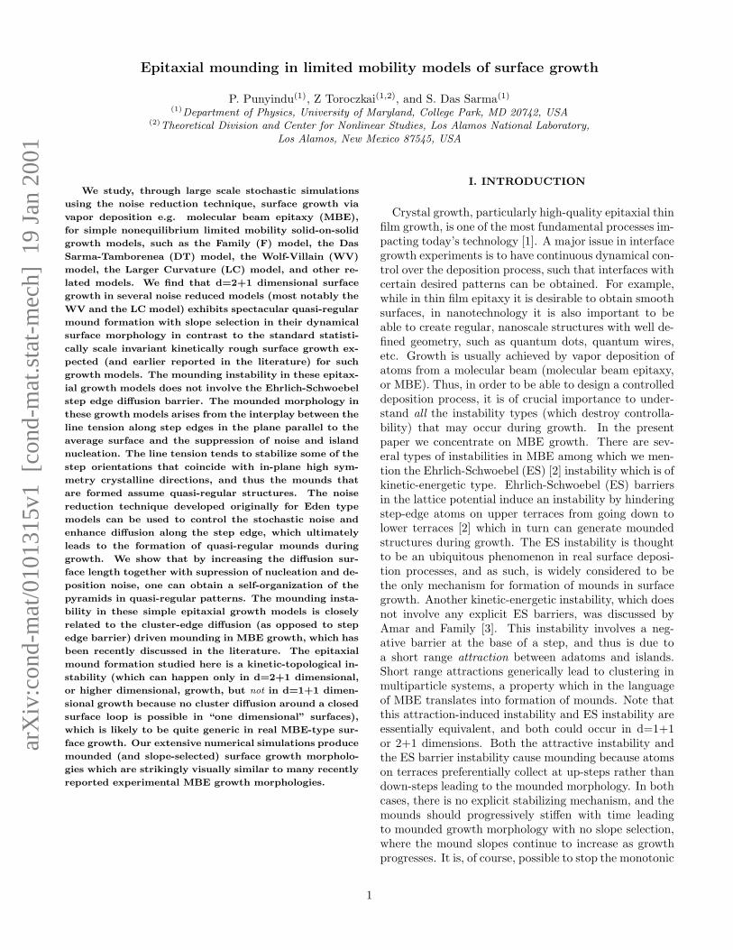
FIG. 1. Mounded morphology created by SED. This is asimulation of the LC model as described in the text.

The purpose of the current article is to discuss a com-pletely different kinetic-topological mechanism, qualita-tively distinct from the ES barrier induced mounding,which leads to spectacular mound formation (see Fig. 1for a colorful example) in MBE growth without involvingany ES barriers (or the closely related island-adatom at-traction mechanism) whatsoever. Based on the directstochastic numerical simulations of a large number ofMBE-related nonequilibrium limited mobility solid-on-solid epitaxial growth models studied in this paper webelieve that epitaxial mounding of the type discussedhere is quite generic, and may actually apply to a va-riety of experimental situations where mounded growthmorphologies (with slope selection) have been observed.The mechanism underlying the mounding instability dis-cussed in this paper is closely related to that proposed intwo recent publications [4,5] although its widespread ap-plicability to well-known limited mobility MBE growthmodels, as described here, has not earlier been appre-ciated in the literature. The mounding instability dis-cussed in this paper, being topological in nature, can hap-pen only on physical two-dimensional surfaces (d=2+1dimensions growth) or in (unphysical) higher (d>2+1)dimensional systems, in contrast to ES type instabilitieswhich, being of energetic origin, are allowed in all dimen-sions.

The instability most recently discovered by Pierre-Louis, D’Orsogna, and Einstein [4], and independently by

Ramana Murty and Copper [5] is entirely different fromES instabilities, because it is not of kinetic-energetic na-ture (involving potential barriers) but rather of a kinetic-topologic nature. This instability is generated by strongdiffusion along the edges of monoatomic steps, and itsnet effect in two or higher dimensions is to create quasi-regular shaped mounds on the substrate (see Fig. 1).For simplicity of formulation we will call this instabilitythe step-edge diffusion, or SED instability. What comesas a bit of a surprise is that in spite of its simplicityas a mechanism, it has not apparently been recognizedthat the SED mechanism may actually be playing a domi-nant role in many epitaxial mounding instabilities. Thereare two reasons for this, one is probably because the ESinstability has inadvertently and tacitly been acceptedas the only mechanism for mounding, and therefore themounded surface morphologies coming from experimentshave been apriori analyzed with the ES mechanism inmind, and the second reason is that SED is not easy tosee in simulations unless other conditions (related to re-duced noise) are met in addition to the existence of edge-current, which we will discuss in details in the presentpaper.

In this paper we discuss the SED instability, and an-alyze its effects on various growth models, giving botha simple continuum and discrete description. The SEDis shown to exist in a large number of discrete, limitedmobility growth models, and we identify the conditionsunder which SED-induced epitaxial mounding is mani-fested. We study the instability by producing dynamicalgrowth morphologies through direct numerical simula-tions and by analyzing the measured height-height cor-relation functions [6] of the simulated morphologies. Thispaper is organized as follows: in Section II we define anumber of limited mobility growth models (SubsectionII.A) studied here, we briefly review the noise reduc-tion technique (Subsection II.B), then present a seriesof simulated growth morphologies, both from early andlate times, with and without noise reduction (SubsectionII.C); in Section III we describe and discuss the SEDmechanism, by first presenting a continuum descriptionin terms of local currents (Subsection III.A) and its dis-crete counterpart with particular emphasis on the Wolf-Villain and Das Sarma - Tamborenea models (Subsec-tion III.B); in Subsection III.C we introduce the notionof conditional site occupation rates to analyze the effectsof noise reduction; Section IV is devoted to the prop-erties of the mounded morphologies with the emphasison the relevance of the height-height correlation function(Subsection IV.A), where we note possible comparisonwith experiments and discuss the relevance of the globaldiffusion current in the simulations for the mounding in-stability.

2

II. MORPHOLOGIES OF DISCRETE LIMITED

MOBILITY GROWTH MODELS

A. Models

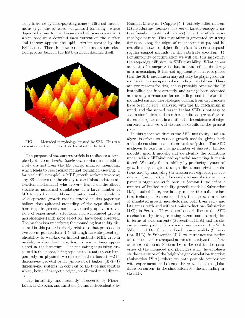
All the models studied here are dynamical limited mo-bility growth models in which an adatom is allowed to dif-fuse (according to specific sets of diffusion rules for eachmodel) within a finite diffusion length of l sites. The dif-fusion process is instantaneous and once the adatom hasfound its final site, it is incorporated permanently intothe substrate and can no longer move. These models arealso based on the solid-on-solid (SOS) constraint wherebulk vacancies and overhangs are not allowed. Desorp-tion from the growth front is neglected.

Family model

DT model

WV model

LC model

FIG. 2. Schematic configurations defining the diffusiongrowth rules in one dimension for various dynamical growthmodels discussed in this paper. Here l = 1.

With this SOS constraint, growth can be described ona coarse-grained level by the continuity equation

∂h

∂t+ ∇ · j = FΩ + η(x, t), (1)

where h(x, t) is the surface height measured in the growthdirection, j is the local (coarse-grained) surface diffusioncurrent, F is the incoming particle flux, Ω = a⊥ad

‖ is thesurface cell volume with a⊥ and a‖ being the lattice con-stants in the growth direction and in the d-dimensionalsubstrate, respectively. The shot noise is Gaussian un-correlated white noise with correlator:

〈η(x, t)η(x′, t′)〉 = Dδ(x − x′)δ(t − t′) (2)

where the amplitude of the fluctuations D is directly pro-portional to the average incoming particle flux throughthe relation: D = FΩ2.

The most general form of this continuity equation [8]which preserves all the symmetries of the problem can bewritten as:

∂h

∂t= ν2∇2h − λ4∇4h + λ22∇2(∇h)2 + ... + η,

(3)

where h from now on indicates the height fluctuationaround the average interface height 〈h〉. Note that theunit of time in our simulations is defined through 〈h〉;we arbitrarily choose the deposition rate of 1 monolayer(ML) per second, and all simulations are done with peri-odic boundary conditions along the substrate.

1. Family model

This is a model introduced by Family (F) [9] withthe simplest diffusion rule: adatoms diffuse to the localheight minima sites within range l (see the one dimen-sional version in Fig. 2). This is a well studied model andit is described on a coarse-grained level by the continuumEdwards-Wilkinson [10] equation ∂h

∂t = ν∇2h + η andhence the model asymptotically belongs to the Edward-Wilkinson (EW) universality class.

2. Das Sarma-Tamborenea model

The Das Sarma-Tamborenea (DT) model was pro-posed [11] as a simple limited mobility nonequilibriummodel for MBE growth. In this model, an adatom israndomly dropped on an initially flat substrate. If theadatom already has a coordination number of two ormore (i.e. one from the neighbor beneath it to satisfythe SOS condition, and at least one lateral neighbor) atthe original deposition site, it is incorporated at that site.If the adatom does not have a lateral nearest neighbor atthe deposition site, it is allowed to search, within a finitediffusion length, and diffuse to a final site with highercoordination number than at the original deposition site.In the case where there is no neighbor with higher coordi-nation number, the adatom will remain at the depositionsite. At the end of the diffusion process, the adatombecomes part of the substrate and the next adatom isdeposited.

It is important to note that adatoms in the DT modelsearch for final sites with higher coordination numberscompared to the deposition site. The final sites are notnecessarily the local sites with maximum coordinationnumbers. In other words, in the DT model adatoms tryto increase, but not necessarily maximize, the local co-ordination number. Also, deposited adatoms with more

3

than one nearest-neighbor bond do not move at all in theDT model.

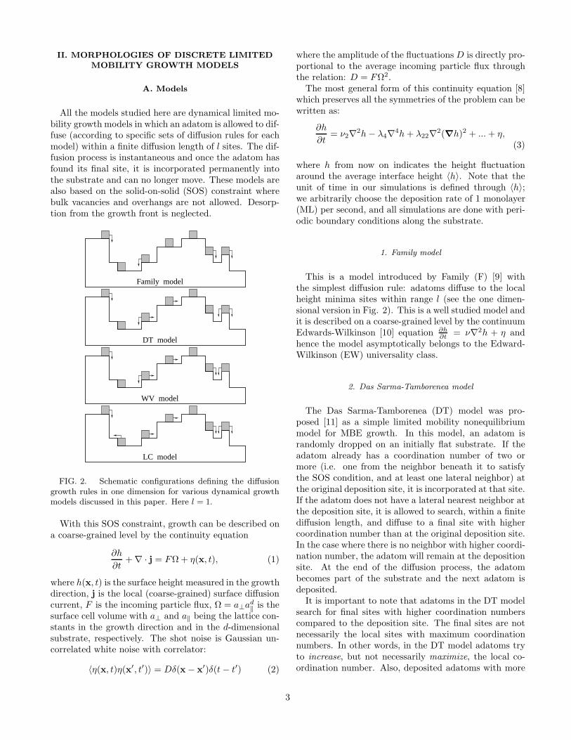
FIG. 3. Morphologies from F model with nr = 1 (top)and nr = 5 (bottom) from substrates of size L = 100 × 100after 106 ML.

3. Wolf-Villain model

The Wolf-Villain (WV) model [12] is very similar tothe DT model in the sense that diffusion is controlledby the local coordination number. There are, however,two important distinctions between the two models. Forone thing, in the WV model, an adatom with lateralnearest neighbors can still diffuse if it can find a finalsite with higher coordination number. The other differ-ence is that, adatoms in the WV model try to maximize

the coordination number, and not just to increase it asin the DT model (see Fig. 2). The two models havevery similar behavior in one dimensional (d=1+1) sim-ulations, and there have been substantial confusion re-garding these two models in the literature. But in twodimensional (d=2+1) systems, after an initial crossoverperiod, the two models behave very differently, as will beshown in this paper.

4. Kim - Das Sarma class of conserved growth models

A number of discrete growth models can be definedby applying the approach originally developed by Kimand Das Sarma [13] for obtaining precise discrete coun-terparts of continuum conserved growth equations. Inthis method, the surface current j is expressed as thegradient of a scalar field K, which in turn is written as a

combination of h and its various differential forms, ∇2h,(∇h)2, ... etc., where certain combinations are ruled outby symmetry constraints:

j(x, t) = −∇K , (4)

where

K = ν2h − λ4∇2h + λ22(∇h)2 + ... (5)

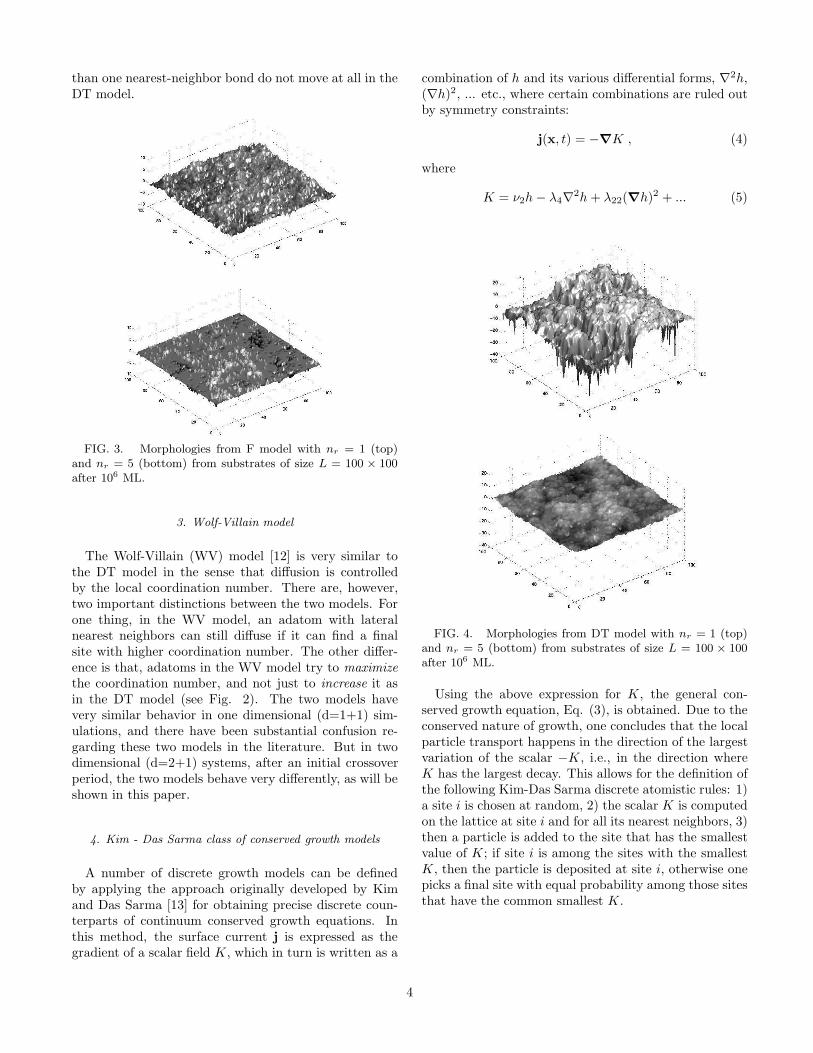
FIG. 4. Morphologies from DT model with nr = 1 (top)and nr = 5 (bottom) from substrates of size L = 100 × 100after 106 ML.

Using the above expression for K, the general con-served growth equation, Eq. (3), is obtained. Due to theconserved nature of growth, one concludes that the localparticle transport happens in the direction of the largestvariation of the scalar −K, i.e., in the direction whereK has the largest decay. This allows for the definition ofthe following Kim-Das Sarma discrete atomistic rules: 1)a site i is chosen at random, 2) the scalar K is computedon the lattice at site i and for all its nearest neighbors, 3)then a particle is added to the site that has the smallestvalue of K; if site i is among the sites with the smallestK, then the particle is deposited at site i, otherwise onepicks a final site with equal probability among those sitesthat have the common smallest K.

4

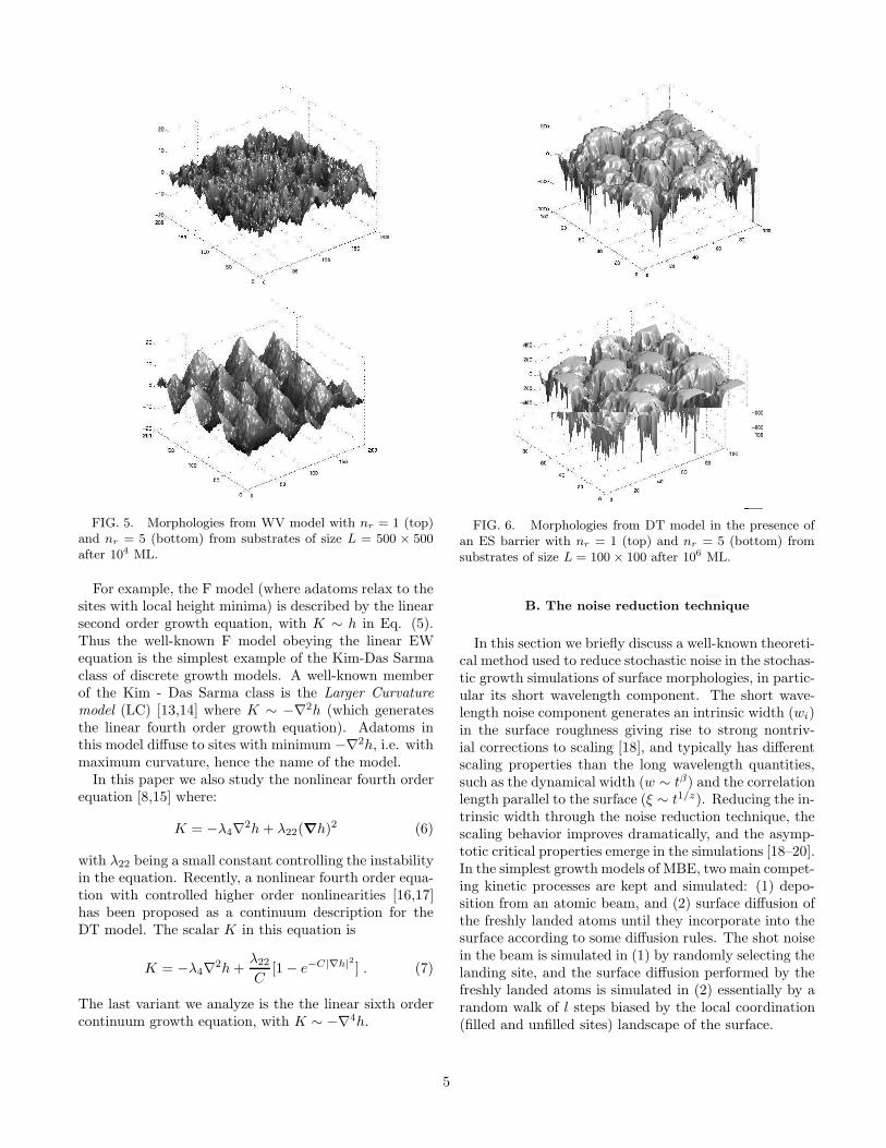
FIG. 5. Morphologies from WV model with nr = 1 (top)and nr = 5 (bottom) from substrates of size L = 500 × 500after 104 ML.

For example, the F model (where adatoms relax to thesites with local height minima) is described by the linearsecond order growth equation, with K ∼ h in Eq. (5).Thus the well-known F model obeying the linear EWequation is the simplest example of the Kim-Das Sarmaclass of discrete growth models. A well-known memberof the Kim - Das Sarma class is the Larger Curvature

model (LC) [13,14] where K ∼ −∇2h (which generatesthe linear fourth order growth equation). Adatoms inthis model diffuse to sites with minimum −∇2h, i.e. withmaximum curvature, hence the name of the model.

In this paper we also study the nonlinear fourth orderequation [8,15] where:

K = −λ4∇2h + λ22(∇h)2 (6)

with λ22 being a small constant controlling the instabilityin the equation. Recently, a nonlinear fourth order equa-tion with controlled higher order nonlinearities [16,17]has been proposed as a continuum description for theDT model. The scalar K in this equation is

K = −λ4∇2h +λ22

C[1 − e−C|∇h|2 ] . (7)

The last variant we analyze is the the linear sixth ordercontinuum growth equation, with K ∼ −∇4h.

FIG. 6. Morphologies from DT model in the presence ofan ES barrier with nr = 1 (top) and nr = 5 (bottom) fromsubstrates of size L = 100 × 100 after 106 ML.

B. The noise reduction technique

In this section we briefly discuss a well-known theoreti-cal method used to reduce stochastic noise in the stochas-tic growth simulations of surface morphologies, in partic-ular its short wavelength component. The short wave-length noise component generates an intrinsic width (wi)in the surface roughness giving rise to strong nontriv-ial corrections to scaling [18], and typically has differentscaling properties than the long wavelength quantities,such as the dynamical width (w ∼ tβ) and the correlationlength parallel to the surface (ξ ∼ t1/z). Reducing the in-trinsic width through the noise reduction technique, thescaling behavior improves dramatically, and the asymp-totic critical properties emerge in the simulations [18–20].In the simplest growth models of MBE, two main compet-ing kinetic processes are kept and simulated: (1) depo-sition from an atomic beam, and (2) surface diffusion ofthe freshly landed atoms until they incorporate into thesurface according to some diffusion rules. The shot noisein the beam is simulated in (1) by randomly selecting thelanding site, and the surface diffusion performed by thefreshly landed atoms is simulated in (2) essentially by arandom walk of l steps biased by the local coordination(filled and unfilled sites) landscape of the surface.

5

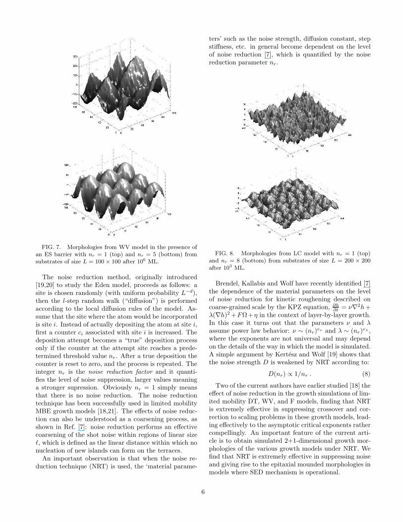
FIG. 7. Morphologies from WV model in the presence ofan ES barrier with nr = 1 (top) and nr = 5 (bottom) fromsubstrates of size L = 100 × 100 after 106 ML.

The noise reduction method, originally introduced[19,20] to study the Eden model, proceeds as follows: asite is chosen randomly (with uniform probability L−d),then the l-step random walk (“diffusion”) is performedaccording to the local diffusion rules of the model. As-sume that the site where the atom would be incorporatedis site i. Instead of actually depositing the atom at site i,first a counter ci associated with site i is increased. Thedeposition attempt becomes a “true” deposition processonly if the counter at the attempt site reaches a prede-termined threshold value nr. After a true deposition thecounter is reset to zero, and the process is repeated. Theinteger nr is the noise reduction factor and it quanti-fies the level of noise suppression, larger values meaninga stronger supression. Obviously nr = 1 simply meansthat there is no noise reduction. The noise reductiontechnique has been successfully used in limited mobilityMBE growth models [18,21]. The effects of noise reduc-tion can also be understood as a coarsening process, asshown in Ref. [7]: noise reduction performs an effectivecoarsening of the shot noise within regions of linear sizeℓ, which is defined as the linear distance within which nonucleation of new islands can form on the terraces.

An important observation is that when the noise re-duction technique (NRT) is used, the ‘material parame-

ters’ such as the noise strength, diffusion constant, stepstiffness, etc. in general become dependent on the levelof noise reduction [7], which is quantified by the noisereduction parameter nr.

FIG. 8. Morphologies from LC model with nr = 1 (top)and nr = 8 (bottom) from substrates of size L = 200 × 200after 103 ML.

Brendel, Kallabis and Wolf have recently identified [7]the dependence of the material parameters on the levelof noise reduction for kinetic roughening described oncoarse-grained scale by the KPZ equation, ∂h

∂t = ν∇2h +λ(∇h)2 +FΩ+ η in the context of layer-by-layer growth.In this case it turns out that the parameters ν and λassume power law behavior: ν ∼ (nr)

eν and λ ∼ (nr)eλ ,

where the exponents are not universal and may dependon the details of the way in which the model is simulated.A simple argument by Kertesz and Wolf [19] shows thatthe noise strength D is weakened by NRT according to:

D(nr) ∝ 1/nr . (8)

Two of the current authors have earlier studied [18] theeffect of noise reduction in the growth simulations of lim-ited mobility DT, WV, and F models, finding that NRTis extremely effective in suppressing crossover and cor-rection to scaling problems in these growth models, lead-ing effectively to the asymptotic critical exponents rathercompellingly. An important feature of the current arti-cle is to obtain simulated 2+1-dimensional growth mor-phologies of the various growth models under NRT. Wefind that NRT is extremely effective in suppressing noiseand giving rise to the epitaxial mounded morphologies inmodels where SED mechanism is operational.

6

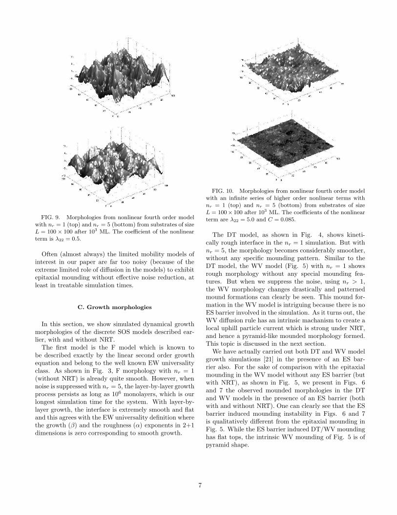
FIG. 9. Morphologies from nonlinear fourth order modelwith nr = 1 (top) and nr = 5 (bottom) from substrates of sizeL = 100 × 100 after 103 ML. The coefficient of the nonlinearterm is λ22 = 0.5.

Often (almost always) the limited mobility models ofinterest in our paper are far too noisy (because of theextreme limited role of diffusion in the models) to exhibitepitaxial mounding without effective noise reduction, atleast in treatable simulation times.

C. Growth morphologies

In this section, we show simulated dynamical growthmorphologies of the discrete SOS models described ear-lier, with and without NRT.

The first model is the F model which is known tobe described exactly by the linear second order growthequation and belong to the well known EW universalityclass. As shown in Fig. 3, F morphology with nr = 1(without NRT) is already quite smooth. However, whennoise is suppressed with nr = 5, the layer-by-layer growthprocess persists as long as 106 monolayers, which is ourlongest simulation time for the system. With layer-by-layer growth, the interface is extremely smooth and flatand this agrees with the EW universality definition wherethe growth (β) and the roughness (α) exponents in 2+1dimensions is zero corresponding to smooth growth.

FIG. 10. Morphologies from nonlinear fourth order modelwith an infinite series of higher order nonlinear terms withnr = 1 (top) and nr = 5 (bottom) from substrates of sizeL = 100× 100 after 103 ML. The coefficients of the nonlinearterm are λ22 = 5.0 and C = 0.085.

The DT model, as shown in Fig. 4, shows kineti-cally rough interface in the nr = 1 simulation. But withnr = 5, the morphology becomes considerably smoother,without any specific mounding pattern. Similar to theDT model, the WV model (Fig. 5) with nr = 1 showsrough morphology without any special mounding fea-tures. But when we suppress the noise, using nr > 1,the WV morphology changes drastically and patternedmound formations can clearly be seen. This mound for-mation in the WV model is intriguing because there is noES barrier involved in the simulation. As it turns out, theWV diffusion rule has an intrinsic machanism to create alocal uphill particle current which is strong under NRT,and hence a pyramid-like mounded morphology formed.This topic is discussed in the next section.

We have actually carried out both DT and WV modelgrowth simulations [21] in the presence of an ES bar-rier also. For the sake of comparison with the epitaxialmounding in the WV model without any ES barrier (butwith NRT), as shown in Fig. 5, we present in Figs. 6and 7 the observed mounded morphologies in the DTand WV models in the presence of an ES barrier (bothwith and without NRT). One can clearly see that the ESbarrier induced mounding instability in Figs. 6 and 7is qualitatively different from the epitaxial mounding inFig. 5. While the ES barrier induced DT/WV moundinghas flat tops, the intrinsic WV mounding of Fig. 5 is ofpyramid shape.

7

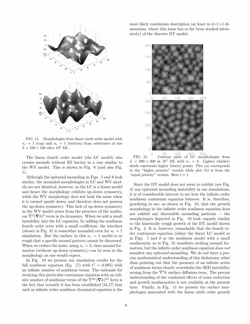
FIG. 11. Morphologies from linear sixth order model withnr = 1 (top) and nr = 5 (bottom) from substrates of sizeL = 100 × 100 after 106 ML.

The linear fourth order model (the LC model) alsocreates mounds without ES barrier in a way similar tothe WV model. This is shown in Fig. 8 (and also Fig.1).

Although the epitaxial mounding in Figs. 5 and 8 looksimilar, the mounded morphologies in LC and WV mod-els are not identical, however, as the LC is a linear modeland hence the morphology exhibits up-down symmetry,while the WV morphology does not look the same whenit is turned upside down, and therefore does not possessthe up-down symmetry. This lack of up-down symmetryin the WV model arises from the presence of the nonlin-ear ∇2(∇h)2 term in its dynamics. When we add a smallinstability into the LC equation, by adding the nonlinearfourth order term with a small coefficient, the interface(shown in Fig. 9) is somewhat mounded even for nr = 1simulation. But the surface in this nr = 1 model is sorough that a specific mound pattern cannot be discerned.When we reduce the noise, using nr = 5, clear mound for-mation (without up-down symmetry) can be seen in themorphology as one would expect.

In Fig. 10 we present our simulation results for thefull nonlinear equation (Eq. (7) with C = 0.085) withan infinite number of nonlinear terms. The rationale forstudying this particular continuum equation with an infi-nite number of nonlinear terms of the ∇2n(∇h)2n form isthe fact that recently it has been established [16,17] thatsuch as infinite order nonlinear dynamical equation is the

most likely continuum description (at least in d=1+1 di-mensions, where this issue has so far been studied inten-sively) of the discrete DT model.

FIG. 12. Contour plots of LC morphologies fromL = 200 × 200 at 103 ML with nr = 8. Lighter (darker)shade represents higher (lower) points. Plot (a) correspondsto the “higher priority” version while plot (b) is from the“equal priority” version. Here l = 1.

Since the DT model does not seem to exhibit (see Fig.4) any epitaxial mounding instability in our simulations,it is of considerable interest to see how the infinite ordernonlinear continuum equation behaves. It is, therefore,gratifying to see, as shown in Fig. 10, that the growthmorphology in the infinite order nonlinear equation doesnot exhibit any discernible mounding patterns — themorphologies depicted in Fig. 10 look vaguely similarto the kinetically rough growth of the DT model shownin Fig. 4. It is, however, remarkable that the fourth or-der continuum equation (either the linear LC model asin Figs. 1 and 8 or the nonlinear model with a smallnonlinearity as in Fig. 9) manifests striking mound for-mation, but the infinite order nonlinear equation does not

manifest any epitaxial mounding. We do not have a pre-cise mathematical understanding of this dichotomy otherthan pointing out that the presence of an infinite seriesof nonlinear terms clearly overwhelm the SED instabilityarising from the ∇4h surface diffusion term. The preciseunderstanding of the combined effects of noise reductionand growth nonlinearities is not available at the presenttime. Finally, in Fig. 11 we present the surface mor-phologies associated with the linear sixth order growth

8

equation. The mounding pattern can be barely seen inthe nr = 1 simulation. But the spectacular mound for-mation can be seen clearly when we reduce the noise(nr = 5).

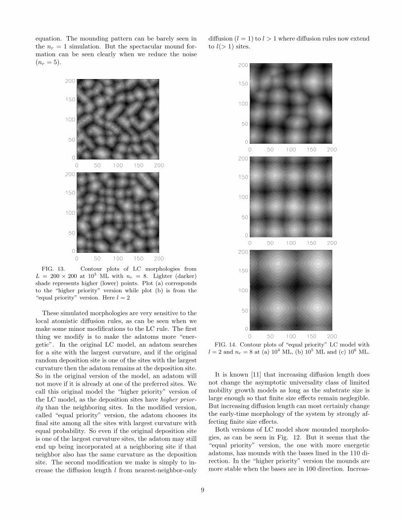
FIG. 13. Contour plots of LC morphologies fromL = 200 × 200 at 103 ML with nr = 8. Lighter (darker)shade represents higher (lower) points. Plot (a) correspondsto the “higher priority” version while plot (b) is from the“equal priority” version. Here l = 2

These simulated morphologies are very sensitive to thelocal atomistic diffusion rules, as can be seen when wemake some minor modifications to the LC rule. The firstthing we modify is to make the adatoms more “ener-getic”. In the original LC model, an adatom searchesfor a site with the largest curvature, and if the originalrandom deposition site is one of the sites with the largestcurvature then the adatom remains at the deposition site.So in the original version of the model, an adatom willnot move if it is already at one of the preferred sites. Wecall this original model the “higher priority” version ofthe LC model, as the deposition sites have higher prior-

ity than the neighboring sites. In the modified version,called “equal priority” version, the adatom chooses itsfinal site among all the sites with largest curvature withequal probability. So even if the original deposition siteis one of the largest curvature sites, the adatom may stillend up being incorporated at a neighboring site if thatneighbor also has the same curvature as the depositionsite. The second modification we make is simply to in-crease the diffusion length l from nearest-neighbor-only

diffusion (l = 1) to l > 1 where diffusion rules now extendto l(> 1) sites.

FIG. 14. Contour plots of “equal priority” LC model withl = 2 and nr = 8 at (a) 104 ML, (b) 105 ML and (c) 106 ML.

It is known [11] that increasing diffusion length doesnot change the asymptotic universality class of limitedmobility growth models as long as the substrate size islarge enough so that finite size effects remain neglegible.But increasing diffusion length can most certainly changethe early-time morphology of the system by strongly af-fecting finite size effects.

Both versions of LC model show mounded morpholo-gies, as can be seen in Fig. 12. But it seems that the“equal priority” version, the one with more energeticadatoms, has mounds with the bases lined in the 110 di-rection. In the “higher priority” version the mounds aremore stable when the bases are in 100 direction. Increas-

9

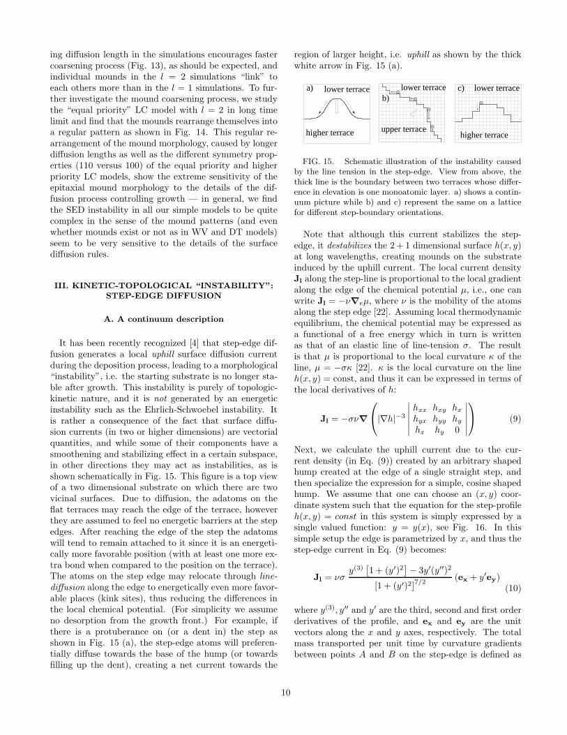
ing diffusion length in the simulations encourages fastercoarsening process (Fig. 13), as should be expected, andindividual mounds in the l = 2 simulations “link” toeach others more than in the l = 1 simulations. To fur-ther investigate the mound coarsening process, we studythe “equal priority” LC model with l = 2 in long timelimit and find that the mounds rearrange themselves intoa regular pattern as shown in Fig. 14. This regular re-arrangement of the mound morphology, caused by longerdiffusion lengths as well as the different symmetry prop-erties (110 versus 100) of the equal priority and higherpriority LC models, show the extreme sensitivity of theepitaxial mound morphology to the details of the dif-fusion process controlling growth — in general, we findthe SED instability in all our simple models to be quitecomplex in the sense of the mound patterns (and evenwhether mounds exist or not as in WV and DT models)seem to be very sensitive to the details of the surfacediffusion rules.

III. KINETIC-TOPOLOGICAL “INSTABILITY”:

STEP-EDGE DIFFUSION

A. A continuum description

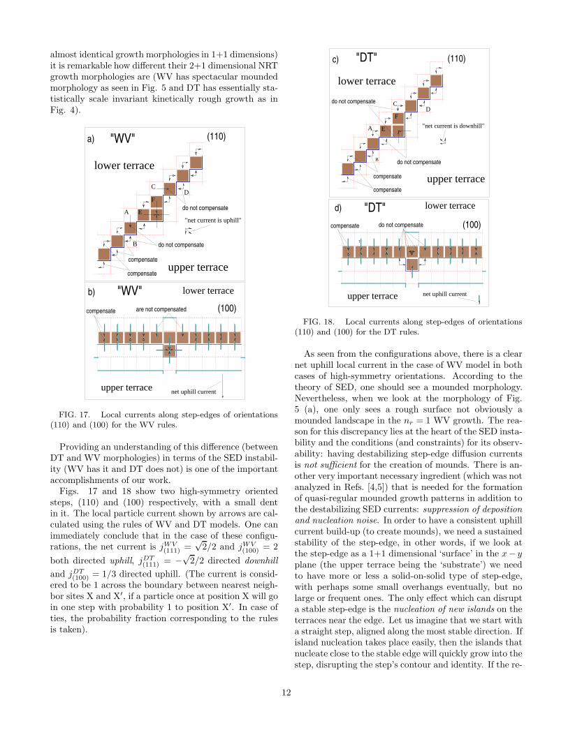
It has been recently recognized [4] that step-edge dif-fusion generates a local uphill surface diffusion currentduring the deposition process, leading to a morphological“instability”, i.e. the starting substrate is no longer sta-ble after growth. This instability is purely of topologic-kinetic nature, and it is not generated by an energeticinstability such as the Ehrlich-Schwoebel instability. Itis rather a consequence of the fact that surface diffu-sion currents (in two or higher dimensions) are vectorialquantities, and while some of their components have asmoothening and stabilizing effect in a certain subspace,in other directions they may act as instabilities, as isshown schematically in Fig. 15. This figure is a top viewof a two dimensional substrate on which there are twovicinal surfaces. Due to diffusion, the adatoms on theflat terraces may reach the edge of the terrace, howeverthey are assumed to feel no energetic barriers at the stepedges. After reaching the edge of the step the adatomswill tend to remain attached to it since it is an energeti-cally more favorable position (with at least one more ex-tra bond when compared to the position on the terrace).The atoms on the step edge may relocate through line-

diffusion along the edge to energetically even more favor-able places (kink sites), thus reducing the differences inthe local chemical potential. (For simplicity we assumeno desorption from the growth front.) For example, ifthere is a protuberance on (or a dent in) the step asshown in Fig. 15 (a), the step-edge atoms will preferen-tially diffuse towards the base of the hump (or towardsfilling up the dent), creating a net current towards the

region of larger height, i.e. uphill as shown by the thickwhite arrow in Fig. 15 (a).

a) lower terrace

higher terrace

lower terrace

upper terrace

b)lower terracec)

higher terrace

FIG. 15. Schematic illustration of the instability causedby the line tension in the step-edge. View from above, thethick line is the boundary between two terraces whose differ-ence in elevation is one monoatomic layer. a) shows a contin-uum picture while b) and c) represent the same on a latticefor different step-boundary orientations.

Note that although this current stabilizes the step-edge, it destabilizes the 2 + 1 dimensional surface h(x, y)at long wavelengths, creating mounds on the substrateinduced by the uphill current. The local current densityJl along the step-line is proportional to the local gradientalong the edge of the chemical potential µ, i.e., one canwrite Jl = −ν∇eµ, where ν is the mobility of the atomsalong the step edge [22]. Assuming local thermodynamicequilibrium, the chemical potential may be expressed asa functional of a free energy which in turn is writtenas that of an elastic line of line-tension σ. The resultis that µ is proportional to the local curvature κ of theline, µ = −σκ [22]. κ is the local curvature on the lineh(x, y) = const, and thus it can be expressed in terms ofthe local derivatives of h:

Jl = −σν∇

|∇h|−3

∣

∣

∣

∣

∣

∣

hxx hxy hx

hyx hyy hy

hx hy 0

∣

∣

∣

∣

∣

∣

(9)

Next, we calculate the uphill current due to the cur-rent density (in Eq. (9)) created by an arbitrary shapedhump created at the edge of a single straight step, andthen specialize the expression for a simple, cosine shapedhump. We assume that one can choose an (x, y) coor-dinate system such that the equation for the step-profileh(x, y) = const in this system is simply expressed by asingle valued function: y = y(x), see Fig. 16. In thissimple setup the edge is parametrized by x, and thus thestep-edge current in Eq. (9) becomes:

Jl = νσy(3)

[

1 + (y′)2]

− 3y′(y′′)2

[1 + (y′)2]7/2

(ex + y′ey)(10)

where y(3), y′′ and y′ are the third, second and first orderderivatives of the profile, and ex and ey are the unitvectors along the x and y axes, respectively. The totalmass transported per unit time by curvature gradientsbetween points A and B on the step-edge is defined as

10

the line-integral of the edge current density:

IAB =

∫ B

A

ds Jl (11)

where ds is the integration element along the curve of thestep-edge. In the following we illustrate that this currentpoints toward the base of the higher step.

A Bstraight step−edge

x

yds

FIG. 16. A straight step-edge with a hump. The step-edgecurrent density generated by the local curvature gradientalong the hump creates a net uphill current.

Let us choose a step-profile given by y(x) = a cos (bx)between the points xA = −π/b and xB = π/b. Afterperforming the integrals in Eq. (11), one obtains:

IAB = −4νσb

15

[

1 + 11z + 6z2

(1 + z)2E(i

√z)

−1 + 3z

1 + zK(i

√z)

]

ey (12)

where z = a2b2 is a dimensionless number, and K(k)and E(k) are complete elliptic integrals of first and sec-ond kinds respectively. Since 1+11z+6z2 > 1+4z+3z2,and E(i

√z) > K(i

√z), for all z > 0, the mass-current

has a negative y component (the x component is zerobecause of symmetry), i.e., it points towards the baseof the higher step, uphill. In the limit of small humps,z ≪ 1 (small slopes approximation), K(i

√z) ≃ π

4 (1− z4 ),

E(i√

z) ≃ π4 (1+ z

4 ), so the current becomes proportionalto the square of the hump’s height, IAB ∼ −πνσb3a2

and for peaked humps (z ≫ 1), K(i√

z) ≃ ln (4√

z)/√

z,E(i

√z) ≃ √

z the current depends linearly on the heightof the hump, IAB ∼ 8

5σνb2a. The same analysis can berepeated when there is a dent in the step profile, withsimilar conclusions. Certainly, the currents expressedabove are instantaneous local currents. If one is inter-ested in the evolution of the step profile, one can employsimple geometrical considerations (see [22,23]) to write:

∂y

∂t= vn

√

1 + (y′)2 (13)

where y = y(x, t), vn is the normal step-edge veloc-ity and the prime denotes derivative with respect to x.

Assuming that the mass transport is solely due to thestep-edge current, one has vnds = −(∂Jl/∂x)dx, withds = dx

√

1 + (y′)2. Thus Eq. (13) takes the form:

∂y

∂t= −∂Jl

∂x= −νσ

(

y(4)

[1 + (y′)2]2− 10y′y′′y(3)

[1 + (y′)2]3

−3[1 − 5(y′)2](y′′)3

[1 + (y′)2]4

)

. (14)

In the limit of small slopes, y′ << 1, y′′ << 1, y(3) << 1,y(4) << 1, and so from Eq. (14) it follows that: ∂y/∂t =−νσy(4), after keeping the leading term only. This is thewell known Mullins equation for the dynamic relaxationof a step-edge, related to the fourth order linear growthequation, Eq. (6) with λ22 = 0, followed by the LC modelin our growth simulations.

The continuum description presented here com-pellingly demonstrates the possibility of a destabilizinguphill current arising entirely from step edge diffusion —an SED instability without any ES barriers, as discussedin Refs. [4,5] recently.

B. A discrete description

In reality the deposition process (and our simulation oflimited mobility models) takes place on the discrete andatomistic crystalline lattice, which introduces an orienta-tion dependence of the line tension σ. One would natu-rally expect that the high-symmetry, in-plane crystallinedirections will have the largest σ, these being the moststable. However, there is a hierarchy even among thesehigh-symmetry orientations, as is illustrated in Figs. 15(b) and 15 (c). Fig. 15 (b) shows a step-edge alignedalong a diagonal of the square lattice and in Fig. 15 (c)the step-edge is oriented along one of the main axes of thelattice. While the step is stable along the diagonal, it isnot as stable along the main axis, since in this latter case(of Fig. 15 (c)) in order for an atom to reach a highercoordination site along the line, it has to detach itselffrom the step-edge (to become an adatom) first, which isenergetically less favorable.

Let us now analyze in more detail the effects of SEDin the case of the two most important MBE-motivatedlimited mobility models, WV and DT models. The dif-fusion rules for the mobile atoms for these two modelsare only slightly different: in the case of WV model par-ticles seek to maximize their coordination while in theDT model they only seek to increase it. Neverthelessthe two models present completely different behaviors.As we have seen in Subsection II.C, the NRT version ofWV model produces mounded structures, however thisdoes not happen for the DT model. In the following weexplain this unexpected difference between WV and DTmodels based on local SED currents. Given the rather“minor” differences between DT and WV rules (and their

11

almost identical growth morphologies in 1+1 dimensions)it is remarkable how different their 2+1 dimensional NRTgrowth morphologies are (WV has spectacular moundedmorphology as seen in Fig. 5 and DT has essentially sta-tistically scale invariant kinetically rough growth as inFig. 4).

lower terrace

upper terracecompensate

compensate

B

A E

F

CD

do not compensate

"net current is uphill"

do not compensate

"WV"a) (110)

lower terrace"WV"b)

compensate are not compensated

upper terrace net uphill current

(100)

FIG. 17. Local currents along step-edges of orientations(110) and (100) for the WV rules.

Providing an understanding of this difference (betweenDT and WV morphologies) in terms of the SED instabil-ity (WV has it and DT does not) is one of the importantaccomplishments of our work.

Figs. 17 and 18 show two high-symmetry orientedsteps, (110) and (100) respectively, with a small dentin it. The local particle current shown by arrows are cal-culated using the rules of WV and DT models. One canimmediately conclude that in the case of these configu-rations, the net current is jWV

(111) =√

2/2 and jWV(100) = 2

both directed uphill, jDT(111) = −

√2/2 directed downhill

and jDT(100) = 1/3 directed uphill. (The current is consid-

ered to be 1 across the boundary between nearest neigh-bor sites X and X′, if a particle once at position X will goin one step with probability 1 to position X′. In case ofties, the probability fraction corresponding to the rulesis taken).

B

do not compensate

do not compensate

upper terrace

lower terrace

compensate

compensate

F

EA

CD

"DT"c) (110)

"net current is downhill"

1

lower terrace

upper terrace net uphill current

compensate do not compensate

"DT"d)

(100)

FIG. 18. Local currents along step-edges of orientations(110) and (100) for the DT rules.

As seen from the configurations above, there is a clearnet uphill local current in the case of WV model in bothcases of high-symmetry orientations. According to thetheory of SED, one should see a mounded morphology.Nevertheless, when we look at the morphology of Fig.5 (a), one only sees a rough surface not obviously amounded landscape in the nr = 1 WV growth. The rea-son for this discrepancy lies at the heart of the SED insta-bility and the conditions (and constraints) for its observ-ability: having destabilizing step-edge diffusion currentsis not sufficient for the creation of mounds. There is an-other very important necessary ingredient (which was notanalyzed in Refs. [4,5]) that is needed for the formationof quasi-regular mounded growth patterns in addition tothe destabilizing SED currents: suppression of deposition

and nucleation noise. In order to have a consistent uphillcurrent build-up (to create mounds), we need a sustainedstability of the step-edge, in other words, if we look atthe step-edge as a 1+1 dimensional ‘surface’ in the x− yplane (the upper terrace being the ‘substrate’) we needto have more or less a solid-on-solid type of step-edge,with perhaps some small overhangs eventually, but nolarge or frequent ones. The only effect which can disrupta stable step-edge is the nucleation of new islands on theterraces near the edge. Let us imagine that we start witha straight step, aligned along the most stable direction. Ifisland nucleation takes place easily, then the islands thatnucleate close to the stable edge will quickly grow into thestep, disrupting the step’s contour and identity. If the re-

12

laxation time of the disrupted contour is larger than thenucleation time, small newly grown islands will disruptthe step even further until it ceases to exist. In this casethe SED instability will not manifest in the mound for-mation because the necessary condition for mound for-mation is not satisfied globally although there may belocal uphill current. Thus, noise may prevent the SEDinstability from manifesting a global mounded instability.

The importance of noise suppression for the SED in-stability is strikingly apparent from comparing Figs. 5(a) and 5 (b) for the WV model. The NRT version hasmounded morphology and the nr = 1 version does not.However for the DT model, one finds no such regularmounded structures even when noise and nucleation isstrongly supressed (Fig. 4). The reason for this differ-ence is that in the DT model the SED current is essen-tially downhill (and thus is stabilizing). Depending onthe edge configuration (for example the (100) edge inFig. 18) one may find a small uphill current in the DTmodel, however it is statistically not significant to desta-bilize the whole surface. There will be a weak moundingtendency at early times, when the ∇4h diffusion term isrelevant and when the height-height correlation functionshows some oscillations (see [6]), indicating the presenceof this term, but then it will be quickly taken over by thestabilizing downhill current and nucleation events. Thus,the DT model, at best, will exhibit some weak and irreg-ular epitaxial mounding [6], but not a regular patternedmounded morphology.

Another important point is that mounding due to theSED instability does not require any growth nonlinear-

ity to be present. This is obvious from the fact that theLC model, which is strictly linear by construction, showsspetacular epitaxial mounding induced by the SED in-stability. In the following subsection we analyze in moredetails the effects of noise reduction on the SED instabil-ity.

C. Noise reduction method: a numerical way to

control the step edge diffusion instability

As emphasized in the previous subsection, a necessaryingredient for creating mounds by SED is the suppres-sion of noise. In the following we restrict our analysis todiscrete limited mobility models, and frequently use forcomparison WV and DT models. Unfortunately, rigorousanalytical calculations are practically impossible for dis-crete and nonlinear dynamical growth models of DT andWV types. However, we make an attempt by introducingthe proper quantities to pinpoint the effects of noise re-duction on these two models and actually show the majordifference between the two models in one and two sub-strate dimensions in the context of SED instability. First,we introduce the notion of conditional occupation rates.The conditional occupation rate fi associated with site

i in a particular height-configuration is the net gain oftransition rates coming from the contribution of all theneighbors within a distance of l sites on the surface andfrom the growth direction (from the deposition beam).

1/2 1/2

1/2 1/2

1/2 1/211

1

1

111

1

11

111

11

11

111

oi

= 1 1 0 0 1 0 0 0 2 0 05/22 2 5/2 2

"DT"

1 1 11

1

1 1 1

1 1 1

1

1

1 1 1 11/21/2

1

1/2 1/2

1 1

1

1 1 1 3 0 30 1 0 0 2 0 0oi = 0 3/2 5/2

"WV"

FIG. 19. Conditional occupation probabilities for two par-ticular configurations in 1 + 1 dimensions for DT and WVmodels. The fi-s that differ for the DT from WV are set inbold italics. Here l = 1.

The fi-s can easily be calculated once the diffusionrules are known. If Wi→i′ is the transition rate for anatom landed on site i to be incorporated at site i′ (whichis a nearest neighbor when l = 1), then:

fi = 1 +

il∑

i′

(Wi′→i −Wi→i′) (15)

where the unity in front of the sum represents the con-tribution from the beam and il means summing thecontributions over all the neighbors of site i within a dis-tance l. The fi-s are obviously conditioned to the eventthat there is an atom landed on site i or on the neighborsi′. It is important to emphasize that these quantities inEq. (15) are introduced for the no-desorption case only:once an atom is incorporated in the surface it stays thatway. If one wishes to add desorption to the model, thenthe evaporation rates have to be included in Eq. (15) aswell (the rates in Eq. (15) are all diffusion rates ).

Let us now illustrate in light of the two models WV andDT, the conditional occupation rates, in 1+1 and 2+1 di-mensions. Figs. 19 and 20 show the fi-s for particularconfigurations for one and two dimensional substrates re-spectively. The fractional transition rates mean that themotion of the atom is probabilistic: it will choose withequal probability among the available identical states.This is in fact the source of the diffusion noise ηc, aris-ing from the stochastic atomistic hopping process, whichshould be added to the right hand side of Eq. (1), how-ever, it is an irrelevant contribution in the long wave-length scaling in the renormalization group sense. Theconditional occupation rates fi are small rational num-

13

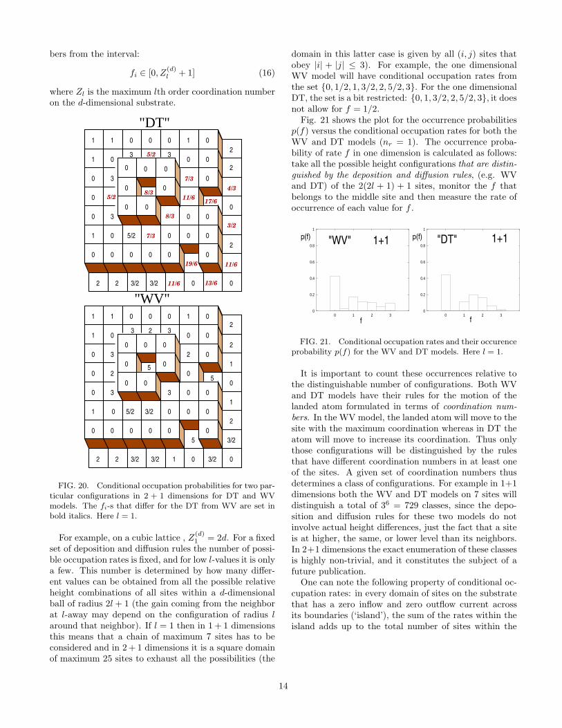
bers from the interval:

fi ∈ [0, Z(d)l + 1] (16)

where Zl is the maximum lth order coordination numberon the d-dimensional substrate.

3 3

1 0 0 0

0

0

3/2 3/2 00

00 0 0

00

0

0

0

0

0

0 0 0 0 0

0 0

0

0

0

0

0

0

0

1

1

1

1

2

2

2

22

3

3

5/2

11/6

7/3

8/3

5/2

5/2

8/3

3/2

13/6

11/6

7/3

17/6

4/3

19/6

11/6

"DT"

0

0 0 0 0

00

0

0

0

0

0

0 0 0

0

0

0 0 0

0

0

0

0

0

0

0

0

0

0

0

0

0

0

0

5

5

5

1

1

1

1

111

13

3

3 3

3

2 2

2

2

2

22

2

5/2 3/2

3/2 3/2 3/2

3/2

"WV"

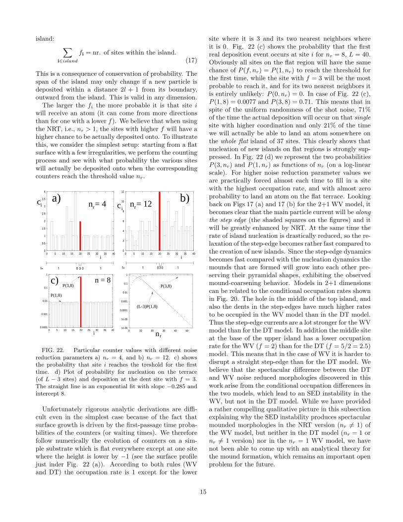
FIG. 20. Conditional occupation probabilities for two par-ticular configurations in 2 + 1 dimensions for DT and WVmodels. The fi-s that differ for the DT from WV are set inbold italics. Here l = 1.

For example, on a cubic lattice , Z(d)1 = 2d. For a fixed

set of deposition and diffusion rules the number of possi-ble occupation rates is fixed, and for low l-values it is onlya few. This number is determined by how many differ-ent values can be obtained from all the possible relativeheight combinations of all sites within a d-dimensionalball of radius 2l + 1 (the gain coming from the neighborat l-away may depend on the configuration of radius laround that neighbor). If l = 1 then in 1 + 1 dimensionsthis means that a chain of maximum 7 sites has to beconsidered and in 2 + 1 dimensions it is a square domainof maximum 25 sites to exhaust all the possibilities (the

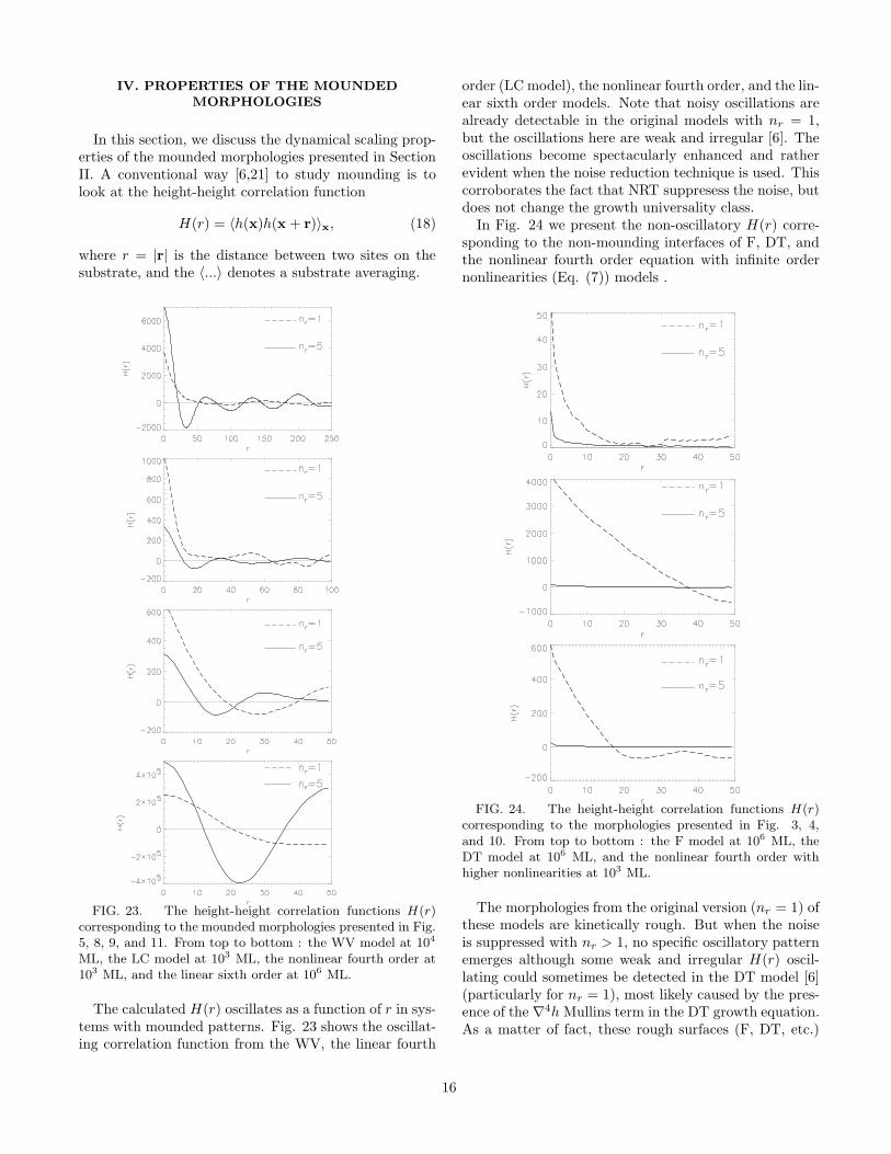
domain in this latter case is given by all (i, j) sites thatobey |i| + |j| ≤ 3). For example, the one dimensionalWV model will have conditional occupation rates fromthe set 0, 1/2, 1, 3/2, 2, 5/2, 3. For the one dimensionalDT, the set is a bit restricted: 0, 1, 3/2, 2, 5/2, 3, it doesnot allow for f = 1/2.

Fig. 21 shows the plot for the occurrence probabilitiesp(f) versus the conditional occupation rates for both theWV and DT models (nr = 1). The occurrence proba-bility of rate f in one dimension is calculated as follows:take all the possible height configurations that are distin-

guished by the deposition and diffusion rules, (e.g. WVand DT) of the 2(2l + 1) + 1 sites, monitor the f thatbelongs to the middle site and then measure the rate ofoccurrence of each value for f .

0

0.2

0.4

0.6

0.8

1

0 1 2 30

0.2

0.4

0.6

0.8

1

0 1 2 3ff

p(f) p(f)"WV" 1+1 1+1"DT"

FIG. 21. Conditional occupation rates and their occurenceprobability p(f) for the WV and DT models. Here l = 1.

It is important to count these occurrences relative tothe distinguishable number of configurations. Both WVand DT models have their rules for the motion of thelanded atom formulated in terms of coordination num-

bers. In the WV model, the landed atom will move to thesite with the maximum coordination whereas in DT theatom will move to increase its coordination. Thus onlythose configurations will be distinguished by the rulesthat have different coordination numbers in at least oneof the sites. A given set of coordination numbers thusdetermines a class of configurations. For example in 1+1dimensions both the WV and DT models on 7 sites willdistinguish a total of 36 = 729 classes, since the depo-sition and diffusion rules for these two models do notinvolve actual height differences, just the fact that a siteis at higher, the same, or lower level than its neighbors.In 2+1 dimensions the exact enumeration of these classesis highly non-trivial, and it constitutes the subject of afuture publication.

One can note the following property of conditional oc-cupation rates: in every domain of sites on the substratethat has a zero inflow and zero outflow current acrossits boundaries (‘island’), the sum of the rates within theisland adds up to the total number of sites within the

14

island:∑

i∈island

fi = nr. of sites within the island.(17)

This is a consequence of conservation of probability. Thespan of the island may only change if a new particle isdeposited within a distance 2l + 1 from its boundary,outward from the island. This is valid in any dimension.

The larger the fi the more probable it is that site iwill receive an atom (it can come from more directionsthan for one with a lower f). We believe that when usingthe NRT, i.e., nr > 1, the sites with higher f will have ahigher chance to be actually deposited onto. To illustratethis, we consider the simplest setup: starting from a flatsurface with a few irregularities, we perform the countingprocess and see with what probability the various siteswill actually be deposited onto when the correspondingcounters reach the threshold value nr.

0

0.5

1

1.5

2

2.5

3

3.5

4

0 5 10 15 20 25 30 35 400

2

4

6

8

10

12

0 5 10 15 20 25 30 35 40

ci c i

i i

n = 4 n = 12r r

3 11f= 00 30 0f= 1 1

a) b)

0.0001

0.001

0.01

0.1

1

0 5 10 15 20 25 30 35 401e-06

1e-05

0.0001

0.001

0.01

0.1

1

0 10 20 30 40 50i

c) n = 8

P(1,8)

P(3,8)

n r

P(3,8)

(L-3)P(1,8)

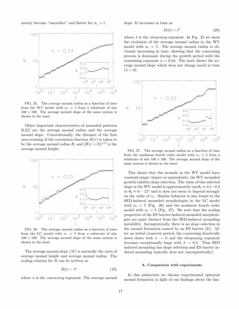
FIG. 22. Particular counter values with different noisereduction parameters a) nr = 4, and b) nr = 12. c) showsthe probability that site i reaches the treshold for the firsttime. d) Plot of probability for nucleation on the terrace(of L − 3 sites) and deposition at the dent site with f = 3.The straight line is an exponential fit with slope −0.285 andintercept 8.

Unfortunately rigorous analytic derivations are diffi-cult even in the simplest case because of the fact thatsurface growth is driven by the first-passage time proba-bilities of the counters (or waiting times). We thereforefollow numerically the evolution of counters on a sim-ple substrate which is flat everywhere except at one sitewhere the height is lower by −1 (see the surface profilejust inder Fig. 22 (a)). According to both rules (WVand DT) the occupation rate is 1 except for the lower

site where it is 3 and its two nearest neighbors whereit is 0. Fig. 22 (c) shows the probability that the firstreal deposition event occurs at site i for nr = 8, L = 40.Obviously all sites on the flat region will have the samechance of P (f, nr) = P (1, nr) to reach the threshold forthe first time, while the site with f = 3 will be the mostprobable to reach it, and for its two nearest neighbors itis entirely unlikely: P (0, nr) = 0. In case of Fig. 22 (c),P (1, 8) = 0.0077 and P (3, 8) = 0.71. This means that inspite of the uniform randomness of the shot noise, 71%of the time the actual deposition will occur on that single

site with higher coordination and only 21% of the timewe will actually be able to land an atom somewhere onthe whole flat island of 37 sites. This clearly shows thatnucleation of new islands on flat regions is strongly sup-pressed. In Fig. 22 (d) we represent the two probabilitiesP (3, nr) and P (1, nr) as functions of nr (on a log-linearscale). For higher noise reduction parameter values weare practically forced almost each time to fill in a sitewith the highest occupation rate, and with almost zeroprobability to land an atom on the flat terrace. Lookingback on Figs 17 (a) and 17 (b) for the 2+1 WV model, itbecomes clear that the main particle current will be along

the step edge (the shaded squares on the figures) and itwill be greatly enhanced by NRT. At the same time therate of island nucleation is drastically reduced, so the re-laxation of the step-edge becomes rather fast compared tothe creation of new islands. Since the step-edge dynamicsbecomes fast compared with the nucleation dynamics themounds that are formed will grow into each other pre-serving their pyramidal shapes, exhibiting the observedmound-coarsening behavior. Models in 2+1 dimensionscan be related to the conditional occupation rates shownin Fig. 20. The hole in the middle of the top island, andalso the dents in the step-edges have much higher ratesto be occupied in the WV model than in the DT model.Thus the step-edge currents are a lot stronger for the WVmodel than for the DT model. In addition the middle siteat the base of the upper island has a lower occupationrate for the WV (f = 2) than for the DT (f = 5/2 = 2.5)model. This means that in the case of WV it is harder todisrupt a straight step-edge than for the DT model. Webelieve that the spectacular difference between the DTand WV noise reduced morphologies discovered in thiswork arise from the conditional occupation differences inthe two models, which lead to an SED instability in theWV, but not in the DT model. While we have provideda rather compelling qualitative picture in this subsectionexplaining why the SED instability produces spectacularmounded morphologies in the NRT version (nr 6= 1) ofthe WV model, but neither in the DT model (nr = 1 ornr 6= 1 version) nor in the nr = 1 WV model, we havenot been able to come up with an analytical theory forthe mound formation, which remains an important openproblem for the future.

15

IV. PROPERTIES OF THE MOUNDED

MORPHOLOGIES

In this section, we discuss the dynamical scaling prop-erties of the mounded morphologies presented in SectionII. A conventional way [6,21] to study mounding is tolook at the height-height correlation function

H(r) = 〈h(x)h(x + r)〉x, (18)

where r = |r| is the distance between two sites on thesubstrate, and the 〈...〉 denotes a substrate averaging.

FIG. 23. The height-height correlation functions H(r)corresponding to the mounded morphologies presented in Fig.5, 8, 9, and 11. From top to bottom : the WV model at 104

ML, the LC model at 103 ML, the nonlinear fourth order at103 ML, and the linear sixth order at 106 ML.

The calculated H(r) oscillates as a function of r in sys-tems with mounded patterns. Fig. 23 shows the oscillat-ing correlation function from the WV, the linear fourth

order (LC model), the nonlinear fourth order, and the lin-ear sixth order models. Note that noisy oscillations arealready detectable in the original models with nr = 1,but the oscillations here are weak and irregular [6]. Theoscillations become spectacularly enhanced and ratherevident when the noise reduction technique is used. Thiscorroborates the fact that NRT suppresess the noise, butdoes not change the growth universality class.

In Fig. 24 we present the non-oscillatory H(r) corre-sponding to the non-mounding interfaces of F, DT, andthe nonlinear fourth order equation with infinite ordernonlinearities (Eq. (7)) models .

FIG. 24. The height-height correlation functions H(r)corresponding to the morphologies presented in Fig. 3, 4,and 10. From top to bottom : the F model at 106 ML, theDT model at 106 ML, and the nonlinear fourth order withhigher nonlinearities at 103 ML.

The morphologies from the original version (nr = 1) ofthese models are kinetically rough. But when the noiseis suppressed with nr > 1, no specific oscillatory patternemerges although some weak and irregular H(r) oscil-lating could sometimes be detected in the DT model [6](particularly for nr = 1), most likely caused by the pres-ence of the ∇4h Mullins term in the DT growth equation.As a matter of fact, these rough surfaces (F, DT, etc.)

16

merely become “smoother” and flatter for nr > 1.

FIG. 25. The average mound radius as a function of timefrom the WV model with nr = 5 from a substrate of size100 × 100. The average mound slope of the same system isshown in the inset

Other important characteristics of mounded patterns[6,21] are the average mound radius and the averagemound slope. Conventionally, the distance of the firstzero-crossing of the correlation function H(r) is taken tobe the average mound radius R, and [H(r = 0)]1/2 is theaverage mound height.

FIG. 26. The average mound radius as a function of timefrom the LC model with nr = 5 from a substrate of size100 × 100. The average mound slope of the same system isshown in the inset

The average mound slope (M) is naturally the ratio ofaverage mound height and average mound radius. Thescaling relation for R can be written as

R(t) ∼ tn (19)

where n is the coarsening exponent. The average mound

slope M increases in time as

M(t) ∼ tλ (20)

where λ is the steepening exponent. In Fig. 25 we showthe evolution of the average mound radius in the WVmodel with nr = 5. The average mound radius is ob-viously increasing in time, showing that the coarseningprocess is dominant during the growth period with thecoarsening exponent n = 0.24. The inset shows the av-erage mound slope which does not change much in time(λ ∼ 0).

FIG. 27. The average mound radius as a function of timefrom the nonlinear fourth order model with nr = 5 from asubstrate of size 100 × 100. The average mound slope of thesame system is shown in the inset

This shows that the mounds in the WV model haveconstant magic ‘slopes’ or equivalently, the WV moundedgrowth exhibits slope selection. The value of this selectedslope in the WV model is approximately tan θ0 ≈ 0.1−0.2or θ0 ≈ 6 − 12 and it does not seem to depend stronglyon the value of nr. Similar behavior is also found in theSED-induced mounded morphologies in the LC modelwith nr = 5 (Fig. 26) and the nonlinear fourth ordermodel with nr = 5 (Fig. 27). We note that the scalingproperties of the ES barrier-induced mounded morpholo-gies are quite distinct from the SED-induced moundinginstability. Asymptotically, there is no slope selection inthe mound formation caused by an ES barrier [21]. Af-ter an initial crossover period, the coarsening drasticallyslows down with n → 0 and the steepening exponentbecomes exceptionally large with λ → 0.5. Thus SEDinduced mounding has slope selection and ES barrier in-duced mounding typically does not (asymptotically).

A. Comparison with experiments

In this subsection we discuss experimental epitaxialmound formation in light of our findings about the lim-

17

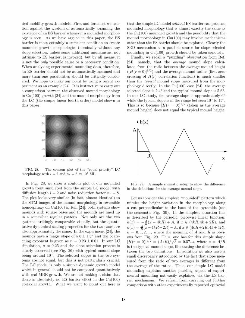
ited mobility growth models. First and foremost we cau-tion against the wisdom of automatically assuming theexistence of an ES barrier whenever a mounded morphol-ogy is seen. As we have argued in this paper, the ESbarrier is most certainly a sufficient condition to createmounded growth morphologies (nominally without anyslope selection, unless some additional mechanisms, notintrinsic to ES barrier, is invoked), but by all means, itis not the only possible cause or a necessary condition.When analyzing experimental mounding data, therefore,an ES barrier should not be automatically assumed andmore than one possibilities should be critically consid-ered. We hope to make our point by using a recent ex-periment as an example [24]. It is instructive to carry outa comparison between the observed mound morphologyin Cu(100) growth [24] and the mound morphology fromthe LC (the simple linear fourth order) model shown inthis paper.

FIG. 28. The contour plot of the “equal priority” LCmorphology with l = 2 and nr = 8 at 104 ML.

In Fig. 28, we show a contour plot of our moundedgrowth front simulated from the simple LC model withdiffusion length l = 2 and noise reduction factor nr = 8.The plot looks very similar (in fact, almost identical) tothe STM images of the mound morphology in reversiblehomoepitaxy on Cu(100) in Ref. [24]; both systems showmounds with square bases and the mounds are lined upin a somewhat regular pattern. Not only are the twosystems strikingly comparable visually, but the quanti-tative dynamical scaling properties for the two cases arealso approximately the same. In the experiment [24], themounds have a magic slope of 5.6 ± 1.3 and the coars-ening exponent is given as n = 0.23 ± 0.01. In our LCsimulation, n ≈ 0.25 and the slope selection process isclearly observed (see Fig. 26) with typical mound slopebeing around 10. The selected slopes in the two sys-tems are not equal, but this is not particularly crucial.The LC model is only a simple dynamic growth modelwhich in general should not be compared quantitativelywith real MBE growth. We are not making a claim thatthere is absolutely no ES barrier effect in the Cu(100)epitaxial growth. What we want to point out here is

that the simple LC model without ES barrier can producemounded morphology that is almost exactly the same asthe Cu(100) mounded growth and the possibility that themound morphology in Cu(100) may involve mechanismsother than the ES barrier should be explored. Clearly theSED mechanism as a possible source for slope selectedmounding in Cu(100) growth should be taken seriously.

Finally, we recall a “puzzling” observation from Ref.[24], namely, that the average mound slope calcu-lated from the ratio between the average mound height([H(r = 0)]1/2) and the average mound radius (first zerocrossing of H(r) correlation function) is much smallerthan the typical mound slope measured from the mor-phology directly. In the Cu(100) case [24], the averageselected slope is 2.4 and the typical mound slope is 5.6.In our LC study, the average slope is approximately 6

while the typical slope is in the range between 10 to 15.This is so because [H(r = 0)]1/2 (taken as the averagemound height) does not equal the typical mound height.

R

A

h(x)

x

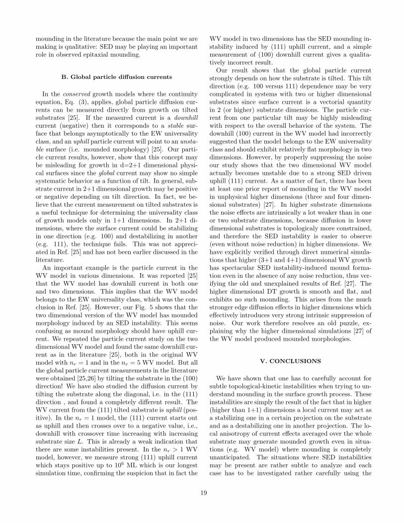
FIG. 29. A simple shematic setup to show the differencein the definitions for the average mound slope.

Let us consider the simplest “mounded” pattern whichmimics the height variation in the morphology alonga cut perpendicular to the base of the pyramids (seethe schematic Fig. 29). In the simplest situation thisis described by the periodic, piecewise linear function:h(x) = −A

R (x − 4kR) + A, if x ∈ (4kR, 4k + 2R), and

h(x) = AR (x−4kR−2R)−A, if x ∈ (4kR+2R, 4k+4R),

k = 0, 1, 2, ..., where the meaning of A and R is obvi-ous from Fig. 29. Thus, one has for this simple shape[H(r = 0)]1/2 = (A/R)/

√3 = 0.57..s, where s = A/R

is the typical mound slope, illustrating the difference be-tween the two definitions. In addition we also have asmall discrepancy introduced by the fact that slope mea-sured from the ratio of two averages is different fromthe average of the ratios. Thus, our simple LC modelmounding explains another puzzling aspect of experi-mental mounding not easily explained via the ES bar-rier mechanism. We refrain from carrying out furthercomparison with other experimentally reported epitaxial

18

mounding in the literature because the main point we aremaking is qualitative: SED may be playing an importantrole in observed epitaxial mounding.

B. Global particle diffusion currents

In the conserved growth models where the continuityequation, Eq. (3), applies, global particle diffusion cur-rents can be measured directly from growth on tiltedsubstrates [25]. If the measured current is a downhill

current (negative) then it corresponds to a stable sur-face that belongs asymptotically to the EW universalityclass, and an uphill particle current will point to an unsta-

ble surface (i.e. mounded morphology) [25]. Our parti-cle current results, however, show that this concept maybe misleading for growth in d=2+1 dimensional physi-cal surfaces since the global current may show no simplesystematic behavior as a function of tilt. In general, sub-strate current in 2+1 dimensional growth may be positiveor negative depending on tilt direction. In fact, we be-lieve that the current measurement on tilted substrates isa useful technique for determining the universality classof growth models only in 1+1 dimensions. In 2+1 di-mensions, where the surface current could be stabilizingin one direction (e.g. 100) and destabilizing in another(e.g. 111), the technique fails. This was not appreci-ated in Ref. [25] and has not been earlier discussed in theliterature.

An important example is the particle current in theWV model in various dimensions. It was reported [25]that the WV model has downhill current in both oneand two dimensions. This implies that the WV modelbelongs to the EW universality class, which was the con-clusion in Ref. [25]. However, our Fig. 5 shows that thetwo dimensional version of the WV model has moundedmorphology induced by an SED instability. This seemsconfusing as mound morphology should have uphill cur-rent. We repeated the particle current study on the twodimensional WV model and found the same downhill cur-rent as in the literature [25], both in the original WVmodel with nr = 1 and in the nr = 5 WV model. But allthe global particle current measurements in the literaturewere obtained [25,26] by tilting the substrate in the (100)direction! We have also studied the diffusion current bytilting the substrate along the diagonal, i.e. in the (111)direction , and found a completely different result. TheWV current from the (111) tilted substrate is uphill (pos-itive). In the nr = 1 model, the (111) current starts outas uphill and then crosses over to a negative value, i.e.,downhill with crossover time increasing with increasingsubstrate size L. This is already a weak indication thatthere are some instabilities present. In the nr > 1 WVmodel, however, we measure strong (111) uphill currentwhich stays positive up to 106 ML which is our longestsimulation time, confirming the suspicion that in fact the

WV model in two dimensions has the SED mounding in-stability induced by (111) uphill current, and a simplemeasurement of (100) downhill current gives a qualita-tively incorrect result.

Our result shows that the global particle currentstrongly depends on how the substrate is tilted. This tiltdirection (e.g. 100 versus 111) dependence may be verycomplicated in systems with two or higher dimensionalsubstrates since surface current is a vectorial quantityin 2 (or higher) substrate dimensions. The particle cur-rent from one particular tilt may be highly misleadingwith respect to the overall behavior of the system. Thedownhill (100) current in the WV model had incorrectlysuggested that the model belongs to the EW universalityclass and should exhibit relatively flat morphology in twodimensions. However, by properly suppressing the noiseour study shows that the two dimensional WV modelactually becomes unstable due to a strong SED drivenuphill (111) current. As a matter of fact, there has beenat least one prior report of mounding in the WV modelin unphysical higher dimensions (three and four dimen-sional substrates) [27]. In higher substrate dimensionsthe noise effects are intrinsically a lot weaker than in oneor two substrate dimensions, because diffusion in lowerdimensional substrates is topologicaly more constrained,and therefore the SED instability is easier to observe(even without noise reduction) in higher dimensions. Wehave explicitly verified through direct numerical simula-tions that higher (3+1 and 4+1) dimensional WV growthhas spectacular SED instability-induced mound forma-tion even in the absence of any noise reduction, thus ver-ifying the old and unexplained results of Ref. [27]. Thehigher dimensional DT growth is smooth and flat, andexhibits no such mounding. This arises from the muchstronger edge diffusion effects in higher dimensions whicheffectively introduces very strong intrinsic suppression ofnoise. Our work therefore resolves an old puzzle, ex-plaining why the higher dimensional simulations [27] ofthe WV model produced mounded morphologies.

V. CONCLUSIONS

We have shown that one has to carefully account forsubtle topological-kinetic instabilities when trying to un-derstand mounding in the surface growth process. Theseinstabilities are simply the result of the fact that in higher(higher than 1+1) dimensions a local current may act asa stabilizing one in a certain projection on the substrateand as a destabilizing one in another projection. The lo-cal anisotropy of current effects averaged over the wholesubstrate may generate mounded growth even in situa-tions (e.g. WV model) where mounding is completelyunanticipated. The situations where SED instabilitiesmay be present are rather subtle to analyze and eachcase has to be investigated rather carefully using the

19

noise reduction technique. The fact that SED mound-ing instability exists in the noise reduced WV, LC, andthe nonlinear fourth order continuum model, but not inF, DT, and the infinite order nonlinear model shows thatthe kinetic-topological nature of SED mounding may notbe obvious at all in a given situation. We note here thatthe DT model also exhibits very weak mound-like mor-phologies [6]. However, the weak mound-like structuresin the DT model arise from the fact that the roughnessexponent of the model is exceptionally large (arising fromthe presence of the ∇4h term in the growth equation).The mounds (and the oscillation in the height correla-tion H(r)) in the 2+1 DT model are random and irreg-ular while the SED-induced mound formations (in e.g.noise reduced WV model) exhibit regular patterns withstrong periodic oscillations in H(r).

One of our important findings is that SED genericallyleads to slope-selected mounded morphology whereasthe ES instability generically leads to slope steepeningmounding. We believe that many of the slope selectedmounding morphologies observed in MBE experiments(with typical selected slopes being small ∼ 10 or less)may actually arise from the kinetic-topological mound-ing we find generically in the LC or the WV model inthis paper. Further experimental and theoretical work isrequired to settle the competing roles of various instabil-ities contributing to epitaxial mounding in real surfacegrowth.

ACKNOWLEDGMENTS

This work is supported by the NSF-DMR-MRSEC atthe University of Maryland and by the US-ONR. ZTalso acknowledges partial support from the DOE undercontract W-7405-ENG-36 during the final stage of themanuscript preparation.

REFERENCES

[1] Z. Toroczkai and E.D. Williams, Phys. Today 52, 24(1999).

[2] R. L. Schwoebel, J. Appl. Phys. 40 614 (1966); G. Ehrlichand F. G. Hudda, J. Chem. Phys. 44, 1039 (1966).

[3] J. G. Amar and F. Family, Phys. Rev. Lett. 77 4584(1996).

[4] O. Pierre-Louis, M.R. D’Orsogna, and T.L. Einstein,Phys. Rev. Lett. 82, 3661 (1999).

[5] M. V. Ramana Murty and B.H. Cooper, Phys. Rev. Lett.83, 352 (1999) .

[6] S. Das Sarma, P. Punyindu, and Z. Toroczkai Surf. Sci.Lett. 457, L369 (2000).

[7] L. Brendel, H. Kallabis, and D. E. Wolf, Phys. Rev. E,58, 664 (1998).

[8] Z. W. Lai and S. Das Sarma, Phys. Rev. Lett. 66, 2348(1991).

[9] F. Family, J. Phys. A 19, L441 (1986).[10] S. F. Edwards and D. R. Wilkinson, Proc. R. Soc. Lon-

don, Ser. A 381, 17 (1982).[11] S. Das Sarma and P. I. Tamborenea, Phys. Rev. Lett. 66,

325 (1991); P. I. Tamborenea and S. Das Sarma, Phys.Rev. E 48, 2575 (1993).

[12] D. Wolf and J. Villain, Europhys. Lett. 13, 389 (1990).[13] J. M. Kim and S. Das Sarma, Phys. Rev. Lett. 72, 2903

(1994).[14] J. Krug, Phys. Rev. Lett. 72, 2907 (1994).[15] J. Villain, J. Phys. (France) I 1, 19 (1991).[16] C. Dasgupta, S. Das Sarma, and J. M. Kim, Phys. Rev.

E 54, R4552 (1996); C. Dasgupta, J. M. Kim, M. Dutta,and S. Das Sarma, Phys. Rev. E 55, 2235 (1997).

[17] A. Kundagrami and C. Dasgupta, Physica A 270, 135(1999).

[18] P. Punyindu and S. Das Sarma, Phys. Rev. E 57, R4863(1998).

[19] J. Kertesz and D. E. Wolf, J. Phys. A 21, 747 (1988).[20] D.E. Wolf and J. Kertesz, Europhys. Lett. 4, 651 (1987).[21] S. Das Sarma and P. Punyindu, Surf. Sci. Lett. 424, L339

(1999).[22] J. Krug, Adv.Phys. 46 139 (1997).[23] W. W. Mullins, in Metal Surfaces: Structure, Energetics

and Kinetics, eds. N.A. Gjostein and W. D. Robertson(Metals Park, Ohio: American Society of Metals, 1963).See also C. Herring, J. Appl. Phys. 21, 301 (1950).

[24] J.-K. Zuo and J.F. Wendelken, Phys. Rev. Lett. 78, 2791(1997).

[25] J. Krug, M. Plishke and M. Siegert, Phys. Rev. Lett. 70,3271 (1993).

[26] J. Krug, private communications.[27] M. Kotrla and P. Smilauer, Phys. Rev. B 53, 13777

(1996); P. Smilauer and M. Kotrla, Europhys. Lett. 27,261 (1994).

20