Accepted Manuscript

Environment assisted energy transfer indimer system

Salman Khan, M. Ibrahim, M.K. Khan

PII: S0003-4916(13)00270-4DOI: http://dx.doi.org/10.1016/j.aop.2013.11.009Reference: YAPHY 66385

To appear in: Annals of Physics

Received date: 29 May 2013Accepted date: 13 November 2013

Please cite this article as: S. Khan, M. Ibrahim, M.K. Khan, Environment assisted energytransfer indimer system, Annals of Physics (2013), http://dx.doi.org/10.1016/j.aop.2013.11.009

This is a PDF file of an unedited manuscript that has been accepted for publication. As aservice to our customers we are providing this early version of the manuscript. The manuscriptwill undergo copyediting, typesetting, and review of the resulting proof before it is published inits final form. Please note that during the production process errors may be discovered whichcould affect the content, and all legal disclaimers that apply to the journal pertain.

Environment Assisted Energy Transfer in Dimer System

Salman Khan†,∗ M. Ibrahim‡, and M. K. Khan‡

†Department of Physics, COMSATS Institute of Information Technology,

Chak Shahzad, Islamabad, Pakistan. and

‡Department of Physics, Quaid-i-Azam University, Islamabad, Pakistan.

(Dated: November 10, 2013)

Abstract

The influence of collective and multilocal environments on the energy transfer between the levels

of a dimer is studied. The dynamics of energy transfer are investigated by considering coupling

of collective environment with the levels of the dimer in the presence of both two individual and

mutually correlated multilocal environments. It is shown that every way of coupling we consider

assists, though differently, the probability of transition between the levels of dimer. The probability

of transition is strongly enhanced when the two local environments are mutually correlated.

PACS: 05.60.Gg; 03.65.Yz; 82.20. Rp

Keywords: Entanglement, Decoherence, Quantum Transport

∗Electronic address: sksafi@comsats.edu.pk

1

*ManuscriptClick here to view linked References

I. INTRODUCTION

The control of the loss of quantum correlations in simple systems under the influence of

external noise is of great importance for practical application of quantum computation and

for the development of quantum information processing devices [1–6]. The quantum coher-

ence between different components of a system may last long enough for totally isolated

quantum systems. For example, entanglement between components of a composite system

may survive against the decaying parameter (time) upto a considerable value. However,

completely isolating realistic physical systems from their environment is quite impractical.

It is now a well established fact that the unavoidable interaction of a quantum system

with its environment rapidly destroys the quantum coherence and hence limits the prac-

tical realization of quantum computers, information processing and storage of information

[7]. On the other hand, there are some recent studies based on spectroscopic observations

that predict long-lived quantum coherence in biological species, such as the photosynthetic

light-harvesting complexes of a species of green sulfur bacteria [8, 9], a species of purple

bacteria [10] and two species of cryptophyte algae [11]. It has also been suggested that the

persistent presence of quantum entanglement speeds up the electronic excitation transfer in

photosynthesis [12].

Recently, the effect of quantum coherence on electronic energy transfer in a simple model

of an aggregate of monomers that interact through dipole-dipole forces was investigated in

Ref. [13]. It is shown that in such systems quantum effects bring nothing new than what

the classical effects present. On the other hand, counter-intuitively, it has also been inves-

tigated that a dissipative quantum network subject to dephasing can exhibit an enhanced

capacity for transmission of classical information [14]. Excitons are created when Chro-

mophoric complexes absorbs light and are then transported to a reaction center where it is

used to trigger more processes to bind its energy in a chemical form. The enhancement of

quantum transport due to environmental influences in such systems has also been reported

[15–18]. The dynamic of energy transfer in a dimer system in the presence of two local spin

environments is studied in Ref. [19], where each level of the dimer system interacts with its

own local environment and it is shown that the existence of the local environments causes a

drastic increase in the transition probability. The role of entanglement in the enhancement

of quantum transport has also been studied [20–22].

2

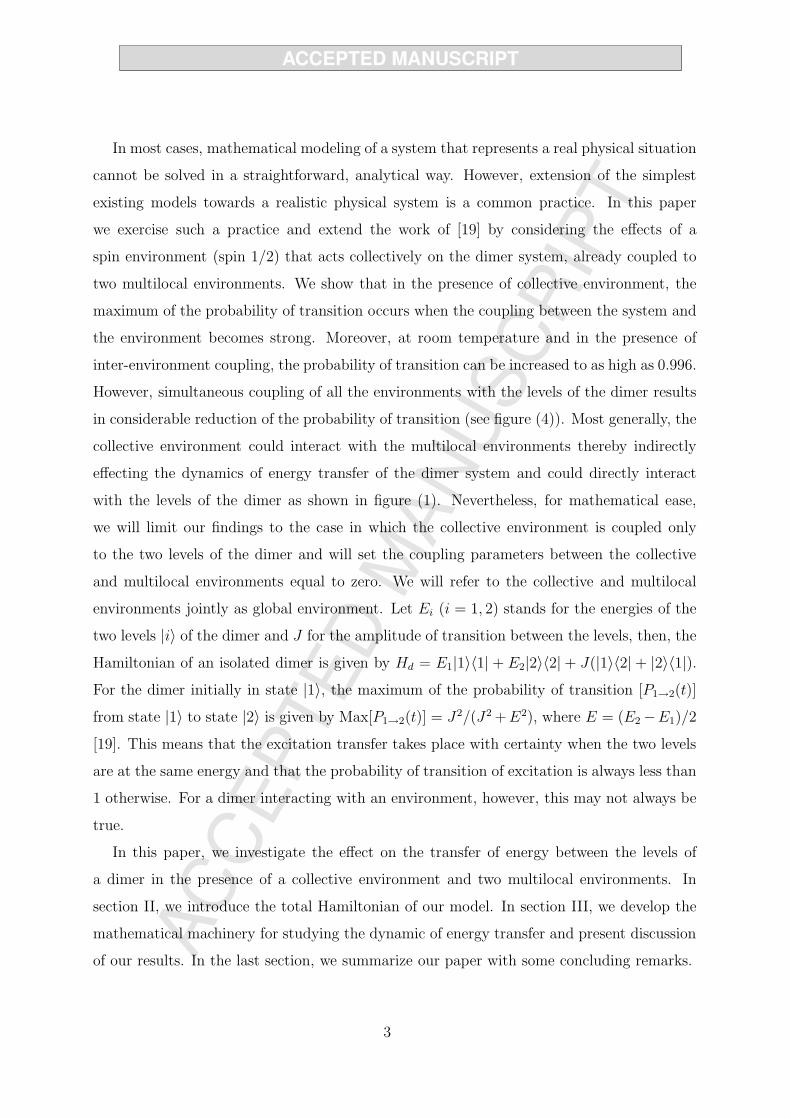
In most cases, mathematical modeling of a system that represents a real physical situation

cannot be solved in a straightforward, analytical way. However, extension of the simplest

existing models towards a realistic physical system is a common practice. In this paper

we exercise such a practice and extend the work of [19] by considering the effects of a

spin environment (spin 1/2) that acts collectively on the dimer system, already coupled to

two multilocal environments. We show that in the presence of collective environment, the

maximum of the probability of transition occurs when the coupling between the system and

the environment becomes strong. Moreover, at room temperature and in the presence of

inter-environment coupling, the probability of transition can be increased to as high as 0.996.

However, simultaneous coupling of all the environments with the levels of the dimer results

in considerable reduction of the probability of transition (see figure (4)). Most generally, the

collective environment could interact with the multilocal environments thereby indirectly

effecting the dynamics of energy transfer of the dimer system and could directly interact

with the levels of the dimer as shown in figure (1). Nevertheless, for mathematical ease,

we will limit our findings to the case in which the collective environment is coupled only

to the two levels of the dimer and will set the coupling parameters between the collective

and multilocal environments equal to zero. We will refer to the collective and multilocal

environments jointly as global environment. Let Ei (i = 1, 2) stands for the energies of the

two levels |i〉 of the dimer and J for the amplitude of transition between the levels, then, the

Hamiltonian of an isolated dimer is given by Hd = E1|1〉〈1| + E2|2〉〈2| + J(|1〉〈2| + |2〉〈1|).For the dimer initially in state |1〉, the maximum of the probability of transition [P1→2(t)]

from state |1〉 to state |2〉 is given by Max[P1→2(t)] = J2/(J2 +E2), where E = (E2 −E1)/2

[19]. This means that the excitation transfer takes place with certainty when the two levels

are at the same energy and that the probability of transition of excitation is always less than

1 otherwise. For a dimer interacting with an environment, however, this may not always be

true.

In this paper, we investigate the effect on the transfer of energy between the levels of

a dimer in the presence of a collective environment and two multilocal environments. In

section II, we introduce the total Hamiltonian of our model. In section III, we develop the

mathematical machinery for studying the dynamic of energy transfer and present discussion

of our results. In the last section, we summarize our paper with some concluding remarks.

3

II. DIMER WITH DECOHERENCE

The total Hamiltonian of the dimer coupled to a global environment can be written as

H = Hd + HM1 + HM2 + Hc + HdM1 + HdM2 + Hdc, (1)

where subscripts d, Mi, and c stand for dimer, multilocal environments and collective envi-

ronment, respectively. The subscripts dMi and dc represent the interaction part of the total

Hamiltonian between the levels of dimer and the respective environments. If we consider the

multilocal and collective environments to consist of independent spins of spin 1/2 particles

in the spin star configuration [23], then, the Hamiltonians of the multilocal environments

and of the collective environment can be written as

Hn = αn

Nn∑

k=1

σk,nz

2, (2)

where n = {Mi, c}, σz is the Pauli phase flip matrix and Nn is the number of independent

spins in the corresponding bath. If γMi and γc represent the coupling strengths of the

multilocal and collective environments, respectively, with the levels of the dimer, then the

interaction parts of the total Hamiltonian can be written as

Hdn =Nn∑

k=1

γn|i〉〈i|σk,n

z

2. (3)

The total Hamiltonian can be rewritten in a more convenient way in terms of the collective

spin operator Szn, as follows [19]

H = J(|1〉 〈2|+ |2〉 〈1|) + αcSzc +

2∑

i=1

(Ei |i〉 〈i| + αMiSzMi (4)

+ γMi |i〉 〈i|SzMi + γc |i〉 〈i|Sz

c ),

where

Szn =

Nn∑

k=1

σk,nz

2. (5)

The projectors |i〉 〈j| of the dimer system in terms of Pauli matrices can be expressed as

follows

|1〉 〈1| =I2 − σz

2, |2〉 〈2| =

I2 + σz

2,

|2〉 〈1| = σ+, |1〉 〈2| = σ−, (6)

4

1

0

2

E1

E2

J

�c

�c

�1

q

CM 2

M 1

�2

FIG. 1: Scheme of the dimer coupled to multilocal and collective environments, where each envi-

ronment consists of independent spins in spins star configurations. The two levels with energies

E1 6= E2 have amplitudes of transition probability J . Each level |1〉 and |2〉 is coupled with its

local and collective environments with coupling constants γM1, γM2 and γc. The dashed double

arrow indicates the possiblity of correlations between the multilocal baths with strength q.

where I2 is the 2 × 2 identity matrix, σ± = σx ± iσy are the spin raising and lowering

operators and the bases are chosen such that |1〉 =(01

). Using Eq. (6) and the fact that

5

γc |i〉 〈i|Szc = γc(|1〉 〈1|Sz

c1 + |2〉 〈2|Szc2), the total Hamiltonian becomes

H =

(E1

2+

E2

2+

γM1

2Sz

M1 +γM2

2Sz

M2 +γc

2(Sz

c1 + Szc2)

)I2

+ [E2 − E1

2− γM1S

zM1 − γM2S

zM2

2+

γc

2(Sz

c2 − Szc1)]σz

+ Jσx + αM1SzM1 + αM2S

zM2 + αcS

zc , (7)

where σx and σy are Pauli spin operators and Szci are the collective spin operators of the

spins of collective bath that interact with the corresponding levels of the dimer.

III. TRANSITION ANALYSIS

In this section we present our results for the transition probability between the levels of

the dimer under different environmental conditions. In the first case, we consider the envi-

ronments at zero temperature. Under such constraint, the spins of the global environment

are all in the ground state. The initial state of the global environment is a pure state and

is given by

|ΨB(0)〉 =

∣∣∣∣NM1

2,−NM1

2

⟩⊗∣∣∣∣NM2

2,−NM2

2

⟩⊗∣∣∣∣Nc

2,−Nc

2

⟩, (8)

where Nn is the number of spins in each environment and |j, m〉 are the eigenvectors of the

angular momentum operator S2 and Sz with eigenvalues j(j + 1) and m, respectively. The

state of the composite system at any time t can be written in the form

|Ψtotal(t)〉 =

2∑

i=1

Ci(t) |i〉 ⊗ |ΨB(0)〉

=

C2(t)

C1(t)

⊗ |ΨB(0)〉 (9)

where Ci(t) are the probability amplitudes for dimer to be in either of the two states. We

consider that initially (t = 0) the excitation is in level |1〉 of the dimer, then, C1(0) = 1

and C2(0) = 0. Moreover, we assume that N ′c spins of the collective bath are coupled with

level |1〉 and Nc − N ′c with level |2〉 of the dimer. Then, the solution of time dependent

Schrodinger equation

H |Ψtotal(t)〉 = i~∂ |Ψtotal(t)〉

∂t,

6

with Hamiltonian in its matrix form given by

H =

(E2−E1

2− γM1Sz

M1−γM2SzM2

2) +

γc(Szc2−Sz

c1)

2J

J −(E2−E1

2− γM1Sz

M1−γM2SzM2

2)− γc(Sz

c2−Szc1)

2

,

(10)

results in

i

∂C2(t)∂t

∂C1(t)∂t

=

[(E2−E1

2− γM2NM2−γM1NM1

4) + γc

4(2N ′

c −Nc)]C2(t) + JC1(t)

JC2(t)−[

E2−E1

2− γM2NM2−γM1NM1

4+ γc

4(2N ′

c − Nc)]C1(t)

. (11)

Note that in Eq. (10) we have ignored the first part of the total Hamiltonian of Eq. (7),

because it commutes with all the rest terms in the Hamiltonian. Its contribution is to add

a global phase that leaves the dynamics of probabilities of transition unaffected. In deriving

Eq. (11), we have taken inner product with 〈ΨB(0)| and have used the fact that

Szi |ΨB(0)〉 = −Ni

2|ΨB(0)〉 , 〈ΨB(0)| |ΨB(0)〉 = 1.

It is straightforward to solve Eq. (11) for the probability amplitudes, which results in

C1(t) = cos[t

√J2 + (∆ +

γc

4(2N ′

c −Nc))2]

+ i∆ + γc

4(2N ′

c − Nc)√J2 + (∆ + γc

4(2N ′

c − Nc))2sin[t

√J2 + (∆ +

γc

4(2N ′

c − Nc))2], (12)

C2(t) = iJ√

J2 + (∆ + γc

4(2N ′

c − Nc))2

sin[t

√J2 + (∆ +

γc

4(2N ′

c − Nc))2] exp[−i(E2 − E1)t

2], (13)

where ∆ = E2−E1

2− γ2NM2−γ1NM1

4. The probability of transition P1→2(t) from level |1〉 to

level |2〉 of the dimer is given by

P1→2(t) = |C2(t)|2 =J2

J2 + (∆ + γc

4(2N ′

c − Nc))2

× sin2[t

√J2 + (∆ +

γc

4(2N ′

c −Nc))2]. (14)

It can be seen that switching off the coupling of the dimer with collective environment,

Eq. (14) reduces to the result of Ref. [19]. To further investigate the dynamics of the

probability of transition in the present set up, we first switch off the coupling of multilocal

7

02

46

810

0.0

0.2

0.4

0.6

0.8

1.0

0.0

0.1

0.2

0.3

0.4

0.5

0 2 4 6 8 10

0.0

0.1

0.2

0.3

0.4

0.5

t

c

0

0.13

0.25

0.38

0.50

0.63

0.75

0.88

1.0

1

t

c

P2

(a)

02

46

810

0.0

0.2

0.4

0.6

0.8

1.0

0.0

0.1

0.2

0.3

0.4

0.5

t

c

0 2 4 6 8 10

0.0

0.1

0.2

0.3

0.4

0.5

0

0.13

0.25

0.38

0.50

0.63

0.75

0.88

1.0

t

c

1P

2

(b)

FIG. 2: (color online) The transition probability is plotted against the coupling parameter γc(ps−1)

with collective environment and time t(ps). The coupling parameters of multilocal baths in Fig 2(a)

are γM1 = γM2 = 0 and in Fig 2(b) they are γM1 = 10ps−1, γM2 = 2ps−1. The other parameters

for both figures are set to, NM1 = 10, NM2 = 20, N ′c = 4, N ′ = 20, E2−E1 = 20ps−1, J = 10ps−1.

environments (γ1 = γ2 = 0) with the levels of dimer and consider only the effect of collective

environment. The dynamics of the probability of transition for this case is shown in figure

(2a). It is seen that the difference in energy, which reduces the probability of transition

between the levels, is compensated by the coupling with collective environment. That is,

the collective environment assists to increase the probability of transition between the levels.

Figure (2b) shows the dynamics of the probability of transition when the coupling with

multilocal environments is also present. One can see that not only the maximum probability

of transition is achievable but also the maximum of the probability of transition shifts to

the region of strong correlation between the environment and the dimer system. The inset

in each figure shows the contour map of the corresponding surface plot.

Next, we consider a more realistic physical situation of baths at nonzero temperature and

investigate the influence on transition between the levels of dimer when coupled to such a

global environment. The initial density matrix for the global environment being at nonzero

8

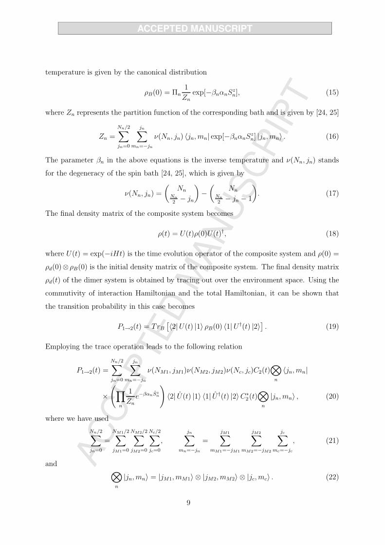
temperature is given by the canonical distribution

ρB(0) = Πn1

Znexp[−βnαnSz

n], (15)

where Zn represents the partition function of the corresponding bath and is given by [24, 25]

Zn =

Nn/2∑

jn=0

jn∑

mn=−jn

ν(Nn, jn) 〈jn, mn| exp[−βnαnSzn] |jn, mn〉 . (16)

The parameter βn in the above equations is the inverse temperature and ν(Nn, jn) stands

for the degeneracy of the spin bath [24, 25], which is given by

ν(Nn, jn) =

(Nn

Nn

2− jn

)−(

NnNn

2− jn − 1

). (17)

The final density matrix of the composite system becomes

ρ(t) = U(t)ρ(0)U(t)†, (18)

where U(t) = exp(−iHt) is the time evolution operator of the composite system and ρ(0) =

ρd(0)⊗ρB(0) is the initial density matrix of the composite system. The final density matrix

ρd(t) of the dimer system is obtained by tracing out over the environment space. Using the

commutivity of interaction Hamiltonian and the total Hamiltonian, it can be shown that

the transition probability in this case becomes

P1→2(t) = TrB

[〈2|U(t) |1〉 ρB(0) 〈1|U †(t) |2〉

]. (19)

Employing the trace operation leads to the following relation

P1→2(t) =

Nn/2∑

jn=0

jn∑

mn=−jn

ν(NM1, jM1)ν(NM2, jM2)ν(Nc, jc)C2(t)⊗

n

〈jn, mn|

×(∏

n

1

Zne−βαnSz

n

)〈2| U(t) |1〉 〈1| U †(t) |2〉C∗

2(t)⊗

n

|jn, mn〉 , (20)

where we have used

Nn/2∑

jn=0

=

NM1/2∑

jM1=0

NM2/2∑

jM2=0

Nc/2∑

jc=0

,

jn∑

mn=−jn

=

jM1∑

mM1=−jM1

jM2∑

mM2=−jM2

jc∑

mc=−jc

, (21)

and⊗

n

|jn, mn〉 = |jM1, mM1〉 ⊗ |jM2, mM2〉 ⊗ |jc, mc〉 . (22)

9

Using the fact that

exp[−βnαnSzn] |jn, mn〉 = exp[−βnαnmn] |jn, mn〉 , (23)

the above equation can be reduced to the following form

P1→2(t) =1

ZM1ZM2Zc

Nn/2∑

jn=0

jn∑

mn=−jn

ν(NM1, jM1)ν(NM2, jM2)ν(Nc, jc)

× exp[−(∑

i

βMiαMimMi + βcαcmc)]

× J2

J2 + (∆mMi− γc

2(2m′

c − mc))2

× sin2[t

√J2 + (∆mMi

− γc

2(2m′

c −mc))2], (24)

where ∆mMi= E2−E1

2+ γM2mM2−γM1mM1

2and m′

c is the net spin quantum number of spins in

02

46

810

0.0

0.2

0.4

0.6

0.8

1.0

0.0

0.2

0.4

0.6

0.8

1.0

t

c

0.88

0.88

0.88

0 2 4 6 8 10

0.0

0.2

0.4

0.6

0.8

1.0

0

0.13

0.25

0.38

0.50

0.63

0.75

0.88

1.0

t

c

1P2

(a)

02

46

810

0.0

0.2

0.4

0.6

0.8

1.0

0.0

0.2

0.4

0.6

0.8

1.0

t

c

0 2 4 6 8 10

0.0

0.2

0.4

0.6

0.8

1.0

0

0.13

0.25

0.38

0.50

0.63

0.75

0.88

1.0

t

c

1P2

(b)

FIG. 3: (color online) The transition probability is plotted against the coupling parameter γc(ps−1)

with collective environment and time t(ps). The temperature of the baths in Fig 2(a) is 77K, and

in Fig 2(b) it is 300K. The other parameters for both figures are set to, N ′c = 4, N ′ = 20,

E2 − E1 = 20 ps−1, J = 10 ps−1, αc = 250 ps−1..

the collective environment interacting with level |1〉 of the dimer. We confirm that in the

absence of collective environment, Eq. (24) reduces to the result of Ref. [19]. The probability

10

of transition when only the collective environment is coupled with the levels of the dimer is

plotted in figure 3(a, b) for two different temperatures of the environment. In both cases, the

environment assists to increases the probability of transition. The peaks happen at different

sets of values of the plotting parameters, such that the coupling parameter γc is higher

for delayed time t. At room temperature, the maximum of the probability of transition

spreads over a larger range of the plotting parameters and at lower temperature the peaks

get sharp and thus are defined by a narrow range of the parameters. In the range of large

values of γc, the peaks, at room temperature, rapidly get flat, however, the probability of

transition does not go abruptly to zero. In either case, the environment assists the transition

probability, however, its maximum value is smaller at room temperature than its value at

lower temperature. As before, for more clarity, we include contour map in the inset of each

figure.

In figure (4a), we show the behavior of the probability of transition between the levels

of the dimer when it is coupled to the global environment with γM1 = 0. In this case, the

peaks occur at stronger coupling between the environment and the system and are sharp

enough. The maximum is not as high as in the absence of multilocal environments. The

situation when all the environments are coupled with the levels of the dimer is shown in

figure (4b). One can see that the maximum is strongly reduced in this case. Moreover, if

the temperature of all the baths are set to 77K, the probability of transition goes to zero

for the chosen values of other parameters. The inset in each figure is the contour map of

the data of the corresponding surface plot. It is important to note that all the peaks that

correspond to increased transition rate in all of the above cases occur on time scales of the

order of a few hundred femtosecond, which corresponds to experimental observation [8, 9]

and theoretical predictions [15].

It is quite impractical to completely abandon inter environments interactions, therefore,

we also consider the effects of such interactions on the probability of transition. However,

including all possible interactions between the environments will, mathematically, make

the solution of the problem very complicated. To avoid such mathematical difficulties, we

consider the case in which only the multilocal environments are coupled with each other

through an Ising like interaction and have no interaction with the collective environment.

Under this condition the Hamiltonian HM of the multilocal environments takes the form

11

02

46

810

1214

0.0

0.1

0.2

0.3

0.4

0.5

0.6

0.7

0.0

0.2

0.4

0.6

0.8

1.0

c

t

0 2 4 6 8 10 12 14

0.0

0.2

0.4

0.6

0.8

1.0

0

0.088

0.18

0.26

0.35

0.44

0.53

0.61

0.70

t

c

1P2

(a)

02

46

810

1214

0.00

0.02

0.04

0.06

0.08

0.10

0.12

0.14

0.16

0.0

0.2

0.4

0.6

0.8

1.0

t

c

0 2 4 6 8 10 12 14

0.0

0.2

0.4

0.6

0.8

1.0

0

0.020

0.040

0.060

0.080

0.10

0.12

0.14

0.16

c

t

1P

2

(b)

FIG. 4: (color online) The transition probability is plotted against the coupling parameter γc(ps−1)

with collective environment and time t(ps). (a) The coupling of level |1〉 with its local environment

is switched off. The other parameters for both figures are set to, NM2 = J = 10 ps−1, α2 = αc =

300ps−1, γM1 = γM2 = 2 ps−1, N ′c = 4, N ′ = 20, E2 − E1 = 20 ps−1, J = 10, T2 = Tc = 77K. (b)

All the environments are on. The additional parameters are set to α1 = 300ps−1, γM1 = 2 ps−1,

T1 = 300K, NM1 = 2.

[19]

HM = aM1SzM1 + aM2S

zM2 + qSz

M1SzM2, (25)

where q is the coupling strength between the multilocal environments. For non-zero tem-

perature, the initial density matrix of the environment can be written as

ρB(0) =1

ZcZMexp

[−∑

n

βn(αnSzn) + qβMSz

M1SzM2

], (26)

12

where ZM is the partition function of the correlated multilocal environments and is given by

ZM =

NMi/2∑

jMi=0

ji∑

mMi=−ji

ν(NM1, jM1)ν(NM2, jM2)

× 〈jM1, mM1| exp[−βMαM1SzM1] |jM1, mM1〉

× 〈jM2, mM2| e−βMαM2SzM2 |jM2, mM2〉

× 〈jM1, mM1| 〈jM2, mM2| e−βMqSzM1Sz

M2 |jM1, mM1〉 |jM2, mM2〉 .

(27)

Note that in Eq. (27), we have taken βM = βM1 = βM2. The final density matrix ρ(t) can be

obtained, as before, by using Eq. (18) with ρB(0) given by Eq. (26). It is straightforward to

find the probability of transition by using Eq. (19) with U(t) = exp(−iHM t), where HM is

the Hamiltonian given by Eq. (25). After carrying out the trace operation, the probability

of transition simplifies to the following form

P1→2(t) =

Nn/2∑

jn=0

jn∑

mn=−jn

ν(NM1, jM1)ν(NM2, jM2)ν(Nc, jc)C2 (t)

× 1

ZM〈jM1, mM1| e−βMαM1Sz

M1 |jM1, mM1〉

× 〈jM2, mM2| e−βM αM2SzM2 |jM2, mM2〉 〈jM1, mM1|

〈jM2, mM2| e−βMqSzM1Sz

M2 |jM1, mM1〉 |jM2, mM2〉

× 1

Zc

〈jc, mc| e−βcαcSzc |jc, mc〉C∗

2 (t) 〈2| U(t) |1〉 〈1| U †(t) |2〉 (28)

With the help of Eq. (23) we can rewrite Eq. (28) in the following form

P1→2(t) =1

ZcZM

Nn/2∑

jn=0

jn∑

mn=−jn

ν(NM1, jM1)ν(NM2, jM2)ν(Nc, jc)

× exp[−βM(∑

i

αMimMi + qmM1mM2)− βcαcmc]

× J2

J2 + (∆mMi− γc

2(2m′

c −mc))2sin2[t

√J2 + (∆mMi

− γc

2(2m′

c −mc))2],

(29)

where use of the following relation is made

|C2 (t)|2 =J2

J2 +[∆mMi

− γc

2(2m′

c −mc)]2 sin2(t

√J2 +

[∆mMi

− γc

2(2m′

c − mc)]2

).

13

05

1015

2025

30

0.0

0.2

0.4

0.6

0.8

1.0

0

2

4

6

8

10

c

q0 5 10 15 20 25 30

0

2

4

6

8

10

0

0.13

0.25

0.38

0.50

0.63

0.75

0.88

1.0

c

q

1P2

(a)

05

1015

2025

30

0.0

0.2

0.4

0.6

0.8

1.0

0

2

4

6

8

10

q

c

0 5 10 15 20 25 30

0

2

4

6

8

10

0

0.13

0.25

0.38

0.50

0.63

0.75

0.88

1.0

c

q

1P2

(b)

FIG. 5: (color online) The transition probability is plotted against the coupling parameter γc(ps−1)

with collective environment and the coupling parameter q(ps−1) between the multilocal environ-

ments. The coupling of level |1〉 with its local environment is switched off. The other param-

eters for both figures are set to, NM1 = 22, NM2 = Nc = 20, J = 10 ps−1, t = 0.155ps

αM1 = αM2 = αc = 250ps−1, γM1 = γM2 = 0.8 ps−1, N ′c = 6, N ′ = 20, E2 − E1 = 20 ps−1.

In Eq. (29) all the terms have meanings unchanged. The influence of correlation between

the two local environments on the probability of transition in the presence of collective

environment is shown in figure (5) for two different temperatures of the baths. Figure (5a)

shows the situation when all the baths are at 77K and figure (5b) represents the case for

300K of the baths. For lower temperature of the baths (77K), the probability of transition

goes as high as 0.996 and at 300K temperature of the baths it drops to 0.97, which is

still high than when the collective environment is absent [19]. At low baths’ temperature,

the probability of transition oscillates and the amplitude damps as the coupling strength

increases. Whereas at high baths’ temperature, the oscillatory behavior is not persistent

and dies out soon. The behavior can more clearly be observed in the corresponding contour

map given in the inset of each figure.

14

IV. SUMMARY

In summary, we have investigated the energy transfer between the levels of a dimer in

the presence of different spin environments. We have considered the simplest, among the

many possible, ways of interactions between the environment and the levels of the dimer.

Generally saying, it is shown that in the presence of collective environment with biologically

applicable parameters ranges and time scales, both ways of coupling- the correlated and

uncorrelated multilocal environment, assists the transfer of energy in the dimer system. In

particular, the increase in probability of transition strongly depends on the temperature

of the environment as well as on mutual coupling between the environments. It is shown

that at higher temperature, stronger coupling between the levels of the dimer and the

environment is needed for maximizing the probability of transition. In the absence of

inter-environment coupling, the global environment, although assists the transport of

energy, however, the maximum of transition of probability is considerably reduced. The

quantum transport is considerably enhanced when inter-environment coupling is present.

[1] M. A. Nielson and I. L. Chuang, Quantum Computation and Quantum Information (Cam-

bridge University Press, Cambridge, England, 2000).

[2] C. H. Bennett and G. Brassard, in Proceedings of the IEEE Conference on Computers, Sys-

tems, and Signal Processing, Bangalore (IEEE, New York, 1984), p. 175.

[3] A. K. Ekert, Phys. Rev. Lett. 67, 661 (1991).

[4] P.W. Shor, SIAM J. Comput. 26, 1484 (1997).

[5] A. Muller, H. Zbinden, and N. Gisin, Europhys. Lett. 33, 335 (1996).

[6] D. Deutsch and R. Josza, Proc. R. Soc. A 439, 553 (1992).

[7] H.P. Breuer and F. Petruccione. The Theory of Open Quantum Systems (Oxford University

Press, New York, 2002).

[8] G. Panitchayangkoon, D. Hayes, K. A. Fransted, J. R. Caram, E. Harel, J.Wen, R. E. Blanken-

ship, and G. S. Engel., Proc. Natl. Acad.Sci. U.S.A. 107, 12766 (2010).

[9] G. S. Engel, T. R. Calhoun, E. L. Read, T. K. Ahn, T. Mancal, Y. C. Cheng, R. E. Blanken-

15

ship, and G. R. Fleming., Nature (London) 446. 782 (2007).

[10] H. Lee, Y.C. Cheng and G. R. Fleming, Science 316, 1462 (2007).

[11] E. Collini et al., Nature (London) 463, 644 (2010).

[12] S. Hoyer, M. Sarovar, and K. B. Whaley, New J. Phys. 12, 065041 (2010).

[13] J. S. Briggs and A. Eisfeld., Phys. Rev. E 83, 051911 (2011).

[14] M. B. Plenio and S. F. Huelga., New J. Phys. 10 113019 (2008).

[15] J. Adolphs and T. Renger., Biophys. J. 91 2778 (2006).

[16] P. Rebentrost, M. Mohseni and A. J. Aspuru-Guzik., Phys. Chem. B 113, 9942 (2009).

[17] K. M. Gaab and C. J. Bardeen J. Chem. Phys. 121 7813 (2004).

[18] P. Rebentrost, M. Mohseni, I. Kassal, S. Lloyd and A. Aspuru-Guzik., New J. Phys. 11, 033003

(2009).

[19] I. Sinayskiy, A. Marais, F. Petruccione, and A. Ekart., Phys. Rev. Lett. 108, 020602 (2012).

[20] M. Sarovar et al. Nature Phys. 6, 462 (2010).

[21] F. Caruso et al., Phys. Rev. A 81, 06234 (2010).

[22] T. Scholak et al., Phys. Rev. E 83, 021912 (2011).

[23] H. P. Breuer, D. Burgarth, and F. Petruccione, Phys. Rev. B 70, 045323 (2004).

[24] J. Wesenberg and K. Molmer, Phys. Rev. A 65, 062304 (2002).

[25] Y. Hamdouni, M. Fannes, and F. Petruccione, Phys. Rev. B 73, 245323 (2006).

16

Highlights

• The dynamics of energy transfer between the levels of a dimer are studied.• Coupling of collective as well as individual environments are considered.

• The environments are in spin star configurations.

• The environment assists the energy transfer between the levels.

• For correlated multilocal environments, the transition probability is almost 100%.