Enhancing Digital Images Using Feed Forward Neural Network

[Pushpavalli, 3(7): July, 2014] ISSN: 2277-9655 Scientific Journal Impact Factor: 3.449

(ISRA), Impact Factor: 1.852

http: // www.ijesrt.com(C)International Journal of Engineering Sciences & Research Technology

[819-831]

IJESRT INTERNATIONAL JOURNAL OF ENGINEERING SCIENCES & RESEARCH

TECHNOLOGY

Enhancing Digital Images Using Feed Forward Neural Network

R.Pushpavalli*1, G.Sivaradje2 *1,2 ECE Department, Pondicherry Enginering College, India

[email protected]

Abstract A neural filtering technique is proposed to enhance the digital images when images are contaminated by

impulse noise. This filter is obtained by combining nonlinear filter and feed forward neural network with back

propagation algorithm. Nonlinear filtering output is converted into one dimensional sequence in four different ways

for neural network training. The neural network is trained using three well known images and the network

architecture is tuned to optimization. Using this optimized structure, unknown images are tested. Extensive

simulation results show that the proposed intelligent filter is superior performance than the other existing neural

filters and nonlinear filters in terms of eliminating impulse noise and preserving edges and fine details.

Keywords: Nonlinear filter, impulse noise, intelligent technique, feed forward neural network.

Introduction Digital images are often corrupted by

impulse noise during image transmission over

communication channel or image acquisition.

Filtering is an essential part of any signal processing

system, which involves estimation of a signal

degraded by additive noise. Several filtering

techniques have been reported over the years, for

various applications. In early stages, linear filters are

important tool for removal of noise on digital images.

However, this filter removing noise in predetermined

region with prior knowledge of the noise. In real time

application, prior knowledge of the noise is

unpredictable one. In addition to this, linear filter is

well suited for Gaussian noise removal. It degrades

the image quality while images are contaminated by

impulse noise. In image processing problems,

nonlinear filtering techniques are preferred for image

denoising. In general, the filters having good edge

and image detail preservation properties are highly

desirable for image filtering. The median filter and its

variants are among the most commonly used filters

for impulse noise removal. The median filters, when

applied uniformly across the image, tend to modify

both noisy as well as noise free pixels, resulting in

blurred and distorted features. Recently, some

modified forms of the median filter have been

proposed to overcome these limitations [1-5]. In

these variants of the median filter, the pixel value is

modified only when it is found corrupted with noise.

These variants of the median filter still retain the

basic rank order structure of the filter. Among these

filters, the center weighted median filters (CWMFs)

give a large weight to the central pixel, while

choosing between the current pixel and the median

value. In order to avoid the influence of the noisy

pixels on the filtered output, impulse detection

filtering had been investigated [6-27].

In order to address these issues, many neural

networks have been investigated for image denoising

[28-40]. In the last few years, there has been a

growing interest in the applications of soft computing

techniques, such as neural networks and fuzzy

systems, to the problems in digital signal processing.

Neural networks are low-level computational

structures that perform well when dealing with raw

data although neural networks can learn.

Neural networks are composed of simple elements

operating in parallel. These elements are inspired by

biological nervous systems. As in nature, the network

function is determined largely by the connections

between elements. This type of training is used to

perform a particular function by adjusting the values

of the connections (weights) between elements.

Commonly neural networks are adjusted or trained to

a specific target output which is based on a

comparison of the output and the target, until the

network output matches the target. Typically many

such input-target pairs are needed to train a network.

A feed forward neural architecture with back

propagation learning algorithms have been

investigated to satisfy both noise elimination and

edges and fine details preservation properties when

digital images are contaminated by higher level of

impulse noise. Back propagation is a common

http://www.ijesrt.com/

mailto:[email protected]




[819-831]

method of training artificial neural networks

algorithm so as to minimize the objective function. It

is a multi-stage dynamic system optimization

method. It is a supervised learning method, and is a

generalization of the delta rule.

In addition to these, the back-propagation learning

algorithm is computationally efficient in which its

complexity is linear in the synaptic weights of the

network. The input-output relation of a feed forward

adaptive neural network can be viewed as a powerful

nonlinear mapping. Conceptually, a feed forward

adaptive network is actually a static mapping

between its input and output spaces. Even though,

intelligent techniques required certain pattern of data

to learn the input. This filtered image data pattern is

given through nonlinear filter for training of the

input. Therefore, intelligent filter performance

depends on conventional filters performance. This

work aims to achieving good de-noising without

compromising on the useful information of the

signal.

In this paper, a new technique is proposed which

improves the image quality. The proposed filter is

carried in three steps. In first steps, input image is

denoised by nonlinear filter. The two dimensional

filtered image output is converted into one

dimensional sequence in four different ways and each

sequence is combined with feed forward neural

network for training in second step. Many numbers of

architectures have been trained and based on error

minimization; particular architecture has been

selected for each separate sequence. This each trained

data sequence is recovered to its original sequence

and then these sequences are integrated using image

data fusion system. The trained architecture is

optimized for testing the unknown image data.

Simulation results show that the proposed filter

exhibit superior performance than the other filtering

techniques.

The paper is organized as follows. Section 2

discusses the noise model. Section 3 presents the

proposed filtering. The simulation results with

different images are presented in section 4 to

demonstrate the efficacy of the proposed algorithm.

Finally, conclusions are given in section 5.

Noise Model Fundamentally, there are three standard

noise models, which model the types of noise

encountered in most images; they are additive noise,

multiplicative noise and impulse noise. Digital image

are often corrupted by salt and pepper noise (or

impulse noise). Impulse noise is considered for

proposed work. For images corrupted by salt-and-

pepper noise (respectively fixed-valued noise), the

noisy pixels can take only the maximum and the

minimum values (respectively any random value) in

the dynamic range. In other words, an image

containing salt-and-pepper noise will have dark

pixels in bright region and bright pixels in dark

regions. A digital image function is given by f(i,j)

where (i,j) is spatial coordinate and f is intensity at

point(i,j). let f(i,j) be the original image, g(i,j) be the

noise image version and ƞ be the noise function,

which returns random values coming from an

arbitrary distribution. Then the additive noise is given

by the equation (1)

( , ) ( , ) ( , )g i j f i j i j (1)

Impulse noise is caused by malfunctioning pixels in

camera sensors, dead pixels, faulty memory locations

in hardware, erroneous transmission in a channel,

analog to digital converter, malfunctioning CCD

elements (i.e. hot and dead pixels) and flecks of dust

inside the camera most commonly cause the

considered kind of noise etc. It also creeps into the

images because of bit errors in transmission, faulty

memory locations and erroneous switching during

quick transients. Two common types of impulse

noise are the salt and pepper noise and the random

valued noise. The proposed filter first detects the

Salt and pepper noise present in digital images in

very efficient manner and then removes it. As the

impulse noise is additive in nature, noise present in a

region does not depend upon the intensities of pixels

in that region. Image corrupted with impulse noise

contain pixels affected by some probability. The

intensity of gray scale pixel is stored as an 8-bit

integer giving 256 possible different shades of gray

going from black to white, which can be represented

as a [0,L-1] (L is 255) integer interval. In this paper

the impulse noise is considered. In case of images

corrupted by this kind of salt and pepper noise,

intensity of the pixel Aij at location (i,j) is described

by the probability density function given by the

following equation (2)

( ) 1

ija

ij ij ij

ijb

p for A a

f A p for A Y

p for A b

(2)

where a is the minimum intensity (dark dot); b is the

maximum intensity (light dot); pa is the probability of

intensity (a) generation; pb is the probability of

intensity (b) generation; p is the noise density, and Yij

is the intensity of the pixel at location (i,j) in the

uncorrupted image. If either pa or pb is zero the

impulse noise is called unipolar noise. If neither


http://en.wikipedia.org/wiki/Artificial_neural_network

http://en.wikipedia.org/wiki/Supervised_learning

http://en.wikipedia.org/wiki/Delta_rule




[819-831]

probability is zero and especially if they are equal,

impulse noise is called bipolar noise or salt-and-

pepper noise.

Proposed Filtering Algorithm The proposed filter is made by a nonlinear

filter, neural filter and image data fusion. The

proposed filter is carried in three steps. In first steps,

input image is denoised by nonlinear filter. The two

dimensional filtered image output is converted in to

one dimensional sequence in four ways and each

sequence is combined with feed forward neural

network for training in second step. All trained image

sequence is integrated using image data fusion

system. Then the trained architecture is optimized for

testing the unknown image data.

A Feed forward Neural Network is a flexible system

trained by heuristic learning techniques derived from

neural networks can be viewed as a 3-layer neural

network with weights and activation functions.

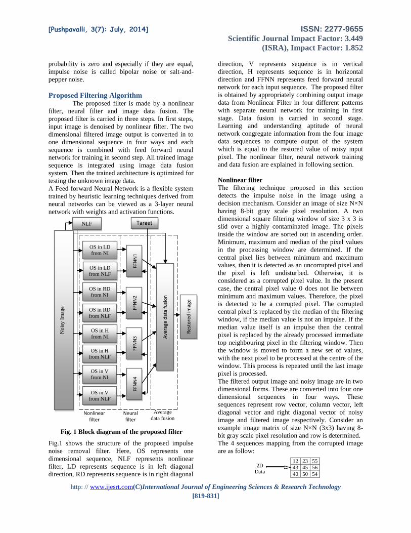
Fig. 1 Block diagram of the proposed filter

Fig.1 shows the structure of the proposed impulse

noise removal filter. Here, OS represents one

dimensional sequence, NLF represents nonlinear

filter, LD represents sequence is in left diagonal

direction, RD represents sequence is in right diagonal

direction, V represents sequence is in vertical

direction, H represents sequence is in horizontal

direction and FFNN represents feed forward neural

network for each input sequence. The proposed filter

is obtained by appropriately combining output image

data from Nonlinear Filter in four different patterns

with separate neural network for training in first

stage. Data fusion is carried in second stage.

Learning and understanding aptitude of neural

network congregate information from the four image

data sequences to compute output of the system

which is equal to the restored value of noisy input

pixel. The nonlinear filter, neural network training

and data fusion are explained in following section.

Nonlinear filter

The filtering technique proposed in this section

detects the impulse noise in the image using a

decision mechanism. Consider an image of size N×N

having 8-bit gray scale pixel resolution. A two

dimensional square filtering window of size 3 x 3 is

slid over a highly contaminated image. The pixels

inside the window are sorted out in ascending order.

Minimum, maximum and median of the pixel values

in the processing window are determined. If the

central pixel lies between minimum and maximum

values, then it is detected as an uncorrupted pixel and

the pixel is left undisturbed. Otherwise, it is

considered as a corrupted pixel value. In the present

case, the central pixel value 0 does not lie between

minimum and maximum values. Therefore, the pixel

is detected to be a corrupted pixel. The corrupted

central pixel is replaced by the median of the filtering

window, if the median value is not an impulse. If the

median value itself is an impulse then the central

pixel is replaced by the already processed immediate

top neighbouring pixel in the filtering window. Then

the window is moved to form a new set of values,

with the next pixel to be processed at the centre of the

window. This process is repeated until the last image

pixel is processed.

The filtered output image and noisy image are in two

dimensional forms. These are converted into four one

dimensional sequences in four ways. These

sequences represent row vector, column vector, left

diagonal vector and right diagonal vector of noisy

image and filtered image respectively. Consider an

example image matrix of size N×N (3x3) having 8-

bit gray scale pixel resolution and row is determined.

The 4 sequences mapping from the corrupted image

are as follow:

Target

No

isy

Im

age

FFN

N4

Net

wo

rk

stru

ctu

re

for

trai

nin

g A

vera

ge d

ata

fusi

on

Res

tore

d im

age

Net

wo

rk

stru

ctu

re f

or

trai

nin

g

OS in LD from NI

Neural filter

NLF

OS in RD

from NLF

OS in H

from NI

OS in V

from NLF

OS in V

from NI

OS in H from NLF

OS in LD

from NLF

OS in RD

from NI

FFN

N3

Net

wo

rk

stru

ctu

re

for

trai

nin

g

FFN

N2

Net

wo

rk

stru

ctu

re

for

trai

nin

g

FFN

N1

Net

wo

rk

stru

ctu

re

for

trai

nin

g

Average

data fusion Nonlinear

filter

12 23 55

43 45 56

40 50 54

2D Data





[819-831]

1) 2D image matrix is converted in to row sequence

and is given by

{ [1, :], [2, :], [3, :], [4, :], .., [ , :]}aRV A ALR A ALR A N (3)

where A[i,:] represents the ith row vector of the

corrupted image; ALR represents the left and right

symmetrical image of the corrupted image.

2) 2D image matrix is converted in to column vector

sequence and is given by

{ [:,1], [:, 2], [:, 3], [:, 4], ..., [:, ]}aCV A AUL A AUL A N (4)

where A[:,i] represents the ith row vector of the

corrupted image; AUL represents the upper and lower

symmetrical image of the corrupted image.

3) 2D image matrix is converted in to left diagonal

vector sequence and is given by

{ ( , 1), ( , 2), ( , 3), ( , 4), ... ( , 2 1)}T T

aLD D A D A D A D A D A N (5)

where, D(A,i) represents the ith diagonal matrix of the

image matrix A; AT represents the vector transpose

matrix of the image matrix A; A represents the

corrupted image.

4) 2D image matrix is converted in to right diagonal

vector sequence and is given by { ( 90,1), ( 90, 2), ( 90, 3), ( 90, 4), ... ( 90, 2 1)}aRD D A D A D A D A D A N

(6)

where, A90 represents the ith that has been counter

clock-wise rotated by 90 degree by the corrupted

image matrix. Then each one dimensional sequence

of noisy image and filtered image data are trained

using feed forward neural network with back

propagation algorithm seperately. Different

architechtures are trained for each one dimensional

sequence of data. Based on the image quality, a

particular trained architecture is selected for the

proposed work.

Feed forward Neural Network

In feed forward neural network, back propagation

algorithm is popular general nonlinear modelling tool

because it is very suitable for tuning by optimization

and one to one mapping between input and output

data. The input-output relationship of the network is

as shown in Fig.2.

Fig.2 Feed Forward Neural Network Architecture

In Fig.2, xm represents the total number of input

image pixels as data, nkl represents the number

neurons in the hidden unit, k represents he number

hidden layer and l represents the number of neurons

in each hidden layer. A feed forward back

propagation neural network consists of two layers.

The first layer or hidden layer, has a tan sigmoid (tan-

sig) activation function is represented by

( ) tanh( )yi vi (7)

This function is a hyperbolic tangent which ranges

from -1 to 1, yi is the output of the ith node (neuron)

and vi is the weighted sum of the input and the second

layer or output layer, has a linear activation function.

Thus, the first layer limits the output to a narrow

range, from which the linear layer can produce all

Hidden

Layer 1

n12

.

.

.

n16

x1

Hidden

Layer 2

Tra

ined

Dat

a’s

n11 n21

n22

n26

x2

x3

Output

Layer

.

.

. .

.

.

Input

Layer

12 23 55

43 45 56

40 50 54

Column vector (1D data) from 2D data

12 43 40 50 45 23 55 56 54

12 23 55

43 45 56

40 50 54

Row vector (1D data) from 2D data

12 43 55 56 45 43 40 50 54

12 23 55

43 45 56

40 50 54

Right diagonal vector (1D data) from 2D data

54 50 56 55 45 40 43 23 12

12 23 55

43 45 56

40 50 54

Left diagonal vector (1D data) from 2D data

12 23 43 40 45 55 56 50 54





[819-831]

values. The output of each layer can be represented

by

( )1 ,1 ,1

Y f W X bNx NxM M N

(8)

where Y is a vector containing the output from each

of the N neurons in each given layer, n represents

number of hidden layers; n=1, 2,…n, W is a matrix

containing the weights for each of the M inputs for

all N neurons, X is a vector containing the inputs, b is

a vector containing the biases and f(·) is the

activation function for both hidden layer and output

layer.

The trained network was created using the neural

network toolbox from Matlab9b.0 release. In a back

propagation network, there are two steps during

training. The back propagation step calculates the

error in the gradient descent and propagates it

backwards to each neuron in the hidden layer. In the

second step, depending upon the values of activation

function from hidden layer, the weights and biases

are then recomputed, and the output from the

activated neurons is then propagated forward from

the hidden layer to the output layer. The network is

initialized with random weights and biases, and was

then trained using the Levenberq-Marquardt

algorithm (LM). The weights and biases are updated

according to

1

1 [ ]T T

Dn Dn J J I J e

(9)

where Dn is a matrix containing the current weights

and biases, Dn+1 is a matrix containing the new

weights and biases, e is the network error, J is a

Jacobian matrix containing the first derivative of e

with respect to the current weights and biases, I is the

identity matrix and µ is a variable that increases or

decreases based on the performance function. The

gradient of the error surface, g, is equal to JTe.

Training of the Feed Forward Neural Network

Feed forward neural network is training using back

propagation algorithm. There are two types of

training or learning modes in back propagation

algorithm namely sequential mode and batch mode

respectively. In sequential learning, a given input

pattern is propagated forward and error is determined

and back propagated, and the weights are updated.

Whereas, in Batch mode learning; weights are

updated only after the entire set of training network

has been presented to the network. Thus the weight

update is only performed after every epoch. It is

advantageous to accumulate the weight correction

terms for several patterns. To improve the image

quality, batch mode learning is selected for the

proposed neural network training. For better

understanding, the back propagation learning

algorithm can be divided into two phases:

propagation and weight update. In first phase,

propagation involves the following steps: a) Forward

propagation of a training pattern's input through the

neural network in order to generate the propagation's

output activations. b) Backward propagation of the

propagation's output activations through the neural

network using the training pattern's target in order to

generate the deltas of all output and hidden neurons.

In second phase, each weight-synapse follows the

following steps: a) multiply its output delta and input

activation to get the gradient of the weight. b) Bring

the weight in the opposite direction of the gradient by

subtracting a ratio of it from the weight.

This ratio influences the speed and quality of

learning; it is called the learning rate. The sign of the

gradient of a weight indicates where the error is

increasing; this is why the weight must be updated in

the opposite direction. Repeat phase 1 and 2 until the

performance of the network is satisfactory.

In addition, neural network recognizes certain pattern

of data only and also it entails difficulties to learn

logically to identify the error data from the given

input image. In order to improve the learning and

understanding properties of neural network, filtered

output image data is introduced to the neural network

for training. In this paper, training is carried in three

stages. In first stage, noisy input data and filtered

output data are converted in to four different pattern

of one dimensional sequences namely row vector,

column vector, left diagonal vector and right diagonal

vector respectively. Four neural network

architectures are used for these four sequences

separately.

In second stage, one dimensional sequence of noisy

data and filtered data are inputs for neural network

training structure. Each feed forward neural network

is trained for different architectures. Based on the

quantitative measurements, a particular architecture

is selected for next stage. FFNN1 is trained using

single hidden layer with 4 neurons, FFNN2 is trained

using two hidden layers with 5 neurons in each layer,

FFNN3 is trained using single hidden layer with 6

neurons and FFNN4 is trained using single hidden

layer with 7 neurons. Noise free image is considered

as a target image for training data and then average is

calculated for these four sequences of data for neural

network training in next stage.

In this stage, the average data is again trained using

FFNN for image enhancement. This stage is referred

as third stage. Back propagation is pertained as

network training principle and the parameters of this

network are then iteratively tuned. Once the training





[819-831]

of the neural network is completed, its internal

parameters are fixed and the network is combined

with the nonlinear filter output and noisy image to

construct the proposed technique, as shown in Fig.3.

While training a neural network, network structure is

fixed. The performance evaluation is obtained

through simulation results and shown to be superior

performance to other existing filtering techniques in

terms of impulse noise elimination and edges and

fine detail preservation properties.

The feed forward neural network used in the structure

of the proposed filter acts like a mixture operator and

attempts to construct an enhanced output image by

combining the information from the Nonlinear

filtered output image and noisy image. The rules of

mixture are represented by the rules in the rule base

of the neural network and the mixture process is

implemented by the mechanism of the neural

network. The feed forward neural network is trained

by using back propagation algorithm and the

parameters of the neural network are then iteratively

tuned using the Levenberg–Marquardt optimization

algorithm, so as to minimize the learning error, e.

The neural network trained structure is optimized and

the tuned parameters are fixed for testing the

unknown images. The internal parameters of the

neural network are optimized by training.

Fig.3 Training of the Feed forward Neural Network

Fig.4 represents the setup used for training and here,

the parameters of this network are iteratively

optimized so that its output converges to original

noise free image by which the definition, completely

removes the noise from its input image. The well

known images are trained using this selected neural

network and the network structure is optimized. The

unknown images are tested using optimized neural

network structure.

In order to get effective filtering performance,

already existing neural network filters are trained

with image data and tested using equal noise density.

But in practical situation, information about the noise

density of the received signal is unpredictable one.

Therefore; in this paper, the neural network

architecture is trained using denoised three well

known images which are corrupted by adding

different noise density levels of 0.4, 0.45, 0.5 and 0.6

noise density level and also trained for different

hidden layers with different number of neurons.

Noise density with 0.45 gave optimum solution for

NLF output

No

isy

im

age

for

trai

nin

g

OS in LD from NI

Av

erag

e dat

a fu

sion

X

FF

NN

1 a1

OS in RD from NI

OS in H from NI

OS in V from NI

OS in LD from NLF

OS in RD from NLF

OS in H from NLF

e 1=t 1

-a1

FF

NN

2

FF

NN

3

FF

NN

4

OS in H from NLF

X

X

X

e 2=t 2

-a2

e 3

=t 3

-a3

e 4=t 4

-a4

a2

a3

a4

Target

FF

NN

X

a

e=t-

a

Tra

ined

im

age

Nonlinear

filter

Neural

filter

Average

data fusion





[819-831]

both lower and higher level noise corruption.

Therefore images are corrupted with 45% of noise is

selected for training. Then the performance error of

the given trained data and trained neural network

structure are observed for each network. Among

these neural network Structures, the trained neural

network structure with the minimum error level is

selected (10-3) and this trained network structures are

fixed for testing the received image signal.

Network is trained for 30 different architectures and

the corresponding network structure is fixed. PSNR

is measured on Lena test image for all architectures

with various noise densities. Among these, based on

the maximum PSNR values; selected architectures is

summarized in table 4 for Lena image corrupted with

70% impulse noise. Finally, based on the accuracy,

optimum solution and the maximum PSNR value;

neural network architecture with noise density of

0.45 and two hidden layers with 7 neurons in each

hidden layer is selected for training.

Fig.4 Performance of training image: (a1, 2 and 3) original

images, (b1,2 and 3) images corrupted with 45% of noise and

(c1, 2 and 3) trained images

Fig.4 shows the images which are used for training.

Three different images are used for network. This

noise density level is well suited for testing the

different noise level of unknown images in terms of

quantitative and qualitative metrics. The image

shown in Fig.4 (a1,2 and3) are the noise free training

image: cameraman, Baboonlion and ship. The size of

an each training image is 256 x 256. The images in

Fig.4 (b1, 2 and 3) are the noisy training images and are

obtained by corrupting the noise free training image

by impulse noise of 45% noise density. The image in

Fig.4 (c1, 2 and 3) are the trained images by neural

network. The images in Fig.4 (b) and (a) are

employed as the input and the target (desired) images

during training, respectively.

Testing of unknown images using trained

structure of neural network

The optimized architecture that obtained the best

performance for training with three images has

196608 data in the input layer, two hidden layers and

7 neurons in each layer and one output layer. The

network trained with 45% impulse noise shows

superior performance for testing under various noise

levels. Also, to ensure faster processing, only the

corrupted pixels from test images are identified and

processed by the optimized neural network structure.

As the uncorrupted pixels do not require further

processing, they are directly taken as the output. The

chosen network has been extensively tested for

several images with different level of impulse noise.

Fig.5 Testing of the images using optimized feed forward

adaptive neural network structure

Fig.5 shows the exact procedure for taking corrupted

data for testing the received image signals for the

proposed filter. In order to reduce the computation

time in real time implementation; in the first stage,

three different class of filters are applied on unknown

images and then pixels (data) from filtered outputs of

Nonlinear filtered output data and noisy image data

are obtained and applied as inputs for optimized

neural network structure for testing; these pixels are

corresponding to the pixel position of the corrupted

pixels on noisy image.

At the same time, noise free pixels from input are

directly taken as output pixels. The tested pixels are

No

isy

imag

e fo

r te

stin

g

NFT

1

Den

ois

ed I

mag

e p

ixel

s

usi

ng

FF

NN

Net

wo

rk

Denoised

Image

FF N

etw

ork

tra

ined

str

uct

ure

Uncorrupted

pixels on Noisy image

Pixels extracted

from NLF

corresponding

to the corrupted pixels position

on noisy image

(a1)

(b1)

a1

a2

a3

b1

b2

b3

c1

c2

c3





[819-831]

replaced in the same location on corrupted image

instead of noisy pixels. The most distinctive feature

of the proposed filter offers excellent line, edge, and

fine detail preservation performance and also

effectively removes impulse noise from the image.

Usually conventional filters give denoised image

output and then these images are enhanced using

these conventional outputs as input for neural filter

while these outputs are combined with the network.

Since, networks need certain pattern to learn and

understand the given data.

Filtering of the noisy image

The noisy input image is processed by sliding the 3x3

filtering window on the image. This filtering window

is considered for a nonlinear filter. The window is

started from the upper-left corner of the noisy input

image, and moved rightwards and progressively

downwards in a raster scanning fashion. For each

filtering window, the nine pixels contained within the

window of noisy image are first fed to the nonlinear

filter. Next, the center pixel of the filtering window

on an output of the conventional filtered output for

different sequences are applied to the appropriate

input for data fusion and then the output of data

fusion is again trained using neural network. Finally,

the restored image is obtained at the output of this

network.

Results and discussion The performance of the proposed filtering

technique for image quality enhancement is tested for

various level impulse noise densities. Four images

are selected for testing with size of 256 x 256

including Baboon, Lena, Pepper and Ship. All test

images are 8-bit gray level images. The experimental

images used in the simulations are generated by

contaminating the original images by impulse noise

with different level of noise density. The experiments

are especially designed to reveal the performances of

the filters for different image properties and noise

conditions. The performances of all filters are

evaluated by using the peak signal-to-noise ratio

(PSNR) criterion, which is defined as more objective

image quality measurement and is given by the

equation (10)

2

25510 log10PSNR

MSE

(10)

where

21( ( , ) ( , )

1 1

M NMSE x i j y i j

i jMN

(11)

Here, M and N represents the number of rows and

column of the image and ( , )x i j and ( , )y i j

represents the original and the restored versions of a

corrupted test image, respectively. Since all

experiments are related with impulse noise. Table 1 PSNR obtained by applying proposed filter on

Lena image corrupted with 70 % of impulse noise

S.No

Neural network architecture

PSNR No. of

hidden

layers

No. of neuron in each

hidden layer

Layer 1 Layer2 Layer3

1 1 15 - - 21.3581

2 1 17 - - 25.2442

3 1 23 - - 25.2480

4 2 2 3 - 25.2342

5 2 4 4 - 25.2345

6 2 6 7 - 25.1636

7 2 7 7 - 25.2514

8 3 8 9 - 25.2351

Table 2 Training parameters for feed forward neural

network

S.No Parameters Achieved

1 Performance error 0.000869

2 Learning Rate (LR) 0.01

3 No. of epochs taken to meet

the performance goal 3000

4 Time taken to learn 3105seconds

Table 3 Bias and Weight updation in optimized training

neural network

Weight Bias

1st H

idd

en l

ayer

Weights from

x1 to n11 18.85

-

17.49

Weights from

x1 to n12 22.97

-

20.01

Weights from

x1 to n13 -16.66

10.94

Weights from

x1 to n14 19.77

-9.11

Weights from

x1 to n15 532.9

-

140.8

7

Weights from

x1 to n16 -13.34

3.35

Weights from

x1 to n17 -14.74

-1.65

2nd

Hi

dd

en

la ye r Weights from 7.23;0.12;-4.88; -1.20





[819-831]

n1,2,..7 to n21 2.28;1.49;0.27;-

0.05

Weights from

n1,2,..7 to n22

6.36;4.47;-5.07;

2.04;5.95;29.93;-

1.33

-7.12

Weights from

n1,2,..7 to n23

-8.13;-9.44;24.15;

36.53;-

8.30;28.74;50.30

8.40

Weights from

n1,2,..7 to n24

-3.02;0.89;0.45;-

.19; 138.9;312.1;-

85.10

86.52

Weights from

n1,2,..7 to n25

-

9.07;10.62;4.02;4.

01;-0.03;-0.41;-

86.50

-

83.85

Weights from

n1,2,..7 to n26

-1.02;4.30;3.17;-

0.42;-0.108;1.45;-

6.03

-4.58

Weights from

n1,2,..7 to n27

-9.92;-9.29;9.44;-

8.71; -

22.60;57.54;-9.61

8.00

Ou

tpu

t la

yer

Weights from

n21 to o 0.10

-1.65

Weights from

n22 to o -4.69

Weights from

n23 to o

2.77

Weights from

n24 to o

-0.16

Weights from

n25 to o

0.44

Weights from

n26 to o -0.12

Weights from

n27 to o 0.003

The experimental procedure to evaluate the

performance of a proposed filter is as follows: The

noise density is varied from 10% to 90% with 10%

increments. For each noise density step, the four test

images are corrupted by impulse noise with that noise

density. This generates four different experimental

images, each having the same noise density. These

images are restored by using the operator under

experiment, and the PSNR values are calculated for

the restored output images. By this method nine

different PSNR values representing the filtering

performance of that operator for different image

properties, then this technique is separately repeated

for all noise densities from 10% to 90% to obtain the

variation of the average PSNR value of the proposed

filter as a function of noise density. The entire input

data are normalized in to the range of [0 1], whereas

the output data is assigned to one for the highest

probability and zero for the lowest probability.The

architecture with two hidden layer and 7 neurons in

each layer yielded the best performance. The various

parameters for the neural network training for all the

patterns are given in Table 2.

In Table 2, Performance error represents Mean

square error (MSE). It is a sum of the statistical bias

and variance. The neural network performance can be

improved by reducing both the statistical bias and the

statistical variance. However there is a natural trade-

off between the bias and variance. Learning Rate is a

control parameter of training algorithms, which

controls the step size when weights are iteratively

adjusted. The learning rate is a constant in the

algorithm of a neural network that affects the speed

of learning. It will apply a smaller or larger

proportion of the current adjustment to the previous

weight If LR is low, network will learn all

information from the given input data and it takes

long time to learn. If it is high, network will skip

some information from the given input data and it

will make fast training. However lower learning rate

gives better performance than higher learning rate.

The learning time of a simple neural-network model

is obtained through an analytic computation of the

Eigen value spectrum for the Hessian matrix, which

describes the second-order properties of the objective

function in the space of coupling coefficients. The

results are generic for symmetric matrices obtained

by summing outer products of random vectors.

During the training of neural network, bias and

weights in each neurons are updated from inputs to

hidden layers and hidden layers to output layer and

these updation are summarized in Table 3.

Fig.6 Performance error graph for feed forward neural

network with back propagation algorithm

In Fig.6 and Fig.7 represent Performance error graph

for error minimization and training state respectively.

This Learning curves produced by networks using





[819-831]

non-random (fixed-order) and random submission of

training and also this shows the error goal and error

achieved by the neural system.

Fig. 7 Performance of gradient for feed forward neural

network with back propagation algorithm

Fig.8 Performance of Test image: Lena (a) Noise free

images, (b) image corrupted by 70% impulse noise, (c)

images restored by MF, (d) images restored by WMF,(e)

images restored by CWMF, (f)images restored by

TSMF,(g)images restored by NID, (h)imagesrestored by

MDBSMF, (i) images restored by DBSMF, (j)images

restored by NFT, (k) images restored by MDBUTMF, (l)

images restored by NBPPFT and (m) image restored by

proposed filter

In order to prove the effectiveness of this filter,

existing filtering techniques are experimented and

compared with the proposed filter for visual

perception and subjective evaluation on Lena image

including the standard Median Filter (MF), the

Weighted median filter (WMF), the Center weighted

median filter (CWMF), the Tri state median filter

(TSMF), a New impulse detector (NID), Multiple

decision based median filter (MDBSMF), Decision

based median filter (DBSMF), Nonlinear filter (NF),

Neural based post processing filtering techniques

(NBPPFT), An artificial intelligent technique for

image enhancement (AIT) and proposed filter in

Fig.8.

Table 4. Performance of PSNR for different filtering

techniques on Lena image corrupted with various % of

impulse noise

Filtering

Techniques

Noise percentage

10 30 50 70 90

MF 31.74 23.20 15.28 9.98 6.58

WMF 23.97 22.58 20.11 15.73 8.83

CWMF 28.72 20.28 14.45 10.04 6.75

TSMF 31.89 23.96 15.82 10.33 6.58

NID 37.90 28.75 23.42 14.65 7.77

MDBSMFS 34.83 24.79 16.99 11.28 6.97

DBSMF 40.8 31.0 22.6 13.42 7.06

NFT 39.30 32.70 27.73 23.73 17.69

MDBUTMF 38.42 30.47 24.92 18.84 10.03

NBPPFT 40.75 34.11 28.77 24.25 18.08

Proposed

Filter 47.64 37.18 30.45 25.25 18.39

Lena test image contaminated with the impulse noise

of various densities are summarized in Table4 for

quantitative metrics for different filtering techniques

and compared with the proposed filtering technique

and is graphically illustrated in Fig.9. The

summarized values for nonlinear filter are graphically

illustrated in Fig.10 for the performance comparison

of the proposed intelligent filter. This qualitative

measurement proves that the proposed filtering

technique outperforms the other filtering schemes for

the noise densities up to 70%.

The PSNR performance explores the quantitative

measurement. In order to check the performance of

the feed forward neural network, percentage

improvement (PI) in PSNR is also calculated for

performance comparison between conventional filters

a

b

c

e

f

g

h

d

m

l

i

j

k

l





[819-831]

and proposed neural filter for Lena image and is

summarized in Table 5. This PI in PSNR is

calculated by the following equation 8.

100PSNR PSNRNFCF

PI x

PSNRCF

(8)

where PI represents percentage in PSNR, PSNRCF

represents PSNR for conventional filter and PSNRNF

represents PSNR values for the designed neural filter.

Here, the conventional filters are combined with

neural network which gives the proposed filter, so

that the performance of conventional filter is

improved.

10 20 30 40 50 60 70 80 905

10

15

20

25

30

35

40

45

50

Noise level

PS

NR

MF

WMF

CWMF

TSMF

NID

MDBSMF

DBSMF

NFT

MDBUTMF

NBPPFT

proposed filter

Fig.9 PSNR obtained using proposed filter and compared

with different filtering techniques on Lena image

corrupted with different densities of impulse noise

10 20 30 40 50 60 70 80 9015

20

25

30

35

40

45

50

Noise percentage

PS

NR

NLF

proposed filter

Fig.10 PSNR obtained using proposed filter and

compared with nonlinear filtering technique on Lena

image corrupted with different densities of impulse noise

Table 5. Percentage improvement in PSNR obtained on

Lena image corrupted with different level of impulse

noise

Noise

%

Proposed

filter (PF) NF1

PI for

PF

10 47.64 39.30 21.22

20 41.57 35.66 16.57

40 33.10 30.01 10.29

60 28.05 25.50 10.02

80 21.62 21.01 2.903

90 18.39 17.69 3.957

In Table 5, the summarized PSNR values for

conventional filters namely NF and DBSMF seem to

perform well for human visual perception when

images are corrupted up to 30% of impulse noise.

These filters performance are better for quantitative

measures when images are corrupted up to 50% of

impulse noise. In addition to these, image

enhancement is nothing but improving the visual

quality of digital images for some application. In

order to improve the performance of visual quality of

image using these filters, image enhancement as well

as reduction in misclassification of pixels on a given

image is obtained by applying Feed forward neural

network with back propagation algorithm.

The summarized PSNR values in Table 5 for the

proposed neural filter appears to perform well for

human visual perception when images are corrupted

up to 70% of impulse noise. These filters

performance are better for quantitative measures

when images are corrupted up to 80% of impulse

noise. PI is graphically illustrated in Fig.11.

10 20 30 40 50 60 70 80 902

4

6

8

10

12

14

16

18

20

22

Noise percentage

PI

in P

SN

R

PI in PSNR for the proposed filter





[819-831]

Fig.11 PI in PSNR obtained on Lena image for the

proposed filter corrupted with various densities of mixed

impulse noise

Fig.12 Performance of test images:(a1,2 and 3) original

images,(b1,2 and 3) images corrupted with 70% of noise and

(d1, 2 and 3) images enhanced by proposed filter.

Table 6 PSNR values obtained by applying proposed

filtering technique on different test images corrupted with

various densities of impulse noise

Noise % Baboon Lena Pepper Rice

10 41.37 47.6402 50.28 45.42

20 36.84 41.5799 44.53 39.53

30 31.80 37.1844 40.85 35.27

40 28.16 33.1073 36.37 31.43

50 25.73 30.4572 33.56 28.56

60 23.05 28.0538 31.14 26.35

70 20.16 25.2514 28.73 23.54

80 17.38 21.6247 24.52 19.88

90 14.43 18.3916 21.34 17.37

Digital images are nonstationary process; therefore

depends on properties of edges and homogenous

region of the test images, each digital images having

different quantitative measures. Fig.12 illustrate the

subjective performance for proposed filtering

Technique for Baboon, Lena, Pepper and Rice

images: noise free image in first column, images

corrupted with 50% impulse noise in second

column, Images restored by proposed Filtering

Technique in third column. This will felt out the

properties of digital images. Performance of

quantitative analysis is evaluated and is summarized

in Table.6.

10 20 30 40 50 60 70 80 9010

15

20

25

30

35

40

45

50

55

Noise percentage

PS

NR

Baboon

Lena

Pepper

Rice

Fig. 13 PSNR obtained by applying proposed filter

technique for different images corrupted with various

densities of mixed impulse noise

This is graphically illustrated in Fig.13. This

qualitative and quantitative measurement shows that

the proposed filtering technique outperforms the

other filtering schemes for the noise densities up to

50%. Since there is an improvement in PSNR values

of all images up to 70% while compare to PSNR

values of conventional filters output which are

selected for inputs of the network training.

The qualitative and quantitative performance of

Pepper and Rice images are better than the other

images for the noise levels ranging from 10% to

70%. But for higher noise levels, the Pepper image

is better. The Baboon image seems to perform poorly

for higher noise levels. Based on the intensity level or

brightness level of the image, it is concluded that the

performance of the images like pepper, Lena, Baboon

and Rice will change. Since digital images are

nonstationary process.

The proposed filtering technique is found to have

eliminated the impulse noise completely while

preserving the image features quite satisfactorily.

This novel filter can be used as a powerful tool for

efficient removal of impulse noise from digital

images without distorting the useful information in

the image and gives more pleasant for visual

perception.

In addition, it can be observed that the proposed filter

for image enhancement is better in preserving the

a1

a2

a3

b3

b2

b1

c1

c2

c3

a4

4

b4

c4

a1





[819-831]

edges and fine details than the other existing filtering

algorithm. It is constructed by appropriately

combining a nonlinear filter and a neural network.

This technique is simple in implementation and in

training; the proposed operator may be used for

efficiently filtering any image corrupted by impulse

noise of virtually any noise density. Further, it can be

observed that the proposed filter for image quality

enhancement is better in preserving the edges and

fine details than the other existing filtering algorithm.

Conclusion Neural Filtering Technique for image

enhancement is described in this paper. The efficacy

of this proposed filter is illustrated by applying the

filter on various test images contaminated by

different levels of noise. This filter outperforms the

existing median based filter in terms of qualitative

and quantitative measures. The corrupted pixels from

input image only taken as input for neural network;

As a result, misclassification of pixels is avoided. So

that the proposed filter output images are found to be

pleasant for visual perception. Further, the proposed

filter is suitable for real-time implementation, and

applications because of its adaptive in nature.

References 1. J.Astola and P.Kuosmanen Fundamental of

Nonlinear Digital Filtering. NewYork:CRC,

1997.

2. I.Pitas and .N.Venetsanooulos, Nonlinear

Digital Filters:Principles Applications. Boston,

MA: Kluwer, 1990.

3. W.K. Pratt, Digital Image Processing, Wiley,

1978.

4. Sebastian hoyos and Yinbo Li, “Weighted

Median Filters Admitting Complex -Valued

Weights and their Optimization”, IEEE

transactions on Signal Processing, Oct. 2004,

52, (10), pp. 2776-2787.

5. M. Barni, V. Cappellini, and A. Mecocci, “Fast

vector median filter based on Euclidian norm

approximation”, IEEE Signal Process. Lett.,

vol.1, no. 6, pp. 92– 94, Jun. 1994.

6. T.Chen, K.-K.Ma, and L.-H.Chen, “Tristate

median filter for image denoising”, IEEE

Trans.Image Process., 1991, 8, (12), pp.1834-

1838.

7. E.Abreu, M.Lightstone, S.K.Mitra, and K.

Arakawa, “A new efficient approach for the

removal of impulse noise from highly corrupted

images”, IEEE Trans. Image Processing, 1996,

5, (6), pp. 1012–1025.

8. T.Sun and Y.Neuvo, “Detail preserving median

filters in image processing”, Pattern

Recognition Lett., April 1994, 15, (4), pp.341-

347.

9. Zhang and M.- A. Karim, “A new impulse

detector for switching median filters”, IEEE

Signal Process. Lett., Nov. 2002, 9, (11), pp.

360–363.

10. Z. Wang and D. Zhang, “Progressive Switching

median filter for the removal of impulse noise

from highly corrupted images”, IEEE Trans.

Circuits Syst. II, Jan. 2002, 46, (1), pp.78–80.

11. H.-L. Eng and K.-K. Ma, “Noise adaptive soft

–switching median filter,” IEEE Trans.Image

Processing, , Feb. 2001, 10, (2), pp. 242–25.

12. Pei-Eng Ng and Kai - Kuang Ma, “A Switching

median filter with boundary Discriminative noise

detection for extremely corrupted images”, IEEE

Transactions on image Processing, June 2006,

15, (6), pp.1500-1516.

13. Tzu – Chao Lin and Pao - Ta Yu, “salt –

Pepper Impulse noise detection”, Journal of

Information science and engineering, June

2007, 4, pp189-198.

14. E.Srinivasan and R.Pushpavalli, “ Multiple

Thresholds Switching Median Filtering for

Eliminating Impulse Noise in Images”,

International conference on Signal

Processing, CIT, Aug. 2007.

15. R.Pushpavalli and E.Srinivasan, “Multiple

Decision Based Switching Median Filtering for

Eliminating Impulse Noise with Edge and

Fine Detail preservation Properties”,

International conference on Signal Processing,

CIT , Aug. 2007.

16. Yan Zhouand Quan-huanTang, “Adaptive Fuzzy

Median Filter for Images Corrupted by Impulse

Noise”, Congress on image and signal

processing, 2008, 3, pp. 265 – 269.

17. Shakair Kaisar and Jubayer AI Mahmud, “ Salt

and Pepper Noise Detection and removal by

Tolerance based selective Arithmetic Mean

Filtering Technique for image restoration”,

IJCSNS, June 2008, 8,(6), pp. 309 – 313.

18. T.C.Lin and P.T.Yu, “Adaptive two-pass median

filter based on support vector machine for

image restoration ”, Neural Computation, 2004,

16, pp.333-354,

19. Madhu S.Nair, K.Revathy, RaoTatavarti, "An

Improved Decision Based Algorithm For

Impulse Noise Removal", Proceedings of

International Congress on Image and Signal

Processing - CISP 2008, IEEE Computer Society





[819-831]

Press, Sanya, Hainan, China, May 2008, 1,

pp.426-431.

20. V.Jayaraj and D.Ebenezer,“A New Adaptive

Decision Based Robust Statistics Estimation

Filter for High Density Impulse Noise in Images

and Videos”, International conference on

Control, Automation, Communication and

Energy conversion, June 2009, pp 1 - 6.

21. Fei Duan and Yu – Jin Zhang,“A Highly

Effective Impulse Noise Detection Algorithm for

Switching Median Filters”, IEEE Signal

processing Letters, July 2010, 17,(7), pp. 647 –

650.

22. R.Pushpavalli and G.Sivaradje, “Nonlinear

Filtering Technique for Preserving Edges and

Fine Details on Digital Image”, International

Journal of Electronics and Communication

Engineering and Technology, January 2012, 3,

(1),pp29-40.

23. R.Pushpavalli and E.Srinivasan, “Decision

based Switching Median Filtering Technique for

Image Denoising”, CiiT International journal

of Digital Image Processing, Oct.2010, 2, (10),

pp.405-410.

24. R. Pushpavalli, E. Srinivasan and S.Himavathi,

“A New Nonlinear Filtering technique”, 2010

International Conference on Advances in Recent

Technologies in Communication and

Computing, ACEEE, Oct. 2010, pp1-4.

25. R. Pushpavalli and G.Sivaradje, “New Tristate

Switching Median Filter for Image

Enhancement” International Journal of

Advanced research and Engineering

Technology, January-June 2012, 3, (1), pp.55-

65.

26. A.Fabijanska and D.Sankowski, “ Noise

adaptive switching median-based filter for

impulse noise removal from extremely

corrupted images”, IET image processing,

July 2010, 5, (5), pp.472-480.

27. S.Esakkirajan, T,Veerakumar, Adabala.N

Subramanyam, and C.H. Premchand,

“Removal of High Density Salt & pepper

Noise Through Modified Decision based

Unsymmetric Trimmed Median Filter”, IEEE

Signal processing letters, May 2011, 18, (5),

pp.287-290.

28. A. L. Betker, T. Szturm, Z. oussavi1,“Application

of Feed forward Back propagation Neural

Network to Center of Mass Estimation for Use in

a Clinical Environment”, IEEE Proceedings of

Engineering in Medicine and Biology Society,

April 2004, Vol.3, 2714 – 2717.

29. Chen Jindu and Ding Runtao Ding, “A

Feed forward neural Network for Image

processing”, in IEEE proceedings of ICSP,

pp.1477-1480, 1996.

30. Wei Qian, Huaidong Li, Maria Kallergi,

Dansheng Song and Laurence P. Clarke,

“Adaptive Neural Network for Nuclear

Medicine Image Restoration”, Journal of VLSI

Signal Processing, vol. 18, 297–315, 1998,

Kluwer Academic Publishers.

31. R.Pushpavalli, G.Shivaradje, E. Srinivasan and

S.Himavathi, “ Neural Based Post Processing

Filtering Technique For Image Quality

Enhancement”, International Journal of

Computer Applications, January-2012.

32. Gaurang Panchal , Amit Ganatra, Y P Kosta and

Devyani Panchal, “Forecasting Employee

Retention Probability using Back Propagation

Neural Network Algorithm”, Second

International Conference on Machine Learning

and Computing,2010, pp.248-251.

33. Sudhansu kumar Misra, Ganpati panda and

Sukadev mehar, “Cheshev Functional link

Artificial neural Networks for Denoising of

Image Corrupted by Salt & Pepper Noise”,

International journal of recent Trends in

Engineering, may 2009, 1, (1), pp.413-417.

34. Weibin Hong, Wei Chen and Rui Zhang, “ The

Application of Neural Network in the Technology

of Image processing”, Proceedings of the

International Conference of Engineers and

Computer Sciences, 2009, 1.

35. A new methos of denoising mixed noise using

limited Grayscale Pulsed Coupled Neural

Network”, Cross Quad-Regional Radio Science

and Wireless Technology Conference, 2011,

pp.1411-1413.

36. Shamik Tiwari, Ajay kumar Singh and

V.P.Shukla, “Staistical Moments based Noise

Classification using Feed Forward back

Propagation neural Network”, International

journal of Computer Applications, March 2011,

18, (2), pp.36-40.

37. Anurag Sharma, “Gradient Descent Feed

Forward Neural Networks for Forecasting the

Trajectories”, International Journal of

Advanced Science and Technology, September

2011, 34, pp.83-88.

38. Zhigang Zeng and Jun Wang, “Advances in

Neural Network Research and Applications”,

Lecture notes on springer, 2010.

39. Chen Junhong and Zhang Qinyu, "Image

Denoising Based on Combined Neural Networks

Filter", International Conference on Information


http://www.springerlink.com/content/?Editor=Zhigang+Zeng

http://www.springerlink.com/content/?Editor=Jun+Wang

http://ieeexplore.ieee.org/xpl/mostRecentIssue.jsp?punumber=5362513




[819-831]

Engineering and Computer Science, 2009.

ICIECS 2009. pp.1-4, 19-20 Dec. 2009.

40. V. Pranava Jyothy, K. Padmavathi, Removal of

High Density Salt and Pepper Noise in Videos

through MDBUTMF",International Journal of

Recent Technology and Engineering (IJRTE),

pp 2277-3878,Volume-2, Issue-2, May 2013




Enhancing Digital Images Using Feed Forward Neural Network

Documents

Transcript of Enhancing Digital Images Using Feed Forward Neural Network