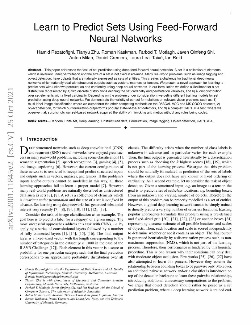
1

Learn to Predict Sets Using Feed-ForwardNeural Networks

Hamid Rezatofighi, Tianyu Zhu, Roman Kaskman, Farbod T. Motlagh, Javen Qinfeng Shi,Anton Milan, Daniel Cremers, Laura Leal-Taixé, Ian Reid

Abstract—This paper addresses the task of set prediction using deep feed-forward neural networks. A set is a collection of elementswhich is invariant under permutation and the size of a set is not fixed in advance. Many real-world problems, such as image tagging andobject detection, have outputs that are naturally expressed as sets of entities. This creates a challenge for traditional deep neuralnetworks which naturally deal with structured outputs such as vectors, matrices or tensors. We present a novel approach for learning topredict sets with unknown permutation and cardinality using deep neural networks. In our formulation we define a likelihood for a setdistribution represented by a) two discrete distributions defining the set cardinally and permutation variables, and b) a joint distributionover set elements with a fixed cardinality. Depending on the problem under consideration, we define different training models for setprediction using deep neural networks. We demonstrate the validity of our set formulations on relevant vision problems such as: 1)multi-label image classification where we outperform the other competing methods on the PASCAL VOC and MS COCO datasets, 2)object detection, for which our formulation outperforms popular state-of-the-art detectors, and 3) a complex CAPTCHA test, where weobserve that, surprisingly, our set-based network acquired the ability of mimicking arithmetics without any rules being coded.

Index Terms—Random Finite set, Deep learning, Unstructured data, Permutation, Image tagging, Object detection, CAPTCHA.

F

1 INTRODUCTION

D EEP structured networks such as deep convolutional (CNN)and recurrent (RNN) neural networks have enjoyed great suc-

cess in many real-world problems, including scene classification [1],semantic segmentation [2], speech recognition [3], gaming [4], [5],and image captioning [6]. However, the current configuration ofthese networks is restricted to accept and predict structured inputsand outputs such as vectors, matrices, and tensors. If the problem’sinputs and/or outputs cannot be modelled in this way, all theselearning approaches fail to learn a proper model [7]. However,many real-world problems are naturally described as unstructureddata such as sets [7], [8]. A set is a collection of elements whichis invariant under permutation and the size of a set is not fixed inadvance. Set learning using deep networks has generated substantialinterest very recently [7], [8], [9], [10], [11], [12], [13].

Consider the task of image classification as an example. Thegoal here is to predict a label (or a category) of a given image. Themost successful approaches address this task with CNNs, i.e. byapplying a series of convolutional layers followed by a numberof fully connected layers [1], [14], [15], [16]. The final outputlayer is a fixed-sized vector with the length corresponding to thenumber of categories in the dataset (e.g. 1000 in the case of theILSVR Challenge [17]). Each element in this vector is a score orprobability for one particular category such that the final predictioncorresponds to an approximate probability distribution over all

• Hamid Rezatofighi is with the Department of Data Science and AI, Facultyof Information Technology, Monash University, Melbourne, Australia.E-mail: hamid.rezatofighi@monash.edu

• Tianyu Zhu is with Department of Electrical and Computer SystemsEngineering, Monash University, Melbourne, Australia.

• Farbod T. Motlagh, Javen Qinfeng Shi, and Ian Reid are with the School ofComputer Science, The university of Adelaide, Australia.

• Anton Milan is with Amazon. This work was done prior to joining Amazon.• Roman Kaskman, Daniel Cremers, and Laura Leal-Taixé, are with Technical

University of Munich, Germany.

classes. The difficulty arises when the number of class labels isunknown in advance and in particular varies for each example.Then, the final output is generated heuristically by a discretizationprocess such as choosing the k highest scores [18], [19], whichis not part of the learning process. We argue that this problemshould be naturally formulated as prediction of the sets of labelswhere the output does not have any known or fixed ordering orcardinality. As a second example, let us consider the task of objectdetection. Given a structured input, e.g. an image as a tensor, thegoal is to predict a set of orderless locations, e.g. bounding boxes,from an unknown and varying number of objects. Therefore, theoutput of this problem can be properly modelled as a set of entities.However, a typical deep learning network cannot be simply trainedto directly predict a varying number of orderless locations. Existingpopular approaches formulate this problem using a pre-definedand fixed-sized grid [20], [21], [22], [23] or anchor boxes [24]representing a coarse estimate of all possible locations and scalesof objects. Then, each location and scale is scored independentlyto determine whether or not it contains an object. The final outputis generated heuristically by a discretization process such as non-maximum suppression (NMS), which is not part of the learningprocess. Therefore, their performance is hindered by this heuristicprocedure. This is one reason why their solutions can only dealwith moderate object occlusion. Few works [25], [26], [27] havealso attempted to learn this process. However they assume therelationship between bounding boxes to be pairwise only. Moreover,an additional pairwise network and/or a classifier is introduced ontop of the detection backbone to learn these pairwise relationships,introducing additional unnecessary computations to the problem.We argue that object detection should rather be posed as a setprediction problem, where a deep learning network is trained end-

arX

iv:2

001.

1184

5v2

[cs

.CV

] 2

5 O

ct 2

021

2

A Feed-Forward Backbone

Encoded Feature

Set cardinality

OutputLayer

Permutation as alatent variable

States, e.g. BBoxParameters

MLP, CNN or Transformer

Outputs

+

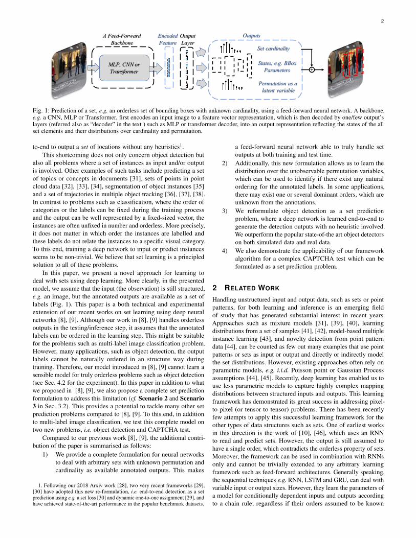
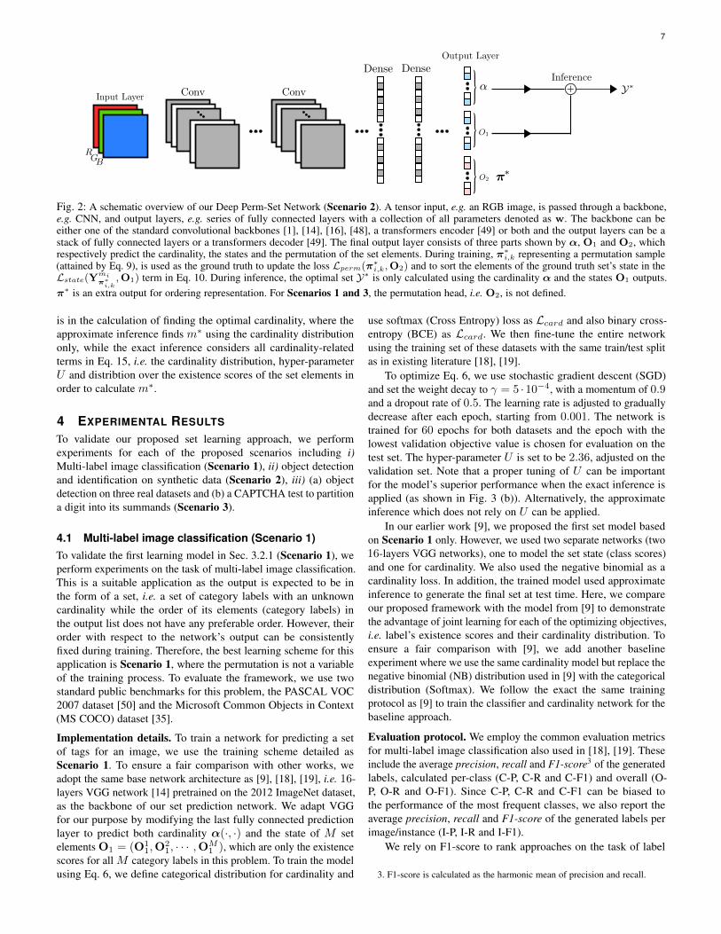
Fig. 1: Prediction of a set, e.g. an orderless set of bounding boxes with unknown cardinality, using a feed-forward neural network. A backbone,e.g. a CNN, MLP or Transformer, first encodes an input image to a feature vector representation, which is then decoded by one/few output’slayers (referred also as “decoder” in the text ) such as MLP or transformer decoder, into an output representation reflecting the states of the allset elements and their distributions over cardinality and permutation.

to-end to output a set of locations without any heuristics1.This shortcoming does not only concern object detection but

also all problems where a set of instances as input and/or outputis involved. Other examples of such tasks include predicting a setof topics or concepts in documents [31], sets of points in pointcloud data [32], [33], [34], segmentation of object instances [35]and a set of trajectories in multiple object tracking [36], [37], [38].In contrast to problems such as classification, where the order ofcategories or the labels can be fixed during the training processand the output can be well represented by a fixed-sized vector, theinstances are often unfixed in number and orderless. More precisely,it does not matter in which order the instances are labelled andthese labels do not relate the instances to a specific visual category.To this end, training a deep network to input or predict instancesseems to be non-trivial. We believe that set learning is a principledsolution to all of these problems.

In this paper, we present a novel approach for learning todeal with sets using deep learning. More clearly, in the presentedmodel, we assume that the input (the observation) is still structured,e.g. an image, but the annotated outputs are available as a set oflabels (Fig. 1). This paper is a both technical and experimentalextension of our recent works on set learning using deep neuralnetworks [8], [9]. Although our work in [8], [9] handles orderlessoutputs in the testing/inference step, it assumes that the annotatedlabels can be ordered in the learning step. This might be suitablefor the problems such as multi-label image classification problem.However, many applications, such as object detection, the outputlabels cannot be naturally ordered in an structure way duringtraining. Therefore, our model introduced in [8], [9] cannot learn asensible model for truly orderless problems such as object detection(see Sec. 4.2 for the experiment). In this paper in addition to whatwe proposed in [8], [9], we also propose a complete set predictionformulation to address this limitation (cf. Scenario 2 and Scenario3 in Sec. 3.2). This provides a potential to tackle many other setprediction problems compared to [8], [9]. To this end, in additionto multi-label image classification, we test this complete model ontwo new problems, i.e. object detection and CAPTCHA test.

Compared to our previous work [8], [9]. the additional contri-bution of the paper is summarised as follows:

1) We provide a complete formulation for neural networksto deal with arbitrary sets with unknown permutation andcardinality as available annotated outputs. This makes

1. Following our 2018 Arxiv work [28], two very recent frameworks [29],[30] have adopted this new re-formulation, i.e. end-to-end detection as a setprediction using e.g. a set loss [30] and dynamic one-to-one assignment [29], andhave achieved state-of-the-art performance in the popular benchmark datasets.

a feed-forward neural network able to truly handle setoutputs at both training and test time.

2) Additionally, this new formulation allows us to learn thedistribution over the unobservable permutation variables,which can be used to identify if there exist any naturalordering for the annotated labels. In some applications,there may exist one or several dominant orders, which areunknown from the annotations.

3) We reformulate object detection as a set predictionproblem, where a deep network is learned end-to-end togenerate the detection outputs with no heuristic involved.We outperform the popular state-of-the art object detectorson both simulated data and real data.

4) We also demonstrate the applicability of our frameworkalgorithm for a complex CAPTCHA test which can beformulated as a set prediction problem.

2 RELATED WORK

Handling unstructured input and output data, such as sets or pointpatterns, for both learning and inference is an emerging fieldof study that has generated substantial interest in recent years.Approaches such as mixture models [31], [39], [40], learningdistributions from a set of samples [41], [42], model-based multipleinstance learning [43], and novelty detection from point patterndata [44], can be counted as few out many examples that use pointpatterns or sets as input or output and directly or indirectly modelthe set distributions. However, existing approaches often rely onparametric models, e.g. i.i.d. Poisson point or Gaussian Processassumptions [44], [45]. Recently, deep learning has enabled us touse less parametric models to capture highly complex mappingdistributions between structured inputs and outputs. This learningframework has demonstrated its great success in addressing pixel-to-pixel (or tensor-to-tensor) problems. There has been recentlyfew attempts to apply this successful learning framework for theother types of data structures such as sets. One of earliest worksin this direction is the work of [10], [46], which uses an RNNto read and predict sets. However, the output is still assumed tohave a single order, which contradicts the orderless property of sets.Moreover, the framework can be used in combination with RNNsonly and cannot be trivially extended to any arbitrary learningframework such as feed-forward architectures. Generally speaking,the sequential techniques e.g. RNN, LSTM and GRU, can deal withvariable input or output sizes. However, they learn the parameters ofa model for conditionally dependent inputs and outputs accordingto a chain rule; regardless if their orders assumed to be known

3

or unknown during the training process [10]. To this end, thesesequential learning techniques may not be an appropriate choicefor encoding and decoding sets (verified also by our experiments).

Alternatively the feed-forward neural networks has beenrecently attempted to be applied for inputting or outputting sets.Most existing approaches on set learning [7], [11], [12] havefocused on the problem of encoding a set with a feed-forwardneural network by using, e.g. a shared network followed by asymmetrical pooling function [7], a permutation invariant poolinglayer [11] or a permutation invariant representation for sets [12].The similar concepts has been independently developed by thecommunity working to encode point clouds using feed-forwardneural networks [32], [33]. However, in all these works, the outputsof neural networks are either assumed to be a tensor or a set withthe same entities of the input set, which prevents this approachto be used for the problems that require output sets with arbitraryentities. In this paper, we are instead interested in learning amodel to output an arbitrary set. Somewhat surprisingly, thereare only few works on learning to predict sets using deep neuralnetworks [8], [9], [13]. The most related work to our problem is ourpreviously proposed framework [8] which seamlessly integratesa deep learning framework into set learning in order to learn tooutput sets. However, the approach only formulates the outputswith unknown cardinality and does not consider the permutationvariables of sets in the learning step. Therefore, its application islimited to the problems with a fixed order output such as imagetagging and diverges when trying to learn unordered output setsas for the object detection problem. In this paper, we incorporatethese permutations as unobservable variables in our formulation,and estimate their distribution during the learning process. Ourunified set prediction framework has the potential to reformulatesome of the existing problems, such as object detection, and totackle a set of new applications, such as a logical CAPTCHA testwhich cannot be trivially solved by the existing architectures.

3 DEEP PERM-SET NETWORK

A set is a collection of elements which is invariant underpermutation and the size of a set is not fixed in advance, i.e.Y = {y1, · · · ,ym} ,m ∈ N∗. A statistical function describing afinite-set variable Y is a combinatorial probability density func-tion p(Y) defined by p(Y) = p(m)Umpm({y1,y2, · · · ,ym}),where p(m) is the cardinality distribution of the set Y andpm({y1,y2, · · · ,ym}) is a symmetric joint probability densitydistribution of the set given known cardinality m. U is the unitof hyper-volume in the feature space, which cancels out theunit of the probability density pm(·) making it unit-less, andthereby avoids the unit mismatch across the different dimensions(cardinalities) [43].

Throughout the paper, we use Y = {y1, · · · ,ym} fora set with unknown cardinality and permutation, Ym ={y1, · · · ,ym}m for a set with known cardinality m but unknownpermutation and Ym

π = (yπ1 , · · · ,yπm) for an ordered set withknown cardinality (or dimension) m and permutation π, whichmeans that the m set elements are ordered under the permutationvector π = (π1, π2, . . . , πm). Note that an ordered set with knowndimension and permutation exactly corresponds to a tensor, e.g. avector or a matrix.

According to the permutation invariant property of the sets,the set Ym with known cardinality m can be expressed by anordered set with any arbitrary permutation, i.e. Ym := {Ym

π |∀π ∈

Π}, where, Π is the space of all feasible permutation Π ={π1,π2, · · · ,πm!} and |Π| = m!. Therefore, the probabilitydensity of a set Y with unknown permutation and cardinalityconditioned on the input x and the model parameters w is definedas

p(Y|x,w)=p(m|x,w)×Um×pm(Ym|x,w),

=p(m|x,w)×Um×∑∀π∈Π

pm(Ymπ ,π|x,w). (1)

The parameter vector w models both the cardinality distribution ofthe set elements p(m|·) as well as the joint state distributionof set elements and their permutation for a fixed cardinalitypm(Ym

π ,π|·).The above formulation represents the probability density of

a set which is very general and completely independent of thechoices of cardinality, state and permutation distributions. It isthus straightforward to transfer it to many applications that requirethe output to be a set. Definition of these distributions for theapplications in this paper will be elaborated later.

3.1 Posterior distributionLet D = {(xi,Yi)} be a training set, where each training samplei = 1, . . . , n is a pair consisting of an input feature (e.g. image),xi ∈ Rl and an output set Yi = {y1,y2, . . . ,ymi},yk ∈Rd,mi ∈ N∗. The aim is now to learn the parameters w toestimate the set distribution in Eq. (1) using the training samples.

To learn the parameters w, we assume that the training samplesare independent from each other and the distribution p(x) fromwhich the input data is sampled is independent from both theoutput and the parameters. Then, the posterior distribution over theparameters can be derived as

p(w|D) ∝ p(D|w)p(w)

∝n∏i=1

[p(mi|xi,w)× Umi ×

∑∀π∈Π

pm(π|xi,w)

× pm(Ymiπ |xi,w,π)

]p(w).

Note that pm(Ymiπ ,π|·) is decomposed according to the chain rule

and p(x) is eliminated as it appears in both the numerator and thedenominator. We also assume that the outputs in the set are derivedfrom an independent and identically distributed (i.i.d.) cluster pointprocess model. Therefore, the full posterior distribution can bewritten as

p(w|D) ∝n∏i=1

[p(mi|xi,w)× Umi×

∑∀π∈Π

(pm(π|xi,w)×

πmi∏σ=π1

p(yσ|xi,w,π))]

p(w).

(2)

We would like to re-emphasize that the assumption here is thatthe annotated labels, Yi, are available as a set of entities, e.g. a setof image tags or bounding boxes, and this means that we might nothave any knowledge if there exist any natural ordering structurein the data. Our proposed solution is capable of inferring thesepotential ordering structures (if they exist at all) in the data bylearning the distribution over the permutations, i.e. pm(π|·, ·). Wecan also assume that pm(π|·, ·) is uniform over all permutations(i.e. the order does not matter) and learn the model accordingly.Moreover, in some applications, e.g. image tagging, we can assume

4

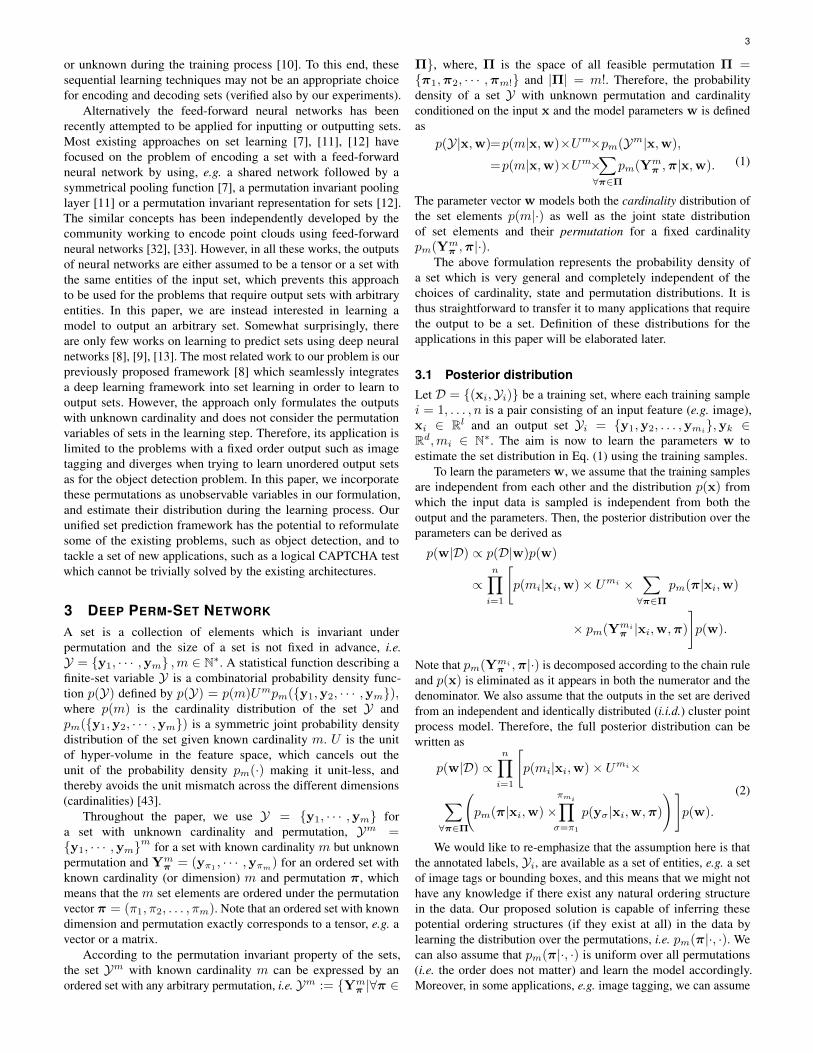
TABLE 1: All mathematical symbols and notations used throughout the paper.Symbol/Notation Definition

m Cardinality variableπ Permutation variable

π or (π1, π2, . . . , πm) Permutation vector for m elementsN∗ Space of all non-negative integer numbers

Π or {π1,π2, · · · ,πm!} Space of all feasible permutations for a vector with cardinality mY or {y1, · · · ,ym} Set with unknown permutation and cardinalityYm or {y1, · · · ,ym}m Set with unknown permutation, but known cardinalityYm

π or (yπ1 , · · · ,yπm ) Set with known permutation and cardinality (or a tensor)x Input data as a tensor (e.g. an RGB image)w Collection of model parameters (e.g. all deep neural network parameters)

D or {(xi,Yi)} Training datasetU Unit of hyper-volume in the feature space

p(m) Distribution over the cardinality variable m (a discrete distribution)pm(·) Joint distribution of m variables (m is known)

that the permutation of the outputs for all the training data for thetraining stage can be consistently fixed. Therefore, in this casethe permutation is not a random variable and will be eliminatedfrom the posterior distribution. The learning process for each ofthese scenarios is slightly different, therefore, in the next sectionwe detail them as Scenarios 1, 2 and 3.

3.2 Learning

For learning the parameters in the aforementioned scenarios, weuse a point estimate for the posterior, i.e. p(w|D) = δ(w =w∗|D), where w∗ is computed using the MAP estimator, i.e.w∗ = argminw − log (p (w|D)). Since w in this paper isassumed to be the parameters of a feed-forward deep neuralnetwork, to estimate w∗, we use commonly used stochasticgradient decent (SGD), where one iteration is performed aswk = wk−1 − η−∂ log(p(wk−1|D))

∂wk−1, where η is the learning rate.

3.2.1 Scenario 1: Permutation can be fixed during training

In some problems, although the output labels represent a set(without any preferred ordering), during training step they canbe consistently ordered in an structure way. For example, in multi-label image classification problem, all possible tags can be orderedin an arbitrary way, e.g. (Person, Dog, Bike,· · · ) or (Dog, Person,Bike, · · · ), but they can be fixed to be the exactly same order forall training instances during training step.

In this scenario, since π is not a random variable in this case,p(yσ|xi,w,π) = p(yσ|xi,w). Therefore the term pm(π|·, ·) ismarginalized out from the posterior distribution

p(w|D) ∝n∏i=1

[p(mi|xi,w)× Umi×

mi∏σ=1

p(yσ|xi,w)×∑∀π∈Π

(pm(π|xi,w))︸ ︷︷ ︸=1

]p(w),

(3)

and it is simplified as

p(w|D) ∝n∏i=1

[p(mi|xi,w)× Umi×

mi∏σ=1

p(yσ|xi,w)

]p(w).

(4)

Therefore, for learning the parameters of a neural network w, wehave

w∗ =argminw− log (p (w|D)) ,

=argminw

n∑i=1

[− log (p(mi|xi,w))︸ ︷︷ ︸

Lcard(·)

−����mi logU︸ ︷︷ ︸removed

+mi∑σ=1

(− log

(p(yσ|xi,w)

)︸ ︷︷ ︸Lstate(·)

)]+ γ‖w‖22,

(5)

w∗ =argminw

n∑i=1

[Lcard (mi,α (xi,w))+

mi∑σ=1

(Lstate(yσ,Oσ

1 (xi,w))

)]+ γ‖w‖22.

(6)

where γ is the regularisation parameter, which is also known as theweight decay parameter and is commonly used in training neuralnetworks. Lcard(·,α(·, ·)) and Lstate(·,Oσ

1 (·, ·)) represent cardi-nality and state losses, respectively, where α(·, ·) and Oσ

1 (·, ·) arerespectively the part of output layer of the neural network, whichpredict the cardinality and the state of each of mi set elements.

Implementation insight: In this scenario, the training proce-dure is simplified to jointly optimize cardinality Lcard(·,α(·, ·))and state Lstate(·,Oσ

1 (·, ·)) losses under a pre-fixed permutationof output labels 2.

The cardinality loss, Lcard(·,α(·, ·)), can be the negative logof any discrete distribution such as Poisson, binomial, negativebinomial, categorical (softmax) or Dirichlet-categorical (cf. [8], [9],[28]). Therefore, α(·, ·) represents the parameters of this discretedistribution, e.g. a single parameter for Poisson orM+1 parameters(i.e. M + 1 event probabilities for set with maximum cardinalityM ) for a categorical distribution. We will compare some of thosecardinality losses for the image tagging problem in Sec. 4.

For the state loss, Lstate(·,Oσ1 (·, ·)), with variable output set

cardinality, we assume that the maximum set cardinality to begenerated is known. This would be a practical assumption for someapplications, e.g. image tagging, where the output set is always asubset of the maximum sized set with all pre-defined M labels,i.e. Y ⊆ {`1, `2, · · · , `M}. Therefore, the output of the networkfor this part would be the collection of the states and existencescore for all M set elements, i.e. O1 = (O1

1,O21, · · · ,OM

1 ). In

2. This is only possible for some applications, where the outputs are categoryor class labels rather than instance labels, e.g. multi-label image classification.

5

image tagging, the state loss, Lstate(·,Oσ1 (·, ·)) can be simply a

loss defined over the predicted existence score for each M labels inan image, e.g. a logistic regression or binary cross entropy (BCE)loss. Remember that, in this scenario, the assignment of the truth(labels in image tagging) to the index of the outputs is known andfixed during training.

3.2.2 Scenario 2: Learning the distribution over the permu-tations

In the problems, where the outputs are set of instances, insteadof a set of categories or classes, similar to the previous scenario,we cannot create a consistent fixed ordering representation for allinstances during training procedure.

In this scenario, we assume that the permutation cannot be fixedat training time. Therefore, the posterior distribution is exactly asdefined in Eq. (2). For learning the parameters and in order tooptimize the negative logarithm of the posterior over the parameters,i.e. − log (p (w|D)), we need to marginalize over all permutationsin every iteration of SGD, which is combinatorial and can becomeintractable even for relatively small-sized problems. To addressthis, we approximate this marginalization with the most significantpermutations (the permutation samples with high probability) foreach training instance from the samples attained in each iterationof SGD, i.e.

pm(π|xi,w) =∑∀π̂i∈Π

ωπ̂i(xi,w)δ[π − π̂i]

≈ 1

Nκ

∑∀π∗

i,k∈Π

ω̃π∗i,k(xi,w)δ[π − π∗i,k],

(7)

where δ[·] is the Kronecker delta and∑∀π̂∈Π ωπ̂(·, ·) = 1. π̂i

is one of the all possible permutations for the training instancei, and π∗i,k is the most significant permutation for the traininginstance i, sampled from pm(π|·, ·)×

∏πmiσ=π1

p(yσ|·, ·,π) duringkth iteration of SGD (using Eq. 9). The weight ω̃π∗

i,k(·, ·) is

proportional to the number of the same permutation samplesπ∗i,k(·, ·), extracted during all SGD iterations for the traininginstance i and Nκ is the total number of SGD iterations. Therefore,∑∀π∗

i,k∈Π ω̃π∗i,k(·, ·)/Nκ = 1. Note that at every iteration, as

the parameter vector w is updated, the best permutation π∗i,k canchange accordingly even for the same instance xi. This allows thenetwork to traverse through the entire space Π and to approximatepm(π|xi,w) by a set of significant permutations. To this end,pm(π|xi,w) is assumed to be point estimates for each iterationof SGD. Therefore,

p(wk|D)∝∼n∏i=1

[p(mi|xi,wk)×Umi×ω̃π∗

i,k(xi,wk)

×πmi∏σ=π1

p(yσ|xi,wk,π∗i,k)

]p(wk).

(8)

In summary, to learn the parameters of the network w, the bestpermutation sample for each instance i in each SGD iteration k,i.e. π∗i,k is attained by solving the following assignment problem,

first:

π∗i,k = arg minπ∈Π− log

(pm(π|·, ·)×

πmi∏σ=π1

p(yσ|·, ·,π))

= arg minπ∈Π

Lperm(π,O2(xi,wk−1)

)+

πmi∑σ=π1

(Lstate

(yσ,O

σ1 (xi,wk−1)

)),

(9)

and then use the sampled permutation π∗i,k to apply standardback-propagation as follows:

wk = wk−1 − η−∂ log (p (wk−1|D))

∂wk−1

= wk−1 − ηn∑i=1

[∂Lcard(mi,α)

∂α.∂α

∂w+

∂Lperm(π∗i,k,O2

)∂O2

.∂O2

∂w+

π∗mi∑

σ=π∗1

∂Lstate(yσ,O

σ1

)∂Oσ

1

.∂Oσ

1

∂w

]+ 2γw,

(10)

where Lcard(·,α(·, ·)), Lperm(·,O2(·, ·)) andLstate(·,Oσ

1 (·, ·)) respectively represent cardinality permutationand state losses, which are defined on the part of output layerof the neural network respectively representing the cardinality,α(·, ·), the permutation, O2(·, ·), and the state of each of mi setelements, Oσ

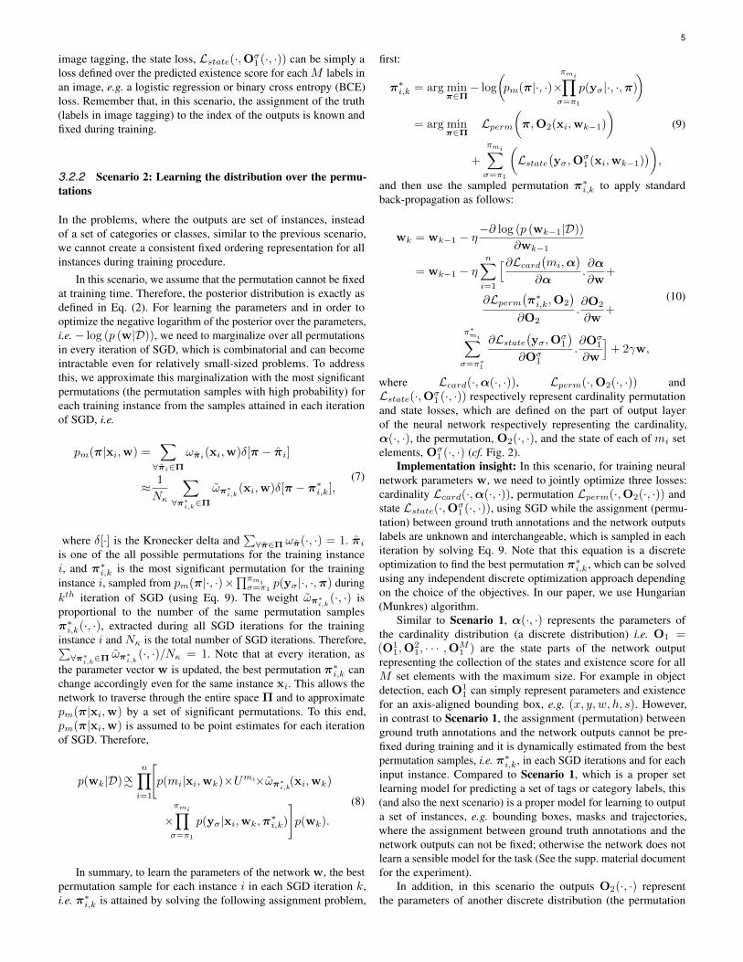
1 (·, ·) (cf. Fig. 2).Implementation insight: In this scenario, for training neural

network parameters w, we need to jointly optimize three losses:cardinality Lcard(·,α(·, ·)), permutation Lperm(·,O2(·, ·)) andstate Lstate(·,Oσ

1 (·, ·)), using SGD while the assignment (permu-tation) between ground truth annotations and the network outputslabels are unknown and interchangeable, which is sampled in eachiteration by solving Eq. 9. Note that this equation is a discreteoptimization to find the best permutation π∗i,k, which can be solvedusing any independent discrete optimization approach dependingon the choice of the objectives. In our paper, we use Hungarian(Munkres) algorithm.

Similar to Scenario 1, α(·, ·) represents the parameters ofthe cardinality distribution (a discrete distribution) i.e. O1 =(O1

1,O21, · · · ,OM

1 ) are the state parts of the network outputrepresenting the collection of the states and existence score for allM set elements with the maximum size. For example in objectdetection, each O1

1 can simply represent parameters and existencefor an axis-aligned bounding box, e.g. (x, y, w, h, s). However,in contrast to Scenario 1, the assignment (permutation) betweenground truth annotations and the network outputs cannot be pre-fixed during training and it is dynamically estimated from the bestpermutation samples, i.e. π∗i,k, in each SGD iterations and for eachinput instance. Compared to Scenario 1, which is a proper setlearning model for predicting a set of tags or category labels, this(and also the next scenario) is a proper model for learning to outputa set of instances, e.g. bounding boxes, masks and trajectories,where the assignment between ground truth annotations and thenetwork outputs can not be fixed; otherwise the network does notlearn a sensible model for the task (See the supp. material documentfor the experiment).

In addition, in this scenario the outputs O2(·, ·) representthe parameters of another discrete distribution (the permutation

6

distribution), where each discrete value in this distribution definesa unique permutation π of M set elements (the biggest set) andits ground truth for each input instance in each SGD iteration isattained from Eq. 9, i.e. π∗i,k. Note that the ground truth annotationsare assumed to be a set, i.e. we do not have any preference abouttheir ordering or we do no have any prior knowledge if thereis indeed any specific ordering structure in the annotations. Bylearning from the sampled permutations during SGD, we can havean extra information about the ordering structure of the annotations,i.e. there exist a single or multiple orders which matter or theproblem is truly orderless.

3.2.3 Scenario 3: Order does not matterThis scenario is a special case of Scenario 2 where the assignment(order) between the truth and the outputs can not be fixed duringtraining step; However in this case, we do not consider learning theordering structure (if exist any) in the annotations. For example, inthe object detection problem, we may consider knowing the state ofset of bounding boxes only, but ignoring how the bounding boxesare assigned (permuted) to the model output during training.

Therefore, in this case the distribution over the permutations,i.e. pm(π|·, ·), can be assumed to be uniform, i.e. a normalizedconstant value for all permutations and all input instances,

pm(π|xi,w) = pm(π) = ω ∀π ∈ Π (11)

In this case, the posterior distribution in each SGD iteration(Eq. 8) is simplified as

p(wk|D)∝∼n∏i=1

[p(mi|xi,wk)×Umi×ω

×πmi∏σ=π1

p(yσ|xi,wk,π∗i,k)

]p(wk),

(12)

where π∗i,k is the best permutation sample for each instance iin each iteration of SGD k, attained by solving the followingassignment problem:

π∗i,k = arg minπ∈Π− log

( πmi∏σ=π1

p(yσ|·, ·,π))

= arg minπ∈Π

πmi∑σ=π1

Lstate(yσ,O

σ1 (xi,wk−1)

) (13)

To learn the parameters w, the sampled permutation π∗i,k is usedfor back-propagation, i.e.

wk = wk−1 − η−∂ log (p (wk−1|D))

∂wk−1

= wk−1 − ηn∑i=1

[∂Lcard(mi,α)

∂α.∂α

∂w+

π∗mi∑

σ=π∗1

∂Lstate(yσ,O

σ1

)∂Oσ

1

.∂Oσ

1

∂w

]+ 2γw.

(14)

Implementation insight: The definition and implementationsdetails for the outputs, i.e. α(·, ·)) and Oσ

1 (·, ·) and their losses,i.e. Lcard(·,α(·, ·)), and Lstate(·,Oσ

1 (·, ·)) are identical to Sce-nario 2. The only difference is that the term Lperm(·,O2(·, ·))disappears from Eqs. 9 and 10.

Closely looking into Eqs. 9, 10, 13 and 14 in both Scenarios2 and 3 and considering Lstate(·, ·) only in these equations, thisloss can be found under different names in the literature, e.g.

Hungarian [46], Earth mover’s and Chamfer [47] loss, where anassignment problem between the output of the network and groundtruth needs be determined before the loss calculation and back-propagation. However, as explained in Eq. 7, these types of thelosses are not actually permutation invariant losses and they areindeed a practical approximation for sampling (the best sample)from the permutation, as latent variable, in each SGD iteration.

3.3 Inference

The inference process for all three scenarios is identical becausethe inference is independent from the definition of the permutationdistribution as shown below.

Having learned the network parameters w∗, for a test inputx+, we use a MAP estimate to generate a set output, i.e. Y∗ =argmin

Y− log

(p(Y|D,x+,w∗)

)Y∗ =argmin

m,Ym− log

(p(m|x+,w∗)

)−m logU−

log∑π∈Π

(pm(π|x+,w∗)×

πm∏σ=π1

p(yσ|x+,w∗,π)

).

Note that in contrast to the learning step, the process how the setelements during the prediction step are sorted and represented,does not affect the output values. Another way to explain this isthat the permutation is defined during training procedure only asit is applied on the ground truth labels for calculating the loss.Therefore, it does not affect the inference process. To this end,the product

∏πmσ=π1

p(yσ|x+,w∗,π) is identical for any possiblepermutation, i.e. ∀π ∈ Π. Therefore, it can be factorized from thesummation, i.e.

log∑π∈Π

(pm(π|x+,w∗)×

πm∏σ=π1

p(yσ|x+,w∗,π))

= log

(m∏σ=1

p(yσ|x+,w∗)×∑π∈Π

pm(π|x+,w∗)︸ ︷︷ ︸=1

)

=m∑σ=1

log(p(yσ|x+,w∗)

).

Therefore, the inference is simplified to

Y∗ = argminm,Ym

− log(p(m|x+,w∗)︸ ︷︷ ︸

α

)−m logU −

m∑σ=1

log(p(yσ|x+,w∗)︸ ︷︷ ︸

Oσ1

).

(15)

Implementation insight: Solving Eq. 15 corresponds tofinding the optimal set Y∗ = (m∗,Ym∗

), which is the exactsolution of the problem. As shown in [8], this problem can beoptimally and efficiently calculated using few simple operations,e.g. sorting, max and summation operations. Note that the unit ofhyper-volume U is assumed as a constant hyper-parameter, tunedfrom the validation set of the data such that the best performanceon this set is ensured.

An alternative to evaluate the models is an approximatedinference [9], where the set cardinality is first approximatedusing m∗ = argminm − log

(p(m|x+,w∗)

)and then all M

set elements are sorted according to their existence scores and thestate of top m∗ set elements are shown as the final output. Themain key difference between the exact and approximate inferences

7

{

{{

Fig. 2: A schematic overview of our Deep Perm-Set Network (Scenario 2). A tensor input, e.g. an RGB image, is passed through a backbone,e.g. CNN, and output layers, e.g. series of fully connected layers with a collection of all parameters denoted as w. The backbone can beeither one of the standard convolutional backbones [1], [14], [16], [48], a transformers encoder [49] or both and the output layers can be astack of fully connected layers or a transformers decoder [49]. The final output layer consists of three parts shown by α, O1 and O2, whichrespectively predict the cardinality, the states and the permutation of the set elements. During training, π∗

i,k representing a permutation sample(attained by Eq. 9), is used as the ground truth to update the loss Lperm(π∗

i,k,O2) and to sort the elements of the ground truth set’s state in theLstate(Ymi

π∗i,k

,O1) term in Eq. 10. During inference, the optimal set Y∗ is only calculated using the cardinality α and the states O1 outputs.π∗ is an extra output for ordering representation. For Scenarios 1 and 3, the permutation head, i.e. O2, is not defined.

is in the calculation of finding the optimal cardinality, where theapproximate inference finds m∗ using the cardinality distributiononly, while the exact inference considers all cardinality-relatedterms in Eq. 15, i.e. the cardinality distribution, hyper-parameterU and distribtion over the existence scores of the set elements inorder to calculate m∗.

4 EXPERIMENTAL RESULTS

To validate our proposed set learning approach, we performexperiments for each of the proposed scenarios including i)Multi-label image classification (Scenario 1), ii) object detectionand identification on synthetic data (Scenario 2), iii) (a) objectdetection on three real datasets and (b) a CAPTCHA test to partitiona digit into its summands (Scenario 3).

4.1 Multi-label image classification (Scenario 1)To validate the first learning model in Sec. 3.2.1 (Scenario 1), weperform experiments on the task of multi-label image classification.This is a suitable application as the output is expected to be inthe form of a set, i.e. a set of category labels with an unknowncardinality while the order of its elements (category labels) inthe output list does not have any preferable order. However, theirorder with respect to the network’s output can be consistentlyfixed during training. Therefore, the best learning scheme for thisapplication is Scenario 1, where the permutation is not a variableof the training process. To evaluate the framework, we use twostandard public benchmarks for this problem, the PASCAL VOC2007 dataset [50] and the Microsoft Common Objects in Context(MS COCO) dataset [35].

Implementation details. To train a network for predicting a setof tags for an image, we use the training scheme detailed asScenario 1. To ensure a fair comparison with other works, weadopt the same base network architecture as [9], [18], [19], i.e. 16-layers VGG network [14] pretrained on the 2012 ImageNet dataset,as the backbone of our set prediction network. We adapt VGGfor our purpose by modifying the last fully connected predictionlayer to predict both cardinality α(·, ·) and the state of M setelements O1 = (O1

1,O21, · · · ,OM

1 ), which are only the existencescores for all M category labels in this problem. To train the modelusing Eq. 6, we define categorical distribution for cardinality and

use softmax (Cross Entropy) loss as Lcard and also binary cross-entropy (BCE) as Lcard. We then fine-tune the entire networkusing the training set of these datasets with the same train/test splitas in existing literature [18], [19].

To optimize Eq. 6, we use stochastic gradient descent (SGD)and set the weight decay to γ = 5 ·10−4, with a momentum of 0.9and a dropout rate of 0.5. The learning rate is adjusted to graduallydecrease after each epoch, starting from 0.001. The network istrained for 60 epochs for both datasets and the epoch with thelowest validation objective value is chosen for evaluation on thetest set. The hyper-parameter U is set to be 2.36, adjusted on thevalidation set. Note that a proper tuning of U can be importantfor the model’s superior performance when the exact inference isapplied (as shown in Fig. 3 (b)). Alternatively, the approximateinference which does not rely on U can be applied.

In our earlier work [9], we proposed the first set model basedon Scenario 1 only. However, we used two separate networks (two16-layers VGG networks), one to model the set state (class scores)and one for cardinality. We also used the negative binomial as acardinality loss. In addition, the trained model used approximateinference to generate the final set at test time. Here, we compareour proposed framework with the model from [9] to demonstratethe advantage of joint learning for each of the optimizing objectives,i.e. label’s existence scores and their cardinality distribution. Toensure a fair comparison with [9], we add another baselineexperiment where we use the same cardinality model but replace thenegative binomial (NB) distribution used in [9] with the categoricaldistribution (Softmax). We follow the exact the same trainingprotocol as [9] to train the classifier and cardinality network for thebaseline approach.

Evaluation protocol. We employ the common evaluation metricsfor multi-label image classification also used in [18], [19]. Theseinclude the average precision, recall and F1-score3 of the generatedlabels, calculated per-class (C-P, C-R and C-F1) and overall (O-P, O-R and O-F1). Since C-P, C-R and C-F1 can be biased tothe performance of the most frequent classes, we also report theaverage precision, recall and F1-score of the generated labels perimage/instance (I-P, I-R and I-F1).

We rely on F1-score to rank approaches on the task of label

3. F1-score is calculated as the harmonic mean of precision and recall.

8

0 0.2 0.4 0.6 0.8 1Recall

0

0.2

0.4

0.6

0.8

1P

reci

sion

BCEBCE ( k=m[GT])Joint BCEJoint BCE ( k=m[GT])GT Prediction

(a)

100 101 102 103

U

0.4

0.5

0.6

0.7

0.8

F1

(b)

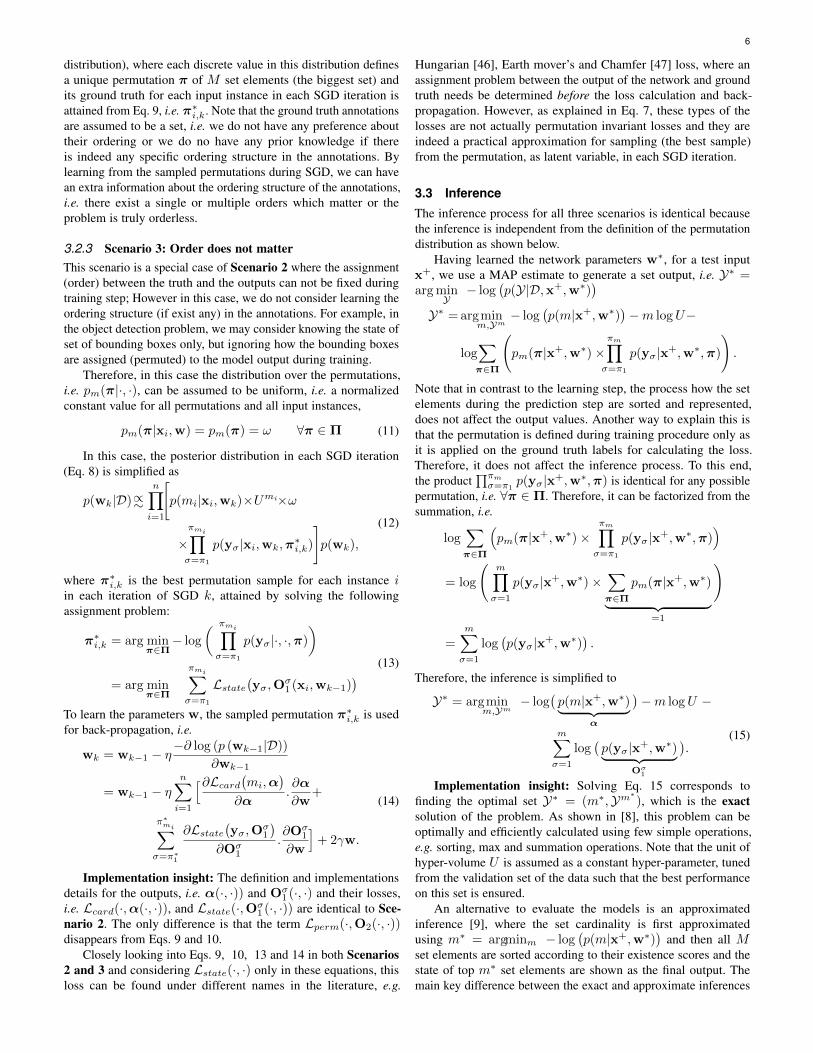
Fig. 3: (a) Precision/recall curves for the classification scores whenthe classifier is trained independently (red solid line) and when itis trained jointly with the cardinality term using our proposed jointapproach (black solid line) on PASCAL VOC dataset. The circlesrepresent the upper bound when ground truth cardinality is used forthe evaluation of the corresponding classifiers. The ground truthprediction is shown by a blue triangle. (b) The value of F1 againstthe value of hyper-parameter U in log-scale (PASCAL VOC).

prediction. A method with better performance has a precision/recallvalue that has a closer proximity to the perfect point shown by theblue triangle in Fig. 3. To this end, for the classifiers such as BCEand Softmax, we find the optimal evaluation parameter k = k∗

that maximises the F1-score. For the set network model in [9] (DS)and our proposed framework with joint backbone network (JDS),prediction/recall is not dependent on the value of k. Rather, onesingle value for precision, recall and F1-score is computed.

PASCAL VOC 2007.

We first test our approach on the Pascal Visual Object Classesbenchmark [50], which is one of the most widely used datasetsfor detection and classification. This dataset includes 9963 imageswith a 50/50 split for training and test, where objects from 20pre-defined categories have been annotated by bounding boxes.Each image contains between 1 and 7 unique objects.

We first investigate if the learning using the shared backbone(joint learning) improves the performance of cardinality andclassifier. Fig. 3 (a) shows the precision/recall curves for theclassification scores when the classifier is trained solely usingbinary cross-entropy (BCE) loss (red solid line) and when itis trained using the same loss jointly with the cardinality term(Joint BCE). We also evaluate the precision/recall values when theground truth cardinality m[GT ] is provided. The results confirmour claim that the joint learning indeed improves the classificationperformance. We also calculate the mean absolute error of thecardinality estimation when the cardinality term using the DCloss is learned jointly and independently as in [9]. The meanabsolute cardinality error of our prediction on PASCAL VOC is0.31± 0.54, while this error is 0.33± 0.53 when the cardinalityis learned independently.

We compare the performance of our proposed set network, i.e.JDS (BCE-DC), with traditional learning approaches trained usingclassification losses only, i.e. softmax and BCE losses, while duringthe inference, the labels with the best k value are extracted as themodel’s output labels.

For the set based approaches, we included our model in [9]when the classifier is binary cross entropy and the cardinality lossis negative binomial, i.e. DS (BCE-NB). In addition, Table 2 (a)reports the results for the deep set network when the cardinalityloss is replaced by a categorical loss, i.e. (BCE-SftMx). The results

show that we outperform the other approaches w.r.t. all three typesof F1-scores. In addition, our joint formulation allows for a singletraining step to obtain the final model, while our model in [9]learns two VGG networks to generate the output sets.

Microsoft COCO.The MS-COCO [35] benchmark is another popular benchmark

for image captioning, recognition, and segmentation. The datasetincludes 123K images and over 500k annotated object instancesfrom 80 categories. The number of unique objects for each imagevaries between 0 and 18. Around 700 images in the training set donot contain any of the 80 classes and there are only a handful ofimages that have more than 10 tags. Most images contain betweenone and three labels. We use 83K images with identical training-validation split as [9], and the remaining 40K images as test data.

The classification results on this dataset are reported in Tab. 2(b). The results once again show that our approach consistentlyoutperforms our traditional and set based baselines measuredby F1-score. Our approach also outperform a recurrent basedapproach [19], which uses VGG-16 as the backbone along with arecurrent neural network to generate a set of labels. Due to thisimprovement, we achieve state-of-the-art results on this dataset aswell. Some examples of label prediction using our proposed setnetwork model and comparison with other deep set networks areshown in Fig. 4.

4.2 Object detection (Scenario 2 & 3)Our second experiment is used to test our set formulation forthe task of object detection using the model trained according toScenario 3 on three real detection dataset, including (i) a processedand cropped pedestrian dataset from MOTChallenge [51], [52], (ii)PASCAL VOC 2007 [50], and (iii) MS COCO [35]. We also assessour set formulation for the task of object detection using the modeltrained according to Scenario 2 on synthetically generated datasetin order to demonstrate the advantage and the limitation of thisscenario. This experiment and all the details can be found in thesupplementary material document.

Formulation, training losses and inference details. Weformulate object detection as a set prediction problem Y ={y1, · · · ,ym}, where each set element represents a boundingbox as y = (x, y, w, h, `) ∈ R4 × L, where (x, y) and (w, h)are respectively the bounding boxes’ position and size and ` ∈ Lrepresents the class label for this set element.

We train a feed-forward neural network including a backboneand few decoder layers using Scenario 3 with loss heads directlyattached to the final output layer. According to Eqs. (13, 14), thereare two main terms (losses) that need to be defined for this task.Firstly, for cardinality Lcard(·), a categorical loss (Softmax) is usedas the discrete distribution model. Secondly, the state loss Lstate(·)consists of two parts in this problem: i) the bounding box regressionloss between the predicted output states and the permuted groundtruth states, ii) the classification loss for `. For the bounding boxregression, we use two options: 1) Smooth L1-loss only and 2)Smooth L1-loss along with the Generalized Intersection over Union(GIoU) [53] loss. The cross-entropy loss is also used for the classlabel `. The permutation is estimated iteratively using alternationaccording to Eq. (13) using Hungarian (Munkres) algorithm.

For the pedestrian detection as a single class object detectionproblem, we use the exact inference, explained in Sec. 3.3. However,since the extension of this exact inference for multi-class objectdetection is not trivial, we apply the approximated inference

9

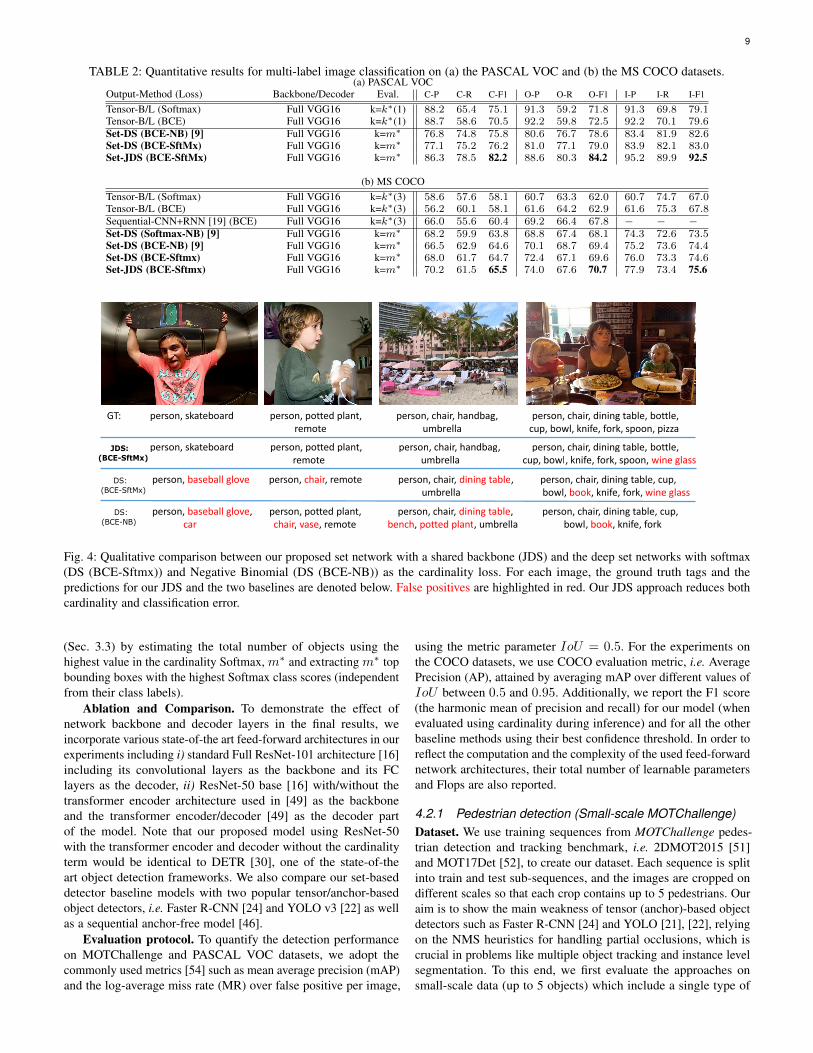
TABLE 2: Quantitative results for multi-label image classification on (a) the PASCAL VOC and (b) the MS COCO datasets.(a) PASCAL VOC

Output-Method (Loss) Backbone/Decoder Eval. C-P C-R C-F1 O-P O-R O-F1 I-P I-R I-F1

Tensor-B/L (Softmax) Full VGG16 k=k∗(1) 88.2 65.4 75.1 91.3 59.2 71.8 91.3 69.8 79.1Tensor-B/L (BCE) Full VGG16 k=k∗(1) 88.7 58.6 70.5 92.2 59.8 72.5 92.2 70.1 79.6Set-DS (BCE-NB) [9] Full VGG16 k=m∗ 76.8 74.8 75.8 80.6 76.7 78.6 83.4 81.9 82.6Set-DS (BCE-SftMx) Full VGG16 k=m∗ 77.1 75.2 76.2 81.0 77.1 79.0 83.9 82.1 83.0Set-JDS (BCE-SftMx) Full VGG16 k=m∗ 86.3 78.5 82.2 88.6 80.3 84.2 95.2 89.9 92.5

(b) MS COCOTensor-B/L (Softmax) Full VGG16 k=k∗(3) 58.6 57.6 58.1 60.7 63.3 62.0 60.7 74.7 67.0Tensor-B/L (BCE) Full VGG16 k=k∗(3) 56.2 60.1 58.1 61.6 64.2 62.9 61.6 75.3 67.8Sequential-CNN+RNN [19] (BCE) Full VGG16 k=k∗(3) 66.0 55.6 60.4 69.2 66.4 67.8 − − −Set-DS (Softmax-NB) [9] Full VGG16 k=m∗ 68.2 59.9 63.8 68.8 67.4 68.1 74.3 72.6 73.5Set-DS (BCE-NB) [9] Full VGG16 k=m∗ 66.5 62.9 64.6 70.1 68.7 69.4 75.2 73.6 74.4Set-DS (BCE-Sftmx) Full VGG16 k=m∗ 68.0 61.7 64.7 72.4 67.1 69.6 76.0 73.3 74.6Set-JDS (BCE-Sftmx) Full VGG16 k=m∗ 70.2 61.5 65.5 74.0 67.6 70.7 77.9 73.4 75.6

GT: person, skateboard person, potted plant, person, chair, handbag, person, chair, dining table, bottle,remote umbrella cup, bowl, knife, fork, spoon, pizza

person, skateboard person, potted plant, person, chair, handbag, person, chair, dining table, bottle,remote umbrella cup, bowl, knife, fork, spoon, wine glass

person,

Cbaseball glove person, chair, remote person, chair, dining table, person, chair, dining table, cup,

umbrella bowl, book, knife, fork, wine glass

person, baseball glove, person, potted plant, person, chair, dining table, person, chair, dining table, cup, car chair, vase, remote bench, potted plant, umbrella bowl, book, knife, fork

DS: (BCE-SftMx)

DS: (BCE-NB)

JDS: (BCE-SftMx)

Fig. 4: Qualitative comparison between our proposed set network with a shared backbone (JDS) and the deep set networks with softmax(DS (BCE-Sftmx)) and Negative Binomial (DS (BCE-NB)) as the cardinality loss. For each image, the ground truth tags and thepredictions for our JDS and the two baselines are denoted below. False positives are highlighted in red. Our JDS approach reduces bothcardinality and classification error.

(Sec. 3.3) by estimating the total number of objects using thehighest value in the cardinality Softmax, m∗ and extracting m∗ topbounding boxes with the highest Softmax class scores (independentfrom their class labels).

Ablation and Comparison. To demonstrate the effect ofnetwork backbone and decoder layers in the final results, weincorporate various state-of-the art feed-forward architectures in ourexperiments including i) standard Full ResNet-101 architecture [16]including its convolutional layers as the backbone and its FClayers as the decoder, ii) ResNet-50 base [16] with/without thetransformer encoder architecture used in [49] as the backboneand the transformer encoder/decoder [49] as the decoder partof the model. Note that our proposed model using ResNet-50with the transformer encoder and decoder without the cardinalityterm would be identical to DETR [30], one of the state-of-theart object detection frameworks. We also compare our set-baseddetector baseline models with two popular tensor/anchor-basedobject detectors, i.e. Faster R-CNN [24] and YOLO v3 [22] as wellas a sequential anchor-free model [46].

Evaluation protocol. To quantify the detection performanceon MOTChallenge and PASCAL VOC datasets, we adopt thecommonly used metrics [54] such as mean average precision (mAP)and the log-average miss rate (MR) over false positive per image,

using the metric parameter IoU = 0.5. For the experiments onthe COCO datasets, we use COCO evaluation metric, i.e. AveragePrecision (AP), attained by averaging mAP over different values ofIoU between 0.5 and 0.95. Additionally, we report the F1 score(the harmonic mean of precision and recall) for our model (whenevaluated using cardinality during inference) and for all the otherbaseline methods using their best confidence threshold. In order toreflect the computation and the complexity of the used feed-forwardnetwork architectures, their total number of learnable parametersand Flops are also reported.

4.2.1 Pedestrian detection (Small-scale MOTChallenge)Dataset. We use training sequences from MOTChallenge pedes-trian detection and tracking benchmark, i.e. 2DMOT2015 [51]and MOT17Det [52], to create our dataset. Each sequence is splitinto train and test sub-sequences, and the images are cropped ondifferent scales so that each crop contains up to 5 pedestrians. Ouraim is to show the main weakness of tensor (anchor)-based objectdetectors such as Faster R-CNN [24] and YOLO [21], [22], relyingon the NMS heuristics for handling partial occlusions, which iscrucial in problems like multiple object tracking and instance levelsegmentation. To this end, we first evaluate the approaches onsmall-scale data (up to 5 objects) which include a single type of

10

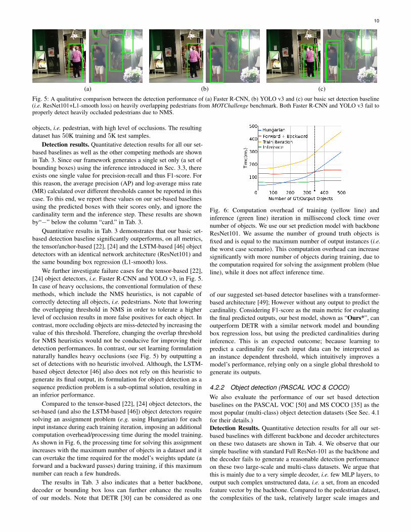
(a) (b) (c)

Fig. 5: A qualitative comparison between the detection performance of (a) Faster R-CNN, (b) YOLO v3 and (c) our basic set detection baseline(i.e. ResNet101+L1-smooth loss) on heavily overlapping pedestrians from MOTChallenge benchmark. Both Faster R-CNN and YOLO v3 fail toproperly detect heavily occluded pedestrians due to NMS.

objects, i.e. pedestrian, with high level of occlusions. The resultingdataset has 50K training and 5K test samples.

Detection results. Quantitative detection results for all our set-based baselines as well as the other competing methods are shownin Tab. 3. Since our framework generates a single set only (a set ofbounding boxes) using the inference introduced in Sec. 3.3, thereexists one single value for precision-recall and thus F1-score. Forthis reason, the average precision (AP) and log-average miss rate(MR) calculated over different thresholds cannot be reported in thiscase. To this end, we report these values on our set-based baselinesusing the predicted boxes with their scores only, and ignore thecardinality term and the inference step. These results are shownby“−” below the column “card.” in Tab. 3.

Quantitative results in Tab. 3 demonstrates that our basic set-based detection baseline significantly outperforms, on all metrics,the tensor/anchor-based [22], [24] and the LSTM-based [46] objectdetectors with an identical network architecture (ResNet101) andthe same bounding box regression (L1-smooth) loss.

We further investigate failure cases for the tensor-based [22],[24] object detectors, i.e. Faster R-CNN and YOLO v3, in Fig. 5.In case of heavy occlusions, the conventional formulation of thesemethods, which include the NMS heuristics, is not capable ofcorrectly detecting all objects, i.e. pedestrians. Note that loweringthe overlapping threshold in NMS in order to tolerate a higherlevel of occlusion results in more false positives for each object. Incontrast, more occluding objects are miss-detected by increasing thevalue of this threshold. Therefore, changing the overlap thresholdfor NMS heuristics would not be conducive for improving theirdetection performances. In contrast, our set learning formulationnaturally handles heavy occlusions (see Fig. 5) by outputting aset of detections with no heuristic involved. Although, the LSTM-based object detector [46] also does not rely on this heuristic togenerate its final output, its formulation for object detection as asequence prediction problem is a sub-optimal solution, resulting inan inferior performance.

Compared to the tensor-based [22], [24] object detectors, theset-based (and also the LSTM-based [46]) object detectors requiresolving an assignment problem (e.g. using Hungarian) for eachinput instance during each training iteration, imposing an additionalcomputation overhead/processing time during the model training.As shown in Fig. 6, the processing time for solving this assignmentincreases with the maximum number of objects in a dataset and itcan overtake the time required for the model’s weights update (aforward and a backward passes) during training, if this maximumnumber can reach a few hundreds.

The results in Tab. 3 also indicates that a better backbone,decoder or bounding box loss can further enhance the resultsof our models. Note that DETR [30] can be considered as one

Fig. 6: Computation overhead of training (yellow line) andinference (green line) iteration in millisecond clock time overnumber of objects. We use our set prediction model with backboneResNet101. We assume the number of ground truth objects isfixed and is equal to the maximum number of output instances (i.e.the worst case scenario). This computation overhead can increasesignificantly with more number of objects during training, due tothe computation required for solving the assignment problem (blueline), while it does not affect inference time.

of our suggested set-based detector baselines with a transformer-based architecture [49]; However without any output to predict thecardinality. Considering F1-score as the main metric for evaluatingthe final predicted outputs, our best model, shown as “Ours*”, canoutperform DETR with a similar network model and boundingbox regression loss, but using the predicted cardinalities duringinference. This is an expected outcome; because learning topredict a cardinality for each input data can be interpreted asan instance dependent threshold, which intuitively improves amodel’s performance, relying only on a single global threshold togenerate its outputs.

4.2.2 Object detection (PASCAL VOC & COCO)We also evaluate the performance of our set based detectionbaselines on the PASCAL VOC [50] and MS COCO [35] as themost popular (multi-class) object detection datasets (See Sec. 4.1for their details.)Detection Results. Quantitative detection results for all our set-based baselines with different backbone and decoder architectureson these two datasets are shown in Tab. 4. We observe that oursimple baseline with standard Full ResNet-101 as the backbone andthe decoder fails to generate a reasonable detection performanceon these two large-scale and multi-class datasets. We argue thatthis is mainly due to a very simple decoder, i.e. few MLP layers, tooutput such complex unstructured data, i.e. a set, from an encodedfeature vector by the backbone. Compared to the pedestrian dataset,the complexities of the task, relatively larger scale images and

11

TABLE 3: Detection results on the pedestrian detection dataset (Cropped MOTChallenge) measured by mAP, F1 score and MR rate. Theabbreviations“BB", “Card.”, “Hun.”, “Trans.”, “En.”, and “Dec.” mean “bounding box”, “Cardinality”, “Hungarian Algorithm”, “Transformer”,“Encoder” and “Decoder”, respectively.

Output (Method) Backbone/Decoder BB loss Card. mAP ↑ F1↑ MR ↓ Parameters Flops

Tensor (Faster R-CNN [24]) Full ResNet101 L1 7 0.68 0.76 0.48 42M 23.2GTensor (YOLO v3 [22]) Full ResNet101 L1 7 0.70 0.76 0.48 59M 24.4GSequential (LSTM-Hun. [46]) ResNet101/LSTM L1 7 0.61 0.62 0.59 47.3M 15.7GSet (Ours) Full ResNet101 L1 − 0.85 0.86 0.25 46.8M 15.7GSet (Ours) Full ResNet101 L1+GIoU − 0.85 0.86 0.24 46.8M 15.7GSet (Ours) Full ResNet101 L1+GIoU X − 0.86 − 46.8M 15.7GSet (DETR [30]) ResNet50+Trans. En/Trans. Dec. L1+GIoU − 0.87 0.86 0.17 41M 11.1GSet (Ours*) ResNet50+Trans. En./Trans. Dec. L1+GIoU X − 0.87 − 41M 11.1G

TABLE 4: Detection results for the set-based baselines using different backbones and decoders on (a) Pascal VOC and (b) MS COCO measuredby mAP, the best F1 scores and MR. All these baselines use L1+GIoU as their bounding box regression loss. The abbreviations “Card.”, “Trans.”,“En.”, and “Dec.” mean “Cardinality”,“Transformer”, “Encoder” and “Decoder”, respectively.

(a) PASCAL VOC

Backbone/Decoder Card. mAP ↑ F1↑ MR ↓ Parameters Flops

ResNet50/Trans. En. − 0.62 0.43 0.52 32M 47.8GResNet50/Trans. Dec. − 0.64 0.56 0.47 33M 45.7GResNet50+Trans. En./Trans. Dec. [30] − 0.70 0.71 0.42 41M 49.4GResNet50+Trans. En./Trans. Dec. X − 0.72 − 41M 49.5G

(b) MS COCO

Card. AP ↑ F1↑ Parameters Flops

− 0.29 0.45 32M 83.9G− 0.37 − 33M 75.9G− 0.42 0.61 41M 85.8GX − 0.64 41M 86.0G

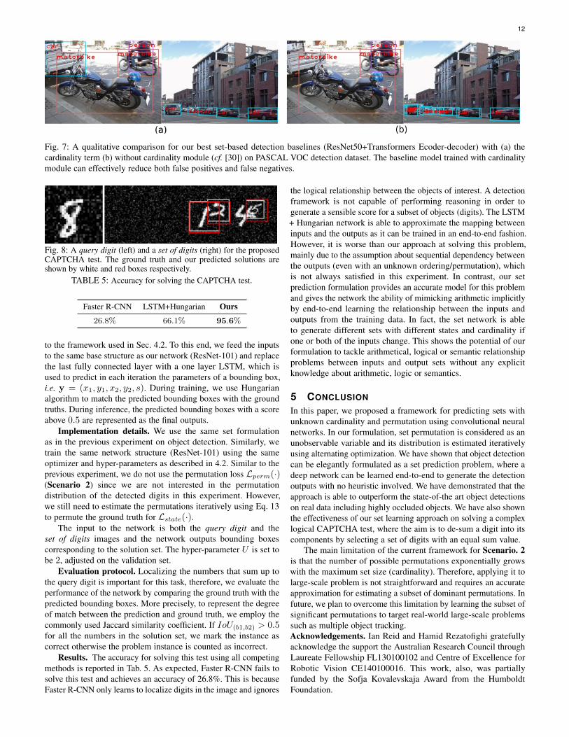
considerably higher number of instances challenge this very simpleMLP decoders for this task. To address this, we replace theseMLP layers by two new, but more reliable, output layer decoders,i.e. transformer encoder or decoder architecture [49]. Resultsin Tab. 4 verify that even with a smaller backbone model, e.g.the convolutional layers of ResNet-50, in combination with atransformer encoder [49] or decoder [49], our model can generatea performance comparable to the state-of-the-art object detectors inthese two datasets. The performance gap between these baselineswith different backbones and decoders in MS COCO (as morechallenging dataset) is more significant. This reflects the importanceof a proper choice of the backbone and the decoder in these set-based detection models in challenging and large-scale datasets.Comparing with many existing tensor/anchor-based detectionalgorithms, DETR as a set-based detector is currently one ofthe best performing detectors in these two datasets with respectto mAP and AP metrics. However, our results in Tab. 4 (last tworows) indicate that our full model with the cardinality module canimprove the performance our DETR baseline with respect to F1score. Fig. 7 represents few detection examples comparing DETRmodel detection output using the best threshold against our modelusing the cardinality value during the inference.

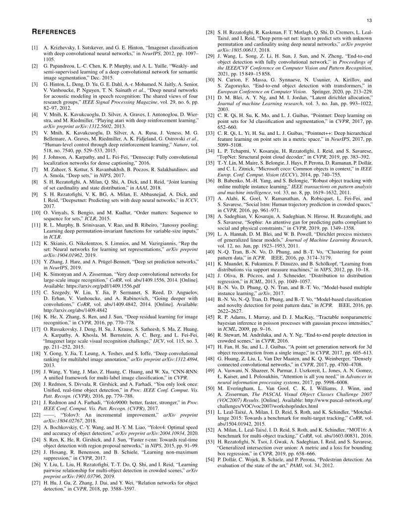
4.3 CAPTCHA test for de-summing a digit (Scenario 3)We also evaluate our set formulation on a CAPTCHA test wherethe aim is to determine whether a user is a human or not by amoderately complex logical test. In this test, the user is asked todecompose a query digit shown as an image (Fig. 8 (left)) into aset of digits by clicking on a subset of numbers in a noisy image(Fig. 8 (right)) such that the summation of the selected numbers isequal to the query digit.

In this puzzle, it is assumed there exists only one valid solution(including an empty response). We target this complex puzzle withour set learning approach. What is assumed to be available as thetraining data is a set of spotted locations in the set of digits imageand no further information about the represented values of query

digit and the set of digits is provided. In practice, the annotation canbe acquired from the users’ click when the test is successful. In ourcase, we generate a dataset for this test from the real handwritingMNIST dataset.

Data generation. The dataset is generated using the MNISTdataset of handwritten digits. The query digit is generated byrandomly selecting one of the digits from MNIST dataset. Givena query digit, we create a series of random digits with differentlength such that there exists a subset of these digits that sums up tothe query digit. Note that in each instance there is only one solution(including empty) to the puzzle. We place the chosen digits in arandom position on a 300×75 blank image with different rotationsand sizes. To make the problem more challenging, random whitenoise is added to both the query digit and the set of digits images(Fig. 8). The produced dataset includes 100K problem instances fortraining and 10K images for evaluation, generated independentlyfrom MNIST training and test sets.

Baseline methods. Considering the fact that only a set oflocations is provided as ground truth, this problem can be seenas an analogy to the object detection problem. However, the keydifference between this logical test and the object detection problemis that the objects of interest (the selected numbers) change as thequery digit changes. For example, in Fig. 8, if the query digitchanges to another number, e.g. 4, the number {4} should be onlychosen. Thus, for the same set of digits, now {1, 2, 5} would belabeled as background. Since any number can be either backgroundor foreground conditioned on the query digit, this problem cannotbe trivially formulated as an object detection task. To prove thisclaim, as a baseline, we attempt to solve the CAPTCHA problemusing a detector, e.g. Faster R-CNN, with the same base structureas our network (ResNet-101) and trained on the exactly same dataincluding the query digit and the set of digits images4.

As an additional baseline, we also present a solution to this setproblem using the LSTM-based detection model [10], [46], similar

4. To ensure inputting one single image into the ResNet-101 backbone, werepresent both the query digit and set of digits by a single image such that thequery digit always appears in the bottom left corner of the set of digits image.

12

Fig. 7: A qualitative comparison for our best set-based detection baselines (ResNet50+Transformers Ecoder-decoder) with (a) thecardinality term (b) without cardinality module (cf. [30]) on PASCAL VOC detection dataset. The baseline model trained with cardinalitymodule can effectively reduce both false positives and false negatives.

Fig. 8: A query digit (left) and a set of digits (right) for the proposedCAPTCHA test. The ground truth and our predicted solutions areshown by white and red boxes respectively.

TABLE 5: Accuracy for solving the CAPTCHA test.

Faster R-CNN LSTM+Hungarian Ours

26.8% 66.1% 95.6%

to the framework used in Sec. 4.2. To this end, we feed the inputsto the same base structure as our network (ResNet-101) and replacethe last fully connected layer with a one layer LSTM, which isused to predict in each iteration the parameters of a bounding box,i.e. y = (x1, y1, x2, y2, s). During training, we use Hungarianalgorithm to match the predicted bounding boxes with the groundtruths. During inference, the predicted bounding boxes with a scoreabove 0.5 are represented as the final outputs.

Implementation details. We use the same set formulationas in the previous experiment on object detection. Similarly, wetrain the same network structure (ResNet-101) using the sameoptimizer and hyper-parameters as described in 4.2. Similar to theprevious experiment, we do not use the permutation loss Lperm(·)(Scenario 2) since we are not interested in the permutationdistribution of the detected digits in this experiment. However,we still need to estimate the permutations iteratively using Eq. 13to permute the ground truth for Lstate(·).

The input to the network is both the query digit and theset of digits images and the network outputs bounding boxescorresponding to the solution set. The hyper-parameter U is set tobe 2, adjusted on the validation set.

Evaluation protocol. Localizing the numbers that sum up tothe query digit is important for this task, therefore, we evaluate theperformance of the network by comparing the ground truth with thepredicted bounding boxes. More precisely, to represent the degreeof match between the prediction and ground truth, we employ thecommonly used Jaccard similarity coefficient. If IoU(b1,b2) > 0.5for all the numbers in the solution set, we mark the instance ascorrect otherwise the problem instance is counted as incorrect.

Results. The accuracy for solving this test using all competingmethods is reported in Tab. 5. As expected, Faster R-CNN fails tosolve this test and achieves an accuracy of 26.8%. This is becauseFaster R-CNN only learns to localize digits in the image and ignores

the logical relationship between the objects of interest. A detectionframework is not capable of performing reasoning in order togenerate a sensible score for a subset of objects (digits). The LSTM+ Hungarian network is able to approximate the mapping betweeninputs and the outputs as it can be trained in an end-to-end fashion.However, it is worse than our approach at solving this problem,mainly due to the assumption about sequential dependency betweenthe outputs (even with an unknown ordering/permutation), whichis not always satisfied in this experiment. In contrast, our setprediction formulation provides an accurate model for this problemand gives the network the ability of mimicking arithmetic implicitlyby end-to-end learning the relationship between the inputs andoutputs from the training data. In fact, the set network is ableto generate different sets with different states and cardinality ifone or both of the inputs change. This shows the potential of ourformulation to tackle arithmetical, logical or semantic relationshipproblems between inputs and output sets without any explicitknowledge about arithmetic, logic or semantics.

5 CONCLUSION

In this paper, we proposed a framework for predicting sets withunknown cardinality and permutation using convolutional neuralnetworks. In our formulation, set permutation is considered as anunobservable variable and its distribution is estimated iterativelyusing alternating optimization. We have shown that object detectioncan be elegantly formulated as a set prediction problem, where adeep network can be learned end-to-end to generate the detectionoutputs with no heuristic involved. We have demonstrated that theapproach is able to outperform the state-of-the art object detectionson real data including highly occluded objects. We have also shownthe effectiveness of our set learning approach on solving a complexlogical CAPTCHA test, where the aim is to de-sum a digit into itscomponents by selecting a set of digits with an equal sum value.

The main limitation of the current framework for Scenario. 2is that the number of possible permutations exponentially growswith the maximum set size (cardinality). Therefore, applying it tolarge-scale problem is not straightforward and requires an accurateapproximation for estimating a subset of dominant permutations. Infuture, we plan to overcome this limitation by learning the subset ofsignificant permutations to target real-world large-scale problemssuch as multiple object tracking.Acknowledgements. Ian Reid and Hamid Rezatofighi gratefullyacknowledge the support the Australian Research Council throughLaureate Fellowship FL130100102 and Centre of Excellence forRobotic Vision CE140100016. This work, also, was partiallyfunded by the Sofja Kovalevskaja Award from the HumboldtFoundation.

13

REFERENCES

[1] A. Krizhevsky, I. Sutskever, and G. E. Hinton, “Imagenet classificationwith deep convolutional neural networks,” in NeurIPS, 2012, pp. 1097–1105.

[2] G. Papandreou, L.-C. Chen, K. P. Murphy, and A. L. Yuille, “Weakly- andsemi-supervised learning of a deep convolutional network for semanticimage segmentation,” Dec. 2015.

[3] G. Hinton, L. Deng, D. Yu, G. E. Dahl, A.-r. Mohamed, N. Jaitly, A. Senior,V. Vanhoucke, P. Nguyen, T. N. Sainath et al., “Deep neural networksfor acoustic modeling in speech recognition: The shared views of fourresearch groups,” IEEE Signal Processing Magazine, vol. 29, no. 6, pp.82–97, 2012.

[4] V. Mnih, K. Kavukcuoglu, D. Silver, A. Graves, I. Antonoglou, D. Wier-stra, and M. Riedmiller, “Playing atari with deep reinforcement learning,”arXiv preprint arXiv:1312.5602, 2013.

[5] V. Mnih, K. Kavukcuoglu, D. Silver, A. A. Rusu, J. Veness, M. G.Bellemare, A. Graves, M. Riedmiller, A. K. Fidjeland, G. Ostrovski et al.,“Human-level control through deep reinforcement learning,” Nature, vol.518, no. 7540, pp. 529–533, 2015.

[6] J. Johnson, A. Karpathy, and L. Fei-Fei, “Densecap: Fully convolutionallocalization networks for dense captioning,” 2016.

[7] M. Zaheer, S. Kottur, S. Ravanbakhsh, B. Poczos, R. Salakhutdinov, andA. Smola, “Deep sets,” in NIPS, 2017.

[8] S. H. Rezatofighi, A. Milan, Q. Shi, A. Dick, and I. Reid, “Joint learningof set cardinality and state distribution,” in AAAI, 2018.

[9] S. H. Rezatofighi, V. K. BG, A. Milan, E. Abbasnejad, A. Dick, andI. Reid, “Deepsetnet: Predicting sets with deep neural networks,” in ICCV,2017.

[10] O. Vinyals, S. Bengio, and M. Kudlur, “Order matters: Sequence tosequence for sets,” ICLR, 2015.

[11] R. L. Murphy, B. Srinivasan, V. Rao, and B. Ribeiro, “Janossy pooling:Learning deep permutation-invariant functions for variable-size inputs,”in ICLR.

[12] K. Skianis, G. Nikolentzos, S. Limnios, and M. Vazirgiannis, “Rep theset: Neural networks for learning set representations,” arXiv preprintarXiv:1904.01962, 2019.

[13] Y. Zhang, J. Hare, and A. Prügel-Bennett, “Deep set prediction networks,”in NeurIPS, 2019.

[14] K. Simonyan and A. Zisserman, “Very deep convolutional networks forlarge-scale image recognition,” CoRR, vol. abs/1409.1556, 2014. [Online].Available: https://arxiv.org/pdf/1409.1556.pdf

[15] C. Szegedy, W. Liu, Y. Jia, P. Sermanet, S. Reed, D. Anguelov,D. Erhan, V. Vanhoucke, and A. Rabinovich, “Going deeper withconvolutions,” CoRR, vol. abs/1409.4842, 2014. [Online]. Available:http://arxiv.org/abs/1409.4842

[16] K. He, X. Zhang, S. Ren, and J. Sun, “Deep residual learning for imagerecognition,” in CVPR, 2016, pp. 770–778.

[17] O. Russakovsky, J. Deng, H. Su, J. Krause, S. Satheesh, S. Ma, Z. Huang,A. Karpathy, A. Khosla, M. Bernstein, A. C. Berg, and L. Fei-Fei,“Imagenet large scale visual recognition challenge,” IJCV, vol. 115, no. 3,pp. 211–252, 2015.

[18] Y. Gong, Y. Jia, T. Leung, A. Toshev, and S. Ioffe, “Deep convolutionalranking for multilabel image annotation,” arXiv preprint arXiv:1312.4894,2013.

[19] J. Wang, Y. Yang, J. Mao, Z. Huang, C. Huang, and W. Xu, “CNN-RNN:A unified framework for multi-label image classification,” in CVPR.

[20] J. Redmon, S. Divvala, R. Girshick, and A. Farhadi, “You only look once:Unified, real-time object detection,” in Proc. IEEE Conf. Comput. Vis.Patt. Recogn. (CVPR), 2016, pp. 779–788.

[21] J. Redmon and A. Farhadi, “Yolo9000: better, faster, stronger,” in Proc.IEEE Conf. Comput. Vis. Patt. Recogn. (CVPR), 2017.

[22] ——, “Yolov3: An incremental improvement,” arXiv preprintarXiv:1804.02767, 2018.

[23] A. Bochkovskiy, C.-Y. Wang, and H.-Y. M. Liao, “Yolov4: Optimal speedand accuracy of object detection,” arXiv preprint arXiv:2004.10934, 2020.

[24] S. Ren, K. He, R. Girshick, and J. Sun, “Faster r-cnn: Towards real-timeobject detection with region proposal networks,” in NIPS, 2015, pp. 91–99.

[25] J. Hosang, R. Benenson, and B. Schiele, “Learning non-maximumsuppression,” in CVPR, 2017.

[26] Y. Liu, L. Liu, H. Rezatofighi, T.-T. Do, Q. Shi, and I. Reid, “Learningpairwise relationship for multi-object detection in crowded scenes,” arXivpreprint arXiv:1901.03796, 2019.

[27] H. Hu, J. Gu, Z. Zhang, J. Dai, and Y. Wei, “Relation networks for objectdetection,” in CVPR, 2018, pp. 3588–3597.

[28] S. H. Rezatofighi, R. Kaskman, F. T. Motlagh, Q. Shi, D. Cremers, L. Leal-Taixé, and I. Reid, “Deep perm-set net: learn to predict sets with unknownpermutation and cardinality using deep neural networks,” arXiv preprintarXiv:1805.00613, 2018.

[29] J. Wang, L. Song, Z. Li, H. Sun, J. Sun, and N. Zheng, “End-to-endobject detection with fully convolutional network,” in Proceedings ofthe IEEE/CVF Conference on Computer Vision and Pattern Recognition,2021, pp. 15 849–15 858.

[30] N. Carion, F. Massa, G. Synnaeve, N. Usunier, A. Kirillov, andS. Zagoruyko, “End-to-end object detection with transformers,” inEuropean Conference on Computer Vision. Springer, 2020, pp. 213–229.

[31] D. M. Blei, A. Y. Ng, and M. I. Jordan, “Latent dirichlet allocation,”Journal of machine Learning research, vol. 3, no. Jan, pp. 993–1022,2003.

[32] C. R. Qi, H. Su, K. Mo, and L. J. Guibas, “Pointnet: Deep learning onpoint sets for 3d classification and segmentation,” in CVPR, 2017, pp.652–660.

[33] C. R. Qi, L. Yi, H. Su, and L. J. Guibas, “Pointnet++: Deep hierarchicalfeature learning on point sets in a metric space,” in NeurIPS, 2017, pp.5099–5108.

[34] L. P. Tchapmi, V. Kosaraju, H. Rezatofighi, I. Reid, and S. Savarese,“TopNet: Structural point cloud decoder,” in CVPR, 2019, pp. 383–392.

[35] T.-Y. Lin, M. Maire, S. Belongie, J. Hays, P. Perona, D. Ramanan, P. Dollár,and C. L. Zitnick, “Microsoft coco: Common objects in context,” in IEEEEurop. Conf. Comput. Vision (ECCV), 2014, pp. 740–755.

[36] B. Babenko, M.-H. Yang, and S. Belongie, “Robust object tracking withonline multiple instance learning,” IEEE transactions on pattern analysisand machine intelligence, vol. 33, no. 8, pp. 1619–1632, 2011.

[37] A. Alahi, K. Goel, V. Ramanathan, A. Robicquet, L. Fei-Fei, andS. Savarese, “Social lstm: Human trajectory prediction in crowded spaces,”in CVPR, 2016, pp. 961–971.

[38] A. Sadeghian, V. Kosaraju, A. Sadeghian, N. Hirose, H. Rezatofighi, andS. Savarese, “Sophie: An attentive gan for predicting paths compliant tosocial and physical constraints,” in CVPR, 2019, pp. 1349–1358.

[39] L. A. Hannah, D. M. Blei, and W. B. Powell, “Dirichlet process mixturesof generalized linear models,” Journal of Machine Learning Research,vol. 12, no. Jun, pp. 1923–1953, 2011.

[40] N.-Q. Tran, B.-N. Vo, D. Phung, and B.-T. Vo, “Clustering for pointpattern data,” in ICPR. IEEE, 2016, pp. 3174–3179.

[41] K. Muandet, K. Fukumizu, F. Dinuzzo, and B. Schölkopf, “Learning fromdistributions via support measure machines,” in NIPS, 2012, pp. 10–18.

[42] J. Oliva, B. Póczos, and J. Schneider, “Distribution to distributionregression,” in ICML, 2013, pp. 1049–1057.

[43] B.-N. Vo, D. Phung, Q. N. Tran, and B.-T. Vo, “Model-based multipleinstance learning,” arXiv, 2017.

[44] B.-N. Vo, N.-Q. Tran, D. Phung, and B.-T. Vo, “Model-based classificationand novelty detection for point pattern data,” in ICPR. IEEE, 2016, pp.2622–2627.

[45] R. P. Adams, I. Murray, and D. J. MacKay, “Tractable nonparametricbayesian inference in poisson processes with gaussian process intensities,”in ICML, 2009, pp. 9–16.

[46] R. Stewart, M. Andriluka, and A. Y. Ng, “End-to-end people detection incrowded scenes,” in CVPR, 2016.

[47] H. Fan, H. Su, and L. J. Guibas, “A point set generation network for 3dobject reconstruction from a single image,” in CVPR, 2017, pp. 605–613.

[48] G. Huang, Z. Liu, L. Van Der Maaten, and K. Q. Weinberger, “Denselyconnected convolutional networks,” in CVPR, 2017, pp. 4700–4708.

[49] A. Vaswani, N. Shazeer, N. Parmar, J. Uszkoreit, L. Jones, A. N. Gomez,Ł. Kaiser, and I. Polosukhin, “Attention is all you need,” in Advances inneural information processing systems, 2017, pp. 5998–6008.

[50] M. Everingham, L. Van Gool, C. K. I. Williams, J. Winn, andA. Zisserman, The PASCAL Visual Object Classes Challenge 2007(VOC2007) Results. [Online]. Available: http://www.pascal-network.org/challenges/VOC/voc2007/workshop/index.html

[51] L. Leal-Taixé, A. Milan, I. D. Reid, S. Roth, and K. Schindler, “Motchal-lenge 2015: Towards a benchmark for multi-target tracking,” CoRR, vol.abs/1504.01942, 2015.

[52] A. Milan, L. Leal-Taixé, I. D. Reid, S. Roth, and K. Schindler, “MOT16: Abenchmark for multi-object tracking,” CoRR, vol. abs/1603.00831, 2016.

[53] H. Rezatofighi, N. Tsoi, J. Gwak, A. Sadeghian, I. Reid, and S. Savarese,“Generalized intersection over union: A metric and a loss for boundingbox regression,” in CVPR, 2019, pp. 658–666.

[54] P. Dollár, C. Wojek, B. Schiele, and P. Perona, “Pedestrian detection: Anevaluation of the state of the art,” PAMI, vol. 34, 2012.

14

Hamid Rezatofighi is a lecturer at the Facultyof Information Technology, Monash University,Australia. Before that, he was an Endeavour Re-search Fellow at the Stanford Vision Lab (SVL),Stanford University and a Senior Research Fellowat the Australian Institute for Machine Learning(AIML), The University of Adelaide. His mainresearch interest focuses on computer vision andvision-based perception for robotics, includingobject detection, multi-object tracking, humantrajectory and pose forecasting and human col-

lective activity recognition. He has also research expertise in Bayesianfiltering, estimation and learning using point process and finite setstatistics

Alan Tianyu Zhu is a computer vision PhD can-didate at Monash University since 2018. He hasreceived Bachelor of Engineering and Sciencefrom Monash University with first class Honoursin 2017. He is also a machine learning researchassociate at Faculty of IT, Monash University onlearning with less labels projects. His currentresearch focus is attention mechanisms, objectdetection and multi object tracking.

Roman Kaskman received his B.Sc. degreein Computer Science from Tallinn University ofTechnology, Estonia, in 2015 and M.Sc. degreein Computer Science from Technical Universityof Munich, Germany, in 2019. He was a stu-dent research assistant at Siemens CorporateTechnology from 2018 to 2020. Since 2020 he isworking at SnkeOS GmbH as a Machine LearningEngineer.

Farbod T. Motlagh is a Software Engineer atGoogle. He studied Computer Science at the Uni-versity of Adelaide and graduated with first classHonours in 2019. During his honours degree, hewas a research assistant at Australian Institute forMachine Learning (AIML) where he worked onunsupervised representation learning and metriclearning.

Javen Qinfeng Shi is the Founding Directorof Probabilistic Graphical Model Group at theUniversity of Adelaide, Director in Advanced Re-leasing and Learning of Australian Institute forMachine Learning (AIML), and the Chief Scientistof Smarter Regions. He is a leader in machinelearning in both high-end AI research and alsoreal world applications with high impacts. He isrecognised both locally and internationally forthe impact of his work, through an impressiverecord of publishing in the highest ranked venue

in the field of Computer Vision & Pattern Recognition (22 CVPR papers),through an impeccable record of ARC funding (including his DECRA, 2DP as 1st CI, 4 LP as Co-CI).

Anton Milan is a Sr. Applied Scientist at Ama-zon Robotics AI. He studied Computer Scienceand Philosophy at the University of Bonn andreceived his PhD in May 2013. In 2014 he joinedthe Australian Centre for Visual Technologies(ACVT) at the University of Adelaide as a post-doctoral researcher. He was at ETH in 2015 andat the University of Bonn in 2016 as a visitingresearcher.

Daniel Cremers studied physics and mathemat-ics in Heidelberg and New York. After his PhD inComputer Science he spent two years at UCLAand one year at Siemens Corporate Researchin Princeton. From 2005 until 2009 he was asso-ciate professor at the University of Bonn. Since2009 he holds the Chair of Computer Vision andArtificial Intelligence at the Technical University ofMunich. In 2018 he organized the largest everEuropean Conference on Computer Vision inMunich. He is member of the Bavarian Academy

of Sciences and Humanities. In 2016 he received the Gottfried WilhelmLeibniz Award, the biggest award in German academia. He is co-founderand chief scientific officer of the high-tech startup Artisense.

Laura Leal-Taixé is s Professor at the TechnicalUniversity of Munich, Germany. She received herBachelor and Master degrees in Telecommunica-tions Engineering from the Technical University ofCatalonia (UPC), Barcelona. She did her MasterThesis at Northeastern University, Boston, USAand received her PhD degree (Dr.-Ing.) from theLeibniz University Hannover, Germany. Duringher PhD she did a one-year visit at the VisionLab at the University of Michigan, USA. She alsospent two years as a postdoc at the Institute of

Geodesy and Photogrammetry of ETH Zurich, Switzerland and oneyear at the Technical University of Munich. She is the recipient of theprestigious Sofja Kovalevskaja Award from the Humboldt Foundation andthe Google Faculty Award. Her research interests are dynamic sceneunderstanding, in particular multiple object tracking and segmentation,as well as machine learning for video analysis.

Ian Reid is the Head of the School of ComputerScience at the University of Adelaide. He is aFellow of Australian Academy of Science andFellow of the Academy of Technological Sciencesand Engineering, and held an ARC AustralianLaureate Fellowship 2013-18. Between 2000 and2012 he was a Professor of Engineering Scienceat the University of Oxford. His research interestsinclude robotic vision, SLAM, visual scene un-derstanding and human motion analysis. He haspublished 330 papers. He serves on the program

committees of various national and international conferences, includingas Program Chair for the Asian Conference on Computer Vision 2014and General Chair Asian Conference on Computer Vision 2018. He wasan Area Editor for T-PAMI, 2010-2017.