Enhanced effects from tiny flexible in-wall blips and shear flow

J. Fluid Mech. (2015), vol. 772, pp. 16–41. c© Cambridge University Press 2015doi:10.1017/jfm.2015.193

16

Enhanced effects from tiny flexible in-wall blipsand shear flow

Luisa Pruessner1 and Frank Smith1,†1Department of Mathematics, University College London, London WC1E 6BT, UK

(Received 9 May 2014; revised 3 February 2015; accepted 24 March 2015;first published online 28 April 2015)

Fluid motion at high Reynolds number over a flexible in-wall blip (a compliant bumpor dip in an otherwise fixed wall) is considered theoretically for a very short blipburied low inside a boundary layer. Only the near-wall shear of the oncoming flowaffects the local motion past the tiny blip. Slowly evolving features are examinedfirst to allow for variations in the incident flow. Linear and nonlinear solutionsshow that at certain parameter values (eigenvalues) intensifications occur in whichthe interactive effect on flow and blip shape is larger by an order of magnitudethan at most parameter values. Similar findings apply to the boundary layer withseveral tiny blips present or to channel flows with blips of almost any length. Theseintensifications lead on to fully nonlinear unsteady motion as a second stage, aftersome delay, thus combining with finite-time breakups to form a distinct path intotransition of the flow.

Key words: drag reduction, flow–structure interactions, flow–vessel interactions

1. IntroductionThis work is on fluid flow at high Reynolds number over a partly flexible surface.

We are concerned especially with a flexible in-wall blip (a compliant patch forming abump or a dip of finite length) which is tiny in the sense that its representative lengthscales along and normal to the otherwise fixed solid wall are very small comparedwith those of a boundary layer that is flowing over the wall. In fact the blip oftheoretical concern here is so short and buried so low inside the boundary layer thatonly the near-wall part of the oncoming shear flow affects the local motion over theblip. Similar concern applies if several blips are present.

The applications motivating the work originally are in external flows in aerodynam-ics, sailing and past ice sheets. Carpenter & Garrad (1985), Carpenter & Sen (1990),Gajjar & Sibanda (1996) and Gad-el-Hak (2000) primarily address perturbations fora compliant surface on an airfoil and find modes of instability stemming from thoseassociated with a fixed surface. Fitt & Pope (2001) and Alben & Shelley (2008)discuss sail and flag flutter on inviscid grounds largely while Forbes (1988) andSquire (1996) consider and compute surface waves and travelling loads on a modelof an elastic plate. A common aim in aerodynamics and sailing for example is topromote drag reduction in which the near-surface flow is tripped beneficially causing

† Email address for correspondence: [email protected]

mailto:[email protected]

http://crossmark.crossref.org/dialog/?doi=10.1017/jfm.2015.193&domain=pdf




Tiny flexible blips and shear flow 17

transition to turbulence, as reviewed by Gad-el-Hak (2000) and Schlichting & Gersten(2004). In many racing events (P. Bond, Private communication, 2010) engineeringmethods to reduce drag play an increasing part for rigid and flexible winged gliders,yachts, sails and hulls; the methods range from introducing surface-mounted trips(fixed bumps) or wall suction to special coatings or compliant surfaces intendedto affect the boundary layer (Gad-el-Hak 2000). The beneficial placing of a fixedtrip depends sensitively however on the imposed pressure gradients and the localvelocity profiles within the boundary layer. We are interested here in whether aso-called tuneable trip effect using a flexible blip instead may help produce total dragreduction, given that strong winds alter the oncoming flow and in particular alter theincident wall shear stress (WSS) significantly.

Previous relevant work tends to centre on periodic assumptions in the theoreticalfluid/surface interaction, as in the pioneering studies of Benjamin (1960), Carpenter& Garrad (1985) and Gajjar & Sibanda (1996), or on relatively large streamwiselength scales that exceed the boundary-layer thickness to induce Tollmien–Schlichtinginstabilities (Smith 1979; Lagrée 2000), or both. Our interest is more in a tinyfinite-length blip or several blips with fixed surface upstream and downstream,implying that periodicity is absent and the streamwise length scales are relativelysmall.

Applications also exist to internal flow such as that within a channel or pipe. SeeHall & Smith (1982) and Green, Ovenden & Smith (2009) on flexible-wall analysisand the very interesting string of studies by Pedley (2000), Guneratne & Pedley(2006), Kudenatti, Bujurke & Pedley (2012) and Pihler-Puzovic & Pedley (2013),on collapsible channel flows. The lateral pressure difference across the flexible blipsurface is assumed to be directly related to the blip shape as in the external-flowreferences above. Here again the studies to date have tended to focus on length scalesand corresponding time scales substantially larger than those of current concern.

Section 2 considers the incompressible viscous laminar properties due to the blipshape and the latter’s response to the fluid flow to yield two-way interaction in aplanar setting, the typical blip length l∗ being much less than the typical developmentlength L∗ of the boundary layer. Slowly evolving features are examined during a firststage to allow for significant changes in the parameters including the incident WSS.Linear and nonlinear interactive solutions for a single blip are investigated in §§ 3and 4 which confirm the occurrence of intensifications, i.e. unduly large effects foundfor certain parameter values or eigenvalues. Special interest arises in forcing at lowamplitudes because the intensifications and weakly nonlinear interactions appear to beunusual and lead on to rapidly evolving features as a second stage. Section 5 findslinear and nonlinear intensifications in the presence of many blips. These magnifiedeffects for one or more tiny flexible blips are discussed further in § 6 along withpotential repercussions.

2. Short blips

The typical tiny flexible blip is mounted on a solid surface such as an airfoil orbluff-body surface but the blip is so localised that the solid part of the surface maybe considered as quasi-flat for most of our purposes. Concerning (first) the fluiddynamics, far from the surface the fluid is moving with a given constant velocityparallel to that flat part of the surface. The working below for two-dimensionalflows incorporating short blips is expressed conveniently in terms of non-dimensionalflow velocities (u, v), corresponding Cartesian coordinates (x, y), time t and pressure

18 L. Pruessner and F. Smith

p, such that the dimensional versions are U∗(u, v), L∗(x, y), L∗t/U∗ and ρ∗U∗2p,

respectively. Here U∗ is the representative fluid velocity, taken to be the free-streamvalue above for definiteness, while L∗ is the typical length factor introduced in § 1,ρ∗ is the uniform density of the incompressible fluid and the temporal factor L∗/U∗taken is the typical transport time. The continuity and Navier–Stokes equations ofmomentum balance are then

div u= 0, (2.1a)ut + (u · ∇)u=−∇ p+ Re−1∇2 u, (2.1b)

in vector form. The velocity vector u = (u, v), pressure p and coordinates x, y aregenerally of order unity except near the flat part of the solid surface which is locatedalong the axis y= 0. In particular u is given by (1, 0) in the far field and the leadingedge of the airfoil can be taken as the origin without loss of generality. The Reynoldsnumber is given by Re=U∗L∗/ν∗ where ν∗ is the uniform kinematic viscosity of thefluid. The blip starts at an order-unity distance downstream x0 say from the airfoilleading edge, the representative length of the blip is now ` which is `∗/L∗ and theprime concern is with the properties induced for short blips for which ` is small, whenthe Reynolds number is comparatively large.

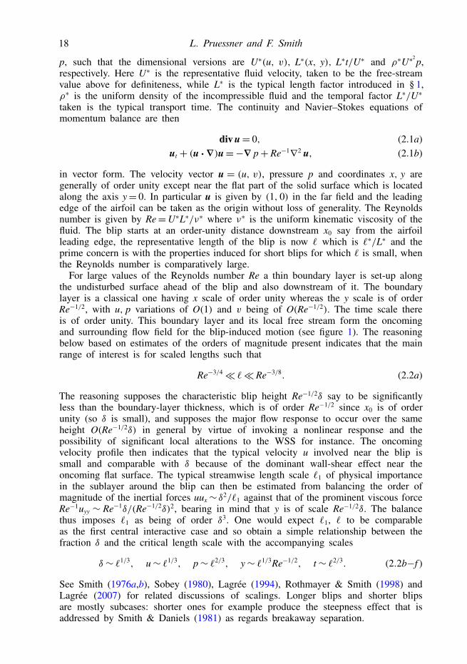
For large values of the Reynolds number Re a thin boundary layer is set-up alongthe undisturbed surface ahead of the blip and also downstream of it. The boundarylayer is a classical one having x scale of order unity whereas the y scale is of orderRe−1/2, with u, p variations of O(1) and v being of O(Re−1/2). The time scale thereis of order unity. This boundary layer and its local free stream form the oncomingand surrounding flow field for the blip-induced motion (see figure 1). The reasoningbelow based on estimates of the orders of magnitude present indicates that the mainrange of interest is for scaled lengths such that

Re−3/4� `� Re−3/8. (2.2a)

The reasoning supposes the characteristic blip height Re−1/2δ say to be significantlyless than the boundary-layer thickness, which is of order Re−1/2 since x0 is of orderunity (so δ is small), and supposes the major flow response to occur over the sameheight O(Re−1/2δ) in general by virtue of invoking a nonlinear response and thepossibility of significant local alterations to the WSS for instance. The oncomingvelocity profile then indicates that the typical velocity u involved near the blip issmall and comparable with δ because of the dominant wall-shear effect near theoncoming flat surface. The typical streamwise length scale `1 of physical importancein the sublayer around the blip can then be estimated from balancing the order ofmagnitude of the inertial forces uux∼ δ2/`1 against that of the prominent viscous forceRe−1uyy ∼ Re−1δ/(Re−1/2δ)2, bearing in mind that y is of scale Re−1/2δ. The balancethus imposes `1 as being of order δ3. One would expect `1, ` to be comparableas the first central interactive case and so obtain a simple relationship between thefraction δ and the critical length scale with the accompanying scales

δ ∼ `1/3, u∼ `1/3, p∼ `2/3, y∼ `1/3Re−1/2, t∼ `2/3. (2.2b−f )

See Smith (1976a,b), Sobey (1980), Lagrée (1994), Rothmayer & Smith (1998) andLagrée (2007) for related discussions of scalings. Longer blips and shorter blipsare mostly subcases: shorter ones for example produce the steepness effect that isaddressed by Smith & Daniels (1981) as regards breakaway separation.


U

U

Y Y

X

U

Main part of boundary layer

Sublayer

Sublayer

Multi-BLIPS

BLIP

(a) (b)

FIGURE 1. The major parts of the flow/body interaction: the short-scale flow structurewhich comprises a viscous–inviscid sublayer surrounded by the main part of the incidentboundary layer. Here (a) is for a single blip and shows the whole boundary layer while(b) is for the corresponding configuration with several or many blips, shown closer to thewall where to leading order the incident flow is a uniform shear.

So far we have taken the time scale to respond to the inertial force. In the nextsection we will take it to be slower, yielding quasi-steady behaviour; the time scalel2/3 reasserts itself later however through a process of intensifications.

The lower limitation in (2.2a) corresponds to the sublayer height |y| becomingcomparable with the streamwise scale ` and producing a quite tiny region governedby the full system (2.1) in normalised form. In contrast the upper limitation in (2.2a)is associated with the triple deck stage where the thin sublayer around the blipexperiences a substantial feedback of pressure which arises from interaction withthe flow outside the surrounding boundary layer. In between, where the range (2.2a)applies, the sublayer is controlled by thin-layer dynamics alone. Moreover, the rangeof validity in (2.2a) which is verified above is actually quite a large one in terms ofthe scales covered.

The flow structure is therefore concentrated primarily in the thin sublayer offigure 1. The flexible blip of unknown shape in 1(a) occupies the range 0 < X < 1and has height comparable with the sublayer height, whereas the surface is fixed andsolid outside that range; 1(b) is for several or many blips. The blips can be humps ordents. The thick dashed line between the sublayer and the rest of the boundary layerindicates the lack of displacement over these short length scales. In the sublayer atleading order

(u, v, p)= (`1/3U, `−1/3Re−1/2V, `2/3P), with x− x0= `X, y= `1/3Re−1/2Y, t= `2/3T,(2.3)

and all of the capital-lettered quantities are generally of order unity. The full system(2.1) then reduces to the well-known condensed flow interaction (Smith 1976a,b;Smith & Daniels 1981) given by

U =ΨY, V =−ΨX, (2.4a,b)

UT +UUX + VUY =−PX(X, T)+UYY, (2.4c)


with the unknown scaled pressure P(X, T) being independent of Y because of they-momentum equation. The relevant boundary conditions are

U = 0, V = ∂f /∂T, at Y = f (X, T), (2.4d,e)

U − λY→ 0 as Y→∞ (2.4f )

for no slip on the moving blip surface and to match with the outer flow responsein turn. The requirement (2.4f ) of effectively zero displacement in Y corresponds tothe feedback effect from the flow outside the sublayer being relatively small. Thefunction f in (2.4d,e) denotes the unknown scaled shape of the blip surface whichis addressed further just below while the positive O(1) factor λ in (2.4f ) is the givenscaled incident WSS, namely Re−1/2(∂u/∂y) at y = 0, in the surrounding boundarylayer locally: see figure 1.

Concerning (second) the blip surface shape as it responds to the fluid flow overthe blip, the shape and the flow interact via the local pressure as in the modelsused by Carpenter & Garrad (1985), Gajjar & Sibanda (1996), Davies & Carpenter(1997) and Pruessner (2013) and others. The assumptions made are primarily thoseof the widely used membrane-model type as in the references immediately abovewith particularly interesting background discussions of linearly elastic materials andallied facets relevant here being in Takagi & Balmforth (2011) as well as Vella, Kim& Mahadevan (2004), Stewart, Waters & Jensen (2009), Singh, Lister & Vella (2014)and Xu, Billingham & Jensen (2014). This then gives the wall equation

e1ηxxxx + e2ηxx + e3η+ e4ηtt + e5ηt = p− p0. (2.5)

In this simple plate membrane model the unknown blip shape is y = η(x, t) andthe non-dimensional constant coefficients en are (e1, e2, e3, e4, e5) = (−B∗/U∗2L∗3,T∗t /U

∗2L∗, −κ∗L∗/U∗2, M∗/L∗, C∗/U∗)/ρ∗ with M∗, C∗, B∗, κ∗, T∗t being the mass

density, the damping constant, the flexural rigidity, the spring stiffness and thelongitudinal tension respectively, while p0 is the non-dimensional base pressurerelative to the oncoming pressure level which is taken to be zero. The values of theabove quantities are determined experimentally or are tabulated for certain materials.The scaled version appropriate to the short-blip application is then

e1 fXXXX + e2 fXX + e3 f + e4 fTT + e5 fT = P− P0 (2.6a)

where η = Re−1/2δf , e1 = Re−1/2e1/(`4δ), e2 = Re−1/2e2/(`

2δ), e3 = Re−1/2e3/δ, e4 =Re−1/2e4/δ

5, e5 = Re−1/2e5/δ3, P0 = `−2/3p0. In particular e1 < 0, e2 > 0, e3 < 0. The

coefficients are sensitive to the blip length scale ` (recall δ in (2.2b−f )) and to Rebut in applications of interest here the dominant coefficient can sometimes be e2. Theboundary conditions on f are

f = fX = 0 at X = 0, 1 (2.6b)

if the end points of the single blip are taken as X=0,1 for definiteness. Representativeinitial conditions have the shape f and pressures P, P0 being zero.

The nonlinear governing system is therefore (2.4a–f ), (2.6a,b). Fair agreementbetween theoretical results based on the system and experimental results or directsimulations is found in the prescribed-shape case (Smith 1976a,b; Sobey 1980;Rothmayer & Smith 1998). This system whether with prescribed wall shape or


flexible shape then appears to require numerical treatment usually: see the nextsection. On the other hand if P0 is zero then there is simply no disturbance. Thus, alinearised version which is also helpful and intriguing in its own right has f beingsmall and so (2.4a–f ) reduce to linear equations for small U − λY, V, P. Use of aFourier transform in X for example as in Stewartson (1970), Smith (1976a,b) andGuneratne & Pedley (2006) along with inversion and convolution properties thenyields for quasi-steady flow the integro-differential relation

P=−γ∫ X

0f (s)(X − s)−2/3 ds (2.7)

between P, f for X > 0, thus replacing (2.4a–f ). Here γ =−3 Ai′(0)λ5/3/Γ (1/3) is apositive constant {≈0.289838λ5/3}. The parabolic nature of the flow contribution onits own is then clear. Also the unknown blip f is again assumed to start at the stationX = 0 for definiteness and the pressure P there is zero. In the streamwise directionthe only boundary conditions imposed on U, V, P are at the upstream end of thefirst blip, where U = λY , V = P = 0, and we note that it is inappropriate to fix thedownstream pressure on the current short length scales. The nature of the problem issomewhat mixed, being parabolic upstream of the blip(s), then elliptic over the lengthof a blip, then parabolic at all streamwise stations where there is no blip, and soon, but the overall upstream influence of a relatively long triple-deck in external flow(Stewartson 1970; Smith 1982) or the long Re1/7 (multiplied by the channel width)axial length in internal flow (Smith 1977; Luo & Pedley 1996) is insignificant forthe present short blips. Likewise the corresponding flow-dominated linear instabilitiesexisting over the longer scales are inactive in the present setting. The fully nonlinearunsteady condensed flow (2.4a)–(2.6b) with |∂/∂T| of order unity can neverthelesslead to a finite-time breakup, Smith (1988) and Peridier, Smith & Walker (1991), asa nonlinear by-pass into deep transition as seen later in §§ 4 and 6. The motivationalsettings of § 1 however are more concerned with quasi-steady behaviour initially inwhich |∂/∂T| is relatively small.

It can be seen immediately that a positive f shape corresponding to a bumprather than a dent provokes negative pressures, which makes sense physically interms of an adverse pressure gradient on the front face of the blip and a favourablepressure gradient most likely on the rear face, together with a lag in the responsedue to convolution. Likewise a pressure rise followed by a fall is expected for adent. The persistence of the pressure response downstream of the end point X = 1 isevident from (2.7) (the integral is then from 0 to 1) and represents a wake effect. Anormalisation is now applied. With U, V, P, Y, T, f normalised by factors λm wherem is 2/3, 1/3, 4/3, −(1/3), −(2/3), −(1/3) in turn (see the references above) andthe representative X already normalised to unity by definition of blip length, theflow contributions throughout (2.4) are thus normalised to O(1) whereas the shapecontributions in (2.6a) have orders |e|λ−1/3 on the left compared with λ4/3 and P0successively on the right-hand side. Here only the steady case is considered for nowand |e| refers to the typical size of the wall coefficients en, n = 1, 2, 3, all of thewall coefficients being supposed to be of the same order for convenience. Hence theactive ratios indicate two major parameters, namely Γ1, Γ2 defined by

Γ1 = P0/λ4/3 and Γ2 = |e|/λ5/3. (2.8a,b)

When Γ1, Γ2 are of order unity the fluid-shape interaction is fully nonlinear, while ifΓ1 is small then linearised theory holds since the normalised responses in P, f become


of order Γ1. In the subsequent calculations we tend to take |e| as given as O(1) andvary the incoming shear factor λ and the relative base pressure P0 in order to helpexplore the main two-dimensional parameter space. There are many other parametersof course detailing relative wall coefficients and blip distributions for example. Thelinear and nonlinear responses for a single blip are examined in the next two sectionswhereas those from the presence of multiple blips are addressed in § 5.

3. Results and intensifications

The influences of various physical factors are discussed in the following subsections.Analytical and numerical treatments of (2.4a–f ), (2.6a,b) appear necessary. Thenumerical method we adopted is a finite difference one and, in brief, it comprisesan iterative process of guessing the scaled shape f for all X in the range, thensolving (2.4a–f ) for the scaled pressure P or using (2.7) if applicable, then updatingf from integration of (2.6a,b), and continuing to iterate thus between the flow andwall equations until successive iterates differ by a specified small tolerance, typically10−6 in P. This is with a prescribed under-pressure value P0 in (2.6a) and witha Prandtl transposition introduced into (2.4a–f ) in order to deal with the no-sliprequirement accurately. The treatment applies with modifications for both the linearand the nonlinear cases, abetted by analysis in §§ 3–5, for quasi-steady slowly varyingflow. Results are presented in figures 2–9. These tend to confirm the expectation fromthe previous section of adverse and favourable pressure gradients over the typical blipas well as corresponding reductions and increases respectively in the scaled WSS,∂U/∂Y at Y = 0, along with response lags and with a clear wake effect in termsof the wall pressure downstream of the blip. Both linear and nonlinear quasi-steadyflows will be considered at first below before the emphasis moves on to the linearregime for reasons (namely the occurrence of intensifications and blowups) that willbecome apparent.

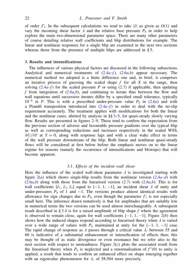
3.1. Effects of the incident wall shearHere the influence of the scaled wall-shear parameter λ is investigated starting withfigure 2(a) which shows single-blip results from the nonlinear version (2.4a–d) with(2.6a,b) along with those from the linearised version (2.7) with (2.6a,b). This is forwall coefficients [e1, e2, e3] equal to [−1, 1, −1], an incident shear λ of unity andunder-pressures P0 of 1 and −1. The versions produce almost identical results withallowance for sign changes due to P0, even though the parameter Γ1 is not especiallysmall here. The inference drawn tentatively is that for amplitudes that are suitably lowin numerical terms the two versions can be used almost interchangeably. A subsequentresult described in § 3.4 is for a raised amplitude of blip shape f where the agreementis observed to remain close, again for wall coefficients [−1, 1,−1]. Figure 2(b) thenshows how the induced shapes respond according to linearised theory when λ is variedover a wide range of values with P0 maintained at unity for the [−1, 1, −1] case.The rapid change of response as λ passes through a critical value λc between 55 and60 is indicative of a substantial enhancement or intensification of effects then; thismay be thought of as static divergence or even resonance but we refer also to thenext section with respect to unsteadiness. Figure 2(c) plots the associated result fromthe linearised theory when P0 is neglected and a renormalisation of f ′′(0) to unity isapplied, a result that tends to confirm an enhanced effect on shape emerging togetherwith an eigenvalue phenomenon for λc of 58.504 more precisely.


0 0.25 0.50 0.75 1.00 1.25 1.50 0 0.2

0.02

0

–0.02

–0.04

–0.06

0 0.2 0.4 0.6 0.8 1.0

0.01

0.02

0.03

Normalised f

0.04

0.4

7.5

–7.5

5.0

–5.0

2.5

–2.5

0

0.6 0.8 1.0

P

P

f

f

f

70

80

4050

45

75

65

X X

X

(a) (b)

(c)

FIGURE 2. (a) Numerical results for a single blip with wall coefficients [e1, e2, e3]of [−1, 1, −1], incoming shear λ of unity and P0 = 1 or −1, showing blip shape f ,slope f ′ and fluid-flow pressure P versus scaled distance X. Linearised and low-amplitudenonlinear calculations are compared (light and dark). (b) As (a) but λ varying from 1to 80: linearised results for shape. (c) Normalised shape at λ = λc ≈ 58.504, the firstintensification value, from linearised theory.

The effect of the flow on the blip shape itself (being an integral or lagged effect)is a gradual build-up with downstream distance. The blip hump rises for instance, sothe induced flow pressure falls, certainly along the front face of the hump, and thescaled wall shear rises; hence this supplements the under-pressure influence tendingto pull the blip surface down, with the WSS then decreasing on the leeward face ofthe upward blip; if the conditions are just right the interaction leads to intensification.

3.2. Effects of base pressureThe influence of the under-pressure is investigated via figure 3, showing the blip shape,fluid pressure and WSS produced over the [−1, 1,−1] flexible blip with the incidentshear λ maintained at unity. The scaled under-pressures P0 imposed cover a wide


0

0

200

200

200

500

500

50

50

501

2

3

4

–1

0.2 0.4 0.6 0.8 1.0

P

f

X

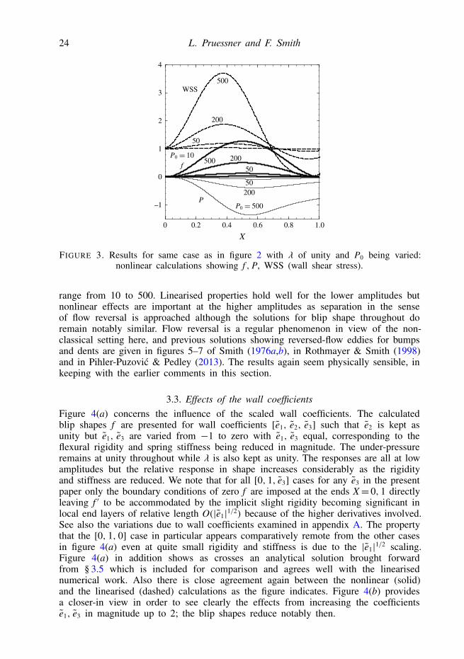
FIGURE 3. Results for same case as in figure 2 with λ of unity and P0 being varied:nonlinear calculations showing f , P, WSS (wall shear stress).

range from 10 to 500. Linearised properties hold well for the lower amplitudes butnonlinear effects are important at the higher amplitudes as separation in the senseof flow reversal is approached although the solutions for blip shape throughout doremain notably similar. Flow reversal is a regular phenomenon in view of the non-classical setting here, and previous solutions showing reversed-flow eddies for bumpsand dents are given in figures 5–7 of Smith (1976a,b), in Rothmayer & Smith (1998)and in Pihler-Puzovic & Pedley (2013). The results again seem physically sensible, inkeeping with the earlier comments in this section.

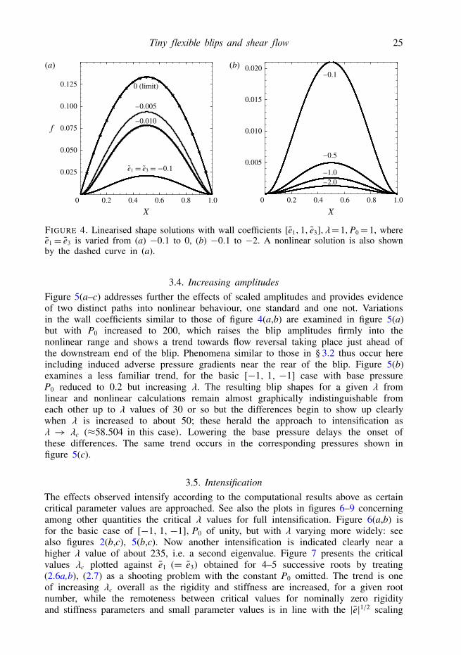
3.3. Effects of the wall coefficientsFigure 4(a) concerns the influence of the scaled wall coefficients. The calculatedblip shapes f are presented for wall coefficients [e1, e2, e3] such that e2 is kept asunity but e1, e3 are varied from −1 to zero with e1, e3 equal, corresponding to theflexural rigidity and spring stiffness being reduced in magnitude. The under-pressureremains at unity throughout while λ is also kept as unity. The responses are all at lowamplitudes but the relative response in shape increases considerably as the rigidityand stiffness are reduced. We note that for all [0, 1, e3] cases for any e3 in the presentpaper only the boundary conditions of zero f are imposed at the ends X= 0, 1 directlyleaving f ′ to be accommodated by the implicit slight rigidity becoming significant inlocal end layers of relative length O(|e1|1/2) because of the higher derivatives involved.See also the variations due to wall coefficients examined in appendix A. The propertythat the [0, 1, 0] case in particular appears comparatively remote from the other casesin figure 4(a) even at quite small rigidity and stiffness is due to the |e1|1/2 scaling.Figure 4(a) in addition shows as crosses an analytical solution brought forwardfrom § 3.5 which is included for comparison and agrees well with the linearisednumerical work. Also there is close agreement again between the nonlinear (solid)and the linearised (dashed) calculations as the figure indicates. Figure 4(b) providesa closer-in view in order to see clearly the effects from increasing the coefficientse1, e3 in magnitude up to 2; the blip shapes reduce notably then.


0 0.2 0.4 0.6 0.8 1.0 0

0 (limit)

0.2 0.4 0.6 0.8 1.0

0.020

0.015

0.010–0.010

–0.1

–0.5

–1.0–2.0

0.005

–0.005

0.050

0.075

0.100

0.125

0.025

X

f

X

(a) (b)

FIGURE 4. Linearised shape solutions with wall coefficients [e1,1, e3],λ=1,P0=1, wheree1= e3 is varied from (a) −0.1 to 0, (b) −0.1 to −2. A nonlinear solution is also shownby the dashed curve in (a).

3.4. Increasing amplitudesFigure 5(a–c) addresses further the effects of scaled amplitudes and provides evidenceof two distinct paths into nonlinear behaviour, one standard and one not. Variationsin the wall coefficients similar to those of figure 4(a,b) are examined in figure 5(a)but with P0 increased to 200, which raises the blip amplitudes firmly into thenonlinear range and shows a trend towards flow reversal taking place just ahead ofthe downstream end of the blip. Phenomena similar to those in § 3.2 thus occur hereincluding induced adverse pressure gradients near the rear of the blip. Figure 5(b)examines a less familiar trend, for the basic [−1, 1, −1] case with base pressureP0 reduced to 0.2 but increasing λ. The resulting blip shapes for a given λ fromlinear and nonlinear calculations remain almost graphically indistinguishable fromeach other up to λ values of 30 or so but the differences begin to show up clearlywhen λ is increased to about 50; these herald the approach to intensification asλ → λc (≈58.504 in this case). Lowering the base pressure delays the onset ofthese differences. The same trend occurs in the corresponding pressures shown infigure 5(c).

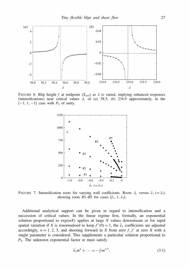
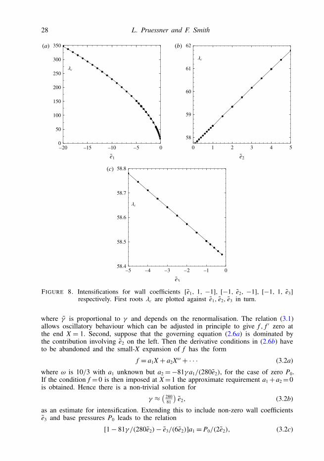
3.5. IntensificationThe effects observed intensify according to the computational results above as certaincritical parameter values are approached. See also the plots in figures 6–9 concerningamong other quantities the critical λ values for full intensification. Figure 6(a,b) isfor the basic case of [−1, 1, −1], P0 of unity, but with λ varying more widely: seealso figures 2(b,c), 5(b,c). Now another intensification is indicated clearly near ahigher λ value of about 235, i.e. a second eigenvalue. Figure 7 presents the criticalvalues λc plotted against e1 (= e3) obtained for 4–5 successive roots by treating(2.6a,b), (2.7) as a shooting problem with the constant P0 omitted. The trend is oneof increasing λc overall as the rigidity and stiffness are increased, for a given rootnumber, while the remoteness between critical values for nominally zero rigidityand stiffness parameters and small parameter values is in line with the |e|1/2 scaling


0

0

0.2 0.4 0.6 0.8 1.0

50

50

30

50

50

30

10

0 0.2 0.4 0.6 0.8 1.0 0 0.2 0.4 0.6 0.8 1.0–1

2

3

1 2

3

4

10

–0.75

–0.50

–0.5

–0.5

–0.5

–1.0

–2.0

–0.25

–1.00

–1.25

–1.50

P

P

f

f

X X

X

(a) (b)

(c)

FIGURE 5. Influences of increasing amplitude for different λ values: (a) λ= 1 with P0=200, wall [e1, 1, e3] where e1 = e3 ranges from −2 to −0.5, nonlinear computations off ,P, WSS; (b) λ= 10, 30, 50 with P0= 0.2, wall [−1, 1,−1], comparing nonlinear (dashedcurves) and linearised (solid) predictions for f ; (c) is as (b) but for P.

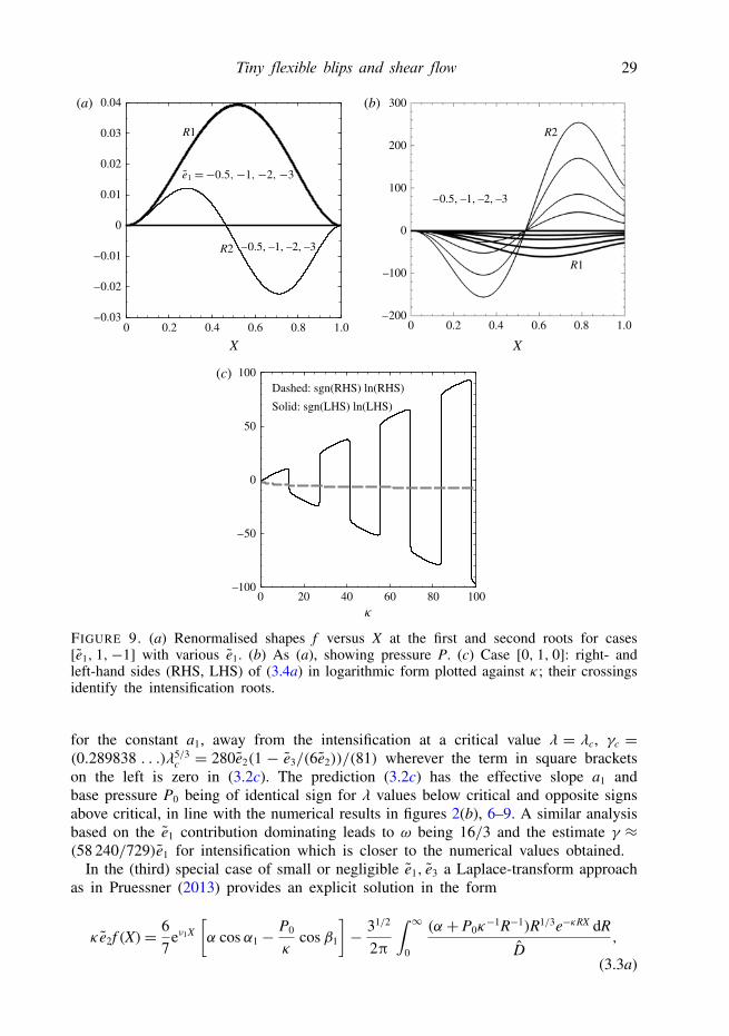
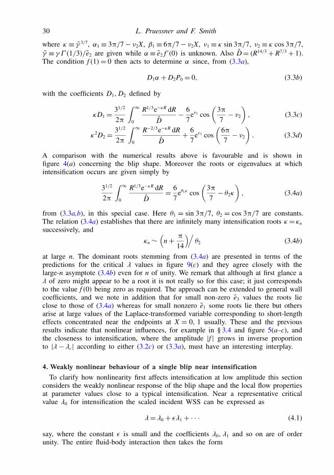
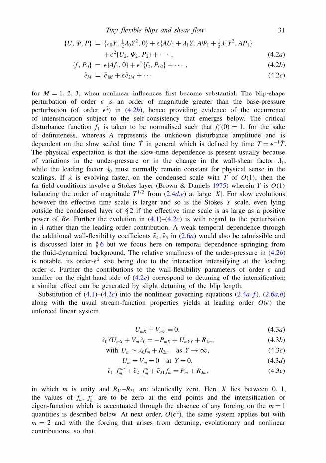
described in § 3.3. The close-in results suggest that each root for zero rigidity andstiffness may propagate more than one set of roots R1, R2 and so on among thoseshown for non-zero rigidity and stiffness. In figure 8(a–c) by contrast we show thefirst-root eigenvalues associated with intensification for cases where each of e1, e2, e3is varied separately in order to present a different slice through the parameter space,which connects with the parameter study in appendix A and accompanying analysis.Next, figure 9(a,b) gives plots of the shapes f and induced pressures P from both thefirst and second roots in wall cases [e1, 1, −1] with the coefficient e1 being variedbetween −0.5 and −3. We see little change in f over the range for a given set offirst or second roots whereas the pressure P alters considerably for each set, which isphysically sensible because of the different incident shear values, and the maximummagnitude of the pressure depends almost linearly on e1. Shown in figure 9(c) is aplot relevant to the special case of [0, 1, 0] described at the end of the current sectionand confirming the existence of multiple roots.


0.02

0

234.5 235.0 235.5 236.0234.058.2 58.4 58.6 58.8 59.058.0

0.04

–0.02

–0.04

2

0

4

–2

–4

(a) (b)

FIGURE 6. Blip height f at midpoint (Xmid) as λ is varied, implying enhanced responses(intensifications) near critical values λc of (a) 58.5, (b) 234.9 approximately, in the[−1, 1,−1] case with P0 of unity.

00

250

500

750

1000

1250

–1.0 –0.8 –0.6 –0.4 –0.2

R1

R2

R3

R4R5

FIGURE 7. Intensification roots for varying wall coefficients. Roots λc versus e1 (= e3)showing roots R1–R5 for cases [e1, 1, e3].

Additional analytical support can be given in regard to intensification and asuccession of critical values. In the linear regime first, formally, an exponentialsolution proportional to exp(mX) applies at large X values downstream or for rapidspatial variation if X is renormalised to keep f ′′(0)= 1, the en coefficients are adjustedaccordingly, n= 1, 2, 3, and shooting forward in X from zero f , f ′ at zero X with asingle parameter is considered. This supplements a particular solution proportional toP0. The unknown exponential factor m must satisfy

e1m4 + · · · =−γm1/3, (3.1)


0 1 2 3 54

0

00

50

58

58.8

58.7

58.6

58.5

58.4

59

60

61

62

100

150

200

250

300

350

–1

–10–15–20

–2–3–5

–5

–4

(a) (b)

(c)

FIGURE 8. Intensifications for wall coefficients [e1, 1, −1], [−1, e2, −1], [−1, 1, e3]respectively. First roots λc are plotted against e1, e2, e3 in turn.

where γ is proportional to γ and depends on the renormalisation. The relation (3.1)allows oscillatory behaviour which can be adjusted in principle to give f , f ′ zero atthe end X = 1. Second, suppose that the governing equation (2.6a) is dominated bythe contribution involving e2 on the left. Then the derivative conditions in (2.6b) haveto be abandoned and the small-X expansion of f has the form

f = a1X + a2Xω + · · · (3.2a)

where ω is 10/3 with a1 unknown but a2=−81γ a1/(280e2), for the case of zero P0.If the condition f =0 is then imposed at X=1 the approximate requirement a1+a2=0is obtained. Hence there is a non-trivial solution for

γ ≈ ( 28081

)e2, (3.2b)

as an estimate for intensification. Extending this to include non-zero wall coefficientse3 and base pressures P0 leads to the relation

[1− 81γ /(280e2)− e3/(6e2)]a1 = P0/(2e2), (3.2c)


0 0.2–0.03

–0.02

–0.01

0

0.01

0.02

0.03

0.04

0.4 0.6 0.8 1.0 0 0.2 0.4

–0.5, –1, –2, –3

–0.5, –1, –2, –3

0.6 0.8 1.0

0 20 40 60 80

–50

50

0

100–100

–200

–100

100

0

100

200

300

R1

R1R2

R2

Dashed: sgn(RHS) ln(RHS)

Solid: sgn(LHS) ln(LHS)

X X

(a) (b)

(c)

FIGURE 9. (a) Renormalised shapes f versus X at the first and second roots for cases[e1, 1,−1] with various e1. (b) As (a), showing pressure P. (c) Case [0, 1, 0]: right- andleft-hand sides (RHS, LHS) of (3.4a) in logarithmic form plotted against κ; their crossingsidentify the intensification roots.

for the constant a1, away from the intensification at a critical value λ = λc, γc =(0.289838 . . .)λ5/3

c = 280e2(1 − e3/(6e2))/(81) wherever the term in square bracketson the left is zero in (3.2c). The prediction (3.2c) has the effective slope a1 andbase pressure P0 being of identical sign for λ values below critical and opposite signsabove critical, in line with the numerical results in figures 2(b), 6–9. A similar analysisbased on the e1 contribution dominating leads to ω being 16/3 and the estimate γ ≈(58 240/729)e1 for intensification which is closer to the numerical values obtained.

In the (third) special case of small or negligible e1, e3 a Laplace-transform approachas in Pruessner (2013) provides an explicit solution in the form

κ e2f (X)= 67

eν1X

[α cos α1 − P0

κcos β1

]− 31/2

2π

∫ ∞0

(α + P0κ−1R−1)R1/3e−κRX dR

D,

(3.3a)


where κ ≡ γ 3/7, α1 ≡ 3π/7− ν2X, β1 ≡ 6π/7− ν2X, ν1 ≡ κ sin 3π/7, ν2 ≡ κ cos 3π/7,γ ≡ γΓ (1/3)/e2 are given while α≡ e2 f ′(0) is unknown. Also D= (R14/3+R7/3+ 1).The condition f (1)= 0 then acts to determine α since, from (3.3a),

D1α +D2P0 = 0, (3.3b)

with the coefficients D1,D2 defined by

κD1 = 31/2

2π

∫ ∞0

R1/3e−κR dR

D− 6

7eν1 cos

(3π

7− ν2

), (3.3c)

κ2D2 = 31/2

2π

∫ ∞0

R−2/3e−κR dR

D+ 6

7eν1 cos

(6π

7− ν2

). (3.3d)

A comparison with the numerical results above is favourable and is shown infigure 4(a) concerning the blip shape. Moreover the roots or eigenvalues at whichintensification occurs are given simply by

31/2

2π

∫ ∞0

R1/3e−κR dR

D= 6

7eθ1κ cos

(3π

7− θ2κ

), (3.4a)

from (3.3a,b), in this special case. Here θ1 = sin 3π/7, θ2 = cos 3π/7 are constants.The relation (3.4a) establishes that there are infinitely many intensification roots κ=κn

successively, and

κn ∼(

n+ π

14

)/θ2 (3.4b)

at large n. The dominant roots stemming from (3.4a) are presented in terms of thepredictions for the critical λ values in figure 9(c) and they agree closely with thelarge-n asymptote (3.4b) even for n of unity. We remark that although at first glance aλ of zero might appear to be a root it is not really so for this case; it just correspondsto the value f (0) being zero as required. The approach can be extended to general wallcoefficients, and we note in addition that for small non-zero e3 values the roots lieclose to those of (3.4a) whereas for small nonzero e1 some roots lie there but othersarise at large values of the Laplace-transformed variable corresponding to short-lengtheffects concentrated near the endpoints at X = 0, 1 usually. These and the previousresults indicate that nonlinear influences, for example in § 3.4 and figure 5(a–c), andthe closeness to intensification, where the amplitude |f | grows in inverse proportionto |λ− λc| according to either (3.2c) or (3.3a), must have an interesting interplay.

4. Weakly nonlinear behaviour of a single blip near intensification

To clarify how nonlinearity first affects intensification at low amplitude this sectionconsiders the weakly nonlinear response of the blip shape and the local flow propertiesat parameter values close to a typical intensification. Near a representative criticalvalue λ0 for intensification the scaled incident WSS can be expressed as

λ= λ0 + ελ1 + · · · (4.1)

say, where the constant ε is small and the coefficients λ0, λ1 and so on are of orderunity. The entire fluid-body interaction then takes the form


{U, Ψ, P} = {λ0Y, 12λ0Y2, 0} + ε{AU1 + λ1Y, AΨ1 + 1

2λ1Y2, AP1}+ ε2{U2, Ψ2, P2} + · · · , (4.2a)

{f , P0} = ε{Af1, 0} + ε2{f2, P02} + · · · , (4.2b)eM = e1M + εe2M + · · · (4.2c)

for M = 1, 2, 3, when nonlinear influences first become substantial. The blip-shapeperturbation of order ε is an order of magnitude greater than the base-pressureperturbation (of order ε2) in (4.2b), hence providing evidence of the occurrenceof intensification subject to the self-consistency that emerges below. The criticaldisturbance function f1 is taken to be normalised such that f ′′1 (0) = 1, for the sakeof definiteness, whereas A represents the unknown disturbance amplitude and isdependent on the slow scaled time T in general which is defined by time T = ε−1T .The physical expectation is that the slow-time dependence is present usually becauseof variations in the under-pressure or in the change in the wall-shear factor λ1,while the leading factor λ0 must normally remain constant for physical sense in thescalings. If λ is evolving faster, on the condensed scale with T of O(1), then thefar-field conditions involve a Stokes layer (Brown & Daniels 1975) wherein Y is O(1)balancing the order of magnitude T1/2 from (2.4d,e) at large |X|. For slow evolutionshowever the effective time scale is larger and so is the Stokes Y scale, even lyingoutside the condensed layer of § 2 if the effective time scale is as large as a positivepower of Re. Further the evolution in (4.1)–(4.2c) is with regard to the perturbationin λ rather than the leading-order contribution. A weak temporal dependence throughthe additional wall-flexibility coefficients e4, e5 in (2.6a) would also be admissible andis discussed later in § 6 but we focus here on temporal dependence springing fromthe fluid-dynamical background. The relative smallness of the under-pressure in (4.2b)is notable, its order-ε2 size being due to the interaction intensifying at the leadingorder ε. Further the contributions to the wall-flexibility parameters of order ε andsmaller on the right-hand side of (4.2c) correspond to detuning of the intensification;a similar effect can be generated by slight detuning of the blip length.

Substitution of (4.1)–(4.2c) into the nonlinear governing equations (2.4a–f ), (2.6a,b)along with the usual stream-function properties yields at leading order O(ε) theunforced linear system

UmX + VmY = 0, (4.3a)λ0YUmX + Vmλ0 =−PmX +UmYY + R1m, (4.3b)

with Um ∼ λ0fm + R2m as Y→∞, (4.3c)Um = Vm = 0 at Y = 0, (4.3d)

e11 f ′′′′m + e21 f ′′m + e31 fm = Pm + R3m, (4.3e)

in which m is unity and R11–R31 are identically zero. Here X lies between 0, 1,the values of fm, f ′m are to be zero at the end points and the intensification oreigen-function which is accentuated through the absence of any forcing on the m= 1quantities is described below. At next order, O(ε2), the same system applies but withm = 2 and with the forcing that arises from detuning, evolutionary and nonlinearcontributions, so that


R12 =−dA/dTU1 − Aλ1(YU1X + V1)− A2(U1U1X + V1U1Y), (4.4a)R22 = Aλ1f1, (4.4b)

R32 =−P02 − A(e12 f ′′′′1 + e22 f ′′1 + e32 f1). (4.4c)

These forcings are affected by the leading-order flow and wall solutions of course aswell as by the small under-pressure. In particular R12, R22 are flow-field effects whileR32 constitutes the wall effect.

The solution of (4.3a–e) may be obtained by means of a Fourier transform(superscripted F) applied in X, which allows (4.3a,b) to be cast as a forced Airyequation for the scaled flow shear. Hence,

(∂um/∂y)F = [(iαλ0)−1/3I(ξ)+ Bm]Ai(ξ) (4.5a)

where α is the transform variable, Ai is the Airy function, ξ = (iαλ0)1/3Y and

I(ξ)=∫ ξ

0(Ai(q))−2

[∫ q

∞Ai(ξ )RF

1mξ dξ]

dq. (4.5b)

Use of (4.3c,d) then enables the unknown shear constant Bm to be determined in termsof the scaled pressure which is found to be given by

PFm = 3λ5/3

0 (iα)−1/3Ai′(0)f Fm + Γ F. (4.6a)

Here

(iα)Γ F =−Ai(0)I′(0)+ 3Ai′(0){∫ ∞

0Ai(ξ)I(ξ) dξ + (iα)2/3λ2/3

0 RF2m

}. (4.6b)

So the wall balance (4.3e) requires the relation

e11 f ′′′′m + e21 f ′′m + e31 fm =−γ∫ X

0fm(s)(X − s)−2/3 ds+ R42(X) (4.7a)

to hold, in which R42(X) = Γ (X) + R32(X). The factor multiplying the integral onthe right in (4.7a) agrees with the intensified value of that in (2.7) as required forconsistency. The relation (4.7a), which is subject to the end conditions

fm = f ′m = 0 at X = 0, 1, (4.7b)

acts at leading order (m= 1) to define the intensified blip shape in normalised formbut also acts, at the second order (m=2) where the R terms are non-zero, to provide asolvability constraint that helps control the unknown amplitude. This constraint stemsfrom use of the normalised function q(X) say that is adjoint to f1(X) and can be shownfrom (4.7a,b) when m= 1 to be given by q(X)= f1(1− X). Multiplication through byq(X) in (4.7a) when m= 2 then leads to the requirement that∫ 1

0R42(X)q(X) dX = 0 (4.8)

which constitutes an amplitude equation. A substitution of the effects from (4.4a–c)in the requirement (4.8) yields the amplitude equation for A(T) as

d1dA

dT+ d7A+ d6A2 + P02 = 0, (4.9a)


7.5

10

–7.5–10

5.0

5

–5.0

–5

2.5–2.5 0

0

10

–10

5

–5

0

7.5–7.5 5.0–5.0 2.5–2.5 03

3

–3 2

2

–2

–2

1

1

–1

–1

0

0

A

A

A

A

A A

A

A

(a) (b)

(c)

FIGURE 10. (a) The phase-plane solution with horizontal axis A∗ = d6A/|d7| and vertical•A∗

for times |d7|T/d1, associated with weakly nonlinear evolution in or near intensification.(b) Evolution of amplitude A when d7= T,P02= 0.25 with d1, d6 normalised to unity, forvarious small kicks in amplitude at large negative T . Quasi-steady states denoted qss areshown for comparison. (c) As (b) but P02 =−0.25.

whered7 ≡ d2λ1 + d3e12 − d4e22 + d5e32 (4.9b)

and it can be shown that all the coefficients d1–d6 are positive; a calculation gives theestimates 0.422, 0.392, 14.76, 0.362, 0.029, 1.11 in turn. The latter values are for thecentral example of the wall coefficients e1, e2, e3 being −1, 1,−1 respectively whereaseffects over a wide range of variation in these wall coefficients are investigated inappendix A.

The amplitude equation (4.9a) encapsulating the nonlinear response in terms of theamplitude function A(T) is Riccati-like and yields the phase-plane diagram drawn infigure 10(a), when d1, d6, d7 are independent of time T , which tends to confirm the


significance of only the signs of the coefficients above. Varying the scaled pressure P02

yields the different sets of trajectories with positive, zero or negative intercept values(+, 0,− respectively) at zero A while d7 being positive or negative is responsible forthe left–right reflection of the curves. Here d7 may be positive or negative dependingon the four parts which constitute that coefficient. The arrows indicate directionalong the trajectories with increasing time: rightwards in the upper half plane andleftwards in the lower half. The normalised diagram, plotting (d6d1/|d7|2) dA/dTagainst d6A/|d7|, shows first that if the scaled under-pressure P02 is negative then onany solution trajectory there are two roots of the quadratic equation correspondingto zero time derivative, one root having positive amplitude and the other negative,and all trajectories are also connected with a large-amplitude asymptote in whichdA/dT ∝ A2 with a negative coefficient of proportionality. On the other hand if P02

is positive then two roots are found if d72 > 4d6P02 (in which case the roots are of

the same sign), one root in the marginal case where equality holds and no real rootsotherwise. Again the connection with a large-amplitude asymptote is clear. Whetherthe under-pressure is positive or negative, the greater of the two amplitude roots actsas an attractor and the lesser one as a repellor whenever two roots exist, whereasthe large-amplitude asymptote which is featured on the left-hand side of the diagramwith A tending to negative infinity serves as an attractor in every instance. The initialvalue of A and subsequent evolution with scaled time can play a key role in decidingthe eventual outcome for the evolving amplitude. The choice of outcomes is

A→[−d7 + (d72 − 4d6P02)

1/2]/(2d6) as T→∞, for d72 > 4d6P02, (4.10a)

A∼−(d1/d6)(T0 − T)−1 as T→ T0 − . (4.10b)

The steady-state value in (4.10a) can be positive or negative, being dependent uponthe values of P02 and the coefficient d7, and is consistent with the value −P02/(d2λ1)

for the linear steady regime and results of § 3 when λ approaches the critical valueidentified there with prescribed en coefficients. This links with the quasi-steadybehaviour of § 3 at low amplitudes.

In contrast the blow-up behaviour in (4.10b) occurs at a finite scaled time and issuch that the fully nonlinear system (2.4a–f ), (2.6a,b) is reinstated over a shortertime scale around the blow-up time T of approximately ε−1T0. This is because whenT − ε−1T0 becomes of order unity the denominator in (4.10b) becomes of order ε,making A grow as large as ε−1 and therefore causing the U-perturbation and |f | in(4.2a,b) to become of order unity. Saturation as in (4.10a) and blow-up to full (strong)nonlinearity within a finite scaled time as in (4.10b) are the two main possibilitiesfor the weakly nonlinear near-intense response, then, while the latter full nonlinearityleads on to the strong break-up route discussed later in terms of transition.

Concerning (4.9a,b) further the results in figure 10(b,c) are formally for varyingλ1 from large negative to large positive values which force d7 to pass smoothlyfrom negative to positive; specifically this is normalised to d7 = T with d1 = d6 = 1.The scaled base pressure is ±0.25. The low-amplitude asymptotes for large negativetimes T match with the quasi-steady behaviour found in § 3 whereas blow-up ofthe amplitude A can be produced within a finite time, confirming the nonlinearprogression to the strong break-up route mentioned at the conclusion of the previousparagraph.


5. Intensifications for many blips

Interactive solutions for multi-blips are now considered. Solutions for four blipsare presented in figure 11(a,b), with the values of the wall coefficients fixed at(−1, 1, −1). These are linear results. Also solutions for one, two or three blipscorrespond to terminating the calculation just before the second, third or fourth blipsuccessively. In figure 11(a) two different arrangements of the four under-pressuresare considered, for parameter λ of unity, and it is apparent that the interactionsbetween the successive blips are relatively mild in these cases. In figure 11(b) λis increased to a near-critical value of 55 where the interactions are seen to beconsiderable. When P0 is positive the minimum pressure produced decreases withdownstream distance X and the maximum pressure also decreases, and in additionthe scaled pressure P starts from a non-zero value at the beginning of all but thefirst blip because of the wake effect. For linear or nonlinear intensifications the wakeeffects in the induced pressure field can play a substantial role in the total interactionproduced by a configuration of many blips, as described below.

Supposing the configuration consists of a sequence of blips that are of identicallength (normalised to unity), identical material and so on, but not necessarily spacedout equally, we consider the most upstream one first. This approach ties in withthe mixed parabolic–elliptic nature of the entire fluid/body interaction. Near or inintensifications the first blip produces a dominant scaled pressure response P andscaled shape response F which in the incipient nonlinear range have amplitude oforder ε, that is small as in § 4, and these act as eigenfunctions. The associatedunder-pressure P0 is only of order ε2 then and acts at second order to help controlthe detailed amplitude evolution; thus, the dominant pressure response varies as thesquare root of the forcing pressure. The main point now concerns the O(ε) pressureP and the fact that it exhibits a wake contribution as referred to in § 3, a contributionwhich extends over the second blip in particular. As a consequence the forcingpressure for the second blip is also of O(ε). Moreover this blip is augmented, as it isidentical to the first blip, and so it produces the very same eigenfunction response asbefore except that, crucially, the amplitude is of order ε1/2 since the forcing pressure(replacing under-pressure effect) is now of order ε. The overall effect is thereforelarger on the second blip and begins as if anew. Also the mechanism can continueafresh to further blips downstream: the pressure wake effect from the second blipis O(ε1/2), extends over the third blip, produces O(ε1/4) amplitudes in pressure andshape on the third blip; the pressure wake effect from the third blip is O(ε1/4),extends over the fourth blip, produces O(ε1/8) amplitudes in pressure and shape there;and so on.

The prediction then is of an increasing trend of pressure and shape amplitudes withincreasing distance downstream, and likewise for the wall-shear perturbations. Thetrend has the enhanced amplitude sequence:

ε, ε1/2, ε1/4, ε1/8, ε1/16, . . . (5.1)

from blip to successive blip for the above case of several identically constituted blips(see figure 11c) whereas for example the sequence is

ε, ε1/2, ε1/2, ε1/2, ε1/4, . . . (5.2)


0 0.2 0.4 0.6 0.8 1.0

0

0

1 2

2

–2

–6

–4

0

1

2

3

4

–1

–3

–2

3 4 50 1 2 3 4 5

PP

P

f

ff

f

f

f

X X

X

(a) (b)

(c)

FIGURE 11. Two or more blips. (a) Linearised f , P versus X with successivebase-pressures P0 of 1,1,1,1 (thin curves) or 1,−1,1,−1 (thick), blip lengths unity, λ=1,wall case [−1, 1,−1]. (b) Linearised f ,P with base pressures 1, 1, 1, 1, blip lengths unity,λ= 55 (just below intensification), wall case [−1, 1,−1]. (c) Weakly nonlinear heights ffor the equimaterial setting of (5.1), equally or unequally spaced blips, yielding heightsε, ε1/2, etc., as X increases; not to scale. Results for 2 blips stop before the third, 3 blipsstop before the fourth, and so on.

for the case of two identical blips followed by any two differently constituted blipsand then identical ones again. Each of the two different blips here provokes amaintained amplitude in shape and pressure because of the wake-pressure effect fromits immediate predecessor and so delays the enhancement but does not prevent itcontinuing downstream. Overall, the increasing downstream trend and mechanisminvolved seem to add weight to the significance of non-periodicity in the overallconfiguration.

The same or similar reasoning extends to configurations other than the identical-blips one above, as (5.2) indicates. A combination of the workings in this and theprevious sections points to a succession of linked nonlinear amplitude equations whichare of considerable interest for future research.


c

t

b

a

Subcritical

Supercritical

(i) (ii) (iii) (iv)

FIGURE 12. Sketch, not to scale, of effects of changing incident shear λ: curve a showsresponse of max |WSS| if λ varies slowly as in b from subcritical to supercritical; whenλ variation is instead as in c the response remains close to c. Time scales (i)–(iv), . . . areslow, fast, faster, faster, . . . .

6. Further commentsThree points (i)–(iii) stand out in conclusion.

(i) Inferences on flow transition. The work has shown that when the wall shear ofthe incident boundary layer flow acquires certain critical values (eigenvalues) a tinyflexible blip can, after some delay, rise or fall to a magnitude much greater thanis otherwise the case. This intensification (§ 3, § 5) along with blowup (§ 4 and seenext paragraph) points to a tuneable trip being feasible over a wide parameter rangein the boundary layer. Both shear and wall flexibility are required for the presentintensifications and fast growth mechanisms to occur as the present scales lie outsidethe usual boundary-layer instability of Tollmien–Schlichting waves (Smith 1979).

Intensification leads to a non-standard path into transition from low amplitudes, asfigure 12 indicates by showing schematically the effects of gradually changing theoncoming shear λ for the regime of relatively low base pressures. Curve a showsthe response of the maximal |WSS| when λ varies slowly as in b from subcriticalto supercritical. The response produces only a small disturbance from λ over thequasi-steady temporal scale (i) of § 3 until a critical value λ = λc is encountered atwhich stage (ii) weakly nonlinear amplification can occur (§ 4), leading to stronglynonlinear evolution over the faster time scale (iii) of (2.4a–f ), (2.6a,b). This isfollowed by finite-time blowup as in Smith (1988) and Peridier et al. (1991) whichprovokes the even faster evolution (iv) described by Davies, Bowles & Smith (2003)(see also Cassel & Conlisk 2014; Gargano et al. 2014) with further restructuringand deep transition towards turbulence taking place. The time scales (i)–(iv) etc. forresponse a are slow, fast, faster, faster, etc. The boosted nonlinear behaviour in a doesnot arise however without the intensification associated with a critical λ. Thus whenthe incident λ variation is subcritical throughout as in c the response remains closeto c. It is noted that the incident λ values b, c do not change scale. The variation


in surrounding conditions can be by means of varying Reynolds number rather thanshear as in the figure.

(ii) Comparisons. A connection can be made here with the recent work on non-flexiblebut dynamic roughnesses (Huebsch 2006; Huebsch et al. 2012) which are similarlysmall and numerous distributed on an airfoil surface. These show considerable effectson transition and on the mean-flow alteration in particular similar to those discussedabove. Detailed comparisons may follow. An additional contrast can be made withthe works on internal motions cited in the introduction, since the present study basedon small-scale condensed flow holds also for internal motions with comparativelyshort flexible blips. In particular Guneratne & Pedley (2006), Kudenatti et al. (2012)and Pihler-Puzovic & Pedley (2013) and related papers are all on longer lengthand time scales and largely involve the 1/7-power length scaling of viscous–inviscidinteraction that brings cross-channel pressure gradients into play (Smith 1977) as wellas upstream influence in the steady case and Tollmien–Schlichting-like instabilitiesin the unsteady case (Hall & Smith 1982). Such overall upstream influence andunderlying flow instabilities are absent in effect over the short scales of currentconcern whether the flow is external or internal. Moreover, the current concernincludes influences (due to e1, e3) from flexural rigidity and spring stiffness whichare absent in the papers above. Nevertheless comparison is possible. The results inour figures 7, 9(c) with regard to higher roots can be compared, with rigidity andstiffness neglected, and they seem to agree with those in Guneratne & Pedley’s (2006)figure 5 in two ways: the first is for ‘shorter’ length scales (large σ in Guneratneand Pedley) and the second is for ‘longer’ scales (small σ ). Both of these ranges oflength scales yield fixed displacement of the wall layer(s) in effect, namely zero orthe average of the wall shapes respectively as described in Smith (1976a,b), Smith(1977) and Sobey (2000), the former length scales being analogous with our range(2.2a). The comparison takes into account the different incident wall shears and wallcoefficients for the internal and external applications and the factor of two associatedwith the average mentioned above in the case of much longer length scales. Thepresent theory thus covers a wide range in internal channel flows, specifically

Re−1/2�| x |� Re1/7 and Re1/7�| x |� Re, (6.1a,b)

with allowance for that factor of two (and noting that this Re is based on channelwidth). The intensified or critical values from (3.4a,b) for short blips are in the sameclose neighbourhood as the numerical values in Guneratne & Pedley (2006) at largeσ . The corresponding analytical values for ‘long’ blips are, from the factor of twoabove, simply given by

(Critical tension for ‘long’ blips)/(that for short blips)= 2. (6.2)

The change in critical values here is due to the mitigating effect of the oppositechannel wall for the ‘long’ cases. In comparison, on a logarithmic scale the numericalvalues of spacings between the large-σ roots are approximately the same as thosebetween small-σ roots in Guneratne & Pedley (2006), suggesting consistency with theprediction (6.2).

(iii) Further work. It will also be interesting to extend the tiny-flexible-blip studyto the highly nonlinear regime as in Smith & Daniels (1981) producing longer-scaleseparations. Some evidence for this appears in Smith (1976a,b) and Pihler-Puzovic &Pedley (2013). In terms of the parameters of § 2 the regime corresponds to Γ1∼ 1 but


Γ2� 1. Future studies should investigate unsteadiness associated with the influencesof mass density and damping in the wall response in addition to that considered in§ 4. The initial effect of the damping proportional to e4 in (2.5) is merely to alterthe coefficient of the single derivative in (4.9a), raising the interesting possibility ofa change in sign of the coefficient and hence a change in the physical mechanism,whereas that of the mass density represented by e5 is to introduce a second derivativein scaled time and this alters the physical nature and implications of the amplitudeequation to a greater extent.

AcknowledgementsThanks are due to P. Bond (Bristol, Oxford), G. Johnson (BAe Systems), R. Lewis

(TotalSim), for very helpful discussion throughout, to G. Johnson for certain detailedcomments, to A. Rothmayer (Iowa State) for pointing out certain references, toEPSRC (UK) grant numbers GR/T11364/01, EP/G501831/1, EP/H501665/1, forCASE support of LP, and to industry (TotalSim) for continued interest and support.Helpful comments by the referees are acknowledged gratefully also.

Appendix A. Nonlinear coefficients as the wall parameters varyThis appendix describes the behaviour of certain quantities as the scaled wall

parameters vary. The major quantities are the eigenvalue λc and the constants

C1 =∫ 1

0q(x) dx, J1 =

∫ 1

0q1(x)q(x) dx, C3 =

∫ 1

0q2(x)q(x) dx, (A 1a−c)

D1 =∫ 1

0f ′′′′1 (x)q(x) dx, D2 =

∫ 1

0f ′′1 (x)q(x) dx, D3 =

∫ 1

0f1(x)q(x) dx, (A 2a−c)

which arise in the nonlinear study in § 4. Here q(X) is f1(1 − X) as defined in thatsection while q1(X) is the integral of f1(s) with respect to s from zero to X and q2(X)is the integral of 3f ′1(s)(X − s)(1/3) with respect to s from zero to X. The findingsare that the above constants when evaluated for the (first) resonant value of λ varyrelatively little, by less than 1 % over e1 values from −1 to −20. The normalisationf ′′1 (0) = 1 is assumed. Similar comparatively small variations in the values of theconstants in (A 1), (A 2) occur over a wide range of wall coefficients e2, e3.

The most significant point is that there is no change in sign of any of theconstants as the wall coefficients vary. So in particular since these constants arelargely proportional to the contributions d1 to d6 in (4.9a), (4.9b) the results infigure 10(a) remain valid throughout.

These findings are complemented by an asymptotic analysis holding for small orlarge values of the wall coefficients as follows.

First, analysis of the orders of the terms in the integro-differential equation resultingfrom (2.6a) combined with (2.7) when f = f1, λ= λ0 at intensification with zero P0 ineffect indicates that: whenever en� 1 then λ5/3

0 is O(en) (i.e. a1 increases linearly withen); whenever en� 1 then λ5/3

0 is O(1); in most cases of small or large en the shapef is typically O(1) since the condition f ′′(0)= 1 is applied. The sole exception is forsmall e1, where thin end layers of length order e(1/4)1 occur near x = 0, 1 (in whichf is of order e(1/2)1 ) due to the highest derivative and these lead to f being typicallyO(e(1/4)1 ) for almost the whole x-range.


Second, similar reasoning extends to the nonlinear coefficients C1, J1, etc., as en

becomes large or small. Thus, in nearly all cases C1 remains O(1) since f (x) andq(x) are O(1), and similarly J1, C3, D1, D2, D3 are O(1). The only exceptional caseis for small e1 where, since f is typically O(e(1/4)1 ), C1 must be O(e(1/4)1 ); likewiseJ1,C3,D1,D2,D3 are all O(e(1/2)1 ) because they are shape-squared effects.

All of the trends in the analysis here agree reasonably well with the trends found innumerical studies of the six constants as the wall coefficients become small or large.

REFERENCES

ALBEN, A. & SHELLEY, M. J. 2008 Flapping states of a flag in an inviscid fluid: bistability andthe transition to chaos. Phys. Rev. Lett. 100, 074301.

BENJAMIN, T. B. 1960 Effects of a flexible boundary on hydrodynamic stability. J. Fluid Mech. 9,513–532.

BROWN, S. N. & DANIELS, P. G. 1975 On the viscous flow about the trailing edge of a rapidlyoscillating plate. J. Fluid Mech. 67, 743–761.

CARPENTER, P. W. & GARRAD, A. D. 1985 The hydrodynamic stability of flow over Kramer-typecompliant surfaces. Part I, Tollmien–Schlichting instabilities. J. Fluid Mech. 165, 465–510.

CARPENTER, P. W. & SEN, P. K. 1990 Effects of boundary-layer growth on the linear regimeof transition over compliant walls. In Laminar–Turbulent Transition. IUTAM Symp, ToulouseFrance, pp. 123–128. Springer.

CASSEL, K. W. & CONLISK, A. T. 2014 Unsteady separation in vortex-induced boundary layers.Phil. Trans. R. Soc. Lond. A 372, 1–19.

DAVIES, C. J., BOWLES, R. I. & SMITH, F. T. 2003 On the spiking stages in deep transition andunsteady separation. J. Engng Maths 45, 227–245.

DAVIES, C. J. & CARPENTER, P. W. 1997 Instabilities in a plane channel flow between compliantwalls. J. Fluid Mech. 352, 205–243.

FITT, A. D. & POPE, M. P. 2001 The unsteady motion of two-dimensional flags with bendingstiffness. J. Engng Maths 40, 227–248.

FORBES, L. K. 1988 Surface waves of large amplitude beneath an elastic sheet. Part 2, Galerkinsolution. J. Fluid Mech. 188, 491–508.

GAD-EL-HAK, M. 2000 Flow Control: Passive, Active, and Reactive Flow Management. CambridgeUniversity Press.

GAJJAR, J. S. B. & SIBANDA, P. 1996 The hydrodynamic stability of channel flow with compliantboundaries. Theor. Comput. Fluid Dyn. 8, 105–129.

GARGANO, F., SAMMARTINO, M., SCIACCA, V. & CASSEL, K. W. 2014 Analysis of complexsingularities in high-Reynolds-numbers Navier–Stokes solutions. J. Fluid Mech. 747, 381–421.

GREEN, J. E. F., OVENDEN, N. C. & SMITH, F. T. 2009 Flow in a multi-branching vessel withcompliant walls. J. Engng Maths 64, 353–365.

GUNERATNE, J. C. & PEDLEY, T. J. 2006 High-Reynolds-number steady flow in a collapsible channel.J. Fluid Mech. 569, 151–184.

HALL, P. & SMITH, F. T. 1982 A suggested mechanism for non-linear wall roughness effects onhigh Reynolds-number flow stability. Stud. Appl. Maths 66, 241–265.

HUEBSCH, W. W. 2006 Two-dimensional simulation of dynamic surface roughness for aerodynamicflow control. J. Aircraft 43, 353–362.

HUEBSCH, W. W., GALL, P. D., HAMBURG, S. D. & ROTHMAYER, A. P. 2012 Dynamic roughnessas a means of leading-edge separation flow control. J. Aircraft 49, 108–115.

KUDENATTI, R. B., BUJURKE, N. M. & PEDLEY, T. J. 2012 Stability of two-dimensional collapsible-channel flow at high Reynolds number. J. Fluid Mech. 705, 371–386.

LAGRÉE, P.-Y. 1994 Mixed convection at small Richardson number on triple-deck scales (‘Convectionthermique mixte faible nombre de Richardson dans le cadre de la triple couche’). C. R. Acad.Sci. Paris II 318, 1167–1173.


LAGRÉE, P.-Y. 2000 Erosion and sedimentation of a bump in fluvial flow. C. R. Acad. Sci. Paris II328, 869–874.

LAGRÉE, P.-Y. 2007 Interactive boundary layer in a Hele Shaw cell. Z. Angew. Math. Mech. 87 (7),486–498.

LUO, X. Y. & PEDLEY, T. J. 1996 A numerical simulation of unsteady flow in a two-dimensionalcollapsible channel. J. Fluid Mech. 314, 191–225.

PEDLEY, T. J. 2000 Blood flow in arteries and veins. In Perspectives in Fluid Dynamics (ed.G. K. Batchelor, H. K. Moffatt & M. G. Worster), Cambridge University Press.

PERIDIER, V. J., SMITH, F. T. & WALKER, J. D. A. 1991 Vortex induced boundary layer separation.Part 2. Unsteady interacting boundary layer theory. J. Fluid Mech. 232, 133–165.

PIHLER-PUZOVIC, D. & PEDLEY, T. J. 2013 Stability of high-Reynolds-number flow in a collapsiblechannel. J. Fluid Mech. 714, 536–561.

PRUESSNER, L. 2013 Waves on flexible surfaces. PhD thesis, University College London, UK.ROTHMAYER, A. P. & SMITH, F. T. 1998 The Handbook of Fluid Dynamics (ed. R. W. Johnson),

chap. 23–25, CRC Press.SCHLICHTING, H. & GERSTEN, K. 2004 Boundary-Layer Theory. Springer.SINGH, K., LISTER, J. R. & VELLA, D. 2014 A fluid-mechanical model of elastocapillary coalescence.

J. Fluid Mech. 745, 621–646.SMITH, F. T. 1976a Flow through constricted or dilated pipes and channels: part 1. Q. J. Mech.

Appl. Maths 29, 343–364.SMITH, F. T. 1976b Flow through constricted or dilated pipes and channels: part 2. Q. J. Mech.

Appl. Maths 29, 365–376.SMITH, F. T. 1977 Upstream interactions in channel flows. J. Fluid Mech. 79, 631–655.SMITH, F. T. 1979 On the non parallel flow stability of the Blasius boundary layer. Proc. R. Soc.

Lond. A 366, 91–109.SMITH, F. T. 1982 On the high Reynolds number theory of laminar flows. IMA J. Appl. Maths 28,

207–281.SMITH, F. T. 1988 Finite time break up can occur in any unsteady interacting boundary layer.

Mathematika 35, 256–273.SMITH, F. T. & DANIELS, P. G. 1981 Removal of Goldstein’s singularity at separation in flow past

obstacles in wall layers. J. Fluid Mech. 110, 1–38.SOBEY, I. 1980 On flow through furrowed channels. Part 1. Calculated flow patterns. J. Fluid Mech.

86, 1–26.SOBEY, I. 2000 Introduction to Interactive Boundary Layer Theory. Oxford University Press.SQUIRE, V. A. 1996 Moving Loads on Ice Plates, vol. 45. Springer.STEWART, P. S., WATERS, S. L. & JENSEN, O. E. 2009 Local and global instabilities of flow in a

flexible-walled channel. Eur. J. Mech. (B/Fluids) 28, 541–557.STEWARTSON, K. 1970 On laminar boundary layers near corners. Q. J. Mech. Appl. Maths 23,

137–152.TAKAGI, D. & BALMFORTH, N. J. 2011 Peristaltic pumping of rigid objects in an elastic tube.

J. Fluid Mech. 672, 219–244.VELLA, D., KIM, H.-Y. & MAHADEVAN, L. 2004 The wall-induced motion of a floating flexible

train. J. Fluid Mech. 502, 89–98.XU, F., BILLINGHAM, J. & JENSEN, O. E. 2014 Resonance-driven oscillations in a flexible-channel

flow with fixed upstream flux and a long downstream rigid segment. J. Fluid Mech. 746,368–404.

Enhanced effects from tiny flexible in-wall blips and shear flow

Documents

Transcript of Enhanced effects from tiny flexible in-wall blips and shear flow