ENGR 2113 ECE Math
374
ENGR 2113 ECE Math Collection Editor: David Waldo
-
Upload
khangminh22 -
Category
Documents
-
view
0 -
download
0
Transcript of ENGR 2113 ECE Math

ENGR 2113 ECE Math
Collection Editor:David Waldo


ENGR 2113 ECE Math
Collection Editor:David Waldo
Authors:
Susan DeanKenny M. Felder
Barbara Illowsky, Ph.D.
David LanePaul E Pfeiffer
Sunil Kumar Singh
Online:< http://cnx.org/content/col11224/1.1/ >
C O N N E X I O N S
Rice University, Houston, Texas

This selection and arrangement of content as a collection is copyrighted by David Waldo. It is licensed under theCreative Commons Attribution License 2.0 (http://creativecommons.org/licenses/by/2.0/).Collection structure revised: August 27, 2010PDF generated: October 10, 2013For copyright and attribution information for the modules contained in this collection, see p. 352.
Table of Contents
1 Sampling and Data
1.1 Key Terms . . . . . . . . . . . . . . . . . . . . . . . . . . . . . . . . . . . . . . . . . . . . . . . . . . . . . . . . . . . . . . . . . . . . . . . . . . . . . . . . . . . 11.2 Data . . . . . . . . . . . . . . . . . . . . . . . . . . . . . . . . . . . . . . . . . . . . . . . . . . . . . . . . . . . . . . . . . . . . . . . . . . . . . . . . . . . . . . . . . 31.3 Sampling . . . . . . . . . . . . . . . . . . . . . . . . . . . . . . . . . . . . . . . . . . . . . . . . . . . . . . . . . . . . . . . . . . . . . . . . . . . . . . . . . . . . 91.4 Variation . . . . . . . . . . . . . . . . . . . . . . . . . . . . . . . . . . . . . . . . . . . . . . . . . . . . . . . . . . . . . . . . . . . . . . . . . . . . . . . . . . . . 151.5 Answers and Rounding Off . . . . . . . . . . . . . . . . . . . . . . . . . . . . . . . . . . . . . . . . . . . . . . . . . . . . . . . . . . . . . . . . . 171.6 Frequency . . . . . . . . . . . . . . . . . . . . . . . . . . . . . . . . . . . . . . . . . . . . . . . . . . . . . . . . . . . . . . . . . . . . . . . . . . . . . . . . . . 171.7 Summary . . . . . . . . . . . . . . . . . . . . . . . . . . . . . . . . . . . . . . . . . . . . . . . . . . . . . . . . . . . . . . . . . . . . . . . . . . . . . . . . . . . 221.8 Practice: Sampling and Data . . . . . . . . . . . . . . . . . . . . . . . . . . . . . . . . . . . . . . . . . . . . . . . . . . . . . . . . . . . . . . . . 23Solutions . . . . . . . . . . . . . . . . . . . . . . . . . . . . . . . . . . . . . . . . . . . . . . . . . . . . . . . . . . . . . . . . . . . . . . . . . . . . . . . . . . . . . . . . 26
2 Descriptive Statistics
2.1 Stem and Leaf Graphs (Stemplots), Line Graphs and Bar Graphs . . . . . . . . . . . . . . . . . . . . . . . . . . . . . 272.2 Histograms . . . . . . . . . . . . . . . . . . . . . . . . . . . . . . . . . . . . . . . . . . . . . . . . . . . . . . . . . . . . . . . . . . . . . . . . . . . . . . . . . 312.3 Measures of the Center of the Data . . . . . . . . . . . . . . . . . . . . . . . . . . . . . . . . . . . . . . . . . . . . . . . . . . . . . . . . . . 352.4 Skewness and the Mean, Median, and Mode . . . . . . . . . . . . . . . . . . . . . . . . . . . . . . . . . . . . . . . . . . . . . . . . . 382.5 Measures of the Spread of the Data . . . . . . . . . . . . . . . . . . . . . . . . . . . . . . . . . . . . . . . . . . . . . . . . . . . . . . . . . . 392.6 Summary of Formulas . . . . . . . . . . . . . . . . . . . . . . . . . . . . . . . . . . . . . . . . . . . . . . . . . . . . . . . . . . . . . . . . . . . . . . 482.7 Practice 1: Center of the Data . . . . . . . . . . . . . . . . . . . . . . . . . . . . . . . . . . . . . . . . . . . . . . . . . . . . . . . . . . . . . . . . 492.8 Practice 2: Spread of the Data . . . . . . . . . . . . . . . . . . . . . . . . . . . . . . . . . . . . . . . . . . . . . . . . . . . . . . . . . . . . . . . 52Solutions . . . . . . . . . . . . . . . . . . . . . . . . . . . . . . . . . . . . . . . . . . . . . . . . . . . . . . . . . . . . . . . . . . . . . . . . . . . . . . . . . . . . . . . . 54
3 Sets and Counting
3.1 Sets . . . . . . . . . . . . . . . . . . . . . . . . . . . . . . . . . . . . . . . . . . . . . . . . . . . . . . . . . . . . . . . . . . . . . . . . . . . . . . . . . . . . . . . . . 573.2 Subsets . . . . . . . . . . . . . . . . . . . . . . . . . . . . . . . . . . . . . . . . . . . . . . . . . . . . . . . . . . . . . . . . . . . . . . . . . . . . . . . . . . . . . 613.3 Venn Diagrams (optional) . . . . . . . . . . . . . . . . . . . . . . . . . . . . . . . . . . . . . . . . . . . . . . . . . . . . . . . . . . . . . . . . . . . 683.4 Union of sets . . . . . . . . . . . . . . . . . . . . . . . . . . . . . . . . . . . . . . . . . . . . . . . . . . . . . . . . . . . . . . . . . . . . . . . . . . . . . . . . 693.5 Intersection of sets . . . . . . . . . . . . . . . . . . . . . . . . . . . . . . . . . . . . . . . . . . . . . . . . . . . . . . . . . . . . . . . . . . . . . . . . . . 783.6 Difference of sets . . . . . . . . . . . . . . . . . . . . . . . . . . . . . . . . . . . . . . . . . . . . . . . . . . . . . . . . . . . . . . . . . . . . . . . . . . . . 883.7 Working with two sets . . . . . . . . . . . . . . . . . . . . . . . . . . . . . . . . . . . . . . . . . . . . . . . . . . . . . . . . . . . . . . . . . . . . . 1003.8 Working with three sets . . . . . . . . . . . . . . . . . . . . . . . . . . . . . . . . . . . . . . . . . . . . . . . . . . . . . . . . . . . . . . . . . . . . 1073.9 Cartesian product . . . . . . . . . . . . . . . . . . . . . . . . . . . . . . . . . . . . . . . . . . . . . . . . . . . . . . . . . . . . . . . . . . . . . . . . . . 1163.10 Cartesian Product (exercise) . . . . . . . . . . . . . . . . . . . . . . . . . . . . . . . . . . . . . . . . . . . . . . . . . . . . . . . . . . . . . . . 1253.11 Probability Concepts – Probability . . . . . . . . . . . . . . . . . . . . . . . . . . . . . . . . . . . . . . . . . . . . . . . . . . . . . . . . 1323.12 Probability Concepts – Permutations . . . . . . . . . . . . . . . . . . . . . . . . . . . . . . . . . . . . . . . . . . . . . . . . . . . . . . 1373.13 Probability Concepts – Combinations . . . . . . . . . . . . . . . . . . . . . . . . . . . . . . . . . . . . . . . . . . . . . . . . . . . . . 1383.14 Tree Diagrams (optional) . . . . . . . . . . . . . . . . . . . . . . . . . . . . . . . . . . . . . . . . . . . . . . . . . . . . . . . . . . . . . . . . . . 139Solutions . . . . . . . . . . . . . . . . . . . . . . . . . . . . . . . . . . . . . . . . . . . . . . . . . . . . . . . . . . . . . . . . . . . . . . . . . . . . . . . . . . . . . . . 143
4 Probability Topics
4.1 Probability Topics . . . . . . . . . . . . . . . . . . . . . . . . . . . . . . . . . . . . . . . . . . . . . . . . . . . . . . . . . . . . . . . . . . . . . . . . . . 1454.2 Probability . . . . . . . . . . . . . . . . . . . . . . . . . . . . . . . . . . . . . . . . . . . . . . . . . . . . . . . . . . . . . . . . . . . . . . . . . . . . . . . . . 1464.3 Terminology . . . . . . . . . . . . . . . . . . . . . . . . . . . . . . . . . . . . . . . . . . . . . . . . . . . . . . . . . . . . . . . . . . . . . . . . . . . . . . . 1464.4 Two Basic Rules of Probability . . . . . . . . . . . . . . . . . . . . . . . . . . . . . . . . . . . . . . . . . . . . . . . . . . . . . . . . . . . . . . 1494.5 Independent and Mutually Exclusive Events . . . . . . . . . . . . . . . . . . . . . . . . . . . . . . . . . . . . . . . . . . . . . . . 1524.6 Contingency Tables . . . . . . . . . . . . . . . . . . . . . . . . . . . . . . . . . . . . . . . . . . . . . . . . . . . . . . . . . . . . . . . . . . . . . . . . 1554.7 Summary of Formulas . . . . . . . . . . . . . . . . . . . . . . . . . . . . . . . . . . . . . . . . . . . . . . . . . . . . . . . . . . . . . . . . . . . . . 1594.8 Practice 1: Contingency Tables . . . . . . . . . . . . . . . . . . . . . . . . . . . . . . . . . . . . . . . . . . . . . . . . . . . . . . . . . . . . . 1604.9 Practice 2: Calculating Probabilities . . . . . . . . . . . . . . . . . . . . . . . . . . . . . . . . . . . . . . . . . . . . . . . . . . . . . . . . 162

iv
4.10 Homework . . . . . . . . . . . . . . . . . . . . . . . . . . . . . . . . . . . . . . . . . . . . . . . . . . . . . . . . . . . . . . . . . . . . . . . . . . . . . . . 1634.11 Review . . . . . . . . . . . . . . . . . . . . . . . . . . . . . . . . . . . . . . . . . . . . . . . . . . . . . . . . . . . . . . . . . . . . . . . . . . . . . . . . . . . 174Solutions . . . . . . . . . . . . . . . . . . . . . . . . . . . . . . . . . . . . . . . . . . . . . . . . . . . . . . . . . . . . . . . . . . . . . . . . . . . . . . . . . . . . . . . 176
5 Discrete Random Variables5.1 Discrete Random Variables . . . . . . . . . . . . . . . . . . . . . . . . . . . . . . . . . . . . . . . . . . . . . . . . . . . . . . . . . . . . . . . . . 1815.2 Probability Distribution Function (PDF) for a Discrete Random Variable . . . . . . . . . . . . . . . . . . . . 1825.3 Mean or Expected Value and Standard Deviation . . . . . . . . . . . . . . . . . . . . . . . . . . . . . . . . . . . . . . . . . . . 1835.4 Common Discrete Probability Distribution Functions . . . . . . . . . . . . . . . . . . . . . . . . . . . . . . . . . . . . . . . 1865.5 Binomial . . . . . . . . . . . . . . . . . . . . . . . . . . . . . . . . . . . . . . . . . . . . . . . . . . . . . . . . . . . . . . . . . . . . . . . . . . . . . . . . . . . 1865.6 Geometric (optional) . . . . . . . . . . . . . . . . . . . . . . . . . . . . . . . . . . . . . . . . . . . . . . . . . . . . . . . . . . . . . . . . . . . . . . . 1895.7 Hypergeometric (optional) . . . . . . . . . . . . . . . . . . . . . . . . . . . . . . . . . . . . . . . . . . . . . . . . . . . . . . . . . . . . . . . . . 1925.8 Poisson . . . . . . . . . . . . . . . . . . . . . . . . . . . . . . . . . . . . . . . . . . . . . . . . . . . . . . . . . . . . . . . . . . . . . . . . . . . . . . . . . . . . 1945.9 Summary of Functions . . . . . . . . . . . . . . . . . . . . . . . . . . . . . . . . . . . . . . . . . . . . . . . . . . . . . . . . . . . . . . . . . . . . . 1975.10 Practice 1: Discrete Distribution . . . . . . . . . . . . . . . . . . . . . . . . . . . . . . . . . . . . . . . . . . . . . . . . . . . . . . . . . . . 1995.11 Practice 2: Binomial Distribution . . . . . . . . . . . . . . . . . . . . . . . . . . . . . . . . . . . . . . . . . . . . . . . . . . . . . . . . . . 2005.12 Practice 3: Poisson Distribution . . . . . . . . . . . . . . . . . . . . . . . . . . . . . . . . . . . . . . . . . . . . . . . . . . . . . . . . . . . 2025.13 Practice 4: Geometric Distribution . . . . . . . . . . . . . . . . . . . . . . . . . . . . . . . . . . . . . . . . . . . . . . . . . . . . . . . . . 2035.14 Practice 5: Hypergeometric Distribution . . . . . . . . . . . . . . . . . . . . . . . . . . . . . . . . . . . . . . . . . . . . . . . . . . . 2055.15 Homework . . . . . . . . . . . . . . . . . . . . . . . . . . . . . . . . . . . . . . . . . . . . . . . . . . . . . . . . . . . . . . . . . . . . . . . . . . . . . . . 2065.16 Review . . . . . . . . . . . . . . . . . . . . . . . . . . . . . . . . . . . . . . . . . . . . . . . . . . . . . . . . . . . . . . . . . . . . . . . . . . . . . . . . . . . 2165.17 Lab 1: Discrete Distribution (Playing Card Experiment) . . . . . . . . . . . . . . . . . . . . . . . . . . . . . . . . . . . 2195.18 Lab 2: Discrete Distribution (Lucky Dice Experiment) . . . . . . . . . . . . . . . . . . . . . . . . . . . . . . . . . . . . . 2235.19 Binomial Distribution . . . . . . . . . . . . . . . . . . . . . . . . . . . . . . . . . . . . . . . . . . . . . . . . . . . . . . . . . . . . . . . . . . . . . 226Solutions . . . . . . . . . . . . . . . . . . . . . . . . . . . . . . . . . . . . . . . . . . . . . . . . . . . . . . . . . . . . . . . . . . . . . . . . . . . . . . . . . . . . . . . 230
6 Continuous Random Variables6.1 Continuous Random Variables . . . . . . . . . . . . . . . . . . . . . . . . . . . . . . . . . . . . . . . . . . . . . . . . . . . . . . . . . . . . . 2376.2 Continuous Probability Functions . . . . . . . . . . . . . . . . . . . . . . . . . . . . . . . . . . . . . . . . . . . . . . . . . . . . . . . . . . 2396.3 The Uniform Distribution . . . . . . . . . . . . . . . . . . . . . . . . . . . . . . . . . . . . . . . . . . . . . . . . . . . . . . . . . . . . . . . . . . 2426.4 The Exponential Distribution . . . . . . . . . . . . . . . . . . . . . . . . . . . . . . . . . . . . . . . . . . . . . . . . . . . . . . . . . . . . . . . 2496.5 Summary of the Uniform and Exponential Probability Distributions . . . . . . . . . . . . . . . . . . . . . . . . 2556.6 Practice 1: Uniform Distribution . . . . . . . . . . . . . . . . . . . . . . . . . . . . . . . . . . . . . . . . . . . . . . . . . . . . . . . . . . . . 2566.7 Practice 2: Exponential Distribution . . . . . . . . . . . . . . . . . . . . . . . . . . . . . . . . . . . . . . . . . . . . . . . . . . . . . . . . 2596.8 Homework . . . . . . . . . . . . . . . . . . . . . . . . . . . . . . . . . . . . . . . . . . . . . . . . . . . . . . . . . . . . . . . . . . . . . . . . . . . . . . . . 2616.9 Review . . . . . . . . . . . . . . . . . . . . . . . . . . . . . . . . . . . . . . . . . . . . . . . . . . . . . . . . . . . . . . . . . . . . . . . . . . . . . . . . . . . . 2676.10 Lab: Continuous Distribution . . . . . . . . . . . . . . . . . . . . . . . . . . . . . . . . . . . . . . . . . . . . . . . . . . . . . . . . . . . . . 270Solutions . . . . . . . . . . . . . . . . . . . . . . . . . . . . . . . . . . . . . . . . . . . . . . . . . . . . . . . . . . . . . . . . . . . . . . . . . . . . . . . . . . . . . . . 273
7 The Normal Distribution7.1 The Normal Distribution . . . . . . . . . . . . . . . . . . . . . . . . . . . . . . . . . . . . . . . . . . . . . . . . . . . . . . . . . . . . . . . . . . . 2777.2 The Standard Normal Distribution . . . . . . . . . . . . . . . . . . . . . . . . . . . . . . . . . . . . . . . . . . . . . . . . . . . . . . . . . 2787.3 Z-scores . . . . . . . . . . . . . . . . . . . . . . . . . . . . . . . . . . . . . . . . . . . . . . . . . . . . . . . . . . . . . . . . . . . . . . . . . . . . . . . . . . . . 2797.4 Areas to the Left and Right of x . . . . . . . . . . . . . . . . . . . . . . . . . . . . . . . . . . . . . . . . . . . . . . . . . . . . . . . . . . . . . 2817.5 Calculations of Probabilities . . . . . . . . . . . . . . . . . . . . . . . . . . . . . . . . . . . . . . . . . . . . . . . . . . . . . . . . . . . . . . . . 2817.6 Summary of Formulas . . . . . . . . . . . . . . . . . . . . . . . . . . . . . . . . . . . . . . . . . . . . . . . . . . . . . . . . . . . . . . . . . . . . . 2857.7 Practice: The Normal Distribution . . . . . . . . . . . . . . . . . . . . . . . . . . . . . . . . . . . . . . . . . . . . . . . . . . . . . . . . . . 2867.8 Homework . . . . . . . . . . . . . . . . . . . . . . . . . . . . . . . . . . . . . . . . . . . . . . . . . . . . . . . . . . . . . . . . . . . . . . . . . . . . . . . . 2887.9 Review . . . . . . . . . . . . . . . . . . . . . . . . . . . . . . . . . . . . . . . . . . . . . . . . . . . . . . . . . . . . . . . . . . . . . . . . . . . . . . . . . . . . 2947.10 Lab 1: Normal Distribution (Lap Times) . . . . . . . . . . . . . . . . . . . . . . . . . . . . . . . . . . . . . . . . . . . . . . . . . . . 2967.11 Lab 2: Normal Distribution (Pinkie Length) . . . . . . . . . . . . . . . . . . . . . . . . . . . . . . . . . . . . . . . . . . . . . . . 299Solutions . . . . . . . . . . . . . . . . . . . . . . . . . . . . . . . . . . . . . . . . . . . . . . . . . . . . . . . . . . . . . . . . . . . . . . . . . . . . . . . . . . . . . . . 301
8 Appendix
Available for free at Connexions <http://cnx.org/content/col11224/1.1>
v
8.1 Practice Final Exam 1 . . . . . . . . . . . . . . . . . . . . . . . . . . . . . . . . . . . . . . . . . . . . . . . . . . . . . . . . . . . . . . . . . . . . . . . 3058.2 Practice Final Exam 2 . . . . . . . . . . . . . . . . . . . . . . . . . . . . . . . . . . . . . . . . . . . . . . . . . . . . . . . . . . . . . . . . . . . . . . . 3148.3 English Phrases Written Mathematically . . . . . . . . . . . . . . . . . . . . . . . . . . . . . . . . . . . . . . . . . . . . . . . . . . . . 3248.4 Symbols and their Meanings . . . . . . . . . . . . . . . . . . . . . . . . . . . . . . . . . . . . . . . . . . . . . . . . . . . . . . . . . . . . . . . 3258.5 Formulas . . . . . . . . . . . . . . . . . . . . . . . . . . . . . . . . . . . . . . . . . . . . . . . . . . . . . . . . . . . . . . . . . . . . . . . . . . . . . . . . . . 3308.6 Some Mathmatical Formulas . . . . . . . . . . . . . . . . . . . . . . . . . . . . . . . . . . . . . . . . . . . . . . . . . . . . . . . . . . . . . . . 332Solutions . . . . . . . . . . . . . . . . . . . . . . . . . . . . . . . . . . . . . . . . . . . . . . . . . . . . . . . . . . . . . . . . . . . . . . . . . . . . . . . . . . . . . . . 336
9 Tables . . . . . . . . . . . . . . . . . . . . . . . . . . . . . . . . . . . . . . . . . . . . . . . . . . . . . . . . . . . . . . . . . . . . . . . . . . . . . . . . . . . . . . . . . . . . . 339Glossary . . . . . . . . . . . . . . . . . . . . . . . . . . . . . . . . . . . . . . . . . . . . . . . . . . . . . . . . . . . . . . . . . . . . . . . . . . . . . . . . . . . . . . . . . . . . .340Index . . . . . . . . . . . . . . . . . . . . . . . . . . . . . . . . . . . . . . . . . . . . . . . . . . . . . . . . . . . . . . . . . . . . . . . . . . . . . . . . . . . . . . . . . . . . . . . . 348Attributions . . . . . . . . . . . . . . . . . . . . . . . . . . . . . . . . . . . . . . . . . . . . . . . . . . . . . . . . . . . . . . . . . . . . . . . . . . . . . . . . . . . . . . . . . 352
Available for free at Connexions <http://cnx.org/content/col11224/1.1>

vi
Available for free at Connexions <http://cnx.org/content/col11224/1.1>

Chapter 1
Sampling and Data
1.1 Key Terms1
In statistics, we generally want to study a population. You can think of a population as an entire collectionof persons, things, or objects under study. To study the larger population, we select a sample. The idea ofsampling is to select a portion (or subset) of the larger population and study that portion (the sample) togain information about the population. Data are the result of sampling from a population.
Because it takes a lot of time and money to examine an entire population, sampling is a very practicaltechnique. If you wished to compute the overall grade point average at your school, it would make senseto select a sample of students who attend the school. The data collected from the sample would be thestudents’ grade point averages. In presidential elections, opinion poll samples of 1,000 to 2,000 people aretaken. The opinion poll is supposed to represent the views of the people in the entire country. Manu-facturers of canned carbonated drinks take samples to determine if a 16 ounce can contains 16 ounces ofcarbonated drink.
From the sample data, we can calculate a statistic. A statistic is a number that is a property of the sample.For example, if we consider one math class to be a sample of the population of all math classes, then theaverage number of points earned by students in that one math class at the end of the term is an example ofa statistic. The statistic is an estimate of a population parameter. A parameter is a number that is a propertyof the population. Since we considered all math classes to be the population, then the average number ofpoints earned per student over all the math classes is an example of a parameter.
One of the main concerns in the field of statistics is how accurately a statistic estimates a parameter. Theaccuracy really depends on how well the sample represents the population. The sample must contain thecharacteristics of the population in order to be a representative sample. We are interested in both thesample statistic and the population parameter in inferential statistics. In a later chapter, we will use thesample statistic to test the validity of the established population parameter.
A variable, notated by capital letters like X and Y, is a characteristic of interest for each person or thing ina population. Variables may be numerical or categorical. Numerical variables take on values with equalunits such as weight in pounds and time in hours. Categorical variables place the person or thing into acategory. If we let X equal the number of points earned by one math student at the end of a term, then Xis a numerical variable. If we let Y be a person’s party affiliation, then examples of Y include Republican,Democrat, and Independent. Y is a categorical variable. We could do some math with values of X (calculatethe average number of points earned, for example), but it makes no sense to do math with values of Y(calculating an average party affiliation makes no sense).
1This content is available online at <http://cnx.org/content/m16007/1.17/>.
Available for free at Connexions <http://cnx.org/content/col11224/1.1>
1

2 CHAPTER 1. SAMPLING AND DATA
Data are the actual values of the variable. They may be numbers or they may be words. Datum is a singlevalue.
Two words that come up often in statistics are mean and proportion. If you were to take three exams inyour math classes and obtained scores of 86, 75, and 92, you calculate your mean score by adding the threeexam scores and dividing by three (your mean score would be 84.3 to one decimal place). If, in your mathclass, there are 40 students and 22 are men and 18 are women, then the proportion of men students is 22
40and the proportion of women students is 18
40 . Mean and proportion are discussed in more detail in laterchapters.
NOTE: The words "mean" and "average" are often used interchangeably. The substitution of oneword for the other is common practice. The technical term is "arithmetic mean" and "average" istechnically a center location. However, in practice among non-statisticians, "average" is commonlyaccepted for "arithmetic mean."
Example 1.1Define the key terms from the following study: We want to know the average (mean) amount
of money first year college students spend at ABC College on school supplies that do not includebooks. We randomly survey 100 first year students at the college. Three of those students spent$150, $200, and $225, respectively.
SolutionThe population is all first year students attending ABC College this term.
The sample could be all students enrolled in one section of a beginning statistics course at ABCCollege (although this sample may not represent the entire population).
The parameter is the average (mean) amount of money spent (excluding books) by first year col-lege students at ABC College this term.
The statistic is the average (mean) amount of money spent (excluding books) by first year collegestudents in the sample.
The variable could be the amount of money spent (excluding books) by one first year student.Let X = the amount of money spent (excluding books) by one first year student attending ABCCollege.
The data are the dollar amounts spent by the first year students. Examples of the data are $150,$200, and $225.
1.1.1 Optional Collaborative Classroom Exercise
Do the following exercise collaboratively with up to four people per group. Find a population, a sample,the parameter, the statistic, a variable, and data for the following study: You want to determine the average(mean) number of glasses of milk college students drink per day. Suppose yesterday, in your English class,you asked five students how many glasses of milk they drank the day before. The answers were 1, 0, 1, 3,and 4 glasses of milk.
Available for free at Connexions <http://cnx.org/content/col11224/1.1>

3
1.2 Data2
Data may come from a population or from a sample. Small letters like x or y generally are used to representdata values. Most data can be put into the following categories:
• Qualitative• Quantitative
Qualitative data are the result of categorizing or describing attributes of a population. Hair color, bloodtype, ethnic group, the car a person drives, and the street a person lives on are examples of qualitative data.Qualitative data are generally described by words or letters. For instance, hair color might be black, darkbrown, light brown, blonde, gray, or red. Blood type might be AB+, O-, or B+. Researchers often prefer touse quantitative data over qualitative data because it lends itself more easily to mathematical analysis. Forexample, it does not make sense to find an average hair color or blood type.
Quantitative data are always numbers. Quantitative data are the result of counting or measuring attributesof a population. Amount of money, pulse rate, weight, number of people living in your town, and thenumber of students who take statistics are examples of quantitative data. Quantitative data may be eitherdiscrete or continuous.
All data that are the result of counting are called quantitative discrete data. These data take on only certainnumerical values. If you count the number of phone calls you receive for each day of the week, you mightget 0, 1, 2, 3, etc.
All data that are the result of measuring are quantitative continuous data assuming that we can measureaccurately. Measuring angles in radians might result in the numbers π
6 , π3 , π
2 , π , 3π4 , etc. If you and your
friends carry backpacks with books in them to school, the numbers of books in the backpacks are discretedata and the weights of the backpacks are continuous data.
NOTE: In this course, the data used is mainly quantitative. It is easy to calculate statistics (like themean or proportion) from numbers. In the chapter Descriptive Statistics, you will be introducedto stem plots, histograms and box plots all of which display quantitative data. Qualitative data isdiscussed at the end of this section through graphs.
Example 1.2: Data Sample of Quantitative Discrete DataThe data are the number of books students carry in their backpacks. You sample five students.Two students carry 3 books, one student carries 4 books, one student carries 2 books, and onestudent carries 1 book. The numbers of books (3, 4, 2, and 1) are the quantitative discrete data.
Example 1.3: Data Sample of Quantitative Continuous DataThe data are the weights of the backpacks with the books in it. You sample the same five students.The weights (in pounds) of their backpacks are 6.2, 7, 6.8, 9.1, 4.3. Notice that backpacks carryingthree books can have different weights. Weights are quantitative continuous data because weightsare measured.
Example 1.4: Data Sample of Qualitative DataThe data are the colors of backpacks. Again, you sample the same five students. One student hasa red backpack, two students have black backpacks, one student has a green backpack, and onestudent has a gray backpack. The colors red, black, black, green, and gray are qualitative data.
NOTE: You may collect data as numbers and report it categorically. For example, the quiz scoresfor each student are recorded throughout the term. At the end of the term, the quiz scores arereported as A, B, C, D, or F.
2This content is available online at <http://cnx.org/content/m16005/1.18/>.
Available for free at Connexions <http://cnx.org/content/col11224/1.1>

4 CHAPTER 1. SAMPLING AND DATA
Example 1.5Work collaboratively to determine the correct data type (quantitative or qualitative). Indicate
whether quantitative data are continuous or discrete. Hint: Data that are discrete often start withthe words "the number of."
1. The number of pairs of shoes you own.2. The type of car you drive.3. Where you go on vacation.4. The distance it is from your home to the nearest grocery store.5. The number of classes you take per school year.6. The tuition for your classes7. The type of calculator you use.8. Movie ratings.9. Political party preferences.
10. Weight of sumo wrestlers.11. Amount of money won playing poker.12. Number of correct answers on a quiz.13. Peoples’ attitudes toward the government.14. IQ scores. (This may cause some discussion.)
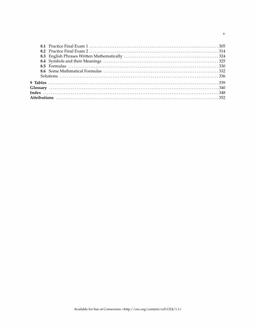
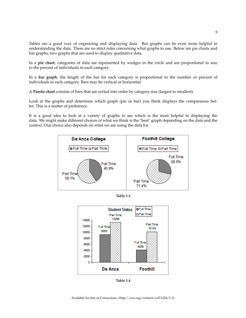
Qualitative Data DiscussionBelow are tables of part-time vs full-time students at De Anza College in Cupertino, CA and Foothill Col-lege in Los Altos, CA for the Spring 2010 quarter. The tables display counts (frequencies) and percentagesor proportions (relative frequencies). The percent columns make comparing the same categories in the col-leges easier. Displaying percentages along with the numbers is often helpful, but it is particularly importantwhen comparing sets of data that do not have the same totals, such as the total enrollments for both col-leges in this example. Notice how much larger the percentage for part-time students at Foothill College iscompared to De Anza College.
De Anza College
Number Percent
Full-time 9,200 40.9%
Part-time 13,296 59.1%
Total 22,496 100%
Table 1.1
Foothill College
Number Percent
Full-time 4,059 28.6%
Part-time 10,124 71.4%
Total 14,183 100%
Table 1.2
Available for free at Connexions <http://cnx.org/content/col11224/1.1>
5
Tables are a good way of organizing and displaying data. But graphs can be even more helpful inunderstanding the data. There are no strict rules concerning what graphs to use. Below are pie charts andbar graphs, two graphs that are used to display qualitative data.
In a pie chart, categories of data are represented by wedges in the circle and are proportional in sizeto the percent of individuals in each category.
In a bar graph, the length of the bar for each category is proportional to the number or percent ofindividuals in each category. Bars may be vertical or horizontal.
A Pareto chart consists of bars that are sorted into order by category size (largest to smallest).
Look at the graphs and determine which graph (pie or bar) you think displays the comparisons bet-ter. This is a matter of preference.
It is a good idea to look at a variety of graphs to see which is the most helpful in displaying thedata. We might make different choices of what we think is the "best" graph depending on the data and thecontext. Our choice also depends on what we are using the data for.
Table 1.3
Table 1.4
Available for free at Connexions <http://cnx.org/content/col11224/1.1>
6 CHAPTER 1. SAMPLING AND DATA
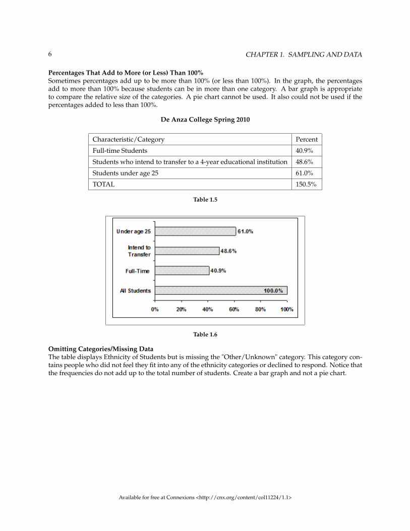
Percentages That Add to More (or Less) Than 100%Sometimes percentages add up to be more than 100% (or less than 100%). In the graph, the percentagesadd to more than 100% because students can be in more than one category. A bar graph is appropriateto compare the relative size of the categories. A pie chart cannot be used. It also could not be used if thepercentages added to less than 100%.
De Anza College Spring 2010
Characteristic/Category Percent
Full-time Students 40.9%
Students who intend to transfer to a 4-year educational institution 48.6%
Students under age 25 61.0%
TOTAL 150.5%
Table 1.5
Table 1.6
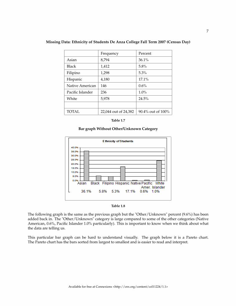
Omitting Categories/Missing DataThe table displays Ethnicity of Students but is missing the "Other/Unknown" category. This category con-tains people who did not feel they fit into any of the ethnicity categories or declined to respond. Notice thatthe frequencies do not add up to the total number of students. Create a bar graph and not a pie chart.
Available for free at Connexions <http://cnx.org/content/col11224/1.1>
7
Missing Data: Ethnicity of Students De Anza College Fall Term 2007 (Census Day)
Frequency Percent
Asian 8,794 36.1%
Black 1,412 5.8%
Filipino 1,298 5.3%
Hispanic 4,180 17.1%
Native American 146 0.6%
Pacific Islander 236 1.0%
White 5,978 24.5%
TOTAL 22,044 out of 24,382 90.4% out of 100%
Table 1.7
Bar graph Without Other/Unknown Category
Table 1.8
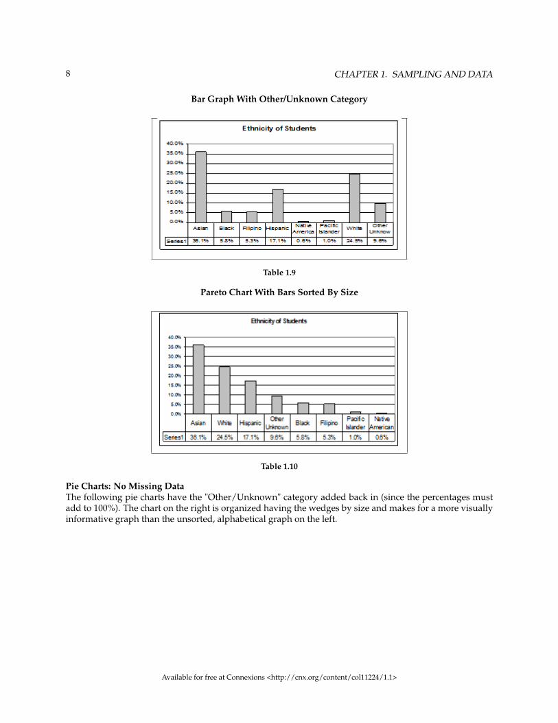
The following graph is the same as the previous graph but the "Other/Unknown" percent (9.6%) has beenadded back in. The "Other/Unknown" category is large compared to some of the other categories (NativeAmerican, 0.6%, Pacific Islander 1.0% particularly). This is important to know when we think about whatthe data are telling us.
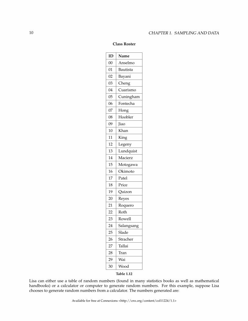
This particular bar graph can be hard to understand visually. The graph below it is a Pareto chart.The Pareto chart has the bars sorted from largest to smallest and is easier to read and interpret.
Available for free at Connexions <http://cnx.org/content/col11224/1.1>
8 CHAPTER 1. SAMPLING AND DATA
Bar Graph With Other/Unknown Category
Table 1.9
Pareto Chart With Bars Sorted By Size
Table 1.10
Pie Charts: No Missing DataThe following pie charts have the "Other/Unknown" category added back in (since the percentages mustadd to 100%). The chart on the right is organized having the wedges by size and makes for a more visuallyinformative graph than the unsorted, alphabetical graph on the left.
Available for free at Connexions <http://cnx.org/content/col11224/1.1>

9
Table 1.11
1.3 Sampling3
Gathering information about an entire population often costs too much or is virtually impossible. Instead,we use a sample of the population. A sample should have the same characteristics as the population itis representing. Most statisticians use various methods of random sampling in an attempt to achieve thisgoal. This section will describe a few of the most common methods.
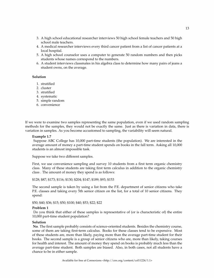
There are several different methods of random sampling. In each form of random sampling, each memberof a population initially has an equal chance of being selected for the sample. Each method has pros andcons. The easiest method to describe is called a simple random sample. Any group of n individuals isequally likely to be chosen by any other group of n individuals if the simple random sampling technique isused. In other words, each sample of the same size has an equal chance of being selected. For example, sup-pose Lisa wants to form a four-person study group (herself and three other people) from her pre-calculusclass, which has 31 members not including Lisa. To choose a simple random sample of size 3 from the othermembers of her class, Lisa could put all 31 names in a hat, shake the hat, close her eyes, and pick out 3names. A more technological way is for Lisa to first list the last names of the members of her class togetherwith a two-digit number as shown below.
3This content is available online at <http://cnx.org/content/m16014/1.17/>.
Available for free at Connexions <http://cnx.org/content/col11224/1.1>
10 CHAPTER 1. SAMPLING AND DATA
Class Roster
ID Name
00 Anselmo
01 Bautista
02 Bayani
03 Cheng
04 Cuarismo
05 Cuningham
06 Fontecha
07 Hong
08 Hoobler
09 Jiao
10 Khan
11 King
12 Legeny
13 Lundquist
14 Macierz
15 Motogawa
16 Okimoto
17 Patel
18 Price
19 Quizon
20 Reyes
21 Roquero
22 Roth
23 Rowell
24 Salangsang
25 Slade
26 Stracher
27 Tallai
28 Tran
29 Wai
30 Wood
Table 1.12
Lisa can either use a table of random numbers (found in many statistics books as well as mathematicalhandbooks) or a calculator or computer to generate random numbers. For this example, suppose Lisachooses to generate random numbers from a calculator. The numbers generated are:
Available for free at Connexions <http://cnx.org/content/col11224/1.1>

11
.94360; .99832; .14669; .51470; .40581; .73381; .04399
Lisa reads two-digit groups until she has chosen three class members (that is, she reads .94360 as the groups94, 43, 36, 60). Each random number may only contribute one class member. If she needed to, Lisa couldhave generated more random numbers.
The random numbers .94360 and .99832 do not contain appropriate two digit numbers. However the thirdrandom number, .14669, contains 14 (the fourth random number also contains 14), the fifth random numbercontains 05, and the seventh random number contains 04. The two-digit number 14 corresponds to Macierz,05 corresponds to Cunningham, and 04 corresponds to Cuarismo. Besides herself, Lisa’s group will consistof Marcierz, and Cunningham, and Cuarismo.
Besides simple random sampling, there are other forms of sampling that involve a chance process for get-ting the sample. Other well-known random sampling methods are the stratified sample, the clustersample, and the systematic sample.
To choose a stratified sample, divide the population into groups called strata and then take a proportionatenumber from each stratum. For example, you could stratify (group) your college population by departmentand then choose a proportionate simple random sample from each stratum (each department) to get a strat-ified random sample. To choose a simple random sample from each department, number each member ofthe first department, number each member of the second department and do the same for the remaining de-partments. Then use simple random sampling to choose proportionate numbers from the first departmentand do the same for each of the remaining departments. Those numbers picked from the first department,picked from the second department and so on represent the members who make up the stratified sample.
To choose a cluster sample, divide the population into clusters (groups) and then randomly select some ofthe clusters. All the members from these clusters are in the cluster sample. For example, if you randomlysample four departments from your college population, the four departments make up the cluster sample.For example, divide your college faculty by department. The departments are the clusters. Number eachdepartment and then choose four different numbers using simple random sampling. All members of thefour departments with those numbers are the cluster sample.
To choose a systematic sample, randomly select a starting point and take every nth piece of data from alisting of the population. For example, suppose you have to do a phone survey. Your phone book contains20,000 residence listings. You must choose 400 names for the sample. Number the population 1 - 20,000and then use a simple random sample to pick a number that represents the first name of the sample. Thenchoose every 50th name thereafter until you have a total of 400 names (you might have to go back to the ofyour phone list). Systematic sampling is frequently chosen because it is a simple method.
A type of sampling that is nonrandom is convenience sampling. Convenience sampling involves usingresults that are readily available. For example, a computer software store conducts a marketing study byinterviewing potential customers who happen to be in the store browsing through the available software.The results of convenience sampling may be very good in some cases and highly biased (favors certainoutcomes) in others.
Sampling data should be done very carefully. Collecting data carelessly can have devastating results. Sur-veys mailed to households and then returned may be very biased (for example, they may favor a certaingroup). It is better for the person conducting the survey to select the sample respondents.
True random sampling is done with replacement. That is, once a member is picked that member goesback into the population and thus may be chosen more than once. However for practical reasons, in mostpopulations, simple random sampling is done without replacement. Surveys are typically done withoutreplacement. That is, a member of the population may be chosen only once. Most samples are taken fromlarge populations and the sample tends to be small in comparison to the population. Since this is the case,
Available for free at Connexions <http://cnx.org/content/col11224/1.1>

12 CHAPTER 1. SAMPLING AND DATA
sampling without replacement is approximately the same as sampling with replacement because the chanceof picking the same individual more than once using with replacement is very low.
For example, in a college population of 10,000 people, suppose you want to randomly pick a sample of 1000for a survey. For any particular sample of 1000, if you are sampling with replacement,
• the chance of picking the first person is 1000 out of 10,000 (0.1000);• the chance of picking a different second person for this sample is 999 out of 10,000 (0.0999);• the chance of picking the same person again is 1 out of 10,000 (very low).
If you are sampling without replacement,
• the chance of picking the first person for any particular sample is 1000 out of 10,000 (0.1000);• the chance of picking a different second person is 999 out of 9,999 (0.0999);• you do not replace the first person before picking the next person.
Compare the fractions 999/10,000 and 999/9,999. For accuracy, carry the decimal answers to 4 place deci-mals. To 4 decimal places, these numbers are equivalent (0.0999).
Sampling without replacement instead of sampling with replacement only becomes a mathematics issuewhen the population is small which is not that common. For example, if the population is 25 people, thesample is 10 and you are sampling with replacement for any particular sample,
• the chance of picking the first person is 10 out of 25 and a different second person is 9 out of 25 (youreplace the first person).
If you sample without replacement,
• the chance of picking the first person is 10 out of 25 and then the second person (which is different) is9 out of 24 (you do not replace the first person).
Compare the fractions 9/25 and 9/24. To 4 decimal places, 9/25 = 0.3600 and 9/24 = 0.3750. To 4 decimalplaces, these numbers are not equivalent.
When you analyze data, it is important to be aware of sampling errors and nonsampling errors. The actualprocess of sampling causes sampling errors. For example, the sample may not be large enough. Factorsnot related to the sampling process cause nonsampling errors. A defective counting device can cause anonsampling error.
In reality, a sample will never be exactly representative of the population so there will always besome sampling error. As a rule, the larger the sample, the smaller the sampling error.
In statistics, a sampling bias is created when a sample is collected from a population and somemembers of the population are not as likely to be chosen as others (remember, each member of thepopulation should have an equally likely chance of being chosen). When a sampling bias happens, therecan be incorrect conclusions drawn about the population that is being studied.
Example 1.6Determine the type of sampling used (simple random, stratified, systematic, cluster, or conve-
nience).
1. A soccer coach selects 6 players from a group of boys aged 8 to 10, 7 players from a group ofboys aged 11 to 12, and 3 players from a group of boys aged 13 to 14 to form a recreationalsoccer team.
2. A pollster interviews all human resource personnel in five different high tech companies.
Available for free at Connexions <http://cnx.org/content/col11224/1.1>
13
3. A high school educational researcher interviews 50 high school female teachers and 50 highschool male teachers.
4. A medical researcher interviews every third cancer patient from a list of cancer patients at alocal hospital.
5. A high school counselor uses a computer to generate 50 random numbers and then picksstudents whose names correspond to the numbers.
6. A student interviews classmates in his algebra class to determine how many pairs of jeans astudent owns, on the average.
Solution
1. stratified2. cluster3. stratified4. systematic5. simple random6. convenience
If we were to examine two samples representing the same population, even if we used random samplingmethods for the samples, they would not be exactly the same. Just as there is variation in data, there isvariation in samples. As you become accustomed to sampling, the variability will seem natural.
Example 1.7Suppose ABC College has 10,000 part-time students (the population). We are interested in the
average amount of money a part-time student spends on books in the fall term. Asking all 10,000students is an almost impossible task.
Suppose we take two different samples.
First, we use convenience sampling and survey 10 students from a first term organic chemistryclass. Many of these students are taking first term calculus in addition to the organic chemistryclass . The amount of money they spend is as follows:
$128; $87; $173; $116; $130; $204; $147; $189; $93; $153
The second sample is taken by using a list from the P.E. department of senior citizens who takeP.E. classes and taking every 5th senior citizen on the list, for a total of 10 senior citizens. Theyspend:
$50; $40; $36; $15; $50; $100; $40; $53; $22; $22Problem 1Do you think that either of these samples is representative of (or is characteristic of) the entire
10,000 part-time student population?
SolutionNo. The first sample probably consists of science-oriented students. Besides the chemistry course,some of them are taking first-term calculus. Books for these classes tend to be expensive. Mostof these students are, more than likely, paying more than the average part-time student for theirbooks. The second sample is a group of senior citizens who are, more than likely, taking coursesfor health and interest. The amount of money they spend on books is probably much less than theaverage part-time student. Both samples are biased. Also, in both cases, not all students have achance to be in either sample.
Available for free at Connexions <http://cnx.org/content/col11224/1.1>

14 CHAPTER 1. SAMPLING AND DATA
Problem 2Since these samples are not representative of the entire population, is it wise to use the results to
describe the entire population?
SolutionNo. For these samples, each member of the population did not have an equally likely chance of
being chosen.
Now, suppose we take a third sample. We choose ten different part-time students from the dis-ciplines of chemistry, math, English, psychology, sociology, history, nursing, physical education,art, and early childhood development. (We assume that these are the only disciplines in whichpart-time students at ABC College are enrolled and that an equal number of part-time studentsare enrolled in each of the disciplines.) Each student is chosen using simple random sampling.Using a calculator, random numbers are generated and a student from a particular discipline isselected if he/she has a corresponding number. The students spend:
$180; $50; $150; $85; $260; $75; $180; $200; $200; $150Problem 3Is the sample biased?
SolutionThe sample is unbiased, but a larger sample would be recommended to increase the likelihood
that the sample will be close to representative of the population. However, for a biased samplingtechnique, even a large sample runs the risk of not being representative of the population.
Students often ask if it is "good enough" to take a sample, instead of surveying the entire popula-tion. If the survey is done well, the answer is yes.
1.3.1 Optional Collaborative Classroom Exercise
Exercise 1.3.1As a class, determine whether or not the following samples are representative. If they are not,
discuss the reasons.
1. To find the average GPA of all students in a university, use all honor students at the univer-sity as the sample.
2. To find out the most popular cereal among young people under the age of 10, stand outsidea large supermarket for three hours and speak to every 20th child under age 10 who entersthe supermarket.
3. To find the average annual income of all adults in the United States, sample U.S. congress-men. Create a cluster sample by considering each state as a stratum (group). By using simplerandom sampling, select states to be part of the cluster. Then survey every U.S. congressmanin the cluster.
4. To determine the proportion of people taking public transportation to work, survey 20 peo-ple in New York City. Conduct the survey by sitting in Central Park on a bench and inter-viewing every person who sits next to you.
5. To determine the average cost of a two day stay in a hospital in Massachusetts, survey 100hospitals across the state using simple random sampling.
Available for free at Connexions <http://cnx.org/content/col11224/1.1>
15
1.4 Variation4
1.4.1 Variation in Data
Variation is present in any set of data. For example, 16-ounce cans of beverage may contain more or lessthan 16 ounces of liquid. In one study, eight 16 ounce cans were measured and produced the followingamount (in ounces) of beverage:
15.8; 16.1; 15.2; 14.8; 15.8; 15.9; 16.0; 15.5
Measurements of the amount of beverage in a 16-ounce can may vary because different people make themeasurements or because the exact amount, 16 ounces of liquid, was not put into the cans. Manufacturersregularly run tests to determine if the amount of beverage in a 16-ounce can falls within the desired range.
Be aware that as you take data, your data may vary somewhat from the data someone else is taking for thesame purpose. This is completely natural. However, if two or more of you are taking the same data andget very different results, it is time for you and the others to reevaluate your data-taking methods and youraccuracy.
1.4.2 Variation in Samples
It was mentioned previously that two or more samples from the same population, taken randomly, andhaving close to the same characteristics of the population are different from each other. Suppose Doreen andJung both decide to study the average amount of time students at their college sleep each night. Doreen andJung each take samples of 500 students. Doreen uses systematic sampling and Jung uses cluster sampling.Doreen’s sample will be different from Jung’s sample. Even if Doreen and Jung used the same samplingmethod, in all likelihood their samples would be different. Neither would be wrong, however.
Think about what contributes to making Doreen’s and Jung’s samples different.
If Doreen and Jung took larger samples (i.e. the number of data values is increased), their sample results(the average amount of time a student sleeps) might be closer to the actual population average. But still,their samples would be, in all likelihood, different from each other. This variability in samples cannot bestressed enough.
1.4.2.1 Size of a Sample
The size of a sample (often called the number of observations) is important. The examples you have seenin this book so far have been small. Samples of only a few hundred observations, or even smaller, aresufficient for many purposes. In polling, samples that are from 1200 to 1500 observations are consideredlarge enough and good enough if the survey is random and is well done. You will learn why when youstudy confidence intervals.
Be aware that many large samples are biased. For example, call-in surveys are invariable biasedbecause people choose to respond or not.
4This content is available online at <http://cnx.org/content/m16021/1.15/>.
Available for free at Connexions <http://cnx.org/content/col11224/1.1>

16 CHAPTER 1. SAMPLING AND DATA
1.4.2.2 Optional Collaborative Classroom Exercise
Exercise 1.4.1Divide into groups of two, three, or four. Your instructor will give each group one 6-sided die.
Try this experiment twice. Roll one fair die (6-sided) 20 times. Record the number of ones, twos,threes, fours, fives, and sixes you get below ("frequency" is the number of times a particular faceof the die occurs):
First Experiment (20 rolls)
Face on Die Frequency
1
2
3
4
5
6
Table 1.13
Second Experiment (20 rolls)
Face on Die Frequency
1
2
3
4
5
6
Table 1.14
Did the two experiments have the same results? Probably not. If you did the experiment a thirdtime, do you expect the results to be identical to the first or second experiment? (Answer yes orno.) Why or why not?
Which experiment had the correct results? They both did. The job of the statistician is to seethrough the variability and draw appropriate conclusions.
1.4.3 Critical Evaluation
We need to critically evaluate the statistical studies we read about and analyze before accepting the resultsof the study. Common problems to be aware of include
• Problems with Samples: A sample should be representative of the population. A sample that is notrepresentative of the population is biased. Biased samples that are not representative of the popula-tion give results that are inaccurate and not valid.
Available for free at Connexions <http://cnx.org/content/col11224/1.1>

17
• Self-Selected Samples: Responses only by people who choose to respond, such as call-in surveys areoften unreliable.
• Sample Size Issues: Samples that are too small may be unreliable. Larger samples are better if possible.In some situations, small samples are unavoidable and can still be used to draw conclusions, eventhough larger samples are better. Examples: Crash testing cars, medical testing for rare conditions.
• Undue influence: Collecting data or asking questions in a way that influences the response.• Non-response or refusal of subject to participate: The collected responses may no longer be represen-
tative of the population. Often, people with strong positive or negative opinions may answer surveys,which can affect the results.
• Causality: A relationship between two variables does not mean that one causes the other to occur.They may both be related (correlated) because of their relationship through a different variable.
• Self-Funded or Self-Interest Studies: A study performed by a person or organization in order to sup-port their claim. Is the study impartial? Read the study carefully to evaluate the work. Do notautomatically assume that the study is good but do not automatically assume the study is bad either.Evaluate it on its merits and the work done.
• Misleading Use of Data: Improperly displayed graphs, incomplete data, lack of context.• Confounding: When the effects of multiple factors on a response cannot be separated. Confounding
makes it difficult or impossible to draw valid conclusions about the effect of each factor.
1.5 Answers and Rounding Off5
A simple way to round off answers is to carry your final answer one more decimal place than was presentin the original data. Round only the final answer. Do not round any intermediate results, if possible. If itbecomes necessary to round intermediate results, carry them to at least twice as many decimal places as thefinal answer. For example, the average of the three quiz scores 4, 6, 9 is 6.3, rounded to the nearest tenth,because the data are whole numbers. Most answers will be rounded in this manner.
It is not necessary to reduce most fractions in this course. Especially in Probability Topics (Section 4.1), thechapter on probability, it is more helpful to leave an answer as an unreduced fraction.
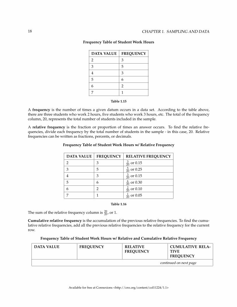
1.6 Frequency6
Twenty students were asked how many hours they worked per day. Their responses, in hours, are listedbelow:
5; 6; 3; 3; 2; 4; 7; 5; 2; 3; 5; 6; 5; 4; 4; 3; 5; 2; 5; 3
Below is a frequency table listing the different data values in ascending order and their frequencies.
5This content is available online at <http://cnx.org/content/m16006/1.8/>.6This content is available online at <http://cnx.org/content/m16012/1.20/>.
Available for free at Connexions <http://cnx.org/content/col11224/1.1>
18 CHAPTER 1. SAMPLING AND DATA
Frequency Table of Student Work Hours
DATA VALUE FREQUENCY
2 3
3 5
4 3
5 6
6 2
7 1
Table 1.15
A frequency is the number of times a given datum occurs in a data set. According to the table above,there are three students who work 2 hours, five students who work 3 hours, etc. The total of the frequencycolumn, 20, represents the total number of students included in the sample.
A relative frequency is the fraction or proportion of times an answer occurs. To find the relative fre-quencies, divide each frequency by the total number of students in the sample - in this case, 20. Relativefrequencies can be written as fractions, percents, or decimals.
Frequency Table of Student Work Hours w/ Relative Frequency
DATA VALUE FREQUENCY RELATIVE FREQUENCY
2 3 320 or 0.15
3 5 520 or 0.25
4 3 320 or 0.15
5 6 620 or 0.30
6 2 220 or 0.10
7 1 120 or 0.05
Table 1.16
The sum of the relative frequency column is 2020 , or 1.
Cumulative relative frequency is the accumulation of the previous relative frequencies. To find the cumu-lative relative frequencies, add all the previous relative frequencies to the relative frequency for the currentrow.
Frequency Table of Student Work Hours w/ Relative and Cumulative Relative Frequency
DATA VALUE FREQUENCY RELATIVEFREQUENCY
CUMULATIVE RELA-TIVEFREQUENCY
continued on next page
Available for free at Connexions <http://cnx.org/content/col11224/1.1>

19
2 3 320 or 0.15 0.15
3 5 520 or 0.25 0.15 + 0.25 = 0.40
4 3 320 or 0.15 0.40 + 0.15 = 0.55
5 6 620 or 0.30 0.55 + 0.30 = 0.85
6 2 220 or 0.10 0.85 + 0.10 = 0.95
7 1 120 or 0.05 0.95 + 0.05 = 1.00
Table 1.17
The last entry of the cumulative relative frequency column is one, indicating that one hundred percent ofthe data has been accumulated.
NOTE: Because of rounding, the relative frequency column may not always sum to one and the lastentry in the cumulative relative frequency column may not be one. However, they each should beclose to one.
The following table represents the heights, in inches, of a sample of 100 male semiprofessional soccer play-ers.
Frequency Table of Soccer Player Height
HEIGHTS(INCHES)
FREQUENCY RELATIVEFREQUENCY
CUMULATIVERELATIVEFREQUENCY
59.95 - 61.95 5 5100 = 0.05 0.05
61.95 - 63.95 3 3100 = 0.03 0.05 + 0.03 = 0.08
63.95 - 65.95 15 15100 = 0.15 0.08 + 0.15 = 0.23
65.95 - 67.95 40 40100 = 0.40 0.23 + 0.40 = 0.63
67.95 - 69.95 17 17100 = 0.17 0.63 + 0.17 = 0.80
69.95 - 71.95 12 12100 = 0.12 0.80 + 0.12 = 0.92
71.95 - 73.95 7 7100 = 0.07 0.92 + 0.07 = 0.99
73.95 - 75.95 1 1100 = 0.01 0.99 + 0.01 = 1.00
Total = 100 Total = 1.00
Table 1.18
The data in this table has been grouped into the following intervals:
• 59.95 - 61.95 inches• 61.95 - 63.95 inches• 63.95 - 65.95 inches• 65.95 - 67.95 inches• 67.95 - 69.95 inches• 69.95 - 71.95 inches• 71.95 - 73.95 inches• 73.95 - 75.95 inches
Available for free at Connexions <http://cnx.org/content/col11224/1.1>
20 CHAPTER 1. SAMPLING AND DATA
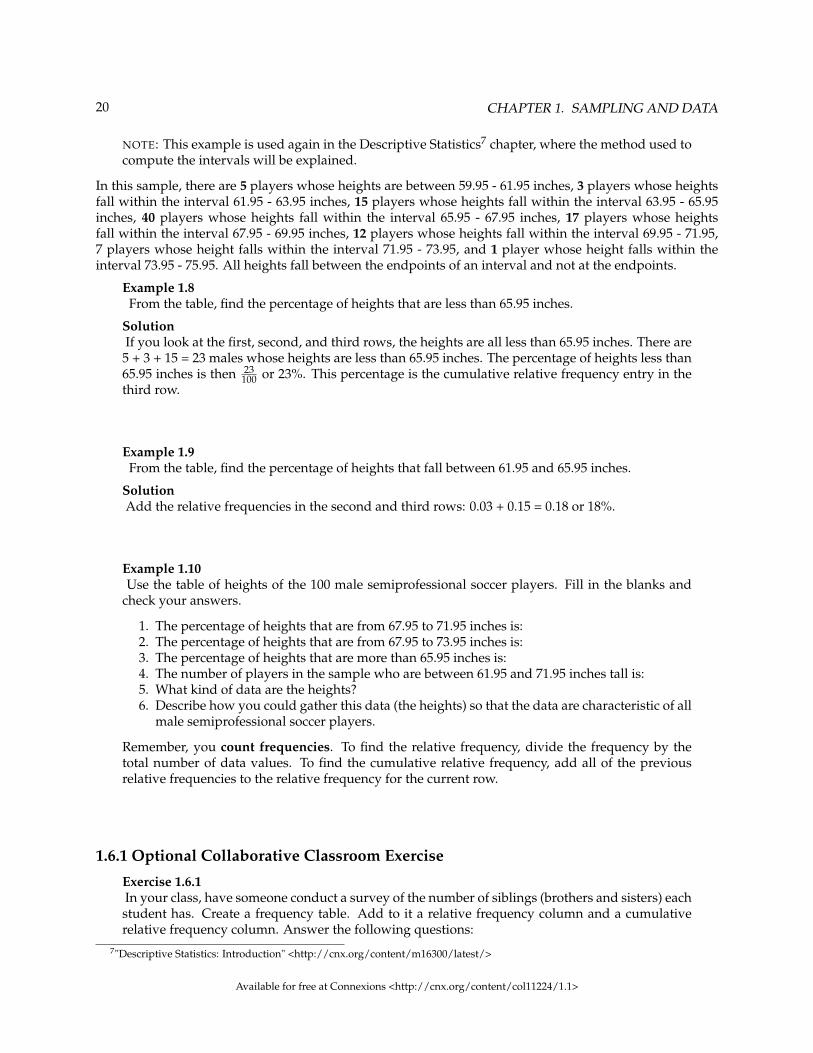
NOTE: This example is used again in the Descriptive Statistics7 chapter, where the method used tocompute the intervals will be explained.
In this sample, there are 5 players whose heights are between 59.95 - 61.95 inches, 3 players whose heightsfall within the interval 61.95 - 63.95 inches, 15 players whose heights fall within the interval 63.95 - 65.95inches, 40 players whose heights fall within the interval 65.95 - 67.95 inches, 17 players whose heightsfall within the interval 67.95 - 69.95 inches, 12 players whose heights fall within the interval 69.95 - 71.95,7 players whose height falls within the interval 71.95 - 73.95, and 1 player whose height falls within theinterval 73.95 - 75.95. All heights fall between the endpoints of an interval and not at the endpoints.
Example 1.8From the table, find the percentage of heights that are less than 65.95 inches.
SolutionIf you look at the first, second, and third rows, the heights are all less than 65.95 inches. There are5 + 3 + 15 = 23 males whose heights are less than 65.95 inches. The percentage of heights less than65.95 inches is then 23
100 or 23%. This percentage is the cumulative relative frequency entry in thethird row.
Example 1.9From the table, find the percentage of heights that fall between 61.95 and 65.95 inches.
SolutionAdd the relative frequencies in the second and third rows: 0.03 + 0.15 = 0.18 or 18%.
Example 1.10Use the table of heights of the 100 male semiprofessional soccer players. Fill in the blanks and
check your answers.
1. The percentage of heights that are from 67.95 to 71.95 inches is:2. The percentage of heights that are from 67.95 to 73.95 inches is:3. The percentage of heights that are more than 65.95 inches is:4. The number of players in the sample who are between 61.95 and 71.95 inches tall is:5. What kind of data are the heights?6. Describe how you could gather this data (the heights) so that the data are characteristic of all
male semiprofessional soccer players.
Remember, you count frequencies. To find the relative frequency, divide the frequency by thetotal number of data values. To find the cumulative relative frequency, add all of the previousrelative frequencies to the relative frequency for the current row.
1.6.1 Optional Collaborative Classroom Exercise
Exercise 1.6.1In your class, have someone conduct a survey of the number of siblings (brothers and sisters) eachstudent has. Create a frequency table. Add to it a relative frequency column and a cumulativerelative frequency column. Answer the following questions:
7"Descriptive Statistics: Introduction" <http://cnx.org/content/m16300/latest/>
Available for free at Connexions <http://cnx.org/content/col11224/1.1>
21
1. What percentage of the students in your class has 0 siblings?2. What percentage of the students has from 1 to 3 siblings?3. What percentage of the students has fewer than 3 siblings?
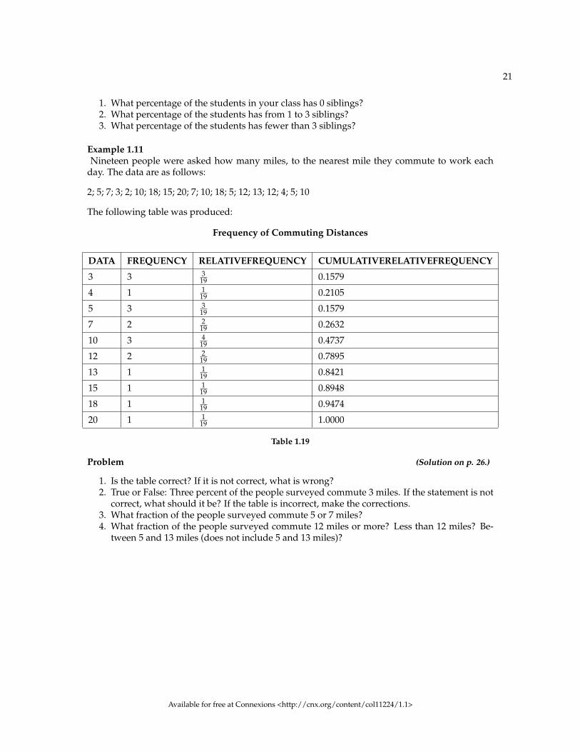
Example 1.11Nineteen people were asked how many miles, to the nearest mile they commute to work each
day. The data are as follows:
2; 5; 7; 3; 2; 10; 18; 15; 20; 7; 10; 18; 5; 12; 13; 12; 4; 5; 10
The following table was produced:
Frequency of Commuting Distances
DATA FREQUENCY RELATIVEFREQUENCY CUMULATIVERELATIVEFREQUENCY
3 3 319 0.1579
4 1 119 0.2105
5 3 319 0.1579
7 2 219 0.2632
10 3 419 0.4737
12 2 219 0.7895
13 1 119 0.8421
15 1 119 0.8948
18 1 119 0.9474
20 1 119 1.0000
Table 1.19
Problem (Solution on p. 26.)
1. Is the table correct? If it is not correct, what is wrong?2. True or False: Three percent of the people surveyed commute 3 miles. If the statement is not
correct, what should it be? If the table is incorrect, make the corrections.3. What fraction of the people surveyed commute 5 or 7 miles?4. What fraction of the people surveyed commute 12 miles or more? Less than 12 miles? Be-
tween 5 and 13 miles (does not include 5 and 13 miles)?
Available for free at Connexions <http://cnx.org/content/col11224/1.1>

22 CHAPTER 1. SAMPLING AND DATA
1.7 Summary8
Statistics
• Deals with the collection, analysis, interpretation, and presentation of data
Probability
• Mathematical tool used to study randomness
Key Terms
• Population• Parameter• Sample• Statistic• Variable• Data
Types of Data
• Quantitative Data (a number)· Discrete (You count it.)· Continuous (You measure it.)
• Qualitative Data (a category, words)
Sampling
• With Replacement: A member of the population may be chosen more than once• Without Replacement: A member of the population may be chosen only once
Random Sampling
• Each member of the population has an equal chance of being selected
Sampling Methods
• Random· Simple random sample· Stratified sample· Cluster sample· Systematic sample
• Not Random· Convenience sample
Frequency (freq. or f)
• The number of times an answer occurs
Relative Frequency (rel. freq. or RF)
• The proportion of times an answer occurs• Can be interpreted as a fraction, decimal, or percent
Cumulative Relative Frequencies (cum. rel. freq. or cum RF)
• An accumulation of the previous relative frequencies
8This content is available online at <http://cnx.org/content/m16023/1.10/>.
Available for free at Connexions <http://cnx.org/content/col11224/1.1>

23
1.8 Practice: Sampling and Data9
1.8.1 Student Learning Outcomes
• The student will construct frequency tables.• The student will differentiate between key terms.• The student will compare sampling techniques.
1.8.2 Given
Studies are often done by pharmaceutical companies to determine the effectiveness of a treatment program.Suppose that a new AIDS antibody drug is currently under study. It is given to patients once the AIDSsymptoms have revealed themselves. Of interest is the average(mean) length of time in months patientslive once starting the treatment. Two researchers each follow a different set of 40 AIDS patients from thestart of treatment until their deaths. The following data (in months) are collected.
Researcher A 3; 4; 11; 15; 16; 17; 22; 44; 37; 16; 14; 24; 25; 15; 26; 27; 33; 29; 35; 44; 13; 21; 22; 10; 12; 8; 40; 32;26; 27; 31; 34; 29; 17; 8; 24; 18; 47; 33; 34
Researcher B 3; 14; 11; 5; 16; 17; 28; 41; 31; 18; 14; 14; 26; 25; 21; 22; 31; 2; 35; 44; 23; 21; 21; 16; 12; 18; 41; 22;16; 25; 33; 34; 29; 13; 18; 24; 23; 42; 33; 29
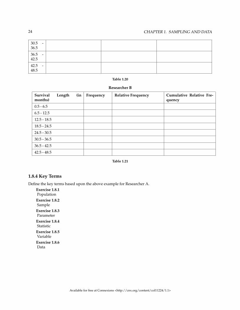
1.8.3 Organize the Data
Complete the tables below using the data provided.
Researcher A
SurvivalLength(inmonths)
Frequency Relative Frequency Cumulative Relative Fre-quency
0.5 - 6.5
6.5 -12.5
12.5 -18.5
18.5 -24.5
24.5 -30.5
continued on next page
9This content is available online at <http://cnx.org/content/m16016/1.16/>.
Available for free at Connexions <http://cnx.org/content/col11224/1.1>
24 CHAPTER 1. SAMPLING AND DATA
30.5 -36.5
36.5 -42.5
42.5 -48.5
Table 1.20
Researcher B
Survival Length (inmonths)
Frequency Relative Frequency Cumulative Relative Fre-quency
0.5 - 6.5
6.5 - 12.5
12.5 - 18.5
18.5 - 24.5
24.5 - 30.5
30.5 - 36.5
36.5 - 42.5
42.5 - 48.5
Table 1.21
1.8.4 Key Terms
Define the key terms based upon the above example for Researcher A.Exercise 1.8.1Population
Exercise 1.8.2Sample
Exercise 1.8.3Parameter
Exercise 1.8.4Statistic
Exercise 1.8.5Variable
Exercise 1.8.6Data
Available for free at Connexions <http://cnx.org/content/col11224/1.1>

25
1.8.5 Discussion Questions
Discuss the following questions and then answer in complete sentences.Exercise 1.8.7List two reasons why the data may differ.
Exercise 1.8.8Can you tell if one researcher is correct and the other one is incorrect? Why?
Exercise 1.8.9Would you expect the data to be identical? Why or why not?
Exercise 1.8.10How could the researchers gather random data?
Exercise 1.8.11Suppose that the first researcher conducted his survey by randomly choosing one state in the
nation and then randomly picking 40 patients from that state. What sampling method would thatresearcher have used?Exercise 1.8.12Suppose that the second researcher conducted his survey by choosing 40 patients he knew. Whatsampling method would that researcher have used? What concerns would you have about thisdata set, based upon the data collection method?
Available for free at Connexions <http://cnx.org/content/col11224/1.1>

26 CHAPTER 1. SAMPLING AND DATA
Solutions to Exercises in Chapter 1
Solution to Example 1.5, Problem (p. 4)Items 1, 5, 11, and 12 are quantitative discrete; items 4, 6, 10, and 14 are quantitative continuous; and items2, 3, 7, 8, 9, and 13 are qualitative.Solution to Example 1.10, Problem (p. 20)
1. 29%2. 36%3. 77%4. 875. quantitative continuous6. get rosters from each team and choose a simple random sample from each
Solution to Example 1.11, Problem (p. 21)
1. No. Frequency column sums to 18, not 19. Not all cumulative relative frequencies are correct.2. False. Frequency for 3 miles should be 1; for 2 miles (left out), 2. Cumulative relative frequency
column should read: 0.1052, 0.1579, 0.2105, 0.3684, 0.4737, 0.6316, 0.7368, 0.7895, 0.8421, 0.9474, 1.3. 5
194. 7
19 , 1219 , 7
19
Available for free at Connexions <http://cnx.org/content/col11224/1.1>

Chapter 2
Descriptive Statistics
2.1 Stem and Leaf Graphs (Stemplots), Line Graphs and Bar Graphs1
One simple graph, the stem-and-leaf graph or stem plot, comes from the field of exploratory data analy-sis.It is a good choice when the data sets are small. To create the plot, divide each observation of data intoa stem and a leaf. The leaf consists of a final significant digit. For example, 23 has stem 2 and leaf 3. Fourhundred thirty-two (432) has stem 43 and leaf 2. Five thousand four hundred thirty-two (5,432) has stem543 and leaf 2. The decimal 9.3 has stem 9 and leaf 3. Write the stems in a vertical line from smallest thelargest. Draw a vertical line to the right of the stems. Then write the leaves in increasing order next to theircorresponding stem.
Example 2.1For Susan Dean’s spring pre-calculus class, scores for the first exam were as follows (smallest tolargest):
33; 42; 49; 49; 53; 55; 55; 61; 63; 67; 68; 68; 69; 69; 72; 73; 74; 78; 80; 83; 88; 88; 88; 90; 92; 94; 94; 94; 94;96; 100
Stem-and-Leaf Diagram
Stem Leaf
3 3
4 299
5 355
6 1378899
7 2348
8 03888
9 0244446
10 0
Table 2.1
The stem plot shows that most scores fell in the 60s, 70s, 80s, and 90s. Eight out of the 31 scores orapproximately 26% of the scores were in the 90’s or 100, a fairly high number of As.
1This content is available online at <http://cnx.org/content/m16849/1.17/>.
Available for free at Connexions <http://cnx.org/content/col11224/1.1>
27

28 CHAPTER 2. DESCRIPTIVE STATISTICS
The stem plot is a quick way to graph and gives an exact picture of the data. You want to look for an overallpattern and any outliers. An outlier is an observation of data that does not fit the rest of the data. It issometimes called an extreme value. When you graph an outlier, it will appear not to fit the pattern of thegraph. Some outliers are due to mistakes (for example, writing down 50 instead of 500) while others mayindicate that something unusual is happening. It takes some background information to explain outliers.In the example above, there were no outliers.
Example 2.2Create a stem plot using the data:
1.1; 1.5; 2.3; 2.5; 2.7; 3.2; 3.3; 3.3; 3.5; 3.8; 4.0; 4.2; 4.5; 4.5; 4.7; 4.8; 5.5; 5.6; 6.5; 6.7; 12.3
The data are the distance (in kilometers) from a home to the nearest supermarket.Problem (Solution on p. 54.)
1. Are there any values that might possibly be outliers?2. Do the data seem to have any concentration of values?
HINT: The leaves are to the right of the decimal.
Another type of graph that is useful for specific data values is a line graph. In the particular line graphshown in the example, the x-axis consists of data values and the y-axis consists of frequency points. Thefrequency points are connected.
Example 2.3In a survey, 40 mothers were asked how many times per week a teenager must be reminded to dohis/her chores. The results are shown in the table and the line graph.
Number of times teenager is reminded Frequency
0 2
1 5
2 8
3 14
4 7
5 4
Table 2.2
Available for free at Connexions <http://cnx.org/content/col11224/1.1>

29
Bar graphs consist of bars that are separated from each other. The bars can be rectangles or they can berectangular boxes and they can be vertical or horizontal.
The bar graph shown in Example 4 has age groups represented on the x-axis and proportions on the y-axis.
Example 2.4By the end of 2011, in the United States, Facebook had over 146 million users. The tableshows three age groups, the number of users in each age group and the proportion (%) ofusers in each age group. Source: http://www.kenburbary.com/2011/03/facebook-demographics-revisited-2011-statistics-2/
Age groups Number of Facebook users Proportion (%) of Facebook users
13 - 25 65,082,280 45%
26 - 44 53,300,200 36%
45 - 64 27,885,100 19%
Table 2.3
Available for free at Connexions <http://cnx.org/content/col11224/1.1>

30 CHAPTER 2. DESCRIPTIVE STATISTICS
Example 2.5The columns in the table below contain the race/ethnicity of U.S. Public Schools: High SchoolClass of 2011, percentages for the Advanced Placement Examinee Population for that classand percentages for the Overall Student Population. The 3-dimensional graph shows theRace/Ethnicity of U.S. Public Schools (qualitative data) on the x-axis and Advanced PlacementExaminee Population percentages on the y-axis. (Source: http://www.collegeboard.com andSource: http://apreport.collegeboard.org/goals-and-findings/promoting-equity)
Race/Ethnicity AP Examinee Population Overall Student Population
1 = Asian, Asian American or Pa-cific Islander
10.3% 5.7%
2 = Black or African American 9.0% 14.7%
3 = Hispanic or Latino 17.0% 17.6%
4 = American Indian or AlaskaNative
0.6% 1.1%
5 = White 57.1% 59.2%
6 = Not reported/other 6.0% 1.7%
Table 2.4
Go to Outcomes of Education Figure 222 for an example of a bar graph that shows unemployment rates ofpersons 25 years and older for 2009.
NOTE: This book contains instructions for constructing a histogram and a box plot for the TI-83+and TI-84 calculators. You can find additional instructions for using these calculators on the TexasInstruments (TI) website3 .
2http://nces.ed.gov/pubs2011/2011015_5.pdf3http://education.ti.com/educationportal/sites/US/sectionHome/support.html
Available for free at Connexions <http://cnx.org/content/col11224/1.1>
31
2.2 Histograms4
For most of the work you do in this book, you will use a histogram to display the data. One advantage of ahistogram is that it can readily display large data sets. A rule of thumb is to use a histogram when the dataset consists of 100 values or more.
A histogram consists of contiguous boxes. It has both a horizontal axis and a vertical axis. The horizontalaxis is labeled with what the data represents (for instance, distance from your home to school). The verticalaxis is labeled either Frequency or relative frequency. The graph will have the same shape with eitherlabel. The histogram (like the stemplot) can give you the shape of the data, the center, and the spread of thedata. (The next section tells you how to calculate the center and the spread.)
The relative frequency is equal to the frequency for an observed value of the data divided by the totalnumber of data values in the sample. (In the chapter on Sampling and Data5, we defined frequency as thenumber of times an answer occurs.) If:
• f = frequency• n = total number of data values (or the sum of the individual frequencies), and• RF = relative frequency,
then:
RF =fn
(2.1)
For example, if 3 students in Mr. Ahab’s English class of 40 students received from 90% to 100%, then,
f = 3 , n = 40 , and RF = fn = 3
40 = 0.075
Seven and a half percent of the students received 90% to 100%. Ninety percent to 100 % are quantitativemeasures.
To construct a histogram, first decide how many bars or intervals, also called classes, represent the data.Many histograms consist of from 5 to 15 bars or classes for clarity. Choose a starting point for the firstinterval to be less than the smallest data value. A convenient starting point is a lower value carried outto one more decimal place than the value with the most decimal places. For example, if the value with themost decimal places is 6.1 and this is the smallest value, a convenient starting point is 6.05 (6.1 - 0.05 = 6.05).We say that 6.05 has more precision. If the value with the most decimal places is 2.23 and the lowest valueis 1.5, a convenient starting point is 1.495 (1.5 - 0.005 = 1.495). If the value with the most decimal places is3.234 and the lowest value is 1.0, a convenient starting point is 0.9995 (1.0 - .0005 = 0.9995). If all the datahappen to be integers and the smallest value is 2, then a convenient starting point is 1.5 (2 - 0.5 = 1.5). Also,when the starting point and other boundaries are carried to one additional decimal place, no data valuewill fall on a boundary.
Example 2.6The following data are the heights (in inches to the nearest half inch) of 100 male semiprofessionalsoccer players. The heights are continuous data since height is measured.
60; 60.5; 61; 61; 61.5
63.5; 63.5; 63.5
64; 64; 64; 64; 64; 64; 64; 64.5; 64.5; 64.5; 64.5; 64.5; 64.5; 64.5; 64.54This content is available online at <http://cnx.org/content/m16298/1.14/>.5"Sampling and Data: Introduction" <http://cnx.org/content/m16008/latest/>
Available for free at Connexions <http://cnx.org/content/col11224/1.1>

32 CHAPTER 2. DESCRIPTIVE STATISTICS
66; 66; 66; 66; 66; 66; 66; 66; 66; 66; 66.5; 66.5; 66.5; 66.5; 66.5; 66.5; 66.5; 66.5; 66.5; 66.5; 66.5; 67; 67;67; 67; 67; 67; 67; 67; 67; 67; 67; 67; 67.5; 67.5; 67.5; 67.5; 67.5; 67.5; 67.5
68; 68; 69; 69; 69; 69; 69; 69; 69; 69; 69; 69; 69.5; 69.5; 69.5; 69.5; 69.5
70; 70; 70; 70; 70; 70; 70.5; 70.5; 70.5; 71; 71; 71
72; 72; 72; 72.5; 72.5; 73; 73.5
74
The smallest data value is 60. Since the data with the most decimal places has one decimal (forinstance, 61.5), we want our starting point to have two decimal places. Since the numbers 0.5,0.05, 0.005, etc. are convenient numbers, use 0.05 and subtract it from 60, the smallest value, forthe convenient starting point.
60 - 0.05 = 59.95 which is more precise than, say, 61.5 by one decimal place. The starting point is,then, 59.95.
The largest value is 74. 74+ 0.05 = 74.05 is the ending value.
Next, calculate the width of each bar or class interval. To calculate this width, subtract the startingpoint from the ending value and divide by the number of bars (you must choose the number ofbars you desire). Suppose you choose 8 bars.
74.05− 59.958
= 1.76 (2.2)
NOTE: We will round up to 2 and make each bar or class interval 2 units wide. Rounding up to 2 isone way to prevent a value from falling on a boundary. Rounding to the next number is necessaryeven if it goes against the standard rules of rounding. For this example, using 1.76 as the widthwould also work.
The boundaries are:
• 59.95• 59.95 + 2 = 61.95• 61.95 + 2 = 63.95• 63.95 + 2 = 65.95• 65.95 + 2 = 67.95• 67.95 + 2 = 69.95• 69.95 + 2 = 71.95• 71.95 + 2 = 73.95• 73.95 + 2 = 75.95
The heights 60 through 61.5 inches are in the interval 59.95 - 61.95. The heights that are 63.5 arein the interval 61.95 - 63.95. The heights that are 64 through 64.5 are in the interval 63.95 - 65.95.The heights 66 through 67.5 are in the interval 65.95 - 67.95. The heights 68 through 69.5 are in theinterval 67.95 - 69.95. The heights 70 through 71 are in the interval 69.95 - 71.95. The heights 72through 73.5 are in the interval 71.95 - 73.95. The height 74 is in the interval 73.95 - 75.95.
The following histogram displays the heights on the x-axis and relative frequency on the y-axis.
Available for free at Connexions <http://cnx.org/content/col11224/1.1>

33
Example 2.7The following data are the number of books bought by 50 part-time college students at ABC
College. The number of books is discrete data since books are counted.
1; 1; 1; 1; 1; 1; 1; 1; 1; 1; 1
2; 2; 2; 2; 2; 2; 2; 2; 2; 2
3; 3; 3; 3; 3; 3; 3; 3; 3; 3; 3; 3; 3; 3; 3; 3
4; 4; 4; 4; 4; 4
5; 5; 5; 5; 5
6; 6
Eleven students buy 1 book. Ten students buy 2 books. Sixteen students buy 3 books. Six studentsbuy 4 books. Five students buy 5 books. Two students buy 6 books.
Because the data are integers, subtract 0.5 from 1, the smallest data value and add 0.5 to 6, thelargest data value. Then the starting point is 0.5 and the ending value is 6.5.Problem (Solution on p. 54.)Next, calculate the width of each bar or class interval. If the data are discrete and there are not toomany different values, a width that places the data values in the middle of the bar or class intervalis the most convenient. Since the data consist of the numbers 1, 2, 3, 4, 5, 6 and the starting point is0.5, a width of one places the 1 in the middle of the interval from 0.5 to 1.5, the 2 in the middle ofthe interval from 1.5 to 2.5, the 3 in the middle of the interval from 2.5 to 3.5, the 4 in the middle ofthe interval from _______ to _______, the 5 in the middle of the interval from _______ to _______,and the _______ in the middle of the interval from _______ to _______ .
Available for free at Connexions <http://cnx.org/content/col11224/1.1>

34 CHAPTER 2. DESCRIPTIVE STATISTICS
Calculate the number of bars as follows:
6.5− 0.5bars
= 1 (2.3)
where 1 is the width of a bar. Therefore, bars = 6.
The following histogram displays the number of books on the x-axis and the frequency on they-axis.
Using the TI-83, 83+, 84, 84+ Calculator InstructionsGo to the Appendix (14:Appendix) in the menu on the left. There are calculator instructions for enteringdata and for creating a customized histogram. Create the histogram for Example 2.
• Press Y=. Press CLEAR to clear out any equations.• Press STAT 1:EDIT. If L1 has data in it, arrow up into the name L1, press CLEAR and arrow down. If
necessary, do the same for L2.• Into L1, enter 1, 2, 3, 4, 5, 6• Into L2, enter 11, 10, 16, 6, 5, 2• Press WINDOW. Make Xmin = .5, Xmax = 6.5, Xscl = (6.5 - .5)/6, Ymin = -1, Ymax = 20, Yscl = 1, Xres
= 1• Press 2nd Y=. Start by pressing 4:Plotsoff ENTER.• Press 2nd Y=. Press 1:Plot1. Press ENTER. Arrow down to TYPE. Arrow to the 3rd picture (his-
togram). Press ENTER.• Arrow down to Xlist: Enter L1 (2nd 1). Arrow down to Freq. Enter L2 (2nd 2).• Press GRAPH• Use the TRACE key and the arrow keys to examine the histogram.
2.2.1 Optional Collaborative Exercise
Count the money (bills and change) in your pocket or purse. Your instructor will record the amounts. As aclass, construct a histogram displaying the data. Discuss how many intervals you think is appropriate. Youmay want to experiment with the number of intervals. Discuss, also, the shape of the histogram.
Record the data, in dollars (for example, 1.25 dollars).
Construct a histogram.
Available for free at Connexions <http://cnx.org/content/col11224/1.1>
35
2.3 Measures of the Center of the Data6
The "center" of a data set is also a way of describing location. The two most widely used measures of the"center" of the data are the mean (average) and the median. To calculate the mean weight of 50 people,add the 50 weights together and divide by 50. To find the median weight of the 50 people, order the dataand find the number that splits the data into two equal parts (previously discussed under box plots in thischapter). The median is generally a better measure of the center when there are extreme values or outliersbecause it is not affected by the precise numerical values of the outliers. The mean is the most commonmeasure of the center.
NOTE: The words "mean" and "average" are often used interchangeably. The substitution of oneword for the other is common practice. The technical term is "arithmetic mean" and "average" istechnically a center location. However, in practice among non-statisticians, "average" is commonlyaccepted for "arithmetic mean."
The mean can also be calculated by multiplying each distinct value by its frequency and then dividing thesum by the total number of data values. The letter used to represent the sample mean is an x with a barover it (pronounced "x bar"): x.
The Greek letter µ (pronounced "mew") represents the population mean. One of the requirements for thesample mean to be a good estimate of the population mean is for the sample taken to be truly random.
To see that both ways of calculating the mean are the same, consider the sample:
1; 1; 1; 2; 2; 3; 4; 4; 4; 4; 4
x =1 + 1 + 1 + 2 + 2 + 3 + 4 + 4 + 4 + 4 + 4
11= 2.7 (2.4)
x =3× 1 + 2× 2 + 1× 3 + 5× 4
11= 2.7 (2.5)
In the second calculation for the sample mean, the frequencies are 3, 2, 1, and 5.
You can quickly find the location of the median by using the expression n+12 .
The letter n is the total number of data values in the sample. If n is an odd number, the median is the middlevalue of the ordered data (ordered smallest to largest). If n is an even number, the median is equal to thetwo middle values added together and divided by 2 after the data has been ordered. For example, if thetotal number of data values is 97, then n+1
2 = 97+12 = 49. The median is the 49th value in the ordered data.
If the total number of data values is 100, then n+12 = 100+1
2 = 50.5. The median occurs midway between the50th and 51st values. The location of the median and the value of the median are not the same. The uppercase letter M is often used to represent the median. The next example illustrates the location of the medianand the value of the median.
Example 2.8AIDS data indicating the number of months an AIDS patient lives after taking a new antibody
drug are as follows (smallest to largest):
3; 4; 8; 8; 10; 11; 12; 13; 14; 15; 15; 16; 16; 17; 17; 18; 21; 22; 22; 24; 24; 25; 26; 26; 27; 27; 29; 29; 31; 32;33; 33; 34; 34; 35; 37; 40; 44; 44; 47
Calculate the mean and the median.
6This content is available online at <http://cnx.org/content/m17102/1.13/>.
Available for free at Connexions <http://cnx.org/content/col11224/1.1>
36 CHAPTER 2. DESCRIPTIVE STATISTICS
SolutionThe calculation for the mean is:
x = [3+4+(8)(2)+10+11+12+13+14+(15)(2)+(16)(2)+...+35+37+40+(44)(2)+47]40 = 23.6
To find the median, M, first use the formula for the location. The location is:
n+12 = 40+1
2 = 20.5
Starting at the smallest value, the median is located between the 20th and 21st values (the two24s):
3; 4; 8; 8; 10; 11; 12; 13; 14; 15; 15; 16; 16; 17; 17; 18; 21; 22; 22; 24; 24; 25; 26; 26; 27; 27; 29; 29; 31; 32;33; 33; 34; 34; 35; 37; 40; 44; 44; 47
M = 24+242 = 24
The median is 24.
Using the TI-83,83+,84, 84+ CalculatorsCalculator Instructions are located in the menu item 14:Appendix (Notes for the TI-83, 83+, 84,84+ Calculators).
• Enter data into the list editor. Press STAT 1:EDIT• Put the data values in list L1.• Press STAT and arrow to CALC. Press 1:1-VarStats. Press 2nd 1 for L1 and ENTER.• Press the down and up arrow keys to scroll.
x = 23.6, M = 24
Example 2.9Suppose that, in a small town of 50 people, one person earns $5,000,000 per year and the other 49
each earn $30,000. Which is the better measure of the "center," the mean or the median?
Solutionx = 5000000+49×30000
50 = 129400
M = 30000
(There are 49 people who earn $30,000 and one person who earns $5,000,000.)
The median is a better measure of the "center" than the mean because 49 of the values are 30,000and one is 5,000,000. The 5,000,000 is an outlier. The 30,000 gives us a better sense of the middle ofthe data.
Another measure of the center is the mode. The mode is the most frequent value. If a data set has twovalues that occur the same number of times, then the set is bimodal.
Example 2.10: Statistics exam scores for 20 students are as followsStatistics exam scores for 20 students are as follows:
50 ; 53 ; 59 ; 59 ; 63 ; 63 ; 72 ; 72 ; 72 ; 72 ; 72 ; 76 ; 78 ; 81 ; 83 ; 84 ; 84 ; 84 ; 90 ; 93ProblemFind the mode.
Available for free at Connexions <http://cnx.org/content/col11224/1.1>
37
SolutionThe most frequent score is 72, which occurs five times. Mode = 72.
Example 2.11Five real estate exam scores are 430, 430, 480, 480, 495. The data set is bimodal because the scores
430 and 480 each occur twice.
When is the mode the best measure of the "center"? Consider a weight loss program that advertisesa mean weight loss of six pounds the first week of the program. The mode might indicate that mostpeople lose two pounds the first week, making the program less appealing.
NOTE: The mode can be calculated for qualitative data as well as for quantitative data.
Statistical software will easily calculate the mean, the median, and the mode. Some graphingcalculators can also make these calculations. In the real world, people make these calculationsusing software.
2.3.1 The Law of Large Numbers and the Mean
The Law of Large Numbers says that if you take samples of larger and larger size from any population,then the mean x of the sample is very likely to get closer and closer to µ. This is discussed in more detail inThe Central Limit Theorem.
NOTE: The formula for the mean is located in the Summary of Formulas (Section 2.6) sectioncourse.
2.3.2 Sampling Distributions and Statistic of a Sampling Distribution
You can think of a sampling distribution as a relative frequency distribution with a great many samples.(See Sampling and Data for a review of relative frequency). Suppose thirty randomly selected studentswere asked the number of movies they watched the previous week. The results are in the relative frequencytable shown below.
# of movies Relative Frequency
0 5/30
1 15/30
2 6/30
3 4/30
4 1/30
Table 2.5
If you let the number of samples get very large (say, 300 million or more), the relative frequency tablebecomes a relative frequency distribution.
A statistic is a number calculated from a sample. Statistic examples include the mean, the median and themode as well as others. The sample mean x is an example of a statistic which estimates the populationmean µ.
Available for free at Connexions <http://cnx.org/content/col11224/1.1>
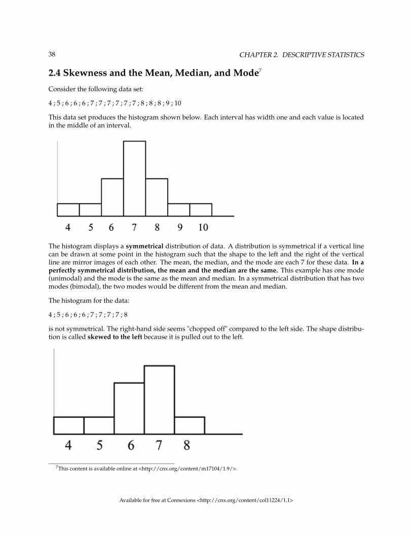
38 CHAPTER 2. DESCRIPTIVE STATISTICS
2.4 Skewness and the Mean, Median, and Mode7
Consider the following data set:
4 ; 5 ; 6 ; 6 ; 6 ; 7 ; 7 ; 7 ; 7 ; 7 ; 7 ; 8 ; 8 ; 8 ; 9 ; 10
This data set produces the histogram shown below. Each interval has width one and each value is locatedin the middle of an interval.
The histogram displays a symmetrical distribution of data. A distribution is symmetrical if a vertical linecan be drawn at some point in the histogram such that the shape to the left and the right of the verticalline are mirror images of each other. The mean, the median, and the mode are each 7 for these data. In aperfectly symmetrical distribution, the mean and the median are the same. This example has one mode(unimodal) and the mode is the same as the mean and median. In a symmetrical distribution that has twomodes (bimodal), the two modes would be different from the mean and median.
The histogram for the data:
4 ; 5 ; 6 ; 6 ; 6 ; 7 ; 7 ; 7 ; 7 ; 8
is not symmetrical. The right-hand side seems "chopped off" compared to the left side. The shape distribu-tion is called skewed to the left because it is pulled out to the left.
7This content is available online at <http://cnx.org/content/m17104/1.9/>.
Available for free at Connexions <http://cnx.org/content/col11224/1.1>

39
The mean is 6.3, the median is 6.5, and the mode is 7. Notice that the mean is less than the median andthey are both less than the mode. The mean and the median both reflect the skewing but the mean moreso.
The histogram for the data:
6 ; 7 ; 7 ; 7 ; 7 ; 8 ; 8 ; 8 ; 9 ; 10
is also not symmetrical. It is skewed to the right.
The mean is 7.7, the median is 7.5, and the mode is 7. Of the three statistics, the mean is the largest, whilethe mode is the smallest. Again, the mean reflects the skewing the most.
To summarize, generally if the distribution of data is skewed to the left, the mean is less than the median,which is often less than the mode. If the distribution of data is skewed to the right, the mode is often lessthan the median, which is less than the mean.
Skewness and symmetry become important when we discuss probability distributions in later chapters.
2.5 Measures of the Spread of the Data8
An important characteristic of any set of data is the variation in the data. In some data sets, the data valuesare concentrated closely near the mean; in other data sets, the data values are more widely spread out fromthe mean. The most common measure of variation, or spread, is the standard deviation.
The standard deviation is a number that measures how far data values are from their mean.
The standard deviation
• provides a numerical measure of the overall amount of variation in a data set• can be used to determine whether a particular data value is close to or far from the mean
The standard deviation provides a measure of the overall variation in a data setThe standard deviation is always positive or 0. The standard deviation is small when the data are allconcentrated close to the mean, exhibiting little variation or spread. The standard deviation is larger whenthe data values are more spread out from the mean, exhibiting more variation.
8This content is available online at <http://cnx.org/content/m17103/1.15/>.
Available for free at Connexions <http://cnx.org/content/col11224/1.1>

40 CHAPTER 2. DESCRIPTIVE STATISTICS
Suppose that we are studying waiting times at the checkout line for customers at supermarket A andsupermarket B; the average wait time at both markets is 5 minutes. At market A, the standard deviationfor the waiting time is 2 minutes; at market B the standard deviation for the waiting time is 4 minutes.
Because market B has a higher standard deviation, we know that there is more variation in the wait-ing times at market B. Overall, wait times at market B are more spread out from the average; wait times atmarket A are more concentrated near the average.
The standard deviation can be used to determine whether a data value is close to or far from the mean.Suppose that Rosa and Binh both shop at Market A. Rosa waits for 7 minutes and Binh waits for 1 minuteat the checkout counter. At market A, the mean wait time is 5 minutes and the standard deviation is 2minutes. The standard deviation can be used to determine whether a data value is close to or far from themean.
Rosa waits for 7 minutes:
• 7 is 2 minutes longer than the average of 5; 2 minutes is equal to one standard deviation.• Rosa’s wait time of 7 minutes is 2 minutes longer than the average of 5 minutes.• Rosa’s wait time of 7 minutes is one standard deviation above the average of 5 minutes.
Binh waits for 1 minute.
• 1 is 4 minutes less than the average of 5; 4 minutes is equal to two standard deviations.• Binh’s wait time of 1 minute is 4 minutes less than the average of 5 minutes.• Binh’s wait time of 1 minute is two standard deviations below the average of 5 minutes.• A data value that is two standard deviations from the average is just on the borderline for what many
statisticians would consider to be far from the average. Considering data to be far from the mean if itis more than 2 standard deviations away is more of an approximate "rule of thumb" than a rigid rule.In general, the shape of the distribution of the data affects how much of the data is further away than2 standard deviations. (We will learn more about this in later chapters.)
The number line may help you understand standard deviation. If we were to put 5 and 7 on a number line,7 is to the right of 5. We say, then, that 7 is one standard deviation to the right of 5 because5 + (1) (2) = 7.
If 1 were also part of the data set, then 1 is two standard deviations to the left of 5 because5 + (−2) (2) = 1.
• In general, a value = mean + (#ofSTDEV)(standard deviation)• where #ofSTDEVs = the number of standard deviations• 7 is one standard deviation more than the mean of 5 because: 7=5+(1)(2)• 1 is two standard deviations less than the mean of 5 because: 1=5+(−2)(2)
Available for free at Connexions <http://cnx.org/content/col11224/1.1>

41
The equation value = mean + (#ofSTDEVs)(standard deviation) can be expressed for a sample and for apopulation:
• sample: x = x + (#o f STDEV) (s)• Population: x = µ + (#o f STDEV) (σ)
The lower case letter s represents the sample standard deviation and the Greek letter σ (sigma, lower case)represents the population standard deviation.
The symbol x is the sample mean and the Greek symbol µ is the population mean.
Calculating the Standard DeviationIf x is a number, then the difference "x - mean" is called its deviation. In a data set, there are as manydeviations as there are items in the data set. The deviations are used to calculate the standard deviation.If the numbers belong to a population, in symbols a deviation is x − µ . For sample data, in symbols adeviation is x− x .
The procedure to calculate the standard deviation depends on whether the numbers are the entire popula-tion or are data from a sample. The calculations are similar, but not identical. Therefore the symbol usedto represent the standard deviation depends on whether it is calculated from a population or a sample.The lower case letter s represents the sample standard deviation and the Greek letter σ (sigma, lower case)represents the population standard deviation. If the sample has the same characteristics as the population,then s should be a good estimate of σ.
To calculate the standard deviation, we need to calculate the variance first. The variance is an average ofthe squares of the deviations (the x− x values for a sample, or the x − µ values for a population). Thesymbol σ2 represents the population variance; the population standard deviation σ is the square root ofthe population variance. The symbol s2 represents the sample variance; the sample standard deviation s isthe square root of the sample variance. You can think of the standard deviation as a special average of thedeviations.
If the numbers come from a census of the entire population and not a sample, when we calculate the aver-age of the squared deviations to find the variance, we divide by N, the number of items in the population.If the data are from a sample rather than a population, when we calculate the average of the squared devi-ations, we divide by n-1, one less than the number of items in the sample. You can see that in the formulasbelow.
Formulas for the Sample Standard Deviation
• s =√
Σ(x−x)2
n−1 or s =√
Σ f ·(x−x)2
n−1• For the sample standard deviation, the denominator is n-1, that is the sample size MINUS 1.
Formulas for the Population Standard Deviation
• σ =√
Σ(x−µ)2
N or σ =√
Σ f ·(x−µ)2
N• For the population standard deviation, the denominator is N, the number of items in the population.
In these formulas, f represents the frequency with which a value appears. For example, if a value appearsonce, f is 1. If a value appears three times in the data set or population, f is 3.
Sampling Variability of a StatisticThe statistic of a sampling distribution was discussed in Descriptive Statistics: Measuring the Center ofthe Data. How much the statistic varies from one sample to another is known as the sampling variability ofa statistic. You typically measure the sampling variability of a statistic by its standard error. The standard
Available for free at Connexions <http://cnx.org/content/col11224/1.1>
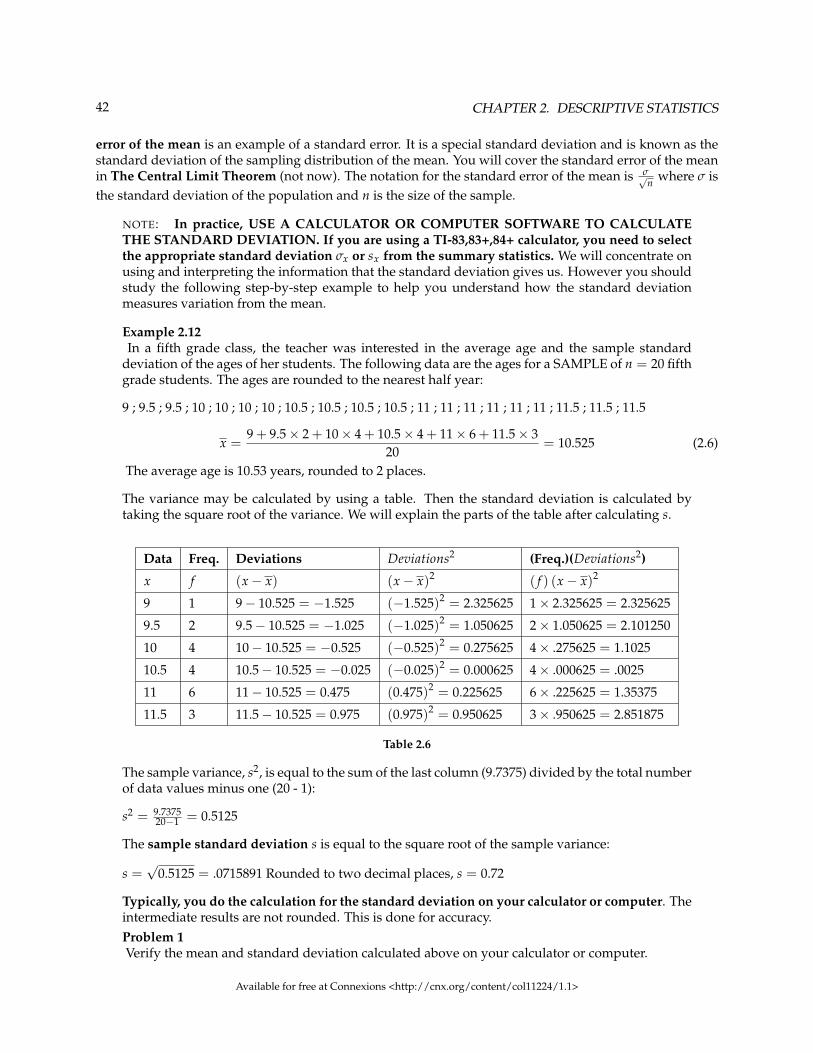
42 CHAPTER 2. DESCRIPTIVE STATISTICS
error of the mean is an example of a standard error. It is a special standard deviation and is known as thestandard deviation of the sampling distribution of the mean. You will cover the standard error of the meanin The Central Limit Theorem (not now). The notation for the standard error of the mean is σ√
n where σ isthe standard deviation of the population and n is the size of the sample.
NOTE: In practice, USE A CALCULATOR OR COMPUTER SOFTWARE TO CALCULATETHE STANDARD DEVIATION. If you are using a TI-83,83+,84+ calculator, you need to selectthe appropriate standard deviation σx or sx from the summary statistics. We will concentrate onusing and interpreting the information that the standard deviation gives us. However you shouldstudy the following step-by-step example to help you understand how the standard deviationmeasures variation from the mean.
Example 2.12In a fifth grade class, the teacher was interested in the average age and the sample standard
deviation of the ages of her students. The following data are the ages for a SAMPLE of n = 20 fifthgrade students. The ages are rounded to the nearest half year:
9 ; 9.5 ; 9.5 ; 10 ; 10 ; 10 ; 10 ; 10.5 ; 10.5 ; 10.5 ; 10.5 ; 11 ; 11 ; 11 ; 11 ; 11 ; 11 ; 11.5 ; 11.5 ; 11.5
x =9 + 9.5× 2 + 10× 4 + 10.5× 4 + 11× 6 + 11.5× 3
20= 10.525 (2.6)
The average age is 10.53 years, rounded to 2 places.
The variance may be calculated by using a table. Then the standard deviation is calculated bytaking the square root of the variance. We will explain the parts of the table after calculating s.
Data Freq. Deviations Deviations2 (Freq.)(Deviations2)
x f (x− x) (x− x)2 ( f ) (x− x)2
9 1 9− 10.525 = −1.525 (−1.525)2 = 2.325625 1× 2.325625 = 2.325625
9.5 2 9.5− 10.525 = −1.025 (−1.025)2 = 1.050625 2× 1.050625 = 2.101250
10 4 10− 10.525 = −0.525 (−0.525)2 = 0.275625 4× .275625 = 1.1025
10.5 4 10.5− 10.525 = −0.025 (−0.025)2 = 0.000625 4× .000625 = .0025
11 6 11− 10.525 = 0.475 (0.475)2 = 0.225625 6× .225625 = 1.35375
11.5 3 11.5− 10.525 = 0.975 (0.975)2 = 0.950625 3× .950625 = 2.851875
Table 2.6
The sample variance, s2, is equal to the sum of the last column (9.7375) divided by the total numberof data values minus one (20 - 1):
s2 = 9.737520−1 = 0.5125
The sample standard deviation s is equal to the square root of the sample variance:
s =√
0.5125 = .0715891 Rounded to two decimal places, s = 0.72
Typically, you do the calculation for the standard deviation on your calculator or computer. Theintermediate results are not rounded. This is done for accuracy.Problem 1Verify the mean and standard deviation calculated above on your calculator or computer.
Available for free at Connexions <http://cnx.org/content/col11224/1.1>

43
SolutionUsing the TI-83,83+,84+ Calculators
• Enter data into the list editor. Press STAT 1:EDIT. If necessary, clear the lists by arrowing upinto the name. Press CLEAR and arrow down.
• Put the data values (9, 9.5, 10, 10.5, 11, 11.5) into list L1 and the frequencies (1, 2, 4, 4, 6, 3)into list L2. Use the arrow keys to move around.
• Press STAT and arrow to CALC. Press 1:1-VarStats and enter L1 (2nd 1), L2 (2nd 2). Do notforget the comma. Press ENTER.
• x=10.525• Use Sx because this is sample data (not a population): Sx=0.715891
• For the following problems, recall that value = mean + (#ofSTDEVs)(standard deviation)• For a sample: x = x + (#ofSTDEVs)(s)• For a population: x = µ + (#ofSTDEVs)( σ)• For this example, use x = x + (#ofSTDEVs)(s) because the data is from a sample
Problem 2Find the value that is 1 standard deviation above the mean. Find (x + 1s).
Solution(x + 1s) = 10.53 + (1) (0.72) = 11.25
Problem 3Find the value that is two standard deviations below the mean. Find (x− 2s).
Solution(x− 2s) = 10.53− (2) (0.72) = 9.09
Problem 4Find the values that are 1.5 standard deviations from (below and above) the mean.
Solution
• (x− 1.5s) = 10.53− (1.5) (0.72) = 9.45• (x + 1.5s) = 10.53 + (1.5) (0.72) = 11.61
Explanation of the standard deviation calculation shown in the tableThe deviations show how spread out the data are about the mean. The data value 11.5 is farther from themean than is the data value 11. The deviations 0.97 and 0.47 indicate that. A positive deviation occurs whenthe data value is greater than the mean. A negative deviation occurs when the data value is less than themean; the deviation is -1.525 for the data value 9. If you add the deviations, the sum is always zero. (Forthis example, there are n=20 deviations.) So you cannot simply add the deviations to get the spread of thedata. By squaring the deviations, you make them positive numbers, and the sum will also be positive. Thevariance, then, is the average squared deviation.
The variance is a squared measure and does not have the same units as the data. Taking the square rootsolves the problem. The standard deviation measures the spread in the same units as the data.
Available for free at Connexions <http://cnx.org/content/col11224/1.1>

44 CHAPTER 2. DESCRIPTIVE STATISTICS
Notice that instead of dividing by n=20, the calculation divided by n-1=20-1=19 because the data is a sam-ple. For the sample variance, we divide by the sample size minus one (n− 1). Why not divide by n? Theanswer has to do with the population variance. The sample variance is an estimate of the population vari-ance. Based on the theoretical mathematics that lies behind these calculations, dividing by (n− 1) gives abetter estimate of the population variance.
NOTE: Your concentration should be on what the standard deviation tells us about the data. Thestandard deviation is a number which measures how far the data are spread from the mean. Let acalculator or computer do the arithmetic.
The standard deviation, s or σ, is either zero or larger than zero. When the standard deviation is 0, there isno spread; that is, the all the data values are equal to each other. The standard deviation is small when thedata are all concentrated close to the mean, and is larger when the data values show more variation fromthe mean. When the standard deviation is a lot larger than zero, the data values are very spread out aboutthe mean; outliers can make s or σ very large.
The standard deviation, when first presented, can seem unclear. By graphing your data, you can get abetter "feel" for the deviations and the standard deviation. You will find that in symmetrical distributions,the standard deviation can be very helpful but in skewed distributions, the standard deviation may not bemuch help. The reason is that the two sides of a skewed distribution have different spreads. In a skeweddistribution, it is better to look at the first quartile, the median, the third quartile, the smallest value, andthe largest value. Because numbers can be confusing, always graph your data.
NOTE: The formula for the standard deviation is at the end of the chapter.
Example 2.13Use the following data (first exam scores) from Susan Dean’s spring pre-calculus class:
33; 42; 49; 49; 53; 55; 55; 61; 63; 67; 68; 68; 69; 69; 72; 73; 74; 78; 80; 83; 88; 88; 88; 90; 92; 94; 94; 94; 94;96; 100
a. Create a chart containing the data, frequencies, relative frequencies, and cumulative relativefrequencies to three decimal places.
b. Calculate the following to one decimal place using a TI-83+ or TI-84 calculator:
i. The sample meanii. The sample standard deviationiii. The medianiv. The first quartilev. The third quartilevi. IQR
c. Construct a box plot and a histogram on the same set of axes. Make comments about the boxplot, the histogram, and the chart.
Solution
Available for free at Connexions <http://cnx.org/content/col11224/1.1>
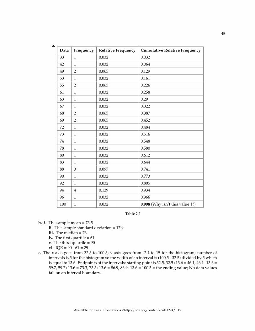
45
a.Data Frequency Relative Frequency Cumulative Relative Frequency
33 1 0.032 0.032
42 1 0.032 0.064
49 2 0.065 0.129
53 1 0.032 0.161
55 2 0.065 0.226
61 1 0.032 0.258
63 1 0.032 0.29
67 1 0.032 0.322
68 2 0.065 0.387
69 2 0.065 0.452
72 1 0.032 0.484
73 1 0.032 0.516
74 1 0.032 0.548
78 1 0.032 0.580
80 1 0.032 0.612
83 1 0.032 0.644
88 3 0.097 0.741
90 1 0.032 0.773
92 1 0.032 0.805
94 4 0.129 0.934
96 1 0.032 0.966
100 1 0.032 0.998 (Why isn’t this value 1?)
Table 2.7
b. i. The sample mean = 73.5ii. The sample standard deviation = 17.9iii. The median = 73iv. The first quartile = 61v. The third quartile = 90vi. IQR = 90 - 61 = 29
c. The x-axis goes from 32.5 to 100.5; y-axis goes from -2.4 to 15 for the histogram; number ofintervals is 5 for the histogram so the width of an interval is (100.5 - 32.5) divided by 5 whichis equal to 13.6. Endpoints of the intervals: starting point is 32.5, 32.5+13.6 = 46.1, 46.1+13.6 =59.7, 59.7+13.6 = 73.3, 73.3+13.6 = 86.9, 86.9+13.6 = 100.5 = the ending value; No data valuesfall on an interval boundary.
Available for free at Connexions <http://cnx.org/content/col11224/1.1>
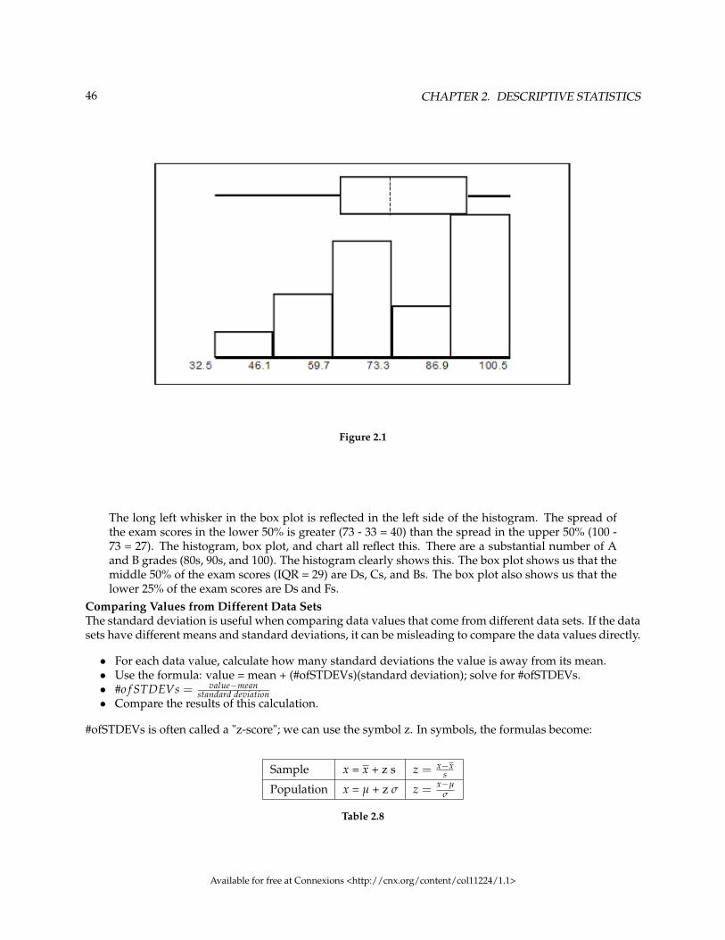
46 CHAPTER 2. DESCRIPTIVE STATISTICS
Figure 2.1
The long left whisker in the box plot is reflected in the left side of the histogram. The spread ofthe exam scores in the lower 50% is greater (73 - 33 = 40) than the spread in the upper 50% (100 -73 = 27). The histogram, box plot, and chart all reflect this. There are a substantial number of Aand B grades (80s, 90s, and 100). The histogram clearly shows this. The box plot shows us that themiddle 50% of the exam scores (IQR = 29) are Ds, Cs, and Bs. The box plot also shows us that thelower 25% of the exam scores are Ds and Fs.
Comparing Values from Different Data SetsThe standard deviation is useful when comparing data values that come from different data sets. If the datasets have different means and standard deviations, it can be misleading to compare the data values directly.
• For each data value, calculate how many standard deviations the value is away from its mean.• Use the formula: value = mean + (#ofSTDEVs)(standard deviation); solve for #ofSTDEVs.• #o f STDEVs = value−mean
standard deviation• Compare the results of this calculation.
#ofSTDEVs is often called a "z-score"; we can use the symbol z. In symbols, the formulas become:
Sample x = x + z s z = x−xs
Population x = µ + z σ z = x−µσ
Table 2.8
Available for free at Connexions <http://cnx.org/content/col11224/1.1>

47
Example 2.14Two students, John and Ali, from different high schools, wanted to find out who had the highestG.P.A. when compared to his school. Which student had the highest G.P.A. when compared to hisschool?
Student GPA School Mean GPA School Standard Deviation
John 2.85 3.0 0.7
Ali 77 80 10
Table 2.9
SolutionFor each student, determine how many standard deviations (#ofSTDEVs) his GPA is away fromthe average, for his school. Pay careful attention to signs when comparing and interpreting theanswer.
#o f STDEVs = value−meanstandard deviation ; z = x−µ
σ
For John, z = #o f STDEVs = 2.85−3.00.7 = −0.21
For Ali, z = #ofSTDEVs = 77−8010 = −0.3
John has the better G.P.A. when compared to his school because his G.P.A. is 0.21 standarddeviations below his school’s mean while Ali’s G.P.A. is 0.3 standard deviations below hisschool’s mean.
John’s z-score of −0.21 is higher than Ali’s z-score of −0.3 . For GPA, higher values arebetter, so we conclude that John has the better GPA when compared to his school.
The following lists give a few facts that provide a little more insight into what the standard deviation tellsus about the distribution of the data.For ANY data set, no matter what the distribution of the data is:
• At least 75% of the data is within 2 standard deviations of the mean.• At least 89% of the data is within 3 standard deviations of the mean.• At least 95% of the data is within 4 1/2 standard deviations of the mean.• This is known as Chebyshev’s Rule.
For data having a distribution that is MOUND-SHAPED and SYMMETRIC:
• Approximately 68% of the data is within 1 standard deviation of the mean.• Approximately 95% of the data is within 2 standard deviations of the mean.• More than 99% of the data is within 3 standard deviations of the mean.• This is known as the Empirical Rule.• It is important to note that this rule only applies when the shape of the distribution of the data is
mound-shaped and symmetric. We will learn more about this when studying the "Normal" or "Gaus-sian" probability distribution in later chapters.
**With contributions from Roberta Bloom
Available for free at Connexions <http://cnx.org/content/col11224/1.1>
48 CHAPTER 2. DESCRIPTIVE STATISTICS
2.6 Summary of Formulas9
Commonly Used Symbols
• The symbol Σ means to add or to find the sum.• n = the number of data values in a sample• N = the number of people, things, etc. in the population• x = the sample mean• s = the sample standard deviation• µ = the population mean• σ = the population standard deviation• f = frequency• x = numerical value
Commonly Used Expressions
• x ∗ f = A value multiplied by its respective frequency• ∑ x = The sum of the values• ∑ x ∗ f = The sum of values multiplied by their respective frequencies• (x− x) or (x− µ) = Deviations from the mean (how far a value is from the mean)• (x− x)2 or (x− µ)2 = Deviations squared• f (x− x)2 or f (x− µ)2 = The deviations squared and multiplied by their frequencies
Mean Formulas:
• x = ∑ xn or x = ∑ f · x
n• µ = ∑ x
N or µ= ∑ f ·xN
Standard Deviation Formulas:
• s =√
Σ(x−x)2
n−1 or s =√
Σ f ·(x−x)2
n−1
• σ =√
Σ(x−µ)2
N or σ =√
Σ f ·(x−µ)2
N
Formulas Relating a Value, the Mean, and the Standard Deviation:
• value = mean + (#ofSTDEVs)(standard deviation), where #ofSTDEVs = the number of standard devi-ations
• x = x+ (#ofSTDEVs)(s)• x = µ + (#ofSTDEVs)(σ)
9This content is available online at <http://cnx.org/content/m16310/1.9/>.
Available for free at Connexions <http://cnx.org/content/col11224/1.1>

49
2.7 Practice 1: Center of the Data10
2.7.1 Student Learning Outcomes
• The student will calculate and interpret the center, spread, and location of the data.• The student will construct and interpret histograms an box plots.
2.7.2 Given
Sixty-five randomly selected car salespersons were asked the number of cars they generally sell in oneweek. Fourteen people answered that they generally sell three cars; nineteen generally sell four cars; twelvegenerally sell five cars; nine generally sell six cars; eleven generally sell seven cars.
2.7.3 Complete the Table
Data Value (# cars) Frequency Relative Frequency Cumulative Relative Frequency
Table 2.10
2.7.4 Discussion Questions
Exercise 2.7.1 (Solution on p. 54.)What does the frequency column sum to? Why?
Exercise 2.7.2 (Solution on p. 54.)What does the relative frequency column sum to? Why?
Exercise 2.7.3What is the difference between relative frequency and frequency for each data value?
Exercise 2.7.4What is the difference between cumulative relative frequency and relative frequency for each datavalue?
2.7.5 Enter the Data
Enter your data into your calculator or computer.
10This content is available online at <http://cnx.org/content/m16312/1.12/>.
Available for free at Connexions <http://cnx.org/content/col11224/1.1>

50 CHAPTER 2. DESCRIPTIVE STATISTICS
2.7.6 Construct a Histogram
Determine appropriate minimum and maximum x and y values and the scaling. Sketch the histogrambelow. Label the horizontal and vertical axes with words. Include numerical scaling.
2.7.7 Data Statistics
Calculate the following values:Exercise 2.7.5 (Solution on p. 54.)Sample mean = x =
Exercise 2.7.6 (Solution on p. 54.)Sample standard deviation = sx =
Exercise 2.7.7 (Solution on p. 54.)Sample size = n =
2.7.8 Calculations
Use the table in section 2.11.3 to calculate the following values:Exercise 2.7.8 (Solution on p. 54.)Median =
Exercise 2.7.9 (Solution on p. 54.)Mode =
Exercise 2.7.10 (Solution on p. 54.)First quartile =
Exercise 2.7.11 (Solution on p. 54.)Second quartile = median = 50th percentile =
Exercise 2.7.12 (Solution on p. 55.)Third quartile =
Exercise 2.7.13 (Solution on p. 55.)Interquartile range (IQR) = _____ - _____ = _____
Exercise 2.7.14 (Solution on p. 55.)10th percentile =
Exercise 2.7.15 (Solution on p. 55.)70th percentile =
Available for free at Connexions <http://cnx.org/content/col11224/1.1>

51
Exercise 2.7.16 (Solution on p. 55.)Find the value that is 3 standard deviations:
a. Above the meanb. Below the mean
2.7.9 Box Plot
Construct a box plot below. Use a ruler to measure and scale accurately.
2.7.10 Interpretation
Looking at your box plot, does it appear that the data are concentrated together, spread out evenly, orconcentrated in some areas, but not in others? How can you tell?
Available for free at Connexions <http://cnx.org/content/col11224/1.1>

52 CHAPTER 2. DESCRIPTIVE STATISTICS
2.8 Practice 2: Spread of the Data11
2.8.1 Student Learning Outcomes
• The student will calculate measures of the center of the data.• The student will calculate the spread of the data.
2.8.2 Given
The population parameters below describe the full-time equivalent number of students (FTES) each yearat Lake Tahoe Community College from 1976-77 through 2004-2005. (Source: Graphically Speaking by BillKing, LTCC Institutional Research, December 2005 ).
Use these values to answer the following questions:
• µ = 1000 FTES• Median = 1014 FTES• σ = 474 FTES• First quartile = 528.5 FTES• Third quartile = 1447.5 FTES• n = 29 years
2.8.3 Calculate the Values
Exercise 2.8.1 (Solution on p. 55.)A sample of 11 years is taken. About how many are expected to have a FTES of 1014 or above?
Explain how you determined your answer.Exercise 2.8.2 (Solution on p. 55.)75% of all years have a FTES:
a. At or below:b. At or above:
Exercise 2.8.3 (Solution on p. 55.)The population standard deviation =
Exercise 2.8.4 (Solution on p. 55.)What percent of the FTES were from 528.5 to 1447.5? How do you know?
Exercise 2.8.5 (Solution on p. 55.)What is the IQR? What does the IQR represent?
Exercise 2.8.6 (Solution on p. 55.)How many standard deviations away from the mean is the median?
Additional Information: The population FTES for 2005-2006 through 2010-2011 was given in an updatedreport. (Source: http://www.ltcc.edu/data/ResourcePDF/LTCC_FactBook_2010-11.pdf). The data are re-ported here.
Year 2005-06 2006-07 2007-08 2008-09 2009-10 2010-11
Total FTES 1585 1690 1735 1935 2021 1890
11This content is available online at <http://cnx.org/content/m17105/1.12/>.
Available for free at Connexions <http://cnx.org/content/col11224/1.1>

53
Table 2.11
Exercise 2.8.7 (Solution on p. 55.)Calculate the mean, median, standard deviation, first quartile, the third quartile and the IQR.
Round to one decimal place.Exercise 2.8.8Construct a boxplot for the FTES for 2005-2006 through 2010-2011 and a boxplot for the FTES for
1976-1977 through 2004-2005.Exercise 2.8.9 (Solution on p. 55.)Compare the IQR for the FTES for 1976-77 through 2004-2005 with the IQR for the FTES for 2005-2006 through 2010-2011. Why do you suppose the IQRs are so different?
Available for free at Connexions <http://cnx.org/content/col11224/1.1>

54 CHAPTER 2. DESCRIPTIVE STATISTICS
Solutions to Exercises in Chapter 2
Solution to Example 2.2, Problem (p. 28)The value 12.3 may be an outlier. Values appear to concentrate at 3 and 4 kilometers.
Stem Leaf
1 1 5
2 3 5 7
3 2 3 3 5 8
4 0 2 5 5 7 8
5 5 6
6 5 7
7
8
9
10
11
12 3
Table 2.12
Solution to Example 2.7, Problem (p. 33)
• 3.5 to 4.5• 4.5 to 5.5• 6• 5.5 to 6.5
Solutions to Practice 1: Center of the Data
Solution to Exercise 2.7.1 (p. 49)65
Solution to Exercise 2.7.2 (p. 49)1
Solution to Exercise 2.7.5 (p. 50)4.75
Solution to Exercise 2.7.6 (p. 50)1.39
Solution to Exercise 2.7.7 (p. 50)65
Solution to Exercise 2.7.8 (p. 50)4
Solution to Exercise 2.7.9 (p. 50)4
Solution to Exercise 2.7.10 (p. 50)4
Available for free at Connexions <http://cnx.org/content/col11224/1.1>
55
Solution to Exercise 2.7.11 (p. 50)4
Solution to Exercise 2.7.12 (p. 50)6
Solution to Exercise 2.7.13 (p. 50)6 − 4 = 2
Solution to Exercise 2.7.14 (p. 50)3
Solution to Exercise 2.7.15 (p. 50)6
Solution to Exercise 2.7.16 (p. 51)
a. 8.93b. 0.58
Solutions to Practice 2: Spread of the Data
Solution to Exercise 2.8.1 (p. 52)6
Solution to Exercise 2.8.2 (p. 52)
a. 1447.5b. 528.5
Solution to Exercise 2.8.3 (p. 52)474 FTES
Solution to Exercise 2.8.4 (p. 52)50%
Solution to Exercise 2.8.5 (p. 52)919
Solution to Exercise 2.8.6 (p. 52)0.03
Solution to Exercise 2.8.7 (p. 53)mean = 1809.3
median = 1812.5standard deviation = 151.2First quartile = 1690Third quartile = 1935IQR = 245Solution to Exercise 2.8.9 (p. 53)Hint: Think about the number of years covered by each time period and what happened to higher educa-
tion during those periods.
Available for free at Connexions <http://cnx.org/content/col11224/1.1>

56 CHAPTER 2. DESCRIPTIVE STATISTICS
Available for free at Connexions <http://cnx.org/content/col11224/1.1>
Chapter 3
Sets and Counting
3.1 Sets1
Set theory is about studying collection of objects. The collection may comprise anything or any abstraction.It can be purely abstract thing like numbers or abstraction of real thing like students studying in class XI ina school. The members of collection can be numbers, letters, titles of books, people, teachers, provinces –virtually anything - even other collections. Further, it need not be finite. For example, a set of integers hasinfinite members. For a set, only requirement is that the members of a collection are properly defined.
Definition 3.1: SetA set is a collection of well defined objects.
In other words, the member of set is clearly identifiable. The terms “object”, “member” or “element” meansame thing and are used interchangeably.
3.1.1 How to represent a set?
A set is denoted by capital letters like “A”, “B”, “C” etc. In choosing a symbol for a set, it is generallyconvenient to use a capital letter that identifies with the set. For example, it is appropriate to use symbol“V” to represent collection of vowels in English alphabet.
On the other hand, the members or elements of a set are denoted by small letters like “a”,”b”,”c” etc.
Membership of a set is denoted by the symbol “ ∈” . Its literal meaning is “belongs to”. If an object doesnot belong to a set, then we convey the same, using symbol “ /∈ ”.
a ∈ A : we read this as “a” belongs to set "A".
a /∈ A : we read this as “a” does not belong to set "A".
The set is represented in two ways :
• Roaster form• Set builder form
1This content is available online at <http://cnx.org/content/m15194/1.3/>.
Available for free at Connexions <http://cnx.org/content/col11224/1.1>
57

58 CHAPTER 3. SETS AND COUNTING
3.1.1.1 Roaster form
All elements of the set are listed with a comma (“,”) in between and the listing itself is enclosed withinbraces “{“ and “}”. The order or sequence of elements within the set is not important – though desirable.
The set of numbers, which divide 12, is written as :
A = {1, 2, 3, 4, 6, 12}
If a pattern or sequence is easily made out, then we can use ellipsis ("...") to represent continuity of suchpattern. This type of representation is particularly useful to represent an infinite set. Clearly, sequence ofmembers in this type of representation is important.
The set of even numbers is written as,
B = {2, 4, 6, 8 . . . . . . . . . }
The roaster form is limited in certain circumstance. For example, we can not represent set of real numbersin roaster form. Real numbers is an infinite set, but the elements of this set do not follow a pattern or havea particular sequence. As such, we can not define same with the help of ellipsis.
Every member of the set is unique and distinct. However, we encounter situations in which collection canhave repeated elements. For example, the set representing scores of three students can be a set of threenumbers one of which is repeated :
S = {80, 80, 70}
We need to reduce such collection as :
⇒ S = {80, 80, 70} = {80, 70}
3.1.1.2 Set builder form
Collections are often characterized by a common property. We can, therefore, define members of a set interms of the common property. However, we need to ensure that objects outside the collection do not havethe same common property.
The construction of qualification for the common property is quite flexible. Only thing is that we need tobe explicit in what we mean. Generally, we denote the member by a symbol like “x” and then define themembership. Consider the examples :
A = {x: x is a vowel in English alphabet}
Available for free at Connexions <http://cnx.org/content/col11224/1.1>

59
B = {x: x is an integer and 0 < x < 10}
The roaster equivalents of two sets are :
A = {a, e, i, o, u}
B = {1, 2, 3, 4, 5, 6, 7, 8, 9}
Can we write set “B” as the one which comprises single digit natural number? Yes. Thus, we can seethat there are indeed different ways to define and identify members and hence the flexibility in definingcollection.
We should be careful in using words like “and” and “or” in writing qualification for the set. Consider theexample here :
C = {x: x ∈ Z and 2 < x < 4}
Both conditional qualifications are used to determine the collection. The elements of the set as definedabove are integers. Thus, the only member of the set is “3”.
Now, let us consider an example, which involves “or” in the qualification,
C = {x: x ∈ A or x ∈ B}
The member of this set can be elements belonging to either of two sets "A" and "B". The set consists ofelements (i) belonging exclusively to set "A", (ii) elements belonging exclusively to set "B" and (iii) elementscommon to sets "A" and "B".
3.1.1.3 Example
Problem 1 : A set in roaster form is given as :
A = {52
6,
62
7,
72
8}
Write the set in “set builder form”.
Solution : We see here that we are dealing with natural numbers. The numerators are square of naturalnumbers in sequence. The number in denominator is one more than numerator for each member. We candenote natural number by “n”. Clearly, if numerator is “ n2 ”, then denominator is “n+1”. Therefore, theexpression that represent a member of the set is :
Available for free at Connexions <http://cnx.org/content/col11224/1.1>
60 CHAPTER 3. SETS AND COUNTING
x =n2
n + 1
However, this set is not an infinite set. It has exactly three members. Therefore, we need to specify “n”so that only members of the set are exclusively denoted by the above expression. We see here that “n” isgreater than 4, but “n” is less than 8. For representing three elements of the set,
5 ≤ n ≤ 7
We can write the set, now, in the builder form as :
A = {x : x =n2
n + 1, where "n" is a natural number and 5 ≤ n ≤ 7}
In set builder form, the sequence within the range is implied. It means that we start with the first validnatural number and proceed sequentially till the last valid natural number.
3.1.2 Some important sets representing numbers
Few key number sets are used regularly in mathematical context. As we use these sets often, it is convenientto have predefined symbols :
• P(prime numbers)• N (natural numbers)• Z (integers)• Q (rational numbers)• R (real numbers)
We put a superscript “+”, if we want to specify membership of only positive numbers, where appropriate." Z+ ", for example, means set of positive integers.
3.1.3 Empty set
An empty set has no member or object. It is denoted by symbol “φ” and is represented by a pair of braceswithout any member or object.
φ = {}
The empty set is also called “null” or “void” set. For example, consider a definition : “the set of integerbetween 1 and 2”. There is no integer within this range. Hence, the set corresponding to this definition isan empty set. Consider another example :
B = {x : x2 = 4 and x is odd}
Available for free at Connexions <http://cnx.org/content/col11224/1.1>
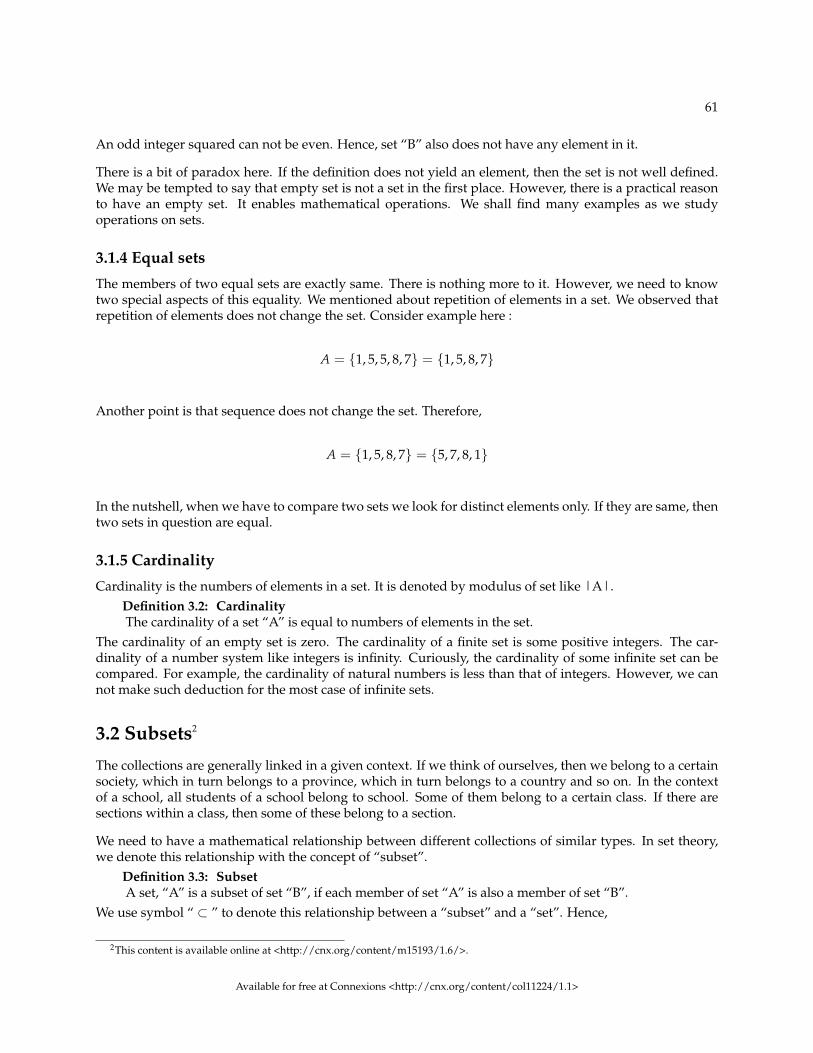
61
An odd integer squared can not be even. Hence, set “B” also does not have any element in it.
There is a bit of paradox here. If the definition does not yield an element, then the set is not well defined.We may be tempted to say that empty set is not a set in the first place. However, there is a practical reasonto have an empty set. It enables mathematical operations. We shall find many examples as we studyoperations on sets.
3.1.4 Equal sets
The members of two equal sets are exactly same. There is nothing more to it. However, we need to knowtwo special aspects of this equality. We mentioned about repetition of elements in a set. We observed thatrepetition of elements does not change the set. Consider example here :
A = {1, 5, 5, 8, 7} = {1, 5, 8, 7}
Another point is that sequence does not change the set. Therefore,
A = {1, 5, 8, 7} = {5, 7, 8, 1}
In the nutshell, when we have to compare two sets we look for distinct elements only. If they are same, thentwo sets in question are equal.
3.1.5 Cardinality
Cardinality is the numbers of elements in a set. It is denoted by modulus of set like |A|.Definition 3.2: CardinalityThe cardinality of a set “A” is equal to numbers of elements in the set.
The cardinality of an empty set is zero. The cardinality of a finite set is some positive integers. The car-dinality of a number system like integers is infinity. Curiously, the cardinality of some infinite set can becompared. For example, the cardinality of natural numbers is less than that of integers. However, we cannot make such deduction for the most case of infinite sets.
3.2 Subsets2
The collections are generally linked in a given context. If we think of ourselves, then we belong to a certainsociety, which in turn belongs to a province, which in turn belongs to a country and so on. In the contextof a school, all students of a school belong to school. Some of them belong to a certain class. If there aresections within a class, then some of these belong to a section.
We need to have a mathematical relationship between different collections of similar types. In set theory,we denote this relationship with the concept of “subset”.
Definition 3.3: SubsetA set, “A” is a subset of set “B”, if each member of set “A” is also a member of set “B”.
We use symbol “ ⊂ ” to denote this relationship between a “subset” and a “set”. Hence,
2This content is available online at <http://cnx.org/content/m15193/1.6/>.
Available for free at Connexions <http://cnx.org/content/col11224/1.1>

62 CHAPTER 3. SETS AND COUNTING
A ⊂ B
We read this symbolic representation as : set “A” is a subset of set “B”. We express the intent of relationshipas :
A ⊂ B i f x ∈ A, then x ∈ B
It is evident that set "B" is larger of the two sets. This is sometimes emphasized by calling set "B" as the“superset” of "A". We use the symbol “ ⊃ ” to denote this relation :
B ⊃ A
If set "A" is not a subset of "B", then we write this symbolically as :
A 6⊂ B
3.2.1 Important results / deductions
Some of the important characteristics and related deductions are presented here :
3.2.1.1 Equality of two sets
It is clear that set “B” is inclusive of subset “A”. It means that “B” may have additional elements over andabove those common with “B”. In case, all elements of “B” are also in “A”, then two sets are equal. Weexpress this symbolically as :
I f A ⊂ B and B ⊂ A, then A = B.
This is true in other direction as well :
I f A = B, then A ⊂ B and B ⊂ A.
We can write two instances in a single representation as :
A ⊂ B and B ⊂ A⇔ A = B
The symbol “⇔ ” means that relation holds in either direction.
Available for free at Connexions <http://cnx.org/content/col11224/1.1>

63
3.2.1.2 Relation with itself
Every set is subset of itself. This is so because every element is present in itself.
3.2.1.3 Relation with Empty set
Empty set is a subset of every set. This deduction is direct consequence of the fact that empty set has noelement. As such, this set is subset of all sets.
3.2.2 Proper subset
We have seen from the deductions above that special circumstance of “equality” can blur the distinctionbetween “set” and “subset”. In order to emphasize, mother-child relation between sets, we coin the term“proper subset”. If every element of set “B” is not present in set “A”, then “A” is a “proper” subset of set“B”; otherwise not. This means that set “B” is a larger set, which, besides other elements, also includes allelements of set “A”.
Set of vowels in English alphabet, “V”, is a “proper” subset of set of English alphabet, “E”. All elements of“V” are present in “E”, but not all elements of “E” are present in “V”.
There is a bit of conventional differences. Some write a “proper” subset relation using symbol “ ⊂ ” andwrite symbol “ ⊆ ” to mean possibility of equality as well. We have chosen not to differentiate two subsettypes.
3.2.3 Number system
The number system is one such system, in which different number groups are related. Natural number is asubset of integers. integers are subset of rational numbers and rational numbers are subset of real numbers.None of these sets are equal. Hence, relations are described by proper subsets.
N ⊂ Z
We can write the chain of relation among number sets :
⇒ P ⊂ N ⊂ Z ⊂ Q ⊂ R
However, irrational numbers are also subset of real numbers, but irrational numbers is not rational num-bers. We represent this relation by emphasizing that rational numbers is not a subset of irrational numbersor vice-versa. We depict this relation as :
Q (rational numbers) 6⊂ T (irrational numbers)
But irrational numbers is subset of real numbers. The real numbers comprises of only two subsets at thehighest level – rational and irrational. Therefore, irrational numbers is the remaining collection after de-ducting rational numbers from real numbers.
Following the logic, we define set of irrational numbers as :
Available for free at Connexions <http://cnx.org/content/col11224/1.1>

64 CHAPTER 3. SETS AND COUNTING
T (irrational numbers) = {x : x ∈ R and x /∈ Q}
3.2.4 Power set
Power set is formed of all possible subsets of a given set. It is denoted as P(A).Definition 3.4: Power setThe collection of all subsets of a set “A” is called power set, P(A).
For example, consider a set given by :
A = {1, 3, 4}
What are the possible subsets? There are three subsets consisting of individual elements: {1}, {3} and {4}.Then, elements taken two at a time form following subsets : {1,3}, {1,4} and {3,4}. Since order or sequencedoes not matter in set representation, there are only three subsets of two elements taken together. Now,the elements taken three at a time form the only one subset : {1,3,4}. Remember, a set is a subset of itself.Further, empty set (φ) is subset of any set. Hence, φ is also a subset of the given set “A”.
The set comprising of all possible subsets of given set “A” is :
P (A) = {φ, {1}, {3}, {4}, {1, 3}, {1, 4}, {3, 4}, {1, 3, 4}}
We note two important points from this representation of power set :
1: The elements of a power set are themselves sets. In other words, every element of a power set is a set.
2: If the numbers of elements (cardinality) in a set is “n”, then numbers of elements in power set is 2n .
For a set having three elements, the total numbers of elements in the power set is :
⇒ m = 2n = 23 = 8
We can see that this result is consistent with the illustration given above. We should, here, emphasize toavoid confusion that counting of elements of a set (cardinality) excludes empty set. It is, however, countedas members of power set.
3.2.5 Example
Problem 1: The finite sets “A” and “B” have “m” and “n” numbers of elements respectively. The totalnumbers of subsets of “A” is 56 more than the total numbers of subsets of “B”. Find “m” and “n”.
Solution : According to relation obtained for power set, the total numbers of subsets of “A” and “B” are :
kA = 2m
Available for free at Connexions <http://cnx.org/content/col11224/1.1>

65
kB = 2n
According to question,
kA − KB = 56
⇒ 2m − 2n = 56
We need to find two equations to find “m” and “n”. For this we seek expansion of “56” in terms of powersof “2”.
56 = 8X7 = 8 (8− 1) = 23(
23 − 1)
In order to get this form, we rearrange the expression on the LHS of the earlier equation as :
⇒ 2n (2m−n − 1)
= 23(
23 − 1)
Equating powers of similar base,
n = 3 and m = 6
3.2.6 Intervals
Intervals is an alternative way to represent a subset of real numbers. Real numbers is represented bya number line having infinite membership. We can think any segment of this number line as subset orinterval. Consider an interval, where “a” and “b” belongs to real numbers and a < b :
a < x < b
The value of “x” falls between “a” and “b”. For example, an interval 2<x<4 is a collection of all pointslying between end points 2 and 4. The important thing is that this interval does not include end points andis called “open” interval. We can represent this collection as a set in “set builder form” as :
{x : x ∈ R and 2 < x < 4}
Alternatively, we can use pair of small brackets to represent open interval as :
Available for free at Connexions <http://cnx.org/content/col11224/1.1>

66 CHAPTER 3. SETS AND COUNTING
(2, 4)
The two forms of representations are equivalent. The later form is obviously an easier and convenientrepresentation of the subset of real number. We use small braket “(“ or “)” to denote interval that excludesend point. Likewise, we use square bracket “[“ or “]” to denote interval that includes end point. We canrepresent a “close” interval as [2,4]. This interval is equivalent to :
[2, 4] = 2 ≤ x ≤ 4
We can have combination of “open” and “close” brackets like :
(2, 4] = 2 < x ≤ 4
As a reminder, we should note that interval corresponding to real numbers or its subset is an infinite set aswe can have infinite points on the line segment corresponding to an interval.
3.2.6.1 Graphical representation
The graphical representation uses a segment of line on the number line representing real numbers. The linesegment is demarcated by a pair of two small circles – a filled circle to mean that end point is included inthe interval and an unfilled circle to mean that end point is excluded from the interval.
Let us consider a,b ∈ R and a < b, then
(a, b) = a < x < b
[a, b) = a ≤ x < b
(a, b] = a < x ≤ b
[a, b] = a ≤ x ≤ b
Graphically,
Available for free at Connexions <http://cnx.org/content/col11224/1.1>

67
Intervals
Figure 3.1: Representation on real number line.
3.2.6.2 Set of real numbers
The real numbers is represented graphically by a straight line. The question that we seek to be answer hereis whether the set of integers is bounded by infinity. In other words, whether we can define interval of realnumbers like :
[−∞, ∞]
The literal meaning of infinity is “unboundedness”. Infinity is considered as a large number, which mayeither be positive or negative. It does not have a finite (fixed) value. Infinity, therefore, is not a part of realnumber system. It does not lie on the real number line. For this reason, we can not assign infinity to a realvariable like (though we do generally):
x = ∞
It follows, then, that appropriate interval, representing real numbers, is open at both ends :
R = −∞ < x < ∞ = (−∞, ∞)
3.2.6.2.1 Interval of real numbers greater than or less than a given value
In the interval form, we can write the set of real numbers greater than a given value, "a", as :
Available for free at Connexions <http://cnx.org/content/col11224/1.1>
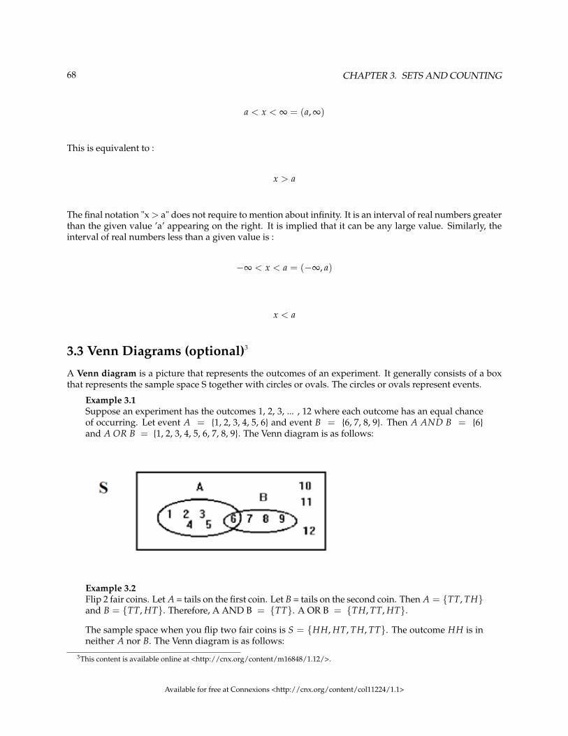
68 CHAPTER 3. SETS AND COUNTING
a < x < ∞ = (a, ∞)
This is equivalent to :
x > a
The final notation "x > a" does not require to mention about infinity. It is an interval of real numbers greaterthan the given value ’a’ appearing on the right. It is implied that it can be any large value. Similarly, theinterval of real numbers less than a given value is :
−∞ < x < a = (−∞, a)
x < a
3.3 Venn Diagrams (optional)3
A Venn diagram is a picture that represents the outcomes of an experiment. It generally consists of a boxthat represents the sample space S together with circles or ovals. The circles or ovals represent events.
Example 3.1Suppose an experiment has the outcomes 1, 2, 3, ... , 12 where each outcome has an equal chanceof occurring. Let event A = {1, 2, 3, 4, 5, 6} and event B = {6, 7, 8, 9}. Then A AND B = {6}and A OR B = {1, 2, 3, 4, 5, 6, 7, 8, 9}. The Venn diagram is as follows:
Example 3.2Flip 2 fair coins. Let A = tails on the first coin. Let B = tails on the second coin. Then A = {TT, TH}and B = {TT, HT}. Therefore, A AND B = {TT}. A OR B = {TH, TT, HT}.
The sample space when you flip two fair coins is S = {HH, HT, TH, TT}. The outcome HH is inneither A nor B. The Venn diagram is as follows:
3This content is available online at <http://cnx.org/content/m16848/1.12/>.
Available for free at Connexions <http://cnx.org/content/col11224/1.1>
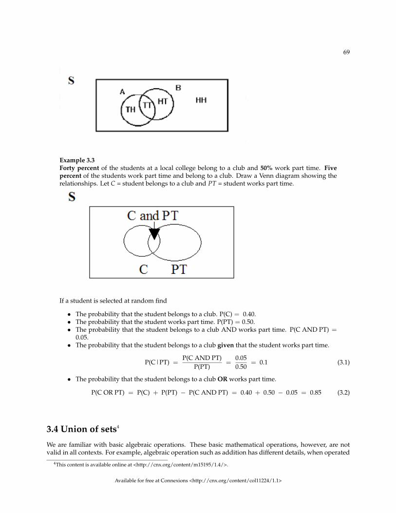
69
Example 3.3Forty percent of the students at a local college belong to a club and 50% work part time. Fivepercent of the students work part time and belong to a club. Draw a Venn diagram showing therelationships. Let C = student belongs to a club and PT = student works part time.
If a student is selected at random find
• The probability that the student belongs to a club. P(C) = 0.40.• The probability that the student works part time. P(PT) = 0.50.• The probability that the student belongs to a club AND works part time. P(C AND PT) =
0.05.• The probability that the student belongs to a club given that the student works part time.
P(C|PT) =P(C AND PT)
P(PT)=
0.050.50
= 0.1 (3.1)
• The probability that the student belongs to a club OR works part time.
P(C OR PT) = P(C) + P(PT) − P(C AND PT) = 0.40 + 0.50 − 0.05 = 0.85 (3.2)
3.4 Union of sets4
We are familiar with basic algebraic operations. These basic mathematical operations, however, are notvalid in all contexts. For example, algebraic operation such as addition has different details, when operated
4This content is available online at <http://cnx.org/content/m15195/1.4/>.
Available for free at Connexions <http://cnx.org/content/col11224/1.1>

70 CHAPTER 3. SETS AND COUNTING
on vectors. Clearly, we expect that these operations will also be not same in the case of sets – which arecollections and not individual elements.
Nevertheless, set operations bear resemblance to algebraic operation. For example, when we combine (notadd) two sets, then the operation involved is called “union”. We can see that there is resemblance of theintent of addition, subtraction etc in the case of sets also.
3.4.1 Venn diagrams
Venn diagrams are pictorial representation of sets/subsets and relationship that the sets/subsets haveamong them. It helps us to analyze relationship and carry out valid set operations in a relatively easiermanner vis – a – vis symbolic representation.
3.4.1.1 Universal set
Universal set is the largest set among collection of sets. Importantly, it is not the collection of everythingas might be conjectured by the nomenclature. For example, "R", is universal set comprising of all realnumbers. The rational numbers, integers and natural numbers are its subset. In other consideration, wecan call integers as universal set. In that case, sets such as {1,2,3}, prime numbers, even numbers, oddnumbers are subset of the universal set of integers.
The universal set is pictorially represented by a region enclosed within a rectangle on Venn diagram. Forillustration, consider the universal set of English alphabets and universal set of first 10 natural numbers asshown in the top row of the figure
Universal set
Figure 3.2: The universal set is represented by a region enclosed within a rectangle.
Many times, however, we may not be required to list elements of a universal set. In such case, we repre-sent the universal set simply by a rectangle and the symbol for universal set, “U”, in the corner. This isparticularly helpful, where number of elements in universal set are very large.
Available for free at Connexions <http://cnx.org/content/col11224/1.1>
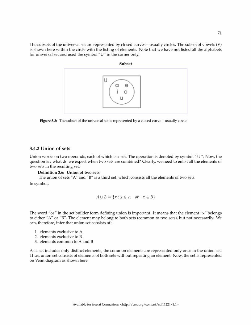
71
The subsets of the universal set are represented by closed curves – usually circles. The subset of vowels (V)is shown here within the circle with the listing of elements. Note that we have not listed all the alphabetsfor universal set and used the symbol “U” in the corner only.
Subset
Figure 3.3: The subset of the universal set is represented by a closed curve – usually circle.
3.4.2 Union of sets
Union works on two operands, each of which is a set. The operation is denoted by symbol " ∪ ". Now, thequestion is : what do we expect when two sets are combined? Clearly, we need to enlist all the elements oftwo sets in the resulting set.
Definition 3.6: Union of two setsThe union of sets “A” and “B” is a third set, which consists all the elements of two sets.
In symbol,
A ∪ B = {x : x ∈ A or x ∈ B}
The word “or” in the set builder form defining union is important. It means that the element “x” belongsto either “A” or “B”. The element may belong to both sets (common to two sets), but not necessarily. Wecan, therefore, infer that union set consists of :
1. elements exclusive to A2. elements exclusive to B3. elements common to A and B
As a set includes only distinct elements, the common elements are represented only once in the union set.Thus, union set consists of elements of both sets without repeating an element. Now, the set is representedon Venn diagram as shown here.
Available for free at Connexions <http://cnx.org/content/col11224/1.1>

72 CHAPTER 3. SETS AND COUNTING
Union of two sets
Figure 3.4: The representation of union on Venn diagram
For illustration of working with union, let us consider two sets of positive integers as given here,
A = {1, 2, 3, 4, 5, 6}
B = {4, 5, 6, 7, 8}
The union of two sets is :
⇒ A ∪ B = {1, 2, 3, 4, 5, 6, 4, 5, 6, 7, 8}
But repetition of elements in a set does not change it. Hence, we need not repeat elements in the resultingunion.
⇒ A ∪ B = {1, 2, 3, 4, 5, 6, 7, 8}
Available for free at Connexions <http://cnx.org/content/col11224/1.1>

73
Here, universal set is natural numbers. The representation of union of joint sets is shown in the figure. Wecan observe that very construction of union on Venn diagram ensures that elements are not repeated.
Union of two sets
Figure 3.5: The representation of union on Venn’s diagram
3.4.2.1 Interpretation of union set
Let us examine the defining set of union :
A ∪ B = {x : x ∈ A or x ∈ B}
We consider an arbitrary element, say “x”, of the union set. Then, we interpret the conditional meaning as:
I f x ∈ A ∪ B, then x ∈ A or x ∈ B.
Can we emphasize this conditional meaning in reverse order :
I f x ∈ A or x ∈ B, then x ∈ A ∪ B.
Available for free at Connexions <http://cnx.org/content/col11224/1.1>

74 CHAPTER 3. SETS AND COUNTING
Yes, we can agree with the second conditional meaning as well. We, therefore, conclude that the statementswork in both ways. We write two statements together as :
x ∈ A ∪ B⇔ x ∈ A or x ∈ B
We can reach yet another conclusion by observing representation of union set on Venn diagram. Now, ifan arbitrary element “x” does not belong to union set, then it is clear that it does not belong to the regionrepresented by the union set on the Venn’s diagram. Hence,
Union of two sets
Figure 3.6: The representation of union on Venn’s diagram
I f x /∈ (does not belong ) A ∪ B⇒ x /∈ A and x /∈ B.
The important thing to note here is the word “and” in place of “or” used before. Think about it. Here twoconditions follow simultaneously. If an element does not belong to an union set, then it will not belongto either of individual sets simultaneously. Now, the next thing to consider is whether this conditionalstatement will be true other way round as well?
I f x /∈ A and x /∈ B⇒ x /∈ A ∪ B.
Available for free at Connexions <http://cnx.org/content/col11224/1.1>

75
Yes, we can agree to this statement. We, therefore, conclude that the statements work in both ways. Wewrite two statements together with the help of two ways arrow sign as :
x /∈ A ∪ B⇔ x /∈ A and x /∈ B.
3.4.2.2 Union of disjoint sets
Consider students in class X and class XI. Let us denote the respective sets as "T" for tenth and "E" foreleventh class. Clearly, union i.e. combination of two sets should include elements from each of the sets.Hence,
T ∪ E = students in class X and XI
This is a straight forward union of two sets. The resulting set comprises of all elements present in both thesets. Since it is not possible that students studying in class X are also students of XI, we are sure that thenumbers of elements in the union is sum of numbers of students in each class. As there is no commonalitybetween two sets, it is a union of two “disjoint” sets. We conclude here that union of two disjoint sets hasno common elements.
3.4.2.3 Union with subset
The set “B” consists of all elements of its subset “A”. In other words, the elements of a subset “A” alsobelongs to the set “B”. The operation of union is combining elements of two sets. The union with a subset,therefore, consists of elements from both “A” and “B”. However, all elements of “A” are also the elementsof “B”. Therefore, we find that union set is same as the superset “B”. Symbolically,
I f A ⊂ B, then B ∪ A = B.
We can check this deduction with the help of an example. Let us consider two sets as :
A = {4, 5, 6}
B = {1, 2, 3, 4, 5, 6}
Here, we see that A ⊂ B. Now,
B ∪ A = {1, 2, 3, 4, 5, 6, 4, 5, 6} = {1, 2, 3, 4, 5, 6} = B
Available for free at Connexions <http://cnx.org/content/col11224/1.1>

76 CHAPTER 3. SETS AND COUNTING
Union with subset
Figure 3.7: The representation of union with subset on Venn diagram
3.4.2.4 Multiple unions
If A1, A2, A3, . . . . . . . . . , An is a finite family of sets, then their unions, one after another, is denoted as :
A1 ∪ A2 ∪ A3 ∪ . . . . . . · · · ∪ An
3.4.3 Important results
In this section we shall discuss some of the important characteristics/ deductions for the union operation.
3.4.3.1 Idempotent law
The literal meaning of the word “idempotent” is “unchanged when multiplied by itself”. Following theclue, the union of a set with itself is the set itself. This is an equivalent statement conveying the meaning of“idempotent” in the context of union. Symbolically,
A ∪ A = A
The union set consists of distinct elements and common elements taken once. Between two sets here, allelements are common. The union set consists of all elements of either set.
Available for free at Connexions <http://cnx.org/content/col11224/1.1>

77
3.4.3.2 Identity law
The algebraic operators like addition and multiplication have defined identities, which does not changethe other operand of the operator. For example, if we add “0” to a number, it remains same. Hence, “0” isadditive identity. Similarly, “1” is multiplicative identity.
In the case of union, we find that union of a set with empty set does not change the set. Hence, empty set isunion identity.
A ∪ φ = A
As there is no element in empty set, union has same elements as that in “A”.
3.4.3.3 Law of U
All sets are subsets of universal set for a given context. We have seen that union with subset results in theset itself. Clearly, union of universal set with its subset will result in the universal set itself.
U ∪ A = U
3.4.3.4 Commutative law
In order to assess whether commutative property holds or not, we consider the example, used earlier. Letthe sets be :
A = {1, 2, 3, 4, 5, 6}
B = {4, 5, 6, 7, 8}
Then,
A ∪ B = {1, 2, 3, 4, 5, 6, 4, 5, 6, 7, 8} = {1, 2, 3, 4, 5, 6, 7, 8}
B ∪ A = {4, 5, 6, 7, 8, 1, 2, 3, 4, 5, 6} = {1, 2, 3, 4, 5, 6, 7, 8}
Thus, we see that order of operands with respect to the union operator is not differentiating. We can alsoappreciate this law on Venn diagram, which does not change by changing positions of sets across unionoperator.
Available for free at Connexions <http://cnx.org/content/col11224/1.1>

78 CHAPTER 3. SETS AND COUNTING
3.4.3.5 Associative law
The associative property also holds with respect to union operator. We know that associative property isabout changing the place of parentheses as here :
(A ∪ B) ∪ C = A ∪ (B ∪ C)
The parentheses simply change the precedence of operation. On Venn diagram, union involving three setsappears same, irrespective of whether we apply union operation in a particular sequence.
Union of three sets
Figure 3.8: Associative law
3.5 Intersection of sets5
We have pointed out that a set representing a real situation is not an isolated collection. Sets, in general,overlaps with each other. It is primarily because a set is defined on few characteristics, whereas elementsgenerally can possess many characteristics. Unlike union, which includes all elements from two sets, theintersection between two sets includes only common elements.
Definition 3.7: Intersection of two setsThe intersection of sets “A” and “B” is the set of all elements common to both “A” and “B”.
5This content is available online at <http://cnx.org/content/m15196/1.2/>.
Available for free at Connexions <http://cnx.org/content/col11224/1.1>

79
The use of word “and” between two sets in defining an intersection is quite significant. Compare it withthe definition of union. We used the word “or” between two sets. Pondering on these two words, whiledeciding membership of union or intersection, is helpful in application situation.
The intersection operation is denoted by the symbol, " ∩ ". We can write intersection in set builder form as :
Intersection of two sets
Figure 3.9: The intersection set consists of elements common to two sets.
A ∩ B = {x : x ∈ A and x ∈ B}
Again note use of the word “and” in set builder qualification. We can read this as “x” is an element, whichbelongs to set “A” and set “B”. Hence, it means that “x” belongs to both “A” and “B”.
In order to understand the operation, let us consider the earlier example again,
A = {1, 2, 3, 4, 5, 6}
B = {4, 5, 6, 7, 8}
Available for free at Connexions <http://cnx.org/content/col11224/1.1>

80 CHAPTER 3. SETS AND COUNTING
Then,
A ∩ B = {4, 5, 6}
On Venn diagram, an intersection is the region intersected by circles, which represent two sets.
Intersection of two sets
Figure 3.10: The intersection set consists of elements common to two sets.
3.5.1 Interpretation of Intersection set
Let us examine the defining set of intersection :
A ∩ B = {x : x ∈ A and x ∈ B}
We consider an arbitrary element, say “x”, of the intersection set. Then, we interpret the conditional mean-ing as :
I f x ∈ A ∩ B⇒ x ∈ A and x ∈ B.
Available for free at Connexions <http://cnx.org/content/col11224/1.1>

81
The conditional statement is true in opposite direction as well. Hence,
I f x ∈ A and x ∈ B⇒ x ∈ A ∩ B.
We summarize two statements with two ways arrow as :
x ∈ A ∩ B⇔ x ∈ A and x ∈ B
In addition to two ways relation, there is an interesting aspect of intersection. Intersection is subset of eitherof two sets. From Venn diagram, it is clear that :
Intersection of two sets
Figure 3.11: The intersection set consists of elements common to two sets.
(A ∩ B) ⊂ A
and
(A ∩ B) ⊂ B
Available for free at Connexions <http://cnx.org/content/col11224/1.1>

82 CHAPTER 3. SETS AND COUNTING
3.5.1.1 Intersection with a subset
Since all elements of a subset is present in the set, it emerges that intersection with subset is subset. Hence,if “A” is subset of set “B”, then :
B ∩ A = A
3.5.1.2 Intersection of disjoint sets
If no element is common to two sets “A” and “B” , then the resulting intersection is an empty set :
A ∩ B = φ
In that case, two sets “A” and “B” are “disjoint” sets.
3.5.1.3 Multiple intersections
If A1, A2, A3, . . . . . . . . . , An is a finite family of sets, then their intersections one after another is denoted as :
A1 ∩ A2 ∩ A3 ∩ . . . . . . .∩ An
3.5.2 Important results
In this section we shall discuss some of the important characteristics/ deductions for the intersection oper-ation.
3.5.2.1 Idempotent law
The intersection of a set with itself is the set itself.
A ∩ A = A
This is because intersection is a set of common elements. Here, all elements of a set is common with itself.The resulting intersection, therefore, is set itself.
3.5.2.2 Identity law
The intersection with universal set yields the set itself. Hence, universal set functions as the identity of theintersection operator.
A ∩U = A
It is easy to interpret this law. Only the elements in "A" are common to universal set. Hence, intersection,being the set of common elements, is set "A".
Available for free at Connexions <http://cnx.org/content/col11224/1.1>

83
3.5.2.3 Law of empty set
Since empty set is element of all other sets, it emerges that intersection of an empty set with any set is anempty set (empty set is only common element between two sets).
φ ∩ A = φ
3.5.2.4 Commutative law
The order of sets around intersection operator does not change the intersection. Hence, commutative prop-erty holds in the case of intersection operation.
A ∩ B = B ∩ A
3.5.2.5 Associative law
The associative property holds with respect to intersection operator.
(A ∩ B) ∩ C = A ∩ (B ∩ C)
The intersection of sets “A” and “B” on Venn’s diagram is :
Available for free at Connexions <http://cnx.org/content/col11224/1.1>
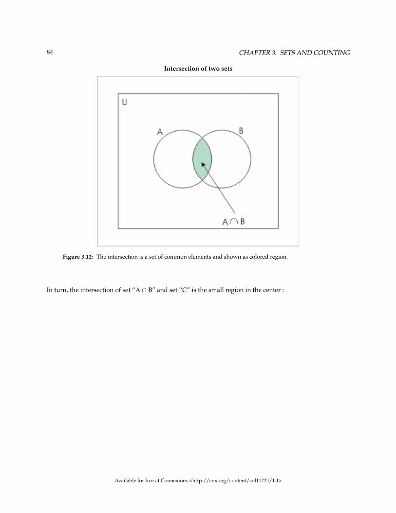
84 CHAPTER 3. SETS AND COUNTING
Intersection of two sets
Figure 3.12: The intersection is a set of common elements and shown as colored region.
In turn, the intersection of set “A ∩ B” and set “C” is the small region in the center :
Available for free at Connexions <http://cnx.org/content/col11224/1.1>

85
Intersection inloving three sets
Figure 3.13: Intersection of a set with "the intersection set of two sets"
It is easy to visualize that the ultimate intersection is independent of the sequence of operation.
3.5.2.6 Distributive law
The intersection operator( ∩ ) is distributed over union operator ( ∪ ) :
A ∩ (B ∪ C) = (A ∩ B) ∪ (A ∩ C)
We can check out this relation with the help of Venn diagram. For convenience, we have not shown theuniversal set. In the first diagram on the left, the colored region shows the union of sets “B” and “C” ie.B ∪ C . The colored region in the second diagram on the right shows the intersection of set “A” with theunion obtained in the first diagram i.e. B ∪ C .
Available for free at Connexions <http://cnx.org/content/col11224/1.1>

86 CHAPTER 3. SETS AND COUNTING
Distributive law
Figure 3.14: Distribution of intersection operator over union operator
We can now interpret the colored region in the second diagram from the point of view of expression on theright hand side of the equation :
A ∩ (B ∪ C) = (A ∩ B) ∪ (A ∩ C)
The colored region is indeed the union of two intersections : " A ∪ B" and " A ∪ C" . Thus, we conclude thatdistributive property holds for "intersection operator over union operator".
In the same manner, we can prove distribution of “union operator over intersection operator” :
A ∪ (B ∩ C) = (A ∪ B) ∩ (A ∪ C)
3.5.2.6.1 Analytical proof
Distributive properties are important and used for practical application. In this section, we shall provethe same in analytical manner. For this, let us consider an arbitrary element “x”, which belongs to set "A ∩ (B ∪ C)" :
x ∈ A ∩ (B ∪ C)
Available for free at Connexions <http://cnx.org/content/col11224/1.1>

87
Then, by definition of intersection :
⇒ x ∈ A and x ∈ (B ∪ C)
⇒ x ∈ A and (x ∈ B or x ∈ C)
⇒ (x ∈ A and x ∈ B) or (x ∈ A and x ∈ C)
⇒ (x ∈ A ∩ B) or (x ∈ A ∩ C)
⇒ x ∈ (A ∩ B) or (A ∩ C)
⇒ x ∈ (A ∩ B) ∪ (A ∩ C)
But, we had started with " A ∩ (B ∪ C) " and used its definition to show that “x” belongs to another set. Itmeans that the other set consists of the elements of the first set – at the least. Thus,
⇒ A ∩ (B ∪ C) ⊂ (A ∩ B) ∪ (A ∩ C)
Similarly, we can start with " (A ∩ B) ∪ (A ∩ C) " and reach the conclusion that :
⇒ (A ∩ B) ∪ (A ∩ C) ⊂ A ∩ (B ∪ C)
If sets are subsets of each other, then they are equal. Hence,
⇒ A ∩ (B ∪ C) = (A ∩ B) ∪ (A ∩ C)
Proceeding in the same manner, we can also prove other distributive property of “union operator overintersection operator” :
A ∪ (B ∩ C) = (A ∪ B) ∩ (A ∪ C)
Available for free at Connexions <http://cnx.org/content/col11224/1.1>

88 CHAPTER 3. SETS AND COUNTING
3.6 Difference of sets6
We can extend the concept of subtraction, used in algebra, to the sets. If a set “B” is subtracted from set “A”,the resulting difference set consists of elements, which are exclusive to set “A”. We represent the symbol ofdifference of sets as “A-B” and pronounce the same as “A minus B”.
Definition 3.8: Difference of setsThe difference of sets “A-B” is the set of all elements of “A”, which do not belong to “B”.
In the set builder form, the difference set is :
A− B = {x : x ∈ A and x /∈ B}
and
B− A = {x : x ∈ B and x /∈ A}
On Venn’s diagram, the difference "A-B" is the region of “A”, which excludes the common region with set“B”.
Difference of two sets
Figure 3.15: The difference of two sets is a disjoint set.
6This content is available online at <http://cnx.org/content/m15198/1.2/>.
Available for free at Connexions <http://cnx.org/content/col11224/1.1>

89
3.6.1 Interpretation of difference set
Let us examine the defining set of intersection :
A− B = {x : x ∈ A and x /∈ B}
We consider an arbitrary element, say “x”, of the difference set. Then, we interpret the conditional meaningas :
I f x ∈ A− B⇒ x ∈ A and x /∈ B.
The conditional statement is true in opposite direction as well. Hence,
I f x ∈ A and x /∈ B⇒ x ∈ A− B.
We can summarize two statements with two ways arrow as :
I f x ∈ A− B⇔ x ∈ A and x /∈ B.
3.6.1.1 Composition of a set
From Venn’s diagram, we observe that if we derive union of (A∩ B) to either of the difference sets, then weget the complete individual set.
Available for free at Connexions <http://cnx.org/content/col11224/1.1>

90 CHAPTER 3. SETS AND COUNTING
Difference of two sets
Figure 3.16: The difference of two sets is a disjoint set.
A = (A− B) ∪ (A ∩ B)
and
B = (B− A) ∪ (A ∩ B)
3.6.1.2 Difference of sets is not commutative
The positions of sets about minus operator affect the result. It is clear from the figure above, where “A-B”and “B-A” represent different regions on Venn’s diagram. As such, the difference of sets is not commutative.Let us consider the example used earlier, where :
A = {1, 2, 3, 4, 5, 6}
A = {4, 5, 6, 7, 8}
Available for free at Connexions <http://cnx.org/content/col11224/1.1>

91
Then,
⇒ A− B = {1, 2, 3}
and
⇒ B− A = {7, 8}
Clearly,
⇒ A− B 6= B− A
3.6.1.3 Symmetric difference
From the Venn’s diagram, we can see that union of two sets is equal to three distinct regions. Alterna-tively, we can say that the region represented by the union of two sets is equal to the sum of the regionsrepresenting three “disjoint” sets (i) difference set A-B (ii) intersection set " A ∩ B" and (iii) difference setB-A.
Difference of two sets
Figure 3.17: The difference of two sets is a disjoint set.
Available for free at Connexions <http://cnx.org/content/col11224/1.1>

92 CHAPTER 3. SETS AND COUNTING
We use the term “symmetric set” for combining two differences as marked on Venn’s diagram. It is denotedas “ A∆B”.
A∆B = (A− B) ∪ (B− A)
3.6.2 Complement of a set
The complement is a special case of the difference operation. The set in question is subtracted from uni-versal set, “U”. Thus, one of the sets in difference operation is fixed. We define complement of a set as itsdifference with universal set, "U". The complement of a set is denoted by the same symbol as that of set,but with an apostrophe. Hence, complement of set A is set A’.
Definition 3.9: Complement of a setThe complement of a set “A” consists of elements, which are elements of “U”, but not the elementsof “A”.
We write the complement set in terms of set builder form as :
A′ = {x : x ∈ U and x /∈ A}
Note that elements of A’ does not belong to set “A”. On Venn’s diagram, the complement of “A” is theremaining region of the universal set.
Available for free at Connexions <http://cnx.org/content/col11224/1.1>

93
Complement of a set
Figure 3.18: The complement of a set is the remaining region of the universal set.
3.6.2.1 Interpretation of complement
Proceeding as before we can read the conditional statement for the complement with the help of two waysarrow as :
x ∈ A′ ⇔ x ∈ U and x /∈ A
In terms of minus or difference operation,
A′ = U − A
It is clear from the representation on Venn’s diagram that the universal set comprises of two distinct sets –set A and complement set A’.
⇒ U = A ∪ A′
Available for free at Connexions <http://cnx.org/content/col11224/1.1>
94 CHAPTER 3. SETS AND COUNTING
3.6.2.2 Compliment of universal set
The complement of universal set is empty set. It is so because difference of union set with itself is the emptyset (see Venn’s diagram).
U′ = {x : x ∈ U and x /∈ U} = φ
3.6.2.3 Complement of empty set
The complement of the empty set is universal set. It is so because difference of union set with the empty setis universal set (see Venn’s diagram).
φ′ = {x : x ∈ U and x /∈ φ} = U
3.6.2.4 Complement of complement set is set itself
The complement of complement set is set itself. The complement set is defined as :
A′ = U − A
Now, complement of complement set is :
⇒ (A′) ′ = (U − A) ′
Let us consider the example, where :
U = {1, 2, 3, 4, 5, 6, 7, 8}
A = {1, 2, 3, 4, 5, 6}
Then,
⇒ A′ = {1, 2, 3, 4, 5, 6, 7, 8} − {1, 2, 3, 4, 5, 6} = {7, 8}
Again taking complement, we have :
(A′) ′ = {1, 2, 3, 4, 5, 6, 7, 8} − {7, 8} = {1, 2, 3, 4, 5, 6} = A
Available for free at Connexions <http://cnx.org/content/col11224/1.1>
95
3.6.2.5 Union with complement set
The union of a set with its complement is universal set :
A ∪ A′ = {x : x ∈ U and x ∈ A} ∪ {x : x ∈ U and x ∈ A} = U
From Venn’s diagram also, we see that universal set consists of set A and component A’.
U = A ∪ A′
The two sets on the right side of the equation are disjoint sets. Hence,
A ∪ A′ = U
3.6.2.6 Intersection with complement set
There is nothing common between set A and its component A’. Thus, intersection of a set with its comple-ment yields the empty set,
A ∩ A′ = φ
3.6.3 De-morgan’s laws
In the real world situation, we want to negate a condition of incidence. For example, consider a class in theschool. Some students play either basketball or football or both, but there are students, who play neitherbasketball nor football. We have to identify later category of students as a set.
Let the set of students playing basketball be “B” and that playing football be “F”. Then, students who donot play basketball is complement set B’ and students who do not play football is complement set F’. Wehave shown these complement sets separately for visualization. Actually, these complement sets are drawnto the same universal set, "U".
Two complement sets are but overlapping sets. There are students in the set B’ who play football andthere are students in the set F’, who play basketball. In order to remove those students playing othergame, we intersect two complements. The members of the intersection of two complements, therefore,represent students who play neither basketball nor football. This intersection is shown as third bottomVenn’s diagram in the figure.
Available for free at Connexions <http://cnx.org/content/col11224/1.1>

96 CHAPTER 3. SETS AND COUNTING
Intersection
Figure 3.19: Intersection of two component sets
Looking at the intersection of two complement sets, however, we observe that this is equal to the comple-ment of union “ B ∪ F ”. This conclusion can be derived from basic interpretation as well. We know thatunion “ B∪ F ” represents students, who play either or both games. The component of the union, therefore,represents, who neither play basketball nor football.
This fact, as a matter of fact, is the first De-morgan’s law. Symbolically,
B′ ∩ F′ = (B ∪ F) ′
The second De-morgan’s law is :
B′ ∪ F′ = (B ∩ F) ′
In the parlance of illustration given earlier, let us interpret right hand side of the second De-morgan’s law.The intersection “ B ∩ F ” represents students playing both games. Its complement, therefore, representsstudents who do not play both games, but may play one of them.
Available for free at Connexions <http://cnx.org/content/col11224/1.1>

97
Component set
Figure 3.20: Component of intersection of two sets
3.6.3.1 Analytical proof
Here, we shall prove first De-morgan’s law in this section. The second law can be proved in similar fashion.Let us consider an arbitrary element “x” belonging to set ( A ∪ B )’.
x ∈ (A ∪ B) ′
⇒ x /∈ (A ∪ B)
Then, by definition of union,
⇒ x /∈ {x : x ∈ A or x ∈ B}
Here, “not or” is interpreted same as “and”,
Available for free at Connexions <http://cnx.org/content/col11224/1.1>
98 CHAPTER 3. SETS AND COUNTING
⇒ x /∈ A and x /∈ B
⇒ x ∈ A′ and x ∈ B′
⇒ x ∈ A′ ∩ B′
But, we had started with ( A ∪ B )’ and used its definition to show that “x” belongs to another set. It meansthat the other set consists of the elements of the first set – at the least. Thus,
(A ∪ B) ′ ⊂ A′ ∩ B′
Similarly, we can start with A′ ∩ B′ and reach the conclusion that :
A′ ∩ B′ ⊂ (A ∪ B) ′
If sets are subsets of each other, then they are equal. Hence,
A′ ∩ B′ = (A ∪ B) ′
3.6.3.2 Example
Problem 1: In the reference of students in a class, the set “B” represents students, who play basketball. Theset “F” represents students, who play football. The set “B” and “F” are left and right circles respectivelyon the Venn’s diagram shown below. Identify regions marked 1 to 8 on the Venn’s diagram. Also interpretregions identified by combination U – (6+7).
Available for free at Connexions <http://cnx.org/content/col11224/1.1>

99
sets
Figure 3.21: Interpreting sets
Solution :The meaning of regions market 1 – 8 are as given hereunder :
1 : B-F : It represents the difference of “B” and “F”. It consists of students, who play basketball, but notfootball.
2 : F-B : It represents the difference of “F” and “B”. It consists of students, who play football, but notbasketball.
3 : B ∩ F : It represents the intersection of two sets. It consists of students, who play both basketball andfootball.
4 : B: It represents the set “B”. It is union of two disjoint sets “B-F” and “ B ∪ F ”. It consists of students,who play basketball.
5 : F: It represents the set “F”. It is union of two disjoint sets “F-B” and “ B ∩ F ”. It consists of students,who play football.
6 : B∪F: It represents the union set of set “B” and “F”. Equivalently, it is union of three disjoint sets “B-F”,“ B ∩ F ” and “F-B”. It consists of students, who play either of two games or both.
7 : ( B ∪ F )’: It represents the component of union set “ B ∪ F ”. It consists of students, who play neitherbasketball nor football.
8 : (B− F) ∪ (F− B) : It represents union of two disjoint difference sets “B-F” and “F-B”. It consists ofstudents, who play only one game.
Available for free at Connexions <http://cnx.org/content/col11224/1.1>

100 CHAPTER 3. SETS AND COUNTING
The region, identified by U – (6+7), is complement of “ B∩ F ”. It represents students, who do not play bothgames, but may play one of them.
3.7 Working with two sets7
There are finite numbers of elements in finite set. This allows us to analyze numbers of elements in differentsets that results from the operations carried on them. In this module, we shall study different operations onsets in the context of practical applications. However, we shall limit ourselves to the interaction, involvingtwo sets. The interaction, involving three sets, will be dealt in a separate module.
We use a specific notation to represent the numbers of elements in a set. For example, the numbers in set"A" is represented as "n(A)", whereas we denote numbers of elements in the union as "n( A ∪ B )".
3.7.1 Elements in the union of two sets
The area, demarcated with solid line, in the Venn’s diagram, shows the union of two sets denoted by ( A∪ B). We want to know the numbers of elements in this union in terms of numbers of elements in individualsets.
Union of two sets
Figure 3.22: The common elements in the union set is counted only once.
The sum of the numbers in the individual sets is generally greater than the numbers in the union. Thereason is that union includes common elements only once. On the other hand, sum of the numbers of
7This content is available online at <http://cnx.org/content/m15199/1.2/>.
Available for free at Connexions <http://cnx.org/content/col11224/1.1>
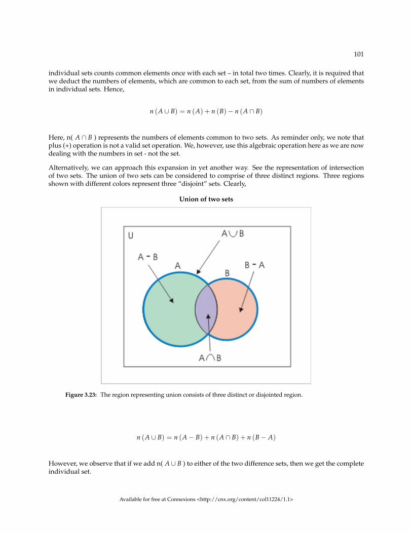
101
individual sets counts common elements once with each set – in total two times. Clearly, it is required thatwe deduct the numbers of elements, which are common to each set, from the sum of numbers of elementsin individual sets. Hence,
n (A ∪ B) = n (A) + n (B)− n (A ∩ B)
Here, n( A ∩ B ) represents the numbers of elements common to two sets. As reminder only, we note thatplus (+) operation is not a valid set operation. We, however, use this algebraic operation here as we are nowdealing with the numbers in set - not the set.
Alternatively, we can approach this expansion in yet another way. See the representation of intersectionof two sets. The union of two sets can be considered to comprise of three distinct regions. Three regionsshown with different colors represent three “disjoint” sets. Clearly,
Union of two sets
Figure 3.23: The region representing union consists of three distinct or disjointed region.
n (A ∪ B) = n (A− B) + n (A ∩ B) + n (B− A)
However, we observe that if we add n( A∪ B ) to either of the two difference sets, then we get the completeindividual set.
Available for free at Connexions <http://cnx.org/content/col11224/1.1>

102 CHAPTER 3. SETS AND COUNTING
n (A) = n (A− B) + n (A ∩ B)
⇒ n (A− B) = n (A)− n (A ∩ B)
and
n (B) = n (B− A) + n (A ∩ B)
⇒ n (B− A) = n (B)− n (A ∩ B)
Substituting for the numbers of the difference set in the equation for the numbers in the union set, we have:
⇒ n (A ∪ B) = n (A)− n (A ∩ B) + n (A ∩ B) + n (B)− n (A ∩ B)
⇒ n (A ∪ B) = n (A) + n (B)− n (A ∩ B)
3.7.1.1 Numbers of elements in the union of “disjoint” sets
Since there are no common elements between two disjoint sets, the intersection between disjoint sets is anempty set. Hence,
n (A ∪ B) = n (A) + n (B)
3.7.2 Application
Application of set theory to real situation is keyed to the interpretation of wordings and description. In or-der to efficiently employ the concepts of set theory to real world situations, we need to interpret descriptionof collection appropriately.
Once collections are interpreted correctly, rest is easy. There are indeed fewer mathematical operationsinvolved here. Most of these relate to determination of numbers of elements in a set. In this section, weshall first recapitulate or reinterpret different collections and then work with few representative situationsfor analysis (if we are confident then we can skip the recapitulation part).
Available for free at Connexions <http://cnx.org/content/col11224/1.1>

103
3.7.2.1 Set
In real situation, we identify a collection with certain characteristic common to elements. For example, aset of students in a class is based on the characteristic that each student is member of that class. This typeof interpretation, however, is generally restrictive and leads to misinterpretation. We tend to think that thecollection is isolated in itself, which is obviously wrong.
We need to free our mind from thinking set as an isolated entity. Some of the students might be membersof another collection like that of basketball team, whereas some others might be members of a particularhouse, say “Amity house” and so on
In the nutshell, we consider set as a collection, which has multiple intersections with other collections.
A set
Figure 3.24: A set has multiple intersections with other collections.
3.7.2.1.1 Example
Problem 1: In the house of total 200 students, 140 students play basketball and 80 students play football.Each student of the house plays at least one of these two games. How many students play both basketballand football?
Solution : The individual sets here are students playing basket ball (B) and football (F). Hence,
n (B) = 140
Available for free at Connexions <http://cnx.org/content/col11224/1.1>
104 CHAPTER 3. SETS AND COUNTING
n (F) = 80
Clearly, there is no bar that a students playing basketball can not play football. This is also evident from thesum of the numbers in each set. The sum is 140 + 80 = 220, whereas total numbers of students in the houseis 200 only. Thus, there are students who play both games. We can interpret the total numbers as the unionof two individual sets. Hence, applying expansion for the numbers of a union :
n (A ∪ B) = n (A) + n (B)− n (A ∩ B)
The students who play both games constitute the intersection of two individual sets.
Putting values,
⇒ n (B ∪ F) = 140 + 80− 200 = 20
3.7.2.2 Universal set and complement
Universal is inclusive of all related sets. If we observe the Venn’s diagram consisting of two individual sets,then we realize that largest closed region within the universal set is the union involving two sets i.e (A∪B).This union, however, is a subset of U. There is remaining area within the universal set, which is called thecomponent of this union.
Now we know that a union represents elements which belong to either set exclusively or belong commonlywith other sets. It means that the complement of union represents the region, which can not be defined bythe characterizing criteria of the union. This complement of union, therefore, represents situations which isdescribed in terms of “neither or nor” type. Actually, this set is given by De-morgan’s first law.
3.7.2.2.1 Example
Problem 2: In a house of total 200 students, 100 students play basketball, 60 students play football and 20play both games. How many students play neither basketball nor football?
Solution : We have already discussed that “neither nor” condition is same as that of De-morgan’s first law:
n (B′ ∩ F′) = n (B ∪ F) ′
Now expanding the right hand term, we have :
⇒ n (B′ ∩ F′) = n (B ∩ F) ′ = U − n (B ∪ F)
Available for free at Connexions <http://cnx.org/content/col11224/1.1>

105
Further using formula for the numbers in a union,
⇒ n (B′ ∩ F′) = U − n (B)− n (F) + n (B ∩ F)
Putting values,
⇒ n (B′ ∩ F′) = 200− 100− 60 + 20 = 60
This is the required answer. However, there remains a question : why do we consider total numbers ofstudents as the numbers in universal set, “U”, unlike previous example in which this number correspondsto numbers in the union of individual sets. Remember, earlier question had the phrase “Each student ofthe house plays at least one of these two games”. This ensured that total numbers represented the union aseveryone was playing one of two games. Such restriction is not there in this example. In fact, we saw thatthere are students who are not playing either of two games at all! Thus, total number represents universalset in this example.
3.7.2.3 Union
Union of two sets “A” and “B” conveys the meaning of consisting three categories of elements (i) elementsexclusively belonging to “A” (ii) elements exclusively belonging to “B” and (iii) (i) elements commonlybelonging to “A” and “B”. In totality, we see that union conveys the meaning of “or” – the elements maybelong either to a particular set or to both sets.
3.7.2.3.1 Example
Problem 3: In a group of students, 40 students study either English or Mathematics. Of these 25 studentsstudy Mathematics, 10 students study both Mathematics and English. How many students study English?
Solution : The word “or” in the first sentence indicates that union of students studying Mathematics (M)or English (E) or both is 40. Using formula, we have :
n (M ∪ E) = n (M) + n (E)− n (M ∩ E)
⇒ n (E) = n (M ∪ E)− n (M) + n (M ∩ E)
Putting values,
⇒ n (E) = 40− 25 + 10 = 25
Available for free at Connexions <http://cnx.org/content/col11224/1.1>

106 CHAPTER 3. SETS AND COUNTING
3.7.2.4 Difference
In the case of intersection of two sets, we have noted that difference represents the exclusive or isolated set,which is not common to other set. From the Venn’s diagram, we also observe that a given set is actuallycomposed of two sets (i) difference set and (ii) intersection set.
n (A) = n (A− B) + n (A ∩ B)
and
n (B) = n (B− A) + n (A ∩ B)
3.7.2.4.1 Example
Problem 4: In a house of 200 students, 120 students study Mathematics, 60 students study English and40 students study both Mathematics and English. Find in the house : (i) students who study Mathemat-ics but not English (ii) students who study English, but not Mathematics (iii) students who study eitherMathematics or English and (iv) students who neither study Mathematics nor English.
Solution : Let us first characterize collections as given in the question. Two sets are given one for those whostudy Mathematics (M) and other for those who study English(E). The addition of numbers of individualsets is 120 + 60 = 180, which is less than total numbers of students. Hence, total numbers of 200 correspondsto universal set. Here,
U = 200; n (M) = 120; n (E) = 60 and n (M ∩ E) = 40.
(i) Students studying Mathematics, but not English means that we need to find the numbers in the differenceof set i.e M – E.
n (M− E) = n (M)− n (M ∩ E)
⇒ n (M− E) = 120− 40 = 80
(ii) Students studying Mathematics, but not English means that we need to find the numbers in the differ-ence of set i.e E – M.
n (E−M) = n (E)− n (M ∩ E)
⇒ n (E−M) = 60− 40 = 20
Available for free at Connexions <http://cnx.org/content/col11224/1.1>

107
(iii) Students who study either Mathematics or English is equal to the numbers in the union of two sets.
n (M ∪ E) = n (M) + n (E)− n (M ∩ E)
Putting values,
⇒ n (M ∪ E) = 120 + 60− 40 = 140
(iv) Students who study neither Mathematics nor English is equal to the numbers in the compliment of theunion of two sets.
n (M ∪ E) ′ = U − n (M ∪ E) = 200− 140 = 60
3.8 Working with three sets8
Working with three sets is similar as working with two sets. The underlying characteristics of set operationsare same. The union and intersection of sets are carried out with three sets - one after another. Notably,union and intersection operations are commutative. This allows us to extend these set operations to thirdset in any sequence. Venn’s diagram enables us to visualize resulting set. In this module, we shall first for-mulate expression for the numbers in the union of three sets. Subsequently, we shall apply the formulationto real time analysis - using both graphical (Venn diagram) and analytical methods.
The union, involving three sets, can be considered in terms of union of a set with "union of other two sets".In that sense, union of three sets represent elements which belong to either of three sets. Here, we want tofind the expression of numbers of elements in the union set, which is represented as :
n (A ∪ B ∪ C)
Before, we work on the expansion of this term, let us first find out what does the term " A∪ B∪C " representon Venn’s diagram? The figure below shows the representation of this term :
8This content is available online at <http://cnx.org/content/m15203/1.3/>.
Available for free at Connexions <http://cnx.org/content/col11224/1.1>

108 CHAPTER 3. SETS AND COUNTING
Union of three sets
Figure 3.25: The union set represent elements of three sets combined together.
The set shown in the figure above consists of following class of elements :
1. The elements, which are exclusive of sets “A”, “B” and “C” respectively.2. The elements, which are common to a pair of two sets at a time.3. The elements, which are common to all three sets.
In the figure below, the common areas between a pair of two sets are marked “1”, “2” and “3”. The commonarea among all three sets is marked “4”.
Available for free at Connexions <http://cnx.org/content/col11224/1.1>

109
Union of three sets
Figure 3.26: The union consists of disjointed regions.
3.8.1 Union of three sets
As discussed earlier, the sum of numbers of individual sets is greater than the number of elements in “A ∪ B ∪ C ”, unless the sets are disjoint sets. It is imperative that we account for the repetition of commonelements. Proceeding as in the case of union of two sets, we deduct the intersections between each pair ofsets as :
n (A ∪ B ∪ C) = n (A) + n (B) + n (C)− n (A ∩ B)− n (A ∩ C)− n (B ∩ C)
In this manner, we account for common elements between two sets. However, we have deducted elements"common to all three sets" in this process – three times. On the other hand, the elements "common to allthree sets" are present in the numbers of each of the individual sets - in total three times as there are threesets. Ultimately, we find that we have not counted the elements common to all sets at all. It means that weneed to account for the elements common to all three sets. In order to add this number, we first need toknow – what does this common area (marked 4) represent symbolically?
In the earlier module, we have seen that the area marked “4” is represented by “ A ∩ B ∩ C ”. Hence, thecorrect expansion for the numbers of elements in the union, involving three set, is :
⇒ n (A ∪ B ∪ C) = n (A) + n (B) + n (C)− n (A ∩ B)− n (A ∩ C)− n (B ∩ C) + n (A ∩ B ∩ C)
Available for free at Connexions <http://cnx.org/content/col11224/1.1>

110 CHAPTER 3. SETS AND COUNTING
NOTE: This result is an important result as the same is used while studying probability.
3.8.1.1 Union of three sets (Analytical method)
We can achieve this result analytically as well. Here, we consider “A” as one set and “ (B ∪ C) “ as otherset. Then, we apply the relation, which has been obtained for the numbers in the union of two sets as :
n (A ∪ B ∪ C) = n (A) + n (B ∪ C)− n [A ∩ (B ∪ C)]
Applying result for the union of two sets for “ n (B ∪ C) ”, we have :
n (B ∪ C) = n (B) + n (C)− n (B ∩ C)
Putting in the expression for “ n (A ∪ B ∪ C) ”,
⇒ n (A ∪ B ∪ C) = n (A) + n (B) + n (C)− n (B ∩ C)− n [A ∩ (B ∪ C)]
At this stage, our task is to evaluate “ n [A ∩ (B ∪ C)] ”, Recall that we have worked with the distributiveproperty of “intersection operator over union operator”. Following distributive property,
⇒ n [A ∩ (B ∪ C)] = n [(A ∩ B) ∪ (A ∩ C)]
We can treat each of the terms in the small bracket on the right hand side of the above equation as a set.Applying relation obtained for the numbers in the union of two sets again, we have :
⇒ n [A ∩ (B ∪ C)] = n (A ∪ B) + n (A ∪ C)− n [(A ∩ B) ∩ (A ∩ C)]
The last term in above equation is :
[(A ∩ B) ∩ (A ∩ C)] = (A ∩ B ∩ C)
Hence,
⇒ n [A ∩ (B ∪ C)] = n (A ∪ B) + n (A ∪ C)− n [(A ∩ B ∩ C)]
Now, putting this expression in the expression of the numbers in the union involving three sets and rear-ranging terms, we have :
Available for free at Connexions <http://cnx.org/content/col11224/1.1>
111
⇒ n (A ∪ B ∪ C) = n (A) + n (B) + n (C)− n (A ∩ B)− n (A ∩ C)− n (B ∩ C) + n (A ∩ B ∩ C)
In the nutshell, we find that numbers of elements in the union, here, is equal to the sum of numbers in theindividual sets, minus elements common to two sets taken at a time, plus elements common to all threesets.
3.8.2 Illustration
In this section, we shall work with an example, which is quite intuitive of the analysis, involving three sets.We shall see that analysis of set operations in terms of Venn’s diagram is very direct and simple. As such,we shall first attempt analyze situation with Venn’s diagram.
However, we need to emphasize that extension of set concepts to calculus, probability and other branchesof mathematics require that we develop analytical skill with respect to set operations. Keeping this aspectin mind, we shall also work the solution, using analytical method.
Problem : In a town, a total 100000 people read newspaper. Out of these, 40 % read newspaper “A”, 30% read newspaper “B”, 10 % read newspaper “C”. It is found that 5% read both “A” and “B”; 4% readboth “A” and “C”; and 3% read both “B” and “C”. Also, 2% of the people read all three newspapers. Findnumbers (i) who read only “A” (ii) who read only “B” (iii) who read neither of three newspapers.
We define three sets “A”, “B” and “C”, corresponding to people reading newspapers “A”, “B” and “C”respectively. From question, we have :
n (A) = 0.4X100000 = 40000
n (B) = 0.3X100000 = 30000
n (C) = 0.1X100000 = 10000
n (A ∩ B) = 0.05X100000 = 5000
n (A ∩ C) = 0.04X100000 = 4000
n (B ∩ C) = 0.03X100000 = 3000
n (A ∩ B ∩ C) = 0.2X100000 = 2000
Available for free at Connexions <http://cnx.org/content/col11224/1.1>

112 CHAPTER 3. SETS AND COUNTING
3.8.2.1 Venn’s diagram method
We observe that sum of the individual sets is less than total numbers of people , reading newspaper, in thetown. Hence, total reading population represents universal set, “U”. The representations of these sets areshown on Venn’s diagram. Note that we have split the elements common to a pair of two sets in two parts(a) elements exclusive to intersection of two sets and (b) elements common to all three sets.
Union of three sets
Figure 3.27: The regions common to sets.
From the diagram,
(i) The required set is the region of “A” not common to “B” and “C”. This region represents elements,which are exclusive to set “A”. Thus, numbers of people reading only “A” is :
n1 = 40000− (3000 + 2000 + 2000) = 33000
(ii) The required set is the region of “B” not common to “A” and “C”. This region represents elements,which are exclusive to set “B”. Thus, numbers of people reading only “B” is :
n2 = 30000− (3000 + 1000 + 2000) = 24000
Available for free at Connexions <http://cnx.org/content/col11224/1.1>

113
(iii) The required set is the remaining region of universal set “U” i.e. complement of the union of threesets. Now, proceeding as before, people who read newspaper “C” only is (see Venn’s diagram above):
n3 = 100000− (2000 + 1000 + 2000) = 5000
Hence, the required number is :
Union of three sets
Figure 3.28: The regions representing people, who read neither of three newspapers.
n4 = 100000− (33000 + 24000 + 5000 + 3000 + 2000 + 1000 + 2000)
⇒ n4 = 30000
3.8.2.2 Analytical method
(i) Here we are required to find the numbers of people reading only “A”. It is clear that this set is part ofthe people, who do not read newspapers “B” and “C”. As discussed in the case of two sets, the numbers ofpeople who read neither “B” and “C” is given by De-morgan’s first equation,
Available for free at Connexions <http://cnx.org/content/col11224/1.1>

114 CHAPTER 3. SETS AND COUNTING
B′ ∩ C′ = (B ∪ C) ′
Intersection of two complement sets
Figure 3.29: The region representing people, who read neither of two newspapers.
For clarity, we have shown this region in the Venn’s diagram. We should realize that this intersection of twosets also includes people who read newspaper “A”. However, we are required to know numbers of people,who read newspaper “A” only. The exclusion people reading other newspaper as well are not part of ourrequired set.
The remaining set (refer Venn’s diagram) represent area consisting of people who exclusively read news-paper “A” or who do not read any of three newspapers. Now, we need the intersection of set A with theremaining region to obtain the numbers, who read only newspaper “A”. Hence, required number is :
n1 = n (A ∩ B′ ∩ C′)
Using De-morgan’s equation,
n1 = n (A ∩ B′ ∩ C′) = n [A ∩ (B ∪ C) ′]
Available for free at Connexions <http://cnx.org/content/col11224/1.1>

115
⇒ n1 = n [A ∩ [U − (B ∪ C)]] = n [(A ∩U)− A ∩ (B ∪ C)]
⇒ n1 = n [A− A ∩ (B ∪ C)] = n (A)− n [A ∩ (B ∪ C)]
Using distributive property of intersection over union,
⇒ n1 = n (A)− n [(A ∩ B) ∪ (A ∩ C)]
Using formula of expansion of union of two sets,
⇒ n1 = n (A)− [n (A ∩ B) + n (A ∩ C)− n [(A ∩ B) ∩ (A ∩ C)]]
⇒ n1 = n (A)− [n (A ∩ B) + n (A ∩ C)− n (A ∩ B ∩ C)]
We see that values of each term on the right hand side are given. Putting these values,
⇒ n1 = 40000− [5000 + 4000− 2000] = 33000
(ii) Here we are required to find the numbers of people reading only “B”. Proceeding as before,
n2 = n (B)− [n (B ∩ A) + n (B ∩ C)− n (B ∩ A ∩ C)]
⇒ n2 = n (B)− [n (A ∩ B) + n (B ∩ C)− n (A ∩ B ∩ C)]
Putting values,
⇒ n2 = 30000− [5000 + 3000− 2000] = 24000
(iii) In order to find the numbers of people, who read neither of three newspapers, we first find union ofthree sets. The union represents people who read either of these newspapers – one, two or all three. Clearly,people, who do not read either of these papers constitute a complement of this union.
Available for free at Connexions <http://cnx.org/content/col11224/1.1>

116 CHAPTER 3. SETS AND COUNTING
n3 = (A ∪ B ∪ C) ′ = U − (A ∪ B ∪ C)
Using expansion for the numbers in the union of three sets,
⇒ n3 = U − [n (A) + n (B) + n (C)− n (A ∩ B)− n (A ∩ C)− n (B ∩ C) + n (A ∩ B ∩ C)]
Putting values, we have :
⇒ n3 = 100000− [40000 + 30000 + 10000− 5000− 4000− 3000 + 2000] = 30000
3.9 Cartesian product9
We have seen that set operations convey the notion of arithmetic operations. One such similar operation isproduct of two sets called “Cartesian product”. Since sets are collection – not a single quantity, the productoperation here involves combining or pairing each of the elements of one set with that of another set.
We use symbol “X” to denote product operation. The Cartesian product of two sets “A” and “B” is symbol-ically represented as :
A× B
It is important to understand that we do not multiply elements as we do in arithmetic – instead we pairelements together. This is the meaning of “product” for the sets. We denote one such pair within a pair ofsmall brackets like :
(a, b)
where a ∈ A and b ∈ B.
Note that elements from two sets are separated by comma.
3.9.1 Ordered pair
The order of pairing is important. The pair (a,b) and (b,a) are different. This ordering is required as thereare real time situations, where order makes a difference. Consider for example, we are required to findthe integers which can be formed from two integer subsets like {1,2,3} and {3,4,5}. Clearly, “13” and “31”represent different integers. We need to distinguish them. All pairs formed from two sets should be distinct.
Keeping this restriction in mind, let us work out an example to find ordered pairs formed from elements oftwo sets.
9This content is available online at <http://cnx.org/content/m15207/1.5/>.
Available for free at Connexions <http://cnx.org/content/col11224/1.1>
117
A = set of first letter of the names of cities = {N, D, H}
B = set of numbers denoting flight numbers = {001, 002, 003}
All possible ordered pairs formed from two sets are :
(N, 001) , (N, 002) , (N, 003) , (D, 001) , (D, 002) , (D, 003) , (H, 001) , (H, 002) , (H, 003)
There are all together 9 ordered pairs. From this example, we can deduce a method for writing orderedpairs from two sets. We begin with the first elements of two sets. Progressively, we change the elementsfrom the second set till it is exhausted, while keeping the elements from the first set unchanged. Then, weswitch to “next” element from first set and start with “first” from the second set. Again, we change theelements from the second set progressively till it is exhausted, while keeping the elements from the first setunchanged. We continue in this manner till all elements from the first set is also exhausted.
From this discussion, it is also evident that two ordered pairs are equal if and only if the corresponding firstand second elements are equal.
3.9.2 Cartesian product
The Cartesian product of two sets is defined in terms of ordered pairs.Definition 3.10: Cartesian productThe Cartesian product of two non-empty sets “A” and “B” is the set of all ordered pairs of the
elements from two sets.We should emphasize the use of word “non-empty”, The Cartesian product of a non-empty set with anempty set is equal to empty set.
A× φ = φ
On the other hand, if one of the sets is infinite, then resulting Cartesian product is also infinite.
We express the Cartesian product set in set building form as :
A× B = {(x, y) : x ∈ A, y ∈ B}
Here, use of "," in the set builder form is equivalent to "and". Therefore, we can write Cartesian product oftwo sets also as :
A× B = {(x, y) : x ∈ A and y ∈ B}
Available for free at Connexions <http://cnx.org/content/col11224/1.1>

118 CHAPTER 3. SETS AND COUNTING
Further, we can emphasize two ways validity of the conditional statements as in the case of other set oper-ators :
I f (x, y) ∈ A× B⇔ x ∈ A and y ∈ B
3.9.2.1 Graphical representation
The ordered pairs can be represented in the form of tabular cells or points of intersection of perpendicularlines. The elements of one set are represented as rows, whereas elements of other set are represented ascolumns. Look at the representation of ordered pairs by points in the figure for the example given earlier.
Cartesian product
Figure 3.30: The elements of one set are represented as rows, whereas elements of other set are representedas columns.
Note that there are a total of 9 intersection points, corresponding to 9 ordered pairs.
3.9.2.2 Examples
3.9.2.2.1
Problem 1 : If(
x2 − 1, y + 2)
= (0, 2) , find “x” and “y”.
Solution : Two ordered pairs are equal. It means that corresponding elements of the ordered pairs areequal. Hence,
⇒ x2 − 1 = 0
⇒ x = 1 or − 1
and
Available for free at Connexions <http://cnx.org/content/col11224/1.1>

119
⇒ y + 2 = 2
⇒ y = 0
3.9.2.2.2
Problem 2 : If A = {5,6,7,2}, B={3,5,6,1} and C = {4,1,8}, then find (A ∩ B)× (B ∩ C) .
Solution : In order to evaluate the given expression, we first find out the intersections given in the brackets.
⇒ A ∩ B = {5, 6}
⇒ B ∩ C = {1}
Thus,
(A ∩ B)× (B ∩ C) = {(6, 1) , (5, 1)}
Note that the elements in the given set are not ordered. It is purposely given this way to emphasize thatorder is requirement of ordered pair – not that of a set.
3.9.2.3 Numbers of elements
We have seen that ordered pairs are represented graphically by the points of intersection. The numbers ofintersections equal to the product of numbers of rows and columns. Thus, if there are “p” elements in theset “A” and “q” elements in the set “B”, then total numbers of ordered pairs are “pq”. In symbolic notation,
n (A× B) = pq
3.9.3 Multiple products
Like other set operations, the product operation can also be applied to a series of sets in sequence. IfA1, A2, . . . . . . .., An is a finite family of sets, then their Cartesian product, one after another, is symbolicallyrepresented as :
A1 × A2 × . . . . . . . . . . . . . . . .× An
Available for free at Connexions <http://cnx.org/content/col11224/1.1>

120 CHAPTER 3. SETS AND COUNTING
This product is set of group of ordered elements. Each group of ordered elements comprises of “n” ele-ments. This is stated as :
A1 × A2 × . . .× An = {(x1,x2, . . . , xn) : x1 ∈ A1,x2 ∈ A2, . . . , xn ∈ An}
3.9.3.1 Ordered triplets
The Cartesian product A× A× A is set of triplets. This product is defined as :
A× A× A = {(x, y, z) : x, y, z ∈ A}
We can also represent Cartesian product of a given set with itself in terms of Cartesian power. In general,
⇒ An = A× A× . . . . . .× A
where “n” is the Cartesian power. If n = 2, then
⇒ A2 = A× A
This Cartesian product is also called Cartesian square.
3.9.3.1.1 Example
Problem 3 : If A = {-1,1}, then find Cartesian cube of set A.
Solution : Following the method of writing ordered sequence of numbers, the product can be written as :
A× A× A = {(−1,−1,−1) , (−1,−1, 1) , (−1, 1,−1) ,
(−1, 1, 1) , (1,−1,−1) , (1,−1, 1) , (1, 1,−1) , (1, 1, 1)}
The total numbers of elements are 2x2x2 = 8.
3.9.3.2 Cartesian Coordinate system
The Cartesian product, consisting of ordered triplets of real numbers, represents Cartesian three dimen-sional space.
R× R× R = {(x, y, z) : x, y, z ∈ R}
Available for free at Connexions <http://cnx.org/content/col11224/1.1>

121
Each of the elements in the ordered triplet is a coordinate along an axis and each ordered triplet denotes apoint in three dimensional coordinate space.
Cartesian coordinate system
Figure 3.31: The coordinate of a point is an ordered tripplet.
Similarly, the Cartesian product " R× R " consisting of ordered pairs defines a Cartesian plane or Cartesiancoordinates of two dimensions. It is for this reason that we call three dimensional rectangular coordinatesystem as Cartesian coordinate system.
3.9.4 Commutative property of Cartesian product
The Cartesian product is set of ordered pair. Now, the order of elements in the ordered pair depends on theposition of sets across product sign. If sets "A" and "B" are unequal and non-empty sets, then :
A× B 6= B× A
In general, any operation involving Cartesian product that changes the "order" in the "ordered pair" willyield different result.
However, if "A" and "B" are non-empty, but equal sets, then the significance of the order in the "orderedpair" is lost. We can use this fact to formulate a law to verify "equality of sets". Hence, if sets "A" and "B"are two non-empty sets and
Available for free at Connexions <http://cnx.org/content/col11224/1.1>

122 CHAPTER 3. SETS AND COUNTING
A× B = B× A
Then,
A = B
It can also be verified that this condition is true other way also. If sets "A" and "B" are equal sets, thenA× B = B× A . The two way conditional statements can be symbolically represented with the help of twoways arrow,
A× B = B× A⇔ A = B
3.9.5 Distributive property of product operator
The distributive property of product operator holds for other set operators like union, intersection and dif-ference operators. We write equations involving distribution of product operator for each of other operatorsas :
A× (B ∪ C) = (A× B) ∪ (A× C)
A× (B ∩ C) = (A× B) ∩ (A× C)
A× (B− C) = (A× B)− (A× C)
Here, sets “A”,”B” and “C” are non-empty sets. In order to ascertain distributive property product operatorover other set operators we need to check validity of the equations given above.
We can check these relations proceeding from the defining statements. For the time being, we reason thatsequence of operation on either side of the equation does not affect the “order” in the “ordered pair”.Hence, distributive property should hold for product operator over three named operators. Let us checkthis with an example :
A = {a, b}, B = {1, 2} and C = {2, 3}
1: For distribution over union operator
⇒ LHS = A× (B ∪ C) = {a, b} × {1, 2, 3}
Available for free at Connexions <http://cnx.org/content/col11224/1.1>

123
⇒ LHS = {(a, 1) , (a, 2) , (a, 3) , (b, 1) , (b, 2) , (b, 3)}
Similarly,
⇒ RHS = (A× B) ∪ (A× C) = {(a, 1) , (a, 2) , (b, 1) , (b, 2)} ∪ {(a, 2) , (a, 3) , (b, 2) , (b, 3)}
⇒ RHS = {(a, 1) , (a, 2) , (a, 3) , (b, 1) , (b, 2) , (b, 3)}
Hence,
⇒ A× (B ∪ C) = (A× B) ∪ (A× C)
2: For distribution over intersection operator
⇒ LHS = A× (B ∩ C) = {a, b} × {2}
⇒ LHS = {(a, 2) , (b, 2)}
Similarly,
⇒ RHS = (A× B) ∩ (A× C) = {(a, 1) , (a, 2) , (b, 1) , (b, 2)} ∩ {(a, 2) , (a, 3) , (b, 2) , (b, 3)}
⇒ RHS = {(a, 2) , (b, 2)}
Hence,
⇒ A× (B ∩ C) = (A× B) ∩ (A× C)
3: For distribution over difference operator
Available for free at Connexions <http://cnx.org/content/col11224/1.1>

124 CHAPTER 3. SETS AND COUNTING
⇒ LHS = A× (B− C) = {a, b} × {1}
⇒ LHS = {(a, 1) , (b, 1)}
Similarly,
⇒ RHS = (A× B)− (A× C) = {(a, 1) , (a, 2) , (b, 1) , (b, 2)} − {(a, 2) , (a, 3) , (b, 2) , (b, 3)}
⇒ RHS = {(a, 1) , (b, 1)}
Hence,
⇒ A× (B− C) = (A× B)− (A× C)
3.9.5.1 Analytical proof
Let us consider an arbitrary ordered pair (x,y), which belongs to Cartesian product set “ A × (B ∪ C) ”.Then,
⇒ (x, y) ∈ A× (B ∪ C)
By the definition of product of two sets,
⇒ x ∈ A and y ∈ (B ∪ C)
By the definition of union of two sets,
⇒ x ∈ A and (y ∈ B or y ∈ C)
⇒ (x ∈ A and y ∈ B) or (x ∈ A and y ∈ C)
⇒ (x, y) ∈ A× B or (x, y) ∈ A× C
Available for free at Connexions <http://cnx.org/content/col11224/1.1>
125
By the definition of union of two sets,
⇒ (x, y) ∈ (A× B) ∪ (A× C)
But, we had started with " A× (B ∪ C) " and used definitions to show that ordered pair “(x,y)” belongs toanother set. It means that the other set consists of the elements of the first set – at the least. Thus,
⇒ A× (B ∪ C) ⊂ (A× B) ∪ (A× C)
Similarly, we can start with " (A× B) ∪ (A× C) " and reach the conclusion that :
⇒ (A× B) ∪ (A× C) ⊂ A× (B ∪ C)
If sets are subsets of each other, then they are equal. Hence,
⇒ A× (B ∪ C) = (A× B) ∪ (A× C)
Proceeding in the same manner, we can also prove distribution of product operator over intersection anddifference operators,
A× (B ∩ C) = (A× B) ∩ (A× C)
A× (B− C) = (A× B)− (A× C)
3.10 Cartesian Product (exercise)10
Note : The results of some of the questions (3 - 7) are of generic nature. As such, they can also be treatedas theorems on Cartesian products.
10This content is available online at <http://cnx.org/content/m15209/1.2/>.
Available for free at Connexions <http://cnx.org/content/col11224/1.1>

126 CHAPTER 3. SETS AND COUNTING
3.10.1 Worked out exercises
3.10.1.1
Problem 1 : Cartesian product " A× B " consists of 6 elements. If three of these are (1,2), (2,3) and (3,3), thenfind Cartesian product set " B× A ".
Solution : We need to know two sets “A” and “B” in order to evaluate " B× A ". First elements of orderedpairs of " A× B " are elements of set “A”. Hence, “1”,”2” and “3” are the elements of set “A”. On the otherhand, second elements of ordered pairs of AXB are elements of set “B”. Hence, “2” and “3” are elements ofset “B”.
Now, it is given that there are total 6 elements in the Cartesian product, which is equal to the product ofnumbers of elements in two sets i.e. 3 X 2. It means that we have identified all elements of sets “A” and“B”.
A = {1, 2, 3}
B = {2, 3}
Following the rule for writing Cartesian product in terms of ordered pairs, we have :
⇒ B× A = {(1, 2) , (1, 3) , (2, 2) , (2, 3) , (3, 2) , (3, 3)}
3.10.1.2
Problem 2 : Two sets are given as : A = {1,2} and B = {3,4}. Find the total numbers of subsets of " A× B ".Also write power set of AXB in roaster form.
Solution : The total numbers of elements in the Cartesian product " A× B " is “pq”, where “p” and “q”are the numbers of elements in the individual sets “A” and “B” respectively. The all possible subsets thatcan be formed including empty set and the product " A× B " itself is :
n = 2pq = 22X2 = 24 = 16
Now, the Cartesian product is :
⇒ A× B = {(1, 3) , (1, 4) , (2, 3) , (2, 4)}
The corresponding power set comprises of empty set, 4 sets with elements comprising of one element plus6 sets with elements comprising of two elements taken at a time plus 4 sets with elements comprising ofthree elements taken at a time plus set itself. There are total of 16 subsets. The power set is set of all subsetsas its elements :
Available for free at Connexions <http://cnx.org/content/col11224/1.1>

127
⇒ P (A× B) = {φ, {(1, 3)}, {(1, 4)}, {(2, 3)}, {(2, 4)},
{(1, 3) , (1, 4)}, {(1, 3) , (2, 3)}, {(1, 3) , (2, 4)}, {(1, 4) , (2, 3)}, {(1, 4) , (2, 4)}, {(2, 3) , (2, 4)},
{(1, 3) , (1, 4) , (2, 3)}, {(1, 3) , (1, 4) , (2, 4)}, {(1, 3) , (2, 3) , (2, 4)}, {(1, 4) , (2, 3) , (2, 4)}
{(1, 3) , (1, 4) , (2, 3) , (2, 4)}}
It is easy to follow a scheme to write combination in which order is not relevant. We can denote each of theordered pair with a symbol like :
A× B = {a, b, c, d}
As pointed out for generating combination for ordered pair, we can start with the left element and keepchanging the last element of the combination till all combinations are exhausted. Here, power set in termsof symbols is :
P (A× B) = {φ, {a}, {b}, {c}, {d},
{(a, b) , {(a, c)}, {(a, d)}, {(b, c) , {(b, d)}, {(c, d)},
{(a, b, c)}, {(a, b, d)}, {(a, c, d)}, {(b, c, d)},
{(a, b, c, d)}}
Available for free at Connexions <http://cnx.org/content/col11224/1.1>
128 CHAPTER 3. SETS AND COUNTING
3.10.1.3
Problem 3 : If " A ⊂ B " and "C" is any non-empty set, then prove that :
A× C ⊂ B× C
Solution : Let us first discuss the logic of the relation here. The elements of set “A” are common to set“B”. Now Cartesian product of set "A" with set “C” will yield ordered pairs, which are common with theordered pairs of the Cartesian product "B" with "C". However, as set “B” is either larger than or equal to,but not smaller than “A”, it follows that above relation should hold.
Now, we prove the relation analytically. Let an arbitrary ordered pair (x,y) belongs to Cartesian product "A× C ".
(x, y) ∈ A× C
According to definition of Cartesian product,
⇒ x ∈ A and y ∈ C
But “A” is subset of “B”. Hence, x ∈ B .
⇒ x ∈ B and y ∈ C
Again, applying definition of Cartesian product,
(x, y) ∈ B× C
This means that :
⇒ A× C ⊂ B× C
3.10.1.4
Problem 4 : If A ⊂ B and C ⊂ D , then prove that :
A× C ⊂ B× D
Solution : Let an arbitrary ordered pair (x,y) belongs to Cartesian product " A× C ".
Available for free at Connexions <http://cnx.org/content/col11224/1.1>

129
(x, y) ⊂ A× C
According to definition of Cartesian product,
⇒ x ∈ A and y ∈ C
But “A” is subset of “B”. Hence, x ∈ B . Also, “C” is subset of “D”. Hence, y ∈ D .
⇒ x ∈ B and y ∈ D
Again, applying definition of Cartesian product,
⇒ (x, y) ∈ CXD
This means that :
⇒ A× C ⊂ B× D
3.10.1.5
Problem 5 : For any given four sets “A”, “B”, “C” and “D”, prove that :
(A× B) ∩ (C× D) = (A ∩ C)× (B ∩ D)
Solution : Let an arbitrary ordered pair (x,y) belongs to intersection set “ (A× B) ∩ (C× D) ”. Then,
(x, y) ∈ (A× B) ∩ (C× D)
Applying definition of intersection,
⇒ (x, y) ∈ A× B and (x, y) ∈ C× D
Applying definition of Cartesian product,
⇒ (x ∈ A and y ∈ B) and (x ∈ C and y ∈ D)
Available for free at Connexions <http://cnx.org/content/col11224/1.1>

130 CHAPTER 3. SETS AND COUNTING
⇒ (x ∈ A and x ∈ C) and (y ∈ B and y ∈ D)
Applying definition of intersection,
⇒ (x ∈ A ∩ C) and (y ∈ B ∩ D)
Again, applying definition of Cartesian product,
⇒ (x, y) ∈ (A ∩ C) X (B ∩ D)
This means that :
⇒ (A× B) ∩ (C× D) ⊂ (A ∩ C)× (B ∩ D)
Similarly, starting from RHS, we can prove that :
⇒ (A ∩ C)× (B ∩ D) ⊂ (A× B) ∩ (C× D)
If sets are subsets of each other, then they are equal. Hence,
⇒ (A× B) ∩ (C× D) = (A ∩ C)× (B ∩ D)
3.10.1.6
Problem 6 : Let “A” and “B” be two non-empty sets. If the numbers of common elements be “n” betweensets “A” and “B”, then find the common elements between Cartesian products “ A× B ” and “ B× A ”.
Solution : The common elements between sets “A” and “B” is “n”. This means :
n (A ∩ B) = n
We are required to evaluate the expression,
n [(A× B) ∩ (B× A)]
Available for free at Connexions <http://cnx.org/content/col11224/1.1>
131
We have earlier seen that four given sets,
(A× B) ∩ (C× D) = (A ∩ C)× (B ∩ D)
If we put C = B and D = A in this equation, then expression on the left hand side of the equation becomeswhat is required.
⇒ (A× B) ∩ (B× A) = (A ∩ B)× (B ∩ A)
⇒ n [(A× B) ∩ (B× A)] = n [(A ∩ B)]× n [(B ∩ A)]
⇒ n [(A× B) ∩ (B× A)] = nXn = n2
3.10.1.7
Problem 7 : Let “A”, “B” and “C” be three sets. Then prove that :
AX (B′ ∪ C′) ′ = (A× B) ∩ (A× C)
Solution : From first De-morgan’s theorem, we know that :
(B ∪ C) ′ = B′ ∩ C′
Applying to the LHS, we have :
⇒ A× (B′ ∪ C′) ′ = A× [(B′) ′ ∩ (C′) ′]
Now, component of complement set is set itself. Hence,
⇒ A× (B′ ∪ C′) ′ = A× (B ∩ C)
Applying distributive property of product operator over intersection operator, we have :
⇒ A× (B′ ∪ C′) ′ = (A× B) ∩ (A× C)
Available for free at Connexions <http://cnx.org/content/col11224/1.1>

132 CHAPTER 3. SETS AND COUNTING
3.10.1.8
Problem 8 : Let “A”, “B” and “C” be three sets. Then prove that :
AX (B′ ∩ C′) ′ = (A× B) ∪ (A× C)
Solution : From second De-morgan’s theorem, we know that :
(B ∩ C) ′ = B′ ∪ C′
Applying to the LHS, we have :
⇒ A× (B′ ∩ C′) ′ = A× [(B′) ′ ∪ (C′) ′]
Now, component of complement set is set itself. Hence,
⇒ A× (B′ ∩ C′) ′ = A× (B ∪ C)
Applying distributive property of product operator over union operator, we have :
⇒ A× (B′ ∩ C′) ′ = (A× B) ∪ (A× C)
3.11 Probability Concepts – Probability11
If you flip a coin, what is the chance of getting heads? That’s easy: 50/50. In the language of probability,we say that the probability is 1
2 . That is to say, half the time you flip coins, you will get heads.
So here is a harder question: if you flip two coins, what is the chance that you will get heads both times?I asked this question of my son, who has good mathematical intuition but no training in probability. Hisimmediate answer: 1
3 . There are three possibilities: two heads, one heads and one tails, and two tails. Sothere is a 1
3 chance of getting each possibility, including two heads. Makes sense, right?
But it is not right. If you try this experiment 100 times, you will not find about 33 “both heads” results, 33“both tails,” and 33 “one heads and one tails.” Instead, you will find something much closer to: 25 “bothheads,” 25 “both tails,” and 50 “one of each” results. Why?
Because hidden inside this experiment are actually four different results, each as likely as the others. Theseresults are: heads-heads, heads-tails, tails-heads, and tails-tails. Even if you don’t keep track of what “or-der” the coins flipped in, heads-tails is still a different result from tails-heads, and each must be counted.
And what if you flip a coin three times? In this case, there are actually eight results. In case this is gettinghard to keep track of, here is a systematic way of listing all eight results.
11This content is available online at <http://cnx.org/content/m19073/1.3/>.
Available for free at Connexions <http://cnx.org/content/col11224/1.1>

133
Available for free at Connexions <http://cnx.org/content/col11224/1.1>

134 CHAPTER 3. SETS AND COUNTING
First Coin Second Coin Third Coin End Result
Heads
HeadsHeads HHH
Tails HHT
TailsHeads HTH
Tails HTT
Tails
HeadsHeads THH
Tails THT
TailsHeads TTH
Tails TTT
Table 3.1
When you make a table like this, the pattern becomes apparent: each new coin doubles the number ofpossibilities. The chance of three heads in a row is 1
8 . What would be the chance of four heads in row?
Let’s take a slightly more complicated—and more interesting—example. You are the proud inventor of theSongWriter 2000tm.
Figure 3.32
The user sets the song speed (“fast,” “medium,” or “slow”); the volume (“loud” or “quiet”); and the style(“rock” or “country”). Then, the SongWriter automatically writes a song to match.
How many possible settings are there? You might suspect that the answer is 3 + 2 + 2 = 7, but in fact thereare many more than that. We can see them all on the following “tree diagram.”
Available for free at Connexions <http://cnx.org/content/col11224/1.1>

135
Figure 3.33
If you start at the top of a tree like this and follow all the way down, you end up with one particular kindof song: for instance, “fast loud country song.” There are 12 different song types in all. This comes frommultiplying the number of settings for each knob: 3× 2× 2 = 12.
Now, suppose the machine has a “Randomize” setting that randomly chooses the speed, volume, and style.What is the probability that you will end up with a loud rock song that is not slow? To answer a questionlike this, you can use the following process.
1. Count the total number of results (the “leaves” in the tree) that match your criterion. In this case thereare 2: the “fast-loud-rock” and “medium-loud-rock” paths.
2. Count the total number of results: as we said previously, there are 12.3. Divide. The probability of a non-slow loud rock song is 2/12, or 1/6.
Note that this process will always give you a number between 0 (no results match) and 1 (all results match).Probabilities are always between 0 (for something that never happens) and 1 (for something that is guaran-teed to happen).
But what does it really mean to say that “the probability is 1/6?” You aren’t going to get 1/6 of a song. Oneway to make this result more concrete is to imagine that you run the machine on its “Randomize” setting100 times. You should expect to get non-slow loud rock songs 1 out of every 6 times; roughly 17 songs willmatch that description. This gives us another way to express the answer: there is a 17% probability of anygiven song matching this description.
3.11.1 The multiplication rule
We can look at the above problem another way.
What is the chance that any given, randomly selected song will be non-slow? 23 . That is to say, 2 out of
every three randomly chosen songs will be non-slow.
Now...out of those 23 , how many will be loud? Half of them. The probability that a randomly selected song
is both non-slow and loud is half of 23 , or 1
2 ×23 , or 1
3 .
And now, out of that 13 , how many will be rock? Again, half of them: 1
2 ×13 . This leads us back to the
conclusion we came to earlier: 1/6 of randomly chosen songs will be non-slow, loud, rock songs. But it alsogives us an example of a very general principle that is at the heart of all probability calculations:
When two events are independent, the probability that they will both occur is the probability of one,multiplied by the probability of the other.
What does it mean to describe two events as “independent?” It means that they have no effect on eachother. In real life, we know that rock songs are more likely to be fast and loud than slow and quiet. Our
Available for free at Connexions <http://cnx.org/content/col11224/1.1>
136 CHAPTER 3. SETS AND COUNTING
machine, however, keeps all three categories independent: choosing “Rock” does not make a song morelikely to be fast or slow, loud or quiet.
In some cases, applying the multiplication rule is very straightforward. Suppose you generate two differentsongs: what is the chance that they will both be fast songs? The two songs are independent of each other,so the chance is 1
3 ×13 = 1
9 .
Now, suppose you generate five different songs. What is the chance that they will all be fast? 13 ×
13 ×
13 ×
13 ×
13 , or
(13
)5, or 1 chance in 243. Not very likely, as you might suspect!
Other cases are less obvious. Suppose you generate five different songs. What is the probability that noneof them will be a fast song? The multiplication rule tells us only how to find the probability of “this andthat”; how can we apply it to this question?
The key is to reword the question, as follows. What is the chance that the first song will not be fast, andthe second song will not be fast, and the third song will not be fast, and so on? Expressed in this way, thequestion is a perfect candidate for the multiplication rule. The probability of the first song being non-fast is23 . Same for the second, and so on. So the probability is
( 23)5
, or 32/243, or roughly 13%.
Based on this, we can easily answer another question: if you generate five different songs, what is theprobability that at least one of them will be fast? Once again, the multiplication rule does not apply directlyhere: it tells us “this and that,” not “this or that.” But we can recognize that this is the opposite of theprevious question. We said that 13% of the time, none of the songs will be fast. That means that the other87% of the time, at least one of them will!
Available for free at Connexions <http://cnx.org/content/col11224/1.1>

137
3.12 Probability Concepts – Permutations12
In the game of “Solitaire” (also known as “Pa-tience” or “Klondike”), seven cards are dealt outat the beginning, as shown to the left: one face-up, and the other six face-down. (A bunch of othercards are dealt out too, but let’s ignore that rightnow.)A complete card deck has 52 cards. Assum-ing that all you know is the 7 of spades showing,how many possible “hands” (the other six cards)could be showing underneath?What makes this a“permutations” problem is that order matters: ifan ace is hiding somewhere in those six cards, itmakes a big difference if the ace is on the first po-sition, the second, etc. Permutations problems canalways be addressed as an example of the multi-plication rule, with one small twist.
Table 3.2
• How many cards might be in the first position, directly under the showing 7?• 51. That card could be anything except the 7 of spades.• For any given card in first position, how many cards might be in second position?
12This content is available online at <http://cnx.org/content/m19072/1.2/>.
Available for free at Connexions <http://cnx.org/content/col11224/1.1>
138 CHAPTER 3. SETS AND COUNTING
• 50. The seven of spades, and the next card, are both “spoken for.” So there are 50 possibilities left inthis position.
• So how many possibilities are there for the first two positions combined?• 51× 50, or 2,550.• So how many possibilities are there for all six positions?• 51× 50× 49× 48× 47× 46, or approximately 1.3× 10¹⁰; about 10 billion possibilities!
This result can be expressed (and typed into a calculator) more concisely by using factorials.
A “factorial” (written with an exclamation mark) means “multiply all the numbers from 1 up to this num-ber.” So 5! means 1× 2× 3× 4× 5 = 120.
What is 7!5! ? Well, it is 1×2×3×4×5×6×7
1×2×3×4×5 , of course. Most of the terms cancel, leaving only 6× 7 = 42.
And what about 51!45! ? If you write out all the terms, you can see that the first 45 terms cancel, leaving
46× 47× 48× 49× 50× 51, which is the number of permutations we want. So instead of typing into yourcalculator six numbers to multiply (or sixty numbers or six hundred, depending on the problem), you canalways find the answer to a permutation problem by dividing two factorials. In many calculators, thefactorial option is located under the “probability” menu for this reason.
3.13 Probability Concepts – Combinations13
Let’s start once again with a deck of 52 cards. But this time, let’s deal out a poker hand (5 cards). Howmany possible poker hands are there?
At first glance, this seems like a minor variation on the Solitaire question above. The only real differenceis that there are five cards instead of six. But in face, there is a more important difference: order does notmatter. We do not want to count “Ace-King-Queen-Jack-Ten of spades” and “Ten-Jack-Queen-King-Ace ofspades” separately; they are the same poker hand.
To approach such question, we begin with the permutations question: how many possible poker hands arethere, if order does matter? 52× 51× 50× 49× 48, or 52!
47! . But we know that we are counting every possiblehand many different times in this calculation. How many times?
The key insight is that this second question—“How many different times are we counting, for instance,Ace-King-Queen-Jack-Ten of spades?”—is itself a permutations question! It is the same as the question“How many different ways can these five cards be rearranged in a hand?” There are five possibilities forthe first card; for each of these, four for the second; and so on. The answer is 5! which is 120. So, sincewe have counted every possible hand 120 times, we divide our earlier result by 120 to find that there are
52!(47!)(5!) , or about 2.6 Million possibilities.
This question—“how many different 5-card hands can be made from 52 cards?”—turns out to have a sur-prisingly large number of applications. Consider the following questions:
• A school offers 50 classes. Each student must choose 6 of them to fill out a schedule. How manypossible schedules can be made?
• A basketball team has 12 players, but only 5 will start. How many possible starting teams can theyfield?
• Your computer contains 300 videos, but you can only fit 10 of them on your iPod. How many possibleways can you load your iPod?
13This content is available online at <http://cnx.org/content/m19071/1.2/>.
Available for free at Connexions <http://cnx.org/content/col11224/1.1>
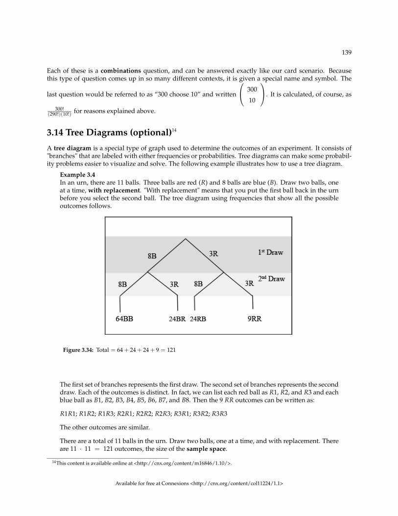
139
Each of these is a combinations question, and can be answered exactly like our card scenario. Becausethis type of question comes up in so many different contexts, it is given a special name and symbol. The
last question would be referred to as “300 choose 10” and written
300
10
. It is calculated, of course, as
300!(290!)(10!) for reasons explained above.
3.14 Tree Diagrams (optional)14
A tree diagram is a special type of graph used to determine the outcomes of an experiment. It consists of"branches" that are labeled with either frequencies or probabilities. Tree diagrams can make some probabil-ity problems easier to visualize and solve. The following example illustrates how to use a tree diagram.
Example 3.4In an urn, there are 11 balls. Three balls are red (R) and 8 balls are blue (B). Draw two balls, oneat a time, with replacement. "With replacement" means that you put the first ball back in the urnbefore you select the second ball. The tree diagram using frequencies that show all the possibleoutcomes follows.
Figure 3.34: Total = 64 + 24 + 24 + 9 = 121
The first set of branches represents the first draw. The second set of branches represents the seconddraw. Each of the outcomes is distinct. In fact, we can list each red ball as R1, R2, and R3 and eachblue ball as B1, B2, B3, B4, B5, B6, B7, and B8. Then the 9 RR outcomes can be written as:
R1R1; R1R2; R1R3; R2R1; R2R2; R2R3; R3R1; R3R2; R3R3
The other outcomes are similar.
There are a total of 11 balls in the urn. Draw two balls, one at a time, and with replacement. Thereare 11 · 11 = 121 outcomes, the size of the sample space.
14This content is available online at <http://cnx.org/content/m16846/1.10/>.
Available for free at Connexions <http://cnx.org/content/col11224/1.1>
140 CHAPTER 3. SETS AND COUNTING
Problem 1 (Solution on p. 143.)List the 24 BR outcomes: B1R1, B1R2, B1R3, ...
Problem 2Using the tree diagram, calculate P(RR).
SolutionP(RR) = 3
11 ·3
11 = 9121
Problem 3Using the tree diagram, calculate P(RB OR BR).
SolutionP(RB OR BR) = 3
11 ·8
11 + 811 ·
311 = 48
121
Problem 4Using the tree diagram, calculate P(R on 1st draw AND B on 2nd draw).
SolutionP(R on 1st draw AND B on 2nd draw) = P(RB) = 3
11 ·8
11 = 24121
Problem 5Using the tree diagram, calculate P(R on 2nd draw given B on 1st draw).
SolutionP(R on 2nd draw given B on 1st draw) = P(R on 2nd | B on 1st) = 24
88 = 311
This problem is a conditional. The sample space has been reduced to those outcomes that alreadyhave a blue on the first draw. There are 24 + 64 = 88 possible outcomes (24 BR and 64 BB).Twenty-four of the 88 possible outcomes are BR. 24
88 = 311 .
Problem 6 (Solution on p. 143.)Using the tree diagram, calculate P(BB).
Problem 7 (Solution on p. 143.)Using the tree diagram, calculate P(B on the 2nd draw given R on the first draw).
Example 3.5An urn has 3 red marbles and 8 blue marbles in it. Draw two marbles, one at a time, this timewithout replacement from the urn. "Without replacement" means that you do not put the firstball back before you select the second ball. Below is a tree diagram. The branches are labeled withprobabilities instead of frequencies. The numbers at the ends of the branches are calculated bymultiplying the numbers on the two corresponding branches, for example, 3
11 ·2
10 = 6110 .
Available for free at Connexions <http://cnx.org/content/col11224/1.1>

141
Figure 3.35: Total = 56 + 24 + 24 + 6110 = 110
110 = 1
NOTE: If you draw a red on the first draw from the 3 red possibilities, there are 2 red left to drawon the second draw. You do not put back or replace the first ball after you have drawn it. Youdraw without replacement, so that on the second draw there are 10 marbles left in the urn.
Calculate the following probabilities using the tree diagram.Problem 1P(RR) =
SolutionP(RR) = 3
11 ·2
10 = 6110
Problem 2 (Solution on p. 143.)Fill in the blanks:
P(RB OR BR) = 311 ·
810 + (___)(___) = 48
110
Problem 3 (Solution on p. 143.)P(R on 2d | B on 1st) =
Problem 4 (Solution on p. 143.)Fill in the blanks:
P(R on 1st and B on 2nd) = P(RB) = (___)(___) = 24110
Problem 5 (Solution on p. 143.)P(BB) =
Problem 6P(B on 2nd | R on 1st) =
Available for free at Connexions <http://cnx.org/content/col11224/1.1>
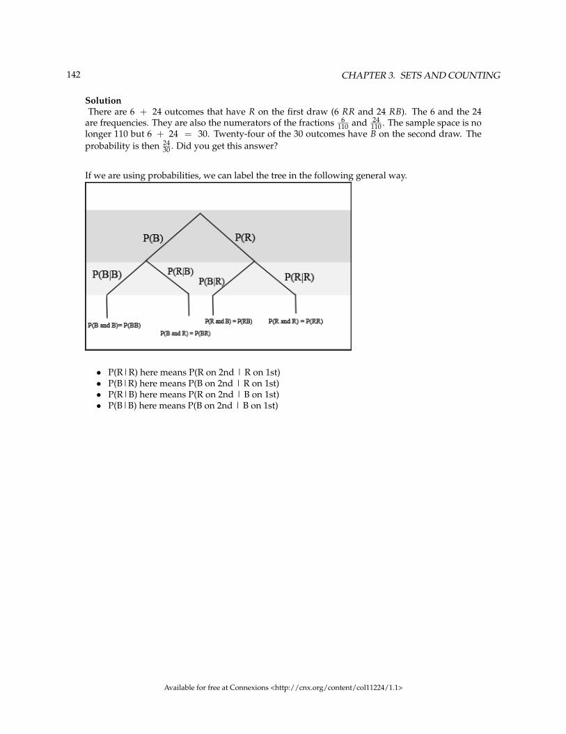
142 CHAPTER 3. SETS AND COUNTING
SolutionThere are 6 + 24 outcomes that have R on the first draw (6 RR and 24 RB). The 6 and the 24
are frequencies. They are also the numerators of the fractions 6110 and 24
110 . The sample space is nolonger 110 but 6 + 24 = 30. Twenty-four of the 30 outcomes have B on the second draw. Theprobability is then 24
30 . Did you get this answer?
If we are using probabilities, we can label the tree in the following general way.
• P(R|R) here means P(R on 2nd | R on 1st)• P(B|R) here means P(B on 2nd | R on 1st)• P(R|B) here means P(R on 2nd | B on 1st)• P(B|B) here means P(B on 2nd | B on 1st)
Available for free at Connexions <http://cnx.org/content/col11224/1.1>
143
Solutions to Exercises in Chapter 3
Solution to Example 3.4, Problem 1 (p. 139)B1R1; B1R2; B1R3; B2R1; B2R2; B2R3; B3R1; B3R2; B3R3; B4R1; B4R2; B4R3; B5R1; B5R2; B5R3; B6R1;
B6R2; B6R3; B7R1; B7R2; B7R3; B8R1; B8R2; B8R3Solution to Example 3.4, Problem 6 (p. 140)P(BB) = 64
121Solution to Example 3.4, Problem 7 (p. 140)P(B on 2nd draw | R on 1st draw) = 8
11
There are 9 + 24 outcomes that have R on the first draw (9 RR and 24 RB). The sample space is then9 + 24 = 33. Twenty-four of the 33 outcomes have B on the second draw. The probability is then 24
33 .Solution to Example 3.5, Problem 2 (p. 141)P(RB or BR) = 3
11 ·8
10 +( 8
11) ( 3
10)
= 48110
Solution to Example 3.5, Problem 3 (p. 141)P(R on 2d | B on 1st) = 3
10Solution to Example 3.5, Problem 4 (p. 141)P(R on 1st and B on 2nd) = P(RB) =
( 311) ( 8
10)
= 24110
Solution to Example 3.5, Problem 5 (p. 141)P(BB) = 8
11 ·7
10
Available for free at Connexions <http://cnx.org/content/col11224/1.1>

144 CHAPTER 3. SETS AND COUNTING
Available for free at Connexions <http://cnx.org/content/col11224/1.1>
Chapter 4
Probability Topics
4.1 Probability Topics1
4.1.1 Student Learning Outcomes
By the end of this chapter, the student should be able to:
• Understand and use the terminology of probability.• Determine whether two events are mutually exclusive and whether two events are independent.• Calculate probabilities using the Addition Rules and Multiplication Rules.• Construct and interpret Contingency Tables.• Construct and interpret Venn Diagrams (optional).• Construct and interpret Tree Diagrams (optional).
4.1.2 Introduction
It is often necessary to "guess" about the outcome of an event in order to make a decision. Politicians studypolls to guess their likelihood of winning an election. Teachers choose a particular course of study basedon what they think students can comprehend. Doctors choose the treatments needed for various diseasesbased on their assessment of likely results. You may have visited a casino where people play games chosenbecause of the belief that the likelihood of winning is good. You may have chosen your course of studybased on the probable availability of jobs.
You have, more than likely, used probability. In fact, you probably have an intuitive sense of probability.Probability deals with the chance of an event occurring. Whenever you weigh the odds of whether or notto do your homework or to study for an exam, you are using probability. In this chapter, you will learn tosolve probability problems using a systematic approach.
4.1.3 Optional Collaborative Classroom Exercise
Your instructor will survey your class. Count the number of students in the class today.
• Raise your hand if you have any change in your pocket or purse. Record the number of raised hands.• Raise your hand if you rode a bus within the past month. Record the number of raised hands.• Raise your hand if you answered "yes" to BOTH of the first two questions. Record the number of
raised hands.1This content is available online at <http://cnx.org/content/m16838/1.11/>.
Available for free at Connexions <http://cnx.org/content/col11224/1.1>
145

146 CHAPTER 4. PROBABILITY TOPICS
Use the class data as estimates of the following probabilities. P(change) means the probability that a ran-domly chosen person in your class has change in his/her pocket or purse. P(bus) means the probability thata randomly chosen person in your class rode a bus within the last month and so on. Discuss your answers.
• Find P(change).• Find P(bus).• Find P(change and bus) Find the probability that a randomly chosen student in your class has change
in his/her pocket or purse and rode a bus within the last month.• Find P(change| bus) Find the probability that a randomly chosen student has change given that
he/she rode a bus within the last month. Count all the students that rode a bus. From the groupof students who rode a bus, count those who have change. The probability is equal to those who havechange and rode a bus divided by those who rode a bus.
4.2 Probability2
Probability is a mathematical tool used to study randomness. It deals with the chance (the likelihood) ofan event occurring. For example, if you toss a fair coin 4 times, the outcomes may not be 2 heads and 2tails. However, if you toss the same coin 4,000 times, the outcomes will be close to half heads and half tails.The expected theoretical probability of heads in any one toss is 1
2 or 0.5. Even though the outcomes of afew repetitions are uncertain, there is a regular pattern of outcomes when there are many repetitions. Afterreading about the English statistician Karl Pearson who tossed a coin 24,000 times with a result of 12,012heads, one of the authors tossed a coin 2,000 times. The results were 996 heads. The fraction 996
2000 is equalto 0.498 which is very close to 0.5, the expected probability.
The theory of probability began with the study of games of chance such as poker. Predictions take the formof probabilities. To predict the likelihood of an earthquake, of rain, or whether you will get an A in thiscourse, we use probabilities. Doctors use probability to determine the chance of a vaccination causing thedisease the vaccination is supposed to prevent. A stockbroker uses probability to determine the rate ofreturn on a client’s investments. You might use probability to decide to buy a lottery ticket or not. In yourstudy of statistics, you will use the power of mathematics through probability calculations to analyze andinterpret your data.
4.3 Terminology3
Probability is a measure that is associated with how certain we are of outcomes of a particular experimentor activity. An experiment is a planned operation carried out under controlled conditions. If the result isnot predetermined, then the experiment is said to be a chance experiment. Flipping one fair coin twice isan example of an experiment.
The result of an experiment is called an outcome. A sample space is a set of all possible outcomes. Threeways to represent a sample space are to list the possible outcomes, to create a tree diagram, or to create aVenn diagram. The uppercase letter S is used to denote the sample space. For example, if you flip one faircoin, S = {H, T} where H = heads and T = tails are the outcomes.
An event is any combination of outcomes. Upper case letters like A and B represent events. For example,if the experiment is to flip one fair coin, event A might be getting at most one head. The probability of anevent A is written P (A).
2This content is available online at <http://cnx.org/content/m16015/1.11/>.3This content is available online at <http://cnx.org/content/m16845/1.13/>.
Available for free at Connexions <http://cnx.org/content/col11224/1.1>

147
The probability of any outcome is the long-term relative frequency of that outcome. Probabilities arebetween 0 and 1, inclusive (includes 0 and 1 and all numbers between these values). P (A) = 0 meansthe event A can never happen. P (A) = 1 means the event A always happens. P (A) = 0.5 means theevent A is equally likely to occur or not to occur. For example, if you flip one fair coin repeatedly (from 20to 2,000 to 20,000 times) the relative fequency of heads approaches 0.5 (the probability of heads).
Equally likely means that each outcome of an experiment occurs with equal probability. For example, ifyou toss a fair, six-sided die, each face (1, 2, 3, 4, 5, or 6) is as likely to occur as any other face. If youtoss a fair coin, a Head(H) and a Tail(T) are equally likely to occur. If you randomly guess the answer to atrue/false question on an exam, you are equally likely to select a correct answer or an incorrect answer.
To calculate the probability of an event A when all outcomes in the sample space are equally likely,count the number of outcomes for event A and divide by the total number of outcomes in the sample space.For example, if you toss a fair dime and a fair nickel, the sample space is {HH, TH, HT, TT} where T =tails and H = heads. The sample space has four outcomes. A = getting one head. There are two outcomes{HT, TH}. P (A) = 2
4 .
Suppose you roll one fair six-sided die, with the numbers {1,2,3,4,5,6} on its faces. Let event E = rolling anumber that is at least 5. There are two outcomes {5, 6}. P (E) = 2
6 . If you were to roll the die only a fewtimes, you would not be surprised if your observed results did not match the probability. If you were toroll the die a very large number of times, you would expect that, overall, 2/6 of the rolls would result in anoutcome of "at least 5". You would not expect exactly 2/6. The long-term relative frequency of obtainingthis result would approach the theoretical probability of 2/6 as the number of repetitions grows larger andlarger.
This important characteristic of probability experiments is the known as the Law of Large Numbers: asthe number of repetitions of an experiment is increased, the relative frequency obtained in the experimenttends to become closer and closer to the theoretical probability. Even though the outcomes don’t happenaccording to any set pattern or order, overall, the long-term observed relative frequency will approach thetheoretical probability. (The word empirical is often used instead of the word observed.) The Law of LargeNumbers will be discussed again in Chapter 7.
It is important to realize that in many situations, the outcomes are not equally likely. A coin or die maybe unfair, or biased . Two math professors in Europe had their statistics students test the Belgian 1 Eurocoin and discovered that in 250 trials, a head was obtained 56% of the time and a tail was obtained 44%of the time. The data seem to show that the coin is not a fair coin; more repetitions would be helpful todraw a more accurate conclusion about such bias. Some dice may be biased. Look at the dice in a game youhave at home; the spots on each face are usually small holes carved out and then painted to make the spotsvisible. Your dice may or may not be biased; it is possible that the outcomes may be affected by the slightweight differences due to the different numbers of holes in the faces. Gambling casinos have a lot of moneydepending on outcomes from rolling dice, so casino dice are made differently to eliminate bias. Casino dicehave flat faces; the holes are completely filled with paint having the same density as the material that thedice are made out of so that each face is equally likely to occur. Later in this chapter we will learn techniquesto use to work with probabilities for events that are not equally likely.
"OR" Event:An outcome is in the event A OR B if the outcome is in A or is in B or is in both A and B. For example, letA = {1, 2, 3, 4, 5} and B = {4, 5, 6, 7, 8}. A OR B = {1, 2, 3, 4, 5, 6, 7, 8}. Notice that 4 and 5 areNOT listed twice.
"AND" Event:An outcome is in the event A AND B if the outcome is in both A and B at the same time. For example, letA and B be {1, 2, 3, 4, 5} and {4, 5, 6, 7, 8}, respectively. Then A AND B = {4, 5}.
Available for free at Connexions <http://cnx.org/content/col11224/1.1>

148 CHAPTER 4. PROBABILITY TOPICS
The complement of event A is denoted A’ (read "A prime"). A’ consists of all outcomes that are NOT in A.Notice that P (A) + P (A’) = 1. For example, let S = {1, 2, 3, 4, 5, 6} and let A = {1, 2, 3, 4}. Then,A’ = {5, 6}. P (A) = 4
6 , P (A’) = 26 , and P (A) + P (A’) = 4
6 + 26= 1
The conditional probability of A given B is written P (A|B). P (A|B) is the probability that event A willoccur given that the event B has already occurred. A conditional reduces the sample space. We calculatethe probability of A from the reduced sample space B. The formula to calculate P (A|B) is
P (A|B) = P(AANDB)P(B)
where P (B) is greater than 0.
For example, suppose we toss one fair, six-sided die. The sample space S = {1, 2, 3, 4, 5, 6}. Let A =face is 2 or 3 and B = face is even (2, 4, 6). To calculate P (A|B), we count the number of outcomes 2 or 3 inthe sample space B = {2, 4, 6}. Then we divide that by the number of outcomes in B (and not S).
We get the same result by using the formula. Remember that S has 6 outcomes.
P (A|B) = P(A and B)P(B) = (the number of outcomes that are 2 or 3 and even in S) / 6
(the number of outcomes that are even in S) / 6 = 1/63/6 = 1
3
Understanding Terminology and SymbolsIt is important to read each problem carefully to think about and understand what the events are. Under-standing the wording is the first very important step in solving probability problems. Reread the problemseveral times if necessary. Clearly identify the event of interest. Determine whether there is a conditionstated in the wording that would indicate that the probability is conditional; carefully identify the condi-tion, if any.
Exercise 4.3.1 (Solution on p. 176.)In a particular college class, there are male and female students. Some students have long hair andsome students have short hair. Write the symbols for the probabilities of the events for parts (a)through (j) below. (Note that you can’t find numerical answers here. You were not given enoughinformation to find any probability values yet; concentrate on understanding the symbols.)
• Let F be the event that a student is female.• Let M be the event that a student is male.• Let S be the event that a student has short hair.• Let L be the event that a student has long hair.
a. The probability that a student does not have long hair.b. The probability that a student is male or has short hair.c. The probability that a student is a female and has long hair.d. The probability that a student is male, given that the student has long hair.e. The probability that a student has long hair, given that the student is male.f. Of all the female students, the probability that a student has short hair.g. Of all students with long hair, the probability that a student is female.h. The probability that a student is female or has long hair.i. The probability that a randomly selected student is a male student with short hair.j. The probability that a student is female.
**With contributions from Roberta Bloom
Available for free at Connexions <http://cnx.org/content/col11224/1.1>

149
4.4 Two Basic Rules of Probability4
4.4.1 The Multiplication Rule
If A and B are two events defined on a sample space, then: P(A AND B) = P(B) · P(A|B).
This rule may also be written as : P (A|B) = P(A AND B)P(B)
(The probability of A given B equals the probability of A and B divided by the probability of B.)
If A and B are independent, then P(A|B) = P(A). Then P(A AND B) = P(A|B) P(B) becomesP(A AND B) = P(A) P(B).
4.4.2 The Addition Rule
If A and B are defined on a sample space, then: P(A OR B) = P(A) + P(B)− P(A AND B).
If A and B are mutually exclusive, then P(A AND B) = 0. Then P(A OR B) = P(A) + P(B)− P(A AND B)becomes P(A OR B) = P(A) + P(B).
Example 4.1Klaus is trying to choose where to go on vacation. His two choices are: A = New Zealand and B
= Alaska
• Klaus can only afford one vacation. The probability that he chooses A is P(A) = 0.6 and theprobability that he chooses B is P(B) = 0.35.
• P(A and B) = 0 because Klaus can only afford to take one vacation• Therefore, the probability that he chooses either New Zealand or Alaska is P(A OR B) =
P(A) + P(B) = 0.6 + 0.35 = 0.95. Note that the probability that he does not choose to goanywhere on vacation must be 0.05.
Example 4.2Carlos plays college soccer. He makes a goal 65% of the time he shoots. Carlos is going to attempttwo goals in a row in the next game.
A = the event Carlos is successful on his first attempt. P(A) = 0.65. B = the event Carlos issuccessful on his second attempt. P(B) = 0.65. Carlos tends to shoot in streaks. The probabilitythat he makes the second goal GIVEN that he made the first goal is 0.90.Problem 1
What is the probability that he makes both goals?
SolutionThe problem is asking you to find P(A AND B) = P(B AND A). Since P(B|A) = 0.90:
P(B AND A) = P(B|A) P(A) = 0.90 ∗ 0.65 = 0.585 (4.1)
Carlos makes the first and second goals with probability 0.585.
Problem 2What is the probability that Carlos makes either the first goal or the second goal?
4This content is available online at <http://cnx.org/content/m16847/1.11/>.
Available for free at Connexions <http://cnx.org/content/col11224/1.1>

150 CHAPTER 4. PROBABILITY TOPICS
SolutionThe problem is asking you to find P(A OR B).
P(A OR B) = P(A) + P(B) − P(A AND B) = 0.65 + 0.65− 0.585 = 0.715 (4.2)
Carlos makes either the first goal or the second goal with probability 0.715.
Problem 3Are A and B independent?
SolutionNo, they are not, because P(B AND A) = 0.585.
P(B) · P(A) = (0.65) · (0.65) = 0.423 (4.3)
0.423 6= 0.585 = P(B AND A) (4.4)
So, P(B AND A) is not equal to P(B) · P(A).
Problem 4Are A and B mutually exclusive?
SolutionNo, they are not because P(A and B) = 0.585.
To be mutually exclusive, P(A AND B) must equal 0.
Example 4.3A community swim team has 150 members. Seventy-five of the members are advanced swim-
mers. Forty-seven of the members are intermediate swimmers. The remainder are novice swim-mers. Forty of the advanced swimmers practice 4 times a week. Thirty of the intermediate swim-mers practice 4 times a week. Ten of the novice swimmers practice 4 times a week. Suppose onemember of the swim team is randomly chosen. Answer the questions (Verify the answers):Problem 1
What is the probability that the member is a novice swimmer?
Solution28
150
Problem 2What is the probability that the member practices 4 times a week?
Solution80
150
Problem 3What is the probability that the member is an advanced swimmer and practices 4 times a week?
Available for free at Connexions <http://cnx.org/content/col11224/1.1>

151
Solution40
150
Problem 4What is the probability that a member is an advanced swimmer and an intermediate swimmer?
Are being an advanced swimmer and an intermediate swimmer mutually exclusive? Why or whynot?
SolutionP(advanced AND intermediate) = 0, so these are mutually exclusive events. A swimmer cannotbe an advanced swimmer and an intermediate swimmer at the same time.
Problem 5Are being a novice swimmer and practicing 4 times a week independent events? Why or why
not?
SolutionNo, these are not independent events.
P(novice AND practices 4 times per week) = 0.0667 (4.5)
P(novice) · P(practices 4 times per week) = 0.0996 (4.6)
0.0667 6= 0.0996 (4.7)
Example 4.4Studies show that, if she lives to be 90, about 1 woman in 7 (approximately 14.3%) will developbreast cancer. Suppose that of those women who develop breast cancer, a test is negative 2% of thetime. Also suppose that in the general population of women, the test for breast cancer is negativeabout 85% of the time. Let B = woman develops breast cancer and let N = tests negative. Supposeone woman is selected at random.Problem 1What is the probability that the woman develops breast cancer? What is the probability that
woman tests negative?
SolutionP(B) = 0.143 ; P(N) = 0.85
Problem 2Given that the woman has breast cancer, what is the probability that she tests negative?
SolutionP(N|B) = 0.02
Problem 3What is the probability that the woman has breast cancer AND tests negative?
Available for free at Connexions <http://cnx.org/content/col11224/1.1>

152 CHAPTER 4. PROBABILITY TOPICS
SolutionP(B AND N) = P(B) · P(N|B) = (0.143) · (0.02) = 0.0029
Problem 4What is the probability that the woman has breast cancer or tests negative?
SolutionP(B OR N) = P(B) + P(N) − P(B AND N) = 0.143 + 0.85− 0.0029 = 0.9901
Problem 5Are having breast cancer and testing negative independent events?
SolutionNo. P(N) = 0.85; P(N|B) = 0.02. So, P(N|B) does not equal P(N)
Problem 6Are having breast cancer and testing negative mutually exclusive?
SolutionNo. P(B AND N) = 0.0029. For B and N to be mutually exclusive, P(B AND N) must be 0.
4.5 Independent and Mutually Exclusive Events5
Independent and mutually exclusive do not mean the same thing.
4.5.1 Independent Events
Two events are independent if the following are true:
• P (A|B) = P (A)• P (B|A) = P (B)• P (A AND B) = P (A) · P (B)
Two events A and B are independent if the knowledge that one occurred does not affect the chance theother occurs. For example, the outcomes of two roles of a fair die are independent events. The outcomeof the first roll does not change the probability for the outcome of the second roll. To show two events areindependent, you must show only one of the above conditions. If two events are NOT independent, thenwe say that they are dependent.
Sampling may be done with replacement or without replacement.
• With replacement: If each member of a population is replaced after it is picked, then that member hasthe possibility of being chosen more than once. When sampling is done with replacement, then eventsare considered to be independent, meaning the result of the first pick will not change the probabilitiesfor the second pick.
5This content is available online at <http://cnx.org/content/m16837/1.14/>.
Available for free at Connexions <http://cnx.org/content/col11224/1.1>

153
• Without replacement:: When sampling is done without replacement, then each member of a popu-lation may be chosen only once. In this case, the probabilities for the second pick are affected by theresult of the first pick. The events are considered to be dependent or not independent.
If it is not known whether A and B are independent or dependent, assume they are dependent until youcan show otherwise.
4.5.2 Mutually Exclusive Events
A and B are mutually exclusive events if they cannot occur at the same time. This means that A and B donot share any outcomes and P(A AND B) = 0.
For example, suppose the sample space S = {1, 2, 3, 4, 5, 6, 7, 8, 9, 10}. LetA = {1, 2, 3, 4, 5}, B = {4, 5, 6, 7, 8}, and C = {7, 9}. A AND B = {4, 5}. P(A AND B) =210 and is not equal to zero. Therefore, A and B are not mutually exclusive. A and C do not have anynumbers in common so P(A AND C) = 0. Therefore, A and C are mutually exclusive.
If it is not known whether A and B are mutually exclusive, assume they are not until you can show other-wise.
The following examples illustrate these definitions and terms.
Example 4.5Flip two fair coins. (This is an experiment.)
The sample space is {HH, HT, TH, TT} where T = tails and H = heads. The outcomes are HH,HT, TH, and TT. The outcomes HT and TH are different. The HT means that the first coinshowed heads and the second coin showed tails. The TH means that the first coin showed tailsand the second coin showed heads.
• Let A = the event of getting at most one tail. (At most one tail means 0 or 1 tail.) Then A canbe written as {HH, HT, TH}. The outcome HH shows 0 tails. HT and TH each show 1 tail.
• Let B = the event of getting all tails. B can be written as {TT}. B is the complement of A. So,B = A’. Also, P (A) + P (B) = P (A) + P (A’) = 1.
• The probabilities for A and for B are P (A) = 34 and P (B) = 1
4 .• Let C = the event of getting all heads. C = {HH}. Since B = {TT}, P (B AND C) = 0.
B and C are mutually exclusive. (B and C have no members in common because you cannothave all tails and all heads at the same time.)
• Let D = event of getting more than one tail. D = {TT}. P (D) = 14 .
• Let E = event of getting a head on the first roll. (This implies you can get either a head or tailon the second roll.) E = {HT, HH}. P (E) = 2
4 .• Find the probability of getting at least one (1 or 2) tail in two flips. Let F = event of getting
at least one tail in two flips. F = {HT, TH, TT}. P(F) = 34
Example 4.6Roll one fair 6-sided die. The sample space is {1, 2, 3, 4, 5, 6}. Let event A = a face is odd. ThenA = {1, 3, 5}. Let event B = a face is even. Then B = {2, 4, 6}.
• Find the complement of A, A’. The complement of A, A’, is B because A and B togethermake up the sample space. P(A) + P(B) = P(A) + P(A’) = 1. Also, P(A) = 3
6 and P(B) = 36
• Let event C = odd faces larger than 2. Then C = {3, 5}. Let event D = all even faces smallerthan 5. Then D = {2, 4}. P(C and D) = 0 because you cannot have an odd and even face atthe same time. Therefore, C and D are mutually exclusive events.
Available for free at Connexions <http://cnx.org/content/col11224/1.1>

154 CHAPTER 4. PROBABILITY TOPICS
• Let event E = all faces less than 5. E = {1, 2, 3, 4}.Problem (Solution on p. 176.)
Are C and E mutually exclusive events? (Answer yes or no.) Why or why not?• Find P(C|A). This is a conditional. Recall that the event C is {3, 5} and event A is {1, 3, 5}.
To find P(C|A), find the probability of C using the sample space A. You have reduced thesample space from the original sample space {1, 2, 3, 4, 5, 6} to {1, 3, 5}. So, P(C|A) = 2
3
Example 4.7Let event G = taking a math class. Let event H = taking a science class. Then, G AND H = takinga math class and a science class. Suppose P(G) = 0.6, P(H) = 0.5, and P(G AND H) = 0.3. AreG and H independent?
If G and H are independent, then you must show ONE of the following:
• P(G|H) = P(G)• P(H|G) = P(H)• P(G AND H) = P(G) · P(H)
NOTE: The choice you make depends on the information you have. You could choose any of themethods here because you have the necessary information.
Problem 1Show that P(G|H) = P(G).
SolutionP(G|H) = P(G AND H)
P(H) = 0.30.5 = 0.6 = P(G)
Problem 2Show P(G AND H) = P(G) · P(H).
SolutionP (G) · P (H) = 0.6 · 0.5 = 0.3 = P(G AND H)
Since G and H are independent, then, knowing that a person is taking a science class does notchange the chance that he/she is taking math. If the two events had not been independent (thatis, they are dependent) then knowing that a person is taking a science class would change thechance he/she is taking math. For practice, show that P(H|G) = P(H) to show that G and H areindependent events.
Example 4.8In a box there are 3 red cards and 5 blue cards. The red cards are marked with the numbers 1, 2,and 3, and the blue cards are marked with the numbers 1, 2, 3, 4, and 5. The cards are well-shuffled.You reach into the box (you cannot see into it) and draw one card.
Let R = red card is drawn, B = blue card is drawn, E = even-numbered card is drawn.
The sample space S = R1, R2, R3, B1, B2, B3, B4, B5. S has 8 outcomes.
• P(R) = 38 . P(B) = 5
8 . P(R AND B) = 0. (You cannot draw one card that is both red and blue.)• P(E) = 3
8 . (There are 3 even-numbered cards, R2, B2, and B4.)• P(E|B) = 2
5 . (There are 5 blue cards: B1, B2, B3, B4, and B5. Out of the blue cards, there are2 even cards: B2 and B4.)
Available for free at Connexions <http://cnx.org/content/col11224/1.1>

155
• P(B|E) = 23 . (There are 3 even-numbered cards: R2, B2, and B4. Out of the even-numbered
cards, 2 are blue: B2 and B4.)• The events R and B are mutually exclusive because P(R AND B) = 0.• Let G = card with a number greater than 3. G = {B4, B5}. P(G) = 2
8 . Let H = blue cardnumbered between 1 and 4, inclusive. H = {B1, B2, B3, B4}. P(G|H) = 1
4 . (The only card inH that has a number greater than 3 is B4.) Since 2
8 = 14 , P(G) = P(G|H) which means that
G and H are independent.
Example 4.9In a particular college class, 60% of the students are female. 50 % of all students in the class havelong hair. 45% of the students are female and have long hair. Of the female students, 75% havelong hair. Let F be the event that the student is female. Let L be the event that the student haslong hair. One student is picked randomly. Are the events of being female and having long hairindependent?
• The following probabilities are given in this example:• P(F ) = 0.60 ; P(L ) = 0.50• P(F AND L) = 0.45• P(L|F) = 0.75
NOTE: The choice you make depends on the information you have. You could use the first orlast condition on the list for this example. You do not know P(F|L) yet, so you can not use thesecond condition.
Solution 1Check whether P(F and L) = P(F)P(L): We are given that P(F and L) = 0.45 ; but P(F)P(L) =(0.60)(0.50)= 0.30 The events of being female and having long hair are not independent becauseP(F and L) does not equal P(F)P(L).
Solution 2check whether P(L|F) equals P(L): We are given that P(L|F) = 0.75 but P(L) = 0.50; they are notequal. The events of being female and having long hair are not independent.
Interpretation of ResultsThe events of being female and having long hair are not independent; knowing that a student isfemale changes the probability that a student has long hair.
**Example 5 contributed by Roberta Bloom
4.6 Contingency Tables6
A contingency table provides a way of portraying data that can facilitate calculating probabilities. The tablehelps in determining conditional probabilities quite easily. The table displays sample values in relationto two different variables that may be dependent or contingent on one another. Later on, we will usecontingency tables again, but in another manner. Contingincy tables provide a way of portraying data thatcan facilitate calculating probabilities.
Example 4.10Suppose a study of speeding violations and drivers who use car phones produced the following
fictional data:
6This content is available online at <http://cnx.org/content/m16835/1.12/>.
Available for free at Connexions <http://cnx.org/content/col11224/1.1>

156 CHAPTER 4. PROBABILITY TOPICS
Speeding violation inthe last year
No speeding violationin the last year
Total
Car phone user 25 280 305
Not a car phone user 45 405 450
Total 70 685 755
Table 4.1
The total number of people in the sample is 755. The row totals are 305 and 450. The column totalsare 70 and 685. Notice that 305 + 450 = 755 and 70 + 685 = 755.
Calculate the following probabilities using the tableProblem 1P(person is a car phone user) =
Solutionnumber of car phone users
total number in study = 305755
Problem 2P(person had no violation in the last year) =
Solutionnumber that had no violation
total number in study = 685755
Problem 3P(person had no violation in the last year AND was a car phone user) =
Solution280755
Problem 4P(person is a car phone user OR person had no violation in the last year) =
Solution( 305755 + 685
755)− 280
755 = 710755
Problem 5P(person is a car phone user GIVEN person had a violation in the last year) =
Solution2570 (The sample space is reduced to the number of persons who had a violation.)
Problem 6P(person had no violation last year GIVEN person was not a car phone user) =
Solution405450 (The sample space is reduced to the number of persons who were not car phone users.)
Available for free at Connexions <http://cnx.org/content/col11224/1.1>

157
Example 4.11The following table shows a random sample of 100 hikers and the areas of hiking preferred:
Hiking Area Preference
Sex The Coastline Near Lakes and Streams On Mountain Peaks Total
Female 18 16 ___ 45
Male ___ ___ 14 55
Total ___ 41 ___ ___
Table 4.2
Problem 1 (Solution on p. 176.)Complete the table.
Problem 2 (Solution on p. 176.)Are the events "being female" and "preferring the coastline" independent events?
Let F = being female and let C = preferring the coastline.
a. P(F AND C) =b. P (F) · P (C) =
Are these two numbers the same? If they are, then F and C are independent. If they are not, thenF and C are not independent.
Problem 3 (Solution on p. 176.)Find the probability that a person is male given that the person prefers hiking near lakes and
streams. Let M = being male and let L = prefers hiking near lakes and streams.
a. What word tells you this is a conditional?b. Fill in the blanks and calculate the probability: P(___|___) = ___.c. Is the sample space for this problem all 100 hikers? If not, what is it?
Problem 4 (Solution on p. 176.)Find the probability that a person is female or prefers hiking on mountain peaks. Let F = being
female and let P = prefers mountain peaks.
a. P(F) =b. P(P) =c. P(F AND P) =d. Therefore, P(F OR P) =
Example 4.12Muddy Mouse lives in a cage with 3 doors. If Muddy goes out the first door, the probability thathe gets caught by Alissa the cat is 1
5 and the probability he is not caught is 45 . If he goes out the
second door, the probability he gets caught by Alissa is 14 and the probability he is not caught is 3
4 .The probability that Alissa catches Muddy coming out of the third door is 1
2 and the probabilityshe does not catch Muddy is 1
2 . It is equally likely that Muddy will choose any of the three doorsso the probability of choosing each door is 1
3 .
Available for free at Connexions <http://cnx.org/content/col11224/1.1>
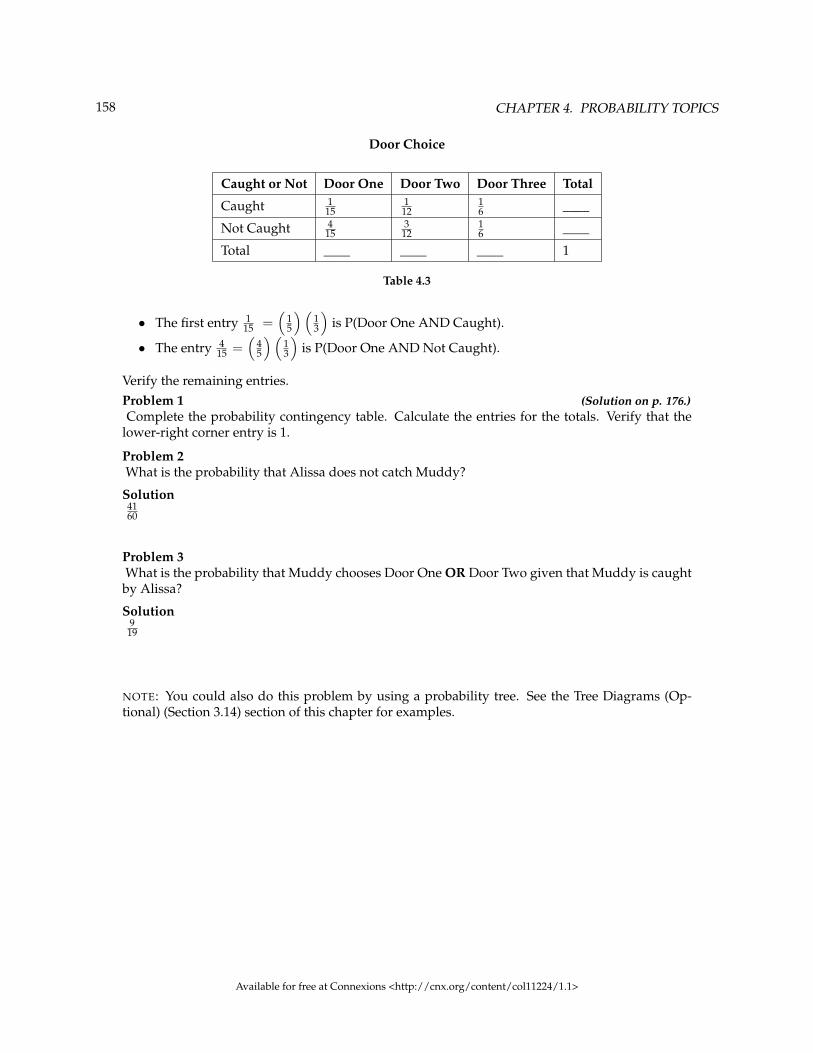
158 CHAPTER 4. PROBABILITY TOPICS
Door Choice
Caught or Not Door One Door Two Door Three Total
Caught 115
112
16 ____
Not Caught 415
312
16 ____
Total ____ ____ ____ 1
Table 4.3
• The first entry 115 =
(15
) (13
)is P(Door One AND Caught).
• The entry 415 =
(45
) (13
)is P(Door One AND Not Caught).
Verify the remaining entries.Problem 1 (Solution on p. 176.)Complete the probability contingency table. Calculate the entries for the totals. Verify that the
lower-right corner entry is 1.
Problem 2What is the probability that Alissa does not catch Muddy?
Solution4160
Problem 3What is the probability that Muddy chooses Door One OR Door Two given that Muddy is caughtby Alissa?
Solution9
19
NOTE: You could also do this problem by using a probability tree. See the Tree Diagrams (Op-tional) (Section 3.14) section of this chapter for examples.
Available for free at Connexions <http://cnx.org/content/col11224/1.1>
159
4.7 Summary of Formulas7
Formula 4.1: ComplementIf A and A’ are complements then P (A) + P(A’ ) = 1Formula 4.2: Addition RuleP(A OR B) = P(A) + P(B)− P(A AND B)Formula 4.3: Mutually ExclusiveIf A and B are mutually exclusive then P(A AND B) = 0 ; so P(A OR B) = P(A) + P(B).Formula 4.4: Multiplication Rule
• P(A AND B) = P(B)P(A|B)• P(A AND B) = P(A)P(B|A)
Formula 4.5: IndependenceIf A and B are independent then:
• P(A|B) = P(A)• P(B|A) = P(B)• P(A AND B) = P(A)P(B)
7This content is available online at <http://cnx.org/content/m16843/1.5/>.
Available for free at Connexions <http://cnx.org/content/col11224/1.1>

160 CHAPTER 4. PROBABILITY TOPICS
4.8 Practice 1: Contingency Tables8
4.8.1 Student Learning Outcomes
• The student will construct and interpret contingency tables.
4.8.2 Given
An article in the New England Journal of Medicine , reported about a study of smokers in California andHawaii. In one part of the report, the self-reported ethnicity and smoking levels per day were given. Of thepeople smoking at most 10 cigarettes per day, there were 9886 African Americans, 2745 Native Hawaiians,12,831 Latinos, 8378 Japanese Americans, and 7650 Whites. Of the people smoking 11-20 cigarettes perday, there were 6514 African Americans, 3062 Native Hawaiians, 4932 Latinos, 10,680 Japanese Americans,and 9877 Whites. Of the people smoking 21-30 cigarettes per day, there were 1671 African Americans, 1419Native Hawaiians, 1406 Latinos, 4715 Japanese Americans, and 6062 Whites. Of the people smoking at least31 cigarettes per day, there were 759 African Americans, 788 Native Hawaiians, 800 Latinos, 2305 JapaneseAmericans, and 3970 Whites. ((Source: http://www.nejm.org/doi/full/10.1056/NEJMoa033250) )
4.8.3 Complete the Table
Complete the table below using the data provided.
Smoking Levels by Ethnicity
SmokingLevel
AfricanAmerican
NativeHawaiian
Latino JapaneseAmericans
White TOTALS
1-10
11-20
21-30
31+
TOTALS
Table 4.4
4.8.4 Analyze the Data
Suppose that one person from the study is randomly selected.Exercise 4.8.1 (Solution on p. 177.)Find the probability that person smoked 11-20 cigarettes per day.
Exercise 4.8.2 (Solution on p. 177.)Find the probability that person was Latino.
8This content is available online at <http://cnx.org/content/m16839/1.11/>.
Available for free at Connexions <http://cnx.org/content/col11224/1.1>
161
4.8.5 Discussion Questions
Exercise 4.8.3 (Solution on p. 177.)In words, explain what it means to pick one person from the study and that person is “Japanese
American AND smokes 21-30 cigarettes per day.” Also, find the probability.Exercise 4.8.4 (Solution on p. 177.)In words, explain what it means to pick one person from the study and that person is “Japanese
American OR smokes 21-30 cigarettes per day.” Also, find the probability.Exercise 4.8.5 (Solution on p. 177.)In words, explain what it means to pick one person from the study and that person is “Japanese
American GIVEN that person smokes 21-30 cigarettes per day.” Also, find the probability.Exercise 4.8.6Prove that smoking level/day and ethnicity are dependent events.
Available for free at Connexions <http://cnx.org/content/col11224/1.1>
162 CHAPTER 4. PROBABILITY TOPICS
4.9 Practice 2: Calculating Probabilities9
4.9.1 Student Learning Outcomes
• Students will define basic probability terms.• Students will calculate probabilities.• Students will determine whether two events are mutually exclusive or whether two events are inde-
pendent.
NOTE: Use probability rules to solve the problems below. Show your work.
4.9.2 Given
48% of all Californians registered voters prefer life in prison without parole over the death penalty fora person convicted of first degree murder. Among Latino California registered voters, 55% prefer lifein prison without parole over the death penalty for a person convicted of first degree murder. (Source:http://field.com/fieldpollonline/subscribers/Rls2393.pdf ).37.6% of all Californians are Latino (Source: U.S. Census Bureau).
In this problem, let:
• C = Cali f ornians (registered voters) pre f erring li f e in prison without parole over the death penalty f or a person convicted o f f irst degree murder• L = Latino Cali f ornians
Suppose that one Californian is randomly selected.
4.9.3 Analyze the Data
Exercise 4.9.1 (Solution on p. 177.)P (C) =
Exercise 4.9.2 (Solution on p. 177.)P (L) =
Exercise 4.9.3 (Solution on p. 177.)P (C|L) =
Exercise 4.9.4In words, what is " C | L"?
Exercise 4.9.5 (Solution on p. 177.)P (L AND C) =
Exercise 4.9.6In words, what is “L and C”?
Exercise 4.9.7 (Solution on p. 177.)Are L and C independent events? Show why or why not.
Exercise 4.9.8 (Solution on p. 177.)P (L OR C) =
Exercise 4.9.9In words, what is “L or C”?
Exercise 4.9.10 (Solution on p. 177.)Are L and C mutually exclusive events? Show why or why not.
9This content is available online at <http://cnx.org/content/m16840/1.12/>.
Available for free at Connexions <http://cnx.org/content/col11224/1.1>
163
4.10 Homework10
Exercise 4.10.1 (Solution on p. 177.)Suppose that you have 8 cards. 5 are green and 3 are yellow. The 5 green cards are numbered
1, 2, 3, 4, and 5. The 3 yellow cards are numbered 1, 2, and 3. The cards are well shuffled. Yourandomly draw one card.
• G = card drawn is green• E = card drawn is even-numbered
a. List the sample space.b. P (G) =c. P (G|E) =d. P (G AND E) =e. P (G OR E) =f. Are G and E mutually exclusive? Justify your answer numerically.
Exercise 4.10.2Refer to the previous problem. Suppose that this time you randomly draw two cards, one at a
time, and with replacement.
• G1 = first card is green• G2 = second card is green
a. Draw a tree diagram of the situation.b. P (G1 AND G2) =c. P (at least one green) =d. P (G2 | G1) =e. Are G2 and G1 independent events? Explain why or why not.
Exercise 4.10.3 (Solution on p. 178.)Refer to the previous problems. Suppose that this time you randomly draw two cards, one at a
time, and without replacement.
• G1= first card is green• G2= second card is green
a. Draw a tree diagram of the situation.b. P (G1 AND G2) =c. P(at least one green) =d. P (G2|G1) =e. Are G2 and G1 independent events? Explain why or why not.
Exercise 4.10.4Roll two fair dice. Each die has 6 faces.
a. List the sample space.b. Let A be the event that either a 3 or 4 is rolled first, followed by an even number. Find P (A).c. Let B be the event that the sum of the two rolls is at most 7. Find P (B).
10This content is available online at <http://cnx.org/content/m16836/1.21/>.
Available for free at Connexions <http://cnx.org/content/col11224/1.1>
164 CHAPTER 4. PROBABILITY TOPICS
d. In words, explain what “P (A|B)” represents. Find P (A|B).e. Are A and B mutually exclusive events? Explain your answer in 1 - 3 complete sentences,
including numerical justification.f. Are A and B independent events? Explain your answer in 1 - 3 complete sentences, including
numerical justification.
Exercise 4.10.5 (Solution on p. 178.)A special deck of cards has 10 cards. Four are green, three are blue, and three are red. When a
card is picked, the color of it is recorded. An experiment consists of first picking a card and thentossing a coin.
a. List the sample space.b. Let A be the event that a blue card is picked first, followed by landing a head on the coin toss.
Find P(A).c. Let B be the event that a red or green is picked, followed by landing a head on the coin toss. Are
the events A and B mutually exclusive? Explain your answer in 1 - 3 complete sentences,including numerical justification.
d. Let C be the event that a red or blue is picked, followed by landing a head on the coin toss. Arethe events A and C mutually exclusive? Explain your answer in 1 - 3 complete sentences,including numerical justification.
Exercise 4.10.6An experiment consists of first rolling a die and then tossing a coin:
a. List the sample space.b. Let A be the event that either a 3 or 4 is rolled first, followed by landing a head on the coin toss.
Find P(A).c. Let B be the event that a number less than 2 is rolled, followed by landing a head on the coin
toss. Are the events A and B mutually exclusive? Explain your answer in 1 - 3 completesentences, including numerical justification.
Exercise 4.10.7 (Solution on p. 178.)An experiment consists of tossing a nickel, a dime and a quarter. Of interest is the side the coin
lands on.
a. List the sample space.b. Let A be the event that there are at least two tails. Find P(A).c. Let B be the event that the first and second tosses land on heads. Are the events A and B
mutually exclusive? Explain your answer in 1 - 3 complete sentences, including justification.
Exercise 4.10.8Consider the following scenario:
• Let P(C) = 0.4• Let P(D) = 0.5• Let P(C|D) = 0.6
a. Find P(C AND D) .b. Are C and D mutually exclusive? Why or why not?c. Are C and D independent events? Why or why not?d. Find P(C OR D) .e. Find P(D|C).
Available for free at Connexions <http://cnx.org/content/col11224/1.1>
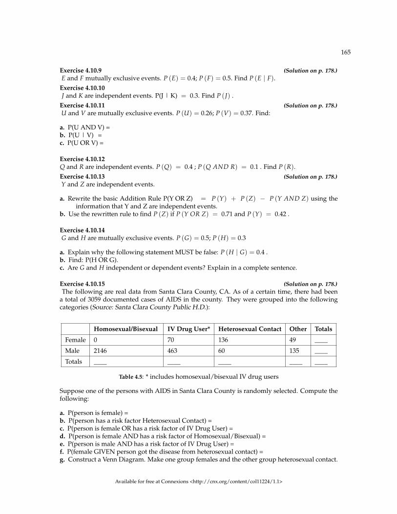
165
Exercise 4.10.9 (Solution on p. 178.)E and F mutually exclusive events. P (E) = 0.4; P (F) = 0.5. Find P (E | F).
Exercise 4.10.10J and K are independent events. P(J | K) = 0.3. Find P (J) .
Exercise 4.10.11 (Solution on p. 178.)U and V are mutually exclusive events. P (U) = 0.26; P (V) = 0.37. Find:
a. P(U AND V) =b. P(U | V) =c. P(U OR V) =
Exercise 4.10.12Q and R are independent events. P (Q) = 0.4 ; P (Q AND R) = 0.1 . Find P (R).Exercise 4.10.13 (Solution on p. 178.)Y and Z are independent events.
a. Rewrite the basic Addition Rule P(Y OR Z) = P (Y) + P (Z) − P (Y AND Z) using theinformation that Y and Z are independent events.
b. Use the rewritten rule to find P (Z) if P (Y OR Z) = 0.71 and P (Y) = 0.42 .
Exercise 4.10.14G and H are mutually exclusive events. P (G) = 0.5; P (H) = 0.3
a. Explain why the following statement MUST be false: P (H | G) = 0.4 .b. Find: P(H OR G).c. Are G and H independent or dependent events? Explain in a complete sentence.
Exercise 4.10.15 (Solution on p. 178.)The following are real data from Santa Clara County, CA. As of a certain time, there had been
a total of 3059 documented cases of AIDS in the county. They were grouped into the followingcategories (Source: Santa Clara County Public H.D.):
Homosexual/Bisexual IV Drug User* Heterosexual Contact Other Totals
Female 0 70 136 49 ____
Male 2146 463 60 135 ____
Totals ____ ____ ____ ____ ____
Table 4.5: * includes homosexual/bisexual IV drug users
Suppose one of the persons with AIDS in Santa Clara County is randomly selected. Compute thefollowing:
a. P(person is female) =b. P(person has a risk factor Heterosexual Contact) =c. P(person is female OR has a risk factor of IV Drug User) =d. P(person is female AND has a risk factor of Homosexual/Bisexual) =e. P(person is male AND has a risk factor of IV Drug User) =f. P(female GIVEN person got the disease from heterosexual contact) =g. Construct a Venn Diagram. Make one group females and the other group heterosexual contact.
Available for free at Connexions <http://cnx.org/content/col11224/1.1>

166 CHAPTER 4. PROBABILITY TOPICS
Exercise 4.10.16Solve these questions using probability rules. Do NOT use the contingency table above. 3059
cases of AIDS had been reported in Santa Clara County, CA, through a certain date. Those caseswill be our population. Of those cases, 6.4% obtained the disease through heterosexual contactand 7.4% are female. Out of the females with the disease, 53.3% got the disease from heterosexualcontact.
a. P(person is female) =b. P(person obtained the disease through heterosexual contact) =c. P(female GIVEN person got the disease from heterosexual contact) =d. Construct a Venn Diagram. Make one group females and the other group heterosexual contact.
Fill in all values as probabilities.
Exercise 4.10.17 (Solution on p. 178.)The following table identifies a group of children by one of four hair colors, and by type of hair.
Hair Type Brown Blond Black Red Totals
Wavy 20 15 3 43
Straight 80 15 12
Totals 20 215
Table 4.6
a. Complete the table above.b. What is the probability that a randomly selected child will have wavy hair?c. What is the probability that a randomly selected child will have either brown or blond hair?d. What is the probability that a randomly selected child will have wavy brown hair?e. What is the probability that a randomly selected child will have red hair, given that he has
straight hair?f. If B is the event of a child having brown hair, find the probability of the complement of B.g. In words, what does the complement of B represent?
Exercise 4.10.18A previous year, the weights of the members of the San Francisco 49ers and the Dallas Cowboyswere published in the San Jose Mercury News. The factual data are compiled into the followingtable.
Shirt# ≤ 210 211-250 251-290 290≤1-33 21 5 0 0
34-66 6 18 7 4
66-99 6 12 22 5
Table 4.7
For the following, suppose that you randomly select one player from the 49ers or Cowboys.
a. Find the probability that his shirt number is from 1 to 33.b. Find the probability that he weighs at most 210 pounds.
Available for free at Connexions <http://cnx.org/content/col11224/1.1>

167
c. Find the probability that his shirt number is from 1 to 33 AND he weighs at most 210 pounds.d. Find the probability that his shirt number is from 1 to 33 OR he weighs at most 210 pounds.e. Find the probability that his shirt number is from 1 to 33 GIVEN that he weighs at most 210
pounds.f. If having a shirt number from 1 to 33 and weighing at most 210 pounds were independent
events, then what should be true about P(Shirt# 1-33 | ≤ 210 pounds)?
Exercise 4.10.19 (Solution on p. 179.)Approximately 281,000,000 people over age 5 live in the United States. Of
these people, 55,000,000 speak a language other than English at home. Ofthose who speak another language at home, 62.3% speak Spanish. (Source:http://www.census.gov/hhes/socdemo/language/data/acs/ACS-12.pdf )
Let: E = speak English at home; E’ = speak another language at home; S = speak Spanish;
Finish each probability statement by matching the correct answer.
Probability Statements Answers
a. P(E’) = i. 0.8043
b. P(E) = ii. 0.623
c. P(S and E’) = iii. 0.1957
d. P(S|E’) = iv. 0.1219
Table 4.8
Exercise 4.10.20The probability that a male develops some form of cancer in his lifetime is 0.4567 (Source: Ameri-can Cancer Society). The probability that a male has at least one false positive test result (meaningthe test comes back for cancer when the man does not have it) is 0.51 (Source: USA Today). Some ofthe questions below do not have enough information for you to answer them. Write “not enoughinformation” for those answers.
Let: C = a man develops cancer in his lifetime; P = man has at least one false positive
a. Construct a tree diagram of the situation.b. P (C) =c. P(P|C) =d. P(P|C’ ) =e. If a test comes up positive, based upon numerical values, can you assume that man has cancer?
Justify numerically and explain why or why not.
Exercise 4.10.21 (Solution on p. 179.)In 1994, the U.S. government held a lottery to issue 55,000 Green Cards (permits for non-citizens
to work legally in the U.S.). Renate Deutsch, from Germany, was one of approximately 6.5 millionpeople who entered this lottery. Let G = won Green Card.
a. What was Renate’s chance of winning a Green Card? Write your answer as a probability state-ment.
b. In the summer of 1994, Renate received a letter stating she was one of 110,000 finalists chosen.Once the finalists were chosen, assuming that each finalist had an equal chance to win, whatwas Renate’s chance of winning a Green Card? Let F = was a finalist. Write your answer asa conditional probability statement.
Available for free at Connexions <http://cnx.org/content/col11224/1.1>

168 CHAPTER 4. PROBABILITY TOPICS
c. Are G and F independent or dependent events? Justify your answer numerically and alsoexplain why.
d. Are G and F mutually exclusive events? Justify your answer numerically and also explain why.
NOTE: P.S. Amazingly, on 2/1/95, Renate learned that she would receive her Green Card – truestory!
Exercise 4.10.22Three professors at George Washington University did an experiment to determine if economists
are more selfish than other people. They dropped 64 stamped, addressed envelopes with $10 cashin different classrooms on the George Washington campus. 44% were returned overall. From theeconomics classes 56% of the envelopes were returned. From the business, psychology, and historyclasses 31% were returned. (Source: Wall Street Journal )
Let: R = money returned; E = economics classes; O = other classes
a. Write a probability statement for the overall percent of money returned.b. Write a probability statement for the percent of money returned out of the economics classes.c. Write a probability statement for the percent of money returned out of the other classes.d. Is money being returned independent of the class? Justify your answer numerically and explain
it.e. Based upon this study, do you think that economists are more selfish than other people? Explain
why or why not. Include numbers to justify your answer.
Exercise 4.10.23 (Solution on p. 179.)The chart below gives the number of suicides estimated in the U.S. for a recent year by age, race
(black and white), and sex. We are interested in possible relationships between age, race, and sex.We will let suicide victims be our population. (Source: The National Center for Health Statistics,U.S. Dept. of Health and Human Services)
Race and Sex 1 - 14 15 - 24 25 - 64 over 64 TOTALS
white, male 210 3360 13,610 22,050
white, female 80 580 3380 4930
black, male 10 460 1060 1670
black, female 0 40 270 330
all others
TOTALS 310 4650 18,780 29,760
Table 4.9
NOTE: Do not include "all others" for parts (f), (g), and (i).
a. Fill in the column for the suicides for individuals over age 64.b. Fill in the row for all other races.c. Find the probability that a randomly selected individual was a white male.d. Find the probability that a randomly selected individual was a black female.e. Find the probability that a randomly selected individual was black
Available for free at Connexions <http://cnx.org/content/col11224/1.1>

169
f. Find the probability that a randomly selected individual was male.g. Out of the individuals over age 64, find the probability that a randomly selected individual was
a black or white male.h. Comparing “Race and Sex” to “Age,” which two groups are mutually exclusive? How do you
know?i. Are being male and committing suicide over age 64 independent events? How do you know?
The next two questions refer to the following: The percent of licensed U.S. drivers (from a recent year)that are female is 48.60. Of the females, 5.03% are age 19 and under; 81.36% are age 20 - 64; 13.61% are age65 or over. Of the licensed U.S. male drivers, 5.04% are age 19 and under; 81.43% are age 20 - 64; 13.53% areage 65 or over. (Source: Federal Highway Administration, U.S. Dept. of Transportation)
Exercise 4.10.24Complete the following:
a. Construct a table or a tree diagram of the situation.b. P(driver is female) =c. P(driver is age 65 or over | driver is female) =d. P(driver is age 65 or over AND female) =e. In words, explain the difference between the probabilities in part (c) and part (d).f. P(driver is age 65 or over) =g. Are being age 65 or over and being female mutually exclusive events? How do you know
Exercise 4.10.25 (Solution on p. 179.)Suppose that 10,000 U.S. licensed drivers are randomly selected.
a. How many would you expect to be male?b. Using the table or tree diagram from the previous exercise, construct a contingency table of
gender versus age group.c. Using the contingency table, find the probability that out of the age 20 - 64 group, a randomly
selected driver is female.
Exercise 4.10.26Approximately 86.5% of Americans commute to work by car, truck or van. Out of that group,
84.6% drive alone and 15.4% drive in a carpool. Approximately 3.9% walk to work and approxi-mately 5.3% take public transportation. (Source: Bureau of the Census, U.S. Dept. of Commerce.Disregard rounding approximations.)
a. Construct a table or a tree diagram of the situation. Include a branch for all other modes oftransportation to work.
b. Assuming that the walkers walk alone, what percent of all commuters travel alone to work?c. Suppose that 1000 workers are randomly selected. How many would you expect to travel alone
to work?d. Suppose that 1000 workers are randomly selected. How many would you expect to drive in a
carpool?
Exercise 4.10.27Explain what is wrong with the following statements. Use complete sentences.
a. If there’s a 60% chance of rain on Saturday and a 70% chance of rain on Sunday, then there’s a130% chance of rain over the weekend.
b. The probability that a baseball player hits a home run is greater than the probability that hegets a successful hit.
Available for free at Connexions <http://cnx.org/content/col11224/1.1>

170 CHAPTER 4. PROBABILITY TOPICS
4.10.1 Try these multiple choice questions.
The next two questions refer to the following probability tree diagram which shows tossing an unfaircoin FOLLOWED BY drawing one bead from a cup containing 3 red (R), 4 yellow (Y) and 5 blue (B) beads.For the coin, P (H) = 2
3 and P (T) = 13 where H = "heads" and T = "tails”.
Figure 4.1
Exercise 4.10.28 (Solution on p. 179.)Find P(tossing a Head on the coin AND a Red bead)
A. 23
B. 515
C. 636
D. 536
Exercise 4.10.29 (Solution on p. 179.)Find P(Blue bead).
A. 1536
B. 1036
C. 1012
D. 636
The next three questions refer to the following table of data obtained from www.baseball-almanac.com11
showing hit information for 4 well known baseball players. Suppose that one hit from the table is randomlyselected.
11http://cnx.org/content/m16836/latest/www.baseball-almanac.com
Available for free at Connexions <http://cnx.org/content/col11224/1.1>

171
NAME Single Double Triple Home Run TOTAL HITS
Babe Ruth 1517 506 136 714 2873
Jackie Robinson 1054 273 54 137 1518
Ty Cobb 3603 174 295 114 4189
Hank Aaron 2294 624 98 755 3771
TOTAL 8471 1577 583 1720 12351
Table 4.10
Exercise 4.10.30 (Solution on p. 179.)Find P(hit was made by Babe Ruth).
A. 15182873
B. 287312351
C. 58312351
D. 418912351
Exercise 4.10.31 (Solution on p. 179.)Find P(hit was made by Ty Cobb | The hit was a Home Run)
A. 418912351
B. 1141720
C. 17204189
D. 11412351
Exercise 4.10.32 (Solution on p. 179.)Are the hit being made by Hank Aaron and the hit being a double independent events?
A. Yes, because P(hit by Hank Aaron | hit is a double) = P(hit by Hank Aaron)B. No, because P(hit by Hank Aaron | hit is a double) 6= P(hit is a double)C. No, because P(hit is by Hank Aaron | hit is a double) 6= P(hit by Hank Aaron)D. Yes, because P(hit is by Hank Aaron | hit is a double) = P(hit is a double)
Exercise 4.10.33 (Solution on p. 179.)Given events G and H: P(G) = 0.43 ; P(H) = 0.26 ; P(H and G) = 0.14
A. Find P(H or G)B. Find the probability of the complement of event (H and G)C. Find the probability of the complement of event (H or G)
Exercise 4.10.34 (Solution on p. 179.)Given events J and K: P(J) = 0.18 ; P(K) = 0.37 ; P(J or K) = 0.45
A. Find P(J and K)B. Find the probability of the complement of event (J and K)C. Find the probability of the complement of event (J or K)
Available for free at Connexions <http://cnx.org/content/col11224/1.1>
172 CHAPTER 4. PROBABILITY TOPICS
Exercise 4.10.35 (Solution on p. 180.)United Blood Services is a blood bank that serves more than 500 hospitals in 18 states. Accord-
ing to their website, http://www.unitedbloodservices.org/humanbloodtypes.html, a person withtype O blood and a negative Rh factor (Rh−) can donate blood to any person with any bloodtype.Their data show that 43% of people have type O blood and 15% of people have Rh− factor; 52%of people have type O or Rh− factor.
A. Find the probability that a person has both type O blood and the Rh− factorB. Find the probability that a person does NOT have both type O blood and the Rh− factor.
Exercise 4.10.36 (Solution on p. 180.)At a college, 72% of courses have final exams and 46% of courses require research papers. Supposethat 32% of courses have a research paper and a final exam. Let F be the event that a course has afinal exam. Let R be the event that a course requires a research paper.
A. Find the probability that a course has a final exam or a research project.B. Find the probability that a course has NEITHER of these two requirements.
Exercise 4.10.37 (Solution on p. 180.)In a box of assorted cookies, 36% contain chocolate and 12% contain nuts. Of those, 8% contain
both chocolate and nuts. Sean is allergic to both chocolate and nuts.
A. Find the probability that a cookie contains chocolate or nuts (he can’t eat it).B. Find the probability that a cookie does not contain chocolate or nuts (he can eat it).
Exercise 4.10.38 (Solution on p. 180.)A college finds that 10% of students have taken a distance learning class and that 40% of studentsare part time students. Of the part time students, 20% have taken a distance learning class. Let D= event that a student takes a distance learning class and E = event that a student is a part timestudent
A. Find P(D and E)B. Find P(E | D)C. Find P(D or E)D. Using an appropriate test, show whether D and E are independent.E. Using an appropriate test, show whether D and E are mutually exclusive.
Exercise 4.10.39 (Solution on p. 180.)When the Euro coin was introduced in 2002, two math professors had their statistics students testwhether the Belgian 1 Euro coin was a fair coin. They spun the coin rather than tossing it, and itwas found that out of 250 spins, 140 showed a head (event H) while 110 showed a tail (event T).Therefore, they claim that this is not a fair coin.
A. Based on the data above, find P(H) and P(T).B. Use a tree to find the probabilities of each possible outcome for the experiment of tossing the
coin twice.C. Use the tree to find the probability of obtaining exactly one head in two tosses of the coin.D. Use the tree to find the probability of obtaining at least one head.
Exercise 4.10.40A box of cookies contains 3 chocolate and 7 butter cookies. Miguel randomly selects a cookie andeats it. Then he randomly selects another cookie and eats it also. (How many cookies did he take?)
Available for free at Connexions <http://cnx.org/content/col11224/1.1>
173
A. Draw the tree that represents the possibilities for the cookie selections. Write the probabilitiesalong each branch of the tree.
B. Are the probabilities for the flavor of the SECOND cookie that Miguel selects independent ofhis first selection? Explain.
C. For each complete path through the tree, write the event it represents and find the probabilities.D. Let S be the event that both cookies selected were the same flavor. Find P(S).E. Let T be the event that both cookies selected were different flavors. Find P(T) by two different
methods: by using the complement rule and by using the branches of the tree. Your answersshould be the same with both methods.
F. Let U be the event that the second cookie selected is a butter cookie. Find P(U).
**Exercises 33 - 40 contributed by Roberta Bloom
Available for free at Connexions <http://cnx.org/content/col11224/1.1>

174 CHAPTER 4. PROBABILITY TOPICS
4.11 Review12
The first six exercises refer to the following study: In a survey of 100 stocks on NASDAQ, the averagepercent increase for the past year was 9% for NASDAQ stocks. Answer the following:
Exercise 4.11.1 (Solution on p. 180.)The “average increase” for all NASDAQ stocks is the:
A. PopulationB. StatisticC. ParameterD. SampleE. Variable
Exercise 4.11.2 (Solution on p. 180.)All of the NASDAQ stocks are the:
A. PopulationB. StatisticC. ParameterD. SampleE. Variable
Exercise 4.11.3 (Solution on p. 180.)9% is the:
A. PopulationB. StatisticC. ParameterD. SampleE. Variable
Exercise 4.11.4 (Solution on p. 180.)The 100 NASDAQ stocks in the survey are the:
A. PopulationB. StatisticC. ParameterD. SampleE. Variable
Exercise 4.11.5 (Solution on p. 180.)The percent increase for one stock in the survey is the:
A. PopulationB. StatisticC. ParameterD. SampleE. Variable
12This content is available online at <http://cnx.org/content/m16842/1.9/>.
Available for free at Connexions <http://cnx.org/content/col11224/1.1>
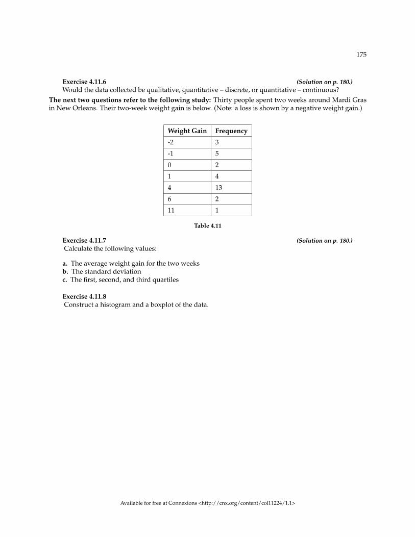
175
Exercise 4.11.6 (Solution on p. 180.)Would the data collected be qualitative, quantitative – discrete, or quantitative – continuous?
The next two questions refer to the following study: Thirty people spent two weeks around Mardi Grasin New Orleans. Their two-week weight gain is below. (Note: a loss is shown by a negative weight gain.)
Weight Gain Frequency
-2 3
-1 5
0 2
1 4
4 13
6 2
11 1
Table 4.11
Exercise 4.11.7 (Solution on p. 180.)Calculate the following values:
a. The average weight gain for the two weeksb. The standard deviationc. The first, second, and third quartiles
Exercise 4.11.8Construct a histogram and a boxplot of the data.
Available for free at Connexions <http://cnx.org/content/col11224/1.1>

176 CHAPTER 4. PROBABILITY TOPICS
Solutions to Exercises in Chapter 4
Solution to Exercise 4.3.1 (p. 148)
a. P(L’)=P(S)b. P(M or S)c. P(F and L)d. P(M|L)e. P(L|M)f. P(S|F)g. P(F|L)h. P(F or L)i. P(M and S)j. P(F)
Solution to Example 4.6, Problem (p. 154)No. C = {3, 5} and E = {1, 2, 3, 4}. P (C AND E) = 1
6 . To be mutually exclusive, P (C AND E) must be0.Solution to Example 4.11, Problem 1 (p. 157)
Hiking Area Preference
Sex The Coastline Near Lakes and Streams On Mountain Peaks Total
Female 18 16 11 45
Male 16 25 14 55
Total 34 41 25 100
Table 4.12
Solution to Example 4.11, Problem 2 (p. 157)
a. P(F AND C) = 18100 = 0.18
b. P (F) · P (C) = 45100 ·
34100 = 0.45 · 0.34 = 0.153
P(F AND C) 6= P (F) · P (C), so the events F and C are not independent.Solution to Example 4.11, Problem 3 (p. 157)
a. The word ’given’ tells you that this is a conditional.b. P(M|L) = 25
41c. No, the sample space for this problem is 41.
Solution to Example 4.11, Problem 4 (p. 157)
a. P(F) = 45100
b. P(P) = 25100
c. P(F AND P) = 11100
d. P(F OR P) = 45100 + 25
100 −11
100 = 59100
Solution to Example 4.12, Problem 1 (p. 158)
Available for free at Connexions <http://cnx.org/content/col11224/1.1>

177
Door Choice
Caught or Not Door One Door Two Door Three Total
Caught 115
112
16
1960
Not Caught 415
312
16
4160
Total 515
412
26 1
Table 4.13
Solutions to Practice 1: Contingency Tables
Solution to Exercise 4.8.1 (p. 160)35,065
100,450Solution to Exercise 4.8.2 (p. 160)
19,969100,450
Solution to Exercise 4.8.3 (p. 161)4,715
100,450Solution to Exercise 4.8.4 (p. 161)
36,636100,450
Solution to Exercise 4.8.5 (p. 161)4715
15,273
Solutions to Practice 2: Calculating Probabilities
Solution to Exercise 4.9.1 (p. 162)0.48
Solution to Exercise 4.9.2 (p. 162)0.376
Solution to Exercise 4.9.3 (p. 162)0.55
Solution to Exercise 4.9.5 (p. 162)0.2068
Solution to Exercise 4.9.7 (p. 162)No
Solution to Exercise 4.9.8 (p. 162)0.6492
Solution to Exercise 4.9.10 (p. 162)No
Solutions to Homework
Solution to Exercise 4.10.1 (p. 163)
a. {G1, G2, G3, G4, G5, Y1, Y2, Y3}b. 5
8c. 2
3d. 2
8e. 6
8f. No
Available for free at Connexions <http://cnx.org/content/col11224/1.1>
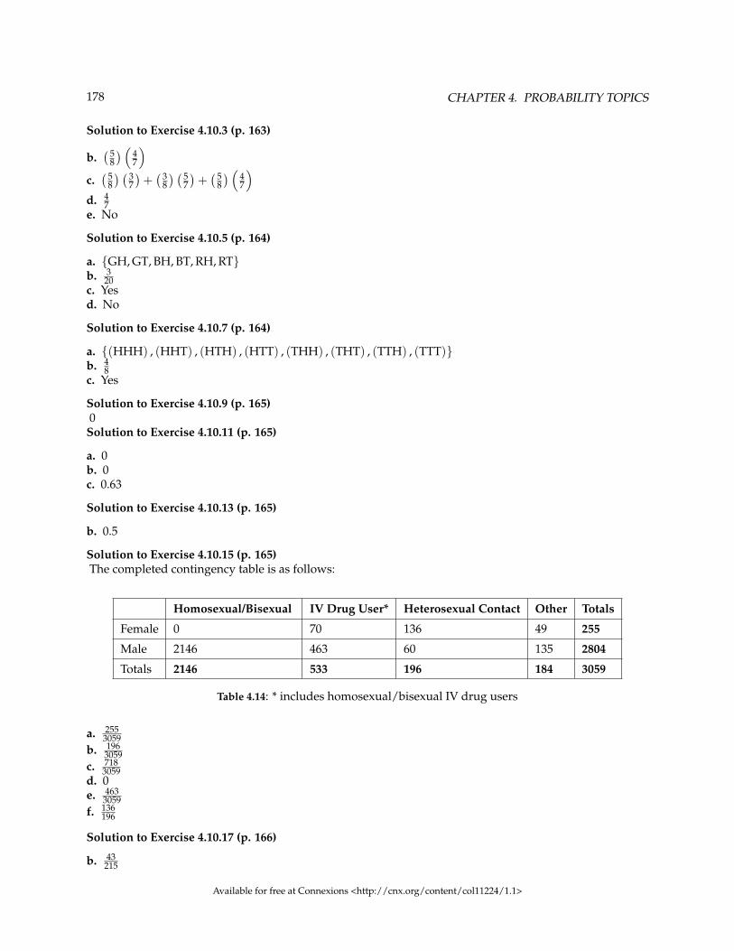
178 CHAPTER 4. PROBABILITY TOPICS
Solution to Exercise 4.10.3 (p. 163)
b.( 5
8) ( 4
7
)c.( 5
8) ( 3
7)+( 3
8) ( 5
7)+( 5
8) ( 4
7
)d. 4
7e. No
Solution to Exercise 4.10.5 (p. 164)
a. {GH, GT, BH, BT, RH, RT}b. 3
20c. Yesd. No
Solution to Exercise 4.10.7 (p. 164)
a. {(HHH) , (HHT) , (HTH) , (HTT) , (THH) , (THT) , (TTH) , (TTT)}b. 4
8c. Yes
Solution to Exercise 4.10.9 (p. 165)0
Solution to Exercise 4.10.11 (p. 165)
a. 0b. 0c. 0.63
Solution to Exercise 4.10.13 (p. 165)
b. 0.5
Solution to Exercise 4.10.15 (p. 165)The completed contingency table is as follows:
Homosexual/Bisexual IV Drug User* Heterosexual Contact Other Totals
Female 0 70 136 49 255
Male 2146 463 60 135 2804
Totals 2146 533 196 184 3059
Table 4.14: * includes homosexual/bisexual IV drug users
a. 2553059
b. 1963059
c. 7183059
d. 0e. 463
3059f. 136
196
Solution to Exercise 4.10.17 (p. 166)
b. 43215
Available for free at Connexions <http://cnx.org/content/col11224/1.1>

179
c. 120215
d. 20215
e. 12172
f. 115215
Solution to Exercise 4.10.19 (p. 167)
a. iiib. ic. ivd. ii
Solution to Exercise 4.10.21 (p. 167)
a. P (G) = 0.008b. 0.5c. dependentd. No
Solution to Exercise 4.10.23 (p. 168)
c. 2205029760
d. 33029760
e. 200029760
f. 2372029760
g. 50106020
h. Black females and ages 1-14i. No
Solution to Exercise 4.10.25 (p. 169)
a. 5140c. 0.49
Solution to Exercise 4.10.28 (p. 170)C
Solution to Exercise 4.10.29 (p. 170)A
Solution to Exercise 4.10.30 (p. 171)B
Solution to Exercise 4.10.31 (p. 171)B
Solution to Exercise 4.10.32 (p. 171)C
Solution to Exercise 4.10.33 (p. 171)
A. P(H or G) = P(H) + P(G) − P(H and G) = 0.26 + 0.43 − 0.14 = 0.55B. P( NOT (H and G) ) = 1 − P(H and G) = 1 − 0.14 = 0.86C. P( NOT (H or G) ) = 1 − P(H or G) = 1 − 0.55 = 0.45
Solution to Exercise 4.10.34 (p. 171)
A. P(J or K) = P(J) + P(K) − P(J and K); 0.45 = 0.18 + 0.37 − P(J and K) ; solve to find P(J and K) = 0.10B. P( NOT (J and K) ) = 1 − P(J and K) = 1 − 0.10 = 0.90C. P( NOT (J or K) ) = 1 − P(J or K) = 1 − 0.45 = 0.55
Available for free at Connexions <http://cnx.org/content/col11224/1.1>

180 CHAPTER 4. PROBABILITY TOPICS
Solution to Exercise 4.10.35 (p. 172)
A. P(Type O or Rh−) = P(Type O) + P(Rh−) − P(Type O and Rh−)0.52 = 0.43 + 0.15 − P(Type O and Rh−); solve to find P(Type O and Rh−) = 0.066% of people have type O Rh− blood
B. P( NOT (Type O and Rh−) ) = 1 − P(Type O and Rh−) = 1 − 0.06 = 0.9494% of people do not have type O Rh− blood
Solution to Exercise 4.10.36 (p. 172)
A. P(R or F) = P(R) + P(F) − P(R and F) = 0.72 + 0.46 − 0.32 = 0.86B. P( Neither R nor F ) = 1 − P(R or F) = 1 − 0.86 = 0.14
Solution to Exercise 4.10.37 (p. 172)
Let C be the event that the cookie contains chocolate. Let N be the event that the cookie contains nuts.A. P(C or N) = P(C) + P(N) − P(C and N) = 0.36 + 0.12 − 0.08 = 0.40B. P( neither chocolate nor nuts) = 1 − P(C or N) = 1 − 0.40 = 0.60
Solution to Exercise 4.10.38 (p. 172)
A. P(D and E) = P(D|E)P(E) = (0.20)(0.40) = 0.08B. P(E|D) = P(D and E) / P(D) = 0.08/0.10 = 0.80C. P(D or E) = P(D) + P(E) − P(D and E) = 0.10 + 0.40 − 0.08 = 0.42D. Not Independent: P(D|E) = 0.20 which does not equal P(D) = .10E. Not Mutually Exclusive: P(D and E) = 0.08 ; if they were mutually exclusive then we would need to have
P(D and E) = 0, which is not true here.
Solution to Exercise 4.10.39 (p. 172)
A. P(H) = 140/250; P(T) = 110/250C. 308/625D. 504/625
Solutions to Review
Solution to Exercise 4.11.1 (p. 174)
C. Parameter
Solution to Exercise 4.11.2 (p. 174)
A. Population
Solution to Exercise 4.11.3 (p. 174)
B. Statistic
Solution to Exercise 4.11.4 (p. 174)
D. Sample
Solution to Exercise 4.11.5 (p. 174)
E. Variable
Solution to Exercise 4.11.6 (p. 175)quantitative - continuousSolution to Exercise 4.11.7 (p. 175)
a. 2.27b. 3.04c. -1, 4, 4
Available for free at Connexions <http://cnx.org/content/col11224/1.1>
Chapter 5
Discrete Random Variables
5.1 Discrete Random Variables1
5.1.1 Student Learning Outcomes
By the end of this chapter, the student should be able to:
• Recognize and understand discrete probability distribution functions, in general.• Calculate and interpret expected values.• Recognize the binomial probability distribution and apply it appropriately.• Recognize the Poisson probability distribution and apply it appropriately (optional).• Recognize the geometric probability distribution and apply it appropriately (optional).• Recognize the hypergeometric probability distribution and apply it appropriately (optional).• Classify discrete word problems by their distributions.
5.1.2 Introduction
A student takes a 10 question true-false quiz. Because the student had such a busy schedule, he or shecould not study and randomly guesses at each answer. What is the probability of the student passing thetest with at least a 70%?
Small companies might be interested in the number of long distance phone calls their employees makeduring the peak time of the day. Suppose the average is 20 calls. What is the probability that the employeesmake more than 20 long distance phone calls during the peak time?
These two examples illustrate two different types of probability problems involving discrete random vari-ables. Recall that discrete data are data that you can count. A random variable describes the outcomesof a statistical experiment in words. The values of a random variable can vary with each repetition of anexperiment.
In this chapter, you will study probability problems involving discrete random distributions. You will alsostudy long-term averages associated with them.
5.1.3 Random Variable Notation
Upper case letters like X or Y denote a random variable. Lower case letters like x or y denote the value of arandom variable. If X is a random variable, then X is written in words. and x is given as a number.
1This content is available online at <http://cnx.org/content/m16825/1.14/>.
Available for free at Connexions <http://cnx.org/content/col11224/1.1>
181

182 CHAPTER 5. DISCRETE RANDOM VARIABLES
For example, let X = the number of heads you get when you toss three fair coins. The sample space for thetoss of three fair coins is TTT; THH; HTH; HHT; HTT; THT; TTH; HHH. Then, x = 0, 1, 2, 3. X is inwords and x is a number. Notice that for this example, the x values are countable outcomes. Because youcan count the possible values that X can take on and the outcomes are random (the x values 0, 1, 2, 3), X isa discrete random variable.
5.1.4 Optional Collaborative Classroom Activity
Toss a coin 10 times and record the number of heads. After all members of the class have completed theexperiment (tossed a coin 10 times and counted the number of heads), fill in the chart using a heading likethe one below. Let X = the number of heads in 10 tosses of the coin.
x Frequency of x Relative Frequency of x
Table 5.1
• Which value(s) of x occurred most frequently?• If you tossed the coin 1,000 times, what values could x take on? Which value(s) of x do you think
would occur most frequently?• What does the relative frequency column sum to?
5.2 Probability Distribution Function (PDF) for a Discrete RandomVariable2
A discrete probability distribution function has two characteristics:
• Each probability is between 0 and 1, inclusive.• The sum of the probabilities is 1.
Example 5.1A child psychologist is interested in the number of times a newborn baby’s crying wakes its motherafter midnight. For a random sample of 50 mothers, the following information was obtained. LetX = the number of times a newborn wakes its mother after midnight. For this example, x = 0, 1, 2,3, 4, 5.
P(x) = probability that X takes on a value x.
2This content is available online at <http://cnx.org/content/m16831/1.14/>.
Available for free at Connexions <http://cnx.org/content/col11224/1.1>

183
x P(x)
0 P(x=0) = 250
1 P(x=1) = 1150
2 P(x=2) = 2350
3 P(x=3) = 950
4 P(x=4) = 450
5 P(x=5) = 150
Table 5.2
X takes on the values 0, 1, 2, 3, 4, 5. This is a discrete PDF because
1. Each P(x) is between 0 and 1, inclusive.2. The sum of the probabilities is 1, that is,
250
+1150
+2350
+950
+4
50+
150
= 1 (5.1)
Example 5.2Suppose Nancy has classes 3 days a week. She attends classes 3 days a week 80% of the time, 2days 15% of the time, 1 day 4% of the time, and no days 1% of the time. Suppose one week israndomly selected.Problem 1 (Solution on p. 230.)Let X = the number of days Nancy ____________________ .
Problem 2 (Solution on p. 230.)X takes on what values?
Problem 3 (Solution on p. 230.)Suppose one week is randomly chosen. Construct a probability distribution table (called a PDF
table) like the one in the previous example. The table should have two columns labeled x and P(x).What does the P(x) column sum to?
5.3 Mean or Expected Value and Standard Deviation3
The expected value is often referred to as the "long-term"average or mean . This means that over the longterm of doing an experiment over and over, you would expect this average.
The mean of a random variable X is µ. If we do an experiment many times (for instance, flip a fair coin, asKarl Pearson did, 24,000 times and let X = the number of heads) and record the value of X each time, theaverage is likely to get closer and closer to µ as we keep repeating the experiment. This is known as theLaw of Large Numbers.
NOTE: To find the expected value or long term average, µ, simply multiply each value of therandom variable by its probability and add the products.
3This content is available online at <http://cnx.org/content/m16828/1.16/>.
Available for free at Connexions <http://cnx.org/content/col11224/1.1>

184 CHAPTER 5. DISCRETE RANDOM VARIABLES
A Step-by-Step ExampleA men’s soccer team plays soccer 0, 1, or 2 days a week. The probability that they play 0 days is 0.2, theprobability that they play 1 day is 0.5, and the probability that they play 2 days is 0.3. Find the long-termaverage, µ, or expected value of the days per week the men’s soccer team plays soccer.
To do the problem, first let the random variable X = the number of days the men’s soccer team plays soccerper week. X takes on the values 0, 1, 2. Construct a PDF table, adding a column xP (x). In this column,you will multiply each x value by its probability.
Expected Value Table
x P(x) xP(x)
0 0.2 (0)(0.2) = 0
1 0.5 (1)(0.5) = 0.5
2 0.3 (2)(0.3) = 0.6
Table 5.4: This table is called an expected value table. The table helps you calculate the expected value orlong-term average.
Add the last column to find the long term average or expected value:(0) (0.2) + (1) (0.5) + (2) (0.3) = 0 + 0.5 + 0.6 = 1.1.
The expected value is 1.1. The men’s soccer team would, on the average, expect to play soccer 1.1 daysper week. The number 1.1 is the long term average or expected value if the men’s soccer team plays soccerweek after week after week. We say µ = 1.1
Example 5.3Find the expected value for the example about the number of times a newborn baby’s crying
wakes its mother after midnight. The expected value is the expected number of times a newbornwakes its mother after midnight.
x P(X) xP(X)
0 P(x=0) = 250 (0)
( 250)
= 0
1 P(x=1) = 1150 (1)
(1150
)= 11
50
2 P(x=2) = 2350 (2)
( 2350)
= 4650
3 P(x=3) = 950 (3)
( 950)
= 2750
4 P(x=4) = 450 (4)
(450
)= 16
50
5 P(x=5) = 150 (5)
(150
)= 5
50
Table 5.5: You expect a newborn to wake its mother after midnight 2.1 times, on the average.
Add the last column to find the expected value. µ = Expected Value = 10550 = 2.1
ProblemGo back and calculate the expected value for the number of days Nancy attends classes a week.
Construct the third column to do so.
Solution2.74 days a week.
Available for free at Connexions <http://cnx.org/content/col11224/1.1>
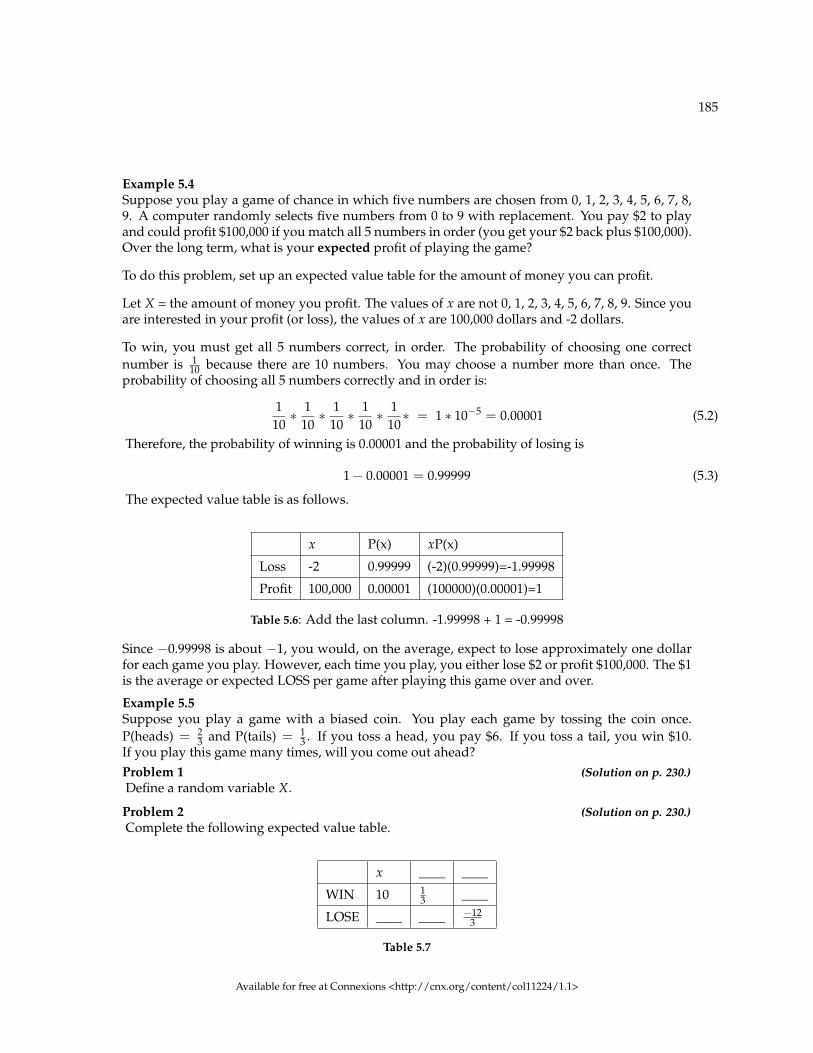
185
Example 5.4Suppose you play a game of chance in which five numbers are chosen from 0, 1, 2, 3, 4, 5, 6, 7, 8,9. A computer randomly selects five numbers from 0 to 9 with replacement. You pay $2 to playand could profit $100,000 if you match all 5 numbers in order (you get your $2 back plus $100,000).Over the long term, what is your expected profit of playing the game?
To do this problem, set up an expected value table for the amount of money you can profit.
Let X = the amount of money you profit. The values of x are not 0, 1, 2, 3, 4, 5, 6, 7, 8, 9. Since youare interested in your profit (or loss), the values of x are 100,000 dollars and -2 dollars.
To win, you must get all 5 numbers correct, in order. The probability of choosing one correctnumber is 1
10 because there are 10 numbers. You may choose a number more than once. Theprobability of choosing all 5 numbers correctly and in order is:
110∗ 1
10∗ 1
10∗ 1
10∗ 1
10∗ = 1 ∗ 10−5 = 0.00001 (5.2)
Therefore, the probability of winning is 0.00001 and the probability of losing is
1− 0.00001 = 0.99999 (5.3)
The expected value table is as follows.
x P(x) xP(x)
Loss -2 0.99999 (-2)(0.99999)=-1.99998
Profit 100,000 0.00001 (100000)(0.00001)=1
Table 5.6: Add the last column. -1.99998 + 1 = -0.99998
Since −0.99998 is about −1, you would, on the average, expect to lose approximately one dollarfor each game you play. However, each time you play, you either lose $2 or profit $100,000. The $1is the average or expected LOSS per game after playing this game over and over.
Example 5.5Suppose you play a game with a biased coin. You play each game by tossing the coin once.P(heads) = 2
3 and P(tails) = 13 . If you toss a head, you pay $6. If you toss a tail, you win $10.
If you play this game many times, will you come out ahead?Problem 1 (Solution on p. 230.)Define a random variable X.
Problem 2 (Solution on p. 230.)Complete the following expected value table.
x ____ ____
WIN 10 13 ____
LOSE ____ ____ −123
Table 5.7
Available for free at Connexions <http://cnx.org/content/col11224/1.1>

186 CHAPTER 5. DISCRETE RANDOM VARIABLES
Problem 3 (Solution on p. 230.)What is the expected value, µ? Do you come out ahead?
Like data, probability distributions have standard deviations. To calculate the standard deviation (σ) of aprobability distribution, find each deviation from its expected value, square it, multiply it by its probability,add the products, and take the square root . To understand how to do the calculation, look at the table forthe number of days per week a men’s soccer team plays soccer. To find the standard deviation, add theentries in the column labeled (x− µ)2 · P (x) and take the square root.
x P(x) xP(x) (x -µ)2P(x)
0 0.2 (0)(0.2) = 0 (0− 1.1)2 (.2) = 0.242
1 0.5 (1)(0.5) = 0.5 (1− 1.1)2 (.5) = 0.005
2 0.3 (2)(0.3) = 0.6 (2− 1.1)2 (.3) = 0.243
Table 5.8
Add the last column in the table. 0.242 + 0.005 + 0.243 = 0.490. The standard deviation is the square rootof 0.49. σ =
√0.49 = 0.7
Generally for probability distributions, we use a calculator or a computer to calculate µ and σ to reduceroundoff error. For some probability distributions, there are short-cut formulas that calculate µ and σ.
5.4 Common Discrete Probability Distribution Functions4
Some of the more common discrete probability functions are binomial, geometric, hypergeometric, andPoisson. Most elementary courses do not cover the geometric, hypergeometric, and Poisson. Your instruc-tor will let you know if he or she wishes to cover these distributions.
A probability distribution function is a pattern. You try to fit a probability problem into a pattern or distri-bution in order to perform the necessary calculations. These distributions are tools to make solving prob-ability problems easier. Each distribution has its own special characteristics. Learning the characteristicsenables you to distinguish among the different distributions.
5.5 Binomial5
The characteristics of a binomial experiment are:
1. There are a fixed number of trials. Think of trials as repetitions of an experiment. The letter n denotesthe number of trials.
2. There are only 2 possible outcomes, called "success" and, "failure" for each trial. The letter p denotesthe probability of a success on one trial and q denotes the probability of a failure on one trial. p + q = 1.
3. The n trials are independent and are repeated using identical conditions. Because the n trials are in-dependent, the outcome of one trial does not help in predicting the outcome of another trial. Anotherway of saying this is that for each individual trial, the probability, p, of a success and probability, q,of a failure remain the same. For example, randomly guessing at a true - false statistics question hasonly two outcomes. If a success is guessing correctly, then a failure is guessing incorrectly. Suppose
4This content is available online at <http://cnx.org/content/m16821/1.6/>.5This content is available online at <http://cnx.org/content/m16820/1.17/>.
Available for free at Connexions <http://cnx.org/content/col11224/1.1>

187
Joe always guesses correctly on any statistics true - false question with probability p = 0.6. Then,q = 0.4 .This means that for every true - false statistics question Joe answers, his probability of success(p = 0.6) and his probability of failure (q = 0.4) remain the same.
The outcomes of a binomial experiment fit a binomial probability distribution. The random variable X =the number of successes obtained in the n independent trials.
The mean, µ, and variance, σ2, for the binomial probability distribution is µ = np and σ2 = npq. Thestandard deviation, σ, is then σ = √npq.
Any experiment that has characteristics 2 and 3 and where n = 1 is called a Bernoulli Trial (named afterJacob Bernoulli who, in the late 1600s, studied them extensively). A binomial experiment takes place whenthe number of successes is counted in one or more Bernoulli Trials.
Example 5.6At ABC College, the withdrawal rate from an elementary physics course is 30% for any giventerm. This implies that, for any given term, 70% of the students stay in the class for the entireterm. A "success" could be defined as an individual who withdrew. The random variable is X =the number of students who withdraw from the randomly selected elementary physics class.
Example 5.7Suppose you play a game that you can only either win or lose. The probability that you win anygame is 55% and the probability that you lose is 45%. Each game you play is independent. If youplay the game 20 times, what is the probability that you win 15 of the 20 games? Here, if youdefine X = the number of wins, then X takes on the values 0, 1, 2, 3, ..., 20. The probability of asuccess is p = 0.55. The probability of a failure is q = 0.45. The number of trials is n = 20. Theprobability question can be stated mathematically as P (x = 15).
Example 5.8A fair coin is flipped 15 times. Each flip is independent. What is the probability of getting morethan 10 heads? Let X = the number of heads in 15 flips of the fair coin. X takes on the values 0, 1,2, 3, ..., 15. Since the coin is fair, p = 0.5 and q = 0.5. The number of trials is n = 15. The probabilityquestion can be stated mathematically as P (x > 10).
Example 5.9Approximately 70% of statistics students do their homework in time for it to be collected andgraded. Each student does homework independently. In a statistics class of 50 students, what isthe probability that at least 40 will do their homework on time? Students are selected randomly.Problem 1 (Solution on p. 230.)This is a binomial problem because there is only a success or a __________, there are a definite
number of trials, and the probability of a success is 0.70 for each trial.
Problem 2 (Solution on p. 230.)If we are interested in the number of students who do their homework, then how do we define
X?
Problem 3 (Solution on p. 230.)What values does x take on?
Problem 4 (Solution on p. 230.)What is a "failure", in words?
The probability of a success is p = 0.70. The number of trial is n = 50.Problem 5 (Solution on p. 230.)If p + q = 1, then what is q?
Available for free at Connexions <http://cnx.org/content/col11224/1.1>

188 CHAPTER 5. DISCRETE RANDOM VARIABLES
Problem 6 (Solution on p. 230.)The words "at least" translate as what kind of inequality for the probability question P (x____40).The probability question is P (x ≥ 40).
5.5.1 Notation for the Binomial: B = Binomial Probability Distribution Function
X ∼ B (n, p)
Read this as "X is a random variable with a binomial distribution." The parameters are n and p. n = numberof trials p = probability of a success on each trial
Example 5.10It has been stated that about 41% of adult workers have a high school diploma but do not pursueany further education. If 20 adult workers are randomly selected, find the probability that at most12 of them have a high school diploma but do not pursue any further education. How many adultworkers do you expect to have a high school diploma but do not pursue any further education?
Let X = the number of workers who have a high school diploma but do not pursue any furthereducation.
X takes on the values 0, 1, 2, ..., 20 where n = 20 and p = 0.41. q = 1 - 0.41 = 0.59. X ∼ B (20, 0.41)
Find P (x ≤ 12) . P (x ≤ 12) = 0.9738. (calculator or computer)
Using the TI-83+ or the TI-84 calculators, the calculations are as follows. Go into 2nd DISTR. Thesyntax for the instructions are
To calculate (x = value): binompdf(n, p, number) If "number" is left out, the result is the binomialprobability table.
To calculate P (x ≤ value): binomcdf(n, p, number) If "number" is left out, the result is the cumu-lative binomial probability table.
For this problem: After you are in 2nd DISTR, arrow down to binomcdf. Press ENTER. Enter20,.41,12). The result is P (x ≤ 12) = 0.9738.
NOTE: If you want to find P (x = 12), use the pdf (binompdf). If you want to find P(x>12), use 1 -binomcdf(20,.41,12).
The probability at most 12 workers have a high school diploma but do not pursue any furthereducation is 0.9738
The graph of x ∼ B (20, 0.41) is:
Available for free at Connexions <http://cnx.org/content/col11224/1.1>
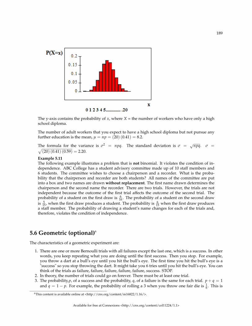
189
The y-axis contains the probability of x, where X = the number of workers who have only a highschool diploma.
The number of adult workers that you expect to have a high school diploma but not pursue anyfurther education is the mean, µ = np = (20) (0.41) = 8.2.
The formula for the variance is σ2 = npq. The standard deviation is σ = √npq. σ =√
(20) (0.41) (0.59) = 2.20.
Example 5.11The following example illustrates a problem that is not binomial. It violates the condition of in-dependence. ABC College has a student advisory committee made up of 10 staff members and6 students. The committee wishes to choose a chairperson and a recorder. What is the proba-bility that the chairperson and recorder are both students? All names of the committee are putinto a box and two names are drawn without replacement. The first name drawn determines thechairperson and the second name the recorder. There are two trials. However, the trials are notindependent because the outcome of the first trial affects the outcome of the second trial. Theprobability of a student on the first draw is 6
16 . The probability of a student on the second drawis 5
15 , when the first draw produces a student. The probability is 615 when the first draw produces
a staff member. The probability of drawing a student’s name changes for each of the trials and,therefore, violates the condition of independence.
5.6 Geometric (optional)6
The characteristics of a geometric experiment are:
1. There are one or more Bernoulli trials with all failures except the last one, which is a success. In otherwords, you keep repeating what you are doing until the first success. Then you stop. For example,you throw a dart at a bull’s eye until you hit the bull’s eye. The first time you hit the bull’s eye is a"success" so you stop throwing the dart. It might take you 6 tries until you hit the bull’s eye. You canthink of the trials as failure, failure, failure, failure, failure, success. STOP.
2. In theory, the number of trials could go on forever. There must be at least one trial.3. The probability,p, of a success and the probability, q, of a failure is the same for each trial. p + q = 1
and q = 1− p. For example, the probability of rolling a 3 when you throw one fair die is 16 . This is
6This content is available online at <http://cnx.org/content/m16822/1.16/>.
Available for free at Connexions <http://cnx.org/content/col11224/1.1>

190 CHAPTER 5. DISCRETE RANDOM VARIABLES
true no matter how many times you roll the die. Suppose you want to know the probability of gettingthe first 3 on the fifth roll. On rolls 1, 2, 3, and 4, you do not get a face with a 3. The probability foreach of rolls 1, 2, 3, and 4 is q = 5
6 , the probability of a failure. The probability of getting a 3 on thefifth roll is 5
6 ·56 ·
56 ·
56 ·
16 = 0.0804
X = the number of independent trials until the first success. The mean and variance are in the summary inthis chapter.
Example 5.12You play a game of chance that you can either win or lose (there are no other possibilities) untilyou lose. Your probability of losing is p = 0.57. What is the probability that it takes 5 games untilyou lose? Let X = the number of games you play until you lose (includes the losing game). ThenX takes on the values 1, 2, 3, ... (could go on indefinitely). The probability question is P (x = 5).
Example 5.13A safety engineer feels that 35% of all industrial accidents in her plant are caused by failure ofemployees to follow instructions. She decides to look at the accident reports (selected randomlyand replaced in the pile after reading) until she finds one that shows an accident caused by failureof employees to follow instructions. On the average, how many reports would the safety engineerexpect to look at until she finds a report showing an accident caused by employee failure to followinstructions? What is the probability that the safety engineer will have to examine at least 3 reportsuntil she finds a report showing an accident caused by employee failure to follow instructions?
Let X = the number of accidents the safety engineer must examine until she finds a report showingan accident caused by employee failure to follow instructions. X takes on the values 1, 2, 3, .... Thefirst question asks you to find the expected value or the mean. The second question asks you tofind P (x ≥ 3). ("At least" translates as a "greater than or equal to" symbol).
Example 5.14Suppose that you are looking for a student at your college who lives within five miles of you. Youknow that 55% of the 25,000 students do live within five miles of you. You randomly contact stu-dents from the college until one says he/she lives within five miles of you. What is the probabilitythat you need to contact four people?
This is a geometric problem because you may have a number of failures before you have the onesuccess you desire. Also, the probability of a success stays the same each time you ask a student ifhe/she lives within five miles of you. There is no definite number of trials (number of times youask a student).Problem 1Let X = the number of ____________ you must ask ____________ one says yes.
SolutionLet X = the number of students you must ask until one says yes.
Problem 2 (Solution on p. 230.)What values does X take on?
Problem 3 (Solution on p. 230.)What are p and q?
Problem 4 (Solution on p. 231.)The probability question is P(_______).
Available for free at Connexions <http://cnx.org/content/col11224/1.1>
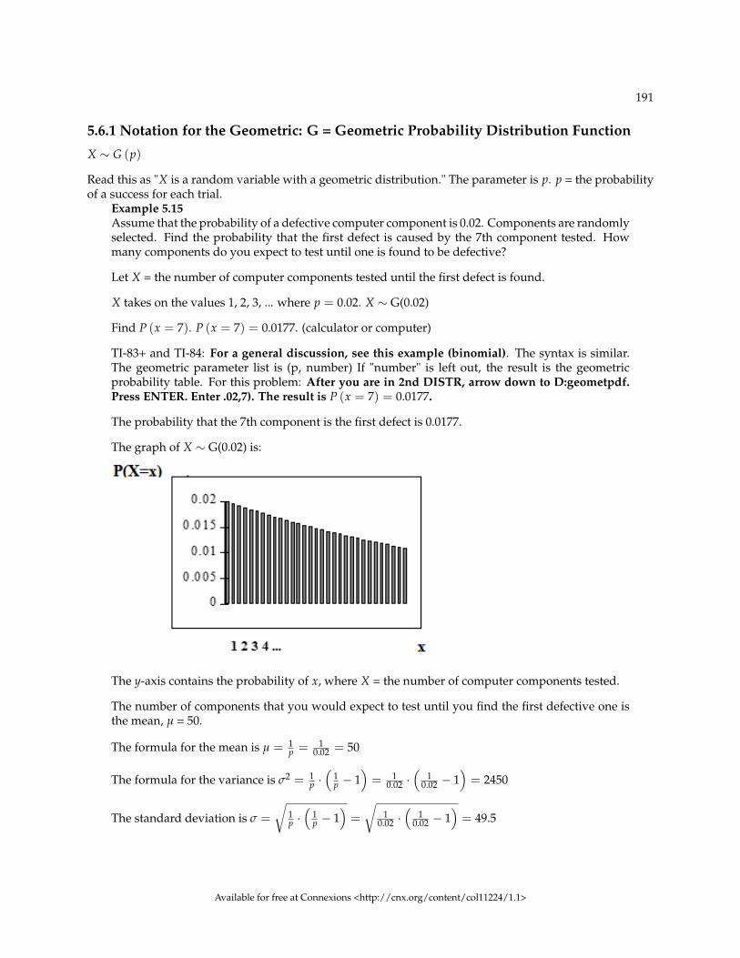
191
5.6.1 Notation for the Geometric: G = Geometric Probability Distribution Function
X ∼ G (p)
Read this as "X is a random variable with a geometric distribution." The parameter is p. p = the probabilityof a success for each trial.
Example 5.15Assume that the probability of a defective computer component is 0.02. Components are randomlyselected. Find the probability that the first defect is caused by the 7th component tested. Howmany components do you expect to test until one is found to be defective?
Let X = the number of computer components tested until the first defect is found.
X takes on the values 1, 2, 3, ... where p = 0.02. X ∼ G(0.02)
Find P (x = 7). P (x = 7) = 0.0177. (calculator or computer)
TI-83+ and TI-84: For a general discussion, see this example (binomial). The syntax is similar.The geometric parameter list is (p, number) If "number" is left out, the result is the geometricprobability table. For this problem: After you are in 2nd DISTR, arrow down to D:geometpdf.Press ENTER. Enter .02,7). The result is P (x = 7) = 0.0177.
The probability that the 7th component is the first defect is 0.0177.
The graph of X ∼ G(0.02) is:
The y-axis contains the probability of x, where X = the number of computer components tested.
The number of components that you would expect to test until you find the first defective one isthe mean, µ = 50.
The formula for the mean is µ = 1p = 1
0.02 = 50
The formula for the variance is σ2 = 1p ·(
1p − 1
)= 1
0.02 ·(
10.02 − 1
)= 2450
The standard deviation is σ =√
1p ·(
1p − 1
)=√
10.02 ·
(1
0.02 − 1)
= 49.5
Available for free at Connexions <http://cnx.org/content/col11224/1.1>

192 CHAPTER 5. DISCRETE RANDOM VARIABLES
5.7 Hypergeometric (optional)7
The characteristics of a hypergeometric experiment are:
1. You take samples from 2 groups.2. You are concerned with a group of interest, called the first group.3. You sample without replacement from the combined groups. For example, you want to choose a
softball team from a combined group of 11 men and 13 women. The team consists of 10 players.4. Each pick is not independent, since sampling is without replacement. In the softball example, the
probability of picking a women first is 1324 . The probability of picking a man second is 11
23 if a womanwas picked first. It is 10
23 if a man was picked first. The probability of the second pick depends on whathappened in the first pick.
5. You are not dealing with Bernoulli Trials.
The outcomes of a hypergeometric experiment fit a hypergeometric probability distribution. The randomvariable X = the number of items from the group of interest. The mean and variance are given in thesummary.
Example 5.16A candy dish contains 100 jelly beans and 80 gumdrops. Fifty candies are picked at random. Whatis the probability that 35 of the 50 are gumdrops? The two groups are jelly beans and gumdrops.Since the probability question asks for the probability of picking gumdrops, the group of interest(first group) is gumdrops. The size of the group of interest (first group) is 80. The size of thesecond group is 100. The size of the sample is 50 (jelly beans or gumdrops). Let X = the numberof gumdrops in the sample of 50. X takes on the values x = 0, 1, 2, ..., 50. The probability questionis P (x = 35).
Example 5.17Suppose a shipment of 100 VCRs is known to have 10 defective VCRs. An inspector randomlychooses 12 for inspection. He is interested in determining the probability that, among the 12, atmost 2 are defective. The two groups are the 90 non-defective VCRs and the 10 defective VCRs.The group of interest (first group) is the defective group because the probability question asks forthe probability of at most 2 defective VCRs. The size of the sample is 12 VCRs. (They may benon-defective or defective.) Let X = the number of defective VCRs in the sample of 12. X takes onthe values 0, 1, 2, ..., 10. X may not take on the values 11 or 12. The sample size is 12, but thereare only 10 defective VCRs. The inspector wants to know P (x ≤ 2) ("At most" means "less than orequal to").
Example 5.18You are president of an on-campus special events organization. You need a committee of 7 to plana special birthday party for the president of the college. Your organization consists of 18 womenand 15 men. You are interested in the number of men on your committee. If the members of thecommittee are randomly selected, what is the probability that your committee has more than 4men?
This is a hypergeometric problem because you are choosing your committee from two groups(men and women).Problem 1 (Solution on p. 231.)Are you choosing with or without replacement?
Problem 2 (Solution on p. 231.)What is the group of interest?
7This content is available online at <http://cnx.org/content/m16824/1.16/>.
Available for free at Connexions <http://cnx.org/content/col11224/1.1>
193
Problem 3 (Solution on p. 231.)How many are in the group of interest?
Problem 4 (Solution on p. 231.)How many are in the other group?
Problem 5 (Solution on p. 231.)Let X = _________ on the committee. What values does X take on?
Problem 6 (Solution on p. 231.)The probability question is P(_______).
5.7.1 Notation for the Hypergeometric: H = Hypergeometric Probability DistributionFunction
X∼H (r, b, n)
Read this as "X is a random variable with a hypergeometric distribution." The parameters are r, b, and n. r= the size of the group of interest (first group), b = the size of the second group, n = the size of the chosensample
Example 5.19A school site committee is to be chosen randomly from 6 men and 5 women. If the committeeconsists of 4 members chosen randomly, what is the probability that 2 of them are men? Howmany men do you expect to be on the committee?
Let X = the number of men on the committee of 4. The men are the group of interest (first group).
X takes on the values 0, 1, 2, 3, 4, where r = 6, b = 5 , and n = 4. X ∼ H(6, 5, 4)
Find P (x = 2). P (x = 2) = 0.4545 (calculator or computer)
NOTE: Currently, the TI-83+ and TI-84 do not have hypergeometric probability functions. Thereare a number of computer packages, including Microsoft Excel, that do.
The probability that there are 2 men on the committee is about 0.45.
The graph of X∼H(6, 5, 4) is:
Available for free at Connexions <http://cnx.org/content/col11224/1.1>

194 CHAPTER 5. DISCRETE RANDOM VARIABLES
The y-axis contains the probability of X, where X = the number of men on the committee.
You would expect m = 2.18 (about 2) men on the committee.
The formula for the mean is µ = n·rr+b = 4·6
6+5 = 2.18
The formula for the variance is fairly complex. You will find it in the Summary of the DiscreteProbability Functions Chapter (Section 5.9).
5.8 Poisson8
Characteristics of a Poisson experiment:
1. The Poisson gives the probability of a number of events occurring in a fixed interval of time or space ifthese events happen with a known average rate and independently of the time since the last event. Forexample, a book editor might be interested in the number of words spelled incorrectly in a particularbook. It might be that, on the average, there are 5 words spelled incorrectly in 100 pages. The intervalis the 100 pages.
2. The Poisson may be used to approximate the binomial if the probability of success is "small" (suchas 0.01) and the number of trials is "large" (such as 1000). You will verify the relationship in thehomework exercises. n is the number of trials and p is the probability of a "success."
Poisson probability distribution. The random variable X = the number of occurrences in the interval ofinterest. The mean and variance are given in the summary.
Example 5.20The average number of loaves of bread put on a shelf in a bakery in a half-hour period is 12. Ofinterest is the number of loaves of bread put on the shelf in 5 minutes. The time interval of interestis 5 minutes. What is the probability that the number of loaves, selected randomly, put on the shelfin 5 minutes is 3?
Let X = the number of loaves of bread put on the shelf in 5 minutes. If the average number ofloaves put on the shelf in 30 minutes (half-hour) is 12, then the average number of loaves put onthe shelf in 5 minutes is
8This content is available online at <http://cnx.org/content/m16829/1.16/>.
Available for free at Connexions <http://cnx.org/content/col11224/1.1>

195
( 530)· 12 = 2 loaves of bread
The probability question asks you to find P (x = 3).
Example 5.21A certain bank expects to receive 6 bad checks per day, on average. What is the probability of thebank getting fewer than 5 bad checks on any given day? Of interest is the number of checks thebank receives in 1 day, so the time interval of interest is 1 day. Let X = the number of bad checksthe bank receives in one day. If the bank expects to receive 6 bad checks per day then the averageis 6 checks per day. The probability question asks for P (x < 5).
Example 5.22You notice that a news reporter says "uh", on average, 2 times per broadcast. What is the probabil-ity that the news reporter says "uh" more than 2 times per broadcast.
This is a Poisson problem because you are interested in knowing the number of times the newsreporter says "uh" during a broadcast.Problem 1 (Solution on p. 231.)What is the interval of interest?
Problem 2 (Solution on p. 231.)What is the average number of times the news reporter says "uh" during one broadcast?
Problem 3 (Solution on p. 231.)Let X = ____________. What values does X take on?
Problem 4 (Solution on p. 231.)The probability question is P(______).
5.8.1 Notation for the Poisson: P = Poisson Probability Distribution Function
X ∼ P(µ)
Read this as "X is a random variable with a Poisson distribution." The parameter is µ (or λ). µ (or λ) = themean for the interval of interest.
Example 5.23Leah’s answering machine receives about 6 telephone calls between 8 a.m. and 10 a.m. What is
the probability that Leah receives more than 1 call in the next 15 minutes?
Let X = the number of calls Leah receives in 15 minutes. (The interval of interest is 15 minutes or14 hour.)
x = 0, 1, 2, 3, ...
If Leah receives, on the average, 6 telephone calls in 2 hours, and there are eight 15 minutes inter-vals in 2 hours, then Leah receives
18 · 6 = 0.75
calls in 15 minutes, on the average. So, µ = 0.75 for this problem.
X ∼ P(0.75)
Find P (x > 1). P (x > 1) = 0.1734 (calculator or computer)
Available for free at Connexions <http://cnx.org/content/col11224/1.1>
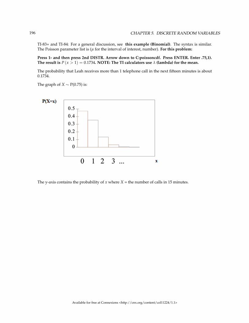
196 CHAPTER 5. DISCRETE RANDOM VARIABLES
TI-83+ and TI-84: For a general discussion, see this example (Binomial). The syntax is similar.The Poisson parameter list is (µ for the interval of interest, number). For this problem:
Press 1- and then press 2nd DISTR. Arrow down to C:poissoncdf. Press ENTER. Enter .75,1).The result is P (x > 1) = 0.1734. NOTE: The TI calculators use λ (lambda) for the mean.
The probability that Leah receives more than 1 telephone call in the next fifteen minutes is about0.1734.
The graph of X ∼ P(0.75) is:
The y-axis contains the probability of x where X = the number of calls in 15 minutes.
Available for free at Connexions <http://cnx.org/content/col11224/1.1>

197
5.9 Summary of Functions9
Formula 5.1: BinomialX∼B (n, p)
X = the number of successes in n independent trials
n = the number of independent trials
X takes on the values x = 0,1, 2, 3, ...,n
p = the probability of a success for any trial
q = the probability of a failure for any trial
p + q = 1 q = 1− p
The mean is µ = np. The standard deviation is σ = √npq.Formula 5.2: GeometricX∼G (p)
X = the number of independent trials until the first success (count the failures and the first success)
X takes on the values x= 1, 2, 3, ...
p = the probability of a success for any trial
q = the probability of a failure for any trial
p + q = 1
q = 1− p
The mean is µ = 1p
The standard deviation is σ =√
1p
((1p
)− 1)
Formula 5.3: HypergeometricX∼H (r, b, n)
X = the number of items from the group of interest that are in the chosen sample.
X may take on the values x= 0, 1, ..., up to the size of the group of interest. (The minimum valuefor X may be larger than 0 in some instances.)
r = the size of the group of interest (first group)
b= the size of the second group
n= the size of the chosen sample.
n ≤ r + b
The mean is: µ = nrr+b
9This content is available online at <http://cnx.org/content/m16833/1.11/>.
Available for free at Connexions <http://cnx.org/content/col11224/1.1>
198 CHAPTER 5. DISCRETE RANDOM VARIABLES
The standard deviation is: σ =√
rbn(r+b−n)(r+b)2(r+b−1)
Formula 5.4: PoissonX ∼ P(µ)
X = the number of occurrences in the interval of interest
X takes on the values x = 0, 1, 2, 3, ...
The mean µ is typically given. (λ is often used as the mean instead of µ.) When the Poisson isused to approximate the binomial, we use the binomial mean µ = np. n is the binomial numberof trials. p = the probability of a success for each trial. This formula is valid when n is "large" andp "small" (a general rule is that n should be greater than or equal to 20 and p should be less thanor equal to 0.05). If n is large enough and p is small enough then the Poisson approximates thebinomial very well. The variance is σ2 = µ and the standard deviation is σ = √µ
Available for free at Connexions <http://cnx.org/content/col11224/1.1>

199
5.10 Practice 1: Discrete Distribution10
5.10.1 Student Learning Outcomes
• The student will analyze the properties of a discrete distribution.
5.10.2 Given:
A ballet instructor is interested in knowing what percent of each year’s class will continue on to the next,so that she can plan what classes to offer. Over the years, she has established the following probabilitydistribution.
• Let X = the number of years a student will study ballet with the teacher.• Let P (x) = the probability that a student will study ballet x years.
5.10.3 Organize the Data
Complete the table below using the data provided.
x P(x) x*P(x)
1 0.10
2 0.05
3 0.10
4
5 0.30
6 0.20
7 0.10
Table 5.9
Exercise 5.10.1In words, define the Random Variable X.
Exercise 5.10.2P (x = 4) =
Exercise 5.10.3P (x < 4) =
Exercise 5.10.4On average, how many years would you expect a child to study ballet with this teacher?
5.10.4 Discussion Question
Exercise 5.10.5What does the column "P(x)" sum to and why?
Exercise 5.10.6What does the column "x ∗ P(x)" sum to and why?
10This content is available online at <http://cnx.org/content/m16830/1.14/>.
Available for free at Connexions <http://cnx.org/content/col11224/1.1>

200 CHAPTER 5. DISCRETE RANDOM VARIABLES
5.11 Practice 2: Binomial Distribution11
5.11.1 Student Learning Outcomes
• The student will construct the Binomial Distribution.
5.11.2 Given
The Higher Education Research Institute at UCLA collected data from 203,967 incoming first-time,full-time freshmen from 270 four-year colleges and universities in the U.S. 71.3% of those students repliedthat, yes, they believe that same-sex couples should have the right to legal marital status. (Source:http://heri.ucla.edu/PDFs/pubs/TFS/Norms/Monographs/TheAmericanFreshman2011.pdf). )
Suppose that you randomly pick 8 first-time, full-time freshmen from the survey. You are interestedin the number that believes that same sex-couples should have the right to legal marital status
5.11.3 Interpret the Data
Exercise 5.11.1 (Solution on p. 231.)In words, define the random Variable X.
Exercise 5.11.2 (Solution on p. 231.)X∼___________
Exercise 5.11.3 (Solution on p. 231.)What values does the random variable X take on?
Exercise 5.11.4Construct the probability distribution function (PDF).
x P(x)
Table 5.10
Exercise 5.11.5 (Solution on p. 231.)On average (u), how many would you expect to answer yes?
Exercise 5.11.6 (Solution on p. 231.)What is the standard deviation (σ) ?
11This content is available online at <http://cnx.org/content/m17107/1.18/>.
Available for free at Connexions <http://cnx.org/content/col11224/1.1>

201
Exercise 5.11.7 (Solution on p. 231.)What is the probability that at most 5 of the freshmen reply “yes”?
Exercise 5.11.8 (Solution on p. 231.)What is the probability that at least 2 of the freshmen reply “yes”?
Exercise 5.11.9Construct a histogram or plot a line graph. Label the horizontal and vertical axes with words.
Include numerical scaling.
Available for free at Connexions <http://cnx.org/content/col11224/1.1>
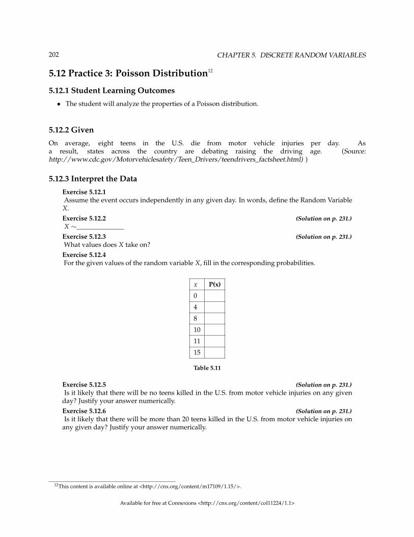
202 CHAPTER 5. DISCRETE RANDOM VARIABLES
5.12 Practice 3: Poisson Distribution12
5.12.1 Student Learning Outcomes
• The student will analyze the properties of a Poisson distribution.
5.12.2 Given
On average, eight teens in the U.S. die from motor vehicle injuries per day. Asa result, states across the country are debating raising the driving age. (Source:http://www.cdc.gov/Motorvehiclesafety/Teen_Drivers/teendrivers_factsheet.html) )
5.12.3 Interpret the Data
Exercise 5.12.1Assume the event occurs independently in any given day. In words, define the Random VariableX.Exercise 5.12.2 (Solution on p. 231.)X ∼______________
Exercise 5.12.3 (Solution on p. 231.)What values does X take on?
Exercise 5.12.4For the given values of the random variable X, fill in the corresponding probabilities.
x P(x)
0
4
8
10
11
15
Table 5.11
Exercise 5.12.5 (Solution on p. 231.)Is it likely that there will be no teens killed in the U.S. from motor vehicle injuries on any given
day? Justify your answer numerically.Exercise 5.12.6 (Solution on p. 231.)Is it likely that there will be more than 20 teens killed in the U.S. from motor vehicle injuries on
any given day? Justify your answer numerically.
12This content is available online at <http://cnx.org/content/m17109/1.15/>.
Available for free at Connexions <http://cnx.org/content/col11224/1.1>

203
5.13 Practice 4: Geometric Distribution13
5.13.1 Student Learning Outcomes
• The student will analyze the properties of a geometric distribution.
5.13.2 Given:
Use the information from the Binomial Distribution Practice (Section 5.11) shown below.
The Higher Education Research Institute at UCLA collected data from 203,967 incoming first-time,full-time freshmen from 270 four-year colleges and universities in the U.S. 71.3% of those students repliedthat, yes, they believe that same-sex couples should have the right to legal marital status. (Source:http://heri.ucla.edu/PDFs/pubs/TFS/Norms/Monographs/TheAmericanFreshman2011.pdf )
Suppose that you randomly select freshman from the study until you find one who replies “yes.”You are interested in the number of freshmen you must ask.
5.13.3 Interpret the Data
Exercise 5.13.1In words, define the Random Variable X.
Exercise 5.13.2 (Solution on p. 232.)X ∼
Exercise 5.13.3 (Solution on p. 232.)What values does the random variable X take on?
Exercise 5.13.4Construct the probability distribution function (PDF). Stop at x = 6.
x P(x)
1
2
3
4
5
6
Table 5.12
Exercise 5.13.5 (Solution on p. 232.)On average(µ), how many freshmen would you expect to have to ask until you found one who
replies "yes?"Exercise 5.13.6 (Solution on p. 232.)What is the probability that you will need to ask fewer than 3 freshmen?
13This content is available online at <http://cnx.org/content/m17108/1.17/>.
Available for free at Connexions <http://cnx.org/content/col11224/1.1>

204 CHAPTER 5. DISCRETE RANDOM VARIABLES
Exercise 5.13.7Construct a histogram or plot a line graph. Label the horizontal and vertical axes with words.
Include numerical scaling.
Available for free at Connexions <http://cnx.org/content/col11224/1.1>

205
5.14 Practice 5: Hypergeometric Distribution14
5.14.1 Student Learning Outcomes
• The student will analyze the properties of a hypergeometric distribution.
5.14.2 Given
Suppose that a group of statistics students is divided into two groups: business majors and non-businessmajors. There are 16 business majors in the group and 7 non-business majors in the group. A randomsample of 9 students is taken. We are interested in the number of business majors in the group.
5.14.3 Interpret the Data
Exercise 5.14.1In words, define the Random Variable X.
Exercise 5.14.2 (Solution on p. 232.)X ∼
Exercise 5.14.3 (Solution on p. 232.)What values does X take on?
Exercise 5.14.4Construct the probability distribution function (PDF) for X.
x P(x)
Table 5.13
Exercise 5.14.5 (Solution on p. 232.)On average(µ), how many would you expect to be business majors?
14This content is available online at <http://cnx.org/content/m17106/1.13/>.
Available for free at Connexions <http://cnx.org/content/col11224/1.1>

206 CHAPTER 5. DISCRETE RANDOM VARIABLES
5.15 Homework15
Exercise 5.15.1 (Solution on p. 232.)1. Complete the PDF and answer the questions.
x P (X = x) x · P (X = x)
0 0.3
1 0.2
2
3 0.4
Table 5.14
a. Find the probability that x = 2.b. Find the expected value.
Exercise 5.15.2Suppose that you are offered the following “deal.” You roll a die. If you roll a 6, you win $10. If
you roll a 4 or 5, you win $5. If you roll a 1, 2, or 3, you pay $6.
a. What are you ultimately interested in here (the value of the roll or the money you win)?b. In words, define the Random Variable X.c. List the values that X may take on.d. Construct a PDF.e. Over the long run of playing this game, what are your expected average winnings per game?f. Based on numerical values, should you take the deal? Explain your decision in complete sen-
tences.
Exercise 5.15.3 (Solution on p. 232.)A venture capitalist, willing to invest $1,000,000, has three investments to choose from. The first
investment, a software company, has a 10% chance of returning $5,000,000 profit, a 30% chance ofreturning $1,000,000 profit, and a 60% chance of losing the million dollars. The second company,a hardware company, has a 20% chance of returning $3,000,000 profit, a 40% chance of returning$1,000,000 profit, and a 40% chance of losing the million dollars. The third company, a biotechfirm, has a 10% chance of returning $6,000,000 profit, a 70% of no profit or loss, and a 20% chanceof losing the million dollars.
a. Construct a PDF for each investment.b. Find the expected value for each investment.c. Which is the safest investment? Why do you think so?d. Which is the riskiest investment? Why do you think so?e. Which investment has the highest expected return, on average?
Exercise 5.15.4A theater group holds a fund-raiser. It sells 100 raffle tickets for $5 apiece. Suppose you purchase4 tickets. The prize is 2 passes to a Broadway show, worth a total of $150.
a. What are you interested in here?
15This content is available online at <http://cnx.org/content/m16823/1.21/>.
Available for free at Connexions <http://cnx.org/content/col11224/1.1>
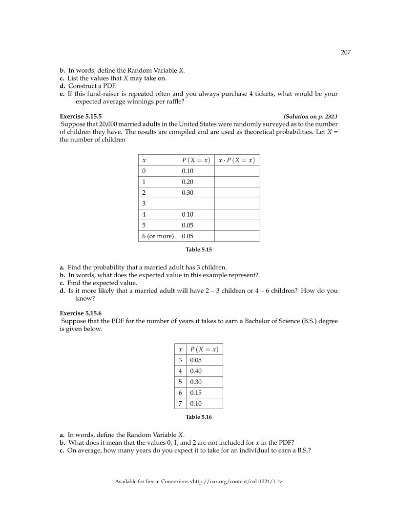
207
b. In words, define the Random Variable X.c. List the values that X may take on.d. Construct a PDF.e. If this fund-raiser is repeated often and you always purchase 4 tickets, what would be your
expected average winnings per raffle?
Exercise 5.15.5 (Solution on p. 232.)Suppose that 20,000 married adults in the United States were randomly surveyed as to the numberof children they have. The results are compiled and are used as theoretical probabilities. Let X =the number of children
x P (X = x) x · P (X = x)
0 0.10
1 0.20
2 0.30
3
4 0.10
5 0.05
6 (or more) 0.05
Table 5.15
a. Find the probability that a married adult has 3 children.b. In words, what does the expected value in this example represent?c. Find the expected value.d. Is it more likely that a married adult will have 2 – 3 children or 4 – 6 children? How do you
know?
Exercise 5.15.6Suppose that the PDF for the number of years it takes to earn a Bachelor of Science (B.S.) degree
is given below.
x P (X = x)
3 0.05
4 0.40
5 0.30
6 0.15
7 0.10
Table 5.16
a. In words, define the Random Variable X.b. What does it mean that the values 0, 1, and 2 are not included for x in the PDF?c. On average, how many years do you expect it to take for an individual to earn a B.S.?
Available for free at Connexions <http://cnx.org/content/col11224/1.1>
208 CHAPTER 5. DISCRETE RANDOM VARIABLES
5.15.1 For each problem:
a. In words, define the Random Variable X.b. List the values that X may take on.c. Give the distribution of X. X∼
Then, answer the questions specific to each individual problem.Exercise 5.15.7 (Solution on p. 232.)Six different colored dice are rolled. Of interest is the number of dice that show a “1.”
d. On average, how many dice would you expect to show a “1”?e. Find the probability that all six dice show a “1.”f. Is it more likely that 3 or that 4 dice will show a “1”? Use numbers to justify your answer
numerically.
Exercise 5.15.8More than 96 percent of the very largest colleges and universities (more than 15,000 to-
tal enrollments) have some online offerings. Suppose you randomly pick 13 such insti-tutions. We are interested in the number that offer distance learning courses. (Source:http://en.wikipedia.org/wiki/Distance_education)
d. On average, how many schools would you expect to offer such courses?e. Find the probability that at most 6 offer such courses.f. Is it more likely that 0 or that 13 will offer such courses? Use numbers to justify your answer
numerically and answer in a complete sentence.
Exercise 5.15.9 (Solution on p. 232.)A school newspaper reporter decides to randomly survey 12 students to see if they will attend Tet(Vietnamese New Year) festivities this year. Based on past years, she knows that 18% of studentsattend Tet festivities. We are interested in the number of students who will attend the festivities.
d. How many of the 12 students do we expect to attend the festivities?e. Find the probability that at most 4 students will attend.f. Find the probability that more than 2 students will attend.
Exercise 5.15.10Suppose that about 85% of graduating students attend their graduation. A group of 22 graduatingstudents is randomly chosen.
d. How many are expected to attend their graduation?e. Find the probability that 17 or 18 attend.f. Based on numerical values, would you be surprised if all 22 attended graduation? Justify your
answer numerically.
Exercise 5.15.11 (Solution on p. 233.)At The Fencing Center, 60% of the fencers use the foil as their main weapon. We randomly survey25 fencers at The Fencing Center. We are interested in the numbers that do not use the foil as theirmain weapon.
d. How many are expected to not use the foil as their main weapon?e. Find the probability that six do not use the foil as their main weapon.f. Based on numerical values, would you be surprised if all 25 did not use foil as their main
weapon? Justify your answer numerically.
Available for free at Connexions <http://cnx.org/content/col11224/1.1>

209
Exercise 5.15.12Approximately 8% of students at a local high school participate in after-school sports all four
years of high school. A group of 60 seniors is randomly chosen. Of interest is the number thatparticipated in after-school sports all four years of high school.
d. How many seniors are expected to have participated in after-school sports all four years of highschool?
e. Based on numerical values, would you be surprised if none of the seniors participated in after-school sports all four years of high school? Justify your answer numerically.
f. Based upon numerical values, is it more likely that 4 or that 5 of the seniors participated inafter-school sports all four years of high school? Justify your answer numerically.
Exercise 5.15.13 (Solution on p. 233.)The chance of having an extra fortune in a fortune cookie is about 3%. Given a bag of 144 fortunecookies, we are interested in the number of cookies with an extra fortune. Two distributions maybe used to solve this problem. Use one distribution to solve the problem.
d. How many cookies do we expect to have an extra fortune?e. Find the probability that none of the cookies have an extra fortune.f. Find the probability that more than 3 have an extra fortune.g. As n increases, what happens involving the probabilities using the two distributions? Explain
in complete sentences.
Exercise 5.15.14There are two games played for Chinese New Year and Vietnamese New Year. They are almost
identical. In the Chinese version, fair dice with numbers 1, 2, 3, 4, 5, and 6 are used, along witha board with those numbers. In the Vietnamese version, fair dice with pictures of a gourd, fish,rooster, crab, crayfish, and deer are used. The board has those six objects on it, also. We will playwith bets being $1. The player places a bet on a number or object. The “house” rolls three dice. Ifnone of the dice show the number or object that was bet, the house keeps the $1 bet. If one of thedice shows the number or object bet (and the other two do not show it), the player gets back his$1 bet, plus $1 profit. If two of the dice show the number or object bet (and the third die does notshow it), the player gets back his $1 bet, plus $2 profit. If all three dice show the number or objectbet, the player gets back his $1 bet, plus $3 profit.
Let X = number of matches and Y= profit per game.
d. List the values that Y may take on. Then, construct one PDF table that includes both X & Y andtheir probabilities.
e. Calculate the average expected matches over the long run of playing this game for the player.f. Calculate the average expected earnings over the long run of playing this game for the player.g. Determine who has the advantage, the player or the house.
Exercise 5.15.15 (Solution on p. 233.)According to the South Carolina Department of Mental Health web site, for
every 200 U.S. women, the average number who suffer from anorexia is one(http://www.state.sc.us/dmh/anorexia/statistics.htm16 ). Out of a randomly chosen group of600 U.S. women:
d. How many are expected to suffer from anorexia?e. Find the probability that no one suffers from anorexia.
16http://www.state.sc.us/dmh/anorexia/statistics.htm
Available for free at Connexions <http://cnx.org/content/col11224/1.1>
210 CHAPTER 5. DISCRETE RANDOM VARIABLES
f. Find the probability that more than four suffer from anorexia.
Exercise 5.15.16The average number of children a Japanese woman has in her lifetime is 1.37. Suppose that one
Japanese woman is randomly chosen.( http://www.mhlw.go.jp/english/policy/children/children-childrearing/index.html 17
MHLW’s Pamphlet)
d. Find the probability that she has no children.e. Find the probability that she has fewer children than the Japanese average.f. Find the probability that she has more children than the Japanese average.
Exercise 5.15.17 (Solution on p. 233.)The average number of children a Spanish woman has in her life-
time is 1.47. Suppose that one Spanish woman is randomly chosen.(http://www.typicallyspanish.com/news/publish/article_4897.shtml 18 ).
d. Find the probability that she has no children.e. Find the probability that she has fewer children than the Spanish average.f. Find the probability that she has more children than the Spanish average .
Exercise 5.15.18Fertile (female) cats produce an average of 3 litters per year. (Source: The Humane Society of
the United States). Suppose that one fertile, female cat is randomly chosen. In one year, find theprobability she produces:
d. No litters.e. At least 2 litters.f. Exactly 3 litters.
Exercise 5.15.19 (Solution on p. 233.)A consumer looking to buy a used red Miata car will call dealerships until she finds a dealership
that carries the car. She estimates the probability that any independent dealership will have thecar will be 28%. We are interested in the number of dealerships she must call.
d. On average, how many dealerships would we expect her to have to call until she finds one thathas the car?
e. Find the probability that she must call at most 4 dealerships.f. Find the probability that she must call 3 or 4 dealerships.
Exercise 5.15.20Suppose that the probability that an adult in America will watch the Super Bowl is 40%. Each
person is considered independent. We are interested in the number of adults in America we mustsurvey until we find one who will watch the Super Bowl.
d. How many adults in America do you expect to survey until you find one who will watch theSuper Bowl?
e. Find the probability that you must ask 7 people.f. Find the probability that you must ask 3 or 4 people.
17http://www.mhlw.go.jp/english/policy/children/children-childrearing/index.html18http://www.typicallyspanish.com/news/publish/article_4897.shtml
Available for free at Connexions <http://cnx.org/content/col11224/1.1>

211
Exercise 5.15.21 (Solution on p. 233.)A group of Martial Arts students is planning on participating in an upcoming demonstration.
6 are students of Tae Kwon Do; 7 are students of Shotokan Karate. Suppose that 8 students arerandomly picked to be in the first demonstration. We are interested in the number of ShotokanKarate students in that first demonstration. Hint: Use the Hypergeometric distribution. Look inthe Formulas section of 4: Discrete Distributions and in the Appendix Formulas.
d. How many Shotokan Karate students do we expect to be in that first demonstration?e. Find the probability that 4 students of Shotokan Karate are picked for the first demonstration.f. Suppose that we are interested in the Tae Kwan Do students that are picked for the first demon-
stration. Find the probability that all 6 students of Tae Kwan Do are picked for the firstdemonstration.
Exercise 5.15.22The chance of a IRS audit for a tax return with over $25,000 in income is about 2% per year. We
are interested in the expected number of audits a person with that income has in a 20 year period.Assume each year is independent.
d. How many audits are expected in a 20 year period?e. Find the probability that a person is not audited at all.f. Find the probability that a person is audited more than twice.
Exercise 5.15.23 (Solution on p. 233.)Refer to the previous problem. Suppose that 100 people with tax returns over $25,000 are ran-
domly picked. We are interested in the number of people audited in 1 year. One way to solve thisproblem is by using the Binomial Distribution. Since n is large and p is small, another discretedistribution could be used to solve the following problems. Solve the following questions (d-f)using that distribution.
d. How many are expected to be audited?e. Find the probability that no one was audited.f. Find the probability that more than 2 were audited.
Exercise 5.15.24Suppose that a technology task force is being formed to study technology awareness among in-
structors. Assume that 10 people will be randomly chosen to be on the committee from a groupof 28 volunteers, 20 who are technically proficient and 8 who are not. We are interested in thenumber on the committee who are not technically proficient.
d. How many instructors do you expect on the committee who are not technically proficient?e. Find the probability that at least 5 on the committee are not technically proficient.f. Find the probability that at most 3 on the committee are not technically proficient.
Exercise 5.15.25 (Solution on p. 234.)Refer back to Exercise 4.15.12. Solve this problem again, using a different, though still acceptable,distribution.Exercise 5.15.26Suppose that 9 Massachusetts athletes are scheduled to appear at a charity benefit. The 9 are ran-domly chosen from 8 volunteers from the Boston Celtics and 4 volunteers from the New EnglandPatriots. We are interested in the number of Patriots picked.
d. Is it more likely that there will be 2 Patriots or 3 Patriots picked?
Available for free at Connexions <http://cnx.org/content/col11224/1.1>

212 CHAPTER 5. DISCRETE RANDOM VARIABLES
Exercise 5.15.27 (Solution on p. 234.)On average, Pierre, an amateur chef, drops 3 pieces of egg shell into every 2 batters of cake he
makes. Suppose that you buy one of his cakes.
d. On average, how many pieces of egg shell do you expect to be in the cake?e. What is the probability that there will not be any pieces of egg shell in the cake?f. Let’s say that you buy one of Pierre’s cakes each week for 6 weeks. What is the probability that
there will not be any egg shell in any of the cakes?g. Based upon the average given for Pierre, is it possible for there to be 7 pieces of shell in the
cake? Why?
Exercise 5.15.28It has been estimated that only about 30% of California residents have adequate earthquake sup-
plies. Suppose we are interested in the number of California residents we must survey until wefind a resident who does not have adequate earthquake supplies.
d. What is the probability that we must survey just 1 or 2 residents until we find a Californiaresident who does not have adequate earthquake supplies?
e. What is the probability that we must survey at least 3 California residents until we find a Cali-fornia resident who does not have adequate earthquake supplies?
f. How many California residents do you expect to need to survey until you find a Californiaresident who does not have adequate earthquake supplies?
g. How many California residents do you expect to need to survey until you find a Californiaresident who does have adequate earthquake supplies?
Exercise 5.15.29 (Solution on p. 234.)Refer to the above problem. Suppose you randomly survey 11 California residents. We are inter-
ested in the number who have adequate earthquake supplies.
d. What is the probability that at least 8 have adequate earthquake supplies?e. Is it more likely that none or that all of the residents surveyed will have adequate earthquake
supplies? Why?f. How many residents do you expect will have adequate earthquake supplies?
The next 2 questions refer to the following: In one of its Spring catalogs, L.L. Bean® advertised footwear on29 of its 192 catalog pages.
Exercise 5.15.30Suppose we randomly survey 20 pages. We are interested in the number of pages that advertise
footwear. Each page may be picked at most once.
d. How many pages do you expect to advertise footwear on them?e. Is it probable that all 20 will advertise footwear on them? Why or why not?f. What is the probability that less than 10 will advertise footwear on them?
Exercise 5.15.31 (Solution on p. 234.)Suppose we randomly survey 20 pages. We are interested in the number of pages that advertise
footwear. This time, each page may be picked more than once.
d. How many pages do you expect to advertise footwear on them?e. Is it probable that all 20 will advertise footwear on them? Why or why not?f. What is the probability that less than 10 will advertise footwear on them?
Available for free at Connexions <http://cnx.org/content/col11224/1.1>

213
g. Reminder: A page may be picked more than once. We are interested in the number of pagesthat we must randomly survey until we find one that has footwear advertised on it. Definethe random variable X and give its distribution.
h. What is the probability that you only need to survey at most 3 pages in order to find one thatadvertises footwear on it?
i. How many pages do you expect to need to survey in order to find one that advertises footwear?
Exercise 5.15.32Suppose that you roll a fair die until each face has appeared at least once. It does not matter in
what order the numbers appear. Find the expected number of rolls you must make until each facehas appeared at least once.
5.15.2 Try these multiple choice problems.
For the next three problems: The probability that the San Jose Sharks will win any given game is 0.3694based on a 13 year win history of 382 wins out of 1034 games played (as of a certain date). An upcomingmonthly schedule contains 12 games.Let X = the number of games won in that upcoming month.
Exercise 5.15.33 (Solution on p. 234.)The expected number of wins for that upcoming month is:
A. 1.67B. 12C. 382
1043D. 4.43
Exercise 5.15.34 (Solution on p. 234.)What is the probability that the San Jose Sharks win 6 games in that upcoming month?
A. 0.1476B. 0.2336C. 0.7664D. 0.8903
Exercise 5.15.35 (Solution on p. 234.)What is the probability that the San Jose Sharks win at least 5 games in that upcoming month
A. 0.3694B. 0.5266C. 0.4734D. 0.2305
For the next two questions: The average number of times per week that Mrs. Plum’s cats wake her up atnight because they want to play is 10. We are interested in the number of times her cats wake her up eachweek.
Exercise 5.15.36 (Solution on p. 234.)In words, the random variable X =
A. The number of times Mrs. Plum’s cats wake her up each weekB. The number of times Mrs. Plum’s cats wake her up each hourC. The number of times Mrs. Plum’s cats wake her up each night
Available for free at Connexions <http://cnx.org/content/col11224/1.1>

214 CHAPTER 5. DISCRETE RANDOM VARIABLES
D. The number of times Mrs. Plum’s cats wake her up
Exercise 5.15.37 (Solution on p. 234.)Find the probability that her cats will wake her up no more than 5 times next week.
A. 0.5000B. 0.9329C. 0.0378D. 0.0671
Exercise 5.15.38 (Solution on p. 234.)People visiting video rental stores often rent more than one DVD at a time. The probability
distribution for DVD rentals per customer at Video To Go is given below. There is 5 video limitper customer at this store, so nobody ever rents more than 5 DVDs.
x 0 1 2 3 4 5
P(X=x) 0.03 0.50 0.24 ? 0.07 0.04
Table 5.17
A. Describe the random variable X in words.B. Find the probability that a customer rents three DVDs.C. Find the probability that a customer rents at least 4 DVDs.D. Find the probability that a customer rents at most 2 DVDs.
Another shop, Entertainment Headquarters, rents DVDs and videogames. The probability distri-bution for DVD rentals per customer at this shop is given below. They also have a 5 DVD limit percustomer.
x 0 1 2 3 4 5
P(X=x) 0.35 0.25 0.20 0.10 0.05 0.05
Table 5.18
E. At which store is the expected number of DVDs rented per customer higher?F. If Video to Go estimates that they will have 300 customers next week, how many DVDs do they
expect to rent next week? Answer in sentence form.G. If Video to Go expects 300 customers next week and Entertainment HQ projects that they will
have 420 customers, for which store is the expected number of DVD rentals for next weekhigher? Explain.
H. Which of the two video stores experiences more variation in the number of DVD rentals percustomer? How do you know that?
Exercise 5.15.39 (Solution on p. 234.)A game involves selecting a card from a deck of cards and tossing a coin. The deck has 52 cards
and 12 cards are "face cards" (Jack, Queen, or King) The coin is a fair coin and is equally likely toland on Heads or Tails
• If the card is a face card and the coin lands on Heads, you win $6
Available for free at Connexions <http://cnx.org/content/col11224/1.1>

215
• If the card is a face card and the coin lands on Tails, you win $2• If the card is not a face card, you lose $2, no matter what the coin shows.
A. Find the expected value for this game (expected net gain or loss).B. Explain what your calculations indicate about your long-term average profits and losses on
this game.C. Should you play this game to win money?
Exercise 5.15.40 (Solution on p. 235.)You buy a lottery ticket to a lottery that costs $10 per ticket. There are only 100 tickets available
be sold in this lottery. In this lottery there is one $500 prize, 2 $100 prizes and 4 $25 prizes. Findyour expected gain or loss.Exercise 5.15.41 (Solution on p. 235.)A student takes a 10 question true-false quiz, but did not study and randomly guesses each an-
swer. Find the probability that the student passes the quiz with a grade of at least 70% of thequestions correct.Exercise 5.15.42 (Solution on p. 235.)A student takes a 32 question multiple choice exam, but did not study and randomly guesses eachanswer. Each question has 3 possible choices for the answer. Find the probability that the studentguesses more than 75% of the questions correctly.Exercise 5.15.43 (Solution on p. 236.)Suppose that you are perfoming the probability experiment of rolling one fair six-sided die. Let Fbe the event of rolling a "4" or a "5". You are interested in how many times you need to roll the diein order to obtain the first “4 or 5” as the outcome.
• p = probability of success (event F occurs)• q = probability of failure (event F does not occur)
A. Write the description of the random variable X. What are the values that X can take on? Findthe values of p and q.
B. Find the probability that the first occurrence of event F (rolling a “4” or “5”) is on the secondtrial.
C. How many trials would you expect until you roll a “4” or “5”?
**Exercises 38 - 43 contributed by Roberta Bloom
Available for free at Connexions <http://cnx.org/content/col11224/1.1>
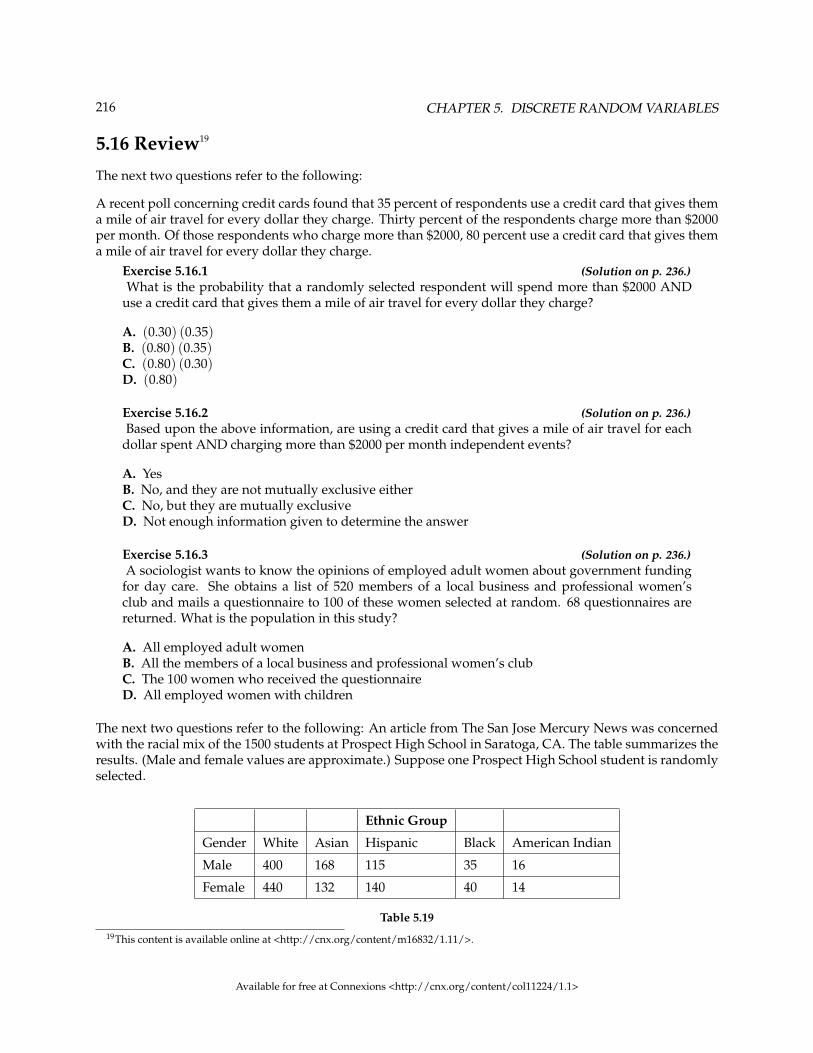
216 CHAPTER 5. DISCRETE RANDOM VARIABLES
5.16 Review19
The next two questions refer to the following:
A recent poll concerning credit cards found that 35 percent of respondents use a credit card that gives thema mile of air travel for every dollar they charge. Thirty percent of the respondents charge more than $2000per month. Of those respondents who charge more than $2000, 80 percent use a credit card that gives thema mile of air travel for every dollar they charge.
Exercise 5.16.1 (Solution on p. 236.)What is the probability that a randomly selected respondent will spend more than $2000 AND
use a credit card that gives them a mile of air travel for every dollar they charge?
A. (0.30) (0.35)B. (0.80) (0.35)C. (0.80) (0.30)D. (0.80)
Exercise 5.16.2 (Solution on p. 236.)Based upon the above information, are using a credit card that gives a mile of air travel for each
dollar spent AND charging more than $2000 per month independent events?
A. YesB. No, and they are not mutually exclusive eitherC. No, but they are mutually exclusiveD. Not enough information given to determine the answer
Exercise 5.16.3 (Solution on p. 236.)A sociologist wants to know the opinions of employed adult women about government funding
for day care. She obtains a list of 520 members of a local business and professional women’sclub and mails a questionnaire to 100 of these women selected at random. 68 questionnaires arereturned. What is the population in this study?
A. All employed adult womenB. All the members of a local business and professional women’s clubC. The 100 women who received the questionnaireD. All employed women with children
The next two questions refer to the following: An article from The San Jose Mercury News was concernedwith the racial mix of the 1500 students at Prospect High School in Saratoga, CA. The table summarizes theresults. (Male and female values are approximate.) Suppose one Prospect High School student is randomlyselected.
Ethnic Group
Gender White Asian Hispanic Black American Indian
Male 400 168 115 35 16
Female 440 132 140 40 14
Table 5.1919This content is available online at <http://cnx.org/content/m16832/1.11/>.
Available for free at Connexions <http://cnx.org/content/col11224/1.1>

217
Exercise 5.16.4 (Solution on p. 236.)Find the probability that a student is Asian or Male.
Exercise 5.16.5 (Solution on p. 236.)Find the probability that a student is Black given that the student is Female.
Exercise 5.16.6 (Solution on p. 236.)A sample of pounds lost, in a certain month, by individual members of a weight reducing clinic
produced the following statistics:
• Mean = 5 lbs.• Median = 4.5 lbs.• Mode = 4 lbs.• Standard deviation = 3.8 lbs.• First quartile = 2 lbs.• Third quartile = 8.5 lbs.
The correct statement is:
A. One fourth of the members lost exactly 2 pounds.B. The middle fifty percent of the members lost from 2 to 8.5 lbs.C. Most people lost 3.5 to 4.5 lbs.D. All of the choices above are correct.
Exercise 5.16.7 (Solution on p. 236.)What does it mean when a data set has a standard deviation equal to zero?
A. All values of the data appear with the same frequency.B. The mean of the data is also zero.C. All of the data have the same value.D. There are no data to begin with.
Exercise 5.16.8 (Solution on p. 236.)The statement that best describes the illustration below is:
Figure 5.1
A. The mean is equal to the median.B. There is no first quartile.C. The lowest data value is the median.D. The median equals (Q1+Q3)
2
Available for free at Connexions <http://cnx.org/content/col11224/1.1>

218 CHAPTER 5. DISCRETE RANDOM VARIABLES
Exercise 5.16.9 (Solution on p. 236.)According to a recent article (San Jose Mercury News) the average number of babies born with
significant hearing loss (deafness) is approximately 2 per 1000 babies in a healthy baby nursery.The number climbs to an average of 30 per 1000 babies in an intensive care nursery.
Suppose that 1000 babies from healthy baby nurseries were randomly surveyed. Find the proba-bility that exactly 2 babies were born deaf.Exercise 5.16.10 (Solution on p. 236.)A “friend” offers you the following “deal.” For a $10 fee, you may pick an envelope from a box
containing 100 seemingly identical envelopes. However, each envelope contains a coupon for afree gift.
• 10 of the coupons are for a free gift worth $6.• 80 of the coupons are for a free gift worth $8.• 6 of the coupons are for a free gift worth $12.• 4 of the coupons are for a free gift worth $40.
Based upon the financial gain or loss over the long run, should you play the game?
A. Yes, I expect to come out ahead in money.B. No, I expect to come out behind in money.C. It doesn’t matter. I expect to break even.
The next four questions refer to the following: Recently, a nurse commented that when a patient calls themedical advice line claiming to have the flu, the chance that he/she truly has the flu (and not just a nastycold) is only about 4%. Of the next 25 patients calling in claiming to have the flu, we are interested in howmany actually have the flu.
Exercise 5.16.11 (Solution on p. 236.)Define the Random Variable and list its possible values.
Exercise 5.16.12 (Solution on p. 236.)State the distribution of X .
Exercise 5.16.13 (Solution on p. 236.)Find the probability that at least 4 of the 25 patients actually have the flu.
Exercise 5.16.14 (Solution on p. 236.)On average, for every 25 patients calling in, how many do you expect to have the flu?
The next two questions refer to the following: Different types of writing can sometimes be distinguishedby the number of letters in the words used. A student interested in this fact wants to study the number ofletters of words used by Tom Clancy in his novels. She opens a Clancy novel at random and records thenumber of letters of the first 250 words on the page.
Exercise 5.16.15 (Solution on p. 236.)What kind of data was collected?
A. qualitativeB. quantitative - continuousC. quantitative – discrete
Exercise 5.16.16 (Solution on p. 236.)What is the population under study?
Available for free at Connexions <http://cnx.org/content/col11224/1.1>

219
5.17 Lab 1: Discrete Distribution (Playing Card Experiment)20
Class Time:
Names:
5.17.1 Student Learning Outcomes:
• The student will compare empirical data and a theoretical distribution to determine if everyday ex-periment fits a discrete distribution.
• The student will demonstrate an understanding of long-term probabilities.
5.17.2 Supplies:
• One full deck of playing cards
5.17.3 Procedure
The experiment procedure is to pick one card from a deck of shuffled cards.
1. The theorectical probability of picking a diamond from a deck is: _________2. Shuffle a deck of cards.3. Pick one card from it.4. Record whether it was a diamond or not a diamond.5. Put the card back and reshuffle.6. Do this a total of 10 times7. Record the number of diamonds picked.8. Let X = number of diamonds. Theoretically, X ∼ B (_____, _____)
5.17.4 Organize the Data
1. Record the number of diamonds picked for your class in the chart below. Then calculate the relativefrequency.
20This content is available online at <http://cnx.org/content/m16827/1.12/>.
Available for free at Connexions <http://cnx.org/content/col11224/1.1>

220 CHAPTER 5. DISCRETE RANDOM VARIABLES
x Frequency Relative Frequency
0 __________ __________
1 __________ __________
2 __________ __________
3 __________ __________
4 __________ __________
5 __________ __________
6 __________ __________
7 __________ __________
8 __________ __________
9 __________ __________
10 __________ __________
Table 5.20
2. Calculate the following:a. x =b. s =
3. Construct a histogram of the empirical data.
Figure 5.2
Available for free at Connexions <http://cnx.org/content/col11224/1.1>

221
5.17.5 Theoretical Distribution
1. Build the theoretical PDF chart based on the distribution in the Procedure section above.
x P (x)
0
1
2
3
4
5
6
7
8
9
10
Table 5.21
2. Calculate the following:
a. µ =____________b. σ =____________
3. Construct a histogram of the theoretical distribution.
Figure 5.3
Available for free at Connexions <http://cnx.org/content/col11224/1.1>

222 CHAPTER 5. DISCRETE RANDOM VARIABLES
5.17.6 Using the Data
Calculate the following, rounding to 4 decimal places:
NOTE: RF = relative frequency
Use the table from the section titled "Theoretical Distribution" here:
• P (x = 3) =• P (1 < x < 4) =• P (x ≥ 8) =
Use the data from the section titled "Organize the Data" here:
• RF (x = 3) =• RF (1 < x < 4) =• RF (x ≥ 8) =
5.17.7 Discussion Questions
For questions 1. and 2., think about the shapes of the two graphs, the probabilities and the relative frequen-cies, the means, and the standard deviations.
1. Knowing that data vary, describe three similarities between the graphs and distributions of the theo-retical and empirical distributions. Use complete sentences. (Note: These answers may vary and stillbe correct.)
2. Describe the three most significant differences between the graphs or distributions of the theoreticaland empirical distributions. (Note: These answers may vary and still be correct.)
3. Using your answers from the two previous questions, does it appear that the data fit the theoreticaldistribution? In 1 - 3 complete sentences, explain why or why not.
4. Suppose that the experiment had been repeated 500 times. Which table (from "Organize the data"and "Theoretical Distributions") would you expect to change (and how would it change)? Why? Whywouldn’t the other table change?
Available for free at Connexions <http://cnx.org/content/col11224/1.1>

223
5.18 Lab 2: Discrete Distribution (Lucky Dice Experiment)21
Class Time:
Names:
5.18.1 Student Learning Outcomes:
• The student will compare empirical data and a theoretical distribution to determine if a Tet gamblinggame fits a discrete distribution.
• The student will demonstrate an understanding of long-term probabilities.
5.18.2 Supplies:
• 1 game “Lucky Dice” or 3 regular dice
NOTE: For a detailed game description, refer here. (The link goes to the beginning of DiscreteRandom Variables Homework. Please refer to Problem #14.)
NOTE: Round relative frequencies and probabilities to four decimal places.
5.18.3 The Procedure
1. The experiment procedure is to bet on one object. Then, roll 3 Lucky Dice and count the number ofmatches. The number of matches will decide your profit.
2. What is the theoretical probability of 1 die matching the object? _________3. Choose one object to place a bet on. Roll the 3 Lucky Dice. Count the number of matches.4. Let X = number of matches. Theoretically, X ∼ B (______, ______)5. Let Y = profit per game.
5.18.4 Organize the Data
In the chart below, fill in the Y value that corresponds to each X value. Next, record the number of matchespicked for your class. Then, calculate the relative frequency.
1. Complete the table.
x y Frequency Relative Frequency
0
1
2
3
Table 5.2221This content is available online at <http://cnx.org/content/m16826/1.12/>.
Available for free at Connexions <http://cnx.org/content/col11224/1.1>

224 CHAPTER 5. DISCRETE RANDOM VARIABLES
2. Calculate the Following:
a. x =b. sx =c. y =d. sy =
3. Explain what x represents.4. Explain what y represents.5. Based upon the experiment:
a. What was the average profit per game?b. Did this represent an average win or loss per game?c. How do you know? Answer in complete sentences.
6. Construct a histogram of the empirical data
Figure 5.4
5.18.5 Theoretical Distribution
Build the theoretical PDF chart for X and Y based on the distribution from the section titled "The Procedure".
1.x y P (x) = P (y)
0
1
2
3
Available for free at Connexions <http://cnx.org/content/col11224/1.1>

225
Table 5.23
2. Calculate the following
a. µx =b. σx =c. µy =
3. Explain what µx represents.4. Explain what µy represents.5. Based upon theory:
a. What was the expected profit per game?b. Did the expected profit represent an average win or loss per game?c. How do you know? Answer in complete sentences.
6. Construct a histogram of the theoretical distribution.
Figure 5.5
5.18.6 Use the Data
Calculate the following (rounded to 4 decimal places):
NOTE: RF = relative frequency
Use the data from the section titled "Theoretical Distribution" here:
1. P (x = 3) =____________2. P (0 < x < 3) =____________3. P (x ≥ 2) =____________
Available for free at Connexions <http://cnx.org/content/col11224/1.1>

226 CHAPTER 5. DISCRETE RANDOM VARIABLES
Use the data from the section titled "Organize the Data" here:
1. RF (x = 3) =____________2. RF (0 < x < 3) =____________3. RF (x ≥ 2) = ____________
5.18.7 Discussion Question
For questions 1. and 2., consider the graphs, the probabilities and relative frequencies, the means and thestandard deviations.
1. Knowing that data vary, describe three similarities between the graphs and distributions of the theo-retical and empirical distributions. Use complete sentences. (Note: these answers may vary and stillbe correct.)
2. Describe the three most significant differences between the graphs or distributions of the theoreticaland empirical distributions. (Note: these answers may vary and still be correct.)
3. Thinking about your answers to 1. and 2.,does it appear that the data fit the theoretical distribution?In 1 - 3 complete sentences, explain why or why not.
4. Suppose that the experiment had been repeated 500 times. Which table (from "Organize the Data" or"Theoretical Distribution") would you expect to change? Why? How might the table change?
5.19 Binomial Distribution22
When you flip a coin, there are two possible outcomes: heads and tails. Each outcome has a fixed prob-ability, the same from trial to trial. In the case of coins, heads and tails each have the same probability of1/2. More generally, there are situations in which the coin is biased, so that heads and tails have differentprobabilities. In the present section, we consider probability distributions for which there are just two pos-sible outcomes with fixed probability summing to one. These distributions are called are called binomialdistributions.
5.19.1 A Simple Example
The four possible outcomes that could occur if you flipped a coin twice are listed in Table 5.24: Four PossibleOutcomes. Note that the four outcomes are equally likely: each has probability 1/4. To see this, note thatthe tosses of the coin are independent (neither affects the other). Hence, the probability of a head on Flip 1and a head on Flip 2 is the product of Pr [H] and Pr [H], which is 1/2× 1/2 = 1/4. The same calculationapplies to the probability of a head on Flip one and a tail on Flip 2. Each is 1/2× 1/2 = 1/4.
Four Possible Outcomes
Outcome First Flip Second Flip
1 Heads Heads
2 Heads Tails
3 Tails Heads
4 Tails Tails
Table 5.2422This content is available online at <http://cnx.org/content/m11024/2.8/>.
Available for free at Connexions <http://cnx.org/content/col11224/1.1>

227
The four possible outcomes can be classifid in terms of the number of heads that come up. The numbercould be two (Outcome 1), one (Outcomes 2 and 3) or 0 (Outcome 4). The probabilities of these possibilitiesare shown in Table 5.25: Probabilities of Getting 0,1, or 2 heads. and in Figure 5.6. Since two of the outcomesrepresent the case in which just one head appears in the two tosses, the probability of this event is equal to1/4 + 1/4 = 1/2. Table 5.24: Four Possible Outcomes summarizes the situation.
Probabilities of Getting 0,1, or 2 heads.
Number of Heads Probability
0 1/4
1 1/2
2 1/4
Table 5.25
Figure 5.6: Probabilities of 0, 1, and 2 heads.
Figure 5.6 is a discrete probability distribution: It shows the probability for each of the values on the X-axis.Defining a head as a "success," Figure 5.6 shows the probability of 0, 1, and 2 successes for two trials (flips)for an event that has a probability of 0.5 of being a success on each trial. This makes Figure 5.6 an exampleof a binomial distribution.
5.19.2 The Formula for Binomial Probabilities
The binomial distribution consists of the probabilities of each of the possible numbers of successes on Ntrials for independent events that each have a probability of π(the Greek letter pi) of occurring. For the coin
Available for free at Connexions <http://cnx.org/content/col11224/1.1>
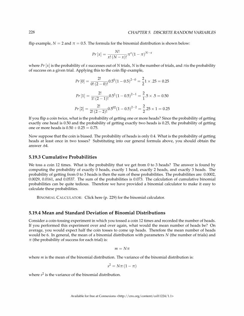
228 CHAPTER 5. DISCRETE RANDOM VARIABLES
flip example, N = 2 and π = 0.5. The formula for the binomial distribution is shown below:
Pr [x] =N!
x! (N − x)!πx(1− π)N−x
where Pr [x] is the probability of x successes out of N trials, N is the number of trials, and πis the probabilityof success on a given trial. Applying this to the coin flip example,
Pr [0] =2!
0! (2− 0)!0.50(1− 0.5)2−0 =
22
1× .25 = 0.25
Pr [1] =2!
1! (2− 1)!0.51(1− 0.5)2−1 =
21
.5× .5 = 0.50
Pr [2] =2!
2! (2− 2)!0.502(1− 0.5)2−2 =
22
.25× 1 = 0.25
If you flip a coin twice, what is the probability of getting one or more heads? Since the probability of gettingexactly one head is 0.50 and the probability of getting exactly two heads is 0.25, the probability of gettingone or more heads is 0.50 + 0.25 = 0.75.
Now suppose that the coin is biased. The probability of heads is only 0.4. What is the probability of gettingheads at least once in two tosses? Substituting into our general formula above, you should obtain theanswer .64.
5.19.3 Cumulative Probabilities
We toss a coin 12 times. What is the probability that we get from 0 to 3 heads? The answer is found bycomputing the probability of exactly 0 heads, exactly 1 head, exactly 2 heads, and exactly 3 heads. Theprobability of getting from 0 to 3 heads is then the sum of these probabilities. The probabilities are: 0.0002,0.0029, 0.0161, and 0.0537. The sum of the probabilities is 0.073. The calculation of cumulative binomialprobabilities can be quite tedious. Therefore we have provided a binomial calculator to make it easy tocalculate these probabilities.
BINOMIAL CALCULATOR: Click here (p. 229) for the binomial calculator.
5.19.4 Mean and Standard Deviation of Binomial Distributions
Consider a coin-tossing experiment in which you tossed a coin 12 times and recorded the number of heads.If you performed this experiment over and over again, what would the mean number of heads be? Onaverage, you would expect half the coin tosses to come up heads. Therefore the mean number of headswould be 6. In general, the mean of a binomial distribution with parameters N (the number of trials) andπ (the probability of success for each trial) is:
m = Nπ
where m is the mean of the binomial distribution. The variance of the binomial distribution is:
s2 = Nπ (1− π)
where s2 is the variance of the binomial distribution.
Available for free at Connexions <http://cnx.org/content/col11224/1.1>

229
Let’s return to the coin tossing experiment. The coin was tossed 12 times so N = 12. A coin has a probabilityof 0.5 of coming up heads. Therefore, π = 0.5. The mean and standard deviation can therefore be computedas follows:
m = Nπ = 12× 0.5 = 6
s2 = Nπ (1− π) = 12× 0.5× (1.0− 0.5) = 3.0
Naturally, the standard deviation (s) is the square root of the variance(s2).
5.19.5 Binomial Calculator
This media object is a Java applet. Please view or download it at<binomialprob.binomialProb.class>
Available for free at Connexions <http://cnx.org/content/col11224/1.1>

230 CHAPTER 5. DISCRETE RANDOM VARIABLES
Solutions to Exercises in Chapter 5
Solution to Example 5.2, Problem 1 (p. 183)Let X = the number of days Nancy attends class per week.
Solution to Example 5.2, Problem 2 (p. 183)0, 1, 2, and 3
Solution to Example 5.2, Problem 3 (p. 183)
x P (x)
0 0.01
1 0.04
2 0.15
3 0.80
Table 5.26
Solution to Example 5.5, Problem 1 (p. 185)X = amount of profit
Solution to Example 5.5, Problem 2 (p. 185)
x P (x) xP (x)
WIN 10 13
103
LOSE -6 23
−123
Table 5.27
Solution to Example 5.5, Problem 3 (p. 186)Add the last column of the table. The expected value µ = −2
3 . You lose, on average, about 67 cents eachtime you play the game so you do not come out ahead.Solution to Example 5.9, Problem 1 (p. 187)failure
Solution to Example 5.9, Problem 2 (p. 187)X = the number of statistics students who do their homework on time
Solution to Example 5.9, Problem 3 (p. 187)0, 1, 2, . . ., 50
Solution to Example 5.9, Problem 4 (p. 187)Failure is a student who does not do his or her homework on time.
Solution to Example 5.9, Problem 5 (p. 187)q = 0.30
Solution to Example 5.9, Problem 6 (p. 188)greater than or equal to (≥)
Solution to Example 5.14, Problem 2 (p. 190)1, 2, 3, . . ., (total number of students)
Solution to Example 5.14, Problem 3 (p. 190)
• p = 0.55• q = 0.45
Available for free at Connexions <http://cnx.org/content/col11224/1.1>

231
Solution to Example 5.14, Problem 4 (p. 190)P (x = 4)
Solution to Example 5.18, Problem 1 (p. 192)Without
Solution to Example 5.18, Problem 2 (p. 192)The men
Solution to Example 5.18, Problem 3 (p. 193)15 men
Solution to Example 5.18, Problem 4 (p. 193)18 women
Solution to Example 5.18, Problem 5 (p. 193)Let X = the number of men on the committee. x = 0, 1, 2, . . ., 7.
Solution to Example 5.18, Problem 6 (p. 193)P(x>4)
Solution to Example 5.22, Problem 1 (p. 195)One broadcast
Solution to Example 5.22, Problem 2 (p. 195)2
Solution to Example 5.22, Problem 3 (p. 195)Let X = the number of times the news reporter says "uh" during one broadcast.x = 0, 1, 2, 3, ...Solution to Example 5.22, Problem 4 (p. 195)P(x > 2)
Solutions to Practice 2: Binomial Distribution
Solution to Exercise 5.11.1 (p. 200)X= the number that reply “yes”
Solution to Exercise 5.11.2 (p. 200)B(8,0.713)
Solution to Exercise 5.11.3 (p. 200)0,1,2,3,4,5,6,7,8
Solution to Exercise 5.11.5 (p. 200)5.7
Solution to Exercise 5.11.6 (p. 200)1.28
Solution to Exercise 5.11.7 (p. 201)0.4151
Solution to Exercise 5.11.8 (p. 201)0.9990
Solutions to Practice 3: Poisson Distribution
Solution to Exercise 5.12.2 (p. 202)P(8)
Solution to Exercise 5.12.3 (p. 202)0,1,2,3,4,...
Solution to Exercise 5.12.5 (p. 202)No
Solution to Exercise 5.12.6 (p. 202)No
Available for free at Connexions <http://cnx.org/content/col11224/1.1>

232 CHAPTER 5. DISCRETE RANDOM VARIABLES
Solutions to Practice 4: Geometric Distribution
Solution to Exercise 5.13.2 (p. 203)G(0.713)
Solution to Exercise 5.13.3 (p. 203)1,2,. . .
Solution to Exercise 5.13.5 (p. 203)1.4
Solution to Exercise 5.13.6 (p. 203)0.9176
Solutions to Practice 5: Hypergeometric Distribution
Solution to Exercise 5.14.2 (p. 205)H(16,7,9)
Solution to Exercise 5.14.3 (p. 205)2,3,4,5,6,7,8,9
Solution to Exercise 5.14.5 (p. 205)6.26
Solutions to Homework
Solution to Exercise 5.15.1 (p. 206)
a. 0.1b. 1.6
Solution to Exercise 5.15.3 (p. 206)
b. $200,000;$600,000;$400,000c. third investmentd. first investmente. second investment
Solution to Exercise 5.15.5 (p. 207)
a. 0.2c. 2.35d. 2-3 children
Solution to Exercise 5.15.7 (p. 208)
a. X = the number of dice that show a 1b. 0,1,2,3,4,5,6c. X∼B
(6, 1
6
)d. 1e. 0.00002f. 3 dice
Solution to Exercise 5.15.9 (p. 208)
a. X = the number of students that will attend Tet.b. 0, 1, 2, 3, 4, 5, 6, 7, 8, 9, 10, 11, 12c. X∼B(12,0.18)d. 2.16
Available for free at Connexions <http://cnx.org/content/col11224/1.1>
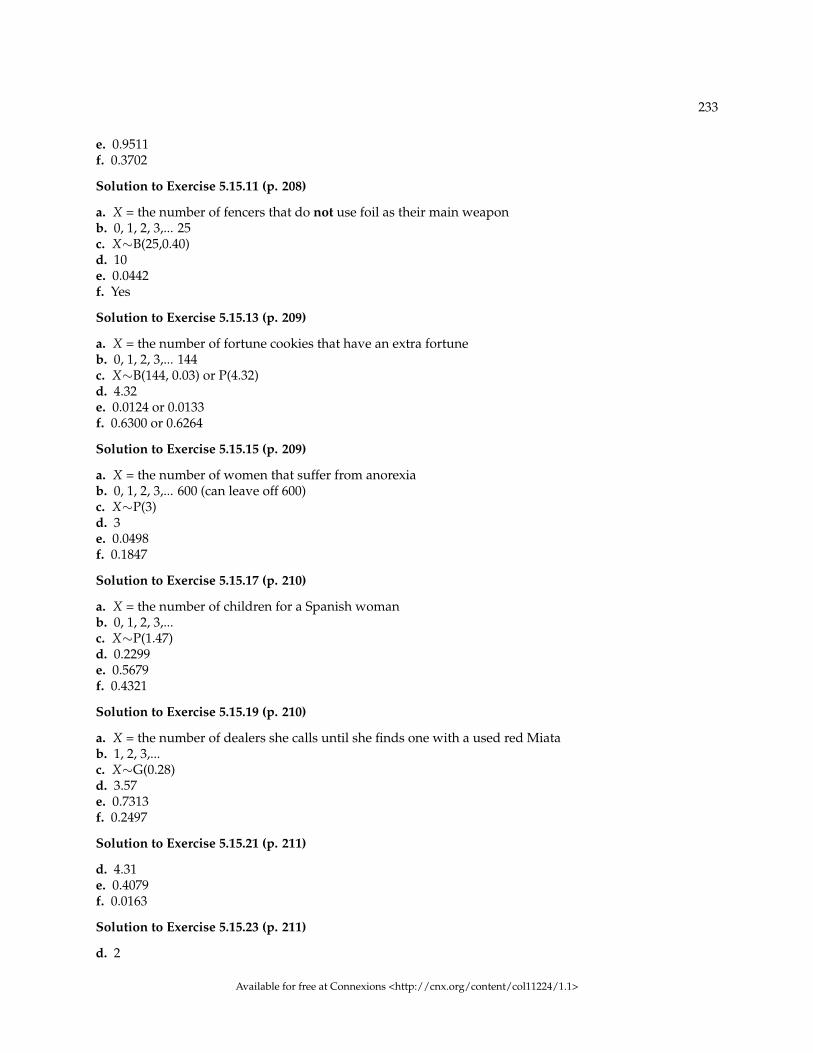
233
e. 0.9511f. 0.3702
Solution to Exercise 5.15.11 (p. 208)
a. X = the number of fencers that do not use foil as their main weaponb. 0, 1, 2, 3,... 25c. X∼B(25,0.40)d. 10e. 0.0442f. Yes
Solution to Exercise 5.15.13 (p. 209)
a. X = the number of fortune cookies that have an extra fortuneb. 0, 1, 2, 3,... 144c. X∼B(144, 0.03) or P(4.32)d. 4.32e. 0.0124 or 0.0133f. 0.6300 or 0.6264
Solution to Exercise 5.15.15 (p. 209)
a. X = the number of women that suffer from anorexiab. 0, 1, 2, 3,... 600 (can leave off 600)c. X∼P(3)d. 3e. 0.0498f. 0.1847
Solution to Exercise 5.15.17 (p. 210)
a. X = the number of children for a Spanish womanb. 0, 1, 2, 3,...c. X∼P(1.47)d. 0.2299e. 0.5679f. 0.4321
Solution to Exercise 5.15.19 (p. 210)
a. X = the number of dealers she calls until she finds one with a used red Miatab. 1, 2, 3,...c. X∼G(0.28)d. 3.57e. 0.7313f. 0.2497
Solution to Exercise 5.15.21 (p. 211)
d. 4.31e. 0.4079f. 0.0163
Solution to Exercise 5.15.23 (p. 211)
d. 2
Available for free at Connexions <http://cnx.org/content/col11224/1.1>

234 CHAPTER 5. DISCRETE RANDOM VARIABLES
e. 0.1353f. 0.3233
Solution to Exercise 5.15.25 (p. 211)
a. X = the number of seniors that participated in after-school sports all 4 years of high schoolb. 0, 1, 2, 3,... 60c. X~P (4.8)d. 4.8e. Yesf. 4
Solution to Exercise 5.15.27 (p. 212)
a. X = the number of shell pieces in one cakeb. 0, 1, 2, 3,...c. X~P (1.5)d. 1.5e. 0.2231f. 0.0001g. Yes
Solution to Exercise 5.15.29 (p. 212)
d. 0.0043e. nonef. 3.3
Solution to Exercise 5.15.31 (p. 212)
d. 3.02e. Nof. 0.9997h. 0.3881i. 6.6207 pages
Solution to Exercise 5.15.33 (p. 213)D: 4.43
Solution to Exercise 5.15.34 (p. 213)A: 0.1476
Solution to Exercise 5.15.35 (p. 213)C: 0.4734
Solution to Exercise 5.15.36 (p. 213)A: The number of times Mrs. Plum’s cats wake her up each week
Solution to Exercise 5.15.37 (p. 214)D: 0.0671
Solution to Exercise 5.15.38 (p. 214)Partial Answer:
A: X = the number of DVDs a Video to Go customer rentsB: 0.12C: 0.11D: 0.77Solution to Exercise 5.15.39 (p. 214)The variable of interest is X = net gain or loss, in dollars
Available for free at Connexions <http://cnx.org/content/col11224/1.1>

235
The face cards J, Q, K (Jack, Queen, King). There are(3)(4) = 12 face cards and 52 – 12 = 40 cards that are notface cards.
We first need to construct the probability distribution for X. We use the card and coin events to determinethe probability for each outcome, but we use the monetary value of X to determine the expected value.
Card Event $X net gain or loss P(X)
Face Card and Heads 6 (12/52)(1/2) = 6/52
Face Card and Tails 2 (12/52)(1/2) = 6/52
(Not Face Card) and (H or T) –2 (40/52)(1) = 40/52
Table 5.28
• Expected value = (6)(6/52) + (2)(6/52) + (–2) (40/52) = –32/52• Expected value = –$0.62, rounded to the nearest cent• If you play this game repeatedly, over a long number of games, you would expect to lost 62 cents per
game, on average.• You should not play this game to win money because the expected value indicates an expected aver-
age loss.
Solution to Exercise 5.15.40 (p. 215)Start by writing the probability distribution. X is net gain or loss = prize (if any) less $10 cost of ticket
X = $ net gain or loss P(X)
$500–$10=$490 1/100
$100–$10=$90 2/100
$25–$10=$15 4/100
$0–$10=$–10 93/100)
Table 5.29
Expected Value = (490)(1/100) + (90)(2/100) + (15)(4/100) + (–10) (93/100) = –$2. There is an expected lossof $2 per ticket, on average.Solution to Exercise 5.15.41 (p. 215)
• X = number of questions answered correctly• X∼B(10, 0.5)• We are interested in AT LEAST 70% of 10 questions correct. 70% of 10 is 7. We want to find the
probability that X is greater than or equal to 7. The event "at least 7" is the complement of "less thanor equal to 6".
• Using your calculator’s distribution menu: 1 – binomcdf(10, .5, 6) gives 0.171875• The probability of getting at least 70% of the 10 questions correct when randomly guessing is approx-
imately 0.172
Solution to Exercise 5.15.42 (p. 215)
• X = number of questions answered correctly• X∼B(32, 1/3)
Available for free at Connexions <http://cnx.org/content/col11224/1.1>

236 CHAPTER 5. DISCRETE RANDOM VARIABLES
• We are interested in MORE THAN 75% of 32 questions correct. 75% of 32 is 24. We want to findP(x>24). The event "more than 24" is the complement of "less than or equal to 24".
• Using your calculator’s distribution menu: 1 - binomcdf(32, 1/3, 24)• P(x>24) = 0.00000026761• The probability of getting more than 75% of the 32 questions correct when randomly guessing is very
small and practically zero.
Solution to Exercise 5.15.43 (p. 215)A: X can take on the values 1, 2, 3, .... p = 2/6, q = 4/6
B: 0.2222C: 3
Solutions to Review
Solution to Exercise 5.16.1 (p. 216)C
Solution to Exercise 5.16.2 (p. 216)B
Solution to Exercise 5.16.3 (p. 216)A
Solution to Exercise 5.16.4 (p. 217)0.5773
Solution to Exercise 5.16.5 (p. 217)0.0522
Solution to Exercise 5.16.6 (p. 217)B
Solution to Exercise 5.16.7 (p. 217)C
Solution to Exercise 5.16.8 (p. 217)C
Solution to Exercise 5.16.9 (p. 218)0.2709
Solution to Exercise 5.16.10 (p. 218)B
Solution to Exercise 5.16.11 (p. 218)X = the number of patients calling in claiming to have the flu, who actually have the flu. X = 0, 1, 2, ...25
Solution to Exercise 5.16.12 (p. 218)B (25, 0.04)
Solution to Exercise 5.16.13 (p. 218)0.0165
Solution to Exercise 5.16.14 (p. 218)1
Solution to Exercise 5.16.15 (p. 218)C
Solution to Exercise 5.16.16 (p. 218)All words used by Tom Clancy in his novels
Available for free at Connexions <http://cnx.org/content/col11224/1.1>
Chapter 6
Continuous Random Variables
6.1 Continuous Random Variables1
6.1.1 Student Learning Outcomes
By the end of this chapter, the student should be able to:
• Recognize and understand continuous probability density functions in general.• Recognize the uniform probability distribution and apply it appropriately.• Recognize the exponential probability distribution and apply it appropriately.
6.1.2 Introduction
Continuous random variables have many applications. Baseball batting averages, IQ scores, the lengthof time a long distance telephone call lasts, the amount of money a person carries, the length of time acomputer chip lasts, and SAT scores are just a few. The field of reliability depends on a variety of continuousrandom variables.
This chapter gives an introduction to continuous random variables and the many continuous distributions.We will be studying these continuous distributions for several chapters.
NOTE: The values of discrete and continuous random variables can be ambiguous. For example,if X is equal to the number of miles (to the nearest mile) you drive to work, then X is a discreterandom variable. You count the miles. If X is the distance you drive to work, then you measurevalues of X and X is a continuous random variable. How the random variable is defined is veryimportant.
6.1.3 Properties of Continuous Probability Distributions
The graph of a continuous probability distribution is a curve. Probability is represented by area under thecurve.
The curve is called the probability density function (abbreviated: pdf). We use the symbol f (x) to rep-resent the curve. f (x) is the function that corresponds to the graph; we use the density function f (x) todraw the graph of the probability distribution.
1This content is available online at <http://cnx.org/content/m16808/1.12/>.
Available for free at Connexions <http://cnx.org/content/col11224/1.1>
237

238 CHAPTER 6. CONTINUOUS RANDOM VARIABLES
Area under the curve is given by a different function called the cumulative distribution function (abbre-viated: cdf). The cumulative distribution function is used to evaluate probability as area.
• The outcomes are measured, not counted.• The entire area under the curve and above the x-axis is equal to 1.• Probability is found for intervals of x values rather than for individual x values.• P (c < x < d) is the probability that the random variable X is in the interval between the values c and
d. P (c < x < d) is the area under the curve, above the x-axis, to the right of c and the left of d.• P (x = c) = 0 The probability that x takes on any single individual value is 0. The area below the
curve, above the x-axis, and between x=c and x=c has no width, and therefore no area (area = 0).Since the probability is equal to the area, the probability is also 0.
We will find the area that represents probability by using geometry, formulas, technology, or probabilitytables. In general, calculus is needed to find the area under the curve for many probability density functions.When we use formulas to find the area in this textbook, the formulas were found by using the techniquesof integral calculus. However, because most students taking this course have not studied calculus, we willnot be using calculus in this textbook.
There are many continuous probability distributions. When using a continuous probability distribution tomodel probability, the distribution used is selected to best model and fit the particular situation.
In this chapter and the next chapter, we will study the uniform distribution, the exponential distribution,and the normal distribution. The following graphs illustrate these distributions.
Figure 6.1: The graph shows a Uniform Distribution with the area between x=3 and x=6 shaded to repre-sent the probability that the value of the random variable X is in the interval between 3 and 6.
Available for free at Connexions <http://cnx.org/content/col11224/1.1>

239
Figure 6.2: The graph shows an Exponential Distribution with the area between x=2 and x=4 shaded torepresent the probability that the value of the random variable X is in the interval between 2 and 4.
Figure 6.3: The graph shows the Standard Normal Distribution with the area between x=1 and x=2 shadedto represent the probability that the value of the random variable X is in the interval between 1 and 2.
**With contributions from Roberta Bloom
6.2 Continuous Probability Functions2
We begin by defining a continuous probability density function. We use the function notation f (x). Inter-mediate algebra may have been your first formal introduction to functions. In the study of probability, thefunctions we study are special. We define the function f (x) so that the area between it and the x-axis isequal to a probability. Since the maximum probability is one, the maximum area is also one.
For continuous probability distributions, PROBABILITY = AREA.
2This content is available online at <http://cnx.org/content/m16805/1.9/>.
Available for free at Connexions <http://cnx.org/content/col11224/1.1>

240 CHAPTER 6. CONTINUOUS RANDOM VARIABLES
Example 6.1Consider the function f (x) = 1
20 for 0 ≤ x ≤ 20. x = a real number. The graph of f (x) = 120 is a
horizontal line. However, since 0 ≤ x ≤ 20 , f (x) is restricted to the portion between x = 0 andx = 20, inclusive .
f (x) = 120 for 0 ≤ x ≤ 20.
The graph of f (x) = 120 is a horizontal line segment when 0 ≤ x ≤ 20.
The area between f (x) = 120 where 0 ≤ x ≤ 20 and the x-axis is the area of a rectangle with base
= 20 and height = 120 .
AREA = 20 · 120 = 1
This particular function, where we have restricted x so that the area between the function andthe x-axis is 1, is an example of a continuous probability density function. It is used as a tool tocalculate probabilities.
Suppose we want to find the area between f (x) = 120 and the x-axis where 0 < x < 2 .
AREA = (2− 0) · 120 = 0.1
(2− 0) = 2 = base of a rectangle
120 = the height.
The area corresponds to a probability. The probability that x is between 0 and 2 is 0.1, which canbe written mathematically as P(0<x<2) = P(x<2) = 0.1.
Suppose we want to find the area between f (x) = 120 and the x-axis where 4 < x < 15 .
Available for free at Connexions <http://cnx.org/content/col11224/1.1>
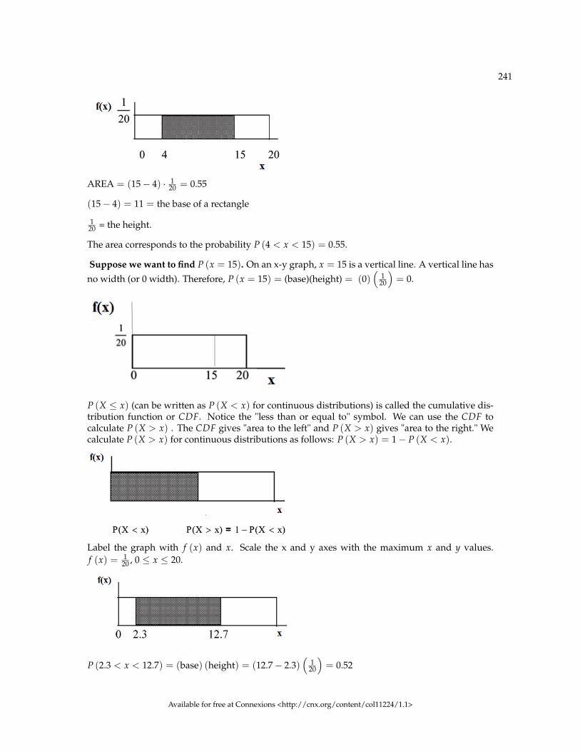
241
AREA = (15− 4) · 120 = 0.55
(15− 4) = 11 = the base of a rectangle
120 = the height.
The area corresponds to the probability P (4 < x < 15) = 0.55.
Suppose we want to find P (x = 15). On an x-y graph, x = 15 is a vertical line. A vertical line hasno width (or 0 width). Therefore, P (x = 15) = (base)(height) = (0)
(1
20
)= 0.
P (X ≤ x) (can be written as P (X < x) for continuous distributions) is called the cumulative dis-tribution function or CDF. Notice the "less than or equal to" symbol. We can use the CDF tocalculate P (X > x) . The CDF gives "area to the left" and P (X > x) gives "area to the right." Wecalculate P (X > x) for continuous distributions as follows: P (X > x) = 1− P (X < x).
Label the graph with f (x) and x. Scale the x and y axes with the maximum x and y values.f (x) = 1
20 , 0 ≤ x ≤ 20.
P (2.3 < x < 12.7) = (base) (height) = (12.7− 2.3)(
120
)= 0.52
Available for free at Connexions <http://cnx.org/content/col11224/1.1>

242 CHAPTER 6. CONTINUOUS RANDOM VARIABLES
6.3 The Uniform Distribution3
Example 6.2The previous problem is an example of the uniform probability distribution.
Illustrate the uniform distribution. The data that follows are 55 smiling times, in seconds, of aneight-week old baby.
10.4 19.6 18.8 13.9 17.8 16.8 21.6 17.9 12.5 11.1 4.9
12.8 14.8 22.8 20.0 15.9 16.3 13.4 17.1 14.5 19.0 22.8
1.3 0.7 8.9 11.9 10.9 7.3 5.9 3.7 17.9 19.2 9.8
5.8 6.9 2.6 5.8 21.7 11.8 3.4 2.1 4.5 6.3 10.7
8.9 9.4 9.4 7.6 10.0 3.3 6.7 7.8 11.6 13.8 18.6
Table 6.1
sample mean = 11.49 and sample standard deviation = 6.23
We will assume that the smiling times, in seconds, follow a uniform distribution between 0 and 23seconds, inclusive. This means that any smiling time from 0 to and including 23 seconds is equallylikely. The histogram that could be constructed from the sample is an empirical distribution thatclosely matches the theoretical uniform distribution.
Let X = length, in seconds, of an eight-week old baby’s smile.
The notation for the uniform distribution is
X ∼ U (a,b) where a = the lowest value of x and b = the highest value of x.
The probability density function is f (x) = 1b−a for a ≤ x ≤ b.
For this example, x ∼ U (0, 23) and f (x) = 123−0 for 0 ≤ x ≤ 23.
Formulas for the theoretical mean and standard deviation are
µ = a+b2 and σ =
√(b−a)2
12
For this problem, the theoretical mean and standard deviation are
µ = 0+232 = 11.50 seconds and σ =
√(23−0)2
12 = 6.64 seconds
Notice that the theoretical mean and standard deviation are close to the sample mean and standarddeviation.
Example 6.3Problem 1What is the probability that a randomly chosen eight-week old baby smiles between 2 and 18
seconds?
SolutionFind P (2 < x < 18).
3This content is available online at <http://cnx.org/content/m16819/1.17/>.
Available for free at Connexions <http://cnx.org/content/col11224/1.1>

243
P (2 < x < 18) = (base) (height) = (18− 2) · 123 = 16
23 .
Problem 2Find the 90th percentile for an eight week old baby’s smiling time.
SolutionNinety percent of the smiling times fall below the 90th percentile, k, so P (x < k) = 0.90
P (x < k) = 0.90
(base) (height) = 0.90
(k− 0) · 123 = 0.90
k = 23 · 0.90 = 20.7
Problem 3Find the probability that a random eight week old baby smiles more than 12 seconds KNOWINGthat the baby smiles MORE THAN 8 SECONDS.
SolutionFind P (x > 12|x > 8) There are two ways to do the problem. For the first way, use the fact that
this is a conditional and changes the sample space. The graph illustrates the new sample space.You already know the baby smiled more than 8 seconds.
Write a new f (x): f (x) = 123−8 = 1
15
for 8 < x < 23
P (x > 12|x > 8) = (23− 12) · 115 = 11
15
Available for free at Connexions <http://cnx.org/content/col11224/1.1>

244 CHAPTER 6. CONTINUOUS RANDOM VARIABLES
For the second way, use the conditional formula from Probability Topics with the original distri-bution X ∼ U (0, 23):
P (A|B) = P(A AND B)P(B) For this problem, A is (x > 12) and B is (x > 8).
So, P (x > 12|x > 8) = (x>12 AND x>8)P(x>8) = P(x>12)
P(x>8) =11231523
= 0.733
Example 6.4Uniform: The amount of time, in minutes, that a person must wait for a bus is uniformly dis-tributed between 0 and 15 minutes, inclusive.Problem 1What is the probability that a person waits fewer than 12.5 minutes?
SolutionLet X = the number of minutes a person must wait for a bus. a = 0 and b = 15. x ∼ U (0, 15). Writethe probability density function. f (x) = 1
15−0 = 115 for 0 ≤ x ≤ 15.
Find P (x < 12.5). Draw a graph.
P (x < k) = (base) (height) = (12.5− 0) · 115 = 0.8333
The probability a person waits less than 12.5 minutes is 0.8333.
Available for free at Connexions <http://cnx.org/content/col11224/1.1>

245
Problem 2On the average, how long must a person wait?
Find the mean, µ, and the standard deviation, σ.
Solutionµ = a+b
2 = 15+02 = 7.5. On the average, a person must wait 7.5 minutes.
σ =√
(b−a)2
12 =√
(15−0)2
12 = 4.3. The Standard deviation is 4.3 minutes.
Problem 3Ninety percent of the time, the time a person must wait falls below what value?
NOTE: This asks for the 90th percentile.
SolutionFind the 90th percentile. Draw a graph. Let k = the 90th percentile.
P (x < k) = (base) (height) = (k− 0) ·(
115
)0.90 = k · 1
15
k = (0.90) (15) = 13.5
k is sometimes called a critical value.
The 90th percentile is 13.5 minutes. Ninety percent of the time, a person must wait at most 13.5minutes.
Example 6.5Uniform: Suppose the time it takes a nine-year old to eat a donut is between 0.5 and 4 minutes,inclusive. Let X = the time, in minutes, it takes a nine-year old child to eat a donut. Then X ∼U (0.5, 4).Problem 1 (Solution on p. 273.)The probability that a randomly selected nine-year old child eats a donut in at least two minutes
is _______.
Problem 2 (Solution on p. 273.)Find the probability that a different nine-year old child eats a donut in more than 2 minutes giventhat the child has already been eating the donut for more than 1.5 minutes.
Available for free at Connexions <http://cnx.org/content/col11224/1.1>
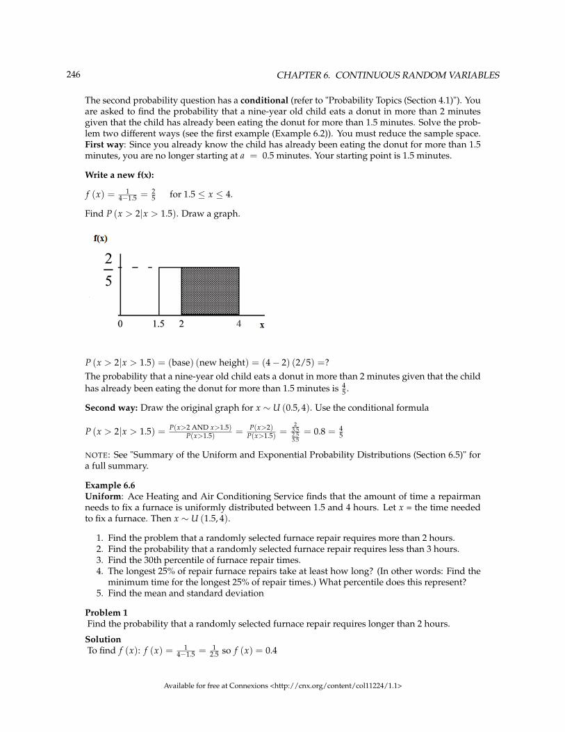
246 CHAPTER 6. CONTINUOUS RANDOM VARIABLES
The second probability question has a conditional (refer to "Probability Topics (Section 4.1)"). Youare asked to find the probability that a nine-year old child eats a donut in more than 2 minutesgiven that the child has already been eating the donut for more than 1.5 minutes. Solve the prob-lem two different ways (see the first example (Example 6.2)). You must reduce the sample space.First way: Since you already know the child has already been eating the donut for more than 1.5minutes, you are no longer starting at a = 0.5 minutes. Your starting point is 1.5 minutes.
Write a new f(x):
f (x) = 14−1.5 = 2
5 for 1.5 ≤ x ≤ 4.
Find P (x > 2|x > 1.5). Draw a graph.
P (x > 2|x > 1.5) = (base) (new height) = (4− 2) (2/5) =?The probability that a nine-year old child eats a donut in more than 2 minutes given that the childhas already been eating the donut for more than 1.5 minutes is 4
5 .
Second way: Draw the original graph for x ∼ U (0.5, 4). Use the conditional formula
P (x > 2|x > 1.5) = P(x>2 AND x>1.5)P(x>1.5) = P(x>2)
P(x>1.5) =2
3.52.53.5
= 0.8 = 45
NOTE: See "Summary of the Uniform and Exponential Probability Distributions (Section 6.5)" fora full summary.
Example 6.6Uniform: Ace Heating and Air Conditioning Service finds that the amount of time a repairmanneeds to fix a furnace is uniformly distributed between 1.5 and 4 hours. Let x = the time neededto fix a furnace. Then x ∼ U (1.5, 4).
1. Find the problem that a randomly selected furnace repair requires more than 2 hours.2. Find the probability that a randomly selected furnace repair requires less than 3 hours.3. Find the 30th percentile of furnace repair times.4. The longest 25% of repair furnace repairs take at least how long? (In other words: Find the
minimum time for the longest 25% of repair times.) What percentile does this represent?5. Find the mean and standard deviation
Problem 1Find the probability that a randomly selected furnace repair requires longer than 2 hours.
SolutionTo find f (x): f (x) = 1
4−1.5 = 12.5 so f (x) = 0.4
Available for free at Connexions <http://cnx.org/content/col11224/1.1>
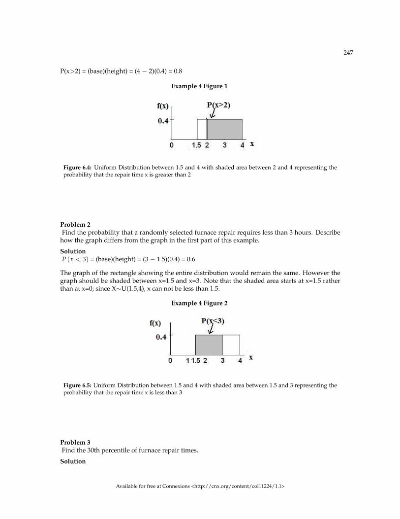
247
P(x>2) = (base)(height) = (4 − 2)(0.4) = 0.8
Example 4 Figure 1
Figure 6.4: Uniform Distribution between 1.5 and 4 with shaded area between 2 and 4 representing theprobability that the repair time x is greater than 2
Problem 2Find the probability that a randomly selected furnace repair requires less than 3 hours. Describe
how the graph differs from the graph in the first part of this example.
SolutionP (x < 3) = (base)(height) = (3 − 1.5)(0.4) = 0.6
The graph of the rectangle showing the entire distribution would remain the same. However thegraph should be shaded between x=1.5 and x=3. Note that the shaded area starts at x=1.5 ratherthan at x=0; since X∼U(1.5,4), x can not be less than 1.5.
Example 4 Figure 2
Figure 6.5: Uniform Distribution between 1.5 and 4 with shaded area between 1.5 and 3 representing theprobability that the repair time x is less than 3
Problem 3Find the 30th percentile of furnace repair times.
Solution
Available for free at Connexions <http://cnx.org/content/col11224/1.1>

248 CHAPTER 6. CONTINUOUS RANDOM VARIABLES
Example 4 Figure 3
Figure 6.6: Uniform Distribution between 1.5 and 4 with an area of 0.30 shaded to the left, representing theshortest 30% of repair times.
P (x < k) = 0.30
P (x < k) = (base) (height) = (k− 1.5) · (0.4)
0.3 = (k − 1.5) (0.4) ; Solve to find k:0.75 = k − 1.5 , obtained by dividing both sides by 0.4k = 2.25 , obtained by adding 1.5 to both sides
The 30th percentile of repair times is 2.25 hours. 30% of repair times are 2.5 hours or less.
Problem 4The longest 25% of furnace repair times take at least how long? (Find the minimum time for
the longest 25% of repairs.)
Solution
Example 4 Figure 4
Figure 6.7: Uniform Distribution between 1.5 and 4 with an area of 0.25 shaded to the right representingthe longest 25% of repair times.
P (x > k) = 0.25
P (x > k) = (base) (height) = (4− k) · (0.4)
0.25 = (4 − k)(0.4) ; Solve for k:
Available for free at Connexions <http://cnx.org/content/col11224/1.1>

249
0.625 = 4 − k , obtained by dividing both sides by 0.4−3.375 = −k , obtained by subtracting 4 from both sidesk=3.375
The longest 25% of furnace repairs take at least 3.375 hours (3.375 hours or longer).
Note: Since 25% of repair times are 3.375 hours or longer, that means that 75% of repair times are3.375 hours or less. 3.375 hours is the 75th percentile of furnace repair times.
Problem 5Find the mean and standard deviation
Solution
µ = a+b2 and σ =
√(b−a)2
12
µ = 1.5+42 = 2.75 hours and σ =
√(4−1.5)2
12 = 0.7217 hours
NOTE: See "Summary of the Uniform and Exponential Probability Distributions (Section 6.5)" fora full summary.
**Example 5 contributed by Roberta Bloom
6.4 The Exponential Distribution4
The exponential distribution is often concerned with the amount of time until some specific event occurs.For example, the amount of time (beginning now) until an earthquake occurs has an exponential distri-bution. Other examples include the length, in minutes, of long distance business telephone calls, and theamount of time, in months, a car battery lasts. It can be shown, too, that the value of the change that youhave in your pocket or purse approximately follows an exponential distribution.
Values for an exponential random variable occur in the following way. There are fewer large values andmore small values. For example, the amount of money customers spend in one trip to the supermarketfollows an exponential distribution. There are more people that spend less money and fewer people thatspend large amounts of money.
The exponential distribution is widely used in the field of reliability. Reliability deals with the amount oftime a product lasts.
Example 6.7Illustrates the exponential distribution: Let X = amount of time (in minutes) a postal clerk
spends with his/her customer. The time is known to have an exponential distribution with theaverage amount of time equal to 4 minutes.
X is a continuous random variable since time is measured. It is given that µ = 4 minutes. To doany calculations, you must know m, the decay parameter.
m = 1µ . Therefore, m = 1
4 = 0.25
4This content is available online at <http://cnx.org/content/m16816/1.15/>.
Available for free at Connexions <http://cnx.org/content/col11224/1.1>

250 CHAPTER 6. CONTINUOUS RANDOM VARIABLES
The standard deviation, σ, is the same as the mean. µ = σ
The distribution notation is X~Exp (m). Therefore, X~Exp (0.25).
The probability density function is f (x) = m · e−m·x The number e = 2.71828182846... It is a numberthat is used often in mathematics. Scientific calculators have the key "ex." If you enter 1 for x, thecalculator will display the value e.
The curve is:
f (x) = 0.25 · e− 0.25·x where x is at least 0 and m = 0.25.
For example, f (5) = 0.25 · e− 0.25·5 = 0.072
The graph is as follows:
Notice the graph is a declining curve. When x = 0,
f (x) = 0.25 · e− 0.25·0 = 0.25 · 1 = 0.25 = m
Example 6.8Problem 1Find the probability that a clerk spends four to five minutes with a randomly selected customer.
SolutionFind P (4 < x < 5).
The cumulative distribution function (CDF) gives the area to the left.
P (x < x) = 1− e−m·x
P (x < 5) = 1− e−0.25·5 = 0.7135 and P (x < 4) = 1− e−0.25·4 = 0.6321
Available for free at Connexions <http://cnx.org/content/col11224/1.1>

251
NOTE: You can do these calculations easily on a calculator.
The probability that a postal clerk spends four to five minutes with a randomly selected customeris
P (4 < x < 5) = P (x < 5)− P (x < 4) = 0.7135− 0.6321 = 0.0814
NOTE: TI-83+ and TI-84: On the home screen, enter (1-e^(-.25*5))-(1-e^(-.25*4)) or enter e^(-.25*4)-e^(-.25*5).
Problem 2Half of all customers are finished within how long? (Find the 50th percentile)
SolutionFind the 50th percentile.
P (x < k) = 0.50, k = 2.8 minutes (calculator or computer)
Half of all customers are finished within 2.8 minutes.
You can also do the calculation as follows:
P (x < k) = 0.50 and P (x < k) = 1− e−0.25·k
Therefore, 0.50 = 1− e−0.25·k and e−0.25·k = 1− 0.50 = 0.5
Take natural logs: ln(
e−0.25·k)
= ln (0.50). So, −0.25 · k = ln (0.50)
Solve for k: k = ln(.50)−0.25 = 2.8 minutes
Available for free at Connexions <http://cnx.org/content/col11224/1.1>
252 CHAPTER 6. CONTINUOUS RANDOM VARIABLES
NOTE: A formula for the percentile k is k = LN(1−AreaToTheLe f t)−m where LN is the natural log.
NOTE: TI-83+ and TI-84: On the home screen, enter LN(1-.50)/-.25. Press the (-) for the negative.
Problem 3Which is larger, the mean or the median?
SolutionIs the mean or median larger?
From part b, the median or 50th percentile is 2.8 minutes. The theoretical mean is 4 minutes. Themean is larger.
6.4.1 Optional Collaborative Classroom Activity
Have each class member count the change he/she has in his/her pocket or purse. Your instructor willrecord the amounts in dollars and cents. Construct a histogram of the data taken by the class. Use 5intervals. Draw a smooth curve through the bars. The graph should look approximately exponential. Thencalculate the mean.
Let X = the amount of money a student in your class has in his/her pocket or purse.
The distribution for X is approximately exponential with mean, µ = _______ and m = _______. The standarddeviation, σ = ________.
Draw the appropriate exponential graph. You should label the x and y axes, the decay rate, and the mean.Shade the area that represents the probability that one student has less than $.40 in his/her pocket or purse.(Shade P (x < 0.40)).
Example 6.9On the average, a certain computer part lasts 10 years. The length of time the computer part lastsis exponentially distributed.Problem 1What is the probability that a computer part lasts more than 7 years?
SolutionLet x = the amount of time (in years) a computer part lasts.
µ = 10 so m = 1µ = 1
10 = 0.1
Find P (x > 7). Draw a graph.
P (x > 7) = 1− P (x < 7).
Since P (X < x) = 1− e−mx then P (X > x) = 1− (1− e−m·x) = e−m·x
P (x > 7) = e−0.1·7 = 0.4966. The probability that a computer part lasts more than 7 years is 0.4966.
Available for free at Connexions <http://cnx.org/content/col11224/1.1>
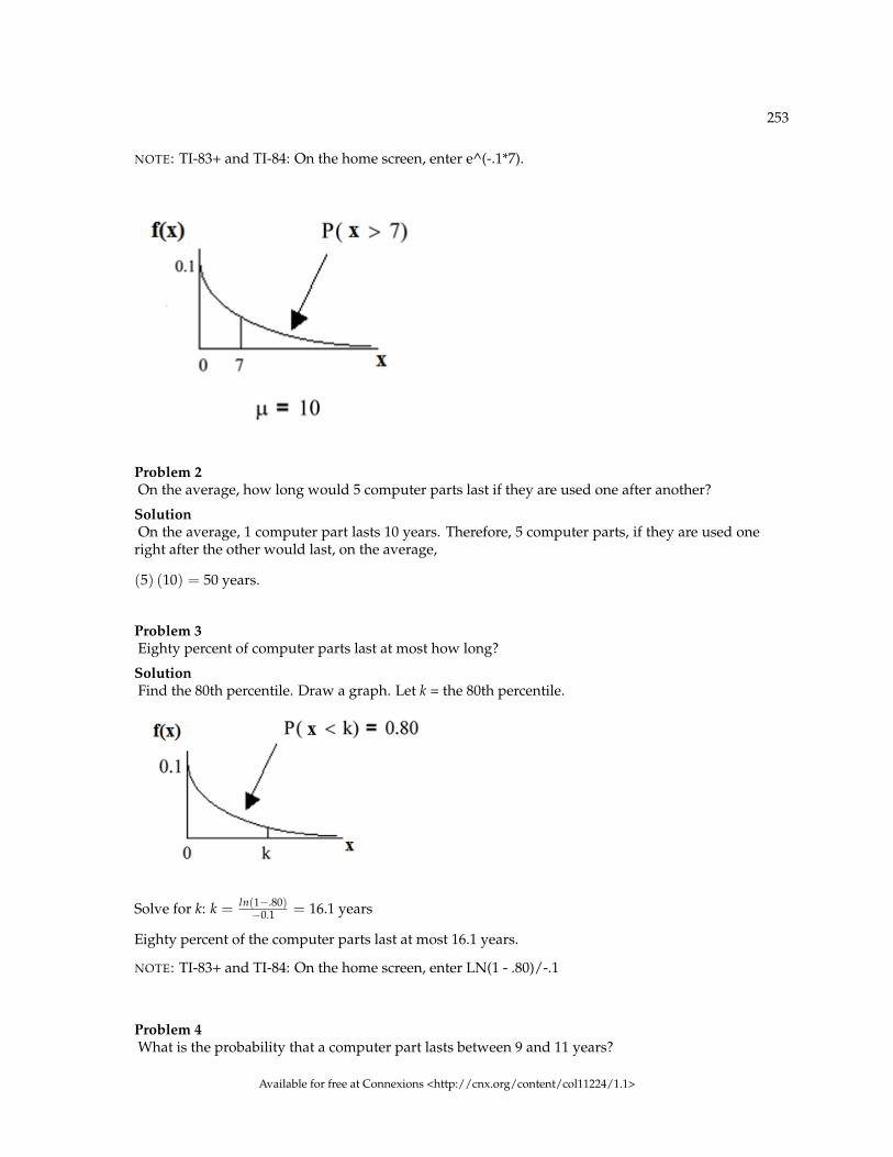
253
NOTE: TI-83+ and TI-84: On the home screen, enter e^(-.1*7).
Problem 2On the average, how long would 5 computer parts last if they are used one after another?
SolutionOn the average, 1 computer part lasts 10 years. Therefore, 5 computer parts, if they are used one
right after the other would last, on the average,
(5) (10) = 50 years.
Problem 3Eighty percent of computer parts last at most how long?
SolutionFind the 80th percentile. Draw a graph. Let k = the 80th percentile.
Solve for k: k = ln(1−.80)−0.1 = 16.1 years
Eighty percent of the computer parts last at most 16.1 years.
NOTE: TI-83+ and TI-84: On the home screen, enter LN(1 - .80)/-.1
Problem 4What is the probability that a computer part lasts between 9 and 11 years?
Available for free at Connexions <http://cnx.org/content/col11224/1.1>

254 CHAPTER 6. CONTINUOUS RANDOM VARIABLES
SolutionFind P (9 < x < 11). Draw a graph.
P (9 < x < 11) = P (x < 11) − P (x < 9) =(1− e−0.1·11) − (1− e−0.1·9) = 0.6671 − 0.5934 =
0.0737. (calculator or computer)
The probability that a computer part lasts between 9 and 11 years is 0.0737.
NOTE: TI-83+ and TI-84: On the home screen, enter e^(-.1*9) - e^(-.1*11).
Example 6.10Suppose that the length of a phone call, in minutes, is an exponential random variable with decayparameter = 1
12 . If another person arrives at a public telephone just before you, find the probabilitythat you will have to wait more than 5 minutes. Let X = the length of a phone call, in minutes.Problem (Solution on p. 273.)
What is m, µ, and σ? The probability that you must wait more than 5 minutes is _______ .
NOTE: A summary for exponential distribution is available in "Summary of The Uniform andExponential Probability Distributions (Section 6.5)".
Available for free at Connexions <http://cnx.org/content/col11224/1.1>
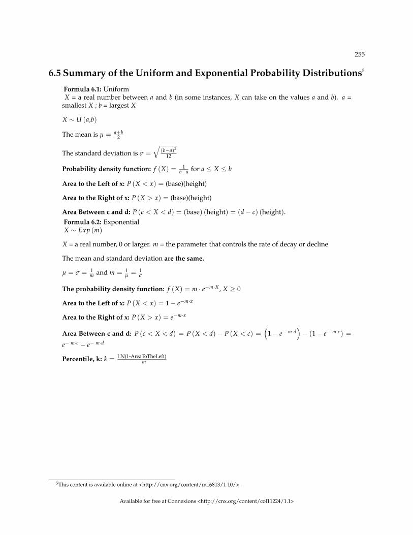
255
6.5 Summary of the Uniform and Exponential Probability Distributions5
Formula 6.1: UniformX = a real number between a and b (in some instances, X can take on the values a and b). a =
smallest X ; b = largest X
X ∼ U (a,b)
The mean is µ = a+b2
The standard deviation is σ =√
(b−a)2
12
Probability density function: f (X) = 1b−a for a ≤ X ≤ b
Area to the Left of x: P (X < x) = (base)(height)
Area to the Right of x: P (X > x) = (base)(height)
Area Between c and d: P (c < X < d) = (base) (height) = (d− c) (height).Formula 6.2: ExponentialX ∼ Exp (m)
X = a real number, 0 or larger. m = the parameter that controls the rate of decay or decline
The mean and standard deviation are the same.
µ = σ = 1m and m = 1
µ = 1σ
The probability density function: f (X) = m · e−m·X , X ≥ 0
Area to the Left of x: P (X < x) = 1− e−m·x
Area to the Right of x: P (X > x) = e−m·x
Area Between c and d: P (c < X < d) = P (X < d)− P (X < c) =(
1− e− m·d)− (1− e− m·c) =
e− m·c − e− m·d
Percentile, k: k = LN(1-AreaToTheLeft)−m
5This content is available online at <http://cnx.org/content/m16813/1.10/>.
Available for free at Connexions <http://cnx.org/content/col11224/1.1>

256 CHAPTER 6. CONTINUOUS RANDOM VARIABLES
6.6 Practice 1: Uniform Distribution6
6.6.1 Student Learning Outcomes
• The student will analyze data following a uniform distribution.
6.6.2 Given
The age of cars in the staff parking lot of a suburban college is uniformly distributed from six months (0.5years) to 9.5 years.
6.6.3 Describe the Data
Exercise 6.6.1 (Solution on p. 273.)What is being measured here?
Exercise 6.6.2 (Solution on p. 273.)In words, define the Random Variable X.
Exercise 6.6.3 (Solution on p. 273.)Are the data discrete or continuous?
Exercise 6.6.4 (Solution on p. 273.)The interval of values for x is:
Exercise 6.6.5 (Solution on p. 273.)The distribution for X is:
6.6.4 Probability Distribution
Exercise 6.6.6 (Solution on p. 273.)Write the probability density function.
Exercise 6.6.7 (Solution on p. 273.)Graph the probability distribution.
a. Sketch the graph of the probability distribution.
Figure 6.8
6This content is available online at <http://cnx.org/content/m16812/1.14/>.
Available for free at Connexions <http://cnx.org/content/col11224/1.1>
257
b. Identify the following values:
i. Lowest value for x:ii. Highest value for x:iii. Height of the rectangle:iv. Label for x-axis (words):v. Label for y-axis (words):
6.6.5 Random Probability
Exercise 6.6.8 (Solution on p. 273.)Find the probability that a randomly chosen car in the lot was less than 4 years old.
a. Sketch the graph. Shade the area of interest.
Figure 6.9
b. Find the probability. P (x < 4) =
Exercise 6.6.9 (Solution on p. 273.)Out of just the cars less than 7.5 years old, find the probability that a randomly chosen car in the
lot was less than 4 years old.
a. Sketch the graph. Shade the area of interest.
Available for free at Connexions <http://cnx.org/content/col11224/1.1>
258 CHAPTER 6. CONTINUOUS RANDOM VARIABLES
Figure 6.10
b. Find the probability. P (x < 4 | x < 7.5) =
Exercise 6.6.10: Discussion QuestionWhat has changed in the previous two problems that made the solutions different?
6.6.6 Quartiles
Exercise 6.6.11 (Solution on p. 273.)Find the average age of the cars in the lot.
Exercise 6.6.12 (Solution on p. 273.)Find the third quartile of ages of cars in the lot. This means you will have to find the value such
that 34 , or 75%, of the cars are at most (less than or equal to) that age.
a. Sketch the graph. Shade the area of interest.
Figure 6.11
b. Find the value k such that P (x < k) = 0.75.c. The third quartile is:
Available for free at Connexions <http://cnx.org/content/col11224/1.1>

259
6.7 Practice 2: Exponential Distribution7
6.7.1 Student Learning Outcomes
• The student will analyze data following the exponential distribution.
6.7.2 Given
Carbon-14 is a radioactive element with a half-life of about 5730 years. Carbon-14 is said to decay exponen-tially. The decay rate is 0.000121 . We start with 1 gram of carbon-14. We are interested in the time (years)it takes to decay carbon-14.
6.7.3 Describe the Data
Exercise 6.7.1What is being measured here?
Exercise 6.7.2 (Solution on p. 274.)Are the data discrete or continuous?
Exercise 6.7.3 (Solution on p. 274.)In words, define the Random Variable X.
Exercise 6.7.4 (Solution on p. 274.)What is the decay rate (m)?
Exercise 6.7.5 (Solution on p. 274.)The distribution for X is:
6.7.4 Probability
Exercise 6.7.6 (Solution on p. 274.)Find the amount (percent of 1 gram) of carbon-14 lasting less than 5730 years. This means, find
P (x < 5730).
a. Sketch the graph. Shade the area of interest.
Figure 6.12
7This content is available online at <http://cnx.org/content/m16811/1.11/>.
Available for free at Connexions <http://cnx.org/content/col11224/1.1>
260 CHAPTER 6. CONTINUOUS RANDOM VARIABLES
b. Find the probability. P (x < 5730) =
Exercise 6.7.7 (Solution on p. 274.)Find the percentage of carbon-14 lasting longer than 10,000 years.
a. Sketch the graph. Shade the area of interest.
Figure 6.13
b. Find the probability. P (x > 10000) =
Exercise 6.7.8 (Solution on p. 274.)Thirty percent (30%) of carbon-14 will decay within how many years?
a. Sketch the graph. Shade the area of interest.
Figure 6.14
b. Find the value k such that P (x < k) = 0.30.
Available for free at Connexions <http://cnx.org/content/col11224/1.1>
261
6.8 Homework8
For each probability and percentile problem, DRAW THE PICTURE!Exercise 6.8.1Consider the following experiment. You are one of 100 people enlisted to take part in a study to
determine the percent of nurses in America with an R.N. (registered nurse) degree. You ask nursesif they have an R.N. degree. The nurses answer “yes” or “no.” You then calculate the percentageof nurses with an R.N. degree. You give that percentage to your supervisor.
a. What part of the experiment will yield discrete data?b. What part of the experiment will yield continuous data?
Exercise 6.8.2When age is rounded to the nearest year, do the data stay continuous, or do they become discrete?Why?Exercise 6.8.3 (Solution on p. 274.)Births are approximately uniformly distributed between the 52 weeks of the year. They can be
said to follow a Uniform Distribution from 1 – 53 (spread of 52 weeks).
a. X ∼b. Graph the probability distribution.c. f (x) =d. µ =e. σ =f. Find the probability that a person is born at the exact moment week 19 starts. That is, find
P (x = 19) =g. P (2 < x < 31) =h. Find the probability that a person is born after week 40.i. P (12 < x | x < 28) =j. Find the 70th percentile.k. Find the minimum for the upper quarter.
Exercise 6.8.4A random number generator picks a number from 1 to 9 in a uniform manner.
a. X~b. Graph the probability distribution.c. f (x) =d. µ =e. σ =f. P (3.5 < x < 7.25) =g. P (x > 5.67) =h. P (x > 5 | x > 3) =i. Find the 90th percentile.
Exercise 6.8.5 (Solution on p. 274.)The time (in minutes) until the next bus departs a major bus depot follows a distribution withf (x) = 1
20 where x goes from 25 to 45 minutes.
a. Define the random variable. X =8This content is available online at <http://cnx.org/content/m16807/1.14/>.
Available for free at Connexions <http://cnx.org/content/col11224/1.1>
262 CHAPTER 6. CONTINUOUS RANDOM VARIABLES
b. X~c. Graph the probability distribution.d. The distribution is ______________ (name of distribution). It is _____________ (discrete or con-
tinuous).e. µ =f. σ =g. Find the probability that the time is at most 30 minutes. Sketch and label a graph of the distri-
bution. Shade the area of interest. Write the answer in a probability statement.h. Find the probability that the time is between 30 and 40 minutes. Sketch and label a graph of
the distribution. Shade the area of interest. Write the answer in a probability statement.i. P (25 < x < 55) = _________. State this in a probability statement (similar to g and h ), draw
the picture, and find the probability.j. Find the 90th percentile. This means that 90% of the time, the time is less than _____ minutes.k. Find the 75th percentile. In a complete sentence, state what this means. (See j.)l. Find the probability that the time is more than 40 minutes given (or knowing that) it is at least
30 minutes.
Exercise 6.8.6According to a study by Dr. John McDougall of his live-in weight loss program at St. Helena
Hospital, the people who follow his program lose between 6 and 15 pounds a month until theyapproach trim body weight. Let’s suppose that the weight loss is uniformly distributed. We areinterested in the weight loss of a randomly selected individual following the program for onemonth. (Source: The McDougall Program for Maximum Weight Loss by John A. McDougall,M.D.)
a. Define the random variable. X =b. X~c. Graph the probability distribution.d. f (x) =e. µ =f. σ =g. Find the probability that the individual lost more than 10 pounds in a month.h. Suppose it is known that the individual lost more than 10 pounds in a month. Find the proba-
bility that he lost less than 12 pounds in the month.i. P (7 < x < 13 | x > 9) = __________. State this in a probability question (similar to g and h),
draw the picture, and find the probability.
Exercise 6.8.7 (Solution on p. 274.)A subway train on the Red Line arrives every 8 minutes during rush hour. We are interested in thelength of time a commuter must wait for a train to arrive. The time follows a uniform distribution.
a. Define the random variable. X =b. X~c. Graph the probability distribution.d. f (x) =e. µ =f. σ =g. Find the probability that the commuter waits less than one minute.h. Find the probability that the commuter waits between three and four minutes.i. 60% of commuters wait more than how long for the train? State this in a probability question
(similar to g and h), draw the picture, and find the probability.
Available for free at Connexions <http://cnx.org/content/col11224/1.1>
263
Exercise 6.8.8The age of a first grader on September 1 at Garden Elementary School is uniformly distributed
from 5.8 to 6.8 years. We randomly select one first grader from the class.
a. Define the random variable. X =b. X~c. Graph the probability distribution.d. f (x) =e. µ =f. σ =g. Find the probability that she is over 6.5 years.h. Find the probability that she is between 4 and 6 years.i. Find the 70th percentile for the age of first graders on September 1 at Garden Elementary School.
Exercise 6.8.9 (Solution on p. 275.)Let X~Exp(0.1)
a. decay rate=b. µ =c. Graph the probability distribution function.d. On the above graph, shade the area corresponding to P (x < 6) and find the probability.e. Sketch a new graph, shade the area corresponding to P (3 < x < 6) and find the probability.f. Sketch a new graph, shade the area corresponding to P (x > 7) and find the probability.g. Sketch a new graph, shade the area corresponding to the 40th percentile and find the value.h. Find the average value of x.
Exercise 6.8.10Suppose that the length of long distance phone calls, measured in minutes, is known to have an
exponential distribution with the average length of a call equal to 8 minutes.
a. Define the random variable. X =b. Is X continuous or discrete?c. X~d. µ =e. σ =f. Draw a graph of the probability distribution. Label the axes.g. Find the probability that a phone call lasts less than 9 minutes.h. Find the probability that a phone call lasts more than 9 minutes.i. Find the probability that a phone call lasts between 7 and 9 minutes.j. If 25 phone calls are made one after another, on average, what would you expect the total to be?
Why?
Exercise 6.8.11 (Solution on p. 275.)Suppose that the useful life of a particular car battery, measured in months, decays with parameter0.025. We are interested in the life of the battery.
a. Define the random variable. X =b. Is X continuous or discrete?c. X~d. On average, how long would you expect 1 car battery to last?e. On average, how long would you expect 9 car batteries to last, if they are used one after another?f. Find the probability that a car battery lasts more than 36 months.
Available for free at Connexions <http://cnx.org/content/col11224/1.1>

264 CHAPTER 6. CONTINUOUS RANDOM VARIABLES
g. 70% of the batteries last at least how long?
Exercise 6.8.12The percent of persons (ages 5 and older) in each state who speak a language at home other than
English is approximately exponentially distributed with a mean of 9.848 . Suppose we randomlypick a state. (Source: Bureau of the Census, U.S. Dept. of Commerce)
a. Define the random variable. X =b. Is X continuous or discrete?c. X~d. µ =e. σ =f. Draw a graph of the probability distribution. Label the axes.g. Find the probability that the percent is less than 12.h. Find the probability that the percent is between 8 and 14.i. The percent of all individuals living in the United States who speak a language at home other
than English is 13.8 .
i. Why is this number different from 9.848%?ii. What would make this number higher than 9.848%?
Exercise 6.8.13 (Solution on p. 275.)The time (in years) after reaching age 60 that it takes an individual to retire is approximately
exponentially distributed with a mean of about 5 years. Suppose we randomly pick one retiredindividual. We are interested in the time after age 60 to retirement.
a. Define the random variable. X =b. Is X continuous or discrete?c. X~d. µ =e. σ =f. Draw a graph of the probability distribution. Label the axes.g. Find the probability that the person retired after age 70.h. Do more people retire before age 65 or after age 65?i. In a room of 1000 people over age 80, how many do you expect will NOT have retired yet?
Exercise 6.8.14The cost of all maintenance for a car during its first year is approximately exponentially dis-
tributed with a mean of $150.
a. Define the random variable. X =b. X~c. µ =d. σ =e. Draw a graph of the probability distribution. Label the axes.f. Find the probability that a car required over $300 for maintenance during its first year.
Available for free at Connexions <http://cnx.org/content/col11224/1.1>

265
6.8.1 Try these multiple choice problems
The next three questions refer to the following information. The average lifetime of a certain new cellphone is 3 years. The manufacturer will replace any cell phone failing within 2 years of the date of purchase.The lifetime of these cell phones is known to follow an exponential distribution.
Exercise 6.8.15 (Solution on p. 275.)The decay rate is
A. 0.3333B. 0.5000C. 2.0000D. 3.0000
Exercise 6.8.16 (Solution on p. 275.)What is the probability that a phone will fail within 2 years of the date of purchase?
A. 0.8647B. 0.4866C. 0.2212d. 0.9997
Exercise 6.8.17 (Solution on p. 275.)What is the median lifetime of these phones (in years)?
A. 0.1941B. 1.3863C. 2.0794D. 5.5452
The next three questions refer to the following information. The Sky Train from the terminal to the rentalcar and long term parking center is supposed to arrive every 8 minutes. The waiting times for the train areknown to follow a uniform distribution.
Exercise 6.8.18 (Solution on p. 275.)What is the average waiting time (in minutes)?
A. 0.0000B. 2.0000C. 3.0000D. 4.0000
Exercise 6.8.19 (Solution on p. 275.)Find the 30th percentile for the waiting times (in minutes).
A. 2.0000B. 2.4000C. 2.750D. 3.000
Exercise 6.8.20 (Solution on p. 275.)The probability of waiting more than 7 minutes given a person has waited more than 4 minutes
is?
A. 0.1250
Available for free at Connexions <http://cnx.org/content/col11224/1.1>

266 CHAPTER 6. CONTINUOUS RANDOM VARIABLES
B. 0.2500C. 0.5000D. 0.7500
Available for free at Connexions <http://cnx.org/content/col11224/1.1>

267
6.9 Review9
Exercise 6.9.1 – Exercise 6.9.7 refer to the following study: A recent study of mothers of junior high schoolchildren in Santa Clara County reported that 76% of the mothers are employed in paid positions. Of thosemothers who are employed, 64% work full-time (over 35 hours per week), and 36% work part-time. How-ever, out of all of the mothers in the population, 49% work full-time. The population under study is madeup of mothers of junior high school children in Santa Clara County.
Let E =employed, Let F =full-time employmentExercise 6.9.1 (Solution on p. 275.)
a. Find the percent of all mothers in the population that NOT employed.b. Find the percent of mothers in the population that are employed part-time.
Exercise 6.9.2 (Solution on p. 275.)The type of employment is considered to be what type of data?
Exercise 6.9.3 (Solution on p. 275.)Find the probability that a randomly selected mother works part-time given that she is employed.Exercise 6.9.4 (Solution on p. 276.)Find the probability that a randomly selected person from the population will be employed OR
work full-time.Exercise 6.9.5 (Solution on p. 276.)Based upon the above information, are being employed AND working part-time:
a. mutually exclusive events? Why or why not?b. independent events? Why or why not?
Exercise 6.9.6 - Exercise 6.9.7 refer to the following: We randomly pick 10 mothers from the above popu-lation. We are interested in the number of the mothers that are employed. Let X =number of mothers thatare employed.
Exercise 6.9.6 (Solution on p. 276.)State the distribution for X.
Exercise 6.9.7 (Solution on p. 276.)Find the probability that at least 6 are employed.
Exercise 6.9.8 (Solution on p. 276.)We expect the Statistics Discussion Board to have, on average, 14 questions posted to it per week.We are interested in the number of questions posted to it per day.
a. Define X.b. What are the values that the random variable may take on?c. State the distribution for X.d. Find the probability that from 10 to 14 (inclusive) questions are posted to the Listserv on a
randomly picked day.
Exercise 6.9.9 (Solution on p. 276.)A person invests $1000 in stock of a company that hopes to go public in 1 year.
• The probability that the person will lose all his money after 1 year (i.e. his stock will beworthless) is 35%.
9This content is available online at <http://cnx.org/content/m16810/1.11/>.
Available for free at Connexions <http://cnx.org/content/col11224/1.1>

268 CHAPTER 6. CONTINUOUS RANDOM VARIABLES
• The probability that the person’s stock will still have a value of $1000 after 1 year (i.e. noprofit and no loss) is 60%.
• The probability that the person’s stock will increase in value by $10,000 after 1 year (i.e. willbe worth $11,000) is 5%.
Find the expected PROFIT after 1 year.Exercise 6.9.10 (Solution on p. 276.)Rachel’s piano cost $3000. The average cost for a piano is $4000 with a standard deviation of
$2500. Becca’s guitar cost $550. The average cost for a guitar is $500 with a standard deviationof $200. Matt’s drums cost $600. The average cost for drums is $700 with a standard deviation of$100. Whose cost was lowest when compared to his or her own instrument? Justify your answer.Exercise 6.9.11 (Solution on p. 276.)
For each statement below, explain why each is either true or false.
a. 25% of the data are at most 5.b. There is the same amount of data from 4 – 5 as there is from 5 – 7.c. There are no data values of 3.d. 50% of the data are 4.
Exercise 6.9.12 – Exercise 6.9.13 refer to the following: 64 faculty members were asked the number ofcars they owned (including spouse and children’s cars). The results are given in the following graph:
Exercise 6.9.12 (Solution on p. 276.)Find the approximate number of responses that were “3.”
Exercise 6.9.13 (Solution on p. 276.)Find the first, second and third quartiles. Use them to construct a box plot of the data.
Exercise 6.9.14 – Exercise 6.9.15 refer to the following study done of the Girls soccer team “Snow Leop-ards”:
Hair Style Hair Color
blond brown black
ponytail 3 2 5
plain 2 2 1
Available for free at Connexions <http://cnx.org/content/col11224/1.1>

269
Table 6.2
Suppose that one girl from the Snow Leopards is randomly selected.Exercise 6.9.14 (Solution on p. 276.)Find the probability that the girl has black hair GIVEN that she wears a ponytail.
Exercise 6.9.15 (Solution on p. 276.)Find the probability that the girl wears her hair plain OR has brown hair.
Exercise 6.9.16 (Solution on p. 276.)Find the probability that the girl has blond hair AND that she wears her hair plain.
Available for free at Connexions <http://cnx.org/content/col11224/1.1>

270 CHAPTER 6. CONTINUOUS RANDOM VARIABLES
6.10 Lab: Continuous Distribution10
Class Time:
Names:
6.10.1 Student Learning Outcomes:
• The student will compare and contrast empirical data from a random number generator with theUniform Distribution.
6.10.2 Collect the Data
Use a random number generator to generate 50 values between 0 and 1 (inclusive). List them below. Roundthe numbers to 4 decimal places or set the calculator MODE to 4 places.
1. Complete the table:
__________ __________ __________ __________ __________
__________ __________ __________ __________ __________
__________ __________ __________ __________ __________
__________ __________ __________ __________ __________
__________ __________ __________ __________ __________
__________ __________ __________ __________ __________
__________ __________ __________ __________ __________
__________ __________ __________ __________ __________
__________ __________ __________ __________ __________
__________ __________ __________ __________ __________
Table 6.3
2. Calculate the following:
a. x =b. s =c. 1st quartile =d. 3rd quartile =e. Median =
6.10.3 Organize the Data
1. Construct a histogram of the empirical data. Make 8 bars.
10This content is available online at <http://cnx.org/content/m16803/1.13/>.
Available for free at Connexions <http://cnx.org/content/col11224/1.1>

271
Figure 6.15
2. Construct a histogram of the empirical data. Make 5 bars.
Figure 6.16
Available for free at Connexions <http://cnx.org/content/col11224/1.1>

272 CHAPTER 6. CONTINUOUS RANDOM VARIABLES
6.10.4 Describe the Data
1. Describe the shape of each graph. Use 2 – 3 complete sentences. (Keep it simple. Does the graph gostraight across, does it have a V shape, does it have a hump in the middle or at either end, etc.? Oneway to help you determine a shape, is to roughly draw a smooth curve through the top of the bars.)
2. Describe how changing the number of bars might change the shape.
6.10.5 Theoretical Distribution
1. In words, X =2. The theoretical distribution of X is X ∼ U (0, 1). Use it for this part.3. In theory, based upon the distribution X ∼ U (0, 1), complete the following.
a. µ =b. σ =c. 1st quartile =d. 3rd quartile =e. median = __________
4. Are the empirical values (the data) in the section titled "Collect the Data" close to the correspondingtheoretical values above? Why or why not?
6.10.6 Plot the Data
1. Construct a box plot of the data. Be sure to use a ruler to scale accurately and draw straight edges.2. Do you notice any potential outliers? If so, which values are they? Either way, numerically justify your
answer. (Recall that any DATA are less than Q1 – 1.5*IQR or more than Q3 + 1.5*IQR are potentialoutliers. IQR means interquartile range.)
6.10.7 Compare the Data
1. For each part below, use a complete sentence to comment on how the value obtained from the datacompares to the theoretical value you expected from the distribution in the section titled "TheoreticalDistribution."
a. minimum value:b. 1st quartile:c. median:d. third quartile:e. maximum value:f. width of IQR:g. overall shape:
2. Based on your comments in the section titled "Collect the Data", how does the box plot fit or not fitwhat you would expect of the distribution in the section titled "Theoretical Distribution?"
6.10.8 Discussion Question
1. Suppose that the number of values generated was 500, not 50. How would that affect what you wouldexpect the empirical data to be and the shape of its graph to look like?
Available for free at Connexions <http://cnx.org/content/col11224/1.1>

273
Solutions to Exercises in Chapter 6
Solution to Example 6.5, Problem 1 (p. 245)0.5714
Solution to Example 6.5, Problem 2 (p. 245)45
Solution to Example 6.10, Problem (p. 254)
• m = 112
• µ = 12• σ = 12
P (x > 5) = 0.6592
Solutions to Practice 1: Uniform Distribution
Solution to Exercise 6.6.1 (p. 256)The age of cars in the staff parking lot
Solution to Exercise 6.6.2 (p. 256)X = The age (in years) of cars in the staff parking lot
Solution to Exercise 6.6.3 (p. 256)Continuous
Solution to Exercise 6.6.4 (p. 256)0.5 - 9.5
Solution to Exercise 6.6.5 (p. 256)X ∼ U (0.5, 9.5)
Solution to Exercise 6.6.6 (p. 256)f (x) = 1
9Solution to Exercise 6.6.7 (p. 256)
b.i. 0.5b.ii. 9.5b.iii. 1
9b.iv. Age of Carsb.v. f (x)
Solution to Exercise 6.6.8 (p. 257)
b.: 3.59
Solution to Exercise 6.6.9 (p. 257)
b: 3.57
Solution to Exercise 6.6.11 (p. 258)µ = 5
Solution to Exercise 6.6.12 (p. 258)
b. k = 7.25
Available for free at Connexions <http://cnx.org/content/col11224/1.1>

274 CHAPTER 6. CONTINUOUS RANDOM VARIABLES
Solutions to Practice 2: Exponential Distribution
Solution to Exercise 6.7.2 (p. 259)Continuous
Solution to Exercise 6.7.3 (p. 259)X = Time (years) to decay carbon-14
Solution to Exercise 6.7.4 (p. 259)m = 0.000121
Solution to Exercise 6.7.5 (p. 259)X ∼ Exp(0.000121)
Solution to Exercise 6.7.6 (p. 259)
b. P (x < 5730) = 0.5001
Solution to Exercise 6.7.7 (p. 260)
b. P (x > 10000) = 0.2982
Solution to Exercise 6.7.8 (p. 260)
b. k = 2947.73
Solutions to Homework
Solution to Exercise 6.8.3 (p. 261)
a. X~U (1, 53)c. f (x) = 1
52 where 1 ≤ x ≤ 53d. 27e. 15.01f. 0g. 29
52h. 13
52i. 16
27j. 37.4k. 40
Solution to Exercise 6.8.5 (p. 261)
b. X~U (25, 45)d. uniform; continuouse. 35 minutesf. 5.8 minutesg. 0.25h. 0.5i. 1j. 43 minutesk. 40 minutesl. 0.3333
Solution to Exercise 6.8.7 (p. 262)
b. X~U (0, 8)d. f (x) = 1
8 where 0 ≤ x ≤ 8e. 4
Available for free at Connexions <http://cnx.org/content/col11224/1.1>

275
f. 2.31g. 1
8h. 1
8i. 3.2
Solution to Exercise 6.8.9 (p. 263)
a. 0.1b. 10d. 0.4512e. 0.1920f. 0.4966g. 5.11h. 10
Solution to Exercise 6.8.11 (p. 263)
c. X~Exp (0.025)d. 40 monthse. 360 monthsf. 0.4066g. 14.27
Solution to Exercise 6.8.13 (p. 264)
c. X~Exp(
15
)d. 5e. 5g. 0.1353h. Beforei. 18.3
Solution to Exercise 6.8.15 (p. 265)A
Solution to Exercise 6.8.16 (p. 265)B
Solution to Exercise 6.8.17 (p. 265)C
Solution to Exercise 6.8.18 (p. 265)D
Solution to Exercise 6.8.19 (p. 265)B
Solution to Exercise 6.8.20 (p. 265)B
Solutions to Review
Solution to Exercise 6.9.1 (p. 267)
a. 24%b. 27%
Solution to Exercise 6.9.2 (p. 267)Qualitative
Available for free at Connexions <http://cnx.org/content/col11224/1.1>
276 CHAPTER 6. CONTINUOUS RANDOM VARIABLES
Solution to Exercise 6.9.3 (p. 267)0.36
Solution to Exercise 6.9.4 (p. 267)0.7636
Solution to Exercise 6.9.5 (p. 267)
a. No,b. No,
Solution to Exercise 6.9.6 (p. 267)B (10, 0.76)
Solution to Exercise 6.9.7 (p. 267)0.9330
Solution to Exercise 6.9.8 (p. 267)
a. X = the number of questions posted to the Statistics Listserv per dayb. x = 0, 1, 2, ...c. X~P (2)d. 0
Solution to Exercise 6.9.9 (p. 267)$150
Solution to Exercise 6.9.10 (p. 268)Matt
Solution to Exercise 6.9.11 (p. 268)
a. Falseb. Truec. Falsed. False
Solution to Exercise 6.9.12 (p. 268)16
Solution to Exercise 6.9.13 (p. 268)2, 2, 3
Solution to Exercise 6.9.14 (p. 269)5
10 = 0.5Solution to Exercise 6.9.15 (p. 269)
715
Solution to Exercise 6.9.16 (p. 269)2
15
Available for free at Connexions <http://cnx.org/content/col11224/1.1>

Chapter 7
The Normal Distribution
7.1 The Normal Distribution1
7.1.1 Student Learning Outcomes
By the end of this chapter, the student should be able to:
• Recognize the normal probability distribution and apply it appropriately.• Recognize the standard normal probability distribution and apply it appropriately.• Compare normal probabilities by converting to the standard normal distribution.
7.1.2 Introduction
The normal, a continuous distribution, is the most important of all the distributions. It is widely usedand even more widely abused. Its graph is bell-shaped. You see the bell curve in almost all disciplines.Some of these include psychology, business, economics, the sciences, nursing, and, of course, mathematics.Some of your instructors may use the normal distribution to help determine your grade. Most IQ scores arenormally distributed. Often real estate prices fit a normal distribution. The normal distribution is extremelyimportant but it cannot be applied to everything in the real world.
In this chapter, you will study the normal distribution, the standard normal, and applications associatedwith them.
7.1.3 Optional Collaborative Classroom Activity
Your instructor will record the heights of both men and women in your class, separately. Draw histogramsof your data. Then draw a smooth curve through each histogram. Is each curve somewhat bell-shaped? Doyou think that if you had recorded 200 data values for men and 200 for women that the curves would lookbell-shaped? Calculate the mean for each data set. Write the means on the x-axis of the appropriate graphbelow the peak. Shade the approximate area that represents the probability that one randomly chosenmale is taller than 72 inches. Shade the approximate area that represents the probability that one randomlychosen female is shorter than 60 inches. If the total area under each curve is one, does either probabilityappear to be more than 0.5?
1This content is available online at <http://cnx.org/content/m16979/1.12/>.
Available for free at Connexions <http://cnx.org/content/col11224/1.1>
277

278 CHAPTER 7. THE NORMAL DISTRIBUTION
The normal distribution has two parameters (two numerical descriptive measures), the mean (µ) and thestandard deviation (σ). If X is a quantity to be measured that has a normal distribution with mean (µ) andthe standard deviation (σ), we designate this by writing
NORMAL:X∼N (µ, σ)
The probability density function is a rather complicated function. Do not memorize it. It is not necessary.
f (x) = 1σ·√
2·π · e− 1
2 ·(x−µ
σ )2
The cumulative distribution function is P (X < x) . It is calculated either by a calculator or a computer orit is looked up in a table. Technology has made the tables basically obsolete. For that reason, as well asthe fact that there are various table formats, we are not including table instructions in this chapter. See theNOTE in this chapter in Calculation of Probabilities.
The curve is symmetrical about a vertical line drawn through the mean, µ. In theory, the mean is the sameas the median since the graph is symmetric about µ. As the notation indicates, the normal distributiondepends only on the mean and the standard deviation. Since the area under the curve must equal one, achange in the standard deviation, σ, causes a change in the shape of the curve; the curve becomes fatter orskinnier depending on σ. A change in µ causes the graph to shift to the left or right. This means there are aninfinite number of normal probability distributions. One of special interest is called the standard normaldistribution.
7.2 The Standard Normal Distribution2
The standard normal distribution is a normal distribution of standardized values called z-scores. A z-score is measured in units of the standard deviation. For example, if the mean of a normal distribution is5 and the standard deviation is 2, the value 11 is 3 standard deviations above (or to the right of) the mean.The calculation is:
x = µ + (z) σ = 5 + (3) (2) = 11 (7.1)
The z-score is 3.
The mean for the standard normal distribution is 0 and the standard deviation is 1. The transformation
z = x−µσ produces the distribution Z∼ N (0, 1) . The value x comes from a normal distribution with
mean µ and standard deviation σ.
2This content is available online at <http://cnx.org/content/m16986/1.7/>.
Available for free at Connexions <http://cnx.org/content/col11224/1.1>
279
7.3 Z-scores3
If X is a normally distributed random variable and X∼N (µ, σ), then the z-score is:
z =x− µ
σ(7.2)
The z-score tells you how many standard deviations that the value x is above (to the right of) or below(to the left of) the mean, µ. Values of x that are larger than the mean have positive z-scores and values of xthat are smaller than the mean have negative z-scores. If x equals the mean, then x has a z-score of 0.
Example 7.1Suppose X ∼ N (5, 6). This says that X is a normally distributed random variable with meanµ = 5 and standard deviation σ = 6. Suppose x = 17. Then:
z =x− µ
σ=
17− 56
= 2 (7.3)
This means that x = 17 is 2 standard deviations (2σ) above or to the right of the mean µ = 5.The standard deviation is σ = 6.
Notice that:
5 + 2 · 6 = 17 (The pattern is µ + zσ = x.) (7.4)
Now suppose x = 1. Then:
z =x− µ
σ=
1− 56
= −0.67 (rounded to two decimal places) (7.5)
This means that x = 1 is 0.67 standard deviations (− 0.67σ) below or to the left of the meanµ = 5. Notice that:
5 + (−0.67) (6) is approximately equal to 1 (This has the pattern µ + (−0.67) σ = 1 )
Summarizing, when z is positive, x is above or to the right of µ and when z is negative, x is to theleft of or below µ.
Example 7.2Some doctors believe that a person can lose 5 pounds, on the average, in a month by reducinghis/her fat intake and by exercising consistently. Suppose weight loss has a normal distribution.Let X = the amount of weight lost (in pounds) by a person in a month. Use a standard deviationof 2 pounds. X∼N (5, 2). Fill in the blanks.Problem 1 (Solution on p. 301.)
Suppose a person lost 10 pounds in a month. The z-score when x = 10 pounds is z = 2.5(verify). This z-score tells you that x = 10 is ________ standard deviations to the ________ (rightor left) of the mean _____ (What is the mean?).
Problem 2 (Solution on p. 301.)Suppose a person gained 3 pounds (a negative weight loss). Then z = __________. This z-score
tells you that x = −3 is ________ standard deviations to the __________ (right or left) of the mean.Suppose the random variables X and Y have the following normal distributions: X ∼N (5, 6) andY ∼ N (2, 1). If x = 17, then z = 2. (This was previously shown.) If y = 4, what is z?
z =y− µ
σ=
4− 21
= 2 where µ=2 and σ=1. (7.6)
3This content is available online at <http://cnx.org/content/m16991/1.10/>.
Available for free at Connexions <http://cnx.org/content/col11224/1.1>

280 CHAPTER 7. THE NORMAL DISTRIBUTION
The z-score for y = 4 is z = 2. This means that 4 is z = 2 standard deviations to the right ofthe mean. Therefore, x = 17 and y = 4 are both 2 (of their) standard deviations to the right oftheir respective means.
The z-score allows us to compare data that are scaled differently. To understand the concept,suppose X ∼N (5, 6) represents weight gains for one group of people who are trying to gainweight in a 6 week period and Y ∼N (2, 1) measures the same weight gain for a second groupof people. A negative weight gain would be a weight loss. Since x = 17 and y = 4 are each 2standard deviations to the right of their means, they represent the same weight gain relative totheir means.
The Empirical RuleIf X is a random variable and has a normal distribution with mean µ and standard deviation σ then theEmpirical Rule says (See the figure below)
• About 68.27% of the x values lie between -1σ and +1σ of the mean µ (within 1 standard deviation ofthe mean).
• About 95.45% of the x values lie between -2σ and +2σ of the mean µ (within 2 standard deviations ofthe mean).
• About 99.73% of the x values lie between -3σ and +3σ of the mean µ (within 3 standard deviations ofthe mean). Notice that almost all the x values lie within 3 standard deviations of the mean.
• The z-scores for +1σ and –1σ are +1 and -1, respectively.• The z-scores for +2σ and –2σ are +2 and -2, respectively.• The z-scores for +3σ and –3σ are +3 and -3 respectively.
The Empirical Rule is also known as the 68-95-99.7 Rule.
Example 7.3Suppose X has a normal distribution with mean 50 and standard deviation 6.
• About 68.27% of the x values lie between -1σ = (-1)(6) = -6 and 1σ = (1)(6) = 6 of the mean 50.The values 50 - 6 = 44 and 50 + 6 = 56 are within 1 standard deviation of the mean 50. Thez-scores are -1 and +1 for 44 and 56, respectively.
• About 95.45% of the x values lie between -2σ = (-2)(6) = -12 and 2σ = (2)(6) = 12 of the mean50. The values 50 - 12 = 38 and 50 + 12 = 62 are within 2 standard deviations of the mean 50.The z-scores are -2 and 2 for 38 and 62, respectively.
• About 99.73% of the x values lie between -3σ = (-3)(6) = -18 and 3σ = (3)(6) = 18 of the mean50. The values 50 - 18 = 32 and 50 + 18 = 68 are within 3 standard deviations of the mean 50.The z-scores are -3 and +3 for 32 and 68, respectively.
Available for free at Connexions <http://cnx.org/content/col11224/1.1>

281
7.4 Areas to the Left and Right of x4
The arrow in the graph below points to the area to the left of x. This area is represented by the probabilityP (X < x). Normal tables, computers, and calculators provide or calculate the probability P (X < x).
The area to the right is then P (X > x) = 1− P (X < x).
Remember, P (X < x) = Area to the left of the vertical line through x.
P (X > x) = 1− P (X < x) =. Area to the right of the vertical line through x
P (X < x) is the same as P (X ≤ x) and P (X > x) is the same as P (X ≥ x) for continuous distributions.
7.5 Calculations of Probabilities5
Probabilities are calculated by using technology. There are instructions in the chapter for the TI-83+ andTI-84 calculators.
NOTE: In the Table of Contents for Collaborative Statistics, entry 15. Tables has a link to a tableof normal probabilities. Use the probability tables if so desired, instead of a calculator. The tablesinclude instructions for how to use then.
Example 7.4If the area to the left is 0.0228, then the area to the right is 1− 0.0228 = 0.9772.
Example 7.5The final exam scores in a statistics class were normally distributed with a mean of 63 and a
standard deviation of 5.Problem 1Find the probability that a randomly selected student scored more than 65 on the exam.
SolutionLet X = a score on the final exam. X∼N (63, 5), where µ = 63 and σ = 5
Draw a graph.
Then, find P (x > 65).
P (x > 65) = 0.3446 (calculator or computer)
4This content is available online at <http://cnx.org/content/m16976/1.5/>.5This content is available online at <http://cnx.org/content/m16977/1.12/>.
Available for free at Connexions <http://cnx.org/content/col11224/1.1>

282 CHAPTER 7. THE NORMAL DISTRIBUTION
The probability that one student scores more than 65 is 0.3446.
Using the TI-83+ or the TI-84 calculators, the calculation is as follows. Go into 2nd DISTR.
After pressing 2nd DISTR, press 2:normalcdf.
The syntax for the instructions are shown below.
normalcdf(lower value, upper value, mean, standard deviation) For this problem: normal-cdf(65,1E99,63,5) = 0.3446. You get 1E99 ( = 1099) by pressing 1, the EE key (a 2nd key) and then 99.Or, you can enter 10^99 instead. The number 1099 is way out in the right tail of the normal curve.We are calculating the area between 65 and 1099. In some instances, the lower number of the areamight be -1E99 ( = −1099). The number −1099 is way out in the left tail of the normal curve.
HISTORICAL NOTE: The TI probability program calculates a z-score and then the probability fromthe z-score. Before technology, the z-score was looked up in a standard normal probability table(because the math involved is too cumbersome) to find the probability. In this example, a standardnormal table with area to the left of the z-score was used. You calculate the z-score and look upthe area to the left. The probability is the area to the right.
z = 65−635 = 0.4 . Area to the left is 0.6554. P (x > 65) = P (z > 0.4) = 1− 0.6554 = 0.3446
Problem 2Find the probability that a randomly selected student scored less than 85.
SolutionDraw a graph.
Then find P (x < 85). Shade the graph. P (x < 85) = 1 (calculator or computer)
The probability that one student scores less than 85 is approximately 1 (or 100%).
The TI-instructions and answer are as follows:
normalcdf(0,85,63,5) = 1 (rounds to 1)
Problem 3Find the 90th percentile (that is, find the score k that has 90 % of the scores below k and 10% of
the scores above k).
SolutionFind the 90th percentile. For each problem or part of a problem, draw a new graph. Draw the
x-axis. Shade the area that corresponds to the 90th percentile.
Let k = the 90th percentile. k is located on the x-axis. P (x < k) is the area to the left of k. The 90thpercentile k separates the exam scores into those that are the same or lower than k and those that
Available for free at Connexions <http://cnx.org/content/col11224/1.1>

283
are the same or higher. Ninety percent of the test scores are the same or lower than k and 10% arethe same or higher. k is often called a critical value.
k = 69.4 (calculator or computer)
The 90th percentile is 69.4. This means that 90% of the test scores fall at or below 69.4 and 10% fallat or above. For the TI-83+ or TI-84 calculators, use invNorm in 2nd DISTR. invNorm(area to theleft, mean, standard deviation) For this problem, invNorm(0.90,63,5) = 69.4
Problem 4Find the 70th percentile (that is, find the score k such that 70% of scores are below k and 30% of
the scores are above k).
SolutionFind the 70th percentile.
Draw a new graph and label it appropriately. k = 65.6
The 70th percentile is 65.6. This means that 70% of the test scores fall at or below 65.5 and 30% fallat or above.
invNorm(0.70,63,5) = 65.6
Example 7.6A computer is used for office work at home, research, communication, personal finances, educa-tion, entertainment, social networking and a myriad of other things. Suppose that the averagenumber of hours a household personal computer is used for entertainment is 2 hours per day.Assume the times for entertainment are normally distributed and the standard deviation for thetimes is half an hour.Problem 1Find the probability that a household personal computer is used between 1.8 and 2.75 hours per
day.
SolutionLet X = the amount of time (in hours) a household personal computer is used for entertainment.x∼N (2, 0.5) where µ = 2 and σ = 0.5.
Find P (1.8 < x < 2.75).
The probability for which you are looking is the area between x = 1.8 and x =2.75. P (1.8 < x < 2.75) = 0.5886
Available for free at Connexions <http://cnx.org/content/col11224/1.1>

284 CHAPTER 7. THE NORMAL DISTRIBUTION
normalcdf(1.8,2.75,2,0.5) = 0.5886
The probability that a household personal computer is used between 1.8 and 2.75 hours per dayfor entertainment is 0.5886.
Problem 2Find the maximum number of hours per day that the bottom quartile of households use a personalcomputer for entertainment.
SolutionTo find the maximum number of hours per day that the bottom quartile of households uses a
personal computer for entertainment, find the 25th percentile, k, where P (x < k) = 0.25.
invNorm(0.25,2,.5) = 1.66
The maximum number of hours per day that the bottom quartile of households uses a personalcomputer for entertainment is 1.66 hours.
Available for free at Connexions <http://cnx.org/content/col11224/1.1>

285
7.6 Summary of Formulas6
Formula 7.1: Normal Probability DistributionX∼N (µ, σ)
µ = the mean σ = the standard deviationFormula 7.2: Standard Normal Probability DistributionZ∼N (0, 1)
z = a standardized value (z-score)
mean = 0 standard deviation = 1Formula 7.3: Finding the kth PercentileTo find the kth percentile when the z-score is known: k = µ + (z) σ
Formula 7.4: z-scorez = x−µ
σ
Formula 7.5: Finding the area to the leftThe area to the left: P (X < x)Formula 7.6: Finding the area to the rightThe area to the right: P (X > x) = 1− P (X < x)
6This content is available online at <http://cnx.org/content/m16987/1.5/>.
Available for free at Connexions <http://cnx.org/content/col11224/1.1>

286 CHAPTER 7. THE NORMAL DISTRIBUTION
7.7 Practice: The Normal Distribution7
7.7.1 Student Learning Outcomes
• The student will analyze data following a normal distribution.
7.7.2 Given
The life of Sunshine CD players is normally distributed with a mean of 4.1 years and a standard deviationof 1.3 years. A CD player is guaranteed for 3 years. We are interested in the length of time a CD playerlasts.
7.7.3 Normal Distribution
Exercise 7.7.1Define the Random Variable X in words. X =
Exercise 7.7.2X∼
Exercise 7.7.3 (Solution on p. 301.)Find the probability that a CD player will break down during the guarantee period.
a. Sketch the situation. Label and scale the axes. Shade the region corresponding to the probabil-ity.
Figure 7.1
b. P (0 < x < _________) = _________ (Use zero (0) for the minimum value of x.)
Exercise 7.7.4 (Solution on p. 301.)Find the probability that a CD player will last between 2.8 and 6 years.
a. Sketch the situation. Label and scale the axes. Shade the region corresponding to the probabil-ity.
7This content is available online at <http://cnx.org/content/m16983/1.10/>.
Available for free at Connexions <http://cnx.org/content/col11224/1.1>

287
Figure 7.2
b. P (_______ < x < _______) = _________
Exercise 7.7.5 (Solution on p. 301.)Find the 70th percentile of the distribution for the time a CD player lasts.
a. Sketch the situation. Label and scale the axes. Shade the region corresponding to the lower70%.
Figure 7.3
b. P (x < k) = _________. Therefore, k = __________.
Available for free at Connexions <http://cnx.org/content/col11224/1.1>
288 CHAPTER 7. THE NORMAL DISTRIBUTION
7.8 Homework8
Exercise 7.8.1 (Solution on p. 301.)According to a study done by De Anza students, the height for Asian adult males is normally
distributed with an average of 66 inches and a standard deviation of 2.5 inches. Suppose oneAsian adult male is randomly chosen. Let X =height of the individual.
a. X∼_______(_______,_______)b. Find the probability that the person is between 65 and 69 inches. Include a sketch of the graph
and write a probability statement.c. Would you expect to meet many Asian adult males over 72 inches? Explain why or why not,
and justify your answer numerically.d. The middle 40% of heights fall between what two values? Sketch the graph and write the
probability statement.
Exercise 7.8.2IQ is normally distributed with a mean of 100 and a standard deviation of 15. Suppose one
individual is randomly chosen. Let X =IQ of an individual.
a. X∼_______(_______,_______)b. Find the probability that the person has an IQ greater than 120. Include a sketch of the graph
and write a probability statement.c. Mensa is an organization whose members have the top 2% of all IQs. Find the minimum IQ
needed to qualify for the Mensa organization. Sketch the graph and write the probabilitystatement.
d. The middle 50% of IQs fall between what two values? Sketch the graph and write the proba-bility statement.
Exercise 7.8.3 (Solution on p. 301.)The percent of fat calories that a person in America consumes each day is normally distributed
with a mean of about 36 and a standard deviation of 10. Suppose that one individual is randomlychosen. Let X =percent of fat calories.
a. X∼_______(_______,_______)b. Find the probability that the percent of fat calories a person consumes is more than 40. Graph
the situation. Shade in the area to be determined.c. Find the maximum number for the lower quarter of percent of fat calories. Sketch the graph
and write the probability statement.
Exercise 7.8.4Suppose that the distance of fly balls hit to the outfield (in baseball) is normally distributed with
a mean of 250 feet and a standard deviation of 50 feet.
a. If X = distance in feet for a fly ball, then X∼_______(_______,_______)b. If one fly ball is randomly chosen from this distribution, what is the probability that this ball
traveled fewer than 220 feet? Sketch the graph. Scale the horizontal axis X. Shade the regioncorresponding to the probability. Find the probability.
c. Find the 80th percentile of the distribution of fly balls. Sketch the graph and write the probabil-ity statement.
8This content is available online at <http://cnx.org/content/m16978/1.20/>.
Available for free at Connexions <http://cnx.org/content/col11224/1.1>
289
Exercise 7.8.5 (Solution on p. 301.)In China, 4-year-olds average 3 hours a day unsupervised. Most of the unsupervised children livein rural areas, considered safe. Suppose that the standard deviation is 1.5 hours and the amountof time spent alone is normally distributed. We randomly survey one Chinese 4-year-old living ina rural area. We are interested in the amount of time the child spends alone per day. (Source: SanJose Mercury News)
a. In words, define the random variable X. X =b. X∼c. Find the probability that the child spends less than 1 hour per day unsupervised. Sketch the
graph and write the probability statement.d. What percent of the children spend over 10 hours per day unsupervised?e. 70% of the children spend at least how long per day unsupervised?
Exercise 7.8.6In the 1992 presidential election, Alaska’s 40 election districts averaged 1956.8 votes per district
for President Clinton. The standard deviation was 572.3. (There are only 40 election districts inAlaska.) The distribution of the votes per district for President Clinton was bell-shaped. Let X =number of votes for President Clinton for an election district. (Source: The World Almanac andBook of Facts)
a. State the approximate distribution of X. X∼b. Is 1956.8 a population mean or a sample mean? How do you know?c. Find the probability that a randomly selected district had fewer than 1600 votes for President
Clinton. Sketch the graph and write the probability statement.d. Find the probability that a randomly selected district had between 1800 and 2000 votes for
President Clinton.e. Find the third quartile for votes for President Clinton.
Exercise 7.8.7 (Solution on p. 301.)Suppose that the duration of a particular type of criminal trial is known to be normally distributedwith a mean of 21 days and a standard deviation of 7 days.
a. In words, define the random variable X. X =b. X∼c. If one of the trials is randomly chosen, find the probability that it lasted at least 24 days. Sketch
the graph and write the probability statement.d. 60% of all of these types of trials are completed within how many days?
Exercise 7.8.8Terri Vogel, an amateur motorcycle racer, averages 129.71 seconds per 2.5 mile lap (in a 7 lap
race) with a standard deviation of 2.28 seconds . The distribution of her race times is normallydistributed. We are interested in one of her randomly selected laps. (Source: log book of TerriVogel)
a. In words, define the random variable X. X =b. X∼c. Find the percent of her laps that are completed in less than 130 seconds.d. The fastest 3% of her laps are under _______ .e. The middle 80% of her laps are from _______ seconds to _______ seconds.
Available for free at Connexions <http://cnx.org/content/col11224/1.1>

290 CHAPTER 7. THE NORMAL DISTRIBUTION
Exercise 7.8.9 (Solution on p. 301.)Thuy Dau, Ngoc Bui, Sam Su, and Lan Voung conducted a survey as to how long customers at
Lucky claimed to wait in the checkout line until their turn. Let X =time in line. Below are theordered real data (in minutes):
0.50 4.25 5 6 7.25
1.75 4.25 5.25 6 7.25
2 4.25 5.25 6.25 7.25
2.25 4.25 5.5 6.25 7.75
2.25 4.5 5.5 6.5 8
2.5 4.75 5.5 6.5 8.25
2.75 4.75 5.75 6.5 9.5
3.25 4.75 5.75 6.75 9.5
3.75 5 6 6.75 9.75
3.75 5 6 6.75 10.75
Table 7.1
a. Calculate the sample mean and the sample standard deviation.b. Construct a histogram. Start the x− axis at −0.375 and make bar widths of 2 minutes.c. Draw a smooth curve through the midpoints of the tops of the bars.d. In words, describe the shape of your histogram and smooth curve.e. Let the sample mean approximate µ and the sample standard deviation approximate σ. The
distribution of X can then be approximated by X∼f. Use the distribution in (e) to calculate the probability that a person will wait fewer than 6.1
minutes.g. Determine the cumulative relative frequency for waiting less than 6.1 minutes.h. Why aren’t the answers to (f) and (g) exactly the same?i. Why are the answers to (f) and (g) as close as they are?j. If only 10 customers were surveyed instead of 50, do you think the answers to (f) and (g) would
have been closer together or farther apart? Explain your conclusion.
Exercise 7.8.10Suppose that Ricardo and Anita attend different colleges. Ricardo’s GPA is the same as the av-
erage GPA at his school. Anita’s GPA is 0.70 standard deviations above her school average. Incomplete sentences, explain why each of the following statements may be false.
a. Ricardo’s actual GPA is lower than Anita’s actual GPA.b. Ricardo is not passing since his z-score is zero.c. Anita is in the 70th percentile of students at her college.
Exercise 7.8.11 (Solution on p. 302.)Below is a sample of the maximum capacity (maximum number of spectators) of sports
stadiums. The table does not include horse racing or motor racing stadiums. (Source:http://en.wikipedia.org/wiki/List_of_stadiums_by_capacity)
Available for free at Connexions <http://cnx.org/content/col11224/1.1>
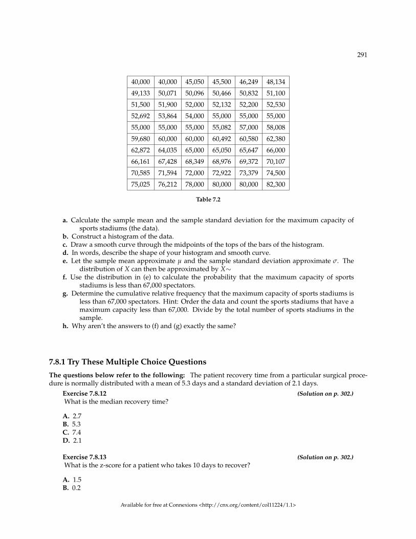
291
40,000 40,000 45,050 45,500 46,249 48,134
49,133 50,071 50,096 50,466 50,832 51,100
51,500 51,900 52,000 52,132 52,200 52,530
52,692 53,864 54,000 55,000 55,000 55,000
55,000 55,000 55,000 55,082 57,000 58,008
59,680 60,000 60,000 60,492 60,580 62,380
62,872 64,035 65,000 65,050 65,647 66,000
66,161 67,428 68,349 68,976 69,372 70,107
70,585 71,594 72,000 72,922 73,379 74,500
75,025 76,212 78,000 80,000 80,000 82,300
Table 7.2
a. Calculate the sample mean and the sample standard deviation for the maximum capacity ofsports stadiums (the data).
b. Construct a histogram of the data.c. Draw a smooth curve through the midpoints of the tops of the bars of the histogram.d. In words, describe the shape of your histogram and smooth curve.e. Let the sample mean approximate µ and the sample standard deviation approximate σ. The
distribution of X can then be approximated by X∼f. Use the distribution in (e) to calculate the probability that the maximum capacity of sports
stadiums is less than 67,000 spectators.g. Determine the cumulative relative frequency that the maximum capacity of sports stadiums is
less than 67,000 spectators. Hint: Order the data and count the sports stadiums that have amaximum capacity less than 67,000. Divide by the total number of sports stadiums in thesample.
h. Why aren’t the answers to (f) and (g) exactly the same?
7.8.1 Try These Multiple Choice Questions
The questions below refer to the following: The patient recovery time from a particular surgical proce-dure is normally distributed with a mean of 5.3 days and a standard deviation of 2.1 days.
Exercise 7.8.12 (Solution on p. 302.)What is the median recovery time?
A. 2.7B. 5.3C. 7.4D. 2.1
Exercise 7.8.13 (Solution on p. 302.)What is the z-score for a patient who takes 10 days to recover?
A. 1.5B. 0.2
Available for free at Connexions <http://cnx.org/content/col11224/1.1>

292 CHAPTER 7. THE NORMAL DISTRIBUTION
C. 2.2D. 7.3
Exercise 7.8.14 (Solution on p. 302.)What is the probability of spending more than 2 days in recovery?
A. 0.0580B. 0.8447C. 0.0553D. 0.9420
Exercise 7.8.15 (Solution on p. 302.)The 90th percentile for recovery times is?
A. 8.89B. 7.07C. 7.99D. 4.32
The questions below refer to the following: The length of time to find a parking space at 9 A.M. follows anormal distribution with a mean of 5 minutes and a standard deviation of 2 minutes.
Exercise 7.8.16 (Solution on p. 302.)Based upon the above information and numerically justified, would you be surprised if it took
less than 1 minute to find a parking space?
A. YesB. NoC. Unable to determine
Exercise 7.8.17 (Solution on p. 302.)Find the probability that it takes at least 8 minutes to find a parking space.
A. 0.0001B. 0.9270C. 0.1862D. 0.0668
Exercise 7.8.18 (Solution on p. 302.)Seventy percent of the time, it takes more than how many minutes to find a parking space?
A. 1.24B. 2.41C. 3.95D. 6.05
Exercise 7.8.19 (Solution on p. 302.)If the mean is significantly greater than the standard deviation, which of the following statementsis true?
I . The data cannot follow the uniform distribution.II . The data cannot follow the exponential distribution..III . The data cannot follow the normal distribution.
Available for free at Connexions <http://cnx.org/content/col11224/1.1>

293
A. I onlyB. II onlyC. III onlyD. I, II, and III
Available for free at Connexions <http://cnx.org/content/col11224/1.1>

294 CHAPTER 7. THE NORMAL DISTRIBUTION
7.9 Review9
The next two questions refer to: X ∼ U (3, 13)Exercise 7.9.1 (Solution on p. 302.)Explain which of the following are false and which are true.
a: f (x) = 110 , 3 ≤ x ≤ 13
b: There is no mode.c: The median is less than the mean.d: P (x > 10) = P (x ≤ 6)
Exercise 7.9.2 (Solution on p. 302.)Calculate:
a: Meanb: Medianc: 65th percentile.
Exercise 7.9.3 (Solution on p. 302.)Which of the following is true for the above box plot?
a: 25% of the data are at most 5.b: There is about the same amount of data from 4 – 5 as there is from 5 – 7.c: There are no data values of 3.d: 50% of the data are 4.
Exercise 7.9.4 (Solution on p. 302.)If P (G | H) = P (G), then which of the following is correct?
A: G and H are mutually exclusive events.B: P (G) = P (H)C: Knowing that H has occurred will affect the chance that G will happen.D: G and H are independent events.
Exercise 7.9.5 (Solution on p. 302.)If P (J) = 0.3, P (K) = 0.6, and J and K are independent events, then explain which are correct
and which are incorrect.
A: P (JandK) = 0B: P (JorK) = 0.9C: P (JorK) = 0.72D: P (J) 6= P (J | K)
9This content is available online at <http://cnx.org/content/m16985/1.10/>.
Available for free at Connexions <http://cnx.org/content/col11224/1.1>

295
Exercise 7.9.6 (Solution on p. 303.)On average, 5 students from each high school class get full scholarships to 4-year colleges. Assumethat most high school classes have about 500 students.
X = the number of students from a high school class that get full scholarships to 4-year school.Which of the following is the distribution of X?
A. P(5)B. B(500,5)C. Exp(1/5)D. N(5, (0.01)(0.99)/500)
Available for free at Connexions <http://cnx.org/content/col11224/1.1>

296 CHAPTER 7. THE NORMAL DISTRIBUTION
7.10 Lab 1: Normal Distribution (Lap Times)10
Class Time:
Names:
7.10.1 Student Learning Outcome:
• The student will compare and contrast empirical data and a theoretical distribution to determine ifTerry Vogel’s lap times fit a continuous distribution.
7.10.2 Directions:
Round the relative frequencies and probabilities to 4 decimal places. Carry all other decimal answers to 2places.
7.10.3 Collect the Data
1. Use the data from Terri Vogel’s Log Book11. Use a Stratified Sampling Method by Lap (Races 1 – 20)and a random number generator to pick 6 lap times from each stratum. Record the lap times belowfor Laps 2 – 7.
_______ _______ _______ _______ _______ _______
_______ _______ _______ _______ _______ _______
_______ _______ _______ _______ _______ _______
_______ _______ _______ _______ _______ _______
_______ _______ _______ _______ _______ _______
_______ _______ _______ _______ _______ _______
Table 7.3
2. Construct a histogram. Make 5 - 6 intervals. Sketch the graph using a ruler and pencil. Scale the axes.
10This content is available online at <http://cnx.org/content/m16981/1.18/>.11"Collaborative Statistics: Data Sets": Section Lap Times <http://cnx.org/content/m17132/latest/#element-244>
Available for free at Connexions <http://cnx.org/content/col11224/1.1>
297
Figure 7.4
3. Calculate the following.a. x =b. s =
4. Draw a smooth curve through the tops of the bars of the histogram. Use 1 – 2 complete sentences todescribe the general shape of the curve. (Keep it simple. Does the graph go straight across, does ithave a V-shape, does it have a hump in the middle or at either end, etc.?)
7.10.4 Analyze the Distribution
Using your sample mean, sample standard deviation, and histogram to help, what was the approximatetheoretical distribution of the data?
• X ∼• How does the histogram help you arrive at the approximate distribution?
7.10.5 Describe the Data
Use the Data from the section titled "Collect the Data" to complete the following statements.
• The IQR goes from __________ to __________.• IQR = __________. (IQR=Q3-Q1)• The 15th percentile is:• The 85th percentile is:• The median is:• The empirical probability that a randomly chosen lap time is more than 130 seconds =• Explain the meaning of the 85th percentile of this data.
Available for free at Connexions <http://cnx.org/content/col11224/1.1>

298 CHAPTER 7. THE NORMAL DISTRIBUTION
7.10.6 Theoretical Distribution
Using the theoretical distribution from the section titled "Analyse the Distribution" complete the followingstatements:
• The IQR goes from __________ to __________.• IQR =• The 15th percentile is:• The 85th percentile is:• The median is:• The probability that a randomly chosen lap time is more than 130 seconds =• Explain the meaning of the 85th percentile of this distribution.
7.10.7 Discussion Questions
• Do the data from the section titled "Collect the Data" give a close approximation to the theoreticaldistibution in the section titled "Analyze the Distribution"? In complete sentences and comparing theresult in the sections titled "Describe the Data" and "Theoretical Distribution", explain why or whynot.
Available for free at Connexions <http://cnx.org/content/col11224/1.1>

299
7.11 Lab 2: Normal Distribution (Pinkie Length)12
Class Time:
Names:
7.11.1 Student Learning Outcomes:
• The student will compare empirical data and a theoretical distribution to determine if data from theexperiment follow a continuous distribution.
7.11.2 Collect the Data
Measure the length of your pinkie finger (in cm.)
1. Randomly survey 30 adults. Round to the nearest 0.5 cm.
_______ _______ _______ _______ _______
_______ _______ _______ _______ _______
_______ _______ _______ _______ _______
_______ _______ _______ _______ _______
_______ _______ _______ _______ _______
_______ _______ _______ _______ _______
Table 7.4
2. Construct a histogram. Make 5-6 intervals. Sketch the graph using a ruler and pencil. Scale the axes.
3. Calculate the Following
12This content is available online at <http://cnx.org/content/m16980/1.16/>.
Available for free at Connexions <http://cnx.org/content/col11224/1.1>
300 CHAPTER 7. THE NORMAL DISTRIBUTION
a. x =b. s =
4. Draw a smooth curve through the top of the bars of the histogram. Use 1-2 complete sentences todescribe the general shape of the curve. (Keep it simple. Does the graph go straight across, does ithave a V-shape, does it have a hump in the middle or at either end, etc.?)
7.11.3 Analyze the Distribution
Using your sample mean, sample standard deviation, and histogram to help, what was the approximatetheoretical distribution of the data from the section titled "Collect the Data"?
• X ∼• How does the histogram help you arrive at the approximate distribution?
7.11.4 Describe the Data
Using the data in the section titled "Collect the Data" complete the following statements. (Hint: order thedata)
REMEMBER: (IQR = Q3−Q1)
• IQR =• 15th percentile is:• 85th percentile is:• Median is:• What is the empirical probability that a randomly chosen pinkie length is more than 6.5 cm?• Explain the meaning the 85th percentile of this data.
7.11.5 Theoretical Distribution
Using the Theoretical Distribution in the section titled "Analyze the Distribution"
• IQR =• 15th percentile is:• 85th percentile is:• Median is:• What is the theoretical probability that a randomly chosen pinkie length is more than 6.5 cm?• Explain the meaning of the 85th percentile of this data.
7.11.6 Discussion Questions
• Do the data from the section entitled "Collect the Data" give a close approximation to the theoreticaldistribution in "Analyze the Distribution." In complete sentences and comparing the results in thesections titled "Describe the Data" and "Theoretical Distribution", explain why or why not.
Available for free at Connexions <http://cnx.org/content/col11224/1.1>
301
Solutions to Exercises in Chapter 7
Solution to Example 7.2, Problem 1 (p. 279)This z-score tells you that x = 10 is 2.5 standard deviations to the right of the mean 5.
Solution to Example 7.2, Problem 2 (p. 279)z = -4. This z-score tells you that x = −3 is 4 standard deviations to the left of the mean.
Solutions to Practice: The Normal Distribution
Solution to Exercise 7.7.3 (p. 286)
b. 3, 0.1979
Solution to Exercise 7.7.4 (p. 286)
b. 2.8, 6, 0.7694
Solution to Exercise 7.7.5 (p. 287)
b. 0.70, 4.78years
Solutions to Homework
Solution to Exercise 7.8.1 (p. 288)
a. N (66, 2.5)b. 0.5404c. Nod. Between 64.7 and 67.3 inches
Solution to Exercise 7.8.3 (p. 288)
a. N (36,10)b. 0.3446c. 29.3
Solution to Exercise 7.8.5 (p. 289)
a. the time (in hours) a 4-year-old in China spends unsupervised per dayb. N (3, 1.5)c. 0.0912d. 0e. 2.21 hours
Solution to Exercise 7.8.7 (p. 289)
a. The duration of a criminal trialb. N (21, 7)c. 0.3341d. 22.77
Solution to Exercise 7.8.9 (p. 290)
a. The sample mean is 5.51 and the sample standard deviation is 2.15e. N (5.51, 2.15)f. 0.6081g. 0.64
Available for free at Connexions <http://cnx.org/content/col11224/1.1>

302 CHAPTER 7. THE NORMAL DISTRIBUTION
Solution to Exercise 7.8.11 (p. 290)
a. The sample mean is 60,136.4 and the sample standard deviation is 10,468.1.e. N (60136.4, 10468.1)f. 0.7440g. 0.7167
Solution to Exercise 7.8.12 (p. 291)B
Solution to Exercise 7.8.13 (p. 291)C
Solution to Exercise 7.8.14 (p. 292)D
Solution to Exercise 7.8.15 (p. 292)C
Solution to Exercise 7.8.16 (p. 292)A
Solution to Exercise 7.8.17 (p. 292)D
Solution to Exercise 7.8.18 (p. 292)C
Solution to Exercise 7.8.19 (p. 292)B
Solutions to Review
Solution to Exercise 7.9.1 (p. 294)
a: Trueb: Truec: False – the median and the mean are the same for this symmetric distributiond: True
Solution to Exercise 7.9.2 (p. 294)
a: 8b: 8c: P (x < k) = 0.65 = (k− 3) ∗
(1
10
). k = 9.5
Solution to Exercise 7.9.3 (p. 294)
a: False – 34 of the data are at most 5
b: True – each quartile has 25% of the datac: False – that is unknownd: False – 50% of the data are 4 or less
Solution to Exercise 7.9.4 (p. 294)D
Solution to Exercise 7.9.5 (p. 294)
A: False - J and K are independent so they are not mutually exclusive which would imply dependency(meaning P(J and K) is not 0).
B: False - see answer C.C: True - P(J or K) = P(J) + P(K) - P(J and K) = P(J) + P(K) - P(J)P(K) = 0.3 + 0.6 - (0.3)(0.6) = 0.72. Note that
P(J and K) = P(J)P(K) because J and K are independent.
Available for free at Connexions <http://cnx.org/content/col11224/1.1>

303
D: False - J and K are independent so P(J) = P(J|K).
Solution to Exercise 7.9.6 (p. 295)A
Available for free at Connexions <http://cnx.org/content/col11224/1.1>

304 CHAPTER 7. THE NORMAL DISTRIBUTION
Available for free at Connexions <http://cnx.org/content/col11224/1.1>

Appendix
8.1 Practice Final Exam 11
Questions 1-2 refer to the following:
An experiment consists of tossing two 12-sided dice (the numbers 1-12 are printed on the sides of eachdice).
• Let Event A = both dice show an even number• Let Event B = both dice show a number more than 8
Exercise 8.1.1 (Solution on p. 336.)Events A and B are:
A. Mutually exclusive.B. Independent.C. Mutually exclusive and independent.D. Neither mutually exclusive nor independent.
Exercise 8.1.2 (Solution on p. 336.)Find P (A|B)
A. 24
B. 16144
C. 416
D. 2144
Exercise 8.1.3 (Solution on p. 336.)Which of the following are TRUE when we perform a hypothesis test on matched or paired sam-
ples?
A. Sample sizes are almost never small.B. Two measurements are drawn from the same pair of individuals or objects.C. Two sample means are compared to each other.D. Answer choices B and C are both true.
Questions 4 - 5 refer to the following:
118 students were asked what type of color their bedrooms were painted: light colors, dark colors or vibrantcolors. The results were tabulated according to gender.
1This content is available online at <http://cnx.org/content/m16304/1.17/>.
Available for free at Connexions <http://cnx.org/content/col11224/1.1>
305

306 APPENDIX
Light colors Dark colors Vibrant colors
Female 20 22 28
Male 10 30 8
Table 8.1
Exercise 8.1.4 (Solution on p. 336.)Find the probability that a randomly chosen student is male or has a bedroom painted with light
colors.
A. 10118
B. 68118
C. 48118
D. 1048
Exercise 8.1.5 (Solution on p. 336.)Find the probability that a randomly chosen student is male given the student’s bedroom is
painted with dark colors.
A. 30118
B. 3048
C. 22118
D. 3052
Questions 6 – 7 refer to the following:
We are interested in the number of times a teenager must be reminded to do his/her chores each week. Asurvey of 40 mothers was conducted. The table below shows the results of the survey.
x P (x)
0 240
1 540
2
3 1440
4 740
5 440
Table 8.2
Exercise 8.1.6 (Solution on p. 336.)Find the probability that a teenager is reminded 2 times.
A. 8B. 8
40C. 6
40D. 2
Exercise 8.1.7 (Solution on p. 336.)Find the expected number of times a teenager is reminded to do his/her chores.
Available for free at Connexions <http://cnx.org/content/col11224/1.1>

APPENDIX 307
A. 15B. 2.78C. 1.0D. 3.13
Questions 8 – 9 refer to the following:
On any given day, approximately 37.5% of the cars parked in the De Anza parking structure are parkedcrookedly. (Survey done by Kathy Plum.) We randomly survey 22 cars. We are interested in the number ofcars that are parked crookedly.
Exercise 8.1.8 (Solution on p. 336.)For every 22 cars, how many would you expect to be parked crookedly, on average?
A. 8.25B. 11C. 18D. 7.5
Exercise 8.1.9 (Solution on p. 336.)What is the probability that at least 10 of the 22 cars are parked crookedly.
A. 0.1263B. 0.1607C. 0.2870D. 0.8393
Exercise 8.1.10 (Solution on p. 336.)Using a sample of 15 Stanford-Binet IQ scores, we wish to conduct a hypothesis test. Our claim
is that the mean IQ score on the Stanford-Binet IQ test is more than 100. It is known that thestandard deviation of all Stanford-Binet IQ scores is 15 points. The correct distribution to use forthe hypothesis test is:
A. BinomialB. Student’s-tC. NormalD. Uniform
Questions 11 – 13 refer to the following:
De Anza College keeps statistics on the pass rate of students who enroll in math classes. In a sample of 1795students enrolled in Math 1A (1st quarter calculus), 1428 passed the course. In a sample of 856 studentsenrolled in Math 1B (2nd quarter calculus), 662 passed. In general, are the pass rates of Math 1A and Math1B statistically the same? Let A = the subscript for Math 1A and B = the subscript for Math 1B.
Exercise 8.1.11 (Solution on p. 336.)If you were to conduct an appropriate hypothesis test, the alternate hypothesis would be:
A. Ha: pA = pBB. Ha: pA > pBC. Ho: pA = pBD. Ha: pA 6= pB
Exercise 8.1.12 (Solution on p. 336.)The Type I error is to:
Available for free at Connexions <http://cnx.org/content/col11224/1.1>
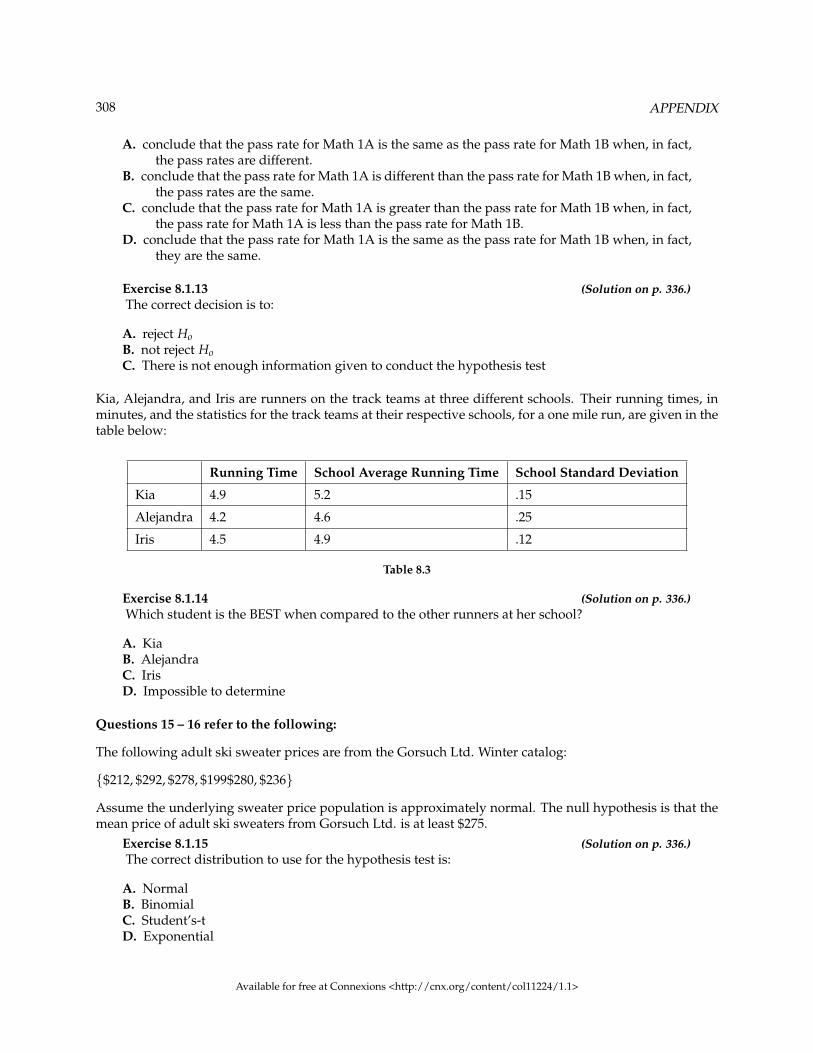
308 APPENDIX
A. conclude that the pass rate for Math 1A is the same as the pass rate for Math 1B when, in fact,the pass rates are different.
B. conclude that the pass rate for Math 1A is different than the pass rate for Math 1B when, in fact,the pass rates are the same.
C. conclude that the pass rate for Math 1A is greater than the pass rate for Math 1B when, in fact,the pass rate for Math 1A is less than the pass rate for Math 1B.
D. conclude that the pass rate for Math 1A is the same as the pass rate for Math 1B when, in fact,they are the same.
Exercise 8.1.13 (Solution on p. 336.)The correct decision is to:
A. reject HoB. not reject HoC. There is not enough information given to conduct the hypothesis test
Kia, Alejandra, and Iris are runners on the track teams at three different schools. Their running times, inminutes, and the statistics for the track teams at their respective schools, for a one mile run, are given in thetable below:
Running Time School Average Running Time School Standard Deviation
Kia 4.9 5.2 .15
Alejandra 4.2 4.6 .25
Iris 4.5 4.9 .12
Table 8.3
Exercise 8.1.14 (Solution on p. 336.)Which student is the BEST when compared to the other runners at her school?
A. KiaB. AlejandraC. IrisD. Impossible to determine
Questions 15 – 16 refer to the following:
The following adult ski sweater prices are from the Gorsuch Ltd. Winter catalog:
{$212, $292, $278, $199$280, $236}
Assume the underlying sweater price population is approximately normal. The null hypothesis is that themean price of adult ski sweaters from Gorsuch Ltd. is at least $275.
Exercise 8.1.15 (Solution on p. 336.)The correct distribution to use for the hypothesis test is:
A. NormalB. BinomialC. Student’s-tD. Exponential
Available for free at Connexions <http://cnx.org/content/col11224/1.1>

APPENDIX 309
Exercise 8.1.16 (Solution on p. 336.)The hypothesis test:
A. is two-tailedB. is left-tailedC. is right-tailedD. has no tails
Exercise 8.1.17 (Solution on p. 336.)Sara, a statistics student, wanted to determine the mean number of books that college professors
have in their office. She randomly selected 2 buildings on campus and asked each professor in theselected buildings how many books are in his/her office. Sara surveyed 25 professors. The typeof sampling selected is a:
A. simple random samplingB. systematic samplingC. cluster samplingD. stratified sampling
Exercise 8.1.18 (Solution on p. 336.)A clothing store would use which measure of the center of data when placing orders for the
typical "middle" customer?
A. MeanB. MedianC. ModeD. IQR
Exercise 8.1.19 (Solution on p. 336.)In a hypothesis test, the p-value is
A. the probability that an outcome of the data will happen purely by chance when the null hy-pothesis is true.
B. called the preconceived alpha.C. compared to beta to decide whether to reject or not reject the null hypothesis.D. Answer choices A and B are both true.
Questions 20 - 22 refer to the following:
A community college offers classes 6 days a week: Monday through Saturday. Maria conducted a study ofthe students in her classes to determine how many days per week the students who are in her classes cometo campus for classes. In each of her 5 classes she randomly selected 10 students and asked them how manydays they come to campus for classes. Each of her classes are the same size. The results of her survey aresummarized in the table below.
Number of Days on Campus Frequency Relative Frequency Cumulative Relative Frequency
1 2
2 12 .24
3 10 .20
4 .98
5 0
6 1 .02 1.00
Available for free at Connexions <http://cnx.org/content/col11224/1.1>

310 APPENDIX
Table 8.4
Exercise 8.1.20 (Solution on p. 336.)Combined with convenience sampling, what other sampling technique did Maria use?
A. simple randomB. systematicC. clusterD. stratified
Exercise 8.1.21 (Solution on p. 336.)How many students come to campus for classes 4 days a week?
A. 49B. 25C. 30D. 13
Exercise 8.1.22 (Solution on p. 336.)What is the 60th percentile for the this data?
A. 2B. 3C. 4D. 5
The next two questions refer to the following:
The following data are the results of a random survey of 110 Reservists called to active duty to increasesecurity at California airports.
Number of Dependents Frequency
0 11
1 27
2 33
3 20
4 19
Table 8.5
Exercise 8.1.23 (Solution on p. 336.)Construct a 95% Confidence Interval for the true population mean number of dependents of
Reservists called to active duty to increase security at California airports.
A. (1.85, 2.32)B. (1.80, 2.36)C. (1.97, 2.46)D. (1.92, 2.50)
Exercise 8.1.24 (Solution on p. 336.)The 95% confidence Interval above means:
Available for free at Connexions <http://cnx.org/content/col11224/1.1>
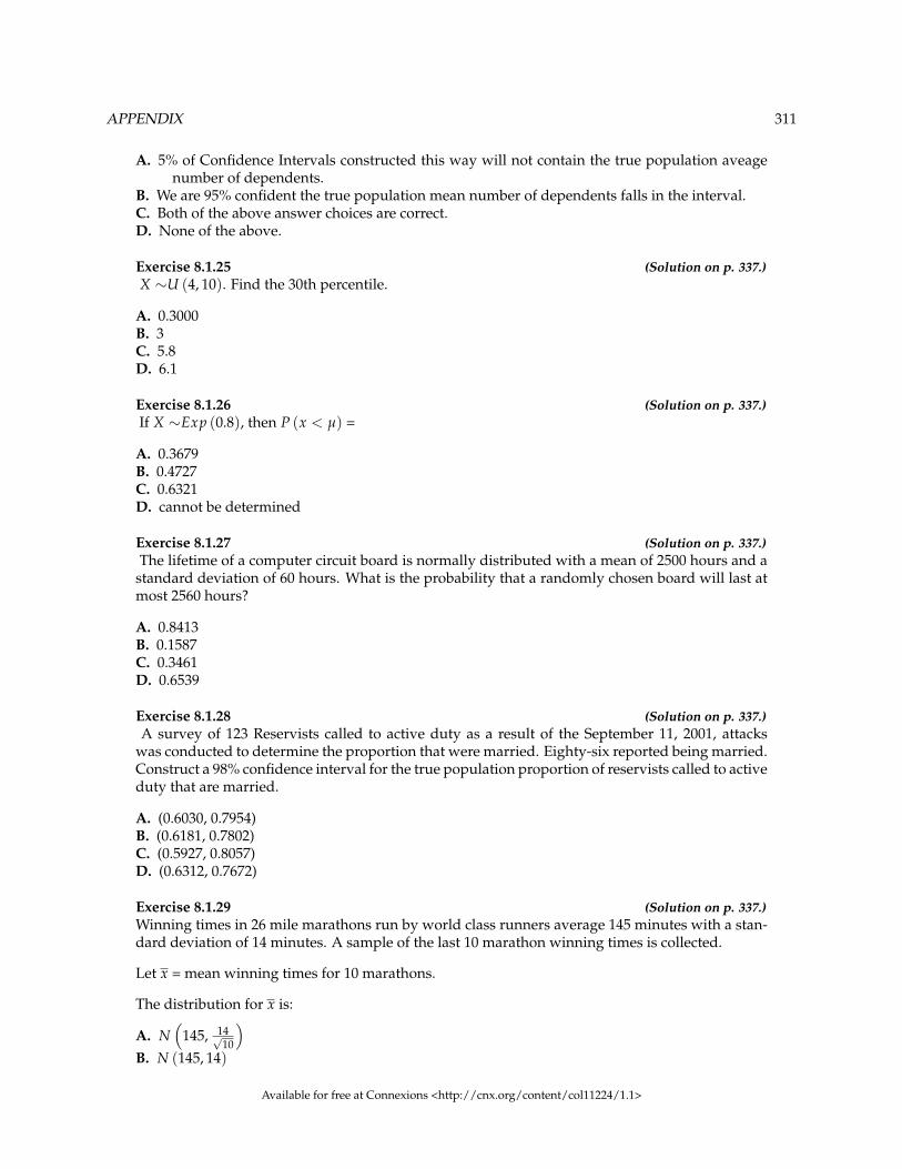
APPENDIX 311
A. 5% of Confidence Intervals constructed this way will not contain the true population aveagenumber of dependents.
B. We are 95% confident the true population mean number of dependents falls in the interval.C. Both of the above answer choices are correct.D. None of the above.
Exercise 8.1.25 (Solution on p. 337.)X ∼U (4, 10). Find the 30th percentile.
A. 0.3000B. 3C. 5.8D. 6.1
Exercise 8.1.26 (Solution on p. 337.)If X ∼Exp (0.8), then P (x < µ) =
A. 0.3679B. 0.4727C. 0.6321D. cannot be determined
Exercise 8.1.27 (Solution on p. 337.)The lifetime of a computer circuit board is normally distributed with a mean of 2500 hours and a
standard deviation of 60 hours. What is the probability that a randomly chosen board will last atmost 2560 hours?
A. 0.8413B. 0.1587C. 0.3461D. 0.6539
Exercise 8.1.28 (Solution on p. 337.)A survey of 123 Reservists called to active duty as a result of the September 11, 2001, attacks
was conducted to determine the proportion that were married. Eighty-six reported being married.Construct a 98% confidence interval for the true population proportion of reservists called to activeduty that are married.
A. (0.6030, 0.7954)B. (0.6181, 0.7802)C. (0.5927, 0.8057)D. (0.6312, 0.7672)
Exercise 8.1.29 (Solution on p. 337.)Winning times in 26 mile marathons run by world class runners average 145 minutes with a stan-dard deviation of 14 minutes. A sample of the last 10 marathon winning times is collected.
Let x = mean winning times for 10 marathons.
The distribution for x is:
A. N(
145, 14√10
)B. N (145, 14)
Available for free at Connexions <http://cnx.org/content/col11224/1.1>
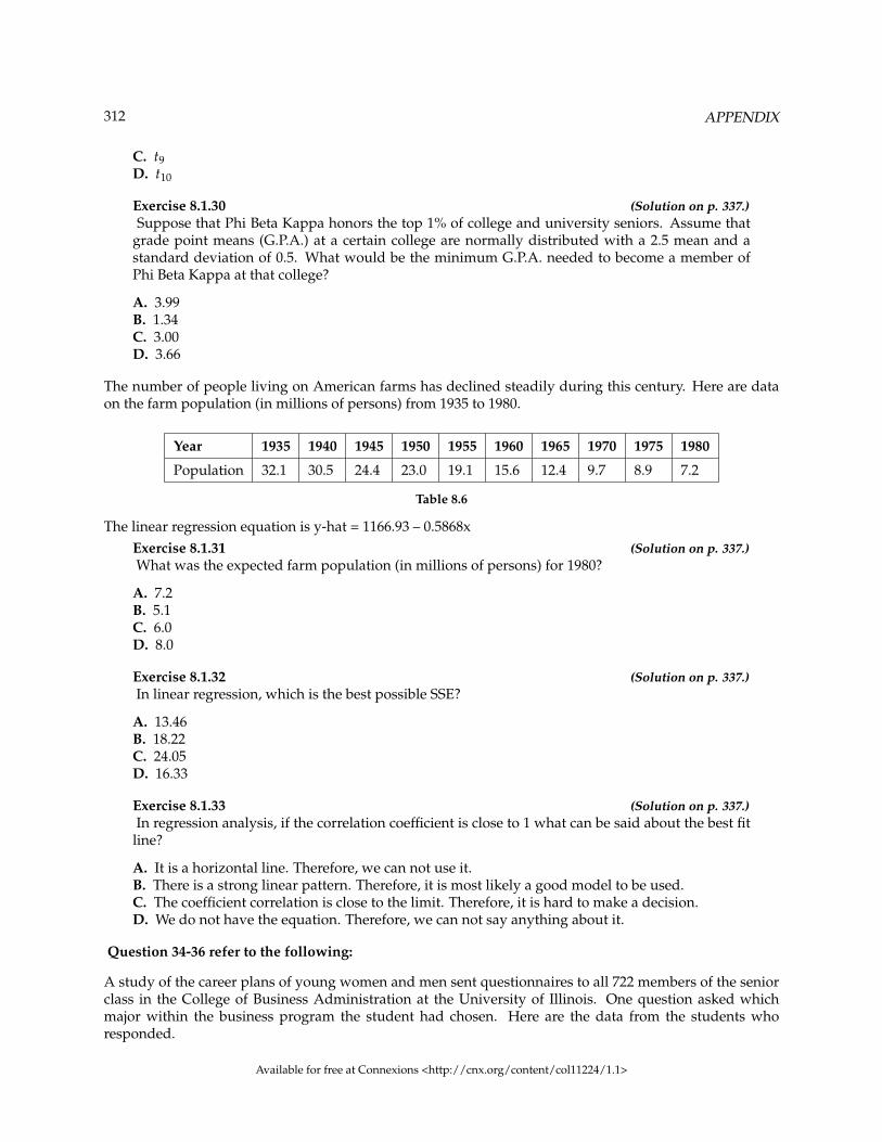
312 APPENDIX
C. t9D. t10
Exercise 8.1.30 (Solution on p. 337.)Suppose that Phi Beta Kappa honors the top 1% of college and university seniors. Assume that
grade point means (G.P.A.) at a certain college are normally distributed with a 2.5 mean and astandard deviation of 0.5. What would be the minimum G.P.A. needed to become a member ofPhi Beta Kappa at that college?
A. 3.99B. 1.34C. 3.00D. 3.66
The number of people living on American farms has declined steadily during this century. Here are dataon the farm population (in millions of persons) from 1935 to 1980.
Year 1935 1940 1945 1950 1955 1960 1965 1970 1975 1980
Population 32.1 30.5 24.4 23.0 19.1 15.6 12.4 9.7 8.9 7.2
Table 8.6
The linear regression equation is y-hat = 1166.93 – 0.5868xExercise 8.1.31 (Solution on p. 337.)What was the expected farm population (in millions of persons) for 1980?
A. 7.2B. 5.1C. 6.0D. 8.0
Exercise 8.1.32 (Solution on p. 337.)In linear regression, which is the best possible SSE?
A. 13.46B. 18.22C. 24.05D. 16.33
Exercise 8.1.33 (Solution on p. 337.)In regression analysis, if the correlation coefficient is close to 1 what can be said about the best fit
line?
A. It is a horizontal line. Therefore, we can not use it.B. There is a strong linear pattern. Therefore, it is most likely a good model to be used.C. The coefficient correlation is close to the limit. Therefore, it is hard to make a decision.D. We do not have the equation. Therefore, we can not say anything about it.
Question 34-36 refer to the following:
A study of the career plans of young women and men sent questionnaires to all 722 members of the seniorclass in the College of Business Administration at the University of Illinois. One question asked whichmajor within the business program the student had chosen. Here are the data from the students whoresponded.
Available for free at Connexions <http://cnx.org/content/col11224/1.1>
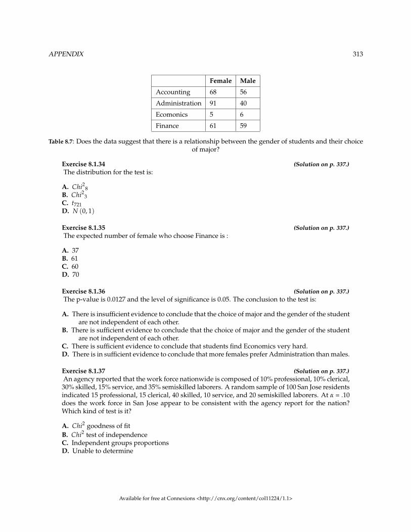
APPENDIX 313
Female Male
Accounting 68 56
Administration 91 40
Ecomonics 5 6
Finance 61 59
Table 8.7: Does the data suggest that there is a relationship between the gender of students and their choiceof major?
Exercise 8.1.34 (Solution on p. 337.)The distribution for the test is:
A. Chi28B. Chi23C. t721D. N (0, 1)
Exercise 8.1.35 (Solution on p. 337.)The expected number of female who choose Finance is :
A. 37B. 61C. 60D. 70
Exercise 8.1.36 (Solution on p. 337.)The p-value is 0.0127 and the level of significance is 0.05. The conclusion to the test is:
A. There is insufficient evidence to conclude that the choice of major and the gender of the studentare not independent of each other.
B. There is sufficient evidence to conclude that the choice of major and the gender of the studentare not independent of each other.
C. There is sufficient evidence to conclude that students find Economics very hard.D. There is in sufficient evidence to conclude that more females prefer Administration than males.
Exercise 8.1.37 (Solution on p. 337.)An agency reported that the work force nationwide is composed of 10% professional, 10% clerical,30% skilled, 15% service, and 35% semiskilled laborers. A random sample of 100 San Jose residentsindicated 15 professional, 15 clerical, 40 skilled, 10 service, and 20 semiskilled laborers. At α = .10does the work force in San Jose appear to be consistent with the agency report for the nation?Which kind of test is it?
A. Chi2 goodness of fitB. Chi2 test of independenceC. Independent groups proportionsD. Unable to determine
Available for free at Connexions <http://cnx.org/content/col11224/1.1>

314 APPENDIX
8.2 Practice Final Exam 22
Exercise 8.2.1 (Solution on p. 337.)A study was done to determine the proportion of teenagers that own a car. The population
proportion of teenagers that own a car is the
A. statisticB. parameterC. populationD. variable
The next two questions refer to the following data:
value frequency
0 1
1 4
2 7
3 9
6 4
Table 8.8
Exercise 8.2.2 (Solution on p. 337.)The box plot for the data is:
A.
B.
C.2This content is available online at <http://cnx.org/content/m16303/1.16/>.
Available for free at Connexions <http://cnx.org/content/col11224/1.1>

APPENDIX 315
D.
Exercise 8.2.3 (Solution on p. 337.)If 6 were added to each value of the data in the table, the 15th percentile of the new list of values
is:
A. 6B. 1C. 7D. 8
The next two questions refer to the following situation:
Suppose that the probability of a drought in any independent year is 20%. Out of those years in which adrought occurs, the probability of water rationing is 10%. However, in any year, the probability of waterrationing is 5%.
Exercise 8.2.4 (Solution on p. 337.)What is the probability of both a drought and water rationing occurring?
A. 0.05B. 0.01C. 0.02D. 0.30
Exercise 8.2.5 (Solution on p. 337.)Which of the following is true?
A. drought and water rationing are independent eventsB. drought and water rationing are mutually exclusive eventsC. none of the above
The next two questions refer to the following situation:
Suppose that a survey yielded the following data:
Favorite Pie Type
gender apple pumpkin pecan
female 40 10 30
male 20 30 10
Table 8.9
Exercise 8.2.6 (Solution on p. 337.)Suppose that one individual is randomly chosen. The probability that the person’s favorite pie is
apple or the person is male is:
Available for free at Connexions <http://cnx.org/content/col11224/1.1>
316 APPENDIX
A. 4060
B. 60140
C. 120140
D. 100140
Exercise 8.2.7 (Solution on p. 337.)Suppose Ho is: Favorite pie type and gender are independent.
The p-value is:
A. ≈ 0B. 1C. 0.05D. cannot be determined
The next two questions refer to the following situation:
Let’s say that the probability that an adult watches the news at least once per week is 0.60. We randomlysurvey 14 people. Of interest is the number that watch the news at least once per week.
Exercise 8.2.8 (Solution on p. 337.)Which of the following statements is FALSE?
A. X ∼ B (14, 0.60)B. The values for x are: {1, 2, 3, ..., 14}C. µ = 8.4D. P (X = 5) = 0.0408
Exercise 8.2.9 (Solution on p. 337.)Find the probability that at least 6 adults watch the news.
A. 614
B. 0.8499C. 0.9417D. 0.6429
Exercise 8.2.10 (Solution on p. 337.)The following histogram is most likely to be a result of sampling from which distribution?
Available for free at Connexions <http://cnx.org/content/col11224/1.1>
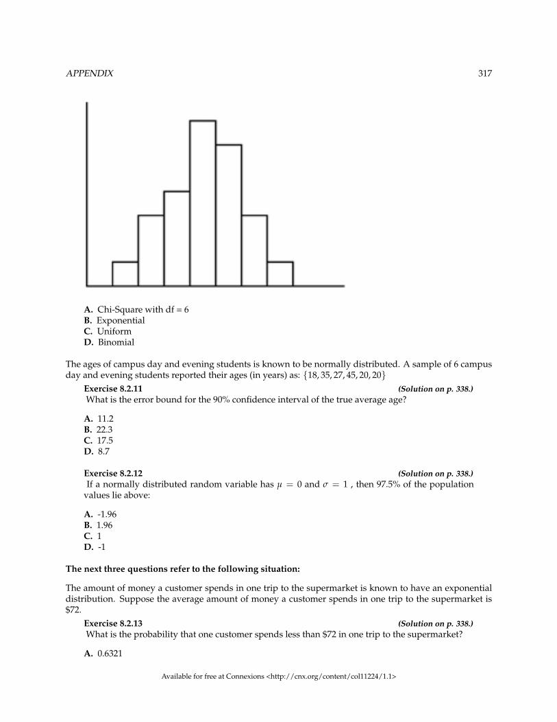
APPENDIX 317
A. Chi-Square with df = 6B. ExponentialC. UniformD. Binomial
The ages of campus day and evening students is known to be normally distributed. A sample of 6 campusday and evening students reported their ages (in years) as: {18, 35, 27, 45, 20, 20}
Exercise 8.2.11 (Solution on p. 338.)What is the error bound for the 90% confidence interval of the true average age?
A. 11.2B. 22.3C. 17.5D. 8.7
Exercise 8.2.12 (Solution on p. 338.)If a normally distributed random variable has µ = 0 and σ = 1 , then 97.5% of the population
values lie above:
A. -1.96B. 1.96C. 1D. -1
The next three questions refer to the following situation:
The amount of money a customer spends in one trip to the supermarket is known to have an exponentialdistribution. Suppose the average amount of money a customer spends in one trip to the supermarket is$72.
Exercise 8.2.13 (Solution on p. 338.)What is the probability that one customer spends less than $72 in one trip to the supermarket?
A. 0.6321
Available for free at Connexions <http://cnx.org/content/col11224/1.1>

318 APPENDIX
B. 0.5000C. 0.3714D. 1
Exercise 8.2.14 (Solution on p. 338.)How much money altogether would you expect next 5 customers to spend in one trip to the
supermarket (in dollars)?
A. 72B. 722
5C. 5184D. 360
Exercise 8.2.15 (Solution on p. 338.)If you want to find the probability that the mean of 50 customers is less than $60, the distribution
to use is:
A. N (72, 72)B. N
(72, 72√
50
)C. Exp (72)D. Exp
(1
72
)The next three questions refer to the following situation:
The amount of time it takes a fourth grader to carry out the trash is uniformly distributed in the intervalfrom 1 to 10 minutes.
Exercise 8.2.16 (Solution on p. 338.)What is the probability that a randomly chosen fourth grader takes more than 7 minutes to take
out the trash?
A. 39
B. 79
C. 310
D. 710
Exercise 8.2.17 (Solution on p. 338.)Which graph best shows the probability that a randomly chosen fourth grader takes more than 6
minutes to take out the trash given that he/she has already taken more than 3 minutes?
Available for free at Connexions <http://cnx.org/content/col11224/1.1>

APPENDIX 319
Exercise 8.2.18 (Solution on p. 338.)We should expect a fourth grader to take how many minutes to take out the trash?
A. 4.5B. 5.5C. 5D. 10
The next three questions refer to the following situation:
At the beginning of the quarter, the amount of time a student waits in line at the campus cafeteria is nor-mally distributed with a mean of 5 minutes and a standard deviation of 1.5 minutes.
Exercise 8.2.19 (Solution on p. 338.)What is the 90th percentile of waiting times (in minutes)?
A. 1.28B. 90C. 7.47D. 6.92
Exercise 8.2.20 (Solution on p. 338.)The median waiting time (in minutes) for one student is:
A. 5B. 50C. 2.5D. 1.5
Exercise 8.2.21 (Solution on p. 338.)Find the probability that the average wait time of 10 students is at most 5.5 minutes.
A. 0.6301B. 0.8541C. 0.3694
Available for free at Connexions <http://cnx.org/content/col11224/1.1>

320 APPENDIX
D. 0.1459
Exercise 8.2.22 (Solution on p. 338.)A sample of 80 software engineers in Silicon Valley is taken and it is found that 20% of them earnapproximately $50,000 per year. A point estimate for the true proportion of engineers in SiliconValley who earn $50,000 per year is:
A. 16B. 0.2C. 1D. 0.95
Exercise 8.2.23 (Solution on p. 338.)If P (Z < zα) = 0. 1587 where Z∼N (0, 1) , then α is equal to:
A. -1B. 0.1587C. 0.8413D. 1
Exercise 8.2.24 (Solution on p. 338.)A professor tested 35 students to determine their entering skills. At the end of the term, after
completing the course, the same test was administered to the same 35 students to study theirimprovement. This would be a test of:
A. independent groupsB. 2 proportionsC. matched pairs, dependent groupsD. exclusive groups
Exercise 8.2.25 (Solution on p. 338.)A math exam was given to all the third grade children attending ABC School. Two random
samples of scores were taken.
n x s
Boys 55 82 5
Girls 60 86 7
Table 8.10
Which of the following correctly describes the results of a hypothesis test of the claim, “There isa difference between the mean scores obtained by third grade girls and boys at the 5 % level ofsignificance”?
A. Do not reject Ho. There is insufficient evidence to conclude that there is a difference in themean scores.
B. Do not reject Ho. There is sufficient evidence to conclude that there is a difference in the meanscores.
C. Reject Ho. There is insufficient evidence to conclude that there is no difference in the meanscores.
D. Reject Ho. There is sufficient evidence to conclude that there is a difference in the mean scores.
Available for free at Connexions <http://cnx.org/content/col11224/1.1>

APPENDIX 321
Exercise 8.2.26 (Solution on p. 338.)In a survey of 80 males, 45 had played an organized sport growing up. Of the 70 females surveyed,25 had played an organized sport growing up. We are interested in whether the proportion formales is higher than the proportion for females. The correct conclusion is:
A. There is insufficient information to conclude that the proportion for males is the same as theproportion for females.
B. There is insufficient information to conclude that the proportion for males is not the same asthe proportion for females.
C. There is sufficient evidence to conclude that the proportion for males is higher than the pro-portion for females.
D. Not enough information to determine.
Exercise 8.2.27 (Solution on p. 338.)Note: Chi-Square Test of a Single Variance; Not all classes cover this topic. From past experience,
a statistics teacher has found that the average score on a midterm is 81 with a standard deviationof 5.2. This term, a class of 49 students had a standard deviation of 5 on the midterm. Do the dataindicate that we should reject the teacher’s claim that the standard deviation is 5.2? Use α = 0.05.
A. YesB. NoC. Not enough information given to solve the problem
Exercise 8.2.28 (Solution on p. 338.)Note: F Distribution Test of ANOVA; Not all classes cover this topic. Three loading machines
are being compared. Ten samples were taken for each machine. Machine I took an average of 31minutes to load packages with a standard deviation of 2 minutes. Machine II took an average of 28minutes to load packages with a standard deviation of 1.5 minutes. Machine III took an average of29 minutes to load packages with a standard deviation of 1 minute. Find the p-value when testingthat the average loading times are the same.
A. the p–value is close to 0B. p–value is close to 1C. Not enough information given to solve the problem
The next three questions refer to the following situation:
A corporation has offices in different parts of the country. It has gathered the following information con-cerning the number of bathrooms and the number of employees at seven sites:
Number of employees x 650 730 810 900 102 107 1150
Number of bathrooms y 40 50 54 61 82 110 121
Table 8.11
Exercise 8.2.29 (Solution on p. 338.)Is the correlation between the number of employees and the number of bathrooms significant?
A. YesB. NoC. Not enough information to answer question
Available for free at Connexions <http://cnx.org/content/col11224/1.1>

322 APPENDIX
Exercise 8.2.30 (Solution on p. 338.)The linear regression equation is:
A. y = 0.0094− 79.96xB. y = 79.96 + 0.0094xC. y = 79.96− 0.0094xD. y = −0.0094 + 79.96x
Exercise 8.2.31 (Solution on p. 338.)If a site has 1150 employees, approximately how many bathrooms should it have?
A. 69B. 91C. 91,954D. We should not be estimating here.
Exercise 8.2.32 (Solution on p. 338.)Note: Chi-Square Test of a Single Variance; Not all classes cover this topic. Suppose that a sampleof size 10 was collected, with x = 4.4 and s = 1.4 .
Ho : σ2= 1.6 vs. Ha : σ2 6= 1.6. Which graph best describes the results of the test?
Exercise 8.2.33 (Solution on p. 338.)64 backpackers were asked the number of days their latest backpacking trip was. The number of
days is given in the table below:
# of days 1 2 3 4 5 6 7 8
Frequency 5 9 6 12 7 10 5 10
Table 8.12
Conduct an appropriate test to determine if the distribution is uniform.
A. The p–value is > 0.10. There is insufficient information to conclude that the distribution is notuniform.
B. The p–value is < 0.01. There is sufficient information to conclude the distribution is not uni-form.
C. The p–value is between 0.01 and 0.10, but without alpha (α) there is not enough information
Available for free at Connexions <http://cnx.org/content/col11224/1.1>
APPENDIX 323
D. There is no such test that can be conducted.
Exercise 8.2.34 (Solution on p. 338.)Note: F Distribution test of One-Way ANOVA; Not all classes cover this topic. Which of the
following statements is true when using one-way ANOVA?
A. The populations from which the samples are selected have different distributions.B. The sample sizes are large.C. The test is to determine if the different groups have the same means.D. There is a correlation between the factors of the experiment.
Available for free at Connexions <http://cnx.org/content/col11224/1.1>
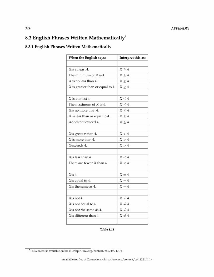
324 APPENDIX
8.3 English Phrases Written Mathematically3
8.3.1 English Phrases Written Mathematically
When the English says: Interpret this as:
Xis at least 4. X ≥ 4
The minimum of X is 4. X ≥ 4
X is no less than 4. X ≥ 4
X is greater than or equal to 4. X ≥ 4
X is at most 4. X ≤ 4
The maximum of X is 4. X ≤ 4
Xis no more than 4. X ≤ 4
X is less than or equal to 4. X ≤ 4
Xdoes not exceed 4. X ≤ 4
Xis greater than 4. X > 4
X is more than 4. X > 4
Xexceeds 4. X > 4
Xis less than 4. X < 4
There are fewer X than 4. X < 4
Xis 4. X = 4
Xis equal to 4. X = 4
Xis the same as 4. X = 4
Xis not 4. X 6= 4
Xis not equal to 4. X 6= 4
Xis not the same as 4. X 6= 4
Xis different than 4. X 6= 4
Table 8.13
3This content is available online at <http://cnx.org/content/m16307/1.6/>.
Available for free at Connexions <http://cnx.org/content/col11224/1.1>

APPENDIX 325
8.4 Symbols and their Meanings4
Symbols and their Meanings
Chapter (1st used) Symbol Spoken Meaning
Sampling and Data √ The square root of same
Sampling and Data π Pi 3.14159. . . (a specificnumber)
Descriptive Statistics Q1 Quartile one the first quartile
Descriptive Statistics Q2 Quartile two the second quartile
Descriptive Statistics Q3 Quartile three the third quartile
Descriptive Statistics IQR inter-quartile range Q3-Q1=IQR
Descriptive Statistics x x-bar sample mean
Descriptive Statistics µ mu population mean
Descriptive Statistics s sx sx s sample standard devia-tion
Descriptive Statistics s2 s2x s-squared sample variance
Descriptive Statistics σ σx σx sigma population standarddeviation
Descriptive Statistics σ2 σ2x sigma-squared population variance
Descriptive Statistics Σ capital sigma sum
Probability Topics {} brackets set notation
Probability Topics S S sample space
Probability Topics A Event A event A
Probability Topics P (A) probability of A probability of A occur-ring
Probability Topics P (A | B) probability of A given B prob. of A occurringgiven B has occurred
Probability Topics P (AorB) prob. of A or B prob. of A or B or bothoccurring
continued on next page
4This content is available online at <http://cnx.org/content/m16302/1.9/>.
Available for free at Connexions <http://cnx.org/content/col11224/1.1>

326 APPENDIX
Probability Topics P (AandB) prob. of A and B prob. of both A and Boccurring (same time)
Probability Topics A’ A-prime, complementof A
complement of A, not A
Probability Topics P (A’) prob. of complement ofA
same
Probability Topics G1 green on first pick same
Probability Topics P (G1) prob. of green on firstpick
same
Discrete Random Vari-ables
PDF prob. distribution func-tion
same
Discrete Random Vari-ables
X X the random variable X
Discrete Random Vari-ables
X ∼ the distribution of X same
Discrete Random Vari-ables
B binomial distribution same
Discrete Random Vari-ables
G geometric distribution same
Discrete Random Vari-ables
H hypergeometric dist. same
Discrete Random Vari-ables
P Poisson dist. same
Discrete Random Vari-ables
λ Lambda average of Poisson dis-tribution
Discrete Random Vari-ables
≥ greater than or equal to same
Discrete Random Vari-ables
≤ less than or equal to same
Discrete Random Vari-ables
= equal to same
Discrete Random Vari-ables
6= not equal to same
continued on next page
Available for free at Connexions <http://cnx.org/content/col11224/1.1>

APPENDIX 327
Continuous RandomVariables
f (x) f of x function of x
Continuous RandomVariables
pd f prob. density function same
Continuous RandomVariables
U uniform distribution same
Continuous RandomVariables
Exp exponential distribu-tion
same
Continuous RandomVariables
k k critical value
Continuous RandomVariables
f (x) = f of x equals same
Continuous RandomVariables
m m decay rate (for exp.dist.)
The Normal Distribu-tion
N normal distribution same
The Normal Distribu-tion
z z-score same
The Normal Distribu-tion
Z standard normal dist. same
The Central Limit The-orem
CLT Central Limit Theorem same
The Central Limit The-orem
X X-bar the random variable X-bar
The Central Limit The-orem
µx mean of X the average of X
The Central Limit The-orem
µx mean of X-bar the average of X-bar
The Central Limit The-orem
σx standard deviation of X same
The Central Limit The-orem
σx standard deviation ofX-bar
same
The Central Limit The-orem
ΣX sum of X same
continued on next page
Available for free at Connexions <http://cnx.org/content/col11224/1.1>
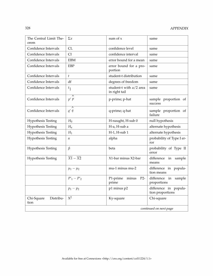
328 APPENDIX
The Central Limit The-orem
Σx sum of x same
Confidence Intervals CL confidence level same
Confidence Intervals CI confidence interval same
Confidence Intervals EBM error bound for a mean same
Confidence Intervals EBP error bound for a pro-portion
same
Confidence Intervals t student-t distribution same
Confidence Intervals df degrees of freedom same
Confidence Intervals t α2
student-t with a/2 areain right tail
same
Confidence Intervals p’^p p-prime; p-hat sample proportion of
success
Confidence Intervals q’^q q-prime; q-hat sample proportion of
failure
Hypothesis Testing H0 H-naught, H-sub 0 null hypothesis
Hypothesis Testing Ha H-a, H-sub a alternate hypothesis
Hypothesis Testing H1 H-1, H-sub 1 alternate hypothesis
Hypothesis Testing α alpha probability of Type I er-ror
Hypothesis Testing β beta probability of Type IIerror
Hypothesis Testing X1− X2 X1-bar minus X2-bar difference in samplemeans
µ1 − µ2 mu-1 minus mu-2 difference in popula-tion means
P’1 − P’2 P1-prime minus P2-prime
difference in sampleproportions
p1 − p2 p1 minus p2 difference in popula-tion proportions
Chi-Square Distribu-tion
X2 Ky-square Chi-square
continued on next page
Available for free at Connexions <http://cnx.org/content/col11224/1.1>

APPENDIX 329
O Observed Observed frequency
E Expected Expected frequency
Linear Regression andCorrelation
y = a + bx y equals a plus b-x equation of a line
^y y-hat estimated value of y
r correlation coefficient same
ε error same
SSE Sum of Squared Errors same
1.9s 1.9 times s cut-off value for out-liers
F-Distribution andANOVA
F F-ratio F ratio
Table 8.14
Available for free at Connexions <http://cnx.org/content/col11224/1.1>

330 APPENDIX
8.5 Formulas5
Formula 8.1: Factorialn! = n (n− 1) (n− 2) ... (1)
0! = 1Formula 8.2: Combinations( n
r)
= n!(n−r)!r!
Formula 8.3: Binomial DistributionX ∼ B (n, p)
P (X = x) =( n
x)
pxqn−x , for x = 0, 1, 2, ..., nFormula 8.4: Geometric DistributionX ∼ G (p)
P (X = x) = qx−1 p , for x = 1, 2, 3, ...Formula 8.5: Hypergeometric DistributionX ∼ H (r, b, n)
P (X = x) =
(( r
x )(
bn−x
)(
r+bn
))
Formula 8.6: Poisson DistributionX ∼ P (µ)
P (X = x) = µxe−µ
x!Formula 8.7: Uniform DistributionX ∼ U (a, b)
f (X) = 1b−a , a < x < b
Formula 8.8: Exponential DistributionX ∼ Exp (m)
f (x) = me−mx , m > 0, x ≥ 0Formula 8.9: Normal DistributionX ∼ N
(µ, σ2)
f (x) = 1σ√
2πe−(x−µ)2
2σ2 , −∞ < x < ∞
Formula 8.10: Gamma FunctionΓ (z) =
∫ ∞0 xz−1e−xdx z > 0
Γ(
12
)=√
π
Γ (m + 1) = m! for m, a nonnegative integer
otherwise: Γ (a + 1) = aΓ (a)Formula 8.11: Student-t DistributionX ∼ td f
5This content is available online at <http://cnx.org/content/m16301/1.7/>.
Available for free at Connexions <http://cnx.org/content/col11224/1.1>

APPENDIX 331
f (x) =
(1+ x2
n
)−(n+1)2 Γ( n+1
2 )√
nπΓ( n2 )
X = Z√Yn
Z ∼ N (0, 1) , Y ∼ X2d f ,n = degrees of freedom
Formula 8.12: Chi-Square DistributionX ∼ X2
d f
f (x) = xn−2
2 e−x2
2n2 Γ( n
2 ), x > 0 , n = positive integer and degrees of freedom
Formula 8.13: F DistributionX ∼ Fd f (n),d f (d)
d f (n) =degrees of freedom for the numerator
d f (d) =degrees of freedom for the denominator
f (x) =Γ( u+v
2 )Γ( u
2 )Γ( v2 )( u
v) u
2 x( u2−1)
[1 +
( uv)
x−.5(u+v)]
X = YuWv
, Y, W are chi-square
Available for free at Connexions <http://cnx.org/content/col11224/1.1>
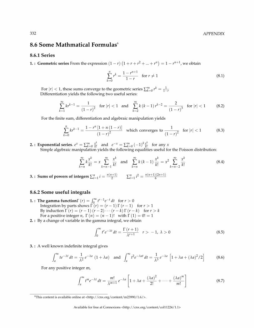
332 APPENDIX
8.6 Some Mathmatical Formulas6
8.6.1 Series
1. : Geometric series From the expression (1− r)(1 + r + r2 + ... + rn) = 1− rn+1, we obtain
n
∑k=0
rk =1− rn+1
1− rfor r 6= 1 (8.1)
For |r| < 1, these sums converge to the geometric series ∑∞k=0 rk = 1
1−rDifferentiation yields the following two useful series:
∞
∑k=1
krk−1 =1
(1− r)2 for |r| < 1 and∞
∑k=2
k (k− 1) rk−2 =2
(1− r)3 for |r| < 1 (8.2)
For the finite sum, differentiation and algebraic manipulation yields
n
∑k=0
krk−1 =1− rn [1 + n (1− r)]
(1− r)2 which converges to1
(1− r)2 for |r| < 1 (8.3)
2. : Exponential series. ex = ∑∞k=0
xk
k! and e−x = ∑∞k=0 (−1)k xk
k! for any xSimple algebraic manipulation yields the following equalities useful for the Poisson distribution:
∞
∑k=n
kxk
k!= x
∞
∑k=n−1
xk
k!and
∞
∑k=n
k (k− 1)xk
k!= x2
∞
∑k=n−2
xk
k!(8.4)
3. : Sums of powers of integers ∑ni=1 i = n(n+1)
2 ∑ni=1 i2 = n(n+1)(2n+1)
6
8.6.2 Some useful integrals
1. : The gamma functionΓ (r) =∫ ∞
0 tr−1e−t dt for r > 0Integration by parts shows Γ (r) = (r− 1) Γ (r− 1) for r > 1By induction Γ (r) = (r− 1) (r− 2) · · · (r− k) Γ (r− k) for r > kFor a positive integer n, Γ (n) = (n− 1)! with Γ (1) = 0! = 1
2. : By a change of variable in the gamma integral, we obtain∫ ∞
0tre−λt dt =
Γ (r + 1)λr+1 r > − 1, λ > 0 (8.5)
3. : A well known indefinite integral gives∫ ∞
ate−λt dt =
1λ2 e−λa (1 + λa) and
∫ ∞
at2e−λat dt =
1λ3 e−λa
[1 + λa + (λa)2/2
](8.6)
For any positive integer m,
∫ ∞
atme−λt dt =
m!λm+1 e−λa
[1 + λa +
(λa)2
2!+ · · ·+ (λa)m
m!
](8.7)
6This content is available online at <http://cnx.org/content/m23990/1.6/>.
Available for free at Connexions <http://cnx.org/content/col11224/1.1>
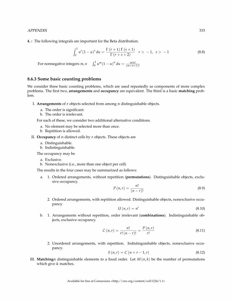
APPENDIX 333
4. : The following integrals are important for the Beta distribution.∫ 1
0ur(1− u)s du =
Γ (r + 1) Γ (s + 1)Γ (r + s + 2)
r > − 1, s > − 1 (8.8)
For nonnegative integers m, n∫ 1
0 um(1− u)n du = m!n!(m+n+1)!
8.6.3 Some basic counting problems
We consider three basic counting problems, which are used repeatedly as components of more complexproblems. The first two, arrangements and occupancy are equivalent. The third is a basic matching prob-lem.
I. Arrangements of r objects selected from among n distinguishable objects.
a. The order is significant.b. The order is irrelevant.
For each of these, we consider two additional alternative conditions.
a. No element may be selected more than once.b. Repitition is allowed.
II. Occupancy of n distinct cells by r objects. These objects are
a. Distinguishable.b. Indistinguishable.
The occupancy may be
a. Exclusive.b. Nonexclusive (i.e., more than one object per cell)
The results in the four cases may be summarized as follows:
a. 1. Ordered arrangements, without repetition (permutations). Distinguishable objects, exclu-sive occupancy.
P (n, r) =n!
(n− r)!(8.9)
2. Ordered arrangements, with repitition allowed. Distinguishable objects, nonexclusive occu-pancy.
U (n, r) = nr (8.10)
b. 1. Arrangements without repetition, order irrelevant (combinations). Indistinguishable ob-jects, exclusive occupancy.
C (n, r) =n!
r! (n− r)!=
P (n, r)r!
(8.11)
2. Unordered arrangements, with repetition. Indistinguishable objects, nonexclusive occu-pancy.
S (n, r) = C (n + r− 1, r) (8.12)
III. Matchingn distinguishable elements to a fixed order. Let M (n, k) be the number of permutationswhich give k matches.
Available for free at Connexions <http://cnx.org/content/col11224/1.1>

334 APPENDIX
Example 8.1: n = 5Natural order 1 2 3 4 5
Permutation 3 2 5 4 1 (Two matches– positions 2, 4)We reduce the problem to determining m (n, 0), as follows:
1. Select k places for matches in C (n, k) ways.2. Order the n− k remaining elements so that no matches in the other n− k places.
M (n, k) = C (n, k) M (n− k, 0) (8.13)
Some algebraic trickery shows that M (n, 0) is the integer nearest n!/e. These are easily calculated bythe MATLAB command M = round(gamma(n+1)/exp(1)) For example
� M = round(gamma([3:10]+1)/exp(1));
� disp([3:6;M(1:4);7:10;M(5:8)]')
3 2 7 1854
4 9 8 14833
5 44 9 133496
6 265 10 1334961
8.6.4 Extended binomial coefficients and the binomial series
: The ordinary binomial coefficient is C (n, k) = n!k!(n−k)! for integers n > 0, 0 ≤ k ≤ n
For any real x, any integer k, we extend the definition by
C (x, 0) = 1, C (x, k) = 0 for k < 0, and C (n, k) = 0 for a positive integer k > n (8.14)
and
C (x, k) =x (x− 1) (x− 2) · · · (x− k + 1)
k!otherwise (8.15)
Then Pascal’s relation holds: C (x, k) = C (x− 1, k− 1) + C (x− 1, k)The power series expansion about t = 0 shows
(1 + t)x = 1 + C (x, 1) t + C (x, 2) t2 + · · · ∀ x, − 1 < t < 1 (8.16)
For x = n, a positive integer, the series becomes a polynomial of degree n.
8.6.5 Cauchy’s equation
1. Let f be a real-valued function defined on (0, ∞), such that
a. f (t + u) = f (t) + f (u) for t, u > 0, andb. There is an open interval I on which f is bounded above (or is bounded below).
Then f (t) = f (1) t ∀ t > 02. Let f be a real-valued function defined on (0, ∞) such that
a. f (t + u) = f (t) f (u) ∀ t, u > 0, andb. There is an interval on which f is bounded above.
Then, either f (t) = 0 for t > 0 , or there is a constant a such that f (t) = eat for t > 0
[For a proof, see Billingsley, Probability and Measure, second edition, appendix A20]
Available for free at Connexions <http://cnx.org/content/col11224/1.1>

APPENDIX 335
8.6.6 Countable and uncountable sets
A set (or class) is countable iff either it is finite or its members can be put into a one-to-one correspondencewith the natural numbers.Examples
• The set of odd integers is countable.• The finite set {n : 1 ≤ n ≤ 1000} is countable.• The set of all rational numbers is countable. (This is established by an argument known as diagonal-
ization).• The set of pairs of elements from two countable sets is countable.• The union of a countable class of countable sets is countable.
A set is uncountable iff it is neither finite nor can be put into a one-to-one correspondence with the naturalnumbers.Examples
• The class of positive real numbers is uncountable. A well known operation shows that the assumptionof countability leads to a contradiction.
• The set of real numbers in any finite interval is uncountable, since these can be put into a one-to-onecorrespondence of the class of all positive reals.
Available for free at Connexions <http://cnx.org/content/col11224/1.1>
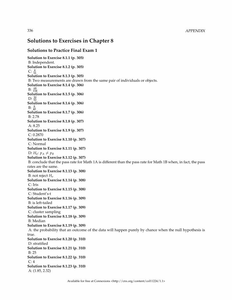
336 APPENDIX
Solutions to Exercises in Chapter 8
Solutions to Practice Final Exam 1
Solution to Exercise 8.1.1 (p. 305)B: Independent.
Solution to Exercise 8.1.2 (p. 305)C: 4
16Solution to Exercise 8.1.3 (p. 305)B: Two measurements are drawn from the same pair of individuals or objects.
Solution to Exercise 8.1.4 (p. 306)B: 68
118Solution to Exercise 8.1.5 (p. 306)D: 30
52Solution to Exercise 8.1.6 (p. 306)B: 8
40Solution to Exercise 8.1.7 (p. 306)B: 2.78
Solution to Exercise 8.1.8 (p. 307)A: 8.25
Solution to Exercise 8.1.9 (p. 307)C: 0.2870
Solution to Exercise 8.1.10 (p. 307)C: Normal
Solution to Exercise 8.1.11 (p. 307)D: Ha: pA 6= pB
Solution to Exercise 8.1.12 (p. 307)B: conclude that the pass rate for Math 1A is different than the pass rate for Math 1B when, in fact, the passrates are the same.Solution to Exercise 8.1.13 (p. 308)B: not reject Ho
Solution to Exercise 8.1.14 (p. 308)C: Iris
Solution to Exercise 8.1.15 (p. 308)C: Student’s-t
Solution to Exercise 8.1.16 (p. 309)B: is left-tailed
Solution to Exercise 8.1.17 (p. 309)C: cluster sampling
Solution to Exercise 8.1.18 (p. 309)B: Median
Solution to Exercise 8.1.19 (p. 309)A: the probability that an outcome of the data will happen purely by chance when the null hypothesis is
true.Solution to Exercise 8.1.20 (p. 310)D: stratified
Solution to Exercise 8.1.21 (p. 310)B: 25
Solution to Exercise 8.1.22 (p. 310)C: 4
Solution to Exercise 8.1.23 (p. 310)A: (1.85, 2.32)
Available for free at Connexions <http://cnx.org/content/col11224/1.1>
APPENDIX 337
Solution to Exercise 8.1.24 (p. 310)C: Both above are correct.
Solution to Exercise 8.1.25 (p. 311)C: 5.8
Solution to Exercise 8.1.26 (p. 311)C: 0.6321
Solution to Exercise 8.1.27 (p. 311)A: 0.8413
Solution to Exercise 8.1.28 (p. 311)A: (0.6030, 0.7954)
Solution to Exercise 8.1.29 (p. 311)A: N
(145, 14√
10
)Solution to Exercise 8.1.30 (p. 312)D: 3.66
Solution to Exercise 8.1.31 (p. 312)B: 5.1
Solution to Exercise 8.1.32 (p. 312)A: 13.46
Solution to Exercise 8.1.33 (p. 312)B: There is a strong linear pattern. Therefore, it is most likely a good model to be used.
Solution to Exercise 8.1.34 (p. 313)B: Chi23
Solution to Exercise 8.1.35 (p. 313)D: 70
Solution to Exercise 8.1.36 (p. 313)B: There is sufficient evidence to conclude that the choice of major and the gender of the student are not
independent of each other.Solution to Exercise 8.1.37 (p. 313)A: Chi2 goodness of fit
Solutions to Practice Final Exam 2
Solution to Exercise 8.2.1 (p. 314)B: parameter
Solution to Exercise 8.2.2 (p. 314)A
Solution to Exercise 8.2.3 (p. 315)C: 7
Solution to Exercise 8.2.4 (p. 315)C: 0.02
Solution to Exercise 8.2.5 (p. 315)C: none of the above
Solution to Exercise 8.2.6 (p. 315)D: 100
140Solution to Exercise 8.2.7 (p. 316)A: ≈ 0
Solution to Exercise 8.2.8 (p. 316)B: The values for x are: {1, 2, 3, ..., 14}
Solution to Exercise 8.2.9 (p. 316)C: 0.9417
Available for free at Connexions <http://cnx.org/content/col11224/1.1>
338 APPENDIX
Solution to Exercise 8.2.10 (p. 316)D: Binomial
Solution to Exercise 8.2.11 (p. 317)D: 8.7
Solution to Exercise 8.2.12 (p. 317)A: -1.96
Solution to Exercise 8.2.13 (p. 317)A: 0.6321
Solution to Exercise 8.2.14 (p. 318)D: 360
Solution to Exercise 8.2.15 (p. 318)B: N
(72, 72√
50
)Solution to Exercise 8.2.16 (p. 318)A: 3
9Solution to Exercise 8.2.17 (p. 318)D
Solution to Exercise 8.2.18 (p. 319)B: 5.5
Solution to Exercise 8.2.19 (p. 319)D: 6.92
Solution to Exercise 8.2.20 (p. 319)A: 5
Solution to Exercise 8.2.21 (p. 319)B: 0.8541
Solution to Exercise 8.2.22 (p. 320)B: 0.2
Solution to Exercise 8.2.23 (p. 320)A: -1
Solution to Exercise 8.2.24 (p. 320)C: matched pairs, dependent groups
Solution to Exercise 8.2.25 (p. 320)D: Reject Ho. There is sufficient evidence to conclude that there is a difference in the mean scores.
Solution to Exercise 8.2.26 (p. 321)C: There is sufficient evidence to conclude that the proportion for males is higher than the proportion for
females.Solution to Exercise 8.2.27 (p. 321)B: No
Solution to Exercise 8.2.28 (p. 321)B: p-value is close to 1.
Solution to Exercise 8.2.29 (p. 321)B: No
Solution to Exercise 8.2.30 (p. 322)C: y = 79.96x− 0.0094
Solution to Exercise 8.2.31 (p. 322)D: We should not be estimating here.
Solution to Exercise 8.2.32 (p. 322)A
Solution to Exercise 8.2.33 (p. 322)A: The p–value is > 0.10. There is insufficient information to conclude that the distribution is not uniform.Solution to Exercise 8.2.34 (p. 323)C: The test is to determine if the different groups have the same means.
Available for free at Connexions <http://cnx.org/content/col11224/1.1>

Tables1
NOTE: When you are finished with the table link, use the back button on your browser to returnhere.
Tables (NIST/SEMATECH e-Handbook of Statistical Methods, http://www.itl.nist.gov/div898/handbook/,January 3, 2009)
• Student-t table2
• Normal table3
• Chi-Square table4
• F-table5
• All four tables can be accessed by going to http://www.itl.nist.gov/div898/handbook/eda/section3/eda367.htm6
95% Critical Values of the Sample Correlation Coefficient Table
• 95% Critical Values of the Sample Correlation Coefficient7
NOTE: The url for this table is http://cnx.org/content/m17098/latest/
1This content is available online at <http://cnx.org/content/m19138/1.3/>.2http://www.itl.nist.gov/div898/handbook/eda/section3/eda3672.htm3http://www.itl.nist.gov/div898/handbook/eda/section3/eda3671.htm4http://www.itl.nist.gov/div898/handbook/eda/section3/eda3674.htm5http://www.itl.nist.gov/div898/handbook/eda/section3/eda3673.htm6http://www.itl.nist.gov/div898/handbook/eda/section3/eda367.htm7http://cnx.org/content/m17098/latest/
Available for free at Connexions <http://cnx.org/content/col11224/1.1>
339

340 GLOSSARY
Glossary
A AverageA number that describes the central tendency of the data. There are a number of specializedaverages, including the arithmetic mean, weighted mean, median, mode, and geometric mean.
B Bernoulli TrialsAn experiment with the following characteristics:• There are only 2 possible outcomes called “success” and “failure” for each trial.• The probability p of a success is the same for any trial (so the probability q = 1− p of a
failure is the same for any trial).
Binomial DistributionA discrete random variable (RV) which arises from Bernoulli trials. There are a fixed number, n,of independent trials. “Independent” means that the result of any trial (for example, trial 1)does not affect the results of the following trials, and all trials are conducted under the sameconditions. Under these circumstances the binomial RV X is defined as the number of successesin n trials. The notation is: X∼B (n, p). The mean is µ = np and the standard deviation isσ = √npq. The probability of exactly x successes in n trials is P (X = x) =
( nx)
pxqn−x.
binomial distributionsA probability distribution for independent events for which there are only two possibleoutcomes such as a coin flip. If one of the two outcomes is defined as a success, then theprobability of exactly x successes out of N trials (events) is given by:
Pr [x] =N!
x! (N − x)!πx(1− π)N−x
where π is the probability of success one one trial.
C CardinalityThe cardinality of a set “A” is equal to numbers of elements in the set.
Cartesian productThe Cartesian product of two non-empty sets “A” and “B” is the set of all ordered pairs of theelements from two sets.
Complement of a setThe complement of a set “A” consists of elements, which are elements of “U”, but not theelements of “A”.
Conditional ProbabilityThe likelihood that an event will occur given that another event has already occurred.
conditional probabilityThe probability that event A occurs given that event B has already occurred is called theconditional probability of A given B. Symbolically, this is written as Pr [ A | B]. The probabilityit rains on Monday given that it rained on Sunday would be written asPr (Rain on Sunday, Rain on Monday).
Available for free at Connexions <http://cnx.org/content/col11224/1.1>
GLOSSARY 341
Contingency Table
The method of displaying a frequency distribution as a table with rows and columns to showhow two variables may be dependent (contingent) upon each other. The table provides an easyway to calculate conditional probabilities.
Continuous Random Variable
A random variable (RV) whose outcomes are measured.
Example: The height of trees in the forest is a continuous RV.
continuous variables
Variables that can take on any value in a certain range. Time and distance are continuous;gender, SAT score and "time rounded to the nearest second" are not. Variables that are notcontinuous are known asdiscrete variables. No measured variable is truly continuous;however, discrete variables measured with enough precision can often be consideredcontinuous for practical purposes.
Cumulative Relative Frequency
The term applies to an ordered set of observations from smallest to largest. The CumulativeRelative Frequency is the sum of the relative frequencies for all values that are less than or equalto the given value.
D Data
A set of observations (a set of possible outcomes). Most data can be put into two groups:qualitative (hair color, ethnic groups and other attributes of the population) and quantitative(distance traveled to college, number of children in a family, etc.). Quantitative data can beseparated into two subgroups: discrete and continuous. Data is discrete if it is the result ofcounting (the number of students of a given ethnic group in a class, the number of books on ashelf, etc.). Data is continuous if it is the result of measuring (distance traveled, weight ofluggage, etc.)
Difference of sets
The difference of sets “A-B” is the set of all elements of “A”, which do not belong to “B”.
Discrete Random Variable
A random variable (RV) whose outcomes are counted.
discrete
Variables that can only take on a finite number of values are called "discrete variables." Allqualitative variables are discrete. Some quantitative variables are discrete, such asperformance rated as 1,2,3,4, or 5, or temperature rounded to the nearest degree. Sometimes, avariable that takes on enough discrete values can be considered to be continuous for practicalpurposes. One example is time to the nearest millisecond. Variables that can take on an infinitenumber of possible values are called continuous variables.
E Equally Likely
Each outcome of an experiment has the same probability.
Event
A subset in the set of all outcomes of an experiment. The set of all outcomes of an experiment iscalled a sample space and denoted usually by S. An event is any arbitrary subset in S. It cancontain one outcome, two outcomes, no outcomes (empty subset), the entire sample space, etc.Standard notations for events are capital letters such as A, B, C, etc.
Available for free at Connexions <http://cnx.org/content/col11224/1.1>
342 GLOSSARY
Expected Value
Expected arithmetic average when an experiment is repeated many times. (Also called themean). Notations: E (x) , µ. For a discrete random variable (RV) with probability distributionfunction P (x) ,the definition can also be written in the form E (x) = µ = ∑ xP (x) .
Experiment
A planned activity carried out under controlled conditions.
Exponential Distribution
A continuous random variable (RV) that appears when we are interested in the intervals of timebetween some random events, for example, the length of time between emergency arrivals at ahospital. Notation: X~Exp (m). The mean is µ = 1
m and the standard deviation is σ = 1m . The
probability density function is f (x) = me−mx, x ≥ 0 and the cumulative distribution functionis P (X ≤ x) = 1− e−mx.
F Frequency
The number of times a value of the data occurs.
G Geometric Distribution
A discrete random variable (RV) which arises from the Bernoulli trials. The trials are repeateduntil the first success. The geometric variable X is defined as the number of trials until the firstsuccess. Notation: X∼ G (p). The mean is µ = 1
p and the standard deviation is
σ =√
1p ·(
1p − 1
)The probability of exactly x failures before the first success is given by the
formula: P (X = x) = p (1− p)x−1.
H Hypergeometric Distribution
A discrete random variable (RV) that is characterized by
• A fixed number of trials.• The probability of success is not the same from trial to trial.
We sample from two groups of items when we are interested in only one group. X is defined asthe number of successes out of the total number of items chosen. Notation: X~H (r, b, n) .,where r = the number of items in the group of interest, b = the number of items in the group notof interest, and n = the number of items chosen.
I independent events
Intuitively, two events A and B are independent if the occurrence of one has no effect on theprobability of the occurrence of the other. For example, if you throw two dice, the probabilitythat the second one comes up 1 is independent of whether the first die came up 1. Formally, thiscan be stated in terms of conditional probabilities: Pr [ A | B] = Pr [A] andPr [ B | A] = Pr [B].
Independent Events
The occurrence of one event has no effect on the probability of the occurrence of any other event.Events A and B are independent if one of the following is true: (1). P (A|B) = P (A) ; (2)P (B|A) = P (B) ; (3) P (AandB) = P (A) P (B).
Intersection of two sets
The intersection of sets “A” and “B” is the set of all elements common to both “A” and “B”.
Available for free at Connexions <http://cnx.org/content/col11224/1.1>

GLOSSARY 343
L levels of measurement
Measurement scales differ in their level of measurement. There are four common levels ofmeasurement:
• Nominal scales are only labels.• Ordinal Scales are ordered but are not truly quantitative. Equal intervals on the ordinal
scale do not imply equal intervals on the underlying trait.• Interval scales are are ordered and equal intervals equal intervals on the underlying trait.
However, interval scales do not have a true zero point.• Ratio scales are interval scales that do have a true zero point. With ratio scales, it is sensible
to talk about one value being twice as large as another, for example.
M Mean
A number that measures the central tendency. A common name for mean is ’average.’ The term’mean’ is a shortened form of ’arithmetic mean.’ By definition, the mean for a sample (denotedby x) is x = Sum of all values in the sample
Number of values in the sample , and the mean for a population (denoted by µ) is
µ = Sum of all values in the populationNumber of values in the population .
Median
A number that separates ordered data into halves. Half the values are the same number orsmaller than the median and half the values are the same number or larger than the median.The median may or may not be part of the data.
Mode
The value that appears most frequently in a set of data.
Mutually Exclusive
An observation cannot fall into more than one class (category). Being in more than one categoryprevents being in a mutually exclusive category.
N nominal scale
A nominal scale is one of four Levels of Measurement. No ordering is implied, andaddition/subtraction and multiplication/division would be inappropriate for a variable on anominal scale. {Female, Male} and {Buddhist, Christian, Hindu, Muslim} have no naturalordering (except alphabetic). Occasionally, numeric values are nominal: for instance, if avariable was coded as Female=1, Male=2, the set {1, 2} is still nominal.
Normal Distribution
A continuous random variable (RV) with pdf f(x) = 1σ√
2πe−(x−µ)2/2σ2, where µ is the mean of
the distribution and σ is the standard deviation. Notation: X ∼ N (µ, σ). If µ = 0 and σ = 1, theRV is called the standard normal distribution.
O ordinal scale
One of four levels of measurement, an ordinal scale is a set of ordered values. However, there isno set distance between scale values. For instance, for the scale: (Very Poor, Poor, Average,Good, Very Good) is an ordinal scale. You can assign numerical values to an ordinal scale:rating performance such as 1 for "Very Poor," 2 for "Poor," etc, but there is no assurance that thedifference between a score of 1 and 2 means the same thing as the difference between a score ofand 3.
Outcome (observation)
Available for free at Connexions <http://cnx.org/content/col11224/1.1>

344 GLOSSARY
A particular result of an experiment.
Outlier
An observation that does not fit the rest of the data.
P Poisson Distribution
A discrete random variable (RV) that counts the number of times a certain event will occur in aspecific interval. Characteristics of the variable:
• The probability that the event occurs in a given interval is the same for all intervals.• The events occur with a known mean and independently of the time since the last event.
The distribution is defined by the mean µ of the event in the interval. Notation: X~P (µ). Themean is µ = np. The standard deviation is σ = √µ. The probability of having exactly x
successes in r trials is P (X = x) = e−µ µx
x! . The Poisson distribution is often used to approximatethe binomial distribution when n is “large” and p is “small” (a general rule is that n should begreater than or equal to 20 and p should be less than or equal to .05).
Population
The collection, or set, of all individuals, objects, or measurements whose properties are beingstudied.
Power set
The collection of all subsets of a set “A” is called power set, P(A).
Probability
A number between 0 and 1, inclusive, that gives the likelihood that a specific event will occur.The foundation of statistics is given by the following 3 axioms (by A. N. Kolmogorov, 1930’s):Let S denote the sample space and A and B are two events in S . Then:
• 0 ≤ P (A) ≤ 1;.• If A and B are any two mutually exclusive events, then P (AorB) = P (A) + P (B).• P (S) = 1.
probability distribution
For a discrete random variable, a probability distribution contains the probability of eachpossible outcome. The sum of all probabilities is always 1.0.
Probability Distribution Function (PDF)
A mathematical description of a discrete random variable (RV), given either in the form of anequation (formula) , or in the form of a table listing all the possible outcomes of an experimentand the probability associated with each outcome.
Example: A biased coin with probability 0.7 for a head (in one toss of the coin) is tossed 5 times.We are interested in the number of heads (the RV X = the number of heads). X is Binomial, so
X ∼ B (5, 0.7) and P (X = x) =
5
x
.7x.35−xor in the form of the table:
Available for free at Connexions <http://cnx.org/content/col11224/1.1>
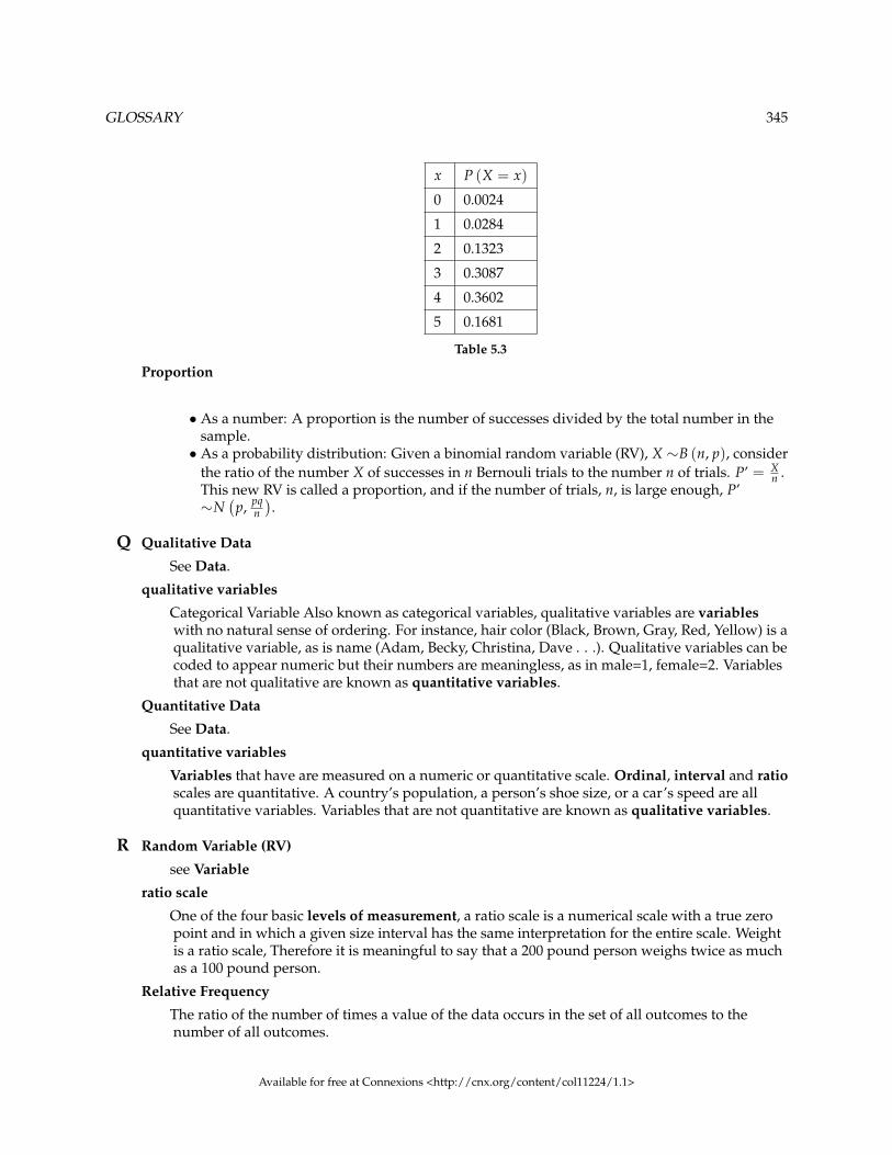
GLOSSARY 345
x P (X = x)
0 0.0024
1 0.0284
2 0.1323
3 0.3087
4 0.3602
5 0.1681
Table 5.3
Proportion
• As a number: A proportion is the number of successes divided by the total number in thesample.• As a probability distribution: Given a binomial random variable (RV), X ∼B (n, p), consider
the ratio of the number X of successes in n Bernouli trials to the number n of trials. P’ = Xn .
This new RV is called a proportion, and if the number of trials, n, is large enough, P’∼N
(p, pq
n).
Q Qualitative Data
See Data.
qualitative variables
Categorical Variable Also known as categorical variables, qualitative variables are variableswith no natural sense of ordering. For instance, hair color (Black, Brown, Gray, Red, Yellow) is aqualitative variable, as is name (Adam, Becky, Christina, Dave . . .). Qualitative variables can becoded to appear numeric but their numbers are meaningless, as in male=1, female=2. Variablesthat are not qualitative are known as quantitative variables.
Quantitative Data
See Data.
quantitative variables
Variables that have are measured on a numeric or quantitative scale. Ordinal, interval and ratioscales are quantitative. A country’s population, a person’s shoe size, or a car’s speed are allquantitative variables. Variables that are not quantitative are known as qualitative variables.
R Random Variable (RV)
see Variable
ratio scale
One of the four basic levels of measurement, a ratio scale is a numerical scale with a true zeropoint and in which a given size interval has the same interpretation for the entire scale. Weightis a ratio scale, Therefore it is meaningful to say that a 200 pound person weighs twice as muchas a 100 pound person.
Relative Frequency
The ratio of the number of times a value of the data occurs in the set of all outcomes to thenumber of all outcomes.
Available for free at Connexions <http://cnx.org/content/col11224/1.1>
346 GLOSSARY
S Sample
A portion of the population understudy. A sample is representative if it characterizes thepopulation being studied.
Sample Space
The set of all possible outcomes of an experiment.
Set
A set is a collection of well defined objects.
Standard Deviation
A number that is equal to the square root of the variance and measures how far data values arefrom their mean. Notation: s for sample standard deviation and σ for population standarddeviation.
Standard Normal Distribution
A continuous random variable (RV) X~N (0, 1) .. When X follows the standard normaldistribution, it is often noted as Z~N (0, 1).
Subset
A set, “A” is a subset of set “B”, if each member of set “A” is also a member of set “B”.
T Tree Diagram
The useful visual representation of a sample space and events in the form of a “tree” withbranches marked by possible outcomes simultaneously with associated probabilities(frequencies, relative frequencies).
U Uniform Distribution
A continuous random variable (RV) that has equally likely outcomes over the domain,a < x < b. Often referred as the Rectangular distribution because the graph of the pdf has theform of a rectangle. Notation: X~U (a, b). The mean is µ = a+b
2 and the standard deviation is
σ =√
(b−a)2
12 The probability density function is f (X) = 1b−a for a < x < b or a ≤ x ≤ b. The
cumulative distribution is P (X ≤ x) = x−ab−a .
Union of two sets
The union of sets “A” and “B” is a third set, which consists all the elements of two sets.
V Variable (Random Variable)
A characteristic of interest in a population being studied. Common notation for variables areupper case Latin letters X, Y, Z,...; common notation for a specific value from the domain (set ofall possible values of a variable) are lower case Latin letters x, y, z,.... For example, if X is thenumber of children in a family, then x represents a specific integer 0, 1, 2, 3, .... Variables instatistics differ from variables in intermediate algebra in two following ways.
• The domain of the random variable (RV) is not necessarily a numerical set; the domain maybe expressed in words; for example, if X = hair color then the domain is {black, blond, gray,green, orange}.•We can tell what specific value x of the Random Variable X takes only after performing the
experiment.
variables
Available for free at Connexions <http://cnx.org/content/col11224/1.1>
GLOSSARY 347
Something that can take on different values. For example, different subjects in an experimentweight different amounts. Therefore "weight" is a variable in the experiment. Or, subjects maybe given different doses of a drug. This would make "dosage" a variable. Variables can bedependent or independent, qualitative or quantitative, and continuous or discrete.
Variance
Mean of the squared deviations from the mean. Square of the standard deviation. For a set ofdata, a deviation can be represented as x− x where x is a value of the data and x is the samplemean. The sample variance is equal to the sum of the squares of the deviations divided by thedifference of the sample size and 1.
Venn Diagram
The visual representation of a sample space and events in the form of circles or ovals showingtheir intersections.
Z z-score
The linear transformation of the form z = x−µσ . If this transformation is applied to any normal
distribution X~N (µ, σ) , the result is the standard normal distribution Z~N (0, 1). If thistransformation is applied to any specific value x of the RV with mean µ and standard deviationσ , the result is called the z-score of x. Z-scores allow us to compare data that are normallydistributed but scaled differently.
Available for free at Connexions <http://cnx.org/content/col11224/1.1>

348 INDEX
Index of Keywords and Terms
Keywords are listed by the section with that keyword (page numbers are in parentheses). Keywordsdo not necessarily appear in the text of the page. They are merely associated with that section. Ex.apples, § 1.1 (1) Terms are referenced by the page they appear on. Ex. apples, 1
( (i), 112, 113(ii), 112, 115(iii), 112, 115
1 1 :, 991:, 64, 122
2 2 :, 992:, 64, 123
3 3 :, 993:, 123
4 4 :, 99
5 5 :, 99
6 6 :, 99
7 7 :, 99
8 8 :, 99
A A AND B, § 4.3(146)A OR B, § 4.3(146)addition, § 4.4(149)algebra, § 3.11(132), § 3.12(137), § 3.13(138)answer, § 1.5(17)area, § 6.2(239)average, § 1.1(1), § 5.3(183)
B bar, § 2.2(31)Bernoulli, § 5.5(186), § 5.15(206)Bernoulli Trial, 187binomial, § 5.4(186), § 5.5(186), § 5.9(197),§ 5.15(206)Binomial coefficients, § 8.6(332)Binomial Distribution, § 5.19(226), 227binomial distributions, 226binomial probability distribution, 187Binomial series, § 8.6(332)box, § 2.7(49), § 6.10(270)boxes, § 2.2(31)
C Cardinality, 61cards, § 5.17(219)cartesian, § 3.9(116), § 3.10(125)Cartesian product, 117categorical, § 1.1(1)Cauchy’s equation, § 8.6(332)chance, § 4.3(146), § 4.5(152)Chi-Square, § 9(339)cluster, § 1.7(22)cluster sample, § 1.3(9)combinations, § 3.13(138)Complement of a set, 92complements, § 3.1(57), § 3.2(61), § 3.4(69),§ 3.5(78), § 3.7(100), § 3.8(107), § 3.9(116),§ 3.10(125)condition, § 4.5(152)conditional, § 4.3(146), § 4.10(163), 246conditional probability, 148contingency, § 4.6(155), § 4.8(160)contingency table, 155Continuous, § 1.2(3), 3, § 1.7(22), § 6.1(237),§ 6.2(239), § 6.3(242), § 6.4(249), § 6.5(255),§ 6.6(256), § 6.7(259), § 6.8(261), § 6.9(267),§ 6.10(270)continuous random variable, 249convenience, § 1.7(22)Convenience sampling, § 1.3(9)Countable and uncountable sets, § 8.6(332)Counting, § 1.2(3)Counting problems, § 8.6(332)critical value, 283cumulative, § 1.6(17), § 1.7(22)cumulative distribution function (CDF), 250Cumulative relative frequency, 18
D data, § 1.1(1), 2, § 1.2(3), § 1.4(15), § 1.7(22),§ 1.8(23), § 2.2(31)descriptive, § 2.1(27), § 2.7(49)deviation, § 2.7(49)diagram, § 3.1(57), § 3.2(61), § 3.3(68),§ 3.4(69), § 3.5(78), § 3.7(100), § 3.8(107),
Available for free at Connexions <http://cnx.org/content/col11224/1.1>
INDEX 349
§ 3.9(116), § 3.10(125), § 3.14(139)dice, § 5.18(223)difference, § 3.1(57), § 3.2(61), § 3.4(69),§ 3.5(78), § 3.7(100), § 3.8(107), § 3.9(116),§ 3.10(125)Difference of sets, § 3.6(88), 88Discrete, § 1.2(3), 3, § 1.7(22), § 5.1(181),§ 5.2(182), § 5.3(183), § 5.4(186), § 5.5(186),§ 5.6(189), § 5.7(192), § 5.8(194), § 5.9(197),§ 5.10(199), § 5.15(206), § 5.16(216), § 5.17(219),§ 5.18(223)distribution, § 5.1(181), § 5.2(182), § 5.5(186),§ 5.6(189), § 5.7(192), § 5.8(194), § 5.10(199),§ 5.16(216), § 5.17(219), § 5.18(223), § 6.1(237),§ 6.2(239), § 6.3(242), § 6.4(249), § 6.5(255),§ 6.6(256), § 6.7(259), § 6.8(261), § 6.9(267),§ 6.10(270)
E elementary, § 2.1(27), § 2.3(35), § 2.4(38),§ 2.5(39), § 2.6(48), § 2.7(49), § 2.8(52),§ 3.3(68), § 3.14(139), § 4.4(149), § 4.6(155),§ 4.7(159), § 4.8(160), § 4.9(162), § 4.10(163),§ 4.11(174), § 5.1(181), § 5.2(182), § 5.3(183),§ 5.4(186), § 5.5(186), § 5.6(189), § 5.7(192),§ 5.8(194), § 5.9(197), § 5.10(199), § 5.12(202),§ 5.13(203), § 5.14(205), § 5.15(206), § 5.16(216),§ 5.17(219), § 5.18(223), § 6.1(237), § 6.2(239),§ 6.3(242), § 6.4(249), § 6.5(255), § 6.6(256),§ 6.7(259), § 6.8(261), § 6.9(267), § 6.10(270),§ 7.1(277), § 7.2(278), § 7.3(279), § 7.4(281),§ 7.5(281), § 7.6(285), § 7.7(286), § 7.8(288),§ 7.9(294), § 7.10(296), § 7.11(299), § 8.1(305),§ 8.2(314), § 8.3(324), § 8.4(325), § 8.5(330)empirical, § 6.10(270)equally likely, § 4.3(146), 147event, § 4.3(146), 146, § 4.10(163)exclusive, § 4.5(152), § 4.9(162), § 4.10(163)exercise, § 4.8(160), § 5.15(206), § 5.16(216),§ 5.17(219), § 5.18(223), § 6.6(256), § 6.7(259),§ 6.9(267), § 6.10(270)exercises, § 4.11(174)expected, § 5.3(183)expected value, 183experiment, § 4.3(146), 146, § 5.1(181),§ 5.5(186), § 5.7(192), § 5.8(194), § 5.17(219),§ 5.18(223)exponential, § 6.1(237), § 6.4(249), 249,§ 6.5(255), § 6.7(259)
F f, § 9(339)formula, § 4.7(159), § 5.9(197), § 6.5(255)frequency, § 1.6(17), 18, § 1.7(22), § 1.8(23), 31,
§ 2.7(49), § 4.3(146)function, § 5.2(182), § 5.4(186), § 5.5(186),§ 5.6(189), § 5.7(192), § 5.9(197), § 5.16(216),§ 6.1(237), § 6.3(242), § 6.4(249), § 6.6(256),§ 6.7(259), § 6.8(261), § 6.9(267)functions, § 6.2(239)
G geometric, § 5.4(186), § 5.6(189), § 5.9(197),§ 5.15(206)graph, § 2.1(27), § 6.1(237), § 6.6(256),§ 6.7(259), § 6.8(261)
H histogram, § 2.2(31), § 2.7(49), § 6.10(270)homework, § 2.7(49), § 4.8(160), § 4.11(174),§ 5.15(206), § 5.16(216), § 5.17(219), § 5.18(223),§ 6.6(256), § 6.7(259), § 6.8(261), § 6.9(267),§ 6.10(270)hypergeometric, § 5.4(186), § 5.7(192),§ 5.15(206)hypergeometric probability, 192hypergeometrical, § 5.9(197)
I independent, 149, § 4.5(152), 152, § 4.9(162),§ 4.10(163)Integrals, § 8.6(332)intersection, § 3.1(57), § 3.2(61), § 3.4(69),§ 3.5(78), § 3.7(100), § 3.8(107), § 3.9(116),§ 3.10(125)Intersection of two sets, 78Introduction, § 4.1(145), § 5.1(181)
K key terms, § 4.3(146)
L lab, § 5.17(219), § 5.18(223), § 6.10(270)large, § 5.3(183)law, § 5.3(183)leaf, § 2.1(27)likelihood, § 4.2(146)long term, § 4.3(146)long-term, § 5.3(183)
M mean, 2, 35, § 2.7(49), § 5.3(183), 183measurement, § 1.4(15)Measuring, § 1.2(3)median, 35, § 2.7(49)mode, 36, § 2.7(49)multiplication, § 4.4(149)mutually, § 4.5(152), § 4.9(162), § 4.10(163)mutually exclusive, 149, 153
N nonsampling errors, § 1.3(9)Normal, § 9(339)Note :, 125
Available for free at Connexions <http://cnx.org/content/col11224/1.1>

350 INDEX
numbers, § 5.3(183)numerical, § 1.1(1)
O outcome, § 4.3(146), 146, § 4.5(152)outlier, 28
P parameter, § 1.1(1), 1, § 1.7(22)PDF, § 5.2(182)percentile, § 2.7(49)permutations, § 3.12(137)plot, § 2.7(49), § 6.10(270)Poisson, § 5.4(186), § 5.8(194), § 5.9(197),§ 5.15(206)Poisson probability distribution, 194population, § 1.1(1), 1, 15, § 1.7(22), § 6.9(267)Power set, 64practice, § 1.8(23), § 2.7(49), § 4.8(160),§ 4.9(162), § 4.11(174), § 5.16(216), § 6.6(256),§ 6.7(259), § 6.9(267)probability, § 1.7(22), § 3.3(68), § 3.11(132),§ 3.12(137), § 3.13(138), § 3.14(139), § 4.1(145),§ 4.2(146), 146, § 4.3(146), 147, § 4.4(149),§ 4.5(152), § 4.6(155), § 4.7(159), § 4.8(160),§ 4.9(162), § 4.10(163), § 4.11(174), § 5.2(182),§ 5.3(183), § 5.4(186), § 5.5(186), § 5.6(189),§ 5.7(192), § 5.8(194), § 5.9(197), § 5.10(199),§ 5.16(216), § 5.17(219), § 5.18(223), § 6.1(237),§ 6.2(239), § 6.3(242), § 6.5(255), § 6.6(256),§ 6.7(259), § 6.9(267)probability distribution function, 182problem, § 5.15(206)Problem 1 :, 59, 118, 126Problem 1:, 64, 98, 103Problem 2 :, 119, 126Problem 2:, 104Problem 3 :, 120, 128Problem 3:, 105Problem 4 :, 128Problem 4:, 106Problem 5 :, 129Problem 6 :, 130Problem 7 :, 131Problem 8 :, 132Problem :, 111proper, § 3.1(57), § 3.2(61), § 3.4(69), § 3.5(78),§ 3.7(100), § 3.8(107), § 3.9(116), § 3.10(125)proportion, § 1.1(1), 2
Q Qualitative, § 1.2(3), § 1.7(22)Qualitative data, 3Quantitative, § 1.2(3), § 1.7(22)Quantitative data, 3
quartile, § 2.7(49)
R random, § 1.7(22), § 4.2(146), § 5.1(181),§ 5.2(182), § 5.3(183), § 5.4(186), § 5.5(186),§ 5.6(189), § 5.7(192), § 5.8(194), § 5.9(197),§ 5.10(199), § 5.15(206), § 5.16(216), § 5.17(219),§ 5.18(223), § 6.1(237), § 6.2(239), § 6.3(242),§ 6.4(249), § 6.5(255), § 6.6(256), § 6.7(259),§ 6.8(261), § 6.9(267)random sampling, § 1.3(9)random variable, 181randomness, § 4.2(146)relative, § 1.6(17), § 1.7(22), § 4.3(146)relative frequency, 18, 31replacement, § 1.7(22)representative, § 1.1(1)review, § 4.11(174), § 5.16(216), § 6.9(267)round, § 1.5(17)rounding, § 1.5(17)rule, § 4.4(149)
S sample, § 1.1(1), 1, § 1.3(9), § 1.4(15), § 1.7(22)sample space, 139, § 4.3(146), 146, 149samples, 15sampling, § 1.1(1), 1, § 1.3(9), § 1.4(15),§ 1.7(22), § 1.8(23)sampling distribution, 37sampling errors, § 1.3(9)sampling variability of a statistic, 41Series, § 8.6(332)Set, 57sets, § 3.1(57), § 3.2(61), § 3.4(69), § 3.5(78),§ 3.7(100), § 3.8(107), § 3.9(116), § 3.10(125)simple, § 1.7(22)simple random sampling, § 1.3(9)size, § 1.4(15)Solution :, 59, 64, 99, 103, 104, 105, 106, 118,119, 120, 126, 126, 128, 128, 129, 130, 131, 132standard, § 2.7(49)standard deviation, 39standard normal distribution, 278statistic, § 1.1(1), 1, § 1.7(22), 37Statistics, § 1.2(3), § 1.3(9), § 1.4(15), § 1.5(17),§ 1.6(17), § 1.7(22), § 1.8(23), § 2.1(27),§ 2.3(35), § 2.4(38), § 2.5(39), § 2.6(48),§ 2.7(49), § 2.8(52), § 3.3(68), § 3.14(139),§ 4.1(145), § 4.2(146), § 4.3(146), § 4.4(149),§ 4.5(152), § 4.6(155), § 4.7(159), § 4.8(160),§ 4.9(162), § 4.10(163), § 4.11(174), § 5.1(181),§ 5.2(182), § 5.3(183), § 5.4(186), § 5.5(186),§ 5.6(189), § 5.7(192), § 5.8(194), § 5.9(197),§ 5.10(199), § 5.12(202), § 5.13(203), § 5.14(205),
Available for free at Connexions <http://cnx.org/content/col11224/1.1>
INDEX 351
§ 5.15(206), § 5.16(216), § 5.17(219), § 5.18(223),§ 5.19(226), § 6.1(237), § 6.2(239), § 6.3(242),§ 6.4(249), § 6.5(255), § 6.6(256), § 6.7(259),§ 6.8(261), § 6.9(267), § 6.10(270), § 7.1(277),§ 7.2(278), § 7.3(279), § 7.4(281), § 7.5(281),§ 7.6(285), § 7.7(286), § 7.8(288), § 7.9(294),§ 7.10(296), § 7.11(299), § 8.1(305), § 8.2(314),§ 8.3(324), § 8.4(325), § 8.5(330)stem, § 2.1(27)stemplot, § 2.1(27)stratified, § 1.7(22)stratified sample, § 1.3(9)Student-t, § 9(339)Subset, 61subsets, § 3.1(57), § 3.2(61), § 3.4(69), § 3.5(78),§ 3.7(100), § 3.8(107), § 3.9(116), § 3.10(125)summary, § 6.5(255)systematic, § 1.7(22)systematic sample, § 1.3(9)
T table, § 4.6(155), § 4.8(160), § 9(339)Terminology, § 4.3(146)tree, § 3.14(139)tree diagram, 139trial, § 5.5(186)
U uniform, § 6.1(237), § 6.3(242), § 6.5(255),§ 6.6(256), § 6.10(270)
uniform distribution, 242union, § 3.1(57), § 3.2(61), § 3.4(69), § 3.5(78),§ 3.7(100), § 3.8(107), § 3.9(116), § 3.10(125)Union of two sets, 71unions, § 3.1(57), § 3.2(61), § 3.4(69), § 3.5(78),§ 3.7(100), § 3.8(107), § 3.9(116), § 3.10(125)universal, § 3.1(57), § 3.2(61), § 3.4(69),§ 3.5(78), § 3.7(100), § 3.8(107), § 3.9(116),§ 3.10(125)
V variability, § 1.4(15)variable, § 1.1(1), 1, § 1.7(22), § 5.1(181),§ 5.2(182), § 5.3(183), § 5.4(186), § 5.5(186),§ 5.6(189), § 5.7(192), § 5.8(194), § 5.9(197),§ 5.10(199), § 5.15(206), § 5.16(216), § 5.17(219),§ 5.18(223), § 6.1(237), § 6.3(242), § 6.4(249),§ 6.5(255), § 6.6(256), § 6.7(259), § 6.9(267)variables, § 6.8(261)variance, 41variation, § 1.4(15)venn, § 3.1(57), § 3.2(61), § 3.3(68), § 3.4(69),§ 3.5(78), § 3.7(100), § 3.8(107), § 3.9(116),§ 3.10(125)Venn diagram, 68
W with replacement, § 1.3(9)without replacement, § 1.3(9)
Z z-scores, 278
Available for free at Connexions <http://cnx.org/content/col11224/1.1>
352 ATTRIBUTIONS
Attributions
Collection: ENGR 2113 ECE MathEdited by: David WaldoURL: http://cnx.org/content/col11224/1.1/License: http://creativecommons.org/licenses/by/2.0/
Module: "Sampling and Data: Key Terms"Used here as: "Key Terms"By: Susan Dean, Barbara Illowsky, Ph.D.URL: http://cnx.org/content/m16007/1.17/Pages: 1-2Copyright: Maxfield FoundationLicense: http://creativecommons.org/licenses/by/3.0/
Module: "Sampling and Data: Data"Used here as: "Data"By: Susan Dean, Barbara Illowsky, Ph.D.URL: http://cnx.org/content/m16005/1.18/Pages: 3-9Copyright: Maxfield FoundationLicense: http://creativecommons.org/licenses/by/3.0/
Module: "Sampling and Data: Sampling"Used here as: "Sampling"By: Susan Dean, Barbara Illowsky, Ph.D.URL: http://cnx.org/content/m16014/1.17/Pages: 9-15Copyright: Maxfield FoundationLicense: http://creativecommons.org/licenses/by/3.0/
Module: "Sampling and Data: Variation and Critical Evaluation"Used here as: "Variation"By: Susan Dean, Barbara Illowsky, Ph.D.URL: http://cnx.org/content/m16021/1.15/Pages: 15-17Copyright: Maxfield FoundationLicense: http://creativecommons.org/licenses/by/3.0/
Module: "Sampling and Data: Answers and Rounding Off"Used here as: "Answers and Rounding Off"By: Susan Dean, Barbara Illowsky, Ph.D.URL: http://cnx.org/content/m16006/1.8/Page: 17Copyright: Maxfield FoundationLicense: http://creativecommons.org/licenses/by/3.0/
Available for free at Connexions <http://cnx.org/content/col11224/1.1>

ATTRIBUTIONS 353
Module: "Sampling and Data: Frequency, Relative Frequency, and Cumulative Frequency"Used here as: "Frequency"By: Susan Dean, Barbara Illowsky, Ph.D.URL: http://cnx.org/content/m16012/1.20/Pages: 17-21Copyright: Maxfield FoundationLicense: http://creativecommons.org/licenses/by/3.0/
Module: "Sampling and Data: Summary"Used here as: "Summary"By: Susan Dean, Barbara Illowsky, Ph.D.URL: http://cnx.org/content/m16023/1.10/Page: 22Copyright: Maxfield FoundationLicense: http://creativecommons.org/licenses/by/3.0/
Module: "Sampling and Data: Practice 1"Used here as: "Practice: Sampling and Data"By: Susan Dean, Barbara Illowsky, Ph.D.URL: http://cnx.org/content/m16016/1.16/Pages: 23-25Copyright: Maxfield FoundationLicense: http://creativecommons.org/licenses/by/3.0/
Module: "Descriptive Statistics: Stem and Leaf Graphs (Stemplots), Line Graphs and Bar Graphs"Used here as: "Stem and Leaf Graphs (Stemplots), Line Graphs and Bar Graphs"By: Susan Dean, Barbara Illowsky, Ph.D.URL: http://cnx.org/content/m16849/1.17/Pages: 27-30Copyright: Maxfield FoundationLicense: http://creativecommons.org/licenses/by/3.0/
Module: "Descriptive Statistics: Histogram"Used here as: "Histograms"By: Susan Dean, Barbara Illowsky, Ph.D.URL: http://cnx.org/content/m16298/1.14/Pages: 31-34Copyright: Maxfield FoundationLicense: http://creativecommons.org/licenses/by/3.0/
Module: "Descriptive Statistics: Measuring the Center of the Data"Used here as: "Measures of the Center of the Data"By: Susan Dean, Barbara Illowsky, Ph.D.URL: http://cnx.org/content/m17102/1.13/Pages: 35-37Copyright: Maxfield FoundationLicense: http://creativecommons.org/licenses/by/3.0/
Available for free at Connexions <http://cnx.org/content/col11224/1.1>

354 ATTRIBUTIONS
Module: "Descriptive Statistics: Skewness and the Mean, Median, and Mode"Used here as: "Skewness and the Mean, Median, and Mode"By: Susan Dean, Barbara Illowsky, Ph.D.URL: http://cnx.org/content/m17104/1.9/Pages: 38-39Copyright: Maxfield FoundationLicense: http://creativecommons.org/licenses/by/3.0/
Module: "Descriptive Statistics: Measuring the Spread of the Data"Used here as: "Measures of the Spread of the Data"By: Susan Dean, Barbara Illowsky, Ph.D.URL: http://cnx.org/content/m17103/1.15/Pages: 39-47Copyright: Maxfield FoundationLicense: http://creativecommons.org/licenses/by/3.0/
Module: "Descriptive Statistics: Summary of Formulas"Used here as: "Summary of Formulas"By: Susan Dean, Barbara Illowsky, Ph.D.URL: http://cnx.org/content/m16310/1.9/Page: 48Copyright: Maxfield FoundationLicense: http://creativecommons.org/licenses/by/3.0/
Module: "Descriptive Statistics: Practice 1"Used here as: "Practice 1: Center of the Data"By: Susan Dean, Barbara Illowsky, Ph.D.URL: http://cnx.org/content/m16312/1.12/Pages: 49-51Copyright: Maxfield FoundationLicense: http://creativecommons.org/licenses/by/2.0/
Module: "Descriptive Statistics: Practice 2"Used here as: "Practice 2: Spread of the Data"By: Susan Dean, Barbara Illowsky, Ph.D.URL: http://cnx.org/content/m17105/1.12/Pages: 52-53Copyright: Maxfield FoundationLicense: http://creativecommons.org/licenses/by/3.0/
Module: "Sets"By: Sunil Kumar SinghURL: http://cnx.org/content/m15194/1.3/Pages: 57-61Copyright: Sunil Kumar SinghLicense: http://creativecommons.org/licenses/by/2.0/
Module: "Subsets"By: Sunil Kumar SinghURL: http://cnx.org/content/m15193/1.6/Pages: 61-68Copyright: Sunil Kumar SinghLicense: http://creativecommons.org/licenses/by/2.0/
Available for free at Connexions <http://cnx.org/content/col11224/1.1>

ATTRIBUTIONS 355
Module: "Probability Topics: Venn Diagrams (optional)"Used here as: "Venn Diagrams (optional)"By: Susan Dean, Barbara Illowsky, Ph.D.URL: http://cnx.org/content/m16848/1.12/Pages: 68-69Copyright: Maxfield FoundationLicense: http://creativecommons.org/licenses/by/3.0/
Module: "Union of sets"By: Sunil Kumar SinghURL: http://cnx.org/content/m15195/1.4/Pages: 69-78Copyright: Sunil Kumar SinghLicense: http://creativecommons.org/licenses/by/2.0/
Module: "Intersection of sets"By: Sunil Kumar SinghURL: http://cnx.org/content/m15196/1.2/Pages: 78-87Copyright: Sunil Kumar SinghLicense: http://creativecommons.org/licenses/by/2.0/
Module: "Difference of sets"By: Sunil Kumar SinghURL: http://cnx.org/content/m15198/1.2/Pages: 88-100Copyright: Sunil Kumar SinghLicense: http://creativecommons.org/licenses/by/2.0/
Module: "Working with two sets"By: Sunil Kumar SinghURL: http://cnx.org/content/m15199/1.2/Pages: 100-107Copyright: Sunil Kumar SinghLicense: http://creativecommons.org/licenses/by/2.0/
Module: "Working with three sets"By: Sunil Kumar SinghURL: http://cnx.org/content/m15203/1.3/Pages: 107-116Copyright: Sunil Kumar SinghLicense: http://creativecommons.org/licenses/by/2.0/
Module: "Cartesian product"By: Sunil Kumar SinghURL: http://cnx.org/content/m15207/1.5/Pages: 116-125Copyright: Sunil Kumar SinghLicense: http://creativecommons.org/licenses/by/2.0/
Available for free at Connexions <http://cnx.org/content/col11224/1.1>

356 ATTRIBUTIONS
Module: "Cartesian Product (exercise)"By: Sunil Kumar SinghURL: http://cnx.org/content/m15209/1.2/Pages: 125-132Copyright: Sunil Kumar SinghLicense: http://creativecommons.org/licenses/by/2.0/
Module: "Probability Concepts – Probability"By: Kenny M. FelderURL: http://cnx.org/content/m19073/1.3/Pages: 132-136Copyright: Kenny M. FelderLicense: http://creativecommons.org/licenses/by/2.0/
Module: "Probability Concepts – Permutations"By: Kenny M. FelderURL: http://cnx.org/content/m19072/1.2/Pages: 137-138Copyright: Kenny M. FelderLicense: http://creativecommons.org/licenses/by/2.0/
Module: "Probability Concepts – Combinations"By: Kenny M. FelderURL: http://cnx.org/content/m19071/1.2/Pages: 138-139Copyright: Kenny M. FelderLicense: http://creativecommons.org/licenses/by/2.0/
Module: "Probability Topics: Tree Diagrams (optional)"Used here as: "Tree Diagrams (optional)"By: Susan Dean, Barbara Illowsky, Ph.D.URL: http://cnx.org/content/m16846/1.10/Pages: 139-142Copyright: Maxfield FoundationLicense: http://creativecommons.org/licenses/by/2.0/
Module: "Probability Topics: Introduction"Used here as: "Probability Topics"By: Susan Dean, Barbara Illowsky, Ph.D.URL: http://cnx.org/content/m16838/1.11/Pages: 145-146Copyright: Maxfield FoundationLicense: http://creativecommons.org/licenses/by/3.0/
Module: "Sampling and Data: Probability"Used here as: "Probability"By: Susan Dean, Barbara Illowsky, Ph.D.URL: http://cnx.org/content/m16015/1.11/Page: 146Copyright: Maxfield FoundationLicense: http://creativecommons.org/licenses/by/3.0/
Available for free at Connexions <http://cnx.org/content/col11224/1.1>

ATTRIBUTIONS 357
Module: "Probability Topics: Terminology"Used here as: "Terminology"By: Susan Dean, Barbara Illowsky, Ph.D.URL: http://cnx.org/content/m16845/1.13/Pages: 146-148Copyright: Maxfield FoundationLicense: http://creativecommons.org/licenses/by/3.0/
Module: "Probability Topics: Two Basic Rules of Probability"Used here as: "Two Basic Rules of Probability"By: Susan Dean, Barbara Illowsky, Ph.D.URL: http://cnx.org/content/m16847/1.11/Pages: 149-152Copyright: Maxfield FoundationLicense: http://creativecommons.org/licenses/by/3.0/
Module: "Probability Topics: Independent & Mutually Exclusive Events"Used here as: "Independent and Mutually Exclusive Events"By: Susan Dean, Barbara Illowsky, Ph.D.URL: http://cnx.org/content/m16837/1.14/Pages: 152-155Copyright: Maxfield FoundationLicense: http://creativecommons.org/licenses/by/3.0/
Module: "Probability Topics: Contingency Tables"Used here as: "Contingency Tables"By: Susan Dean, Barbara Illowsky, Ph.D.URL: http://cnx.org/content/m16835/1.12/Pages: 155-158Copyright: Maxfield FoundationLicense: http://creativecommons.org/licenses/by/3.0/
Module: "Probability Topics: Summary of Formulas"Used here as: "Summary of Formulas"By: Susan Dean, Barbara Illowsky, Ph.D.URL: http://cnx.org/content/m16843/1.5/Page: 159Copyright: Maxfield FoundationLicense: http://creativecommons.org/licenses/by/3.0/
Module: "Probability Topics: Practice"Used here as: "Practice 1: Contingency Tables"By: Susan Dean, Barbara Illowsky, Ph.D.URL: http://cnx.org/content/m16839/1.11/Pages: 160-161Copyright: Maxfield FoundationLicense: http://creativecommons.org/licenses/by/3.0/
Available for free at Connexions <http://cnx.org/content/col11224/1.1>

358 ATTRIBUTIONS
Module: "Probability Topics: Practice II"Used here as: "Practice 2: Calculating Probabilities"By: Susan Dean, Barbara Illowsky, Ph.D.URL: http://cnx.org/content/m16840/1.12/Page: 162Copyright: Maxfield FoundationLicense: http://creativecommons.org/licenses/by/3.0/
Module: "Probability Topics: Homework"Used here as: "Homework"By: Susan Dean, Barbara Illowsky, Ph.D.URL: http://cnx.org/content/m16836/1.21/Pages: 163-173Copyright: Maxfield FoundationLicense: http://creativecommons.org/licenses/by/3.0/
Module: "Probability Topics: Review"Used here as: "Review"By: Susan Dean, Barbara Illowsky, Ph.D.URL: http://cnx.org/content/m16842/1.9/Pages: 174-175Copyright: Maxfield FoundationLicense: http://creativecommons.org/licenses/by/2.0/
Module: "Discrete Random Variables: Introduction"Used here as: "Discrete Random Variables"By: Susan Dean, Barbara Illowsky, Ph.D.URL: http://cnx.org/content/m16825/1.14/Pages: 181-182Copyright: Maxfield FoundationLicense: http://creativecommons.org/licenses/by/3.0/
Module: "Discrete Random Variables: Probability Distribution Function (PDF) for a Discrete Random Vari-able"Used here as: "Probability Distribution Function (PDF) for a Discrete Random Variable"By: Susan Dean, Barbara Illowsky, Ph.D.URL: http://cnx.org/content/m16831/1.14/Pages: 182-183Copyright: Maxfield FoundationLicense: http://creativecommons.org/licenses/by/3.0/
Module: "Discrete Random Variables: Mean or Expected Value and Standard Deviation"Used here as: "Mean or Expected Value and Standard Deviation"By: Susan Dean, Barbara Illowsky, Ph.D.URL: http://cnx.org/content/m16828/1.16/Pages: 183-186Copyright: Maxfield FoundationLicense: http://creativecommons.org/licenses/by/3.0/
Available for free at Connexions <http://cnx.org/content/col11224/1.1>
ATTRIBUTIONS 359
Module: "Discrete Random Variables: Common Discrete Probability Distribution Functions"Used here as: "Common Discrete Probability Distribution Functions"By: Susan Dean, Barbara Illowsky, Ph.D.URL: http://cnx.org/content/m16821/1.6/Page: 186Copyright: Maxfield FoundationLicense: http://creativecommons.org/licenses/by/3.0/
Module: "Discrete Random Variables: Binomial"Used here as: "Binomial"By: Susan Dean, Barbara Illowsky, Ph.D.URL: http://cnx.org/content/m16820/1.17/Pages: 186-189Copyright: Maxfield FoundationLicense: http://creativecommons.org/licenses/by/3.0/
Module: "Discrete Random Variables: Geometric (optional)"Used here as: "Geometric (optional)"By: Susan Dean, Barbara Illowsky, Ph.D.URL: http://cnx.org/content/m16822/1.16/Pages: 189-191Copyright: Maxfield FoundationLicense: http://creativecommons.org/licenses/by/3.0/
Module: "Discrete Random Variables: Hypergeometric (optional)"Used here as: "Hypergeometric (optional)"By: Susan Dean, Barbara Illowsky, Ph.D.URL: http://cnx.org/content/m16824/1.16/Pages: 192-194Copyright: Maxfield FoundationLicense: http://creativecommons.org/licenses/by/3.0/
Module: "Discrete Random Variables: Poisson (optional)"Used here as: "Poisson"By: Susan Dean, Barbara Illowsky, Ph.D.URL: http://cnx.org/content/m16829/1.16/Pages: 194-196Copyright: Maxfield FoundationLicense: http://creativecommons.org/licenses/by/3.0/
Module: "Discrete Random Variables: Summary of the Discrete Probability Functions"Used here as: "Summary of Functions"By: Susan Dean, Barbara Illowsky, Ph.D.URL: http://cnx.org/content/m16833/1.11/Pages: 197-198Copyright: Maxfield FoundationLicense: http://creativecommons.org/licenses/by/3.0/
Available for free at Connexions <http://cnx.org/content/col11224/1.1>

360 ATTRIBUTIONS
Module: "Discrete Random Variables: Practice 1: Discrete Distributions"Used here as: "Practice 1: Discrete Distribution"By: Susan Dean, Barbara Illowsky, Ph.D.URL: http://cnx.org/content/m16830/1.14/Page: 199Copyright: Maxfield FoundationLicense: http://creativecommons.org/licenses/by/3.0/
Module: "Discrete Random Variables: Practice 2: Binomial Distribution"Used here as: "Practice 2: Binomial Distribution"By: Susan Dean, Barbara Illowsky, Ph.D.URL: http://cnx.org/content/m17107/1.18/Pages: 200-201Copyright: Maxfield FoundationLicense: http://creativecommons.org/licenses/by/3.0/
Module: "Discrete Random Variables: Practice 3: Poisson Distribution"Used here as: "Practice 3: Poisson Distribution"By: Susan Dean, Barbara Illowsky, Ph.D.URL: http://cnx.org/content/m17109/1.15/Page: 202Copyright: Maxfield FoundationLicense: http://creativecommons.org/licenses/by/3.0/
Module: "Discrete Random Variables: Practice 4: Geometric Distribution"Used here as: "Practice 4: Geometric Distribution"By: Susan Dean, Barbara Illowsky, Ph.D.URL: http://cnx.org/content/m17108/1.17/Pages: 203-204Copyright: Maxfield FoundationLicense: http://creativecommons.org/licenses/by/3.0/
Module: "Discrete Random Variables: Practice 5: Hypergeometric Distribution"Used here as: "Practice 5: Hypergeometric Distribution"By: Susan Dean, Barbara Illowsky, Ph.D.URL: http://cnx.org/content/m17106/1.13/Page: 205Copyright: Maxfield FoundationLicense: http://creativecommons.org/licenses/by/3.0/
Module: "Discrete Random Variables: Homework"Used here as: "Homework"By: Susan Dean, Barbara Illowsky, Ph.D.URL: http://cnx.org/content/m16823/1.21/Pages: 206-215Copyright: Maxfield FoundationLicense: http://creativecommons.org/licenses/by/3.0/
Available for free at Connexions <http://cnx.org/content/col11224/1.1>

ATTRIBUTIONS 361
Module: "Discrete Random Variables: Review"Used here as: "Review"By: Susan Dean, Barbara Illowsky, Ph.D.URL: http://cnx.org/content/m16832/1.11/Pages: 216-218Copyright: Maxfield FoundationLicense: http://creativecommons.org/licenses/by/3.0/
Module: "Discrete Random Variables: Lab I"Used here as: "Lab 1: Discrete Distribution (Playing Card Experiment)"By: Susan Dean, Barbara Illowsky, Ph.D.URL: http://cnx.org/content/m16827/1.12/Pages: 219-222Copyright: Maxfield FoundationLicense: http://creativecommons.org/licenses/by/3.0/
Module: "Discrete Random Variables: Lab II"Used here as: "Lab 2: Discrete Distribution (Lucky Dice Experiment)"By: Susan Dean, Barbara Illowsky, Ph.D.URL: http://cnx.org/content/m16826/1.12/Pages: 223-226Copyright: Maxfield FoundationLicense: http://creativecommons.org/licenses/by/3.0/
Module: "Binomial Distribution"By: David LaneURL: http://cnx.org/content/m11024/2.8/Pages: 226-229Copyright: David LaneLicense: http://creativecommons.org/licenses/by/3.0/
Module: "Continuous Random Variables: Introduction"Used here as: "Continuous Random Variables"By: Susan Dean, Barbara Illowsky, Ph.D.URL: http://cnx.org/content/m16808/1.12/Pages: 237-239Copyright: Maxfield FoundationLicense: http://creativecommons.org/licenses/by/3.0/
Module: "Continuous Random Variables: Continuous Probability Functions"Used here as: "Continuous Probability Functions"By: Susan Dean, Barbara Illowsky, Ph.D.URL: http://cnx.org/content/m16805/1.9/Pages: 239-241Copyright: Maxfield FoundationLicense: http://creativecommons.org/licenses/by/3.0/
Module: "Continuous Random Variables: The Uniform Distribution"Used here as: "The Uniform Distribution"By: Susan Dean, Barbara Illowsky, Ph.D.URL: http://cnx.org/content/m16819/1.17/Pages: 242-249Copyright: Maxfield FoundationLicense: http://creativecommons.org/licenses/by/3.0/
Available for free at Connexions <http://cnx.org/content/col11224/1.1>
362 ATTRIBUTIONS
Module: "Continuous Random Variables: The Exponential Distribution"Used here as: "The Exponential Distribution"By: Susan Dean, Barbara Illowsky, Ph.D.URL: http://cnx.org/content/m16816/1.15/Pages: 249-254Copyright: Maxfield FoundationLicense: http://creativecommons.org/licenses/by/3.0/
Module: "Continuous Random Variables: Summary of The Uniform and Exponential Probability Distribu-tions"Used here as: "Summary of the Uniform and Exponential Probability Distributions"By: Susan Dean, Barbara Illowsky, Ph.D.URL: http://cnx.org/content/m16813/1.10/Page: 255Copyright: Maxfield FoundationLicense: http://creativecommons.org/licenses/by/2.0/
Module: "Continuous Random Variables: Practice 1"Used here as: "Practice 1: Uniform Distribution"By: Susan Dean, Barbara Illowsky, Ph.D.URL: http://cnx.org/content/m16812/1.14/Pages: 256-258Copyright: Maxfield FoundationLicense: http://creativecommons.org/licenses/by/3.0/
Module: "Continuous Random Variables: Practice 2"Used here as: "Practice 2: Exponential Distribution"By: Susan Dean, Barbara Illowsky, Ph.D.URL: http://cnx.org/content/m16811/1.11/Pages: 259-260Copyright: Maxfield FoundationLicense: http://creativecommons.org/licenses/by/3.0/
Module: "Continuous Random Variables: Homework"Used here as: "Homework"By: Susan Dean, Barbara Illowsky, Ph.D.URL: http://cnx.org/content/m16807/1.14/Pages: 261-266Copyright: Maxfield FoundationLicense: http://creativecommons.org/licenses/by/3.0/
Module: "Continuous Random Variables: Review"Used here as: "Review"By: Susan Dean, Barbara Illowsky, Ph.D.URL: http://cnx.org/content/m16810/1.11/Pages: 267-269Copyright: Maxfield FoundationLicense: http://creativecommons.org/licenses/by/3.0/
Available for free at Connexions <http://cnx.org/content/col11224/1.1>

ATTRIBUTIONS 363
Module: "Continuous Random Variables: Lab I"Used here as: "Lab: Continuous Distribution"By: Susan Dean, Barbara Illowsky, Ph.D.URL: http://cnx.org/content/m16803/1.13/Pages: 270-272Copyright: Maxfield FoundationLicense: http://creativecommons.org/licenses/by/2.0/
Module: "Normal Distribution: Introduction"Used here as: "The Normal Distribution"By: Susan Dean, Barbara Illowsky, Ph.D.URL: http://cnx.org/content/m16979/1.12/Pages: 277-278Copyright: Maxfield FoundationLicense: http://creativecommons.org/licenses/by/3.0/
Module: "Normal Distribution: Standard Normal Distribution"Used here as: "The Standard Normal Distribution"By: Susan Dean, Barbara Illowsky, Ph.D.URL: http://cnx.org/content/m16986/1.7/Page: 278Copyright: Maxfield FoundationLicense: http://creativecommons.org/licenses/by/2.0/
Module: "Normal Distribution: Z-scores"Used here as: "Z-scores"By: Susan Dean, Barbara Illowsky, Ph.D.URL: http://cnx.org/content/m16991/1.10/Pages: 279-280Copyright: Maxfield FoundationLicense: http://creativecommons.org/licenses/by/3.0/
Module: "Normal Distribution: Areas to the Left and Right of x"Used here as: "Areas to the Left and Right of x"By: Susan Dean, Barbara Illowsky, Ph.D.URL: http://cnx.org/content/m16976/1.5/Page: 281Copyright: Maxfield FoundationLicense: http://creativecommons.org/licenses/by/2.0/
Module: "Normal Distribution: Calculations of Probabilities"Used here as: "Calculations of Probabilities"By: Susan Dean, Barbara Illowsky, Ph.D.URL: http://cnx.org/content/m16977/1.12/Pages: 281-284Copyright: Maxfield FoundationLicense: http://creativecommons.org/licenses/by/3.0/
Available for free at Connexions <http://cnx.org/content/col11224/1.1>

364 ATTRIBUTIONS
Module: "Normal Distribution: Summary of Formulas"Used here as: "Summary of Formulas"By: Susan Dean, Barbara Illowsky, Ph.D.URL: http://cnx.org/content/m16987/1.5/Page: 285Copyright: Maxfield FoundationLicense: http://creativecommons.org/licenses/by/3.0/
Module: "Normal Distribution: Practice"Used here as: "Practice: The Normal Distribution"By: Susan Dean, Barbara Illowsky, Ph.D.URL: http://cnx.org/content/m16983/1.10/Pages: 286-287Copyright: Maxfield FoundationLicense: http://creativecommons.org/licenses/by/3.0/
Module: "Normal Distribution: Homework"Used here as: "Homework"By: Susan Dean, Barbara Illowsky, Ph.D.URL: http://cnx.org/content/m16978/1.20/Pages: 288-293Copyright: Maxfield FoundationLicense: http://creativecommons.org/licenses/by/2.0/
Module: "Normal Distribution: Review"Used here as: "Review"By: Susan Dean, Barbara Illowsky, Ph.D.URL: http://cnx.org/content/m16985/1.10/Pages: 294-295Copyright: Maxfield FoundationLicense: http://creativecommons.org/licenses/by/3.0/
Module: "Normal Distribution: Normal Distribution Lab I"Used here as: "Lab 1: Normal Distribution (Lap Times)"By: Susan Dean, Barbara Illowsky, Ph.D.URL: http://cnx.org/content/m16981/1.18/Pages: 296-298Copyright: Maxfield FoundationLicense: http://creativecommons.org/licenses/by/2.0/
Module: "Normal Distribution: Normal Distribution Lab II"Used here as: "Lab 2: Normal Distribution (Pinkie Length)"By: Susan Dean, Barbara Illowsky, Ph.D.URL: http://cnx.org/content/m16980/1.16/Pages: 299-300Copyright: Maxfield FoundationLicense: http://creativecommons.org/licenses/by/3.0/
Available for free at Connexions <http://cnx.org/content/col11224/1.1>

ATTRIBUTIONS 365
Module: "Collaborative Statistics: Practice Final Exam 1"Used here as: "Practice Final Exam 1"By: Susan Dean, Barbara Illowsky, Ph.D.URL: http://cnx.org/content/m16304/1.17/Pages: 305-313Copyright: Maxfield FoundationLicense: http://creativecommons.org/licenses/by/3.0/
Module: "Collaborative Statistics: Practice Final Exam 2"Used here as: "Practice Final Exam 2"By: Susan Dean, Barbara Illowsky, Ph.D.URL: http://cnx.org/content/m16303/1.16/Pages: 314-323Copyright: Maxfield FoundationLicense: http://creativecommons.org/licenses/by/3.0/
Module: "Collaborative Statistics: English Phrases Written Mathematically"Used here as: "English Phrases Written Mathematically"By: Susan Dean, Barbara Illowsky, Ph.D.URL: http://cnx.org/content/m16307/1.6/Page: 324Copyright: Maxfield FoundationLicense: http://creativecommons.org/licenses/by/3.0/
Module: "Collaborative Statistics: Symbols and their Meanings"Used here as: "Symbols and their Meanings"By: Susan Dean, Barbara Illowsky, Ph.D.URL: http://cnx.org/content/m16302/1.9/Pages: 325-329Copyright: Maxfield FoundationLicense: http://creativecommons.org/licenses/by/2.0/
Module: "Collaborative Statistics: Formulas"Used here as: "Formulas"By: Susan Dean, Barbara Illowsky, Ph.D.URL: http://cnx.org/content/m16301/1.7/Pages: 330-331Copyright: Maxfield FoundationLicense: http://creativecommons.org/licenses/by/3.0/
Module: "Appendix B to Applied Probability: some mathematical aids"Used here as: "Some Mathmatical Formulas"By: Paul E PfeifferURL: http://cnx.org/content/m23990/1.6/Pages: 332-335Copyright: Paul E PfeifferLicense: http://creativecommons.org/licenses/by/3.0/
Module: "Tables"By: Susan DeanURL: http://cnx.org/content/m19138/1.3/Page: 339Copyright: Susan DeanLicense: http://creativecommons.org/licenses/by/2.0/
Available for free at Connexions <http://cnx.org/content/col11224/1.1>

ENGR 2113 ECE MathCollaborative Statistics was written by Barbara Illowsky and Susan Dean, faculty members at De AnzaCollege in Cupertino, California. The textbook was developed over several years and has been used inregular and honors-level classroom settings and in distance learning classes. This textbook is intended forintroductory statistics courses being taken by students at two– and four–year colleges who are majoring infields other than math or engineering. Intermediate algebra is the only prerequisite. The book focuses onapplications of statistical knowledge rather than the theory behind it.
About ConnexionsSince 1999, Connexions has been pioneering a global system where anyone can create course materials andmake them fully accessible and easily reusable free of charge. We are a Web-based authoring, teaching andlearning environment open to anyone interested in education, including students, teachers, professors andlifelong learners. We connect ideas and facilitate educational communities.
Connexions’s modular, interactive courses are in use worldwide by universities, community colleges, K-12schools, distance learners, and lifelong learners. Connexions materials are in many languages, includingEnglish, Spanish, Chinese, Japanese, Italian, Vietnamese, French, Portuguese, and Thai. Connexions is partof an exciting new information distribution system that allows for Print on Demand Books. Connexionshas partnered with innovative on-demand publisher QOOP to accelerate the delivery of printed coursematerials and textbooks into classrooms worldwide at lower prices than traditional academic publishers.