pdf - UCSB ECE
81
1
-
Upload
khangminh22 -
Category
Documents
-
view
2 -
download
0
Transcript of pdf - UCSB ECE

1

2
[email protected] http://www.ece.ucsb.edu/~parhami
This is a draft of the forthcoming book
Dependable Computing: A Multilevel Approach, by Behrooz Parhami, publisher TBD
ISBN TBD; Call number TBD
All rights reserved for the author. No part of this book may be reproduced, stored in a retrieval system, or transmitted in any form or by any means, electronic, mechanical,
photocopying, microfilming, recording, or otherwise, without written permission. Contact the author at: ECE Dept., Univ. of California, Santa Barbara, CA 93106-9560, USA ([email protected])
Dedication
To my academic mentors of long ago:
Professor Robert Allen Short (1927-2003),
who taught me digital systems theory
and encouraged me to publish my first research paper on
stochastic automata and reliable sequential machines,
and
Professor Algirdas Antanas Avižienis (1932- )
who provided me with a comprehensive overview
of the dependable computing discipline
and oversaw my maturation as a researcher.
About the Cover
The cover design shown is a placeholder. It will be replaced by the actual cover image
once the design becomes available. The two elements in this image convey the ideas that
computer system dependability is a weakest-link phenomenon and that modularization &
redundancy can be employed, in a manner not unlike the practice in structural
engineering, to prevent failures or to limit their impact.

Last modified: 2020-11-01
Dependable Computing: A Multilevel Approach (B. Parhami, UCSB)
12
Structure at a Glance
The multilevel model on the right of the following table is shown to emphasize its
influence on the structure of this book; the model is explained in Chapter 1 (Section 1.4).

Last modified: 2020-11-01
Dependable Computing: A Multilevel Approach (B. Parhami, UCSB)
258
IV Errors: Informational Distorations
“To err is human––to blame it on someone else is even more human.”
Jacob's law
“Let me put it this way, Mr. Amor. The 9000 series is the most reliable computer ever made. No 9000 computer has ever made a mistake or distorted information. We are all, by any practical definition of the words, foolproof and incapable of error.”
HAL, an on-board “superintelligent” computer in the movie “2001: A Space Odyssey”
Chapters in This Part
13. Error Detection
14. Error Correction
15. Self-Checking Modules
16. Redundant Disk Arrays
An error is any difference in a system’s state (contents of its memory elements)
compared with a reference state, as defined by its specification. Errors are either
built into a system by improper initialization or develop due to fault-induced
deviations. Error models characeterize the information-level consequences of
logic faults. Countermeasures against errors are available in the form of error-
detecting and error-correcting codes, which are the information-level counterparts
of fault testing and fault masking at the logic level. Redundant information
representation to detect and/or correct errors has a long history in the realms of
symbolic codes and electronic communication. We present a necessarily brief
overview of coding theory, adding to the classical methods a number of options
that are particularly suitable for computation, as opposed to communication.
Applications of coding techniques to the design of self-checking modules and
redundant arrays of independent disks conclude this part of the book.
Ideal
Defective
Faulty
Erroneous
Malfunctioning
Degraded
Failed

Last modified: 2020-11-01
Dependable Computing: A Multilevel Approach (B. Parhami, UCSB)
259
13 Error Detection
”Thinking you know when in fact you don’t is a fatal mistake, to which we are all prone.”
Bertrand Russell
“In any collection of data, the figure most obviously correct, beyond all need of checking, is the mistake.”
Finagle’s Third Law
“An expert is a person who has made all the mistakes that can be made in a very narrow field.”
Niels Bohr
Topics in This Chapter
13.1. Basics of Error Detection
13.2. Checksum Codes
13.3. Weight-Based and Berger Codes
13.4. Cyclic Codes
13.5. Arithmetic Error-Detecting Codes
13.6. Other Error-Detecting Codes
One way of dealing with errors is to ensure their prompt detection, so that they
can be counteracted by appropriate recovery actions. Another approach, discussed
in Chapter 10, is automatic error correction. Error detection requires some form of
result checking that might be done through time and/or informational redundancy.
Examples of time redundancy include retry, variant computation, and output
verification. The simplest form of informational redundancy is replication, where
each piece of information is duplicated, triplicated, and so on. This would imply a
redundancy of at least 100%. Our focus in this chapter is on lower-redundancy,
and thus more efficient, error-detecting codes.

Last modified: 2020-11-01
Dependable Computing: A Multilevel Approach (B. Parhami, UCSB)
260
13.1 Basics of Error Detection
A method for detecting transmission/computation errors, used along with subsequent
retransmission/recomputation, can ensure dependable communication/computation. If the
error detection scheme is completely fool-proof, then no error will ever go undetected
and we have at least a fail-safe mode of operation. Retransmissions and recomputations
are most effective in dealing with transient causes that are likely to disappear over time,
thus making one of the subsequent attempts successful. In practice, no error detection
scheme is completely fool-proof and we have to use engineering judgment as to the
extent of the scheme’s effectiveness vis-à-vis its cost, covering for any weaknesses via
the application of complementary methods.
Error detection schemes have been used since ancient times. Jewish scribes are said to
have devised methods, such as fitting a certain exact number of words on each line/page
or comparing a sample of a new copy with the original [Wikipedia], to prevent errors
during manual copying of text, thousands of years ago. When an error was discovered,
the entire page, or in cases of multiple errors, the entire manuscript, would be destroyed,
an action equivalent to the modern retransmission or recomputation. Discovery of the
Dead Sea Scrolls, dating from about 150 BCE, confirmed the effectiveness of these
quality control measures.
The most effective modern error detection schemes are based on redundancy. In the most
common set-up, k-bit information words are encoded as n-bit codewords, n > k. Changing
some of the bits in a valid codeword produces an invalid codeword, thus leading to
detection. The ratio r/k, where r = n – k is the number of redundant bits, indicates the
extent of redundancy or the coding cost. Hardware complexity of error detection is
another measure of cost. Time complexity of the error detection algorithm is a third
measure of cost, which we often ignore, because the process can almost always be
overlapped with useful communication/computation.
Figure 13.1a depicts the data space of size 2k, the code space of size 2n, and the set of 2n –
2k invalid codewords, which, when encountered, indicate the presence of errors.
Conceptually, the simplest redundant represention for error detection consists of
replication of data. For example, triplicating a bit b, to get the corresponding codeword
bbb allows us to detect errors in up to 2 of the 3 bits. For example, the valid codeword
000 can change to 010 due to a single-bit error or to 110 as a result of 2 bit-flips, both of

Last modified: 2020-11-01
Dependable Computing: A Multilevel Approach (B. Parhami, UCSB)
261
which are invalid codewords allowing detection of the errors. We will see in Chapter 14
that the same triplication scheme allows the correction of single-bit errors in lieu of
detection of up to 2 bit-errors.
A possible practical scheme for using duplication is depicted in Fig. 13.2a. The desired
computation y = f(x) is performed twice, preceded by encoding of the input x
(duplication) and succeeded by comparison to detect any disagreement between the two
results. Any error in one copy of x, even if accompanied by mishaps in the associated
computation copy, is detectable with this scheme. A variant, shown in Fig. 13.2b, is
based on computing 𝑦 in the second channel, with different outputs being a sign of
correctness. One advantage of the latter scheme, that is, endocing x as x�̅�, over straight
duplication, or xx, is that it can detect any unidirectional error (0s changing to 1s, or 1s to
0s, but not both at the same time), even if the errors span both copies.
(a) Data and code spaces (b) Triplication at the bit level
Fig. 13.1 Data and code spaces in general (sizes 2k and 2n) and for
bit-level triplication (sizes 2 and 8).
(a) Straight duplication (b) Inverted duplication
Fig. 13.2 Straight and inverted duplication are examples of high-
redundancy encodings.

Last modified: 2020-11-01
Dependable Computing: A Multilevel Approach (B. Parhami, UCSB)
262
Example 13.parity: Odd/even parity checking One of the simplest and oldest methods of
protecting data against accidental corruption is the use of a single parity bit for k bits of data (r =
1, n = k + 1). Show that the provision of an even or odd parity bit, that is, an extra bit that makes
the parity of the (k + 1)-bit codeword even or odd, will detect any single bit-flip or correct an
erasure error. Also, describe the encoding, decoding, and error-checking processes.
Solution: Any single bit-flip will change the parity from even to odd or vice versa, thus being
detectable. An erased bit value can be reconstructed by noting which of the two possibilities
would make the parity correct. During encoding, an even parity bit can be derived by XORing all
data bits together. An odd parity bit is simply the complement of the corresponding even parity
bit. No decoding is needed, as the code is separable. Error checking consists of recomputing the
parity bits and comparing it against the existing one.
Representing a bit b by the bit-pair (b, 𝑏) is known as two-rail encoding. A two-rail-
encoded signal can be inverted by exchanging its two bits, turning (b, 𝑏) into (𝑏, b).
Taking the possibility of error into account, a two-rail signal is written as (t, c), where
under error-free operation we have t = b (the true part) and c = 𝑏 (the complement part).
Logical inversion will then convert (t, c) into (c, t). Logical operators, other than
inversion, can also be defined for two-rail-encoded signals:
NOT: (𝑡, 𝑐) = (c, t) (13.1.2rail)
AND: (t1, c1) (t2, c2) = (t1t2, c1 c2)
OR: (t1, c1) (t2, c2) = (t1 t2, c1c2)
XOR: (t1, c1) (t2, c2) = (t1c2 t2c1, t1t2 c1c2)
The operators just defined propagate any input errors to their outputs, thus facilitating
error detection. For example, it is readily verified that (0, 1) (1, 1) = (1, 1) and (0, 1)
(0, 0) = (0, 0).
A particularly useful notion for the design and assessment of error codes is that of
Hamming distance, defined as the number of positions in which two bit-vectors differ.
The Hamming distance of a code is the minimum distance between its codewords. For
example, it is easy to see that a 5-bit code in which all codewords have weight 2 (the 2-
out-of-5 code) has Hamming distance 2. This code has 10 codewords and is thus suitable
for representing the decimal digits 0-9, among other uses.
Last modified: 2020-11-01
Dependable Computing: A Multilevel Approach (B. Parhami, UCSB)
263
To detect d errors, a code must have a minimum distance of d + 1. Correction of c errors
requires a code distance of at least 2c + 1. For correcting c errros as well as detecting d
errors (d > c), a minimum Hamming distance of c + d + 1 is needed. Thus, a single-error-
correcting/double-error-detecting (SEC/DED) code requires a minimum distance of 4.
We next review the types of errors and various ways of modeling them. Error models
capture the relationships between errors and their causes, including circuit faults. Errors
are classified as single or multiple (according to the number of bits affected), inversion or
erasure (flipped or unrecognizable/missing bits), random or correlated, and symmetric or
asymmetrice (regarding the likelihood of 01 or 10 inversions). Note that Nonbinary
codes have substitution rather than inversion errors. For certain applications, we also
need to deal with transposition errors (exchange of adjacent symbols). Also note that
errors are permanent by nature; in our terminology, we have transient faults, but no such
thing as transient errors.
Error codes, first used for and developed in connection with communication on noisy
channels, were later applied to protecting stored data against corruption. In computing
applications, where data is manipulated in addition to being transmitted and stored, a
commonly applied strategy is to use coded information during transmission and storage
and to strip/reinstate the redundancy via decoding/encoding before/after data
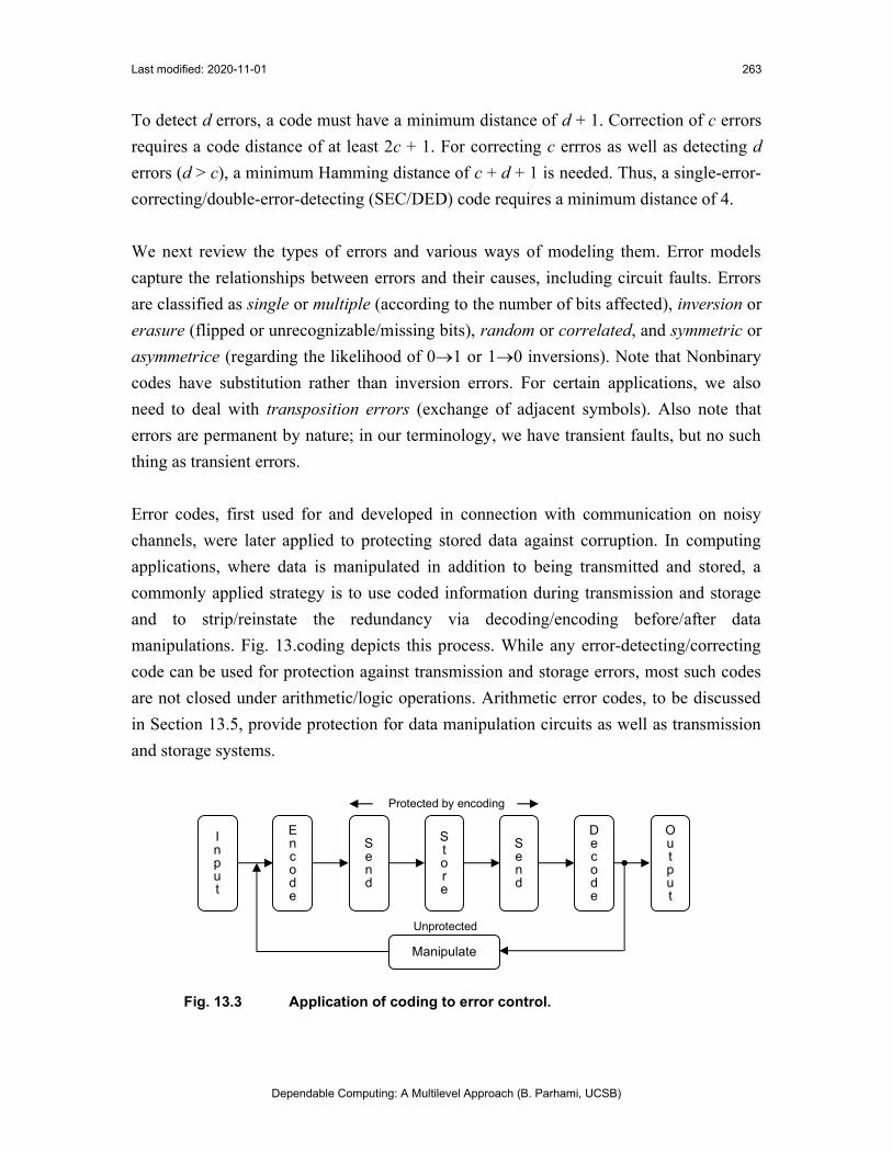
manipulations. Fig. 13.coding depicts this process. While any error-detecting/correcting
code can be used for protection against transmission and storage errors, most such codes
are not closed under arithmetic/logic operations. Arithmetic error codes, to be discussed
in Section 13.5, provide protection for data manipulation circuits as well as transmission
and storage systems.
Fig. 13.3 Application of coding to error control.
I npu t
E n c o d e
S e n d
S t o r e
S e n d
D e c o d e
O u t pu t
Manipulate
Protected by encoding
Unprotected

Last modified: 2020-11-01
Dependable Computing: A Multilevel Approach (B. Parhami, UCSB)
264
We end this section with a brief review of criteria used to judge the effectiveness of error-
detecting as well as error-correcting codes. These include redundancy (r redundant bits
used for k information bits, for an overhead of r/k), encoding circuit/time complexity,
decoding circuit/time complexity (nonexistent for separable codes), error detection
capability (single, double, b-bit burst, byte, unidirectional), and possible closure under
operations of interest.
Note that error-detecting and error-correcting codes used for dependability improvement
are quite different from codes used for privacy and security. In the latter case, a simple
decoding process would be detrimental to the purpose for which the code is used.

Last modified: 2020-11-01
Dependable Computing: A Multilevel Approach (B. Parhami, UCSB)
265
13.2 Checksum Codes
Checksum codes constitute one of the most widely used classes of error-detecting codes.
In such codes, one or more check digits or symbols, computed by some kind of
summation, are attached to data digits or symbols.
Example 13.UPC: Universal product code, UPC-A In UPC-A, an 11-digit decimal product
number is augmented with a decimal check digit, which is considered the 12th digit and is
computed as follows. The odd-indexed digits (numbering begins with 1 at the left) are added up
and the sum is multiplied by 3. Then, the sum of the even-indexed digits is added to the previous
result, with the new result subtracted from the next higher multiple of 10, to obtain a check digit in
[0-9]. For instance, given the product number 03600029145, its check digit is computed thus. We
first find the weighted sum 3(0 + 6 + 0 + 2 + 1 + 5) + 3 + 0 + 0 + 9 + 4 = 58. Subtracting the latter
value from 60, we obtain the check digit 2 and the codeword 036000291452. Describe the error-
detection algorithm for UPC-A code. Then show that all single-digit substitution errors and nearly
all transposition errors (switching of two adjacent digits) are detectable.
Solution:
To detect errors, we recompute the check digit per the process outlined in the problem statement
and compare the result against the listed check digit. Any single-digit substitution error will add to
the weighted sum a positive or negative error magnitude that is one of the values in [1-9] or in
{12, 15, 18, 21, 24, 27}. None of the listed values is a multiple of 10, so the error is detectable. A
transposition error will add or subtract an error mangnitude that is the difference between 3a + b
and 3b + a, that is, 2(a – b). As long as a – b 5, the error magnitude will not be divisible by 10
and the error will be detectable. The undetectable exceptions are thus adjacent transposed digits
that differ by 5 (i.e., 5 and 0; 6 and 1; etc.).
Generalizing from Example 13.UPC, checksum codes are characterized as follows. Given
the data vector x1, x2, … , xk, we attach a check digit xk+1 to the right end of the vector
so as to satisfy the check equation
∑ 𝑤 𝑥 = 0 mod A (13.2.chksm)
where the wj are weights associated with the different digit positions and A is a check
constant. With this terminology, the UPC-A code of example 13.UPC has the weight
vector 3, 1, 3, 1, 3, 1, 3, 1, 3, 1, 3, 1 and the check constant A = 10. Such a checksum
code will detect all errors that add to the weighted sum an error magnitude that is not a
multiple of A. In some variants of checksum codes, the binary representations of the
vector elements are XORed together rather than added (after multiplication by their

Last modified: 2020-11-01
Dependable Computing: A Multilevel Approach (B. Parhami, UCSB)
266
corresponding weights). Because the XOR operation is simpler and faster, such XOR
checkcum codes have a speed and cost advantage, but they are not as strong in terms of
error detection capabilities.

Last modified: 2020-11-01
Dependable Computing: A Multilevel Approach (B. Parhami, UCSB)
267
13.3 Weight-Based and Berger Codes
The 2-out-of-5 or 5-bit weight-2 code, alluded to in Section 13.1, is an instance of
constant-weight codes. A constant-weight n-bit code consists of codewords having the
weight w and can detect any unidirectional error, regardless of the number of bit-flips.
Example 13.cwc: Capabilities of constant-weight codes How many random or bidirectional
errors can be detected by a w-out-of-n, or n-bit weight-w, code? How many errors can be
corrected? How should we choose the code weight w so as to maximize the number of codewords?
Solution: Any codeword of a constant-weight code can be converted to another codeword by
flipping a 0 bit and a 1 bit. Thus, code distance is 2, regardless of the values of the parameters w
and n. With a minimum distance of 2, the code can detect a single random error and has no error
correction capability. The number of codewords is maximized if we choose w = n/2 for even n or
one of the values (n – 1)/2 or (n + 1)/2 for odd n.
Another weight-based code is the separable Berger code, whose codewords are formed as
follows. We count the number of 0s in a k-bit data word and attach to the data word the
representation of the count as a log2(k + 1)-bit binary number. Hence, the codewords
are of length n = k + r = k + log2(k + 1). Using a vertical bar to separate the data part
and check part of a Berger code, here are some examples of codewords with k = 6:
000000|110; 000011|100; 101000|100; 111110|001.
A Berger code can detect all unidirectional errors, regardless of the number of bits
affected. This is because 01 flips can only decrease the count of 0s in the data part, but
they either leave the check part unchanged or increase it. As for random errors, only
single errors are guaranteed to be detectable (why?). The following example introduces
an alternate form of Berger code.
Example 13.Berger: Alternate form of Berger code Instead of attaching the count of 0s as a
binary number, we may attach the 1’s-complement (bitwise complement) of the count of 1s. What
are the error-detection capabilities of the new variant?
Solution: The number of 1s increases by 01flips, thus increasing the count of 1s and decreasing
its 1’s-complement. A similar opposing direction of change applies to 10 flips. Thus, all
unidirectional errors remain detectable.

Last modified: 2020-11-01
Dependable Computing: A Multilevel Approach (B. Parhami, UCSB)
268
13.4 Cyclic Codes
A cyclic code is any code in which a cyclic shift of a codeword always results in another
codeword. A cyclic code can be characterized by its generating polynomial G(x) of
degree r, with all of the coefficients being 0s and 1s. Here is an example generator
polynomial of degree r = 3:
G(x) = 1 + x + x3 (13.4.GenP)
Multiplying a polynomial D(x) that represents a data word by the generator polynomial
G(x) produces the codeword polynomial V(x). For example, given the 7-bit data word
1101001, associated with the polynomial 1 + x + x3 + x6, the corresponding codeword is
obtained via a polynomical multiplication in which coefficients are added modulo 2:
V(x) = D(x) G(x) = (1 + x + x3 + x6)( 1 + x + x3) (13.4.CodeW)
= 1 + x2 + x7 + x9
The result in equation 13.4.CodeW corresponds to the 10-bit codeword 1010000101.
Because of the use of polynomial multiplication to form codewords, a given word is a
valid codeword iff the corresponding polynomial is divisible by G(x).
The polynomial G(x) of a cyclic code is not arbitrary, but must be a factor of 1 + xn. For
example, given that
1 + x15 = (1 + x)(1 + x + x2)(1 + x + x4)(1 + x3 + x4)(1 + x + x2
+ x3 + x4) (13.4.poly)
several potential choices are available for the generator polynomial of a 16-bit cyclic
code. Each of the factors on the right-hand side of equation 13.4.poly, or the product of
any subset of the 5 factors, can be used as a generator polynomial. The resulting 16-bit
cyclic codes will be different with respect to their error detection capabilities and
encoding/decoding schemes.
An n-bit cyclic code with k bits’ worth of data and r bits of redundancy (generator
polynomial of degree r = n – k) can detect all burst errors of width less than r. This is
because the burst error polynomial xi E(x), where E(x) is of degree less than r, cannot be
divisible by the degree-r generator polynomial G(x).
Last modified: 2020-11-01
Dependable Computing: A Multilevel Approach (B. Parhami, UCSB)
269
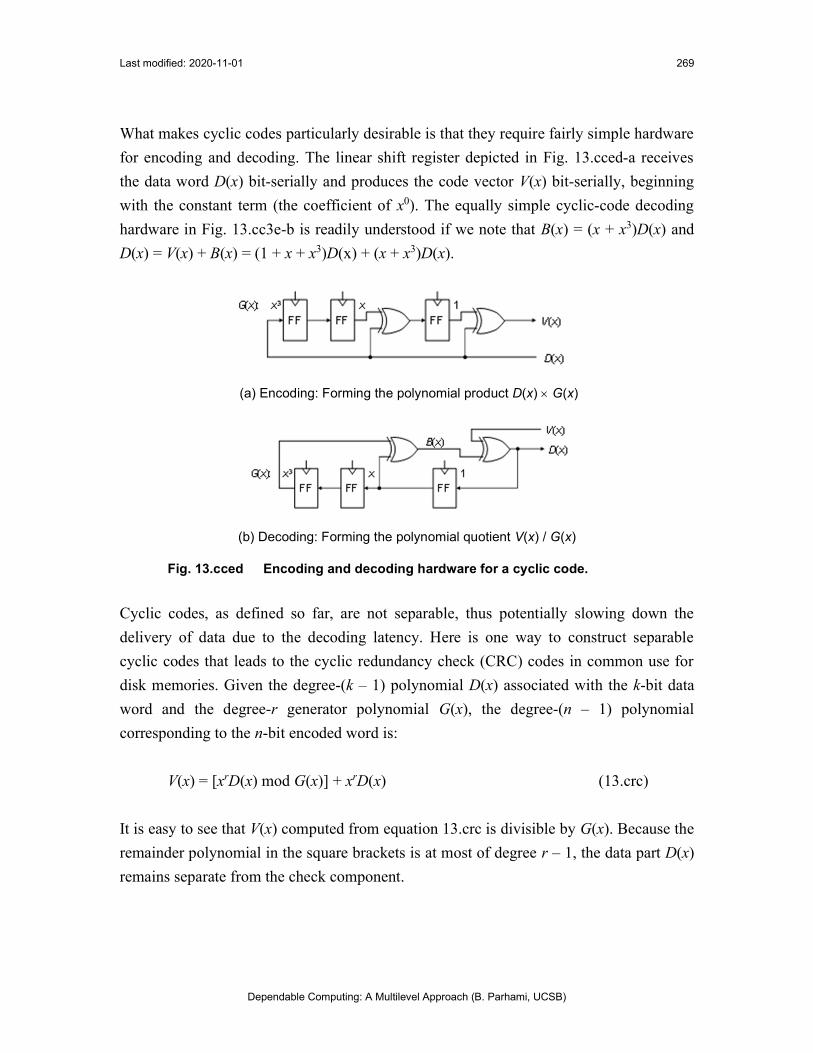
What makes cyclic codes particularly desirable is that they require fairly simple hardware
for encoding and decoding. The linear shift register depicted in Fig. 13.cced-a receives
the data word D(x) bit-serially and produces the code vector V(x) bit-serially, beginning
with the constant term (the coefficient of x0). The equally simple cyclic-code decoding
hardware in Fig. 13.cc3e-b is readily understood if we note that B(x) = (x + x3)D(x) and
D(x) = V(x) + B(x) = (1 + x + x3)D(x) + (x + x3)D(x).
(a) Encoding: Forming the polynomial product D(x) G(x)
(b) Decoding: Forming the polynomial quotient V(x) / G(x)
Fig. 13.cced Encoding and decoding hardware for a cyclic code.
Cyclic codes, as defined so far, are not separable, thus potentially slowing down the
delivery of data due to the decoding latency. Here is one way to construct separable
cyclic codes that leads to the cyclic redundancy check (CRC) codes in common use for
disk memories. Given the degree-(k – 1) polynomial D(x) associated with the k-bit data
word and the degree-r generator polynomial G(x), the degree-(n – 1) polynomial
corresponding to the n-bit encoded word is:
V(x) = [xrD(x) mod G(x)] + xrD(x) (13.crc)
It is easy to see that V(x) computed from equation 13.crc is divisible by G(x). Because the
remainder polynomial in the square brackets is at most of degree r – 1, the data part D(x)
remains separate from the check component.

Last modified: 2020-11-01
Dependable Computing: A Multilevel Approach (B. Parhami, UCSB)
270
Example 13.CRC1: Separable cyclic code Consider a CRC code with 4 data bits and the
generator polynomial G(x) = 1 + x + x3. Form the CRC codeword associated with the data word
1001 and check your work by verifying the divisibility of the resulting polynomial V(x) by G(x).
Solution: Dividing x3D(x) = x3 + x6 by G(x), we get the remainder x + x2. The code-vector
polynomial is V(x) = [x3D(x) mod G(x)] + x3D(x) = x + x2 + x3 + x6, corresponding to the codeword
0111001. Rewriting V(x) as x(1 + x + x3) + x3(1 + x + x3) confirms that it is divisible by G(x).
Example 13.CRC2: Even parity as CRC code Show that the use of a single even parity bit is a
special case of CRC and derive its generator polynomial G(x).
Solution: Let us take an example data word 1011, with D(x) = 1 + x2 + x3 and its even-parity
coded version 11011 with V(x) = 1 + x + x3 + x4 (note that the parity bit precedes the data). Given
that the remainder D(x) mod G(x) is a single bit, the generator polynomial, if it exists, must be
G(x) = 1 + x. We can easily verify that (1 + x2 + x3) mod (1 + x) = 1. For a general proof, we note
that xi mod (1 + x) = 1 for all values of i. Therefore, the number of 1s in the data word, which is
the same as the number of terms in the polynomial D(x), determines the number of 1s that must be
added (modulo 2) to form the check bit. The latter process coincides with the definition of an even
parity-check bit.

Last modified: 2020-11-01
Dependable Computing: A Multilevel Approach (B. Parhami, UCSB)
271
13.5 Arithmetic Error-Detecting Codes
Arithmetic error-detecting codes came about because of the unsuitability of conventional
codes in dealing with arithmetic errors. There are two aspects to the problem. First,
ordinary coded numbers are not closed under arithmetic operations, leading to the need
for removing the redundancy via decoding, performing arithmetic, and finally encoding
the result. Meanwhile, data remains unprotected between the decoding and encoding
steps (Fig. 13.3). Second, logic fault in arithmetic circuits can lead to errors that are more
extensive than single-bit, double-bit, burst, and other errors targeted by conventional
codes. Let us consider an example of the latter problem.
Example 13.arith1: Errors caused by single faults in arithmetic circuits Show that a single
logic fault in an unsigned binary adder can potentially flip an arbitrary number of bits in the sum.
Solution: Consider the addition of two 16-bit unsigned binary numbers 0010 0111 0010 0001 and
0101 1000 1101 0011, whose correct sum is 0111 1111 1111 0100. Indexing the bit positions from
the right end beginning with 0, we note that during this particular addition, the carry signal going
from position 3 to position 4 is 0. Now suppose that the output of the carry circuit in that position
is s-a-1. The erroneous carry of 1 will change the output to 1000 0000 0000 0100, flipping 12 bits
in the process and changing the numerical value of the ouput by 16.
Characterization of arithmetic errors is better done via the value added to or subtracted
from a correct result, rather than by the number of bits affected. When the amount added
or subtracted is a power of 2, as in Example 13.arith1, we say that we have an arithmetic
error of weight 1, or a single arithmetic error. When the amount added or subtracted can
be expressed as the sum or difference of two different powers of 2, we say we have an
arithmetic eror of weight 2, or double arithmetic error.
Example 13.arith2: Arithmetic weight of error Consider the correct sum of two unsigned
binary numbers to be 0111 1111 1111 0100.
a. Characterize the arithmetic errors that transform the sum to 1000 0000 0000 0100.
b. Repeat part a for the transformation to 0110 0000 0000 0100.
Solution:
a. The error is +16 = +24, thus it is characterized as a positive weight-1 or single error.
b. The error is –32 752 = –215 + 24, thus it is characterized as a negative weight-2 or double error.

Last modified: 2020-11-01
Dependable Computing: A Multilevel Approach (B. Parhami, UCSB)
272
Arithmetic error-detecting codes are characterized by the arithmetic weights of detectable
errors. Furthermore, they allow arithmetic operations to be performed directly on coded
operands, either by the usual arithmetic algorithms or by specially modified versions that
are not much more complex. We will discuss two classes of such codes in the remainder
of this section: product codes and residue codes.
Product or AN codes form a class of arithmetic error codes in which a number N is
encoded by the number AN, where A is the code or check constant, chosen according to
the discussion that follows. Detecting all weight-1 arithmetic errors requires only that A
be odd. Particularly suitable odd values for A include numbers of the form 2a – 1, because
such low-cost check constants make the encoding and decoding processes simple.
Arithmetic errors of weight 2 or more may go undetected. For example, the error
magnitude 32 736 = 215 – 25 would be undetectable with A = 3, 11, or 31.
For AN codes, encoding consists of multiplication by A, an operation that becomes shift-
subtract for A = 2a – 1. Error detection consists of verifying divisibility by A. Decoding
consists of division by A. both of the latter operations can be performed quite efficiently
a-bit-at-a-time when A = 2a – 1. This is because given (2a – 1)x, we can find x from:
x = 2ax – (2a – 1)x (13.5.div)
Even though both x and 2ax are unknown, we do know that 2ax ends with a 0s. Thus,
equation 13.5.div allows us to compute the rightmost a bits of x, which become the next a
bits of 2ax. This a-bit-at-a-time process continues until all bits of x have been derived.
Example 13.arith3: Decoding the 15x code What 16-bit unsigned binary number is represented
by 0111 0111 1111 0100 1100 in the low-cost product code 15x?
Solution: We know that 16x is of the form ●●●● ●●●● ●●●● ●●●● 0000. We use equation
13.5.div to find the rightmost 4 bits of x as 0000 – 1100 = 0100, remembering the borrow-out in
position 3 for the next step. We now know that 16x is of the form ●●●● ●●●● ●●●● 0100 0000.
In the next step, we find 0100 – 0100 (–1) = (–1) 1111, where a parenthesized –1 indicates
borrow-in/out. We now know 16x to be of the form ●●●● ●●●● 1111 0100 0000. The next 4
digits of x are found thus: 1111 – 1111 (–1) = (–1) 1111. We now know 16x to be of the form
●●●● 1111 1111 0100 0000. The final 4 digits of x are found thus: 1111 – 0111 (–1) = 0111.
Putting all the pieces together, we have the answer x = 0111 1111 1111 0100.

Last modified: 2020-11-01
Dependable Computing: A Multilevel Approach (B. Parhami, UCSB)
273
The arithmetic operations of addition and subtraction on product-coded operands are
straightforward, because they are done exactly as ordinary addition and subtraction.
Ax Ay = A(x y) (13.5.addsub)
Multiplication requires a final correction via division by A, given that Ax Ay = A2xy.
Even though it is possible to perform the division Ax / Ay via premultiplying Ax by A,
performing the ordinary division A2x / Ay, and doing a final correction to ensure that the
remainder is of correct sign and within the acceptable range, the added complexity may
be unacceptable in many applications. Calculating the square-root of Ax via applying a
standard square-rooting algorithm to A2x encounters problems similar to division.
Note that product codes are nonseparable, because data and redundant check information
are intermixed. We next consider a class of separable arithmetic error-detecting codes.
A residue error-correcting code represents an integer N by the pair (N, C = |N|A), where
|N|A is the residue of N modulo the chosen check modulus A. Because the data part N and
the check part C are separate, decoding is trivial. To encode a number N, we must
compute |N|A and attach it to N. This is quite easy for a low-cost modulus A = 2a – 1:
simply divide the number N into a-bit chunks, beginning at its right end, and add the
chunks together modulo A. Modulo-(2a – 1) addition is just like ordinary a-bit addition,
with the adder’s carry-out line connected to its carry-in line, a configuration known as
end-around carry.
Example 13.mod15: Computing low-cost residues Compute the mod-15 residue.of the 16-bit
unsigned binary number 0101 1101 1010 1110.
Solution: The mod-15 residue of x is obtained thus: 0101 + 1101 + 1010 + 1110 mod 15.
Beginning at the right end, the first addition produces an outgoing carry, leading to the mod-15
sum 1110 + 1010 – 10000 + 1 = 1001. Next, we get 1001 + 1101 – 10000 + 1 = 0111. Finally, in
the last step, we get: 0111 + 0101 = 1100. Note that the end-around carry is 1 in all three steps.
For an arbitrary modulus A, we can use table-lookup to compute |N|A. Suppose that the
number N can be divided into m chunks of size b bits. Then, we need a table of size 2bm,
having 2b entries per chunk. For each chunk, we consult the corresponding part of the

Last modified: 2020-11-01
Dependable Computing: A Multilevel Approach (B. Parhami, UCSB)
274
table, which stores the mod-A residues all possible b-bit chunks in that position, adding
all the entries thus read out, modulo A.
An inverse residue code uses the check part D = A – C instead of C = |N|A. This change is
motivated by the fact that certain unidirectional errors that are prevalent in VLSI circuits
tend to change the values of N and C in the same direction, raising the possibility that the
error will go undetected. For example if the least-significant bits of N and C both change
from 0 to 1, the value of both N and C will be increased by 1, potentially causing a match
between the residue of the erroneous N value and the erroneous C value. Inverse residue
encoding eliminates this possibility, given that unidirectional errors will affect the N and
D parts in opposite directions.

Last modified: 2020-11-01
Dependable Computing: A Multilevel Approach (B. Parhami, UCSB)
275
13.6 Other Error-Detecting Codes
The theory of error-detecting codes is quite extensive. One can devise virtually an infinite
number of different error-detecting codes and entire textbooks have been devoted to the
study of such codes. Our study in the previous sections of this chapter was necessarily
limited to codes that have been found most useful in the design of dependable computer
systems. This section is devoted to the introduction and very brief discussion of a number
of other error-detecting codes, in an attempt to fill in the gaps.
Erasure errors lead to some symbols to become unreadable, effectively reducing the
length of a codeword from n to m, when there are n – m erasures. The code ensures that
the original k data symbols are recoverable from the m available symbols. When m = k,
the erasure code is optimal, that is, any k bits can be used to reconstruct the n-bit
codeword and thus the k-bit data word. Near-optimal erasure codes require (1 + )k
symbols to recover the original data, where > 0. Examples of near-optimal erasure
codes include Tornado codes and low-density parity-check (LDPC) codes.
Given that 8-bit bytes are important units of data representation, storage, and
transmission in modern digital systems, codes that use bytes as their symbols are quite
useful for computing applications. As an example, a single-byte-error-correcting, double-
byte-error-detecting code [Kane82] may be contemplated.
Most codes are designed to deal with random errors, with particular distributions across a
codeword (say, uniform distribution). In certain situations, such as when bits are
transmitted serially or when a surface scratch on a disk affects a small disk area, the
possibility that multiple adjacent bits are adversely affected by an undesirable event
exists. Such errors, referred to “burst errors,” are characterized by their extent or length.
For example, a single-bit-error-correcting, 6-bit-burst-error-detecting code might be of
interest in such contexts. Such a code would correct a single random error, while
providing safety against a modest-length burst error.
In this chapter, we have seen error-detecting codes applied at the bit-string or word level.
It is also possible to apply coding at higher levels of abstraction. Error-detecting codes
that are applicable at the data structure level (robust data structures) or at the application
level (algorithm-based error tolerance) will be discussed in Chapter 20.

Last modified: 2020-11-01
Dependable Computing: A Multilevel Approach (B. Parhami, UCSB)
276
Problems
13.1 Checksum codes
a. Describe the checksum scheme used in the (9 + 1)-digit international serial book number (ISBN) code and state its error detecting capabilities.
b. Repeat part a for the (12 + 1)-digit ISBN code that replaced the older code in 2005.
c. Repeat part a for the (8 + 1)-digit bank identification or routing number code that appears to the left of account number on bank checks.
13.2 Detecting substitution and transposition errors
Consider the design of an n-symbol q-ary code that detects single substitution or transposition errors.
a. Show that for q = 2, the code can have 2n/3 codewords.
b. Show that for q 3, the code can have qn–1 codewords.
c. Prove that the results of parts a and b are optimal [Abde98].
13.3 Unidirectional error-detecting codes
An (n, t) Borden code is an n-bit code composed of n/2-out-of-n codewords and all codewords of the form m-out-of-n, where m = n/2 mod (t + 1). Show that the (n, t) Borden code is an optimal t-unidirectional error-detecting code [Pies96].
13.4 Binary cyclic codes
Prove or disprove the following for a binary cyclic code.
a. If x + 1 is a factor of G(x), the code cannot have codewords on odd weight.
b. If V(x) is the polynomial associated with some codeword, then so is xiV(x) mod (1 + xn) for any i.
c. If the generator polynomial is divisible by x + 1, then the all-1s vector is a codeword [Pete72].
13.5 Error detection in UPC-A
a. Explain why all one-digit errors are caught by UPC-A coding scheme based on mod-10 checksum on 11 data digits and 1 check digit, using the weight vector 3 1 3 1 3 1 3 1 3 1 3 1.
b. Explain why all transposition errors (adjacent digits switching positions) are not caught.
13.6 Error detection for performance enhancement
Read the article [Blaa09] and discuss, in one typewritten page, how error detection methods can be put to other uses, such as speed enhancement and energy economy.
13.7 Parity generator or check circuit
Present the design of a logic circuit that accepts 8 data bits, plus 1 odd or even parity bit, and either checks the parity or generates a parity bit.
13.8 The 10-digit ISBN code

Last modified: 2020-11-01
Dependable Computing: A Multilevel Approach (B. Parhami, UCSB)
277
In the old, 10-digit ISBN code, the 9-digit book identifier x1x2x3x4x5x6x7x8x9 was augmented with a 10th check digit x10, derived as (11 – W) mod 11, where W is the modulo-11 weighted sum 1i9 (11 – i)xi. Because the value of x10 is in the range [0, 10], the check digit is written as X when the residue is 10.
a. Provide an algorithm to check the validity of the 10-digit ISBN code x1x2x3x4x5x6x7x8x9x10.
b. Show that the code detects all single-digit substitution errors.
c. Show that the code detects all single transposition errors.
d. Since a purely numerical code would be more convenient, it is appealing to replace the digit value X, when it occurs, with 0. How does this change affect the code’s capability in detecting substitution errors?
e. Repeat part d for transposition errors.
13.9 Binary cyclic codes
A check polynomial H(x) is a polynomial such that V(x)H(x) = 0 mod (xn + 1) for any data polynomial V(x).
a. Prove that each cyclic code has a check polynomial and show how to derive it.
b. Sketch the design of a hardware unit that can check the validity of a data word.
13.10 Shortening a cyclic code
Starting with a cyclic code of redundancy r, consider shortening the code in its first or last s bits by choosing all codewords that contain 0s in those positions and then deleting the positions.
a. Show that the resulting code is not a cyclic code.
b. Show that the resulting code still detects all bursts of length r, provided they don’t wrap around.
c. Provide an example of an undetectable burst error of length r that wraps around.
13.11 An augmented Berger code
In a code with a 63-bit data part, we attach both the number of 0s and the number of 1s in the data as check bits (two 6-bit checks), getting a 75-bit code. Assess this new code with respect to redundancy, ease of encoding and decoding, and error detection/correction capability, comparing it in particular to Berger code.
13.12 A modified Berger code
In a Berger code, when the number of data bits is k = 2a, we need a check part of a + 1 bits to represent counts of 0s in the range [0, 2a], leading to a code length of n = k + a + 1. Discuss the pros and cons of the following modified Berger code and deduce whether the modification is worthwhile. Counts of 0s in the range [0, 2a – 1] are represented as usual as a-bit binary numbers. The count 2a is represented as 0, that is, the counts are considered to be modulo-2a.

Last modified: 2020-11-01
Dependable Computing: A Multilevel Approach (B. Parhami, UCSB)
278
References and Further Readings
[Abde98] Abdel-Ghaffar, K. A. S., “Detecting Substitutions and Transpositions of Characters,” Computer J., Vol. 41, No. 4, pp. 238-242, 1998.
[Aviz71] Avizienis, A., “Arithmetic Error Codes: Cost and Effectiveness Studies for Application in Digital System Design,” IEEE Trans. Computers, pp. 1322-1331.
[Aviz73] Avizienis, A., “Arithmetic Algorithms for Error-Coded Operands,” IEEE Trans. Computers, Vol. 22, No. 6, pp. 567-572, June 1973.
[Berg61] Berger, J. M., “A Note on Error Detection Codes for Asymmetric Channels,” Information and Control, Vol. 4, pp. 68-73, March 1961.
[Blaa09] Blaauw, D. and S. Das, “CPU, Heal Thyself,” IEEE Spectrum, Vol. 46, No. 8, pp. 41-43 and 52-56, August 2009.
[Chen06] Cheng, C. and K. K. Parhi, “High-Speed Parallel CRC Implementation Based on Unfolding, Pipelining, and Retiming,” IEEE Trans. Circuits and Systems II, Vol. 53, No. 10, pp. 1017-1021, October 2006.
[Das09] Das, S., et al., “RazorII: In Situ Error Detection and Correction for PVT and SER Tolerance,” IEEE J. Solid-State Circuits, Vol. 44, No. 1, pp. 32-48, January 2009.
[Garn66] Garner, H. L., “Error Codes for Arithmetic Operations,” IEEE Trans. Electronic Computers,
[Grib16] Gribaudo, M., M. Iacono, and D. Manini, “Improving Reliability and Performances in Large Scale Distributed Applications with Erasure Codes and Replication,” Future Generation Computer Systems, Vol. 56, pp. 773-782, March 2016.
[Kane82] Kaneda, S. and E. Fujiwara, “Single Byte Error Correcting Double Byte Error Detecting Codes for Memory Systems,” IEEE Trans. Computers, Vol. 31, No. 7, pp. 596-602, July 1982..
[Knut86] Knuth, D. E., “Efficient Balanced Codes,” IEEE Trans. Information Theory, Vol. 32, No. 1, pp. 51-53, January 1986.
[Parh78] Parhami, B. and A. Avizienis, “Detection of Storage Errors in Mass Memories Using Arithmetic Error Codes,” IEEE Trans. Computers, Vol. 27, No. 4, pp. 302-308, April 1978.
[Pete59] Peterson, W. W. and M. O. Rabin, “On Codes for Checking Logical Operations,” IBM J.,
[Pete72] Peterson, W. W. and E. J. Weldon Jr., Error-Correcting Codes, MIT Press, 2nd ed., 1972.
[Pies96] Piestrak, S. J., “Design of Self-Testing Checkers for Borden Codes,” IEEE Trans. Computers, pp. 461-469, April 1996.
[Raab16] Raab, P., S. Kramer, and J. Mottok, “Reliability of Data Processing and Fault Compensation in Unreliable Arithmetic Processors,” Microprocessors and Microsystems, Vol. 40, pp. 102-112, February 2016.
[Rao74] Rao, T. R. N., Error Codes for Arithmetic Processors, Academic Press, 1974.
[Rao89] Rao, T. R. N. and E. Fujiwara, Error-Control Coding for Computer Systems, Prentice Hall, 1989.
[Wake75] Wakerly, J. F., “Detection of Unidirectional Multiple Errors Using Low-Cost Arithmetic Error Codes,” IEEE Trans. Computers
[Wake78] Wakerly, J. F., Error Detecting Codes, Self-Checking Circuits and Applications, North-Holland, 1978.

Last modified: 2020-11-01
Dependable Computing: A Multilevel Approach (B. Parhami, UCSB)
279
14 Error Correction
“Error is to truth as sleep is to waking. As though refreshed, one returns from erring to the path of truth.”
Johann Wolfgang von Goethe, Wisdom and Experience
“Don’t argue for other people’s weaknesses. Don’t argue for your own. When you make a mistake, admit it, correct it, and learn from it / immediately.”
Stephen R. Covey
Topics in This Chapter
14.1. Basics of Error Correction
14.2. Hamming Codes
14.3. Linear Codes
14.4. Reed-Solomon and BCH Codes
14.5. Arithmetic Error-Correcting Codes
14.6. Other Error-Correcting Codes
Automatic error correction may be used to prevent distorted subsystem states
from adversely affecting the rest of the system, in much the same way that fault
masking is used to hinder the fault-to-error transition. Avoiding data corruption,
and its service- or result-level consequences, requires prompt error correction;
otherwise, errors might lead to malfunctions, thus moving the computation one
step closer to failure. To devise cost-effective error correction schemes, we need a
good understanding of the types of errors that might be encountered and the cost
and correction capabilities of various informational redundancy methods; hence,
our discussion of error-correcting codes in this chapter.

Last modified: 2020-11-01
Dependable Computing: A Multilevel Approach (B. Parhami, UCSB)
280
14.1 Basics of Error Correction
Instead of detecting errors and performing some sort of recovery action such as
retransmission or recomputation, one may aim for providing sufficient redundancy in the
code so as to correct the most common errors quickly. In contrast to the backward
recovery methods associated with error detection followed by additional actions, error-
correcting codes are said to allow forward recovery. In practice, we may use an error
correction scheme for simple, common errors in conjunction with error detection for rarer
or more extensive error patterns. A Hamming single-error-correcting/double-error-
detecting (SEC/DED) code provides a good example.
Error-correcting codes were also developed for communication over noisy channels and
were later adopted for use in computer systems. Notationally, we proceed as in the case
of error-detecting codes, discussed in Chapter 13. In other words, we assume that k-bit
information words are encoded as n-bit codewords, n > k. Changing some of the bits in a
valid codeword produces an invalid codeword, thus leading to detection, and with
appropriate provisions, to correction. The ratio r/k, where r = n – k is the number of
redundant bits, indicates the extent of redundancy or the coding cost. Hardware
complexity of error correction is another measure of cost. Time complexity of the error
correction algorithm is a third measure of cost, which we often ignore, because we
expect correction events to be very rare.
Figure 14.1a depicts the data space of size 2k, the code space of size 2n, and the set of 2n –
2k invalid codewords, which, when encountered, indicate the presence of errors.
Conceptually, the simplest redundant represention for error correction consists of
replication of data. For example, triplicating a bit b to get the corresponding codeword
bbb allows us to correct an error in 1 of the 3 bits. Now, if the valid codeword 000
changes to 010 due to a single-bit error, we can correct the error, given that the erroneous
value is closer to 000 than to 111. We saw in Chapter 13 that the same triplication
scheme can be used for the detection of single-bit and double-bit errors in lieu of
correction of a single-bit error. Of course, triplication does not have to be applied at the
bit leval. A data bit-vector x of length k can be triplicated to become the 3k-bit codeword
xxx. Referring to Fig. 14.1b, we note that if the voter is triplicated to produce three copies
of the result y, the modified circuit would supply the coded yyy version of y, which can
then be used as input to other circuits.

Last modified: 2020-11-01
Dependable Computing: A Multilevel Approach (B. Parhami, UCSB)
281
(a) Data and code spaces (b) Triplication as coding
Fig. 14.1 Data and code spaces for error-correction coding in general
(sizes 2k and 2n) and for triplication (sizes 2k and 23k).
The high-redundancy triplication code corresponding to the voting scheme of Fig. 14.1b
is conceptually quite simple. However, we would like to have lower-redundancy codes
that offer similar protection against potential errors. To correct a single-bit error in an n-
bit (non)codeword with r = n – k bits of redundancy, we must have 2r > k + r, which
dictates slightly more than log2 k bits of redunadancy. One of our challenges in this
chapter is to determine whether we can approach this lower bound and come up with
highly efficient single-error-correcting codes and, if not, whether we can get close to the
bound. More generally, the challenge of designing efficient error-correcting codes with
different capabilities is what will drive us in the rest of this chapter. Let us begin with an
example that achieves single-error correction and double-error detection with a
redundancy of r = 2 𝑘 + 1 bits.
Example 14.1: Two-dimensional error-correcting code A conceptually simple error-
correcting code is as follows. Let the width k of our data word be a perfect square and arrange the
bits of a given data word in a 2D square matrix (in row-major order, say). Now attach a parity bit
to each row, yielding a new bit-matrix with √𝑘 rows and √𝑘 + 1 columns. Then attach a parity bit
to each column of the latter matrix, ending up with a (√𝑘 + 1) (√𝑘 + 1) bit-matrix. Show that
this coding scheme is capable of correcting all single-bit errors and detecting all double-bit errors.
Provide an example of a triple-bit error that goes undetected.
Solution: A single bit-flip will cause the parity check to be violated for exactly one row and one
column, thus pinpointing the location of the erroneous bit. A double-bit error is detectable because
it will lead to the violation of parity checks for 2 rows (when the errors are in the same column),
2 columns, or 2 rows and 2 columns. A pattern of 3 errors may be such that there are 2 errors in
row i and 2 errors in column j (one of them shared), leading to no parity check violation.

Last modified: 2020-11-01
Dependable Computing: A Multilevel Approach (B. Parhami, UCSB)
282
The criteria used to judge error-correcting codes are quite similar to those used for error-
detecting codes. These include redundancy (r redundant bits used for k information bits,
for an overhead of r/k), encoding circuit/time complexity, decoding circuit/time
complexity (nonexistent for separable codes), error correction capability (single, double,
b-bit burst, byte, unidirectional), and possible closure under operations of interest.
Greater correction capability generally entails more redundancy. To correct c errors, a
minimum code distance of 2c + 1 is necessary. Codes may also have a combination of
correction and detection capabilities. To correct c errors and additionally detect d errors,
where d > c, a miminum code distance of c + d + 1 is needed. For example, a SEC/DED
code cannot have a distance of less than 4.
The notion of an adequate Hamming distance in a code allowing error correction is
illustrated in Fig. 14.dist, though the reader must bear in mind that the 2D representation
of codewords and their distances is somewhat inaccurate. Let each circle in Fig. 14.dist
represent a word, with the red circles labeled c1, c2, and c3 representing codewords and all
others corresponding to noncodewords. The Hamming distance between words is
represented by the minimal number or horizontal, vertical, or diagonal steps on the grid
needed to move from one word to the other. It is easy to see that the particular code in
Fig. 14.dist has minimum distance 3, given that we can get from c3 to c1 or c2 in 3 steps
(1 vertical move and 2 diagonal moves).
Fig. 14.dist Illustration of how a code with Hamming distance of 3 might
allow the correction of single-bit errors.
c1 c2
c3
e1 e2 e3

Last modified: 2020-11-01
Dependable Computing: A Multilevel Approach (B. Parhami, UCSB)
283
For each of the three codewords, distance-1 and distance-2 words from it are highlighted
by drawing a dashed box through them. For each codeword, there are 8 distance-1 words
and 16 distance-2 words. We note that distance-1 words, colored yellow, are distinct for
each of the three codewords. Thus, if a single-bit error transforms c1 to e1, say, we know
that the correct word is c1, because e1 is closer to c1 than to the other two codewords.
Certain distance-2 noncodewords, such as e2, are similarly closest to a particular valid
codeword, which may allow their correction. However, as seen from the example of the
noncodeword e3, which is at distance 2 from all three valid codewords, some double-bit
errors may not be correctable in a distance-3 code.
Last modified: 2020-11-01
Dependable Computing: A Multilevel Approach (B. Parhami, UCSB)
284
14.2 Hamming Codes
Hamming codes take their name from Richard W. Hamming, an American scientist who
is rightly recognized as their inventor. However, while Hamming’s publication of his idea
was delayed by Bell Laboratory’s legal department as part of their patenting strategy,
Claude E. Shannon independently discovered and published the code in his seminal 1949
book, The Mathematical Theory of Communication [Nahi13].
We begin our discussion of Hamming codes with the simplest possible example: a (7, 4)
single-error-correcting (SEC) code, with n = 7 total bits, k = 4 data bits, and r = 3
redundant parity-check bits. As depicted in Fig. 14.H74-a, each parity bit is associated
with 3 data bits and its value is chosen to make the group of 4 bits have even parity.
Thus, the data word 1001 is encoded as the codeword 1001|101. The evenness of parity
for pi’s group is checked by computing the syndrome si and verifying that it is 0. When
all three syndromes are 0s, the word is error-free and no correction is needed. When the
syndrome vector s2s1s0 contains one or more 1s, the combination of values point to a
unique bit that is in error and must be flipped to correct the 7-bit word. Figure 14.H74-b
shows the correspondence between the syndrome vector and the bit that is in error.
Encoding and decoding circuitry for the Hamming (7. 4) SEC code of Fig. 14.H74 are
shown in Fig. 14. Hed.
The redundancy of 3 bits for 4 data bits (3/7 43%) in the (7, 4) Hamming code of Fig.
14.H74 is unimpressive, but the situation gets better with more data bits. We can
construct (15, 11), (31, 26), (63, 57), (127, 120), (255, 247), (511, 502), and (1023, 1013)
SEC Hamming codes, with the last one on the list having a redundancy of only 10/1023,
which is less than 1%. The general pattern is having 2r – 1 total bits with r check bits. In
this way, the r syndrome bits can assume 2r possible values, one of which corresponds to
the no-error case and the remaining 2r – 1 are in one-to-one correspondence with the
code’s 2r – 1 bits. It is easy to see that the redundancy is in general r/(2r – 1), which
approaches 0 for very wide codes.

Last modified: 2020-11-01
Dependable Computing: A Multilevel Approach (B. Parhami, UCSB)
285
(a) Parity bits and syndromes (b) Error correction table
Fig. 14.H74 A Hamming [7, 4] SEC code, with n = 7 total bits, k = 4 data
bits, and r = 3 redundant parity-check bits.
Fig. 14.Hed Encoder and decoder (composed of syndrome generator
and error corrector) circuits for the Hamming (7, 4) SEC
code of Fig. 14.H4.

Last modified: 2020-11-01
Dependable Computing: A Multilevel Approach (B. Parhami, UCSB)
286
Fig. 14.pcm Matrix formulation of Hamming SEC code.
We next discuss the structure of the parity check matrix H for an (n, k) Hamming code.
As seen in Fig. 14.pcm, the columns of H hold all the possible bit patterns of length n – k,
except the all-0s pattern. Hence, n = 2n–k – 1 is satisfied for any Hamming SEC code. The
last n – k columns of the parity check matrix form the identity matrix, given that (by
definition) each parity bit is included in only one parity set. The error syndrome s of
length r is derived by multiplying the r n parity check matrix H by the n-bit received
word, where matrix-vector multiplication is done by using the AND operation instead of
multiplication and the XOR operation instead of addition.
By rearranging the columns of H so that they appear in ascending order of the binary
numbers they represent (and, of course, making the corresponding change in the
codeword), we can has the syndrome vector correspond to the column number directly
(Fig. 14.rpcm-a), allowing us to use the simple error corrector depicted in Fig. 14.rpcm-b.
(a) Rearranged parity check matrix (b) Error correction
Fig. 14.rpcm Matrix formulation of Hamming SEC code.

Last modified: 2020-11-01
Dependable Computing: A Multilevel Approach (B. Parhami, UCSB)
287
(a) Rearranged parity check matrix (b) Error correction
Fig. 14.gpcm Matrix formulation of Hamming SEC code.
The parity check matrix and the error corrector for a general Hamming code are depicted
in Fig. 14.gpcm.
Associated with each Hamming code is an n d generator matrix G such that the product
of G by the d-element data vector is the n-element code vector. For example:
⎣⎢⎢⎢⎢⎢⎡1000110
0100101
0010111
0001011⎦⎥⎥⎥⎥⎥⎤
×
𝑑𝑑𝑑𝑑
=
⎣⎢⎢⎢⎢⎢⎡𝑑𝑑𝑑𝑑𝑝𝑝𝑝 ⎦⎥⎥⎥⎥⎥⎤
(14.2.gen)
Recall that matrix-vector multiplication is done with AND/XOR instead of multiply/add.
To convert a Hamming SEC code into a SEC-DED code, we add a row of all 1s and a
column corresponding to the extra parity bit pr to the parity check matrix, as shown in
Fig. 14.secded-a. [Elaborate further on the check matrix, the effects of a double-bit error,
and the error corrector in Fig. 14.secded-b.]

Last modified: 2020-11-01
Dependable Computing: A Multilevel Approach (B. Parhami, UCSB)
288
(a) Augmented parity check matrix (b) Error correction
Fig. 14.secded Hamming SEC-DED code.

Last modified: 2020-11-01
Dependable Computing: A Multilevel Approach (B. Parhami, UCSB)
289
14.3 Linear Codes
Hamming codes are examples of linear codes, but linear codes can be defined in other
ways too. A code is linear iff given any two codewords u and v, the bit-vector w = u v
is also a codeword. Throughout the discussion that follows, data and code vectors are
considered to be column vectors. A linear code can be characterized by its generator
matrix or parity check matrix. The n k (n rows, k columns) generator matrix G, when
multiplied by a k-vector d, representing the data, produces the n-bit coded version u of
the data
u = G d (14.3.enc)
where matrix-vector multiplication for this encoding process is performed by using
modulo-2 addition (XOR) in lieu of standard addition. Checking of codewords is
performed by multiplying the (n – k) n parity check matrix H by the potentially
erroneous n-bit codeword v
s = H v (14.3.chk)
with an all-0s syndrome vector s indicating that v is a correct codeword.
Example: A Hamming code as a linear code
Example: A non-Hamming linear code
All linear codes have the following two properties:
1. The all-0s vector is a codeword.
2. The code’s distance equals the minimum Hamming weight of its codewords.

Last modified: 2020-11-01
Dependable Computing: A Multilevel Approach (B. Parhami, UCSB)
290
14.4 Reed-Solomon and BCH Codes
In this section, we introduce two widely used classes of codes that allow flexible design
of a variety of codes with desired error correction capabilities and simple decoding, with
one class being a subclass of the other. Alexis Hocquenghem in 1959 [Hocq59], and
later, apparently independently, Raj Bose and D. K. Ray-Chaudhuri in 1960 [Bose60],
invented a class of cyclic error-correcting codes that are named BCH codes in their
honor. Irving S. Reed and Gustave Solomon [Reed60] are credited with developing a
special class of BCH codes that has come to bear their names.
We begin by discussing Reed-Solomon (RS) error-correcting codes. RS codes are non-
binary, in the sense of having a multivalued symbol set from which data and check
symbols are drawn. A popular instance of the latter code, which has been used in CD
players, digital audiotapes, and digital television is the RS(255, 223) code: it has 8-bit
symbols, 223 bytes of data, and 32 check bytes, for an informational redundancy of
32/255 = 12.5% (the redundancy rises to 32/223 = 14.3% if judged relative to data bytes,
rather than the total number of bytes in the code). The aforementioned code can correct
up to 16 symbol errors. A symbol error is defined as any change in the symbol value, be
it flipping of only one bit or changing of any number of bits in the symbol. When
symbols are 8 bits wide, symbol error is also referred to as a “byte error.”
In general, a Reed-Solomom code requires 2t check sysmbols, each s bits wide, if it is to
correct up to t symbol errors. To correct t errors, which implies a disntance-(2t + 1)-code,
the number k of data symbols must satisfy:
k 2s – 1 – 2t (14.4.RS)
Inequality 14.4.RS suggests that the symbol bit-width s grows with the data length k, and
this may be viewed as a disadvantage of RS codes. One important property of RS codes
is that they guarantee optimal mimimum code distance, given the code parameters.
Theorem 14.RSdist (minimum distance of RS codes): An (n, k) Reed-Solomon code has
the optimal minimum distance n – k + 1.
Last modified: 2020-11-01
Dependable Computing: A Multilevel Approach (B. Parhami, UCSB)
291
In what follows, we focus on the properties of t-error-correcting RS codes with n = 2s – 1
code symbols, n – r = 2s – 1 – 2t data symbols, and r = 2t check symbols. Such a code is
characterized by its degree-2t generator polynomial:
g(x) = ∏ (𝑥 + α ) = x2t + g2t–1x2t–1 + … + g1x + g0 (14.4.RSgen)
In equation 14.4.RSgen, b is usually 0 or 1 and is a primitive element of GF(2s). Recall
that a primitive element is one that generates all nonzero elements of the field by its
powers. For example, three different representations of the of elements in GF(23) are
shown in Table 14.GF8.. As usual, the product of the generator polynomial and the data
polynomial yields the code polynomial, and thus the corresponding codeword. All
polynomial coefficients are s-bit numbers and all arithmetic is performed modulo 2s.
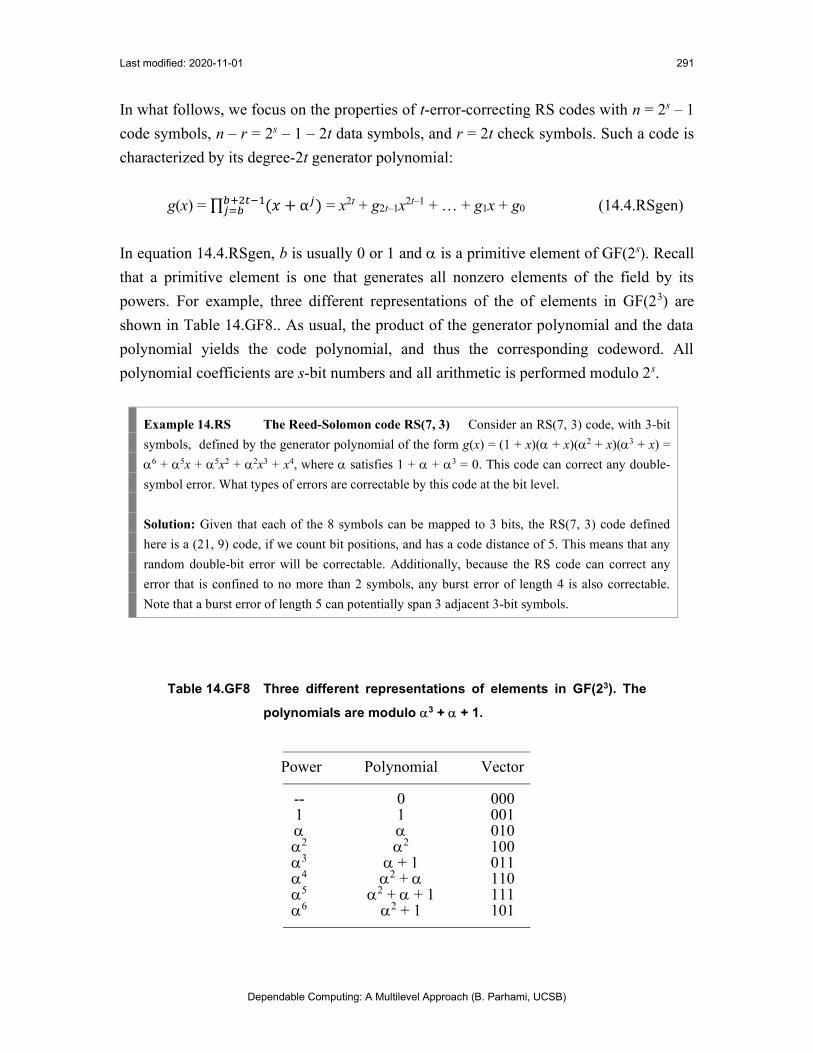
Example 14.RS The Reed-Solomon code RS(7, 3) Consider an RS(7, 3) code, with 3-bit
symbols, defined by the generator polynomial of the form g(x) = (1 + x)( + x)(2 + x)(3 + x) =
6 + 5x + 5x2 + 2x3 + x4, where satisfies 1 + + 3 = 0. This code can correct any double-
symbol error. What types of errors are correctable by this code at the bit level.
Solution: Given that each of the 8 symbols can be mapped to 3 bits, the RS(7, 3) code defined
here is a (21, 9) code, if we count bit positions, and has a code distance of 5. This means that any
random double-bit error will be correctable. Additionally, because the RS code can correct any
error that is confined to no more than 2 symbols, any burst error of length 4 is also correctable.
Note that a burst error of length 5 can potentially span 3 adjacent 3-bit symbols.
Table 14.GF8 Three different representations of elements in GF(23). The
polynomials are modulo 3 + + 1.
––––––––––––––––––––––––––––––– Power Polynomial Vector
––––––––––––––––––––––––––––––– -- 0 000 1 1 001 010 2 2 100 3 + 1 011 4 2 + 110 5 2 + + 1 111 6 2 + 1 101
–––––––––––––––––––––––––––––––

Last modified: 2020-11-01
Dependable Computing: A Multilevel Approach (B. Parhami, UCSB)
292
Reed-Solomon codes can also be introduced via a matrix formulation in lieu of
polynomials. [Elaborate]
BCH codes Have the advantage of being binary codes, thus avoiding the additional
burden of converting nonbinary symbols into binary via encoding. A BCH(n, k) code can
be characterized by its n (n – k) parity check matrix P which allows the computation of
the error syndrome via the vector-matrix multiplication W P, where W is the received
word. For example, Fig. 14.BCH shows the how the syndrome for BCH(15, 7) code is
computed. This example code shown is also characterized by it generator polynomial:
g(x) = 1 + x4 + x6 + x7 + x8 (14.4.BCH)
Practical applications of BCH codes include the use of BCH(511, 493) as a double-error-
correcting code in a video coding standard for videophones and the use of BCH(40, 32)
as SEC/DED code in ATM communication.
Fig. 14.BCH The parity check matrix and syndrome generation via
vector-matrix multiplication for BCH(15, 7) code.

Last modified: 2020-11-01
Dependable Computing: A Multilevel Approach (B. Parhami, UCSB)
293
14.5 Arithmetic Error-Correcting Codes
Consider the (7, 15) biresidue code, which uses mod-7 and mod-15 residues of a data
words as its check parts. The data word can be up to 12 bits wide and the attached check
parts are 3 and 4 bits, respectively, for a total code width of 19 bits. Figure 14.bires
shows the syndromes generated when data is corrupted by a weight-1 arithmetic error,
corresponding to the addition or subtraction of a power of 2 to/from the data. Because all
the syndromes in this table up to the error magnitude 211 are distinct, such weight-1
arithmetic errors are correctable by this code.
In general, a biresidue code with relativel prime low-cost check moduli A = 2a – 1 and B
= 2b – 1 supports ab bits of data for weight-1 error correction. The representational
redundancy of the code is:
(a + b)/ab = 1/a + 1/b (14.5.redun)
Thus, by increasing the values of a and b, we can reduce the amount of redundancy.
Figure 14.brH compares such biresidue codes with the Hamming SEC code in terms of
code and data widths. Figure 14.brarith shows a general scheme for performing
arithmetic operations and checking of results with biresidue-coded operands. The scheme
is very similar to that of residue codes for addition, subtraction, and multiplication,
except that two residue checks are required. Division and square-rooting remain difficult.
Fig. 14.bires Syndromes for single arithmetic errors, having magnitudes
that are powers of 2, in the (7, 15) biresidue code.

Last modified: 2020-11-01
Dependable Computing: A Multilevel Approach (B. Parhami, UCSB)
294
Fig. 14.brH A comparison of biresidue arithmetic codes with Hamming
SEC codes in terms of code and data widths.
Fig. 14.brarith Arithmetic operations and checking of results for biresidue-
coded operands.

Last modified: 2020-11-01
Dependable Computing: A Multilevel Approach (B. Parhami, UCSB)
295
14.6 Other Error-Correcting Codes
As in the case of error-detecting codes, we have only scratched the surface of the vast
theory of error-correcting codes in the preceding sections. So as to present a more
complete picture of the field, which is reflected in many excellent textbooks some of
which are cited in the references section, we touch upon a number of other error-
correcting codes in this section. The codes include:
Reed-Muller codes: RM codes have a recursive contruction, with smaller codes used to
build larger ones.
Turbo codes: Turbo codes are highly efficient separable codes with iterative (soft)
decoding. A data word is augmented with two check words, one obtained directly from
an encoder and a second one formed based on an interleaved version of the data. The two
encoders for Turbo codes are generally identical. Soft decoding means that each of two
decoders provides an assessment of the probability of a bit being 1. The two decoders
then exchange information and refine their estimates iteratively. Turbo codes are
extensively used in cell phones and other communication applications.
Low-density parity-check codes: In LPDC codes, each parity check is defined on a
small set of bits, so both encoding and error checking are very fast; error correction is
more difficult and entails an iterative process.
Information dispersal: In this scheme, data is encoded in n pieces, such that any k of the
pieces would be adequate for reconstruction. Such codes are useful for protecting privacy
as well as data integrity.
In this chapter, we have seen error-correcting codes applied at the bit-string or word
level. It is also possible to apply coding at higher levels of abstraction. Error-correcting
codes that are applicable at the data structure level (robust data structures) or at the
application level (algorithm-based error tolerance) will be discussed in Chapter 20.

Last modified: 2020-11-01
Dependable Computing: A Multilevel Approach (B. Parhami, UCSB)
296
Problems
14.1 A Hamming SEC code
Consider the (15, 11) Hamming SEC code, with 11 data bits d0-d10 and 4 parity bits p0-p3.
a. Write down the parity check matrix H for this code.
b. Rearrange the columns of H so that the syndrome directly identifies the location of an erroneous bit.
c. Find the generator matrix of the resulting Hamming SEC code.
d. Use the generator matrix of part c to encode a particular data word that you choose, introduce a single-bit error in the resulting codeword, and verify that the syndrome generated by the parity check matrix correctly identifies the location of the error.
14.2 Hamming SEC/DED codes
For data words of widths 4 through 64, in increments of 4 bits, specify the total number of bits required by a Hamming SEC/DED code.
14.3 Redundancy for error correction
Show that it is impossible to have a double error-correcting code with 16 information bits and 8 check bits (i.e., k = 16, r = 8, n = k + r = 24). Then, derive a lower bound on the number of check bits for double error correction with k information bits.
14.4 Error detection vs. error correction
Figures 13.1a and 14.1a appear identical at first sight. See if you can identify a key difference and its significance in the two figures.
14.5 2D error-correcting code
Show that in the code defined in Example 14.1, the resulting (√𝑘 + 1) (√𝑘 + 1) matrix will be the same whether we attach the row parity bits first, followed by column parities, or vice versa.
14.6 Cyclic Hamming codes
Some cyclic codes are Hamming codes.
a. Show that there are 30 distinct binary (7, 4) Hamming codes.
b. Show that the (7, 4) cyclic code with G(x) = 1 + x2 + x3 is one of the Hamming codes in part a.
c. Show that the (7, 4) cyclic code with G(x) = 1 + x + x3 is one of the Hamming codes in part a.
d. Show that the codes in parts b and c are the only cyclic codes among the 30 codes of part a.
14.7 Product of codes
There are various ways in which two codes can be combined (“multiplied”) to form a new code. One way is a generalized version of the 2D parity code of Example 14.1. The k = k1k2 data bits are arranged in column-major order into a k1 k2 matrix, which is augmented along the columns by r1 check bits, so that each column is a codeword of a separable (n1, k1) code of distance d1, and along the columns by r2 check bits of a separable (n2, k2) code of distance d2. The result is an (n1n2, k1k2) code.
a. Characterize the resulting code if each of the row and column codes is a Hamming (7, 4) code.

Last modified: 2020-11-01
Dependable Computing: A Multilevel Approach (B. Parhami, UCSB)
297
b. Show that the burst-error-correcting capability of the code of part b is greater than its random-error-correcting capability.
c. What is the distance of the product of two codes of distances d1 and d2? Hint: Assume that each of the two codes contains the all-0s codeword and a codeword of weight equal to the code distance.
d. What can we say about the burst-error-correction capability of the product of two codes in general?
14.8 Redundancy bounds for binary error-correcting codes
Let 𝑉(𝑛,𝑚) = ∑𝑛𝑖
and consider an n-bit c-error-correcting code with code rate R = 1 – r/n (i.e., with r redundant bits).
a. Prove the Hamming lower bound for redundancy: r log2 V(n, c)
b. Prove the Gilbert-Varshamov upper bound for redundancy: r log2 V(n, 2c)
c. Plot the two bounds for n up to 1000 and discuss.
14.9 Reliable digital filters
Study the paper [Gao15] and prepare a 1-page summary (single-spaced, with at most one figure) highlighting how error-correcting codes are used to ensure reliable computation in the particular application domain discussed.
14.10 Two-dimensional error checking
A class grade list has m variously weighted columns (homework assignments, projects, exams, and the like) and n rows. For each column, the mean, median, minimum, and maximum of the n student grades are calculated and listed at the bottom. For each row, the weighted sum or composite grade is calculated and entered on the right. Devise a scheme, similar to a 2D code, for checking the grade calculations for possible errors and discuss the error detection or correction capabilities of your scheme.
14.x Title
Intro
a. xxx
b. xxx

Last modified: 2020-11-01
Dependable Computing: A Multilevel Approach (B. Parhami, UCSB)
298
References and Further Readings
[AlBa93] Al-Bassam, S. and B. Bose, “Design of Efficient Error-Correcting Balanced Codes,” IEEE Trans. Computers, pp. 1261-1266.
[Araz87] Arazi, B., A Commonsense Approach to the Theory of Error-Correcting Codes, MIT Press, 1987.
[Bose60] Bose, R. C. and D. K. Ray-Chaudhhuri, “On a Class of Error Correcting Binary Group Codes,” Information and Control, Vol. 3, pp. 68-79, 1960.
[Bruc92] Bruck, J. and M. Blaum, “New Techniques for Constructing EC/AUED Codes,” IEEE Trans. Computers, pp. 1318-1324, October 1992.
[Gao15] Gao, Z., P. Reviriego, W. Pan, Z. Xu, M. Zhao, J. Wang, and J. A. Maestro, “Fault Tolerant Parallel Filters Based on Error Correction Codes,” IEEE Trans. VLSI Systems, Vol. 23, No. 2, pp. 384-387, February 2015.
[Garr04] Garrett, P., The Mathematics of Coding Theory, Prentice Hall, 2004, p. 283.
[Guru09] Guruswami, V. and A. Rudra, “Error Correction up to the Information-Theoretic Limit,” Communications of the ACM, Vol. 52, No. 3, pp. 87-95, March 2009.
[Hank00] Hankerson, R. et al., Coding Theory and Cryptography: The Essentials, Marcel Dekker, 2000, p. 120.
[Hocq59] Hocquenghem, A., “Codes Correcteurs d’Erreurs,” Chiffres, Vol. 2, pp. 147-156, September 1959.
[Kund90] Kundu, S. and S. M. Reddy, “On Symmetric Error Correcting and All Unidirectional Error Detecting Codes,” IEEE Trans. Computers, pp. 752-761, June 1990.
[Lin88] Lin, D. J. and B. Bose, “Theory and Design of t-Error Correcting and d(d>t)-Unidirectional Error Detecting (t-EC d-UED) Codes,” IEEE Trans. Computers, pp. 433-439.
[More06] Morelos-Zaragoza, R. H., The Art of Error Correcting Coding, Wiley, 2006.
[Nahi13] Nahin, P. J., The Logician and the Engineer: How George Boole and Claude Shannon Created the Information Age, Princeton, 2013.
[Pete72] Peterson, W. W. and E. J. Weldon Jr., Error-Correcting Codes, MIT Press, 2nd ed., 1972.
[Plan97] Plank, J. S., “A tutorial on Reed–Solomon coding for fault‐tolerance in RAID‐like systems,” Software: Practice and Experience, Vol. 27, No. 9, 1997, pp. 995-1012.
[Rao89] Rao, T. R. N. and E. Fujiwara, Error-Control Coding for Computer Systems, Prentice Hall, 1989
[Reed60] Reed, I. and G. Solomon, “Polynomial Codes over Certain Finite Fields,” SIAM J. Applied Mathematics, Vol. 8, pp. 300-304, 1960.
[Skla04] Sklar, B. and F. J. Harris, “The ABCs of Linear Block Codes,” IEEE Signal Processing, Vol. 21, No. 4, pp. 14-35, July 2004.
[Tay16] Tay, T. F. and C.-H. Chang, “A Non-Iterative Multiple Residue Digit Error Detection and Correction Algorithm in RRNS,” IEEE Trans. Computers, Vol. 65, No. 2, pp. 396-, February 2016.

Last modified: 2020-11-01
Dependable Computing: A Multilevel Approach (B. Parhami, UCSB)
299
15 Self-Checking Modules
“I have not failed. I’ve just found 10,000 ways that won’t work.”
Thomas Edison
“But the Committee of the Mending Apparatus now came forward, and allayed the panic with well-chosen words. It confessed that the Mending Apparatus was itself in need of repair.”
E.M. Forester, The Machine Stops
Topics in This Chapter
15.1. Checking of Function Units
15.2. Error Signals and Their Combining
15.3. Totally Self-Checking Design
15.4. Self-Checking Checkers
15.5. Practical Self-Checking Design
15.6. Self-Checking State Machines
We observed in Chapter 9 that testing of digital circuits is quite difficult, given
that a circuit’s internal points may be inadequately controllable or observable.
This difficulty motivated us to consider design method for testable logic circuits
in Chapter 11. In self-checking design, which is the topic of this chapter, we go
one step further: we ensure that any fault from a predefined class of faults is either
masked, in the sense of not affecting the correct output of the circuit, or detected,
because it produces an invalid output. Distinguishing valid and invalid outputs is
made possible by the use of error-detecting codes.

Last modified: 2020-11-01
Dependable Computing: A Multilevel Approach (B. Parhami, UCSB)
300
15.1 Checking of Function Units
It is possible to check the operation of a function unit without the high circuit/area and
power overheads of replication, which entails a redundancy of at least 100%. A number
of methods are available to us for this purpose, which we shall discuss in this chapter.
Among these methods, those based on coding of the function unit’s input and output are
the most rigorous and readily verifiable.
Consider the input and output data spaces in Fig. 15.1a. The encoded input space is
divided into code space and error space; ditto for the encoded output space. The function
f to be realized maps points from the input code space into the output code space (the
solid arrow in Fig. 15.1a). This represents the normal functioning of the self-checking
circuit, during which the validity of the output is verified by the self-checking code
checker in Fig. 15.1b. When a particular fault occurs in the function unit, the desiger
should ensure that either an error-space output is producted by the circuit or else the fault
is masked by producing the correct output (the dashed arrows in Fig. 15.1a). Thus, the
challenge of self-checking circuit design is to come of for strategies to ensure that any
fault from a designated fault-class of interest is either detected by the output it produces
or produces the correct output. This chapter is devoted to a review of such design
strategies and ways of assessing their effectiveness.
(a) Mappings for self-checking design (b) Self-checking function unit
Fig. 15.1 Data and code spaces in general (sizes 2k and 2n) and for
bit-level triplication (sizes 2 and 8).

Last modified: 2020-11-01
Dependable Computing: A Multilevel Approach (B. Parhami, UCSB)
301
Figure 15.1b contains two blocks, each of which can be faulty or fault-free. Thus, we
need to consider four cases in deriving a suitable design process.
Both the function unit and the checker are okay: This is the expected or normal
mode of operation during which correct results are obtained and certified.
Only the function unit is okay: False alarm may be raised by the faulty checker,
but this situation is safe.
Only the checker is okay: We have either no output error or a detectable error.
Neither the function unit nor the checker is okay: The faulty checker may miss
detecting a fault-induced error at the function unit output. This problem leads us
to the design of checkers with at least two output lines; a single check signal, if
stuck-at-okay, will go undetected, thus raising the possibility that a double fault of
this kind is eventually encountered. We say that undetected faults increase the
probability of fault accumulation.

Last modified: 2020-11-01
Dependable Computing: A Multilevel Approach (B. Parhami, UCSB)
302
15.2 Error Signals and Their Combining
This section to be based on the following slides:

Last modified: 2020-11-01
Dependable Computing: A Multilevel Approach (B. Parhami, UCSB)
303
15.3 Totally Self-Checking Design
This section to be based on the following slides:
Self-monitoring circuits

Last modified: 2020-11-01
Dependable Computing: A Multilevel Approach (B. Parhami, UCSB)
304
15.4 Self-Checking Checkers
This section to be based on the following slides:

Last modified: 2020-11-01
Dependable Computing: A Multilevel Approach (B. Parhami, UCSB)
305
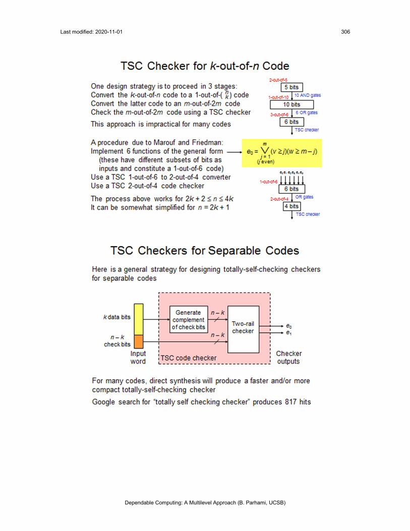
Last modified: 2020-11-01
Dependable Computing: A Multilevel Approach (B. Parhami, UCSB)
306

Last modified: 2020-11-01
Dependable Computing: A Multilevel Approach (B. Parhami, UCSB)
307
15.5 Self-Checking State Machines
This section to be based on the following slides:

Last modified: 2020-11-01
Dependable Computing: A Multilevel Approach (B. Parhami, UCSB)
308
15.6 Practical Self-Checking Design
Design based on parity codes
Design with residue encoding
FPGA-based design
General synthesis rules
Partially self-checking design
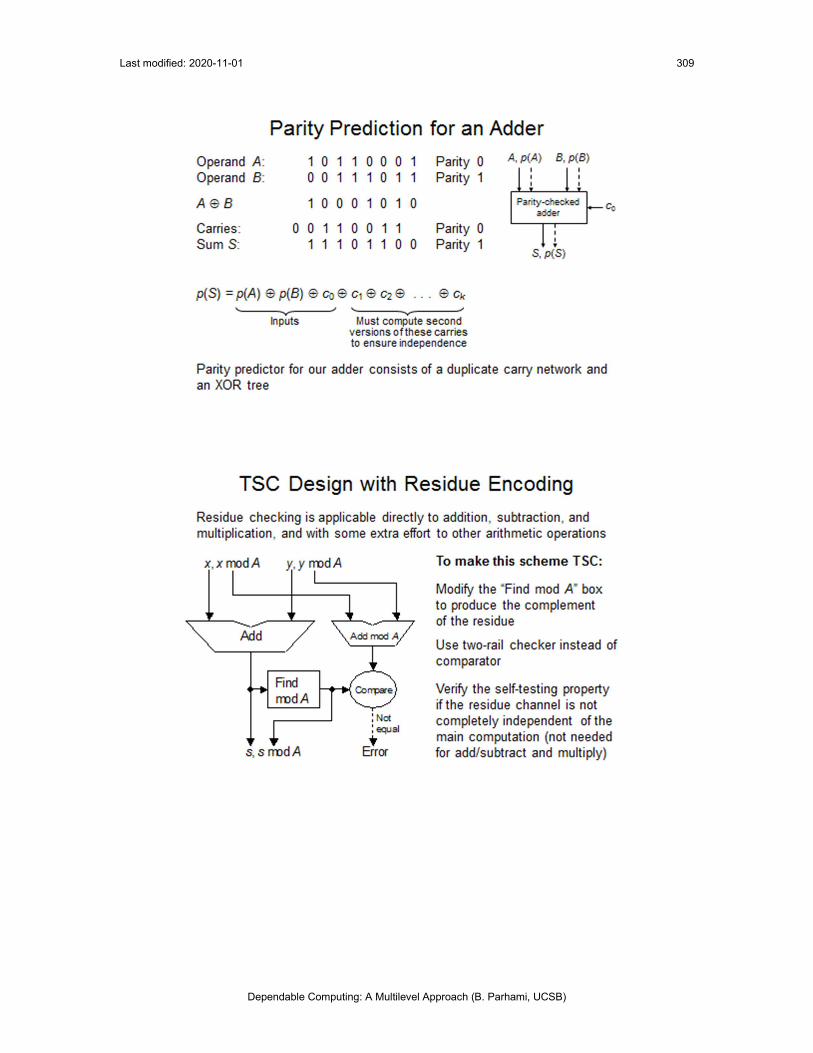
Last modified: 2020-11-01
Dependable Computing: A Multilevel Approach (B. Parhami, UCSB)
309

Last modified: 2020-11-01
Dependable Computing: A Multilevel Approach (B. Parhami, UCSB)
310

Last modified: 2020-11-01
Dependable Computing: A Multilevel Approach (B. Parhami, UCSB)
311
Last modified: 2020-11-01
Dependable Computing: A Multilevel Approach (B. Parhami, UCSB)
312
Problems
15.1 Self-checking checker for 2-out-of-4 code
Show that a self-checking checker for 2-out-of-4 code can be built from three 2-input OR gates and three 2-input AND gates.
15.2 Self-checking m-out-of-n code checkers
Consider the following strategy for designing a self-checking checker for an m-out-of-n code. Begin by dividing the n inputs into two roughly equal subsets S = {s1, s2, . . . , sk} and T = {t1, t2, . . . , tn–k}. Then, select the nonnegative integers A and B such that A + B = 2q – 1 – m for an arbitrary integer q. Next, design two circuits to compute U = A + ∑ 𝑠 and V = B + ∑ 𝑡 .
a. Complete the description of the design. Hint: What is U + V for codewords and noncodewords?
b. Show that the resulting design is indeed self-checking.
c. Design a self-checking checker for 3-out-of-6 code based on this method.
15.3 Dependability and other system attributes
Read the article [Blaa09] and discuss, in one typewritten page, how dependable computing methods can be put to other uses, such as speed enhancement and energy economy.
15.4 Self-checking Berger-code checkers
a. Design a totally self-checking checker for a Berger code with 31 data bits and 5 check bits.
b. Describe how your design in the answer to part a will change when the Berger code’s check part holds 31 – count(1s), instead of the commonly used count(0s).
c. Extend your answer to part b to the general case of k data bits and r = log2(k + 1) check bits.
15.5 Totally-self-checking decoder
Suppose that the correct functioning of a 2-to-4 decoder is to be monitored. Design a totally-self-checking checker to be used at the output of the decoder. Show that your design is indeed totally self-checking.
15.6 Totally-self-checking checker
Consider a code with multiple parity check bits applied to different subsets of the data bits. Hamming SEC and SEC/DED codes are examples of this class of parity-based codes. Devise a strategy for designing a totally self-checking checker for such a code. Fully justify your answer.
15.7 Coded computing
Read the article [Dutt20] and answer the following questions, using no more than a couple of sentences for each answer.
a. What is coded computing?
b. How do the codes used in the article differ from discrete codes of Chapters 13-14 in our textbook?
c. What are the “seven dwarfs”?
d. Which four of the seven dwarfs do the authors tackle?
e. Why do you think the other three dwarfs were not considered?

Last modified: 2020-11-01
Dependable Computing: A Multilevel Approach (B. Parhami, UCSB)
313
15.8 Use of parity-preserving and parity-inverting codes
Intro

Last modified: 2020-11-01
Dependable Computing: A Multilevel Approach (B. Parhami, UCSB)
314
References and Further Readings
[Akba14] Akbar, M. A. and J.-A. Lee, “Comments on ‘Self-Checking Carry-Select Adder Design Based on Two-Rail Encoding’,” IEEE Trans. Circuits and Systems I, Vol. 61, No. 7, pp. 2212-2214, July 2014.
[Ande73] Anderson, D. A. and G. Metze, “Design of Totally Self-Checking Check Circuits for m-out-of-n Codes,” IEEE Trans. Computers
[Ashj77] Ashjaee, M. J. and S. M. Reddy, “On Totally Self-Checking Checkers for Separable Codes,” IEEE Trans. Computers, pp. 737-744, August 1977.
[Chan99] Chang, W.-F. and C.-W. Wu, “Low-Cost Modular Totally Self-Checking Checker Design for m-out-of-n Codes,” IEEE Trans. Computers, Vol. 48, No. 8, pp. 815-826, August 1999.
[Chua78] Chuang, H. and S. Das, “Design of Fail-Safe Sequential Machines Using Separable Codes,” IEEE Trans. Computers, Vol. 27, No. 3, pp. 249-251, March 1978.
[Dutt20] Dutta, S., H. Jeong, Y. Yang, V. Cadambe, T. M. Low, and P. Grover, “Addressing Unreliability in Emerging Devices and Non-von Neumann Architectures Using Coded Computing,” Proceedings of the IEEE, Vol. 108, No. 8, pp. 1219-1234, August 2020.
[Gait08] Details to be supplied
[Lala01] Lala, P. K., Self-checking and Fault-Tolerant Digital Design, Morgan Kaufmann, 2001.
[Lala03] Lala, P. K. and A. L. Burress, “Self-Checking Logic Design for FPGA Implementation,” IEEE Trans. Instrumentation and Measurement, Vol. 52, No. 5, pp. 1391-1398, October 2003.
[Parh76] Parhami, B., “Design of Self-Monitoring Logic Circuits for Applications in Fault-Tolerant Digital Systems,” Proc. Int’l Symp. Circuits and Systems, 1976.
[Wake78] Wakerly, J. F., Error Detecting Codes, Self-Checking Circuits and Applications, North-Holland, 1978.

Last modified: 2020-11-01
Dependable Computing: A Multilevel Approach (B. Parhami, UCSB)
315
16 Redundant Disk Arrays
“Success is the ability to go from one failure to another with no loss of enthusiasm.”
Winston Churchill
“If two men on the same job agree all the time, then one is useless. If they disagree all the time, then both are useless.”
Darryl F. Zanuck
Topics in This Chapter
16.1. Disk Drives and Disk Arrays
16.2. Disk Mirroring and Striping
16.3. Data Encoding Schemes
16.4. RAID and Its Levels
16.5. Disk Array Performance
16.6. Disk Array Reliability Modeling
Large storage capacities are required in many modern computer applications.
Early in the history of high-performance computing, special disk drives were
developed to cater to the capacity and reliability needs of such applications.
Beginning in the late 1980s, however, it was realized that economy of scale
favored the use of low-cost disk drives, produced in high volumes for the personal
computer market. Even though each such disk unit is fairly reliable, when arrays
of hundreds or perhaps thousands of them are used to offer multiterabyte capacity,
potential data loss due to disk failure becomes a serious concern. In this chapter,
we study methods for building reliable disk arrays.

Last modified: 2020-11-01
Dependable Computing: A Multilevel Approach (B. Parhami, UCSB)
316
16.1 Disk Drives and Disk Arrays
Magnetic disk drives form the main vehicles for supplying stable archival storage in
many applications. Since the inception of hard disk drive in 1956, the recording density
of these storage devices has grown exponentially, much like the exponential growth in
the density of integrated circuits. Currently, tens of gigabytes of information can be
stored on each cm2 of disk surface, making it feasible to provide terabyte-class disk
drives for personal use and petabyte-class archival storage for enterprise systems.
Amdahl’s rules of thumb for system balance dictate that for each GIPS of performance
one needs 1 GB of main memory and 100 GB of disk storage. Thus the trend toward ever
greater performance brings with it the need for ever larger secondary storage.
Figure 16.1 shows a typical disk memory configuration and the terminology associated
with its design and use. There are 1-12 platters mounted on a spindle that rotates at
speeds of 3600 to well over 10,000 revolutions per minute. Data is recorded on both
surfaces of each platter along circular tracks. Each track is divided into several sectors,
with a sector being the unit of data transfer into and out of the disk. The recording density
is a function of the track density (tracks per centimeter or inch) and the linear bit density
along the track (bits per centimeter or inch). In the year 2010, the areal recording density
of inexpensive commercial disks was in the vicinity of 100 Gb/cm2. Early computer disks
had diameters of up to 50 cm, but modern disks are seldom outside the range of 1.0-3.5
inches (2.5-9.0 cm) in diameter.
The recording area on each surface does not extend all the way to the center of the
platter because the very short tracks near the middle cannot be efficiently utilized. Even
so, the inner tracks are a factor of 2 or more shorter than the outer tracks. Having the
same number of sectors on all tracks would limit the track (and, hence, disk capacity) by
what it is possible to record on the short inner tracks. For this reason, modern disks put
more sectors on the outer tracks. Bits recorded in each sector include a sector number at
the beginning, followed by a gap to allow the sector number to be processed and noted by
the read/write head logic, the sector data, and error detection/correction information.
There is also a gap between adjacent sectors. It is because of these gaps, the sector
number, and error-coding overhead, plus spare tracks that are often used to allow for
“repairing” bad tracks discovered at the time of manufacturing testing and in the course
of disk memory operation (see Section 6.2), that a disk’s formatted capacity is much
lower than its raw capacity based on data recording density.

Last modified: 2020-11-01
Dependable Computing: A Multilevel Approach (B. Parhami, UCSB)
317
Track 0 Track 1
Track c – 1
Sector
Recording area
Spindle
Direction of rotation
Platter
Read/write head
Actuator
Arm
Track 2
Figure 16.1 Disk memory elements and key terms.
An actuator can move the arms holding the read/write heads, of which we have as many
as there are recording surfaces, to align them with a desired cylinder consisting of tracks
with same diameter on different recording surfaces. Reading of very closely spaced data
on the disk necessitates that the head travel very close to the disk surface (within a
fraction of a micrometer). The heads are prevented from crashing onto the surface by a
thin cushion of air. Note that even the tiniest dust particle is so large in comparison with
the head separation from the surface that it will cause the head to crash onto the surface.
Such head crashes damage the mechanical parts and destroy a great deal of data on the
disk. To prevent these highly undesirable events, hard disks are typically sealed in
airtight packaging.
Disk performance is related to access latency and data transfer rate. Access latency is the
sum of cylinder seek time (or simply seek time) and rotational latency, the time needed
for the sector of interest to arrive under the read/write head. Thus:
Disk access latency = Seek time + Rotational latency (16.1.access)
A third term, the data transfer time, is often negligible compared with the other two and
can be ignored.
Seek time depends on how far the head has to travel from its current position to the target
cylinder. Because this involves a mechanical motion, consisting of an acceleration phase,
a uniform motion, and a deceleration or braking phase, one can model the seek time for
moving by c cylinders as follows, where , , and are constants:

Last modified: 2020-11-01
Dependable Computing: A Multilevel Approach (B. Parhami, UCSB)
318
Seek time = + (c – 1) + 1c (16.1.seek)
The linear term (c – 1), corresponding to the uniform motion phase, is a rather recent
addition to the seek-time equation; older disks simply did not have enough tracks, and/or
a high enough acceleration, for uniform motion to kick in.
Rotational latency is a function of where the desired sector is located on the track. In the
best case, the head is aligned with the track just as the desired sector is arriving. In the
worst case, the head just misses the sector and must wait for nearly one full revolution.
So, on average, the rotational latency is equal to the time for half a revolution:
Average rotational latency = 30
rpm s =
30 000
rpm ms (16.1.avgrl)
Hence, for a rotation speed of 10 000 rpm, the average rotational latency is 3 ms and its
range is 0-6 ms.
The data transfer rate is related to the rotational speed of the disk and the linear bit
density along the track. For example, suppose that a track holds roughly 2 Mb of data and
the disk rotates at 10,000 rpm. Then, every minute, 2 1010 bits pass under the head.
Because bits are read on the fly as they pass under the head, this translates to an average
data transfer rate of about 333 Mb/s = 42 MB/s. The overhead induced by gaps, sector
numbers, and CRC encoding causes the peak transfer rate to be somewhat higher than the
average transfer rate thus computed.
Figure 16.2 The three components of access time for a disk.

Last modified: 2020-11-01
Dependable Computing: A Multilevel Approach (B. Parhami, UCSB)
319
While hard disk drives continue to grow in capacity, there are applications for which no
single disk can satisfy the storage needs. There are other applications that need high data
rates, in excess of what can be provided by a single disk, so as to keep a large number of
computational units usefully busy. In such cases, arrays of disks, sometimes numbering
in hundreds or thousands, are used.
Modern disk drives are highly reliable, boasting MTTFs that are measured in decades.
With hundreds or thousands of drives in the same disk-array system, however, a few
failures per year or even per month are to be expected. Thus, to avoid data loss which is
critically important for systems dealing with large data bases, reliability improvement
measures are required.
The intersection of the two requirements just discussed (improved capacity and
throughput on one side and higher reliability on the other), brought about the idea of
using a redundant array of independent disks (RAID) in lieu of a single disk unit. Another
motivating factor for RAID in the mid 1980s was that it no longer made economic sense
to design and manufacture special high-capacity, high-reliability disk units for mainframe
and supercomputer applications, given that the same capacity and throughput could be
provided by combining low-cost disks, mass-produced for the personal computer market.
In fact, the letter “I” in RAID originally stood for “Inexpensive.”
The steep downward trend in the per-gigabyte price of disk memories, and thus of RAID
systems, has made such storage systems affordable even for personal applications, such
as home storage servers.
Much of our discussion in this chapter is in terms of magnetic hard-disk drives, the
common components in RAID systems. Even though SSD storage has different failure
mechanisms (they contain no moving parts to fail, but suffer from higher error rates and
limited erase counts), applicable high-level concepts are pretty much the same. Please
refer to [Jere11] for issues involved in designing SSD RAIDS. A good overview of SSD
RAID challenges and of products available on the market is provided in [CW13].

Last modified: 2020-11-01
Dependable Computing: A Multilevel Approach (B. Parhami, UCSB)
320
16.2 Disk Mirroring and Striping
The two ideas of disk mirroring and striping are foundational in the composition of RAID
systems, so we discuss them here in detail before reviewing the structure of modern
redundant disk arrays.
Mirroring refers to duplicating each data file on a separate disk, so that it remains
available in the event of the original disk failing. The original file copy and the mirror
copy are updated together and are thus fully synchronized. Read operations, however,
take place on the original copy. So, even though a mirrored disk system provides no
improvement in access speed performance or data transfer bandwidth, it offers high
reliability due to acting as a two-way parallel system. Only if both disks containing the
original file and its mirror copy fail will we have data loss. The drawback of 100%
redundancy in storage space is what motivated the development of subsequent RAID
schemes based on various forms of low-redundancy data encoding. Mirroring is
sometimes referred to as Raid level 1 (RAID1, for short), because it was the first form of
redundancy applied to disk arrays.
In disk striping, we divide our data into smaller pieces, perhaps all the way down to the
byte or bit level, and store the pieces on different disks, so that all those pieces can be
read out or written into concurrently. This increases the disk system’s read and write
bandwidth for large files, but has the drawback that all the said disks must be functional
for us to be able to recover or manipulate the file. The disk system in effect behaves as a
series system and will thus have a lower reliability than a single disk. Striping is
sometimes referred to as RAID level 0 (RAID0, for short), even though no data
redundancy is involved in it.

Last modified: 2020-11-01
Dependable Computing: A Multilevel Approach (B. Parhami, UCSB)
321

Last modified: 2020-11-01
Dependable Computing: A Multilevel Approach (B. Parhami, UCSB)
322
16.3 Data Encoding Schemes
The key idea for making disk arrays reliable is to spread each data block across multiple
disks in encoded form, so that the failure of one (or a small number) of the disk drives
does not lead to data loss. Many different encoding schemes have been tried or proposed
for this purpose. One feature that makes the encoding simpler compared with arbitrary
error-correcting codes is the fact that standard disk drives already come with strong error-
detecting and error-correcting codes built in. It is extremely unlikely, though not totally
impossible, for a data error on a specific disk drive to go undetected. This possibility is
characterized by the disk’s bit error rate (BER), which for modern disk drives is on the
order of 10–15. This vanishingly small probability of reading corrupt data off a disk
without detecting the error can be ignored for most practical applications, leading to the
assumption that disk data errors can be detected with perfect accuracy.
So, for all practical purposes, disk errors at the level of data access units (say sectors) are
of the erasure kind, rendering codes capable of dealing with erasure errors adequate for
encoding of data blocks across multiple disks. The simplest such code is duplication.
Note that duplication is inadequate for error correction with arbitrary errors. In the latter
case, when the two data copies disagree, there is no way of finding out which copy is in
error. However, if one of the two copies is accidentally lost or erased, then the other copy
supplies the correct data. Simple parity or checksum schemes can also be used for
erasure-error correction. Again, with arbitrary (inversion) errors, a parity bit or checksum
can only detect errors. The same parity bit or checksum, however, can be used to
reconstruct a lost or erased bit/byte/word/block.
Fig. 16.parity Parity-coded bits and blocks of data across multiple disks.
There are 4 data bits/bytes/words/blocks, followed by a
parity bit/byte/word/block.

Last modified: 2020-11-01
Dependable Computing: A Multilevel Approach (B. Parhami, UCSB)
323
Whether parity encoding is done with bits or blocks of data, the concepts are the same, so
we proceed with the more practical block-level parity encoding. The parity block P for
the four blocks A, B, C, and D of data depicted in Fig. 16.parity is obtained as:
P = A B C D (16.3.prty)
Then, if one of the blocks, say B, is lost or erased, it can be rebuilt thus:
B = A C D P (16.3.rbld)
Note that if the disk drive holding the block B becomes inaccessible, one needs to read
the entire contents of the other four disks in order to reconstruct all the lost blocks. This is
a time-consuming process, raising the possibility that a second disk fails before the
reconstruction is complete. This is why it may be desirable to include a second coding
scheme to allow the possibility of two disk drive failures. For example, we may use a
second coding scheme in which the check block Q is derived from the data blocks A, B,
C, and D in a way that is different from P:
Q = g(A, B, C, D) (16.3.chk2)
Then, the data will continue to be protected even during the rebuilding process after the
first disk failure.

Last modified: 2020-11-01
Dependable Computing: A Multilevel Approach (B. Parhami, UCSB)
324
16.4 RAID and Its Levels
We have already alluded to RAID0 (provides high performance, but no error tolerance),
RAID1 (provides high data integrity, but is an overkill in terms of redundancy), and
RAID10 (more accurately, RAID1/0) as precursors of the more elaborate RAID2-RAID6
schemes to be discussed in this section.
Fig. 16.levels Schematic representation of key RAID levels and their
associated redundancy schemes.

Last modified: 2020-11-01
Dependable Computing: A Multilevel Approach (B. Parhami, UCSB)
325
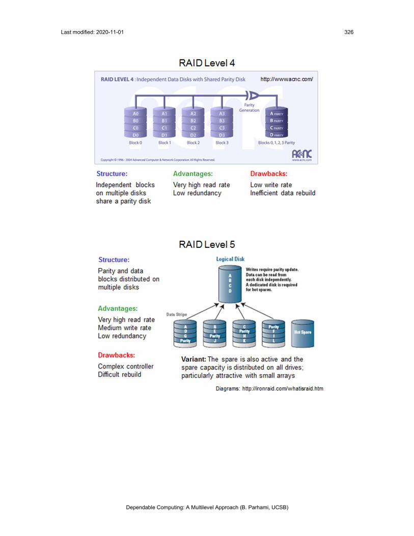
Last modified: 2020-11-01
Dependable Computing: A Multilevel Approach (B. Parhami, UCSB)
326

Last modified: 2020-11-01
Dependable Computing: A Multilevel Approach (B. Parhami, UCSB)
327

Last modified: 2020-11-01
Dependable Computing: A Multilevel Approach (B. Parhami, UCSB)
328
16.5 Disk Array Performance
This section to be based on the following slides:

Last modified: 2020-11-01
Dependable Computing: A Multilevel Approach (B. Parhami, UCSB)
329

Last modified: 2020-11-01
Dependable Computing: A Multilevel Approach (B. Parhami, UCSB)
330
16.6 Disk Array Reliability Modeling
This section to be based on the following slides and notes.
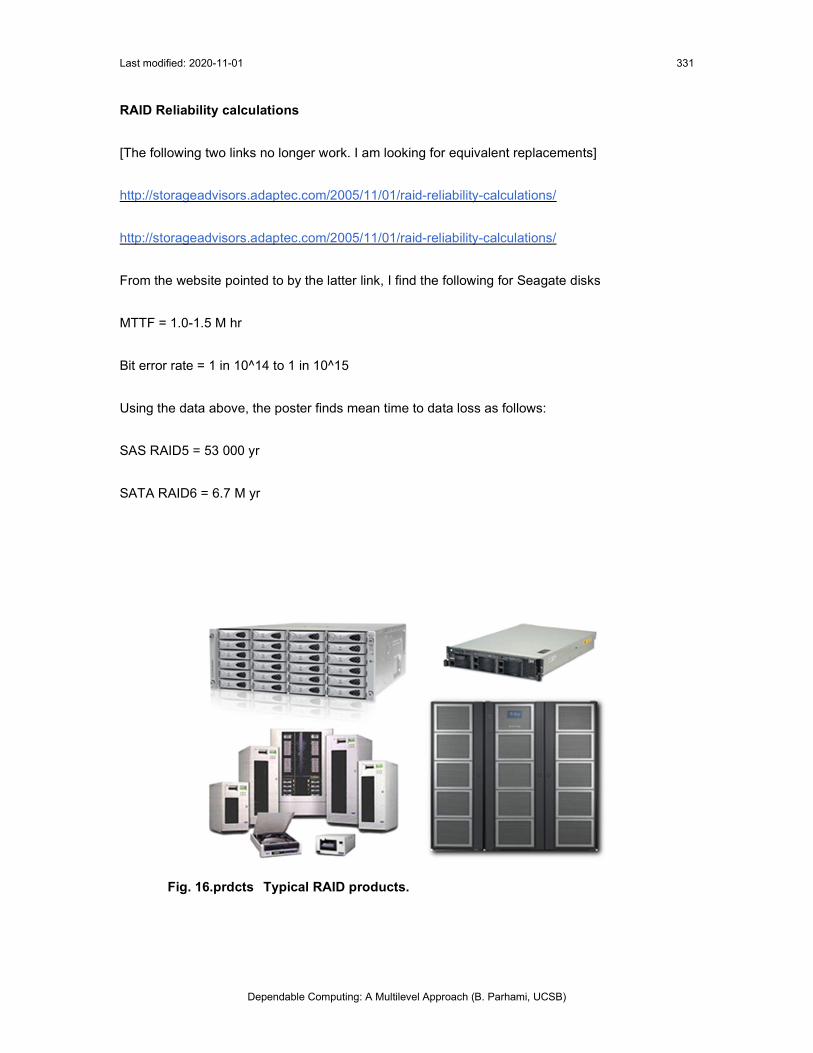
Last modified: 2020-11-01
Dependable Computing: A Multilevel Approach (B. Parhami, UCSB)
331
RAID Reliability calculations
[The following two links no longer work. I am looking for equivalent replacements]
http://storageadvisors.adaptec.com/2005/11/01/raid-reliability-calculations/
http://storageadvisors.adaptec.com/2005/11/01/raid-reliability-calculations/
From the website pointed to by the latter link, I find the following for Seagate disks
MTTF = 1.0-1.5 M hr
Bit error rate = 1 in 10^14 to 1 in 10^15
Using the data above, the poster finds mean time to data loss as follows:
SAS RAID5 = 53 000 yr
SATA RAID6 = 6.7 M yr
Fig. 16.prdcts Typical RAID products.

Last modified: 2020-11-01
Dependable Computing: A Multilevel Approach (B. Parhami, UCSB)
332

Last modified: 2020-11-01
Dependable Computing: A Multilevel Approach (B. Parhami, UCSB)
333
Problems
16.1 System with two disk drives
Discuss the pros and cons of using two identical disk drives as independent storage units, in a RAID0 configuration, or in a RAID1 configuration.
16.2 Hybrid RAID architectures
Besides RAID 10, discussed in Section 16.4, there are other hybrid RAID architectures. Perform an Internet search to identify two such hybrid architectures, describe each one briefly, and compare the two with respect to cost and reliability.
16.3 Disk array reliability evaluation
A computer’s input/output system is composed of the following components, with the given MTTF values: (1) Four disk drives, at 0.5M hr each; (2) Four IDE cables, at 2M hr each; (3) One IDE controller, at 5M hr; (4) A power supply, at 0.1M hr. Assume exponential distribution of component lifetimes and similar disk controller complexities for all systems.
a. Derive the MTTF and mean time to data loss (MTDL) for this I/O system.
b. Expanding storage needs forces the computer system manager to double the number of disk drives and to use RAID0 for organizing them. What are the new system’s MTTF and MTDL?
c. Reliability concerns motivates the computer system manager to convert to a 6-disk RAID3 system, with one parity disk and a hot spare disk. Reconstructing data on the spare disk takes 2 hr. Calculate the new system’s MTTF and MTDL.
d. Some time later, the computer system manager decides to switch to a RAID5 configuration, without adding any storage space. Does this action improve or degrade the MTDL?
16.4 Disk failure rate modeling
The figure below plots the expected remaining time to the next failure in a cluster node as a function of time elapsed since the last failure, with both times given in minutes [PDSI09].
a. Assuming that the situation for disk memories is similar, why does this data refute the assumption
that disk lifetimes are exponentially distributed?
b. Which distribution is called for in lieu of exponential distribution?
16.5 Disk array reliability
Suppose each disk in a disk array with d data disks and r parity (redundant) disks fails independently with probability p over a 1-year period. Assume that the control system never fails and ignore the recovery time.
a. Consider a disk array with d = 2 and r = 1. What is the expected number of disk failures in a year?
b. What is the reliability of the disk array of part a over a 1-year period?
c. Consider a disk array with d = 3 and r = 2. What is the expected number of disk failures in a year?

Last modified: 2020-11-01
Dependable Computing: A Multilevel Approach (B. Parhami, UCSB)
334
d. What is the reliability of the disk array of part c over a 1-year period?
e. For p = 0.1, which is more reliable: The disk array of part a or that of part c?
f. For p = 0.6, which is more reliable: The disk array of part a or that of part c?
16.6 RAID 5 with different parity group sizes
We have 11 identical disks and want to build a RAID system with an effective capacity equivalent to 8 disks. Discuss the pros and cons of the following schemes (both using the RAID 5 architecture) in terms of data loss probability and ease/latency of data reconstruction.
a. Nine disks are used as a single parity group and 2 disks are designated as spares.
b. Ten disks are arranged into two separate parity groups of 5 disks each and 1 disk is designated as spare.
Last modified: 2020-11-01
Dependable Computing: A Multilevel Approach (B. Parhami, UCSB)
335
References and Further Readings
[Chen94] Chen, P. M., E. K. Lee, G. A. Gibson, R. H. Katz, and D. A. Patterson, “RAID: High-Performance Reliable Secondary Storage,” ACM Computing Surveys, Vol. 26, No. 2, pp. 145-185, June 1994.
[Corn12] Cornwell, M., “Anatomy of a Solid-State Drive,” Communications of the ACM, Vol. 55, No. 12, pp. 59-63, December 2012.
[CW13] Computer Weekly, “SSD RAID Essentials; What You Need to Know about Flash and RAID.” http://www.computerweekly.com/feature/SSD-RAID-essentials-What-you-need-to-know-about-flash-and-RAID
[Eler07] Elerath, J., “Hard Disk Drives: The Good, the Bad and the Ugly,” ACM Queue, Vol. 5, No. 6, pp. 28-37, September-October 2007.
[Feng05] Feng, G.-L., R. H. Deng, F. Bao, and J.-C. Shen, “New Efficient MDS Array Codes for RAID—Part I: Reed-Solomon-Like Codes for Tolerating Three Disk Failures,” IEEE Trans. Computers, Vol. 54, No. 9, pp. 1071-1080, September 2005.
[Feng05a] Feng, G.-L., R. H. Deng, F. Bao, and J.-C. Shen, “New Efficient MDS Array Codes for RAID—Part II: Rabin-Like Codes for Tolerating Multiple (4) Disk Failures,” IEEE Trans. Computers, Vol. 54, No. 12, pp. 1473-1483, December 2005.
[Gray00] Gray, J. and P. Shenoy, “Rules of Thumb in Data Engineering,” Microsoft Research MS-TR-99-100, revised ed., March 2000.
[Grib16] Gribaudo, M., M. Iacono, and D. Manini, “Improving Reliability and Performances in Large Scale Distributed Applications with Erasure Codes and Replication,” Future Generation Computer Systems, Vol. 56, pp. 773-782, March 2016.
[Jere11] Jeremic, N., G. Muhl, A. Busse, and J. Richling, “The Pitfalls of Deploying Solid-State Drive RAIDs,” Proc. 4th Int’l Conf. Systems and Storage, Article No. 14, 2011.
[Patt88] Patterson, D. A., G. Gibson, and R. H. Katz, “A Case for Redundant Arrays of Inexpensive Discs,”
[PDSI09] Petascale Data Storage Institute, “Analyzing Failure Data,” project Web site, accessed on November 8, 2012: http://www.pdl.cmu.edu/PDSI/FailureData/index.html
[Plan97] Plank, J. S., “A tutorial on Reed–Solomon coding for fault‐tolerance in RAID‐like systems,” Software: Practice and Experience, Vol. 27, No. 9, 1997, pp. 995-1012.
[Schr07] Schroeder, B. and G. A. Gibson, “Understanding Disk Failure Rates: What Does an MTTF of 1,000,000 Hours Mean to You?” ACM Trans. Storage, Vol. 3, No. 3, Article 8, 31 pp., October 2007.
[Thom09] Thomasian, A. and M. Blaum, “Higher Reliability Redundant Disk Arrays: Organization, Operation, and Coding,” ACM Trans. Storage, Vol. 5, No. 3, pp. 7-1 to 7-59, November 2009.
[WWW1] News and reviews of storage-related products, http://www.storagereview.com/guide/index.html (This link is obsolete; it will be replaced by a different resource in future).
[WWW2] Battle Against Any RAID-F (Free, Four, Five), http://www.baarf.com (accessed on November 8, 2012).