
enginering1.pdf - Gece Kitaplığı
261
-
Upload
khangminh22 -
Category
Documents
-
view
0 -
download
0
Transcript of enginering1.pdf - Gece Kitaplığı


İmtiyaz Sahibi / Publisher • Yaşar Hız
Genel Yayın Yönetmeni / Editor in Chief • Eda Altunel
Editörler/ Editors • Assoc. Prof. Dr. Selahattin Bardak
Assist. Prof. Dr. Nesli Aydın
Assist. Prof. Dr. Yalçın Boztoprak
Kapak & İç Tasarım / Cover & Interior Design • Gece Kitaplığı
Birinci Basım / First Edition • © Aralık 2021
ISBN • 978-625-8075-43-4
© copyright Bu kitabın yayın hakkı Gece Kitaplığı’na aittir.
Kaynak gösterilmeden alıntı yapılamaz, izin almadan hiçbir yolla çoğaltılamaz.
The right to publish this book belongs to Gece Kitaplığı. Citation can not be shown without the source, reproduced in any way
without permission.
Gece Kitaplığı / Gece PublishingTürkiye Adres / Turkey Address: Kızılay Mah. Fevzi Çakmak 1.
Sokak Ümit Apt. No: 22/A Çankaya / Ankara / TRTelefon / Phone: +90 312 384 80 40
web: www.gecekitapligi.come-mail: [email protected]
Baskı & Cilt / Printing & VolumeSertifika / Certificate No: 47083
Research & Reviews in Engineering - I
December, 2021
EditorsAssoc. Prof. Dr. Selahattin Bardak
Assist. Prof. Dr. Nesli AydınAssist. Prof. Dr. Yalçın Boztoprak


CONTENTSChapter 1DESIGNING AN ELECTRONIC POSTURE CORRECTOR CORSET Züleyha DEĞİRMENCİ ........................................................................1Zeynep YAŞAR ......................................................................................1Chapter 2DESIGN AND IMPLEMENTATION OF THE ASPIRATION AND IRRIGATION PUMP FOR ABSCESS TREATMENTAdem GÖLCÜK ....................................................................................23 Muhammed Bakır DALMIZRAK ........................................................23Chapter 3PRELIMINARY CHARACTERIZATION PROPERTIES OF SAMPLE BORON(COLEMANITE) FROM BALIKESIR (BIGADIÇ) REGION AND IMPORTANCEOyku Bilgin ...........................................................................................43Chapter 4DURABILITY OF MORTARS MADE WITH BIO-BASED ASHESMustafa EKEN .......................................................................................57Ela AVSAROGLU ................................................................................57Chapter 5A COINTEGRATION RELATIONSHIP BETWEEN WHEAT PRICES IN TURKEY IN THE LONG RUNBurcu ERDAL ........................................................................................85Hasan VURAL .......................................................................................85Chapter 63D PRINTED HORN ANTENNA WITH PCB MICROSTRIP FEED FOR X-KA BAND APPLICATIONAYSU BELEN .......................................................................................99Chapter 7CS DOPANT ROLE ON ELECTRICAL, MICROSTRUCTURAL AND CRYSTALLINITY OF Y-123 SUPERCONDUCTING MATERIALSMustafa Burak TURKOZ ......................................................................111Asaf Tolga ULGEN ..............................................................................111

Chapter 8HYDRO-ECONOMIC DESIGN CONCEPT FOR MICRO-IRRIGATION SYSTEM SUBMAINS UNIT NETWORK-I: DESIGN PROCEDUREGürol YILDIRIM ...................................................................................127Chapter 9HYDRO-ECONOMIC DESIGN CONCEPT FOR MICRO-IRRIGATION SYSTEM SUBMAINS UNIT NETWORK-I: CASE STUDYGürol YILDIRIM ...................................................................................147Chapter 10THE ROLE OF BIOTECHNOLOGY ABOUT FOOD WASTE RECYCLING IN TURKEY Sevcan Aytaç Korkmaz ..........................................................................163Sümeyye GÜVENDI GÜNDOĞDU ...................................................163Chapter 11IMPLEMENTING BALANCED ITERATIVE REDUCING AND CLUSTERING USING HIERARCHIES (BIRCH) ALGORITHM STEP BY STEP AND APPLYING TO THE DATASETS CONTAINING JOB-ADSYunus DOĞAN ......................................................................................179Feriştah DALKILIÇ ...............................................................................179Alp KUT ................................................................................................179Kemal Can KARA .................................................................................179Uygar TAKAZOĞLU ............................................................................179Chapter 12INNOVATION PROCESS OF ELECTRIC VEHICLESHilmi Zenk .............................................................................................201Faruk GÜNER .......................................................................................201Chapter 13 STANDARD TEST METHODS FOR DETERMINING BITÜMEN BINDERS AND ASPHALT PAVEMENTS PROPERTIESSAVAS GURDAL ................................................................................225Chapter 14AN ELECTROCHEMICAL MEMBRANE SEPARATION PROCESS: ELECTRODIALYSISBelgin Karabacakoğlu ............................................................................241

Chapter 1DESIGNING AN ELECTRONIC POSTURE CORRECTOR CORSET
Züleyha DEĞİRMENCİ1
Zeynep YAŞAR2
1
2
1 Gaziantep Üniversitesi, Mühendislik Fakültesi, Tekstil Mühendisliği Bölümü, Gazian-tep, Türkiye2 Gaziantep Üniversitesi, Mühendislik Fakültesi, Ürün Geliştirme ve Tasarım Mühendis-liği Bölümü, Gaziantep, Türkiye

Züleyha Deği̇rmenci̇, Zeynep Yaşar2 .
1. Introduction
Electronic textiles (e-textiles) are derived from the combination of textile materials with electronic evenings to serve a particular purpose. The elements that make up the system are designed for each product, as invisible as possible and cannot be easily integrated into other systems. They are easy to adapt to issues such as e-textiles, measurement, power control response. It is thought that the clothes of the future can be controlled by computers. In this study, the latest developments in smart textile, materials and their production processes are mentioned. Each technique shows the advantages and disadvantages and our aim is to emphasize a possible balance between flexibility, ergonomics, low power consumption, integration and ultimately autonomy. [ 1].
The common feature of textile materials is protection from external factors and aesthetic features. Today, smart textiles are used to bring a new dimension to textiles to meet the rapidly changing needs of consumers. With the electronic measurement and storage features of these systems, new wearable electronic systems emerge. In this article, the concept of i-textile is presented together with building blocks for its realization. It also describes the design and development of Smart Shirt, a smart garment. This t-shirt allows detection, monitoring and data processing devices to be combined. The article discusses the implications of product implementation and health service transformation. Finally, we discuss developments to advance this paradigm and turn passive textiles into new generation interactive or “smart” textiles. [2]
There are many applications of wearable electronic clothing that can record from sports to artistic space. In this study wearable devices that can read and record data and Systems are described. ensory function of garments It is obtained with fabric strain sensors based on teeth coated with polypropylene or carbon filled tires. Conductive materials are used. Piezo resistive systems are used in fabric. Also attached to the strain fabric strips to form conductive tracks at strategic points. The sensory system of the smart shirt produced can be divided into two parts: first, the textile part (where a wearable device receives biomechanical signals and a hardware / software location), and the other is the area where the wireless communication system stores the acquired data. [3]
Although many ideas have been put forward on electronic yarns and textiles, they are not suitable for practical use. In addition to chemical / mechanical strength and high electrical conductivity, important materials qualities; touchability, wearability, lightness and “smart” functionality. The aim of this study is to convert cotton ropes into smart e-textiles using a polyelectrolyte based coating with carbon nanotubes (CNTs). Nano pipes

.3Research & Reviews in Engineering
(20 z / cm) provide efficient charging transfer over the network, making them promising materials for garments with high information content. In addition to the integrated moisture sensing, CNT - cotton yarns show that the main protein of blood, albumin, can be used to detect with high sensitivity and selectivity. Despite future challenges, the results of this study show that these materials can be applied as simple, sensitive, selective and versatile wearable bio-monitoring and medical sensors. [4].
Babies who are taken to intensive care unit after being born are very sensitive and vulnerable to external conditions. Designed in this study, Smart Jacket, body sensor and cable networks allows the user to continuously monitor. With the help of this coat, the clinically monitored baby, family and hospital will have more comfortable conditions. Here we describe the first version of the neonatal coat that provides ECG measurement with textile electrodes. It also explores a new solution for skin contact difficulties caused by textile electrodes. Jackets have aesthetic features that appeal to parents and medical personnel with new wearable technologies. A design process in close contact with users and experts leads to a balanced integration of technology, user focus and aesthetics. It shows prototype and experimental results obtained in clinical setting [5].
In this study, wearable devices (a smart shirt, a leotard and a glove) that can read and record the vital signs and movements of a person using the smart garment system are discussed. The detection function of garments is based on piezo-resistant fabric sensors based on carbon-charged tires (CLR) and different conductive materials. This study was carried out to demonstrate the feasibility of intelligent garments that can monitor vital signs and human posture. The results show that electroactive functions can be applied to the same weaving system where vital signs and movements are converted into readable signals and transmitted to detailing devices [ 6].
The emergence of wearable textile systems in recent years exhibited the need for wireless communication tools integratable into garments. In literature, several planar antenna designs based on textile materials have been presented, however, without an adapted feeding structure for wearable applications. An aperture-coupled patch antenna (ACPA) meets this requirement since the rigid coaxial feed is replaced by a microstrip feed line that couples its power into the antenna through an aperture in the ground plane. This letter presents the first ACPA entirely made out of textile material. The result is a highly efficient, fully flexible, and wearable antenna that is integratable into garments. In order to overcome difficulties with feeding structures for wearable antennas, we designed the first ACPA entirely made out of textile material. Excellent agreement was found between the simulated and the experimental results, even when bending

Züleyha Deği̇rmenci̇, Zeynep Yaşar4 .
the antenna or bringing it in the vicinity of the human body. Furthermore, the antenna provides sufficient antenna gain to be applied in a wireless link. The outcome of our research is an antenna that is integratable into wearable textile systems for body and personal area networks operating in the 2.45-GHz ISM band [7].
Wearable teechnology is already in our life. The latest generation of Apple Watch includes AFib (Atrial fibrillation) detection. Atrial fibrillation is a heart arrhythmia that affects about 1% of the population worldwide. It’s mostly detected in adults over the age of 60, and in those with high blood pressure and diabetes. Atrial fibrillation is the leading cause of stroke, with sufferers being five times more likely to have a stroke than those without it. The KardiaMobile and KardiaBand wearable devices incorporate the Apple watch’s heart rate sensor. If the sensor detects an unusual heartbeat, the devices alert the user to place their fingers on a small electrocardiogram (ECG) pad on the watch band. The devices then visually display the user’s heartbeat, and announce whether the heartbeat is normal or the user is experiencing atrial fibrillation. In the future, wearables will be used to collect biometric data, such as heart rate (ECG and HRV), brainwave (EEG), and muscle bio-signals (EMG). They will also be used to monitor the elderly. Being able to review data transmitted from a wearable device means that a patient doesn’t have to be transported to a medical facility, and this has the potential of saving millions of dollars a year [8].
1.1 Problem statement
Today, the development of technology and fast lifestyle have led people to a still life. Inactive life, which has become one of the biggest problems of our age, has brought many health problems with it. Especially sedentary life, muscle weakness, psychological factors cause posture disorders. Many reasons such as dealing with a computer / mobile phone, spending a long time at a desk, sitting in wrong positions cause posture disorder. Employees who spend most of the day at the desk experience neck pain, low back pain and back pain due to inactivity in the skeletal system and posture disorder. These pains cause loss of strength and muscle over time. Designing an auxiliary product in order to avoid these pains is the primary aim of the study.
With the designed posture corrector corset, it is aimed to maintain the correct posture of the person and to increase mobility. The user is warned with this corset every time the user’s posture is disturbed. With this warning, the user is expected to correct his/her posture. Thanks to these warnings to be given after every bad stop, the user will make a habit of standing correctly after a while. In this way, the negative effects caused by bad posture will be reduced. In the first part of this article, explanations

.5Research & Reviews in Engineering
on correct posture will be given, wearable technology, materials to be used in the study and circuit system will be explained in the next sections, the smart corset system will be introduced in the next section and the study will be completed with the results section.
2. Correct posture
Posture is the positioning of each part of the body in the most appropriate position relative to the adjacent segment and the whole body; In its simplest definition, it is the correct posture of the skeletal system. The body obtains the correct posture by working in harmony with many musculoskeletal and joint structures during activities [9]. There are two different stances. Dynamic posture and static posture. Dynamic posture; walking, running, etc. that our body has done using muscle, bone and joint groups. It is called the moving postures that it takes during the movements. Static posture; It is the immobility of our body’s musculoskeletal system in a fixed position within a certain range of joint motion [10].
2.1 What should be the correct posture?
Correct and good posture is the position where minimum energy is used and the least strain on ligaments, bones and joints. The normal curves of the spine are preserved, do not cause pain, are not tiring and the appearance is aesthetic. For a good posture, there should be strong muscles around the spine, physical fitness, and awareness [11]. Figure 1 shows posture disorders and correct posture.
Figure 1. Correct posture and posture disorders [12]
2.2 Effects of posture disorders on our lives
Poor posture causes physical and mental health problems. These health problems can become permanent in our lives. It has negative effects on spine health. It increases the load on the spine by changing the natural curvature of the spine. There is a pronounced curvature in the spine, a natural dimple in the neck and a natural hump in the back and

Züleyha Deği̇rmenci̇, Zeynep Yaşar6 .
a natural dimple in the waist. The lateral curvature of the spine does not exceed 3-5 degrees. When viewed from the back, the spine is practically straight. After years of standing in the same position and bad standing at a desk, the natural curvatures of the spine disappear. Excessive tension in the spine causes damage to the integrity of the spine, compression of the discs, degeneration, stretching, lengthening or shortening of the ligaments, compression of the joints, spasms and weakening of the muscles around the spine. Thus, it causes the discs to weaken, compression and erosion of the spine. These changes not only cause long-term pain and discomfort, but the new condition also impairs the spine’s ability to absorb shock and maintain proper balance [13].
It causes bad posture, depression and stress. Those who habitually age poor posture earlier are more depressed and more anxious. People with good spinal health have higher levels of testosterone. This gives them a sense of strength and control and lowers their levels of the stress hormone cortisol. Correct posture is important to have positive hormones that affect our body positively and to perceive yourself and the world around you happier [13].
2.2.1. Digestive problems
Bad posture also affects the digestive system. Staying in unnatural positions for a long time adversely affects all internal organs. Improper sitting and standing compresses the intestines, which negatively affects digestion and causes gastrointestinal problems such as acid, reflux, flatulence and hernias. Even more surprisingly, poor posture can also affect metabolism, leading to weight gain and fat accumulation around the belly[13].
2.2.2. Increased pain
It causes poor posture, chronic spinal pain (waist, neck, back) and disc degeneration. This is due to increased tension in the muscles, joints, tendons, other soft tissues and bones around the spine. Poor posture can cause pain in parts of the body, including the hips, shoulders, and neck. May cause headache. Your body composition supports the weight of various body parts, but much more is placed on the tissues to support it in poor posture. For example, when the head is tilted forward, the load on the vertebrae of the spine may increase three to four times. In a bad sitting position, the weight of the breasts increases several times, putting extra strain on the back vertebrae and shoulder joints. Good posture allows your body to support the weight of your head and other body parts effortlessly [13].

.7Research & Reviews in Engineering
2.2.3. Cardiovascular and lung problems
Poor posture damages the digestive system as well as the lungs and heart. An Australian study on poor posture has shown that people sitting at their desks all day have a shortened life span and an increased risk of cardiovascular disease. Part of this increased risk is because poor posture also restricts blood and oxygen flow, making breathing, speaking, and physical exercise difficult. Every cell in the body needs oxygen to live and do its job, so it’s important to help oxygen circulate around the body as freely as possible [13].
3.Wearable electronics
Wearable technology is a general term used to describe any clothing or object that contains the technology you wear. The technology of the century we live in has a significant impact on clothing production, fashion and designs. Today, at the point reached in technology, important developments have been made in the field of wearable technologies. Wearable technology products have emerged with the use of information and communication technologies on clothes and combining technology with textiles. Since the 2000s, smart textiles have started to gain an important place in the textile and ready-to-wear sectors [14].
3.1 Historical development of wearable technology
Wearable technology first appeared in 1510 with the ‘Nuremberg Egg’. This watch, which could be hung around the neck, was difficult to carry. In 1600, the Abacus ring is a product used for calculations. The air conditioning hat, which was produced in the UK in 1800 against perspiration, has a pioneering feature in the field of wearable technology. The Pigeon camera was used for the first time in World War I by the German pharmacist Julius Neubronner in 1907 to see enemy lines. This product is very important for camera and photography technique and Drone Technology in wearable technology. In 1955, the Roulette shoe was designed by Professor Edward T. and Claude S. to satisfy the game results on the roulette table. In 1975, the Pulsar Calculator, a pioneer in smart watches and wristbands, was produced. Walkman, a portable cassette player, was produced by Sony in 1979. Kintaro Hattori designed the Seıko Uc 2000 Wrist PC in 1981. Considered the pioneer of Google Glass technology in 1989, Private Eye is a product consisting of a head-mounted display and battery. In 1990 and afterwards, Sneakerphone, which is both a shoe and a phone, has been distributed by Spor Illustrated as a promotion. Levis ICD jacket, which features mobile phone, headphones and music player, was introduced in the 2000s [15]. With the advancement of technology, many wearable products have been developed and continue to be developed, produced and designed until the 2000s and today, when there were significant advances

Züleyha Deği̇rmenci̇, Zeynep Yaşar8 .
in wearable technology.
3.2 Wearable technology products
Wearable technologies; Wearable health technologies are divided into three main categories as wearable textile technologies and wearable consumer electronics [16]. These products can be expressed as smart watches, smart clothing, smart shoes, head-mounted displays, smart wristbands, smart jewelry, smart glasses and body worn computers. When wearable technology products are categorized according to the body; It can be examined as head, eye, arm, leg-foot, ear, body, wrist and other products [17,18].
3.3 Wearable technology usage areas
Wearable technology products have many uses. It is used in health, education, tourism, fashion, entertainment, sports, security, industry, military and many other sectors. In this paper, an electronic corset was designed so technology about corset was investigated.
3.4 Technology for posture disorders
Medical corsets help to eliminate posture disorders and reduce back and waist pain. These corsets provide strong and flexible support in the back area. Generally, it has a flexible structure [19]. There are wires and magnetic baleens at the supporting points. Examples are given in Figures 2 and 3.
Figure 2. Magnetic corset with spine support [20]
Figure 3.Adjustable back corrector corset [21]

.9Research & Reviews in Engineering
3.5. Wearable devices for posture disorders
Today, there are wearable products developed to improve posture disorders and maintain correct posture. In this section, examples about developed wearable devices will be given.
3.5.1.Kodgem straight
It is a wearable device that stimulates with vibrations when the posture is disturbed. It monitors the posture throughout the day and provides graphical display of the data it receives thanks to its mobile application. It is available in exercises to improve the back and chest muscles in the mobile application [22]. The device is given in Figure 4.
Figure 4. Kodgem straight apparatus [23]
3.5.2. Upright go 2
Equipped with multi-sensor technology, the device detects body movements. It provides the opportunity to monitor the status of posture throughout the day, thanks to the mobile application. Thanks to the vibration alarm, it notifies and tracks the exercise time. The device is given in Figure 5.
Figure 5. Uprıght go 2 [24]
3.5.3. Lumo lift
It is a small plastic rectangular magnetic device designed to be worn just below the collarbone, and consists of a sensor. It is a small posture coach and activity tracker working with its mobile app. [25] The device is given in Figure 6.

Züleyha Deği̇rmenci̇, Zeynep Yaşar10 .
Figure 6. Lumo lift [25]
4. Circuit information and method used
In this section, circuit information, circuit block diagram, materials used in the units, flow diagram of the study are mentioned.
4.1 Circuit block diagram
The circuit block diagram of the wearable posture organizer corset operation is given in Figure 7. The circuit consists of three units. These units are; sensor unit, control unit and power unit. The sensor unit is the unit that gives feedback to the user according to the posture information. The control unit is the unit where posture information is received, evaluated and warned to the user according to this evaluation. Provides control between units. The feeding unit is the unit where the power requirement of the circuit is provided.
Figure 7. The circuit block diagram of the wearable posture organizer corset

.11Research & Reviews in Engineering
*Black line means information connections; dashed lines mean feed connections.
4.2 Materials used in the sensor unit
4.2.1.MPU6050 6 Axis Acceleration and Gyro Sensor- GY-521
It is a 6-axis IMU sensor board with a 3-axis gyro and a 3-axis angular accelerometer. (Figure 8) There is a voltage regulator on the board. It can be operated with a supply voltage between 3 and 5 V. Both accelerometer and gyro outputs give I²C outputs from separate channels. It can output with a resolution of 16 bits on each axis [26]. The characteristics of the sensor are as follows: operating voltage: 3-5V, gyro measurement range: + 250 500 1000 2000 ° / s, angular accelerometer measurement range: ± 2 ± 4 ± 8 ± 16 g and communication: standard I²C [26].
Figure 8. MPU6050 GY-521 Sensor [26]
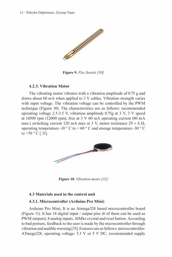
4.2.2.Flex Sensör
Flex sensor has a resistance. (Figure 9) The more the sensor is bent, the more resistance it has. It is a circuit element whose resistance increases with bending. Features are as follows: k bending life> 1 million times, height ≤ 0.43mm, temperature range: -35 ◦C - + 80 C, flat state resistance: 10 kΩ, resistance tolerance: ± 30%, bending resistance range: 60 kΩ - 110 kΩ and power values: 0.5 Watt in steady state; peak value 1Watt [24,28,29].
Züleyha Deği̇rmenci̇, Zeynep Yaşar12 .
Figure 9. Flex Sensör [30]
4.2.3. Vibration Motor
The vibrating motor vibrates with a vibration amplitude of 0.75 g and draws about 60 mA when applied to 3 V cables. Vibration strength varies with input voltage. The vibration voltage can be controlled by the PWM technique (Figure 10). The characteristics are as follows: recommended operating voltage 2.5-3.5 V, vibration amplitude 0.75g at 3 V, 3 V speed at 14500 rpm (12000 rpm), free at 3 V 60 mA operating current (80 mA max.) switching current 120 mA max at 3 V, motor resistance 29 ± 6 Ω, operating temperature -10 ° C to + 60 ° C and storage temperature -30 ° C to +70 ° C [ 31].
Figure 10. Vibration motor [32]
4.3 Materials used in the control unit
4.3.1. Microcontroller (Arduino Pro Mini)
Arduino Pro Mini; It is an Atmega328 based microcontroller board (Figure 11). It has 14 digital input / output pins (6 of them can be used as PWM outputs), 8 analog inputs, 16Mhz crystal and reset button. According to bad posture, feedback to the user is made by the microcontroller through vibration and audible warning [33]. Features are as follows: microcontroller: ATmega328, operating voltage: 3.3 V or 5 V DC, recommended supply

.13Research & Reviews in Engineering
voltage: maximum 12 V DC, d Digital input / output pins: 14 (6 of them support PWM output), analog input pins: 6 and DC current per input / output pin: 40 Ma [33].
Figure 11. Arduino Pro Mini [33]
4.3.2.Buzzer
It is a type of auditory warning device that works on mechanical, electromechanical or piezoelectric principles. [34] It can provide different audio signals according to the voltage supplied. It provides feedback to the user by making an audible warning to the user (Figure 12).
Figure 12. Buzzer [35]
4.4 Materials used in the feeding unit
4.4.1.LiPo Battery
LiPo is the abbreviation of Lithium Polymer (Figure 13) batteries. It is a rechargeable Lithium-Ion battery type that uses polymer electrolyte instead of liquid electrolyte [36]

Züleyha Deği̇rmenci̇, Zeynep Yaşar14 .
Figure 13. LiPo battery [37]
4.4.2.TP4056 Lipo Charger
It is a product that can charge lithium batteries with micro USB input via USB. BAT- and BAT + pins on the card (Figure 14) are the battery connection point. It can be charged by connecting to this port with a 3.7V battery[38].
Figure 14. TP4056 Lipo Charger [38]
4.5 Circuit Flow Chart
The steps and diagram of the data flow in the device are explained in this section. Circuit flow chart is given in Figure 15.
1. Start - The device is turned on.
2. Monitor User Status - The posture status of the user is being monitored.
3. Is the angle measured greater than the specified threshold? - Compare the value measured by the microdenter with the value determined. Decide if the user’s posture is correct.
4. Flex sensor bent? - Microcontroller checks whether the Flex sensor is bent or not. If it is bent, it means that the user is bent.
5. Vibration feedback active - If the user is not in the correct posture, the user is warned with vibration feedback.

.15Research & Reviews in Engineering
6. Audible warning unit is active - If the user is not in the correct position, the user is warned with an audible warning.
7. Turn Device Off - Device is Off.
Figure 15. Circuit flow chart
5.Results and Discussion
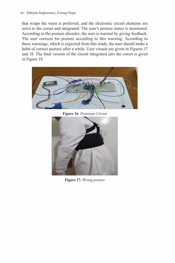
Circuit trials were carried out on the breadboard in the corset study that provides feedback according to the user’s posture. Software work has been done on the Arduino program. Circuit elements have been checked with test software before being integrated into the circuit. It has been observed in the experiments that each unit in the circuit works without any problems. The prototype circuit is shown in Figure 16. In order for the circuit whose electronic part is completed to perceive the posture correctly, a corset
Züleyha Deği̇rmenci̇, Zeynep Yaşar16 .
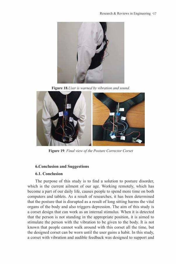
that wraps the waist is preferred, and the electronic circuit elements are sewn to the corset and integrated. The user’s posture status is monitored. According to the posture disorder, the user is warned by giving feedback. The user corrects his posture according to this warning. According to these warnings, which is expected from this study, the user should make a habit of correct posture after a while. User visuals are given in Figures 17 and 18. The final version of the circuit integrated into the corset is given in Figure 19.
Figure 16. Prototype Circuit
Figure 17. Wrong posture
.17Research & Reviews in Engineering
Figure 18.User is warned by vibration and sound.
Figure 19. Final view of the Posture Corrector Corset
6.Conclusion and Suggestions
6.1. Conclusion
The purpose of this study is to find a solution to posture disorder, which is the current ailment of our age. Working remotely, which has become a part of our daily life, causes people to spend more time on both computers and tablets. As a result of researches, it has been determined that the posture that is disrupted as a result of long sitting harms the vital organs of the body and also triggers depression. The aim of this study is a corset design that can work as an internal stimulus. When it is detected that the person is not standing in the appropriate position, it is aimed to stimulate the person with the vibration to be given to the body. It is not known that people cannot walk around with this corset all the time, but the designed corset can be worn until the user gains a habit. In this study, a corset with vibration and audible feedback was designed to support and

Züleyha Deği̇rmenci̇, Zeynep Yaşar18 .
maintain correct posture. A corset is preferred so that the sensors can perceive the posture well. The information obtained from the sensors on the corset is evaluated by the microcontroller and feedback is provided according to the user’s posture. If bad posture is detected, feedback to the user is made with vibration and audible warning. It has been observed in the experiments that all units work together.
6.2. Suggestions
By improving the electronic circuit design of the prototype obtained in the study, it can be ensured that the device occupies less space. The device is integrated into the corset so that the device can detect posture. The corset used over time may cause discomfort to the user. It may cause sweating or the user may not get positive results if the corset is worn over the dress. Therefore, the corset should be designed in the most ergonomic way. By integrating different features into the wearable posture corrector corset, multiple needs can be met by the same corset.
Conflict of Interest
No conflict of interest was declared by the authors.

.19Research & Reviews in Engineering
References
1. Stoppa, M., & Chiolerio, A. (2014). Wearable electronics and smart texti-les: a critical review. sensors, 14(7), 11957-11992.
2. Park, S., & Jayaraman, S. (2003). Smart textiles: Wearable electronic sys-tems. MRS bulletin, 28(8), 585-591.
3. Mazzoldi, A., De Rossi, D., Lorussi, F., Scilingo, E. P., & Paradiso, R. (2002). Smart textiles for wearable motion capture systems. AUTEX Re-search Journal, 2(4), 199-203.
4. Shim, B. S., Chen, W., Doty, C., Xu, C., & Kotov, N. A. (2008). Smart electronic yarns and wearable fabrics for human biomonitoring made by carbon nanotube coating with polyelectrolytes. Nano letters, 8(12), 4151-4157.
5. Bouwstra, S., Chen, W., Feijs, L., & Oetomo, S. B. (2009, June). Smart jacket design for neonatal monitoring with wearable sensors. In 2009 Sixth International Workshop on Wearable and Implantable Body Sensor Networks (pp. 162-167). IEEE.
6. De Rossi, D., Carpi, F., Lorussi, F., Mazzoldi, A., Paradiso, R., Scilingo, E. P., & Tognetti, A. (2003). Electroactive fabrics and wearable biomoni-toring devices. AUTEX Research Journal, 3(4), 180-185.
7. Hertleer, C., Tronquo, A., Rogier, H., Vallozzi, L., & Van Langenhove, L. (2007). Aperture-coupled patch antenna for integration into wearable tex-tile systems. IEEE antennas and wireless propagation letters, 6, 392-395.
8. Wearable technology. https://interestingengineering.com/the-questions-a-risewhile-wearable-technology-is-changing-how-we-track-our-medi-cal-condition, 12.12.2018.
9. []Ercan D.H., 2019. “Çocukluk Çağından İtibaren Görülen Postür (Duruş) Bozuklukları”, Kapadokya Montessori, Intl.: https://montessori.kapadok-ya. edu.tr/makaleler/cocukluk-cagindan-itibaren-gorulen-postur-durus bozukluklari, 21.010.2020
10. Demiral E., Postür nedir? Intl.:https://www.yenialanya.com/makale /3799104/erkandemiral/ postur-nedir, 12.12.2020.
11. Çeliker R., Duruş Bozuklukları. Intl.: http://www. reyhanceliker.com. tr/durus-bozukluklari, DP-1134.html, 12.12.2020.
12. https://lakecountrypt.com/posture-problems-and-prevention/, 10.01.2021
13. Uslu T., 2020.Kötü duruşun sağlığa olumsuz etkileri nelerdir? Intl: https: //www.hurriyet.com.tr/aile/kotu-durusun-sagliga-olumsuz-etkileri nele-rdir, 12.12.2020
14. G. E. Şubesi, “İçindekiler,” pp. 1–16, 2017.

Züleyha Deği̇rmenci̇, Zeynep Yaşar20 .
15. GİYİLEBİLİR TEKNOLOJİNİN TARİHİ, 2020. Intl:. https: //www. aca-baaa .com /2020/08/giyilebilir-teknoloji-nedir.html, 30.12.2020.
16. S. Geli and D. Ba, “G ı̇ y ı̇ leb ı̇ l ı̇ r teknoloj ı̇ ler,” 2020.
17. Özgüner Kılıç H., “Giyilebilir Teknoloji Ürünleri Pazarı ve Kullanım Alanları,” Aksaray Üniversitesi İktisadi ve İdari Bilim. Fakültesi Derg., vol. 9, no. 4, pp. 99–112, 2017.
18. https://www.i-scoop.eu/wearables-market-outlook-2020-drivers-new- markets/, https://dergipark.org.tr/tr/download/article-file/418241, 12.12.2020
19. Türk, B. 2019. Kamburluk korsesi işe yarar mı? Faydaları nelerdir? https://www.benguturk.com/haber/28234/kamburluk-korsesi-ise-yararmi-fayda-lari-nelerdir, 20.01.2021
20. https://www.gittigidiyor.com/kozmetik-kisisel-bakim/medikal-orto-pedik-manyetik-miknatisli-dik-durus-korsesi-dik-durus-durma-apara-ti-kamburluk-korsesi_pdp_556839481, 19.01.2021
21. https://urun.n11.com/korse/medikal-kamburluk-onleyici-ortope-dik-dik-durus-korsesi-P324722677, 19.01.2021
22. Kodgem Straight-Dik Durmak İçin Teknolojik Çözüm, 2020.https:// arikovani.com/projeler/straight-ile-dik-dur/detay, 20.21.2021
23. https://www.hepsiburada.com/kodgem-straight-kisisel-durus-antreno-ru-pm-HB000011ALVX, 20.21.2021
24. https://www.monofe.com/urun/27873/upright-go-2-akilli-durus-cihazi.html, 20.21.2021
25. https://www.lumobodytech.com/lumo-lift/, 20.21.2021
26. MPU6050 6 Eksen İvme ve Gyro Sensörü-GY-521, https:// www. robo-tistan. com/mpu6050-6-eksen-ivme-ve-gyro-sensoru-6-dof-3-axis-accel-erometer-and-gyros, 18.01.2021
27. https://www.motorobit.com/urun/mpu6050-6-eksen-ivme-ve-gyro-senso-ru-gy-521, 18.01.2021
28. Flex Sensör Nedir? 2017.Intl: https://www.ismitekno.com/flex-sensor- nedir. html, 18.01.2021
29. Otomasyon Dergisi, Esneklik Sensörü ve Uygulama Alanları (2018). Intl: http://otomasyondergisi.com.tr/arsiv/yazi/84-esneklik-sensoru-ve-uygu-lama-alanlari/, 18.01.2021
30. https://www.f1depo.com/22-Flex-Sensor,PR-2335.html
31. Vibration Motor. https:// www. direnc .net/mini- vibration -motor –27 mm-seeedstudio, 18.01.2021
32. https://www.direnc.net/mini-vibration-motor-27mm-seeedstudio, 18.01.2021

.21Research & Reviews in Engineering
33. https://www.robotistan.com/arduino-pro-mini-328-3v8mhz-headerli., 18.01.2021
34. Sinan C.B, 2015. https://sinancanbayrak.com/buzzer-nedir-nasil-calisir-nicin-kullanilir-kac-cesit-buzzer-vardir/,18.01.2021
35. https://www.pcboard.ca/minipiezo-buzzer, 18.01.2021
36. https://maker.robotistan.com/lipo-pil-rehberi/, 18.01.2021
37. Lipo Batarya.https://www.robotistan.com/37-v-1s-lipo-batarya-1100-mah-25c, 18.01.2021
38. Lithiım Battery Charger.https://www.robotistan.com/tlp4056-37v-sarj-aleti-5v-1a-lithium-battery-charger, 18.01.2021

Züleyha Deği̇rmenci̇, Zeynep Yaşar22 .

Chapter 2DESIGN AND IMPLEMENTATION OF THE ASPIRATION AND IRRIGATION PUMP FOR ABSCESS TREATMENT
Adem GÖLCÜK1
Muhammed Bakır DALMIZRAK2
1 Selcuk Universiry, Faculty of Technology, Biomedical engineering, Konya, Turkey (ORCID: 0000-0002-6734-5906)2 Istanbul Arel University, Vocational High School, Mechatronics Department, İstanbul, Tur-key (ORCID: -0000-0002-3828-4577)

Adem Gölcük, Muhammed Bakır Dalmizrak24 .
1. INTRODUCTION
Considering today’s technology, innovations occur day by day and new products surpass the previous products. New generation aspiration and irrigation pumps are produced depending on the technological deve-lopments. With the aspiration and irrigation pump, internal abscess, inter-nal cyst, the gastric irrigation and the discharge of harmful fluids from the body are performed. Aspiration devices used today work manually. When the harmful fluids in the patient’s body need to be expelled from the body, healthcare professionals should wait next to the patient and follow the pro-cedure continuously. A new aspiration and irrigation pump that can work automatically has been designed to eliminate such problems. Although the designed device is non-invasive, it will be used to clean the abscessed area that doctors reach by invasive methods. Thanks to the designed device, he-althcare workers will be able to remove harmful liquids manually or auto-matically by determining the process time and fluid flow rate. In the study, a peristaltic pump and stepper motor, inspired by a hemodialysis device, were used. Two solenoid valves were used to control the flow of harmful liquids collected from the patient and the clean solution fluid to be given to the patient. Also, in the designed device, fluid flow sensor and pressure sensor are used to control the discharge of harmful liquids from the body.
The devices used in intensive care, emergency departments, clinics and operating theaters to draw harmful fluids and particles from the body into the collection jar with suction power are called aspiration devices (MEGEP, 2011). Aspiration and irrigation pumps are used in processes where fluid flow occurs such as cleaning the internal cyst and internal ab-scess and removing harmful fluids from the body, as well as gastric lavage (Michaels, Johnson, & Thomas, 2012). The design and usage methods of the aspiration devices used today have been investigated by using article reviews and the experience of healthcare professionals working in hospi-tals. It is observed that patients suffer and healthcare professionals spend a lot of time during the use of these devices. During the cleaning of harmful liquids, it was observed that the process takes quite a long time in existing devices and a blockage occurs in the drain tubes of the device. Due to the-se blockages, the patient suffers and healthcare workers cannot leave the patient.
As a result of the researches for the solution of this problem, a new aspiration and irrigation pump were designed based on the working logic of the hemodialysis device. One of the important differences of the desig-ned device from the existing aspiration devices is the discharge of abscess fluid and the administration of clean solution to the patient’s body with a peristaltic pump.

.25Research & Reviews in Engineering
An aspirator device has been built for the collection, storage and pro-cessing of dangerous liquids. Such an aspirator device was especially crea-ted since the blood and fluids of people with AIDS should not be touched. The device consists of a container to collect hazardous liquids and a motor pump to draw the liquid into the container. In addition, since the clot accu-mulation in the pump will cause the pump to rust and the motor operating the pump to overheat, the pump was cleaned with washing liquid. An ad-vanced treatment and containment system were also implemented to pre-vent potentially hazardous liquids from circulating inside the pump. Also, the container in which the hazardous liquid is kept is designed in a way that dangerous liquids do not come into contact with healthcare workers and can be transported safely (Heironimus, El-Sabaaly, & Pludeman, 1997). A fluid aspirator was developed for patients with middle ear infections and the doctors treating them. It was observed that middle ear infcetion causes pain, discomfort and hearing loss for patients. Thanks to this device, it is aimed to make the treatment of middle ear infection more comfortable and easy. Before this device, doctors used traditional syringes to treat middle ear infection. Traditional syringes required the physician to operate the sy-ringe by pulling the piston. The syringe assembly of this device is adjusted to allow greater control by the operator by operating the syringe assembly when the piston is pressed from the other side. It was also stated that the needles of traditional syringes are dangerous for patients. However, Hill’s needle was designed to retract or deform when it touches bony structures (Hill, 2000). An aspirator device was made to extract body fluids. Body fluids were drawn from the airtight area with a manually operated pump. Two one-way valves were placed inside the device. The first valve was used to remove and discharge of harmful liquids in the liquid collector. The second valve was used to prevent liquids from overflowing out of the fluid collector. Body fluids were removed mechanically (Maitz & Hauser, 1990). An aspirator device was made to remove mucus and other excess body fluids by creating a vacuum with the suction tube. Two tubes were placed inside the device. The first tube was used to create a vacuum, and the second tube was used to draw fluid from the body and collect it in a container (Rosenblatt, 1989). A method and apparatus were developed for the discharge of harmful fluids in the patient’s body and to be used in cases where hospital staff should not touch this liquid. Thanks to the de-vice, body fluid was discharged by pouring from the suction box into the hospital sink and into the sanitary sewage system (Miller, Hollen, Hand, & Anderson, 2004). The device was developed to discharge blood and other body fluids from the patient’s body during surgery. It was seen in the rese-arch that two tons of fluid that must be disposed each month. Such liquids should be considered infectious medical waste and should be discharged in accordance with established standards. A suction container was used
Adem Gölcük, Muhammed Bakır Dalmizrak26 .
to dispose of these fluids. This suction container must be disposed of as waste after each process or must be cleaned and disinfected for reuse. This process was shown to increase the risk of healthcare workers being expo-sed to hazardous wastes (Michaels et al., 2012). In the study, nasal spray was mounted to the air intake connector and the air evacuation connector in the aspiration device. The spray tube was connected to a mucus colle-ctor. Thus, when the mucus carrying some air enters the mucus collector, the mucus is left behind and the air is drawn from the second aspiration channel by an air pump. Thanks to this device, mucus was absorbed imme-diately after being liquefied (Wang, Chen, Chen, Fang, & Huang, 2003). A device is designed to remove fluid and debris from the ear canal using a vacuum device. Before the device was designed, it was seen that there are many devices to extract liquid and particles from different orifices of hu-man and animal bodies. However, these devices were found to be harmful to human ears. With the device, fluids and debris are safely removed wit-hout any damage to the ear skin or the skin of the ear canal. An ear vacuum device with a fan and a motor was made to do this cleaning. A collection tank was made to pour the liquid and other parts drawn from the ear canal. Fluids drawn from the ear were poured here. The device was placed in the ear canal and a vacuum was produced to draw fluid and particles into the collection tank. The liquid drawn by the ball valve in the collection tank was prevented from leaking to the vacuum motor and damaging the motor (Spilman, 2000). With the device, it is ensured that fluids and irritants col-lected from the body during surgical procedures are eliminated. This devi-ce was made to minimize the environmental impact of the fluids collected during surgical procedures and to be disposed of properly. It was found that the disposable suction boxes of previous devices were difficult to set up, use, and dispose of liquids. It was also observed that there is a risk of infection for healthcare workers. For example, the boxes had to be opened to pour the liquids in the suction box of previous devices into the sewer, which posed a risk to healthcare workers. With the device, the liquid in the collection unit is automatically discharged into the sewer. Later, the collection unit was cleaned with disinfectant. After cleaning, the aspiration device is ready to use (Kerwin et al., 1997).
The treatment methods of 9 patients diagnosed and treated for prostate abscess between 1998-2000 were examined. Medline data were compa-red with those described in the literature. As a result of the studies, micro abscesses will be able to recover without surgery. It is also recommended that prostate abscess should be treated with broad-spectrum antibiotics and surgical drainage (Oliveira, Andrade, Porto, Pereira Filho, & Vinhaes, 2003). Needle aspiration is effective and safe in the treatment of pyogenic liver abscess. In addition, it should be considered as the first option as

.27Research & Reviews in Engineering
an alternative to the drainage method in multiple abscesses (Yu, Lo, Kan, & Metreweli, 1997). The optimum method of pyogenic liver abscess was researched and a new treatment method was presented. 169 patients with pyogenic liver abscess treated in India between 2001-2006 were studied. As a result of the examination, it was observed that the mortality rate in pa-tients treated surgically was lower than in non-surgical treatment methods. Therefore, surgical drainage and antibiotics are necessary for treatment(-Malik, Bari, Rouf, & Wani, 2010). It was studied on a patient undergoing hemodialysis treatment. Kidney abscess in the patient was diagnosed by needle aspiration accompanied by tomography. The patient was treated with antibiotics and aspiration(Wang et al., 2003). Differences between transurethral resection and needle aspiration in treating prostate abscess were investigated. Patients diagnosed with prostate abscess for 10 years at Gangnam Severance Hospital were studied. They treated 23 patients with transurethral resection treatment method and 18 patients with needle as-piration. In the transurethral resection method, the treatment period of the patients was 10.2 days on average, while the average treatment duration was 23.5 days in needle aspiration (Jang, Lee, Lee, & Chung, 2012). 22 pa-tients with liver abscess were treated with catheter drainage for 9 years. 17 patients were treated without surgery. 4 patients were treated with surgery. 1 patient died. As a result of the study, catheter drainage is recommended for the treatment of liver abscesses. Surgical treatment is needed in patients with liver abscess (Juul, Sztuk, Torp-Pedersen, & Burcharth, 1990). Pre-serving the indications, 62 patients were treated by ultrasound with percu-taneous catheter drainage. 90% success was achieved. There was no intes-tinal perforation and bleeding in the studies (Jansen, Truong, Sparenberg, & Schumpelick, 1997). Pyogenic ventriculitis is a serious infection. It is often resistant to antibiotic therapy. Therefore, continuous intraventricular irrigation therapy is recommended. However, this method is a bit slow and increases the risk of a second infection. In addition, this method is insuffi-cient in removing adherent purulent. A side cutting aspiration device was used to treat the case of pyogenic ventriculitis and ventricular empyema was cleared in all patients (Lang et al., 2018).
2. MATERIAL AND METHOD
In this section, information was given about the steps during the de-sign of the aspiration and irrigation pump, the sensors, electronic equip-ment and the peristaltic pump(DALMIZRAK, 2021).
2.1. Aspiration Device and Irrigation Pump Design
The block diagram of the aspiration and irrigation pump is given in Figure 1.

Adem Gölcük, Muhammed Bakır Dalmizrak28 .
Figure 1. The block diagram of the aspiration and irrigation pump(DALMIZRAK, 2021).
As it is seen in the block diagram in Figure-1, Touch Screen, Liquid Flow Sensor, Pressure Sensor, MicroController, Stepper Motor, Solenoid Valve, Peristaltic Pump and Peristaltic Pump tube are used in the desig-ned device. The prototype picture of the designed aspiration and irrigation pump is shown in Figure 2.

.29Research & Reviews in Engineering
Figure 2. Aspiration and irrigation pump(DALMIZRAK, 2021).
The peristaltic pump designed for the aspiration and irrigation device discharges the abscess fluid from the patient’s body by squeezing the peris-taltic tube. When the peristaltic pump rotates backward (counterclockwi-se), it takes the abscess fluid from the patient’s body, and when it rotates in the forward direction (clockwise), it gives clean solution liquid to the patient’s body, removing the obstructions and cleansing the patient’s abs-cess area. If abscess fluid does not come out of the patient’s body during the period determined by the doctor, the device considers this as obstruc-tion and delivers clean solution liquid to the patient’s body to remove this obstruction.
Outputs are produced in line with the information received from the microprocessor pressure sensor and the liquid flow sensor. Microprocessor outputs are transmitted to the stepper motor driver and the driver controls the stepper motor.
2.1.1. Stm32f407Microcontroller
In the designed device, STM32F407 microcontroller was used to read data from fluidity and pressure sensors, read commands from the touch panel, decide the rotation direction and speed of the peristaltic pump, open and close the solenoid valves and generate a pulse signal for the rotation speed of the stepper motor. In short, it is the brain of the device. The pres-sure sensor used in the project is analog sensors, and the fluidity sensor is a digital sensor. ADC feature of the microcontroller was used to read data from the pressure sensor. The analog data produced by the sensors were converted into 10-bit digital data in the microcontroller. I2C communicati-on protocol was used to read data from the fluidity sensor. The commands

Adem Gölcük, Muhammed Bakır Dalmizrak30 .
from the touch panel were read with the USAT6 global interrupt. The serial communication speed (baud rate) between the microcontroller and the tou-ch panel was set to 9600. This microcontroller decides which is open and which is closed out of the 2 solenoid valves used in the device. It produces signal 1 for the valve it wants to open and signal 0 for the valve it wants to close. Therefore, two I / O pins of the microcontroller are used to cont-rol these valves. This microcontroller also controls the rotation direction and speed of the peristaltic pump. Timer interrupter was used to generate the pulse signal to the stepper motor that moves the peristatic pump. The frequency of the timer interrupt was set to 4000Hz. The rotation speed of the stepper motor is adjusted by generating a pulse signal with the com-mands in this interrupt. Figure 3 shows the microcontroller kit used for the device.
Figure 3. Stm32f407 Discovery Development Kit (STMicroelectronics, 2011)
Microcontrollers, also called Central Processing Unit, are program-mable electronic components. Microcontrollers differ according to their production types. Manufacturer information of the microprocessor used in this study is given in Table 1.
Table 1. Microprocessor Basic Specifications (STMicroelectronics, 2011)
CPU Arm 32-bit Cortex-M4 CPUMEMORY 1MB Flash + 192 SRAMCrystal Frequence 4-16MHz CLKFrequency 168MHz Freq

.31Research & Reviews in Engineering
2.1.2. Touch Screen
Doctors command the designed device on the touch panel. There are clear solution fluid duration, abscess fluid time, Automatic / Manual, Tar-get Flow Rate, Start / Stop, initial start options to control the designed device on the touch screen. In addition, the data read from the pressure and flow sensors are displayed on this screen.
It is determined how many seconds the clean solution fluid will be sent to the patient’s body with the duration of the clean solution fluid, and how many seconds the dirty water will be drawn from the patient’s body with the duration of the abscess fluid. It is determined in which mode the device will work with Automatic / Manual option While the device is operating in automatic mode, it expels the abscess fluid from the patient during the set time and again sends clean water to the patient’s body. This process is repeated continuously until the device is stopped. If there is no fluid flow out during the period determined by the doctor while discharging the abs-cess fluid, the device perceives it as an obstruction and automatically starts to give clean water. With the first start option, it is determined whether the device starts by discharging the abscess fluid or by giving the patient clean water. In manual mode, the device works continuously according to the selection in the first start option. For example, if the first starting option is the removal of abscess fluid, the device continuously discharges the abs-cess fluid from the patient’s body until it is stopped. A step value between 0 and 10 must be entered to determine the target flow rate. With this step option, the flow rate of liquids is adjusted due to the rotation speed of the motor. When step 0 is selected, the fluid flow rate is the least, when 10 is selected, the fluid flow rate is the highest. The default value of this option is 0. With the Start / Stop button, the device is started and stopped. The default value of this button is “Start” and the device is not working. After making the necessary settings for the operation of the device on the touch screen, the device starts operating when the “Start” button is pressed, and this button changes to “Stop”. When the “Stop” button is pressed, the de-vice in operation is stopped. Figure 4 shows the image of the touch screen used in this study.

Adem Gölcük, Muhammed Bakır Dalmizrak32 .
Figure 4. Touch Screen(DALMIZRAK, 2021).
Touch panels are produced in different sizes and different output power depending on the production purpose. Manufacturer information of the touch screen used in this study is given in Table 2.
Table 2. Touch Screen Specifications (Nextion, 2011)
Touch Screen Type CapacitiveLCD Type TFT Rear Light LEDScreen Size 154.21 × 85.92 mmResolution 1024 × 600 pixelOperating voltage 3.0 ~ 3.6 V
2.1.3. Liquid Pressure Sensor
The pressure sensor is placed at a point closest to the patient’s body and measures the pressure in the peristaltic tube. The motor and the speed of the motor were controlled according to the pressure value measured by the pressure sensors. The system is stopped in case of pressure increase due to the blockage that may occur during the discharge of the dirty liquid with the pressure sensors. When such a situation occurs, doctors are war-ned with an alarm sound. The pressure sensor detects the pressure in the peristaltic tube and converts it to an analog signal. This analog signal is read with the ADC feature of the microcontroller and converted into digital signals. Figure 5 shows the pressure sensor used in the system.

.33Research & Reviews in Engineering
Figure 5. Pressure Sensor (Atek, 2010)
Manufacturer information of the pressure sensor used in the study is given in Table 3.
Table 3. Pressure Sensor Specifications (Atek, 2010)
Measuring Range 0…100mbarOperating Current 4-20 mAOperating voltage 0-10 VResponse Time 1 msOperating Temperature -40 …+85
The pin structure of the pressure sensor used for this study is given in Table 4.
Table 4. The pin structure of BCT 22 pressure sensor (Atek, 2010)
Pin1 Pin2 Pin3GND VDC ANALOG OUTPUT
2.1.4. Liquid Flow Sensor
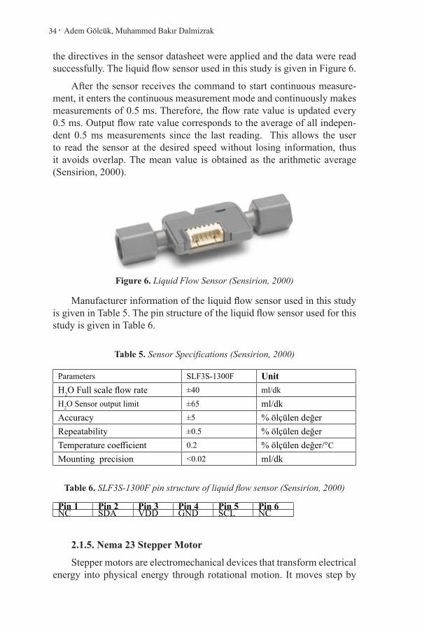
The liquid flow sensor measures the flow rate of the liquid drawn from the patient in ml / min. SLF3S-1300F series liquid flow sensor produced by Sensirion company was used in this study. This sensor is a digital sensor and I2C communication protocol was used to read the data from this sen-sor with the microcontroller. While preparing the microcontroller codes,
Adem Gölcük, Muhammed Bakır Dalmizrak34 .
the directives in the sensor datasheet were applied and the data were read successfully. The liquid flow sensor used in this study is given in Figure 6.
After the sensor receives the command to start continuous measure-ment, it enters the continuous measurement mode and continuously makes measurements of 0.5 ms. Therefore, the flow rate value is updated every 0.5 ms. Output flow rate value corresponds to the average of all indepen-dent 0.5 ms measurements since the last reading. This allows the user to read the sensor at the desired speed without losing information, thus it avoids overlap. The mean value is obtained as the arithmetic average (Sensirion, 2000).
Figure 6. Liquid Flow Sensor (Sensirion, 2000)
Manufacturer information of the liquid flow sensor used in this study is given in Table 5. The pin structure of the liquid flow sensor used for this study is given in Table 6.
Table 5. Sensor Specifications (Sensirion, 2000)
Parameters SLF3S-1300F UnitH2O Full scale flow rate ±40 ml/dkH2O Sensor output limit ±65 ml/dkAccuracy ±5 % ölçülen değerRepeatability ±0.5 % ölçülen değer Temperature coefficient 0.2 % ölçülen değer/°CMounting precision <0.02 ml/dk
Table 6. SLF3S-1300F pin structure of liquid flow sensor (Sensirion, 2000)
Pin 1 Pin 2 Pin 3 Pin 4 Pin 5 Pin 6NC SDA VDD GND SCL NC
2.1.5. Nema 23 Stepper Motor
Stepper motors are electromechanical devices that transform electrical energy into physical energy through rotational motion. It moves step by

.35Research & Reviews in Engineering
step. It produces analog rotational motion output against the pulse signals applied to its inputs. It provides this rotational movement step by step with very precise control. Nema 23 stepper motor has stators, rotors and bea-rings in its structure. Stator has eight poles. Bearings are connected to the rotor and this provides an easier rotation to the shaft. Energy is supplied to the coils from the adapter. Then, depending on what speed and how long the motor rotates, a pulse signal is given to the coils(Stoianovici, Patriciu, Petrisor, Mazilu, & Kavoussi, 2007). The Nema 23 stepper motor used in the study is given in Figure 7.
Figure 7. Nema 23 Stepper Motor (Stepperonline, 2007)
Manufacturer information of the Nema 23 stepper motor used in the study is given in Table 7.
Table 7. Nema 23 Stepper Motor Specifications (Stepperonline, 2007)
Holding Torque 2.2 Nm
Current 3.0 Amper
Voltage 3.6 Volt
Flange Size 57×57 mm
Number of Cables 8 adet
In the designed device, this stepper motor is used to rotate the peripps-taltic pump forward (clockwise) or backward (counterclockwise). With the forward rotation of the motor, clean water goes to the patient’s body, and when it rotates backward, the abscess fluid is discharged from the patient’s body.
2.1.6. Motor Driver Control Circuit (CWD556)
The motor driver control circuit controls the motion of the stepper mo-tor according to the commands from the microprocessor unit. The motor

Adem Gölcük, Muhammed Bakır Dalmizrak36 .
driver board used for the designed device is protected against overheating, high current and low voltage and short circuit. The motor driver control circuit controls the stepper motor used for the movement of the pump. The motor driver control circuit is placed between the microprocessor unit and the motor. The current setting of the motor driver is made according to the type of stepper motor. The board where the driver is located is grounded in the metal part. Pulse, Dir and Enable signals were sent from the micro-controller to the motor driver circuit. According to these signals, the motor driver card adjusts whether the motor will move or not, the direction of rotation and the speed. Figure 8 shows the motor driver control circuit used in this study.
Figure 8. Motor Driver Control Circuit (CW-motor, 1995)
Motor drivers vary depending on the type and power of the motor to be used in the system. There are different drivers and different driving met-hods for each motor. Manufacturer information of the motor driver control circuit used in this study is given in Table 8.
Table 8. Motor Driver Specifications (CW-motor, 1995)
Power 280WVoltage 24VDC ~ 50VDCCircuit 1.5A ~ 5.6A Phase 2 PhasesShort circuit protection Yes
Using the Current Table and Pulse Table on the motor driver card, the current drawn by the motor and the angle of each step are determined. The switches of the motor driver card are adjusted as given in table 9 and the full rotation of the motor of 3600 is completed at 800 steps.
Table 9. Pulse Table
PULSE SW5 SW6 SW7 SW8800 OFF ON ON ON

.37Research & Reviews in Engineering
2.1.7. Peristaltic Pump
It is a mechanical unit designed to create the vacuum that realizes fluid flow. Computer aided design was used in the process of realizing this system. This designed pump rotates forward or backward together with the stepper motor, squeezes the peristaltic pump tube and creates a vacuum in the tube. Liquid flow occurs with this vacuum. Liquid flow occurs in two directions. While the pump rotates forward (clockwise), clean water is de-livered to the patient’s body, while the pump rotates backward, the abscess fluid in the patient’s body is discharged. The pump designed for this device is given in Figure 9.
Figure 9. Peristaltic Pump
2.1.8. Solenoid Valve
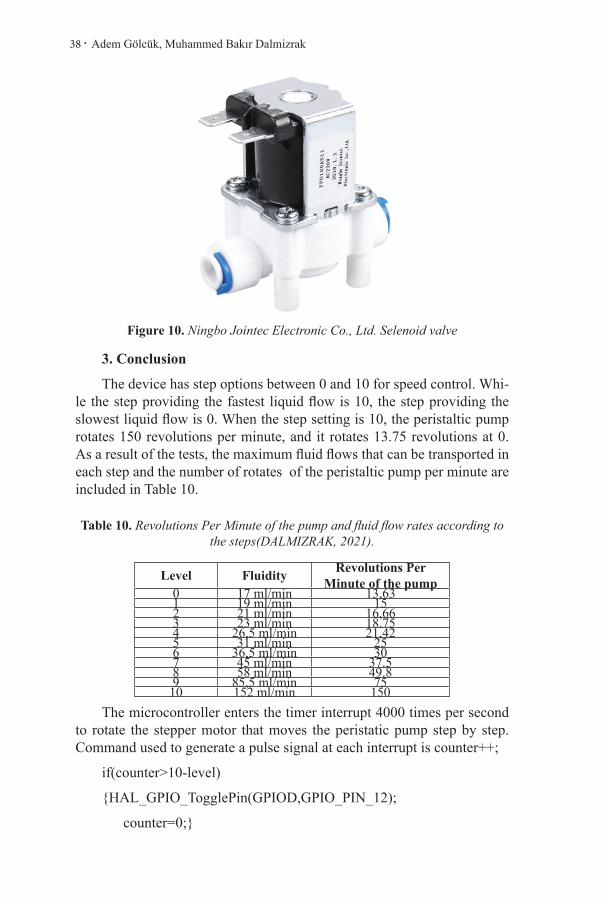
Two solenoid valves were used in the designed device to control the directions of liquid flows. These valves are named as Solution Solenoid Valve and Dirty Solenoid Valve in Figure-1. The Solution Solenoid Valve is connected to the clean water peristaltic tube, and the Dirty solenoid val-ve is connected to the peritaltic tube from which the abscess fluid is disc-harged. When clean water is given to the patient, the microcontroller opens the Solution Solenoid Valve and closes the Dirty Solenoid Valve. When the abscess fluid is discharged from the patient’s body, the microcontroller opens the Dirty Solenoid Valve and closes the Solution Solenoid Valve. The solenoid valve used for the designed device is given in Figure 10.
Adem Gölcük, Muhammed Bakır Dalmizrak38 .
Figure 10. Ningbo Jointec Electronic Co., Ltd. Selenoid valve
3. Conclusion
The device has step options between 0 and 10 for speed control. Whi-le the step providing the fastest liquid flow is 10, the step providing the slowest liquid flow is 0. When the step setting is 10, the peristaltic pump rotates 150 revolutions per minute, and it rotates 13.75 revolutions at 0. As a result of the tests, the maximum fluid flows that can be transported in each step and the number of rotates of the peristaltic pump per minute are included in Table 10.
Table 10. Revolutions Per Minute of the pump and fluid flow rates according to the steps(DALMIZRAK, 2021).
Level Fluidity Revolutions Per Minute of the pump
0 17 ml/min 13,631 19 ml/min 152 21 ml/min 16,663 23 ml/min 18.754 26,5 ml/min 21,425 31 ml/min 256 36,5 ml/min 307 45 ml/min 37.58 58 ml/min 49.89 85,5 ml/min 75
10 152 ml/min 150The microcontroller enters the timer interrupt 4000 times per second
to rotate the stepper motor that moves the peristatic pump step by step. Command used to generate a pulse signal at each interrupt is counter++;
if(counter>10-level)
{HAL_GPIO_TogglePin(GPIOD,GPIO_PIN_12);
counter=0;}

.39Research & Reviews in Engineering
As it is understood from this command, PortD.12 pin generates the pulse signal. The frequency of the generated pulse signal is determined according to the value of the level variable. For example, when the value of the level variable is 10, because this pin is reversed at each interrupt, a pulse signal is generated 2000 times a second from this pin. Table 11 shows the frequency of the pulse signal generated for each step and the calculati-on of revolutions per minute of the peristaltic pump. The results of the tests and the calculated results are exactly the same.
Table 11. Calculation of revolutions per minute of the peristaltic pump according to the steps(DALMIZRAK, 2021)
LevelComparison
if(counter>10-level)
Pulse Countpulse/sn
Revolutions Per Second of the pump
Revolutions Per Minute of the
pump10 counter>0 4000/1=4000/2=2000 2000/800=2.5 2.5*60=1509 counter>1 4000/2=2000/2=1000 1000/800=1.25 1.25*60=75
8 counter>2 4000/3=1333.33/2= 666.665 666.665/800=0.83 0.83*60=49.8
7 counter>3 4000/4=1000/2=500 500/800=0.625 0.625*60=37.56 counter>4 4000/5=800/2=400 400/800=0.5 0.5*60=30
5 counter>5 4000/6=666.67/2= 333.335 333.335/800=0.42 0.42*60=25
4 counter>6 4000/7=571.429/2= 285.714 285.714/800=0.357 0.357*60=21.42
3 counter>7 4000/8=500/2=250 250/800=0.3125 0.3125*60=18.75
2 counter>8 4000/9=444.444/2= 222.222 222.222/800=0.277 0.277*60=16.66
1 counter>9 4000/10=400/2=200 200/800=0.25 0.25*60=15
0 counter>10 4000/11=363.636/2= 181.818 181.818/800=0.227 0.227*60=13.63
4. Discussion
Since the aspiration devices used in today’s technology work manu-ally, it is a waste of time for doctors and patients suffer a lot of pain. In this study, a new aspiration and irrigation pump was designed based on the working logic of the hemodialysis device. With this device, it is aimed to make patients suffer less during treatment and save time for healthcare professionals. This designed device works automatically until it is stopped after doctors make the initial settings. During the study, when necessary, the patient is given clean solution liquid to clean the abscessed area and harmful fluids are expelled from the patient’s body. The designed device is a non-invasive device, but it cleans abscessed areas that surgeons reach with invasive methods. It is understood that the designed device can be used as a result of the tests conducted in the workshop environment and

Adem Gölcük, Muhammed Bakır Dalmizrak40 .
interviews with healthcare professionals. After obtaining the ethics com-mittee permissions and other necessary documents, the designed device will be mass produced and put into service of healthcare professionals.
Compliance with ethical standards
Funding: This study was funded by Selçuk University BAP Coordi-nator (grant number 19201122).
Conflict of interest The authors declare no conflicts of interest.
Ethical approval This article does not contain any studies with hu-man participants or animals performed by any of the authors.
.41Research & Reviews in Engineering
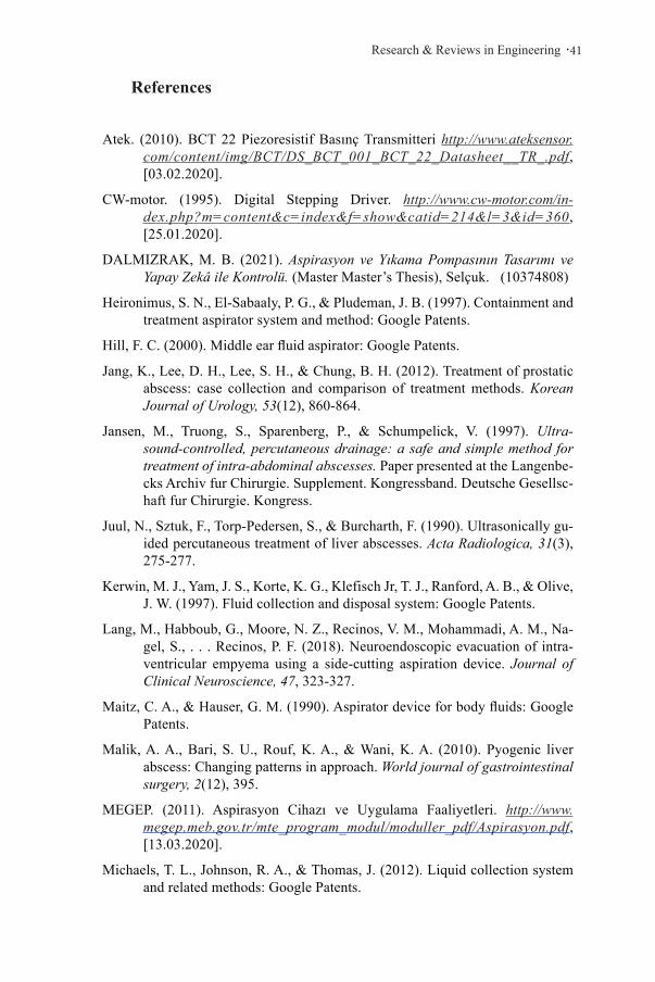
References
Atek. (2010). BCT 22 Piezoresistif Basınç Transmitteri http://www.ateksensor.com/content/img/BCT/DS_BCT_001_BCT_22_Datasheet__TR_.pdf, [03.02.2020].
CW-motor. (1995). Digital Stepping Driver. http://www.cw-motor.com/in-dex.php?m=content&c=index&f=show&catid=214&l=3&id=360, [25.01.2020].
DALMIZRAK, M. B. (2021). Aspirasyon ve Yıkama Pompasının Tasarımı ve Yapay Zekâ ile Kontrolü. (Master Master’s Thesis), Selçuk. (10374808)
Heironimus, S. N., El-Sabaaly, P. G., & Pludeman, J. B. (1997). Containment and treatment aspirator system and method: Google Patents.
Hill, F. C. (2000). Middle ear fluid aspirator: Google Patents.
Jang, K., Lee, D. H., Lee, S. H., & Chung, B. H. (2012). Treatment of prostatic abscess: case collection and comparison of treatment methods. Korean Journal of Urology, 53(12), 860-864.
Jansen, M., Truong, S., Sparenberg, P., & Schumpelick, V. (1997). Ultra-sound-controlled, percutaneous drainage: a safe and simple method for treatment of intra-abdominal abscesses. Paper presented at the Langenbe-cks Archiv fur Chirurgie. Supplement. Kongressband. Deutsche Gesellsc-haft fur Chirurgie. Kongress.
Juul, N., Sztuk, F., Torp-Pedersen, S., & Burcharth, F. (1990). Ultrasonically gu-ided percutaneous treatment of liver abscesses. Acta Radiologica, 31(3), 275-277.
Kerwin, M. J., Yam, J. S., Korte, K. G., Klefisch Jr, T. J., Ranford, A. B., & Olive, J. W. (1997). Fluid collection and disposal system: Google Patents.
Lang, M., Habboub, G., Moore, N. Z., Recinos, V. M., Mohammadi, A. M., Na-gel, S., . . . Recinos, P. F. (2018). Neuroendoscopic evacuation of intra-ventricular empyema using a side-cutting aspiration device. Journal of Clinical Neuroscience, 47, 323-327.
Maitz, C. A., & Hauser, G. M. (1990). Aspirator device for body fluids: Google Patents.
Malik, A. A., Bari, S. U., Rouf, K. A., & Wani, K. A. (2010). Pyogenic liver abscess: Changing patterns in approach. World journal of gastrointestinal surgery, 2(12), 395.
MEGEP. (2011). Aspirasyon Cihazı ve Uygulama Faaliyetleri. http://www.megep.meb.gov.tr/mte_program_modul/moduller_pdf/Aspirasyon.pdf, [13.03.2020].
Michaels, T. L., Johnson, R. A., & Thomas, J. (2012). Liquid collection system and related methods: Google Patents.

Adem Gölcük, Muhammed Bakır Dalmizrak42 .
Miller, M., Hollen, M. C., Hand, J. M., & Anderson, B. G. (2004). Method and apparatus for disposing of bodily fluids from a container: Google Patents.
Nextion. (2011). Nextion NX8048T070 - Generic 7.0” HMI TFT LCD Touch. https://nextion.tech/datasheets/nx8048t070/, [26.01.2020].
Oliveira, P., Andrade, J. A., Porto, H. C., Pereira Filho, J. E., & Vinhaes, A. F. (2003). Diagnosis and treatment of prostatic abscess. International braz j urol, 29(1), 30-34.
Rosenblatt, R. (1989). Aspirator for collection of bodily fluids: Google Patents.
Sensirion. (2000). SLF3S-1300F Liquid Flow Sensor. https://www.sensirion.com/fileadmin/user_upload/customers/sensirion/Dokumente/4_Liquid_Flow_Meters/Liquid_Flow/Sensirion_Liquid_Flow_Sensor_SLF3S-1300F_Da-tasheet_EN_D1.pdf, [14.04.2020].
Spilman, D. A. (2000). Ear vacuum: Google Patents.
Stepperonline. (2007). Nema 23 stepper motor. https://www.omc-stepperonline.com/download/23HS22-2804S.pdf, [25.01.2020].
STMicroelectronics. (2011). Discovery kit with STM32F407VG MCU. https://www.st.com/resource/en/data_brief/stm32f4discovery.pdf, [25.01.2020].
Stoianovici, D., Patriciu, A., Petrisor, D., Mazilu, D., & Kavoussi, L. (2007). A new type of motor: pneumatic step motor. IEEE/ASME Transactions On Mechatronics, 12(1), 98-106.
Wang, I.-K., Chen, Y.-M., Chen, Y.-C., Fang, J.-T., & Huang, C.-C. (2003). Suc-cessful treatment of renal abscess with percutaneous needle aspiration in a diabetic patient with end stage renal disease undergoing hemodialysis. Renal failure, 25(4), 653-657.
Yu, S. C., Lo, R. H., Kan, P., & Metreweli, C. (1997). Pyogenic liver abscess: treatment with needle aspiration. Clinical radiology, 52(12), 912-916.

Chapter 3PRELIMINARY CHARACTERIZATION PROPERTIES OF SAMPLE BORON(COLEMANITE) FROM BALIKESIR (BIGADIÇ) REGION AND IMPORTANCE
Oyku BİLGİN1
1 Şırnak University, Faculty of Engineering, Department of Mining Engineering, Şırnak
Oyku Bilgin44 .
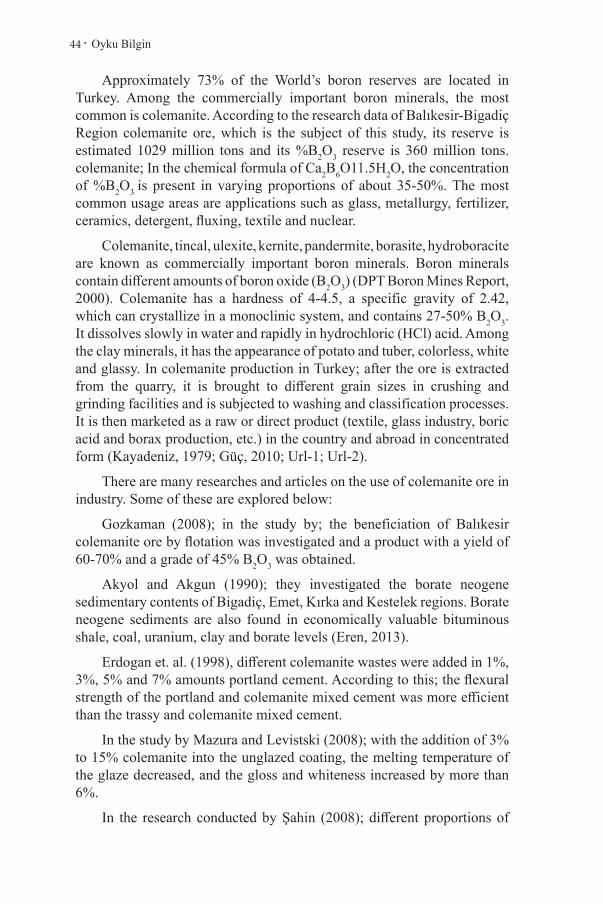
Approximately 73% of the World’s boron reserves are located in Turkey. Among the commercially important boron minerals, the most common is colemanite. According to the research data of Balıkesir-Bigadiç Region colemanite ore, which is the subject of this study, its reserve is estimated 1029 million tons and its %B2O3 reserve is 360 million tons. colemanite; In the chemical formula of Ca2B6O11.5H2O, the concentration of %B2O3 is present in varying proportions of about 35-50%. The most common usage areas are applications such as glass, metallurgy, fertilizer, ceramics, detergent, fluxing, textile and nuclear.
Colemanite, tincal, ulexite, kernite, pandermite, borasite, hydroboracite are known as commercially important boron minerals. Boron minerals contain different amounts of boron oxide (B2O3) (DPT Boron Mines Report, 2000). Colemanite has a hardness of 4-4.5, a specific gravity of 2.42, which can crystallize in a monoclinic system, and contains 27-50% B2O3. It dissolves slowly in water and rapidly in hydrochloric (HCl) acid. Among the clay minerals, it has the appearance of potato and tuber, colorless, white and glassy. In colemanite production in Turkey; after the ore is extracted from the quarry, it is brought to different grain sizes in crushing and grinding facilities and is subjected to washing and classification processes. It is then marketed as a raw or direct product (textile, glass industry, boric acid and borax production, etc.) in the country and abroad in concentrated form (Kayadeniz, 1979; Güç, 2010; Url-1; Url-2).
There are many researches and articles on the use of colemanite ore in industry. Some of these are explored below:
Gozkaman (2008); in the study by; the beneficiation of Balıkesir colemanite ore by flotation was investigated and a product with a yield of 60-70% and a grade of 45% B2O3 was obtained.
Akyol and Akgun (1990); they investigated the borate neogene sedimentary contents of Bigadiç, Emet, Kırka and Kestelek regions. Borate neogene sediments are also found in economically valuable bituminous shale, coal, uranium, clay and borate levels (Eren, 2013).
Erdogan et. al. (1998), different colemanite wastes were added in 1%, 3%, 5% and 7% amounts portland cement. According to this; the flexural strength of the portland and colemanite mixed cement was more efficient than the trassy and colemanite mixed cement.
In the study by Mazura and Levistski (2008); with the addition of 3% to 15% colemanite into the unglazed coating, the melting temperature of the glaze decreased, and the gloss and whiteness increased by more than 6%.
In the research conducted by Şahin (2008); different proportions of

.45Research & Reviews in Engineering
colemanite waste (5-45%) were added to the brick clay as raw or calcined. As a result, here, raw colemanite waste caused fragmentation of the brick structure. However, calcined colemanite waste increased the strength of the brick and reduced water absorption. It has been determined that calcined colemanite is suitable for use in brick making.
In the review made by Gençel (2009); colemanite mineral was used as concrete aggregate and physical and mechanical properties of concrete were investigated. According to this; it was determined that the mechanical and physical properties of the concrete to which colemanite was added decreased and the shielding efficiency was better.
Binici et al. (2010) in the experiments conducted by; high strength and durability of colemanite and barite added concretes were investigated.
Budak (2014), in the study by; the colemanite mineral obtained from Balıkesir-Bigadiç Eti Maden Operations was crushed, milled and screened, and boric acid extraction from the colemanite mineral was carried out using carbon dioxide in an aqueous medium. As a result of this study, the extraction efficiency of boric acid from colemanite mineral with CO2 under supercritical conditions in the aquatic environment was found to be approximately 98% (60°C, 2 hours, +20-40 µm).
Targan et al. (2003) in the experiments conducted by; colemanite wastes, coal fly ash, natural pozzolan and coal bottom ash were used as cement/concrete additives. It was observed that the final setting time increased in cement mixtures using natural pozzolana.
In the study conducted by Korçak (2014); colemanite wastes were used instead of natural gypsum in cement production and the performance of cement was investigated. Cement sample was prepared by adding colemanite wastes varying between 3% and 10% to the cement clinker. According to this; when colemanite is used as an additive in cement, it increases the setting time and decreases the compressive strength. It has been determined that 5% colemanite waste added to cement can be used as an additive that delays setting time, such as natural gypsum.
In the study conducted by Yeşilçiçek (2016), the stabilization capabilities of a highly elastic clayey road subgrade, colemanite waste and lime additives are investigated.
Yaltay (2015) conducted experiments on the physical properties of lightweight concrete obtained by using colemanite additives in cement. He added coarse and fine-grained pumice to the concrete mix. It has been determined that concrete samples give better results in compressive strength with the addition of colemanite.

Oyku Bilgin46 .
In the study conducted by Yarar (1973); the enrichment of a low grade colemanite ore taken from Bigadiç region by flotation method was investigated. In the experiments, the colemanite sample was obtained with 45-47% B2O3 tenor and 72-93% yield.
In the research conducted by Tok (2018); enrichment experiments were carried out with a multi-gravity separator, rocking table and falcon concentrator on the washed colemanite samples with a grade of 32%-36% (B2O3) taken from Eti Mining Businesses/Emet facility, and the most efficient results were obtained with MGS. Accordingly, the concentrate with a B2O3 grade of 44.93% was obtained with a yield of 97.51%.
In the research conducted by Eyyüboğlu (2013); colemanite (B2O3) concentrator waste in amounts of 5.56%, 10.47% and 15.89% was used as cement additive. In addition, clinker and gypsum were added at the rates of 1%, 3%, 5% and 10%. Accordingly, physical and chemical analyzes of the cement mixtures were made. As a result, it was determined that the amount of colemanite was not very effective.
In this study; chemical analysis, true density, thin section, SEM analysis and experiments were carried out to determine the preliminary characterization properties of the colemanite sample from Balıkesir (Bigadiç) region. Afterwards, the results of the analysis are interpreted by conducting research for enrichment. According to this; calcite minerals are found in the colemanite sample.
Colemanite Formations of Balıkesir/Bigadiç and Turkey
Boron deposits in Turkey are generally formed as a result of volcanic activity. Balıkesir (Bigadiç and Sultançayır), Bursa (Kestelek), Kütahya (Emet) and Eskişehir (Kırka) boron deposits are located in playa lake sediments with miocene volcanism. Boron minerals, claystone, sandstone, conglomerate, shale, limestone, tuff and marl in alternating successions; it occurred in claystone, mudstone, shale and tuffs. In general, lenticular structures in sedimentary layers are in the form of thin bands, lateral wedges and alternations. In all boron deposits in Turkey; limestone precipitation is present in boron-containing units. The world’s highest grade and wide boron deposits (colemanite, tincal, ulexite) are found in Turkey. Colemanite (calcium borate), ulexite (sodium-calcium borate), borax (sodium borate) is sufficient to meet the world’s need for a long time in terms of reserve and grade. All of the boron reserves are located in the Western Anatolian Region of Turkey. Turkish boron reserves-million tons are given in Table 1. (Helvacı, 1983; Floyd vd., 1998; Helvacı ve Orti, 1998; Helvacı ve Alonso, 2000)

.47Research & Reviews in Engineering
Table 1 Turkish boron reserves (million tons), (Helvacı, 1983; Floyd vd., 1998; Helvacı ve Orti, 1998; Helvacı ve Alonso, 2000)
City District-Region
Mineral Name Mineral Type Reserve (million tons)
Reserve (million tons) (B2O3 content)
Balıkesir Bigadiç Tülü, Acep, Simav colemanite is most commonly, by-product ulexite
1029 360
Susurluk Aziziye, Tulu, Salmanlı
Sundurgu Kireçlik, Kurtpınar
Küçükler Faraş, Günevi, Sultançayırı, Beğendikler, Yeniköy
Kütahya Emet Hisarcık, Harmanköy, Espey, Killik
colemanite 886 310
Bursa Kestelek Kestelek colemanite 8.1 2.8
Eskişehir Kırka Kırka borax, ulexite and colemanite
519 130
Boron deposits in Turkey:
• Boron reserves in Turkey have 70% of those in the world.
• Boron deposits were formed in Miocene aged playa-lake environments in Turkey.
• All of the boron deposits are hydrothermal and volcanic activity deposits.
• Boron minerals; It was formed as lenticular structures in sedimentary rocks such as claystone, tuff, shale, mudstone and thin-banded limestone.
• Claystone and limestone deposits are common in boron deposits.
• In boron deposits, there are coal deposits formed before boron precipitation.
• The depositional sequence of the boron mineral has a structure that starts with Ca-borates and continues in the form of Ca-sodium and Na-borates, respectively.
• Production is carried out in Turkey in commercially used borax (Na-borate), ulexite (Na-Ca borate) and colemanite (Ca-borate) deposits.

Oyku Bilgin48 .
Balıkesir (Bigadiç) boron deposits are found in different zones within the basin in the NE-SW trending neogene aged playa lake sediments. Volcano-sedimentary sequences in the region consist of basal volcanite, limestone, lower tuff, lower borate, upper tuff, upper borate and olivine basalt sections from the lower part to the upper part. Neogene sequences are unconformably overlying the Mesozoic and Paleozoic basement complexes. (Helvacı ve Alaca 1984; Helvacı, 1995; Helvacı, 1994; Helvacı ve Orti, 1998; Helvacı, 2003)
Boron and Colemanite Production
Colemanite mineral is generally produced in Turkey, USA, Argentina, Peru, Serbia and Mexico with a B2O3 grade of 50.8% (Url-3). It is processed into boron derivatives in the ore preparation/enrichment facilities established in the region where the boron mine is located in Turkey. Colemanite; boron is the most widely used mineral commercially. The B2O3 content is around 40%. The ore, which becomes a concentrated product in the facilities, is packaged and offered for sale after the ground product is obtained after crushing and grinding processes.
Colemanite formations at 400 m depth are also mined by solution mining method. Here, after adding hydrochloric acid (5%) to the ore bed, it is kept for 8 hours and the resulting solution is brought to the surface by pumping. Then, by adding lime, colemanite mineral containing 43% B2O3 grade is produced. Boric acid is also produced using the same method (Dokuzuncu Kalkınma Planı, 2008).
Colemanite and ulexite concentrated products are obtained in the boron enterprise, which was established in the Osmanca village, 12 km northeast of the Bigadiç district in Balıkesir (Bigadiç). Simav, Tülü, Acep and Kestelek quarries are operated in Bigadiç region. The ores extracted from the quarry are enriched in the concentrator facilities and turned into concentrated products, ground colemanite and refined boron products, and sold all over the world. Bigadiç Boron Plant carries out the milled product production with modern technology at all production stages.
Emet Boron Enterprise; it was established in Espey, 4 km away from the town of Emet, and Hisarcık, 12 km away. Colemanite production in the Emet region is extracted by open pit operation (Espey and Hisarcık). After the ore extracted from the quarry is enriched in the concentrator facilities, it is used as a concentrated product or as boric acid in the facility within the enterprise.
Kırka Boron Enterprise; It was established 70 km south of Eskişehir province, 4.5 km west of Kırka region. The mine, where the world's largest tincal reserve is located, is extracted by open pit method and the produced

.49Research & Reviews in Engineering
tincal ore (concentrated) is converted into boron derivatives within the enterprise to produce borax pentahydrate.
Kestelek Boron Plant; It was established in Kestelek, which is 23 km away from Mustafakemalpaşa district. Here, colemanite mineral is mined by open pit method. Then, colemanite ore is turned into colemanite concentrate in the beneficiation plant and offered for sale (Url-4).
Usage areas of boron
The main usage areas of boron minerals are; glass, ceramics, fertilizer, metallurgy, falxing and nuclear applications.
• Glass industry:
In the glass industry, boron minerals (colemanite) are used to increase the coefficient of thermal expansion, to be resistant, to reduce the melting point, and to prevent crystallization. Apart from the production of borosilicate glass, boron oxide is also preferred in the production of textile type and insulation type glass fiber. Areas where boron-containing glasses are used; it can be listed as the manufacture of special oven dishes, liquid crystal indicators, laboratory equipment, headlights and signal glasses of cars. On the other hand, boron added glasses; it is used in the electronics industry, aerospace industry and nuclear reactors.
• Ceramic industry:
Boron minerals (boron oxide, colemanite, borax, etc.) are used in the production of ceramics and enamel glazes, as they provide a stable structure at the melting temperature, thermal compatibility, expansion coefficient regulation, homogeneous melting and low segregation. By adding boron to the glazing content, glass formation is provided in the first stage of melting. Boron oxide ratios in the production of ceramic glazes are between 8% and 24% by weight. In the production of kitchen utensils, the amount of boron in leaded glazes is 10% to 24%, and in lead-free glazes it is approximately 8%. The ratio of B2O3 in enamel glazes is between 8% and 32%. On the other hand, there is 10% B2O3 in acid-resistant steel enamels and 32% boron in powdered titanium glazes. The amount of 17% to 32% of the raw materials in the enamel is boron oxide, and aqueous borax is generally preferred. The amount of boron (colemanite) that makes the ceramic resistant to scratching is between 3% and 24%. In some cases, boron oxide or anhydrous borax is also used. (Dokuzuncu kalkınma planı, kimya sanayii özel ihtisas komisyonu, 2008; Url-4).
• Metallurgical industry:
In the gold refinery industry, glassy and compact slags are made by adding colemanite to the powdered slag in the iron and steel industry to

Oyku Bilgin50 .
dissolve metal oxides. In ladle metallurgy, approximately 10 kg to 30 kg of slag occurs per tonne of steel.
• Fertilizer industry:
Since it has low solubility in the fertilizer industry, colemanite is preferred in fertilizers produced for sandy soils.
• Fluxing industry:
Boric acid and alkali metal borates can dissolve many metals and can be used as fluxes. Especially in steel making, colemanite, ulexite etc. products are used as flux. Colemanite mineral provides lime stabilization and reduces the melting time. It also ensures the elimination of sulfur and phosphorus from high carbon steels. It is used as coating flux in copper alloys. Borax is used in gold analysis and refining. On the other hand, boric acids are added in the production of silver-brass flux.
• Nuclear industry:
In nuclear applications, boron-containing steel materials, titanium-boron alloys, boron carbides in atomic reactors are used. about 1 boron atom; it absorbs 1 neutron. For this reason, boron(B10) is preferred for systems that control atomic reactors, cooling pools and reactors with alarm. In addition, colemanite mineral is used in nuclear waste storage.
Material and Method
In this study, chemical analysis, real density analysis, thin section and SEM analysis experiments of the colemanite sample brought from Balıkesir-Bigadiç Region were carried out. The chemical analysis results of the boron (colemanite) sample are given in Table 2. When the results are examined, it is seen that the Al, Ti and Fe ratios are quite low, the CaO ratio is 27.75% and the B2O3 value is approximately 36%.
Table 2 Chemical analysis of the colemanite sample
Chemical Analysis ColemaniteB2O3 36,05Na2O 0,02MgO 0,15Al2O3 0,05SiO2 0.35P2O5 <0,1K2O 0,01CaO 27,75TiO2 0,01MnO <0,1Fe2O3 0,03A.Za. (1050oC) 35,4
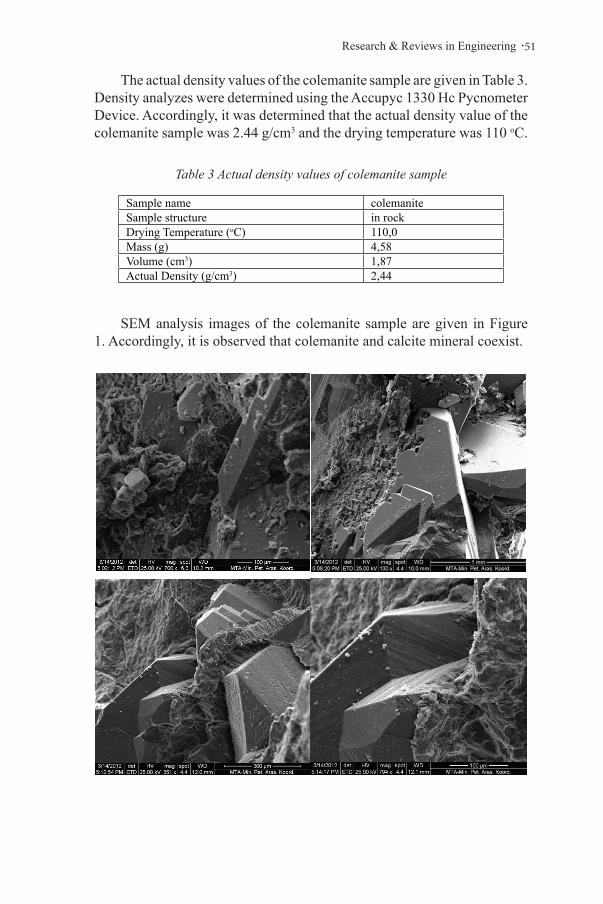
.51Research & Reviews in Engineering
The actual density values of the colemanite sample are given in Table 3. Density analyzes were determined using the Accupyc 1330 Hc Pycnometer Device. Accordingly, it was determined that the actual density value of the colemanite sample was 2.44 g/cm3 and the drying temperature was 110 oC.
Table 3 Actual density values of colemanite sample
Sample name colemaniteSample structure in rockDrying Temperature (oC) 110,0Mass (g) 4,58Volume (cm3) 1,87Actual Density (g/cm3) 2,44
SEM analysis images of the colemanite sample are given in Figure 1. Accordingly, it is observed that colemanite and calcite mineral coexist.

Oyku Bilgin52 .
Figure 1. SEM analysis images of colemanite-calcite sample
In Figure 2, thin section 1st nicol and 2nd nicol images of the colemanite sample are given.
Figure 2 Colemanite thin section views of 1st nicol and 2nd nikol
Results and discussion
Boron minerals are generally brought to the industry by applying processes such as raw ore, ore preparation (crushing, screening, sizing, classification, grinding, etc.) after being extracted from the quarry. In this context, Balıkesir/Bigadiç Boron Enterprise has been exporting to many countries of the world by obtaining ground boron products since 1998. In addition, it produces high value-added products with its innovation and state-of-the-art sustainability vision from mining activities to the production stage.
Colemanite ore; it is also sold as refined products (such as boric acid, refined-calcined borax decahydrate, anhydrous boric acid, refined-calcined borax pentahydrate, calcined tincal, synthetic-calcined-refined colemanite, calcined ulexite) (Güyagüler, 2001; Yogurtcuoğlu, 2019). The grade of

.53Research & Reviews in Engineering
the commercially important colemanite ore should be around 50%. Since the sample in which this study was made has a grade of 36%, enrichment and separation processes can be recommended. It is known from previous studies that the colemanite grade increases by applying methods such as flotation, MGS, Falcon, shaking table, which are among the ore enrichment methods. Apart from these methods, low grade colemanite ores are also used as cement additives. It is one of the commonly used methods to obtain H3BO3 (boric acid) by dissolving the colemanite sample in sulfuric acid solutions at a temperature of (80-90°C) and following methods such as cleaning, filtration, cooling, evaporation, crystallization of the impurities, washing and drying of the crystals (Kalafatlıoğlu at al. , 2000; Yoğurtcuoğlu and Dalgalı, 2019; Yoğurtcuoğlu 2019). It can be suggested to evaluate the colemanite sample examined within the scope of this study by applying the specified enrichment and separation methods, by increasing the concentrate grade or by obtaining H3BO3 (boric acid).

Oyku Bilgin54 .
References
Akyol, E. ve Akgün, F. (1990). Bigadiç, Kestelek, Emet ve Kırka boratlı neojen tortullarının palinolojisi. MTA Dergisi, 111, 165-173.
Binici, H., Sevinç, A., H. ve Durgun, Y.,M., (2010). Barit, bazaltik pomza, kole-manit ve yüksek fırın cürufu katkılın betonların özellikleri. KSÜ Mühen-dislik Bilimleri Dergisi, 13, 1.
Budak A., (2014). Borik asit üretimindeki kolemanit karbondioksit reaksiyonun-da basınç etkisinin araştırılması. Süleyman Demirel Üniversitesi, Fen Bi-limleri Enstitüsü, Yüksek Lisans Tezi, Çevre Mühendisliği Anabilim Dalı, Isparta, p:122.
Dokuzuncu Kalkınma Planı, (2008). Bor-Soda Külü-Krom Kimyasalları Çalışma Grubu Raporu. Kimya Sanayii Özel İhtisas Komisyonu, s:138.
Erdoğan, Y., Zeybek, M., S., ve Demirbaş, A., (1998). Cement mixes containing colemanite from concentrator wastes. Cement and Concrete Research, 28, 4, 605-609.
Eren F., (2013). Göcenoluk (Kırka) borat yatağı sondajlarının mineralojik ve pet-rografik değerlendirilmesi. Dokuz Eylül Üniversitesi Fen Bilimleri Ensti-tüsü Yüksek Lisans Tezi Jeoloji Mühendisliği Bölümü, Ekonomik Jeoloji Anabilim Dalı, Mart, 2013, İzmir, p:96.
Eyüboğlu, S., (2013). Kolemanit konsantratör atıklarının çimento üretiminde de-ğerlendirilmesi. Yüksek Lisans Tezi, Balıkesir Üniversitesi, Fen Bilimleri Enstitüsü, Balıkesir.
Gençel, O., (2009). Hamile ratlarda oksidatif strese neden olan radyasyona karşı kolemanitli betonun koruyucu etkisinin araştırılması. Doktora Tezi, Süley-man Demirel Üniversitesi, Fen Bilimleri Enstitüsü, Isparta.
Gözkaman Ç., (2008). Kolemanit flotasyonunun kimyasal ve mekanik özellik-lerinin incelenmesi. Yıldız Teknik Üniversitesi, Fen Bilimleri Enstitüsü, Metalurji ve Malzeme Mühendisliği Anabilimdalı, Üretim Metalurjisi Anabilimdalı, Doktora tezi, İstanbul, 79.
Güç E., (2010). Kolemanit içeriğindeki arseniğin biyoliç ile uzaklaştırılması. Çu-kurova Üniversitesi Fen Bilimleri Enstitüsü” Yüksek Lisans Tezi, Biyotek-noloji Anabilim Dalı, Adana, p:112.
Güyagüler, T., (2001). Türkiye bor potansiyeli. 4 Endüstriyel Hammaddeler, İz-mir, Türkiye, 18-27.
Helvacı C., (2003). Türkiye borat yatakları, jeolojik konumu, ekonomik önemi ve bor politikası. Baü Fen Bil. Enst. Derg.5.1.
Helvacı, C., ve Alaca, O., (1984). Bigadiç borat yataklarının jeolojisi ve mine-ralojisi: T.J.K. 38. Bilimsel ve Teknik Kurultay Bildiri Özetleri, 110-111.
.55Research & Reviews in Engineering
Helvacı, C., (1994). Mineral assemblages and formation of the Kestelek and Sul-tançayır borate deposits. Proceedings of 29th International Geological Congress, Kyoto, Part A, 245-264.
Helvacı, C., (1995). Stratigraphy, mineralogy and genesis of the Bigadiç borate deposits, Western Turkey. Economic Geology,90, 1237-1260.
Helvacı, C., Orti, F., (1998). Sedimantology and diagenesis of miocene colema-nite-ulexite deposits (western Anatolia, Turkey). Journal of Sedimentary Research, 68, 1021-1033.
Kalafatoğlu, İ.E., Örs, N., Özdemir, S.S., (2000). Hisarcık kolemanitinin sülfürik asitle çözünme davranışı. IV. Ulusal Kimya Mühendisliği Kongresi, İstan-bul, Türkiye, 263-268.
Kayadeniz İ., Gülensoy H. ve Yusufoğlu İ., (1979). Arsenikli kolemanit cevher-lerindeki arseniğin vakum kalsinasyon yöntemi ile giderilmesi. TÜBİTAK, Mühendislik Araştırma Grubu, Proje No. 198, İstanbul.
Korçak, Ö., (2014). Kolemanit atıklarının çimento üretiminde kullanılması ve çimentonun performans özelliklerinin geliştirilmesi. Doktora Tezi, Gazi Üniversitesi, Fen Bilimleri Enstitüsü, Ankara.
Mazura, N., V., ve Levistkii, I., A., (2008). Use of colemanite for ımproving the quality of unfritted glazes. Springer Science and Business Media, 1, 20-23.
Şahin, Ş., E., (2008). Ham ve kalsine kolemanit atıklarının tuğla yapımında kul-lanım olanaklarının araştırılması. Yüksek Lisans Tezi, Dumlupınar Üniver-sitesi, Fen Bilimleri Enstitüsü, Kütahya.
Targan, Ş., Erdoğan, Y., Olgun, A., Zeybek, B., ve Sevinç, V., (2003). Influen-ce of natural pozzolan, colemanite ore waste, bottom ash and fly ash on the properties of portland cement. Cement and Concrete Research, 33, 8, 1175-1182.
Tok, S., (2018). Emet kolemanit zenginleştirme tesisi düşük tenörlü konsantre-sinin bor içeriğinin yükseltilmesi. Afyon Kocatepe Üniversitesi Fen Bi-limleri Enstitüsü Maden Mühendisliği Anabilim Dalı, Yüksek Lisans Tezi, Afyon, p: 97.
Yaltay, N., (2015). Kolemanit katkılı çimento ile üretilen pomza agregalı hafif betonun fiziksel özelliklerinin araştırılması. Doktora Tezi, Fırat Üniversi-tesi, Fen Bilimleri Enstitüsü, Elazığ.
Yarar, B., (1973). Düşük tenörlü kolemanit cevherinin flotasyon yolu ile zengin-leştirilmesi. Türkiye Madencilik Bilimsel ve Teknik III. Kongresi, Ankara, 571-588.
Yeşilçiçek, H., (2016). Kolemanitin zemin stabilizasyonunda kullanılabilirliğinin araştırılması. Karadeniz Teknik Üniversitesi Fen Bilimleri Enstitüsü İnşa-at Mühendisliği Anabilim Dalı Yüksek Lisans Tezi, Trabzon, p:127.

Oyku Bilgin56 .
Yogurtcuoğlu E. (2019). Sülfürik asitli ortamda kolemanit ve üleksit içeren bor atıklarının davranışı. Karadeniz Chem. Sci. Tech., 4.
Yoğurtcuoğlu, E. ve Dalgalı, O., (2019). Bigadiç kolemanit ve üleksit şlam atıkla-rının yığın liçi ile değerlendirilmesi. Uluslararası Bor Sempozyumu, 102-106, Nevşehir, Türkiye.
URL-1 http://www.mta.gov.tr/v3.0/bilgi-merkezi/kolemanit
URL-2 http://www.etimaden.gov.tr/kolemanit
URL-3 http://www.sbb.gov.tr/wp content/uploads/2018/11/09_KimyaSanayii_BorSodaKuluKromKimya.pdf
URL-4 Eti Maden İşletmeleri Genel Müdürlüğü, 2004, https://www.etimaden.gov.tr/bigadic
http://www.etimaden.gov.tr/storage/pages/March2019/5-1-ogutulmus-kolema-nit.pdf

Chapter 4DURABILITY OF MORTARS MADE WITH BIO-BASED ASHES
Mustafa EKEN1
Ela AVSAROGLU2
1 Dr. Kahramanmaras Istiklal University Elbistan Vocational School Department of Constru-ction Technology,2 Dr. Lecturer Kahramanmaras Sutcu Imam University Vocational School of Technical Sciences Department of Construction Technology e-mail: [email protected]; 05062661858 e-mail: ela¬[email protected] 05321731314

Mustafa Eken, Ela Avsaroglu58 .
1. INTRODUCTION
While considering concrete as an economic value, certain factors must be taken into account as it consists of a combination of physical as-sets such as sand, gravel and cement and the scarcity and exhaustion of these resources, the environmental damage that occur while they are ob-tained. According to the statistics, it is known that today over 10 billion tons of concrete is produced [1]. Population estimates indicate that the world population will increase between 1.5 and 9 billion in 44 years. Pop-ulation growth will increase the demand for concrete, hence the need and consumption of raw materials. It is predicted that the amount of concrete demand in the world will reach up to 18 billion tons in 2050 [2]. While producing concrete, it is also necessary to look for cost-effective solutions that will increase the usefulness of concrete. Rapid increase of industri-alization brought out certain problems and affected life to a great extent. Some recent researchers mentioned that this rapid increase caused cement industry to experience problems in maintaining the supply-demand bal-ance to start to search for new low-cost raw materials that can be added to cement production in accordance with the standards. Thus, importance of waste materials has increased, regarding the environmental problems. Be-sides, the concept of sustainability has gained great significance bringing the question to transfer resources to future generations. It should be kept in mind that natural resources are not infinite and, if not used carefully, they will one day run out [3-4]. It is of great importance to exploit and re-cycle the wastes in order to protect natural resources and meet the resource needs [5]. It is stated that, thanks to recycling, besides the elimination of environmental pollution, there will also be a decrease in the need for stor-age areas to be used for waste [6].
Turkey is very rich in terms of the total annual production of field crops and the amount of waste [7]. The total amount of solid waste is over 13 tons. When analyzed, the main products with the highest share in it are the agricultural products wheat, barley, corn, cotton and sunflower. The use and utilization of agricultural wastes in concrete and mortar produc-tion and the fact that these products can replace the materials used as raw materials [8-9] can be defined as a social value that forms the basis of sus-tainability and respect for the environment [10]. Turkey is in the 14th place in the world with its 213 thousand 188 square kilometers agricultural fields and in the 40th place in terms of agricultural areas with 3 acres per person. Turkey’s land area is 769 thousand 632 square kilometers and only 27,7 percent is used as agricultural area. Based on this rate, it is in the 4th place among the 15 countries which have the highest proportion of agricultural areas. However, despite the size of the agricultural production with these values, there are numerous agricultural wastes to be recycled in Turkey.

.59Research & Reviews in Engineering
Durability of concrete is defined as the strength and resistance to the conditions stemming from environmental factors such as physical, chemi-cal, biological corrosions and the capacity to maintain concrete’s other ex-isting properties [11]. Sulphates and acids, which are among the durability problems, are known as aggressive chemicals that affect the durability of concrete and mortar structures. Sulphates from the soil and groundwater can cause the expansion of samples to deteriorate, affecting the long-term durability of concrete structures. These aggressive waters cause cracking of concrete and mortar specimens, decomposition, expansion and dam-age [12-13]. The durability values of the samples exposed to acid and its effect are related to the number of days the mortars are exposed to these aggressive waters. These aggressive waters disrupt the long-term mortar structures, create auto-stress in the reference sample with a network of mi-cro cracks, and produce products which expand (gypsum and ettringite), affecting the structure in a negative way [14]. In recent years, agricultural wastes have been widely used in the building sector [15]. We can see the mortar production with different use of waste materials in the literature: Wang et al. [16] used rice, straw, and coke powder as an alternative to ce-ment; Aprianti et al. [17] used rice husk, palm oil fuel, sugar cane bagasse, wood waste, bamboo leaf and corn cob ashes to replace certain percentag-es of cement in concrete; Aksogan et al. [18] used corn stalk, wheat straw, sunflower stalk ashes as additives in concrete production with improved durability properties; Modani et al. [19] produced lightweight concrete from sugar cane ash. In other studies, Olutoge et al., [20], Buari et al., [21] and Kanagalakshmi et al. [22] used peanut shell as an agricultural waste to replace cement and fine aggregate in concrete; Ismail et al. [23] used sugar cane to replace fine aggregate in concrete; Panesar et al. [24] used cork instead of cement. Ozturk et al., [25] used tobacco waste in the production of lightweight concrete.
Umoh et al. [26] used bamboo to replace a part of the cement and Cobreros et al. [27] produced mortar from banana waste ash as pozzolanic material in concrete. Furthermore, Eisa [28] used olive as an agricultural waste product to replace a part of the cement as an alternative material. Kanning et al. [29] used banana waste ash in mortar production. Benman-sour et al. [30] used date-palm tree ash in producing mortar and Cordeiro et al. [31] used elephant grass in the production of mortar by reducing the amount of cement. With the use of these agricultural wastes, the environ-mental damage of concrete / mortar production will be reduced, green-house gas emissions will be minimized, the waste of natural resources will be reduced and worthless waste will be utilized making contribution to the economy.
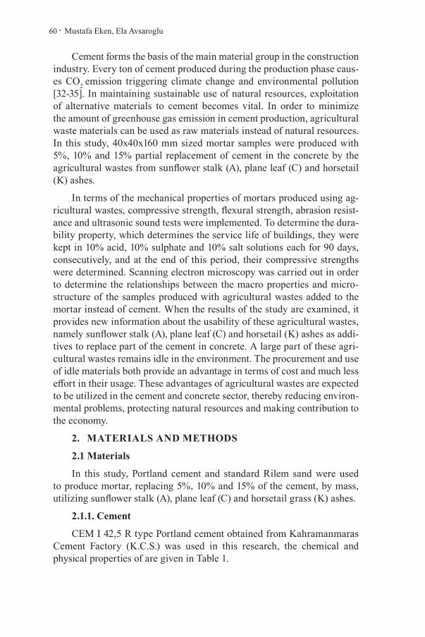
Mustafa Eken, Ela Avsaroglu60 .
Cement forms the basis of the main material group in the construction industry. Every ton of cement produced during the production phase caus-es CO2 emission triggering climate change and environmental pollution [32-35]. In maintaining sustainable use of natural resources, exploitation of alternative materials to cement becomes vital. In order to minimize the amount of greenhouse gas emission in cement production, agricultural waste materials can be used as raw materials instead of natural resources. In this study, 40x40x160 mm sized mortar samples were produced with 5%, 10% and 15% partial replacement of cement in the concrete by the agricultural wastes from sunflower stalk (A), plane leaf (C) and horsetail (K) ashes.
In terms of the mechanical properties of mortars produced using ag-ricultural wastes, compressive strength, flexural strength, abrasion resist-ance and ultrasonic sound tests were implemented. To determine the dura-bility property, which determines the service life of buildings, they were kept in 10% acid, 10% sulphate and 10% salt solutions each for 90 days, consecutively, and at the end of this period, their compressive strengths were determined. Scanning electron microscopy was carried out in order to determine the relationships between the macro properties and micro-structure of the samples produced with agricultural wastes added to the mortar instead of cement. When the results of the study are examined, it provides new information about the usability of these agricultural wastes, namely sunflower stalk (A), plane leaf (C) and horsetail (K) ashes as addi-tives to replace part of the cement in concrete. A large part of these agri-cultural wastes remains idle in the environment. The procurement and use of idle materials both provide an advantage in terms of cost and much less effort in their usage. These advantages of agricultural wastes are expected to be utilized in the cement and concrete sector, thereby reducing environ-mental problems, protecting natural resources and making contribution to the economy.
2. MATERIALS AND METHODS
2.1 Materials
In this study, Portland cement and standard Rilem sand were used to produce mortar, replacing 5%, 10% and 15% of the cement, by mass, utilizing sunflower stalk (A), plane leaf (C) and horsetail grass (K) ashes.
2.1.1. Cement
CEM I 42,5 R type Portland cement obtained from Kahramanmaras Cement Factory (K.C.S.) was used in this research, the chemical and physical properties of are given in Table 1.

.61Research & Reviews in Engineering
Table 1: Chemical and physical properties of cement (%)
CHEMICAL PROPERTIES PHYSICAL PROPERTIESComponents by weight CementSiO2 20.03 specific density (g/cm3) 3.10Al2O3 4.84 Blaine specific surface (cm2/g) 3210Fe2O3 2.42 Start of setting (min) 155CaO 62.45 End of setting (min) 267MgO 2.61MnO -K2O 0.80TiO2 -Cr2O3 -SO3 3.55Na2O 0.60B2O3 -Other 2.70
2.1.2. Sand
Standard Rilem sand (CEN), each pack of which is 1350 g in weight, round grained and with at least 98% SiO2 content, was used as fine aggregate in the production of mortar samples in this study. The granulometry of CEN standard sand is given in Table 2.
Table 2. Granulometry of CEN standard sand
Square mesh size (mm) 2.00 1.60 1.00 0.50 0.16 0.08Cumulative remaining (% ) 0 7±2 33±2 67±2 87±2 99±1
2.1.3. Sunflower stalk ash
Sunflower is the most preferred agricultural product in our country in terms of cultivation area. It has an important share among the agricultural products with an annual production amount of approximately 1 964 385 thousand tons [36]. 1.4 tons of sunflower stalks are obtained from one ton of sunflower agricultural products [37]. The sunflower stalks remaining in the planting area after the harvest, which have an important place in the agricultural economy, pose a problem for farmers. The burning of the

Mustafa Eken, Ela Avsaroglu62 .
stalks affects the fertility of the soil in the cultivation area and harms the environment. Utilization of agricultural waste products will eliminate the harm to the field and the environment. Furthermore, it will provide addi-tional employment for agricultural workers in the region.
2.1.4. Plane leaf ash
Plane trees are abundant in Kahramanmaras region as it is a very suitable species for the climate of the region. Storing thousands of tons of dried plane leaves poses a problem and burning them unconsciously in open areas also causes environmental pollution. This study will contribute to ecological balance by the use of plane leaf ashes in concrete production after being collected and burned by appropriate techniques.
2.1.5. Horsetail grass
Horsetail plant, found in the ground and water-borne areas, particular-ly likes loose sandy, loamy, clay-dominated and sandy-loam soils. Horse-tail grass is found on the water’s edge, swamps, beneath meadows and pastures, and also in orchards [38]. Horsetail grass was used in the pro-duction of mortar after being properly collected and burned under control. Chemical and physical analyzes of agricultural wastes used in this study were carried out in KCS Kahramanmaras Cement AS. The chemical anal-ysis of agricultural waste ashes is given in Table 3.
Table 3. Chemical analysis of agricultural waste ashes (%)
Components by weight A C K
16.65

.63Research & Reviews in Engineering
Total
2.2. Method
2.2.1. Mixing ratios
In this study, samples were produced in order to examine the effects of agricultural waste ashes, which were substituted in different ratios instead of part of the cement in mortar samples. This replacement was made by 5%, 10% and 15%, by mass, according to TS 196-1 [39]. Three prismatic mortar samples were produced for each mixture. In the preparation of the reference and agricultural waste ash added mortar samples, the w / c ratio (0.5) was kept constant and CEN standard sand was used. The mixing ratios and names of the reference and other samples with sunflower stalk ash (A), plane leaf ash (C) and horsetail grass ash (K) are given in Table 4.
Table 4. Amounts of material forming the mixture (kg / m3)
Mixing code Material Contribution
Rates (%)Portland Cement (g)
Ash Rate (g)
Sand Rate (g)
Water Rate (g)
Water / Binder ratio
R Reference - 450 - 1350 225 0.50
A5Sunflower stalk ash
5 427.5 22.5 1350 225 0.50
A10 10 405 45 1350 225 0.50
A15 15 382.5 67.5 1350 225 0.50
C5Plane leaves ash
5 427.5 22.5 1350 225 0.50
C10 10 405 45 1350 225 0.50
C15 15 382.5 67.5 1350 225 0.50
K5Horsetail grass ash
5 427.5 22.5 1350 225 0.50
K10 10 405 45 1350 225 0.50
K15 15 382.5 67.5 1350 225 0.50
2.2.2. Test procedure
In the experimental study, 40x40x160 mm size prismatic mortar samples were used. All samples were cured in water saturated with lime at 22 ° C for 7, 28 and 90 days. Compressive strength, flexural strength, ultrasonic sound and capillary water absorption tests were performed on the mortar samples. In order to examine the durability properties of the mortars, their compressive strength values were analyzed after being exposed to salt environments of 10% HCI, 10% Na2SO4 and 10% NaCl each for 90 days.

Mustafa Eken, Ela Avsaroglu64 .
2.2.3. Compressive strength
The samples obtained after the determination of the flexural strength test as two half prisms were used to determine the 7, 28 and 90 days compressive strength values of the reference and agricultural waste added samples. Each sample was placed in the compressive test machine and the pressure was applied. A total of 60 samples were used to determine the compressive strength. The compressive strength values were determined in accordance with TS EN 196-1 [40] standards by keeping the loading speed constant at 1.5 MPa/sec in the compressive test machine with 250 kN capacity (Figure 1). Compressive strength values found by equation (1) are given in Table 5.
(1)
Rc: Compressive strength (N/ mm2)
fc: breaking load (N)
1600: Cross sectional area (40x40) mm2
2.2.4. Flexural strength
A single point loading system was used to determine the 7, 28 and 90 days flexural strength values. Samples prepared with 10 different mixing ratios in 40x40x160 mm dimensions were placed in the flexural testing apparatus (Figure 1) with 15 kN capacity in accordance with standard TS EN 196-1. The loading speed was kept constant at 0.4 kN / sec and the flexural strength values were calculated by applying equation (2) on a total of 30 samples. Flexural strength values are given in Table 5.
(2)
Rf: Flexural strength (N/mm2)
Ff: Force applied to break the prism (N)
l: Prism dimensions (mm)
b: Prism edge length (mm)

.65Research & Reviews in Engineering
Figure 1. a) Compressive and flexural device of mortar samples, b) Flexural strength application, c) Compressive strength application
2.2.5. Ultrasound velocity measurement
The values of the ultrasound transmission velocity were calculated on the mortar samples by the test known as the undamaged test, at certain rates at different ages. The arrival time and wave velocities of the sound waves transmitted by the probe tips placed at the ends of the mortar at the ultrasound transmission speed were calculated. It can be said that there is a relationship between ultrasound velocity values of mortars and their compressive strength and can be used in strength comparisons [40]. The average of the measured values for each mortar sample for ultrasound velocities was determined by equation 3 calculation method in accordance with the ASTM 579-05 [41] standard. Ultrasonic sound permeability values are given in Table 5.
(3)
V = Wave speed (meters / second),
S = Distance between wave surfaces sent to prism samples (meters),
t = Time of arrival of the wave (micro seconds).
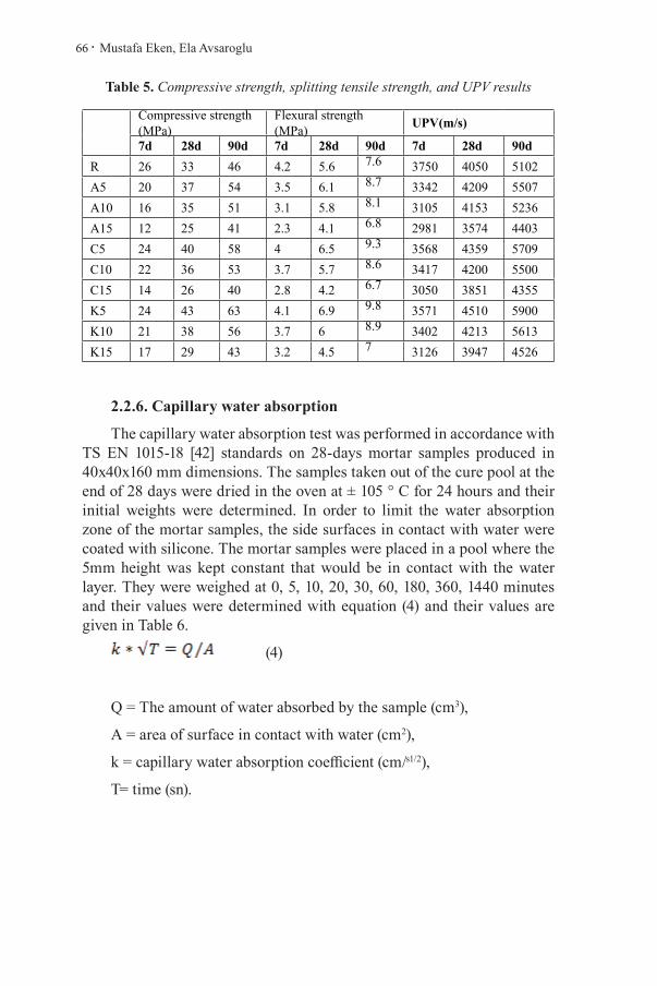
Mustafa Eken, Ela Avsaroglu66 .
Table 5. Compressive strength, splitting tensile strength, and UPV results
Compressive strength (MPa)
Flexural strength (MPa) UPV(m/s)
7d 28d 90d 7d 28d 90d 7d 28d 90dR 26 33 46 4.2 5.6 7.6 3750 4050 5102A5 20 37 54 3.5 6.1 8.7 3342 4209 5507A10 16 35 51 3.1 5.8 8.1 3105 4153 5236A15 12 25 41 2.3 4.1 6.8 2981 3574 4403C5 24 40 58 4 6.5 9.3 3568 4359 5709C10 22 36 53 3.7 5.7 8.6 3417 4200 5500C15 14 26 40 2.8 4.2 6.7 3050 3851 4355K5 24 43 63 4.1 6.9 9.8 3571 4510 5900K10 21 38 56 3.7 6 8.9 3402 4213 5613K15 17 29 43 3.2 4.5 7 3126 3947 4526
2.2.6. Capillary water absorption
The capillary water absorption test was performed in accordance with TS EN 1015-18 [42] standards on 28-days mortar samples produced in 40x40x160 mm dimensions. The samples taken out of the cure pool at the end of 28 days were dried in the oven at ± 105 ° C for 24 hours and their initial weights were determined. In order to limit the water absorption zone of the mortar samples, the side surfaces in contact with water were coated with silicone. The mortar samples were placed in a pool where the 5mm height was kept constant that would be in contact with the water layer. They were weighed at 0, 5, 10, 20, 30, 60, 180, 360, 1440 minutes and their values were determined with equation (4) and their values are given in Table 6.
(4)
Q = The amount of water absorbed by the sample (cm3),
A = area of surface in contact with water (cm2),
k = capillary water absorption coefficient (cm/s1/2),
T= time (sn).

.67Research & Reviews in Engineering
Table 6. Capillary water absorption values
Samples 0 min 5 min 10 min 20 min 30 min 60 min 180 min 360 min 720 min 1440 min
R 547.3 550.87 551.03 551.13 551.18 551.33 551.78 552.16 553.31 554.63
A5 544.9 555.27 555.48 555.63 555.64 555.83 556.37 557.12 558.39 560.3
A10 536.15 545.04 545.27 545.61 545.82 546.31 548.26 550.61 554.55 561.76
A15 525.08 527.76 528.19 528.49 528.68 529.17 530.79 533.11 537.23 544.5
C5 538.81 541.05 541.3 541.48 541.55 541.83 542.64 543.92 545.81 549.67
C10 546.19 556.12 556.42 556.73 556.9 557.47 559.43 561.97 565.91 573.15
C15 526.8 530.12 530.43 530.63 530.87 531.35 532.75 534.86 538.26 544.52
K5 530.3 531.26 531.75 531.64 531.82 532.03 532.72 533.66 535.29 538.97
K10 519.9 522.06 522.46 522.58 522.72 523.25 524.57 526.18 528.7 533.5
K15 510.16 514.12 514.84 515.7 516.12 517.48 521.07 525.48 531.64 541.93
2.2.7. Exposure to acid, sulphate and salt environments
In the study, the compressive strength values of the mortar samples of 40x40x160 mm size produced from cement with agricultural wastes at 5%, 10% and 15% were exposed to saline environments of 10% HCI, 10% Na2SO4 and 10% NaCl each for 90 days. Then, their compressive strengths were measured and the computed strength losses are given in Table 7.
Table 7. Residual compressive strength results at 90 days.
Sam
ples
Compressive strength (MPa)Compressive strength loss (%) (a1)
Compressive strength loss (%) (b1)
Compressive strength loss (%) (c1)
28 days (water)
90 days (water)
90 days (acid)(a)
90 days (sulfate) (b)
90 days (salt)(c)
R 33 46 27.6 27.36 28.4 40.00 40.52 38.26
A5 37 54 39.13 39.07 39.95 27.54 27.65 26.02
A10 35 51 36.3 36.01 36.87 28.82 29.39 27.71
A15 25 41 28.32 28.69 29.01 30.93 30.02 29.24
C5 40 58 44.04 44.11 45.08 24.07 23.95 22.28
C10 36 53 38.12 38.4 39.11 28.08 27.55 26.21
C15 26 40 27.01 27.56 27.88 32.48 31.10 30.30
K5 43 63 50.04 50.16 51.02 20.57 20.38 19.02
K10 38 56 41.16 41.46 42.49 26.50 25.96 24.13
K15 29 43 30.07 30.19 31.12 30.07 29.79 27.63

Mustafa Eken, Ela Avsaroglu68 .
3. RESULTS
The results obtained from the experiments which investigates the strength and durability properties of the mortar samples produced by replacing part of the cement in concrete by sunflower stalk, plane leaf, and horsetail are given below.
3.1. Compressive strength of mortar samples
The 7, 28 and 90-days compressive strengths of the samples with ag-ricultural waste additives are given in Figure 2.
Figure 2. The effect of agricultural waste additive on compressive strength at different ages
The 7-day compressive strength of the mortar samples produced with agricultural waste in all mixing ratios was lower than the R (reference) sample. However, when the 28 days compressive strength values were examined, the highest value was for K5 sample being 43 MPa, with an increase of 21.21% compared to the reference sample. When the 28 days values of sunflower stalk ashes were examined, the highest value of the A5 sample was found to be higher than the reference with an increase of 12%, while the value for A10 was higher than the reference sample with an increase of 6%. However, the A15 sample had a lower value than the reference sample with a decrease of 24%. When the 28 days values of plane leaf ashes were examined, it was observed that the highest value, which was for C5 sample, had an increase of 21% compared to the reference sample, while C10 sample had a higher value with 9% increase, whereas, C15 sample showed a decrease of 24%. From the 28 days samples for the ones with horsetail grass ashes, the highest value was obtained for K5 sample with an increase of 30%, while K10 sample had an increase of 15%, whereas, the K15 sample showed a decrease of 12%. When the

.69Research & Reviews in Engineering
90 days values were examined, the highest value was obtained for the K5 sample with long curing time, with a 37% increase compared to the reference sample. Among the 90 days samples with sunflower stalk ash, the A5 sample had the highest value with an increase of 17% compared to the reference sample, while A10 had an increase rate of 10%, whereas, A15 showed a decrease of 11%. The sample with the highest value Among 90 days mortar samples with plane leaf ash, the sample with the highest value was sample C5, with an increase of 26% than the reference, while sample C10 had an increase of 15%, whereas, sample C15 had a decrease of 13%. Among the 90 days samples with horsetail ash, K5 had the highest value with an increase rate of 37%, while K10 showed an increase of 21%, whereas, K15 showed a decrease of 7% compared to the reference sample. When all the compressive strength values are examined, it is observed that the compressive strength values decrease as the ash additive ratios increase (Figure 3). On the other hand, the long curing times have a positive effect on the compressive strength values of the mortar samples produced by agricultural wastes (Figure 4).
Figure 3. The effect of agricultural waste ash additive ratio on compressive strength change at different ages

Mustafa Eken, Ela Avsaroglu70 .
Figure 4. Relation of curing time and compressive strength for samples with different kinds and ratios of additives.
3.2. Flexural strength of mortar samples
The 7, 28 and 90-day flexural strengths of mortar samples with agricultural waste are given in Figure 5.
Figure 5. Relation of agricultural waste additive ratio and flexural strength at different ages
When the 7-day flexural strength values were examined, the reference sample had the highest value with 4.2 MPa. When the 28-day flexural strength values were examined, the highest value was obtained for sample K5 with 6.9 MPa. Among the 28-day mortar samples with sunflower stalk ash, while the sample with the highest strength was A5 with an increase
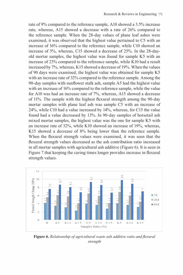
.71Research & Reviews in Engineering
rate of 9% compared to the reference sample, A10 showed a 3.5% increase rate, whereas, A15 showed a decrease with a rate of 26% compared to the reference sample. When the 28-day values of plane leaf ashes were examined, it was observed that the highest value pertained to C5 with an increase of 16% compared to the reference sample, while C10 showed an increase of 5%, whereas, C15 showed a decrease of 25%. In the 28-day-old mortar samples, the highest value was found for sample K5 with an increase of 23% compared to the reference sample, while K10 had a result increased by 7%, whereas, K15 showed a decrease of 19%. When the values of 90 days were examined, the highest value was obtained for sample K5 with an increase rate of 32% compared to the reference sample. Among the 90-day samples with sunflower stalk ash, sample A5 had the highest value with an increase of 16% compared to the reference sample, while the value for A10 was had an increase rate of 7%, whereas, A15 showed a decrease of 11%. The sample with the highest flexural strength among the 90-day mortar samples with plane leaf ash was sample C5 with an increase of 24%, while C10 had a value increased by 14%, whereas, for C15 the value found had a value decreased by 13%. In 90-day samples of horsetail ash mixed mortar samples, the highest value was the one for sample K5 with an increase rate of 32%, while K10 showed an increase of 19%, whereas, K15 showed a decrease of 8% being lower than the reference sample. When the flexural strength values were examined, it was seen that the flexural strength values decreased as the ash contribution ratio increased in all mortar samples with agricultural ash additive (Figure 6). It is seen in Figure 7 that keeping the curing times longer provides increase in flexural strength values.
Figure 6. Relationship of agricultural waste ash additive ratio and flexural strength

Mustafa Eken, Ela Avsaroglu72 .
Figure 7. Flexural strength curing time relationship
Within the scope of the study, a relationship was established between the compressive and flexural strength values of the samples, which were prepared with different kinds and proportions of agricultural waste additi-ves and the results are presented in Figure 8. When the graph is examined, it is seen that there is nearly a linear relationship between the compressive and flexural strength values. Furthermore, this straight line passing throu-gh the origin renders the two strength values directly proportional with each other.
Figure 8. Compressive and flexural strength correlation relationship
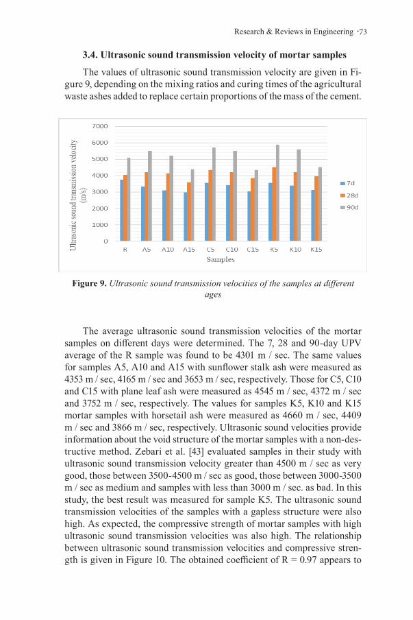
.73Research & Reviews in Engineering
3.4. Ultrasonic sound transmission velocity of mortar samples
The values of ultrasonic sound transmission velocity are given in Fi-gure 9, depending on the mixing ratios and curing times of the agricultural waste ashes added to replace certain proportions of the mass of the cement.
Figure 9. Ultrasonic sound transmission velocities of the samples at different ages
The average ultrasonic sound transmission velocities of the mortar samples on different days were determined. The 7, 28 and 90-day UPV average of the R sample was found to be 4301 m / sec. The same values for samples A5, A10 and A15 with sunflower stalk ash were measured as 4353 m / sec, 4165 m / sec and 3653 m / sec, respectively. Those for C5, C10 and C15 with plane leaf ash were measured as 4545 m / sec, 4372 m / sec and 3752 m / sec, respectively. The values for samples K5, K10 and K15 mortar samples with horsetail ash were measured as 4660 m / sec, 4409 m / sec and 3866 m / sec, respectively. Ultrasonic sound velocities provide information about the void structure of the mortar samples with a non-des-tructive method. Zebari et al. [43] evaluated samples in their study with ultrasonic sound transmission velocity greater than 4500 m / sec as very good, those between 3500-4500 m / sec as good, those between 3000-3500 m / sec as medium and samples with less than 3000 m / sec. as bad. In this study, the best result was measured for sample K5. The ultrasonic sound transmission velocities of the samples with a gapless structure were also high. As expected, the compressive strength of mortar samples with high ultrasonic sound transmission velocities was also high. The relationship between ultrasonic sound transmission velocities and compressive stren-gth is given in Figure 10. The obtained coefficient of R = 0.97 appears to

Mustafa Eken, Ela Avsaroglu74 .
be a satisfactory value in specifying the relationship between them. In this study, it was observed that the ultrasound transmission velocities increa-sed with the increase in the curing times of mortars, and decreased with the increase in the ash additive ratio.
Figure 10. Ultrasonic sound transmission velocities and compressive strength relationship
3.5. Durability
The compressive strength values of the mortars kept in 10% HCl (acid), 10% MgSO4 (sulphate) and 10% NaCl (salt) solution for 90 days in order to determine the durability properties of the mortar samples against aggressive waters are given, respectively, in Figures 11, 12 and 13.
3.5.1. Acid effect
Figure 11. The effect of HCl acid environment on the compressive strength

.75Research & Reviews in Engineering
When the durability performances of the produced mortar samples were tested in 10% HCl acid solution for 90 days, the highest strength loss ratio was obtained in the R sample with a strength loss of 40%. Among all samples, K5 showed the highest strength after being kept in 10% HCl acid environment for 90 days with 50.04 MPa and 20.57% strength loss. When the mortar samples with sunflower stalk ash additive were exam-ined, sample A5 showed the highest resistance against HCl acid environ-ment with 39.13 MPa and 27.54% strength loss, while sample A10 showed a strength of 36.30 MPa and 28.82% strength loss, the A15 sample showed a strength of 28.32 MPa and 30.93% strength loss. When the performanc-es of the plane leaf ash additive were examined, sample C5 showed the highest resistance against HCl acid environment with 44.04 MPa and 24.07% strength loss, while sample C10 showed a strength of 38.12 MPa and 28.08% strength loss, the C15 sample showed a strength of 27.01 MPa and 32.48% strength loss. When the performance of horsetail ash additive were examined, sample K5 showed the highest resistance against HCl acid environment with 50.04 MPa and 20.57% strength loss, while sample K10 showed a strength of 41.16 MPa and 26.50% strength loss, the K15 showed a strength of 30.07MPa and 31.56% strength loss. Considering the values given in Figure 11, as the agricultural waste ash additive ratio increases, the strength values of the mortars against HCl acid environment decrease and the strength loss ratios increase.
3.5.2. Sulphate effect
Figure 12. The effect of sulphate environment on the compressive strength
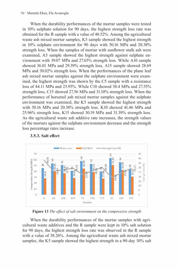
Mustafa Eken, Ela Avsaroglu76 .
When the durability performances of the mortar samples were tested in 10% sulphate solution for 90 days, the highest strength loss rate was obtained for the R sample with a value of 40.52%. Among the agricultural waste ash mixed mortar samples, K5 sample showed the highest strength in 10% sulphate environment for 90 days with 50.16 MPa and 20.38% strength loss. When the samples of mortar with sunflower stalk ash were examined, A5 sample showed the highest strength against sulphate en-vironment with 39.07 MPa and 27.65% strength loss. While A10 sample showed 36.01 MPa and 29.39% strength loss, A15 sample showed 28.69 MPa and 30.02% strength loss. When the performances of the plane leaf ash mixed mortar samples against the sulphate environment were exam-ined, the highest strength was shown by the C5 sample with a resistance loss of 44.11 MPa and 23.95%. While C10 showed 38.4 MPa and 27.55% strength loss, C15 showed 27.56 MPa and 31.10% strength loss. When the performance of horsetail ash mixed mortar samples against the sulphate environment was examined, the K5 sample showed the highest strength with 50.16 MPa and 20.38% strength loss. K10 showed 41.46 MPa and 25.96% strength loss, K15 showed 30.19 MPa and 31.39% strength loss. As the agricultural waste ash additive rate increases, the strength values of the mortars against the sulphate environment decrease and the strength loss percentage rates increase.
3.5.3. Salt effect
Figure 13 The effect of salt environment on the compressive strength
When the durability performances of the mortar samples with agri-cultural waste additives and the R sample were kept in 10% salt solution for 90 days, the highest strength loss rate was observed in the R sample with a value of 38.26%. Among the agricultural waste ash mixed mortar samples, the K5 sample showed the highest strength in a 90-day 10% salt

.77Research & Reviews in Engineering
environment with 51.02 MPa and 19.02% strength loss. When the samples of mortar with sunflower stalk and ash were examined, A5 sample showed the highest strength against salt environment with 39.95 MPa and 26.02% strength loss. A10 sample showed 36.87 MPa and 27.71% strength loss, while A15 sample showed 29.01 MPa and 29.24% strength loss. When the performances of the plane leaf ash mixed mortar samples against the salt environment were examined, the highest strength was shown by the C5 sample with 45.08 MPa and 22.28% strength loss. While C10 showed a strength loss of 39.11 MPa and 26.21%, C15 showed a strength loss of 27.88 MPa and 30.30%. When the performance of horsetail ash mixed mortar samples against the salt environment was examined, the K5 sam-ple showed the highest strength with 51.02 MPa and a resistance loss of 19.02%. K10 showed 42.49 MPa and 24.13% strength loss, K15 showed 31.12 MPa and 29.27% strength loss. As the agricultural waste ash additive rate increases, the strength values of the mortars against the salt environ-ment decrease and the strength loss% rates increase.
3.5.4. Capillary water absorption rate of mortar samples
Capillary coefficients obtained depending on the amount of water absorbed as a result of the capillary water absorption test are shown in Figure 14 for the samples in this study.
Figure 14. Capillary water absorption graph
When the capillary water absorption graph was examined, the rate of water absorption increased in the first minutes, but showed a decreasing trend in all samples in later times. The reference sample had the highest coefficient of capillarity in the first 20 minutes. The samples with the low-est capillarity coefficient among the samples of mortar with agricultural waste were the samples with numbers A5, C5 and K5. It can be said that
Mustafa Eken, Ela Avsaroglu78 .
the higher the capillarity coefficient as the additive ratio of the mortar sam-ples increases, it creates the hollow structure due to lumping in the mortar.
3. CONCLUSIONS
Cement used in concrete production is among the most central build-ing materials of the construction industry. A large amount of energy is needed during cement production and at the same time, it has an important share in environmental pollution with the greenhouse gas it emits. In order to preserve the natural balance and maintain sustainability, it is necessary to reduce the amount of cement production by utilizing agricultural waste materials. The large amount of agricultural waste in our country is the biggest problem of farmers. The most common waste consumption meth-od is burning the waste. In this method, soil structure and living species are damaged. Therefore, it has become a necessity to evaluate agricultural wastes while getting rid of it. At the same time, with the utilization of these wastes, additional employment will be created for the farmers in the region. In this study, mortars containing sunflower stalk ash, plane leaf ash and horsetail ash from their agricultural wastes were investigated for be-ing used to replace cement in certain proportions in construction industry. The following evaluations have been based on the results.
Compressive strength of mortar samples;
• When the 7, 28 and 90-day compressive strength values of the mortar samples produced with agricultural wastes are examined, the high-est values are obtained for sample K5 involving horsetail grass ashes to replace 5% of cement, by mass, with 21%, 30% and 37% increases at dif-ferent ages, respectively, compared to the reference sample.
• With the effect of these results, it has been determined that the optimum value of agricultural waste additive ratio is between 5-10%.
• Long curing times, in all mortars with the tested additives, has a positive effect on compressive strength values.
Flexural strength of mortar samples;
• When the 7, 28 and 90-day flexural strength values of the sam-ples with agricultural waste additives were examined, the 7-day R sam-ple showed a higher value than all the samples with additives. However, with the increase in curing time, the K5 sample with horsetail grass ashes showed the highest flexural strength value with an increase rate of 28% and 32%, respectively, in the two later ages.
• As the additive rate increased, the flexural strength values de-creased despite the increase of curing time
.79Research & Reviews in Engineering
• Although the curing time increased, It was concluded that flexural strength values and compressive strength values coincide when consider-ing the results in the graphs examined.
Ultrasound velocity of mortar samples;
• In the study, it is observed that the rate of ultrasonic sound trans-mission increases with the increase of the curing time of mortars with agricultural waste, and decreases in the ultrasound transmission rate de-pending on the contribution rate with the increase in the ash additive ratio. When the ultrasound transmission rates on different days were examined, it was observed that the K5 agricultural waste-added mortar sample gave the best result.
• As the void ratio of the ultrasonic sound transmission speed in-creases, the sound transmission speed decreases, and it is stated that the amount of void ratio affects the strength values. The coefficient R = 0.97 obtained from the relationship between ultrasonic sound velocities and compressive strength emerges as a satisfactory value in determining the relationship between them.
Durability of mortar samples;
• When the resistance of the agricultural waste ash mixed mortar samples against aggressive water such as acid, sulphate and salt is exam-ined, the strength values decrease as the ash contribution ratio increases. All ash added samples yielded less strength loss than the reference sample. The sample that gave the best result against aggressive water was the sam-ple with K5.
• It can be said that the resistance of the mortar samples with agri-cultural waste additives against aggressive water is caused by the waste ash added to the mixture by making the mortar samples more imperme-able and forming a film layer on the surface.
• It is stated that the mortar samples produced with agricultural wastes are resistant to aggressive water by balancing the pH level.
Capillary water absorption rate of mortar samples;
• It was determined that the capillary coefficient of the R sample, which does not contain agricultural waste, has the highest rate in the first minutes.
• The samples with the lowest capillarity coefficient among the sam-ples of mortar with agricultural waste additives are the samples A5, C5 and K5.

Mustafa Eken, Ela Avsaroglu80 .
• As the amount of agricultural waste additives increases, the cap-illary water absorption rate increases due to the gaps formed during the process.
4. ACKNOWLEDGMENTS
In this section, the credits to all received supports may be given.
.81Research & Reviews in Engineering
5. REFRENCES
1. MEYER, C., “The greening of the concrete industry”, Cement Concrete Composites, v. 31, pp. 199–206, Jan. 2009.
2. MEHTA P. K., MONTEIRO P. J. M., Concrete: microstructure, proper-ties, and materials. 3rd ed. New York, McGraw – Hill. 2006.
3. ALPARSLAN, B., GULTEKIN, A. B., DIKMEN, Ç. B., “Examining the scope of ecological building design criteria solar homes in turkey”, 5th In-ternational Advanced Technologies Symposium, pp. 2067-2072, Karabuk – Turkey, May. 2009.
4. Esin, T., Yuksek, ı., “Environmentally friendly ecological structures”, 5th International Advanced Technologies Symposium, pp. 2067-2072, Ka-rabuk-Turkey, May. 2009.
5. RASHAD, A., “Cementitious materials and agricultural wastes as na-tural fine aggregate replacement in conventional mortar and concrete”, Journal of Building Engineering, v. 5, pp. 119–141, March, 2016.
6. ABHISHEK, J., RANSINCHUNG N. R., “Behavioural study of pave-ment quality concrete containing construction, industrial and agricultural wastes” International Journal of Pavement Research and Technology, v. 11 (5), pp. 488–501, September, 2018.
7. BaSCetinCelik A., OztUrk, H. H., Karaca, C. “Biomass energy in agri-cultural production facilities in turkey”, IV. New and Renewable Energy Resources Symposium Proceedings Book, pp. 101-109, Kayserı-Turkey, Now. 2007.
8. CORINALDESI, V., MAZZOLI, A., SIDDIQUE, R., “Characterization of lightweight mortars containing Wood processing by-products waste”, Construction and Building Materials, v. 123, pp. 281–289, October, 2016.
9. SINGHA, M., SIDDIQUEB, R., “Effect of coal bottom ash as partial replacement of sand on properties of concrete”, Resources Conservation and Recycling, v. 72 pp. 20–32, 2013.
10. MURRAY, A., SKENE, K., HAYNES, K., “The circular economy: an In-terdisciplinary exploration of the concept and application in a global con-text”, Journal of Business Ethics, v. 140 (3), pp. 369–380, February, 2017.
11. Rostam, S., “Durability of concrete structures, workshop report, ceb & rilem international workshop”, Department of Structural Engineering Te-chnical, pp. 432, Copenhagen, May, 1983.
12. TUMIDAJSKI, P. J., CHAN, G. W., PHILIPOSE, K. E., “An effective diffusivity for sulfate transport into concrete”, Cement. Concrete. Resear-ch, v. 25 (6), pp. 1159–1163, 1995.
13. Hooton, R. D., “Influence of silica fume replacement of cement on physi-cal properties and resistance to sulfate attack, freezing and thawing, and
Mustafa Eken, Ela Avsaroglu82 .
alkali silica reactivity”, Aci Material J., v. 90 (2), pp. 143–151, March, 1993.
14. Taheni, K., Abderrazek, K., Basma, S., “Durability of mortars made with sand washing waste”, Construction and Building Materials, v. 122, pp. 728–735, September, 2016.
15. Mo, H. K., Alengaram, J. U., Jumaat, Z. M., Yap, P. S., “Green concrete partially comprised of farming waste residues: a review”, Journal of Cle-aner Production, v. 117, pp. 122-138, March, 2016.
16. Wang, W., Wu, C., “Benefits of adding rice straw coke powder to cement mortar and the subsequent reduction of carbon emissions”, Construction and Building Materials, v. 47, pp. 616–622, October, 2013.
17. Aprianti, E., Shafigh, P., Bahri, S., Farahani, J. N., “Supplementary ce-mentitious materials origin from agricultural wastes – a review”, Constru-ction and Building Materials, v. 74, pp. 176–187, January, 2015.
18. AksoGan, O., Binici, H., Ortlek, E., “Durability of concrete made by par-tial replacement of fine aggregate by colemanite and barite and cement by ashes of corn stalk, wheat straw and sunflower stalk ashes”, Construction and Building Materials, v. 106, pp. 253–263, January, 2016.
19. Modani, P. O., Vyawahare, M. R., “Utilization of bagasse ash as a partial replacement of fine aggregate in concrete”, Procedia Engineering, v. 51, pp. 25–29, December, 2013.
20. OLUTOGE, F. A., BUARI, T. A., ADELEKE, J. S., ”Characteristics stren-gth and durability of groundnut shell ash blended”, International Journal of Scientific & Engineering Research, v. 4 (7), pp. 2022–2034, July, 2013.
21. Buari, T.A., Ademola, S.A., Ayegbokiki, S.T., “Characteristic strength of groundnut shell ash and ordinary portland cement blended concrete in ni-geria”, Iosr Journal Of Engineering (IOSRJEN), v. 3 (7), pp. 1–7, July, 2013.
22. Kanagalakshmi, A.S., Velu, S., Tamilnathan, R., “Study of peanut shell beams on shear and flexure”, International Conference On Engineering Trends and Science and Humanities (ICETSH), 32–44, 2015.
23. Ismail, Z.Z., Jaeel, A.J., “A novel use of undesirable wild giant reed bio-mass to replace aggregate in concrete”, Construction and Building Mate-rials, v. 67, pp. 68– 73, January, 2014.
24. Panesar, D.K., Shindman, B., “The mechanical, transport and thermal pro-perties of mortar and concrete containing waste cork”, Cement Concrete Composite, v. 34, pp. 982–992, October, 2012.
25. Ozturk, T., Bayrakl, M., “The possibilities of using tobacco wastes in producing lightweight concrete”, Materials Science Agricultural Engine-ering International: The Cigr Journal, vol. 7, pp. 1–9, September, 2005.
.83Research & Reviews in Engineering
26. Umoh, A.A., Odesola, I., “Characteristics of bamboo leaf ash blended ce-ment paste and mortar”, Civil Engineering Dimension, v. 17 (1), pp. 22-28, March, 2015.
27. Cobreros, C., Reyes-Araiza, J.L., Manzano-Ramirez, A., Nava, R., Rodri-guez, M., Mondragon-Figueroa, M., Apatiga, L.M., Rivera-Munoz, E.M., “Barley straw ash: pozzolanic activity and comparison with other natural and artificial pozzolans from mexico”, Cement Bio resources, v. 10 (2), pp. 3757-3774, May, 2015.
28. Eisa, A., “Properties of concrete incorporating recycled post-consumer environmental wastes”, International Journal of Concrete Structures and Materials, v. 8 (3), pp. 251-258, September, 2014.
29. Kanning, R.C., Portella, K.F., Braganca, M.O.G.P., Bonato, M.M., dos Santos, J.C.M., “Banana leaves ashes as pozzolan for concrete and mortar of portland cement”, Construction and Building Materials, v. 54, pp. 460-465, March, 2014.
30. Benmansour, N., Agoudjil, B., Gherabli, A., Kareche, A., Boudenne, A., “Thermal and mechanical performance of natural mortar reinforced with date palm fibers for use as insulating materials in building”, Energy Buil-dings, v. 81, pp. 98-104, October, 2014.
31. Cordeiro, G.C., Sales, C.P., “Pozzolanic activity of elephant grass ash and its influence on the mechanical properties of concrete”, Cement and Concrete Composites, v. 55, pp. 331-336, January, 2015.
32. Gao, T., Shen, L., Shen, M., Chen, F., Liu, L., Gao, L., “Analysis on difference of carbon dioxide emission from cement production and the-ir major determinants”, Journal of Cleaner Production, v. 103, 160-170, September, 2015.
33. Alsubari, B., Shafigh, P., Jumaat, M.Z., “Utilization of high-volume tre-ated palm oil fuel ash to produce sustainable self-compacting concrete”, Journal of Cleaner Production, v. 137, pp. 982-996, July, 2016.
34. Maraghechı, H., Salwockı, S., Rajabıpour, F., “Utilisation of alkali acti-vated glass powder in binary mixtures with portland cement, slag, fly ash and hydrated lime”, Materials and Structures, v. 50(1), pp. 1-14, 2017.
35. Teıxeıra, E.R. Mateus, R., Camõesa, A. F., Bragança, L., Branco, F.G., “Comparative environmental life-cycle analysis of concretes using bio-mass and coal fly ashes as partial cement replacement material”, Journal of Cleaner Production, v. 112, pp. 2221-2230, October, 2016.
36. Medical Waste Control Regulation, https://www.resmigazete.gov.tr/es-kiler/2017/01/20170125-2.htm. Accessed in January 2017.
37. Binici, H., Eken, M., Dolaz, M., Aksogan, O., Kara, M., “An environ-mentally friendly thermal insulation material from sunflower stalk, textile waste and stubble fibres”, Construction and Building Materials, v. 51, pp. 24–33, January, 2014.

Mustafa Eken, Ela Avsaroglu84 .
38. Özer, Z., Tursun, N., Önen H., 2001. Yabancı otlarla sağlıklı yaşam:(Gıda ve tedavi). Renk Yayınları, 2001.
39. TS EN 196-1, “Cement Test Methods - Part 1: Strength Determination”, Turkish Standards Institute, Ankara, (2002).
40. Mutuk, T., Mesci, B., “Analysis of mechanical properties of cement con-taining boron waste and rice husk ash using full factorial design”, Journal of Cleaner Production, v. 69, pp. 128-132, April, 2014.
41. ASTM C597-02, Standard Test Method for Pulse Velocity Through Concrete. American Society for Testing and Materials, Philadelphia. 2009.
42. TS EN 1015-18, “Methods of Test for Mortar For Masonry - Part 18: Determination Of Water Absorption Coefficient Due To Capillary Action Of Hardened Mortar” Turkish Standards Institute, Ankara, 2004.
43. ZEBARI Z., BEDIRHANOĞLU İ., AYDIN E., “Prediction of concrete pressure resistance with ultrasonic sound wave speed”, Dicle University Engineering Faculty, v. 8(1), pp. 43-52, December, 2017

Chapter 5A COINTEGRATION RELATIONSHIP BETWEEN WHEAT PRICES IN TURKEY IN THE LONG RUN
Burcu ERDAL1
Hasan VURAL2
1 Araş. Gör. Dr. Burcu ERDAL, Bursa Uludağ Üniversitesi Ziraat Fakültesi Tarım Ekonomisi Bölümü2 Prof. Dr. Hasan VURAL, Bursa Uludağ Üniversitesi Ziraat Fakültesi Tarım Ekonomisi Bö-lümü

Burcu ERDAL, Hasan VURAL86 .
1. Introduction
Grain, which takes place in plant production in Turkey’s agriculture, is very important due to its feature of being a basic food in human nutrition. In addition to its importance in nutrition, it also forms the basis of the country’s agricultural economy. Grain production in Turkey contributes more economically and socially than other agricultural products in terms of the livelihood of millions of agricultural producers and the raw materials it provides to agriculture-based industry. Besides these; Grain is the most consumed agricultural product group in the world. Due to this feature, it is also very important in terms of export (Kızılaslan 2004). Grain products are grown in every region in Turke in terms of climate and geographical characteristics.
Turkey has 23.9 million hectares of agricultural land and the most part of this land is composed of the grain products group with a 49% share. Wheat ranks first with a 67% share in the total grain production area (Anonim, 2017).
As in all agricultural products, marketing is one of the most important factors in wheat. Wheat marketing in Turkey is carried out by TMO, commodity exchanges and traders. The products sold from the producer to TMO, commodity exchanges and traders are sold to feed factories and the food industry, and some of them are exported. TMO makes sales by keeping some of the product purchased from the manufacturer in stock. Thus, in cases where wheat supply is insufficient, it can meet the demand of the domestic market by purchasing products through imports.
Exchanges in the wheat marketing structure are the exchanges where agricultural products are traded. There are three types of exchanges related to agriculture. These exchanges are commodity exchanges, commodity exchanges, and futures exchanges (Rehber,2013)
Commodity exchanges are institutions where agricultural products are purchased and sold at prices formed according to the supply and demand balance, sales are registered and prices are declared to the public (Albayrak et al. 2010). As it is a fully competitive environment, prices are formed in free market conditions (Sephton, 1993). The main purpose of the commodity exchanges is to provide producers with an environment of marketing their products at satisfactory prices. Thanks to the commodity exchanges, full competition market conditions are actualized and they serve very useful purposes such as the formation of prices according to the supply and demand balance, providing the price stability by decreasing the mobility of the product prices, preventing tax frauds and assisting in the implementation of modern marketing management (Doğan 2010). Wheat marketing channels in Turkey consist usually of commodity exchanges,

.87Research & Reviews in Engineering
Turkish Soil Products Office (TMO) and merchants.
In this study, the commodity exchanges operating in the most active way in wheat marketing in Turkey were determined, the time series of the stock prices of the wheat types of Anatolian Hard Red Wheat, White Semi-Hard Wheat, and Anatolian Durum Wheat were examined and the seasonal variations in prices and the price balance among commodity exchanges, in the long run, was determined.
Lumsdaine and Papell (1997) Unit Root Test and Johansen et.al. (2000) Cointegration Test were used to determine whether there is a long-term relationship between wheat stock prices.
2. Material and Method
Wheat price series of commodity exchanges used in the study were obtained from Konya, Karaman, Çorum, Eskişehir, Polatlı Commodity Exchanges, and TMO reports. In this study, commodity exchange monthly sales price values of three wheat types, namely Anatolian Durum Wheat, Anatolian Hard Red Wheat, and Anatolian White Semi-Hard Wheat were used. The commodity exchanges where these wheat types are traded the most were determined and the prices of these exchanges were taken into consideration. The data consist of monthly wheat prices obtained from Karaman, Konya and Çorum Commodity Exchanges for Anatolian Durum Wheat, Konya, Eskisehir, and Polatli Commodity Exchanges for Anatolian Hard Red Wheat, and Konya and Eskisehir Commodity Exchanges for Anatolian White Semi-Hard Wheat. The study consists of monthly prices that cover the 11-year period starting from January 2005 to December 2015 (inclusive) and is based on 132 observation data. The prices used in the study are kg/TRY units. The prices of the wheat types are inflation-adjusted values which were disclosed by the 2003-based Producer Price Index set by the Turkish Statistical Institute (TUIK). Co-integration analyses were applied to the inflation-adjusted price series.
The most important feature of time series is that they are non-stationary. This nonstationary series mean value does not remain constant over time, the mean value changes over time. is change. In order to perform robust econometric analyzes on its basis, first of all, this diagnosing the problem and revealing a long-term relationship between the variables, if any. is of great importance. In this context, the wheat mentioned above in this study In order to determine the long-term relationship between the time series of the stock exchanges, the series and Papell whether there is a structural break with the presence of a unit root. (1997) To reveal the long-term relationship between Unit Root Test and Johansen et al.al.(2000) Cointegration Test was performed.

Burcu ERDAL, Hasan VURAL88 .
2.1.Time Series and the Concept of Stationarity
Data used in econometric studies; time series data is divided into three as cross section data and mixed data which is the combination of time series data and cross section data. If the same cross-sectional unit is monitored over time, such mixed data is called panel data. (Gujarati 1999).
In this study, time series data is used for long-term market stability analysis among stock markets. A time series is a numerical sequence consisting of each numerical item in a given time period. The time series can consist of daily, monthly, weekly, annual, quarterly data. to time series; daily closing prices of stock indices, monthly unemployment figures, annual wheat yields, etc. as. (Maddala 1992).Time series are divided into two in terms of their deterministic and stochastic properties. The constant, trend and seasonality factors in the series are effective on the series.Cyclical fluctuations; in the form of fluctuations around a trend.Irregular movements; It occurs due to random or temporary factors that cannot be predicted when, how and to what extent(Göktaş 2005). In econometrics, time series analyzes are generally performed to explain the relationship between the series. The effects of the change in one time series on other time series are tried to be explained with the help of econometric models(Göktaş 2005). It is important that the series are stationary in studies using time series data. In time series analysis, the results obtained when working with non-stationary series are not realistic. It causes unreal relationships between variables. Even if there is no significant relationship between the variables, there seems to be a significant relationship. Therefore, when working with time series, it is necessary to test the stationarity of the series first. In econometric studies, a probabilistic process whose mean and variance do not change over time and whose common variance between two periods depends only on the distance between two periods, not on the period in which this common variance is calculated, is said to be stationary. (Gujarati 1999).
In non-stationary series, using methods such as taking logarithms, taking differences, filtering and de-trend ensure stationarity and at the same time, the series is free from seasonal effects (Işığıçok 1994). There is a difference between stationary and non-stationary series in time series There are differences. There are many tests for testing stationarity in time series. In this study in determining the presence of stagnation that includes structural breaks. Lumsdaine and Papell (1997) Unit Root test was performed.
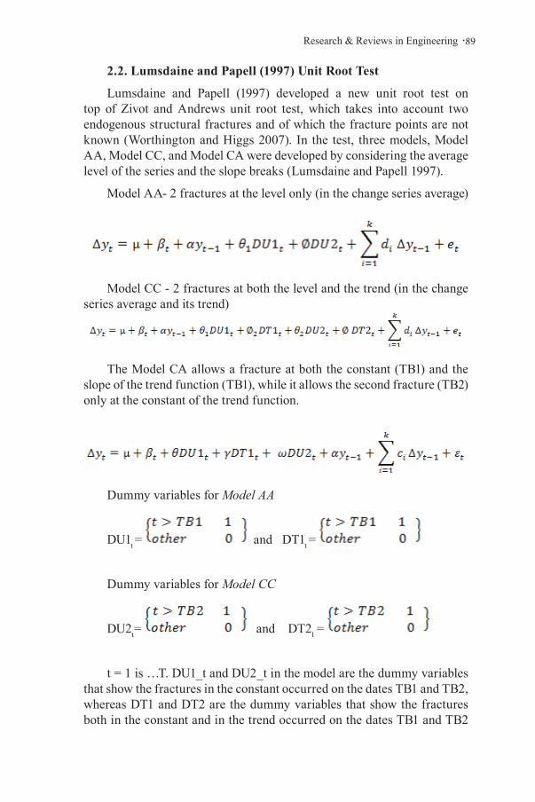
.89Research & Reviews in Engineering
2.2. Lumsdaine and Papell (1997) Unit Root Test
Lumsdaine and Papell (1997) developed a new unit root test on top of Zivot and Andrews unit root test, which takes into account two endogenous structural fractures and of which the fracture points are not known (Worthington and Higgs 2007). In the test, three models, Model AA, Model CC, and Model CA were developed by considering the average level of the series and the slope breaks (Lumsdaine and Papell 1997).
Model AA- 2 fractures at the level only (in the change series average)
Model CC - 2 fractures at both the level and the trend (in the change series average and its trend)
The Model CA allows a fracture at both the constant (TB1) and the slope of the trend function (TB1), while it allows the second fracture (TB2) only at the constant of the trend function.
Dummy variables for Model AA
DU1t = and DT1t =
Dummy variables for Model CC
DU2t= and DT21 =
t = 1 is …T. DU1_t and DU2_t in the model are the dummy variables that show the fractures in the constant occurred on the dates TB1 and TB2, whereas DT1 and DT2 are the dummy variables that show the fractures both in the constant and in the trend occurred on the dates TB1 and TB2

Burcu ERDAL, Hasan VURAL90 .
(Tuna and Öztürk 2016).
TB1 refers to the first fracture and TB2 refers to the second fracture. To determine α, which is all possible pairs of fractions, t-statistics are used. In the yt series, the null hypothesis, which assumes that there is no exogenous structural fracture and is not stationary, is tested against the alternative hypothesis that defends that the yt series is stationary and also defends the existence of structural fractures at two different unknown dates (Pahlavani and Harvie 2008).
In the determination of fracture dates TB1 and TB2, the date pairs that make the statistic t of the α value to a minimum are selected. If the t-critical value is less than the t-statistical value then H0 is rejected and the series is said to be stationary (Narayan and Popp 2010).
In the Lumsdaine-Papell (1997) unit root test, H0 hypothesis states that there is no structural fracture in the series, in other words, there is a unit root in the series, whereas the alternative hypothesis H1 indicates that the series is stable.
H0: There is a unit root in the series, the series is not stationary.
H1: There is no unit root in the series, the series is stationary.
2.3 Cointegration Analysis
In econometric analyses, the existence of a long-term relationship between variables is called cointegration (An and Brown 2010). In case the series considered are not stationary at the level and become stationary when the first differences are considered, it is necessary to perform cointegration tests to investigate whether the linear compositions of these series are in balance (Tarı 2015). Given the fact that the linear compositions of these series can be stationary even if the handled series are not stationary at the level, it is of great importance to establish the long-term relationship between the series (Dritsakis 2012).
Co-integration between the variables is possible if a variable in the model has a stochastic trend that affects all variables but not external, permanent shocks. (Dikmen, 2012).
Johansen and Julselius (1990) have developed a cointegration test that takes into account the structural changes that occur in the series over time. In the test process, models with assumptions about structural fractures are defined. The test process for the two-variable model used in the study is as follows (Camerero et al. 2010):

.91Research & Reviews in Engineering
In this study, the fracture was tested at the slope and at the level and Model 3 (CT) was used. In the model, β is the cointegration matrix and α is the weight of the cointegration vector parameters.
In the Johansen cointegration analysis;
H0: r = 0 no cointegration relationship
H1: r ≥ 1 there is at least 1 cointegration relationship
The number of cointegration relationships (long-term equilibrium relationships) shown here with r can be at most up to one minus (n-1) of the number of variables (Crowder and Hamed, 1993). Rejection or acceptance of hypotheses is determined by eigenvalues and trace statistics (Pascual 2003, Benli 2014).
3. Research Findings and Discussion
In this part of the study, the long term between the time series of the stock markets In order to determine the relationship, it is aimed to determine whether there is a structural break in the series.Lumsdaine and Papell (1997) revealed the long-term relationship with the Unit Root Test.The results of the Johansen et al. (2000) Cointegration Test, which was carried out to put given. Exchange prices of wheat types used in tests on exchange basis presented in tables before the test results.
Lumsdaine-Papell Unit Root Test results showed that the series had a unit root at a 5% significance level in all-time series. In order to determine the cointegration between price series in the long run, the first difference of the series was taken and they were made stable.
The appropriate lag length of VAR model which was established for the Johansen cointegration test was determined according to the test results. AICC, SBC/BIC, and HQ test results were used to determine the lag length of the VAR model for each stock market. The test results were significant at a 5% significance level. The most appropriate lag length for the VAR model for Konya Commodity Exchange and Eskişehir Commodity
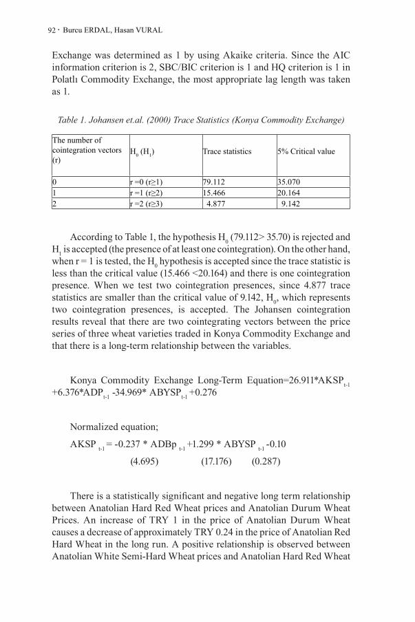
Burcu ERDAL, Hasan VURAL92 .
Exchange was determined as 1 by using Akaike criteria. Since the AIC information criterion is 2, SBC/BIC criterion is 1 and HQ criterion is 1 in Polatlı Commodity Exchange, the most appropriate lag length was taken as 1.
Table 1. Johansen et.al. (2000) Trace Statistics (Konya Commodity Exchange)
The number of cointegration vectors (r)
H0 (H1) Trace statistics 5% Critical value
0 r =0 (r≥1) 79.112 35.0701 r =1 (r≥2) 15.466 20.1642 r =2 (r≥3) 4.877 9.142
According to Table 1, the hypothesis H0 (79.112> 35.70) is rejected and H1 is accepted (the presence of at least one cointegration). On the other hand, when r = 1 is tested, the H0 hypothesis is accepted since the trace statistic is less than the critical value (15.466 <20.164) and there is one cointegration presence. When we test two cointegration presences, since 4.877 trace statistics are smaller than the critical value of 9.142, H0, which represents two cointegration presences, is accepted. The Johansen cointegration results reveal that there are two cointegrating vectors between the price series of three wheat varieties traded in Konya Commodity Exchange and that there is a long-term relationship between the variables.
Konya Commodity Exchange Long-Term Equation=26.911*AKSPt-1 +6.376*ADPt-1 -34.969* ABYSPt-1 +0.276
Normalized equation;
AKSP t-1 = -0.237 * ADBp t-1 +1.299 * ABYSP t-1 -0.10
(4.695) (17.176) (0.287)
There is a statistically significant and negative long term relationship between Anatolian Hard Red Wheat prices and Anatolian Durum Wheat Prices. An increase of TRY 1 in the price of Anatolian Durum Wheat causes a decrease of approximately TRY 0.24 in the price of Anatolian Red Hard Wheat in the long run. A positive relationship is observed between Anatolian White Semi-Hard Wheat prices and Anatolian Hard Red Wheat

.93Research & Reviews in Engineering
prices. An increase of TRY 1 in the price of Anatolian White Semi-Hard Wheat causes an increase of approximately TRY 1.3 in Anatolian Red Hard Wheat price. In this context, there is a high sensitivity between the prices of these two products. An increase of TRY 1 in one of them increases the price of the other by one and a half times in the long run.
Table 2. Johansen et al (2000) Trace Statistics (Eskisehir Commodity Exchange)
The number of cointegration vectors (r)
H0 (H1) Trace statistics 5% Critical value
0 r =0 (r≥1) 19.915 20.1641 r =1 (r≥2) 5.872 9.142
The analysis of the Johansen cointegration results above reveals that the trace statistics are less than the critical value. In this case, since 5.872<9.142, the hypothesis H0, which supports the existence of 1 cointegration vector, is accepted. Therefore, since there is 1 co-integrating vector between the Anatolian Hard Red Wheat and Anatolian White Semi-Hard Wheat price series traded on the Eskişehir Commodity Exchange, it is possible to indicate that there is a long-term relationship between the variables.
Eskişehir Commodity Exchange Long-Term Equation = 20.492 xAKSPt-1 -19.439 ABYSPt-1 -1.670
Normalized Equation;
AKSPt-1 = 0.949ABYSPt-1 +0.081
(6.698) (0.724)
There is a positive relationship between Anatolian Hard Red Wheat prices and Anatolian White Semi-Hard Wheat prices and a significant relationship was found between them according to the t statistic values. An increase of TRY 1 in Anatolian White Semi-Hard Wheat price will increase the price of Anatolian Hard Red wheat by TRY 0.95.

Burcu ERDAL, Hasan VURAL94 .
Table 3. Johansen et.al. (2000) Trace Statistics (Polatlı Commodity Exchnage)
The number of cointegration vectors (r)
H0 (H1) Trace statistics 5% Critical value
0 r =0 (r≥1) 46.486 20.1641 r =1 (r≥2) 6.036 9.142
According to the results of the cointegration test, since 46.486>20.164, H0 is rejected and H1 alternative hypothesis, which asserts that there is at least one cointegration, is accepted. However, since 6.036<9.142, the H0 hypothesis is accepted and cointegration between variables and the existence of a long-term relationship are indicated.
Polatlı Commodity Exchange Long-Term Equation=17.204 * AKSPt-1 -17.346 * ABYSPt-1 -1.465
Normalized Equation;
AKSPt-1 = 1.008 * ABYSPt-1 +0.085
(11.917) (1.212)
There is a positive relationship between the prices of Anatolian Hard Red Wheat prices and Anatolian White Semi-Hard Wheat prices. The t statistic values indicate the existence of a significant relationship. An increase of TRY 1 in Anatolian White Semi-Hard Wheat price will increase the price of Anatolian Hard Red Wheat by TRY 1.01.
4. Conclusion
Agricultural activities are affected by risks and uncertainties more than other sector activities due to their unique characteristics and dependence on natural conditions. There is often a supply and demand mismatch in the agricultural sector.
For these reasons, the agricultural sector is the most supported sector. Most of the supports One of its most important goals is to ensure stability in the market and consistency in prices. is coming. However, such support is often not enough. Providing the opportunity to sell agricultural products in a free competitive market environment, and Commodity exchanges operating in order to ensure stability in the market are importance for agricultural sector. The importance of commodity exchanges in the marketing of agricultural products is quite large. ommodity exchanges, which have the characteristics of an organized market, are where supply and demand are intense determination of the real value of the products in agricultural product markets and enables it to be bought and sold. Realize the farmer’s product through commodity exchanges. It helps to reduce the state’s support and financial burden, as it has the opportunity to sell at a
.95Research & Reviews in Engineering
higher value.it helps. For this reason, full and effective use of commodity exchanges in our country It is also of great importance in terms of our agricultural policies.
In this study, Lumsdaine and Papell (1997) Unit Root Test and Johansen et.al. (2000) Cointegration Test were used to determine whether there is a long-term relationship between wheat stock prices.
An increase of TRY 1 in the price of Anatolian Durum Wheat, which is traded in Konya Commodity Exchange, causes a decrease of approximately TRY 0.24 in the price of Anatolian Hard Red Wheat in the long run. A positive relationship is observed between the prices of Anatolian White Semi-Hard Wheat and the prices of Anatolian Hard Red Wheat. An increase of TRY 1 in the price of Anatolian White Semi-Hard Wheat causes an increase of approximately TRY 1.3 in the price of Anatolian Hard Red Wheat. In this context, there is a high sensitivity between the prices of these two products. An increase of TRY 1 in one of the products causes a one and a half-fold increase in the price of the other in the long run.
There is a co-integrating vector between the Anatolian Hard Red and Anatolian White Semi-Hard Wheat price series traded on the Eskişehir Commodity Exchange. There is a positive relationship between Anatolian Hard Red Wheat prices and Anatolian White Semi-Hard Wheat Prices and a significant relationship is found according to the t statistic values. An increase of TRY 1 in Anatolian White Semi-Hard Wheat price will increase the price of Anatolian Hard Red wheat by TRY 0.95.
The presence of a co-integrating vector was determined between the price series of Anatolian Hard Red Wheat and Anatolian White Semi-Hard Wheat traded on the Polatlı Commodity Exchange. There is a positive relationship between Anatolian Hard Red Wheat prices and Anatolian White Semi-Hard Wheat Prices. The t statistics value indicate the existence of a significant relationship. An increase of TRY 1 in Anatolian White Semi-Hard Wheat price will increase the price of Anatolian Hard Red Wheat by TRY 1.01.
At least one co-integrating vector is present in the stock price series. Thus, a long-term relationship is observed between wheat varieties price series on a stock exchange basis. This case reveals that there is a strong price interaction in the commodity exchanges examined. Price formations of different wheat varieties traded on the same stock exchange are occurred by affecting each other. This is important for predicting wheat prices in advance.
Bu çalışma doktora tezinden üretilmiştir.

Burcu ERDAL, Hasan VURAL96 .
REFERENCES
Albayrak, M., Taşdan, K., Güneş, E., Saner, G., Atiş, E., Çukur, F., Pezi-koğlu, F., 2010. Küresel Rekabet Açısından Türkiye’de Tarım Ve Gıda Ürünlerinin Pazarlama Sistemlerine Bakış: Mevcut Yapı, Sorunlar Fırsat-lar, Hedefler. Türkiye Ziraat Mühendisliği VII. Teknik Kongresi, 11-15 Ocak 2010, Ankara.
An,L.,Brown,D. 2010. Equity Market Integration between the US and BRIC Countries: Evidence from Unit Root and Cointegration Test. Research Journal of Internatıonal Studies,16: 15-24.
Anonim, 2017.TUİK. Tarım İstatistikleri. http://www.tüik.gov.tr-(Erişim Tarihi: 10.06.2019).
Benli, Y.K. 2014. Türkiye Borsasının Gelişmekte Olan Ülkeler Borsaları İle Eş-bütünleşme Analizi. Yönetim ve Ekonomi Araştırmaları Dergisi,23:18-32.
Camarero, M., Cuestas, J.C., Ordonez, J. 2010. Purchasing Power Parity ver-sus the EU in the Mediterranean countries, Purchasing Power Parity and Real Exchange Rates, ISBN13:978-0-415-55865-5.
Dikmen,N.,2012. Ekonometri, Temel Kavramlar ve Uygulamalar.Dora Yayıncı-lık,Bursa, 381s.
Doğan, B.B. 2010. Ticaret Borsaciliğinin Dünyada Ve Türkiye’deki Gelişim Sü-reçlerine Genel Bir Bakış. Atatürk Üniversitesi İktisadi ve İdari Bilimler Dergisi, 24 (1):43-61.
Dritsakis, N. 2012. Structural Breaks, Cointegration and the Demand for Money in Greece. The IUP Journal of Applied Economics, Vol. XI, No.3.
Johansen, S., Julselius, K. 1990. Maximum Likelihood Estimation and Inferen-ce Cointegration – With Applications to the Demand for Money, Oxford Bulleting of Economics and Statistics (52), 169-210.
Lumsdaine, R.L., Papell, D.H.1997. Multiple Trend Breaks and the Unit-Root Hypothesis. Review of Economics and Statistics, (79): 212-218.
Madalla,G.S. 1992.Introduction to Econometrics. Macmillan Publishing Com-pany, New York, 631s.
Narayan, P.K., Popp,S. 2010. A New Unit Root Test With Two Structural Bre-aks İn Level And Slope At Unknown Time. Journal of Applied Statisti-cs,37(9): 1425–1438.
Pahlavani,M.,Harvie,C.,2008. Multiple Structural Breaks in Korea’s Macro-economic Data:An Application Of The Lumsdaine And Papell Test. The Journal Of The Korean Economy, 9(3): 425-441.
Pascual, A. G. 2003. Assessing European Stock Market Co(integration). Econo-mic Letters, 78:(197-203).

.97Research & Reviews in Engineering
Sephton, P.1993. Hedging wheat and canola at the Winnipeg Commodity Exc-hange. Applied Financial Economics. (3)67-72
Tarı,R. 2015. Ekonometri. Umuttepe Yayınları, Kocaeli, 534s.
Tuna,G., Öztürk,M. 2016. Piyasa Etkinliğinin Yapısal Kırılmalı Birim KökTest-leri İle İncelenmesi: Türkiye Pay Senedi Piyasası Uygulaması. Uluslara-rası Yönetim İktisat ve İşletme Dergisi, ICAFR 16 Özel Sayısı.
Crowder, W.J., Hamed,A. 1993.A Cointegration Test for Oil Futures Mar-ket Efficiency, The Journal of Futures Markets (1986-1998); New York Vol. 13, Iss. 8,
Worthington, A. C., Higgs, H. 2007. Assessing Financial Integration in Europe-an Union Equity Markets, 1990-2006: Panel Unit Root and Multivariate Cointegration and Causality Evidence. University of Wollongong, School of Accounting and Finance Working Paper Series. 7(10):1-20

Burcu ERDAL, Hasan VURAL98 .

Chapter 63D PRINTED HORN ANTENNA WITH PCB MICROSTRIP FEED FOR X-KA BAND APPLICATION
AYSU BELEN1
1 Lecturer, İskenderun Technical University, Iskenderun Vocational School of Higher Ed-ucation, [email protected], ORCID ID: 0000-0001-5038-424X

Aysu Belen100 .
I. Introduction
Horn antenna designs are one of the commonly used antenna models that being used by researchers for applications that requires wide operation band and high gain characteristics [1-3]. Although these designs are preferred for many applications, due to their disadvantage of being large in size their applications become limited in certain areas, or requires methods for size reduction or minimization techniques. Although there are many different techniques for size reduction of horn antennas such as dielectric loading of horn aperture usage of meta-materials etc. [4-7], each of the mentioned methods has their own disadvantages such as increasing the overall weight of the antenna which become another limiting aspect for certain applications such as avionic systems, or increased manufacturing cost and complexity of the design. A viable solution for size reduction and low cost manufacturing of horn antennas is to feed the antenna aperture structure using a Microstrip antenna design instead of traditional and long length waveguide structure. Microstrip antenna designs are preferred by many researchers due to their unique advantages of being small in size, compact, low cost, and easy to manipulate the polarization and operation frequency [8-12].
Another method for design and realization of low cost antenna models is the 3D printing technology. Thanks to the recent advances in field of 3D printing technology, these devices are now affordable compared to their early times and can be used in many different applications such as education, medicine, art, jewellery and engineering [13-17]. The applications of 3D printing technology in field of microwave engineering had gain the interest of many researches due to the abilities of being fast and low cost prototyping of antenna designs that usually are high cost and requires high end manufacturing stations such as CNC which sometimes might become even infeasible for certain type of designs [18]. Some examples for the applications of 3D printing technology in field of microwave engineering can be named as fabrication of transmission lines [19], filters [20], absorbers [21], microwave antenna designs [22-30], and other types of RF components [31-34].
In this work design a realization of a low cost and small size horn antenna with high performance measures is taken under the study. For size reduction of antenna stage instead of traditional waveguide port feed a Microstrip patch antenna has been used. The horn antenna is prototyped via the use of 3D printing technology and being coated with metal. In the next section the design procedure of the proposed Horn Antenna with PCB Microstrip Feed alongside of its simulated results are presented. In Section III, the experimental results of the 3D printed antenna had been presented. And finally work ends with a brief conclusion in section IV.

.101Research & Reviews in Engineering
II. Design of Horn Antenna with PCB Microstrip Feed
In this section, the design procedure of the proposed Horn Antenna with Microstrip Feed (HAMF) is presented. In Fig. 1 the schematic of the proposed antenna design is presented. The patch antenna given in Fig. 1 will be used as feed for the horn antenna. The patch antenna design is consist of a dipole radiator in top layer and a defected ground structure in for better adjustment of resonance frequency. The horn antenna is taken as a traditional pyramid horn design for study. The selected material for patch antenna design is modelled on a FR4 substrate with height of 1.56 [mm] and relative dielectric permittivity of 4.6.
The aim of the work is to present a horn antenna with Microstrip feed for X band applications, for this mean the design parameters of the antenna are determined by using EM-simulation driven optimization process. The cost function given in Eqs. 1-3 have been used for optimization process.
* =arg min ( )Hx
x x (1)
where the objective function is defined as
{ }1 2 1 11 2( ) max [ , ] : | ( , ) | | ( , ) |c cH f f f C S f C D f= ∈ +x x x (2)
The cost function defined in Eqs. (1), (2) is a minimax task oriented towards minimizing the antenna designs reflection characteristics (S11) and directivity (D) for the given operating frequencies of fc1 to fc2. C1 and C2 are constant weighting coefficients for the design optimization where for this work is taken as unity. The optimally design parameters of the design is obtained after 100 function evaluation using Trust Region optimization algorithm are presented in Table I.
SMA Port
L1
L2
W1
W3
W4 W
5
L3
Substratecopper
H
gap
Microstrip Feed
W7
W6
L5L4
Figure 1. Schematic view of the Horn Antenna and Microstrip patch feed.
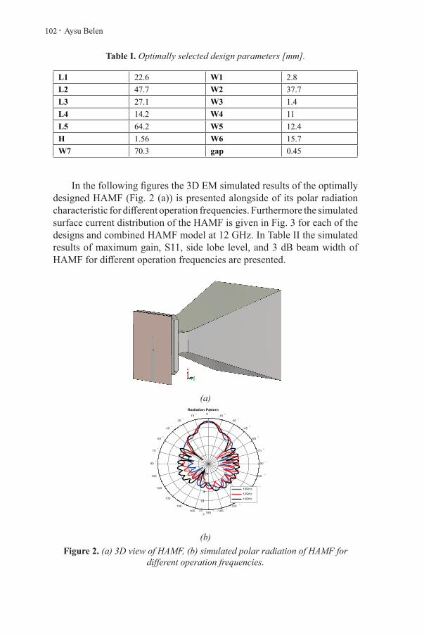
Aysu Belen102 .
Table I. Optimally selected design parameters [mm].
L1 22.6 W1 2.8L2 47.7 W2 37.7L3 27.1 W3 1.4L4 14.2 W4 11L5 64.2 W5 12.4H 1.56 W6 15.7W7 70.3 gap 0.45
In the following figures the 3D EM simulated results of the optimally designed HAMF (Fig. 2 (a)) is presented alongside of its polar radiation characteristic for different operation frequencies. Furthermore the simulated surface current distribution of the HAMF is given in Fig. 3 for each of the designs and combined HAMF model at 12 GHz. In Table II the simulated results of maximum gain, S11, side lobe level, and 3 dB beam width of HAMF for different operation frequencies are presented.
(a)Radiation Pattern
0 °15 °
30 °
45 °
60 °
75 °
90 °
105 °
120 °
135 °
150 °
165 °180 ° -165 °
-150 °
-135 °
-120 °
-105 °
-90 °
-75 °
-60 °
-45 °
-30 °-15 °
-20
-10
0
10
20
10GHz
12GHz
14GHz
(b)Figure 2. (a) 3D view of HAMF, (b) simulated polar radiation of HAMF for
different operation frequencies.
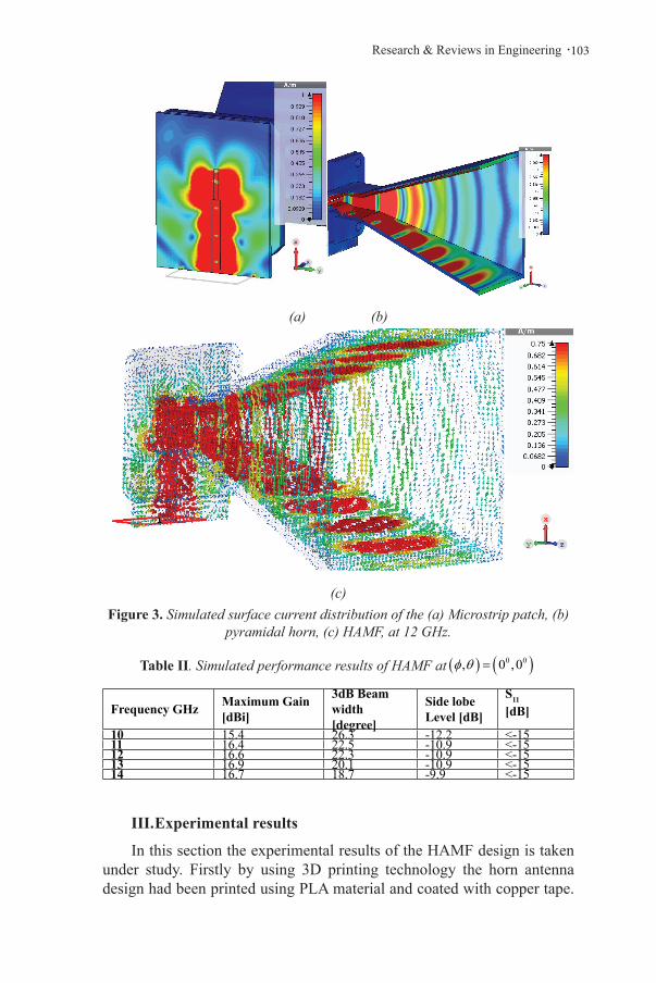
.103Research & Reviews in Engineering
(a) (b)
(c)Figure 3. Simulated surface current distribution of the (a) Microstrip patch, (b)
pyramidal horn, (c) HAMF, at 12 GHz.
Table II. Simulated performance results of HAMF at ( ) ( )0 0, 0 ,0φ θ =
Frequency GHz Maximum Gain [dBi]
3dB Beam width [degree]
Side lobe Level [dB]
S11
[dB]
10 15.4 26.3 -12.2 <-1511 16.4 22.5 -10.9 <-1512 16.6 22.3 -10.9 <-1513 16.9 20.1 -10.9 <-1514 16.7 18.7 -9.9 <-15
III. Experimental results
In this section the experimental results of the HAMF design is taken under study. Firstly by using 3D printing technology the horn antenna design had been printed using PLA material and coated with copper tape.

Aysu Belen104 .
The Microstrip feed antenna and measurement setup of HAMF design are presented in Fig. 4. The HAMF design is achieved by placing the feed Microstrip patch antenna into the 3D printed horn antenna port. The measurements of the 3D printed SMPA are carried out utilizing R&S®ZVL vector network analyzer a Network Analyzer with a measurement range of 9 kHz-13.5 GHz, alongside two identical antennas, A-info, LB8180, 0.8-18 GHz Broadband Horn Antenna [35-36].
(a) (b)
(c) (d)
Figure 4. (a) 3D view of HAMF, (b) simulated polar radiation of HAMF for different operation frequencies.
In Fig. 5 the measured and simulated performance of the HAMF design is presented. As it can be seen, the proposed design achieves an ultra-wide band operation frequency (10-14 GHz, bandwidth > %30) and peak realized gain value of 16.3 dBi. As it can be seen both simulated and measured characteristics are in agreement. A furthered performance comparison of simulated and measured characteristics are presented in Table III.

.105Research & Reviews in Engineering
8 9 10 11 12 13 14 15 16
Frequency GHz
-30
-25
-20
-15
-10
-5
0
S11
dB
Measurement
Simulation
(a)
9 10 11 12 13 14 15 16
frequency
9
10
11
12
13
14
15
16
17
Max
Gai
n dB
Measurement
Simulation
(b)
-100 -80 -60 -40 -20 0 20 40 60 80 100
Theta
-15
-10
-5
0
5
10
15
Gai
n dB
Simulation
Measurement
-100 -80 -60 -40 -20 0 20 40 60 80 100
Theta
-15
-10
-5
0
5
10
15
Gai
n dB
Frequency = 12 GHz
Simualtion
Measurement
(c) (d)

Aysu Belen106 .
-100 -80 -60 -40 -20 0 20 40 60 80 100
Theta
-10
-5
0
5
10
15
Gai
n dB
Frequency = 14 GHz
Simulation
Measurement
(e)Figure 5. Simulated ad Measured (a) scattering parameter, (b) maximum gain
over frequency, radiation pattern at (c) 10 GHz, (d) 12 GHz, (e) 14 GHz.
Table III. Measured performance characteristics of antenna (dB)
f [GHz] Simulated MeasuredGain [dBi] S11 [dB]
10 15.4 14.1 <-1511 16.4 14.9 <-2012 16.6 15.2 <-2013 16.9 15.1 <1014 16.7 15.3 <-10
IV. Conclusion
Due to their wide operation band and high gain characteristics, Horn antenna designs are being favoured by many designers. In this work, in order to reduce the size of these favoured antenna designs, which is one of the most commonly faced disadvantage of these antennas, a viable solution for both size reduction and low cost manufacturing of horn antennas is studied. This problem can be achieved by instead of traditional and long length waveguide structures, by placing a microstrip antenna design as feed of the horn structure. Another aspect for low cost manufacturing technique considered in this work is the usage of 3D printing technology. The simulated and measured performance of the HAMF is compared and found to be in agreement. As it can be seen form the results, HAMF design achieves an ultra-wide band operation of 10-14 GHz (bandwidth > %30) and maximum measured gain value of 16.3 dBi.
.107Research & Reviews in Engineering
V. References
[1] S.V. Yadav, A. Chittora, (2021). A compact ultra-wideband transverse electromagnetic mode horn antenna for high power microwave applicati-ons. Microw Opt Technol Lett. 2021; 63: 264– 270.
[2] N. Abu Talip Yusof, S.M. Shaharum, A.A. Mohd Faudzi, S. Khatun, M.S. Abdul Karim, S.F. Hazali (2019) Design of Ultra-Wideband (UWB) Horn Antenna for Non-destructive Fruit Quality Monitoring. In: Md Zain Z. et al. (eds) Proceedings of the 10th National Technical Seminar on Un-derwater System Technology 2018. Lecture Notes in Electrical Engine-ering, vol 538. Springer, Singapore. https://doi.org/10.1007/978-981-13-3708-6_45
[3] M.A. Belen, P. Mahouti, P. (2019). Realization of Dielectric Sheets for Gain Improvement of Ultra-Wideband Horn Antennas Using 3D Printer Technology. Applied Computational Electromagnetics Society Journal, 34(5).
[4] J. Y. Deng, L. Rui-Qing, L. Wei, Z. Yin, S. Dongquan, Z. Xiao-Miao, and G. Li-Xin (2020). Horn Antenna with Miniaturized Size and Increased Gain by Loading Slow Wave Periodic Metal Blocks. IEEE Transactions on Antennas and Propagation 69, no. 4: 2365-2369.
[5] Y. Zhang, J.Y. Deng, D. Sun, J.Y. Yin, L. Guo, (2021). Compact Slow-Wave SIW H-Plane Horn Antenna with Increased Gain for Vehi-cular Millimeter Wave Communication. IEEE Transactions on Vehicular Technology.
[6] Z. Yue, Y. Liu, & P. Zhu, (2019, October). Design of a Miniaturized Double Ridged Horn Antenna. In 2019 International Symposium on An-tennas and Propagation (ISAP) (pp. 1-2). IEEE.
[7] X. Chen, Y. Jiaao and P. Shirui (2018). Miniaturized Circularly Polari-zed Horn Antenna with a Single-Arm Spiral Structure for X-band, Proce-edings of the 2018 International Conference on Information Science and System, pp. 215-217.
[8] A. H. Wahyudi, C. E. Santosa, and J.T.S. Sumantyo, (2018). Develop-ment of Broadband LHCP Pyramidal Horn Antenna with Septum Gaus-sian Profile Polarizer for CP-SAR Sensor Onboard Microsatellite. Open Journal of Antennas and Propagation 6, no. 04: 73.
[9] M. Tekbaş, A. Toktaş, and G. Çakır (2020). Design of a dual polarized mmwave horn antenna using decoupled microstrip line feeder. 2020 Inter-national Conference on Electrical Engineering (ICEE), pp. 1-4. IEEE.
[10] K.P Esselle, A.K. Verma, (2008). Wideband high-gain circularly polarized stacked microstrip antennas with an optimized C-type feed and a short horn. IEEE transactions on antennas and propagation, 56(2), 578-581.

Aysu Belen108 .
[11] A. Nuaimi, M.K. Taher, and W. Hong, (2014). Discrete dielectric reflectar-ray and lens for E-band with different feed, IEEE Antennas and Wireless Propagation Letters 13, pp.947-950.
[12] V. Midtben, G. K. Kristian, and T.S. Lande, (2017). 3D printed horn an-tenna with PCB microstrip feed for UWB radar applications. IEEE MTT-S International Microwave Workshop Series on Advanced Materials and Processes for RF and THz Applications (IMWS-AMP), pp. 1-3. IEEE, 2017.
[13] J. Gopinathan, I. Noh (2018). Recent trends in bioinks for 3D printing. Biomaterials research, 22(1), 1-15.
[14] A. Dawood, B. M. Marti, V. Sauret-Jackson, and A. Darwood, (2019), 3D printing in dentistry. British dental journal 219, no. 11, pp. 521-529.
[15] N. Shahrubudin, T.C. Lee, R. Ramlan, (2019). An overview on 3D prin-ting technology: Technological, materials, and applications. Procedia Ma-nufacturing, 35, 1286-1296.
[16] L. Zhenbin, M. Zhang, B. Bhandari, and Y. Wang, (2017). 3D printing: Printing precision and application in food sector. Trends in Food Science & Technology 69, pp. 83-94.
[17] Y. Qian, H. Dong, J. Su, J. Han, B. Song, Q. Wei, and Y. Shi, (2018).A review of 3D printing technology for medical applications.” Engineering 4, no. 5, pp. 729-742.
[18] A. Belen, F. Güneş, M.A. Belen, P. Mahouti, (2020). 3D printed wideband flat gain multilayer nonuniform reflectarray antenna for X-band applicati-ons. Int J Numer Model El. 33:e2753. https://doi.org/10.1002/jnm.2753
[19] P. I. Deffenbaugh, T.M. Weller, and K.H. Church (2015). Fabrication and microwave characterization of 3-D printed transmission lines.” IEEE Mic-rowave and wireless components letters 25, no. 12, pp. 823-825.
[20] C. Tomassoni, O.A. Peverini, G. Venanzoni, G. Addamo, F. Paonessa, and G. Virone, (2020). 3D printing of microwave and millimeter-wave fil-ters: Additive manufacturing technologies applied in the development of high-performance filters with novel topologies.” IEEE Microwave Maga-zine 21, no. 6, pp. 24-45.
[21] R. Kronberger, and S. Patrick, (2016). New 3D printed microwave meta-material absorbers with conductive printing materials. 2016 46th Europe-an Microwave Conference (EuMC), pp. 596-599. IEEE, 2016.
[22] M. A. Belen, and P. Mahouti, (2018) Design and realization of quasi Yagi antenna for indoor application with 3D printing technology. Microwave and Optical Technology Letters, 60(9), pp.2177-2181.
[23] A. G. Lopez, R. Chandra, A. J. Johansson, (2013). Optimization and fab-rication by 3D printing of a volcano smoke antenna for UWB applications.

.109Research & Reviews in Engineering
In 2013 7th European Conference on Antennas and Propagation (EuCAP) (pp. 1471-1473). IEEE.
[24] P. Mahouti, M.A. Belen, F. Güneş, R. Yurt, (2019) Design and realization of multilayered cylindrical dielectric lens antenna using 3D printing tech-nology. Microwave and Optical Technology Letters, 61(5), pp.1400-1403.
[25] M. A. Belen, P. Mahouti, (2020). Design of nonuniform substrate dielec-tric lens antennas using 3D printing technology. Microwave and Optical Technology Letters 62, no. 2, 756-762.
[26] M.M. Honari, M. Rashid , S. Hossein, and M. Pedram (2018). Investiga-tion of the 3D printing roughness effect on the performance of a dielectric rod antenna. IEEE Antennas and Wireless Propagation Letters 17, no. 11, 2075-2079.
[27] A. Belen, F. Güneş, M. A. Belen, and P. Mahouti, (2020). 3D printed wideband flat gain multilayer nonuniform reflectarray antenna for X‐band applications.” International Journal of Numerical Modelling: Electronic Networks, Devices and Fields 33, no. 6,e2753.
[28] A. Castro, T. B. Babakhani, and S. K. Sharma, (2017). Design and de-velopment of a multimode waveguide corrugated horn antenna using 3D printing technology and its comparison with aluminium-based prototype. IET Microwaves, Antennas & Propagation 11, no. 14, 1977-1984.
[29] A. Belen, P. Mahouti, F. Güneş, and Ö. Tari, (2021). Gain Enhancement of a Traditional Horn Antenna using 3D Printed Square-Shaped Multi-layer Dielectric Lens for X-band Applications. Applied Computational Electro-magnetics Society Journal 36, no. 2.
[30] C. Shemelya, M. Zemba, M. Liang, X. Yu, D. Espalin, R. Wicker, E. Mac-Donald, (2016). Multi‐layer archimedean spiral antenna fabricated using polymer extrusion 3D printing. Microwave and Optical Technology Let-ters, 58(7), 1662-1666.
[31] J.A. Byford, M.I.M Ghazali, S. Karuppuswami, B.L. Wright, and P. Cha-hal (2017). Demonstration of RF and microwave passive circuits through 3-D printing and selective metalization. IEEE Transactions on Compo-nents, Packaging and Manufacturing Technology, 7(3), 463-471.
[32] W.J. Otter, S. Lucyszyn, (2016, July). 3-D printing of microwave com-ponents for 21st century applications. 2016 IEEE MTT-S International Microwave Workshop Series on Advanced Materials and Processes for RF and THz Applications (IMWS-AMP) (pp. 1-3). IEEE.
[33] A.F. Gomez-Torrent, A. Teberio, J.M. Martinez, I. Percaz, I. Arnedo, I. Maestrojuan, I. Arregui, (2017). A study of the additive manufacturing technology for RF/microwave components. 2017 11th European Confer-ence on Antennas and Propagation (EUCAP), pp. 567-571. IEEE, 2017.
[34] A. Perigaud, S. Bila, O. Tantot, N. Delhote, S. Verdeyme, (2016) 3D print-ing of microwave passive components by different additive manufactur-

Aysu Belen110 .
ing technologies.IEEE MTT-S International Microwave Workshop Series on Advanced Materials and Processes for RF and THz Applications (IM-WS-AMP) (pp. 1-4). IEEE.
[35] https: / /www.rohde-schwarz.com/sg/product/zvl-productstart-page_63493-9014.html
[36] A-info, LB8180, 0.8-18 GHz Broadband Horn Antenna. Available at: http://www.ainfoinc.com/en/ p_ant_h_brd.asp, Accessed on August 15, 2017

Chapter 7CS DOPANT ROLE ON ELECTRICAL, MICROSTRUCTURAL AND CRYSTALLINITY OF Y-123 SUPERCONDUCTING MATERIALS
Mustafa Burak TURKOZ1 Asaf Tolga ULGEN 2
1 Assoc.Prof., Karabuk University, Department of Electric and Electronic Engineering, Karabuk-Turkey, 78000 Orcid ID 0000-0002-4127-76502 Assoc.Prof, Sirnak University, Department of Electric-Electronic Engineering, Sirnak–Turkey, 73000 Orcid ID 0000-0002-7112-5607

Mustafa Burak Turkoz, Asaf Tolga Ulgen112 .
1. Introduction
Material appears in every field such as construction industry, medicine, industry, automotive, technology, various fields of research, infrastructure and engineering in the world that surrounds us in our daily life [1–4]. Especially the energy materials can take more places in the heavy-industrial technology, advanced medicine and engineering sectors, innovative energy infrastructure, and large-scale applications as regards the magnetic energy storage, power transmission, refrigeration, materials engineering, sensitive process control, spintronics, advanced automotive sectors, power transmission, future fault current limiter technology, magnetic resonance imaging, medical diagnosis, metallurgical, electric power cable, electro-optic, future hydrogen society, motors, particle accelerators, levitated trains, power transmission cable, magnetic separation, global electric power network, nuclear magnetic resonance and renewable energy sectors [5–10]. This is because, with the rapid improvement in the technology, willingness of people to keep up with technology and considerable increment in the growth of population day by day in the worldwide energy consumption requirements much more increase and hence much more nature sources are destroyed. On this basis, the excess energy usage (overuse) should be prevented as much as possible in all application areas. For example, energy dissipation forms the basis of energy consumption problems in the industrial power systems. That is exactly why humanity needs to use superconducting materials (without resistance and loss of energy) for leaving a cleaner world to next generation. In other words, the preference of superconducting material provides a strong motivation for the efficient use of energy. Accordingly, the superconductivity suppling reliable, clean, efficient, economic, cheap and power quality to human beings is one of the only solutions for overcoming the energy conservation and related ecological energy problems so that the world for the next generation can be secured. Hence, the use of superconducting materials in the daily life technology and industry has an importance for the energy management planning and operation based on the energy production / protection / consumption / distribution / storage / supply-demand balance. Consequently, the energy management methodology consists of three main objectives: resource conservation, climate protection grounded on environmental awareness and cost savings. In this respect, the energy management discipline is directly related to the fact that the activities in daily life are performed without any compromise but in low energy consuming. This is exactly why the humanbeings totally require the superconducting materials in the application fields.
In more detail, the superconductors can be used in many application fields without any resistance no resistance under the certain current and

.113Research & Reviews in Engineering
applied magnetic fields. In the literature, the superconducting materials are examined in two main groups: these are type-I and type-II [11–13]. The type-I superconducting parents discovered firstly in 1911 by Onnes are extensively known as conventional superconductors and are soft type materials and pioneers of superconductivity [14]. On the other hand, the type-II superconducting parents known as the hard ceramic materials are composed of the oxygen deficit multi-layered perovskite structures. Among the parents, the type-II superconducting materials exhibit the indispensable features large critical temperature/current density carrying ability/ magnetic field carrying capability, thermodynamic stability and electronic characteristics. Similarly, low resistivity, energy consumption and losses are acceptable Intriguing characteristic behavior [15–17]. In the type-II superconducting parents, the YBa2Cu3O7-y ceramic superconductor with superior characteristic features is one of the perfect candidates for the usage in the potential application fields such as especially heavy-industrial technology, advanced medicine and engineering sectors, innovative energy infrastructure, and large-scale applications.
In the present work, the influence of Cs/Ba partial substitution in the Y1Ba2-xCsxCu3O7 crystal structure on the electrical, crystallinity, superconducting and microstructural morphological properties of Y1Ba2Cu3O7 superconducting compound is extensively investigated with the assistant of dc electrical resistivity at the environmental temperature (ρ-T), powder X-ray diffraction (XRD) and scanning electron microscopy (SEM) experimental tests. The experimental findings indicate that the aliovalent Cs/Ba partial substitution seems to be not a wise choice for the permanent and radical solutions for the global energy requirements.
2. Experimental details
In the present work, the partial replacement of aliovalent Ba2+ for Cs1+ ions in the superconducting Y1Ba2-xCsxCu3O7-y ceramic compounds (x=0.05 and x=0.30) is adjusted by the conventional solid-state reaction route using the high-purity precursor chemical nitrate compounds of Y, Cu, Cs and Ba material obtained from Sigma Aldrich and Alfa Aesar exclusive distributor. The chemical nitrate compounds are separately prepared to be approximately 3mg of raw materials in a molar ratio of 1:2-x:x:3. Here the different molecular weight ratios of 0.5 and 3% are weighed by means of the electronic balance in the atmospheric air. The general reactions performed in the stoichiometric proportion to produce a chemically homogeneous mixture throughout the study are provided below:
Y(NO3).6(H2O) + Cu(NO3)2.3(H2O) + (2-x) Ba(NO3)2 + xCsNO3 →
Y1Ba2-xCsxCu3O7 + k(N2O) + b(NO2)+ k(NO)+ 6H2O…

Mustafa Burak Turkoz, Asaf Tolga Ulgen114 .
The chemical of mixture is annealed at the temperature of 550 °C for 2 h release the gasses regarding the nitrogenous or nitrogenous-containing and any impurity residuals to produce the aliovalent Cs/Ba partial substituted Y1Ba2-xCsxCu3O7-y superconducting materials. The homogeneous mixture of chemicals is exposed to the calcination process at the constant temperature of 800 °C for the duration of 24 h in a tube furnace at the heating rate of 5 °C per min. After right, the environmental temperature is reduced towards the room temperature with a cooling rate of 5 ºC per min. The blackish powder of chemicals is subjected to mix in an agate mortar during 2 h with the aid of hand to obtain the homogeneous structure within the desired particle size [18]. The resultant powder is automatically pelletized under 10 tons in the normal atmospheric pressure conditions to make the cylindrical samples with a diameter of 13 mm so that we overcome to reduce the granular structure and inter-grain contact problems in the bulk Y-123 superconducting crystal structure [19]. The solid samples pelletized are sintered at the temperature of 970 ºC (known as the optimum annealing temperature for the Y-123 superconducting phase) for 20 h (received as the optimum annealing-time) in the furnace [20]. The heating and cooling rates are adjusted as in the calcination process. After 20-hour annealing time, the environmental temperature of 970 ºC is decreased down to the temperature of 720 °C with 1 °C/min cooling rate. It is at this temperature that a certain amount of oxygen flow is sent to the system to recover the oxygen lost along with the firing process until 400 °C environmental temperature [21].
Effects of aliovalent Cs/Ba partial replacement on the electrical, crystallinity, superconducting and microstructural morphological properties of polycrystalline Y1Ba2-xCsxCu3O7-y ceramic compounds prepared with different cesium dopant ratio are experimentally investigated by the dc electrical resistivity, powder XRD and scanning electron microscope measurements. On this basis, the variation of dc electrical resistivity tests is examined with the aid of the conventional four-probe method using the cryo-cooler system. Experimental findings are captured in the present of 5 mA in 25-110 K temperature range with the assistant of a programmable nano-voltmeter and current source. The measurement signals are taken within the accuracy of about ±0.1 K. At the same time, the XRD measurement results are obtained from the well-defined diffraction peaks of Y1Ba2-xCsxCu3O7-y materials using an X-Ray diffractometer (SHIMADZU 6000) with CuKa target source providing a monochromatic beam with the wavelength of 1.5418 Å in the range 2θ = 10°–60°. The signals gathered at 3°/min a scan speed and 0.02° step increment at room temperature in air atmosphere are monitored with a well-equipped computer. The surface morphology, grain connectivity and crystallinity quality features of bulk
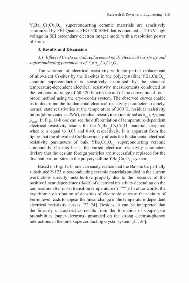
.115Research & Reviews in Engineering
Y1Ba2-xCsxCu3O7-y superconducting ceramic materials are sensitively scrutinized by FEI-Quanta FEG 250 SEM that is operated at 20 kV high voltage in SEI (secondary electron image) mode with a resolution power of 3 nm.
3. Results and Discussion
3.1. Effect of Cs/Ba partial replacement on dc electrical resistivity and superconducting parameters of Y1Ba2-xCsxCu3O7
The variation of electrical resistivity with the partial replacement of aliovalent Cs-sites by the Ba-sites in the polycrystalline YBa2Cu3O7-y ceramic superconductor is sensitively examined by the standard temperature-dependent electrical resistivity measurements conducted at the temperature range of 60-120 K with the aid of the conventional four-probe method using the cryo-cooler system. The observed curves enable us to determine the fundamental electrical resistivity parameters; namely, normal state resistivities at the temperature of 300 K, residual resistivity ratios (abbreviated as RRR), residual resistivities (identified as ρres), ∆ρ, and ρ100K. In Fig. 1a-b one can see the differentiation of temperature-dependent electrical resistivity results for the Y1Ba2-xCsxCu3O7 materials prepared when x is equal to 0.05 and 0.40, respectively. It is apparent from the figure that the aliovalent Cs/Ba seriously affects the fundamental electrical resistivity parameters of bulk YBa2Cu3O7-y superconducting ceramic compounds. On this basis, the varied electrical resistivity parameters declare that the cesium foreign particles are successfully replaced for the divalent barium-sites in the polycrystalline YBa2Cu3O7-y system.
Based on Fig. 1a-b, one can easily realize that the Ba-site Cs partially substituted Y-123 superconducting ceramic materials studied in the current work show directly metallic-like property due to the presence of the positive linear dependence (dρ/dt) of electrical resistivity depending on the temperature after onset transition temperature ( onset
cT ). In other words, the logarithmic distribution of densities of electronic states at the vicinity of Fermi level leads to appear the linear change in the temperature-dependent electrical resistivity curves [22–24]. Besides, it can be interpreted that the linearity characteristics results from the formation of cooper-pair probabilities (super-electrons) grounded on the strong electron-phonon interactions in the bulk superconducting crystal system [25, 26].

Mustafa Burak Turkoz, Asaf Tolga Ulgen116 .
Figure 1 Differentiation of temperature-dependent electrical resistivity results for Y1Ba2-xCsxCu3O7 materials prepared by a) x=0.05 and b) x=0.40.
According to the experimental findings, it is obvious that the increment (from 0.05 to 0.40) in the aliovalent Cs/Ba partial replacement in the polycrystalline Y1Ba2-xCsxCu3O7 superconducting ceramic materials
(a)
(b)
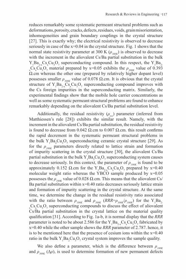
.117Research & Reviews in Engineering
reduces remarkably some systematic permeant structural problems such as deformations, porosity, cracks, defects, residues, voids, grain misorientation, inhomogeneities and grain boundary couplings in the crystal structure [27]. This is exactly why; the electrical resistivity is observed to decrease seriously in case of the x=0.04 in the crystal structure. Fig. 1 shows that the normal state resistivity parameter at 300 K (ρ300K) is observed to decrease with the increment in the aliovalent Cs/Ba partial substitution in the bulk Y1Ba2-xCsxCu3O7 superconducting compound. In this respect, the Y1Ba2-
xCsxCu3O7 material prepared by x=0.05 exhibits the ρ300K value of 0.393 Ω.cm whereas the other one (prepared by relatively higher dopant level) possesses smaller ρ300K value of 0.078 Ω.cm. It is obvious that the crystal structure of Y1Ba2-xCsxCu3O7 superconducting compound improves with the Cs foreign impurities in the superconducting matrix. Similarly, the experimental findings show that the mobile hole carrier concentrations as well as some systematic permeant structural problems are found to enhance remarkably depending on the aliovalent Cs/Ba partial substitution level.
Additionally, the residual resistivity (ρres) parameter (inferred from Matthiessen’s rule [28]) exhibits the similar result. Namely, with the increment in the aliovalent Cs/Ba partial substitution, the residual resistivity is found to decrease from 0.042 Ω.cm to 0.007 Ω.cm. this result confirms the rapid decrement in the systematic permeant structural problems in the bulk Y1Ba2Cu3O7 superconducting ceramic crystal structure [29]. As for the ρ100K parameters directly related to lattice strain and formation of impurity scattering in the crystal structure [30], the aliovalent Cs/Ba partial substitution in the bulk Y1Ba2Cu3O7 superconducting system causes to decrease seriously. In this context, the parameter of ρ100K is found to be approximately 0.152 Ω.cm for the Y1Ba2-xCsxCu3O7 prepared by x=0.40 molecular weight ratio whereas the YBCO sample produced by x=0.05 possesses the ρ100K value of 0.028 Ω.cm. This means that the aliovalent Cs/Ba partial substitution within x=0.40 ratio decreases seriously lattice strain and formation of impurity scattering in the crystal structure. At the same time, we determine the change in the residual resistivity ratio associated with the ratio between ρ100K and ρ300K (RRR=ρ300K/ρ100K) for the Y1Ba2-
xCsxCu3O7 superconducting compounds to discuss the effect of aliovalent Cs/Ba partial substitution in the crystal lattice on the material quality qualification [31]. According to Fig. 1a-b, it is normal display that the RRR parameter is noted to be about 2.586 for the Y1Ba2-xCsxCu3O7 fabricated by x=0.40 while the other sample shows the RRR parameter of 2.787. hence, it is to be mentioned here that the presence of cesium ions within the x=0.40 ratio in the bulk Y1Ba2Cu3O7 crystal system improves the sample quality.
We also define a parameter, which is the difference between ρ100K and ρ300K (∆ρ), is used to determine formation of new permanent defects

Mustafa Burak Turkoz, Asaf Tolga Ulgen118 .
and disorders in the Y1Ba2Cu3O7 crystal lattice. It is obvious from the figure that the ρ values are calculated to be about 0.341 Ω.cm and 0.050 Ω.cm for the Y1Ba2-xCsxCu3O7 prepared by x=0.05 and x=0.40 molecular weight ratio, respectively. This is attribution to the fact that conductivity characteristic feature refines with increasing the aliovalent Cs/Ba partial substitution level due to the refinement of disorders and defects in the bulk Y1Ba2Cu3O7 superconducting system. Lastly, we deal with the role of aliovalent Cs/Ba partial substitution on the variation in the superconducting transition temperatures (offset, offset
cT and onset, onsetcT ) deduced from the
temperature-dependent electrical resistivity curves. It is apparent that both the offset
cT and onsetcT temperatures are strongly dependent upon the cesium
foreign impurity level in the bulk Y1Ba2Cu3O7 superconducting system. It is well known that the offset
cT temperature is the transition of normal state into superconducting phase of inter-granular regions in the crystal system [32]. When the environment temperature decreases down offset
cT value, the sample exhibits superconducting nature. On the other hand, the onset
cT temperature is related to beginning of superconductivity in the transgranular regions in the crystal system and is useful parameter to determine the fundamental thermodynamic quantities of a material [33–35]. The offset
cTand onset
cT also enable us to discuss the change in the degree of broadening parameter ( cT∆ = onset
cT - offsetcT ) depending on the aliovalent Cs/Ba partial
substitution in the Y1Ba2-xCsxCu3O7 superconducting system. Numerically, the Y1Ba2-xCsxCu3O7 prepared for x=0.05 shows 91.6 K and 92.4 K for the
offsetcT and onset
cT parameters, respectively. As for the parameters of second sample, the offset
cT and onsetcT parameters are found to be about 89.8 K and
91.4 K, respectively. The cT∆ parameters are obtained to be about 0.8 K and 0.6 K for the bulk Y1Ba2-xCsxCu3O7 produced by x=0.05 and x=0.40 molecular weight ratio, respectively.
3.2. SEM and XRD examinations for bulk Y1Ba2-xCsxCu3O7 ceramic materials
The role of aliovalent Cs/Ba partial substitution in the superconducting system on the microstructural morphological properties of polycrystalline Y1Ba2-xCsxCu3O7 superconducting compounds is structurally examined by the scanning electron microscopy (SEM) technique. One can see the SEM photomicrographs in the secondary electron image mode with 5000X magnification using high voltage of 20 kV. One can encounter the SEM micrographs for the bulk Y1Ba2-xCsxCu3O7 produced by x=0.05 and x=0.40 in Fig. 2 and Fig. 3, respectively.
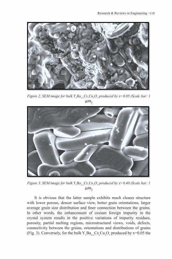
.119Research & Reviews in Engineering
Figure 2. SEM image for bulk Y1Ba2-xCsxCu3O7 produced by x=0.05 (Scale bar: 1
)
Figure 3. SEM image for bulk Y1Ba2-xCsxCu3O7 produced by x=0.40 (Scale bar: 1
)
It is obvious that the latter sample exhibits much clearer structure with lower porous, denser surface view, better grain orientations, larger average grain size distribution and finer connection between the grains. In other words, the enhancement of cesium foreign impurity in the crystal system results in the positive variations of impurity residues, porosity, partial melting regions, microstructural views, voids, defects, connectivity between the grains, orientations and distributions of grains (Fig. 3). Conversely, for the bulk Y1Ba2-xCsxCu3O7 produced by x=0.05 the
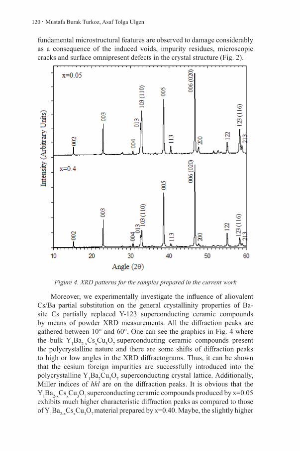
Mustafa Burak Turkoz, Asaf Tolga Ulgen120 .
fundamental microstructural features are observed to damage considerably as a consequence of the induced voids, impurity residues, microscopic cracks and surface omnipresent defects in the crystal structure (Fig. 2).
Figure 4. XRD patterns for the samples prepared in the current work
Moreover, we experimentally investigate the influence of aliovalent Cs/Ba partial substitution on the general crystallinity properties of Ba-site Cs partially replaced Y-123 superconducting ceramic compounds by means of powder XRD measurements. All the diffraction peaks are gathered between 10° and 60°. One can see the graphics in Fig. 4 where the bulk Y1Ba2-xCsxCu3O7 superconducting ceramic compounds present the polycrystalline nature and there are some shifts of diffraction peaks to high or low angles in the XRD diffractograms. Thus, it can be shown that the cesium foreign impurities are successfully introduced into the polycrystalline Y1Ba2Cu3O7 superconducting crystal lattice. Additionally, Miller indices of hkl are on the diffraction peaks. It is obvious that the Y1Ba2-xCsxCu3O7 superconducting ceramic compounds produced by x=0.05 exhibits much higher characteristic diffraction peaks as compared to those of Y1Ba2-xCsxCu3O7 material prepared by x=0.40. Maybe, the slightly higher

.121Research & Reviews in Engineering
offsetcT and onset
cT parameters are related to the intensity of characteristic diffraction peaks. Moreover, both of the samples prepared in the current work crystallize in the orthorhombic space group P4/mmm with a little distortion. When the aliovalent Cs/Ba partial substitution level is x=0.05, the orthorhombicity characteristic is found to more improve. In the figure, it is obvious that the characteristic peaks identified by the Miller indices of 006, 005, 103 and 003 are observed to be higher as compared to the other characteristic peaks. Moreover, we cannot determine the solubility limit for the cesium foreign impurity in the bulk Y1Ba2-xCsxCu3O7 superconducting crystal structure for the samples studied due to the nonexistence of any various phases including the cesium impurity and other cations in the XRD diffractograms. In other words, the cesium particles are totally solved in the Y1Ba2-xCsxCu3O7 superconducting system [36-37].
4. Conclusion
In the present work, the crucial role of aliovalent Cs/Ba partial replacement in the polycrystalline Y1-xErxBa2Cu3O7-y superconducting ceramic compounds on the general crystallinity, electrical, superconducting and microstructural morphological properties of Y1Ba2Cu3O7 superconducting compound is experimentally examined by means of temperature-dependent electrical resistivity, powder X-ray diffraction and scanning electron microscopy measurements. The experimental test results show that the cesium foreign particles are substituted successfully for the barium-sites in the Y1Ba2Cu3O7 crystal lattice. Moreover, dc electrical resistivity measurement results indicate that the Y1Ba2-xCsxCu3O7 material prepared by x=0.40 possesses smaller normal state resistivities at the temperature of 300 K, residual resistivities, ∆ρ and ρ100K parameters as compared to those of Y1Ba2-xCsxCu3O7 sample produced by x=0.05. Conversely, the former material has higher residual resistivity ratio. This is in attribution to the fact that the enhancement of aliovalent Cs/Ba partial substitution in the Y1Ba2-xCsxCu3O7 crystal lattice reduces remarkably some systematic permeant structural problems. Similarly, the lattice strain and formation of impurity scattering in the crystal structure are extensively eliminated in case of the substitution level of x=0.40 due to the refinement in the material quality qualification. Furthermore, the sample produced by x=0.05 obtains higher offset
cT value of 91.6 K and onsetcT value
of 92.4 K. The cT∆ parameters are observed to be about 0.8 K and 0.6 K for the Y1Ba2-xCsxCu3O7 produced by x=0.05 and x=0.40 molecular weight ratio, respectively. As for the crystallinity and microstructural morphological properties, the YBCO sample produced by x=0.05 shows larger orthorhombicity characteristic while the other sample prepared by x=0.40 presents much clearer structure with lower porous, denser surface

Mustafa Burak Turkoz, Asaf Tolga Ulgen122 .
view, better grain orientations, larger average grain size distribution and finer connection between the grains.
To sum up, the polycrystalline Y1Ba2-xCsxCu3O7 material prepared by x=0.40 is found to be more appropriate to use in the potential application fields including the heavy-industrial technology, advanced medicine and engineering sectors, innovative energy infrastructure, and large-scale applications.
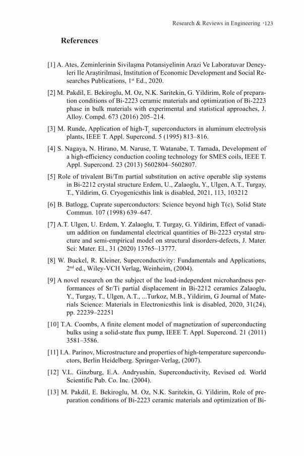
.123Research & Reviews in Engineering
References
[1] A. Ates, Zeminlerinin Sivilaşma Potansiyelinin Arazi Ve Laboratuvar Deney-leri Ile Araştirilmasi, Institution of Economic Development and Social Re-searches Publications, 1st Ed., 2020.
[2] M. Pakdil, E. Bekiroglu, M. Oz, N.K. Saritekin, G. Yildirim, Role of prepara-tion conditions of Bi-2223 ceramic materials and optimization of Bi-2223 phase in bulk materials with experimental and statistical approaches, J. Alloy. Compd. 673 (2016) 205–214.
[3] M. Runde, Application of high-Tc superconductors in aluminum electrolysis plants, IEEE T. Appl. Supercond. 5 (1995) 813–816.
[4] S. Nagaya, N. Hirano, M. Naruse, T. Watanabe, T. Tamada, Development of a high-efficiency conduction cooling technology for SMES coils, IEEE T. Appl. Supercond. 23 (2013) 5602804–5602807.
[5] Role of trivalent Bi/Tm partial substitution on active operable slip systems in Bi-2212 crystal structure Erdem, U., Zalaoglu, Y., Ulgen, A.T., Turgay, T., Yildirim, G. Cryogenicsthis link is disabled, 2021, 113, 103212
[6] B. Batlogg, Cuprate superconductors: Science beyond high T(c), Solid State Commun. 107 (1998) 639–647.
[7] A.T. Ulgen, U. Erdem, Y. Zalaoglu, T. Turgay, G. Yildirim, Effect of vanadi-um addition on fundamental electrical quantities of Bi-2223 crystal stru-cture and semi-empirical model on structural disorders-defects, J. Mater. Sci: Mater. El., 31 (2020) 13765–13777.
[8] W. Buckel, R. Kleiner, Superconductivity: Fundamentals and Applications, 2nd ed., Wiley-VCH Verlag, Weinheim, (2004).
[9] A novel research on the subject of the load-independent microhardness per-formances of Sr/Ti partial displacement in Bi-2212 ceramics Zalaoglu, Y., Turgay, T., Ulgen, A.T., ...Turkoz, M.B., Yildirim, G Journal of Mate-rials Science: Materials in Electronicsthis link is disabled, 2020, 31(24), pp. 22239–22251
[10] T.A. Coombs, A finite element model of magnetization of superconducting bulks using a solid-state flux pump, IEEE T. Appl. Supercond. 21 (2011) 3581–3586.
[11] I.A. Parinov, Microstructure and properties of high-temperature supercondu-ctors, Berlin Heidelberg. Springer-Verlag, (2007).
[12] V.L. Ginzburg, E.A. Andryushin, Superconductivity, Revised ed. World Scientific Pub. Co. Inc. (2004).
[13] M. Pakdil, E. Bekiroglu, M. Oz, N.K. Saritekin, G. Yildirim, Role of pre-paration conditions of Bi-2223 ceramic materials and optimization of Bi-
Mustafa Burak Turkoz, Asaf Tolga Ulgen124 .
2223 phase in bulk materials with experimental and statistical approaches, J. Alloy. Compd. 673 (2016) 205–214.
[14] H.K. Onnes, Further experiments with Liquid Helium. D. On the change of Electrical Resistance of Pure Metals at very low Temperatures, etc. V. The Disappearance of the resistance of mercury, Koninklijke Nederlandsche Akademie van Wetenschappen Proceedings, 14 (1911) 113–115.
[15] S.Y. Oh, H.R. Kim, Y.H. Jeong, O.B. Hyun, C.J. Kim, Joining of Bi-2212 high-T-c superconductors and metals using indium solders, Physica C 463–465 (2007) 464–467.
[16] M. Chen, W. Paul, M. Lakner, L. Donzel, M. Hoidis, P. Unternaehrer, R. We-der, M. Mendik, 6.4 MVA resitive fault current limiter based on Bi-2212 superconductor, Physica C 372 (2002) 1657–1663.
[17] J.D. Hodge, H. Muller, D.S. Applegate, Q. Huang, A resistive fault current limiter based on high temperature superconductors, Appl. Supercond. 3 (1995) 469–482.
[18] N.K. Saritekin, Y. Zalaoglu, G. Yildirim, M. Dogruer, C. Terzioglu, A. Varil-ci, O. Gorur, Determination of solid solubility level of Ho nanoparticles in Y-123 superconducting matrix and strong Cu-1 site preference of nano-particles, J. Alloys Comp. 610 (2014) 361–371.
[19] U. Erdem, M.B. Turkoz, G. Yıldırım, Y. Zalaoglu, S. Nezir, Refinement of Fundamental Characteristic Properties with Homovalent Er/Y Partial Rep-lacement of YBa2Cu3O7-y Ceramic Matrix, alloys and compounds. 2021, 884, 161131
[20] M. B. Turkoz, S. Nezir, C. Terzioglu, A. Varilci, G. Yildirim, Investigation of Lu effect on YBa2Cu3O72d superconducting compounds, J Mater Sci: Mater Electron (2013) 24:896–905, DOI 10.1007/s10854-012-0846-y
[21] O. Gorur, Y. Ozturk, G. Yildirim, M. Dogruer, C. Terzioglu, Sn diffusion coefficient and activation energy determined by way of XRD measure-ment and evaluation of micromechanical properties of Sn diffused YBa-2Cu3O7-x superconducting ceramics, J. Mater. Sci.: Mater. Electron. 24 (2013) 3063–3072.
[22] M. Li, Y. Zhang, Y. Li, Y. Qi, Granular superconductivity in polycrystalline Bi2Sr2CaCu2O8+γ by homovalent La substitution on Bi sites, J. Non-Cryst. Solids 356 (2010) 2831–2835.
[23] X. Xu, J.H. Kim, S. X. Dou, S. Choi, J.H. Lee, H. W. Park, M. Rindfleish, M. Tomsic, A correlation between transport current density and grain con-nectivity in MgB2/Fe wire made from ball-milled boron, J. Appl. Phys. 105 (2009) 103913.
[24] S.B. Guner, Y. Zalaoglu, T. Turgay, O. Ozyurt, A.T. Ulgen, M. Dogruer, G. Yildirim, A detailed research for determination of Bi/Ga partial substi-tution effect in Bi-2212 superconducting matrix on crucial characteristic features, J. Alloy. Compd. 772, (2019) 388–398.

.125Research & Reviews in Engineering
[25] P.B. Allen, Y.E. Picket, H. Krakauer, Phys. Rev. B 37 (1988) 7482–7490.
[26] S. Martin, M. Gurvitch, C.E. Rice, A.F. Hebard, P.L. Gammel, R.M. Fle-ming, A.T. Fiory, Phys. Rev. B 39 (1989) 9611–9613.
[27] M. Sahoo, D. Behera Effect of Ti Doping on Structural and Superconducting Property of YBa2Cu3O7−y High Tc Superconductor J Supercond Nov Magn (2014) 27:83–93
[28] J. Ekin, Experimental techniques for low-temperature measurements: cryos-tat design, material properties and superconductor critical-current testing, Oxford University Press, New York, (2006).
[29] M. Li, Y. Zhang, Y. Li, Y. Qi, Granular superconductivity in polycrystalline Bi2Sr2CaCu2O8+γ by homovalent La substitution on Bi sites, J. Non-Cryst. Solids 356 (2010) 2831–2835.
[30] Akkurt, B., Erdem, U., Zalaoglu, Y., ...Turgay, T., Yildirim, G.Evaluation of crystallographic and electrical-superconducting features of Bi-2223 advanced ceramics with vanadium additionJournal of Materials Science: Materials in Electronicsthis link is disabled, 2021, 32(4), pp. 5035–5049
[31] Erdem, U., Akkurt, B., Ulgen, A.T., ...Turgay, T., Yildirim, G. Effect of an-nealing ambient conditions on crack formation mechanisms of bulk Bi-2212 ceramic systems Journal of Asian Ceramic Societiesthis link is di-sabled, 2021
[32] R. Awad, A.I. Abou-Aly, M.M.H. Abdel Gawad, I. G-Eldeen, The influence of SnO2 nano-particles addition on the vickers microhardness of (Bi, Pb)-2223 superconducting phase, J. Supercond. Nov. Magn. 25 (2012) 739–745.
[33] G. Burns, High-temperature Superconductivity: an Introduction, Academic Press, New York, (1991).
[34] N.K. Sartekin, M. Pakdil, G. Yildirim, M. Oz, T. Turgay, Decrement in metastability with Zr nanoparticles inserted in Bi-2223 superconducting system and working principle of hybridization mechanism, J. Mater. Sci: Mater. El. 27 (2016) 956–965.
[35] S. Safran, H. Ozturk, F. Bulut, O. Ozturk, Experimental and theoretical ap-proaches for electrical, magnetic, micromechanical, and structural chara-cterization of BSCCO ceramic superconductors, Ceramics International, 44 (2018) 11674–11681
[36] S. Vinu, P.M. Sarun, A. Biju, R. Shabna, P. Guruswamy, U. Syamaprasad, The influence of sintering temperature on the microstructure and super-conducting properties of Bi1.7Pb0.4Sr1.8Nd0.2Ca1.1Cu2.1O8+x superconductor, Supercond. Sci. Technol. 21 (2008) 045001–045005.
[37] R. Shabna, P.M. Sarun, S. Vinu, A. Biju, U. Syamaprasad, Doping controlled metal to insulator transition in the (Bi, Pb)-2212 system, Supercond. Sci. Technol. 22 (2009) 045016–045022

Mustafa Burak Turkoz, Asaf Tolga Ulgen126 .

Chapter 8HYDRO-ECONOMIC DESIGN CONCEPT FOR MICRO-IRRIGATION SYSTEM SUBMAINS UNIT NETWORK-I: DESIGN PROCEDURE
Gürol YILDIRIM1
1 Professor of Civil Engineering, Vice Rector, Giresun University, Engineering Faculty, Civil Engineering Department, Head of Hydraulics Division, 28100, Giresun, Turkey. E-mail: [email protected] ; [email protected] ORCID number: 0000-0003-1899-5379
This chapter was produced from the author’s Master’s, and MSc. theses under the author’s supervision.
Gürol Yıldırım128 .
INTRODUCTION
Water required by crops is supplied by nature in the form of precipitation, but when it becomes scarce or its distribution does not coincide with demand peaks, it is then necessary to supply it artificially, by irrigation. Several irrigation methods are available, and the selection of one depends on factors such as water availability, crop, soil characteristics, land topography, and associated cost. In the near future, irrigated agriculture will need to produce two-thirds of the increase in food products required by a larger population (English et al., 2002). The growing dependence on irrigated agriculture coincides with an accelerated competition for water and increased awareness of unintended negative consequences of poor design and management (Cai et al., 2003). Drip irrigation water application uniformity is one of the major factors that determine irrigation efficiency. The main objective in drip irrigation design is the uniform distribution of water delivered through the emitters. Generally, the Christiansen uniformity coefficient (CU), distribution uniformity (DU), emission uniformity (EU), coefficient of variation (CV), and the maximum relative flow difference (qv) are used to evaluate the uniformity of microirrigation systems (Christiansen 1942; Keller and Karmelli 1974; Keller and Bliesner 1990; Wu and Barragan 2000). Among the uniformity parameters mentioned above, CU and CV must be calculated based on a group of sample readings or from all samples (Wu and Barragan 2000). DU is calculated as the mean of the lowest 25 % of emitter flow rates divided by the mean emitter flow rate. EU is recommended for microirrigation design and the evaluation of system uniformity by the ASAE standards (ASAE 2003).
Several authors have proposed numerical (Bralts & Segerlind, 1985; Dandy & Hassanli, 1996; Kang & Nishiyama, 1996) or analytical solutions (Baiamonte, 2018; Baiamonte, Provenzano, & Rallo, 2015; Barragan, Cots, Monserrat, & Sanz, 1998; Zhang, Wu, & Zhu, 2013) using with the aforementioned design approach. Under the traditional design paradigm, design and operating costs are not a design criteria but the result of the hydraulic requirements. There is little research that put the economic variables at the heart of the drip irrigation system design. The main objective of this work is to propose a method for the drip irrigation units design based on economic criteria. The minimisation of a simplified objective cost function considering the main design and operating costs is used for the design approach. A set of analytical expressions to calculate the diameters and the average operating pressure head are deduced from the minimum condition of the objective function.
Under this approach, hydraulic variables are not matched alone but are the consequence of the economic optimisation. It is shown the expected

.129Research & Reviews in Engineering
optimum yield increase with agricultural irrigation. To achieve this, soil properties of the land to be irrigated, amount and quality of irrigation conditions, topographic situation, size and shape of the land, plant type, climate characteristics, irrigation conditions. Today, the interest of both growers and commercial organizations in underground drip irrigation systems. Subsurface drip irrigation relates to other irrigation methods in micro irrigation systems. See other irrigation methods in this configuration. Underground drip irrigation, which is one of the micro irrigation systems methods, is the one with the highest water use efficiency. Today, with the advancement of technology and increased areas of conscious viticulture, pressurized irrigation methods that minimize the use of water in vineyards instead of surface irrigation methods make it preferable. The underground drip irrigation system, whose use of the last drip is becoming widespread day by day, consists of the most important pressurized irrigation methods that provide significant water savings.
OBJECTIVES
The objectives of this research were to combine hydraulic emission uniformity and total annual cost of trickle (drip) irrigation subunits in one objective function, express this objective function in terms of basic design parameters such as emitter and lateral spacing and manifold diameter, and then utilize optimization techniques to select optimum spacing between emitters and laterals to maximize the objective function. The decision variables that were considered in the optimization process included emitter and lateral spacing and manifold diameter. Moreover, the optimum manifold pipe size obtained from combined economical and hydraulic analysis is different from the pipe size obtained from economic analysis only.
ADVANTAGES
Many concerns as to the advantages of drip irrigation have been and are still being made; currently, the following advantages are recognized:
* The evaporative component of evapotranspiration is reduced, as only a limited area of the soil is wetted.
* The higher degree of inbuilt management that localized irrigation offers reduces substantially deep percolation and runoff losses, thus attaining
higher irrigation efficiencies. Consequently, localized irrigation is considered as water-saving technology;
* The limited wetted area results in reduced weed growth.
* Applicable to all forms of plots.

Gürol Yıldırım130 .
* Unaffected by wind.
* Reduced operating costs and labor. Human intervention is reduced to the periodic inspection of equipment for filtering and control, and the proper operation of drippers;
* Reduced risk of fungal diseases;
* Reduced sensitivity to the use of salt water. The salts are leached to each application and, rained at the periphery of the bulb humidifying outside the scope of the active root zone. No risk of damage to the aerial parts of plants by spraying of saline water.
DISADVANTAGES
The major disadvantages of localized irrigation are:
*Localized systems are prone to clogging because of the very small aperture of the water emitting devices hence the need for proper filtration and, at times chemigation .
*The movement of salts to the fringes of the wetted area of the soil may cause salinity problems through the leaching of salts by rain to the main root volume. This can be avoided if the system is turned on when it rains, especially when the amount of rain is not enough to leach the salts beyond the root zone depth.
* Rodents, dogs and other animals in search of water can damage the lateral lines.
* For crops of very high population density, the system may be uneconomic because of the large number of laterals and emitters required.
* The relatively high investment cost of the system.
* The spatial development of the root zone is limited and concentrated in the vicinity of the dripper making plants more susceptible to wind.
DESIGN REQUIREMENT
It is necessary to design a suitable and economically viable system to deliver a predefined amount of water at the root zone of each plant at regular intervals. In general, following steps are involved in design of drip irrigation system.
Step 1. Calculation of crop water requirement,
Step 2. Selection of dripper,
Step 3. Design and selection of lateral,
Step 4. Design and selection of sub main,

.131Research & Reviews in Engineering
Step 5. Design of selection of main line,
Step 6. Selection of Filter and fertigation equipment,
Step 7. Selection of pump,
Step 8. Selection of other fittings and accessories.
EVALUATION ON WATER REQUIREMENT
Land and Water Development Division of Food agriculture organization, (FAO), is developed software named CROPWAT to evaluate the irrigation water requirement. CROPWAT is meant as a practical tool to carry out standard calculations for reference evapotranspiration (ETO), crop water requirements, irrigation requirements, and more specifically the design and management of irrigation schemes. It allows the development of recommendations for improved irrigation practices, the planning of irrigation schedules under varying water supply conditions, and the assessment of production under rain fed conditions or deficit irrigation (Clark and Smith, 1998). Results of crop evapotranspiration are obtained by appling the CROPWAT software.
Cropping patterns and cropping intensity greatly affect the amounts of water needed to be supplied to an irrigation scheme. A selected cropping pattern must consider the crops that can be grown successfully in the area, local needs, areas needed for pastures, and available water resources.
IRRIGATION WATER REQUIREMENT
The irrigation water requirement of an area is based on following factors:
Type of crop (crop coefficient), Source of water, Weather data (Class A pan evaporation data), soil type srea under cultivation the monthly irrigation water requirement can be estimated on the basis of monthly pan evaporation data and crop coefficient by using the following equation
Vm = Kc × Kp × Cc × Ep × A (1)
where,
Vm=Monthly irrigation water requirement,L
Kc = Crop coefficient,
Cc = Canopy factor (Cc = 1.0, for closely spaced field crop, Cc = wetted area /plant area, for orchard and vegetables crop),
Kp = Pan evaporation factor (generally it is 0.8)
Ep = Normal monthly pan evaporation, mm,

Gürol Yıldırım132 .
A = Area to be irrigated, m² capacity of drip system Factor affects the drip system capacity
Irrigation water requirement, daily operating hours, Irrigation interval, water application efficiency drip irrigation system is generally not recommended to operate for more than 1.5 - 2.0 hours at a stretch to avoid losses of water through leaching,
Irrigation interval generally is not kept more than three days to avoid moisture stress to plants.
Equation to estimate capacity of drip system:
Q = A × CU × T / (ηa × t) (2)
where,
Q = Capacity of drip system, lps
A = Total cultivated area, m²
T = Irrigation interval, days
ηa=Water application efficiency (in fraction),
t = Duration of each irrigation, h
Discharge required per plant (Qp) can simply be estimated by dividing the drip capacity (Q) by the number of plants (n) in the area
Qp = Q/n (3)
Length of main, submain and lateral lines Length of main, submain and lateral lines can be calculated with the help of length, width and total number of equal sized blocks in a field, as follows:
Length of main line = width of block (if number of block i.e. NB = 1, in small fields) Length of main, submain and lateral lines
Total length of main line
(Lm) = (Nв -1) × width of block (if NB>1) (4)
Length of submain line
(Ls ) = width of block (Bw) ,
No submain if NB = 1
Total length of submain = Ls × NB (5)
Length of lateral line (LL ) = Length of block (BL )
Total length of lateral = LL × NB × NR (6)
where,
.133Research & Reviews in Engineering
NR = Number of plant row per block Number of drippers and laterals In orchard and vegetables crops, drippers are installed close to each plant, laterals are placed along each row of plant, number of laterals is taken equal to the number of plant rows.
Number of laterals and drippers
NLS = LS ÷ S (7)
where,
NLS = Number of laterals per submain
LS = Length of sub main pipe, m
S = Spacing between two rows of laterals, m
In large fields total number of laterals is estimated by multiplying the laterals per submain and the number of submain used
NL = LM ÷ S (8)
If NB =1;
NL = NLS × Ns (9)
if NB >1;
where,
NL= Total number of laterals
LM = Length of main pipe, m
Numbers of plants per lateral are estimated by dividing the length of lateral pipe by the spacing between two plants
NPL = LL ÷ PS (10)
Where,
NPL = Number of plants per lateral
LL = Length of lateral pipe, m
PS = Spacing between two plants, m Number of drippers per plant is estimated as follow:
QP = Q ÷ (NL × NPL) (11)
DP = QP ÷ q (12)
Where,
QP =Discharge required per Plant, lps
Q = Drip Capacity lph

Gürol Yıldırım134 .
NL= Total Number of laterals
NPL = Number of Plants per lateral
NDP = Number of Drippers per plant
q = Dripper discharge, lps
Total Number of Dripper required is estimated using the equations
NDL = NDP × NPL ND = NDL × NL NP = NPL × NL (13)
where,
NDL = Number of drippers per lateral
ND = Total number of drippers,
NP = Total number of Plants,
NL= Total Number of laterals,
NPL = Number of Plants per lateral,
NDP = Number of Drippers per plant,
DIAMETER OF LATERALS
Lateral pipe is selected such that the head loss in lateral pipe is limited within 10 per cent of the operating pressure available at the head of the lateral ,Expected head loss in different diameter pipes are estimated and that smallest diameter pipe is selected in which the head losses are within 10 per cent of the operating pressure ,Lateral pipes having 10, 12, 16 and 20 mm internal diameter with wall thickness varying from 1 to 3 mm are used in drip irrigation system First a smaller diameter lateral pipe should be selected to reduce the total cost of system and the friction losses are estimated by using Equation and then elevation head is added to this. If the variation in total friction losses are found within 10 % of the operating pressure then selected diameter is accepted.
where,
Q: Capacity of drip system, lps
h: Frictional loss in lateral pipe, m
Fd: Factor for multiple outlet (Based on number of outlets),
d: Diameter of lateral pipe, mm
DIAMETER OF MAIN AND SUBMAIN
Selection of the diameter of main and sub-main pipes is done similar to the lateral pipes starting from the smallest size going towards the successively higher size pipes If the variation in total head loss (friction

.135Research & Reviews in Engineering
losses + elevation head) in main and submain pipe are found within 10 % of the operating pressure of the system then selected diameter of sub-main and main pipes are accepted Diameter of main and sub main,
HDPE pipes of 65 mm diameter and more with a pressure rating of 2.5 to 6 kg/cm² are generally recommended for main pipe Pipes with a diameter of 25 to 75 mm and with a pressure rating of 2.50 to 4.0 kg/cm² are used as the sub main pipe, filter is an essential component of the drip system.
Filters are used to minimize or prevent inflow of possible suspended material in the water to the pipe spacing and dripper network. The type of filter needed depends on the water quality and the operating pressure of the drip system.
TOTAL COST
Total cost of the drip system can be estimated by the sum of the costs of its different components and latest rate of component or refer to the catalog of said firm.
DESIGN OF DRIP SYSTEM
Land, plant type, soil type, land slope, climate registration, back flush valve pressure gauge valve sand filter, outline pump, good end cap, lateral dripper valve, sub area line, water supply and water quality.
Determination of plant water requirement peak water requirement,
q= (14)
where,
A = Crop area (m²) = rr (m) × cc (m);
PE = Maximum pan evaporation, mm / day; PC = Pan Coefficient is taken as approximately 0.7 to 0.8; KC = Product coefficient for any product, the value of which depends on foliage characteristics, crop growth stage, environment and geographic location recommended by FAO.
w = Wetted area of the crop,%. When the sun is above the head, it is the area shaded due to the canopy cover, which depends on the growth stage of the plant. The percentage of wetted area covered by the crop ranges from 1/3 to 2/3 of the plant.
Eu = Emission homogeneity of the drip system, decimal.
• Darcy-Weisbach Equation: French engineer Henri Darcy investigated the flow of water in turbulent conditions in long irregular

Gürol Yıldırım136 .
uniform diameter pipes. The dispersion of energy by liquid friction causes a peisometric head to fall in the flow direction. Dimensional analysis can be used to provide a functional relationship between friction loss (hf) and flow parameters. The resulting equation is called the Darcy - Weisbach equation.
(15)
• Hazen - William Formula: Hazen-William formula is the most commonly used head loss formula in the USA. It cannot be used for liquids other than water and was originally developed only for turbulent flow. The results of this equation depend on the value of the friction factor (C) that should be used with the formula, which can be higher (80 to 130) and higher, depending on the pipe type, pipe size and water velocity.
• The formula Hazen-William is given in the equation below:
(16)
where:
hf : friction head loss (m),
C : Hazen - William friction coefficient (depends on pipe roughness),
D : pipe diameter (m),
L : pipe length (m).
Q : discharge (m³⁄s).
Head loss in a distribution pipe can be calculated from [Christiansen (1942)]:
(17)
where:
= head loss in a distribution pipe, m, and
F = Christiansen's reduction factor is equal to or less than 1 and Calculated as:
(18)
Where:
i = counter,
n = total number of openings.

.137Research & Reviews in Engineering
Diameter:
The continuity equation has been reorganized and used as follows to calculate the pipeline diameter (D):
(19)
where:
Q: water flow in the pipeline (m³/ sec).
V: velocity in the pipeline (m / s).
D: pipe diameter (m).
For design purposes, friction head losses (hf) are calculated as the manning equation below.
It can be applied to full and partial pipe flow.
(20)
where:
R: is the hydraulic radius = area / wetted environment.
S: is the slope of the energy grad line = hf / L.
And, n is the roughness factor (n = 0.009 for pipe).
GENERAL PRINCIPLES
Source of Irrigation water
Crops to be grown, topographic conditions, texture of soil, climatic data, layout of drip system, irrigation water requirement, capacity of drip system, length of main, length of sub-main, length of lateral lines.
DESIGN STEPS
Number of laterals and drippers, in orchards and vegetable crops, in close growing field crops, number of fittings and accessories, capacity of main pipe, capacity of sub-main pipe, capacity of lateral pipes. Diameter of lateral pipe, diameter of main pipe, diameter of sub-main pipe, filters, fertilizer applicators, size of pumping unit, total cost of drip system.
SYSTEM LAYOUT
Nodes representing junctions in the network were assigned their respective positions by inputting their coordinates from Arch GIS including their elevations and base demands. Base demands were calculated basing on the plant population of each block. Nodes were connected by the links which represent pipes to come up with a network while assigning them different sizes.

Gürol Yıldırım138 .
Figure 1. The Lay-out of the drip irrigation system.
THEORETICAL PROCEDURE
Trickle irrigation system is a water-distribution system; therefore, the design must be carried out against the flow direction and it must begin from the emitter towards the pumping unit. The basic principles of design of a trickle subunit can be summarized in the following paragraphs. Average emitter discharge can be calculated as follows:
(21)
where:
= average emitter discharge, lph,
= gross depth of irrigation, mm,
= time of application per irrigation, hrs,
= emitter spacing on the lateral, m, and
= lateral spacing on the manifold, m.
Average operational pressure head, , of the emitter can be calculated by using the average emitter discharge in the subunit, , or:
where:

.139Research & Reviews in Engineering
x = exponent of the emitter which depends upon the flow regime in the emitter, and
k = discharge of the emitter when the applied head is equal to unity.
Hazen-William’s formula when combined with the equation of continuity is usually used to calculate friction head loss through the pipes and it can be expressed by:
(23)
where :
= head loss in a carrier pipe due to friction, m,
= discharge at the inlet of the pipe, m3/hr,
= Hazen – William’s friction coefficient,
= inside pipe diameter, mm, and
= pipe length, m.
The head loss in a manifold, , can be calculated from [Christiansen (1942)]:
(24)
where:
= head loss in a manifold pipe, m, and
F = Christiansen’s reduction factor, it is equal to or less than 1 and can be calculated from
(25)
where:
i = counter, and
n = total number of openings.
For laterals on uniform slopes the lateral inlet pressure head, , can be estimated as follows [Keller and Karmeli (1974)] :
(26)
where
Gürol Yıldırım140 .
lateral inlet pressure head, m,
hfl = head loss in a lateral pipe, m,
ÄELl = difference in ground elevation along the lateral, m, and
ç = a factor between 0 and 1 which can be selected according to designer’s experience.
The design of the manifold is similar to that of the lateral, but larger flow rates are involved.
SYSTEM COSTS
In this research costs of drip subunits were divided into two groups namely fixed and pumping costs. Fixed costs of a trickle subunit include the combined costs of emitters, laterals, fittings, and manifold. The total cost of laterals and manifold are computed by multiplying the lengths of pipes by the unit cost of pipe. Costs of emitters, fittings, and connections are computed by multiplying the number of each accessory by its unit cost. In other words
(27)
where:
= unit cost of lateral pipes, $/m,
= unit cost of lateral connections to the manifold, $/piece,
= unit cost of emitter, $/emitter,
= unit cost of the manifold pipe, $/m,
= lateral length in the subunit, m,
= manifold length in the subunit, m,
= fixed cost of trickle subunit, $, and
: a factor equals to 1 if the laterals extend on one side of the manifold and 2 if the laterals extend on both sides of the manifold.
Annual fixed cost depends upon initial cost, life of the system, and compound interest rate and can be computed as follows:
(28)
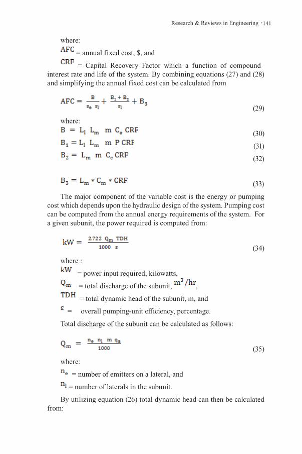
.141Research & Reviews in Engineering
where:
= annual fixed cost, $, and
= Capital Recovery Factor which a function of compoundinterest rate and life of the system. By combining equations (27) and (28) and simplifying the annual fixed cost can be calculated from
(29)
where:
(30)
(31)
(32)
(33)
The major component of the variable cost is the energy or pumping cost which depends upon the hydraulic design of the system. Pumping cost can be computed from the annual energy requirements of the system. For a given subunit, the power required is computed from:
(34)
where :
= power input required, kilowatts,
= total discharge of the subunit, ,
= total dynamic head of the subunit, m, and
= overall pumping-unit efficiency, percentage.
Total discharge of the subunit can be calculated as follows:
(35)
where:
= number of emitters on a lateral, and
= number of laterals in the subunit.
By utilizing equation (26) total dynamic head can then be calculated from:

Gürol Yıldırım142 .
(36)
where:
= head loss in the manifold, m,
= minor head losses in the subunit, m,
= a factor between 0 and 1 which can be selected according to designer's experience, and
= difference in ground elevation along the manifold, m. Friction head loss in a lateral and a manifold can be calculated by combining equations (23) through (25) as follows:
(37)
(38)
where:
= diameter of the lateral pipe, mm,
= manifold pipe diameter, mm, and
= a constant equal to 0.2933 when equals 150.
(39)
(40)
DESIGN PARAMETERS
• Pipe Material: The most common used pipe is GRP (Glass-fiber reinforced polyester pipe). However, the availability of low-cost and long term piping solutions to customers around the world, a long list of features and benefits add up to provide an optimum system of installation and life cycle cost (GRP pipe Catalogue, 2008).
• Flow Rate: The flow rate can be computed from dividing the volume of irrigation water (VOL) on the operating time (T) hours. The volume of irrigation water computed by multiplying the depth of water applied in each watering by the irrigation area.
• Flow Velocity: Flow velocity should be kept low, normally less than (1.5) m/sec, for other than experienced irrigation system designers, to avoid water hammer problems in pipelines. Under no conditions velocities ever exceed (3) m/sec. Velocities in the range of (1.5-3) m/sec are normally used (Clark et al., 1994).

.143Research & Reviews in Engineering
CONCLUSIONS
After the scarcity of fresh water around the world due to the increasing demand with changes in natural conditions and global warming, it becomes necessary to develop new approaches to rationalize water, especially in arid regions such as the Middle East countries. The demand for water for irrigation may consist of more than (80%) of the total amount of water required in these countries. The demand for water is increasing day by day due to global warming and the increasing population of the world. Available water resources are diminishing. The agricultural sector is the main consumer of freshwater resources. Drip irrigation is the most efficient method for using water in an efficient way. To get the expected benefit of drip irrigation depends on projects that have been carefully designed and managed by trained professionals and operate drip irrigation carefully.
The system should be implemented and addressed as proposed in the project. The first investment expenditures for drip irrigation are high, and the implementation of drip irrigation requires a lot of data and skills. Slow irrigation system design is a very important process to improve irrigation application efficiency, emission standardization, and economic return in production. Thus, the optimum design for drip irrigation is one that takes into account the possible uniformity of hydraulic emissions and the total annual cost.
In practice, it is difficult to measure or calculate the flow rate of all emitters, the maximum, minimum, or average flow rate of a sample of emitters along a lateral or in a submain unit are used to evaluate water application uniformity or to design the microirrigation system. A criterion that is sometimes used to inform the hydraulic design of drip irrigation submain units is defined as maximum relative flow difference between the maximum emitter flow rate and minimum emitter flow rate.
The design of drip irrigation units is in most cases examined from an hydraulic point of view. The lateral and submain diameters, or their maximum length for a given diameter, are deduced from the equations defining the energy state of the system. The results showed that as the spacing between emitters and laterals increases the value of the objective function increases up to a certain limit then its value starts to decrease; as hydraulic emission uniformity increases, total annual cost decreases then starts to increase but the differential increase in the hydraulic emission uniformity is very small when compared with the differential increase in the total annual cost.

Gürol Yıldırım144 .
REFERENCES
Baiamonte, G. (2016). Simple relationships for the optimal design of paired drip laterals on uniform slopes. Journal of Irrigation and Drainage En-gineering, 142(2), 04015054 https://doi.org/10. 1061/(ASCE)IR.1943-4774.0000971.
Baiamonte, G. (2017). Design of concave and convex paired sloped drip laterals. Agricultural Water Management, 191, 173e183. https://doi.org/10.1016/j.agwat.2017.06.015.
Baiamonte, G. (2018). Advances in designing drip irrigation laterals. Agri-cultural Water Management, 199, 157e174. https:// doi.org/10.1016/j.agwat.2017.12.015.
Baiamonte, G., Provenzano, G., & Rallo, G. (2015). Analytical approach de-termining the optimal length of paired drip laterals in uniformly sloped fields. Journal of Irrigation and Drainage Engineering, 141(1), 04014042 https://doi.org/10.1061/ (ASCE)IR.1943-4774.0000768.
Barragan, J., Cots, L. l., Monserrat, J., & Sanz, F. (1998). Algunas consideraci-ones sobre el diseno de los sistemas de riego ~ localizado: Influencia del grado de embozamiento en la uniformidad de distribucion. In Proceedings XVI Jornadas Tecnicas sobre riegos, Palma de Mallorca (pp. 260e267).
Bralts, V. F., Edwards, D. M., & Wu, I. P. (1987). Drip irrigation design and evaluation based on the statistical uniformity concept. In D. Hillel (Ed.), Advances in irrigation (Vol. 4, pp. 67e117). New York, USA: Academic press.
Bralts, V. F., & Segerlind, L. J. (1985). Finite element analysis of drip irrigation submain units. Transactions of the ASAE, 28(3), 809e814.
Burt, C. M., Clemens, A. J., Strelkoff, T. S., Solomon, K. H., Bliesner, R. D., Hardy, L. A., et al. (1997). Irrigation performance measures, efficiency and uniformity. Journal of Irrigation and Drainage Engineering, 123(6), 423e442.
Carrion, F., Montero, J., Tarjuelo, J. M., & Moreno, M. A. (2014). Design of sprinkler irrigation subunit of minimum cost with proper operation. App-lication at crop in Spain. Water Resources Management, 28, 5073e5089. https://doi.org/10.1007/s11269- 014-0793-x.
Carrion, F., Tarjuelo, J. M., Hern andez, D., & Moreno, M. A. (2013). Design of microirrigation subunit of minimum cost with proper operation. Irrigation Science, 31(5), 1199e1211. https:// doi.org/10.1007/s00271-013-0399-8.
Dandy, G. C., & Hassanli, A. M. (1996). Optimum design and operation of mul-tiple subunit drip irrigation systems. Journal of Irrigation and Drainage Engineering, 122(5), 265e275.
.145Research & Reviews in Engineering
Juana, L., Losada, A., Rodriguez-Sinobas, L., & Sanchez, R. (2004). Analytical relationships for designing rectangular drip irrigation units. Journal of Irri-gation and Drainage Engineering, 130(1), 47e59. https://doi.org/10.1061/(ASCE)0733-9437(2004) 130:1(47).
Ju, X. L., Wu, P. T., Weckler, P. R., & Zhu, D. L. (2017). Simplified approach for designing length of microirrigation laterals. Applied Engineering in Agriculture, 33(1), 75e82. https://doi.org/ 10.13031/aea.11882. Kang, Y., & Nishiyama, S. (1996). Analysis and design of microirrigation laterals. Journal of Irrigation and Drainage Engineering, 122(2), 75e82.
Keller, J., & Karmeli, D. (1974). Trickle irrigation design parameters. Transacti-ons of the ASAE, 17(4), 678e684.
Koysha, B. F. K. and Yıldırım, G (supervisor) (2021). “Hydro-Economic Design of drip irrigation submain units” “in Turkish”, MSc. thesis, Aksaray Uni-versity, Aksaray, Turkey.
Weckler, P. R., Wu, P. T., Zhu, D. L., Wang, X. K., & Li, Z. (2015). New simp-lified approach for hydraulic design of microirrigation paired laterals. Transactions of the ASABE, 58(6), 1521e1534. https://doi.org/10.13031/trans.58.11092.
Wu, I. P., (1992). Energy gradient line approach for direct hydraulic calculation in drip irrigation design. Irrigation Science, 13, 21-29.
Wu, I. P., ve Yue, R., (1993). Drip lateral design using energy gradient line appro-ach. Transaction ASAE, 36, 2, 389-394.
Wu, I. P., (1997). An assessment of hydraulic design of microirrigation systems. Agricultural Water Management, 32, 275-284.
Yıldırım, G. (2001). “Computer-aided design of micro-irrigation system laterals” MSc. thesis, Istanbul Technical University, Istanbul, Turkey.
Yıldırım, G., ve Ağıralioğlu, N., (2002a). Variation of total friction head losses and uniformity coefficients based on inlet pressure head in trickle laterals. Proc., International Conference on Water Resources Management in Arid Regions, Kuwait Institute for Scientific Research, Kuwait.
Yıldırım, G., ve Ağıralioğlu, N., (2002b). Variation of design parameters in mic-ro-irrigation laterals. Proc., International Conference on Advances of Ci-vil Engineering, Technical University of Istanbul, Istanbul.
Yıldırım, G., ve Ağıralioğlu, N., (2003a). Discussion of “New algorithm for hyd-raulic calculation in irrigation laterals” Journal of Irrigation and Drainage Eng., ASCE, 129, 2, 142-143.

Gürol Yıldırım146 .

Chapter 9HYDRO-ECONOMIC DESIGN CONCEPT FOR MICRO-IRRIGATION SYSTEM SUBMAINS UNIT NETWORK-I: CASE STUDY
Gürol YILDIRIM1
1 Professor of Civil Engineering, Vice Rector, Giresun University, Engineering Faculty, Civil Engineering Department, Head of Hydraulics Division, 28100, Giresun, Turkey. E-mail: [email protected] ; [email protected] ORCID number: 0000-0003-1899-5379
This chapter was produced from the author’s Master’s, and MSc. theses under the author’s supervision.

Gürol Yıldırım148 .
INTRODUCTION
Irrigation systems should be a relevant agent to give solutions to the increasing demand of food, and to the development, sustainability and productivity of the agricultural sector. The design, managing, and operation of irrigation systems are crucial factors to achieve an efficient use of the water resources and the success in the production of crops and orchards.. The design and managing of irrigation systems must have its base in criteria that are relevant, which implies to take into account agronomic, soil, hydraulic, economic, energetic, and environmental factors. The optimal design and managing of irrigation systems at farm level is a factor of the first importance for a rational use of water, economic development of the agriculture and its environmental sustainability. Optimum management of available water resources at farm level is needed because of increasing demands, limited resources, water table variation in space and time, and soil contamination (Kumar and Singh, 2003). Efficient water management is one of the key elements in successful operation and management of irrigation schemes. Irrigation water management involves determining when to irrigate, the amount of water to apply at each irrigation event and during each stage of plant, and operating and maintaining the irrigation system.
The main management objective is to manage the production system for profit without compromising environment and in agreement with water availability. A major management activity involves irrigation scheduling or determining when and how much water to apply, considering the irrigation method and other field characteristics. In practice, it is difficult to measure or calculate the flow rate of all emitters, the maximum, minimum, or average flow rate of a sample of emitters along a lateral or in a submain unit are used to evaluate water application uniformity or to design the microirrigation system. A criterion that is sometimes used to inform the hydraulic design of drip irrigation submain units is defined as maximum relative flow difference between the maximum emitter flow rate and minimum emitter flow rate. The design of drip irrigation units is in most cases examined from an hydraulic point of view. The lateral and submain diameters, or their maximum length for a given diameter, are deduced from the equations defining the energy state of the system. To accomplish the objectives of this study, all design steps of trickle irrigation subunits were converted to mathematical formulas and the objective function was first defined as a fractional function between hydraulic emission uniformity and total annual cost, and the maximum value of the objective function was then found by using an optimization process.

.149Research & Reviews in Engineering
CASE STUDY
Karbala province is one of the so called (middle Euphrates) province situated about (100 km) to the south west of Baghdad. The Geographical location of the city lies between N44ᵒ 40′ and 43.92″ N longitude and E33ᵒ 31′ and32.70″ E latitude. The borders of Karbala province are Anbar to the north and west, Najaf to the south and Babil and part of Baghdad to the east. The main source of irrigation and domestic water is the Hussainia and Bani Hasan canals; these canals take its water from the right bank of the river Euphrates just upstream Hindiya Barrage. The area of Karbala province may be described as a good cultivation landscape producing many types of fruits, vegetables, grains and high quality of dates. Orchards are found almost everywhere. The ground level of the urbans center of the city is about 22-28m (above mean sea level), while the other surrounding and rural areas is about 30-34 m (above mean sea level).
SYSTEM LAYOUT
The arable land of in Karbala province is consisting of around (300000) donum. According to the proposed scheme this area has been divided to in (60) equally agricultural plots. Each irrigation unit consists of a number of farms, the area of each farm is (50) donum, which in turn consists of a number of fields at (5) donum each. Preferably the number of farms in the irrigation unit is divided evenly, so as to facilitate the distribution scheme of plots either on one side or on both sides of the conveyance pipeline, as well as to achieve a suitable flexibility in the rotation of irrigation process.
Table 1. Values of CWR, IR and FWS for Orchards and Citrus.
Gürol Yıldırım150 .
INPUT DATA
Date: the start of each time step (defined by Time Step at the top of the table)
ETo : reference crop Evapotranspiration in millimeters per time step.
Crop Area: the proportion of the area planted with the specified crop in the current cropping pattern.
Crop Kc: average values of crop coefficient for each time step. Note that the “Crop Kc” values in this case are calculated as Kc*Crop Area, so if the crop covers only 50% of the area, the “Crop Kc” values will be half of the Kc values in the crop coefficient data file.
CWR: Crop Water Requirements for this crop. Calculated as ETo * Crop Kc
Total and Effective Rainfall: These are the values obtained by smoothing between the monthly totals.
Irrig. Req.: Irrigation Requirements for this crop in millimeters for the current time step.
FWS: Field Water Supply in liters per second per hectare assuming continuous supply and the Irrigation Efficiency shown at the top of the table (Clarke and smith, 1998).
Depending on the peak consumptive use for design of the irrigation system , the crop water requirement (consumptive use) equal to (7) mm/day and the field water supply (duty) for orchards and agricultural crops equal (0.64 and 0.54) l/sec/ha respectively.
CALCULATIONS Average ETo is calculated as 39.59 mm/per 30 day, or 3.959 cm per
30 day time step
The “Crop Kc” = 0.4
The Crop Water Requirement (CWR) is therefore 39.59*0.4 = 15.84 mm per 30 days
Effective rain neglected, so the Irrigation Requirement is 15.84mm per 30 days
The Field Water Supply for one hectare is calculated using 1 hectare * 15.84 mm *
(100/Irrigation Efficiency)

.151Research & Reviews in Engineering
FWS = 100m * 100m * 15.84/1000m * (100/75) m3 per 30 days = 211.2 m3 per 30 days
or 7.04 m³/day = 0.00008 m³/second
Table 2. The Calculations of Fws by Excel Program.
MAIN LINE DESIGN
The main line is designed to carry the maximum system capacity required for the plants in the farm plot; Q = 0.45 LPs.
For sizing purposes we take it as 1 LPs
From tables, a discharge of 1 LPs through a pipe of 50mm diameter the friction loss would be 0.68m per 100 length. Friction head loss = 0.68* (0.88) conversion factor = 0.5984 Because the proposed system uses multiple openings, the friction loss is taken as 1/3 of the total friction loss; that is, 0.5984/3= 0.1995m. Thus the loss in the mains is within the 1.0 m/100m and a pipe of 50 mm diameter will be ideal for the design layout.
Gürol Yıldırım152 .
SUBMAIN LINE DESIGN
The sub-main line is designed to carry the maximum discharge required for total number of plants in the farm plot.
Maximum discharge required = No. of plants * peak discharge per plant
=7200*1.7=1238.4 l/p/h =0.34 LPs Friction Head loss in pipes (m) Total length =100.0 Equivalent length
=32 Straight connectors
=16 Equivalent length of tee, bends etc
=13 Total length
=129 or 130 m
From standard tables, It would be seen that for a discharge of 0.34 LPs through a pipe of 37.5 mm diameter the friction loss would be 0.38m per 100 length or 0.494 for 130m equivalent length. Friction head loss = 0.494* (0.88) conversion factor = 0.435. Because the proposed system uses multiple openings, the friction loss is taken as 1/3 of the total friction loss; that is, 0.435/3= 0.145m. Thus the loss in the mains is within the 1.0 m/100 m and a pipe of 37.5 mm diameter will be ideal for the design layout.
LATERAL LINE DESIGN
A lateral is selected in such a way that the pressure difference from the proximate end to the last emitter does not exceed 10% of the normal operating head which in the present case is 4m. the maximum permissible variation in friction loss in the pipe is thus 4*10/50 = 0.8 m for as lateral of 50m length.
EPANET SOFTWARE
EPANET is computer software that performs extended period simulation of hydraulic and water quality behavior within pressurized pipe networks. A network consists of pipes, nodes (pipe junctions), pumps, valves and storage tanks or reservoirs. EPANET tracks the flow of water in each pipe, the pressure at each node, the height of water in each tank, and the concentration of chemical species throughout the network during a simulation period comprised of multiple time steps. In addition to chemical species, water age and source tracing can also be simulated. EPANET is designed to be a research tool for improving the understanding of the movement and fate of water constituents within distribution systems. It can be used for many different kinds of applications in distribution systems analysis: sampling program design, hydraulic model calibration, and chlorine residual analysis. EPANET software was applied on the network

.153Research & Reviews in Engineering
at two cases using the measured emitter flow rates and the total pressure in the field in order to show the pressure distribution in the network and then comparing the results of EPANET software with measured pressures in the network.
Figure 1. Flow chart of EPANET program
IRRIGATION SYSTEM HYDRAULIC MODELING
For this particular project, it was done using EPANET software. Pipe sizes were determined and this led to preparation of a pipe schedule for the system. This was through the following steps; setting the inputs for the model, modeling the system layout, assigning patterns, running the
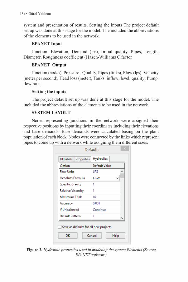
Gürol Yıldırım154 .
system and presentation of results. Setting the inputs The project default set up was done at this stage for the model. The included the abbreviations of the elements to be used in the network.
EPANET Input
Junction, Elevation, Demand (lps), Initial quality, Pipes, Length, Diameter, Roughness coefficient (Hazen-Williams C factor
EPANET Output
Junction (nodes), Pressure , Quality, Pipes (links), Flow (lps), Velocity (meter per second), Head loss (meter), Tanks: inflow; level; quality; Pump: flow rate.
Setting the inputs
The project default set up was done at this stage for the model. The included the abbreviations of the elements to be used in the network.
SYSTEM LAYOUT
Nodes representing junctions in the network were assigned their respective positions by inputting their coordinates including their elevations and base demands. Base demands were calculated basing on the plant population of each block. Nodes were connected by the links which represent pipes to come up with a network while assigning them different sizes.
Figure 2. Hydraulic properties used in modeling the system Elements (Source EPANET software)

.155Research & Reviews in Engineering
Figure 3. Hydraulic properties used in modeling the system Elements (Source EPANET software)
Figure 4. Hydraulic properties used in modeling the system Elements (Source EPANET software).

Gürol Yıldırım156 .
Figure 5. Shows System Layout with the velocity in the pipe network during operation.(Source EPANET model)
Figure 6. shows System Layout with the Demand and velocity in the pipe network during operation.(Source EPANET model) (V≤1.5).

.157Research & Reviews in Engineering
Figure 7. Profile of Demand between Distance (m) and Demand (Lps)
Figure 8. Profile of Pressure between Distance (m) and Pressure (m).

Gürol Yıldırım158 .
Figure 9. Profile of Base Demand between Distance (m) and Base Demand (Lps).
Figure 10. Profile of Head between Distance (m) and Head (m).

.159Research & Reviews in Engineering
Figure 11. Profile of Pump Curve between Flow (Lps) and Head (m).
Figure 12. The inputs and outputs data at EPANET software.
CONCLUSIONS
Efficient irrigation systems design at farm level appear to be a very important aspect for the irrigated agriculture and a key factor due to the competition for water resources with other sectors and to permit the economical and environmental sustainability of agriculture. In general, surface and pressurized irrigation systems can attain a reasonable level of efficiency, when they are well designed, adequately operated and appropriately selected for specific conditions; because irrigation is site specific. Automation of the irrigation systems coupled with sensor

Gürol Yıldırım160 .
and equipments to register the information of the irrigation process are important topic that must be developed in order to use the systems with their total potentiality. Regulated deficit irrigation proposed to control vegetative growth in orchards produce, in addition, savings in irrigation water without reducing yield. Thus, deficit irrigation has been demonstrated as a useful tool to improve irrigation management at a field scale.

.161Research & Reviews in Engineering
REFERENCES
Baiamonte, G. (2016). Simple relationships for the optimal design of paired drip laterals on uniform slopes. Journal of Irrigation and Drainage En-gineering, 142(2), 04015054 https://doi.org/10. 1061/(ASCE)IR.1943-4774.0000971.
Baiamonte, G. (2017). Design of concave and convex paired sloped drip laterals. Agricultural Water Management, 191, 173e183. https://doi.org/10.1016/j.agwat.2017.06.015.
Baiamonte, G. (2018). Advances in designing drip irrigation laterals. Agri-cultural Water Management, 199, 157e174. https:// doi.org/10.1016/j.agwat.2017.12.015.
Baiamonte, G., Provenzano, G., & Rallo, G. (2015). Analytical approach de-termining the optimal length of paired drip laterals in uniformly sloped fields. Journal of Irrigation and Drainage Engineering, 141(1), 04014042 https://doi.org/10.1061/ (ASCE)IR.1943-4774.0000768.
Barragan, J., Cots, L. l., Monserrat, J., & Sanz, F. (1998). Algunas consideraci-ones sobre el diseno de los sistemas de riego ~ localizado: Influencia del grado de embozamiento en la uniformidad de distribucion. In Proceedings XVI Jornadas Tecnicas sobre riegos, Palma de Mallorca (pp. 260e267).
Bralts, V. F., Edwards, D. M., & Wu, I. P. (1987). Drip irrigation design and evaluation based on the statistical uniformity concept. In D. Hillel (Ed.), Advances in irrigation (Vol. 4, pp. 67e117). New York, USA: Academic press.
Bralts, V. F., & Segerlind, L. J. (1985). Finite element analysis of drip irrigation submain units. Transactions of the ASAE, 28(3), 809e814.
Burt, C. M., Clemens, A. J., Strelkoff, T. S., Solomon, K. H., Bliesner, R. D., Hardy, L. A., et al. (1997). Irrigation performance measures, efficiency and uniformity. Journal of Irrigation and Drainage Engineering, 123(6), 423e442.
Carrion, F., Montero, J., Tarjuelo, J. M., & Moreno, M. A. (2014). Design of sprinkler irrigation subunit of minimum cost with proper operation. App-lication at crop in Spain. Water Resources Management, 28, 5073e5089. https://doi.org/10.1007/s11269- 014-0793-x.
Carrion, F., Tarjuelo, J. M., Hern andez, D., & Moreno, M. A. (2013). Design of microirrigation subunit of minimum cost with proper operation. Irrigation Science, 31(5), 1199e1211. https:// doi.org/10.1007/s00271-013-0399-8.
Dandy, G. C., & Hassanli, A. M. (1996). Optimum design and operation of mul-tiple subunit drip irrigation systems. Journal of Irrigation and Drainage Engineering, 122(5), 265e275.

Gürol Yıldırım162 .
Juana, L., Losada, A., Rodriguez-Sinobas, L., & Sanchez, R. (2004). Analytical relationships for designing rectangular drip irrigation units. Journal of Irri-gation and Drainage Engineering, 130(1), 47e59. https://doi.org/10.1061/(ASCE)0733-9437(2004) 130:1(47).
Ju, X. L., Wu, P. T., Weckler, P. R., & Zhu, D. L. (2017). Simplified approach for designing length of microirrigation laterals. Applied Engineering in Agriculture, 33(1), 75e82. https://doi.org/ 10.13031/aea.11882. Kang, Y., & Nishiyama, S. (1996). Analysis and design of microirrigation laterals. Journal of Irrigation and Drainage Engineering, 122(2), 75e82.
Keller, J., & Karmeli, D. (1974). Trickle irrigation design parameters. Transacti-ons of the ASAE, 17(4), 678e684.
Koysha, B. F. K. and Yıldırım, G (supervisor) (2021). “Hydro-Economic Design of drip irrigation submain units” “in Turkish”, MSc. thesis, Aksaray Uni-versity, Aksaray, Turkey.
Weckler, P. R., Wu, P. T., Zhu, D. L., Wang, X. K., & Li, Z. (2015). New simp-lified approach for hydraulic design of microirrigation paired laterals. Transactions of the ASABE, 58(6), 1521e1534. https://doi.org/10.13031/trans.58.11092.
Wu, I. P., (1992). Energy gradient line approach for direct hydraulic calculation in drip irrigation design. Irrigation Science, 13, 21-29.
Wu, I. P., ve Yue, R., (1993). Drip lateral design using energy gradient line appro-ach. Transaction ASAE, 36, 2, 389-394.
Wu, I. P., (1997). An assessment of hydraulic design of microirrigation systems. Agricultural Water Management, 32, 275-284.
Yıldırım, G. (2001). “Computer-aided design of micro-irrigation system laterals” MSc. thesis, Istanbul Technical University, Istanbul, Turkey.
Yıldırım, G., ve Ağıralioğlu, N., (2002a). Variation of total friction head losses and uniformity coefficients based on inlet pressure head in trickle laterals. Proc., International Conference on Water Resources Management in Arid Regions, Kuwait Institute for Scientific Research, Kuwait.
Yıldırım, G., ve Ağıralioğlu, N., (2002b). Variation of design parameters in mic-ro-irrigation laterals. Proc., International Conference on Advances of Ci-vil Engineering, Technical University of Istanbul, Istanbul.
Yıldırım, G., ve Ağıralioğlu, N., (2003a). Discussion of “New algorithm for hyd-raulic calculation in irrigation laterals” Journal of Irrigation and Drainage Eng., ASCE, 129, 2, 142-143.
Yıldırım, G., ve Ağıralioğlu, N., (2003b). Discussion of “Continuous outflow variation along irrigation laterals: effect of the number of outlets” Journal of Irrigation and Drainage Eng., ASCE, 129, 5, 382-386.

Chapter 10THE ROLE OF BIOTECHNOLOGY ABOUT FOOD WASTE RECYCLING IN TURKEY
Sevcan Aytaç KORKMAZ1
Sümeyye GÜVENDİ GÜNDOĞDU2
1 Fırat University, Electronic Technology Department Elazığ, Turkey2 Fırat University, Biotechnology Department, Elazığ, Turkey

Sevcan Aytaç Korkmaz, Sümeyye Güvendi Gündoğdu164 .
Introduction
Food is a vital factor for humanity. The energy that humanity needs to survive is produced from consumed foods. The human body meets the carbohydrates, proteins, lipids, minerals, vitamins and water it needs by feeding.
While the processed or harvested foods reach the end consumer or during industrial production, some consumable parts of the foods are thrown away or not used for various reasons. There are foods whose smell, color and texture do not appeal to the palate, and even thrown away because they are not wanted to be consumed. This situation causes food waste. The food waste issue has become undeniable not only in our country but also all over the world.
The importance of food is increasing due to factors; increasing population, globalization, climate changes and drought. Food consumption has increased as well as food production. Efforts are being made and precautions are being taken around the world to ensure that food is not wasted. FAO (Food and Agriculture Organization of the United Nations), UNEP ( The United Nations Environment Programme), IFAD (The International Fund for Agricultural Development), WHO (World Health Organization), TMO (Turkish Grain Board), TISVA (Turkish Foundation For Waste Reduction ), Republic Of Turkey Ministry Of Agriculture And Forestry take an active role in this field.
It can be mentioned that there are ideas and actions that oppose food waste being just waste. For sustainability of food, it is usual for the recycling of food wastes, obtaining bioproducts from wastes, its role in enzyme technology, its effect on microorganisms, contribution to bioremediation, activating wastes in the industrial industry, and operating in the fields of medicine, pharmacy, environment, agriculture and animal husbandry.
Food Waste in the World and in Turkey
Causes of food losses and food waste in low-income countries; harvesting methods, storage possibilities, cooling conditions, packaging and limited marketing systems due to geographical reasons. In middle-income and high-income countries, the causes of food losses and food waste are consumer behavior in addition to losses in the supply chain [1].
In the report published by FAO in 2011, it is stated that the amount of food that is safe for human consumption is wasted around 1.3 billion tons per year worldwide [1].
One-third of food production is garbage, which accounts for 8% of GHG (greenhouse gases) that trigger climate change. This figure mean
.165Research & Reviews in Engineering
87% of global road transport emissions [2].
According to the report published in FAO 2020, it is estimated that 690 million people globally are undernourished for 2019. This figure represents 8.9% of the world population [3].
In food waste report published by UNEP in 2019, global food waste is 931 million tons (61% households, 26% food service, 13% retail). According to the UNEP report in 2021, annual food waste in Turkey is 7 762 575 tons. The annual waste rate per person is 93 kg. According to an other study, among the countries in the Western Asia (Armenia, Azerbaijan, Cyprus, Iraq, Israel, Oman, Saudi Arabia, Palestine, Yemen, United Arab Emirates, Syria, Qatar, Lebanon, Kuwait, Jordan, Georgia, Bahrain) the annual highest The country that wastes food is Turkey [4].
All these losses mean not only the production of food in vain, but also the loss of one third of energy, manpower and labors during production [5].
In its report published in 2019, Turkish Foundation For Waste Reduction emphasizes the urgency of efficient use of all resources in preventing and reducing food waste [6].
FAO stated in the international congress on “Global Food Loss And Food Waste” that there is a need for a beneficial use for safe foods that are preferred to be thrown away and suitable for consumption [1].
The Importance of the Research
Humanity loses its wealth as a result of wastes damaging the environment, natural resources, sustainability in nature and in life, human health, the future of generations, biodiversity of living things such as animals and plants, climate, energy and technology. Nature and living life are at risk. By the understanding of the importance of waste management, it is possible to lead a life giving to nature instead of taking it from nature, not stealing from the lives of people and other living things, living without fear of depletion of energy and natural resources, without threatening the present and the future. With this viewpoint, in research, which includes studies, objectives and statistical data for quality life, vitality and the future; actions, scientific researches, ministry projects, state-sponsored in Turkey in the last 5 years have been researched and gathered together. It is aimed to investigate the effects and contributions of biotechnological methods, which aim to use living organisms with technological methods for the production of products and services [7], on the recycling of food wastes.
Literature Review
A study was carried out on the generation of electrical energy in order to eliminate the energy deficit by providing bioenergy conversion from

Sevcan Aytaç Korkmaz, Sümeyye Güvendi Gündoğdu166 .
beers that deteriorate and become food waste. After determining the beer waste as biomass, 2150 L of waste per day was produced as a result of anaerobic degradation, and 163 m3 of biogas per day was produced and the produced biogas was converted into 766.1 kWh electrical energy with a gas turbine engine [8].
By producing vinegar from various apple wastes, apples were prevented from being garbage, and it was suggested that the vinegars produced can be used for cleaning purposes with the advantage of being economical. According to the prosess that can be easily made at home; by using materials such as apple waste, bulgur wheat, Saccaromyces Cerevisia, apple vinegar, potable water, granulated sugar, rock salt, food waste in households can be recycled [9].
Bacillus licheniformis VO1 is selected as the bacterial strain. It was inoculated in solid phase fermentation medium that containing plantal wastes such as apple, melon, banana, orange peels under favorable conditions. It was determined that the highest solid substrate belonged to apple peels and α-amylase production was obtained. By the Carbon and Nitrogen sources are added to the fermentation medium containing high yield apple peels, the highest α-amylase production was obtained from the medium containing starch first and then yeast extract. According to the study, this bacterial strain belonging to the Bacillus class can be used in fruit juice production or in production areas where apple waste is used to produce α-amylase from apple waste. α-amylase, which has a high functionality in the field of biotechnology, is active in many areas as food, medicine, textile and cleaning equipments [10].
Bacillus licheniformis VO7 was inoculated into solid phase fermentation medium with optimum conditions in the medium consisting of agricultural wastes such as apple peel, banana peel, watermelon peel and orange peel for the production of α-amylase belonging to the hydrolase group, due to the wide range of usage areas and the ability to be obtained from microorganisms. The highest yield of α-amylase was produced from banana peels with 1500 μm particle size at temperature 50 °C, acidity at 6 and 24 hours. This recylcing, which can prevent environmental pollution, has shown that the waste of banana fruit with high production is too valuable to be garbage [11].
In order not to lose the high antioxidants contained in olive and olive kernels, which are the waste of olive and olive oil, which are produced in our country, bioconversion has been achieved by drying with the freeze drying method and microencapsulation, and a powder product that can be used both functionally and as a natural additive has been obtained [12].
The effects of parameters such as mushroom mycelium growth,

.167Research & Reviews in Engineering
productivity, biological efficiency, time, harvest time on compost were determined by mixing oak sawdust with certain percentages of industrial olive pulp wastes and yarn factory wastes. The highest efficiency means having the highest C/N ratio. Pleurotus ostreatus (oyster mushroom) grown on 75% oak sawdust + 25% olive pulp and 75% oak sawdust + 25% yarn waste was found to be positive morphologically [13].
The red peel waste of pistachio (Pistacia vera), which is a popular product in the Southeastern Region of Turkey, was determined as raw material. In the production of cultivated mushrooms (Agaricus Bisporus (L.) Sing), it has been determined that the fermented pistachio shell compost of 25% can be used in cultivated mushroom cultivation, mixed with different ratios as compost [14].
A study was conducted on the culture of Lentinus sajor-caju (Fr.) Fr., which is included in the oyster mushroom group, as compost of lignocellulosic wastes such as clover straw (T. repens), wheat straw and paper waste. It has been determined that two months is ideal time for compost to be produced by breeding the main mycelium culture of Lentinus sajor-caju (Fr.) Fr. and producing seed mycelium, and so a positive result has been obtained [15].
Tea, which is one of the most consumed beverages in our country, has a lot of waste. A study was conducted on the biosorption of Cu2+ ion from wastewater and it was determined that tea waste is a good sorbent with the Langmuir isotherm model from the adsorption isotherm models (Langmuir, Freundlich and DubininRadushkevic) [16].
It has been determined that composting of waste mushroom compost and tea waste organic fertilizers and inorganic fertilizers provides benefits as fertilizer for fenugreek plant (Trigonella Foenum Graecum) cultivation. It has been stated as a study that the waste mushroom compost and tea wastes generated after the harvest in mushroom production will provide positive environmental and economic benefits [17].
Heavy metals are found in high amounts in wastewater, negatively affecting human health and the environment. It is essential to remove heavy metals from these waters. Heavy metal biosorption is more economical thanks to the easy availability of agricultural and food wastes. Black cumin pulp was used to remove Fe (III) ion from wastewater and high efficiency was obtained with the Langmuir isotherm model [18].
On the determination of citrus wastes and citrus seeds as biomass, the possibility of using them for the production of pyrolysis oil, which is bio oil, by the thermochemical process, pyrolysis, was investigated. It was determined that the pyrolysis oil obtained was close to the diesel engine [19].

Sevcan Aytaç Korkmaz, Sümeyye Güvendi Gündoğdu168 .
Biomass was determined as sugar beet, opium poppy pulp and rice hulls. As a result of using these biomass separately, double and triple pairings and the most preferred pyrolysis and co-pyrolysis applications, bio oil structures were examined, compared and different values of bio oil were obtained by using GC-MS (Gas Chromatograph Mass Spectrometer), FT-IR Spectrometer and Calorimeter [20].
Solid, liquid and gas efficiencies were evaluated by pyrolysis application at different temperatures by mixing Arguvan lignite with low calorific value and walnut shell from Hekimhan region, and it was concluded that the solid product produced could be used as a smokeless fuel to reduce environmental pollution [21].
Some Clostridium species metabolize air polluting gases such as CO, CO2, N2, H2. They are take charge in the direct production of bioethanol, a renewable energy. Dried fruit and vegetable wastes in lignocellulosic structure were converted into biochar and for the waste gas released as a by-product in the pyrolysis of wastes, heat pretreatment was applied to the mixed culture containing Methanogens, Archaea species and Clostridium species and bioethanol was produced. By obtaining both biochar and bioethanol, the conversion of food wastes such as fruits and vegetables into energy has been realized [22].
Pomegranate pulp (Punica Granatum L.), chestnut peel (Castanea sativa Mill), clover stalks (Medicado sativa L.) and common reed (Phramites australis) determined as biomass, polyvinyl chloride and plastic raw materials with expired shelf life, mixed in different proportions. and it was subjected to pyrolysis process by thermogravimetric analysis method. Subsequently, the resulting products were characterized by FT-IR, elemental analysis and GC-MS methods, and it was concluded that they could be converted into chemicals that would not harm the environment [23].
The olive pulp sample taken from the food factory producing olive oil was fermented with various bacteria in an oxygen-free medium. At the end of the fermentation, biogas and hydrogen production studies were carried out at room conditions with economical and low energy. Subsequently, it was observed that the yield increased depending on the substrate concentration [24].
Method
Biogas Production
Biogas is the flammable gas obtained in the form of CH4 and CO2 under anaerobic conditions (oxygen-free environment) as a result of the determination of plant wastes such as biological wastes, industrial organic
.169Research & Reviews in Engineering
food wastes, corn and sugar beet as biomass. Since CH4 (methane) gas creates 23 times more greenhouse effect than CO2 (carbon dioxide) gas, the damage to the environment is reduced by converting waste into biogas [25].
Biogas converted from organic waste is biomass, also known biomass energy [26].
By producing biogas from waste;
Reduction of odor, that is a problem, during the prosess,
Protection of water resources,
Destruction of pathogenic microorganisms and wild plants,
Prevention the reproduction of insects and flies,
It contributes positively to the environment in reducing greenhouse gas emissions [27].
Biogas production from food waste depends on the composition of the food waste, the C/N ratio, acidity and buffer capacity, temperature, and the presence of alternative electron acceptors [27].
Biogas usage areas; generation of heat, steam generator, electric generation (fuel cells, cogeneration, gas turbine + generator), vehicle fuels, feeding for the natural gas line, and chemical production [27].
Compost
It is called composting when food wastes with organic content gain a soil-like structure (compost) by utilizing aerobic and anaerobic microorganisms. This method, which accelerates the integration of waste with nature and is useful for the field of agriculture, is one of the effective methods in the recycling of food wastes [28].
Advantages of composting;
Stabilize the soil by increasing efficiency of soil,
Can be used commercially,
Affects fertilizer processing positively,
Affects land applications positively,
It does not pollute the soil,
Inactivates pathogens,
Used as bedding material for animals,
It does not contain microorganisms that will cause disease,
Sevcan Aytaç Korkmaz, Sümeyye Güvendi Gündoğdu170 .
A transaction fee is provided for farmers.
Disadvantages of composting;
Increase in time and money for large and medium farms,
Great/large area requirement,
Odor formed before the final stage,
Necessity of optimum air conditions,
Marketing need for sales,
Loss of N (Nitrogen) value,
Diversion of waste from soil,
Exclusion from the farm group,
Slow release of materials in the compost [28].
Various wastes such as household food waste, fish waste, slaughterhouse waste, by-products and wastes generated during food production processing, leaves, polluted water, dry grass can be recycled by using compost method [29].
Pyrolysis
Pyrolysis takes place in thermochemical processes, which is one of the energy production technologies from biomass. It is the process of obtaining gas as a result of the decomposition of the organic content of the biomass under anaerobic conditions. Solid, liquid and gaseous products are formed thanks to the pyrolysis process [30].
The liquid product formed as a result of the pyrolysis process is bio oil.
The parameters for pyrolysis; temperature, The rate of heating, pressure, particle size, medium for pyrolysis, catalysis and residence time [31].
Advantages of pyrolysis;
There is no need for large area for storage,
It can produce with very high capacity,
High opportunities of end product marketing,
It provide reduction of water pollution,
Its efficiency and its speed are high,
.171Research & Reviews in Engineering
Provides the usage of various raw materials, is easy and economical,
It ensures that the energy production is local [32].
Solid State Fermentation
Solid state (substrate) fermentation (SSF) is generally defined as the growth of microorganisms on solids in the absence or very little free water. There must be sufficient moisture in the solid matrix in the substrate form [33].
Solid state fermentation processes are an effective method in waste area [33]. It provides fermentation of water-insoluble substrates [34]. The solid state method can be applied to the development of bioreactors (fermentors), modeling and production of various microbial products, with food, feed, various primary and secondary metabolites (enzymes, organic acids, amino acids) and bioprocesses such as bioleaching, biopulping, bioremediation, biobeneficiation [35].
For solid state fermentation;
The parameters for microbial activity (microbial selection, pH, oxygen level..),
The necessary parameters for the fermentation to occur on the solid substrate (selection of substrate, substrate particle size, substrate moisture contents…),
Water availability for solid state fermentation; (moisture activity, temperature, water binding feature…),
Purification of the final product is necessary [36, 37].
Conclusion
So far, a lot of work has been done in biotechnology and machine education [38-58]. In this article, In the recycling of food waste, different products that can be used in many areas are obtained with biotechnological methods. When looking at the diversity of academic studies and the end or by-products of the developed technologies, useful products that can be used in the industrial field are obtained. Thanks to the studies carried out, food waste, which is too precious to be thrown away, changes the perspective of the society.
As a result of the researches; It is important that the number of recycling facilities established for the bioconversion of food organic wastes in our country is low. With the intense execution of the projects; it is essential that people, families and even students in schools gain awareness at a child age. As a result of the food waste in households being 61%, families should

Sevcan Aytaç Korkmaz, Sümeyye Güvendi Gündoğdu172 .
separate their food and deliver it to the areas determined by the states [38].
It is not difficult to transform into a Turkey that targets quality. According to the hierarchical order, the state, ministries, municipalities and NGOs (Non-Governmental Organization) can operate in this field and guide the public. Activities, projects and actions that can be organized with media organs, social organization, seminars and conferences should be organized continuously. Waste collection areas where food waste can be collected in cities and even in villages should be fixed and collections should be made by municipalities without delay.
Every level we take for a better life and future is vital. The possibility of bioconversion should be emphasized and implemented quite frequently in order to encourage the producer, the consumer and the laws in line with the wastes and by-products of each consumed product.
With the recycling and repeated use of food waste, the interest in food will regain the value it deserves by people. The importance and vital value of food will take its place at the top as it should be. Many projects that have been put into action with many studies will be rewarded and it will be understood that food is not a product that can only be bought with money and thrown away. Otherwise, it will not be difficult for humanity to accelerate the end of the world, to prevent sustainability, to darken the future for tomorrow.

.173Research & Reviews in Engineering
References
[1] FAO. (2011). Global Food Losses and Food Waste.
[2] FAO. (2014). Food wastage footprint & Climate Change.
[3] FAO, IFAD, UNICEF, W. and W. (2020). The State of Food Security and Nutrition in the World 2020. Içinde The State of Food Security and Nutri-tion in the World 2020. https://doi.org/10.4060/ca9692en
[4] United Nations Environment Programme. (2021). Food Waste Index.
[5] TEKİNER, İ. H., MERCAN, N. N., KAHRAMAN, A., & ÖZEL, M. (2021). Dünya ve Türkiye’de gıda israfı ve kaybına genel bir bakış. İs-tanbul Sabahattin Zaim Üniversitesi Fen Bilimleri Enstitüsü Dergisi, 3(2), 123–128. https://doi.org/10.47769/izufbed.884219
[6] Türkiye İsrafı Önleme Vakfı. (2019). 2019 Sayılarla İsraf Raporu. Içinde 2019 Sayılarla İsraf Raporu.
[7] Tanyolaç, B., Kaya, H. B., Soya, S., & Akkale, C. (2012). Biyoteknoloji ve Biyoinformatik. Moleküler Biyoloji, January, 599–655.
[8] Hıraoğlu, İ. (2021). Bozulan ve Atık Hale Gelen Biraların Elektrik Ener-jisine Dönüştürülmesi Bioethanol Production from Chlamydomonas re-inhardtii and its Bioprocess Design via SuperPro Designer View project Bozulan ve Atık Hale Gelen Biraların Elektrik Enerjisine Dönüştürülme.
[9] Tangüler, H., Mert, H., İlman, F., Yücel, B., & Gençtürk, S. (2021). Elma atıklarından elma sirkesi üretimi üzerine bir araştırma A research on the production of apple vinegar from apple wastes. Niğde Ömer Halisdemir Üniversitesi Mühendislik Bilimleri Dergisi, 10(1), 132–139. https://doi.org/10.28948/ngmuh.673508
[10] AKCAN, N. (2021a). Bacillus licheniformis VO1’den α-Amilaz Üretimi için Tarımsal Endüstriyel Atıkların ve Fiziksel Faktörlerin İncelenmesi. Iğdır Üniversitesi Fen Bilimleri Enstitüsü Dergisi, 58–67.
[11] AKCAN, N. (2021b). Muz Kabuğu: Katı Faz Fermantasyonunda Bacil-lus licheniformis VO7 tarafından α-Amilaz Üretimi için Potansiyel bir Substrat. Türk Tarım ve Doğa Bilimleri Dergisi, 501–510. https://doi.org/10.30910/turkjans.782230
[12] Taş, E. N., & Ötleş, S. (2021). Zeytin çekirdeği antioksidanlarının don-durarak kurutma tekniği ile mikroenkapsülasyonu: toz ürünün fiziksel ve kimyasal karakterizasyonu Microencapsulation of olive stone antioxi-dants by freeze-drying technique: physical and chemical characterization of powder product. Bilim. Derg. / NOHU J. Eng. Sci, 10(1), 140–149. https://doi.org/10.28948/ngmuh.740797
[13] SÖZBİR, G. D. (2021). İSTİRİDYE MANTARININ (Pleurotus ostreatus) YETİŞTİRİLMESİNDE BAZI ENDÜSTRİYEL ATIKLARIN KULLA-

Sevcan Aytaç Korkmaz, Sümeyye Güvendi Gündoğdu174 .
NIM OLANAKLARININ BELİRLENMESİ Gonca DÜZKALE SÖZ-BİR. Turkish Journal of Forest Science, 5(1), 187–197.
[14] Taş, S., Tekı̇n, H., & KILIÇ, İ. H. (2021). Kültür Mantarı (Agaricus Bispo-rus (L.) Sing) Yetiştiriciliğinde Kırmızı Antepfıstığı Kabuğu Kompostu-nun Kullanılabilirliği. ZEUGMA BIOLOGICAL SCIENCE, 2(1), 27–37.
[15] Oruk, İ., & Akyüz, M. (2020). Lignoselülozik Atıkların Lentinus sajor-ca-ju (Fr.) Fr.’nin Kültüründe Değerlendirilmesi. The Journal of Fungus, 11(1), 12–18. https://doi.org/10.30708.mantar.608440
[16] Aslan, Ş., Yildiz, S., & Öztürk, M. (2020). Sentetik atıksulardan atık çay sorbentine Cu+2 biyosorpsiyonu: Kinetikler, eşitlikler ve termodinamik. Pamukkale Üniversitesi Mühendislik Bilimleri Dergisi, 1–9. https://doi.org/10.5505/pajes.2020.27374
[17] Akşahin, V., & Gülser, F. (2020). Bazı Organik Materyallerin ve İnorga-nik Gübrelerin Çemen Bitkisinin Gelişimine Etkileri. BURSA ULUDAĞ ÜNİVERSİTESİ ZİRAAT FAKÜLTESİ DERGİSİ, 34(2), 255–266.
[18] İŞLEK COŞKUN, Y. (2020). Çörekotu Posasi Kullanilarak SulardanDe-mı̇r(Iii)İyonunGı̇derı̇lmesı̇. Uludağ Üniversitesi Mühendislik Fakültesi Dergisi, 25(2), 961–980. https://doi.org/10.17482/uumfd.715236
[19] AÇIK, M. (2019). TURUNÇGİL ATIKLARINDAN PİROLİZ YÖNTE-Mİ İLE PİROLİTİK YAĞ ÜRETİMİNİN OPTİMİZASYONU.
[20] Arabacı, G. (2018). ŞEKER PANCARI, HAŞHAŞ KÜSPESİ VE PİRİNÇ KABUĞU BİYOKÜTLELERİNDEN PİROLİZ VE KOPİROLİZ YÖN-TEMLERİ İLE BİYOYAĞ ELDESİ YÜKSEK LİSANS TEZİ AFYON KOCATEPE ÜNİVERSİTESİ FEN BİLİMLERİ ENSTİTÜSÜ KİMYA MÜHENDİSLİĞİ ANABİLİM DALI.
[21] Aksoğan Korkmaz, A. (2021). DÜŞÜK ISIL DEĞERLİ LİNYİT VE ATIK BİYOKÜTLENİN DUMANSIZ YAKIT OLARAK KULLANILABİLİR-LİĞİNİN ARAŞTIRILMASI. Uludağ Üniversitesi Mühendislik Fakültesi Dergisi, 26(1), 1–14. https://doi.org/10.17482/uumfd.805313
[22] Keskı̇n, T., & Duman, G. (2020). Piroliz gazından karışık kültür kullanı-larak sentezgaz fermentasyonu ile biyoetanol üretimi: Isıl ön işlem etkisi. Pamukkale Üniversitesi Mühendislik Bilimleri Dergisi, 26(7), 1299–1307. https://doi.org/10.5505/pajes.2019.52284
[23] Temiz, Ü. İ. (2020). FARKLI BİYOKÜTLE-ATIK KARIŞIMLARININ TGA YÖNTEMİYLE BİRLİKTE PİROLİZİ Yüksek Lisans Tezi.
[24] Türkmenler, H., Aslan, M., & Gümüş, M. (2018). ZEYTİN KÜSPESİ ÇÖ-ZELTİSİNİN DERİŞİME BAĞLI BİYOGAZ VE HİDROJEN POTAN-SİYELİNİN İNCELENMESİ. Içinde Adıyaman Üniversitesi Mühendislik Bilimleri Dergisi (C. 8).
[25] Çelikkaya, H. (2016). Biyogaz. Fırat Kalkınma Ajansı Development Agency, 8.

.175Research & Reviews in Engineering
[26] TÜRKİYE KOJENERASYON DERNEĞİ. (y.y.). Biyokütle Nedir. Tari-hinde 10 Mayıs 2021, adresinden erişildi http://kojenturk.org/tr/biyokut-le-nedir-8
[27] Çallı, P. D. B. (2012). ATIKLARDAN BİYOGAZ ÜRETİMİ.
[28] Öztürk, P. D. M. (2017). HAYVAN GÜBRESİNDEN VE ATIKLARDAN KOMPOST ÜRETİMİ.
[29] Ergülen, A., Töke, L. B., Erbakan, N., Siyasal, Ü., Fakültesi, B., & Bölü-mü, İ. (2020). Çukurova Üniversitesi İİBF Dergisi Küreselleşmeyle Olu-şan Atık Sorununu Çözmeye Yönelik Yaklaşımlar.
[30] ÜÇGÜL, Y. D. D. İ., & AKGÜL, D. G. (2010). Biyokütle Teknolojisi. YEKARUM DERGİ, 1(1), 3–11.
[31] KEÇECİ, A. (2006). HAŞHAŞ ( papaver somniferum L.) YAĞ ENDÜST-RİSİ YAN ÜRÜNÜNDEN SIVI YAKIT ÜRETİMİNİN İNCELENMESİ.
[32] Piroliz Nedir? Nasıl Gerçekleşir? (2019). elektrik port. https://www.elekt-rikport.com/teknik-kutuphane/piroliz-nedir-nasil-gerceklesir/22447#ad-i-mage-0
[33] Pandey, A. (1992). Recent Process Developments in Solid-State Fer-mentation. Process Biochemistry, 27(2), 109–117. https://doi.or-g/10.1016/0032-9592(92)80017-W
[34] AFŞİN, M. (2010). KATI FAZ FERMANTASYON (SOLID STATE FER-MENTATION; SSF),T.C. DİCLE ÜNİVERSİTESİ FEN BİLİMLERİ ENSTİTÜSÜ, BİYOLOJİ ANABİLİM DALI, YÜKSEK LİSANS TEZİ BİYOLOJİ.
[35] Pandey, A. (2003). Solid-state fermentation. Biochemical Engineering Journal, 13(2–3), 81–84. https://doi.org/10.1016/S1369-703X(02)00121-3
[36] Konak, Ü. İ., Karakaş, B., Certel, M., Erem, F., & Akdeniz Üniversitesi, Mühendislik Fakültesi, Gıda Mühendisliği Bölümü, A. (2012). Katı Faz Fermentasyon Yöntemi ile Enzim Üretimi. Academic Food Journal, 10(3), 84–92.
[37] Singhania, R. R., Patel, A. K., Soccol, C. R., & Pandey, A. (2009). Recent advances in solid-state fermentation. Biochemical Engineering Journal, 44(1), 13–18. https://doi.org/10.1016/j.bej.2008.10.019
[38] Korkmaz, S. A. (2018). DETECTING CELLS USING IMAGE SEG-MENTATION OF THE CERVICAL CANCER IMAGES TAKEN FROM SCANNING ELECTRON MICROSCOPE. The Online Journal of Scien-ce and Technology-January, 8(1).
[39] KORKMAZ, S. A. (2017). VARIATION OF DRIVING CONCENT-RATION WITH DRIVER PERCEPTION THROUGH IN-CAR VIEW ROAD SCENE AS VISUAL STIMULANT. The Online Journal of Scien-ce and Technology-July, 7(3).

Sevcan Aytaç Korkmaz, Sümeyye Güvendi Gündoğdu176 .
[40] Korkmaz, S. A., & Poyraz, M. (2016, October). Path planning for rescue vehicles via segmented satellite disaster images and GPS road map. In Image and Signal Processing, BioMedical Engineering and Informatics (CISP-BMEI), International Congress on (pp. 145-150). IEEE.
[41] Korkmaz, S. A., Akçiçek, A., Bínol, H., & Korkmaz, M. F. (2017, Septem-ber). Recognition of the stomach cancer images with probabilistic HOG feature vector histograms by using HOG features. In Intelligent Systems and Informatics (SISY), 2017 IEEE 15th International Symposium on (pp. 000339-000342). IEEE.
[42] Korkmaz, S. A. (2018). LBP Özelliklerine Dayanan Lokasyon Koruyan Projeksiyon (LPP) Boyut Azaltma Metodunun Farklı Sınıflandırıcılar Üzerindeki Performanslarının Karşılaştırılması. Sakarya University Jour-nal of Science, 22(4), 1-1.
[43] Korkmaz, S. A., Esmeray, F. (2018). “Classification with Random Forest Based on Local Tangent Space Alignment and Neighborhood Preserving Embedding for MSER features: MSER_DFT_LTSA-NPE_RF.” Internati-onal Journal of Modern Research in Engineering and Technology, 3.2:31-37.
[44] Korkmaz, S. A. (2018). Recognition of the Gastric Molecular Image Based on Decision Tree and Discriminant Analysis Classifiers by using Discrete Fourier Transform and Features.Applied Artificial Intelligence, 32(7-8), 629-643.
[45] Korkmaz, S. A., & Esmeray, F. (2018). A New Application Based on GP-LVM, LMNN, and NCA for Early Detection of the Stomach Cancer. App-lied Artificial Intelligence, 32(6), 541-557.
[46] Korkmaz, S. A. (2021). Classification of histopathological gastric images using a new method. Neural Computing and Applications, 1-16.
[47] Korkmaz, S. A., & Poyraz, M. (2014). A New Method Based for Diagno-sis of Breast Cancer Cells from Microscopic Images: DWEE—JHT. Jour-nal of medical systems, 38(9), 92.
[48] Sengur, A., Turkoglu, I., & Ince, M. C. (2007). Wavelet packet neural networks for texture classification. Expert systems with applications, 32(2), 527-533.
[49] Sengur, A., Turkoglu, I., & Ince, M. C. (2008). Wavelet oscillator neural networks for texture segmentation. Neural Network World, 18(4), 275.
[50] Korkmaz, S. A., & Binol, H. (2017). Analysis of Molecular Structure Ima-ges by using ANN, RF, LBP, HOG, and Size Reduction Methods for early Stomach Cancer Detection. Journal of Molecular Structure.
[51] KORKMAZ, Sevcan Aytaç, et al. A expert system for stomach cancer images with artificial neural network by using HOG features and linear discriminant analysis: HOG_LDA_ANN. In: Intelligent Systems and In-

.177Research & Reviews in Engineering
formatics (SISY), 2017 IEEE 15th International Symposium on. IEEE, (2017):000327-000332.
[52] Turkoglu, I. (2007). Hardware implementation of varicap diode’s ANN model using PIC microcontrollers. Sensors and Actuators A: Physical, 138(2), 288-293.
[53] Korkmaz, S. A., & Poyraz, M. (2015). Least square support vector machi-ne and minumum redundacy maximum relavance for diagnosis of breast cancer from breast microscopic images. Procedia-Social and Behavioral Sciences, 174, 4026-4031.
[54] Korkmaz, S. A., Korkmaz, M. F., & Poyraz, M. (2016). Diagnosis of bre-ast cancer in light microscopic and mammographic images textures using relative entropy via kernel estimation. Medical & biological engineering & computing, 54(4), 561-573.
[55] Korkmaz, S. A., & Korkmaz, M. F. (2015). A new method based cancer detection in mammogram textures by finding feature weights and using Kullback–Leibler measure with kernel estimation. Optik-International Journal for Light and Electron Optics, 126(20), 2576-2583.
[56] Korkmaz, S. A., & Eren, H. (2013, December). Cancer detection in mam-mograms estimating feature weights via Kullback-Leibler measure. In Image and Signal Processing (CISP), 2013 6th International Congress on (Vol. 2, pp. 1035-1040). IEEE.
[57] Korkmaz, S. A., Korkmaz, M. F., Poyraz, M., & Yakuphanoglu, F. (2016). Diagnosis of breast cancer nano-biomechanics images taken from atomic force microscope. Journal of Nanoelectronics and Optoelectronics, 11(4), 551-559.
[58] Korkmaz, S. A., Poyraz, M., Bal, A., Binol, H., Özercan, I. H., Korkmaz, M. F., & Aydin, A. M. (2015). New methods based on mRMR_LSSVM and mRMR_KNN for diagnosis of breast cancer from microscopic and mammography images of some patients. International Journal of Biome-dical Engineering and Technology, 19(2), 105-117.

Sevcan Aytaç Korkmaz, Sümeyye Güvendi Gündoğdu178 .

Chapter 11IMPLEMENTING BALANCED ITERATIVE REDUCING AND CLUSTERING USING HIERARCHIES (BIRCH) ALGORITHM STEP BY STEP AND APPLYING TO THE DATASETS CONTAINING JOB-ADS
Yunus DOĞAN1
Feriştah DALKILIÇ2
Alp KUT3
Kemal Can KARA4
Uygar TAKAZOĞLU5
1 Dr. Öğr. Üyesi Yunus DOĞAN, Department of Computer Engineering, Faculty of Engineering, Dokuz Eylül University, Izmir, Turkey. Corresponding Author, E-mail: [email protected], ORCID: 0000-0002-0353-50142 Dr. Öğr. Üyesi Feriştah DALKILIÇ, Department of Computer Engineering, Faculty of Engineering, Do-kuz Eylül University, Izmir, Turkey. E-mail: [email protected], ORCID: 0000-0001-7528-51093 Prof. Dr. Alp KUT, Department of Computer Engineering, Faculty of Engineering, Dokuz Eylül Uni-versity, Izmir, Turkey. E-mail: [email protected], ORCID: 0000-0002-5781-334X4 Ar-Ge Müdürü, Kemal Can KARA, Kariyer.net R&D Centre, Istanbul, Turkey, E-mail: [email protected], ORCID: 0000-0001-5938-98995 Veri Bilimcisi, Uygar TAKAZOĞLU, Kariyer.net R&D Centre, Istanbul, Turkey, E-mail: [email protected], ORCID: 0000-0002-9276-5339
Yunus Doğan, Feriştah Dalkiliç, Alp Kut, Kemal Can Kara, Uygar Takazoğlu180 .
Introduction
In its most basic form, it was aimed to write the BIRCH algorithm in this study, and it was implemented on job postings. C# language was chosen for coding and Object-Oriented coding was performed. There are two types of learning methods used in the field of Machine Learning. The main target learning method for the projects is Unsupervised Learning. With the clustering method, previously unlabeled data is divided into groups. In clustering the data, common features are used so that similar and close data groups are created, and each data is defined.
Balanced Iterative Reducing and Clustering using Hierarchies (BIRCH) clustering method was chosen for the projects. This stream mining algorithm has been used for several areas like medical (Barham, 2020), traffic simulation (Dimara et al., 2020), finance (Huang, 2020) and recommender systems (Katarya & Saini, 2021; Tsarouchis et al., 2021). Also, this algorithm gives successful results on Natural Language Processing studies (Yilmaz et al., 2019; Gündoğan & Kaya, 2021) and Big Data studies (Ramadhani et al., 2020; Fakir & El Iklil, 2021). It basically uses the hierarchical property of the tree structure to re-cluster larger and previously clustered data groups. Clustering is done by calculating the distances of various metric features of existing clusters. Thus, the clusters that form more densely are called Clustering Feature (CF). Due to its tree property, the root node consists of non-leaf nodes and leaf nodes. The maximum number of records that each cluster can contain and the number of entries that the CF tree, that is, the node, will have are determined as parameters. New entries are formed at the root node and clusters are started to be placed into these entries according to their distance from each other. The most important step is the distance calculation to be made for the new record according to the metrics belonging to that cluster, and this calculation is made with all the entries belonging to the root and the closest entry is determined. In line with the given parameters, as soon as there are entries with enough clusters and nodes with enough entries, the tree starts to branch, and new nodes are formed by using the tree structure. In this way, nodes are formed by branching; there are entries in the nodes and clusters in each entry. With each new record that finds a suitable set and settles in, the entry and the hierarchical center points of the entry within the parent nodes are updated. The number of center points is the same as the metric properties belonging to the clusters. As a result, this algorithm is the clustered state of the clusters (Gupta, 2021). All the elements that form the basis of the BIRCH algorithm are shown in Figure 1.
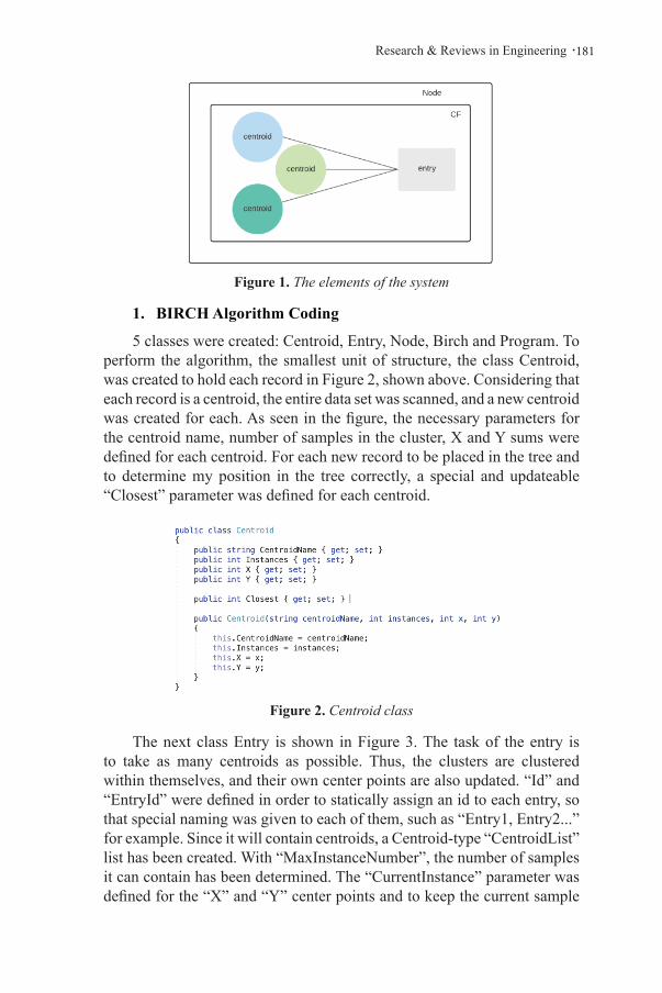
.181Research & Reviews in Engineering
Figure 1. The elements of the system
1. BIRCH Algorithm Coding
5 classes were created: Centroid, Entry, Node, Birch and Program. To perform the algorithm, the smallest unit of structure, the class Centroid, was created to hold each record in Figure 2, shown above. Considering that each record is a centroid, the entire data set was scanned, and a new centroid was created for each. As seen in the figure, the necessary parameters for the centroid name, number of samples in the cluster, X and Y sums were defined for each centroid. For each new record to be placed in the tree and to determine my position in the tree correctly, a special and updateable “Closest” parameter was defined for each centroid.
Figure 2. Centroid class
The next class Entry is shown in Figure 3. The task of the entry is to take as many centroids as possible. Thus, the clusters are clustered within themselves, and their own center points are also updated. “Id” and “EntryId” were defined in order to statically assign an id to each entry, so that special naming was given to each of them, such as “Entry1, Entry2...” for example. Since it will contain centroids, a Centroid-type “CentroidList” list has been created. With “MaxInstanceNumber”, the number of samples it can contain has been determined. The “CurrentInstance” parameter was defined for the “X” and “Y” center points and to keep the current sample

Yunus Doğan, Feriştah Dalkiliç, Alp Kut, Kemal Can Kara, Uygar Takazoğlu182 .
number in it that plays a role in determining these points. These parameters were used while creating each new entry. As the nodes start to fill up and new entries will be created for each entry as soon as the branching occurs, the Entry-type “EntryOfEntry” list was created.
Figure 3. Entry classThe first function of the Entry class, IsAvaliable, is shown on Figure 4.
Figure 4. IsAvaliable function
If the new incoming centroid is placed in it as a parameter, it checks whether the maximum number of samples is exceeded. If not, bool is returned false. As soon as the true bool returns, the centroid will be placed in the list and the NewCenterEntry function has been created in order to determine the current center point of the entry, as shown in Figure 5. The centroid list of the inserted entry was completely navigated, and the total x, y and number of samples were determined. Center points were updated by dividing the total x and y by the total number of samples. There are parent entries to which the center points of each entry are connected as they should be updated within themselves. After the appropriate node and the appropriate entry in the node were determined and placed, the center update was made for the parent node. As seen in Figure 6, the entry list belonging to the entry was scrolled and the x, y and number of samples of the centroids in each connected entry were collected. Center points were updated by dividing the total x and y by the total number of samples.

.183Research & Reviews in Engineering
Figure 5. NewCenterEntry method
There are parent entries to which the center points of each entry are connected as they should be updated within themselves. After the appropriate node and the appropriate entry in the node were determined and placed, the center update was made for the parent node. As seen in Figure 6, the entry list belonging to the entry was scrolled and the x, y and number of samples of the centroids in each connected entry were collected. Center points were updated by dividing the total x and y by the total number of samples.
Figure 6. NewCenterParent method
The last method of the Entry class is the NewCurrentInstance method on Figure 7. It was aimed to update the number of instances of the entry. As shown in the figure, the current sample number is obtained by taking the number of samples from the settled centroid.
Figure 7. NewCurrentInstances method

Yunus Doğan, Feriştah Dalkiliç, Alp Kut, Kemal Can Kara, Uygar Takazoğlu184 .
Another class shown on Figure 8 is Node. Since the tree structure is used, nodes are needed to create the structure.
Figure 8. Node class
Each node that will form the tree structure has a list of entry type. Based on the BIRCH algorithm, the “MaxEntryNumber” variable and accordingly the “Available” parameter in bool type were created to keep the maximum number that each node can take into it. In order to complete the tree structure, all nodes except the root node are expected to have parent and child nodes. To perform this task, a Node type “ParentNode” and a Node type List “ChildNode” were created. The only function belonging to this class is the IsAvaliable function, as seen in Figure 9. It checks both the entry list in the node and the entries that the entry has.
Figure 9. IsAvaliable function
In order to realize this application, the remaining two classes are the Birch class and the Program class. The Birch class, which is one of these two classes working in conjunction with each other, has methods and functions for the implementation of the application. As shown in Figure 11 above, firstly, “MaxInstanceNumber” and “MaxEntryNumber” variables were created upon shaping the algorithm and thus the tree. In the Program class, which is the class that contains an object main function from the Birch class, after the maximum number of instances and the maximum number of entries are given and the tree is created, the root node must be created to begin the creation of the tree, and a “ParentNode” of Node type
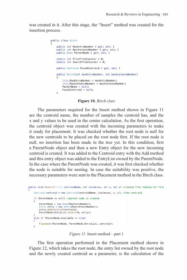
.185Research & Reviews in Engineering
was created in it. After this stage, the “Insert” method was created for the insertion process.
Figure 10. Birch class
The parameters required for the Insert method shown in Figure 11 are the centroid name, the number of samples the centroid has, and the x and y values to be used in the center calculation. As the first operation, the centroid object was created with the incoming parameters to make it ready for placement. It was checked whether the root node is null for the new centroids to be placed on the root node first. If the root node is null, no insertion has been made in the tree yet. In this condition, first a ParentNode object and then a new Entry object for the new incoming centroid is created. It was added to the Centroid entry with the Add method and this entry object was added to the EntryList owned by the ParentNode. In the case where the ParentNode was created, it was first checked whether the node is suitable for nesting. In case the suitability was positive, the necessary parameters were sent to the Placement method in the Birch class.
Figure 11. Insert method – part 1
The first operation performed in the Placement method shown in Figure 12, which takes the root node, the entry list owned by the root node and the newly created centroid as a parameter, is the calculation of the

Yunus Doğan, Feriştah Dalkiliç, Alp Kut, Kemal Can Kara, Uygar Takazoğlu186 .
distances between the current node and the entries owned by the node and the newly created centroid. The distances will be calculated, and the centroid will be placed in the cluster with the closest features. With the FindClosest function in the Birch class, the index of the closest entry was found, and the closest variable of the centroid object was determined. In the next step, the number of samples existing in the closest entry and the number of samples owned by the newly created centroid were collected. If the entry is still suitable, the centroid was placed in the closest entry. In case the eligibility condition is not met, that is, the entry contains the maximum number of samples; the new entry into the node was checked this time. When appropriate, a new entry was created, the new centroid was added to this entry, and this entry was inserted into the entry list owned by the node. By giving the index of the entry to which, the centroid is closest as a parameter to the Insert function of the list, it is brought to a position side by side with the entry that is closest in the list. If there are other entries in it, an index has been shifted thanks to the Insert function.
Figure 12. Placement method
The FindClosest function in the Placement method is as shown in Figure 13. Entry list and newly created centroid are sent as parameters to this function. It was navigated through the entry list and its distances with the centroid were calculated. The CalculateDistance function was used for this calculation. Entry and centroid were sent as parameters. Both the entry has its own center points, and the centroid has its own x and y values. Manhattan Distance is used in this function to calculate the distance. After the distance is returned, the comparison was made in the FindClosest function, and the closest index found was returned to the Placement function.

.187Research & Reviews in Engineering
Figure 13. FindClosest and CalculateDistance functions
If the newly created centroid fails to settle in the root node, different actions are required. For this, as shown in Figure 14, it was first checked whether the node has a child node. If the child node is not found, the operation to be done is the fragmentation operation. The SplitManagement method was created to split the tree, and the node, the entry list of the node and the centroid were sent as parameters.
Figure 14. Insert method – part 2
In order to break up the node, the SplitManagement method consisted of two parts. The first part is as shown in Figure 15.
Figure 15. SplitManagement function – part 1

Yunus Doğan, Feriştah Dalkiliç, Alp Kut, Kemal Can Kara, Uygar Takazoğlu188 .
There is a centroid that cannot be in the hand. Since the node is divided into two child nodes, left and right, it must first find the entry that this centroid is close to. The closest entry index was detected with FindClosest. For the fragmentation to be done correctly, the index “splitIndex” variable to be fragmented was determined according to whether there is an odd or even number of entries in the node. “Left” and “right” objects were created for the main entries that will be used for the broken node. The entries belonging to the node were added in order into the “left” entry object before the Index that needed to be broken down. After the index that needs to be broken down, the remaining entries belonging to the node are added to the “right” entry object in order.
The second part of the SplitManagement method, as shown in Figure 16, exists to place the newly created centroid in the correct position in the entry list belonging to the “right” entry object, which is the main entry for the split tree. At the beginning of the SplitManagement method, the entry to which the new centroid is closest was found. In this way, if the splitIndex is close to a previous entry, it is inserted as the first element in the Entry type list of the “right” entry. If the splitIndex is greater than and equal to, the insert operation was performed side by side with the entry it is close to. At this stage, after the placement was made, the NewCenterParent function was used for “left” and “right” entries to update the center points with the current entries they contain. The last remaining operation is the node assignment with these new main entries and the entry lists they have. For this, the Split method was created.
Figure 16. SplitManagement function – part 2
The Split method of the Birch class is shown in Figure 17. The left entry and the right entry, which will belong to the node and the children of the node, are given as parameters. A node named “leftNonLeaf” and a node named “rightNonLeaf” were created as Node objects. A “left” entry was inserted into the left node, and a “right” entry was inserted into the right node. As shown in Figure 8, a list named ChildNode of Node type was
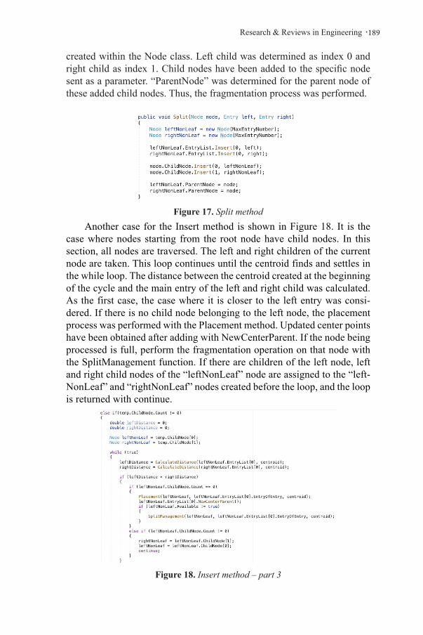
.189Research & Reviews in Engineering
created within the Node class. Left child was determined as index 0 and right child as index 1. Child nodes have been added to the specific node sent as a parameter. “ParentNode” was determined for the parent node of these added child nodes. Thus, the fragmentation process was performed.
Figure 17. Split methodAnother case for the Insert method is shown in Figure 18. It is the
case where nodes starting from the root node have child nodes. In this section, all nodes are traversed. The left and right children of the current node are taken. This loop continues until the centroid finds and settles in the while loop. The distance between the centroid created at the beginning of the cycle and the main entry of the left and right child was calculated. As the first case, the case where it is closer to the left entry was consi-dered. If there is no child node belonging to the left node, the placement process was performed with the Placement method. Updated center points have been obtained after adding with NewCenterParent. If the node being processed is full, perform the fragmentation operation on that node with the SplitManagement function. If there are children of the left node, left and right child nodes of the “leftNonLeaf” node are assigned to the “left-NonLeaf” and “rightNonLeaf” nodes created before the loop, and the loop is returned with continue.
Figure 18. Insert method – part 3
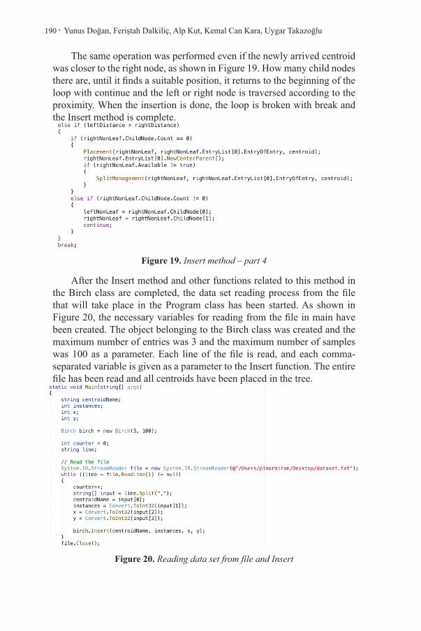
Yunus Doğan, Feriştah Dalkiliç, Alp Kut, Kemal Can Kara, Uygar Takazoğlu190 .
The same operation was performed even if the newly arrived centroid was closer to the right node, as shown in Figure 19. How many child nodes there are, until it finds a suitable position, it returns to the beginning of the loop with continue and the left or right node is traversed according to the proximity. When the insertion is done, the loop is broken with break and the Insert method is complete.
Figure 19. Insert method – part 4
After the Insert method and other functions related to this method in the Birch class are completed, the data set reading process from the file that will take place in the Program class has been started. As shown in Figure 20, the necessary variables for reading from the file in main have been created. The object belonging to the Birch class was created and the maximum number of entries was 3 and the maximum number of samples was 100 as a parameter. Each line of the file is read, and each comma-separated variable is given as a parameter to the Insert function. The entire file has been read and all centroids have been placed in the tree.
Figure 20. Reading data set from file and Insert

.191Research & Reviews in Engineering
Another process for the application is the Print method. In the first stage, a tree structure with leaves was considered. Figure 21 shows a recursive function. A recursive function is required to traverse all the leaves of the tree over the non-leaf nodes. The tree is started from the left child node owned by the root node. It continues until the left child node is null, that is, until the child node is not a child node. As soon as there was no child node, the entry list in that node was browsed and the centroids in the entries were found and each of them was written on the screen. In addition, the center of each cluster was written on the screen as x and y. Then, the right child of the child node is checked. The same procedure was performed for him. In this nested function, each one from the leftmost cluster to the rightmost cluster was written on the screen, respectively.
Figure 21. PrintLeafNodes recursive function
In the second stage, it was thought that only the root node existed. Figure 22 belongs to the Print method. It was checked if root node is child node. If not, the entry list of the root node is searched, and each centroid is written to the screen. If the root node has children, the “ParentNode” root node is sent as a parameter to the PrintLeafNodes recursive function, and the process of writing to the screen is completed.

Yunus Doğan, Feriştah Dalkiliç, Alp Kut, Kemal Can Kara, Uygar Takazoğlu192 .
Figure 22. Print method
The data set in Figure 23 was used for the print method. Also, Figure 23 shows the result of calling the Print function inside the main method of the Program class after the Insert operation.
Figure 23. The output of print method
The last process for this application is the Search method. In the first stage, a tree structure with leaves was considered. A recursive function is shown in Figure 24. This function took a node and a Centroid object named “searchCentroid” as parameters. This object is the centroid that the user wants to search in the tree. As in the print operation, each one is looped through, starting from the left until the nodes have no children. When the leaf nodes were reached, each centroid of each entry in the entry list they had was compared with the “searchCentroid”.

.193Research & Reviews in Engineering
Figure 24. SearchTree recursive function
In the case where the number of instances and the x and y values are the same, the “FoundCentroid” object, which is created globally within the Birch class, is determined here. Thus, if the tree is completely traversed and the searched centroid is not found, it is understood that it is not found if it remains null. In case of a match, the cluster in which the centroid is located and the “SearchTreeCounter” defined as statically globally in the Birch class, is also written to the screen.
In the second stage of the search process, only the root node was considered to exist. The Search method is shown in Figure 25. It is checked if root node is child node. If not, the entry list of the root node was searched, and each centroid was compared with the “searchCentroid”. When Centroid is found, necessary information is written on the screen. If the root node has children, “ParentNode” root node and “searchCentroid” are sent as parameters to the SearchTreeNodes recursive function and the search is performed. If Centroid is not found, the required information is written on the screen.

Yunus Doğan, Feriştah Dalkiliç, Alp Kut, Kemal Can Kara, Uygar Takazoğlu194 .
Figure 25. Search method
A different dataset was used as output. A Search operation was performed for an object named “searchCentroid”, which is shown in Figure 26, which exists in this data set. First, print operation was performed for the existing data set in the output. For the centroid, which is understood to be in the first cluster from here, it was determined that the centroid sought in the last line of the output of Figure 27 was the same as the c10 centroid and was included in the first cluster, and it was printed on the screen.
Figure 26. The output of Search method
2. BIRCH Algorithm Tests
After the BIRCH algorithm was coded, different datasets were selected for the application part. The first part of the application was coded on Python and its purpose is to apply K-Means clustering on the data at hand, and then to apply clustering again with the updated and modified BIRCH algorithm on the newly formed clusters on C#. After the re-clustering is completed, it is aimed to perform a test phase on a different data set, then to enter a new job posting in addition to the Search function and to suggest to the user. The data sets consisting of three parts belong to Kariyer.net. The first data set called “texts” was created by collecting job postings in different fields. The second dataset acts as a corpus called “titles”, which consists of different and descriptive words. The third data set consists of 1s and 0s about which word the job advertisements named “outfile” contain in the corpus according to the second data set. As the first step on Python, for the K-Means clustering algorithm, operations were started on these three data sets sequentially and the “outfile” file was read first, as shown in Figure 27. It was determined that there were 3039 pieces of data in the file.
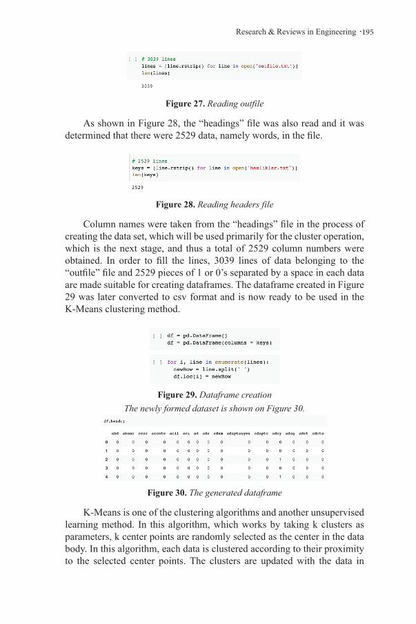
.195Research & Reviews in Engineering
Figure 27. Reading outfile
As shown in Figure 28, the “headings” file was also read and it was determined that there were 2529 data, namely words, in the file.
Figure 28. Reading headers file
Column names were taken from the “headings” file in the process of creating the data set, which will be used primarily for the cluster operation, which is the next stage, and thus a total of 2529 column numbers were obtained. In order to fill the lines, 3039 lines of data belonging to the “outfile” file and 2529 pieces of 1 or 0’s separated by a space in each data are made suitable for creating dataframes. The dataframe created in Figure 29 was later converted to csv format and is now ready to be used in the K-Means clustering method.
Figure 29. Dataframe creationThe newly formed dataset is shown on Figure 30.
Figure 30. The generated dataframe
K-Means is one of the clustering algorithms and another unsupervised learning method. In this algorithm, which works by taking k clusters as parameters, k center points are randomly selected as the center in the data body. In this algorithm, each data is clustered according to their proximity to the selected center points. The clusters are updated with the data in

Yunus Doğan, Feriştah Dalkiliç, Alp Kut, Kemal Can Kara, Uygar Takazoğlu196 .
the center points and clustering is done again with the new center points. This process continues until there is no change in the center points of the clusters [3] (Figure 31).
Figure 31. K-Means operations
The prepared data set was subjected to this algorithm. As a result of previous tests on the number of clusters to be formed, 302 as the optimal number of the cluster was chosen as the elbow point among the different cluster numbers. Then, with the “fit_predict” function, first the cluster centers were calculated, and it was determined which cluster each sample belonging to the resulting data set was in. On Figure 32, the clusters in which the first 10 samples are located after the estimation process is shown [4].
Figure 32. Distribution of instances in clusters
Clusters have center points. Considering that there are 2529 columns in the resulting data set, each cluster formed has 2529 center points. After the calculation, some of the center points are shown with the “cluster_centers_” function on Figure 33.
Figure 33. Center points of clusters
Then, as shown in Figure 34, the advertisements in each cluster were made into a list.

.197Research & Reviews in Engineering
Figure 34. Conversion of job-ads sets to lists
First, a new “txt” file was created, as seen in Figure 35, in order to create the file that will be used on C#, which is the last step with this list. First, the cluster name was assigned in a loop so that it would go through all the clusters. With the list of announcements belonging to the clusters obtained in the previous stage, each advertisement has been added, and finally, the “cluster_centers_” function has been added to the existing 2529 center points for each cluster.
Figure 35. Generating “txt” file for BIRCH algorithm
The example of the first cluster from the file created as the last step is shown on Figure 36. After that the data set was saved as “ads.txt”.
Figure 36. A new file sample

Yunus Doğan, Feriştah Dalkiliç, Alp Kut, Kemal Can Kara, Uygar Takazoğlu198 .
3. Conclusion
BIRCH algorithm, which is a stream mining algorithm, was used in this project. Job postings and three different data sets in total, shaped by these job postings, were determined to be studied. The task of each data set and the link between them were examined. Python was worked on for the first part of the application. Before the first cluster operation, the available data sets were made available. A dataframe was created with the first data set, which was shaped so that each text of job postings could use its own features as metrics, and the data set for the words that make up a corpus in order for these texts to have metric properties.
For the first stage, the K-Means clustering algorithm was investigated. Afterwards, the first clustering operation was performed by using the library on Python with the optimally selected number of clusters. The resulting 302 clusters were analyzed with the help of functions from the library.
With the completion of this stage, a new data set was created. The clusters from the K-Means operation were retrieved. A new data set was created by taking the cluster name for each, the indexes of the job postings they contain, and the center points of each cluster. Thus, a total of 3039 job postings were clustered and a new data set was created with 302 clusters consisting of these.
For the second part, a start was made on C#. All implementations were completed in C# by planning for the required new classes and functions.

.199Research & Reviews in Engineering
References
Barham, M. M. (2020). An Improved BIRCH Algorithm for Breast Cancer Clus-tering (Doctoral dissertation, Middle East University).
Dimara, A., Triantafyllidis, D., Krinidis, S., Kitsikoudis, K., Ioannidis, D., An-tipas, S., & Tzovaras, D. (2020, December). Fusing Birch with G. Boos-ting for improving temporal traffic congestion tailored to port gates: Case Study in Patras, Greece. In 2020 IEEE 17th International Conference on Smart Communities: Improving Quality of Life Using ICT, IoT and AI (HONET) (pp. 1-5). IEEE.
Fakir, Y., & El Iklil, J. (2021, May). Clustering Techniques for Big Data Mi-ning. In International Conference on Business Intelligence (pp. 183-200). Springer, Cham.
Gupta, A., “Balanced iterative reducing and clustering using hierarchies - birch,” Medium, 03-Jun-2021. [Online]. Available: https://medium.com/geek-culture/balanced-iterative-reducing-and-clustering-using-hierarchies-bir-ch-1428bb06bb38.
Gündoğan, E., & Kaya, M., (2021), Konu benzerliğine dayalı makale tavsiye sistemi. Computer Science, (Special), 175-183.
Hatipoglu, E., “Machine learning - clustering (Kümeleme) - K-means algorit-hm -hierarchical clustering” Medium, 15-Jul-2018. [Online]. Available: https://medium.com/@ekrem.hatipoglu/machine-learning-clustering-k%-C3%BCmeleme-k-means-algorithm-part-13-be33aeef4fc8. [Accessed: 10-Oct-2021]
Huang, Y. (2020). Financial Investment Recommendation in Coastal Areas Based on Improved Clustering Algorithm. Journal of Coastal Research, 110(SI), 215-218.
Katarya, R., & Saini, R. (2021). Enhancing the wine tasting experience using greedy clustering wine recommender system. Multimedia Tools and App-lications, 1-34.
Ramadhani, F., Zarlis, M., & Suwilo, S. (2020). Improve BIRCH algorithm for big data clustering. In IOP Conference Series: Materials Science and En-gineering (Vol. 725, No. 1, p. 012090). IOP Publishing.
Scikit, “Sklearn.cluster.kmeans,”. [Online]. Available: https://scikit-learn.org/stable/modules/generated/sklearn.cluster.KMeans.html. [Accessed: 10-Oct-2021].
Tsarouchis, S. F., Vartholomaios, A. S., Bountouridis, I. P., Karafyllis, A., Chry-sopoulos, A. C., & Mitkas, P. A. (2021, June). Science4Fashion: An Auto-nomous Recommendation System for Fashion Designers. In IFIP Interna-tional Conference on Artificial Intelligence Applications and Innovations (pp. 729-742). Springer, Cham.

Yunus Doğan, Feriştah Dalkiliç, Alp Kut, Kemal Can Kara, Uygar Takazoğlu200 .
Yilmaz, Z. A., Wang, S., Yang, W., Zhang, H., & Lin, J. (2019, November). App-lying BERT to document retrieval with birch. In Proceedings of the 2019 Conference on Empirical Methods in Natural Language Processing and the 9th International Joint Conference on Natural Language Processing (EMNLP-IJCNLP): System Demonstrations (pp. 19-24).

Chapter 12INNOVATION PROCESS OF ELECTRIC VEHICLES
Hilmi ZENKFaruk GÜNER
1. INTRODUCTION
Considering with a global projection, one of the biggest problems for humanity is undoubtedly climate change. The most important source of the global climate change phenomenon, which is now felt by everyone, in other words, the source of global warming is fossil fuels that emit excessive amounts of carbon into the atmosphere (Zenk, 2018a). Unfortunately, the damage of these fossil fuels is not limited to the environment, but also in the form of a continuous increase in the prices of products and services in economic activities on a global scale. Limited natural reserves necessitate the use of renewable resources or, more precisely, clean and green energy, as an alternative to electricity generation using conventional methods based on oil and coal (Zenk, 2018b). Renewable energy sources are wind power (Guner et al., 2021), solar power (Zenk, 2019a), hydro power (Güner and Zenk, 2020), biofuel power (Şenol and Zenk, 2020), geothermic energy etc. However, years of studies have shown that it is more practical and easier to convert solar energy directly into electrical energy (Zenk and Akpinar, 2013a). On average, Europe’s energy consumption was around 30 percent cleaner in 2020 than in 2015. The European Union aims to reduce carbon emissions by 50 percent by 2030. Similarly, the production and use of renewable energy has more than doubled in the last two decades in the United States. With the help of technological developments in the production phase, the cost of electricity produced from renewable energy sources is decreasing day by day (Zenk, 2019b), making renewable energy sources more attractive. It is very important for the continuation of all vitality that the classic vehicle industry with internal combustion engines, which is one of the sources that cause global warming by emitting harmful gases to the atmosphere, turns into an electric vehicle industry that uses electrical energy produced from renewable energy sources and has no harm to the environment. Then, any work that will improve the development of electric vehicles, improve their systems and eliminate their disadvantages against existing internal combustion engine vehicles is worthy of appreciation and support.
As it is known, electric vehicles are machines that provide the propulsion power by means of electric motors by taking the necessary energy for movement from the battery, in which the electrical energy previously produced from any energy source is stored by chemical methods. Although they are quieter and more environmentally friendly than conventional internal combustion vehicles, and they are more efficient due to their regenerative braking, the most important handicaps are the longer full charge time and shorter supply range.
It needs suitable power electronic circuits to convert the electrical energy in the charged battery groups of electric vehicles into AC or DC

electrical energy at different amplitude levels required by the AC or DC motors it has by design.
If the driving power is to be provided by DC motors, a DC-DC converter is needed (Zenk, 2018c). These DC-DC converters are buck (Zenk, 2018d), boost (Rashid, 2017), buck-boost (Zenk, 2017), forward (Mohan et al., 2003), flyback (Zenk, 2018e), zeta (Zenk, 2018f), push-pull (Zenk, 2016a), Cuk (Zenk and Akpinar, 2014) or SEPIC (Zenk, 2016b). It can be provided with type converters. Again, these converters are controlled with classical controllers such as P (Zenk et al., 2019), PI (Zenk and Altinkok, 2017), PD, PID (Zenk and Akpinar, 2013b) controller or by using advanced control methods such as fuzzy logic (Zenk et al, 2011, and Zenk, 2020) artificial neural networks vector control based methods, model prediction control and genetic algorithms.
Electric vehicles (EV) and fossil fuel-consuming Internal Combustion Engine (ICE) vehicles, whose historical process will be explained in more detail, have recently been introduced to the market and have started economic competition. Until recently, the energy density obtained with battery technology was much less than the energy density obtained from fossil fuels, which made ICE vehicles more preferred by the end users and competition developed against electric vehicles. The emergence of environmental problems, the oil crisis and the limited oil reserves caused electric vehicles to attract attention and show a rapid development process in the last quarter of the 20th century. Today, various electric vehicles with different technologies have started to hit the roads, and EVs with many new technologies are being studied. It is possible to structurally classify electric vehicles as battery electric vehicles (BEV), hybrid vehicles (HEV) and fuel cell vehicles (FCV) (Kahveci, 2013).
2. BATTERY ELECTRIC VEHICLES
2.1. History of Battery Electric Vehicles
It has started to develop since the end of the 18th century with a series of scientific advances in the field of electric vehicles, engine systems and batteries. This process, as a result of Luigi Galvani’s studies since the 1780s, was published in a book in 1791 with the name “Explaining the effect of electricity on muscle movement”, which he discovered using 2 metals and frog legs. By developing these works of Alessandra Volta, she managed to produce a current by arranging a circuit from two metals and a cloth or cardboard soaked in salt water. Volta begins with Alessandra Volta’s discovery of the non-rechargeable battery in 1800, as a result of a series of experiments on frogs, using copper and zinc discs instead of cloth and cardboard to increase electrolyte conductivity. Other researchers have called this basic battery the “Volta Battery”. Michael

Faraday demonstrated the basic principle of today’s electric motors by using the Volta Battery in 1821. Accordingly, when current flows through the conductor in the magnetic field, a force acts on this conductor. In 1828 Hungarian Ányos István Jedlik demonstrated the first device containing the three main components of practical direct current motors, the stator, rotor and commutator.
The first examples of electric vehicles date back to the 1830s in various sources. Of these, Scottish inventor Robert Anderson is known as the inventor of the first crude electric car. He became famous for releasing the first electric car prototype using non-rechargeable batteries (Graham et al., 2018). While the exact date is uncertain, the years Robert Anderson made this remarkable breakthrough in science were between 1832 and 1839. In another study, American inventor Thomas Davenport developed a battery-powered electric motor in 1834 and used it to power a small model car over a short distance. This vehicle was a small locomotive designed using two electromagnets, a pivot and a battery. This work paved the way for the electrification logic of trams. A short time later, Dutch chemistry professor and inventor Sibrandus Stratingh invented the first battery-electric vehicle, seen in Figure-1, in 1835.
Figure 1. One of the first electric vehicles (URL-1)
Non-rechargeable batteries were used as an energy source in these first electric vehicles and therefore they could not be commercially available. However, the development of rechargeable lead-acid batteries in 1859 led
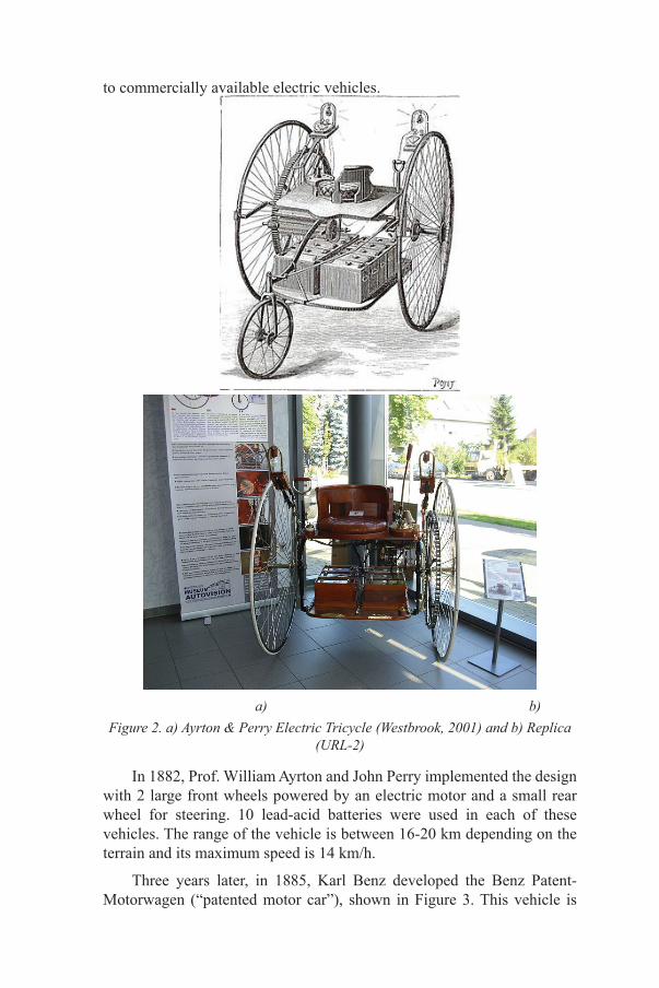
to commercially available electric vehicles.
a) b)Figure 2. a) Ayrton & Perry Electric Tricycle (Westbrook, 2001) and b) Replica
(URL-2)
In 1882, Prof. William Ayrton and John Perry implemented the design with 2 large front wheels powered by an electric motor and a small rear wheel for steering. 10 lead-acid batteries were used in each of these vehicles. The range of the vehicle is between 16-20 km depending on the terrain and its maximum speed is 14 km/h.
Three years later, in 1885, Karl Benz developed the Benz Patent-Motorwagen (“patented motor car”), shown in Figure 3. This vehicle is
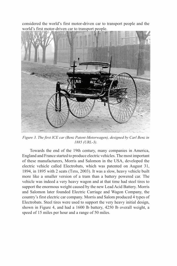
considered the world’s first motor-driven car to transport people and the world’s first motor-driven car to transport people.
Figure 3. The first ICE car (Benz Patent-Motorwagen), designed by Carl Benz in 1885 (URL-3).
Towards the end of the 19th century, many companies in America, England and France started to produce electric vehicles. The most important of these manufacturers, Morris and Salomon in the USA, developed the electric vehicle called Electrobats, which was patented on August 31, 1894, in 1895 with 2 seats (Tırıs, 2003). It was a slow, heavy vehicle built more like a smaller version of a tram than a battery powered car. The vehicle was indeed a very heavy wagon and at that time had steel tires to support the enormous weight caused by the new Lead Acid Battery. Morris and Salomon later founded Electric Carriage and Wagon Company, the country’s first electric car company. Morris and Salom produced 4 types of Electrobats. Steel tires were used to support the very heavy initial design, shown in Figure 4, and had a 1600 lb battery, 4250 lb overall weight, a speed of 15 miles per hour and a range of 50 miles.

Figure 4. The first design of the electric vehicle called Electrobats, made in 1894 (URL-4).
As research increased, the weight of other models was reduced, making them much more useful. The second model has two 1.5 hp engines, pneumatic tires and a rear-wheel steering design, with a battery weight of 640 lb and a total weight of 1650 lbs, with a speed of 32 km/h - a range of 40 km per charge. The fourth prototype, shown in Figure 5, is lighter than the others and was produced in late 1895. Reaching two 75 lb engines, a 350 lb battery and a total weight of 800 lbs, this model was the most efficient of the designs, with a range of 20-25 miles at a speed of 15 miles per hour.
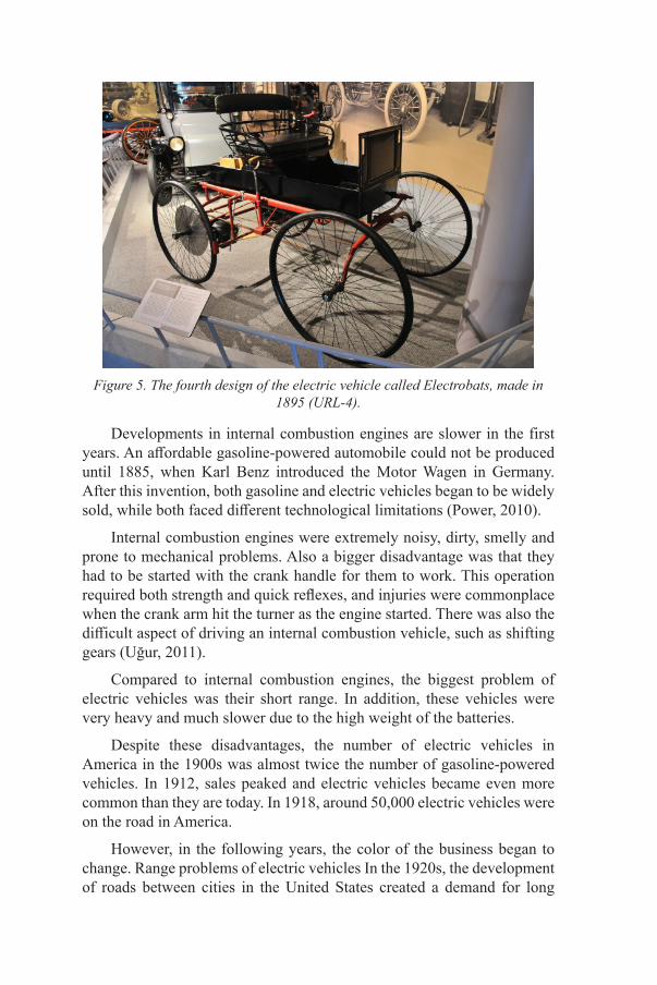
Figure 5. The fourth design of the electric vehicle called Electrobats, made in 1895 (URL-4).
Developments in internal combustion engines are slower in the first years. An affordable gasoline-powered automobile could not be produced until 1885, when Karl Benz introduced the Motor Wagen in Germany. After this invention, both gasoline and electric vehicles began to be widely sold, while both faced different technological limitations (Power, 2010).
Internal combustion engines were extremely noisy, dirty, smelly and prone to mechanical problems. Also a bigger disadvantage was that they had to be started with the crank handle for them to work. This operation required both strength and quick reflexes, and injuries were commonplace when the crank arm hit the turner as the engine started. There was also the difficult aspect of driving an internal combustion vehicle, such as shifting gears (Uğur, 2011).
Compared to internal combustion engines, the biggest problem of electric vehicles was their short range. In addition, these vehicles were very heavy and much slower due to the high weight of the batteries.
Despite these disadvantages, the number of electric vehicles in America in the 1900s was almost twice the number of gasoline-powered vehicles. In 1912, sales peaked and electric vehicles became even more common than they are today. In 1918, around 50,000 electric vehicles were on the road in America.
However, in the following years, the color of the business began to change. Range problems of electric vehicles In the 1920s, the development of roads between cities in the United States created a demand for long
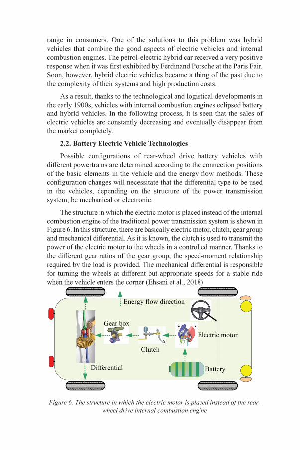
range in consumers. One of the solutions to this problem was hybrid vehicles that combine the good aspects of electric vehicles and internal combustion engines. The petrol-electric hybrid car received a very positive response when it was first exhibited by Ferdinand Porsche at the Paris Fair. Soon, however, hybrid electric vehicles became a thing of the past due to the complexity of their systems and high production costs.
As a result, thanks to the technological and logistical developments in the early 1900s, vehicles with internal combustion engines eclipsed battery and hybrid vehicles. In the following process, it is seen that the sales of electric vehicles are constantly decreasing and eventually disappear from the market completely.
2.2. Battery Electric Vehicle Technologies
Possible configurations of rear-wheel drive battery vehicles with different powertrains are determined according to the connection positions of the basic elements in the vehicle and the energy flow methods. These configuration changes will necessitate that the differential type to be used in the vehicles, depending on the structure of the power transmission system, be mechanical or electronic.
The structure in which the electric motor is placed instead of the internal combustion engine of the traditional power transmission system is shown in Figure 6. In this structure, there are basically electric motor, clutch, gear group and mechanical differential. As it is known, the clutch is used to transmit the power of the electric motor to the wheels in a controlled manner. Thanks to the different gear ratios of the gear group, the speed-moment relationship required by the load is provided. The mechanical differential is responsible for turning the wheels at different but appropriate speeds for a stable ride when the vehicle enters the corner (Ehsani et al., 2018)
Differential
Electric motor
Clutch
Gear box
Battery
Energy flow direction
Figure 6. The structure in which the electric motor is placed instead of the rear-wheel drive internal combustion engine
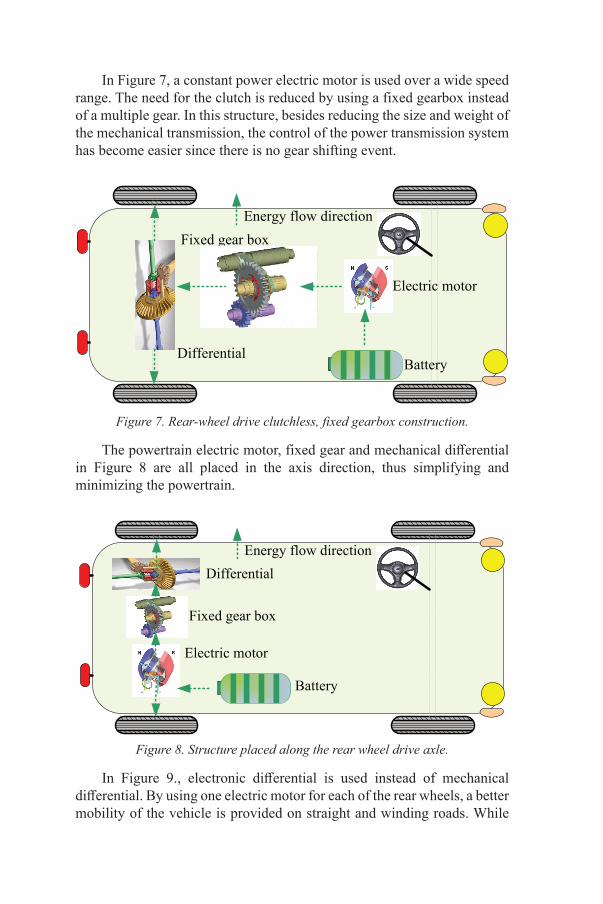
In Figure 7, a constant power electric motor is used over a wide speed range. The need for the clutch is reduced by using a fixed gearbox instead of a multiple gear. In this structure, besides reducing the size and weight of the mechanical transmission, the control of the power transmission system has become easier since there is no gear shifting event.
Differential
Electric motor
Fixed gear box
Battery
Energy flow direction
Figure 7. Rear-wheel drive clutchless, fixed gearbox construction.
The powertrain electric motor, fixed gear and mechanical differential in Figure 8 are all placed in the axis direction, thus simplifying and minimizing the powertrain.
Differential
Electric motor
Fixed gear box
Battery
Energy flow direction
Figure 8. Structure placed along the rear wheel drive axle.
In Figure 9., electronic differential is used instead of mechanical differential. By using one electric motor for each of the rear wheels, a better mobility of the vehicle is provided on straight and winding roads. While

the vehicle is moving along the bend, the motors on the right and left turn the wheels according to the direction of the vehicle at a speed determined in accordance with the electronic differential algorithm.
Electric motorFixed Gear Battery
Energy flow direction
Figure 9. Rear wheel drive independent wheel motor structure.
In Figure 10, the drive is built into the wheels, like the motors, to further simplify the powertrain. This arrangement is referred to as “in-wheel driving” in the literature. Fixed gear can be used to reduce engine speed and increase torque.
Electric motor
Fixed Gear
Battery
Fixed Gear
Energy flow direction
Figure 10. Rear wheel drive structure.
Figure 11 shows the structure where there is no mechanical gear between the electric motors and the drive wheels. The most important feature of the motors used here is that they are external rotors. These outer rotor motors should have low speed and high starting torque [38].

Electric motor
Battery
Electric motor
Battery
Energy flow direction
Figure 11. The structure using a rear wheel drive outer rotor motor.
3. HYBRID ELECTRIC VEHICLES (HEV)
Vehicles that use more than one type of energy as an energy source are called hybrid electric vehicles. Hybrid vehicles are designed with the aim of improving the range problem of electric vehicles and the carbon emission problems of ICE vehicles. One of the methods to be used to reduce carbon emissions is to use a fossil fuel engine that will produce low emissions regardless of the vehicle’s speed and acceleration, as another method, to ensure zero emissions by using only electrical energy when appropriate.
3.1. History of Hybrid Electric Vehicles
In the history of technology, it is accepted that the first hybrid design car called “Mixte-Wagen” was made by Ferdinand Porsche in 1902. Working with Ludwig Lohner, a Viennese phaeton manufacturer, Porsche produced an electric vehicle that can be classified in the serial hybrid vehicle category (URL-5). In the designed vehicle, it was based on the principle of converting the mechanical power produced by the internal combustion engine into electrical energy from a generator and converting it back into mechanical energy in four separate electric motors located on the wheels.

a) b)
Figure 12. a) The first hybrid vehicle in history (URL-6) and b) replica (URL-7)
There are many hybrid electric vehicles in the automotive market. Toyota’s Toyota Prius model, Honda’s Honda Insight model and Honda Civic Hybrid series are examples of hybrid vehicles. The answer to the question of whether hybrid vehicles can still completely replace classical ICE vehicles is related to how technology will evolve. The avoidance of automotive companies to meet the necessary technological investments and the lack of infrastructure to be created by filling stations to charge hybrid vehicles limit the share of hybrid vehicles in the automotive sales pie. In order to establish this infrastructure, governments need to invest significantly. Another obstacle to the widespread use of hybrid vehicles is the price disadvantage of conventional vehicles. On the other hand, many states have regulated their taxation system according to gas emission in order to encourage environmentalist vehicles. These countries are trying to eliminate the price disadvantage of green vehicles by making tax deductions for green vehicles and by taking additional taxes from non-environmental vehicles (URL-8).
3.2. Hybrid Electric Vehicle Technologies
As it is known, hybrid electric vehicles (HEA) are vehicles with two energy sources, one main source and at least one auxiliary source. Generally, fossil fuels or hydrogen are used as the main energy source (MES), while chemical batteries, flywheels, and supercapacitors can be used as auxiliary energy sources (AES). Today, in HEA, fossil fuels are generally used as MES, and chemical batteries and supercapacities are used as AES.
Hybrid vehicles are designed in three structures: serial, parallel and serial-parallel. In order to use multiple energy sources efficiently, a central energy management system (EMS) is needed in the vehicle. EMS can sequentially activate MES, AES or both, using appropriate algorithms

to provide the energy to move the vehicle. In order to increase vehicle efficiency, EMS manages the energy recovery with the dynamic braking method during braking, when going downhill or while driving at a constant speed on a flat road.
3.2.1. Series Hybrid Electric Vehicles
Series hybrid electric vehicles (SHEV) use only an electric motor as the propulsion motor. In terms of these features, they are similar to battery electric vehicles. The internal combustion (ICE) engine works in conjunction with a generator to supply the electric motor it needs to drive the vehicle. A general powertrain system of SHEV is given in Figure 13.
Electric motor
Battery
G
~- Inverter
ElectricalEnergy Direction
Mechanical Energy Direction
Generator
Internal-combustion engine
Figure 13. Enhanced powertrain for rear-wheel drive or front-wheel drive SHEV
The control center of the serial hybrid vehicle is responsible for the operation of the EMS, evaluating the inputs and switching between the different operating modes. Since the volume of the ICE in a serial hybrid vehicle is only used for power transmission, it is smaller than in a conventional vehicle with the same features. The control system is operated within a certain range that will include the ICE, the point where the efficiency is highest. In this way, emission values have been reduced both by reducing the volume and by providing continuous high efficiency operation. Auxiliary energy sources, on the other hand, can be used to drive the vehicle without using fossil fuels until the energy is depleted, except in situations that require sudden power such as sudden acceleration of the vehicle and climbing a hill. EMS also manages the recovery of energy when braking or going downhill.
In SHEA, since the ICE engine does not have a mechanical connection with the power transmission system, it can be placed anywhere, except the passenger cabin. This provides a lot of flexibility in the design of the

vehicle. Using only the electric motor as the drive motor can eliminate the need for a gearbox. However, the mechanical, electrical and chemical energy conversion steps of these vehicles reduce their efficiency. Since SHEA also needs to meet the needs of urban use, electric drive motors and battery groups should be chosen quite large.
3.2.2. Parallel Hybrid Electric Vehicles
Parallel Hybrid Electric Vehicles (PHEV), unlike SHEV, provide their movement with both ICE and electric motor. In Figure 14. the structure of parallel hybrid vehicles in general is given.
Electric motor Battery
~- Inverter
ElectricalEnergy Direction
Mechanical Energy Direction
Internal-combustion engine
Figure 14. An example of a PHEV rear-drive design.
In the PHEV design, unlike the SHEV design, there is a mechanical connection between the ICE and the wheels. In the PHEA design, ICE provides the general movement of the vehicle. The electric motor (EM) activates only as an aid in sudden accelerations and uphill climbs. Vehicle acceleration can be shared with both EM and ICE. For this reason, designs can be made with different power draw logic such as only EM Mode, only ICE Mode, ICE - EM power sharing mode. For these sudden power needs, they are met with a smaller powerful EM than the electric motor in SHEA. However, this engine does not have the power to move the vehicle alone. There is no need for an extra generator in PHEA. Thus, the energy conversion steps are reduced. Combining ICE and electric motor outputs with mechanical coupling complicates the control of PHEA under different operating conditions. Also, in Parallel Charge mode, the ICE can charge the batteries by operating the EM as a generator, while providing torque for traction.
Parallel Hybrid Electric Vehicles can be designed in different structures such as split shaft drive, common shaft drive, front and rear drive.

3.2.3. Series-Parallel Hybrid Electric Vehicle Configuration
This configuration, seen in Figure 15, includes more driving modes as it includes serial and parallel hybrid configurations separately. In this design, the system allows both serial Mode charging and power-sharing driving. That is, ICE cuts off the mechanical energy flow from the wheels when necessary and can only be connected to the generator to generate electrical energy.
Electric motor Battery
~- Inverter
ElectricalEnergy Direction
Mechanical Energy Direction
Internal-combustion engine
GGenerator
Figure 15. Serial-Parallel HEV configuration.
3.3. Externally Rechargeable Hybrid Electric Vehicle Designs
The fact that the vehicle battery can be charged from an external source, that is, via the network, changes both the battery characteristics and the basic operating algorithm of the vehicle’s Energy Management System. Since electric vehicles have a very flexible design, although there is no definitive binding definition for any method, in rechargeable hybrid vehicles, the EM and battery system are designed to cover the entire drive as energy and power characteristics. ICE is used as a charge balancing unit, or in broader terms, for a range increasing purpose. There are even serial rechargeable hybrid electric vehicles in which the ICE is completely independent of wheel loads.
3.4. Hybrid Vehicle Energy Management Systems
Due to the efficient use of the limited battery capacity of a non-rechargeable hybrid electric vehicle, it is operated in a limited charging range under constant voltage due to its battery life feature. The charge of the batteries in these vehicles oscillates between the maximum allowable balances (SOCmax) and the minimum charge balances (SOCmin), as seen
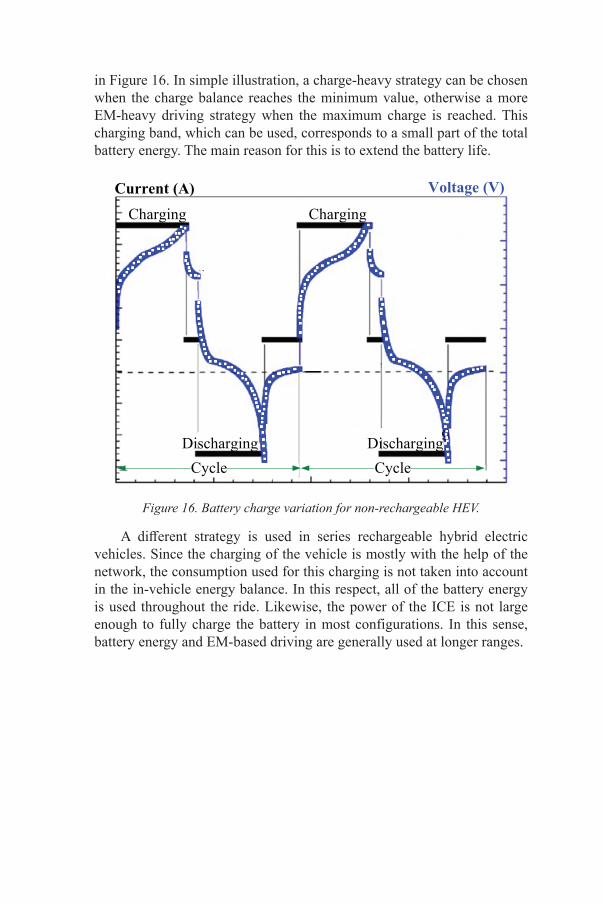
in Figure 16. In simple illustration, a charge-heavy strategy can be chosen when the charge balance reaches the minimum value, otherwise a more EM-heavy driving strategy when the maximum charge is reached. This charging band, which can be used, corresponds to a small part of the total battery energy. The main reason for this is to extend the battery life.
Discharging Discharging
Charging ChargingCurrent (A) Voltage (V)
CycleCycle
Figure 16. Battery charge variation for non-rechargeable HEV.
A different strategy is used in series rechargeable hybrid electric vehicles. Since the charging of the vehicle is mostly with the help of the network, the consumption used for this charging is not taken into account in the in-vehicle energy balance. In this respect, all of the battery energy is used throughout the ride. Likewise, the power of the ICE is not large enough to fully charge the battery in most configurations. In this sense, battery energy and EM-based driving are generally used at longer ranges.

SOCmin
SOCmaxSO
C
Discharging Mode ChargeBalanceModeCharging Mode Discharging
Mode
Figure 17. Battery charge change for serial rechargeable hybrid electric vehicles.
Figure 17. shows the battery charge profile and strategies used for a typical rechargeable HEV. Until the charge reaches a certain value, while the vehicle is operating in the mode for charge consumption, charge balancing mode becomes active when the charge reaches a critical point. In this case, while the ICE starts to operate at more frequent intervals, the battery charge is released at a certain value. In de-charge mode, ICE is only used to respond to peak power requests. For serial rechargeable hybrid electric vehicles, the strategies and configurations are generally as explained above, but there are other applications as well.
4. EV Energy Storage Units
The main energy storage unit in electric vehicles, where the most advanced technologies in energy conversion are used, is undoubtedly the batteries that convert chemical energy into electrical energy. Apart from batteries, hydrogen stored for use in fuel cells, flywheels and supercapacitors are energy storage units that can be preferred according to vehicle design and technology. A selection is made among these storage units according to the intended use, cost and cycle life of the vehicle.
4.1. Batteries
The battery, which is one of the most common practical energy sources today and was discovered by chance in 1800, is a device used to store chemical energy and convert it into an electrical form. Technically, a battery is formed by the combination of two or more electrical cells. Cells formed by positive and negative electrodes with electrolytes between them convert chemical energy into electrical energy or electrical energy into chemical Energy (Zenk and Ertuğral, 2018a). A large number of

batteries with different structures can be obtained by combining different metals and electrolytes. However, the types of commercially valuable and rechargeable batteries that can be used in electric vehicles are limited; lead acid, nickel iron, nickel cadmium, nickel iron hydride, lithium polymer and lithium iron, sodium sulfide and sodium metal chloride. It is also possible to come across batteries that are filled by changing the metal inside (Zenk and Ertuğral, 2018b).
4.2. Super Capacities
Supercapacitors are used in applications that require long-term compact energy storage rather than very fast charge/discharge. These applications can be automobiles, buses, trains, cranes and elevators, energy recovery braking used, short-term energy storage or burst mode. Supercapacitors can be designed to have a specific energy of a few Wh/kg and a specific power of kW/kg. In terms of these features, they cannot store the energy that will bring a vehicle to a sufficient range on their own. However, they are very effective in meeting the power needed in sudden accelerations and heavy traffic, in cases where there are many stops and starts. For this reason, they are widely used as an auxiliary source in battery, fuel cell or hybrid vehicles. Since they have very short charge and discharge times, it is possible to charge them with the energy to be recovered during braking. Supercapacitors, which withstand the high currents to be drawn from the main energy source or to be obtained by recovery, extend the durability and life of the main energy source. In addition, the high cost is seen as the biggest disadvantage.
4.3. Flywheels
The most important feature of the flywheel, which is used in all vehicles, is that it can store the energy that will be lost and allow it to be used when necessary. Generally, the geometric shape of a flywheel is a kind of cylindrical disk with large diameter and small width. Since flywheels are mechanical systems that can store kinetic energy by stretching the materials in their structure, their specific energies can reach 50 Wh/kg and their specific power can reach 2000 W/kg. In ICE vehicles, flywheels, which can be considered small, are used to dampen the vibrations that occur during the first start of the engine and its sudden acceleration. Flywheels are used in electric vehicles to store kinetic energy during braking and then to convert it back into kinetic energy when moving. Their efficiency is high compared to chemical batteries, their life cycle is very long, their performance is the same even after long usage and there is no toxic gas emission. The balancing forces on the flywheel itself make it difficult to control the vehicle when the vehicle is going up and down a slope or entering a bend. In addition, they have not become widespread in terms of

use, since damage to the flywheel in the event of an accident may lead to new accidents with the energy stored on it.
4.4. Fuel Cells
Fuel cells, like batteries, make chemical transformations. However, these are systems in which pure hydrogen is used as fuel and converted into electrical energy for this conversion. In fuel cells, a chemical reaction takes place with two electrodes as anode and cathode, and the structure formed by the electrolyte through which the ions will move. Different types of fuel cells are produced according to the type of electrolyte in their structures. Fuel cell vehicles have a longer range than battery powered vehicles. Compared to ICE vehicles, their efficiency is higher and there are no harmful gas emissions. Fuel cell vehicles have advantages as well as disadvantages that cause them not to be commercialized. Chief among these is their high cost. In addition, it is difficult to remove the water formed as a result of the chemical reaction from the cell. Again, due to the heat released as a result of the chemical reaction, they need a cooling system. Obtaining, storing and transmitting hydrogen, which is used as a fuel, requires addressing different problems.
References
Zenk, H. (2018a). Investigation of Energy Efficiency in Turkey. Annals of the Faculty of Engineering Hunedoara, 16(1), 93-96.
Zenk, H. (2018b). Low Cost Provides of the Energy Needs of Plateau Houses by Using Photovoltaic Systems. Turkish Journal of Agriculture-Food Science and Technology, 6(12), 1768-1774.
Güner, F., Başer, V., & Zenk, H. (2021). Evaluation of offshore wind power plant sustainability: a case study of Sinop/Gerze, Turkey. International Journal of Global Warming, 23(4), 370-384.
Zenk, H. (2019a). Comparison of the performance of photovoltaic power genera-tion-consumption system with push-pull converter under the effect of five different types of controllers. International Journal of Photoenergy, 2019.
Guner, F., & Zenk, H. (2020). Experimental, Numerical and Application Analysis of Hydrokinetic Turbine Performance with Fixed Rotating Blades. Ener-gies, 13(3), 766.
Şenol, H., & Zenk, H. (2020). Determination of the biogas potential in cities with hazelnut production and examination of potential energy savings in Turkey. Fuel, 270, 117577.
Zenk, H. & Akpinar, A. S. (2013a). Solar Power Generation Potentials of The Houses in Turkey. International Conference on Environmental Science and Technology (ICOEST 2013).
Zenk, H. (2019b). The Electric Energy Potential of Samsun City from Animal Manure. European Journal of Science and Technology, (17), 1307-1312.
Zenk, H. (2018c). Comparison of Electrical Performances of Power Electronics Switches and an Effective Switch Selection Algorithm. Acta Physica Po-lonica A, 133(4), 897-901.
Zenk, H. (2018d). Comparison of Output Parameters of Two-Phase Interleaved Buck Converter Using Different Type Control Methods. Journal of Mul-tidisciplinary Engineering Science Studies (JMESS), 4(11), 2271-2276.
Rashid, M. H. (Ed.). (2017). Power electronics handbook. Butterworth-Heine-mann.
Zenk, H. (2017). High Performance DC Converter Designs With Controlled By A Simulink Software For Electric Motors. International Journal of Enginee-ring and Information Systems (IJEAIS), 1(10), 58-66.
Mohan, N., Undeland, T. M., & Robbins, W. P. (2003). Power electronics: con-verters, applications, and design. John wiley & sons.
Zenk, H. (2018e). An Effective Flyback Converter Design for PMDC Motor Control. Karadeniz Fen Bilimleri Dergisi, 8(2), 207-215.

Zenk, H. (2018f). Effective Control of the Developmental Current of a Serial DC Motor with a Fuzzy Tuned-PI Controller Zeta Converter. Karadeniz Fen Bilimleri Dergisi, 9(1), 196-211.
Zenk, H. (2016a). In push-pull converter output voltage stability comparison with using fuzzy logic, PI and PID controllers. International Journal of Engine-ering Research and Management (IJERM), 3(12), 1-6.
Zenk, H., & Akpinar, A. S. (2014). Dynamic Performance Comparison of Cúk Converter with DC Motor Driving and Using PI, PID, Fuzzy Logic Types Controllers. Universal Journal of Electrical and Electronic Engineering, 2(2), 90-96.
Zenk, H. (2016b). A Comparative Application of Performance of the SEPIC Converter Using PI, PID and Fuzzy Logic Controllers for PMDC Motor Speed Analysis. Journal of Multidisciplinary Engineering Science Studies (JMESS), 2(12), 1226-1231.
Zenk, H., Şenol, H., & Güner, F. (2019). Lunar Excursion Module Landing Cont-rol System Design with P, PI and PID Controllers. Karadeniz Fen Bilim-leri Dergisi, 9(2), 390-405.
Zenk, H., & Altinkok, A. (2017). Output Voltage Control of PI And Fuzzy Logic Based Zeta Converter. IOSR Journal of Electrical and Electronics Engine-ering (IOSR-JEEE), 12(6), 63-70.
Zenk, H., & Akpinar, A. S. (2013b). PI, PID and fuzzy logic controlled SSSC connected to a power transmission line, voltage control performance com-parison. In 4th International Conference on Power Engineering, Energy and Electrical Drives (pp. 1493-1497). IEEE.
Zenk, H., Zenk, O., & Akpinar, A. S. (2011). Two different power control system load-frequency analysis using fuzzy logic controller. In 2011 International Symposium on Innovations in Intelligent Systems and Applications (pp. 465-469). IEEE.
Zenk, H. (2020) Fotovoltaik Enerji Kaynaklı İkili Yapılı Flyback Dönüştürü-cünün Fuzzy-Tuned PI ve Fractional PID Tipi Denetleyicilerle Gerilim Kararlılığının Karşılaştırılması. Karadeniz Fen Bilimleri Dergisi, 10(2), 443-465.
Kahveci, H. (2013). Doğrudan sürüşlü elektrikli araçlar için bulanık mantık ta-banlı elektronik diferansiyel sisteminin gerçeklenmesi (Doctoral disserta-tion, Karadeniz Teknik Üniversitesi).
Graham, J. D., Messer, N. M., Hartmann, D., Lane, B. W., Carley, S., & Crook-ham, C. (2011). Plug-in electric vehicles: a practical plan for progress. School of Public and Environmental Affairs at Indiana University, Bloo-mington, Indiana.
URL-1: https://www.electricvehiclesnews.com/History/historyearlyII.htm
Westbrook, M. H., & Westbrook, M. H. (2001). The Electric Car: Development and future of battery, hybrid and fuel-cell cars (No. 38). Iet.
URL-2: https://de.wikipedia.org/wiki/Ayrton_%26_Perry_Electric_Tricycle#ci-te_ref-2
URL-3: https://tr.wikipedia.org/wiki/Benz_Patent-Motorwagen#Teknik_veriler
Tırıs, M. (2003). Elektrikli Araçlar. TÜBİTAK-MAM Yayını, Kocaeli.
URL-4: https://www.kcstudio.com/electrobat.html.
Power, J. D. (2010). Drive green 2020: more hope than reality. A Special Report by JD Power and Associates.(Kasım 2010), (s 2).
Uğur, E. (2011). Prototip bir elektrikli araç üzerinde enerji yönetim sisteminin uygulanması. (Master dissertation, Yıldız Teknik Üniversitesi).
Ehsani, M., Gao, Y., Longo, S., & Ebrahimi, K. M. (2018). Modern electric, hyb-rid electric, and fuel cell vehicles. CRC press.
URL-5:https://tr.wikipedia.org/wiki/Hibrit_(otomobil)
URL-6:https://de.wikipedia.org/wiki/Lohner-Porsche#/media/Datei:GenevaMo-torShow2011.jpg
URL-7: https://tr.wikipedia.org/wiki/Hibrit_(otomobil)
URL-8: http://www.hybrid-vehicle.org/hybrid-vehicle-history.html
Zenk, O., & Ertuğral, B. (2018a). An Investigation of Increasing the Performance of Electric Rickshaw-Pedicab Batteries. International Journal of Enginee-ring and Information Systems (IJEAIS), 2(12).
Zenk H., & Ertuğral B. (2018b). Comparison of the Electrical Performance of NiCd, NiMH and Li-Ion Batteries by Simulation. International Conferen-ce on Agriculture, Technology, Engineering and Sciences (ICATES 2018), 1(1), 352-363.


Chapter 13 STANDARD TEST METHODS FOR DETERMINING BITÜMEN BINDERS AND ASPHALT PAVEMENTS PROPERTIES
Savas GURDAL1
1 Dr., Science and Technology Application and Research Center, Çanakkale Onsekiz Mart Uni-versity, Turkey, E-mail: [email protected] ORCID: 0000-0002-1149-4371
Savas Gurdal226 .
1. Introduction
The properties of bitumen play an important role in determining the performance of asphalt pavements (Corte,2001) Characterization of bitumen binders in engineering applications is important for determining the effects of temperature and strain ( Remišová and Holý, 2017)
Empirical studies on asphalt pavements were defined in the 1950s. But, most of these studies were renewed in the 1980s. Since then, many new devices, tests and equipment have been developed. In addition, with the computer’s intense entry into our lives, it has become easier and more reliable to reach the results. Most of the countries around the world have started to implement design and testing procedures in asphalt pavement technology. Bitumen has been classified in different degrees according to its mechanical properties since the earliest times. The most important feature in determining the grade of bitumen has always been the degree of penetration. Due to the increasing traffic and recycling needs over time, it has been deemed necessary to perform performance tests of bitumen. In addition, with the new regulations made in petrochemical facilities in recent years, different types of bitumen binders have been offered to the public(rheofalt.com, 2021).
The total number of standard axle repetitions increasing day by day on the roads, higher performance demand has necessitated long-term performance estimation of pavements. The performance of the superstructure; It depends on many factors, including design, application and the quality of the material used. The first application in asphalt pavements is the mix design process. The mixture of bitumen binder and aggregate must be of good quality in order for the asphalt pavement to be least affected by the traffic life and the effects of the environment( Celko, Kovac and Decky,2011; Durcanska et. al, 2013)
The quality of bitumen is indicated by many indicators. In this study, tests used in bitumen binder and asphalt pavements are listed to guide researchers.
2. Test Methods
Standard test methods for determining bitümen binders and asphalt pavements properties listed below to guide researchers. In each test, valid standards related to the relevant test are shown.
• Needle Penetration
• Flash and Fire Points
• Specific Gravity Test
• Solubility

.227Research & Reviews in Engineering
• Softening Point of Bitumen (Ring-and-Ball Apparatus)
• Water Content in Bituminous Materials
• Settlement in Bitumen Emulsions ( 5 Days)
• Distilation and Evaporation Residue Test
• Ductility Testing
• Storage Stability Test
• Fraas Breaking Point Test
• Elastic Recovery of Bitumen
• Superpave Gyratory Compactor (SGC)
• Rolling Thin Film Oven Test (RTFOT)
• Rheological Properties of Asphalt Binder Using a Dynamic Shear Rheometer (DSR)
• Presure Agıng Vessel (PAV)
• Flexural-Creep Stiffness with Bending Beam Rheometer (BBR)
• Direct Tension Test (DTT)
• Indirect Tensile Strength Test (IDT)
• Rotational Viscometer Tests
2.1. Needle Penetration
Identification in bitumen is based on the penetration grade and penetration grade helps to determine the class of the bitumen. The penetration grade of bitumen is determined by the penetration and softening point test. Penetration grade bitumens have a thermoplastic property that causes the material to soften at high temperatures and harden at lower temperatures. This relationship between temperature and viscosity is important in determining the performance parameters of bitumen such as adhesion, rheology, durability and application temperatures (rheofalt.com, 2021).
The device is used to measure the needle pricking depth/penetration of samples at the load, time and temperature defined in the relevant standard.
The distance that a standard needle vertically sinks into the bitumen binder for a certain time (5 seconds) under a certain load (100 g) is found in 0.1mm.

Savas Gurdal228 .
Figure 1. Needle Penetration Test Scheme
Penetration value is inversely proportional to consistency. The hardness or consistency of the bituminous binder is determined. The higher the penetration, the softer the bitumen. As the consistency increases, the bitumen hardens (Jensen, 2006)
Figure 2. Consistency varies with temperature
Standards
ASTM D946-09
EN 12591-2009Table 1. ASTM Standard for Bitumen Penetration Grade
Standard Bitumen Penetration GradeASTM D946-09 40-50 60-70 85-100 120-150 200-230

.229Research & Reviews in Engineering
Table 2. EN standard for Bitumen Penetration Grade
Standard Bitumen Penetration GradeEN 12591-2009 20-30 30-45 35-50 40-60 50-70 70-100 160-220
2.2. Flash and Fire Points
Flash point of bitumen is the lowest temperature, at the bitumen vapor comes into contact with the flame and shines temporarily but there is no combustion process. This test is important to determine the risk of ignition and ignition that may occur while the heating of the bitumen during application. Heating is performed according to the flash point and necessary precautions can be taken.
Flash point determination is made with Cleveland Open Container and Tagliabue Closed Container depending on the characteristics of the bitumen.
Standards
TS EN ISO 2592
TS 1171
2.3. Specific Gravity Test
While calculating the specific gravity of bituminous materials, its weight in a certain volume at 25 °C is measured. Then It is proportioned to the air of the degased distilled water of the same temperature and volume. The specific gravity of bitumen is usually determined by the pycnometer method.
Standards
TS 1087
2.4. Solubility
Bitumen is dissolved in organic solvents such as trichloroethylene, carbon sulfide, benzene to determine the mineral substances that are present in little or no bitumen. Its solubility in trichloroethylene is expected to be at least 99%.
Standards
TS EN 12592
ASTM D2042
2.5. Softening Point of Bitumen
Scope of this experiment is measure the sensitivity of bitumen to temperature. The method called the ring-ball method is applied. The

Savas Gurdal230 .
temperature, where the bitumen begins to flow, the softening point is determined. Bitumen with high viscosity also has a high softening point. Mixture temperatures are also high in hot mixtures prepared with that kind of bitumen (Jensen, 2006).
The following procedure is applied during the experiment:
The bitumen in a standard ring mold with a ball on is placed in a water-filled beaker.
Then the bitumen begins to be heated.
As the material softens, the ball touches the bottom and this temperature is recorded
This is the softening point of the bitumen.
Standards
TS EN 1427
ASTM D36
2.6. Water Content in Bituminous Materials
Determination of water content in bituminous materials is applied on the basis of distillation of bitumen with volatile solvents. In the experiment, the solvent and sample are distilled under graduated reflux. Then, water and solvent are condensed. The water steam is separated in the condenser, while the solvent returns to the distillation vessel for further distillation. After the distilation water content is calculated.
Standards
ASTM D95
ASTM D244
AASHTO T55
2.7. Settlement in Bitumen Emulsions ( 5 Days)
Settlement in Bitumen Emulsions method applied when bitumen mixtures need storage. This method should not be applied if the bitumen mixtures do not need storage. The procedures applied in the method are as follows:
Bitumen is taken into a measuring tape at room temperature.
The bitumen mixture is kept for 5 days.
After 5 days, samples are taken from the upper and lower parts of the bitumen mixture and the residual amounts are determined.

.231Research & Reviews in Engineering
The difference between the lower and upper part should be less than 5%.
Standards
TS EN 122
2.8. Distilation and Evaporation Residue Test
In asphalt emulsions and asphalts, distillation and evaporation processes are performed in order to determine the amount of bitumen in the pavement. Different methods can be used in the application of distillation and evaporation processes.
Standards
ASTM D6934
TS 122
2.9. Ductility Testing
Bu deney kapsamında, bitümlü bağlayıcının 25, 13 ve 7 oC gibi sıcaklıklarda kohezyondan oluşan uzama veya çekme dayanımı belirlenir. Çalışma sıcaklığına getirilen bir su banyosu içerisindeki bitüm 50mm/dk hız ile çekilir. Bitümün kopma anındaki uzama miktarı ölçülür ve yük uzama eğrisinde karşılık gelen noktadan deformasyon enerjisi hesplanmaktadır (utest.com, 2021)
Within the scope of this test, the ductility or tensile strength of the bituminous binder, which is formed by cohesion at temperatures such as 25 °C, 13 °C and 7 °C, is determined. The bitumen in a water bath at operating temperature is withdrawn at a speed of 50mm/min. The amount of elongation of the bitumen at break is measured and the deformation energy is calculated from the corresponding point on the load elongation curve (isfalt.istanbul, 2021)
Standards
EN 13398
ASTM D113
D6084
AASHTO T51
2.10. Storage Stability Test
In this experiment, the cigar tube test (CTT) is used to determine the storage stability. The thin film size aluminum tube is filled with bitumen binder and placed upright in the oven. The temperature is set to 163 °C and waited for 48 hours. Then, samples quickly taken from the oven are kept
Savas Gurdal232 .
in the deep freezer for at least 4 hours. Afterwards, these tubes are cut into 3 parts. The softening point is determined by taking parts from these 3 samples. If the difference between the lower and the upper parts is more than 2.2 °C, it is called not stable. Sample preparation, sample production and temperature conditioning are performed according to ASTM D7173-05 instruction. ( Zhang and Hu, 2013).
Calculation equation:
(G*/sin δ)max - (G*/sin δ)avg
Separation, % = x 100
(G*/sin δ)avg
G* : shear modulus
δ : phase angle
(G*/sin δ) max = higher value,
(G*/sin δ) avg average value
Standards
EN 13399:2017
ASTM D7173-05
2.11. Fraas Breaking Point Test
The Fraas Breakpoint test is applied to bitumen and modified bitumen. The aim of this experiment is to determine the behavior of bitumen at low temperature. Temperature, Where the bitumen breaks and critical hardness are determined.
In this context, the bitumen sample is applied as a thin film on both sides of a metal sheet. Afterwards, the metal layer is started to be cooled at a constant rate. Then, the bitumen film is stretched until cracking is observed on the film. The temperature at which the first cracking is observed is called the Fraas break point.
Standards
EN 12593
2.12. Elastic Recovery of Bitumen
The elastic recovery test is generally applied to modified bitumen. The purpose of the experiment is to determine the elastic recovery and elastic deformation of bitumen at room temperature. Elastic recovery rate of modified bitumen must be minimum 60%. This experiment is done

.233Research & Reviews in Engineering
in a ductility device. The elongation at break is measured by pulling the bitumen formed in the form of briquettes from both ends at a speed of 50 mm/min at 25 °C.
Standards
TS EN 13398
2.13. Superpave Gyratory Compactor (SGC)
Superpave Gyratory Compactor is used for compacting the mixtures prepared for the design of asphalt pavements. It is a simulation model designed to determine the effect of highway traffic density on asphalt pavements.
The implementation of the experiment is as follows:
4500 grams of aggregate with appropriate grain size is prepared.
Bitumen, aggregate and mixer are prepared at 150 °C for 3 hours.
The determined amount of bitumen and aggregate is mixed at 135 °C for 20 hours.
SGC is prepared by preheating.
The mixture is taken into a sample container of 150 mm diameter and compacted.
During the compression process, the height of the cylinder is measured for each rotation and the volume is calculated (Jensen, 2006).
Afterwards, 50 mm high samples are sliced for Indirect Tensile Tests (IDT).
Standards
EN 12697-31
ASTM D6925
AASHTO T312
2.14. Rolling Thin Film Oven Test (RTFOT)
Aim of the RTFOT test is to simulation of the aging bitumen with the effect of heat and air during the preparation, laying and compaction of asphalt mixtures. So, both physical tests are carried out on aged bitumen and the mass loss that will occur in asphalt is determined. In addition to the expected mass loss during the aging of the bitumen, some asphalts may also increase in weight since oxidized products may occur.
The implementation of this experiment is as follows;
Savas Gurdal234 .
35 gram bitumen sample is placed in 8 cylinders on a table that rotates at 15 rpm in an oven.
The samples are hold at 163 °C for 85 minutes.
Air with a flow with 4000 ml/minute is sprayed on to samples.
At the end of the period, 2 of these samples are selected and the mass loss is measured.
The calculated mass loss is a simulation of the short-term hardening of the bitumen during heating, laying, storage and transportation. The bitumen in the other 6 cylinders is used in the dynamic shear test.
Standards
EN 12607-1
ASTM D2872
AASHTO T240
2.15. Dynamic Shear Rheometer (DSR)
The dynamic shear rheometer is used to determine the rheological properties such as dynamic shear modulus (G*) and phase angle (δ) depending on time at medium and high temperatures. The resistance of the material against deformation under shear stress is called the dynamic shear modulus (G*). It consists of two components, elastic and viscous. The relative amount of irreversible and reversible deformations is called the phase angle (δ). G* and δ change When the temperature of the experiment and the frequency of loading change.
DSR Application is as follows;
Asphalt samples with a thickness of 2 mm are tested between two parallel plates.
While the bottom plate is fixed, the top plate oscillates at a frequency of 10 radians per second, simulating traffic loading traffic.
G* and δ values are calculated by software with rheometer. It is accepted that G*/sin δ =1 at superpave conditions and at the specified temperature.
Standards
TS EN 14770
AASHTO T315
Astm D7175-15

.235Research & Reviews in Engineering
2.16. Presure Agıng Vessel (PAV)
The simulating of the hardening in long-term pavement service conditions such as 5-10 years is determined in PRESURE AGING VESSEL (PAV) While the short-term hardening conditions of the bitumen binder are determined by the RTFO test. Firsty, RTFOT test is applied to bitumen binders then, 50 grams samples are placed in containers. These sample containers are taken into a pressurized aging vessel and aged under 2.1 MPa air pressure and 100 °C for 20 hours. At the end of aging, the aging effects of the coating during its service life will be simulated. The residue obtained after this process is de-gassed in a vacuum oven for 35 minutes and is directed to the DSR test. After this test, bending beam rheometry and direct tensile tests are applied to the bitumen binder samples obtained as hardened (Jensen, 2006)
Standards
EN 14769
ASTM D6521
AASHTO R28
2.17. Flexural-Creep Stiffness with Bending Beam Rheometer (BBR)
BBR is used to determine the amount of relaxation and stiffness under constant load at low temperatures. It is generally applied to determine the flexural-creep properties of bituminous binders in the range of 30 Mpa to 1 Gpa. The overall focus of the experiment is to apply a constant load to the middle of the sample at a specified loading time and measure it as a time-bending function. The stiffness of the sample is calculated from the deflection and standard beam properties against this loading time.
In the BBR test, engineering beam theory is used to measure the stiffness of a beam at low temperature. Creep stiffness and m-value are measured within the scope of the test. Creep stiffness indicates a value of asphalt against constant loading. The m-value shows that how asphalt works. Rigid properties should change as loads are applied to the asphalt. The operating temperature applied in this experiment varies between 0 °C -36 °C. In the experiment, a single point creep load is applied to an asphalt beam of 125 mm length, 12.5 mm width and 6.25 mm height in a liquid bath for 60 minutes at the desired temperature and the creep occurring in the material is measured according to the elastic beam theory at constant temperature and load. After initial loading and conditioning is complete, a constant load of 980 mN is applied to the center of the material for 240 seconds and the degree of deflection is measured. Load and time-deflection curves are continuously generated throughout the test.
Savas Gurdal236 .
Standards
EN 14771
ASTM D6648
AASHTO T313
2.18. Direct Tension Test (DTT)
The direct tensile test is used to measure the strain and fracture stress of the bitumen binder at low temperatures. This experiment is carried out in the temperature range of 0 °C and -36 °C, where the fracture behavior of the bitumen binder is observed. If sufficient yielding occurs during the tensile stress process, it is called ductile, and if it breaks without any creep, it is called brittle. Bitumen, which does not crack under low temperatures and traffic loads, is expected to show some ductile properties. Bitumen binder with this feature is shown as a good binder. Direct tensile test can be applied to bitumen samples aged with PAV and RTFOT and to untreated bitumen samples.
Standards
ASTM D6723
AASTHO T 314
AASHTO PP 42
2.19. Indirect Tensile Strength Test (IDT)
Indirect tensile strength test (IDT) is applied for evaluating the performance of asphalt pavements is fatigue cracking resistance Which is the one of the most important criteria for asphalt pavements. This test allows us to evaluate about horizontal, vertical loading and crack initiation. (Karimi et al., 2017).
The creep strengths are measured at 0 °C, -10 °C and -20 °C temperatures under 100 seconds of constant load at a speed of 12.5 mm/min until the breaking point. In this test the fracture energy (Fracture Energy, FE) Which required for the determination of fatigue and thermal fracture is determined. The FE value is accepted as an indicator of the resistance for the bitumen and aggregate mixture against fatigue cracking.
Asphalt pavements are prepared in the Superpave Gyratory Compactor device with a height of 50 mm and a diameter of 150 mm for indirect tensile strength test. The transducer is mounted on both surfaces of the samples. Stress-strain curves are measured every 0.01 seconds while the load is applied and data is collected. FE values are calculated by analyzing the data.

.237Research & Reviews in Engineering
Standard
ASTM D6931-12
AASHTO T 322-03
2.20. Rotational Viscometer Tests
Viscosity is a measure of the bitumen’s resistance to flow and its consistency. The more solid the bitumen, the higher the viscosity of the bitumen. The purpose of this test is to determine the flow properties of asphalt pavements when heated for application purposes. Brookfield viscosity device is used to determine the properties of bitumen during filling, discharging and pumping processes at 135 °C.
The method is called Brookfield Viscosity, in which the torque applied to the shaft measures the relative resistance of the shaft to rotation and provides a measurement of the dynamic viscosity of the sample. The device has a spoon that rotates at 20 rpm. Asphalt must have a viscosity value of at max. 3 Pa at 135 °C operating temperature.
Standards
ASTM D 4402.
TS 117
3. Conclusion
The performance of the superstructure; It depends on many factors, including design, application and the quality of the material used. Due to the increasing traffic and recycling needs over time, it has been deemed necessary to perform performance tests of bitumen. Tests used in bitumen binder and asphalt pavements are told in this study to guide researchers.

Savas Gurdal238 .
References
AASHTO R28, Standard Practice for Accelerated Aging of Asphalt Binder Using a Pressurized Aging Vessel (PAV)
AASHTO T315, Standard Method of Test for Determining the Rheological Pro-perties of Asphalt Binder Using a Dynamic Shear Rheometer (DSR)
AASHTO T55, Standard Method of Test for Water in Petroleum Products and Bituminous Materials by Distillation
AASHTO T312, Standard Method of Test for Preparing and Determining the Density of Asphalt Mixture Specimens by Means of the Superpave Gyra-tory Compactor
AASHTO T240, Standard Method of Test for Effect of Heat and Air on a Moving Film of Asphalt Binder (Rolling Thin-Film Oven Test)
AASHTO T313, Standard Method of Test for Determining the Flexural Creep Stiffness of Asphalt Binder Using the Bending Beam Rheometer (BBR)
AASTHO T 314, Standard Method of Test for Determining the Fracture Proper-ties of Asphalt Binder in Direct Tension (DT)
AASHTO T51, Standard Method of Test for Ductility of Asphalt Materials
AASHTO PP 42, Standard Practıce For Determınatıon Of Low-Temperature Per-formance Grade (Pg) Of Asphalt Bınders
AASHTO T 322-03, Standard Method of Test for Determining the Creep Comp-liance and Strength of Hot Mix Asphalt (HMA) Using the Indirect Tensile Test Device
ASTM D 4402, Standard Test Method for Viscosity Determination of Asphalt at Elevated Temperatures Using a Rotational Viscometer
ASTM D946-09, Penetration-Graded Asphalt Cement for Use in Pavement Cons-truction
ASTM D6648, Standard Test Method For Determining The Flexural Creep Stiff-ness Of Asphalt Binder Using The Bending Beam Rheometer (BBR)
ASTM D6934, Standard Test Method For Residue By Evaporation Of Emulsified Asphalt
ASTM D6723, Standard Test Method for Determining the Fracture Properties of Asphalt Binder in Direct Tension (DT)
ASTM D36, Standard Test Method For Softening Point Of Bitumen (Ring-And-Ball Apparatus)
ASTM D95, Standard Test Method For Water In Petroleum Products And Bitumi-nous Materials By Distillation
ASTM D244, Standard Test Methods And Practices For Emulsified Asphalts

.239Research & Reviews in Engineering
ASTM D113, Standard Test Method For Ductility Of Asphalt Materials
ASTM D2042, Standard Test Method For Solubility Of Asphalt Materials In Tri-chloroethylene
ASTM D6084, Standard Test Method for Elastic Recovery of Asphalt Materials by Ductilometer
ASTM D7173-05, Standard Practice For Determining The Separation Tendency Of Polymer From Polymer Modified Asphalt
ASTM D2872, Standard Test Method For Effect Of Heat And Air On A Moving Film Of Asphalt (Rolling Thin-Film Oven Test)
ASTM D6925, Standard Test Method For Preparation And Determination Of The Relative Density Of Hot Mix Asphalt (HMA) Specimens By Means Of The Superpave Gyratory Compactor
ASTM D6931-12, Standard Test Method For Indirect Tensile (IDT) Strength Of Bituminous Mixtures
ASTM D6521, Standard Practice For Accelerated Aging Of Asphalt Binder Using A Pressurized Aging Vessel (PAV) (Standard + Redline PDF Bundle)
Astm D7175-15, Standard Test Method For Determining The Rheological Pro-perties Of Asphalt Binder Using A Dynamic Shear Rheometer
D. Durcanska, M. Decky, R. Licbinsky, R and J. Huzlik, “Project SPENS – sus-tainable pavement for European new member states”, Komunikacie, vol. 15, pp. 49-55, 2013.
EN 14771, Bitumen and bituminous binders. Determination of the flexural creep stiffness. Bending Beam Rheometer (BBR)
EN 14769, Bitumen and bituminous binders. Accelerated long-term ageing con-ditioning by a Pressure Ageing Vessel (PAV)
EN 12697-31, Bituminous mixtures. Test methods Specimen preparation by gy-ratory compactor
EN 12607-1, Bitumen and bituminous binders. Determination of the resistance to hardening under influence of heat and air RTFOT method
EN 13398, Bitumen and bituminous binders - Determination of the elastic reco-very of modified bitumen
EN 12591-2009, Bitumen and bituminous binders
EN 12593, Bitumen and bituminous binders. Determination of the Fraass brea-king point
Eva Remišová and Michal Holý, 2017 IOP Conf. Ser.: Mater. Sci. Eng. 245 032003
J. F. Corte, 2001, Development and uses of hard-grade asphalt and of high-modu-lus asphalt mixes in France, Transp. Res. Circul. 503 12-31.

Savas Gurdal240 .
J. Celko, M. Kovac, and M. Decky, “Analysis of selected pavement serviceability parameters”,
Komunikacie, vol. 13, pp. 56-62, ISSN 1335-4205, 2011.
H. Jahanbakhsh, Mohammad M. Karimi & Nader Tabatabaee (2017) Experimen-tal and numerical investigation of low-temperature performance of modi-fied asphalt binders and mixtures, Road Materials and Pavement Design, 18:6, 1353-1374,
TS EN 14770, Bitumen and bituminous binders. Determination of complex shear modulus and phase angle. Dynamic Shear Rheometer (DSR)
TS 117, Standard Methods of Test for Saybold Viscosity
TS EN 13398, Bitumen and bituminous binders. Determination of the elastic recovery of modified bitumen
TS 122, Standard Methods of Distillation Test for Cut-Back Asphaltic Products
TS EN ISO 2592, Determination of flash and fire points
TS 1171, Determination of flash point-Tag closed tester
TS 1087, Method of Test for Specific Gravity Of Bituminous Materials
TS EN 12592, Bitumen and bituminous binders - Determination of solubility
TS EN 1427, Bitumen and bituminous binders. Determination of the softening point. Ring and Ball method
Wayne Jensen, Crumb Rubber in Performance-Graded Asphalt Binder, Nebraska Department of Transportation Research Reports, 2006, North Dakota Sta-te University—Fargo,U.S.A.
Zhang, F., Hu, C. 2013. The research for SBS and SBR compound modified asphalts with polyphosphoric acid and sulfur. Construction and Bu-ilding Materials, 43: 461–468. Elsevier Ltd. doi:10.1016/j.conbuild-mat.2013.03.001.
https://rheofalt.com/pen-corrector/empirical-pavement-design
https://www.utest.com.tr/tr/37144/BITUM
https://isfalt.istanbul/tr/

Chapter 14AN ELECTROCHEMICAL MEMBRANE SEPARATION PROCESS: ELECTRODIALYSIS
Belgin KARABACAKOĞLU1
1 Assist. Prof. Dr. Belgin Karabacakoğlu, Eskişehir Osmangazi University, Chemical Engi-neering Department, Eskişehir/Turkey, [email protected], ORCID ID: 0000-0002-3157-7609.

Belgin Karabacakoğlu242 .
1. Introduction
The most important feature that makes membrane separation techniques different from other techniques is the present membrane as the other phase. The membrane provides an intermediate surface between the two stack phases that can be liquid or gas, which can increase yield and selectivity (Scott and Hughes, 1996). Usually, these processes are faster, more efficient, and cheaper than other separation techniques. In addition, in most cases these processes are carried out at room temperature. This provides a great advantage in the processing and separation of heat-sensitive species (Pinto et al., 1999). Developments and progress in membrane technology have been more in the last 20 years and found the application area in many industrial sectors such as chemistry, petrochemical, mineral and metallurgy, food, biotechnology, drugs, electronics, paper and pulp, and water treatment. Membrane processes can compete with physical separation methods such as selective adsorption, absorption, solvent extraction, distillation, cryogenic (overcooling) gas separation, and crystallization (Scott and Hughes, 1996).
Electrodialysis (ED), which is the most commonly used electrochemical membrane separation process; is the combination of electrolysis and dialysis processes. The separation process takes place by moving ionic species under the influence of an electric field along the membrane with selective permeability. The driving force in the mass transfer is the electrical potential gradient between the anode and the cathode and the concentration difference of the adjacent compartments. The classical ED operation is arranged in ion-exchange membranes between the two electrodes to obtain dilute solution from the concentrated solution. The number of ion-exchange membranes is at least two. This number increases according to the cap capacity of the ed module. The increase in the number of ion-exchange membranes increases the surface area of ion migration. The number of membrane pairs in the ed modules with the plate frame design is increased to enlarge the scale.ED process takes place much faster than dialysis. In high current density values, the transport of species is further accelerated. Moreover, ion exchange membranes used in the ED cell increase the selectivity of the process. The combined use of these two processes was first used in the demineralization of sugar solution by Maigrot and Sabates in 1890. The first article about electrodialysis published in a scientific journal was made by Morse and Pierce in 1903. Significant advances in ion-exchange membranes have been made in the electrodialysis method, and it has taken its place among the most important processes of today. ED processes are used in many industrial scales such as food technology, desalination of salt from the seawater, cleaning of industrial wastes (Pinto

.243Research & Reviews in Engineering
Carmelo Garcıa 1999)(Al-Amshawee et al., 2020)
Desalination is one of the developing areas of the electrodialysis technique. Reverse Osmosis is the common membrane separation technique to obtain fresh water from seawater or well water. The most used membrane separation technique is reverse osmosis to obtain clean water from seawater or well water in the world. While the electrical energy is used to pump the supply water to the membrane module in reverse osmosis; It is necessary to create potential differences in the cell in the electrodialysis. The need for electrical energy for reverse osmosis and ed is close to each other, but the water acquisition rate is 90% for the ED process. . The water gain ratio is at a maximum of 65% for reverse osmosis (Curto, Franzitta, & Guercio, 2021). ED process can become much more economical when supported by alternative energy sources such as solar power panels. In the world desalinating market, the share of the ED technique is only 2.4%, but new and more effective module designs are developed.
2. Electrodialysis System
An ED system employed in the batch recycled mode was given in Figure 1. The electrodialysis system consists of a ED cell, direct current power supply, and peristaltic pumps.
Figure 1. Electrodialysis system.
An electrodialysis cell usually has a plate and frame design (Strathmann, 2010). On the outside of the cell, there are two electrodes to

Belgin Karabacakoğlu244 .
which electric current is applied. On the inside, ion exchange membranes are placed between the electrodes (Figure 2). Separators are also used to separate adjacent membranes, create partitions and promote turbulence (Kraaijeveld, Sumberova, Kuindersma, & Wesselingh, 1995).
Figure 2. Plate and frame ED module (Strathmann, 2010)
There are two different types of processes in the electrodialysis process, batch and continuous. As with all membrane-based processes, the efficiency of electrodialysis in long-term use can be affected by the degradation or fouling of ion-exchange membranes. In most laboratory applications, batch processes are preferred because it is easy to replace contaminated membranes and electrodes with new ones. In industrial applications, it is applied continuously (Parulekar, 1998).
2.2. Electrodialysis Cell
A typical electrodialysis cell consisting of anion and cation exchange membrane series arranged alternately between an anode and a cathode is shown in Figure 3. If an ionic solution, such as an aqueous salt solution, is pumped into these cells and an electrical potential difference is established between the anode and the cathode, negatively charged anions move towards the anode and positively charged cations move towards the cathode.
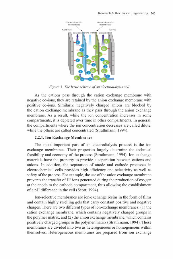
.245Research & Reviews in Engineering
Figure 3. The basic scheme of an electrodialysis cell
As the cations pass through the cation exchange membrane with negative co-ions, they are retained by the anion exchange membrane with positive co-ions. Similarly, negatively charged anions are blocked by the cation exchange membrane as they pass through the anion exchange membrane. As a result, while the ion concentration increases in some compartments, it is depleted over time in other compartments. In general, the compartments where the ion concentration decreases are called dilute, while the others are called concentrated (Strathmann, 1994).
2.2.1. Ion Exchange Membranes
The most important part of an electrodialysis process is the ion exchange membranes. Their properties largely determine the technical feasibility and economy of the process (Strathmann, 1994). Ion exchange materials have the property to provide a separation between cations and anions. In addition, the separation of anode and cathode processes in electrochemical cells provides high efficiency and selectivity as well as safety of the process. For example, the use of the anion exchange membrane prevents the transfer of H+ ions generated during the production of oxygen at the anode to the cathode compartment, thus allowing the establishment of a pH difference in the cell (Scott, 1994).
Ion-selective membranes are ion-exchange resins in the form of films and contain highly swelling gels that carry constant positive and negative charges. There are two different types of ion-exchange membranes: (1) the cation exchange membrane, which contains negatively charged groups in the polymer matrix, and (2) the anion exchange membrane, which contains positively charged groups in the polymer matrix (Strathmann, 1994). These membranes are divided into two as heterogeneous or homogeneous within themselves. Heterogeneous membranes are prepared from ion exchange

Belgin Karabacakoğlu246 .
resins and generally show a high electrical resistance and relatively poor mechanical strength due to their high swelling with water. Homogeneous membranes are made by attaching ionic groups to a cross-linked copolymer film based on polystyrene, polytetrafluoroethylene, or polyfluoride vinyl ether and divinyl benzene (Scoot and Hughes, 1996). Apart from these, there are inorganic membranes containing silica, bentonite, and oxyhydrates of aluminum and zirconium. However, ion exchange membranes are mostly made of synthetic polymers (Scott, 1994).
The typical structure of a cation exchange membrane is shown in Figure 4. The membrane consists of a polymer matrix containing fixed negatively charged groups. These negatively charged groups are in mutual equilibrium with stable positively charged cations, called counter-ions, to ensure electro-neutrality. Since mobile anions, called co-ions, carry the same charge as fixed negatively charged groups, they are more or less repelled by electrostatic forces. This process is called Donnan repulsion. In a cation exchange membrane carrying fixed negatively charged groups, only cations are allowed to pass due to the repulsion of co-ions. Since anion exchange membranes carry constant positive charges in the polymer matrix, all cations are repelled and only anions are allowed to pass (Scott, 1994).
Figure 4. Model of a cation exchange membrane (Scott, 1994)
For a cation exchange membrane in a dilute solution of a strong electrolyte, the cation concentration in the membrane is usually greater than in the solution. Because the cations are held by the negatively charged ions in the membrane. On the other hand, the concentration of mobile ions in the solution is higher than in the membrane. Thus, a concentration difference is established between the membrane and the solution. This difference acts as the driving force for mobile cations to move into solution and mobile anions to move towards the membrane (Strathmann, 1994).
While anion exchange membranes are made from strong or weak bases, cation exchange membranes are made of strong or weak acids (Scott and Hughes, 1996). The ion exchange groups used in the membranes are given in Table 1.
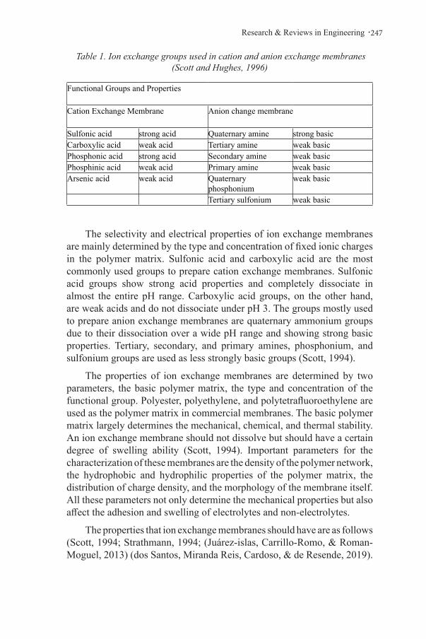
.247Research & Reviews in Engineering
Table 1. Ion exchange groups used in cation and anion exchange membranes (Scott and Hughes, 1996)
Functional Groups and Properties
Cation Exchange Membrane Anion change membrane
Sulfonic acid strong acid Quaternary amine strong basicCarboxylic acid weak acid Tertiary amine weak basicPhosphonic acid strong acid Secondary amine weak basicPhosphinic acid weak acid Primary amine weak basicArsenic acid weak acid Quaternary
phosphoniumweak basic
Tertiary sulfonium weak basic
The selectivity and electrical properties of ion exchange membranes are mainly determined by the type and concentration of fixed ionic charges in the polymer matrix. Sulfonic acid and carboxylic acid are the most commonly used groups to prepare cation exchange membranes. Sulfonic acid groups show strong acid properties and completely dissociate in almost the entire pH range. Carboxylic acid groups, on the other hand, are weak acids and do not dissociate under pH 3. The groups mostly used to prepare anion exchange membranes are quaternary ammonium groups due to their dissociation over a wide pH range and showing strong basic properties. Tertiary, secondary, and primary amines, phosphonium, and sulfonium groups are used as less strongly basic groups (Scott, 1994).
The properties of ion exchange membranes are determined by two parameters, the basic polymer matrix, the type and concentration of the functional group. Polyester, polyethylene, and polytetrafluoroethylene are used as the polymer matrix in commercial membranes. The basic polymer matrix largely determines the mechanical, chemical, and thermal stability. An ion exchange membrane should not dissolve but should have a certain degree of swelling ability (Scott, 1994). Important parameters for the characterization of these membranes are the density of the polymer network, the hydrophobic and hydrophilic properties of the polymer matrix, the distribution of charge density, and the morphology of the membrane itself. All these parameters not only determine the mechanical properties but also affect the adhesion and swelling of electrolytes and non-electrolytes.
The properties that ion exchange membranes should have are as follows (Scott, 1994; Strathmann, 1994; (Juárez-islas, Carrillo-Romo, & Roman-Moguel, 2013) (dos Santos, Miranda Reis, Cardoso, & de Resende, 2019).
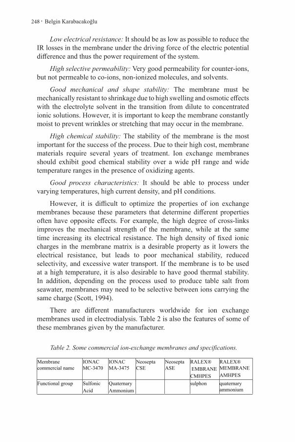
Belgin Karabacakoğlu248 .
Low electrical resistance: It should be as low as possible to reduce the IR losses in the membrane under the driving force of the electric potential difference and thus the power requirement of the system.
High selective permeability: Very good permeability for counter-ions, but not permeable to co-ions, non-ionized molecules, and solvents.
Good mechanical and shape stability: The membrane must be mechanically resistant to shrinkage due to high swelling and osmotic effects with the electrolyte solvent in the transition from dilute to concentrated ionic solutions. However, it is important to keep the membrane constantly moist to prevent wrinkles or stretching that may occur in the membrane.
High chemical stability: The stability of the membrane is the most important for the success of the process. Due to their high cost, membrane materials require several years of treatment. Ion exchange membranes should exhibit good chemical stability over a wide pH range and wide temperature ranges in the presence of oxidizing agents.
Good process characteristics: It should be able to process under varying temperatures, high current density, and pH conditions.
However, it is difficult to optimize the properties of ion exchange membranes because these parameters that determine different properties often have opposite effects. For example, the high degree of cross-links improves the mechanical strength of the membrane, while at the same time increasing its electrical resistance. The high density of fixed ionic charges in the membrane matrix is a desirable property as it lowers the electrical resistance, but leads to poor mechanical stability, reduced selectivity, and excessive water transport. If the membrane is to be used at a high temperature, it is also desirable to have good thermal stability. In addition, depending on the process used to produce table salt from seawater, membranes may need to be selective between ions carrying the same charge (Scott, 1994).
There are different manufacturers worldwide for ion exchange membranes used in electrodialysis. Table 2 is also the features of some of these membranes given by the manufacturer.
Table 2. Some commercial ion-exchange membranes and specifications.
Membrane commercial name
IONAC MC-3470
IONAC MA-3475
Neosepta CSE
Neosepta ASE
RALEX® EMBRANECMHPES
RALEX® MEMBRANEAMHPES
Functional group SulfonicAcid
QuaternaryAmmonium
sulphon quaternary ammonium
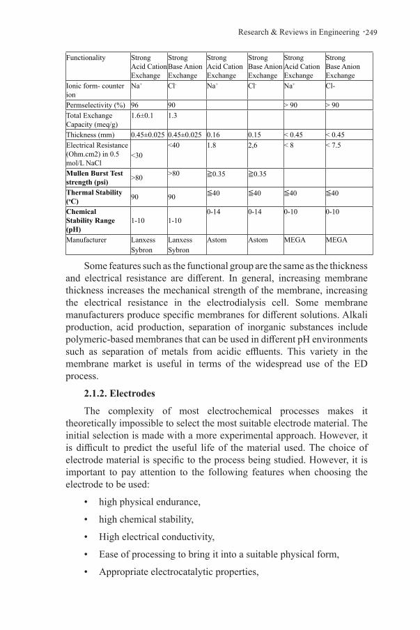
.249Research & Reviews in Engineering
Functionality Strong Acid Cation Exchange
Strong Base Anion Exchange
Strong Acid Cation Exchange
Strong Base Anion Exchange
Strong Acid Cation Exchange
Strong Base Anion Exchange
Ionic form- counter ion
Na+ Cl- Na+ Cl- Na+ Cl-
Permselectivity (%) 96 90 > 90 > 90Total Exchange Capacity (meq/g)
1.6±0.1 1.3
Thickness (mm) 0.45±0.025 0.45±0.025 0.16 0.15 < 0.45 < 0.45Electrical Resistance (Ohm.cm2) in 0.5 mol/L NaCl
<30<40 1.8 2,6 < 8 < 7.5
Mullen Burst Test strength (psi) >80 >80 ≧0.35 ≧0.35
Thermal Stability (oC) 90 90 ≦40 ≦40 ≦40 ≦40
Chemical Stability Range (pH)
1-10 1-100-14 0-14 0-10 0-10
Manufacturer LanxessSybron
LanxessSybron
Astom Astom MEGA MEGA
Some features such as the functional group are the same as the thickness and electrical resistance are different. In general, increasing membrane thickness increases the mechanical strength of the membrane, increasing the electrical resistance in the electrodialysis cell. Some membrane manufacturers produce specific membranes for different solutions. Alkali production, acid production, separation of inorganic substances include polymeric-based membranes that can be used in different pH environments such as separation of metals from acidic effluents. This variety in the membrane market is useful in terms of the widespread use of the ED process.
2.1.2. Electrodes
The complexity of most electrochemical processes makes it theoretically impossible to select the most suitable electrode material. The initial selection is made with a more experimental approach. However, it is difficult to predict the useful life of the material used. The choice of electrode material is specific to the process being studied. However, it is important to pay attention to the following features when choosing the electrode to be used:
• high physical endurance,
• high chemical stability,
• High electrical conductivity,
• Ease of processing to bring it into a suitable physical form,
• Appropriate electrocatalytic properties,

Belgin Karabacakoğlu250 .
• Long service life,
• Does not create pollution,
• Low cost,
• Security,
• Easily obtainable and repairable.
Table 3. The most used electrode materials (Walsh and Pletcher, 1993)
CATHODES ANODES
Hg, Pb, Ni Pt, Pt/Ti, Ir/Ti, Pt-Ir/Ti (Pt/Nb, Pt/Ta)
Graphite and other forms of carbon, often with organics and polymers, are treated at certain temperatures to improve porosity, density, corrosion resistance, moisture
Graphite or other forms of carbon (machined)Pb in acid – sulfate environmentTi, Nb, or C on PbO2
Steels Ni in alkaline medium
stainless steels
Coating of low H2 overpotential materials on steelExp: Ni, Ni/Al, Ni/Zn
Dimensionally stable anodesBoron doped diamond electrodes
Ni-Mo–Fe or Ni-Mo–Cr alloys Fe3O4
TiOx Ti4O7 with conductive ceramic
Both two electrodes in an ED cell must have sufficient mechanical strength, resistance to erosion, and ability to withstand physical effects by electrolyte, reactants, and products. In the case of inert electrodes, resistance to chemical influences is important and corrosion, undesirable oxide, hydride, or undesirable organic films should be avoided both under process conditions and in passive states. The physical shape of the electrodes is often very important. The surface conditions and shape of an electrode should be considered according to the requirement for product separation such as gas or solids. As a result, the electrode cost should be low and it should be used efficiently for as long as possible (Walsh and Pletcher, 1993). Commonly used electrode materials are shown in Table 3.
A general advantage of metal electrodes is their high conductivity. In solid electrodes, it is quite easy to increase precision and reproducibility with forced transport. Their surface can be improved by electrical deposition or chemical treatments. The latter situation is more common with carbon electrodes. Another benefit of using metal electrodes is the

.251Research & Reviews in Engineering
ease of construction and repair of the electrode material (Brett and Brett, 1993).
Carbon, which is one of the electrodes commonly used in the electrodialysis process, exists in various forms. Electrochemical reactions are normally slower with carbon than with metal electrodes. Electron transfer kinetics depends on the structure and surface preparation. Carbon has high surface activity. Bonds with hydrogen, hydroxyl, and carboxyl, and sometimes quinones, can form on the carbon surface. The presence of these groups indicates that the behavior of these electrodes is very sensitive to pH. The presence of functional groups has been used to refine the electrode surface to obtain new electrode properties. The modification of carbon electrodes is among the subjects attracting attention in recent years. Various types of carbon are used as electrodes. These are glassy carbon, carbon fibers, black carbon, various types of graphite, and carbon paste (combined in an inert structure and contains graphite particles). The most widely used of these is glassy carbon, which is isotropic. However, electrode construction is very difficult due to its hardness and brittleness. Carbon fibers have a diameter similar to the thickness of a hair strand (2–20 µm). Its construction is generally provided from both polyacrylonitrile (PAN) and pitch. Apart from being used as a microelectrode, it is used in porous electrodes where high electrolysis efficiency is required (Brett and Brett, 1993). Also, three-dimensional electrodes such as carbon cloth, carbon felt, and mesh-shaped glassy carbon is different forms of carbon electrodes. Since these electrodes have a high area per unit electrode volume and high mass transfer characteristics, their use in electrochemical processes is increasing (Walsh and Pletcher, 1993).
Steel, which is used to make metal electrodes, is an important electrode material because it is very cheap compared to similar materials. It is essentially an iron-carbon alloy and can be cast into a workable state. Various types of steel can be a combination of 25 or more elements, and their physical properties change accordingly. Stainless steels are iron-chromium-nickel alloys and contain 16-28% chromium and 6-20% nickel.
3. Electrodialysis Applications
Electrodialysis is a process for the selective transport of ions in the aqueous solution. Therefore, it is widely used for the removal of various components from water and wastewater. The most important advantage of the ED method also allows substance recovery. Research in this field has gained acceleration since 2004.(Gurreri, Tamburini, Cipollina, & Micale, 2020).

Belgin Karabacakoğlu252 .
One of the most important constraints in terms of the availability of electrodialysis is energy consumption. In a study conducted by Chen et al., electrodialysis was used to produce drinking water from brackish water with a salinity of 3500 mg/L. The permselectivity of the heterogeneous anion and cation exchange membranes used in the cell is above 90%. To increase the cell performance, the ion exchange resin was filled between membranes and different applications have been made for solution feeding inputs. According to these regulations, high salinity removal was reached by 40% less energy consumption than the classic application. (Chen, Wang, Liu, Zhao, & Li, 2020).
The most widely used technique for the removal of metal ions from plating wastewater is chemical precipitation. However, with this method, metal ions in the wastewater are formed a secondary pollutant as a metal sludge, and a second separation process, which usually requires heat treatment, is required to recover the metal from this sludge. In addition, large amounts of chemicals are used. Min et al used a commercial electrodialysis system to separate metals from real plating wastewater. The electrodialysis cell contains 5 pairs of anion and cation exchange membranes, Neosepta CMX-SB and Neosepta AMX-SB, respectively. There are 22.3 mg/L Cu2+ and 24.4 mg/L Ni2+ ions in the waste water. In the studies carried out in potentiostatic mode at different voltage values, 6, 12, and 18 V, the optimum voltage was determined as 12 V and 99.9% Cu2+ and 99.3% Ni2+ removal were obtained in 25 minutes at this voltage. In addition, the recovery rates in the dilute chamber were over 90% (Min, Choi, Jang, Lee, & Park, 2019).
In the study by dos Santos et al., Cr (VI) removal was carried out to use a commercial membrane module. The module has 10 anions exchange and 11 cation exchange membranes. Titanium electrodes covered with platinum and titanium were used The removal efficiency of chromium (VI) was more than 99% in 75 min of treatment (dos Santos et al., 2019).
Although electrodialysis studies seem to focus on desalination and removal and recovery of metals from metal plating wastewater, they can also be used for the separation of electrolytes with different ionic properties. Commercial membrane manufacturers produce membranes suitable for different areas of use, and continuous research and innovations are taking place, especially in polymeric membranes. The main components in ED systems are ion-exchange membranes and electrodes, the type and surface area of these components affect system performance. General applications are given in Table 4 (Scott and Hughes, 1996; Fidaleo and Moresi, 2006).

.253Research & Reviews in Engineering
Table 4. ED applications (Fidaleo and Moresi, 2006; Scott and Hughes, 1996)
Desalination of salt water Salt removal from sugar solutions
Whey demineralization Production of table salt from sea water
Deacidification of fruit juicesConversion of salts to corresponding free acids and basesanalytical processes
Tartaric wine stabilization Desalination from amino acid solutions
Purification of the protein Regeneration of photographic chemicals, silver recovery
Nitrate removal from drinking water Purification of electrophoresis plating baths
Concentration of acetic acid Recovery of water and valuable products from industrial wastewater
It is possible to purchase electrodialysis systems that contain pumps, solution tanks, a power supply, and an ED cell or cells. The most important advantage of ED systems is that they are relatively small and modular. ED systems are also sufficient to increase the number of membrane pairs without increasing the system dimensions for scale enlargement. A wide range of ED cells can be found in the market from lab scale to industrial scale. The number of membrane pairs reaches 1200 in the cells on the industrial scale. In this way, high surface area and separation capacity is achieved by increasing the number of membranes of the system.
4. Conclusion
Electrodialysis was an electrochemical membrane separation process using ion-exchange membranes. The anion exchange and cation exchange membranes used in the ED cell and the electrodes used as anode and cathode are effective on the separation performance. It is not very difficult to choose the suitable membrane for the separation process to be made among the many commercially produced ion exchange membranes with different properties, but from an economic point of view, different membrane types can be tried and the suitable membrane can be selected. The electrodialysis method is particularly useful for the separation of components from dilute feed streams. ED systems can be used with different separation processes. In the ED cell, it is necessary to apply an external voltage with a DC power source to transport ions from one compartment to the other. The applied voltage is used not only for ion migration but also for the redox reactions taking place at the electrodes. If the required electrical energy is provided by one of the renewable energy sources such as solar panels and wind turbines, the process becomes more economical. As a result, it can be stated that electrodialysis will find more usage areas.

Belgin Karabacakoğlu254 .
References
Al-Amshawee, S., Yunus, M. Y. B., Azoddein, A. A. M., Hassell, D. G., Dakhil, I. H., & Abu Hasan, H. (2020). Electrodialysis desalination for water and wastewater: A review. Chemical Engineering Journal, 380. doi:ARTN 122231 10.1016/j.cej.2019.122231
Brett, C.M.A., Brett, A.M.O., 1993, Electrochemistry: Principles, Methods and Applications, Oxford University Press.
Chen, Q. B., Wang, J., Liu, Y., Zhao, J., & Li, P. (2020). Novel energy-efficient electrodialysis system for continuous brackish water desalination: Inno-vative stack configurations and optimal inflow modes. Water Res, 179, 115847. doi:10.1016/j.watres.2020.115847
Curto, D., Franzitta, V., & Guercio, A. (2021). A Review of the Water Desalinati-on Technologies. Applied Sciences, 11(2). doi:10.3390/app11020670
dos Santos, C. S. L., Miranda Reis, M. H., Cardoso, V. L., & de Resende, M. M. (2019). Electrodialysis for removal of chromium (VI) from effluent: Analysis of concentrated solution saturation. Journal of Environmental Chemical Engineering, 7(5). doi:10.1016/j.jece.2019.103380
Fidaleo, M., Moresi, M., 2006, Electrodialysis applications in the food industry, Advances in Food and Nutrition Research, 51, 265-360.
Gurreri, L., Tamburini, A., Cipollina, A., & Micale, G. (2020). Electrodialysis Applications in Wastewater Treatment for Environmental Protection and Resources Recovery: A Systematic Review on Progress and Perspectives. Membranes (Basel), 10(7). doi:10.3390/membranes10070146
Juárez-islas, F., Carrillo-Romo, F., & Roman-Moguel, G. (2013). Metals Sepa-ration by the Joint Process of Facilitated Transport and Electrodialysis (Electromembrane process), Employing a Liquid Membrane Compound by D2ehpa–Kerosene–Formamide. Canadian Metallurgical Quarterly, 38(3), 187-192. doi:10.1179/cmq.1999.38.3.187
Kraaijeveld, G., Sumberova, V., Kuindersma, S., & Wesselingh, H. (1995). Mo-deling Electrodialysis Using the Maxwell-Stefan Description. Chemical Engineering Journal and the Biochemical Engineering Journal, 57(2), 163-176. doi:Doi 10.1016/0923-0467(94)02940-7
Min, K. J., Choi, S. Y., Jang, D., Lee, J., & Park, K. Y. (2019). Separation of me-tals from electroplating wastewater using electrodialysis. Energy Sources, Part A: Recovery, Utilization, and Environmental Effects, 41(20), 2471-2480. doi:10.1080/15567036.2019.1568629
Parulekar, S. J. (1998). Optimal current and voltage trajectories for minimum energy consumption in batch electrodialysis. Journal of Membrane Scien-ce, 148(1), 91-103. doi:10.1016/s0376-7388(98)00148-3

.255Research & Reviews in Engineering
Pinto Carmelo Garcıa , M. E. F. L., Jose Luis Perez Pavon, Bernardo Moreno Cordero. (1999). Analytical applications of separation techniquesthrou-gh membranes. Laboratory Automation and Information Management 34, 115-130.
Strathmann, H., 1994, Electrodialytic membrane processes and their practical application, Environmental Oriented Electrochemistry, 495-533.
Scott, K., 1994, Membrane Materials, Transport and Electrodialysis, An Inten-sive Course on Electrochemical Process Engineering, The University of Newcastle Upon Tyne, UK.
Scott, K., Hughes, R., 1996, Industrial Membrane Seperation Technology, Sprin-ger.
Strathmann, H. (2010). Electrodialysis, a mature technology with a multitude of new applications. Desalination, 264(3), 268-288. doi:10.1016/j.de-sal.2010.04.069
Walsh, F.C., Pletcher, D., 1993, Industrial Electrochemistry, Second Edition, Springer.