“Submitted to ISCC ‘2000”

1

Energy/Throughput Tradeoffs of TCP Error Control Strategies

V. Tsaoussidis, H. Badr, K. Pentikousis, X. GeDepartment Computer Science,

State University of NY at Stony BrookNY 11794, USA

Abstract

Today’s universal communications increasingly involve mobile and battery-powered devices

(e.g. hand-held, laptop, IP-phone) over wired and wireless networks. Energy efficiency, as well as

throughput, are becoming service characteristics of dominant importance in communication

protocols. The wide applicabilit y of IP-networks/devices, and the wide range of TCP-based

applications, have rendered TCP the de facto reliable transport protocol standard not only for

wired, but also for wireless and mixed (wired/wireless) communications. TCP’s congestion control

algorithms have recently been refined to achieve higher throughput. Even with these modifications,

however, TCP versions do not incorporate a flexible error recovery strategy that is responsive to

distinct environmental characteristics and device constraints. We have compared the energy- and

throughput-efficiency of TCP error control strategies based on results gathered from our

implementation of TCP Tahoe, Reno, and New Reno. We show that, depending on the frequency and

duration of the error, each demonstrates appropriate behavior under specific circumstances, with

Tahoe more-or-less the most energy conserving of the three. None of them, however, possesses a

clear-cut overall advantage that would render it the version of choice for wired/wireless

heterogeneous networks.

“Submitted to ISCC ‘2000”

2

1. Introduction

Throughput eff iciency of TCP has been a focus of intensive attention during the past few

years. However, the energy/throughput tradeoff has not been adequately studied in the literature.

This tradeoff is becoming more important due to the wide applicabil ity of mobile networking,

which often involves the use of battery-powered devices (e.g. hand-held, laptop, IP-phone). The

energy-conserving capabil ity of communication protocols can play an important role in determining

the operational lifetime of such devices. In particular, functionality at the transport layer can have

significant impact on energy consumption.

The key for eff icient energy/throughput tradeoffs in reliable transport protocols, as

demonstrated by the tests presented here, is the error control mechanism. Error control is usually a

two-step process: error detection, followed by error recovery. Most transport protocols such as TCP

detect errors by monitoring the sequence of data segments received and/or acknowledged. When

timeouts are correctly configured, a missing segment is taken to indicate an error, namely that the

segment is lost. Reliable protocols usually implement an error-recovery strategy based on two

techniques: retransmission of missing segments; and downward adjustment of the sender's window

size and readjustment of the timeout period. Retransmission of unsuccessfully-attempted segments,

of course, entails additional energy expenditure and results in lower effective throughput. Thus, the

energy efficiency of error-control strategies cannot be studied without taking into account the

associated mechanisms for recovery. For example, timeouts, and adjustments of the congestion

window and its threshold, play a significant role in the overall throughput and energy-expenditure

performance. While the net outcome of the recovery process has to be the retransmission of the

missing segments, the nature of the error actually should play a determining role in defining the

recovery strategy used.

“Submitted to ISCC ‘2000”

3

Until recently, TCP was studied in the context of its throughput eff iciency over more-or-less

“homogeneous” environments (e.g. wired vs. wireless); consequently, homogeneity was also

reflected in the nature of the errors that were considered (e.g. congestion/transmission errors vs.

random/burst/fading-channel errors). Jacobson [5]was the first to study the impact of retransmission

on throughput, based on experiments with congested wired networks. More recently, others have

also been devoting attention to TCP throughput and proposing modifications in order to enhance its

performance. Floyd & Henderson, for example, have shown that TCP throughput in wired

environments can be made to improve using Partial Acknowledgments and Fast Recovery [4]. On

the other hand, Balakrishnan et al. [2], Lakshman & Madhow [7], and others (e.g. [6]), have shown

that TCP throughput degrades when the protocol is used over satellite or wireless links. Problems

might arise, however, in the near future:

� Today’s TCP applications are expected to run in physically heterogeneous, but functionally

integrated, wired/wireless environments. The modifications proposed do not satisfy this

universal functionality since they do not flexibly adjust the recovery strategy to the variable

nature of the errors.

� The motivating force driving these modifications ignores the energy/throughput tradeoff, which

is becoming a key performance issue.

The only published studies of TCP energy consumption are by Zorzi et al. [3, 12, 13]. The

authors present results, which have been widely reported in the recent literature, based on a

stochastic model of TCP behavior. While the model makes some radically simplifying assumptions

in order to maintain analytic tractability, no proper validation of its accuracy has been reported, so it

remains unclear how these simpli fying assumptions might invalidate the results. Moreover, the

authors’ conclusions are based on the additional energy expenditure caused by channel impairments

“Submitted to ISCC ‘2000”

4

only in the context of retransmitted data; extended communication time as well as operation-

specific characteristics are not taken into account1.

In this paper we present comparative results on the energy and throughput performance of

TCP Tahoe, Reno, and New Reno. Historically, TCP Tahoe was the first modification to TCP [8].

The newer TCP Reno included the Fast Recovery algorithm [1]. This was followed by New Reno

[4] and the Partial Acknowledgment mechanism for multiple losses in a single window of data. In

the context of heterogeneous wired/wireless environments, our results show that, by and large, there

is little to choose between these three versions in terms of the energy/throughput tradeoff. In

exceptional scenarios of rather intensive error conditions, Tahoe, although the oldest version,

performs better than Reno and New Reno with respect to both energy and throughput. Reno and

New Reno, however, might yield minor throughput achievements under milder error conditions.

2. TCP Overview

TCP error-control mechanism has some energy-conserving capabil ities: in response to

segment drops, TCP reduces its window size and therefore conserves transmission effort. The aim

here is not only to alleviate congested switches, but also to avoid unnecessary retransmission that

degrade the protocol’s performance. TCP Tahoe, Reno and New Reno, all use essentially the same

algorithm at the receiver, but implement different variations of the transmission process at the

sender. The receiver accepts segments out of sequence, but delivers them in order to the protocols

above. It advertises a window size, and the sender ensures that the number of unacknowledged

bytes does not exceed this size. For each segment correctly received, the receiver sends an

acknowledgment which includes the sequence number identifying the next in-sequence segment.

The sender implements a congestion window that defines the maximum number of transmitted-but-

1 In this paper, we are able to corroborate only one of their major conclusions, namely, the relative energy efficiency ofTahoe.

“Submitted to ISCC ‘2000”

5

unacknowledged segments permitted. This adaptive window can increase and decrease, but never

exceeds the receiver's advertised window. TCP applies graduated multiplicative and additive

increases to the sender's congestion window. The versions of the protocol differ from each other

essentially in the way that the congestion window is manipulated in response to acknowledgments

and timeouts, and the manner in which delivered or missing segments are acknowledged.

2.1. TCP Tahoe, Reno, and New Reno

TCP error-control mechanism is primarily oriented towards congestion control. Congestion

control can be beneficial also for the flow that experiences it, since avoiding unnecessary

retransmission can lead to better throughput [5]. The basic idea is for each source to determine how

much capacity is available in the network, so that it knows how many segments it can safely have in

transit. TCP utilizes acknowledgments to pace the transmission of segments and interprets timeout

events as indicating congestion. In response, the TCP sender reduces the transmission rate by

shrinking its window. Tahoe and Reno are the two most common reference implementations for

TCP. New Reno is a modified version of Reno that attempts to solve some of Reno’s performance

problems when multiple packets are dropped from a single window of data. These three versions of

TCP share the same problem so far as retransmission is concerned. They either retransmit at most

one dropped packet per RTT (Round Trip Time), or retransmit packets that might have already been

delivered successfully.

TCP Tahoe

TCP Tahoe congestion-control algorithm includes Slow Start, Congestion Avoidance, and

Fast Retransmit[1, 5]. It also implements a RTT-based estimation of the retransmission timeout. In

the Fast Retransmit mechanism, a number of successive (the threshold is usually set at three),

duplicate acknowledgments (dacks) carrying the same sequence number triggers off a

“Submitted to ISCC ‘2000”

6

retransmission without waiting for the associated timeout event to occur. The window adjustment

strategy for this “early timeout” is the same as for the regular timeout: Slow Start is applied. The

problem, however, is that Slow Start is not always efficient, especially if the error was purely

transient or random in nature, and not persistent. In such a case the shrinkage of the congestion

window is, in fact, unnecessary, and renders the protocol unable to fully utilize the available

bandwidth of the communication channel during the subsequent phase of window re-expansion.

TCP Reno

TCP Reno introduces Fast Recovery in conjunction with Fast Retransmit. The idea behind

Fast Recovery is that a dack is an indication of available channel bandwidth since a segment has

been successfully delivered. This, in turn, implies that the congestion window (cwnd) should

actually be incremented. So, for each dack, cwnd is increased by one. Receiving the threshold

number of dacks triggers Fast Recovery: the sender retransmits one segment, halves cwnd, and sets

the congestion threshold to cwnd. Then, instead of entering Slow Start as in Tahoe, the sender

increases its cwnd by the dack threshold number. Thereafter, and for as long as the sender remains

in Fast Recovery, cwnd is increased by one for each additional dack received. This procedure is

called “ inflating” cwnd. The Fast Recovery stage is completed when an acknowledgment (ack) for

new data is received. The sender then sets cwnd to the current congestion threshold value

(“deflating” the window), and resets the dack counter. In Fast Recovery, cwnd is thus effectively

set to half its previous value in the presence of dacks, rather than performing Slow Start as for a

general retransmission timeout.

TCP Reno’s Fast Recovery can be effective when there is only one segment drop from a

window of data, given the fact that Reno retransmits at most one dropped segment per RTT. The

problem with the mechanism is that it is not optimized for multiple packet drops from a single

window, and this could negatively impact performance.

“Submitted to ISCC ‘2000”

7

New Reno

New Reno addresses the problem of multiple segment drops from a single window. In

effect, it can avoid many of the retransmit timeouts of Reno. The New Reno modification

introduces a partial acknowledgment strategy in Fast Recovery. A partial acknowledgment is

defined as an ack for new data which does not acknowledge all segments that were in flight at the

point when Fast Recovery was initiated. It is thus an indication that not all data sent before entering

Fast Recovery has been received. In Reno, the partial ack causes exit from Fast Recovery. In New

Reno, it is an indication that (at least) one segment is missing and needs to be retransmitted. In this

way, when multiple packets are lost from a window of data, New Reno can recover without waiting

for a retransmission timeout. Notice that the algorithm still retransmits at most one segment per

RTT. New Reno can improve throughput under multiple segment drops from a single window.

However, the retransmission triggered off by a partial ack might be for a delayed rather than lost

segment; thus, the strategy risks making multiple successful transmissions for the segment, which

can seriously impact its energy efficiency with no compensatory gain in throughput.

3. Testing environment and methodology

The three versions of TCP were implemented using the x-kernel protocol framework [11].

We ran tests simulating a fairly low bandwidth environment, since we are primarily interested in

heterogeneous wired/wireless environments. The tests were carried out in a single session, with the

client and the server running on two directly connected dedicated hosts, so as to avoid unpredictable

conditions with distorting effects on the protocol's performance.

In order to simulate error conditions, we developed a “virtual protocol” , VDELDROP,

which was configured between TCP and IP. VDELDROP’s core mechanism consists of a 2-state

“Submitted to ISCC ‘2000”

8

continuous-time Markov chain. Each state has a mean sojourn time mi�and a drop rate ri (i=1, 2)

whose values are set by the user. The drop rate ri takes a value between 0 and 1, and determines

the proportion of segments to be dropped during state i. Thus, when it visits state i , the mechanism

remains there for an exponentially-distributed amount of time with mean mi , during which it drops

a proportion ri of segments being transmitted, and then transits to the other state.

In our experiments we configured the two states to have equal mean sojourn time. The value

of this mean time varied from experiment to experiment, of course, but was always set equal for the

two states. Furthermore, one state was always configured with a zero drop rate. Thus, simulated

error conditions during a given experiment alternated between “On” and “Off” phases during which

drop actions were in effect and were suspended, respectively. Error conditions of various intensity,

persistence and duration could thus be simulated, depending on the choice of mean state-sojourn

time and drop rate for the On state.

4. Results and Discussion

All tests reported here were undertaken using 5-MByte (5,242,880 bytes) data sets for

transmission. The purpose of the tests was to evaluate the behavior of the protocols in response to

changes in the network environment, such as simulated congestion, and transmission errors of

different intensity and duration. We took measurements of the total connection time and of the total

number of bytes transmitted (i.e. including protocol control overhead transmissions, data segment

retransmission, etc.). Both factors significantly affect energy expenditure as well as throughput.

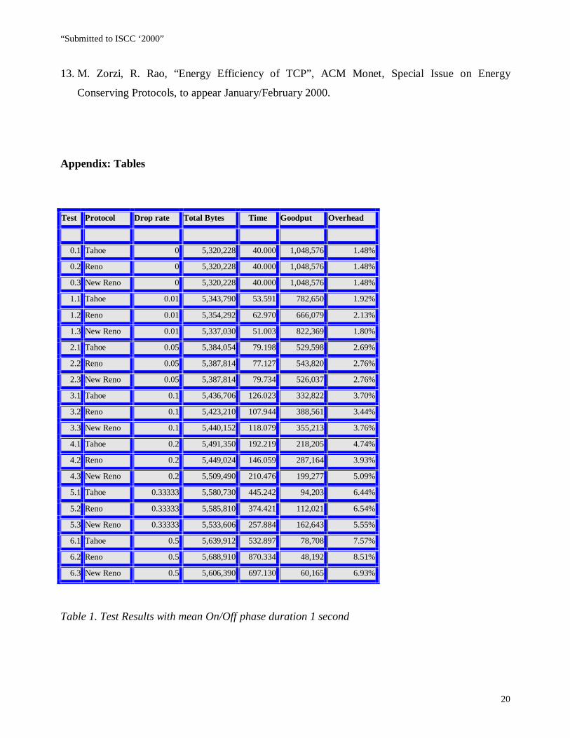
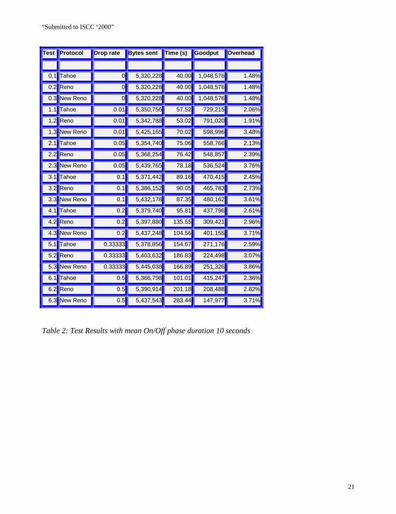
Detailed results are presented in the Tables 1 & 2 (see Appendix). In Table 1 we present results for

VDELDROP with mean On/Off phase duration of 1 second, while for Table 2 this mean duration is

10 seconds. In order to represent the (transmission) energy expenditure overhead required to

complete reliable transmission under different conditions, we use Overhead as a metric. This is the

“Submitted to ISCC ‘2000”

9

total extra number of bytes the protocol transmits, expressed as a percentage, over and above the 5

MBytes delivered to the application at the receiver, from connection initiation through to

connection termination. The Overhead is thus given by the formula: Overhead =

100*(Total - Base)/5Mbytes, where,

� Base is the number of bytes delivered to the high-level protocol at the receiver. It is a fixed 5

Mbytes data set for all tests.

� Total is the total of all bytes transmitted by the sender and receiver transport layers, and is

given in the column Total Bytes. This includes protocol control overhead, data segment

retransmission, as well as the delivered data.

The time overhead required to complete reliable transmission under different conditions is given in

column Time. The measured performance of the protocols is given in column Goodput using the

formula: Goodput = Original Data / Connection Time, where,

� Original Data is the 5-MBytes data set.

� Connection Time is the amount of time required for completion of data delivery, from

connection initiation to connection termination.

For VDELDROP, the DROP Rate reported is the dropping rate for segments during the On

phases, not the averaged overall drop rate across On/Off phases. An entry of 0 in the DROP rate

column signifies error-free conditions.

4.1 Effective Throughput Performance (Goodput)

It can be observed from Chart 1 below that for frequent On/Off phase changes (here, with 1-

second mean phase duration) Tahoe, Reno, and New Reno exhibit similar behavior. The differences

“Submitted to ISCC ‘2000”

10

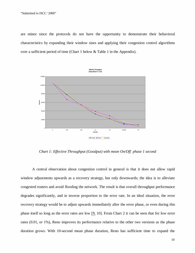
are minor since the protocols do not have the opportunity to demonstrate their behavioral

characteristics by expanding their window sizes and applying their congestion control algorithms

over a sufficient period of time (Chart 1 below & Table 1 in the Appendix).

Chart 1: Effective Throughput (Goodput) with mean On/Off phase 1 second

A central observation about congestion control in general is that it does not allow rapid

window adjustments upwards as a recovery strategy, but only downwards; the idea is to alleviate

congested routers and avoid flooding the network. The result is that overall throughput performance

degrades significantly, and in inverse proportion to the error rate. In an ideal situation, the error

recovery strategy would be to adjust upwards immediately after the error phase, or even during this

phase itself so long as the error rates are low [9, 10]. From Chart 2 it can be seen that for low error

rates (0.01, or 1%), Reno improves its performance relative to the other two versions as the phase

duration grows. With 10-second mean phase duration, Reno has sufficient time to expand the

Effective Throughput(drop phase of 1 sec)

0

200,000

400,000

600,000

800,000

1,000,000

1,200,000

0 0.01 0.05 0.1 0.2 0.33333 0.5

Drop rate

bit

s/se

c

Tahoe Reno New Reno

“Submitted to ISCC ‘2000”

11

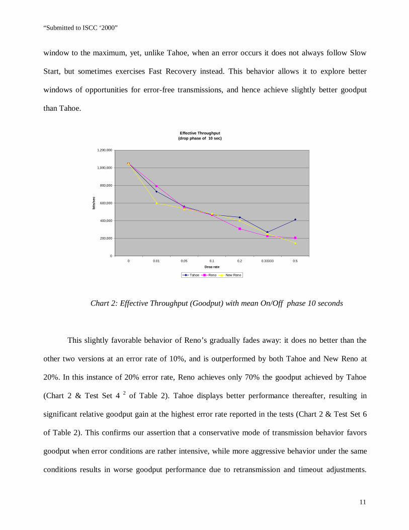
window to the maximum, yet, unlike Tahoe, when an error occurs it does not always follow Slow

Start, but sometimes exercises Fast Recovery instead. This behavior allows it to explore better

windows of opportunities for error-free transmissions, and hence achieve slightly better goodput

than Tahoe.

Chart 2: Effective Throughput (Goodput) with mean On/Off phase 10 seconds

This slightly favorable behavior of Reno’s gradually fades away: it does no better than the

other two versions at an error rate of 10%, and is outperformed by both Tahoe and New Reno at

20%. In this instance of 20% error rate, Reno achieves only 70% the goodput achieved by Tahoe

(Chart 2 & Test Set 4 2 of Table 2). Tahoe displays better performance thereafter, resulting in

significant relative goodput gain at the highest error rate reported in the tests (Chart 2 & Test Set 6

of Table 2). This confirms our assertion that a conservative mode of transmission behavior favors

goodput when error conditions are rather intensive, while more aggressive behavior under the same

conditions results in worse goodput performance due to retransmission and timeout adjustments.

Effective Throughput(drop phase of 10 sec)

0

200,000

400,000

600,000

800,000

1,000,000

1,200,000

0 0.01 0.05 0.1 0.2 0.33333 0.5

Drop rate

bit

s/se

c

Tahoe Reno New Reno

“Submitted to ISCC ‘2000”

12

For this case of 50% error rate and a mean On/Off phase duration of 10 seconds, Tahoe

immediately shrinks its window and effectively does not get the chance to re-expand it; Reno enters

a Fast Recovery phase, continuing data transmission until a timeout event occurs; New Reno

interprets the acknowledgments during Fast Recovery as partial acknowledgments, and hence

retransmits in order to recover faster from multiple losses. Thus, despite more bytes being injected

into the network by Reno and New Reno, the goodput achieved by Tahoe is almost double (Chart 2

& Test Set 6 of Table 2).

4.2 Energy Issues

Calculation of specific energy functions would provide measures of energy saving for TCP

versions of perhaps dubious precision. Energy expenditure is device-, operation-, and application-

specific. It can only be measured with precision on a specific device, running each protocol version

separately, and reporting the battery power consumed per version. Energy is consumed at different

rates during various stages of communication, and the amount of expenditure depends on the

current operation. For example, the transmitter/receiver expend different amounts of energy when

they, respectively, are sending or receiving segments, are waiting for segments to arrive, and are

idle. Hence, pace [13], an estimation of additional energy expenditure cannot be based solely on the

byte overhead due to retransmission, since overall connection time might have been extended while

waiting or while attempting only a moderate rate of transmission. On the other hand, the estimation

cannot be based solely on the overall connection time either, since the distinct operations performed

during that time (e.g. transmission vs. idle) consume different levels of energy. Nevertheless, the

potential for energy saving can be gauged from the combination of time and byte overhead savings

achieved. Based on these metrics, we can estimate lower bounds for the energy consumption. Since

2 i.e. the set of three tests numbered 4.1, 4.2 & 4.3.

“Submitted to ISCC ‘2000”

13

an idle state is not involved in TCP operations (the sender/receiver is either sending

segments/acknowledgments, or waiting for acknowledgments/segments), a lower bound can be

determined based on the assumption that the additional time used by a protocol is spent in a waiting

state.

As with goodput, the difference between the three TCP versions with respect to overhead is

also not significant under rapidly changing conditions with On/Off phases of 1-second mean

duration (see Chart 3). This remains largely true for Tahoe and Reno with longer On/Off phases

Chart 3: Overhead with mean On/Off phase 1 second

of mean duration 10 seconds, especially under mild error rates (Chart 4), although it should be

noted that their relative overhead due to retransmission is much lower for 10-second mean phase

duration than for the 1-second phases (compare Charts 3 & 4, and Overhead for Test Sets 6 of

Tables 1 & 2).

Overhead(drop phase of 1 sec)

0.00%

1.00%

2.00%

3.00%

4.00%

5.00%

6.00%

7.00%

8.00%

9.00%

0 0.01 0.05 0.1 0.2 0.33333 0.5

Drop rate

Tahoe Reno New Reno

“Submitted to ISCC ‘2000”

14

Interesting observations can be made about the energy consumption of the three protocol

versions from the tests with mean duration 10 seconds. Firstly, New Reno wastes a significantly

larger amount of energy on retransmission and extended communication time at all error rates

reported in Table 2. During these prolonged On phases, it attempts to recover from multiple losses

as it did previously under the 1-second phases, but now the aggressive retransmission which results

from partial acknowledgments is not always successful as the error phase persists (Chart 4).

Chart 4: Overhead with mean On/Off phase 10 seconds

Secondly, under error rates of 20% Reno expends more transmission effort and achieves worse

throughput than Tahoe. Under this scenario, Reno’s window has been expanded significantly and

relatively aggressive retransmission takes place for a while, although we have entered a persistent

error-prone phase. Tahoe, on the other hand, using Slow Start instead of Fast Recovery, shrinks its

window immediately, hence avoiding segment drops that would have otherwise entailed

Overhead(drop phase of 10 sec)

0.00%

0.50%

1.00%

1.50%

2.00%

2.50%

3.00%

3.50%

4.00%

4.50%

0 0.01 0.05 0.1 0.2 0.33333 0.5

Drop rate

Tahoe Reno New Reno

“Submitted to ISCC ‘2000”

15

retransmission, and resumes window expansion when conditions permit it. Communication time is

extended for Reno by 40 seconds (i.e. by approximately 42%) more than for Tahoe (Chart 5 and

Test Set 4 of Table 2), and hence more energy is expended during additional transmission and

waiting states. However, if we assume that Reno remains in a waiting state throughout its 40-second

additional time, expending energy at a rate only 1/10th of that expended by Tahoe during its

connection time, this would result in a lower bound for the additional energy expenditure of 4.2%

compared to Tahoe.

Chart 5: Connection time with mean On/Off phase 10 seconds

At an error rate of 50%, Reno’s energy overhead relative to Tahoe can be gauged from the

additional 0.50% of retransmission overhead and the additional 100 seconds of extended

communication time (Charts 4 & 5, and Test Set 6 of Table 2). If we again assume that Reno spends

only the same amount time in the transmission state as does Tahoe, and so expends energy during

its entire 100-second additional time in a waiting state, a lower bound for its additional energy

Transmission time(drop phase of 10 sec)

0.000

50.000

100.000

150.000

200.000

250.000

300.000

0 0.01 0.05 0.1 0.2 0.33333 0.5

Drop rate

seco

nd

s

Tahoe Reno New Reno

“Submitted to ISCC ‘2000”

16

expenditure of 10% more than the energy consumed by Tahoe can be calculated as was done above

(see Test Set 6 of Table 2). However, it is reasonable to expect that the real additional energy

expenditure is, in fact, larger since the assumptions we have made favor Reno somewhat.

The situation for New Reno is even worse. Behaving more aggressively in case of multiple

losses, it temporarily (i.e. until a timeout event occurs) maximizes retransmission effort, although

the chances of getting segments through undamaged are slim under a persistent, 10-second mean

error phase with 50% drop rate.

4.3 The Energy/Throughput Tradeoff

Energy expenditure, as exempli fied by the three TCP versions studied here, does not achieve

proportional throughput gains. In fact, it does not even necessarily always result in any throughput

gain at all . Charts 6 below, abstracted from the tests reported in Table 2, summarize the

energy/throughput tradeoff behavior of the three TCP versions for On/Off phases of mean duration

10 seconds. The charts plot Overhead (and hence additional transmission energy expended) vs.

Goodput (which thus incorporates total connection time) at the various error rates for the On phases.

It can be observed from Reno’s chart that goodput degrades though more transmission effort

is expended. Reno, however, achieves the same goodput with a 50% as with a 33% error rate, but

expends less overhead. In this particular instance, additional energy expenditure is only wasting

bandwidth which could, perhaps, have been used by other flows. In contrast, under the same

scenario (33% & 50% error rates, respectively), Tahoe’s goodput improves, yet its overhead (and

hence, energy expenditure) decreases slightly. A representative example of the kind of tradeoff that

can occur may be observed from Test Set 2 of Table 2. New Reno achieves approximately the same

goodput as the other two versions of TCP, yet it expends significantly more transmission effort.

Energy expenditure can, indeed, sometimes gain returns of improved goodput as can be seen, for

“Submitted to ISCC ‘2000”

17

example, from the comparison of New Reno with Reno in Tests 4.2 & 4.3 of Table2: New Reno’s

throughput and energy expenditure, both, are higher than Reno’s.

Chart 6: The energy/throughput tradeoff in Tahoe, Reno, New Reno

with mean On/Off phase 10 seconds

Tahoe trade-off(drop phase of 10 sec)

0

00

00

00

00

000

000

0.00% 0.50% 1.00% 1.50% 2.00% 2.50% 3.00% 3.50% 4.00%

Overhead

0 %

1 %

5 %

50 %

33 %

20 %

10 %

Reno trade-off(drop phase of 10 sec)

0

200,000

400,000

600,000

800,000

1,000,000

1,200,000

0.00% 0.50% 1.00% 1.50% 2.00% 2.50% 3.00% 3.50% 4.00

Overhead

Th

rou

gh

pu

t (b

/s)

33 %

20 %

10 %

5 %

1 %

0 %

50 %

New Reno trade-off(drop phase of 10 sec)

0

200,000

400,000

600,000

800,000

1,000,000

1,200,000

0.00% 0.50% 1.00% 1.50% 2.00% 2.50% 3.00% 3.50% 4.00% 4.50%

Overhead

Th

rou

gh

pu

t (b

/s)

33 %

20 %

10 %

5 %

1 %

0 %

50 %

“Submitted to ISCC ‘2000”

18

Nevertheless, this extra energy expenditure is not eff icient, as is demonstrated by Tahoe in Test 4.1,

which has the best goodput and overhead of the three: goodput improves significantly when the

downward window adjustment is rapid. A notable case of this can be observed from Charts 2, 4, &

5 (also see Test Set 6 of Table 2). At an intensive error rate of 50% under persistent error phases of

mean duration 10 seconds, Tahoe significantly outperforms the other two versions in both energy

and throughput.

5. Conclusion

Our results for the energy/throughput tradeoffs of TCP Tahoe, Reno and New Reno demonstrate

that their performance is, by and large, fairly similar. Tahoe performs distinctly better when errors

are intensive and persistent, however, none of them displays the flexibility required for a universal

error control algorithm in a heterogeneous wired/wireless environment.

Under relatively persistent error conditions (e.g. burst errors) which, however, are not occurring

very frequently, backing off immediately, as does Tahoe, proves to be the correct strategy since a

graduated decrease of the window size can have the following undesirable consequences:

1. Large windows of data could continue to be transmitted for a period of time (until the window

shrinks) despite the prevail ing error phase, and therefore effective throughput is degraded and

energy expenditure grows.

2. Timeouts are extended and hence, when an error-free phase occurs, its presence cannot be

swiftly detected.

3. Using Fast Recovery (Reno), we go into a Congestion Avoidance phase which implements a

linear increase in the window, possibly starting from rather a small window size. Slow Start

(Tahoe’s reaction to losses, even during Congestion Avoidance) can recover faster once a

prolonged error phase lapses.

“Submitted to ISCC ‘2000”

19

The relative efficiency of Reno can be observed under persistent phases with relatively low

error rates. In contrast, New Reno can be the protocol of choice only for environments with

relatively infrequent and short/random errors. According to our results, not only are its throughput

achievements minor under more persistent error phases, but additional overhead due to

retransmission is also much higher.

References

1. M. Allman, V. Paxson, W. Stevens, "TCP Congestion Control", RFC 2581, April 1999

2. H. Balakrishnan, V. Padmanabhan, S. Seshan, and R. Katz, “ A comparison of mechanisms for

improving TCP performance over wireless links” , ACM/IEEE Transactions on Networking,

December 1997.

3. A. Chockalingam, M. Zorzi, R. R. Rao, “Performance of TCP on Wireless Fading Links with

memory” , in Proc. of IEEE ICC’98, June 1998

4. S. Floyd, T. Henderson, “The New Reno Modification to TCP’s Fast Recovery Algorithm”,

RFC 2582, April 1999.

5. V. Jacobson, “Congestion avoidance and control” in Proc. of ACM SIGCOMM ’88, August

1988.

6. A. Kumar, “Comparative performance analysis of versions of TCP in a local network with a

lossy link” , ACM/IEEE Transactions on Networking, August 1998.

7. T. Lakshman, U. Madhow, “The performance of TCP/IP for networks with high bandwidth-

delay products and random loss” , IEEE/ACM Transactions on Networking, pp. 336-350, June

1997.

8. J. Postel, Transmission Control Protocol, RFC 793, September 1981

9. V. Tsaoussidis, H. Badr, R. Verma, "Wave and Wait: An Energy-saving Transport Protocol for

Mobile IP-Devices", in Proc. of IEEE ICNP ’99, Oct. 1999.

10. V. Tsaoussidis, H. Badr, “The Wave and Probe Communication Mechanisms”, submitted to

IEEE/ACM Transactions on Networking.

11. The X-kernel: www.cs.arizona.edu/xkernel

12. M. Zorzi, R. Rao, “Energy Eff iciency of TCP”, MoMUC ’99, San Diego, Cali fornia, 1999

“Submitted to ISCC ‘2000”

20

13. M. Zorzi, R. Rao, “Energy Eff iciency of TCP”, ACM Monet, Special Issue on Energy

Conserving Protocols, to appear January/February 2000.

Appendix: Tables

Test Protocol Drop rate Total Bytes Time Goodput Overhead

0.1 Tahoe 0 5,320,228 40.000 1,048,576 1.48%

0.2 Reno 0 5,320,228 40.000 1,048,576 1.48%

0.3 New Reno 0 5,320,228 40.000 1,048,576 1.48%

1.1 Tahoe 0.01 5,343,790 53.591 782,650 1.92%

1.2 Reno 0.01 5,354,292 62.970 666,079 2.13%

1.3 New Reno 0.01 5,337,030 51.003 822,369 1.80%

2.1 Tahoe 0.05 5,384,054 79.198 529,598 2.69%

2.2 Reno 0.05 5,387,814 77.127 543,820 2.76%

2.3 New Reno 0.05 5,387,814 79.734 526,037 2.76%

3.1 Tahoe 0.1 5,436,706 126.023 332,822 3.70%

3.2 Reno 0.1 5,423,210 107.944 388,561 3.44%

3.3 New Reno 0.1 5,440,152 118.079 355,213 3.76%

4.1 Tahoe 0.2 5,491,350 192.219 218,205 4.74%

4.2 Reno 0.2 5,449,024 146.059 287,164 3.93%

4.3 New Reno 0.2 5,509,490 210.476 199,277 5.09%

5.1 Tahoe 0.33333 5,580,730 445.242 94,203 6.44%

5.2 Reno 0.33333 5,585,810 374.421 112,021 6.54%

5.3 New Reno 0.33333 5,533,606 257.884 162,643 5.55%

6.1 Tahoe 0.5 5,639,912 532.897 78,708 7.57%

6.2 Reno 0.5 5,688,910 870.334 48,192 8.51%

6.3 New Reno 0.5 5,606,390 697.130 60,165 6.93%

Table 1. Test Results with mean On/Off phase duration 1 second

“Submitted to ISCC ‘2000”

21

Test Protocol Drop rate Bytes sent Time (s) Goodput Overhead

0.1 Tahoe 0 5,320,228 40.00 1,048,576 1.48%

0.2 Reno 0 5,320,228 40.00 1,048,576 1.48%

0.3 New Reno 0 5,320,228 40.00 1,048,576 1.48%

1.1 Tahoe 0.01 5,350,756 57.52 729,215 2.06%

1.2 Reno 0.01 5,342,788 53.02 791,020 1.91%

1.3 New Reno 0.01 5,425,165 70.02 598,996 3.48%

2.1 Tahoe 0.05 5,354,740 75.06 558,766 2.13%

2.2 Reno 0.05 5,368,254 76.42 548,857 2.39%

2.3 New Reno 0.05 5,439,765 78.18 536,524 3.76%

3.1 Tahoe 0.1 5,371,442 89.16 470,415 2.45%

3.2 Reno 0.1 5,386,152 90.05 465,783 2.73%

3.3 New Reno 0.1 5,432,178 87.35 480,162 3.61%

4.1 Tahoe 0.2 5,379,740 95.81 437,796 2.61%

4.2 Reno 0.2 5,397,880 135.55 309,421 2.96%

4.3 New Reno 0.2 5,437,248 104.56 401,155 3.71%

5.1 Tahoe 0.33333 5,378,856 154.67 271,176 2.59%

5.2 Reno 0.33333 5,403,632 186.83 224,498 3.07%

5.3 New Reno 0.33333 5,445,038 166.89 251,326 3.86%

6.1 Tahoe 0.5 5,366,798 101.01 415,247 2.36%

6.2 Reno 0.5 5,390,914 201.18 208,488 2.82%

6.3 New Reno 0.5 5,437,543 283.44 147,977 3.71%

Table 2: Test Results with mean On/Off phase duration 10 seconds