SANDIA REPORT

SAND2011-7281 Unlimited Release Printed November 2011

Energy-Water Analysis of the 10-Year WECC Transmission Planning Study Cases

Vince Tidwell, Howard Passell, Barbara Moreland, Cesar Castillo

Prepared by Sandia National Laboratories Albuquerque, New Mexico 87185

Sandia National Laboratories is a multi-program laboratory managed and operated by Sandia Corporation, a wholly owned subsidiary of Lockheed Martin Corporation, for the U.S. Department of Energy’s National Nuclear Security Administration under Contract DE-AC04-94AL85000.

Approved for public release; further dissemination unlimited.

2

Issued by Sandia National Laboratories, operated for the United States Department of Energy by

Sandia Corporation.

NOTICE: This report was prepared as an account of work sponsored by an agency of the United

States Government. Neither the United States Government, nor any agency thereof, nor any of

their employees, nor any of their contractors, subcontractors, or their employees, make any

warranty, express or implied, or assume any legal liability or responsibility for the accuracy,

completeness, or usefulness of any information, apparatus, product, or process disclosed, or

represent that its use would not infringe privately owned rights. Reference herein to any specific

commercial product, process, or service by trade name, trademark, manufacturer, or otherwise,

does not necessarily constitute or imply its endorsement, recommendation, or favoring by the

United States Government, any agency thereof, or any of their contractors or subcontractors. The

views and opinions expressed herein do not necessarily state or reflect those of the United States

Government, any agency thereof, or any of their contractors.

Printed in the United States of America. This report has been reproduced directly from the best

available copy.

Available to DOE and DOE contractors from

U.S. Department of Energy

Office of Scientific and Technical Information

P.O. Box 62

Oak Ridge, TN 37831

Telephone: (865) 576-8401

Facsimile: (865) 576-5728

E-Mail: reports@adonis.osti.gov

Online ordering: http://www.osti.gov/bridge

Available to the public from

U.S. Department of Commerce

National Technical Information Service

5285 Port Royal Rd.

Springfield, VA 22161

Telephone: (800) 553-6847

Facsimile: (703) 605-6900

E-Mail: orders@ntis.fedworld.gov

Online order: http://www.ntis.gov/help/ordermethods.aspx

3

SAND2011-7281

Unlimited Release

November 2011

Energy-Water Analysis of the 10-year WECC Transmission Planning Study Cases

Vince Tidwell, Howard Passell, Barbara Moreland, Cesar Castillo

Sandia National Laboratories P.O. Box 5800

Albuquerque, New Mexico 87185-1137

Abstract

In 2011 the Department of Energy’s Office of Electricity embarked on a comprehensive program

to assist our Nation’s three primary electric interconnections with long term transmission

planning. Given the growing concern over water resources in the western U.S. the Western

Electricity Coordinating Council (WECC) requested assistance with integrating water resource

considerations into their broader electric transmission planning. The result is a project with three

overarching objectives:

1. Develop an integrated Energy-Water Decision Support System (DSS) that will enable

planners in the Western Interconnection to analyze the potential implications of water

stress for transmission and resource planning.

2. Pursue the formulation and development of the Energy-Water DSS through a strongly

collaborative process between the Western Electricity Coordinating Council (WECC),

Western Governors’ Association (WGA), the Western States Water Council (WSWC)

and their associated stakeholder teams.

3. Exercise the Energy-Water DSS to investigate water stress implications of the

transmission planning scenarios put forward by WECC, WGA, and WSWC.

The foundation for the Energy-Water DSS is Sandia National Laboratories’ Energy-Power-

Water Simulation (EPWSim) model (Tidwell et al. 2009). The modeling framework targets the

shared needs of energy and water producers, resource managers, regulators, and decision makers

at the federal, state and local levels. This framework provides an interactive environment to

explore trade-offs, and “best” alternatives among a broad list of energy/water options and

objectives. The decision support framework is formulated in a modular architecture, facilitating

tailored analyses over different geographical regions and scales (e.g., state, county, watershed,

interconnection). An interactive interface allows direct control of the model and access to real-

time results displayed as charts, graphs and maps. The framework currently supports modules for

4

calculating water withdrawal and consumption for current and planned electric power

generation; projected water demand from competing use sectors; and, surface and groundwater

availability.

The lead laboratory for this effort is Sandia National Laboratories (Sandia) supported by other

national laboratories, a university, and an industrial research institute. Specific participants

include Argonne National Laboratory (Argonne), Idaho National Laboratory (INL), the National

Renewable Energy Laboratory (NREL), Pacific Northwest National Laboratory (PNNL), the

University of Texas (UT), and the Electric Power Research Institute (EPRI).

WECC’s long range planning is organized according to two target planning horizons, a 10-year

and a 20-year. This study supports WECC in the 10-year planning endeavor. In this case the

water implications associated with four of WECC’s alternative future study cases (described

below) are calculated and reported. In future phases of planning we will work with WECC to

craft study cases that aim to reduce the thermoelectric footprint of the interconnection and/or

limit production in the most water stressed regions of the West.

5

Table of Contents

_Toc298140620

1. Introduction ................................................................................................................................. 7

1.1 Background on Energy and Water in the Western and Texas Interconnections Project ...... 7

1.2 Purpose of This Study ........................................................................................................... 8

2. Methods....................................................................................................................................... 9

2.1 Demographic Sector.............................................................................................................. 9

2.2 Thermoelectric Water Demand ........................................................................................... 10

2.3 Non-Thermoelectric Water Demand ................................................................................... 12

2.4 Water Supply ...................................................................................................................... 14

2.5 Interactive Interface ............................................................................................................ 15

2.6 Database .............................................................................................................................. 15

3. Results ....................................................................................................................................... 16

3.1 Water and Electric Power in 2010 ...................................................................................... 16

3.2. Study Case Analyses .......................................................................................................... 18

4. Next Steps ................................................................................................................................. 24

5. Summary ................................................................................................................................... 26

6. References ................................................................................................................................. 27

Appendix A: Water Withdrawal and Consumption and Parasitic Energy Factors ....................... 29

6

[Page Left Intentionally Blank’

7

1. Introduction In 2005 thermoelectric power production accounted for withdrawals of 140 billion gallons per

day (BGD) representing 41% of total freshwater withdrawals, making it the largest user of water

in the U.S., slightly ahead of irrigated agriculture (Kenny et al. 2009). In contrast thermoelectric

water consumption is projected at 3.7 BGD or about 3% of total U.S. consumption (NETL

2008). Thermoelectric water consumption is roughly equivalent to that of all other industrial

demands and represents one of the fastest growing sectors since 1980. In fact thermoelectric

consumption is projected to increase by 42 to 63% between 2005 and 2030 (NETL 2008). This

projected range in growth is a function of many factors including the fuel mix of the future

power plant fleet, cooling technology, and green house gas emissions controls. As such, water

availability will be an important consideration in the siting of any new power plant; however,

water is not the only consideration. Other important siting requirements include access to fuels,

transmission capacity, proximity to population centers/sensitive areas, environmental constraints,

and cost.

1.1 Background on Energy and Water in the Western and Texas Interconnections Project

The Department of Energy’s Office of Electricity has embarked on a comprehensive program to

assist our Nation’s three primary electric interconnections with long term transmission planning.

Given the growing concern over water resources in the western U.S. the Western Electricity

Coordinating Council (WECC) requested assistance with integrating water resource

considerations into their broader electric transmission planning. The result is a project with three

overarching objectives:

4. Develop an integrated Energy-Water Decision Support System (DSS) that will enable

planners in the Western Interconnection to analyze the potential implications of water

stress for transmission and resource planning.

5. Pursue the formulation and development of the Energy-Water DSS through a strongly

collaborative process between the Western Electricity Coordinating Council (WECC),

Western Governors’ Association (WGA), the Western States Water Council (WSWC)

and their associated stakeholder teams.

6. Exercise the Energy-Water DSS to investigate water stress implications of the

transmission planning scenarios put forward by WECC, WGA, and WSWC.

The foundation for the Energy-Water DSS is Sandia National Laboratories’ Energy-Power-

Water Simulation (EPWSim) model (Tidwell et al. 2009). The modeling framework targets the

shared needs of energy and water producers, resource managers, regulators, and decision makers

at the federal, state and local levels. This framework provides an interactive environment to

explore trade-offs, and “best” alternatives among a broad list of energy/water options and

objectives. The decision support framework is formulated in a modular architecture, facilitating

tailored analyses over different geographical regions and scales (e.g., state, county, watershed,

interconnection). An interactive interface allows direct control of the model and access to real-

time results displayed as charts, graphs and maps. The framework currently supports modules for

calculating water withdrawal and consumption for current and planned electric power

8

generation; projected water demand from competing use sectors; and, surface and groundwater

availability.

The lead laboratory for this effort is Sandia National Laboratories (Sandia) supported by other

national laboratories, a university, and an industrial research institute. Specific participants

include Argonne National Laboratory (Argonne), Idaho National Laboratory (INL), the National

Renewable Energy Laboratory (NREL), Pacific Northwest National Laboratory (PNNL), the

University of Texas (UT), and the Electric Power Research Institute (EPRI).

Although not addressed here, a complimentary project with the Electric Reliability Council of

Texas (ERCOT) is in progress aimed at assisting in long term transmission planning and

accompanying water resource issues.

1.2 Purpose of This Study

WECC’s long range planning is organized according to two target planning horizons, a 10-year

and a 20-year. This study supports WECC in the 10-year planning endeavor. In this case the

water implications associated with four of WECC’s alternative future study cases (described

below) are calculated and reported. In future phases of planning we will work with WECC to

craft study cases that aim to reduce the thermoelectric footprint of the interconnection and/or

limit production in the most water stressed regions of the West.

This initial study utilizes analysis tools and data (e.g., the Energy, Water and Power Simulation

model, see description below) that are very much in the development stage. Over the next two

years of this project significant improvements are scheduled for both the model and the data that

drives the model (see Next Steps below). As such the results given below should be viewed as

preliminary. Reasons for conducting this analysis so early in the project include:

1) Establish working numbers relative to thermoelectric water use, where it is located, and

where/how it is likely to grow.

2) Begin dialogue toward developing water related metrics that can be used in long-range

transmission planning.

3) Cultivate experience in integrating water resource planning with long term electric power

transmission planning.

As a first step toward understanding how information from this and future water related analyses

might support long-range transmission planning, four considerations are provided:

1) Identify regions where siting of future electric power generation may be at risk due to

potential water scarcity;

2) Evaluate power plant and electric system vulnerabilities due to drought;

3) Identify and deploy technological or management options for planners and plant managers to

account for water availability when siting and designing electric generation; and

4) Prepare governors, industry, and regulators to understand the long-term challenges and

potential trade-offs associated with electricity and water supply decisions.

9

2. Methods This analysis makes use of the Energy, Water and Power Simulation (EPWSim) model

developed by Sandia National Laboratory (Tidwell et al. 2009). This decision framework

is formulated within a system dynamics architecture (e.g., Sterman 2000) and implemented

within the commercial software package Studio Expert 2008, produced by Powersim, Inc.

(www.powersim.com). The model is designed to operate on an annual time step with a spatial

extent that includes the WECC service area. The duration of the simulation extends from 2010 to

2020, the current planning horizon for WECC. EPWSim has been modified to accept

thermoelectric power production data directly from WECC’s PROMOD modeling. Specifically,

WECC provides PROMOD output in the form of annual and monthly power production for each

thermoelectric power plant (existing and future) in the WECC. This data is then used to calculate

the water implications of the proposed fleet/operational schedules.

At its highest level, EPWSim is organized according to four primary sectors, demography,

thermoelectric water demand, non-thermoelectric water demand, and water supply. The

demographic sector model simulates changes in population and gross state product (GSP) that in

turn drives the demand for water in the non-thermoelectric sector. Within the thermoelectric

water demand module, thermoelectric power production output from WECC’s PROMOD model

is used to calculate associated water withdrawals and consumption at each thermoelectric plant

in the WECC. The model allows control of the type of cooling (i.e., open-loop, closed-loop

tower, closed-loop pond, or air cooled) and source of water (surface water, groundwater, saline)

utilized in all new construction. For the non-thermoelectric water demand module both

withdrawals and consumption are calculated according to the primary use sectors, municipal,

industrial, mining, livestock, and agriculture. These growing demands are then compared to

various water supply metrics to identify regions of limited water availability.

The nexus between electric power generation and water resource use must be viewed through the

lens of multiple reference systems (e.g., interconnection, watersheds, states, and counties). To

facilitate cross reference system analysis, the model is seeded with data representing the highest

level of detail that is publically available. These data include such factors as population at the

county level, changes in per capita water use at the state level, and stream gauge data at the

watershed level. From these disparate scales the data are translated to a compatible reference

system for analysis and observation. Translation is accomplished according to a simple areal or

population weighted aggregation scheme. Lookup tables of the weighting functions necessary to

move from one reference system to another have been developed to streamline this process.

Below a brief description of each model sector is provided.

2.1 Demographic Sector

Population and gross state product (GSP) are the primary factors influencing the demand for

non-thermoelectric water within the model. Both are simulated on an annual basis, computed at

the county level. Population and gross state product growth rates are treated as exogenous

variables to the model and thus allow full control by the user. The manner in which population

and gross state product influence the demand for water is defined in the non-thermoelectric water

demand module description below.

10

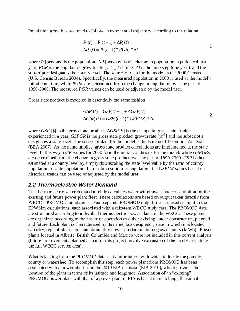
Population growth is assumed to follow an exponential trajectory according to the relation

tPGRtPtP

tPtPtP

ccc

ccc

**)1()(

)()1()( 1

where P [persons] is the population, P [persons] is the change in population experienced in a

year, PGR is the population growth rate [yr-1

], t is time, t is the time step (one year), and the

subscript c designates the county level. The source of data for the model is the 2000 Census

(U.S. Census Bureau 2004). Specifically, the measured population in 2000 is used as the model’s

initial condition, while PGRs are determined from the change in population over the period

1990-2000. The measured PGR values can be used or adjusted by the model user.

Gross state product is modeled in essentially the same fashion

tGSPGRtGSPtGSP

tGSPtGSPtGSP

sss

sss

**)1()(

)()1()( 2

where GSP [$] is the gross state product, GSP [$] is the change in gross state product

experienced in a year, GSPGR is the gross state product growth rate [yr-1

] and the subscript s

designates a state level. The source of data for the model is the Bureau of Economic Analysis

(BEA 2007). As the name implies, gross state product calculations are implemented at the state

level. In this way, GSP values for 2000 form the initial conditions for the model, while GSPGRs

are determined from the change in gross state product over the period 1990-2000. GSP is then

estimated at a county level by simply downscaling the state level value by the ratio of county

population to state population. In a fashion similar to population, the GSPGR values based on

historical trends can be used or adjusted by the model user.

2.2 Thermoelectric Water Demand

The thermoelectric water demand module calculates water withdrawals and consumption for the

existing and future power plant fleet. These calculations are based on output taken directly from

WECC’s PROMOD simulations. Four separate PROMOD output files are used as input to the

EPWSim calculations, each associated with a different WECC study case. The PROMOD data

are structured according to individual thermoelectric power plants in the WECC. These plants

are organized according to their state of operation as either existing, under construction, planned

and future. Each plant is characterized by its name, bus designator, state in which it is located,

capacity, type of plant, and annual/monthly power production in megawatt-hours (MWh). Power

plants located in Alberta, British Columbia and Mexico were not included in this current analysis

(future improvements planned as part of this project involve expansion of the model to include

the full WECC service area).

What is lacking from the PROMOD data set is information with which to locate the plant by

county or watershed. To accomplish this step, each power plant from PROMOD has been

associated with a power plant from the 2010 EIA database (EIA 2010), which provides the

location of the plant in terms of its latitude and longitude. Association of an “existing”

PROMOD power plant with that of a power plant in EIA is based on matching all available

11

PROMOD information with that found in EIA. Specifically, information on plant name, the bus

name (which often corresponded to the name of a city or county), plant capacity, type of plant,

and the state location were used to match plants. In total 827 existing power plants were

associated in this manner. A very solid match (matching multiple criteria) was possible for most

of the plants. In fact, only about 50 of the plant matches were based on only two or three criteria.

Obviously, the under construction, planned and future power plants are not included in the EIA

database. A total of 153 power plants fall into these categories. To determine the location of

these plants required a different approach. In this case a web search was performed based on the

name of the plant. In most cases we were able to identify the plant and get a location. For the few

that could not be located in this manner the state and bus name were used to estimate the location

of the plant.

The provided PROMOD data sets only detail operations in a single year, the final year of the

planning horizon (2020). To configure the data to calculate future water demand by year (2010-

2020) some assumptions concerning the date a future power plant comes on line were necessary.

To do this plants categorized as under construction were assumed to come on line in the years

2011-2013, planned coming on line from 2014-2016, and future plants coming on line 2017-

2020. This distribution is roughly based on the time required to move a plant from construction,

planned or unplanned status to operational. Power production rates are assumed to remain

constant year to year.

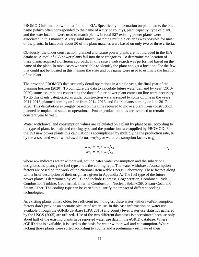
Water withdrawal and consumption values are calculated on a plant by plant basis, according to

the type of plant, its projected cooling type and the production rate supplied by PROMOD. For

the 153 new power plants this calculation is accomplished by multiplying the production rate, pi,

by the associated water withdrawal factor, wwff,c,, or water consumption factor, wcff,c

where ww indicates water withdrawal, wc indicates water consumption and the subscript i

designates the plant, f the fuel type and c the cooling type. The water withdrawal/consumption

factors are based on the work of the National Renewable Energy Laboratory. These factors along

with a brief description of their origin are given in Appendix A. The fuel type of the future

power plants is determined by WECC and include Biomass, Cogeneration, Combined Cycle,

Combustion Turbine, Geothermal, Internal Combustion, Nuclear, Solar-CSP, Steam-Coal, and

Steam-Other. The cooling type can be varied to quantify the impact of different cooling

technologies.

As existing plants utilize older, less efficient technologies, these water withdrawal/consumption

factors don’t provide an accurate picture of water use. In this case information on water use

available through the eGRID database (EPA 2010) and county level water use statistics gathered

by the USGS (2005) are utilized. Use of the two different databases is necessitated because only

about half of the existing plants have reported water use data in the eGRID database. Where

eGRID data is available, it is used as the basis for water withdrawal and consumption. Where

lacking those plants were sorted according to county and a preliminary estimate of their

3

12

withdrawal and consumption is made using equation 3. These values are then adjusted in a

proportional manner so as to match the measured USGS data (2005 data for withdrawal and

1995 data for consumption). As production rates vary between years and between the different

WECC study cases, adjustment to these historical water use rates is necessary. This is

accomplished through a proportional adjustment using the production rate associated with the

measured water use rate, po, and that of the future power production rate, pf

4

where wu denotes water use (either withdrawal or consumption) and the subscripts o and f stand

for initial and future, respectively.

The final step involves determining the source of water for the power plant. This is accomplished

using the EPA (2010) and USGS (2005) data. For plants with source water specified in the

eGRID database, that designation is used. Otherwise the USGS data was used in a manner

similar to that described for establishing water withdrawal and consumption. Distribution of

source water between groundwater and surface water for future plants is handled in a manner

consistent with Equation 9 below.

2.3 Non-Thermoelectric Water Demand

The non-thermoelectric water demand module within EPWSim projects the future demand for

water according to five different use sectors: municipal (including domestic, public supply, and

commercial), industrial, agriculture, mining and livestock. Water withdrawal and consumption

are tracked separately as are the resulting return flows. Also modeled is the source of the

withdrawal, whether that be surface water, groundwater, or a non-potable source.

Water use statistics published by the U.S. Geological Survey (USGS) serve as the primary data

source for the EPWSim analyses (Kenny et al. 2009; Hutson et al. 2005; Solley et al. 1990;

1995). Every five years since 1950 the nation’s water-use data have been compiled and

published by the USGS. Collection of this data is a collaborative effort between the USGS, state

and local water agencies, and utilities. However, the level of detail at which these data are

reported varies from year to year. Data from the 1985, 1990, and 1995 campaigns provide the

most comprehensive picture of water use in the U.S. and also are the last years that consumptive

water use was compiled. The last published water census by the USGS is 2005 (no reported

consumptive use). As such, our projections of future water withdrawals utilize data from 1985-

2005 while consumptive use projections are limited to data from the 1985-1995 campaigns.

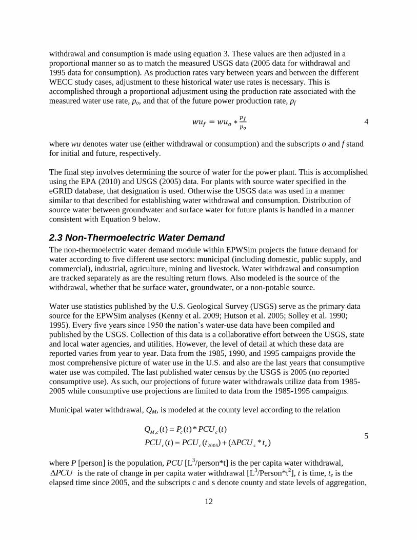
Municipal water withdrawal, QM, is modeled at the county level according to the relation

)*()()(

)(*)()(

2005

,

escc

cccM

tPCUtPCUtPCU

tPCUtPtQ

5

where P [person] is the population, PCU [L3/person*t] is the per capita water withdrawal,

PCU is the rate of change in per capita water withdrawal [L3/Person*t

2], t is time, te is the

elapsed time since 2005, and the subscripts c and s denote county and state levels of aggregation,

13

respectively. In this way, municipal water withdrawal is a function of both changing population

and per capita water withdrawal. Changes in population are calculated according to the county

level population growth rates reported by the Census Bureau (2004), as described above, while

PCU is based on historical trends (see below). Recognizing that care must be exercised when

extending historical trends into the future, limits are placed on the total allowable change.

Specifically, PCU is not allowed to increase or decrease by more than 20% over the duration

of the simulation. This limit is set based on the assumption that changes beyond ±20% would

likely require major structural changes to the system, for example the extent to which an

individual home owner might implement conservation measures. Once this maximum change is

achieved PCU is held constant throughout the rest of the simulation. Per capita water

withdrawal rates published for 2005, PCU(t2005), serve as the initial condition for the model.

Rates of change in per capita water withdrawal, PCU , were calculated by simple linear

regression using data from the USGS. Recognizing that meaningful trends in PCU could not be

extracted at the county/watershed level (data were erratic, displaying little correlation across the

three data sets), PCU values were calculated from data aggregated at the state level. Each

regression was inspected according to “goodness of fit”. In cases where the regression did not

accurately represent the perceived trends (i.e., R2<0.6) data were fitted by hand.

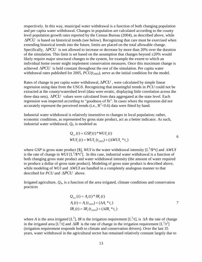
Industrial water withdrawal is relatively insensitive to changes in local population; rather,

economic conditions, as represented by gross state product, act as a better indicator. As such,

industrial water withdrawal, QI, is modeled as

)*()()(

)(*)()(

2005

,

escc

cccI

tWUItWUItWUI

tWUItGSPtQ

6

where GSP is gross state product [$], WUI is the water withdrawal intensity [L3/$*t] and WUI

is the rate of change in WUI [L3/$*t

2]. In this case, industrial water withdrawal is a function of

both changing gross state product and water withdrawal intensity (the amount of water required

to produce a dollar of gross state product). Modeling of gross state product is described above,

while modeling of WUI and WUI are handled in a completely analogous manner to that

described for PCU and PCU above.

Irrigated agriculture, QA, is a function of the area irrigated, climate conditions and conservation

practices

)*()()(

)*()()(

)(*)()(

2005

2005

,

escc

escc

cccA

tIRtIRtIR

tAtAtA

tIRtAtQ

7

where A is the area irrigated [L2], IR is the irrigation requirement [L

3/t], is A the rate of change

in the irrigated area [L2/t] and IR is the rate of change in the irrigation requirement [L

3/t

2]

(irrigation requirement responds both to climate and conservation drivers). Over the last 35

years, water withdrawal in the agricultural sector has remained relatively constant largely due to

14

limited increases in the area irrigated and offsetting improvements in irrigation efficiencies

(KENNY ET AL. 2009). For this reason, irrigation water withdrawal is assumed to remain

constant over the duration of the simulation. Nevertheless, the model is designed to easily permit

future changes to irrigated agriculture.

Other water use sectors such as mining and livestock fail to show a strong trend with population,

GSP, or any other simple metric. Thus, water withdrawal in the livestock sector, QL, is simply

modeled by extending its historical water withdrawal trend into the future

)*()()( ,2005,, esLcLcL tQtQtQ 8

where LQ is the rate of change in water withdrawal by the livestock sector [L3/t

2]. It is

calculated and implemented in a fashion similar to PCU and WUI above. Likewise, future

water withdrawal by the mining sector is modeled according to Equation 8, with an appropriate

change in parameters.

Once water withdrawal is calculated the fraction consumed and discharged to the waste water

treatment plant is determined. Consumptive use is calculated in an identical fashion to that in

equations 5-8 above, again using the data available from the USGS (2005). The only difference

is that consumptive use trends were calculated from data limited to the USGS census in 1985,

1990 and 1995. Also, the 1995 data serve as point from which future consumptive use values are

calculated. Waste water discharges are calculated as the difference between use and

consumption.

As the demand for water in a particular sector changes over time, so too will the mix of

withdrawals from groundwater, surface water and non-potable sources. Historical trends relative

to changes in groundwater abstraction are used to project future supply choices

)*()()( ,2005,, esncncn tGWftGWftGWf 9

where GWFn,c(t2005) is the fraction of supply taken from groundwater in 2005 [%], snGWf , is

rate of change in the fraction taken from groundwater [%/t] and the subscript n designates the

water use sector. snGWf , is calculated and applied similarly to that of PCU and WUI .

Likewise the percent water coming from non-potable sources is allowed to change, in this case

according to a user defined rate of change (set by a slider bar). The resulting supply taken from

surface water is fully determined by that not taken from groundwater or non-potable sources.

2.4 Water Supply

Stream gauge statistics based on extended sampling periods provide one of the best measures of

surface water availability. As these gauged flows are affected by activities upstream of the

gauge, the measured statistics account for upstream reservoir operations, evaporative losses,

groundwater-stream interaction, withdrawals, etc. In this way, the mean daily flow provides a

good measure of the average surface water supply available at the gauge location, while the

accompanying exceedance flows provide a measure of the variability in supply at that point.

15

Likewise, the gauged average daily base flow index (that portion of the stream flow contributed

by groundwater discharge) provides a good measure of the sustainable groundwater recharge

available for use.

The basis of the water supply modeling is the USGS National Hydrographic Dataset (NHD).

Specifically, the USGS has stream flow data from 23,000 gauges in which the available sampling

record has been statistically analyzed to give the minimum and maximum daily flows, mean

daily flow, key percentiles (1, 5, 10, 20, 25, 50, 75, 80, 90, 95, 99) of daily flow (exceedance

values), and the base flow index (Stewart et al. 2006). For each watershed the NHD gauge with

the longest record and which is the closest to the point of watershed discharge has been

identified. Specifically, surface and groundwater availability has been compiled at the

accounting unit (6-digit Hydrologic Unit Code [HUC]) level (167 watersheds across the western

U.S.). As future activities upstream of the gauge will affect streamflow, the 2006 stream gauge

statistics are adjusted in the model for changes in consumptive use upstream of the gauge.

Specifically, changes in water consumption (post 2006) are sequentially aggregated across

watersheds from headwater to the gauge. The aggregated consumption is then subtracted from

the long term gauge statistics to yield an adjusted measure of water availability.

By combining projected water demands with the physical water supply provides a meaningful

way to project regions prone to limited water availability. That is, where the demand for water

approaches the available water supply, tension over water allocation is possible.

2.5 Interactive Interface

The decision support tool is designed to be accessible to the professional and lay public alike,

requiring no specialized software (Excel is the only requirement). The model operates on a

laptop computer and can be used to demonstrate key variables and processes associated with the

electric power-water nexus. The model operates in real-time with a user-friendly interface that

includes slider bars, buttons and switches for changing key input variables, and real-time output

graphs, tables, and geospatial maps (displayed interactively through Google Earth™) showing

results. These features allow a wide range of users to experiment with alternative electric power-

water use strategies and learn from the results. Ultimately, the model can be distributed to users

on CD or via the internet.

2.6 Database

Data supporting EPWSim is organized and managed within an Excel Database that

communicates directly with the model software. The database stores initial conditions as well as

key parameters and rates of change needed by the model. The database is organized according to

a number of worksheets each of which contain data supporting a specific module of the model.

Specifically, there are worksheets that contain data concerning, population; gross state product;

power plant locations; thermoelectric water use factors (by plant type); water use rates by sector

and location; mean and exceedance gauge data by watershed; and, associated lookup tables for

translation between different reference systems.

Beyond the baseline data used by the model, the database also includes various calculations

needed to prepare these data for use in the model. Calls to the database from the model are fully

automated within the simulation environment.

16

3. Results Our analysis starts with a review of conditions as of 2010; that is, the water demand across

different use sectors; current competition between thermoelectric power production and other

water use sectors; and, the state of water availability across the U.S. Attention then turns to

projecting future electric power and water demands. To help with this four alternative study

cases, as described below, are explored. In each case the consequences for water withdrawals

and consumption are considered as well as how such change influences the nexus between water

and energy (e.g., where water might limit the production of electricity). It should be noted that

the scenarios considered here are but a small subset of scenarios, policies, and action metrics that

could be investigated.

In efforts to see the big picture in the detailed results given below, we begin by stating four key

conclusions from this initial analysis:

Conclusion 1: Thermoelectric generation has the potential to drive a significant increase

in water consumption by 2020.

Conclusion 2: Water demands for thermoelectric use are relatively small in relation to

water demands for agriculture; however, thermoelectric demands are growing while

agriculture has remained steady over the past 40 years.

Conclusion 3: A key feature of the projected growth in thermoelectric water demand is

that it corresponds to basins where it will compete with rapid growth in the municipal and

industrial sectors. Most of the projected thermoelectric growth is also planned for basins

characterized by limited water availability.

Conclusion 4: The study cases do perform differently with respect to water withdrawal

and consumption suggesting the opportunity to engineer solutions to the water and energy

nexus in the West.

3.1 Water and Electric Power in 2010

Figure 1 shows the distribution of water withdrawal and consumption in 2010 across the use

sectors of municipal, industrial, thermoelectric, mining, livestock and agriculture for the WECC

Interconnection (U.S. use only, future analyses will consider the full WECC service area). In

total, 117 BGD of freshwater are withdrawn from surface and groundwater resources while 92.6

BGD are consumed (water that is lost to evaporation and thus not returned directly to a surface

or groundwater body for further use in the basin). In terms of freshwater withdrawals

thermoelectric production requires 1.9 BGD or 2% of the regional withdrawals. If saline water is

considered a total of 9.6 BGD are withdrawn making thermoelectric power production the third

largest user of water in the western interconnect. The largest freshwater withdrawal is by

irrigated agriculture at 96 BGD (82%), followed by municipal at 14.6 BGD (12%). Other

withdrawals include industry at 1.6 BGD (1%), mining at 0.5 BGD (1%) and livestock at 2.7

BGD (2%). Of these withdrawals, 29.6 BGD is extracted from groundwater resources.

The consumptive water use picture is similar. Irrigated agriculture dominates consumption at

87.6 BGD, or 95% of all consumption. Other freshwater consumptive uses include municipal at

3.2 BGD (3%), livestock at 0.7 BGD (1%), industrial at 0.4 BGD (0.4%) mining at 0.4 BGD

(0.4%) and thermoelectric at 0.4 BGD (0.4%). Although irrigation dominates both water

17

withdrawal and consumption this sector has realized effectively no growth over the last 40 years

(KENNY ET AL. 2009). Likewise, livestock and mining have maintained relatively level use

over this same time period. In contrast, municipal, industrial, and thermoelectric sectors have

been growing and are expected to continue growing, as will be shown later.

Of particular interest to this project is the thermoelectric power sector. To take a closer look at

this sector, thermoelectric power production and its associated water withdrawal and

consumption is disaggregated by power plant fuel type (Figure 2). A review of Figure 2 indicates

that thermoelectric power production in the WECC is predominately from coal-stream

production followed by natural gas combined cycle and nuclear. Thermoelectric water

withdrawals are almost evenly distributed between these three fuel types. These withdrawals are

largely the result of a limited number of power plants with open-loop cooling. Thermoelectric

water consumption shows a very different trend with coal-fired plants being responsible for the

vast majority of the consumption reflecting the relatively large number of plants and their

associated high consumptive use of water (see Appendix A).

Figures 1 and 2, which are aggregated at the interconnection-level, tell only a part of the story. In

particular, water withdrawal and consumption are not uniformly distributed across the

interconnection. Figure 3 presents water withdrawal and consumption by state. While the water

use picture in each state is dominated by irrigation, the total withdrawal and consumption across

states differ considerably. The states also differ in the degree to which the non-agricultural water

use sectors contribute to the water withdrawal and consumption statistics (e.g., more populous

states are characterized by higher non-agricultural water use). Withdrawals for thermoelectric

power production are evident in California, Washington and Wyoming.

These water demands are further disaggregated to the watershed level (Figure 4). The most

striking feature of these maps is the very different spatial arrangement of the demands.

Thermoelectric withdrawals and consumption vary from watershed to watershed with many

watersheds having no water use. Only a few watersheds are characterized by large thermoelectric

withdrawals, where the handful of plants that utilize open-loop cooling are located. In contrast,

thermoelectric consumption is more evenly distributed with an apparent trend toward higher

consumption to the east and lower consumption in the west. This trend reflects the tendency

toward more coal-fired plants in the east relative to gas-fired in the west.

In contrast, non-thermoelectric water use is measured in every watershed and the withdrawal and

consumption patterns are very similar to each other. While non-thermoelectric withdrawal and

consumption patterns are similar these patterns are very different from that of the thermoelectric

sector. The non-thermoelectric water use pattern is dominated by irrigated agriculture, following

key basins such as the Central Valley of California, Columbia River, Snake River, Platte River,

and the Lower Colorado.

Like water withdrawal and consumption, water supply is not uniformly distributed across the

West, ranging from a temperate climate in the Northwest to an arid climate in the desert

Southwest. Defining the water supply available for human use is a complex and often

contentious issue. Water supply depends on variability of the climate, the physical hydrology of

the basin, the engineered infrastructure to store and convey the water, the legal institutions that

18

manage and allocate the resource, as well as the personal values of those living in the basin.

Given this complexity we cannot definitively define the water supply; rather, we are forced to

depend on proxies that provide insight into specific aspects of water supply. Here the mean

gauged stream flow (a measure of surface water that is on average physically available in a

watershed), the 5th

percentile stream flow (a measure of surface water available on the driest

days of the year), and gauged base flow (a measure of the sustainable recharge to the watershed’s

groundwater aquifers) is used.

Limited water availability for future development is likely to occur where the demand for water

exceeds the accessible supply. Several general displays have been developed to explore the ratio

of supply to demand; specifically, maps are developed at the 6-digit HUC level based on the

ratio of water supply to water demand. Where this ratio is large, limited water availability is

unlikely, where the ratio is small supply is on the order of demand thus there is little room for

new growth. For purposes of this analysis, areas prone to limited water availability are taken as

regions with a supply to demand ratio of 2 or less. While this value is somewhat arbitrary it does

represent a natural threshold in the data. As noted above, three different metrics have been

formulated one for surface water availability, another for low flow conditions, and a third for

groundwater availability. These are shown in Figure 5.

A quick review of the mean surface water supply to demand ratio (Figure 5a) clearly reveals that

much of the western U.S. is likely subject to limited water availability (as measured by this

metric), with only the far north and Upper Colorado River characterized by ratios above 2. This

result simply reflects both the aridity of the West and the high water use due to irrigated

agriculture. The low flow ratio (Figure 5b) shows similar results to that of the mean surface

water availability but at increased spatial extent. Limited groundwater availability (Figure 5c) is

indicated largely in the Great Plains, in the Southwest, and the Great Basin again reflecting the

combined effect of arid climate and irrigated agriculture. While we recognize that these are

imperfect metrics results are similar to water stress regions identified by the U.S. Bureau of

Reclamation in the Water 2025 Assessment (2010) and the U.S. Geological Survey in their 2009

Groundwater Report (Reilly 2008).

3.2. Study Case Analyses

Figure 5 clearly indicates that much of the western U.S. is characterized by limited water

availability for future development and in fact, many areas are already realizing the squeeze of

water resource issues. However, every indication suggests that the demand for water is going to

increase. Based on projections from the U.S. Census Bureau, population within the WECC is

expected to grow from 75M in 2010 to 83M by 2020, an 11% increase. Over the same period of

time electric power demand is project to grow from 664 to 740 million megawatt hours

(MMWh) (EIA 2010), also an 11% increase.

We do not know exactly how population will grow, how power and water use characteristics

will change in time, how the electric power plant fleet will evolve to meet the growing needs, or

do we know what policies may be enacted that impact the energy and water sectors. For this

reason we utilize a series of potential future realities, termed study cases, to explore the nexus

between energy and water. These include:

19

1. Transmission Expansion Planning Policy Committee (TEPPC) Base Case. This test case

is designated as PC0. This study case is based on Balancing Authority load forecasts and

renewable resource utilization that complies with state Renewable Portfolio Standard

(RPS) targets.

2. State Provincial Steering Committee (SPSC) Reference Case. This test case is designated

as PC1. This study case replaces Balancing Authority loads with state-adjusted load

forecasts. Renewable resources have been modified to reflect RPS targets based on the

state-adjusted loads.

3. SPSC High Load Case. This test case is designated as PC2. This study case utilizes the

state-adjusted load forecasts and increases them by 10%. Renewable resources have been

modified to reflect RPS targets based on the state-adjusted loads.

4. SPSC High Demand Side Management Case. This test case is designated as PC3. This

study case decreases the state-adjusted load forecasts to reflect achievement of the “full

economic energy efficiency potential throughout the West”. Renewable resources have

been modified to reflect RPS targets based on the state-adjusted loads.

We now project into the future 10 years, to the year 2020. As future demands are uncertain the

analysis utilizes four alternative study case realities (as described above). The ultimate goal is to

quantify tradeoffs in terms of water withdrawal and consumption relative to the four study cases.

Also of interest is understanding the extent to which new thermoelectric power production will

compete with growing demands in other water use sectors for limited water resources in the

western U.S. Other analyses will help identify new power plants sited in basins prone to limited

water availability (e.g., locations where permitting is likely to be difficult). Taken together this

information will help better inform long-range transmission planning.

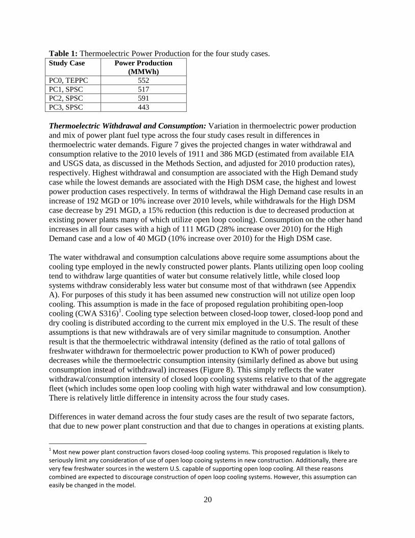
Power Production: Ultimately, new water demands for WECC operations will depend on the

extent of thermoelectric power production. Each of the four study cases result in a different level

of total thermoelectric power production (Table 1). As would be expected the SPSC High

Demand Case yields the highest production at 591 MMWh while the SPSC High Demand Side

Management study case yields the lowest demand (443 MMWh), representing a 33% difference

between high and low production. Figure 6 shows the mix of new thermoelectric power

production by fuel type for the TEPPC Base Case. Much of this new production comes from

natural gas combined cycle (NGCC) plants with supporting supplies from geothermal, solar CSP

and coal-steam (Figure 6). Limited new production is also provided by gas-combustion cycle,

and biofuels. This mix of new production is very closely replicated in the other three study cases.

As such, noted differences in production across the study cases (Table 1) are largely the result of

changes to operations of existing power plants. The SPSC Reference case is characterized by a

decrease in existing coal-steam and NGCC production relative to the Base Case, while the High

Demand Case involves increased production by existing NGCC and to a lesser extent Biofuel

plants. The High DSM case involves reductions to coal-steam and NGCC plants and to a lesser

extent solar CSP relative to the base case.

20

Table 1: Thermoelectric Power Production for the four study cases.

Study Case Power Production

(MMWh)

PC0, TEPPC 552

PC1, SPSC 517

PC2, SPSC 591

PC3, SPSC 443

Thermoelectric Withdrawal and Consumption: Variation in thermoelectric power production

and mix of power plant fuel type across the four study cases result in differences in

thermoelectric water demands. Figure 7 gives the projected changes in water withdrawal and

consumption relative to the 2010 levels of 1911 and 386 MGD (estimated from available EIA

and USGS data, as discussed in the Methods Section, and adjusted for 2010 production rates),

respectively. Highest withdrawal and consumption are associated with the High Demand study

case while the lowest demands are associated with the High DSM case, the highest and lowest

power production cases respectively. In terms of withdrawal the High Demand case results in an

increase of 192 MGD or 10% increase over 2010 levels, while withdrawals for the High DSM

case decrease by 291 MGD, a 15% reduction (this reduction is due to decreased production at

existing power plants many of which utilize open loop cooling). Consumption on the other hand

increases in all four cases with a high of 111 MGD (28% increase over 2010) for the High

Demand case and a low of 40 MGD (10% increase over 2010) for the High DSM case.

The water withdrawal and consumption calculations above require some assumptions about the

cooling type employed in the newly constructed power plants. Plants utilizing open loop cooling

tend to withdraw large quantities of water but consume relatively little, while closed loop

systems withdraw considerably less water but consume most of that withdrawn (see Appendix

A). For purposes of this study it has been assumed new construction will not utilize open loop

cooling. This assumption is made in the face of proposed regulation prohibiting open-loop

cooling (CWA S316)1. Cooling type selection between closed-loop tower, closed-loop pond and

dry cooling is distributed according to the current mix employed in the U.S. The result of these

assumptions is that new withdrawals are of very similar magnitude to consumption. Another

result is that the thermoelectric withdrawal intensity (defined as the ratio of total gallons of

freshwater withdrawn for thermoelectric power production to KWh of power produced)

decreases while the thermoelectric consumption intensity (similarly defined as above but using

consumption instead of withdrawal) increases (Figure 8). This simply reflects the water

withdrawal/consumption intensity of closed loop cooling systems relative to that of the aggregate

fleet (which includes some open loop cooling with high water withdrawal and low consumption).

There is relatively little difference in intensity across the four study cases.

Differences in water demand across the four study cases are the result of two separate factors,

that due to new power plant construction and that due to changes in operations at existing plants.

1 Most new power plant construction favors closed-loop cooling systems. This proposed regulation is likely to

seriously limit any consideration of use of open loop cooing systems in new construction. Additionally, there are very few freshwater sources in the western U.S. capable of supporting open loop cooling. All these reasons combined are expected to discourage construction of open loop cooling systems. However, this assumption can easily be changed in the model.

21

As noted above, construction and operation of the new power plant fleet is quite consistent

across the four study cases and so too are the associated new water withdrawals and

consumption. Withdrawals associated with new plant construction are limited to a range of 108

MGD to 87 MGD, while consumption varies between 100 MGD to 83 MGD (across the four

study cases). In contrast changes in withdrawal across all existing power plants range from an

increase of 86 MGD to a decrease of 374 MGD, while consumption varies between an increase

of 11 MGD to a decrease of 43 MGD. Thus, the apparent differences between the four study

cases are due largely to changes in operations at existing plants.

The manner with which water withdrawal and consumption for new construction is distributed

by fuel type is given in Figure 6. It is noted that water withdrawal and consumption are similarly

distributed by fuel type. Comparing new power production with new water

withdrawal/consumption indicates a distinct difference in water use across the different fuel

types (also see Appendix A). Specifically, NGCC has lower water withdrawal and consumption

requirements relative to that for either coal-steam, geothermal or solar CSP (e.g., NGCC has the

largest new power production; however, coal-steam, geothermal and solar CSP all have greater

water demands).

Of particular interest is where these new water demands for thermoelectric production are

located. Figure 9 shows the water consumption for new power plants constructed between 2010

and 2020 for the TEPPC Base Case. As noted above there is very little difference between the

four study cases and hence maps for these other study cases are not given. Likewise withdrawals

are essentially the same as that given for consumption and hence results are not duplicated here.

From the map of water consumption it is evident that new thermoelectric power production is not

uniformly distributed over the west. Rather, production tends to be concentrated in southern

California, western Arizona and southern Nevada. Demands are also focused in a couple of

watersheds in the Great Plains. These demands are particularly important as they represent new

demands which must be satisfied with existing and limited water resources.

Future thermoelectric demands are also influenced by changes in production at existing plants.

Figure 10 shows total thermoelectric water consumption by 6-digit watershed for the four study

cases. As noted previously, most of the differences evident in these maps are due to changes in

production at existing plants. Reduced production and thus demand at an existing plant

represents an opportunity to transfer the un-needed water to a new use, namely a new

thermoelectric power plant. Although careful inspection is required to see differences such trends

are evident along the southern coast of California, the Central Valley of California and around

southern Nevada.

For completeness, Figure 11 shows 2020 withdrawals of saline water for thermoelectric cooling.

A total of 5600 MGD of saline water is withdrawn and 12 MGD are consumed. Much of the

coastal saline water use is associated with open loop cooling and thus the reason for the

relatively high withdrawals. In this phase of analysis, no new use of saline water use for

thermoelectric production has been projected; however, this is an option we will be considering

in detail as this project progresses.

22

Competing Demands: New water demands in the thermoelectric power sector will have to

compete with rapid growth in the municipal and industrial sectors. Between 2010 and 2020

municipal and industrial withdrawals are projected to increase by 837 MGD and 154 MGD while

consumptive use is expected to see a rise of 364 MGD and 43 MGD, respectively. Figure 7

compares the projected growth between thermoelectric, municipal and industrial sectors. In

rough terms growth in the thermoelectric sector (all study cases) is comparable to the growth

projected for all other industrial needs and is about 25% of the growth projected for the

municipal sector. Little to no growth is projected for the agricultural, livestock and mining

sectors as economic expansion in these sectors has largely been offset by improvements in water

use efficiency over the last 40 years.

An important aspect of this growth is that it will largely be focused around the large urban

centers in the West. Figure 12 shows where new demands for non-thermoelectric water

(municipal and industrial) consumption are likely to be concentrated. Significant growth is found

along the west coast, southern Arizona, southern Nevada, and the front range in Utah and

Colorado. This growth in non-thermoelectric demand in many cases overlaps projected new

demands for thermoelectric power production (Figure 12). Competing demands are particularly

evident along the California coast, southern California and southern Nevada.

Thermoelectric Development in Regions with Limited Water Availability: Of particular interest

to this study is where current and projected thermoelectric power production is likely to be

impacted by water availability. As a first step in this endeavor the three water availability metrics

(surface water, low flow, and groundwater) shown in Figure 5 have been updated to reflect water

usage in 2020. Comparison of the 2010 (Figure 5) and 2020 water stress maps show almost no

difference. This should come as little surprise as the increase in consumptive use over this time is

only on the order of 1% (see above). This increase in consumption is generally small relative to

the absolute water supply, particularly in the less water stress prone watersheds. Given the small

differences between 2010 and 2020 the 2020 maps are not presented here.

The next step involves distinguishing the water source for new thermoelectric withdrawals and

consumption. As noted above, for the current analysis we have assumed a potable water source

will be pursued either surface water or groundwater; however, the analysis will be broadened to

non-potable sources in the next phase of analysis. The future source distribution for new

thermoelectric power plants is simply assumed to follow the current groundwater to surface

water distribution by 6-digit HUC watershed.

The final step to identify at risk plants involves mapping new consumption by thermoelectric

cooling (TEPPC Base Case) onto watersheds in basins with limited water availability; that is,

those watersheds where the supply to demand ratio is below two (i.e., watersheds marked white

in Figure 5). Specifically, Figure 13 shows projected future water consumption by thermoelectric

power production to be met by a surface water source and which corresponds to a watershed with

limited surface water availability. This map shows where it will be unusually difficult or

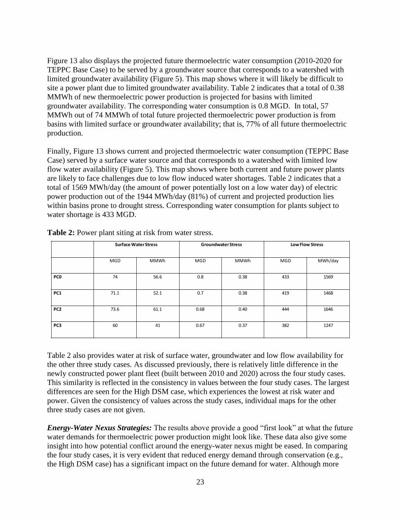
expensive to obtain a surface water right/permit for a new thermoelectric power plant. Table 2

indicates that a total of 56.6 MMWh of new electric power production is needed in basins prone

to limited surface water availability. Water consumption of 74 MGD is associated with this at

risk power production.

23

Figure 13 also displays the projected future thermoelectric water consumption (2010-2020 for

TEPPC Base Case) to be served by a groundwater source that corresponds to a watershed with

limited groundwater availability (Figure 5). This map shows where it will likely be difficult to

site a power plant due to limited groundwater availability. Table 2 indicates that a total of 0.38

MMWh of new thermoelectric power production is projected for basins with limited

groundwater availability. The corresponding water consumption is 0.8 MGD. In total, 57

MMWh out of 74 MMWh of total future projected thermoelectric power production is from

basins with limited surface or groundwater availability; that is, 77% of all future thermoelectric

production.

Finally, Figure 13 shows current and projected thermoelectric water consumption (TEPPC Base

Case) served by a surface water source and that corresponds to a watershed with limited low

flow water availability (Figure 5). This map shows where both current and future power plants

are likely to face challenges due to low flow induced water shortages. Table 2 indicates that a

total of 1569 MWh/day (the amount of power potentially lost on a low water day) of electric

power production out of the 1944 MWh/day (81%) of current and projected production lies

within basins prone to drought stress. Corresponding water consumption for plants subject to

water shortage is 433 MGD.

Table 2: Power plant siting at risk from water stress.

Table 2 also provides water at risk of surface water, groundwater and low flow availability for

the other three study cases. As discussed previously, there is relatively little difference in the

newly constructed power plant fleet (built between 2010 and 2020) across the four study cases.

This similarity is reflected in the consistency in values between the four study cases. The largest

differences are seen for the High DSM case, which experiences the lowest at risk water and

power. Given the consistency of values across the study cases, individual maps for the other

three study cases are not given.

Energy-Water Nexus Strategies: The results above provide a good “first look” at what the future

water demands for thermoelectric power production might look like. These data also give some

insight into how potential conflict around the energy-water nexus might be eased. In comparing

the four study cases, it is very evident that reduced energy demand through conservation (e.g.,

the High DSM case) has a significant impact on the future demand for water. Although more

Surface Water Stress Groundwater Stress Low Flow Stress

MGD MMWh MGD MMWh MGD MWh/day

PC0 74 56.6 0.8 0.38 433 1569

PC1 71.1 52.1 0.7 0.38 419 1468

PC2 73.6 61.1 0.68 0.40 444 1646

PC3 60 41 0.67 0.37 382 1247

24

difficult to see in the data is that changes in the mix of power plant fuel type also influence the

amount of water withdrawn and consumed (see Figures 2 and 6).

There are several ways that planners could further use this data to reduce impacts on water

resources and thus ease conflict around siting of future power plants. One option involves

coordinating the retirement (or substantial reduction in operation) of a power plant with the siting

of another. That is coordinate these actions so that the water rights associated with the retired

plant could be transferred to the new plant. In this way no “new” demand for water would be

realized.

Figure 13 can be viewed as a priority list for new power plant construction where alternative

sources of water might be considered (i.e., new plants sited in basins with limited water

availability). One option would be to consider use of dry or hybrid cooling at some of these

power plants. Of course such decision must also consider factors such as cost, availability of

land, and operational efficiency of the plants (loss of power production during hot periods).

Plants sited in basins with limited water availability might also consider use of a non-freshwater

source, such as brackish, saline, municipal waste water or produced water. Figure 11 shows were

saline water is currently being used by the electric power industry. Characterization of these

non-potable sources of water will be a focus of future phases of analysis.

If air cooling or non-potable water sources are not an option there are a few of other solutions.

First, considerations of changing the plant fuel type to a lower water use or non-thermoelectric

type could be made. Second, the plant could be moved to another basin where competition for

water is less acute. Finally, the plant could look to retire water from a low value use and transfer

it to thermoelectric production.

In the next phase of analysis these tradeoffs will be integrated directly into the 20-year

transmission planning process as an objective or constraint on the multi-criteria optimization

problem.

4. Next Steps The study results reported above are based on the EPWSIM model and associated data. This

model was developed under the auspices of other project funding. While EPWSIM provides

valuable insights to the energy-water nexus, it is limited in many ways. For this reason

significant efforts associated with the Energy and Water in the Western and Texas

Interconnections Project are aimed at upgrading and expanding this model and associated data.

Below a brief overview of planned changes to the model and database are given.

Thermoelectric Water Use Calculator: Initial estimates of water withdrawals and consumption

at existing and future power plants have been provided in the results section. These results are

based on information from a wide variety of sources including EIA and the USGS. There are

significant limitations associated with each of these data sources, many of which the EIA and

USGS are working to correct. As such, efforts are being made to improve on the current data

toward estimating water use at a unit level basis. Key features to the analysis is to improve on

existing information on unit type details, associated cooling technology, and source of water

(surface water, groundwater, municipal supplied, municipal waste water, saline, or brackish).

25

Efforts will likewise be made to acquire operational water use data from the current fleet of

power plants. This analysis will also provide insight into drought related impacts on water use

(e.g., effects of humidity and temperature ). Other issues to be considered include potential

impacts due to new policies on open-loop cooling and/or carbon emissions.

Other Water for Energy Requirements: Significant future water use may be required in the

extraction and processing of primary energy fuel sources. These include traditional sources such

as coal, natural gas, uranium, oil, as well as liquid fuels for transportation. Our analysis will also

look at potential trends in non-traditional sources such as biofuels, oil shales, and gas shales.

These efforts will work to characterize the likely extent of water withdrawals and consumption

for both extraction of these fuels and their processing. Where these demands for water will be

located is also be a key feature of our analysis. A variety of future scenarios will be developed to

address potential evolutionary paths that these traditional and non-traditional fuels may take.

Water Supply/Demand/Institutional Controls: Future water demands for energy development

need to be put in the broader context of competition with other water use sectors as well as the

future availability of water. An initial analysis has been provided above; however, significant

opportunities have been identified toward its improvement. Specific improvements include the

need to utilize state water planning data as the basis for projecting future demands and supply;

the need to characterize institutional controls (e.g., water rights, compacts) that regulate access to

physical water; and, expanding and vetting the metrics utilized in assessing water availability.

The project team will work directly with state water managers to acquire, integrate and vet

regional water use and supply data into the energy-water decision support system. This effort

will utilize information from regional water planning as the basis of the analysis. These plans

generally include information on current water use and projected water use (high and low cases).

These plans also include information on current water supply and any planned projects to

augment supply (e.g., reservoir, interbasin transfers, desalination projects). This analysis will

also address non-fresh sources such as municipal wastewater, brackish water, saline water, and

produced water.

Just because water is physically available in a basin does not mean that it is available for use.

Interstate/international compacts and water rights further regulate how much water can be used

in a basin and for what use. The project team will work with state water managers to model the

institutional controls on water within their state. Key information needs include river compacts

and treaties, unappropriated water, agricultural water rights, adjudication status, status of Indian

water rights, location of special administrative areas, and special regulatory policies.

Ultimately all of this water related information will need to be distilled down to a few key

metrics, similar to those given in Figure 5. Ultimately these metrics will be designed to indicate

where development of water for thermoelectric water use would be most welcome. This

development potential must distinguish between surface water, groundwater and the various non-

potable water supplies. Such maps of water availability have significant implications for water

management within a given state. For this reason, water managers will need to be intimately

involved in deciding how to craft appropriate metrics and approve their final form.

26

Drought Vulnerability: Water supplies limited by drought pose a threat to power production at

existing and future thermoelectric power plants. A limited analysis of this effect is given in by

current and future plants located in basins subject to low flow water stress. Drought will also

impact production at hydroelectric power facilities. Recently a study has been completed to

review pertinent literature on drought and its impact on western water supply. This information

was combined with available power plant drought contingency plan information to assess

regional vulnerability to drought. This was done for both hydroelectric and thermoelectric

facilities. Results are currently being reviewed to determine whether a more detailed analysis on

a plant by plant basis is warranted.

Transmission Planning Integration: Another key improvement over this analysis will be the

integration of water data directly into the transmission planning process. Specifically, water

related data will be used to set objectives and/or constraints in WECC’s multi-criteria

optimization process that will be used to maximize the placement of future power and

transmission expansion projects. This will allow iteration on the transmission process so as to

achieve a future that minimizes impact on regional water resources balanced with other key

considerations such as cost, reliability, and transmission/operational efficiency.

5. Summary This analysis supports WECC’s 10-year planning study by investigating the water implications

of four alternative study cases: TEPPC Base Case, SPSC Reference Case, High Demand Case

and the High DSM Case. This initial study utilized analysis tools and data (e.g., the Energy,

Water and Power Simulation model, see description below) that are in the development stage.

Over the next two years of this project significant improvements are scheduled for both the

model and the data that drives the model. As such the results given above should be viewed as

preliminary. However, these results should assist in:

4) Establishing some working numbers relative to thermoelectric water use, where it is

located, and where/how it is likely to grow.

5) Beginning dialogue toward developing water related metrics that can be used in long-

range transmission planning.

6) Cultivating experience in integrating water resource planning with long term electric

power transmission planning.

Four key findings from this preliminary analysis have been identified, which include:

Conclusion 1: Thermoelectric generation has the potential to drive a significant increase

in water consumption by 2020.

Conclusion 2: Water demands for thermoelectric use are relatively small in relation to

water demands for agriculture; however, thermoelectric demands are growing while

agriculture has remained steady over the past 40 years.

Conclusion 3: A key feature of the projected growth in thermoelectric water demand is

that it corresponds to basins where it will compete with rapid growth in the municipal and

industrial sectors. Most of the projected thermoelectric growth is also planned for basins

with limited water availability.

27

Conclusion 4: The study cases do perform differently with respect to water withdrawal

and consumption suggesting the opportunity to engineer solutions to the water and energy

nexus in the West.

The study results reported above are based on the EPWSIM model and associated data. While

EPWSIM provides valuable insights to the energy-water nexus, it is limited in many ways. For

this reason significant efforts associated with the Energy and Water in the Western and Texas

Interconnections Project are aimed at upgrading and expanding this model and associated data.

Planned additions include expanding the thermoelectric water use calculator; including water use

for the extraction and refining of primary energy fuels; integration of state level data and

engagement of state water managers in characterizing current and future water demands, water

supplies, and institutional controls; assessment of power plant vulnerability to drought; and,

integration of water data directly into long-term transmission planning.

6. References BEA (Bureau of Economic Analysis), 2007. Gross Domestic Product by State. U.S. Department

of Commerce, http://www.bea.gov/regional/gsp/ As of December 10, 2007.

EIA (Energy Information Administration), 2010. 2010 Net Generation by State by Type of

Producer by Energy Source (EIA-906).

EPA (U.S. Environmental Protection Agency), 2010. Emissions & Generation Resource

Integrated Database (eGRID), version 1.0. Available at: 9.

http://www.epa.gov/cleanenergy/energyresources/egrid/index.html.

NETL, 2008. Estimating Freshwater Needs to Meet Future Thermoelectric Generation

Requirements, 2008 Update. DOE/NETL- 400/2008/1339, 2008.

Hutson, S.S., N.L. Barber, J.F. Kenny, K.S. Linsey, D.S. Lumia, and M.A. Maupin, 2005.

Estimated use of water in the United States in 2005, U.S. Geological Survey Circular 1268.

Kenny, R.F., N.L. Barber, S.S. Hutson, K.S. Linsey, J.K. Lovelace and M.A. Maupin, 2009.

Estimated use of water in the United States in 2005, U.S. Geological Survey Circular 1344, 52p.

Reilly, T.E.,K.F. Dennehy, W.M. Alley, and W.L. Cunningham, 2008, Ground-Water

Availability in the United States, U.S. Geological Survey Circular 1323, 70 pages.

Solley, W.B., R.R. Pierce, and H.A. Perlman, 1995. Estimated Use of Water in the United States

in 1995, U.S. Geological Survey Circular 1200.

Solley, W.B., R.R. Pierce, and H.A. Perlman, 1990. Estimated Use of Water in the United States

in 1990, U.S. Geological Survey Circular 1081.

Sterman, J. D., 2000. Business Dynamics, Systems Thinking and Modeling for a Complex

World. McGraw-Hill, Boston. 982 pp.

28

Stewart, D.W., A. Rea and D.M Wolock, 2006. USGS Streamgages Linked to the Medium

Resolution NHD Geospatial Data Presentation Form: Vector Digital Data. US Geological Survey

DS-195.

Tidwell, V.C., P.H. Kobos, L. Malczynski, G. Klise and W. Hart, 2009, Decision Support for

Integrated Water-Energy Planning, SAND Report, SAND2009-6521, Sandia National

Laboratories, Albuquerque, NM.

U.S. Census Bureau, 2004. Statistical Abstract of the United States: 2004-2005. Available at

http://www.census.gov/prod/2004pubs/o4statab/pop.pdf. Accessed in August, 2008.

U.S. Bureau of Reclamation, 2010, WATER 2025 Preventing Crises and Conflict in the West,

available at: http://water.wikia.com/wiki/Water_2025.

U.S.G.S. (U.S. Geological Survey), 1985, 1990, 1995, 2000, 2005. Water Use in the United

States, Available at http://water.usgs.gov/watuse/ Accessed in November, 2010.

29

Appendix A: Water Withdrawal and Consumption and Parasitic Energy Factors Prepared by: National Renewable Energy Laboratory (NREL)

NREL Point of Contact: Jordan Macknick

jordan.macknick@nrel.gov

(303) 275-3828

December 1, 2010

Overview:

This document contains initial water withdrawal/consumption factors and parasitic energy use

factors, developed for use in the Energy-Water Analysis for the Western and Texas

Interconnects. Table 1 contains initial water consumption factors for renewable electricity

technologies. Table 2 contains initial water consumption factors for non-renewable electricity

technologies. Table 3 contains initial water withdrawal factors for non-renewable electricity

technologies. Renewable water withdrawal factors are assumed to equal water consumption

factors. Table 4 contains parasitic loss factors for different types of cooling systems.

Methods:

We consider water withdrawals and consumption for the operational phase only. Operational

water use in this study includes cleaning, cooling, and other process-related needs that occur

during electricity generation, such as flue gas desulfurization (FGD) in coal facilities. The energy

technologies addressed here consist of configurations of coal, natural gas, nuclear, geothermal,

biopower, wind, solar photovoltaic (PV), and concentrating solar power (CSP) technologies.

Cooling system technologies considered include wet recirculating technologies (cooling towers),

once-through cooling system (open loop cooling), air-cooled condensing (dry cooling), hybrid

wet and dry cooling systems (hybrid cooling), and pond cooling systems.

Estimates of water consumption and withdrawal have been calculated irrespective of geographic

location. Withdrawal and consumption factors are often reported in terms of water intensity that

are annual averages; water intensity of facilities may change from diurnal and seasonal variations

in temperatures and humidity levels, but these inter-annual variations are not examined. This

review did not alter (except for unit conversion) or audit for accuracy the estimates of water use

published in studies. Also, because estimates are used as published, considerable methodological

inconsistency is inherent which limits comparability. Additionally, no distinction is made

between water types, which may include freshwater, saline water, or municipal waste water.

Data sources include published academic literature, state and Federal government agency

reports, non-governmental organizations’ (NGO) reports, and industry submissions to

government agencies for permitting procedures.

Certain sources report ranges of water consumption and withdrawal factors in place of specific

values. If traceable individual case studies form the basis for the range given, the individual

values are included as independent estimates within the set of estimates that are statistically

analyzed. If a range is given and the underlying data points are not given, then the midpoint of

30

that range is used for calculating an average value, and the high and low extremes are used for

determining extreme ranges. This method of addressing ranges may lead to a slight bias toward

data sources reporting explicit cases, and may also underestimate actual water use at facilities, as

the midpoint of the range extremes are in general less than values reported from individual

facilities.

Linking to WECC Fuel Type Designations:

The table below provides more detailed information than is currently designated in the WECC

PROMOD database. This particularly applies to new power plants where water withdrawal and

consumption are based on the water use factors (and not on historic demands). Below we note

the associations we used between the WECC fuel type designations and the fuel type water use

factors utilized.

WECC Designator Water Use Factor from Table Below

Biomass Steam

Cogeneration No Water Use

Combined Cycle Natural Gas Combined Cycle

Combustion Turbine No Water Use

Geothermal Average of All Technologies

Internal Combustion No Water Use

Nuclear Generic

Solar-CSP Average of Trough and Power Tower

Steam-Coal Generic

Steam-Other Natural Gas Steam

Cooling technology is defined according to the study case assumptions.

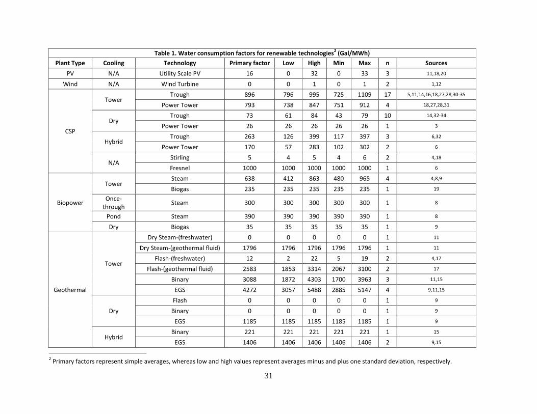
31

Table 1. Water consumption factors for renewable technologies2 (Gal/MWh)

Plant Type Cooling Technology Primary factor Low High Min Max n Sources

PV N/A Utility Scale PV 16 0 32 0 33 3 11,18,20

Wind N/A Wind Turbine 0 0 1 0 1 2 1,12

CSP

Tower Trough 896 796 995 725 1109 17 5,11,14,16,18,27,28,30-35

Power Tower 793 738 847 751 912 4 18,27,28,31

Dry Trough 73 61 84 43 79 10 14,32-34

Power Tower 26 26 26 26 26 1 3

Hybrid Trough 263 126 399 117 397 3 6,32

Power Tower 170 57 283 102 302 2 6

N/A Stirling 5 4 5 4 6 2 4,18

Fresnel 1000 1000 1000 1000 1000 1 6

Biopower

Tower Steam 638 412 863 480 965 4 4,8,9

Biogas 235 235 235 235 235 1 19

Once-through

Steam 300 300 300 300 300 1 8

Pond Steam 390 390 390 390 390 1 8

Dry Biogas 35 35 35 35 35 1 9

Geothermal

Tower

Dry Steam-(freshwater) 0 0 0 0 0 1 11

Dry Steam-(geothermal fluid) 1796 1796 1796 1796 1796 1 11

Flash-(freshwater) 12 2 22 5 19 2 4,17

Flash-(geothermal fluid) 2583 1853 3314 2067 3100 2 17

Binary 3088 1872 4303 1700 3963 3 11,15

EGS 4272 3057 5488 2885 5147 4 9,11,15

Dry

Flash 0 0 0 0 0 1 9

Binary 0 0 0 0 0 1 9

EGS 1185 1185 1185 1185 1185 1 9

Hybrid Binary 221 221 221 221 221 1 15

EGS 1406 1406 1406 1406 1406 2 9,15

2 Primary factors represent simple averages, whereas low and high values represent averages minus and plus one standard deviation, respectively.

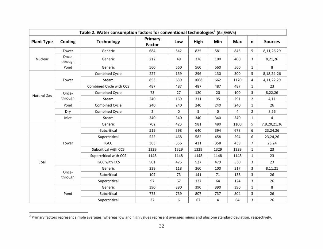
32

Table 2. Water consumption factors for conventional technologies3 (Gal/MWh)

Plant Type Cooling Technology Primary Factor

Low High Min Max n Sources

Nuclear

Tower Generic 684 542 825 581 845 5 8,11,26,29

Once-through

Generic 212 49 376 100 400 3 8,21,26

Pond Generic 560 560 560 560 560 1 8

Natural Gas

Tower

Combined Cycle 227 159 296 130 300 5 8,18,24-26

Steam 853 639 1068 662 1170 4 4,11,22,29

Combined Cycle with CCS 487 487 487 487 487 1 23

Once-through

Combined Cycle 73 27 120 20 100 3 8,22,26

Steam 240 169 311 95 291 2 4,11

Pond Combined Cycle 240 240 240 240 240 1 26

Dry Combined Cycle 2 0 5 0 4 2 8,26

Inlet Steam 340 340 340 340 340 1 4

Coal

Tower

Generic 702 423 981 480 1100 5 7,8,20,21,36

Subcritical 519 398 640 394 678 6 23,24,26

Supercritical 525 468 582 458 594 6 23,24,26

IGCC 383 356 411 358 439 7 23,24

Subcritical with CCS 1329 1329 1329 1329 1329 1 23

Supercritical with CCS 1148 1148 1148 1148 1148 1 23

IGCC with CCS 501 475 527 479 530 3 23

Once-through

Generic 239 118 360 100 317 3 8,11,21

Subcritical 107 73 141 71 138 3 26

Supercritical 97 67 127 64 124 3 26

Pond

Generic 390 390 390 390 390 1 8

Subcritical 773 739 807 737 804 3 26

Supercritical 37 6 67 4 64 3 26

3 Primary factors represent simple averages, whereas low and high values represent averages minus and plus one standard deviation, respectively.

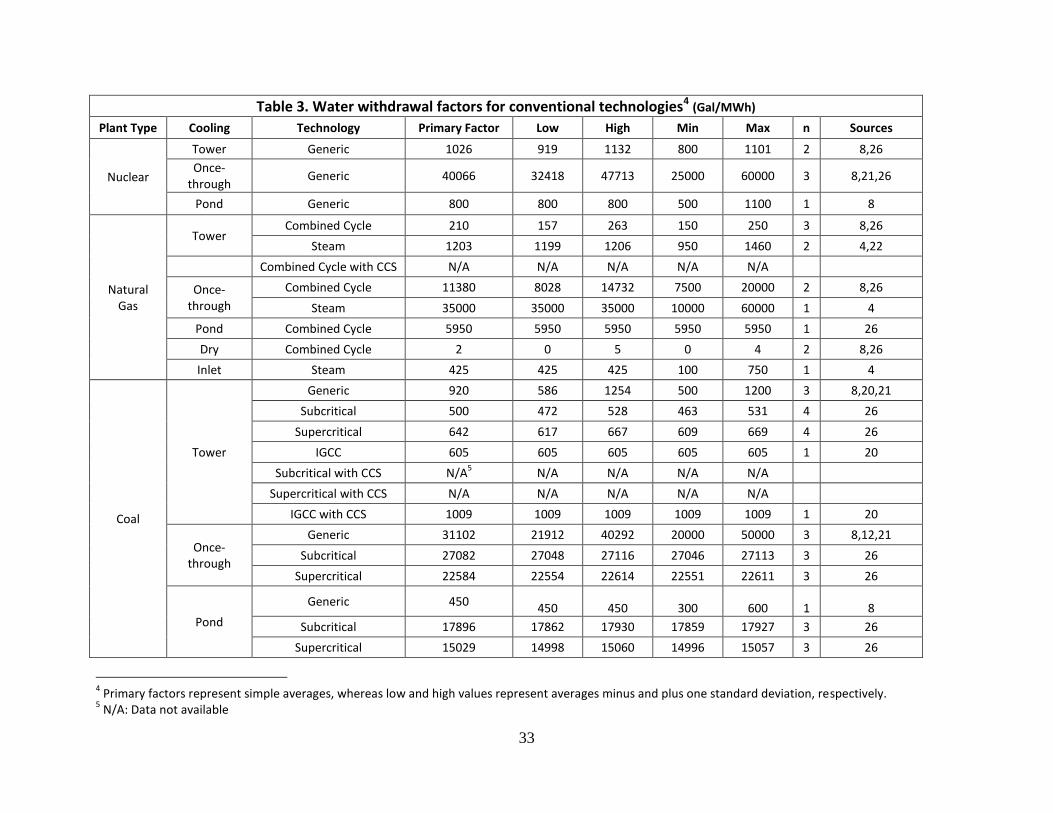
33

Table 3. Water withdrawal factors for conventional technologies4 (Gal/MWh)

Plant Type Cooling Technology Primary Factor Low High Min Max n Sources

Nuclear

Tower Generic 1026 919 1132 800 1101 2 8,26

Once-through

Generic 40066 32418 47713 25000 60000 3 8,21,26

Pond Generic 800 800 800 500 1100 1 8

Natural Gas

Tower Combined Cycle 210 157 263 150 250 3 8,26

Steam 1203 1199 1206 950 1460 2 4,22

Combined Cycle with CCS N/A N/A N/A N/A N/A

Once-

through

Combined Cycle 11380 8028 14732 7500 20000 2 8,26

Steam 35000 35000 35000 10000 60000 1 4

Pond Combined Cycle 5950 5950 5950 5950 5950 1 26

Dry Combined Cycle 2 0 5 0 4 2 8,26

Inlet Steam 425 425 425 100 750 1 4

Coal

Tower

Generic 920 586 1254 500 1200 3 8,20,21

Subcritical 500 472 528 463 531 4 26

Supercritical 642 617 667 609 669 4 26

IGCC 605 605 605 605 605 1 20

Subcritical with CCS N/A5 N/A N/A N/A N/A

Supercritical with CCS N/A N/A N/A N/A N/A

IGCC with CCS 1009 1009 1009 1009 1009 1 20

Once-through

Generic 31102 21912 40292 20000 50000 3 8,12,21

Subcritical 27082 27048 27116 27046 27113 3 26

Supercritical 22584 22554 22614 22551 22611 3 26

Pond

Generic 450 450 450 300 600 1 8

Subcritical 17896 17862 17930 17859 17927 3 26

Supercritical 15029 14998 15060 14996 15057 3 26

4 Primary factors represent simple averages, whereas low and high values represent averages minus and plus one standard deviation, respectively.

5 N/A: Data not available

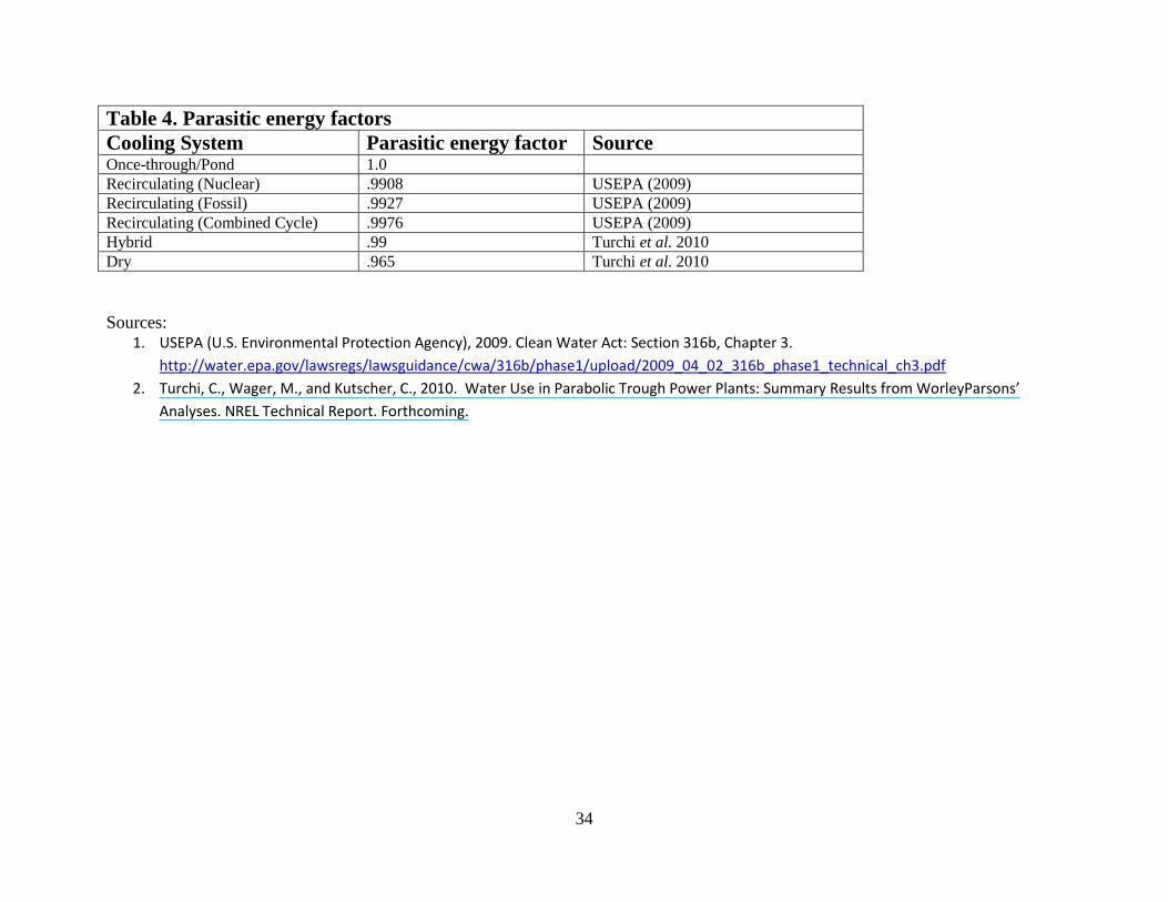
34

Table 4. Parasitic energy factors

Cooling System Parasitic energy factor Source Once-through/Pond 1.0

Recirculating (Nuclear) .9908 USEPA (2009)

Recirculating (Fossil) .9927 USEPA (2009)

Recirculating (Combined Cycle) .9976 USEPA (2009)

Hybrid .99 Turchi et al. 2010

Dry .965 Turchi et al. 2010

Sources: 1. USEPA (U.S. Environmental Protection Agency), 2009. Clean Water Act: Section 316b, Chapter 3.

http://water.epa.gov/lawsregs/lawsguidance/cwa/316b/phase1/upload/2009_04_02_316b_phase1_technical_ch3.pdf

2. Turchi, C., Wager, M., and Kutscher, C., 2010. Water Use in Parabolic Trough Power Plants: Summary Results from WorleyParsons’

Analyses. NREL Technical Report. Forthcoming.

35

References for water consumption and withdrawal factors

1. AWEA (American Wind Energy Association). 1996. AWEA estimate based on data

obtained in personal communication with Brian Roach, Fluidyne Corp., December 13, 1996. Accessed online: http://www.awea.org/faq/wwt_environment.html#How%20much%20water%20do%20wind%20turbines%20use%20compared%20with%20conventional%20power%20plants

2. Berndes, G. 2008. Water demand for global bioenergy production: trends, risks, and opportunities. Report commissioned by the German Advisory Council on Global Change (WBGU). Chalmers University of Technology, Gotenborg, Sweden.

3. BrightSource Energy. 2007. Application for Certification, Volumes I and II, for the Ivanpah Solar Electric Generating System. Submitted to California Energy Commission Docket Unit on August 31, 2007.

4. CEC (California Energy Commission). 2008. 2007 environmental performance report of California's electrical generation system. Staff Report. CEC-700-2007-016-SF.

5. Cohen, G., Kearney, D., and G. Kolb. 1999. Final report on the operation and maintenance improvement program for concentrating solar power plants. Sandia National Laboratories Report. SAND99-1290.

6. DOE (U.S. Department of Energy). 2008. Report to Congress: concentrating solar power commercial application study: reducing water consumption of concentrating solar power electricity generation.

7. Dziegielewski, B., T. Bik et al. 2006. Water Use Benchmarks for Thermoelectric Power Generation. Project Completion Report. Research Report of the Department of Geography and Environmental Resources, Southern Illinois University Carbondale. 203 pp., Carbondale, Illinois. August 15, 2006.

8. EPRI (Electric Power Research Institute. 2002b. Water and sustainability (Volume 2): an assessment of water demand, supply, and quality in the U.S.-the next half century. 1006785.

9. EPRI, and DOE, 1997: Renewable Energy Technology Characterizations. EPRI Topical Report-109496, December

10. Giusti, E.V. and E.L. Meyer. 1977. Water consumption by nuclear power plants and some hydrological implications. Geological Survey Circular 745.

11. Gleick P., ed. 1993. Water in crisis: a guide to the world's fresh water resources. New York: Oxford University Press.

12. Inhaber, H. 2004. Water use in renewable and conventional electricity production. Energy Sources. 26:309-322.

13. Kagel, Alyssa, Diana Bates, and Karl Gawell. 2007. A Guide to Geothermal Energy and the Environment., Washington, D.C.: Geothermal Energy Association. Washington DC

14. Kelly, B. 2006. Nexant parabolic trough solar power plant systems analysis. Task 2: comparison of wet and dry Rankine cycle heat rejection. NREL Subcontractor Report. NREL/SR-550-40163.

15. Kozubal, E. and C. Kutscher. 2003. Analysis of a Water-Cooled Condenser in Series with an Air-Cooled Condenser for a Proposed 1-MW Geothermal Power Plant. Geothermal Resources Council Transactions, Vol. 27.

16. Kutscher, C., and A. Buys. 2006. Analysis of wet/dry hybrid cooling for a parabolic trough power plant. NREL Report.

17. Layton, D.W. 1979. Water-related impacts of geothermal energy production in California' s

imperial valley

36

18. Leitner, A. 2002. Fuel from the sky: solar power’s potential for western energy supply. NREL Subcontractor Report. NREL/SR-550-32160.

19. Mann, M., and P. Spath, 1997: Life Cycle Assessment of a Biomass Gasification Combined-Cycle System. NREL Technical Report-TP-430-23076, December

20. Meridian Corporation. 1989. Energy system emissions and materiel requirements. Prepared for DOE.

21. NETL (National Energy Technology Laboratory). 2004. Estimating freshwater needs to meet 2025 electricity generating capacity forecasts. DOE/NETL Report.

22. NETL (National Energy Technology Laboratory). 2005. Power plant water management R&D Program Summary. DOE/NETL.

23. NETL (National Energy Technology Laboratory). 2007a. Cost and performance baseline for fossil energy plants. Volume 1: bituminous coal and natural gas to electricity final report. DOE/NETL-2007-1281.

24. NETL (National Energy Technology Laboratory). 2007b. Power plant water usage and loss study. 2007 Update. DOE/NETL.

25. NETL (National Energy Technology Laboratory). 2007c. 2007 Coal Plant Database. Accessed online: http://www.netl.doe.gov/energy-analyses/hold/technology.html

26. NETL (National Energy Technology Laboratory). 2009a. Estimating freshwater needs to meet future thermoelectric generation requirements-2009 update. DOE/NETL-400/2009/1339.

27. Sargent & Lundy LLC Consulting Group. 2003. Assessment of parabolic trough and power tower solar technology cost and performance forecasts. NREL Subcontractor Report. NREL/SR-550-34440.

28. Stoddard, L., Abiecunas, J., and R. O’Connell. 2006. Economic, energy, and environmental benefits of concentrating solar power in California. NREL Subcontractor Report. NREL/SR-550-39291.

29. Tellinghuisen, S. 2008. A Sustainable Path: Meeting Nevada’s Water and Energy

Demands. Western Resource Advocates.

30. Turchi, C., Wager, M., and Kutscher, C., 2010. Water Use in Parabolic Trough Power

Plants: Summary Results from WorleyParsons’ Analyses. NREL Technical Report.

Forthcoming.

31. Viebahn, P., Kronshage, S., and F. Trieb. 2008. Final report on technical data, costs, and life cycle inventories of solar thermal power plants. New Energy Externalities Developments for Sustainability (NEEDS). Deliverable #12.2-RS Ia.

32. WorleyParsons Group, Inc. 2008. FPLE-Beacon solar energy project dry cooling evaluation. Prepared for FPL Energy. FPLS-0-LI-450-0001 Rev B.

33. WorleyParsons Group, Inc. 2009. Analysis of wet and dry condensing 125 MW parabolic trough power plants. Prepared for NREL. NREL-2-ME-REP-0002 Rev 0.

34. WorleyParsons Group, Inc. 2010a. Material Input for Life Cycle Assessment Task 5 Subtask 2: O&M Schedules. Prepared for NREL. NREL-0-LS-019-0005

35. WorleyParsons Group, Inc. 2010b. Parabolic Trough Reference Plant for Cost Modeling with the Solar Advisor Model. Prepared for NREL. WRA (Western Resource Advocates). 2008. A sustainable path: meeting Nevada’s water and energy demands. Special Report.

36. Yang X. and B. Dziegielewski, 2007. Water Use by Thermoelectric Power Plants in the U.S. Journal AWRA 43(1):- February

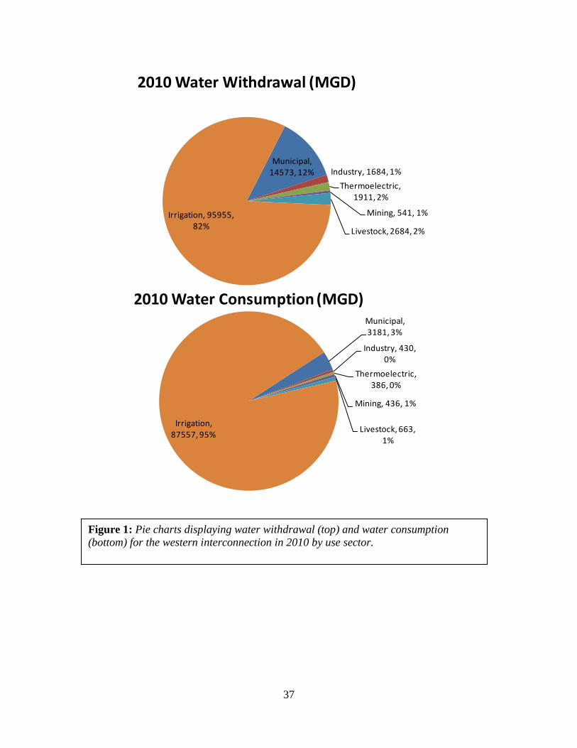
37

Municipal, 14573, 12% Industry, 1684, 1%

Thermoelectric, 1911, 2%

Mining, 541, 1%

Livestock, 2684, 2%

Irrigation, 95955, 82%

2010 Water Withdrawal (MGD)

Figure 1: Pie charts displaying water withdrawal (top) and water consumption

(bottom) for the western interconnection in 2010 by use sector.

Municipal, 3181, 3%

Industry, 430, 0%

Thermoelectric, 386, 0%

Mining, 436, 1%

Livestock, 663, 1%

Irrigation, 87557, 95%

2010 Water Consumption (MGD)

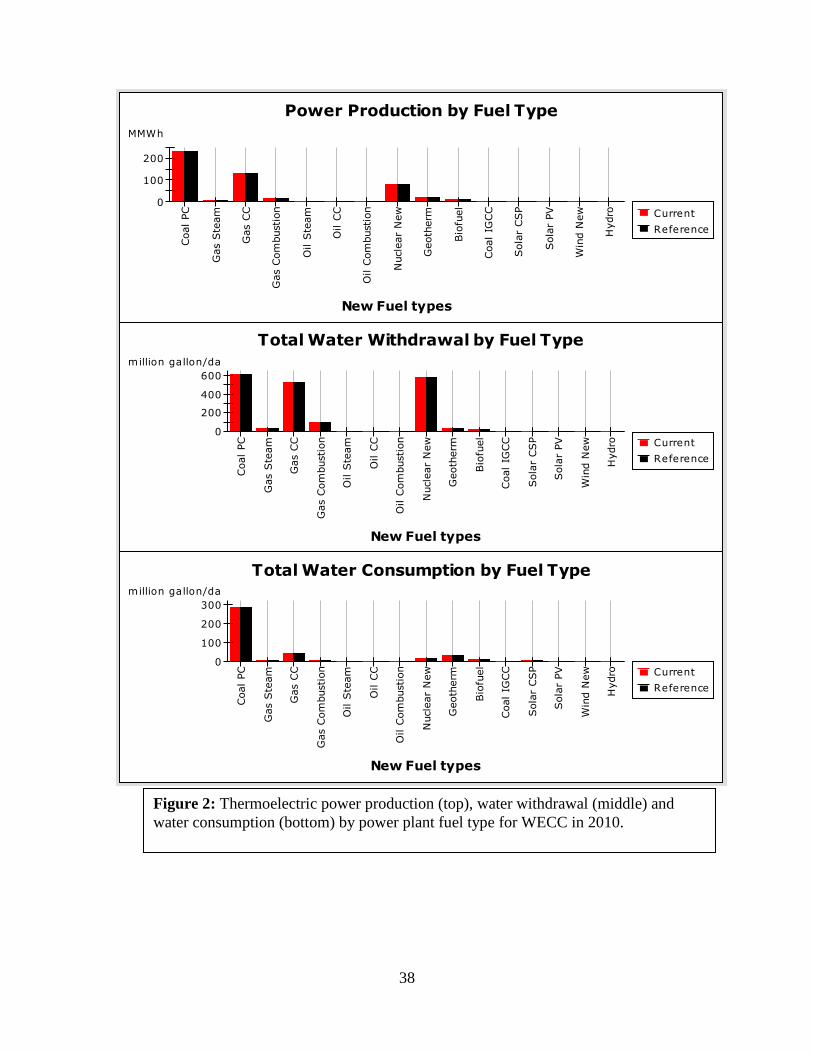
38

Total Water Withdrawal by Fuel Type

Coal PC

Gas S

team

Gas C

C

Gas C

om

bustion

Oil S

team

Oil C

C

Oil C

om

bustion

Nucle

ar

New

Geoth

erm

Bio

fuel

Coal IG

CC

Sola

r CSP

Sola

r PV

Win

d N

ew

Hydro

0

200

400

600

million gallon/da

Current

Reference

New Fuel types

Total Water Consumption by Fuel Type

Coal PC

Gas S

team

Gas C

C

Gas C

om

bustion

Oil S

team

Oil C

C

Oil C

om

bustion

Nucle

ar

New

Geoth

erm

Bio

fuel

Coal IG

CC

Sola

r CSP

Sola

r PV

Win

d N

ew

Hydro

0

100

200

300

million gallon/da

Current

Reference

New Fuel types

Power Production by Fuel Type

Coal PC

Gas S

team

Gas C

C

Gas C

om

bustion

Oil S

team

Oil C

C

Oil C

om

bustion

Nucle

ar

New

Geoth

erm

Bio

fuel

Coal IG

CC

Sola

r CSP

Sola

r PV

Win

d N

ew

Hydro

0

100

200

MMWh

Current

Reference

New Fuel types

Figure 2: Thermoelectric power production (top), water withdrawal (middle) and

water consumption (bottom) by power plant fuel type for WECC in 2010.

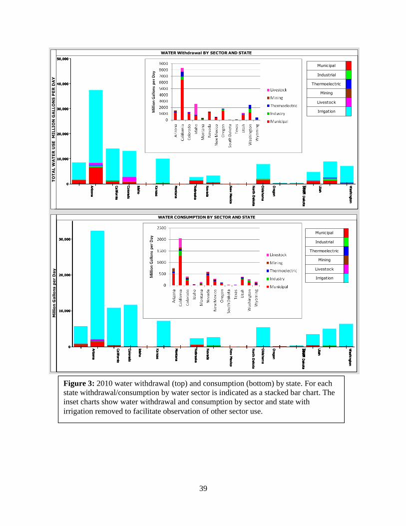
39

Ariz

ona

Califo

rnia

Colo

rado

Idaho

Kansas

Monta

na

Nebra

ska

Nevada

New

Mexic

o

North

Dakota

Okla

hom

a

Ore

gon

South

Dakota

Texas

Uta

h

Washin

gto

n

Wyom

ing

0

10,000

20,000

30,000

40,000

50,000

Ariz

ona

Califo

rnia

Colo

rado

Idaho

Kansas

Monta

na

Nebra

ska

Nevada

New

Mexic

o

North

Dakota

Okla

hom

a

Ore

gon

South

Dakota

Texas

Uta

h

Washin

gto

n

Wyom

ing

0

10,000

20,000

30,000

40,000

50,000

Municipal

Industrial

Thermoelectric

Mining

Livestock

Irrigation

Ariz

ona

Califo

rnia

Colo

rado

Idaho

Kansas

Monta

na

Nebra

ska

Nevada

New

Mexic

o

North

Dakota

Okla

hom

a

Ore

gon

South

Dakota

Texas

Uta

h

Washin

gto

n

Wyom

ing

0

10,000

20,000

30,000

40,000

50,000

Ariz

ona

Califo

rnia

Colo

rado

Idaho

Kansas

Monta

na

Nebra

ska

Nevada

New

Mexic

o

North

Dakota

Okla

hom

a

Ore

gon

South

Dakota

Texas

Uta

h

Washin

gto

n

Wyom

ing

0

10,000

20,000

30,000

40,000

50,000

Ariz

ona

Califo

rnia

Colo

rado

Idaho

Kansas

Monta

na

Nebra

ska

Nevada

New

Mexic

o

North

Dakota

Okla

hom

a

Ore

gon

South

Dakota

Texas

Uta

h

Washin

gto

n

Wyom

ing

0

10,000

20,000

30,000

40,000

50,000

Ariz

ona

Califo

rnia

Colo

rado

Idaho

Kansas

Monta

na

Nebra

ska

Nevada

New

Mexic

o

North

Dakota

Okla

hom

a

Ore

gon

South

Dakota

Texas

Uta

h

Washin

gto

n

Wyom

ing

0

10,000

20,000

30,000

40,000

50,000

WATER Withdrawal BY SECTOR AND STATET

OT

AL W

AT

ER

US

E M

ILLIO

N G

ALLO

NS

PE

R D

AY

Ariz

ona

Califo

rnia

Colo

rado

Idaho

Kansas

Monta

na

Nebra

ska

Nevada

New

Mexic

o

North

Dakota

Okla

hom

a

Ore

gon

South

Dakota

Texas

Uta

h

Washin

gto

n

Wyom

ing

0

10,000

20,000

30,000

Ariz

ona

Califo

rnia

Colo

rado

Idaho

Kansas

Monta

na

Nebra

ska

Nevada

New

Mexic

o

North

Dakota

Okla

hom

a

Ore

gon

South

Dakota

Texas

Uta

h

Washin

gto

n

Wyom

ing

0

10,000

20,000

30,000

Municipal

Industrial

Thermoelectric

Mining

Livestock

Irrigation

Ariz

ona

Califo

rnia

Colo

rado

Idaho

Kansas

Monta

na

Nebra

ska

Nevada

New

Mexic

o

North

Dakota

Okla

hom

a

Ore

gon

South

Dakota

Texas

Uta

h

Washin

gto

n

Wyom

ing

0

10,000

20,000

30,000

Ariz

ona

Califo

rnia

Colo

rado

Idaho

Kansas

Monta

na

Nebra

ska

Nevada

New

Mexic

o

North

Dakota

Okla

hom

a

Ore

gon

South

Dakota

Texas

Uta

h

Washin

gto

n

Wyom

ing

0

10,000

20,000

30,000

Ariz

ona

Califo

rnia

Colo

rado

Idaho

Kansas

Monta

na

Nebra

ska

Nevada

New

Mexic

o

North

Dakota

Okla

hom

a

Ore

gon

South

Dakota

Texas

Uta

h

Washin

gto

n

Wyom

ing

0

10,000

20,000

30,000

Ariz

ona

Califo

rnia

Colo

rado

Idaho

Kansas

Monta

na

Nebra

ska

Nevada

New

Mexic

o

North

Dakota

Okla

hom

a

Ore

gon

South

Dakota

Texas

Uta

h

Washin

gto

n

Wyom

ing

0

10,000

20,000

30,000

WATER CONSUMPTION BY SECTOR AND STATE

Millio

n G

allo

ns p

er

Da

y

Figure 3: 2010 water withdrawal (top) and consumption (bottom) by state. For each

state withdrawal/consumption by water sector is indicated as a stacked bar chart. The

inset charts show water withdrawal and consumption by sector and state with

irrigation removed to facilitate observation of other sector use.

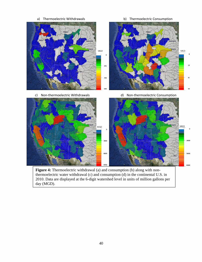
40

a) Thermoelectric Withdrawals b) Thermoelectric Consumption

c) Non-thermoelectric Withdrawals d) Non-thermoelectric Consumption

Figure 4: Thermoelectric withdrawal (a) and consumption (b) along with non-

thermoelectric water withdrawal (c) and consumption (d) in the continental U.S. in

2010. Data are displayed at the 6-digit watershed level in units of million gallons per

day (MGD).

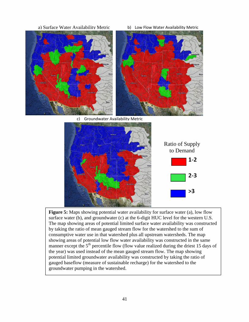
41

a) Surface Water Availability Metric b) Low Flow Water Availability Metric

c) Groundwater Availability Metric

Figure 5: Maps showing potential water availability for surface water (a), low flow

surface water (b), and groundwater (c) at the 6-digit HUC level for the western U.S.

The map showing areas of potential limited surface water availability was constructed

by taking the ratio of mean gauged stream flow for the watershed to the sum of

consumptive water use in that watershed plus all upstream watersheds. The map

showing areas of potential low flow water availability was constructed in the same

manner except the 5th

percentile flow (flow value realized during the driest 15 days of

the year) was used instead of the mean gauged stream flow. The map showing

potential limited groundwater availability was constructed by taking the ratio of

gauged baseflow (measure of sustainable recharge) for the watershed to the

groundwater pumping in the watershed.

Ratio of Supply

to Demand

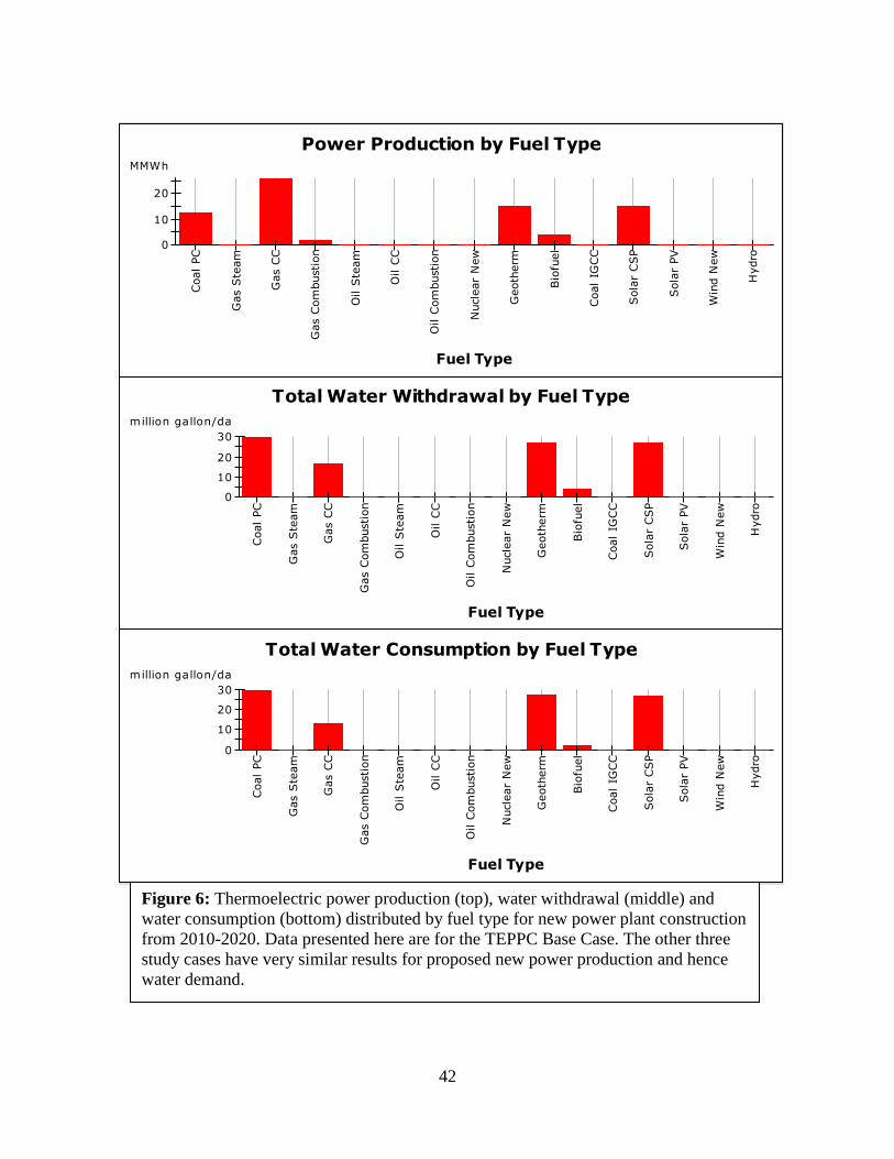
42

Total Water Withdrawal by Fuel Type

Coal PC

Gas S

team

Gas C

C

Gas C

om

bustion

Oil S

team

Oil C

C

Oil C

om

bustion

Nucle

ar

New

Geoth

erm

Bio

fuel

Coal IG

CC

Sola

r CSP

Sola

r PV

Win

d N

ew

Hydro

0

10

20

30

million gallon/da

Fuel Type

Total Water Consumption by Fuel Type

Coal PC

Gas S

team

Gas C

C

Gas C

om

bustion

Oil S

team

Oil C

C

Oil C

om

bustion

Nucle

ar

New

Geoth

erm

Bio

fuel

Coal IG

CC

Sola

r CSP

Sola

r PV

Win

d N

ew

Hydro

0

10

20

30

million gallon/da

Fuel Type

Power Production by Fuel Type

Coal PC

Gas S

team

Gas C

C

Gas C

om

bustion

Oil S

team

Oil C

C

Oil C

om

bustion

Nucle

ar

New

Geoth

erm

Bio

fuel

Coal IG

CC

Sola

r CSP

Sola

r PV

Win

d N

ew

Hydro

0

10

20

MMWh

Fuel Type

Figure 6: Thermoelectric power production (top), water withdrawal (middle) and

water consumption (bottom) distributed by fuel type for new power plant construction

from 2010-2020. Data presented here are for the TEPPC Base Case. The other three

study cases have very similar results for proposed new power production and hence

water demand.

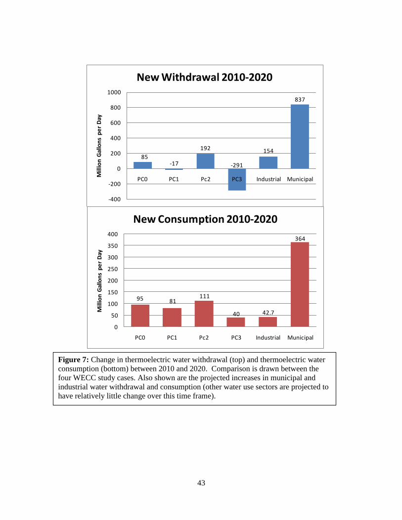
43

Figure 7: Change in thermoelectric water withdrawal (top) and thermoelectric water

consumption (bottom) between 2010 and 2020. Comparison is drawn between the

four WECC study cases. Also shown are the projected increases in municipal and

industrial water withdrawal and consumption (other water use sectors are projected to

have relatively little change over this time frame).

85-17

192

-291

154

837

-400

-200

0

200

400

600

800

1000

PC0 PC1 Pc2 PC3 Industrial Municipal

Mill

ion

Gal

lon

s p

er

Day

New Withdrawal 2010-2020

95 81111

40 42.7

364

0

50

100

150

200

250

300

350

400

PC0 PC1 Pc2 PC3 Industrial Municipal

Mill

ion

Gal

lon

s p

er

Day

New Consumption 2010-2020

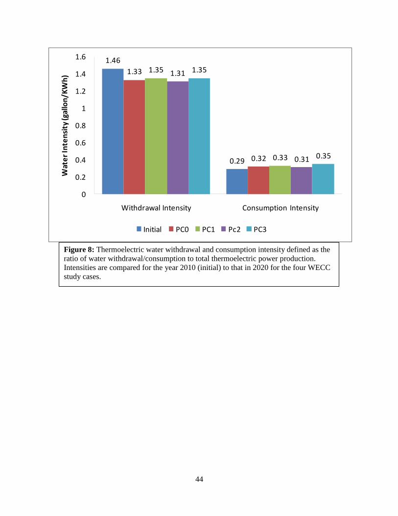
44

1.46

0.29

1.33

0.32

1.35

0.33

1.31

0.31

1.35

0.35

0

0.2

0.4

0.6

0.8

1

1.2

1.4

1.6

Withdrawal Intensity Consumption Intensity

Wat

er

Inte

nsi

ty (g

allo

n/K

Wh

)

Initial PC0 PC1 Pc2 PC3

Figure 8: Thermoelectric water withdrawal and consumption intensity defined as the

ratio of water withdrawal/consumption to total thermoelectric power production.

Intensities are compared for the year 2010 (initial) to that in 2020 for the four WECC

study cases.

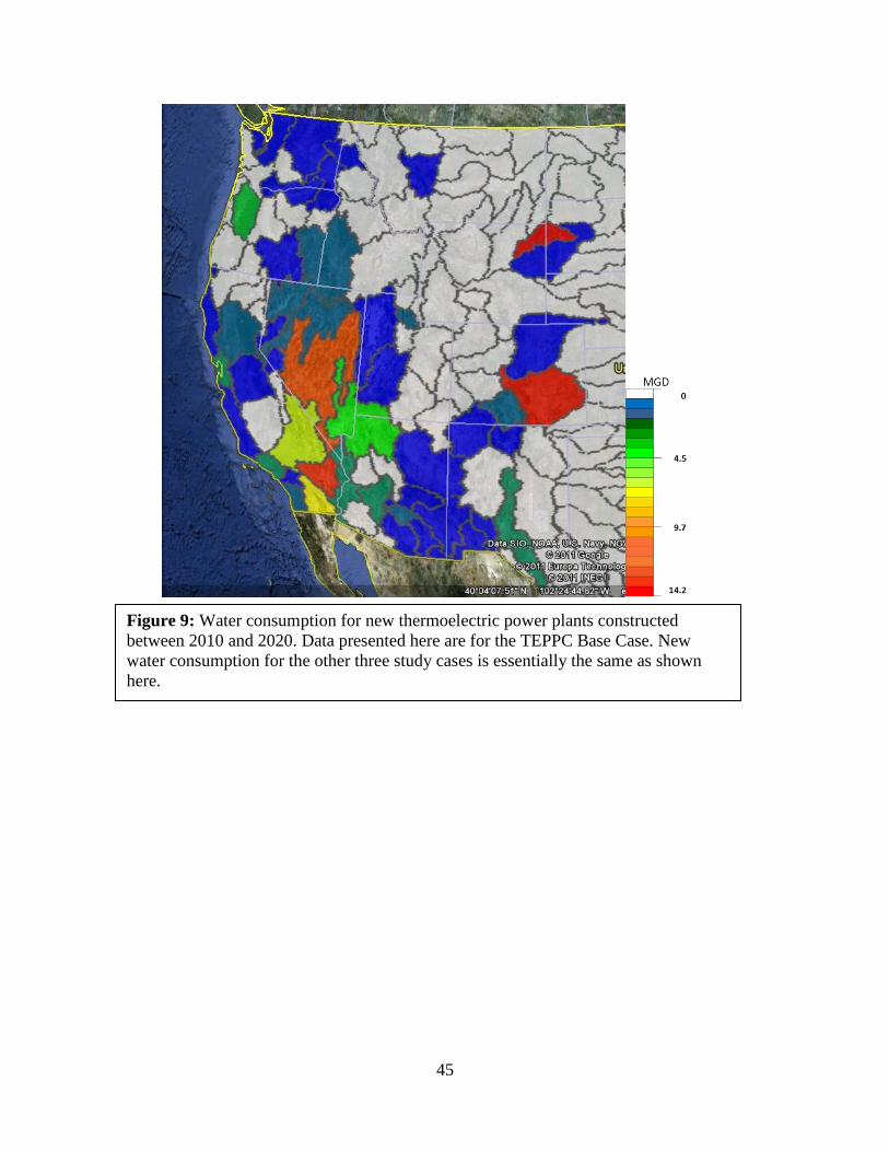
45

Figure 9: Water consumption for new thermoelectric power plants constructed

between 2010 and 2020. Data presented here are for the TEPPC Base Case. New

water consumption for the other three study cases is essentially the same as shown

here.

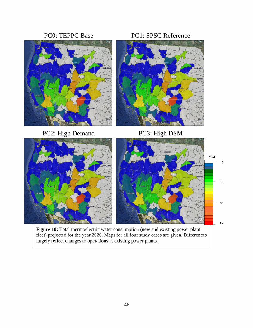
46

PC0: TEPPC Base PC1: SPSC Reference

PC2: High Demand PC3: High DSM

Figure 10: Total thermoelectric water consumption (new and existing power plant

fleet) projected for the year 2020. Maps for all four study cases are given. Differences

largely reflect changes to operations at existing power plants.

MGD

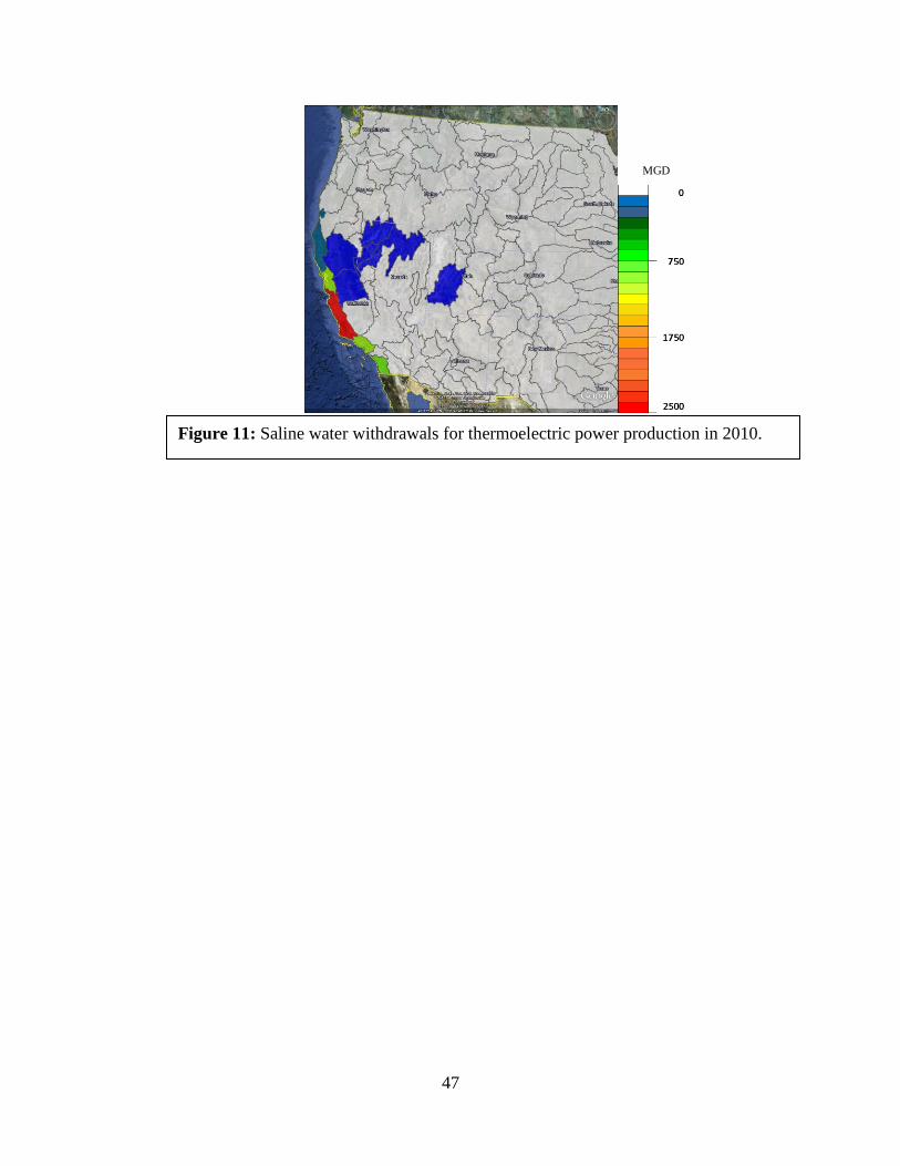
47

MGD

Figure 11: Saline water withdrawals for thermoelectric power production in 2010.

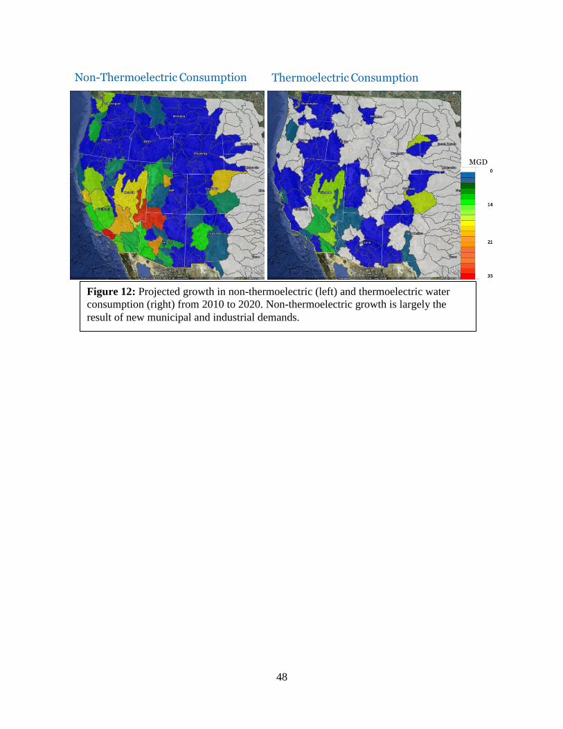
48

Non-Thermoelectric Consumption Thermoelectric Consumption

MGD

Figure 12: Projected growth in non-thermoelectric (left) and thermoelectric water

consumption (right) from 2010 to 2020. Non-thermoelectric growth is largely the

result of new municipal and industrial demands.

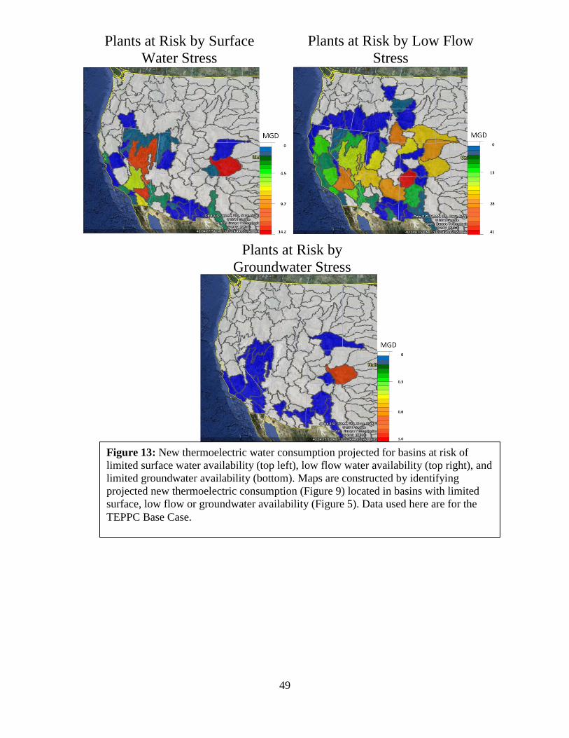
49

Plants at Risk by

Groundwater Stress

Plants at Risk by Surface

Water Stress

Plants at Risk by Low Flow

Stress

Figure 13: New thermoelectric water consumption projected for basins at risk of

limited surface water availability (top left), low flow water availability (top right), and

limited groundwater availability (bottom). Maps are constructed by identifying

projected new thermoelectric consumption (Figure 9) located in basins with limited

surface, low flow or groundwater availability (Figure 5). Data used here are for the

TEPPC Base Case.

50

Distribution 1 MS 0899 RIM- Reports Management, 9532 (electronic copy)

1 MS 1137 Stephanie Kuzio, 6926 (electronic copy)

1 MS 1137 Vincent Tidwell, 6926 (electronic copy)

1 MS1137 Len Malczynski, 6926 (electronic copy)

1 MS1137 Peter Kobos, 6926 (electronic copy)

1 MS1137 Barbie Moreland, 6926 (electronic copy)

1 MS1137 Cesar Castillo, 6926 (electronic copy)

1 MS1137 Howard Passell, 6926 (electronic copy)

1 MS0751 Barry Roberts, 6911 (electronic copy)