Energy thresholds for the existence of breather solutions and traveling

waves on lattices. ∗

J. Cuevas,

Departamento de Fisica Aplicada I, Escuela Universitaria Politenica,

C/ Virgen de Africa, 7, University of Sevilla,

41011 Sevilla, Spain

N. I. Karachalios,

Department of Mathematics, University of the Aegean,

Karlovassi, 83200 Samos, Greece

F. Palmero,

Departamento de Fisica Aplicada I, ETSI Informatica,

Avd. Reina Mercedes s/n, University of Sevilla,

41012 Sevilla, Spain

Abstract

We discuss the existence of breathers and of energy thresholds for their formation in DNLS lattices withlinear and nonlinear impurities. In the case of linear impurities we present some new results concerningimportant differences between the attractive and repulsive impurity which is interplaying with a powernonlinearity. These differences concern the coexistence or the existence of staggered and unstaggered breatherprofile patterns.

We also distinguish between the excitation threshold (the positive minimum of the power observed whenthe dimension of the lattice is greater or equal to some critical value) and explicit analytical lower boundson the power (predicting the smallest value of the power a discrete breather one-parameter family), whichare valid for any dimension. Extended numerical studies in one, two and three dimensional lattices justifythat the theoretical bounds can be considered as thresholds for the existence of the frequency parametrizedfamilies.

The discussion reviews and extends the issue of the excitation threshold in lattices with nonlinear impu-rities while lower bounds, with respect to the kinetic energy, are also discussed for traveling waves in FPUperiodic lattices.

1 Introduction

The energy threshold for the formation of a discrete breather in a nonlinear lattice [7], is defined as the positivelower energy bound possessed by the breather. This definition was given in the remarkable paper of S. Flach,K. Kladko and R. MacKay [6]. They considered a generic class of Hamiltonian systems and showed by heuristicand numerical arguments that the energy of a discrete breather family has a positive lower bound for latticedimension N greater than or equal to some critical dimension Nc. On the other hand, when N < Nc the energygoes to zero as the amplitude goes to zero. It was further predicted that the critical dimension Nc depends ondetails of the system but is typically 2 and never greater than 2. Furthermore, for N > Nc, the minimum inenergy should occur at positive amplitude and finite localization length.

Particular examples concerning the studies of [6] are the discrete nonlinear Schrodinger equation DNLS andthe nonlinear Klein-Gordon lattice (DKG). For the DNLS equation [5, 12],

iψn + ǫ(∆dψ)n + |ψn|2σψn = 0, σ > 0, n = (n1, n2, . . . , nN ) ∈ ZN , (1.1)

∗Keywords and Phrases: DNLS lattices, FPU lattices, discrete breathers, traveling waves, energy thresholds, impurities.

AMS Subject Classification: 37L60; 35Q55; 47J30.

1

Energy thresholds on lattices 2

the results of [6] were rigorously justified by M. Weinstein in the key work [22]. In (1.1), ǫ > 0 is a discretizationparameter ǫ ∼ h−2 with h being the lattice spacing, and (∆dψ)n stands for the N -dimensional discrete Laplacian

(∆dψ)n∈ZN =∑

m∈Nn

ψm − 2Nψn, (1.2)

where Nn denotes the set of 2N nearest neighbors of the point in ZN with label n.

In [22], the existence of the energy excitation threshold was proved through the consideration of the con-strained minimization problem

IR = inf H[φ] : P[φ] = R , (1.3)

where H[φ] and P[φ] are the fundamental conserved quantities

H[φ] = ǫ(−∆dφ, φ)2 −1

σ + 1

∑

n∈ZN

|φn|2σ+2, (1.4)

P[φ] =∑

n∈ZN

|φn|2, (1.5)

the Hamiltonian and the power, respectively. For instance, it was proved in [22, Theorem 3.1, pg. 678] thatif 0 < σ < 2

N , the variational problem (1.3) has a solution for all R > 0 and there is no excitation threshold.On the other hand, when σ ≥ 2

N , there exists an excitation threshold Rthresh such that (a) if R > Rthresh thenIR < 0, and a solution of (1.3) exists and (b) if R < Rthresh then IR = 0, and there is no solution (i.e a groundstate minimizer) of (1.3).

Actually, when −∞ < IR < 0 the infimum in (1.3) is attained. On the other hand, when IR ≥ 0 it followsthat IR = 0 (see [22, Proposition 3.1, pg. 679]) and there is no ground state minimizer (see [22, Proposition4.2 (d), pg. 680].

In the light of the results of Weinstein, the critical dimension predicted by Flach, Kladko and MacKay couldbe defined from (1.1) as

Nc =2

σ. (1.6)

However such a definition has a meaning in DNLS when it gives integer values of Nc ≥ 1. Restricted to integervalues of σ, we get that Nc = 2 for σ = 1 and Nc = 1 for σ = 2 in consistence with the predictions of [7]. Whenσ ≥ 3, Nc from (1.6) is not an integer, however it suggests that Nc = 1. This implementation for integer valuesof σ is consistent with the predictions of [7] and in equivalence with the definition of the critical exponent (1.1).It is also verified by the numerical studies of [2, 3] and of the present paper. It is important to mention that thecritical dimension Nc can be greater than 2 for a large classes of Hamiltonian systems, as it is reported in [11].

The excitation energy threshold concerns “breathers” as time-periodic solutions

ψn(t) = eiωtφn, ω > 0, n ∈ ZN , t ∈ R, (1.7)

φn ∈ ℓ2,

spatially localized since φn → 0 as |n| → ∞ (as an element of ℓ2-here |n| = max1≤i≤N |ni|). Actually Rthresh

corresponds to a minimum on the power attained by the ground-state breather ψn(t) = eiωctφn for a certain ωc

(as a Lagrange multiplier associated to the ground state minimizer φn of (1.3)).A different type of lower bounds on the power of DB for DNLS systems but with the same flavor in applica-

tions, was derived in our recent works [2, 3]. Using simple arguments based on variational methods [1] or fixedpoint theorems [10] to establish the existence of solutions (1.7), we were able to show the existence of explicitlygiven lower bounds on the power of breathers on either finite or infinite DNLS lattices and for different typesof nonlinearities (saturable or power). Although some of them depend explicitly on the dimension, a majordifference with the excitation threshold of [6, 22] existing only when N > Nc, is that they are valid for anydimension. Thus they do not predict the energy threhshold of [6, 22] but actually the smallest value of thepower a DB can have: no periodic localized solution can have power less than the prescribed estimates. Thisdifference becomes evident in the case of the power nonlinearity and in the case where σ < 2/N , the case wherethe excitation threshold of [6, 22] do not exists: The numerical studies of [2, 3] established the existence ofbreathers of small frequencies with power very close to the theoretical estimates, the latter becoming sharp

Energy thresholds on lattices 3

especially for small values of σ. On the other hand, when σ > 2/N , the theoretical estimates become sharp forthe power of breathers associated with large values of σ and large frequencies. Similar findings hold also for theDNLS with saturable nonlinearity. Due to these reasons it is necessary to distinguish these lower bounds fromthe excitation energy threshold of [6, 22].

The lower bounds are “local” in the sense that they are predicting the smallest value of power a breather canhave for any given frequency ω. Thus the explicit lower bounds can be useful as a theoretical estimation frombelow of the minimal power (or energy) of localized excitations of prescribed frequency ω, for arbitrary valuesof σ,N . This fact has been justified in the examples considered in [2, 3]: Tracing out the theoretical estimatesvarying ω it has been justified that the lower bounds are satisfied by the DB families considered (parametrizedby frequency) and in a sharp manner in many cases and members of the DB families, especially in the casewhere the excitation threshold do not appears.

Our aim in this work is to discuss possible extensions of our observations on the lower bounds for the energyof DB in two classes of inhomogeneous DNLS systems as well as to other localized structures such as travelingwaves in FPU lattices. In the context of the DNLS, an important example is that of the interplay of a focusingpower nonlinearity with a linear impurity, discussed in Section 2. Such mechanisms are often responsible forthe excitation of impurity modes, which are spatially localized oscillatory states at the impurity sites. Ourmotivation was initiated from [17] and the numerous physical applications listed (arising from superconductorsand the dynamics of electron-phonon interactions, to the defect modes in photonic crystals). We considerboth the attractive and the repulsive impurity cases. For the existence of nontrivial breathers, we followtwo alternative but equivalent approaches. For the focusing case we follow the variational approach via themountain pass theorem and prove some first lower bounds on the power. Although the defocusing case can bereduced to the focusing one but with the opposite sign of the impurity (under a staggering transformation),the alternative approach of constrained minimization problems revealed new and interesting conditions on theexistence of breathers. For instance, a vast difference between the attractive and the repulsive case is verified:while the repulsive case is associated only with the existence of staggered patterns, in the repulsive case wederive sufficient conditions on the the impurity parameter for the coexistence of both staggered and unstaggeredpatterns (Theorem 2.7-Remark 2.8). We remark that such a scenario was demonstrated in [9] for Klein-Gordonlattices. As in the mountain pass approach, the constrained minimization of the defocusing case comes togetherwith the derivation of the lower bounds on the power of the staggered patterns in the repulsive case and thecoexisting staggered and unstaggered patterns in the attractive one.

The numerical studies performed, not only verify that the lower bounds are satisfied but also justify thatthese exact values can be fairly used as a sharp approximation of the smallest possible value of the power in thelattice as the limiting case of small σ, ω indicate. This limiting case is also in accordance with the observationsand analysis of [6], on the behavior of DB families in the small amplitude limit.

In the light of the numerical findings of Section 2, we continue in Section 3 the study of the DNLS lattice withnonlinear impurities [14, 15, 16, 21], initiated in [3]. We review the existence proof of the excitation thresholdby generalizing the concentration compactness arguments of [22], to the most general case of sign-changingnonlinear impurities. To emphasize the differences between the excitation thresholds and the lower bounds onthe power, the latter derived in [3] are also reviewed numerically in the case of nonlinearity exponents where theexcitation threshold do not appears. This numerical study verifies that the value of the findings of Section 2,are justified for the DNLS with nonlinear impurities. The particular examples we consider are that of a DNLSlattice with a single and a sign changing impurity.

The thresholds of the nature discussed in the present paper can be derived alternatively by using fixed pointarguments. This approach has been proved useful for the treatment of the saturable DNLS [2]. Apart from theDNLS lattices, we claim that these methods can be useful in the study of energy thresholds for other interestinglocalized structures in nonlinear lattices. As a first step to these extensions we derive a lower bound on theenergy for traveling waves in Fermi-Pasta-Ulam (FPU) lattices. The lower bound concerns the average kineticenergy of the traveling wave for the standard polynomial anharmonic potential which includes the classical FPUstudy as a special case. The FPU system is considered in a periodic lattice and the lower bound concerns wavesof given speed c > c∗. The value c∗ is given explicitly, and as the lower bound, depends also on the numberof lattice sites. The condition c > c∗ although stronger is in consistency with the restrictions imposed by theanalytical results of [8, 23]. The derivation of the lower bound and its discussion is given in Section 4.

Energy thresholds on lattices 4

2 Existence of localized modes in finite DNLS lattices with local

inhomogeneity.

This section is devoted to the DNLS model with a local inhomogeneity studied in [17], supplemented withDirichlet boundary conditions

iψn + ǫ(∆dψ)n + χnψn + γ|ψn|2σψn = 0, ||n|| ≤ K, (2.1)

ψn = 0, ||n|| > K, (2.2)

where ||n|| = max1≤i≤N |ni| for n = (n1, n2, . . . , nN ) ∈ ZN . Here γ ∈ R is the the anharmonicity parameter.

Problem (2.1)-(2.2) will be treated by appropriate variatonal methods. For the impurity χ, we consider twopossible alternative cases:

(A) (Attractive impurity) χn > 0, for all n ∈ ZNK .

(R) (Repulsive impurity) χn < 0, for all n ∈ ZNK .

The case of a single linear impurity (or single point defect) χn = αδn,n0can be treated with almost identical

manner as the attractive and the repulsive impurity. This example will serve for testing numerically thetheoretical results which will be presented in this section.

Preliminaries. For convenience to the reader, we recall from [2, 3] some preliminary information on variousnorms and quantities, that will be thoroughly used in the sequel.

The finite dimensional problem (2.11)–(2.12) is formulated in the finite dimensional subspaces of the sequencespaces ℓp, 1 ≤ p ≤ ∞,

ℓp(ZNK) = φ ∈ ℓp : φn = 0 for ||n|| > K . (2.3)

Note that in the case of the infinite lattice ZN

||φ||q ≤ ||φ||p, 1 ≤ p ≤ q ≤ ∞ (2.4)

0 ≤ ǫ(−∆dφ, φ)2 ≤ 4ǫN∑

n∈ZN

|φn|2. (2.5)

For the finite dimensional subspaces it is needless to say that ℓp(ZNK) ≡ C

(2K+1)N

, endowed with the norm

||φ||p =

∑

||n||≤K

|φn|p

1p

,

and that the well known equivalence of norms ,

||φ||q ≤ ||φ||p ≤ (2K + 1)N(q−p)

qp ||φ||q, 1 ≤ p ≤ q <∞, (2.6)

holds. For an 1D-lattice n = 1, . . . ,K, the eigenvalues of the discrete Dirichlet Laplacian −∆dφ = λφ, with φreal, are given explicitly by

λn = 4 sin2

(

nπ

4(K + 1)

)

, n = 1, . . . ,K.

In the case of the N-dimensional discrete Laplacian, the eigenvalues are:

λ(n1,n2,...,nN ) = 4

[

sin2

(

n1π

4(K + 1)

)

+ sin2

(

n2π

4(K + 1)

)

+ . . .+ sin2

(

nNπ

4(K + 1)

)]

,

nj = 1, . . . ,K j = 1, . . . , N.

Clearly, the principal eigenvalue of the discrete Dirichlet problem −∆dφ = λφ, with φ real is given by

λ1 ≡ λ(1,1,...,1) = 4N sin2

(

π

4(K + 1)

)

.

Energy thresholds on lattices 5

Restricting the variational characterization of the eigenvalues of the discrete Laplacian in the finite dimensionalsubspaces ℓ2(ZN

K), it follows that λ1 > 0, can be characterized as

λ1 = infφ ∈ ℓ2(ZN

K)φ 6= 0

(−∆dφ, φ)2∑

||n||≤K |φn|2. (2.7)

Then (2.7) implies the inequality

ǫλ1

∑

||n||≤K

|φn|2 ≤ ǫ(−∆dφ, φ)2 ≤ 4ǫN∑

||n||≤K

|φn|2. (2.8)

From (2.8), we find directly that λ1 satisfies the bound

λ1 ≤ 4N. (2.9)

Of course, the upper bound (2.9) follows also from the explicit formula for λ1 given above.

2.1 Mountain pass approach in the focusing case γ > 0.

In the focusing case γ > 0, substituting the time-periodic solution

ψn(t) = eiΩtφn, Ω ∈ R, (2.10)

to (2.1), the stationary analogue of (2.1) reads as

−ǫ(∆dφ)n + Ωφn − χnφn = γ|φn|2σφn, ||n|| ≤ K, (2.11)

φn = 0, ||n|| > K. (2.12)

Attractive impurity. Motivated by [17, page 3] and considering the case of the anticontinuum limit ǫ = 0,it follows directly that the attractive impurity (A) only supports time-periodic solutions (2.10) with Ω > 0. Wehave the following

Theorem 2.1 (Unstaggered patterns) We consider the DNLS equation (2.1) assuming that (A) is satisfied. If

maxn∈ZN

K

χn < Ω, (2.13)

there exists a nontrivial φ ∈ ℓ2(ZNK) such that ψn(t) = eiΩtφn, Ω > 0 is a solution of the DNLS equation (2.1).

Moreover the power of the nontrivial unstaggered periodic solution satisfies the lower bound

[

ǫλ1 + Ω − maxn∈ZNKχn

γ

]

1σ

< R2. (2.14)

Proof: We shall follow the variational (minimax) approach of [3, 10]. For instance we seek non-trivial breathersas critical points of C1-functional E : ℓ2 → R defined as

E(φ) =ǫ

2(−∆dφ, φ)2 +

Ω

2

∑

||n||≤K

|φn|2 −1

2

∑

||n||≤K

χn|φn|2 −γ

2σ + 2

∑

||n||≤K

|φn|2σ+2, (2.15)

showing their existence by the mountain pass Theorem (MPT). It can be verified as in [2, 3, 10] that E is aC1(ℓ2(ZN

K),R)-functional. Since we are in a discrete setting it follows directly that any critical point of E is asolution of (2.1).

We proceed by verifying that E possesses the mountain pass geometry. Since E(0) = 0, we seek next for theexistence of z ∈ ℓ2(ZN

K) with ||z||22 = θ2, satisfying E(z) > 0. Now from (2.6), (2.8) and (2.13) we have that

E(z) ≥ ǫ

2(−∆dz, z)2 +

Ω

2

∑

||n||≤K

|zn|2 −maxn∈ZN

Kχn

2

∑

||n||≤K

|zn|2 −γ

2σ + 2

∑

||n||≤K

|zn|2σ+2

≥(

ǫλ1 + Ω − maxn∈ZN

K

χn

)

θ2

2− γθ2σ+2

2σ + 2. (2.16)

Energy thresholds on lattices 6

Then, it follows from (2.16) that if condition (2.13) holds, there exists z ∈ ℓ2(ZNK) with norm ||z||22 = θ2

satisfying

[

(

σ + 1

γ

)

(ǫλ1 + Ω − maxn∈ZN

K

χn)

]1σ

> θ2,

for which E(z) > 0. We consider next the element ζ = tη ∈ ℓ2(ZNK), for some t > 0 and η ∈ ℓ2(ZN

K) with||η||2 = 1 and we observe that

E(ζ) =t2

2ǫ(−∆dη, η)2 +

Ωt2

2− t2

2

∑

||n||≤K

χn|ηn|2 −γt2σ+2

2σ + 2

∑

||n||≤K

|ηn|2σ+2. (2.17)

Taking the limit as t → +∞ we get from condition (A), that E(tη) → −∞. Thus, we derive the existence ofζ ∈ ℓ2(ZN

K) such that E [ζ] < 0, by setting t sufficiently large.The final step is to verify that the functional E satisfies the Palais-Smale (PS) condition. That is, to show

that for any sequence φmm∈N ∈ ℓ2(ZNK) such that |E(φm)| is bounded and E ′(φm) → 0 as n→ ∞, there exists

a convergent subsequence. In fact, since ℓ2(ZNK) is finite dimensional it suffices to verify that such a sequence is

bounded. Considering a sequence φm of ℓ2(ZNK) be such that |E(φm)| < M ′ for some M ′ > 0 and E ′(φm) → 0

as m→ ∞, we get similarly to (2.16), that for m sufficiently large

M ′ ≥ E(φm) − 1

2σ + 2〈E ′(φm), φm〉

=

(

1

2− 1

2σ + 2

)

ǫ(−∆dφm, φm)2 + Ω||φm||22

−(

1

2− 1

2σ + 2

)

∑

||n||≤K

χn|(φm)n|2

≥ 2σ

2(2σ + 2)(ǫλ1 + Ω − max

n∈ZNK

χn)||φm||22. (2.18)

Condition (2.13) is required once again, to get from (2.18) that the sequence φmm∈N is bounded. Thereforethe functional E possesses the geometry required by the MPT and satisfies condition (PS), proving the existenceof a nontrivial breather solution (2.10).

From (2.1) we get that

ǫ(−∆dφ, φ)2 + Ω∑

||n||≤K

|φn|2 −∑

||n||≤K

χn|φn|2 − γ∑

||n||≤K

|φn|2σ+2 = 0. (2.19)

Working similarly to (2.16), we have from (2.19) the inequality

γ

∑

||n||≤K

|φn|2

σ+1

≥ γ∑

||n||≤K

|φn|2σ+2

≥ ǫ(−∆dφ, φ)2 + Ω∑

||n||≤K

|φn|2 − maxn∈ZN

K

χn

∑

||n||≤K

|φn|2,

implying that the power R2 =∑

||n||≤K |φn|2 of the critical point satisfies

γR2σ+2 ≥ (ǫλ1 + Ω − maxn∈ZN

K

χn)R2,

from which the estimate (2.14), readily follows.

The results of Theorem 2.1 can be extended to the particular example of the single point defect by similararguments.

Corollary 2.2 (Unstaggered patterns) For the DNLS system (2.1)-(2.2) with a single point defect χn = αδn,n0,

α > 0 (attractive impurity), the power of the unstaggered periodic solution ψn(t) = eiΩtφn, Ω > 0 with Ω > α,satisfies the lower bound

[

ǫλ1 + Ω − α

γ

]1σ

< R2, σ > 0. (2.20)

Energy thresholds on lattices 7

Remark 2.3 Note that without considering the anticontinuum limit ǫ = 0, the restriction

α < Ω + ǫλ1,

is derived for the existence of a nontrivial breather solution. However, since the condition holds for any arbitraryǫ > 0, this fact clearly implies that α < Ω. Condition α < Ω can be also derived if one considers initially theanticontinuum limit case ǫ = 0.

Repulsive impurity. It is interesting that when the impurity is repulsive (R) (cf. [17, page 3]), the case of theanticontinuum limit ǫ = 0 implies the existence of both staggered patterns and unstaggered patterns. Staggeredpatterns are given in the ansatz

ψn(t) = e−iωtφn, ω > 0, (2.21)

while the unstaggered ones are (2.10) with Ω > 0 (or (2.21) with ω = −Ω < 0).It should be pointed out that distinguishing staggered and unstaggered patterns is of physical significance

[13]. In the framework of waveguide arrays, the staggered solutions display out-of-phase fields between the neigh-bor noncentral waveguides (oscillators) whereas the unstaggered ones display in-phase fields in these noncentralwaveguides.

Working in a very similar manner as for the proof of Theorem 2.1, we have

Theorem 2.4 We consider the DNLS equation (2.1) assuming that condition (R) is satisfied. (i) (Staggeredpatterns) For any ω < −maxn∈ZN

Kχn there exists a nontrivial φ ∈ ℓ2(ZN

K) such that ψn(t) = e−iωtφn, ω > 0 is

a solution of the DNLS equation (2.1). Moreover the power of the nontrivial staggered periodic solution satisfiesthe lower bound

[

ǫλ1 − ω − maxn∈ZNKχn

Λ

]

1σ

< R2. (2.22)

(ii) (Unstaggered patterns). For any Ω > 0 there exists a nontrivial φ ∈ ℓ2(ZNK) such that ψn(t) = eiΩtφn, Ω > 0

is a solution of the DNLS equation (2.1). Moreover the power of the nontrivial unstaggered periodic solutionsatisfies the lower bound

[

ǫλ1 + Ω − maxn∈ZNKχn

Λ

]

1σ

< R2. (2.23)

In the case of a single point defect with a repulsive impurity we have

Corollary 2.5 (i)(Staggered patterns) For the DNLS system (2.1)-(2.2) with a single point defect χn = αδn,n0,

α < 0 (repulsive impurity), the power of a staggered periodic solution ψn(t) = e−iωtφn with 0 < ω < −α,satisfies the lower bound

[

ǫλ1 − ω − α

Λ

]1σ

< R2, −α > 0. (2.24)

(ii) (Unstaggered patterns) Any unstaggered solution ψn(t) = eiΩtφn with Ω > 0 satisfies the lower bound

[

ǫλ1 + Ω − α

Λ

]1σ

< R2, −α > 0. (2.25)

2.2 Constrained minimization problems for the defocusing case γ < 0

The defocusing case γ = −Λ < 0 can be reduced to the focusing one but with the opposite sign of the impurityunder the staggering transformation. This transformation is defined as

ψn → (−1)|n|ψn, |n| =

N∑

i=1

ni, (2.26)

Energy thresholds on lattices 8

(see [13, pg. 066606-7]). We follow this approach in this section which means that we shall consider thedefocusing DNLS

iψn + ǫ(∆dψ)n + χnψn − Λ|ψn|2σψn, Λ > 0 ||n|| ≤ K, (2.27)

ψn = 0, ||n|| > K.

The reason for considering alternatively the defocusing problem is that this approach allows for a derivation ofnew conditions on the impurity χn for the proof of a coexistence result of staggered an unstaggered solutions. Weremark that it was not possible to observe these new conditions by the mountain pass approach of the previoussection for the focusing case. On the contrary, the derivation of these new conditions was possible by theconsideration constrained minimization problems for the defocusing case, that will be used in the sequel.

We are seeking breathers again in the ansatz

ψn(t) = e−iΩtφn, Ω ∈ R. (2.28)

Substituting (2.28) in (2.27) we get that φn satisfies the

−ǫ(∆dφ)n − Ωφn − χnφn = −Λ|φn|2σφn, ||n|| ≤ K, (2.29)

φn = 0, ||n|| > K.

Attractive case. As it was already mentioned, considering the attractive case with the condition (A) for theimpurity is equivalent with the case of the repulsive case for the focusing DNLS (2.1), due to (2.26). Howeverit should be emphasized that the corresponding energy functional do not possesses the mountain pass geometry.Thus we shall consider a constrained minimization problem for the linear energy functional. We start byseeking for staggered patterns (2.28) with Ω > 0. The existence of solutions (2.28) with Ω > 0, will be given byminimizing the linear energy

EΩ[φ] = ǫ(−∆dφ, φ)2 − Ω∑

||n||≤K

|φn|2 −∑

||n||≤K

χn|φn|2, Ω > 0. (2.30)

More precisely, we consider the minimization problem on ℓ2(ZNK)

inf

EΩ[φ] :∑

|n|≤K

|φn|2σ+2 = M > 0

. (2.31)

The functional EΩ is bounded from below: Consider the ball

B =

φ ∈ ℓ2(ZNK) :

∑

|n|≤K

|φn|2σ+2 = M

. (2.32)

Then, we have that

EΩ[φ] ≥ −Ω∑

|n|≤K

|φn|2 −∑

||n||≤K

χn|φn|2

≥ (−Ω − maxn∈ZN

K

χn)C22

∑

||n||≤K

|φn|2σ+2

1σ+1

= (−Ω − maxn∈ZN

K

χn)C22M

1σ+1 .

As we are restricted to the finite dimensional space ℓ2(ZNK), it follows that any minimizing sequence associated

with the variational problem (2.31) is precompact: any minimizing sequence has a subsequence, converging to

a minimizer. Thus Eω attains its infimum at a point φ in B.To derive the variational equation for Eω, we set

LR[φ] =∑

|n|≤K

|φn|2σ+2,

Energy thresholds on lattices 9

recalling that

〈L′R[φ], ψ〉 = (2σ + 2)Re

∑

|n|≤K

|φn|2σφnψ, for all ψ ∈ ℓ2(ZNK).

Then by the Lagrange multiplier rule,⟨

E ′Ω[φ] − λL′

R[φ], ψ⟩

= 2(−∆dφ, ψ)2 − 2ΩRe∑

||n||≤K

φnψn − 2Re∑

|n|≤K

χnφnψn

−µ(M)Re∑

||n||≤K

|φn|2σφnψn = 0, for all ψ ∈ ℓ2(ZNK). (2.33)

Setting ψ = φ in (2.33), we obtain

EΩ[φ] = (−∆dφ, φ)2 − Ω∑

|n|≤K

|φn|2 −∑

|n|≤K

χn|φn|2 =µ(M)

2

∑

|n|≤K

|φ|2σ+2. (2.34)

Furthermore, since

EΩ[φ] ≤ 4ǫN∑

|n|≤K

|φn|2 − Ω∑

|n|≤K

|φn|2 −∑

|n|≤K

χn|φn|2, (2.35)

we get that EΩ[φ] < 0 if

Ω > 4ǫN − minn∈ZN

K

χn, (2.36)

is satisfied. Note that condition (2.36) is fullfiled for all Ω > 0 if 4ǫN < minn∈ZNKχn. On the other hand, it is

required that Ω > 4ǫN − minn∈ZNKχn > 0, if 4ǫN > minn∈ZN

Kχn.

Then assuming (2.36), we find that µ(M) < 0. The constant µ(M)/2 can be scaled out from (2.34) by

setting φ = (−µ(M)/2)−1/2σ

φ. Scaling further with φ = (1/Λ))−1/2σ

φ we get that the non trivial solution of(2.29) satisfies the energy equation

(−∆dφ, φ)2 − Ω∑

|n|≤K

|φn|2 −∑

|n|≤K

χn|φn|2 = −Λ∑

|n|≤K

|φ|2σ+2. (2.37)

From (2.37), (2.6) and (2.8) it follows that

Λ

∑

||n||≤K

|φn|2

σ+1

≥ Λ∑

||n||≤K

|φn|2σ+2

≥ −ǫ(−∆dφ, φ)2 + Ω∑

||n||≤K

|φn|2 + minn∈ZN

K

χn

∑

||n||≤K

|φn|2

≥(

Ω − 4Nǫ+ minn∈ZN

K

χn

)

∑

||n||≤K

|φn|2,

implying that the power R2 =∑

||n||≤K |φn|2 of the critical point satisfies

[

Ω − 4Nǫ+ minn∈ZNKχn

Λ

]

1σ

< R2, σ > 0. (2.38)

The attractive impurity-defocusing case supports also unstaggered patterns. This is compatible with theapproach of subsection (2.1). For convenience we set in (2.29) Ω = −ω < 0. The anticontinuum limit suggeststhat an unstaggered pattern ψn(t) = eiωtφn exists if 0 < ω < minn∈ZN

Kχn. Minimizing again the linear energy,

instead of (2.36), we require that

0 < ω < minn∈ZN

K

χn − 4ǫN, minn∈ZN

K

χn > 4ǫN. (2.39)

Energy thresholds on lattices 10

This time, the power of the critical point satisfies

[

minn∈ZNKχn − 4Nǫ− ω

Λ

]

1σ

< R2, σ > 0. (2.40)

when (2.39) is satisfied. We summarize in

Theorem 2.7 (i) (Staggered patterns) For the defocusing DNLS system with an attractive impurity (A) thereexists a nontrivial staggered periodic solution ψn(t) = e−iΩtφn, Ω > 0

for all Ω > 0, if 4ǫN < minn∈ZN

K

χn, (2.41)

for all Ω > 4ǫN − minn∈ZN

K

χn > 0, if 4ǫN > minn∈ZN

K

χn. (2.42)

and power satisfying the lower bound (2.38). In the case of an attractive single point defect χn = αδn,n0, α > 0,

the power of a staggered periodic solution with Ω > 4Nǫ− α, satisfies the lower bound

[

Ω − 4Nǫ+ α

Λ

]1σ

< R2, σ > 0, Ω > 0 if 4ǫN < α, (2.43)

[

Ω − 4Nǫ+ α

Λ

]1σ

< R2, σ > 0, Ω > 4ǫN − α if α < 4ǫN. (2.44)

(ii) (Unstaggered patterns) The defocusing DNLS system with an attractive impurity (A) supports also unstag-gered patterns

ψn(t) = eiωtφn, 0 < ω < minn∈ZN

K

χn − 4ǫN, if 4ǫN < minn∈ZN

K

χn,

with power satisfying (2.40). In the case of an attractive single point defect χn = αδn,n0, α > 0, the power of

an unstaggered periodic solution with 0 < ω < α− 4ǫN , satisfies the lower bound

[

α− 4Nǫ− ω

Λ

]1σ

< R2, σ > 0, 0 < ω < α− 4ǫN, if 4ǫN < α. (2.45)

Remark 2.8 The consideration of the defocusing DNLS with the attractive impurity revealed conditions onthe impurity for coexistence of both patterns in the attractive case. Apart of verifying the coexistence result ofsubsection 2.1-Theorem 2.4 for the equivalent focusing DNLS with repulsive impurity, the approach on mini-mizing the linear energy clarified the conditions on the impurity for this coexistence. More precisely, it followsthat when 4ǫN < α we have coexistence of staggered patterns of any Ω > 0 and unstaggered patterns at leastin the range 0 < ω < α − 4ǫN . This is a vast difference with the defocusing DNLS with repulsive impuritywhich supports solutions only of one sign as it was shown for its equivalent analogue, the focusing one with theattractive impurity. This it will again justified in the next paragraph.

A similar scenario was demonstrated for Klein–Gordon lattices in Ref. [9].

Repulsive case. In the repulsive case (R), it can be easily seen by considering equation (2.29) in the anticon-tinuum limit ǫ = 0 that DNLS (2.27) supports only staggered patterns (2.28) with Ω > 0. This is in agreementwith the alternative approach of subsection 2.1 which considers the focusing case. For the proof of solutions(2.28) with Ω > 0 we work exactly as for the proof of Theorem 2.7. The linear energy is bounded from belowsince

EΩ[φ] ≥ −ΩC22M

1σ+1 .

Having the corresponding minimizer φ at hand, we observe this time that EΩ[φ] < 0 for frequencies

Ω > 4ǫN − minn∈ZN

K

χn, − minn∈ZN

K

χn > 0.

Thus we have

Energy thresholds on lattices 11

Theorem 2.9 (Staggered patterns) For the defocusing DNLS system with a repulsive impurity (R) there existsa nontrivial staggered periodic solution ψn(t) = e−iΩtφn, Ω > 0 for all Ω > 4ǫN − minn∈ZN

Kχn > 0. and power

satisfying the lower bound

[

Ω − 4Nǫ− minn∈ZNKχn

Λ

]

1σ

< R2, σ > 0, − minn∈ZN

K

χn > 0. (2.46)

In the case of a repulsive single point defect χn = αδn,n0, α < 0, the power of the staggered periodic solution

(2.28) with Ω > 4Nǫ− α, satisfies the lower bound

[

Ω − 4Nǫ− α

Λ

]1σ

< R2, σ > 0, Ω > 4ǫN − α, −α > 0. (2.47)

Note, as it is mentioned before, that the focusing DNLS with repulsive linear impurity is equivalent to thiscase, because of the corresponding stationary states, under a staggering transformation and a frequency change,reduces to the defocussing case with opposite sign of the impurity parameter.

2.3 Numerical studies in the linear impurity case

This section is devoted to the numerical study of the DNLS system with the local inhomogeneity (2.1)-(2.2).The presentation is focused on testing the results of the alternative approach of constrained minimization forthe defocusing case γ < 0 presented in Section 2.2. Our aim is to investigate numerically the coexistence resultof both staggered and unstaggered patterns in the attractive case of the single point defect χn = αδn,n0

ofTheorem 2.7, as well as, the corresponding lower bounds (2.43)-(2.44), on the power of the staggered and (2.45)for the unstaggered breathers respectively. The numerical study concerns 1D and 2D lattices.

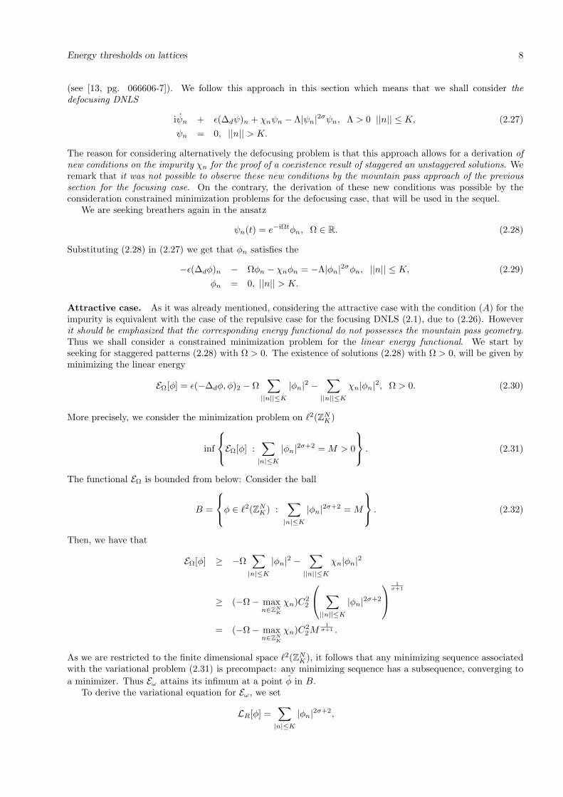
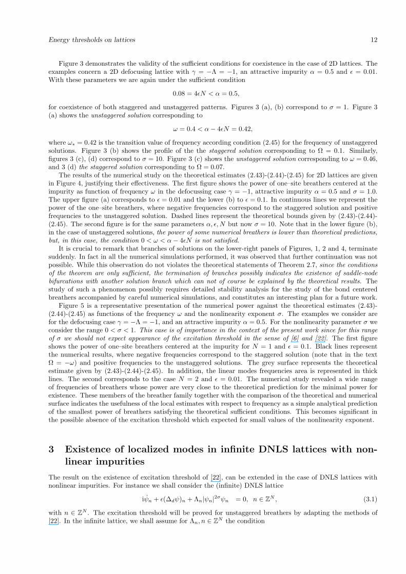
The first panel of pictures in Figure 1 concerns the numerical study for an 1D defocusing lattice γ = −Λ = −1and attractive impurity α = 0.5 with parameters ǫ = 0.1 and σ = 1. This example corresponds to the casewhere the parameters are satisfying condition

0.4 = 4ǫN < α = 0.5.

Thus, we are in the case where, according to Theorem 2.7, the sufficient conditions for coexistence of bothstaggered and unstaggered breathers is expected. Figures 1 (a), (b) and (c) is a full justification of these sufficientconditions. In (c) the profile of the one-site staggered breather centered at the impurity with frequency Ω = 0.6.According to the theoretical prediction, under condition 4ǫN < α we have existence of staggered solutions forany Ω > 0. On the other hand we should have coexistence of unstaggered patterns of frequency at least in therange

0 < ω < α− 4ǫN = 0.1,

where ω∗ = 0.1 can be considered as the transition value of frequency for coexistence. Picture (b) showsthe profile of the one-site unstaggered solution in the transition value ω∗ = 0.1 while (a) shows the profile ofthe unstaggered solution with frequency ω = 0.05 within the theoretical range 0 < ω < 0.1. The numericaljustification of the lower bounds (2.43)-(2.44) for the staggered solutions and (2.45) for the unstaggered is shownin the final picture (d), where the power of one–site breathers centered at the impurity as function of frequencyω is demonstrated. The upper picture (a) corresponds to ǫ = 0.01 and the lower picture (b) to ǫ = 0.1. Incontinuous lines we represent the numerical power, where negative frequencies correspond to the staggeredsolutions (note that in the text Ω = −ω) and positive frequencies to the unstaggered solutions. Dashed linesrepresent the theoretical lower bound given by (2.43)-(2.44) and (2.45), dash-dotted line the frequency of thelinear impurity mode, dotted line the frequency given by ω = α − 4ǫN , and the dark area corresponds to thelinear modes frequencies. Both cases justify that the theoretical estimates can be particularly useful as anexplicit prediction of the smallest value of the power for breathers satisfying the conditions of Theorem 2.7.

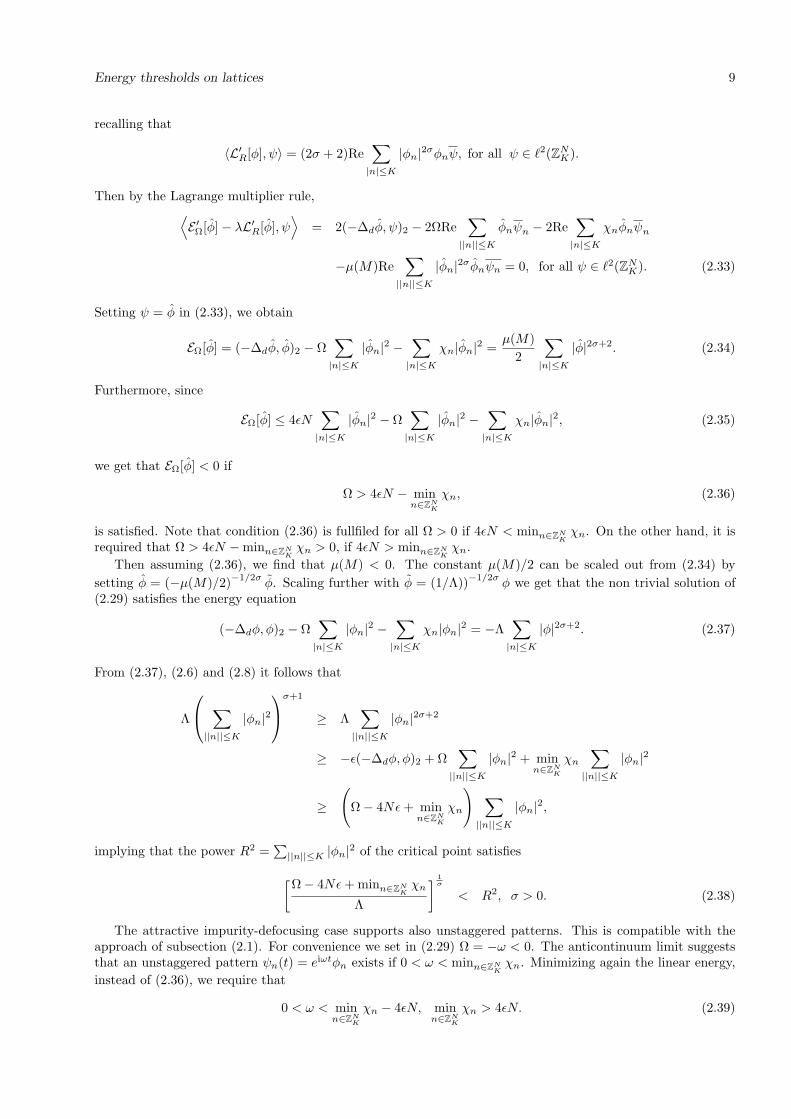
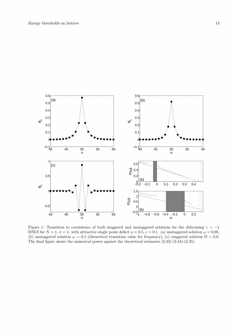
In Figure 2 the same defocusing example concerning the parameters α, ǫ,N as in Figure 1 is considered, butthis time for “large” nonlinearity parameter σ = 10. Figure 2 (a) shows the unstaggered solution correspondingto ω = 0.05, 2 (b) the unstaggered solution corresponding to ω = 0.1, the transition value predicted theoretically,and 2 (c) the staggered solution corresponding to Ω = 0.6. The final figure (d) is showing the behavior of thetheoretical bounds against the numerical power, and verify that the breathers corresponding to σ = 10 are thereal examples of breathers with power converging in a sharp manner to the analytical lower bounds.

Energy thresholds on lattices 12

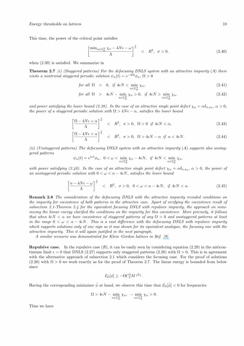
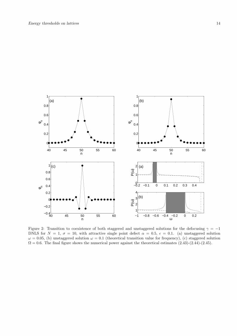
Figure 3 demonstrates the validity of the sufficient conditions for coexistence in the case of 2D lattices. Theexamples concern a 2D defocusing lattice with γ = −Λ = −1, an attractive impurity α = 0.5 and ǫ = 0.01.With these parameters we are again under the sufficient condition

0.08 = 4ǫN < α = 0.5,

for coexistence of both staggered and unstaggered patterns. Figures 3 (a), (b) correspond to σ = 1. Figure 3(a) shows the unstaggered solution corresponding to

ω = 0.4 < α− 4ǫN = 0.42,

where ω∗ = 0.42 is the transition value of frequency according condition (2.45) for the frequency of unstaggeredsolutions. Figure 3 (b) shows the profile of the the staggered solution corresponding to Ω = 0.1. Similarly,figures 3 (c), (d) correspond to σ = 10. Figure 3 (c) shows the unstaggered solution corresponding to ω = 0.46,and 3 (d) the staggered solution corresponding to Ω = 0.07.

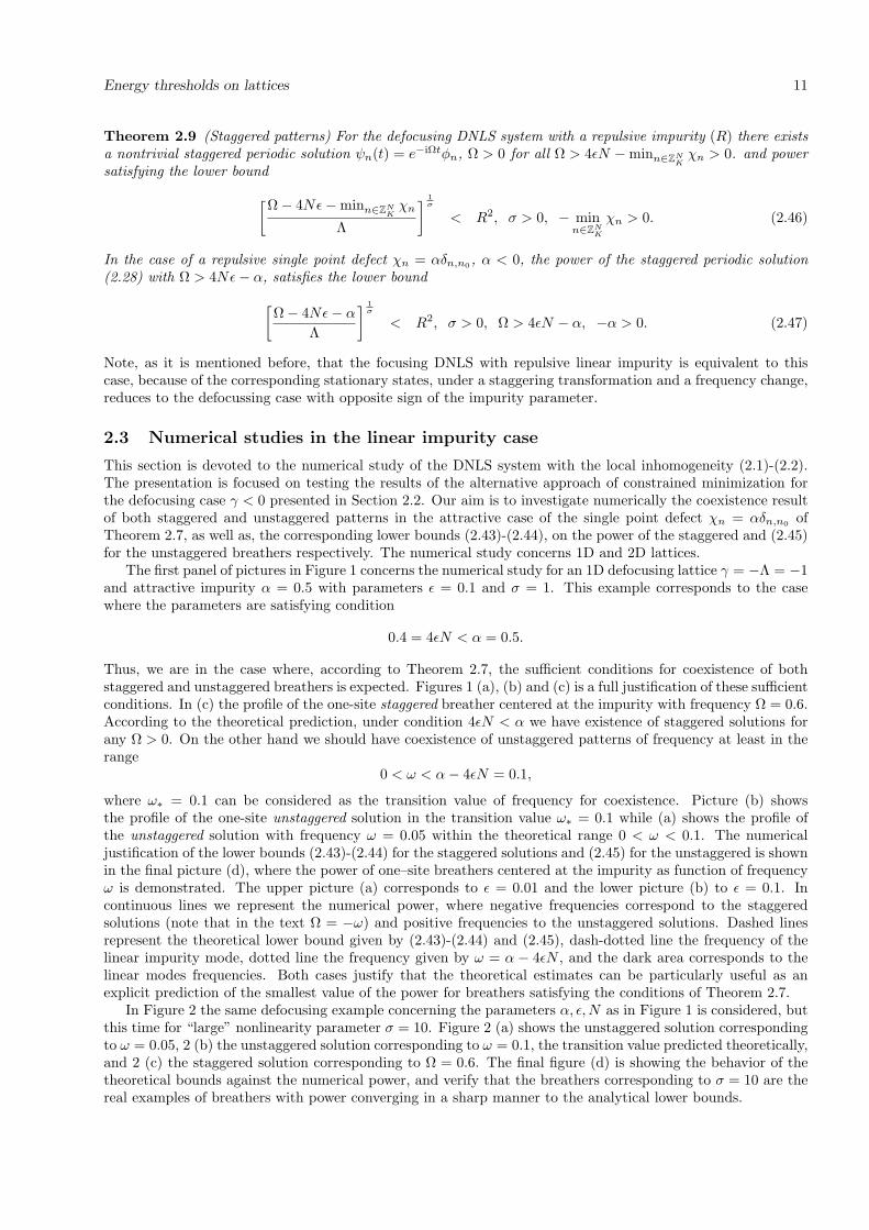
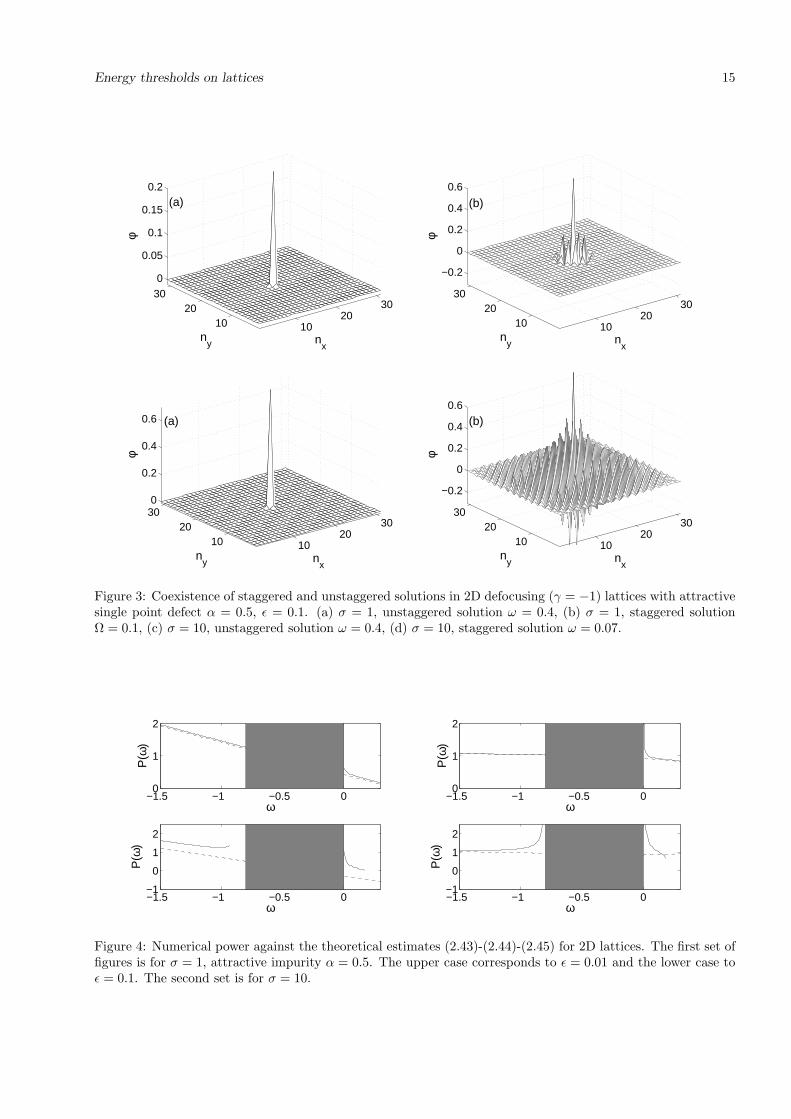
The results of the numerical study on the theoretical estimates (2.43)-(2.44)-(2.45) for 2D lattices are givenin Figure 4, justifying their effectiveness. The first figure shows the power of one–site breathers centered at theimpurity as function of frequency ω in the defocussing case γ = −1, attractive impurity α = 0.5 and σ = 1.0.The upper figure (a) corresponds to ǫ = 0.01 and the lower (b) to ǫ = 0.1. In continuous lines we represent thepower of the one–site breathers, where negative frequencies correspond to the staggered solution and positivefrequencies to the unstaggered solution. Dashed lines represent the theoretical bounds given by (2.43)-(2.44)-(2.45). The second figure is for the same parameters α, ǫ,N but now σ = 10. Note that in the lower figure (b),in the case of unstaggered solutions, the power of some numerical breathers is lower than theoretical predictions,but, in this case, the condition 0 < ω < α− 4ǫN is not satisfied.

It is crucial to remark that branches of solutions on the lower-right panels of Figures, 1, 2 and 4, terminatesuddenly. In fact in all the numerical simulations performed, it was observed that further continuation was notpossible. While this observation do not violates the theoretical statements of Theorem 2.7, since the conditionsof the theorem are only sufficient, the termination of branches possibly indicates the existence of saddle-nodebifurcations with another solution branch which can not of course be explained by the theoretical results. Thestudy of such a phenomenon possibly requires detailed stability analysis for the study of the bond centeredbreathers accompanied by careful numerical simulations, and constitutes an interesting plan for a future work.

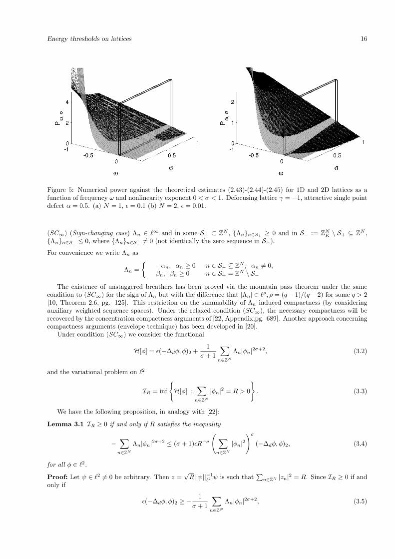
Figure 5 is a representative presentation of the numerical power against the theoretical estimates (2.43)-(2.44)-(2.45) as functions of the frequency ω and the nonlinearity exponent σ. The examples we consider arefor the defocusing case γ = −Λ = −1, and an attractive impurity α = 0.5. For the nonlinearity parameter σ weconsider the range 0 < σ < 1. This case is of importance in the context of the present work since for this rangeof σ we should not expect appearance of the excitation threshold in the sense of [6] and [22]. The first figureshows the power of one–site breathers centered at the impurity for N = 1 and ǫ = 0.1. Black lines representthe numerical results, where negative frequencies correspond to the staggered solution (note that in the textΩ = −ω) and positive frequencies to the unstaggered solutions. The grey surface represents the theoreticalestimate given by (2.43)-(2.44)-(2.45). In addition, the linear modes frequencies area is represented in thicklines. The second corresponds to the case N = 2 and ǫ = 0.01. The numerical study revealed a wide rangeof frequencies of breathers whose power are very close to the theoretical prediction for the minimal power forexistence. These members of the breather family together with the comparison of the theoretical and numericalsurface indicates the usefulness of the local estimates with respect to frequency as a simple analytical predictionof the smallest power of breathers satisfying the theoretical sufficient conditions. This becomes significant inthe possible absence of the excitation threshold which expected for small values of the nonlinearity exponent.

3 Existence of localized modes in infinite DNLS lattices with non-

linear impurities

The result on the existence of excitation threshold of [22], can be extended in the case of DNLS lattices withnonlinear impurities. For instance we shall consider the (infinite) DNLS lattice

iψn + ǫ(∆dψ)n + Λn|ψn|2σψn = 0, n ∈ ZN , (3.1)

with n ∈ ZN . The excitation threshold will be proved for unstaggered breathers by adapting the methods of

[22]. In the infinite lattice, we shall assume for Λn, n ∈ ZN the condition

Energy thresholds on lattices 13

40 45 50 55 60−0.1

0

0.1

0.2

0.3

0.4

0.5

0.6

n

φ n

(a)

40 45 50 55 60−0.1

0

0.1

0.2

0.3

0.4

0.5

0.6

n

φ n

(b)

40 45 50 55 60

−0.5

0

0.5

1

n

φ n

(c)

−1 −0.8 −0.6 −0.4 −0.2 0 0.2−0.5

0

0.5

1

1.5

ω

P(ω

)

(a)

(b)

−0.2 −0.1 0 0.1 0.2 0.3 0.40

0.2

0.4

0.6

P(ω

)

(a)

Figure 1: Transition to coexistence of both staggered and unstaggered solutions for the defocusing γ = −1DNLS for N = 1, σ = 1, with attractive single point defect α = 0.5, ǫ = 0.1. (a) unstaggered solution ω = 0.05,(b) unstaggered solution ω = 0.1 (theoretical transition value for frequency), (c) staggered solution Ω = 0.6.The final figure shows the numerical power against the theoretical estimates (2.43)-(2.44)-(2.45).

Energy thresholds on lattices 14

40 45 50 55 60

0

0.2

0.4

0.6

0.8

1

n

φ n

(a)

40 45 50 55 60

0

0.2

0.4

0.6

0.8

1

n

φ n

(b)

40 45 50 55 60−0.4

−0.2

0

0.2

0.4

0.6

0.8

1

n

φ n

(c)

−1 −0.8 −0.6 −0.4 −0.2 0 0.2

1

2

3

4

ω

P(ω

)

(b)

−0.2 −0.1 0 0.1 0.2 0.3 0.40

1

2

P(ω

)

(a)

Figure 2: Transition to coexistence of both staggered and unstaggered solutions for the defocusing γ = −1DNLS for N = 1, σ = 10, with attractive single point defect α = 0.5, ǫ = 0.1. (a) unstaggered solutionω = 0.05, (b) unstaggered solution ω = 0.1 (theoretical transition value for frequency), (c) staggered solutionΩ = 0.6. The final figure shows the numerical power against the theoretical estimates (2.43)-(2.44)-(2.45).

Energy thresholds on lattices 15

1020

30

1020

300

0.05

0.1

0.15

0.2

nx

ny

(a)

φ

1020

30

1020

30

−0.2

0

0.2

0.4

0.6

nx

ny

(b)

φ

1020

30

1020

300

0.2

0.4

0.6

nx

ny

(a)

φ

1020

30

1020

30

−0.2

0

0.2

0.4

0.6

nx

ny

(b)φ

Figure 3: Coexistence of staggered and unstaggered solutions in 2D defocusing (γ = −1) lattices with attractivesingle point defect α = 0.5, ǫ = 0.1. (a) σ = 1, unstaggered solution ω = 0.4, (b) σ = 1, staggered solutionΩ = 0.1, (c) σ = 10, unstaggered solution ω = 0.4, (d) σ = 10, staggered solution ω = 0.07.

−1.5 −1 −0.5 0−1

0

1

2

ω

P(ω

)

−1.5 −1 −0.5 00

1

2

ω

P(ω

)

−1.5 −1 −0.5 0−1

0

1

2

ω

P(ω

)

−1.5 −1 −0.5 00

1

2

ω

P(ω

)

Figure 4: Numerical power against the theoretical estimates (2.43)-(2.44)-(2.45) for 2D lattices. The first set offigures is for σ = 1, attractive impurity α = 0.5. The upper case corresponds to ǫ = 0.01 and the lower case toǫ = 0.1. The second set is for σ = 10.

Energy thresholds on lattices 16

Figure 5: Numerical power against the theoretical estimates (2.43)-(2.44)-(2.45) for 1D and 2D lattices as afunction of frequency ω and nonlinearity exponent 0 < σ < 1. Defocusing lattice γ = −1, attractive single pointdefect α = 0.5. (a) N = 1, ǫ = 0.1 (b) N = 2, ǫ = 0.01.

(SC∞) (Sign-changing case) Λn ∈ ℓ∞ and in some S+ ⊂ ZN , Λnn∈S+

≥ 0 and in S− := ZNK \ S+ ⊆ Z

N ,Λnn∈S

−

≤ 0, where Λnn∈S−

6= 0 (not identically the zero sequence in S−).

For convenience we write Λn as

Λn =

−αn, αn ≥ 0 n ∈ S− ⊆ ZN , αn 6= 0,

βn, βn ≥ 0 n ∈ S+ = ZN \ S−

The existence of unstaggered breathers has been proved via the mountain pass theorem under the samecondition to (SC∞) for the sign of Λn but with the difference that |Λn| ∈ ℓρ, ρ = (q− 1)/(q− 2) for some q > 2[10, Theorem 2.6, pg. 125]. This restriction on the summability of Λn induced compactness (by consideringauxiliary weighted sequence spaces). Under the relaxed condition (SC∞), the necessary compactness will berecovered by the concentration compactness arguments of [22, Appendix,pg. 689]. Another approach concerningcompactness arguments (envelope technique) has been developed in [20].

Under condition (SC∞) we consider the functional

H[φ] = ǫ(−∆dφ, φ)2 +1

σ + 1

∑

n∈ZN

Λn|φn|2σ+2, (3.2)

and the variational problem on ℓ2

IR = inf

H[φ] :∑

n∈ZN

|φn|2 = R > 0

. (3.3)

We have the following proposition, in analogy with [22]:

Lemma 3.1 IR ≥ 0 if and only if R satisfies the inequality

−∑

n∈ZN

Λn|φn|2σ+2 ≤ (σ + 1)ǫR−σ

(

∑

n∈ZN

|φn|2)σ

(−∆dφ, φ)2, (3.4)

for all φ ∈ ℓ2.

Proof: Let ψ ∈ ℓ2 6= 0 be arbitrary. Then z =√R||ψ||−1

ℓ2 ψ is such that∑

n∈ZN |zn|2 = R. Since IR ≥ 0 if andonly if

ǫ(−∆dφ, φ)2 ≥ − 1

σ + 1

∑

n∈ZN

Λn|φn|2σ+2, (3.5)

Energy thresholds on lattices 17

inserting z in (3.5), we derive as in [22, Proposition 3.1, pg. 679] the inequality (3.4). ⋄Using (SC∞), we remark that (3.5) is satisfied if R is such that

∑

n∈S−

αn|φn|2σ+2 ≤ (σ + 1)ǫR−σ

(

∑

n∈ZN

|φn|2)σ

(−∆dφ, φ)2, for all φ ∈ ℓ2. (3.6)

The next Proposition is a consequence of the condition (SC∞) and [22, Theorem 4.1,pg. 682]:

Lemma 3.2 Assuming condition (SC∞), there exists a constant K > 0 such that if σ ≥ 2N , the inequality

∑

n∈S−

αn|φn|2σ+2 ≤ K

(

∑

n∈ZN

|φn|2)σ

(−∆dφ, φ)2, (3.7)

holds for all for all φ ∈ ℓ2.

Proof:. By condition (SC∞) and the discrete analogue of the Sobolev-Gagliardo-Nirenberg inequality

∑

n∈ZN

|φn|2σ+2 ≤ C

(

∑

n∈ZN

|φn|2)σ

(−∆dφ, φ)2, (3.8)

of [22, Theorem 4.1,pg. 682], we have∑

n∈S−

αn|φn|2σ+2 ≤ supn∈ZN

αn∑

n∈ZN

|φn|2σ+2

≤ supn∈ZN

αnC(

∑

n∈ZN

|φn|2)σ

(−∆dφ, φ)2.

Thus K = supn∈ZN αnC. ⋄Let us note that under condition (SC∞) the sign of

∑

n∈ZN Λn|φn|2σ+2 is indefinite. However as it isexpected and shown in [3], the existence of unstaggered breathers should be supported mainly by the focusingpart of the nonlinearity. Thus it is natural to claim that the existence and the global threshold for unstaggeredbreathers will be defined from inequality (3.7). Note that (3.7) is a stronger inequality than (3.4), since if φ ∈ ℓ2

satisfies (3.7), then it satisfies (3.4). In analogy with [22, Eq. 4.2, pg. 680], if K∗ is the infimum over all suchconstants, the excitation threshold denoted by Rsc in the case will be defined for the case σ ≥ 2

N by the equation

(σ + 1)ǫ(Rsc)−σ = K∗. (3.9)

This claim will be justified by a simple treating the defocusing part of the nonlinearity, as well as of the inequality(3.7), on the way to extend the results of [22].

Proposition 3.3 Assume condition (SC∞) and let σ ≥ 2N . We define

Rsc =(

(σ + 1)ǫKσ,N)

1σ (3.10)

where Kσ,N = inf

(∑

n∈ZN |φn|2)σ

(−∆dφ, φ)2∑

n∈S−

αn|φn|2σ+2=

1

K∗. (3.11)

A. Assume that ||φ||2ℓ2 = R. Then

H[φ] ≥ ǫ(−∆dφ, φ)2

[

1 −(

R

Rsc

)σ]

. (3.12)

B. If R < Rsc then IR = 0 and there is no ground state minimizer of (3.3).

Proof: A. Using (SC∞) and inequality (3.7) with its best constant K∗ we derive that

H[φ] = ǫ(−∆dφ, φ)2 +1

σ + 1

∑

n∈S+

βn|φn|2σ+2 − 1

σ + 1

∑

n∈S−

αn|φn|2σ+2

≥ ǫ(−∆dφ, φ)2 −1

σ + 1

∑

n∈S−

αn|φn|2σ+2

≥ ǫ(−∆dφ, φ)2 − ǫ(Rsc)−σRσ(−∆dφ, φ)2,

Energy thresholds on lattices 18

thus (3.12).B. Assuming that R < Rthresh, it follows from (3.12) that IR ≥ 0. We consider next some ψ ∈ ℓ2 such that

ψnn∈ZNK

= ψnn∈S++ ψnn∈S

−

, such that

ψnn∈S+= 0,

ψnn∈S−

6= 0

||ψ||ℓ2 =

√R

λ, where λ > 0 arbitrary.

Then considering zλ =√R||ψ||−1

ℓ2 ψ we observe that

||zλ||2ℓ2 = R

and

H[zλ] = ǫ(−∆dψ, ψ)2 −λ2σ+2

σ + 1

∑

n∈S−

αn|ψn|2σ+2.

For λ sufficiently large, we get that H[zλ] < 0. Therefore if R < Rsc we should have IR = 0. We assume that

the infimum is attained at a state φ for which

ǫ(−∆dφ, φ)2 = − 1

σ + 1

∑

n∈S+

βn|φn|2σ+2 +1

σ + 1

∑

n∈S−

αn|φn|2σ+2, (3.13)

∑

n∈ZN

|φn|2 = R.

Inserting again inequality (3.7) with its best constant K∗ into (3.13) we deduce that

ǫ(−∆dφ, φ)2 ≤ 1

σ + 1

∑

n∈S−

αn|φn|2σ+2 ≤ ǫ

(

R

Rsc

)σ

< ǫ(−∆dφ, φ)2. ⋄

The last theorem concludes that Rsc is an excitation threshold for σ ≥ 2N .

Theorem 3.4 Assume condition (SC∞) and let σ ≥ 2N . If R > Rsc then IR < 0 and there exists a minimizer

of the variational problem (3.3).

Proof: We shall justify first that if R > Rsc then IR < 0: By the definitions (3.10-(3.11) of Rsc and Kσ,N itfollows that a φ∗ ∈ ℓ2 must exist which do not satisfy inequality (3.7), hence

∑

n∈S−

αn|φ∗n|2σ+2 ≥ (σ + 1)ǫR−σ

(

∑

n∈ZN

|φ∗n|2)σ

(−∆dφ∗, φ∗)2, R > Rsc. (3.14)

Then (3.14) clearly implies that

∑

n∈S−

αn|φ∗n|2σ+2 ≥ (σ + 1)ǫR−σ

∑

n∈S−

|φ∗n|2

σ

(−∆dφ∗, φ∗)S

−

, R > Rsc, (3.15)

where (·, ·)S−

, denotes the piece of (·, ·)2 in the part S− of the lattice. Now we consider the element ζ ∈ ℓ2,defined as

ζ =√R||θ||−1

ℓ2 θ, where θn =

φ∗n, n ∈ S−0, n ∈ S+.

Then we observe that

H[ζ] = ǫR||θ||−2ℓ2 (−∆dφ

∗, φ∗)S−

− Rσ+1

σ + 1||θ||−2σ−2

ℓ2

∑

n∈S−

αn|φ∗n|2σ+2

< ǫR||θ||−2ℓ2 (−∆dφ

∗, φ∗)S−

−Rσ+1||θ||−2σ−2ℓ2 ǫR−σ

∑

n∈S−

|φ∗n|2

σ

(−∆dφ∗, φ∗)S

−

= 0

Energy thresholds on lattices 19

since ||θ||2ℓ2 =∑

n∈S−

|φ∗n|2. Hence IR < 0.We proceed by showing the existence of a minimizer. Clearly, IR is bounded form below since

H[φ] ≥ − 1

σ + 1

∑

n∈S−

αn|φn|2σ+2

≥ − 1

σ + 1

∑

n∈ZN

αn|φn|2σ+2

≥ − 1

σ + 1sup

n∈ZN

αn supn∈ZN

|φn|2σ∑

n∈ZN

αn|φn|2

≥ − 1

σ + 1Rσ+1.

The final step is to prove that every minimizing sequence associated with the variational problem (3.3) isprecompact modulo phase translations (cf. [22, Theorem 2.1, pg. 677]. Let ψmm∈N a minimizing sequence.Then by the fact that IR < 0, we have that

H[ψm] ≤ IR

2, for m large enough. (3.16)

Then it follows from (3.16) that

||φm||2σ+2ℓ2 sup

n∈ZN

|Λn| ≥ −∑

n∈ZN

Λn|φmn |2σ+2 ≥ −σ + 1

2IR > 0. (3.17)

The lower bound (3.17) shows that the vanishing scenario [22, Theorem 7.1 (2), pg. 689] is excluded for aminimizing sequence. Now we consider a sequence φmm∈N in ℓ2 such that

||φm||2ℓ2 → ρ, and H[φm] → IR. (3.18)

The sequence

ψm =√R||φm||−1

ℓ2 φm,

is a minimizing sequence and satisfies (3.17), thus ρ > 0. We prove that

ρ = R. (3.19)

By contradiction, we suppose that

0 < ρ < R. (3.20)

We consider the sequences ζmm∈N, ηmm∈N satisfying the dichotomy scenario [22, Theorem 7.1 (3), pg. 689]:This means that for all ǫ > 0, there exists m0 ≥ 1 such that for all m > m0

||ψmk − (ζk + ηk)||ℓ2 ≤ ǫ,∣

∣||ζk||2ℓ2 − ρ∣

∣ ≤ ǫ, (3.21)∣

∣||ηk||2ℓ2 − (R− ρ)∣

∣ ≤ ǫ,

with disjoint supports satisfying distance(suppζk, suppηk) → ∞. Note that there exists c > 0 such that

∣

∣

∣

∣

∣

∑

n∈ZN

Λn|ψmkn |2σ+2 −

∑

n∈ZN

Λn|ζkn|2σ+2 −

∑

n∈ZN

Λn|ζkn|2σ+2

∣

∣

∣

∣

∣

≤ c supn∈Z

|ψmkn − ζk

n − ηkn|∑

n∈ZN

|ψmkn |2σ+1 → 0, as k → ∞, (3.22)

due to (3.21) and (2.4). Similarly, by (3.21) and (2.5) we can verify that

∣

∣(−∆dψmk , ψmk)2 − (−∆dζ

k, ζk)2 − (−∆dηk, ηk)2

∣

∣→ 0, as k → ∞. (3.23)

Energy thresholds on lattices 20

Using both (3.22) and (3.23), one yields

limk→∞

H[ψmk ] = limk→∞

H[ζk] + limk→∞

H[ηk], (3.24)

limk→∞

H[ζk] + limk→∞

H[ηk] = IR. (3.25)

We can easily see that for any φ ∈ ℓ2 and λ > 0,

H[φ] =1

λ2H[λφ] − λ2σ − 1

σ + 1

∑

n∈S+

βn|φn|2σ+2 +λ2σ − 1

σ + 1

∑

n∈S−

αn|φn|2σ+2

=1

λ2H[λφ] − λ2σ − 1

σ + 1

∑

n∈ZN

Λn|φn|2σ+2.

Setting λk =√

R||ζk||

ℓ2, µk =

√R

||ηk||ℓ2

we have ||λkζk||2ℓ2 = R and ||µkη

k||2ℓ2 = R and

H[ζk] =1

λ2k

H[λkζk] − λ2σ

k − 1

σ + 1

∑

n∈ZN

Λn|ζkn|2σ+2 ≥ IR

λ2k

− λ2σk − 1

σ + 1

∑

n∈ZN

Λn|ζkn|2σ+2,

H[ηk] =1

µ2k

H[µkζk] − µ2σ

k − 1

σ + 1

∑

n∈ZN

Λn|ηkn|2σ+2 ≥ IR

µ2k

− µ2σk − 1

σ + 1

∑

n∈ZN

Λn|ηkn|2σ+2.

From these inequalities and the definition of IR it follows that

H[ζk] + H[ηk] ≥ IR

(

1

λ2k

+1

µ2k

)

− λ2σk − 1

σ + 1

∑

n∈ZN

Λn|ζkn|2σ+2 − µ2σ

k − 1

σ + 1

∑

n∈ZN

Λn|ηkn|2σ+2. (3.26)

We shall pass to the limit in (3.26) as k → ∞: We observe that

limk→∞

(

1

λ2k

+1

µ2k

)

=ρ

R+R− ρ

R= 1,

as well as, that due to the assumption (3.20)

limk→∞

λ2σk =

Rσ

ρσ> 1,

limk→∞

µ2σk =

Rσ

(R− ρ)σ> 1.

Then by using (3.22) we infer that

limk→∞

H[ζk] + H[ηk] ≥ IR − ξ − 1

σ + 1lim

k→∞

∑

n∈ZN

Λn|ψmkn |2σ+2, ξ = min

Rσ

ρσ,

Rσ

(R− ρ)σ

.

Application of the lower bound (3.17) to ψmk implies the inequality

IR − ξ − 1

σ + 1lim

k→∞

∑

n∈ZN

Λn|ψmkn |2σ+2 ≥ IR − ξ − 1

2IR > IR,

since IR < 0. In conclusion,

limk→∞

H[ζk] + H[ηk] > IR,

which contradicts (3.25). Henceforth the dichotomy scenario must be excluded. ⋄

Energy thresholds on lattices 21

1 1.1 1.2 1.3 1.4 1.5 1.6 1.7 1.8 1.9 20

0.2

0.4

0.6

0.8

1

1.2

1.4

1.6

1.8

2

Ω

PΩ

Nonlinear impurity. σ=2. N=1. ε=0.25

1.1 1.2 1.3 1.41

1.01

1.02

1.03

1.04

1 1.1 1.2 1.3 1.4 1.5 1.6 1.7 1.8 1.9 20

0.5

1

1.5

2

2.5

Ω

PΩ

Nonlinear impurity. σ=10. N=1. ε=0.25

1.5 2 2.5 3 3.51.09

1.1

1.11

1.12

1.13

1.2 1.3 1.4 1.5 1.6 1.7 1.8 1.9 20

0.2

0.4

0.6

0.8

1

1.2

1.4

1.6

1.8

2

Ω

PΩ

Sign−changing nonlinearity. σ=1. N=2. ε=0.15

1.26 1.28 1.3 1.32 1.34 1.360.79

0.795

0.8

0.805

0.81

0.815

0.82

1.2 1.3 1.4 1.5 1.6 1.7 1.8 1.9 20

0.5

1

1.5

2

2.5

Ω

PΩ

Sign−changing nonlinearity. σ=2. N=2. ε=0.15

1.3 1.4 1.5 1.6 1.71.04

1.05

1.06

1.07

1.08

1.09

1.1

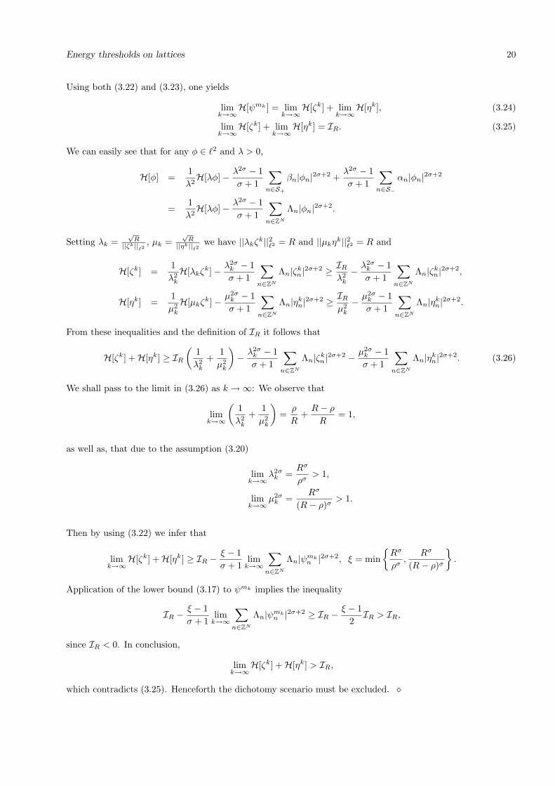
Figure 6: Numerical power for single site breathers centered at the nonlinear impurity site for N = 1, 2. (a)Single nonlinear impurity σ = 2, N = 1 (σ = σcrit), (b) Single nonlinear impurity σ = 10, N = 1 (σ > σcrit),(c) Sign-changing impurity σ = 1, N = 2 (σ = σcrit), (d) Sign-changing impurity σ = 2, N = 2 (σ > σcrit). Theinsets show magnifications of the region where the power of periodic solutions attains the excitation thresholdRsc of Theorem 3.4.

Energy thresholds on lattices 22

0.6 0.7 0.8 0.9 1 1.1 1.2 1.3 1.4 1.50

0.2

0.4

0.6

0.8

1

1.2

1.4

1.6

1.8

2

Ω

PΩ

Nonlinear impurity. σ=1. N=3. ε=0.05

0.65 0.7 0.75 0.8

0.4

0.45

0.5

0.6 0.7 0.8 0.9 1 1.1 1.2 1.3 1.4 1.50

0.2

0.4

0.6

0.8

1

1.2

1.4

1.6

1.8

2

Ω

PΩ

Nonlinear impurity. σ=2. N=3. ε=0.05

0.65 0.7 0.75 0.8 0.85

0.7

0.72

0.74

0.76

0.6 0.7 0.8 0.9 1 1.1 1.2 1.3 1.4 1.50

0.2

0.4

0.6

0.8

1

1.2

1.4

1.6

1.8

2

Ω

PΩ

Sign−changing nonlinearity. σ=1. N=3. ε=0.05

0.62 0.64 0.66 0.68 0.7 0.720.38

0.39

0.4

0.41

0.42

0.43

0.44

−1 −0.9 −0.8 −0.7 −0.6 −0.5 −0.4 −0.3 −0.2 −0.1 00

0.2

0.4

0.6

0.8

1

1.2

1.4

1.6

1.8

2

Ω

PΩ

Sign−changing nonlinearity. σ=2. N=3. ε=0.05

−0.14 −0.12 −0.1 −0.08 −0.060.695

0.7

0.705

0.71

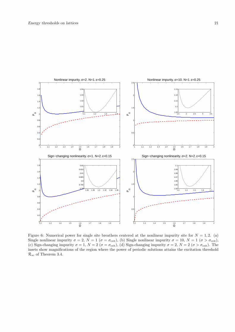
Figure 7: 3D DNLS lattices with nonlinear impurities. (a) Numerical power for single site breathers centeredat the nonlinear impurity site for the single nonlinear impurity σ = 1, N = 3 (σ > σcrit), (b) for the singlenonlinear impurity σ = 2, N = 3 (σ > σcrit), (c) for the sign-changing impurity σ = 1, N = 3. (d) Numericalpower for single site unstaggered breathers far from the sign-changing impurity σ = 2, N = 3. The insets showmagnifications of the region where the power of each breather family attains the excitation threshold Rsc ofTheorem 3.4 in the 3D case.

3.1 Numerical studies in the case of nonlinear impurities

In this section we present numerical studies for the DNLS lattices with nonlinear impurities with a twofoldpurpose. The first aim is to present the numerical verification on the existence of the excitation threshold.The second is to review the lower bounds derived in [3], emphasizing the differences between the lower boundsand the excitation thresholds. The present study is also extended to 3D-lattices, thus covering all the casesof physical significance with respect to the dimension. The models we consider are those of a single nonlinearimpurity, Λn = δn,0 [14, 15, 16, 21], and of a sign-changing anharmonic parameter. In the latter, we haveconsidered the simplest case where all sites have Λn = 1 except for one of them which is −1.

The panel of pictures in figure 6, demonstrates the results of the numerical study for 1D and 2D lattices.For these cases, the critical exponent σcrit = 2/N for the nonlinearity exponent σ is

σcrit = 2, for N = 1

σcrit = 1, for N = 2,

and the study concerns cases σ ≥ σcrit where the excitation threshold appears. This numerical study gives thenumerical verification of Theorem 3.4 on the generalization of the existence of the excitation threshold in the

Energy thresholds on lattices 23

1 1.1 1.2 1.3 1.4 1.5 1.6 1.7 1.8 1.9 20

0.5

1

1.5

2

2.5

Ω

PΩ

Sign−changing nonlinearity. σ=0.1. N=1. ε=0.25

1.2 1.3 1.4 1.5 1.6 1.7 1.8 1.9 20

0.5

1

1.5

2

2.5

Ω

PΩ

Sign−changing nonlinearity. σ=0.1. N=2. ε=0.15

−30 −20 −10 0 10 20 30−0.04

−0.02

0

0.02

0.04

0.06

0.08

0.1

0.12

0.14

0.16

n

φ n

Sign−changing nonlinearity. σ=0.1. N=1. ε=0.25. Ω=1.28

−10

−5

0

5

10

−10

−5

0

5

10−0.02

0

0.02

0.04

0.06

0.08

0.1

0.12

n1

Sign−changing nonlinearity. σ=0.1. N=2. ε=0.15. Ω=1.32

n2

φ n1,n

2

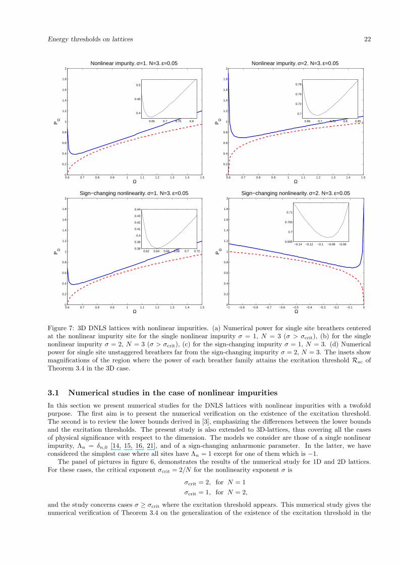
Figure 8: Numerical power for single site staggered breathers centered at the nonlinear impurity site, for theDNLS with sign-changing impurity for σ = 0.1 < σcrit. (a) N = 1, (b) N = 2. The lower bound Rlb(Ω) isfulfilled. (c), (d) Breather profiles with power close to the lower bound.

Energy thresholds on lattices 24

case of nonlinear impurities. The inset in each picture demonstrates the positive lower energy bound Rsc ofTheorem 3.4. The numerical power as well as the excitation threshold Rsc has been calculated for staggeredbreathers of the defocusing DNLS. The numerical power has been drawn against the theoretical lower bound

Rlb :=

[

Ω − 4Nǫ

maxn∈S+Λn

]1σ

< R2, Ω > 4ǫN, σ > 0, (3.27)

derived in [3, Theorem 3.1, pg. 77], and justifies that Rlb is fulfilled for breathers with frequency Ω > 4ǫN .Picture (b) indicates that Rlb(Ω) is becoming a satisfactory estimate for large σ and for large values of frequenciesΩ, as an Ω-dependent lower bound for existence.

The effectiveness and strength of the theoretical explicit lower bounds become even more apparent in the3D-lattices. In Figure 7, the numerical study of (3.27) for the cases N = 1, 2 in [3] is extended to the caseN = 3. For the 3D-lattice, the critical exponent is

σcrit =2

3, for N = 3.

The examples considered σ = 1, 2 correspond to the supercritical case σ > σcrit and the insets in each picturejustify numerically the appearance of the excitation threshold Rsc in the three dimensional lattice. The rangeof frequencies 0.8 < Ω < 1 in pictures (a), (b), (c), corresponds to the members of the staggered breatherfamily with power approaching the lower bound Rlb(Ω) with increased accuracy and in a quite sharp mannerfor σ > σcrit. The insets in each picture justify numerically the appearance of the excitation threshold Rsc inthe three dimensional lattice. To elucidate further the difference between the excitation threshold Rsc and thelower bound Rlb(Ω), let us remark that the example of frequencies 0.8 < Ω < 1 corresponds to frequenciesΩ > Ωthresh =the frequency of the minimizer on which the excitation threshold Rsc is attained. In the example(c), it is found that Rsc = 0.6968 at Ωthresh = 0.69. Picture (d) in particular, shows the numerical power of thefamily of unstaggered breathers which are infinitely far from the sign-changing impurity against the theoreticalestimate

Rlb(Ω) =

[

ǫλ1 − Ω

−minn∈S−

Λn

]1σ

< R2, Ω ∈ (−∞, ǫλ1), σ > 0,

of [3, Remark 3.2, pg. 80]. Estimate (3.28) is valid for any unstaggered breather ψn(t) = e−iΩtφn, for any Ω < 0.The range of frequencies −0.5 < Ω < −0.2 in (d), corresponds to the members of the unstaggered breatherfamily far from the impurity with power very close to the lower bound Rlb(Ω). For this breather family it isfound that Rsc = 0.6970 at Ωthresh = −0.09. We remark here that a complete study of Rlb(Ω) requires also thestudy of the unstaggered breathers which are centered at the site adjacent to the impurity, since our numericalstudies revealed that there is a range of frequency for which the smallest power breather is attained for thiskind of breather family.

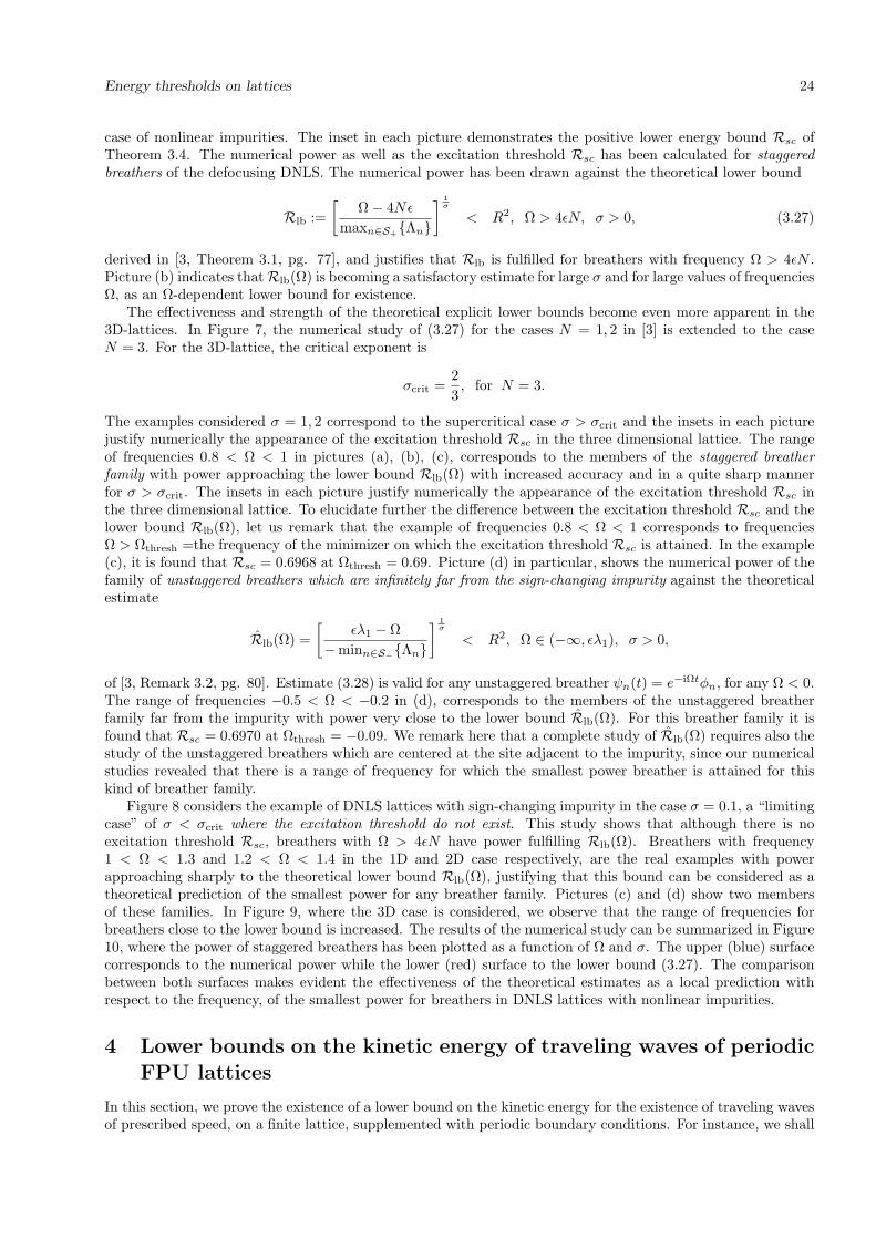
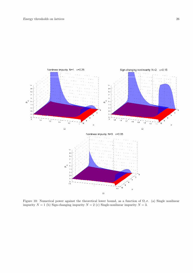
Figure 8 considers the example of DNLS lattices with sign-changing impurity in the case σ = 0.1, a “limitingcase” of σ < σcrit where the excitation threshold do not exist. This study shows that although there is noexcitation threshold Rsc, breathers with Ω > 4ǫN have power fulfilling Rlb(Ω). Breathers with frequency1 < Ω < 1.3 and 1.2 < Ω < 1.4 in the 1D and 2D case respectively, are the real examples with powerapproaching sharply to the theoretical lower bound Rlb(Ω), justifying that this bound can be considered as atheoretical prediction of the smallest power for any breather family. Pictures (c) and (d) show two membersof these families. In Figure 9, where the 3D case is considered, we observe that the range of frequencies forbreathers close to the lower bound is increased. The results of the numerical study can be summarized in Figure10, where the power of staggered breathers has been plotted as a function of Ω and σ. The upper (blue) surfacecorresponds to the numerical power while the lower (red) surface to the lower bound (3.27). The comparisonbetween both surfaces makes evident the effectiveness of the theoretical estimates as a local prediction withrespect to the frequency, of the smallest power for breathers in DNLS lattices with nonlinear impurities.

4 Lower bounds on the kinetic energy of traveling waves of periodic

FPU lattices

In this section, we prove the existence of a lower bound on the kinetic energy for the existence of traveling wavesof prescribed speed, on a finite lattice, supplemented with periodic boundary conditions. For instance, we shall

Energy thresholds on lattices 25

0.6 0.7 0.8 0.9 1 1.1 1.2 1.3 1.4 1.50

0.2

0.4

0.6

0.8

1

1.2

1.4

1.6

1.8

2

Ω

PΩ

Sign−changing nonlinearity. σ=0.1. N=3. ε=0.05

0.8 0.82 0.84 0.86 0.88 0.9 0.92 0.94 0.96 0.98 10

0.005

0.01

0.015

0.02

0.025

Ω

PΩ

Sign−changing nonlinearity. σ=0.1. N=3. ε=0.05

Figure 9: (a) Numerical power for single site staggered breathers centered at the nonlinear impurity site, for theDNLS with sign-changing impurity for σ = 0.1 < σcrit for N = 3. (b) Magnification for the range of frequencies0.8 < Ω < 1.

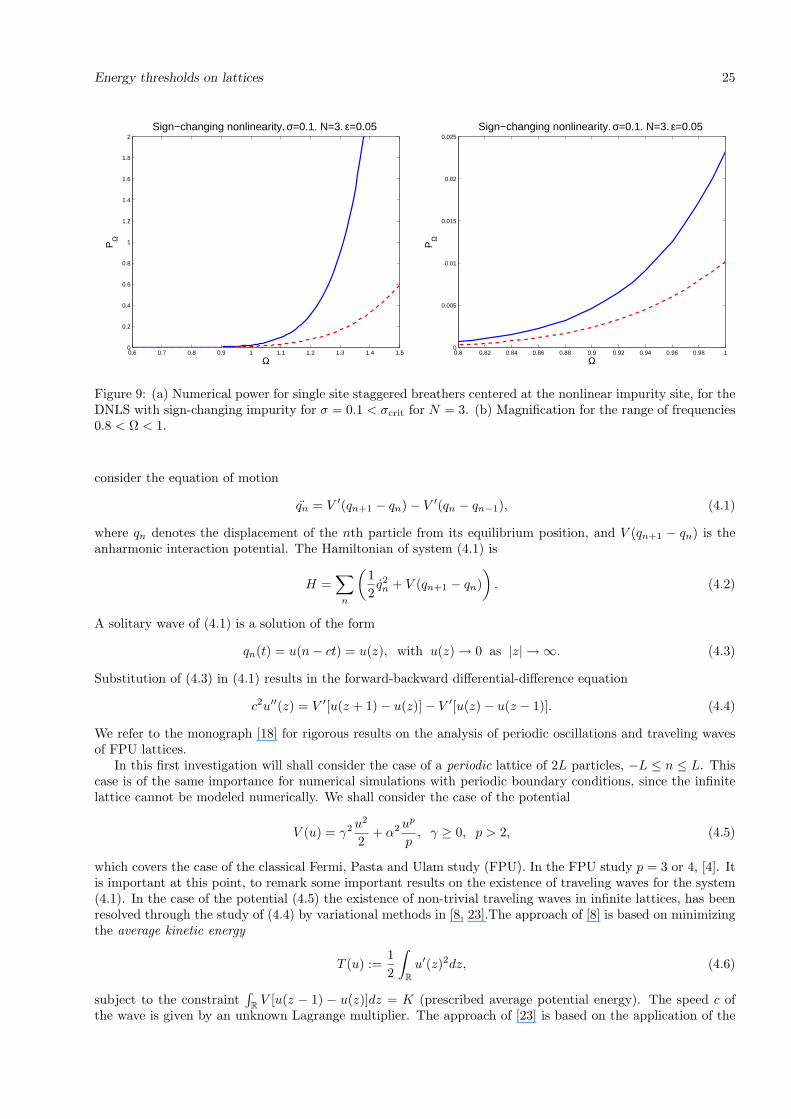
consider the equation of motion

qn = V ′(qn+1 − qn) − V ′(qn − qn−1), (4.1)

where qn denotes the displacement of the nth particle from its equilibrium position, and V (qn+1 − qn) is theanharmonic interaction potential. The Hamiltonian of system (4.1) is

H =∑

n

(

1

2q2n + V (qn+1 − qn)

)

. (4.2)

A solitary wave of (4.1) is a solution of the form

qn(t) = u(n− ct) = u(z), with u(z) → 0 as |z| → ∞. (4.3)

Substitution of (4.3) in (4.1) results in the forward-backward differential-difference equation

c2u′′(z) = V ′[u(z + 1) − u(z)] − V ′[u(z) − u(z − 1)]. (4.4)

We refer to the monograph [18] for rigorous results on the analysis of periodic oscillations and traveling wavesof FPU lattices.

In this first investigation will shall consider the case of a periodic lattice of 2L particles, −L ≤ n ≤ L. Thiscase is of the same importance for numerical simulations with periodic boundary conditions, since the infinitelattice cannot be modeled numerically. We shall consider the case of the potential

V (u) = γ2u2

2+ α2u

p

p, γ ≥ 0, p > 2, (4.5)

which covers the case of the classical Fermi, Pasta and Ulam study (FPU). In the FPU study p = 3 or 4, [4]. Itis important at this point, to remark some important results on the existence of traveling waves for the system(4.1). In the case of the potential (4.5) the existence of non-trivial traveling waves in infinite lattices, has beenresolved through the study of (4.4) by variational methods in [8, 23].The approach of [8] is based on minimizingthe average kinetic energy

T (u) :=1

2

∫

R

u′(z)2dz, (4.6)

subject to the constraint∫

RV [u(z − 1) − u(z)]dz = K (prescribed average potential energy). The speed c of

the wave is given by an unknown Lagrange multiplier. The approach of [23] is based on the application of the

Energy thresholds on lattices 26

Figure 10: Numerical power against the theoretical lower bound, as a function of Ω, σ. (a) Single nonlinearimpurity N = 1 (b) Sign-changing impurity N = 2 (c) Single-nonlinear impurity N = 3.

Energy thresholds on lattices 27

mountain pass theorem, providing the existence of nontrivial traveling waves of prescribed speed c. For instance:(a) in the case of the potential (4.5) with p = 2m + 1, m ∈ N, equation (4.4) has a nontrivial nondecreasingsolution for every c > γ.(b) In the case of the potential (4.5) with p = 2m, m ∈ N, equation (4.4) has a pair of opposite nontrivialsolutions, one nondecreasing and the other nonincreasing, for every c > γ.

We remark that monotonicity properties are considered in the sense that the corresponding wave profile is amonotone function or, equivalently, the relative displacement profile is either positive or negative (see [18], [19,pg. 1225], [23, Section 3 & pg. 274]). This notion of monotonicity has a physical implementation. Increasingwaves are expansion waves while decreasing waves are compression waves [18, pg. 78].

The case of the periodic lattice was considered in [19]. The existence of periodic traveling waves withprescribed speed and arbitrary period is proved with mountain pass arguments, while the existence of waveswith minimal possible averaged action (ground waves) is proved by the Nehari variational principle.

Motivated by these existence results, we shall apply the fixed-point argument of [2], this time to the problem(4.4)-(4.5), to derive an explicit lower bound Tthresh on the average kinetic energy (4.6) satisfied by travelingwaves of sufficiently large speed c > c∗. The lower bound Tthresh is a threshold for the existence of travelingwaves of speed c > c∗ in the sense that we should not expect traveling waves qn(t) = u(z) of speed c > c∗ withaverage kinetic energy T (u) ≤ Tthresh. This result is given in Theorem 4.5.

4.1 Derivation of the lower bound on the average kinetic energy

Problem (4.4) in the periodic lattice is naturally formulated in Sobolev spaces of periodic functions used in [19]:For instance, (4.4) will be considered in the Hilbert space of periodic functions

X1 :=

u ∈ H1(R) : u′(z + 2L) = u′(z), u(0) = 0

,

endowed with the scalar product and induced norm

(u, v)1 =

∫ L

−L

u′(z)v′(z)dt, ||u||21 =

∫ L

−L

u′(z)2dt.

It can be easily checked that with the normalizing condition u(0) = 0, the Poincare inequality

∫ L

−L

u(z)2dt ≤ C(L)

∫ L

−L

u′(z)2dt, (4.7)

holds with C(L) = L2, while the optimal constant C(L) = L2

π2 can be used when one considers the Hilbert spaceof 2L-periodic functions. We rewrite equation (4.4) as

−u′′(z) =1

c2V ′[u(z) − u(z − 1)] − V ′[u(z + 1) − u(z)] . (4.8)

To apply the fixed point argument, we shall need the existence of solutions to an auxiliary problem related to(4.4)-(4.5). For convenience to the reader we recall Friedrich’s extension Theorem.

Theorem 4.2 Let L0 : D(L0) ⊆ X0 → X0 be a linear symmetric operator on the Hilbert space X0 with itsdomain D(L0) being dense in X0. Assume that there exists a constant c > 0 such that

(L0u, u)X0≥ c||u||2X0

for all u ∈ D(L0).

Then L0 has a self-adjoint extension L : D(L) ⊆ X1 ⊆ X0 → X0where X1 denotes the energy Hilbert spaceendowed with the energy scalar product (u, v)X1

= (Lu, v)X0for all u, v ∈ X1 and the energy norm ||u||2X1

=(Lu, v)X0

. Furthermore, the operator equation

Lu = f, f ∈ X0,

has a unique solution u ∈ D(L). In addition, if L : X1 → X ∗1 denotes the energy extension of L, then L is the

canonical isomorphism from X1 to its dual X ∗1 and the operator equation

Lu = f, f ∈ X ∗1 ,

has also a unique solution u ∈ X1.

Energy thresholds on lattices 28

It is well known that Theorem 4.2 is applicable to the operator L0 : D(L0) ⊆ L2(−L,L) → L2(−L,L),L0u = −u′′(z), with domain of definition the space D(L0) the space of C∞-functions on [−L,L]. Since D(L0)is dense in X0, and inequality (4.7) holds, the Friedrich’s extension of L0 is the operator L : D(L) → X0 where

D(L) =

u ∈ X1 : Lu ∈ L2(−L,L)

.

The operator equation

−u′′(z) = f, for every f ∈ L2(−L,L) (4.9)

has a unique solution in D(L). Thus as an auxiliary problem we shall consider the equation

−u′′(z) =1

c2V ′[ψ(z) − ψ(z − 1)] − V ′[ψ(z + 1) − ψ(z)] , (4.10)

for some fixed ψ ∈ X1. We also recall the following key lemma [19, Lemma 1,pg. 1225].

Lemma 4.3 The linear operators

A1u = u(z + 1) − u(z) =

∫ z+1

z

u′(s)ds, A2u(z) = u(z) − u(z − 1) =

∫ z

z−1

u(s)ds,

are continuous from X1 to L2(−L,L) ∩ L∞(−L,L) and ||Aiu||∞ ≤ ||u||1, ||Au||0 ≤ ||u||1, i = 1, 2.

With Lemma 4.3 in hand we may proceed to the proof of

Proposition 4.4 For any ψ ∈ X1, the equation (4.10) has a unique solution u ∈ D(L).

Proof: Equation (4.10) can be rewritten as

−u′′(z) =1

c2V ′[A2ψ(z)] − V ′[A1ψ(z)] , (4.11)

where V ′(s) = γ2s+ sp−1. Note that

∫ L

−L

|V ′[A2ψ(z)] − V ′[A1ψ(z)]|2dz ≤ γ4

∫ L

−L

|A2ψ(z) −A1ψ(z)|2dz

+ α4

∫ L

−L

∣

∣[A2ψ(z)]p−1 − [A1ψ(z)]p−1∣

∣

2dz. (4.12)

To estimate the second term of the right-hand side of (4.12) we shall use the inequality

∫ L

−L

|sp−11 − sp−1

2 |2 ≤ (p− 1)2∫ L

−L

∫ 1

0

|ξ|p−2|s1 − s2|dθ2

, (4.13)

where s1, s2 ∈ R, and ξ = θs1 + (1 − θ)s2, θ ∈ (0, 1). Then, we have that

∫ L

−L

∣

∣[A2ψ(z)]p−1 − [A1ψ(z)]p−1∣

∣

2dz ≤ (p− 1)2||ξ||2(p−2)

∞

∫ L

−L

|A2ψ(z) −A1ψ(z)|2dz, (4.14)

where ξ = θA2ψ(z) + (1 − θ)A1ψ(z). By using Lemma 4.3, we deduce that ||ξ||2(p−2)∞ ≤ ||ψ||2(p−2)

1 and from(4.12) and (4.14) the inequality

||V ′[A2ψ] − V ′[A1ψ]||20 ≤ (γ4 + α4||ψ||2(p−2)1 )||A2ψ −A1ψ||20

≤ 4(γ4 + α4||ψ||2(p−2)1 )||ψ||21.

Thus V[ψ(z)] = V ′[A2ψ(z)] − V ′[A1ψ(z)] defines a map V : X1 → L2(−L,L). Thus, from Friedrich’s extensionTheorem 4.2, equation (4.10)

−u′′(z) =1

c2V[ψ(z)], (4.15)

Energy thresholds on lattices 29

for any ψ ∈ X1 has a unique solution u ∈ H2(−L,L) ∩ X1.

Let us now consider for some R > 0 the closed ball of X1, BR := ψ ∈ X1 : ||ψ||1 ≤ R. Proposition 4.4shows that the map S : X1 → X1 defined as

S[ψ] = u,

where u is the unique solution of the auxiliary problem (4.15), is well defined. Hence we may consider ψ1, ψ2 ∈ BR

such thatu = S[ψ1] and v = S[ψ2].

Then the difference U = u− v satisfies the equation

−U ′′(z) =1

c2V[ψ1(z)] − V[ψ2(z)]

=1

c2V ′[A1ψ2(z)] − V ′[A1ψ1(z)] + V ′[A2ψ1(z)] − V ′[A2ψ2(z)] . (4.16)

From Lemma 4.3 the linear operators Ai : X1 → L2(−L,L) ∩ L∞(−L,L) are globally Lipschitz,

||Aiψ1 −Aiψ2||0 ≤ ||ψ1 − ψ2||1, (4.17)

||Aiψ1 −Aiψ2||∞ ≤ ||ψ1 − ψ2||1.

Using once again the inequality (4.13) we get that

∫ L

−L

∣

∣[A1ψ2(z)]p−1 − [A1ψ1(z)]

p−1∣

∣

2dz ≤ (p− 1)2||Ψ||2(p−2)

∞

∫ L

−L

|A1ψ2(z) −A1ψ1(z)|2dz, (4.18)

where this time Ψ = θA1ψ2(z) + (1 − θ)A1ψ1(z). From Lemma 4.3, we have

||Ψ||∞ ≤ θ||A1ψ2||∞ + (1 − θ)||A1ψ1||∞≤ θ||ψ2||1 + (1 − θ)||ψ1||1.

Therefore, since ψ1, ψ2 ∈ BR, we have that ||Ψ||∞ ≤ R. Thus by using (4.17) and (4.18) we deduce the inequality

||V ′[A1ψ1] − V ′[A1ψ2]||0 ≤ γ2||ψ1 − ψ2||1 + α2(p− 1)Rp−2||ψ1 − ψ2||1.

By the same token,

||V ′[A2ψ1] − V ′[A2ψ2]||0 ≤ γ2||ψ1 − ψ2||1 + α2(p− 1)Rp−2||ψ1 − ψ2||1.

Hence, for the right-hand side of (4.16) we get

||V[ψ1(z)] − V[ψ2(z)]||0 ≤ 2(γ2 + α2(p− 1)Rp−2)||ψ1 − ψ2||1. (4.19)

Next, by multiplying (4.16) in the L2(−L,L)-scalar product and the usual trick, the estimate

||U ||21 ≤ 1

c2||V[ψ1(z)] − V[ψ2(z)]||0 ||U ||0

≤ 2C12

c2(γ2 + α2(p− 1)Rp−2)||ψ1 − ψ2||1 ||U ||1

≤ 1

2||U ||21 +

2C

c4(γ2 + α2(p− 1)Rp−2)2||ψ1 − ψ2||21, (4.20)

follows. Note that the Poincare inequality (4.7) has been used. From (4.20), we conclude with

||U ||21 = ||S[ψ1] − S[ψ2]||21 ≤ 4C

c4(γ2 + α2(p− 1)Rp−2)2||ψ1 − ψ2||21. (4.21)

From (4.21), we observe that if the Lipschitz constant

2√

C

c2(γ2 + α2(p− 1)Rp−2) < 1, (4.22)

Energy thresholds on lattices 30

the map S : BR → BR is a contraction. Hence the map S satisfies the assumptions of the Banach-fixed pointtheorem and has a unique fixed point. By (4.5), we have that V(0) = 0. Therefore we deduce that if (4.22)holds, the unique fixed point is the trivial one. Thus nontrivial solutions exist only if (4.22) is violated, that iswhen

2√

C

c2(γ2 + α2(p− 1)Rp−2) > 1. (4.23)

On the account of (4.23), we may summarize in

Theorem 4.5 Consider the system (4.1)-(4.5) in the periodic lattice of 2L particles, −L ≤ n ≤ L. Everynontrivial traveling wave solution qn(t) = u(n− ct) = u(z) with speed

c >√

2C14 γ = c∗ (4.24)

must have average kinetic energy T (u) = 12

∫ L

−Lu′(z)2dz satisfying the lower bound

Tthresh :=1

2

(

c2 − 2√

Cγ2

2α2(p− 1)L

)

2p−2

< T (u). (4.25)

Clearly (4.24) do not contradicts the the condition c > γ for the existence of traveling waves in the caseof the potential (4.5). We may implement (4.25) as a threshold value on the average kinetic energy for theexistence of traveling waves of relatively high-speed c > c∗.

Acknowledgements. We would to thank the referee for reading carefully the manuscript and giving valuablecorrections and suggestions, improving considerably the presentation of the manuscript. We would like also tothank Professors J. C. Eilbeck, A. A. Pankov and D. E. Pelinovsky for valuable discussions and suggestions.

References

[1] S. N. Chow and J. K. Hale. Methods of Bifurcation Theory, Grundlehren der mathematischen Wis-senschaften – A series of Comprehensive Studies in Mathematics 251, Springer-Verlag, New-York, 1982.

[2] J. Cuevas, J. C. Eilbeck and N. I. Karachalios. Thresholds for time periodic solutions on the DiscreteNonlinear Schrodinger Equation with saturable and power nonlinearity. Discrete Cont. Dyn. Syst. 21 (2)(2008), 445-475.

[3] J. Cuevas, J. C. Eilbeck and N. I. Karachalios. A lower bound for the power of periodic solutions of thedefocusing discrete nonlinear Schrodinger equation. Dyn. Partial Differ. Equ. 5 (2008), no. 1, 69–85.

[4] D. B. Duncan, J. C. Eilbeck, H. Feddersen and J. A. D. Wattis. Solitons on lattices. Phys. D 68 (1993),1-11.

[5] J. C. Eilbeck and M. Johansson. The Discrete Nonlinear Schrodinger Equation-20 Years on. “Localizationand Energy transfer in Nonlinear Systems, eds L. Vazquez, R.S. MacKay, M.P. Zorzano. World Scientific,Singapore, (2003), 44-67.

[6] S. Flach, K. Kladko and R. MacKay. Energy thresholds for discrete breathers in one-, two-, and threedimensional lattices. Phys. Rev. Lett. 78 (1997), 1207-1210.

[7] S. Flach and A. V. Gorbach. Discrete breathers – Advances in theory and applications. Physics Reports467 (2008), No. 1-3, 1-116.

[8] G. Friesecke and J. D. Wattis. Existence Theorem for Solitary waves on lattices. Commun. Math. Phys.161 (1994), 391-418.

[9] G. James, B. Sanchez–Rey and J. Cuevas. Breathers in inhomogeneous nonlinear lattices : an analysis viacentre manifold reduction . Rev. Math. Phys. 21 (2009), 1-58.

Energy thresholds on lattices 31

[10] N. I. Karachalios. A remark on the existence of breather solutions for the Discrete Nonlinear SchrodingerEquation: The case of site dependent anharmonic parameter, Proc. Edinburgh Math. Society 49 no.1,(2006), 115-129.

[11] M. Kastner. Energy Thresholds for Discrete Breathers, Phys. Rev. Lett 92, no. 10, (2004) 104301.

[12] P. G. Kevrekidis, K. Ø. Rasmussen and A. R. Bishop. The discrete nonlinear Schrodinger equation: Asurvey of recent results, Int. Journal of Modern Physics B 15 (2001), 2833-2900.

[13] P. G. Kevrekidis, H. Susanto and Z. Chen. High-order-mode soliton structures in two-dimensional latticeswith defocusing nonlinearity, Phys. Rev. E 74 (2006), 066606.

[14] M. I. Molina. Nonlinear Impurity in a square lattice, Phys. Rev. B 60 (1999), 2276-2280.

[15] M. I. Molina and H. Bahlouli. Conductance through a single nonlinear impurity, Phys. Lett. A 294 (2002),87-94.

[16] M. I. Molina. Nonlinear Impurity in a lattice: Dispersion effects, Phys. Rev. B 67 (2003), 054202.

[17] F. Palmero, R. Carretero-Gonzalez, J. Cuevas, P. Kevrekidis and W. Krolikowski. Solitons in one dimen-sional nonlinear Schrodinger lattices with a local inhomogeneity. Physical Review E 77 (2008), 036614.

[18] A. A. Pankov. Travelling waves and periodic oscillations in Fermi-Pasta-Ulam lattices. Imperial CollegePress 2005.

[19] A. A. Pankov and K. Pfluger. Travelling waves in Lattice Dynamical systems. Math. Meth. Appl. Sc. 23

(2000), 1223-1235.

[20] A. A. Pankov and N. Zakharchenko. On some discrete variational problems, Special issue dedicated toAntonio Avantaggiati on the occasion of his 70th birthday. Acta Appl. Math. 65 (2001), 295303.

[21] G. P. Tsironis, M. I. Molina and D. Hennig. Generalized nonlinear impurity in a linear chain, Phys. Rev.E 50, (1994), 2365-2368.

[22] M. Weinstein. Excitation thresholds for nonlinear localized modes on lattices, Nonlinearity 12 (1999), 673-691.

[23] M. Willem and D. Smets. Solitary Waves with prescribed speed on lattices. J. Funct. Anal, 149 (1997),266-275.

[24] E. Zeidler. Nonlinear functional analysis and its applications, Vol. II/A. Linear Monotone Operators.Springer-Verlag, New York, 1990.