Down deep in the holler: chasing seeds and stories in southern Appalachia
Upload
khangminh22Category
view
2download
0
ENERGY EFFICIENCY IN APPALACHIA HOW MUCH MORE IS AVAILABLE, AT WHAT COST, AND BY WHEN?
Prepared by:
in partnership with the
Georgia Institute of Technology
American Council for an Energy-Efficient Economy and
Alliance to Save Energy


ENERGY EFFICIENCY IN APPALACHIA
HOW MUCH MORE IS AVAILABLE, AT WHAT COST,
AND BY WHEN?
Marilyn A. Brown,1 John A. “Skip” Laitner,2 Sharon “Jess” Chandler,1
Elizabeth D. Kelly,1 Shruti Vaidyanathan,2 Vanessa McKinney,2
Cecelia “Elise” Logan,1 and Therese Langer2
March 2009
Revised May 2009
1Georgia Institute of Technology (GA Tech) 2American Council for an Energy Efficient Economy (ACEEE)


Table of Contents
iii
TABLE OF CONTENTS EXECUTIVE SUMMARY............................................................................................................. xi 1. INTRODUCTION ................................................................................................................... 1 1.1 RATIONALE AND GOALS OF THE STUDY ............................................................. 1 1.2 BACKGROUND ............................................................................................................ 4 1.2.1 Overview of the Appalachian Region ............................................................... 4 1.2.2 Energy Use in Appalachia .................................................................................. 5 1.2.2.1 Energy Consumption by Source ......................................................... 6 1.2.2.2 Energy Consumption by Sector .......................................................... 7 1.2.2.3 Energy Prices ..................................................................................... 9 1.2.2.4 Carbon Footprint ............................................................................... 9 1.3 STRUCTURE OF REPORT ......................................................................................... 11 2. METHODOLOGY ................................................................................................................ 13 2.1 THE BASELINE FORECAST ...................................................................................... 13 2.2 DEFINITION OF ECONOMIC ENERGY-EFFICIENCY POTENTIAL ................... 15 2.2.1 Cost-Effectiveness Tests .................................................................................. 16 2.2.2 Life-Cycle of Energy Savings .......................................................................... 17 2.3 ENERGY-EFFICIENCY POLICY BUNDLES ............................................................ 18 2.4 ALTERNATIVE FUTURES......................................................................................... 20 2.4.1 Region-at-Risk Scenario ................................................................................... 21 2.4.2 High-Tech Investment Boost Scenario ............................................................. 22 2.5 DEEPER MODELING .................................................................................................. 22 3. ENERGY EFFICIENCY IN RESIDENTIAL BUILDINGS ............................................ 23 3.1 INTRODUCTION TO RESIDENTIAL BUILDINGS IN APPALACHIA .................. 23 3.2 POLICY OPTIONS FOR RESIDENTIAL ENERGY EFFICIENCY .......................... 26 3.2.1 Research, Development, and Demonstration ................................................... 26 3.2.2 Financing .......................................................................................................... 26 3.2.3 Financial Incentives .......................................................................................... 27 3.2.4 Voluntary Agreements ...................................................................................... 27 3.2.5 Regulations ....................................................................................................... 27 3.2.6 Information Dissemination, Training and Capacity Building .......................... 28 3.3 MODELED SAVINGS IN APPALACHIAN RESIDENTIAL BUILDINGS ............. 28 3.3.1 Residential Building Codes with Third Party Verification .............................. 28 3.3.2 Expanded Low-Income Weatherization Assistance ......................................... 32 3.3.3 Residential Retrofit Incentive with Reseal Energy Labeling and On-Bill Financing ....................................................................... 35 3.3.4 Super-Efficient Appliance Deployment ........................................................... 38 3.4 SUMMARY OF RESULTS .......................................................................................... 43 4. ENERGY EFFICIENCY IN COMMERCIAL BUILDINGS ........................................... 47 4.1 INTRODUCTION TO COMMERCIAL BUILDINGS IN APPALACHIA ................ 47 4.2 POLICY OPTIONS FOR COMMERCIAL ENERGY EFFICIENCY ......................... 48 4.2.1 Research, Development, and Demonstration ................................................... 50 4.2.2 Financing .......................................................................................................... 50

Energy Efficiency in Appalachia, SEEA
iv
4.2.3 Financial Incentives .......................................................................................... 51 4.2.4 Voluntary Agreements ...................................................................................... 51 4.2.5 Regulations ....................................................................................................... 51 4.2.6 Information Dissemination, Training and Capacity Building .......................... 52 4.3 MODELED SAVINGS IN APPALACHIAN COMMERCIAL BUILDINGS ............ 52 4.3.1 Commercial Model Building Energy Codes with Third Party Verification ....................................................................................................... 52 4.3.2 Support for Commissioning of Existing Commercial Buildings ...................... 55 4.3.3 Efficient Commercial HVAC and Lighting Retrofit Incentive ........................ 57 4.3.4 Tightened Office Equipment Standards with Efficient Use Incentive ............. 63 4.4 SUMMARY OF EFFICIENCY POTENTIAL FOR COMMERCIAL BUILDINGS ..................................................................................... 64 5. ENEGY EFFICIENCY IN INDUSTY ................................................................................ 69 5.1 INDUSTRIAL ENERGY USE IN APPALACHIA ...................................................... 69 5.2 POLICY OPTIONS FOR INDUSTRIAL ENERGY EFFICIENCY ............................ 70 5.2.1 Research, Development, and Demonstration ................................................... 72 5.2.2 Financing .......................................................................................................... 72 5.2.3 Financial Incentives .......................................................................................... 72 5.2.4 Regulations ....................................................................................................... 73 5.2.5 Information Dissemination and Training ......................................................... 74 5.3 MODELED SAVINGS IN APPALACHIAN INDUSTRY .......................................... 75 5.3.1 Expanded Industrial Assessment Center Initiative (IACs) ............................... 75 5.3.2 Increasing Energy Savings Assessments .......................................................... 78 5.3.3 Supporting Combined Heat and Power with Incentives ................................... 82 5.4 SUMMARY OF RESULTS FOR INDUSTRIAL ENERGY EFFICIENCY ............... 86 6. ENERGY EFFICIENCY IN TRANSPORTATION .......................................................... 89 6.1 TRANSPORTATION ENERGY USE IN APPALACHIA .......................................... 89 6.2 POLICY OPTIONS FOR TRANSPORTATION ENERGY EFFICIENCY ................ 90 6.3 MODELED SAVINGS IN THE TRANSPORTATION SECTOR .............................. 92 6.3.1 Enabling Pay-As-You-Drive Insurance ............................................................ 92 6.3.2 Clean Car Standards ......................................................................................... 95 6.3.3 SmartWay Heavy Truck Efficiency Loan Program ......................................... 98 6.3.4 Speed Limit Enforcement ............................................................................... 100 6.4 SUMMARY OF RESULTS FOR TRANSPORTATION POLICY BUNDLES ........ 103 7. MACROECONOMIC RESULTS: EMPLOYMENT, INCOME, AND ECONOMIC ACTIVITY ................................................................................................... 107 7.1 METHODOLOGY ...................................................................................................... 107 7.2 ILLUSTRATING THE METHODOLOGY: APPALACHIAN JOBS FROM EFFICIENCY GAINS .................................................................................... 108 7.3 IMPACTS OF RECOMMENDED ENERGY-EFFICIENCY POLICIES ................. 111 8. SUMMARY AND CONCLUSIONS.................................................................................. 115 8.1 ECONOMY-WIDE RESULTS ................................................................................... 115 8.2 RESULTS BY SECTOR ............................................................................................. 122 8.2.1 Residential Buildings ...................................................................................... 122 8.2.2 Commercial Buildings .................................................................................... 123

Table of Contents
v
8.2.3 Industry ........................................................................................................... 124 8.2.4 Transportation ................................................................................................. 124 8.3 CONCLUSIONS ......................................................................................................... 125 9. REFERENCES .................................................................................................................... 127 ACKNOWLEDGEMENTS ......................................................................................................... 135 APPENDIX A ARC ENERGY-EFFICIENCY POLICY INVENTORY APPENDIX B RESIDENTIAL POLICY AND METHODOLOGY DETAIL APPENDIX C COMMERCIAL POLICY AND METHODOLOGY DETAIL APPENDIX D INDUSTRIAL SITES APPENDIX E TRANSPORTATION APPENDIX F DEEPER MODEL APPENDIX G SENSITIVITIES AT SECTOR LEVEL

Energy Efficiency in Appalachia, SEEA
vi
LIST OF FIGURES ES.1 Potential Displacement of Appalachian Energy Consumption by Cost-Effective Efficiency Resources ..............................................................................................................xiv ES.2 Share of Cost-Effective Efficiency Resources by Sector ........................................................ xv ES.3 Annual Investment and Energy Savings: 2010-2030 ............................................................xvi ES.4 Sensitivity Analysis of Benefit/Cost Ratios for the Total Resource Cost Test With Carbon ―Adders‖ ......................................................................................................... xvii 1.1 The Economics of Compact Fluorescent Light Bulbs .............................................................. 3 1.2 Sub-regions in Appalachia ........................................................................................................ 4 1.3 Energy Consumption Projections of the Appalachian Region by Source, 2006-2030 ............. 6 1.4 Energy Consumption Shares in the U.S. and Appalachia by End-Use Sectors, 2006 .............. 7 1.5 Energy Consumption Projections by Sector of the Appalachian Region, 2006-2030 .............. 7 1.6 Energy Consumption for Electric Power Generation, 2006 ...................................................... 8 1.7 Energy Consumption for Electric Power Generation in the Appalachian Region, 2006-2030 .................................................................................................................... 8 1.8 Carbon Footprints of 17 Metropolitan Areas in (or Surrounding) the Appalachian Region, 2005 ................................................................................................ 10 2.1 ARC Energy Consumption Forecast ....................................................................................... 15 2.2 ARC 2006 Energy Consumption of Fuels Modeled in this Study .......................................... 18 3.1 Residential Sector Energy Sources by Fuel, 2006 .................................................................. 23 3.2 Residential Energy Consumption Forecast for the Appalachian Region ................................ 23 3.3 Map of Residential Footprints ................................................................................................. 24 3.4 Annual Investment and Energy Savings from Residential Building Codes, 2010-2030 ........ 31 3.5 Annual Investment and Energy Savings from Expanded Weatherization, 2010-2030 ........... 35 3.6 Annual Investment and Energy Savings from Existing Home Retrofits, 2010-2030 ............. 38 3.7 Percent ENERGY STAR Sales by Appliance by State, 2006 ................................................. 39 3.8 Annual Investment and Energy Savings from Super-Efficient Appliance Deployment, 2010-2030 .......................................................................................................... 41 3.9 Schematic of an Air-Source Integrated Heat Pump ................................................................ 42 3.10 Cumulative Energy Savings from Integrated Heat Pump in Appalachian Region ................. 43 3.11 Residential Energy Savings by Policy Bundle ........................................................................ 44 3.12 Residential Primary Energy Consumption With and Without Policy Packages (Quads), 2006-2030 ....................................................................... 44 3.13 Comparison of Appalachian Residential Delivered Energy Consumption Forecast Under Four Cases (Quads), 2006-2030 .................................................................... 45 3.14 Annual Investment and Energy Savings from Combined Residential Policy Packages, 2010-2030 ................................................................................................... 45 4.1 Commercial Sector Energy Sources by Fuel, 2006 ................................................................. 47 4.2 Commercial Energy Consumption Forecast for the Appalachian Region .............................. 47 4.3 Annual Investment and Energy Savings from Commercial Building Codes, 2010-2030 ....... 55 4.4 Annual Investment and Energy Savings for Commissioning, 2010 -2030 ............................. 57 4.5 Percent of ARC Commercial Floorspace Lit When Buildings are Open and Closed, 2003 ........................................................................................................... 58 4.6 Percent of ARC Commercial Floorspace Heated and Cooled, 2003 ...................................... 59 4.7 Annual Investments and Energy Savings from HVAC and Lighting Retrofits, 2010-2030 ... 60 4.8 Diagram of an LED ................................................................................................................. 61

Table of Contents
vii
4.9 U.S. Energy Consumption for Lighting Through 2007 .......................................................... 62 4.10 Annual Investment and Energy Savings from Office Equipment Standards, 2010-2030 ....... 64 4.11 Commercial Primary Energy Savings by Policy Package (trillion Btu), 2030 ....................... 65 4.12 Cumulative Savings by Policy Package with Commissioning Included in Retrofits (trillion Btu), 2030 .................................................................................................................. 65 4.13 Commercial Consumption With and Without Policy Packages (trillion Btu, Primary), 2006-2030 .......................................................................................... 66 4.14 Annual Investments and Energy Savings for the Commercial Policy Package, 2010-2030 ................................................................................................................ 66 5.1 Energy Consumption Forecast for Industry ............................................................................ 69 5.2 Industrial Energy Sources by Fuel, 2006 ................................................................................ 69 5.3 Annual Investment and Energy Savings from IACs, 2010-2030 ............................................ 78 5.4 Annual Investment and Savings from Increased Assessments, 2010-2030 ............................ 80 5.5 Laboratory Prototype Boiler .................................................................................................... 81 5.6 Comparison of Estimated Energy Savings from Super Boiler to Industrial Baseline
Consumption (trillion Btu), 2010-2030 ................................................................................... 82 5.7 Annual Investment and Energy Savings from Supported CHP, 2010-2030 ........................... 85 5.8 Industrial Energy Savings by Policy Package, (trillion Btu), 2030 ......................................... 86 5.9 Industrial Energy Consumption With and Without Energy Efficiency................................... 86 5.10 Annual Investment and Energy Savings from Industrial Policy Package, 2010-2030 ............ 87 6.1 Appalachian Region Transportation Consumption Forecast (quads), 2006-2030 .................. 89 6.2 Transportation Sector Energy Sources by Fuel, 2006 ............................................................. 90 6.3 Pay-As-You-Drive Public Investment and Returns ................................................................ 94 6.4 Annual Investment and Energy Savings from a New Clean Car Standard, 2010-2030 .......... 98 6.5 Annual Investments and Energy Savings from SmartWay Loans ........................................ 100 6.6 Speed Limit Enforcement ...................................................................................................... 102 6.7 Primary Energy Savings by Policy Package (trillion Btu), 2030 .......................................... 103 6.8 Transportation Primary Energy Consumption With and Without Policy Packages (quads), 2006-2030 ..................................................................................... 103 6.9 Annual Investments and Energy Savings from Transportation Policy Packages, 2010-2030.................................................................................................. 104 7.1 Net Job Impacts for Appalachia (2008-2030) ....................................................................... 113 7.2 Wages and Gross Regional Product Impacts for Appalachia (million 2006$), 2008-2030 .................................................................................................. 114 8.1 Potential Displacement of Appalachian Energy Consumption by Cost-Effective Efficiency Resources ..................................................................................... 115 8.2 Share of Cost-Effective Efficiency Resources by Sector (Primary Energy in trillion Btu, 2030) .................................................................................. 115 8.3 Primary Energy Savings (excluding Commercial Commissioning), by Sector (2030 million Btu) ................................................................................................................. 115 8.4 Share of Cost-Effective Efficiency Resources by Fuel Type and Sector (Primary Energy in trillion Btu, 2030) .................................................................................. 119 8.5 Annual Investment and Energy Savings: 2010-2030 ........................................................... 122 8.6 Sensitivity Analysis of Benefit/Cost Ratios Based on Alternative Discount Rates .............. 123 8.7 Sensitivity Analysis of Benefit/Cost Ratios for the Total Resource Cost Test With Carbon ―Adders‖ .......................................................................................................... 124

Energy Efficiency in Appalachia, SEEA
viii
LIST OF TABLES
ES.1 Energy-Efficiency Policy Portfolio ........................................................................................ xii ES.2 Cost-Effective Efficiency Resources as a Percent of Projected Primary Energy Consumption in the Appalachian Region in 2020 and 2030 ................................................... xv ES.3 Financial and Economic Impact of Energy-Efficiency Investment in Appalachia .............. xvii 1.1 Appalachian Region Energy Consumption Forecast from Annual Energy Outlook, 2006 to 2030 (quads) ................................................................................................................. 5 1.2 Energy Consumption by Source, 2006 ...................................................................................... 6 1.3 Average Energy Prices to All Users in Appalachia and the United States ............................... 9 2.1 Population Weighted Census Division Portions ..................................................................... 14 2.2 Appalachian State Population Portion Estimates and Projections, 2006-2030 ....................... 14 2.3 Benefits and Costs Included in the Economic Test ................................................................. 17 2.4 Energy-Efficiency Policy Portfolio ......................................................................................... 19 2.5 Range of Impacts of a Carbon Cap-and-Trade System on Fossil Energy Prices .................... 21 3.1 Policy Actions that Support Residential Energy Efficiency ................................................... 25 3.2 Status of Appalachian State Residential Building Energy Codes and Percent of ENERGY STAR Qualified New Homes ............................................................................ 29 3.3 Energy Savings from Residential Building Codes .................................................................. 30 3.4 Costs and Savings from Residential Building Codes .............................................................. 31 3.5 Insulation Requirements for Manufactured Homes ................................................................ 32 3.6 Poverty Rates for Appalachian States, 2005 ........................................................................... 33 3.7 Energy Savings from Expanded Weatherization .................................................................... 34 3.8 Costs and Savings from Expanded Weatherization ................................................................ 34 3.9 Energy Savings from Existing Home Retrofits ....................................................................... 37 3.10 Costs and Savings from Existing Home Retrofits ................................................................... 37 3.11 Energy Savings from Super-Efficient Appliance Deployment ............................................... 40 3.12 Costs and Savings from Super-Efficient Appliance Deployment ........................................... 40 3.13 Results of Economic Tests for Residential Policies ................................................................ 46 4.1 Median Lifetimes for Selected Building Types ...................................................................... 48 4.2 Policy Actions that Support Commercial Energy Efficiency .................................................. 49 4.3 State Commercial Building Energy Codes .............................................................................. 53 4.4 Energy Savings from Commercial Building Codes ................................................................ 54 4.5 Costs and Savings from Commercial Building Codes ............................................................ 54 4.6 Energy Savings from Commissioning of Existing Commercial Buildings ............................. 56 4.7 Costs and Savings from Commissioning of Existing Commercial Buildings ......................... 57 4.8 Energy Savings from HVAC and Lighting Retrofits .............................................................. 59 4.9 Costs and Savings from HVAC and Lighting Retrofits .......................................................... 60 4.10 Projected Lumens per Watt ..................................................................................................... 61 4.11 Electricity and Lighting Demand in the Appalachian Region ................................................ 62 4.12 Energy Savings from Office Equipment Standards ................................................................ 63 4.13 Costs and Savings from Office Equipment Standards ............................................................ 64 4.14 Results of Economic Tests for Commercial Policies .............................................................. 67 5.1 Top Industrial Employers in the Appalachian Region ............................................................ 70 5.2 Policy Actions that Support Industrial Energy Efficiency ...................................................... 71 5.3 Current Industrial Net Metering Programs in Appalachian Region ........................................ 74

Table of Contents
ix
5.4 IAC Assessments to Date ........................................................................................................ 76 5.5 Energy Savings from IACs ..................................................................................................... 77 5.6 Costs and Savings IACs .......................................................................................................... 77 5.7 Example of Save Energy Now Energy Savings Assessments ................................................. 79 5.8 Energy Savings from Increasing Assessments and Training .................................................. 80 5.9 Costs and Savings from Increasing Assessments and Training .............................................. 80 5.10 Summary of CHP-Supportive Policies in Connecticut ........................................................... 84 5.11 Energy Savings from Supported CHP ..................................................................................... 85 5.12 Costs and Savings from Supported CHP ................................................................................. 85 5.13 Summary of Economic Tests for Industrial Policy Bundles ................................................... 88 6.1 CAFE Fuel Savings ................................................................................................................. 90 6.2 Policies That Support Transportation Energy Efficiency ....................................................... 91 6.3 Estimated Impacts of a Mileage Pay-As-You-Drive Insurance Program ............................... 93 6.4 Energy Savings and Costs for a Pay-As-You-Drive Insurance Program ................................ 94 6.5 Proposed Clean Car Standards for Greenhouse Gases, 2009-2020......................................... 96 6.6 Proposed Fuel Economy Standards 2020-2030 ...................................................................... 97 6.7 Light-Duty Vehicle Fuel Savings in Appalachia from Adoption of Clean Car Standards ..... 97 6.8 Energy Savings and Costs from Adoption of Clean Car Standards ........................................ 98 6.9 Savings from Low-Interest Loans for Heavy Truck Efficiency Improvements ...................... 99 6.10 Energy Savings and Costs from Heavy Truck Efficiency Improvements............................. 100 6.11 Estimated Benefits of Improved Speed Limit Enforcement – Light-Duty and Heavy-Duty Vehicles .................................................................................. 101 6.12 Energy Savings and Costs from Speed Limit Enforcement .................................................. 102 6.13 Results of Economic Tests for Transportation Policy Bundles ............................................. 105 7.1 Job Impacts from Commercial Building Efficiency Improvements ..................................... 109 7.2 Financial Impacts from Energy-Efficiency Policy Scenario ................................................. 112 7.3 Economic Impact of Energy-Efficiency Investment in Appalachia ...................................... 113 8.1 Energy Savings from Individual Policies .............................................................................. 117 8.2 Cost-Effective Efficiency Resources as a Percent of Projected Primary Energy Consumption in the Appalachian Region in 2020 and 2030 ................................................. 120 8.3 Cost-Effective Efficiency Resources as a Percent of Projected Primary Energy Consumption in the Appalachian Region in 2020 and 2030 (Excluding Commercial Building Commissioning) ..................................................................................................... 121 8.4 Results of Economic Tests for Four Sectors and All Sectors ............................................... 123

Energy Efficiency in Appalachia, SEEA
x

Executive Summary
xi
EXECUTIVE SUMMARY In 2006, the Appalachian Regional Commission (ARC) prepared a report – Energizing Appalachia: A Regional Blueprint for Economic and Energy Development – that articulates the ARC energy goal: ―Develop the Appalachian Region‘s energy potential to increase the supply of locally produced, clean, affordable energy, and to create and regain jobs‖ (ARC, 2006). The report identified three strategic objectives that support this goal, one of which involved developing energy efficiency within the Region. To more fully articulate this strategic objective, ARC commissioned an assessment of ―the potential long-term energy efficiency gains for the Appalachian Region over current baseline projections from introducing a range of advanced efficiency standards for each energy end-use sector, and to detail the economic and environmental impacts from the technologies and investment required to attain these objectives.‖ Energy Efficiency in Appalachia presents the results of this assessment. It addresses several essential questions:
How big are the energy-efficiency resources in Appalachia?
How quickly can these energy-efficiency resources be realized?
What policies and programs can most effectively translate these resources into energy savings?
What impact will such policies and programs have on jobs and wages in Appalachia? The Energy Challenges Facing Appalachia The Appalachian Region faces daunting energy challenges and opportunities. As an historic center of coal production in the United States, Appalachia and energy have long been intertwined. With 7.95 percent of the U.S. population, Appalachia produces 35 percent of the nation‘s coal output, employs two-thirds of the nation‘s coal miners, and generates approximately 15 percent of the total U.S. electrical output. The Region‘s annual consumption of 7.98 quadrillion Btu (quads) in 2006 produces a per capita energy intensity that slightly surpasses the national average, reflecting the historically cheap price of energy in the Region. The Energy Information Administration (EIA) forecasts that this comparative energy price advantage will continue through 2030. Compared with the rest of the nation, Appalachia spends slightly more of its energy on residential and commercial uses, reflecting both its high reliance on electricity for heating and cooling, and its relatively inefficient building stock. The Region‘s energy consumption is expected to grow to 10.1 quads by 2030, a growth of 28 percent over 2006 levels, which is considerably higher than the 19 percent growth forecast for the United States. As is the case nationwide, the EIA projects that coal will increase its share of energy use in the Region as part of the major expansion of coal use that is anticipated in the 2015-2030 timeframe, if restrictions on CO2 emissions are not legislated. Prior research suggests that residential and commercial consumers in this Region are fairly insensitive to short-term to increases in the price of electricity. One study concluded that residential and commercial users in Appalachia would need to experience a doubling of electricity prices in order to produce a 15 to 17 percent reduction in electricity consumption. This lack of responsiveness to electricity price changes, which is similar to behavior in other regions of the country and for other fuels, suggests that strong policy interventions will be needed to promote energy-efficient purchases
Energy Efficiency in Appalachia, SEEA
xii
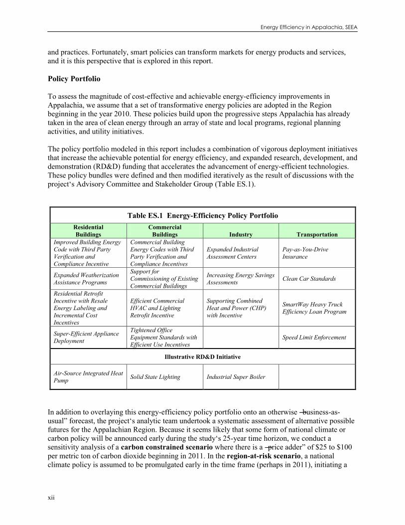
and practices. Fortunately, smart policies can transform markets for energy products and services, and it is this perspective that is explored in this report. Policy Portfolio To assess the magnitude of cost-effective and achievable energy-efficiency improvements in Appalachia, we assume that a set of transformative energy policies are adopted in the Region beginning in the year 2010. These policies build upon the progressive steps Appalachia has already taken in the area of clean energy through an array of state and local programs, regional planning activities, and utility initiatives. The policy portfolio modeled in this report includes a combination of vigorous deployment initiatives that increase the achievable potential for energy efficiency, and expanded research, development, and demonstration (RD&D) funding that accelerates the advancement of energy-efficient technologies. These policy bundles were defined and then modified iteratively as the result of discussions with the project‘s Advisory Committee and Stakeholder Group (Table ES.1).
Table ES.1 Energy-Efficiency Policy Portfolio Residential Buildings
Commercial Buildings
Industry
Transportation
Improved Building Energy Code with Third Party Verification and Compliance Incentive
Commercial Building Energy Codes with Third Party Verification and Compliance Incentives
Expanded Industrial Assessment Centers
Pay-as-You-Drive Insurance
Expanded Weatherization Assistance Programs
Support for Commissioning of Existing Commercial Buildings
Increasing Energy Savings Assessments Clean Car Standards
Residential Retrofit Incentive with Resale Energy Labeling and Incremental Cost Incentives
Efficient Commercial HVAC and Lighting Retrofit Incentive
Supporting Combined Heat and Power (CHP) with Incentive
SmartWay Heavy Truck Efficiency Loan Program
Super-Efficient Appliance Deployment
Tightened Office Equipment Standards with Efficient Use Incentives
Speed Limit Enforcement
Illustrative RD&D Initiative
Air-Source Integrated Heat Pump Solid State Lighting Industrial Super Boiler
In addition to overlaying this energy-efficiency policy portfolio onto an otherwise ―business-as-usual‖ forecast, the project‘s analytic team undertook a systematic assessment of alternative possible futures for the Appalachian Region. Because it seems likely that some form of national climate or carbon policy will be announced early during the study‘s 25-year time horizon, we conduct a sensitivity analysis of a carbon constrained scenario where there is a ―price adder‖ of $25 to $100 per metric ton of carbon dioxide beginning in 2011. In the region-at-risk scenario, a national climate policy is assumed to be promulgated early in the time frame (perhaps in 2011), initiating a

Executive Summary
xiii
shift in the way energy is produced and used. However, in this scenario the shift takes place without the aid of fundamentally different technologies. With a premium on the price of fossil fuels, energy-efficient technologies are highly cost-effective; however, the difficult economic conditions dampen investments. In the high-tech investment boost scenario, the country produces significant material, technology, and process advances in the performance and cost competitiveness of clean-energy supply technologies, most notably clean coal. As a result of the successful investment climate that results, energy efficiency is also able to play an enhanced role in the Region. These last two scenarios are not modeled. Methodology For the purposes of this study, energy efficiency refers to the long-term reduction in energy consumption resulting from the increased deployment and improved performance of energy-efficient equipment and practices. Program potential is the cost-effective energy-efficiency improvements that would occur in response to specific policies such as subsidies and information dissemination. We do not examine the impact of energy-efficiency investments on demand reductions, which is critical to electric power planners. Nor do we examine the role of demand-response or load-management programs aimed strictly at shifting on-peak consumption to off-peak hours. This project uses a variety of sources of data, models, and energy-engineering analyses to estimate Appalachia‘s energy-efficiency program potential. Results of past energy-efficiency program evaluations is the basis of estimating the administrative and implementation costs of each energy-efficiency policy bundle. Our analysis of potential in each sector uses a common baseline forecast, common energy price projections, identical discount rates for calculating cost-effectiveness, and the same economic tests of cost-effectiveness (the participants cost test and the total resource cost test). The specific data sources and methodologies are summarized in each of the sector chapters and are described in greater detail in Appendices B through G. The results of these policy analyses are then input into a dynamic input-output model to evaluate the macro-economic impacts of proposed policies. In addition, the project team created an Advisory Committee and Stakeholder group to review and guide the research. The following two examples illustrate how the policies are modeled and preview some of the results:
Residential Building Codes: All Appalachian states are assumed to adopt the 2006 International Energy Conservation Code (IECC) by 2009 and more efficient codes every three years thereafter. Codes are assumed to become effective the year following adoption. Third-party verification of measures occurs, and an incentive to builders is provided for the period 2010-2020. This results in an 80 percent compliance rate. To illustrate, the 419,000 single and multi-family homes projected to be built from 2013 to 2015 in Appalachia are assumed to conform to the 2009 IECC code and therefore use 18 percent less energy for space heating, space cooling, and water heating than they would have if built to 2005 current practice. Homes built from 2016 to 2019 are assumed to use 30 percent less energy. With $281.5 million in program spending and an additional $2.1 billion in customer investments over the 2010-2030 period, the Appalachian Region could see net cumulative savings of 1.0 quads of energy and $16.3 billion in energy bills by 2030.
Increased Energy Savings Assessments and Training: Large industrial facilities receive expanded training and assistance on how to pinpoint energy-efficiency improvements in systems throughout their complex. Each assessment takes three days and involves plant

Energy Efficiency in Appalachia, SEEA
xiv
7.0
7.5
8.0
8.5
9.0
9.5
10.0
10.5
11.0
11.5
2006 2009 2012 2015 2018 2021 2024 2027 2030
Qu
adri
llio
n B
tu
AEO 2007 AEO 2008 With Policy Packages
personnel to achieve acceptance and training to enable future in-house assessments. It is assumed that over 60 percent of available assessments are completed by 2030, and all recommendations are executed. On average each assessment results in reducing overall site consumption by roughly nine percent. With $23 million in program spending and an additional $8 billion in customer investments over the 2010-2030 period, the Appalachian Region could see net cumulative savings of 18.7 quads of energy and $43.3 billion in energy bills by 2030.
Magnitude of the Energy-Efficiency Resource in Appalachia The engineering-economic modeling conducted in this study indicates that an ambitious package of energy-efficiency policies implemented throughout Appalachia in 2010 could result in significant energy savings. According to the latest EIA ―business-as-usual‖ forecast, Appalachia will require 9.2 quads of energy in 2020 and 10.1 quads in 2030. In contrast, a bold energy-efficiency initiative could cut that consumption by between 9 and 12 percent to approximately 8 quads in 2020 and by between 23 and 28 percent to less than 8 quads in 2030. (The upper bound includes savings from commercial building commissioning, while the lower bound does not.) Such a bold and aggressive initiative could shrink the energy budget required by the Region in 2030 to less than the Region consumed in 2006 – more than offsetting the forecast growth in energy use (Figure ES.1). Table ES.2 shows that the most significant savings are in electricity overall, representing a reduction of between 11 and 15 percent in 2020 rising to between 27 and 33 percent in 2030. Motor gasoline consumption is reduced by almost as much: 11 percent in 2020 and 33 percent in 2030. Natural gas savings are next in order of magnitude, saving between 5 and 7 percent of the forecast consumption in 2020, and between 14 and 20 percent of the forecast consumption in 2030.
Figure ES.1 Potential Displacement of Appalachian Energy Consumption by Cost-Effective Efficiency Resources

Executive Summary
xv
Table ES.2 Cost-Effective Efficiency Resources as a Percent of Projected Primary Energy Consumption in the
Appalachian Region in 2020 and 2030a
2020 2030 Electricity 10.5 – 15.4 27.2 – 33.1
Natural Gas 4.7 – 6.8 14.2 – 19.5
Gasoline 10.7 33.1
All Fuels 8.8 – 11.9 23.4 – 27.8 a The upper bound includes savings from commercial building commissioning, while the lower bound does not.
Dividing the cost-effective energy-efficiency resources by sector helps explain the prominent potential for reduced electricity consumption, since the vast majority of electricity produced in the U.S. is consumed in residential and commercial buildings, which are prominently featured in Fig. ES.2. Taking into account the energy lost in the generation and transmission of electricity as well as losses from ―end-use‖ equipment such as motors, lighting, and air conditioning, 68 percent of the energy-efficiency potential in Appalachia resides in the electricity system. The next largest wedge of energy savings potential comes from motor gasoline
consumption by vehicles (17 percent), followed by natural gas savings potential in the commercial, residential, and industrial sectors (12 percent).
As Figure ES.3 illustrates, energy savings expand at a slightly increasing pace over the 20-year period. In contrast, public investments (including incentives plus program administrative costs) drop from approximately $700 million per year during the first decade to slightly less than $500 million in the second decade, reflecting the sun-setting of several program subsidies and incentives in the year 2020.
Figure ES.2 Share of Cost-Effective Efficiency Resources by Sector
(Primary Energy in trillion Btu, 2030)
Primary Energy Savings, by Sector (2030, Trillion Btu)
Residential
374
15%
Industrial
621
25%
Transportation
457
18%
Commercial
1030
42%

Energy Efficiency in Appalachia, SEEA
xvi
0
1
1
2
2
3
3
2010 2015 2020 2025 2030
Qu
adri
llio
n B
TU
0
1
1
2
2
3
3
4
4
5
5
Bill
ion
20
06
$
Primary Energy Savings Public Investment Private Investment Economic and Job Impacts In Appalachia, the electric utility and the natural gas sectors directly and indirectly employ about 5.3 and 3.7 jobs, respectively, for every $1 million of spending. But, sectors vital to energy-efficiency improvements, like construction and manufacturing, utilize 13.3 and 8.3 jobs per $1 million of spending. Once job gains and losses are netted out in each year, the analysis suggests that, by diverting expenditures away from non-labor intensive energy sectors, the cost-effective energy policies can positively impact the larger Appalachia economy – even in the early years, but especially in the later years of the analysis as the energy savings continue to mount. An early program stimulus that drives a higher level of efficiency investments can create more than 15,000 net new jobs each year in the first five years of the study, rising to an estimated average of 60,000 net new jobs over the last decade of the analysis. The annual energy bill savings begins with a modest first year benefit of almost $800 million. As the policy portfolio spurs further investment in energy efficiency, the annual consumer energy bill savings rise to more than $27 billion by 2030. These savings directly benefit the consumers who make these investments, but they also help to moderate energy prices for all consumers because they reduce overall demand growth. These investments also increase both wages and Gross Regional Product (GRP) throughout Appalachia.
Figure ES.3 Annual Investment and Energy Savings: 2010-2030

Executive Summary
xvii
0
2
4
6
8
10
Ben
efit
-to
-Co
st R
atio
50% Lower than Energy Prices 0.97 3.40 1.04 1.66 1.65
25% Lower than Energy Prices 1.46 5.10 1.56 2.49 2.48
Retail Energy Prices 1.94 6.80 2.08 3.33 3.31
Energy Prices with $25/MtC Tax 2.15 6.59 2.67 3.41 3.45
Energy Prices with $50/MtC Tax 2.35 7.42 3.26 3.49 3.58
Energy Prices with $100/MtC Tax 2.75 9.09 4.45 3.65 3.84
Residential Commercial Industrial Transportation Total
Table ES.3 Financial and Economic Impact of Energy-Efficiency
Investment in Appalachia Macroeconomic Impacts 2010 2013 2020 2030
Annual Consumer Outlays (millions $2006) 1,083 2,734 4,564 6,165
Annual Energy Savings (millions $2006) 788 2,577 9,944 27,567
Annual Net Consumer Savings (millions $2006) (295) (157) 5,380 21,402
Jobs (Actual) 16,231 15,466 37,268 77,378
Wages (million $2006) 517 450 1,169 3,018
GRP (million $2006) 763 444 1,197 3,056 The principal estimate used in this project to monetize the avoided costs of potential energy savings is the retail price of energy. Figure ES.4 shows what would happen to the cost-effectiveness tests of the energy-efficiency policy portfolio if the value of the avoided costs were inflated as the result of a national climate policy that imposed a cost of $25 to $100 per metric ton of carbon dioxide emissions. Such a policy would significantly raise the benefit/cost ratios of the policy packages in three sectors: commercial, residential, and industrial. Because of the lower carbon content of gasoline and diesel, there is a much smaller impact on the cost-effectiveness of the transportation sector‘s energy savings potential. Across all of the sectors, the carbon-inflated avoided costs make investments in energy efficiency more cost-effective compared with the business-as-usual scenario. Figure ES.4 also shows that even if retail energy prices are 50 percent higher than the cost to the wholesaler or distributor, the combined sector policy packages remain cost-effective.
Figure ES.4 Sensitivity Analysis of Benefit/Cost Ratios for the Total Resource Cost Test With Carbon “Adders”

Energy Efficiency in Appalachia, SEEA
xviii
The Value of Exploiting Appalachia’s Energy-Efficiency Potential Policy action aimed at exploiting the energy-efficiency potential described in this report would set Appalachia on a course toward a sustainable and prosperous energy future. The Region‘s energy-efficiency resources could go a long way toward meeting its future energy needs while ensuring its continued economic and environmental health. The problem is that energy-efficiency upgrades require consumer and business investment and they take time away from other priorities. With so many demands on financial and human capital, energy-efficiency improvements tend to be given a low priority. Through a combination of information dissemination and education, financial assistance, regulations, and capacity building, consumers, businesses, and industry can be encouraged to take advantage of energy-efficiency opportunities. In addition, expanded RD&D is needed to innovate and deploy transformational technologies that expand the efficiency potential. By exploiting the Region‘s substantial energy-efficiency resources, Appalachia can cut the energy bills of its households, businesses and industries, create ―green‖ jobs, and grow its economy. The ability to convert this vision into a reality will depend on the willingness of business and government leaders to implement and champion the kinds of policies modeled here. .

Chapter 1: Introduction
1
1 INTRODUCTION Perhaps at no time since the mid-1970s has the Appalachian Region faced so many energy challenges. Fuel prices for oil, gasoline, natural gas, and coal have risen dramatically and now match or exceed previous all-time highs. These spiraling costs are compounded by double-digit economic growth rates in China and India, which are driving up the cost of steel, aluminum, and other materials necessary to expand the Region‘s energy infrastructure. The growing reliance on oil imports raises questions about the long-term energy security of the Region‘s petroleum-dominant transportation system. Concerns about greenhouse gas emissions and mountaintop removal are placing new constraints on coal mining and the construction of coal plants, resulting in numerous cancelled projects and the loss of billions of dollars.1 ―Not in my backyard‖ (NIMBY) attitudes have allowed local opposition to routinely trump regional needs for new energy resources and infrastructure. After decades of steadily expanding energy consumption, it is hard to imagine how another 25 years (or century) of similar growth in energy demand can be accommodated. As a result, policymakers at all levels of government want to know how much of the forecasted growth in energy consumption can be met by improved energy efficiency. They also want to know what types of policies, programs, and technologies hold the greatest potential to curb the growth of energy consumption – at the least cost. Energy Efficiency in Appalachia focuses on these issues. 1.1 RATIONALE AND GOALS OF THE STUDY In 2006, the Appalachian Regional Commission (ARC) prepared a report – Energizing Appalachia: A Regional Blueprint for Economic and Energy Development – that documented the energy situation within the Appalachian Region. It also articulated the ARC energy goal: ―Develop the Appalachian Region‘s energy potential to increase the supply of locally produced, clean, affordable energy, and to create and regain jobs‖ (ARC, 2006). Three strategic objectives support this goal, focusing on the development of energy efficiency, renewable energy, and conventional energy resources within the Region. In conjunction with the development of Energizing Appalachia, ARC commissioned two studies, one on the Economic Development Potential of Conventional and Potential Alternative Sources in Appalachian Counties (Glasmeier and Bell, 2006) and another on Energy Efficiency and Renewable Energy in Appalachia: Policy and Potential (Center for Business and Economic Research (CBER), 2006). Together these reports provide a detailed assessment of conventional and unconventional fossil energy sources as well as the full range of renewable energy resources. The potential for energy-efficiency improvements in the Region, however, is treated more anecdotally by highlighting some of the Region‘s innovative energy-saving system designs, reviewing energy-efficiency policies, and comparing energy intensity levels in the Region to those of the nation. Although there have been a large number of studies highlighting positive opportunities for energy-efficiency investments in individual states, across the nation, and even within various states within Appalachia (Laitner and
1 There are many examples of recently cancelled coal plant projects in the Appalachian region. For example, several years ago American Electric Power (AEP) proposed to build the Mountaineer integrated gasification combined cycle (IGCC) coal plant next to the existing Mountaineer generating station along the Ohio River in Mason County, West Virginia. In April 2008, the West Virginia State Corporation Commission (SCC) rejected the plant after judging that its cost estimates were not credible (http://www.sourcewatch.org/index.php?title=Mountaineer).

Energy Efficiency in Appalachia, SEEA
2
McKinney, 2008a), there is no current quantitative estimate of the economic potential for energy-efficiency improvements for the Region as a whole. To fill this gap, Energy Efficiency in Appalachia assesses the potential for cost-effective energy-efficiency gains across the Region‘s residential, commercial, industrial, and transportation sectors. With 2006 as a baseline, it focuses on projections for the years 2013, 2020, and 2030 under the assumption that transformative energy policies are adopted within the Region in the year 2010. Evidence is mounting that energy efficiency is a large, affordable, and feasible energy resource. It can be as reliable as the construction of new power plants and the purchase of power via long-term contracts or spot markets. It has been shown to be a valuable, ―front-line‖ strategy against global climate change because it offers a ―no regrets‖ approach: investments in energy efficiency can save consumers and businesses money while reducing pollution and greenhouse gas (GHG) emissions.2 A large potential for improved efficiency exists in numerous appliances and energy-consuming equipment and practices. For instance, high-quality adjustable-speed electronic motor drives, once exotic and costly, are now mass-produced in Asia and are widely used because of their protective and soft-start circuits. High-efficiency compact fluorescent lamps sell for a fifth of their 1983 price, now that a billion are made yearly. Real prices have fallen several fold in 15 years for electronic lighting ballasts and heat-reflecting window coatings. Hybrid electric cars offer fuel economy performance in a standard range vehicle that was unachievable ten years ago. The economic potential for energy efficiency continues to grow (Lovins, 2007). States across the nation are meeting one to two percent of their electricity consumption each year with energy efficiency at a cost of approximately $0.03 per kilowatt-hour (kWh) compared with projected costs of $0.05 to $0.07 per kWh of electricity from coal, gas combined cycle, wind or nuclear plants (Brown and Chandler, 2008; Kushler, York and Witte, 2004). Results from California, New York, Vermont, and other states show that energy efficiency represents a low-cost, low-risk energy strategy. California, in part due to aggressive and sustained energy-efficiency measures, has kept per capita electricity use flat over recent decades (National Academy of Sciences, 2008). This is in direct contrast to national trends over the last 25 years, where U.S. per capita electricity use as a whole has risen about 50 percent. Rufo and Coito (2002) have shown that the potential for further energy-efficiency improvements in California remains strong. A similar potential for aggressive and sustained energy-efficiency programs has been demonstrated in Vermont and other states, where electricity consumption per capita has remained fairly flat while the state‘s economy has grown significantly. Thus, these states have shown that energy demand growth can be significantly reduced without compromising economic growth. The challenge is to move these energy-efficiency ―best practices‖ to the rest of the country.
2 Indeed as the meta-review provided by Laitner and McKinney (2008a) suggests, the evidence points to a potential 20 to 30 percent efficiency gain compared to normal business-as-usual projections. Perhaps more critically, the benefits of this level of potential efficiency improvement appear to outweigh the costs by roughly two-to-one.

Chapter 1: Introduction
3
Together, energy efficiency and demand response can delay or completely avoid the need for expensive new generation and transmission investments, thus keeping the future cost of electricity affordable and freeing up energy dollars to be spent on other resources to expand the Region‘s economy. A greater share of the dollars invested in energy efficiency goes to local companies that create new jobs compared with conventional electricity resources where much of the money flows out of the Region to equipment manufacturers and fuel suppliers.
Layers of energy inefficiency exist throughout the economy. For example, converting coal at the power plant into useable light given off by incandescent lamps is only three percent efficient (National Academy of Sciences, 2008). By simply replacing incandescent bulbs with compact fluorescents, a four-fold improvement in efficiency can be achieved. Consider the economics shown in Figure 1.1. The payback period can be quite short – in this case for compact fluorescent light (CFL) bulbs, less than a year or as little as a month, depending on how may hours each day the CFL is used. However, as with many (but not all) energy-efficiency improvements, consumers need to purchase a more expensive device in order to generate the energy savings. How can reluctant consumers be persuaded to pay more up front to save money in the future when they often do not understand the sometimes complex economic analysis that goes into such a purchasing decision?
Energy-efficiency policy mechanisms are numerous and are implemented at all levels of government from the local jurisdiction and state to the regional and national scale. To make matters more complicated, energy-efficiency measures and incentives can be delivered by a multiplicity of actors and agents, including independent organizations, non-government statewide organizations, fully integrated independently owned utilities, unaffiliated distribution companies, as well as government agencies (Harrington and Murray, 2003). In this report, we use the typology developed by Geller (2003) to inventory existing policies and to consider alternatives (see Appendix A). Geller‘s typology includes regulatory policies (regulations, market obligations, and market reforms); fiscal measures (financial incentives, financing, and pricing); enabling policies (capacity building, dissemination and training, and research, development, and demonstration); and voluntary approaches (planning techniques, procurement policies, and voluntary agreements). By expanding existing energy-efficiency policies and by implementing new policy approaches that tackle key barriers, create new incentives, set minimum standards, and enable change, how much energy efficiency can be stimulated? Which technologies hold the greatest potential and what policies and programs can most effectively translate that potential into reality? These are the essential questions addressed by this study.
Figure 1.1 The Economics of Compact Fluorescent Light Bulbs
(Brown, 2008)

Energy Efficiency in Appalachia, SEEA
4
1.2 BACKGROUND 1.2.1 Overview of the Appalachian Region The Appalachian Region tracks the spine of the Appalachian Mountains, starting in northern Mississippi and sweeping northeast through southern New York. It includes all of West Virginia and parts of twelve additional states: Alabama, Georgia, Kentucky, Maryland, Mississippi, New York, North Carolina, Ohio, Pennsylvania, South Carolina, Tennessee, and Virginia. With a population of 23.9 million in 2006, the Region is home to 7.95 percent of the U.S. population. In 1965 the Federal government established the Appalachian Regional Commission (ARC), an economic development agency composed of the governors of the 13 states and a co-chair appointed by the president. Local participation is provided by local development districts. In the early years of the ARC, the Region was divided into three contiguous and relatively homogeneous sub-regions based on topography, demographics and economics (Figure 1.2). The South sub-region has the highest population growth rate (estimated at 1.13 percent annually), while the North has the slowest growth rate (estimated at 0.28 percent). These three sub-regions include 410 counties and contain parts of four Census Divisions. The cross-walk between these three sub-regions, four Census Divisions, and 410 counties is critical to apportioning numerous data elements that are key to the analysis of efficiency resources. 1.2.2 Energy Use in Appalachia As an historic center of coal production in the United States, Appalachia and energy have been intimately intertwined. Appalachian mines produce 35 percent of the nation‘s coal output, and the Region employs two-thirds of the nation‘s coal miners (ARC, 2006). Much of this coal is burned in Appalachian power plants to produce electricity for the Region‘s consumers and for export to surrounding markets, especially those in the large metropolitan areas that circle the Region. Appalachian coal generated approximately 15 percent of the total U.S. electrical output, worth $16 billion in 2005 (ARC, 2006). Almost 150,000 jobs are generated by the Appalachian energy industry, with hundreds of thousands more producing and distributing energy products and services (ARC, 2006). The intensity of energy use in the Appalachian Region is slightly higher than that of the nation as a whole. In 2006, the Region consumed 7.94 quadrillion Btu (quads) of energy, or 332.7 MMBtu per capita, slightly more than the U.S. average of 331.6 MMBtu per capita. When indexed to personal income, the Region is considerably more energy intensive than the national average (CBER, 2006, p. 41). According to the CBER (2006), the above-average consumption rates are ―likely due to high rates of electrification in some states, which may increase overall energy use, and a somewhat
Figure 1.2 Sub-regions in Appalachia (www.arc.gov/index.do?nodeId=938)

Chapter 1: Introduction
5
elevated share of manufacturing; the ARC counties account for about 26 percent of manufacturing income in the ARC states, but only 24.5 percent of the population (p. 42).‖ Based on population weighed extrapolations from the Census Division forecasts of energy consumption from EIA‘s Annual Energy Outlook 2008, the Region‘s energy consumption is expected to grow by 28 percent to 10.14 quads in 2030. This is considerably higher than the 19 percent growth forecast for the U.S. (EIA, 2008a, Table A2).
Table 1.1 Appalachian Region Energy Consumption Forecast from Annual Energy Outlook, 2006 to 2030 (quads)
(EIA, 2008a)
Year Total Residential Buildings
Commercial Buildings Industry Transportation
2006 7.94 1.80 1.50 2.42 2.22 2013 8.45 1.96 1.64 2.51 2.34 2020 9.12 2.16 1.89 2.65 2.42 2030 10.14 2.47 2.26 2.87 2.54
1.2.2.1 Energy Consumption by Source3
The Appalachian Region‘s energy consumption of 7.94 quadrillion Btu in 2006 represents 7.98 percent of the total energy use of the United States. Compared to the share of the energy consumption of each fuel in the United States on average, Appalachia consumed six percent more energy from coal, and three percent more nuclear energy. On the other hand, the Region consumed less energy from oil and natural gas, compared to the national average.
3 The energy consumption data of the Appalachian region were driven with the projections of business-as-usual scenario from the Annual Energy Outlook 2007 (EIA, 2007a). All of the 410 counties included in the region were located over the four census divisions such as the East North Central, East South Central, Middle Atlantic, and South Atlantic regions. Based on the population proportion of Appalachia in each census division, the energy use of the entire Appalachian Region was aggregated. The energy price data of the region was driven from the Annual Energy Outlook 2008 (EIA, 2008a). Based on the proportional approach that used in the consumption data, the weighted average of the prices of the four census regions was calculated for this analysis.

Energy Efficiency in Appalachia, SEEA
6
0
1
23
4
5
6
7
89
10
11
2006 2009 2012 2015 2018 2021 2024 2027 2030
Qu
adri
llio
n B
tu
Other Liquid Fuels Motor GasolineNatural Gas CoalBiofuels and Renewables Nuclear Power
Table 1.2 Energy Consumption by Source, 2006 (EIA, 2008a)
Source United States Appalachia
Quadrillion Btu Share (%) Quadrillion
Btu Share (%)
Liquefied Petroleum Gases 2.65 2.7 0.07 0.8 Motor Gasoline 17.62 17.7 1.43 18.0 Distillate Fuel Oil 8.77 8.8 0.74 9.4 Residual Fuel Oil 1.69 1.7 0.15 1.8 Other Liquid Fuels 9.33 9.4 0.58 7.3 Natural Gas 22.30 22.4 1.34 16.8 Coal 22.50 22.6 2.25 28.4 Biofuels and Renewables 6.27 6.3 0.47 5.9 Nuclear Power 8.21 8.2 0.90 11.3 Total 99.52 7.94
Fuels may not sum to total due to rounding
As is the case nationwide, coal is forecast to increase its share of energy use in the Region between 2015 and 2030, in the absence of restrictions on CO2 emissions (Table 1.2 and Figure 1.3). However, the market share of western coal is expected to increase, while Appalachian coal production is forecast by EIA to decline slightly. ―Although producers in Central Appalachia are well situated to supply coal to new generating capacity in the Southeast, that portion of the Appalachian basin has been mined extensively, and production costs have been increasing more rapidly than in other Regions.‖ (EIA, 2008a, p. 84) With 67 percent of the nation‘s jobs in the U.S. coal industry supporting only 35 percent of U.S. coal production, Appalachia has significantly lower levels of labor productivity and therefore higher costs. In contrast, the Powder River Basin has vast remaining surface-minable reserves that can be reached by large earth-moving equipment with significant benefits from economies of scale.
Figure 1.3 Energy Consumption Projections of the Appalachian Region by Source, 2006-2030
(EIA, 2008a)

Chapter 1: Introduction
7
18.0%
28.4%
18.9%
30.5%32.7%
20.9%
27.9%
22.7%
0%
5%
10%
15%
20%
25%
30%
35%
Residential Commercial Industrial Transportation
U.S. Appalachia
1.2.2.2 Energy Consumption by Sector
In 2006, the Appalachian Region spent 1.85 quadrillion Btu (quads) in the residential sector; 1.47 quadrillion Btu in the commercial sector; 2.62 quadrillion Btu in the industrial sector; and 2.16 quadrillion Btu in the transportation sector (Figure 1.4). Compared with the nation as a whole, Appalachia consumes slightly more of its energy on residential and commercial uses and less in the industrial and transportation sectors. Energizing Appalachia (ARC, 2006, p. 8) suggests that the significant difference in the residential sector ―probably reflects the lower efficiency of the Region‘s housing stock.‖ It may also be a function of the Region‘s dual heating and cooling seasons, which requires either space heating or air conditioning most months of the year to maintain indoor comfort. The energy consumption of each sector is forecast to increase over the next 25 years, expanding consumption in 2030 to 2.47 quadrillion Btu (24 percent) in the residential sector, 2.26 quadrillion Btu (22 percent) in the commercial sector, 2.87 quadrillion Btu (28 percent) in the industrial sector, and 2.54 quadrillion Btu (25 percent) in the transportation sector (Table 1.1).
0
1
2
3
4
5
6
7
8
9
10
11
2006 2009 2012 2015 2018 2021 2024 2027 2030
Qu
adri
llio
n B
tu
Residential Commercial Industrial Transportation
Figure 1.4 Energy Consumption Shares in the U.S. and Appalachia by End-Use Sectors, 2006
(EIA, 2008a)
Figure 1.5 Energy Consumption Projections by Sector of the Appalachian Region, 2006-2030
(EIA, 2008a)

Energy Efficiency in Appalachia, SEEA
8
Appalachia largely depends on coal to generate electric power, as does the United States. Because coal mining is a major industry in the Region and Appalachia is an exporter of electric power, coal contributes 57 percent of the energy consumption for electric power generation. Compared to the nation as a whole, Appalachia depends more on coal and nuclear and less on natural gas and renewable sources (Figure 1.6).
United States
Fuel Oil
1.6%
Natural Gas
16.2%
Coal
51.8%
Nuclear
20.8%
Renewable
9.5%
Electricity Imports
0.2%
Appalachia
Fuel Oil
2%
Natural Gas
11%
Coal
57%
Nuclear
25%
Renewable
5%
Electricity Imports
0%
Corresponding to the total energy consumption projections, EIA projects that Appalachia will increase its share of coal consumption for electricity generation between 2020 and 2030 (Figure 1.7).
0
0.5
1
1.5
2
2.5
3
3.5
4
4.5
5
5.5
2006 2009 2012 2015 2018 2021 2024 2027 2030
Qu
adri
llio
n B
tu
Fuel Oil Natural Gas Coal
Nuclear Power Renewable Electricity Imports
Figure 1.6 Energy Consumption for Electric Power Generation, 2006 (EIA, 2008a)
Figure 1.7 Energy Consumption for Electric Power Generation in the Appalachian Region, 2006-2030
(EIA, 2008a)

Chapter 1: Introduction
9
1.2.2.3 Energy Prices Energy in Appalachia is relatively cheap, and EIA forecasts that this comparative advantage will continue through 2030 (Table 1.3). Appalachia‘s prices for motor gasoline, distillate fuel oil, natural gas, coal, and electricity are all lower than U.S. averages. The only exception is liquefied petroleum gases (LPG), which cost more in Appalachia than on average in the United States. This high price may explain why LPG usage in Appalachia constitutes such a small fraction of the Region‘s energy budget (0.8 percent vs. 2.7 percent for the nation). An analysis by the Center for Business and Economic Research (2006) suggests that residential and commercial consumers in this Region are fairly insensitive in the short-run to increases in the price of electricity. This lack of responsiveness to electricity price changes, which is similar to behavior in other Regions of the country, suggests the magnitude of policy change needed to alter the consumption of energy. With price elasticities of -0.15 and -0.17, the CBER results indicated that residential and commercial users in Appalachia would need to experience a doubling of electricity prices in order to produce a 15 to 17 percent reduction in electricity consumption. If this price insensitivity applies across all energy sources, which is likely, strong policy interventions will be needed to promote energy-efficient purchases and practices. The good news is that smart policies can, indeed, get the job done (Brown, et al, 2001; Geller et al., 2006). And it is this perspective that we actively explore in the analysis that follows.
Table 1.3 Average Energy Prices to All Users in Appalachia and the United States (in 2006 dollars per million Btu)
(EIA, 2008a)
Source The United States Appalachia
2006 2013 2020 2030 2006 2013 2020 2030
Liquefied Petroleum Gases 20.35 18.61 18.59 19.82 17.39 18.44 18.61 20.10
Motor Gasoline 21.06 19.51 19.64 20.37 15.70 14.73 15.11 16.37
Distillate Fuel Oil 18.56 17.07 17.20 18.74 13.74 13.10 13.33 14.92
Natural Gas 9.22 8.06 7.98 9.36 7.75 6.65 6.78 8.05
Metallurgical Coal 3.54 3.75 3.42 3.60 2.49 2.72 2.53 2.77
Electricity 26.10 25.40 25.23 25.93 18.39 18.94 19.13 20.16
1.2.2.4 Carbon Footprint
When the slightly greater intensity of energy consumption in Appalachia is compounded by the coal-intensity of the Region‘s electricity production and its lower-than-average use of natural gas, the Region‘s carbon footprint expands well beyond the national average. Energy use in Appalachia is

Energy Efficiency in Appalachia, SEEA
10
estimated to have contributed about 480 million metric tons of carbon dioxide emissions in 2006, based on all energy consumption across all sectors: residential, commercial, industrial, and transportation. These emissions are expected to grow to about 600 million metric tons by 2030.4 This translates to about 20.2 metric tons of carbon dioxide per person in 2006 (or 5.5 metric tons of carbon), which is forecast to increase to 21 metric tons per person in 2030. In comparison, the U.S. carbon footprint was 19.6 metric tons of carbon dioxide in 2006, declining to an estimated 18.7 metric tons in 2030. A recent study by Brown, Southworth and Sarzynski (2008) estimated the per capita carbon footprint of the nation‘s largest 100 metropolitan areas. Seventeen of these metro areas lie either entirely within the Appalachian Region or span the metro area‘s boundary. (Figure 1.8) The average carbon footprint of these seventeen metropolitan areas exceeds the national average by approximately 25 percent. Thus, from a climate policy perspective, the Appalachian Region is more vulnerable to the costs associated with any national climate policy, compared with most areas of the country.
4 These numbers are from this study‘s population weighted aggregate Appalachian forecast based on the AEO 2008 (EIA, 2008a).
Figure 1.8 Carbon Footprints of 17 Metropolitan Areas in (or Surrounding) the Appalachian Region, 2005*
(Brown, Southworth, and Sarzynski, 2008)
*Carbon footprint refers to the metric tons of carbon emissions per capita from the consumption of residential electricity, residential fuels, the energy consumed by light duty vehicles, and the fuels used by freight trucks.

Chapter 1: Introduction
11
1.3 STRUCTURE OF REPORT This report is organized into eight chapters followed by references and numerous appendices. The chapters can be grouped into four sections:
Methodology and Policy Analysis (Chapter 2): Provides a broad overview of the methodology used in the policy analysis and energy-efficiency resource assessments. This chapter also outlines the policy bundles modeled in the analysis and describes the alternative future scenarios that could shape their influence. In addition to the ―business-as-usual‖ forecast, these scenarios include the ―region-at-risk‖ and ―high-tech-investment-boost‖ scenarios. Energy-Efficiency Resource Assessments (Chapters 3-6): Estimates the total potential for cost-effective efficiency in each of the Region‘s major sectors: residential, commercial, industrial, and transportation sectors. These assessments begin with a description of energy consumption in the Region and the energy-efficiency levels assumed in the ―business-as-usual‖ forecast. It then describes each of the policy bundles, the methodology used to analyze them, and the estimates of energy savings and costs. The chapters end by describing the estimated cost-effectiveness of each policy bundle, both individually and for the sector as a whole. Economy Wide Results (Chapter 7): Estimates the economy-wide engineering and economic results. In addition to presenting the economy-wide cost-effectiveness tests, this chapter characterizes the employment impacts and workforce requirements of each scenario. Summary and Conclusions (Chapter 8): The report ends with a discussion of its findings. This includes a comparison of the results with other assessments of cost-effective energy efficiency. It also discusses the package of policy bundles in terms of its political feasibility.
These chapters are supplemented by detailed appendices that provide additional explanation, assumptions and analysis details. Appendix A summarizes the Region-wide inventory of energy-efficiency policies. Appendices B through E provide additional information about the methodology used to analyze each sector. Appendix F provides further information on the baseline analysis and the use of the Dynamic Energy Efficiency Policy Evaluation Routine (DEEPER) model to integrate the sector-specific results into a macroeconomic evaluation of the policies as they might impact the Region. Finally Appendix G presents a sensitivity analysis of the cost-effectiveness estimates, including an assessment of higher fossil fuel prices that could arise in a carbon-constrained future.

Energy Efficiency in Appalachia, SEEA
12

Chapter 2: Methodology
13
2 METHODOLOGY A variety of sources of data and models are used in energy-engineering analyses to forecast the energy savings potential, administrative, and implementation costs of each energy-efficiency policy bundle. These methodologies are summarized in each of the sector chapters and are described in greater detail in Appendices B through E. The results of these policy analyses are then input into the DEEPER model created by ACEEE to evaluate the macro-economic impacts of proposed policies. In addition, the project team created an Advisory Group and Stakeholder group to review and guide the research. For the purposes of this study, energy efficiency refers to the long-term reduction in energy consumption as a result of the increased deployment and improved performance of energy-saving equipment and practices. In the electricity sector, energy efficiency is also a low-cost contributor to system adequacy – the ability of the electric system to supply the aggregate energy demand at all times. When applied to transportation systems, energy efficiency is a major contributor to energy security. In addition, environmental benefits often come hand-in-hand with energy efficiency, along with productivity gains and job growth. At the same time, energy efficiency typically requires increased utility and government costs to transform markets. This chapter describes the methodology used to estimate how much energy-efficiency improvement could occur in Appalachia that would be cost-effective and feasible given the wide array of associated costs and benefits. 2.1 THE BASELINE FORECAST The ―business-as-usual‖ baseline forecast of Appalachian energy consumption derived for this study is based on supplemental data from the National Energy Modeling System (NEMS) used to support the Annual Energy Outlook (EIA, 2007a; 2008a). The Appalachian Region baseline forecast is derived from population-weighted portions of the four census divisions comprising the 410-county Region. Regional populations within each census division were calculated using the Regional Economic Models, Inc. (REMI)5 estimates of population by county for 2002, based on ARC sub-region growth rates (North 0.28 percent, Central 0.39 percent, and South 1.13 percent). While the AEO-based method used here does not result in county-by-county populations that exactly match REMI‘s 2020 and 2030 forecast, they are generally within a close margin. For example, the total Appalachian Region‘s population is less than 0.2 percent higher in 2020 and less than two percent lower in 2030 in this study compared with the REMI forecast. Total census division populations are based on the AEO 2007 population forecast (EIA, 2007a). Over the study horizon, the Appalachian Region is increasingly weighted in three of the four census divisions. In contrast, the proportion of the Region‘s population residing in the South Atlantic census division (from Virginia through Georgia) shrinks over time; this is likely due to much higher growth rates in the non-Appalachian portions (especially coastal areas) of the South Atlantic division (Table 2.1).
5 REMI, 2007

Energy Efficiency in Appalachia, SEEA
14
Table 2.1 Population Weighted Census Division Portions
(EIA, 2007a, REMI, 2007)
Year Total ARC Population
%
Middle Atlantic
East North
Central
South Atlantic
East South
Central 2006 23,862,608 16.79 3.18 14.29 41.56 2013 25,056,158 17.11 3.18 13.56 43.27 2020 26,331,378 17.26 3.19 13.14 44.80 2030 28,307,471 17.66 3.26 12.61 47.10
Using the same estimates of county population described above, portions of each state population were also developed (Table 2.2). These state population portions are used when modeling administrative costs for several of the policy packages.
Table 2.2 Appalachian State Population Portion Estimates and Projections, 2006-2030 (WV = 100%)
YEAR %
AL GA KY MD MS NY NC OH PA SC TN VA
2006 25.7 29.0 16.4 32.2 50.6 5.6 66.5 12.9 24.1 15.1 41.7 22.7
2013 25.9 28.2 16.7 30.6 50.4 5.7 61.5 13.0 25.7 15.3 42.4 22.5
2020 26.1 27.8 17.2 29.3 50.6 5.8 57.0 13.2 27.5 15.7 43.3 22.5
2030 26.3 27.7 18.1 27.9 51.3 6.0 51.3 13.7 30.8 16.4 44.5 22.8
Using REMI estimates, the Gross Appalachian Regional Product (GRP) would almost double between 2006 and 2030, growing to $1,320 billion (in 1996-$). The Region‘s annual growth rate of about 2.4 percent is significantly lower than the EIA forecast of a 2.9 percent annual GDP growth nationwide. Given the inertia that characterizes most economic systems, we can imagine that the distribution of distressed and prosperous counties in the Region would not change much over our planning horizon. This business-as-usual ―baseline‖ future paints the Appalachian Region over the next 25 years, much as it is today. In this scenario, the nation remains uncommitted to climate policy, coal continues to be an economically competitive energy resource, and oil persists as the dominant transportation fuel. As such, energy efficiency still is expected to carry the external benefits of reduced greenhouse gas emissions and improved energy security. Many energy-efficiency investments are more cost-effective than many supply-side options, but numerous barriers including the policy environment often hinder energy-efficiency investments (Prindle, 2007; Brown and Chandler, 2008).

Chapter 2: Methodology
15
7.0
7.5
8.0
8.5
9.0
9.5
10.0
10.5
11.0
11.5
2006 2009 2012 2015 2018 2021 2024 2027 2030Q
uad
rilli
on
Btu
AEO 2007 AEO 2008
Nevertheless, some amount of ―naturally occurring energy-efficiency improvement‖ is incorporated in the baseline forecast. The magnitude of this can be highlighted by comparing the Annual Energy Outlooks published in 2007 and 2008 (EIA, 2007a; 2008a) (Figure 2.1). The AEO 2008 includes several strong efficiency policies promulgated in the Energy Independence and Security Act of 2007 (EISA, 2007), which were not reflected in the AEO 2007. In addition, the AEO 2008 uses higher energy prices and a slower GDP growth rate. Based on the AEO 2007, energy consumption in the Appalachian Region was forecast to grow to 11.2 quads by 2030. In contrast, the forecast based on the AEO 2008 is 11 percent lower, projecting 10.1 quads of energy consumed in the Appalachian Region in 2030. The biggest difference is in the transportation sector where 40 percent stricter fuel economy standards for vehicles are required in 2020. 2.2 DEFINITION OF ECONOMIC ENERGY-EFFICIENCY POTENTIAL When evaluating the potential for any energy alternative to be deployed in future years, four types of estimates are generally used (Rufo and Coito, 2002; NYSERDA, 2003; Eldridge, Elliott, Neubauer, 2008).
Technical potential refers to the complete penetration of all energy-efficient applications that are technologically feasible, regardless of economic cost-effectiveness.
Economic potential is defined as that portion of the technical potential that is judged cost-effective.
Maximum achievable potential is defined as the amount of cost-effective (economic) potential that is achievable over time under the most aggressive program scenario possible. It takes into account administrative and program costs as well as market barriers that prevent 100 percent market penetration.
Program potential is the subset of maximum achievable potential that would occur in response to specific policies such as subsidies and information dissemination aimed at promoting the deployment of cost-effective energy efficiency.
Energy Efficiency in Appalachia estimates the program potential for energy-efficiency improvements in each of the Region‘s four sectors. Our analysis of potential in each sector uses a common baseline forecast, identical energy price projections (Table 1.2), the same discount rates for calculating cost-effectiveness, and the same economic tests of cost-effectiveness.
Figure 2.1 ARC Energy Consumption Forecast (Quads) (EIA, 2007a, 2008a)

Energy Efficiency in Appalachia, SEEA
16
2.2.1 Cost-Effectiveness Tests Many cost-effectiveness tests have been used to estimate the economic payback to investments in energy efficiency. Four tests, in particular, are most common: the participants cost test, total resource cost test, rate impact measure, and societal test. Each of these tests answers a distinct set of questions (NAPEE, 2007a, p. 5-2).
Participants Cost Test: Is it worth it to the customer to install energy efficiency? Is a customer likely to want to participate in a program that promotes energy efficiency? Total Resource Cost Test: What is the Regional benefit of the energy-efficiency project including the net costs and benefits to the utility and its customers? Is more or less money required by the Region to pay for energy needs? Ratepayer Impact Measure: What is the impact of the energy-efficiency program on the utility‘s operating margin? Would the project require an increase in rates to reach the same operating margin? Societal Test: What is the overall benefit to the community of the energy-efficiency program, including indirect benefits? Are all of the benefits (including indirect benefits) greater than all of the costs regardless of who pays the costs and who receives the benefits?
We use the participants test and the total resource cost test to evaluate the cost-effectiveness of each of the modeled energy policies and each sector‘s bundle of policies. The participants test compares the costs and benefits experienced by participants in the energy policy or program. If the net present value of their benefits is greater than the net present value of their costs, then the benefit/cost ratio is greater than 1.0 and the policy is cost-effective. Typically these net present value calculations use a discount value of 10 percent to reflect the private-sector nature of the investments made. The total resource cost (TRC) test was developed originally to evaluate demand-side management (DSM) programs operated by utilities (OTA, 1993). It is a measure of the total net benefits of a program from the point of view of the utility and its ratepayers as a whole. A policy or program is cost-effective if it does not increase the total costs of meeting the customers‘ service needs. We use a seven percent discount rate to calculate these net present values, which is the rate recommended by the Office of Management and Budget‘s Circular No. A-94 (p. 8). The benefits and costs included in these two economic tests, along with their discount rates, are summarized in Table 2.3.

Chapter 2: Methodology
17
Table 2.3 Benefits and Costs Included in the Economic Tests
Energy-Efficiency Benefits Energy-Efficiency Costs
Participants Cost Test
Reduction in energy bill, plus incentives from utility and government programs (10 percent discount rate)
Participants‘ direct investment, plus incentives from utility and government programs (10 percent discount rate)
Total Resource Cost Test Avoided supply costs (based on retail energy prices) (seven percent discount rate)
Utility and government program costs (including administrative costs and incentives to participants) plus participants‘ direct investment (seven percent discount rate)
We are not able to use the ratepayer impact measure (RIM) test because we are unable to estimate the utility‘s change in revenues or costs as the result of the policies modeled here. We are also not able to use the societal test because of the wide range of co-benefits and costs produced by energy-efficiency policies. For example, no consensus exists today to place a value on avoiding the emission of a ton of carbon dioxide (Tol, 2005). Similarly, it is difficult to put a value on the time lost and activities foregone by drivers and passengers as a result of speed limit enforcement, or the lives saved. Typically, the RIM test is the most difficult to pass, while the societal and participants tests are the easiest. 2.2.2 Life-Cycle of Energy Savings The energy required to produce a unit of fuel or electricity for consumption by an ―end-user‖ can be large relative to the energy contained in the ―delivered‖ unit of fuel or electricity. Energy is required to mine coal and drill for petroleum; energy is used to create the compressed air that drives natural gas pipelines; fuels are used to propel the trains and barges that ship coal; and energy is lost in the transmission of electricity from the power plant to the consumer. Energy is also embodied in the power plants, trucks, trains, and other equipment that comprises the energy production and delivery supply chain. As a result, various ―adders‖ have been created to augment the energy contained in the delivered fuel or electricity to account for the full life cycle of energy consumed. As explained below, we use the electricity adder in this study, but we do not use adders for other fuels. In the case of electricity, 2.2 million Btu are lost in the electric generation, transmission and distribution steps that deliver 1 million Btu to the consumer in the form of delivered energy. That is, 68.5 percent of the energy embodied in the fuel used to generate electricity in the United States in 2006 is lost principally in the form of waste heat (EIA, 2008a, Table A2). These electricity-related losses do not include the energy required to mine the coal or the energy embodied in the various supply chain equipment. However, this adder of 2.2 is a typical factor used to more completely account for the energy saved when less energy is used by the consumer, and we use it in Energy

Energy Efficiency in Appalachia, SEEA
18
Efficiency in Appalachia. This adder is justifiable because most electricity-related losses occur in the Appalachian Region. The same is not true of the energy-related losses associated with the delivery of other fuels to consumers in Appalachia. EPA (2006, Table 14, p. 55) suggests a range of ―adders‖ that convert the greenhouse gas content of fuels into life-cycle measures, based on the energy used to refine and transport fuels. For passenger cars, the fuel cycle add-on for gasoline ranges from 0.24 to 0.31, which means that saving a million Btu of energy by consuming less gasoline in fuel-efficient cars, actually saves 1.24 to 1.31 million Btu when the energy lost in refining and transportation is included. The adder for truck diesel is slightly lower, ranging from 0.15 to 0.25. However, most of these life cycle energy losses occur outside of the Appalachian Region, since little petroleum refining occurs within the Region. As a result, we do not plus up the energy content of delivered petroleum fuels. Figure 2.2 estimates how much of each modeled fuel was consumed in each of the four sectors in 2006 in Appalachia. Thus, it ignores the consumption of fuels by sectors that we do not address explicitly by our policy bundles, such as natural gas and electricity in transportation and coal and petrochemical feedstocks and coal used by industry. Altogether, we model 6.9 quads of the 7.9 quads that comprised the Appalachian energy budget in 2006. Slightly more than half (3.6 quads) of the modeled energy is electricity (delivered + electric-related losses).
0
500
1000
1500
2000
2500
3000
3500
4000
trill
ion
Btu
Transportation 719.79 1430.04
Industrial 1084.98 378.82 96.48
Commercial 1198.85 220.10 43.31
Residential 1364.22 302.29 60.69
Electricity Natural Gas Fuel Oil Diesel Motor Gasoline
3648.05
901.21
200.47
719.79
1430.04
2.3 ENERGY-EFFICIENCY POLICY BUNDLES To assess the magnitude of cost-effective and achievable energy-efficiency improvements in Appalachia, we assume that a set of transformative energy policies are adopted in the Region beginning in the year 2010. The policy bundles include a combination of vigorous deployment policies that increase the achievable potential for energy efficiency, and expanded RD&D funding that accelerates the advancement of energy-efficient technologies. These policy bundles were defined and then modified iteratively as the result of discussions with the project‘s Advisory Committee.
Figure 2.2 ARC 2006 Energy Consumption of Fuels Modeled in this Study

Chapter 2: Methodology
19
To aid in the definition of these bundles of policies, a policy inventory was created for each state, detailing active and imminent (promulgated but not in effect) policies. These inventories were reviewed by state energy offices in the Region and revised accordingly to reflect the latest policy actions. The inventory of state policies is described further in Appendix A. Forecasting the economic payback to energy R&D has traditionally been challenging. As a result, we chose an illustrative case study approach. The potential impact of three specific R&D projects is illustrated in independent assessments to highlight the potential benefits of transformational technologies. Specifically, we examine the:
Air-source integrated heat pump
Solid state lighting
Industrial super boiler Table 2.4 summarizes the package of fifteen policies that are assumed to be implemented in each sector. In many cases, policies could be feasibly adopted and implemented at any level of government in this Region (national, regional, state, or local). The Energy-Efficiency Resource Assessments developed for each sector (Chapters 3-6) describe these policies in fuller details; however, they do not proscribe the governmental agencies that should administer them.

Energy Efficiency in Appalachia, SEEA
20
Table 2.4 Energy-Efficiency Policy Portfolio Residential Buildings
Commercial Buildings
Industry
Transportation
Improved Building Energy Code with Third Party Verification and Compliance Incentive
Commercial Building Energy Codes with Third Party Verification and Compliance Incentives
Expanded Industrial Assessment Centers
Pay-as-You-Drive Insurance
Expanded Weatherization Assistance Programs
Support for Commissioning of Existing Commercial Buildings
Increasing Energy Savings Assessments Clean Car Standards
Residential Retrofit Incentive with Resale Energy Labeling and Incremental Cost Incentives
Efficient Commercial HVAC and Lighting Retrofit Incentive
Supporting Combined Heat and Power (CHP) with Incentive
SmartWay Heavy Truck Efficiency Loan Program
Super-Efficient Appliance Deployment
Tightened Office Equipment Standards with Efficient Use Incentives
Speed Limit Enforcement
Illustrative RD&D Initiative
Air-Source Integrated Heat Pump (IHP). Accelerated RD&D is assumed to result in the commercialization of a single system based on heat pumping technology that provides space heating and cooling, water heating, ventilation and dehumidification and humidification.
Solid State Lighting. Accelerated RD&D is expected to produce technology improvements that bring brighter LEDs and provide light equivalent to existing fluorescent fixtures with 25 to 45 percent less electricity usage.
Super Boiler. A combination of enhanced design features could increase industrial package boiler efficiency from 75 percent to 95 percent. Many boilers used today are more than 40 years old, suggesting a large energy-savings opportunity.
2.4 ALTERNATIVE FUTURES In keeping with Peter Schwartz‘s The Art of the Long View (1991) and other advocates of scenario analysis, the project‘s analytic team undertook a systematic assessment of alternative possible futures for the Appalachian Region. Our goal was to consider the range of drivers and change agents that could cause energy efficiency in the Region to play a role quite distinct from simply imposing an aggressive energy-efficiency campaign on an otherwise ―business-as-usual‖ trajectory. The process involved identifying possible drivers of change, brainstorming a wide range of possible futures they could create, and then down-selecting to a small number of scenarios for further consideration. Because it seems likely that some form of national climate or carbon policy will be announced early during the study‘s 25-year time horizon, we assume that in any alternative future a price will be placed on greenhouse gas emissions. We also model the impact of this possible future policy, at least partially, by conducting a sensitivity analysis of the policy bundle‘s cost-effectiveness. Specifically, we consider a range of carbon prices (from $25 to $100 per metric ton of carbon dioxide) beginning in 2011. These carbon ―adders‖ result in higher retail prices for fossil-based fuels, as shown in Table 2.5 with respect to today‘s retail energy prices. Using these higher prices, we calculate alternative net

Chapter 2: Methodology
21
present benefits from the energy saved by the policy bundles, resulting in a range of higher benefit/cost ratios. The results of this sensitivity analysis are summarized in Chapter 8 and detailed in Appendix G for each of the study‘s fifteen policies.
Table 2.5 Range of Impacts of a Carbon Cap-and-Trade System on Fossil Energy Prices (Source: Brown and Atamturk, 2008)
Carbon Tax/Penalty
($/MtC)
Natural Gas
($/ccf)
Coal ($/short
ton)
Distillate Fuel Oil ($/gal)
Motor Gasoline ($/gal)
Electricity ($/MWh)
Average CCGT Coal
$25 $0.04 (0.49%)
$13.00 (52.20%)
$0.07 (3.13%)
$0.06 (2.77%)
$4.43 (4.17%)
$2.50 (2.36%)
$6.50 (6.13%)
$50 $0.07 (0.98%)
$26.00 (104.39%)
$0.14 (6.26%)
$0.12 (5.55%)
$8.85 (8.35%)
$5.00 (4.72%)
$13 (12.26%)
$100 $0.15 (1.96%)
$53.00 (208.79%)
$0.28 (12.52%)
$0.24 (11.09%)
$17.70 (16.70%)
$10.00 (9.43%)
$26 (24.53%)
In addition, two scenarios emerged from our brainstorming session that appeared to bracket distinct futures for the Region: a ―region-at-risk‖ scenario and a ―high-tech investment boost‖ scenario. As with any scenario analysis, we do not expect that either of these alternatives will exactly come to pass. Rather, we assume that they characterize a range of plausible possibilities. 2.4.1 Region-at-Risk Scenario In the region-at-risk future, a national climate policy is assumed to be promulgated early in the time frame (perhaps in 2011), initiating a shift in the way energy is produced and used. However, in this scenario the shift takes place without the aid of fundamentally different technologies. For example, there is no great leap forward in cellulosic ethanol, clean coal, or hydrogen fuel cell vehicles. In this alternative reference scenario, the Region faces economic troubles due to the higher cost of operating coal plants and the subsequent reduced demand for coal across the country. The Region‘s annual GRP growth is significantly dampened in this scenario, especially in counties where coal mining dominates. Counties near metropolitan areas or with a more varied economic base may not be impacted as heavily. Overlaying on this scenario a set of vigorous deployment policies would result in public-private investments that are able to cushion these negative economic impacts and could help the Region adapt to a low-carbon future. With a premium on the price of fossil fuels, energy-efficient technologies are highly cost-effective; however, the difficult economic conditions dampen investments.

Energy Efficiency in Appalachia, SEEA
22
2.4.2 High-Tech Investment Boost Scenario In the high-tech investment boost scenario, a national climate policy is assumed to be promulgated early in the time frame, identical to the policy assumed in the Region-at-risk case. But in this case, by 2015-2020 the country produces significant material, technology, and process advances in the performance and cost competitiveness of clean energy supply technologies, most notably clean coal. The ability to cost-effectively capture and sequester carbon allows the Region to maintain its economic base in industrial and coal sectors even in the face of public concern over climate. Technological breakthroughs also allow coal to be gasified and used to produce hydrogen for the growing demand for fuel cell technologies, and cellulosic ethanol becomes cost-competitive in the 2015-2030 timeframe. This future offers a picture of optimism for the Appalachian Region as coal retains its value and receives a new use for producing vehicle fuels. The Region‘s annual GRP growth rate is expected to rise as a result. Without the advancement of energy-efficient technologies and vigorous deployment policies in combination with more cost-competitive low-carbon supply options, energy-efficiency investments may have more difficulty gaining market share. In contrast, overlaying on this more prosperous high-tech boost, a set of vigorous deployment policies would result in public-private investments that can significantly decrease the Region‘s energy intensity. With capital made available from the successful launch of clean coal and other low-carbon fuels and motivated by effective energy-efficiency policies, consumers are able to trim their energy consumption and cut their energy bills. The successful investment climate can thus greatly enhance the role energy efficiency plays in the Region. 2.5 DEEPER MODELING The ACEEE model – Dynamic Energy Efficiency Policy Evaluation Routine (DEEPER) – was used to assess the macroeconomic impacts of the policy scenarios. This includes estimates of the net employment and income effects as well as the impact on GRP. DEEPER is a dynamic input-output model that adapts the policy scenario results into a form that enables us to provide a richer assessment of economic impacts that would result from the policy suite. See Appendix F for a detailed description of the DEEPER model.

Chapter 3: Residential Buildings
23
1.2
1.4
1.6
1.8
2.0
2.2
2.4
2.6
2.8
3.0
3.2
2006 2009 2012 2015 2018 2021 2024 2027 2030
Qu
adri
llio
n B
tu
AEO 2007 AEO 2008
3 ENERGY EFFICIENCY IN RESIDENTIAL BUILDINGS 3.1 INTRODUCTION TO RESIDENTIAL BUILDINGS IN APPALACHIA The Appalachian residential sector consumed about 1.8 quads of energy in 2006 at a cost of about $14 billion (2006 dollars).6 Electricity and natural gas comprised the majority of delivered energy at 49 percent and 35 percent, respectively, excluding electricity related losses; these drop to 24 percent and 17 percent, respectively, when losses are included (Figure 3.1) (EIA, 2008a). The primary end use for energy was space heating (36.8 percent), followed by water heating (13.3 percent), and miscellaneous electric load (8.2 percent) (EIA, 2008a).
Liquid Fuels
Subtotal
6%
Natural Gas
17%
Electricity
24%
Electricity
Related
Losses
51%
Renewable
Energy
2%
From 2008 to 2030, residential energy consumption in the Appalachian Region is expected to increase between 30 percent and 32 percent up to between 2.47 and 2.58 quads, see Figure 3.2 (EIA, 2007a; 2008a). The lower forecasted growth in residential energy consumption is the result of the AEO 2008 forecast, which projects higher energy prices, slower economic growth, and stronger lighting and appliance standards as a result of the Energy Independence and Security Act of 2007. Each of these factors subdues the growth in energy use, compared with the AEO 2007 forecast. 6 Costs include those for liquid propane gas, distillate fuel oil, natural gas, and electricity based on population-weighted average Appalachian prices. Other fuels, such as kerosene, coal, and renewable energy were also used by Appalachian households in 2006 but excluded from the cost given.
Figure 3.2 Residential Energy Consumption Forecast for the Appalachian Region (Quads)
(EIA, 2007a; 2008a)
Figure 3.1 Residential Sector Energy Sources by Fuel, 2006 (EIA, 2008a)

Energy Efficiency in Appalachia, SEEA
24
Figure 3.3 Map of Residential Footprints (values can be found in Appendix B)
On a per capita basis, Appalachia, as a whole, had residential electric energy intensity of 58 million Btu and residential fuel intensity of 20 million Btu in 2005, compared to a national average of 50 million Btu and 22 million Btu (EIA, 2008a). The higher intensity of residential electricity use in the Region is possibly a function of the Region‘s reliance on electricity for home heating and air conditioning and often high numbers of Heating Degree Days (HDD) and Cooling Degree Days (CDD) in the mixed climate. It may also reflect the Region‘s relatively inefficient building stock. The Appalachian Region does have lower residential fuel intensity than the national average, reflecting lower use of propane, natural gas, and fuel oil; likely due to relative accessibility of electricity to fuels, at least outside of the metropolitan areas. While the Appalachian Region is largely rural, seventeen metropolitan areas are at least partially within the Region. Also in 2005, Appalachian metropolitan areas averaged per capita residential electric intensity of 63 million Btu and residential fuel intensity of 28 million Btu, compared to the top 100 metropolitan average of 41 and 21 million Btu, respectively, see Figure 3.3 (Brown, Southworth, and Sarzynski, 2008). These data, while averages, show that the largest 100 metropolitan areas are more energy efficient for residential fuels and residential electricity, per capita, than the nation as a whole, while Appalachian metropolitan areas are more energy intense than the Appalachian Region as a whole. Comparing Appalachia to the rest of the nation offers anecdotal evidence to the potential for energy efficiency.
3.2 POLICY OPTIONS FOR RESIDENTIAL ENERGY EFFICIENCY This study models four policy packages to encourage energy efficiency in residential buildings: Model Building Energy Codes, Expansion of the Weatherization Assistance Program, Existing Home Retrofits, and Super-Efficient Appliance Deployment. There are several other kinds of policies that could be used to encourage more efficient use of energy in residential buildings. Table 3.1 lists examples of policy actions, including those modeled; these policies could be used as substitutions to the modeled packages, or as complementary actions. While this study sought to model policies that have been shown to reduce energy consumption in the past by overcoming barriers to efficiency in residential buildings, policy makers in Appalachia may seek to target different barriers or segments of the residential market. For example, the policy of expanding Weatherization Assistance targets the barriers of high first costs and lack of access to capital for the low-income market segment; the other policies do not specifically target this segment of the population (Brown et al., 2008). Many current polices, see Appendix A, are focused on reaching different segments of the market (consumers of all income groups, construction contractors, manufacturers) to overcome the barrier of lack of trusted information; policy makers may choose to continue to target this barrier with their limited resources rather than attempting to target the barrier of ―high costs‖ (Brown et al., 2008) That being said, the actual form of policies adopted within the Appalachian Region will depend on the specific goals and capacity of each policy making body.

Chapter 3: Residential Buildings
25
Table 3.1 Policy Actions that Support Residential Energy Efficiency
Actions Residential Building Codes Weatherization Retrofits
Super-Efficient Appliance
Deployment
Research, Development, and Demonstration
Support for research and development in advanced building processes and materials
Development of new insulation, heating, and cooling technologies useful for the local climate
Development of new insulation, heating, and cooling technologies useful for the local climate
Support for research and development for innovation in appliance performance
Financing
Low or no-interest loans for incremental cost of improvements for new construction Support for Energy-Efficiency Mortgages (EEMs)
N/A
Low or No-Interest Loans for Incremental Cost of Improvements for Existing Buildings
Low or No-Interest Loans for ENERGY STAR® Appliances
Financial Incentives
Incremental cost rebates to builders for homes that meet or exceed building energy code Permit fee or Property tax reductions for efficient homes
Grants or publicly funded provision of retrofits
Incremental cost rebates or grants for retrofits Tax credits for efficient purchases
Incremental cost rebates or grants for efficient appliances Tax credits for efficient purchases Appliance Buyback Programs
Pricing N/A N/A N/A N/A
Voluntary Agreements
Agreement between major builders in the area to meet or exceed code
N/A N/A N/A
Regulations
Model Building Energy Code legislation Allowing third party compliance inspection Energy-efficiency rating and labeling
N/A
Allowing third party compliance inspection Resale energy rating and labeling
Broad appliance standards with tighter requirements Standby Efficiency Standards
Information Dissemination & Training
Training architects, builders, contractors, and code enforcement officials
Training contractors, weatherization officials, and community providers Public Awareness campaigns to inform consumers of the benefits of conservation and efficiency measures
Training architects and contractors Public Awareness campaigns to inform consumers of the benefits of conservation and efficiency measures Advanced metering (interior, real-time, with price signal)
Public Awareness campaigns to inform consumers of the benefits of conservation and efficiency measures Advanced metering (interior, real-time, with price signal)
Procurement N/A N/A N/A Government efficient appliance lead by example programs

Energy Efficiency in Appalachia, SEEA
26
Table 3.1 Policy Actions that Support Residential Energy Efficiency
Actions Residential Building Codes Weatherization Retrofits
Super-Efficient Appliance
Deployment
Market Reforms N/A N/A Enable On-bill Financing for Retrofits
N/A
Planning Techniques
Evaluation and monitoring for feedback
N/A N/A N/A
Capacity Building
Centers for energy efficiency to train next generation of architects, builders, retrofitters
Centers for energy efficiency to train next generation of architects, builders, retrofitters
Centers for energy efficiency to train next generation of architects, builders, retrofitters
N/A
This table describes policy actions available that could further the savings from the policy packages modeled in this study. The policy actions shown in italics are modeled in this study, while the others are not.
3.2.1 Research, Development, and Demonstration (RD&D) Developing advanced building processes and technologies can help to improve the performance of new buildings (and some retrofit buildings). Research in this area drives the capability to meet greater efficiency levels over time. In addition, RD&D programs help to offset commercialization barriers, especially those of uncertain performance and costs, by pushing innovations out of the laboratory (Brown et al., 2008). Having a research program, especially when combined with commercialization and deployment efforts, allows a state or locality to keep talented researchers and money for new technology from leaving the area. Research and development programs can work hand in hand with capacity building and technology pull measures. Both South Carolina‘s ―SC Launch!‖ and Kentucky‘s ―Energy Research and Development Grants for Renewable Energy and Energy Efficiency‖ are examples of state efforts to encourage innovation. 3.2.2 Financing Financing policies can help to reduce the ―first cost‖ burden, making efficient investments more affordable. Loans available for incremental costs to builders and homeowners allow them to invest in more efficient equipment and materials; buyers (who are passed the cost through builders) and homeowners then benefit from lower energy consumption and greater comfort levels. Many utilities offer loans for efficiency improvements; for example, Bristol Tennessee Essential Services (BTES) offers loans up to $10,000 for qualified homeowners through their ―Energy Savers Loan Program‖ (BTES, 2008). Because incremental costs for more efficient homes and retrofit materials are not very high, and the turnaround is fairly short, revolving loan funds can be utilized. Supporting Energy-Efficiency Mortgages, which offer lower rates for qualified efficient homes, by streamlining verification of the residence‘s performance and connecting consumers with suitable lenders, can ease the first cost to buyers of efficient new homes without significant public cost.

Chapter 3: Residential Buildings
27
3.2.3 Financial Incentives Financial incentive policies can provide carrots to builders and new home buyers, also addressing the barrier of high costs. For example, PG&E (California) operates a residential new construction program that provides an incentive of $400 or $500 to builders per ENERGY STAR home; it also provides incentives for outfitting compliant homes with energy-efficient appliances (PG&E, 2008). Vine (1996) presented compliance levels from California, Oregon, and Washington and found that utility residential new construction programs achieved near 100 percent compliance from builders while residences built outside of the program were found to fall short of the code-prescribed level of efficiency by six percent or more.7 Within the Appalachian Region, the New York State Energy Research and Development Authority (NYSERDA) offers incentives for energy-efficient multifamily buildings through their ―EnergySmart Multifamily Performance Program‖ and ―Green Affordable Housing Options.‖ Using another approach, the city of Asheville, NC, offers rebates on building permit fees for certain sustainable building practices. By offering incentives to builders, such policies increase the supply of efficient buildings. Virginia adopted legislation in 2007 allowing local governments the ability to create a new classification and incentivize tax rates for buildings that are 30 percent more efficient than the Virginia Uniform Building Code; this type of policy, when implemented by towns and cities that can afford such incentives, can increase demand for efficient homes by offering buyers lower taxes. Wisconsin offers ―cash-back‖ to builders or homebuyers for meeting Wisconsin‘s ENERGY STAR heating, cooling, and lighting performance objectives (WFOE, 2008). 3.2.4 Voluntary Agreements Voluntary agreements have been used by the U.S. DOE to motivate private builders to construct more energy-efficient homes. DOE‘s Building America program is an example of voluntary innovation by many leading builders, and it offers a competitive advantage to participating builders.8 Programs like these can reduce uncertainties and prevent any one builder from facing all the costs of innovating while knowing that imitators will also be able to reap the rewards. 3.2.5 Regulations Regulating building practices, enabling innovative financing and verification mechanisms, and requiring the provision of information can lead to more efficient homes. Model energy codes set new minimum levels of efficiency; and by periodically reviewing and updating code requirements, current building practices can keep up with advances in construction materials and practices. Some regulations set the foundation for other policies to work; for example, regulating contractors enables third party verification of savings and labeling while regulating lenders or utility actions enables on-bill financing or energy-efficient mortgages.9 With a third-party contracting program,
7 Utility residential new construction programs offer incentives to builders to meet or exceed model energy codes. 8 http://www.buildingamerica.gov 9 On-bill financing refers to programs, run through utility or municipal energy retailers, that allow consumers to acquire a favorable loan for energy-efficient retrofits or upgrades that are paid back through their energy savings; this is conceptually similar to the services offered by energy services companies (ESCOs) through ―performance contracting.‖
Energy Efficiency in Appalachia, SEEA
28
builders or retrofitters would be required to contract with a state or locally certified third party to verify compliance; any expenses associated with inspection and verification would be undertaken by the builder or contractor rather than the jurisdiction. California, New York, and Washington already use this type of program for building energy codes, with high compliance rates (EPA, 2006; Smith and McCullough, 2001; Vine, 1996). However, allowing for third party contracting takes time; for example, the state of Washington spent three years (with utility funding) setting up training and certification programs to move their non-residential code to a system allowing for third party inspection (Kunkle, 1997). 3.2.6 Information Dissemination, Training, and Capacity Building Training and information as well as capacity building programs can support the goals of improved energy performance by ensuring that a knowledgeable workforce is prepared to produce efficient homes. Information dissemination programs include TV and radio outreach, flyers, conferences, websites, school visits, and other media. Training programs include certification for particular trades, seminars to keep government officials current, and testing for professional licenses. Capacity building refers to developing schools, centers, and technology specific parks; in general, they are designed specifically to build the capacity of an area or a people to achieve a goal – in this case, energy efficiency. There are several examples of training, information, and capacity building programs already at work in the Appalachian Region (see Appendix A). To illustrate, Kentucky offers financial support to public universities and colleges participating in energy efficiency and renewable energy research. Also, West Virginia‘s Building Professional‘s Energy Training Program offers seminars on current building and code topics. 3.3 MODELED SAVINGS IN APPALACHIAN RESIDENTIAL BUILDINGS The following sections describe each of the modeled policies in more detail and estimate their projected savings. At the end of the chapter, aggregated results for the sector are reported along with a discussion of the findings. Appendix B provides greater detail on the modeling methodology. 3.3.1 Residential Building Codes with Third Party Verification Residential building energy codes define engineering and construction requirements to meet particular efficiency targets for new residential buildings.10 Building energy codes impact consumption based on structural changes – as such, they primarily impact heating and cooling loads. Appendix B.1 presents the methodology for estimating savings for residential energy codes. Ten of the 13 states in the Appalachian Region require new construction of residential buildings to meet recent building codes. Five of these 10 states enforce the most recent 2006 IECC code (Table
10 These codes affect residential structures with fewer than three stories; residential structures with more than three stories are considered commercial buildings. Since the number of floors is not included in building data, all residential units in Appalachia are assumed to be under three stories. This could be a slight distortion if there are a great number of high rise apartment complexes in the region, but the generally rural and suburban region is not expected to have many high rise units.

Chapter 3: Residential Buildings
29
3.2). However, compliance rates are unknown and efforts to improve new buildings beyond code are uneven. Nine Appalachian states have less than three percent penetration rates for ENERGY STAR Qualified New Homes, while the top performer, Nevada, had a 71 percent penetration rate (ENERGY STAR, 2008).11 The higher penetration rates are found in states where state and local governments and homebuilders have publicly committed to ENERGY STAR goals. For example, in Nevada, 23 of 54 home builders who are ENERGY STAR partners have committed to build all their homes to ENERGY STAR specifications.12
Table 3.2 Status of Appalachian State Residential Building Energy Codes and Percent of ENERGY STAR Qualified New Homes
State Residential Energy Code Mandatory?
ENERGY STAR Qualified
% Alabama 2000 IECC No <3 Georgia 2006 IECC Yes <3 Kentucky 2006 IRC Yes 3-11 Maryland 2006 IRC Yes 3-11 Mississippi PRIOR 92 MEC No <3 New York 2004 IECC Yes 13 N. Carolina 2003 IECC Yes <3 Ohio 2006 IECC Yes 13 Pennsylvania 2006 IECC Yes <3 S. Carolina 2003 IECC Yes <3 Tennessee 92 MEC No <3 Virginia 2003 IECC Yes <3 W. Virginia 2003 IRC Yes <3
Establishing mandatory residential energy codes in Alabama, Mississippi, and Tennessee, keeping all of the Appalachian states up-to-date with codes, and driving greater code compliance could have a significant impact on consumption across the Region over time. Building energy codes are most successful when suppliers and consumers of new residences are motivated to improve the energy performance of the new home, and when their compliance can be verified. Ensuring greater compliance will require third-party verification of measures; accordingly, staff engineers or inspectors would need to be hired and trained to verify installation of proper measures. Greater education of consumers could also encourage market demand for compliance from builders. This study assumes that all Appalachian counties adopt, or are otherwise subject to, the 2006 IECC by 2009 and subsequently more efficient codes every three years thereafter; codes are assumed to become effective the year following adoption. To illustrate, the 419,000 single and multi-family homes projected to be built from 2013 to 2015 in Appalachia are assumed to be built to the 2009 IECC code and therefore use 18 percent less energy for space heating, space cooling, and water 11 ENERGY STAR penetration rates reflect ENERGY STAR‘s calculation of the portion of new site built single family homes in a state that meet ENERGY STAR requirements. 12 Nevada‘s ENERGY STAR factsheet describes how Nevada is achieving high penetration: http://www.naseo.org/taskforces/energystar/factsheets/Nevada07.pdf

Energy Efficiency in Appalachia, SEEA
30
heating than they would have if built to 2005 current practice. Homes built from 2016 to 2019 are assumed to use 30 percent less energy (Appendix B, p. 3). Third-party verification of measures is also assumed, and the administrative personnel are assumed to serve in training and liaison roles. While the actual verification of compliance is completed by a third-party hired by the builder, the codes officials train and approve these verification firms; officials also provide random verification spot checks as well as ongoing training and support to verifiers and construction firms. These codes lead to substantial energy savings as shown in Table 3.3. By 2030, four percent of the forecast residential energy consumption in Appalachia is offset by this one policy. These savings are similar to those modeled recently by the Eldridge et al. (2008) assessment of energy-efficiency potential in Maryland. Advanced building codes generated electricity savings of two percent of Maryland‘s projected consumption in 2025.
Table 3.3 Energy Savings from Residential Building Codes
Year Electricity Savings
Natural Gas Savings
Fuel Oil Savings
Total Primary Energy Saved
% of Sector
Primary Energya (GWh) (trillion Btu) (trillion Btu) (trillion Btu)
2010 25.23 0.15 0.03 0.54 0.03 2013 201.19 1.14 0.19 4.22 0.22 2020 1,586.97 8.01 1.21 32.42 1.50 2030 4,888.73 22.46 3.15 98.66 4.00
a Based on the EIA, 2008a forecast.
The costs reported in Table 3.4 include an incremental investment cost for more efficient building of $1,000 real 2006 dollars per new home constructed. The administrative costs reflect new personnel; two training staff per state (costs apportioned) and one verification liaison per 10,000 constructed homes per year who works with third-party verification firms and construction firms to ensure that compliance is achieved. The annual energy savings increase from $10 million in 2010 to $1.6 billion in 2030.

Chapter 3: Residential Buildings
31
Table 3.4 Costs and Savings from Residential
Building Codes
Year Energy Savings
Admin Costs
Investment Costs
(million 2006$)
(million 2006$)
(million 2006$)
2010 10.30 10.21 102.00 2013 73.70 11.18 113.03 2020 530.71 10.42 102.21 2030 1,607.90 9.83 91.48
Figure 3.4 shows how investment and energy savings vary over the study period. Public investment is the administrative costs of the program while private investment is the incremental costs of improvement. If there were some form of public incentive for meeting or exceeding the codes, public investment would be higher while private investment would be lower.
0
20
40
60
80
100
120
2010 2015 2020 2025 2030
Trill
ion
BTU
0
20
40
60
80
100
120
140
Mill
ion
20
06
$
Energy Savings Public InvestmentPrivate Investment
The Residential Building Energy Code with Third-Party Verification is cost-effective with a benefit-to-cost ratio of about 3.4 for participants and about 3.7 for total resource costs. With $220.5 million in program spending and an additional $2.2 billion in customer investments over the 2010-2030 period, the Appalachian region could see net cumulative savings of 802.5 trillion Btu, saving $13.1 billion in energy bills by 2030. This is the equivalent of about 4.0 percent of the EIA‘s forecast consumption of residential energy in the Appalachian Region in 2030 or 18.9 percent of forecast growth (EIA, 2008a).
Figure 3.4 Annual Investment and Energy Savings from Residential Building Codes, 2010-2030

Energy Efficiency in Appalachia, SEEA
32
Box 3.1. Manufactured Housing Codes The Appalachian Region has a growing proportion of homes that are manufactured off-site. This type of single family home has a higher stock turnover rate than stick built homes, but a lower average energy efficiency. Requirements for manufactured housing efficiency have not changed since 1994, but EISA 2007 requires DOE to establish new standards based on the 2009 IECC by 2011; see Table 3.5 for insulation requirements for the current code (EISA, 2007, Sec. 413, 24 CFR 3280).
Table 3.5 Insulation Requirements for Manufactured Homes (24 CFR 3280)
Zone # Single-Wide Double-Wide 1 2 3 1 2 3
Ceiling R-14 R-19 R-19 R-14 R-22 R-22 Walls R-11 R-13 R-19 R-11 R-13 R-19 Floor R-11 R-19 R-19 R-14 R-19 R-22
ASHRAE (2005) found savings of 24-29 percent in heating and cooling energy needs for manufactured homes meeting the ENERGY STAR requirements compared to those meeting current codes; further, they found that these ENERGY STAR homes would just barely meet the requirements of 2006 IECC. ENERGY STAR qualified manufactured homes must be designed, produced, and installed in accordance with EPA guidelines by an ENERGY STAR certified manufactured housing plant. Manufactured housing plants can be certified by a third party Quality Assurance Provider who is certified by the EPA to perform plant inspections. After meeting several requirements for design and installation, at least three homes of the same design must be proven in the field before the plant can apply for ENERGY STAR certification. Many manufactured housing plants in Appalachian states are already ENERGY STAR partners; however, only a few have produced a significant number of ENERGY STAR labeled manufactured homes (EPA, 2008). Because a large portion of national manufactured homes are produced in Appalachian states by a few companies, it may be easier to influence building practices in this area than it is with stick-built homes. If all new mobile homes in the Appalachian region were built to ENERGY STAR requirements, saving 25 percent in heating and cooling end-uses, the region could have cumulative annual savings of 4 trillion Btu (site) by 2030 or about 6.8 percent of all mobile home consumption (site). A more aggressive mobile home standard that increases from 25 percent in 2010 to 50 percent by 2030 could save more than six trillion Btu (site) or about 10.3 percent of all mobile home energy consumption (site). 3.3.2 Expanded Low-Income Weatherization Assistance Weatherization programs improve the efficiency of homes for low-income persons. These programs reduce energy consumption and therefore lower energy costs while improving comfort, health, and safety. Nationally, 25 percent of households are considered to be eligible for weatherization assistance under the Weatherization Assistance Program (WAP); eligibility is determined by income
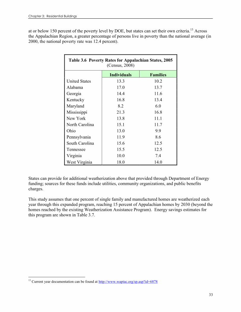
Chapter 3: Residential Buildings
33
at or below 150 percent of the poverty level by DOE, but states can set their own criteria.13 Across the Appalachian Region, a greater percentage of persons live in poverty than the national average (in 2000, the national poverty rate was 12.4 percent).
Table 3.6 Poverty Rates for Appalachian States, 2005 (Census, 2008)
United States
Individuals Families 13.3 10.2
Alabama 17.0 13.7 Georgia 14.4 11.6 Kentucky 16.8 13.4 Maryland 8.2 6.0 Mississippi 21.3 16.8 New York 13.8 11.1 North Carolina 15.1 11.7 Ohio 13.0 9.9 Pennsylvania 11.9 8.6 South Carolina 15.6 12.5 Tennessee 15.5 12.5 Virginia 10.0 7.4 West Virginia 18.0 14.0
States can provide for additional weatherization above that provided through Department of Energy funding; sources for these funds include utilities, community organizations, and public benefits charges. This study assumes that one percent of single family and manufactured homes are weatherized each year through this expanded program, reaching 15 percent of Appalachian homes by 2030 (beyond the homes reached by the existing Weatherization Assistance Program). Energy savings estimates for this program are shown in Table 3.7.
13 Current year documentation can be found at http://www.waptac.org/sp.asp?id=6878

Energy Efficiency in Appalachia, SEEA
34
Table 3.7 Energy Savings from Expanded Weatherization
Year
Electricity Savings
Natural Gas Savings
Fuel Oil Savings
Total Primary Energy Saved
% of Sector
Primary Energy (GWh) (trillion Btu) (trillion Btu) (trillion Btu)
2010 113.95 0.54 0.11 2.27 0.12 2013 461.47 2.19 0.43 9.24 0.47 2020 1,299.61 6.19 1.19 26.23 1.22 2030 2,612.21 12.13 2.21 53.00 2.15
Table 3.8 investment costs are based on an investment of $2,300 per home and administrative cost are set at a level of 10 percent of the investment (the Federally defined limit for such costs). Energy savings reflect the consumer‘s bill savings based on their reduced consumption and forecast energy prices (EIA, 2008a).
Table 3.8 Costs and Savings from Expanded Weatherization
Year Energy Savings Admin Costs Investment Costs
(million 2006$) (million 2006$) (million 2006$)
2010 20.41 17.18 171.77 2013 78.35 17.80 177.97 2020 217.81 19.22 192.22 2030 455.48 21.01 210.11
Figure 3.5 shows how investments in weatherization and energy savings change over the study period. There is no private investment assumed in this model for expanded weatherization. The public investment includes the administrative costs and the cost of improvements; if the low-income weatherization program were designed as a cost-share program; public investments would be lower while private investment would be higher.

Chapter 3: Residential Buildings
35
0
10
20
30
40
50
60
2010 2015 2020 2025 2030
Trill
ion
BTU
0
50
100
150
200
250
Mill
ion
20
06
$
Energy Savings Public Investment
Weatherization of low-income homes has been touted as an effective program for more than 20 years. As mentioned above, not only does weatherization reduce energy bills for low-income consumers, it also improves comfort, health, and safety for the families served – the existing program favors homes with children and the elderly. In addition, if energy bills are lower, consumers will be more likely to be able to pay their bills, and less likely to request heating bill assistance funds, like LIHEAP, or shirk on payment, leading to charge-offs. These non-energy benefits can be
considerable; Schweitzer and Tonn (2002) determined that the non-energy benefits of
weatherization were about $3,809 over the lifetime of the retrofits, and most of these benefits accrue to society as a whole.14 More detail on benefits and costs are in the summary of this chapter. The Expanded Low-Income Weatherization Assistance Program is cost-effective over the lifetime of the measures with a benefit-to-cost ratio of about 2.1 for participants and about 1.3 for total resource costs. With $4 billion in program spending over the 2010-2030 period, the Appalachian Region could see net cumulative savings of 1.1 quads, saving $11.4 billion in energy bills by 2050. This is the equivalent of about 2.1 percent of the EIA‘s forecast consumption in 2030 or 10.2 percent of forecast growth (EIA, 2008a). 3.3.3 Residential Retrofit Incentive with Resale Energy Labeling and On-Bill Financing Policies to encourage existing home retrofits can reduce the financial barriers faced by homeowners in that they tend to have high discount rates and lack adequate access to capital (Brown and Chandler, 2008). In addition, retrofit of existing homes innovates within the current stock of homes rather than waiting for new, more efficient homes to be built. This innovation alleviates efficiency problems with slow housing turnover (survival rates of 98-99.7 percent). Homeowners are already turning to retrofits for comfort and safety; remodeling expenditures doubled for owner-occupied homes over the 1995-2005 decade with extra insulation as a popular project (AIA, 2006a, b). However, the interval for a major home renovation, including the envelope/shell is 30-50 years. This long interval suggests that each renovation not bringing a home to meet current standards is a lost opportunity (Jakob, 2006). Banfi et al. (2008) found that consumers (both renters and owners) report a willingness to pay for energy-efficient measures, such as windows, insulation, and ventilation technologies, that is higher than the cost of the same measure‘s installation; they suggest that this may represent either an overstatement of willingness to pay or an indication that the market has not fully developed.
14 Schweitzer and Tonn (2002) report savings in 2001 dollars; to remain consistent with the currency of this report, the $3,346 in reported 2001 savings was converted to 2006 dollars.
Figure 3.5 Annual Investment and Energy Savings from Expanded Weatherization, 2010-2030
Energy Efficiency in Appalachia, SEEA
36
The present analysis assumes the retrofit program runs as an incentive measure for 20 percent of investment cost, to accompany two other policies – home energy disclosure and on-bill financing. While the incentive only lasts for 10 years – to 2020 – the program continues to provide support for the disclosure and financing mechanisms as well as public awareness campaigns until 2030. Home energy disclosure would provide information to home buyers (for new and resale residences) on the energy efficiency of the home. In Kansas, home energy disclosures have been required on new residential construction since 2001, but legislation in 2007 extended the requirement to include resale homes (Kansas, 2007a; KEC, 2008). While policy makers might expect opposition from industry, realtors, and architects, for such a requirement, recent history shows that this is not a concern. The Kansas experience shows strong support from these groups (Aron, 2007; Bell, 2007; Neu Smith, 2007). Also, resale energy labeling could encourage home buyers to recognize the energy costs of the homes they are considering and may drive greater investment in retrofits before or after homes are sold. On-bill financing refers to programs, run through utility or municipal energy retailers that allow consumers to acquire a favorable loan for energy-efficient retrofits or upgrades that are paid back through their energy savings. This is conceptually similar to the services offered by energy services companies as ―performance contracting.‖ On-bill financing reduces the first cost to the consumers (and allows for pass-through of costs to the next owner). This could make the costs less daunting and allow for homeowners to pass the costs on if they have to sell their home before these costs are paid for by the energy savings (Brown, Southworth, and Sarzynski, 2008). Kansas has also passed legislation to allow utilities to enter into contracts with customers, or landlords of customers, to finance energy-efficiency improvements; the amount must be approved by the Kansas Corporation Commission and would be repaid through energy savings (Kansas, 2007b). Some utilities in the Appalachian Region already offer on-bill payment of financing for energy efficiency. An example is Cherokee Electric Cooperative in Alabama which offers the Energy Conservation Home Improvement Loan Program with low-interest loans for up to 10 years and on-bill payment (Cherokee, 2008). Regardless of the form of the program, retrofits of homes would offer greater savings per home than weatherization and are not limited to low-income homeowners. Programs of this nature could encourage investment in rental properties and larger homes. For this policy, we assume that two percent of all existing single family homes are retrofit each year from 2010 to 2030. The costs per home are more than under the weatherization program – $3,400 per home. Resale energy labeling would require an additional field in the Multiple Listing Service for home energy consumption. It is not envisioned to require a Home Energy Rating System or audit; both of these have been shown to be costly and therefore engender opposition from real estate professionals. Instead, utilities (or other energy providers) would be required to provide the information on average consumption. This is information that the utilities (or other energy providers) would already have and does not require an audit as utilities generally have incentive to have correct consumption information for billing purposes. Administrative costs on the part of the government are expected to be minimal. Energy consumption information should be provided on an average annual or average monthly basis for the whole residence and per square foot for each fuel used in the home provided by an energy company (electricity, natural gas, fuel oil, etc). Labeling programs provide potential buyers with information on the energy integrity of homes. They do not mandate efficiency improvements, but may encourage improvements when energy costs are

Chapter 3: Residential Buildings
37
high. These can easily be compared to the provision of the U.S. Environmental Protection Agency (EPA) mileage estimates provided for new vehicle sales; consumers may choose more efficient vehicles based on this information. The energy savings reported in Table 3.9 amounts to a 7.3 percent reduction of residential energy consumption. It translates to a simple payback of about six years, following an incremental investment of $3,400 per retrofit home. This payback period is considerably longer than some studies claim for retrofits (see Appendix B.3); however, lower energy prices in Appalachia and a greater reliance on electricity for heat can explain some of this difference.
Table 3.9 Energy Savings from Existing Home Retrofits
Year Electricity
Savings Natural Gas
Savings Fuel Oil Savings
Total Primary Energy Saved
% of Sector
Primary Energy (GWh) (trillion Btu) (trillion Btu) (trillion Btu)
2010 382 2.23 0.43 8.11 0.42 2013 1,535 9.04 1.72 32.76 1.67 2020 4,222 25.52 4.68 91.47 4.24 2030 8,241 49.75 8.58 180.20 7.30
The costs reported in Table 3.10 are based on the incremental cost of $3,400 for efficient retrofits, and a small administrative staff to support oversight of labeling and incentive distribution. The energy bill savings are based on forecast energy prices and modeled energy savings by census division (EIA, 2008a).
Table 3.10 Costs and Savings from Existing Home Retrofits
Year
Energy Savings Admin Costs Investment Costs
(million 2006$) (million 2006$) (million 2006$)
2010 75 0.99 466 2013 288 0.99 483 2020 790 0.98 523 2030 1,631 0.33 572

Energy Efficiency in Appalachia, SEEA
38
0
20
40
60
80
100
120
140
160
180
200
2010 2015 2020 2025 2030
Trill
ion
BTU
0
100
200
300
400
500
600
700
Mill
ion
20
06
$
Energy Savings Public InvestmentPrivate Investment
Figure 3.6 shows how investments and energy savings change over the study horizon. The modeled program assumes that private investment continues, and picks up the difference when the incentive for efficient retrofits is removed. As such, this program is modeled as a market transformation. Over the first 10 years, when there is an incentive, consumers become familiar with the energy labeling, and on-bill financing mechanisms become commonplace. By 2020, consumers and the contractors performing retrofits are interested in ensuring greater energy efficiency with their retrofits and are willing to cover the entire incremental costs of these improvements. In total, the Efficient Residential Retrofit Incentive with Enabling Home Labeling and On-Bill Financing is cost-effective with a benefit-to-cost ratio of about 1.5 for participants (all retrofit home occupants) and about 1.7 for total resource costs; more detail on benefits and costs are in the summary of this chapter. With $1.1 billion in program spending and an additional $9.86 billion in private investments over the 2010-2030 period, the Appalachian Region could see net cumulative savings of 3.8 quads, saving $33.5 billion in energy bills by 2050. This is the equivalent of 7.3 percent of the EIA‘s forecast consumption in 2030 or 34.6 percent of forecast growth (EIA, 2008a). 3.3.4 Super-Efficient Appliance Deployment About one-quarter of residential energy consumption goes to support lighting and appliances. While new incandescent bulb efficiency requirements within EISA 2007 are expected to reduce the lighting load, significant reductions in other appliances and electronics are not currently forecast. While energy-efficient dishwashers have nearly achieved sales saturation, less than one-third of clothes washers and refrigerators sold in 2006 met ENERGY STAR requirements (ENERGY STAR, 2007).
Figure 3.6 Annual Investment and Energy Savings from Existing Home Retrofits, 2010-2030

Chapter 3: Residential Buildings
39
0%
10%
20%
30%
40%
50%
60%
70%
80%
90%
100%
AL GA KY MD MS NC NY OH PA SC TN VA WV U.S.
Average
Air-Conditioners Clothes WashersDish Washers Refrigerators
Policies to encourage greater adoption of energy-efficient appliances and electronics come in many forms. States offer sales tax holidays, tax credits, and rebates for energy-efficient appliances. Georgia started an ENERGY STAR sales tax holiday in 2005, with other states, like North Carolina, Virginia, and West Virginia following; in the same spirit, New York is considering eliminating sales tax on ENERGY STAR labeled appliances and light bulbs (Hayes, 2008). In Japan, the most efficient equipment and appliances set the new target consumption rates (as opposed to a minimum standard set before development like our ENERGY STAR program); this ―Top Runner‖ program has exceeded the savings expectations of the Energy Conservation Center, Japan (ECCJ, 2008). Regional support to remove poor performing appliances from the market could significantly reduce energy consumption in newly purchased products while a companion replacement effort could accelerate stock turnover for outdated appliances and equipment. For example, New York Power Authority has a refrigerator replacement program in place for public housing residents.15 This study assumes that super-efficient appliances are available at technology development rates of three percent more efficient than forecast every five years, so the most efficient appliances in 2025 are nine percent more efficient than stock efficiency in the Annual Energy Outlook 2008 baseline forecast (EIA, 2008a). The model considers eleven residential end-uses (see Appendix B.4). An incentive of 40 percent of the incremental cost is offered for adoption of these appliances from 2010 to 2015; from 2015 to 2020, the incentive is 20 percent of the incremental cost. These incentives are expected to drive 50 percent of appliance replacements and new purchases to super-efficient appliances available for that end-use from 2010 to 2020; after 2020, only 40 percent of new purchases are of super-efficient appliances. While this policy represents an aggressive demand pull mechanism, higher demand could drive the technology improvements faster and lead to lower incremental costs in the long run. It is envisioned that the incentive would target manufacturers,
15 For information about New York Power Authority‘s refrigerator program see http://www.nypa.gov/services/esprograms2.htm
Figure 3.7 Percent ENERGY STAR Sales by Appliance by State, 2006 (ENERGY STAR, 2007)

Energy Efficiency in Appalachia, SEEA
40
distributers, and contractors; and that it would be coupled with public information campaigns for consumers. By 2020, 0.7 percent of the residential sector‘s energy demand would be saved as a result of this policy, increasing to 1.7 percent in 2030. The energy savings expected from this program are shown in Table 3.11.
Table 3.11 Energy Savings from Super-Efficient Appliance Deployment
Year
Electricity Savings
Natural Gas Savings
Fuel Oil Savings
Total Primary Energy Saved
% of Sector
Primary Energy (GWh) (trillion Btu) (trillion Btu) (trillion Btu)
2010 51 0.02 0.00 0.75 0.04 2013 207 0.06 0.00 3.03 0.15 2020 957 0.30 0.00 14.25 0.66 2030 2,736 0.82 0.00 41.65 1.69
Table 3.12 shows the costs and energy bill savings from the Super-Efficient Appliance Deployment. The energy bill savings are based on modeled energy savings and forecast energy prices by fuel and census division (EIA, 2008a). Administrative costs include only the program staff costs while investment costs include the whole incremental cost of more energy-efficiency appliances.
Table 3.12 Costs and Savings from Super-Efficient Appliance Deployment
Year
Energy Savings Admin Costs Investment Costs
(million 2006$) (million 2006$) (million 2006$)
2010 5.68 0.02 5.57 2013 22.12 0.02 5.67 2020 101.62 0.08 17.97 2030 294.31 0.11 26.31

Chapter 3: Residential Buildings
41
Figure 3.8 shows how investments and energy savings change over time. It is clear that the five year cycle represents a significant cost increase as the incremental cost of the super-efficient appliances are assumed to rise with greater efficiency required. Public investment remains quite low, although it does reflect an incentive of 40 percent of the incremental cost until 2015 and 20 percent until 2020 on top of the administrative costs. Private investment is lower until 2020 due to the incentive. Because the policy is a designed to pull demand towards efficient products, the policy transforms the market to a more efficient equilibrium.
0
10
20
30
40
50
60
70
80
90
100
2010 2015 2020 2025 2030
Trill
ion
BTU
0
5
10
15
20
25
30
Mill
ion
20
06
$
Energy Savings Public InvestmentPrivate Investment
The Super-Efficient Appliance Deployment Program is cost-effective with a benefit-to-cost ratio of about 6.7 for participants (everyone who uses appliances replaces something during this period because all modeled appliances have lifetimes of less than 20 years) and about 7.0 for total resource costs. With $27.8 million in program spending and an additional $271 million in customer investments over the 2010-2030 period, the Appalachian region could see net cumulative savings of 345 trillion Btu, saving $2.4 billion in energy bills by 2030. This is the equivalent of about 1.7 percent of the EIA‘s forecast consumption in 2030 or 8.0 percent of forecast growth (EIA, 2008a).
Figure 3.8 Annual Investment and Energy Savings from Super-Efficient Appliance Deployment, 2010-2030

Energy Efficiency in Appalachia, SEEA
42
Box 3.2 Research and Development Example: Air-Source Integrated Heat Pumps
A major manufacturer has partnered with Oak Ridge National Laboratory (ORNL) on the development of air-source integrated heat pumps (AS-IHP). Integrated heat pumps provide space heating and cooling, water heating, ventilation, and dehumidification into a single system. Efficiencies are gained over traditional HVAC systems by making use of otherwise wasted energy (e.g., heat rejected by the space cooling operation can be used for water heating). Heat pumps are a central part of the DOE‘s efforts to develop net-zero energy housing, or homes that produce as much energy as they consume. This technology could provide nearly 60 percent savings in both cold and mixed humid climates (even greater in hot or temperate climates), relative to a baseline system. Incremental capital costs for this advanced HVAC system are not expected to be prohibitive, ranging from $2,500 to $3,200 (2006 dollars) greater than a baseline system, with payback times averaging around eight years in cold and mixed climates (Baxter, 2006). The incremental costs are kept low because of shared components of the HVAC system and the ability to use otherwise wasted energy.
Figure 3.9 Schematic of an Air-Source Integrated Heat Pump (Baxter, 2006)
The residential sector is responsible for approximately one third of all energy consumed in the U.S., and this holds true for the Appalachian Region as well. A new HVAC technology such as the AS-IHP that is 60 percent more efficient than traditional technologies could dramatically reduce residential energy demand (Baxter, 2006). Space heating and cooling, and water heating combined account for about 70 percent of all residential energy consumption.

Chapter 3: Residential Buildings
43
0
5
10
15
20
25
30
35
40
2010 2015 2020 2025 2030
Trill
ion
Btu
Figure 3.10 Cumulative Energy Savings from Integrated Heat
Pump in Appalachian Region (Trillion Btu)
The AS-IHP is still in the development stages and is not yet commercially available. Within an average Appalachian home, installation of the AS-IHP would save approximately 37 million Btu per year. This estimate is based on the energy use of the AS-IHP in Appalachian climates as compared to the average amount of energy used in an Appalachian home on space heating and cooling, and water heating. As with any new technology it is difficult to estimate what the market potential will be, but a study from the IEA Heat Pump Programme (2006) suggests that heat pumps could reach 30 percent of the market. Figure 3.10 shows the estimated the amount of energy that could be saved from installing the AS-IHP in 30 percent of all new homes built between 2010 and 2030, assuming household energy consumption remains consistent. Roughly 1.6 trillion Btu would be saved annually under this scenario. Because the integrated heat pump is not easily adaptable to retrofits, they were not included in these estimates. The air source integrated heat pump could provide substantial energy savings to households in the Appalachian Region. However, high upfront costs may stall its adoption by the market. Policies that support or require installment of energy-efficient technologies in all new housing, as well as incentivize retrofitting energy-efficient technologies in existing houses, would help push integrated heat pumps into the market more quickly. 3.4 SUMMARY OF RESULTS The residential sector can quickly deliver cost-effective energy savings to consumers (Brown, et al., 2001; McKinsey, 2007). This chapter provides further evidence suggesting that Appalachian Region investments in residential programs can generate benefits to the Appalachian Region‘s residents that more than exceed their public and private investment costs. Based on the residential program and policy bundles described in this chapter, building energy codes and efficient retrofits have the largest potential for energy savings (Figure 3.11). Together they account for approximately three-fourths of the 374 trillion Btu of residential savings that are projected to occur in the year 2030.

Energy Efficiency in Appalachia, SEEA
44
Figure 3.12 Residential Primary Energy Consumption With and Without Policy Packages (Quads), 2006-2030
1.2
1.4
1.6
1.8
2
2.2
2.4
2.6
2.8
3
3.2
2006 2009 2012 2015 2018 2021 2024 2027 2030
Qu
adri
llio
n B
tu
AEO 2007 AEO 2008 With Policy Packages
Residential
Building Codes
98.66
26%
Expanded
Weatherization
53.00
14%
Existing Home
Retrofits
180.20
49%
Super-Efficient
Appliance
Deployment
41.65
11%
Figure 3.12 shows that implementation of these policy bundles could significantly curb the growth in residential energy consumption forecast for the Appalachian Region to 2030, with nearly flat consumption from 2028 to 2030. These four policies generate savings of 15.1 percent of AEO 2008 forecast consumption in 2030 (EIA, 2008a). These estimated savings are generally lower, but not dramatically different, than other studies for states in the
Region. Efficiency potential studies completed for Georgia Power and the Georgia Environmental Facilities Authority found maximum achievable
electric efficiencies of nine percent over 10 years and 9.4 percent over five years, respectively (ICF, 2005; Nexant, 2007). A study for North Carolina found a maximum achievable potential for residential electric efficiency of 16.9 percent over a 10 year horizon (GDS Associates, 2006). An efficiency potential study for Kentucky modeled minimally and moderately aggressive scenarios with residential savings of 2.7 percent and 8.2 percent, respectively, over 10 years (KPPC, 2007). More recently, a report by ACEEE et al. (2008) modeled residential savings for Virginia at 26 percent of their forecast electricity consumption in 2025.
Figure 3.11 Residential Energy Savings by Policy Bundle, 2030 (trillion Btu)

Chapter 3: Residential Buildings
45
Figure 3.13 Comparison of Appalachian Residential Delivered Energy Consumption Forecast Under Four Cases (Quads), 2006-2030
(EIA, 2008a)
0.00
0.20
0.40
0.60
0.80
1.00
1.20
2006 2009 2012 2015 2018 2021 2024 2027 2030
Qu
adri
llio
n B
tu (
del
iver
ed)
AEO 2008 Reference High TechnologyFrozen Building Technology Model Savings
0
50
100
150
200
250
300
350
400
2010 2015 2020 2025 2030
Trill
ion
BTU
0
100
200
300
400
500
600
700
800
Mill
ion
20
06
$
Energy Savings Public InvestmentParticipant Investment
In addition to comparing our modeled savings case with the AEO 2008‘s Reference case, we can also compare the savings forecast with two of the AEO 2008 alternative cases: one representing the ―Frozen Building Technology‖ option and another reflecting the ―High Technology‖ alternative (Figure 3.13). It is clear from this figure that our estimated savings from the reference case are much greater when compared to the ―Frozen Building Technology‖ case and still noticeably more energy-efficient than the ―High Technology‖ case. When considering this package of residential policies from the participants‘ perspective, the simple payback declines from about 4.2 years to about two years over the study horizon. The shortened payback period is largely driven by the gains in new residential building efficiency without a corresponding increase in incremental costs; it also follows an increasing cost of energy (a Btu saved in 20 years is worth more than a Btu saved today). It is assumed that materials, technology, and practice will improve over time to reduce the incremental cost of efficient buildings. The Existing Home Retrofit Program and Super-Efficient Appliance Deployment Program maintain paybacks of around six years and one year, respectively, throughout the study period. Participants do not make an investment in the expanded weatherization program as modeled, so the payback period is not considered.
Figure 3.14 shows how public and private investments and energy savings change over the study horizon. The energy savings continue to accumulate at a persistent pace across the 20-year planning horizon. In contrast, the public investment drops in 2020 when the subsidies for retrofitting existing housing stock and incentives for super-efficient appliances are sunset, while the participants costs increase in a compensatory manner. The economic feasibility of policy packages is a function of how the policy costs and benefits are distributed over time and across
customer classes and residential subgroups. For the residential energy-efficiency policies modeled, the super-efficient appliance deployment, and building codes are the most cost-effective see Table 3.13. However, consideration of non-energy benefits often drive adoption of policies such as
Figure 3.14 Annual Investment and Energy Savings from Combined Residential Policy Packages, 2010-2030

Energy Efficiency in Appalachia, SEEA
46
expanded weatherization, which has the lowest total resource cost test across the four policies, but offers substantial health, comfort, and safety benefits to low-income households. Similarly, consumers often adopt more efficient retrofit measures to remove drafts or reduce noise in addition their energy benefits. Measures are only counted for benefits over their useful lives; in this analysis, we have considered retrofit and weatherization savings to accrue for 20 years. For building codes and efficient appliances, we make the conservative assumption that the market would have caught up to our program by 2030, so we do not consider benefits after this time.
Table 3.13 Results of Economic Tests for Residential Policies
Residential Building
Codes
Expanded Weatherization
Existing Home
Retrofits
Super-Efficient Appliance
Deployment Total
Participants Test NPV Benefits (billion 2006$) 3.17 3.37 6.72 0.64 13.90
NPV Costs (billion 2006$) 0.92 1.60 4.36 0.09 6.98
Net Benefits-Costs (billion 2006$)
2.25 1.77 2.36 0.54 6.92
B/C Ratio 3.44 2.10 1.54 6.75 1.99 Total Resource Cost Test
NPV Benefits (billion 2006$) 4.69 2.80 9.36 0.90 17.75
NPV Costs (billion 2006$) 1.26 2.23 5.52 0.13 9.14
Net Benefits-Costs (billion 2006$)
3.43 0.57 3.84 0.78 8.61
B/C Ratio 3.72 1.26 1.70 7.05 1.94 The combined residential policy package is cost-effective with a benefit-to-cost ratio of about 2.0 for participants and about 1.9 for total resource costs. With $5.1 billion in program spending and an additional $12.3 billion in customer investments over the 2010-2030 period, the Appalachian Region could cost-effectively reduce its energy consumption by 6.0 quads, saving $60.4 billion in energy bills. The savings in 2030 represent the equivalent of 18.7 percent of the EIA‘s forecast consumption or 71.7 percent of forecast growth (EIA, 2008a).

Chapter 4: Commercial Buildings
47
Electricity
25%
Electricity
Related
Losses
55%
Natural Gas
15%
Liquid Fuels
Subtotal
4%
Coal
0%
Renewable
Energy
1%
1.2
1.4
1.6
1.8
2.0
2.2
2.4
2.6
2.8
3.0
3.2
2006 2009 2012 2015 2018 2021 2024 2027 2030
Qu
adri
llio
n B
tu
AEO 2007 AEO 2008
4 ENERGY EFFICIENCY IN COMMERCIAL BUILDINGS 4.1 INTRODUCTION TO COMMERCIAL BUILDINGS IN APPALACHIA The Appalachian commercial sector consumed about 1.47 quads of energy in 2006, while total expenditures were more than $10 billion (2006 dollars).16 Electricity (55 percent) and natural gas (32 percent) were the dominant forms of delivered energy, excluding electricity related losses (EIA, 2008a). When losses are included, the contribution from electricity and natural gas drops to 25 and 15 percent, respectively. From 2008 to 2030, commercial energy consumption in the Appalachian Region is expected to increase between 45 percent and 63 percent up to between 2.26 and 2.55 quads, Figure 4.2 (EIA, 2007a; 2008a). According to these forecasts, energy consumption is growing more rapidly in commercial buildings than in any other sector.
Commercial buildings offer significant energy-efficiency potential – mostly through upgrades to existing building stocks. Due to the longevity of commercial buildings and an economy that is ever more service based, new commercial buildings represent even less of the total stock of commercial buildings than new homes represent of the residential stock each year. See Table 4.1 for median commercial building lifetimes.
16 Costs include those for distillate fuel oil, residual fuel oil, natural gas, and electricity based on population-weighted average Appalachian prices. Other fuels, such as liquid propane gas, kerosene, coal, and renewable energy were also used by Appalachian commercial buildings in 2006 but excluded from the cost given.
Figure 4.2 Commercial Energy Consumption Forecast for the Appalachian Region (Quads), 2006-2030
(EIA, 2007a; 2008a)
Figure 4.1 Commercial Sector Energy Sources by Fuel, 2006
(EIA, 2008a)

Energy Efficiency in Appalachia, SEEA
48
Table 4.1 Median Lifetimes for Selected Building Types (EIA, 2008b, Table 12)
Median Expected Lifetime (years) Gammaa
Assembly 80 1.8 Education 80 2.6 Food Sales 65 2.5 Food Service 65 2.5 Health Care 65 2.3 Lodging 69 2 Large Office 73 2 Small Office 73 2 Mercantile/Service 65 1.8 Warehouse 80 1.6 Other 75 2.5 a ‗Gamma‘ is the ―rate at which buildings retire near their median expected lifetime‖ (EIA, 2008b).
Types of commercial buildings and end uses in the Appalachian Region differ slightly from national averages. The most significant differences in floorspace are in three building types: the Region has more floorspace in ―Assembly‖ and less in ―Food Sales‖ and ―Warehouse.‖17 The Appalachian Region does not differ significantly from national averages in commercial end-uses. 4.2 POLICY OPTIONS FOR COMMERCIAL ENERGY EFFICIENCY This study models four policies, coupled with incentives, to encourage energy efficiency in commercial buildings: Commercial Building Energy Codes with Third Party Verification, Support for Commissioning of Existing Commercial Buildings, Efficient Commercial HVAC and Lighting Retrofit Incentive, and Tightened Office Equipment Standards with Efficient Use Incentive. There are several other kinds of policies that could be used to encourage more efficient use of energy in commercial buildings. Table 4.2 lists examples of policy actions, including those modeled; listed policies could be used as substitutions or complementary actions. The actual form of policies adopted within the Appalachian Region will depend on the specific goals and capacity of each policy making body.
17 Religious worship buildings are included in assembly.

Chapter 4: Commercial Buildings
49
Table 4.2 Policy Actions that Support Commercial Energy Efficiency
Actions Commercial Building Codes
Existing Building Commissioning
HVAC and Lighting Retrofits
Office Equipment Standards
Research, Development, and Demonstration
Support for research and development in advanced building processes and materials
Development of new insulation, heating, and cooling technologies useful for the local climate
Development of new lighting, heating, cooling, and ventilation technologies useful for the local conditions
Support for research and development for innovation in appliance performance
Financing
Low or no-interest loans for incremental cost of improvements for new construction Enable performance contracting
N/A
Low or no-interest loans for incremental cost of improvements for existing buildings Enable performance contracting
Low or no-interest loans for ENERGY STAR equipment Enable performance contracting
Financial Incentives
Incentives to builders for exceeding codes Rebates or lower fees for builders for LEED or ENERGY STAR ratings
Incentives for cost of commissioning study and necessary repairs or replacements
Incremental cost incentives for efficient retrofits Tax credits for efficient purchases
Incentives to use efficiency features and lower consumption Tax credits for efficient purchases Equipment buyback programs
Pricing N/A N/A N/A N/A
Voluntary Agreements
Agreement between major builders in the area to meet or exceed code
N/A N/A N/A
Regulations
Model Building Energy Code Legislation Allowing third-party compliance inspection
N/A Tighter lighting and HVAC equipment standards
Tighter office equipment standards Standby efficiency standards
Information Dissemination & Training
Training Architects, Builders, Contractors, and Code Enforcement Officials Public Awareness campaigns to inform consumers of the benefits of conservation and efficiency measures
Training Architects, Builders, Contractors, and Building Managers Public Awareness campaigns to inform consumers of the benefits of conservation and efficiency measures
Training Architects, Builders, Contractors, and Building Managers Awareness campaigns to inform executives of the benefits of efficiency measures Advanced metering or billing methods
Awareness campaigns to inform executives of the benefits of conservation and efficiency measures Advanced metering and billing
Procurement Government lead by example procurement programs
Government lead by example procurement programs
Government lead by example procurement programs
Government lead by example procurement programs
Market Reforms N/A N/A N/A N/A

Energy Efficiency in Appalachia, SEEA
50
Table 4.2 Policy Actions that Support Commercial Energy Efficiency
Actions Commercial Building Codes
Existing Building Commissioning
HVAC and Lighting Retrofits
Office Equipment Standards
Planning Techniques
Low or No-Interest Loans for Incremental Cost of Improvements for New Construction
N/A N/A N/A
Capacity Building
Centers for energy efficiency to train next generation of architects, builders, retrofitters
Centers for energy efficiency to train next generation of architects, builders, retrofitters
Centers for energy efficiency to train next generation of architects, builders, retrofitters
N/A
This table describes policy actions available that could further the savings from the policy packages modeled in this study. The policy actions shown in italics are modeled in this study, while the others are not.
4.2.1 Research, Development, and Demonstration Developing advanced building processes and technologies can help to improve the performance of commercial buildings. Building materials and construction and renovation processes are especially important in commercial buildings where ownership changes hands – leading to renovations – many times in the course of the building‘s lifetime. Supporting advanced building materials and process research can help a state or locality to keep talented researchers and money for new technology from leaving the area. Research and development programs can work hand-in-hand with capacity building measures. Demonstration projects can be integrally linked to state procurement programs to help pull new technologies out of the research pipeline. Some states and localities create lead-by-example programs specifically requiring that government buildings must meet stricter standards or achieve year over year savings; these types of procurement programs help generate a demand pull that can keep innovations coming to the marketplace. 4.2.2 Financing Financing policies can help to reduce the ―first cost‖ burden, making efficient investments more affordable. Loans available for incremental costs to builders allow them to invest in more efficient equipment and materials; commercial building owners/buyers (who are passed the cost through builders) and commercial building lessees then benefit from lower energy consumption and greater comfort levels. Many commercial buildings are plagued with the economic reality of the principle (owner) not being responsive to the agent‘s (lessees) needs; if owners do not pay the energy bills, they have less of an incentive to invest in equipment with a higher cost. Mississippi‘s Energy Investment Loan program is broad-based and geared towards helping to drive innovation and offers loans from $15,000 to $300,000 at three percent below prime for capital improvements or design and development of innovative energy conservation practices. North Carolina also has a broad-based loan program based on a service contract structure; the Energy Improvement Loan Program (EILP) provides loans, secured with a letter of credit for non-government borrowers, with interest rates of one percent or three percent, depending on the project, for renewable energy, recycled energy, or energy savings. A more targeted loan program, the New

Chapter 4: Commercial Buildings
51
York Energy Smart Loan Fund, provides for reduced interest rates compared to the lender‘s normal rate for certain renewable or energy efficiency improvements.18 State agency performance contracting is a popular financing mechanism. To illustrate, in New York, the New York Power Authority offers performance contracting for state-owned buildings and schools.19 Some states do not allow agencies to enter into contracts that cover more than the current fiscal year, which can prevent cost effective energy-efficient improvements. While performance contracting may present fiscal complications, it can save energy and taxpayer money in the long run. 4.2.3 Financial Incentives Tax credits, rebates, reduced fees, and grants can all be used as financial incentives to encourage efficient technologies and practices for commercial buildings. Incentives help to reduce the burden of high costs and may help drive capital towards energy-efficiency improvements. There are many examples of financial incentives already in place throughout Appalachia and the rest of the nation. For example, Maryland‘s Green Building Tax Credit program encourages more efficient new large (more than 20,000 square feet) commercial buildings in targeted areas by offering a credit up to eight percent of the cost of building construction. In New York, there is both a prequalified cost-reduction program and a tax credit available for certain retrofits and new commercial buildings.20 Financial incentives are also used for transfers within state government: for example, Virginia‘s Technical Assistance Grant Program offers grants for technical assistance to reduce energy consumption in support of Executive Order 48, which calls for reducing energy consumption in state government facilities. Similarly, West Virginia‘s Lighting Grants Program provides 50/50 matching grants to state and local government facilities and schools; nonprofit hospitals, and public libraries for lighting improvements having a payback less than five years based on an EPA ENERGY STAR lighting audit. 4.2.4 Voluntary Agreements Voluntary agreements, where builders agree to work towards greater efficiency, can have significant savings. For example, the Model Conservation Code in the northwest was gradually adopted by states as codes after builders innovated through voluntary standards (EPA, 2006). The Building America and Rebuild America programs are good examples of national voluntary innovation programs, with many leading builders, states, and national laboratories partnered together to improve building materials, technologies, and process. 4.2.5 Regulations Regulating minimum efficiency levels through promulgation of standards and codes can reduce proliferation of poorly performing equipment, buildings, and practices. Model energy codes, subject to review and update, set a new minimum level of efficiency; this ensures that the average new
18 The interest rate reduction for New York‘s Energy Smart Loan Fund for most of the state is up to 4.0 percent (400 basis points). Con Edison customers may be eligible to receive an interest rate reduction up to 6.5 percent (650 basis points) less than a Participating Lender's or Lessor's normal market rate. See http://www.nyserda.org/loanfund.default.asp 19 Details about New York Power Authority‘s performance contracting program can be found at: http://www.nypa.gov/services/esp.htm 20 See http://www.nyserda.org/programs/Existing_Facilities/default.html and http://www.dec.ny.gov/regs/4475.html

Energy Efficiency in Appalachia, SEEA
52
commercial building doesn‘t fall too far behind the leading new commercial buildings as materials, practices, and habits change. Regulation and standards-setting can be done at all levels of government; however, local and state standards and regulations are subject to pre-emption by the federal government. Some regulations set the foundation for other processes to work; for example, regulating contractors enables third party verification of savings and labeling while regulating lenders or utility actions enables performance contracting or other favorable financing options.21 With a third-party verification program, builders or retrofitters would be required to contract with a state or locally certified third party to verify compliance; any expenses associated with inspection and verification would be undertaken by the builder or contractor rather than the jurisdiction. California, New York, and Washington already use this type of program for building energy codes, with high compliance rates (EPA, 2006; Smith and McCullough 2001; Vine 1996). However, allowing for third party contracting takes time; for example, from adoption to effectiveness, the state of Washington spent three years (with utility funding) setting up training and certification programs to move their non-residential code to a system allowing for third party inspection (Kunkle, 1997). 4.2.6 Information Dissemination & Training and Capacity Building Lack of sufficient, trusted information is almost always a barrier to energy efficiency; there is simply not enough time for people and organizations to learn about energy savings measures and figure out how to incorporate the measures in a beneficial way (Brown et al., 2008). Training and information as well as capacity building programs can support the goals of improved energy performance by ensuring that there is a knowledgeable workforce in place to produce efficient homes. Most states offer programs to provide information to consumers through websites, printed brochures or flyers, and seminars or workshops. An example of capacity building is West Virginia‘s Building Energy Use Centers which provide the state with educational centers and the technical expertise to support programs like Saving Energy in West Virginia Schools. 4.3 MODELED SAVINGS IN APPALACHIAN COMMERCIAL BUILDINGS 4.3.1 Commercial Building Energy Codes with Third Party Verification Building codes lay out requirements for new building construction. For commercial buildings, model building energy codes, like the International Energy Conservation Code (IECC), are developed by either the ASHRAE or the International Code Council (ICC). One of the requirements for modifications to the code is that they be cost effective. A problem that arises with modeling building energy code savings is dealing with under- or over-compliance. In some cases, the newer code recommendations are such an improvement that there is compliance with the newer code before its adoption (over-compliance); therefore, the assumption that existing buildings do not already meet the newer code (built into an efficiency model) would lead to an over-estimation of savings. In other cases, promulgated codes are not enforced, and under-compliance with the existing codes could lead to an under-estimation of savings.
21 See section 4.2.1 for examples of financing mechanisms

Chapter 4: Commercial Buildings
53
As shown in Table 4.3, three of the 13 Appalachian states do not have mandatory commercial building energy codes: Alabama, Mississippi, and Tennessee. Four of the ten states with mandatory codes have dated vintages from 2003.
Table 4.3 State Commercial Building Energy Codes
State Commercial Energy Code Mandatory
Alabama1 ASHRAE/IESNA 90.1-2001 No Georgia ASHRAE/IESNA 90.1-2004 Yes Kentucky 2006 IECC and 2006 IBC Yes Maryland 2006 IECC Yes Mississippi2 ASHRAE 90-1975 No New York 2006 IECC Yes N. Carolina3 2003 IECC (ASHRAE 90.1-2004) Yes Ohio 2006 IECC (ASHRAE 90.1-2004) Yes Pennsylvania 2006 IECC (ASHRAE 90.1-2004) Yes S. Carolina 2003 IECC Yes Tennessee4 ASHRAE 90A-1980 and 90B-1975 No Virginia 2006 IECC Yes W. Virginia 2003 IECC No 1 Alabama‘s code is state specific – the Alabama Building Energy Conservation Code is mandatory for state government buildings and recommended for other commercial buildings (ADECA, 2005). There are also local adoptions of 2003 and 2006 IECC. 2 Mississippi‘s commercial code is mandatory for state government buildings, public buildings, and high-rises (BCAP, 2008). 3 North Carolina‘s code is state specific, but it is based on the 2003 IECC with reference to the ASHRAE 90.1-2004. 4 Tennessee is scheduled to update to the 2003 IECC on January 1, 2009 (TNleg, 2008).
The policy package modeled here assumes that all states within the Appalachian Region adopt the 2006 IECC commercial code or equivalent in 2009 with an effective date of 2010. The initial savings are assumed to come exclusively from lighting with this change, as the major difference between the 2001 and 2003 IECC (and 2004 ASHRAE 90.1) commercial code was in lighting density requirements. If the shell efficiencies are significantly different from the current practice in Mississippi and Tennessee (with codes based on ASHRAE 1975 and 1980 versions), savings for space heating and cooling in new buildings will be underestimated. Documentation of the methodology for calculating savings from improved commercial building energy codes can be found in Appendix C.1. These savings are assumed to be made through 80 percent compliance with model building code legislation enabled by third-party verification of code compliance.

Energy Efficiency in Appalachia, SEEA
54
Energy savings from Commercial Building Codes are expected to be about 2.3 percent of forecast commercial consumption by 2030 (Table 4.4). For comparison, this is about half the percent of energy savings estimated for residential building codes with third-party verification (see Chapter 3).
Table 4.4 Energy Savings from Commercial Building Codes
Year Electricity
Savings Natural Gas
Savings Fuel Oil Savings
Total Primary
Energy Saved
% of Sector
Primary Energy (GWh) (trillion Btu) (trillion Btu) (trillion Btu)
2010 84 0.00 0.00 0.92 0.06 2013 391 0.05 0.01 4.34 0.27 2020 1,551 0.73 0.11 18.48 0.98 2030 3,993 3.12 0.00 51.09 2.26
Costs for administering the commercial building energy codes are less than $2 million, annually, and includes two training personnel per state (apportioned) and one verification liaison per 10 million new square feet of commercial floorspace. Investment costs reflect the incremental cost of meeting the codes and increase from around $37 million in 2010 to nearly $47 million in 2030. Energy bill savings grow from almost $8 to $388 million over the study‘s time horizon (Table 4.5).
Table 4.5 Costs and Savings from Commercial Building Codes
Year Energy Savings Admin Costs Investment
Costs
(million 2006$) (million 2006$) (million 2006$)
2010 7.95 1.60 37.47 2013 36.03 1.63 38.80 2020 144.65 1.72 42.39 2030 387.87 1.83 46.74

Chapter 4: Commercial Buildings
55
Figure 4.3 Annual Investment and Energy Savings from Commercial Building Codes, 2010-2030
0
10
20
30
40
50
60
2010 2015 2020 2025 2030
Trill
ion
BTU
0
5
10
15
20
25
30
35
40
45
50
Mill
ion
20
06
$
Energy Savings Public Investment Private Investment
Figure 4.3 illustrates the time-line of expenditures and savings for commercial building codes. Public investment (administrative costs and incentives) remains less than $2 million throughout the program while private investment increases to cover the incremental costs of more efficient commercial buildings. Annual savings grow steadily throughout the study horizon because of the long lifetime of building stock and a growing number of commercial buildings are
meeting energy codes. The Commercial Building Energy Codes with Third Party Verification is cost-
effective with a benefit-to-cost ratio of about 2.5 for participants and about 2.8 for society. With $36.2 million in program spending and an additional $887.7 million in customer investments over the 2010-2030 period, the Appalachian region could see net cumulative savings of 441.5 trillion Btu, saving $3.4 billion in energy bills by 2030. This is the equivalent of about 2.3 percent of the EIA‘s forecast consumption or 7.3 percent of forecast growth (EIA, 2008a). 4.3.2 Support for Commissioning of Existing Commercial Buildings Building a commercial structure is a complicated process, combining architectural design and construction as well as building systems design (e.g., HVAC) and installation. Often many different designers, contractors, and subcontractors are a part of the process, and as the complexity of the project increases, so does the probability of incorrect installation. In addition to problems with construction or installation, as a building matures, equipment can become obsolete or be altered to operate off-design. Building commissioning is a multi-phase process to ensure building performance is as designed and that the building‘s operation meets the needs of its occupants. According to the New York State Energy Research and Development Authority (NYSERDA, 2004) the commissioning of existing buildings should include four steps: planning, investigation, implementation, and handoff. Through measurement and inspection, a building‘s envelope, HVAC equipment, and other systems are evaluated against initial design documentation and corrective actions are taken, often with resulting energy savings. Commissioning existing buildings in the Appalachian Region could lead to immediate energy savings. In a meta-analysis conducted by Lawrence Berkeley National Laboratory, up to 57 percent of the total building energy was saved, though the median value for buildings that did not purchase thermal products was 10 percent (Mills et al., 2004). One policy that currently supports commissioning of existing buildings in the Appalachian Region is the NYSERDA Existing Facilities Program (NCSC/IREC, 2008). This program provides financial incentives for energy-efficiency improvements to most non-single family structures. Actions undertaken to correct off design performance that cost more than $10,000 are eligible for energy rate

Energy Efficiency in Appalachia, SEEA
56
rebates as well as reduction in demand rate charges. A public benefit fund is the source of funds for this program. Findings from the LBNL meta-analysis (Mills et al., 2004) and a study by Portland Energy Conservation and Oak Ridge National Laboratory (Haasl and Sharp, 1999) were used to estimate the energy savings potential in the ARC Region. The modeled program consists of commissioning incentives for the first ten years of the program as well as program administration to lead public-awareness campaigns, evaluate private-sector commissioning companies, study program effectiveness, and suggest program improvements as needed. Details of the modeling methodology are provided in Appendix C.2. Energy savings from commissioning of existing buildings are shown in Table 4.6. Modeled savings from commissioning grow from about three trillion Btu in the first year of the program to 391 trillion Btu by 2030. Energy savings grow from 7.8 percent of forecast commercial energy consumption in 2020 to 17 percent in 2030.
Table 4.6 Energy Savings from Commissioning of Existing Commercial Buildings
Year Electricity
Savings Natural Gas
Savings Fuel Oil Savings
Total Primary
Energy Saved
% of Sector
Primary Energy (GWh) (trillion Btu) (trillion Btu) (trillion Btu)
2010 213 0.69 0.38 3.25 0.21 2013 1,868 5.84 1.50 28.11 1.72 2020 9,886 30.54 5.82 148.15 7.82 2030 26,611 76.51 11.46 390.77 17.26
The costs and savings related to the commissioning of existing commercial buildings can be found in Table 4.7. Energy savings are based on savings by fuel and forecast energy prices (EIA, 2008a). Administrative costs include costs of personnel to distribute and monitor incentives as well as provide information to increase awareness of the benefits of commissioning. Investment costs reflect the full cost of commissioning, both public incentive and private expenditure.

Chapter 4: Commercial Buildings
57
Figure 4.4 Annual Investment and Energy Savings for Commissioning, 2010-2030
0
50
100
150
200
250
300
350
400
450
2010 2015 2020 2025 2030
Trill
ion
BTU
0
20
40
60
80
100
120
140
160
Mill
ion
20
06
$
Energy Savings Public Investment Private Investment
Table 4.7 Costs and Savings from Commissioning of Existing Commercial Buildings
Year Energy Savings Admin Costs Investment
Costs
(million 2006$) (million 2006$) (million 2006$)
2010 22.67 1.33 22.68 2013 183.16 5.02 72.57 2020 971.08 8.44 129.70 2030 2,759.95 9.70 151.39
The public investment, including administrative costs and an incentive, rises and falls over the first ten years, as a reflection of the declining incentive rate. Private investment grows to a steady state while annual energy savings increase the entire study horizon (Figure 4.4). Support for Commissioning of Existing Commercial Buildings is cost-effective with a benefit-to-cost ratio of about 8.1 for participants and about 9.5 for total resource costs. With $522 million in program spending and an additional $2.4 billion in customer investments over the 2010-2030 period, the Appalachian Region could see net cumulative savings of 3.5 quads, saving $23.4 billion in energy bills by 2030. This is the equivalent of about 17.3 percent of the EIA‘s forecast consumption or 56.1 percent of forecast growth (EIA, 2008a). 4.3.3 Efficient Commercial HVAC and Lighting Retrofit Incentive Retrofits are designed as improvements to existing buildings. Major structural renovations to commercial buildings may occur only once or twice during its lifetime. In contrast, commercial lighting and HVAC equipment are replaced more frequently. A commercial retrofit program would include incentives and information to accelerate adoption of more efficient products. This type of program helps to induce stock turnover – removing the least efficient equipment, while also fostering investment in newer technology. High demand for the most efficient products can drive investment in commercialization of even better equipment, which in turn pushes the market to a more efficient average and can reduce the costs of efficiency as a product attribute. The modeling methodology for commercial retrofits is detailed in Appendix C.3.

Energy Efficiency in Appalachia, SEEA
58
Figure 4.5 Percent of ARC Commercial Floorspace Lit When Buildings are Open and Closed, 2003 (million square feet)
(Source: EIA, 2007b)
Lighting represents about 13 percent of commercial energy consumption in the Appalachian Region (EIA, 2008a). Savings in lighting have a short payback and offer great opportunities – especially for buildings designed before computers were commonplace. For example, computer workstations require less ambient lighting than paper workstations. In addition, newer lights give off greater lighting, so fewer lights are needed even in areas where non-computer work is occurring. Savings come through upgrading magnetic to basic or premium electronic ballasts, greater lumens per watt for newer lamps, and fewer lamps overall. Retrofitting lighting assumes that lighting as an end-use will become 60 percent more efficient than forecast by 2030. Of this 60 percent, 14 percent is for replacement of ballasts, the other 46 percent is an assumed technology development and decrease in lamps per square foot. This model reflects adoptions of efficient technology without changing the standards for lighting; if standards are tightened, savings expected from an incentivized retrofit would need to be reduced in comparison to a new forecast stock efficiency. Reductions in lighting energy use have been shown to increase heating loads while reducing cooling loads; however, there is less of an increase in heating because this usually occurs at night (Sezgen and Koomey, 1998). The present study does not model this effect for the Appalachian Region; future research may examine this effect and adjust forecast savings. In addition to savings discussed here via retrofit of lighting equipment, some energy used for lighting could be saved through conservation and management practices. About half of the commercial floorspace in the ARC is reported to be at least partially lit when the building is closed (Figure 4.5).
0
500
1000
1500
2000
2500
3000
3500
4000
4500
5000
5500
Lit When Open Lit When Closed
Mill
ion
Sq
uar
e Fe
et
Zero percent 1 to 50 percent51 to 99 percent 100 percent
In addition to lighting, we model savings from retrofit of heating, ventilation, and cooling (HVAC) equipment – which accounts for about 28 percent of commercial consumption in the Appalachian Region. Most of the commercial floorspace in the Region is heated or cooled (Figure 4.6). Table 4.5 shows several types of polices that could complement or substitute for the modeled program of incentivizing highly efficient replacements for lighting and HVAC retrofits.

Chapter 4: Commercial Buildings
59
Figure 4.6 Percent of ARC Commercial Floorspace Heated and Cooled, 2003 (million square feet)
(EIA, 2007b)
0
500
1000
1500
2000
2500
3000
3500
4000
4500
5000
5500
Heated Cooled
Mill
ion
Sq
uar
e Fe
et
Not Heated/Cooled 1 to 50 percent51 to 99 percent 100 percent
Modeled energy savings from HVAC and Lighting Retrofits exceed 10 percent of forecast commercial consumption by 2020 and reach almost 20 percent by 2030 (Table 4.8).
Table 4.8 Energy Savings from HVAC and Lighting Retrofits
Year Electricity
Savings Natural Gas
Savings Fuel Oil Savings
Total Primary
Energy Saved
% of Sector
Primary Energy (GWh) (trillion Btu) (trillion Btu) (trillion Btu)
2010 712 1.50 0.41 9.44 0.60 2013 3,489 7.46 1.28 46.66 2.85 2020 14,129 29.70 4.46 194.55 10.27 2030 31,661 61.40 8.33 447.08 19.74
Energy bill savings are based on savings by fuel and forecast energy prices (EIA, 2008a). The administrative costs reflect personnel to distribute incentives, monitor performance, and provide information. Investment costs represent the total incremental cost of the efficient technologies, including incentives. Table 4.9 illustrates these costs and savings for select years.

Energy Efficiency in Appalachia, SEEA
60
Figure 4.7 Annual Investments and Energy Savings from HVAC and Lighting Retrofits, 2010-2030
0
50
100
150
200
250
300
350
400
450
500
2010 2015 2020 2025 2030
Trill
ion
BTU
0
50
100
150
200
250
300
350
400
450
Mill
ion
20
06
$
Energy Savings Public Investment Private Investment
Table 4.9 Costs and Savings from HVAC and Lighting Retrofits
Year Energy Savings Admin Costs Investment
Costs
(million 2006$) (million 2006$) (million 2006$)
2010 87.88 0.47 217.75 2013 403.56 1.93 225.31 2020 1,607.94 5.78 245.08 2030 3,688.81 11.04 79.17
Figure 4.7 shows the annual public investment, including administrative costs and incentives, rising slowly during the incentive period (2010 to 2020) and then dropping to a maintenance level that covers administrative costs for continuing education and outreach efforts. Private investment, incremental costs minus incentives until 2020, continues to grow until it plateaus and drops. The drop is caused by a decrease in the rate of retrofit – rather than five additional percent of buildings retrofit, only one percent are retrofit in the last years of the study horizon; this is due to reaching a large percentage of buildings over the aggressive first years of the program. Savings grow rapidly until 2027 when their growth is slowed by the same phenomenon.
The Efficient Commercial HVAC and Lighting Retrofit Incentive is cost-effective with a benefit-to-cost ratio of about 4.8 for participants and about 5.9 for total resource costs. With $1.2 billion in program spending and an additional $5.4 billion in customer investments over the 2010-2030 period, the Appalachian Region could see net cumulative savings of 9.4 quads, saving $83.8 billion in energy bills by 2050. This is the equivalent of about 19.7 percent of the EIA‘s forecast consumption or 64.2 percent of forecast growth (EIA, 2008a).

Chapter 4: Commercial Buildings
61
Box 4.1 Research and Development Example: Solid State Lighting (SSL) Solid-state lighting (SSL) is a form of lighting technology that is dramatically more efficient than conventional lighting technologies, such as incandescent and fluorescent bulbs. Light emitting diodes (LEDs) are the form of SSL that hold the most market potential. Colored light LEDs have been on the market for several years – they are often used in traffic lights, exit signs, and other lights that remain on almost constantly. As research has progressed, costs have gone down steadily. However, the development of white light LEDs is a recent technological breakthrough.
Figure 4.8 Diagram of an LED
Unlike other lighting technologies, LEDs use electric current passed through semiconductors to produce light. Different colors of light are created by using different materials in the diode. Technology improvements are expected to bring brighter white light LEDs that provide light as good as or better than existing fluorescent fixtures with 25 to 45 percent less electricity usage. With successful R&D in these products, energy savings nationwide over all sectors could be as high as three to four quads (Navigant, 2006). As SSL technology advances, it is likely to become better suited to a broader array of applications. Future R&D goals include improving the light quality, increasing efficiency, and reducing prices. The potential energy savings will depend on how quickly and to what extent these developments occur. SSL was originally chosen to represent the technology‘s potential for the commercial sector, and although it will have the greatest impact there, SSL is also expected to transform residential and industrial lighting demand. Therefore, our analysis of LEDs potential includes all three sectors. Under the aggressive research and development agenda being pursued by the U.S. Department of Energy, these substantial energy savings are very possible. A recent study on the market potential of SSL technology by Navigant (2006) determined that by 2027, LEDs could completely replace incandescent lighting and substantially replace most other forms of lighting in all sectors – residential, commercial, and industrial. Because incandescent bulbs are the least efficient form of lighting currently on the market, replacement of these bulbs with LEDs translates into tremendous savings of electricity. Table 4.10 illustrates the savings that could be achieved from LEDs in comparison to lighting retrofits. Total market penetration potential by 2027 is estimated at 89 percent to 95 percent, depending on the sector (Navigant, 2006). With this level of the market switching to LEDs, other forms of lighting would be rendered almost obsolete.
Table 4.10 Projected Lumens per Watt
2007 2012 2017 2022 2027 LED 53.1 111 155.3 175 183.1 Lighting Retrofitsa 40.9 66.2 80.3 95.4 107.8 AEO 2008 (EIA, 2008a) 40.9 43.7 45.0 45.8 46.4 a Lighting retrofit efficiency only applicable to commercial sector; AEO 2008 forecast for commercial sector lighting efficiency is included for comparison

Energy Efficiency in Appalachia, SEEA
62
Overall, the Navigant (2006) study estimates that LEDs could lead to 30 percent or more electricity saved annually. Following AEO 2008 estimates, in 2006 lighting accounted for approximately 26 percent of electricity usage in the Appalachian Region. By 2030 its share is expected to drop to 19 percent, in part due to recent Congressional action on lighting standards. Applying these percentages to our projections of electricity use in Appalachia, we estimate the amount of electricity consumed for lighting purposes was estimated, and the results are presented in Table 4.11.
Table 4.11 Electricity and Lighting Demand in the Appalachian Region
2006 2013 2020 2030 Electricity Demand (Quads) 1.14 1.25 1.37 1.56 Percent Electricity Used in Lighting 25.8 21.2 21.2 19.0 Electricity Used in Lighting (Quads) 0.29 0.27 0.29 0.30
Figure 4.9 shows the estimated savings of primary energy for national energy consumption. The reference case in this analysis does not account for the changes in lighting standards beginning in 2008, so the energy savings attributable to LEDs estimated by Navigant are larger than possible with the updated base case scenario.
Figure 4.9 U.S. Energy Consumption for Lighting Through 2007 (Quads) Lighting demand for the Appalachian Region is expected to increase by little more than 10 percent between 2006 and 2030 (EIA, 2008a). However, under the LED scenario lighting demand would be expected to decrease by more than 20 percent. If in 2030 the Region used 20 percent less energy for lighting than projected, a savings of 0.06 quads, or 3.8 percent of the projected BAU electricity consumption, would be expected for that year alone. Although the significant savings will not begin before 2015, the long term effects of LEDs on the electricity consumption in the Appalachian Region are substantial for all sectors.

Chapter 4: Commercial Buildings
63
4.3.4 Tightened Office Equipment Standards with Efficient Use Incentive Appliance and equipment standards have been successfully applied since 1977 in the United States to set minimum efficiency levels for new appliances and equipment. However, standards have been developed more for residential appliances than commercial equipment. Rosenquist et al. (2006) use a national model of energy savings through appliance and equipment standards and find that the commercial sector standards have greater net present value than standards in the residential sector, in general. Standard-setting for office equipment – especially standby power rates – could provide savings in this sector with lower public costs than an incentive. Currently, end-uses like cooking and office equipment are not covered by Federal standards for commercial and industrial equipment; however, the EPA has developed ENERGY STAR guidelines for many of these products.22 Our current model focuses only on office equipment, including: computers, copiers, printers, monitors, multi-function devices, fax machines, and scanners. Savings are based on the forecast for ―office equipment‖ as an end-use and not on proposed savings by technology, like copiers, because the EIA forecast, on which this model is based, does not provide more technology specific data. Methodology for estimating savings from commercial equipment standards can be found in Appendix C.4. Energy savings from Office Equipment Standards are expected to be almost three percent of forecast commercial consumption by 2020 and more than six percent in 2030 (Table 4.12).
Table 4.12 Energy Savings from Office Equipment Standards
Year Electricity
Savings Natural Gas
Savings Fuel Oil Savings
Total Primary
Energy Saved
% of Sector
Primary Energy (GWh) (trillion Btu) (trillion Btu) (trillion Btu)
2010 387 0.00 0.00 4.21 0.27 2013 1,060 0.00 0.00 11.62 0.71 2020 4,673 0.00 0.00 53.20 2.81 2030 12,017 0.00 0.00 143.16 6.32
The administrative and investment costs and energy bill savings related to office equipment standards and incentives can be found in Table 4.13. Energy bill savings are based on modeled savings and forecast electricity prices (EIA, 2008a). Administrative costs reflect personnel to promulgate standards, distribute incentives, and provide public information. Investment costs are the total incremental cost of more efficient equipment compared to stock efficiency, including incentives.
22 Chapter 7 of the Buildings Energy Data Book provides details on Federal standards: http://buildingsdatabook.eren.doe.gov/ChapterView.aspx?chap=7#2). ENERGY STAR guidelines for office equipment can be found at: http://www.energystar.gov/index.cfm?fuseaction=find_a_product.showProductCategory&pcw_code=OEF

Energy Efficiency in Appalachia, SEEA
64
Figure 4.10 Annual Investment and Energy Savings from Office Equipment Standards, 2010-2030
0
20
40
60
80
100
120
140
160
2010 2015 2020 2025 2030
Trill
ion
BTU
0
10
20
30
40
50
60
Mill
ion
20
06
$
Energy Savings Public Investment Private Investment
Table 4.13 Costs and Savings from Office Equipment Standards
Year Energy Savings Admin Costs Investment
Costs
(million 2006$) (million 2006$) (million 2006$)
2010 37.83 0.53 49.77 2013 96.71 0.33 25.75 2020 420.04 1.71 28.01 2030 1,098.05 3.11 31.67
The code adoption cycle is evident in the changing annual costs over the program horizon (Figure 4.10). In 2010, the costs are high as standards become effective and the newer equipment is still expensive to adopt. However, the cost ―bumps‖ are smaller for subsequent standards changes; this is expected because the standard has a ―built-in‖ increase that can be anticipated and met at lower cost than the first standard. Energy savings (all electric) rise over the study horizon
with larger jumps associated with each new standard.
These results suggest that tightening standards on other equipment – especially cooking equipment which is a large end-use – could also significantly reduce commercial energy consumption. The Tightened Office Equipment Standards with Efficient Use Incentive is cost-effective with a benefit-to-cost ratio of about 8.6 for participants and about 9.9 for total resource costs. With $96.8 million in program spending and an additional $612.6 million in customer investments over the 2010-2030 period, the Appalachian Region could see net cumulative savings of 1.3 quads, saving $10.7 billion in energy bills by 2035. This is the equivalent of 6.3 percent of the EIA‘s forecast consumption or 20.6 percent of forecast growth (EIA, 2008a). 4.4 SUMMARY OF EFFICIENCY POTENTIAL FOR COMMERCIAL BUILDINGS Our analysis of commercial building policies suggests that moving existing buildings and equipment to the best practice produces much greater energy savings in the Appalachian Region than improving new buildings (Figure 4.11).

Chapter 4: Commercial Buildings
65
Figure 4.12 Cumulative Savings by Policy Package with Commissioning Included in Retrofits (trillion Btu), 2030
Commercial
Building Codes
51.1
5%
Commissioning
391
38%
Lighting
Retrofits
148
14%
HVAC Retrofits
299
29% Office
Equipment
Standards
143
14%
However, a policy that promotes accelerated turnover of HVAC and lighting equipment would likely be used by those buildings under commissioning. Therefore, we do not expect savings from commissioning and retrofits to be completely additive. Figure 4.12 shows the relative efficiency contribution with commissioning considered as wholly included in retrofits of lighting and HVAC.
Commercial
Building Codes
51.1
8%
Lighting
Retrofits
148
23%
HVAC Retrofits
299
47%
Office
Equipment
Standards
143
22%
Figure 4.11 Commercial Primary Energy Savings by Policy Package (trillion Btu), 2030

Energy Efficiency in Appalachia, SEEA
66
1.2
1.4
1.6
1.8
2
2.2
2.4
2.6
2.8
3
3.2
2006 2009 2012 2015 2018 2021 2024 2027 2030
Qu
adri
llio
n B
tu
AEO 2007With Policy PackagesAEO 2008With Policy Packages excluding Commissioning
0
200
400
600
800
1000
1200
2010 2015 2020 2025 2030
Trill
ion
BTU
0
100
200
300
400
500
600
700
Mill
ion
20
06
$
Energy SavingsEnergy Savings without CommissioningPublic InvestmentPublic Investment without CommissioningPrivate InvestmentPrivate Investment without Commissioning
If the four policy packages presented here provide additive results, the forecast growth would be more than completely offset by efficiency, over 200 trillion Btu less than 2006 consumption (Figure 4.13).23 Even with commissioning considered a subset of retrofits, there are significant savings (28 percent of forecast commercial consumption in 2030) – with efficiency offsetting about 92 percent of forecast growth in commercial sector consumption. Since the AEO 2008 forecast already includes new efficiency requirements from EISA 2007, it is clear that these policies provide even greater savings.
Figure 4.14 shows how investments and energy savings change over time. Public investment (administrative costs and incentives) peaks around 2015, declines as incentive percentages decrease to commissioning programs, and drops off to a maintenance level to support education and outreach after 2020; when commissioning is included in retrofits, the peak disappears. Private investment continues to grow and peaks in 2026. The drop in private investment does not reflect an end to the market transformation
effect of these programs; rather, it demonstrates the saturation of commercial buildings with retrofit or new buildings
and continues at a much slower pace to continuously update this vintage of buildings to better performance. Table 4.14 shows the net present value through the participants and total resource cost tests. These reported figures are aggregate, individual costs and benefits will vary greatly – especially at the participant level where complexities of commercial buildings will favor some structures and uses much more than others. These estimated savings are in line with contemporary electricity efficiency studies for states in the Region. Efficiency potential studies completed for Georgia Power and the Georgia Environmental Facilities Authority found maximum achievable electric efficiencies of 11 percent over 10 years and 9.6 percent over five years, respectively (ICF, 2005; Nexant, 2007). A 23 While the AEO 2007 (EIA, 2007a) and AEO 2008 (EIA, 2008a) forecasts are shown, the savings are based on and subtracted from the AEO 2008.
Figure 4.13 Commercial Consumption With and Without Policy Packages (trillion Btu, Primary), 2006-2030
Figure 4.14 Annual Investments and Energy Savings for the Commercial Policy Package, 2010-2030

Chapter 4: Commercial Buildings
67
study for North Carolina found a maximum achievable potential for commercial electric efficiency of 12 percent over a 10 year horizon (GDS Associates, 2006). An efficiency potential study for Kentucky modeled minimally and moderately aggressive scenarios with commercial savings of 1.5 percent and 6.8 percent, respectively, over 10 years (KPPC, 2007). More recently, a report by ACEEE et al. (2008) presented commercial savings for Virginia at 28 percent of their forecast electricity consumption in 2025.
Table 4.14 Results of Economic Tests for Commercial Policies
Building
Codes Commissioning Retrofit Equipment Standards Total
Participants Test NPV Benefits (billion 2006$) 0.89 8.48 13.41 2.65 25.44
NPV Costs (billion 2006$) 0.35 1.05 2.78 0.31 4.49
Net Benefits-Costs (billion 2006$)
0.54 7.43 10.63 2.34 20.95
B/C Ratio 2.54 8.08 4.83 8.62 5.67 Total Resource Cost Test
NPV Benefits (billion 2006$) 1.29 13.61 20.60 3.81 39.31
NPV Costs (billion 2006$) 0.46 1.43 3.50 0.39 5.78
Net Benefits-Costs (billion 2006$)
0.82 12.18 17.09 3.42 33.52
B/C Ratio 2.78 9.52 5.88 9.89 6.80 The commercial policy package modeled in this study is cost-effective with a benefit-to-cost ratio of about 5.7 for participants and about 6.8 for total resource costs. With $1.9 billion in program spending and an additional $9.3 billion in customer investments over the 2010-2030 period, the Appalachian region could see net cumulative savings of 19.3 quads, saving $156.9 billion in energy bills by 2050. This is the equivalent of about 46 percent of the EIA‘s forecast consumption in 2030 or 148 percent of forecast growth from 2010-2030 (EIA, 2008a). The above discussion includes all four policies as additive. As discussed previously, commissioning and retrofit of HVAC and lighting may not be additive. If commissioning results are not considered, the policy package is still cost-effective with a benefit-to-cost ratio of about 4.9 for participants and about 5.9 for total resource costs. With $1.3 billion in program spending and an additional $6.9 billion in customer investments over the 2010-2030 period, the Appalachian Region could see net cumulative savings of 11.1 quads, saving $100.1 billion in energy bills by 2050. This is the equivalent of about 28.3 percent of the EIA‘s forecast consumption in 2030 or 92.1 percent of forecast growth from 2010-2030 (EIA 2008a).

Energy Efficiency in Appalachia, SEEA
68

Chapter 5: Industry
69
Figure 5.1 Energy Consumption Forecast for Industry (Quads) (EIA, 2007a; 2008a)
1.2
1.4
1.6
1.8
2.0
2.2
2.4
2.6
2.8
3.0
3.2
2006 2009 2012 2015 2018 2021 2024 2027 2030
Qu
adri
llio
n B
tu
AEO 2007 AEO 2008
5 ENERGY EFFICIENCY IN INDUSTRY 5.1 INDUSTRIAL ENERGY USE IN APPALACHIA The industrial sector currently comprises about 30 percent of overall energy use within the Appalachian Region. According to the EIA‘s 2008 Annual Energy Outlook, industrial consumption will remain large, though its market share will decrease slightly to 28 percent by 2030 (EIA, 2008a). The full baseline forecasts of industrial energy consumption in the Appalachian Region are illustrated in Figure 5.1. The difference seen in the forecast beyond 2022 reflects a projection of slower growth in energy-intensive industry nationwide, which is estimated to be ―0.7 percent, relative to the 1.9 percent growth of less energy-intensive industry‖ (EIA, 2008a). This nationwide trend is expected to also occur in the Appalachian Region.
Industrial users consume a wide variety of energy sources and use them as heat and work sources. Primary fuels are also used as feedstock chemicals in the manufacture of good such as plastics. Figure 5.2 illustrates the variety of energy used by Appalachian industry. Electricity and its related generation, transmission, and distribution losses account for 45 percent of the energy used by industry while liquid fuels and natural gas comprise 23 and 15 percent of industrial energy use, respectively; note that site use is not dominated by electricity as it is in the residential and commercial sectors.
The Appalachian Region is home to a wide variety of industries, employing residents in all of the industrial North American Classification System (NAICS) code
categories. The top eight industrial employers are shown in Table 5.1. Energy-intensive industries in the Region include pulp and paper, chemical manufacturing, and mining.
Figure 5.2 Industrial Energy Sources by Fuel, 2006 (EIA, 2008a)
Liquid Fuels
Subtotal
23%
Natural Gas
16%
Coal
7%Renewable
Energy
9%
Electricity
14%
Electricity
Related Losses
31%

Energy Efficiency in Appalachia, SEEA
70
Table 5.1 Top Industrial Employers in the Appalachian Region (IMPLAN, 2006)
NAICS Division Percent of Industrial Employment
Wholesale trade 19 Transportation equipment 7 Fabricated metal products 7 Food products 6 Furniture and related products 5 Machinery manufacturing 5 Plastics and rubber products 5 Wood products 5
While accounting for more energy consumption than any other sector, industry benefits from having fewer unique users; therefore, education and information dissemination can occur more rapidly and with less cost. In addition, action at one industrial site can have more impact on energy consumption than action at one residence or commercial enterprise. Because industrial energy-efficiency improvements are often process or plant specific, it is difficult to characterize the potential for energy savings in this sector. Nevertheless, some policies can be discussed at a high level of aggregation. In particular, three policies are investigated in this study with regards to the industrial sector and are described below. 5.2 POLICY OPTIONS FOR INDUSTRIAL ENERGY EFFICIENCY This study in industrial energy efficiency investigates three policies: expansion of industrial assessment centers (IACs), energy savings assessment (ESA) training, and combined heat and power (CHP) incentives. Many types of policies could be used to encourage more efficient use of energy in industry. Examples of policy actions are shown in Table 5.2. The policies and programs listed could be used as substitutions for or complementary actions to the ones that were modeled in this study. The actual form of policies adopted within the Appalachian Region will depend on the critical barriers and market failures that inhibit the market uptake of energy-efficient technologies and practices, which vary across industries and subregions of Appalachia. The specific choice of policies will also reflect the goals and capacity of state and local agencies.

Chapter 5: Industry
71
Table 5.2 Policy Actions that Support Industrial Energy Efficiency
Actions Expansion of Industrial Assessment Centers
Energy Savings Assessments
Industrial Combined Heat and Power
Research, Development, and Demonstration
Increased equipment and system performance; reduced installed cost
Increased equipment and system performance; reduced installed cost
Increased equipment and system performance; reduced installed cost
Financing Low or no interest loans for capital improvements
Low or no interest loans for capital improvements
Low or no-interest loans for CHP equipment purchase
Financial Incentives
Assistance with energy audit costs; grants and tax credits
Grants and tax credits Grants and tax credits
Pricing – – Reduced rates for natural gas for CHP users
Voluntary Agreements N/A N/A N/A
Regulations Equipment standards Equipment standards Net metering and feed-in tariffs; equipment standards
Information Dissemination & Training
Campaigns to inform small- to medium-sized industrial sites of potential for energy and cost savings
Training for on-site personnel during first assessment; Software tools to perform future assessments; Campaign to inform large industrial sites of the potential for energy and cost savings
Assessments to evaluate CHP feasibility at site; Campaign to inform industrial sites of the potential for energy and cost savings
Procurement Assistance with equipment procurement to lessen lead times
Assistance with equipment procurement to lessen lead times
Assistance with equipment procurement to lessen lead times
Market Reforms Public assistance fund Public assistance fund Public assistance fund
Planning Techniques
Outage management to facilitate energy-efficiency upgrades; zoning and land use planning
Outage management to facilitate energy-efficiency upgrades; zoning and land use planning
Outage management to facilitate energy-efficiency upgrades; zoning and land use planning
Capacity Building Increase the number of industrial assessment personnel
Software development N/A
This table describes policy actions available that could further the savings from the policy packages modeled in this study. The policy actions shown in italics are modeled in this study, while the others are not.

Energy Efficiency in Appalachia, SEEA
72
5.2.1 Research, Development, and Demonstration Research, development, and demonstration of energy-efficient technologies are necessary to continually improve performance and reduce the cost of advanced equipment and practices, both of which affect adoption rates. The West Virginia and Maryland Industries of the Future Programs and the North Carolina Combined Heat and Power Center are examples of Appalachian organizations that are encouraging innovation in industrial energy efficiency. The Maryland Industries of the Future Program (IFP) has several goals. Its goals related to research are to help establish relationships between universities and develop funding for research and development that supports industry in the state of Maryland. These goals could directly aid in the development of future energy-efficient technologies while also providing economic development to the Region. The North Carolina Combined Heat and Power Center supports efforts in the development and implementation of combined heat and power (CHP) systems, which can reduce energy consumption. This center partners with several other centers throughout the Appalachian Region to promote the installation of CHP systems in the Southeast and the development of improved systems for future use. 5.2.2 Financing Though industrial energy-efficiency improvements can often pay for themselves within a few years, they also can require large capital investment to implement. Opportunities for loans in order to finance improvements can increase penetration of energy-efficient technologies into industry; loan programs are attractive because these loans can be repaid with the money saved by reduced energy consumption. An example of a loan program applicable to the industrial sector in the Appalachian Region is the North Carolina Energy Improvement Loan Fund (EILF). Under this program, with a bank letter of credit, an industrial site can receive a one percent loan for energy recycling or renewable energy projects or a three percent loan on projects that reduce energy demand, yield energy cost savings, or are energy-efficient. 5.2.3 Financial Incentives Reducing the cost of energy-efficiency improvements through financial incentives can increase the participation in new programs, yielding energy savings for the industrial site and Appalachia. As the program grows, it may be possible to lessen the incentives once the program‘s impact is demonstrated. Currently there are several state financial incentive programs that aid in the reduction of energy consumption in the Appalachian Region, two of which are the Kentucky Sales Tax Exemption for Manufacturing Facilities and the Ohio Energy Loan Fund (ELF) grants for energy-efficiency projects in manufacturing. Under the Kentucky program, an industrial site can receive a rebate on sales tax paid on an energy-efficiency project that maintains or increases the site‘s productivity while reducing its energy consumption by 15 percent or more. Under the Ohio ELF project, energy efficiency, distributed generation (including CHP), and renewable energy projects are eligible to apply for a grant to cover a portion of project expenses.

Chapter 5: Industry
73
5.2.4 Regulations Regulations can have a large impact on the availability and affordability of energy-efficient equipment. Without regulation, the availability of energy-efficiency products and equipment is dependent on market conditions. While markets could drive manufacturers to produce more efficiency components due to demand, regulations at the state or national level ensure these technologies are available to the public and provide a more secure market to those companies producing the equipment, reducing the risk of research, development, and introduction to the market. Affordability of an efficient device is impacted not only by its purchase price; it is also greatly affected by the utility framework under which it operates. Regulations pertaining to the ―buy-back‖ of electricity are critical to systems that generate electricity on-site, such as CHP systems. If a site produces more electricity than it uses at that location, the following could occur: (1) the electricity is not returned to the electrical grid (wasted), (2) low feed-in tariff where the electricity is returned to the grid, and the site is paid a set rate that is less than the rate it pays to buy from the grid, (3) the electricity is returned to the grid, and the meter runs backwards (i.e., the electricity is bought by the utility at the same rate it sells electricity to the customer, called ―net metering‖), or (4) high feed-in tariff where the electricity is returned to the grid, and the utility pays a premium price for it (e.g., photovoltaic power in Germany). Example scenarios (3) and (4) offer the site higher compensation, and, therefore, could aid in adoption of power-producing technologies. Table 5.3 lists net metering programs in the Appalachian Region.

Energy Efficiency in Appalachia, SEEA
74
Table 5.3 Current Industrial Net Metering Programs in Appalachian Region (NCSC/IREC, 2008)
State Size Limit Applicable Technologies
Georgia Up to 100 kW PV, Wind, Fuel Cells
New York Up to 2 MW Photovoltaics, Wind
North Carolina Up to 100 kW Photovoltaics, Landfill Gas, Wind, Biomass, Anaerobic Digestion, Small Hydroelectric
Pennsylvania Up to 3 MW
Solar Thermal Electric, Photovoltaics, Landfill Gas, Wind, Biomass, Hydroelectric, Fuel Cells, Municipal Solid Waste, CHP/Cogeneration, Waste Coal, Coal-Mine Methane, Anaerobic Digestion, Other Distributed Generation Technologies
Ohio Must be sized to meet some or all of customer‘s load
Solar Thermal Electric, Photovoltaics, Landfill Gas, Wind, Biomass, Hydroelectric, Fuel Cells, Microturbines
South Carolina Up to 100 kW Photovoltaics, Landfill Gas, Wind, Biomass, Small Hydroelectric
Virginia Up to 500 kW Solar Thermal Electric, Photovoltaics, Wind, Biomass, Hydroelectric, Geothermal Electric, Municipal Solid Waste, Tidal Energy, Wave Energy
If high feed-in tariffs for energy-efficient systems were expanded to encompass all energy-efficient and renewable power production, distributed generation could have a large impact on reducing the Region‘s fossil energy consumption. 5.2.5 Information Dissemination and Training As shown in Table 5.2, information dissemination and training are important to all three of the policy bundles investigated in this study. Educating the industrial owners and workforce is key to propagating adoption of energy-efficient equipment and practices. An example of an information dissemination and training program active in the Appalachian Region is the North Carolina Energy Management Program Industry Extension. This organization develops and implements educational material and holds workshops in the area of industrial energy efficiency. The group also conducts industrial surveys and gathers information related to current system configurations and operations to provide guidance to those interested in improving site energy efficiency.

Chapter 5: Industry
75
In addition to state-specific programs, another organization that could provide assistance with public education is the Hollings Manufacturing Extension Partnership (MEP). The groups participating in this partnership are publically-funded, not-for-profit state or university entities that assist manufacturing facilities in a wide variety of ways, from streamlining processes to implementing energy-savings programs (NIST, 2008). This well-established partnership could aid in information dissemination and training throughout the Appalachian Region. 5.3 MODELED SAVINGS IN APPALACHIAN INDUSTRY The following sections describe each of the modeled policies in more detail and estimate potential energy savings as well as the costs associated with implementation of each policy. At the end of the chapter, aggregated results for the sector are reported along with a discussion of the findings. Greater detail on the modeling methodology used to estimate the potential for industrial energy-efficiency improvements can be found in Appendix D. 5.3.1 Expanded Industrial Assessment Center Initiative (IACs) Currently, there are 26 DOE Industrial Assessment Centers (IACs) located throughout the U.S. (DOE/EERE, 2008a). These centers are university-based, and teams comprised of both faculty and students perform thorough analyses at small to medium-sized industrial facilities24 within their local region. These assessments suggest savings improvements in energy efficiency, waste minimization, pollution prevention, and productivity. Table 5.4 illustrates the activities of this program in the Appalachian states, including number of assessments and implementation rate of recommendations.
24 less than $2.5 million in energy expenditures per year (Soderlund, 2008)

Energy Efficiency in Appalachia, SEEA
76
Table 5.4 IAC Assessments to Date (DOE/EERE, 2008a)
State Number of Assessments
Recommended Actions
Average Payback (years)
Implemented Actions
Average Payback (years)
Implementa-tion Rate
(%) Alabama 116 849 1.5 334 1.3 39 Georgia 648 4,401 1.6 1,905 1.6 43 Kentucky 202 1,269 1.2 462 1.0 36 Maryland 42 361 1.0 181 0.9 50 Mississippi 300 1,971 1.1 701 0.8 36 North Carolina 319 2,488 1.0 1,187 0.7 48
New York 498 3,552 1.1 1,727 0.9 49 Ohio 853 5,808 1.1 2,968 1.0 51 Pennsylvania 341 2,933 1.1 1,343 0.9 46 South Carolina 92 668 1.5 308 1.4 46
Tennessee 468 2,989 1.0 1,367 0.8 46 Virginia 258 1,708 1.2 775 1.2 45 West Virginia 110 1,147 1.6 622 1.9 54
Most of the recommended improvements have corresponding energy savings. For example, it was recommended to an aircraft parts manufacturer in West Virginia that it should switch to a more efficient light source. This switch would save an estimated 686 MW-hr of electricity per year, which is 6.6 percent of the site‘s annual electricity use. The replacement would pay for itself in little over a year (DOE/EERE, 2008a). Other projects, such as improving logistics within each site, primarily yield financial savings; however, energy savings could be a secondary benefit. Expanding the capacity of Industrial Assessment Centers in Appalachia, through added personnel at existing locations and increasing the number of affiliated universities in the Region, could greatly improve the energy efficiency of industry in the Region. In 2007, the states that comprise the Appalachian Region benefitted from 163 industrial assessments from 11 centers. Based on population-weighting, approximately 40 of those occurred within the boundaries of ARC. To support the expansion of industrial assessment within the Appalachian Region, several programs were investigated. These policy components are shown in Table 5.2. These three components will aid in reaching nearly 100 percent of sites by 2030. To reach as many small- to medium-sized locations as possible, advertising, and information will be needed. In addition, program personnel may need to travel to sites for in-person visits to discuss the benefits of industrial assessment. Once sites request an assessment, personnel should be available to act. In order to increase the number of industrial assessments within the Region, additional personnel will be added at current industrial assessment centers located within the Region. If needed, additional universities could be asked to join a center to keep up with demand.

Chapter 5: Industry
77
In order to model the potential benefits of increasing IAC capacity, findings from recent industrial assessments were compiled for each NAICS code in each Appalachian subregion. The resulting information was used with Appalachian Region employment statistics and population growth estimates to determine potential energy savings. The results of implementing increased IAC capacity are shown in Tables 5.5 and 5.6. Details of the IAC modeling, including base data, assumptions, and methodology are detailed in Appendix D.1.
Table 5.5 Energy Savings from IACs
Year Electricity
Savings Natural Gas
Savings Fuel Oil Savings
Total Primary
Energy Saved
% of Sector
Primary Energy (GWh) (trillion Btu) (trillion Btu) (trillion Btu)
2010 10 0.06 0.00 0.17 0.01 2013 631 3.27 0.00 10.45 0.42 2020 3,243 16.75 0.00 53.63 2.18 2030 7,261 37.37 0.00 119.95 4.87
Table 5.6 Costs and Savings from IACs
Year Energy Savings Admin Costs Investment
Costs
(million 2006$) (million 2006$) (million 2006$)
2010 0.84 0.68 1.81 2013 46.94 2.45 43.30 2020 238.45 2.96 55.08 2030 582.80 3.15 59.31

Energy Efficiency in Appalachia, SEEA
78
Figure 5.3 Annual Investment and Energy Savings from IACs, 2010-2030
0
20
40
60
80
100
120
140
2010 2015 2020 2025 2030
Trill
ion
BTU
0
10
20
30
40
50
60
70
Mill
ion
20
06
$
Energy Savings Public Investment Private Investment
These savings figures assume that IACs are able to increase from approximately 40 assessments per year in the Appalachian Region to having assessed nearly all small- to medium-sized facilities by 2030 through an increase in workforce and number of centers located in or near the 13-state Region. In 2010, the increase in IAC capacity is minimal; however, by 2020, it is estimated that the total energy used by industry in Appalachia could be reduced by 2.2 percent. By 2030, the energy savings could increase to 4.9 percent of the projected sector use. This represents only part of the energy-efficiency gains possible in the Region and is additive to the other industrial policy efficiency gains. The Expanded Industrial Assessment Centers Initiative is cost-effective with a benefit-to-cost ratio of about 5.0 for participants and about 5.9 for society. With $57.3 million in program spending, which includes the cost of each assessment, and an additional $1 billion in customer investments for capital improvements over the 2010-2030 period, the Appalachian Region could see net cumulative savings of 2.5 quads, cutting $11.9 billion from energy bills by 2050. This is the equivalent of about 4.9 percent of the EIA‘s forecast consumption in 2030, or 29.6 percent of forecast growth (EIA, 2008a). 5.3.2 Increasing Energy Savings Assessments Like industrial assessments, energy savings assessments (ESAs) can provide plant and facility managers with the tools they need to take control of their energy use; however, these assessments take place at large industrial sites and only on one system at a time.25 The impact of energy savings assessments on energy and economic savings has been documented by the U.S. DOE‘s Save Energy Now program. Save Energy Now assessments conducted in 2006 included identification of ways to reduce natural gas use in steam and process heat as well as on-site training of appropriate personnel to use the Save Energy Now software. Approximately 16 assessments were performed in the Appalachian Region during this time. These assessments were focused and quick (three days) and integrally involved the plant personnel to achieve buy in and capacity building for future in-house assessments. While only considering natural gas consumption in steam and process heat, the 200 assessments, which occurred nationwide, found an average of 8.8 percent energy savings annually with a payback of less than two years for most recommendations (Wright et al., 2007). An example of the results of one site energy savings assessment is shown in Table 5.7.
25 Large industrial sites are defined by DOE as those having greater than $2.5 million in energy expenditures per year (Soderlund, 2008)

Chapter 5: Industry
79
Table 5.7 Example of Save Energy Now Energy Savings Assessments (DOE/EERE, 2008b)
Shaw Industries (Flooring Manufacturing), Dalton, GA
System Assessed: Steam
Recommendations Implemented: Boiler control optimization, installation of waste water heat exchanger, stack economizer
Annual Energy Savings: 93,000 MMBtu Annual Energy Cost Savings: $872,000 Simple Payback of Projects: 1.7 years
The programs that support energy savings assessment and training are shown in Table 5.2. These components are similar to the ones described above; however, two additional pieces aid in reaching the targeted number of systems: training of on-site personnel and software tools for second generation (and beyond) assessments. When the first assessment is conducted at a site, plant personnel are trained to perform future assessments on other large, energy-intensive systems within the plant and given software tools to aid them with this work. Once successful training has taken place, a site is self-sufficient and can continue to discover energy savings as resources allow. While not modeled in the current study, adhering to standards such as ANSI/MSE 2000:2005 is one way to insure proper prioritization of energy-efficiency projects and sustained benefits of systems already implemented. An initial ESA could be the springboard for a manufacturing facility to get started on the ANSI/MSE 2000:2005 path. This standard provides a framework for industrial sites to continuously improve energy efficiency while maintaining accountability for past, current, and future projects through a feedback loop between technical personnel and management (Meffert, 2007). Though equivalent benefits of following ANSI/MSE 2000:2005 can be achieved through continuing to conduct ESAs by onsite personnel, following a standard may make it easier for a facility to achieve maximum energy savings. Information gathered by the Save Energy Now program was used as a basis to estimate the potential of energy-savings assessments under various policy scenarios. The results of Increasing Energy Savings Assessments are shown in Tables 5.8 and 5.9. The policy bundle is estimated to cut the Region‘s industrial consumption by five percent in 2020, growing to 16.8 percent in 2030 when 413 trillion Btu are estimated to be saved. Details of the ESA program modeling, including data, assumptions, and methodology are shown in Appendix D.2.

Energy Efficiency in Appalachia, SEEA
80
Figure 5.4 Annual Investment and Savings from Increased Assessments, 2010-2030
0
50
100
150
200
250
300
350
400
450
2010 2015 2020 2025 2030
Trill
ion
BTU
0
200
400
600
800
1000
1200
Mill
ion
20
06
$
Energy Savings Public Investment Private Investment
Table 5.8 Energy Savings from Increasing Assessments and Training
Year Electricity
Savings Natural Gas
Savings Fuel Oil Savings
Total Primary
Energy Saved
% of Sector
Primary Energy (GWh) (trillion Btu) (trillion Btu) (trillion Btu)
2010 106 1.06 0.00 2.26 0.09 2013 914 7.67 0.00 18.07 0.73 2020 6,422 50.14 0.00 123.18 5.00 2030 21,344 170.34 0.00 413.08 16.77
Table 5.9 Costs and Savings from Increasing Assessments and Training
Year Energy Savings Admin Costs Investment
Costs
(million 2006$) (million 2006$) (million 2006$)
2010 11.65 0.88 14.74 2013 84.38 0.88 55.88 2020 565.60 1.15 395.16 2030 2,103.57 1.33 1,137.71
Figure 5.4 shows low public investment (administrative costs and incentives). Unlike the IAC program, the financial costs of each assessment are incurred by each industrial site; therefore, the public investment for the ESA program is lower, averaging about $1 million each year. In contrast, private levels of investment grow to $1.1 billion in 2030, while the value of energy savings is nearly twice as great – at $2.1 billion.
Increasing Energy Savings Assessments is cost-effective with a benefit-to-cost ratio of about 2.8 for participants and about 3.3 for
society. With $23 million in program spending and an additional $8 billion in customer investments over the 2010-2030 period, the Appalachian Region could see net cumulative savings of 8.7 quads,

Chapter 5: Industry
81
saving $43.3 billion in energy bills by 2030. This is the equivalent of about 16.8 percent of the EIA‘s forecast consumption in 2030, or 101.8 percent of forecast growth (EIA, 2008a).
Box 5.1 Industrial R&D: Super Boiler A combination of enhanced design features could increase industrial package boiler efficiency from 85 percent to 95 percent fuel-to-steam efficiency (Madgett, 2008). For improved heat transfer, super boilers use advanced firetubes with extended surfaces that help achieve a compact design, which reduces size, weight, and footprint. The advanced heat recovery system combines compact economizers, a humidifying air heater, and a patented transport membrane condenser. Many boilers used today are more than 40 years old, suggesting a large energy-savings opportunity (Gemmer, 2007). This technology provides compelling economic benefits to accelerate replacement of aging boilers.
Figure 5.5 Laboratory Prototype Boiler
(Rabovister and Knight, 2005) The super boiler is estimated to be six to12 percent more efficient than a conventional boiler. The first commercial demonstrations have been installed and sales are expected to begin around 2009 or 2010. There is not yet a complete study on the market penetration potential of this technology, but its target market is approximately 53 percent of the total boiler market. Boilers have traditionally been replaced at an average of about one percent per year (Energetics, 2008). However, with the current opportunities presented by the large number of aging boilers, we can expect a higher replacement rate than this over the next decade. In addition to the need to replace aging boilers, increasing energy costs can accelerate boiler replacement. With incentives such as tax credits or rebates for companies purchasing super boilers, replacement of conventional boilers could be increased even further. The Appalachian Region, particularly the southern portion, makes heavy use of boilers, and widespread installation of a more efficient boiler could mean tremendous savings, in energy and financial cost. The first demonstration super boiler has a projected payback of less than two years and saves thousands of dollars in energy costs annually (Energetics, 2008).

Energy Efficiency in Appalachia, SEEA
82
0
20
40
60
80
100
120
140
160
2010 2015 2020 2025 2030
Trill
ion
Btu
Super Boiler AEO 2008 Baseline
Figure 5.6 Comparison of Estimated Energy Savings from Super Boiler to Industrial Baseline Consumption (trillion Btu), 2010-2030
Currently, about 32 percent of all primary energy used in the industrial sector goes to powering boilers within the Appalachian Region (EIA, 1998; 2002). Assuming that super boilers replace one percent of all boilers within the Appalachian region annually, and the average improvement in efficiency with the super boiler is 10 percent. This new technology could save a total of 172 trillion Btu between 2010 and 2030, in addition to projected baseline savings. A 10 percent improvement in energy efficiency over a conventional new boiler can mean thousands of dollars saved in energy costs for an industrial site. Replacing only one percent of conventional boilers annually, the super boiler would deliver significant industry-wide savings. Still, policies that support the purchase and installation of energy-efficient technologies like the super boiler could result in even greater savings for industry. 5.3.3 Supporting Combined Heat and Power with Incentives Combined heat and power (CHP) can offer significant energy use reductions by avoiding energy waste through heat loss. Many CHP systems consist of a prime mover, which produces electricity. The prime mover is coupled with one or more thermally-activated technologies, and these thermal systems use the prime mover‘s hot exhaust as an energy input to create a useful product such as steam or hot water that would otherwise be generated by using other high-value energy sources such as electricity or natural gas. The systems considered in the current study are of this type. Other types of systems could make use of fluids compressed to aid in transport (e.g., district steam used for space

Chapter 5: Industry
83
heating) that, instead of being throttled down to a site‘s required system pressure, is coupled with a turbine, which generates power while also reducing pressure. These types of systems are not modeled in this analysis; however, they do have the potential to yield additional energy savings for the Appalachian Region. Other forms of recycled energy systems recover heat from an industrial process stream (e.g., a coking plant) and reuse it to drive another, lower temperature process (e.g., a drying operation). Such recycled energy systems are evaluated in industrial and energy savings assessments; therefore, they were not included in the CHP portion of this study. To determine the savings industrial CHP systems could yield, the current state of these systems in the Region must be established. It is estimated that there are currently six GW of installed CHP prime mover capacity at 198 sites within the ARC Region (EEA, 2007). CHP system performance and cost information were used to model CHP systems in order to quantify energy savings and financial costs for the Region in today‘s market. The information gained from these models, coupled with current industrial installation figures and growth projections, led to an estimation of the potential for savings for the Region under various policy regimes. The policies and programs evaluated in support of industrial CHP are shown in Table 5.2. Facilities may need assistance in identifying where CHP makes the most sense in their processes; training and information or audit programs could be helpful with this process. Also, managers may not be able to identify funds to cover the up-front cost of an upgrade. Grants and tax credits can reduce the first cost while low-interest loan programs, which can be paid back through energy cost savings, can reduce the financial hurdle of the investment without creating a large public burden.26 Currently few states in the Appalachian Region have energy policies that support CHP installations; however, other states have aggressive incentive programs and other financial assistance to aid in increasing energy efficiency through the use of waste heat. Connecticut is one such state. A summary of Connecticut‘s energy programs related to CHP is provided in Table 5.10.
26 This is the sort of program offered by Energy Service Companies (ESCOs) which are not always trusted by industry due to their process specific needs. Industrial managers may require training and financial assistance in lieu of ESCO services to allow for protection of what might be a trade secret.
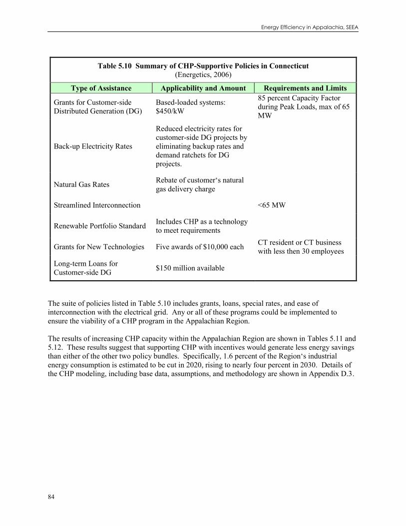
Energy Efficiency in Appalachia, SEEA
84
Table 5.10 Summary of CHP-Supportive Policies in Connecticut (Energetics, 2006)
Type of Assistance Applicability and Amount Requirements and Limits
Grants for Customer-side Distributed Generation (DG)
Based-loaded systems: $450/kW
85 percent Capacity Factor during Peak Loads, max of 65 MW
Back-up Electricity Rates
Reduced electricity rates for customer-side DG projects by eliminating backup rates and demand ratchets for DG projects.
Natural Gas Rates Rebate of customer‘s natural gas delivery charge
Streamlined Interconnection <65 MW
Renewable Portfolio Standard Includes CHP as a technology to meet requirements
Grants for New Technologies Five awards of $10,000 each CT resident or CT business with less then 30 employees
Long-term Loans for Customer-side DG $150 million available
The suite of policies listed in Table 5.10 includes grants, loans, special rates, and ease of interconnection with the electrical grid. Any or all of these programs could be implemented to ensure the viability of a CHP program in the Appalachian Region. The results of increasing CHP capacity within the Appalachian Region are shown in Tables 5.11 and 5.12. These results suggest that supporting CHP with incentives would generate less energy savings than either of the other two policy bundles. Specifically, 1.6 percent of the Region‘s industrial energy consumption is estimated to be cut in 2020, rising to nearly four percent in 2030. Details of the CHP modeling, including base data, assumptions, and methodology are shown in Appendix D.3.

Chapter 5: Industry
85
Figure 5.7 Annual Investment and Energy Savings from Supported CHP, 2010-2030
0
10
20
30
40
50
60
70
80
90
100
2010 2015 2020 2025 2030
Trill
ion
BTU
0
50
100
150
200
250
300
Mill
ion
20
06
$
Energy Savings Public Investment Private Investment
Table 5.11 Energy Savings from Supported CHP
Year Electricity
Savings Natural Gas
Savings Fuel Oil Savings
Total Primary
Energy Saved
% of Sector
Primary Energy (GWh) (trillion Btu) (trillion Btu) (trillion Btu)
2010 0.00 0.00 0.00 0.00 0.00 2013 2,793 -20.10 0.00 11.67 0.47 2020 9,655 -69.46 0.00 40.35 1.64 2030 21,081 -151.66 0.00 88.10 3.58
Table 5.12 Costs and Savings from Supported CHP
Year Energy Savings Admin Costs Investment
Costs
(million 2006$) (million 2006$) (million 2006$)
2010 0.00 0.61 0.00 2013 28.07 0.88 180.04 2020 104.03 1.51 194.78 2030 128.14 2.95 238.67
Figure 5.7 shows the annual investments by private and public entities and the energy savings from supporting CHP. This policy bundle is supported by a large public cost-share throughout the study horizon. These incentives rise rapidly to more than $100 million in 2011 and continue to increase throughout the 20-year time frame. Reducing and eventually eliminating these incentives would perhaps represent a more defensible public policy for the Region. Supporting Combined Heat and Power
with Incentives is not cost-effective as modeled with a benefit-to-cost ratio of about
0.6 for participants and about 0.3 for total resource costs; low forecast electricity prices drive this result. CHP is cost-effective for many individual industrial and commercial facilities. With $2.5

Energy Efficiency in Appalachia, SEEA
86
1.2
1.4
1.6
1.8
2
2.2
2.4
2.6
2.8
3
3.2
2006 2009 2012 2015 2018 2021 2024 2027 2030
Qu
adri
llio
n B
tu
AEO 2007 AEO 2008 With Policy Packages
billion in program spending and an additional $4 billion in customer investments over the 2010-2030 period, the Appalachian Region could see net cumulative savings of 1.9 quads, saving $3.3 billion in energy bills by 2050. This is the equivalent of 3.6 percent of the EIA‘s forecast consumption in 2030, or 21.7 percent of forecast growth (EIA, 2008a). 5.4 SUMMARY OF RESULTS FOR INDUSTRIAL ENERGY EFFICIENCY Based on the industrial program and policy bundles described above, ESAs have the largest potential for energy savings (Figure 5.8)
Figure 5.9 shows that implementation of these policy bundles could eliminate the growth in industrial energy consumption forecast, actually reducing consumption to levels below those in 2006, for the Appalachian Region to 2030. Savings with these three policies are estimated to be 27 percent of forecast consumption in 2030.
Savings in 2030 (Trillion Btu, Delivered)
IAC
62.14
20%
ESA
243.16
80%
CHP offsets 79.73
Trillion Btu of
these delivered
savings (due to
switching)
Savings in 2030 (Trillion Btu, Primary)
IAC, 119.95, 19%
CHP, 88.10, 14%
ESA, 413.08,
67%
Figure 5.8 Industrial Energy Savings by Policy Package (trillion Btu), 2030
Figure 5.9 Industrial Energy Consumption With and Without Energy Efficiency (2010-2030)

Chapter 5: Industry
87
Figure 5.10 shows how investments and energy savings change over time for the industrial policy packages. Although the public contribution to the CHP policy is quite large, private investment is much larger.
0
100
200
300
400
500
600
700
2010 2015 2020 2025 2030
Trill
ion
BTU
0
200
400
600
800
1000
1200
1400
1600
Mill
ion
20
06
$
Energy Savings Public Investment Private Investment These estimated savings are similar to other efficiency studies for states in the Region. A recent report by ACEEE et al. (2008) presented an industrial potential for Virginia of 25 percent of their forecast electricity consumption in 2025 without CHP (they combined commercial and industrial CHP in their analysis). Efficiency potential studies completed for Georgia Power and the Georgia Environmental Facilities Authority found maximum achievable electric efficiencies of 10 percent over 10 years and 6.6 percent over five years, respectively (ICF, 2005; Nexant, 2007). Similarly, a study for North Carolina found a maximum achievable potential for industrial electric efficiency of 12 percent over a 10 year horizon (GDS Associates, 2006). An efficiency potential study for Kentucky modeled cost effective industrial electricity savings of 15.5 percent and natural gas savings of 10.3 percent over 10 years in that state (KPPC, 2007).
A summary of the economic tests performed on the various industrial policies is shown in Table 5.13.
Figure 5.10 Annual Investment and Energy Savings from Industrial Policy Package, 2010-2030

Energy Efficiency in Appalachia, SEEA
88
Table 5.13 Summary of Economic Tests for Industrial Policy Bundles
IAC ESA CHP Total
Participants Test NPV Benefits (billion 2006$) 1.86 5.57 1.53 8.96
NPV Costs (billion 2006$) 0.37 1.96 2.38 4.70
Net Benefits-Costs (billion 2006$)
1.49 3.61 -0.84 4.26
B/C Ratio 5.03 2.84 0.65 1.91 Total Resource Cost Test
NPV Benefits (billion 2006$) 3.00 9.53 0.97 13.51
NPV Costs (billion 2006$) 0.51 2.89 3.09 6.50
Net Benefits-Costs (billion 2006$)
2.49 6.64 -2.12 7.01
B/C Ratio 5.85 3.30 0.31 2.08 The Industrial Policy Package is cost-effective with a benefit-to-cost ratio of about 1.9 for participants and about 2.1 for society. With $2.5 billion in program spending and an additional $13.1 billion in customer investments over the 2010-2030 period, the Appalachian Region could see net cumulative savings of 13.0 quads, saving $58.5 billion in energy bills by 2050. This is the equivalent of about 27.9 percent of the EIA‘s forecast consumption in 2030, or 153 percent of forecast growth (EIA, 2008a).

Chapter 6: Transportation
89
1.2
1.4
1.6
1.8
2.0
2.2
2.4
2.6
2.8
3.0
3.2
2006 2009 2012 2015 2018 2021 2024 2027 2030
Qu
adri
llio
n B
tu
AEO 2007 AEO 2008
6 ENERGY EFFICIENCY IN TRANSPORTATION 6.1 TRANSPORTION ENERGY USE IN APPALACHIA The Appalachian transportation sector consumed 11.6 billion gallons of gasoline and 2.8 billion gallons of diesel in 2006. The transportation sector offers significant energy-efficiency potential through the implementation of stricter standards, enforcement, and a variety of policies. This analysis estimates the energy savings potential from both light- and heavy-duty highway vehicles.27 Heavy-duty consumption of diesel fuel is expected to grow along with population to reach 3.5 billion gallons by 2030 while gasoline consumption will reach 14.8 billion gallons by 2030. However, the passage of new Corporate Average Fuel Economy (CAFE) standards by the 2007 Energy Independence and Security Act (EISA, 2007) will significantly reduce gasoline consumption in Appalachia by 2030.
Light duty gasoline consumption is also projected out to 2030 in Figure 6.1. Forecast growth in consumption falls steeply when the savings that result from the new CAFE standards are considered. The 2007 projection estimates that transportation energy consumption will reach 2.98 quads by 2030 while the 2008 AEO ARC adjusted projection estimates consumption of 2.54 quads by 2030.28 EISA established a CAFE of at least 35 miles per gallon for cars and light trucks by 2020, a 40 percent increase over today's fuel economy standard. Fuel savings documented in the transportation policy options that follow are estimated based on a reference case that
incorporates the effect of new CAFE standards. Our estimates of gasoline savings in Appalachia due to the increase in fuel economy to 35 mpg by 2020 are shown in detail in Table 6.1.
27 Throughout this analysis, we have considered gasoline only in light-duty analysis, and we have considered diesel only in heavy-duty analysis. We recognize that these segments of the sector are not exclusively using these fuels, but they represent the largest percentage of consumed fuel. Savings would also be expected in other fuels used in the sector, but they are not modeled. 28 Please note that energy savings in Table 6.1 were obtained by running a stock model and do not match the consumption figures shown in Figure 6.1.
Figure 6.1 Appalachian Region Transportation Consumption Forecast (quads), 2006-2030
(EIA, 2007a; 2008a)

Energy Efficiency in Appalachia, SEEA
90
Table 6.1 CAFE Fuel Savings
Year
Motor Gasoline
Total Primary Energy Saved % of Sector Primary
Energy (million gallons) (trillion Btu)
2010 22 3 0.1 2013 337 42 1.8 2020 1,843 229 9.5 2030 4,222 524 20.9
The bulk of energy consumed in the transportation sector comes from motor gasoline (63 percent); diesel is another important source (23 percent) while propane, natural gas, ethanol blends, electricity, and other fuels are relied on less (see Figure 6.2).
Motor
Gasoline
63%
Diesel
23%
Other
14%
6.2 POLICY OPTIONS FOR TRANSPORTATION ENERGY EFFICIENCY The policy bundles described in detail in this report include pay-as-you-drive (PAYD) Insurance, Clean Car Standards, low-interest loans for heavy-duty efficiency improvements, and a stricter enforcement of speed limits. Progress has been made around the country on many of the policies discussed. Several experimental PAYD programs are already in place: GMAC offers a mileage-based discount in Arizona, Indiana, Illinois, and Pennsylvania; and Progressive Insurance has a pilot program in Minnesota and is launching one in Texas, where the Legislature has passed a bill allowing companies to offer mileage-based coverage. California recently approved regulations increasing the mileage-based component of insurance rates, and Oregon is providing tax credits to insurers offering pay-as-you-drive policies.
Figure 6.2 Transportation Sector Energy Sources by Fuel, 2006 (EIA, 2008a)

Chapter 6: Transportation
91
Georgia is conducting a PAYD study, and Washington a pilot project, both funded by the Federal Highway Administration.29 Similarly, several states have taken action with regards to fuel economy standards. Fourteen states have currently signed on to California‘s Clean Car Standard, vowing to reduce greenhouse gas emissions by 30 percent of 2002 levels by 2016. These states are still awaiting approval from the EPA to continue with implementation. Table 6.2 highlights the supporting policies that will ensure successful implementation of the options discussed in this chapter.
Table 6.2 Policies That Support Transportation Energy Efficiency
Actions PAYD Clean Car Standards
Heavy-Duty Efficiency Loans
Improved Speed limit Enforcement
Research, Development, and Demonstration
Demonstration or pilot programs for PAYD insurance schemes
Vehicle R&D to encourage development of low-emissions vehicles
N/A N/A
Financing N/A N/A
Low-interest loans for the purchase of new high-efficiency vehicles or the retrofit of existing trucks with approved energy-efficiency technologies
N/A
Financial Incentives
Monetary incentives to insurance companies for each PAYD policy issued
Tax incentives and feebates for efficient vehicles support Clean Car Standards
Rebates and tax incentives to encourage fleet-wide adoption of efficient technologies for heavy trucks
N/A
Pricing PAYD Insurance N/A N/A N/A
Voluntary Agreements
Agreement from insurers to participate on a voluntary basis at the outset of the program
N/A N/A N/A
Regulations
Removal of regulatory obstacles to allow implementation of mileage-base insurance premiums
Clean Car Standards Fuel economy standards for heavy-duty vehicles
Reduced state speed limits, Improved Speed Limit Enforcement
29 Federal Highway Administration, Value Pricing Project Quarterly Report October-December 2006, http://ops.fhwa.dot.gov/tolling_pricing/value_pricing/quarterlyreport/qtr4rpt06/; Sightline Institute, Pay-as-You-Drive Pilot in Washington, http://daily.sightline.org/daily_score/archive/2007/03/29/pay-as-you-drive-pilot-in-washington (2007)

Energy Efficiency in Appalachia, SEEA
92
Table 6.2 Policies That Support Transportation Energy Efficiency
Actions PAYD Clean Car Standards
Heavy-Duty Efficiency Loans
Improved Speed limit Enforcement
Information Dissemination & Training
Industry-wide workshops on PAYD insurance schemes.
N/A N/A
Consumer educational resources targeting road safety and fuel economy savings derived from driving at the speed limit
Procurement N/A
Purchase of fleet vehicles that individually meet the GHG standard
N/A N/A
Market Reforms N/A N/A N/A N/A Planning Techniques N/A N/A N/A N/A
Capacity Building N/A N/A N/A N/A
This table describes policy actions available that could further the savings from this policy; those in italics are modeled in this study while the others are not.
6.3 MODELED SAVINGS IN THE TRANSPORTATION SECTOR 6.3.1 Enabling Pay-As-You-Drive Insurance One reason that people use their vehicles as much as they do is that a high percentage of total driving costs are ―fixed‖ costs, i.e., they are independent of the number of miles driven. The impacts of driving, however, are very dependent on how much people drive. One approach to reducing miles driven is to convert a largely fixed cost, such as insurance, to a variable cost. ―Pay-as-you-drive‖ (PAYD) insurance accomplishes this by having the rate paid by an individual depend heavily on the number of miles driven. Drivers would pay a portion of their premiums up front, and the remainder would be charged in proportion to mileage, as determined by a mileage tracking device or periodic odometer readings. In principle, this makes sense from the insurance industry‘s perspective as well, because those who drive fewer miles have lower accident exposure, on average. The 2005 Federal transportation funding law ―SAFETEA-LU‖ includes a $3 million per year set-aside for experimental, market-based incentive programs like PAYD insurance. Several states have already applied for funding.30 A PAYD program could be an insurance company policy or product, but some action on the part of states may be required to remove regulatory obstacles to changing the basis for premiums or to promote the program. The policy proposed here is to phase in PAYD insurance in the Appalachian Region, starting with a pilot program. For three years beginning in 2009, Appalachian states would offer incentives for insurance policies based largely on miles driven. More specifically, the Region (or entities within the Region) would grant $200 to insurance agencies for each one-year policy they
30 Environmental Defense, Pay-As-You-Drive Auto Insurance, http://www.environmentaldefense.org/article.cfm?contentid=2205

Chapter 6: Transportation
93
write for which 80 percent or more of the pre-program policy cost is scaled by the ratio of miles driven to the state average miles driven. The incentive is necessary so long as PAYD is optional; without it, insurance companies may be concerned about losing revenues from the low-mileage customers who would choose such a policy without being able to offset these costs with higher premiums for high-mileage customers. Should the pilot program prove successful, we recommend phasing in a mandatory PAYD insurance program over the next ten years. Insurance companies would be responsible for converting a percentage of their policies to PAYD, with the percentage increasing each year until PAYD is universal in 2020. Along with implementing PAYD insurance, the state should educate vehicle owners on how they can reduce their insurance payments by driving less. The program proposed here begins with a three-year pilot program subsidized by the Region. The Region would offer insurance companies a $200 incentive per PAYD policy, with goals of 2,000 policies in 2009, 10,000 policies in 2010, and 20,000 policies in 2011. A mandatory program would then be phased in over the next ten years. Miles driven would be monitored using the odometer or an added tracking device. Numbers would periodically be reported back to insurance companies to ensure compliance with regulations. This program would be expected to result in a four percent reduction in driving and vehicle miles traveled (VMT), and consequently light-duty vehicle energy use, by 2020. Table 6.3 presents the projected impacts by year.
Table 6.3 Estimated Impacts of a Mileage Pay-As-You Drive Insurance Program
Year Diesel Motor Gasoline Total Primary
Energy Saved % of Sector Primary Energy
(million gallons) (million gallons) (trillion Btu) 2010 0.00 0.65 0.08 0.00 2013 0.00 130.80 16.24 0.69 2020 0.00 540.45 67.11 2.77 2030 0.00 595.54 73.95 2.91
Insurance companies could incur substantial per-vehicle monitoring costs during the pilot phase of the proposed program for distribution of mileage tracking devices and data collection expenses. However, once the program becomes mandatory, per-vehicle costs would decline as tracking device costs decline and data collection and analysis is spread over a large number of vehicles.31 We assume a per-vehicle cost of $40 per vehicle per year in the pilot phase and $10 per vehicle; thereafter these costs are represented as administrative costs in Table 6.4. While we have considered these costs as administrative costs in this analysis, they will not necessarily be borne by the public office administrating the enabling program; rather, they will not necessarily be borne by the insurance companies and likely passed on to consumers, who will benefit.
31 Bordoff and Noel, 2008

Energy Efficiency in Appalachia, SEEA
94
0
10
20
30
40
50
60
70
80
2010 2015 2020 2025 2030
Trill
ion
BTU
0
50
100
150
200
250
Mill
ion
20
06
$
Energy Savings Public Investment Private Investment
Table 6.4 Energy Savings and Costs a Pay-As-You Drive Insurance Program
Year Energy Savings Admin Costs Investment
Costs (million 2006$) (million 2006$) (million 2006$)
2010 1.60 4.69 2.00 2013 311.57 55.04 0.00 2020 1,298.31 217.44 0.00 2030 1,506.42 232.83 0.00
Although many states and several insurance companies have shown an interest in PAYD insurance, implementation to date has been limited. In a voluntary program, companies already in the market could lose low-mileage customers to new companies that can afford to offer these drivers mileage-based premiums without having to subsidize coverage for high-mileage drivers. To avoid this potential source of opposition to the program, the state could offer incentives only for policies that insurance companies write for their existing customers or for drivers new to the state. When the program becomes mandatory, this concern disappears, because reduced premiums for low-mileage drivers will be offset by increased premiums for high-mileage drivers. Like other pricing policies designed to reduce miles driven and promote alternative travel modes, PAYD insurance may raise questions of equity, especially in rural areas, where alternatives to driving are not readily available. Insurance premiums are generally lower in rural areas than in urban areas, however, so high-mileage premiums would be smaller there. Moreover, in a PAYD program, a rural driver's annual mileage would be compared to that of other rural drivers for purposes of determining the insurance premium. Also, low-income drivers generally drive less than higher-income drivers, and low-income drivers as a group consequently would be net beneficiaries of pay-as-you-drive insurance programs.32 Objections to PAYD insurance have also been raised based on privacy concerns. This is particularly the case when the proposed mileage verification system relies upon GPS-based information. A system based on periodic odometer readings will probably be adequate for such a program, however.
32 Bordoff and Noel, 2008
Figure 6.3 Pay-As-You-Drive Public Investment and Returns

Chapter 6: Transportation
95
An alternative approach to reduce VMT through monetary incentives would be increasing the state gas tax. The average gas tax in the Appalachian states stands at $0.22 per gallon.33 As noted above, PAYD insurance would in effect increase the variable cost of driving by $0.048 per mile. Achieving the same result by raising the gas tax would require an increase of roughly $1.33 per gallon in the gas tax, something that would not be popular with the general public.34 Also, a gas tax increase, unlike PAYD insurance, would increase the tax burden in aggregate unless offset by reductions in other taxes such as income tax. PAYD insurance is one of many measures that could be adopted to reduce vehicle miles traveled, which include fees to enter metropolitan areas, parking pricing, enhanced transit, and improved land use policies to promote compact development. PAYD insurance is used here to signal the importance of a comprehensive approach to energy efficiency in the transportation sector, which must include system efficiency as well as vehicle efficiency. Supporting PAYD insurance is cost-effective with a benefit-to-cost ratio of more than 1,000 for participants and about 7.3 for total resource costs. With $3.4 billion in program spending over the 2010-2030 period, the Appalachian Region could see net cumulative savings of 1.6 quads, saving $32.0 billion in energy bills by 2044. This is the equivalent of about 2.9 percent of the EIA‘s forecast consumption in 2030, or 27.9 percent of forecast growth (EIA 2008a). 6.3.2 Clean Car Standards The energy efficiency of automobiles relates directly to their emissions of carbon dioxide, the dominant greenhouse gas (GHG). States developing plans to reduce GHG emissions are eager to include cars and light trucks, which contribute 27 percent to U.S. GHG emissions.35 Fourteen states have adopted a Clean Car standard, introduced by California, that will reduce greenhouse gas emissions from new vehicles by 30 percent in 2016 while cutting emissions of traditional pollutants as well. These states are: Arizona, California, Connecticut, Maine, Maryland, Massachusetts, New Jersey, New Mexico, New York, Oregon, Pennsylvania, Rhode Island, Vermont, and Washington. Legislation has been introduced in Minnesota, Nevada, Tennessee, and Texas as well. Measures available to meet these states‘ GHG requirements include increased use of alternative fuels and improved air conditioners, for example. But in practice, the primary pathway to meeting the standard will be improvements in vehicle fuel efficiency. Thus, the adoption of the Clean Car Standard throughout the ARC Region could greatly improve vehicle fuel efficiency, thereby helping to meet the energy-efficiency goal. This would come about through accelerated penetration of technologies that are already entering the market, such as variable valve timing, cylinder deactivation, and five-speed transmissions, as well as increased sales of hybrid and diesel vehicles. Despite the recent passage of higher light-duty CAFE standards, many consumers and policymakers are still eager to see the more stringent California emissions criteria implemented nationwide. In addition to increasing efficiency faster in the near term than the new CAFE standards do, California‘s
33 Federal Highway Administration, http://www.fhwa.dot.gov/ohim/mmfr/dec07/trmfuel.cfm 34 A gas tax increase of $1.33 per gallon would in fact reduce fuel consumption by more than a PAYD policy in the long-term because it would affect not only the amount people drive but also their choice of vehicle. We are proposing other mechanisms to increase vehicle efficiency, however. 35 U.S. EPA, ―Greenhouse Gas Emissions from Transportation and Other Mobile Sources,‖ http://www.epa.gov/otaq/greenhousegases.htm

Energy Efficiency in Appalachia, SEEA
96
standards will continue to rise after 2016. California has indicated its intention of extending the GHG standards to levels that would raise average fuel economy to at least 40 mpg by 2020.36 Based on these developments and the existence of cost-effective technologies to further increase fuel economy after 2020, we propose going above and beyond the California program to aim for a combined standard of 50 miles per gallon by 2030. Appalachia‘s adoption of Clean Car Standards means that new vehicles sold in the Region by each manufacturer would need to meet the requirements shown in Table 6.5 for GHG emissions, on average and also the fuel economy goals that we propose highlighted in Table 6.6. The standards divide vehicles into two categories; larger vehicles are allowed higher emissions than smaller vehicles.
Table 6.5 Proposed Clean Car Standards for Greenhouse Gases, 2009-2020a
Year
CO2-equivalent emissions standard (g/mi) Passenger cars and small
trucks/SUVs Large trucks/SUVs
Near-term
2009 323 439 2010 301 420 2011 267 390 2012 233 361
Mid-term
2013 227 355 2014 222 350 2015 213 341 2016 205 332
Long-term
2017 195 310 2018 185 285 2019 180 270 2020 175 265
a CARB, 2008
36 Comparison of Greenhouse Gas Reductions under CAFE Standards and ARB Regulations Adopted Pursuant to AB1493, CARB, 2008

Chapter 6: Transportation
97
Table 6.6 Proposed Fuel Economy Standards 2020-2030
Year Fuel Economy Standards (mpg)
Combined (Passenger cars, small trucks/SUVs and large trucks/SUVs)
2021 42.1 2022 42.9 2023 43.8 2024 44.7 2025 45.6 2026 46.5 2027 47.4 2028 48.2 2029 49.1 2030 50.0
Implementing the Clean Car Standard in the Appalachian Region would result in the energy savings and costs, beyond those of the Federal CAFE program, shown in Tables 6.7 and 6.8. Table 6.7 shows that the savings, modeled only for gasoline and not diesel fueled vehicles, would amount to just 2.6 percent of forecast consumption in 2020, but more than 13 percent in 2030.
Table 6.7 Light-Duty Vehicle Fuel Savings in Appalachia from Adoption of Clean Car Standards
Year Diesel Motor
Gasoline Total Primary Energy Saved % of Sector
Primary Energy (million gallons)
(million gallons) (trillion Btu)
2010 0.00 0.00 0.00 0.00 2013 0.00 87.24 10.83 0.46 2020 0.00 516.19 64.09 2.65 2030 0.00 2,720.23 337.76 13.48
Table 6.8 shows the costs and monetary savings for select years in the study period; private investment grows from just about $50 million in 2010 to more than $2 billion in 2030 to keep up with the standard. Administrative costs remain low.

Energy Efficiency in Appalachia, SEEA
98
0
50
100
150
200
250
300
350
2010 2015 2020 2025 2030
Trill
ion
BTU
0
400
800
1200
1600
2000
2400
Mill
ion
20
06
$
Energy Savings Public Investment Private Investment
Table 6.8 Energy Savings and Costs from Adoption of Clean Car Standards
Year Energy Savings Admin Costs Investment
Costs (million 2006$) (million 2006$) (million 2006$)
2010 0.00 4.29 51.60 2013 207.82 4.29 376.65 2020 1,240.03 4.29 1,235.41 2030 6,880.83 4.29 2,207.77
Figure 6.4 shows the growth in energy savings is rapid over the study horizon with a large private investment. States adopting Clean Car Standards have done so through their Federal Clean Air Act compliance programs. The Clean Air Act allows states to choose between the Federal vehicle pollution control program overseen by the U.S. Environmental Protection Agency (EPA) and the Low Emission Vehicle program devised by the California Air Resources Board (CARB). The latter program is the Clean Car Standards discussed here. However, in order for the standards to come into effect, the State of California must obtain a waiver from the EPA. This waiver was denied by the EPA in February 2008, but California and the 14 other states that have adopted the Clean Car Standards have filed a suit to overturn this denial. The New Clean Car Standard is cost-effective with a benefit-to-cost ratio of about 2.1 for participants and about 2.5 for total resource costs. With $90.1 million in program spending and an additional $24.8 billion in customer investments over the 2010-2030 period, the Appalachian Region could see net cumulative savings of 5.4 quads, saving $108.2 billion in energy bills by 2044. This is the equivalent of about 11.3 to 13.3 percent of the EIA‘s forecast consumption in 2030, or 46.9 to 127.4 percent of forecast growth (EIA, 2007a; 2008a). 6.3.3 SmartWay Heavy Truck Efficiency Loan Program The Appalachian Development Highway System (ADHS) is the first highway system authorized by Congress for the purpose of stimulating economic development and will eventually be a complex
Figure 6.4 Annual Investment and Energy Savings from a New Clean Car Standard, 2010-2030

Chapter 6: Transportation
99
network that connects the Appalachian Region to national markets. Vehicle miles traveled by freight trucks on the ADHS is expected to grow by 400 percent by 2035.37 Due to the level of commercial activity that takes place on the ADHS, heavy trucks make up a significant portion of total vehicle miles traveled in the Appalachian Region. Tractor-trailers dominate heavy-duty fuel usage due to their high annual mileage and relatively low fuel economy. Trucking companies are sensitive to fuel costs, which are typically second only to labor among their business expenses; a tractor-trailer may consume well in excess of $50,000 of fuel annually. Truck manufacturers may therefore be more aggressive in improving the fuel economy of their products than are light-duty vehicle manufacturers. Yet substantial barriers to efficiency do exist in the truck market, including the rapid turnover of trucks from first to second owner and the absence of standards for heavy-duty fuel economy, or even a standardized test procedure to measure it. Consequently, there are numerous technologies and strategies available to improve fuel economy that are not fully utilized. Indeed, average fuel economy for new tractor-trailers could be raised by over 50 percent through a variety of cost-effective existing and emerging technologies, including aerodynamics, engine improvements, transmission enhancements, and weight reduction. 38 Our proposal is to establish a low-interest loan program, beginning in 2009, to promote the purchase of new trucks or the retrofit of existing trucks with approved energy-efficiency technologies and equipment. In particular, equipment in the efficiency package identified by U.S. EPA‘s SmartWay Transport Partnership would be eligible. This SmartWay upgrade kit, which includes aerodynamic add-ons for trailers, efficient tires, and auxiliary power units (APUs) allowing long-distance truckers to dramatically reduce idling, has been found to reduce fuel consumption by 15 percent or more while reducing emissions. We estimate savings from the loan program for truck efficiency equipment, beginning with its application to the improvements identified by SmartWay. Determining what trucks are likely candidates for the program requires a breakdown of the heavy-duty truck stock. By far the biggest consumers of diesel fuel in the aggregate are ―heavy-heavy‖ trucks (those having Gross Vehicle Weight of at least 26,000 pounds), primarily tractor-trailers. Estimated diesel savings are shown in Table 6.9.
Table 6.9 Savings from Low-Interest Loans for Heavy Truck Efficiency Improvements
Year Diesel Motor
Gasoline Total Primary Energy Saved % of Sector
Primary Energy (million gallons)
(million gallons) (trillion Btu)
2010 29.19 0.00 4.03 0.18 2013 73.75 0.00 10.18 0.44 2020 128.87 0.00 17.79 0.73 2030 138.96 0.00 19.19 0.77
37 Cambridge Systematics, 2008 38 Langer, 2004

Energy Efficiency in Appalachia, SEEA
100
0
5
10
15
20
25
2010 2015 2020 2025 2030
Trill
ion
BTU
0
50
100
150
200
250
300
350
400
Mill
ion
20
06
$
Energy Savings Public Investment Private Investment
Table 6.10 shows energy cost savings resulting from reduced consumption of diesel through this loan program; the savings are based on forecast diesel prices (EIA, 2008a). Administrative costs are flat over the program horizon while investment costs decline over time.
Table 6.10 Energy Savings and Costs from Heavy Truck Efficiency Improvements
Year Energy Savings Admin Costs Investment
Costs (million 2006$) (million 2006$) (million 2006$)
2010 74.93 4.29 337.90 2013 183.62 4.29 287.85 2020 321.16 4.29 21.35 2030 371.53 4.29 25.01
Figure 6.5 shows that a constant public investment yields dramatically increasing energy savings in the first years of the program but plateaus around 2017. Private investment is expected to be much higher in the first years of the program. The heavy truck efficiency loan program is likely to be welcomed by trucking companies, especially those with small- to medium-size fleets. With the projected expansion of commercial trucking activity that is expected to take place in the Appalachian Region by 2035, fuel efficiency will be crucial to the operation of trucking fleets, and smaller companies will have more difficulty in affording the SmartWay upgrades described here without financial assistance. The SmartWay Heavy Truck Efficiency Loan Program is cost-effective with a benefit-to-cost ratio of about 1.3 for participants and about 1.6 for total resource costs. With $90.1 million in program spending over the 2010-2030 period, the Appalachian Region could see net cumulative savings of 0.5 quads, saving $10.1 billion in energy bills by 2044. This is the equivalent of about 0.8 percent of the EIA‘s forecast consumption in 2030, or 7.2 percent of forecast growth (EIA, 2008a). 6.3.4 Speed Limit Enforcement At high speeds, vehicle efficiency falls off rapidly with further increases in speed, as aerodynamic drag begins to dominate vehicle energy requirements. The speed at which fuel economy is highest varies from vehicle to vehicle, but is typically below 60 miles per hour (mph) for a light-duty
Figure 6.5 Annual Investments and Energy Savings from SmartWay Loans

Chapter 6: Transportation
101
vehicle.39 Federal Highway Administration tests of nine light-duty vehicles in 1997 found that fuel economy declined on average by 3.1 percent when speed increased from 55 mph to 60 mph and by 8.2 percent increasing from 65 to 70 mph.40 For a heavy truck such as a tractor trailer, fuel economy declines by about two percent per mph at highway speeds.41 Thus, slowing high-speed driving would be one means of improving the real-world efficiencies of cars and trucks. This could be accomplished either by reducing the maximum speed limit or by more stringently enforcing the existing speed limits. Rather than lowering current speed limits, this policy proposes more stringently enforcing the existing speed limits for vehicles in the Appalachian Region. Doing so could both increase highway safety and provide fuel savings. Given demands on the time of police and highway patrol, additional enforcement would best be approached through other means, including increased use of radar, lasers and speed cameras, and education. In many states across the country, recommended practice is to set speed limits at the 85th percentile of driving that occurs on the roadway. In reality, speed limits are set lower than this for most roads; on average, over half of all traffic travels over the speed limit. The energy savings that result from an improved enforcement of speed limits for both light- and heavy-duty vehicles are shown below in Table 6.11.
Table 6.11 Estimated Benefits of Improved Speed Limit Enforcement – Light-Duty and Heavy-Duty Vehicles
Year Diesel Motor
Gasoline Total Primary Energy Saved % of Sector
Primary Energy (million gallons)
(million gallons) (trillion Btu)
2010 33.03 140.13 21.96 0.97 2013 34.78 145.33 22.85 0.98 2020 36.46 150.12 23.67 0.98 2030 39.32 165.43 25.97 1.02
Table 6.12 shows that no private investment is expected to occur for reducing speed limits; however, a constant administrative cost is assumed.
39 ―Drive more efficiently.‖ U.S.DOE and U.S. EPA, http://www.fueleconomy.gov/feg/driveHabits.shtml. 40 Davis and Diegel, 2006 41 ―Factors Affecting Truck Fuel Economy,‖ Goodyear Tire, http://www.goodyear.com/truck/pdf/radialretserv/Retread_S9_V.pdf
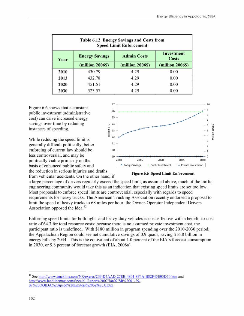
Energy Efficiency in Appalachia, SEEA
102
19
20
21
22
23
24
25
26
27
2010 2015 2020 2025 2030
Trill
ion
BTU
0
1
2
3
4
5
6
7
8
9
10
Mill
ion
20
06
$
Energy Savings Public Investment Private Investment
Table 6.12 Energy Savings and Costs from Speed Limit Enforcement
Year Energy Savings Admin Costs Investment
Costs (million 2006$) (million 2006$) (million 2006$)
2010 430.79 4.29 0.00 2013 432.78 4.29 0.00 2020 451.51 4.29 0.00 2030 523.57 4.29 0.00
Figure 6.6 shows that a constant public investment (administrative cost) can drive increased energy savings over time by reducing instances of speeding. While reducing the speed limit is generally difficult politically, better enforcing of current law should be less controversial, and may be politically viable primarily on the basis of enhanced public safety and the reduction in serious injuries and deaths from vehicular accidents. On the other hand, if a large percentage of drivers regularly exceed the speed limit, as assumed above, much of the traffic engineering community would take this as an indication that existing speed limits are set too low. Most proposals to enforce speed limits are controversial, especially with regards to speed requirements for heavy trucks. The American Trucking Association recently endorsed a proposal to limit the speed of heavy trucks to 68 miles per hour; the Owner-Operator Independent Drivers Association opposed the idea.42 Enforcing speed limits for both light- and heavy-duty vehicles is cost-effective with a benefit-to-cost ratio of 64.3 for total resource costs; because there is no assumed private investment cost, the participant ratio is undefined. With $180 million in program spending over the 2010-2030 period, the Appalachian Region could see net cumulative savings of 0.9 quads, saving $16.8 billion in energy bills by 2044. This is the equivalent of about 1.0 percent of the EIA‘s forecast consumption in 2030, or 9.8 percent of forecast growth (EIA, 2008a).
42 See http://www.truckline.com/NR/exeres/CB4D4AAD-27EB-4801-8F4A-B82F45E03D70.htm and http://www.landlinemag.com/Special_Reports/2007/Jan07/SR%2001-29-07%20OOIDA%20speed%20limiters%20by%20JJ.htm
Figure 6.6 Speed Limit Enforcement

Chapter 6: Transportation
103
6.4 SUMMARY OF RESULTS FOR TRANSPORTATION POLICY BUNDLES Transportation efficiency is rarely modeled in efficiency potential studies, partly because states and local governments, who usually commission such studies, do not historically regulate transportation energy distribution in the same way that they address electricity and natural gas. There have been recent state efforts in this sector, following California, to regulate vehicle efficiency through clean car standards. Our model suggests that standards could provide substantial savings, nearly three-fourths of our total transportation savings in 2030 come from new clean car savings (see Figure 6.7).
Transportation Energy Savings in 2030, by Policy (Trillion Btu,
Primary)
Clean Car
Standard
338
74%
Pay-as-you-
Drive
73.9
16%
SmartWay
19.2
4%
Speed Limits
26.0
6% Figure 6.8 shows that the combined transportation package reduces consumption to less than 2006 levels by 2022 with savings roughly doubling what is estimated by the EIA to come from the new efficiency requirements in EISA 2007.
1.2
1.4
1.6
1.8
2
2.2
2.4
2.6
2.8
3
3.2
2006 2009 2012 2015 2018 2021 2024 2027 2030
Qu
adri
llio
n B
tu
AEO 2007 AEO 2008 With Policy Packages
Figure 6.9 shows that public investment remains low for the entire study horizon while private investment climbs quickly from 2010 to 2016 and steadily thereafter; the bumps in the private
Figure 6.7 Primary Energy Savings by Policy Package (trillion Btu), 2030
Figure 6.8 Transportation Primary Energy Consumption With and Without Policy Packages (quads), 2006-2030

Energy Efficiency in Appalachia, SEEA
104
investment line represent peaks in investment in the Pay-as-you-Drive and SmartWay programs. Annual energy savings grow, in an exponential fashion, for the entire period.
0
50
100
150
200
250
300
350
400
450
500
2010 2015 2020 2025 2030
Trill
ion
BTU
0
500
1000
1500
2000
2500
Mill
ion
20
06
$
Energy Savings Public Investment Private Investment
Table 6.13 shows the benefit/cost ratios for each transportation policy bundle as well as test results for combined policy implementation.
Figure 6.9 Annual Investments and Energy Savings from Transportation Policy Packages, 2010-2030

Chapter 6: Transportation
105
Table 6.13 Results of Economic Tests for Transportation Policy Bundles
Clean Car Standard
Pay-As-You-Drive Insurance
SmartWay Speed Limits Total
Participants Test NPV Benefits (billion 2006$) 14.94 6.87 2.37 4.39 28.57
NPV Costs (billion 2006$) 7.11 0.01 1.78 0.00 8.89
Net Benefits-Costs (billion 2006$)
7.83 6.86 0.60 4.39 19.68
B/C Ratio 2.10 1,340 1.34 – 3.21
Total Resource Cost Test
NPV Benefits (billion 2006$) 25.49 10.20 3.37 5.98 45.04
NPV Costs (billion 2006$) 10.00 1.39 2.05 0.09 13.54
Net Benefits-Costs (billion 2006$)
15.49 8.80 1.32 5.89 31.49
B/C Ratio 2.55 7.31 1.64 64.32 3.33
The transportation sector policy package is cost-effective with a benefit-to-cost ratio of about 3.2 for participants and about 3.3 for total resource costs. With $3.7 billion in program spending and an additional $27.6 billion in customer investments over the 2010-2030 period, the Appalachian Region could see net cumulative savings of 8.3 quads, saving $167.1 billion in energy bills by 2044. This is the equivalent of about 30.1 percent of the EIA‘s forecast consumption in 2030, or 172.4 percent of forecast growth (EIA, 2008a).

Energy Efficiency in Appalachia, SEEA
106
Box 6.1 Intermodal Improvements Several opportunities have been identified to improve the freight transportation network in the Appalachian Region through intermodal investments. Such improvements have been driven first and foremost by the Region's goal of economic growth, based on better integration with the rest of the country. Tapping into areas of growth in the national and global economies will require up-to-date approaches to moving goods, which today increasingly implies the use of energy-efficient technologies and modes. Consequently, energy-efficient freight movement, while perhaps not the driver of new transportation investment, could be a key element of the Region‘s economic development program. At the same time, to the extent that modern intermodal services draw freight from adjacent Regions, they could cause energy consumption within the Appalachian Region to increase, despite reducing energy consumption overall. Among the intermodal projects in progress or under consideration to serve the Appalachian Region are:
the Central Corridor Doublestack Initiative, to allow stacked intermodal containers to travel by rail along the Norfolk Southern route from Norfolk to Columbus;
the South Carolina Inland Port, which would alleviate space and congestion pressures at the Port of Charleston by sending containers by rail from the port to an inland processing and transfer facility; and
the Port of Pittsburgh Container-on-Barge, to provide a water alternative to trucking for high-value goods traveling throughout the inland waterway system of the Appalachian Region and the Gulf Coast. (Rahall Transportation Institute and Wilbur Smith Associates, 2004)
Each of these three examples represents an opportunity to increase the efficiency of the goods movement system while reducing energy use by diverting freight from trucks to other modes. Rail and barge operations generally consume far less energy per ton-mile than trucks. While these projects are designed to attract the rapidly-growing and lucrative container flows associated with international trade, is it important to note that projected growth in freight traffic is largely tied to intraregional activity (Rahall Transportation Institute and Wilbur Smith Associates, 2004). Much of this shorter-distance freight will necessarily travel by truck, but if alternative modes can serve some intraregional traffic, freight energy use will decline. Aside from highways, freight infrastructure has historically been funded by the private sector. Today there is a crucial role for regional and national governments in the development and funding of this infrastructure, particularly for intermodal freight, given the large public costs and benefits of the goods movement system, the need for multi-state cooperation, the need for freight facilities serving multiple, competing carriers, and constraints on freight carriers‘ ability to invest in innovative projects.

Chapter 7: Macroeconomic Results
107
7 MACROECONOMIC RESULTS: EMPLOYMENT, INCOME, AND ECONOMIC ACTIVITY
Up to this point in the analysis we have examined the potential costs and benefits of implementing policies that might stimulate greater levels of energy efficiency within the Appalachian Region. The evidence suggests that smart policies and programs can drive more productive investments in energy-efficient technologies, and they can do so in ways that reduce the Region‘s total energy bill. But the question remains, what does this mean for the Regional economy? Do the higher gains in energy productivity – that is, do the increased levels of efficiency investment with their concomitant reduction in the need for conventional energy resources – create a net economic boost for Appalachia? Or, does the diversion of revenues away from energy-related industries negatively impact the Regional economy? In this chapter, we explore those issues and we present the analytical results of an economic model used to evaluate the impact of efficiency investments on jobs, income, and the overall size of the economy. A recent meta-review of some past 48 energy policy studies done within the United States suggests that if investments in more efficient technologies are cost-effective, the impacts on the economy should be small but net positive (Laitner and McKinney, 2008). As shown elsewhere in the report, it turns out that from a total resource cost perspective, the benefits (i.e., the energy bill savings) outweigh both the policy costs and investments by about two and one-half times. In other words, the energy-efficiency policy recommendations highlighted in the ―Region-at-Risk‖ scenario result in a substantial savings for households and businesses compared to the costs of implementing the policies. As we also discuss below, this consumer energy bill savings can drive a significant increase in the number of net new jobs within the Appalachian Region.43 In fact, continued investments in energy-efficiency resources would maintain the energy resource benefits for many years into the future, well beyond the period of analysis examined in this report.44 The Region therefore has the opportunity to transition its energy markets to a more sustainable pattern of energy production and consumption in ways that benefit consumers. 7.1 METHODOLOGY The macroeconomic evaluation that we report in this chapter is undertaken in three separate steps. First, we calibrate ACEEE‘s economic assessment model called DEEPER (Dynamic Energy Efficiency Policy Evaluation Routine) to reflect the economic profile of the Appalachian economy (Laitner and McKinney, forthcoming). This is done for the period 2006 (the base year of the model) through 2030 (the last year of the analysis). In this respect, we incorporate the anticipated investment and spending patterns that are suggested by the standard forecast modeling assumptions. These range from typical spending by businesses and households in the analytical period to the anticipated construction of new electric power plants and other energy-related spending that might also be highlighted in the forecast. Second, we transform the set of key efficiency scenario results
43 As we use the term here, the word ―consumer‖ refers to any one who buys and uses energy. Thus, we include both households and businesses as among the consumers who benefit from greater investments in energy efficiency. 44 As we note elsewhere, the policy analysis ends in the year 2030. Yet, many of the investments we describe have a technology of perhaps 15 years. This means that investments made in 2030 would continue to pay for themselves through perhaps the year 2044 and beyond; and none of those ongoing energy bill savings are reflected in the analysis described in this chapter.

Energy Efficiency in Appalachia, SEEA
108
from the policy analysis into the direct inputs which are needed for the economic model. The resulting inputs include such parameters as:
1. The level of annual policy and/or program spending that drives the key policy scenario investments;
2. The capital and operating costs associated with more energy-efficient technologies; 3. The energy bill savings that result from the various energy-efficiency policies described in
the main body of the report; and 4. Finally, a set of calibration or diagnostic model runs to check both the logic and the internal
consistency of the modeling results. So that we can more fully characterize the analysis that was completed for this report, we next provide a simplified working example of how the modeling is done. We first describe the financial assumptions that underpin the analysis. We then highlight the analytical technique by showing the kinds of calculations that are used and then summarize the overall results in terms of net job impacts. Following this example, we then review the net impacts of the various policies as evaluated in our DEEPER model. A more detailed description of the economic model is presented in Appendix F. 7.2 ILLUSTRATING THE METHODOLOGY: APPALACHIAN JOBS FROM
EFFICIENCY GAINS To illustrate how a job impact analysis might be done, we will use the simplified example of installing one hundred million dollars of efficiency improvements within large office buildings throughout the Appalachian Region. Office buildings (traditionally large users of energy due to heating and air-conditioning loads, significant use of electronic office equipment, and the large numbers of persons employed and served) provide substantial opportunities for energy-saving investments. The results of this example are summarized in Table 7.1. The assumption used in this example is that the investment has a positive benefit/cost ratio of 2.0. In other words, the assumption is that for every dollar of cost used to increase a building‘s overall energy efficiency, the upgrades might be expected to return a total of two dollars in reduced electricity and natural gas costs over the useful life of the technologies. This ratio is similar but generally lower to those cited elsewhere in this report. At the same time, if we anticipate that the efficiency changes will have an expected life of roughly 15 years, then we can establish a 15-year period of analysis. In this illustration, we further assume that the efficiency upgrades take place in the first year of the analysis, while the electricity bill savings occur in years one through 15.

Chapter 7: Macroeconomic Results
109
Table 7.1 Job Impacts from Commercial Building Efficiency Improvements
Expenditure Category Amount (million $)
Employment Coefficient
Job Impact
Installing Efficiency Improvements in Year One $100 13 1,300
Diverting Expenditures to Fund Efficiency Improvements $-100 12 -1,200
Energy Bill Savings in Years One through 15 $200 12 2,400
Lower Utility Revenues in Years One through 15 $-200 5 -1,000
Net 15-Year Change $0.0 1,500
Note: The employment multipliers are adapted from the appropriate sector multipliers found in Appendix F. The benefit/cost ratio is assumed to be 2.0. The jobs impact is the result of multiplying the row change in expenditure by the row multiplier. The sum of these products yields a working estimate of total net job-years over the 15-year time horizon. To find the average annual net jobs in this simplified analysis we would divide the total job-years by 15 years which, of course, gives us an estimated net gain of 100 jobs per year for each of the 15 years. For more details, see the text that follows.
The analysis assumes that we are interested in the net effect of employment and other economic changes. This means we must first examine all changes in household and business expenditures – both positive and negative – that result from a movement toward greater levels of energy efficiency. Although more detailed and complicated within the DEEPER model, for this heuristic exercise we then multiply each change in expenditures by the appropriate sector employment coefficient (adapted from the values shown in Appendix F). The sum of these products will then yield the net result for which we are looking. In our example above, there are four separate changes in expenditures, each with their separate impact. As Table 7.1 indicates, the net impact of the scenario suggests a cumulative gain of 1,500 jobs in each of the 15-year period of analysis. This translates into an average net increase of 100 jobs each year for 15 years. In other words, the $100 million efficiency investment made in Appalachian office buildings is projected to sustain an average of 100 jobs each year over a 15-year period compared to a ―business-as-usual‖ scenario. The economic assessment of the alternative energy scenarios was carried out in a very similar manner as the example described above. That is, the changes in energy expenditures brought about by investments in energy-efficiency and renewable technologies were matched with their appropriate employment multipliers. There are several modifications to this technique, however. First, it was assumed that only 72 percent of both the efficiency investments and the savings are spent within the Appalachian Region. We based this initial value on the Minnesota IMPLAN Group, Inc. (IMPLAN, 2008) dataset as it describes local purchase patterns that typically now occur in the

Energy Efficiency in Appalachia, SEEA
110
Region. We anticipate that this is a conservative assumption since most efficiency and renewable energy installations are likely (or could be) carried out by local contractors and dealers. If the set of policies encourages greater local participation so that the share was increased to 90 percent, for example, the net jobs might grow another 15 percent compared to our standard scenario exercise. At the same time, the scenario also assumes Appalachia provides only 40 percent of the manufactured products consumed within the Region. But again, a concerted effort to build manufacturing capacity for the set of clean energy technologies would increase the benefits from developing a broader in-state energy efficiency and renewable energy manufacturing capability. Second, an adjustment in the employment impacts was made to account for assumed future changes in labor productivity. As outlined in the Bureau of Labor Statistics Outlook 2006–2016, productivity rates are expected to vary widely among sectors (BLS, 2008). For instance, drawing from the BLS data we would expect that electric utilities might increase labor productivity by 1.8 percent annually while the business and personal service sectors of the economy might increase productivity by 2.2 percent per year. This means, for example, that we might expect a one million dollar expenditure for utility services in the year 2030 would support only 68 percent of the jobs that the same expenditure would have supported in 2008, while other services sectors of the economy would support only 62 percent of the jobs as in 2008. Third, for purposes of estimating energy bill savings, it was assumed that all energy prices within Appalachia would follow the same growth rate as those published by the Energy Information Administration in its Annual Energy Outlook (EIA, 2008a).45 Fourth, it was assumed that approximately 80 percent of the efficiency investments‘ upgrades are financed by bank loans that carry an average eight percent interest rate over a five-year period. To limit the scope of the analysis, however, no parameters were established to account for any changes in interest rates as less capital-intensive technologies (i.e., efficiency investments) are substituted for conventional supply strategies, or in labor participation rates – all of which might affect overall spending patterns. Fortunately, however, it is unlikely that these sensitivities would greatly impact the overall outcome of this analysis. While the higher cost premiums associated with the energy-efficiency investments might be expected to drive up the level of borrowing (in the short term), and therefore interest rates, this upward pressure would be offset to some degree by the investment avoided in new power plant capacity, exploratory well drilling, and new pipelines. Similarly, while an increase in demand for labor would tend to increase the overall level of wages (and thus lessen economic activity), the job benefits are small compared to the current level of unemployment or underemployment in the Region. Hence the effect would be negligible. Fifth, as described in the previous chapters for the buildings, industrial, and transportation end-use sectors it was assumed that a program and marketing expenditure would be required to promote market penetration of the efficiency improvements. Since these vary significantly by policy bundle we don‘t summarize them here but payment for these policy and program expenditures were treated as if new taxes were levied on the Region commensurate with the level of energy demands within the Region. Hence, the positive program spending impacts are offset by reduced revenues elsewhere in the economy. 45 In fact, we used a population-weighted average of regional energy prices referenced in the Annual Energy Outlook as they overlapped with the states and counties found within the jurisdiction of the Appalachian Regional Commission.

Chapter 7: Macroeconomic Results
111
Sixth, it should be noted that the full effects of the efficiency investments are not accounted for since the savings beyond 2030 are not incorporated in the analysis. Nor does the analysis include other benefits and costs that can stem from the efficiency investments. Non-energy benefits can include increased worker productivity, comfort and safety, and water savings, while non-energy costs can include aesthetic issues associated with compact fluorescent lamps and increased maintenance costs due to a lack of familiarity with new energy-efficiency equipment (NAPEE, 2007b, p. 3-8). Productivity benefits, for example, can be substantial, especially in the industrial sector. Industrial investments that increase energy efficiency often result in achieving other economic goals such as improved product quality, lower capital and operating costs, increased employee productivity, or capturing specialized product markets (see, for example, Worrell et al., 2003). To the extent these ―co-benefits‖ exceed any non-energy costs, the economic impacts of an energy-efficiency initiative in Appalachia would be more favorable than those reported here. Finally, although we show how the calculations would look from an employment perspective, we don‘t show the same kind of data or assumptions for either income or for impacts on the Gross Regional Product (the sum of value-added contributions to the Appalachian Regional economy). Nonetheless, the approach is very similar to that described for net job impacts. 7.3 IMPACTS OF RECOMMENDED ENERGY-EFFICIENCY POLICIES For each year in the analytical period, the given change in a sector spending pattern (relative to the reference scenario) was matched to the appropriate sectoral impact coefficients. Two points are worth special note: first, it was important to match the right change in spending to the right sector of the Appalachian economy; and second, these coefficients change over time. For example, labor productivity changes mean that there may be fewer jobs supported by a one million dollar expenditure today compared to that same level of spending in 2030. Both the negative and positive impacts were summed to generate the estimated net results shown in the series of tables that follow. Presented here are two basic sets of macroeconomic impacts for the benchmark years of 2010, 2013, 2020, and 2030. These include the financial flows that result from the policies described in the previous chapters. They also include the net jobs, income, and GRP impacts that result from the changed investment and spending patterns. Table 7.2 presents the changes in consumer expenditures that result from these policies. While the first row in the table presents the full cost of the energy-efficiency policies, programs, and investments, the utility customers will likely borrow a portion of the money to pay for these investments. Thus, ―annual consumer outlays,‖ estimated at about $1,083 million 2010, rise to $6,165 million (or nearly $6.2 billion) in 2030. These outlays include actual ―out-of-pocket‖ spending for programs and investments, along with money borrowed to underwrite the larger technology investments. The annual energy bill savings reported in Table 7.1 are a function of reduced energy purchases from the many Appalachian utilities and other energy providers within the Region. As we further highlight in the table that follows, the annual energy bill savings begins with a modest first year benefit of $708 million. As more and more investments are directed toward the purchase of more energy-efficient technologies, the annual consumer energy bill savings rise to about $27.6 billion by 2030.

Energy Efficiency in Appalachia, SEEA
112
Table 7.2 Financial Impacts from Energy-Efficiency Policy Scenario
(Millions of 2006 $) 2010 2013 2020 2030
Annual Consumer Outlays 1,083 2,734 4,564 6,165
Annual Energy Savings 788 2,577 9,944 27,567
Annual Net Consumer Savings (295) (157) 5,380 21,402
Cumulative Net Energy Savings (295) (1,230) 15,226 150,809
‗Annual‘ refers to the total that is reported in the benchmark year while ‗Cumulative‘ is the total from previous years beginning in 2010 through the benchmark year. Annual consumer outlays include administrative costs to run programs, incentives provided to consumers, investments in energy-efficiency devices and interest paid on loans needed to underwrite the needed efficiency investments. Annual energy savings is the reduced energy bill expenditures that benefit both households and businesses within a given year. The net savings is the difference between savings and outlays. The numbers in parentheses are losses in that specific year.
Perhaps the critical element that jumps out in Table 7.2 is that, in the early years and especially as the policies ramp up quickly to simulate a greater level of efficiency improvements, the consumer outlays outweigh the energy bill savings. In 2010, the net costs begin at $295 million and rise through 2013. Although not shown in the table, this remains the case through the year 2014 when the savings show a small net return of $11 million. These savings mount steadily through the year 2030 by when they nearly reach an estimated $21.4 billion for the Region as a whole. The last row of the table highlights cumulative impacts with losses peaking in 2013 and ending in 2015 (not shown). By 2030 the net cumulative savings over the period 2010 through 2030 are strongly net positive at just under $151 billion. While the annual net consumer savings first turn positive in 2014 – four years after the policy initiatives are in operation – the simple payback period to participants is much shorter, ranging from 1.54 to 3.75 years, from 2010 to 2030 or 2.24 to 3.75 from 2011 to 2030, depending on the year of participation. The shortest payback is for investments made in 2010 and the longest in 2011, in the aggregate. The benefits, from a TRC perspective, outweigh costs by about 3.3 times. At this point we then have the financial flows estimated as they are distributed across the end-use sectors described earlier in the report. The question then becomes what might be the impacts on the Regional economy as we‘ve been able to evaluate them for a given year using the DEEPER model. The modeling then evaluates impact on jobs and wages sector-by-sector, and evaluates their contribution to Appalachia‘s Gross Regional Product (GRP), which is a sum of the net gain in value-added contributions provided by the energy productivity gains throughout all sectors of the Regional economy. As with the previous table on financial impacts, Table 7.3 highlights the net impacts for the benchmark years 2010, 2013, 2020, and 2030.

Chapter 7: Macroeconomic Results
113
Table 7.3 Economic Impact of Energy-Efficiency Investment in Appalachia
Macroeconomic Impacts 2010 2013 2020 2030
Jobs (Actual) 16,231 15,466 37,268 77,378
Wages (million $2006) 517 450 1,169 3,018
GRP (million $2006) 763 444 1,197 3,056 Given both the financial flows and the modeling framework, the analysis suggests a net contribution to the Appalachian employment base as measured by full-time jobs equivalent. In the year 2010 we see a small net increase of 16,231 jobs which increases to a significantly larger total of 77,378 net jobs by 2030. This significantly positive impact might seem to provide us with a counterintuitive result. The early years of the policy scenarios show small net cost to the economy. Yet we continue to see a net increase in jobs. How is this possible? In Appalachia, the electric utility and the natural gas service sectors directly and indirectly employ about 5.3 and 3.7 jobs, respectively, for every $1 million of spending (as highlighted in the multiplier table in Appendix F). But, sectors vital to energy-efficiency improvements, like construction and manufacturing, utilize 13.3 and 8.3 jobs per $1 million of spending. Once job gains and losses are netted out in each year, and following a similar logic shown in Table 7.1, the analysis suggests that, by diverting expenditures away from non-labor intensive energy sectors, the cost-effective energy policies can positively impact the larger Appalachia economy – even in the early years, but especially in the later years of the analysis as the energy savings continue to mount. To highlight the results of this analysis in a little more detail, Figure 7.1 provides year-by-year impacts on net jobs within the Appalachia Region. Figure 7.2 highlights the anticipated net gain to the state‘s wage and salary compensation and GRP, both measured in millions of 2006 dollars.
0
10
20
30
40
50
60
70
80
2010 2015 2020 2025 2030
Job
s (t
ho
usa
nd
s)
Figure 7.1 Net Job Impacts for Appalachia (2008-2030)

Energy Efficiency in Appalachia, SEEA
114
The end result of this policy analysis, then, suggests that an early program stimulus which drives a higher level of efficiency investments can actually increase economic impact, creating an average of 16,000 net new jobs each year in the first five years of the study, and rising to an estimated average of 60,000 net new jobs over the last decade of the analysis. This is roughly equivalent to the employment that would be directly and indirectly supported by the construction and operation of 480 small manufacturing plants within Appalachia. As indicated by Figure 7.2, these investments also increase both wages and Gross Regional Product throughout Appalachia.
0.0
0.5
1.0
1.5
2.0
2.5
3.0
3.5
2010 2015 2020 2025 2030
Bill
ion
20
06
$
Wages GSP
In short, the more efficient use of energy resources provides a cost-effective redirection of spending away from less labor-intensive sectors into those sectors that provide a greater number of jobs within Appalachia. Similarly, cost-effective energy productivity gains also redirect spending away from sectors that provide a smaller rate of value-added into those sectors with slightly higher levels of value-added returns per dollar of revenue. The extent to which these benefits are realized will depend on the willingness of business and policy leaders to implement the recommendations that are at the heart of this report and found earlier in this assessment.
Figure 7.2 Wages and Gross Regional Product Impacts for Appalachia (million 2006$), 2008-2030

Chapter 8: Summary and Conclusions
115
7.0
7.5
8.0
8.5
9.0
9.5
10.0
10.5
11.0
11.5
2006 2009 2012 2015 2018 2021 2024 2027 2030
Qu
adri
llio
n B
tu
AEO 2007 AEO 2008 With Policy Packages
8 SUMMARY AND CONCLUSIONS 8.1 ECONOMY-WIDE RESULTS An aggressive package of energy-efficiency policies implemented throughout Appalachia beginning in 2010 could deliver significant cost-effective energy savings. According to the latest EIA ―business-as-usual‖ forecast, Appalachia will require 9.2 quads of energy in 2020 and 10.1 quads in 2030. In contrast, a bold energy-efficiency initiative could cut that consumption by between 9 and 12 percent to 8.2 quads in 2020 and by between 23 and 28 percent to 7.7 quads in 2030. Such a bold and aggressive initiative could shrink the energy budget required by the Region in 2030 to less than the Region consumed in 2006 – more than offsetting the forecast growth in energy use (Figure 8.1). In 2030, most of the energy-efficiency resources (42 percent) come from efficiency programs for commercial buildings. The remaining energy savings come mostly from industrial energy uses (25 percent), followed by transportation (18 percent) and residences (15 percent). Accounting for 28 percent of energy use in Appalachia but only 18 percent of the energy efficiency resources, transportation has a relatively low energy-efficiency potential. This conclusion is understandable given the newly legislated energy-efficiency standards that require 40 percent stricter vehicle fuel economy standards by 2020. These savings are incorporated in the AEO 2008 baseline. Primary Energy Savings, by Sector (2030, Trillion Btu)
Residential
374
15%
Industrial
621
25%
Transportation
457
18%
Commercial
1030
42%
Figure 8.1 Potential Displacement of Appalachian Energy Consumption by Cost-Effective Efficiency Resources
Figure 8.3 Share of Cost-Effective Efficiency Resources by Sector, Excluding Commercial
Commissioning (Primary Energy in trillion Btu, 2030)
Figure 8.2 Share of Cost-Effective Efficiency Resources by Sector
(Primary Energy in trillion Btu, 2030)
Primary Energy Savings (excluding Commercial Commissioning),
by Sector (2030, Trillion Btu)
Residential
374
18%
Commercial
641
30%Industrial
621
30%
Transportation
457
22%

Energy Efficiency in Appalachia, SEEA
116
Consider the case where the energy-savings potential from the commissioning of commercial buildings is excluded from the estimation of energy efficiency resources (because of its unknown degree of overlap with the commercial building retrofit incentive program). In this situation, the total energy-efficiency potential in 2030 would be 0.4 quads smaller. At the same time, these energy efficiency resources would be much more evenly distributed across the four end-use sectors (Figure 8.3). Examining the potential energy-efficiency impacts of individual policies draws attention to five policy instruments that substantially ―move the market‖ (Table 8.1). The efficient commercial HVAC and lighting retrofit incentive has the largest impact, reducing commercial energy consumption by 10 percent in 2020 and by almost 20 percent in 2030. Support for commissioning of existing commercial buildings is the next most significant policy in terms of saving energy in the year 2030. It cuts commercial energy consumption in 2030 by an additional 17 percent. The expanded industrial assessment centers policy, which targets small- to medium-sized industrial sites, has the third largest impact in 2030. By that year, it is assumed that all of the eligi ble sites have had an energy assessment and 80 percent of the cost-effective recommendations are adopted, producing a 17 percent reduction in the Region‘s industrial energy consumption. Clean car standards offer the fourth largest potential for saving energy and are by far the most influential of the four transportation policy packages modeled here. By accelerating the fuel economy improvements of combined passenger cars, small trucks/SUVs and large trucks/SUVs to 50 mpg in 2030, 13 percent of the transportation energy use forecast for that year can be reduced. Finally, providing retrofit incentives for existing homes in combination with resale energy labeling has the fifth largest energy impact in 2030; it cuts the residential sectors projected energy consumption by four percent in 2020 and by seven percent in 2030.

Chapter 8: Summary and Conclusions
117
Table 8.1 Energy Savings from Individual Policies (trillion Btu of primary energy saved per year)*
Primary Energy
Savings: 2013
Primary Energy
Savings: 2020
Primary Energy
Savings: 2030
Residential Buildings
Improved Building Energy Code with Third Party Verification and Compliance Incentive 5.3 (0.3%) 40.5 (1.9%) 123.3 (5.0%)
Expanded Weatherization Assistance Programs 9.2 (0.5%) 26.2 (1.2%) 53.0 (2.1%)
Residential Retrofit Incentive with Resale Energy Labeling and Incremental Cost Incentives 32.8 (1.7%) 91.5 (4.2%) 180.2 (7.3%)
Super-Efficient Appliance Deployment 6.1 (0.3%) 28.5 (1.3%) 97.0 (3.9%)
Commercial Buildings
Commercial Building Energy Codes with Third Party Verification and Compliance Incentives 5.4 (0.3%) 23.1 (1.2%) 63.9 (2.8%)
Support for Commissioning of Existing Commercial Buildings 28.1 (1.7%) 148.1 (7.8%) 390.8 (17.3%)
Efficient Commercial HVAC and Lighting Retrofit Incentive 46.7 (2.9%) 194.5 (10.3%) 447.1 (19.7%)
Tightened Office Equipment Standards with Efficient Use Incentives 11.6 (0.7%) 53.2 (2.8%) 143.2 (6.3%)
Industry
Expanded Industrial Assessment Centers 18.1 (0.7%) 123.2 (5.0%) 413.1 (16.8%)
Increasing Energy Savings Assessments 10.4 (0.4%) 53.6 (2.2%) 119.9 (4.9%)
Supporting Combined Heat and Power (CHP) with Incentive 11.7 (0.5%) 40.3 (1.6%) 88.1 (3.6%)
Transportation
Pay-as-You-Drive Insurance 16.2 (0.7%) 67.1 (2.8%) 73.9 (2.9%)
Clean Car Standards 10.8 (0.5%) 64.1 (2.6%) 337.8 (13.3%)
SmartWay Heavy Truck Efficiency Loan Program 10.3 (0.4%) 17.9 (0.7%) 19.3 (0.8%)
Speed Limit Enforcement 22.8 (1.0%) 23.7 (1.0%) 26.0 (1.0%)
*Also expressed as a percent of the energy to be consumed in that year based on the ―business-as-usual‖ forecast.

Energy Efficiency in Appalachia, SEEA
118
Most of the policies modeled in this study spur innovation and technology improvement, as would be the case, for instance, with clean car standards of 50 mpg. In order to illustrate the potential for a concerted energy-efficiency RD&D initiative to expand clean energy opportunities in Appalachia, we analyzed three transformational technologies that appear to hold great promise for the region. The results are summarized in Box 8.1, and the background details are presented in Chapters 3, 4, and 5.
Box 8.1 The Promise of RD&D to Expand the Efficiency Potential of Three Transformational Technologies
Air-source integrated heat pump
Accelerated RD&D is assumed to result in the commercialization of a single system based on heat pumping technology that provides space heating and cooling, water heating, ventilation and dehumidification, and humidification. It is still in the development stages and is not yet commercially available; however, it could provide substantial energy savings to homes is the Appalachian Region. Within an average Appalachian home, installation of the AS-IHP would save approximately 37 million Btu per year. If this heat pump system were installed in 30 percent of all new homes built in Appalachia between 2010 and 2030, energy consumption in the residential sector could be reduced by 35 trillion Btu in the year 2030.
Solid State Lighting Accelerated RD&D is expected to produce technology improvements that bring brighter LEDs and provide light equivalent to existing fluorescent fixtures with 25 to 45 percent less electricity usage. Lighting demand for the Appalachian Region is expected to increase by little more than 10 percent between 2006 and 2030 (EIA, 2008a). However, under the LED scenario lighting demand would be expected to decrease by more than 20 percent. If by 2030, LED lighting fully penetrated the Appalachian Region, the Region would use 20 percent less energy for lighting than projected, saving 60 trillion Btu in that year.
Industrial super boiler A combination of enhanced design features could increase industrial package boiler efficiency from 75 percent to 95 percent. Many boilers used today are more than 40 years old, suggesting a large energy-savings opportunity. The Appalachian Region, particularly the southern portion, makes heavy use of boilers and widespread installation of a more efficient boiler could mean tremendous savings, in energy and financial cost. Assuming that super boilers replace one percent of all boilers within the Appalachian Region annually, and the average improvement in efficiency with the super boiler is 10 percent, this new technology could save almost 20 trillion Btu in 2030 and a total of 172 trillion Btu between 2010 and 2030.
Dividing the cost-effective energy-efficiency resources fostered by the entire policy portfolio into fuel types and sectors highlights the prominence of the potential for reduced electricity consumption. Taking into account the energy lost in the generation and transmission of electricity as well as losses from ―end-use‖ equipment such as motors, lighting, and air conditioning, 69 percent of the energy-efficiency potential in Appalachia resides in the electricity system (i.e., 1.7 quads of the 2.5 quads of energy-efficiency potential in 2030). The next largest wedge of energy-savings potential comes from motor gasoline consumption by vehicles (17 percent), followed by savings potentials from natural gas, fuel oil, and diesel end-uses (14 percent).

Chapter 8: Summary and Conclusions
119
The 1.7 quads of electricity-efficiency potential in 2030 represent a potential savings of 33 percent relative to the projected consumption of electricity in 2030 (that is, 5.2 quads of primary energy). It represents 106 percent of the anticipated 1.6 quads of load growth in 2030.
0
500
1000
1500
2000
Trill
ion
Btu
Transportation 0.0 0.0 0.0 24.8 432
Industrial 565 56.0 0.0 0.0 0.0
Commercial 871 141 20.5 0.0 0.0
Residential 274 85.1 13.9 0.0 0.0
Electric
Savings
Natural Gas
Savings
Fuel Oil
Savings
Diesel
Savings
Motor
Gasoline
1710
28234 24.8
432
Tables 8.2 and 8.3 provide additional detail on the cost-effective efficiency resources estimated to be available in the Appalachian Region. Table 8.2 shows savings with the commercial building commissioning program included, and Table 8.3 shows savings assuming that the savings from commercial building commissioning are included in retrofit savings for the commercial sector as a whole. These results suggest that overall efficiency resources could save between 9 and 12 percent of estimated energy consumption in 2020, and between 23 and 28 percent of estimated energy consumption in 2030. The most significant savings are in electricity overall; between 11 and 15 percent in 2020 rising to between 27 and 33 percent in 2030. Motor gasoline consumption is reduced by almost as much: 11 percent in 2020 and 33 percent in 2030. Natural gas savings are next in order of magnitude, saving between 5 and 7 percent of the forecast consumption in 2020, and between 14 and 20 percent of the forecast consumption in 2030. Again, this illustrates the ability of an aggressive energy efficiency initiative tp shrink the energy budget required by the Region in 2030 to less than the Region consumed in 2006 – thereby more than offsetting the forecast growth in energy use.
Figure 8.4 Share of Cost-Effective Efficiency Resources by Fuel Type and Sector (Primary Energy in trillion Btu, 2030)

Energy Efficiency in Appalachia, SEEA
120
Table 8.2 Cost-Effective Efficiency Resources as a Percent of Projected Primary
Energy Consumption in the Appalachian Region in 2020 and 2030
2020
Residential %
Commercial %
Industrial %
Transportation %
Total %
Electricity 5.4 22.3 18.0 0.0 15.4
Natural Gas 10.9 22.9 -0.7 0.0 6.8
Fuel Oil 11.0 21.4 0.0 0.0 1.9
Diesel 0.0 0.0 0.0 3.6 3.6
Gasoline 0.0 0.0 0.0 10.7 10.7
All Fuels 7.6 21.9 8.2 7.1 11.9
2030 Electricity 11.1 46.2 42.4 0.0 33.1
Natural Gas 22.6 47.6 14.5 0.0 19.5
Fuel Oil 23.9 46.6 0.0 0.0 3.5
Diesel 0.0 0.0 0.0 3.3 3.3
Gasoline 0.0 0.0 0.0 33.1 33.1
All Fuels 15.1 45.6 21.7 18.0 27.8
Several states in the region have commissioned estimates of their cost-effective electricity-efficiency potential – including Georgia, New York, North Carolina, and Virginia. Each of these state studies uses a distinct planning horizon and set of methodological assumptions, resulting in divergent results. For example, Georgia focuses on the 2005-2010 time frame, and estimates that 56 percent of load growth, or nine percent of the forecast electricity consumption in 2010 could be met with cost-effective electric-efficiency improvements. North Carolina focuses on 2007-2017 and concludes that 85 percent of load growth could be met, or 14 percent. Virginia examines the period 2007-2025, and concludes that 58 percent of load growth could be met, or 25 percent of the forecast load in 2025. Energy Efficiency in Appalachia estimates a higher level of electricity-efficiency potential, but it also has a longer planning horizon.

Chapter 8: Summary and Conclusions
121
Table 8.3 Cost-Effective Efficiency Resources as a Percent of Projected Primary Energy Consumption in the Appalachian Region in 2020 and 2030
(Excluding Commercial Building Commissioning)
2020
Residential
% Commercial
% Industrial
% Transportation
% Total
% Electricity 5.4 8.2 18.0 0.0 10.5
Natural Gas 10.9 11.4 -0.7 0.0 4.7
Fuel Oil 11.0 9.4 0.0 0.0 1.3
Diesel 0.0 0.0 0.0 3.6 3.6
Gasoline 0.0 0.0 0.0 10.7 10.7
All Fuels 7.6 8.5 8.2 7.1 8.8
2030 Electricity 11.1 30.2 42.4 0.0 27.2
Natural Gas 22.6 21.8 14.5 0.0 14.2
Fuel Oil 23.9 20.3 0.0 0.0 2.3
Diesel 0.0 0.0 0.0 3.3 3.3
Gasoline 0.0 0.0 0.0 33.1 33.1
All Fuels 15.1 28.3 21.7 18.0 23.4 At a national scale, the Scenarios for a Clean Energy Future (Brown et al., 2001) estimated that advanced policies to promote clean energy technologies, if implemented in 2000 could cut U.S. electricity consumption in 2020 by 24 percent, with no net cost to the economy. More recently, McKinsey & Company (2007) identified a significant amount of ―negative cost‖ carbon abatement opportunity, primarily from cost-saving energy-efficiency investments. Findings of Energy Efficiency in Appalachia are consistent with these two major national assessments. According to the macroeconomic analysis reported in Chapter 7, cumulative net benefits from the Appalachian energy-efficiency initiative modeled here take time to materialize. In the early years before the policies have had a chance to ramp up, the consumer outlays outweigh the energy bill savings. Overall, the value of cumulative energy savings does not exceed cumulative costs until the year 2017 – the year the initiative breaks even. However, from the participants‘ perspective, the payback is much quicker, ranging from 2.0 to 2.9 years depending on the year of participation between 2011 and 2030. The time required to recover participant expenses is generally shortest in the commercial sector and longest in the industrial sector.

Energy Efficiency in Appalachia, SEEA
122
0
1
1
2
2
3
3
2010 2015 2020 2025 2030
Qu
adri
llio
n B
TU
0
1
1
2
2
3
3
4
4
5
5
Bill
ion
20
06
$
Primary Energy Savings Public Investment Private Investment
As Figure 8.5 illustrates, energy savings expand at a slightly increasing pace over the 20-year period. In contrast, public investments drop from approximately $650 million per year during the first decade to slightly less than $450 million in the second decade, reflecting the sun setting of several program subsidies and incentives in the year 2020. The public expenditures are much smaller than the private investment of nearly $5 billion in 2030. As Table 8.4 shows, the economy-wide package of energy-efficiency policies is highly cost-effective. From the participants‘ perspective, the benefit/cost ratios range from 1.9 in the industrial sector to 5.7 in the commercial sector, with an overall average of approximately 3.1. Based on the total resource cost test, the benefit/cost ratios range from 1.9 in the residential sector to 6.8 for commercial buildings, with an overall average of 3.4. As the result of $5.8 billion in program spending (in net present value terms, $10.8 billion cumulative), supplemented by an NPV of $25 billion in customer investments ($59.7 billion cumulative) over the 2010 to 2030 period, program participants in the Appalachian Region could see energy bill savings worth a net present value of $84 billion by 2030. Most of the public investment supports residential (NPV $3.2 billion) policies, followed by commercial (NPV $1.4 billion), and industrial (NPV $1.2 billion) policies, while much less is expended on programs in the transportation sector (NPV $238 million). The costs to participants are greatest in the transportation sector and least in the commercial sector. With $10.8 billion in program spending and an additional $59.7 billion in customer investments over the 2010-2030 period, the Appalachian Region could see net cumulative savings of 23.2 quads, saving $218.4 billion in energy bills by 2030. This is the equivalent of 23 to 28 percent of the EIA‘s forecast consumption in 2030 or more than 100 percent of forecast growth (EIA, 2008a). The macroeconomic analysis suggests that the energy-efficiency policy bundles would have a net contribution to the Appalachian employment base as measured by full-time jobs equivalent. In the year 2010 we see a small net increase of 16,231 jobs, which increases to a significantly larger total of 77,378 net jobs by 2030.
Figure 8.5 Annual Investment and Energy Savings: 2010-2030
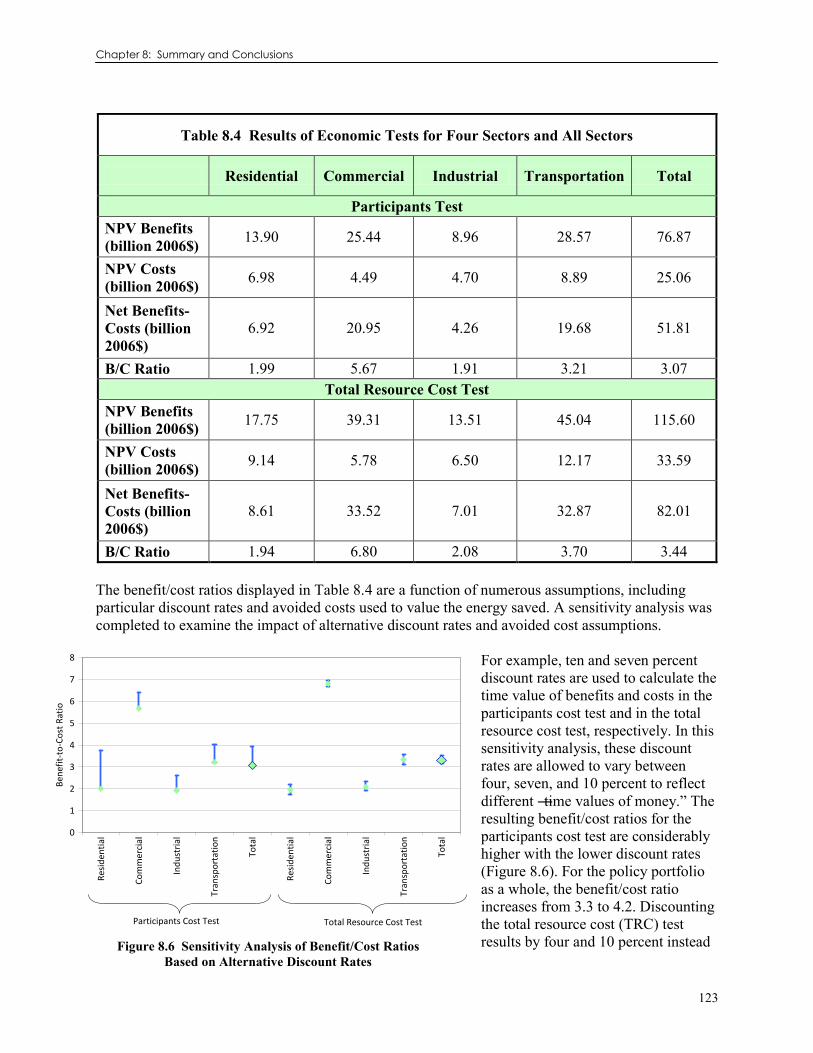
Chapter 8: Summary and Conclusions
123
0
1
2
3
4
5
6
7
8
Res
iden
tial
Co
mm
erci
al
Ind
ust
rial
Tran
spo
rtat
ion
Tota
l
Res
iden
tial
Co
mm
erci
al
Ind
ust
rial
Tran
spo
rtat
ion
Tota
l
Ben
efit
-to
-Co
st R
atio
Participants Cost Test Total Resource Cost Test
Table 8.4 Results of Economic Tests for Four Sectors and All Sectors
Residential Commercial Industrial Transportation Total
Participants Test NPV Benefits (billion 2006$) 13.90 25.44 8.96 28.57 76.87
NPV Costs (billion 2006$) 6.98 4.49 4.70 8.89 25.06
Net Benefits-Costs (billion 2006$)
6.92 20.95 4.26 19.68 51.81
B/C Ratio 1.99 5.67 1.91 3.21 3.07 Total Resource Cost Test
NPV Benefits (billion 2006$) 17.75 39.31 13.51 45.04 115.60
NPV Costs (billion 2006$) 9.14 5.78 6.50 12.17 33.59
Net Benefits-Costs (billion 2006$)
8.61 33.52 7.01 32.87 82.01
B/C Ratio 1.94 6.80 2.08 3.70 3.44 The benefit/cost ratios displayed in Table 8.4 are a function of numerous assumptions, including particular discount rates and avoided costs used to value the energy saved. A sensitivity analysis was completed to examine the impact of alternative discount rates and avoided cost assumptions.
For example, ten and seven percent discount rates are used to calculate the time value of benefits and costs in the participants cost test and in the total resource cost test, respectively. In this sensitivity analysis, these discount rates are allowed to vary between four, seven, and 10 percent to reflect different ―time values of money.‖ The resulting benefit/cost ratios for the participants cost test are considerably higher with the lower discount rates (Figure 8.6). For the policy portfolio as a whole, the benefit/cost ratio increases from 3.3 to 4.2. Discounting the total resource cost (TRC) test results by four and 10 percent instead Figure 8.6 Sensitivity Analysis of Benefit/Cost Ratios
Based on Alternative Discount Rates

Energy Efficiency in Appalachia, SEEA
124
0
2
4
6
8
10
Ben
efit
-to
-Co
st R
atio
50% Lower than Energy Prices 0.97 3.40 1.04 1.66 1.65
25% Lower than Energy Prices 1.46 5.10 1.56 2.49 2.48
Retail Energy Prices 1.94 6.80 2.08 3.33 3.31
Energy Prices with $25/MtC Tax 2.15 6.59 2.67 3.41 3.45
Energy Prices with $50/MtC Tax 2.35 7.42 3.26 3.49 3.58
Energy Prices with $100/MtC Tax 2.75 9.09 4.45 3.65 3.84
Residential Commercial Industrial Transportation Total
of seven does not have a large impact on the benefit/cost ratios. The overall TRC benefit/cost ratio for the portfolio package varies between 3.5 and 4.0. Similarly, the principal estimate used in this project to monetize the avoided costs of potential energy savings is the retail price of energy. Figure 8.7 shows what would happen to the cost-effectiveness tests if the value of the avoided cost was cut in half (as might happen, for instance, if power plant costs were to decline significantly or if new inexpensive fuels were to flood the market). It also examines the benefit/cost ratios if avoided costs were inflated (e.g., in conjunction with the promulgation of a nationwide carbon cap-and-trade system). The lowest avoided costs drive the residential and industrial programs to borderline cost-effective. In contrast, inflating energy costs by $25 to $100 per metric ton of carbon dioxide significantly raises the benefit/cost ratios of the policy packages targeting the commercial, residential, and industrial sectors. There is a much smaller effect on the cost-effectiveness of the transportation sector energy-savings potential – due to the lower carbon content of gasoline and diesel. Across all of the sectors, the carbon-inflated avoided costs make investments in energy efficiency more cost-effective compared with the business-as-usual scenario. 8.2 RESULTS BY SECTOR 8.2.1 Residential Buildings From 2008 to 2030, Appalachian residential energy consumption is forecast to increase 30-32 percent, to approximately 2.5 quads (EIA, 2007a; 2008a). Numerous barriers to efficiency improvements are expected to limit the Region‘s adoption of more efficient technologies and practices. Foremost among these is the first-cost, or incremental cost, of more efficient products and materials; while high costs are a barrier across the nation, the higher rates of poverty and lower average incomes in Appalachia magnify this issue. Each of the policies proposed for the residential sector include an anticipated ―incentive‖ portion to help overcome this barrier. Energy Efficiency in Appalachia demonstrates the potential for residential efficiency to curb the Region‘s growing energy demand, by focusing on building efficient new homes, improving the performance of existing homes, and pulling the appliance stock towards best available technology. Home construction practices and lighting are expected to improve, roughly doubling the efficiency of homes built today, through tighter building codes and stricter enforcement – enforced through third-party compliance verification. A two-tiered retrofit program, providing no-cost weatherization services to low-income households and a cost-share for other households, is expected to significantly
Figure 8.7 Sensitivity Analysis of Benefit/Cost Ratios for the Total Resource Cost Test With Carbon “Adders”

Chapter 8: Summary and Conclusions
125
improve the heating and cooling efficiency of about 40 percent of the existing building stock. Appliances are targeted through an incentive program for super-efficient appliances; due to appliance lifetimes, this method improves the stock appliance efficiency over the study horizon. Considering energy benefits alone, these policies are cost-effective with a benefit-to-cost ratio of about 2.0 for participants and about 1.9 for society. Improving home performance is assumed to be even more cost-beneficial when non-energy benefits are quantified, especially improved health and safety for the elderly and most vulnerable children in the community. These three focus areas (new homes, thermal envelopes, and appliances), modeled here through four policy packages, are estimated to provide cumulative annual savings of about 370 trillion Btu in 2030. This represents more than half of the estimated growth in consumption over the study horizon. With $5.1 billion in program spending and an additional $12.3 billion in customer investments over the 2010-2030 period, the Appalachian Region could see net cumulative savings of 6.0 quads, saving $60.4 billion in energy bills by 2050. This is the equivalent of about 18.7 percent of the EIA‘s forecast consumption in 2030 or 71.7 percent of forecast growth (EIA, 2008a). 8.2.2 Commercial Buildings Commercial energy consumption in Appalachia is forecast to increase 45-63 percent from 2006 to 2030, to approximately 2.4 quads (EIA, 2007a; 2008a). More efficient technologies and practices are especially important in existing commercial building stock, which is not expected to be replaced over the study horizon. Ensuring that retiring equipment is replaced by the most efficient technology can be a challenge due to high relative costs, low management priority for energy costs, and principal agent issues. The policies suggested by this study for the commercial sector address these barriers. Commercial building savings are anticipated in this study through efficient new building construction, commissioning and retrofit of existing building stock, and adoption with proper use of efficient office equipment. New building construction practices and lighting methods are expected to improve, roughly doubling the efficiency of buildings constructed today, through tighter building codes and third-party compliance verification. Commissioning generally ensures that design efficiencies are achieved; modifications based on commissioning studies achieve about 10 percent savings over non-commissioned buildings (Mills et. al, 2004). Addressing compliance and commissioning help to overcome principle agent issues in that builders (and often the owners) of commercial buildings will not be responsible for energy costs. Ensuring that retrofit HVAC and lighting equipment are completed with the most efficient technologies and methods presents higher first costs that can be overcome with incentives; these retrofits are cost-effective without incentives, but limited access to capital and financing for energy-efficiency improvements can hinder their adoption (Brown and Chandler, 2008). While adoption of efficient office equipment is increasing, use of efficiency features is still low because of a generally low management priority for efficiency; tightening standards while offering incentives for application of the technology can significantly reduce electricity consumption at a small cost. The Commercial Policy Package is cost-effective with a benefit-to-cost ratio of about 5.7 for participants and about 6.8 for society. With $1.9 billion in program spending and an additional $9.3 billion in customer investments over the 2010-2030 period, the Appalachian region could see net cumulative savings of 9.5 quads, saving $72.5 billion in energy bills by 2030. This is the equivalent of about 45.6 percent of the EIA‘s forecast consumption in 2030 or 148.3 percent of forecast growth from 2010-2030 (EIA, 2008a).

Energy Efficiency in Appalachia, SEEA
126
8.2.3 Industry Industry in Appalachia currently comprises 30 percent of overall energy use within the Region. According to the EIA‘s 2008 Annual Energy Outlook, industry is expected to continue to use a large proportion of energy in Appalachia though its market share will decrease slightly down to 28 percent by 2030 (EIA, 2008a). Energy costs for industry can be substantial, and, though many are keenly aware of the impact energy efficiency can have on the ―bottom line,‖ hurdles such as large initial capital costs and down time needed to install updated equipment often prevent action in industry. Through structured programs that help mitigate these challenges, a large impact in the rate of energy consumption could be achieved. The industrial portion of the current study investigates three programs, which, together, would audit industrial sites and make recommendations for energy-efficiency improvements; help support the installation of new equipment; train industrial site personnel to continue to make improvements; and promote the use of systems that utilize waste heat to provide a useful product, such as steam. Through expansion of current programs, small- to medium-sized industrial sites can take advantage of government-funded energy auditing to help them make decisions on cost-effective, high-impact changes that can be made to improve their energy consumption. Large industrial facilities can receive training on how to pinpoint improvements in systems throughout their complex to improve energy efficiency, on average reducing overall site consumption by roughly nine percent (Wright et al., 2007). In plants that require thermal inputs, systems that produce electric power can be placed on-site, and the hot exhaust can be used as ―free‖ energy to drive equipment that would ordinarily require natural gas, saving total energy for the Region. These types of programs are a large step in the direction of reduced energy demand. No policy or program comes without some financial costs; however, based on the energy saved through the policy bundles modeled in the current study, the financial benefits far outweigh the costs. The four actions achieved through three programs are estimated to provide an annual energy savings of 670 trillion Btu by 2030, which reduces the sector‘s total energy consumption below 2007 levels. The Industrial Policy Package is cost-effective with a benefit-to-cost ratio of about 1.9 for participants and about 2.1 for society. With $2.5 billion in program spending and an additional $13.1 billion in customer investments over the 2010-2030 period, the Appalachian Region could see net cumulative savings of 5.2 quads, saving $22.6 billion in energy bills by 2030. This is the equivalent of about 21.7 to 27.9 percent of the EIA‘s forecast consumption in 2030, or 90.0 to 153.1 percent of forecast growth (EIA, 2007a; 2008a). 8.2.4 Transportation The transportation sector in the Appalachian Region shows enormous energy savings potential. Appalachian transportation energy consumption is forecast to increase to 2.54 quads by 2030 (EIA, 2008a). The stricter CAFE standards promulgated in 2007 alone should reduce primary energy consumption for the sector by at least 21 percent by 2030. If the standards are combined with other policies modeled in this report, total primary energy savings could reach 35 percent by 2030. Future investments targeted at moving Appalachia‘s freight more efficiently could bring about additional fuel savings not modeled in this analysis. The biggest contributor to total savings outside of the new fuel economy regulations is the extension of the Clean Car Standard program we propose in this analysis, which would bring about gasoline savings of 2.72 billion gallons a year by 2030 –

Chapter 8: Summary and Conclusions
127
approximately 13.5 percent of total primary transportation energy consumption in the Appalachian Region. Numerous barriers to efficiency improvements are expected to limit the Region‘s adoption of more efficient technologies and practices. Foremost among these is the first-cost, or incremental cost, of more efficient products and materials; while high costs are a barrier across the nation, the higher rates of poverty and lower average incomes in Appalachia magnify this issue. Each of the policies proposed for the residential sector include an anticipated ―incentive‖ portion to help overcome this barrier. The transportation policy options presented here are a cost-effective way of realizing energy-savings potential in Appalachia. The benefit/cost ratios indicate that the high cost of implementation associated with some of the transportation policies is far outweighed by the total benefits incurred. If all policy options were to be implemented in combination, participants would receive approximately $2 for every additional $1 spent. Similarly, every additional $1 spent on implementation would reap $3.14 in total benefit. While implementation of such policies might depend on a variety of economic and political conditions, this report demonstrates that there is significant opportunity in Appalachia for large energy savings in the transportation sector. Carefully crafted policies that target vehicles fuel economy, vehicle-miles traveled (VMT) and driving behavior will lead to increased energy efficiency in the transportation sector. The transportation sector policy package is cost-effective with a benefit-to-cost ratio of about 3.2 for participants and about 3.7 for total resource costs. With $0.4 billion in program spending and an additional $27.6 billion in customer investments over the 2010-2030 period, the Appalachian Region could see net cumulative savings of $80.4 billion in energy bills by 2030 and $167.1 billion by 2044. This is the equivalent of about 30.1 percent of the EIA‘s forecast consumption in 2030 or 172.4 percent of forecast growth from 2010-2030 (EIA, 2008a). 8.3 CONCLUSIONS Policy action aimed at exploiting the energy-efficiency potential described in this report would set Appalachia on a course toward a sustainable and prosperous energy future. The Region‘s energy-efficiency resources could go a long way toward meeting its future energy needs while ensuring its continued economic and environmental health. The problem is that energy-efficiency upgrades require consumer and business investment and they take time away from other priorities. With so many demands on financial and human capital, energy-efficiency upgrades tend to be given a low priority. Through a combination of information dissemination and education, financial assistance, regulations, and capacity building, consumers, businesses, and industry can be encouraged to take advantage of energy-efficiency opportunities. In addition, expanded research, development, and demonstration is needed to innovate and deploy transformational technologies that expand the efficiency potential. By exploiting the Region‘s substantial energy-efficiency resources, Appalachia can cut the energy bills of its households, businesses and industries, create ―green‖ jobs, and grow its economy. The ability to convert this vision into a reality will depend on the willingness of business and policy leaders to implement the recommendations that are at the heart of this report.

Energy Efficiency in Appalachia, SEEA
128

Chapter 9: References
129
9 REFERENCES Alabama Department of Economic and Community Affairs (ADECA). 2005. Alabama Building
Energy Conservation Code (ABECC) 2004. http://www.adeca.alabama.gov/C0/Building%20Energy%20Codes/default.aspx
American Council for an Energy-Efficient Economy, Summit Blue Consulting, ICF International,
Synapse Energy Economics. 2008. Energizing Virginia: Efficiency First. Washington, DC: ACEEE E085. http://www.aceee.org/pubs/e085.htm
American Institute of Architects (AIA). 2006a.
http://www.aia.org/aiarchitect/thisweek06/0623/0623remodeling1_b.gif ———. 2006b. http://www.aia.org/aiarchitect/thisweek06/0915/0915b_housingq2.cfm American Society of Heating, Refrigerating and Air-Conditioning Engineers (ASHRAE). 2005.
―National Energy Savings Potential in HUD-Code Housing from Thermal Envelope and HVAC Equipment Improvements.‖ American Society of Heating, Refrigerating, and Air-Conditioning Engineers Transactions.
Appalachian Regional Commission (ARC). 2006. Energizing Appalachia: A Regional Blueprint for
Economic and Energy Development. http://www.arc.gov/images/newsandevents/publications/energyblueprint/energyblueprint.pdf
Aron, Trudy. 2007. Letter from American Institute of Architects in Kansas to Senate Utilities
Committee. http://www.kslegislature.org/committeeminutes/07-08/senate/sutils/suAllDocs/testimony/2007/02142007TAronProHB2036.pdf
Building Codes Assistance Project (BCAP). 2008. Mississippi Code Status. http://www.bcap-
energy.org/node/77 Banfi, Silvia, Mehdi Farsi, Massimo Filippini, and Martin Jakob. 2008. ―Willingness to Pay for
Energy-Saving Measures in Residential Buildings.‖ Energy Economics 30 2: 503-516. Baxter, Van. 2006. Business Case Analysis of Two Integrated Heat Pump HVAC Systems for Near-
Zero-Energy Homes. Oak Ridge, TN: Oak Ridge National Laboratory. http://www.ornl.gov/sci/btc/pdfs/Baxter_ORNL%20AS%20and%20GS%20IHP%20Biz-Case_9-3-06.pdf
Bell, Luke. 2007. Letter from Kansas Association of Realtors to Senate Utilities Committee. Feb. 13.
http://www.kslegislature.org/committeeminutes/07-08/senate/sutils/suAllDocs/testimony/2007/02142007LBellProHB2036.pdf
Bordoff, J.E. and P.J. Noel. 2008. Pay-as-you-drive Auto Insurance: A Simple Way to Reduce
Driving-Related Harms and Increase Equity, The Brookings Institution. http://payasyoudrive.com.au/Resources/PDF/PAYDAutoInsuranceASimpleWayToReduceDrivingRelatedHarmsAndIncreaseEquity.pdf

Energy Efficiency in Appalachia, SEEA
130
Brown, Marilyn. 2008. ―Energy Insights from Policy Expert Marilyn Brown.‖
http://www.gatech.edu/energybuzz/Q22008/ Brown, Marilyn and Nilgun Atamturk. 2008. ―Potential Impacts of Energy and Climate Policies on
the U. S. Pulp and Paper Industry,‖ Georgia Institute of Technology School of Public Policy Working Paper #40, June, 2008. http://www.spp.gatech.edu/faculty/workingpapers.php
Brown, Marilyn and Sharon ―Jess‖ Chandler. 2008. ―Governing Confusion: How Statutes, Fiscal
Policy, and Regulations Impede Clean Energy Technologies,‖ Stanford Law and Policy Review, (19) 3: 472-509. http://slpr.stanford.edu/previous/Volume19.html#Issue3
Brown, M., J. Chandler, M. Lapsa, and B. Sovacool. 2008. Carbon Lock-In: Barriers to Deploying
Carbon Change Mitigation Technologies. (Rev 2 January 2008). ORNL/TM-2007/124. Oak Ridge, TN.: Oak Ridge National Laboratory.
Brown, Marilyn A.; Mark D. Levine; Walter Short; Jonathan G. Koomey. 2001. ―Scenarios for a
Clean Energy Future,‖ Energy Policy, 29 (14): 1179-1196. Brown, Marilyn, F. Southworth and A. Sarzynzki. 2008. Shrinking the Carbon Footprint of
Metropolitan America. Washington, DC: The Brookings Institution. http://www.brookings.edu/~/media/Files/rc/reports/2008/05_carbon_footprint_sarzynski/carbonfootprint_report.pdf
Bristol Tennessee Essential Service (BTES). 2008. ―Energy Savings Loan Program.‖
http://www.btes.net/btesenergysavings.html Building Codes Assistance Project (BCAP). 2008. Mississippi Code Status. http://www.bcap-
energy.org/node/77 California Air Resources Board (CARB). 2008. ―Comparison of Greenhouse Gas Reductions For All
Fifty United States Under Cafe Standards and ARB Regulations Adopted Pursuant To AB1493.‖ http://www.arb.ca.gov/cc/ccms/reports/pavley-addendum.pdf
Cambridge Systematics. 2008. ―Economic Impact Study of Completing the Appalachian
Development Highway System.‖ http://www.arb.ca.gov/cc/ccms/reports/pavley-addendum.pdf Center for Business and Economic Research (CBER). 2006. Energy Efficiency and Renewable
Energy in Appalachia: Policy and Potential. http://www.arc.gov/images/reports/2006/energy/arc_renewable_energy_full.pdf
Cherokee Electric Cooperative (Cherokee). 2008. EC Home Improvement Program Website.
http://www.cherokee-electric.org/advantage/echome.htm Davis, S. and S. Diegel. 2006. Transportation Energy Data Book, Edition 25. Oak Ridge, TN: Oak
Ridge National Laboratory. Eldridge, Maggie, R. Neal Elliott, and Max Neubauer. 2008. ― State-Level Energy Efficiency
Analysis: Goals, Methods and Lessons Learned.‖ Proceedings of the 2008 ACEEE Summer Study

Chapter 9: References
131
on Energy Efficiency in Buildings. Washington, DC: American Council for an Energy-Efficient Economy.
Eldridge, Maggi, Neal Elliott, William Prindle, Katie Ackerly, John ―Skip‖ Laitner, Vanessa
McKinney, Steve Nadel, and Max Neubauer, Alison Silverstein, Bruce Hedman, Anne Hampson, and Ken Darrow. 2008. Energy Efficiency: The First Fuel for a Clean Future: Resources for Meeting Maryland’s Electricity Needs. Report E082. Washington, DC: ACEEE.
Energetics. 2006. ―U.S. CHP Incentives List.‖
http://www.energetics.com/madri/pdfs/USCHPIncentiveslist(5-12-06).pdf Energetics. ―Summary of 20 Emerging, Energy-Saving Industrial Technologies. National Academy
of Sciences,‖ unpublished manuscript. Energy Conservation Center, Japan (ECCJ). 2008. ―Developing the World's Best Energy-Efficient
Appliances (Japan's "Top Runner" Standard) REVISED EDITION/JAN 2008.‖ http://www.eccj.or.jp/top_runner/index.html
Energy Independence and Security Act of 2007 (EISA). 2007. Public Law 110-140, 110th Congress.
http://frwebgate.access.gpo.gov/cgi-bin/getdoc.cgi?dbname=110_cong_public_laws&docid=f:publ140.110.pdf
Energy and Environmental Analysis, Inc. (EEA). 2007. Combined Heat and Power Installation
Database. http://www.eea-inc.com/chpdata/index.html Energy Information Administration (EIA). 1998. 1998 Manufacturing Energy Consumption Survey:
Consumption and Expenditures Tables. http://www.eia.doe.gov/emeu/mecs/ ———. 2002. 2002 Manufacturing Energy Consumption Survey: Consumption and Expenditures
Tables. http://www.eia.doe.gov/emeu/mecs/ ———. 2007a. Annual Energy Outlook 2007.
http://tonto.eia.doe.gov/ftproot/forecasting/0383(2007).pdf ———. 2007b. Commercial Building Energy Consumption Survey 2003.
http://www.eia.doe.gov/emeu/cbecs/ Energy Information Administration (EIA). 2008a. Annual Energy Outlook 2008.
http://www.eia.doe.gov/oiaf/aeo/ ———. 2008b. Commercial Demand Module. Report #: DOE/EIA-0554(2008).
http://www.eia.doe.gov/oiaf/aeo/assumption/pdf/commercial.pdf ENERGY STAR. 2007. ―ENERGY STAR® Qualified Buildings and Manufacturing Plants.‖
http://www.energystar.gov/ia/business/es_labeled_list.pdf ———. 2008. ENERGY STAR Qualified New Homes Market Indices for States. http://www.energystar.gov/index.cfm?fuseaction=qhmi.showHomesMarketIndex

Energy Efficiency in Appalachia, SEEA
132
GDS Associates. 2006. A study of the feasibility of energy efficiency as an eligible resource as part of a renewable portfolio standard for the state of North Carolina. http://www.ncuc.commerce.state.nc.us/reps/NCRPSEnergyEfficiencyReport12-06.pdf
Geller, Howard. 2003. Energy Revolution. Washington, DC: Island Press. Geller, Howard, Philip Harrington, Arthur H. Rosenfeld, Satoshi Tanishima, and Fridtjof Unander.
2006. ―Polices for Increasing Energy Efficiency: Thirty Years of Experience in OECD Countries.‖ Energy Policy, 34:556–73.
Gemmer, Bob. 2007. Super Boiler Update. Presentation at Manufacturers Conference, American
Boiler Manufacturers Association. http://www1.eere.energy.gov/industry/combustion/pdfs/abma_2007.pdf
Glasmeier, Amy and Tom Bell, 2006. Economic Development Potential of Conventional and
Potential Alternative Energy Sources in Appalachian Counties, Washington, DC: Appalachian Regional Commission. http://www.arc.gov/images/reports/2006/energy/arc_altenergy_full.pdf
Haasl, Tudi and Terry Sharp, 1999. A Practical Guide for Commissioning Existing Buildings.
Portland Energy Conservation, Inc. and Oak Ridge National Laboratory for the U.S. Department of Energy, contract number DE-AC05-96OR22464, http://eber.ed.ornl.gov/commercialproducts/RetroCommissioningGuide-w-cover.pdf
Harrington, Cheryl, and Catherine Murray. 2003. Who should deliver ratepayer funded energy
efficiency? Washington, DC: Regulatory Assistance Project.
http://www.raponline.org/showpdf.asp?PDF_URL=Pubs/RatePayerFundedEE/RatePayerFunded
EEFull.pdf Hayes, Jim. 2008. ―Time To Eliminate The Sales Tax On Energy Star Purchases.‖
http://assembly.state.ny.us/mem/?ad=148&sh=story&story=27881 ICF Consulting. 2005. Assessment of Energy Efficiency Potential in Georgia.
http://www.gefa.org/index.aspx?page=192 International Energy Agency Heat Pump Programme (IEA). 2006. ‖The Potential Impact of Heat
Pumps on Energy Policy Concerns.‖ http://heatpumpcentre.org/ Jakob, Martin. 2006. ―Marginal costs, cost dynamics and co-benefits of energy efficiency
investments in the residential buildings sector,‖ Energy Policy 34:172–187. Kansas legislature (Kansas). 2007a. HB 2036. http://www.kslegislature.org/bills/2008/2036.pdf
(Kansas code 66-1228 as amended). ———. 2007b. HB 2278. http://www.kslegislature.org/bills/2008/2278.pdf Kansas Energy Commission (KEC). 2008. ―Kansas Energy Plan 2008.‖
http://kec.kansas.gov/energy_plan/energy_plan_08.pdf
Chapter 9: References
133
Kentucky Pollution Prevention Center (KPPC), University of Louisville, and ACEEE. 2007. Kentucky Energy Efficiency Potential Study: An Overview of Kentucky's Energy Consumption and Energy Potential. http://louisville.edu/kppc/files/kppc/KYE2PotentialStudyFinalReport82207_508.pdf
Kunkle, Rick. 1997. The Washington State Energy Code: Energy Code Privatization - The Utility
Code Group Story. http://www.energycodes.gov/implement/documents/case_private.doc Kushler, Martin, Dan York, and Patti Witte. 2004. Five Years In: An Examination of the First Half-
Decade of Public Benefits Energy Efficiency Policies. Washington, DC: American Council for an Energy Efficient Economy, Table 5.
Laitner, John A. ―Skip‖ and Vanessa McKinney. 2008a. Positive Returns: State Energy Efficiency
Analyses Can Inform U.S. Energy Policy Assessments. Washington, D.C.: American Council for an Energy-Efficient Economy.
———. Forthcoming. Draft DEEPER Documentation. Washington, DC: American Council for an
Energy-Efficient Economy. Langer, T. 2004. ―Energy Savings through Increased Fuel Economy for Heavy-Duty Trucks.‖
http://www.bipartisanpolicy.org/files/news/finalReport/III.4.a%20-%20Heavy-Duty%20Trucks.pdf
Lovins, A. B. 2007. ―Energy Myth Nine – Energy Efficiency Improvements have Already
Reached their Potential.‖ In B. K. Sovacool and M. A. Brown (eds.), Energy and American Society – Thirteen Myths. New York: Springer Publishing Company, 239-264.
Madgett, Melissa. 2008. Personal Communication, Oak Ridge National Laboratory. Meffert, William. 2007. ―ANSI/MSE 2000:2005—A Management System for Energy.‖ Energy and
Environmental Management Center, Georgia Institute of Technology Enterprise Innovation Institute. http://www.superiorenergyperformance.net/pdfs/MSE_2000_GATECH.pdf
McKinsey & Company. 2007. Reducing Greenhouse Gas Emissions: How Much At What Cost?
http://www.mckinsey.com/clientservice/ccsi/greenhousegas.asp Mills, Evan, Hannah Friedman, Tehesia Powell, Norman Bourassa, David Claridge, Tudi Haasl,
Mary Ann Piette. 2004. The Cost Effectiveness of Commercial-Buildings Commissioning. Lawrence Berkeley National Laboratory. Berkeley, CA. http://eetd.lbl.gov/Emills/PUBS/PDF/Cx-Costs-Benefits.pdf
Minnesota IMPLAN Group, Inc. (IMPLAN). 2006. A 2005 dataset for Appalachia (Alabama,
Georgia, Kentucky, Maryland, Mississippi, New York, North Carolina, Ohio, Pennsylvania, South Carolina, Tennessee, and Virginia. Stillwater, Minn.: Minnesota IMPLAN Group, Inc.
Minnesota IMPLAN Group, Inc. (IMPLAN). 2008. A 2006 dataset for Appalachia (Alabama,
Georgia, Kentucky, Maryland, Mississippi, New York, North Carolina, Ohio, Pennsylvania,

Energy Efficiency in Appalachia, SEEA
134
South Carolina, Tennessee, and Virginia. Accessed January. Stillwater, Minn.: Minnesota IMPLAN Group, Inc.
National Action Plan for Energy Efficiency (NAPEE). 2007a. Guide to Resource Planning with
Energy Efficiency. http://www.epa.gov/solar/documents/resource_planning.pdf ———. 2007b. Model Energy Efficiency Program Impact Evaluation Guide.
http://www.epa.gov/cleanrgy/documents/evaluation_guide.pdf National Institute of Standards and Technology (NIST). 2008. ―Hollings Manufacturing Extension
Partnership.‖ http://www.mep.nist.gov/ Navigant Consulting (Navigant). 2006. Energy Savings Potential of Solid State Lighting in General
Illumination Applications. Report prepared for the Office of Energy Efficiency and Renewable Energy, U.S. DOE. http://www.netl.doe.gov/ssl/PDFs/SSL%20Energy%20Savings%20Potential%20Report%202006%20final4.pdf
Neu Smith, Martha. 2007. Letter from Kansas Manufactured Housing Association to Senate Utilities
Committee. Feb. 13. http://www.kslegislature.org/committeeminutes/07-08/senate/sutils/suAllDocs/testimony/2007/02142007MNeuSmithProHB2036.pdf
New York State Energy Research and Development Authority (NYSERDA). 2003. Energy
Efficiency and Renewable Energy Resource Potential Development in New York State. Albany, New York: New York State Energy Research and Development Authority.
———. 2004. Guideline to the Commissioning Process for Existing Buildings, or “Retro-
Commissioning.” Portland Energy Conservation, Inc. http://www.nyserda.org/programs/pdfs/retrocxhandbookfinal040704.pdf Nexant Consulting. 2007. Achievable Energy Efficiency Potential Assessment: Final Study for
Georgia Power. http://www.seealliance.org/documents/GAIRPTechGAPowerPotentialStudy_052007.pdf
North Carolina Solar Center and Interstate Renewable Energy Council (NCSC/IREC). 2008.
Database of State Incentives for Renewables & Efficiency (DSIRE). http://www.dsireusa.org/ Pacific Gas and Electric (PG&E). 2008. ―Residential New Construction Program.‖
http://www.pge.com/mybusiness/energysavingsrebates/incentivesbyindustry/newconstruction/energystar/index.shtml
Prindle, William. 2007. Quantifying the Effects of Market Failures in the End-Use of Energy,
ACEEE Report Number E071, Washington, DC: American Council for an Energy-Efficient Economy. http://www.aceee.org/energy/IEAmarketbarriers.pdf
Rabovitser, Joseph and Rick Knight. 2005. ―Compact Package Boilers Combining Ultra-high-
efficiency and Ultra-low Emissions: Development and Demonstration,‖ Proceedings of Natural Gas Technologies 2005 Conference, Orlando, Florida.

Chapter 9: References
135
Rahall Transportation Institute and Wilbur Smith Associates. 2004. Meeting the Transportation Challenges of the 21st Century: Intermodal Case Studies. http://www.arc.gov/images/reports/interopp/ebinteropp.pdf
Regional Economics Models, Inc. (REMI). 2007. Data provided to the authors by the Appalachian
Regional Commission on December 21, 2007. http://www.remi.com:80/ Rosenquist, Greg, Michael McNeil, Maithili Iyer, Stephen Meyers, and James McMahon. 2006.
―Energy efficiency standards for equipment: Additional opportunities in the residential and commercial sectors.‖ Energy Policy 34:3257-3267.
Rufo, M., and F. Coito. 2002. ―California‘s Secret Energy Surplus: The Potential for Energy
Efficiency.‖ The Energy Foundation, San Francisco. http://www.ef.org/news_reports.cfm?program=viewall&sort=creationdate
Schwartz, Peter. 1991. The Art of the Long View. New York, NY: Doubleday. Schweitzer, Martin and Bruce Tonn. 2002. Non energy benefits from the Weatherization Assistance
Program: A Summary of Findings from the Recent Literature.‖ http://weatherization.ornl.gov/download_files/Con-484-april02.pdf
Sezgen, Osman and Jonathan Koomey. 1998. ―Interactions between lighting and space conditioning
energy use in U.S. commercial buildings.‖ http://enduse.lbl.gov/Info/LBNL-39795.pdf Smith, D.L. and J.J. McCullough. 2001. Alternative Code Implementation Strategies for States.
Office of Building Technology, State, and Community Programs, Office of Energy Efficiency and Renewable Energy, U.S. Department of Energy. http://www.energycodes.gov/implement/pdfs/strategies.pdf
Soderlund, Matthew. 2008. Georgia Institute of Technology Industrial Assessment Center. Personal
Communication. Tennessee Legislature (TNleg). 2008. SB116: AN ACT to amend Tennessee Code Annotated, Title 4,
Chapter 3, Part 7, relative to building codes. http://www.legislature.state.tn.us/bills/currentga/Chapter/PC0907.pdf
Tol, Richard. 2005. ―The Marginal Damage of Carbon Dioxide Emissions: An Assessment of the
Uncertainties,‖ Energy Policy, 33:2064-2074. U.S. Bureau of Labor Statistics (BLS). 2008. Inflation Calculator. http://data.bls.gov/cgi-
bin/cpicalc.pl U.S. Census Bureau (Census). 2008. The 2008 Statistical Abstract of the United States, Table
687. Individuals and Families Below Poverty Level--Number and Rate by State: 2000 to 2005. http://www.census.gov/compendia/statab/cats/income_expenditures_poverty_wealth/income_and_povertystate_and_local_data.html

Energy Efficiency in Appalachia, SEEA
136
U.S. Congress, Office of Technology Assessment (OTA). 1993. Energy Efficiency: Challenges and Opportunities for Electric Utilities, OTA-E-561. Washington, DC: U.S. Government Printing Office.
U.S. Department of Energy Efficiency and Renewable Energy (DOE/EERE). 2008a. Industrial
Technologies Program-IAC Database. http://iac.rutgers.edu/database/about.php ———. 2008b. Save Energy Now Assessment Helps Expand Energy Management Program at Shaw
Industries (Case Study). http://www1.eere.energy.gov/industry/saveenergynow/pdfs/42460.pdf U.S. Environmental Protection Agency (EPA). 2006. Clean Energy-Environment Guide to Action:
Policies, Best Practices, and Action Steps for States. http://www.epa.gov/cleanenergy/documents/gta/guide_action_full.pdf
———. 2008. Efficiency Benefits. U.S. http://www.epa.gov/chp/basic/efficiency.html Vine, Edward. 1996. ―Residential Building Code Compliance: Implications for Evaluating the
Performance of Utility Residential New Construction Programs.‖
http://www.osti.gov/bridge/servlets/purl/418459-Bsrs72/webviewable/418459.pdf Wisconsin Focus on Energy (WFOE). 2008. Focus on Energy Program Website.
http://www.focusonenergy.com/Incentives/Residential/Cash-Back_Rewards/New-Home/ Worrell, E., S. Ramesohl, and G. Boyd. 2003. Towards Increased Policy Relevance in Energy
Modeling. Proceedings of the ACEEE 2003 Summer Study on Energy Efficiency in Industry, Washington, DC: American Council for an Energy-Efficient Economy.
Wright, Anthony, Michaela Martin, Bob Gemmer, Paul Scheihing, and James Quinn. 2007. Results
from the U.S. DOE 2006 Save Energy Now Assessment Initiative: DOE’s Partnership with U.S. Industry to Reduce Energy Consumption, Energy Costs, and Carbon Dioxide Emissions. http://apps1.eere.energy.gov/industry/saveenergynow/partners/pdfs/sena_2006_report_final_09_17_07.pdf

Acknowledgements
137
ACKNOWLEDGEMENTS Funding for this project was provided by the Appalachian Regional Commission (ARC) to the Southeast Energy Efficiency Alliance (SEEA), through a competitive solicitation led by Ben Taube (Executive Director of SEEA). The guidance provided by the project‘s ARC and SEEA managers (Greg Bischak, Katie Whiteman, and Ben Taube) was invaluable. The authors also wish to express their appreciation to the project‘s Advisory and Stakeholders Committees. The Advisory Committee included: Carl Bauer, Director, National Energy Technology Laboratory (Pamala Stasia, Administrative
Specialist) Raymond Boeman, Director, Transportation Program and NTRC User Facility, Oak Ridge National
Laboratory Tom Congdon, Assistant Secretary for Energy, State of New York Richard Hirsh, Professor, History and Science & Technology Studies, Virginia Polytechnic Institute
and State University Carl Irwin, Professor, West Virginia University and Director, WVU National Research Center for
Coal and Energy Richard G Newell, Gendell Associate Professor of Energy and Environmental Economics, Duke
University, Nicholas School of the Environment and Earth Sciences Tony Wright, Director, Industrial Technologies Program, Oak Ridge National Laboratory The Stakeholders Committee included: John Davies, Director, Division of Renewable Energy and Energy Efficiency, Kentucky Governor’s Office of Energy Policy Joe Hoagland, Vice President, Energy Efficiency and Demand Response, Tennessee Valley Authority Joel Yudken, Principal, High Road Strategies, Arlington, Virginia Finally, the authors wish to thank Charles M. Zeh (National Energy Technology Laboratory); Etan
Gumerman (Duke University); Youngsun Baek and Frank Southworth (Georgia Tech); Steve Capanna, Jeff Harris, and Nils Petermann (Alliance to Save Energy); and Neal Elliott (ACEEE) for their insights and review comments on various technical aspects of the report. In addition, we are indebted to Charlotte Franchuk for her careful editing of the report.


ENERGY EFFICIENCY IN APPALACHIA HOW MUCH MORE IS AVAILABLE, AT WHAT COST,
AND BY WHEN?
Appendices APPENDIX A ARC ENERGY-EFFICIENCY POLICY INVENTORY
APPENDIX B RESIDENTIAL POLICY AND METHODOLOGY DETAIL
APPENDIX C COMMERCIAL POLICY AND METHODOLOGY DETAIL
APPENDIX D INDUSTRIAL SITES
APPENDIX E TRANSPORTATION
APPENDIX F DEEPER MODEL
APPENDIX G SENSITIVITIES AT SECTOR LEVEL


Appendix A: ARC Energy Efficiency Policy Inventory
A-1
APPENDIX A: ARC ENERGY EFFICIENCY POLICY INVENTORY A policy inventory was developed to better assess the current status and approach of the Appalachian Region to energy efficiency. The inventory was compiled by Georgia Institute of Technology researchers and sent to state energy offices for review. As of September 2008, ten states have replied with corrections and additions to the inventory (AL, GA, KY, MS, NY, OH, PA, SC, TN, VA, and WV) while two states have yet to respond (MD, and NC). All thirteen state energy offices have been made aware of the purpose and intent of this inventory and will be provided a copy of the complete inventory for their own reference. The Appalachian Region has over 200 policies promoting energy efficiency identified in this inventory. However, they differ in scope, intent, and level of support. Policies are even nested in different levels: locally, state, region, and Federal. There are very few local level policies identified in Appalachia; however, there may be policies in place that were not identified. Figure A.1 shows that 91 percent of policies identified in the region are at the state level. Federal policies are not included in this policy inventory, and no applicable policies were identified at the Regional level. Policies can be organized into 12 distinct categories as described by Geller (2002); Figure A.2 shows how current policies in the region fit within these categories. A description of each policy option along with some examples from current programs in Appalachia follows.
0
5
10
15
20
25
30
35
40
45
50
Capacity Build
ing
Financial In
centiv
es
Financing
Inform
ation D
issem
ination &
Training
Mark
et Oblig
ations
Planning Techniques
Pricing
Procu
rem
entRDD
Regulations
Voluntary
Agre
ements
Mark
et Refo
rms
Figure A.1 Breakdown of Policy Level for Policies in Inventory
Figure A.2 Policy Options (count) in the Appalachian Region
State
192
91%
Local
20
9%

Energy Efficiency in Appalachia, SEEA
A-2
Some policies are designed to fit into more than one of these categories, like market obligation policies that also require state lead-by-example procurement. In this case, policies are not double counted; rather they appear under just one option. RESEARCH, DEVELOPMENT, AND DEMONSTRATION These policies generally are used to get technologies and practices from the lab to the marketplace. Throughout the region, there are three identified policies supporting research, development, and demonstration for energy efficiency. Kentucky, South Carolina, and Virginia have targeted programs for innovation, including energy efficiency; they are all designed as competitive grant programs. New York has an office of energy research, and has been active in efficiency research and development for more than three decades. Kentucky’s Energy Research and Development Grants for Renewable Energy and Energy Efficiency, operated by the Kentucky Office of Energy Policy since 2005, awarded five research and development grants in 2007 via competitive solicitation for renewable energy and energy efficiency initiatives for a total of over $518,000. Perhaps the most well known research effort in the Appalachian region is NYSERDA. Since 1975, NYSERDA has conducted a multifaceted energy and environmental research and development program. NYSERDA’s R&D Program supports the development and commercialization of innovative energy and environmental products, technologies, and processes that improve the quality of life for New York's citizens and help New York businesses to compete and grow in the global economy. NYSERDA R&D activities are organized into seven primary program areas: Energy Resources; Transportation and Power Systems; Energy and Environmental Markets; Industry; Buildings; Transmission and Distribution; and Environmental Research. FINANCING Governments offer financing programs to increase adoption rates for technologies that may have longer paybacks or may not qualify for traditional financing. Financing programs include no interest loans, low interest loans, access to standard rate loans, and the ability to utilize performance contracting (for government agencies). There are 23 financing programs to advance energy efficiency in Appalachia (Figure A.3). Seven of these allow government agencies to contract for energy services, through performance contracting or Energy Service Contracting Organizations (ESCOs), or allow special lease financing, on similar terms, from a government fund. Sixteen are loan programs: three are loans with technical assistance, two are no-interest loan programs, and eleven are low-interest loan programs.

Appendix A: ARC Energy Efficiency Policy Inventory
A-3
0
2
4
6
8
10
12
ESCO Loans Low Interest
Loans
No Interest Loan Lease Financing
Financing
West Virginia, Ohio, and Georgia do not have financing programs for energy efficiency in this policy inventory. Table A.1 shows the number of financing policies by state for those that use this type of policy to promote energy efficiency.
Table A.1 Financing Policies by State State Number of Policies AL 2 KY 1 MD 3 MS 4 NC 2 NY 3 PA 2 SC 2 TN 2 VA 2
Mississippi’s Energy Investment Loan Program provides low interest (three percent below prime) loans “to individuals, partnerships, or corporations, for either capital improvements, or in the design and development of innovative energy conservation processes.” The broad scope of this policy makes it stand out, as most financing programs target one sector or technology. In South Carolina, the ConserFund is a low-interest revolving loan program administered by the SC Energy Office for energy-efficiency improvements in state agencies, public colleges or universities, school districts, local governments, and private nonprofit organizations.
Figure A.3 Financing Mechanisms Used for Energy Efficiency in Appalachia

Energy Efficiency in Appalachia, SEEA
A-4
FINANCIAL INCENTIVES Financial incentives help to encourage early and wider adoption of efficient technologies and practices by reducing or eliminating the incremental cost of adoption of energy-efficient technologies and practices (Geller, 2002, p.55). These incentives come in the form of grants, tax credits, tax exemptions, and rebates. Forty-six programs for energy efficiency in Appalachia come in the form of financial incentives. Twenty-three are grants, while nine are tax credits; five are tax exemptions or tax holidays. Of seven types of rebates, three programs are designed as rebates/reimbursements, two as tax rebates, and two as fee rebates. Single programs are designated as ―tax‖ and ―mix.‖ Figure A.4 shows the frequency of these programs.
0
5
10
15
20
25
Fee Rebate Grants Rebate Tax Tax Credit Tax
Exemption
Tax Rebate Mix
Financial Incentives
The program labeled “tax” provides an interesting example for energy-efficiency financial incentives. In 2007, the Virginia legislature passed a bill that allows local governments to create a new real estate classification for buildings that achieve efficiencies at least 30 percent greater than the Virginia Uniform Building Code; with this new classification, local governments could offer incentivized tax rates for efficient buildings. One city, Roanoke, VA, appears to have taken this option up already. Efficiency Long Island, labeled “mix,” is set to offer a combination of financial incentives; this program is intended to succeed and expand upon Long Island Power Authority’s (LIPA) Clean Energy Initiative that expires at the end of 2008. Efficiency Long Island is a 10-year, $924 million energy-efficiency program that will make a wide array of incentives, rebates and initiatives available to LIPA’s residential and commercial customers to assist them in reducing their energy usage and thereby lowering their bills.
Figure A.4 Financial Incentives for Energy Efficiency Used in Appalachia

Appendix A: ARC Energy Efficiency Policy Inventory
A-5
The breakdown by location can be seen in Table A.2. Alabama and Tennessee have no identified financial incentive programs for energy efficiency. Within North Carolina, two financial incentives are at the local level in Asheville, NC.
Table A.2 Financial Incentives Policies by State
State Number of Policies GA 1 KY 2 MD 4 MS 1 NC 3 NY 19 OH 2 PA 4 SC 5 VA 4
PRICING Pricing policies include added taxes and fees and net-metering programs that encourage energy efficiency. Besides net-metering programs, pricing policies have not been employed by governments in Appalachia. However, states do have varying levels of utility and fuel taxes. These taxes could have some implications for consumption behaviors. Previous research efforts by the ARC identified Regional price elasticities of electricity to be -0.15, -0.17, and -0.55 for residential, commercial, and industrial users, respectively (CBER, 2006). While pricing consumers out of the market for energy could be a concern with the region‘s large proportion of population in poverty, pricing mechanisms could be used with other programs to reduce peak demand. Pricing measures could also be used to discourage excessive use without impacting the average customer bill (when much higher prices are set at levels above typical consumption); a grim trigger policy like this can keep consumption from reaching the trigger point, but will not incentivize reductions below that point. Georgia, Kentucky, Maryland, New York, North Carolina, Ohio, and Pennsylvania have state-wide net-metering programs. In addition, Tennessee‘s Tennessee Valley Authority also sponsors a net-metering type program which uses dual-metering and directly purchasing renewable generated power at 10 cents per kWh. These net-metering programs have varying rules on maximum installation, forms of generation, and payback structures. For example, Pennsylvania’s net-metering policy requires investor-owned utilities to offer the program to residential customers with systems up to 50 kilowatts (kW) in capacity; nonresidential customers with systems up to three megawatts (MW) in capacity. In addition, customers (of any sector) with system capacities between three and five MW must be allowed to participate in net-metering if they make their systems available to the grid during emergencies, or if a microgrid system is in place in order to maintain critical infrastructure. Pennsylvania allows many sources to

Energy Efficiency in Appalachia, SEEA
A-6
be eligible for net metering: photovoltaics (PV), solar-thermal energy, wind energy, hydropower, geothermal energy, biomass energy, fuel cells, combined heat and power (CHP), municipal solid waste, waste coal, coal-mine methane, other forms of distributed generation (DG), and certain demand-side management technologies. VOLUNTARY AGREEMENTS Voluntary Agreements can be faster than regulations at achieving goals set by government officials. Throughout Appalachia, however, voluntary agreements are mainly found as partnerships between state and Federal government organizations. About half (six) of Appalachian states are partners with the U.S. Environmental Protection Agency (EPA) in the Clean Energy Environment program; of these states, Georgia, New York, Ohio, and Pennsylvania were charter state partners, and North Carolina joined shortly after the publication of the Clean Energy-Environment guide to action in 2005. Virginia joined in February of 2008. Several Appalachian states are partners with the Building America and Rebuild America programs. An illustrative voluntary agreement intrastate is Georgia’s Earthcraft house partnership between Southface Energy Institute and the Greater Atlanta Home Builders Association that seeks to provide builders with greater information about comfort and energy efficiency that can be achieved through design and construction practices. REGULATIONS Regulations can set a minimum standard for efficiency to discourage waste. In Appalachia, most states or local governments have building codes for new residential and commercial buildings that meet or exceed the standards of the 2003 International Energy Code. However, only New York and Maryland have efficiency standards for appliances; most of these were preempted by Federal appliance standards in 2005. INFORMATION DISSEMINATION AND TRAINING These programs seek to distribute information, raise public knowledge, provide accessible information, or train persons for particular tasks. Many information programs are packaged with financial assistance; for example, in New York, seven programs are grants with technical assistances. Only two of these are grouped in the information section, while the other five are counted under financial incentives.

Appendix A: ARC Energy Efficiency Policy Inventory
A-7
0
5
10
15
20
25
30
Audits Information Training Technical Assistance
Information Dissemination & Training
Most states in Appalachia use Information Dissemination and Training to promote energy efficiency. The number of programs within states can be seen in Table A.3.
Table A.3 Information Dissemination and Training Policies by State
State Number of Policies AL 4 GA 4 KY 6 MD 6 MS 1 NC 3 NY 4 OH 1 SC 2 TN 2 VA 2 WV 2
PROCUREMENT Procurement programs establish demand for particular products through government acquisition. These programs can also be used to demonstrate the applicability of products or practices. Procurement programs are sometimes combined with market reform or market obligations or state agency financing mechanisms. Seven programs across Appalachia were identified as requiring government agencies to adopt or purchase certain types of equipment.
Figure A.5 Information Dissemination and Training Program Types Used in Appalachia
Energy Efficiency in Appalachia, SEEA
A-8
By January 1, 2008, all Tennessee state agencies, universities, and community colleges having more than 10 state-owned vehicles in their fleet are required to develop and implement plans to increase the state’s use of alternative fuels and hybrid electric or other fuel-efficient or low-emission vehicles. Specifically, they must incorporate a goal to reduce or displace at least 20 percent of the fleet’s consumption of petroleum by January 1, 2010. The goal is reduced to a minimum of 10 percent reduction if the fleet includes vehicles modified for educational, emergency, or public safety purposes or vehicles used for emergency or law enforcement purposes. MARKET REFORMS Sweeping changes to the market for energy can be considered market reforms. These could be privatization, deregulation, reregulation, or other structural changes. Not all market reforms are designed to promote efficiency; this policy inventory does not include deregulation of natural gas or electric utilities as efficiency policies. Surcharges, like public benefits funds, can also be used as market reforms. New York and Pennsylvania have implemented Public Benefits Funds as surcharges on energy bills. The collected funds are used to provide for low income energy bill relief and to incentivize greater renewable energy and energy efficiency. Pennsylvania has its public benefits funds program created through individual settlements with the state’s five major distribution utilities: Metropolitan Edison Company (Met-Ed), Pennsylvania Electric Company (Penelec), PECO Energy (PECO), PP&L (PPL), and Allegheny Power/West Penn Power Company (WPP). These utilities created individual “Sustainable Energy Funds” with the goals of promoting (1) the development and use of renewable energy and advanced clean-energy technologies, (2) energy conservation and efficiency, and (3) sustainable-energy businesses. Each utility has established an oversight board and designated a fund administrator. [Because of this set-up, financial incentives are in the utility service areas rather than state-wide or locality based policies.] MARKET OBLIGATIONS Obligations to have particular fuel or efficiency mixes, such as renewable or sustainable energy portfolio standards, fall under the category of market obligations. New York, North Carolina, Ohio, and Pennsylvania have portfolio standards that include energy efficiency as a qualified source. Virginia has a targeted goal for renewable energy and energy efficiency. North Carolina’s Renewable Energy and Energy Efficiency Portfolio Standard requires investor-owned utilities in the state to supply 12.5 percent of 2020 retail electricity sales in the state from eligible energy resources by 2021. Up to 25 percent of the requirements can be met through energy efficiency technologies, including combined heat-and-power systems powered by non-renewable fuels. After 2018, up to 40 percent of the standard can be met through energy efficiency. The requirements are less stringent for municipal utilities and electric cooperatives, which must meet a target of 10 percent renewables by 2018 and are subject to slightly different rules. Within Ohio’s Alternative Energy Resource Standard (effective January 1, 2009), utilities are required to implement energy efficiency and peak demand reduction programs that achieve a cumulative energy savings of 22 percent by the end of 2025, and reduce peak demand by 1.0 percent in 2009 and 0.75 percent annually thereafter through 2018.

Appendix A: ARC Energy Efficiency Policy Inventory
A-9
CAPACITY BUILDING Capacity Building includes developing centers for energy efficiency that work with the private sector to carry out demonstrations, provide information and training, offer financing, and promote efficiency. Capacity building also allows for the production of local skill building; creating local capacity to carry out necessary energy related activities. Thirteen energy efficiency programs with capacity building focus have been identified in five states (Table A.4). Within Appalachia, most capacity building seems to be achieved through funding of centers at state colleges and universities.
Table A.4 Capacity Building Policies by State
State Number of Policies KY 3 MD 1 NC 2 NY 5 WV 2
The Southeastern Combined Cooling, Heating and Power Regional Application Center (CHPCenterSE), is directed by the Mississippi Development Authority-Energy Division, Mississippi State University’s Micro-CHP Application Center and North Carolina State University’s NC+CHP Application Program. The new Regional center seeks to double the installed CHP capacity in the Southeast by the year 2010. They will also coordinate and conduct education and outreach activities to stimulate market development as guided by a CHP Center Roadmap, which will be developed in the first three months of the project. While this center will be located in North Carolina, it demonstrates how effective interstate cooperation can produce meaningful savings. New York’s Saratoga Technology + Energy Park is a unique venture by the New York State Energy Research and Development Authority (NYSERDA) to provide an “integrated knowledge community.” The park actively recruits innovative energy technology firms to do business within the area. PLANNING TECHNIQUES Integrated planning methods that take into account interactions as well as differential short and long term impacts of policies or practices are considered planning techniques. Five policies in Appalachia were identified as planning for energy efficiency, from North Carolina, New York, and Virginia. In North Carolina, the Division of Bicycle and Pedestrian Transportation (DBPT) works with localities to create a four-year schedule of projects using the locality’s priority listing of needs along with the adopted project selection criteria. All project requests are documented and distinguished as independent or incidental (part of a highway project). Independent project requests are evaluated by DBPT using project selection criteria. A prioritized list of these projects is presented to the North Carolina Bicycle Committee, which reviews the list, makes revisions and recommendations, and
Energy Efficiency in Appalachia, SEEA
A-10
adopts a four-year schedule of projects. The adopted schedule is sent to the North Carolina Board of Transportation for approval and inclusion in the state’s TIP. An example of a local planning effort that is broader in scope is PlaNYC. PlaNYC was developed for New York City as a sustainability plan for the city that identifies energy planning and energy efficiency as significant action objectives. Beyond these policies set in place by state and local governments, there are a number of nationwide programs that are available in Appalachia. These nationwide programs are sponsored by the Federal government or non-profit organizations. REFERENCES Center for Business and Economic Research (CBER). 2006. Energy Efficiency and Renewable
Energy in Appalachia: Policy and Potential. http://www.arc.gov/images/reports/2006/energy/arc_renewable_energy_full.pdf
Geller, Howard. 2002. Energy Revolution: Policies For A Sustainable Future. Island Press.

Appendix B: Residential Policy and Methodology Detail
B-1
APPENDIX B: RESIDENTIAL POLICY AND METHODOLOGY DETAIL
RESIDENTIAL MODEL BUILDING ENERGY CODES Introduction Residential model building energy codes prescribe the minimum level of efficiency that must be achieved in new residential single and multi-family (less than three stories) construction. Manufactured (and mobile) homes are covered under Federal manufactured housing efficiency requirements. Residential building energy codes focus on shell efficiency and construction/design; HVAC and appliances are not specifically addressed. This study assumes that Appalachian counties all adopt the 2006 IECC by 2009 and subsequently more efficient codes every three years thereafter; codes are assumed to become effective the year following adoption. In 2015, this study assumes that the Region ―catches up‖ to the current code cycle; therefore, the code adopted in 2015 is assumed to be a modeled 2015 code rather than the modeled 2012 code. The 2006 IECC simplified codes and compliance by reducing the number of climate zones and separating climate zones by geography rather than just heating degree days (HDD). Compliance may be achieved through meeting prescriptive ―R‖ values, whole house ―UA‖ values, or through building energy simulation software, not including appliances (BECP, 2006). The differences by climate zone can be seen for the four climate zones in the Appalachian Region in Table B.1, and the breakdown of climate zones by state for the Appalachian Region is in Table B.2.
Table B.1 2006 IECC Prescriptive Requirements by Climate Zone (ICC, 2006)
Climate Zone
Fenestration U-Factor
Skylight U-Factor
Glazed Fenestration
SHGC
Ceiling R-
Value
Wood Frame Wall
R-Value
Mass Wall
R-Value
Floor R-
Value
Basement Wall R-Value
Slab R-
Value and
Depth
Crawl Space Wall R-
Value
3 .65 .65 .4 30 13 5 19 0 0 5/13
4 .4 .6 N.R. 36 13 5 19 10/13 10, 2 ft 10/13
5 .35 .6 N.R. 36 19 or 13+5 13 30 10/13 10, 2 ft 10/13
6 .35 .6 N.R. 49 19 or 13+5 15 30 10/13 10, 4 ft 10/13
In the northern climate zones (5 and 6), a vapor retarder is required; in southern climates zones (3), the solar heat gain coefficient must be less than 0.40 (BECP, 2006).

Energy Efficiency in Appalachia, SEEA
B-2
Table B.2 Climate Zones for Appalachian Portions of States
(ICC, 2006) Climate
Zone AL GA KY MS MD NC NY OH PA SC TN VA WV
3 X X X X 4 X X X X X X X X 5 X X X X X X 6 X X
Codes adopted in later years are expected to continue to increase efficiency through reduced heat loss, more efficient windows, duct sealing measures, and passive solar design. Methodology Forecasts of housing starts are available by census division as part of the EIA‘s Annual Energy Outlook 2008 (EIA, 2008). These forecasts are population weighted to the Appalachian portion of each census division to construct a housing start forecast unique to the Region (REMI, 2007). The portion of new housing construction that is single or multi-family homes is set to have a reduced consumption relative to the forecast without building codes.
Building codes are only anticipated to reduce consumption for space heating, space cooling, and water heating loads by improving shell efficiency. The three major fuels used for these purposes (electricity, natural gas, and distillate fuel oil) are modeled for savings. Reduced consumption for other fuels (e.g., wood, kerosene, and LPG) and for other end-uses, such as lighting, may also follow building energy code changes, but they are not
included in this assessment. Figure B.1 shows how energy savings from residential building codes are determined. Energy Savings Energy savings for building energy codes are determined by changing the anticipated efficiency of newly constructed homes. The modeled efficiencies are shown in Table B.3.
Figure B.1 Residential Model Building Energy Code Methodology
Housing Stock by Type by Census Division
ARC Percentage by Census Division
Housing Starts by Type by Census Division
Percent of ARC Housing Stock by Type Constructed under Building Code
by Census Division
Consumption by End-Use by Fuel by Census Division
ARC Consumption by End-Use by Fuel by Census Division
Building Code Relative Efficiency by End-Use by Fuel
ARC Building Code Savings by End-Use by Fuel by Census
Division

Appendix B: Residential Policy and Methodology Detail
B-3
Table B.3 Achievable Efficiencies if Building Codes are Adopted and Enforced
Year Operationala
% Savings Relative
to Baselineb
Potential Code
Homes Built to This Codec
2010 6 2006 IECC 330,105 2013 18 2009 IECC 335,092 2016 30 2015 IECC 329,656 2019 36 2018 IECC 312,876 2022 42 2021 IECC 301,258 2025 48 2024 IECC 303,090 2028 54 2027 IECC 292,890
a The ―Year Operational‖ is in three year increments because we assume a three year code adoption cycle. b Relative savings are to year 2005 RECS estimates for the end-uses modeled to be impacted by building codes: Space Heating, Space Cooling, and Water heating. This is not whole house efficiency. This number should be interpreted to mean that the 418,865 single and multi-family homes built from 2013 to 2015 use 18 percent less energy for space heating, space cooling, and water heating than they would have if built with NEMS assumed efficiencies for the same years. c Single Family and Multi-Family Homes are included. Mobile Homes (about 12 percent of ARC housing units) are not included. Number reflects 80 percent compliance.
The current study‘s estimates of savings relative to the year 2005 RECS estimates are intentionally conservative. Lucas (2006) estimated annual savings of 16-17 percent in West Virginia by adopting the 2003 IECC (unamended) in place of the 2003 IRC with amendments. The 2003 IECC and 2006 IECC are similar in efficiency requirements as the major changes are in ease of compliance and structure. Further, our assumptions are not as aggressive as the ―30 Percent Solution‖ that would set the 2009 IECC for residential buildings at 30 percent more efficient than current model energy code; supporters include many national, regional, utility, and trade organizations (EECC, 2008). Because building codes accelerate the adoption of advanced building materials and technologies that would be adopted in the future anyway, savings beyond 2030 are not included in this analysis. Policy Implementation Cost This policy assumes a change in the way energy codes are handled; therefore, high compliance rates, modeled at 80 percent, do not require significantly higher public administration costs. Because compliance is verified with third parties paid by the construction firms, public administration of the program requires: maintaining a certification program for third-party verifiers, training of construction and verification firms, and periodic review of the competence of third-party verifiers. This study assumes that two training administrators, at $75,000 each, will be required per state (only that portion of the state that is in the ARC is counted as a cost), and one additional verification liaison will be required per every 10,000 homes built in the Appalachian Region per year at $75,000.

Energy Efficiency in Appalachia, SEEA
B-4
A business roundtable study, which included survey results from building code offices around the country concluded that it is ―almost impossible to develop a meaningful relationship between the number of staff, professional competence, or level of service provided by a code enforcement agency and its allocated financial resources‖ (Business Roundtable, 1982). As such, it is unclear what level of program costs will be necessary to achieve successful code compliance in any particular jurisdiction. Incremental investment costs vary by climate zone and current practice. Because current practice is unknown, it is assumed that current homes are built to the prescriptive envelope of each state‘s building energy code. A handful of estimates of compliance costs in areas with similar climate zones to the Appalachian Region are shown in Table B.4. The present study assumes that each home has an incremental cost of $1,000 which likely overestimates costs in climate zone 4 and 5, which makes up most of the Appalachian Region, but may underestimate costs in climate zone 3 and 6.
Table B.4 Incremental Cost Estimates for Building Code Compliance
State Code Studied Climate Zonea
Cost Estimate (per home) Reference
Illinois none to 2006 IECC 4 573-1715 Lucas, 2007
Illinois none to 2006 IECC 5 1173-3062 Lucas, 2007
Iowa 1992 MEC to 2003 IECC 5,6 0-500 Lucas, 2003
Kentucky 1992 MEC to 2000 IECC 4 0-300 Lucas, 2001
West Virginia 2003 IRC amended to 2003 IECC
4 639 Lucas, 2006
West Virginia 2003 IRC amended to 2003 IECC
5 659 Lucas, 2006
a Climate zone is the 2006 IECC climate zone. Previous code cycles had more zones.
This study does not include an incentive for meeting or exceeding the building energy code; however, there are options for incentivizing highly efficiency construction, described below. The actual program or measure used for distributing these incentive funds may have a significant impact on compliance. Several program design options exist. An example would be requiring new residences to have a Home Energy Rating Score (HERS) score below a certain level to get a tax

Appendix B: Residential Policy and Methodology Detail
B-5
credit or rebate. New Mexico passed efficiency legislation in 2007 allowing for builder tax rebates for new homes with a HERS rating of 60 or less (NM, 2007). Another option would be to support utility residential new construction programs. For example, PG&E (California) operates a residential new construction program that provides an incentive of $400 or $500 to builders per ENERGY STAR home; it also provides incentives for outfitting compliant homes with energy efficient appliances (P&GE, 2008). Vine (1996) presented compliance levels from California, Oregon, and Washington and found that utility residential new construction programs achieved near 100 percent compliance from builders while residences built outside of the program were found to be six percent (or more) less efficient than the code prescribed.1 Market Penetration
The purpose of this study is to estimate cost-effective energy savings; since building energy codes are required to be cost-effective before adoption, we assume compliance at 80 percent. Total homes affected by each code are given in Table B.3 (above). EXPANSION OF WEATHERIZATION ASSISTANCE Introduction The Weatherization Assistance Program (WAP) was created by the Energy Conservation and Production Act of 1976 (Title IV) to reduce heating bills for low-income families and seniors. Weatherization programs specifically target heating loads; they have a dual purpose of reducing energy consumption and corresponding bills while improving resident comfort (Schweitzer and Tonn, 2002). This study assumes that each year an additional one percent of homes are weatherized over and above those that would have been weatherized based on current levels. About 19 percent (1,750,093) of Appalachian single family and manufactured homes (15 percent of all homes) are weatherized under this expanded program between 2010 and 2030.2 The present study‘s one percent additional weatherization measure represents an ambitious effort to reduce heating consumption and improve comfort within Appalachian homes. While a disproportionate number of these homes are expected to be in the 410-county Appalachian Region due to higher poverty levels, weatherization data are not available at this level for all states (see Table B.5 for an example from Ohio). Of the 40,391 homes weatherized in the 2007 Program Year in the thirteen Appalachian states, a population weighted estimate assumes 8,856 were in Appalachian Region counties (about one-tenth the annual effort required to meet one percent).
1 Utility residential new construction programs offer incentives to builders to meet or exceed model energy codes. 2 Weatherization assistance is also available to certain small multi-family units, but multi-family structures are not included for this study.

Energy Efficiency in Appalachia, SEEA
B-6
Table B.5 Appalachian Region Households Eligible and Served by Weatherization Assistance Program in Ohio, 2003
(OOEE, 2006)
Region %
Households Eligible for HWAP
% Eligible Households
Served
% Households
Served
Adams 38.10 12.50 5 Athens 40.10 6.70 3 Belmont 35.80 7.20 3 Brown 26.60 9.90 3 Carroll 29.10 3.70 1 Clermont 18.60 4.30 1 Columbiana 30.50 5.60 2 Coshocton 28.80 15.00 4 Gallia 36.80 7.30 3 Guernsey 35.40 7.50 3 Harrison 33.80 7.40 3 Highland 30.30 8.40 3 Hocking 31.00 6.70 2 Holmes 37.70 3.90 1 Jackson 35.80 9.80 4 Jefferson 33.80 5.70 2 Lawrence 38.10 8.30 3 Meigs 39.90 10.50 4 Monroe 34.60 5.70 2 Morgan 38.30 8.10 3 Muskingum 29.60 6.50 2 Noble 33.00 8.70 3 Perry 30.10 8.40 3 Pike 35.70 10.90 4 Ross 28.30 6.60 2 Scioto 38.80 6.40 2 Tuscarawas 27.60 5.00 1 Vinton 37.20 11.20 4 Washington 29.50 6.50 2
The Department of Energy provides funding to states for WAP, although states can also use a portion of LIHEAP funds for weatherization, and states also seek other sources of funding, such as utility partnerships (WAPTAC, 2008). Ohio was the first state to legislatively set aside the maximum of 15 percent of LIHEAP funding for weatherization efforts in 1981 (OOEE, 2006).

Appendix B: Residential Policy and Methodology Detail
B-7
Many states also partner with gas and electric utilities to offer more weatherization services; weatherization improves the client‘s ability to pay for energy bills, so the utilities also benefit (McCold et al., 2008). DeRamos (2002) and OOEE (2006) found that savings and performance were better (up to an additional 30 percent) in homes that received joint utility and weatherization program service. Total funding for each of the Appalachian states and a population weighted Appalachian Region is shown in Table B.6.
Table B.6 WAP Funding from All Sources ($million), 1997-2007 (Census, 2005; WAPTAC, 2008)
State 1997 1998 1999 2000 2001 2002 2003 2004 2005 2006 2007
AL 1.77 2.32 1.96 2.30 2.42 3.12 3.12 3.45 3.46 3.83 3.28 GA 6.82 6.79 6.42 4.79 4.98 6.75 6.85 6.41 6.42 10.33 7.43 KY 10.09 4.91 4.84 6.93 7.61 8.06 7.89 7.32 8.68 10.28 8.96 MD 3.71 1.87 3.04 3.17 3.56 4.54 2.83 4.28 5.46 6.02 5.60 MS 1.02 1.02 1.08 0.98 1.11 1.11 1.62 3.82 1.66 1.85 1.48 NY 33.75 30.16 36.68 59.44 52.39 62.43 62.16 61.22 60.65 65.31 63.60 NC 9.31 8.22 6.81 9.44 8.17 8.85 10.54 9.58 9.92 14.59 9.90 OH 24.88 26.83 31.94 33.47 35.18 32.72 50.41 48.60 49.24 56.64 52.44 PA 17.83 19.11 19.63 25.70 27.02 32.92 32.49 33.72 34.76 43.09 33.12 SC 2.97 2.74 2.39 2.82 3.39 3.62 2.98 3.63 3.63 3.98 3.64 TN 3.83 4.74 4.24 5.50 4.86 6.55 5.98 6.69 6.35 7.24 5.99 VA 4.87 7.44 7.43 9.27 9.74 10.53 9.73 10.82 11.16 15.59 9.97 WV 3.63 2.79 3.98 3.68 5.24 5.90 5.77 5.75 5.75 7.39 7.27
ARCa 28.20 26.61 27.93 33.27 34.44 39.21 41.57 43.01 42.98 54.18 44.50 a ARC Population weights for years 1997-2007 are based on the relative populations in 2005 using Census estimates of population for 2005 and REMI estimates of ARC county populations for 2005. This funding approximation does not claim that any particular WAP funding was distributed in the ARC counties.
Methodology Housing forecasts are available by census division as part of the EIA‘s Annual Energy Outlook 2008 (EIA, 2008). Weatherization savings are calculated by summing the end-use savings by fuel for one percent of single family and manufactured homes each year.
Figure B.2 Expanded Low Income Weatherization Program Methodology
Housing Stock by Type by Census Division
ARC Percentage by Census Division
ARC Housing Stock by Type Weatherized by Census Division
Consumption by End-Use by Fuel by Census Division
ARC Consumption by End-Use by Fuel by Census Division
Weatherization Relative Efficiency by End-Use by Fuel
ARC Weatherization Savings by End-Use by Fuel by Census
Division
Percent of Homes Weatherized

Energy Efficiency in Appalachia, SEEA
B-8
Energy Savings Energy savings for weatherization are based on Berry and Schweitzer‘s (2003) meta-evaluation of state weatherization studies; savings percentages are shown in Table B.7.
Table B.7 Achievable Efficiencies for Weatherization
Fuel End-Use Savings
(Post vs. Pre) Percent
Natural Gas Heating 30.8 Natural Gas Whole House 21.9 Electricity Heating 26.7 Electricity Whole House 10.5
Berry and Schweitzer (2003) found savings for heating oil and propane to be slightly lower than natural gas; however, Shen et al. (1996) found heating oil and propane savings not significantly different from natural gas savings. In the present study, heating oil savings are set at the same levels as natural gas (30.8 percent for heating and 21.9 percent total) and propane savings are not modeled. In hot and humid climates in the southern portion of the Appalachian Region, improvements in space cooling are also made (McCold et al., 2008). This study assumes a 10 percent savings in space cooling energy use. In many weatherization programs, it is standard practice to install a water heater blanket; at a cost of just $10 to $20, these blankets can save four percent to nine percent in water heating costs (DOE/EERE, 2008). Energy savings are modeled to last 20 years. For examination of costs and benefits of this program, savings out to 2050 (for those homes weatherized in 2030) are included. Since the EIA forecast for energy prices ends at 2030, this study assumes that prices and avoided costs are constant at 2030 levels until 2050. This assumption likely underestimates the value of energy saved during the period from 2030 to 2050. Policy Implementation Cost Investment costs are assumed to be $2,300 per home (2006 dollars), as allowed by the Department of Energy program, but funds from other sources (such as utility programs) are assumed to be leveraged to provide greater service levels to clients. An additional 10 percent is assumed to be spent on administration of the program. Weatherization is currently a program with no participant cost-share; the modeled program assumes no private investment.

Appendix B: Residential Policy and Methodology Detail
B-9
Market penetration This study assumes that about 15 percent of Appalachian homes are weatherized under this program expansion from 2010 to 2030. Since this is an extension of the existing weatherization program that we assume will continue over the study horizon, the total number of homes weatherized should be higher. Between the original and extended program, a significant number of qualified homes will be provided weatherization assistance. RETROFIT OF EXISTING HOMES Introduction Retrofitting of existing homes seeks to reduce energy consumption in homes that do not qualify for the Weatherization Assistance Program. It is hoped that, in combination, these two programs could improve the energy consumption levels of most homes in the Region to at least the performance of the 2006 IECC by 2030. Existing home retrofits already occur; however, they do not always target energy-efficient improvements. This study assumes that energy-efficiency improvements are encouraged when homeowners seek to remodel and also whenever siding, roofing, wiring, or heating and cooling equipment would need to be replaced. The retrofit program would probably come in the form of a tax credit, grant, or rebate program. It is designed as an incentive measure to accompany two other policies – home energy disclosure and on-bill financing. Methodology
Housing forecasts are available by census division as part of the EIA‘s Annual Energy Outlook 2008 (EIA, 2008). Retrofit savings are calculated by summing the end-use savings by fuel. The model assumes retrofit of two percent of single family homes each year.
Baseline Energy Savings While it can be compared to the weatherization program, the retrofit program includes more measures, at a greater expense, and should yield higher savings. The assumed efficiency improvements are 50 percent for heating, and 40 percent for cooling, lighting, and water heating loads better than forecast.
Figure B.3 Retrofit of Existing Homes Methodology
Housing Stock by Type by Census Division
ARC Percentage by Census Division
ARC Housing Stock by Type Retrofitted by Census Division
Consumption by End-Use by Fuel by Census Division
ARC Consumption by End-Use by Fuel by Census Division
Retrofit Relative Efficiency by End-
Use by Fuel
ARC Retrofit Savings by End-Use by Fuel by Census Division
Percent of Homes Retrofitted

Energy Efficiency in Appalachia, SEEA
B-10
Energy savings are modeled to last 20 years. For examination of costs and benefits of this program, savings out to 2040 (for those homes undergoing retrofit in 2020) are included. Since the EIA forecast for energy prices ends at 2030, this study assumes that prices and avoided costs are constant at 2030 levels until 2040. This assumption likely underestimates the value of energy saved during the period from 2030 to 2040. Policy Implementation Cost Investment costs are assumed to be $3,400 per home. Retrofits are expected to include items like those suggested by the Energy Efficient Rehab Advisor, which is an online retrofit savings estimator provided by the U.S. Department of Housing and Urban Development (Table B.8 – Table B.10).
Table B.8 Suggested Retrofits, Costs, and Savings for Homes in Central States (HUD, 2005)
Retrofits Cost ($)
Annual Energy Savings
($)
Payback (Years)
Programmable Thermostat 115 195 0.6
Seal Air Leaks 540 401 1.3
Heating and Cooling System Tune-up 191 137 1.4
Seal Duct Leaks 432 285 1.5
Insulate Walls to R11 1015 348 2.9
Upgrade Gas Water Heater 115 21 5.4
Insulate Ceilings to R38 (R30 in warmer climates) 950 169 5.6
Total 3358 1556 2.2 Note: Costs and Savings based on a typical 2000 sq ft home in Nashville, TN, with a finished basement and natural gas heating

Appendix B: Residential Policy and Methodology Detail
B-11
Table B.9 Suggested Retrofits, Costs, and Savings for Homes in
Southeastern States (HUD, 2005)
Retrofits Cost ($)
Annual Energy Savings
($)
Payback (Years)
Programmable Thermostat 115 146 0.8
Heating and Cooling System Tune-up 191 113 1.7
Insulate Ducts 388 108 3.6
Seal Duct Leaks 443 131 3.9
High Efficiency Central Air Conditioner 486 121 4
Seal Air Leaks 554 66 8.4
Insulate Floors to R19 776 85 9.1
Total 2953 770 3.8 Note: Costs and Savings based on a typical 2000 sq ft home in Houston, TX, with a finished basement and natural gas heating
Table B.10 Suggested Retrofits, Costs, and Savings for Homes in
Northeastern States (HUD, 2005)
Retrofits Cost ($)
Annual Energy Savings
($)
Payback (Years)
Programmable Thermostat 115 183 0.6
Heating System Tune-up 96 122 0.8
Seal Duct Leaks 443 311 1.4
Windows (U-factor 0.35) and Skylights (U-factor 0.6 or less) 744 341 2.2
Insulate Ceilings to at least R49 – install vapor retarders 643 268 2.4
Seal Air Leaks 554 66 8.4
Insulate Ducts to R6 443 183 2.4
Total 3038 1474 2.1 Note: Costs and Savings based on a typical 2000 sq ft home in Burlington, VT, with a finished basement and fuel oil heating

Energy Efficiency in Appalachia, SEEA
B-12
These investment costs are expected to be born primarily by the homeowner (participant). A public incentive of 20 percent is assumed until 2020. After 2020, the program is only providing public awareness of energy-efficiency measures, aiding the administration of the residential home energy labeling program, and supporting on-bill financing. Administrative costs are expected to include one administrator at $150,000 and one employee at $75,000 per state, proportioned to ARC counties, for a total of $.99 million per year. After 2020, these administrative costs are reduced to $330,000 per year. Market Penetration This study assumes that about 38 percent of Appalachian single family homes are retrofitted between 2010 and 2030 under this program (accounts for 28 percent of all Appalachian housing units in 2030). RESIDENTIAL EFFICIENT APPLIANCE INCENTIVE Introduction The present study assumes that appliances are improved over time with greater improvements after cyclical updates to the ENERGY STAR guidelines. Thus, the most efficient appliances are modeled to improve to efficiencies three percent better than forecast stock efficiency each five years. For example, modeled end-use appliances consume 97 percent energy relative to stock appliances in 2010; with improvements every five years until they consume 86 percent relative to stock in 2030. This assumption is made because ENERGY STAR guidelines are not available for the period under evaluation (2010-2030). In some cases, appliances are more disaggregate than forecast end-use data allow. For example, ―cooking‖ and ―microwave‖ as end-uses are modeled, while specific ovens and cooktops are not. The present study does not evaluate the secondary market for appliances. When equipment is replaced, it is assumed to be replaced at the current efficiency or the high efficiency level. Reducing the availability of outdated appliances to secondary markets may be necessary to achieve the modeled savings. The best known type of policy for this purpose has been ―bounty‖ programs for refrigerators due to the great technical improvements in energy consumption. Refrigerator recycling programs are in place in 14 states across the nation – no statewide efforts were identified in Appalachia; such programs prevent older less-efficient refrigerators from entering the secondary market (ENERGY STAR, 2008).3
3 New York Power Authority does run a refrigerator recycling program for public housing residents, see http://www.nypa.gov/services/esprograms2.htm

Appendix B: Residential Policy and Methodology Detail
B-13
Methodology
Energy Savings Energy savings are represented by a percentage of end-use consumption. We multiplied the percent savings projected by year to the AEO forecast of consumption for that end-use by turnover for the end-use based on an average equipment lifetime.
Table B.11 Modeled End-Uses for Super-Efficient Appliance Deployment by Fuel
End-use Lifetime
Savings Modeled
Electricity Natural Gas Distillate Cooking 15 X Microwave 6 X Clothes Washer 14 X Dryer 14 X X Freezer 19 X Refrigerator 19 X Security System 10 X DVD Players 8 X Home Audio 5 X PC 8 X TV 8 X
Figure B.4 Residential Super-Efficient Appliance Deployment Methodology

Energy Efficiency in Appalachia, SEEA
B-14
Policy Implementation Cost We assume administrative costs similar to a standards program of $0.13 per MBtu based on 1995 cost of .095/MBtu from the Clean Energy Future study and a 1.32 inflation factor (Interlaboratory Working Group, 2000 [Appendix E]; BLS, 2008). Investment costs vary widely by appliance, brand, model, and location. In order to generalize, we assumed a cost of $30 per MBtu (delivered) saved, representing a three year payback with energy prices at $10 per MBtu. This cost overestimates the incremental cost of some end-use appliances and underestimates others. This program is expected to be accompanied by an incentive program that will cover 40 percent of the incremental costs of adopting the higher efficiency models from 2010 to 2015 and 20 percent from 2015 to 2020. In effect, this market transformation program helps to accelerate the adoption of efficient appliances that would be adopted anyway at some later point in the future. As such, the savings beyond 2030 are not included in this analysis. Market Penetration This study assumes that 50 percent of new purchases or replacement products from 2010 to 2020 and 40 percent from 2020 to 2030 are more efficient than forecast stock efficiency in the Annual Energy Outlook which already assumes some efficiency gains (EIA, 2007; 2008). REFERENCES Berry, Linda and Martin Schweitzer. 2003. Metaevaluation of National Weatherization Assistance
Program Based on State Studies, 1993–2002, ORNL/CON 488. http://weatherization.ornl.gov/pdf/CON_488.pdf
Building Energy Codes Program (BECP). 2006. ―Residential Requirements of the 2006
International Energy Conservation Code.‖ http://www.energycodes.gov/training/presentations/2006iecc_residential.ppt
Business Roundtable, The. 1982.‖ Administration and Enforcement of Building Codes and
Regulations: A Construction Industry Cost Effectiveness Project Report.‖ Washington, D.C. http://curt.org/pdf/155.pdf
De Ramos, Kevin Monte. 2002. ―Lessons Learned from Columbia Gas of Ohio‘s WarmChoice
Program.‖ KMDR Research, Inc. Energy Efficient Codes Coalition (EECC). 2008. Thirty Percent Solution Supporter List.
http://www.thirtypercentsolution.org/modules/smartpartner/ Energy Information Administration (EIA). 2007. Annual Energy Outlook 2007.
http://tonto.eia.doe.gov/ftproot/forecasting/0383(2007).pdf ———. 2008. Annual Energy Outlook 2008. http://www.eia.doe.gov/oiaf/aeo/

Appendix B: Residential Policy and Methodology Detail
B-15
ENERGY STAR 2008. The ENERGY STAR® Recycle My Old Fridge Campaign Website. http://www.recyclemyoldfridge.com/findaprogram.aspx
Interlaboratory Working Group. 2000. Scenarios for a Clean Energy Future. Oak Ridge, TN; Oak
Ridge National Laboratory and Berkeley, CA; Lawrence Berkeley National Laboratory, ORNL/CON-476 and LBNL-44029.
International Code Council (ICC). ―2006 International Energy Conservation Code®.‖
http://www.iccsafe.org/e/prodshow.html?prodid=3800S06 Lucas, R.G. 2001. Assessment of Impacts from Updating Kentucky’s Residential Energy Code to
Comply with the 2000 International Energy Conservation Code. PNNL 13525. http://www.energycodes.gov/implement/pdfs/kentucky_res.pdf
———. 2003. Assessment of Impacts from Updating Iowa’s Residential Energy Code to Comply
with the 2003 International Energy Conservation Code. PNNL 14431. http://www.energycodes.gov/implement/pdfs/iowa_2003_iecc_report.pdf
———. 2006. Energy Efficiency of the 2003 International Energy Conservation Code in West
Virginia. PNNL 16284. http://www.energycodes.gov/implement/pdfs/wv_res_2003_iecc.pdf ———. 2007. Assessment of Impacts from Adopting the 2006 International Energy Conservation
Code for Residential Buildings in Illinois. PNL 16266. http://www.energycodes.gov/implement/pdfs/il_2006_resfinal.pdf
McCold, Lance, Richard Goeltz, Mark Ternes, and Linda Berry. 2008. Texas Field Experiment:
Performance of the Weatherization Assistance Program in Hot-Climate, Low-Income Homes. ORNL CON 499. http://weatherization.ornl.gov/pdf/CON%20499.pdf
New Mexico State Legislature (NM). 2007. SB 0543. Ohio Office of Energy Efficiency (OOEE). 2006. ―Ohio Home Weatherization Assistance Program
Impact Evaluation.‖ http://www.odod.state.oh.us/cms/uploadedfiles/CDD/OEE/200463%20Impact%20Eval%20Final%20070606.pdf
Pacific Gas and Electric (PG&E). 2008. ―Residential New Construction Program.‖
http://www.pge.com/mybusiness/energysavingsrebates/incentivesbyindustry/newconstruction/energystar/index.shtml
Regional Economics Models, Inc. (REMI). 2007. Data provided to the authors by the
Appalachian Regional Commission on Dec 21, 2007. Shen, Lester, David Bohac, Karen Linner, and Timothy Dunsworth. 1996. ―Development of
Production Based Tools and Protocols for the Weatherization Program Assessment: Final Report for Minnesota.‖ http://www.mncee.org/pdf/tech_pubs/96-2.pdf

Energy Efficiency in Appalachia, SEEA
B-16
Schweitzer, Martin and Bruce Tonn. 2002. ―Non energy benefits from the Weatherization Assistance Program: A Summary of Findings from the Recent Literature.‖ http://weatherization.ornl.gov/download_files/Con-484-april02.pdf
U.S. Bureau of Labor Statistics (BLS). 2008. Inflation Calculator. http://data.bls.gov/cgi-
bin/cpicalc.pl U.S. Census Bureau (Census). 2005. There is a ref in Ch 3 for Census 2008 that is a table of data thru
2005 – is this the same ref? U.S. Department of Energy Efficiency and Renewable Energy (DOE/EERE). 2008. ―EERE
Consumer‘s Guide: Insulate Your Water Heater Tank for Energy Savings.‖ http://apps1.eere.energy.gov/consumer/your_home/water_heating/index.cfm/mytopic=13070
U.S. Environmental Protection Agency (EPA). 2006. Clean Energy-Environment Guide to Action:
Policies, Best Practices, and Action Steps for States. http://www.epa.gov/cleanenergy/documents/gta/guide_action_full.pdf
U.S. Housing and Urban Development (HUD). 2005. Energy Efficient Rehab Advisor.
http://www.rehabadvisor.pathnet.org/ (last update October 2005) Vine, Edward. 1996. ―Residential Building Code Compliance: Implications for Evaluating the
Performance of Utility Residential New Construction Programs.‖
http://www.osti.gov/bridge/servlets/purl/418459-Bsrs72/webviewable/418459.pdf Weatherization Assistance Program Technical Assistance Center (WAPTAC). 2008. WAP PY 07
Funding Survey. http://www.waptac.com/si.asp?id=1198

Appendix C: Commercial Policy and Methodology Detail
C-1
APPENDIX C: COMMERCIAL POLICY AND METHODOLOGY DETAIL
COMMERCIAL BUILDING MODEL BUILDING ENERGY CODES Introduction Commercial model building energy codes prescribe the minimum level of efficiency that must be achieved in new commercial buildings.1 The present study assumes that all counties in the Appalachian Region adopt and enforce the 2006 IECC effective by 2010 and update to new building codes every three years. The 2006 IECC reduces the number of climate zones for different requirements; it also reduces the allowed glazing area to 40 percent (from 50 percent). See Table C.1 for details of the 2006 IECC for the climate zones in the Appalachian Region; a breakdown of climate zones by Appalachian state is given in Table C.2. Codes adopted in later years are expected to continue to increase efficiency through reduced heat loss, more efficient windows, duct sealing measures, and passive solar design.
1 A commercial building is anything other than a low-rise (1-3 stories) house, condominium, or apartment (R-2, R-3, and R-4).

Energy Efficiency in Appalachia, SEEA
C-2
Table C.1 2006 IECC Commercial Envelope Prescriptive Requirements by Climate Zone
(ICC, 2006, Table 502.3)
Climate Zone 3 4 5 6
Vertical Fenestration (40 percent maximum of above grade wall)
Framing materials other than metal with or without metal reinforcement or cladding U-factor 0.65 0.4 0.35 0.35 Metal framing with or without thermal break
Curtain Wall/Storefront U-factor 0.6 0.5 0.45 0.45 Entrance Door U-factor 0.9 0.85 0.8 0.8 All Other U-factor1 0.65 0.55 0.55 0.55
Metal SHGC-All Frame Types SHGC: PF < 0.25 0.25 0.4 0.4 0.4 SHGC: 0.25 ≥ PF < 0.25 0.33 NA NA NA SHGC: PF ≥ 0.5 0.4 NA NA NA
Skylights (3% maximum) Glass; U-factor 0.9 0.6 0.6 0.6 Glass; SHGC 0.4 0.4 0.4 0.4 Plastic; U-factor 1.3 1.3 1.3 0.9 Plastic; SHGC 0.35 0.62 0.62 0.62 ¹All others includes operable windows, fixed windows and non-entrance doors. PF: Projection factor
Table C.2 Climate Zones for ARC Portions of States (ICC, 2006)
Climate Zone AL GA KY MS MD NC NY OH PA SC TN VA WV
3 X X X X 4 X X X X X X X X 5 X X X X X X 6 X X

Appendix C: Commercial Policy and Methodology Detail
C-3
While some Appalachian jurisdictions may not currently have the capacity to administer and enforce building codes, regional, national training, or grant programs could help; spillover effects between residential and commercial energy code activities are expected. On July 9, 2008, H.R. 4461 ―Community Building Code Administration Grant Act (CBCAG)‖ passed the house. If passed by the senate (S 2458), enacted, and funded, CBCAG Act would authorize a grant program through the U.S. Department of Housing and Urban Development (HUD) to provide competitive matching funds grants to local jurisdictions to build-up their local building code administration and enforcement capabilities. Methodology New commercial floorspace forecasts are available by building type, by census division as part of the EIA‘s Annual Energy Outlook 2008 (EIA, 2008). We used population weights to the Appalachian portion of each census division to construct a new commercial construction floorspace by building type forecast unique to the Region (REMI, 2007). Building codes are only anticipated to reduce consumption for space heating, space cooling, and lighting loads by improving shell efficiency and reducing/modifying lighting fixtures. The three major fuels used for these purposes, electricity, natural gas, and distillate fuel oil, are modeled for savings. Reduced consumption for other fuels (e.g. wood, kerosene, and LPG) and for other end-uses may also follow building energy code changes, but they are not included in this assessment. Energy Savings Energy savings for building energy codes are determined by changing the anticipated efficiency of newly constructed floorspace. The modeled efficiencies are shown in Table C.3.
Figure C.1 Commercial Model Building Energy Codes Methodology
Percentage of Floorspace Subject to Building Code,
by type
ARC Commercial Building Energy Use Building Energy Use
ARC New Commercial Floorspace, by type
ARC New Commercial Floorspace, by type
ARC Commercial Floorspace, by type ARC Commercial
Floorspace, by type
Program Penetration Rate (100%)
Program Penetration Rate (80%)
Compute Building Code Energy Savings
Percentage of Total Sector Energy Savings
Building Code Energy Savings,
by end-use
Enduse - consumption, by fuel, by building
type

Energy Efficiency in Appalachia, SEEA
C-4
Table C.3 Achievable Efficiencies if Building Codes are Adopted and Enforced
Year Operational1
Lighting Savings Relative to Baseline2
%
Space Heating/ Cooling Savings
Relative to Baseline2
%
Potential Code
Floorspace built to this
code3 (million sq ft)
2010 20 0 2006 IECC 303 2013 30 3 2009 IECC 315 2016 33 6 2012 IECC 328 2019 36 9 2015 IECC 340 2022 39 12 2018 IECC 350 2025 42 15 2021 IECC 361 2028 45 18 2024 IECC 371
1 The ―Year Operational‖ is in three year increments because we assume a three year code adoption cycle. 2 Relative savings are to AEO 2008 forecast of consumption estimates for the end-uses modeled to be impacted by building codes: Space Heating, Space Cooling, and Lighting. 3 All 11 types of commercial buildings are included. Square footage listed is 80 percent of the forecast constructed floorspace during the time the code would be in force; this relates to our assumed compliance rate of 80 percent.
The current study‘s estimates of savings relative to the AEO 2008 (EIA, 2008) estimates are intentionally conservative. Generally untouched by building codes is ―wasted energy‖ from unused energy services in transitional spaces – such as lobbies and hallways. Pitts and Bin Saleh (2007) show that transitional spaces make up 10-40 percent of commercial buildings; further, they model several building designs and conclude that space conditioning savings would be about 13 percent if buildings were designed with a non-cooled, but ventilated, transitional buffer surrounding the main building space. Policy Implementation Cost Administrative costs are assumed to include two training administrators per state, proportioned, at $75,000 each and one additional verification liaison at $75,000 for each 10 million square feet of new floorspace per year. Investment costs are assumed to be $0.30 per square foot of new floorspace. There is no incentive for compliance included; however, enabling and then requiring third-party verification of code compliance can increase compliance. Trainers/verifiers working with code officials can spot-check third-party verification reports and offer guidance to construction and verification firms. Market Penetration The purpose of this study is to estimate cost-effective energy savings; since building energy codes are required to be cost-effective before adoption, we assume compliance at 80 percent. This compliance rate reflects less than total participation because some shirking is expected despite having

Appendix C: Commercial Policy and Methodology Detail
C-5
a third-party verification procedure. Total commercial floorspace affected by each code are given, above, in Table C.3. COMMISSIONING OF EXISTING BUILDINGS Introduction Building commissioning is a multi-phase process to ensure building performance is as designed and that the building‘s operation meets the needs of its occupants. According to the New York State Energy Research and Development Authority (NYSERDA, 2004) the commissioning of existing buildings should include four steps: planning, investigation, implementation, and handoff. Through measurement and inspection, a building‘s envelope, HVAC equipment, and other systems are evaluated against initial design documentation and corrective actions are taken, often with resulting energy savings. As with the residential buildings stock, the retention rate for commercial structures in the ARC Region was assumed to be 98 percent. This assumed, coupled with values for the commercial building floorspace and energy consumption in the ARC yielded both the total building area that would be subject to the commissioning program as well as a baseline commercial building energy intensity value. The energy intensity is then multiplied by the program square footage to yield the baseline energy consumption for existing buildings. Energy Savings Data related to commissioning of existing commercial buildings are generally limited to individual case studies or broad averages made from many different building types. Since data specifically related to the ARC Region were not available, the latter approach was used. In a meta-analysis performed by Evan Mills of Lawrence Berkeley National Laboratory (Mills et al., 2004), the median energy savings yielded after commissioning was 10 percent of site energy for buildings that did not purchase thermal products from outside sources. This value was applied to the applicable building housing stock, and a near linear increase in the total commissioned square footage was assumed. By 2030, all of the floorspace under this program is assumed to be commissioned. All buildings constructed after 2010 were excluded as they are subject to other policies in this assessment. These newer buildings, which may have been commissioned upon construction, could be re-commissioned at a later date; however, building re-commissioning is not addressed under this program. To estimate the total program energy savings, the site energy savings of 10 percent was applied to the square footage to be commissioned during each year. These numbers were then compared with the
Figure C.2 Commissioning of Existing Buildings Energy Savings Methodology
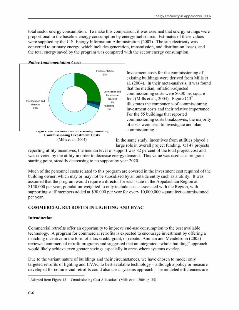
Energy Efficiency in Appalachia, SEEA
C-6
total sector energy consumption. To make this comparison, it was assumed that energy savings were proportional to the baseline energy consumption by energy/fuel source. Estimates of these values were supplied by the U.S. Energy Information Administration (2007). The site electricity was converted to primary energy, which includes generation, transmission, and distribution losses, and the total energy saved by the program was compared with the sector energy consumption. Policy Implementation Costs
Investment costs for the commissioning of existing buildings were derived from Mills et al. (2004). In their meta-analysis, it was found that the median, inflation-adjusted commissioning costs were $0.30 per square foot (Mills et al., 2004). Figure C.32 illustrates the components of commissioning investment costs and their relative importance. For the 55 buildings that reported commissioning costs breakdowns, the majority of costs were used to investigate and plan commissioning.
In the same study, incentives from utilities played a large role in overall project funding. Of 48 projects
reporting utility incentives, the median level of support was 82 percent of the total project cost and was covered by the utility in order to decrease energy demand. This value was used as a program starting point, steadily decreasing to no support by year 2020. Much of the personnel costs related to this program are covered in the investment cost required of the building owner, which may or may not be subsidized by an outside entity such as a utility. It was assumed that the program would require a director for each state in the Appalachian Region at $150,000 per year, population-weighted to only include costs associated with the Region, with supporting staff members added at $90,000 per year for every 10,000,000 square feet commissioned per year. COMMERCIAL RETROFITS IN LIGHTING AND HVAC Introduction Commercial retrofits offer an opportunity to improve end-use consumption to the best available technology. A program for commercial retrofits is expected to encourage investment by offering a matching incentive in the form of a tax credit, grant, or rebate. Amman and Mendelsohn (2005) reviewed commercial retrofit programs and suggested that an integrated ―whole building‖ approach would likely achieve even greater savings especially in areas where systems overlap. Due to the variant nature of buildings and their circumstances, we have chosen to model only targeted retrofits of lighting and HVAC to best available technology – although a policy or measure developed for commercial retrofits could also use a systems approach. The modeled efficiencies are 2 Adapted from Figure 13 ―Commissioning Cost Allocation‖ (Mills et al., 2004, p. 35)
Figure C.3 Breakdown of Existing Building Commissioning Investment Costs
(Mills et al., 2004)
Verification and
Persistance
Tracking
2%
Implementation
27%
Investigation and
Planning
69%Reporting
2%

Appendix C: Commercial Policy and Methodology Detail
C-7
about what would be required, independent of savings in other end-uses, to meet the Building Owners and Manager‘s Association‘s (BOMA) challenge to reduce commercial building consumption by 30 percent by 2012 (BOMA, 2007).
Methodology The present study uses a consumption reduction figure for the four end-uses affected (heating, cooling, ventilation, and lighting). There may be some overlap between savings characterized in the Commissioning of Existing Buildings program and this retrofit program because both target existing building stock. DeCanio and Watkins (1998) found that characteristics of firms are important in their adoption of these cost-effective retrofits. However, data on firm characteristics are not available for the Region, so the present study assumes constant adoption over all types. Energy Savings Energy savings for commercial building retrofits of HVAC and lighting equipment are determined by changing the anticipated efficiency of heating, cooling, ventilation, and lighting end-uses. The modeled efficiencies compared to the stock equipment efficiencies from the AEO 2008 are shown in Table C.4 (EIA, 2008). Savings for duct-sealing alone have been shown to be around 15 percent with a payback of 1.1 years (Jump, Walker, and Modera, 1996; Franconi, Delp, and Modera, 1998). Similarly, Woods (2006)
Figure C.4 Example of Improved Lighting Appearance with Energy Saving Lighting Retrofits (Efficient Lighting, 2008)
Figure C.5 Commercial Retrofit of HVAC and Lighting Methodology
Percentage of
Floorspace Subject to
Retrofit, by type
ARC Commercial Building
Energy Use
ARC Commercial Building
Energy UseARC Commercial
Floorspace, by type
ARC Commercial
Floorspace, by type
Program
Penetration
Rate
Program
Penetration
Rate
Compute Retrofit Energy
Savings
Percentage of Total Sector
Energy Savings
Retrofit Energy
Savings, by end-
use, by fuel
Retrofit Energy
Savings, by end-
use, by fuel
HVAC End-use
consumption, by fuel, by
building type
Lighting End-use
consumption, by fuel, by
building type

Energy Efficiency in Appalachia, SEEA
C-8
describes several cases of air sealing (rooftops, doors, windows) where savings were between 19 and 35 percent with paybacks from less than half a year to around five years.
AEO 2008 Present
AEO 2008 Present
AEO 2008 Present
AEO 2008 Present
AEO 2008 Present
AEO 2008 Present
AEO 2008 Present
2010 42.90 61.29 1.18 1.68 2.96 4.23 0.25 0.35 0.77 1.10 0.92 1.32 0.78 1.112011 43.34 63.73 1.19 1.75 3.01 4.43 0.25 0.37 0.77 1.14 0.94 1.38 0.78 1.152012 43.70 66.21 1.20 1.81 3.06 4.64 0.25 0.38 0.77 1.17 0.96 1.45 0.78 1.182013 44.00 68.76 1.20 1.88 3.10 4.85 0.25 0.39 0.78 1.21 0.97 1.52 0.78 1.222014 44.27 71.41 1.21 1.95 3.14 5.07 0.25 0.41 0.78 1.26 0.99 1.59 0.78 1.262015 44.52 74.19 1.22 2.03 3.18 5.30 0.26 0.43 0.78 1.30 1.00 1.67 0.78 1.312016 44.74 77.14 1.22 2.11 3.22 5.55 0.26 0.44 0.78 1.35 1.01 1.74 0.78 1.352017 44.96 80.29 1.23 2.19 3.25 5.81 0.26 0.46 0.78 1.40 1.02 1.83 0.78 1.402018 45.16 83.62 1.23 2.28 3.29 6.09 0.26 0.48 0.78 1.45 1.04 1.92 0.79 1.452019 45.33 87.18 1.24 2.38 3.32 6.38 0.26 0.50 0.79 1.51 1.05 2.01 0.79 1.512020 45.49 90.99 1.25 2.49 3.35 6.70 0.26 0.53 0.79 1.57 1.06 2.11 0.79 1.572021 45.64 93.14 1.25 2.56 3.38 6.90 0.27 0.54 0.79 1.61 1.07 2.17 0.79 1.612022 45.77 95.35 1.26 2.62 3.41 7.10 0.27 0.56 0.79 1.64 1.07 2.24 0.79 1.642023 45.91 97.68 1.27 2.69 3.44 7.31 0.27 0.57 0.79 1.68 1.08 2.30 0.79 1.682024 46.04 100.09 1.27 2.76 3.46 7.53 0.27 0.59 0.79 1.72 1.09 2.37 0.79 1.722025 46.15 102.56 1.28 2.84 3.49 7.75 0.27 0.60 0.79 1.76 1.10 2.44 0.79 1.762026 46.26 105.13 1.28 2.92 3.51 7.98 0.27 0.62 0.79 1.80 1.10 2.51 0.79 1.802027 46.35 107.79 1.29 3.00 3.53 8.22 0.27 0.64 0.79 1.85 1.11 2.58 0.79 1.842028 46.43 110.54 1.29 3.08 3.56 8.47 0.27 0.65 0.80 1.90 1.11 2.65 0.79 1.892029 46.52 113.45 1.30 3.17 3.58 8.72 0.28 0.67 0.80 1.94 1.12 2.73 0.79 1.932030 46.59 116.49 1.31 3.26 3.59 8.98 0.28 0.69 0.80 1.99 1.12 2.81 0.79 1.98
Space Heating Space Cooling Space Heating
Electricity Natural Gas DistillateLighting (lumens
per watt) Space Heating Space CoolingVentilation (cubic feet per minute per
a The present study also considers savings for Ventilation provided by natural gas and distillate fuel oil. These are small portions of the equipment stock, and the AEO 2008 did not include stock efficiency data for these fuels in their forecast (EIA, 2008). Policy Implementation Cost Administration of a retrofit incentive program (such as allowing for a tax credit or grant) is not expected to be burdensome. One administrator at $75,000 per 500 million square feet of retrofit space per year is assumed. Investment costs are set at $1.00 per retrofit square foot. This assumption is general because data were not available on equipment capacity and age at the level of detail required for modeling by equipment costs. If data are collected at this level in a future analysis, the costs could better approximate the true investment necessary to achieve these savings. We assume these costs are reasonable. For example, a 5,000 square foot building would have an incremental cost of $5,000. This assumes that the building was already undergoing replacement of equipment; the incremental costs represent the difference in cost for purchasing higher efficiency equipment. The present study includes an assumption of a significant 30 percent incentive to undergo commercial retrofits; the incentive is in place from 2010 to 2020. While this makes adoption more likely, it increases the public cost of the program. An incentive program at a lower level could be
Table C.4 Modeled End-Use Efficiencies for Retrofit Equipment Compared to AEO 2008 Stock Equipment
(EIA, 2008)a
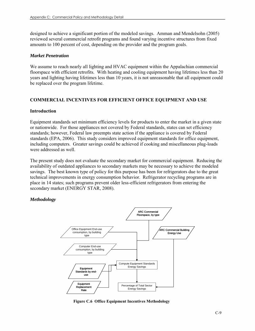
Appendix C: Commercial Policy and Methodology Detail
C-9
designed to achieve a significant portion of the modeled savings. Amman and Mendelsohn (2005) reviewed several commercial retrofit programs and found varying incentive structures from fixed amounts to 100 percent of cost, depending on the provider and the program goals. Market Penetration We assume to reach nearly all lighting and HVAC equipment within the Appalachian commercial floorspace with efficient retrofits. With heating and cooling equipment having lifetimes less than 20 years and lighting having lifetimes less than 10 years, it is not unreasonable that all equipment could be replaced over the program lifetime. COMMERCIAL INCENTIVES FOR EFFICIENT OFFICE EQUIPMENT AND USE Introduction Equipment standards set minimum efficiency levels for products to enter the market in a given state or nationwide. For those appliances not covered by Federal standards, states can set efficiency standards; however, Federal law preempts state action if the appliance is covered by Federal standards (EPA, 2006). This study considers improved equipment standards for office equipment, including computers. Greater savings could be achieved if cooking and miscellaneous plug-loads were addressed as well. The present study does not evaluate the secondary market for commercial equipment. Reducing the availability of outdated appliances to secondary markets may be necessary to achieve the modeled savings. The best known type of policy for this purpose has been for refrigerators due to the great technical improvements in energy consumption behavior. Refrigerator recycling programs are in place in 14 states; such programs prevent older less-efficient refrigerators from entering the secondary market (ENERGY STAR, 2008). Methodology
ARC Commercial Building
Energy Use
ARC Commercial Building
Energy Use
ARC Commercial
Floorspace, by type
ARC Commercial
Floorspace, by type
Equipment
Replacement
Rate
Equipment
Replacement
Rate
Compute Equipment Standards
Energy Savings
Percentage of Total Sector
Energy Savings
Equipment
Standards by end-
use
Equipment
Standards by end-
use
Computer End-use
consumption, by building
type
Office Equipment End-use
consumption, by building
type
Figure C.6 Office Equipment Incentives Methodology
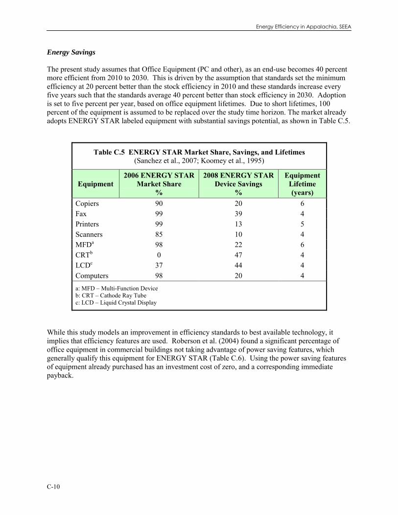
Energy Efficiency in Appalachia, SEEA
C-10
Energy Savings The present study assumes that Office Equipment (PC and other), as an end-use becomes 40 percent more efficient from 2010 to 2030. This is driven by the assumption that standards set the minimum efficiency at 20 percent better than the stock efficiency in 2010 and these standards increase every five years such that the standards average 40 percent better than stock efficiency in 2030. Adoption is set to five percent per year, based on office equipment lifetimes. Due to short lifetimes, 100 percent of the equipment is assumed to be replaced over the study time horizon. The market already adopts ENERGY STAR labeled equipment with substantial savings potential, as shown in Table C.5.
Table C.5 ENERGY STAR Market Share, Savings, and Lifetimes (Sanchez et al., 2007; Koomey et al., 1995)
Equipment 2006 ENERGY STAR
Market Share %
2008 ENERGY STAR Device Savings
%
Equipment Lifetime (years)
Copiers 90 20 6 Fax 99 39 4 Printers 99 13 5 Scanners 85 10 4 MFDa 98 22 6 CRTb 0 47 4 LCDc 37 44 4 Computers 98 20 4 a: MFD – Multi-Function Device b: CRT – Cathode Ray Tube c: LCD – Liquid Crystal Display
While this study models an improvement in efficiency standards to best available technology, it implies that efficiency features are used. Roberson et al. (2004) found a significant percentage of office equipment in commercial buildings not taking advantage of power saving features, which generally qualify this equipment for ENERGY STAR (Table C.6). Using the power saving features of equipment already purchased has an investment cost of zero, and a corresponding immediate payback.

Appendix C: Commercial Policy and Methodology Detail
C-11
Table C.6 Turn Off and Power Management Status of After-Hours Office Equipment, 2000 and 2003
(Roberson et al., 2004, Table 7 p. 16)
Category Type # in 2003
Turn-off Rate
%
Power Management Rate
% 2000 2003 2000 2003
Computers desktop + ICSa 1,498 44 37 5 7 desktop 1,453 36 6 ICSa 45 60 61 Monitors all 1,598 32 29 56 72 CRTb 1,329 32 71 LCDc 269 18 75 Printers all 353 25 23 44 31
monochrome laser 24 53
high-end color 15 61 laser 158 15 60 inkjet 123 31 30 3 0 impact 22 31 27 0 0 thermal 38 18 0 wide format 8 57 75 32 0 solid ink 4 0 75 MFDsd all 79 18 20 56 29 inkjet 16 19 31 laser 63 21 28 Copiers all 33 18 49 32 28 Fax machines 47 2 0 6 Scanners all 34 29 41 60 a ICS- Integrated Computer Systems c LCD – Liquid Crystal Display b CRT – Cathode Ray Tube d MFD – Multi-Function Device
Policy Implementation Cost Administrative costs are relatively low for appliance and equipment standards. In general, standards do not have a consistent expense – administrative costs would be highest in the years of adoption and lowest between adoption cycles. We assume administrative costs of $75,000 per year per 500 million square feet of floorspace. It is assumed that these administrators would be charged with promoting use of energy saving features on office equipment purchased with the program.

Energy Efficiency in Appalachia, SEEA
C-12
Investment costs vary widely by equipment type, brand, model, and location. In order to generalize, we assumed a cost of $0.10 per square foot of floorspace in buildings adopting new equipment (based on an average of nine pieces of office equipment per 1000 gross square foot of building space (Roberson et al., 2004). The density of office equipment will lead to significant variations in costs and savings across building types and specific buildings. This cost overestimates the incremental cost of types of office equipment and underestimates others. This program is expected to be accompanied by an incentive program that will cover 20 percent of the incremental costs of adopting the higher efficiency models until 2020. Market Penetration This study assumes that all office equipment will be replaced with high efficiency equipment (meeting an assumed ENERGY STAR standard) at the end of its lifetime. Savings are compared to the Annual Energy Outlook which already assumes some efficiency gains (EIA, 2007; 2008). REFERENCES Amman, Jennifer Thorne and Eric Mendelsohn. 2005. ―Comprehensive Commercial Retrofit
Programs: A Review of Activity and Opportunities.‖ Report A052. Washington DC: ACEEE. Building Owners and Managers Association, International (BOMA). 2007. ―Market Transformation
Energy Plan and 7 Point Challenge.‖ http://www.boma.org/NR/rdonlyres/EE51F93D-822D-4959-A82F-6A643F6242D1/0/Market_Trans_Web.pdf
DeCanio, Stephen J. and William E. Watkins. 1998. Investment in Energy Efficiency: Do the
Characteristics of Firms Matter? The Review of Economics and Statistics, Vol. 80, No. 1, pp. 95-107.
Efficient Lighting. 2008. Description of Sunwest Properties retrofit.
http://www.efficientlightingco.com/projects/sunwest.htm Energy Information Administration (EIA). 2007. Annual Energy Outlook 2007.
http://tonto.eia.doe.gov/ftproot/forecasting/0383(2007).pdf ———. 2008. Annual Energy Outlook 2008. http://www.eia.doe.gov/oiaf/aeo/ ENERGY STAR. 2008. ―ENERGY STAR Qualified New Homes Market Indices for States.‖
http://www.energystar.gov/index.cfm?fuseaction=qhmi.showHomesMarketIndex Franconi, E., W.W. Delp, M.P. Modera. 1998. Impact of Duct Air-Leakage on VAV Distribution
System Performance. Lawrence Berkeley National Laboratory, LBNL-42417. Jump, David A. Iain S. Walker and Mark P. Modera. 1996. ―Field Measurements of Efficiency and
Duct Retrofit Effectiveness in Residential Forced Air Distribution Systems‖ (Lawrence Berkeley National Laboratory, LBL-38537). Proc. 1996 ACEEE Summer Study, August 1996, Asilomar, CA.

Appendix C: Commercial Policy and Methodology Detail
C-13
International Code Council (ICC). 2006 International Energy Conservation Code®. ‖
http://www.iccsafe.org/e/prodshow.html?prodid=3800S06 Koomey, Jonathan, Michael Cramer, Mary Ann Piette and Joseph Eto, 1995. Efficiency
Improvements in U.S. Office Equipment: Expected Policy Impacts and Uncertainties. Lawrence Berkeley Laboratory. LBL-37383.
Mills, Evan, Hannah Friedman, Tehesia Powell, Norman Bourassa, David Claridge, Tudi Haasl,
Mary Ann Piette. 2004. The Cost Effectiveness of Commercial-Buildings Commissioning. Lawrence Berkeley National Laboratory. Berkeley, CA. http://eetd.lbl.gov/Emills/PUBS/PDF/Cx-Costs-Benefits.pdf
New York State Energy Research and Development Authority (NYSERDA). 2004. Guideline to the
Commissioning Process for Existing Buildings, or “Retro-Commissioning.” Portland Energy Conservation, Inc. http://www.nyserda.org/programs/pdfs/retrocxhandbookfinal040704.pdf
Pitts, Adrian and Jasmi Bin Saleh. 2007. ―Potential for energy saving in building transition spaces.‖
Energy and Buildings 39 7: 815-822. Regional Economics Models, Inc. (REMI). 2007. Data provided to the authors by the
Appalachian Regional Commission on Dec 21, 2007. Roberson, Judy A., Carrie A. Webber, Marla C. McWhinney, Richard E. Brown, Margaret J.
Pinckard, and John F. Busch. 2004. After-hours Power Status of Office Equipment and Inventory of Miscellaneous Plug-Load Equipment. Energy Analysis Department, Lawrence Berkeley National Laboratory, LBNL-53729. http://enduse.lbl.gov/Info/LBNL-53729.pdf
Sanchez, Marla, Richard E. Brown, Gregory K. Homan, and Carrie A. Webber. 2007. DRAFT 2008
Status Report Savings Estimates for the ENERGY STAR Voluntary Labeling Program. Lawrence Berkeley Laboratory. LBL-56380.
U.S. Environmental Protection Agency (EPA). 2006. Clean Energy-Environment Guide to Action:
Policies, Best Practices, and Action Steps for States. http://www.epa.gov/cleanenergy/documents/gta/guide_action_full.pdf
Woods, Tony. 2006. 30 year History proves energy savings from air barrier retrofit.
http://www.buildingenvelopeforum.com/pdf/30energysavings.pdf


Appendix D: Industrial Sites
D-1
APPENDIX D: INDUSTRIAL SITES
D.1 INDUSTRIAL ASSESSMENT CENTERS Introduction Industrial Assessment Centers (IACs) evaluate small- to medium-sized industrial sites (less than $2.5 million in energy consumption per year) and identify savings opportunities in the form of energy efficiency, waste minimization, pollution prevention, and productivity improvement (DOE/EERE, 2008). Expansion of these centers in the Appalachian Region could yield large improvements in energy efficiency at industrial facilities. Examples of industrial assessment findings are shown in Table D.1. Each industrial assessment yields a list of recommendations, which includes a statement of the type of recommended improvement, its cost to implement, the potential energy savings, and a quantification of how much money would be saved per year if each recommendation were implemented.
Table D.1 Examples of Recommended Improvements in Energy Consumption (DOE/EERE, 2008)
State Year Principal Product
Baseline Year Energy Cost
$
Potential Electricity Saved
%
Potential Natural Gas Saved
%
PA 2008 Chain Assemblies 602,793 26 50
WV 2008 Fiberglass Media 1,140,227 10 10
NC 2008 Cutting Tools 584,396 4 0
MS 2008 Wiring Harness Components 218,074 9 0

Energy Efficiency in Appalachia, SEEA
D-2
METHODOLOGY Energy Savings Figure D.1 highlights the process implemented to determine the potential energy savings that could be realized if IACs were expanded in Appalachia. First, findings yielded from industrial assessment in the states that comprise the Appalachian Region were compiled. Information related to productivity improvement and waste minimization was excluded unless there was a stated energy savings associated with these actions. These data include such information as the North American Industry Classification System (NAICS) code, baseline energy usage, recommended changes, potential energy savings, and cost of recommended changes. After these data were compiled, they were averaged by ARC subregion (North, Central, and South) while maintaining the information by separate industrial NAICS codes. Employment figures for the ARC (IMPLAN, 2006) were provided and used along with information provided by the industrial assessments to estimate the number of industrial sites in the ARC Region. In addition, the employment figures and IAC data were used to compute a weighted-average energy savings number by energy type for each site. These averages take into account the weighting of each industry in the subregion. The average values used for analysis are found in Table D.2. Current implementation rates can be on the order of 50 percent. In order to quantify the full potential of this policy bundle, it was assumed that all of the recommended changes are implemented. This may be possible by addressing barriers to implementation through increased education and outreach, assistance with outage planning, and low-interest loans, as mentioned in Table 5.2.
Table D.2 Average Site Energy Savings and Investment Costs for IAC Program (Author‘s calculations; DOE/EERE, 2008)
ARC Subregion Electricity Savings %
Natural Gas Savings %
Implementation Cost $
North 13.6 15.0 245,612
Central 4.9 13.2 121,461
South 11.7 13.4 195,643
Figure D.1 IAC Energy Savings Methodology

Appendix D: Industrial Sites
D-3
Savings in the North subregion were found to be greatest, and the costs required to implement the changes were also the greatest. The Central subregion had much lower savings values related to electricity; however, the costs for changes were also much lower. The differences between the subregions may be due to climate and weighting of various industries in each subregion as well as a limited sample size in the Central region. The Central region is the smallest ARC subregion by area. After estimating the number of sites in the Appalachian Region, the number of sites eligible for IAC assistance was determined. On average, approximately 90 percent of industrial sites are in the small- to medium-size range, and, therefore, eligible for industrial assessment (Soderlund, 2008). These sites represent approximately half of the total energy use in industry. The remaining 10 percent of sites would be eligible for other programs such as Energy Savings Assessments (ESAs) and/or combined heat and power systems. The extensive market penetration of industrial assessments was estimated based upon the success of the current IAC program. Currently, approximately 40 assessments are performed in the Region per year. With a large push, a goal of 100 percent assessment by 2030 in Appalachia was assumed, which would require an eight-fold increase in the current number of assessments per year. With the number of eligible sites determined and a program penetration assumed, the program energy savings by each energy type were determined. Policy Implementation Cost As seen in Table D.2, the investment costs were determined from previous industrial assessment data. Since the IAC program is already in existence, administration costs were assumed to be similar to those already incurred. Each assessment requires approximately $9,000 in funds (Soderlund, 2008). Additionally, in support of the program, each state was assumed to have an administrator in charge of promoting the program. Each program champion was budgeted at $150,000 and that total was then proportioned to the Appalachian Region based on population. D.2 ENERGY SAVINGS ASSESSMENTS Introduction Energy Savings Assessments (ESAs) are evaluations of major energy systems at large industrial sites (greater than $2.5 million in annual energy expenditures). Each assessment only targets one system. The U.S. Department of Energy‘s Save Energy Now program was developed to use ESAs to aid in the reduction of natural gas consumption post hurricane Katrina (Wright et al., 2007). The results summarized by Wright et al. (2007) are for assessments that focused on steam and process heating; however, the program also trains on-site personnel to be able to conduct future ESAs at their location and provides them with tools, such as software, to aid in ESA completion. In addition, while one of the major focuses of the Save Energy Now program is reduction of natural gas usage, ESAs can also be applied to other energy-intensive processes at an industrial site.

Energy Efficiency in Appalachia, SEEA
D-4
Methodology Energy Savings The methodology used to determine ESA program energy savings is shown in Figure D.2. Due to confidentially issues, data, such as those available for industrial assessments, were not available. Data shared by Wright et al. (2007) were listed separately by two categories: NAICS code and state. These sets of data were combined with Appalachian Region employment information and IAC data for specific system savings to estimate weighted-average energy savings values by energy type (Table D.3). The number of industrial sites for which the ESA program would be applicable was determined through the IAC analysis and combined with subregion growth estimates to determine the number of sites available for future assessment. In addition, it was assumed that up to four high-impact assessments could take place at each physical site location. All of these ―virtual sites‖ would be able to be assessed, each increasing the sector energy savings.
Table D.3 Average Site Energy Savings for ESA Program (Author‘s calculations; Wright et al., 2007)
ARC Subregion Electricity Savings %
Natural Gas Savings %
North 11.5 17.5
Central 8.4 12.8
South 7.3 11.1 Once the number of ―virtual sites‖ (or potential assessments) and site energy savings were determined, a penetration rate of 100 percent was assumed for each first assessment. In 2006, it is estimated that only 16 ESAs were performed in Appalachia, based on population-weighting. This was, in part, due to the limited scope of the Save Energy Now program. By 2030, it is estimated that approximately 170 assessments would be completed each year throughout the Region, with almost all being performed by on-site personnel. It was assumed that subsequent assessments would lag the first assessment due to effort required to implement first assessment recommendations. Overall, over
Figure D.2 ESA Energy Savings Calculation Methodology

Appendix D: Industrial Sites
D-5
60 percent of available assessments were completed by 2030. All recommendations have four-year or shorter payback period, and it is assumed that all recommendations were executed. Policy Implementation Costs While the costs of assessing one system in a large-scale industrial plant is similar to the cost of a full industrial assessment for a small- to medium-sized facility, current program infrastructure is much smaller and would require the addition of more administrators. It was assumed that each state would have a program champion, funded at $150,000 per year and proportioned to the Appalachian Region based on population ratios in each state, with support personnel at $90,000 per year, one for every 10 new sites assessed per year in order to continue outreach and education while also monitoring the progress of every site assessed. These personnel would be tasked with tracking the results of initial assessments and for encouraging future assessments at these locations as well as assisting with such tasks as site software updates. Based on the data available from the Save Energy Now program and scaling industrial assessment results yielded the average investment cost values shown in Table D.4.
Table D.4 Average Investment Costs for ESA Program
(Author‘s calculations; Wright et al., 2007)
ARC Subregion Investment Cost (million 2006$)
North 1.5
Central 2.1
South 2.3 D.3 INDUSTRIAL COMBINED HEAT AND POWER Introduction The use of industrial combined heat and power (CHP) systems could have a large impact on industry‘s future consumption of primary energy. Many CHP systems consist of a prime mover, which produces electricity. The prime mover is coupled with one or more thermally-activated technologies, and these thermal systems use the prime mover‘s hot exhaust as an energy input to create a useful product such as steam or hot water that would otherwise be generated by using other high-value energy sources such as electricity or natural gas. The systems considered in the current study are of this type. Other types of systems could make use of fluids compressed to aid in transport (e.g., district steam used for space heating) that, instead of being throttled down to a site‘s required system pressure, is coupled with a turbine, which generates power while also reducing pressure. These types of systems are not modeled in this analysis; however, they do have the potential to yield additional energy savings for the Appalachian Region. When cost-effective for a particular site, so-called recycled energy systems, where heat is recovered from a process stream and reused to drive another, lower temperature process, are included in industrial and energy savings assessments;

Energy Efficiency in Appalachia, SEEA
D-6
therefore, they were not included in the CHP portion of the study. Through the use of this otherwise wasted energy, CHP systems can yield total system thermal efficiencies of up to 80 percent (EPA, 2008). Methodology Energy Savings The methodology used to calculate the energy savings that could result from a CHP program in the Appalachian Region is detailed in Figure D.3. In order to assess the impact of expanding industrial CHP, it was necessary to determine the current level of installed CHP generation capacity in the Region. Information on current CHP installations is maintained in a database funded by the U.S. Department of Energy and administered by Energy and Environment Analysis, Inc. (EEA, 2007). Based upon the installed capacity in each ARC state, a capacity value was determined for the Region. According to this estimate, approximately four percent of the installed capacity in the ARC Region is part of a CHP system. In a study conducted by ACEEE, under an accelerated CHP scenario,1 it is estimated that the share of installed capacity that is also part of a CHP system could reach 19 percent by 2030 (Laitner, 2008). Lemar (2001) estimated that under a ―moderate scenario‖ for CHP expansion and a 20-year time period, 15.7 percent of industrial electricity needs could be met by CHP. Under a much more aggressive scenario, 34.7 percent of industrial electricity could be generated by CHP systems. For the current study, it is assumed that by 2030, CHP‘s share of the Region‘s electricity generation capacity will reach 20 percent. In addition to market penetration, characteristics of grid electricity, CHP prime mover, and site energy needs must be defined. Electricity generated in centralized power plants is subject to direct generation inefficiencies as well as energy losses due to transmission and generation. The electric efficiency related to grid-supplied electricity was calculated from EIA energy data (EIA, 2007). Including losses from generation, transmission, and distribution, the energy efficiency of grid-supplied electricity in the Appalachian Region decreases from 30.3 percent in 2010 to 25.1 percent in 2030. During the same time frame, the national average delivered electric efficiency increases from 31.7 percent in 2010 to 33.4 percent in 2030.
1 An accelerated CHP scenario is one in which the rate of development of CHP in a Region approaches the rates seen in such countries as Finland and the Netherlands over the past 30 years.
Figure D.3 Industrial CHP Energy Savings Methodology

Appendix D: Industrial Sites
D-7
CHP characteristics are highly dependent on the choice of prime mover. The prime mover characteristics used in this study are listed in Table D.5.
Table D.5 Example CHP Prime Mover Characteristics (Elliot, 2008)
Type Size (kW)
Electric Efficiency
(%)
Thermal Output
(Btu/ Wh)
Installed Cost
($/kW)
O&M Costs
($/k Wh)
After-treatment Cost
($/kW) MT 60 24.6 6308 2,739 0.022 500 RE 100 28.4 6100 2,210 0.022 -- MT 250 26.0 4800 2,684 0.013 500 RE 800 35.0 2313 1,640 0.013 300 GT 3,000 26.0 5018 1,690 0.006 210 RE 3,000 35.9 3510 1,130 0.011 200 RE 5,000 39.0 3046 1,130 0.009 150 GT 10,000 29.0 4674 1,298 0.006 140 GT 40,000 37.0 2189 972 0.004 90
MT = Microturbine; RE = Reciprocating Engine; GT = Gas Turbine
In 2000, ONSITE SYCOM Energy Corporation (OSEC) published a study on the market and technical potential of industrial CHP (OSEC, 2000). A result of its analysis was a quantification of the CHP potential by SIC code,2 which also listed such information as size of prime mover as well a ratio of site power and steam requirements. By weighting information on site energy use compiled by OSEC by Appalachian Region industrial site information derived from IAC information, an overall average power to steam ratio for the Region was determined to be 0.87. Average CHP prime mover characteristics for the Region were also determined and are shown in Table D.6.
Table D.6 Average CHP Prime Mover Characteristics for ARC Region
(Author‘s calculations)
Electric Efficiency 32.0%
Thermal Output 2,948 Btu/kWh
Installed Cost $1,227/kW
O&M Costs $0.0061/kWh
After-treatment Cost $150/kW 2 SIC codes where converted to approximate NAICS codes in order to determine Region characteristics.
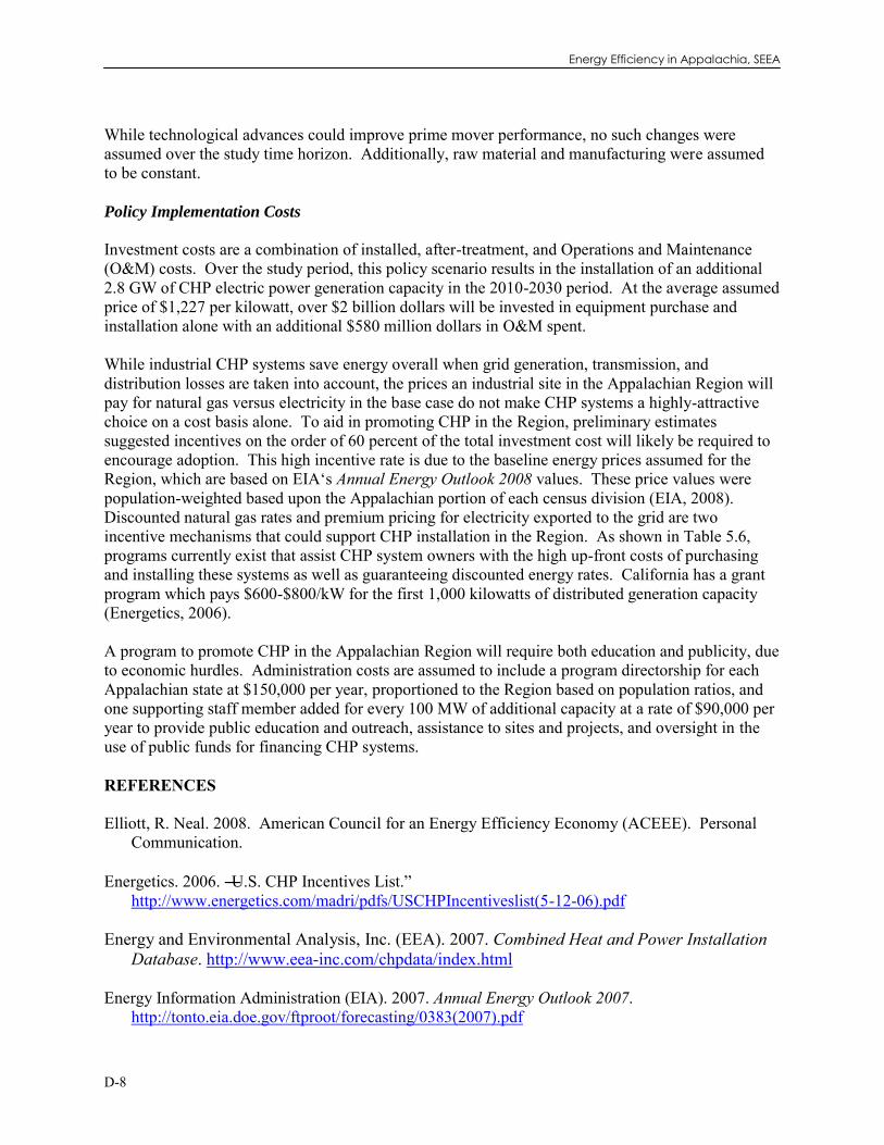
Energy Efficiency in Appalachia, SEEA
D-8
While technological advances could improve prime mover performance, no such changes were assumed over the study time horizon. Additionally, raw material and manufacturing were assumed to be constant. Policy Implementation Costs Investment costs are a combination of installed, after-treatment, and Operations and Maintenance (O&M) costs. Over the study period, this policy scenario results in the installation of an additional 2.8 GW of CHP electric power generation capacity in the 2010-2030 period. At the average assumed price of $1,227 per kilowatt, over $2 billion dollars will be invested in equipment purchase and installation alone with an additional $580 million dollars in O&M spent. While industrial CHP systems save energy overall when grid generation, transmission, and distribution losses are taken into account, the prices an industrial site in the Appalachian Region will pay for natural gas versus electricity in the base case do not make CHP systems a highly-attractive choice on a cost basis alone. To aid in promoting CHP in the Region, preliminary estimates suggested incentives on the order of 60 percent of the total investment cost will likely be required to encourage adoption. This high incentive rate is due to the baseline energy prices assumed for the Region, which are based on EIA‘s Annual Energy Outlook 2008 values. These price values were population-weighted based upon the Appalachian portion of each census division (EIA, 2008). Discounted natural gas rates and premium pricing for electricity exported to the grid are two incentive mechanisms that could support CHP installation in the Region. As shown in Table 5.6, programs currently exist that assist CHP system owners with the high up-front costs of purchasing and installing these systems as well as guaranteeing discounted energy rates. California has a grant program which pays $600-$800/kW for the first 1,000 kilowatts of distributed generation capacity (Energetics, 2006). A program to promote CHP in the Appalachian Region will require both education and publicity, due to economic hurdles. Administration costs are assumed to include a program directorship for each Appalachian state at $150,000 per year, proportioned to the Region based on population ratios, and one supporting staff member added for every 100 MW of additional capacity at a rate of $90,000 per year to provide public education and outreach, assistance to sites and projects, and oversight in the use of public funds for financing CHP systems. REFERENCES Elliott, R. Neal. 2008. American Council for an Energy Efficiency Economy (ACEEE). Personal
Communication. Energetics. 2006. ―U.S. CHP Incentives List.‖
http://www.energetics.com/madri/pdfs/USCHPIncentiveslist(5-12-06).pdf Energy and Environmental Analysis, Inc. (EEA). 2007. Combined Heat and Power Installation
Database. http://www.eea-inc.com/chpdata/index.html Energy Information Administration (EIA). 2007. Annual Energy Outlook 2007.
http://tonto.eia.doe.gov/ftproot/forecasting/0383(2007).pdf

Appendix D: Industrial Sites
D-9
———. 2008. Annual Energy Outlook 2008. http://www.eia.doe.gov/oiaf/aeo/ Laitner, John A. ‖Skip‖. 2008. Amercian Council for an Energy-Efficiency Economy (ACEEE).
Personal Communication. Lemar, Paul, Jr. 2001. ―The potential impact of policies to promote combined heat and power in
U.S. industry.‖ Energy Policy, 29, pp. 1243-1254. Minnesota IMPLAN Group, Inc. (IMPLAN). 2006. A 2005 dataset for Appalachia (Alabama,
Georgia, Kentucky, Maryland, Mississippi, New York, North Carolina, Ohio, Pennsylvania, South Carolina, Tennessee, and Virginia. Stillwater, Minn.: Minnesota IMPLAN Group, Inc.
ONSITE SYCOM Energy Corporation (OSEC). 2000. The Market and Technical Potential for
Combind Heat and Power in the Commercial/Institutional Sector (Revision 1). http://www.eere.energy.gov/de/pdfs/chp_comm_market_potential.pdf
Soderlund, Matthew. 2008. Georgia Institute of Technology Industrial Assessment Center. Personal
Communication. U.S. Department of Energy Energy Efficiency and Renewable Energy (DOE/EERE). 2008a.
Industrial Technologies Program-IAC Database. http://iac.rutgers.edu/database/about.php U.S. Environmental Protection Agency (EPA). 2008. Efficiency Benefits.
http://www.epa.gov/chp/basic/efficiency.html Wright, Anthony, Michaela Martin, Bob Gemmer, Paul Scheihing, and James Quinn. 2007. Results
from the U.S. DOE 2006 Save Energy Now Assessment Initiative: DOE’s Partnership with U.S. Industry to Reduce Energy Consumption, Energy Costs, and Carbon Dioxide Emissions. http://apps1.eere.energy.gov/industry/saveenergynow/partners/pdfs/sena_2006_report_final_09_17_07.pdf


Appendix E: Transportation
E-1
APPENDIX E: TRANSPORTATION REFERENCE CASE ENERGY EFFICIENCY IN AEO 2008 (EIA, 2008) The 2008 Annual Energy Outlook (AEO) projects energy consumption and prices based on energy-efficiency legislation enacted in the 2007 Energy Independence and Security Act (EISA, 2007). EISA established a Corporate Average Fuel Economy (CAFE) standard of at least 35 miles per gallon for cars and light trucks by 2020, a 40 percent improvement over today‘s fuel economy standard. Based on national fleet turnover data, we estimate that the new CAFE standard will reduce national light-duty vehicle fuel consumption by 22 percent by 2030. A host of additional policies are necessary to achieve an even more significant decrease in fuel consumption nationally and in the Appalachian Region. All policy-specific fuel savings documented in this analysis are additional to Reference Case fuel savings from the updated CAFE standard relative to a scenario with no change to fuel economy standards (Table E.1). All AEO projections cited here are national projections and have been scaled down by population proportion for the Appalachian Region. Please note that our estimate that gasoline savings will amount to 0.52 quads by 2030 differs slightly from AEO 2008 estimate that the new CAFE regulations will save 0.48 quads a year by 2030.
Table E.1 2008 EISA CAFE Fuel Savings
Year
Gasoline Savings
%
Gasoline Savings
(million gallons)
Gasoline Savings (quads)
2010 0.2 22 0.00 2011 1 81 0.01 2012 1 186 0.02 2013 3 337 0.04 2014 4 507 0.06 2015 5 661 0.08 2016 6 844 0.10 2017 7 1,056 0.13 2018 9 1,293 0.16 2019 10 1,556 0.19 2020 12 1,843 0.23 2021 14 2,125 0.26 2022 15 2,400 0.30 2023 16 2,665 0.33 2024 17 2,920 0.36

Energy Efficiency in Appalachia, SEEA
E-2
Table E.1 2008 EISA CAFE Fuel Savings
Year
Gasoline Savings
%
Gasoline Savings
(million gallons)
Gasoline Savings (quads)
2025 19 3,164 0.39 2026 19 3,397 0.42 2027 20 3,620 0.45 2028 21 3,831 0.48 2029 22 4,032 0.50 2030 22 4,222 0.52
CURRENT TRANSPORTATION ENERGY CONSUMPTION IN THE APPALACHIAN REGION Gasoline consumption in the ARC Region in 2008 is estimated at 12.1 billion gallons. Gasoline use is expected to grow along with population and total vehicle miles travelled to reach 14.9 billion gallons by 2030. Similarly, consumption of diesel fuel will rise from 2.9 billion gallons in 2008 to 3.5 billion gallons by 2030. This study considers energy consumption of highway modes only. PAY-AS-YOU-DRIVE INSURANCE Introduction Pay-as-you-drive insurance programs convert some of the fixed costs associated with driving into variable costs dependent on the total distance driven by a vehicle over a given year. Drivers would pay a portion of their premiums up front, and the remainder would be charged in proportion to mileage, as determined by periodic odometer readings or a mileage tracking device. Methodology Energy Savings To determine the reduction in total VMT driven in Appalachia that will result from a pay-as-you-drive insurance scheme, we followed the above methodology. Estimates of the reduction in vehicle-miles traveled (VMT), and therefore energy use, resulting from a PAYD policy depend upon the price elasticity of travel demand, i.e., the percent change in travel resulting from each percent increase in the cost of travel. Estimates of elasticity vary considerably among those who Figure E.1 Pay-As-You-Drive Insurance Energy
Savings Methodology
Cost-elasticity of driving
Average cost of insurance in
ARC
Average VMT/vehicle
Average fuel economy
Per gallon cost of gasoline
Compute insurance cost/mile
Compute gasoline cost/mile
Compute % increase in variable costs
Compute % VMT reduction
Compute VMT under scenario
Compute gasoline consumption and
savings using VMT and gallons/mile
data

Appendix E: Transportation
E-3
study them, and differ also according to the time elapsed between the change in price and the response to it. We use here a value of -0.1 for the long-term elasticity of driving with respect to gasoline price; that is, over 10-15 years, we assume there is a one percent reduction in driving for a 10 percent increase in gasoline price.1 At $3.04 per gallon, gasoline for an automobile or light truck having the average on-road fuel economy of 20.2 miles per gallon costs 14 cents per mile.2 The average cost of an insurance policy in the Appalachian Region in 2005 was $785, and we assume that vehicles in Appalachia are driven 12,000 miles per year, roughly the national average.3 This means an average insurance cost of 6.5 cents per mile. If 80 percent of the cost of the insurance premium was charged on a per-mile basis, the average cost per mile would then be $0.052 per mile, about 37 percent of the per-mile cost of fuel.4 Variable driving costs would increase by 37 percent as a result. An elasticity of -0.1 implies a corresponding reduction in driving of about four percent. Thus 100 percent adoption of PAYD insurance would be expected to reduce car and light truck energy use in Appalachia by about four percent over 10-15 years. Policy Implementation Costs During the pilot stage of the pay-as-you-drive insurance option, the ARC will grant $200 to insurance agencies for each one-year policy that is mileage based. We assume that 2,000 such policies will be sold in 2009, 10,000 in 2010 and 20,000 in 2011. Therefore, ARC can expect to pay incentives of $400,000 in 2009, $1.7 million in 2010 and $3.3 million in 2020 (2006 dollars). Administrative costs were estimated based on the assumption that each Appalachian state will employ one administrator for the program at a cost of $150,000 and two program staff at the cost of $90,000. These costs were scaled by the Appalachian population in each state to estimate ARC-specific administrative costs. Also included in administrative costs is the cost of implementation incurred by insurance companies. Insurance companies could incur substantial per-vehicle monitoring costs during the pilot phase of the proposed program for distribution of mileage tracking devices and data collection expenses. However, once the program becomes mandatory, per-vehicle costs would decline as tracking device costs decline and data collection and analysis is spread over a large number of vehicles. We assume a per-vehicle cost of $40 per vehicle per year in the pilot phase and $10 per vehicle thereafter. 5
1 Greene and Leiby, 2006; Litman, 2008 2 EIA, 2006 3 Insurance rates from Bureau of Labor Statistics http://data.bls.gov; miles per year calculated from 2005 vehicle registration 4 Bordoff and Noel (2008) assume that 84 percent of the insurance premium is charged on a per-mile basis. 5 Bordoff and Noel, 2008

Energy Efficiency in Appalachia, SEEA
E-4
Table E.2 Summary of Energy Savings Financial Costs For Pay-As-You-Drive Insurance
Year Reduction in
VMT %
Sector Primary Energy Savings
%
Investment Costs
(2006$)
Admn Costs (2006$)
2009 0.00 0.0007 4,370,000 2010 0.01 0.0035 4,690,000 2011 0.01 0.0071 5,090,000 2012 0.60 0.4161 34,526,596 2013 1.00 0.6931 55,037,088 2014 1.40 0.9725 75,833,244 2015 1.80 1.2526 96,918,060 2016 2.20 1.5317 118,294,558 2017 2.60 1.8077 139,965,788 2018 3.00 2.0862 161,934,830 2019 3.40 2.3638 184,204,789 2020 4.00 2.7799 217,436,109 2021 4.00 2.7837 218,928,132 2022 4.00 2.7849 220,430,599 2023 4.00 2.7959 221,943,583 2024 4.00 2.8096 223,467,158 2025 4.00 2.8280 225,001,398 2026 4.00 2.8535 226,546,378 2027 4.00 2.8771 228,102,172 2028 4.00 2.9039 229,668,858 2029 4.00 2.9345 231,246,510 2030 4.00 2.9692 232,835,205
CLEAN CAR STANDARD Introduction Appalachia‘s adoption of the Clean Car Standard means that new vehicles sold in the Region by each manufacturer would need to meet the requirements shown in Table E.3 for GHG emissions, on average. Our analysis of the energy savings that result from such a policy assumes that ARC will aim to achieve the long-term standards outlined below, standards that correspond to an average fleet fuel efficiency goal of 50 miles-per-gallon by 2030.

Appendix E: Transportation
E-5
Table E.3 Proposed Clean Car Program Greenhouse Gas Tailpipe Standards, 2009-2020
(California Air Resources Boarda)
Year CO2-equivalent emissions standard (g/mi)
Combined (Passenger cars and small trucks/ SUVs and large trucks/SUVs)
Near-term
2009 375.2 2010 359.5 2011 322.4 2012 290.6
Mid-term
2013 284.6 2014 279.6 2015 270.6 2016 262.2
Long-term
2017 246.8 2018 230.0 2019 220.5 2020 215.5
a Comparison of Greenhouse Gas Reductions under CAFE Standards and ARB Regulations Adopted Pursuant to AB1493, CARB, 2008
Methodology Energy Savings Figure E.2 highlights the methodology used to determine energy savings resulting from implementation of the Clean Car Standard. Annual average fuel economy figures under the policy scenario case were obtained by assuming that the proposed greenhouse gas standards are met entirely through an increase in new vehicle fuel economy, then running a stock model run to determine fuel consumption for the entire vehicle stock. National light-duty vehicle miles traveled were scaled by ARC population to approximate ARC-specific data. Results showed that implementation of the Clean Car Standard will save the Appalachian Region more than 18 percent in energy consumption by 2030.
Figure E.2 Clear Car Standard Energy Savings Methodology
Grams per mile emissions by year under Clean Car
Standard
Compute associated mile per gallon average by year for
new vehicles
ARC population by year
Compute gasoline consumption by year using vehicle stock
model
Compute energy savings from reference case under Clean Car
Standard

Energy Efficiency in Appalachia, SEEA
E-6
Policy Implementation Cost The California Air Resources Board (CARB) estimated the increase in the purchase cost of vehicles as the new standards are phased in over the period 2009-2016. The extra first cost is less than $100 in the early years (2009-2010), but then rises to about $277-367 by 2012 and about $1,000 by 2016. We then projected costs between 2016 and 2030 based on the assumption that the increase in purchase cost of vehicles would reach $1,500 by 2020 and $3,000 by 2030. Using these cost estimates, and assuming that vehicle sales per capita in the Appalachian Region remain constant through 2030, we estimate that the Clean Car Standard leads to an investment in vehicle efficiency totaling $11.83 billion in the period 2009-2030, on a 2006 value basis. The resulting savings in fuel costs over the lifetime of these vehicles (on average 15 years) would equal about $19.8 billion (present value), assuming gasoline prices remain at their 2007 levels. This gives a net economic benefit of $7.9 billion (2006 dollars) over the life of the vehicles purchased in 2009-2030. Here, fuel savings exclude the average gasoline tax amount for Appalachia (22.0 cents per gallon). Hence the net economic benefits reflect the loss to the Region in fuel tax revenues but not the wealth transfer from the state to consumers.6 Administrative costs were estimated based on the assumption that each Appalachian state will employ one administrator for the program at a cost of $150,000 and two program staff at the cost of $90,000. These costs were scaled by the Appalachian population in each state to estimate ARC-specific administrative costs.
6 It should also be noted that the loss in the state‘s gasoline tax receipts is in the context of growing gasoline consumption; adoption of the Clean Car Standard would slow the growth in gasoline use, and therefore gasoline tax receipts, but they would not actually decline.

Appendix E: Transportation
E-7
Table E.4 Summary of Energy Savings and Financial Costs for Clean Car Standard
Year
Gasoline Savings
%
Sector Primary Energy Savings
%
Investment Costs
(2006$)
Admn Costs (2006$)
2011 0.2 0.14 163,701,381 4,290,000 2012 0.5 0.37 262,023,382 4,290,000 2013 0.7 0.46 376,648,018 4,290,000 2014 0.8 0.56 473,497,511 4,290,000 2015 1.0 0.72 656,280,630 4,290,000 2016 1.3 0.88 842,672,776 4,290,000 2017 1.7 1.17 938,888,979 4,290,000 2018 2.3 1.57 1,036,410,917 4,290,000 2019 3.0 2.07 1,135,252,158 4,290,000 2020 3.8 2.65 1,235,409,919 4,290,000 2021 4.8 3.34 1,326,994,975 4,290,000 2022 5.9 4.13 1,419,801,686 4,290,000 2023 7.2 5.03 1,513,842,668 4,290,000 2024 8.6 6.02 1,609,130,654 4,290,000 2025 10.1 7.10 1,705,678,493 4,290,000 2026 11.6 8.26 1,803,499,154 4,290,000 2027 13.2 9.48 1,902,605,727 4,290,000 2028 14.9 10.77 2,003,011,420 4,290,000 2029 16.6 12.11 2,104,729,565 4,290,000 2030 18.3 13.49 2,207,773,617 4,290,000
SMARTWAY HEAVY-DUTY EFFICIENCY LOANS Introduction Despite the availability of numerous programs and technologies to increase the efficiency of heavy trucks, trucking companies do not consistently take advantage of such options to reduce their overall diesel consumption. Barriers to adoption include high first costs, the rapid turnover of commercial trucks, limited manufacturer technology development investment and lack of a standard fuel economy test for trucks. Nevertheless, average fuel economy for new tractor-trailers could be raised by over 50 percent through a variety of cost-effective existing and emerging technologies. The program we propose is to provide low-interest loans for the purchase of a specific package of equipment to improve the efficiency of new or existing trucks. This is EPA's SmartWay package,

Energy Efficiency in Appalachia, SEEA
E-8
which consists of efficient tires, auxiliary power units, and aerodynamic devices. EPA estimates that the SmartWay package will typically improve tractor-trailer fuel economy by 12-15 percent. Methodology Energy Savings About 2.1 billion miles are driven annually by long-distance trucks,7 i.e., those having a primary range of operation over 500 miles, of Class 7 and 8 (i.e., those having gross vehicle weight rating of 26,000 lbs. or more) that are registered in the Appalachian states. These are the trucks that would use auxiliary power units, since they would frequently be away from their home bases at night. To determine the number of long distance trucks that would use auxiliary power units, we scaled national data from the 2002 Vehicle Inventory and Use Survey (VIUS) by a population ratio and thus estimated that the Appalachian Region has approximately 19,997 long-distance trucks. Of these we estimate that 20 percent already have anti-idling technology, leaving 15,998 trucks eligible to acquire auxiliary power units. Fuel consumption at idle is roughly one gallon per hour, and typical annual hours of idling is 1,830 per year. A diesel-fueled APU uses on the order of 0.18 gallons per hour, resulting in net savings for these trucks of 1,500 gallons per year.8 The other efficiency equipment in the SmartWay upgrade kit, namely energy-efficient tires and trailer side skirts, is beneficial to the somewhat larger set of heavy-heavy trucks that travel largely at highway speeds. We assume that trucks typically driving 200 or more miles per day fall into this category; there are 34,731 such trucks registered in the Appalachian Region. We estimate, based on EPA‘s documentation, that the SmartWay package saves about 12-15 percent in fuel consumption, that the fuel savings from this equipment alone totals eight percent. The EPA has demonstrated that a low-interest loan program would allow truckers purchasing equipment in the SmartWay package to realize fuel cost savings that would exceed their monthly loan payments. We assume that usage of the loan program ramps up over five years, reaching 75 percent of trucks eligible for the various types of equipment by 2012. This results in a four percent reduction in fuel consumption over the entire truck stock by 2030. Policy Implementation Costs Administrative cost values are based on the assumption that each ARC state requires one administrator costing the state $150,000 and two additional staff costing $90,000 each. These costs are then apportioned by the percentage of total state population that resides within the ARC Region. 7 Scaled from national data obtained from VIUS 8 Stodolsky, Gaines, and Vyas, 2000
Figure E.3 SmartWay Heavy Duty Efficiency Loan Program Energy Savings Methodologya
a All national VIUS data was scaled to the Appalachian Region using Appalachia population estimates.
VIUS Data (# of long
distance trucks)
VIUS Data (# of medium-to-long distance trucks)
Trucks eligible for idling reduction
Hours per vehicle idling
per year
APU fuel savings
Total diesel gallons
saved per
year
Average mpg
Average miles traveled per
truck
Fuel savings from aero
technology
Fuel savings from efficient
tires
Total diesel gallons
saved per
year
Total percent diesel savings

Appendix E: Transportation
E-9
Regarding investment costs, the typical SmartWay upgrade kit costs $16,500.9 Based on the fuel savings associated with that package and decline in truck miles per year over time, we estimate that the benefit/cost ratio for the package will be about two-to-one over the life of the truck. Private investment is expected to be higher at the beginning of the program effort, so the benefit/cost ratio varies year to year. For truck loans granted through 2020, fuel cost savings out to 2030 total $2.6 billion (2006 dollars). If we assume the benefit/cost ratio for the SmartWay upgrades is two-to-one, then cost of the program through 2020 would be about $1.3 billion, giving a net savings of $1.3 billion during 2009-2030. Results
Table E.5 Summary of Energy Savings and Financial Costs for SmartWay Heavy Duty Efficiency Loans
Year
Diesel Savings %
Sector Primary Energy Savings
%
Investment Costs
(2006$)
Admn Costs (2006$)
2010 0.98 0.18 337,898,964 4,290,000 2011 1.47 0.27 355,138,295 4,290,000 2012 1.96 0.36 358,899,782 4,290,000 2013 2.36 0.43 287,852,837 4,290,000 2014 2.75 0.50 288,418,413 4,290,000 2015 3.14 0.58 297,185,679 4,290,000 2016 3.53 0.65 301,991,611 4,290,000 2017 3.93 0.73 295,200,513 4,290,000 2018 3.93 0.73 17,079,986 4,290,000 2019 3.93 0.73 17,997,312 4,290,000 2020 3.93 0.74 21,353,420 4,290,000 2021 3.93 0.74 22,010,579 4,290,000 2022 3.93 0.74 19,771,778 4,290,000 2023 3.93 0.75 21,844,172 4,290,000 2024 3.93 0.75 21,747,168 4,290,000 2025 3.93 0.75 22,722,709 4,290,000 2026 3.93 0.76 24,284,094 4,290,000 2027 3.93 0.76 25,236,861 4,290,000 2028 3.93 0.76 22,972,164 4,290,000 2029 3.93 0.76 21,304,921 4,290,000 2030 3.93 0.77 25,012,852 4,290,000
9 U.S. EPA ―Innovative Financing – Frequently Asked Questions,‖ http://epa.gov/smartway/documents/420f07027.htm

Energy Efficiency in Appalachia, SEEA
E-10
SPEED LIMIT ENFORCEMENT Introduction At high speeds, vehicle efficiency falls off rapidly with further increases in speed, as aerodynamic drag begins to dominate vehicle energy requirements. The speed at which fuel economy is highest varies from vehicle to vehicle, but is typically below 60 miles per hour (mph) for a light-duty vehicle.10 Federal Highway Administration tests of nine light-duty vehicles in 1997 found that fuel economy declined on average by 3.1 percent when speed increased from 55 mph to 60 mph and by 8.2 percent increasing from 65 to 70 mph.11 For a heavy truck such as a tractor trailer, fuel economy declines by about two percent per mph at highway speeds.12 Thus, slowing high-speed driving would be one means of improving the real-world efficiencies of cars and trucks. This could be accomplished either by reducing the maximum speed limit or by more stringently enforcing the existing speed limits. Methodology Energy Savings To estimate energy savings from additional enforcement, we assume that:
1. 50 percent of vehicles on highways in the Appalachian Region are exceeding speed limits;
2. they are exceeding the limit by five miles per hour on average; and
3. their fuel economy is consequently eight percent lower than it would be traveling at the speed limit.
In Appalachia, we assume that 60 percent of all travel is conducted on highways (based on the national average13). This leads to an estimate of energy savings of up to 2.2 percent from improved enforcement of speed limits for all vehicles. If we assume the enforcement program leads to a 50 percent reduction in speeding, estimated energy savings for both heavy and light-duty vehicles would be as shown in Tables E.6 and E.7. Policy Implementation Costs The cost to the Region for this effort could be paid for in full or in part from additional revenue from speeding fines collected in each state. Administrative costs associated with this policy option are
10 ―Drive more efficiently,‖ U.S.DOE and U.S. EPA, http://www.fueleconomy.gov/feg/driveHabits.shtml 11 Davis and Diegel, 2006 12 ―Factors Affecting Truck Fuel Economy,‖ Goodyear Tire, http://www.goodyear.com/truck/pdf/radialretserv/Retread_S9_V.pdf 13 Federal Highway Administration, Highway Statistics, 2006, http://www.fhwa.dot.gov/policy/ohim/hs06/index.htm
Figure E.4 Speed Limit Enforcement Energy Savings Methodology
Proportion of total driving done on
highways
Reduction in diesel and gasoline consumption
for slower vehicles
Overall reduction in consumption w/
complete compliance
Overall diesel and gasoline savings
given 50%
compliance
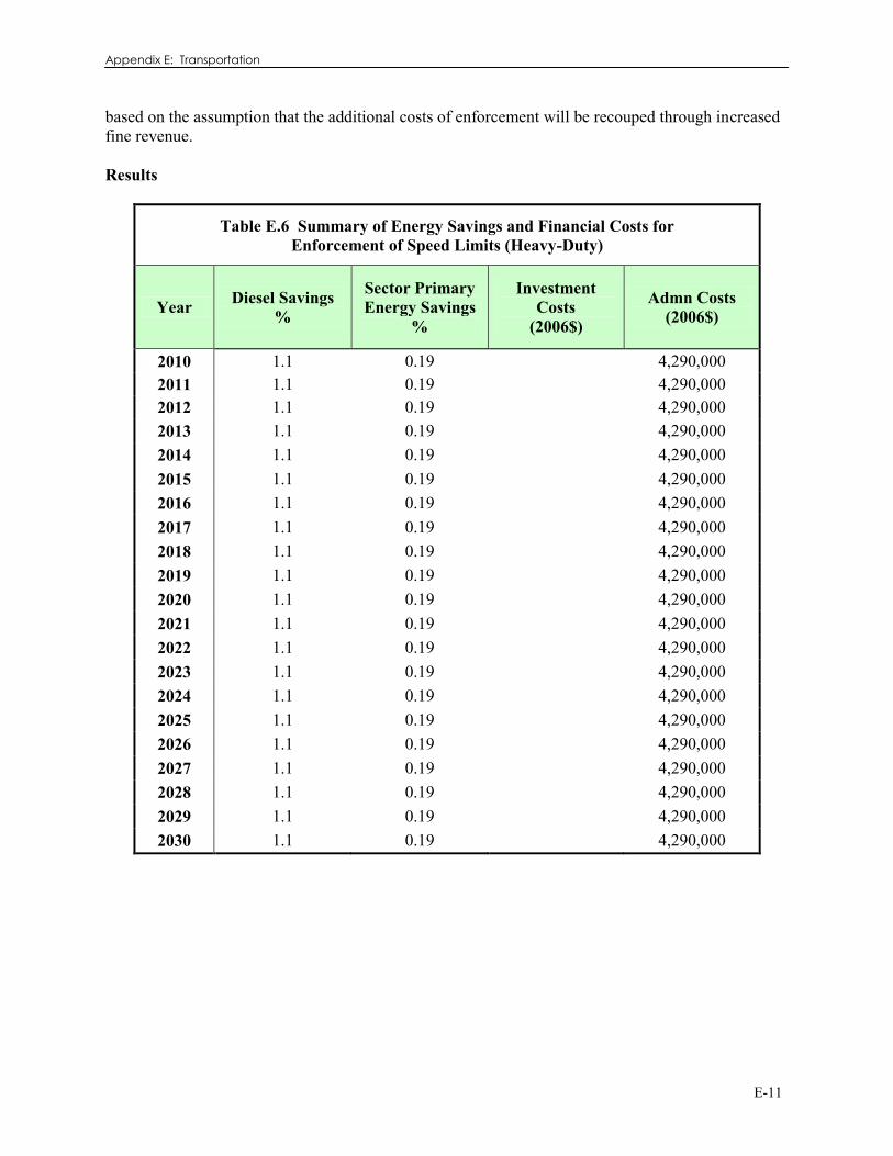
Appendix E: Transportation
E-11
based on the assumption that the additional costs of enforcement will be recouped through increased fine revenue. Results
Table E.6 Summary of Energy Savings and Financial Costs for Enforcement of Speed Limits (Heavy-Duty)
Year Diesel Savings %
Sector Primary Energy Savings
%
Investment Costs
(2006$)
Admn Costs (2006$)
2010 1.1 0.19 4,290,000 2011 1.1 0.19 4,290,000 2012 1.1 0.19 4,290,000 2013 1.1 0.19 4,290,000 2014 1.1 0.19 4,290,000 2015 1.1 0.19 4,290,000 2016 1.1 0.19 4,290,000 2017 1.1 0.19 4,290,000 2018 1.1 0.19 4,290,000 2019 1.1 0.19 4,290,000 2020 1.1 0.19 4,290,000 2021 1.1 0.19 4,290,000 2022 1.1 0.19 4,290,000 2023 1.1 0.19 4,290,000 2024 1.1 0.19 4,290,000 2025 1.1 0.19 4,290,000 2026 1.1 0.19 4,290,000 2027 1.1 0.19 4,290,000 2028 1.1 0.19 4,290,000 2029 1.1 0.19 4,290,000 2030 1.1 0.19 4,290,000

Energy Efficiency in Appalachia, SEEA
E-12
Table E.7 Summary of Energy Savings and Financial Costs for Enforcement of Speed Limits (Light-Duty)
Year Gasoline Savings
%
Sector Primary Energy Savings
%
Investment Costs
(2006$)
Admn Costs (2006$)
2010 1.1 0.76 4,290,000 2011 1.1 0.76 4,290,000 2012 1.1 0.76 4,290,000 2013 1.1 0.77 4,290,000 2014 1.1 0.77 4,290,000 2015 1.1 0.77 4,290,000 2016 1.1 0.77 4,290,000 2017 1.1 0.77 4,290,000 2018 1.1 0.77 4,290,000 2019 1.1 0.77 4,290,000 2020 1.1 0.77 4,290,000 2021 1.1 0.77 4,290,000 2022 1.1 0.77 4,290,000 2023 1.1 0.77 4,290,000 2024 1.1 0.78 4,290,000 2025 1.1 0.78 4,290,000 2026 1.1 0.79 4,290,000 2027 1.1 0.80 4,290,000 2028 1.1 0.80 4,290,000 2029 1.1 0.81 4,290,000 2030 1.1 0.82 4,290,000
REFERENCES Bordoff, J.E. and P.J. Noel. 2008. Pay-as-you-drive Auto Insurance: A Simple Way to Reduce
Driving-Related Harms and Increase Equity, The Brookings Institution. http://payasyoudrive.com.au/Resources/PDF/PAYDAutoInsuranceASimpleWayToReduceDrivingRelatedHarmsAndIncreaseEquity.pdf
California Air Resources Board (CARB). 2008. Comparison of Greenhouse Gas Reductions For All
Fifty United States Under Cafe Standards And ARB Regulations Adopted Pursuant To AB1493 http://www.arb.ca.gov/cc/ccms/reports/pavley-addendum.pdf

Appendix E: Transportation
E-13
Davis, S. and S. Diegel. 2006. Transportation Energy Data Book, Edition 25. Oak Ridge, TN: Oak Ridge National Laboratory.
Energy Independence and Security Act of 2007, Public Law 110-140, 110th Congress (EISA). 2007.
http://frwebgate.access.gpo.gov/cgi-bin/getdoc.cgi?dbname=110_cong_public_laws&docid=f:publ140.110.pdf
Energy Information Administration (EIA). 2006. Annual Energy Outlook 2006, p. 145.
http://www.eia.doe.gov/oiaf/archive.html ———. 2008. Annual Energy Outlook 2008. http://www.eia.doe.gov/oiaf/aeo/ Greene, D.L. and P.N. Leiby. 2006. The Oil Security Metrics Model.
http://cta.ornl.gov/cta/Publications/Reports/ORNL_TM_2006_505.pdf Litman, T. 2008. Transportation Elasticities: How Prices and Other Factors Affect Travel Behavior,
Online TDM Encyclopedia,Victoria Transportation Policy Institute. http://www.vtpi.org/tdm/tdm11.htm#_Toc119831339
Stodolsky, F., L. Gaines, and A. Vyas. 2000. Analysis of technology options to reduce the fuel
consumption of idling trucks. Argonne, IL: Center for Transportation Research, Argonne National Laboratory.


Appendix F: The DEEPER Model
F-1
APPENDIX F: THE DEEPER MODEL
The Dynamic Energy Efficiency Policy Evaluation Routine – or the DEEPER Model – is a 15-sector quasi-dynamic input-output impact model of the U.S. economy.1 Despite its more conventional input-output framework, it is in the tradition of so-called general equilibrium models following the logic of Hanson and Laitner (forthcoming) and Laitner and Hanson (2006). Although an updated model with a new name, the model actually has a 16-year history of use and development. See, for example, Geller, DeCicco, and Laitner (1992), Laitner, Bernow, and DeCicco (1998), and Laitner and McKinney (2008) for a review of past modeling efforts in this tradition. The DEEPER model is generally used to evaluate the macroeconomic impacts of a variety of energy-efficiency and climate policies at both the state and national level. The national model now evaluates policies for the period 2008 through 2050. For the Appalachia specific analysis, however, the DEEPER Model covers the period between 2008 through 2030. As it is now designed, the model accepts policy inputs in the form of investments and expenditures as described throughout the report. It then evaluates the changed pattern of expenditures for the net direct and indirect impacts on the different sectors of the Regional economy. DEEPER is an Excel-based analytical tool that consists generally of six sets of key modules or groups of worksheets. These six sets of modules now include: Global data: The information in this module consists of the economic time series data and key model coefficients and parameters necessary to generate the final model results. The time series data includes the projected reference case energy quantities such as trillion Btus and kilowatt-hours, as well as the key energy prices associated with their use. It also includes the projected gross domestic product, wages and salary earnings, and levels of employment as well as information on key technology cost and performance characteristics. The sources of economic information include data from the Energy Information Administration, the Bureau of Economic Analysis, the Bureau of Labor Statistics, and Economy.com. The cost and performance characterization of key technologies is derived from available studies completed by ACEEE and others, as well as data from the Energy Information Administration‘s (EIA) National Energy Modeling System (NEMS). One of the more critical assumptions in this study is that alternative patterns of electricity consumption will change and/or defer the mix of investments in conventional power plants. Although we can independently generate these impacts within DEEPER, we can also substitute assumptions from the ICF Integrated Planning Model (IPM) and similar models as they may have different characterizations of avoided costs or alternative patterns of power plant investment and spending. Macroeconomic model: This set of modules contains the ―production recipe‖ for the Region‘s economy for a given ―base year‖ – in this case, 2006, which is the latest year for which a complete set of economic accounts are available for the Regional economy. The I-O data, currently purchased from the Minnesota IMPLAN Group (IMPLAN, 2008), is essentially a set of input-output accounts that specify how different sectors of the economy buy (purchase inputs) from and sell (deliver
1 There is nothing particularly special about this number of sectors. The goal is to provide sufficient detail to show key negative and positive impacts while maintaining a manageable sized model. If we choose to reflect a different mix of sectors and stay within the 15 x 15 matrix, that can be done easily. If we wish to expand the number of sectors, that would take some minor programming changes or adjustments to reflect the larger matrix.

Energy Efficiency in Appalachia, SEEA
F-2
outputs) to each other. In this case, the model is now designed to evaluate impacts for 15 different sectors, including: Agriculture, Oil and Gas Extraction, Coal Mining, Other Mining, Construction, Manufacturing, Electric Utilities, Natural Gas Distribution, Transportation, and Other Public Utilities (including water and sewage), Wholesale & Retail Trade, Services, Finance, Government, and Households. Given the I-O assumptions mapped out for the Appalachian Region, the table that follows highlights the Type I Multipliers for each of the major sector activities within DEEPER. These multipliers refer to the direct and indirect job impacts per million dollars of revenue received by a particular sector, and the direct and indirect income and contributions to value-added (or Gross Regional Product) created by the expenditure of one dollar within each sector. Almost the first thing that jumps out from Table F.1 is the relative low values shown for energy-related sectors compared to almost all other sectors of the economy. For example, electric utilities provide a total of 5.3 direct and indirect jobs per million dollars of revenue that they receive. All other sectors show a significantly higher impact in this regard. It is these differences that are underscored in the heuristic analysis shown in Table 7.1 in the main report. Although not quite as pronounced there is a similar pattern for both wages and salaries and contributions to the GRP. Hence, any cost-effective adjustment to the energy production patterns of the Appalachian Regional economy should leave to a small but net positive impact on the economy.
Table F.1 Appalachia Economic Multipliers for Key Sectors
SECTOR Type I Multiplier Jobs (per million
$ of final demand)
Type I Multiplier
Compensation (per dollar of final demand)
Type I Multiplier Value-Added
(per dollar of final demand)
Agriculture 21.5 0.224 0.646 Oil and Gas Extraction 5.1 0.167 0.742 Coal Mining 6.0 0.335 0.712 Other Mining 7.6 0.365 0.740 Construction 13.3 0.429 0.720 Manufacturing 8.3 0.338 0.630 Petroleum Refining 2.6 0.095 0.311 Electric Utility Services 5.3 0.285 0.818 Natural Gas Utility Services 3.7 0.204 0.552 Transportation Other Public Utilities 11.0 0.418 0.747 Wholesale Trade 15.3 0.461 0.863 Services 14.1 0.415 0.834 Financial Services 8.6 0.385 0.828 Governmental Services 19.7 0.885 0.974

Appendix F: The DEEPER Model
F-3
Investment, expenditures and energy savings: Based on the scenarios mapped into the model, this worksheet translates the energy policies into a dynamic array of physical energy impacts, investment flows, and energy expenditures over the desired period of analysis. It estimates the needed investment path for an alternative mix of energy efficiency and other technologies (including efficiency gains on both the end-use and the supply side). It also provides an estimate of the avoided investments needed by the electric generation sector. These quantities and expenditures feed directly into the final demand module of the model which then provides the accounting that is needed to generate the set of annual changes in final demand (see the related module description below). Price dynamics: There are two critical drivers that impact energy prices within DEEPER. The first is a set of carbon charges that are added to retail prices of energy depending on the level of desired level of emission reductions and also depending on the available set of alternatives to achieve those reductions. The second is the price of energy as it might be affected by changed consumption patterns. In this case, DEEPER employs an independent algorithm to generate energy price impacts as they reflect changed demand. Hence, the reduced demand for natural gas in the end-use sectors, for example, might offset increased demand by utility generators. If the net change is a decrease in total natural gas consumption, the wellhead prices might be lowered. Depending on the magnitude of the carbon charge, the change in retail prices might either be higher or lower than the set of reference case prices. This, in turn, will impact the demand for energy as it is reflected in the appropriate modules. In effect, then, DEEPER scenarios rely on both a change in prices and quantities to reflect changes in overall investments and expenditures. For this analysis, however, we have used the conservative assumption that price dynamics remain unchanged. Final demand: Once the changes in spending and investments have been established and adjusted to reflect changes in prices within the other modules of DEEPER, the net spending changes in each year of the model are converted into sector-specific changes in final demand. This, in turn, drives the input-output model according to the following predictive model:
X = (I-A)-1 * Y where: X = total industry output by sector I = an identity matrix consisting of a series of 0‘s and 1‘s in a row and column format for each sector (with the 1‘s organized along the diagonal of the matrix) A = the production or accounting matrix also consisting of a set of production coefficients for each row and column within the matrix Y = final demand, which is a column of net changes in final demand by sector This set of relationships can also be interpreted as ∆X = (I-A)-1 * ∆Y
which reads, a change in total sector output equals the inverted (I-A) matrix times a change in the final spending demand for each sector. Employment quantities are adjusted annually according to exogenous assumptions about labor productivity in each of the sectors (based on Bureau of Labor Statistics forecasts). Table 7.1 in the main report illustrates the approach suggested by this perspective.

Energy Efficiency in Appalachia, SEEA
F-4
Results: For each year of the analytical time horizon (again out to 2030 for the Appalachia specific analysis), the model copies each set of results into this module in a way that can also be exported to a separate report. There are other support spreadsheets as well as routines in visual basic programming that support the automated generation of model results and reporting. For more detail on the model assumptions and economic relationships, again please refer to the forthcoming model documentation (Laitner and McKinney, forthcoming). And as alluded in the beginning of this appendix, for a review of how an I-O framework might be integrated into other kinds of modeling activities, see Hanson and Laitner (forthcoming). While not an equilibrium model we borrow from some key concepts of mapping technology representation into DEEPER using the general scheme outlined in Laitner and Hanson (2006). REFERENCES Geller, Howard, John DeCicco, and John A. ―Skip‖ Laitner. 1992. Energy Efficiency and Job
Creation: The Employment and Income Benefits from Investing in Energy Conserving Technologies," Washington, DC: The American Council for an Energy-Efficient Economy.
Hanson, Donald A. and John ―Skip‖ Laitner. Forthcoming. ―Input-Output Equations Embedded
within Climate and Energy Policy Analysis Models.‖ Forthcoming in Faye Duchin and Sangwon Suh, Editors., Input-Output Analysis Handbook. New York, N.Y.: Kluwer Academic Press.
Laitner, John A. ―Skip‖ and Donald A. Hanson. 2006. ―Modeling Detailed Energy-Efficiency
Technologies and Technology Policies within a CGE Framework.‖ Energy Journal, Special Edition, Hybrid Modeling of Energy-Environment Policies: Reconciling Bottom-Up and Top-Down, pp. 151-69.
Laitner, John A. ―Skip,‖ Stephen Bernow, and John DeCicco. 1998. ―Employment and Other
Macroeconomic Benefits of an Innovation-Led Climate Strategy for the United States.‖ Energy Policy, 26(5), 425–433.
Laitner, John A. ―Skip‖ and Donald A. Hanson. 2006. ―Modeling Detailed Energy-Efficiency
Technologies and Technology Policies within a CGE Framework.‖ Energy Journal, Special Edition, ―Hybrid Modeling of Energy-Environment Policies: Reconciling Bottom-Up and Top-Down,‖ pp. 151-69.
Laitner, John A. ―Skip‖ and Vanessa McKinney. 2008. Positive Returns: State Energy Efficiency
Analyses Can Inform U.S. Energy Policy Assessments. Washington, D.C.: American Council for an Energy-Efficient Economy.
———. Forthcoming. Draft DEEPER Documentation. Forthcoming. Washington, DC: American
Council for an Energy-Efficient Economy. Minnesota IMPLAN Group, Inc. (IMPLAN). 2008. A 2006 dataset for Appalachia (Alabama,
Georgia, Kentucky, Maryland, Mississippi, New York, North Carolina, Ohio, Pennsylvania, South Carolina, Tennessee, and Virginia. Accessed January. Stillwater, Minn.: Minnesota IMPLAN Group, Inc.

Appendix G: Sensitivities at Sector Level
G-1
APPENDIX G: SENSITIVITIES AT SECTOR LEVEL
SUPPLEMENTAL TABLES
Table G.1 Carbon Footprint and Consumption Data for 17 Appalachian Metropolitan Areas (Brown and Logan, 2008)
% in ARC SubregionResidential
ElectricityResidential Fuel
Light Duty
VehicleFreight Trucks
Residential
ElectricityResidential Fuel
Light Duty
VehicleFreight Trucks
Albany-Schenectady-Troy, NY 20% Northern 0.38 0.58 1.23 0.33 36.88 38.06 63.64 16.45
Allentown-Bethlehem-Easton, PA-
NJ 25% Northern 0.56 0.47 0.96 0.37 38.19 29.69 49.84 18.70
Cincinnati-Middletown, OH-KY-IN 13% Northern 1.25 0.45 1.14 0.44 59.46 31.50 58.91 21.86
Harrisburg-Carlisle, PA 33% Northern 0.62 0.53 1.32 0.72 42.54 33.38 68.24 36.17
New York-Northern New Jersey-
Long Island, NY-NJ-PA4% Northern 0.23 0.44 0.66 0.16 21.78 27.43 34.33 8.07
Pittsburgh, PA 100% Northern 0.54 0.55 0.91 0.27 36.93 34.91 47.18 13.66
Scranton--Wilkes-Barre, PA 100% Northern 0.58 0.55 1.01 0.51 39.79 34.99 52.27 25.79
Washington-Arlington-Alexandria,
DC-VA-MD-WV5% Northern 1.61 0.35 0.98 0.17 62.02 23.76 50.86 8.72
Youngstown-Warren-Boardman,
OH-PA33% Northern 0.77 0.43 1.01 0.54 36.33 30.21 52.46 27.32
Lexington-Fayette, KY 17% Central 1.48 0.24 1.10 0.64 63.60 16.92 56.94 32.07
Nashville-Davidson--Murfreesboro,
TN23% Central 1.15 0.19 1.32 0.57 74.21 13.53 68.19 28.48
Atlanta-Sandy Springs-Marietta, GA 43% Southern 0.84 0.21 1.22 0.41 51.01 15.28 63.26 20.61
Birmingham-Hoover, AL 100% Southern 0.99 0.16 1.34 0.42 64.55 10.83 69.03 21.17
Chattanooga, TN-GA 100% Southern 1.05 0.20 1.27 0.59 68.00 14.43 65.77 29.42
Greenville, SC 67% Southern 0.57 0.14 0.87 0.28 56.56 10.30 45.16 13.92
Knoxville, TN 100% Southern 1.07 0.20 1.40 0.46 68.91 14.50 72.50 23.35
Memphis, TN-MS-AR 13% Southern 0.99 0.18 1.16 0.53 64.20 13.31 60.07 26.65
Total Top 100 Metros 0.61 0.31 1.00 0.31 41.35 21.14 51.93 15.32
Appalachian Metro Average 1.05 0.42 1.35 0.53 63.21 28.07 69.90 26.60
Annual metric tons of carbon emitted per person Annual Mbtu consumed per capita
DISCOUNT RATE SENSITIVITIES The discount rates used in analysis can have a significant impact on the results of cost effectiveness tests. Since this study seeks to identify policies that are cost-effective, the choice of discount rate has been conservatively selected for the base analysis at seven percent for the total resource cost test and 10 percent for participants. Discount rates are generally accepted to be higher for private investment than public programs due to the greater societal concern for the future. This sensitivity analysis reports the benefit-to-cost ratio at discount rates of four, seven, and ten percent for both participants and the total resource costs. Figures G. 1 – G. 4 show the discount rate sensitivity for each of the policies within the four modeled sectors.

Energy Efficiency in Appalachia, SEEA
G-2
0.00
1.00
2.00
3.00
4.00
5.00
6.00
7.00
8.00
9.00
Res
iden
tial
Bu
ildin
g
Co
des
Exp
and
ed
Wea
ther
izat
ion
Exis
tin
g H
om
e
Ret
rofi
ts
Sup
er-E
ffic
ien
t
Ap
plia
nce
De
plo
ymen
t
Tota
l
Res
iden
tial
Bu
ildin
g
Co
des
Exp
and
ed
Wea
ther
izat
ion
Exis
tin
g H
om
e
Ret
rofi
ts
Sup
er-E
ffic
ien
t
Ap
plia
nce
De
plo
ymen
t
Tota
l
BC
Rat
io
Participants Cost Test Total Resource Cost Test
0.00
1.00
2.00
3.00
4.00
5.00
6.00
7.00
8.00
9.00
10.00
11.00
12.00
13.00
14.00
Co
mm
erci
al B
uild
ing
Co
des
Co
mm
issi
on
ing
HV
AC
an
d L
igh
tin
g
Ret
rofi
ts
Off
ice
Equ
ipm
ent
Stan
dar
ds To
tal
Co
mm
erci
al B
uild
ing
Co
des
Co
mm
issi
on
ing
HV
AC
an
d L
igh
tin
g
Ret
rofi
ts
Off
ice
Equ
ipm
ent
Stan
dar
ds To
tal
BC
Rat
io
Participants Cost Test Total Resource Cost Test
Figure G.1 Discount Rate Sensitivities for Residential Sector Policies
Figure G.2 Discount Rate Sensitivity for Commercial Sector Policies

Appendix G: Sensitivities at Sector Level
G-3
0
1
2
3
4
5
6
7
8
IAC ESA CHP Total IAC ESA CHP Total
BC
Rat
io
Participants Cost Test Total Resource Cost Test
0
1
2
3
4
5
6
7
8
9
Cle
an C
ar S
tan
dar
d
Pay
-as-
you
-dri
ve
Insu
ran
ce
Smar
t W
ay
Spee
d L
imit
s
Tota
l
Cle
an C
ar S
tan
dar
d
Pay
-as-
you
-dri
ve
Insu
ran
ce
Smar
t W
ay
Spee
d L
imit
s
Tota
l
BC
Rat
io
Participants Cost Test Total Resource Cost Test
At this scale, the benefit-to-cost ratios cannot be seen for the policies of Supporting Pay as you Drive Insurance or Enforcing Speed Limits because they are too high to show on the same scale. AVOIDED COST SENSITIVITIES The avoided costs of producing the energy that will be saved by a particular policy or measure, or package of policies or measures, can have an enormous impact on the benefit-to-cost ratio on a total resource basis. In our base analysis, we assume that the avoided costs are equal to the energy price forecast; this assumption was driven by low forecast energy prices and general belief that these as
Figure G.3 Discount Rate Sensitivities for the Industrial Sector Policies
Figure G.4 Discount Rate Sensitivities for the Transportation Sector Policies

Energy Efficiency in Appalachia, SEEA
G-4
well as forecast avoided costs are understated. However, there is much uncertainty about future avoided costs, as it will be dependent upon many factors. We have considered lower and higher costs for sensitivity analysis in this study. To model the cost effectiveness of lower avoided costs, we have used rates at 50 percent and 75 percent of forecast retail energy prices. To model the cost effectiveness of higher avoided costs, we have considered the impact of carbon taxes of $25, $50, and $100 per metric ton of carbon (MtC) (Brown & Atamturk, 2008). Figures G.5 – G.8 show how sensitive the cost-effectiveness of the modeled policies are to avoided costs.
0
2
4
6
8
10
12
Residential Policy Package
BC
Rat
io
50% Lower than Energy Prices 1.86 0.63 0.85 3.52 0.97
25% Lower than Energy Prices 2.79 0.94 1.27 5.29 1.46
Retail Energy Prices 3.72 1.26 1.70 7.05 1.94
Energy Prices with $25/MtC Tax 3.96 1.40 1.89 8.32 2.15
Energy Prices with $50/MtC Tax 4.19 1.54 2.08 9.58 2.35
Energy Prices with $100/MtC Tax 4.67 1.84 2.47 12.12 2.75
Residential
Building Codes
Expanded
Weatherization
Existing Home
Retrofits
Super-Efficient
Appliance
Deployment
Total
Overall, the residential policy package is cost-effective for a variety of avoided cost scenarios. If future avoided costs are lower than forecast energy prices, the two residential retrofit programs may not be cost-effective.
Figure G.5 Avoided Cost Sensitivities for the Residential Sector

Appendix G: Sensitivities at Sector Level
G-5
0
2
4
6
8
10
12
14
16
18
Commercial Policy Package
BC
Rat
io
50% Lower than Energy Prices 1.39 4.76 2.94 4.94 3.40
25% Lower than Energy Prices 2.08 7.14 4.41 7.41 5.10
Retail Energy Prices 2.78 9.52 5.88 9.89 6.80
Energy Prices with $25/MtC Tax 3.22 11.05 6.68 11.44 6.61
Energy Prices with $50/MtC Tax 3.66 12.55 7.47 12.99 7.43
Energy Prices with $100/MtC Tax 4.55 15.60 9.06 16.10 9.11
Commercial
Building CodesCommissioning
HVAC and
Lighting
Retrofits
Office
Equipment
Standards
Total
For all modeled avoided costs, the commercial sector policies we have considered will be cost effective over their lifetime.
0
2
4
6
8
10
12
Industrial Policy Package
BC
Rat
io
50% Lower than Energy Prices 2.93 1.65 0.16 1.04
25% Lower than Energy Prices 4.39 2.47 0.24 1.56
Retail Energy Prices 5.85 3.30 0.31 2.08
Energy Prices with $25/MtC Tax 7.13 3.92 0.76 2.67
Energy Prices with $50/MtC Tax 8.37 4.52 1.24 3.26
Energy Prices with $100/MtC Tax 10.93 5.77 2.13 4.45
IAC ESA CHP Total
While most of the policies modeled are cost-effective at most avoided costs, the policy to support combined heat and power modifications for industrial facilities is only cost effective when a carbon tax, or other cause for higher energy prices, is considered.
Figure G.6 Avoided Cost Sensitivities for the Commercial Sector
Figure G.7 Avoided Cost Sensitivities for the Industrial Sector

Energy Efficiency in Appalachia, SEEA
G-6
0
20
40
60
80
Transportation Policy Package
BC
Rat
io
50% Lower than Energy Prices 1.27 3.66 0.82 32.2 1.66
25% Lower than Energy Prices 1.91 5.49 1.23 48.2 2.49
Retail Energy Prices 2.55 7.31 1.64 64.3 3.33
Energy Prices with $25/MtC Tax 2.61 7.49 1.69 65.8 3.41
Energy Prices with $50/MtC Tax 2.67 7.67 1.73 67.2 3.49
Energy Prices with $100/MtC Tax 2.79 8.03 1.82 70.1 3.65
Clean Car
Standard
Pay-as-you-
drive InsuranceSmart Way Speed Limits Total
The benefit-to-cost ratios are extraordinarily high for some of our modeled transportation policies because the policies have low program costs. However, their cost effectiveness is still impacted by avoided costs. The SmartWay loan program, as modeled, would not be cost-effective from a total resource cost perspective if energy prices are much lower than forecast. References Brown, Marilyn and Nilgun Atamturk. 2008. ―Potential Impacts of Energy and Climate Policies on
the U. S. Pulp and Paper Industry,‖ Georgia Institute of Technology School of Public Policy Working Paper #40, June, 2008. http://www.spp.gatech.edu/faculty/workingpapers.php
Marilyn A. Brown and Cecelia (Elise) Logan. 2008. ―The Residential Energy and Carbon
Footprints of the 100 Largest Metropolitan Areas,” Georgia Institute of Technology School of Public Policy Working Paper. http://www.spp.gatech.edu/faculty/workingpapers.php
Figure G.8 Avoided Cost Sensitivities for the Transportation Sector

Copyright © 2022 FDOKUMEN