Journal of Archaeological Science: Reports 3 (2015) 534–548

Contents lists available at ScienceDirect

Journal of Archaeological Science: Reports

j ourna l homepage: ht tp : / /ees.e lsev ie r .com/ jas rep

Empirical study of the effect of count time on the precision and accuracyof pXRF data

Khori Newlander a,⁎, Nathan Goodale b, George T. Jones b, David G. Bailey c

a Department of Anthropology & Sociology, Kutztown University, 15200 Kutztown Road, Kutztown, PA 19530, USAb Anthropology Department, Hamilton College, 198 College Hill Road, Clinton, NY 13323, USAc Geosciences Department, Hamilton College, 198 College Hill Road, Clinton, NY 13323, USA

⁎ Corresponding author at: 401 Meadowcrest Lane, DoE-mail address: newlander@kutztown.edu (K. Newlan

http://dx.doi.org/10.1016/j.jasrep.2015.07.0072352-409X/© 2015 Elsevier Ltd. All rights reserved.

a b s t r a c t

a r t i c l e i n f o

Article history:Received 18 February 2015Received in revised form 20 July 2015Accepted 22 July 2015Available online xxxx

Keywords:Compositional analysisPortable X-ray fluorescence spectrometry(pXRF)Count time

As a cost-effective and non-destructive method for multi-element analysis, portable X-ray fluorescence spec-trometry (pXRF) has the potential for broad archeological application; however, recent applications of pXRF re-main inconsistent. For example, sourcing studies using pXRF have irradiated artifacts and geologic sourcematerials for widely varying amounts of time. In this study, we investigate the effect of count time on the preci-sion and accuracy of pXRF data obtained for two geologic standards, aswell as for obsidian, fine-grained volcanic(e.g., andesites, dacites), metamorphic, and chert specimens from the North American Great Basin. We find thatthe precision and reliability of pXRF data does not improve significantly at count times greater than 180 s. Ouranalysis also indicates that count time has little bearing on the accuracy or validity of pXRF data, as expectedfrom the mathematical relationships between count time, intensity, and concentration. Finally, we demonstratethat a well-calibrated pXRF instrument generates compositional data comparable to data obtained using otheranalytical methods. We offer this study as a step toward the development of a consistent and rigorous analyticalprotocol for archeological applications of pXRF.

© 2015 Elsevier Ltd. All rights reserved.

1. Introduction

A few years ago, Craig and colleagues (2007:2013) observed thatportable X-ray fluorescence spectrometry (pXRF) would allow thenon-destructive, multi-element analysis of large samples of artifacts innon-traditional settings (e.g., in the field). Since that time, archeologistshave increasingly employed pXRF for the compositional analysis of arti-facts and geologic source materials, both in the field and in the lab. Sev-eral studies have demonstrated that the analysis of compositional dataobtained using pXRF can effectively discriminate sources of obsidianin several regions of the world (Craig et al., 2007; Forster and Grave,2012; Frahm, 2013a; Frahm et al., 2014; Nazaroff et al., 2010; Phillipsand Speakman, 2009; Rademaker, 2012; Sheppard et al., 2011). Giventhe favorable results achieved with obsidian, archeologists have usedpXRF for the compositional analysis of fine-grained volcanic (FGVs,e.g., andesites, dacites, and basalts) artifacts (Goodale et al., 2012;Grave et al., 2012), glass beads (Liu et al., 2012), earthenware and stone-ware ceramics (Forster et al., 2011; Mitchell et al., 2012; Tykot et al.,2013), and metals (Karydas, 2007; Karydas et al., 2004). For the mostpart, these analyses have generated compositional data useful for dis-criminating raw material sources, assessing manufacturing techniques,

uglassville, PA 19518, USA.der).

and addressing other anthropological questions (though for a discus-sion of the difficulties in using pXRF for the compositional analysis of ce-ramics see Speakman et al., 2011).

Nevertheless, concerns remain regarding the precision, reliability,accuracy, and validity of the compositional data obtained by pXRF in-struments. In a well-known paper on obsidian sourcing, RichardHughes (1998) observed that analytical precision concerns the repeat-ability and stability of measurement. More recently, Frahm (2012)noted that, despite our best efforts, compositional analyses are rarelyconducted under the same analytical conditions. Rather, we oftencarry out the compositional analysis of artifacts and geologic specimensin separate sessions over months or years, during which time analyticalconditions may vary even if all procedures remain the same. Given thisreality, Frahm (2012) recommended dividing the concept of precisioninto two: repeatability and reproducibility. Repeatability refers to theagreement between sequential measurements obtained under identicalconditions. Reproducibility refers to the agreement between sequentialmeasurements obtained under different conditions, replacing whatHughes (1998) termed reliability. By accuracy we mean the agreementbetween the elemental concentrations we obtained using pXRF and thereported elemental concentrations obtained for the same specimensusing other analytical methods. Finally, we define conceptual validityas the ability of an analytical technique, when combinedwith data anal-ysis, to discriminate raw material sources and correctly assign artifactsto those sources (following Frahm, 2012, after Neff, 1998). With the

535K. Newlander et al. / Journal of Archaeological Science: Reports 3 (2015) 534–548

concept of validity, we move to the archeological application of compo-sitional analysis.

Recent contributions by Speakman and Shackley (2013) and Frahm(2013a, 2013b) have framed the debate regarding archeological appli-cations of pXRF, focusing, in particular, on systematic evaluation of theanalytical precision and accuracy of data generated using pXRF. Ratherthan enter directly into this discussion, we heed Shackley's (2010:18,italics in original) earlier advice to “slow down a bit and take PXRF forwhat it really is—an emerging and rapidly changing technology thathas the potential tomake very real changes to our discipline.” To achievethis potential, Shackley (2010) encouraged archeologists using pXRF totake the time to establish a rigorous and consistent analytical protocolthrough systematic experimentation.

Experiments have included comparisons between data generatedusing handheld pXRF (HHpXRF) instruments and other analyticalmethods. Nazaroff et al.'s (2010) study of Mesoamerican obsidians,Craig et al.'s (2007) study of Peruvian obsidians, and Goodale et al.'s(2012) study of FGVs from eastern Nevada all found systematic differ-ences between compositional data obtained with HHpXRF and lab-based XRF (labXRF, including energy-dispersive [ED] and wavelength-dispersive [WD]XRF). Likewise, Forster andGrave (2012) reported slightoffsets between compositional data generated using HHpXRF and dataobtained using other analytical methods. Given these differences, theseanalysts, as well as Speakman and Shackley (2013) (Shackley, 2010,2011, 2012), have encouraged the calibration of pXRF instrumentsusing geologic standards to provide accurate data that are comparableacross pXRF instruments and other analytical methods (also see Conreyet al., 2014).

Additionally, Shackley (2010, 2012) urged experimentation regard-ing the effect of artifact size and surface morphology on data obtainedusing pXRF. Using labXRF, Davis et al. (1998) demonstrated that preci-sion improved for several analytes when the target specimenmeasuredmore than 1.5–2.0 mm thick and 10–15 mm in diameter (also seeJackson and Hampel, 1993; Lundblad et al., 2008). Frahm (2013a) dem-onstrated that pXRF data also are influenced by artifact size. Frahm(2013a) analyzed two wafers of National Institute of Standards andTechnology (NIST) Standard Reference Material (SRM) 610: one 3 mmthick and 12mm in diameter, the other 3 mm thick and 4 mm in diam-eter. In this study, Frahm (2013a:Fig. 3) obtained significantly differentconcentrations of Mn, Rb, Sr, Ti, Zn, and Zr for these two wafers, andboth wafers yielded values that differed significantly from the certifiedvalues. Furthermore, the concentrations Frahm (2013a:Fig. 3) obtainedfor Mn, Rb, Ti, Zn, and Zr on the 4mmdiameter wafer exhibited greaterpercent relative errors (calculated as the percent difference betweenthe value obtained using pXRF and the value reported by NIST) thanthe concentrations obtained for these analytes on the 12 mm diameterwafer. Interestingly, Frahm (2013a:Fig. 3) found that the 4 mm diame-ter wafer yielded higher concentrations of Mn, Rb, Sr, Zn, and Zr thanthe 12 mm diameter wafer. These results conflict with Davis et al.'s(1998) observation that lower element intensities should result whena sample is too small to cover the detector window due to the relativedeficit in x-rays from the sample. In Frahm's (2013a) study, both waferswere smaller than the detector window of the pXRF instrument(20 mm), so lower concentrations for these analytes might have beenexpected. Clearly, more experimentation is warranted on the precise ef-fects of artifact size on pXRF data.

The irregular surfaces of artifacts alsomay causemeasurement prob-lems due to the difficulty of isolating the effects of surface morphologyon X-ray intensity from the absorption and enhancement effects of therock matrix on X-ray intensity (Hughes, 1986; Jones et al., 1997). Inpractice, various analysts have found that labXRF (particularly EDXRF)generated similar compositional data for obsidian and basalt flakes,flat surfaces, and pressed powdered pellets, despite differences in thesurface morphology of these samples (e.g., Hughes, 1986; Lundbladet al., 2008, 2011:Table 4.4; Shackley, 2011:Table 2; Shackley andHampel, 1993). As for pXRF, Frahm (2013a:Tables 1, 2) found that the

relative standard deviation (RSD; a measure of precision equivalent tothe coefficient of variation expressed as a percent) obtained for small(often b10 mm in diameter) Anatolian obsidian chips with irregularsurface morphologies was greater than the RSD obtained for polishedbasalt standards. Similarly, Liritzis and Zacharias (2011:132) suggestedthat pXRF data “are affected by surface roughness effects, more so thandesktop EDXRF instruments” due to the presence of an air gap betweenthe sample and pXRF analyzer.

These experiments have begun to define a consistent and rigorousanalytical protocol for archeological applications of pXRF, but inconsis-tencies remain. For example, Frahm (2013a) observed that the counttime (“live time”) reported for sourcing studies that used pXRF variedbetween 60 s and 300 s. By comparison, most obsidian analysts usinglab-based EDXRF in the U.S. irradiate their specimens for 150–300 s(Shackley, 2011:31). Forster and Grave (2012) briefly examined the ef-fect of count time on the precision and accuracy of pXRF analyses of An-atolian obsidians. They found that irradiation for 300 s provided themost precise and accurate results for analytes commonly used to dis-criminate obsidian sources (e.g., Rb, Sr, Y).

Forster and Grave's (2012) results are not surprising, as they followfrom fundamental principles of XRF spectrometry. When a sample isbombardedwith x-rays, some electrons are dislodged from their orbitals,temporarily destabilizing their atoms. When this happens, outer shellelectrons quickly fill the void left by the dislodged inner electrons, releas-ing energy of an intensity indicative of the concentrations of the ele-ments in the sample (Hughes, 1986; Shackley, 2011). In theory,fluorescent intensities are converted into analyte concentrations usingsimple linear equations. In reality, the relationship between fluorescentintensity and concentration is complicated by the sample matrix, meth-od of sample preparation, and measurement conditions (Stiko andZawisza, 2012). Calibration of our instruments using well-characterizedinternational standards helps us correct for the various spectroscopicand non-spectroscopic interferences that complicate translating fluores-cent intensities into analyte concentrations.

Count time, as one measurement condition, is directly related to ra-diation intensity, but it does not change the fundamental relationshipbetween intensity and concentration. As a result, increasing counttime should have little effect on the accuracy of compositional data ob-tained using XRF (e.g., Angeles-Chavez et al., 2012). Instead, accuracy isa function of spectral corrections and instrument calibration. We pro-vide an empirical demonstration of this point using pXRF. Increasingcount time does decrease the counting error (i.e., the statistical uncer-tainty associated with random counting error) that accompanies eachconcentration. As a result, increasing count time should increase thelikelihood that a series of measurements on the same specimen willyield similar results. Nevertheless, we expect that there will be a pointatwhich increasing count time no longer improves repeatability and re-producibility. Thus, our study expands upon the work of Forster andGrave (2012) by exploring the effect of count time on the precision (re-peatability), reliability (reproducibility), accuracy, and validity of pXRFdata over a wider range of count times (15 s to 300 s) for differenttypes of toolstone from the North American Great Basin.

2. Materials & methods

Our analysis included two geologic standards (NIST 278 and U.S.Geological Survey standard RGM-1), as well as specimens from obsidi-an, FGV, metamorphic, and chert sources used by the prehistoric inhab-itants of central and eastern Nevada (Table 1, Fig. 1). Although volcanicdeposits containing obsidian tend to occur along the perimeter of theGreat Basin (Stewart, 1980; Thomas, 2011), obsidian was conveyedover long distances. Obsidian from Panaca Summit (also known as Mo-dena Area), TempiuteMountain (also known as Timpahute Range), andWildhorse Canyon are well-represented at Paleoindian sites in easternNevada (Jones et al., 2003, 2012). In contrast to obsidian, several sourcesof artifact-quality FGVs are readily available in eastern Nevada,

Table 1Toolstone sources used in the analysis.

Source name Material

Panaca Summit (PS) ObsidianTempiute Mountain (TM) ObsidianWildhorse Canyon (WHC) ObsidianJakes Wash (JW) TrachyandesiteLittle Smoky Quarry (LSQ) DaciteMurry Canyon (MC) TrachyandesiteSource 21 (Long Valley “Jade”) Greenschist (5G 4/1)Source 11 Dark yellowish orange (10YR 6/6) to

moderate yellowish brown (10YR 5/4) chertSource 24 (Mahoney Canyon) Moderate reddish brown (10R 4/6) chertTosawihi (T) Light gray (N7) to yellowish gray (5Y 8/1)

opalite

536 K. Newlander et al. / Journal of Archaeological Science: Reports 3 (2015) 534–548

occurring in Tertiary-age extrusive lavas that range in composition be-tween andesite and rhyolite (Jones et al., 1997).Metamorphosed basaltsoccur in similar depositional contexts in the study area. For example,Source 21 consists of nodules of greenschist that occur as inclusionswithin a Tertiary-age volcanic ash flow in southern Long Valley.Paleoindian sites in Butte and Jakes Valleys include many artifacts de-rived from Source 21. Cherts (i.e., “fine-grained siliceous sedimentaryrock of biogenic, biochemical or chemogenic origin;” Stow, 2009:184)occur within most of the Paleozoic sedimentary units that dominatethe region (Hose and Blake, 1976; Kleinhampl and Ziony, 1985). Many

Fig. 1. Location of toolstone sources used in the analysis. Obsidian sources are represented bysented by circles. The box encloses a well-studied area within a Terminal Pleistocene/Early Hoations are defined in Table 1.

of these cherts occur as small nodules of poor quality and likely werenot used for stone tools (Newlander, 2012); however, the three chertsources included here all evince prehistoric use. Tosawihi is one of thebest known and most extensively used chert quarries in the region(Elston and Raven, 1992; Lyons et al., 2003), and Sources 11 and 24both exhibit evidence of cobble testing and early-stage reduction. Weanalyzed the flattest surface available for two specimens from each ofthe toolstone sources listed in Table 1.

To acquire these pXRF data, we used an Olympus Delta Premium Se-ries pXRF spectrometer equipped with a tantalum (Ta) anode X-raytube. This is a HHpXRF that we operate “within the paradigmof labXRF”(Frahm and Doonan, 2013:1428). We employ HHpXRF in a lab in orderto analyze a large number of samples at low costs. We make our use ofpXRF explicit here because we are concerned with comparing the re-sults we obtain using pXRF with the large body of compositional dataothers (e.g., Richard E. Hughes, Craig E. Skinner, M. Steven Shackley,Richard M. Conrey) have generated by using (primarily) labXRF forsource rocks from the Great Basin (e.g., Goodale et al., 2012). According-ly, our pXRF analyses are informed by and often checked against a longhistory of labXRF analysis of obsidians, FGVs, and geologic standards atHamilton College.

We operated the pXRF instrument in 3-beam “obsidian-soil” mode,with each beam optimized for the fluorescence of a different suite of ele-ments (Table 2). The “obsidian-soil”mode is an Olympus-specific modi-fied Fundamental Parameters calibration built by analyzing powdered

stars. FGV sources are represented by squares. Chert and metamorphic sources are repre-locene material conveyance pattern in eastern Nevada (Jones et al., 2003, 2012). Abbrevi-

Table 2Analytical parameters for 3-beam “obsidian-soil”mode.

Beam Voltage (kV) Amperage (μA) Filter Elements

1 40 100 3 Primary: U, Sr, Zr, Th, Nb, Mo, Ag, Cd, Sn, SbAlso: Ti, V, Cr, Mn, Fe, Co, Ni, Cu, Zn, W, Hg, As, Se, Au, Pb, Bi, Rb, light elements

2 40 100 2 Primary: Fe, Co, Ni, Cu, Zn, W, Hg, As, Se, Au, Pb, Bi, RbAlso: Ti, V, Cr, Mn, U, Sr, Zr, Th, Nb, Mo, Ag, Cd, Sn, Sb, light elements

3 15 200 5 Primary: P, S, Cl, K, Ca, Ti, V, Cr, MnAlso: Fe, light elements

537K. Newlander et al. / Journal of Archaeological Science: Reports 3 (2015) 534–548

volcanic rock standards from the National Institute of Standards andTechnology (NIST 278), the United States Geological Survey (RGM-1),the University of Georgia Center for Applied Isotope Studies (GBOR-01,MTNM-01, SATU-07), and an in-house standard (OBS-1 Glass Butte,OR) for 12 elements (K, Ca, Ti, Mn, Fe, Zn, Rb, Sr, Zr, Nb, Pb, Th).

Theperformanceof our pXRF instrument using this calibration is dem-onstrated in Table 3, which provides summary statistics for analyses ofNIST 278 run between September 2013 and April 2014. Because weused NIST 278 to build our calibration, these results do not provide atruly independent assessment of our calibration. Nevertheless, the perfor-mance of NIST 278 does provide a sense of the overall analytical precisionand accuracy of the datawe obtained using this calibration.Most analytesexhibit a low RSD and low relative error. The exceptions (especially Pband Th) illustrate thatmeasurement error tends to increase as concentra-tion decreases, as noted by Speakman and Shackley (2013:Fig. 4). Addi-tionally, Zn was not accurately characterized for NIST 278, at least bycomparison to the value (55ppm) recommended byNIST. Yet as reportedon the GeoRem website (http://georem.mpch-mainz.gwdg.de/; Jochumet al., 2005), several other compositional analyses of NIST 278 haveyielded values of 45–50 ppm for Zn, much closer to the concentrationswe obtained using pXRF. Thus, the concentrations we obtained for Znusing pXRFmay be accurate and precise, even if this analyte is often of lit-tle use in discriminating toolstone sources (particularly obsidians) inmany regions of the world (Shackley, 2011:25).

For this study, we acquired pXRF data at beam times varying at 5 sintervals between 5 s and 100 s for each of the three beams. Becausewe ran our pXRF instrument in 3-beam mode, these different beamtimes correspond to total analytical count times that varied between15 s and 300 s.

3. Results & discussion

3.1. International Geologic Standards: NIST 278 and RGM-1

We begin our discussion with an examination of the reproducibilityand accuracy of pXRF data for two international geologic standards:

Table 3Summary statistics for NIST 278 (n = 96) and comparison to reported concentrationvalues (in ppm).

Analyte Measuredmean (ppm)

Measured std.dev. (ppm)

RSD(%)

Reported (ppm) Relativeerror (%)

K 36,398.6 416.3 1.1 34,523.8 ± 166.0a 5.4Ca 7059.9 316.7 4.5 7026.5 ± 14.3a 0.5Ti 1538.4 109.2 7.1 1468.0 ± 41.9a 4.8Mn 442.4 59.3 13.4 402.5 ± 15.5a 9.9Fe 14,318.0 166.6 1.2 14,255.5 ± 139.8a 0.4Zn 44.8 2.2 4.9 55 ± 4b 18.5Rb 122.9 1.2 1.0 127.5 ± 0.3a 3.6Sr 64.5 1.1 1.7 63.5 ± 0.1a 1.6Zr 289.0 6.8 2.4 281 ± 2b 2.8Nb 19.3 0.8 4.1 18 ± 1b 7.2Pb 19.2 4.2 21.9 16.4 ± 0.2a 17.1Th 16.0 6.0 37.5 12.4 ± 0.3a 29.0

a From National Institute of Standards and Technology (1992).b From Speakman and Shackley (2013:Table 3).

NIST 278 (a powdered obsidian standard from Clear Lake, NewberryCrater, Oregon) and RGM-1 (a powdered rhyolite standard from GlassMountain,Medicine LakeHighlands Volcanic Field, northern California).We use the term reproducibility in our study because we are interestedin the agreement between elemental concentrations obtained usingpXRF at different count times (i.e., under slightly different analyticalconditions). To track the effect of count time on the reproducibility of el-emental concentrationsmeasured for NIST 278,we plotted the standarddeviation (i.e., the 1σ-error on the counting statistics) provided by thepXRF instrument for each analyte as a function of time. Plottingcounting error as a function of time allowed us to assess (a) the stabilityof measurement, an important ingredient of analytical precision in theway Hughes (1998) initially defined it; and (b) the reproducibility ofthe compositional data generated by pXRF. We reasoned that decreas-ing counting errorwould indicate greatermeasurement stability and in-crease the likelihood that a series of measurements on the same objectwould agree. Because increasing count time decreases counting error,increasing count time should also increase the reproducibility of thecompositional data generated by pXRF. Yet, as we noted earlier, we ex-pected that at some point, increasing count time would no longer im-prove reproducibility. As Fig. 2 demonstrates, the standard deviationof each analyte concentration decreases rapidly to an inflection pointthat tends to occur at a beam time between 40 and 60 s.When the stan-dard deviations are used to calculate RSDs, several analytes have RSDsb5% at all beam times. The RSDs for Nb, Zn, and Pb only fall below 5%at beam times greater than 60 s. The RSDs for Th approximate 10% atbeam times greater than 50 s. The highermeasurement error associatedwith Nb, Zn, Pb, and Th is not unexpected, as these analytes occur inlower concentrations in NIST 278 than other analytes. In general, in-creasing count time beyond 120 to 180 s does not significantly decreasethe counting error associated with the compositional data we obtainedusing pXRF for NIST 278.

We are also interested in the accuracy of our pXRF data, as we oftenwish to compare the compositional datawe obtain using pXRFwith leg-acy data obtained using other analytical methods. Table 4 provides acomparison between the concentrations we obtained at several differ-ent beam times and the reported concentrations for NIST 278 for oursuite of twelve analytes. To quantitatively express the accuracy of ourpXRF data, we calculated the percent relative error for each analyte ateach beam time. Given the basic principles of XRF, we were not sur-prised to find that the accuracy of most analytes does not improve ascount time increases. Several analytes (Ca, Ti, Mn, Fe, Rb, Sr, Zr) exhibitrelative errors of less than 5% for most beam times and especially forbeam times longer than 40 s. Those analytes that exhibit higher relativeerrors (Nb, Pb, Th) at shorter beam times tend to exhibit lower relativeerrors at beam times of 60 s or more.

Additionally, the data reported in Table 4 provide an alternative as-sessment of the reproducibility of the compositional data we obtainedusing pXRF. Most analytes are characterized by low relative errors atbeam times of 40 s or 60 s. In fact, for several analytes, the relative errorsat 40 s or 60 s are lower than the relative errors at 100 s. These data sug-gest to us that the elemental concentrations we obtained using pXRF atbeam times of 40 s or 60 s are often more likely to agree with—to moreclosely reproduce—reported elemental concentrations for NIST 278than pXRF data obtained at a beam time of 100 s. In sum, our analysis

Fig. 2. Comparison plots of standard deviations of analytes for twomeasurements of NIST 278. The analytes are separated to best display the patterning in these data: (A) K, Ca, Fe, and Ti;(B) Mn, Zr, Th, and Zn; (C) Sr, Rb, Pb, and Nb.

Table 4Comparison of observed and reported concentration values (in ppm) for NIST 278 at different beam times. Percent relative error is provided in parentheses. Reported values are the sameas in Table 3. The top and bottom sets of observed values for each analyte represent two measurements using pXRF.

Analyte Reported (ppm) Observed (ppm)

5 s 20 s 40 s 60 s 80 s 100 s

K 34,523.8 ± 166.0 36,844 (6.7) 36,642 (6.1) 35,755 (3.6) 36,577 (5.9) 36,043 (4.4) 37,021 (7.2)36,889 (6.9) 37,123 (7.5) 36,403 (5.4) 36,709 (6.3) 36,452 (5.6) 36,765 (6.5)

Ca 7026.5 ± 14.3 6759 (3.8) 7565 (7.7) 6691 (4.8) 6946 (1.1) 6831 (2.8) 7014 (0.2)7172 (2.1) 7657 (9.0) 6826 (2.9) 6842 (2.6) 6906 (1.7) 6988 (0.5)

Ti 1468.0 ± 41.9 1586 (8.0) 1754 (19.5) 1453 (1.0) 1512 (3.0) 1481 (0.9) 1533 (4.4)1536 (4.6) 1747 (19.0) 1490 (1.5) 1493 (1.7) 1485 (1.2) 1522 (3.7)

Mn 402.5 ± 15.5 391 (2.9) 539 (33.9) 409 (1.6) 411 (2.1) 412 (2.4) 412 (2.4)416 (3.4) 560 (39.1) 399 (0.9) 406 (0.9) 414 (2.9) 409 (1.6)

Fe 14,255.5 ± 139.8 14,387 (0.9) 13,851 (2.8) 13,937 (2.2) 14,115 (1.0) 14,259 (0.0) 14,262 (0.0)13,983 (1.9) 14,172 (0.6) 13,885 (2.6) 14,257 (0.0) 14,227 (0.2) 14,355 (0.7)

Zn 55 ± 4 46 (16.5) 47 (14.5) 44.5 (19.1) 44.1 (19.8) 42.3 (23.1) 45.1 (18.0)36 (34.5) 46 (16.4) 40.4 (26.5) 42.1 (23.5) 44.4 (19.3) 46.2 (16.0)

Rb 127.5 ± 0.3 129 (1.2) 121.6 (4.6) 122.4 (4.0) 123.1 (3.5) 123.7 (3.0) 122.5 (3.9)121 (5.1) 123 (2.8) 121.1 (5.0) 123.8 (2.9) 122.3 (4.1) 125.5 (1.6)

Sr 63.5 ± 0.1 70 (10.2) 64.4 (1.4) 63.9 (0.6) 62.4 (1.7) 63.6 (0.2) 65.1 (2.5)64 (0.8) 67.3 (6.0) 64.6 (1.7) 63.3 (0.3) 64.6 (1.7) 65.9 (3.8)

Zr 281 ± 2 300 (6.8) 278 (1.1) 287 (2.1) 290 (3.2) 289.4 (3.0) 294.5 (4.8)297 (5.7) 280 (0.4) 290 (3.2) 290 (3.2) 290.7 (3.5) 294.2 (4.7)

Nb 18 ± 1 21.3 (18.3) 20 (11.1) 19.2 (6.7) 18.4 (2.2) 18.5 (2.8) 19.1 (6.1)21.4 (18.9) 20.3 (12.8) 19.3 (7.2) 18.9 (5.0) 18.5 (2.8) 18.9 (5.0)

Pb 16.4 ± 0.2 16 (2.4) 28.3 (72.6) 17.2 (4.9) 15.4 (6.1) 16.5 (0.6) 15.8 (3.7)19 (5.9) 23.6 (43.9) 15 (8.5) 16.2 (1.2) 16.8 (2.4) 15.7 (4.3)

Th 12.4 ± 0.3 Not meas. 30 (141.9) 13.7 (10.5) 12.6 (1.6) 15.2 (22.6) 12.3 (0.8)15 (21.0) 28 (125.8) 11.3 (8.9) 12.9 (4.0) 12 (3.2) 12.1 (2.4)

538 K. Newlander et al. / Journal of Archaeological Science: Reports 3 (2015) 534–548

Fig. 3. Comparison plots of standard deviations of analytes for two measurements of RGM-1. The analytes are separated to best display the patterning in these data: (A) K, Ca, Fe, and Ti;(B) Mn, Zr, Th, and Zn; (C) Sr, Rb, Pb, and Nb.

Table 5Comparison of observed and reported concentration values (in ppm) for RGM-1 at different beam times. Percent relative error is provided in parentheses. Reported values are fromUnitedStates Geological Survey (1995). The top and bottom sets of observed values for each analyte represent two measurements using pXRF.

Analyte Reported (ppm) Observed (ppm)

5 s 20 s 40 s 60 s 80 s 100 s

K 35,685.7 ± 829.9 39681 (11.2) 37769 (5.8) 38324 (7.4) 38691 (8.4) 38690 (8.4) 38799 (8.7)38693 (8.4) 38596 (8.2) 38847 (8.9) 38347 (7.5) 38978 (9.2) 38355 (7.5)

Ca 8220.2 ± 500.7 8342 (1.5) 8339 (1.4) 8305 (1.0) 8347 (1.5) 8591 (4.5) 8514 (3.6)8856 (7.7) 8511 (3.5) 8523 (3.7) 8370 (1.8) 8504 (3.5) 8347 (1.5)

Ti 1617.8 ± 119.8 1628 (0.6) 1525 (5.7) 1550 (4.2) 1588 (1.8) 1591 (1.7) 1594 (1.5)1563 (3.4) 1588 (1.8) 1578 (2.5) 1590 (1.7) 1573 (2.8) 1573 (2.8)

Mn 280 ± 30 299 (6.8) 274 (2.1) 289 (3.2) 290 (3.6) 295 (5.4) 294 (5.0)280 (0) 292 (4.3) 293 (4.6) 283 (1.1) 291 (3.9) 296 (5.7)

Fe 12,997.7 ± 209.6 12318 (5.2) 12617 (2.9) 12781 (1.7) 12706 (2.2) 12888 (0.8) 12762 (1.8)12697 (2.3) 12789 (1.6) 12757 (1.9) 12709 (2.2) 12854 (1.1) 12745 (1.9)

Zn 32 33 (3.1) 26.6 (16.9) 27.7 (13.4) 29.2 (8.8) 25.9 (19.1) 28.5 (10.9)23 (28.1) 32 (0) 29.6 (7.5) 27.8 (13.1) 29.1 (9.1) 27 (15.6)

Rb 150 ± 8 148 (1.3) 146.1 (2.6) 145.9 (2.7) 145.8 (2.8) 146.7 (2.2) 146.7 (2.2)148 (1.3) 144.8 (3.5) 146.2 (2.5) 146.8 (2.1) 146.8 (2.1) 146.3 (2.5)

Sr 110 ± 10 108 (1.8) 103.4 (6.0) 108 (1.8) 108.4 (1.5) 106.9 (2.8) 108.1 (1.7)103 (6.4) 106 (3.6) 102.9 (6.5) 106.1 (3.5) 105.8 (3.8) 108.5 (1.4)

Zr 220 ± 20 215 (2.3) 225 (2.3) 224 (1.8) 225.3 (2.4) 225.5 (2.5) 225.4 (2.5)222 (0.9) 224 (1.8) 220 (0) 222 (0.9) 222.9 (1.3) 224.1 (1.9)

Nb 8.9 ± 0.6 11 (23.6) 11.2 (25.8) 10.4 (16.9) 10.8 (21.3) 10.6 (19.1) 10.7 (20.2)9.8 (10.1) 10.6 (19.1) 9.7 (9.0) 10.3 (15.7) 10.3 (15.7) 10.7 (20.2)

Pb 24 ± 3 25 (4.2) 18.4 (23.3) 22 (8.3) 23.9 (0.4) 21.8 (9.2) 22.7 (5.4)23 (4.2) 23.6 (1.7) 22.9 (4.6) 23.2 (3.3) 21.7 (9.6) 21.3 (11.3)

Th 15 ± 1.3 16 (6.7) 18 (20.0) 14.1 (6.0) 15 (0) 16.3 (8.7) 17.4 (16.0)19 (26.7) 16 (6.7) 16 (6.7) 15.6 (4.0) 17.1 (14.0) 14.4 (4.0)

539K. Newlander et al. / Journal of Archaeological Science: Reports 3 (2015) 534–548

Fig. 4. Comparison plots of standard deviations of analytes for two TempiuteMt. obsidian specimens. The analytes are separated to best display the patterning in these data: (A) K, Ca, andFe; (B) Ti, Mn, Zr, and Th; (C) Zn, Sr, Rb, Pb, and Nb.

Table 6Lab-based EDXRF data (ppm) from Skinner and Thatcher (2005:Table A1-1) and pXRF data (ppm) for Tempiute Mt. obsidian. Skinner and Thatcher (2005) obtained EDXRF data on ninedifferent specimens collected at the Tempiute Mt. obsidian source. They do not report data for Ca, Th, and K.

Analyte labXRF (ppm) pXRF (ppm)

5 s 20 s 40 s 60 s 80 s 100 s

Ti 699.0 ± 262.9 666.0 ± 36.8 634.0 ± 45.3 652.5 ± 37.5 650.0 ± 24.0 653.0 ± 9.9 672.0 ± 2.8Mn 465.2 ± 54.3 504.5 ± 43.1 497.5 ± 12.0 494.0 ± 9.9 504.0 ± 11.3 505.5 ± 7.8 507.5 ± 0.7Fe 8228.1 ± 660.1 8589.5 ± 94.0 8286.5 ± 379.7 8282.0 ± 323.9 8447.5 ± 365.6 8590.0 ± 123.0 8616.5 ± 27.6Zn 66.8 ± 8.8 57.5 ± 2.1 55.5 ± 4.9 55.3 ± 1.8 58.1 ± 4.3 59.0 ± 0.8 58.2 ± 0.3Rb 197.8 ± 10.4 178.0 ± 8.5 175.3 ± 3.6 176.3 ± 1.6 176.9 ± 6.4 179.9 ± 0.3 180.2 ± 0.2Sr 123.7 ± 6.5 126.5 ± 4.9 120.0 ± 2.8 118.5 ± 1.2 123.7 ± 4.1 123.3 ± 0.1 124.7 ± 1.6Zr 161.0 ± 5.8 158.5 ± 0.7 154.0 ± 2.8 152.7 ± 3.5 155.3 ± 3.7 158.3 ± 0.1 157.9 ± 1.8Nb 27.8 ± 2.0 27.7 ± 0.1 28.5 ± 0 27.7 ± 0.6 28.3 ± 1.1 28.4 ± 0.2 28.5 ± 0.1Pb 25.3 ± 3.9 25.0 ± 1.4 24.1 ± 2.0 25.4 ± 1.1 24.7 ± 0.5 25.5 ± 0.9 25.5 ± 0.8

540 K. Newlander et al. / Journal of Archaeological Science: Reports 3 (2015) 534–548

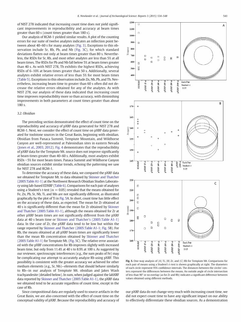
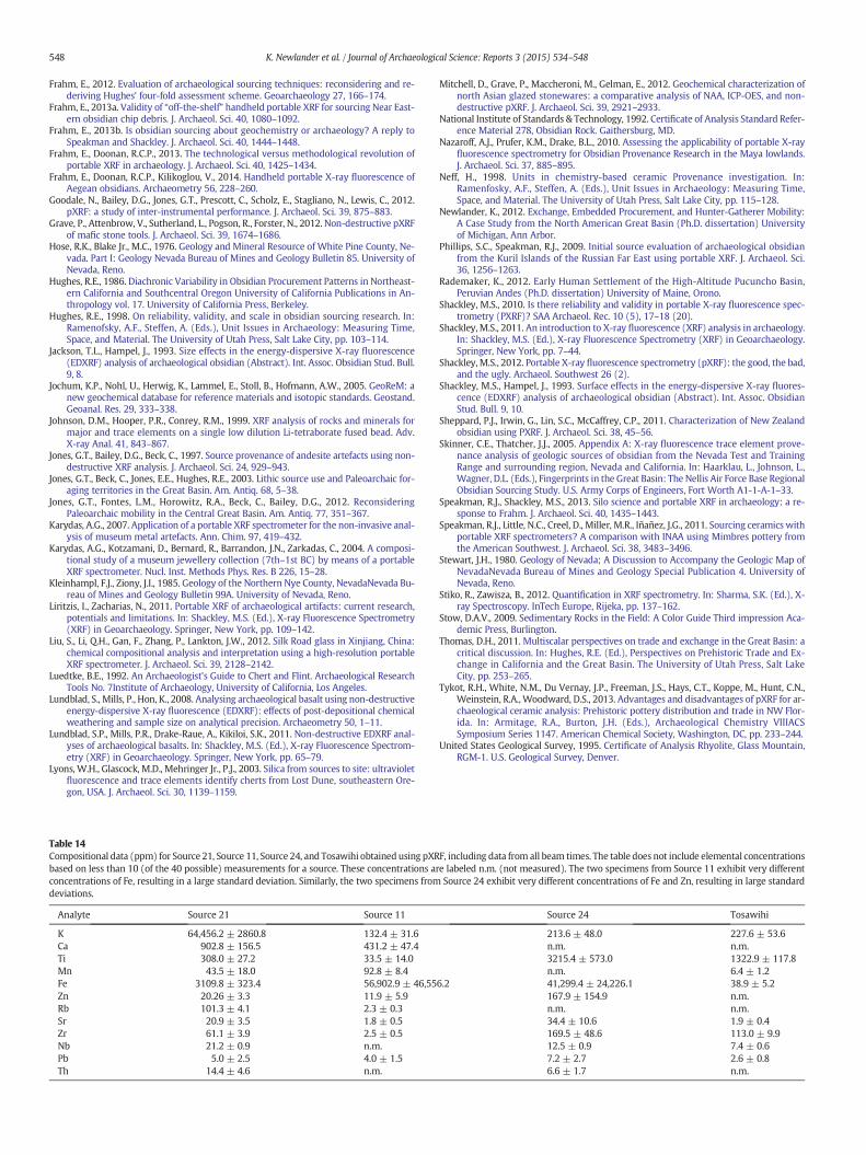
Fig. 5. One-way analysis of (A) Ti, (B) Zr, and (C) Rb for Tempiute Mt. Comparisons foreach pair of means using a Student's t-test is shown graphically at right. The diametersof each circle represent 95% confidence intervals. The distances between the circles' cen-ters represent the differences between the means. An outside angle of circle intersectionof less than 90° or no overlap (as for Zr and Rb) indicates a significant difference betweenvalues obtained using different methods.

541K. Newlander et al. / Journal of Archaeological Science: Reports 3 (2015) 534–548

of NIST 278 indicated that increasing count time does not yield signifi-cant improvements in reproducibility and accuracy at beam timesgreater than 60 s (count times greater than 180 s).

Our analysis of RGM-1 yielded similar results. A plot of the countingerrors for our suite of twelve analytes indicates an inflection point be-tween about 40–60 s for many analytes (Fig. 3). Exceptions to this ob-servation include Sr, Rb, Pb, and Nb (Fig. 3C), for which standarddeviations flatten out only at beam times greater than 80 s. Neverthe-less, the RSDs for Sr, Rb, and most other analytes are less than 5% at allbeam times. The RSDs for Pb and Nb fall below 5% at beam times greaterthan 40 s. As with NIST 278, Th exhibits the highest RSDs, achievingRSDs of 6–10% at beam times greater than 50 s. Additionally, severalanalytes exhibit relative errors of less than 5% for most beam times(Table 5). Exceptions to this observation include Zn, Nb, Pb, and Th. Nev-ertheless, increasing beam time to greater than 60 s often did not de-crease the relative errors obtained for any of the analytes. As withNIST 278, our analysis of these data indicated that increasing counttime improves reproducibility more so than accuracy, with diminishingimprovements in both parameters at count times greater than about180 s.

3.2. Obsidian

The preceding section demonstrated the effect of count time on thereproducibility and accuracy of pXRF data generated for NIST 278 andRGM-1. Next, we consider the effect of count time on pXRF data gener-ated for toolstone sources in the Great Basin, beginning with obsidian.Obsidian from Panaca Summit, Tempiute Mountain, and WildhorseCanyon are well-represented at Paleoindian sites in eastern Nevada(Jones et al., 2003, 2012). Fig. 4 demonstrates that the reproducibilityof pXRF data for the TempiuteMt. source does not improve significantlyat beam times greater than 40–60 s. Additionally, most analytes exhibitRSDs b5% for most beam times. Panaca Summit and Wildhorse Canyonobsidian sources exhibit similar trends, echoing the patterning we sawfor NIST 278 and RGM-1.

To determine the accuracy of these data, we compared the pXRF datawe obtained for Tempiute Mt. to data obtained by Skinner and Thatcher(2005:Table A1-1) at the Northwest Research Obsidian Studies Laborato-ry using lab-basedEDXRF (Table 6). Comparisons for eachpair of analysesusing a Student's t-test (α= 0.05) revealed that the means obtained forFe, Zn, Pb, Sr, Nb, Ti, and Mn are not significantly different, as illustratedgraphically by the plot of Ti in Fig. 5A. In short, count time has little effecton the accuracy of these data, as expected. The mean for Zr obtained at40 s is significantly different than the mean for Zr obtained by Skinnerand Thatcher (2005:Table A1-1), although the means obtained for Zr atother pXRF beam times are not significantly different from the pXRFdata at 40 s beam time or Skinner and Thatcher's (2005:Table A1-1)data. In the case of Zr, the pXRF data tend to be low but within therange reported by Skinner and Thatcher (2005:Table A1-1; Fig. 5B). ForRb, the means obtained at all pXRF beam times are significantly lowerthan the mean Rb concentration obtained by Skinner and Thatcher(2005:Table A1-1) for Tempiute Mt. (Fig. 5C). The relative error associat-ed with the pXRF concentrations for Rb improves slightly with increasedbeam time, but only from 11.4% at 40 s to 8.9% at 100 s. As suggested byour reviewer, spectroscopic interferences (e.g., the sum peaks of Fe) maybe complicating our attempt to accurately analyze Rb using pXRF. Thispossibility is consistent with the greater accuracy we achieved for othermedium elements (e.g., Sr, Nb)—elements that should behave similarlyto Rb—in our analysis of Tempiute Mt. obsidian and Jakes Washtrachyandesite (detailed below). In sum,when judged against the labXRFdata reported by Skinner and Thatcher (2005:Table A1-1), the pXRF datawe obtained tend to be accurate regardless of count time, except in thecase of Rb.

Since compositional data are regularly used to source artifacts in theGreat Basin, we are also concerned with the effect of count time on theconceptual validity of pXRF. Because the reproducibility and accuracy of

our pXRF data do not change verymuchwith increasing count time, wedid not expect count time to have any significant impact on our abilityto effectively differentiate these obsidian sources. As a demonstration

Fig. 6. Bivariate scatterplot of Ti vs. Sr, including pXRF data for all beam times. The ellipsesaround each group are drawn at the 95% confidence level.

Table 7Compositional data (ppm) for Panaca Summit, Tempiute Mt., and Wildhorse Canyon ob-sidian sources obtained using pXRF. Data from all beam times are included; thus, the sum-mary statistics are based on 40measurements for each source (20measurements on eachof 2 specimens).

Analyte Panaca Summit Tempiute Mt. Wildhorse Canyon

K 44,173.4 ± 1518.4 43,204.9 ± 1066.5 42,454.2 ± 959.4Ca 4745.1 ± 271.2 6153.6 ± 203.5 3415.6 ± 139.4Ti 768.9 ± 30.6 657.3 ± 19.8 689.1 ± 15.8Mn 303.2 ± 10.9 501.9 ± 12.0 357.2 ± 6.6Fe 6025.7 ± 229.0 8490.4 ± 226.0 4934.0 ± 107.9Zn 23.7 ± 3.6 57.4 ± 2.9 23.2 ± 1.9Rb 182.7 ± 5.2 178.2 ± 3.2 174.5 ± 2.5Sr 76.6 ± 2.9 122.7 ± 3.2 37.0 ± 1.0Zr 119.3 ± 5.4 156.5 ± 3.6 104.2 ± 1.9Nb 20.2 ± 0.8 28.1 ± 0.7 23.2 ± 0.7Pb 26.8 ± 1.6 24.9 ± 1.2 29.7 ± 1.6Th 31.5 ± 1.9 21.7 ± 2.1 26.2 ± 2.0

542 K. Newlander et al. / Journal of Archaeological Science: Reports 3 (2015) 534–548

of this point, Fig. 6 presents a bivariate scatterplot of Ti vs. Sr that in-cludes pXRF data obtained at all beam times. Significantly, the structurein these data is evident at all beam times. Group-membership probabil-ities calculated usingMahalanobis distances based on Ti and Sr indicateno misclassifications of these obsidian specimens at any beam time. Inshort, count time has no bearing on the conceptual validity of pXRFfor discriminating Panaca Summit, Tempiute Mt., and Wildhorse Can-yon obsidian sources. Table 7 summarizes the pXRF data for all beamtimes for these obsidian sources.

3.3. FGVs

In contrast to obsidian, several sources of artifact-quality FGVs arereadily available in eastern Nevada, occurring in Tertiary-age extrusivelavas that range in composition between andesite and rhyolite (Joneset al., 1997). Fig. 7 demonstrates that the reproducibility of pXRF datafor the Little Smoky Quarry source does not improve significantly atbeam times greater than 40–60 s. Most analytes exhibit RSDs b5% forall beam times. The RSDs for Zn and Nb are less than 5% at beam timesgreater than 20 s. The RSDs for Pb are ~5% at beam times ≥50 s. Thagain exhibits the highest RSDs, with RSDs between 9 and 15% atbeam times ≥55 s. Specimens from the Jakes Wash and Murry CanyonFGV sources exhibit similar trends.

To assess the effect of count time on the accuracy of these data, wecompared the pXRF data we obtained for Jakes Wash to data obtainedusing lab-based WDXRF at the Peter Hooper GeoAnalytical Lab atWashington State University (Table 8). To facilitate comparison ofthese data, we converted the concentrations obtained by WDXRF forTi, Fe, Mn, Ca, and K from weight percent oxide, to weight percent ele-ment (using stoichiometric conversion factors), and then to ppm. Com-parisons for each pair of analyses using a Student's t-test (α = 0.05)revealed that the mean concentrations obtained for Sr, Zr, Ti, Nb, Pb,and Th usingWDXRF are not significantly different than the mean con-centrations obtained for these analytes using pXRF at most beam times.The mean concentrations obtained for Fe, Ca, Mn, K, and Zn usingWDXRF are significantly lower than the mean concentrations obtainedfor these analytes using pXRF, and themean concentration of Rb obtain-ed using WDXRF is significantly greater than the mean concentrationobtained by pXRF.

We trust that the WDXRF data are reproducible and accurate. TheWDXRF data were obtained using calibration curves based upon theanalysis of 105 geologic standards. The elemental concentrations

obtained usingWDXRF are associated with smaller standard deviationsthan the elemental concentrations obtained using pXRF (Table 8), sug-gesting a greater degree of reproducibility for WDXRF. Additionally, acomparison of theWDXRF datawith elemental concentrations reportedby other laboratories yielded relative errors that are b1% for many ele-ments (e.g., Johnson et al., 1999:Table 5). In contrast, the relative errorswe obtained by comparing the pXRF data to theWDXRF data vary from8.1% for Rb to 40% for K. As expected, increasing count time does not im-prove the accuracy of the pXRF data for these analytes. A comparison ofWDXRF and pXRF data for specimens from Little Smoky Quarry andMurry Canyon yielded similar results. Nevertheless, the pXRF data andWDXRF data are highly correlated for these analytes (Table 9, Fig. 8);therefore, these pXRF data can be “corrected” for direct comparisonwith labXRF for FGV sources. As Table 10 demonstrates, the correctedpXRF values for K, Ca, Mn, Fe, Zn, and Rb compare favorably with theWDXRF data obtained for these analytes for specimens from JakesWash. The same is true when comparing the corrected pXRF valueswith theWDXRF data obtained for specimens from Little Smoky Quarryand Murry Canyon.

Finally, Fig. 9 presents a bivariate scatterplot of Rb vs. Sr that includespXRF data obtained at all beam times. Significantly, the structure inthese data is evident at all beam times. Group-membership probabilitiescalculated using Mahalanobis distances based on Rb and Sr indicate nomisclassifications of these FGV specimens at any count time. In short,count time has no bearing on the conceptual validity of pXRF for dis-criminating Little Smoky Quarry, Jakes Wash, and Murry Canyon FGVsources. Table 11 summarizes the pXRF data for all beam times forthese FGV sources.

3.4. Metamorphic and chert sources

Metamorphic rocks and cherts are more common in eastern Nevadathan obsidians and FGVs. Source 21 consists of nodules of greenschistthat occur as inclusionswithin a Tertiary-age volcanic ash flow in south-ern LongValley. The three chert sources included here, Tosawihi, Source11, and Source 24, all evince prehistoric use in the region. Fig. 10 dem-onstrates that the reproducibility of pXRF data for Source 21 does notimprove significantly at beam times greater than 40–60 s. The trendsapparent in Fig. 10 for Source 21 duplicate the general patterns for thegeologic standards, obsidians, and FGVs. The reproducibility of the com-positional data for several analytes is poorer in Source 21 and the cherts,however. For example, the RSDs for Th and Pb in Source 21 never fallbelow 5%. The RSDs for K, Rb, Sr, Zr, Ti, and Pb for Source 11 are all great-er than 10% at most beam times. For Source 24, the RSDs for Th, K, andPb are greater than 10% at most beam times. For Tosawihi, the RSDsfor Mn, Rb, Pb, and Th range between 15 and 30%, whereas the RSDs

Fig. 7.Comparison plots of standard deviations of analytes for two Little SmokyQuarry FGV specimens. The analytes are separated to best display the patterning in these data: (A) K, Ca, Fe,and Ti; (B) Mn, Sr, Zr, and Th; (C) Zn, Rb, Pb, and Nb.

543K. Newlander et al. / Journal of Archaeological Science: Reports 3 (2015) 534–548

Table 8Lab-based WDXRF data (before normalization; n = 7) and pXRF data for Jakes Wash. Note that these WDXRF data are not the same data reported in Jones et al. (1997).

Analyte labXRF (ppm) pXRF (ppm)

5 s 20 s 40 s 60 s 80 s 100 s

K 37,997.6 ± 226.9 52,960.5 ± 270.8 53,348.5 ± 1557.8 52,941.5 ± 690.8 53,348.0 ± 417.2 53,087.5 ± 750.2 53,156.0 ± 213.6Ca 32,880.8 ± 330.2 43,588.5 ± 180.3 44,592.5 ± 10.6 43,640.0 ± 1344.9 44,169.0 ± 1380.3 43,945.0 ± 1781.9 44,243.5 ± 1398.0Ti 5684.7 ± 68.8 5811.0 ± 264.5 5888.0 ± 73.5 5837.0 ± 90.5 5862.5 ± 177.5 5908.0 ± 93.3 5858.5 ± 128.0Mn 695.5 ± 5.3 775.0 ± 63.6 771.5 ± 27.6 760.0 ± 7.1 783.0 ± 18.4 778.0 ± 19.8 776.0 ± 0Fe 42,846.0 ± 736.9 47,355.5 ± 2400.6 47,403.0 ± 1574.0 47565.0 ± 1509.0 47,490.0 ± 1552.8 47,808.0 ± 1284.1 47,041.0 ± 1131.4Zn 83.4 ± 2.1 72.5 ± 7.8 70.0 ± 2.8 72.5 ± 3.5 71.5 ± 0.2 71.7 ± 2.8 69.1 ± 0.1Rb 188.1 ± 0.7 174.0 ± 1.4 178.0 ± 1.4 179.8 ± 0.1 177.8 ± 1.3 177.2 ± 2.0 177.5 ± 1.9Sr 512.6 ± 5.0 498.0 ± 1.4 513.0 ± 11.3 507.0 ± 7.1 514.5 ± 4.9 509.5 ± 3.5 514.5 ± 13.4Zr 297.1 ± 1.2 292.5 ± 6.4 297.5 ± 0.7 294.5 ± 6.4 299.5 ± 2.1 296.0 ± 1.4 292.0 ± 1.4Nb 21.9 ± 0.2 21.8 ± 1.5 22.2 ± 0.2 24.0 ± 0.1 23.9 ± 0.5 23.9 ± 0.5 23.2 ± 0.2Pb 21.4 ± 0.5 16.0 ± 0 24.3 ± 3.3 24.4 ± 0.3 22.8 ± 0.5 22.7 ± 0.8 22.5 ± 0.7Th 23.1 ± 0.4 22.0a 24.0 ± 5.7 25.0 ± 1.4 23.5 ± 2.1 25.1 ± 1.6 23.1 ± 0.7

a This is above the limit of detection in only one specimen at a beam time of 5 s.

544 K. Newlander et al. / Journal of Archaeological Science: Reports 3 (2015) 534–548

for K, Sr, and Fe are greater than 5% for all beam times. For each of thesesources, analytes that exhibit high measurement error are present inlow concentrations; thus, these patterns are not surprising. Additional-ly, some analytes were below the limit of detection in these cherts atshort beam times; other analytes were below the limit of detection atall beam times. For example, data for Mn and Pb were obtained forTosawihi only at beam times greater than 45 s, and Ca, Th, Rb, and Znwere not measured in either specimen from Tosawihi at most beamtimes. Although increasing count timemay improve the reproducibilityof pXRF data for some cherts, these results suggest the same difficultiesin characterizing cherts that we have seen with other analyticalmethods (e.g., laser ablation inductively-coupled plasma mass spec-trometry; Newlander, 2012).

To assess the effect of count time on the accuracy of these data, wecompared the pXRF data we obtained for two specimens of Tosawihiopalite to data obtained by Lyons et al. (2003) using instrumental neu-tron activation analysis (INAA; Table 12). Given the amount of missingdata, statistical comparison is difficult for many of these analytes. Nev-ertheless, the relative errors for K and Fe decrease with increasingcount time. In order to increase the number of measurements for com-parison, Table 13 includes pXRF data for all beam times. Still, Mn, Rb,and Th are represented by few pXRF measurements (n in Table 13).We include Mn, Rb, and Th in our comparison, despite their small sam-ple sizes, because there are so few analytes for which we can comparethe concentrations obtained using pXRF and INAA for Tosawihi. Com-parisons for each pair of analyses using a Student's t-test (α=0.05) re-veal that themeans obtained for K, Mn, Fe, and Rb using INAA and pXRFare significantly different. This result is not surprising given the greaterintra-source variability evident in these data in comparison to the obsid-ian and FGV sources, and the few Tosawihi specimens we have charac-terized using pXRF. Insteadof focusing on the compositional differences,we note that the concentrations we obtained using pXRF fall

Table 9Linear correlations and regression equations between pXRF and WDXRF data calculatedfrom the mean concentrations (ppm) of K, Ca, Mn, Fe, Zn, and Rb for the FGV sources.

Analyte Correlation coefficient (r) Linear regression equation

K 0.982 KXRF = 6883.7899 + 0.5735336 ∗ KPXRF

Ca 0.999 CaXRF = 9558.8614 + 0.5303317 ∗ CaPXRFMn 0.997 MnXRF = −4.431618 + 0.9211964 ∗ MnPXRF

Fe 0.999 FeXRF = 9177.8606 + 0.7107415 ∗ FePXRFZn 0.965 ZnXRF = 26.883333 + 0.7916667 ∗ ZnPXRF

Rb 0.999 RbXRF = 0.6847304 + 1.0524022 ∗ RbPXRF

comfortably within the range of variability reported by Lyons et al.(2003) using INAA.

Finally, Fig. 11 presents bivariate scatterplots of Ti vs. Fe and Sr vs. Fethat include pXRF data obtained at all beam times. Group-membershipprobabilities calculated using Mahalanobis distances based on Ti, Fe,and Sr indicate no misclassifications of these specimens at beam timesgreater than 55 s (too many data at shorter beam times are missing topermit this calculation). In sum, count time has bearing on the concep-tual validity of pXRF for discriminating Source 21, Source 11, Source 24,and Tosawihi only insofar as longer count times bringmore low concen-tration analytes above their limits of detection. Given their highly vari-able lithological and chemical compositions (notice the large standarddeviations in Table 14), it is not surprising that the chert sources aremore difficult to define and to discriminate using pXRF. Many moresamples need to be analyzed to fully define the compositional variationwithin each source. Nevertheless, it is noteworthy that the composition-al data we obtained using pXRF behave as we would expect given themacroscopic variability exhibited by these types of stone. For example,Source 24 and Source 11 have the highest Fe content, as we would ex-pect for red and orange cherts (Luedtke, 1992). Also, the relativelyhigh concentration of K, Fe, and Rb in Source 21 is consistentwithmeta-morphosed basalt nodules occurring as inclusions within a Tertiary-agevolcanic ash flow unit.

4. Conclusion

In their recent literature survey, Frahm and Doonan (2013) foundthat many archeologists are adopting pXRF in order to decrease costsand analytical time, thereby allowing for the analysis of a greater pro-portion of an archeological assemblage. We admit that this is a primaryreason for our use of HHpXRF, even though we operate our instrumentprimarily in a laboratory. Given all of the demands on our time, we sup-pose that most analysts would agree that decreased analytical time isdesirable—provided it is not at the expense of data quality.

Characteristics of pXRF instruments can help us decrease analyticaltime. Modern machines can generate higher count rates, thereby im-proving counting statistics and reducing analytical time, by both in-creasing X-ray tube currents and by increasing detector efficiency andthroughput (Frahm et al., 2014; Liritzis and Zacharias, 2011). Ratherthan trade in one pXRF instrument for another, our analysis indicatedthat we can decrease analytical time without sacrificing data qualityby decreasing count time. Increasing count time does reduce countingerror, but only up to a count time of about 180 s. Increasing counttime beyond about 180 s did not significantly improve the reproducibil-ity of our pXRF data. Furthermore, we found that pXRF data obtained atshort count times (b40–60 s) were almost always as accurate as pXRFdata obtained at longer count times, particularly for geologic standards

Fig. 8. Linear correlation between pXRF and WDXRF data calculated from the mean con-centrations (ppm) of Ca, Fe, and Rb for the FGV sources.

Table 10Lab-based WDXRF data (before normalization; n = 7) and pXRF data for Jakes Wash after corr

Analyte labXRF (ppm) pXRF (ppm)

5 s 20 s 40 s

K 37,997.6 ± 226.9 37,258.4 ± 155.3 37,480.9 ± 893.4 37,2Ca 32,880.8 ± 330.2 32,675.2 ± 95.6 33,207.7 ± 5.6 32,7Mn 695.5 ± 5.3 709.5 ± 58.6 706.3 ± 25.4 6Fe 42,846.0 ± 736.9 42,835.4 ± 1706.2 42,869.1 ± 1118.7 42,9Zn 83.4 ± 2.1 84.3 ± 6.2 82.3 ± 2.2Rb 188.1 ± 0.7 183.8 ± 1.5 188.0 ± 1.5 1

Fig. 9. Bivariate scatterplot of Rb (corrected) vs. Sr, including pXRF data for all beam times.The ellipses around each group are drawn at the 95% confidence level.

Table 11Compositional data (ppm) for Little Smoky Quarry, Jakes Wash, and Murry Canyon FGVsources obtained using pXRF, including data from all beam times. The summary statisticsare based on 40 measurements for each source (20 measurements on each of 2specimens), except for Th. Thwas below the limit of detection for some specimens at shortbeam times; therefore, n= 37 for Little SmokyQuarry, n= 39 for JakesWash, and n=32for Murry Canyon.

Analyte Little Smoky Quarry Jakes Wash Murry Canyon

Ka 29,177.7 ± 477.8 37,261.3 ± 364.6 35,823.9 ± 347.2Caa 32,013.6 ± 1221.7 32,830.7 ± 594.3 38,971.4 ± 875.5Ti 4756.2 ± 83.6 5852.2 ± 127.6 6593.9 ± 193.1Mna 644.6 ± 11.7 706.8 ± 17.1 895.0 ± 19.5Fea 37,208.2 ± 371.3 42,917.9 ± 775.3 49,753.5 ± 1047.1Zna 83.7 ± 1.7 83.3 ± 2.3 84.7 ± 2.3Rba 110.9 ± 2.0 187.9 ± 2.6 157.1 ± 3.2Sr 742.0 ± 16.7 511.9 ± 10.9 652.0 ± 9.4Zr 343.1 ± 6.1 296.5 ± 3.3 244.7 ± 5.1Nb 21.4 ± 1.1 23.6 ± 0.9 19.8 ± 0.8Pb 20.8 ± 1.3 22.4 ± 2.0 18.9 ± 1.2Th 16.1 ± 3.6 25.6 ± 3.1 11.5 ± 2.7

a Data corrected using linear regression equations.

545K. Newlander et al. / Journal of Archaeological Science: Reports 3 (2015) 534–548

and obsidians. This, too, is consistent with fundamental principles of X-ray spectrometry. Nevertheless, cherts may require longer count timesto bring low concentration analytes above their limits of detection.

Significantly, the pXRF data we obtained for Tempiute Mt. obsidianand Tosawihi opalite compared favorably to compositional data obtain-ed using other analytical methods. In the case of Jakes Wash andesite,the pXRF data for several analytes (e.g., Sr, Zr) compared well to labXRFdata, although the pXRF data for other analytes (e.g., Fe, Rb) required“correction” for comparison with labXRF data. In general, comparisonof our pXRF data with legacy data obtained using other analytical

ecting K, Ca, Mn, Fe, Zn, and Rb using linear regression equations.

60 s 80 s 100 s

47.5 ± 396.2 37,480.7 ± 239.3 37,331.3 ± 430.3 37,370.5 ± 122.502.5 ± 713.3 32,983.1 ± 732.0 32,864.3 ± 945.0 33,022.6 ± 741.495.7 ± 6.5 716.9 ± 16.9 712.3 ± 18.2 710.4 ± 084.3 ± 1072.5 42,931.0 ± 1103.6 43,157.0 ± 912.7 42,611.9 ± 804.184.3 ± 2.8 83.4 ± 0.2 83.6 ± 2.2 81.5 ± 0.189.9 ± 0.1 187.7 ± 1.4 187.2 ± 2.1 187.4 ± 2.0

Fig. 10. Comparison plots of standard deviations of analytes for two specimens from Source 21. The analytes are separated to best display the patterning in these data: (A) K, Ca, Fe, and Ti;(B) Mn, Zr, Th, and Zn; (C) Sr, Rb, Pb, and Nb.

546 K. Newlander et al. / Journal of Archaeological Science: Reports 3 (2015) 534–548

Table 13INAA data (n= 15) from Lyons et al. (2003) and average pXRF data (n ≤ 40) from all beam times for Tosawihi. The other analytes for which this pXRF instrument was calibratedwere notwell-measured in both datasets.

Analyte INAA (ppm) pXRF (ppm)

Conc. Range Conc. Range n

K 282.1 ± 93.5 125.8–481.1 228.4 ± 54.1 121–381 39Mn 1.7 ± 2.8 0.2–11.6 6.4 ± 1.2 4.8–8.3 13Fea 75.1 ± 67.0 14.8–215.4 38.9 ± 5.2 28–52 37Rb 0.8 ± 0.2 0.5–1.1 1.2 ± 0.2 1–1.5 7Th 2.1 ± 3.3 0.2–9.6 3.3 ± 0.8 2.6–4.6 6

a Excluding INAA data for Tosawihi-IMR005 (Fe = 668 ppm) as an outlier.

Table 12INAA data (n= 15) from Lyons et al. (2003) and pXRF data (n ≤ 2) obtained at different beam times for Tosawihi. The other analytes for which this pXRF instrument was calibratedwerenot well-measured in both datasets.

Analyte INAA (ppm) pXRF (ppm)

5 s 20 s 40 s 60 s 80 s 100 s

K 282.1 ± 93.5 310.5 ± 74.2 203.0 ± 77.8 216.5 ± 0.7 189.0 ± 25.5 216.0 ± 11.3 296.0 ± 59.4Mn 1.7 ± 2.8 n.m. n.m. n.m. n.m. n.m. 5.2 ± 0.2Fea 75.1 ± 67.0 n.m. 37.5 ± 12.0 36.0 ± 1.4 34.0 ± 5.7 37.5 ± 0.7 40.5 ± 3.5Th 2.1 ± 3.3 n.m. n.m. n.m. n.m. 2.7 ± 0.1 n.m.

n.m. = not measured.a Excluding INAA data for Tosawihi-IMR005 (Fe = 668 ppm) as an outlier.

Fig. 11.Bivariate scatterplots of base-10 logarithms of Ti vs. Fe and Sr vs. Fe, including pXRFdata for all beam times. The ellipses around each group are drawn at the 95% confidencelevel.

547K. Newlander et al. / Journal of Archaeological Science: Reports 3 (2015) 534–548

methodsdemonstrated that awell-calibrated pXRF instrument can gen-erate accurate compositional data. Finally, we were able to distinguishdifferent sources within each type of toolstone at all count times, dem-onstrating the conceptual validity of pXRF for sourcing studies.

As Shackley (2010:20) observed, “We … owe it to our discipline toestablish study protocols for [pXRF] so we can all compare results asin any science.” Absent a rigorous analytical protocol, archeological ap-plications of pXRF will continue to be treated with caution (Grave et al.,2012:1674). We offer these results as a step toward a consistent, rigor-ous analytical protocol for archeological applications of pXRF.

Acknowledgments

This research was supported by NSF DDIG #0911983, NSF MRI#0959297, grants from the University of Michigan, and the Dean of Fac-ulty at Hamilton College. The ideas expressed here are those of the au-thors and do not necessarily reflect the views of these funding agencies.We thank Charlotte Beck and an anonymous reviewer for their helpfulcomments on this analysis.

References

Angeles-Chavez, C., Toledo-Antonio, J.A., Cortes-Jacome, M.A., 2012. Chemical quantifica-tion of Mo–S, W–Si, and Ti–V by energy dispersive X-ray spectroscopy. In: Sharma,S.K. (Ed.), X-ray Spectroscopy. InTech, Rijeka, pp. 119–136.

Conrey, R.M., Goodman-Elgar,M., Bettencourt, N., Seyfarth, A., VanHoose, A.,Wolff, J.A., 2014.Calibration of a portable X-ray fluorescence spectrometer in the analysis of archaeologi-cal samples using influence coefficients. Geochem. Explor. Environ. Anal. 14, 291–301.

Craig, N., Speakman, R., Popelka-FIlcoff, R., Glascock, M., Robertson, J., Shackley, M.S.,Aldenderfer, M., 2007. Comparison of XRF and PXRF for analysis of archaeological ob-sidian from southern Perú. J. Archaeol. Sci. 34, 2012–2024.

Davis, M., Jackson, T., Shackley, M.S., Teague, T., Hampel, J., 1998. Factors affecting theenergy-dispersive X-ray fluorescence (EDXRF) analysis of archaeological obsidian.In: Shackley, M.S. (Ed.), Archaeological Obsidian Studies. Advances in Archaeologicaland Museum Science 3. Springer, New York, pp. 159–180.

Elston, R.G., Raven, C. (Eds.), 1992. Prepared for the Bureau of LandManagement, Elko Re-source Area, ElkoArchaeological Investigations at Tosawihi, a Great Basin Quarry. Part1: The Periphery 2 volumes. Intermountain Research, Silver City.

Forster, N., Grave, P., 2012. Non-destructive PXRF analysis of museum-curated obsidianfrom the Near East. J. Archaeol. Sci. 39, 728–736.

Forster, N., Grave, P., Vickery, N., Kealhofer, L., 2011. Non-destructive analysis using PXRF:methodology and application to archaeological ceramics. X-ray Spectrom. 40,389–398.

548 K. Newlander et al. / Journal of Archaeological Science: Reports 3 (2015) 534–548

Frahm, E., 2012. Evaluation of archaeological sourcing techniques: reconsidering and re-deriving Hughes' four-fold assessment scheme. Geoarchaeology 27, 166–174.

Frahm, E., 2013a. Validity of “off-the-shelf” handheld portable XRF for sourcing Near East-ern obsidian chip debris. J. Archaeol. Sci. 40, 1080–1092.

Frahm, E., 2013b. Is obsidian sourcing about geochemistry or archaeology? A reply toSpeakman and Shackley. J. Archaeol. Sci. 40, 1444–1448.

Frahm, E., Doonan, R.C.P., 2013. The technological versus methodological revolution ofportable XRF in archaeology. J. Archaeol. Sci. 40, 1425–1434.

Frahm, E., Doonan, R.C.P., Kilikoglou, V., 2014. Handheld portable X-ray fluorescence ofAegean obsidians. Archaeometry 56, 228–260.

Goodale, N., Bailey, D.G., Jones, G.T., Prescott, C., Scholz, E., Stagliano, N., Lewis, C., 2012.pXRF: a study of inter-instrumental performance. J. Archaeol. Sci. 39, 875–883.

Grave, P., Attenbrow, V., Sutherland, L., Pogson, R., Forster, N., 2012. Non-destructive pXRFof mafic stone tools. J. Archaeol. Sci. 39, 1674–1686.

Hose, R.K., Blake Jr., M.C., 1976. Geology and Mineral Resource of White Pine County, Ne-vada. Part I: Geology Nevada Bureau of Mines and Geology Bulletin 85. University ofNevada, Reno.

Hughes, R.E., 1986. Diachronic Variability in Obsidian Procurement Patterns in Northeast-ern California and Southcentral Oregon University of California Publications in An-thropology vol. 17. University of California Press, Berkeley.

Hughes, R.E., 1998. On reliability, validity, and scale in obsidian sourcing research. In:Ramenofsky, A.F., Steffen, A. (Eds.), Unit Issues in Archaeology: Measuring Time,Space, and Material. The University of Utah Press, Salt Lake City, pp. 103–114.

Jackson, T.L., Hampel, J., 1993. Size effects in the energy-dispersive X-ray fluorescence(EDXRF) analysis of archaeological obsidian (Abstract). Int. Assoc. Obsidian Stud. Bull.9, 8.

Jochum, K.P., Nohl, U., Herwig, K., Lammel, E., Stoll, B., Hofmann, A.W., 2005. GeoReM: anew geochemical database for reference materials and isotopic standards. Geostand.Geoanal. Res. 29, 333–338.

Johnson, D.M., Hooper, P.R., Conrey, R.M., 1999. XRF analysis of rocks and minerals formajor and trace elements on a single low dilution Li-tetraborate fused bead. Adv.X-ray Anal. 41, 843–867.

Jones, G.T., Bailey, D.G., Beck, C., 1997. Source provenance of andesite artefacts using non-destructive XRF analysis. J. Archaeol. Sci. 24, 929–943.

Jones, G.T., Beck, C., Jones, E.E., Hughes, R.E., 2003. Lithic source use and Paleoarchaic for-aging territories in the Great Basin. Am. Antiq. 68, 5–38.

Jones, G.T., Fontes, L.M., Horowitz, R.A., Beck, C., Bailey, D.G., 2012. ReconsideringPaleoarchaic mobility in the Central Great Basin. Am. Antiq. 77, 351–367.

Karydas, A.G., 2007. Application of a portable XRF spectrometer for the non-invasive anal-ysis of museum metal artefacts. Ann. Chim. 97, 419–432.

Karydas, A.G., Kotzamani, D., Bernard, R., Barrandon, J.N., Zarkadas, C., 2004. A composi-tional study of a museum jewellery collection (7th–1st BC) by means of a portableXRF spectrometer. Nucl. Inst. Methods Phys. Res. B 226, 15–28.

Kleinhampl, F.J., Ziony, J.I., 1985. Geology of the Northern Nye County, NevadaNevada Bu-reau of Mines and Geology Bulletin 99A. University of Nevada, Reno.

Liritzis, I., Zacharias, N., 2011. Portable XRF of archaeological artifacts: current research,potentials and limitations. In: Shackley, M.S. (Ed.), X-ray Fluorescence Spectrometry(XRF) in Geoarchaeology. Springer, New York, pp. 109–142.

Liu, S., Li, Q.H., Gan, F., Zhang, P., Lankton, J.W., 2012. Silk Road glass in Xinjiang, China:chemical compositional analysis and interpretation using a high-resolution portableXRF spectrometer. J. Archaeol. Sci. 39, 2128–2142.

Luedtke, B.E., 1992. An Archaeologist's Guide to Chert and Flint. Archaeological ResearchTools No. 7Institute of Archaeology, University of California, Los Angeles.

Lundblad, S., Mills, P., Hon, K., 2008. Analysing archaeological basalt using non-destructiveenergy-dispersive X-ray fluorescence (EDXRF): effects of post-depositional chemicalweathering and sample size on analytical precision. Archaeometry 50, 1–11.

Lundblad, S.P., Mills, P.R., Drake-Raue, A., Kikiloi, S.K., 2011. Non-destructive EDXRF anal-yses of archaeological basalts. In: Shackley, M.S. (Ed.), X-ray Fluorescence Spectrom-etry (XRF) in Geoarchaeology. Springer, New York, pp. 65–79.

Lyons, W.H., Glascock, M.D., Mehringer Jr., P.J., 2003. Silica from sources to site: ultravioletfluorescence and trace elements identify cherts from Lost Dune, southeastern Ore-gon, USA. J. Archaeol. Sci. 30, 1139–1159.

Table 14Compositional data (ppm) for Source 21, Source 11, Source 24, and Tosawihi obtained using pXRbased on less than 10 (of the 40 possible) measurements for a source. These concentrations aconcentrations of Fe, resulting in a large standard deviation. Similarly, the two specimens fromdeviations.

Analyte Source 21 Source 11

K 64,456.2 ± 2860.8 132.4 ± 31.6Ca 902.8 ± 156.5 431.2 ± 47.4Ti 308.0 ± 27.2 33.5 ± 14.0Mn 43.5 ± 18.0 92.8 ± 8.4Fe 3109.8 ± 323.4 56,902.9 ± 46,55Zn 20.26 ± 3.3 11.9 ± 5.9Rb 101.3 ± 4.1 2.3 ± 0.3Sr 20.9 ± 3.5 1.8 ± 0.5Zr 61.1 ± 3.9 2.5 ± 0.5Nb 21.2 ± 0.9 n.m.Pb 5.0 ± 2.5 4.0 ± 1.5Th 14.4 ± 4.6 n.m.

Mitchell, D., Grave, P., Maccheroni, M., Gelman, E., 2012. Geochemical characterization ofnorth Asian glazed stonewares: a comparative analysis of NAA, ICP-OES, and non-destructive pXRF. J. Archaeol. Sci. 39, 2921–2933.

National Institute of Standards & Technology, 1992. Certificate of Analysis Standard Refer-ence Material 278, Obsidian Rock. Gaithersburg, MD.

Nazaroff, A.J., Prufer, K.M., Drake, B.L., 2010. Assessing the applicability of portable X-rayfluorescence spectrometry for Obsidian Provenance Research in the Maya lowlands.J. Archaeol. Sci. 37, 885–895.

Neff, H., 1998. Units in chemistry-based ceramic Provenance investigation. In:Ramenfosky, A.F., Steffen, A. (Eds.), Unit Issues in Archaeology: Measuring Time,Space, and Material. The University of Utah Press, Salt Lake City, pp. 115–128.

Newlander, K., 2012. Exchange, Embedded Procurement, and Hunter-Gatherer Mobility:A Case Study from the North American Great Basin (Ph.D. dissertation) Universityof Michigan, Ann Arbor.

Phillips, S.C., Speakman, R.J., 2009. Initial source evaluation of archaeological obsidianfrom the Kuril Islands of the Russian Far East using portable XRF. J. Archaeol. Sci.36, 1256–1263.

Rademaker, K., 2012. Early Human Settlement of the High-Altitude Pucuncho Basin,Peruvian Andes (Ph.D. dissertation) University of Maine, Orono.

Shackley, M.S., 2010. Is there reliability and validity in portable X-ray fluorescence spec-trometry (PXRF)? SAA Archaeol. Rec. 10 (5), 17–18 (20).

Shackley, M.S., 2011. An introduction to X-ray fluorescence (XRF) analysis in archaeology.In: Shackley, M.S. (Ed.), X-ray Fluorescence Spectrometry (XRF) in Geoarchaeology.Springer, New York, pp. 7–44.

Shackley, M.S., 2012. Portable X-ray fluorescence spectrometry (pXRF): the good, the bad,and the ugly. Archaeol. Southwest 26 (2).

Shackley, M.S., Hampel, J., 1993. Surface effects in the energy-dispersive X-ray fluores-cence (EDXRF) analysis of archaeological obsidian (Abstract). Int. Assoc. ObsidianStud. Bull. 9, 10.

Sheppard, P.J., Irwin, G., Lin, S.C., McCaffrey, C.P., 2011. Characterization of New Zealandobsidian using PXRF. J. Archaeol. Sci. 38, 45–56.

Skinner, C.E., Thatcher, J.J., 2005. Appendix A: X-ray fluorescence trace element prove-nance analysis of geologic sources of obsidian from the Nevada Test and TrainingRange and surrounding region, Nevada and California. In: Haarklau, L., Johnson, L.,Wagner, D.L. (Eds.), Fingerprints in the Great Basin: The Nellis Air Force Base RegionalObsidian Sourcing Study. U.S. Army Corps of Engineers, Fort Worth A1-1-A-1–33.

Speakman, R.J., Shackley, M.S., 2013. Silo science and portable XRF in archaeology: a re-sponse to Frahm. J. Archaeol. Sci. 40, 1435–1443.

Speakman, R.J., Little, N.C., Creel, D., Miller, M.R., Iñañez, J.G., 2011. Sourcing ceramics withportable XRF spectrometers? A comparison with INAA using Mimbres pottery fromthe American Southwest. J. Archaeol. Sci. 38, 3483–3496.

Stewart, J.H., 1980. Geology of Nevada; A Discussion to Accompany the Geologic Map ofNevadaNevada Bureau of Mines and Geology Special Publication 4. University ofNevada, Reno.

Stiko, R., Zawisza, B., 2012. Quantification in XRF spectrometry. In: Sharma, S.K. (Ed.), X-ray Spectroscopy. InTech Europe, Rijeka, pp. 137–162.

Stow, D.A.V., 2009. Sedimentary Rocks in the Field: A Color Guide Third impression Aca-demic Press, Burlington.

Thomas, D.H., 2011. Multiscalar perspectives on trade and exchange in the Great Basin: acritical discussion. In: Hughes, R.E. (Ed.), Perspectives on Prehistoric Trade and Ex-change in California and the Great Basin. The University of Utah Press, Salt LakeCity, pp. 253–265.

Tykot, R.H., White, N.M., Du Vernay, J.P., Freeman, J.S., Hays, C.T., Koppe, M., Hunt, C.N.,Weinstein, R.A., Woodward, D.S., 2013. Advantages and disadvantages of pXRF for ar-chaeological ceramic analysis: Prehistoric pottery distribution and trade in NW Flor-ida. In: Armitage, R.A., Burton, J.H. (Eds.), Archaeological Chemistry VIIIACSSymposium Series 1147. American Chemical Society, Washington, DC, pp. 233–244.

United States Geological Survey, 1995. Certificate of Analysis Rhyolite, Glass Mountain,RGM-1. U.S. Geological Survey, Denver.

F, including data from all beam times. The table does not include elemental concentrationsre labeled n.m. (not measured). The two specimens from Source 11 exhibit very differentSource 24 exhibit very different concentrations of Fe and Zn, resulting in large standard

Source 24 Tosawihi

213.6 ± 48.0 227.6 ± 53.6n.m. n.m.3215.4 ± 573.0 1322.9 ± 117.8n.m. 6.4 ± 1.2

6.2 41,299.4 ± 24,226.1 38.9 ± 5.2167.9 ± 154.9 n.m.n.m. n.m.34.4 ± 10.6 1.9 ± 0.4169.5 ± 48.6 113.0 ± 9.912.5 ± 0.9 7.4 ± 0.67.2 ± 2.7 2.6 ± 0.86.6 ± 1.7 n.m.