Empirical study of performance of classification and clustering ...

Empirical study of performance of classification

and clustering algorithms on binary data with

real-world applications

by

Stephanie Sherine Nahmias

A Thesis submitted to

the Faculty of Graduate Studies and Research

in partial fulfilment of

the requirements for the degree of

Master of Science

in

Mathematics and Statistics

Carleton University

Ottawa, Ontario, Canada

July 2014

Copyright c

2014 - Stephanie Sherine Nahmias

Abstract

This thesis compares statistical algorithms paired with dissimilarity measures for their

ability to identify clusters in benchmark binary datasets.

The techniques examined are visualization, classification, and clustering. To vi-

sually explore for clusters, we used parallel coordinates plots and heatmaps. The

classification algorithms used were neural networks and classification trees. Cluster-

ing algorithms used were: partitioning around centroids, partitioning around medoids,

hierarchical agglomerative clustering, and hierarchical divisive clustering.

The clustering algorithms were evaluated on their ability to identify the optimal

number of clusters. The “goodness” of the resulting clustering structures was assessed

and the clustering results were compared with known classes in the data using purity

and entropy measures.

Experimental design was employed to test if the algorithms and / or dissimilar-

ity measures had a statistically significant effect on the optimal number of clusters

chosen by our methods as well as whether the algorithms and dissimilarity measures

performed differently from one another.

ii

I dedicate this thesis to my children Tomas and Alexia!

Merci pour votre patience, votre amour et surtout votre encouragement ces derniers

temps, je vous aime tous les deux beaucoup!!

iii

Acknowledgments

First and foremost, I would like to express my sincere gratitude to my thesis super-

visor Dr. Shirley Mills, for her guidance and encouragement. Without her valuable

assistance and support this thesis would not have seen the light.

My thanks also goes to the School of Mathematics and Statistics, Carleton Uni-

versity, for providing the necessary research facilities for completing this thesis.

I would like to thank the mathematicians I have worked with for their guidance,

R knowledge, and support during the course of my research. As well, a big thank you

also goes to great supportive neighbours!!

I would like to thank my parents for their love and continued support during my

time at Carleton University, without their support this would probably have never

seen the light of day.

Finally, I must express my deep gratitude to my dear husband Dennis for his

immense support, constant encouragement and for taking care of me (and the kids)

throughout my study. His patience and the many sacrifices he made allowed me to

complete my program. Thank you for being there for me every step of the way and

for believing in me!

iv

Table of Contents

Abstract ii

Acknowledgments iv

Table of Contents v

List of Tables ix

List of Figures xvi

1 Introduction 1

1.1 Motivation . . . . . . . . . . . . . . . . . . . . . . . . . . . . . . . . . 1

1.2 Data used . . . . . . . . . . . . . . . . . . . . . . . . . . . . . . . . . 1

1.3 Methodologies . . . . . . . . . . . . . . . . . . . . . . . . . . . . . . . 2

1.3.1 Algorithms . . . . . . . . . . . . . . . . . . . . . . . . . . . . 2

1.3.2 Dissimilarity measures . . . . . . . . . . . . . . . . . . . . . . 3

1.3.3 Design of experiments . . . . . . . . . . . . . . . . . . . . . . 3

1.4 Outline . . . . . . . . . . . . . . . . . . . . . . . . . . . . . . . . . . . 3

2 Literature review 5

3 Methodology 13

3.1 Notation . . . . . . . . . . . . . . . . . . . . . . . . . . . . . . . . . . 14

v

3.2 Pre-processing . . . . . . . . . . . . . . . . . . . . . . . . . . . . . . . 15

3.2.1 Binary data . . . . . . . . . . . . . . . . . . . . . . . . . . . . 16

3.2.2 Converting to continuous using principal component analysis . 16

3.3 Data visualisation . . . . . . . . . . . . . . . . . . . . . . . . . . . . . 18

3.3.1 Parallel coordinates plot . . . . . . . . . . . . . . . . . . . . . 18

3.3.2 Heatmap . . . . . . . . . . . . . . . . . . . . . . . . . . . . . . 18

3.4 Classification . . . . . . . . . . . . . . . . . . . . . . . . . . . . . . . 18

3.4.1 Classification trees . . . . . . . . . . . . . . . . . . . . . . . . 19

3.4.2 Artificial Neural Networks . . . . . . . . . . . . . . . . . . . . 21

3.5 Clustering . . . . . . . . . . . . . . . . . . . . . . . . . . . . . . . . . 22

3.5.1 Partitioning algorithms . . . . . . . . . . . . . . . . . . . . . . 23

3.5.2 Hierarchical algorithms . . . . . . . . . . . . . . . . . . . . . . 26

3.5.3 Data types and dissimilarity measures . . . . . . . . . . . . . 32

3.5.4 Cluster evaluation . . . . . . . . . . . . . . . . . . . . . . . . . 34

3.5.5 Experimental design . . . . . . . . . . . . . . . . . . . . . . . 38

4 Voters data 42

4.1 Data pre-processing . . . . . . . . . . . . . . . . . . . . . . . . . . . . 44

4.1.1 Binary data . . . . . . . . . . . . . . . . . . . . . . . . . . . . 44

4.1.2 Converting binary using PCA . . . . . . . . . . . . . . . . . . 44



4.2.2 Heatmap (raw voters data) . . . . . . . . . . . . . . . . . . . 48

4.3 Classification . . . . . . . . . . . . . . . . . . . . . . . . . . . . . . . 50


4.3.2 Neural networks . . . . . . . . . . . . . . . . . . . . . . . . . . 55

4.4 Clustering . . . . . . . . . . . . . . . . . . . . . . . . . . . . . . . . . 57

vi

4.4.1 Choosing the optimal number of clusters . . . . . . . . . . . . 57

4.4.2 Internal indices: goodness of clustering . . . . . . . . . . . . . 63

4.4.3 External indices (using k = 2) . . . . . . . . . . . . . . . . . . 66

5 Zoo data 71

5.1 Data pre-processing . . . . . . . . . . . . . . . . . . . . . . . . . . . . 73

5.1.1 Binary data . . . . . . . . . . . . . . . . . . . . . . . . . . . . 73

5.1.2 Converting binary using PCA . . . . . . . . . . . . . . . . . . 73



5.2.2 Heatmap (raw zoo data) . . . . . . . . . . . . . . . . . . . . . 78

5.3 Classification . . . . . . . . . . . . . . . . . . . . . . . . . . . . . . . 81


5.3.2 Neural networks . . . . . . . . . . . . . . . . . . . . . . . . . . 84

5.4 Clustering . . . . . . . . . . . . . . . . . . . . . . . . . . . . . . . . . 86

5.4.1 Choosing the optimal number of clusters . . . . . . . . . . . . 86


5.4.3 External indices (using k = 7) . . . . . . . . . . . . . . . . . . 96

6 Results of Experimental Design 99

6.1 Evaluating the choice of k . . . . . . . . . . . . . . . . . . . . . . . . 99

6.2 Evaluating the performance (based on ASW) . . . . . . . . . . . . . . 101

7 Summary, conclusion and future work 107

7.1 Summary . . . . . . . . . . . . . . . . . . . . . . . . . . . . . . . . . 107

7.2 Conclusion . . . . . . . . . . . . . . . . . . . . . . . . . . . . . . . . . 109

7.2.1 Data visualisation . . . . . . . . . . . . . . . . . . . . . . . . . 109

7.2.2 Classification . . . . . . . . . . . . . . . . . . . . . . . . . . . 109

vii

7.2.3 Clustering and Internal indices: choice of k . . . . . . . . . . . 109


7.2.5 External indices . . . . . . . . . . . . . . . . . . . . . . . . . . 112

7.3 Future work . . . . . . . . . . . . . . . . . . . . . . . . . . . . . . . . 113

A Voters: Extra 114

A.1 Principal Component Analysis . . . . . . . . . . . . . . . . . . . . . . 114

A.2 Choosing the best k . . . . . . . . . . . . . . . . . . . . . . . . . . . . 116

A.3 External indices: (k = 2) . . . . . . . . . . . . . . . . . . . . . . . . . 121

A.3.1 Partitioning algorithms . . . . . . . . . . . . . . . . . . . . . . 121

A.3.2 Hierarchical algorithms . . . . . . . . . . . . . . . . . . . . . . 123

B Zoo: Extra 135

B.1 Principal Component Analysis . . . . . . . . . . . . . . . . . . . . . . 135

B.2 Internal indices: choosing the best k . . . . . . . . . . . . . . . . . . 137

B.3 External indices: (k = 7) . . . . . . . . . . . . . . . . . . . . . . . . . 142

B.3.1 Partitioning algorithms . . . . . . . . . . . . . . . . . . . . . . 142

B.3.2 Hierarchical algorithms . . . . . . . . . . . . . . . . . . . . . . 147

C Residual Analysis for Experimental Design 170

List of References 170

viii

List of Tables

3.1 Example of a binary data set . . . . . . . . . . . . . . . . . . . . . . 15

3.2 Summary of data type and dissimilarity measure . . . . . . . . . . . . 32

3.3 Representatives for binary units . . . . . . . . . . . . . . . . . . . . . 33

3.4 Interpretation for average silhouette range . . . . . . . . . . . . . . . 35

3.5 The number of degrees of freedom associated with each effect . . . . . 40

3.6 Analysis of variance table for the design . . . . . . . . . . . . . . . . 41

4.1 The attributes of the voters dataset . . . . . . . . . . . . . . . . . . . 43

4.2 PCA summary (voters) . . . . . . . . . . . . . . . . . . . . . . . . . . 44

4.3 Loading matrix for PCA (voters) . . . . . . . . . . . . . . . . . . . . 46

4.4 Misclassification error for a single classification tree (voters) . . . . . 50

4.5 Misclassification error for Neural networks (voters) . . . . . . . . . . 55

4.6 Summary of the ’best k’ based on max ASW (Partitioning algorithms;

voters) . . . . . . . . . . . . . . . . . . . . . . . . . . . . . . . . . . . 58

4.7 Summary of the ’best k’ based on max ASW (Hierarchical algorithms;

voters) . . . . . . . . . . . . . . . . . . . . . . . . . . . . . . . . . . . 58

4.8 Summary of the maximum ASW (Partitioning algorithms; voters) . . 58

4.9 Summary of the maximum ASW (Hierarchical clustering; voters) . . 59

4.10 Average silhouette width (k-means ; voters) . . . . . . . . . . . . . . . 64

4.11 Average silhouette width (PAM; voters) . . . . . . . . . . . . . . . . 65

ix

4.12 Cophenetic correlation coefficient for the hierarchical agglomerative

clustering (voters) . . . . . . . . . . . . . . . . . . . . . . . . . . . . . 66

4.13 Cophenetic correlation coefficient for hierarchcial divisive (voters) . . 66

4.14 Entropy by algorithm for every dissimilarity measure (voters) . . . . 68

4.15 Purity by algorithm for every dissimilarity measure (voters) . . . . . 69

5.1 The attributes of the zoo dataset . . . . . . . . . . . . . . . . . . . . 72

5.2 Animal class distribution . . . . . . . . . . . . . . . . . . . . . . . . . 72

5.3 PCA summary (zoo) . . . . . . . . . . . . . . . . . . . . . . . . . . . 74

5.4 Loading matrix for PCA (zoo) . . . . . . . . . . . . . . . . . . . . . . 75

5.5 Misclassification error for single classification tree (zoo) . . . . . . . . 81

5.6 Misclassification error for Neural networks (zoo) . . . . . . . . . . . . 84

5.7 Summary of the ’best k’ based on max ASW (Partitioning algorithms;

(zoo) . . . . . . . . . . . . . . . . . . . . . . . . . . . . . . . . . . . . 87

5.8 Summary of the ’best k’ based on max ASW (Hierarchical clustering;

(zoo) . . . . . . . . . . . . . . . . . . . . . . . . . . . . . . . . . . . . 87

5.9 Summary of the maximum ASW (Partitioning algorithms; zoo) . . . 87

5.10 Summary of the maximum ASW (Hierarchical algorithms; zoo) . . . . 88

5.11 Average silhouette width (k-means ; zoo) . . . . . . . . . . . . . . . . 93

5.12 Average silhouette width (PAM; zoo) . . . . . . . . . . . . . . . . . . 94

5.13 Cophenetic correlation coefficient for hierarchical agglomerative clus-

tering (zoo) . . . . . . . . . . . . . . . . . . . . . . . . . . . . . . . . 94

5.14 Cophenetic correlation coefficient for hierarchical divisive (zoo) . . . . 95

5.15 Entropy by algorithm for every dissimilarity measure (zoo) . . . . . . 97

5.16 Purity by algorithm for every dissimilarity measure (zoo) . . . . . . . 98

6.1 ANOVA for best k . . . . . . . . . . . . . . . . . . . . . . . . . . . . 100

6.2 Duncan’s multiple test grouping for testing the algorithms (when

choosing optimum k ; α = 0.05) . . . . . . . . . . . . . . . . . . . . . 101

x

6.3 ANOVA for ASW . . . . . . . . . . . . . . . . . . . . . . . . . . . . . 102

6.4 Dataset*Algorithm sliced by Dataset . . . . . . . . . . . . . . . . . . 103

6.5 Dataset*Algorithm sliced by Algorithm . . . . . . . . . . . . . . . . . 103

6.6 Dataset*Dissimilarity measure sliced by Dataset . . . . . . . . . . . . 104

6.7 Dataset*Dissimilarity measure sliced by Dissimilarity Measure . . . . 104

6.8 Duncan’s multiple test grouping for testing the performance of the

algorithms based on ASW (voters) . . . . . . . . . . . . . . . . . . . 105

6.9 Duncan’s multiple test grouping for testing the performance of the

algorithms based on ASW (zoo) . . . . . . . . . . . . . . . . . . . . . 105

6.10 Duncan’s multiple test grouping for the dissimilarity measures (voters) 106

6.11 Duncan’s multiple test grouping for the dissimilarity measures (zoo) . 106

7.1 Misclassification error for classification tree . . . . . . . . . . . . . . . 109

7.2 Misclassification error for neural networks . . . . . . . . . . . . . . . 110

A.1 Full results of summary PCA (voters) . . . . . . . . . . . . . . . . . . 114

A.2 Full results of the PCA loadings (voters) . . . . . . . . . . . . . . . . 115

A.3 Average silhouette width (Single linkage) . . . . . . . . . . . . . . . . 116

A.4 Average silhouette width (Average linkage) . . . . . . . . . . . . . . . 117

A.5 Average silhouette width (Complete linkage) . . . . . . . . . . . . . . 117

A.6 Average silhouette width (Ward linkage) . . . . . . . . . . . . . . . . 118

A.7 Average silhouette width (Centroid linkage) . . . . . . . . . . . . . . 118

A.8 Average silhouette width (McQuitty linkage) . . . . . . . . . . . . . . 119

A.9 Average silhouette width (Median linkage) . . . . . . . . . . . . . . . 119

A.10 Average silhouette width (DIANA) . . . . . . . . . . . . . . . . . . . 120

A.11 Confusion matrix for the k-means procedure with the Jaccard distance 121

A.12 Confusion matrix for the k-means procedure with the Correlation dis-

tance . . . . . . . . . . . . . . . . . . . . . . . . . . . . . . . . . . . . 121

A.13 Confusion matrix from the k-means procedure with Euclidean distance 121

xi

A.14 Confusion matrix for the k means procedure with Manhattan distance 122

A.15 Confusion matrix (PAM) with Jaccard distance . . . . . . . . . . . . 122

A.16 Confusion matrix (PAM) with Correlation distance . . . . . . . . . . 122

A.17 Confusion matrix (PAM) with Euclidean distance . . . . . . . . . . . 123

A.18 Confusion matrix (PAM) with Manhattan distance . . . . . . . . . . 123

A.19 Confusion matrix for single linkage with Jaccard distance . . . . . . . 123

A.20 Confusion matrix for single linkage with Correlation distance . . . . . 124

A.21 Confusion matrix for single linkage with Euclidean distance . . . . . . 124

A.22 Confusion matrix for single linkage with Manhattan distance . . . . . 124

A.23 Confusion matrix for average linkage with Jaccard distance . . . . . . 125

A.24 Confusion matrix for average linkage with Correlation distance . . . . 125

A.25 Confusion matrix for average linkage with Euclidean distance . . . . . 125

A.26 Confusion matrix for average linkage with Manhattan distance . . . . 126

A.27 Confusion matrix for complete linkage with Jaccard distance . . . . . 126

A.28 Confusion matrix for complete linkage with Correlation distance . . . 126

A.29 Confusion matrix for complete linkage with Euclidean distance . . . . 127

A.30 Confusion matrix for complete linkage with Manhattan distance . . . 127

A.31 Confusion matrix for Ward linkage with Jaccard distance . . . . . . . 127

A.32 Confusion matrix for Ward linkage with Correlation distance . . . . . 128

A.33 Confusion matrix for ward linkage with Euclidean distance . . . . . . 128

A.34 Confusion matrix for ward linkage with Manhattan distance . . . . . 128

A.35 Confusion matrix for centroid linkage with Jaccard distance . . . . . 129

A.36 Confusion matrix for centroid linkage with Correlation distance . . . 129

A.37 Confusion matrix for centroid linkage with Euclidean distance . . . . 129

A.38 Confusion matrix for centroid linkage (hclust) Manhattan distance . . 130

A.39 Confusion matrix for McQuitty linkage with Jaccard distance . . . . . 130

A.40 Confusion matrix for McQuitty linkage with Correlation distance . . 130

xii

A.41 Confusion matrix for McQuitty linkage with Euclidean distance . . . 131

A.42 Confusion matrix for McQuitty linkage with Manhattan distance . . . 131

A.43 Confusion matrix for median linkage with Jaccard distance . . . . . . 131

A.44 Confusion matrix for median linkage with Correlation distance . . . . 132

A.45 Confusion matrix for median linkage with Euclidean distance . . . . . 132

A.46 Confusion matrix for median linkage with Manhattan distance . . . . 132

A.47 Confusion matrix for DIANA using Jaccard distance . . . . . . . . . 133

A.48 Confusion matrix for DIANA using Correlation distance . . . . . . . 133

A.49 Confusion matrix for DIANA using Euclidean distance . . . . . . . . 133

A.50 Confusion matrix for DIANA using Manhattan distance . . . . . . . . 134

B.1 Full results of summary PCA (zoo) . . . . . . . . . . . . . . . . . . . 135

B.2 Full results of the PCA loadings (zoo) . . . . . . . . . . . . . . . . . . 136

B.3 Average silhouette width (Single linkage) . . . . . . . . . . . . . . . . 137

B.4 Average silhouette width (Average method) . . . . . . . . . . . . . . 138

B.5 Average silhouette width (Complete method) . . . . . . . . . . . . . . 138

B.6 Average silhouette width (Ward method) . . . . . . . . . . . . . . . . 139

B.7 Average silhouette width (Centroid linkage) . . . . . . . . . . . . . . 139

B.8 Average silhouette width (McQuitty method) . . . . . . . . . . . . . 140

B.9 Average silhouette width (Median method) . . . . . . . . . . . . . . . 140

B.10 Average silhouette width (DIANA) . . . . . . . . . . . . . . . . . . . 141

B.11 Confusion matrix from the k-means procedure with Jaccard distance 142

B.12 Confusion matrix from the k-means with Correlation distance . . . . 143

B.13 Confusion matrix from the k-means with Euclidean distance . . . . . 143

B.14 Confusion matrix from the k-means with Manhattan distance . . . . 144

B.15 Confusion matrix (PAM) with the Jaccard distance . . . . . . . . . . 145

B.16 Confusion matrix (PAM) with Correlation distance . . . . . . . . . . 146

B.17 Confusion matrix (PAM) Euclidean distance . . . . . . . . . . . . . . 146

xiii

B.18 Confusion matrix (PAM) Manhattan distance . . . . . . . . . . . . . 147

B.19 Confusion matrix for single linkage with Jaccard distance . . . . . . . 147

B.20 Confusion matrix for single linkage with Correlation distance . . . . . 148

B.21 Confusion matrix for single linkage with Euclidean distance . . . . . . 148

B.22 Confusion matrix for single linkage with Manhattan distance . . . . . 149

B.23 Confusion matrix for Average linkage with Jaccard distance . . . . . 150

B.24 Confusion matrix for Average linkage with Correlation distance . . . 151

B.25 Confusion matrix for Average linkage with Euclidean distance . . . . 151

B.26 Confusion matrix for Average linkage with Manhattan distance . . . . 152

B.27 Confusion matrix for Complete linkage with Jaccard distance . . . . . 153

B.28 Confusion matrix for Complete linkage with Correlation distance . . . 154

B.29 Confusion matrix for Complete linkage with Euclidean distance . . . 154

B.30 Confusion matrix for Complete linkage with Manhattan distance . . . 155

B.31 Confusion matrix for Ward linkage with Jaccard distance . . . . . . . 156

B.32 Confusion matrix for Ward linkage with Correlation distance . . . . . 157

B.33 Confusion matrix for Ward linkage with Euclidean distance . . . . . . 157

B.34 Confusion matrix for Ward linkage with Manhattan distance . . . . . 158

B.35 Confusion matrix for Centroid linkage with Jaccard distance . . . . . 159

B.36 Confusion matrix for Centroid linkage with Correlation distance . . . 160

B.37 Confusion matrix for Centroid linkage with Euclidean distance . . . . 160

B.38 Confusion matrix for Centroid linkage with Manhattan distance . . . 161

B.39 Confusion matrix for McQuitty linkage with Jaccard distance . . . . . 162

B.40 Confusion matrix for McQuitty linkage with Correlation distance . . 163

B.41 Confusion matrix for McQuitty linkage with Euclidean distance . . . 163

B.42 Confusion matrix for McQuitty linkage with Manhattan distance . . . 164

B.43 Confusion matrix for Median linkage with Jaccard distance . . . . . . 165

B.44 Confusion matrix for Median linkage with Correlation distance . . . . 166

xiv

B.45 Confusion matrix for Median linkage with Euclidean distance . . . . . 166

B.46 Confusion matrix for Median linkage with Manhattan distance . . . . 167

B.47 Confusion matrix for DIANA with Jaccard distance . . . . . . . . . . 167

B.48 Confusion matrix for DIANA with Correlation distance . . . . . . . . 168

B.49 Confusion matrix for DIANA with Euclidean distance . . . . . . . . . 168

B.50 Confusion matrix for DIANA with Manhattan distance . . . . . . . . 169

xv

List of Figures

3.1 Graphical representation of the different clustering methods . . . . . 23

3.2 Graphical representation of single linkage . . . . . . . . . . . . . . . . 28

3.3 Graphical representation of complete linkage . . . . . . . . . . . . . . 28

3.4 Graphical representation of average linkage . . . . . . . . . . . . . . . 29

3.5 Graphical representation of centroid linkage . . . . . . . . . . . . . . 29

3.6 Value of maximum entropy for varying number of clusters [1] . . . . . 38

4.1 Scree plot (voters) . . . . . . . . . . . . . . . . . . . . . . . . . . . . 45

4.2 Parallel coordinates plot of the voters dataset . . . . . . . . . . . . . 48

4.3 Heatmap of the issues in the voters dataset (Rows are voters, Columns

are votes: blue are votes against and purple is votes for) . . . . . . . 49

4.4 Histograms of the cp, number of splits and misclassification rate of 100

iterations on the raw voters boolean dataset . . . . . . . . . . . . . . 51

4.5 Classification tree - complete and pruned on the raw training voters data 52

4.6 Representation of the misclassification on the voters testing set. The

red circles represent the Republicans and the green circles represent

the Democrats. . . . . . . . . . . . . . . . . . . . . . . . . . . . . . . 53

4.7 Classification tree - complete and pruned on the voters PCA training

dataset . . . . . . . . . . . . . . . . . . . . . . . . . . . . . . . . . . . 54

4.8 Voters optimization graph . . . . . . . . . . . . . . . . . . . . . . . . 56

xvi

4.9 ASW versus the number of clusters for the partitioning algorithms

(voters). . . . . . . . . . . . . . . . . . . . . . . . . . . . . . . . . . . 60

4.10 ASW versus the number of clusters for the hierarchical algorithms (vot-

ers). . . . . . . . . . . . . . . . . . . . . . . . . . . . . . . . . . . . . 61

4.11 ASW versus the number of clusters for the remaining hierarchical al-

gorithms (voters). . . . . . . . . . . . . . . . . . . . . . . . . . . . . . 62

4.12 Ordination plot of hierarchical agglomerative Average linkage with Jac-

card distance (voters) . . . . . . . . . . . . . . . . . . . . . . . . . . . 70

5.1 Scree plot (zoo) . . . . . . . . . . . . . . . . . . . . . . . . . . . . . . 74

5.2 Parallel coordinates plot of the zoo dataset . . . . . . . . . . . . . . . 77

5.3 A heatmap of the raw data by animal . . . . . . . . . . . . . . . . . . 78

5.4 A heatmap of the raw data by animal . . . . . . . . . . . . . . . . . . 80

5.5 Histograms of the average of 100 iterations on the raw boolean zoo

dataset . . . . . . . . . . . . . . . . . . . . . . . . . . . . . . . . . . . 82

5.6 Classification tree - complete and pruned on the raw zoo data . . . . 83

5.7 Zoo optimization graph . . . . . . . . . . . . . . . . . . . . . . . . . . 85

5.8 ASW versus the number of clusters for the partitioning algorithms (zoo) 89

5.9 ASW versus the number of clusters for the hierarchical algorithms (zoo) 90

5.10 ASW versus the number of clusters for the remaining hierarchical al-

gorithms (zoo) . . . . . . . . . . . . . . . . . . . . . . . . . . . . . . . 91

C.1 Residual analysis using “best” k response variable . . . . . . . . . . . 170

C.2 Residual analysis using ASW response variable . . . . . . . . . . . . . 171

xvii

Chapter 1

Introduction

The objective of this thesis is to compare statistical algorithms for their ability to

identify clusters in benchmark binary (or boolean) datasets.

1.1 Motivation

The original problem that spurred the writing of this thesis came from the world of

crime statistics. The data involved only binary variables representing either charac-

teristics of a crime or characteristics of the perpetrators of the crime, with criminals

labelled when known. The problem was to identify similar crimes and possibly to

identify serial criminals. Due to the sensitive nature of the particular crime dataset,

for this thesis work, the literature was searched to find possible benchmark datasets

that could be used as surrogates.

1.2 Data used

Two benchmark datasets with somewhat similar characteristics appear in the litera-

ture.

� Congressional voters [2]: This data is available at the UCI Machine Learning

1

2

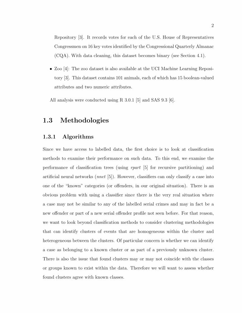
Repository [3]. It records votes for each of the U.S. House of Representatives

Congressmen on 16 key votes identified by the Congressional Quarterly Almanac

(CQA). With data cleaning, this dataset becomes binary (see Section 4.1).

� Zoo [4]: The zoo dataset is also available at the UCI Machine Learning Reposi-

tory [3]. This dataset contains 101 animals, each of which has 15 boolean-valued

attributes and two numeric attributes.

All analysis were conducted using R 3.0.1 [5] and SAS 9.3 [6].

1.3 Methodologies

1.3.1 Algorithms

Since we have access to labelled data, the first choice is to look at classification

methods to examine their performance on such data. To this end, we examine the

performance of classification trees (using rpart [5] for recursive partitioning) and

artificial neural networks (nnet [5]). However, classifiers can only classify a case into

one of the “known” categories (or offenders, in our original situation). There is an

obvious problem with using a classifier since there is the very real situation where

a case may not be similar to any of the labelled serial crimes and may in fact be a

new offender or part of a new serial offender profile not seen before. For that reason,

we want to look beyond classification methods to consider clustering methodologies

that can identify clusters of events that are homogeneous within the cluster and

heterogeneous between the clusters. Of particular concern is whether we can identify

a case as belonging to a known cluster or as part of a previously unknown cluster.

There is also the issue that found clusters may or may not coincide with the classes

or groups known to exist within the data. Therefore we will want to assess whether

found clusters agree with known classes.

3

1.3.2 Dissimilarity measures

With clustering methods, the first concern is how to measure dissimilarity (or simi-

larity). When working with strictly binary variables, Jaccard distance [7] and Corre-

lation measure [8] were used. When working with transformed variables (see Chapter

3 for details), the distance (or dissimilarity) measures used were two measures taken

from the family of Minkowski distance: Euclidean [9] (q = 2) and Manhattan [9]

(q = 1).

1.3.3 Design of experiments

In order to quantitatively analyse results, an experimental design structure was used.

A blocked factorial design was used with algorithms as one factor, dissimilarity (or

distance) measures as a second factor, and the two datasets as blocks. Section 3.5.5

discusses further the design; Section 6 provides the statistical results.

1.4 Outline

The structure of the thesis is as follows:

� Chapter 2 presents a literature review focusing on different clustering algo-

rithms, dissimilarity metrics and cluster validation methods;

� Chapter 3 provides some background theory describing the different clustering

algorithms and the dissimilarity metrics to to be evaluated;

� Chapter 4 presents results from the congressional voters dataset;

� Chapter 5 presents results from the zoo dataset;

� Chapter 6 presents results from the experimental design;

4

� Chapter 7 presents conclusions and future work.

Chapter 2

Literature review

Classification techniques are based on labelled data and are used to assess to which

sub-population new observations belong. Clustering techniques do not need labelled

data and are used to sort cases into groups so that similar observations can be grouped

together to achieve maximum homogeneity within clusters and maximum heterogene-

ity between clusters.

We start by discussing what has been done in classification with binary data.

Classification techniques make use of labelled data to build suitable classification

models to predict the class of a new observation.

The recursive partitioning method creates a classification tree which aims to cor-

rectly classify new observations based on predictor variables. This algorithm has been

applied to widely divergent fields (eg. financial classification [10], medical diagnos-

tic [11]). Although the data used in these experiments are not boolean in nature,

building trees using binary splits could be considered analogous to our problem.

Lu et al. [12] presented a neural network based approach to mining classification

rules using binary coded data. He proposed a method of extracting rules using neural

networks and experimented on a ten (10) variable dataset recoded as a binary string

5

6

(totalling of 37 inputs1). He compared his results with those of decision trees (C4.5)

and found both methods performed similarly, however neural networks generated

fewer rules than C4.5 [13]. This in turn, is reflected in the increased length of time it

took to train the neural networks.

Iqbal et al. [14] researched how classification could be applied to (numeric) crime

data (UCI communities and crime dataset) for predicting crime categories. They

compared Naıve Bayesian and Decision Tree evaluated using precision, recall, accu-

racy and F-measure. The results showed that the decision tree outperformed the

Naıve Bayesian algorithm.

A problem with classification is the fact that a classifier can only classify a case

into one of the known classes. It is unable to classify into groups it is unaware of or to

find “new labels”. For this reason we turn our attention to using clustering methods.

Clustering algorithms can be divided into two groups: partitioning methods and

hierarchical methods. The partitioning method algorithms can be further divided

into two groups: partitioning around centroids and partitioning around medoids. The

hierarchical algorithms can also be further divided into: hierarchical agglomerative

and hierarchical divisive. Clustering methods have at their core a measure of distance

or dissimilarity. This measure creates a challenge when all the predictor variables are

binary (or boolean) in nature.

Kumar et al. [15] proposed k-means clustering after transforming the dichotomous

data by the Wiener transformation. Their test dataset was the lens dataset [16]

(database for fitting contact lenses). The distance measures used were the Squared

Euclidean, City block (Manhattan), Euclidean and Hamming distances for the actual

dataset as well as the transformed dataset. The metrics used to evaluate the clusters

1The thermometer coding (or unary) scheme was used for the binary representation of the con-tinuous variables. In this scheme, natural numbers n are represented by n ones followed by a zero(for non-negative numbers)

7

were: Inter-cluster distance2, Intra-cluster distance3, Sensitivity4 and Specificity5.

After five iterations of the k-means algorithm, on average he found that all four

metrics performed similarly on the actual data, but better on the Wiener transformed

data, and on the transformed data, the Euclidean metric performed the best (only the

squared Euclidean performed poorly when measured with sensitivity and specificity).

Li [17] and Li et al. [18] presented a general binary data clustering model (entropy-

based) which clusters categorical data by way of entropy-type measures. The cate-

gorical variables are coded into indicator variables creating a set of binary variables.

Using the zoo [4] dataset; Li evaluated his model against the k-means algorithm using

several documents datasets (CSTR6, WebKB7, WebKB48, Reuters9) he evaluated his

model, the k-means algorithm, and hierarchical agglomerative clustering10. In both

cases evaluation used misclassification rate and purity. In both instances, his compar-

ison showed that the clustering approaches performed similarly. His entropy-based

(COOLCAT) algorithm was discounted for our current research as its required format

for the input data is the unaltered raw data with no distance measures. Since one

of our goals was to compare statistically the performance of different algorithms in

conjunction with dissimilarity measures, we chose to exclude COOLCAT since it does

not use dissimilarity measures.

Hands and Everitt [19] examined five (5) hierarchical clustering techniques (single

2The distances between the cluster centroids (should be maximized)3The sum of the distances between objects in the same cluster (it should be minimized)4In the medical field, sensitivity measures the ability of the test to be positive when the condition

is actually present.5In the medical field, specificity measures the ability of the test to be negative when the condition

is actually present.6Dataset of the abstracts of technical reports published in the Department of Computer Science

at the University of Rochester between 1991 and 20027Dataset containing webpages gathered from university computer science departments8The typical associated subset of WebKB9The Reuters-21578 Text Categorization collection containing documents collected from Reuters

newswire in 198710His results show the largest values of three different hierarchical agglomerative: single, complete

and UPGMA aggregating policies.

8

linkage, complete linkage, group average, centroid, and Ward’s method) on multivari-

ate binary data, comparing their abilities to recover the original clustering structure.

They controlled various factors including the number of groups, number of variables,

proportion of observations in each group, and group-membership probabilities. The

simple matching coefficient was used as a similarity measure. According to Hands

and Everitt, most of the clustering methods performed similarly, except single linkage,

which performed poorly. Ward’s method did better overall than other hierarchical

methods, especially when the group proportions were approximately equal.

Xiong et al. [20] proposed a new method of divisive hierarchical clustering for

categorical data (termed DHCC) from an optimization perspective based on multiple

correspondence analysis. They evaluated their methods against k-modes11 [21], the

entropy-based model [22], SUBCAD [23], CACTUS [24], and AT-DC [25] algorithms

based on Normalized Mutual Information (NMI), defined as the extent to which a

clustering structure exactly matches the external classification (similar to entropy),

and Category Utility (CU), defined as the difference between the frequency of the cat-

egorical values in a cluster and the frequency in the whole set of objects for clustering

(similar to purity). They conducted their experiments on synthetic data as well as

on the zoo data set, the Congressional voting records, Mushroom dataset, and the

Internet advertisements dataset, all from the UCI Machine Learning Repository [3].

For the voters and the zoo datasets, they concluded that the algorithms all performed

similarly.

Specifically with regard to distance measures, few comparative studies collecting

a variety of binary similarity measures have been done. Hubalek [26] collected 43

similarity measures and used twenty (20) of them for analysis on real data12. They

produced five (5) clusters of related coefficients. Of the twenty (20), Hubalek analyzed

11An extension of the k-means algorithm12Study on the co-occurrence of fungal species of the genus Chaetomium Kunze ex Fires (As-

comycetes) isolated from 869 (n) samples taken from free-living birds and their nests.

9

the Jaccard similarity and the Pearson correlation (also known as the Phi-coefficient,

Yule (1912) coefficient and Pearson&Heron1 13). He determined that the Jaccard

similarity and the Pearson correlation were in different clusters however they yielded

similar results when clustering their fungal species data. Choi et al. [9] surveyed

76 binary similarity/dissimilarity measures used over the last century and grouped

them using hierarchical clustering technique (agglomerative single linkage with the

average clustering method). Warrens [27] categorized different types of dissimilarity

measures into four (4) broad categories. Separately they found, like Hubalek, that the

Jaccard similarity measure and the correlation measure belonged to different clusters.

Warrens explains that the Jaccard coefficient falls within the ecological association

(measuring the degree of association between two locations over different species).

The phi coefficient (the Pearson product-moment correlation for binary data or the

Yule1 similarity measure) is categorized as inter-rater agreement.

Zhang and Srihari [28] compared eight (Jaccard, Dice, Correlation, Yule, Russel-

Rao, Sokal-Michener, Rogers-Tanimoto and Kulzinsky) measures to show the recogni-

tion capability in handwriting identification. They concluded that Rogers-Tanimoto,

Jaccard, Dice, Correlation, and Sokal-Michener all performed similarly and very well.

Kaltenhauseer and Lee [8] studied three similarity/dissimilarity coefficients on bi-

nary data: phi (range from -1 to 1) , phi/phimax, and tetrachoric coefficients, and

their uses in factor analysis. Phi is simply the Pearson product moment formula ap-

plied to binary data; phi/phimax is phi normalised (by dividing phi by the maximum

value it could assume consistent with the set of marginals from its two-way table);

and the tetrachoric coefficient is derived on the assumption that the observed fre-

quencies in the two-way table have an underlying bivariate normal distribution (only

applies to ordinal data). In Kaltenhauser’s simulation study, it was determined that

for factor analysis, phi performed the best for use with binary data.

13Although in his article, he refers to it as the tetrachoric coefficient

10

Finch [29] examined four (4) measures which are known collectively as matching

coefficients (Russell/Rao and Simple Matching both a symmetric binary measure,

and Jaccard introduced by Sneath in 1957 and Dice both to be asymmetric binary)

and compared their performance in correctly clustering simulated test data as well as

real data taken from the National Center for Education Statistics (the data are part

of the Early Childhood Longitudinal Study and pertain to teacher ratings of student

aptitude in a variety of areas, along with actual scores14). Finch concluded that there

was not much difference between the different metrics.

In order to use more conventional metrics, Lu et al. [12] transformed binary vari-

ables to continuous variables by means of Principal Component Analysis (PCA). Jol-

liffe [30] discusses PCA for discrete data and references the work of Gower (1966) [31]

to use PCA for dimension reduction of boolean data. He likens PCA for binary data

to principal coordinate analysis15. Cox (1972) [32] suggests ‘permutational principal

components’ as an alternate to PCA for binary data. This involves transforming

to independent binary variables using permutations. This was demonstrated on a

4-variable example by Bloomfield (1974) [33] and several transformations were ex-

amined. Bloomfield found that there is no method for finding a unique ‘best’ trans-

formation and, for higher dimensional data, the permutational principal components

method would also be computationally overwhelming.

Tan et al. [34] remarks that cluster validation is important to help distinguish

whether there really is non-random structure in the data, to help determine the

“correct” number of clusters, and to help evaluate how well results of a cluster analysis

fit the data by comparing the results of a cluster analysis with externally known

results.

Different measures have been used to evaluate clusters. Tan et al. [34] divides

14The article does not reference from where this dataset was obtained.15Principal coordinate analysis uses distance measures as inputs instead of actual data points as

inputs

11

cluster validity into two different categories: internal and external validation.

Internal validation measures the “goodness” of a clustering structure without any

external information. He uses ASW and SSE for measures of cohesion/separation.

For partitional algorithms there are: Average silhouette width [34] [35], Davies-

Bouldin [35], BIC [35], Calinski-Harabasz index [35], Dunn index [35], NIVA in-

dex [35], Category utility [20], and SSE (error sum of squares) [34] [36]. For hierar-

chical algorithms there is: Cophenetic distance (based on pairwise similarity of cases

in clusters) [34] [37]. Saraccli et al. [37] studied hierarchical agglomerative linkage

methods under two conditions (with and without outliers) by cophenetic correlation.

According to the results from a multivariate standard normal simulated dataset, the

average linkage and centroid linkages methods were recommended.

External validation measures make use of external class labels. These methods

include: Entropy [34] [35], Purity [34] [35] [17] [18], F-measure [34] [35] [14], Preci-

sion [34] [35] [36] [14], Error rate [17] [18], Recall [34] [36] [14], Normalized mutual

information [20],and the Rand index [34] [36].

Determining the correct number of clusters, there are: SSE [34], and Average

Silhouette Width [34].

We have yet to encounter research that quantitatively compares performances of

different clustering algorithms on boolean data. There have been comparisons of

several clustering methods, but none have used an experimental design.

This thesis research was motivated by a serial crime dataset. Due to the sensitive

nature of this particular data, for purposes of this thesis, two datasets (voters and

zoo) that have been used as benchmark datasets in the literature and that have similar

characteristics to the crime dataset were used.

The congressional voters dataset [2] is available at the UCI Machine Learning

Repository [3]. It includes votes by each of the 435 U.S. House of Representatives

Congressmen on 16 key votes identified by the Congressional Quarterly Almanac

12

(CQA). The CQA lists nine (9) different types of votes: voted for, paired for, and

announced for (these three (3) simplified to “yea”), voted against, paired against, and

announced against (these three (3) simplified to “nay”), voted present, voted present

to avoid conflict of interest, and did not vote or otherwise make a position known

(these three (3) simplified to “unknown”) [3]. The data was downloaded from the fol-

lowing site (May 2013): http://archive.ics.uci.edu/ml/datasets/Congressional+

Voting+Records. As stated previously, Xiong et al. [20], when evaluating their algorithm

(DHCC), used the Congressional voters dataset16 as well as others. Using their algorithm,

the voters dataset generated two clusters with good separation between Republican and

Democrat. When comparing their algorithm with the others (ROCK, CACTUS, k -modes,

COOLCAT, LIMBO, SUBCAD, AT-DC), they found that they all performed similarly.

The zoo dataset [4] is available at the UCI Machine Learning Repository [3]. The

dataset contains 101 animals, each of which has 15 Boolean-valued attributes and two

numeric attributes. The “type” attribute appears to be the class attribute. The data

was downloaded from the following site (May 2013): http://archive.ics.uci.edu/ml/

datasets/Zoo. As stated previously, Xiong et al. [20], when evaluating their algorithm

(DHCC), they also used the zoo dataset. Using their algorithm, they found that the mammal

and non-mammal families separated well as well as the bird and fish families, ending up

with four (4) clusters. When comparing their algorithm with the others, they found that

they all performed similarly. As stated above, Li [17] and Li et al. [18] also used the zoo

dataset17 to evaluate COOLCAT against the k-means algorithm. Li noticed that feature 1

is a discriminative feature for class 1, and that feature 8 discriminates for both class 1 and

3 and feature 7 is distributed across all the classes. Li found that the k-means approach

resulted in a purity value of 0.76 and that COOLCAT resulted in a purity of 0.94.

16In their experiment, each of the 16 issues corresponded with the value of ‘Yes’, ‘No’, and ‘?’,thus having 48 categorical values.

17Li recoded the leg feature into 6 boolean attributes, and he removed the duplicate animal ‘frog’.

http://archive.ics.uci.edu/ml/datasets/Congressional+Voting+Records

http://archive.ics.uci.edu/ml/datasets/Congressional+Voting+Records

http://archive.ics.uci.edu/ml/datasets/Zoo

http://archive.ics.uci.edu/ml/datasets/Zoo

Chapter 3

Methodology

This chapter describes the algorithms to be evaluated in this thesis for the purpose of clas-

sifying or clustering binary data. These procedures are applied to two datasets (voters and

zoo) that have been used as benchmark datasets in the literature and that have character-

istics similar to the crime dataset we are interested in. These will be discussed in detail in

Chapters 4 and 5.

We begin by outlining notation used in the thesis and data pre-processing steps. We

then present data exploration via such data visualisation methods as parallel coordinates

plots and heatmaps. This is followed by examining the performance of classifiers to deter-

mine if they can accurately predict/classify the group to which a case belongs. Imperfect

classification is an indication that class labels may not correspond to groups within the

data. The classification approaches used are recursive partitioning (i.e. classification trees)

and artificial neural networks. A drawback with applying a classification approach to the

problem raised in this thesis is that a classifier can only classify an object (or case) into

one of the known labels; it is unable to classify into labels it is unaware of or to find “new

labels”. Hence, if there are cases that do not fit into one of the previously known classes,

or if there are previously unknown classes, a classifier is unable to detect such situations.

The best we can get is a classification tree that shows impurity in its final nodes.

To address the need to identify groupings in our dataset which might not correspond

to the class labels supplied, we consider a clustering approach to our problem and focus on

13

14

partitional and hierarchical algorithms. The chosen clustering algorithms are: partitioning

around centroids (PAC), partitioning around medoids (PAM), hierarchical agglomerative

clustering, and hierarchical divisive clustering.

Each clustering algorithm is based on a dissimilarity measure. Section 3.2 discusses

the dissimilarity measures used. The final section describes measures used to assess the

performance of the algorithms-measures combination.

3.1 Notation

Consider a binary dataset X = (xij)n×p where, for a specific case i (i = 1, ..., n) and feature

j (j = 1, ..., p), xij = 1 if the jth feature is present and xij = 0 otherwise. The number of

cases (or instances) is represented by n and the number of binary features is represented by

p.

For example, the dataset may be denoted by:

X =

X11 X12 X13 . . . X1p

X21 X22 X23 . . . X2p

X31 X32 X33 . . . X3p

......

.... . .

...

Xn1 Xn2 Xn3 . . . Xnp

15

by cases

=

XT1

XT2

XT3

...

XTn

and by variables

=

[X1 X2 X3 � � � Xp

]A typical dataset is shown in Table 3.1.

Table 3.1: Example of a binary data set

Case No. Feature1 Feature2 ... Featurep

1 1 0 . . . 1

2 1 0 . . . 0

3 0 0 . . . 0

4 1 1 . . . 0

5 0 0 . . . 1...

......

. . ....

n 0 1 . . . 0

3.2 Pre-processing

Each dataset requires specific pre-processing steps before any analysis can be completed.

These steps include data cleaning, transformation, and calculating dissimilarity measures.

The specific steps for data cleaning and transformation are discussed in greater detail in

16

the chapters dedicated to those datasets (Chapters 4 and 5). Dissimilarity measures are

discussed Section 3.5.3.

3.2.1 Binary data

We begin with all variables (other than labels) as binary(i.e. raw).

3.2.2 Converting to continuous using principal component

analysis

For some analyses we convert our binary data into principal components in order to work

with more continuous data and to reduce the dimension of the dataset. Data reduction

occurs because only a few of the Principal Components (PCs) are necessary to explain the

majority of the variability in the dataset. PCA is used here (as opposed to factor analysis)

because we do not want to remove any attributes. We want to be able to explain the

majority of the variation with all of the features.

PCA constructs as many orthogonal linear combinations of the original variables as

there are original variables. We obtain p linear combinations of the p original variables in

the matrix X = [X1,X2, � � � ,Xp] in such a way that we form p new variables such that

Yj = lTj X where for case i

Yi1 = l11Xi1 + l12Xi2 + l13Xi3 + � � �+ l1pXip

Yi2 = l21Xi1 + l22Xi2 + l23Xi3 + � � �+ l2pXip

... =...

Yip = lp1Xi1 + lp2Xi2 + lp3Xi3 + � � �+ lppXip

Let the random vector X have covariance matrix Σ with eigenvalues λj

V ar(Y1) = lT1 Σ l1

17

and

Cov(Yi,Yk) = lTi Σ lk

for i, k = 1, � � � , p.

PC1 (i.e. Y1) is the linear combination of lT1 X that maximises V ar(lT1 X) subject to

lT1 l1 = 1; PC2 (i.e. Y2) is the linear combination of lT2 X that maximises V ar(lT2 X) subject

to lT2 l2 = 2 and Cov(Y1,Y2) = 0 (since they need to be independent of each other), etc.

We can show that:

maxl1 6=0

lT1 Σ l1

lT1 l1= V ar(Y1)(= λ1) (3.1)

and is attained when l1 = e1 (the eigenvector associated with the largest eigenvalue λ1) and

maxlk+1⊥e1,··· ,ek

lTk+1Σ lk+1

lTk+1lk+1= V ar(Yk+1)(= λk+1)

and lk+1 = ek+1 (the eigenvector associated with the eigenvalue λk+1 for k = 1, 2, � � � , p� 1

andp∑i=1

V ar(Xi) =

p∑i=1

V ar(Yi)

We obtain p independent components that conserve the total variance in the original

dataset. Geometrically, these linear combinations represent the selection of a new coordinate

system obtained by rotating the original system. The new axes represent the successive

directions of maximum variability. This means that PC1 accounts for the direction of

greatest variability in the original dataset and so on. To reduce the dimension of the dataset,

we drop the latter PCs which explain less of the variance. Visually, we can examine a scree

plot of the variance associated with each PC to determine the number e(< p) of important

PC’s. These e PCs are used to form a new version of the dataset [38].

18

3.3 Data visualisation

Before delving into deeper analysis of the datasets, we begin with an exploratory examina-

tion of the data by way of data visualisation. To do this we will use two (2) techniques.

3.3.1 Parallel coordinates plot

A parallel coordinates plot is used to visualise high-dimensional data. Each data point is

plotted on axes that are arranged parallel to each other rather than at right angles to each

other. We use this visualization to see if there is separation of variables in the dataset. By

using colour to label a specific feature, we can follow trends between the different labelled

classes and note which features separate the classes and which features have a mix of

different classes.

3.3.2 Heatmap

A heatmap is a graphical rectangular matrix of the data with each value in the matrix

represented by a colour. This transformation from numerical data to a colour spectrum is

also used to visualise structure in the data. Each coloured tile represents the level for each

feature. In our case, since we only have two levels (1 and 0) we see two colours.

3.4 Classification

Classification is a supervised learning technique, that provides a mapping from the feature

(or input) space to a label (or class) space. It requires a training set of observations whose

class (or category) memberships are known. The model generated by the classification

algorithm should both fit the input data (training data) well and correctly predict the class

labels of cases it has never seen before (i.e. test data) [34]. To develop a classifier, we divide

the data into a training set (i.e. around 80% of the data) and a testing set (the remainder

of the data). The training set is used to build a classifier. This classifier is then used to

19

predict the classes of the test set. Misclassification error rates are calculated to assess the

“goodness” of the classifier.

In this thesis two types of classification techniques will be used: recursive partitioning

(classification trees), a non-parametric tool, implemented by Breiman et. al [39] and neural

networks, a non-linear tool, first formulated by Alan Turing in 1948 [40] in this research.

3.4.1 Classification trees

Using a labelled data set, a classification tree will be built. It has a flow-chart like structure,

where each internal (or parent) node denotes a test on an attribute, each branch represents

an outcome of the test, and each leaf (or child) node holds a class label. For prediction

purposes, the label for a case can be predicted by following the appropriate path from the

root (starting point of the tree) to the leaf of a tree. The path corresponds to the decision

rule [41].

Data in the form of (X, Y ) = (X1,X2,X3, ...,Xp, Y ) is used to construct a classification

tree, where Y is the label (or the target variable) and the matrix X is composed of the

binary input variables used to build the tree.

The tree is built on binary splits of variables that separate the data in the “best” way,

where “best” is defined by some criterion. Each split of a parent node produces a left child

and a right child. The idea of “best” in this case is a split that decreases some measure of

the total impurity of the child nodes. To find the “best” variable on which to split, all splits

on all individual variables are tested and then the variable split that produces the “best”

is selected. We will elaborate on the idea of “best” later on.

This procedure is recursive. Cases at the resulting left and right nodes are each assessed

in the same way and further splits are made. This process could go on until there is only

one case at the final leaf, but this leads to over-fitting and is of little use for prediction.

The algorithm used for constructing the tree works from the top down by choosing

the “best” variable split at each step to go into each node. This may be accomplished

through the use of different measures of impurity, for example the Entropy measure, the

20

Gini index, and the generalized Gini index. Entropy measures the impurity of a node,

sometimes referred to as the deviance. From all the possible splits, the split that gives the

lowest entropy (i.e.closest to 0.0) is used. In this thesis we use the impurity measure of

generalized Gini, although entropy and the generalized Gini (both used as options in R)

give similar results. With entropy, the impurity at a leaf t is given by:

It = �2∑j at t

ntj log pj|t

where

pj|t =ptjpt

with ptj being the probability that a case reaches leaf t and that it is of class label j and

pt being the probability of reaching leaf t. We estimate the probability at leaf t given class

label j (i.e. pj|t) byntj

ntwhich is the number of cases from class label j that reach leaf t

divided by the total number of cases at leaf t. The entropy at node T is

I(T ) =∑

leaves t∈ T

It

The Gini index gives the impurity at the left leaf by

It =∑

i6=j at tpi|tpj|t = 1�

∑j at t

p2j|t

with pi|t being the probability that a case reaches node t and is of class i.

There is also the generalised Gini index

It = nt∑

i6=j at tpi|tpj|t = nt

1�∑j at t

p2j|t

Since classification trees are unstable (depending on the training set, the resultant trees

can differ greatly), we took 100 different training and testing sets, split 80% training and 20%

testing, and on each pair, trees were built using the entropy index as the splitting criterion

21

on the training sets. To avoid over-fitting, each resultant tree was post-pruned using the

cost-complexity pruning method introduced by Breiman et al. [39]. This method prunes

(or removes) those branches that do not aid in minimizing the predictive misclassification

rate by calculating the cost of adding another variable to the model, called the complexity

parameter (cp). The complexity parameter is a measure of the “cost” of adding another

feature to the model. The desired cp was chosen based on the “1-SE rule” which uses the

largest value of cp with the cross-validation error (xerror) within one-standard deviation

(xstd) of the minimum. Using the resultant pruned tree, the testing sets were put through

the pruned classification trees. The error rate (or misclassification rate was calculated for

each of the 100 datasets and then averaged.

3.4.2 Artificial Neural Networks

Artificial neural networks, a non-linear method, is another classification algorithm consisting

of multiple inputs (the feature vectors) and a single output, as well as a middle layer called

the “hidden layer” consisting of nodes [40]. The basic concept in neural networks is the

weighting of inputs to produce the desired output result [42]. The neural network will

combine these weighted inputs and, combined with a threshold value θ, and activation

function a, provides a predicted output. For a given case (x1, x2, ..., xp), the total input to

a node is:

a = x1w1 + x2w2 + � � �+ xpwp =

p∑i=1

xiwi

where a is a node, xi is the input variable and wi are the weights, i = 1, ..., p.

Suppose that this node has a threshold (θ) such that if a � θ the node will ‘fire’ so the

output predicts as

y =

1 if a � θ

0 if a < 0

The weights and threshold are unknown parameters to be found by training the data.

22

To fit the model to the training data, values of the weights and threshold parameters are

adjusted to produce the desired classification results.

The algorithm does not move when the weights are set to be zero. We find the set of

weights that give a minimum error. These weights are chosen initially to be random values

near zero (0) [40]. The algorithm is an iterative process, stopping when there is no change

to the prediction from the neural net. However, to avoid overfitting, a learning rate α is

used. This α (or weight decay) is used as the allowable difference between responses so that

the algorithm may stop. The weights vary more as the weight decay value increases.

Using the training algorithm from the caret package in R, we tested 1, 2, 5, and 9 nodes

in one hidden layer and decay rates of 5e� 4, 0.001, 0.05, 0.1, with weights in the range of

(�0.1, 0.1) for each training set (using five - fold cross validation). The best number of nodes

in the hidden layer and the best decay rate were determined by examining the maximum

accuracy over all of the above options for each training set. Using these parameters, for

a particular neural net, the misclassification (error) rate was calculated using the testing

set. This process was done using 100 different training and testing sets, split 80% training

and 20% testing. The overall misclassification error is the average of all of the 100 different

training sets.

3.5 Clustering

A problem with classification is the fact that a classifier can only classify a case into one

of the known classes. It is unable to classify into groups it is unaware of or to find “new

labels”. Therefore we also examine clustering methodologies.

Clustering is an unsupervised learning technique that attempts to find groups or clusters

C1, C2, ..., Ck such that members within a group are most similar to each other and most

dissimilar to the members belonging to other groups. This can be achieved by using various

algorithms that differ in their notion of how to form a cluster. We are only interested in

hard clustering, which divides the dataset into a number of non-overlapping subsets such

that each case is in exactly one subset.

23

Clustering techniques are divided into two main categories - partitioning and hierarchi-

cal methods. The latter is further divided into agglomerative and divisive methods. In this

thesis we use the partitioning methods, using k-means and k-medoids, and the hierarchical

method, using agglomerative hierarchical (with all possible linkages) and divisive hierar-

chical. Figure 3.1 is a graphical representation of the different clustering methods and the

algorithms used in this thesis.

Figure 3.1: Graphical representation of the different clustering methods

Clustering is also used as a tool to gain insight into structures within the datasets. But,

a major problem with clustering is the need to know a priori the number of clusters in

the data. In the absence of this knowledge, it could take several steps of trial and error to

determine the ideal number of clusters to create.

3.5.1 Partitioning algorithms

Partitioning methods (commonly referred to as the “top down” approach) start with the

data in one cluster and split the cases into k partitions, where each partition represents a

cluster. Each cluster is represented by a centroid or some other cluster representative such

as a medoid [43].

Partitioning is a recursive approach whereby cases get relocated at each step. The set

of resulting clusters is said to be un-nested. Two approaches to partitioning clustering are:

24

centroid-based clustering, where clusters are represented by a central vector (which may

not necessarily be a member of the dataset) and medoid-based clustering, where clusters

are represented by actual data points (medoids) as centers.

Partition around centroids (PAC)

The k-means clustering method is a centroid-based partitional approach to clustering. Data

clustered by the k-means method partitions cases into k user-specified groups such that the

distance from cases to the assigned cluster centroids is minimized.

The k-means cluster analysis is available through the k-means function in R. The algo-

rithm in R is that of Hartigan and Wong (1979) [44]. The general k-means algorithm is the

following:

1. Make initial random guesses for initial centroids of the clusters;

2. Find the “distance” from each point to every centroid and assign the point to the

closest centroid;

3. Move each cluster centroid to the arithmetic mean of its assigned cases;

4. Repeat the process until convergence (i.e until the centroids do not move).

At each iteration of the k-means procedure, the cluster centroids are altered to minimize

the total within-cluster variance, thus seeking to minimise the sum of squared distances from

each observation to its cluster centroid; i.e. we are minimizing

WSS =K∑k=1

nk∑i=1

kx(k)i � ckk2

where k (k = 1, � � � ,K) is the cluster number, kx(k)i � ckk is the chosen distance measure

between the data point (x(k)i ) within cluster k and cluster centroid ck for cluster k.

To assign a point to the “closest” centroid, a proximity measure that quantifies “closest

centroid” is needed. When concerned with presence or absence of variables, the Jaccard dis-

tance is used for the raw binary data; when measuring the similarity of variables, correlation

25

as distance is used for the raw binary data. Typically, Euclidean distance or Manhattan

distance is used for continuous type data. Based on the literature review, we are focusing

on these distance measures.

While k-means clustering is simple, understandable, and widely used, there are problems

with its use. Results tend to be unstable depending on the random guesses for the initial

centroids of the clusters, so different clustering may occur. In addition, results may vary

depending on distance measure used. Also, the number k of clusters must be pre-determined

before the algorithm is run.

Partition around medoids (PAM )

Another partitioning method algorithm is k-medoids. Introduced by Kaufman and

Rousseeuw [45], it partitions the data points into k user-specified groups, each represented

by a medoid. The term medoid refers to a representative object within a cluster. In R, we

use the PAM algorithm found in the cluster library.

The PAM-algorithm is based on the search for k representative objects or medoids

among the observations in the dataset. These observations should represent the structure

of the data. After finding a set of k-medoids, k clusters are constructed by assigning each

observation to the nearest medoid.

By default, when medoids are not specified, the algorithm first looks for a good initial

set of medoids (this is called the “build” phase) with an initial random guess. Then it finds

a local minimum for the objective function, that is, a solution such that there is no single

switch of an observation with a medoid that will decrease the objective (this is called the

“swap” phase).

The general PAM algorithm as described by Hastie et al. [40] is:

1. The algorithm makes an initial random guess for the initial specified k medoids for

the clusters;

2. For each non-medoid case, calculate the dissimilarity (or cost) between it and each

26

medoid; cost for case i is calculated as:

cost(k)i =

p∑j=1

xi 6=xk

jxij �mkj j

where mk is the medoid;

3. For each medoid, select the cases with the lowest cost to be placed into a cluster;

4. The total cost of the dataset is calculated:

TotalCost =∑

costk

5. Randomly switch the medoid with a non-medoid;

6. Repeat steps 2 to 4 and choose the configuration with the smallest total cost;

7. Repeat step 6 until no further changes to the configuration. This results in the final

configuration with the lowest cost.

Compared to k-means, PAM is more computationally intense since, in order to ensure

that the medoids are truly representative of the observations within a given cluster, the

sums of the distances between cases within a cluster must be constantly recalculated as

cases move around. Like k-means, PAM also requires the number k of clusters to be pre-

determined before the algorithm is run.

3.5.2 Hierarchical algorithms

Alternatively, hierarchical clustering results in a tree-shaped (nesting) structure, achieved

by either an agglomerative or a divisive method [43]. Hierarchical agglomerative clustering

methods begin with each case being a cluster. In this thesis we use the hclust algorithm

as described by Kaufman and Rousseeuw [45]. The agglomerative algorithm hclust() used

in R is found in the cluster library [5]. The divisive hierarchical algorithm starts with one

27

cluster containing all cases. In this thesis the DIANA algorithm described by Kaufman and

Rousseeuw [45] is used.

Agglomerative hierarchical clustering

In agglomerative hierarchical clustering, each case starts in its own cluster and, at each step

and based on examination of distances between cases, the two closest are joined to form a

new cluster. The general agglomerative hierarchical algorithm is the following:

Given a data set X and its dissimilarity measures:

1. Start with each case as its own cluster

2. Among the current clusters, determine the two clusters (here we mean the two cases)

that are most similar (closest);

3. Merge these two clusters into a single cluster;

4. At each stage, distances between the new clusters and each of the old clusters are

computed;

5. Repeat (2)� (4) until only one (1) cluster is remaining.

The merging of clusters involves a combination of linkage method and distance (dissim-

ilarity) measure.

We examine several different linkage methods for merging clusters together (note that in

all cases, a measure of dissimilarity between sets of observations is required). These include

(where d is the dissimilarity measure) [5] :

1. Single linkage (also called the minimum distance method). This considers the distance

between two clusters A, B to be the shortest distance from any case (or point) of one

cluster to any case (or point) of the other cluster [5]

i.e. d(A,B) = mina∈A, b∈B

d(a, b).

28

Figure 3.2: Graphical representation of single linkage

This method tends to find clusters that are drawn out and ”snake”- like.

2. Complete linkage (furthest neighbour or maximum distance method). This considers

the distance between two clusters A, B to be equal to the maximum distance between

any two cases (or points) in each cluster [5]

i.e. d(A,B) = maxa∈A,b∈B

d(a, b).

Figure 3.3: Graphical representation of complete linkage

This method tends to find compact clusters.

3. Average linkage considers the distance d between two clusters A, B to be equal to

the average distance between the points in the two clusters:

i.e. d(A,B) = 1|A||B|

∑a∈A

∑b∈B d(a, b) where jAj and jBj are the number of cases in

cluster A and B respectively.

29

Figure 3.4: Graphical representation of average linkage

4. Centroid (also known as Unweighted Pair-Group Method using Centroids, or UP-

GMC) method calculates the distance between two clusters as the (squared) Euclidean

distance between their centroids or means.

i.e. d(A,B) = kcA − cBk2 where cA and cB denotes are the centroids of clusters A

or B respectively calculated as the arithmetic mean of the cases in the cluster:

i.e. for cluster A the centroid is cA = (x(A)1 , x

(A)2 , ..., x

(A)p )

Figure 3.5: Graphical representation of centroid linkage

5. Ward linkage (Ward’s minimum variance or error sum of squares) minimizes the total

within-cluster variance. At each step the pair of clusters with minimum between-

cluster distance are merged [46]. This produces clusters of more equal size. It uses

total within-cluster sum of squares (SSE) to cluster cases as defined by:

30

SSE =

K∑k=1

nk∑j=1

(x(k)k � xk�)

2

where x(k)k is the jth case in the kth cluster and nk is the total number of cases in the

kth cluster. Although this method is intended for Euclidean data, Mooi [47] found

that it did fine with other metrics.

6. Median (also known as Weighted Pair-Group Method using Centroids, or WPGMC)

method calculates the distance between two clusters as the Euclidean distance be-

tween their weighted centroids.

d(A,B) = kcA � cBk2

where cA is the weighted centroid of A. For instance, if A was created from clusters

C and D, then cA is defined recursively as:

cA = w1(cC + cD)

Although this method is intended for Euclidean dissimilarity measure, Mooi [47] found

that it did fine with other metrics.

7. McQuitty (also known as weighted pair-group method using arithmetic averages)

method depends on a combination of clusters instead of individual observations in

the cluster. When two clusters are to be joined, the distance of the new cluster to

any other cluster is calculated as the average of the distances of the soon to be joined

clusters to that other cluster. For example, if clusters I and J are to be joined into a

new cluster A, then the distance from this new cluster A to cluster B is the average

of the distances from I to B and J to B.

31

This distance is defined as

d(A,B) =1

2(d(I,B) + d(J,B))

where I, J are the other clusters to be joined to form the new cluster A and any other

cluster is denoted by B and depends on the order of the merging steps.

Divisive clustering

Divisive hierarchical clustering does the reverse of agglomerative. It constructs a hierarchy

of clustering, starting with a single cluster containing all n cases and ending with each case

as its own cluster.

Initially, all possibilities to split the data into two clusters are considered and the case

farthest from the rest of the set initiates a new cluster. At each subsequent stage, the

cluster with the largest diameter is selected for division. The new case farthest from the

main cluster will either join the original splinter group or form its own splinter group.

The diameter of a cluster is the largest dissimilarity between any two of its observations.

The process can continue until each cluster contains a single case. The divisive algorithm

proceeds as follows [48]:

1. It starts with a single cluster containing all n cases.

2. In the first step, the case with the largest average dissimilarity to all other cases

initiates a new cluster - a “splinter” group;

3. For each case outside of the splinter group the algorithm reassigns observations that

are closer to the “splinter group” than to the original cluster by calculating :

(a) the distance for case i as the average distance of case i to a case j outside the

splinter group minus the average distance of case i to another case j within the

splinter group:

Di = [average d(i, j)j /2 Rsplinter group]� [average d(i, j)j 2 Rsplinter group]

32

(b) For each case, select that one case for which the difference D is the largest. If

the distance is positive, then that particular case is closest to the splinter group.

4. Step 3 is repeated until all n clusters are formed.

3.5.3 Data types and dissimilarity measures

We will work with the data in raw (binary) form as well as convert it to continuous by

using Principal Components (PC’s). Since clustering techniques are based on a measured

dissimilarity between cases, distance measures are inherent to clustering. In this thesis we

will use four different distance measures and compare their ability to cluster the data. The

four dissimilarity measures are the Jaccard coefficient and the Correlation coefficient (for

the raw data), and Euclidean and Manhattan (for the continuous data).

Table 3.2: Summary of data type and dissimilarity measure

Data Dissimilarity measure

Raw binary data Jaccard coefficient

Raw binary data Correlation as distance

Continuous data (PCA) Euclidean distance

Continuous data (PCA) Manhattan distance

Dissimilarity measures

For a boolean dataset which can be either symmetric or asymmetric, Finch [29] and Bennell

[49] have found that either category (symmetric or asymmetric) behave similarly. Thus we

assume the binary datasets used in this thesis are asymmetric binary.

The Jaccard dissimilarity measure is used as it is the simplest of the dissimilarity mea-

sures and applicable to our crime problem, where we want to measure the degree of associa-

tion between two locations over different criminals. The phi coefficient (correlation metric)

is also used in this research as a distance measure, since it measures the relation of the

crimes committed by the same criminal (or class of criminal) with a new crime.

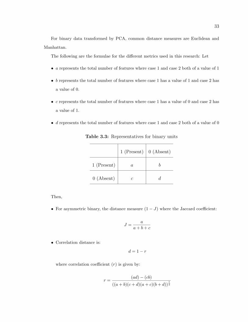
33

For binary data transformed by PCA, common distance measures are Euclidean and

Manhattan.

The following are the formulae for the different metrics used in this research: Let

� a represents the total number of features where case 1 and case 2 both of a value of 1

� b represents the total number of features where case 1 has a value of 1 and case 2 has

a value of 0.

� c represents the total number of features where case 1 has a value of 0 and case 2 has

a value of 1.

� d represents the total number of features where case 1 and case 2 both of a value of 0

Table 3.3: Representatives for binary units

1 (Present) 0 (Absent)

1 (Present) a b

0 (Absent) c d

Then,

� For asymmetric binary, the distance measure (1� J) where the Jaccard coefficient:

J =a

a+ b+ c

� Correlation distance is:

d = 1� r

where correlation coefficient (r) is given by:

r =(ad)� (cb)

((a+ b)(c+ d)(a+ c)(b+ d))12

34

� Euclidean distance: If X1 represents the vector of features for case 1 and X2 represents

the vector features in case 2 then,

d =

√√√√ p∑j=1

(x1j � x2j)2

� Manhattan distance is the absolute distance between two vectors (X1 and X2) mea-

sured along axes at right angles.

d =

p∑j=1

jx1j � x2j j

3.5.4 Cluster evaluation

To evaluate the optimal k, we use Average Silhouette Width (ASW). For internal indices

of “goodness” of clustering, we use the measure of ASW and the Cophenetic Correlation

Coefficient (CPCC). For the external measure of “goodness”, we use entropy and purity.

Determining the number of clusters

The issue with the partitioning algorithms (both around the centroid and the medoid) is

determining the number of centroids or medoids, respectively. For hierarchical algorithms

(agglomerative and divisive) the issue is the splitting method. To statistically compare the

algorithms, we let k fall within a set range and calculate the ASW for each k.

Silhouette width, first introduced by Rousseeuw [50], is a method for assessing the qual-

ity of clustering for partitional methods. It combines the ideas of cohesion and separation

and can be calculated on individual cases, as well as on entire clusters [34].

For a given cluster, the silhouette technique calculates for the ith case of the cluster k a

quality measure si (i = 1, ...,m), known as the silhouette width (m is the number of cases

in cluster k). This value is an indicator of the confidence that the ith case belongs in that

cluster and is calculated as:

si =bi � ai

max(ai, bi)

35

where ai is the average dissimilarity of the ith case to all the other cases in the cluster; bi is

the minimum of the average dissimilarity of the ith case to all cases in another cluster [50]

[35]. For each case the range is �1 � si � +1.

Observations with large and positive si (� 1) imply that the ith case has been assigned

to the appropriate cluster [50]. This is implied since ai must be much smaller than the

smallest bi to be true. If si is around 0 then ai and bi are approximately equal and thus the

case i can be in either cluster [50]. Cases with a negative si have been placed in the wrong

cluster. This is implied since ai must be much larger than bi and thus case i lies on average

closer to the other cluster than the one it was assigned to [50].

The average silhouette width for a cluster is the average of the si for cases in the cluster.

The overall average silhouette width for the entire data is:

ASW =1

N

N∑i=1

si

If there are too many or too few clusters, as may occur when a poor choice of k is used,

some of the clusters will typically display much narrower silhouettes than the other clusters.

If there are too few clusters, and thus different clusters are joined, this will lead to large

“within” dissimilarities (large ai) resulting in small si and hence a small ASW measure. If

there are too many clusters, then some natural clusters have to be divided in an artificial

way, also resulting in small si (since the “between” dissimilarity bi becomes very small).

According to Kaufmann and Rousseuw [45], a value below 0.25 implies that the data are

not structured. Table 3.4 shows how to use this value (as per the R manual) [5].

Range of SC Interpretation

0.71-1.0 A strong structure has been found

0.51-0.70 A reasonable structure has been found

0.26-0.50 The structure is weak and could be artificial

< 0.25 No substantial structure has been found

Table 3.4: Interpretation for average silhouette range

36

To obtain the optimal number of clusters, the Rousseeuw [50] silhouette validation tech-

nique was used.The largest overall average silhouette width (ASW) gives the best clustering

solution (a high ASW value indicates that the clusters are very homogeneous, and that they

are well separated; a value below 0.25 there would be negative silhouette width, suggesting

a lack of homogeneity for the clusters). Therefore the optimal k is that corresponding to

the largest ASW.

Internal indices

Internal indices measure the “goodness” of a clustering without using any external infor-

mation. These are generally based on cohesion or separation or some combination of both.

Cohesion measures how closely related are objects in a cluster; and separation measures

how distinct or well separated a cluster is from other clusters [34].

For partitional algorithms we use the measure of ASW (as explained previously).

For the hierarchical methods we use the cophenetic correlation measure. The cophenetic

similarity or cophenetic distance of two cases is a measure of how similar those two cases

have to be in order to be grouped into the same cluster. The cophenetic distance between

two cases is the height of the dendrogram where the two branches that include the two cases

merge into a single branch. Thus cophenetic correlation coefficient (CPCC) is a standard

measure of how well a hierarchical clustering of a particular type fits the data [51] [34].

One of the most common uses of this measure is to evaluate which type of hierarchical

clustering is best for a particular type of data [34]. The cophenetic distance between two

objects is the distance at which a hierarchical clustering technique puts the two objects

into the same cluster. For example, if at some point in the clustering process, the shortest

distance between the two clusters that are merged is 0.1, then all points in one cluster have

a cophenetic distance of 0.1 with respect to the points in the other cluster. In a cophenetic

distance matrix, the entries are the cophenetic distances between each pair of objects. The

cophenetic distance is different for each hierarchical clustering of a set of points [34].

37

External indices

External indices measure the similarity of clustering to known class labels. The external

indices used in this thesis are the measures of entropy and purity based on external class

labels (supplied with the datasets).

Entropy is a measure to indicate the degree to which each cluster consists of objects of

a single class (i.e. it measures the purity of the class labels (j) in a cluster (k)) [35]. If all

clusters consisted of only cases with a single class label, the entropy would be 0.

First, we compute the class distribution of the data for each cluster. For cluster k, we

compute pjk, the ‘probability’ that a member of cluster k belongs to class j [34].

pjk =njknk

where nk is the number of cases in cluster k and njk is the number of cases of class j

in cluster k [34]. Using this class distribution, the entropy of each cluster k is calculated

using [34]:

ek = �J∑j=1

pjk log2 pjk

where J is the total number of classes. The total entropy for a set of clusters is calculated

as the sum of the entropies of each cluster weighted by the size of each cluster [34]:

e =

K∑k=1

nknek

where K is the number of clusters, nk is the size of cluster k and n is the total number of

cases in the data [34].

Entropy reaches maximum value when all classes have equal probability (p = 1J ). It

can be seen from Figure 3.6 that as the number of classes increase, the maximum entropy

increases as well (eg: For a two (2) class model, the entropy range will be [0, 1] and for a

eight (8) class model the entropy range will be [0, 3] [1]. This is calculated by log2 J where

J is the number of classes.

38

Figure 3.6: Value of maximum entropy for varying number of clusters [1]

Purity measures the extent to which each cluster contains data points from primarily

one class [34]. Continuing from the previous notation, the purity of a cluster k is

purityk = maxjpjk

The overall purity of a clustering is [34]:

purity =K∑k=1

nknpurityk

Purity ranges from 0, which corresponds to bad clustering, to a value of 1, which is perfect

clustering.

3.5.5 Experimental design

Comparative Analysis

The two questions we hope to answer are:

� Are the optimal number k clusters chosen by the differing algorithms statistically

39

significantly different?

� Do the algorithms and measures perform differently from one another (even though

they may all give the same cluster number result)?

We employ a designed experiment to test if the algorithms and/or dissimilarity measures

have a statistically significant effect on the number of optimal clusters identified by the

maximum ASW. To examine the clustering performance of the algorithm/dissimilarity pairs

we use the associated ASW.

With the four dissimilarity metrics, we test the ten clustering algorithms and, using two

datasets as blocks, we examine the effects due to the algorithms or dissimilarity measures

on the choice of cluster number for the optimal k. A blocked design allows for the difference

between datasets, since it is expected that there might be a significant difference between

the datasets. The linear statistical model for our design, a blocked (2 factor) crossed design

with a single replicate, is

yijg = µ+ τi + βj + γg + (τβ)ij + (τγ)ig + (βγ)jg + εijg

i = 1, 2, ..., a

j = 1, 2, ..., b

g = 1, 2, ..., d

Generally, µ is the overall mean, τi, βj , γg represent respectively the effects of factors

A (algorithms), B (dissimilarity measures) and the blocks D (datasets). The (τβ)ij is

the effect of the algorithms-dissimilarity measures interaction; (τγ)ig is the effect of the

algorithms-datasets interaction; (βγ)jg is the effect of the dissimilarity measures-datasets

interaction; and εijg is the random normal error component (which is comprised of the

(τβγ)ijg interaction since there are no replications). All factors are assumed to be fixed.

40

Table 3.5: The number of degrees of freedom associated with each effect

Source of Variation Degrees of freedom level DF

Datasets d� 1 2 1

Algorithm (alg) a� 1 10 9

Dissimilarity Measure b� 1 4 3

Alg-Dissimilarity interaction (a� 1)(b� 1) 27

Alg-Dataset interaction (a� 1)(d� 1) 9

Dis.Measure-Dataset interaction (b� 1)(d� 1) 3

Residual (Error) (a� 1)(b� 1)(d� 1) 27

Total abd� 1 79

41

Table

3.6

:A

nal

ysi

sof

vari

ance

table

for

the

des

ign

Sou

rce

ofV

aria

tion

Sum

ofSquar

esD

FE

xp

ecte

dM

ean

Squar

eF0

Dat

aset

s1 ab

∑ gy2 ..g�

y2 ...

abd

d�

1σ2

+ab∑ γ

2 g

d−1

MSD

MSresid

Alg

orit

hm

1 bd

∑ iy2 i..�

y2 ...

abd

a�

1σ2

+bd

∑ τ2 i

a−1

MSA

MSresid

Dis

sim

ilar

ity

mea

sure

1 ad

∑ jy2 .j.�

y2 ...

abd

b�

1σ2

+ad∑ β

2 j

b−1

MSB

MSresid

Alg

orit

hm

-Dis

sim

ilar

ity

inte

ract

ion

1 d

∑ i

∑ jy2 ij.�

y2 ...

abd�SSA�SSB

(a�

1)(b�

1)σ2

+d∑∑

(τβ)2 ij

(a−1)(b−

1)

MSAB

MSresid

Alg

orit

hm

-Dat

aset

inte

ract

ion

1 b

∑ i

∑ gy2 i.g�

y2 ...

abd�SSA�SSD

(a�

1)(d�

1)σ2

+b∑∑

(τγ)2 ig

(a−1)(d−1)

MSAD

MSresid

Dis

sim

ilar

ity

mea

sure

-Dat

aset

inte

ract

ion

1 a

∑ j

∑ gy2 .jg�

y2 ...

abd�SSB�SSD

(b�

1)(d�

1)σ2

+a∑∑

(βγ)2 j

g

(b−1)(d−1)

MSBD

MSresid

Res

idual

(Err

or)

by

Subtr

acti

on(a�

1)(b�

1)(d�

1)σ2

Tot

al∑ i

∑ j

∑ gy2 ijg�

y2 ...

abd

abd�

1

Chapter 4

Voters data

The voters data set [3] consists of votes by each of the U.S. House of Representatives

Congress-persons (in 1984) on 16 key votes identified by the Congressional Quarterly Al-

manac (CQA). The original dataset has 435 voters and sixteen (16) attributes. An addi-

tional column indicates the political party (267 Democrats and 168 Republicans) of each

congress-persons. We assume it represents the true classification [3]. These 16 key votes are

listed in Table 4.1. The CQA lists nine (9) different types of votes: voted for, paired for, and

announced for (these three simplified to yea), voted against, paired against, and announced

against (these three simplified to nay), voted present, voted present to avoid conflict of

interest, and did not vote or otherwise make a position known (these three simplified to an

unknown disposition(N/A - or missing data)) [3].

The first section describes the data pre-processing, including converting the binary raw

data into continuous with PCA, with an interpretation of the results. The second section is

data exploration with parallel coordinates plots and heatmaps. The third section describes

the results from classification and the fourth section presents the clustering algorithms

results including the choice of optimal k and internal and external validation.

42

43

Table 4.1: The attributes of the voters dataset

key votes

1 Class Name

2 Handicapped-infants

3 Water-project-cost-sharing

4 Adoption-of-the-budget-resolution

5 Physician-fee-freeze

6 El-Salvador-aid

7 Religious-groups-in-schools

8 Anti-satellite-test-ban

9 Aid-to-Nicaraguan-Contras

10 Mx-missile

11 Immigration

12 Synfuels-corporation-cutback

13 Education-spending

14 Superfund-right-to-sue

15 Crime

16 Duty-free-exports

17 Export-administration-act-South-Africa

44

4.1 Data pre-processing

The original data is coded with ‘y’ for the votes for, ‘n’ for the votes against, and ‘?’ for

the voters who did not want to make their positions known. Since we are concerned with

binary data and do not want to treat these missing values as a third value in the features

(Barbara [22] did not use binary data, for each feature they had three levels ), we chose to

delete the cases listwise that contained a missing value, resulting in a boolean dataset with

no missing data. Our dataset ends up to be 232 voters consisting of 124 Democrats and

108 Republicans.

4.1.1 Binary data

The resulting dataset was a binary dataset. For this, we use two dissimilarity (distance)

measures: Jaccard and correlation (see Section 3.5.3).

4.1.2 Converting binary using PCA

To convert from binary to continuous data and to reduce the dimension of the dataset, PCA

was performed using the covariance matrix of the original data on the voters dataset. Table

4.2 summarises the percentage variation explained by the first five PCs (The full table can

be found in Appendix A.1).

Table 4.2: PCA summary (voters)

PC1 PC2 PC3 PC4 PC5

Standard deviation 1.3656 0.5786 0.4993 0.4758 0.4249

Proportion of Variance 0.4887 0.0877 0.0653 0.0593 0.0473

Cumulative Proportion 0.4887 0.5765 0.6418 0.7011 0.7484

Figure 4.1 is the scree plot for the first ten (10) PCs. To reduce the data dimension

we retained the number of components that explained about 75% of the variability in the

original data. (It can be noted that the first four principal components (PCs) explain 70%

45

of the variance in the dataset while the first five PCs explain 74% of the variance in the

dataset.) With this (transformed) dataset we use two dissimilarity measures: Manhattan

and Euclidean.

Figure 4.1: Scree plot (voters)

Table 4.3 is the loading matrix for the first five (5) PCs (the full table can be found in

Appendix A.2). These loadings are the weights applied to the original variables to permit

calculation of the new PC components.

46

Table 4.3: Loading matrix for PCA (voters)

Vote issue PC1 PC2 PC3 PC4 PC5

infants 0.1849 0.1943 -0.0048 0.5970 -0.5882

water -0.0488 0.6852 0.1719 0.3065 0.4329

budget 0.2906 0.0524 0.1839 0.0462 0.1679

physician -0.3109 -0.1367 -0.0617 0.1471 0.0005

es aid -0.3351 0.0211 0.0411 0.0607 -0.1194

religion -0.2533 0.0982 0.2564 -0.2140 0.0743

satellite 0.2758 -0.1633 -0.0426 0.0959 0.0765

n aid 0.3248 -0.0330 0.0380 -0.0325 0.2018

missile 0.3141 -0.0971 0.0381 -0.0289 0.2201

immigration 0.0219 -0.4479 0.7783 0.1864 -0.0119

synfuels 0.0781 0.4222 0.4229 -0.4524 -0.4530

education -0.3129 -0.0864 -0.0936 -0.0593 0.0515

super fund -0.2745 0.1108 0.1964 0.0547 0.2989

crime -0.2716 -0.1478 0.0977 -0.0328 -0.0688

duty free 0.2242 0.0269 -0.0637 -0.4535 -0.0100

export sa 0.1475 -0.0539 0.1229 0.1126 0.1467

From Table 4.3, (highlighting the absolute value of the loadings greater than or equal

to 0.3) we can observe that:

� PC1 explains about 49% of the variance and appears to be a measure of (El-Salvador

aid vsNicaraguan Contras aid) and (Physician fee freeze and Education spending vs

MX missile); or El-Salvador aid, education spending and physician fee freeze vs aid

to the Nicaraguan Contras and the MX-missile project

� PC2 explains about 9% of the variation in the data and appears to be a measure of

the (water project cost sharing and synfuels corporation cutback) vs (immigration);

(i.e. resource spending vs immigration).

� PC3 explains 6.5% of the variation in the data and appears to be a measure of synfuels

47

corporation cutback and immigration.


handicapped infants and water project cost sharing vs synfuels corporation cutback

and duty free exports.


handicapped infants and synfuels corporation cutback vs water project cost sharing.

Thus we begin to see issues that might result in clustering of voting patterns.


We begin by exploring the dataset visually using parallel coordinates plots and heatmaps.


Figure 4.2 represents the parallel coordinates plot (PCP) for the raw binary dataset. Each

line corresponds to a voter and how they voted on the 16 issues. Each colour represents the

class (red lines represent the Republican party; blue lines represent the Democratic party).

The vote issues are ordered by their variation between Republican and Democrats, with the

strongest feature separating out the Republicans on the bottom (Physician) and the weakest

features separating out the Republicans at the top (water) (the feature discriminating the

least between Republicans and Democrats).

If all the Republicans were to vote as Republican and all the Democrats were to vote as

Democrat, then there would be pure red lines and pure blue lines. This is not the case here!

There is a mixture (or blending) of colours where voters split on party lines. The issues

which tend to have cross party voting (as seen by the blending of colour) are: the water

project cost sharing, synfuels corporation cutbacks, handicapped infants, duty free exports,

aid to Nicaraguan Contras, adoption of the budget resolution, and education spending.

This might suggests not two but perhaps three “clusters” of voters - Republican, Democrat

and ”Swing voters”.

48

Figure 4.2: Parallel coordinates plot of the voters dataset

4.2.2 Heatmap (raw voters data)

Figure 4.3 is a graphical representation of the voters dataset where we now use colour to

represent the vote (rather than the voters). The votes against are coloured in blue and votes

for are in purple, and the data is ordered by class (Democrats on top and Republicans on

bottom). Each row represents a different voter and the columns represent each key vote

issue. It is clear from this figure that there is a definite difference in voting patterns between

Republicans and Democrats for certain key votes. These key issues correspond to the issues

with the strongest separation between classes.

The strong issues for Republicans are: Physician, El-Salvador aid, education, adoption

49

of the budget resolution, aid to the Nicaraguan Contras. Although the export administra-

tion act in South Africa shows a strong variation between classes, it does not represent a

strong key issue for the Republicans. Some key issues represent no clear pattern of voting,

suggesting possible “swing” voters (which are also seen in the PCP plot as having low vari-

ation). These key issues are: the water project cost sharing, Synfuels corporation cutbacks,

immigration and handicapped infants.

Figure 4.3: Heatmap of the issues in the voters dataset (Rows are voters, Columnsare votes: blue are votes against and purple is votes for)

50

4.3 Classification

In this section, we examine the ability of two classification techniques, classification trees and

neural networks, to correctly identify the two labelled classes (Republican and Democrat)

in our dataset.


Table 4.4 summarizes the results for both voters datasets (the raw boolean set and the

transformed continuous set). Regardless of which dataset was used, there was no perfect

classification. However the misclassification rate was greatest on the continuous dataset.

Figure 4.4 represents the histograms (on the raw dataset) of frequency of the cp chosen, the

corresponding number of splits and the misclassification rate for the 100 iterations. One

split (resulting in two terminal nodes) is very dominant and the misclassification rate is also

very dominant at 0.05.

Table 4.4: Misclassification error for a single classification tree (voters)

Dataset average error rate

Raw (boolean) 0.04170213

PCA (continuous) 0.1221277

51

Figure 4.4: Histograms of the cp, number of splits and misclassification rate of 100iterations on the raw voters boolean dataset

A typical classification tree and its corresponding pruned tree (on the raw training data)

is represented in Figure 4.5. This particular tree has 13 terminal nodes, and the pruned

tree only has one split at physicians. As we split to the left we obtain one node with 97

Democrats and 1 Republican, and to the right we have one node with 4 Democrats and

83 Republicans. This pruned tree has five (5) misclassified cases. The classification trees,

consistently split on the vote on physician fee freeze.

From the summary function of rpart, we note that the five (5) most key issues that would

52

improve the tree are: Physician fee freeze, El-Salvador aid, Education spending, adoption

of the budget resolution, and Aid to the Nicaraguan Contras. These are the same key issues

that had the strongest separation for Republicans (see 4.2.1, and 4.2.2).

Figure 4.5: Classification tree - complete and pruned on the raw training votersdata

Figure 4.6 represents the misclassification of the voters on the testing set. The red

circles represent the Republicans and the green circles represent the Democrats. It can be

seen that two (2) Republican voters were misclassified as Democrats.

53

Figure 4.6: Representation of the misclassification on the voters testing set. The redcircles represent the Republicans and the green circles represent the Democrats.

Figure 4.7 represents the classification tree and its corresponding pruned tree (on the

continuous training dataset). Even with the over-fitting of the tree, the misclassification

rate is still greater then that on the raw binary dataset. From the summary function, we

notice that splitting on PC1 gives the most improvement on the tree. PC1 corresponds

to: El-Salvador aid, Nicaraguan Contras aid, Physician fee freeze and Education (as seen

in Section 4.1.2 - the same key issues as seen with the raw binary data and the parallel

coordinates plot and the heatmap!)

54

Figure 4.7: Classification tree - complete and pruned on the voters PCA trainingdataset

It is noteworthy to point out that we consistently are unable to match the exact clas-

sification into Republican and Democrat. This indicates an inability to classify consistent

with the party labels in the dataset and supports the idea that voting may not be purely

along party lines (i.e. possibly the existence of a third group which are “swing” voters). In

other words while there are two class labels in the dataset, there might very well be three

groups.

55

4.3.2 Neural networks

As explained in 3.4.2, 100 pairs of training and testing datasets were formulated for both

datasets (the raw boolean and the transformed-by-PCA continuous). The optimal number

of nodes in the hidden layer and the optimal weight decay was used to test the algorithm

and the misclassification rate was calculated for each of the 100 tests datasets. Table 4.5

summarizes the results for both the raw boolean and the transformed (continuous) datasets.

Regardless on which dataset classification was performed, there was no perfect classification.

However the misclassification was greatest on the continuous dataset.

Again, the inability of neural networks to classify consistent with party labels supports

the idea that voting may not be purely along party lines.

Table 4.5: Misclassification error for Neural networks (voters)

Dataset average error rate mode of number of nodes

Raw boolean 0.04489362 9

PCA continuous 0.06489362 1

Figure 4.8 is an example of how the optimal size of the hidden layer and the decay rate

were chosen. In this example, it can be seen that the range of the accuracy (0.892, 0.931).

The optimal size of nodes in the hidden layer and the optimal weight decay is taken to be

at the smallest value of node size for the maximum accuracy. In this case, we would use

five nodes with a weight decay of 0.1.

Since classification techniques suggest the possibility of a third “swing” voting group,

we now turn to using clustering to try to identify groups in the datasets.

56

Figure 4.8: Voters optimization graph

57

4.4 Clustering

We examine results of partitional clustering methods (such as Partitioning around centroids,

partitioning around medoids) hierarchical clustering ones (such as hierarchical agglomera-

tive and hierarchical divisive). Our goal is to see whether the algorithms separate the data

into two classes (Republican and Democrats) in the dataset by means of clustering [3], or

whether they find a third class (“swing” voters) as (possibly) indicated in the classification

section.

We start off by determining the optimal number of clusters for each algorithm/distance

metric combination. Then we evaluate how well the results of the cluster analysis fit the

data using internal measures. Finally we evaluate the results of the cluster analysis based

on the external information provided by the labels.

4.4.1 Choosing the optimal number of clusters

The ASW is a measure of coherence of a clustering solution for all cases in the entire

dataset. We calculate the ASW for k ranging from 2 to 13 using each dissimilarity measure.

In the case of partitional clustering, the k was pre-set in the algorithm, and the ASW

was calculated for each result; for hierarchical clustering, k was determined by cutting the

resultant dendrogram into k = 2, ..., 13 partitions and then the ASW was calculated for

each. Based on the ASW, for each clustering method, the best k was determined by taking

k to be the number of clusters associated with the maximum ASW (i.e. arg maxk ASW

As a graphical representation, a graph of ASW versus the number of clusters was con-

structed for each algorithm. The optimal number of clusters is indicated by the num-

ber of clusters corresponding to a spike in the plot (the largest ASW). The summary

Tables 4.6 and 4.7 return on average the optimal k to be 2. However, the hierarchical

single linkage/correlation metric, the centroid linkage/Jaccard metric, the Centroid link-

age/Manhattan metric, and the McQuitty linkage with both the Jaccard and correlation

metric each have an optimal k of 13, 7, 4, 9, 5 respectively.

58

Table 4.6: Summary of the ’best k’ based on max ASW (Partitioning algorithms;voters)

Data Dissimilarity measurePartitioning clustering algorithm

k-means PAM

BinaryJaccard 2 2

Correlation 2 2

PCEuclidean 2 2

Manhattan 2 2

Table 4.7: Summary of the ’best k’ based on max ASW (Hierarchical algorithms;voters)

DataDissimilarity Hierarchical clustering algorithm

measure Single Average Complete Ward Centroid McQuitty Median DIANA

BinaryJaccard 2 2 2 2 7 9 2 2

Correlation 13 2 2 2 2 5 2 2

PCEuclidean 2 2 2 2 2 2 2 2

Manhattan 2 2 2 2 4 2 2 2

The summary Table 4.8 give the maximum ASW and shows that the best combina-

tion for the partitional algorithms on the binary data is around Centroids (k-means) al-

gorithm/Correlation distance, with an ASW of 0.583445 and 0.472472 for the PC’s. For

the hierarchical algorithms, Table 4.9 shows the best combination is the Divisive algorithm

(DIANA)/Correlation distance with an ASW of 0.644748 for the binary data and 0.609299

for the PC’s.

Table 4.8: Summary of the maximum ASW (Partitioning algorithms; voters)

DataDissimilarity Partitioning clustering algorithm

measure k-means PAM

BinaryJaccard 0.470905 0.464936

Correlation 0.583445 0.579409

PCEuclidean 0.472472 0.468391

Manhattan 0.407971 0.399349

59

Table

4.9

:Sum

mar

yof

the

max

imum

ASW

(Hie

rarc

hic

alcl

ust

erin

g;voters

)

Dat

aD

issi

milar

ity

Hie

rarc

hic

alcl

ust

erin

gal

gori

thm

mea

sure

Sin

gle

Ave

rage

Com

ple

teW

ard

Cen

troi

dM

cQuit

tyM

edia

nD

IAN

A

Bin

ary

Jac

card

-0.1

1624

0.58

650

0.57

287

0.54

184

0.24

118

0.20

491

0.04

330

0.59

7370

Cor

rela

tion

0.07

887

0.62

658

0.63

704

0.61

134

0.63

848

0.43

376

-0.0

9842

0.64

4748

PC

Eucl

idea

n-0

.160

240.

5936

80.

5553

90.

5928

50.

6064

00.

6002

5-0

.012

890.

6092

99

Man

hat

tan

-0.1

6184

0.46

716

0.48

783

0.47

077

0.15

693

0.42

246

-0.0

8906

0.49

9360

60

Figures 4.9, 4.10 and 4.11 represent the average silhouette width (ASW) vs the number

of clusters, plotted for k = 2, ..., 13. The number of clusters corresponding to the maximum

ASW was taken as the optimal number of clusters. As it can be seen from most of the

figures, the optimal number of clusters is at the starting point when k equals to 2. The

partitioning algorithms both have similar trends for all of the metrics. The hierarchical

algorithms have very different trends for each algorithm and within each algorithm the

trends seem to be dependent on the distance metric used.

(a) Partitioning around centroids (b) Partitioning around medoids

Figure 4.9: ASW versus the number of clusters for the partitioning algorithms(voters). On the left, it is partitioning around centroids and on the right ispartitioning around medoids

61

(a) Hierarchical clustering - Single (b) Hierarchical clustering - Average

(c) Hierarchical clustering - Complete (d) Hierarchical clustering - Ward

Figure 4.10: ASW versus the number of clusters for the hierarchical algorithms(voters).

62

(a) Hierarchical clustering - centroid (b) Hierarchical clustering - McQuitty

(c) Hierarchical clustering - medoids (d) Hierarchical divisive clustering

Figure 4.11: ASW versus the number of clusters for the remaining hierarchicalalgorithms (voters).

63

4.4.2 Internal indices: goodness of clustering

The different clustering algorithms were applied using four dissimilarity metrics. Internal

cluster validation was performed for each clustering result. For the partitioning algorithms,

the internal evaluation (or the measure of goodness) was ASW, with the higher the ASW,

the better the clustering. Each algorithm was run with the number of possible clusters

ranging from k = 2 to 13 for each dissimilarity measure. Based on the ASW, for each

clustering method, the goodness of the clustering structure was assessed. The best k was

determined using the value of k associated with the maximum ASW.

In order to validate hierarchical algorithms, the cophenetic correlation coefficient was

used. Cophenetic correlation is a measure of how similar the resulting dendrogram is to the

true or original dissimilarity matrix (as explained in Chapter 3).

Partitioning around centroids

From Table 4.10 it can be noted that the max ASW is 0.583445; this does not suggest a very

strong clustering structure and suggests that k-means may not be an appropriate method

to cluster this dataset. Although the overall cluster structure is not very strong, k-means

is suggesting two clusters.

64

Table 4.10: Average silhouette width (k-means ; voters)

Dissimilarity measures: Jaccard Correlation Euclidean Manhattan

2 clusters 0.470905 0.583445 0.472472 0.407971

3 clusters 0.342147 0.429633 0.326767 0.328730

4 clusters 0.274450 0.331560 0.272920 0.270237

5 clusters 0.204297 0.242026 0.236684 0.237809

6 clusters 0.204061 0.214500 0.245381 0.227955

7 clusters 0.214793 0.193727 0.259814 0.245251

8 clusters 0.208141 0.198605 0.262981 0.254924

9 clusters 0.209085 0.230370 0.269104 0.255121

10 clusters 0.206588 0.229502 0.269347 0.267804

11 clusters 0.215800 0.228875 0.282674 0.268932

12 clusters 0.212965 0.221490 0.301777 0.290044

13 clusters 0.219228 0.207072 0.315416 0.296442

Partitioning around medoids

Table 4.11 provides the ASW for the PAM algorithm for k = 2, ..., 13. It can be seen

noted that the max ASW is 0.579409; again this does not suggest a very strong clustering

structure. This suggests that PAM may not be an appropriate method to cluster this data.

We again observe that, although the overall cluster structure is not very strong, results

suggest k = 2 clusters.

Hierarchical agglomerative

The CPCC values are shown in Table 4.12. Across all the dissimilarity measures, the

hierarchical agglomerative clustering with Average linkage method seems to fit the data the

best.

65

Table 4.11: Average silhouette width (PAM; voters)


2 clusters 0.464936 0.579409 0.468391 0.399349

3 clusters 0.314991 0.343109 0.331068 0.265783

4 clusters 0.143995 0.184782 0.188310 0.180057

5 clusters 0.142101 0.157531 0.201253 0.198505

6 clusters 0.158626 0.186154 0.210059 0.167155

7 clusters 0.168223 0.179742 0.214075 0.212824

8 clusters 0.172408 0.164531 0.229021 0.210709

9 clusters 0.179353 0.174712 0.261261 0.236033

10 clusters 0.178395 0.184568 0.272293 0.243197

11 clusters 0.178141 0.191662 0.285038 0.265238

12 clusters 0.179729 0.209911 0.298158 0.283947

13 clusters 0.184015 0.213096 0.312673 0.289668

Hierarchical divisive

The CPCC values are shown in Table 4.13. The hierarchical divisive clustering with Cor-

relation distance seems to fit the data the best.

From these tables, it would appear that hierarchical algorithms seem to better cluster

this data.

66

Table 4.12: Cophenetic correlation coefficient for the hierarchical agglomerativeclustering (voters)

LinkageDissimilarity measure

Jaccard Correlation Euclidean Manhattan

Single 0.6881167 0.7957377 0.3446236 0.3925971

Average 0.8578649 0.8650772 0.8500259 0.7952189

Complete 0.7592222 0.8055309 0.7937403 0.795702

Ward 0.7464424 0.7817385 0.7926295 0.7017705

Centroid 0.8403807 0.8682078 0.8402479 0.7712171

McQuitty 0.773189 0.7726205 0.7716618 0.7034241

Median 0.2171252 0.6950977 0.71155523 0.4706438

Table 4.13: Cophenetic correlation coefficient for hierarchcial divisive (voters)



DIANA 0.7708616 0.84072 0.8333142 0.8169903

4.4.3 External indices (using k = 2)

The ASW measures cohesiveness of each cluster. A low ASW could be associated with some

individual negative silhouette width and this could be due to voters crossing the floor or

having voted against their party lines.

Purity and entropy results

Tables 4.14 and 4.15 summarize the entropy and purity calculations. On the binary dataset,

the best entropy value is 0.4471, associated with the Average linkage-Jaccard dissimilarity.

For the continuous data, the best (or minimum) entropy value is 0.4125 which is associated

with the Average linkage hierarchical agglomerative algorithm with either the Euclidean or

Manhattan dissimilarity measure. The “best” entropy value is still not very “good” (the

lower the better) suggesting that two clusters may not sufficiently explain this dataset.

67

For the binary dataset, the best purity value is 0.8966 and is associated with the hier-

archical agglomerative Average linkage-Jaccard pair, or with k-means using either Jaccard

or correlation distance. On the continuous dataset, the best purity value is 0.9138 and is

associated with the hierarchical agglomerative Average linkage-Manhattan pair.

68

Table

4.1

4:

Entr

opy

by

algo

rith

mfo

rev

ery

dis

sim

ilar

ity

mea

sure

(voters)

Dat

aD

issi

milar

ity

Par

titi

onal

Hie

rarc

hic

alcl

ust

erin

gal

gori

thm

s

mea

sure

k-means

PA

MSin

gle

Ave

rage

Com

ple

teC

entr

oid

War

dM

cQuit

tyM

edia

nD

IAN

A

Bin

ary

Jac

card

0.45

460.

5197

0.99

270.

4471

0.60

100.

9927

0.58

200.

9918

0.99

270.

4658

Cor

rela

tion

0.45

460.

5510

0.99

270.

5191

0.46

880.

4793

0.56

700.

9927

0.99

390.

4658

Con

tinuou

sP

CE

ucl

idea

n0.

4889

0.55

050.

9927

0.41

250.

4977

0.46

880.

5965

0.46

880.

9801

0.46

58

Man

hat

tan

0.48

890.

5525

0.99

180.

4125

0.50

950.

9927

0.63

200.

5370

0.99

180.

4873

69

Table

4.1

5:

Puri

tyby

algo

rith

mfo

rev

ery

dis

sim

ilar

ity

mea

sure

(voters)

Dat

aD

issi

milar

ity

Par

titi

onal

Hie

rarc

hic

alcl

ust

erin

gal

gori

thm

s

mea

sure

k-means

PA

MSin

gle

Ave

rage

Com

ple

teC

entr

oid

War

dM

cQuit

tyM

edia

nD

IAN

A

Bin

ary

Jac

card

0.89

660.

8793

0.53

450.

8966

0.85

340.

5345

0.83

620.

5388

0.53

450.

8922

Cor

rela

tion

0.89

660.

8664

0.53

450.

8644

0.88

790.

8836

0.86

640.

5345

0.54

310.

8922

Con

tinuou

sP

CE

ucl

idea

n0.

8879

0.87

070.

5345

0.90

950.

8793

0.88

790.

8534

0.88

790.

5259

0.89

22

Man

hat

tan

0.88

790.

807

0.53

880.

9138

0.87

070.

5345

0.84

040.

8534

0.53

880.

8836

70

Figure 4.12: Ordination plot of hierarchical agglomerative Average linkage withJaccard distance (voters)

Ordination plots is a visual aid that provides a two-dimensional (i.e. Dim1, Dim2)

view of multi-dimensional data, such that similar objects are near each other and dissimilar

objects are separated. Ordination plots help in visualising the cluster assignments. Figure

4.12 is the ordination plot of the hierarchical agglomerative Average linkage with Jaccard

distance. There is some overlap of both clusters, suggesting the possible existence of three

clusters in this data.

Chapter 5

Zoo data

We have chosen to use the zoo dataset as our second dataset for a few reasons. First of

all, it is a benchmark dataset and has been used previously for clustering and classification

problems et al. [20], [17] [18]. This dataset has more class labels and less data, which is

more inline with our crime dataset (our motivation for this research). The largest class size

is almost half of the entire dataset, which again is analogous to our crime dataset with the

majority of the crimes classified the same and with smaller numbers of several other crime

categories.

The zoo database available at the UCI Machine Learning Repository [3] contains 101

animals, each of which has fifteen dichotomous attributes and two numeric attributes. The

numeric attributes are “legs” (a set of values f0, 2, 4, 5, 6, 8g) and “type” (integer values in

the range of [1, 7]). The seven classes (“types”) are: mammal, bird, reptile, fish, amphibian,

insect and mollusk et al. as per the externally determined class labels, with distribution as

in Table 5.2.

The first section describes the data pre-processing, including converting the binary raw

data into continuous with PCA, with an interpretation of the results. The second section is

data exploration with parallel coordinates plots and heatmaps. The third section describes

the results from classification and the fourth section presents the clustering algorithms

results, including choice of optimal k, and internal and external validation.

71

72

Table 5.1: The attributes of the zoo dataset

Attributes Type

1 animal name Unique for each instance

2 hair Boolean

3 feathers Boolean

4 eggs Boolean

5 milk Boolean

6 airborne Boolean

7 aquatic Boolean

8 predator Boolean

9 toothed Boolean

10 backbone Boolean

11 breathes Boolean

12 venomous Boolean

13 fins Boolean

14 legs Numeric (set of values: 0, 2, 4, 5, 6, 8)

15 tail Boolean

16 domestic Boolean

17 cat size Boolean

18 type Numeric

Table 5.2: Animal class distribution

Classes Number of animals

Mammal 41

Bird 20

Reptile 5

Fish 13

Amphibian 3

Insect 8

Mollusks et al. 10

73

5.1 Data pre-processing

The original dataset has 101 animals but one animal, (“frog”), appears twice therefore one

of them was removed. Following [17], we also expanded the numeric feature ‘legs’ into six

boolean features which correspond to zero, two, four, five, six and eight legs respectively.

We also added one column with the name of the animal. Since different algorithms require

the data to be either in categorical or numerical format, we created two different datasets

to be read into R. The dataset ‘zoo2’ contains the original features, the added boolean

’legs’ features as well as the class type in factor format. Thus the resulting dataset has 100

observations and 25 variables.

5.1.1 Binary data

For the binary dataset, we use two dissimilarity (distance) measures: Jaccard and correla-

tion.

5.1.2 Converting binary using PCA

To convert from binary to continuous data and to reduce the dimension of the dataset, PCA

was performed on the zoo dataset. Table 5.3 summarises the variance explained by the first

five PCs (The full table can be found in Appendix B). It can be noted that the first three

PCs explain about 67% of the variance in the dataset while the first four PCs explain 74%

of the variance in the dataset. Figure 5.1 is the scree plot for the first ten PCs. For this new

data (and to be consistent with the percent variation explained with the voters dataset),

we will use the first four PCs as the transformed dataset from the original binary dataset.

For this new data, we use two different dissimilarity measures: Manhattan and Euclidean.

74

Table 5.3: PCA summary (zoo)

PC1 PC2 PC3 PC4 PC5

Standard deviation 1.1093 0.8628 0.6837 0.5103 0.4107

Proportion of Variance 0.3394 0.2053 0.1289 0.0718 0.0465

Cumulative Proportion 0.3394 0.5446 0.6736 0.7454 0.7919

Figure 5.1: Scree plot (zoo)

Table 5.4 is the loading matrix for the first four PCs. These loadings are the weights

applied to the original variables to allow the calculation of the new PC components.

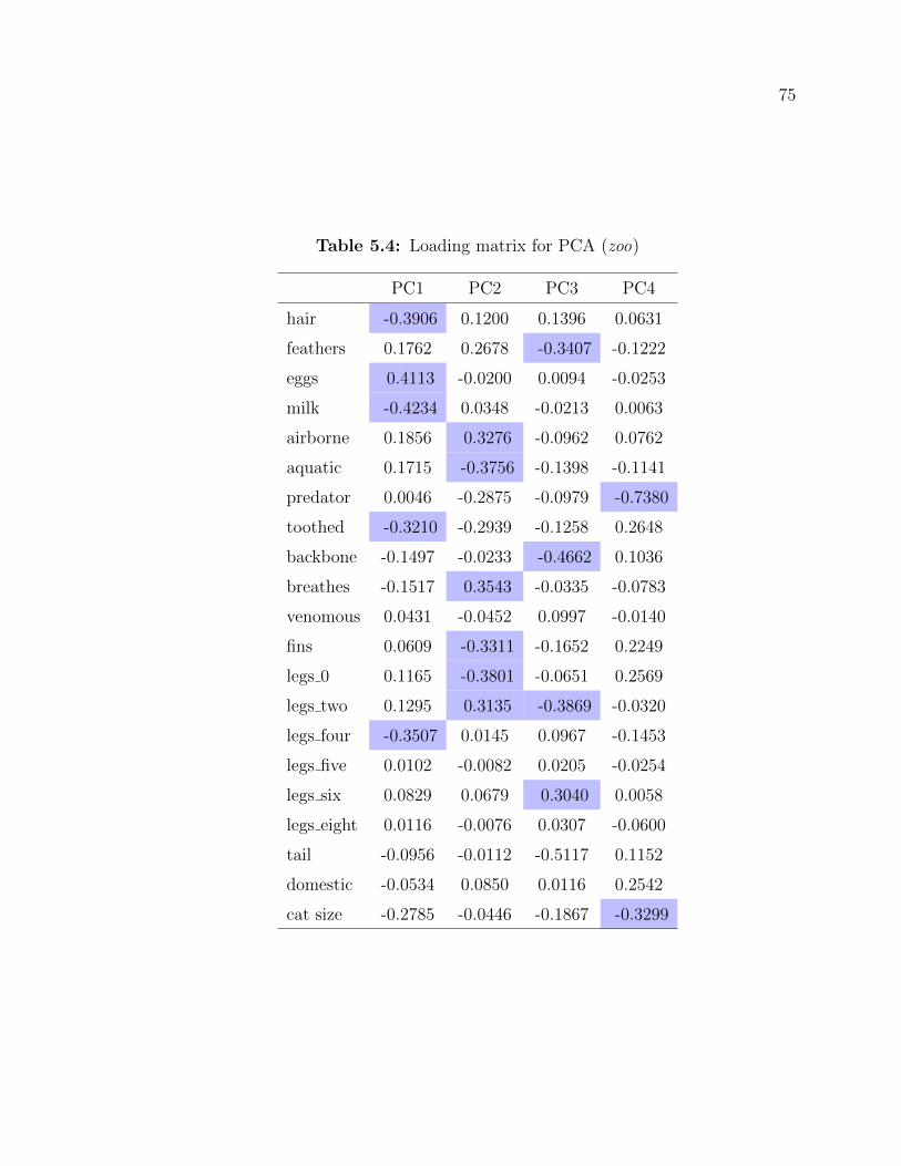
75

Table 5.4: Loading matrix for PCA (zoo)

PC1 PC2 PC3 PC4

hair -0.3906 0.1200 0.1396 0.0631

feathers 0.1762 0.2678 -0.3407 -0.1222

eggs 0.4113 -0.0200 0.0094 -0.0253

milk -0.4234 0.0348 -0.0213 0.0063

airborne 0.1856 0.3276 -0.0962 0.0762

aquatic 0.1715 -0.3756 -0.1398 -0.1141

predator 0.0046 -0.2875 -0.0979 -0.7380

toothed -0.3210 -0.2939 -0.1258 0.2648

backbone -0.1497 -0.0233 -0.4662 0.1036

breathes -0.1517 0.3543 -0.0335 -0.0783

venomous 0.0431 -0.0452 0.0997 -0.0140

fins 0.0609 -0.3311 -0.1652 0.2249

legs 0 0.1165 -0.3801 -0.0651 0.2569

legs two 0.1295 0.3135 -0.3869 -0.0320

legs four -0.3507 0.0145 0.0967 -0.1453

legs five 0.0102 -0.0082 0.0205 -0.0254

legs six 0.0829 0.0679 0.3040 0.0058

legs eight 0.0116 -0.0076 0.0307 -0.0600

tail -0.0956 -0.0112 -0.5117 0.1152

domestic -0.0534 0.0850 0.0116 0.2542

cat size -0.2785 -0.0446 -0.1867 -0.3299

76

From Table 5.4, (highlighting the absolute value of the loadings greater than or equal

to 0.3), we can observe that:

� PC1 explains about 34% of the variance and appears to be a measure of hair, milk,

toothed and four legs vs eggs.


aquatic, fins and no legs versus airborne, breathes and two legs; (i.e. fish vs bird).


feathers, backbone and two legs versus six legs; (i.e. bird vs insect).

� PC4 explains about 7% of the variation in the data and appears to be a strong

measure of predator and catsize.


We begin by exploring the dataset visually using parallel coordinates plots and heatmaps.


Figure 5.2 represents the PCP for the (raw) zoo dataset. The 0.00 value represents the

absence of the feature and the 1.00 value represents the presence of the feature. Each line

corresponds to a specific animal. Each colour represents the group (or class) to which the

animal is said to belong. The animal features are ordered by their variation between classes.

On the bottom are those features that discriminate the most between the classes (milk);

on the top are those features which discriminate the least between the classes (domestic).

If all the animals within their given class shared the same features, then there would be

seven lines, each of a different colour. This is not the case here! There is an orange-brown

line colour or a blending of the colours to achieve this colour; which suggests that there are

some animals that share features with another class of animals.

77

Figure 5.2: Parallel coordinates plot of the zoo dataset

78

5.2.2 Heatmap (raw zoo data)

For the heatmap, colour was used to represent the presence or absence of the animal feature.

Figure 5.4 is a graphical representation of the zoo dataset where the presence of a feature

is coloured in blue and the absence of a feature are coloured in purple. Each row represents

a different animal and the columns represent each feature.

Figure 5.3: A heatmap of the raw data by animal. Rows represent animals, columnsrepresent features

Figure 5.4 represents the same dataset as the previous figure, however the farthest right

column separates the animal class. It is ordered by class with mammals on the bottom,

79

than bird, reptile, fish, amphibian, insect and mollusk on top. From this figure, we can

begin to see which features aid in discriminating between the different animal classes, these

include: milk, feather, backbone, toothed and eggs. These features are seen in the PCP

plot as the variables with high variation. The features which do not help to discriminate

between the classes are: domestic, 5 legged animal and predator. This can be observed

by the features with the most uniform colour across all the features. This indicates that

the presence or absence of that particular feature is specific to very few classes of animals

(usually only one out of the seven classes). These features are seen in the PCP plots as the

low variation variables.

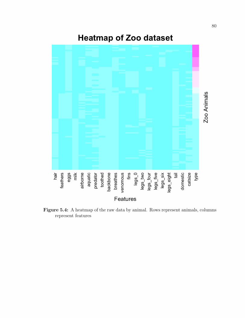
80

Figure 5.4: A heatmap of the raw data by animal. Rows represent animals, columnsrepresent features

81

5.3 Classification

We begin by examining the ability of classification techniques to correctly identify the seven

labelled classes in our dataset.


When constructing a rpart classification tree, the data was split into training (80%) and

testing (20%) sets repeatedly. Trees were built using the generalized Gini index as the

splitting criterion on the training sets, then pruned with the “1-SE” rule for the complexity

parameter (cp) which uses the largest value of cp with the cross-validation error (xerror)

within one-standard deviation (xstd) of the minimum. From the resultant pruned tree, the

testing sets were put through the pruned classification trees. The error rate (or misclassifi-

cation rate) was calculated for each of the 100 datasets and then averaged.

Table 5.5 summarizes the results for both datasets: the raw boolean set and the trans-

formed (continuous) set. Regardless of which dataset was used for classification, there was

no perfect matching. However the misclassification rate was greatest on the continuous

dataset.

Figure 5.5 represents the histograms (on the raw dataset) of frequency of the cp chosen,

the corresponding number of splits, and the misclassification rate for the 100 iterations.

Eight splits seems to be the dominant number of splits.

Table 5.5: Misclassification error for single classification tree (zoo)

Dataset average error rate

Raw boolean 0.08

PCA continuous 0.0985

A typical classification tree and its corresponding pruned tree (on the raw training

data) is represented in Figure 5.6. For this particular case, there is no difference between

the trees. There are eight (8) terminal nodes. These specific trees show no misclassification

error, however “class 7” is separating into two different nodes on the tree.

82

Figure 5.5: Histograms of the average of 100 iterations on the raw boolean zoodataset

83

From the summary function of rpart, we can note that the five (5) key features discrim-

inating between the different classes are: milk, eggs, hair, feathers, and toothed. These are

the same features that had the strongest separation during the visualization step (see 5.2.1

and 5.2.2).

Figure 5.6: Classification tree - complete and pruned on the raw zoo data

This indicates some inability to classify consistent with the classification labels in the

dataset. In other words while there are seven classes labels in the dataset, there might very

well be more or less groups.

84

5.3.2 Neural networks

As explained in 3.4.2, 100 pairs of training and testing datasets were formulated for both

datasets (the raw boolean and the transformed by PCA continuous). The “best” number of

nodes and the “best” weight decay was used to test the algorithm and the misclassification

rate was calculated for each of the 100 test datasets.

Table 5.6 summarizes the results for both datasets, the raw boolean set and the trans-

formed (continuous) set. Regardless of on which dataset classification was performed, there

was again no perfect classification and again the misclassification was greatest on the con-

tinuous dataset. This indicates an inability to classify consistent with the labels in the

dataset.

Table 5.6: Misclassification error for Neural networks (zoo)

Dataset average error rate mode of number of nodes

Raw boolean 0.0555 9

PCA continuous 0.078 9

Figure 5.7 is an example of how the optimal size of the hidden layer and the decay rate

were chosen. In this example, with five nodes in the hidden layer, the accuracy remains

around 0.92.

85

Figure 5.7: Zoo optimization graph

86

5.4 Clustering

We now turn to using clustering to find groups in the dataset. We analyse four cluster-

ing algorithms: Partitioning around centroids, partitioning around medoids, hierarchical

agglomerative and hierarchical divisive. Our goal is to see whether the algorithms can sep-

arate the data into the seven classes (as per the class labels) in the dataset by means of

clustering [3] or whether they find other groups.

We start off by determining the optimal number of clusters for each algorithm/ dissim-

ilarity metric combination. Then we evaluate how well the results of the cluster analysis fit

the data without reference to external information. Finally we evaluate the results of the

cluster analysis based on the externally provided labels.

5.4.1 Choosing the optimal number of clusters

The issue with partitioning algorithms (both around the centroid and medoid) is deter-

mining the number of centroids or medoids before running the algorithm. In the case of

hierarchical algorithms (agglomerative and divisive) the issue is the combining or splitting

method.

The ASW is a measure of coherence of a clustering solution for all objects in the whole

dataset. We chose to calculate the ASW for k = 2, . . . , 13 using each dissimilarity metric.

In the case of partitioning, the k was pre-determined in the algorithm and the ASW was

calculated for each result. For hierarchical clustering, k was determined by cutting the

resultant dendrogram each into k partitions, k = 2, . . . , 13 and then the ASW was calculated

for each. A graph of ASW against the number of clusters was constructed for each algorithm

and the optimal number of clusters is indicated by the number of clusters corresponding to

a spike in the plot (the largest ASW).

The summary Tables 5.7 and 5.8 return a range of optimal k from three (3) to 13.

Hierarchical agglomerative average linkage/Jaccard metric or Euclidean dissimilarity metric,

with McQuitty linkage/Jaccard metric, and with the Median linkage/Correlation metric are

the only pairs to return k = 7 as the optimal number of clusters.

87

Table 5.7: Summary of the ’best k’ based on max ASW (Partitioning algorithms;(zoo)

Data Dissimilarity measurePartitioning clustering algorithm

k-means PAM

BinaryJaccard 6 5

Correlation 6 5

ContinuousEuclidean 4 11

Manhattan 4 3

Table 5.8: Summary of the ’best k’ based on max ASW (Hierarchical clustering;(zoo)

DataDissimilarity Hierarchical clustering algorithm

measure Single Average Complete Ward Centroid McQuitty Median DIANA

BinaryJaccard 11 7 5 9 13 7 11 6

Correlation 13 9 5 6 10 9 7 4

PCEuclidean 11 7 5 5 6 8 10 4

Manhattan 8 8 4 10 5 4 12 5

The summary Tables 5.9 and 5.10 give the maximum ASW and show that the best

combination for the partitioning algorithms is partitioning around centroids (k-means) al-

gorithm with the correlation metric, with an ASW of 0.580956. For the hierarchical al-

gorithms, the best combination is the agglomerative algorithm with centroid linkage and

Euclidean metric, with an ASW of 0.574022.

Table 5.9: Summary of the maximum ASW (Partitioning algorithms; zoo)

DataDissimilarity Partitioning clustering algorithm

measure k-means PAM

BinaryJaccard 0.521827 0.516189

Correlation 0.58594 0.580956

PCEuclidean 0.564267 0.564467

Manhattan 0.556972 0.558431

88

Table

5.1

0:

Sum

mar

yof

the

max

imum

ASW

(Hie

rarc

hic

alal

gori

thm

s;zoo

)

Dat

aD

issi

milar

ity

Hie

rarc

hic

alcl

ust

erin

gal

gori

thm

mea

sure

Sin

gle

Ave

rage

Com

ple

teW

ard

Cen

troi

dM

cQuit

tyM

edia

nD

IAN

A

Bin

ary

Jac

card

0.36

3037

0.52

8712

0.51

4601

0.52

0801

0.42

8291

0.51

7056

0.36

3037

0.54

4081

Cor

rela

tion

0.45

3536

0.51

7189

0.52

4091

0.52

5267

0.50

1060

0.50

2735

0.49

5511

0.52

6947

PC

Eucl

idea

n0.

4968

020.

5679

330.

5602

270.

5662

520.

5740

220.

5582

920.

3508

800.

5580

05

Man

hat

tan

0.33

5940

0.52

2036

0.51

4898

0.53

1047

0.51

7020

0.51

4898

0.41

2357

0.52

6577

89

Figures 5.8, 5.9 and 5.10 represent the average silhouette width vs the number of clusters

plotted for k = 2, . . . , 13. The number of clusters corresponding to the maximum ASW was

taken as the optimal number of clusters. As it can be seen from these figures, the optimum

number of clusters is not consistent. Generally, the metrics each trend similarly for each

algorithm.

(a) Partitioning around the centroids (b) Partitioning around the medoids

Figure 5.8: ASW versus the number of clusters for the partitioning algorithms(zoo). On the left, it is partitioning around the centroids and on the right, it ispartitioning around the medoids

90

(a) Hierarchical clustering - Single (b) Hierarchical clustering - average

(c) Hierarchical clustering - complete (d) Hierarchical clustering - Ward

Figure 5.9: ASW versus the number of clusters for the hierarchical algorithms (zoo).

91

(a) Hierarchical clustering - centroid (b) Hierarchical clustering - McQuitty

(c) Hierarchical clustering - medoids (d) Hierarchical divisive clustering

Figure 5.10: ASW versus the number of clusters for the hierarchical algorithms(zoo).

92


The different clustering algorithms were applied using the four dissimilarity metrics. Inter-

nal cluster validation was performed for each clustering result. For the partitioning algo-

rithms, the internal evaluation (or the measure of goodness) is ASW. The higher the ASW,

the better the clustering. Since this method is not an appropriate method of validating

hierarchical algorithms, the cophenetic correlation coefficient is used for them.

Partitioning around centroids

Each algorithm with each dissimilarity metric was run with the number of possible clusters

ranging from k = 2, . . . , 13. Based on the average silhouette width (ASW), for each cluster-

ing method, the goodness of the clustering structure is assessed. From Table 5.11 it can be

noted that the maximum ASW is 0.585936. This does not suggest a very strong clustering

ensemble. This suggests k-means may not be an appropriate method to cluster this data.

Although the overall cluster structure is not very strong, it suggests between four and six

clusters.

93

Table 5.11: Average silhouette width (k-means ; zoo)


2 clusters 0.347611 0.428075 0.405649 0.414281

3 clusters 0.429547 0.513140 0.471595 0.463245

4 clusters 0.481528 0.549905 0.564267 0.556972

5 clusters 0.519533 0.582260 0.551278 0.539456

6 clusters 0.521827 0.585936 0.511913 0.504474

7 clusters 0.497038 0.562231 0.531215 0.516816

8 clusters 0.454556 0.572527 0.516044 0.509794

9 clusters 0.483478 0.539235 0.542385 0.530952

10 clusters 0.426405 0.465540 0.559144 0.538148

11 clusters 0.421646 0.490142 0.540565 0.552853

12 clusters 0.448010 0.443562 0.556172 0.542545

13 clusters 0.452279 0.468846 0.546742 0.527154

Partitioning around medoids

Table 5.12 gives the ASW for the PAM algorithm for every clustering-metric combination

for k = 2, . . . , 13. It can be seen that the max ASW is 0.580956. Again, this does not

suggest a very strong clustering ensemble, suggesting that PAM may not be an appropriate

method to cluster this data.

From this table, the range of optimal k clusters is: 4 to 11.

Hierarchical agglomerative

The CPCC values are shown in Table 5.13. The hierarchical clustering with Average linkage

method seems to fit the data the best across all the four dissimilarity measures.

94

Table 5.12: Average silhouette width (PAM; zoo)


2 clusters 0.345216 0.424760 0.401330 0.405059

3 clusters 0.427336 0.511154 0.485225 0.444352

4 clusters 0.484139 0.559444 0.560595 0.558431

5 clusters 0.516189 0.580956 0.507278 0.501261

6 clusters 0.405779 0.451837 0.509826 0.510713

7 clusters 0.431195 0.473230 0.531999 0.518054

8 clusters 0.444311 0.503976 0.514482 0.496023

9 clusters 0.474294 0.521942 0.535294 0.511160

10 clusters 0.422312 0.539786 0.548705 0.541214

11 clusters 0.442171 0.480058 0.564467 0.548410

12 clusters 0.437710 0.486950 0.556867 0.542723

13 clusters 0.441168 0.480366 0.536847 0.551696

Table 5.13: Cophenetic correlation coefficient for hierarchical agglomerative clus-tering (zoo)



Single 0.862578 0.7952211 0.7577783 0.6241947

Average 0.9234369 0.8483731 0.8599904 0.8395532

Complete 0.8876186 0.8424761 0.8373628 0.8225777

Ward 0.672414 0.7203869 0.7483626 0.7423837

Centroid 0.871792 0.8192215 0.8243972 0.8269505

McQuitty 0.9154849 0.8430192 0.8463692 0.8267455

Median 0.8300966 0.7913838 0.7322871 0.7114326

95

Hierarchical divisive

The CPCC values are shown in Table 5.14. The hierarchical clustering with the Correlation

metric seems to fit the data the best.

Table 5.14: Cophenetic correlation coefficient for hierarchical divisive (zoo)



DIANA 0.9014647 0.8429325 0.8491403 0.833087

96

5.4.3 External indices (using k = 7)

In this section, only summary statistics will be given. For more details, please refer to the

Appendix B. The summary tables summarise the entropy and purity for each algorithm-

metric combination.

Purity and entropy results

Tables 5.15 and 5.16 summarise the entropy and purity calculations. The best (or minimum)

entropy value for binary dissimilarity metrics is 0.21900 associated with the hierarchical

agglomerative with Centroid linkage and Correlation metric. For the continuous dataset,

the best entropy is 0.23662, associated with the hierarchical agglomerative with Average

linkage or McQuitty linkage, both with the Euclidean dissimilarity metric.

Using the binary dataset, the best purity value is 0.93 associated with the hierarchical

agglomerative Centroid linkage with either the Jaccard dissimilarity metric or the correla-

tion measure. Using the continuous dataset, the best purity value is 0.93 as well, associated

with the hierarchical agglomerative Average linkage/Euclidean metric pair or Complete

linkage/Euclidean metric.

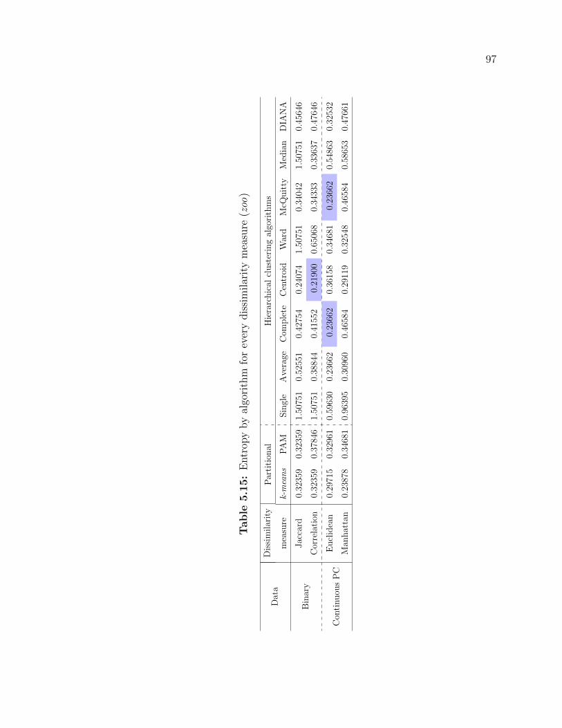
97

Table

5.1

5:

Entr

opy

by

algo

rith

mfo

rev

ery

dis

sim

ilar

ity

mea

sure

(zoo

)

Dat

aD

issi

milar

ity

Par

titi

onal

Hie

rarc

hic

alcl

ust

erin

gal

gori

thm

s

mea

sure

k-means

PA

MSin

gle

Ave

rage

Com

ple

teC

entr

oid

War

dM

cQuit

tyM

edia

nD

IAN

A

Bin

ary

Jac

card

0.32

359

0.32

359

1.50

751

0.52

551

0.42

754

0.24

074

1.50

751

0.34

042

1.50

751

0.45

646

Cor

rela

tion

0.32

359

0.37

846

1.50

751

0.38

844

0.41

552

0.21

900

0.65

068

0.34

333

0.33

637

0.47

646

Con

tinuou

sP

CE

ucl

idea

n0.

2971

50.

3296

10.

5963

00.

2366

20.

2366

20.

3615

80.

3468

10.

2366

20.

5486

30.

3253

2

Man

hat

tan

0.23

878

0.34

681

0.96

395

0.30

960

0.46

584

0.29

119

0.32

548

0.46

584

0.58

653

0.47

661

98

Table

5.1

6:

Puri

tyby

algo

rith

mfo

rev

ery

dis

sim

ilar

ity

mea

sure

(zoo

)

Dat

aD

issi

milar

ity

Par

titi

onal

Hie

rarc

hic

alcl

ust

erin

gal

gori

thm

s

mea

sure

k-means

PA

MSin

gle

Ave

rage

Com

ple

teC

entr

oid

War

dM

cQuit

tyM

edia

nD

IAN

A

Bin

ary

Jac

card

0.91

0.92

0.59

0.88

0.88

0.93

0.59

0.92

0.59

0.88

Cor

rela

tion

0.89

50.

900.

590.

890.

880.

930.

820.

900.

910.

87

Con

tinuou

sP

CE

ucl

idea

n0.

900.

900.

820.

930.

930.

890.

890.

930.

890.

90

Man

hat

tan

0.90

0.89

0.76

0.90

0.89

0.91

0.89

0.89

0.81

0.89

Chapter 6

Results of Experimental Design

To measure whether our results were statistically significant an experimental design ap-

proach is taken. We use two different boolean datasets, with differing complexities, in our

analyses. Two dissimilarity metrics (Jaccard and correlation) were calculated with the raw

data as well as two (Euclidean and Manhattan) with the transformed data . Clustering

methods compared in this research are partitioning around centroids, partitioning around

medoids, hierarchical agglomerative, and hierarchical divisive. The ASW was calculated

for each algorithm-dissimilarity pair for each k ranging from k = 2, . . . , 13 and the cluster

number associated with max ASW was chosen as the optimal k.

The experimental design used to assess statistical significance of our results was ex-

plained in Section 3.5.5. The formal results of this design will be given here. The analyses

were done using SAS 9.3 [6]. When factors are found to be statistically significant we use

Duncan’s multiple-range test [52] as a post hoc test (with α = 0.05) to further explore them.

6.1 Evaluating the choice of k

Using the optimal choice for k for both datasets, we test for significant effects. Table 6.1

presents the analysis of variance results.

The following deductions can be made from Table 6.1:

1. The overall model was highly significant with a p-value of < 0.0001.

99

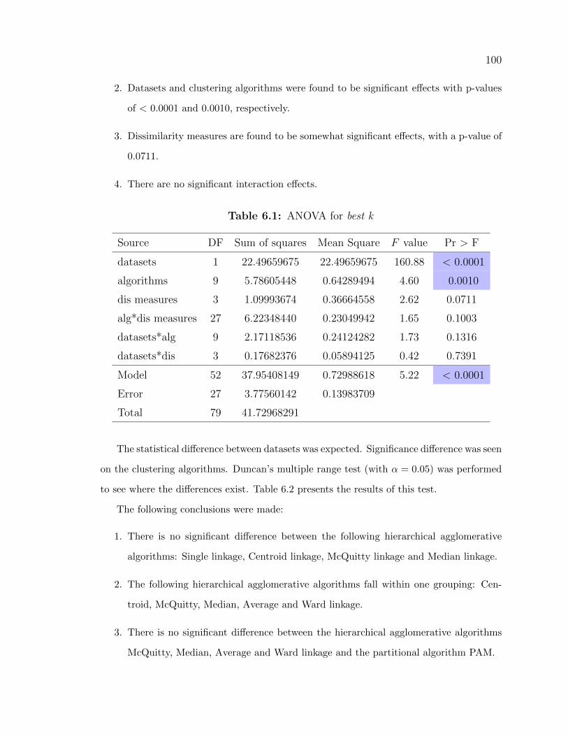
100

2. Datasets and clustering algorithms were found to be significant effects with p-values

of < 0.0001 and 0.0010, respectively.

3. Dissimilarity measures are found to be somewhat significant effects, with a p-value of

0.0711.

4. There are no significant interaction effects.

Table 6.1: ANOVA for best k

Source DF Sum of squares Mean Square F value Pr > F

datasets 1 22.49659675 22.49659675 160.88 < 0.0001

algorithms 9 5.78605448 0.64289494 4.60 0.0010

dis measures 3 1.09993674 0.36664558 2.62 0.0711

alg*dis measures 27 6.22348440 0.23049942 1.65 0.1003

datasets*alg 9 2.17118536 0.24124282 1.73 0.1316

datasets*dis 3 0.17682376 0.05894125 0.42 0.7391

Model 52 37.95408149 0.72988618 5.22 < 0.0001

Error 27 3.77560142 0.13983709

Total 79 41.72968291

The statistical difference between datasets was expected. Significance difference was seen

on the clustering algorithms. Duncan’s multiple range test (with α = 0.05) was performed

to see where the differences exist. Table 6.2 presents the results of this test.

The following conclusions were made:

1. There is no significant difference between the following hierarchical agglomerative

algorithms: Single linkage, Centroid linkage, McQuitty linkage and Median linkage.

2. The following hierarchical agglomerative algorithms fall within one grouping: Cen-

troid, McQuitty, Median, Average and Ward linkage.

3. There is no significant difference between the hierarchical agglomerative algorithms

McQuitty, Median, Average and Ward linkage and the partitional algorithm PAM.

101

4. The following hierarchical agglomerative algorithms Average, Ward linkage, the par-

titional algorithm PAM, k-means and the hierarchical divisive algorithm DIANA

perform similarly.

Table 6.2: Duncan’s multiple test grouping for testing the algorithms (when choosingoptimum k ; α = 0.05)

Duncan Grouping Mean Algorithm

A 2.6144 Single

B A 2.3659 Centroid

B A C 2.3173 McQuitty

B A C 2.2807 Median

B D C 2.0971 Average

B D C 2.0631 Ward

D C 1.8972 PAM

D 1.8195 k-means

D 1.7956 Complete

D 1.7928 DIANA

6.2 Evaluating the performance (based on ASW)

Using the associated ASW value, we test whether the performance of the algorithm - dissim-

ilarity measure differ significantly. Table 6.3 presents the results of the analysis of variance.

The following deduction can be made from Table 6.3:

102

1. The overall model was significant with a p-value of < 0.0001.

2. Datasets, clustering algorithms, and dissimilarity measures were all found to be sig-

nificant with p-values of < 0.0001, < 0.0001 and 0.0003, respectively.

3. The interaction effect of datasets and clustering algorithms was significant with a

p-value of < 0.0001.

4. The interaction effect of datasets and dissimilarity metric was significant with a p-

value of 0.0274.

Table 6.3: ANOVA for ASW

Source DF Sum of squares Mean Square F value Pr > F

datasets 1 0.06870764 0.06870764 45.87 < 0.0001

algorithms 9 0.47183399 0.05253711 35.08 < 0.0001

dissimilarity 3 0.04034081 0.01344694 8.98 0.00030

alg*dis 27 0.04064367 0.00150532 1.00 0.4949

datasets*alg 9 0.19084703 0.02120523 14.16 < 0.0001

datasets*dis 3 0.01596739 0.00532246 3.55 0.0274

Model 52 0.82934053 0.01594886 10.65 < 0.0001

Error 27 0.04044166 0.00149784

Total 79 0.86978219

The statistical difference between datasets was again confirmed. Since there were signif-

icant interactions between datasets and algorithms and datasets and dissimilarity metric,

we examine these further.

The following deductions can be made from Tables 6.4, 6.5, 6.6, and 6.7:

1. Table 6.4 presents the interaction effect of the datasets with the algorithms sliced by

datasets (all the algorithms are grouped for each dataset). As the p-value for the

voters dataset is < 0.0001 and that of the zoo dataset is 0.0261, clustering algorithms

differ significantly for both datasets.

103

2. Table 6.5 presents the interaction effect of the datasets with the algorithms sliced by

algorithms. Single linkage, Centroid linkage, McQuitty linkage and Median linkage

each have a p-value < 0.05, which means that these clustering methods significantly

differ between datasets.

3. Table 6.6 presents the interaction effect of the datasets with the dissimilarity measures

sliced by dataset. Dissimilarity measures showed significant effect only for the voters

dataset.

4. Table 6.7 presents the interaction effect of the datasets with the dissimilarity measures

sliced by dissimilarity measure. Only the Correlation distance showed no significant

difference among the datasets.

Table 6.4: Dataset*Algorithm sliced by Dataset

Dataset p-value

voters dataset < 0.0001

zoo dataset 0.0261

Table 6.5: Dataset*Algorithm sliced by Algorithm

Algorithm p-value

k-means 0.2288

PAM 0.1168

Single < 0.0001

Average 0.4397

Complete 0.4406

Ward 0.6759

Centroid 0.0963

McQuitty 0.0416

Median < 0.0001

DIANA 0.2787

104

Table 6.6: Dataset*Dissimilarity measure sliced by Dataset

Dataset p-value

voters dataset < 0.0001

zoo dataset 0.2985

Table 6.7: Dataset*Dissimilarity measure sliced by Dissimilarity Measure

Dissimilarity measure p-value

Jaccard dissimilarity 0.0013

Correlation distance 0.2567

Euclidean 0.0050

Manhattan < 0.0001

Significance difference was seen with the interaction between datasets and clustering

algorithms. A Duncan’s multiple range test was performed to identify where the difference

exists for each dataset. Tables 6.8 and 6.9 presents the results of this test for the voters

and zoo datasets respectively.


1. The following clustering methods were grouped together for both datasets: Hierar-

chical agglomerative Median linkage and Hierarchical agglomerative Single linkage

2. The following algorithms fall within one grouping (for both datasets): k-means, PAM,

DIANA, Ward, Average, and Complete.

3. k-means performed the best on the zoo dataset.

4. The DIANA linkage performed the best on the voters dataset.

Since significance difference was again seen with the interaction between datasets and

the dissimilarity measures, a Duncan’s multiple range test was performed to identify where

the difference exists for each dataset. Tables 6.10 and 6.11 presents the results of this test

for the voters and zoo datasets respectively.


105

Table 6.8: Duncan’s multiple test grouping for testing the performance of the algo-rithms based on ASW (voters)

Duncan Grouping Mean N algorithm

A 1.10027 4 DIANA

A 1.08860 4 Average

B A 1.08528 4 Complete

B A 1.07979 4 Ward

B A 1.04736 4 k-means

B A 1.03538 4 PAM

B 1.00355 4 Centroid

B 1.00227 4 McQuitty

C 0.76573 4 Median

C 0.74027 4 Single

Table 6.9: Duncan’s multiple test grouping for testing the performance of the algo-rithms based on ASW (zoo)

Duncan Grouping Mean N algorithm

A 1.08106 4 k-means

A 1.07972 4 PAM

A 1.07001 4 DIANA

A 1.06822 4 Ward

A 1.06713 4 Average

A 1.06387 4 Complete

A 1.06082 4 McQuitty

A 1.05070 4 Centroid

B 0.99849 4 Single

B 0.99459 4 Median

106

1. The following dissimilarity measures were grouped together: Correlation and Eu-

clidean.

2. The following dissimilarity measures were grouped together: Jaccard and Manhattan.

3. The voters dataset had the greatest difference between the Correlation (performed

best) and the Manhattan dissimilarity measure (performed worst)

Table 6.10: Duncan’s multiple test grouping for the dissimilarity measures (voters)

Duncan Grouping Mean N metric

A 1.03984 10 Correlation

B A 1.01616 10 Euclidean

B C 0.97541 10 Jaccard

C 0.94799 10 Manhattan

Table 6.11: Duncan’s multiple test grouping for the dissimilarity measures (zoo)

Duncan Grouping Mean N metric

A 1.069104 10 Euclidean

B A 1.059895 10 Correlation

B C 1.047382 10 Manhattan

C 1.037467 10 Jaccard

Chapter 7

Summary, conclusion and future work

7.1 Summary

Our motivation for this research was from the world of crime statistics. We wanted to see

whether we could group similar crimes and we wanted to see if a new crime would fall

into a cluster of crimes committed by a known criminal or if it would be identifiable as a

new cluster associated with a new (unknown) criminal. The specific crime dataset, other

than the variable representing the criminal, was boolean in nature. This thesis research

uses two datasets that are surrogates for the crime dataset and that are benchmarks in the

literature and provides a way of examining statistically the effectiveness of several clustering

algorithms and dissimilarity measures applied to such boolean data.

We began by visualizing our datasets. We were able to identify consistent features which

separated the data well, using both data visualization and later classification methods.

Using the classifiers (i.e. artificial trees and neural networks), we examined whether the

class labels were an accurate description of the structure in the data.

Although classification had a small misclassification error (5%), we were not able to

produce a perfect classifier. Also, even though the misclassification error rate is low, the

techniques are only able to identify known classes.

To further explore structure in the data, clustering methods together with various dis-

similarity measures were applied to the two datasets under study. The optimal number of

107

108

clusters was obtained using the number of clusters corresponding to the maximum ASW for

all the clustering algorithm - dissimilarity measure pairings. While the number of clusters

showed considerable variability, on average, the optimal number of clusters was found to be

two for the voters dataset and seven for the zoo dataset. The mode for the optimal number

of clusters is two for the voters and five for the zoo dataset. The stated number of classes

given with the data was two for the voters and seven for the zoo. Our results are therefore

more in line with the stated ones for the voters dataset than for the zoo dataset.

We used an experimental design to assess if the algorithms and/or dissimilarity measures

had a significant effect on choice of best k. We used internal cluster validation techniques

(ASW and CPCC) to examine the results of the different clustering algorithm - dissimilarity

measure pairings. For the optimal choice of k we found that the only significant effect was

the choice of algorithms. The Single, Centroid, McQuitty and Median hierarchical linkages

group together and are different from Average, Ward, PAM, k-means, Complete and DI-

ANA. This latter group was preferred to the first group. There was no significant effect

of dissimilarity measures, and no interactions between the distance measures and these al-

gorithms. For the performance based on ASW, there was found to be significant effects

of algorithm and distance measures, as well as the interaction with these two factors with

datasets, and no interaction with each other. Algorithms interacted with both datasets sig-

nificantly. In both cases the Single and Median algorithms were grouped together, separated

from the others and did not perform as well. However, dissimilarity measures interaction

only existed for the voters dataset. For both datasets, the Correlation and Euclidean were

grouped together and differed from the Jaccard and Manhattan grouping. Since Correlation

distance was the only one that did not interact with datasets it would be a preferred choice.

For best performance base on ASW, DIANA and Average with the Correlation metric seem

to be coming out the best for either datasets. For optimal choice of k, DIANA and Average

are also grouped together in the preferred grouping

Finally, we use external validation techniques to measure the purity and entropy of the

resultant clusters when the “known” k is used.

109

7.2 Conclusion

7.2.1 Data visualisation

In both datasets, we were able to determine the key variables for separating the data into

natural groups. From the parallel coordinates plots, these variables were the ones showing

the largest variation between the cases. For the voters dataset these were: Physician, El-

Salvador aid, education, adoption of the budget resolution, aid to the Nicaraguan Contras.

We should note that these features also appear strongly in PC1. For the zoo dataset, these

variables were: milk, feathers, backbone, toothed, eggs and hair. Most of these features

(milk, eggs, hair and toothed) appear strongly in PC1.

7.2.2 Classification

With the labelled data, we constructed a classifier using classification trees (rpart). Table

7.1 shows that the raw boolean has a lower misclassification rate than when using PCA

to reduce the data. The resultant trees use the same variables as was seen in the data

visualization part.

Table 7.1: Misclassification error for classification tree

Average error rate

Dataset Voters data Zoo data

Raw boolean 0.04170213 0.0555

PCA continuous 0.1221277 0.078

Using a neural network approach to classification we obtained similar results with respect

to the misclassification rate (see Table 7.2).

7.2.3 Clustering and Internal indices: choice of k

We ran clustering algorithm - dissimilarity metric pairings on both the voters and zoo

datasets and determined the optimal number of clusters based on the largest ASW. A

110

Table 7.2: Misclassification error for neural networks

Average error rate

Dataset Voters data Zoo data

Raw boolean 0.04489362 0.08

PCA continuous 0.06489362 0.0985

balanced experimental design was used to analyze the results.

The optimal number of clusters was taken as the value corresponding to the maximum

ASW for each algorithm-dissimilarity measure pair. This was two (2) for the voters dataset.

The maximum ASW for the partitional algorithms is 0.583445 and for the hierarchical

algorithms it is 0.644748. Both of these ASW demonstrate that a reasonable structure has

been found (see Table 3.4). However, plotting ASW against the number of clusters, there

was no clear spike, indicating that either there was no “best” number of clusters or that the

“best” number of clusters is at k = 2. This could be due to the actual number of classes

being two. For the zoo dataset, the optimal number of clusters ranged from 3 to 13, with

the mode as k = 5. The maximum ASW for the partitional algorithms is 0.580956 and for

the hierarchical algorithms it is 0.574022. This suggests a weak clustering structure in the

data. This could be due to the greater complexity of the data (having seven (7) classes,

with all but one class having a small number of cases.

The least accurate algorithm-metric pairs for determining the optimal k for the voters

dataset were Hierarchical agglomerative single with the correlation measure, hierarchical

agglomerative centroid with the Jaccard dissimilarity measure and McQuitty linkage with

the Jaccard dissimilarity measure; for the zoo dataset the algorithm-metric pairings were

hierarchical agglomerative single with Correlation and centroid linkage with Jaccard. For

both datasets, it appears that Hierarchical agglomerative Single linkage does not work

very well with the correlation distance neither does the hierarchical agglomerative centroid

linkage with the Jaccard dissimilarity measure.

Using an experimental design we tested to determine whether there was a significant

difference for the “best”k as determined by maximum ASW. We confirmed that at the

111

5% level of significance, “best”k differed between the two datasets (as expected) and that

it also differed for the clustering algorithms. There was no significant interaction effect

between either the datasets and algorithms, the datasets and dissimilarity measures and the

clustering algorithms and dissimilarity measures. The Duncan multiple range test grouped

the hierarchical agglomerative McQuitty, Median, Average and Ward linkage. Single linkage

was separated from any other grouping of algorithms and was found to have the largest mean

“best”k amongst all the clustering algorithms. Complete and DIANA are grouped together,

did not overlap with other clustering algorithms, and are to be preferred.


Using the maximum ASW for the partitional algorithms and cophenetic correlation coeffi-

cient for the hierarchical algorithms we examined goodness of clusters.

For the voters dataset the max ASW was 0.583445 with the k-means/correlation com-

bination. This value does not suggest a very strong clustering ensemble. Using the CPCC,

hierarchical clustering with Average linkage method performed well across all the hierar-

chical agglomerative/dissimilarity measures pairings. For the zoo dataset, the max ASW

is 0.585936 with the k-means/correlation combination. This value also does not suggest

a very strong clustering ensemble. Using the CPCC, hierarchical clustering with Jaccard

linkage method performed well across all the hierarchical/dissimilarity measures.

An experimental design was also used to test for differences in max ASW due to the

algorithms. We concluded that at the 5% level of significance, significant differences in

max ASW were due to the two datasets (as expected), the algorithms, the dissimilarity

measures and the two-factor interaction between the datasets and the clustering algorithms

as well as the two-factor interaction between the datasets and the dissimilarity measures.

Having seen significant interaction effects between datasets and algorithms and datasets and

dissimilarity measures, we test for each dataset which algorithms are the same and which

differ, and again for each dataset, we test which dissimilarity measures are the same and

which differ. The p value for the hierarchical agglomerate Single linkage, Centroid linkage,

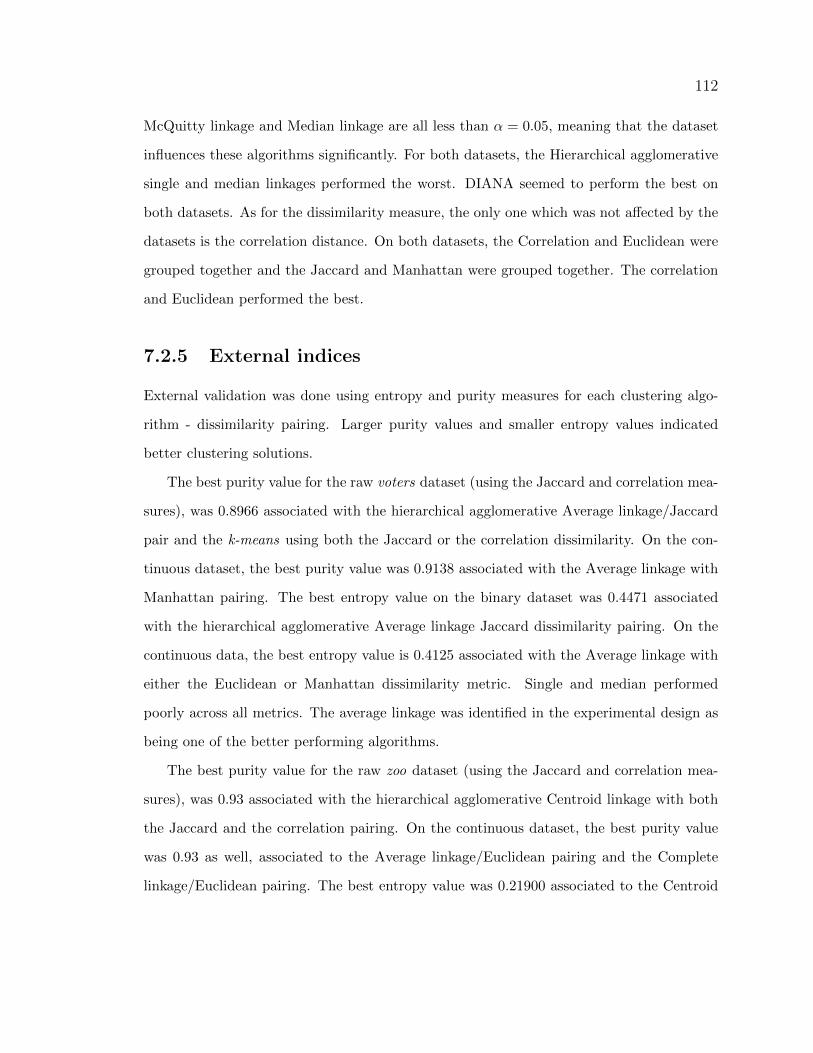
112

McQuitty linkage and Median linkage are all less than α = 0.05, meaning that the dataset

influences these algorithms significantly. For both datasets, the Hierarchical agglomerative

single and median linkages performed the worst. DIANA seemed to perform the best on

both datasets. As for the dissimilarity measure, the only one which was not affected by the

datasets is the correlation distance. On both datasets, the Correlation and Euclidean were

grouped together and the Jaccard and Manhattan were grouped together. The correlation

and Euclidean performed the best.

7.2.5 External indices

External validation was done using entropy and purity measures for each clustering algo-

rithm - dissimilarity pairing. Larger purity values and smaller entropy values indicated

better clustering solutions.

The best purity value for the raw voters dataset (using the Jaccard and correlation mea-

sures), was 0.8966 associated with the hierarchical agglomerative Average linkage/Jaccard

pair and the k-means using both the Jaccard or the correlation dissimilarity. On the con-

tinuous dataset, the best purity value was 0.9138 associated with the Average linkage with

Manhattan pairing. The best entropy value on the binary dataset was 0.4471 associated

with the hierarchical agglomerative Average linkage Jaccard dissimilarity pairing. On the

continuous data, the best entropy value is 0.4125 associated with the Average linkage with

either the Euclidean or Manhattan dissimilarity metric. Single and median performed

poorly across all metrics. The average linkage was identified in the experimental design as

being one of the better performing algorithms.

The best purity value for the raw zoo dataset (using the Jaccard and correlation mea-

sures), was 0.93 associated with the hierarchical agglomerative Centroid linkage with both

the Jaccard and the correlation pairing. On the continuous dataset, the best purity value

was 0.93 as well, associated to the Average linkage/Euclidean pairing and the Complete

linkage/Euclidean pairing. The best entropy value was 0.21900 associated to the Centroid

113

linkage/Correlation pairing. For the continuous dataset, the best entropy is 0.23662, asso-

ciated with the average linkage and McQuitty linkage both with the Euclidean dissimilarity

. The average linkage was identified as being grouped together with the complete linkage

as being better performing algorithms with the Euclidean dissimilarity metric. Single and

median again showed poorer performance.

7.3 Future work

For simplicity, we removed from the voters dataset those cases with missing values. Further

research is needed to determine how to best handle the situation of datasets containing

missing data.

In this research we studied the most common algorithms and used only one transfor-

mation technique. Further research should consider alternate transformations such as the

Wiener transformation as discussed in [15].

Both data sets used in this research are relatively small in size. As the datasets get

larger in number of cases and number of variables, the data sets will tend to be sparser

and thus the clustering algorithms may perform differently from a more compact dataset.

Further research is also to study the scalability of these algorithms onto larger boolean

datasets.

Comparisons with algorithms such as COOLCAT [18], latent trait analysis and bi-

clustering could also be explored.

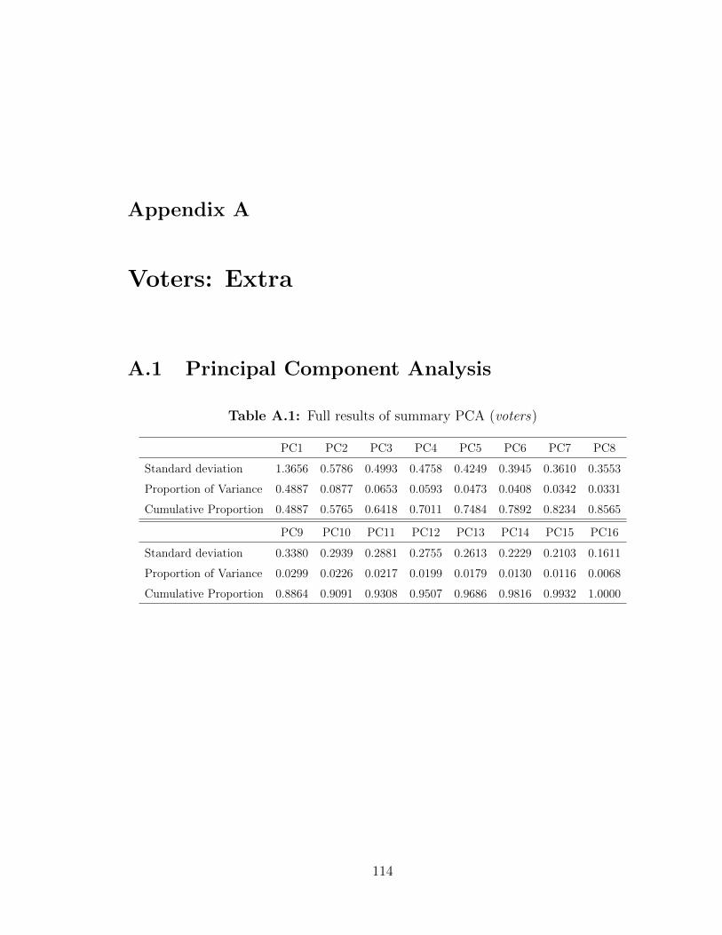
Appendix A

Voters: Extra

A.1 Principal Component Analysis

Table A.1: Full results of summary PCA (voters)

PC1 PC2 PC3 PC4 PC5 PC6 PC7 PC8

Standard deviation 1.3656 0.5786 0.4993 0.4758 0.4249 0.3945 0.3610 0.3553

Proportion of Variance 0.4887 0.0877 0.0653 0.0593 0.0473 0.0408 0.0342 0.0331

Cumulative Proportion 0.4887 0.5765 0.6418 0.7011 0.7484 0.7892 0.8234 0.8565

PC9 PC10 PC11 PC12 PC13 PC14 PC15 PC16

Standard deviation 0.3380 0.2939 0.2881 0.2755 0.2613 0.2229 0.2103 0.1611

Proportion of Variance 0.0299 0.0226 0.0217 0.0199 0.0179 0.0130 0.0116 0.0068

Cumulative Proportion 0.8864 0.9091 0.9308 0.9507 0.9686 0.9816 0.9932 1.0000

114

115

Table

A.2

:F

ull

resu

lts

ofth

eP

CA

load

ings

(voters)

PC

1P

C2

PC

3P

C4

PC

5P

C6

PC

7P

C8

PC

9P

C10

PC

11P

C12

PC

13P

C14

PC

15P

C16

infa

nts

0.18

490.

1943

-0.0

048

0.59

70-0

.588

20.

0669

-0.1

195

0.22

91-0

.304

20.

0650

-0.0

222

0.14

43-0

.169

70.

0062

-0.0

849

-0.0

187

wat

er-0

.048

80.

6852

0.17

190.

3065

0.43

29-0

.202

50.

2357

0.18

360.

1945

0.01

93-0

.146

1-0

.065

3-0

.044

2-0

.127

8-0

.067

90.

0182

bu

dge

t0.

2906

0.05

240.

1839

0.04

620.

1679

0.31

35-0

.342

1-0

.028

0-0

.034

30.

0162

0.37

44-0

.643

8-0

.170

6-0

.106

3-0

.137

5-0

.131

0

physi

cian

-0.3

109

-0.1

367

-0.0

617

0.14

710.

0005

-0.0

312

0.38

250.

1368

0.01

16-0

.089

70.

1503

-0.2

577

-0.3

313

0.62

130.

0397

-0.3

140

esai

d-0

.335

10.

0211

0.04

110.

0607

-0.1

194

0.16

80-0

.033

90.

1480

0.11

92-0

.146

00.

1439

-0.1

941

0.07

650.

1499

-0.0

808

0.82

92

reli

gion

-0.2

533

0.09

820.

2564

-0.2

140

0.07

430.

3547

-0.4

214

0.09

590.

0109

0.11

44-0

.528

00.

1496

-0.2

886

0.24

63-0

.175

0-0

.087

2

sate

llit

e0.

2758

-0.1

633

-0.0

426

0.09

590.

0765

0.45

330.

4199

0.09

28-0

.156

7-0

.269

7-0

.487

3-0

.217

40.

3079

-0.0

166

-0.1

138

0.00

27

nai

d0.

3248

-0.0

330

0.03

80-0

.032

50.

2018

0.03

690.

0813

-0.0

145

-0.2

274

0.11

70-0

.120

10.

0211

-0.4

441

0.06

910.

6700

0.33

29

mis

sile

0.31

41-0

.097

10.

0381

-0.0

289

0.22

01-0

.105

60.

2098

-0.2

347

-0.2

021

0.24

360.

1136

0.23

06-0

.205

10.

2306

-0.6

360

0.25

47

imm

igra

tion

0.02

19-0

.447

90.

7783

0.18

64-0

.011

9-0

.328

90.

0060

0.10

650.

0703

-0.1

352

-0.0

831

-0.0

090

0.01

52-0

.090

60.

0038

0.00

80

syn

fuel

s0.

0781

0.42

220.

4229

-0.4

524

-0.4

530

0.10

810.

3420

-0.2

536

-0.0

442

-0.1

113

0.11

31-0

.019

4-0

.017

60.

0512

0.04

64-0

.035

4

edu

cati

on-0

.312

9-0

.086

4-0

.093

6-0

.059

30.

0515

0.07

260.

1508

-0.0

111

-0.2

390

-0.4

207

0.05

390.

0901

-0.5

155

-0.5

589

-0.1

680

-0.0

102

sup

erfu

nd

-0.2

745

0.11

080.

1964

0.05

470.

2989

0.09

95-0

.088

1-0

.004

3-0

.703

9-0

.054

40.

2492

0.16

660.

3745

0.12

640.

1228

-0.0

655

crim

e-0

.271

6-0

.147

80.

0977

-0.0

328

-0.0

688

0.22

500.

3244

0.19

05-0

.037

10.

7599

0.05

19-0

.098

50.

0224

-0.3

233

0.01

54-0

.019

7

du

tyfr

ee0.

2242

0.02

69-0

.063

7-0

.453

5-0

.010

0-0

.203

1-0

.015

00.

8077

-0.1

417

-0.0

645

0.09

560.

0021

0.01

030.

0230

-0.1

068

-0.0

015

exp

ort

sa0.

1475

-0.0

539

0.12

290.

1126

0.14

670.

5063

0.09

030.

1866

0.39

49-0

.121

10.

3933

0.53

57-0

.011

10.

0262

0.08

43-0

.080

8

116

A.2 Choosing the best k

Hierarchical agglomerative algorithm

Table A.3: Average silhouette width (Single linkage)

Dissimilarity measure: Jaccard Correlation Euclidean Manhattan

2 clusters -0.11624 -0.11676 -0.16024 -0.16184

3 clusters -0.17276 -0.17422 -0.20865 -0.20737

4 clusters -0.17070 -0.21357 -0.25098 -0.22940

5 clusters -0.25356 -0.23614 -0.32651 -0.28431

6 clusters -0.26766 -0.33917 -0.38939 -0.28489

7 clusters -0.30370 -0.46361 -0.38947 -0.28519

8 clusters -0.38286 -0.47051 -0.40272 -0.28523

9 clusters -0.38915 -0.46986 -0.39904 -0.34459

10 clusters -0.39666 -0.46900 -0.39427 -0.35100

11 clusters -0.40187 -0.47266 -0.45419 -0.35668

12 clusters -0.40612 -0.46465 -0.41320 -0.33908

13 clusters -0.40735 0.07887 -0.40901 -0.40623

117

Table A.4: Average silhouette width (Average linkage)

Dissimilarty measure: Jaccard Correlation Euclidean Manhattan

2 clusters 0.58650 0.62658 0.59368 0.46716

3 clusters 0.34468 0.38799 0.38640 0.31317

4 clusters 0.31827 0.41277 0.37882 0.28107

5 clusters 0.23588 0.44422 0.31360 0.23673

6 clusters 0.25301 0.36228 0.30264 0.19441

7 clusters 0.27573 0.31807 0.25454 0.18033

8 clusters 0.25489 0.29587 0.24983 0.16591

9 clusters 0.23879 0.29177 0.19081 0.15663

10 clusters 0.24376 0.26066 0.14217 0.15340

11 clusters 0.22611 0.21483 0.15230 0.15848

12 clusters 0.22070 0.20208 0.16119 0.16699

13 clusters 0.14604 0.19891 0.17477 0.15822

Table A.5: Average silhouette width (Complete linkage)


2 clusters 0.57287 0.63704 0.55539 0.48783

3 clusters 0.34477 0.47342 0.40275 0.29655

4 clusters 0.26206 0.44279 0.37488 0.30205

5 clusters 0.31110 0.24930 0.36686 0.21034

6 clusters 0.21114 0.24899 0.25047 0.20795

7 clusters 0.20826 0.22310 0.22546 0.18385

8 clusters 0.18596 0.21983 0.20457 0.17040

9 clusters 0.16735 0.22363 0.10381 0.20283

10 clusters 0.16912 0.10887 0.13460 0.21583

11 clusters 0.12969 0.10578 0.16817 0.21067

12 clusters 0.12558 0.09412 0.15731 0.20696

13 clusters 0.13423 0.10508 0.16552 0.21757

118

Table A.6: Average silhouette width (Ward linkage)


2 clusters 0.54184 0.61134 0.59285 0.47077

3 clusters 0.40503 0.48218 0.37307 0.31462

4 clusters 0.23496 0.40844 0.15310 0.23248

5 clusters 0.19452 0.24437 0.15692 0.18010

6 clusters 0.12809 0.15209 0.15452 0.19295

7 clusters 0.13140 0.15370 0.18756 0.21096

8 clusters 0.13211 0.15624 0.19305 0.21724

9 clusters 0.11752 0.16051 0.20972 0.22350

10 clusters 0.12412 0.16294 0.21716 0.24921

11 clusters 0.12250 0.13370 0.22433 0.25264

12 clusters 0.13851 0.14020 0.22374 0.25587

13 clusters 0.14502 0.14683 0.23895 0.26177

Table A.7: Average silhouette width (Centroid linkage)


2 clusters 0.04330 0.63848 0.60640 -0.13992

3 clusters -0.14310 0.39920 0.32476 -0.20396

4 clusters -0.16836 0.34529 0.26281 0.15693

5 clusters -0.22101 0.24154 0.22190 0.15245

6 clusters -0.25482 0.24129 0.15437 0.08889

7 clusters 0.24118 0.10507 0.14232 0.09109

8 clusters 0.20646 0.09095 0.14638 0.02981

9 clusters 0.19468 0.08149 0.08353 0.00131

10 clusters 0.12935 0.07819 0.08859 -0.06616

11 clusters 0.08611 0.11054 0.05468 -0.07292

12 clusters 0.07541 0.10843 0.07622 -0.06045

13 clusters 0.06250 0.09850 0.05296 -0.05961

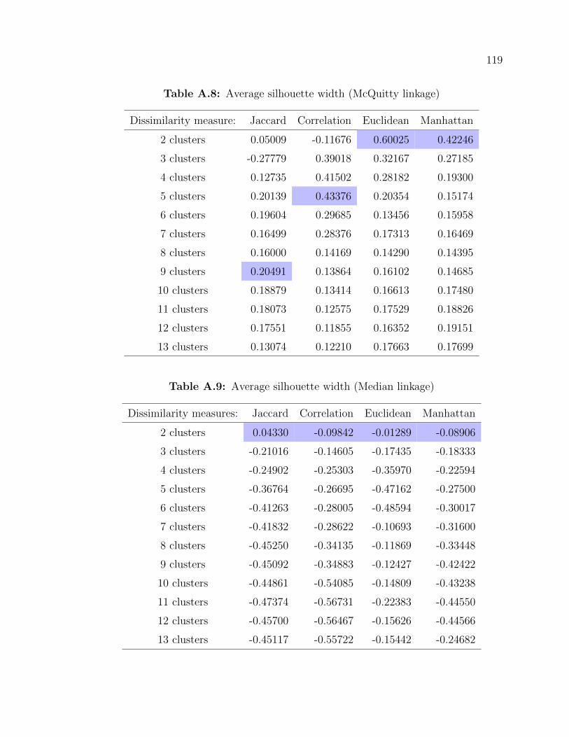
119

Table A.8: Average silhouette width (McQuitty linkage)


2 clusters 0.05009 -0.11676 0.60025 0.42246

3 clusters -0.27779 0.39018 0.32167 0.27185

4 clusters 0.12735 0.41502 0.28182 0.19300

5 clusters 0.20139 0.43376 0.20354 0.15174

6 clusters 0.19604 0.29685 0.13456 0.15958

7 clusters 0.16499 0.28376 0.17313 0.16469

8 clusters 0.16000 0.14169 0.14290 0.14395

9 clusters 0.20491 0.13864 0.16102 0.14685

10 clusters 0.18879 0.13414 0.16613 0.17480

11 clusters 0.18073 0.12575 0.17529 0.18826

12 clusters 0.17551 0.11855 0.16352 0.19151

13 clusters 0.13074 0.12210 0.17663 0.17699

Table A.9: Average silhouette width (Median linkage)


2 clusters 0.04330 -0.09842 -0.01289 -0.08906

3 clusters -0.21016 -0.14605 -0.17435 -0.18333

4 clusters -0.24902 -0.25303 -0.35970 -0.22594

5 clusters -0.36764 -0.26695 -0.47162 -0.27500

6 clusters -0.41263 -0.28005 -0.48594 -0.30017

7 clusters -0.41832 -0.28622 -0.10693 -0.31600

8 clusters -0.45250 -0.34135 -0.11869 -0.33448

9 clusters -0.45092 -0.34883 -0.12427 -0.42422

10 clusters -0.44861 -0.54085 -0.14809 -0.43238

11 clusters -0.47374 -0.56731 -0.22383 -0.44550

12 clusters -0.45700 -0.56467 -0.15626 -0.44566

13 clusters -0.45117 -0.55722 -0.15442 -0.24682

120

Hierarchical divisive algorithm

Table A.10: Average silhouette width (DIANA)


2 clusters 0.597370 0.644748 0.609299 0.499360

3 clusters 0.416263 0.408110 0.387100 0.331115

4 clusters 0.360060 0.311819 0.210122 0.250872

5 clusters 0.306176 0.285249 0.187372 0.228275

6 clusters 0.262711 0.344010 0.235396 0.192195

7 clusters 0.234393 0.281634 0.211924 0.177396

8 clusters 0.175088 0.250001 0.204579 0.153114

9 clusters 0.161649 0.234845 0.197894 0.189449

10 clusters 0.150600 0.164006 0.177885 0.181047

11 clusters 0.141803 0.173826 0.162679 0.173456

12 clusters 0.143560 0.165927 0.150109 0.168382

13 clusters 0.146571 0.163257 0.122797 0.180394

121

A.3 External indices: (k = 2)

A.3.1 Partitioning algorithms

k-means

Table A.11: Confusion matrix for the k-means procedure with the Jaccard distance

Democrat Republican Row Sum

1 19 103 122

2 105 5 110

Col Sum 124 108 232

Table A.12: Confusion matrix for the k-means procedure with the Correlationdistance


1 105 5 110

2 19 103 122

Col Sum 124 108 232

Table A.13: Confusion matrix from the k-means procedure with Euclidean distance


1 19 101 120

2 105 7 112

Col Sum 124 108 232

122

Table A.14: Confusion matrix for the k means procedure with Manhattan distance


1 19 101 120

2 105 7 112

Col Sum 124 108 232

PAM

Table A.15: Confusion matrix (PAM) with Jaccard distance


1 19 99 118

2 105 9 114

Col Sum 124 108 232

Table A.16: Confusion matrix (PAM) with Correlation distance


1 22 99 121

2 102 9 111

Col Sum 124 108 232

123

Table A.17: Confusion matrix (PAM) with Euclidean distance


1 18 96 114

2 106 12 118

Col Sum 124 108 232

Table A.18: Confusion matrix (PAM) with Manhattan distance


1 17 95 112

2 107 13 120

Col Sum 124 108 232

A.3.2 Hierarchical algorithms

Single linkage

Table A.19: Confusion matrix for single linkage with Jaccard distance


1 123 108 231

2 1 0 1

Col Sum 124 108 232

124

Table A.20: Confusion matrix for single linkage with Correlation distance


1 123 108 231

2 1 0 1

Col Sum 124 108 232

Table A.21: Confusion matrix for single linkage with Euclidean distance


1 123 108 231

2 1 0 1

Col Sum 124 108 232

Table A.22: Confusion matrix for single linkage with Manhattan distance


1 124 107 231

2 0 1 1

Col Sum 124 108 232

125

Average linkage

Table A.23: Confusion matrix for average linkage with Jaccard distance


1 20 104 124

2 104 4 108

Col Sum 124 108 232

Table A.24: Confusion matrix for average linkage with Correlation distance


1 27 104 131

2 97 4 101

Col Sum 124 108 232

Table A.25: Confusion matrix for average linkage with Euclidean distance


1 17 104 121

2 107 4 111

Col Sum 124 108 232

126

Table A.26: Confusion matrix for average linkage with Manhattan distance


1 110 6 116

2 14 102 116

Col Sum 124 108 232

Complete linkage

Table A.27: Confusion matrix for complete linkage with Jaccard distance


1 16 90 106

2 108 18 126

Col Sum 124 108 232

Table A.28: Confusion matrix for complete linkage with Correlation distance


1 22 104 126

2 102 4 106

Col Sum 124 108 232

127

Table A.29: Confusion matrix for complete linkage with Euclidean distance


1 101 5 106

2 23 103 126

Col Sum 124 108 232

Table A.30: Confusion matrix for complete linkage with Manhattan distance


1 26 104 130

2 98 4 102

Col Sum 124 108 232

Ward linkage

Table A.31: Confusion matrix for Ward linkage with Jaccard distance


1 34 104 138

2 90 4 94

Col Sum 124 108 232

128

Table A.32: Confusion matrix for Ward linkage with Correlation distance


1 13 90 103

2 111 18 129

Col Sum 124 108 232

Table A.33: Confusion matrix for ward linkage with Euclidean distance


1 20 94 114

2 104 14 118

Col Sum 124 108 232

Table A.34: Confusion matrix for ward linkage with Manhattan distance


1 19 90 109

2 105 18 123

Col Sum 124 108 232

129

Centroid linkage

Table A.35: Confusion matrix for centroid linkage with Jaccard distance


1 123 108 231

2 1 0 1

Col Sum 124 108 232

Table A.36: Confusion matrix for centroid linkage with Correlation distance


1 23 104 127

2 101 4 105

Col Sum 124 108 232

Table A.37: Confusion matrix for centroid linkage with Euclidean distance


1 22 104 126

2 102 4 106

Col Sum 124 108 232

130

Table A.38: Confusion matrix for centroid linkage (hclust) Manhattan distance


1 123 108 231

2 1 0 1

Col Sum 124 108 232

McQuitty linkage

Table A.39: Confusion matrix for McQuitty linkage with Jaccard distance


1 124 107 231

2 0 1 1

Col Sum 124 108 232

Table A.40: Confusion matrix for McQuitty linkage with Correlation distance


1 123 108 231

2 1 0 1

Col Sum 124 108 232

131

Table A.41: Confusion matrix for McQuitty linkage with Euclidean distance


1 22 104 126

2 102 4 106

Col Sum 124 108 232

Table A.42: Confusion matrix for McQuitty linkage with Manhattan distance


1 31 105 136

2 93 3 96

Col Sum 124 108 232

Median linkage

Table A.43: Confusion matrix for median linkage with Jaccard distance


1 123 108 231

2 1 0 1

Col Sum 124 108 232

132

Table A.44: Confusion matrix for median linkage with Correlation distance


1 121 103 224

2 3 5 8

Col Sum 124 108 232

Table A.45: Confusion matrix for median linkage with Euclidean distance


1 121 108 229

2 3 0 3

Col Sum 124 108 232

Table A.46: Confusion matrix for median linkage with Manhattan distance


1 124 107 231

2 0 1 1

Col Sum 124 108 232

133

DIANA

Table A.47: Confusion matrix for DIANA using Jaccard distance


1 20 103 123

2 104 5 109

Col Sum 124 108 232

Table A.48: Confusion matrix for DIANA using Correlation distance


1 20 103 123

2 104 5 109

Col Sum 124 108 232

Table A.49: Confusion matrix for DIANA using Euclidean distance


1 20 103 123

2 104 5 109

Col Sum 124 108 232

134

Table A.50: Confusion matrix for DIANA using Manhattan distance


1 22 103 125

2 102 5 107

Col Sum 124 108 232

Appendix B

Zoo: Extra

B.1 Principal Component Analysis

Table B.1: Full results of summary PCA (zoo)

PC1 PC2 PC3 PC4 PC5 PC6 PC7

Standard deviation 1.1093 0.8628 0.6837 0.5103 0.4107 0.3778 0.3386

Proportion of Variance 0.3394 0.2053 0.1289 0.0718 0.0465 0.0394 0.0316

Cumulative Proportion 0.3394 0.5446 0.6736 0.7454 0.7919 0.8312 0.8629









135

136

Table B.2: Full results of the PCA loadings (zoo)

PC1 PC2 PC3 PC4 PC5 PC6 PC7 PC8 PC9 PC10 PC11

hair -0.39060 0.12004 0.13961 0.06308 0.21318 -0.20480 -0.19134 0.03349 0.20559 -0.02690 0.11449

feathers 0.17616 0.26783 -0.34073 -0.12219 -0.03817 0.07921 -0.03547 -0.08596 -0.03748 -0.02177 -0.03207

eggs 0.41131 -0.02000 0.00944 -0.02527 -0.16735 0.28870 -0.00971 0.06311 0.18059 -0.19633 -0.22830

milk -0.42344 0.03478 -0.02133 0.00626 0.19696 -0.16773 -0.12340 0.02992 -0.12525 -0.07687 0.07807

airborne 0.18560 0.32757 -0.09621 0.07617 0.10667 -0.24958 -0.19576 0.07734 0.56109 -0.05415 -0.05419

aquatic 0.17146 -0.37562 -0.13980 -0.11410 0.11470 0.06661 -0.72737 0.10868 -0.00368 0.31092 -0.06525

predator 0.00463 -0.28754 -0.09787 -0.73800 -0.10015 -0.43061 0.08355 -0.26468 0.13954 -0.25809 -0.01970

toothed -0.32104 -0.29387 -0.12579 0.26483 -0.09009 -0.20587 -0.02150 0.03655 0.01406 -0.03499 -0.29595

backbone -0.14967 -0.02327 -0.46623 0.10357 -0.16190 -0.00385 -0.07088 0.00280 0.02769 -0.03419 -0.31761

breathes -0.15166 0.35427 -0.03345 -0.07835 -0.04424 -0.08243 0.14799 0.10363 0.08838 0.08042 -0.55882

venomous 0.04314 -0.04523 0.09972 -0.01401 -0.05117 -0.16918 0.15232 -0.24272 0.25234 0.79057 -0.11223

fins 0.06094 -0.33114 -0.16516 0.22493 0.24508 -0.01260 -0.03002 0.06595 0.21610 -0.22745 -0.05289

legs 0 0.11653 -0.38012 -0.06507 0.25695 0.11167 -0.07259 0.37965 -0.06711 0.01511 -0.02013 -0.18266

legs two 0.12951 0.31352 -0.38690 -0.03204 0.25357 -0.19264 -0.10339 -0.05567 -0.36047 0.04125 -0.02864

legs four -0.35072 0.01451 0.09670 -0.14532 -0.54217 0.30229 -0.22111 0.06581 0.09651 -0.02303 -0.09322

legs five 0.01018 -0.00821 0.02054 -0.02541 0.00163 0.00364 -0.04502 -0.01253 -0.07167 -0.00724 0.07308

legs six 0.08286 0.06790 0.30404 0.00582 0.15813 -0.04869 -0.06058 0.12807 0.37328 -0.16620 0.02530

legs eight 0.01164 -0.00760 0.03068 -0.06000 0.01718 0.00799 0.05046 -0.05858 -0.05276 0.17534 0.20615

tail -0.09557 -0.01125 -0.51175 0.11523 -0.28215 0.01678 0.17387 0.11348 0.33185 0.08583 0.55448

domestic -0.05336 0.08501 0.01162 0.25419 -0.01701 0.15407 -0.20403 -0.88172 0.10661 -0.16215 0.00673

catsize -0.27854 -0.04458 -0.18669 -0.32988 0.52617 0.59157 0.19270 -0.03448 0.21527 0.08848 -0.07125

PC12 PC13 PC14 PC15 PC16 PC17 PC18 PC19 PC20 PC21

hair -0.28409 0.17761 -0.55302 0.24780 -0.04197 0.27389 -0.20878 -0.15225 -0.07276 0.00000

feathers 0.05722 0.15561 -0.09994 -0.20268 0.49973 0.29211 -0.33538 -0.07518 0.46387 -0.00000

eggs -0.29025 -0.03021 -0.36794 0.25473 -0.27920 -0.09578 0.10534 0.28561 0.35463 -0.00000

milk 0.24429 0.14839 -0.11007 -0.12560 0.02614 -0.26689 0.25716 0.53792 0.41384 -0.00000

airborne -0.02878 0.43135 0.43077 -0.00147 -0.14853 -0.07252 0.06530 0.01734 -0.01370 0.00000

aquatic 0.26909 -0.02917 -0.09211 -0.08635 -0.17889 0.10734 -0.03835 -0.05776 -0.00154 -0.00000

predator -0.01213 -0.02105 -0.02424 0.02996 -0.03106 -0.00524 0.01719 -0.01951 -0.01916 0.00000

toothed -0.32311 -0.24598 0.33652 -0.04818 -0.18389 0.10975 -0.14250 -0.18209 0.45113 -0.00000

backbone -0.20196 -0.04471 -0.03728 -0.09051 0.14394 0.12801 -0.08398 0.51352 -0.50464 0.00000

breathes 0.55380 -0.22861 -0.13679 0.20823 -0.17376 -0.00992 -0.09458 -0.12647 -0.00447 -0.00000

venomous -0.18879 -0.04024 -0.11850 -0.00678 0.22752 -0.21161 0.08637 0.08548 0.09310 -0.00000

fins 0.13971 -0.10802 -0.00831 0.45799 0.54629 -0.27384 0.08880 -0.13963 -0.01582 -0.00000

legs 0 0.20467 0.45003 -0.21662 -0.22727 -0.14162 0.17650 0.06950 -0.07175 -0.02121 0.40825

legs two -0.26652 -0.14895 -0.08351 0.05060 -0.08725 -0.14484 0.35844 -0.24385 -0.02468 0.40825

legs four -0.02759 0.22983 0.03384 0.02218 0.19850 -0.09275 0.26492 -0.22173 0.00034 0.40825

legs five -0.02425 0.04501 0.02489 0.03054 -0.10480 -0.54231 -0.70828 0.08489 -0.03537 0.40825

legs six 0.00532 -0.51826 -0.05793 -0.42603 0.16026 0.13791 0.04463 0.11811 -0.01479 0.40825

legs eight 0.10837 -0.05766 0.29932 0.54998 -0.02510 0.46549 -0.02921 0.33433 0.09570 0.40825

tail 0.17568 -0.20701 -0.16595 -0.04017 -0.22528 -0.05790 0.02711 -0.08355 0.05435 -0.00000

domestic 0.13946 -0.10627 -0.00890 -0.00423 -0.11164 -0.00525 0.01648 -0.02510 -0.01246 0.00000

catsize -0.12374 0.01653 0.13548 -0.05981 -0.11105 -0.01513 -0.00497 -0.04739 0.00540 -0.00000

137

B.2 Internal indices: choosing the best k

Hierarchical agglomerative algorithm

Table B.3: Average silhouette width (Single linkage)


2 clusters -0.011255 -0.071248 0.307607 0.255361

3 clusters 0.008054 -0.098872 0.073210 -0.036053

4 clusters -0.006097 -0.002356 0.147047 -0.044543

5 clusters 0.092268 0.014526 0.018100 0.100568

6 clusters 0.143042 0.012731 0.350344 0.042961

7 clusters 0.167573 0.060950 0.348862 0.063452

8 clusters 0.161187 0.286253 0.403294 0.335940

9 clusters 0.175746 0.157079 0.373336 0.318598

10 clusters 0.167736 0.145538 0.376997 0.312189

11 clusters 0.363037 0.161350 0.496802 0.296980

12 clusters 0.203092 0.199740 0.446455 0.290927

13 clusters 0.219531 0.453536 0.425860 0.285540

138

Table B.4: Average silhouette width (Average method)


2 clusters 0.311000 0.338933 0.474785 0.465855

3 clusters 0.263860 0.486699 0.473855 0.444521

4 clusters 0.178742 0.371830 0.546344 0.501557

5 clusters 0.374231 0.456678 0.551143 0.512128

6 clusters 0.519517 0.512770 0.515240 0.534590

7 clusters 0.528712 0.507289 0.567933 0.512696

8 clusters 0.503056 0.508076 0.558292 0.522036

9 clusters 0.494149 0.517189 0.528869 0.496468

10 clusters 0.490231 0.507228 0.525225 0.485411

11 clusters 0.444217 0.491720 0.512013 0.514196

12 clusters 0.471593 0.487873 0.512836 0.498996

13 clusters 0.471890 0.479014 0.540896 0.506902

Table B.5: Average silhouette width (Complete method)


2 clusters 0.356333 0.385965 0.365850 0.458948

3 clusters 0.302561 0.456464 0.480052 0.412336

4 clusters 0.354882 0.516444 0.552048 0.514898

5 clusters 0.514601 0.524091 0.560227 0.423545

6 clusters 0.444703 0.504037 0.477554 0.441194

7 clusters 0.450375 0.496801 0.521009 0.451768

8 clusters 0.446749 0.516167 0.549858 0.514835

9 clusters 0.411648 0.516650 0.507856 0.497366

10 clusters 0.442132 0.488944 0.512554 0.512913

11 clusters 0.392164 0.483191 0.512588 0.491783

12 clusters 0.362645 0.483959 0.534642 0.474041

13 clusters 0.381212 0.468758 0.517745 0.457155

139

Table B.6: Average silhouette width (Ward method)


2 clusters 0.446853 0.470504 0.469085 0.470408

3 clusters 0.472595 0.473291 0.485434 0.448898

4 clusters 0.504056 0.503172 0.539921 0.506723

5 clusters 0.513815 0.502077 0.566252 0.453377

6 clusters 0.472557 0.525267 0.521873 0.494872

7 clusters 0.510166 0.486771 0.529643 0.518283

8 clusters 0.519274 0.499202 0.497858 0.504933

9 clusters 0.520801 0.505499 0.491509 0.521521

10 clusters 0.488049 0.494295 0.512894 0.531047

11 clusters 0.485953 0.469082 0.539362 0.530212

12 clusters 0.434713 0.430678 0.540941 0.513852

13 clusters 0.433337 0.436459 0.535419 0.516843

Table B.7: Average silhouette width (Centroid linkage)


2 clusters 0.107293 -0.071248 0.249778 0.220269

3 clusters 0.008054 0.021276 0.472386 0.445807

4 clusters 0.105551 0.229759 0.546043 0.501717

5 clusters 0.187936 0.456678 0.546177 0.517020

6 clusters 0.159234 0.445046 0.574022 0.399251

7 clusters 0.167573 0.368667 0.469655 0.511833

8 clusters 0.161187 0.434657 0.500147 0.456143

9 clusters 0.175746 0.454908 0.496849 0.394324

10 clusters 0.167736 0.501060 0.492806 0.414999

11 clusters 0.363037 0.468305 0.506762 0.412066

12 clusters 0.203092 0.420235 0.456416 0.411583

13 clusters 0.428491 0.383344 0.487188 0.377534

140

Table B.8: Average silhouette width (McQuitty method)


2 clusters 0.311000 0.192422 0.298814 0.356872

3 clusters 0.260312 0.297620 0.325341 0.455033

4 clusters 0.174985 0.193825 0.546043 0.514898

5 clusters 0.175368 0.425617 0.424917 0.423545

6 clusters 0.303337 0.448287 0.508299 0.428301

7 clusters 0.517056 0.458057 0.521009 0.451768

8 clusters 0.489360 0.480952 0.558292 0.514835

9 clusters 0.494016 0.502735 0.554649 0.443347

10 clusters 0.490099 0.499703 0.478929 0.422217

11 clusters 0.443268 0.472702 0.462603 0.402230

12 clusters 0.464140 0.467989 0.487640 0.374340

13 clusters 0.444844 0.464142 0.441327 0.401013

Table B.9: Average silhouette width (Median method)


2 clusters -0.011255 -0.071248 -0.102574 -0.038237

3 clusters 0.008054 -0.006528 -0.019953 -0.115617

4 clusters 0.105551 0.092502 0.074320 -0.017361

5 clusters 0.187936 0.313307 0.275424 0.122606

6 clusters 0.159234 0.310697 0.277862 0.383590

7 clusters 0.167573 0.495511 0.200048 0.363591

8 clusters 0.161187 0.422108 0.314293 0.311004

9 clusters 0.175746 0.374840 0.308356 0.358080

10 clusters 0.167736 0.348628 0.350880 0.334398

11 clusters 0.363037 0.396484 0.340081 0.390463

12 clusters 0.203092 0.400295 0.293767 0.412357

13 clusters 0.083162 0.388754 0.297224 0.411839

141

Hierarchical divisive algorithm

Table B.10: Average silhouette width (DIANA)


2 clusters 0.311000 0.253730 0.311355 0.343493

3 clusters 0.334215 0.300876 0.313602 0.464166

4 clusters 0.258671 0.526947 0.558005 0.520698

5 clusters 0.305535 0.477210 0.547286 0.526577

6 clusters 0.544081 0.520816 0.538016 0.462533

7 clusters 0.447373 0.439974 0.486727 0.411236

8 clusters 0.456567 0.453500 0.472258 0.403478

9 clusters 0.469736 0.479208 0.444191 0.443919

10 clusters 0.460829 0.483134 0.456858 0.455089

11 clusters 0.458164 0.484239 0.444523 0.464820

12 clusters 0.489868 0.496578 0.442110 0.468176

13 clusters 0.484353 0.481376 0.488230 0.496427

142

B.3 External indices: (k = 7)

B.3.1 Partitioning algorithms

k-means

Table B.11: Confusion matrix from the k-means procedure with Jaccard distance

“Class”Actual

Row Sum1 2 3 4 5 6 7

1 31 0 0 0 0 0 0 31

2 0 0 0 0 0 0 7 7

3 0 0 4 0 3 0 1 8

4 2 0 1 13 0 0 0 16

5 0 20 0 0 0 0 0 20

6 8 0 0 0 0 0 0 8

7 0 0 0 0 0 8 2 10

Col Sum 41 20 5 13 3 8 10 100

143

Table B.12: Confusion matrix from the k-means with Correlation distance

“Class”Actual

Row Sum1 2 3 4 5 6 7

1 0 0 4 0 3 0 1 8

2 0 0 0 0 0 0 7 7

3 0 20 0 0 0 0 0 20

4 31 0 0 0 0 0 0 31

5 8 0 0 0 0 0 0 8

6 2 0 1 13 0 0 0 16

7 0 0 0 0 0 8 2 10

Col Sum 41 20 5 13 3 8 10 100

Table B.13: Confusion matrix from the k-means with Euclidean distance

“Class”Actual

Row Sum1 2 3 4 5 6 7

1 0 20 0 0 0 0 0 20

2 0 0 0 0 0 0 8 8

3 0 0 0 0 0 8 2 10

4 0 0 1 13 0 0 0 14

5 19 0 0 0 0 0 0 19

6 18 0 0 0 0 0 0 18

7 4 0 4 0 3 0 0 11

Col Sum 41 20 5 13 3 8 10 100

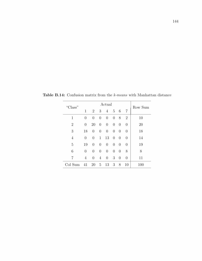
144

Table B.14: Confusion matrix from the k-means with Manhattan distance

“Class”Actual

Row Sum1 2 3 4 5 6 7

1 0 0 0 0 0 8 2 10

2 0 20 0 0 0 0 0 20

3 18 0 0 0 0 0 0 18

4 0 0 1 13 0 0 0 14

5 19 0 0 0 0 0 0 19

6 0 0 0 0 0 0 8 8

7 4 0 4 0 3 0 0 11

Col Sum 41 20 5 13 3 8 10 100

145

PAM

Table B.15: Confusion matrix (PAM) with the Jaccard distance

“Class”Actual

Row Sum1 2 3 4 5 6 7

1 20 0 0 0 0 0 0 20

2 19 0 0 0 0 0 0 19

3 2 0 1 13 0 0 0 16

4 0 20 0 0 0 0 0 20

5 0 0 0 0 0 0 7 7

6 0 0 0 0 0 8 2 10

7 0 0 4 0 3 0 1 8

Col Sum 41 20 5 13 3 8 10 100

146

Table B.16: Confusion matrix (PAM) with Correlation distance

“Class”Actual

Row Sum1 2 3 4 5 6 7

1 20 0 0 0 0 0 0 20

2 19 0 0 0 0 0 0 19

3 2 0 1 13 0 0 1 17

4 0 20 0 0 0 0 0 20

5 0 0 0 0 0 0 6 6

6 0 0 0 0 0 8 2 10

7 0 0 4 0 3 0 1 8

Col Sum 41 20 5 13 3 8 10 100

Table B.17: Confusion matrix (PAM) Euclidean distance

“Class”Actual

Row Sum1 2 3 4 5 6 7

1 19 0 0 0 0 0 0 19

2 19 0 0 0 0 0 0 19

3 0 0 1 13 0 0 0 14

4 0 20 0 0 0 0 0 20

5 0 0 0 0 0 0 7 7

6 3 0 4 0 3 0 1 11

7 0 0 0 0 0 8 2 10

Col Sum 41 20 5 13 3 8 10 100

147

Table B.18: Confusion matrix (PAM) Manhattan distance

“Class”Actual

Row Sum1 2 3 4 5 6 7

1 18 0 0 0 0 0 0 18

2 19 0 0 0 0 0 0 19

3 0 0 1 13 0 0 0 14

4 0 20 0 0 0 0 0 20

5 0 0 0 0 0 0 7 7

6 4 0 4 0 3 0 1 12

7 0 0 0 0 0 8 2 10

Col Sum 41 20 5 13 3 8 10 100

B.3.2 Hierarchical algorithms

Single linkage

Table B.19: Confusion matrix for single linkage with Jaccard distance

“Class”Actual

Row Sum1 2 3 4 5 6 7

1 41 20 5 13 3 0 0 82

2 0 0 0 0 0 0 2 2

3 0 0 0 0 0 0 4 4

4 0 0 0 0 0 8 0 8

5 0 0 0 0 0 0 1 1

6 0 0 0 0 0 0 1 1

7 0 0 0 0 0 0 2 2

Col Sum 41 20 5 13 3 8 10 100

148

Table B.20: Confusion matrix for single linkage with Correlation distance

“Class”Actual

Row Sum1 2 3 4 5 6 7

1 41 20 5 13 3 0 0 82

2 0 0 0 0 0 0 2 2

3 0 0 0 0 0 0 4 4

4 0 0 0 0 0 8 0 8

5 0 0 0 0 0 0 1 1

6 0 0 0 0 0 0 1 1

7 0 0 0 0 0 0 2 2

Col Sum 41 20 5 13 3 8 10 100

Table B.21: Confusion matrix for single linkage with Euclidean distance

“Class”Actual

Row Sum1 2 3 4 5 6 7

1 36 0 0 0 0 0 0 36

2 0 0 5 13 3 0 8 29

3 0 20 0 0 0 0 0 20

4 3 0 0 0 0 0 0 3

5 0 0 0 0 0 8 2 10

6 1 0 0 0 0 0 0 1

7 1 0 0 0 0 0 0 1

Col Sum 41 20 5 13 3 8 10 100

149

Table B.22: Confusion matrix for single linkage with Manhattan distance

“Class”Actual

Row Sum1 2 3 4 5 6 7

1 36 0 5 13 3 0 1 58

2 0 20 0 0 0 0 0 20

3 0 0 0 0 0 0 7 7

4 3 0 0 0 0 0 0 3

5 0 0 0 0 0 8 2 10

6 1 0 0 0 0 0 0 1

7 1 0 0 0 0 0 0 1

Col Sum 41 20 5 13 3 8 10 100

150

Average linkage

Table B.23: Confusion matrix for Average linkage with Jaccard distance

“Class”Actual

Row Sum1 2 3 4 5 6 7

1 37 0 2 0 3 0 0 42

2 4 0 3 13 0 0 0 20

3 0 20 0 0 0 0 0 20

4 0 0 0 0 0 0 7 7

5 0 0 0 0 0 8 0 8

6 0 0 0 0 0 0 1 1

7 0 0 0 0 0 0 2 2

Col Sum 41 20 5 13 3 8 10 100

151

Table B.24: Confusion matrix for Average linkage with Correlation distance

“Class”Actual

Row Sum1 2 3 4 5 6 7

1 37 0 1 0 0 0 0 38

2 4 0 1 13 0 0 0 18

3 0 20 0 0 0 0 0 20

4 0 0 0 0 0 0 7 7

5 0 0 0 0 0 8 2 10

6 0 0 3 0 3 0 0 6

7 0 0 0 0 0 0 1 1

Col Sum 41 20 5 13 3 8 10 100

Table B.25: Confusion matrix for Average linkage with Euclidean distance

“Class”Actual

Row Sum1 2 3 4 5 6 7

1 37 0 0 0 0 0 0 37

2 0 0 1 13 0 0 0 14

3 0 20 0 0 0 0 0 20

4 0 0 0 0 0 0 7 7

5 4 0 0 0 0 0 0 4

6 0 0 0 0 0 8 2 10

7 0 0 4 0 3 0 1 8

Col Sum 41 20 5 13 3 8 10 100

152

Table B.26: Confusion matrix for Average linkage with Manhattan distance

“Class”Actual

Row Sum1 2 3 4 5 6 7

1 34 0 0 0 0 0 0 34

2 0 0 0 13 0 0 0 13

3 0 20 0 0 0 0 0 20

4 0 0 0 0 0 0 7 7

5 4 0 5 0 3 0 1 13

6 0 0 0 0 0 8 2 10

7 3 0 0 0 0 0 0 3

Col Sum 41 20 5 13 3 8 10 100

153

Complete linkage

Table B.27: Confusion matrix for Complete linkage with Jaccard distance

“Class”Actual

Row Sum1 2 3 4 5 6 7

1 36 0 0 0 0 0 0 36

2 4 0 3 13 0 0 0 20

3 0 20 0 0 0 0 0 20

4 0 0 0 0 0 0 7 7

5 0 0 0 0 0 8 2 10

6 1 0 2 0 3 0 0 6

7 0 0 0 0 0 0 1 1

Col Sum 41 20 5 13 3 8 10 100

154

Table B.28: Confusion matrix for Complete linkage with Correlation distance

“Class”Actual

Row Sum1 2 3 4 5 6 7

1 36 0 0 0 0 0 0 36

2 4 0 3 13 0 0 0 20

3 0 20 0 0 0 0 0 20

4 0 0 0 0 0 0 7 7

5 0 0 0 0 0 8 2 10

6 1 0 2 0 3 0 0 6

7 0 0 0 0 0 0 1 1

Col Sum 41 20 5 13 3 8 10 100

Table B.29: Confusion matrix for Complete linkage with Euclidean distance

“Class”Actual

Row Sum1 2 3 4 5 6 7

1 22 0 0 0 0 0 0 22

2 19 0 0 0 0 0 0 19

3 0 0 1 13 0 0 0 14

4 0 20 0 0 0 0 0 20

5 0 0 0 0 0 0 7 7

6 0 0 0 0 0 8 2 10

7 0 0 4 0 3 0 1 8

Col Sum 41 20 5 13 3 8 10 100

155

Table B.30: Confusion matrix for Complete linkage with Manhattan distance

“Class”Actual

Row Sum1 2 3 4 5 6 7

1 18 0 2 0 3 0 1 24

2 19 0 0 0 0 0 0 19

3 0 0 3 13 0 0 0 16

4 0 20 0 0 0 0 0 20

5 0 0 0 0 0 0 7 7

6 4 0 0 0 0 0 0 4

7 0 0 0 0 0 8 2 10

Col Sum 41 20 5 13 3 8 10 100

156

Ward linkage

Table B.31: Confusion matrix for Ward linkage with Jaccard distance

“Class”Actual

Row Sum1 2 3 4 5 6 7

1 30 0 0 0 0 0 0 30

2 0 0 0 13 0 0 0 13

3 0 20 0 0 0 0 0 20

4 0 0 0 0 0 0 7 7

5 10 0 0 0 0 0 0 10

6 0 0 0 0 0 8 2 10

7 1 0 5 0 3 0 1 10

Col Sum 41 20 5 13 3 8 10 100

157

Table B.32: Confusion matrix for Ward linkage with Correlation distance

“Class”Actual

Row Sum1 2 3 4 5 6 7

1 30 0 0 0 0 0 0 30

2 0 0 0 13 0 0 0 13

3 0 20 0 0 0 0 0 20

4 0 0 0 0 0 0 7 7

5 10 0 0 0 0 0 0 10

6 0 0 0 0 0 8 0 8

7 1 0 5 0 3 0 3 12

Col Sum 41 20 5 13 3 8 10 100

Table B.33: Confusion matrix for Ward linkage with Euclidean distance

“Class”Actual

Row Sum1 2 3 4 5 6 7

1 18 0 0 0 0 0 0 18

2 18 0 0 0 0 0 0 18

3 0 0 1 13 0 0 0 14

4 0 20 0 0 0 0 0 20

5 0 0 0 0 0 0 7 7

6 5 0 4 0 3 0 1 13

7 0 0 0 0 0 8 2 10

Col Sum 41 20 5 13 3 8 10 100

158

Table B.34: Confusion matrix for Ward linkage with Manhattan distance

“Class”Actual

Row Sum1 2 3 4 5 6 7

1 19 0 0 0 0 0 0 19

2 19 0 0 0 0 0 0 19

3 0 0 0 13 0 0 0 13

4 0 20 0 0 0 0 0 20

5 0 0 0 0 0 0 7 7

6 3 0 5 0 3 0 1 12

7 0 0 0 0 0 8 2 10

Col Sum 41 20 5 13 3 8 10 100

159

Centroid linkage

Table B.35: Confusion matrix for Centroid linkage with Jaccard distance

“Class”Actual

Row Sum1 2 3 4 5 6 7

class 1 41 20 5 13 3 0 0 82

2 0 0 0 0 0 0 2 2

3 0 0 0 0 0 0 4 4

4 0 0 0 0 0 8 0 8

5 0 0 0 0 0 0 1 1

6 0 0 0 0 0 0 1 1

7 0 0 0 0 0 0 2 2

Col Sum 41 20 5 13 3 8 10 100

160

Table B.36: Confusion matrix for Centroid linkage with Correlation distance

“Class”Actual

Row Sum1 2 3 4 5 6 7

1 37 0 0 0 0 0 0 37

2 4 0 4 13 3 0 7 31

3 0 20 0 0 0 0 0 20

4 0 0 0 0 0 8 0 8

5 0 0 0 0 0 0 1 1

6 0 0 0 0 0 0 2 2

7 0 0 1 0 0 0 0 1

Col Sum 41 20 5 13 3 8 10 100

Table B.37: Confusion matrix for Centroid linkage with Euclidean distance

“Class”Actual

Row Sum1 2 3 4 5 6 7

1 36 0 0 0 0 0 0 36

2 0 0 1 13 0 0 0 14

3 0 20 0 0 0 0 0 20

4 0 0 0 0 0 0 7 7

5 4 0 4 0 3 0 1 12

6 0 0 0 0 0 8 2 10

7 1 0 0 0 0 0 0 1

Col Sum 41 20 5 13 3 8 10 100

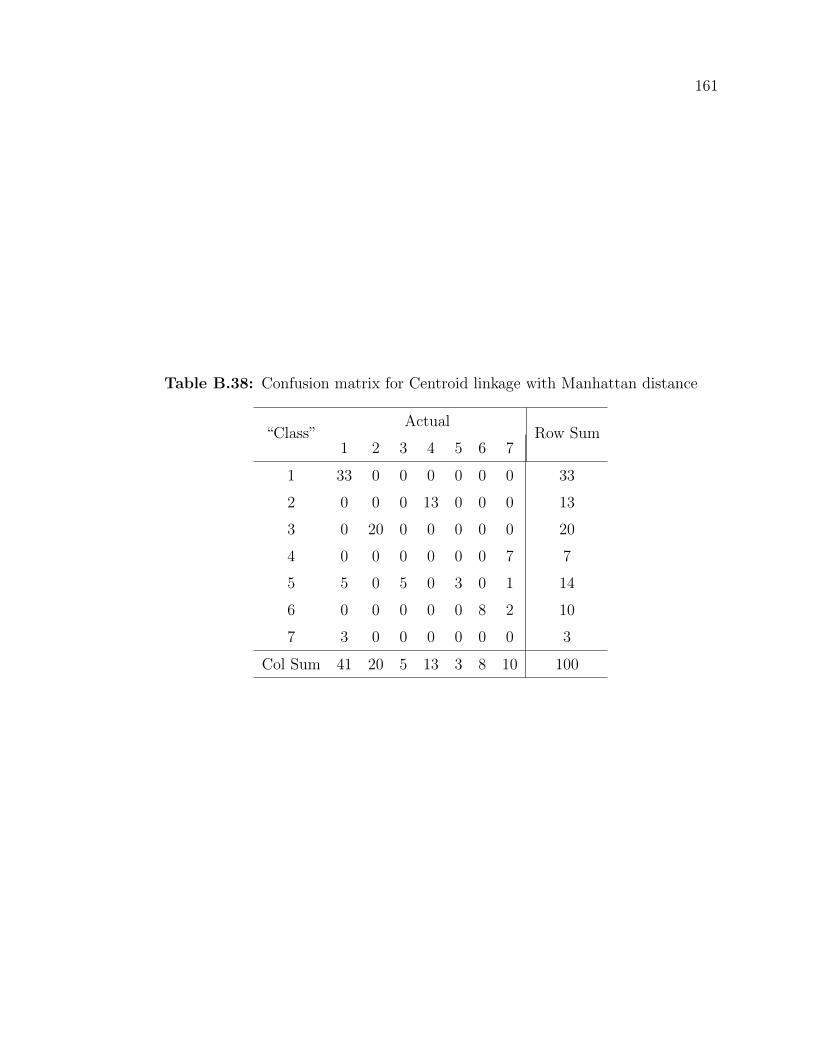
161

Table B.38: Confusion matrix for Centroid linkage with Manhattan distance

“Class”Actual

Row Sum1 2 3 4 5 6 7

1 33 0 0 0 0 0 0 33

2 0 0 0 13 0 0 0 13

3 0 20 0 0 0 0 0 20

4 0 0 0 0 0 0 7 7

5 5 0 5 0 3 0 1 14

6 0 0 0 0 0 8 2 10

7 3 0 0 0 0 0 0 3

Col Sum 41 20 5 13 3 8 10 100

162

McQuitty linkage

Table B.39: Confusion matrix for McQuitty linkage with Jaccard distance

“Class”Actual

Row Sum1 2 3 4 5 6 7

1 41 0 0 0 0 0 0 41

2 0 0 3 13 0 0 0 16

3 0 20 2 0 3 0 0 25

4 0 0 0 0 0 0 4 4

5 0 0 0 0 0 0 5 5

6 0 0 0 0 0 8 0 8

7 0 0 0 0 0 0 1 1

Col Sum 41 20 5 13 3 8 10 100

163

Table B.40: Confusion matrix for McQuitty linkage with Correlation distance

“Class”Actual

Row Sum1 2 3 4 5 6 7

1 40 0 0 0 0 0 0 40

2 0 0 3 13 0 0 4 20

3 0 20 0 0 0 0 0 20

4 0 0 0 0 0 0 5 5

5 0 0 0 0 0 8 0 8

6 1 0 2 0 3 0 0 6

7 0 0 0 0 0 0 1 1

Col Sum 41 20 5 13 3 8 10 100

Table B.41: Confusion matrix for McQuitty linkage with Euclidean distance

“Class”Actual

Row Sum1 2 3 4 5 6 7

1 22 0 0 0 0 0 0 22

2 19 0 0 0 0 0 0 19

3 0 0 1 13 0 0 0 14

4 0 20 0 0 0 0 0 20

5 0 0 0 0 0 0 7 7

6 0 0 0 0 0 8 2 10

7 0 0 4 0 3 0 1 8

Col Sum 41 20 5 13 3 8 10 100

164

Table B.42: Confusion matrix for McQuitty linkage with Manhattan distance

“Class”Actual

Row Sum1 2 3 4 5 6 7

1 18 0 2 0 3 0 1 24

2 19 0 0 0 0 0 0 19

3 0 0 3 13 0 0 0 16

4 0 20 0 0 0 0 0 20

5 0 0 0 0 0 0 7 7

6 4 0 0 0 0 0 0 4

7 0 0 0 0 0 8 2 10

Col Sum 41 20 5 13 3 8 10 100

165

Median linkage

Table B.43: Confusion matrix for Median linkage with Jaccard distance

“Class”Actual

Row Sum1 2 3 4 5 6 7

1 41 20 5 13 3 0 0 82

2 0 0 0 0 0 0 2 2

3 0 0 0 0 0 0 4 4

4 0 0 0 0 0 8 0 8

5 0 0 0 0 0 0 1 1

6 0 0 0 0 0 0 1 1

7 0 0 0 0 0 0 2 2

Col Sum 41 20 5 13 3 8 10 100

166

Table B.44: Confusion matrix for Median linkage with Correlation distance

“Class”Actual

Row Sum1 2 3 4 5 6 7

1 40 0 0 0 0 0 0 40

2 1 0 5 13 3 0 0 22

3 0 20 0 0 0 0 0 20

4 0 0 0 0 0 0 7 7

5 0 0 0 0 0 8 0 8

6 0 0 0 0 0 0 1 1

7 0 0 0 0 0 0 2 2

Col Sum 41 20 5 13 3 8 10 100

Table B.45: Confusion matrix for Median linkage with Euclidean distance

“Class”Actual

Row Sum1 2 3 4 5 6 7

1 40 0 4 0 3 0 1 48

2 0 0 1 13 0 0 0 14

3 1 0 0 0 0 0 0 1

4 0 17 0 0 0 0 0 17

5 0 0 0 0 0 0 7 7

6 0 0 0 0 0 8 2 10

7 0 3 0 0 0 0 0 3

Col Sum 41 20 5 13 3 8 10 100

167

Table B.46: Confusion matrix for Median linkage with Manhattan distance

“Class”Actual

Row Sum1 2 3 4 5 6 7

1 34 0 0 0 0 0 0 34

2 3 0 5 13 3 0 0 24

3 1 0 0 0 0 0 0 1

4 0 8 0 0 0 0 0 8

5 0 0 0 0 0 8 10 18

6 0 12 0 0 0 0 0 12

7 3 0 0 0 0 0 0 3

Col Sum 41 20 5 13 3 8 10 100

DIANA linkage

Table B.47: Confusion matrix for DIANA with Jaccard distance

“Class”Actual

Row Sum1 2 3 4 5 6 7

1 38 0 0 0 0 0 0 38

2 3 0 4 13 3 0 0 23

3 0 20 0 0 0 0 0 20

4 0 0 0 0 0 0 7 7

5 0 0 0 0 0 8 2 10

6 0 0 0 0 0 0 1 1

7 0 0 1 0 0 0 0 1

Col Sum 41 20 5 13 3 8 10 100

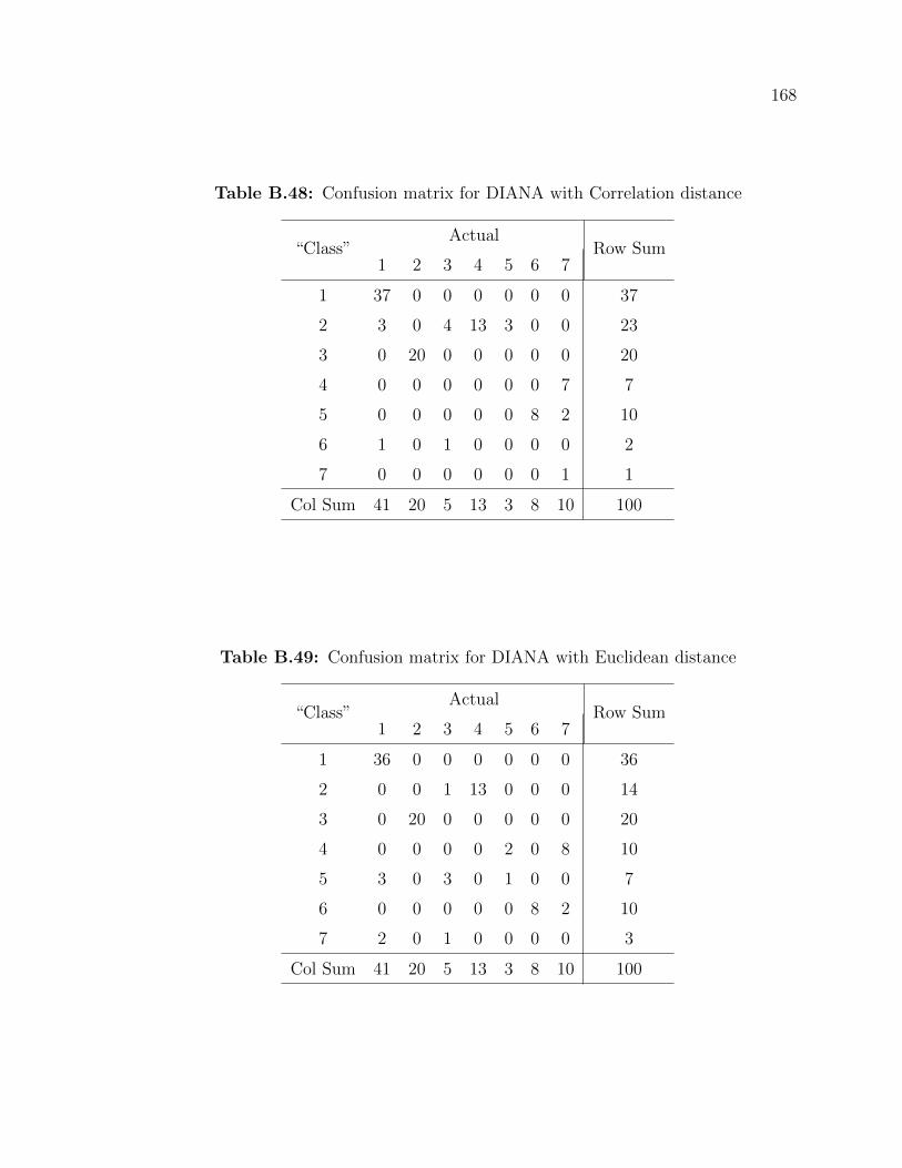
168

Table B.48: Confusion matrix for DIANA with Correlation distance

“Class”Actual

Row Sum1 2 3 4 5 6 7

1 37 0 0 0 0 0 0 37

2 3 0 4 13 3 0 0 23

3 0 20 0 0 0 0 0 20

4 0 0 0 0 0 0 7 7

5 0 0 0 0 0 8 2 10

6 1 0 1 0 0 0 0 2

7 0 0 0 0 0 0 1 1

Col Sum 41 20 5 13 3 8 10 100

Table B.49: Confusion matrix for DIANA with Euclidean distance

“Class”Actual

Row Sum1 2 3 4 5 6 7

1 36 0 0 0 0 0 0 36

2 0 0 1 13 0 0 0 14

3 0 20 0 0 0 0 0 20

4 0 0 0 0 2 0 8 10

5 3 0 3 0 1 0 0 7

6 0 0 0 0 0 8 2 10

7 2 0 1 0 0 0 0 3

Col Sum 41 20 5 13 3 8 10 100

169

Table B.50: Confusion matrix for DIANA with Manhattan distance

“Class”Actual

Row Sum1 2 3 4 5 6 7

1 20 0 1 0 0 0 0 21

2 19 0 1 0 0 0 0 20

3 2 0 1 13 0 0 0 16

4 0 20 0 0 0 0 0 20

5 0 0 2 0 2 0 8 12

6 0 0 0 0 0 8 2 10

7 0 0 0 0 1 0 0 1

Col Sum 41 20 5 13 3 8 10 100

Appendix C

Residual Analysis for Experimental

Design

Figure C.1: Residual analysis using “best” k response variable

170

171

Figure C.2: Residual analysis using ASW response variable

List of References

[1] Kardi Teknomo. Tutorial on Decision Tree, 2009. URL: http:// people.revoledu.com/

kardi/ tutorial/decisiontree/, (2009) retrieved: May 2014.

[2] Congressional Quarterly Almanac. 98th Congress, Voters Congressional Quarterly

Almanac. volume 40, Washington, D.C., 1984. Congressional Quarterly Inc.

[3] K. Bache and M. Lichman. UCI Machine Learning Repository.

http://archive.ics.uci.edu/ ml, 2013. University of California, Irvine, School of

Information and Computer Sciences.

[4] Richard M Forsyth. Neural learning algorithms: some empirical trials. In IEE Collo-

quium on Machine Learning, pages 8/1 – 8/7, London, UK, 1990. IET.

[5] Kurt Hornik. The R FAQ. URL: http://CRAN.R-project.org/doc/FAQ/R-FAQ.html,

(2013) retrieved: February 2014.

[6] SAS Institute. SAS/Graph 9. 3: Reference. SAS Institute, 2011.

[7] Paul Jaccard. Nouvelles recherches sur la distribution florale. Bulletin Soc. Vaudoise

Sci. Nat, 44:223–270, 1908.

[8] Jerome Kaltenhauser and Yuk Lee. Correlation coefficients for binary data in factor

analysis. Geographical Analysis, 8(3):305–313, 1976.

[9] Seung-Seok Choi, Sung-Hyuk Cha, and Charles C Tappert. A survey of binary similar-

ity and distance measures. Journal of Systemics, Cybernetics & Informatics, 8(1):43–

48, 2010.

[10] Halina Frydman, Edward I Altman, and DUEN-LI KAO. Introducing recursive parti-

tioning for financial classification: the case of financial distress. The Journal of Finance,

40(1):269–291, 1985.

[11] Heping Zhang, Chang-Yung Yu, Burton Singer, and Momiao Xiong. Recursive parti-

tioning for tumor classification with gene expression microarray data. Proceedings of

the National Academy of Sciences, 98(12):6730–6735, 2001.

172

173

[12] Hongjun Lu, Rudy Setiono, and Huan Liu. Effective data mining using neural networks.

IEEE Transactions on Knowledge and Data Engineering, 8(6):957–961, 1996.

[13] John Ross Quinlan. C4.5: Programs for machine learning, volume 1. Morgan Kauf-

mann, 1993.

[14] Rizwan Iqbal, Masrah Azrifah Azmi Murad, Aida Mustapha, Payam Hassany Shariat

Panahy, and Nasim Khanahmadliravi. An experimental study of classification algo-

rithms for crime prediction. Indian Journal of Science and Technology, 6(3):4219–4225,

2013.

[15] D Ashok Kumar and MLC Annie. Clustering dichotomous data for health care. Inter-

national Journal of Information Sciences and Techniques (IJIST), 2(2):23–33, 2012.

[16] Ian H Witten and Bruce A MacDonald. Using concept learning for knowledge acqui-

sition. International Journal of Man-Machine Studies, 29(2):171–196, 1988.

[17] Tao Li. A general model for clustering binary data. Proceedings of the Eleventh ACM

SIGKDD International Conference on Knowledge Discovery in Data Mining, pages

188–197, 2005.

[18] Tao Li, Sheng Ma, and Mitsunori Ogihara. Entropy-based criterion in categorical

clustering. In ICML, volume 4, pages 536–543, 2004.

[19] Stephen Hands and Brian Everitt. A Monte Carlo study of the recovery of cluster

structure in binary data by hierarchical clustering techniques. Multivariate Behavioral

Research, 22(2):235–243, 1987.

[20] Tengke Xiong, Shengrui Wang, Andre Mayers, and Ernest Monga. Dhcc: Divisive

hierarchical clustering of categorical data. Data Mining and Knowledge Discovery,

24(1):pages 103–135, 2012.

[21] Huynh V. San, O.M. and Y. Nakamori. An alternative extension of the k-means

algoirthm for clustering categorical data. International Journal of Applied Mathematics

and Computer Science, 14(2):241–247, 2004.

[22] Daniel Barbara, Yi Li, and Julia Couto. Coolcat: an entropy-based algorithm for

categorical clustering. In Proceedings of the eleventh international conference on In-

formation and knowledge management, pages 582–589. ACM, 2002.

[23] Guojun Gan and Jianhong Wu. Subspace clustering for high dimensional categorical

data. ACM SIGKDD Explorations Newsletter, 6(2):87–94, 2004.

[24] Gehrke J. Ganti, V. and R. Ramakrishnan. Cactus: Clustering categorical data using

summaries. ACM SIGKDD, 1999.

174

[25] Manco G. Cesario, E. and R. Ortale. Top-down parameter-free clustering of high

dimensional categorical data. Knowledge and Data Engineering, IEEE Transactions

on, 19(12):1607–1624, 2007.

[26] Zdenek Hubalek. Coefficients of association and similarity, based on binary (presence-

absence) data: an evaluation. Biological Reviews, 57(4):669–689, 1982.

[27] Matthijs J Warrens. On association coefficients for 2� 2 tables and properties that do

not depend on the marginal distributions. Psychometrika, 73(4):777–789, 2008.

[28] Bin Zhang and Sargur N Srihari. Binary vector dissimilarity measures for handwriting

identification. In Electronic Imaging 2003, pages 28–38. International Society for Optics

and Photonics, 2003.

[29] Holmes Finch. Comparison of distance measures in cluster analysis with dichotomous

data. Journal of Data Science, 3(1):85–100, 2005.

[30] Ian Jolliffe. Principal Component Analysis. Wiley Online Library, 2005.

[31] John C Gower. Some distance properties of latent root and vector methods used in

multivariate analysis. Biometrika, 53(3-4):325–338, 1966.

[32] D.R. Cox. The analysis of multivariate binary data. Journal of Applied Stastistics,

21:113–120, 1972.

[33] P Bloomfield. Linear transformations for multivariate binary data. Biometrics, pages

609–617, 1974.

[34] Pang-Ning Tan, Michael Steinbach, and Vipin Kumar. Introduction to Data Mining.

Pearson Education India, 2007.

[35] Erendira Rendon, Itzel Abundez, Alejandra Arizmendi, and Elvia M Quiroz. Internal

versus external cluster validation indexes. International Journal of computers and

communications, 5(1):27–34, 2011.

[36] Lior Rokach and Oded Maimon. Clustering Methods. In Data Mining and Knowledge

Discovery Handbook, pages 321–352. Springer, 2005.

[37] Sinan Saracli, Nurhan Dogan, and Ismet Dogan. Comparison of hierarchical cluster

analysis methods by cophenetic correlation. Journal of Inequalities and Applications,

2013(1):1–8, 2013.

[38] Richard Arnold Johnson and Dean W Wichern. Applied Multivariate Statistical Anal-

ysis. Prentice hall Upper Saddle River, NJ, 5th edition.

[39] Leo Breiman, Jerome H Friedman, Richard A Olshen, and Charles J Stone. Classifi-

cation and Regression Trees. 1984.

175

[40] Jerome Friedman, Trevor Hastie, and Robert Tibshirani. The Elements of Statistical

Learning. Number 1. Springer, 2nd edition, 2009.

[41] Igor Kononenko. Comparison of inductive and naive bayesian learning approaches to

automatic knowledge acquisition. Current Trends in Knowledge Adquisition, pages

190–197, 1990.

[42] S Mills. Data mining lecture notes, 2011. Course notes STAT5703.

[43] P Indira Priya and DK Ghosh. A survey on different clustering algorithms in data

mining technique.

[44] J. A. Hartigan and M. A. Wong. Algorithm: A K-Means clustering algorithm. Journal

of the Royal Statistical Society. Series C (Applied Statistics), 28(1):100–108, 1979.

[45] L Rousseeuw Kaufman and P Rousseeuw. PJ (1990) Finding groups in data: An

introduction to cluster analysis. page 341.

[46] Laura Ferreira and David B Hitchcock. A comparison of hierarchical methods for clus-

tering functional data. Communications in Statistics: Simulation and Computation,

38(9):1925–1949, 2009.

[47] Erik Aart Mooi and Marko Sarstedt. A Concise Guide to Market Research: The

process, data, and methods using IBM SPSS statistics. Springer, 2011.

[48] PS Nagpaul. Guide to advanced data analysis using idams software. Retrieved online

from: www. unesco. org/webworld/idams/advguide/TOC. htm, retrieved: April 2014.

[49] Dr. C. Bennell. Personal conversation, 2013.

[50] Peter J Rousseeuw. Silhouettes: a graphical aid to the interpretation and validation of

cluster analysis. Journal of computational and applied mathematics, 20:53–65, 1987.

[51] Robert R Sokal. The comparison of dendrograms by objective methods. Taxon, 11:33–

40, 1962.

[52] David B Duncan. Multiple range and multiple f tests. Biometrics, 11(1):1–42, 1955.

Empirical study of performance of classification and clustering ...

Documents

Transcript of Empirical study of performance of classification and clustering ...