arX

iv:1

008.

3229

v1 [

mat

h.ST

] 1

9 A

ug 2

010

Empirical likelihood based confidence regions forfirst order parameters of heavy-tailed

distributions

Julien Worms(1) & Rym Worms (2)

(1) Universite de Versailles-Saint-Quantin-En-YvelinesLaboratoire de Mathematiques de Versailles (CNRS UMR 8100),

UFR de Sciences, Bat. Fermat,45 av. des Etats-Unis, 78035 Versailles Cedex,

e-mail : worms@math.uvsq.fr

(2) Universite Paris-Est-CreteilLaboratoire d’Analyse et de Mathematiques Appliquees (CNRS UMR

8050),61 av. du General de Gaulle, 94010 Creteil cedex,

e-mail : rym.worms@u-pec.fr

AMS Classification. Primary 62G32 ; Secondary 62G15.

Keywords and phrases. Extreme values. Generalized Pareto Distribution. Confidenceregions. Empirical Likelihood. Profile empirical likelihood.

Abstract

Let X1, . . . , Xn be some i.i.d. observations from a heavy tailed distributionF , i.e. such that the common distribution of the excesses over a high thresholdun can be approximated by a Generalized Pareto Distribution Gγ,σn with γ > 0.This paper deals with the problem of finding confidence regions for the couple(γ, σn) : combining the empirical likelihood methodology with estimation equa-tions (close but not identical to the likelihood equations) introduced by J. Zhang(2007), asymptotically valid confidence regions for (γ, σn) are obtained and provedto perform better than Wald-type confidence regions (especially those derived fromthe asymptotic normality of the maximum likelihood estimators). By profiling outthe scale parameter, confidence intervals for the tail index are also derived.

1. Introduction

In statistical extreme value theory, one is often interested by the estimation of the so-called tail index γ = γ(F ) of the underlying model F of some i.i.d. sample (X1, . . . , Xn),which is the shape parameter of the Generalized Pareto Distribution (GPD) with distri-bution function (d.f.)

Gγ,σ(x) =

1−(

1 + γxσ

)− 1γ

, for γ 6= 0

1− exp(

− xσ

)

, for γ = 0.

1

The GPD appears as the limiting d.f. of excesses over a high threshold u defined forx ≥ 0 by

Fu(x) := P(X − u ≤ x |X > u), where X has d.f. F .

It was established in J. Pickands (1975) and A. Balkema and L. de Haan (1974) thatF is in the domain of attraction of an extreme value distribution with shape parameterγ if and only if

limu→s+(F )

sup0<x<s+(F )−u

∣

∣

∣Fu(x)−Gγ,σ(u)(x)∣

∣

∣ = 0 (1)

for some positive scaling function σ(·), where s+(F ) = sup{x : F (x) < 1}. This suggeststo model the d.f. of excesses over a high threshold by a GPD. This is the P.O.T method.

Some estimation methods for the couple (γ, σ) in the GPD parametrization have beenproposed. We can cite the maximum likelihood (ML) estimators of R. L. Smith (1987)or the probability weighted moments (PWM) estimators of J. Hosking and J. Wallis(1987). In J. Zhang (2007), the author proposed new estimators based on estimatingequations close to the likelihood equations. Using the reparametrization b = −γ/σ andconsidering X1, . . . , Xn i.i.d. variables with distribution Gγ,σ with σ a fixed value (whichis an important restriction if the aim is to prove asymptotic results), he based his methodon one of the likelihood equations

γ = − 1

n

n∑

i=1

log(1− bXi) (2)

and on the empirical version of the moment equation E((1 − bX1)r) = 1

1−rγ , i.e.

1

n

n∑

i=1

(1− bXi)r − 1

1− rγ= 0

or1

n

n∑

i=1

(1− bXi)r/γ − 1

1− r= 0, (3)

for some parameter r < 1. (2) and (3) yield the estimation equation for b

1

n

n∑

i=1

(1 − bXi)nr(

∑ni=1

log(1−bXi))−1 − 1

1− r= 0, provided b < X−1

(n) and r < 1. (4)

An estimation of γ is then deduced from (2) and σ is estimated using b = −γ/σ .

Zhang proved in J. Zhang (2007) (Theorem 2.2) that for a GPD(γ, σ) sample withγ > −1/2, the estimators he proposed for γ and σ are jointly asymptotically normallydistributed and that they share none of the following drawbacks of the ML and PWMmethods : theoretical invalidity of large sample results for the PWM estimators withlarge positive γ, and computational problems for the ML estimator.

In this paper, we consider the classical P.O.T. framework, where an i.i.d. sampleX1, . . . , Xn with distribution F is observed and, according to (1), a GPD Gγ,σ(un) isfitted to the sample of the excesses over a large threshold un. Noting σn = σ(un), ourgoal is to build confidence regions for the couple (γ, σn) (as well as confidence intervals

2

for the tail index γ) for heavy-tailed distributions (γ > 0 case), starting from Zhang’sestimating equations; therefore the excesses will be approximately GPD distributed andthe parameter σ = σn will be varying with n. To the best of our knowledge, littleattention has been paid to the subject of joint confidence regions (and their coverageprobabilities) for the couple (γ, σn), especially outside the exact GPD framework.

An obvious approach to obtain confidence regions is to use the gaussian approximation.In this work, we consider an alternative method, namely the empirical likelihood method.This method was developped by Owen in A.B. Owen (1988) and A.B. Owen (1990),for the mean vector of i.i.d. observations and has been extended to a wide range of ap-plications, particularly for generalized estimating equations (Y. S. Qin and J. Lawless(1994)) .

In J.C. Lu and L. Peng (2002), this method was applied to construct confidence inter-vals for the tail index of a heavy-tailed distribution (empirical likelihood estimator of thetail index being equal to the Hill estimator). It turned out that the empirical likelihoodmethod performs better than the normal approximation method in terms of coverageprobabilities especially if the calibration method proposed in L. Peng and Y. Qi (2006)is adopted. We will see that it is even more the case for confidence regions.

In Section 2, we explain the empirical likelihood methodology based on Zhang’s equa-tions (2) and (4) , and present some asymptotic results. A simulation study is conductedin Section 3, which compares different methods for constructing confidence regions forthe couple (γ, σn), as well as confidence intervals for γ alone, in terms of coverage prob-abilities. Proofs are given in Section 4 and some details left in the Appendix. Technicaldifficulties are mainly due to the fact that one of the parameters and the distribution ofthe excesses are depending on n.

2. Methodology and statement of the results

2.1. Notations and Assumptions

In this work, the tail index γ is supposed to be positive and F twice differentiablewith well defined inverse F−1. Let V and A be the two functions defined by

U(t) = F−1(1/t) and A(t) = tU ′′(t)

U ′(t)+ 1− γ,

where F = 1− F .We suppose the following first and second order conditions hold (RVρ below stands forthe set of regularly varying functions with coefficient of variation ρ) :

limt→+∞ A(t) = 0 (5)

A is of constant sign at ∞ and there exists ρ ≤ 0 such that |A| ∈ RVρ. (6)

A proof of the following lemma can be found in L. de Haan (1984).

Lemma 1. Under (5) and (6) we have, for all x > 0,(

U(tx)− U(t)

tU ′(t)− xγ − 1

γ

)

/

A(t) −→ Kγ,ρ(x), as t → +∞, (7)

3

where Kγ,ρ(x) :=∫ x

1 uγ−1∫ u

1 sρ−1dsdu, and the following well-known Potter-type boundshold:

∀ǫ > 0, ∃t0, ∀t ≥ t0, ∀x ≥ 1,

(1−ǫ) exp−ǫ log(x) Kγ,ρ(x) ≤(

U(tx)− U(t)

tU ′(t)− xγ − 1

γ

)

/

A(t) ≤ (1+ǫ) expǫ log(x) Kγ,ρ(x).

(8)

2.2. Confidence regions for the couple (γ, σn)

For some r < 1 and positive y, γ, σ, let

g(y, γ, σ) :=

(

log(1 + γy/σ)− γ

(1 + γy/σ)r/γ − 11−r

)

.

Note that, if Z1, . . . , Zn are i.i.d. GPD(γ, σ), then 1n

∑ni=1 g(Zi, γ, σ) = 0 summarizes

equations (2) and (3) of J. Zhang (2007).

Let X1, . . . , Xn be i.i.d. random variables with common d.f. F (satisfying the assump-tions stated in the previous paragraph), and γ0 and σ0(·) be the true parameters such thatrelation (1) is satisfied. For a fixed high threshold un, consider theNn excesses Y1 . . . , YNn

over un. Conditionally on Nn = kn, Y1 . . . , Yknare i.i.d. with common distribution func-

tion Funwhich , according to (1), is approximately Gγ0,σ0n

, where σ0n := σ0(un). Theobjective is to estimate γ0 and σ0n.

Let Sn denote the set of all probability vectors p = (p1, . . . , pkn) such that

∑kn

i=1 pi = 1and pi ≥ 0. The empirical likelihood for (γ, σ) is defined by

L(γ, σ) := sup

{

kn∏

i=1

pi

/

p ∈ Sn and

kn∑

i=1

pig(Yi, γ, σ) = 0

}

and the empirical log likelihood ratio is then defined as

l(γ, σ) := −2(logL(γ, σ)− logL(γn, σn))

where (γn, σn) are maximising L(γ, σ), and are called the maximum empirical likelihoodestimates (MELE) of the true parameters γ0 and σ0n.

Since Theorem 2.1 of J. Zhang (2007) implies that, for r < 1/2, there exists a uniqueand easily computable solution (γn, σn) to the equations

1

kn

kn∑

i=1

log (1 + γYi/σ)− γ = 0 and1

kn

kn∑

i=1

(1 + γYi/σ)r/γ − 1

1− r= 0

i.e. such that k−1n

∑kn

i=1 g(Yi, γn, σn) = 0, it thus comes that L(γn, σn) = k−knn which is

equal to maxγ,σ L(γ, σ) : the MELE estimators (γn, σn) therefore coincides with Zhang’sestimators.

Note however that Zhang worked in the purely GPD framework and that the applicationof his results for constructing confidence regions, based on the asymptotic normalityof (γn, σn), necessarily involves some additional covariance estimation. Our aim is toconstruct confidence regions for (γ, σn) directly, relying on the asymptotic distributionof the empirical likelihood ratio l(γ0, σ0n) stated in the following theorem. Classical

4

advantages of proceeding so are well known : a first one is the avoidance of informationmatrix estimation, a second one is the guarantee of having the confidence region includedin the parameter space (as a matter of fact, in our case, the parameter σ is positive butnothing guarantees that the confidence region for (γ, σ), based on the CLT for (γn, σn)will not contain negative values of σ) . Note in addition that our result is proved inthe general framework (i.e. when the excess distribution function is supposed to be onlyapproximately GPD) and that simulation results show some improvements in terms ofcoverage probability (see next Section).

Note that the empirical log-likelihood ratio l(γ, σ) = −2 log(kknn L(γ, σ)) has a more

explicit expression : following A.B. Owen (1990), the Lagrange multipliers method yields

pi =1

kn(1+ < λ(γ, σ), g(Yi, γ, σ) >)and l(γ, σ) = 2

kn∑

i=1

log (1+ < λ(γ, σ), g(Yi, γ, σ) >) ,

where λ(γ, σ) is determined as the solution of the system

1

kn

kn∑

i=1

(1+ < λ(γ, σ), g(Yi, γ, σ) >)−1

g(Yi, γ, σ) = 0. (9)

Let an := A(

1/F (un))

.

Theorem 1. Under conditions (5) and (6), with γ > 0, conditionally on Nn = kn, if wesuppose that kn tends to +∞ such that

√knan goes to 0 as n → +∞, then for r < 1/2

l(γ0, σ0n)L→ χ2(2), as n → +∞.

This result is the basis for the construction of a confidence region, of asymptotic level1 − α, for the couple (γ0, σ0n) which consists in all (γ, σ) values such that l(γ, σ) ≤ cα,where cα is the 1− α quantile of the χ2(2) distribution.

Note that√knan → 0 was also assumed in J.C. Lu and L. Peng (2002).

2.3. Confidence interval for γ

For a fixed parameter γ, we note σγ the value of σ that minimizes l(γ, σ). Then,l(γ, σγ) is called the profile empirical log likelihood ratio. The following asymptoticalresult is the basis for constructing the confidence intervals for the true parameter γ0 ofthe model.

Theorem 2. Under the same conditions as Theorem 1, if r < 1/3 then, conditionnallyon Nn = kn,

l(γ0, σγ0)

L→ χ2(1), as n → +∞.

This result yields as a confidence interval with asymptotic level 1 − α for the tail indexγ0, the set of all γ values such that l(γ, σγ) ≤ cα, where cα is the 1 − α quantile of theχ2(1) distribution.

Remark 1. Note that the restriction r < 1/3 could be reduced to r < 1/2, but thiswould unnecessarily complicate the proof since most of the time r should be chosennegative (see J. Zhang (2007) for a discussion).

5

3. Simulations

3.1. Simulations for the couple (γ, σ)

In this subsection, we present a small simulation study in order to investigate theperformance of our proposed method for constructing confidence regions for the couple(γ0, σ0n) based on empirical likelihood techniques (Theorem 1). We compare empiri-cal coverage probabilities of the confidence regions (with nominal level 0.95) producedby our empirical likelihood method (EL(0.95)), the normal approximation for the Maxi-mum Likelihood estimators (ML(0.95)) and the normal approximation for the estimatorsproposed in J. Zhang (2007) (Zhang(0.95)).

Before giving more details on the simulation study, let us make the following remarks.

Remark 2. The CLT for the GPD parameters stated in J. Zhang (2007) has beenproved when the underlying distribution is a pure GPD : using Theorem 2.1 in J. Zhang(2007) (which asserts the existence and unicity of the estimator), and following the samemethodology that led to Proposition 2 in Section 4.1, the consistency of the sequence(γ, σn) can be obtained (details are omitted here) and accordingly, by classical meth-ods, the asymptotic normality follows in the general case of the underlying distributionbelonging to the Frechet maximum domain of attraction (assuming that

√knan → 0).

We will therefore use the convergence in distribution of√kn( γ − γ0 , σn/σ0n − 1 ) to

N2(0,Σ(γ0, r)), where

Σ(γ, r) :=

(

(1− r)(1 + (2γ2 + 2γ + r)/(1 − 2r) −1− (r2 + γ2 + γ)/(1− 2r)−1− (r2 + γ2 + γ)/(1− 2r) 2 + ((r − γ)2 + 2γ)/(1− 2r)

)

and consider the corresponding Wald-type confidence region, based on approximatingthe distribution of the statistic ‖√kn(Σ(γ, r))

−1/2( γ− γ0 , σn/σ0n − 1 )‖2 by χ2(2). Thesame methodology is applied for constructing confidence regions based on the MaximumLikelihood estimators (see R. L. Smith (1987)).

Remark 3. The tuning parameter r in (4) is chosen equal to −1/2 (as suggested inJ. Zhang (2007), without any prior information). The empirical likelihood confidenceregion is based on a Fisher calibration rather than a χ2 calibration, as suggested inA.B. Owen (1990) : concretely, this means that our confidence region consists in the setof all (γ, σ) such that l(γ, σ) ≤ f where P( (2(kn − 1)/(kn − 2))F (2, kn − 2) ≤ f ) = 0.95.Indeed, it has been empirically observed that it (uniformly in kn) produces slightly betterresults in terms of coverage probability.

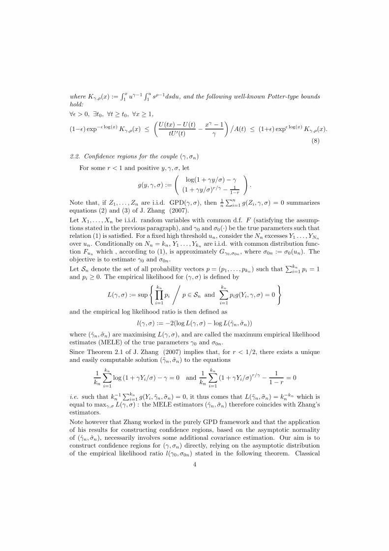
The simulations below are based on 2000 random samples of size n = 1000, generatedfrom the following two distributions: the Frechet distribution with parameter γ > 0given by F (x) = exp(−x−1/γ) (the results for γ = 1 and 1/4 are presented) and theBurr distribution with positive parameters λ and τ given by F (x) = (1 + xτ )−1/λ (theresults for (λ, τ) = (1, 1) and (2, 2) are presented). Note that the tail index for the Burrdistribution is γ = (λτ)−1.

Coverage probabilities EL(0.95), ML(0.95) and Zhang(0.95) are plotted against differentvalues of kn, the number of excesses used. Figure 1 seems to indicate that our methodperforms better in terms of coverage probability, and additional models not presentedhere almost always led to the same ordering : EL better than the bivariate CLT of

6

Zhang’s estimator, itself better than the CLT for the MLE. However, we have observedthat the overall results are not very satisfactory when the tail index γ is small.

(a) Coverage Probability for Burr(1, 1) model,n = 1000

(b) Coverage Probability for Burr(2, 2) model,n = 1000

(c) Coverage Probability for Frechet(1) model,n = 1000

(d) Coverage Probability for Frechet(1/4)model, n = 1000

Figure 1: Coverage Probability for Burr(1, 1), Burr(2, 2), Frechet(1), Frechet(1/4) as a function of thenumber of excesses kn. The dashed line is for ML, the thin solid line for Zhang, and the thick solid linefor EL.

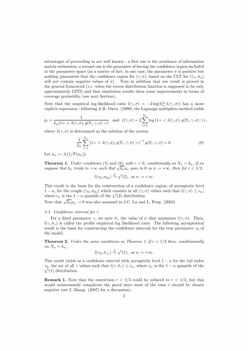
One can wonder if the improvement in coverage probabilities is due to the fact that ourconfidence regions are wider than in the ML and Zhang cases. In practice, it seems infact that the three confidence regions have comparable sizes (our confidence region beingeven a bit smaller). Figure 2 shows these three regions for a simulated Burr(1, 1) randomsample with n = 1000 et kn = 200.

Remark 4. it should be noted that some computational problems occurred when trying7

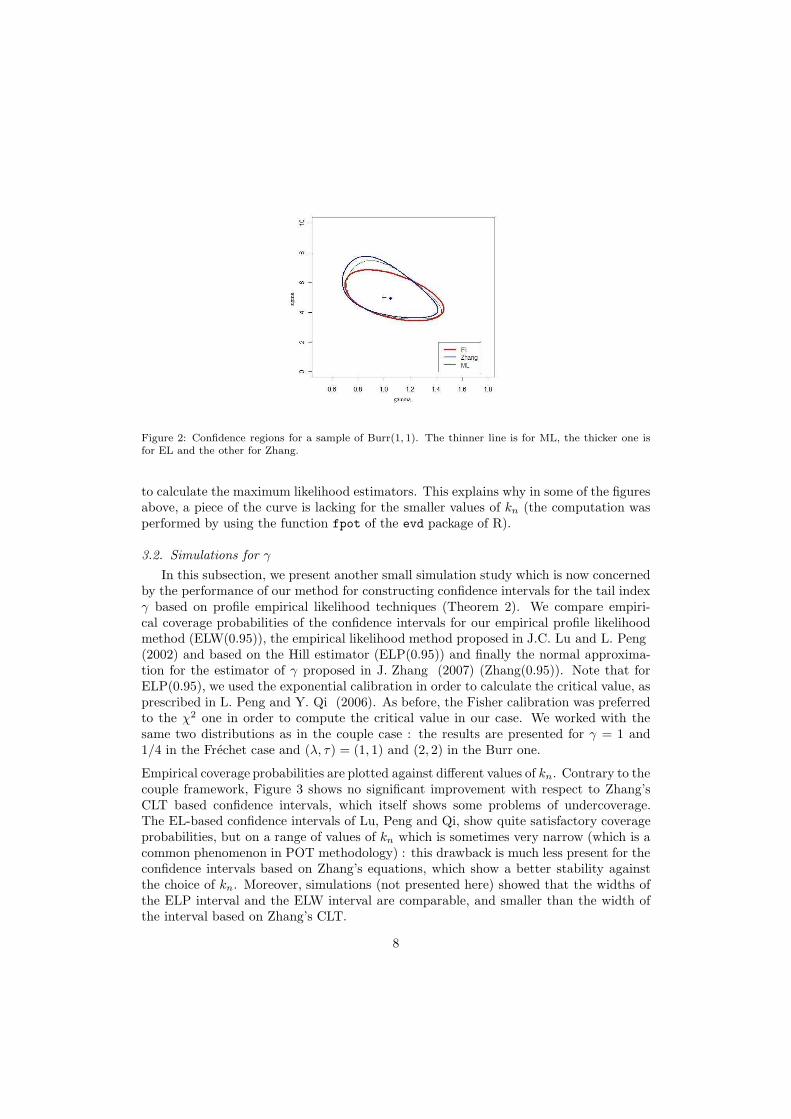
Figure 2: Confidence regions for a sample of Burr(1, 1). The thinner line is for ML, the thicker one isfor EL and the other for Zhang.

to calculate the maximum likelihood estimators. This explains why in some of the figuresabove, a piece of the curve is lacking for the smaller values of kn (the computation wasperformed by using the function fpot of the evd package of R).

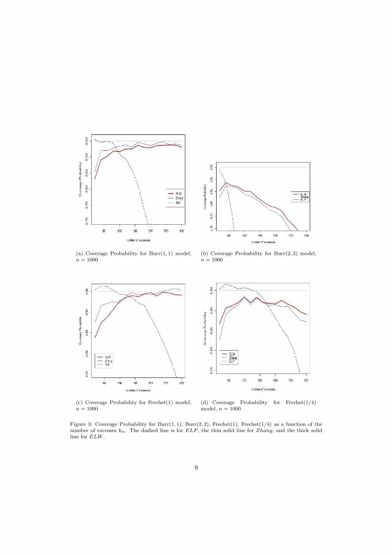
3.2. Simulations for γ

In this subsection, we present another small simulation study which is now concernedby the performance of our method for constructing confidence intervals for the tail indexγ based on profile empirical likelihood techniques (Theorem 2). We compare empiri-cal coverage probabilities of the confidence intervals for our empirical profile likelihoodmethod (ELW(0.95)), the empirical likelihood method proposed in J.C. Lu and L. Peng(2002) and based on the Hill estimator (ELP(0.95)) and finally the normal approxima-tion for the estimator of γ proposed in J. Zhang (2007) (Zhang(0.95)). Note that forELP(0.95), we used the exponential calibration in order to calculate the critical value, asprescribed in L. Peng and Y. Qi (2006). As before, the Fisher calibration was preferredto the χ2 one in order to compute the critical value in our case. We worked with thesame two distributions as in the couple case : the results are presented for γ = 1 and1/4 in the Frechet case and (λ, τ) = (1, 1) and (2, 2) in the Burr one.

Empirical coverage probabilities are plotted against different values of kn. Contrary to thecouple framework, Figure 3 shows no significant improvement with respect to Zhang’sCLT based confidence intervals, which itself shows some problems of undercoverage.The EL-based confidence intervals of Lu, Peng and Qi, show quite satisfactory coverageprobabilities, but on a range of values of kn which is sometimes very narrow (which is acommon phenomenon in POT methodology) : this drawback is much less present for theconfidence intervals based on Zhang’s equations, which show a better stability againstthe choice of kn. Moreover, simulations (not presented here) showed that the widths ofthe ELP interval and the ELW interval are comparable, and smaller than the width ofthe interval based on Zhang’s CLT.

8

(a) Coverage Probability for Burr(1, 1) model,n = 1000

(b) Coverage Probability for Burr(2, 2) model,n = 1000

(c) Coverage Probability for Frechet(1) model,n = 1000

(d) Coverage Probability for Frechet(1/4)model, n = 1000

Figure 3: Coverage Probability for Burr(1, 1), Burr(2, 2), Frechet(1), Frechet(1/4) as a function of thenumber of excesses kn. The dashed line is for ELP , the thin solid line for Zhang, and the thick solidline for ELW .

9

Remark 5. the computation of the profile empirical likelihood l(γ0, σγ0) was performed

using a classical descent algorithm, taking profit of some convexity properties of theprofile empirical likelihood function. Computational details and files can be obtainedfrom the authors (some of them are downloadable on the first author’s webpage).

4. Proofs

Note that we will prove Theorem 2 before Theorem 1 because its proof is moreinvolved and largely includes what is needed to prove Theorem 1.

4.1. Proof of Theorem 2

From now on we work conditionally on {Nn = kn} for some given sequence (kn)satisfying

√knan → 0 as n→ ∞.

Let U1, . . . , Ukndenote independent uniform random variables on [0, 1]. Noticing that

(Y1, . . . , Ykn) has the same joint distribution as (Y1, . . . , Ykn

) defined by

Yi := F−1un

(Ui) = U(1/(UiF (un)))− U(1/F (un))

we see that it suffices to prove Theorem 2 with Yi replacing Yi in the definition of theempirical likelihood. For simplicity we will write Yi instead of Yi in the sequel (note thatthese random variables are i.i.d. but their common distribution varies with n).

Now, defining Zi,n := Yi/σ0n, λ0(θ) := λ(γ0, σ0nθ) and g0(z, t) := g(z, γ0, t), we see thatg0(Zi,n, θ) = g(Yi, γ0, σ0nθ), hence

l0(θ) := l(γ0, σ0nθ) = 2∑kn

i=1 log (1+ < λ(γ0, σ0nθ), g(Yi, γ0, σ0nθ) >)

= 2∑kn

i=1 log (1+ < λ0(θ), g0(Zi,n, θ) >) .

With these preliminaries in mind, we thus need to prove that there exists some localminimizer θ of l0(·) in a neighborhood of θ0 = 1 such that l0(θ) → χ2(1) in distribution,

because l0(θ) = l(γ0, σγ0) with θ = σγ0

/σ0n.

We now state in the following proposition some important results, which will be provedin Section 4.2 and will enable us to proceed with the proof of Theorem 2 following aplan very similar to that found in Y. S. Qin and J. Lawless (1994) (note that here theparameter is one-dimensional whereas the estimating function g0 is R2-valued). We firstintroduce some important notations :

Gn(θ) := 1kn

∑kn

i=1 g0(Zi,n, θ)

Bn(θ) := 1kn

∑kn

i=1 g0(Zi,n, θ)(g0(Zi,n, θ))t

An(θ) := 1kn

∑kn

i=1∂g0∂θ (Zi,n, θ)

Mn(θ) := maxi≤kn‖g0(Zi,n, θ)‖

Note that, although the new parameter θ is scalar, we will write below ‖θ‖ instead of|θ| in order to emphasize the fact that the arguments described below can be appliedto more general frameworks. The same is true about the fact that we use below thenotation θ0 instead of simply the number 1.

10

Proposition 1. Suppose the assumptions of Theorem 2 are valid, and Z is some random

variable distributed as Gγ0,1. If Bn := { θ ∈ R ; ‖θ − θ0‖ ≤ k−1/3n }, then we have,

conditionally to {Nn = kn} and as n→ ∞,

Gn(θ0) = O(

k−1/2n (log log kn)

1/2)

a.s. (10)

√

knGn(θ0)d−→ N (0, B) (11)

Mn(θ0) = o(√

kn) a.s. (12)

Mn(θ) = o(k1/3n ) a.s. uniformly on Bn (13)

An(θ) = A+ o(1) a.s. uniformly on Bn, (14)

Bn(θ) = B + o(1) a.s. uniformly on Bn (15)

Gn(θ) = Gn(θ0) + (A+ o(1))(θ − θ0) = O(k−1/3n ) a.s. unif. on Bn (16)

where

B := E[

g0(Z, θ0)(g0(Z, θ0))t]

=

(

γ2 γr(1−r)2

γr(1−r)2

r2

(1−2r)(1−r)2

)

and

A := E

[

∂g0∂θ

(Z, θ0)

]

=

(

− γγ+1

− r(1−r+γ)(1−r)

)

Recall that λ0(θ) is defined as the solution of the equation

1

kn

kn∑

i=1

(1+ < λ, g0(Zi,n, θ) >)−1

g0(Zi,n, θ) = 0.

Therefore, for θ ∈ Bn, if u = λ0(θ)/‖λ0(θ)‖, usual calculations (see A.B. Owen (1990)for instance) lead to

‖λ0(θ)‖(

utBn(θ)u −Mn(θ)‖Gn(θ)‖)

≤ ‖Gn(θ)‖ (17)

for any n. Statements (11), (12), (15) and (13), (15), (16) thus respectively yield

‖λ0(θ0)‖ = O(k−1/2n ) a.s. and ‖λ0(θ)‖ = O(k−1/3

n ) a.s. uniformly on Bn. (18)

Consequently, if we note γi,n(θ) := < λ0(θ), g0(Zi,n, θ) >, we have

maxi≤n

|γi,n(θ)| ≤ ‖λ0(θ)‖Mn(θ) = o(1) a.s. and uniformly on Bn (19)

and, using (1 + x)−1 = 1 − x + x2(1 + x)−1 and the identity 0 = k−1n

∑kn

i=1(1 +γi,n(θ))

−1g0(Zi,n, θ), we readily have

λ0(θ) = (Bn(θ))−1Gn(θ) + (Bn(θ))

−1Rn(θ)

where Rn(θ) = k−1n

∑kn

i=1(1 + γi,n(θ))−1(γi,n(θ))

2g0(Zi,n, θ). Since for n sufficiently

large we have ‖Rn(θ)‖ ≤ 2k−1n

∑kn

i=1 ‖λ0(θ)‖2‖g0(Zi,n, θ)‖3 ≤ 2‖λ0(θ)‖2Mn(θ) tr(Bn(θ)),relations (12), (13), (15) and (18) imply the following crucial relations (the second oneholding uniformly in θ ∈ Bn)

λ0(θ0) = (Bn(θ0))−1Gn(θ0)+o(k−1/2

n ) a.s. and λ0(θ) = (Bn(θ))−1Gn(θ)+o(k−1/3

n ) a.s..(20)

11

Using the Taylor expansion log(1 + x) = x− 12x

2 + 13x

3(1 + ξ)−3 (for some ξ between 0and x) and statement (19), we can proceed as above and obtain

l0(θ) = 2

kn∑

i=1

log(1 + γi,n(θ)) = 2

kn∑

i=1

γi,n(θ)−kn∑

i=1

(γi,n(θ))2 + R′

n(θ)

where, for n sufficiently large, ‖R′n(θ)‖ ≤ 16

3

∑kn

i=1 |γi,n(θ)|3 = o(1)∑kn

i=1(γi,n(θ))2. Using

relation (20) as well as (15) and (16), we have for ‖θ − θ0‖ ≤ k−1/3n ,

kn∑

i=1

γi,n(θ) = knλ0(θ)tGn(θ) = kn(Gn(θ) + o(k−1/3

n ))t (Bn(θ))−1 Gn(θ)

= kn(Gn(θ))t B−1 Gn(θ) + o(k1/3n )

and similarly,∑kn

i=1(γi,n(θ))2 = kn(Gn(θ))

t B−1 Gn(θ) + o(k1/3n ). Therefore, if θ =

θ0 + uk−1/3n with ‖u‖ = 1, using (16) and the almost sure bound (10) for Gn(θ0), we

obtain

l0(θ) = kn(Gn(θ))t B−1 Gn(θ) + o(k1/3n )

= k1/3n [k1/3n Gn(θ0) + (A+ o(1))u]t B−1[k1/3n Gn(θ0) + (A+ o(1))u] + o(k1/3n )

= k1/3n utAtB−1Au+ o(k1/3n ).

Consequently, if a > 0 denotes the smallest eigenvalue of AtB−1A and ǫ ∈]0, a[, we havefor n sufficiently large

l0(θ) ≥ (a− ǫ)k1/3n almost surely and uniformly for θ ∈ cl(Bn).

On the other hand, we obtain in a similar manner

l0(θ0) = (√

knGn(θ0))tB−1(

√

knGn(θ0)) + o(1) (a.s.)

which converges in distribution to χ2(2) in view of (11), and is also o(log log kn) almostsurely, thanks to (10).

We have thus proved the following

Proposition 2. Under the conditions of Theorem 2, and as n→ ∞ with probability one,the empirical log-likelihood ratio l0(·) admits a local minimizer θ in the interior of the

ball Bn = { θ ∈ R ; ‖θ − θ0‖ ≤ k−1/3n }. This means that almost surely, for n large, there

exists a local minimizer σγ0of the profile empirical log-likelihood σ 7→ l(γ0, σ) such that

σγ0/σ0n is close to 1 with rate k

−1/3n .

Now that we have identified some empirical likelihood estimator θ and proved itconsistently estimates θ0, we want to identify its asymptotic distribution, which willenable us to obtain the convergence in distribution of l0(θ) towards χ

2(1).

As it is done in Y. S. Qin and J. Lawless (1994), we introduce the functions defined on

12

R× R2

Q1,n(θ, λ) =1

kn

kn∑

i=1

(1+ < λ, g0(Zi,n, θ) >)−1g0(Zi,n, θ)

Q2,n(θ, λ) =1

kn

kn∑

i=1

(1+ < λ, g0(Zi,n, θ) >)−1

(

∂g0∂θ

(Zi,n, θ)

)t

λ

and see that (∀θ) Q1,n(θ, λ0(θ)) = 0 (by definition of λ0(θ)), Q1,n(θ, 0) = Gn(θ), and

Q2,n(θ, λ0(θ)) = (∂l0/∂θ)(θ), which is null at θ = θ.

A Taylor expansion of Q1,n and Q2,n between (θ0, 0) and (θ, λ0(θ)) shows that there

exists some (θ∗n, λ∗n) satisfying ‖θ∗n−θ0‖ ≤ ‖θ−θ0‖ ≤ k

−1/3n , ‖λ∗

n‖ ≤ ‖λ0(θ)‖ = O(k−1/3n )

(thanks to Proposition 2 and (18)), and such that(

00

)

=

(

Q1,n(θ, λ0(θ))

Q2,n(θ, λ0(θ))

)

=

(

Q1,n(θ0, 0)Q2,n(θ0, 0)

)

− Sn(θ∗n, λ

∗n)

(

θ − θ0λ0(θ)

)

where

Sn(θ, λ) :=

(

−∂Q1,n/∂θ −∂Q1,n/∂λ−∂Q2,n/∂θ −∂Q2,n/∂λ

)∣

∣

∣

∣

(θ,λ)

Differential calculus leads to

Sn(θ0, 0) =

− 1kn

∑kn

i=1∂g∂θ (Zi,n, θ0)

1kn

∑kn

i=1 g(Zi,n, θ0)(g(Zi,n, θ0))t

0 − 1kn

∑kn

i=1

(

∂g∂θ (Zi,n, θ0)

)t

thus, defining V := (AtB−1A)−1, relations (15) and (14) imply that Sn(θ0, 0) convergesto the matrix

S =

(

−A B0 −At

)

which is invertible with

S−1 =

(

C DE F

)

:=

(

−V AtB−1 −VB−1(I −AV AtB−1) −B−1AV

)

After tedious calculations and use of many of the statements previously derived fromProposition 1, it can be proved that ‖Sn(θ

∗n, λ

∗n)− Sn(θ0, 0)‖ = oP(1) as n→ ∞. Conse-

quently, we obtain, for n sufficiently large( √

kn(θ − θ0)√knλ0(θ)

)

= S−1

( √knGn(θ0) + oP(

√knδn)

oP(√knδn)

)

where δn := ‖θ−θ0‖+‖λ0(θ)‖

(21)

We already know that δn = O(k−1/3n ), but now (21) implies that δn = O(k

−1/2n ) and

therefore we have proved that√

kn(θ − θ0) = C√

knGn(θ0) + oP(1)d→ N (0, CBCt) = N (0, (AtB−1A)−1) (22)

√

knλ0(θ) = E√

knGn(θ0) + oP(1)d→ N (0, EBEt) = N (0, E) (23)

where we have used the fact that the matrix E is symmetric and such that EBE =E, because I − AV AtB−1 is idempotent (note that the rank of E is 2 minus that of

13

AV AtB−1, i.e. rank(E) = 1).

Applying relation (16) to θ = θ, relation (22) yields√

knGn(θ) =√

knGn(θ0) +A√

kn(θ − θ0) + oP(1) = (I +AC)√

knGn(θ0) + oP(1)

= BE(√

knGn(θ0) + oP(1))

and this leads to the following appropriate development for l0(θ), using (23) and (15) :

l0(θ) = 2kn(λ0(θ))tGn(θ)− kn(λ0(θ))

tBn(θ)λ0(θ) +R′n(θ)

= (√

knGn(θ0) + oP(1))t(EBE)(

√

knGn(θ0) + oP(1)) + oP(1) +R′n(θ)

= (√

knGn(θ0))tE(√

knGn(θ0)) + oP(1) +R′n(θ)

where |R′n(θ)| ≤ oP(1)

∑kn

i=1(γi,n(θ))2 = oP(1)

(

(√knGn(θ0))

tE(√knGn(θ0)) + oP(1)

)

.

According to proposition (viii) p.524 of S.S. Rao (1984), since√knGn(θ0) converges

in distribution to N (0, B), and EBE = E with rank(EB) = 1, the quadratic form(√knGn(θ0))

tE(√knGn(θ0)) converges in distribution to χ2(2−1) = χ2(1), and Theorem

2 is proved.

4.2. Proof of Proposition 1

Note that throughout the whole proof, we will write γ instead of γ0 for convenience.

4.2.1. Proof of (10) and (11)

Let us define

Zi =U−γi − 1

γand ∆i(θ) = g0(Zi,n, θ)− g0(Zi, θ),

so that (Zi)1≤i≤knis an i.i.d. sequence with common distribution GPD(γ, 1) and

Gn(θ0) =1

kn

kn∑

i=1

g0(Zi, θ0) +1

kn

kn∑

i=1

∆i(θ0). (24)

If r < 12 , B is well defined as the covariance matrix of g0(Z1, θ0) (a straightforward

calculation gives the expression of B), and consequently the LIL and CLT imply that

1

kn

kn∑

i=1

g0(Zi, θ0) = O(

k−1/2n (log log kn)

1/2)

a.s. and1√kn

kn∑

i=1

g0(Zi, θ0)d−→ N (0, B) .

Therefore, according to (24) and to the assumption√knan → 0 (as n → +∞), in order

to prove (10) and (11) it remains to establish that

1

kn

kn∑

i=1

∆i(θ0) = O(an) a.s. (25)

Since we can take σ0n := σ0(un) = 1F (un)

U ′(

1/F (un))

, and recalling that we consider

Yi = U(1/(UiF (un))) − U(1/F (un)), the application of the Potter-type bounds (8) to

14

t = 1/F (un) and x = 1/Ui yields, for all ǫ > 0 and n sufficiently large,

(1− ǫ)U ǫiKγ,ρ(1/Ui) ≤

Zi,n − Zi

an≤ (1 + ǫ)U−ǫ

i Kγ,ρ(1/Ui) a.s. (26)

In the sequel, we will consider an > 0 for large n (the case an < 0 being similar) andnote Ki = Kγ,ρ(1/Ui), as well as ∆

1i (θ) and ∆2

i (θ) the two components of ∆i(θ).

(i) Control of ∆1i (θ0)

∆1i (θ0) = ln(1 + γZi,n)− ln(1 + γZi) = ln (1 + γUγ

i (Zi,n − Zi)) .

Use of (26) leads to the following bounds (for all ǫ > 0 and n sufficiently large),

1

anln(

1 + anγ(1− ǫ)Uγ+ǫi Ki

)

≤ ∆1i (θ0)

an≤ 1

anln(

1 + anγ(1 + ǫ)Uγ−ǫi Ki

)

a.s.

(27)If we set B+

i := γ(1+ǫ)Uγ−ǫi Ki and B−

i := γ(1−ǫ)Uγ+ǫi Ki, Lemmas 3 and 5 (stated

and proved in the Appendix) imply that B+i and B−

i are both square integrableand therefore maxi≤kn

anB+i and maxi≤kn

anB−i are both, almost surely, o(

√knan),

which is o(1) according to our assumption on (kn).

Consequently, the inequality 23x ≤ ln(1+x) ≤ x (∀x ∈ [0, 1/2]) yields the following

bounds, for all ǫ > 0 and n sufficiently large,

2

3

1

kn

kn∑

i=1

B−i ≤ 1

kn

kn∑

i=1

∆1i (θ0)

an≤ 1

kn

kn∑

i=1

B+i a.s. (28)

and therefore, for every ǫ > 0,

2

3γ(1− ǫ)E(Uγ+ǫ

1 K1) ≤ lim inf 1kn

∑kn

i=1∆1

i (θ0)an

≤ lim sup 1kn

∑kn

i=1∆1

i (θ0)an

≤ γ(1 + ǫ)E(Uγ−ǫ1 K1).

Letting ǫ go to 0 gives a−1n k−1

n

∑kn

i=1 ∆1i (θ0) = O(1) a.s.

(ii) Control of ∆2i (θ0)

∆2i (θ0) = (1 + γZi,n)

r/γ − (1 + γZi)r/γ = U−r

i

(

(1 + γUγi (Zi,n − Zi))

r/γ − 1)

.

In the case r < 0 (the case r > 0 is similar), use of (26) yields the following boundsfor all ǫ > 0 and n large

U−ri

an

(

(

1 + (1 + ǫ)γanUγ−ǫi Ki

)r/γ − 1)

≤ ∆2i (θ0)

an≤ U−r

i

an

(

(

1 + (1− ǫ)γanUγ+ǫi Ki

)r/γ − 1)

(29)

The inequality αx ≤ (1 + x)α − 1 ≤ αcx (∀x ∈ [0, 1/2], where c = (32 )α−1 > 0 and

α = r/γ < 0) yields, for all ǫ > 0 and n sufficiently large,

r(1− ǫ)1

kn

kn∑

i=1

Uγ−r+ǫi Ki ≤

1

kn

kn∑

i=1

∆2i (θ0)

an≤ rc(1+ ǫ)

1

kn

kn∑

i=1

Uγ−r−ǫi Ki a.s. (30)

15

Once again, Lemma 3 ensures that E(Uγ−r±ǫi Ki) and E((Uγ−r±ǫ

i Ki)2) are finite

(because r < 1/2), hence for sufficiently small ǫ > 0

r(1 − ǫ)E(Uγ−r+ǫ1 K1) ≤ lim inf

1

kn

kn∑

i=1

∆2i

an

≤ lim sup1

kn

kn∑

i=1

∆2i (θ0)

an≤ rc(1 + ǫ)E(Uγ−r−ǫ

1 K1) a.s.

Letting ǫ go to 0 yields a−1n k−1

n

∑kn

i=1 ∆2i (θ0) = O(1) a.s. and therefore (25) is

proved.

4.2.2. Proof of (12) and (13)

With ∆i(θ) and Zi being defined as previously, we have

Mn(θ) = maxi≤kn

||g0(Zi,n, θ)|| ≤ maxi≤kn

||g0(Zi, θ)||+maxi≤kn

||∆i(θ)||.

Since the variables g0(Zi, θ0) are square integrable, it comes (Lemma 5)

maxi≤kn

||g0(Zi, θ0)|| = o(√

kn) a.s.

On the other hand, part 1 of Lemma 2 implies that for θ in Bn, ||g0(z, θ)||3 ≤ G1(z), forevery z ≥ 0 and n sufficiently large. Since the variables G1(Zi) are i.i.d. and integrable(part 4 of Lemma 2), using Lemma 5 we thus have

maxi≤kn

||g0(Zi, θ)|| = o(k1/3n ) a.s.

We can now conclude the proof of (12) and (13) by showing that, uniformly for θ in Bn,maxi≤kn

|∆ji (θ)| tends to 0 almost surely for j = 1 or 2. Reminding that γZi = U−γ

i − 1,we can show that

∆1i (θ) = ln

(

1 + γZi,n

θ

)

−ln

(

1 + γZi

θ

)

= ln{

1 + γUγi (1 + (θ − 1)Uγ

i )−1

(Zi,n − Zi)}

.

Let δ > 0 and θ ∈]1 − δ, 1 + δ[. Using (26), we have the following bounds (for all ǫ > 0and n sufficiently large),

1

anln

(

1 + anγ

(

1− ǫ

1 + δ

)

Uγ+ǫi Ki

)

≤ ∆1i (θ)

an≤ 1

anln

(

1 + anγ

(

1 + ǫ

1− δ

)

Uγ−ǫi Ki

)

a.s.

(31)where we supposed that an > 0 (the other case is very similar). Proceeding as for thehandling of ∆1

i (θ0), and using 23x ≤ ln(1 + x) ≤ x for x ∈ [0, 1/2], we obtain : for all

δ > 0, θ ∈]1− δ, 1 + δ[, ǫ > 0 and n sufficiently large,

2

3

(

1− ǫ

1 + δ

)

γUγ+ǫi Ki ≤

∆1i (θ)

an≤(

1 + ǫ

1− δ

)

γUγ−ǫi Ki a.s. (32)

Since (32) ensures that∆1

i (θ)an

is of constant sign, for n large enough we have

supθ∈Bn

maxi≤kn

|∆1i (θ)| ≤

√

knanγ

(

1 + ǫ

1− δ

)

maxi≤knUγ−ǫi Ki√

kna.s.

16

We conclude using Lemmas 3 and 5 and assumption√knan → 0. The proof for ∆2

i (θ)is very similar.

4.2.3. Proof of (14) and (16)

Recall that An(θ) =1kn

∑kn

i=1∂g0∂θ (Zi,n, θ) and let A∗

n(θ) :=1kn

∑kn

i=1∂g0∂θ (Zi, θ), where

the Zi were introduced previously. We write

An(θ) −A = (An(θ) −A∗n(θ)) + (A∗

n(θ)− A∗n(θ0)) + (A∗

n(θ0)−A) (33)

and we will handle separately the three terms on the right hand side above. The thirdterm goes to 0 a.s. according to the strong law of large numbers (SLLN for short) andby definition of the Zi and A. The same is true (uniformly in θ) for the second term,since part 3 of Lemma 2 implies

supθ∈Bn

‖A∗n(θ)−A∗

n(θ0)‖ ≤(

supθ∈Bn

||θ − θ0||)

1

kn

kn∑

i=1

G3(Zi).

and the SLLN applies, thanks to part 4 of Lemma 2. It remains to study the first termof (33) uniformly in θ in order to prove (14). We have

An(θ)−A∗n(θ) =

1

kn

kn∑

i=1

∆i(θ),

where the two components of ∆i(θ) are

∆1i (θ) = −θ−2γZi,n(1 + γZi,n/θ)

−1 + θ−2γZi(1 + γZi/θ)−1

∆2i (θ) = −rθ−2Zi,n(1 + γZi,n/θ)

r/γ−1 + rθ−2Zi(1 + γZi/θ)r/γ−1.

We shall give details for ∆1i (θ) and the case an > 0 (the case an < 0 and the treatment

of ∆2i (θ) can be handled very similarly). Let δ > 0, θ ∈]1 − δ, 1 + δ[, and Vi denote

(1 + γZi/θ)−1. Use of the Potter-type bounds (26) leads to the following bounds (for all

ǫ > 0 and n sufficiently large),

Vi

(

1 + anθ−1(1 + ǫ)γU−ǫ

i KiVi

)−1 ≤ (1 + γZi,n/θ)−1 ≤ Vi

(

1 + anθ−1(1 − ǫ)γU ǫ

iKiVi

)−1a.s.

After multiplication by −θ−2γZi,n and another use of (26), we obtain

−θ−2γZiVi

{

(1 + anB−i )−1 − 1

}

− anθ−2(1 + ǫ)γU−ǫ

i KiVi(1 + anB−i )−1

≤ ∆1i (θ) ≤ −θ−2γZiVi

{

(1 + anB+i )−1 − 1

}

− anθ−2(1 − ǫ)γU ǫ

iKiVi(1 + anB+i )−1

where B−i = θ−1(1−ǫ)γU ǫ

iKiVi and B+i = θ−1(1+ǫ)γU−ǫ

i KiVi. Let us handle the upperbound first. We find easily that (1− δ)Uγ

i ≤ Vi ≤ (1 + δ)Uγi , and therefore, by Lemmas

3 and 5, and assumption√knan → 0,

0 ≤ sup|θ−1|≤δ

maxi≤kn

(

anB+i

)

≤ (1+ ǫ)(1+ δ)(1− δ)−1γanmaxi≤kn

Uγ−ǫi Ki = o(1) a.s. (34)

Consequently, using (1 + x)−1 − 1 = −x(1 + x)−1, for n sufficiently large and uniformlyin θ ∈]1 − δ, 1 + δ[, we find (almost surely)

1kn

∑kn

i=1∆1

i (θ)an

≤ (1+ǫ)(1+δ)2

(1−δ)31kn

∑kn

i=1

(

(1− Uγi )U

γ−ǫi Ki

)

− (1−ǫ)(1−δ)2(1+δ)2 γ 1

kn

∑kn

i=1

(

Uγ+ǫi Ki

)

= O(1)

17

The lower bound can be handled in the same way. Note that (16) is an immediateconsequence of (14).

4.2.4. Proof of (15)

Recall that Bn(θ) = k−1n

∑kn

i=1 g0(Zi,n, θ)g0(Zi,n, θ)t and let

B∗n(θ) := k−1

n

kn∑

i=1

g0(Zi, θ)g0(Zi, θ)t,

where the Zi were introduced previously. We write

Bn(θ)−B = (Bn(θ)−B∗n(θ)) + (B∗

n(θ)−B∗n(θ0)) + (B∗

n(θ0)−B) (35)

The third term in the relation above goes to 0 a.s. according to the SLLN and bydefinition of the Zi and B. Let us deal with the second term. For θ ∈ Bn, there existssome θ∗n between θ0 and θ such that (using parts 1 and 2 of Lemma 2)

‖B∗n(θ)−B∗

n(θ0)‖ ≤ ‖θ − θ0‖.2

kn

kn∑

i=1

∥

∥

∥

∥

∂g0∂θ

(Zi, θ∗n)

∥

∥

∥

∥

‖g0(Zi, θ∗n)‖

≤ k−1/3n max

i≤kn

(G1(Zi))1/3 2

kn

kn∑

i=1

G2(Zi).

Therefore, combining part 4 of Lemma 2, Lemma 5, and the SLLN, we see that ‖B∗n(θ)−

B∗n(θ0)‖ almost surely goes to 0 as n→ ∞, uniformly in θ ∈ Bn.

It remains to study the first term of (35) uniformly in θ in order to prove (15). We have

Bn(θ) −B∗n(θ) =

1

kn

kn∑

i=1

∆ti(θ)g0(Zi, θ) +

1

kn

kn∑

i=1

∆i(θ)(g0(Zi, θ))t +

1

kn

kn∑

i=1

∆i(θ)(∆i(θ))t

= Γt1,n(θ) + Γ1,n(θ) + Γ2,n(θ)

with

∆i(θ)(g0(Zi, θ))t =

(

∆1i (θ)(ln(1 + γ Zi

θ )− γ) ∆1i (θ)((1 + γ Zi

θ )r/γ − 11−r )

∆2i (θ)(ln(1 + γ Zi

θ )− γ) ∆2i (θ)((1 + γ Zi

θ )r/γ − 11−r )

)

and

∆i(θ)(∆i(θ))t =

(

(∆1i (θ))

2 ∆1i (θ) ∆

2i (θ)

∆1i (θ) ∆

2i (θ) (∆2

i (θ))2

)

.

Considering the first element of the matrix Γ1,n(θ), we have

a−1n

∣

∣

∣

1kn

∑kn

i=1 ∆1i (θ)

(

ln(

1 + γ Zi

θ

)

− γ)

∣

∣

∣ ≤√

1kn

∑kn

i=1

(

∆1i(θ)

an

)2√1kn

∑kn

i=1

(

ln(

1 + γ Zi

θ

)

− γ)2

and, applying the Cauchy-Schwarz inequality too for dealing with the other elements ofΓ1,n(θ) and Γ2,n(θ), the convergence Bn(θ) − B∗

n(θ) → 0 (uniformly for θ ∈ Bn) willbe proved as soon as we show that the means over i = 1 to kn of each of the followingquantities are almost surely bounded uniformly for θ ∈ Bn :

(

ln(

1 + γ Zi

θ

)

− γ)2

,(

(

1 + γ Zi

θ

)r/γ − 11−r

)2

,(

∆1i (θ)an

)2

,(

∆2i (θ)an

)2

,∆1

i (θ)∆2i (θ)

(an)2.

18

Using Lemma 2, we see that the first two elements of this list are both uniformly boundedby 1

kn

∑kn

i=1(G1(Zi))2/3 which converges almost surely. On the other hand, according to

relation (32) and since E(U2γ−2ǫ1 K2

1 ) is finite (by Lemma 3), k−1n

∑kn

i=1(∆1i (θ)/an)

2 is

uniformly almost surely bounded. Similarly the same is true for k−1n

∑kn

i=1(∆2i (θ)/an)

2,

as well as for k−1n

∑kn

i=1 ∆1i (θ)∆

2i (θ)/a

2n, and the proof of (15) is over.

4.3. Proof of Theorem 1

We proceed as in the start of the proof of Theorem 2, and consider that the variablesYi are the variables F−1

un(Ui) where (Ui)i≥1 is an i.i.d. sequence of standard uniform

variables. Recall that

l(γ, σ) = 2

kn∑

i=1

log (1+ < λ(γ, σ), g(Yi, γ, σ) >) .

Defining Zi,n = Yi/σ0n, θ0 = (γ0, 1), θ = (γ, s), and

l(θ) = 2

kn∑

i=1

log(

1+ < λ(θ), g(Zi,n, θ) >)

where λ(θ) is such that

1

kn

kn∑

i=1

(

1+ < λ(θ), g(Zi,n, θ) >)−1

g(Zi,n, θ) = 0,

it comes that l(γ0, σ0n) = l(θ0) since g(Zi,n, γ, s) = g(Yi, γ, σ0ns). We thus need to

prove that l(θ0) converges in distribution to χ2(2). Following a very classical outlinein empirical likelihood theory, it is easy to prove that this convergence is guaranteed assoon as we have the following statements (as n→ ∞)

1

kn

kn∑

i=1

g(Zi,n, θ0)P−→ 0,

1

kn

kn∑

i=1

g(Zi,n, θ0)(g(Zi,n, θ0))t P−→ B,

1√kn

kn∑

i=1

g(Zi,n, θ0)d−→ N (0, B), max

i≤kn

‖g(Zi,n, θ0)‖ = oP(√

kn)

However, these statements are included in Proposition 1 and therefore Theorem 1 isproved.

Note : Proposition 1 was stated under the assumption that r < 1/3, but in fact r <1/2 is sufficient in order to prove all the results concerning θ0 only and not for θ in aneighborhood of it (and the covariance matrix B is well defined and invertible as soonas r < 1/2).

5. Conclusion

This work deals with the problem of finding confidence regions for the parameters ofthe approximating GPD distribution in the classical POT framework, for general heavytailed distributions (γ > 0). It is shown that the application of the empirical likelihood

19

(EL) method to the estimating equations of J. Zhang (2007) yields confidence regionswith improved coverage accuracy in comparison to the Wald-type confidence regionsissued from the CLT for some estimators of the couple (γ, σ) (including the maximumlikelihood estimator). It is also observed that coverage accuracy is not always as good asone would expect, which means that this subject (and the related one of EL calibration)would need to be further investigated.

A profile EL based confidence interval for the tail index is also obtained, and itsperformance in terms of coverage probability has been compared to that of the confidenceinterval (CI) described in J.C. Lu and L. Peng (2002) and L. Peng and Y. Qi (2006)(which is known to perform better than the Wald-type CI based on the CLT for theHill estimator). In some simulations, the interval of Lu, Peng and Qi shows betterperformance, but in others this performance is limited to a very short range of numberkn of excesses : this instability with respect to kn is much less present for the CI basedon Zhang’s equations.

We shall finish this conclusion with two remarks. The first is that some of the method-ology of the proof of the profile EL result (inspired by Y. S. Qin and J. Lawless (1994))could prove useful in other settings (Proposition 1 lists properties which yield conver-gence in distribution of empirical likelihood ratio when the observations form a triangulararray). The second remark is that plug-in calibration could be an interesting subject toinvestigate for obtaining CI for γ, in particular in order to shorten computation time.

6. Appendix

Lemma 2. Let γ > 0, r < 1/3 and, for θ > 0,

g0(z, θ) :=

(

g10(z, θ)

g20(z, θ)

)

=

(

ln(1 + γz/θ)− γ

(1 + γz/θ)r/γ − (1− r)−1

)

.

If we consider, for some positive constants c1, c′1, c2, c3 depending on r and γ,

G1(z) = c1(

ln(1 + γz) + (1 + γz)r/γ + c′1)3

G2(z) = c2(

z(1 + γz)−1 + z(1 + γz)r/γ−1)

G3(z) = c3(

z(1 + γz)−1 + z(1 + γz)r/γ−1 + z2(1 + γz)−2 + z2(1 + γz)r/γ−2)

.

then there exists a neighborhood of θ0 = 1 such that for all θ in this neighborhood and∀z ≥ 0,

1. ||g0(z, θ)||3 ≤ G1(z)

2. ||∂g0∂θ (z, θ)|| ≤ G2(z)

3. ||∂2g0∂2θ (z, θ)|| ≤ G3(z)

4. If Z has distribution GPD(γ, 1), then E(Gj(Z)) is finite for each j ∈ {1, 2, 3}.

Proof of Lemma 2 : we shall first give details for part 1, since parts 2 and 3 can betreated similarly.

We shall bound from above |g10(z, θ)| and |g20(z, θ)| in the neighborhood of θ0 = 1. For

20

δ > 0 and θ ∈ [1− δ, 1 + δ], we have,

ln

(

1 +γz

1 + δ

)

− γ ≤ g10(z, θ) ≤ ln

(

1 +γz

1− δ

)

− γ

and if r < 0 (the case r > 0 is similar)(

1 +γz

1− δ

)r/γ

− 1

1− r≤ g20(z, θ) ≤

(

1 +γz

1 + δ

)r/γ

− 1

1− r.

According to Lemma 4, if we take δ < 13 , we thus have (for some positive constant c)

|g10(z, θ)| ≤ ln(1 + γz) + γ + ln(3/2), and |g20(z, θ)| ≤ c(1 + γz)r/γ +1

1− r.

This concludes the proof of part 1.

If U is uniformly distributed on [0, 1], then it is easy to check that the expectationsE [ (ln(1 + γZ))a(1 + γZ)rb/γ ] = γa

E [ (− lnU)aU−rb ] are finite for every a and b in{0, 1, 2, 3} because we assumed that r < 1/3. Therefore E(G1(Z)) is finite. Similarsimple integral calculus leads to the same conclusion for E(G2(Z)) and E(G3(Z)).

Lemma 3. Let γ > 0, α ∈ R, β ≥ 0 and U a uniform [0, 1] random variable .

(i) If 1− α− γ > 0, then E(U−αKγ,ρ(1U )(− lnU)β) is finite.

(ii) If 1− α− 2γ > 0, then E(U−αK2γ,ρ(

1U )(− lnU)β) is finite.

Proof of Lemma 3 : we have

Kγ,ρ(x) = 1ρ

(

xγ+ρ

γ+ρ − xγ

γ

)

+ 1γ+ρ if γ + ρ 6= 0 and ρ 6= 0

= − 1γ

(

lnx− xγ−1γ

)

if γ + ρ = 0 and ρ 6= 0

= 1γ2 (x

γ(γ ln x− 1) + 1) if ρ = 0.

We consider statement (i) and provide details only for the case γ + ρ 6= 0 and ρ 6= 0 (allthe other cases being handled the same way). A simple change in variables readily gives

E(U−αKγ,ρ(1U )(− lnU)β) = 1

ρ(γ+ρ)

∫ +∞

0exp ((α+ γ + ρ− 1)y) yβ dy

− 1ργ

∫ +∞

0exp ((α+ γ − 1)y) yβ dy

+ 1γ(γ+ρ)

∫ +∞

0exp ((α− 1)y) yβ dy.

But∫ +∞

0 euy yβ dy being finite if and only if u < 0, this concludes the proof of (i) sinceγ is positive and ρ is negative, in this case. The proof of statement (ii) involves the samearguments and is thus omitted.

Lemma 4. Let γ > 0, z > 0 and δ ∈ [0, 1/3]. Then,

1

2<

1 + γz1±δ

1 + γz<

3

2and

∣

∣

∣

∣

ln

(

1 +γz

1± δ

)

− ln(1 + γz)

∣

∣

∣

∣

< ln(3/2)

Proof of Lemma 4 : since

1 + γz1+δ

1 + γz= 1− δ

1 + δ

γz

1 + γzand

1 + γz1−δ

1 + γz= 1 +

δ

1− δ

γz

1 + γz21

it is clear that the first ratio is between 12 and 1 and the second one between 1 and 3

2 .The second statement comes from

ln

(

1 +γz

1 + d

)

− ln(1 + γz) = ln

(

1

1 + d

(

1 +d

1 + γz

))

which absolute value is bounded by ln(4/3) for d = δ and by ln(3/2) for d = −δ, since δis assumed to be in [0, 1/3].

Lemma 5. Let (kn) be an integer sequence such that kn → +∞. If (Zi)i≥1 is an i.i.d.sequence of non-negative random variables such that E(|Z1|p) for some p > 0, then

maxi≤kn

|Zi| = o(k1/pn ) almost surely, as n→ ∞.

Proof of Lemma 5 : mimicking the proof of Lemma 11.2 in A.B. Owen (2001), we findthat maxi≤n |Zi| = o(n1/p) almost surely and thus it is also true on the subsequence(kn), so the lemma is proved.

References

A. Balkema and L. de Haan (1974). Residual life time at a great age. In Ann. Probab. 2, pages 792-801.J. Diebolt, A. Guillou and R. Worms (2003). Asymptotic behaviour of the probability-weighted moments

and penultimate approximation. In ESAIM: P&S 7, pages 217-236.J. Diebolt, A. Guillou and I. Rached (2007). Approximation of the distribution of excesses through a

generalized probability-weighted moments method. In J. Statist. Plann. Inference 137, pages 841-857.L. de Haan (1984) Slow variation and characterization of domain of attraction. In Tiago de Olivera, J.

(ed) Statistical extremes and applications, pages 31-48.J. Hosking and J. Wallis (1987). Parameter and quantile estimation for the generalized Pareto distribu-

tion. In Technometrics 29 (3), pages 339–349.J.C. Lu and L. Peng (2002). Likelihood based confidence intervals for the tail index. In Extremes 5,

pages 337-352.A. B. Owen (1988). Empirical likelihood ratio confidence intervals for a single functional. In Biometrika

75(2), pages 237-249.A. B. Owen (1990). Empirical likelihood ratio confidence regions. In Annals of Statistics 18(1) (1990)

90-120.A. B. Owen (2001). Empirical Likelihood. Chapman & HallJ. Pickands III (1975) Statistical inference using extreme order statistics. In Ann. Stat 3, pages 119-131.L. Peng and Y. Qi (2006) A new calibration method of constructing empirical likelihood-based confidence

intervals for the tail index. In Austr.N. Z. J. Stat. 48(1), pages 59-66.Y. S. Qin and J. Lawless (1994). Empirical likelihood and general estimating equations. In Annals of

Statistics 22(1), pages 300-325.S.S. Rao (1984). Linear Statistical Inference and its applications. John Wiley & SonsJ.P. Raoult and R. Worms (2003). Rate of convergence for the generalized Pareto approximation of the

excesses. In Adv. Applied Prob. 35 (4), pages 1007-1027.R. L. Smith (1987). Estimating tails of probability distributions. In Ann. Stat 15, pages 1174-1207.J. Zhang (2007). Likelihood moment estimation for the generalized Pareto distribution. In Australian

& New Zealand J. Stat 49(1), pages 69-77.

22