An individual research presented to the

De La Salle University

School of Economics

Economics Department

Empirical Assessment of E-Government and its Effect on Poverty:

Evidence from Countries with Top Ranking E-Government and Human

Development Indices

In completion of the course requirements in

ECONMET

1st Term, A.Y. 2013-2014

By:

Betonio, Mary Bernadette Joyce B.

Adviser:

Dr. Cesar Rufino

2

TABLE OF CONTENTS

Abstract ------------------------------------------------------------------------------------------------------- 4

I. Introduction ----------------------------------------------------------------------------------------------- 5

1.1. Background of the Study --------------------------------------------------------------------------- 5

1.2. Statement of the Problem -------------------------------------------------------------------------- 7

1.3. Objective --------------------------------------------------------------------------------------------- 8

1.4. Scope and Limitations ------------------------------------------------------------------------------ 9

1.5. Significance of the Study ------------------------------------------------------------------------- 9

II. Review of Related Literature ------------------------------------------------------------------------ 10

2.1. Institutional Characteristics ---------------------------------------------------------------------- 10

- Government Size

- GDP per Capita

- Adult Literacy

- Internet User

2.2. Government’s Economic & Political Capacity ------------------------------------------------ 11

- Government Expenditure

2.3. Managerial Innovation Orientation ------------------------------------------------------------- 12

- Government Effectiveness Index

- Voice and Accountability

- Political Stability Index

- Control of Corruption Index

- Regulatory Quality

- Rule of Law

III. Assessment of E-Governance ----------------------------------------------------------------------- 13

3.1. Theoretical Framework --------------------------------------------------------------------------- 13

- eReadiness

- EGR Framework

3.2. Operational Framework -------------------------------------------------------------------------- 14

- Variable Descriptions

3

- A-Priori Expectations

- Model Specification

3.3. Empirical Results and Interpretation ------------------------------------------------------------ 16

- Initial Regression

- Overall Test of Significance

- Test for Violations

a. Multicollinearity

b. Heteroscedasticity

c. Misspecification

- Corrective Measures and Final Regression

IV. Impact of E-Government to Poverty -------------------------------------------------------------- 21

4.1. Operational Framework -------------------------------------------------------------------------- 21

- Variable Description

- A-Priori Expectation

- Model Specification

4.2. Empirical Results and Interpretation ------------------------------------------------------------ 21

- Initial Regression

- Overall Test of Significance

- Test for Violations

a. Heteroscedasticity

- Corrective Measures and Final Regression

V. Conclusion and Recommendations ----------------------------------------------------------------- 22

VI. Bibliography ------------------------------------------------------------------------------------------- 24

VII. Appendix ---------------------------------------------------------------------------------------------- 27

4

ABSTRACT

Along with the rapid innovations in technology, E-Government initiatives has paved way

to improvements in access to information and opportunities to the society as evident by the

increasing trend of E-Government development in the last decade (United Nations, 2012).

However, many countries are still unaware of these reforms and it opens an impression of bad

governance issues which may lead to cautions and demerits that are still prone to its

implementation. In this study, a cross-sectional analysis was done using 189 countries with high

ranking E-Government index for the period 2011-2012 to look for the drivers of E-Government

effectiveness. It was also assessed to look for significant relationship on poverty estimation and /

or alleviation because of its low effectiveness in developing countries. Results show that adult

literacy, numbers of internet users, government expenditures and regulatory quality are the positive

drivers of E-Government during the period. Also, results suggest that E-Government is actually a

helping tool for poverty alleviation since it has significant positive relationship on Human

Development Index which is an outcome based measure of poverty. These results only show a

potential benefit for the future that leaders and policymakers should maximize for the betterment

of all.

Keywords: E-Government, E-Governance, Human Development index, poverty, ICT

JEL Classification: O1,O15,O3

5

I. Introduction

1.1 Background of the Study

Today, one of the common reforms in the public sector for disseminating information as

well as national development is E-Governance. It was introduced in early 2000. Since then, it

generally promotes government transparency and citizen participation (Garcia-Sanchez et al.,

2012). According to UNESCO (2011), “E-Governance is the use of Information and

Communication Technologies (ICT) by different actors of the society with the aim to improve

their access to information and to build their capacities.”

In a broader perspective and actually what best fits this study is defined by Backus (2001).

He defined E-Governance as an application of electronic means for two main purposes. First is on

the interaction of the government to citizens and to businesses. Second, it is intended for internal

government operations (i.e. public sector). In accordance to this, three major fields of E-

Governance are being governed. These are government to citizens (G2C), government to

businesses (G2B) and government to government (G2G). Patel (2010) was able to summarize these

fields.

G2C includes transactions that give services to basic citizens’ need, health care and

education, as well as income taxes. Basically, it is an application of services that is external to the

government since it is intended for the people who depends on them. Secondly, G2B is another

external application of e-governance. This includes transactions involving business processes such

as dissemination of policies and memo, government rules and regulations, business information,

and forms, licenses, registrations and taxes. Lastly, G2G is the only application that is internal to

the government since it involves activities and services that strengthens its internal operations to

justify and properly make actions. This includes transactions that incorporate transparency,

accountability, effectiveness and efficiency of the government such as records by state

government, and schemes, plans and initiatives to be undertaken.

In general, these are the basic foundation of E-governance. It would be weighed along this

study whether these definitions and purposes are met and actually intended accordingly.

Meanwhile, in the latest survey of United Nations (2012), the report has shown an

increasing trend of e-government initiatives in different parts of the world. The figure below

summarizes this trend by region.

6

Figure 1.1. Advances in Regional E-Government Development in the Last Decade

Source: United Nations E-Government Survey 2012

Figure 1.1 shows that increasing trend is truly evident in the last 10 years with Europe with

the highest ranging approximately from 0.55-0.75 and Africa with the lowest ranging only from

0.2-0.3. This may be quite obvious in terms of its status of whether developed or developing

country. There is also a noticeable trend in Oceania where it had a major downturn in 2003 to 2005

but was able to rise up again in 3 years time. It just indicates that majority of its country, excluding

New Zealand and Australia, were not able to cope up with the rest of the world. As for Americas

and Asia, there is an equal trend during the period, America being higher than Asia which is just

within the average. This could have been brought about by major interactions between these

countries in terms of mostly economic. Also, their similarities in culture and how they work on

things as influenced by the Western culture highlights this connection. On the average, only

Oceania and Africa are below the line.

On the other hand, Figure 1.2 shows the 25 emerging leaders in E-Government on the same

year of report. The UN itself especially recognized them because of its exemplary in the field

despite of what they currently face. Knowing these figures, E-Government has been truly one of

the ways that many nations push for public services reforms. In one way or the other, innovations

in technology paved way for these actions. More specifically, the role of Information and

Communication Technologies (ICTs) mainly contribute to this context. Through a wide variety of

ramifications, it has been promoting efficiency and opportunities to the society. (Arya, 2011)

7

Figure 1.2. Emerging Leaders in E-Government Development

Source: United Nations E-Government Survey 2012

1.2 Statement of the Problem

E-Government started in the early 2000. Since then, it promulgates commonly as a major

instrument for achieving “good governance”. Moreover, the more it is effective, the more it can

lead a nation to good governance; hence, better government. This is being considered as it is since

it was once been mainly intended being an “E-Government promise”. (Saidi and Yared, 2002)

However, supported by the brief statistics in the introduction, the fact that many countries are not

yet included or at least unaware and cannot cope up with E-Government readiness, it still opens

an impression that E-Government is not yet feasible for all especially on worst case scenarios such

as the issue of bad governance (see studies of Ferdous and Simu, 2012; Kettani and Moulin, 2008;

Nurunnabi and Ullah, 2009; and Abrahams and Reid, 2008). Therefore, cautions and demerits are

still prone to its implementation.

8

E-Government simply involves governance in the form of technology. Since this could be

effectively implemented with extensive use of new technologies such as the internet, there is a

danger of security hazards (i.e. hackers). This is a very vital issue since this could involve

important records and information pertaining to the government and the nation as a whole that are

not intended for the public.

Another is the decentralization of banks in which E-Government can also facilitate. This

would create an obstacle mostly for businesspeople. Deceitful acts may be committed by some

like filing fake information and spending public budget for other purposes.

And the most basic yet in need of worth attention is the lack of training and knowledge of

E-Government to the beneficiaries. Since it is newly introduced to the public, it would take time

and incur serious costs to educate them and basically to advertise it. In addition, credibility of the

policymakers is a great necessity. (Ferdous and Simu, 2012)

Having observed these issues, this paper would like to address the gap in the recent

implementation of E-Government by determining certain economic variables that could possibly

affect its stableness and effectiveness. Interestingly, the researcher also observed that there may

exist significant relationship in human development, specifically, on poverty estimation and / or

alleviation, because of its low effectiveness in developing countries.

1.3. Objective

The two main objectives of this study are to estimate and assess the recent emergence of

E-Government and to identify any statistical significance of it on poverty through the assessment

of human development.

- Assessment of E-Government

On this part, the researcher aims to achieve the following objectives:

estimate and assess the recent standing of E-Government

determine significant drivers of E-government

present a statistically tested model that could best explain E-Government

- E-Government on Poverty

On this hand, the objectives are as follows:

estimate and assess the impact of E-Government on poverty

identify any significant effects of E-Government on nations’ poverty

9

provide policymakers an empirically viable direction given the empirically

estimated model

1.4. Scope and Limitations

Inadvertently, E-Government is synonymous to E-Governance. E-Government involves

the institution itself while E-Governance involves the forms of governance that the institution

undertakes. For the purpose of this study, both are taken similarly in terms of its objectives. That

is, both are on the same direction to betterment and development of a nation since it is what the

data actually is.

Due to the limited availability of the data, this paper is focused on 134 out of the initial

189 countries for the period beginning 2011 to the end of 2012. The 189 countries are based on

the latest E-Government Survey 2012 with high ranking E-Government index. The remaining

countries were removed since some of the variables are not readily available for some countries

on the time of observation period. Also, the chosen variables are macroeconomic in nature which

are actually available from different reference database and does not require personal information

from individuals and / or institutions which are more tedious and more time consuming.

1.5. Significance of the Study

There are numbers of government activities that already exist which mostly address

economic efficiency and development. In this study, it would enlighten policymakers, individuals

and business people in evaluating the current stand of the government for its own decision-making.

Since E-Government is quite anew to the economy which was only emerged in the early 2000, this

study will add up to these groups’ option into formulating certain policies and regulations.

Together with the innovation in technology, specially ICTs, assessments on this would be a great

match today. In comparison to the existing empirical studies on E-Government, what makes this

paper different is that, in addition, it also looked on its impact on a very important and very fragile

economic issue (ie. poverty).

10

II. Review of Related Literature

2.1. Institutional Characteristics

- Government Size

When talking about the size and population of a country, there may actually arise a serious

challenge to the economy concerning its administrations involving ICTs. In the case of Botswana,

these factors actually posed a challenge to them because returns on investment are directly related

to population density. (UNESCO-COMNET, 2002) More so, determining how big a government

is would be a great factor in assessing how the economy it governs is doing.

Cited by Garcia-Sanchez, et al. (2012), Pina et al., (2009) and Gandia and Archidona

(2008) found negative relationship between government size and e-government. Because it

requires complex governance of such innovation, having a large population in the government

would lead to several problems. It would be such that handling e-government would basically

require on-hand administration. Since, when the government is too big, it would be difficult for

them to mobilize to the public if they themselves are as concentrated as them; hence it would be

difficult to handle every corners of its internal operations.

- GDP per Capita

GDP per Capita measures the level of income and indicates the level of development of a

country. It also measures economic wealth. In most studies on E-Government, GDP per Capita

was used to proxy for economic development. (Garcia-Sanchez, et al., 2012; Rodriquez-

Dominguez, et al., 2011; Cropf and Krummenacher, 2011) In those studies, commonality shows

that GDP per Capita is highly correlated to e-government and both have direct relationship to each

other. As for this context, this key variable has been considered “the most significant predictor of

online services”. (West, 2004) This means that GDP per Capita would serve as the means of

citizens to actually make use of such innovations because they have that level of income to expense

for it which also means higher chance of E-Government’s effectiveness.

- Adult Literacy

Adult literacy is the rate of the population 15 and above who can read and write a short,

simple statement on everyday life as well as arithmetic calculations. Obviously, this is positively

related to e-government since it would weigh the ability of the person using such innovation.

Higher rate of literacy would lead to a higher volume of information from public administrations

11

which would mean an easier dissemination of E-Government services. (Rodriquez et al., 2011) It

wouldn’t give the government a lot of time and incur that much cost to educate its beneficiaries

hence it is an advantage to them as well because it would tend to raise their passion to serve and

to improve the economy with high-quality services with the E-Government approach.

- Internet Users

In this new and advanced generation, internet became a primary source of people for

different purposes – entertainment, fun, research, communication, etc. Since then, internet has

done lots of function for people’s use. From the time it has been discovered, people become more

aware about the society they live in. What adds up to its innovation is the raging social networking

websites – Facebook, Twitter, Youtube and a lot more. Here, the number of internet users is a great

factor to assess E-Government since most of the services require the access of the internet.

Globally, countries have indeed improved internet infrastructures as their way of communication.

In the early 2000, in which E-Government was introduced, several developing countries actually

made use of the internet for economic development. These includes as well the African region

which is renown as a poor yet developing country. E-Government had been their means such as

busting out corruption with the use of the Internet. (Backus, 2002)

2.2. Government’s Economic & Political Capacity

- Government Expenditure

The most basic requirement of implementing and be able to disseminate the services of E-

Government is the countries government budget. In the Pacific Islands, almost half of them have

intended budgets for ICTs. (UNESCO, 2002) Irish administration also has administrative funds

which they consider as driver of the efficiency of its growth and development leading them to

create and assess its stages of growth model involving E-Government. (de Bri, 2009) And for all

countries that have already implemented E-Government is trying its best to efficiently fund this to

maintain and develop the benefit it gives to its nation.

In the hypothesis of Garcia-Sanchez et al. (2012), government expenditure, considered as

government’s capacity, reflects its resource availability to generate and cover the costs in E-

Government development. In short, high government expenditure implies higher E-Government

effectiveness.

12

2.3. Dimensions of Governance

As provided by the World Governance Indicator (WGI) project of the World Bank Group

(2012), the following indices reflects the different government effectiveness which best describes

and measures governance.

- Government Effectiveness Index

“It reflects perceptions of the quality of public services, the quality of the civil service and

the degree of its independence from political pressures, the quality of policy formulation and

implementation, and the credibility of the government's commitment to such policies.”

- Voice and Accountability

“It reflects perceptions of the extent to which a country's citizens are able to participate in

selecting their government, as well as freedom of expression, freedom of association, and a free

media.”

- Political Stability Index

“It reflects perceptions of the likelihood that the government will be destabilized or

overthrown by unconstitutional or violent means, including politically-motivated violence and

terrorism.”

- Control of Corruption Index

“It reflects perceptions of the extent to which public power is exercised for private gain,

including both petty and grand forms of corruption, as well as "capture" of the state by elites and

private interests.”

- Regulatory Quality

“It reflects perceptions of the ability of the government to formulate and implement sound

policies and regulations that permit and promote private sector.”

- Rule of Law

“It reflects perceptions of the extent to which agents have confidence in and abide by the

rules of society, and in particular the quality of contract enforcement.”

Based on the studies of Garcia-Sanchez (2012) and Rodriguez-Dominguez (2011), all of

these indices, except for Regulatory Quality and Rule of Law because this was not used in their

study, have positive influence to E-Government. This would mainly pertain to the role of politics

in the public sector. In a more concrete view, it would address issues of quality, competence,

13

independence and credibility of the government. (Garcia-Sanchez et al., 2012) As a whole, the

more effective they are, with these variables as its indicator, the more confident that the people

would follow what they introduce to the public.

As for the Regulatory Quality and Rule of Law, the researcher decided to include them

since they might possess significant relation to E-Government given that they are part of the six

dimensions of governance. Apparently, Regulatory Quality and Rule of Law also have positive

influence to implementation of E-Government. Since these variables are quite related in terms of

legal aspect, and that today’s law is dependent on technology and vice versa, it poses a critical

issue on policy initiatives and reluctance of civil servants. Therefore, if the country is law-abiding

and that the policies and regulations in implementation of E-Government are followed, then it

would mean convenience and efficiency to the nation. (Ahmadu, 2005)

III. Assessment of E-Government

3.1. Theoretical Framework

There are two main concepts that support the assessment of E-Government. These are the

eReadiness measurement tools and Electronic Government Readiness (EGR) framework.

eReadiness measurement tools

Dada (2006) defined eReadiness as “a measure of the degree to which a country, nation or

economy may be ready, willing or prepared to obtain benefits which arise from information and

communication technologies (ICT)”. In terms of index, countries are rated in various aspects and

then they are compared and ranked based on the result. With the results, the Digital Divide is able

to be illustrated which refers to the inequalities in technology access. According to Naidoo and

Klopper (2005), a country must be “e-ready” in terms of infrastructure, the accessibility of ICT to

the population at large, and the effect of the legal and regulatory framework on ICT use. This

framework actually identifies five key categories: IT infrastructure, human resources, policies and

regulations, environment (economical, political, cultural), and e-Government (addressing internal

factors affecting it such as public websites and ICT usage by government). (Azab et al., 2009)

Many countries, especially the developing ones, are actually urged to use this framework to

actually aid in the development of their ICT, thus, in case they have been working on E-

Government approach. (Naidoo and Klopper, 2005)

14

EGR framework

On the other hand, EGR framework is assessed according to these methodologies: 1)

secondary data; 2) citizens’ feedback; or 3) policy makers of e-Government projects. (Azab et al.,

2009) It must be investigated however as to the extent of communication between administration

and policy makers. Azab et al. (2009) have actually suggested a new framework using EGR in

public organization arriving four main dimensions that affects its measurement – strategy,

processes, technology, and people.

Basically, these two frameworks are just some of the few concepts that support E-

Government. It mainly shows that E-Government could be assessed in many forms. And, it only

means that it could be maintained and developed continuously varying on the approach that the

policymakers would partake.

3.2. Operational Framework

- Variable Descriptions

VARIABLES SYMBOLS UNIT DESCRIPTION

E-Government Index EGOV index (ranges from 0.0000-1.0000)

Government Size SIZE economically active population ages 15

and up (ILO)

Gross Domestic Product

per Capita GDPPC

constant 2005 US$

(World Bank)

Adult Literacy AL constant 2000 US$

Internet Users IU per 100 people

Government Expenditure GOVEX % of GDP (general government final

consumption expenditure)

Government Effectiveness

Index GEI

estimate of governance (ranges from

approximately -2.5 (weak) to 2.5

(strong) governance performance)

Voice and Accountability

Index VAI

Political Stability Index PSI

Control of Corruption CCI

15

Regulatory Quality RQ

Rule of Law LAW

- A-Priori Expectations

Based on the discussions in the review of related literature, the following a-priori

expectations framework is formulated for each of the explanatory variables.

VARIABLES SIGNS A-PRIORI

SIZE (-)

High government size -> more complex

administration -> higher chance of committing

internal problems -> less effective e-government

GDPPC + High GDP per capita -> high income level -> more

patrons of e-government

AL + High adult literacy -> more informed citizens -> more

efficient e-government

IU + Large no. of internet users -> more patrons of e-

government

GOVEX + High government expenditure -> more resource

credibility -> more quality efficient e-government

GEI + High GE index -> more trustworthy government ->

more effective e-government

VAI + High VA index -> more participative citizens -> more

effective e-government

PSI + High PS index -> more stable government -> more

effective e-government

CCI +

High CC index -> less corruption incidence -> more

attention to the public -> more developed e-

government

RQ + Higher RQ index -> more stable policies -> more

stable government -> more effective e-government

16

LAW +

Higher Rule of Law index -> more transparent

economy -> more control to the public -> higher

chance of e-government dissemination

- Model Specification

EGOVi = β1 + β2 SIZEi + β3 GDPPCi + β4 ALi + β5 IUi + β6 GOVEXi + β7 GEIi + β8 VAIi + β9 PSIi

+ β10 CCIi + β11 RQi + β12 LAWi + μi

H0: βj = 0 vs. H1: βj ≠ 0

where: j=1,2,3,…,12

3.3. Empirical Results and Interpretation

In social science studies, where the author is focusing, the maximum allowable error that

can be committed is 5% which is referred to as the level of significance. It means that if the p-

value of the estimate is lower than 0.05 (p-value < 0.05), it is significant. Given this, the null

hypothesis, which is the status quo, shall be rejected with 95% confidence level. In contrast, the

alternative hypothesis, which is the research agenda of the study, shall be accepted given the

benefit of the doubt. Hence, if the level of significance is greater than or equal to 5%, it is then

insignificant which means that there exists no strong evidence against the null hypothesis.

The estimated model is as follows:

EGOVi = 0.0755256 - 0.000470205 SIZEi + 0.000000790439 GDPPCi + 0.00413768 ALi +

0.00260073 IUi + 0.0000000000000531 GOVEXi + 0.0230814 GEIi - 0.0126497 VAIi

- 0.0126626 PSIi - 0.00120169 CCIi + 0.0470607 RQi + 0.00488383 LAWi + μi

In the initial regression (Appendix 1), it shows that 4 out of the 11 independent variables

in the model are statistically significant at 95% confidence level. These are Adult Literacy (AL),

Internet User (IU), Government Expenditure (GOVEX) and Regulatory Quality (RQ). GOVEX

and RQ have p-value of 0.03750 and 0.1112, respectively, which suggests that there exist strong

evidence against the null hypothesis. For AL and IU, their p-value is 3.01e-015 and 3.10e-06,

respectively. Since it is far below the 0.05 significance criterion for this paper, it suggests that

there is extremely strong evidence against the null hypothesis. Overall, the null hypothesis of these

variables must be rejected at the 95% confidence level. In addition, the p-value for the constant is

also statistically significant. It makes sense such that when all independent variables are equal to

17

0 the model would still suffice by the coefficient of the constant. In this case, its coefficient is

0.0755256 which means that it is the index for E-Government when all other variables are 0.

With coefficient of 0.00413768, EGOV increases by this much for every 1 percent increase

in AL. For IU, EGOV will increase by 0.00260073 when IU increases by 1 unit. It will also

increase by 0.0000000000000531, which is nearly 0, when GOVEX increases by 1 peso unit.

Lastly, EGOV will increase as well by 0.0470607 when RQ increases by 1 unit index. This is all

true in a ceteris paribus setting which would give an accurate analyses and inferences. It is also

apparent that all these variables have positive coefficient implying that they all positively affect

E-Governance which is consistent with the a-priori expectations.

Meanwhile, p-value was highest for the other 7 independent variables: Government Size

(SIZE), Gross Domestic Product per Capita (GDPPC), Government Effectiveness Index (GEI),

Voice and Accountability Index (VAI), Political Stability Index (PSI), Control of Corruption Index

(CCI) and Rule of Law (LAW). However, even if they were not able to meet the criterion for

significance, all of them are still consistent with our a-priori expectation, except for the three

variables – GEI, PSI, and CCI – which makes it counter-intuitive. At this point, this would still be

subject to different tests therefore it would be best to analyze it after. As for the intuitive variables,

it would still give significant analysis for the purpose of this study. Based on the resulting

coefficients from the regression model, the following interpretations of the remaining variables are

as follows.

With coefficient of 0.000000790439, EGOV increases by this much for every 1 unit

increase in GDPPC. For GEI, EGOV will increase by 0.0230814 when it increases by 1 peso unit.

Lastly, EGOV will increase as well by 0.00488383 when LAW increases by 1 unit. As it may

seem, these variables have positive effect on EGOV. All other variables – VAI, PSI and CCI –

have negative effect to the dependent variable with coefficients -0.000470205, -0.0126497, -

0.0126626 and -0.00120169, respectively. Again, these hold true if all else are equal.

Another measure of the significance of a model is the R-squared or coefficient of

determination for multiple regressions. It measures the goodness of fit of the model which must

hold greater than 50%. Satisfying this criterion, the model is deemed feasible. In the regression

results, R-squared is 0.908792. It suggests that 90.88% is the explanatory power of the model in

the real world. 90.88% of the variation in EGOV is explained by the model. Furthermore, to

measure the goodness of fit more accurately, adjusted R-squared is used especially in multiple

18

regressions which this model is categorized. Here, adjusted R-squared is 0.900568 which means

that 90.06% of the variation in EGOV is further explained by the model.

For the EGOV model, the computed F-value is 110.509 (Appendix 2). As generated, the

p-value is 6.01e-058 which is far less than 0.05 and obviously significant at 95% confidence level.

Therefore, we reject the hypothesis that the variables are equal to zero which signifies a plausible

model and that the dependent variable, EGOV, affects the independent variable. Hence, the model

is plausible.

In complementary ways, the t and F test explains the significance of the variables such that

βj ≠ 0. Knowing that, there is actually no need to show both tests especially the F test. But in the

context of multiple regressions, which the EGOV model is, it leads to a very useful and powerful

method of testing statistical hypotheses as suggested by Gujarati (2004).

- Tests for Violations

However, at this point, there is not yet enough evidence to drop the insignificant variables.

Hence, in order to measure that the model is reliable in the real world, different tests will be

conducted to determine whether the model has violated the most critical assumptions.

a. HETEROSCEDASTICITY

One critical assumption of the General Classical Linear Regression Model is

homoscedasticity or the presence of constant variability. It is shown by E(ui,uj) = 0. The violation

of this assumption is heteroscedasticity. This is endemic in cross-sectional studies for four (4) main

reasons:

(1) There are possible outliers.

(2) There may be omitted variable bias (which may indicate volatility).

(3) The model is incorrectly transformed; and

(4) Variation in error learning behaviors may be accounted for.

Now, to diagnose whether EGOV model suffers from heteroscedasticity, two approaches

can be done, either the informal or formal approach. Informal approach is based on graphs through

certain patterns which may be subjective. Because of that, it may vary upon the researcher’s verdict

hence it may not be very reliable for analysis. On the contrary, formal approach is more preferable

in diagnostics. It is based on actual testing. Among the several tests that can be performed, the

three commonly used are Koenker-Basset (KB) test, Breaush-Pagan (BP) test and White’s test.

19

For this study, White’s test is used. It is the most reliable tests among them all because of its

accuracy and with complete package of the Robust option as its corrective measure. That is also

why this has been considered as a revolutionary attempt of Albert White because of the

modification in the OLS method.

The White’s test for this model (Appendix 3) yield a p-value of 0.001405 and it is less than

the critical region criterion which is 0.05. It implies that the null hypothesis must be rejected, that

is, there is no presence of homoscedasticity. Therefore, this result indicates that the violation of

heteroscedasticity is committed.

b. MULTICOLLINEARITY

Another violation of the CLRM is multicollinearity. It is the violation of the assumption of

non-multicollinearity wherein the independent variables are not perfectly or highly correlated.

Multicollinearity is the existence of more than one exact relationship, be it either perfect,

dangerous or tolerable multicollinearity. Perfect multicollinearity indicates exact relationship

among the independent variables. Dangerous multicollinearity indicates imperfectness and yet, as

the name implies, dangerous. Lastly, tolerable multicollinearity will give no problem but still

multicollinearity exists and it would be the task of the researcher to identify.

For this violation, the Variance Inflation Factor will be tested. The result in Appendix 4

clearly shows that overall there is no presence of multicollinearity since the mean VIF is 5.90

which satisfies the condition which the software itself also has defined. That is, threshold for VIF

test is 10. Excluding GEI and CCI, all variable is below 10. Therefore, as a whole, the model still

complies with the assumption of non-multicollinearity.

c. MISSPECIFICATION

Lastly, the misspecification of errors would test if there is any biases within the model.

Specifically, it tests whether the model has omitted variable bias as well as if insignificant variable

is included. A very common test to diagnose misspecification is the Ramsey RESET.

In Appendix 5, the results show that all three scenarios have p-values far greater than 0.05.

With the same rejection rule where p-value is greater than 0.05, the null hypothesis for this test

must be accepted. However, the null hypothesis for Ramsey RESET is actually the research agenda

which is illustrated as:

H0: no specification bias

vs.

20

H1: there exists specification bias

Hence, we can conclude that the research agenda for this test is achieved and that the

EGOV model does not suffer from any specification bias. It suggests that the variables have been

clearly specified without any biases.

- Corrective Measures and Final Regression

Having tested all possible commission of violations for the EGOV model, there are no

signs of multi-collinearity and misspecification of errors. The only critical assumption that was

violated is homoscedasticity. This is not something new given a cross-section data where it is

commonly endemic. The commonly used measures to correct heteroscedasticity are the Weighted

Least Squares (WLS) and the White’s Heteroscedasticity Consistent Ordinary Least Squares

Estimation or also known as the Robust option. One main reason of committing heteroscedasticity

is that the OLS is not anymore BLUE. Hence, it is inefficient. As for WLS, it is considered BLUE

thus viable to correct the violation.

The initial correction used to correct this is the Robust option using the Gretl software.

Evident from the results in Appendix 6, standard errors for some of the variables decreased. As for

the t-ratios, most of them increased which is also implied by the reduced p-values which makes

most of them more significant. Yet, the coefficients with the same signs as well, R-squared and

adjusted R-squared remain unchanged. Moreover, the significant variables remain the same at 95%

confidence level as in the initial regression namely AL, IU, GOVEX, and RQ. The constant is also

still significant at a 90% confidence level.

However, as the software indicated itself, this is still in violation of the assumption of

homoscedasticity since the p-value for its chi-square is still below the acceptance region of the

research agenda. Still, there is not enough evidence that proves the critical assumption. Hence, the

model is still heteroscedastic.

In light to this, the researcher made use of the WLS method which is a modified OLS. In

WLS, “less weight is given to the less precise measurements and more weight to more precise

measurements when estimating the unknown parameters in the model” (www.azdhs.gov). Again,

one of the consequences of heteroscedasticity is that OLS is not BLUE, instead WLS is. Hence,

the latter would yield unbiased and efficient estimators.

With the extensive use of the Gretl software, which makes this easier to undertake, WLS

results are readily available just like the OLS. The yielded results are shown in Appendix 7.

21

As the WLS generated, with AL as the weighted variable, same variables are significant as

before– AL, IU, GOVEX and RQ. This time it is only VAI and PSI that are counter intuitive. The

coefficient, standard error and the t-ratio yield a more correct since WLS provides more correct

and BLUE estimates.

IV. Impact of E-Government to Poverty

4.1. Operational Framework

- Variable Description and A-Priori

VARIABLE SYMBOL UNIT DESCRIPTION INTUITION

Human

Development

Index

HDI index (ranges from 0.0000-

1.0000)

(+) effective E-government ->

high human development ->

reduction of poverty incidence

- Model Specification

HDIi = β1 + β2 EGOVi + μi

H0: βj = 0 vs. H1: βj ≠ 0

4.2. Empirical Results and Interpretation

The result of the two-variable regression in Appendix 8 shows that EGOV is statistically

significant with p-value of 8.53e-061 far less than 0.05. It suggests that there is extremely strong

evidence against the null hypothesis. Again, the same rule of rejection applies. Hence, we reject it

at the 95% confidence level. It is also apparent that EGOV have positive coefficient which implies

positive relationship with Human Development Index (HDI). Clearly, this is consistent with the a-

priori expectation. The coefficient may be interpreted as for every index increase of EGOV will

increase HDI by 0.791533. The p-value for the constant is also statistically significant. Again, it

makes sense that the model would still suffice by its coefficient. In this regression, the coefficient

of the constant is 0.272536 which means that it is the index for Human Development when E-

governance is 0.

Based on the OLS results, the estimated model is given as:

HDIi = 0.272536 + 0.791533LAWi + μi

22

As for the R-squared, it yielded a value of 0.872067 which suggests that 87.21% of the

variation in HDI is explained by the model. By that much is the explanatory power of the model.

It is high enough and evident enough to be applied in the real world. Hence, it may be seen that

the state of e-governance in the 134 countries greatly affects its country’s human development.

The adjusted R-squared is quite the same with the R-squared however it is greatly appreciated in

a multiple regression.

Given these results, it may seem that these are already feasible as a study. However, it is

not an exemption to the different tests whether it has violated the critical assumptions. That is, for

this model, the violation of homoscedasticity.

- Test for Violations

Similar to the test used in the previous regression, the White’s Test is used in this two-

variable model to test if there is the presence of heteroscedasticity. Appendix 9 shows the result.

The White’s Test for this HDI model clearly shows that there is no violation of the

assumption of homoscedasticity. With the same inferences as before, having a p-value greater than

0.05, the null hypothesis is accepted which is actually the research agenda.

- Corrective Measures and Final Regression

Other tests are not necessary anymore for this model. Autocorrelation is endemic in time-

series and specification bias is greatly viable in multiple-variable regressions wherein this model

is not characterized of. Hence, there is no need to look for any corrective measure anymore.

Therefore, we can clearly conclude that the initial regression and the yielded OLS estimates are

deemed to be the final results for the HDI-EGOV model.

V. Conclusion and Recommendations

Based on the empirical results, adult literacy, numbers of internet users, government

expenditures and regulatory quality all have positive influence on E-Government. Gathered from

the data period 2011-2012, it has been statistically proven that these were the drivers of the

dependent variable during the period. It may not be far that until now, these are the key factors of

effective E-Government which is consistent to the increasing trend of E-Government concerning

the observed countries.

As for adult literacy and number of internet users, it implies same effects. It is greatly

evident and clearly contributed from the developed countries such as the US, Europe and several

23

countries in Asia which have been showing an exemplary standing in terms of innovations in

technology. With the raging use of the internet as well especially through social networking sites

and on and on production of newly integrated technologies, it only proves that these are key factors

of all these since it requires excellent technical skills which one can acquire through education.

For government expenditures, it implies that government in different nations has been

urging to put an effort in pushing for E-Government policies. Different studies and actual

evidences have already proven the effectiveness of it hoping that including this study it would also

be an option in their decision making.

Lastly, regulatory quality also shows a significant effect to E-Government which is inclined

with the implications from the effects of government expenditures; it may also be brought by the

urging want of the nation to push for this public reform.

Meanwhile, there is a noticeable result in the final model of E-Government. Although

political stability and voice and accountability have no significant relation to the dependent

variable, the counter intuitive results pose a hanging question. As for this issue, it is already

recommended for future studies to look upon it.

Then, when E-Government was regressed to look for any relationship on Human

Development Index, it also shows a significant positive relationship between the two variables. It

signifies that e-government is actually a helping tool for poverty alleviation since human

development is an outcome based measure of poverty. Therefore, this is something that

policymakers should dwell on because poverty is one of the biggest issue that everyone needs to

address these days.

Based on these results, it suggests that E-Government as a public reform must be taken

cared of as it shows a potential benefit to the future generation. With the raging use of technology

today, it is not far from bringing every nation to growth and development. In order to make it

possible, leaders and policymakers must be able to maximize their authority in implementing

policies for the betterment of all.

24

V. Bibliography

E-Governance. (2011) Retrieved from http://portal.unesco.org/ci/en/ev.php-

URL_ID=3038&URL_DO=DO_TOPIC&URL_SECTION=201.html

Internet Infrastructure and e-Governance in Pacific Islands Countries A Survey on the

Development and Use of the Internet, report prepared by Zwimpfer Communications Ltd,

Wellington New Zealand, April 1999

Joint UNESCO and COMNET-IT Study of E-Governance: Development of Country Profiles /

prepared by the COMNET-IT Foundation.- Paris: UNESCO, 2002. - ii, 97 p. ; 30 cm. -(CI-

2002/WS/1)

United Nations 2012

Abrahams, L. & Newton-Reid, L. (2008). E-Governance for Social and Local Economic

Development: Gauteng City Region perspective. Retrieved from

http://link.wits.ac.za/papers/eGov4SLED-s.pdf

Ahmadu, M. L. (2005). The Legal Aspects of Electronic Government in Pacific Island Countries:

A Reflection. Retrieved from http://www.paclii.org/journals/fJSPL/vol10/1.shtml#fn2

Arya, U. K. (2011) E-governance Enabled Empowerment: Role of IT in Delivering Public Services

in Rural Areas of India. Retrieved from www.umesharya.blogspot.com

Azab, N. A., Kamel, S. & Dafoulas, G. “A Suggested Framework for Assessing Electronic

Government Readiness in Egypt.” Electronic Journal of e-Government Volume 7 Issue 1

2009, pp. 11 - 28, available online at www.ejeg.com

Backus, M. (2001) E-Governance and Developing Countries: Introduction and examples.

Retrieved from

Cropf, R. A. & Krummenacher, W. S. (2010) Information Communication Technologies and the

Virtual Public Sphere: Impacts of Network Structures on Civil Security retrieved from

http://books.google.com.ph/books?id=orsY3L7XrvkC&pg=PA182&lpg=PA182&dq=gd

p+per+capita+and+e-

government&source=bl&ots=ve4DckrqX_&sig=ghLfp37xghAUmgjsDbRYhbbXiyo&hl

=en&sa=X&ei=S3MpUvrwB43rkgX35YG4DQ&ved=0CEsQ6AEwBjgK#v=snippet&q=

expense&f=false

25

Dada, D. (2006) E-Readiness for Developing Countries: Moving the Focus from the Environment

to the Users. Retrieved from

https://www.ejisdc.org/Ojs2/index.php/ejisdc/article/viewFile/219/184

de Brí, F. “An e-Government Stages of Growth Model Based on Research Within the Irish

Revenue Offices.” Electronic Journal of e-Government Volume 7 Issue 4 2009, (pp339 -

348), available online at www.ejeg.com

Ferdous, M. I. & Simu, T. H. (2012). The Role of Government Towards Ensuring Good

Governance in Trade and Commerce in a Developing Country Like Bangladesh. Retrieved

from http://www.iiste.org/Journals/index.php/EJBM/article/view/2483/2505

Garcia-Sanchez, I-M., Cuadrado-Ballasteros, B. & Frias-Aceituno, J-V. (2012) Determinants of

E-Government Development: Some Methodological Issues. Journal of Management and

Strategy, 3, 11-20. http://dx.doi.org/10.5430/jms.v3n3p11

Naidoo, D. E. & Klopper, R. (2005) A Framework of Factors for Determining e-Readiness in

Emerging Societies retrieved from http://alternation.ukzn.ac.za/docs/12.2/06%20Nai.pdf

Patel, A. (2010) E-Governance. Retrieved from http://www.slideshare.net/Ankurpatel94/e-

governance-5139521

Rodriquez-Dominguez, L., Garcia-Sanchez, I-M. & Alvarez, I. G. (2011) From Emerging to

Connected E-Government: The Effects of Socioeconomics and Internal Administration

Characteristics. The International Journal of Digital Accounting Research, 11, 85-109.

DOI: 10.4192/1577-8517-v11_5

Saidi, N. Yared, H. (2002) E-Government: Technology for Good Governance, Development and

Democracy in the Mena Countries. Retrieved from

http://citeseerx.ist.psu.edu/viewdoc/download?doi=10.1.1.196.4360&rep=rep1&type=pdf

Kettani, D., Moulin, B. & Elmahdi, A. Towards a formal framework of impact assessment of E-

Government systems on governance», WSEAS International Conference, Miami, Florida,

USA, November 17-19, 2005.

Nurunnabi, A. A. M. & Ullah, K. T. (2009) E-Governance as an Anti-Corruption Tool for

Government in Bangladesh. AIUB Journal of Business and Economics, 8, 143-164.

http://www.academia.edu/1643358/E-Governance_as_an_Anti-

Corruption_Tool_for_Government_in_Bangladesh

26

Pina, V., Royo, S. & Torres, L. (2009) E-government evolution in EU local governments: a

comparative perspective. Online Information Review, 33(6), 1137-1168.

http://dx.doi.org/10.1108/14684520911011052

Gandía, J.L. & Archidona, M.C. (2008) Determinants of web site information by Spanish city

councils. Online

Information Review, 32, 35-57. http://dx.doi.org/10.1108/14684520810865976

West, D. M. (2004) E-Government and the Transformation of Service Delivery and Citizen

Attitudes. Public Administration Review, 64: 15–27. doi: 10.1111/j.1540-

6210.2004.00343.x

www.azdhs.gov

DATA References:

http://unpan1.un.org/intradoc/groups/public/documents/un/unpan048065.pdf

data.worldbank.org

http://info.worldbank.org/governance/wgi/index.asp

27

APPENDIX

1. Initial EGOV Regression

2. Analysis of Variance (ANOVA)

The table above summarizes the overall significance of the model referred to as the analysis

of variance (ANOVA) or commonly called F-test. It is more realistic tool to measure the

plausibility of the model through joint or collective test. The null and alternative hypothesis for

ANOVA is illustrated as follows:

Sum of squares df Mean square

Regression 4.74864 11 0.431695

Residual 0.476582 122 0.00390641

Total 5.22522 133 0.0392874

R^2 = 4.74864 / 5.22522 = 0.908792

F(11, 122) = 0.431695 / 0.00390641 = 110.509 [p-value 6.01e-058]

Model 1: OLS, using observations 1-134

Dependent variable: EGOV

Coefficient Std. Error t-ratio p-value

const 0.0755256 0.0440326 1.7152 0.08884 *

SIZE -0.000470205 0.000303878 -1.5473 0.12437

GDPPC 7.90439e-07 7.08489e-07 1.1157 0.26676

AL 0.00413768 0.000457929 9.0356 3.01e-015 ***

IU 0.00260073 0.00053181 4.8903 3.10e-06 ***

GOVEX 5.31e-14 2.53e-14 2.1033 0.03750 **

GEI 0.0230814 0.0236897 0.9743 0.33182

VAI -0.0126497 0.0116386 -1.0869 0.27923

PSI -0.0126626 0.0107568 -1.1772 0.24142

CCI -0.00120169 0.0197302 -0.0609 0.95153

RQ 0.0470607 0.0182522 2.5784 0.01112 **

LAW 0.00488383 0.00793941 0.6151 0.53961

Mean dependent var 0.523424 S.D. dependent var 0.198210

Sum squared resid 0.476582 S.E. of regression 0.062501

R-squared 0.908792 Adjusted R-squared 0.900568

F(11, 122) 110.5092 P-value(F) 6.01e-58

28

H0: β1 = β2 = β3 = β4 = β5 = 0

vs.

H1: at least one βj ≠ 0

The null hypothesis (H0) implies implausibility. If it is accepted, not one of the variables

has the capacity to explain the model. On the other hand, the alternative hypothesis (H1) implies

plausibility which is the agenda of this test. It should be that at least one β is not equal to zero. The

rejection rule is the same as that in the t-test. If the p-value is lower than 0.05 at 95% confidence

level, then, there is no evidence that the model is implausible. Hence, the research agenda is

accepted, that is, the model is plausible.

3. White’s Test (EGOV)

White's test for heteroskedasticity

OLS, using observations 1-134

Dependent variable: uhat^2

coefficient std. error t-ratio p-value

-------------------------------------------------------------

const 0.0432099 0.0578084 0.7475 0.4579

SIZE -0.000374851 0.000781049 -0.4799 0.6331

GDPPC 4.10865e-06 5.19909e-06 0.7903 0.4327

AL -0.000537503 0.000885460 -0.6070 0.5463

IU -0.00152786 0.000973127 -1.570 0.1220

GOVEX 4.72777e-013 3.82850e-013 1.235 0.2220

GEI 0.0309331 0.0396463 0.7802 0.4385

VAI 0.0206214 0.0201161 1.025 0.3097

PSI 0.0462024 0.0206660 2.236 0.0294 **

CCI -0.0720523 0.0397394 -1.813 0.0752 *

RQ -0.0179238 0.0284136 -0.6308 0.5307

LAW 0.0147296 0.0190336 0.7739 0.4423

sq_SIZE 2.19423e-06 2.83707e-06 0.7734 0.4425

X2_X3 1.11268e-08 1.08465e-08 1.026 0.3094

X2_X4 -1.54273e-06 7.80478e-06 -0.1977 0.8440

X2_X5 5.99439e-06 8.33443e-06 0.7192 0.4750

X2_X6 0.000000 0.000000 -1.480 0.1445

X2_X7 0.000235056 0.000296197 0.7936 0.4308

X2_X8 -2.79271e-05 0.000170071 -0.1642 0.8702

X2_X9 -0.000222166 0.000132904 -1.672 0.1002

X2_X10 -0.000109493 0.000212856 -0.5144 0.6090

X2_X11 -0.000236421 0.000259734 -0.9102 0.3666

X2_X12 0.000222530 0.000127845 1.741 0.0872 *

sq_GDPPC -1.02188e-011 1.55738e-011 -0.6562 0.5144

X3_X4 -3.07764e-08 5.48248e-08 -0.5614 0.5768

X3_X5 -2.73645e-08 2.33454e-08 -1.172 0.2461

X3_X6 0.000000 0.000000 -7.159 1.89e-09 ***

X3_X7 -1.56113e-06 8.40907e-07 -1.856 0.0686 *

X3_X8 -3.17688e-07 4.98499e-07 -0.6373 0.5265

X3_X9 -4.31056e-07 5.44383e-07 -0.7918 0.4318

X3_X10 2.28761e-06 8.03048e-07 2.849 0.0061 ***

X3_X11 7.81482e-07 5.96662e-07 1.310 0.1956

X3_X12 1.22529e-07 2.16794e-07 0.5652 0.5742

sq_AL 4.06185e-06 4.25583e-06 0.9544 0.3440

X4_X5 6.33829e-06 8.14091e-06 0.7786 0.4395

X4_X6 0.000000 0.000000 -2.491 0.0157 **

X4_X7 -0.000839356 0.000412164 -2.036 0.0464 **

29

X3_X9 -4.31056e-07 5.44383e-07 -0.7918 0.4318

X3_X10 2.28761e-06 8.03048e-07 2.849 0.0061 ***

X3_X11 7.81482e-07 5.96662e-07 1.310 0.1956

X3_X12 1.22529e-07 2.16794e-07 0.5652 0.5742

sq_AL 4.06185e-06 4.25583e-06 0.9544 0.3440

X4_X5 6.33829e-06 8.14091e-06 0.7786 0.4395

X4_X6 0.000000 0.000000 -2.491 0.0157 **

X4_X7 -0.000839356 0.000412164 -2.036 0.0464 **

X4_X8 -0.000106616 0.000208293 -0.5119 0.6108

X4_X9 -0.000350982 0.000234826 -1.495 0.1406

X4_X10 0.000947630 0.000447351 2.118 0.0386 **

X4_X11 0.000671038 0.000370664 1.810 0.0756 *

X4_X12 -0.000482473 0.000175089 -2.756 0.0079 ***

sq_IU 8.01882e-06 7.04581e-06 1.138 0.2599

X5_X6 0.000000 0.000000 6.005 1.49e-07 ***

X5_X7 0.000966405 0.000577474 1.674 0.0998 *

X5_X8 -8.55905e-05 0.000296448 -0.2887 0.7739

X5_X9 -0.000136442 0.000205398 -0.6643 0.5092

X5_X10 -0.000527169 0.000388497 -1.357 0.1802

X5_X11 -0.000852931 0.000489962 -1.741 0.0872 *

X5_X12 0.000412312 0.000177374 2.325 0.0237 **

sq_GOVEX 0.000000 0.000000 4.550 2.92e-05 ***

X6_X7 5.55641e-013 1.08208e-013 5.135 3.69e-06 ***

X6_X8 1.76099e-013 0.000000 4.517 3.29e-05 ***

X6_X9 1.99492e-013 0.000000 3.986 0.0002 ***

X6_X10 -6.24241e-013 1.15504e-013 -5.405 1.38e-06 ***

X6_X11 -1.15722e-013 0.000000 -2.636 0.0108 **

X6_X12 0.000000 0.000000 0.1643 0.8701

sq_GEI 0.00741980 0.0137080 0.5413 0.5905

X7_X8 0.0247961 0.00936262 2.648 0.0105 **

X7_X9 0.0105520 0.00960317 1.099 0.2766

X7_X10 -0.0278998 0.0193703 -1.440 0.1553

X7_X11 -0.0274589 0.0143051 -1.920 0.0600 *

X7_X12 0.00568264 0.00744435 0.7633 0.4485

sq_VAI 0.00678323 0.00430005 1.577 0.1203

X8_X9 0.00820993 0.00529963 1.549 0.1270

X8_X10 -0.00690642 0.00864497 -0.7989 0.4277

X8_X11 -0.0112270 0.00894162 -1.256 0.2145

X8_X12 -0.0106146 0.00483150 -2.197 0.0322 **

sq_PSI 0.00309744 0.00333401 0.9290 0.3569

X9_X10 -0.0240784 0.0122511 -1.965 0.0543 *

X9_X11 -0.00319179 0.00779075 -0.4097 0.6836

X9_X12 0.00708233 0.00311909 2.271 0.0270 **

sq_CCI 0.0118747 0.00935017 1.270 0.2093

X10_X11 0.0200505 0.0134716 1.488 0.1423

X10_X12 -0.00452249 0.00526131 -0.8596 0.3937

sq_RQ 0.00922854 0.00737846 1.251 0.2162

X11_X12 -0.000125656 0.00578708 -0.02171 0.9828

sq_LAW 0.000920785 0.00150933 0.6101 0.5443

Warning: data matrix close to singularity!

Unadjusted R-squared = 0.891029

Test statistic: TR^2 = 119.397885,

with p-value = P(Chi-square(77) > 119.397885) = 0.001405

30

The hypothesis for this test is given as:

H0: homoscedasticity

vs.

H1: heteroscedasticity

Similarly, if the p-value is less than 0.05, the null hypothesis is rejected. However, this is

not the agenda of this test since this indicates homoscedasticity and it is actually what we need to

accept. Therefore, to prove that the critical assumption is satisfied, the null hypothesis must be

accepted.

4. Variance Inflation Factors (VIF) Test

Test statistic: TR^2 = 119.397885,

with p-value = P(Chi-square(77) > 119.397885) = 0.001405

Variance Inflation Factors

Minimum possible value = 1.0

Values > 10.0 may indicate a collinearity problem

SIZE 1.559

GDPPC 4.148

AL 2.138

IU 7.541

GOVEX 1.200

GEI 16.705

VAI 4.184

PSI 2.813

CCI 13.096

RQ 9.366

LAW 2.231

Mean VIF 5.90

31

5. Ramsey RESET

The table below shows the result of this test in three different scenarios – squares only,

cubes only and both squares and cubes.

6. Robust Option

RESET test for specification (squares and cubes)

Test statistic: F = 0.261259,

with p-value = P(F(2,120) > 0.261259) = 0.771

RESET test for specification (squares only)

Test statistic: F = 0.045942,

with p-value = P(F(1,121) > 0.045942) = 0.831

RESET test for specification (cubes only)

Test statistic: F = 0.131008,

with p-value = P(F(1,121) > 0.131008) = 0.718

Model 2: OLS, using observations 1-134

Dependent variable: EGOV

Heteroskedasticity-robust standard errors, variant HC1

Coefficient Std. Error t-ratio p-value

const 0.0755256 0.0307545 2.4558 0.01547 **

SIZE -0.000470205 0.000325566 -1.4443 0.15123

GDPPC 7.90439e-07 5.64391e-07 1.4005 0.16390

AL 0.00413768 0.000380292 10.8803 1.10e-019 ***

IU 0.00260073 0.000701818 3.7057 0.00032 ***

GOVEX 0 0 9.3233 6.20e-016 ***

GEI 0.0230814 0.0303589 0.7603 0.44855

VAI -0.0126497 0.0121039 -1.0451 0.29805

PSI -0.0126626 0.00890555 -1.4219 0.15761

CCI -0.00120169 0.0253863 -0.0473 0.96232

RQ 0.0470607 0.020603 2.2842 0.02409 **

LAW 0.00488383 0.00674656 0.7239 0.47051

Mean dependent var 0.523424 S.D. dependent var 0.198210

Sum squared resid 0.476582 S.E. of regression 0.062501

R-squared 0.908792 Adjusted R-squared 0.900568

White's test for heteroskedasticity -

Null hypothesis: heteroskedasticity not present

Test statistic: LM = 119.398

with p-value = P(Chi-square(77) > 119.398) = 0.00140473

32

7. Final EGOV Regression

White's test for heteroskedasticity -

Null hypothesis: heteroskedasticity not present

Test statistic: LM = 119.398

with p-value = P(Chi-square(77) > 119.398) = 0.00140473

Model 3: WLS, using observations 1-134

Dependent variable: EGOV

Heteroskedasticity-robust standard errors, variant HC1

Variable used as weight: AL

Coefficient Std. Error t-ratio p-value

const 0.0680441 0.0335592 2.0276 0.04478 **

SIZE -0.000552514 0.000353556 -1.5627 0.12071

GDPPC 7.97372e-07 5.85228e-07 1.3625 0.17555

AL 0.00433748 0.000468339 9.2614 8.71e-016 ***

IU 0.00247656 0.000780303 3.1739 0.00190 ***

GOVEX 0 0 15.5812 8.49e-031 ***

GEI 0.0198632 0.0345664 0.5746 0.56659

VAI -0.0142777 0.0130638 -1.0929 0.27658

PSI -0.0131742 0.00979951 -1.3444 0.18132

CCI 0.00231808 0.0278196 0.0833 0.93373

RQ 0.0495702 0.0235748 2.1027 0.03755 **

LAW 0.00449769 0.00731571 0.6148 0.53983

Statistics based on the weighted data:

Sum squared resid 44.58806 S.E. of regression 0.604546

R-squared 0.889666 Adjusted R-squared 0.879718

Statistics based on the original data:

Mean dependent var 0.523424 S.D. dependent var 0.198210

Sum squared resid 0.477844 S.E. of regression 0.062584

33

8. Initial HDI-EGOV Regression

9. White’s Test (HDI-EGOV)

Model 2: OLS, using observations 1-134

Dependent variable: HDI

Coefficient Std. Error t-ratio p-value

const 0.272536 0.0147621 18.4619 2.17e-038 ***

EGOV 0.791533 0.0263875 29.9965 8.53e-061 ***

Mean dependent var 0.686843 S.D. dependent var 0.168004

Sum squared resid 0.480260 S.E. of regression 0.060319

R-squared 0.872067 Adjusted R-squared 0.871098

F(1, 132) 899.7883 P-value(F) 8.53e-61

White's test for heteroskedasticity

OLS, using observations 1-134

Dependent variable: uhat^2

coefficient std. error t-ratio p-value

-------------------------------------------------------

const 0.00825622 0.00627087 1.317 0.1903

EGOV -0.0108246 0.0252136 -0.4293 0.6684

sq_EGOV 0.00317492 0.0233160 0.1362 0.8919

Unadjusted R-squared = 0.017868

Test statistic: TR^2 = 2.394347,

with p-value = P(Chi-square(2) > 2.394347) = 0.302047

34

10. Raw Data

Model 1. EGOV

EGOV SIZE GDPPC AL IU

Albania 0.5161 75.6 3502.6362 96 49.00

Angola 0.3203 62.2 2593.8413 70 14.78

Armenia 0.4997 89.7 2089.1429 100 32.00

Australia 0.8390 64.3 36584.9944 99 79.50

Austria 0.7840 27.1 39815.4487 99 79.80

Azaerbaijan 0.4984 77.5 3119.0592 100 50.00

Bahamas 0.5793 84.4 21022.4491 96 65.00

Bangladesh 0.2991 94.2 568.7266 57 5.00

Belarus 0.6090 30.9 4782.0899 100 39.60

Belgium 0.7718 28.3 36941.2364 99 78.00

Bhutan 0.2942 58.3 1914.8860 53 21.00

Bolivia (Plurinational State of) 0.4658 71.9 1217.7463 91 30.00

Bosnia and Herzegovina 0.5328 37.6 3378.0726 98 60.00

Botswana 0.4186 70.6 6592.7689 84 8.00

Brazil 0.6167 50.3 5721.2895 90 45.00

Bulgaria 0.6132 58.7 4570.5080 98 51.00

Burkina Faso 0.1578 83.7 462.9238 29 3.00

Burundi 0.2288 55.8 151.9968 67 1.11

Cambodia 0.2902 94.5 637.2626 74 3.10

Cameroon 0.3070 93.6 941.0013 71 5.00

Canada 0.8430 53.7 35794.2699 99 83.00

Cape Verde 0.4297 62.2 2886.2026 84 32.00

Chile 0.6769 90.1 9030.7356 99 52.25

China 0.5359 88.9 3120.9297 94 38.30

Colombia 0.6572 65.9 4142.9975 93 40.40

Congo 0.2809 77.6 1922.0324 67 5.60

Costa Rica 0.5397 88.4 5514.7734 96 42.12

Croatia 0.7328 31.7 10809.9948 99 59.64

Czech Republic 0.6491 43 14414.9381 99 72.97

Korea 0.3616 72.5 21226.0272 99 83.80

Denmark 0.8889 20.4 46699.2090 99 90.00

Dominica 0.5561 52.2 6403.5964 88 51.31

Dominican Republic 0.5130 91.1 4931.6267 90 38.58

Ecuador 0.4869 83.1 3432.4811 92 31.40

Egypt 0.4611 66.1 1551.3981 72 39.83

El Salvador 0.5513 87.9 2989.3984 84 18.90

Equatorial Guinea 0.2955 86.3 14245.0686 94 11.50

35

Eritrea 0.2043 9.9 193.5579 68 0.70

Estonia 0.7987 67.3 11317.9148 100 76.50

Ethiopia 0.2306 82.7 241.8178 39 1.10

Finland 0.8505 28.6 38926.3198 99 89.37

France 0.8635 14.5 34405.3834 99 79.58

Gambia 0.2688 74.4 432.6252 50 10.87

Georgia 0.5563 74.6 1966.0071 100 36.56

Germany 0.8079 38.2 37271.0884 99 83.00

Ghana 0.3159 65.7 686.0180 67 14.11

Greece 0.6872 46.3 19809.3373 97 53.00

Grenada 0.5479 93.5 6391.4597 96 38.13

Guatemala 0.4390 91.9 2306.5193 75 12.30

Guyana 0.4549 3.2 1225.0423 99 32.00

Honduras 0.4341 79.7 1535.6987 85 15.90

Hungary 0.7201 19.2 11132.7937 99 70.00

Iceland 0.7835 44 52854.1208 99 95.02

India 0.3829 77.8 1085.7290 63 10.07

Indonesia 0.4949 88 1650.6290 93 12.28

Ireland 0.7149 64.9 45866.9132 99 76.82

Israel 0.8100 35.1 22128.7628 97.1 68.90

Italy 0.7190 24.7 29156.2937 99 56.80

Japan 0.8019 61.1 36160.7619 99 79.05

Jordan 0.4884 56.9 2827.5072 93 34.90

Kazakhstan 0.6844 87.5 5014.8163 100 50.60

Kenya 0.4212 81.5 584.0375 87 28.00

Kuwait 0.5960 63.7 31626.2276 94 74.20

Kyrgyzstan 0.4879 74.9 587.1358 99 20.00

Latvia 0.6604 58.5 7946.4654 100 71.68

Lebanon 0.5139 64.1 7048.4382 90 52.00

Lesotho 0.3501 36.2 902.8285 90 4.22

Liberia 0.2407 97.2 257.6115 61 3.00

Lithuania 0.7333 65.3 9554.6246 100 65.05

Luxembourg 0.8014 54.4 80914.9059 99 90.89

Madagascar 0.3054 86.3 272.7459 64 1.90

Malawi 0.2740 48.6 261.5450 75 3.33

Malaysia 0.6703 81.4 6512.1311 93 61.00

Mali 0.1857 81.4 496.7829 31 2.00

Malta 0.7131 41.7 16253.6909 92 69.22

Mauritania 0.1996 65.9 795.9679 58 4.50

Mauritius 0.5066 80.8 6532.5605 89 34.95

Mexico 0.6240 81.8 8038.1493 93 34.96

Mongolia 0.5443 69.9 1473.6021 97 12.50

36

Montenegro 0.6218 45.3 4662.2377 98 40.00

Morocco 0.4209 76.5 2432.8244 56 53.00

Mozambique 0.2786 76.5 398.5235 56 4.30

Namibia 0.3937 69.7 4200.2297 89 12.00

Nepal 0.2664 91 386.4722 60 9.00

Netherlands 0.9125 36.2 41366.4079 99 92.30

Nicaragua 0.3621 71 1301.9232 78 10.60

Niger 0.1119 88.8 230.0892 29 1.30

Norway 0.8562 50.5 64533.9897 99 93.97

Pakistan 0.2823 90.7 783.3042 55 9.00

Panama 0.5733 89.8 6852.8070 94 42.70

Papua New Guinea 0.2147 71 1018.5392 61 2.00

Paraguay 0.4802 90.4 1769.6467 94 23.90

Peru 0.5230 91.8 4051.6784 90 36.00

Philippines 0.5130 90.8 1433.4764 95 29.00

Portugal 0.7165 35.4 18385.8086 95 57.76

Republic of Moldova 0.5626 51.3 1046.4006 99 38.00

Romania 0.6060 70 5374.9310 98 44.02

Russian Federation 0.7345 70.6 6633.0696 100 49.00

Rwanda 0.3291 76.8 370.9211 71 7.00

Saint Lucia 0.5122 68.5 5994.2213 95 45.00

Saint Vincent and the Grenadines 0.5177 60.9 5343.3612 88 43.01

Saudi Arabia 0.6658 73.4 13944.9696 87 47.50

Senegal 0.2673 77 793.7996 50 17.50

Serbia 0.6312 46.3 3903.5452 98 42.20

Sierra Leone 0.1557 86.3 385.1732 42 0.90

Singapore 0.8474 93.8 34378.9228 95 71.00

Slovakia 0.6292 57.4 14700.8367 99 74.44

Slovenia 0.7492 38.4 18981.5180 100 69.00

South Africa 0.4869 77.6 5923.9946 89 33.97

Spain 0.7770 55.3 25638.1306 98 67.60

Sri Lanka 0.4357 80.5 1724.8264 91 15.00

Swaziland 0.3179 70.6 2413.9529 87 18.13

Sweden 0.8599 7.3 44078.9488 99 94.00

Switzerland 0.8134 65.3 55122.8783 99 85.20

Tajikistan 0.4069 85.9 438.8620 100 13.03

Thailand 0.5093 90.6 3158.0667 94 23.70

The former Yugoslav Rep. of

Macedonia

0.5587 65.1 3490.2224 97 56.70

Togo 0.2143 86.6 401.1225 57 3.50

Tonga 0.4405 58 2681.1399 99 25.00

Tunisia 0.4833 78.3 3687.3402 78 39.10

37

Turkey 0.5281 83.4 8413.3184 91 43.07

Turkmenistan 0.3813 93.6 2981.1688 100 5.00

Uganda 0.3185 86.9 405.3325 73 13.01

Ukraine 0.5653 39 2084.7824 100 28.71

United Kingdom 0.8960 40.3 38032.3967 99 86.84

United Rep. of Tanzania 0.3311 83.4 466.3679 73 12.00

Uruguay 0.6315 76.5 7238.5838 98 51.40

US 0.8687 59.6 42446.7817 99 77.86

Uzbekistan 0.5099 68.1 793.2492 99 30.20

Vanuatu 0.3512 84 2112.5785 83 9.20

Venezuela 0.5585 69.3 6163.9679 96 40.22

Viet Nam 0.5217 77.3 895.9011 93 35.07

Zambia 0.2910 82.1 767.9113 71 11.50

Zimbabwe 0.3583 4.6 419.2361 92 15.70

GDP PGDP GOVEX

Albania 11046904722.5937 8.1610 901540830.8813

Angola 52344988208.5009 19.5105 10212765780.4883

Armenia 6192470335.0949 11.8966 736694466.9438

Australia 816719755924.2720 17.8957 146157377140.9360

Austria 335390807032.4070 18.8219 63127049254.9664

Azaerbaijan 28611386111.8458 11.8151 3380463215.9581

Bahamas 7701174789.2557 14.8393 1142803993.6824

Bangladesh 86936936295.7458 5.7847 5029002995.4499

Belarus 45300738076.9980 13.8947 6294421328.0780

Belgium 408117322986.6260 24.3991 99576916059.6051

Bhutan 1396773362.7987 20.7819 290275349.2569

Bolivia (Plurinational State of) 12572554944.0839 13.7854 1733181832.6025

Bosnia and Herzegovina 12969508307.4892 21.8793 2837640170.4601

Botswana 13097860522.8359 21.8725 2864830847.4251

Brazil 1126722915143.2500 20.6769 232971623759.9030

Bulgaria 33585591873.9233 15.5403 5219285033.4954

Burkina Faso 7404611235.1286 19.3043 1429405055.8453

Burundi 1450104574.7481 27.9942 405944871.5805

Cambodia 9307768894.6911 6.0194 560273533.6033

Cameroon 19908079488.4405 14.9305 2972382239.6576

Canada 1234328707955.8700 20.8850 257790043438.2020

Cape Verde 1415844008.1315 20.7478 293756996.3723

Chile 156308027298.9910 11.6974 18283946137.4062

China 4194935261074.5400 13.0897 549103604832.7040

Colombia 195047317764.5140 16.0505 31306021080.6080

Congo 8121276830.7381 9.9868 811059272.8360

38

Costa Rica 26127231789.0676 18.0862 4725419431.9275

Croatia 46273263786.5668 20.1090 9305091165.3308

Czech Republic 151300459098.4970 20.7286 31362526335.4443

Korea 1056610407106.4500 15.4219 162949727880.6410

Denmark 260141306105.9780 28.3627 73782971056.4905

Dominica 457223186.3497 17.6250 80585549.4516

Dominican Republic 50044164992.7741 7.3597 3683082592.8145

Ecuador 52333258454.0957 12.7730 6684503370.0327

Egypt 123169323025.1020 11.3048 13924035496.2372

El Salvador 18702399997.6356 11.0768 2071629032.7364

Equatorial Guinea 10199412172.3042 3.6619 373491596.0573

Eritrea 1148350300.3250 21.0773 242041333.7221

Estonia 15165190972.7404 19.5196 2960191081.4776

Ethiopia 21616832894.2310 8.0678 1743999021.5121

Finland 209745598968.0970 24.3692 51113376098.6115

France 2249135409799.5300 24.4814 550620668078.0440

Gambia 750589990.2421 9.6115 72143282.6983

Georgia 8814396294.0446 18.1998 1604198825.4272

Germany 3048688305228.0800 19.2768 587689174690.9800

Ghana 17027451089.4532 9.8368 1674957743.8442

Greece 223845036443.5660 17.3826 38910048119.7317

Grenada 671576235.2104 17.0838 114731058.7279

Guatemala 33921006445.8748 10.4656 3550027623.6753

Guyana 968863907.2875 15.4480 149670445.5539

Honduras 11942620568.0853 16.5273 1973795105.1009

Hungary 111013179877.0210 10.1322 11248053836.0803

Iceland 16861204489.1770 25.3593 4275883914.5373

India 1325844885085.3300 11.6176 154031885140.6120

Indonesia 402426049985.4260 8.9918 36185263853.5837

Ireland 209921303323.4470 18.3797 38582991238.0109

Israel 171849758722.5080 23.8959 41065061552.0049

Italy 1770474210992.1000 20.4286 361683251410.2550

Japan 4621970120784.7800 20.4417 944808454238.7510

Jordan 17476821899.0595 19.8873 3475673867.9644

Kazakhstan 83038717997.5596 10.6702 8860365664.5156

Kenya 24545864807.3264 18.0363 4427157065.7550

Kuwait 98822631430.9693 13.5177 13358574685.3912

Kyrgyzstan 3237819005.0148 18.2274 590171611.4457

Latvia 16355287922.2581 15.4968 2534547182.6398

Lebanon 30891824477.8227 13.8074 4265344694.3942

Lesotho 1832304823.1728 33.1433 607286452.0859

Liberia 1050976963.8651 15.1927 159671489.0378

39

Lithuania 28952165577.4448 18.8390 5454291543.0626

Luxembourg 41941998706.6607 16.4283 6890360166.2747

Madagascar 5912839330.2146 9.9570 588742298.2926

Malawi 4042839656.2676 19.9103 804941625.9662

Malaysia 187282169279.3110 13.0238 24391234535.7980

Mali 7161987873.8626 17.0860 1223695754.4190

Malta 6772522911.1282 20.5322 1390548994.6935

Mauritania 2947280393.5679 14.7812 435644030.1408

Mauritius 8401205938.3253 13.4632 1131069847.2021

Mexico 959443417442.1050 11.8646 113834490012.1510

Mongolia 4058608090.7003 13.0252 528642337.7612

Montenegro 2893589861.0497 22.0982 639432127.4177

Morocco 79288834997.3644 15.5907 12361693101.0147

Mozambique 9796251981.5026 14.0228 1373705810.8865

Namibia 9314505033.7656 25.3027 2356820722.2617

Nepal 10495181294.1453 9.6216 1009805140.1707

Netherlands 690532507585.9330 27.9343 192895486804.4380

Nicaragua 7688046828.6094 6.8602 527414960.0445

Niger 3799109120.1443 14.4477 548884082.1478

Norway 319642530073.7290 21.4833 68669786773.3304

Pakistan 137991851851.2450 7.9306 10943636382.3157

Panama 25631430708.9138 10.3711 2658263819.8829

Papua New Guinea 7142991962.7834 8.7493 624960635.7803

Paraguay 11632059344.4040 10.2544 1192796187.0894

Peru 119989998283.8430 9.8270 11791441925.3142

Philippines 136256859017.7020 9.5699 13039685330.2299

Portugal 194098963421.9770 20.0493 38915427669.3047

Republic of Moldova 3726024353.9323 20.4759 762937152.9174

Romania 114941995400.0960 14.3884 16538262097.6357

Russian Federation 948263630426.2200 17.5299 166229508493.7480

Rwanda 4133661691.8591 9.0619 374587736.4489

Saint Lucia 1074590045.6540 16.5611 177963913.7315

Saint Vincent and the

Grenadines

584333945.4717 16.2411 94902298.2591

Saudi Arabia 387136454359.2620 19.7509 76462979994.3172

Senegal 10581933905.1238 8.7000 920628249.7458

Serbia 28334839240.0772 18.9250 5362368683.8855

Sierra Leone 2259229755.7852 10.0863 227872179.9420

Singapore 178210021889.6050 10.1755 18133706001.8015

Slovakia 79360761497.3262 18.0876 14354419349.2906

Slovenia 38966076420.1671 20.3116 7914624059.3067

South Africa 299675673295.6860 21.7656 65226119130.0454

40

Spain 1183830448860.2600 20.9451 247954729512.3510

Sri Lanka 35995402878.1349 14.7876 5322856884.2092

Swaziland 2926094676.0571 15.3109 448011289.6450

Sweden 416511376150.9630 26.3929 109929335540.5810

Switzerland 436154151658.3950 11.1175 48489538301.2903

Tajikistan 3429640364.1970 9.8572 338067531.9838

Thailand 210252495188.7940 13.2591 27877650284.2559

The former Yugoslav Rep. of

Macedonia

7343043943.6692 17.9267 1316364588.3814

Togo 2596186560.0553 9.7556 253272720.6598

Tonga 280323900.0044 17.0970 47926952.0217

Tunisia 39357931504.7073 17.6101 6930990243.1707

Turkey 614665581417.5760 13.9222 85574937329.7184

Turkmenistan 15223839492.7283 9.4902 1444771726.7875

Uganda 14246652672.7892 11.3212 1612887583.4730

Ukraine 95287273151.7531 18.3321 17468127146.4920

United Kingdom 2386626909560.9300 22.1469 528564014638.7250

United Rep. of Tanzania 20992181081.3513 16.3740 3437261191.5905

Uruguay 24491647114.1045 13.1834 3228840343.9551

US 13225900000000.0000 17.3060 2288879213944.0900

Uzbekistan 23274924510.7289 22.7000 5283407863.9355

Vanuatu 510774994.8895 18.0728 92311095.8937

Venezuela 181840904278.7950 11.5178 20944062602.7447

Viet Nam 78695950965.4680 6.4780 5097925063.0063

Zambia 10469545871.6473 20.5772 2154343413.0167

Zimbabwe 5600465031.8355 23.8235 1334227545.9638

GEI VAI PSI CCI RQ LAW

Albania -0.20 0.08 -0.27 -0.61 0.28 -0.49

Angola -1.15 -1.17 -0.33 -1.36 -1.10 -1.23

Armenia -0.09 -0.75 -0.10 -0.62 0.26 -0.41

Australia 1.74 1.43 0.87 2.16 1.79 1.78

Austria 1.66 1.41 1.19 1.44 1.41 1.81

Azaerbaijan -0.79 -1.31 -0.57 -1.13 -0.40 -0.87

Bahamas 0.96 0.98 1.12 1.36 0.49 0.35

Bangladesh -0.85 -0.31 -1.50 -1.00 -0.81 1.04

Belarus -1.09 -1.63 -0.29 -0.74 -1.21 -1.08

Belgium 1.67 1.40 0.88 1.58 1.25 1.45

Bhutan 0.62 -0.48 0.87 0.74 -1.17 0.13

Bolivia (Plurinational State of) -0.41 -0.08 -0.50 -0.46 -0.75 -1.01

Bosnia and Herzegovina -0.76 -0.21 -0.90 -0.32 -0.04 -0.34

Botswana 0.53 0.42 1.04 0.97 0.50 0.66

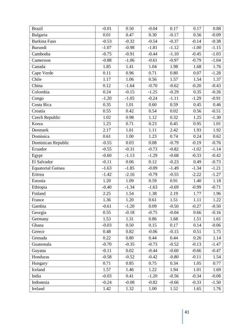
41

Brazil -0.01 0.50 -0.04 0.17 0.17 0.88

Bulgaria 0.01 0.47 0.30 -0.17 0.56 -0.09

Burkina Faso -0.53 -0.32 -0.54 -0.37 -0.14 -0.38

Burundi -1.07 -0.98 -1.81 -1.12 -1.00 -1.15

Cambodia -0.75 -0.91 -0.44 -1.10 -0.45 -1.03

Cameroon -0.88 -1.06 -0.61 -0.97 -0.79 -1.04

Canada 1.85 1.41 1.04 1.98 1.68 1.76

Cape Verde 0.11 0.96 0.71 0.80 0.07 -1.28

Chile 1.17 1.06 0.56 1.57 1.54 1.37

China 0.12 -1.64 -0.70 -0.62 -0.20 -0.43

Colombia 0.24 -0.15 -1.25 -0.29 0.35 -0.26

Congo -1.20 -1.05 -0.24 -1.11 -1.29 -0.91

Costa Rica 0.35 1.01 0.60 0.59 0.45 0.46

Croatia 0.55 0.42 0.54 0.02 0.56 -0.51

Czech Republic 1.02 0.98 1.12 0.32 1.25 -1.30

Korea 1.23 0.71 0.23 0.45 0.95 1.01

Denmark 2.17 1.61 1.11 2.42 1.93 1.92

Dominica 0.61 1.00 1.23 0.74 0.24 0.62

Dominican Republic -0.55 0.03 0.08 -0.79 -0.19 -0.76

Ecuador -0.55 -0.31 -0.73 -0.82 -1.02 -1.14

Egypt -0.60 -1.13 -1.29 -0.68 -0.33 -0.42

El Salvador -0.11 0.06 0.12 -0.23 0.49 -0.73

Equatorial Guinea -1.63 -1.85 -0.09 -1.49 -1.34 -1.21

Eritrea -1.42 -2.16 -0.79 -0.55 -2.22 -1.27

Estonia 1.20 1.09 0.59 0.91 1.40 1.18

Ethiopia -0.40 -1.34 -1.63 -0.69 -0.99 -0.71

Finland 2.25 1.54 1.38 2.19 1.77 1.96

France 1.36 1.20 0.61 1.51 1.11 1.22

Gambia -0.61 -1.20 0.09 -0.50 -0.27 -0.50

Georgia 0.55 -0.18 -0.75 -0.04 0.66 -0.16

Germany 1.53 1.31 0.86 1.68 1.51 1.61

Ghana -0.03 0.50 0.15 0.17 0.14 -0.06

Greece 0.48 0.82 -0.06 -0.15 0.51 1.75

Grenada 0.22 0.80 0.44 0.44 0.26 1.14

Guatemala -0.70 -0.35 -0.73 -0.52 -0.13 -1.47

Guyana -0.11 0.02 -0.44 -0.60 -0.66 -0.47

Honduras -0.58 -0.52 -0.42 -0.80 -0.11 1.54

Hungary 0.71 0.85 0.75 0.34 1.05 0.77

Iceland 1.57 1.46 1.22 1.94 1.01 1.69

India -0.03 0.41 -1.20 -0.56 -0.34 -0.08

Indonesia -0.24 -0.08 -0.82 -0.66 -0.33 -1.50

Ireland 1.42 1.32 1.00 1.52 1.65 1.76

42

Israel 1.20 0.65 -1.30 0.68 1.35 0.98

Italy 0.45 0.94 0.59 -0.01 0.75 -0.43

Japan 1.35 1.02 0.97 1.50 0.90 1.75

Jordan 0.05 -0.88 -0.42 0.04 0.25 0.24

Kazakhstan -0.26 -1.19 -0.17 -1.01 -0.28 -0.63

Kenya -0.54 -0.23 -1.31 -0.87 -0.16 -0.57

Kuwait -0.04 -0.54 0.33 0.07 0.08 0.50

Kyrgyzstan -0.62 -0.75 -1.05 -1.13 -0.21 -0.92

Latvia 0.68 0.74 0.29 0.21 0.95 0.80

Lebanon -0.33 -0.41 -1.55 -0.91 0.02 -0.68

Lesotho -0.28 -0.13 0.27 0.22 -0.61 -0.27

Liberia -1.21 -0.30 -0.50 -0.46 -1.01 1.63

Lithuania 0.68 0.84 0.63 0.29 0.94 0.77

Luxembourg 1.73 1.57 1.33 2.17 1.86 -0.25

Madagascar -0.87 -0.84 -0.88 -0.28 -0.55 -0.84

Malawi -0.43 -0.26 -0.07 -0.36 -0.70 -0.17

Malaysia 1.00 -0.44 0.16 0.00 0.66 -0.39

Mali -0.83 0.14 -0.71 -0.61 -0.40 -0.50

Malta 1.16 1.12 1.00 0.91 1.31 0.88

Mauritania -0.90 -0.95 -1.19 -0.57 -0.78 -0.89

Mauritius 0.76 0.75 0.88 0.62 0.84 0.86

Mexico 0.32 0.09 -0.70 -0.36 0.35 0.89

Mongolia -0.62 -0.01 0.55 -0.67 -0.22 -0.33

Montenegro 0.10 0.25 0.52 -0.21 -0.06 0.03

Morocco -0.22 -0.71 -0.47 -0.26 -0.09 -0.21

Mozambique -0.55 -0.15 0.27 -0.41 -0.40 -1.42

Namibia 0.06 0.33 0.89 0.22 0.08 0.35

Nepal -0.79 -0.53 -1.55 -0.77 -0.72 -0.99

Netherlands 1.79 1.52 1.12 2.17 1.84 1.91

Nicaragua -0.90 -0.58 -0.38 -0.77 -0.35 -0.71

Niger -0.67 -0.30 -0.88 -0.65 -0.51 -0.50

Norway 1.76 1.63 1.35 2.17 1.41 1.89

Pakistan -0.82 -0.83 -2.70 -1.00 -0.61 0.84

Panama 0.10 0.50 -0.11 -0.35 0.41 -0.07

Papua New Guinea -0.74 -0.03 -0.89 -1.12 -0.51 -0.84

Paraguay -0.83 -0.10 -0.72 -0.73 -0.34 -0.86

Peru -0.15 0.05 -0.69 -0.20 0.50 -0.60

Philippines 0.00 -0.01 -1.39 -0.78 -0.26 -0.51

Portugal 0.97 1.12 0.70 1.09 0.66 0.76

Republic of Moldova -0.58 -0.02 -0.13 -0.62 -0.08 0.88

Romania -0.22 0.41 0.12 -0.20 0.72 0.04

Russian Federation -0.40 -0.94 -0.88 -1.09 -0.35 -0.78

43

Rwanda 0.07 -1.29 -0.05 0.45 -0.12 0.70

Saint Lucia 0.86 1.22 0.87 1.24 0.46 0.74

Saint Vincent and the Grenadines 0.77 1.15 0.87 1.06 0.37 -0.31

Saudi Arabia -0.43 -1.84 -0.30 -0.29 0.00 0.07

Senegal -0.44 -0.30 -0.31 -0.62 -0.22 -0.45

Serbia -0.15 0.29 -0.33 -0.20 0.01 -0.01

Sierra Leone -1.16 -0.21 -0.19 -0.69 -0.70 -0.86

Singapore 2.16 -0.19 1.21 2.12 1.83 1.69

Slovakia 0.86 0.95 0.97 0.29 1.03 0.65

Slovenia 0.99 1.03 0.84 0.93 0.63 -2.35

South Africa 0.37 0.57 0.02 0.03 0.44 -1.48

Spain 1.02 1.10 0.13 1.06 1.09 1.20

Sri Lanka -0.08 -0.53 -0.54 -0.42 -0.09 -1.26

Swaziland -0.69 -1.25 -0.47 -0.27 -0.64 -0.42

Sweden 1.96 1.59 1.26 2.22 1.84 1.95

Switzerland 1.89 1.63 1.29 2.02 1.64 1.04

Tajikistan -0.94 -1.35 -1.01 -1.13 -0.97 -0.52

Thailand 0.10 -0.45 -1.02 -0.37 0.24 0.69

The former Yugoslav Rep. of

Macedonia

-0.11 0.01 -0.45 -0.04 0.33 -1.19

Togo -1.36 -0.93 -0.24 -0.99 -0.99 -0.85

Tonga -0.37 0.37 0.97 -0.29 -0.61 0.07

Tunisia 0.02 -0.37 -0.23 -0.21 -0.18 -0.10

Turkey 0.41 -0.17 -0.93 0.10 0.42 0.08

Turkmenistan -1.61 -2.12 0.21 -1.46 -2.05 0.45

Uganda -0.51 -0.54 -1.10 -0.86 -0.11 -0.40

Ukraine -0.83 -0.10 -0.15 -0.99 -0.56 -0.86

United Kingdom 1.55 1.27 0.37 1.54 1.62 1.67

United Rep. of Tanzania -0.54 -0.11 -0.01 -0.52 -0.44 -0.52

Uruguay 0.58 1.12 0.94 1.28 0.41 0.71

US 1.41 1.13 0.54 1.23 1.49 1.60

Uzbekistan -0.77 -2.03 -0.61 -1.34 -1.59 -1.39

Vanuatu -0.24 0.57 1.13 0.35 -0.70 0.23

Venezuela -1.10 -0.92 -1.30 -1.22 -1.49 -1.63

Viet Nam -0.28 -1.48 0.17 -0.59 -0.61 -0.43

Zambia -0.65 -0.20 0.47 -0.51 -0.43 -0.47

Zimbabwe -1.40 -1.46 -1.04 -1.30 -1.90 -1.75

Model 2. EGOV-HDI

EGOV HDI

Albania 0.5161 0.713

Angola 0.3203 0.508

44

Armenia 0.4997 0.729

Australia 0.8390 0.938

Austria 0.7840 0.895

Azaerbaijan 0.4984 0.734

Bahamas 0.5793 0.794

Bangladesh 0.2991 0.515

Belarus 0.6090 0.793

Belgium 0.7718 0.897

Bhutan 0.2942 0.538

Bolivia (Plurinational State of) 0.4658 0.675

Bosnia and Herzegovina 0.5328 0.735

Botswana 0.4186 0.634

Brazil 0.6167 0.73

Bulgaria 0.6132 0.782

Burkina Faso 0.1578 0.343

Burundi 0.2288 0.355

Cambodia 0.2902 0.543

Cameroon 0.3070 0.495

Canada 0.8430 0.911

Cape Verde 0.4297 0.586

Chile 0.6769 0.819

China 0.5359 0.699

Colombia 0.6572 0.719

Congo 0.2809 0.534

Costa Rica 0.5397 0.773

Croatia 0.7328 0.805

Czech Republic 0.6491 0.873

Korea 0.3616 0.909

Denmark 0.8889 0.901

Dominica 0.5561 0.745

Dominican Republic 0.5130 0.702

Ecuador 0.4869 0.724

Egypt 0.4611 0.662

El Salvador 0.5513 0.68

Equatorial Guinea 0.2955 0.554

Eritrea 0.2043 0.351

Estonia 0.7987 0.846

Ethiopia 0.2306 0.396

Finland 0.8505 0.892

France 0.8635 0.893

Gambia 0.2688 0.439

Georgia 0.5563 0.745

45

Germany 0.8079 0.92

Ghana 0.3159 0.558

Greece 0.6872 0.86

Grenada 0.5479 0.77

Guatemala 0.4390 0.581

Guyana 0.4549 0.636

Honduras 0.4341 0.632

Hungary 0.7201 0.831

Iceland 0.7835 0.906

India 0.3829 0.554

Indonesia 0.4949 0.629

Ireland 0.7149 0.916

Israel 0.8100 0.9

Italy 0.7190 0.881

Japan 0.8019 0.912

Jordan 0.4884 0.7

Kazakhstan 0.6844 0.754

Kenya 0.4212 0.519

Kuwait 0.5960 0.79

Kyrgyzstan 0.4879 0.622

Latvia 0.6604 0.814

Lebanon 0.5139 0.745

Lesotho 0.3501 0.461

Liberia 0.2407 0.388

Lithuania 0.7333 0.818

Luxembourg 0.8014 0.875

Madagascar 0.3054 0.483

Malawi 0.2740 0.418

Malaysia 0.6703 0.769

Mali 0.1857 0.344

Malta 0.7131 0.847

Mauritania 0.1996 0.467

Mauritius 0.5066 0.737

Mexico 0.6240 0.775

Mongolia 0.5443 0.675

Montenegro 0.6218 0.791

Morocco 0.4209 0.591

Mozambique 0.2786 0.327

Namibia 0.3937 0.608

Nepal 0.2664 0.463

Netherlands 0.9125 0.921

Nicaragua 0.3621 0.599

46

Niger 0.1119 0.304

Norway 0.8562 0.955

Pakistan 0.2823 0.515

Panama 0.5733 0.78

Papua New Guinea 0.2147 0.466

Paraguay 0.4802 0.669

Peru 0.5230 0.741

Philippines 0.5130 0.654

Portugal 0.7165 0.816

Republic of Moldova 0.5626 0.66

Romania 0.6060 0.786

Russian Federation 0.7345 0.788

Rwanda 0.3291 0.434

Saint Lucia 0.5122 0.725

Saint Vincent and the Grenadines 0.5177 0.733

Saudi Arabia 0.6658 0.782

Senegal 0.2673 0.47

Serbia 0.6312 0.769

Sierra Leone 0.1557 0.359

Singapore 0.8474 0.895

Slovakia 0.6292 0.84

Slovenia 0.7492 0.892

South Africa 0.4869 0.629

Spain 0.7770 0.885

Sri Lanka 0.4357 0.715

Swaziland 0.3179 0.536

Sweden 0.8599 0.916

Switzerland 0.8134 0.913

Tajikistan 0.4069 0.622

Thailand 0.5093 0.69

The former Yugoslav Rep. of

Macedonia

0.5587 0.74

Togo 0.2143 0.459

Tonga 0.4405 0.71

Tunisia 0.4833 0.712

Turkey 0.5281 0.722

Turkmenistan 0.3813 0.698

Uganda 0.3185 0.456

Ukraine 0.5653 0.74

United Kingdom 0.8960 0.875

United Rep. of Tanzania 0.3311 0.476

Uruguay 0.6315 0.792

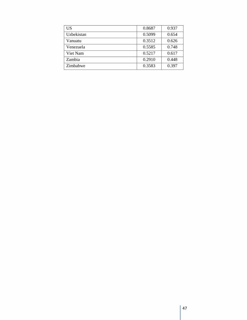
47

US 0.8687 0.937

Uzbekistan 0.5099 0.654

Vanuatu 0.3512 0.626

Venezuela 0.5585 0.748

Viet Nam 0.5217 0.617

Zambia 0.2910 0.448

Zimbabwe 0.3583 0.397