PROCEDURES FOR THE PREPARATION OF

EMISSION INVENTORIES FOR CARBON MONOXIDE AND PRECURSORS OF OZONE

w t

VOLUME I: GENERAL GUIDANCE t

FOR STATIONARY SOURCES

EPA-450/4-91-016 :

PROCEDURES FOR THE PREPARATION OF

EMISSION INVENTORIES FOR CARBON MONOXIDE AND PRECURSORS OF OZONE

VOLUME I: GENERAL GUIDANCE FOR STATIONARY SOURCES i

Alliance Technologies Corporation Chapel Hill, NC

EPA Contract No. 68-D9-0173 EPA Project Officer Mary Ann Warner-Selph

Office Of Air Quality Planning And Standards Office Of Air And Radiation

U. S. Environmental Protection Agency Research Triangle Park, NC 2771 1

May 1991

This report has been reviewed by the Office Of Air Quality Planning And Standards, U. S. Environmental Proteaion Agency, and has been approved for publication as received from the confractor. The contents reflect the views and policies of the Agency, but any mention of trade names or commercial products does not constitute endorsement or recommendation for use.

EPA-45014-9 1-016

I

11

PREFACE

This document is the first volume of a two-volume series designed to provide assistance to air pollution control agencies in preparing and maintaining emissions inventories for carbon monoxide (CO) and precursors of ozone (03. Emissions inventories provide the foundation for most air quality control programs. This document describes procedures for preparing inventories of volatile organic compounds (VOC), oxides of nitrogen (NO3 and CO on a countywide annual or seasonal basis. Such an inventory is required by the 1990 Clean Air Act Amendments for establishing a baseline in 0, nonattainment areas, while an inventory of CO emissions is required for CO nonattainment areas.

The second volume of this series offers technical assistance to those engaged in planning and developing detailed inventories of VOC, NO, and CO for use in photochemical air quality simulation models, Such inventories must be gridded, speciated and temporally allocated (hourly) and are required of the more serious 0, and CO nonattainment areas only.

This first volume has been revised from the 1988 version to include current information pertinent to inventorying emissions of CO and precursors of ozone. This edition includes changes and additions as briefly summarized below:

Reflects emissions inventory requirements of the 1990 Clean Air Acf Amendments for ozone and CO state implementation plans (SIPS).

Discusses the role of EPA’s Aerometric Information Retrieval System (AIRS) in the inventory preparation process. Also, describes requirements for submittal of SIP inventories in on AIRS-compatible computer readable format.

Revises all tables to reflect Standard Industrial Classification (SIC) code changes as found in the 1987 SIC publication.

Addresses questions and comments on the previous edition of Volume 1.

Includes new information on publicly owned treatment works (POlWs) and hazardous waste treatment, storage and disposal facilities (TSDFs) (Chapter 3).

Updates emission factors for stationary source solvent evaporation (Section 4.3).

Summarizes stationary area source emission factors (Table 4.1 0-1) . presented in the document.

Includes default seasonal adjustment factors for the CO season (Chapter 6).

Updates and expands the list of point source categories (Appendix B).

Includes new information on Control Techniques Guidelines (CTGs) and Alternative Conirol Technology documents (ACTS) (Appendix C).

Includes a new section on previously uninventoried source categories (Appendix E).

Updates discussions of associated EPA programs and references pertinent to inventorying. ~

C H Q l M ii

t

TABLE OF CONTENTS

Section Page

Preface ...................................................... ii List of Figures . . . . . . . . . . . . . . . . . . . . . . . . . . . . . . . . . . . . . . . . . . . . . . . . . . . . . . vii List of Tables ........................................................ viii List of Acronyms ....................................................... xi

1.0 INTRODUCTION . . . . . . . . . . . . . . . . . . . . . . . . . . . . . . . . . . . . . . . . . . . . . . . . . . . . 1-1

1.1 Purpose . . . . . . . . . . . . . . . . . . . . . . . . . . . . . . . . . . . . . . . . . . . . . . . . . . . . . . 1-1 1.2 Contents of Volume I . . . . . . . . . . . . . . . . . . . . . . . . . . . . . . . . . . . . . . . . . . . 1-2

2.0 INVENTORY OVERVIEW AND PLANNING .................................. 2-1

2.1 Overview of Inventory Procedures . . . . . . . . . . . . . . . . . . . . . . . . . . . . . . . . . . . 2-1 2.2 General Planning Considerations . . . . . . . . . . . . . . . . . . . . . . . . . . . . . . . . . . . 2-1

2.2.1 Emissions Inventory End Uses ............................... 2-3 2.2.2 Definition of VOC . . . . . . . . . . . . . . . . . . . . . . . . . . . . . . . . . . . . . . . . . 2 4 2.2.3 Sources of VOC Emissions . . . . . ........................... 2 4 2.2.4 Emissions Inventory Staff Requirements ........................ 2-8 2.2.5 Determining Geographical Area to be Inventoried . . . . . . . . . . . . . . . . 2-8 2.2.6 Spatial Resolution ........................................ 2-9 2.2.7 Base Year Selection . . . . . . . . . . . . . . . . . . . . . . . . . . . . . . . . . . . . . . 2-10 . 2.2.8 Rule Effectiveness ...................... : . . . . . . . . . . . . . . . . . 2-10 2.2.9 Temporal Resolution . . . . . . . . . . . . . . . . . . . . . . . . . . . . . . . . . . . . . . 2-10 2.2.1 0 Point/Area Source Distinctions . . . . . . . . . . . . . . . . . . . . . . . . . . . . . . . 2-10 2.2.1 1 Data Collection Methods . . . . . . . . . . . . . . . . . . . . . . . . . . . . . . . . . . . 2-12 2.2.1 2 Exclusion of Nonreactive Compounds and Consideration of

2-12 2.2.1 3 Emissions Projections ...................................... 2-14 2.2.1 4 Status of Existing Inventory ................................. 2-15

2.2.16 Data Handling . . . . . . . . . . . . . . . . . . . . . . . . . . . . . . . . . . . . . . . . . . . . 2-16 2.2.17 Quality Assurance . . . . . . . . . . . . . . . . . . . . . . . . . . . . . . . . . . . . . . . . 2-17 2.2.18 Documentation . . . . . . . . . . . . . . . . . . . . . . . . . . . . . . . . . . . . . . . . . . . 2-17

2-17

Species Information . . . . . . . .. .............................. 2.2.1 5 Corresponding. NO, and CO Inventories ........................ 2-15

2.2.1 9 Anticipated Use of a Photochemical Dispersion Model . . . . . . . . . . . . . 2.2.20 Planning Review . . . . . . . . . . . . . . : . . . . . . . . . . . . . . . . . . . . . . . . . . 2-18

3.0 POINT SOURCE DATA COLLECTION . . . . . . . . . . . . . . . . . . . . . . . . . . . . . . . . . . . . . . 3-1

3.1 Introduction . . . . . . . . . . . . . . . . . . . . . . . . . . . . . . . . . . . . . . . . . . . . . . . . . . 3-1 3.1.1 Statewide Point Source Emissions Inventories for Regional

Modeling . . . . . . . . . . . . . . . . . . . . . . . . . . . . . . . . . . . . . . . . . . . . . . . 3-3 3.2 Questionnaires (Mail Survey Approach) . . . . . . . . . . . . . . . . . . . . . . . . . . . . . . . 3-3

3.2.1 Preparing the Mailing List . . . . . . . . . . . . . . . . . . . . . . . . . . . . . . . . . . . 3-3 3.2.2 Limiting the Size of the Mail Survey . . . . . . . . . . . . . . . . . . . . . . . . . . . . 3-5 3.2.3 Designing the Questionnaires ................................ 3-7 3.2.4 Mailing and Tracking the Questionnaires and Logging Returns . . . . . . 3-9 3.2.5 Recontacting . . . . . . . . . . . . . . . . . . . . . . . . . . . . . . . . . . . . . . . . . . . . . 3-11

3.3 Ptant Inspections . . . . . . . . . . . . . . . . . . . . . . . . . . . . . . . . . . . . . . . . . . . . . . . 3-11 3.4 Other Air Pollution Agency Files . . . . . . . . . . . . . . . . . . . . . . . . . . . . . . . . . . . 3-12

3.4.1 Permjt and Compliance Files . . . . . . . . . . . . . . . . . . . . . . . . . . . . . . . . 3-12 3.4.2 Emissions Statements . . . . . . . . . . . . . . . . . . . . . . . . . . . . . . . . . . . . . . 3-13

CH91-08 iii

..-.. . . ... _^_.I” . .---- .

4 TABLE OF CONTENTS (continued)

Section Page

3.5 Waste Treatment Emissions ...................................... 3-13 3.5.1 Publicly Owned Treatment Works (POTWs) ..................... 3-14 3.5.2 Package P l d s (Wastewater Treatment) ........................ 3-14 3.5.3 Industrial Wastewater Treatment and Hazardous Waste Treatment.

Storage and Disposal Facilities (TSDFs). ...................... 3-15 3.5.3.1 Example Calculation ................................ 3-16

3.5.4 Municipal Solid Waste Landfills . . . . . . . . . . . . . . . . . . . . . . . . . . . . . . 3-18 3.6 Publications . . . . . . . . . . . . . . . . . . . . . . . . . . . . . . . . . . . . . . . . . . . . . . . . . 3-19 3.7 Existing Inventories . . . . . . . . . . . . . . . . . . . . . . . . . . . . . . . . . . . . . . . . . . . . . 3-19 3.8 Rule Effectiveness (RE) . ......................................... 3-20

4.0. AREA SOURCE DATA COLLECTION . . . . . . . . . . . . . . . . . . . . . . . . . . . . . . . . . . . . . 4-1'

4.1 Introduction . . . . . . . . . . . . . . . . . . . . . . . . . . . . . . . . . . . . . . . . . . . . . . . . . . . 4-1 4.1.1 Area Source Inventory Structure and Emphasis . . . . . . . . . . . . . . . . . . 4-1 4.1.2 Source Activity Levels . . . . . . . . . . . . . . . . . . . . . . . . . . . . . . . . . . . . 4-2 . 4.1.3

Emissions . . . . . . . . . . . . . . . . . . . . . . . . . . . . . . . . . . . . . . . . . . . . 4-2

4.2 Gasoline Distribution Losses . . . . . . . . . . . . . . . . . . . . . . . . . . . . . . . . . . . . . . . 4 9

4.2.2 Estimating Gasoline Distribution Emissions ..................... 4-7 4.2.2.1 Tank Truck Unloading (Stage I) . . . . . . . . . . . . . . . . . . . . . . . . 4-7 4.2.2.2 Vehicle Fueling and Underground Tank Breathing . . . . . . . . . . 4-8 4.2.2.3 Losses from Gasoline Tank Trucks in Transit . . . . . . . . . . . . . . 4-8

4.2.4 Petroleum Vessel Loading and Unloading Losses . . . . . . . . . . . . . . . . 4-9 4.3 Stationary Source Solvent Evaporation . . . . . . . . . . . . . . . . . . . . . . . . . . . . . . 4-10

4.3.1 Dry Cleaning . . . . . . . . . . . . . . . . . . . . . . . . . . . . . . . . . . . . . . . . . . . . 4-11 4.3.1.1 Dry Cleaning Methods . . . . . . . . . . . . . . . . . . . . . . . . . . . . . . . 4-11 4.3.1.2 Dry Cleaning Emission Factors and Inventory Methods . . . . . . 4-13

4.3.2 Surface Cleaning . . . . . . . . . . . . . . . . . . . . . . . . . . . . . . . . . . . . . . . . . 4-15

4.3.2.2 Surface Cleaning Emission'Factors and Inventpry Methods . . . 4-17 4.3.3 Surface Coating . . . . . . . . . . . . . . . . . . . . . . . . . . . . . . . . . . . . . . . . . . 4-20

4.3.3.1 Coating Operations . . . . . . . . . . . . . . . . . . . . . . . . . . . . . . . . . 4-21 4.3.3.2 Coating Emission Factors and Inventory Methods . . . . . . . . . . 4-22

4.3.4 Graphic Arts . . . . . . . . . . . . . . . . . . . . . . . . . . . . . . . . . . . . . . . . . . . . 4-25 4.3.4.1 Printing Methods . . . . . . . . . . . . . . . . . . . . . . . . . . . . . . . . . . . 4-26 4.3.4.2 Graphic Arts Emission Factors and Inventory Methods . . . . . . . 4-28

4.3.5 Asphalt Paving . . . . . . . . . . . . . . . . . . . . . . . . . . . . . . . . . . . . . . . . . . 4-29

4.3.7 Commercial/Consumer Solvent Use . . . . . . . . . . . . . . . . . . . . . . . . . . . 4-32 4.3.8 Synthetic Organic Chemical Storage Tanks . . . . . . . . . . . . . . . . . . . . . 4-33 4.3.9 Barge, Tank, Tank Truck, Rail Car and Drum Cleaning . . . . . . . . . . . . . 4-33

4.4 Bioprocess Emissions Sources ........................ . . . . . . . . . . . . . 4-34 4.4.1 Bakeries . . . . . . . . . . . . . . . . . . . . . . . . . . . . . . . . . . . . . . . . . . . . . . . . 4-34 4.4.2 Breweries . . . . . . . . . . : . . . . . . . . . . . . . . . . . . . . . . . . . . . . . . . . . . . 4-34 4.4.3 Wineries . . . . . . . . . . . . . . . . . . . . . . . . . . . . . . . . . . . . . . . . . . . . . . . . 4-35 4.4.4 .Distilleries . . . . . . . . . . . . . . . . . . . . . . . . . . . . . . . . . . . . . . . . . . . . . . 4-35

Methods for Estimating Area Source Activity Levels and

. . . . . . . 4.1.4 Contents of Chapter 4 . . . . . . . . . . . . . . . . . . . . . . . . . . . . . ; 4 4

4.2.1 Determining Gasoline Sales . . . . . . . . . . . . . . . . . . . . . . . . . . . . . . . . . . 4 4

4.2.3 Aircraft Refueling . . . . . . . . . . . . . . . . . . . . . . . . . . . . . . . . . . . . . . . . . 4-9

4.3.2.1 Surface Cleaning Operations . . . . . . . . . . . . . . . . . . . . . . . . . . 4-15 ..

4.3.6 Pesticide Application . . . . . . . . . . . . . . . . . . . . . . . . . . . . . . . . . . . . . 4-31

. .

CH91-08 iv

TABLE OF CONTENTS (continued)

Section Page

4.5 Catastrophic/Accidental Releases ................................... 4-36 4.5.1 OilSpills ............................................... 4-36

4.6 Solid Waste Incineration ......................................... 4-36 4.6.1 OnSite Incineration ....................................... 4-37 4.6.2 Open Burning ............................................. 4-37

4.7 Small Stationary Source Fossil Fuel Use ............................. 4-37 4.7.1 . Fuel Oil Consumption ..................................... 4-39 4.7.2 Coal Consumption ....................... : . . . . . . . . . . . . . . . . 4-40 4.7.3 Natural Gas and Liquified Petroleum Gas Consumption . . . . . . . . . . . . . 441 4.7.4 Other Fuels Consumption . . . . . . . . . . . . . . . . . . . . . . . . . . . . . . . . . . 442 4.7.5 Small Electric Utility Boilers .................................. 442

4.8.1 Forest Fires . . . . . . . . . . . . . . . . . . . . . . . . . . . . . . . . . . . . . . . . . . . . . 4-43 4.8.2 Slash Burning and Prescribed Burning . . . . . . . . . . . . . . . . . . . . . . . . 443 4.8.3 Agricuttural Burning . . . . . . . . . . . . . . . . . . . : . . . . . . . . . . . . . . . . . . . 444 4.8.4 Structure Fires . . . . . . . . . . . . . . . . . . . . . . . . . . . . . . . . . . . . . . . . . . . . 444 4.8.5 Orchard Heaters . . . . . . . . . . . . . . . . . . . . . . . . . . . . . . . . . . . . . . . . . 444 .

4.8.6 Leaking Underground Storage Tanks . . . . . . . . . . . . . . . . . . . . . . . . . . 4-45

4.8 OtherAreaSources . . . . . . . . . . . . . . . . . . . . . . . . . . . . . . . . . . . . . . . . . . . . 4-43 .

4.9 Mobile Sources . . . . . . . . . . . . . . . . . . . . . . . . . . . . . . . . . . . . . . . . . . . . . . . . 445 4.1 0 Summary of Emission Factors . . . . . . . . . . . . . . . . . . . . . . . . . . . . . . . . . . . . . . 4-46

5.0 EMISSIONS CALCULATIONS . . . . . . . . . . . . . . . . . . . . . . . . . . . . . . . . . . . . . . . . . . 5-1

c

5.1 5.2 5.3 5.4 5.5 5.6 5.7 5.8

5.9 5.1 0

Introduction . . . . . . . . . . . . . . . . . . . . . . . . . . . . . . . . . . . . . . . . . . . . . . . . . . SourceTest Data . . . . . . . . . . . . . . . . . . . . . . . . . . . . . . . . . . . . . . . . . . . . . . Material Balance . . . . . . . . . . . . . . . . . . . . . . . . . . . . . . . . . . . . . . . . . . . . . . . Emission Factors . . . . . . . . . . . . . . . . . . . . . . . . . . . . . . . . . . . . . . . . . . . . . . Per Capita and Emissions-per-Employee Factors ....................... Scaling Up the Inventory . . . . . . . . . . . . . . . . . . . . . . . . . . . . . . . . . . . . . . . . . Excluding Nonreactive VOC from Emission Totals . . . . . . . . . . . . . . . . . . . . . . Seasonal Adjustment of the Annual Inventory . . . . . . . . . . . . . . . . . . . . . . . . . 5.8.1 Seasonal Changes in Acti\ii Levels . . . . . . . . . . . . . . . . . . . . . . . . . . 5.8.2 Seasonal Changes in Temperature ........................... 5.8.3 Other Seasonal Adjustment Considerations ..................... 5.8.4' Development and Application of Adjustment Factors . . . . . . . . . . . . . . . Determining Emissions for a Typical Ozone or CO Season Day . . . . . . . . . . . . Emissions Projections . . . . . . . . . . . . . . . . . . . . . . . . . . . . . . . . . . . . . . . . . . . .

5-1 5-2 5-4 5-5

5-10 5-12 5-14 5-17 5-17 5-19 . 5-21 5-21 5-22 5-23

6.0 SUPPORTING DOCUMENTATION AND REPORTING .. . . . . . . . . . . . . . . . . . . . . . . . 6-1

6.1 Introduction . . . . . . . . . . . . . . . . . . . . . . . . . . . . . . . . . . . . . . . . . . . . . . . . . . 6-1 6.2 Reporting Forms . . . . . . . . . . . . . . . . . . . . . . . . . . . . . . . . . . . . . . . . . . . . . . . 6-1 6.3 Supporting Documentation . . . . . . . . . . . . . . . . . . . . . . . . . . . . . . . . . . . . . . . . 6-7

cn91-08

Section

TABLE OF CONTENTS (continued) ,

i(

Page 1 APPENDIX A . GLOSSARY OF IMPORTANT TERMS .............................. APPENDIX B - €MISSIONS REPORTING FORMAT AND SUMMARY LISTINGS OF SOURCE

A-1

CATEGORIES . . . . . . . . . . . . . . . . . . . . . . . . . . . . . . . . . . . . . . . . . . . B-1 APPENDIX C - CONTROL TECHNIQUES GUIDELINES AND ALTERNATIVE CONTROL

TECHNOLOGY DOCUMENTS . . . . . . . . . . . i . . . . . . . . . . . . . . . . . . . C-1 APPENDIX D . EXAMPLE QUESTIONNAIRES ................................... D-1 APPENDIX E . PREVIOUSLY UNINVENTORIED SOURCE CATEGORIES . . . . . . . . . . . . . . . E-1

CH91-08 vi

LIST OF FIGURES

Number Page

4.2-1 Gasoline marketing operations and emission sources ...................... 4-5

4.3-1 Mass balance of solvent used in degreasing operations ..................... 4-18

5.2-1 Example source test data and emissions calculations . . . . . . . . . . . . . . . . . . . . . . 5-3

5.4-1 True vapor pressure (P) of refined petroleum stocks (1 psi to 20 psi RVP) . . . . . . . 5-9

6.2-1 Example pie chart illustrating source category contributions to total emissions . . . . . . . . . . . . . . . . . . . . . . . . . . . . . . . . . . . . . . . . . . . . . . . . . . . . . . 6 4

6.2-2 Example bar graph illustrating source category contributions to total emissions and projected emissions trends . . . . . . . . . . . . . . . . . . . . . . . . . . . . . . . . . . . . . 6-5

6.2-3 Breakdown of organic solvent emissions by source type .................... 6-6

D-1 Example questionnaire . Instruction sheet . . . . . . . . . . . . . . . . . . . . . . . . . . . . .. . . D-2

0-2 . Example questionnaire . General information page . . . . . . . . . . . . . . . . . . . . . . . . . 0-3

D-3 Example questionnaire . Degreasing operations form . . . . . . . . . . . . . . . . . . . . . . . D-4 .

D 4 Example questionnaire . Dry cleaning form . . . . . . . . . . . . . . . . . . . . . . . . . . . . . . D-5

D-5 Example questionnaire . Protective or decorative coatings form . . . . . . . . . . . . . . . D-6 .

D-6 Example questionnaire . Fabric or rubberized coatings form . . . . . . . . . . . . . . . . . . D-7

0-7 Example questionnaire . Miscellaneous surface coating application form . . . . . . . . D-8 .

D-8 Example questionnaire . Ovens and heating equipment form . . . . . . . . . . . . . . . . .

D-9 Example questionnaire . Printing form . . . . . . . . . . . . . . . . . . . . . . . . . . . . . . . . . . D-10

D-9

D-10 Example questionnaire . General solvent usage form . . . . . . . . . . . . . . . . . . . . . . . D-11

D-11 Example questionnaire . Bulk solvent storage form . . . . . . . . . . . . . . . . . . . . . . . . . D-12

Example questionnaire . Control and stack information form . . . . . . . . . . . . . . . . . . . .

D-12 0-13

CH91-08 vii

.

... ..I_ I ... .- ..

. i.. ! I!

t . . .lr .. .p .. $

Number

UST OF TABLES

page

2.2-1 VOC. CO and NO. Emissions Sources . . . . . . . . . . . . . . . . . . . . . . ; . . . . . . . . . . . . 2-5

3.2-1 Standad Industrial Classifications (SICS) Associated with VOC Emissions; Emissions-Per-Employee Ranges . . . . . . . . . . . . . . . . . . . . . . . . . . . . . . . . . . . . 3-6

Solvent Usage in the Dry Cleaning Industry (1989) .......................... 4-12 4.3-1

4.3-2 Recommended Emission Factors for Dry Cleaning . . . . . . . . . . . . . . . . . . . . . . . . . 4-14

4.3-3 Solvent Usage in Surface Cleaning (1 989) . . . . . . . . . . . . . . . . . . . . . . . . . . . . . . . 4-16

4.34 Recommended Emission Factors for Surface Cleaning ...................... 4-19

4.3-5 Breakdown of Coating Consumption and Estimated Solvent Distribution by End Use for 1989 . . . . . : .............................. 4-21

. 4.3-6 Recommended Emission Factors for Surface Coating ..................... ! 4-24

4.3-7 Solvent Usage in Surface Coatings . . . . . . . . . . . . . . . . . . . . . . . . . . . . . . . . . . . . 4-26

4.3-a Solvent Usage in Printing.Ink . . . . . . . . . . . . . . . . . . . . . . . . . . . . . . . . . . . . . . . . . . 4-27 f

4.3-9 Recommended Emission Factors for Graphic Arts . . . . . . . . . . . . . . . . . . . . . . . . . 4-29

4.3-1 0 Recommended Emission Factors for Asphalt Paving . . . . . . . . . . . . . . . . . . . . . . . 4-30

4.6-1 Factors to Estimate Tons of Solid Waste Eurned in On-site Incineration . . . . . . . . . 4-38 4.6-2 Factors to Estimate Tons of Solid Waste Disposal Through Open Burning . . . . . . . 4-38 4.1 0-1 Area Source Categories and Emission Factors . . . . . . . . . . . . . . . . . . . . . . . . . . . . 4-47

5.4-1 Summary of Average Seal Factors (KJ and Wind Speed Exponents (n) . . . . . . . . . 5-7

5.4-2 Average Annual Stock Storage Temperature (TJ as a Function of Tank Paint Color . . . . . . . . . . . . . . . . . . . . . . . . . . . . . . . . . . . . . . . . . . . . . . . . . . . . . 5-8

5.4:3 Average Clingage Factors. C (bbl/1.,000 f f ) . . . . . . . . . . . . . . . . . . . . . . . . . . . . . . 5-8

5.7-1 VOC Speciation Data for Carbon Black Production ......................... 5-16

5.8-1 Area Source Seasonal Adjustment Factors for the Peak Ozone andCOSeasons . . . . . . . . . . . . . . . . . . . . . . . . . . . . . . . . . . . . . . . . . . . . . . . . 5-18

CHSI-MI viii

... ..... .... .... P ..-.

LIST OF TABLES (continued)

Y 3

Number Page

5.10-1 5-24

6.2-1 VOC Emissions Sources with Associated SIC@) . . . . . . . . . . . . . . . . . . . . . . . . . . . 6-3

B-1 Indivi&al Point Source Category Listing . . . . . . . . . . . . . . . . . . . . . . . . . . . . . . . . 8-2

C-1 Summary of CTG Document for Coating of Cans . . . . . . . . . . . . . . . . . . . . . . . . . . C-7

C-2 Summary of CTG Document for Coating of Metal Coils . . . . . . . . . . . . . . . . . . . . . . C-8

C-3 Summary of CTG Document for Coating of Fabric and Vinyi . . . . . . . . . . . . . . . . . . C-9

Growth Indicators for Projecting Emissions Totals for Area Source Categories . . . .

C 4 Summary of CTG Document for Coating of Paper Products . . . . . . . . . . . . . . . . . . C-10

C-5 Summary of CTG Document for Coating in Automobile and Light-Duty Truck Assembly Plants . . . . . . . . . . . . . . . . . . . . . . . . . . . . . . . . . . . . . . . . . . . . C-11

. . . . . . . . . . . . . . . . . . . C-6 Summary of CTG Document for Coating of Metal Furniture c-12

C-7

C-8

c-9

c-10

c-1 1

c-12

c-13

C-14

Summary of CTG Document for Coating of Magnetic Wire . . . . . . . . . . . . . . . . . . . C-13

Summary of CTG Document for Coating of Large Appliances . . . . . . . . . . . . . . . . . C-14

Summary of CTG Document for Tank Truck Gasoline Loading Terminals . . . . . . . . C-15

Summary of CTG Document for Bulk Gasoline Plants . . . . . . . . . . . . . . . . . . . . . . . C-16

Summary of CTG Document for Gasoline Service Stations . Stage I . . . . . . . . . . . . . C.17

Summary of CTG Document for Petroleum Liquid Storage in Fixed-Roof Tanks . . . C-18

Summary of CTG Document for Processes at Petroleum Refineries . . . . . . . . . . . . C-19

C-20 Summary of CTG Document for Cutback Asphalt . . . . . . . . . . . . . . . . . . . . : . . . . .

(2-15

C-16

Summary of CTG Document for Solvent Metal Cleaning . . . . . . . . . . . . . . . . . . . . . C-21

Summary of CTG Document for Surface Coating of Miscellaneous Metal Parts and Products . . . . . . . . . . . . . . . . . . . . . . . . . . . . . . . . . . . . . . . . . . . . . . . . . . . . . C-22

C-17 Summary of CTG Document for Factory Surface Coating of Flat Wood Paneling . . . C-23

CH91-08 ix

LIST OF TABLES (continued)

Number Page '

C-18

c-19

c-20

c-21

C-22

C-23

C-24

C-25

C-26

C-27

C-28

C-29

Summary of CTG Document for Manufacture of Synthesized Pharmaceutical ,Products . . . . . . . . . . . . . . . . . . . . . . . . . . . . . . . . . . . . . . . . . . . . . . . . . . . . . . C-24

Summary of CTG Document for Manufacture of Pneumatic Rubber Tires . . . . . . . . C-25

Summary Qf CTG Document for Graphic Arts . Rotogravure and Flexography . . . . . C-26

Summary of CTG Document for Perchloroethylene Dry Cleaning Systems C-27

Summary of CTG Document for Leaks from Petroleum Refinery Equipment . . . . . . (2-28

Summary of CTG Document for External Floating Roof Tanks . . . . . . . . . . . . . . . . (2-29

. . . . . . .

Summary of CTG Document for Leaks from Gasoline Tank Trucks and Vapor .Collection Systems . . . . . . . . . . . . . . . . . . . . . . . . . . . . . . . . . . . . . . . . . . . . . . . C30

Summary of CTG Document for Volatile Organic Compound Emissions from Large Petroleum Dry Cleaners . . . . . . . . . . . . . . . . . . . . . . . . . . . . . . . . . . . . . . . . . . . . C-31

Summary of CTG Document for Volatile Organic Compound Emissions from ? Manufacture of High-Density Polyethylene, Polypropylene, and Polystyrene Resins . . . . . . . . . . . . . . . . . . . . . . . . . . . . . . . . . . . . . . . . . . . . . . . . . . . . . . . . C32

Summary of CTG Document for Volatile Organic Compound Equipment Leaks from Natural GadGasoline Processing Plants . . . . . . . . . . . . . . . . . . . . . . . . . . . . . . . C-33

Summary of CTG Document for Volatile Organic Compound Leaks from Synthetic Organic Chemical and Polymer Manufacturing Equipment . . . . . . . . . . . . . . . . . C-34 . .

Summary of CTG Document for, the Air Oxidation Process in Synthetic Organic Chemical. Manufacturing Industry . . . . . . . . . . . . . . . . . . . . . . . . . . . . . . . . . . . . C-35

ACT AFS AGST AIB AIRS AMS APCD API AQCR BIA CAAA CAR6 CB4 CEM CMSA co CTG DAF DOE EB EIA EKMA EPA EPS ESD ESP FHWA FMVCP FTP IPP LPG LTO MC MGD MS

' MSA NAAQS NADB NAPAP NEDS

NPDES NRC OAQPS' ocs OMB OSWER PC

NO,

CH91-08

UST OF ACRONYMS

Alternative Control Technology (document) AIRS Faciiii Subsystem aboveground storage tank American Institute of Baking Aerometric Information Retrieval System AIRS Area and Mobile Source Subsystem air pollution control district American Petroleum Institute air quality control region Barbecue Industry Association Clean Air Act Amendments of 1990 California Air Resources Board Carbon Bond 4 (chemical mechanism) continuous emissions monitoring Consolidated Metropolitan Statistical Area carbon monoxide Control Techniques Guidelines dissolved air flotation (units) U.S. Department of Energy electron beam U.S. DOE, Energy Information Administration Empirical Kinetic Modeling Approach U.S. Environmental Protection Agency Emissions Preprocessor System U.S. EPA, OAQPS, Emissions Standard Division electrostatic precipitator Federal Highway Administration Federal Motor Vehicle Control Program Federal Test Procedures Inventory preparation plan liquefied petroleum gas landing and takeoff (cycle) medium cure cutback asphalt million gallons per day medium set emulsified asphalt Metropolitan Statistical Area national ambient air qualtty standard U.S. EPA, National Air Data Branch National Acid Precipitation Assessment Program National Emissions Data System oxides of nitrogen National Pollutant Discharge Elimination Sygem National Response Center U.S. EPA, Office of Air Qualtty Planning and Standards outer continental shelf U.S. Office of Management and Budget U.S. EPA, Office of Solid Waste and Energy Response personal computer

.

(continued)

t

xi

PM

P O W QA QC RACT RC RCRA RE RFP ROM RP RS RVP SAF SAMs SARA sc SCAQMD SCC SIC SlMS SIP SOC SOCMI SRM ss TPY TRlS TSDF UAM UST uv VMT voc voc

PM,,

UST OF ACRONYMS (continued)

particulate matter particulate matter less than ten microns in diameter publicly owned treatment works quality assurance quality control Reasonably Available Control Technology rapid cure cutback asphatt Resource Conservation and Recovery Act rule effectiveness reasonable further progress Regional Oxidant Model rule penetration rapid set emulsified asphalt Reid vapor pressure seasonal adjustment factor SIP Air Pollutant Inventory Management Subsystem Superfund Amendments and Reauthorization Act slow cure cutback asphatt South Coast Air Quallty Management District (California) source classification code Standard Industrial Classification (code) Surface Impoundment Modeling System State Implementation Plan synthetic organic chemical synthetic organic chemical manufacturing industry solid rocket motor slow set emulsified asphatt tons per year Toxic Release Inventory System hazardous waste treatment, storage and disposal facility Urban Airshed Model ~

underground storage tank ultraviolet vehicle miles traveled volatile organic compound(s) volatile organic liquid(s)

c

cnsi-08 xii

CHAPTER 1

INTRODUCTION

I * , &'-

1.1 PURPOSE

The Clean Air Act Amendments of 1990 (CAAA) recognized that many areas across the United States were in violation of the national ambient air quality standards (NAAQS) for ozone and/or carbon monoxide (CO). One of the first activities for developing an air quality control strategy for these areas is to prepare an inventory of the emissions of interest. .Ozone is photochemically produced in the atmosphere when volatile organic compounds (VOC) are mixed with oxides of nitrogen (NOJ and CO in the presence of sunlight. Emissions of CO are more directly related to concentrations of CO in the atmosphere. To develop and implement an effective ozone control strategy, an air pollution control

. agency must compile information on the important sources of these precursor pollutants. Likewise, information on sources of CO emissions must be gathered as a basis for developing CO control strategies. This is the role of the emission inventory-to identify the source types present in an area, the amount of each pollutant emitted and the types of processes and control devices employed at! each plant. Prior to developing an ozone or CO control strategy, the inventory must be used with an. appropriate source/receptor model to relate emissions of VOC, NO, and/or CO to subsequent levels of ozone or CO in the ambient air.

Emission inventories are compiled using methodologies which are described in inventory guideline references. One such reference, Procedures for Emission inventory Preparation, Volumes /-V,'3 was developed as general guidance to those engaged in inventorying criteria pollutants.

This document, published in two volumes, provides guidance to those engaged in planning and compiling CO and ozone precursor emissions inventories (VOC, NO, and CO). It is particularly directed toward areas that are not in atiainment of ozone and CO NAAQS. Volume I is devoted to presenting step by step procedures for compiling the basic emissions inventory. In this context, 'basic' refers to an inventory that provides the type of data needed for establishing a baseline of emissions from which to tract reductions for input to the simplest photochemical ozone source/receptor models, such as the Empirical Kinetic Modeling Approach (EKMA) with some minor modifications and for input to the more complex Urban Airshed Model (UAM) with more invoked modifications as discussed in Volume 11."' The basic or base year inventory is the primary inventory from which ail other ozone precursor and/or CO inventories are derived. These other inventories, which include periodic, reasonable further progress and modeling inventories, are described in the requirements documents for ozone and CO state implementation plans (SIPS),~' The adjusted base year inventory, which will be used as the basis from which to determine 15 percent reductions in VOC emissions (within six years after enactment of the Clean Air Act Amendments of 1990) for moderate and above ozone nonattainment areas, is discussed in the General Preamble.'"

.

.Generally, the basic inventory will produce annual and seasonal emissions estimates of reactive VOC, NO, and/or CO for relatively large areas. Spatial resolution in such an inventory will be at the county, township or equivalent level. While this document emphasizes methods for preparing

1-1

z 3 emissions inventories for VO%, the bulk of these methods are also appropriate for preparing emissions

inventories for NO, and CO. Differences in methods and considerations we noted where they exist.

Volume I/ describes techniques for compiling inventories from the basic inventory of hourly CO or ozone precursor emissions allocated to subcounty grids." Reactive VOC and NO, in such inventories are allocated into various classes or species categories. Such degree of detail is required so that the inventory can be input to various photochemical atmospheric simulation models.

Volume l contains a set of general technical procedures rather than a single prescriptive guideline for completing an emissions inventory. Because users' needs may vary from area to area and certain techniques may be applicable in same areas and not in others, several optional techniques representing various levels of detail are presented for certain source categories. In addition, advantages and disadvantages of these techniques are weighed to help the agency decide what level of detail will be sufficient to meet its needs and objectives and, at the same time, what can be accomplished given the constraints on the inventory compilation effort.

This document is not intended to set forth 'the Environmental Protection Agency's (EPAs) requirements for inventory development or inventory data submittals. Those r'equirements are defined elsewhere.B'@ Moreover, this document does not prescribe what control measures, such as Reasonably Available Control Technology (RACT), should be considered in a specific inventory effort. Although these topics are mentioned in Volume l for discussion and example purposes, the reader should consult EPAs SIP regulations to determine the specific emission inventory and codrol strategy requirements applicable to particular programs. Volume I addresses only anthropogenic sources of emissions. Guidance for estimating biogenic emissions will be issued in July 1991.

1 ? .

1.2 CONTENTS OF VOLUME I

This document emphasizes the development of VOC, NO, and CO emission inventories that. are useful in various facets of an ozone or CO control program. Thus, the bulk of the inventory planning and implementation discussion centers on issues relating to developing an ozone or CO control strategy. These inventories can, of course, be useful to the state agency in other areas, such as in programs dealing with specific toxic organic chemicals. The procedures in this document are generally applicable to developing emissions inventories for use in other program areas and for other pollutants.

-

Volume l is divided into chapters corresponding to the major steps necessary in the basic inventory effort. Chapter 2 discusses planning, an important and often neglected aspect of inventory development efforts. Chapter 3 describes the various ways source and emissions data on individual sources can be collected for use in the point source inventory. Chapter 4 describes area source estimating procedures for making collective activity level and emissions estimates for those sources generally too small or too numerous to be considered individually in the point source inventory. Chapter 5 discusses procedures for making emissions estimates based on the source data collected from the plant contacts, field surveys and questionnaires. Chapter 6 discusses reporting, i.e., the presentation of inventory information in various ways useful to the state agency.

.

Appendix A contains a glossary of important terms used in emissions inventories. Appendix B provides a detailed listing of point source categories. Appendix C contains summary descriptions of the VOC sources for which EPA has published or plans to publish Control Techniques Guidelines (CTG) or Alternative Control Technology (ACT) documents. Appendix D includes example

1-2

questionnaires used in mailing surveys for point source inventories. Appendix E contains information on previously uninventoried source categories.

~ Comments and suggestions regarding the general technical content of this document should be brought to the attention of the Chief, Inventory Guidance and Evaluation Section, Emission Inventory Branch, MD-14, Office of Air Quality Planning and Standards, U.S. Environmental Protection Agency, Hesearch Triangle Park, NC 2771 1.

REFERENCES FOR CHAPTER 1

1.

2.

3.

4.

5.

S.

7.

8.

9.

10.

11.

Procedures for Emission Inventory Preparation, Volume I, Emission Inventory Fundamentals, EPA450/4-81-026a9 U.S. Environmental Protection Agency, Research Triangle Park, NC, September 1981.

Procedures for Emission Inventory Preparation, Volume 11: Point Sources, EPA-450/4-81-026b, U.S. Environmental Protection Agency, Research Triangle Park, NC, September 1981.

Procedures for Emission Inventory Preparation, VOlUme Ill: Area Sources, EPA450/4-81-026~, U.S. Environmental Protection Agency, Research Triangle Park, NC, September 1981.

Procedures for Emission Inventory Preparation, Volume N: Mobile Sources, EPA450/#1-026d, (Revised), U.S. Environmental Protection Agency, Research Triangle Park, NC, July 1989. (To be revised May 1991.)

Procedures for Emission Inventory Preparation, Volume V: Bibliography, EPA450/4-81-026e, U.S. Environmental Protection Agency, Research Triangle Park, NC, September 1981.

c.

Procedures for Applying Ciry-Specific EKMA, EPA-450/4-89-012, U.S. Environmental Protection Agency, Research Triangle Park, NC, July 1989.

User's Manual for OZIPM-4 (Ozone Isopleth PIoiThg with Optional Mechanisms), Volume I, EPA450/4-89-009a, U.S. Environmental Protection Agency, Research Triangle Park, NC, July 1989.

Emission Inventory Requirements for Ozone State Implementation Plans, EPA450/4-91-010, U.S. . Environmental Protection Agency, Research Triangle Park, March 1991.

Emission Inventory Requirements for Carbon Monoxide State Implementation Plans, EPA450/4-91-011, U.S. Environmental Protection Agency, Research Triangle Park, NC, March 1991.

General Preamble for Tile I of the Clean Air Act Amendments of 1990, to be published in the Federal Register, November 1991.

Procedures for the Preparation of Emission Inventories for Carbon Monoxide and Precursors of Ozone, Volume 11, EPA450/4-91-014, U.S. Environmental Protection Agency, Research Triangle Park, NC, June 1991.

1 3

CHAPTER 2

INVENTORY OVERVIEW AND PLANNING

2.1 OVERVIEW OF INVENTORY PROCEDURES

The next several chapters present the 'how to' for compiling the basic emissions inventory. Emphasis is given to methodologies that produce emissions estimates for broad geographical areas and that can be resolved to the county level. Some discussion is devoted to adjusting an annual emissions inventory to reflect conditions during the peak ozone season, which' are the time intervals of primary interest in photochemical ozone production and in CO production, respectively.

Four basic steps are involved in preparing an emissions inventory. The first step is planning. m e agency should define the need for the inventory as well s the constraints that limit the ability of the agency to produce it. All planning aspects discussed in this chapter should be considered prior to the actual data gathering phases of the inventory effort. All proposed procedures and data sources should be documented at the outset and be. subjected to review by all potential users of the final

i .

inventory, including the management and technical staff of the inventory agency.

The second basic step is data collection. A major distinction involves which sources should be considered point sources in the inventory and which should be considered area sources. Fundamentally different data collection procedures are used for these two source types. Individual plant contacts are used to collect point source data, whereas collective information is generally used to estimate area source activity. Much more detailed data are collected and maintained on point sources.

The third basic step in the inventory compilation effort involves an analysls of data collected and the development of emissions estimates for each source. Emissions will be determined individually for each point source, whereas emissions will generally be determined collectively for each area source category. Source test data, material balances, and emission factors are all used to make these estimates. Adjustments are necessary if the VOC inventory is to reflect only reactive VOC and if the resuking emission totals are to be representative of the ozone season. A special adjustment called 'scaling up' is necessary in some cases to account for sources not covered in the point source inventory.

The fourth step is reportlng. Basically, reporting involves presenting the inventory data in a format that setves the agency in developing and implementing an ozone control program or other regulatory effort. Depending on the capabilities of the inventory data handling system, many kinds of reports can be developed that will be useful in numerous facets of the agency's ozone or CO control effort.

2.2 GENERAL PLANNING CONSIDERATIONS

Before an agency begins compiling the emission inventory, the agency's management and technical staff must determine the specific inventory needs with respect to ozone or CO strategy

2-1

development and must define the inventory objectives. Other items to be considered before inventory development actually begins include technical, economic and legal requirements and constraints. The time and resources expended in dealing with these various requirements and constraints vary depending on the agency's needs. This chapter provides guidance to help agency management and technical staff decide how these var;ous considerations can best be addressed with resources available to design and complete the emissions inventory.

In the planning stage, the agency should address a number of questions which typically occur in the emissions inventory development process. The following questions should be answered prior to beginning data collection.

0

0

0

0

0

0

0

H& the point source cutoff level been defined? What level of resolution will be needed in the area source inventory to account for the large number of industrial/commercial solvent users whose emissions are below the chosen point source cutoff level?

How will source data be collected for point and area sources?

What procedures will be used to obtain data from sources to identify nonreactive VOC emissions and exclude them from the inventory?

What inventory data handling system will be used (EPA's Aerometric Information Retrieval System. (AIRS), state system)? What systems will the inventory data be reported to (AIRS, UAM, etc.)? What reporting mechanism will be used? Is compatibility an issue?

8

Does the agency anticipate running a photochemical model using the basic inventory as a starting point for a more resolved inventory? If so, has Volume 11' been reviewed so that the additional data needs and data handling requirements can be considered in the planning stages?

Will emissions projections be needed? What data will the agency need to project emissions? Will general growth factors be used or will facility-specific growth information be solicited during the plant contacts? Will the procedures used for estimating projected emissions be methodologically consistent with those in the base yeat? What will be the projection period, including the end year and intermediate years?

Will the inventory be projected bwed on actual or allowable emissions?

What are the end uses of the emissions inventory (e.g., SIP submittal, toxic emissions inventory development, community or constituency reports, air quality studies, etc.)?

What point and area source categories will be included in the inventory? Are these categories compatible with the source and emissions information available? Are they detailed enough to facilitate making control strategy projections, to readily define emissions of nonreactive VOC and to use photochemical air quality emissions models, if appropriate?

What staff and budget allocations are required and available hi the inventory effort?

2-2

Has the geographical area that will be inventoried been outlined? What kveE of spatial resolution is needed for the source/receptor model that will be used? What are the smallest political jurisdictions within the inventory area for which area source activii level information is readily available?

Is the inventory base year appropriate for the inventory end use? What year has been selected?

What sources will have seasonally varying emissions and what information will be needed to estimate emissions during the ozone or CO season? Will annual or daily emissions be compiled? Will rule effectiveness (RE) be appliki? Will RE be determined for each category or will RE be applied uniformly'?

Can an existing inventory (including background data) be used as a starting point for the update? Are important VOC, NO, or CO sources omitted from the existing database?

Is the inventory to be used in ozone modeling? If so, is a NO, and/or CO inventory needed in addition to a VOC inventory? If so, are all sources of

' NO, and/or CO identified, including those noncombustion industrial processes that do not emit any VOC?

What quality control and quality assurance measures are to be applied to

.

the emissions inventory? c

. What inventory documentation will be requiFed?

Each of these questions is discussed briefly in the following pages,

For the CAAA base year inventories, EPA requires states to prepare a brief inventory preparation plan (IPP) that specifies to EPA how the state intends to develop, document and submit its inventory. The lPPs allow EPA to provide feedback to states to help guide inventory preparation and ensure that emissions estimates are of high quality and are consistent with CAAA requirements.' Specific topics to be addressed in the IPP are given in References 2 and 3. In general, IPP development can be a useful planning tool for the agency.

2.2.1 Emissions Inventory End Uses

The most basic consideration in inventory planning is the ultimate use@) of the emissions . inventory. The end uses of an inventory fall into several categories: (1) air quality studies; (2) air

quality control strategy development; (3) dispersion modeling; and (4) reasonable further progress tracking. The latter two are particularly applicable to nonattainment areas.

An air quality studies inventory could fulfill-any number of data requirements for understanding the relationship between VOC, NO, and CO emissions and ozone concentrations, or the relationship between CO emissions and CO concentrations, in any given study area Usually, inventory requirements are determined only by the inventory agency's study needs. Thus, moh study area inventories are unrestricted, allowing the agency unlimited consideration of inventory methodologies, data reporting formais, projection techniques and the other items discussed in the remaining sections of this chapter.

2-3

f While air quality or emissions Control strategy inVentOneS can be initiated by an individual agency, most inventories are undertaken in response to legal requirements which usually include specific procedures to be used. The most commonly required inventory is the SIP inventory. Requirements for these inventories are outlined in EPA guidance and should be reviewed before the SIP submittals are to be c~mpleted.~'~

In addition l o fulfilling legal requirements, a good control strategy inventory (e.g., the point source listing) can be useful in investigating possible violations of emissions regulations. In the long term, an accurate compilation of emissions will enable an agency to more accurately assess the impact of community growth on air quality. The inventory can achieve a number of program objectives, whether investigative or regulatory in nature.

i

2.2.2 Definition of VOC

EPA defines VOC as 'any organic compound which participates in atmospheric photochemical reactions; or which is measured by a reference test method' (40 CFR, Part 60.2). These organic include all carbonaceous compounds except carbonates, metallic carbides, CO, CO, and carbon, acid. No clear demarcation between volatile and non-volatile organics exists; however, organics whic; evaporate rapidly at ambient temperatures contribute the predominant fraction to the atmospheric burden. I

A few VOC have been exempted from control strategies under ozone SIPS because of their negligibly low photochemical reactivity. These exempt compounds are discussed in Section 2.2.1 2.

A complete discussion of the nomenclature of organic compounds is beyond the scope of this work, although a brief mention of some of the more common generic names may be beneficial. Most common aromatic compounds contain a benzene ring, which is a six carbon ring with the equivalent of three double bonds in a resonant structure. If the compound is not aromatic, it is said to be aliphatic. Aliphatic hydrocarbons include both saturated and unsaturated compounds. Saturated compounds have all single bonds; unsaturated compounds have one or more double or triple bonds. Halogenated compounds contain chlorine, fluorine, bromine or iodine. Alcohols and phenols contain a hydroxyl group (-OH). Ketones and aldehydes contain a carbonyl group (:C=O). Acids contain a carboxylic acid group ( - & a ) . Esters resemble carboxylic acids, having an organic radical, R,

I

,

substituted for hydrogen (-&).

2.2.3 Sources of VOC Emissions

An important consideration affecting the emissions inventory is whether all sources of VOC are included in the inventory. Table 2.2-1 presents those major VOC sources that should be considered in the inventory. Some sources in this table are usually considered point sources; some are usually handled collectively as area sources, while others, such as dry cleaners, can be either point or area sources, depending on the size of each operation and. the particular cutoff made between point and area sources.

The entries in Table 2.2-1 include general source categories but not all of the emitting points that may be associated with any of the particular source categories. For example, petroleum refining operations actually include many emitting points ranging from process heaters to individual seals and pumps. Table B-1 in Appendix B contains a more detailed listing of processes included in the categories shown in Table 2.2-1. General process and emissions information on these sources may

2 4

TABLE 22-1. VOC. CO AND NO, EMISSIONS SOURCES

SOURCES OF EMISSIONS

Storage, Tt.nspor(.tion and Marketing of Petroleum Products and Volatile Organic Uquids (VOL)

Oil and Gaq Production Petroleum Product and Crude Oil Storage Bulk Terminals Bulk Plants.. , Volatile Organic Liquid Storage and Transfer Vessels Barge, Tanker, Tank Truck and Rail Car Cleaning Barges, Tankers, Tank Trucks and Rail Cars in Transit Service Station Loading (Stage I) Service Station Loading (Stage It) Formulation and Packing VOL for Market Local Storage (airpotts, industries that use fuels, solvents and reactants in

their operation)

X X X X X X X X X X x . X '

Industrial Processes X

Petroleum Refineries Natural Gas and Petroleum Product Processing Lube Oil Manufacture Organic Chemical Manufacture Inorganic Chemical Manufacture Iron 8 Steel Production Coke Production Coke By-product Plants Synthetic Fiber Manufacture Polymers and Resins Manufacture Plastic Products Manufacture Fermentation Processes Vegetable Oil P:ocessing Pharmaceutical Manufacturing Rubber Tire Manufacture SBR Rubber Manufacture Ammonia Production Carbon Black Manufacture Phthalic Anhydride Production Terephthalic Acid Production Maleic Anhydride Production Pulp and Paper Mills Primary and Secondary Metals Production Plywood, Particle Board, Pulp Board, Chip or Flake Wood Board Charcoal Production Carbon Electrode and Graphite Prdduction Paint, Varnish and Other Coatings Production Adhesives Production

X X X X X X X X X X X X X X X X X X X X X X X X X X X

X

X X

X

X X X X X X X X

c

X

X X

X

Printing Ink Manufacture X Scrap Metals Clean Up X Adipic Acid Production . x X Coffee Roasting X X Grain Elevators (fumigation) X

(continued) .

2-5

TABLE 2.2-1. VOC, CO AND NO, EMISSIONS SOURCES (continued)

POLLUTANTS .............................. SOURCES OF EMISSIONS

voc co NO, Indu8trl8i Processes (continued)

Mest Smokehouses Asphalt Roofing Manufacture Bakeries Fabric, Thread and Fiber Dying and Finishing Glass Fiber Manufacture Glass Manufacture Soaps, Detergents and Cleaning Agent Manufacturing, Formulation and

Food and Animal Feedstuff Processing and Preparation Bricks and Related Clays

Packaging

Industrial Surface Coating

Large Appliances Magnet Wire Automobile and Light Trucks Cans Metal Coils PapedFabric Wood Furniture Metal Furniture Miscellaneous Metal Parts and Products Flatwood Products Plastic Products Large Ships Large Aircraft

Nonindustrial Surface Coating

Architectural Coatings Auto Refinishing

Other Solvent Use

Degreasing' Dry Cleaning Graphic Arts Adhesives Solvent Extraction Processes Cutback Asphalt Consumer/Commercial Solvent Use Asphalt Roofing Kettles Pesticide Application

X X X X X X X X X X

X X

X X X X X X X X X X X X X

X X

X X

X

X

X X X X x . X X X X . x x

c

~ ~~ -

(continued)

2-6

a TABLE 2.2-1. VOC, CO AND NO, EMISSIONS SOURCES (continued) i

SOURCES OF EMISSIONS

Industrial Fuel Combustion Coal Cleaning Electrical Generation CommerciaWlnstitutional Fuel Combustion Residential Fuel Ccmbustion Resource Recovery Facilities Solid Waste Disposal RecyclelRecovery (Primary Metals) Sewage Sludge Incinerators

Stationary Internal Combustlon'

X

Reciprocating Engines Gas Turbines

Waste Disposal

x X

X x X X

. Publicly Owned Treatment Works Industrial Wastewater Treatment Municipal Landfills Hazardous Waste Treatment, Storage and Disposal Facilities

X X X X

t

Mobile Sources

Highway Vehicles Nonhighway Vehicles

X X X x

X X

'Emissions from these sources may occur from source categories identified elsewhere in Table 2.2-1. For example, carbon monoxide and oxides of nitrogen are emitted from industrial boilers at organic and inorganic manufacturing facilities. Likewise, carbon monoxide and oxides of nitrogen are emitted from reciprocating engines at oil and gaa production facilities. and volatile organic compounds are emitted from many indwtries involved in degreasing operations. An effort should be made to avoid double counting from these sources.

2-7

be obtained from AP-42, Compilation of Air Pollution Emission Factors (including supplements) and a in Appendix C of this document.‘ . ,

Those stationary sources of VOC for which EPA has published CTGs are included in the categories listed in Table 2.2-1 and Appendix B. Summary information on many of these sources is presented in Appendix C. Additional process, emission and control device information is available on these sources in the CTG documents which are available from the Director, Emission Standards Division, MD-13, U.S. Environmental Protection Agency, Research Triangle Park, NC 2771 1. Many of these documents are cited in the following chapters and in Appendix C of this volume.

2.2.4 Emissions Inventory Staff Requirements

Cost and staff requirements should be evaluated in the planning stage of the emissions inventory project. Technical manpower and budget allocations required are a function of the number and type of sources to be inventoried, the pollutants being inventoried, and the desired database detail. These inputs, in turn, are affected by the inventory end use, the size of the inventory area, and the agency’s data handling capabilities. Administrative and secretarial support will be a function of the technical manpower and budget allocations determined by all of the above factors.

2.2.5 Determining Geographical Area to be Inventoried

The responsible agency must determine geographical boundaries within which emissions will be inventoried. Statewide inventories provide a broad comprehensive database. Statewide poh source emissions inventories are required by EPA for the eastern part of the United States for use in the Regional Oxidant Model (ROM). A discussion of these statewide emissions inventories is provided in Section 3.1. The basis for deciding the area to be inventoried should include meteorological and air quality data as well as control strategy considerations.

Most geographic areas for ozone and CO nonattainment designations i l l be defined by EPA by July 13, 1991. These designations will be made under the provisions of the CAAA, which require each state to submit to EPA a list of all areas in the state indicating designations (attainment, nonattainment, unclassifiable) for ozone and CO (or affirming existing designations) and describt their boundaries. The designations will be published in Part 81 of the Code of Federal Regulatior

Because ozone can form many miles downwind from the precursor pollutant sources as a rest, of photochemical reactions, a fairly broad area should be covered by the emissions inventory. At a minimum, the inventory should encompass the defined nonattainment area which is often within the bounds of the Metropolitan Statistical Area (MSA) or Consolidated Metropolitan Statistical Area (CMSA). AIRS Area and Mobile Source Subsystem (AMS) is being designed to include a’status area’ for each nonattainment and attainment area for ozone and CO. These areas must be on a county, city or zone boundary. Ideally, the inventory area should include (1) all major emission sources that may affect the urban area, (2) areas of future industria1,’commercial and residential growth, (3) as many ambient pollutant monitoring stations as possible, and (4) upwind and downwind receptor sites of interest. In this last regard, the inventory area should encompass areas upwind and downwind of the. urban area where peak ozone levels occur. In general, the area inventoried. for a less data intensive source/receptor model, such as EKMA, should be the same as the area to be covered for use in a photochemical dispersion modeL5

’

Modeling considerations are not the only factors influencing the designation of the area covered by the inventory. In many cases, the inventory area will be prescribed to follow certain existing

2-8

Ir

political boundaries. Most commonly, county boundaries are followed. other iurisdictions will be considered, such as cities, towns, townships inventory area inc~ucies a collection of jurisdictions representing ‘air basins or at least areas experiencing common air pollution problems.

In certain cases, however, qparishes. Typically,the

In cases where the inventory area has not been prescribed, or if uncertainties exist about future land use or the effect of meteorological conditions, the agency should include as much area as possible. In this way, the emission inventory used for modeling and control strategy. analyses will include most of the emissions possibly affecting air quality in a given area

Just as under the proposed post-1 987 policy, EPA will require under the CAAA that 100 ton per year pr).and*greater VOC, NO, and CO emissions sources located within 25 miles of the designated nonattainment area be included in the area’s 1990 base year inventory. This requirement is essentially unchanged from the previous policy. As before, good judgment is needed to decide which 100 ton sources to include, in terms of sources near the edge but outside the 25-mile boundary. Generally, all 100 ton sources within 25 miles of the nonattainment boundary must be included. Sources just outside the 25-mile limit may also be included if the state believes that these sources contribute to the area’s nonattainment problem for a variety of reasons (e.g., they have very large emissions, they are influenced by prevailing winds, etc.). A is the states’ responsibility to coordinate the exchange of inventory data for sources in the 25-mile band that may cross state boundaries.

Sources do not have to be included in an area’s 25-mile boundary if they also fall into the specifically designated geographic boundaries of another nonattainment area EPA has prepared maps of the nonattainment areas and their 25-mile boundary zones to show where overlaps occur.\ These maps will be distributed to the Regional offices in the summer of 1991.

2.2.6 Spatial Resolution

For CO nonattainment areas with a design value greater than 12.7 ppm CO and for serious and above and multistate ozone nonattainment areas, photochemical grid modeling is required (ROM or UAM). For these models, mobile and area source emissions must be allocated to square grid cells. The recommended grid square sizes for ROM and UAM.are 1 to 5 km and 2 to 5 km, respectively. -

Because the less data intensive source/receptor models, such as EKMA, are not sensitiie to changes in the location of emissions, data compiled at the county (or county equialent) level’ generally provide sufficient spatial resolution. County limits are logical boundaries for compiling an emission database for two reasons. The first is the areawide nature of the ozone problem. Ozone is generally not a localized problem since formation occurs over a period of several hours, or in some cases, days, as a result of reactions among precursor pollutants emitted Over broad geographical areas. Consequently, less spatial resolution is usually required for volatile organic emissions than for other pollutants.

The second reason for compiling emissions inventories on a county basis is that counties are the smallest basic jurisdiction for which various records appropriate for use in developing area source emissions estimates are typically kept. Thus, since county data provide sufficient resolution for the less data intensive source/receptor relationships and afford the agency ’greater convenience, the county is generally the optimum jurisdictional unit for compiling inventories to be used in developing an ozone control drategy. However, townships may provide a more convenient basis for data collection in certain New England states. Emissions by county (or township) can be summed to compile total emissions for an entire inventory area.

-

2-9

2.2.7 BaseoYear Selection

Selecting the appropriate base year for the emissions inventory is a relatively straightforward task. The selection of the base year may depend on the years for which the agency has good air quality data, if !he agency is attempting to relate air quality and emissions. However, in most control strategy inventories, the inventory base year will be determined by regulatory requirements, such as those set forth by EPA for SIP inventories. 0182 designates 1990 to be the base year for nonattainment areas. In any case, the base year should be determined before initiating data collection.

2.2.8 Rule Effectiveness

An adjustment applicable to base year stationary point and area source emissions is rule effectiveness. RE is a factor applied to an individual source’s or a source category’s average emissions control efficiency to adjust the estimated emissions to more realistic levels. EPA has allowed two approaches to establishing an RE factor. The inventorying agency may apply an RE of 80 percent for all categories. Alternatively, the inventorying agency may develop RES for individual source categories using long term emission and process data, inspection information or other information indicating the RE is other than 80 percent.‘’ Some rules involving source substitution like Dower Reid vapor pressure (RVP) are 100 percent effective.. It should not be necessary to use either of these alternatives in such cases. The EPA document Procedures for Estimating and App/ying Rule Effectiveness in Post- 1987 Base Year Emission Inventories for Ozone and Carbon Monoxide State lmplementation P/ans (June 1989) gives more detailed information on RE.’ Chapter 5 describes the calculation procedures required to apply RE. c

2.2.9 Temporal Resolution

Because simpler source/receptor models are not as sensitive to small-scale temporal variations in emissions, emissions inventories used in these models can be temporally resolved at a more aggregated level than is necessary for the more complex photochemical models. Annual emissions data are collected by most agencies for various reasons, and can be adjusted to reflect average or typical emission rates during the ozone or CO season. The more preferable approach is to collect data that represent average ozone or CO season activii rates and emissions for each source wP3se emissions are likely to differ during the ozone or CO season. If continuous emissions monitc- :q (CEM) are available (utility boilers, etc.), they should be used, particularly where hourly emissions are required for modeling.

The major categories whose emissions may be significantly different during the ‘ozone season are mobile sources and petroleum product storage and handling operations. Of course, any source whose act iv i is known to vary seasonally will have varying emission rates. Seasonal adjustment of emissions is discussed in Chapter 5.

2.2.1 0 Point/Area Source Distinctions

Emissions inventories generally distinguish between point and area sources. Point sburces are those facilities/plants/acivities for which individual source records are maintained in the inventory. Under ideal circumstances, all sources would be considered point sources. In practical applications, only sources that emit (or have the potential to emit) more than some specified cutoff level of VOC are considered point sources. This cutoff level will vary depending on the needs of and resources

2-1 0

available to the agency. Area sources, in contrast, are those activiitles fai w h i i agg+ed source and emissions.information is maintained for entire source categories rather than for each source. Sources that are not treated as point sources must be included as area sources. The cutoff level distinction is especially important in the VOC inventory because there are so many more small sources of VOC than of most ather poflutants. The cutoff level for sources of NO, and CO is less critical because of the significant contribution from large emitters.

If too high a cutoff level tS chosen, many facilities will not be considered individually as point sources, and, if care is not taken, emissions from these sources may not be included in the inventory at all. Techniques are available for 'scaling up' the inventory to account for missing sources (see Section 5.6). Howper, such procedures are invariably less accurate than point source methods.

If too low a cutoff level is chosen, the result will be a significant increase in (1) the number of plant contacts of various sorts that must be made and (2) the size of the point source file that must be maintained. While a low cutoff level may increase the accuracy of the inventory, the tradeoff is that many more resources are needed to compile and maintain the inventory.

An historical common upper limit on the VOC point source cutoff level is 100 tons per year, If resources allow, a lower cutoff level is encouraged: A study in several urban areas has shown the existence of many VOC sources emitting less than 25 tons per year.' Moreover, many of these sources are in categories for which no reliable area source.inventory procedures currently exist. Because of this, some agencies have opted to define lower cutoff levels in order to cover a larger percentage of VOC emissions in2 point source inventory.

I, ,-

For SIP inventory purposes (as defined by the CMA), the point source emissions cutoff! definition for VOC sources is 10 tons per year. The point source cutoffs for NO, and CO are 100 tons per year. While sources with emissions at these levels and above must be inventoried as individual point sources, agencies are encouraged to inventory sources below these cutoffs on an individual point source basis as well. For VOC sources emitting 10 tons per year or more, base year inventory emissions must be determined on an indbidual facility basis. Emissions from sources emitting 10 to 25 tons per year VOC cannot be extrapolated from the results of a survey of a representative sample subset (as was allowed under the proposed post-1987 ozone SIP guidance).

EPA has established the emissions cutoff levels mentioned above specifically for ozone/CO base year SIP emission inventories. These cutoff levels are, in several cases, not necessarily consistent with the 'major source. delineations given in the C A M for VOC, NO, and CO sources. This is because the two types of cutoffs are to be used for different purposes. In several cases, the CAAA have established other major source cutoff definitions for purposes such as the application of RACT, new source review and emissions statements. For example, NO, emissions sources of 25 tons per year have to report emissions for emissions statements. In serious CO nonattainment areas, major sources are defined as those with the potential to emit 50 tons p e r year CO. However, because these other lower cutoffs exist, agencies should consider inventorying sources, especially NO, and CO sources, below 100 tons peiyear, if possible.

Preliminary assessments have indicated that about 20 percent more emissions could be included in the point source category by reducing the cutoff to 10 tons per year. EPA expects that this estimate is conservative because of the limitations of the available databases. -

Deciding the poinvarea source cutoff level should be done carefully. For this reason, the reader is referred to the additional discussion on the point/area source cutoffs in Chapter 3.

2-1 1

i 2.2.1 1 Data Collection Methods

Several data collection methods for point and area source emissions are presented in this volume. However, the inventorying agency must decide which procedures to use in the inventory effort. Point source methods include mail surveys, plant inspections, use of agency permit and compliance files and source listings. Area source methods include modified point source methods, local activity level surveys, apportioning of state and ‘national data, per capita emission factors and emissions-per-employee factors. .

To a certain extent, determining which data collection methods to employ will occur during the data ce.llectionzas the agency receives feedback on the success of data collection. Howbver, the agency should, whenever possible, determine in the planning phase which data collection methods will be used. Determining in advance which methods to use will allow time to obtain necessary reference and support materials and will help to better allocate work hours to the individual data collection tasks as well.

The data collection methods and considerations for their use are discussed in greater depth in Chapters 3 and 4. The reader should refer to these chapters prior to selecting point and area source collection procedures for a VOC emission inventory. Additional information is available from Reference 8.

2.2.1 2 Exclusion of Nonreactive Compounds and Consideration of Species Information

While most VOC uitimately engage in photochemical reactions, some are considerkd nonreactive under atmospheric conditions. Therefore, controls on the emissions of these nonreactive compounds do not contribute to the attainment and maintenance of the national ambient air quality standard for ozone. These nonreactive compounds are listed below:

Methane Ethane Methylene chloride Methyl chloroform (1,1,1 -Trichloroethane) Trichlorofluoromethane (CFC-11) Dichlorodifluoromethane (CFC-12) Chlorodifluoromethane (CFC-22) Triiluoromethane (CFC-23) Trichlorctrifluoroethane (CFC-113) Dichlorotetrafluoroethane (CFC-1.14) Chloropentafluoroethane (CFC-115) 2,2-Dichloro-l, 1,l -trifluoroethane (HCFC-123) 2-Chloro-l,1,1 ,2-tetrafluoroethane (HCFC-124) Pentafluoroethane (HFC-125) 1,1,2,2-Tetrafluoroethane (HFC-134) 1,1,1,2-Tetrafluoroethane (HFC-134a) 1,l -Dichloro-1 -fluoroethane (HCFC-141 b) 1 -Chloro-1 ,1 adifluoroethane (HCFC-142b) 1,1,l-Trifluoroethane (HFC-143a) 1-1 -Difluoroethane (HFC-152a)

2-1 2

The following four classes of perfluorocarbon (PFC):

(1) cyclic, branched or linear, completely fluorinated alkanes

(2) cyclic, branched or linear, completely fluorinated ethers with no unsaturations

(3) cyclic, branched or linear, completely fluorinated tertiary amines with no unsaturations

(4) sutfur-containing perfluorocarbons with no unsaturations and with sulfur bonds only to carbon and fluorine

These compounds should be excluded from emission inventories used for ozone control strategy purposes. Perchloroethylene has not been designated as a nonreactive VOC and should be included in the inventory.. For modeling inventories, however, 1 is necesay to include the nonreactive VOC since the Carbon Bond 4 (CB4) chemical mechanism used in models includes a nonreactive category as well as an explicit category for ethane. If these nonreactive compounds are excluded from the VOC mass which is apportioned using the species profiles and rules about translating these to CB4 categories, the amount of reactive VOC input to the models will be underestimated.

Most of the nonreactive VOC that should be excluded are halogenated organics that find principal applications as cleaners for metals and fabrics, as refrigerants, and as aerosol propellants. Hence, major emitting sources of many of these nonreactive compounds can be readily identified because the sources should be able to specify which solvents are being used in their operations. To this end, solvent use information is generally requested on most questionnaires and should bet solicited in any other types of plant contacts.

All combustion sources will emit methane and lesser amounts of ethane. Most emission sources will not be able to tell the agency what fraction of their VOC emissions are comprised of these nonreactive compounds. Reference 9 should be consutted for information on species compositions of various VOC-emitting sources. Highway vehicles represent the most important combustion source emitting significant quantities of methane. Available EPA emission factors allow the user to exclude methane and ethane from highway vehicle VOC

Even though species data are not needed in the basic inventory, the agency may find it worthwhile in some instances to collect available speciation information when plant contacts and surveys are made during the basic inventory compilation effort. Species data are necessary if an agency anticipates using a photochemical model. Moreover, certain toxic organic materials data may be needed for use in other regulatory programs. If either of these other activities is planned for the near future, species data should be collected at the same time that the other source and emissions data are collected for the basic inventory to minimize the number of contacts required to any one

. source. Where speciation data are not collected directly, source-specific speciation profiles in Reference 9 can be used to develop a VOC inventory grouped into reactivii classes suitable for oxidant modeling, and can also be used to develop preliminary estimates of specific toxic emissions. While this application for a few specific toxics would be fairly practical, speciation of an entir.e area's inventory in this manner is a major project requiring extensive data processing support.

2-13

2.2.1 3 Emissions Projections

An essential element in an ozone or CO control program is emissions projections. Two types of projections are usually made: baseline and control strategy. Baseline projections are estimates of emissions in some future year that take into account the effects of growth and existing control regulations. Because a baseline projection takes anticipated growth into account but does not allow for changes in control regulations, it is essentially an estimate of what emissions would be if no new control measures were put in place. The baseline projection inventory is important in a control program as a reference point in determining if precursor pollutant reduction is sufficient to meet the ambient ozone standard. The baseline projection inventory can serve as an accurate reference point only if expected growth is included.

In contrast, control strategy projections are estimates of emissions in some future year and take additional control measures into consideration. Control strategy projections should be made for the same projection years as the baseline projection inventories. This enables the agency to compare directly the relative effectiveness of each strategy as well as to determine which strategy provides the necessary level of control of ozone precursor emissions as indicated by the source/receptor relationship.

Two fundamentally different approaches can be used in making projections. Simple but somewhat crude projections can be made by multiplying base year summary emission estimates by general growth factors such as industrial output. Typically, such growth factors have been adjusted to reflect some average measure of control reduction for each source category.

The alternative to the above approach is to make detailed projections for each point sour&. In such a detailed approach, information on anticipated expansion, process changes, and control measures is collected from each source at the same time and in the same manner as are the base year source and emissions data. As a result d this approach, an entire inventory file is created for the projection year. This second approach should result in more accurate projections because growth to capactty, new growth and individual control measures can all be taken directly into account. Because of increased accuracy, the agency should consider making projections at the greatest. level of detail possible within given resource constraints. If the agency anticipates building on the basic inventory at some later date in order to run a photochemical model, detailed projections are needed to provide the temporal and spatial resolution necessary in such models. (EPA will publish a separate guidance document on emission projections in July 1991 .)

When making projections, the agency should check that consistent methodologies are used for each source category in both the base year and projection year inventories. If different procedures are used for estimating emissions, the agency cannot be sure that changes in emissions are due to its proposed control program or are simply due to methodological differences. For example, if local dry cleaning solvent consumption is determined from plant questionnaires in the base year, projection year solvent consumption should not be estimated by apportioning projected nationwide solvent use to the local level.

Another important planning factor to consider is the structure of the inventory, which will determine how readily the effect of various control strategies can be estimated. For example, if a certain control measure is to be imposed on ‘perc’ dry cleaning plants, the effect of that control is more readily simu!ated in a projection year inventory if emissions totals for perc plants are maintained separately from emissions from plants using petroleum or fluorocarbon solvents. Thus, the agency should anticipate what control measures are likely candidates for evaluation and should structure the source categories, data elements and reporting capabilities accordingly, so these measures can be

2-1 4

easily reflected in the projection inventory. Table 22-1 and Appendbc B present categories for which control measures have been or will be developed.

2.214 Stetus of Existing Inventory

A major inventory design consideration, especially if the agency is faced with limited resources, is whether an existing inventory can be used as is, or can be selectively modified to meet the current needs of the ozone control program. No specific guidance can be offered here, since existing inventories will obviously differ as will the current needs of each agency. At a minimum, the existing inventory should be examined to see if the appropriate sources have been included and if the emissions data therein are reasonably representative of current conditions. The point source cutoff level should be compared with current requirements. An existing inventory that cannot meet current needs and cannot readily be updated or modified should not be discarded. Previous inventories can serve as a starting point for the development of a mailing list for questionnaire distribution. The agency must be careful, however, not to rely on an existing inventory to the degree that important sources or source categories are excluded. These sources may either have been erroneously omitted when the original was prepared or omitted because sources were never required to obtain permits. In the latter case, many inventories have historically been compiled for particulate.matter (PM) and SO, with little emphasis on sources exclusively emitting VOC. Any backup information kept on the existing inventory, such as the response time required for questionnaires, can also be helpful. Likewise, any specific emission factors, per capita factors or other rules of thumb resulting from a previous inventory may be applicable in a current effort.

Specific guidance for updating 1987,1988 or 1989 ozone SIP inventories to reflect a 1990 base, year is given in References 2 and 3. In general, EPA encourages all states to prepare new 1990 base' year inventories even if they assembled base year inventories for 1987, 1988 or 1989. Specifically, states must receive EPA approval to update the earlier inventories for the SIP 1990 base year inventory.

2.2.1 5 Corresponding NO, and CO Inventories

NO, and CO, along with VOC, are precursor emissions that react to form photochemical oxidants. Consequently, NO, and CO emission inventories are important in an ozone control program. In the EKMA model, estimates of VOC, NO, and CO are directly used to generate the city-specific ozone isopleths.'

NO, and CO emissions are generally easier to inventory than VOC because most originate from combustion sources. Mobile sources and boilers typically account for the bulk of NO, and CO emissions in most urban areas. Other combustion sources include internal combustion engines, incinerators, industrial sources using in-process fuels and various open burning operations. In general, the procedures piesented in this volume will adequately cover all of these sources. Reference 8 was developed as a general guidance for preparing criteria pollutant emission inventories and therefore is also recommended for use in inventorying NO, and CO.

for CO control programs for CO nonattainment areas, a CO inventory representing the CO season (usually winter) is required. This inventory is different from the CO inventory required for ozone nonattainment areas which generally covers the summer season.

2-1 5

2.2.16 Data Handling

While computers are generally used in at least some data handling activities, the extent of the use of computers may vary depending on several factors:

j

availability of a computer

time constraints

size of the inventory database number of calculations to be made variety of tabular summaries to be generated availability of clerical and data handling personnel

Use of a computer becomes significantly more cost effective as the database, the variety of tabular summaries, or the number of iterative tasks increases. In these cases, the computer approach generally requires less time and has the added advantage of forcing organization, consistency, and accuracy.

Some activities which can be performed efficiently and rapidly by computer include:

generating output reports

printing mailing lists and labels maintaining status reports and logs sorting and selective accessing of data

Therefore, during the planning stages, an agency should anticipate the volume and types 4f data handling that will be needed in the inventory effort and weigh relative advantages of using computerized systems. In general, if an agency must deal with large amounts of data, a computerized inventory data handling system allows the agency to spend more time gathering and analyzing the inventory data. In this sense, the computerized approach is superior in large areas having a diversity of sources comprising a complex inventory.

If the agency anticipates use of a photochemical dispersion model, a computerized data handling system such as EPA's Emissions Preprocessor System (EPS) is imperative. The added complexity involved in developing spatially and temporally resolved estimates of several VOC classes from the basic inventory simply represents too much work to complete manually. Data handling requirements for inventories used in photochemical models are discussed in Volume /I.

Quallty assurance is another consideration for selecting a computer system for data handling. ' Emission calculations and editorial checks can be conducted much faster by computer than manually. Thus, quality assurance methods to be used on the emission inventory should be considered when deciding between manual or computer data handling systems.

If the inventory is being prepared to meet certain mandated reporting requirements, such as for ozone or CO nonattainment areas, data reporting requirements should be considered. For ozone and CO SIP emissions inventories, data must be reported in a computer-readable format compatible with the AIRS Facility Subsystem (AFS) for point sources and AMS for area and mobile source^.^' This can be accomplished by using AIRS on-line or by submitting AIRS-compatible data files to EPA in a batch mode.

2-1 6

2.2.1 7 Quality Assurance

Qualii assurance (QA) procedures are used to ensure that data meet a specift level of quali. QA is the result of planning and implementing steps to m u r e and document data quality. A welldesigned QA program promotes user/agency confidence in the data, provides a better assessment of emission inputs to air quality models, and lowers program costs for subsequent data base maintenance.

Conventional QA procedures defined by EPA govern the acquisition and analysis of environmental measurements. These procedures commonly address the fundamental concepts d data accuracy (assessing the difference benNeen measured and true values). Emission inventories are baseddn -ions estimates, and QA and quality control (QC) procedures actually involve checking the comprehensiveness and reasonableness - not the accuracy or precision - of the data

QA functions in both preventive and corrective manners. It is important to identify the component processes of an inventory effort, estimate the potential lacations and impacts of errors, and develop techniques to control (Le., prevent) and correct errors. Errors can occur in the inventary . process as well as in the data.

Guidance for developing a QA program for the preparation of emissions inventories is being updated from the last edition." The updated guidance is scheduled for publication in the summer

' of 1991.

2.2.1 8 Documentation t

Documentation is an integral part of an emissions inventory. When an inventory's supporting materials are documented, errors in procedures, calculations, or assumptions are detected more easily. In addition, a welldocumented inventory will be a defensible database which is valuable in enforcement actions, source impact assessments and development of emission control strategies.

While documentation required by. EPA may evolve during the data collection, calculation and reporting steps of the emissions inventory, these requirements should be anticipated in the planning phase. Planning what level of documentation is required will (1) ensure that important supporting information is properly developed and. maintained, (2) allow extraneous information to be identified and disposed of, thereby reducing the paperwork burden, (3) help determine hard copy file and computer data storage requirements and (4) aid in identifying aspects of the inventory on which to concentrate quality assurance efforts. Thus, planning documentation for the emissions inventory will benefit both the emissions inventory effort and the agency.

'

2.2.1 9 Anticipated Use of a Photochemical Dispersion Model

The basic inventory compiled for use with a less data-intensive source/receptor model can serve as a good starting point for creating a photochemical modeling inventory. If the agency expects to use a photochemical dispersion model at some subsequent date without redoing the existing database, certain considerations should be incorporated in the basic inventory effort from the outset.

An example of such a consideration is given in Section 2.2.16. Because of the extensive data handling activities required in producing a photochemical modeling inventory, a computerized inventory file should be developed from which a 'modeler's tape' can be created. (The modeler's tape is the final inventory product that is actually input to the photochemical model.)

2-1 7

The amount of source data that should be collected during the basic inventoly update will be increased if the agency anticipates the use of a photochemical dispersion model Information sufficient to allow the agency to develop the necessary spatial and temporal resolution and VOC

. classifications is needed by these models. Specifically, (1) detailed locational coordinates and stack data should be obtained for each point source (this information is already maintained in many basic inventory systems), (2) socioeconomic data should be obtained for subsequent area source apportioning, (3) daily and hourly operating patterns are needed for the ozone and/or CO season and (4) VOC and NO, species profiles should be defined for each emissions category. To minimize the number of contacts with any particular source, the agency should obtain as much of this additional information as possible during the contacts made to update the basic inventory. Volume 11 further discusses the data requirements for photochemical modeling inventories.

A third consideration influences the structure of the basic inventory. Because VOC emissions must be apportioned into various classes in the photochemical modeling inventory, the basic inventory should be structured to facilitate this step. To a large extent, this can be accomplished by a judicious choice of source categories. For example, dry cleaning plants using perchloroethylene should be distinguished from those using petroleum solve& because each of these solvents needs to be apportioned differently into VOC classes. As another example, evaporative and exhaust emissions from gasoline-powered vehicles should be distinguished from each other because their emissions mix of organic species will differ. In general, if separate emission totals can be maintained for the important solvents used in an area, and the exhaust/evaporative distinction is maintained for gasoline-powered vehicles, the basic inventory can readily be used for generating the VOC classifications needed by photochemical models. Maintaining separate totals for various solvent types is useful in the basic inventory as well, because the agency can more readily exclude those particular compounds (discussed in Section 2.2.1 2) that do not participate iR ozone formation. As discuwd in Section 2.2.12, speciation profiles in Reference.9 can be used to create a full inventory of VOC reactivity classes appropriate for use on a modeler's tape.

-

The agency should review Volume I/ of this series during the planning stages of the basic inventory process if the agency contemplates using a photochemical model for future modeling analyses.

2.2.20 Planning Review

By the completion of the planning phase of the inventory effort, and prior to initiating the data - collection phase, the agency should ensure that the items listed below have been addressed.

The end use(s) of the inventory are,established.

Source categories have been defined which are compatible with available source and emission information and are of sufficient detail to facilitate control strategy projections excluding' nonreactive compounds.

. An inventory data handling system has been selected and data reporting formats have been defined.

Staff and budget allocations have been made.

The'geographical inventory area has been identified and the necessary spatial allocation determined.

-

.

2-1 8

1 ,

m e inventory base year has been selected.

Decisions have been made on how to adjust emissions seasonaiIy, the temporal basis of emissions, which sources will be seasonally variable, and whether emssions will be compiled annually, daily or hourly.

The point source cutoff has been defined, the relative quantity of sources below the emissions cutoff level has been estimated and scale up and area source procedures have been selected.

*

REFERENCES FOR CHAPTER 2

1.

2.

3.

4.

5.

6.

The best collection methods for point and area source data have been determined, -

Procedures for excluding nonreactive emissions have been established.

The agency has decided how emissions will be projected and the projection period, including end year and intermediate years, has been designated.

The role of existing inventory data has been determined and any previousty omitted important sources have been identified.

All sources of NO, and CO emlssions have been identified, including noncombustion industrial processes which do not emit VOC.

Quality assurance procedures have been selected. c.

The agency's future use of a photochemical dispersion model has been considered and the appropriate adjustments in inventory plans have been made, including review of Volume 11, if necessary.

Procedures for the Preparation of Emission lnventories for Carbon Monoxide and Precursors of Ozone, Volume 11, EPA450/4-91-014, U.S. Environmental Protection Agency, Research Triangle Park, NC, May 1991.

Emission Inventory Requirements for Ozone State Implementation Plans, EPA450/4-91-010, U.S. ' Environmental Protection Agency, Research Triangle Park, NC, March 1991.

Emission Inventory Requirements for Carbon Monoxide State Implementation Plans, EPA45014- 91 -01 1, U.S. Environmental Protection Agency, Research Triangle Park, NC, March 1991.

~

Compilation of Air Po7lutant Emission Factors, Fourth Edition and Supplements, AP42, U.S. Environmental Protection Agency, Research Triaogle Park, NC, September 1985.

Procedures for Applying City-Specific EKMA, EPA450/4-89-012, U.S. Environmental Protection Agency, Research Triangle Park, NC, July 1989.

Procedures for Estimating and Applying Rule Effectiveness in Post-1 987 Base Year Emission Inventories for Ozone and Carbon Monoxide State Implementation Plans, U.S. Environmental Protection Agency, Research Triangle Park, NC, June 1989.

2-1 9

7. Mahesh C. Shah and Frank C. Sherman, 'A Methodology for Estimating VOC Emissions from Industrial Sources,' presented at the 713 Annual Meeting, American Institute of Chemical

Procedures for Emission Inventofy Preparation, Volumes I-V, EPA450/4-81-026 (Revised), ae, U.S. Environmental Protection Agency, Research Triangle Park, NC, September 1981 (Volumes I, II, 111 and V) and May 1991 (Volume IV).

Engineers, Miami Beach, FL, November 1978. t

8.

9. VOCIPM Speciation Data System Documentation and User's Guide, Version 7.32a, EPA450/2-91-002, U.S. Environmental Protection Agency, Research Triangle Park, NC, Novenat;sr 1990.

10. User's Guide to MOBILE4 (Mobile Source Emission Factor Model), EPA-AA-TEB-89-01, U.S. Environmental Protection Agency, Ann Arbor, MI, February 1989. u o be revised May 1991.)

Kersteter, S.L, and R. Battye. Guidance for the Preparation of Qudify Assurance Plans for OJCO SIP Emissions Inventories, EPA450/4-88-023, U.S. Environmental Protection Agency, Research Triangle Park, NC, December 1988.

11.

I

2-20

CHAPTER 3

POINT SOURCE DATA COLLECTION

3.1 INhODU6lON

As discussed in Chapter 2, point sources are those facilities/plams/activlies for which individual records are maintained in the inventory. Inventory planning decisions affecting the scope of the point source inventory include the cutoff level distinguishing point from area sources and data collection procedures for each facilii or category.

Establishing a point source cutoff level not only determines how many point sources will be in the inventory, but also affects the kinds of sources included. As a rule, the lower this cutoff level is, (1) the greater the cost of the inventory, (2) the more confdgnce users will have in the source and emissions data and (3) the more applications that can be made of the inventory. Historicalfy, all faciliies exceeding 100 tons of VOC per year have been inventoried as point sources and each process emission point or set of emission psints per vent has been identified. if possible, a point source cutoff level of less than io0 tons per year, such as the 10 ton per year SIP cutoff, should bd selected to avoid handling the myriad of medium sue VOC and NO, emitters found in most urban areas as area sources. In some cases, the agency may decide to pursue lower cutoff levels or to include all of a certain type of source in the point source inventory, regardless of size. This may be desirable, for example, if all sources in a certain category are subject to control regulations such as RACT.

All planning considerations discussed in Chapter 2 should also be considered prior to collecting the point source data At a minimum, every source category shown in Table 22-1 and the point source categories shown in Appendix 6 should be considered for inclusion, with an emphasis on those RACT categories for which controls are anticipated in the ozone control program. As an aid to the agency, Appendix C contains summary information on each source category for which EPA has published a CTG or an ACT document. This information can help the agency decide whether a given source category (or some segment thereof) should be included in the point source inventory, what processes need to be identified as distinct emitting points, what kinds of controls represent reasonably available technology, and what presumed reductions are related to the implementation of these controls. The CTG and ACT documents cited in Appendix C should be reviewed by the inventory agency, as they contain detailed source, emissions and control device information on the major sources that a VOC iriventory should encompass.

The second major decision regards what particular data collection procedures are to be applied for each point source category. Most point source procedures have two common elements: (1) some sort of direct plant contact and (2) an individual point source record generated as a result of the plant contact and maintained as a separate entry in a point source file. Plant contacts of various sorts can be made. The two most common types of plant contact are the mail survey and direct plant inspections. A type of indirect plant contact also commonly employed is the use of permit applications or compliance files. These three techniques for collecting point source data are discussed in this chapter. Point source emissions must be calculated and reported at the process

3-1

1

level (within a point source) and related to a specific source classification code (SCC) value. That is, emissions are to be reported for each SCC rather than at the 'point' level within a plant. See the ozone and CO Requirements documents for more information on point source reporting requirements.13

It is often difficult to estimate emissions from sources that operate on a batch or intermittent schedule. These sources may be found in many different source categories (Chemical Manufacturing, Surface Coating, etc.). Differing levels of operation may result from varying demand for the product(s), changes in the type of items produced, availability of raw materials and other causes. Emissions from such sources can vary from day to day, month to month or year to year. Personnel involved in such operations may find it difficult to estimate their 'average ozone season. emissions, especially on a daily basis. In determining whether to report intermittent emissions in a SIP inventory, the State agency should solicit the appropriate EPA Regional Office for a decision on a case-by-case basis. This decision should consider whether the intermittent source(s) produced emissions during a typical base year ozone season weekday. In addition, the state agency should also contact the appropriate Regional Office %bout any source that does not operate during the ozone season in the base year because of a strike. Again, decisions should be made on a case-by-case basis. (If the emissions do not appear in the base year inventory, but the plant is expected to begin operation again in the near future, the state agency should include emissions from this source in the future year inventory.)

Another problem associated with these types of facilities is that records of material usage needed for estimating emission rates are often not maintained. The amount and types of materials used fluctuate during times of process changes. Therefore, estimates of emissions based on mateqal usage for a Yypical' operating period are not readily available.

There are a number of ways to address such problems. The most precise approach requires that the source have adequate advanced notice prior to beginning data collection. This requires the agency performing an inventory to plan in advance of the inventory period and to identify the facilities that will be included in the inventory that are likely to have such operations. Those facilities can be contacted before the actual inventory and advised as to what information must be collected. Data can then be averaged over the period of interest (momh, ozone or CO season, year, etc.) either by the agency or the facility. Any such inventory should include information as to the proportion of the facility operating schedule dedicated to each process, as well as separate material usage rates for each process. Such information can then be used to develop emission factors if they do not already exist for such a source category or. process.

Often, time or resources for advanced planning will not be available for a pre-inventory contact of facilities or a sample of facilities. In such cases, the agency may apply general estimates of process schedules, materials usage, and other information from the recollections of plant operators and the available plant records (bills of lading, receipts for raw materials, etc.).

Combinations of the above two approaches may also be undertaken. In such a study, a sample of facilities (either randomly selected or those deemed representative) are contacted before the study period of the inventory. Information. collected for each process should include schedule for the period, type of materials used, quant i of materials used, and the amount of end product produced. Emission factors based on the amount of product for each surveyed process could then be used to estimate emissions from the facilities outside the pre-inventory sample. For example, the amount of each product shipped from a faciiii cotild be collected through facilRy records and could be used with an emission factor to determine an emission rate.

3-2

It should be noted that these approaches are general in nature. Gaining an accurate pictur of the emissions from batch or intermittent processes may be timeconsuming and costly. TF contribution of such processes to the emissions in a study region should be considered befor determining which approach is most appropriate for the particular inventory.

3.1.1 Statewide Point Source Emissions inventories for Regional Modeling

EPA plans to perform regional-scale photochemical modeling for domains covering the easter United States, east of longitude 990W, to provide states with a number of ciitical databases for us in urban-scale modeling required for SIP demonstrations in certain nonattainment areas. Estimatc of future-year air quality concentrations will be provided for use in specifying urban-scale boundal conditions (i.e., incoming transported concentrations) and initial conditions. EPA will provide stat€ with additional meteorological and geographic databases available from the regional modelir applications. The future-year concentration estimates quanttfy the effects of projected growt federal/subregional control programs (e.g., Federal Motor Vehicle Control Program (FMVCP) ar alternate fuels) and local control measures in upwind areas.

For consistency with urban-scale modeling,'l990 emissions are needed for the base c a regional inventory. States in Regions I through VI1 are requested to develop the point sourc emissions needed for this inventory, Le., a statewide 1990 pOint source inventory for VOC, NO, ar CO for facilities emitting 100 tons per year or greater. This inventory is essentially the same as tf inventory traditionally required for an annual National Emissions Data System (NEDS) submittal (th submittal is now being handled through AIRS AFS). The statewide inventories should be preparc in a manner consistent with those developed for nonattainment areas.

'

3.2 QUESTiONNAlRES (MAIL SURVEY APPROACH)

The mail survey is a technique commonly used by air pollution control agencies for gatherir point source emission inventory data. The primary purpose of a mail survey is to obtain source ar emissions data by means of a questionnaire mailed to each facility. In order to conduct this type data gathering operation, the facilities surveyed must be identified; mailing lists must be prepare questionnaires must be designed, assembled and mailed; data handling procedures must L prepared and organized; and response receiving systems must be established.

3.2.1 Preparing the Mailing List

A necessary step in the mail survey is the preparation of a mailing list that tabulates the name, address, and general process category of each facility to be surveyed. The basic function of t b mailing list is to identify those sources to which questionnaires will be sent. The mailing list may ab serve other functions. For example, the general process category information obtained from tt mailing list can assist the agency in determining those categories for which questionnaires must I designed. In addition, the size of the resulting mailing list gives the agency an indication of tt numbers and types of sources that can effectively be considered in the point source inventory witt resource limitations. In this regard, the mailing list can be used to help the agency determine whett- the resources allocated for the compilation effort will be sufficient.

.

3-3

The mailing list is compiled from a variety of informath sources, including the following:

3 f

Exktlng Inventories - A recent or recently updated, well-documented, existing emissions inventory is a good starting point. Hawever, many existing inventories focused on pollutants other than VOC. Thus, certain sources which emit only VOC, such as surface e

mating or solvent U=B, may not be well-represented. Moreover, some VOC sources considered collectively as area sources within the existing inventory may need to be treated as point sources in the updated VOC inventory instead.

3 I 4

Other lnventorles - In addiion to emissions inventories, other environmental inventories rrrrety be useful in identifying plants in various Standard Industrial Classification (SIC) codes. Of particular importance is the Toxic Release Inventory System VIS) , developed annually under the 'Right-to-Know' Law of the Superfund Amendments and Reauthorization Act (SARA Tile Ill)."' The TRlS database gives plant Iwations and SIC codes, as well as quantitative information on emissions of specific toxic chemicals, including many solvents.

In addition, listings of water pollution sources and hazardous waste generators are maintained by state water pollution and hazardous waste agencies. These may be used to identify potential air pollution sources in various SICS which may previously have been treated as area sources in the air pollution inventory.

Other air pollution control agency flles - Compliance, enforcement, permit application, or other air pollution control agency files may provide valuable information on @e location and types of sources in the area of concern. These files can also be used lder to cross check certain information supplied on questionnaires.

Other government agency files - Files maintained by labor departments and tax departments frequentty aid in the preparation of the mailing list Such files will include various state industrial directories in which companies are listed alphabetically by SIC code and county. The information available in these files will vary from state to'state. Thus, it is advisable to contact the appropriate personnel within these agencies to become familiar with what listings are available.

Other local Information sources - The following local information sources can be consulted, where available:

Local industrial directories - A local industrial development authonty may provide a list of the latest sources which operate in the inventory area

- Yellow Pages - The local telephone directory will have names, addresses, and telephone numbers of many industriakommercial emissions sources. However, telephone directory areas often do not correspond to county or .

community boundaries.

- Manufacturers and suppliers - Contact firms that make or supply equipment and materials'such as solvents, storage tanks, gasoline pumps, incinerators, or emissions control equipment used in industries emitting VOC, NO, and CO. Some firms have good contacts within industry and may be

3 4

4

able to provide information concerning the existence and location of such sources.

National publications - The national publications listed below can be used when available. However, the information in them may be older and less accurate than local primary references.

- Dun and Bradstreet, Mi//ion Doliar Direcrog - Companies with sales over $l,OOO,OOO per year are compiled by SIC and county.

- Dun and Bradstreet, Middle Market Direct09 - Companies with sales between $5O,OOO and $l,OOO,OOO per year are compiled by SIC and county.

- Dun and Bradstreet, lndustrid Directoty' .

I

National Business Lists' - Companies are listed by SIC and county with information on financial strength and number of employees.

- Trade and professional society publication^^^'^ - Names and addresses of members are listed along with their type of business.

t

In compiling the final mailing list, special attention should be given to the SIC code associated with each source. SICS are a series of codes devised by the U.S. Office of Management and Budget to classify businesses by economic activii." If an SIC corresponds to one given in Table 3.2-1, an increased likelihood exists that the source is an important source of VOC emissions.

The mailing list should be organized to facilitate the necessary mailing and followup activities. A logical order in which to list companies is by city ar county, then by SIC, and finally, alphabetically. Ordering the list in this manner will increase the efficiency of all subsequent data handling tasks and will allow a quick quality control checking of the resulting listing.

3.2.2 Limiting the Size of the Mail Survey

If more sources are identified on the mailing list than can be handled within available resources, the agency should screen the mailing list in some manner to reduce the number of facilities to be sent questionnaires. This can be done in a number of ways. One way is to limit the mailout to only those sources believed to emit more than a certain quan t i of VOC (or NO, or CO) annually. Appendix C contains estimates of typical VOC emissions associated with industrial processes within many important source categories. These typical emissions estimates can be used to determine if certain operations should be handled as point or area sources. For example, in Table C-21 of Appendix C, typical coin-operated ('coin-op') and commerclal dry cleaning plants are estimated to emit only 1.6 and 3.6'tons per year, resp.ectively. Hence, if the point source cutoff level is 25 tons per year, the agency may decide to treat all coin-op and commercial plants as area sources, and cot send them questionnaires.

.

3-5

TABLE 3.2-1 STANDARD INDUSTRIAL CLASSIFICATIONS' (SICS) ASSOCIATED WITH VOC EMISSIONS; EMISSIONS-PER-EMPLOYE RANGES""

General 2-mil SpecMc &Digit Emlulolm-Per-Empioy~ sic categdes SIC categories Ranges (tom/empioyeetyr)

32 Stone, Clay, etc.

33 Primary Metal

34 Fabricated Metal

35 Machinery

36 Electrical Machinery

37 Transportation Equipment

38 Instruments

20 Food

21 Tobacco

22 Textiles

23 Apparel

24 Lumber &.Wood

25 Furniture Fdures

26 Paper

27 Printing

28 Chemicals

29 Petroleum

30 Rubber, Plastic

31 Leather

Alcoholic beverages 0

Coating (2299, Non-wovens ( ~ g 7 ) , Dyeing (2231)

Finished product (2435), (2493)

. (2511), (2514), (2521), (2542)

Bags, boxes 0, (2657, 0, (2674) Coated papers (2671), (2672)

Newspaper publishing (271 1). Commercial printing (2751), (2754)

Organic chemical mfg. (2821), (2823), (2861), Chemical coating (2851), Specialty chemical (2842), Carbon black (2895)

All companies

Footwear (3021), Plastics (308169)

Mfg. shoes (3149), Bags (3161), Personal goods (3172), Leather refinishing (31 11)

Glass products (3221)

Treating (3398), Tubing (3357)

Screws (3451-2), Metal stampings (3469), Plating (3471), Toll mtg. (3423), (3429)

Industrial machines

Devices (3643), Semiconductors (3674)

Boats (3732), Motor vehicles (371 1-1 5)

Analytical instruments (3826), Optical instruments and lenses (3827), Measuring and controlling devices (3829)

39 Miscellaneous Manufacturing Jewelry (391 4-1 5), Toys (3944). Writing instruments (3951, 3953)

Bulk terminals (5171) 51 Nondurable Goods - Wholesale

.0.075

0.536-0.89

0.024-0.01

0.080.24 .

1 .o-1.25

0.080.5

0.32.0.357

0.11-2.12

0.1 6-0.256

0.13

0.03-0.092

0.1 0-0.267

0.194.281

0.03-0.048

0.04-0.07

0.1 14.855

0.04-0.1 99

0.07-0.59

c

72 Personal Services . Dw cleanins (721 6)

3-6

In many instances, the number of employees in a company will be known, and art estimate of

as are shown in Table 3.2-1. The range of emissions in Table 3.2-1 for some twodigit SIC categories suggests that this technique may yield widely varying estimates of a source’s annual emissions. If

used. This wilt cause an initial overestimate of each point source’s emissions, placing more sources above the determined cutoff level. As a result, questionnaires will be sent to more sources.

the potential magnitude of emissions can be made by applying emissions-per-employee factors, such

the agency has sufficient budgeted resources, the higher emissions-per-employee factors can be

1 %

r

li .

Another method for reducing the mailing list to a manageable size is to make telephone contacts to selected sources within each major category. If there is any doubt about particular source types bew potmially large emitters, brief contacts with plant managers or other appropriate employees at a few representative facilities may indicate if VOC (or No, or CO) emitting processes are common. Moreover, by obtaining activii levels or the number of employees, the agency can estimate what facilities within the source category will be of sufficient size to warrant sending a questionnaire.

3.2.3 Designing the Questionnaires

A questionnaire must be prepared for each facility to be contacted. This canbe done either by preparing industry-specific questionnaires for each source category or by preparing more general questionnaires that encompass many source categories. If sufficient resources are available, use of industry-specific questionnaires is advantageous for certain sources. Such questionnaires are generally shorter because questions not applicable to the particular industry need not be included. In addition, such a questionnaire can use industry-specific terminology that is familiar to those worki in a particular industry. This can enhance communication, reduce confusion and increase inventory accuracy. On the other hand, use of industry-specific questionnaires-has several disadvantages. One disadvantage is that the design of many industry-specific questionnaires can require significant resources. Second, the returned questionnaires must be processed individually because of the variations in format for different industries. Third, industry-specific questionnaires may be incorrectly sent to some sources because of limited prior knowledge of the operations at these sources.

“s

One approach to using industry-specific questionnaires involves review of the questionnaires by engineers familiar with the particular type of source to assure adequate, timely, and accurate responses. A questionnaire can be mailed to every air pollution control district (APCD) permitted source.

.

Another approach is to develop long-form and short-form industry-specific questionnaires. In this approach, long-form questionnaires can be designed to gather detailed information about major industrial groups. Specific process instructions should be developed to accommodate different types of industries. The short-form questionnaires can specifically address certain categories of industries such as: General Industrial, Natural Gas Processing, Grain Elevators, Mineral Products, Wood Products, Metal Products, Cotton Gins and VOC Storage Terminals. Depending on the type of industry, each faciltty will receive either a long-form or a short-form questionnaire.

.

The use of general questionnaires may be advisable i f the mailing list is long, if the agency is unfamiliar with many of the sources on the list, or if agency resources are limited. Oftentimes in practice, a general questionnaire is merely a collection of process-specific questionnaires.

Developing a questionnaire involves identifying and writing the appropriate questions, establishing a suitable format and developing a cover letter and instructions for filling out the questionnaire. The basic rule is to design the questionnaire for the person who will be asked to complete it. The agency should consider that the person who will complete the questionnaire may

3-7

not have the benefit of a technical background in air pollution, engineering, or physical sciences. Hence, questionnaires should be designed to be understood by persons hthout specidized technical training.

The format of the questionnaire should be as simple and as functional as possible. When data handling is to be done by computer, time will be saved if the questionnaire format is designed such that the data entry personnel can readily enter the information directly from each questionnaire. The questions should be well-spaced for easy readability with sufficient area for complete responses. The questionnaire should be as short as possible, as lengthy questionnaires can be intimidating. Also, shorter questionnaires reduce postal costs. When preparing the questionS, use terminology that will be farnjrbr tothe recipient. Each question should be self-explanatory or accompanied by clear directions. 'All necessary information should be solicited on the questionnaire, thus avoiding later requests for additional data Any additional data needed for subsequent application of a photochemical model should also be collected at this time. (volume I/ describes these necessary additional data")

Each questionnaire sent out should be accompanied by a cover letter stating the purpose of the inventory and citing any statutes that require a response from the recipient. The letter should include, for example, a simple explanation of the ozone problem and should relate VOC, NO, and CO emissions to ozone formation. If the inventory is for an ozone or CO nonattainment area, some discussion of the implications of the nonattainment designation might be advisable. Cooperation in filling out and returning the questionnaire should be respectfully requested. In addition, each questionnaire should be accompanied by a set of general procedures and instructions telling the recipient how the questionnaire should be completed and what date it should be returned to tjw agency. In lieu of putting a specific reply date in~the m e r letter, a specific number of Calendahr working days in which to respond can be included. In this manner, delays in mailouts will not require the changing of the repty date in each letter. If a general questionnaire is sent out, the instructions should carefully explain that the questionnaire has been designed for a variety of operations and that some questions or sections of the questionnaire may not apply to a particular facility. In all cases, a contact name, telephone number, and mailing address should be supplied in.case a recipient has questions. The cover letter and instructions can be combined in some cases, but this should only be done when the instructions are brief. Example questionnaires and instructions are shown in Appendix D. A variety of additional examples are presented in Reference 15.

The ultimate use of the data shoutd always be considered when determining the information to request on the questionnaire. Process information should also be requested in addition to general source information such as location, ownership, and nature of business. Since activii levels, including indicators of production and fuel consumption, are generally used with emission factors to estimate emissions from most sources for which source test data are not available, the appropriate activlty levels must be obtained for each type of source. The types of activity levels needed to calculate emissions from point sources are defined for most VOC emitters in AP-42.'" In addition, since many of the emission factors in AP-42 represent emissions in the absence of any controls, control device information should also be obtained in order to estimate controlled emissions. Control device information is also helpful for determining potential reductions in emissions from applying various control strategies, especially for those source categories for which CTG documents have been published. Finally, any information that is needed to make corrected or adjusted emissions estimates should be solicited. For example, since emissions from petroleum product storage and handling operations are dependent on a number of variables, including temperature, tank conditions, and product vapor pressure, appropriate values should be obtained for these variables that will allow the agency to apply the correction factors given in Chapter 4 of AP-42. If seasonal adjustments are considered, special emphasis should be given to variables such as activii levels, temperature, and

Y

1

-

.

3-8

windspeedthat~seasonalvariations inemissions sbaeckl-&-k discussed in Chapter 5 ut this document

Other information may be solicited in the questionnaires depending on the agency's needs in its ozone COCldCOl program. For example, stack data such as stack height and diameter, exhaust gas temperature, and Row rates may be required for modeling purposes. Information on fuec characteristics, generally sutfur, ash and heat contents, may also be desirable. Certain compliance information may be needed if the agency is using the &~~en~ory for enforcement purposes. Information on the name or brand name 04 any solvents is partiarlady helpful to the agency in excluding nonreactive VOC from the emission totals. Process schematics, Rowcharts, and operating logs may,be reqtgsted to be returned with the questionnaire in cases where the soucc~ is unique and/or d p k x Each source should be requested to indude d o c u ~ ? ' ~ ~ W missions estimates or to enclose source test results, if available.

An example instruction sheet and questionnaire package aimed specffically at obtaining information on W e n t users is shown in Appenda D. A number of the elements required in a questionnaire package are illustrated in this example. It should be noted, for example, that the questionnaire will not be applicable to all major VOC-emitting sources. Additional questionnaires must be developed to cover refineries, chemical manufacturers and other VOC sources. Various example questionnaires dealing with many of the major source categories are presented in Reference 15. Before adopting any of the example questionnaires, the agency should carefully consider the objectives of the inventory in an ozone or CO control program, and should then determine if the data supplied in response to these questionnaires will meet these objectives.

Questionnaires accommodating all variations of process operation wen in the same ind# category are difficult to design and keep to a manageable size. Thus, segments of some of the questionnaires may be unformatted, asking the plant contact to describe the source and its emissions. However, unformatted areas on questionnaires should be avoided to minimize confusion both to the person completing the questionnaire and to the agency. Each section of the questionnaire should describe what information is needed, the units in which the data should be expressed, and where on the form the requested data should be located.

While questionnaires are generally used for obtaining point source data, they can be used to collect certain area source data as well. For example, many questionnaire recipients emit so l i l e that the agency may not want to maintain an individual record for each source. Instead, the agency could group them in an area source category, such as small dry cleaning establishments. In some situations, questionnaires can be used to obtain area source information directly. For example, the amount of fuel or solvent consumed collectively by residential and commercial customers may be collected by contacting suppliers. Frequently, area source emissions will be determined through other techniques, such as field surveys or the use of information found in special publications. Area source data collection techniques are included in Chapter 4 of this report.

3.2.4 Malllng and Tracking the Questlonnalres and Logglng Returns

Once the final mailing list has been compiled and the appropriate questionnaire packages are assembled (including mailing label, cover letter, instructions, questionnaires and self-addressed stamped envelope), the agency should proceed with the mailout activities. The mailing of the questionnaires can be performed in two ways. The first method is by registered mail, which informs the agency when a questionnaire is received by the company. This does not guarantee that the company will return the form, but the response rate will probably be somewhat greater than if the questionnaires are sent by first class mail. However, the slight increase in response may not just'w

3-9

the added expense of sending every company a registered letter.. As a compromise, registered mail may be used to contact only major sources.

The second method is to send the questionnaires by conventional first class mail. This method has proven to be effective if the address includes the name of the plant manager or if 'Attention: PLANT MANAGER' is printed on the outside of the envelope. This directs the envelope to the proper supervisory personnel and reduces the chances of the questionnaire package being discarded. It is highly recommended that a stamped envelope be included with each questionnaire as the questionnaire is thus more likely to be returned.

Genera& responses will begin arriving within a few days after mailing. Many of the earty returns may be from companies that are not sources of VOC emissions. Also, some of the questionnaires will be returned to the agency by the postal service because either the establishment is out of business or the company is no longer at the indicated mailing address. New addresses for companies that have moved can be obtained by either calling the establishments, looking up their addresses in the telephone book or contacting an appropriate state or local agency, such as the tax or labor departments.

A simple computer program can be helpful in mailing and logging-in the questionnaires. Such a program should be designed to produce a number of duplicate mailing labels for each source sent a questionnaire. One label is attached to the outside of the envelope containing the questionnaire materials. A second label is attached to the cover letter or instruction sheet of the questionnaire. This facilitates the identification of the questionnaires as they are returned, as well as name and mailing address corrections. Additional mailing labels may be used for other administrative purposes or to recontact those sources whose responses are inadequate. An example label is shown below:

0000 (SIC Code) oo00 (ID Number) INDIVIDUAL'S NAME (or PLANT MANAGER) TlTLE COMPANY NAME STREET CITY, STATE, ZIP CODE

It may be helpful to print the SIC code on the upper left and an assigned identification (ID) number on the upper right of the labels. The ID number is used to keep records of all correspondence with a company. If the study area is large, a county identification number may also be included on the mailing label.

It is important to develop a tracking system to determine the status of each facet of the mail survey. Such a tracking system should tell the agency: (1) to which companies questionnaires are mailed; (2) the dates the questionnaires are mailed and returned; (3) corrected name, address, and SIC information; (4) preliminary information on the nature of the source; (5) whether recontacting is necessary; and (6) the status of the followup contact effort. Tracking can be accomplished manually through the use of worksheets or through the use of a simple computer program. A computer printout of the mailing list can be formatted for use as a tracking worksheet.

As soon as the questionnaires are returned, some useful analyses can be performed. One activ+ty that can help enhance the timely completion of the mail survey, as well as assist in estimating the amount of resources that will be subsequently needed in the inventory effort, is to classify each response by pollutant in one of the fwe categories listed below:

3-1 0

P -point source A - areasource N - No emissions (non-source) OOB - Out of business R - Recontact for reclassification

In addition, the agency can begin performing emissions calculations for those sources that do not supply emissions estimates, and the resulting source and emissions information can begin to be loaded into the inventory files. All responses should then be filed by SIC, source category, geographic location, alphabet or any other criteria that provide orderly access for additional analysis.

3.2.5 Recontacting

The agency may have to recontact a source i f the source does not return the questionnaire at all or if the response provided was inadequate. N.the source does not return the questionnaire as requested, a more formal letter citing statutory reporting requirements on completing the questionnaire can be sent. When the number of sources to be recontacted is small, the information can be obtained through telephone contacts-or plant visits. If the source refuses to complete the questionnaire, the agency may take legal action to force a response or estimate a crude emissions level based on actk4ty levels or number of employees.

Recontacting activities should begin two to four weeks after the questionnaires are mailed. Telephone calls are advantageous when recontacting sources in that direct verbal communication is involved and additional mailing costs can be avoided. Caution is urged that, when making extensive telephone contacts, the agency observe all Federal, state, or other applicable clearance requirements. A second followup mailing may be necessary if a large number of sources must be recontacted. In either case, recontact should be completed 12 to 16 weeks after the first mailing.

'

3.3 PLANT INSPECTIONS

Plant inspections are another common method of gathering point source data During plant inspections, agency personnel usually examine the various processes at a particular facillty and interview appropriate plant personnel. If the agency's resources permit, source testing may be conducted as a part of the plant inspection. Because plant inspections are generally much more time consuming than questionnaires, they are usually performed only at major point sources.

Plant inspections may constitute either the initial contact an agency has with a source or, alternatively, they can be used as a method of recontacting sources either to obtain additional information or to v e r i data that were submitted in the questionnaire. In either case, the goal of plant inspections is to gather source data not ordinarily obtainable through other means. The major advantage of the plant inspection is that it may provide more thorough and accurate information about an emitter than does the questionnaire alone. In addition, errors resulting from a source's misinterpretation of the questionnaire, or the agency's misinterpretation of the response, are avoided. Finally, in cases where a process is unique or complex, the only realistic way for the agency to gain an adequate understanding of the emitting points and the variables affecting emissions is to observe the plant equipment personally and to review the operations and process schematics with the appropriate plant .personnel.

However, the point source questionnaires should not be completed during a plant inspection. Plant managers and engineers usually do not have immediate access to data on equipment

'

3-1 1

specifications, process rates, or solvent purchases. Plant personnel need time prior to and following the plant visit to assemble materials m c e s a ~ ~ to complete questionnaires For these reasons, the agency should make an appointment with the plant personnel and provide the plant manager with questionnaires prior to an inspection.

The data obtained through plant inspections are basidly the same as those solicited by questionnaire. Generally, more data may be obtained than would normally be requested on the questionnaire, such as plant flow diagrams, logs of various prockss variables, photographs of various emission points, and control device characteristics. Naturally, if the plant has source test data for processes within the facility, the agency should obtain test results for use in the inventory. The agency shouBmiew any source test data supplied by a particular plant before using in the inventory to make sure that acceptable sampling and analytical procedures were employed and that the test conditians were reasonably representative of the time period covered by the inventory.

Speciai plant inspection fonns may be developed to help the agency conduct the plant visit Because of the extra resources required, such forms should be developed only when many plant inspections are anticipated, when certain major sources are prevalent, and when the same kind of information will be requested during each visit. This latter condition may not apply to situations where the agency is using the plant inspection as a followup to the questionnaire.

3.4 OTHER AIR POLLUTION AGENCY FILES

The agency may have special files or databases that can be accessed for use in emissigns inventory development. These files may include permit files, compliance files or CAAA emissions statements.

3.4.1 Permit and Compliance Files

During the point source data collection effort, the agency should consider using information included in its own permit and/or compliance files. Permits are typically required for construction, start up, and continuing operation of an emissions source. Permit applications generally include enough information about a potential source to describe the nature of the source as well as to estimate the magnitude of emissions that will result from its operations. The inventory effort should make maximum practical use of information in permit files. At least, the permit application file can be used for the development of the mailing list or for determining the need for a plant inspection or telephone contact when the source comes on line.

Some agencies may also maintain a compliance file, which records the agency's dealing with each source on enforcement matters. For example, a compliance file might contain a list of air pollution regulations applicable to a given source, a history of contacts made with that source on enforcement matters, and an agreed-upon schedule for the source to effect some sort of control measures. Because the compliance file will usually contain basic equipment information as well as baseline emissions data, it can be a useful tool in the inventory effort. Again, at a minimum, each source in the compliance file should be a candidate for the emissions inventory, especially if an SIC code indicates that a source is a potential source of VOC emissions.

m e agency should consult both permit aid compliance files when developing projection inventories. The information therein on propdsed new facilities or control devjce applications on existing facilities will be useful to the agency in determining baseline projection year emissions.

3-12

3.4.2 Emissions Statements I

Section 182(a)(3)(B) of the CAAA states that all ozone nonaeainment areas must submit (within two years after enactment) a SIP revision to require the Owner or operator of each stationary source of VOC or No, to submit an emissions statement. Wfihin three years after enactment, sources in all ozone nonattainment areas must submit their first statements. These emissions statements must be submitted annually thereafter. The state may waive this requirement to any category or stationary source which emits less than 25 tons per year of VOC or NO, if the state provides an adequate inventory of emissions. The purpose of these statements is to monitor the progress of individual sources and to set atmospheric pollutant loading trends to see if they are increasing or decreasing.

The "state should consider using information from these emissions statements to aid in developing the emissions inventory. EPA will issue guidance for emissions statements in November 1991.

3.5 WASTE TREATMENT EMISSIONS

Because these sources are somewhat unique, a special section has been included for inventorying emissions from waste treatment sources. Methodologies have been developed for estimating VOC emissions from municipal landfills and from hazardous waste treatment, storage and disposal facilities (TSDFs) such as land treatment, landfills, surface impoundments and wastewater treatment operations. Emissions can be calculated manually using equations from AP-42 or by using

f In response to requests from state and local air pollution control agencies involved in preparing

VOC and air toxics emissions inventories, EPAs Control Technology Center and Emissions Inventory Branch have developed the Surface Impoundment Modeling System (SIMS). Version 2.0 of SlMS was released in October 1990. SlMS is a personal computer software package for estimating air emissions from surface impoundments and wastewater collection devices. It can be used to estimate emissions from wastewater sources at hazardous waste TSDFs, publicly owned treatment works (POTws), industrial wastewater treatment faciiities and other similar operations.

. recently developed computer models.

SlMS contains models to estimate the air emissions for the following types of devices: diffused air surface impoundments, junction boxes, lift stations, mechanically aerated surface impoundments, non-aerated surface impoundments, surface impoundments with an oil film, sumps and weirs. The SlMS emissions estimates are based on mass transfer models developed by EPA's Emissions Standards Division (ESD) during the evaluations of TSDFs and VOC emissions from industrial wastewater. In some cases, state and local regulatory personnel may not have information on the pollutant profile (flow rate and concentration) in the feed to wastewater treatment systems. For these cases, SlMS can estimate a default inlet pollutant profile for the water discharged from any of 29 industry types.

SlMS is designed for use on an lBMW compatible personal computer. The system is distributed on one 360 Kb diskette with a user's manual (EPA450/4-90-019a) and a background information document (EPA450/4-90-019b).'7*'8 Contact the Emissions Inventory Branch at (91 9)541-0875 or

~ (FTS)629-0875 for more information.

3-1 3

3.5.1 i

Publicly Owned Treatment Works (POTws)

Recent research activities with respect to VOC emissions from POWs have produced emission estimates which support the contention that in the event of heavy chemical loading 85 percent of all volatile pollutants discharged to wastewater treatment systems are stn'pped to the ambient air.'gp Based upon thqe findings and the annual VOC loadings reported for raw P O W influent, a national VOC emissions level of 78,540 megagrams is predicted for POWs annually.P

Additionally the VOC concentration found in P O W influent has been shown to be directly proportional to the industrial contribution to a POTW.2' This implies that national VOC emissions estimates for unacclimated treatment systems can be allocated to the ccunty level based upon the total industrial flow per county.

The total industrial flow discharged to POTWs in 1984 has been reported as 1.6 x 1 Ot2 gallons.25 If it is assumed that the industrial wastewater contribution represents the bulk of the volatile organic constituents of the influent wastestream, an emission factor can be derived by dividing the total estimated VOC emissions by the total industrial flow. The resutts of this calculation provide an emission factor of 1.1 x 10" Ibs VOC emitted/gallon industrial wastewater discharged to a POW. This factor is recommended for estimating VOC emissions from P O W s where measured emissions data are not available. The annual industrial wastewater contribution for an individual P O W can range from 0 to 100 percent. If the actual annual industrial wastewater contribution to the POTws of a county is not known, then 16 percent of the total annual flow (which represents the average indWal discharge percentage for POlWs nationally) can be used to approximate the industrial wastewater discharge.= c

3.5.2 Package Plants (Wastewater Treatment)

Package plants refer to small, automated (usually) domestic waste treatment plants that do not require full-time supervision. In general, these facilities treat less than one million gallons per day (MGD). For example, package plants may be used for subdivision or golf course waste treatment. Principal sources of VOC in wastewater are considered to be from industrial'discharge to the plants. However, runoff and domestic household wastes do contain VOC that are detectable in domestic wastewater influent.

Emissions may originate from a variety of treatment processes depending on the specific treatment scheme. These processes include treatment impoundments and tanks, junction boxes, lii stations, sumps and weirs. VOC are stripped to the ambient air as a result of the treatment processes and air-to-water interface. The current EPA-recommended default values are 16 percent industrial wastewater of total wastewater flow and 0.00011 VOC emitted per gallon of industrial wastewater. Most small wastewater treatment operations emit less than 25 TPY of VOC.

The current methodology for estimating emissions from package plants relies on the results of the most recent Needs Survey (1988) to identify county-level wastewater flows and industrial contribution. The Needs Survey may not include all small wastewater treatment systems. However, an analysis is currently underway by the EPA Office of Water to characterize reporting compliance by small (less than one MGD) treatment systems through the Water Qualii Control Information System (STORET).2B STORET may be a more complete database for identifying wastewater discharges through the National Pollutant Discharge Elimination System (NPDES), but does not track industrial flow and can be costly to access.zs The sources currently missing from the inventories could be computed by cross-indexing Needs Survey sources and STORFT data to identriy and locate the unaccounted sources and retrieve flow data. Point sources should be checked for any wastewater

3-1 4

treatment systems reported there. facility-spdfk data are available* emhiom may be estimated at m process h e 1 using S~MS." SIMS is a process-specific personal computer pq- basedeimkmns * estimation software available through EPA's Office of Air Quaiity Planning and standards (WXWS). This strategy effectively s h i the sources with suffiint facility-specific information the point source inventory.

3.5.3 Industrial Wastewater Treatment and Hazardou8 Waste Treatment, Storage and Disposal Facilities (TSDFs)

Hazardous Kastes are generated in a broad spectrum of industry types and sizes and include general w&e c&gories such as contaminated wastewaters, spent solvent residuals, still bottoms, spent catalysts, electroplating wastes, metal-contaminated sludges, degreasing solvents, leaded tank bodoms, American Petroleum Institute (API) separator sludges and off-specification chemicals. These wastes are generated at an industrial site and treated, stored and/or disposed either on-site at the industrial facility or off-site at a commercial facility. Operations involved in treatment, storage or disposal of hazardous wastes include impoundments and tanks: land treatment; landfills and wastepiles; transfer and handling operations; injection wells; incinerators; and organic compound removal devices.

tdethodologies for estimating VOC emissions from TSDF operations are cunently under development in EPA's ESD. As part of this effort; models for estimating emissions from TSDF operations have been compiled and are discussed in Hazardous Waste Treatment, Storage, end Disposal Facilities (TSO9 -Air Emission Models.n These models can be used to estimate emissions from hazardous waste surface impoundments and open tanks, land treatment, landfills, and wastepiles! as well as from hazardous waste transfer, storage, and handling and industrial wastewater treatment operations. SIMS, as described above, is useful in estimating emissions from wastewater sources at hazardous waste TSDFs and industrial wastewater treatment facilities. The use of the models described above is illustrated below in an example emissions calculation for a surface impoundment.

Another useful modeling program is CHEMDAl7, a LOTUS 1-2am spreadsheet program developed for estimating VOC emissions from wastewater and landfills. It includes emissions models for land treatment systems, open landfills, closed landfills and waste storage piles, as well as various. types of surface impoundments. Contact Penny Lassiier at (91 9)541-5396 or (FTS)629-5396 for more information.

States have reported dmcufties in obtaining information on some of the parameters required for the above models. States should be aware that defauft parameters ar0 available and have been provided due to such problems. For multiple wastestreams with incomplete information, it may be reasonable to run representative wastestreams in the models. It will be useful to discuss a facilii with state and EPA Regional office Resource Conservation and Recovery Act (RCRA) staff. They should be able to provide information collected from facility permitting and from implementation of the new RCRA Accelerated Rule on 'VOC Air Emissions at TSDFs. In addition, lists of TSDFs compiled by EPA's Office of Sdid Waste and Emergency Response (OSWER) have been distributed to the EPA Regional Offices to help agencies identify TSDFs in their areas. The l i s include the facility names, quantity of hazardous wastes managed, faci1.Q location and facility contact. Regional office ozone SIP emissions inventory personnel should be contacted for more information.

Hazardous waste landfill estimates can also be made by sampling at large commercial facilities. Useful sampling schemes, in order or priortty, would be: samples from collectors such as vents in a closed landfill cell; use of flux chambers at several points across a landfill surface; and samples taken downwind of the landfill with back calculation to obtain an emissions estimate.

.

.

3-1 5

1 Publications in the Air/Superfund National Technical Guidance Series are helpful in making

emissions estimates at hazardous waste landfills. There is a four-volume series collectively emitled

of Air Pathway Analyses for Superfund Applications provides a general discussion of air impacts and

1 d 3 I 4 4

Procedures for Conducting Air Pathway Anafyses for Superfund application^.^^' Volume I: Application

provisions for air pathway analysis, including emissions estimates in conjunction kith atmospheric dispersion modeling. Volume I/: Estimation of Baseline Air Emissions at Superfund Sites details the available methods for estimating air emissions prior to any remedial action. Methods described include direct emissions measurement techniques, indirect measurements and predictive emissions modeling. Suggestions are provide for selecting from among the range of methods available given the associated range of costs and uncertainties. Also available are Volume 111: Estimation of Air Emissivns f r m - Clean-up Activities at Superfund Sires and Volume ff: Procedures for Dispersion Modeling and Air Monitoring for Superfund Air Pathway Analysis. These volumes are available through the National Technical Information Service, 5285 Port Royal Road, Springfield, Virginia 221 61 , telephone number (703)487-4650.

: I

3.5.3.7 Example Calculation

An example facility operates a storage impoundment which receives primarily benzene in water at a concentration of 1,000 g/m3. The following input parameters are used:

area (A) depth (0) volume (V) retention time flow temperature (T) windspeed (U,J constituent concentration Henry’s law constant diffusivity in air (benzene), diffusivii in water (benzerie) viscosrly of air density of air

1,500 m2 1.8 m 2.700 m3 20 days 0.0016 m3/s 25°C 4.47 m/s benzene in water 1,000 g/m3 5.5 x io4 atmm3/g mol 0.088 cm2/s 9.8 x I O d cm2/s 1.81 x I O 4 g/cms

c

1.2 x ioJ g/cm3

The basic relationship describing the mass transfer of a VOC from the liquid in a quiescent impoundment to the air can be expressed as:

where E = emission rate (g/s) K = volatilization rate constant (m/s) A = liquid surface area (m?

C, = coocentration of VOC in liquid phase (g/m? C, = concentration of VOC in gas phase (g/m?

Since C, is assumed negligible compared to C,, the equation simplifies to:

E = KAC,

The volatilization rate constant (K) is estimated from a two-phase resistant model that is based upon the liquid-phase mass transfer coefficient (kJ, the gas-phase mass transfer coefficient (kJ, and

3-1 6

Henry's law constant in the form of a partition coefficient (16d. The liquidphase mass transfer coefficient (kJ is calculated for a given U,, and F/D using the following equation:J2J3

= f2.605 x loQ (F/D) + 1.277 x lo-'] U,: (DJ8.5 x m/s

where: U,, = windspeed = 4.47 m/s F/D = fetch/depth = 24.3 ~

k, = 4.2 x lod m/S

The gas-phase / - mass transfer coefficient (16) is calculated using:

de -.I1 (m/s)

- . k, = 4.82 x loa U0.78 Sc,

where: Sc, = Schmidt No. for gas = 1.71 d, = effective diameter = 43.7 m

k, = 7.1 x loJ m/s

The partition coefficient (KJ is calculated as:

K, = H/RT = .225

Volatilization rate constant (K) can now be calculated using:

- 1=1 +t

K = 4.2 x 10" m/s

K i;; k,K,

c

To calculate the concentration in the liquid phase ((23, the following equation is used: .

QC, = KCLH + QCL

C, = QCJ(KA + Q)

where: Q = flow rate = 0.0016 m3/s. C, = influent concentration = 1,000 g/m3

CL = 198 g/m3-

To estimate emissions (E), the equation presented above is used:

E = KAC, = 1.25 g/s = 39 megagramdyear = 43 tonslyear

Thus, benzene emissions from the surface impoundment are estimated to be 39 megagrams per year. Algorithms and example calculations for other: TSDF operations are located in Reference 27.

3-1 7

3.5.4 Municipal Solid Waste Landfills

a Municipal solid waste landfills are regulated under Subtitle D of RCRA and receive primarily . household and/or commercial Waste. In the United States, approximately 209 million megagrams of

waste are received each year by an estimated 6,033 active municipal solid waste landfills. About 54 percent of the 209 million megagrams of waste is household waste and 28 percent is commercial waste.%

VOC emissions are produced from municipal solid waste landfills by three mechanisms: volatilization, chemical reaction and biological deco.mposition of liquicl and solid compounds into other chemiw sperdes. Factors affecting volatilization include: partial pressure of the constituent; - constituent concentration at the liquid-air interface; temperature: and confining pressure. Chemical reactions are also affected by temperature, as well as: waste composition; moisture content; and the practice of separate disposal areas for different waste types. Factors affecting biological decomposition are: nutrient and oxygen availability; refuse composition; age of the landfill; moisture content; temperature: pH; and waste that is toxic to bacteria

An estimate of VOC emissions from landfills is more accurate if field test data and gas generation rate models are used. Procedures for estimating landfill air emissions are being developed by EPA in setting air standards for municipal solid waste landfills. Until these procedures are available and if field test data or if data collection are not available, average emission factors may be used to estimate VOC emissions from municipal solid waste landfills. However, the estimate of emissions will be a crude approximation because of the many factors affecting landfill air emissions which are not considered (e.g., age of landfilled waste, pH, refuse type and composition). An emission factor of 13.6 tons of VOC per year per million tons of refuse.was derived from field data collected by the Sodth Coast Air Qualty Management District (SCAQMD) in California VOC emissions were correlated to the amount of landfilled waste using data from eleven landfills where the moisture content of the refuse was less than 30 percent.% This emission factor represents an estimate of the average annual emissions over the lifetime of a landfill and does not account for changes in emissions over time., (The lifetime of a landfill refers to the time that municipal solid wastes exist in a. landfill, whether the landfill is operating or closed.)

Because the moisture content of a landfill has been found to affect the rate of landfill gas . generation, an additional emission factor was developed for landfills where the moisture content of the landfill is average or above average. The moisture content of a landfill is a function of the annual precipitation in the area concerned as well as the type of refuse. This additional factor of 2.6 was developed to take into account the effect of average or above average moisture content using data from 20 landfills.34

~

To estimate emissions from landfills in a dry area (less than 23 inches of precipitation per year), the emission factor of 13.6 tons VOC per year per million tons of refuse in place should be used. States with less than 23 ioches of precipitation per year ('dry' states) include the following: Arizona, California, Colorado, Hawaii, Idaho, Montana, Nevada, New Mexico, North Dakota, South Dakota, Utah and Wyoming. For average or wet areas (greater than 23 inches of precipitation per year), use the 13.6 factor and multiply by an additional factor of 2.6; the total emission factor for average.or wet areas is then 35.4 tons of VOC per year per million tons of refuse. The average or wet states include all except the twelve states listed previously. Note that these emission factors exclude nonreactive voc.

3-1 a

Example: For a landfill in an area of average precipitation containing 20 miilim tons ot municipal solid waste, emissions would be calculated as follows:

emissions = (20 x Id tons) x (13.6 tons VOC/yr/ld tons) x (26)

= 707 tons VOC/yr or 1.9 tons VOCiday

These emission factors should be used only in cases where a gross approximation of emissions is needed. For a discussion of models and field test procedures that can be used to generate a more reliable erahate: gFVOC emissions from municipal solid waste landfills, see Reference 39.

Municipal solid waste landfill emissions estimates can be modeled using the Landfill Air Emissions Estimation Model developed by the Control Technology Center. The system is distributed on a diskette with a user's guide.35vs Agencies should contact the Control Technology Center at (91 9) 541 -0800 of FTS 629-0800 for more information.

. 3.6 PUBLICATIONS .

Another approach to collecting point source data is to use information found in selected publications. The term 'publication' in this context refers to any industrial and governmental file, periodical, list, or report that contains information on process descriptions, activity levels, or control devices for various kinds of sources, either indwidudly or collectively. Publications are primarily usedt to obtain activity level information on area sources, although to some extent they can also be' employed for point sources. The types of reports that are useful in this method include census reports, chemical business surveys, marketing reports, trade association journals, and energy and fuel consumption reports. As a specific example, federal Power Commission form 67 contains data sufficient to make estimates of emissions from fossil fuel-fired power plants?' As another example, Post's Pu/p and Paper Directory contains equipment and production information with which to estimate approximate emissions from pulp mills.: Periodicals such as The Oil and Gas Journal and Chemical and Engineering News intert?iittently list summary information on individual refineries and chemical manufacturing operations that can also be used to generate emissions estimates.g" Most of these publications will not provide emissionsdata. Instead, emissions should be estimated through use of appropriate activity level emission factors or emissions-per-empbyee factors.

'

As a rule, emissions estimates based on publications should be used only for point sources . where a questionnaire is not received, where no plant coritact can be made, or where it is necessary to get individual estimates of an emissions potential. In these circumstances, the agency should consider use of publications to obtain individual point source data as a defautt mechanism to be employed only if the other approaches described in this document cannot be used. Often, the most appropriate use of such publications is to help the agency in the development of the point source mailing list. In certain instances, publications can also be useful in determining collective estimates of total capacity, production, number of employees, and planned expansion associated with particular industries. This collective information can aid the agency in scaling up the inventory to account for missing sources.

3.7 . EXISTING INVENTORIES

The agency should examine any available inventory that may exist for the particular area of concern before electing to employ one or several of the data-gathering approaches detailed in the

3-1 9

previous sections,. If an inventory of VOC or any other pollutant'has been compiled, and either is . well-maintainijd or was initially welldocumented, many of the data elements in it can be used directly in a new emissions inventory. In many cases, the existing point source information can be made current simply by telephone calls, personal visits, or through the use of abbreviated questionnaires. A limited number of contacts will minimize the effort that both the source and the agency must expend in updating the inventory database.

If the existing inventory is computerized, a retrieval program can be developed which prints out letters and questionnaires. The questionnaires could contain existing inventory data on each source and could ask the source operators to verify or to correct the information. Such a verification form could be use&wRh telephone contacts or plant visits. This approach should reduce the time needed to conduct an inventory and should ease the paperwork burden of the source.

One point should be stressed if an existing inventory is employed. If the inventory that is used as a starting point in the current efiort was not conducted primarily for VOC, a number of major VOC emitting sources may be either omitted from such an inventory or treated collectively as area sources because their emissions of other pollutants are negligible. Hence, the agency should consider the possibility that additional sources may have to be included. Conversely, there may be many sources in an existing inventory that are considered major sources of some other pollutant but not necessarily of VOC, NO, or CO. Care should be taken in this latter instance that a significant quantlty of resources is not expended in soliciting additional information from those sources that are not significant emitters of the pollutant(s) under consideration.

.

3.8 RULE EFFECTIVENESS (RE) I

Inventories prior to 1987 have assumed that regulatory programs would be implemented with full effectiveness, achieving all of the required or intended emissions reductions and maintaining that level over time. However, experience has shown regulatory programs to be less than 100 percent effective for most source categories in most areas of the country. The concept of applying RE in the SIP emissions inventory has evolved from this observation. In short, RE reflects the ability of a regulatory program to achieve all the emissions reductions that could be achieved by full compliance with the applicable regulations at all sources at all times.

RE is especially important for VOC and CO control programs because of the small size, large number and relative complexity of most regulated sources. The sulfur dioxide (SOJ control program does not presently account for rule effectiveness and probably will not in the near future, given the maturty of the SO, program relative to the VOC control program.

Several factors should be taken into account when estimating the effectiveness of a regulatory program. These include: (1) the nature of the regulation (e.g., whether any ambiguities or deficiencies exist, whether test methods and/or recordkeeping requirements are prescribed); (2) the nature of the compliance procedures (e.g., taking into account the long-term performance capabilities of the control); (3) the performance of the source in maintaining compliance over time (e.g., training programs, maintenance schedule, recordkeeping practices); and (4) the performance of the implementing agency in assuring compliance (e.g., training programs, inspection schedules, follow-up procedures). The application of RE in preparing the emissions inventory is necessary since the effectiveness of existing regulations is directly related to emissions levels. RE must also be considered in planning for the expected effect of further regulations.

In the proposed post-1987 ozone/CO policy, it was stated that a factor of 80 percent should be used to estimate RE in the base year inventories. EPA chose this 80 percent factor as a -

3-20

rw- estim;rte ofthe average effectivenessvalues after surveying selected state and local effectiveness of their regulamy progtams for a wide mhge d some of base year inventories under the CAAA, EPA will allow the us8 of the

value, but will also give states the option to derive local category-specific RE factors acumlhg to the guidance contained in Reference 41. However, if rule effectiveness has been determkted fbr a source pegory for a geographic area Using the protocol defined by EPA's Stationary Sowce Compliance DNjSion, this RE should be used.

The 80 percent default or local category-specific RE factor would be applied if the emissions data were determined using emission factors, results of emissions tests or estimated control efficiencifgi, eve&& such data were obtained from a survey of the source. while the 80 percent RE factor may generally be valid, it can vary significantly between source categories and can have a dramatic impact on sources assumed to be controlled at a high efficiency (such as 99.9 percent). Use of the default RE factor should be carefully reviewed under these circumstances. An RE of io0 percent may be applicable in some cases. A direct determination of emissions made upon an evaluation of solvent usage records kept at the source is one of these cases. The data needed for direct determination include volume and density of solvent, coating or ink used at the plant over an extended representative period of time (e.g., a month during the peak ozone season); solvent content of each coating or ink used; and volume and density of all other solvents used at the plant.

Emissions dda from stack tests, even if combined with capture efficiency tests, do not provide assurance of compliance over time and, therefore, would not be a basis for exempting a source from the application of the 80 percent RE factor.

In the SIP inventory, the RE determined for the source category should be applied to ad sources in the category (both point and area sources) with the following exceptions: (1) sources not subject to the regulation; (2) sources achieving compliance by means of an irreversible process change that completely eliminates solvent use; and (3) sources for which emissions are directly determined by calculating solvent use over some time period and assuming all solvent was emitted from the source during the time period. (One hundred (100) percent RE is assumed in this case, as discussed above.)

-

The RE factor should be applied to the estimated control efficiency in the calculation of emissions from a source. An example of the application is given below.

Uncontrolled emissions = 50 Ibs/day

Estimated control equipment efficiency = 90%

Rule effectiveness = 80%

Emissions ,after.control = 50 [l - (0.90)(0.80)]

= 50 [i - 0.721 = 14 Ibslday

Thus, the application of RE results in a total emissions reduction of 72 percent.

In addition to RE, another important regulatory consideration is the extent to which a regulation may affect emissions from a source category, typically an area source category. When estimating

3-21

i 1

emissions using area source methodologies for source categories where a rule or regulation applies, agencies should incorporate an estimate of rule penetration (RP) using the following formulx

. > Rule Uncontrolled emissions

Penetration = covered bv the reuulation x 100 percent Total uncontrolled emissions /

Once controlled emissions and RP are determined, RE should be applied as discussed above. An example showing how to incorporate both RP and RE in the Same source category is given below.

Uncontrufled emissions = 100,OOO TPY

Control efficiency required by the regulation = 95 percent

Rule penetration = 60 percent

Rule effectiveness = 80 percent

Emissions from the category = (1 00,000) [l-(0.60)(0.95)(0.80)] = 54,000 TPY

Further discussions on using RE and RP are given in Reference 41.

I

REFERENCES FOR CHAPTER 3

1.

2.

3.

4.

~ 5.

6.

7.

a.

9.

Toxics in the Community-National and Local Perspectives, the 1988 Toxics Release Inventory National Report, EPA-560/4-90-017, U.S. Environmental Protection Agency, Washington, DC, September 1990.

Emission Inventory Requirements for Ozone State Implementation Plans, EPA-450/4-91-010, U.S. Environmental Protection Agency, Research Triangle Park, NC, March 1991.

Emission Inventory Requirements for Carbon Monoxide State Implementation Plans, EPA450/4-91-011, U.S. Environmental Protection Agency, Research Triangle Park, NC, March 1991.

Facts about SARA Title 111, Section 313: Toxics Release Inventory, PB90-238 908, U.S. Environmental Protection Agency, Washington, DC, 1986.

Million Dollar Directory, Dun and Bradstreet, Inc., New York, NY. Annual publication.

Middle Market Directory, Dun and Bradstreet, Inc., New York, NY. Annual publication.

Industrial Directory, Dun and Bradstreet, Inc., New York, NY. Annual publication.

National Business Lists, Inc., 162 N. Franklin St., Chicago, IL

National Trade and Professional Associations of the United States, Columbia Books, Inc., Washington, DC. Annual publication.

i

3-22

10.

11.

12.

13.

14.

15.

16.

17.

18.

19.

20.

21.

22.

23.

24.

> 4

Encyclopedia of Associations, Volumes 7-3, Gale Research Company, Detroit, MI. Annual publication.

Srandd Industrial Classification Manual, Executive Office of the President, Office of Management and Budget, Washington, DC, 1987.

P. Di Gasbarro and M. Borstein, Methodology for Inventorying Hydrocarbons, EPA-600/4-76-013, U.S. Environmental Protection Agency, Research Triangle Park, NC, March 1976.

L e w Heckmen, 'Organic Emission Inventory Methodology for New York and New Jersey; Presented i the Emission Inventory/Factor Workshop, Raleigh, NC, September 13-1 5, 1977. -

Procedures for the Preparation of Emission Inventories for Volatile Organic Compounds, Volume 11, EPA-450/4-79-018, U.S. Environmental Protection Agency, Research Triangle Park, NC, September 1979. (To be revised May 1991 .)

Development of Questionnaires for Various Emission lnventoty Uses, EPA450/3-78-122, US. Environmental Protection Agency, Research Triangle Park, NC, June 1985.

Compilation of Air Pollution Emission Factors, Fourth Edition and Supplements, AP-42, U.S. Environmental Protection Agency, Research Triangle Park, NC, September 1985. .

Surface Impoundment Modeling System (SIMS) Version 2.0 User's Manual, EPA-450/4-90-019a, i U.S. Environmental Protection Agency, Research Triangle Park, NC, September 1990.

Background Document for Surface Impoundment Modeling (SIMS) Version 2.0, EPA450/4-90-019bI U.S. Environmental Protection Agency, Research Triangle Park, NC, September 1990.

Telecon. Warn, Thomas, Alliance Technologies Corporation, with Cynthia.L Green, Regional Ozone Specialist, Air Programs Branch, U.S. EPA Region I, Boston, Massachusetts, April 1988.

Telecon. Warn, Thomas, Alliance Technologies Corporation, with Roch Baamonde, . Environmental Engineer, Air Programs Branch, U.S. EPA Region II, New York, New York, April 1988.

Written communication on VOC sampling at two POlWs in Illinois from Rebecca Calby, Ambient Assessment Unit, to Steve Rothblatt, Chief, Air and Radiation Branch, US. EPA Region V, Chicago, Illinois, July 23, 1987.

Telecon. Warn, Thomas, Alliance Technologies Corporation, with Penny Lassiter, Chemical and Petroleum Branch, Emission Standards Division, Off ice of Air Quality Planning and Standards, Durham, NC, April 1988.

Report to Congress on the Discharge of Hazardous Waste to Publicly Owned Treatment Works (The Domestic Sewage Study), EPA/530SW-86-004, U.S. Environmental Protection Agency, Office of Water Regulations and Standards, Washington, DC, February 1986. .

Fare of Priority Pollutants in Publicly Owned Treatment Works: Volume 1, Final Report, EPA- 450/1-82303, U.S. Environmental Protection Agency, Effluent Guidelines Division, Washington, DC, September 1982.

3-23

25.

26.

27.

28.

29.

30.

’ 31.

32.

33.

34.

35.

36. .

37.

I I

Technical Tables to the 1984 Needs Survey Report to Congress: Assessment of Needed Publicly Owned Wastewater Treatment Facilities in the United States, EPA430/9-84-011 , U.S. Environmental Protection Agency, Office of Municipal Pollution Control, Washington, DC, February 1985.

Protection Agency, Washington, DC, February 1982

Hazardous Waste Treatment, Storage, and Disposal Facilities (rSD9 - Air Emission Models, EPA450/3-87-026, U.S. Environmental Protection Agency, Research Triangle Park, NC, D??cernt3er 1987.

.

1 4 4 Water Quality Control Information System STORET User Handbook, U.S. Environmental

Procedures for Conducting Air Pathway Analyses for Superfund Applications, Volume I: Application of Air Pathway Analyses for Superfund Applications, EPA450/1-89-001 ( M I S PB90 113374/AS), U.S. Environmental Protection Agency, Research Triangle Park, NC, 1989.

Procedures for Conducting Air Pathway Analyses for Superfund Applications, Volume 11: Estimation of Baseline Air Emissions at Superfund Sites, EPA450/189-002a (NTIS PB89 180053/AS), U.S. Environmental Protection Agency, Research Triangle Park, NC, 1989.

Procedures for Conducting Air Pathway Analyses for Superfund Applications, Volume Ill: Estimation of Air Emissions from Clean-up Activities at Superfund Sites, EPA450/1-89-003 (NTIS PB89 180061/AS), U.S. Environmental Protection Agency, Research Triangle Park, NC, 1989.

Procedures for Conducting Air Pathway Analyses for Superfund Applications, Volume N: Procedures for Dispersion Modeling and Air Monitoring for Superfund Air Pathway Analysis, EPA450/1-89-004 (NTIS PB90 1 13382/AS), U.S. Environmental Protection Agency, Research Triangle Park, NC, 1989.

c

Springer, C., P.D. Lunney, and K.T. Valsaraj. Emission of Hazardous Chemicals from Surface and Near Surface Impoundments to Air. U.S. Environmental Protection Agency, Solid and Hazardous Waste Research Division, Cincinnati, OH. Project Number 8081 61 -02. December 1984.

GCA Corporation. Air Emissions for Quiescent Surface Impoundments- Emissions Data and Model Review. Draft Technical Note. Prepared for U.S. Environmental Protection Agency. Contract No. 68-01 -6871, Assignment 49. August 1985, p. 5-1.

Radian Corporation. Municipal Landfill Air Emissions. Draft of Chapter 3 of Background Information Document for Municipal Landfills.’ Prepared for US. Environmental Protection Agency, March 1988.

Landfill Air Emissions Estimation Model, Version 1.1 (Sofiware) , EPA-600/8-90-085B (Revised), U.S. Environmental Protection Agency, Research Triangle Park, NC, April 1991.

Landfill Air Emissions Estimarion Model from Municipal Landfills - User’s Manual, EPA-600/8-90-08SA, US. Environmental Protection Agency, Research Triangle Park, NC, 1990.

Steam-Electric Plant Air and Water Quality Control Data for the Year Ended December 37, 19xx, Federal Power Commission Form 67. Annual Publication.

3-24

38. Post's Pulp and Paper Directory, Miller Freeman Publications, Inc., 500 Howard Street, San Francisco, CA.

39. Oil and Gas Journal, Petroleum Publishing Co, 1021 S. Sheridan Road, Tulsa, OK. Weekly Publication.

40. Chemical Engineering News, American Chemical Society, Washington, DC.

41, Procedures for Estimating and Applying Rule Effectiveness in Post-1987 Base Year Emission lnventories for Ozone and Carbon Monoxide State Implementation Plans, U.S. Environmental Protection Agency, Research Triangle Park, NC, June 1989.

I

3-25

CHAPTER 4

AREA SOURCE DATA COLLECTION

4.1 INTRODUCTION

The area’ source inventory enables an agency to estimate emissions collectively for those sources that are too small and/or too numerous to be handled indiidually in the point source inventory. While the VOC sources are generally Small and are usually associated with solvent use, most NO, and CO sources are large and are associated with combustion. Considerable attention should be given to the area source inventory, as significant quantities of VOC emissions will generally be associated with the important area source categories. Historically, emissions from. area sources have been underestimated because of few appropriate inventory procedures or little emphasis on obtaining area source data. This chapter provides several approaches to collecting data at the county or county-equivaient level, from which annual and seasonal area source estimates can be derived. This chapter also presents procedures for accounting for emissions from source categories which have been frequently overlooked in previous VOC emissions inventories. c

4.1.1 Area Source Inventory Structure and Emphasis

The importance of area source categories may vary for different areas. For certain areas, inventories may need to include local rescurces or define additional subcategories. Area source categories can be divided into two broad groups characterized as evaporative emissions or fuel combustion emissions. Most evaporative emissions sources, except for service stations whose gasoline vapor emissions result from various loading and fueling operations, are characterized by . some type of solvent use.

Some source categories are usually handled entirely as area sources. However, some source categories may have both area and point source components. tt is important not to count a source’s emissions in bath the point and area source inventories (i.e.idoublecounting). Area source emissions totals should be adjusted downward to reflect emissions included in the point source inventory.

AIRS will be the official repository of all emissions inventory data All SIP data must therefore be submitted in an AIRS-compatible format. Area source data transfer from the area and mobile source PC package to AIRS AMS will be available in May 1992.

Another important consideration in preparing an area source inventory is the extent to which a regulation may cover emissions from the source category. The l op down’ approaches discussed in the next section do not contain specific instructions on how to account for emissiops reductions

4-1

expected to result from applying a regulation. When using these area source methodotogies to estimate emissions, agencies should incorporate an estimate of rule penetration by using the following formula:

Uncontrolled emissions

Total' uncontrolled emissions RP = covered bv the reaulation x 109 percent .

Once uncontrolled emissions and RP are determined, RE should be applied as discussed in Section 3.8. An example of how to incorporate both RP and RE into emissions estimates for the same source-category is presented in Section 5.4.

m e selection and structuring of area source categories are important aspects of the planning process which affect the resources required for inventory completion and the usefulness of the inventory in the agency's ozone or CO control program. Generally, highway vehicles are the largest VOC emitting category and should be emphasized accordingly. All evaporative loss sources may be important, especially those covered by CTGs. Special attention should be given to these VOC sources as well.

Because an important use of the inventory is to study the effects of applying various control measures, the area source categories should be defined so that emissions reductions from anticipated controls on area sources can be readily summarized from the data maintained in the area source files. For example, if the effect of vapor recovery on tank truck unloading emissions at service stations (Stage I control) is to be evaluated, emissions from these operations should be distinguished from vehicle fuel tank loading (Stage II operations) emissions. Also, to estimate the effect of RACT on dry cleaning plants, data for systems using perchloroethylene should be maintained separately from those for sources using petroleum (Stoddard) solvents because of the different control technologies that may be applied to each system. Explicit definition of area source categories will also help the agency exclude nonreactive compounds from the emissions totals. If separate emissions totals are maintained for different solvents in the inventory, most of the nonreactive halogenated solvents can be readily. identified.

4.1.2 Source Activity Levels

Area source emissions are typically estimated by multiplying an emission factor by some known indicator of collective activii for each source category at the county (or coumy-equivalent) level. An activity level is any parameter associated with the activii of a source, such as production rate or fuel consumption, that may be correlated with the air pollutant emissions from that source. For example, the number of landings and takeoffs (LTOs) at an airport provides an estimate of aircraft activity. The number of LTOs can then be multiplied by appropriate emission factors to estimate airport emissions. As another example, the total amount of gasoline handled by service stations in an area can be used to estimate evaporative losses from gasoline marketing. Total emissions from this source category can be estimated by multiplying the gasoline handling activii by an emission factor representing all of the individual handling operations at each service station.

4.1.3 Methods for Estimatlng Area Source Activity Levels and Emissions

Several methodologies are available for estimating area source activii levels and emissions. Estimates can be developed in the following ways: treating area sources as point sources: surveying local activity levels; apportioning national or statewide activrty totals to local inventory areas; using per capita emission factors; and using emissions-per-employee factors. The following section describes the advantages and disadvantages of each .approach.

4-2

1. Apptylng point Sourcu methods to area wurces. Smdl sources that would m, be treated as area sources may be handledas point sources, iffor example, collective actkity Level estimates cannot be readily determinabie for certain source categories.

In ottrec cases, sufficient data may be available on individual sources to allow the agency to estimate a W i levels and emissions for each facility. Records may be available from another agency that show the location and amount of solvent handled by each dry cleaner w h i n the inventory area, so the inventorying agency may be able to calculate emissions for each plant At this point, the agency must decide whether an individual point source record will be coded and maintained for each facility or whether the resulting individual activity levels and emissions estimates wiil be handled collectively in the area source inventory. This decision will depend on the resources available for the point sourcb inverhory and whether the agency elects to handle sources individually or collectively in the projection year inventory. The projection year inventory will produce more accurate projections if sources are treated as point sources, because individual control reductions can be estimated for each facility.

2. Local activity level surveys. In some instances, collective activity level estimates for a given category may be available from a local source. Local trade associations may have data on the amount and types of architectural surface coating, or the amount and types of dry'cleaning solvents used in an area. Tax, highway, energy, and other state or local agency records may provide collective activity level estimates for other area source categories, including gasoline sales and cutback asphalt use. The inventorying agency should survey various local associations and agencies to determine what information is maintained for the area that can be used in the area source inventory. Specific associations or agencies that may be contacted for selected area source activity level information are suggested later in this chapter. c

3. Apportioning state or national totals to the local level. If countywide activii level information is not available locally, state totals may be apportioned to compute local estimates. The quantty of fuel used in railroad locomotives is generally available at the state level from the Department of Energy (DOE). Fuel use can be approximated at the local level by apportioning statewide fuel use to the county level on the basis of miles of track per county. Residential, commercial and industrial fuel consumption are other categories that are commonty handled this way. Drawbacks of this approach are that additional data and resources are needed to apportion activity level estimates to the local level, and accuracy is lost in the process. If state-level data are not available and no alternatives are accessible, national data may be apportioned to the local inventory area. However, apportioning national data to the local level is generally less accurate than most available methods and should be done only when absolutely necessary.

4. Per capita emission factors. Sources in certain area source categories are numerous and diffuse and are difficult to inventory by any of the previously discussed procedures. Solvent evaporation from consumer and commercial products such as waxes, aerosol products and window cleaners cannot be routinely determined for many local sources by the local agency. In addition, it would probably be impossible to develop a survey that would yield such information. Using per capita factors assumes that emissions in a given area can be reasonably associated with population. This assumption is valid over broad areas for certain activities such as dry cleaning, architectural surface coating, small degreasing operations and solvent evaporation from household arid commercial products. Per capita factors should not be developed and used.indiscriminately for sources whose emissions do not correlate well with population. Large, concentrated industries, such as petrochemical facilities, should not be inventoried using per capita factors.

5. Emissions-per-employee factors. This approach uses employment rarher than population as a surrogate activity level indicator. Emissions-per-employee factors are usually used to estimate emissions for those source categories for which an SIC code has been assigned and for

4-3

which employment data (typically by SIC) at the local level are available. oenerally, mi involves SIC categories 2049, as shown in Table 3.1-1. In most cases, a large fraciion at VOC emissions within

. SICS 20-39 will be covered by point source procedures, so the emissions-per-emplayee factor approach can be considered a secondary procedure to m e r emissions from sources that are below the point source cutoff level. This approach can also be used when the agency surveys only a fraction of the area sources within a given category. In thii case, employment is used as an indicator to 'scale up' the inventory to account collectively for missing sources and emissions in the area source inventory. Parameters other than employment, such as sales data or number of facilities, can be used to develop emissions estimates. However, employment is generalty the most readily available parameter. Scaling up is discussed in detail in Chapter 5.

4.1.4 Contents of Chapter 4

1 .t

F

I * , -- -

The remainder of this chapter discusses specific methodologies that may be used to determine emissions for the more important area source categories except for mobile sources. Agencies will be referred to other documents for guidance on inventorying highway and nonhighway mobile sources. In each case, alternative approaches that vary in complexity, cost, and the accuracy of the resulting emissions totals are presented. Although certain approaches may be recommended, local data may suggest using alternative procedures in certain situations.

Category-specific emission factors are provided for many categories and are compiled in a table at the end of the chapter. For updates on emission factors, contact the Emissions Inventory Branch at (91 9) 541 -5522 or FTS 629-5522.

4.2 GASOLINE DISTRIBUTION LOSSES

-

f ..

A generalized flowchart of gasoline marketing operations is shown in Figure 4.2-1. This flowchart depicts the operations typically invoked in transporting gasoline from refineries to final consumption in gasoline-powered vehicles. As Figure 4.2-1, shows, evaporative emissions occur at all points in the distributive process. Those operations generally inventoried as area sources are gasoline dispensing outlets and gasoline tank trucks in transit. Bulk terminals and gasoline bulk plants, which are intermediate distribution points between refineries and outlets, are usually inventoried as point sources.' Most gasoline dispensing outlets emit less than 10 tons of VOC per year and therefore are generally inventoried using area source methods.

VOC emissions from gasoline dispensing Outlets result from vapor losses during tank truck unloading into underground storage tanks, vehicle fueling, and underground storage tank breathing. Evaporative losses from each activity in this source category should be tabulated separately, so that various control reduction measures may be easily evaluated. EPA has made available a CTG for Stage I operations covering gasoline vapors emitted during storage tank filling?

Service stations traditionally have been the primary retail distributors for gasoline. Gasoline can be purchased from other types of businesses, such as.auto repair garages, parking garages and convenience stores. Gasoline may also be distributed to vehicles through various nonretail outlets. . Because outlets other than service stations account for approximately one-quarter of all gasoline handled, care should be taken that all gasoline outlets are covered in the area source inventory."'

4.2.1 Determining Gasoline Sales

Area source gasoline evaporative losses can be inventoried in several ways. The most accurate approach is to acquire gasoline sales data, which can be multiplied by a composite emission factor to determine evaporative losses. Gasoline sales statistics are collected and maintained by petroleum distributors and state motor vehicle and fuel tax offices, as well as federal and local government

voc EM ISSlON SOURCES FAClLlTY GASOLINE FLOW

Storage Tank (Fioating/Fixed

a z "

E e u k

-

I

Loading Rack - Transport Out of Inventory Area t Tanker Truck 1 1 (Area)

T I-

z 5 c

Transport From Other Areas ---- ---- c Storage Tank

(Fixed Roofl

n I Loading Rack I

Transpon Out of Inventory Area -------

Vehicles l i

- __c

Standing Breathing

Transfer-

Transport - . Transfer-

Breathing - Transfer - - Transport - 1

. Point -Source

Inventory

?

Area Source

Transfer- Inventory r Breathing - Dispensing- 1

Figure 4.2-1. Gasoline marketing operations and emission sources.

4-5

agencies involved in transportation planning and energy management. The statistics are developed . from delivery records which are collected from drivers, compiled and sent to petroleum company

are fomarded to the state tax office? As the tax is collected for each gallon sold, the actual total gasoline consumption within a jurisdiction can be backcalculated with the tax formulas. Calculation

Once derived, tax-calculated consumption should be crosschecked with data from associations of service station Owners and operators, oil company distributors, jobbers and other local sources.' Crosschecking is important, since. gasoline for nonhighway uses and gasoline distributed to government agencies may not be taxed. Therefore, care should be taken that all gasoline consumed in the inuentotyarea is accounted for, including that dispensed at man'nas, airports, military bases and government motor pools.

I

accounting &ces. These statistics are summarized by county or other local political jurisdictions and

of fuel consumption from fuel tax data may already be done in some transportation planning agencies.

f 1 ! i

Gasoline distributors may be able to provide consumption data on these sources. However, direct contact with a possible soivce is often the only viable way to determine gasoline consumption from the nonhighway sources of gasoline evaporation. Also, when using fuel tax data to determine gasoline consumption, diesel fuel and any other fuel of low volatility should be excluded from consideration.

Several less desirable alternatives exist for obtaining estimates of gasoline sales in an area Questionnaires have been used in some instances as a means of obtaining informatian on each facility. Information collected in such a questionnaire could include not only the quantity of gasoline dispensed over a given year or season, but also the type of equipment used and the number of employees at the station. While this type of direct plant contact is potentially more accurate becauge information can be obtained on the type of filling and the existence of controls at each statkh, questionnaires may have several drawbacks. A major obstacle is the large number of stations usually present in most areas. In addition, because of the rapid rate at which stations change owners or locations, a current list of sources may be difficult to define. Moreover, since many stations invariably will not respond to the questionnaires, the inventory will have to be scaled up to account for the missing stations. Scaling up can be accomplished using either employment in SIC 5541 or the number of gasoline stations as a indicator of coverage. Scaling up is discussed in Section 5.6.

Contacting gasoline distributors through questionnaires or telephone calls has been discussed as a possible method of checking gasoline consumption obtained through tax records. However, while contacting distributors is a direct source of consumption data, it can be dicul t if there are a large number of distributors, distribution areas which overlap inventory boundaries or a lack of distributor cooperation. Fuel tax data should be easier to obtain in most areas and are therefore preferred over direct contacts to gasoline distributors.

.

Another alternative for estimating gasoline consumption is to use data from various national .publications. The Federal Highway Administration (FHWA) annually publishes Highway Statistics, which contains gasoline consumption data for each state.5 Countywide estimates can be determined by apportioning these statewide totals by the percent of state gasoline station sales occurring within each county. Countywide service station gasoline sales data are available from the Bureau of the Census' Census of Retail Trade.' (Note: Data in the Census of Retail Trade are usually too old to use directly in estimating countywide sales; however, they are useful in allocating other data to the county level.) Other apportioning variables, such as registered vehicles or vehicle miles traveled (VMT), can be used if the local agency feels that their use results in more accurate distributions of hate totals to the county level. These apportioning procedures are used in AIRS AMS to estimate emissions for gasoline service stations. Even if the agency uses local sales data in the area source inventory, this approach should be used as a cross-check of the local consumption estimates. One distinct advantage of using data in Highway Statistics is that sales are tabulated by month which facilitates a seasonal adjustment of the gasoline station emission totals.

4-6

6 -

Another method of estimating gasdine sales b to us8 VMT data avaiCaMe from the ongoing * I

transportation planning process. This alternative is not generally recommended for several reasons. First, it requires M information on both the percent of VMT attributable to desel.versw gasoline

' fuel and the average miles-pergallon fuel efficiency of the gasoline-powered motor fleet. None of these data may be available locally, and using nationwide averages may introduce errors in certain applications. Moreover, highway travel will not account for all gasoline sold at various off-highway applications. For these reasons, fuel sales is the preferred method for determining fuel use. MOBILE4.1 will provide @gallon values adjusted for RVP and temperature so that the fuel sales method can be executed without needing to rely on the generic @gallon values in AP-42.

UsQg st-r local air pollution permit files for inventorying gasoline dispensing outlets is not likely to be an effective alternative. Permit information is not usually collected because of the large number of stations and because each station's emissions are much lower than traditional point source cutoff levels. Registration systems are being attempted in some states where major retail chains are required to compile and submit senrice station lists.' Such a detailed approach is not usually warranted when gasoline distribution data will yield adequate emissions estimates.

4.2.2 Estimating Gasoline Distribution Emissions

The flow of gasoline through the inventory area should be mapped regardless of the approach used to account forgasoline consumption. The best approach is to develop a chart 'showing overall gasoline flow within the geographical area in question, from the point of entry, through bulk storage, to service stations and vehicle loading operations. Figure 4.2-1 illustrates such a flowchart. Construction of this flowchart provides a valuable overview of the gasoline distribution system andt facilitates detection of gross anomalies in the distribution data

Once an estimate of total gasoline sales is made, Stage I gasoline dispensing emissions can be estimated using the average emission factors provided in Section 4.4 ofAP-42.7 Stage II emissions can be estimated using MOBILE4.1. To facilitate the development of control strategy estimates, . separate subcategories should be maintained for tank truck unloading, vehicle fueling, underground tank breathing and tank trucks in transit. When evaluating control scenarios, tank truck unloading and vehicle refueling are defined respectively as Stage I and Stage II controls. A detailed description of gasoline marketing operations is available in Reference 1.

Evaporarive emissions from diesel fuel service station operations can be estimated using the same methodology as for gasoline and AP-42 emission factors for diesel fuel. In general, a service. station selling more than 26 million gallons of diesel fuel per year would emit more than 10 TPY and shouid be considered a point source.

4.2.21 Tank Truck Unloading (Stage I )

Emissions from tank.truck unloading are affected by whether the service station tank is equipped for submerged, splash or balance filling. Therefore, information must be obtained on the fraction of stations using each filling method. A weighted average emission factor can then be based on the quantity of gasoline delivered by each method. A survey of several service stations in the area will produce an estimate of the number of stations employing each filling method. Trade associations are another source of information on station characteristics. Information from. major brand owner/operators may also be readily available, but should be used with care, as company policy may direct the use of certain equipment not representative of all stations within an inventory area.

~

4-7

4.222 Vehicle Fueling and Underground Tank Breathing I

Evaporative losses from vehicle fueling, including spillage, are determined with MOBILE4.1. The MOBILE madel calculates refueling emissions using inputs for RVP and temperature. The output units are @mile and @gallon (adjust for RVP and temperature).

.

Evaporative emissions from underground tank breathing are determined by multiplying gasoline throughput by the appropriate AP-42 emission factors. Gasoline sales data can be used as a collective measure of gasoline throughput. Determining which service stations have vehicle refueling (Stage II) emission controls is important in projection year inventories. If Stage II controls are planned in a pro@ction year, a composite emission factor representing the mix of controlled and uncontrolled refueling operations in the area will have to be determined. Also, EPA is required to establish new Yehicle standards for onboard control of vehicle refueling emissions. MOBILE4.1 can provide a composite g/gallon or @mile emission factor that reflects the mix of controlled and uncontrolled service stations and controlled and uncontrolled vehicles using the appropriate scenario input. Stage II controls are currently not widely implemented but are r6quired in some areas by the CAAA. Underground tank breathing may be affected by Stage II controls but is unaffected by Stage I controls.'

4.2.2.3 Losses from Gasoline Tank Trucks in Transit

Breathing losses from tank trucks during 'the transport of gasoline are caused by leaking delivery trucks, pressure in the tanks, and thermal effects on the vapor and on the liquid. A worst case situation arises if a poorly sealed tank has been loaded with gasoline and pure air becows saturated. During the vaporization process, pressure increases and venting occurs.'

Emission factors for gasoline trucks in transit are given in Section 4.4 of Ap-42. These factors are given in terms of pounds per 1 , 000 gallons (Ib/l@ gallons) of gasoline transferred in two modes: tanks loaded with fuel and tanks returning with vapor. For convenience, these factors may be added and applied to each round trip delivery.

Because some gasoline is delivered to bulk plants rather than delivered directly to service stations from bulk terminals, the amount of gasoline transferred in any area may exceed the-total gasoline consumption due to the additional trips invoked. Therefore, transit emissions invalve not only end consumption but also gasoline transport from outside the inventory area to the intermediate bulk plants, and should be based on total gasoline transferred rather than on consumption. For example, if gasoline sales in an area are 300 million gallons p e r year, and 50 million gallons of this goes through bulk plants, then 350 million gallons is the amount transported by tank trucks and is the appropriate figure to use to estimate transit losses. Nationally, about 25 percent of all gasoline consumed goes through bulk plants, so gasoline distribution in an area could be muttiplied by 1.25 to estimate gasoline transported.' Because this percentage will vary from area to area, the amount of gasoline handled by bulk plants should be obtained from the point source inventory and used in making this adjustment.

One method which can be used to account for bulk-plant handling invokes contacting local air agencies to determine the throughput at bulk plants. If, for example, a small percentage of gasoline passes through bulk plants in the area under consideration, this additional amount would be added to the annual consumption. Emissions from tank trucks in transit, however, will generally be minimal in most areas, and a great deal of effort is not warranted in making this adjustment.

4-8

4.2.3 Alrcrdt Refueling

Jet kerosene (used primarily by commercial turbojet and turboprop aircraft), jet naphtha (used primarily by military aircraft) and aviation gasoline ( p d by aviation reciprocating engines) are the three most common types of aircraft fuels used in the United States. Emissions occur when vapor- laden air in a pattially empty fuel tank is displaced to the atmosphere when the tank in refilled. The quantity of vapor displaced depends on the fuel temperature, fuel vapor pressure, aircraft fuel tank temperature and fuel dispensing rate.

Commercial and general aviation aircraft primarily consume jet kerosene and may not contribute enough emiisiqto be treated as point sources. Their refueling emissions exhibit regional, seasonal and temporal variations determined by the concentration of air traffic at the airports in the study area (typicalty located close to urban areas), the airlines' daily schedules and the travel seasons. Mil- bases consume large quantities of jet naphtha, a more volatile fuel than aviation gasoline or jet kerosene, and may be treated as point sources. Areas with high military or other noncommercial flight activity may exhibit unique seasonal or temporal characteristics that can only be determined by consuting state or local transportation officials,

Emissions from aircraft refueling can be eaimated using fuel sales data by type of fuel multiplied by the corresponding fuel emission factors. State and national fuel sales data are available from Petroleum Markerhg Annual." Local fuel sales may be 0-btained either from local airport officials or by appottioning statelevel fuel sales to airports based on flight activities reported in FA4 Traffic Acfiviry? Emission factors can be developed using the following AP-42 expression:

c EF = 112.46 x S x P x M)

T

where: EF = emission factor in pounds VOC per 1 ,OOO gallons fuel throughput

S = saturation factor of 1.45 (from Table 4.4-1 of AP-42)

P = fuel true vapor pressure in psia (from Table 4.3-2 of AP-42)

M = fuel molecular weight in Ibflbmol (from Table 4.3-1 of AP-42)

T = study temperature in OR

4.2.4 Petroleum Vessel Loading and Unloading Losses

Evaporative VOC emissions from ocean going ships and barges carrying petroleum liquids result from loading losses, ballasting losses and transit losses. Loading losses are the primary source of evaporative emissions from marine vessel operations.' They occur as organic vapors are displaced from the cargo tanks to the atmosphere as the liquid

is loaded into the tanks. These vapors are formed by three processes: (1) formation of vapors in the empty tank by evaporation of the residuals from the previous cargo: (2)vapors transferred to the tank as product is being unloaded; and (3) vapors generated in the tank as the product is being loaded.

. Ballasting losses are a major source of evaporative VOC emissions associated with unloading petroleum liquids at marine terminals. They are generated from the empty cargo tanks when the vapors are displaced to the atmosphere as the cargo tank is loaded with sea water. In addition to

.

*

4-9

the losses associated with loading and unloading, evaporative VOC emissi0ns also occur while the

petroleum storage. cargo is in transit. These transit losses are similar in many ways to breathing losses associated with t

Although there may be certain ports where loading large marine tankers resutts in emissions . greater than 100 TPY, VOC emissions in most parts do not exceed 100 TPY. Emissions are likely to be concentratd in urban coastal areas and ports on inland waterways.

AP-42 gives emission factors for various marine vessel sources such as loading operations on ocean tankers and barges, tank ballasting and transit losses of VOC for the following fuels: gasoline, crude oil, jet naphtha, jet kerosene, distillate oil No.2 and residual oil No.6. The weight of various petroleum cargo shipments in short tons received and shipped through each port (inland and coastal) in the United States is given in Waterborne Commerce of the United States.'o This document also provides statistics on the number of tankers and barges, vessel draft and the direction of travel (i.e., if they are inbound or outbound into a coastal port or upbound or downbound at an inland port). Once the draft and number of vessels are known at each port, an estimate can be made for the amount of petroleum shipped in tankers versus barges. VOC emissions at each port can be estimated by converting the short tons of petroleum into 1,000 gallons and multiplying this by appropriate multipliers and emission factors for tankers or barges available in $42.

4.3 STATIONARY SOURCE SOLVENT EVAPORATION

A solvent is any liquid that is capable of dissolving other substances to form a homogeneops mixture. The dissolved substances, or solutes, may be liquid, solid or gaseous. Many organic chemicals are used as solvents in industrial, commercial and consumer applications. In fact, nearly half of the top 50 organic chemicals produced in the United States are used as solvents to at least some extent." Organic solvents contribLite to VOC emissions when they evaporate into the atmosphere.

The widespread use of organic solvents in all sectors of the economy makes the estimation of solvent emissions a difficult task. The most accurate way to account for solvent emissions in a VOC inventory is to catalog as many sources as possible using the point source methods discussed m Chapter 3. However, a large portion of solvent emissions emanates from small sources that fall below . any reasonable emissions size cutoff, and therefore must be included in the area source inventory. Area sources include a variety of small industrial and commercial solvent users, as well as consumer solvent usage.

In terms of both overall consumption and VOC emissions, the most important solvent uses are cleaning processes and processes in which solvents are used to deliver or apply a product. This section covers the seven solvent uses listed below, all of which fall under the cleaning and application processes.

Dry cleaning

Surface cleaning (degreasing)

Surface coating

Graphic arts

Cutback and emulsified asphatt paving

4-1 0

_ . -

e Pest ic ieappl i ion

' Commercial and consumer solvent use

These uses are all expected to be covered to some degree in the area source inventory. However, some of these categories will span both the point and area source inventories.

Organic solvents are also used as reaction media in the production of synthetic organic chemicals, including pharmaceuticals, plastics and specialty chemicals; and in industrial separation operations, such as vegetable oil extraction. However, these uses account for less than 25 percent of all solvent cons_umption."~" In addition, chemical reactions and separations are generally major industrial operations that should be handled in the point source inventory.

The seven solvent use categories listed above are discussed in detail in the following pages. Processes associated with each category are briefly described, and per capita and per employee emission factors are given. Methods of identifying and allocating point and area sources are also discussed for those categories that span both the point and area source inventories.

Emission factors given in the following sections are meant to be used with population and employment data for the specific metropolitan study area. County-level employment figures to be used whh the per employee factors can be obtained from County Business Patterns.15

4.3.1 Dry Cleaning

Dry cleaning is the solvent cleaning of fabric in a nonaqueous liquid medium. The solventsc used in dry cleaning operations do not swell textile fibers as do processes that employ water and water soluble cleaners. This prevents wrinkles and shrinkage, which is one of the major advantages of dry cleaning over laundering."

Total 1989 solvent consumption for dry cleaning operations exceeded 470 million pounds. Halogenated solvents acccunted for over 40 percent of this total, with an estimated end use consumption of 200 million pounds per year; aliphatics accounted for over one-half, with 267 million pounds; and all other solvents accounted for the remaining end use consumption of about one . percent, or 5 million Table 4.3-1 lists the volumes and percent breakdowns for the various solvents used in dry cleaning operations for 1989.

4.3.7.7 Dly Cleaning Methods

Three basic types of dry cleaning operations are currently used: coin-operated; commercial; and industrial. These operations are described briefly below.

Coin-Operated - Coin-operated dry cleaners (coin-ops) are setf-service or plant-operated units that are usually

part of a laundromat operation. There are usually two coin-op units per facility with an average unit capacit); of 8 to 12 pounds .of clothes.'*

The two basic types of dry cieaning equipment are transfer and dry-to-dry. Transfer equipment consists of separate washer and dryer units and involves manually transferring .clothes from the washer to the dryer. The dry-to-dry process combines the washer and dryer in one unit and eliminates the transfer step. Dry-to-dry equipment can be vented, with residual vapors released to the atmosphere after the drying qcle, or ventless, in which the units are essentially closed systems

.

4-1 1

TABLE 4.3-1. SOLVENT USAGE IN THE DRY CLEANING INDUSTRY (1 989)

f i

CONSUMPTION PERCENT i

ANNUAL

(1 0-1 OF TOTAL CHEMlCAL t P

Halogenated Perchloroethylene 1 82 39 1,1,1 -Trichloroethane 12 2 Trichlorotrifluoroethane (Freon 1 13) 6 1

Mineral spirits 267 57 Aliphatics

Other Unspecified 1 - 5 -

Total 472 100

except for loading and unloading operations. Approximately 67 percent of the dry cleaning industry uses dry-to-dry units, with the remainder being transfer operations. Transfer units are an older technology and all new demand in the dry cleaning industry is for dry-to-dry systems.'6

An estimated 3,400 coin-op units use halogenated solvents." Because National Fire Protection Association codes prohibit the use of highty volatile and flammable substances, there are no coinpp units which use petroleum solvents." The estimated uncontrolled annual VOC emission rate per coin-op unit is 0.4 tons per year." Thus, all coin-op units are expected to be classified as area sources.

Commercial -- Commercial dry cleaners are facilities that offer cleaning services for soiled apparel, leather and

other textile items. These operations are the familiar local dry cleaning establishments which are usually independently-owned businesses." The average capacity of commercial units is 15 to 100 pounds of clothes." Equipment types and processes are the same as those used by coin-operated dry cleaners.

An estimated 26,400 commercial units use halogenated solvents. In addition, an estimated 60,000 commercial units use petroleum solvents. The .estimated uncontrolled annual VOC emission rate for commercial units ranges from 1 to 14 tons per year, with the majorhy having an emission rate of less than 10 tons per year. Thus, a majortty of commercial dry cleaning units are expected to be classified as area sources. Some large transfer machines, Le., machines with a capaclty of 50 to 100 pounds of clothes, are expected to be classified as point source^.'^-'^

Industrial - Industrial dry cleaners are large dry cleaning operations that provide dry cleaned work uniforms

and related work clothing and other selected items to industrial, commercial and government users; These items may belong to the industrial dry cleaner and be supplied to users on a rental basis or they may be the custome:s' own goods. Industrial dry cleaning facilities are usually associated with large water laundry services." The average capacity of industrial units is 140 to 250. pounds of clothes.'6 Equipment types and processes are the same as those. used by coin-operated dry cleaners.

4-1 2

An estimated 200 industrial units use halogenated solvents. In a d d i i , an estimated 60 to 70 industrial units use petroleum solvents. The estimated uncontrolled annual VOC emission rate for industrial units-ranges from 20 to 200 tons per YeW.'"' All industrial units are expected to emit more than 10 tons af VOC per year, and would therefore be classified as point sources.

4.3.7.2 Dty Cleaning Emission factors and Inventory Methods

Developing emissions estimates for dry cleaning operations is complicated by a number of factors. First, although some dry cleaning units are large enough to be ciassied as point sources, the majority fall below any reasonable point source cutoff and, thus, are included in the area source inventory.% Thus, lZpth point and area source methods must be used for this categoly. In addition, waste sol;e"nt recycling complicates the calculation of material balances and estimation of solvent losses for dry cleaning operations. In fact, a portion of the VOC emissions associated with dry cleaning actualty occurs at waste solvent recycling and disposal facilities. Finally, some of the solvents used in dry cleaning are considered photochemically nonreactive.'g

I

i

i

i

Emission Factors - Table 4.3-2 gives recommended emission factors for the dry deaning indust* on a per capita

and per employee basis. These factors were calculated based on the following data sources and assumptions:

. Solvent consumption data were obtained from a solvent study conducted by Frost and Sullivan, with supporting data obtained from other solvent databases."-'*

c The per capita emission factors use an estimated 1989 U.S. population of 245.7 million.P .

. Employment statistics, at the fourdigit SIC level, were obtained from Counry Business Patterns - 7988.

. 100 percent of solvents consumed were assumed to be emitted and these factors were not adjusted for waste solvent recyciitig and disposal or emissions controls.

The per employee factors in Table 4.3-2 are based on employment in SICS 721 5, 'coin-operated laundries and cleaning,' and 721 6, 'dry cleaning plants, except rugs.' SIC 721 8, 'industrial launderers,' is also sometimes included with dry cleaners; however, most facilities in this SIC use detergents or soap and water rather than organic solvents. Any facilities in this SIC which are known to use organic solvents should be treated as point sources.

. .

Of the two sets of factors in Table 4.3-2, the per employee factors are viewed as a more accurate method for emissions estimation. Emissions calculated using these factors will reflect any unusual concentrations of dry cleaning facilities, which would not be revealed using the population- based factors. However, all emission factors in Table 4.3-2 are nationwide averages. Thus, they should be viewed only as defaults, to be replaced with area-specific data wherever possible.

Development of Area-Specific Information - Optimally, all plants may be handled using point source procedures, even in cases where

emissions fall below the point source cutoff. This. may be done by surveying dry cleaning establishments using forms such as those given in Appendix 0. Establishments can most easily be identified from the yellow pages of the local telephone directory.

4-13

I i

TABLE 4.3-2. RECOMMENDED EMISSION FACTORS FOR DRY CLEANING

PER CAPITA FACTOR PER EMPLOYEE FACTOR (I b/vear/person) (I b/vear/emplovee)

TOTAL TOTAL SIC SUBCATEGORY VOC' ORGANICS voc ORGANICS CODES

Dry cleaning (total) 1.8 1.9 2,210 2,300 721 5, 721 6

Halogenated solvents 0.74 0.81 892 980 721 5, 721 6

Coin-operated 0.009 0.01 47 52 721 5 Commercialfindustrial 0.73 0.80 1,090 1,200 721 6

Mineral spirits and other solvents (all facilities) 1.1 1.1 1,800 1,800 721 6

- ~ ~~~

q h e VOC emission factors exclude some noweactive organics (see Section 2.2.12).

The agency could also opt to survey only a representative sample of dry cleaning facilities. Results of the survey could then be used to calculate total dry cleaning emissions using the metho@ discussed in Section 5.6.

At a minimum, the following information is required to develop area specific per employee emission factors: SIC code, number of employees and solvent consumption rates. Information may also be solicited on any destructive pollution control equipment and on the amounts of solvents shipped off-site for disposal.

Emissions would be equal to the total quantity of makeup solvent consumed in the area, less the amount of waste solvent shipped out of the area-for disposal or reprocessing and any amount destroyed by incineration or other destructive control technology. In making this calculation, the agency should take care not to include any dirt or sludge that may be present in the waste solvent being subtracted. Nondestructive controls used at. the dry cleaning facility do not affect this calculation unless the collected solvent is shipped off-site.

By developing area-specific data, the agency can account for any local variations in emissions per employee, resulting from local regulations or other factors. In addition, the agency can account for off-site solvent disposal, which is not taken into account in the default emission factors.

Point Source Emissions - As noted above, some commercial dry cleaners emit more than 10 tons per yeai and all

industrial dry cleaners are expected to exceed this cutoff. These facilities should be included in the point source inventory. In addition, any facilities in SIC 721 8, 'industrial launderers,' which are known to use organic solvents should be included in the point source inventory. Procedures for identifying and handling point sources are discussed in Chapter 3.

When using per employee factors to calculate area source emissions, employment at point sources in the affected SICS should be subtracted from the total regional employment. The area

4-1 4

_. . ,

' I 1

source emissions calculation for commercial and industrial dry clea'ners for a given region WOUM be as follows:

Area moww Total region PmgiOMl Per employee voc *mkuioM = employment - pointaource X emissionfactor

(Iww in SK: 7218 for sic 7238 in SIC 7218 employment (iWW*W

A general breakdown of solvents used in dry cleaning was given in Table 4.3-1. The overall nationwide speciation of dly cleaning emissions would be similar to this breakdown. Additional information on the speciation of emissions in a specifi metropolitan area can be obtained in the emission squrce,weys discussed above. Additional information on speciation of emissions is given in Reference 21.

4.3.2 Surface Cleaning

Surface cleaning, or degreasing, includes the solvent cleaning or condaioning of metal surfaces. and parts, fabricated plastics, electronic and electrical components and other nonporous substrates. These cleaning processes are designed to remove foreign material, such as oils, grease, waxes and moisture, usually in preparation for further treatment, such as painting, electroplating, galvanizing, anodizing or applying conversion coatings.

Total 1989 solvent consumption for surface cleaning operations exceeded 1.7 billion pounds. Halogenated solvents accounted for almost half of this total, with an estimated end use consumption of 870 million pounds per year; aliphatics accounted for more than one-third, with 560 million pounds; and all other solvents (including glycols) accounted for the remaining end use consumption of 294! million pounds.' Table 4.33 lists the volumes and percentage breakdowns for the various solvents used in surface cleaning operations for 1989.

4.3.2.1 Surface Cleaning Operations

Three basic types of surface cleaning operations are currentty used: cold cleaning; vapor cleaning; and in-line or conveyorized cleaning, which can be either a cold or vapor cleaning process. These operations are described briefly below.

Cold Cleaning - Cold cleaning is a batch process in which solvents are applied at room temperature or slightly

heated. Parts are immersed in a solvent, usually mineral spirits. Parts too large for immersion may be sprayed or wiped with a solvent. The primary cold cleaning application is cleaning of tools or metal parts at service and automotive repair stations and manufacturing facilities. Cold cleaners may incorporate covers and freeboards to limit the evaporative loss of solventsp' Freeboard is an increased distance between the solvent level and the top edge of the unit.

There are an estimated 1.3 million cold cleaners in operation, with 70 percent used at service and automotive repair stations and 30 percent at manufacturing facilities. The estimated uncontrolled annual VOC emission rate per cold cleaner is 0.33 tons per year.="' All cold cleaners are expected . to be classified as area sources.

4-1 5

TABLE 4.3-3. SOLVENT USAGE IN SURFACE CLEANING (1 989) i 6

ANNUAL 1

CONSUMPTION PERCENT CHEMICAL / (1 o w OF TOTAL

Halogenated 1,1,1 -Trichloroethane Trichlorotrifluoroethane (Freon 1 13) Trichloroethylene Metkykne &bride Perchloroethylene

Mineral spirits Aliphatics

Glycols Propylene glycol monomethyl ether Ethylene glycol monomethyl ether

Dimethv lamine Unspecified

Other

Total

409 ?04 143 74 40

564

48 7

170 69

1,728

-

23.7 11.8 8.3 4.3 2.3

32.6

2.8 0.4

9.8 4.0

1OO.Q

-

'Includes toluene, cresylic acid, acetone, methyl ethyl ketone, and alcohols.

Vapor Cleaning -- Vapor cleaning is a process in which solvent vapors are condensed on the surface to be

cleaned to dissolve foreign material. This process, which can be a manual batch operation or an automated handling system, involves heating a solvent to its boiling point using steam, electricity, hot water or heat pumps. Solvent vapors rise to the level of the primary condensing coils in the vapor cleaner unit to create a controlled vapor zone that minimizes the vapor loss from the unit. Vapor cleaning units have covers and freeboards to limit the evaporative loss of solvents. Solvent vapors condense on the surfaces of the items lowered into the unit and cany off dissolved materials as they drain to a solvent reservoir or sump. This process continues until the items being cleaned reach the temperature of the vapor.=

Vapor cleaning has-two major advantages over cold cleaning. First, solvent vapors are purer than cold cleaning solutions since impurities from vapor cleaning are normally retained in the waste after the solvent is recovered. Second, cleaned surfaces dry instantly when removed from the vapor zone because of the elevated temperature. Solvents used in vapor cleaning units are usually halogenated compounds. Vapor cleaners are normally used in metalworking operations and manufacturing facilities.

There are an estimated 25,000 to 35,000 vapor cleaners that employ halogenated solvents; a smaller number of these cleaners employ non-halogenated solvents. The estimated uncontrolled annual VOC emissions rate for small vapor cleaners with an air-to-solvent vapor interface area of 4.5 square feet ranges from 1.5 to 3.5 tons per year, depending on working schedules. Emissions for large vapor cleaners with an air-to-solvent vapor interface area of 16.0 square feet range from 5.1 to

~

4-1 6

123 tons per year, depending on working schedulesP The mimated 12,500 to 17,500 smali vapor cleaning units are expected to be classified as area sources. Assuming no emissions controt systems, it is estimated that half of large vapor cleaning units are expectad to be classified as point

'sources and hatf as area sources. This would amount to 6,250 to 8,750 units'in each source classification

1

In-Uno Cleaning - In-line cleaners use automated load systems, typically conveyors, to maintain a continuous feed

to the cleaning unit. These units use both cold and vapor cleaning methods as described above, with the major4 being halogenated solvent vapor cleaning systems. These units are used for large-scale operations and are usually enclosed except for the conveyor inlet and exit. A common application of in-line cleaners is the cleaning of printed circuit boards for the electronic and electrical components industries.=

There are an estimated 2,500 to 4,000 in-line cleaners that employ halogenated solvents; a smaller number of these cleaners employ non-halogenated solvents. The estimated uncontrolled annual VOC emissions rate for in-line cleaners ranges from 24 to 57 tons per year, depending on working schedules.P All in-line cleaners are expected to emit more than 10 tons per year and would therefore be classified as point sources.

4.3.2.2 Surface Cteaning Emission Factors and inventory Methods

Development of emissions estimates for surface cleaning operations is complicated by several factors, First, although some surface cleaning units are large enough to be classified as poind sources, the majorlty will fall below the point source cutoff. Thus, both point and area source methods must be used for this category. In addition, surface cleaning operations are not associated with any particular industrial activity.

Waste solvent recycling complicates !he calculation of material balances and estimation of solvent losses for surface cleaning operations. A portion of the VOC emissions associated with surface cleaning actually occurs at waste solvent recycling and disposal facilities. Finally, many solvents used in surface cleaning are considered photochemically nonreactive.'g~2*

A general chart illustrating the flow. of surface cleaning solvents in an area is presented in Figure 4.3-1. Ideally, the agency could develop an areawide estimate of surface cleaning emissions from both point and area sources from totals in this flowchart. Basically, total areawide emissions would be approximately equal to the amount of solvent purchased for surface cleaning applications minus the quantity of solvent sent to waste solvent recycling and disposal facilities. In practice, such a flowchart would be difficult to develop for several reasons. First, solvent manufacturers, distributors and waste solvent recyclers may be reluctant to disclose sales data and may not know how much of their product is used for deqreasing as opposed to other end uses. Second, they may be unable to determine where their product is used, especially if they are not the final distributors in the area or if they are selling to companies located at a number of sites. Third, some fraction of degreasing solvent most likely will be shipped outside the inventory area. Hence, while it is a valuable concept in understanding degreasing emissions and a possibility in some circumstances, such a flowchart is not considered practical in most areas.

4-1 7

#A c 0 .- U #A .- E w

f

I

. .

1

I'

A

w n

w I1

0 + f m

.e . - . II U- C 0 .- U U .- E w

Figure 4.3-1. Mass balance of solvent used in degreasing operations.

4-1 a

Emission Factors - Tam 4.3-4 gives recommended emission factom for the surface cleaning industry on a per

capita and per employee basis. These factors were @cubed using the following data sources and assumptions:

Solvent consumption data were obtained from a soken audy conducted by Frost and Sullivan, with supporting data obtained from other W e n t database^."''^

The$ per capita emission factors use an estimated 1989 U.S. population of 245.7

Employment statistics, at the fourdigit SIC level, were obtained from €mp/oyment and Wages Annual Averages, 7989.=

' miilion."

It is assumed that 100 percent of solvents consumed are emitted and these factors do not take into account waste solvent recycling and disposal or emission controls.

For the cold cleaning subcategory, it is assumed that 70 percent of total solvent use is in the automotive and transportation repair sh0p.s SICS and 30 percent is in the general manufacturing SICS which reflect industry end use patterns.-

* Based on the uncontrolled em@sion rate of 0.33 tons per cold cleaner and a total estimated 1.3 million cold cleaners, this segment of the surface cleaning industry would account for almost 860 million pounds of solvent consumption. Vapor and in-line cleaners would account for the remaining 870 million pounds of solvent consumption for this source 'category.

TABLE 4.3-4. RECOMMENDED EMISSION FACTORS FOR SURFACE CLEANING

SUBCATEGORY

PER CAPITA FACTOR PER EMPLOYEE FACTOR (1 btyrlparwn) (1bln/ernchwe)

TOTAL TOTAL V O C ORGANICS V O C ORGANICS SICCOOES

Surface Cleaning (Total) 4.3 7.2 87 144 25,33-39,417, 423, 551,552,554556,753

Cold Cleaning Automobile repair

Manufacturing

2.5 2.5 270

1.1 1.1 24

no 417,423,551,552. 554556,753

24 25,3339

Vapor and In-Line Cleaning .. Electronics and electrical - 0.21 1.1 29 150 36 Other 0.49 2.5 9.8 49 25,33-39,417,423,

551,552,554556,753 ~~ ~

?he VOC emission factors exclude some nowreactive organics (see Section 2.2.12).

The emission factors in Table 4.34 are nationwide averages and thus, should be viewed only as defaults to be replaced with area-specific data wherever possible.

4-1 9

Development of Area-SpecMc Information - Ideally, all plants would be handled using point source procedures, even when emissions fall

below the point source cutoff. This is impractical for cold cleaning operations because of the large number of small facilities and the number of industries that use cold cleaning. Even a limited survey . of representatiye facilities would be complicated by the number of industries involved.

However, agencies can use local data in developing emissions for vapor and in-line cleaners. In fact, many of these facilities will probably be covered by the point source inventory. lnformation on the point sources can be used to calculate total point and area source emissions using the methods discussed in Section 5.6.

At a minimum, the following information will be required to develop area specific per employee factors for vapor and in-line cleaners: SIC code, number of employees and solvent consumption rates. Information may also be solicited on any destructive pollution control equipment and on the amounts of solvents shipped off-site for disposal.

Emissions would be equal to the total quantity of makeup solvent consumed in the area, less the amount shipped out of the area for disposal or reprocessing, and less any amount destroyed by incineration or other destructive control technology. In making this calculation, the agency should take care not to subtract any dirt r)r sludge that may be present with the solvent. Nondestructive controls used at the surface cleaning facility do not affect this calculation, unless the collected solvent is shipped off-site.

By developing area-specific data, the agency can account for any local variations in emissioXs per employee, resulting from local regulations or other factors. In addition, the agency can account for off-site solvent disposal, which is not taken into account in the default emission factors.

Point Source Emissions -- As noted above, some vapor cleaners emit more than 10 tons p e r year and all in-line cleaners

are expected to exceed this cutoff. These facilities should be included in the point source inventory. Procedures for identifying and handling point sources are discussed in Chapter 3.

If the default per employee factors are used to calculate area source emissions, employees at point sources in the affected SICS should be subtracted from total regional employment. An equation for this calculation was presented in Section 4.3.1.2.

Emissions Speciation - A general breakdown of solvent used in surface cleaning was given in Table 4.3-3. The overall

nationwide speciation of surface cleaning emissions would be similar to this breakdown. Additional information on the speciation of emissions in a specific metropolitan area can be obtained in the emissions source surveys discussed above. Additional information on speciation of emissions is also given in Reference 21.

4.3h Surface Coating

Surface coatings include paints, enamels, varnishes, lacquers and other product finishes. All of these products include either a water-based or solvent-based liquid carrier which generally evaporates in the drying or curing process. About 3:8 billion pounds of organic solvents, roughly one third of al! solvents purchased in 1989, were used in surface coating operations. These solvents were used both as carriers for the coatings and to clean up painting equipment.

4-20

VOC emissions result from the evaporation of the paint solvent and any additional solvent used to thin the paint. Substantial emissions also result from the use of solvents in cleaning the surface prior to painting and in cleaning painting equipment after use.

Regulations directed at reducing organic solvent emissions have led to the development of high-solids and powder coatings, as well increased use of water-borne coatings. Water-borne coatings still include some organic solvents, but water makes up the main carrier component (generally at least 80 percent) in these formulations. Water-borne coatings currently account for about 75 percent of the dollar value of the overall coatings market."

4.3.3.1 Coating Operations

Table 4.3-5 lists major end uses of surface coatings and gives the estimated breakdown of coating use. The table also lists references for additional information on coating operations,

TABLE 4.3-5. BREAKDOWN OF COATING CONSUMPTION AND ESTIMATED SOLVENT DISTRIBUTION BY END USE FOR7989

COATING USE REFERENCES FOR CATEGORY (1 0' gal/yr)' ADDITIONAL

INFORMATION^

Nonindustrial Architectural coating Traffic paints Automobile refinishing

Furniture and fixtures Metal containers Automobiles (new) Machinery and equipment Appliances Other transportation equipment Sheet, strip, and coil Factory finished wood Electrical insulation Other product coatings

Industrial - Product Coating

532 40 36

92 64 45 37 24 21 21 20 14 57

Industrial - Special Purpose High-performance maintenance Marine coatings Other special purpose coatings

31 . 9 45 -

Total 1,088

26

27 28

I

30 29 29 33 32 33 29 34 29 na

na na na

na = not available "The volume and distribution of coating usage is derived from Frost and Sullivan's Industrial Solvents report and from SRI's Chemical Economics ?These references give information on typical solvent contents of paints and on potential emission controls.'

4-21

emissions and potential emissions control measures. The breakdown of Coating usage in Table 4.3-5 was developed from data given in the Frost and Sullivan marketing report on industrial sdvents and SRl's Chemical Economics Handbook."+"

Table 4.35 divides coating uses into industrial and nonindustrial categories. Nonindustrial uses, especially architectural, account for the bulk of both coating and solvent consumption. Other nonindustrial uses include automobile refinishing and traffic paints. In industry, coatings are used for a wide variety of product finishes, as well as maintenance and other special purposes. The following paragraphs briefly discuss coating operations, with a focus on the nonindustrial categories - architectural coating, automobile refinishing and traffic paints. Industrial uses are also discussed as a group.

Architectural Coatlngs - Architectural coatings, also known as trade paints, are used primarily by homeowners and

painting contractors. Architectural coatings include interior and exterior house and building paints as well as coatings for other surfaces, such as curbs and signs. The coatings are applied by spray, brush or roller and dry or cure at ambient conditions. Oil-based paints and coatings account for about 29 percent of architectural coatings by volume. These typically have volatile solvent contents of about 54 percent. Water-borne paints, which make up the balance of architectural coatings, have substantially lower solvent contents, typically about eight percent.= Architectural coating emissions would be included in the area source inventory.

I

Automobile Refinishingn - Automobile refinishing is the repainting of worn or damaged automobiles, light trucks and other

vehicles. Coating of new cars is not included in this category but falls under industrial coating. In automobile refinishing, lacquers and enamels are usually applied with hand-operated spray guns. Because the vehicles contain heat-sensitive plastics and rubber, the coatings are dried or cured in low-temperature ovens or at ambient conditions.

An estimated 83,100 auto body repair shops in the United States engage in automobile refinishing. About 33,200 of these are small facilities with typical emissions of 1.9 tons per year. There are about 41,300 medium-sized facilities, including 17,000 car dealerships, with typical emissions of 5.3 tons per year. About 8,600 facilities are large shops with typical emissions of 16.2 tons per year. Thus, medium and small auto refinishers will typically be included in the area source inventory, while large facilities should be treated as point sources.

Most medium and large facilities use paint booths, which may be equipped with paint arresters or water curtains to reduce paint aerosol emissions. However, these devices do not reduce VOC emissions.

Traffic Paintsm -- '

. Traffic paints are used to mark pavement. These markings include dividing lines for traffic lanes, parking space markings, crosswalks, arrows and other markings. These markings are usually applied by state or local highway maintenance crews or by contractors during road construction. VOC

4-22

k.i 1 emissions result'from the evaporation of organic solvents during and shortly after the application of

the marking paint. All traffic paint emissions would be included in the area source inventory, since I the emissions are Rat from any specific plant, but instead emanate from the roacfways where markings are applied

Point Sources- - Surface coatings are applied during the manufacture of a wide variety of products, including

furniture, cans, automobiles, other transportation equipment, machinery, appliances, metal coil, flat wood, wire and other miscellaneous products. Coating use rates for many of these industries are given in a b l e 4.3% In addition, coatings are used in maintenance operations at industrial facilities. These industrial surface coating operations should be treated as point sources wherever possible.

4.3.3.2 Coating Emission Factors and inventory Methods

Emission Factors - Table 4.3-6 gives emission factors for surface coating on a per capita and per employee basii.

The table also gives per capita and per employee coating usage factors. These factors were calculated using the following data sources and assumptions:

Solvent consumption data were obtained from a solvent study conducted by Frost and Sullivan, with supporting data obtained from other solvent databa~es."'~' c

The per capita emission factors use an estimated 1989 U.S. population of 245.7 million."

Employment statistics, at the fourdigit SIC level, were obtained from €mp/oyment and Wages Annual Averages, 7989.

It is assumed that 100 percent of solvents consumed are emitted and these factors do not take into account waste coating disposal.

The distribution of solvent emissions among the various subcategories was estimated using the coating use figures given in Table 4.3-5, on water-based coating use rates from the Chemical Economics Handbook and on coating solvent contents given in references specific to the subcategories (see Table 4.3-5).

4-23

f

TABLE 4.3-6. RECOMMENDED EMISSION FACTORS FOR SURFACE COATING ii

VOC EMISSION COATING USAGE FACTORS dbs/year)' FACTORS Iaalhear)

SUBCATEGORY PER PER PER PER SIC CODE(s)

CAPITA EMPLOYEE CAPITA EMPLOYEE

Nonindustrial Architectural AutomoMe refbkhing Traffic markings

Industrial Furniture and fbtures Metal containers Automobiles (new) Machinery and equip. Appliances Other trans. equip. Sheet, strip, and coil Factory finished wood Electrical insulation' Other product coatings High-performance maint Marine coatings Other spec. purpose coat.

4.6 2.3 0.5

2.0 1.3 1 .l 0.7 0.2 0.2 0.5 0.3 0.1 0.6 0.8 0.2 0.8

na . 2.2 3,519 0.1 5 & 0.16

944 0.37 6,029 0.26

0.1 8 0.1 5 77

463 0.10 35 0.08

2,877 0.08 131 0.08 290 0.06 na 0.23 na 0.13 308 0.04 na 0.18

794.

na 221 22b

175 1,218 131 17 181 14 474 40 114 na na

na 47

not applicable 7532 1721

25 341 371 1 35 363 37, except 371 1,373 3479 2426-9,243-245,2492,249!3 3357,3612 . not applicable not applicable 373 not applicable

!

'As shown in Table 4.37,99 percent of the organic solvents used in surface coatings are classified as VOC. bLbs/Lanamile painted.

The emission factors in Table 4.3-6 are nationwide averages. Thus, they should be viewed only I

as defaults to be replaced with area-specific data wherever possible.

Development of Area-Specific Information - The most accurate method of quantifying solvent .emissions from architectural coatings would

be to obtain sales and distribution data from local wholesale and retail suppliers of the coatings. Information should be requested on the quantity of both water-based and solvent-based coatings and on the organic solvent content of each. Sales information for thinning and cleaning solvents must also be obtained.

4-24

Coating usage and solvent content informath assocliit * edwith automobiferefinishingcan be obtained by surveying, a representative sample of auto body shops. Because there are iiterairy thousands at small automobile refinishing shops, the survey approach would onty be practicai tor larger facilities

lnformadiorr on the usage and solvent content of traffic paints can be obtained by contacting state and local highway maintenance departments and contractors engaged in new road construction.

In cases where local regulations limit the coating solvent concerrtrations, emissions can be calculated using the per capita paint use factors in Table 4.3-6 in conjunction with local estimates of paint solvent levels. If this option is used, care should be taken to account for all solvents used in thinning antY eqltpment clean-up.

Point Source Emissions - Industrial surface coating facilities should be treated as point sources wherever possible.

Procedures for identifying and handling point sources are discussed in Chapter 3.

Agencies may elect to survey only a sample d industrial sucface coating facilities, or only those facilities with emissions greater than 10 tons per year. In these cases, information from the surveyed sources can be used to calculate total emissions using the methods discussed in Section 5.6. If this technique is used, separate calculations should be made for each of the industrial surface coating subcategories.

,

If the default per employee factors (from Table 4.3-6) are used to calculate area source! emissions, employment at point sources in the affected SICS should be subtracted from total regional employment. An equation for this calculation was presented in Section 4.3.1.2.

Emissions Speciation - A general breakdown of solvents used in surface coating is given in Table 4.3-7. The overall

nationwide speciation of surface coating emissions would be similar to this breakdown. Addaional information on the speciation of emissions in a specific metropolitan area can be obtained in the emissions source surveys discussed above. Additional information on speciation of coating emissions is also given in Reference 21. Speciation of architectural coatings is also addressed in Reference 35.

4.3.4 Graphic Arts

Graphic arts includes operations that are involved in the printing of newspapers, magazines, books and other printed materials. There are over 60,000 of facilities in the United States that are engaged primarily in graphic arts (SIC 27).= In addition, there is an unknown number of in-house graphic arts operations at plants in other industrial groups.

I Total 1989 solvent consumption for graphic arts applications exceeded 550 million pounds. Aliphatic solvents accounted for more than one-fourth of this total with an estimated end use consumption of 168 million pounds per year; glycol ethers account for over one sixth with 108 million pounds consumed; and all other solvents account for the remaining end use consumption of 275 million pounds.".'" The majority of solvent use in graphic arts operations is consumed in printing ink formulations. Lesser amounts of solvents are used in equipment cleaning and as a component in fountain solutions for dampening systems in lithographic printing. Table 4.3-8 lists the volumes and percent breakdowns for the various solvents used in graphic arts operations for 1989.

4-25

TABLE 4.3-7. SOLVENT USAGE IN SURFACE COATINGS

ANNUAL CONSUMPTION PERCENT OF

CHEMICAL (1 Oqb) TOTAL ~~

Aliphatics Mineral spirits, naphthas, lacquer diluent 786 20.4 Other . 15 0.4

Ketones . - Methyl ethyl ketone Acetone Methyl isobutyl ketone Diacetone alcohol Other

Aromatics Toluene Xylene Other

Alcohols Propanol Ethanol n-Butanol Methanol Other

Glycols Ethylene glycol monobutyl ether Propylene glycol monomethyl ether acetate Diethylene glycol monobutyl ether Ethylene glycol ethyl ether acetate Other glycol ethers and esters Glycols (unsubstituted)

Butyl acetate Ethyl acetate Other

Esters

330 8.6 31 2 8.1 90 2.3 35 0.9 5 0.1

432 307

5

234 21 0 101 90 10

11.2 8.0 0.1

6.1

2.6’ 2.3 0.3

5.5 *

271 7.0 61 1.6 47 1.2 23 0.6

137 3.6 61 1.6

109 97 10

2.8 2.5 0.3

. Miscellaneous Methyl chloroform I

Other 41 1.1 2 0.8

Total 3,850 100

4.3.4.7 Printing Methods

The six basic operations used in graphic arts are lithography, gravure, letterpress, flexography, screen printing and metal decorating. These operations are described briefly below.

4-26

TABLE 4.3-8. SOLVENT USAGE IN PRINTING INKS

ANNUAL CONSUMPTION PERCENT OF

CHEMIC& (IO’Ib) TOTAL F

Aliphatics Mineral spirits and naphthas 149 27.0 Heptane 11 20 n-Paraffins 8 1.5 -

Alcohols * Ethanol

Aromatics Toluene Xylene Other

Esters Propyl acetate . Ethyl acetate Butyl acetate Other

Glycols Ethylene glycol butyl ether Diethylene glycol butyl ether Other diethylene glycol ethers Propylene glycol methyl ether acetate Ethylene glycol ethyl ether acetate Other glycol ethers and esters Glycols (unsubstituted)

Propanol

Ketones Acetone Methyl ethyl ketone

Total

39 10

55 35

5

20

12 25

ia

31 26 21 6 4~

10 10

7.1 1.8

10.0 6.4 0.9

3.6 3.3 2.2 4.6 ,

:

5.6 4.7 3.8 1.1 0.7 1.8 1.8

36 6.5 - 20 ’ 3.6 *

551 100

Lithography - Lithography is the predominant printing process in the graphics arts industry, accounting for

just under half of all printing applications. The lithographic printing process is used in the printing of books, pamphlets and newspapers. Printing operations can be further classified as web or sheet- fed depending upon the type of substrate used. Web presses use a continuous roll (web) of paper or substrate and are normally used for larger printing runs. Sheet-fed presses use individual sheets of paper or substrate in the printing process. There are an estimated 1,800 web lihographic printing operations and 16,000 sheet-fed operations. Emissions emanate from the ink fountain, dampening system, plate and -blanket cylinders, dryer, chill rolls and final product. There is no information available on typical emissions per facility.%

.

4-27

Gravure - The gravure process is used for large volume, high-speed printing of general publications,

including catalogues, magazines and advertisement brochures; folding cartons and flexible packaging; and household items, including Wallpaper, floor coverings and vinyl upholstery. This process is effective in the application of giossy film inks.= Emissions from gravure operations emanate from the ink fountain, press, dryer and chili rolls.’ There are an estimated 265 commercial gravure printing operations (SIC 2754) with annual uncontrolled VOC emissions ranging from 4.5 to 7,000 tons per fa~iiity.’~~~’’

Letterpress - The letterpress printing process is used in printing periodicals and newspapers. However, its

use in both web and sheet-fed applications is declining due to €he increasing use of web lithography for large printing applications and computerized image making for smaller operations.3B Emissions occur from the dryer, chill rolls and printed product, but no information is available on typical per- facility emissions.

Flexography -- Flexography, which is a form of letterpress that uses a flexible plastic or rubber plate in a rotary

web press, is used in the printing of flexible packaging, milk cartons, gift wrap, folding cartoes, . paperboard, paper cups and plates, labels and tapes, and envelopes. Emissions from flexographic printing operations emanate from the ink fountain, press, dryer and chill rolls. Uncontrolled annual VOC emissions for flexographic printing operations range from 4.5 to 1,600 tons per faciiity.js

.

Screen Printing and Metal Decorating - The screen printing process, which can print on virtually any substrate, is used in decorating

products, advertisements and textiles. Screen printing is also used in printing patterns on electronic circuit boards prior to etching, which is a small but growing segment of the printing industry.= Coatings and varnishes are also applied to metal parts and surfaces for decorative purposes. No information is available on the number of facilities engaged in these processes or on typical emissions per facility.

4.3.4.2 Graphic Arts Emission Factors and Inventory Methods

Development of emissions estimates for graphic arts operations is complicated by a number of factors. First, although some graphic arts units are large enough to be classified as point sources, the majority fall below the point source cutoff and, thus, would be included in the area source inventory. Waste solvent recycling also complicates the calculation of material balances and estimation of solvent losses for graphic arts operations, in that a portion of the VOC emissions associated with graphic arts actually occurs. at waste solvent recycling and disposal facilitie~.’~

Emission Factors-

Table 4.3-9 gives recommended emission factors for the graphic arts industry on a per capita basis for facilities with emissions less than 100 tons per year. Because of the number of captive graphic arts operations that are used in industries other than printing and publishing (SIC 27), a per employee factor would be unreliable for calculating emissions. Thus, Table 4.3-9 does not include

4-28

a per employee factor. The per capita factor was ~alcuiated using the following data Sburces and lassumptions:

Sdvem consumption data were obtained from a solvent study conducted by Frost and Sullivan, with supporting data obtained flom other solvent databases.""*

The per capita emission factor uses an estimated 1989 U.S. population of 245.7 million.p

It is assumed that 100 percent of sohrents consumed are emitted and these factors do not take into account waste solvent recyFling and disposal or emissions controls.

1 - . I r -

TABLE 4.3-9. RECOMMENDED EMISSION FACTORS FOR GRAPHIC ARTS

PER CAPITA PER EMPLOYEE FACTOR . FACTOR

(IblpersorVyear) (Ib/employee/year) SIC CODES

Graphic arts, < 100 tons/year 1.3 na not applicable

Development of Area-Specific Information - The large number of graphic arts facilities will hinder any attempt to develop area-specific

information on the smaller sources. Therefore a survey is not recommended for sources under 10 tons/year. If such an effort is undertaken, care must be taken to locate sources in nonprinting: industries (outside SIC 27). Care must also be taken to account for solvents used for thinning and cleanup.

Point Source Emissions -- Some gravure, flexographic and other graphic arts processes will exceed the point source

cutoff. Procedures for identifying and handling point sources are discussed in Chapter 3.

Any emissions associated with point sources under 100 tons per year should be subtracted from the area source inventory. Emissions from point sources greater than or equal to 100 tons should not be subtracted, since they have already been excluded from the factors in Table 4.3-9.

Emissions Speciation - A general breakdown of solvents used in printing inks was given in Table 4.3-8. . The overall

nationwide speciation of graphic arts emissions should be similar to this breakdown. Additional information on the speciation of emissions in a specific metropolitan area can be obtained in the emissions source surveys dis'cussed above. Additionat information on speciation of emissions is also given in Reference 21.

4.3.5 Asphalt Paving

The two types of asphalt paving used for road paving and repair are cutback asphalt and emulsified asphalt. Table 4.3-1 0 gives the recommended emission factors for these paving operations on a per capita and volume basis. Additional information on cutback and emulsified asphalts and on the derivation of emission factors is discussed in the following pages.

4-29

TABLE 4.3-1 0. RECOMMENDED EMISSION FACTORS FOR ASPHALT PAVING

PER CAPITA VOLU M E-B AS ED FACTOR (Ib/barrel asphalt)

(I blpersonlyear)

Cutback asphalt 0.37. 8@

Emulsified asphalt b 9.2 .

'All of the ;missions from asphall paving operations are classified as VOC. *not available

Cutback Asphalt Paving - Cutback asphalt is a type of liquefied road surface that is prepared by blending or 'cutting

back' asphalt cement with various blends of petroleum distillates. Cutback asphalt is used as a pavement sealant, a tack coat and a bonding agent between layers of paving material. Emissions from cutback asphalt operations occur during mixing of asphalt batches, stockpiling, equipment application and the curing of the road surface when petroleum distillates evaporate. The curing process is the largest individual source of VOC emissions in this operation.38

The diluent content of cutback asphalt averages 35 percent. Rapid cure (RC) cutbacks +e gasoline or naphthas as diluents; medium cure (MC) cutbacks use kerosene: and slow cure (SC) rosd oils use low volatility fuel oil-type sohlent~.~' Evaporative losses of diluent range from 95 percent for RC cutback to 70 percent for MC cutback, and 25 percent for SC road oils. Some portion of the diluent is retained permanently in the applied prod~ct.',~'

The Asphalt Institute estimates that one million barrels of cutback asphalt were used in 1989 and the primary diluent was naphthas."' Based on these data and applying the average diluent content of 35 percent, the total estimated solvent use for cutback asphalt for 1989 was 96 million pounds. Of this total, five percent, or 4.8 million pounds, is assumed to be retained in the applied product.

State and local highway departments and highway construction contractors should be contacted for data on cutback asphalt use in an inventory area. If these data are not available or are deemed inadequate, a per capita emission factor may be used for this area source category. The cutback asphalt emission factors in Table 4.3-1 0 were calculated using the following data sources and assumptions:

Solvent consumption was calculated from data obtained from the Asphalt Institute and an average diluent content of 35 percent.

'

Five percent of total solvent use is assumed to be retained in the applied product.

The per capita emission factor uses an estimated 1989 U.S. population of 245.7 million.20

Special petroleum naphthas comprise all VOC emissions from cutback asphalt solvent evaporation.

Many areas have regulated cutback asphalts to limit their application to 'non-ozone' season months or containment periods, typically October through March. In addition, cljtback asphalts are not available during any time of the year in some area^.^'

4-30

Emulsified Asphalt - Emulsified asphalt is a type of liquefied road surfacing material that is used in the same

applications as cutback asphak However, instead of blending asphalt cement with petroleum distillates as in cutback asphalts, emulsified asphalts use a blend of water with an emulsifier, which is generically referred to as soap. The blend media consists of 94 to 98 percent water and 2 to 6 percent soaps. The blend proportions are dependent upon the specific application and operating parameters."

Similar to cutback asphalts, emulsified asphalts can be classified as rapid set (RS), medium set (hlS) or slow set @S) depending upon application and blend percentage. In addition, emulsified asphalts can be classified as either anionic (highfloat) or cationic through the use of particle charge testing. This is adjusted by the amount of soaps added to the blend media."

Estimates on application rates, on a quantity per mile basis, and nationwide annual use of emulsified asphalts are not generally available. An example of an average application rate is 0.33 gallon per square yard for sprayed emulsified asphak'l However, other application rates vary widely.

A composite VOC emission factor of 9.2 pounds per barrel (0.22 pounds per gallon) of emulsified asphalt was developed for the Northeastern Illinois Planning Commission in conjunction with the 1982 ozone SIP.u For estimation of area source emissions from this source category in an inventory area, state and local highway departments, in addition to highway construction contractors, should be contacted for data on emulsified asphalt application totals. Thus, emulsified asphalt area source emissions can be estimated from the above emission factor and inventory area application, totals.

4.3.6 Pesticide Application

Pesticides include any substances used to kill or retard the growth of insects, rodents, fungi, weeds or microorganisms. A number of substances are used as pesticides, including synthetic organics, petroleum solvents and inorganic compounds.

Many pesticide formulations use petroleum solvents as carriers for more active synthetic organic . ingredients. In these formulations, the synthetic organic is labeled the 'active' pest killing ingredknt, while the solvent carrier is labeled 'inert.' Thus, the terms 'active' and 'inert' in pesticide formulations refer to toxicological action, and sho.uld not be interpreted as indicators of photochemical activuy. Both the active and inert ingredients in these formulations evaporate and contribute to VOC emissions.

g.

In some cases the quantity of inert ingrediants in a pesticide will not be specified;since these ingredients need'not be listed on the pesticide label. Based on national consumption figures, the amount of solvent carrier is about 1.45 times the amount of active ir~gredient.'~ Thus, the total potential VOC emissions are 2.45 times the amount of active ingredient.

.

Petroleum distillates are also used alone in pesticide applications. These include 'dormant' and 'summer' oils used to control insects on trees, 'weed oils' for weed control and light mineral oils used on produce to control fungus. These distillates evaporate, contributing to VOC emissions. Inorganic pesticides are not themselves of concern in a VOC inventory, nor are they used with organic solvents.

The bulk of pesticide usage is associated with agriculture, and therefore occurs in rural areas. However, pesticides are also used by municipalities to control mosquitos, insects that threaten trees, and weed growth in shallow lakes or marshes. They are also used in homes and gardens. Thus,

4-31

pesticides and associated solvents may contribute signficantty to the VOC inventory for some urban and suburban areas.

For agricultural pesticides, local, state and Federal departments of agriculture should be contacted to determine the quantities and types used in the inventory area Emissions can then be estimated by assuming that all of the organic pesticides evaporate. This includes synthetic organic pesticides, petroleum solvent pesticides and any petroleum solvents used aS inert ingredients in pesticide formulations. Inorganic pesticides should be excluded from VOC emissions calculations.

Pesticide application in agricultural areas may range from 2 to 5 pounds per year per harvested acre, incigding synthetic organics, carrier solvents and petroleum solvent pesticides. This figure may be used as a check on the figures calculated from local sources. -

Municipal and other pesticide use in urban areas should be determined by contacting the appropriate state or local agencies, including local public health departments, parks departments, and highway departments, as well as private concerns such as utilities, exterminators, and landscapers Urban pesticide emissions can then be calculated in the same manner as described for agricultural pesticides.

A nominal quantity of pesticides is used in homes and gardens. This amount is included in the general commercial and consumer solvent use factor given in the following section.

4.3.7 Commercial/Consumer Solvent Use

t Certain commercial/consumer uses of products containing volatile organics cannot easily be

identified by questionnaires, surveys or other inventory procedures yielding locale-specific emissions estimates. Thus, a factor of 6.3 pounds per capita per year is recommended for estimating emissions from this category. This factor includes the following commercial/consumer subcategories:

Reactive VOC

Household products ~

Toiletries Aerosol products Rubbing compounds Windshield washing fluids Polishes and waxes Nonindustrial adhesives Space deodorants Moth control Laundry detergents and treatment

2.0 Ib/capita/year 1.4 Iblcapitalyear 0.8 Ib/capita/year 0.6 Ib/capita/year 0.6 Ib/capita/year 0.3 Ib/capita/year 0.3 Ib/capita/year 0.2 Ib/capita/year 0.1 Ib/capita/year

< 0.1 Ib/caDita/vear

TOTAL 6.3 Ib/capita/year

The above factors are based on national estimates of solvent use in each of these end use sectors. Because of the difficutty involved in developing local consumption estimates for the myriad products comprising these categories, the agency should generally not try to do ~0.'~'"

It should not be inferred that the commercial/consumer factor is a catchall estimate to account for deficiencies in point source or area source inventories. Specifically, the factor does not include:

4-32

small cold cleaning degreasing OpefatiOns; dry cleaning plants; auto refinishing shops; architectural surface coating applications; graphic arts plants; cutback asphalt paving applications; and agricubrd and municipal pesticide applications. These categories must be inventoried by point or area sourcc procedures and be tabulated separately.

The major organic materials comprising this 6.3 pounds per capita per year factor are special naphthas, alcohols, carbonyls and various other organics. Nonreactive halogenates used in aerosols and other products are excluded from this factor. Thus, this factor differs from what is found in Ap-42. This value should be used in a VOC control program inventory. Speciation data for use in other applications are available in References 19 and 44.

4.3.8 Syrrihetle Organic Chemical Storage Tanks

The synthetic organic chemical (SOC) industries manufacture organic chemicals for various uses in the industrial, commercial and other sectors. The synthetic organic chemicals are stored in tanks by both manufacturers and end-users. Manufacturers may concentrate around particularly industrialized areas or where base chemicals are more readily available, while end-users may be more concentrated in industrialized and populated areas. When placed in storage tanks, these chemicals may be a source of VOC emissions due to breathing losses (standing losses) and working losses (withdrawal losses). These emissions from individual storage tanks will generally be less than 25 TPY and should be included in the area source inventory. Synthetic organic chemical facilities may include a number of storage tanks which may result in total emissions in excess of 25 TPY. As a result, such facilities should be included as point sources in the inventory.

State-level production and consumption for each SOC may be available from various trade! organizations. Storage capacrty data may be available through state agencies or trade organizations. AP-42 contains detailed methods for calculating emission factors based on parameters such as tank size, tank color and tank location (underground or above ground), as well as storage capacity and throughout.

4.3.9 Barge, Tank, Tank Truck, Rail Car and Drum Cleaning

Barges, tanks, tank trucks, rail cars and drums are used ta transport a broad range of different commodities. Rail tank cars and most tank trucks and drums are in dedicated service (carrying one commodity only) and, unless contaminated, are cleaned only prior to repair or testing. Nondedicated tank trucks and drums are cleaned after every trip. Cleaning activiiies may be interrupted due to extreme weather conditions when the ambient temperature is either higher than the flash point or below the freezing point of either the compound or the cleaning agent. Cleaning agents include water, steam, detergents, bases, acids and solvents.

'

.

Barge, tank, tank truck, rail car and drum cleaning may resutt in emissions of VOC, NO, and PM,,. Emissions types and levels depend on the commodity transported, the cleaning agent and the management of chemical residues. Emissions associated with the chemical residue depend on the compound and the quantrty remaining in the container. They may be affected both by viscosrty (which affects the quantity remaining inside the container after unloading) and vapor pressure (which affects the quantity that evaporates). Emissions associated with cleaning agents uses to clean the receptacles depend primarily on the type of agent used, quantity,. ambient temperature and recovery method. The process may be further characterized by location, vehicle or container type, and commodity or waste transported. Although emissions occur in strictly defined locations, it is unlikely that any one cleaning activity releases emissions greater than 25 TPY of VOC, PM,o or trace metals.

AP-42 presents breakdowns of major commodity groups and frequency of tank car cleaning as well as VGC emission factors for several cleaning agents. However, emission factors, through field

4-33

testing, may have to be compiled for all classes of cleaning agents, all pollutants emitted and for general classes of commodities transported. If such emission factors are developed, they can be

~ multiplied by activii data to estimate county-level emissions. Activity data may be obtained from cleaning stations (private industrial stations and commercial truck washes in a county) by estimating the number of vehicles cleaned annually, by cleaning agent and commodity hauled.

4.4 BIOPROCESS EMISSIONS SOURCES

Eioproccss emissions sources include those sources whose emissions result from biological processes (e.g., fermentation). Source categories include bakeries, breweries, distilleries, wineries and silage storage. All categories except silage storage are discussed in this section; silage storage is discussed in Appendix E.

4.4.1 Bakeries

Bakeries emit VOC, primarily ethanol formed by yeast fermentation of bread or dough, during the baking process. Ethanol is emitted through a vent with any combustion product gases. Large commercial bakeri.es may have emissions exceeding 100 TPY and should be considered point sources. In-store and neighborhood baking operations usually emit far less than 100 TPY.

AP-42 emission factors are available for sponge-dough process and straight-dough process baking, but are based on only a few tests.' A technical bulletin from the American Institute of Baking (AIB) identified initial yeast content and total proofingifermentation time as the two key parameters responsible for ethanol emissions.45 These two variables are likely to be difficult to estimate, although a local or regional survey could be undertaken. AIB data can be reviewed to determine if one or more emission factors may be derived from its work. Use of AP-42 or AIB factors requires an estimate of bread production. Sales data, if available, may be used to estimate production. Such data are available in the June 1990 issue of the Bakery Production and Marketing Magazine which was devoted to retail trends and presented national sales in four categories: retail, wholesale, food service and in-store baked goods sales.*

4.4.2 Breweries

Breweries, principally an urban source of pollutants, emit VOC (including ethanol, ethyl acetate, myrcene and some other higher alcohols) from the various brewing process steps. Emissions vary depending on brewery size and process. Brewery process steps vary according to brewery size. Breweries can be classified as large (60,000 barrels per year or more), small (1,000 to 60,000 barrels per year), micro (less than 1,000 barrels per year) and home breweries. The emissions points in a small brewery are the fermenters (usually the largest source of vented VOC emissions), brew kettle, hot wort tank, mash tun, !auter tun and the spent grain tank. Smaller breweries usually operate on an eight-hour per day schedule for about three or four days a week. Emissions points in a large brewery are the brew kettle (the largest source of VOC emissions), strainmaster, beechwood chip . washer, waste beer sump, activated carbon regeneration, mash cooker and rice cooker. . Larger breweries typically operate continuously year round. Some breweries, though considerably large emitters of VOC, have not been included in the historic point source inventory because they emitted less than 100 TPY. Some of these breweries may now be considered point sources; very small breweries should be included in the area source inventory.

The current methodology for estimating emissions from breweries is limited by the availability of emission factors in AP-42, since emission factors are only available for grain handling and spent grain drying. The e'mission factors developed by California Air Resources Board (CARB) are more

4-34

indicative of the emissions from a brewery." State and county emissions can be mimated using these emission factors and the beer production estimates for the United States from the Beer Institute and the Bureau of Alcohol, Tobacco and Firearms. State beer production can be assigned to the county based on SIC employment from County Business Patterns.

4.4.3 Wineries

Ethanol emissions from wineries result from entrainment of ethanol by carbon dioxide during the fermentation process. Although ths is the primary source of ethanol emissions in the wine production process, other emissions occur whenever wine is exposed to air, such as in transfemng or racking, blending and storage for aging purposes. Factors affecting ethand emissions include fermenting 8 parmeters, process equipment design, handling techniques and temperatures. Fermentation, which generally occurs between late August and early October, results in liberation of CO, from the mixture, which entrains a certain amount of ethanol to the atmosphere. Entrainment of ethanol increases with increase in fermentation temperature. Hence, red wine, which is typically fermented at about 80°F, would result in higher emissions than white wine, which is usually fermented at 55°F. After fermentation, the mixture is filtered to extract the remaining solids before the wine is transferred for aging. Fugitiie ethanol emissions from these two processes and from bottling are greater than ethanol losses during aging.

Most wineries are located in rural areas and would most likely be classified as area sources since they are not large enough to be included in the point source inventory. The emission factors for wine production are currentty available from AP-42 and CARB." State-level wine production estimates can be obtained from the Bureau of Alcohol, Tobacco and Firearms; however, these figures do not distinguish between red and white wine." State estimates can be apportioned to various: counties based on employment figures in County Business Patterns. Finally, county estimates may ' be multiplied by the emission factors to compute county-level emissions from wineries.

4.4.4 Distilleries

Ethanol emissions are the largest component of the VOC emitted from distilleries. Distilleries produce both grain alcohol for industrial and fuel purposes, and distilled spirits such as whiskey and brandy for consumption purposes. The starting processes for whiskey and brandy are analogous to beer and wine production, respectively. In addition to these initial processes, distilled spirits manufacturing involves both distilling and aging steps for various fermented products. As a result, the emissions points in the distilled spirits manufacturing process are likely to be the same as in breweries and wineries, with the aging process as an additional source of emissions.

The current methodology for calculating VOC emissions from a distillery uses the AP-42 emission factor for the whiskey aging process. Using the available emission factor, a distillery with a storage capacity of more than 670,000 gallons of whiskey per year would emit approximately 100 TPY and be considered a point source. However, whiskey and gin are distilled from a brew, thus it would be necessary to include emission factors for breweries to estimate the total VOC emissions from a distillery. The statistics on the total amount of spirits distilled in the various states on a monthly basis are available from the Bureau of Alcohol, Tobacco and Firearms.= These production figures can be assigned to various counties using industrial employment figures from County Business Panerns. Multiplying the allocated county-level production figures by the emission factors will give the total amount of VOC emitted for a particular county.

4-35

4.5 CATASTROPHlClACClDENTAL RELEASES

Sources in the catastrophic/accidental release category represent unplanned, unintentional emissions releases associated with evaporation or combustion of material. Source categories include rail car, tank tNck and industrial accidents; natural gas well blowouts; and oil spills. Only oil spills are discussed in this section: the remaining Categories are discussed in Appendix E.

4.5.1 Oil Spills

Oil spills involve .oil tanker accidents, tanker truck accidents and spills and blowouts from oil rigs or pipelines in coastal and inland areas. Because a wide range of fuel types may be spilled, the nature and quantity of emissions can vary. Emissions are also influenced by the clean up procedure and by dispersion and weathering processes. Evaporation of spills produces local VOC emissions. If spills catch fire, additional SO,, CO, CO,, PM, NO, and VOC emissions may result. Other potentially toxic chemical compounds may also be released as a result of chemical cleanup.

Regions having a concentration of refineries and production facilities are likely to have a higher incidence of oil spills. Most terminals and transfer points for petroleum products are in urban areas of these regions. However, larger spills occur on non-urban roads and in non-urban areas during transportation of petroleum products. Finally, oil spills are likely to occur more often in summer than in winter because production and transport of petroleum-products are higher in summer when oil viscosity is higher.

Spills from blowouts on offshore oil platforms may be treated as point sources, while spills from tanker trucks, tankers, and pipeline leaks or explosions may be counted as point or area sourc'es, depending on the amounts of pollutants released. Treating spills as individual point sources eliminates the problems of estimating emissions associated with evaporation, combustion and cleanup procedures. Once the quantity and type of fuel spilled are known, appropriate emission factors can be used to estimate emissions. Some emission factors for spills which are burned are currently available from AP-42. Emission factors for evaporation and clean up are needed to develop emissions estimates for these treatment options.

4.6 SOLID WASTE INCINERATION

Solid waste may consist of any discarded solid materials from industrial, comrnercial/institutional, or residential sources. The materials may be combustible or noncombustible and are often burned to reduce bulk, unless direct burial is either available or practical.

In some areas, soiid waste disposal by burning can be a significant source of organic emissions. The area source solid waste emissions category includes on-site refuse disposal by residential, industrial, and commercial/institutional sources. On-site incineration is the confined burning of waste leaves, landscape refuse, or other refuse or rubbish. Slash and large-scale agricuttural open burning are not included in this emissions category. Large open burning dumps and municipal incinerators are usually classed as point sources, but many smaller incinerators may be so classified, depending on the needs of the agency. For emissions inventory purposes, only solid waste actually burned is of interest. Unfortunately, very little quantitative information about on-site solid waste disposal is available.

Some locales have conducted comprehensive surveys of solid waste disposal practices. Where such a survey is available, it should be used to estimate solid waste quantities. Many such surveys cover only collected waste, however, and are of limited value for determining on-site waste disposal quantities.

4-36

i

If sdid waste survey 'data are not available, quantities are usually estimated by per capita generation factors. Nationwide, it is estimated that about 10 pounds of @id waste are generated per capita p e r day?' By proportioning the various disposal methods, waste generation can be estimated for on-site incineration and open burning. In addition, data useful for estimating area source solid waste quantities are available in several surveys of nationwide solid waste disposal practices.- It should be noted that data on nationwide or regional solid waste generation may yield extremely inaccurate predictions for certain areas. The tremendous variation in solid waste disposal practices from onecommunity to another renders such nationwide averages rough estimates at best. Furthermore, local regulations governing solid waste disposal should be taken into account In some areas and under certain conditions, on-site incineratjon is regulated or may be prohibited. If so, the correspondjng -ration factor@) should not be applied. Under such circumstances, the agency can assume that the solid waste normalty allotted to on-site disposal is handled by some method not involving burning, such as landfilling or resource recovery.

4.6.1 On-Slte Incineration

The waste generation factors given in Table 4.6-1 may be used with appropriate emission factors for VOC, NO, and CO in AP-42 to estimate on-site solid waste incineration by residential, commercial/institutional, and industrial sources. Care should be taken in the application of these waste generation factors. If several on-site incinerators have been identified as point sources, it may be appropriate to reduce or eliminate the area source estimates. In addition, these factors were developed from 1975 data and should be updated to the inventory base year with procedures which can be obtained from AIRS contacts in EPA Regional Offices. If data are available from registration or permit files for solid waste disposal equipment, these data may provide a more accurate estimation, of on-site incineration quantities than the factors given here. Reference 54 presents additional data' on incinerators, such as size of units or controls, that may be useful in making more detailed estimates for on-site incineration.

4.6.2 Open Burning

Few national data are available to estimate open burning activities. However, since many areas require open burning permits, open burning can be best estimated by contacting the most knowledgeable local official and by taking into accouoht the effects of any local open burning restrictions or prohibition. If no local estimates can be made, the waste generation factors in Table 4.6-2 may be used to estimate the quantity Qf solid waste to be mukiplied by the appropriate . VOC, NO, or CO emission factor from AP-42. Note that the factors for residential and commercial/institutional open burning are applied to rural populations. Also, these factors should be updated to inventory base year levels using procedures available from AIRS contacts in EPA Regional Off ices.

~

4.7 SMALL STATIONARY SOURCE FOSSIL FUEL USE

This source category includes small boilers, furnaces, heaters (space and water), and other heating units too small to be considered point sources. Both point and area source combustion equipment produce only small amounts of organics relative to most other sources. Thus, the agency many not consider it worthwhile to perform the detailed procedures given below-if its primary concern is updating the VOC inventory and if an existing inventory already includes combustion. The following procedures may be folbwed if a detailed VOC inventory is needed or if other pollutants, such as NO, or CO, from small stationary source fuel combustion are of concern. Because VOC emissions from this source are estimated by simply multiplying the typical quantity of fuel used by an appropriate emission factor, these techniques are designed to yield fuel use data for various types of combustion equipment. The same methodologies can be used to estimate NO, and CO emissions.

,

4-37

TABLE 4.6-1. FACTORS TO ESTlMATE TONS OF SOUD WASTE BURNED IN ON-SITE INCINERATION'

Residential Commercial/lnstitutional Industrial EPA (Tondl ,000 vons/l,OOO population/ frons/l ,000 mfg

Region populatlon/yr) YO em ployeesly r)

I II

Ill IV v . VI VI1 VI11

IX X

National average

52 11 4 4

61 23 75 87 90 90

64 65 54 23 87 33 37 49 5

29

125 180 560 395 420 345 325 430. 80 170 ,

41 50 335

f

'References 15,52,53, 55.

TABLE 4.6-2. FACTORS TO ESTIMATE TONS OF SOLID WASTE DISPOSAL THROUGH OPEN BURNING'

Residential Industrial (Tondl ,000 Commercla1/1nstitutlonal (Tons/l,000 mfg . .

population/yr) (Tondl ,000 population/yr) employees/yr)

National average 450b . 24b 160

'References 15, 52. 53, 55, 56. bFor rural population only. Open burning is assumed to be banned in urban areas.

Area source stationary source fuel use may be divided into three categories: residential, commercial/institutional, and industrial. Residential dwellings are all structures containing fewer than twenty living units, so that large apartment houses are excluded. Commercial/institutional facilities are establishments engaging in retail and wholesale trade, schools, hospitals, government buildings, and apartment complexes with more than twenty units per structure. The commepcial/institutional category covers all establishments defined by SIC groups 50-99. Industrial fuel combustion includes all manufacturing establishments not classified as point sources. These establishments are defined by SIC groups 20-39.57 Collectively, the three categories account for all stationary fuel combustion activities not usually reported as point sources.

4-38

The area source fuel use total is determined by subtracting all fuel used by point b r c e s from the area-wide total of fuel use. Before a Specific methodology can be applied to calculate area source fuel use, the'total fuel consumed in an area must be determined. Such data are usually obtained from fuel dealers and distributors, published references, or government regulatory agencies. Some fuel retailers maintain sales records that can be a valuable source of information for determining total fuel consumption. The information needed from fuel dealers concerns their annual sales to each source category (preferably by county). The area source totals of residential and commercial/institutional fuel consumption are then the fuel dealers' figures minus any fuel consumed by the fuel dealers. The accuracy of survey results will be significantly reduced if some fuel dealers are overlooked. All fuel dealers may not be able to furnish adequate information. Generally, natural gas dealers can best furnish the required data Other dealers are either reluctant to release informatiorl or simply do not have the detailed breakdowns required.

Unfortunately, these techniques cannot assure that fuel dealer sales accurately represent fuel consumption. Sales of coal to industrial sources or of wood to residential sources, for instance, may represent only a part of the total fuel consumed, since much of the fuel consumed in some areas may not come from retail dealers. Other methods should be used for those cases in which fuel dealers cannot provide adequate data on total fuel sales. However, even incomplete information provided by dealers, can provide insights into fuel use patterns that would not be discovered by other methods. An example questionnaire for obtaining fuel use data from fuel suppliers is included in Reference 58.

Published references are the most common sources of fuel use data. Reports produced by the U.S. Department of Energy contain data on fuel sales and distribution. The advantages of using this information are that data for all parts of the nation are readily available and are updated every year. The drawback to using this material isthat fuel data are reported by state only. They are not! broken down into the desired source categories, and county totals must be estimated by apportioning state totals. This geographical apportioning step, which may also be necessary for data obtained from fuel dealers, can become quite complicated and can involve a large number of calculations.

.

Finally, useful data may sometimes be obtained from federal and state regulatory agencies. The Federal Power Commi.ssion compiles data on f6el used by electric utilities and on natural gas company sales and pipeline distribution.= Sate utility commissions may be able to provide similar data. In addition, state revenue or tax departments may have data that would be helpful for determining fuel usage.

4.7.1 Fuel Oil Consumption

Data collection for fuel oil consumption covers the use of both distillate and residual oil. Distillate oil includes fuel oil grades 1, 2 and 4. Diesel fuel and kerosene also can be considered distillate oils. Nationwide, residential and commercial/institutional sources are the largest consumers of distillate oil. Residual oil includes fuel oil grades 5 and 6. In most areas,.residual oil is not used by residential sources, but significant amounts may be consumed by industrial and commercial/institutional useis. .

Literature data are usually relied upon to determine total fuel oil consumption. Local fuel dealers and government agencies usually have been unable to supply adequate data on fuel use. The data published by the Department of Energy in Petroleum Suppfy Monthly are the most acceptable.s0 For selected years, data are also available from the Census of Manufacturers, published by the Bureau of the Census." This publication is not produced annually, however, so it is of limited use for most area source inventory purposes.

~

4-39

A procedure for determining area source fuel consumption can be found in Census of Manufacturers and other publications.m This procedure involves calculating state fuel oil consumption, subtracting point source consumption data, and allocating fuel oil use into county inventory area

Due to the complexity of the method, it may be very cumbersome to apply on a large scale. . Persons who wish to obtain the computer output for selected counties or further information may contact their EPA Regional Office or the National Air Data Branch, U.S. Environmental Protection Agency, MD-14, Research Triangle Park, NC 2771 1.

A simplified version of the method can be employed, but it sacrifices the accuracy of the results. Variatioris of the method may include using different correlative relationships to predict fuel oil use. For instance, to predict distillate oil used for space heating, equations of the following types may be used:

Oil consumed = # of oil burners x avq size (BTU/hr) x 8,760 (hrlvr) x load 140,000 BTU/gallon

or

Oil consumed = # of oil burners x heat loss (BTU/hr) x heatinq deqree davs x use factor 140,000 BTWgallon x design range (OF)

The heat loss is dependent on the average square feet of building space. The design range is the difference between inside temperature and the design outside temperature for an aream

8

Using these relationships requires collecting substantially more source data and determining local load and use factors. Fuel oil trade association publications, oil dealers and utility companies may be able to provide some of this information.s3 Modifications of the above equations may provide relationships for predicting residential, commercial/institutional or industrial space heating fuel oil use, which can be summed to obtain grid, county or state totals. The derived totals should be adjusted to conform with the state totals given in the literature.8o This step corrects for variations in the parameters used in the above equations.

4.7.2 Coal Consumption

A determination of both anthracite and bituminous coal consumption may be necessary. Anthracite, or hard coal, is found almost exclusively in Pennsylvania and is used in significant quantities only in states within easy shipping distance from Pennsylvania. Anthracite may be consumed by all source categories, atthough most is used by residential sources. Mining of bituminous, or soft coal, is more widespread than that of anthracite, so that bituminous coal is available in most areas of the country. Also considered as bituminous coal are lower grades of subbituminous coal and lignite. Bituminous coal is often preferred by electric utilities, industries, and coke producers. Bituminous coal is also used in some areas for residential and commercial/institutional heating.

The same general techniques used for fuel oil may be adapted to determine coal consumption. Residential coal use is calculated for each county with the following equation:

Tons of coal per dwelling unit = 0.003874 e [7.6414 ~

The number of dwelling units using coal for space heating is obtained from Reference 64 and is updated annually with additional data from Department of Energy or Bureau of the Census data. Degree days are obtained from Reference 65. The coal use predicted by the above equation is

4-40

distributed between anthracite and bituminous coal based on the estimated residential market share of each.m Use of coal for other than space heating purposes is ignored. Methods used for calculation of commerciaVinstitutionaJ and industrial coal use are basiity the same as those used for fuel oil. State totats are obtained from References 67 and 68.

4.7.3 Natural Gas and Uquefied Petroleum Gas Consumption

Few problems should be encountered in determining natural gas use by county. Natural gas companies are usually excellent sources of data If gas companies are unable to supply adequate data, information from the Federal Power Commission, state utilities Commissions and literature may be used." Liquefied petroleum gas (LPG) use may also be considered in area source inventories, but the LPa contribution to total emissions is not significant in most areas. Wherever LPG use is considerable, however, it may be reported as 'equivalent natural gas' by assuming for emissions calcirlations that each gallon of LPG is equivalent to 100 cubic feet of natural gas.

Residential natural gas use by county is computed using the following equation?

Therms of Natural Gas Consumed =

47.5 x A x B 0337 x x E

where A = total number of natural gas customers

B = annual heating degree days I

C = number of dwelling units using natural gas for space heating

D = the larger of the number of dwelling units using natural gas for cooking or hot water heating

E = median number of rooms per dwelling unit

Item A is obtained from American Gas Association reports, B from Local CIimatolagical Data; and C, D and E from the Census of Housing. For annual updates of each parameter, contact the NEDS representative in any EPA Regional Office.

The resulting natural gas use in therms (one therm = 100,OOO Btu) is converted to cubic feet on the basis of natural gas heating value (usually 1 ,OOO to 1,050 Btu per cubic foot). Residential LPG use is computed by county, using a simpler equation based only on number of dwelling units, heating degree days and a regional use factor for LPG consumed in cooking and water heating.

.

Therms of LPG consumed = (376 + 0.209 B) x H + (I x J) + (K x L)

where B = annual heating degree days

' H

I

= number of occupied dwelling units using LPG for space heating

= regional average consumption for water heaters, therms

J = number of occupied dwelling units using p G for water heating - K = regional average consumption for cook Stoves, therms

4 4 1

L = number of occupied dwelling units using LPG for cooking

Regional average therms consumed by water heaters and cooking have been estimated by the American Gas Association and are summarized in Reference 66.

Commercial/institutional and industrial use of natural gas and LPG may be estimated by using the same methodology presented for fuel oil use and by obtaining state totals for fuel use from References 69 and 70. However, since natural gas ut i l i companies usually have excellent records of sales, data preferably are obtained directly from the gas company. If records are not detailed enough to give county totals, some apportioning may be necessary. If fuel use totals for these categories can be obtained directly, use of the equations and procedures for commercialhnstitutional subcategories can be avoided. This step is particularly desirable for a detailed source inventory, since the equations in this section do not always yield accurate predictions of fuel use in a small area.

4.7.4 Other Fuels Consumption

Other fuels which may appear as area source fuels are wood, coke and process gas. Census of Housing data may be used to estimate residential consumption of wood, according to the following equation:m@

Residential wood use (tons/yr) = 0.0017 x NHUHW x HDG x ARPH 5.0

where NHUHW = number of housing units heating with wood HDG = heating degree days ARPH = average room per housing unit

I

Commercial/institutional and industrial wood use are usually ignored, unless surveys of potential sources indicate that wood is consumed by small sources in significant quantities. The most common users of wood as fuel are those wood processing plants that burn wood waste.

Users of coke and process gas can usually be identified only through questionnaire surveys. Neither of these fuels will be used by establishments which are classed as area sources. Process gas use is most common in petroleum refineries, certain chemical processing industries and iron and steel mills. Coke is consumed mainly by iron and steel mills and foundries.

4.7.5 Small Electric Utility Boilers

Small electric utility boilers are the primary electric'generators for many rural communities. They are categorized by the type of fuel used, boiler type, capacity (Le., electric power generated) and location. The wide variety in engineering designs, fuels and regulation practices results in a range of possible emissions and complicated characterization. Emissions generated, including CO, NO, , SO,, VOC and TSP, may originate from cooling towers or smoke stacks or may be fugitive emissions. Boilers which release more than 100 TPY of CO. SO,, NO,, TSP or VOC should be included in the inventory as point sources; boilers emitting smaller quantities of pollutants could either be treated as individual point sources or grouped and treated as part of the area source portion of an inventory.

Small electric utility 'boilers are likely to dominate energy supplies in sparsely populated regions of the country, such as the midwestern, southwestern and mountain states. In areas where small towns are isolated by large expanses of land, small electric utility boilers are likely to be the only source of electricity generation. As is the case with larger facilities, peak demand varies with season and time of day. Winter and the hours between 9:00 a.m. and 5:OO p.m. have increased usage and,

4 4 2

therefore, increased emissions. Peaking Units which operate only during periods of high energy demand contribute emissions on a Sporadic and short-term basis.

m e DOES Energy Information Administration (EIA) has inventoried all electric u t i l i boilers for each state at the county teveL7' The EA also provides data on quantity and type of fossil fuel consumed by every electric generating unit in the United States." Facility names and county locations are specified. In addition, AP-42 provides emission factors for a variety of fossil fuel combustion types. Applying these factors to the small boiler data would yield estimates of annual county-level emissions, by pollutant type and fuel type. The EA has also supplemented its facility- specific data with information on capacity, unit design and air pollution control devices employed in each plant." Calculated emission values may then be adjusted for pollution control devices used in each smail electfit! utility boiler.

"

4.8 OTHER AREA SOURCES

Other area sources include forest fires, slash burning and prescribed burning, agricultural burning, structure fires, orchard heaters, leaking underground storage tanks and natural organic sources. Although often intermittent in nature, many of these sources can produce large quantities of air pollutant emissions. Some of these sources, such as orchard heaters and certain kinds of agricultural burning, are not active during the oxidant season. These area sources are discussed briefly in this section, along with techniques for making crude emissions estimates.

4.8.1 Forest Fires

Forest fires in certain rural areas can produce very large, short term organic emissions.! Estimates of the quantity and types of growth burned in a given area should be available from the US. Forest Service, state forestry or agriculture departments, or local fire protection agencies. If local estimates are not available, the U.S. Forest Service annually publishes Wildfire Statistics, which gives the total acreage burned for each ~tate.7~ However, this document does not provide burned acreage by county, so local fire and forestry officials should be consulted for estimates. If sufficient information cannot be obtained from local officials, the state total from Wildfire Statistics should be apportioned to counties according to forest acreage per county. if this information is not available from the appropriate state or local agency, the total acreage burned can be divided equally among counties with significant forest acreage, as shown on state maps.

Determining tons of growth burned per acre (Yuel loading') is equally important, and local officials should be contacted for this information. The emissions in the study area are then obtained by multiplying the appropriate emission factor for VOC, NO, or CO in AP-42 by the fuel loading, then multiplying this product by the amount of forest acreage burned. .

Average fuel loadings, emission factors, and estimates of organic emissions from forest fires in the various US. Forest Service Regions are presented in Section 11.1 in AP-42.

4.8.2 Slash Burning and Prescribed Burning

Waste from logging operations is often burned under controlled conditions 'to reduce the potential fire hazard in forests and to remove brush that can serve as a host for destructive insects. Prescribed burning is used as a forest management practice to establish favorable seedbeds, remove competing underbrush, accelerate nutrient cycling, control tree pests and contribute other ecological benefits.

Officials from the US. Forest Service and/or state forestry departments should be contacted for estimates of the area burned and the fuel loading (material burned per acre). If an estimate of the

4 4 3

fuel loading cannot be obtained from these or other sources, a fud loading factor of 75 tons per acre for slash burning and 3 tons per acre for prescribed burning can be used.

Prescribed burning can exhibit a seasonal and a diurnal variation. Determining when to bum a stand of trees may involve: selection of the year to bum; selection of the proper stage in the growing cycle; and selection of the times when favorable weather and fuel moisture conditions prevaiL7* Local or state officials should be contacted to determine when prescribed burning is most likely to occur in a given area The emissions inventory can then be adjusted accordingly.

4.8.3 Agricultural Burning -

This source category covers agricultural burning practices used to clear and/or prepare land for planting. Operations included under this category are stubble burning, burning of agricultural crop residues, and burning of standing field crops as part of harvesting (e.g., sugar cane). Little published information is available on this subject, so burning activii estimates must be determined through state agriculture departments or extension sewices. -

Average fuel loadings and organic emission factors for various wastes are provided in Section 2.4 of PP-42. In some cases, agricultural burning may be reported under residential open burning.

4.8.4 Structure Fires

Building fires can also produce short term emissions of organic compounds. The bee procedure for determining information for this source category is to contact local fire departments, fire protection associations (e.g., the National Fire Protection Association) and other agencies for an estimate of the number of structure fires in each county during the year. In the absence of such information, an average of six fires per 1,000 people per year can be

Estimates of the material burned are obtained by multiplying the number.of structure fires by a fuel loading factor of 6.8 tons of material per fire.76 The VOC, NO, and CO emission factors are listed below:

VOC - 11 Ibs/103 tons of material burned NO, - 1.4 Ibs/103 tons of material burned CO - 60 Ibs/103 tons of material burned

4.8.5 Orchard Heaters

In areas where frost threatens orchards, heaters may be used in cold portions of the growing season. County or state agriculture departments will often have data on the number and types of orchard heaters in use. Data can also be obtained from some of the citrus grove operators in the area. These sources should also be able to furnish the period of time the units are fired during the year. An estimate should also be obtained of the number of units fired at any one time. These data may be used to determine heater hours of operation. Emission factors for orchard heaters are presented in Chapter 6 of AP-42. Since the use of heaters does not coincide with the usual months of high ozone formation, this source will be of little concern. However, in some locales; fueled heaters may be left in the orchards for a major portion of the year. This practice will increase evaporative emissions and should be accounted for in the inventory.

.

4-44

4.8.6 Leaking Underground Storage Tanks

It is estimated that in the United States between 100,OOO and 400,OOO underground storage tanks (USTs) may be leaking. Many of these tanks are over 15 years OM and are constructed of steel, which may rust over time. The underground piping connected to these tanks also has the potential to leak. Leaking USTs are of concern because they may result in the contamination of drinking water, subsurface soils, and ground and surface water, and may emit toxic and/or explosive vapors. The contaminated soil and water may also emit VOC.

Although there are currently no national regulations in place for limiting emissions from leaking USTs, research necessary to support estimates of emissions from leaking USTs and from contaminated soil and water is underway.n If a leaking UST is treated as a small point source, emissions from the tank and the area immediately surrounding it can be estimated from actual monitoring of the site and/or from remediation activities.

Remediation can be accomplished by various methods, including soil venting, air stripping of VOC in water, soil aeration, product recovery and carbon adsorption. Each of these methods accounts for initial and final contaminant levels. Many states require monthly reports containing initial and final contaminant levels in order to monitor the progress of remediation. By noting the length of time over which remediation takes place and by summing the contaminant levels emitted over time, an estimate can be made of emissions from a particular site.

4.9 MOBILE SOURCES

A cursory review of mobile source emissions is provided in this section. For a thorougn discussion of mobile source emissions estimation techniques, refer to Procedures for Emission Inventory Preparation, Volume Iv: Mobile Sources.''

For inventory purposes, this category is broken down into highway and nonhighway sources. Highway vehicles included automobiles, buses, trucks and other vehicles traveling on established highway networks. In contrast, nonhighway sources consist of mobile combustion sources such as railroads, aircraft, marine vessels, off-road motorcycles, snowmobiles, farm equipment, construction equipment, industrial equipment and lawn and garden equipment.

Inventory methods of highway and nonhighway mobile source emissions are distinctly different. Highway vehicles are most often inventoried with traffic data compiled by transportation agencies. Development of a highway vehicle emissions inventory can be divided into three main technical areas: development of transportation activity data, generation^ of vehicle emission factors, and use of appropriate emissions calculation methods. Information on transportation activity in the area of concern is collected and processed into a suitable database for use in emissions estimation. Appropriate highway vehicle emission factors are generated. Emission factors and transportation activity data are then combined using appropriate calculation methods to produce an inventory suitable to the analytical level of the overall SIP process, within the constraints of the available data resources.

In most cases, transportation activity data development is based on transportation planning data at the most disaggregated level that can be obtained from the local metropolitan planning organization. Emission factors are generated using the current recommended version of the EPA MOBILE emission factor model. The revised version of MOBILE4, MOBILE4.1, and descriptive documentation are expected in June 1991. MOBILE4.1 must be used to estimate on-road mobile emissions for CAAA SIP inventories. MOBILE4.1 includes capabilities for estimating diurnal and RVP- specific evaporative emissions, on-board evaporative emissions controls, RVP control programs, and other new options. The majority of the changes reflected in MOBILE4.1 are internal, such that there

4 4 5

3” R

1 are essentially no added requirements placed on the user, with the possible exception of generating emissions 6n an hourly basis.

Inventory methods for nonhighway vehicles vary depending on the source. Aircraft emissions, for example, are generally based on the number of LTO cycles performed. Aircraft emission factors can be expressed either in terms of the quantlty of organics emitted per LTO cycle or of the quantity of organics emitted per hour in each mode of LTO operation. Railroads, marine vessels, off-highway motorcycles, and various types of equipment are often inventoried by determining fuel use. Emissions estimates are based either on the total amount of fuel used or on total work output. AP-4s Volume I1 is commonly used to.provide emission factors for nonhighway mobile sources?o

Off-highway internal combustion engines are both gasoline and diesel fuel-powered. The first category includes farm tractors, lawnmowers, motorcycles and snowmobiles. The latter category also includes farm tractors as well as construction equipment, emergency generator power units and compressor engines. While each of these source categories may be relatively small in many areas, their collective emissions rates can be significant.

The following publications should be referred to for guidance on inventorying mobile sources:

AP-42, Volume II: ‘Mobile Sources

Users’ Guide to MOBILE4e0 - 8

Procedures for Emission Inventory Preparation, Volume N: Mobile Sources

How to Perform the Transportation Portion of Your State Air Quality Implementation Plan”

Guidelines for Review of Highway Source Emission Inventories for 7982 State Implementation Plans“

Example Emission Inventory Documentation for 1982 Ozone State Implementation Plans (SIPS)

4.10 SUMMARY OF EMISSION FACTORS

Table 4.10-1 is a summary of area source categories and emission factors. In addition, the table includes the corresponding SIC codes and AP-42 section. For updates on emission factors, contact the Emissions Inventory Branch at (919) 541-5522 or FTS 629-5522.

4-46

a- -

n z a u, w K 0 s 2 0 W O p: 3 0 u)

K 4 a

6 i

m

r

r

W

s

I

A

U a 3 C

C .- c)

8 Y '

9 3 3

l- l- rc 0

b aD

N 3

v)

P

4-48

,

8

l-

l-

.. h

0 T: t

T-

0 V

k 3

m C

4 4 9

tn U

0

z tn

P 3 0 2 I w

a, 0

0 ?! 63

4-50

REFERENCES FOR CHAPTER 4

1.

2.

3.

4.

5.

6.

7.

8.

9.

10.

11.

12.

13.

14.

15.

16.

. 17.

Hydrocarbon Control Strategies for Gasoline Marketing Operations, EPA450/3-7&017, U.S. Environmental Protection Agency, Research Triangle Park, NC, April 1978.

Design Criteria for Stage I Vapor Control Systems for Gasoline Service Stations, U.S. Environmental Protection Agency, Research Triangle Park, NC, November 1975.

Nonattainment Workshops presented by the Florida Department of Environmental Regulation at the Universlty of Central Florida, Orlando, FL June 28-29, 1979.

Lamason, W.H., 'Analysis of Vapor 'Recovery for the Gasoline Marketing Industry; Pinellas County Department of Environmental Management, Clearwater, FL, December 1979. Unpublished.

Highway Statistics, U.S. Department of Transportation, Federal Highway Administration, Washington, DC. Annual publication.

7987 Census of Retail Trade, Bureau of the Census, U.S. Department of Commerce, Washington, DC.

Compilation of Air Pollutant Emission Factors, Fourth Edition and Supplements, AP42, U.S. Environmental Protection Agency, Research Triangle Park, NC, September 1985.

Petroleum Marketing Annual 7988, U.S. Department of Energy, Office of Oil and Gas, Energy Information Administration, Washington, DC, October 1989.

FAA Air Traffic Activity, U.S. Department of Transportation, Federal Aviation Administration, Washington, DC. Annual publicatior?.

t

Waterborne Commerce of the United States, Parts 7-5, U.S. Department of the Army, Corps of Engineers, Water Resources Support Center, New Orleans, LA Annual publication.

lndustrial Sokenfs - Winter 7989, Frost and Sullivan, Inc., New York, NY, 1990.

Chemical Economics Handbook, SRI International, Menlo Park, CA, 1991.

Chemical Marketing Reporter, Schnell Publishing Company, Inc., New York, NY, 1991.

Chemical Products Synopsis, Mannsville Chemical Products Corporation, Asbury Park, NJ, 1991.

County Business Patrerns, U.S. Department of Commerce, Bureau of the Census, Washington, DC. Annual publication.

Dry Cleaning NAPCTAC Package Odine, U.S. Environmental Protection Agency, Research Triangle Park, NC, December 17, 1990,

Control of Volatile Organic Compound Emissions from Large Petroleum Dry Cleaning Systems, EPA-450/3-82-009, U.S. Environmental Protection Agency, . Research Triangle Park, NC, September 1982.

4-51

18.

19.

20.

21.

22.

23.

24.

25.

26.

27.

28.

29.

30.

31.

32.

Control of Organic Emissions from Perchloroethylene Dry Cieaning Systems, EPA450/2-78050, 4 U.S. Environmental Protection Agency, Research Triangle Park, NC, December 1978.

End Use of Solvents Containing Volatile Organic Compounds, EPA450/3-79-032, U.S. Environmental Protection Agency, Research Triangle Park, NC, May 1979. .

The World Almanac and Book of Facts 7990, World Almanac, New York, NY, 1989.

Shareef, Gunseli, et al. Air Emissions Species Manual - Volume 7, Volatile Organic Compound Species Profiles, EPA450/2-88-003a, U.S. Environmentat Protection Agency, Research Triangle Park, NC, April 1988.

Alternative Control Technology Document - Halogenated Solvent Cleaners, EPA450/3-89-030, US. Environmental Protection Agency, Research Triangle Park, NC, August 1989.

Control Techniques for Volatile Organic Emissions From Stationary Sources, EPA45012-78-022, U.S. Environmental Protection Agency, Research Triangle Park, NC, May 1978.

Control of Volatile Organic Emissions from Solvent Metal Cleaning, EPA450/2-77-022, U.S. Environmental Protection Agency, Research Triangle Park, NC, November 1977.

Employment and Wages Annual Averages, 7989, Bulletin 2373, U.S. Department of Labor, Bureau of Labor Statistics, Washington, DC, October 1990.

Control Techniques Guideline for Architectural Surface Coatings, EPA Contract No. 68-02-26i 1 , Acurex Corporation, Mountain View, CA, February 1979.

Athey, Carol, et al. Reduction of Volatile Organic Compound Emissions from Automobile Refinishing, EPA450/3-88-009, U.S. Environmental Protection Agency, Research Triangle Park, NC, October 1988.

Aurand, Gary, et al. Reduction of Volatile Organic Compound Emissions from the Application of Traffic Markings, EPA450/4-88-007, U.S. Environmental Protection Agency, Research Triangle Park, NC, August 1988.

Control of Volatile Organic Emissions from Existing Stationary Sources, Volume 11: Surface Coating of Cans, Coils, Paper, Fabrics, Automobiles and Light-Duty Trucks, EPA450/2-77-088, U.S. Environmental Protection Agency, Research Triangle Park, NC, May 1977.

Control of Volatile Organic Emissions from Existing Stationary Sources, Volume 11: Surface Coating of Metal Furniture, EPA450/2-77-032, U.S. Environmental Protection Agency, Research Triangle Park, NC,-1977.

Control of Volatile Organic Emissions from Existing Stationary Sources, Volume 11: Surface Coating of Magnet Wire, EPA450/2-77-033, U.S. Environmental Protection Agency, Research Triangle Park, NC, 1977.

Control of Volatile Organic Emissions from Existing Stationary Sources, Volume 11: Surface Coating of Large Appliances, EPA450/2-77-034, U.S. Environmental Protection Agency, Research Triangle Park, NC, 1977.

4-52

33. contrd of Volatile Organic Emissions from Existing Stationary Sources, Vo/ume /I: surface Coating of Miscellaneous Metal Parts and Products, EPA450/2-78-015, U.S. Environmental Protection Agency, Research Triangle Park, NC, 1978.

34. Control of Volatile Organic Emissions from Existing Stationary Sources, Volume 11: Surface Coating of flat Wood Paneling, EPA450/2-78-032 U S . Environmental Protection Agency, Research Triangle Park, NC, 1978.

35. Compilation and Speciation of National Emissions Factors for ConsumerlCommercial Solvent Use, EPA-450/2-89-008, U.S. Environmental Protection Agency, Research Triangle Park, NC, April 1989.

Guides to Pollution Prevention: The Commercial Printing Industry, EPA-625/7-90/008, U.S. Environmental Protection Agency, Washington, DC, August 1990.

Publication Rotogravure Printing - Background Information for Proposed Standards, EPA450/3- 80-031 a, U.S. Environmental Protection Agency, Research Triangle Park, NC, October 1980.

36.

37.

38. Control of Volatile Organic Emissions from Existing Stationary Sources - Volume Vlll, EPA450/2- 78-033, U.S. Environmental Protection Agency, Research Triangle Park, NC, December 1978.

39. Control of Volatile Organic Com;oound From Use of Cutback Asphalt, EPA450/2-77-037, U.S. Environmental Protection Agency, Research Triangle Park, NC, December 1977.

40. Telecon. Carlson, Patricia, E.H. Pechan and Associates, with the Asphalt Institute. Cutback: asphalt use. February 22, 1991.

Telecon. Viconovic, George, E.H. Pechsn and Associates, with Steve Muncy, ELF/Asphalt. Emulsified asphalt and related data. April 10, 1991.

41.

42. GCA CorporationRechnology Division. Development of the Area Source Emission Inventory for the 1982 Ozone State Implementation Plan for the Chicago Metropolitan Region of Illinois and Indiana, prepared for the Northeastern Illinois Planning Commission, Contract No. SIC-279, December 1981.

43. Lamason, W. H., 'Technical Discussion of Per Capita Emission Factors and National Emissions of Volatile Organic Compounds for Several Area Source Emission Inventory Categories,' Monitoring and Data Analysis Division, U.S. Environmental Protection Agency, Research Triangle Park, NC, July 1980.

44. Lamason, William H. (USEPA), and Michael B. Rogozen (SAIC), 'Development of VOC Species Profiles and Emission Factors for Twenty Consumer and Commercial Products,' presented 'at 81 st Annual Meeting, Air Pollution Control Association, June 1988.

45. Stitley, J.W., et al., Bakery Oven Ethanol Emissions Experimental and Plant Survey Results, American Institute of Baking Technical Bulletin 9(12): 1-1 1, 1987.

Bakely Production and Marketing Magazine, Gorman Publishing Company, Chicago, IL, July 1990.

Characterization of fermentation Emissions from. California Breweries, California Air Resources Board, Sacramento, CA, October, 1983.

46.

47.

4-53

48.

49.

50.

51.

52.

53.

54.

55.

56.

57.

58.

59.

60.

61.

62.

63.

64.

65.

Characterization of Ethanol Emissions from Wineries, California Air Resources Board, Sacramento, CAI October 1983.

Monthly Statistical Release - Wine, Bureau of Alcohol, Tobacco and Firearms, Washington, DC. Monthly Publication.

Monthly Statistical Release - Distilled Spirits, Bureau of Alcohol, Tobacco and Firearms, Washington, DC. Monthly publication.

Black, R.J., et a/. The National Solid Wasre Survey: An lnterim Report, Service, Rockville, MD, 1968. -

U.S. Public Health

National Survey of Community Solid Waste Practices: lnterim Report, U.S. Department of Health, Education and Welfare, Cincinnati, OH, 1968.

National Survey of Community Solid Waste Practices: Department of Health, Education and Welfare, Cincinnati, OH, 1968.

Preliminary Data Analysis, U.S.

Brinkerhoff, Ronald J., 'Inventory of Intermediate Size Incinerators in the United States - 1972,' Pollution Engineering, 5(11):33-38, November 1973.

Census of Population, Bureau of the Census, U.S. Department of Commerce, Washington; DC. Decennial publication.

OAQPS Data File of Nationwide Emissions, 1971 , Monitoring and Data Analysis Division, d S . Environmental Protection Agency, Research Triangle Park, NC, May 1973. Unpublished report.

Standard Industrial Classification Manual, Executive Office of the President, Off ice of Management and Budget, Washington, DC, 1987.

Development of Questionnaires for Various Emission Inventory Uses, EPA-45013-78-122, U.S.8 Environmental Protection Agency, Research Triangle Park, NC, June 1979.

'Natural Gas Companies Annual Report,' Federal Power Commission Forms 2 and 2-A. Annual publication.

Petroleum Suppiy Monthly, Energy Information Administration, U.S. Department of Energy, Washington, DC. Monthly publication.

.

1987 Census of Manufacturers: Subject Series, 'Fuels and Electricity Consumed,' U.S. Department of Commerce, Washington, DC, 1988.

Development of a Methodology to Allocate Liquid Fossil Fuel Consumption by County, EPA- 450/3-74-021, U.S. Environmental Protection Agency, Research Triangle Park, NC, March 1974.

fuel Trades Fact Book, New England Fuel Institute, Boston, MA, 1973.

7980 Census of Housing, 'Detailed Housing Characteristics,' HC-B Series, Bureau of the Census, U.S. Department of Commerce, Washington, DC, 1980. (1990 version to be published in 1992).

Local Climatological Data: Annual Summary with Comparative Data, U.S. Department of Commerce, Washington, DC. Annual publication.

4-54

66. 1980 National Emissions Data System (NEDS) Fuel Use R e h Monitoring and Data Wsis D ~ i s i i , US. Environmental Protection Agency, Research Triangle Park, NC, October 1980. Unpublished.

67. C d - Bihrminous and Lignite, Bureau of Mines, U.S. Department of the Interior, Washington, DC, 1970.

68. 7980 Census of Housing, 'Advance Report,' Series HC-O/l), Bureau of the Census, U.S. Department of Commerce, Washington, DC, 1981. (1990 version to be published in 1992).

69. Nsrural Gas Monthly, Energy Information Administration, U.S. Department of Energy, Washington, DC. Monthly publication.

70. Ozolins, G., and R. Smith. A Rapid Survey Technique of Estimating Community Air Pollution Emissions, 999-AP-29, US. Department of Health, Education and Welfare, Cincinnati, OH, October 1966.

lnventory of Power Plants in the United States (and associated data tapes), DOE/EIA-0095(88), U.S. Department of Energy, Energy Information Administration, Washington, DC, 1988.

Cost and Qualify of fuels for Nectric Utilily Plants (and associated data tapes), DOUEIA- . 01 91 (88), U.S. Department of Energy, Energy Information Administration, Washington, DC, 1988.

Wilflire Statistics, Forest Service, U.S. Department of Agriculture, Washington, DC. Annudl publication.

71.

72.

73.

74. Brown, Arthur A, and Kenneth P. Davis. 1973. Forest Fire Control and Use. McGraw-Hill Book Company, New York. 684 pp.

75. Stafisrical Abstract of the United States, Bureau of the Census, US. Department of Commerce, Washington, DC. Annual publication.

76. Pacific Environmental Services. Procedures Document for Development of National Air Pollution Emission Trends Report. Prepared for U.S. Environmental Protection Agency, Office of Air Quality Planning and Standards, Research Triangle Park, NC, December 1985.

77. Office of Underground Storage Tanks (OUST), mice of Solid Waste, U.S. Environmental Protection Agency, Washington, DC.

78. Procedures for Emission lnvenfory Preparation, Volume N: Mobile Sources, EPA450/4-81-026d (Revised), US. Environmental Protection Agency, Research Triangle Park, NC, July 1989. (To be revised June 1991.)

79. Compilation of Air Pollutant Emission factors, Volume 11: Mobile Sources, Fourth Edition, AP-42, U.S. Environmental Protection Agency, Office of Mobile Source Air Pollution Control, Ann Arbor, MI, September 1985.

80.. User's Guide to MOBILE4 (Mobile Source Emission factor Model), EPA-AA-TEB-89-01, (To be revised U.S. Environmental Protection Agency, Ann Arbor, MI, February 1989.

May 1991 .)

4-55

81. How to Perform the TfanSpOtWtiOn Portion of Your State. Air Quality Implementation Plan, Technical Guidance of the U.S. Department of Transportation, Federal Highway Administration, and the U.S. Environmental Protection Agency, DOTFHWA 6/80, November 1978.

Guidelines for Review of Highway Source fmission Inventories for 1982 State Implementation Plans, EPA400/12-801)(>2, U.S. Environmental Protection Agency, Office of Air, Noise and Radiation, Washington, DC, December 1980.

82,

83. Example Emission Inventory Documentation for 1982 Ozone State Implementation Plans (SIPS), EPA-450/4-80-033i U.S. Environmental Protection Agency, Research Triangle Park, NC, March t 981.

4-56

CHAPTER 5

EMISSIONS CALCULATIONS

5.1 INTRODUGTION

After planning and data collection, the third basic step in the inventory is the calculation of emissions. A feature of the AMS system (PC and mainframe) currently under development is the performing of emissions calculations for area and mobile sources so states will not need to calculate these emissions themselves. Point source emissions can be directly input to AFS (e.g., measured emissions) or can be calculated by AFS based on emission factors and activity rates. The following discussion describes the calculations that can be performed by AMS or AFS. The calculations involve (1) an analysis of the point and area source data collected by the procedures outlined in the preceding chapters.and (2) the development of emissions estimates for each source. Sections 5.2, 5.3,5.4 and 5.5 discuss the development of emissions estimates based on source test data, material balanc,es, emission factors and per capita and per employee factors.

In cases where no data have been obtained for certain point sources, the agency may choose, to 'scale up' the inventory to account for these missing sources indirectly rather than to spend extra' effort in an attempt to get the necessary information directly from each source. Teehniques for accomplishing this are presented in Section 5.6.

Because reactive, rather than total, VOC emissions are needed in inventories used in ozone control programs, nonreactive VOC must be excluded from the emissions totals for each source category. Section 5.7 of this chapter presents procedures for excluding nonreactive VOC from the inventory.

Section 5.8 discusses the seasonal adjustment of annual emissions inventories. Seasonally adjusted inventories are of interest because, for example, higher ozone concentrations are generally associated with the warmer months of the year, and because VOC emissions from some sources vary seasonally. Thus, since most inventories are developed for an annual period, seasonal adjustment is necessary to emphasize the relative importance of ozone precursor emissions during the warmer months of the ozone season and CO emissions during the cooler months of the CO season. Section 5.9 provides guidance on determining emissions for a typical summer or ozone season day. General guidance provided in these sections can also be used in CO inventories to adjust for the CO season. If an area is classified as nonattainment for both ozone and CO, two seasonally adjusted emissions inventories are required: a peak CO season emissions inventory (generally winter) for CO nonattainment and a peak ozone season emissions inventory (generally summer) for ozone nonattainment.

.

A necessary element in any control program is the projection inventory showing anticipated emissions at some future date(s). Reasonable Further Progress (RFP) projection inventories are necessary under the C A M for demonstrating strategies to achieve the required RFP emissions reductions for moderate and above ozone nonattainment areas. The RFP projection inventory will be used to show how the required 15 percent VOC emissions reduction over the first six years after

5- 1

enactment will be achieved. In addition, emissions projections will be summarized for the intervening years (1 991 through 1995). The calculation of projection year emissions is addressed in Section 5.1 0.

5.2 SOURCE TEST DATA

Another method of estimating a source’s emissions is the use of test data obtained by the agency or supplied by the plant itsetf. The use of source test data reduces the number of assumptions regarding the applicability of generalized emission factors, control device efficiencies, equipment variations, or fuel characteristics. A single source test or series of tests, taken over a sufficiently long time to produce results representative of conditions that would prevail during the time period inventoried, will normally account for most of these variables. The most complete type of source testing is continuous monitoring.

Most source test reports summarize emissions for each plollutant by expressing them in terms of (1) a mass loading rate (weight of pollutant emitted per unit time), (2) an emission factor (weight of pollutant emitted per unit of process activty) or (3) a flue gas concentration (weight or number of moles of pollutant per some weight or volume of flue gas). Generally, when a mass loading rate or emission factor is provided, the resulting emission estimates can be easily calculated. For example, if the average VOC emission rate for the time period tested was 12 Ibs/hr, and the source operated for 16 hrs/day, 350 days/year, daily emissions would be 12 x 16, or 192 Ibs, and the annual emissions would be 192 x 350, or 67,200 Ibs (34 tons). Or, if an emission factor of 5 Ibs of VOC per ton of product was given, and the plant produced 160 tons of product per day for 100 days per year, annual emissions would be 5 x 160 x 100, or 80,000 Ibs (40 tons). 1

If the source test results are expressed in terms of VOC concentrations, the emissions calculations are more detailed. As an example, assume that VOC emissions are expressed as parts per million, as shown in Figure 5.2-1. In this case, the concentration measurements and the flow rate measurements are used to obtain mass loading rates. (A formula for determining mass loading rates is shown as part of the calculations in Figure 5.2-1.) Note that in this example, VOC emissions are expressed as toluene, and a molecular weight of 92 Ibs/lb-mole is used in the mass loading rate formula. If the concentration were expressed in terms of another organic reference compound, the appropriate molecular weight would be used. When the mass loading rate (14.0 Ibs/hr, in this example) has been determined, this rate can be used to establish an average control efficiency: The control efficiency value is necessary in order to apply a rule effectiveness factor in calculating a representative daily emission rate for the inventory. A rule effectiveness of 80 percent is applied in this example.

Two points should be noted when using Source test data to calculate emissions. First, because source tests are generally only conducted over several hours or days, at most, caution is urged in using these data to estimate emissions over longer time intervals or for conditions different from those under which the tests Were performed. Adjustments may be needed to account for differing conditions. Second, a source test supplied by a plant may not adequately describe a given facility’s annual or seasonal operating pattern. In cases where such data are not included in the test reports, an operating rate will have to be obtained in order to make reliable annual or seasonal emissions estimates. This is best done by contacting the plant and obtaining operating information for the period during which the test was conducted. Such information could be obtained from questionnaire data but may not be as accurate.

.

5-2

Source Test Examole

A singlaline paper coating plant has been subjected to M emission tost for VOC emissions. The coating dven t is primarily toiueno md the erniesion concentration8 were measured as toluene. The data averaged for three test NM are as follc4vs:

Stack flow rate (03 = 10,OOO scfm

Emission concentration (CJ = 96 ppm (as toluene)

Fugitive emisqion capture (w = 90 percent (from RACT)

Other information needed to complete the calculations includes:

Plant operation = 16 hourslday, 31 2 dayslyear

Solvent input rate (M,) = 500 tons/year

Rule effectiveness = 80 percent

The emission calculation begins with determination of the average mass loading rate (MJ:

M, = (1 .s x 1 o-~) (MW) (CJ (ad

= (1.58 x 10-7~(92)(9s)(i0,~~

= 14.0 Ibs/hr

where: 1.58 x units correction factor . lbmole x rnin hr x ppm x scf

MW = molecular weigM of toluene (Ib/lbmole)

The emission control efficiency (w is calculated:

4- = ( W W M ,

= [5W - ((14)(16)(312)/2,W0)]/500

= 0.93 or 93 percent control efficiency

The daily emission rate (E,,) after applying rule effectiveness is:

Figure 5.2-1. Example source test data and emissions' calculations.'

5-3

I

5.3 MATERIAL BALANCE

If source test results are not available, the agency can, in some cases, use material balance considerations to estimate emissions. In fact, for some sources, a material balance is the only practical method to estimate VOC emissions accurately. Source testing of low-level, intermittent, or fugitive VOC exhaust streams can be very difficult and costly in many instances. Emissions from solvent evaporation sources are most commonly determined by the use of material balances,

*

Use of a material balance involves the examination of a process to determine if emissions can be estimated solely on knowledge of specific operating parameters and material compos&ions. Although the material balance is a valuable tool in estimating emissions from many sources, its use requires that a measure of the material being ‘balanced‘ be known at each point throughout the process. If such knowledge is not available, and is therefore assumed, serious errors may result.

In the VOC emissions inventory, a material balance is generally used to estimate emissions from solvent evaporation sources. This technique is equally applicable to both point and area sources. The simplest method of material balance is to assume that all solvent consumed by a source process will be evaporated during that process. For instance, it is reasonable to assume that, during many surface coating operations, all of the solvent in the coating evaporates to the atmosphere during the drying process. In such cases, emissions are simply equal to the amount of solvent applied in the surface coating (and added thinneis) as a function of time. As another example, consider a dry cleaning plant that uses Stoddard solvent as the cleaning agent. To estimate emissions, the agency needs only to elicit from each plant the amount of solvent purchased during the time interval of concern, because emissions are assumed equal to the quantity of solvent purchased. I

The assumption that makeup solvent equals emissions also holds in certain more complicated situations. If a nondestructive control device such as condenser or adsorber is employed, this assumption is valid to the extent that the captured solvent is returned to the process. Similarly, if waste solvent reclamation is practiced by a plant, by distillation or ‘boildown; this assumption will be applicable. Both of these practices simply reduce the makeup solvent requirements of an operation, and commensurately, the quantity of solvent lost to the atmosphere.

In the above discussion, the material balance is simplified because of the assumption that all of the consumed solvent evaporates and is emitted to the atmosphere. Situations exist where this assumption is not always reasonable. For example, if a destructive control device such as an afterburner, incinerator or catalytic oxidation unit is employed on the process exhaust, any VOC emissions will be either destroyed or so altered that one could not reasonably assume, without testing the exhaust downstream of the device, the characteristics and quantities of any remaining VOC material. As another example, degreasing emissions will not equal solvent consumption if the waste solvent is sold to a commercial reprocessor. In such a situation, emissions will be the difference of solvent consumed and solvent in the waste sent to the reprocessor. As still another example, some fraction of the diluent used to liqurfy cutback asphalt is believed to be retained in the pavement rather than evaporating after application. The above examples show that, in many cases, if one assumes total evaporation of all consumed solvent, overestimation of emissions will result.

.

Several other situations can complicate the material balance. First, not all of the solvent losses from certain operations such as dry cleaning or degreasing occur at the plant site. Instead, significant quantities of solvent may be evaporated from the waste solvent disposal site, unless the waste solvent is incinerated or disposed of in a manner that precludes subsequent evaporation to the atmosphere, such as by deep well injection. Generally, one can assume that much of the solvent sent-to dispcsal sites will evaporate. The agency should determine whether some solvent associated with vaxus

5-4

operations evaporates at the point of disposal rather than at the point of use as these losses may occur outside of the area covered by the inventory. c

Material balances cannot be employed in some evaporation processes because the amount of material lost is too small to be determined accurately by conventional measurement procedures. As an example, applying material balances to petroleum product storage tanks is not generally feasible, because the breathing and working losses are too small relative to the total average capacity or throughput to be determined readily from changes in the amount of material stored in each tank. In these cases, AP-42 emission factors, developed by special procedures, will have to be applied.’

5.4 EMISSION FACTORS

One of the most useful tools available for estimating emissions from both point and area sources is the emission factor. An emission factor is an estimate of the quantity of pollutant released to the atmosphere as a result of some activity, such as combustion or industrial production, divided by the level of that activity. In most cases emission factors are expressed simply as a single number, with the underlying assumption that a linear relationship exists between emissions and the specified activity level over the probable range of application. Empirical formulas have been developed for several source categories that allow the agency to base its emissions estimates on a number of variables instead of just one. The most important VOC emitters for which a number of variables are needed’ to calculate emissions are highway vehicles and petroleum product storage and handling operations. As a rule, the most reliable emission factors are those based on numerous and representative source tests or on accurate material balance.

The use of an emission factor to estimate emissions from a source necessitates that the agency’ have complete source and control device information. In many cases, including most combustion sources, the emission calculation merely involves the multiplication of the appropriate emission factor by the source activity, such as fuel combustion, for the time interval in question. If a control device is in place, an adjustment factor equal to (1 - fractional control device efficiency) should be multiplied by the uncontrolled emission estimate to account for the effect of the device. In AP-42, as in most cases, emission factors typically represent uncontrolled emissions or emissions before the action of any control device.

The EPA document AFSEF consolidates all currently available emission factors into one document. This document is also available on diskette.‘

When empirical formulas are available, more detailed computations may be needed to estimate emissions. As mentioned above, highway vehicles and petroleum product handling and storage operations are sources for which a number of variables must be considered in the emission calculations. The following is a sample calculation for an external floating roof tank.3 ’

Problem

Estimate the total annual evaporative loss, in pounds per year, given the following information:

Tank description: Welded, external floating roof tank in good condition; mechanical shoe primary seal; 100 ft. diameter; tank shell painted aluminum color.

Motor gasoline; Reid vapor pressure, 10 psi; 6.1 lbslgal liquid stock density; no vapor or liquid composition given; 1.5 million bbl/yr average annual throughput.

Stored product:

5-5

Ambient conditions: 60°F average annual ambient temperature; 10 mi/hr average annual wind

Solution

StandinQ Storaae Loss - Calculate the standing storage loss from Equation 5.41 below:

L, (Ib/yr) = YV"P*DM,K,

The variables in Equation 5.4.1 can be determined as follows:

speed at tank site; assume 14.7 psia atmospheric pressure.

(Equation 5.4-1)

Y

n

V

V"

Ta

T,

RVP

P

P*

1.2 (from Table 5.4-1, for a welded tank with a mechanical shoe primary seal)

1.5 (from Table 5.4-1, for a welded tank with a mechanical shoe primary seal)

10 mi/hr (given)

= 32

6OoF (given)

62.5OF (from Table 5.4-2, for an aluminum color tank in good condition and T, = 60°F)

10 psi (given) I

5.4 psia (from Figure 5.4-1, for 10 psi Reid vapor pressure gasoline and T, = 62.5OF)

14.7 psia (assumed)

5.4 14.7 = 0.114 -

[ 1 + (1 - [5.4/14.7])0.5]2

D = 100 ft (given)

M, = 64 Ibs/lb-mole (typical value for gasoline)

y = 1.0

W, = 5.1 Ibs/gal (approximated assuming W, = 0.08 M,)

To calculate standing storage loss in Ib/yr, multiply the Y, V", P*, D, M, and & values, as in

$(lbs/yr) = (1.2)(32)(0.114)(100)(64)(1 .O) = 28,000 Ibs/yr

Equation 5.4-1 :

5-6

, . , , "

TABLE 5.4-1. SUMMARY OF AVERAGE SEAL FACTORS (KJ AND WIND SPEED EXPONENTS (n)

TANK/SWL TYPE K, n

WELDED TANKS

1. Mechanical shoe seal a. Primary only 1.2

c. Rim-mounted secondary 0.2 b. Shoe-mounted secondary 0.8

2. Liquid mounted resilient filled seal

b. Weather shield 0.8 c. Rim-mounted secondary 0.7

a. Primary only 1.1

1.5 1.2 1 .o

1 io 0.9 0.4

3. Vapor-mount resilient filled seal a. Primary only 1.2 2.3 b. Weather shield 0.9 2.2 c. Rim-mounted secondary 0.2 2.6

RIVETED TANKS a. Mechanical shoe primary only 1.3 1.5

c. Rim-mounted secondary 0.2 1.6 b. Shoe-mounted secondary 1.4 1.2

I

Withdrawal loss - Calculate the withdrawal loss from Equation 5.4-2 below:

1. (Ib/yr) = (0 .943 )Wi ) D

The variables in Equation 5.4-2 can be determined as follows:

(Equation 5.4-2)

Q = 1.5 x lo6 bbl/yr-(given)

C . = 0.001 5 bbl/l,OOO ft2 (from Table 5.4-3, for gasoline in a steel tank with light rust)

W, = . 6.1 Ibs/gal (given)

. D = 100 ft (given)

To calculate withdrawal loss in Ib/yr, use Equation 5.4-2.

1. (Ib/yr) = (0.943) 11.5 x 106)(0.0015)(6.1 100

5-7

TABLE 5.4-2. AVERAGE ANNUAL STOCK STORAGE TEMPERATURE (TJ AS A FUNCTION OF TANK PAINT COLOR

TANK COLOR AVERAGE ANNUAL STOCK

STORAGE TEMPERATURE, T, (F)

. T,'+O White

Alumirilrrn T, + 2.5

Gray Ta + 3.5

Black T, + 5.0

"r, is average annual ambient temperature in degrees Fahrenheit. SOURCE: Evaporation Loss from Fixed Rooj Tanks, Bulletin 251 8, American Petroleum Institute, Washington, DC,

June 1962.

I

TABLE 5.4-3. AVERAGE CLINGAGE FACTORS, C (bbl/l,OOO ft?

SHELL CONDITION

PRODUCT LIGHT RUST DENSE RUST GUNITE-LINED

Gasoline 0.001 5 0.0075 0.15

Crude Oil 0.0060 0.030 0.60

= 129 Ibs/yr

Total Loss - Calculate the total loss from Equation 5.43 balow:

4(lb/yr) = L(lb/yr) + LJlb/yr)

LJlb/yr) = (28,000) + (129) = 28,129 Ib/yr

(Equation 5.4-3)

0.63

0.70 0 80 0.90 1 00

1 .sa n Q ,

- - - 600 - - - -- 700 -

- -100

- 11 0

- 12.0

- 130

- - - - - 1 4 0

- 1 5 0 - 160

17 0

-

/-

S

/- A

I- /

S = SLOPE OF THE ASTM DISTILLATION CURVE / A T OYo EVAPORATED.

= DEG F AT 15?L MINUS DEG F AT 5% 10

IN THE ARSENCE OF DISTILLATION OATA

THE FOLLOWING AVEaAGE VALUE OF S MAY BE USED:

3 AVIATION GASOLINE - 2 LIGET NAPYTHA 19-14 La RVPI 3.5 NAPHTHA (2-8 LS RVPI 2.5

hIOTOR GASOLINE

?

r . 0 ~ 5 D3rhcd lin: illusrrat:s s~rnol: prohlem for R V P = 10 pounds per spuJrc inch. g,iwlin: WJCL (.5 = ? ) a d T. = 6: 5 F SOURCE ‘hcimoerapn drawn from Ihc i i A l d of fa: h J l l o n a l b u r c w of Srdndxds

Figure 5.4-1. True vapor pressure (P) of refined petroleum stocks (1 psi to 20 psi RVP).

5-9

. .. . .- .- ---I-

Following is an example of the application of an emission factor, rule penetration and rule effectiven- to determine Stage I gasoline marketing emissions. For this example, the total county throughput (Q) is 550,300 gallondday and the uncontrolled emission factor (EF) is 11.5 Ibs of vOC/1,000 gallons (from AP-42). The CTG for Stage I cites an average 95 percent control efficiency (En) and the RE is assumed to be 80 percent. Rule penetration or the volume percentage of gasoline transferred that will be subject to the regulation is 93 percent for this example. The assumption is that the remaining seven percent of throughput is not subject to the regulation and thus will not be controlled. The daily emission rate is then calculated:

= 1,856 Ibs VOCIday

This discussion on emission factors has dealt with 'activity level emission factors,' factors that relate emissions with some level of production or. capacrty. This type of emission factor is generally the most accurate, as it physically relates the most appropriate process parameters with emissions. Another type of factor that can be of some use is the emissions-per-employee factor. As briefly discussed in Chapters 3 and 4, emissions-per-employee factors are used to obtain crude emissions estimates from sources for which little equipment, production or other process information is available in the point source inventory. Emissions-per-employee factors represent a tool that can be used to 'scale up' inventories to estimate emissions from point sources for which no data are obtain@ Scaling up the inventory is discussed in the next sections. Generally, because of imprecision in using emissions-per-employee factors, techniques that: estimate emissions directly are considered preferable in most instances.

5.5 PER CAPITA AND EMISSIONS-PER-EMPLOYEE FACTORS

As discussed in Chapter 4, certain area source categories may be too numerous or too diffuse to be inventoried easily. An approach using a per capita factor or an emissions-per-employee factor can be employed to estimate emissions for these categories. Examples of emissions calculations using these two methods, and an example of an area source which is required to meet certain emissions control requirements, are given below.

Example 1. A per capita emission factor is used to calculate VOC emissions from architectural surface coating in a county with a population of 560,000.

Emissions = Population x Per Capita Factor

= 560,000 x 4.6 Ib VOC x 1-ton capitdyr 2,000 Ibs

= 1,288 tons VOCIyr

A seasonal adjustment factor can be applied to determine the average emission rate adjusted to the peak ozone season. The seasonal adjustment factor for architectural surface coating, found in Table 5.8-1, is 1.3. When applied to the annual emissions value, the result is:

5-1 0

= 4.6 tons VOCIpeak ozone season weekday

where: E, = Adjusted emissions, tons VOC/peak ozone season weekday

F, = Seasonal adjustment factor

AR = Act iv i rate, dayslyear

The development and application of seasonal adjustment factors is described in greater detail in Sections 5.8 and 5.9.

Example 2. An emissions-per-employee factor is used to calculate VOC emissions from automobile refinishing. The number of employees in SICS 7531 and 7535 for the county is 672

Emissions = Employment in SIC(s) x Emissions-per-Employee. Factor

= 672 x 2.3 tons VOC employeelyr

: = 1,546 tons VOCIyr .

Example 3. New control procedures are required for perchloroethylene dry cleaning systems in the county. These controls will affect only commercial plants; coin-operated (self-service) . plants will not be affected. From the CTG for perchloroethylene dry cleaning, an average reduction in emissions of 57.5 percent for commercial plants is assumed. The population for the county is 482,700.

Per Capita Factor Emissions = (Population x Coin-Operated Plants) +

Per Capita Factor [Population x Commercial Plants x (1 .O-reduction)]

0.009 Ib VOC 1 ton (482,700) x capita/yr x 2 E s ) +

0.73 Ib VOC 1 ton ( (482,700) x capita/yr x 2,000 Ibs 0.425)

= 2 tonslyr + 75 tons/yr

= 77 tonslyr

5-1 1

5.6 SCALING UP THE INVENTORY

The preceding sections describe general techniques for calculating emissions based on data from questionnaires, source tests and other methods. Although information should be obtained directly from as many sources as possible to enhance inventory accuracy, situations may arise where no data can be gathered from some segment of a source category. The pharmaceutical manufacturing industry is a case in point, with major manufacturers included as point sources and the multitude of small operations, usually employing less than 25 people, not even listed by many agencies, Auto refinishing presents a similar problem since operations are carried out on afairly large scale by a few specialty shops and on a much smaller scale by numerous auto body shops. In these cases, the inventory can be 'scaled up' to provide for a rough accounting of the missing emissions. To the extent that the resulting emissions estimates are generally reported collectively, scaling up can be considered an area source approach. Any VOC source category is a potential candidate for scaling up. .

In scaling up an inventory, the data gathered through plant contacts are used to extrapolate emission data for missing sources. The following formula shows the basic computation involved for a particular source category.

Nonreported = Reported Emissions - . Reported Emissions (Equation 5.6-1) emissions Coverage Fraction .

I

Coverage fraction is a measure of the extent to which some indicator such as employment, number of plants, production, or sales is represented or 'covered' by the questionnaire responses. Since reported emissions are known, and since nonreported emissions are sought in the above equation, the problem becomes one of determining the most appropriate indicator that can be used to estimate the fraction of coverage the agency's point source inventory did obtain.

The most commonly used coverage indicator for scaling up the inventory is the number of When employment within apprcpriate SIC categories is used employees within pertinent SIC

as a measure of coverage, the above equation is transformed into the following relationship: .

Nonreported = Reported Emissions x Total - Reported (Equation 5.6-2) emissions Reported Employment Employment Emissions

In Equation 5.6-2, the ratio of reported emissions to reported employment is an emissions-perAemployee factor. Equation 5.6-2 can be used in either of two ways to estimate missing point source emissions.

The recommended way to use Equation 5.6-2 is to derive values of both reported emissions and reported employment for .each SIC category directly from the local point source database. One advantage of this approach is that the resulting emissions-per-employee factors are tailored to the area of concern. One potential disadvantage is that the resulting factors, if based only on point source data, may not be representative of the smaller sources to which these factors will generally be applied. An example of this direct approach is given:

5-1 2

Example: An area has five plants in SIC 3069 coded as point sources with combined annual emissions of 685 TPY of VOC. Based on employment data coded on the point source forms (or determined by plant contacts), these fwe sources employ 3,250 workers. . According to County Business Patterns, 3,529 persons are employed in SIC 3069 within the same area' Nonreported VOC emissions in SIC 3069 for this county can thus be calculated as:

x 3,529 employees - 685 TPY =[ 3,250 employees Nonreported emissions

= 59 TPY

Hence, in this example, total emissions for the county in SIC 3069 would be estimated as 744 TPY. VOC emissions for the other SIC categories would be scaled up similarly. Note that in the above equation, the term (655/3,250) is an emlssions-per-employee factor, equal to 0.24 1 ton/yr/employee.

The atternative to using values of reported emissions and employment directly from the local point source inventory is to apply emissions-per-employee factors that have been developed from inventory data in other areas. Examples of situations in which this has been done are given in References 6 through 8. Ranges of emissions-per-employee factors for the more important industrial VOC sources are shown in Table 3.2-1 in Chapter 3. If, in the above example, an emissions-per-employee factor of 0.21 had been used from Table 3.2-1 , Equation 5.6-2 would

c become:

Nonreported Emissions = (0.21 TPY/employee x 3,529 employees) - 685 TPY

= 56lPY

One distinct advantage of using 'borrowed' emissions-per-employee factors is that reported employment is not needed, which means that the technique can be used even if employment data are not collected for each point source. However, few emissions-per-employee factors are available in the literature, and an agency generally does not know what specific operations are covered by published factors. Hence, since the applicability of published emissions-per-employee factors to an agency inventory may be questionable, the agency should try to develop emissions-per-employee factors tailored to its own particular area. Moreover, these factors should be developed at the four- digit SIC level to prevent misapplication to employees not engaged in VOC-emitting operations.

Regardless of whether locally developed or published emissions-per-employee factors are used, estimates of total employment within each industrial category are needed in order to use Equation 5.6-2. The most convenient source of employment is the U.S. Department of Commerce's publication County Business Patterns which summarizes employment, generally by county, for SIC categories at the 2-, 3- and 4-digitlevel. Other sources of industrial listings include state departments of labor/industry and various industrial directories. In some cases, employment in various categories will be determined as part of the ongoing transportation planning process in larger urban areas. The agency should determine which of these sources is most current and appropriate for estimating industrial coverage within its jurisdiction. ~

Extreme caution should be exercised when scaling up. This approach is necessarily somewhat inexact, and should not be used to estimate the bulk of VOC emissions in an area. If the

. scaled up emissions totals determined by this approach are significantly greater than the point source totals for the corresponding SIC categories, consideration should be given to expending more effort

5-1 3

in the point source inventory, particularly for the more important sowce categories. Care should also be taken to ensure that any scaling up does not resuit in some inadvertent double accounting of emissions. 'Some portion of the resulting scaled up emission totals may already be accounted for by per capita emission factors or even by the application of other emissions-per-employee factors to the same source category.

5.7 EXCLUDING NONREACTIVE VOC FROM EMISSIONS TOTALS

As discussed in Section 2.2.12, several VOC are considered photochemically nonreactive and thus should be excluded from the inventory used in the agency's ozone control program. 'These nonreactive compounds are listed below:

Methane Ethane Methylene chloride Methyl chloroform (1,l ,1 -Trichloroethane) Trichlorofluoromethane (CFC-11) Dichlorodifluoromethane (CFC-12) Chlorodifluoromethane (CFC-22) Trifluoromethane (CFC-23) Trichlorotrifluoroethane (CFC-113) Dichlorotetrafluoroethane (CFC-114) Chloropentafluoroethane (CFC-115) 2,2-Dichloro-l,1,1 -triiluoroethane (HCFC-1 23) 2-Chloro-l,1,1,2-tetrafluoroethane (HCFC-124) Pentafluoroethane (HFC-125) 1,l ,2,2-Tetrafluoroethane (HFC-134) 1,l ,1,2-Tetrafluoroethane (HFC-134a) 1,l -0ichloro-1-fluoroethane (HCFC-141 b) 1 -Chloro-1 ,1 -difluoroethane (HCFC-142b) 1,l ,1 -Trifluoroethane (HFC-143a) 1,l -Difluoroethane (HFC-152a) The following four classes of perfluorocarbon (PFC):

c

(1) cyclic, branched or linear, completely fluorinated alkanes

(2) cyclic, branched or linear, completely fluorinated ethers with no unsaturations

(3) cyclic, branched or linear, completely fluorinated tertiary amines with no unsaturations

(4) sulfur-containing perfluorocarbons with no uilsaturations and with sulfur bonds only to carbon and fluorine

Perchloroethylene has not been designated as a nonreactive VOC and should be included As mentioned previously, nonreactive VOC should be included in modeling in the inventory.

inventories for correct apportionment of reactive and nonreactive VOC species.

Many of the above compounds are halogenated organics, which find principal application as metal and fabric cleaners, refrigerants and propellants in aerosol products. A major industrial category employing these halogenated compounds is degreasing, which is discussed in Section 4.3.

5-1 4

TO exclude these nonreactive VOC from the degreasing emission totals, the agency should solicit information on the particular type of solvent used in each degreasing unit. If information is obtained on the questionnaire or during the interview, the agency should experience little difficulty in excluding emissions of these nonreactive solvents from the resulting emission totals.

More dffcuity is encountered when excluding nonreactive VOC from degreasers covered in the area source inventory, because numerous solvents will comprise the emission total. Several alternatives are available for determining an average degreasing solvent mix for area sources. One way is simply to summarize the solvent usage from the point source inventory and to apply the resultant mix to the area source total. Another alternative would be to conduct a brief survey of small degreasing,facil~~ in the area If either of these approaches is followed, a separate solvent mix should be determined for cold cleaning units and vapor degreasers and applied accordingly to the emission total for each degreasing category. If these procedures prove unworkable, nationwide data may be used. As an average, 75 percent of the solvent used in small cold cleaners is reactive, whereas only about 60 percent of the solvent used in vapor degreasing is reactive? Because these averages may vary considerably from area to area and with time, local solvent mix data should be used, if reasonabty available.

A small percentage of dry cleaning establishments use trichloro€rifluoroethane (CFC 113) as a fabric cleaning solvent. Information on the type of solvent used at each dry cleaning plant should be obtained during plant contacts so that CFC 113 emissions can be directly excluded. If dry cleaners are treated as area sources in the inventory,'local survey results or other data will be needed to determine the CFC 113 fraction of total cleaning solvent in the area Nationwide, CFC 113 accounts for only about one percent of total annual dry cleaning solvent consumption (see Table 4.3-1). Hence, in most situations, little error is involved if all dry cleaning solvent is assumed' to consist of perchloroethylene and petroleum solvents.

Refrigerants present the largest application for fluorocarbons. The major fluorocarbons used in refrigerators, freezers and air conditioners are fluorocarbons 11 , 12 and 22." Because these are all nonreactive, emissions associated with refrigerant use need not be included in the VOC inventory used in an ozone control program.

Until the stratospheric ozone layer controversy arose, the largest percentage of fluorocarbons. were used as aerosol propellants. Methylene chloride is also used as a propellant in aerpsol products. Aerosol propellant use can be accounted for in the VOC inventory by using the per capita factor suggested in Section 4.3. Much of the propellant used in aerosol products is comprised of nonreactive halogenates, and should not be included in the inventory."."

The agency should be aware of several other end uses of these halogenated compounds that may be encountered in a VOC inventory. The bulk of all trichloroethane is used for metal cleaning, but a small fraction is found in polishes and waxes. This use is also discussed in Section 4.3. Similarly, methylene chloride@ not only used for degreasing and in aerosol products, but is also used in paint removal operations and in the pharmaceutical industry. Likewise, fluorocarbons are also used as blowing agents to increase the insulation properties of urethane foams and used in plastic materials. To the extent that emissions from these various processes are known to be comprised of nonreactive VOC, they should be excluded from the

.

All combustion sources emit methane and lesser amounts of ethane. Since sgurce test data are generally not available for most combustion sources, the agency will have to apply typical VOC species profiles to each source category to estimate the nonreactive fraction. VOC profiles for many source categories are shown in Reference 12. A VOC profile example from this reference is shown in Table 5.7-1, representing carbon black production. Based on Table 5.7-1, methane and ethane

5-1 5

U b 0 a al

C 0

.d U 6

.d u al a v1

al rl .rl ru 0 b PI u 0 >

C 0 .d U u 7 71 0 b4 CL d u 6 4 a C 0 P b4 6 u I

M C

b4 7 U 0 6 ru 7 C 6 *:

.d

4 6 0

.d E N 0 1 0 s o u - t n ......

o o u & a n b k 6

X .d m

44 0

U 0 In 0 0 4 0 m .. tn U c al

M .r( m m

z 4 u u rn

H

I 3 0 al a rn

I s u 9) a rn

0)

z s

b al a

z rn

5

2

a 6 0 k 6 rn

5-1 6

> o o o o o o o * U N - t N c l O \ I -

v.-looooaJ\0 v U N

. . . . . . . .

* I n Q I U N N a J U > O O O ~ . - l O - t

D a J u a D c o a J o \ 0 - l N u N l n I n a f -

. . . . . . . .

I

make up 22.4 percent and 1.4 percent by weight, respectively, of all VOC emitted from this type of combustion. All of the other compounds are photochemically reactive. Hence, total emissions from this source would then have to be multiplied by the quantity [l-(0.224 + 0.14)], or 0.64, to determine the fraction that is reactive and that should be included in the inventory. Methane and ethane emissions can be excluded from other sources in the same manner. In general, no halogenated organics are emitted from combustion processes; hence, methane and ethane are the onty two compoundsto be considered for exclusion from the VOC inventory when dealing with combustion sources.

5.8 SEASONAL ADJUSTMENT OF THE ANNUAL INVENTORY d

Most emissions inventories have traditionally included annual emissions estimates. Hence, all procedures, emission factors, correction factors and activity levels employed in the inventory have been developed to represent annual average conditions. However, because high photochemical ozone levels are generally associated with the warmer months of the year, and because emissions from some sources vary seasonally, the relative importance of ozone precursor emissions should be determined during the warmer months constituting the ozone season. Peak ozone season for most areas of the country is May through September.

Likewise for CO SIPS, the CO emissions inventory should reflect the conditions when peak CO air quality concentrations occur. For many, but not all areas of the country, the peak CO season will be in the winter months.

A seasonally adjusted inventory can be developed in various ways. The more accuratq approach is to compile a separate inventory expressly for a typical day during the peak ozone or Cd season. This could involve developing specific questionnaires, methodologies, seasonal emission factors and correction factors for that typical day.

Another, less preferable atternative is to use the existing annual inventory to adjust those variables affecting emissions for the most important source categories to reflect conditions that prevail during the peak ozone or CO season. This approach provides much of the seasonal specificity of the 'typical day' inventory with a minimal amount d effort. Because adjusting the existing annual inventory is in many cases preferable to developing an additional season-specific inventory, techniques for making such an adjustment are described in the following pages. Table 5.8-1 summarizes seasonal adjustments for area source categories. CO adjustment factors are provided only for the combustion categories. These factors are based in part on those factors used for the National Acid Precipitation Assessment Program (NAPAP).13

The basic procedures for adjusting the annual inventory involve identifying those variables that influence emissions seasonally and substituting appropriate values that reflect conditions during the peak ozone or CO season. Generally, many parameters influence emissions as a function of time. Two of the most important variables are source activity and temperature.

5.8.1 Seasonal Changes in Activity Levels

Source activty for several important categories fluctuates significantly on a seasonal basis. Because VOC emissions are generally a direct function of source activity, seasonal changes in activty levels should be examined for the more important sources in the inventory. For example, VMT may increase in the summer in certain locations due to increased vacation or other travel, possibly leading to somewhat higher VGC emissions from highway vehicles during the summer months. Because of the importance of highway vehicles in many areas, the agency should determine VMT during the ozone season and should use this seasonal rate, rather than an annual average, for estimating

5-1 7

TABLE 5.8-1. AREA SOURCE SEASONAL ADJUSTMENT FACTORS . FOR THE PEAK OZONE AND CO SEASONS

CATEGORY SEASONAL ADJUSTMENT ACTlVrrY DAYS

voc co FACTORS PER WEEK

Gasoline Service Stations Tank Trucks in Transit Tank Truck Unloading (Stage I) Vehicle Fueling (Stage II) Storage Tank Breathing Losses

Solvent Users Degreasing Dry Cleaning Surface Coatings

Architectural Auto Refinishing Other Small Industrial

Graphic Arts Cutback Asphatt Pesticides CommerciaVConsumer

Waste Management Practices POTWS Hazardous Waste TSDFs Municipal Landfills

Stationary Source Fossil Fuel Use Residential Commercial/lnstitutional Industrial

Solid Waste Disposal On-Site Incineration Open Burning

. Structural Fires Field/Slash/Prescribed

Wildfires Burning

Off-Highway Mobile Sources Agricultural Equipment Construction Equipment Industrial Equipment Lawn and Garden Equipment Motorcycles

Seasonal variations in through- put vary from area to area Use average temperature for a summer day where appropriate:

Uniform Uniform

1.3 Uniform Uniform Uniform 0 . 1.3 Uniform

1.4 1.2 Uniform

0.3 0.6 Uniform

Uniform Refer to local regulations and

practices

Uniform

0 Refer to local fire conditions

1.1 Uniform Uniform 1.3 1.3

1.7 1.4 Uniform

Uniform Refer to local

regulations and practices

Uniform

0.4 0.2

0.8 Uniform Uniform 0.3 0.3

6 6 7 7

6 5

7 5 5 5

6

7 7 7

7 6 6

7

7 7

7 7

1

5-1 8

emissions in the inventory. Similarly, the agency should determine if the activity at other important sources changes significantly throughout the year. Other operations that might be more active in the wanner months or, in some cases, active only during the warmer months, include exterior surface coating, asphalt paving, gasoline handling and storage, power plants, open burning, and pesticide applications. On the other hand, some sources, due to summer vacation shutdowns or decreased demand for the product, may be less active during the ozone season. Certain sources, such as residential heating, may exhibit greater activii in colder months, and thus, emissions are greater during the typical CO season. Many sources, particularly industrial facilities, will show no strong seasonal change in activity. Little adjustment needs to be made in these cases to estimate the seasonal emissions component.

. - 5.8.2 Seasonal Changes in Temperature

Another important variable is temperature, especially in that emissions from two of the most important VOC emission sources - highway vehicles and petroleum product handling and storage operations - are significantly influenced by temperature changes. For example, breathing losses from fixed roof storage tanks increase at higher temperatures.

The following empirical formula and reference tables from Section 4.3 in AP-42 show the dependence on these losses of temperature.

L, = 2.26 X l o 2 M,[ P ] D'.73 H'"' r"" F,C& P A P

where: L, = fixed roof breathing loss (Ib/day) 1

M, = molecular weight of vapor in storage tank (Ib/lb mole); See Note 1

PA = average atmospheric pressure at tank location (psia)

P = true vapor pressure at bulk liquid conditions (psia); See Note 2

D = tank diameter (ft)

H = average vapor space height, including roof volume correction (ft); See Note 3 '

T = average ambient temperature change from day to night (OF)

F, = paint factor (dimensionless)

C = adjustment factor for small diameter tanks (dimensionless)

& = crude oil factor (dimensionless); See Note 4

Notes: (1) The molecular weight of the vapor, M,, can be determined by Table 4.3-2 for selected petroleum liquids and volatile organic liquids or by analysis of vapor samples. Where mixtures of organic liquids are stored in a tank, M, can be estimated from the liquid composition. As an example of the latter calculation, consider a liquid known to be composed of components A and B with mole fractions in the liquid X, and >d, respectively. Given the vapor pressures of the pure components, Pa and P,, and the molecular weights of the pure components, M, and M,, M, is calculated:

5-1 9

where: P,, by Raouit’s law, is:

P, = P A + P A

(2) True vapor pressures for organic liquids can be determined from Figures 4.3-5 or 4.3-6, or from Table 4.3-2. In order to use Figures 4.3-5 or 4.3-6, the stored liquid temperature, T,, must be determined in degrees Fahrenheit. T, is determined from Table 4.3-3, given the average annual ambient temperature, T,, in degrees Fahrenheit. True vapor pressure is the-equilibrium partial pressure exerted by a volatile organic liquid, as defined by ASTM-D-2879 or as obtained from standard reference texts. RVP is the absolute vapor pressure of volatile crude oil and volatile nonviscous petroleum liquids, except liquified petroleum gases, as determined by ASTM-D-323.

(3) The vapor space in a cone roof is equal in volume to a cylinder, which has the same base diameter as the cone and is one third the height of the cone. If information is not available, assume H equals one half tank height.

For crude oil, K, = 0.65. For all other organic liquids, K, = 1.0. (4) 1

In the above formula, note that P, the true vapor pressure for a typical gasoline (RVP = lo), ranges from about 5.2 psia at a bulk liquid temperature of 60°F to 8.1 psia at 85°F. For this example, assume PA is 14.7 psia (one atmosphere). Hence, the term [P/(14.7-P)]o.68 varies from about 0.66 to 1.15 over this range of bulk liquid temperatures. (Bulk liquid temperatures typically will exceed averaae ambient temperatures by several degrees, depending on tank co1or.j) This increase of about 70 percent demonstrates that evaporation potentially can be much more significant at higher summer temperatures. r h e empirical formulas for calculating storage tank losses are subject to change as a result of continuing testing programs. Hence, the most current AP-42 supplements should be consulted prior to making any storage tank calculations. ]

At the present time, equations or models are available that account for variations in VOC emissions due to changes in temperature, as well as Reid vapor pressure or true vapor pressure for the following source categories:

Highway Vehicles (MOBILE4.1) Organic Liquid Storage Tanks (AP-42, Volume I , Section 4.3) Loading of Rail Tank Cars, Tank Trucks and Marine Vessels (AP-42, Volume I , Section 4.4)

Of these source categories, highway vehicles are by far the largest emissions source, in some areas accounting for as much as fifty percent or more of the total emissions. Because of the significance of this category and the significant effect of temperature on emissions, use of local summertime temperature is required when running the MOBILE4.1 model for preparing an ozone SIP emission inventory.

5-20

Although e m W i from storage tanks and loading of .fuel delivery equipment are also affected by variations in temperature, these categories generally account for a relatively small portion of the overall inventory. Therefore, use of summertime temperatures is not requjfed for the SIP

. inventory but is encouraged when estimating emissions from these source categories.

There are several other source categories with VOC emissions that are affected by variations in temperature for which temperature-dependent equations are not currently available. One of these categories is automobile refueling, which accounts for a significant portion of the inventory. EPA is currently investigating methods for use in future inventories to estimate emissions from this and other source categories that will reflect the effects of both temperature and vapor pressure. For more information, c o n w David Misenheimer at FTS 629-5473 or (91 9) 541 -5473.

Specific guidance for determining the temperature to use in estimating VOC emissions from stationary sources for ozone SIP emissions inventories is the same as the guidance for determining temperature inputs for MOBILE4.1. This temperature guidance is described in Chapter 4 of Procedures for Emission Inventory Preparation, Volume N: Mobile So~rces.'~ This document is being updated and is scheduled for issue in the summer of 1991.

-

5.8.3 Other Seasonal Adjustment Considerations

While source act iv i and temperature are two of the most important variables in determining seasonal fluctuations in the emissions inventory, other variables may be significant in certain instances. For example, the use of air conditioning affects the magnitude of emissions from highway vehicles. Emissions from floating roof tanks storing gasoline are also dependent on wind speed as well as on the RVP of the gasoline. Typically, gasolines have lower RVP in the summer, which tendd to offset the increase in emissions expected if temperature were the only variable considered in the seasonal adjustment."

No major seasonal fluctuations in emissions are expected for many sources due to changes in process variables or ambient conditions. For example, some industrial surface coating operations such as metal parts painting may use the same amount of solvent in their operations in each season of the year. For these sources, no seasonal adjustment is necessary and the annual emission rate may be assumed equal to the emission rate during the ozone season.

5.8.4 Development and Application of Adjustment Factors

Table 5.8-1 summarizes average seasonal adjustments for many area source categories. The table provides both adjustment factors and number of days of activii per week for the categories. Emissions for a typical ozone or CO season day can be determined by using the following equation:

Seasonal Adjustment Emissionsflypical Day = . Yearlv Emissions x Factor

# Activity Days per Week x 52 weeks

The adjustment factors given in Table 5.81 are national averages. These factors vary from area to area according to local conditions. An agency may want to alter the adjustment factors to represent local conditions. For example, the architectural surface coating adjustment .factor is based

'

on the assumption that 75 percent of the activity takes place Over a seven-month period. If the agency feels that in its area, 75 percent of the archiectural surface coating activity occurs over ten months, the adjustment factor would be:

- 0.75 x 12 = 0.9 10

It is important to note that the adjustment factors for residential and commercial/institutional stationary source fossil fuel use do include heating.

!f an agency wishes to develop its own seasonal adjustment factors (SAF), it must establish the peak ozone or CO season (in number of months) for its area, choose the base year for its initial investigation, identify the point sources within the source category under consideration, and develop a questionnaire for the point sources. The questionnaire should request data for the base year including: annual process activity data; peak ozone or CO season activii data; and the emission factor or estimate. The agency can then develop its own seasonal adjustment factor for the source category using the following equation:

SAF = (Peak Ozone or CO Season Activitv)(l2 months) (Annual Activii)(Peak Ozone or CO Season months)

This emission factor can then be applied to the annual activii information lo estimate season emissions as the AP-42 factors are applied to estimate annual emissions. In establishing the peak ozone or CO season for an area, other than the peak ozone or CO season prescribed by EPA,m agency should consider congruity with adjoining areas, especially in interstate nonattainment are&

5.9 DETERMINING EMISSIONS FOR A TYPICAL OZONE OR CO SEASON DAY

Typical ozone season summer day or CO season winter day emissions for a point source or an area source category can be determined by a variety of methods. As described in Section 5.8.4, the adjustment factors in Table 5.8-1 can be used to estimate emissions for a typical ozone or CO season day for several area source categories. Area source activities associated with gasoline service stations can be adjusted by using seasonal temperature data in the appropriate equations. ~ ~

Point source emissions estimates for sources whose emission factors and/or equations are temperature-dependent should be adjusted for the ozone season using average daytime summer temperatures. Emissions that are dependent on production or percent throughput (percent of activity occurring in the peak ozone or CO season) should be adjusted to reflect average operating rate during the summer period. Surveys or questionnaires sent to the facilities requesting annual process and emissions data should also request information on seasonal variations from those sources whose throughput or production are not uniform throughout the year. Information on days per week of normal operating schedule should also be requested. Surveys requesting process data for a typical summer day should explain that the data should be averaged over one or more months during the summer season.

~ To determine emissions per day from emissions per year for facilities with uniform production or throughput throughour the year, the following equation can be used:

Emissions per day per year daystweek weeks/year -

= (Emissions) c . [ ( Operating) ( Operating) ]

t

i

5-22

For sources with throughput that varies from Season to season, the adjustment fact& should be . applied as in the following example.

Example: Annual emissions = 1.3 tons Summer throughput = 28%

. Summer adjustment factor = 0.28/0.25 = 1.12 Operating schedule = 6 days/week (1.3 tons/yr x 1.1 2 x 2,000 Ib/ton)/(6 days/wk x 52 wks/yr) = 9.3 Ibs/day

Although .?his document addresses mobile sources in a limited way, emissions for highway mobile sources are estimated on a daily basis using seasonally-specific inputs for VMT and other conditions.

5.1 0 EMISSIONS PROJECTIONS

Projection inventories are needed to determine if a given area will achieve or exceed the ozone or CO standard in future years. €PA is currently developing formal, detailed guidance for use in preparing emissions projections. This guidance is slated for distribution in July 1991 and will address projecting emissions for stationary point and area, off-highway mobile and highway mobile sources. States are encouraged to use site-specific and source-specific data in calculating projected emissions whenever possible. In cases where such data are not easily available, EPA guidance will provide alternative approaches and sources of data to implement the approaches. Table 5.10-1 is an example of these alternative data source$. Any source surveys conducted to gather data for the base year inventory should include questions on source growth and expected changes in factors t h d affect emissions.

.

5-23

TABLE 5.10-1. GROWTH INDICATORS FOR PROJECTING EMISSIONS TOTALS FOR AREA SOURCE CATEGORIES

Source Category Growth Indicators Information Sources . Gasoline Marketing

Dry Cieaning

Degreasing (Cold Cleaning)

Architectural Surface Coating

Automobile Refinishing

Small Industrial Surface Coating

Graphic Arts

Asphalt Use - Paving

Asphalt Use - Roofing

Pesticide Applications

Commerical/Consumer Solvent Use

Publicly Owned Treatment Works (POlWs)

Hazardous Waste Treatment, Storage and Disposal Facilities (TSDFs)

Municipal Solid Waste Landfills

Residential Fuel Combustion

gasoline consumption, vehicle use (VMT); population

population; retail service employment

population; industrial employment

population; residential dwelling units

industrial employment

industrial employment

population

population; industrial employment; VMT

industrial employment; construction employment

historical trends; agricultural operations

population

industrial growth; site-specific information I

industrial growth; state planning forecasts

population; state waste disposal plan

population; residential housing units .

US. Department of Transportation; state transporation agency; local MPO; Energy Outlook 1978-1990;’7 state planning and revenue agencies

sohrent supplier; trade association; state planning agencies; local MPO

trade association; state planning agencies; local MPO

local MPO; state planning agencies . OBERS;~* County Business Patterns

OBERS; County Business Patterns

state planning agencies; locql MPO

consutt industry and local road departments; state planning agencies; local MPO

OBERS; County Business Patterns; consult local industry representatives

state department of agriculture; local MPO; state university system (academic study and research results)

local MPO; state planning agencies

state planning agencies; OBERS; County Busiriess Patterns

state planning agencies; local MPO; OBERS; County Business Parterns

local MPO; state planning agencies

local MPO and U.S. and World Energy Outlook Through 7990, Projection hrerdependence;” state Dlannina aaencies

(continued)

5-24

I TABLE 5.10-1. G R O W INDICATORS FOR PROJECTING EMISSIONS TOTALS

FOR AREA SOURCE CATEGORIES (continued)

Source Cptegory Growth Indlcators Information Sources

CmmericalJnstitutional Fuel Combustion

Industrial Fuel Combustion - . -.

Aircraft (Commercial and General) .

Aircraft, Military

Railroads

Oceangoing and River Cargo Vessels

Motorboats

Off-Highway Motorcycles

Agricultural Equipment

Construction Equipment

. Industrial Equipment

Lawn and Garden Equipment

On-site Incineration

Open Burning

commericaVinstitutiional employment (SIC codes 20- 39); population; land use area

industrial employment (SIC codes 50-99); industrial land use .

industrial employment; site- specific projections; state planning projections

state planning projections; site-specific projections

industrial growth; 'revenue ton-miles

traffic at locks, dams, and ports; cargo tonnage

population

population

agricultural land use; agricultural employment

industry growth

industrial employment (SIC codes 10-14, 20-39, 50-51); industrial land use area

population; single-unit housing

population; local regulations; industrial growth

population; local regulations; industrial employment

local MPO; land use projections; OBERS; County Business Patterns; state planning agencies

local MPO; land use projections; state planning agencies

local airport authority: MPO; state aviation system plan; state transportation agencies; FAA publications; projected land use maps

local airport authorities; appropriate military agencies; state planning agencies

US. Interstate Commerce Commission annual railroad reports; Yearbook of Railroad Facts,a state planning agencie OBERS; County Business Patterns

local port authorities; U.S. Maritime Administration; U.S. Amy Corps of Engineers; Waterborne Commerce of the United States"

state planning agencies; local MPO

state planning agencies; local MPO

local MPO; Census of Agriculture

state planning agencies; OBERS; County Business Patterns

local MPO; OBERS; County Business Patterns

local MPO; state planning agencies

local regulating agencies and MPO; state plannlng agencies; OBERS; County Business Patterns

local agencies; state planning aaencies: local MPO: OBERS: C';unfy Business Patterns

(continued)

5-25

TABLE 5.1 0-1. GROWTH INDICATORS FOR PROJECTING EMISSIONS TOTALS FOR AREA SOURCE CATEGORIES (continued)

Source Category Growth Indicators Information Sources

Fires: Managed Burning, local regulations; land use Agricultural Fietd Burning, practices and local agriculture officials Frost Control (Orchard Heaters)

state planning agencies; state

Forest Wildfires historical average local, state and federal forest management officials

Structural Fires population local MPO; state planning agencies

I

5-26

REFERENCES FOR CHAPTER 5 i 1.

2.

3.

4.

5..

6.

7.

8.

9.

10.

' 11.

12.

13.

14.

15.

CompiWm of Air Pollutant Emission Factors, Fourth Edition and Supplements, AP42, U.S. Environmental Protectioh Agency, Research Triangle Park, NC, September 1985.

NRS Facjity Subsystem Source Classifications Codes and Emission Factor Listing for Criteria Air Pollufants, EPA450/4-90-003, US. Environmental Protection Agency, Research Triangle Park, NC, March 1990.

EwrporatMo Loss from External Floating-Roof Tanks, Second Edition, API Pubiication 2517, American Petroleum Institute, Washington, DC, February 1980.

Standard lndusvial Classification Manual, Executive Office of the President, office of Management and Budget, Washington, DC, 1987.

County Business Patterns, U.S. Department of Commerce, Bureau of the Census, Washington, DC. Annual publication.

Lew Heckman, 'Organic Emission Inventory Methodology for New York and New Jersey,' presented at the Emission Inventory/Factor Wwkshop, Raleigh, NC, September 13-1 5, 1977.

Shah, Malesh C., and Frank C. Sherman, 'A Methodology for Estimating VOC Emissions From Industrial Sources,' paper presented at the 713 Annual Meeting, American Institute of, Chemical Engineers, November 1978.

Methodology for Inventorying Hydrocarbons, EPA-600/4-76-013, U.S. Environmental Protection Agency, Research Triangle Park, NC, March 1977.

Control of Volatile Oryanic Emissions from Solvent Metal Cleaning, EPA450/2-7?-022, U.S. Environmental Protection Agency, Research Triangle Park, NC, November 1977.

David M. Pitts, Emissions Control Options for the Synrheric Organic Chemicals Manufacturing Industry, EPA Contract Number 68-02-2577, Hydroscience, Inc., Knoxviile, TN, June 1979.

End Use of Solvents Containing Volatile Organic Compounds, EPA450/3-79-032, U.S. Environmental Protection Agency, Research Triangle Park, NC, May 1979.

.

Air Emissions Species Manual, Volume I: VOC Species Profiles, EPA450/2-88403a, U.S. Environmental Protection Agency, Research Triangle Park, NC, April 1988.

The 7985 NAPAP Emissions Inventory: Development of Temporal Allocation Factors, EPA-600/7-89-01 Od, U.S. Environmental Protection Agency, Research Triangle Park, NC, April 1990.

Procedures for Emission Inventory Preparation, Volume AI: Mobile Sources, EPA450/4-81-026d (Revised), U.S. Environmental Protection Agency, Research Triangle Park, NC, July 1989. (To be revised May 1991.)

Local Climatological Data Monthly Summary, National Climatic Data Center, Asheville, NC.

5-27 '

16. Motor Gasolines, Winter 79xx, National Institute for Petroleum and Energy Research, Bartlemille, OK Yearly publication.

17. Energy Outook 197&7990, Exxon Company, Houston, TX, May 1972.

18. 1985 OBERS BEA Regional Projections, Volume 2: Metropolitan Statistical Area Projections to 2035, U.S. Department of Commerce, Bureau of Economic Analyses, Washington, DC, 1985.

1 9. US. and World Energy Outlook Through 7990, Projection Interdependence, U.S. Congressional Research Service, Washington, DC, November 1977.

20. Yearbook of Railroad Facts, Association of American Railroads, Washington, DC. Annual publication.

21. Waterborne Commerce of the United Staies - 7988, U.S. Department of the Army, Corps of Engineers, Fort Behroir, VA, 1990.

5-28

CHAPTER 6

SUPPORTING DOCUMENTATION AND REPORTING

6.1 INTRODUC%ON

The final phase in developing an emissiOnS inventory is the presentation atthe data which have been collected, compiled and analyzed. The data can be presented in a variety of forms, from unorganized raw data listings to aggregate summary reports. Generally, the form in which the data will be presented is determined by how the data can be most efficiently summarized, and more importantly, why the inventory was conducted.

Documentation supporting the inventory is a necessary part of all summary reports. However, the degree of documentation, like the reporting format, will also depend on the end use of the

In thii chapter, some examples of both inventory data presentation and documentation will be discussed , as well as how inventory end uses can determine both the presentation and the documentation. Specific SIP documentation requirements are given in Section 5 of References 1 and 2

’ inventory data

4

6.2 REPORTING FORMS

The purpose of the emissions inventory is the primary consideration in deciding on a reporting format. An inventory developed only for research purposes can be presented in many forms. For example, a raw data listing, which basically presents the data compiled in the inventory, could consist simply of computer printouts of sources and emissions. The printouts would require no add~onal preparations for agency internal use.

On the other hand, reports which are for use outside an agency will usually be more formal than reports for internal use. External use reports, such as public information pamphlets and emissions control program documents, require formatting which clearly presents summarized inventory data Since these reports summarize the inventory data, they are rderred to as summary reports.

A summary report includes information that has been aggregated and organbed in some manner during the reporting process. For instance, a summary report of total VOC emissions from all dry cleaners in an area would involve totaling emissions estimates stored in certain file records. In many instances, some analysis d the data might also be performed in the process of preparing a summary report. A more formal summary report will convey the inventory information clearty and concisely to the document reader.

6-1

An example of formal inventory reports are SIP submissions or other control strat& inventory reports. All SIP emissions inventory data (for base year, periodic and modeling inventories) must be submitted in a written and in an AlRSGompatible format. EPA will provide PC software for states to perform preliminary inventory preparation activiiiq. Point source data transfer from the SIP Air Pollutant Inventory Management System (SAMs) PC package to AIRS AFS will be possible beginning in January 1992. Area source data transfer from the new area and mobile source PC package to AIRS AMS will be available in May 1992. For more information on data management, contact the National Air Data Branch (NADB) at (91 9) 541 -5582 or FTS 629-5582 and/or refer to the Requirements documents for ozone and CO SIPS.'*~

Each area source category will have a corresponding area source category code number in AMs. EPA will issue a list of area source category code numbers with associated standard units and coding manual documentation for the AMS PC system. Version 1.0 will be released in July 1991. Codes can be accessed online from AIRS or can be obtained by contacting NADB. In addition, the source activii level and emission factor for each area source category must be reported to AMs. In fact, AMS will not allow the entry of an emissions value per se (except for biogenic emissions), but will require the entry of activii level and emission factor with fuel or control parameters, as appropriate, for each area source category. AMS will then calculate the emissions value.

Each point source will also have source category codes. These codes are listed in hard copy and on disk? In contrast to the reporting method for area source activii levels and emission factors, point source reporting can be done by reporting activity levels (e.g., annual or seasonal fuel process rates) and emission factors to AFS and allowing AFS to calculate emissions or by reporting emissions directly.

Because requirements may differ for each agency as well as for different years, the most recent Federal Register or local administrative code should be consulted when reporting control program inventories. Table 6.2-1 gives VOC emission sources with their associated SIC(s).

:

In addition to required reporting formats, a wide variety of tables and graphic displays can be employed to present inventory data Charts, tables and graphs can quickly convey to the reader emission breakdowns by industries, geographical areas or source size. Emissions trends and the effects of control programs can also be tabulated or graphed. Several examples of tables and graphs are included here to provide some ideas on how data can be presented.

Figure 6.2-1 is an example of a pie chart illustrating the relative importance of VOC emission sources. Figure 6.2-2 is an example of how to show the relative importance of sources by bar graphs. Note that projection year emissions can be compared with base year emissions. Figure 6.23, an expansion of a sub-part of Figure 6.2-2, provides the reader with a detailed breakdown of organic solvent emissions by source type. Other figures and tables may be used if they illustrate the particular characteristics of an emission inventory.

.

How the inventory data can most efficiently be summarized will depend on time and manpower available to assemble a report. Tabular reports are the most common kind of report, as they can be readily generated from computerized inventory systems. Certain types of graphic displays, on the other hand, are difficult to produce using a computer and require time and staff to develop by hand. Most of the AIRS AFS raw data and summary reports available to the public are of the tabular variety. Contact NAD6 for information on AIRS report formats.

Summary inventory data tables, together with raw listings of equipment, activity levels and emissions from individual sourcss, constitute the most frequently used reports in the development and implementation of an ozone control program. Since there exists a need at certain levels to be able

.

6-2

TMLE 6.2-1‘ VOC EMlSStONS SOURCES WlTH L

voc EwsszoN SOURCE SIC

mdMuk.tlngOtVOC

- Q.so(tnr .nd Qud~ Oil Storage - Synthda 0rg.nio ChemM Storage and

- SMp .nd Bug. T ~ w of VOC - Bug. end Tmker Cleaning - Bulk Gasofhe Terminals - Bardlrw Bulk manta - Service Station Loading (Stage I) - Setvke Station Unloading (Stage II) - o h m IndwM.l- - Woieum Refinerim - L u W i l Maniilrrcture - Organic Chemical Manufacture - Inorganic Chemical Manufacture - Paint Manufacture - Fermentation Processes - Vegetable Oil Processing - Pharmaceutical and Cosmetic Manufacture - P l d c Products Manufacture - Rubber Tire Manufacture - SBR Rubber Manufacture - Textile Po mers and Resin Manufacture - Synthetic kber Manufacture - Iron and Steel Manufacture - Other Metal Manufacture - others

- Large Appliancea . - Magnet Wire - Automobiles and Trucks - Can - Metal Coils - Paper - Paperboard - Fabric

-Wood Products

- Metal Products

- Plastic Products - Large Ships - Large Aircraft - Others

TWdW

lndurtrw SUrfK. coating

Nonlndwtrirl Surhce coclttng - Architectural Coatings - Auto Refinishing - Others

Other Solvent Use - Degreasing - Dry Cleaning - Commercial Printing - Other Graphic A r b - Adhesives

- Cutback AsphaIUAsphatt Cement - Solvent Extraction Processes - Consumer/Commercial Solvent Use - Other

Olher Miscdlaneous Sources - Fuel Combustion - Solid Waste Dismsal - Forest, Agricuttdral and Other Open Burning - Pesticide Application - Waste Solvent Recovery Processes - Stationary lntemal Combustion Engines

1311,~1321,138189, &ll-99,4[#5 4212-15, 4228.4~1,4581,461249

5169, 5191 4499 4499 5171 51 71 s54i 5541 e, 4226,5172

291 1 2992

2833,283536,284142 286149,2891-99,2999 2812-13, 2819, 2873-79

2816,2851 208245 2074-79

2833.38,284144 3081-89

3011,7534 2822,3021,3052,3061,3069

2821,2823,2861 2823,2824 331 2-25 3331 -99

2011-68,MB699,2T113Cr9,2371-98

3585,363139,3651 3546,3621,3643

371 1-1 6 3411-12 - . . ._ . -

3444,3449,3479 2621,2656 2671 -72,2676,2678-79

2621 I 2631 I 2652-53.2657.2675.2679 221 1-99,2399,2591

24S29,2431-49,2452,2491-99,2511-12,2515,2517,2521, 2531,2541,3995

2514,2522,2512.2599,3412-99,3511-69.3581-82,3586-99 2821,2823,308189,3432

3731 3721-28

3575,3577-78,3612-29,364148, 3652,3721-28,37323924. 3996.99

7349 551 1,5521,7532.7538-39,9621

4581, 8322,971 1

2511-99,3312-3999,4173,4231,5511,5521,554161,7532-39 7211-19 271 1-91

2754,2796,3993 2434-39,244149,2451-99,2511-12,2517,2521,2531,2541, 26?7,2789,3021,3061,3087-88,3142-99,3711-99,3812-73,

2911-99 2951.2952

5812, 8731

0711, 08114851 0711, 0721, 0723, 0762,0782. 0783,0851,7342

4952-53, 951 1

- WasteManagement Practices 4953, 951 1

0 c.

6 4

I I

2 v

T I

7 -

L

LL

I 7- 1

I

0 0 0 0 C CY

0 0

F t- s-

0 0 0 0

C fi. L3 u7 0 . 0 0

C 0 0. 0 1 . o 0 0 f ) . N z . 0

0 -=

6-5

0 0 0 cy

0 c) c) c

0 C 0 F

350

3 00

250

200

150

100

50

0

M

L

K

J I

H

G

F

E

8 A

M-OTHER ORGANIC EVAPORATION

K-PLASTIC FAGRICATION

J - AUBBEFI FAGRICATION 1 - OTHER SOLVENTS 3 DRY CLEANE3S H- PE9C

G-OEGAEASERS

I

F-WATER 0ASE 1 - COML 8 COM. COATINGS 1 E-SOLVENT BASE

0-WATER BASE

C-SOLVENT BASE

INOUSTRIAL COATINGS

8-OTHEA ORGANIC C C W ] STORAGE TANKS A- SOLVENT

Figure 6.2-3. Breakdown of organic solvent emissions by source type.

6-6

6.3 SUPPORTING DOCUMENTATION

Emissions inventory documentation is highty useful for all inventory purposes. while inventories developed Tor irkhal use may nat require the same degree d docwnentation as SIP inventories, good documentation of all inventories will help an agency when more formal inventories must be developed Therefore, compiling and maintaining documentation in support d data are recommended in all emissions inventories. Agencies should refer to Reference 4 for examples of emissions inventory documentation.

Documentation entails keeping a record of ail methods, assumptions, example calculations, references and results employed in the compilation effm The goal of documentation is to be able to explain to both the agency and outside users how the inventq was compiled and how reliable the inventory is.

The following documentation items are suggested to achieve these inventory goals.

A

B.

C.

D.

E.

F.

Background information should be presented on the reasocIs for compiling the imentq,l its future uses, how it evoked and the significance of changes from emissions of previous years. The sourcdreceptor relationship used for ozone control strategy development should be specified.

The geographical area covered by the inventory should be specified. This may be a county, air basin, air quality control region (AQCR), etc. A map depicting the area should be included.

Population, employment and economic data used in projections should be presented. These include data used in calculating emissions with per capita emissions-and emissions-per-employee factors (see Item H).

The time intetval represented by the emissions inventory should be specified (e.g., annual, seasonal, hourly, etc.).

Traffic data for the inventory area should be summarized and presented. &urnentation should include descriptions of procedures and models used in estimating the following: VMT, traffic speeds, miles of roadway for each roadway classification, hot and cold start percentages, hot soak and in transit emissions, average annual miles driven by vehicle model year, vehicle age distribution, traff@ parameters for local (off network) traffic, traffic parameters for roadway outside-of the transportation planning area but inside the inventory area, and any other parameters which significantly affect the highway vehicle emissions ddulatiom.

Any proposed or promulgated control strategy programs that will affect the baseline inventory should be noted. In control strategy inventories, graphs and tables illustrating progress toward air quality goals should be included.

6-7

G.

H.

Baseline emissions estimates should be summarized by source category in tabular format. These emissions estimates should exclude nonreactive VOC.

1. Source categories for which the em'hsions are negliiible should be listed as 'Neg.'

2 Source categories for which there are no emissions in the study area should be listed as '0.''

A narrative should also be presented for each category of the inventory. The narrative should contain at least the following:

1.

2.

3.

4.

5.

6.

7.

Procedures used to collect the data - Procedures should be presented which describe completely how the data were collected and analyzed. A concise point source/area source definition should also be included.

Sources of the data - A complete description of the types of sources accessed in the course of compiling the inventory should be presented. These sources would include, for example, permit files, inspection reports, source test data, actual company inquiries, other agencies, etc. A statement should be included assessing the completeness of the data collected.

Copies of questionnaires - Samples of questionnaires mailed to ~arious source categories for the collection of data should be included as part of the inventory documentation. I

Questionnaire statistics - Statistics regarding the questionnaire should be presented. This information may include:

a. The number of questionnaires sent

b. The number for which response was received

c. The method of extrapolating available information for nonrespondents

d. Any assumptions made regarding the data received or not received.

Emission factor cltatlon - Emission factors used for emission calculations should be clearly stated. Factors from sources other than AP-42 may be used, but a rationale for the use of these other factors should be provided. Source test data are preferred over emission factors.

Method of calculation - Sample calculations for each type of computation should be presented, to allow for an independent verification of the computations. (Some emission factors are frequently misused.) Techniques for excluding nonreactive VOC from the inventory should be described.

Assumptions - Any assumptions made in any part of the procedures should be clearly stated.

8. Items not included - Any sources of emissi0ns which are not induded in the inventory should be itembed in the narrative. A statement as to why these sources were excluded should be presented. Possible reasons for exclusion carM be:

a

b.

The emissions from these sources are known to be negligible.

No emission factors exist and no source test data are available to allow computation of these emissions.

Emissions from these sources have been taken into account by considering a background ozone concentration.

c. + , I -

9. U S ~ of references - A list of references should be included as a find section of the narrative.

Additional items should be included in the inventory documentation if they will further clarify and support the inventory.

Once an inventory is well-documented and is technically sound, it can be useful for several years with only annual updating. In certain cases, adequate documentation may allow the agency to forego an update of certain portiom of the inventory, so that more resources can be devoted to higher priority items in an ozone control program.

Technically correct and welldocumented invemories are always in the best interest of all air! pollution management agencies.

REFERENCES FOR CHAPTER 6

1.

2.

3.

4.

Emission Inventory Requirements for Ozone State Implementation Plans, EPA450/4-91-1110, U.S. Environmental Protection Agency, Research Triangle Park, NC. March 1991.

Emission Inventory Requirements for Carbon Monoxide State Implementation Plans, EPA450/4-91-011, U.S. Environmental Protection Agency, Research, Triangle Park, NC, March 1991.

AIRS Facility Subsystem Source Classification Codes and Emission Factor Listing for Criteria Air Pollutants, EPA450/4-90-003, U.S. Environmerital Protection Agency, Research Triangle Park, NC, March 1990.

Example Emission Inventory Documentation for Post- 7 987 Ozone Srate Implementation Plans (SIPS), EPA450/4-89-d18, U.S. Environmental Protection Agency, Research Triangle Park, NC, October 1989.

6-9

APPENDIX A

GLOSSARY OF IMPORTANT TERMS

Activity level: Any variable parameter associated with the operation-of a source (e.g., production rate, fuel consumption, etc.) that may be correlated with the air pollutant emissions from that source.

Aerometric information Retrieval System (AIRS): A computer-based repository of information about airborne pollution in the United States. The system is administered by EPA's National Air Data Branch (NADB) in the Office of Air Quality Planning and Standards (OAQPS). Point source emissions data will be stored on AIRS Facility Subsystem (AFS). Area and mobile source emissions data will be stored on AIRS Area and Mobile Sources Subsystem (AMs).

AP-42 EPA Document Number AP42, Compilation of Air Pollutant Emission Factors, Environmental Protection Agency, Research Triangle Park, North Carolina Supplements are published regularly. This document includes process descriptions and emission factors for a broad range! of criteria pollutant emission sources.

Area source: Normally, an aggregation of all sources not defined as point sources in a specific geographic area Area sources usually include all mobile sources and any stationary sources too small, difficult, or numerous to classify as point sources. The area source emissions are assumed to be spread over a broad area

Baseline projection: Estimate of emissions expected in future years, based on a growth and emission control scenario. Baseline emissions controls for a given projection year include only those controls that have been legally mandated at the time of preparing the projection.

Breathing loss: Loss of vapors from storage tanks due to diurnal warming and cooling.

Clean Air Act Amendments of 1990 (CAAA): The C A M were passed by Congress in October 1990 and signed into law by President Bush on November 15, 1990. November 15, 1990 is considered the date of enactment of the CAAA. Tile I of the CAAA addresses the topic of NAAQS nonattainment, including standards for ozone and CO.

Control strategy projectlon Inventory: An inventory of emissions, for a future year, which differs from the baseline inventory in that it takes into account the expected impact of a proposed control strategy.

Correction factors: Special multipliers employed in emissions calculations to adjust the resulting emissions estimates more accurately by taking into account special parameters such as

' temperature, pressure, operating load, etc. Appropriate correction factors are particularly important in accurately calculating organic emissions from mobile sources and petroleum product storage and handling operations.

A-1

Degreaslng: Any operation in which impurities such as greases'and oils are removed from a surface using an organic solvent.

Diffusion modeilng: A mathematical technique for calculating the atmospheric distribution of air pollutants based on emissions data and meteorological data for an area Also referred to as dispersion modeling.

Documentation (Inventory): A compilation of the methods, assumptions, calculations, references, etc., that are employed in the development of an inventory.

Dry cleaning: The practice of cleaning textile materials by treatment with organic solvents. The most common dry cleaning solvents are perchloroethylene and Stoddard.

Emlsslon factor: An estimate of the rate at which a pollutant is released to the atmosphere as the resutt of some activity, divided by the rate of that activity (e.g., production rate or throughput).

Emission inventory: A compilation of information relating to sources of pollutant emissions, including location, quantity of emissions, number and type of control devices, stack dimensions and gas flow rates, and additional pertinent details.

Empirical Kinetic Modeling Approach (EKMA): A sourceheceptor relationship developed by EPA for estimating the overall reduction of volatile organic compound levels needed in an urban area based on existing oxidant levels and VOC/NO, ratios.

Evaporative losses: Emissions caused by the vaporization of materials (generally solvents) at normal I

atmospheric temperature and pressure conditions.

Exhaust gas: Any gas, along with any particulate matter and uncombined water contained therein, emitted from a source to the atmosphere.

Fugitive organics: Organic compounds that are not emitted from a source through stacks, vents, or other confined air strealm.

Gasoline marketing operations: The operations and systems associated with the transportation of gasoline from refineries to bulk terminals, to bulk storage, to dispensing outlets and to vehicle gas tanks.

Grlddlng and subcounty allocation: The practice of distributing emissions or any other parameter from a larger geographical area (usually a county) to a smaller geographic area (Le., a grid) using data presumed to be proportional to the parameter being distributed.

Hydrocarbons: Any compounds containing only carbon and 'hydrogen. The term 'hydrocarbon' is often used synonymously with 'volatile organic compound,' although the latter also includes hydrocarbon derivatives, as well.

Imprecision (emissions Inventory): That error in an emissions inventory due to the variabilrty (or random error) in the data used in determining the inventory.

Inaccuracy (emissions Inventory): That error in an emissions inventory due to omissions, errors and biases in the data used in determining the inventory.

A-2

Ozone precursors: Volatile organic compounds and oxides d nitrogen, as air pollutant emissions and as air contaminants which undergo a series of reactions under the influenix of uitcaviolet light from the sun, to form photochemical oxidants, including ozone.

Ozone season: That period of the year during which conditions for photochemical ozone formation are most favorable. Generally, sustained periods of direct sunlight (Le., long days, small cloud cover) and warm temperatures.

Paraffins: Saturated, nonaromatic hydrogen compounds, also known as long-chain alkanes.

Photochemistry: The chemistry of reactions which involve light as the source of activation energy. - Photochemical model (ah quality): A detailed computer model that estimates ozone concentrations

both as a function of space and time by directly simulating all of the physical and chemical processes that occur during the photochemical process.

Polnt source: Generally, any stationary source for which individual records are collected and maintained. Point sources are usually defined as any facility which releases more than a specified amount of a pollutant.

Process varlable: Any condition associated with the operation of a process, including the quantities and properties of any materials entering or leaving any point in the process, which is, or may readily be, monitored, measured, etc., during the normal course of process operation.

Process weight rate: The process weight charged per unit of time. The term is loosely usb interchangeably with operating rate. However, operating rate may cover either input to or output from a process, whereas strictly speaking, process weight rate should cover only material input to a process.

Reactivity: A measure of the rate and extent to which a volatile organic compound will react, in the presence of sunlight and nitrogen oxides, to form photochemical ozone.

Reasonably Available Control Technology (RACT): Reasonably available control technology is ~

defined as the lowest emissions limit that a particular source is capable of meeting by the application of control technology. that is reasonably available considering technical and economic feasibility.

Rule Effectiveness (RE): A measure of the ability of the regulatory program to achieve all the emissions reductions that could be achieved by full compliance with the applicable regulations at all sources at all times. It reflects the assumption that regulations typically are not 100 percent effective due to limitations of control techniques or shortcomings in the enforcement process. EPA allows the use of an 80 percent default value, but gives states the option to derive local, category-specific RE factors.

Rule Penetration (RP): With regard to penetration into the inventory, it is the portion (in percent) of '

the area source category that is covered by the regulation.

Seasonal adjustment: Used with reference to annual average rates of pollutant emissions, this is the factor need-ed to calculate daily or hourly average rates for one season (in the case of ozone, summer rates are most commonly required).

Inventory: A compilation of source, Control deviice, emissions and other information relating to sburces of a pollutant or group of pollutants.

Land use projection: Estimate of land use in a future year (often given in terms of land use maps representing the projected conditions).

Material balance: Technique used to estimate emissions from a source by accounting for the

Methane: The simplest hydrocarbon species; often excluded from VOC measurements or inventories

weights of one or more substances in all incoming and outgoing process streams.

because it is essentially unreactive in atmospheric photochemical reactions.

Mobile source: Any moving source of air pollutants, such as automobiles, vessels, locomotives,

Motor vehicles: Motor powered vehicles such as automobiles, trucks, motorcycles and buses,

aircraft, etc.

operated primarily on streets and highways.

National Emissions Data System (NEDS): An automatic data processing system developed by EPA for storage and retrieval of source and emissions data NEDS has been replaced by AIRS (see AIRS).

Nitric oxide (or nitrogen oxide): One of the two oxides of nitrogen which are collectively referred to as NO, (9.v.). The amount of nitric oxide (NO) in NO, is often reported in terms of the! equivalent weight of nitrogen dioxide (NOJ, in which case its true weight is only 30/46 of the reported weight.

Nitrogen dioxide: One of the two oxides of nitrogen which are collectively referred to as NO, (qv.). The total weight of NO, is often reported 'as nitrogen dioxide (NOJ', which is not the true weight of the mixture but the weight which would be attained if all the nitric oxide (NO) were converted to NO,

Nonmethane: Excluding methane (CHJ.

Nonmethane hydrocarbon: All hydrocarbons, or all VOC, except methane.

Office of Business Economics, Research Servlce (OBERS): Acronym used in reference to projections prepared jointly by the U.S. Department of Commerce, Bureau of Economic Affairs, Office of Business Economics, and the US. Department of Agriculture, Economic Research Service, for the US. Water Resources Council.

Oxides of nftrogen: In air pollution usage, this comprises nitric oxide (NO) and nitrogen dioxide (NOJ; usual!y expressed in terms of the equivalent amount of NO,.

Ozone: Three atoms of oxygen (OJ combined through complex photochemical reactions involving volatile organic compounds and oxides of nitrogen; the principal chemical component of the photochemical oxidah formed in photochemical air pollution.

= Ozone control strategy: A plan developed by an agency to control ambient ozone levels within its jurisdiction.

A 3

Standard lndwtrfal Classtflcatlon (SIC) Coder: A series d codes devised by the office of . Management and Budget to cfassi estaMiments accordii to the type d ecMKwnic activi

in which they are engaged.

State Impkmntalon Plan (SIP) Inventorles: Emissions inventories required as part of the overall State lmplementat*m Plan for achieving the Natiorral Ambient Air Q W i Standards. States are required under the Clean Air Act to submit these plans to the U.S. Environmental Protection Agency.

Solvent: Any organic compound, generally liquid, that is used to dissolve another compound or g r q of compounds.

Source: Any person, device or property that contributes to air pollution.

Source category: Any group of similar sources. For inst-, all residential dwelling units would constitute a source category.

Source (process) information: Information c o l l ~ e d on each point source in an inventory that describes that source, such as location, fuel use and fuel characteristics, operational data, stack data or other identifiers. Source information, together with emissions and control device data, comprise the basic elements of an emissions inventory. For area sources, this information is usually limited to activity levels.

Source/receptor model: A model of relatienship that predicts ambient ozone levels based on. precursor emissions strengths (of NO, and VOC) and various meteorological parameters.' Source/receptor models ma)i range in complexity from simple empirical or statistical relationships (such as rollback or the Empirical Kinetic Modeling Approach (EKMA)) to detailed photochemical atmospheric simulation models.

Source test: Oirect measurement of pollutants in the exhaust stream(s) of a facili.

Spatial resolutlon: The degree to which the location of a source can be pinpointed geographicalty within an inventory area

Species: With regard to VOC, a specific chemical which is part of a particular volatile organic compound, such as methane, 2-hexane, l,l,l-trichloroethane, etc. With regard to NO,, a species is either nitric oxide (NO) or nitrogen oxide (NO&

Species class: Any grouping of VOC compounds, combined in accordance with regulatory policy or rules specified by input instructions for a photochemical simulation model. 'Also called 'reactive class' or 'reactivity class.' .

Stack parameters: Parameters characteristic of a stack and stack gases, as required far input to some models. Typically included are stack height, inner diameter, volume flow rate and temperature of gas, all of which are needed to calculate effective stack height (i.e., stack height plus plume rise).

Stationary source: A source which remains at a fwed location while emitting pollutants. Generalty, any nonmobile source of air pollutants.

A-5

4 3

Surface coating: Operations involving the application of paints, varnishes, lacquers, inks, fabric coatings, adhesives and other coating materials. Emissions of organic compounds result when the volatile portion of the coating evaporates.

Surrogate Indicator: (1) For spatial resolution, a quantity for which distribution over an area is known or accurately estimated and which may be assumed similar to the emissions distribution from some source category for which spatial allocation is unknown. (2) For growth, a quantity for which official growth projections are available which may be assumed similar to that of activity in some source category for which projections are needed.

(1) The process of determining or estimating what emissions may be associated with various seasons of the year, days of the week, or hours of the day, given annual totals or averages. (2) A measure of the smallest time interval with which emissions can be associated in an inventory.

Temporal resolution:

Transportation planning model: A system of computer programs which are used in simulating the performance of existing and future transportation systems in an urban area

Urban Alrshed Model (UAM): An air quality simulation model that provides estimates of pollutant concentrations for a gridded network of receptors, using assumptions regarding the exchange of air between hypothetical box-like cells in the atmosphere above an emissions grid system. Mathematically, this is known as an Eulerian model (cf. Trajectory model).

Urban Transportation Planning System: An urban transportation planning battery of compder programs distributed jointly by the Urban Mass Transit Administration and the Federal Highway Administration.

Vehicle mlles traveled (VMT): An estimated total of number of miles traveled by all vehicles, or by all vehicles of a given category, in a specified region for a specified period of time: often used as a surrogate indicator for spatial resolution of motor vehicle emissions.

Vehicle mix: Composition of vehicular traffic as determined by the fraction of vehicle miles traveled by each class of vehicle.

Volatile organlc compounds (VOC): Organic compounds include all compounds of carbon except carbonates, metallic carbides, carbon monoxide, carbon dioxide, and carbonic acid. A volatile organic compound (VOC) is any organic compound that, when released to the atmosphere, can remain long enough to participate in photochemical reactions. While there is no clear line of demarcation between volatile and nonvolatile organics, the predominant fraction of the VOC burden is made up of compounds which evaporate rapidly at ambient temperatures.

Volume percent: The number of volumes of a given component in 100 volumes of a mixture. In gaseous mixtures, equivalent to mole percent.

Weight percent: The number of weight or mass units'of a given component in 100 units of a mixture.

Zone: A subdivision of a study area, constituting the smallest geographic area for which data are aggregated and basic analyses made.

A-6

APPENDIX B

EMISSIONS REPORTING FORMAT AND SUMMARY LISTINGS OF SOURCE CATEGORIES

The Clean Air Act Amendments of 1990 require states to develop a comprehensive, accurate and current inventory for all actual emissions of VOC, NO, and CO in each nonattainment area The inventory must include emissions of these pollutants from stationary point and area sources, on-road mobile sources and non-road mobile sources. Emission inventory information for base year, periodic, RFP projection and modelling inventories must be provided to EPA in bath written and computerized formats. Computerized submittals must be input to AIRS, with point source data on SAMs or on the AIRS AFS and with area and mobile source data on AIRS AMs. If states do not input SIP inventory data directly to AIRS, they must submit data in a computer-readable AlRScompatible format. References 1 and 2 describe ozone and CO SIP inventory format requirements respectively.

Table 8-1 is a summary listing of point source categories. These listings can be used to develop VOC, NO, and CO emissions inventories.

I

REFERENCES FOR APPENDIX B

1. Emission lnventory Requirements for Ozone State Implementation Plans, EPA-450/4-91-010, U.S. Environmental Protection Agency, Research Triangle Park, NC, March 1991.

2. Emission lnventory Requirements for Carbon Monoxide State Implementation Plans, EPA-450/4- 91 -01 1, US. Environmental Protection Agency, Research Triangle Park, NC, March 1991.

B-1

TABLE 6-1. INDWIDUAL POINT SOURCE CATEGORY LISTING

STORAGE, TRANSPORTATION AND MARKETING OF PETROLEUM PRODUCTS AND VOUTILE ORGANIC LIQUIDS (VOL)

011 and Gas Production Storage Fugitives Other Process Units (specify)

Natural Gas and Gasoline Processing Storage Fugitives Other Process Units (specify)

011 Processing Storage Fugitives Other Process Units (specify)

Tank Farms (specify material stored) Fixed Roof Tanks External Floating Roof Tanks

Primary Seals Secondary Seals

Internal Floating Roof Tanks

Bulk Gasoline and VOL Terminals Leaks from Valves, Flanges, Meters, Pumps Vapor Collection Losses Vapor Control Unit Losses Filling Losses from Uncontrolled Loading Racks Tank Truck Vapor Leaks from Loading of Gasoline Non-Tank Farm Storage

Gasoline Bulk Plants Gasoline Bulk Storage Loading and Unloading Racks (Controlled and Uncontrolled) Tank Truck Vapor Leaks from Loading and Unloading of Gasoline Leaks from Valves, Flanges, Meters, Pumps

Barge and Tanker Transfer Gasoline LoadingBarge Crude Oil BallastingTanker

Barge and Tanker Cleaning

(continued)

8-2

TABLE 6-1. INDiViDUAL POINT SOURCE CATEGORY LISTING (contDnued)

INDUSTRIAL PROCESSES

Petroleum Refineries Process Drains and Wastewater Separators Vacuum Producing Systems Process Unit Turnarounds Fugitive Leaks from Seals, Valves, Flanges, Pressure Relief Devices, Drains Otkx Prmass Emissions such as Heaters, Boilers, Catalytic Cracker Regenerators (specify)

Lube Oil Manufacture

Pharmaceutical Manufacture Process Units such as Vacuum Dryers, Reactors, Distillation Units, Filters, Extractors,

Centrifuges, Crystallizers Major Production Equipment such as Exhaust Systems and Air Dryers Storage and Transfer Other Process Units (speclty)

.

Rubber Tire Manufacture Undertread and Sidewall Cementing Bead Dipping Bead Swabbing Tire Building Tread End Cementing Green Tire Spraying Tire Curing Solvent Mixing Solvent Storage Other Process Units (spectfy)

Styrene Butadiene Rubber Manufacture Blowdown Tanks Stream Stripper Prestorage Tanks Other Process Units (specrfy)

c

Vegetable Oil Oil Extraction and Desolventization Meal Preparation Oil Refining Fugitiie Leaks Solvent Storage Other Process Units (spec@)

(continued)'

B 3

TABLE 6-1. INDIVIDUAL POINT SOURCE CATEGORY USTlNG (contlnued)

INDUSTRIAL PROCESSES (Continued)

Organlc Chemlcal Manufacture (specify major chemicals) Fugitive Leaks from Seals, Valves, Flanges, Pressure Relief Devices, Drains Air Oxidation Units Wastewater Separators Storage and Transfer &her Process Units (specify)

Polymer and Resin Manufacture Catalyst Preparation Reactor Vents Separation of Reactants, Solvents and Diluents from Product Raw Material Storage Solvent Storage Other Process Units (specify)

Plastic Parts Manufacture

Solvent Consumption Adhesives Consumption Other Process Units (spec@)

. Mold Release

Inorganic Chemical Manufacture Fugitive Leaks from Seals, Valves, Flanges, Pressure, Relief Devices, Drains Storage and Transfer Other Process Units (specify)

Fermentation Processes Fermentation Tank Venting Aging (Wine or Whiskey) Other Process Units (spec@)

Iron and Steel Manufacture Coke Production

Coke Pushing Coke Oven Doors Coke Byproduct Plant Coke Charging Coal Preheater Topside Leaks Quenching Battery Stacks

Sintering Electric Arc Furnaces Other Process Units (specify)

(continued)

8 4

TABLE B-1. INDMDUAL POINT SOURCE CATEGORY LISTING (continued)

INDUSTRIAL PROCESSES (continued)

Synthetic Fiber Manufacture Dope Preparation Filtration Fiber Extrusion - Solvent Recovery Takeup Stretching, Washing, Drying, Crimping, Finishing F i k Stofage - Residual Solvent Evaporation Equipment Cleanup Solvent Storage Other Process Units (spec@)

Chemical Manufacturing Adipic Acid Nitric Acid Other

Mineral Products Cement Glass Other

INDUSTRIAL SURFACE COATING

Large Appliances Cleaning and Pretreatment Prime Spray, Flow, or Dip Coating Operations Topcoat Spray Coating Mixing Coating and Solvent Storage Equipment Cleanup Other Process Emissions (specify)

I

Magnet Wlre Cleaning and Pretreatment Coating Application and Curing Coating Mixing Coating and Solvent Storage Equipment Cleanup Other Process Emissions (specify)

(continued)

B-5

TABLE 8-1. INDIVIDUAL POINT SOURCE CATEGORY USTING (contlnued)

INDUSTRIAL SURFACE COATING (continued)

Automobllez, and UgM Duty Trucks Cleaning and Pretreatment Prime Application, Electrodeposition, Dip or Spray Prime Surfacing Operations Topcoat Operation Repair Topcoat Application Area Coating Mixing Coating and Solvent Storage Equipment Cleanup Other Process Emissions (specify)

Cans Cleaning and Pretreatment Two Piece and Exterior Base Coating Interior Spray Coating Sheet Basecoating (Interior) Sheet Basecoating (Exterior) Side Seam Spray Coating End Sealing Compound Lithography Over Varnish Coating Mixing Coating and Solvent Storage Equipment Cleanup Other Process Emissions (specify)

.

Paper Coating Operations Coating Mixing Coating and Solvent Storage Equipment Cleanup Other Process Emissions (specify)

Coil Coating Prime Coating Finish Coating Solvent Mixing Solvent Storage Equipment Cleanup Other Process Emissions (specdy)

(continued)

B-6

TABLE B-1. INDIVIDUAL POINT SOURCE CATEGORY USTINO (contlnued)

jNDUSTRIAL SURFACE COATING (continued)

Fabric Coating Operations Coating Mixing Coating and Sotvent Storage Equipment Cleanup Other Process Emissions (specify)

Metai and Wood Furniture Cleaning and Pretreatment Coating Operations Coating Mixing Coating and Solvent Storage Equipment Cleanup Other Process Emissions (specrty)

Flatwood Products Filler Sealer Basecoat Topcoat Inks Coating Mixing Coating and Solvent Storage Equipment Cleanup Other Process Emissions (specdy)

Plastic Products Cleaning and Pretreatment Cleaning Operations, Flow, Dip, Spray Coating Mixing Coating and Solvent Storage Equipment Cleanup Other Process Emissions (specify)

Large Ships Cleaning and Pretreatment Prime Coat Operation Topcoat Operation Coating Mixing Coating and Solvent Storage Equipment Cleanup Other Process Emissions (specrfy)

(continued)

8-7

TABLE B-1. INDIVIDUAL POINT SOURCE CATEGORY USTlNG (contlnued)

INDUSlRlAL SURFACE COATING (contlnued)

Large Altcraft Cleaning and Pretreatment Prime Coat Operation Topcoat Operating Coating and Solvent Storage Equipment Cleanup Other Process Emissions (specify)

Miscellaneous Metal Parts and Products Cleanhg and Pretreatment Coating Operations, Flow, Dip, Spray Coating Mixing Coating and Soivent Storage Equipment Cleanup Other Process Emissions (specify)

OTHERSOLVENTUSE

Dry Cleaning Perchloroethylene Petroleum Other

Degreaslng Open Top Vapor Degreasing Conveyorized Degreasing - Vapor Conveyorized Degreasing - Cold Cleaning

Solvent Extraction Processes

Adhesives Adhesive Application Solvent Mixing Solvent Storage Other Process Emissions (specdy)

' Graphic Arts Letter Press Rotogravure Offset Lithography Ink Mixing

* Solvent Storage

(continued)

B-8

TABLE B-1. INDIVIDUAL POINT SOURCE CATEGORY LISTING (contlnud

WASTE DISPOSAL

Municipal Waste Combustion

Refuse Derived Fuel (RDF) M a s s Bum Co-fired Other

Lardfills

Hazardous Waste Treatment, Storage and Dlsposal Facilities (TSDFs) Lagoons Tanks Mixing Aeration Landfills Other

Publicly Owned Treatment Works (POTWs) Tanks Lagoons Aeration Mixing Digestion Other

Industrial Wastewater Treatment Tanks Lagoons Aeration Mixing Digestion Other

Industrial Boilers Co-firing (spectfy major substances and co-firing fuels, such as oil, gas, coal, etc.)

EXTERNAL FUEL COMBUSTION

Utility Boilers Industrial Boilers Cornrnercial/lnstitutional Boilers Other External Fuel Combustion

(continued)

B-9

I

TABLE B-1 . INDIVIDUAL POINT SOURCE CATEGORY LISTING (continued)

STATIONARY INTERNAL COMBUSTION

Reciprkating Engines Gas Turbines

B-1 0

APPENDIX C

CONTROL TECHNIQUES GUIDELINES AND ALTERNATIVE CONTROL TECHNOLOGY DOCUMENTS

C-1 CTG BACKGROUND

The Clean Air Act Amendments of 1977 required each state having a nonattainment area to adopt and submit a revised SIP that would meet the requirements of Section 110 and Subpart D of the Act. The ozone plan portion of the SIP submissions were to contain regulations which reflected the application of RACT to stationary sources for which CTGs had been published.

Eleven CTGs covering fifteen VOC source categories were published prior to January 1978. These first eleven CTGs were:

Surface Coating of Cans, Coils, Paper, Fabric, Automobiles, and tight Duty Trucks

Surface Coating of Metal Furniture (EPA450/2-77-032)

Surface Coating for Insulation of Magnetic Wire (EPA450/2-77-033)

(EPA450/2-77-008) I

b

Surface Coating of Large Appfiances (EPA450/2-77-034)

Storage of Petroleum Liquids in Fixed Roof Tanks (EPA450/2-77#6)

Bulk Gasoline Plants (EPA450/2-77-035)

Soivent Metal Cleaning (EPA450/2-77-022)

Use of Cutback Asphalt (EPA450/2-77-037)

Refinery Vacuum Producing Systems, wastewater Separators, and Process Unit Turnarounds (EPA450/2-77-025)

Hydrocarbons fPom Tank Gasoline Loading Terminals (EPA450/2-77-026)

Design Criteria for Stage I Vapor Control Systems, Gasoline Service Stations, U.S. €PA, OAQPS, November 1975. Unpublished.

For each source category,. a CTG describes the source, identifies the VOC emissions points, discusses the applicable control methods, analyzes the costs required to implemeht the control methods, and recommends regulations for limiting VOC emissions from the source. .

c-1

A document entitled RegulatOty Guidance for Control of Volatile Organic Compound Emissions from 75 Categories of Stationary SOUfCeS, EPA-905/2-78001, was published in April 1978. This document provides guidance to the states in preparing RACT regulations for the fifteen source categories l i e d above.

In December 1978, a document entitled Summary of Group I Control Technique Guideline Documents for Control of Volatile Organic Emissions from Existing Stationaty Sources, EPA450/3-78-120, was published. This document provides an overview of the affected source facilities, the magnitude of the VOC em'ssions from the facilities, and the recommended VOC emission limits.

EPA published an additional nine CTGs (Group II) in 1978. These nine CTGs covered the following source categories:

Leaks from Petroleum Refinery Equipment (EPA450/2-78-036)

Surface Coating of Miscellaneous Metal Parts and Products (EPA450/2-7&015)

. Surface Coating of Flat Wood Paneling (EPA450/2-78-032)

. Manufacture of Synthesized Pharmaceutical Products (EPA450/2-78-029)

Manufacture of Pneumatic Rubber Tires (EPA450/2-7&030)

Graphic Arts - Rotogravure and Flexography (EPA450/2-78433)

Petroleum Liquid Storage in External Floating Roof Tanks (EPA450/2-78-047)

Perchloroethylene Dry Cleaning Systems (EPA450/2-78050)

. Leaks from Gasoline Tank Trucks and Vapor Collection Systems (EPA450/2-78051)

A regulatory guidance document was developed from these Group II CTGs. Published in September 1979 and entitled Guidance to State and Local Agencies in Preparing Regulations To Control Volatile Organic Compounds from Ten Stationary Source Categories (EPA450/2-79-004), this document provides assistance to state and local agencies in preparing M C T regulations for the ten industrial categories covered by the Group II documents.

In June 1980, EPA began preparing Control Techniques Guidelines for additional source categories. Group 111 contains five additional source categories. Since September 1982, Group Ill CTG documents have been published for these fve categories.

Control of VOC Emissions from Large Petroleum Dry Cleaners (EPA450/3-82-009)

Control of VOC Emissions from Manufacture of High Density Polyethylene, Polypropylene and Polystyrene Resins (EPA450/3-83-008)

, . Natural Gas/Gasoline Processing Plants (EPA450/3-83007)

. SOCMI Fugitive (EPA450/3-83-006)

SOCMI - Air Oxidation (EPA450/3-84-015)

c-2

In August 1980, EPA began a VOC Source Screening Study. This study resulted in the publication d a single document summaming emissi0n control technology for additional VOC source categories. The VOC source categories listed below were addressed in this study.

Lubrk ion oil manufacture

Barge and tanker cleaning

Pla&S parts painting

Oil and gas production storage tanks

Solvent extraction processes

Asphalt air blowing

Wine making

Beer making

Petroleum coking processes

Flares - petroleum refineries

Flares - organic chemical manufacture

Surface coating - large ships

Surface coating - large aircraft

Surface coating - wood furniture

C-2 GROUPS I 8 II CTG SUMMARIES

Summaries of Group I and II CTG documents are presented in this appendix for the convenience of the reader Fables C-1 through C-24). These summaries have been extracted directly from two documems developed by EPAs Control Programs Development Division at Research Triangle Park, NC.'" The summaries are intended to present an overview of the affected source facilities, the magnitude of the VOC emissions from the facilities, and the recommended VOC emissions limits. More information about the recommended control techniques for an individual source category can be obtained by referring to the specific CTG documents. The regulatory guidance cited previously (EPA450/2-79-004) discusses areas of difficulty in converting CTG information into regulatory language, a compilation of industry comments on CTG information after conversion into regulatory format, and identification of specific areas of industry concern.

Group 111 CTGs were summarized for inclusion in this document and are found in Tables C-25 through C-29.

C 3

. .. I

C-3 ALTERNATIVE CONTROL TECHNOLOGY DOCUMENTS

Alternative Control Technology documents provide background informafion on emissions control options. Unlike CTGs, ACTs do not establish RACT limits or require promulgation of air pollution control regulations. Air pollution control agencies may us8 ACTs as technical references or guidance when independently setting RACT or other emissions control requirements within their own jurisdictions. Conversely, CTGs establish RACT limits. Agencies with jurisdiction over nonattainment areas containing source categories for which RACT limits have been established are required to promulgate regulations that implement RACT.

Tina following fwe ACTs have been published:

Alternative Control Technology Document - Halogenated Solvent Cleaners, EPA-45013-89- 030, August 1989

Reduction of Volatile Organic Compound Emissions from the Application of Traffic Markings, EPA-450/3-88-007, August 1988

Alternative Control Technology Document - Ethylene Oxide SterilizationlFumigation Operations,, EPA450/3-89-007, March 1989

Reduction of Volatile Organic Compound Emissions from Automobile Refinishing, EPA- 450/3-8aoog

Organic Waste Process Vents, EPA-450/3-91-007, December 1990 1

C 4 ADDITIONAL CTG PROJECTS AND OTHER FEDERAL MEASURES

Fifteen additional CTGs are currently under development in response to the 1990 CAAA, Section 183, Subparts A and B.. The projects are summarized below. The status of the projects can be determined by contacting Robert Blaszczak of the Control Technology Center at (919) 541-0800 or FTS 629-0800.

0 SOCMI Reactor Processes

Synthetic Organic Chemical Manufacturing industry (SOCMI) Distillation Operatlons

SOCMI Batch Processes - Information has been collected to document controls, emissions reductions and associated costs for controlling batch process industries.

Wood Furniture Manufacturing - Detailed survey information from nine companies has been received and is undergoing review.

Plastic Parts - Business Machines Coatings - The information gathering phase is 0

proceeding. Two plants have been visited to update and supplement data collected about six years ago for the new source performance standard for this category.

Plastic Parts - Other Coatings - The information gathering phase is proceeding. Four plants have been visited to obtain additional coating and process data The National Paint and Coatings Association is providing information on the coatings available for the wide variety of products covered by this project.

c4

e

.

e

Offwd uthography - A draft document summarizing avaikrble data on processes emissions, controls and state regulations was completed in May 1990. Hwever, the information contained in this draft document indicated that more detailed information was needed. A summary of state regulations has been provided and detailed survey information from several companies has been obtained.

Clean-up Solvents - The Preliminary technical study has been completed and is under review. Preliminary conclusions i n d i i e that much work is needed to identify major users of clean-up solvents.

PesUcldes Appllcatlon - Pesticide formulation and use pattern information have been collected and California use data have been analyzed. Specific techniques to reduce VOC emissions from pesticide use are being studied.

Petroleum and Industrial Wastewater - Thii source category is fairly broad, addressing wastewater streams in several types of industrial facilities. Some of these wastewater. streams also contain toxics and will be regulated under the CAAA.

ConsumerlCommerclal Products - A symposium and several meetings have been conducted with consumer products industry representatives to discuss ongoing EPA activities associated with consumer and commercial products and to enlist industry cooperation in EPA information gathering efforts. Portions of the report that deal with aerosol products and with the fate of VOC in wastewater and landfils have been drafted. Efforts currently in progress include studies on underarm deodorants and, antiperspirants, aerosol spray paints and an inventory of VOC in consumer products. '

ArchitecturaVlndustrial Coatlngs - This project was delayed because of difficulty in obtaining confidential raw data from a CARB survey of the architectural coating industry and in securing the Office of Management and Budget (OMB) approval for an EPA survey. Upon OMB approval, EPA will conduct an extensive survey on the performance of architecturaflndustrial maintenance coatings.

It is expected that this source category will be treated entirely as a subset of the consumer/commercia! prpduct category, addressed in the consumer/commercial products study and covered by a national rule rather than guidelines.

Adhesives - Data needs for this project are still being assessed.

Autobody Refinishing - Questionnaires were sent to six major manufacturers of auto refinishing coatings in May 1990. As of November 1990, only three manufacturers had responded. The effect of the response delays on the schedule is unknown.

Marine Vessel Loading and Unloadlng - A draft technical support document containing national baseline emissions, control costs and emissions reduction estimates was distributed for public review and comment in October 1990. Standards are to be proposed in September 1991 and promulgated in November 1992.

c-5

REFERENCES FOR APPENDIX C

1. Summery of Group I Control Technique Guideline Documents for Control of Volatile Organic Emissions from Existing Stationary Sources, EPA4W3-78-120, U.S. Environmental Protection Agency, Research Triangle Park, NC, December 1978.

Summary of Group I1 Control Technique Guideline Documents for Control of Volatile Organic Emissions from Existing Stationary Sources, EPA450/280M)l, US. Environmental Protection Agency, Research Triangle Park, NC, December 1979.

2.

C -6

.. ,

105 T O W Y R SOURCE

S I Z E

CTG EHI SSION L I N T

voc REDUCTIOI i

PER F A C I L I T Y

TABLE C-I. SUMMARY OF CTG DOCUMENT FOR COATING OF CANS

Typical can coating facilities as represented in the CTG wOulG r l l

The recomnended YOC emission limits are: a. Sheet coating, two-piece exterior 0.34 kg/l (2.8 lb/gal)* b. Two- and three-piece interior 0.51 kg/l (4.2 lb/gal)' c. Two-piece end exterior 0.51 kg/l (4.2 lb/gal)* d. Three-piece side Sean; 0.66 kg/l (5.5 lb/gal)' e. End seal compound 0.44 kg11 (3.7 lb/gal)*

The actual percent reduction w i l l vary depending on the solvent

approach or exceed 100 TPY VOC emissions if uncontmlled.

t

content of the existing coatings and the control method selected. Implementation of the recommended control methods can reduce VG: eris- sions by 65 to 100 percent.

AFFECTED Two- and three-PieCt can surface coatins lines including the I FACILITIE 1applicltiDn areas and the drying ovens.

COSTS

I

I

NUME' AFFECT OF E 3 I Estimated to be 46C affected facilities nationwide.

~~

BASIS: 5,000 scfm facility using thermal or catalytic incinera- tion with primary heat recovery, or adsorption with recovered solvent credlted at fuel value.

CAPITAL COST: $125,000 - 5162,000

COST EFFECTIVENESS: -5135 - $706.?er ton VOC AK~UALIZED COST: 142,ogc - 571,003

Estirated annual emissions from can coating facilities are l q r ) , O 0 9 Hg/yr (159.039 tonlyr) whi:h recresen: about 0.5 percec? of the e s t i e a x : na:ion*.ide VOC eri <<ions. _.

Typical annual eniissions froa can coating lines cac vary fro:: 12 X; ( 1 4 tons) for end sealing to 24t H; (260 tonj for twcr-piece crn m a t - ins for a plan: average o f 310 Hs (34G ton:.

FACILITY

c-7

TABLE C-2. SUMMARY OF CTG DOCUMENT FOR COATING OF METAL COILS

C o i l sur face c o a t i n s l i n e s i n c l u d i n s t h e a p l i c a t i o n a r e t s , t n t ary- i n s ovens, and the quench are2s.

Est imated t o be 180 f a c i l i t i e s n a t i o m i d q .

Es t i aa ted annual emissions fron: c o i l coa t i ns f a r i l i t i e r are 32.330 t'.;.'yr (33,050 K O Q ' y r j , , wnich r e D r e s e r . t about 0.1 Derccnt o f t n r esLi- mated nationwide V O i ea iss ions .

Average annual VO: e a i s s i o n f o r a t y p i c a l f e : i l i t y i s esrictrz: t o be 1613 Mg (ZOO ton).

6 2 9 : 2 I t i s e s t i m t e d that 2 x 10 a ( 2 x 1C f i ) o f c:il c s a r t d csuid r e s u l t i n a p o c e n t i a l e a i s s i o n o f 1OC tons o f YOC.

The r e c o m n d e d YOC emission l i m i t i s 0.31 kg per l i t e r o f coa t i ng minus water (2.6 l b l g a l ) .

The ac tua l percent r e d u c t i o n w i l l vary dependins on the Solvefi t content o f the c x i s t i n c coa t inss and the c o n t r o l method selected. mentat ion o f the recomenoed c o n t r o l w t h o d s can reduce Yac emissions t)' 70 t o 98 percent .

I G l e -

B A S I S : 15.00G scfm f a c i l i t y us ing i n c i n e r a t i o n w i t h p r i f i a ry h e 2 l

C a p i t a l Cost: $170,000 Annualized cos t : 2 S 70,003 Cost e f f e c t i vcness :

recovery.

SS1 - $93 per t o n VOC

103 TOhIYP. SOURCE SIZE

I

I

Et!!SSION

RE DUCT I Ot:

FACILITY

C-8

TABLE C-3. SUMMARY OF CTG DOCUMENT FOR COAVNG OF FABRIC AND VINYL

MFECTES F A C I L I T I E S

.

Fabric an5 vinyl sur face c0atin.g l i n e s including t h C rppl ica t ior . a reas and the drying ovens. coc t ings ap? l ie4 t o f a b r i c . decore t ivo , o r p r o t e c t i v e topcoat appl ied over vinyl coated f i o r i : o r v i n i t sneots .

Fabric coa t ing i x l u o e s a ? ) types c! Vinyl coa t in? r e f e r s t o any pr ic t in ; .

EK:TSiO,:f voc NAT10:i;i3E

VOC E):! ss 1 or; RkLZE P E R FA: 1 L I T Y

c-9

Esti f ia te? annilal eicissior. fro: f a b r i c c o a t i n s 0pzratior.s a r c 100,;iCC The vinyl scpmc: of the f t t r i c i ~~ - : : r )

V O t fro; f a b r i c cco:ir,; ri;- &;yr (110.09s t o n l y r ) . e:;:s a h u : 3 1 , O X E;;.'yr (CL,303 t o n / y r ) . r e s e n t s ab0,Jt S.C'o?rcent O f t hz es t i r s tec! V o c e c i s s i o c s na:icr.-;fi.

Averagc annual VOC errissions a r e e s t i m t e d t o be 850 Hc (9:; tor . ; .

100 TOri/YR So'"'' SIZE

CTG EKI 5s 101:

L I U I T

voc REOUCTIOf i

PER F K C I L I T Y

Any b u t t h e r n a l l e s t f a b r i c coa t ing f a c i l i t i e s should exceed ei;is- s ions of 10; ton lyr o f VOC.

The reconmended YOC emission l i m i t s a re : a.

b. Vinyl coat ing 0.45 kS per l i t e r o f coat ing minus water

The ac tua l percent reduct ion wi l l vary depending on tne SClveCK

Fabric coat ino 0 .35 'kg per l i t e r of coa t ing minus water ( 2 . 9 l b / g a l ) .

( 3 .8 l b / g a l ) . - content of t h e e x i s t i n g coc t ings and t h e control metnod sele:tea. Implementation of the recomnended cont ro l w t h o d s can reduce VOC e z l s - s ions by 83 t o 10G percent .

t

r

P a p e r s u r f a c e c o a t i n g l i n e s i n c l u d i n q t h e a 2 9 l i c a t i o c area!. ar.2 K I I L ACFECTE3 ' d r y i n g o v e n s . Tne CTG documen: a p t l i e s t o m a n u f a t c u r i n ; cf a 3 e z r i v c

F A C I L I T I E S t a p e s , a d h e s i v e l a b e l s , d e c o r a t e d P a p e r . book c o v e r s , o f f i c t ca:.ier P a p e r , c a r b a n p a p e r , t y p e w r i t e r r i b b o n s , and p h z t o g r a c c i c f i l a ; .

TABLE C-4. SUMMARY OF CTG DOCUMENT FOR SURFACE COATING OF PAPER PRODUCTS

VO: IY:fE:Of;T

t ; : ; !C f ; - ' : !X

voc EKISSIOL RAfiCi: PE,: F L i I L I T Y

1OC TON/YR SoURcE

S I Z E

-- E s t i m a t e d annual e s i s s i o n s a r e 323 ,002 f!;lyr (35C.93: tar . ' y r ) . 0;

t h i s a m s u n t , t h e m a n u f a c t u r e o f p r e s s u r e S e n s i t i v E t a j e j an: l i t e l : . i s e s t i m i t e t t c e r i t 2Ej,O05 F!;.'yr (233,030 t o r . / y r ) . c;a:inc o f t a o e r p r o d u c t s r e p r e s e n t a b o u t 1 .2 p e r c e c ; o f n t : i m r i C i V3:

e m i s s i o n s .

E e i s s i o r r frcf t i . .

---- E m i s s i o n s f r o c t p i c a i p a p e r c o a t i n g l i n e s car; v a r y f r 3 c .i3 t c

453 k g / h r (50 t o 1 .000 l b / h r ) . A p l a n t may have 1 t o 20 c c t ; i n S l i r d c > . I t i s e s t i n a t e ? t h a t the a n n u a l a v e r a g e VOC er ; , i s s ion f r o e p z j e r c;rtins p l a n t s i s 1,480 Hg ( 1 , 6 3 0 t o n ) .

Based on t h e d a t a g i v e n , a p l a n t w i t h one l a r g e l i n e o r tk;

s m a l l l i n e s c a n e x c e e d 100 t o n l y r o f V O t e m i s s i o n s .

CTC

E ' ~ ~ ~ ~ ~ t '

voc REDUCTIOh'

P E 2 F A C I L I T Y

COSTS

c-io

The r e c o m n d e d VOC e m i s s i o n l i m i t i s 0.35 kg p e r l i t e r o f c o a t i n g minus w a t e r (2 .9 l b / g a l ) .

- The a c t u a l p e r c e n t r e d u c t i o n will i a r y dependin ; 06 t h e sc1ver.r

c o n t e n t o f t h e e x i s t i n g c o a t i n s s and :he c o n t r o l methad se1e: ted. I m p l e w n t a t i o r , of t h e r e c o m n d e d c o n t r o l mthoCS c a n reduce Vir; e m i s s i o n s by 80 t o 99 p e r c e n t .

15,000 scfm f a c i l i t y u s i n g i n c i n e r a t i o 6 w i t h - p r i m t r y n e f i r e c o v e r y o r a d s o r p t i o n w i t h r e c o v e r e d s o l v e n t c r e d i t e d a t f u e l f a i u i .

- BASIS:

C a p i t a l c o s t : L15C.000 - 132(3.,033 A n n u a l i z e d c o s t : C 60.003 - I 75.CC3 Cost e f f e c t i v e n e s s : L3: - 540 p e r t o n VOC

.-

I

TABLE C-5. SUMMARY OF CTG DOCUMENT FOR COATING IN AUTOMOBILE AND LIGHT-DUTY TRUCK ASSEMBLY PLANTS

k F i E C T i t f X : C I T I E S

A u t o m b i l e and l i g h t - d u t y t r u c k s u r f a c e c o a t i n s l i n e s i n c l u z i n ; uti

The CTG p r a v i d e s n@ exer::ians b u t n t t e r t n a t i t m;i nc: t i

a p ? l i c a t i o n a r e a s , t h e f l a s h c f f a r e r s , an: t h e d r y i n ; ovens.

re2sona: le t o c o n v e r t a n e x i s t i n g u t t e r - t x r n e d i p p r i r f i coa:ic.; s y s r i - .

X i F E c Y i : I d e n t i f i e d f o r t h e y e a r 1977 t o be 4 7 p l a n t s nat ionwid: . f K I L I T l i S

- - - - I . VOC

c X : : : I O ‘ : Z t iLTI Xi! 31

E s t i m a r e d a n n u a l e r r i s s i o n s f r o m a u t o and l i g h ; d u t y t ru: , p;ar.:i a r e OG,OOj H;!yr (lO0,OOS t o c ’ y r ) . T h i . i s a b o u t 0.3 pcrcer . r C f

e$: imr tcd vO: e? i s 5 i o n s na t ionv. i do.

E m i i s i o n s f r o = t y o i c a l c o a r i n ; l i n e s car , v a r y f r s r . i7C t c 1.b;: V3f

R;’;:: PEE F A i 1 LITY

k o / h r (6% t o 4,029 l b / n r ) . Average a n n u a l e a i s s i o q s a r e e s t i m t e : :: L i 2,383 tts (2,62G t o n ) o e r s u t j r c t p l a n t .

CTG . E M I S S I O K

L l H I T

voc REDUCSIOI;

P E R FkCI L ITY

The r e c o m n d e d VOC e m i s s i o n l imi t s a r e :

a . Prim c o a t i n g 0.23 k 5 / l ( 1 . 5 l b / g a l ) minus w a t f r b. Top c o a t i n g 0.34 k 5 / l ( 2 . 8 l b / g z l ) minus w a t e r c . F i n a l r e p a i r c o a t i n g 0 . 5 8 k g / l ( 4 . 8 lb . ’gal) Kinus Eater

The a c t u a l p e r c e n t r e d u c t i o n w i l l v a r y d e p e n d i n s on t h e s c l v e c t --

c o n t e n t o f t h e e x i s t i n g c o a t i n q s and the c o n t r o l n e t n o d s e l e c t e c . I t y l e m n t a t i o n o f t h e r e c o m n d e d m t h o d s c a n r e d u c e VOC c a i s i i c n i i L r :

a . Pr ime c o a t i n g - 80 t o 93 p e r c e n t . b. Too c o a t i n g - 75 t o 52 p e r c e n t . c . f i , n a l r e p a i r c o a t i n g - n o t a v a i l a b l e

COSTS C a c i t a l c o s t : . 16,500,000 - SSG,OOC,OOC

St , O K ,000 - 125 . O X , G Z A n t l u a l i r e d c o s t : ,

C a s t e f f e c t i v e n e s s : 11 ,096 - E2,OOC p e r . t x VOC

c-11

I

AFFECTED FACILITIES

NUEEEf or AFFECTZD

FACILITIES

TABLE C-6. SUMMARY OF CTG DOCUMENT FOR COATING OF METAL FURNITURE

He:a\ f u r n i t u r e s u r f a c e c o a t i n g l i n e s i nc lud inc . t he aPC1iCat ion and f l a s h c f f a reas , and the d r y i n g ovens. .

A p p r o x i m t e l y 1,400 f a c i l i t i e s would be a f f e c t e d na:icr,t:\y.

VG: EY!CSIC:* UhX PEi:

FAC I L ITY

EK!SZ10!;5 y r ) . T h i s r e g r e s e n t s about 0.3 pe rcen t o f e i t i r n a t e d 1'0: HAT i 01;- i DE m i s s i o n s na t i onw ide . - - I

Es t ima ted average annua l VOC e n i s s i o n s a r e 70 E; (80 t o n ) p e r f a c i l i t y .

100 TOt;/YR

'IZE

For a r o d e l d i p c o a t i n g l i n e , a p l a n t c o a t i n g ( w i t h nc p r i m e r ; , l.SOO.050 m 2 (16,2Ct.000 f t 2 ) o f s h e l v i n g p e r yea r would e c i t

about 106 tOn/y r .

CTG EX I SS I OIi

L I H l T

YOC REDUCTIOK

P E R FACILTTY

The r e c o m n d e d YOC e m i s s i o n l i m i t is 0.3E kg p e r l i t e r of c o a t i n g minus wa te r (3.0 l b / g a l ) .

The a c t u a l pe rcen t r e d u c t i o n w i l l v a r y dependins on tne sol.1er.t c o n t e n t o f t h e e x i s t i n g c o a t i n g s and t h e c o n t r o l msthad se1t:ted. I m p l e m n t a t i o n o f t h e r e c o m n d e d c o n t r o l methods can reduce VS: emiss ions by 50 t o 99 pe rcen t .

COSTS

2 BASIS: A d i p c o a t i n g f a c i l i t y c o a t i n s 7,002,000 f t c f sht i . i r . ; p e r y e a r c o n v e r t i n g t o wa te r -bo rne o r e l e c t r o d e p o s i t i o n :

C a p i t a l c o s t : . f 3,000 - fl24.00G Annua l i zed c o s t : $11.000 - s 25.00; Cost e f f e c t i v e n e s s : f4a0 - 5657 p e r t o n VOC --

c-12

TABLE C-7. SUMMARY OF CTG DOCUMENT FOR COATING OF MAGNETIC WIRE

AFFECTED r FACILITIES

NUICZER OF AFFECTED

FACILITIES

voc EKISSICIS

NATIOK'k'IDi

voc EN1 ss I or:

RANGE PER FACI L ITY

100 TON/YR SOUfiCE

S I Z E

CTG EHI 5 S I ON

L I N T

FACI L ITY

COSTS L

Y i r c c o a t i n g oven.

Es t i na ted t o be 33 p l a n t s nat ionwide. I t i s not unusual f o r a sirt coa t ing p l a n t t o have 50 c o a t i n g ovens.

CTG s ta tes t h a t t he re I s no way t o know how much solver,: Is actuzll!, en i r ted . About 29,500 m e t r i c tons (32,500 t o n ) o f sc l ven t a rc use6 E;:?. year bu t much o f th is i s c o n t r o l l e d .

kg/hr ( 2 6 l b / h r ) .

e s t i m t e d t o be 314 Hg

Eaissions fron: a t y p i c a l u n c o n t r o l l e d oven w i l l be ap;roximztely li The average annurl emissions o f VOC per p lar , t re

(340 t o n ) .

CTG i nd i ca tes that each o f t he f a c i l i t i e s , ff uncon t ro l l ed , cou ld e a s i l y exceed 100

The r e c o m n d e d V M emiss ion l i m i t i s 0.20 kg per l i t e r o f c o a t i n g minus u a t e r (1.7 lb/ga!). *

The ac tua l pe rcen t r e d u c t i o n w i l l vary depending on the so l ven t content o f the e x i s t i n g coa t ings and the c o n t r o l method se lected. I n p l e m n t a t i o n of the recomnended c o n t r o l methods can reduce VOC emissions by 90 percent.

~~

BASIS:

C a p i t a l cost: Approximately f22(1,000 Annualized cost: $8f,000 - s115,ooo Cost e f f e c t i veness : $105 - $100 per ton VOC

10.000 SCfm f a c i l i t y c o n t r o l l i n g VOC by use o f i n c i n e r a t i o a w i t h p r i m r y heat recovery.

C-13

1

TABLE C-8. SUMMARY OF CTG DOCUMENT FOR COATING LARGE APPLIANCES

NUF::lf O F A: F ECT i 3 FACILITIES

YOt EP.ISSIOt;S

NLTIONh'ISE

voc EK: $5 10:.

RA!;:: PEK FACIL J T Y

106 TOK/YR SOUfiCE

S I Z E

Estimated to be about 270 plants nationwide.

Estimated annual ecissions are 42.000 &/yr (4€,000 ton/jr) vhich represen: aDOut 0.2 Percent o f estimated nationwide VOC esissions.

The average annual VOC enissions are e s t i m t e d to be 170 Ms (le5 ton).

Extrapolating the rodel facility data, a plant coatins ii1,03: clothes washer cabinets per year would exceed 100 tonlyr emissicni o f uncontrolled YOC.

BASIS: 768,000 clothes washer cabinets coated per year usins various combinations of control techniques.

COSTS' Capital cost: $70.000 - $1,250,000 Annualized cost: (S3S0,OOO) - S35G.000 Cost effectiveness: ($1,050) - $1,180 per ton VOC

VOC REDUCTION

PER FACILITY

($ - - - ) indicates Savings

The actual percent reduction will vary depending on the solvent content o f the existing coatings and the control method selected. Inplewntation of the recomnended control methods can reduce VOC emissions by 79 to 95 percent.

I

c-14

TABLE c-s. SUMMARY OF CTG DOCUMENT FOR TANK TRUCK GASOUNE LOADING TERMINALS

AFFECTED F K I L I T I E S

NUESEZ OF AFFECT E 5

FACI L IT IES

voc E PI1 5 5 I o!:s NAT I OCL'I DE

100 TO!;.'Yfi SOURCE SIZE

CTG EHI 5 s I ON

1 I H I T

VOC R E DUCT1 OC

PER FACILITY

COSTS

Any tank t ruck loading opera t ions a t t h e primar) whslesale o u r l c r

A f a c i l i t y which d e l i v e r s under 20.030 ga!lGay i s cover57 t) tn;

According t o the Bureau of Census, t n e r e were 1.925 t c c i n a i s ir,

f o r gaso l ine which d e l i v e r s a t l e a s t 76.003 l , i ter /day (20.002 g a i / d a , * ) . \

CTC f o r bulk p l a n t s .

1972. Current e s t i a a t e s a r e about 1,6CC r e m i n a l s nat ionvioe.

-

Estimated annual emissions a r e 250.000 Hg,!yr (275,003 ton 'yr ) wnich represec t about 0.9 percent o f e s t i m c e d VOC ec iss ions nat ion-idE.

Vi thout vapor recovery systems. VOC -err.issions car. rang5 f r c c C . 6 tc 1.4 g'l,OC3 l i t e r s of throughput ( 5 t o 12 lb/ l ,O03 g a l ) . s i z e f a c i l i t y having a throdghput of 953,OX l i ter /da.v ( 2 5 3 , 3 X Sii'i;. -> * I VO: emissions a r e es t imated t o be 200 Hq/yr (220 t o n j y r ) .

For a n uncontrol led f a c i l i t y w i t h f ixed roof tanks, d l j j , O X l r t e r /day (35,003 gal lday) p l a n t would r e s u l t i n VOC ee iss ion o f 121. tar, 'yt ' . For an uncontrol led f a c i l i t y with f l o a t i n g roof tanks , a 45;,065 l i L t r / d a y (120.000 gal /day) f a c i l i t y would r e s u l t i n VOC ec iss ions of 100 ton/yr .

o f gasol ine loaded. recovery/control systems. d u r i n q operat ion i S a requirement.

Far i ty; i ; r l

.

The recommended emission l i m i t I s 80 mg/ l i te r (0.67 l b / 1 , 0 0 0 ~ g z l ) This l i m i t i s based on submerged f i l l and vapor

No l eaks i n the vapor c o l l e c t i o n s y s t e r

A minimum control o f 87 percent i s expected f o r the loadins f a c i l i t y .

Capi ta l cos t : Annualized cos t : Cost e f f e c t i v e n e s s :

BASIS: 250.000 ga l lday f a c i l i t y with a c t i v e vapor cont ro l s y s t e r s . f140.000 - 1195.005

20.000 - I 30,OOC f 120 - $165 per ton VDC

C-15

c

.

AFFECTEC FXClLITlES

HUMSER O f A i F i C T E 3

iACILITIES

TABLE C-10. SUMMARY OF CTG DOCUMENT FOR B U M GASOLINE PLANTS

A w h c l e s a l e g a s o l i n e d i s t r i t u t i o n f a c i l i:) u:.i:t. h i s a r,zxil.-::

F a c i l i t i e s ctnich d e l i v e r o v e r 20,003 g a l / d a y a r e c o v e r e 3 ur.&r P o t e n t i a l l y s e v e r e econor . ic t l a r$sr . ic fray o i

d a i l y t h r o u g n p u t o f 76,000 l i t e r s (20,003 g a l ) o f g a s c l i n c .

t h e CTC f o r t e r r ; i n a l s . e n c o u n t e r e d by b u l k p l a n t s b h i c h d e l i v e r l e s s t h a n 4,632 5?.l, 'oe).

. T h e r e were 2 3 . 3 6 7 b u l k p l a n t s i n 1972 a c c o r d i n > t o the Bureau o f Census . g a s o l i n e p l a n t s n a t i o n G i d e .

C u r r e n t e s t i m a t e s a r e a b o u t 16.0;;. bu lk

voc Et! 1 z s I oris N & T i O , ' . - - -

1 - ~ ~ ~

E s t i r z t e 5 a n n u a l e n i s s i o n s a r e 150 ,000 Mg/yr ( 1 E 3 , 0 K n tor,/yr j which r e p r e s e n t a b a u t 0 . 6 p e r c e n t o f e s t i s a t e ? VG:

e n i s s i o n s m t i o n w i d e .

EK:SSIC):, RA:,;;

PEi i FACILITY

1OG TOt i /YR SOURCE

SIZE

E m i s s i o n l i m i t s r e c o m n d e d i n t e r n s of equipment s p e c i i i c a t i o r a a 1 t e r n a t i v e s : CTG

a p p r o x i r r a r i n s 4 . 4 kg/day (20 I b / d a y ) plus a r a n q c o f 0 . 2 t o 3 . 0 5 ' 1 , 0 0 0 l i t e r s t h r o u q h p u t (2.0 t o 25.0 lb!1,00; g a l ) . f o r t Kg;l;ai s i z e f a c i l i t y h a v i n g a t h r o u g n p u t of 16.903 l i t e r / d a y (5.0;; + l / d a y ) a v e r a g e YOC e m i s s i o n s a r e e s t i m t e d t o k I S Hq/yr (1; t0c.y:;.

Hone.

EHISSION L I H I T

A l t e r n a t i v e 1 22 p e r c e n t A1 t e r n a t i v e 2 54 p e r c e n t A l t e r n a t i v e 3 7 7 p e r c e n t

~

voc REDUCTION

P E a F AC I LITY

27 p e r c w t 64 p e r c e c t 92 p e r c e n t

1 . 2 . 3 .

S u b k r g e d f i l l o f o u t g c i n g t a n k t r u c k s . A l t e r n a t i v e 1 + v a p o r b a l a n c e for i n c m i n ; t r a n s f t r . A l t e r n a t i v e 2 + v a p o r b a l a n c e f o r o u t g o i n g t r a n s f e r .

E m i s s i o n R e d u c t i o n s I T o t a l P l a n t I A l l T r a n s f e r : I

8

BASIS: 4,000 g a l i d a y t h r o u g h p u t u s i n g submerged f i l l and v a p o r b a l a n c e f o r b o t h incoming and o u t g o i n g t r a n s f e r s :

COSTS C a p i t a l c o s t : 14,000 - Sl0,OC)O A n n u a l i z e d c o s t : S 1OG - 5 1.200 Cost e f f e c t i v e n e s s : 13 - 190 p e r t o n VOC

C-16

TABLE c-11. 'SUMMARY OF CTG DOCUMENT FOR GASOLINE SERVICE STATIONS - STAGE I

AFFECTED FACI L IT1 E S

NUUSE?. O i AFFE CTEO

FAC I L !T 1 ES

voc EP.1SS 10KS

NL5 IOfin'I 3;

voc E H l S S I O I ~

RAIiGE PE2 FAC I L ITY ,k 100 TON/YR

I

REDUCT I ON

COSTS'

Transfer o f gasol ine from del ivery t rucks t o s e r v i c e s t a t i o n

Ho exemotions were noted i n t h e "Design C r i t e r i a f o r Stage I s to rage tanks.

Vapor cont ro l Systems."

Estimated t o be 180.000 retE.il gaso l ine s e r v i c e s t a t i o n s

For t r a n s f e r o f gasol ine t o serv ice s t a t i o n s torage t a n k s , VOC

nationwide. There a re 240,000 o ther gasol ine dispensing o u t l e t s .

en iss ions estimated t o be 400,000 Mglyr (440,003 t o n l y r ) which represents about 1 . 5 percent of estimated V O t emissions nationwide.

~ ~~ ~

Yithout vapor c o n t r o l s , YOC knissions a r e es t imcted t o b* 1.4 kg!1,000 l i t e r s (11.5 lb/1,000 g a l ) of throughput. f a c i l i t y having a throughput of 151.000 l i t e r l m o (40.000 g a l / m ) V O t emissions would be 2.5 Hg/yr (2.8 ton /yr ) f o r Stage 1 .

For a typ ica l

. For an uncontrolled f a c t l i t y , 1 2,300,000 l i t e r /mo (750,OOC Very g a l / m ) throughput r e s u l t s i n VOC emfssions o f 100 t o n l y r .

feu s e r v i c e s t a t i o n s w i l l have t h i s s i z e throughput. Include both S t a g e ' l and Stage 11 losses .

The emissions

Emission l i m i t s reconmended i n terms o f equipment s p e c i f i c a t i o a s . Recomrended cont ro ls a r e submerged f i l l o f s torage tanks , vapor balar,ce between t ruck and t a n k , and a leak f r e e t n x k and vapor t r a n s f e r syster;,

' Stage I control can reduce t r a n s f e r l o s s e s by 95+ percent and t o t a l f a c i l i t y losses by 50 percent .

~~~~~ ~

BASIS: Application of submerged f i l l rnd vapor balance t o a s e r v i c e s t a t i o n with t h r e e tanks.

Capi ta l c o s t : 1600. Annualized cos t : ($200 1 Cost e f f e c t i v e n e s s : * ($110) per ton VOC.

(&--) i n d i c a t e s ravings

!

C-17

TABLE C-12. SUMMARY OF CTG DOCUMENT FOR PETROLEUM LIQUID STORAGE IN

s i z e---t/~ m a I 1 I M e d i u m 6 C a p a c i t y ( g a l ) 4 2 0 lo3 2.3 x 10

D i m n s ions diam. x h t . ( f t ) 5 0 - x 30 100 x 40

VOC E m i s s i o n s G a s o l i n e ( n g / y r ) 12 - 113 52 - 535

( t o n / y r 1 3 - 125 57 - 5 9 0 2 8 - 311 Crude Oil ( H g / y r i 7 - 65

( t o n / y r ) 6 - 12 30 - 340

A f FE CT E D FACILITIES

NUKSEi? 9.c AFFECTED

FXCl L I T 1 ES

voc EK! S S 1 ONS

NATI OK:; DE

~ a r g e

6 . 3 x loE

150 x 4 8

123 - 1 . 3 5 3 135 - 1.490 66 - 756 7 5 - 8 7 i

voc

E K I ss I oli

RANGE

PER

FACILITY

V a r i a b l e d e p e n d i n g on many p a r a m t e r s l n c l u d i n q t h e t y p e and v a p o r p r e s s u r e a: t h e p e t r o l e u m l i q u i d s t o r e d , s c h e d u l e o f t a n k f i l l i n g and e m p t y i n s , and t h e g e o g r a p h i c l o c a t i o n o f t a n k . 100 t o n l y r e n l i s s i o n s o f Yoc.

of i n t e r n a l f l o a t i n g r o o f s or a l t e r n a t i v e e q u i v a l e n t c o n t r o l . c o n t r o l s tire n o t s p e c i f i e d i n t h e CTC document .

As shown above a medium s i z e t a n k c a n e a s i l y exceed

E m i s s i o n l i m i t s r e c o m n d e d i n t e r m s o f equipment s p e c i f i c a t i o n s : I n s t i l - 1 s t i:! Types of a i t e r c a t i v e

~-

100 TON/YR SOURCE

SIZE

BASIS: 55,003 bbl ( 2 , 3 1 0 , 0 0 0 g a l ) rredium s i z e tanL w i t h g a s o l i n e or c r u d c 2 1 1 , w i t h t r J e v a p o r p r e s s u r e r a n o e o f 14 t o 6 9 kPa ( 2 t o 10 p s i a ) and 5 t o ii t u r m \ i r , p e r y e a r .

C a p i t a l c o s t : $31,000 A n n u a l i z e d c o s t : 3(70,000) t o 2,100 C o s t e f f e c t i v e n e s s : ( 5 1 2 3 ) - $73 p e r t o n VOC

~ ~~

CTG EflI SS I ON

L I f l I T

voc RE DUCT I ON

P E R fAC I L ITY

COSTS'

FIXED-ROOF TANKS

F i x e d - r o o f s t o r a q e t a n k s h a v i n g a c a p a c i t y g r e a t e r t h a n 153,003 l i t e r s (4C.00:

F i x e d - r o o f t a n k s wfiich have c a j a c i t i e s l e r r tr.2:. g a l or 950 b b l ) and s t o r i n g P e t r O l e u r t l i q u i d s which have a t r u e v a p o r p r e s s g r t g r c a t e r thar , 10.5 kFa ( 1 . 5 P s i a ) . 1,505,003 l i t e r s (420,000 g a l o r 1 0 , 0 0 3 b b l ) used t o s t o r e produced c r u d e o i l ar.: c o n d e n s a t e p r i o r t o l e a s e c u s t o d y t r a n s f e r a r e exerst.

E s t i m a t e d f o r t h e y e a r 1976 t o be 7.300 t a n k s n a t i o n w i d e .

( I - ) i n d i c a t e s s a v i n g s

VOC e m i s s i o n r e d u c t i o n o f 90+ p e r c e n t can be a c h i e v e d by i n s t a l l a t i o n of i n t e r n a l f l o a t i n g roofs .

C-18

A f FECTED . FAClLITIES

NUKSER 3F AFFECTED

FAC I L I T 1 ES

VOC EHI ss IONS NAT IONUI DE

voc €HI ss ION

RANGE PER

FAC I1 ITY

100 TON/YR SOURCE SIZE

CTG EXISSIOH LIMIT

voc RE DUCT I ON

FAC I L ITY PER

COSTS'

TABLE C-13. SUMMARY OF CTG DOCUMENT FOR PROCESSES AT PETROLEUM REFINERIES

The a f f e c t e d f a c i l i t i e s and opera t i ons are: a. Vacuuin producing systems (VPS) b. Uastewater separators (US) c. Process u n i t turnarounds (PUT) - ( i . e . , shutdown, r e p a i r

o r inspect ion, and s t a r t up o f a process u n i t ) . The CTG provides no exemptions.

No estimates o f t he number of i n d i v i d u a l f a c i l i t i e s are ava i l ab le . There a r e approx imate ly 285 r e f i n e r i e s nationwide.

Estimated annual nat ionwide emissions. from vacuus producing sys:izS (VPS), wastewater s tpa ra to rs (US), and process un i t turnarounds (PUT) are 730,000 MgIyr (800,000 t o n / y r ) which represent about 2.7 percen t o f est imated YOC emissions nat ionwide.

- ~ ~~

The est imated average annual VbC emissions from a f f e c t e d f a c i l i t i e s Emission f a c t o r s u s ~ d a t a pecroleum r e f i n e r y a r e 2,560 Mg (2.820 t on ) .

f o r e s t i m a t i n g uncon t ro l l ed , r e a c t i v e VOC emissions are:

a. VPS - 1 4 5 kg/lO:m: ( 50 lb/10; b b l ) r e f i n e r y throughput b. US - 570 kg/103m3 (200 lb /103 b b l ) r e f i n e r y throuqnput c. PUT - 860 kg/lO m (301 l b / l O b b l ) r e f i n e r y throughpdt

The f o l l o w i n g annual r e f i n e r y througnputs w i l l r e s u l t i n 100 t o n i y r uncon t ro l \ ed VOC emis5ions f rom each a f f e c t e d f a c i l i t y type:

3 3 6 a. VPS - 627 x 10jm3 (3 .9 x lo6 b b l ) b. US - 160 x 103m3 (1.0 x l o 6 b b l ) c. PUT - 105 x 10 m (0.67 x 10 b b l )

Emission l i m i t s r e c o m n d e d i n te rns o f equipment specification:: a. VPS - i n c i n e r a t i o n o f VOC emissions from condensers b. US - cover ing separator forebays c. PUT - combustion o f vapor vented f rom vessels

Implementing the recomended c o n t r o l s can reduce VOC emissions bj: a. VPS - 100 percent b. US - 95 percent c. PUT - 98 percent.

BASIS: r e c o m n d e d c o n t r o l equipment.

--

-- A 15,900 m3/day (lO0,OOO b b l l d a y ) r e f i n e r y us ing th2

U S PUT - 10 u n i t s -- VPS

C a o i t a l cos t s1,ooo: 2 4 - 5 2 63 5s Annualized cos t S1,COO: ( 95) - (89 ) (310) 26 Cost e f fec t i veness S i t o n : (103) - (96) ( 90) 5 --

( I - ) i n d i c a t e s savings

c-19

t

AFFECTE 0 FAC I L IT I ES

I

8

NUl.i6ER O f AFiiCTiO

FACIL IT I ES

voc E HI ss IOKS

IX7 I 01;; I G i

roc EHISSIOr; RAf iGE PER FAC I L I T Y

100 T O t i / Y R S O U R C E SIZE

CTG EH I 55 I ON

LIHIS

voc REDUCT I3N

P E R FACILITY

TABLE C-14. SUMMARY OF CTG DOCUMENT FOR CUTBACK ASPHALT

Ho es t imates were obtained.

Estimated annual emissions a re 655,000 Hglyr (720,005 ton!yrj. represents about 2.4 percent of est imated VOC emjssions nationh,ide.

Tnis

Estimated VOC emissions frolr. cutback asphal t produ--' c L i o n a r e : a. 0.078 k S / k g ( t o n / t o n ) o f slow cure asphal t . b. 0.209 k g / k g ( t o n / t o n ) of mediua cure aspnal t . c. 0.204 kg /kg ( t o n / t o n ) o f rap id cure asphal t .

-~ ~~

Not genera l ly appl icable t o t h i s source category s ince the main source5 o f emissions a r e t h e road s u r f a c e s wher'e t h e aspnal t i s appl ied.

S u b s t i t u t e water and n o n v o l a t i l e m u l s i f i e r f o r petroleum d i s t i l l a t e biending s tock,

YOC cmisslon reduct ions a r c approximately 100 percent.

BASIS: j l f f e r e n c e between cutback a n d emulsif ied asphal t . A p r i c e d i f f e r e n t i a l ,f 5 cent /ga l lon savings t o 1 cent /ga l lon penalty r e s u l t s i n . a cos t e f - fec t iveness range of ( 5 7 3 ) - $15 per ton YOt.

The major cos t assoc ia ted with control of VOC i s the pr ice COSTS'

* (S - - - ) ind ica tes savings

c-20

TABLE c-15. SUMMARY OF CTG DOCUMENT FOR SOLVENT METAL CLEANING

(7L--)

AFFECTED F A C l L I T I E I

1 I . . indicate; savings

~~

N U l l t E R OF AFFE C T E O

F A t 1 L I 'I I E S

VOC . EM1 SS I OMS

NAT lO!G 1 DE

voc EM1 5s ION

FACILITY RANGE PER

100 TON/YR

S I Z E soum

CTG EHI 5 5 I ON

L I M I T

voc REDUCT I ON

FACI LI TY PER

COSTS

Three types o f SOlVm: degreasers a r e a f fec ted : a. Cold cleaner: batch loaded, nonboiling solvent deoreaser . b. Open top vapor degreaser : batch load, bo i l ing sc lvent

c. Conveyorized degreaser : continuously loaded. Conveyorized degrraser .

so lvent degreaser , e i t h e r bo i l ing or nonboiling. Open top vapor degreasers smaller than 1 n 2 of open area a r e excc;i

from the appl ice t ion o f r e f r i g e r a t e d c h i l l e r s o carbcn adrorbers . . a r e exempt f r o m a requirement f o r a major control device.

year 1974 a r e :

Conveyorized degreasers Smaller than 2.0 mf; of ai r /vapor i n t e r f a c e

Estimates o f the number O f solvent degreasers nationwidr f o r thc

a . Cold c leaners ( C C ) - 1,220.003. b. Open top vapor degreasers (OT) - 21;OOO. c. Conveyorized degreasers (CO) - 3,700.

Estimates o f annual nationwide m i s s i o n s are: a . b. c .

C C - 380,000 Hg!yr (419,000 t o n l y r ) . OT - 200,000 Mg/yr (221,000 t o n / y r ) CD - 100,000 Hglyr (110,000 t o n l y r )

whtch represent about 2.5 percent of es t imated YOC emtssiofls nationwide.

-- ~~

Averaged emissfon r a t e s per dcgrtascr : CC - 0.3 ng/yr 10.3 t o n / y r ) .

. b. OT - 10 Hq/yr (11 t o n / y r ) . CD - 27 Hg/yr (30 ton/yr ) .

a.

c.

Data i n d i c a t e t h a t on an average 10 open top degreasers o r 4 con- veyorized degreasers my emi t 100 ton/yr .

The VOC emission l i m i t is r e c o m n d e d i n tenus of equipment spec i - f i c a t i o n s and operat ion procedures. as simple as I actnually opera ted tank cover cr as complex a s a carbor, adsorpt ion system depending on t h e type, s i z e , . a n d design o f the de gre a s e r.

Required control equipment can be

The ac tua l percent VOC reduct ion w i l l vary depending on the c o n t r s l cuuipmnt i n s t a l l e d a n d the opera t iona l proce.dures followed. R e c o m n d - ed control methods can reduce VOC emissions by:

a. b. c.

CC - 50 t o 53 percent (+ 20 percent). ' OT - 4 5 t o 60 percent (+ 15 percent ) . CO - 25 t o 60 percent (+ 10 percent ) .

9 2 BASIS: CC o f 0.5 m work area using h i h v o l a t i l i t y solvent ( a )

and low v o l a t i l i t y so lvent ( b ) ; OT o f 1.67 m work a r e a ; and C D o f 3.9 m2 work a rea .

CC-a

co 7.5 - 260) - 260 0.3 - 10.3

c-21

I

TABLE C-16. SUMMARY OF CTG DOCUMENT FOR SURFACE COATING OF MISCELLANEOUS METAL PARTS AND PRODUCTS

Coatlnx cr:,ne RccoauendeJ 1111 car lun method

0.C2 ka/l (1.5 lblsal) A. Alr ur forcvd a l r d r i e d

b . C l e a r coa t 0 .S2 kg/l ( 6 . 1 l b l p l ) c. No nr l n l r i g u r n c c o l o r

chnnyc o r ann11 n u n b e r o i c o l u r r r p p l l r d

1. Prwdr r coaclngr 0.05 k g l l ( 0 . 4 Ib /pa l )

2. Other 0.36 k B i 1 (3.0 Iblnol ) J. Ourdoor . h a r s h e x p o s u r e

o r extreme p r r f o r m n n c c clioroctcrlstlcs '

11 El."

0 . 4 2 kg/I (1.5 lh/l::il)

0.16 ku/l (3.0 l b l g a l ) e. F r c q w n c c o l o r clranpc. lrrrs n d w r o l c o l o r . o p ~ i l l c d . o r f i r s t c o a t on u n t r c s r c d f c r r o u a s u h r t r n t e

--.. _. - P e r c c n r rr.dkocclon l n VOC m l a r l o n a

P r o c e r r w d l f l c n r l o n ( coac lny /cqu lpmenc cltnnpc) 50-98 Bxlirurt p a s trcocmcnt 90+

-- --- -- .- - n n r i s : A meliturn r t r c coating l i n e (- 7L3,OW a'lyr. - 8 = IO' f c ' / y r ) w i t h n l n n l c or two coat o p c r r c l o n urinR f l w - c o o t . d i p - c o a l . u r r l i roy -cu r t a p p l l c o c l o n s . n e r e n t e # cover chr COLI. o f w w e r a l dlffcrenc VOC c o n c r o l optlong.

CnplcAI C0.C 2 0 - 1 . 8 3 1 (51000)

' A n n u r l l z r d c o a t (51000)

(27)*-602

C-22

I

TABLE C-17. SUMMARY OF CTG DOCUMENT FOR FACTORY SURFACE COATING OF FIATWOOD PANELING

b. -- VOC rct1tic.c lirn p e r fncillty ( f n l i l c 2-1 p . 2 - 6 ) '

Cue t n (Tiihlc 1-2

- --_--

A f f e c t e d f a c l 1 I c1 ea ( p . 1-11.

52

10 1

h p l cn1 1:lISL

[ $1 orlo)

\nntirtllrrd rnxt. [ sioo:,)

155 52 155

i24.6 . 200.8 234. 4-

The a f f e r i w l f:icl Ilticx are fnctorler clxit s u r f a c e C U D C tilo f t i l l u w l n ~ : t y ~ w * [ i f I l a c wood panels :

a. llardwood plyvood b. P a r t i c l c b o a r d c. Hnrdboard

- ..-- A f f e r t c d F a c i l l c i e s Na t ionwide T o c n l

n. Hardwood plywood b. P s r c l c l c b o a r d c. Hardbonrd

247 80 67

------ 8 . 4 = lo" Hg/yr (9.3 * lo' COnB/yr) esc lmaced f o r 1977 v h l c h r u p r r u e n c n ahouc 0.5 p e r c e n t of acaclonary a o u r c e e r c l s a c e d em1 anlona .

P n c e r i t l a l VOC c m i s u l o n n p e r c o a t e d a u r t a c e a r e a a c e : ---.-_- --.

0 . 4 t o 8 .0 kK/\Oo m2 (0.8 co 16.5 l b / 1 0 0 0 f c 2 ) depencl lnx ne1 the c o o c i n g / c l t r i n g p r o c e s s os w e l l as t h e c o a t i n g macerlalu uwucl.

-. --.--__------ k 1 M C d on t l ic . VOC cmlanion ronpc above . a 100 cpy s o u r c e would rorir n m l n l m t m annual t h r o u g h p u t o f :

1.8 1 10: L e ) 7.7 I O G a t a n d a r d p u n e l s l y r

Utbcre n ncmclord p o n c l l n 2.97 m2 (32 f c 2 ) . _-_----- Recomaended limltaclon

nnd p t i r c l c l c b o a r d (6.0 l b VOC/lOOO f t z )

Nacirrnl f l n l n h Iiordwood p lyuood 5 . 8 kg VOCllOO n2) (12.0 I b VOC/lOOO f t 2 )

4 . 8 k g VOCllOO mz) C l a w I f t f l n l s h e s fo r h s r d - b o a r d pnne l ln l : (10.0 l b VOCllOOO f c 2 )

70 LO YO p e r c e n t VOC emiaeion r e d u c c l o n . d e p e n d l n g on coaclng mcct ta l nnd coverage. CtlrOuRh u s e of w a t e r - b o r n e coaclngo. I n c l n e r a c i o n , aduorpclon, u l c r a v l o l e c c u r l n g or e l e c c r o n beam c u r 1 nR.

P r i n t e d hardwood p l y v o o d 2.9 'kg VOC/loO m?

---

n-: 511 i f ta:

- - --- --- - ~ - _ _

C-23

TABLE C-18. SUMMARY OF CTG DOCUMENT FOR MANUFACTURE OF SYNTHESIZED PHARMACEUTICAL PRODUCTS

~~

Synchesized pharmeceut ical BUnUfsCturing f a C i l i t i e 8 . S p e c i f i c aourcas i n c l u d e :

1. Dryer8 . 5 . F i l t e r s 2. Reactor8 6 . E x t r a c t i o n equfpmenc 3. D i r c i l l a t i o n Uni t s 7 . Centr i fukee 4. Scorage and t r a n s f e r ' 8. C r y s t a l l i z e r s .

of voc

Af f a c t e d fACi l f t i0 . (p. 1-4Is

~~

Estimated 800 p l r n r s n a t i o n v i d e Number Of . a f f e c t e d f a c i l i t i e s (p. 1 - 2 ) f

voc amisuioris nacionwide

50,000 Hg/yr (55,000 tons/yr) es t imated for 1977 vhlch r e p r e s e n t s abouc 0.3 percent of s t a t i o n a r y source es t imated VOC emissions.

N o t a v a i l a b l e voc range p e r

. amiss lon

t + l i t y

100 ton /yr mource s i z e

I Not a v r l l a b l e

1. a. Surface condensers or e q u i v a l e n t c o n t r o l on v e n t s from r e a c t o r s , d i s t i l l a t i o n o p e r a t i o n s , c r y s t a i l f z e r s . cen- t r i f u g e s , and vacuum d r y e r s t h a t e m i t 6 . 8 kg/day (15 l b / d a y ) o r more VOC.

Sur face condeneers m e t meet c e r t a i n temperature v e r s u s VOC vapor prensure c r i t e r i a .

b.

2 . A d d i t i o n a l s p e c i f i c emiss ion r e d u c t i o n s are requi red f o r air d r y e r s , product ion equipment exhaus t systems, and s t o r a g e and t r a n s f e r of VOC.

Encloeures o r covers 4 r e recommended for ro t a ry V ~ C U D f i l t e r e , p r o c e s s i n g l i q u i d c o n t a i n i n g VOC and In-process tanks.

Repair of components l e a k i n g l i q u i d s c o n t a i n i n g VOC.

3.

4.

Not a v a i l a b l e

CTC '.

amiss i o n licit (p. 1 - S ) *

voc r e d u c t i o n p a r f n c i l f t y

Corn cs (pp. 5-14 t o ! 4 2 ) *

C a p i t a l and Annualized Cost graphs a r e provided f o r t h e fo l lowing types , f c o n t r o l equipment: velrsels, carbon a d s o r p t i o n sys tems, thermal and c a c a l y c i c i n c i n e r a t i o n oystems, water cooled condensers , c h i l l e d v a t e r and b r i n e cooled con- j e n s e r s , f reon cooled condensers , packed bed scrubbers and v e n t u r i gcruhhers.

c o n s e r v a t i o n v e n t s , f l o a t i n g r o o f s , p r e s s u r e

S a t e f f e c t i v e n e s s d a t a I s not c a l c u l a t e d f o r t y p i c a l p lancs .

-The source of t h e a u m r y informat ion is t h e i n d i c a t e d pagc(s) i n "Control o f V o l a r i l e Organic k n i e e i o n s from Hsnufacture of Synthes ized P h a r n a c e u t i c a l Products , " EQA-450/2-?8-029.

C-24

TABLE C-19. SUMMARY OF CTG DOCUMENT FOR MANUFACTURE OF PNEUMATIC RUBBER TIRES

C a p i t a l c o a t ( $1000) Annual ized c o s t ( $1000) Cost e f f e c t i v e n e s s ( S I H g ) ( S I ton)

-~ Af f ec t e d f r e i li t i ea (pp. 1-1, 1-3) *

Under t r e a d Tread end Green t i r e cemen c i n g s p r a y i n g Bead d i p p i n g cementing

15-450

92-280 70-985 100- 340 118-490

130-340 115-250 135- 3 75

166-505 1,4?,-20,800 1,160-3,880 202-839 150-458 1.340-18, aoo i,o00-3,500 184-76 3

Number of a f f e c t ed f n c i l l t i e s (p . 2-21 *

v oc emies i o n s n a t i o n v i d e (p . 1-21 * voc emirs i o n r a n g e p e r f a c i l i t y (p . 1-21 * 100 t o n a / y r s o u r c e s i z e (p . 2-81 * CTC e m i r s i o n l id t (p. 4-2)

voc r e d u c t i o n p e r f a c i l i t y (p . 1-11 *

c o s c s

4-15) ' (pp. 4-11,

Rubber t i r e m a n u f a c t u r i n g P l a n t s , p roducing p a s s e n g e r car, and l i g h t and medirrm d u t y t r u c k tires. O p e r a t i o n s a € f e c t c d arc: u n d e r t r e a d cement ing , bead d i p p i n g , t r e a d end cementing, and green. t i r e s p r a y i n g .

Xaxlmum of 62 r u b b e r t i r e p l a n t s n a t i o n v i d e

1976 VOC emias iona e s t i m a t e f rom r u b b e r t i r e m a n u f a c t u r i n g t o t a l l e d 88,200 Ug/yr ( 9 7 , 2 0 0 t o n a / y r ) . .of t o c a l n a t i o n a l VOC e m i v a i o n s From s t a t i o n a r y s o u r c e s .

Thfs q u a n c i t y r e p r e s e n t s 0.6 p e r c e n t

The a v e r a g e t i r e p l a n t i s e s t i m a t e d t o release 4,000 kg p e r day (8,820 l b / d a y ) of e m l e e i o n s o r 1 ,000 Mg VOC p e r y e a r (1,100 t o n s i y r ) .

The model p l a n t , p r o d u c i n g 16 ,000 t i r e s / d a y , h a s p o t e n t i a l t o emit 1,460 Mg/yr ( 1 , 6 0 0 t o n s VOC/yr). mate ly 1.000 t i r e s / d a y would b e a p o t e n t i a l 100 t o n s / y r s o u r c e .

VOC e m i s s i o n s r e d u c t i o n Erm t h e a f f e c t e d o p e r a t i o n s is recommended through u s e o f carbon a d s o r p t i o n or i n c i n e r a t i o n . Water-based c o a t - i n g s m y b e used f o r g r e e n t i r e s p r a y i n g .

T h e r e f o r e a p l a n t p r o d u c i n g a p p r o x i -

a . Carbon a d s o r p t i o n g l v e s an o v e r a l l e f f i c i e n c y of 62-86 p e r c e n t i n r e d u c i n g VOC e m i s s i o n s , when a p p l i e d t o t h e a f f e c t e d o p e r a t i o n s .

b . I n c i n e r a t i o n g i v e s an o v e r a l l e f f i c i e n c y of 59-81 p e r c e n t when a p p l i e d t o t h e a f f e c t e d o p e r a t i o n s .

c. Water-based c o a t g n g s , a p p l i e d t o g r e e n t i r e s p r a y i n g , p r o v i d e an o v e r a l l e m i s s i o n r e d u c t i o n e f f i c i e n c y of 97 p e r c e n t .

*The s o u r c e of t h e summary i n f o m a t i o n is t h e i n d i c a t e d p a g e ( s ) i n "Concrol of V o l o t f l e Organic Emiesions from M a n u f a c t u r e of Pneumacic Rubber T i r e s , " EPA-4 501 2 - 78-0 30.

C-25

I

TABLE C-20. SUMMARY OF CTG DOCUMENT FOR GRAPHIC ARTS * ROTOGRAVURE AND . FLEXOGRAPHY

A f f e c t cd f a c i l l t l c n ( p . 1-1)*

Number o f a f f c c t ed f a c i l i r i e s ( p . 2 - 5 ) *

voc emins ions na t 1 onw 1 d e ( p . 2-81 *

voc emiscr ion r a n g e p e r f a c i l i t y ( c o l c u l a t e d )

1QO t on8 / y r o o u r c e s l r e

CTC emiss f on limit

1-31 * (PP. 1-2,

?OC r e d u c t i o n ,er f a c i l i t y

F lexogrnp l r l c and r o t o g r a v u r e p r o c e s e c s a p p l i e d L O pub1 l cn t l t t r l ; I I I ~

packng lng p r i n c l n K .

a .

b .

P u b l l c a t i o n p r i n t i n g is done in l a r g e p r i n t i n g p l a n t s . tiiiiithi*rIti~:

mere a re a p p r o x i m a t e l y 13 t o 1 4 t housand g r a v u r e p r l n t i n ) : t m l t s and 30 thousand f l e x o g r a p h i c p r i n t i n g u n i t s .

t h a n 50 in t o t a l .

a. Gravure 100.000 Hg/yr 1976 (110,000 c o n s / y r )

b. Flexography ~ . o o o M / y r 1 9 7 8 (33,000 t o n s / y r )

This r e p r e s e n t s a b o u t 0 . 8 p e r c e n t of s t a e i o n a r y s o u r c e cstimacetl emf ee ions . a . Crnvure 7 .4 t i g / p r t n c i n g u n i t p e r y e a r

b . F l cxography 1 & / p r i n t i n g u n i t per y e a r

(8 .2 t o n s / u n i t )

(1.1 c o n s / p r i n t i n g u'nit p e r y e a r )

A p l o n t vlll b e a p o t e n t l a 1 100 t o n s / y r VOC s o u r c e I f I t u s e s 110-180 & (120-200 t o n s ) of ink p e r y e a r , v h e r e t h e s o l v e n t c o n c e n t r a t i o n is 50-85 p e r c e n t .

UYC o f v a t e r - b o r n e o r h i g h s o l i d s i n k s mee t ing c e r t a i n c o m p o s i t i o n c r i t e r i a or t h c u s e of C a p t u r e and c o n t r o l equipment v h l c h p r o v i d e s :

75 pc rcenc o v e r a l l VOC r e d u c t i o n where a p u b l i c a t i o n r o t o g r a v u r e p r o c e s s is employed;

6 5 p e r c e n t o v e r a l l VOC r e d u c t i o n v h e r e a packag ing roto- r o t o g r a v u r e p r o c e s s is employed; o r ,

60 p e r c e n t o v e r a l l VOC r e d u c t i o n v h e r e e f l e x o g r a p h i c p r i n t i n g p r o c e s s is employed.

a.

b .

c.

Same as CTC limlt above .

Ca r b on V O C control option I n c l n e r a t o r I n c i n e r a t o r a d s o r p t i o n

Ink u s n g e , WYr 7 2,500 3,500 ( t o n s / y r ) (7 .7 ) (2 ,750) (3 ,860) V K c o n c e n t r a t i o n ppm

C a p i t a l c o a t 94,000 500 500 1,200

72,800 Annua l i zed c o s t

C o a t e f f e c t l v e n e s u s/HK 8 , 3 6 0 1,650 S l t o n 7 , 5 7 0 1.480

*The s o u r c e of t h e summary i n f o r m a t i o n is t h e i n d i c a t e d page number i n " C o n t r o l of V o l a c l l e Organ ic Emiss ions from E x i s t i n e S c a t i o n a r y S o u r c e s , Volume VII I : G r a p h i c . Arts - Rotogravure and F lexography , " EPA-450/2-70-033.

a +Nunhers i n p a r e n t h e s e s a r e s a v i n g s .

C-26

TABLE C-21. SUMMARY OF CTG DOCUMENT FOR PERCHLOROETHYLENE DRY CLEANING SYSTEMS

Number of a f f ec c ed f a c i l i t i e e

voc e m i I a i o n s nac i o n u i de (PP. 1-2, 2-11 *

voc emiee i o n range p e r f a c i l l t y (p. 5-2)*

100 tone /y r s o u r c e s i z e (extrapolated)

CTC emission lid t (pp. 6-1 - 6-41 *

voc reduc t ion p e r f a c i l i t y (PP. 2-5, 2-7)”

COS t 8 (p . 4-5)*

- A f f c c t c d 1aci l i t i c s a r e co in -ope ra t ed , commercial, and i n d u s t r i a l d ry c l e a n i n g Eyatems ulitch u t i l i z e p e r c h l o r o e t h y l e n e a s s o l v e n t .

a . Coin-op 14,900 b. Commercial 4 b , 600 c. I n d u s t r i a l 2 30

21,400 Hg/yr (23,500 t o n s / y r ) a . Coin-op b . Commercial 123,000 He/yr (135,000 tone /y r ) E. I n d u s t r i a l 13,600 Mg/yr (15,000 tons /y r ) The e s t ima ted 158,000 Mg VOC/yr.is 0 .9 pe rcen t of t o t a l s t a t i o n a r y uourcc e s t ima ted emissions.

’ Uncon t ro l l ed VOC emissions

Tyoe of p l a n t kq/yr ( l b / v r ) a. Coin-op 1,460 ( 3,200) b. Commercial 3,240 (7,200) c. I n d u s t r i a l 32,400 (72,000)

-~

A l a r g o i n d u s t r i a l d r y c l e a n i n g . p l a n t , proce’ssing 750 Hg ( 8 2 5 tons) df c l o t h e s p e r y e a r , would be a p o t e n t i a l 100 tons VOC p e r y e a r Source.

~- -

a . Rpductlon of d r y e r o u t l e t c o n c e n t r a t i o n t o less than 100 ppm VOC, by means oE carbon a d s o r p t i o n . ( F a c i l i t i e s w i th inadequa te space o r steam c a p a c i t y f o r ‘adsorbers are excluded.)

b . Reduction of VOC emissions from f i l t e r and d i s t i l l a t l o n wastes.

c. E l i m i n a t e l i q u i d and v a p o r l e a k s .

Carbon. a d s o r p t i o n a p p l i e d t o commercial and i n d u s t r i a l p l a n t s wi 11 reduce o v c r a l l VOC emiss ions by 40-75 percen t .

Bas i s : Carbon adso rbe r s f o r a commercial p l a n t c l e a n i n g 46,000 kg (100,000 l b ) of c l o t h e s p e r y e a r .

c a p i t a l c o s t $4,500 Annualized c o s t .$300 Cost e f f e c t i v e n e s s $90 c r e d i t/Hg

$80 c r e d i t / t o n

“Ihe aourcc of t he summary in fo rma t ion is t h e i n d i c a t e d page number i n “Con t ro l o€ V o l a t i l c Organic Emiasions from P e r c h l o r o e t h y l e n e Dry Cleaning Systems ,‘I EPA-450/2-78-050.

C-27

TABLE C-22. SUMMARY OF CTG DOCUMENT FOR LEAKS FROM PETROLEUM REFINERY EQUIPMENT

AffecLcd f ncl 1 I. t l c n (p. 6 - 1 ) *

~

Number of L1 f f e c t c J f e c l L l t l c 9

~

voc emlucrlonu '

n a t i o n w i d e ( p . 5 - 1 ) *

voc rmlcrcrione rnnge pcr f a c l l 1 t y ( p . 3-2)*

UT(; cml tlu1 on llrnlcs (p. 1 - 3 ) *

voc r e d u c t i o n pcr f n c l l l t y (cu 1 cul i lccd)

( p . L - 8 ) "

- C O H E H

P~-cCrolcum r e f I n e r y equipment i n c l u d i n g pump s e a l s , compressor R C 3 1 S . ycal 011 d e g a s s i n g v e n t s , p l p e l l n e v a l v e s , f l a n g e s and o c h e r c o n n e c t i o n s , p r e s s u r e r e l i e f d e v i c e s , p r o c e s s d r a i n s , and open cnded p i p e s .

'Illere were 311 p e t r o l e u m r e f i n e r i e s i n t h e n a t i o n as of J n n u a r y 1, 1979. ;.

The esc lmnted VOC e m i s s i o n s na t ionwide a r e 170,000 Mg/year, o r ubouc 1 p e r c e n t of t h e Coca1 VOC e m i s s i o n s from s t a t i o n e r y xources.

The p o t e n t i a l VOC e m i s s i o n s p e r l e a k i n g s o u r c e range from 1.0 t o 10 kg/day.

~ ~~ ~ ~

A s i n g l e l e a k l n g 6o.urce has t h e p o t e n t i a l t o emi t 0.4 t o 3.7 Mg VOClyear (0.5 t o 4.1 ton/yr). 227 l e a k i n g components would emit 100 t o n s / y e a r of VOC. A model mcdlum s i z e r e f i n e r y may have 90,000 l e a k i n g components.

I f a l c n k f n g component h a s a VOC c o n c e n t r a t i o n oE o v e r 10,000 ppm a t t l ~ c p ~ t c n t i a l l e a k s o u r c e , i t should b e scheduled f o r maln- t c n a n c e and r e p a i r e d within 1 5 dayfi.

A r e f i n e r y v i t h becueen 25 and

Es t lmated t o p r e v e n t t h e r e l e a s e o f 1821.1 & / y e a r (2007.4 t o n / y e a r ) o € VOC a t a model medium s i z e r e f i n e r y (15,900 m3/day) by r e d u c i n g e m i s s i o n s f r o m 2933.6 M g (3233.5 con) t o 1112.5 Ms (12215.1 con) per y e a r

B a s i s : (lOU,Ono bbl /dag/) r e f i n e r y ( F o u r t h q u a r t e r 1977 d o l l a r s ) .

A monitoring and main tenance program f o r a 15,900 m3/day

Tnu t rumen l a cion Cap i t a 1 Cos t 8,800

T o t a l Anniinl Ized C o s t s 11 5 , 0 0 0

C o s t E f f c c r l v c n c s s $ / P I S (86.85) t $1 toll ( 7 8 . 8 1 ) t

*nlc HOUrCe of t h e sirmmiry I n f o r m a r l o n I s t h e i n d i c a t e d page number(s) in "Control or VolaLllc Organic Compound Leaks f rom P e t r o l c u m R e f i n e r y Equipment," EPA-4 5 0 / 2 - 7 R - U 3 h .

'Number; I n parentheses are r a v i n g s .

I

C-28

TABLE C-23. SUMMARY OF CTG DOCUMENT FOR EXTERNAL FLOATING ROOF TANKS

? l ie re Is un estimated 13,800 i n t e r n a l and e x t e r n a l f l o a c i n g roof t a n k s chat a r e l a r g e r than 150,000 l i t e r s (~0,000 g a l ) . The number of ex-

AT fcctcd f s c l l i c l e s ( p . 1-2)*

E x t e r n a l f l o a t i n g r o o f t a n k s l a r g e r t h a n 150,000 l i t e r s (40,000 g a l ) # c o r i n g p c t r o l c w n l i q u i d s . S e e e x c e p t i o n s noced i n t e x t .

Number of a t f acted f n c i l i t i e e (p . 2-11"

voc cnlea i o n e nn c i onul de ( p . 1 - 2 ) *

voc e m i s e l o n r a n g e p c r I a c i l i t y (PP. 3-3, 3-91 *

100 t o n e / y r n o u r c c s i z e

CTC 0 m l B . S i on lfmlt (PP. 5-11 5 - 4 ) *

~~ ~

VOC r c d u c t j o n p e r f a c l l l t y (PP. 3-3, 3-91 *

,QI cec imated 65,000 Hg (71,630 cons) of VOC ~ 3 s e m i t t e d i n 1978 which r e p r e s e n t s a b o u t 4 . 0 p e r c e n t of s t a t i o n a r y s o u r c e e s t i m a t e d e m i s s i o n s .

Tne c m i s s l o n range :or a 30.5 m (100 f t ) ' d i a m e c e r t a n k s t o r i n g 41.4 kPa ( 6 p s i ) v a p o r p r e s s u r e g a s o l i n e is 2 1 2 Me/yr ( 2 3 3 c o n s l y r ) for a s l i g h t l y gapped pr imary s c a l t o 2.2 Mg/yr (2.4 t o n s / y r ) for a t i g h t r l w m o u n c e d secondary seal over a tigh,c p r i m a r y s e a l .

No cl lnglc f l o a t i n g roof t a n k i s e x p e c t e d t b e m i t more t h a n 100 t o n a / y r .

A c o n t l n u o u s secondary s e a l p r e q u i v a l e n t c l o s u r e on a l l a f f e c t e d e t o r a g c t a n k s , p l u s C e r t a i n i n s p e c t f o n and r e c o r d k e e p i n g requi remenee .

Rnnges from about 200 t o 2 Mg/yr ( 2 2 0 CO 2.2' t o n s l y r ) .

~ ~ ~-

B a e i s : E x t e r n a l f l o a t i n g r o o f t a n k 30.5 m (100 P t ) i n d i a m e t e r w i t h a c n p a c i t y of 8.91 x lo6 l i t e r s (55.000 b b l ) c o n t r o l l e d by a rim mounted scrontlary sc3l.

C a p i t a l c o s t 16 .9 ($1000)

Annual ized C O Y C 3.3 tslooo) Cost c f f c c c i v e n e s s ( $ / M d * (66>+-3 ,655 ( $ / t o n ) . (59I t -3 ,316

I

c

*The e o u r c c of t h c a u m a r y i n f o r m a t i o n is t h e i n d i c a t e d pap,e(s) i n " C o n t r o l of V o l a t i l e O r g a n i c Emienione from Pctroleurn Liquid S c o r a g e i n E x t e r n a l F l o a t i n g Roof T a n k s , " EPA-4 5012- 78-007,

'Humberu In p a r e n c h e e l e i n d i c a t e c r e d i t s .

C-29

TABLE C-24. SUMMARY OF CTG DOCUMENT FOR LEAKS FROM GASOLINE TANK TRUCKS AND VAPOR COLLECTION SYSTEMS

~

A f f e c t e d f ac i li cies ( p . 2 ) *

~

Number of a f f e c t ad f a c i l i t i e s

voc emiss ion8 nationwide

VOC emioe i o n r a n g e p e r f A C i l l Cy

GTG e m i s e i o n l l m i t

end 2 ) (PP. 1

voc r e d u c t i o n per f a c i l i t y

Couta

8 . G a s o l i n e t a n k t r u c k s t h a t are equipped f o r vapor c o l l e c t i o n .

'b . Vapor c o l l e c t i o n systems a c b u l k t e r m i n o l e , b u l k p l a n t s , and s e r v i c e e t a t i o n s t h a t a r e equipped w i t h vapor b a l a n c e a n d / o r vapor p r o c e s s i n g eye ceme .

Not avaf l a b l e

~~

Not a v a i l a b l e

Not a v a i l a b l e

Tne c o n t r o l apptoa:h is a comoinacion of t e s t i n g , m o n i t o r i n g , and equ ip - ment d e s i g n t o e n s u r e chac good main tenance p r a c t i c e s a r e employed c o p r e v e n t l e a k s from t r u c k t a n k s or t a n k compartments and v a p o r c o l l e c t i o n sys tems d u r i n g g a s o l l n e t r a n e f e r a t b u l k p l a n t s , b u l k t e r m i n a l s , and s e r v i c e s t a t i o n s . A l e a k is a r e a d i n g g r e a t e r t h a n o r e q u a l t o 100 p e r c e n t of t h e LEL a t 2 . 5 cm from a p o t e n t i a 1 . l e a k s o u r c e a s d e t e c c c d by a combusc ib le gas d e t e c t o r .

Not a v a i l a b l e

,

Not a v a i l a b l e

*%e s o u r c e of che summary i n f o r m a t i o n is t h e i n d i c a c e d page number in "Control of V o l a t i l e Organic Compound Leoks from C a s o l l n e Tank T r u c k s and Vapor C o l l e c t i o n Systems, ' ' EPA- 4 50/2- 7 8-0 5 1.

c30

TABLE C-25. SUMMARY OF CTG DOCUMENT FOR VOLATILE ORGANIC COMPOUND EMISSIONS FROM LARGE PETROLEUM DRY CLEANERS

AFFECTED FACILITIES (P. 2-11

NUMBER OF AFFECTED FACILITIES (P. 2-21

voc EMISSIONS NATIONWIDE (p. 2-15)

voc EMISSIONS PER FACILITY (p. 2-13).

100 TON/YR SOURCE SIZE (D. 2-16)

Only large facilities that use petroleum dry cleaning solvents.

Approximately 230 industrial plants used petroleum dry cleaning solvents in 1979.

The average range of baseline emissions nationwide for two model plants (1 979) : I II

2,4003,300 mg/yr 28,800 mg/yr (2.600-3,600 tons/vr) - (26.200 tons/vrl

15.5 to 46 kg total plant emissions per 100 kg dry weight of articles cleaned.

Approximately 5,400 Ib/day of articies to be cleaned.

8

CTG EMISSION LIMIT (p. 3-26)

voc REDUCTION PER FACILITY (p. 3-25)

~

For model plants: I It Average of baseline 819-930 mg/yr 8,100 mg/yr emissions (900-1,020 tons/yr) (8,905 tons/yr)

Overall plant reduction of 66 to 72 percent over existing levels.

COSTS (in thousands of June, 1980 dollars) (P. 5-7)

Plant I Plant II Capital Costs 77.31 169.78 Annualized Costs 8.86 19.34 Difference from Existing

Annual Costs (20.89) (34.?3) 1 Cost Effectiveness 0.48-0.64 0.37 ~ ($io3/mg voc)

C-31

TABLE c-26. SUMMARY OF CTG DOCUMENT FOR vouTiE ORGANIC COMPOUND EMISSIONS FROM MANUFACTURE OF HIGH-DENSITY POLYETHYLENE, POLYPROPYLENE, AND POLYSTYRENE RESINS

AFFECTED FACILITIES (Pa 2-11

NUMSER OF AFFECTED FACILITIES (pp. 2-2, 2-1 2, 2-1 9)

VOC EMISSIONS

(calculated)

100 TONRR SOURCE SIZE

NATIONWIDE

Industries that convert monomer or chemical intermediate materials into polymer products, including plastic materials, synthetic resins, synthetic rubbers and organic fibers covered by SIC codes 2821,2822, 2823 and 2824.

Producing:

High Density Polvpropvlene Polvethvlene (HDPE) Polvstvrene

Polvpropvlene HDPE Polvstvrene

24 not enumerated not enumerated .

64,124,970 29,549,000 472,240 - 5,905,250 mg/Y r mg/Y r mg/y r

Data not given.

CTG EMISSION LIMIT

VOC REDUCTION PER FAClLlTY

Polypropylene: 98% by weight Polyethylene: 98% by weight Polystyrene:

98% reduction over uncontrolled for a model plant (total plant)

0.1 2 kg V O W ,OOO kg product (96.1 % in steam, 40% in air)

TI = Thermal Incineration F = Flare

Reflects recovery credit for styrene

COSTS (for Model Plants)

(pp. 5-1 7, 5-1 8, 5-1 9)

C-32

Polvpropvlene HDPE Polvstvrene Capital. 635,900 (TI) 557,400 (TI) 28,000 (Steam) costs ($) 90,600 (F) 54,500 (F) 32,300 (Air)

Annualized 186,700 (TI) 166,000 (TI) -146,700'" (Steam) Costs ($/yr) 65,700 (F) 47,400 (F) 5,660 (Air)

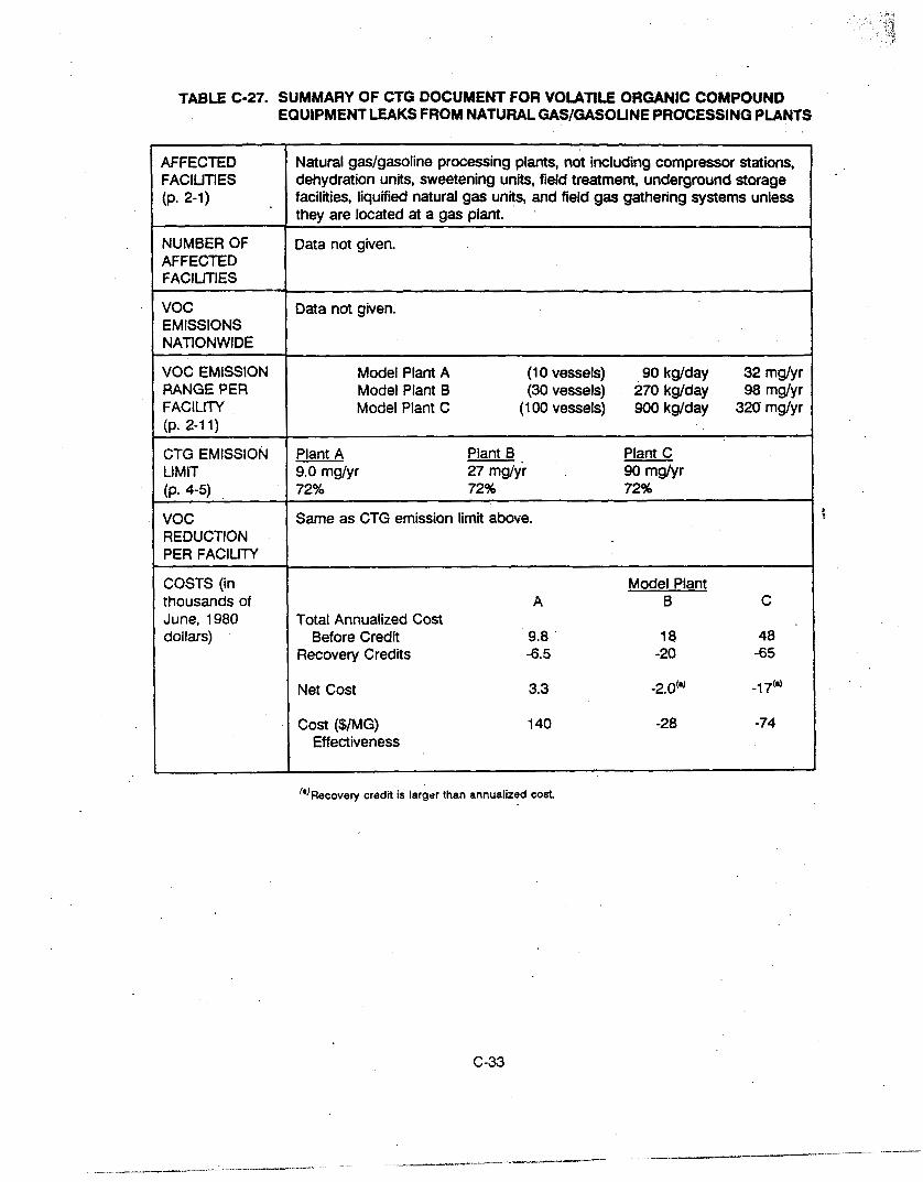
TABLE c-27. SUMMARY OF CTG DOCUMENT FOR vounw ORGANJC COMPOUND EQUIPMENT LEAKS FROM NATURAL GAS/GASOUNE PROCESSING PLANTS

AFFECTED FACILITIES (Pa 2-11

NUMBER OF AFFECTED FACILITIES

voc EMISSIONS NATIONWIDE

VOC EMISSION RANGE PER FACILITY (P. 2-1 1)

CTG EMISSION LIMIT (P. 4-51

voc REDUCTION PER FACILITY

COSTS (in thousands of June, 1980 dollars)

Natural gadgasoline processing plants, not including compressor stations, dehydration units, sweetening units, field treatment, underground storage facilities, liquified natural gas units, and field gas gathering systems unless they are located at a gas plant.

Data not given.

Data not given.

~

Model Plant A (10 vessels) 90 kg/day 32 mg/yr Model Plant B (30 vessels) 270 kg/day 98 mdyr Model Plant C (1 00 vessels) 900 kg/day 320 mg/yr

~

Plant A -. Plant B Plant C 3.0 mg/yr 27 mg/yr 90 mg/yr 72% 72% 72%

Same as CTG emission limit above.

~ ~ ~~~

Model Plant A B C

Total Annualized Cost Before Credit 9.8 18 48

Recovery Credits -6.5 -20 -65

Net Cost 3.3 -2.0'4 -1 7'4

Cost ($/MG) Effectiveness

140 -28 -74

%ecovery credit is larger than annualized c o d

C-33

TABLE c-28. SUMMARY OF CTG DOCUMENT FOR vounE ORGANIC LEAKS FROM SYNTHETIC ORGANIC CHEMICAL AND POLYMER MANUFACTURING EQUIPMENT

AFFECTED FACILITIES (P. 2-11

NUMBER OF AFFECTED FACl LIT1 ES

voc EMISSIONS NATIONWIDE

voc EMISSION RANGE PER FACILITY (p. 2-11)

100 TON/YR SOURCE SITE

CTG EMISSION LIMIT (p. 5-10)

voc REDUCTION PER FACILITY

COSTS (PP. 5-1 1, 5-1 2)

Equipment in process units which produce synthetic organic chemicals and polymers (polyethylene, polypropylene, and polystyrene).

Data not given.

Data not given.

For three model units with varying complexity, uncontrolled emission estimates are: A - 39 mg/yr B - 151 mg/yr C - 470 mdvr

The complexlty of the facility (Le., number of valves flanges, etc.) is at least equally as important as the size in determining emission levels. Totals of types of sources multiplied by the emission factors for that equipment (p. 2-21) will :. identifv 100 ton/vr sources. '

Percent reduction in all model units is 36% under RACT.

Same as CTG emission limit above.

Costs per model plant are balanced below with recovery at product.

Recovery Annualized cost Model Plant Initial Costs'" Credits(b) cost'b) Effectiveness

A $1 5,900 $6,200 $5,600 $370/mg B $35,800 $24,000 $4,300 $77/mg C $91,200 $74,000 $2,300 $1 3/n?g

("One time cost. (*'Annualized creditkost.

C-34

TABLE C-29. SUMMARY OF CTG DOCUMENT FOR THE AIR OXIDATION PROCESS IN SYNTHETIC ORGANIC CHEMICAL MANUFACTURING INDUSTRY

AFFECTED FACILITIES (P. 2-11

NUMBER OF AFFECTED FACILmES (pp. 2-3, 2-18) -

VOC EMISSIONS NATIONWIDE

Those facilities that produce chemicals included in the synthetic organic chemical manufacturing industry by reacting more chemicals' with oxygen, ammonia, or halogens, and air.

There are 161 faciliies operated under 59 companies which produce one or more of the 36 air oxidation chemicals.

40, 390 mg/yr (p. 4-3)

VOC EMISSION RANGE'" PER FACILITY --1 0.0205 kg/hr - 2150 kg/hr

100 TON/YR SOURCE SIZE

CTG EMISSION LIMIT (P. 4-5)

VOC REDUCTION PER FACILITY

COST EFFECTIVENESS (p. 5-24)

~-

Data not given.

Average plant emissions for facilities required to control VOC = 31.2 mg/yr. Average plant emissions for facilities not required to control VOC = 560 mg/yr.

Thermal oxidation - 98% for facilities with controls; 53% above baseline for total VOC. Only 14 of 47 plants in nonattainment zones would control VOC emissions under RACT.

$1 600/mg@' VOC controlled

I 1

(')Figures are from the 59 facilities for which data is represented. @'June 1980 dollars. ~

c-35

APPENDIX D - EXAMPLE QUESTIONNAIRES

A general discussion of the design and us8 of questionnaires k presented in Chapter 3. This appendm contains example questionnaires for inventorying VOC emissions from sotvent use. The inclusion of these questionnaires does not imply an endorsement by EPA or a requirement to use them. They are presented merely to show the basic structure, possible content and various alternatives available.

Additional example questionnaires and backgmund discussion on questionnaire development are available in Reference 1. These questionnaires are also not required or endorsed by EPA. The reader is simply referred to the document for additional information.

The primary consideration in developing questionnaires is the inventory agency’s data requirements. The agency’s needs will determine whether to use general or industry-specific questionnaires and what data to elicit. Discussion on general versus industry-specific questionnaires is included in both Chapter 3 and Reference 1.

Several caveats should be observed when reviewing the questionnaires in this Appendix ’ industry-specific questionnaires must be developed for refineries, chemical manufacturers and some other sources. For a VOC emissions inventory, each questionnaire design should be consistent with the data requirements of emission factors in AP-42, CTG documents or any other references. These references should be reviewed during the development of questionnaires. In addition, local or state regulations should be consuhed before mailing questionnaires to ensure that all clearance requirements for the forms are met. For example, EPA questionnaire forms must be approved by the Office of Management and Budget prior to release to more than ten sources. Finally, the caveats mentioned in Chapter 3 should be noted.

Reference for Appendix D

1. Development of Questionnaires for Various Emission Inventory Uses, EPA450/3-78-122, U.S. Environmental Protection Agency, Research Triangle Park, NC, June 1979. .

i

i

GENERAL INSTRUCTIONS

ORGANIC SOLVENT SOURCE QUESTIONNAIRE

1. All questions should be directed to (name, address, phone number).

2. This questionnaire is aimed at obtaining information from a wide vadety of solvent users. The complete questionnaire includes the following pages:

Page A - GENERAL INFORMATION B - DEGREASING OPERATIONS C - DRY CLEANING OPERATIONS D - PROTECTIVE OR DECORATIVE COATINGS E - FABRIC OR RUBBERIZED COATINGS F - MISCELLANEOUS SURFACE COATINGS G -OVENS H -PRINTING I - GENERAL SOLVENT USE J - BULK SOLVENT STORAGE K - CONTROL AND STACK INFORMATION

3. Annual or average summer day data should reflect average operating data for the period from to . 8

4. Fill in the descriptive information and amount of sotvent or solvent-containing materials used for each device operating under county permits as shown in the example on each page. (Note: These examples are for illustration only and may not represent actual operating conditions.)

5. In the event that data are not available on an indvidual device basis, use best estimates from total plant usage to complete Item 4.

If the type@) and/or percentages of solvents in coatings, inks, etc., are not known, include sufficient information on the manufacturer, type and stock number so that this breakdown can be obtained. A copy of a supplier's invoice would be adequate.

6.

7. Complete pages I, J and K

8. The emissions data that will be generated during this program will generally' be public information. If certain process, operation or material information is considered confidential and should be considered a trade secret, indicate such (spec'w a procedure and specdy how confidential data will be handled).

Figure D-1. Example questionnaire - Instruction sheet. -

D-2

n a i l i n q Address C+:y z i p

Pe:son to Contacr Abouc Form

Telephone . T i t l e .

Xpproxinacc NurcSer of Etployces

Nature of Business (Include S I C )

Noma1 0gcra:inq Schedule for Caletidar Yea:

Hrs/Oay Days /Week Y e c ks / Y e a r

Approximace Percent Seasonal 0pcra:ion:

Cec.-Zrb. I Hdr.-Mav I 'June-hua. I Se=c.-Nov.] 1 I I I

Are hydrocarban o r orqanic s o l v e n t concaininq matcrirls such as cleaning f l u i d s , c o a c r ~ i g s , adhes ives , inks , etc. us.4 L I I your operatron?

NO If y e s . please complctc tho appropriacr Corns -yes __-. cncloscd. H d e aJrlitiorirl cuorcs I f ncccssary. I Organic S O l V e I I t S

arc no: i n use plcase s i g n and r e c u m . -

SLq nacurc

Figure 0-2. Example questionnaire - General information page.

D 3

I

m u I I U U 0 L# 0.

" 3

n a a Y C v

0 YI

c. 0 Y C J

-

I I

Figure D-3. Example questionnaire - Degreasing operations form.

D 4

3

C m U

U

c 0

Y

. . 4 N

. - -

I

Figure D-4. Example questionnaire - Dry cleaning form.

0-5

v) W z t- - a 0 U

(3 z c < 0 U w

- a

n C 0

W > - c U W

I /

I 1 I

Figure D-5. Example questionnaire - Protective or decorative coatings form.

D-6

.o U YI 5

P

Y m 0 V

0 Q W Y U C

*.

q n H Q Q C

.rl m u w u n . 9 : . . M n

I I

I I

I

I I

Figure D-6. Example questlonnalre - Fabrbor rubberized coatings form.

0-7

I

Figure 0-7. Example questionnaire - Miscellaneous surface coating application form.

D-8

W

m

L

0 0 0 0 0 -

0 -4

. -

7- I

I

Figure D-8. Example questionnaire - Ovens and heating equipment form.

0-9

c

I I I Figure D-9. Example questionnaire - Printlng form.

D-I 0

GENERAL SOLVENT USAGE

nd ~ W U c of ocher rolvcnrs iioc i d e n t i f i e d vreh equipmcnc havlnq a

e o ~ t y pcrmie EhJe uorc us& r t your facalicy d u i 1 1 q calendar year

00 noe incluctc any so lvcncs that have been inc ludcd 8 ~ ~ e w h e r e

i n c h i s qucstaoiuiAiru.

TYPE AEOUNT (CAL/YR)

S OLV ENT RET URN ED

~ i 3 t any s o l v e n t s rccurned to supplier or co1lec:ed for reproccsrinq. Aqain,

d o n o t include any s o l v e n t s that have been so spec i f ied elsevharr in t h i s '

qucr ti onnaire.

TYPE AMOUHT ' (GAL/HR)

Figure'D-10. Example questlonnalre - General sohrent usage form.

D-11

BULK SOCVEI I T S T O R A G E

SAmerqed f i l l , s p l a s h f i l l , rtrurn vrnc line, adsorbet .

OPER'ATIONAL MODIFICATIONS

?lease s t a t e the chanqes i n t y p e and est imated annual consuqxion of tol-

Include v e n t planned :or a l l operations f o r c a l e n d a r y e x s

any informition on control equipment a d e i t i o n s 0: w d i f i c z t i o n s :

I

Figure D-1 1 . Example questionnaire - Bulk solvent storage form.

D-12

~ r ~ s r R u & ' I OXS :

1. Provide in fo rm-c icn on a l l d c v i c c s that cmic orqarlic ccopounds chrouqh a s t a c k , v rnc or ochor C C ~ A I W ~ cmssiorl Four:. s c p ~ r s : c yerinrc:: c h 3 C VCnC Chi'ouyh J C o l . m o n s t x k . A sinplc Jrawitrq nay be provided cc) IJUCCC: i ? l u u c r s c c Chc physrcaL c o r i l i ~ u r ~ c l o n .

f ~ ~ : t r r r f y a i l cnlcs under

. _ 2 . I d c o c i f y chc. primary ornar1zc comoound co l l c ro l mcc:ld usad ( i f any) such

' I S s€-.dr burfkzs . ~ : : u ~ u c z s . carzon adsorption, condcnscrs. e::. N O C C : c h i s d e v i c c .%Y hsvc it: own p c r a i c nuzac r , I f s o , i d e n c i f y .

3. . h d i = s c c i n s c a l l a c r z n Jacc of c o n c r o l e q u i p c n F .

4 . I n d i c a c c approxinaca e t l i c i c n c y ( i f k n o w ) .

5 . prov ide che fo l lowing i i fo rmac ion :

I k i a h c - d i s t a n c e above ground co d i s c h a r q r poinr ( f e e t ) Dimecer - i n s i d e Ciamcccr ac d i s e h a r q e po111c (Lcec) -

taoce: i f noc c.i:rulai, i n sc r - , d i m e c e r ( i r i f ees ) of equivalent circular arcd which 'can be c a l c u l a c e d by

De - 1.128 A

w h o c A is che measured or e s t i m a t e d c r o s s - s c c c i o n a l area i n sq f t and De is chc e q u i v a l e n c d iamcccr .

Tcmi,craCure - ac discilnrqc point in 'P v e i o c i c v - ac d i scha rqe Toinc in ft/sec Flow r a c e - ac d i s c b a r q c i n accual c u b i c f c e c . p e r minute (ACFM)

Desfqn condi:ions w y r used in l i e u of aczual test d a r a .

Figure D-12. Example questionnaire - Control and stack information form.

D-13

APPENDIX E

PREVIOUSLY UNINVENTORIED SOURCE CATEGORIES

E-1 ’ INTRODUCTION

Several source categories that have not been included in traditional emissions inventories have recently been identified. Although some of these previously uninventoried source categories may be considered point sources, the majority are considered area sources. This chapter identifies these categories and provides general guidance for inventorying and estimating emissions from them. It should be noted that the guidance presented here is very general and preliminary. Research is underway to investigate these source categories more thoroughly and develop detailed emissions estimation guidance and emission factors. It is therefore not required that these source categories be included in the inventory at this time. If specific data are available for these categories, however, it should be included in the emissions inventory. If Wal, state or regional agencies have access to information on these previously uninventoried source categories, it is requested that they contact the Emissions Inventory Branch at (919) 541-0875 or FTS 629-0875.

The previously uninventoriad source categories are aggregated under the following major

I

headings:

Bioprocess Emissions Sources (Section E-2) Catastrophic/Accidental Releases (Section E-3) Evaporative Emissions Sources (Section Ea) Ozone Emissions Sources (Section E-5) Small-Scale Combustion Emissions Sources (Section E-6) Waste Treatment and Disposal (Section E-7)

Some overlap occurs between headings. Source categories have been assigned to what is considered their primary heading. References for data sources and information are provided at the end of this Appendix.

E-2 BIOPROCESS EMISSIONS SOURCES

Bioprocess ernissions,sources include those sources whose emissions result from biological processes (e.9.. fermentation). Source categories include bakeries, breweries, distilleries, wineries and silage storage. Silage storage is discussed in this Appendix; all other categories are discussed in Chapter 4.

€4.1 Silage Storage .

The principal gases produced in silos during the silage-making process are CO, and NO,, including nitrous oxide (N,O), nitric oxide (NO) and nitrogen dioxide (NO& These silo gases are formed within the porous silage mass and ultimately diffuse into the siio headspace as the new silage settles. These gases are typically heavier than air and so displace the air in the silo headspace as they are vented through the top- of the silos. CO, is the end-product from oxidation of the plant

*

E-1

material by bacteria as part of the ensiling process. NO, is formed through three processes: (1) in a plant when it is exposed to some adverse weather condition, such as a drought followed by periods of rainfall; (2) through addition of fertilizer; and (3) through addition of material to the silage. The amount of silo gases formed varies with the type of silage material (e.g., alfalfa, soybean, corn, etc.). The methods of silage making also vary by region. In some parts of the country, silage is made by digging a hole in the ground, lining and filling the pit, and then covering the silage material with a plastic sheet. In other regions, silage is stored in solid structure silos. Silage storage principally occurs in rural areas during winter months.

County-wide estimates of each crop type harvested for silage are readily available from the Census of Agriculture.' Multiplying these estimates by the appropriate emission factors will provide county-wide emissions estimates of various gases produced from the silage storage. However, emission factors should be developed for all crop types.

E-3 CATASTROPHIC/ACCIDENTAL RELEASES

Sources in the catastrophiclaccidental release category represent unplanned, unintentional emissions releases associated with evaporation or combustion of material. Source categories include rail car, tank truck and industrial accidents; natural gas well blowouts; and oil spills. All categories except oil spills are presented in this Appendix; oil spills are discussed in Chapter 4.

E-3.1 Rail Car, Tank Truck and Industrial Accidents

Catastrophic releases from rail car, tank truck and industrial accidents are usually chemihl spills, with or without combustion. Unless the release occurs at a source otherwise counted as a point source, catastrophic releases are usually not included in point source inventories. The emissions depend on the material released, remediation efforts and weather conditions. The nature of catastrophic releases makes precise description of the released materials difficult, VOC species emitted are dependent on the material released. VOC, NO, and CO emissions are possible if combustion takes place. Air toxics may also be emitted. Air pollutants from catastrophic and accidental releases may enter the atmosphere through evaporation or combustion of solid or liquid materials or release of gaseous materials.

Estimating emissions from catastrophic releases requires information on the chemicals released and their potential air pollutant emissions, Local officials should be contacted to determine effectiveness of remediation for the releases and rule effectiveness for reporting requirements. Potential emissions may then be adjusted accordingly. ~

Releases of hazardous chemicals are required by law to be reported to the National Response Center (NRC). The NRC compiles data on reported releases: access to these data is guaranteed by the Freedom of Information Act. The compliance rate for this legislation is expected to be fairly high, especially for large spills. fiule effectiveness is expected to be between 0.85 and 0.95. Data reponed for each accident include, but are not restricted to, the following: date of release; material released; media affected (water, air, etc.); mode (train, ship, truck, etc.); and location. Agencies requesting information from the NRC should send a written request to the National Response Center, U.S. Coast Guard Headquarters, Room 261 1, 21 00 2nd Street S.W., Washington, DC 20593.

E-3.2 Natural Gas Well Blowouts

Natural gas well blowouts are unexpected and uncontrolled releases of gas from exploratory and production wells. They are confined to rural and off-shore areas of gas-producing states, primarily the Gulf states and California. Blowouts have been defined technically as 'events where encountered formation pressure exceeds the mud column pressure allowing the formation fluid to flow

E-2

uncontrotled out of the M e , into the sea or air? Gas wells pn'mariry release methane and smalt amounts of H,S, ethane and propane. The amount of gas released and the time required to contai~ the release depend on the nature Of the particular field (e.g., formation pressure), the design of the drilling and welt rig, and local environmental conditions. Blowouts may occur on the outer continental shelf (OCS) or inland during exploration, development, production or work-over phases. OCS blowouts are of particular concern due to the complexity of containing releases. Some blowouts are large enough to merit consideration as point sources if methane is inventoried

.

Several factors need to be considered when analyzing existing gas and oil blowout data and research results. First, changes in drilling environments and technologies affect blowout frequency. Second, with a ribing demand for natural gas, conventional production in new regions and unconventdnal production from sources such as tight sands may effect both the frequency and magnitude of natural gas losses. Available data may be insufficient to estimate natural gas losses from well blowouts in the United States. However, the American Gas Association, the Interstate Natural Gas Association and the Natural Gas Supply Association are currently involved in research to estimate losses from natural gas well blowouts? If an estimate of the total natural gas lost due to blowouts becomes available or estimable, losses could be apportioned to states (or counties) based on gas well population. Apportionment to the county level could also be based on employment data in the natural gas drilling sector as reported in Counry Business Patterns.'

E 4 EVAPORATIVE EMISSIONS SOURCES

Most evaporative emissions sources, with the exception of fuel loading and refueling operations, are associated with some type of solvent use. Emissions from fuel loading and refueling operations result from evaporation of the fuel. The following source categories are discussed in this Appendix: *

lawn care products; automotive fluids and fluid leaks: automotive rustproofing and undercoating; service station activities, including lubricating and repair: laminating; research and testing laboratories: and oil and gas production, including well drilling and field activii.

E4.1 Lawn Care Products

Lawn care products are usually manually applied to residential and commercial lawns, parks and recreation properties, and golf courses. Evaporation of solvents and carriers of organic chemicals in lawn care products, primarily in pesticides and fertilizers, results in releases of VOC, TSP and PM,,. Regional emissions vary significantly as consumption varies between and within regions with greater emissions occurring in urban areas during the growing season.

Emissions from lawn care products could be estimated by multiplying the emissions factor by total lawn care chemical consumption. One method wouM be to use the factor (0.9) for the volatile organic fraction of pesticides from Chapter 4 of this document to represent the volatile organic fraction of lawn care products. Chemical application rates can be estimated by consulting local agronomists and landscape professionals, while land use could be determined by consuking local planning or real estate agencies. Lawn care Lhemical usage can be determined by multiplying the application rates by the corresponding facilii acreage (Le.: residential lawns, commercial lawns, parks and recreational properties, and golf courses). Summing the usage from these categories would give an estimate of total lawn care chemical consumption. Multiplying the 0.9 factor by the totai chemical consumption would result in an estimate of VOC emissions from lawn care products.

.

E4.2 Automotive Fluids and Fluid Leaks

Automotive fluids include brake fluid, steering f1uid;transmission fluid, windshield washing fluid, windshield deicers, crankcase oil, engine starting fluids, engine coolant and gas-line antifreeze. Additives such as oxidation inhibitors, rust inhibitors, antiwear agents, detergents and dispersants,

E -3

pour-point depressants, viscosity index improvers and foam inhibitors are added in varying combinations to most automotive fluids.

VOC emissions from automotive fluids are associated with draining, refilling, overfiliing or replacing fluids and from running and standing losses. Emissions occur both at the point of application, mainly at service stations and residences, and at the vehicle. Emissions may peak during rush hours due to higher engine temperature and emissions from engine coolants and antifreeze may be greater during summer and winter months. Emissions levels are likely to be low, yet very widely distributed.

Em'matkrg county-level VOC emissions from automotive fluids requires vehicle registration data by class and estimates of the amount of fluid used per vehicle by fluid type and vehicle class. Emission factors could be developed through field studies to determine emissions per unit volume of automobile fluid, by fluid type and running/standing/refilling mode. County emissions can then be computed by fluid type, vehicle class, and running/standing/refilling mode.

E-4.3 Automotive Rustproofing/Undercoatlng

-

Automotive rustproofing/undercoating is the application of sohrent-based coatings to prevent cars from rusting. This category covers the application of undercoating after a car teaves the plant, such as at a dealership or a body shop. Since emissions from these individual sources would probably not exceed 25 TPY automotive rustproofing and undercoating are considered as area sources of pollutants. Rustproofing and undercoating products may emit VOC, including aromatic

Undercoatings are used to protect a car from rusting caused by climate, salts on roads, and exposure to sea spray (salt). As a result, consumption of undercoatings may be higher in coastal areas and in colder, wetter regions during the months preceding winter.

: and aliphatic hydrocarbons, silicates and lead. ..

EPA has developed a profile for one formulation of ~ndercoating.~ However, a representative emission factor cannot be developed without data on formulations of other undercoatings and market shares of each of these formulations. A survey of automotive shops may yield data on types and amounts of undercoatings used. Regional estimates of consumption and product formulation can be applied to population data to estimate emissions for the area under study.

E4.4 Service Station Activities - Lubricating

. Lubrication is the application of a substance of low viscosity between two adjacent solid surfaces (one of which is in motion) to reduce friction, heat and wear between the surfaces. A lubricating grease is a mixture of mineral oils with soaps (most commonly, soaps of sodium, calcium, barium, aluminum, lead, lithium, potassium and zinc). Oils thickened with residuum, petrolatum or wax may be called greases. Grease specifications are determined by the speed, load, temperature, environment and metals in the desired appli~ation?~' Synthetic lubricants are organic fluids used where petroleum-derived lubricants are inadequate. Each type has at least one property not found in conventional lubricants. The major types are polyglycols (hydraulic and brake fluids), phosphate esters (fire-resistant), dibasic acid esters (aircraft turbine engines), chlorofluorocarbons (aerospace), silicone oils and greases (electric motors, antifriction bearings), silicate esters (heat transfer agents and hydraulic fluids), neopentyl poly01 esters (turbine engines) and polyphenyl ethers (excellent heat and oxidation resistance, but poor low temperature performance).'

Lubrication and greasing activities emit VOC and other air toxics. Those emissions occur Emissions per vehicle and/or during refilling or replacing and as a result of standing losses.

E 4

emissions per service station are expected to be lesS than 25 TPY and should be included in area source inventories,

Estima~ing emissions from lubrication and greasing activities requires county-lwei data on the number d sewice stations, the number of vehicles serviced by class in each station and the amount of fluid used per vehicle by fluid type and vehicle class. These data could be used to estimate total fluid used by type and vehicle class. Emission factors should be developed to determine emissions per unit volume of fluid used. This factor may be broken down by fluid type, pollutant emitted, and standing/refilling mode. Pollutant emissions per county by fluid type, pollutant type, vehicle class and standing/refilling mode could be estimated by multiplying the emission factors by the computed volume of fluid us$.

E 4 5 Senrlce Station Activities - Repair

Service station repair activities require the use of engine degreasers, automotive brake cleaners, engine starting fluids and solvents that clean carburetors and chokes. The evaporation of solve& and propellants that occurs during the application of these cleaning products generates VOC emissions, primarily butane.

t

i

VOC emission factors for carburetor and choke cleaners, brake cleaners, engine degreasers and engine starting fluids are available from Compilation and Speciation of National Emission Factors

’ for Consumer/Cornrnercia/ Solvent Use. However, these emission factors were developed using sales data and may not reflect the actual VOC emissions from automobile repair. Multiplying county-level vehicle registration by the appropriate emission factors will yield county-wide estimates of VOC

.

emissions resulting from automobile repair. t

E4.6 Laminating

Lamination is the bonding of layers of materials together for structural, protective or decorative purposes. Laminating encompasses commercial and industrial applications, ranging from industrial production of pipe and building materials to commercial activities such as home building. Typical laminating markets are construction and packaging. Laminating products include counter tops, wall panels, cabinetry and speciatty packaging.

Adhesives used in the laminating process are sources of VOC emissions. Some particulate matter is also generated from the handling of filler materials and the trimming during finishing operations. Industrial applications emitting more than 25 TPY of VOC should be categorized in point source inventories under solvent emissions from adhesives. Commercial laminating is applied predominantly in urban areas and is likely to emit less than ten TPY

Current methods used to estimate emissions from solvent uses either allocate national consumption to the area under study based on employment and population statistics or apply a per capita factor to solvent use.’ *Estimating emissions resulting from specific solvents (like laminating) in a study area requires emission factors to be determined from formulation data of brand-specific products. Product-specific information requires regional market surveys and sales statistics. Many of these data may be obtained from manufacturers and trade associations. However, formulations and market shares may be subject to constant change due to economic and technological changes in the market.

,

E4.7 ‘Research and Testing Laboratories

Research and testing laboratories are low-level consumers of a wide variety of potentially toxic solvents and chemical substances and have been identified for review under Tile 111 of the CAAA.

E-5

Most laboratories are equipped with chemical fume hoods and building exhausts which vent the emissions directly to the atmosphere. Large medical research facilities are likely to have on-site ethylene oxide sterilizers and toxic waste incinerators which also emit to the atmosphere. Emissions may result from chemical mixing, chemical reactions, equipment cleanmg and washing, and chemical storage (in laboratories and in stock rooms). These laboratories are usually located in institutions such as universities, and in research and commercial laboratories such as medical testing laboratories. These laboratories may be concentrated mostly in urban and suburban areas.

VOC may be emitted from solvents such as acetone, chloroform, and ethanol, which are usually volatile and potentially toxic. The total amount of VOC emitted from a research and testing laboratory is unlikely to exceed 100 TPY Seasonal and temporal characteristics depend on the type of research laboratory. Universities would probably use the bulk of their solvents from September through May. Most research and development laboratories would follow f i e day per week and eigM hour per day schedules. Some combustion pollutants (e.g., CO and NO,.) may also be emitted from on-site incinerators; however, the quantcies emitted are likely to be insignificant.

To estimate emissions from research and testing laboratories, companies that manufacture reagent grade solvents and other votatile organic compounds should be identified. If these companies can be assured that confidentiality of their sales figures will be maintained, annual estimates of the volume of various solvents sold can be obtained. The species that are consumed in significant quantities can then be identified. These annual volumes can be allocated to various states based on the amount of federal funds allocated to a state for research or This estimate of state solvent and chemical consumption can then be allocated to each county based on employment in the research, development-and testing services sector as given in County Business Patterns.

E 4 8 Oil and Gas Production - Well Drilling

Oil and gas well drilling results in emissions of VOC, methane, ethane and, if gas is flared, H,S and SO,, CO, CO, and NO,. Most onshore wells are located in rural areas while offshore wells may be located off the coast of both urban and rural areas. Emissions from an individual drilling operation will most likely be less than 25 tons per year and should be included in the area source inventory. Oil or gas exploratory drilling activities are found mainly in Texas, Oklahoma, New Mexico, Ohio, Pennsylvania and West Virginia. In states which do not allow the flaring of gas (e.g., West Virginia), emissions resulting from drilling may be minimal. In states which allow gas to be flared, additional emissions associated with the vented gas are generated.

API has developed emission factors for each component of gas- and oil-producing facilities.” For states that do not allow venting of gas from drilling, emissions may be computed using the API emission factors. Data needed to apply these emission factors include the number of wells drilled and the components associated with each well. In 1985, API published We// Completion and footage Drilled in the Unired States, 7970-7982.’2 If these data have been updated, the most recent year’s data can be used ta estimate the number of wells drilled in the United States. States that allow venting of gas during exploratory drilling may have an additional source of emissions associated with this vented gas. However, data for the emissions from the vented gas may not be readily available.

E4.9 Oil and Gas Production - Field Activity

Field activlty components of oil aqd gas production include extraction operations during which oil and gas are brought to the surface, separation of liquefied petroleum gases and sweetening of natural gas that contains sutfur. The extraction and separation activities result in emissions of ethane, methane, heavier hydrocarbons and H,S. Sweetening of natural gas emits H,S and SO,. Hydrocarbons and H,S emissions may result from leaks in the component parts of the wellhead and

E-6

venting of gas during production operations. Although an individual well,may release.less than 2$ tons d pollutants per year, an oil 01 gas field may comain many wells from which total emissions may exceed 25 tom per year.

Emission factors for each component of oil- and gas-production faciliies are documented in several sources. API has hydrocarbon field activity emission factors for methane, ethane, butane, propane, pentane and heavier hydrocarbons." AP42 contains an emission factor for SO, emissions from gas sweetening.'' To estimate emissions from a facilii, all components a! the facilii must be inventoried and the corresponding emission factors applied. Emission factors for each component differ by type of production (oil or gas) and well location (onshore versus offshore). State officials can be consu8qd to determine the reporting requirements for oil and gas field activity. For states with strict reporting requirements, there may be enough data to estimate the number of wells per county. For other states, county-level field activii should be estimated based on the number of wells in the state. The Natural Gas Annual publishes annual data on the number of producing natural gas and condensate wells in each state." These data can be apportioned to the county level based on employment in the oil and gas production sectors obtained from County Business Patterns under SIC code 131 I.

To determine SO, emissions, the average H,S content of gas in the state must be estimated. Often, the sulfur removed during the sweetening process is sold; therefore, the amount of sulfur that is produced and sold .by each county or state may be used to estimate the amount of H,S in the gas. API may be able to provide average wellhead composition based on fuel produced and location of the wellhead. State officials should be able to provide information on wellheads in their states. tf neither API nor state officials are able to help in determining wellhead profiles in each state, data from t wellhead studies by API, CAR6 and others can be used to estimate the profile. After the wellhead profile is determined or estimated for each state, the emission factors reported by API can be applied to estimate total emissions by hydrocarbon group.

E-5 OZONE EMISSIONS SOURCES

Sources under this major heading emit ozone directly as a result of some activity. Only one category, ultraviolet and electron beam curable coating, is discussed in this Appendix.

E-5.1 Ultraviolet and Electron Beam Curable Coating

Radiation curable coatings and inks (ultraviolet (UV) and electron beam (€6)) are high-solid formulations used as substitutes for conventional solvent-based thermal curable systems. Traditionally, coatings consist of a solid polymer dissolved in a solvent and further diluted with solvent. The solvent ranges from 50 to 90 percent of the coating formulations. After the coating is applied, the substrate being coated is sent through a dryer to evaporate the solvent. Radiation curable coating technology is currently being used in surface treatment, electronics, pigmented resins, and adhesives. The radiation source for these systems is either an ultraviolet light or an accelerated electron beam. Theoretically, radiation curable coatings can. be solvent-free, but to retain desirable properties such as viscosity and easy application, some solvent is added.

Radiation curable coating systems which use solvent-containing coatings emit VOC. Particulate matter may be emitted when paint sprays are atomized. Ozone formation may result under certain circumstances at very low wavelengths. In addition, some radiation curable coating components are thought to be mildly toxic, but not much is known about long-term exposure to coating formulas used in UV and EB curing. Each commercial formulation would need to be examined individually to determine toxicity.

E-7

W and EB curable coatings are replacing current coatings-related point and area sources. Their production and use would have large point source, small point source and some area source components. Since most UV and E6 curable systems are expected to be used in industrial rather than consumer or commercial settings, these systems may have a more urban characteristic.

One method to determine VOC emissions from UV and EB curable coatings processes would use current assumptions concerning solvent use in UV and EB coating and emission factors for conventional coating applications. The result might be a range of emissions representing 40 to 60 percent of the VOC emissions from conventional uses of solvents in the applicable coatings ~ategories.‘~~’”” A second method may be developed when more information is available on UV and E6 curable coating use, market penetration, solvent content, emission factors for air toxics and ozone, etc. The second methodology would result in more detailed emissions estimates than the first methodology.

E-6 SMALL-SCALE COMBUSTION EMISSIONS SOURCES *

This major category includes small boilers and heaters, as well as other combustion activities. These sources generally produce only small amounts of organic emissions relative to other sources. The methodologies given can be used to estimate VOC, NO, and CO emissions. ,

Source categories discussed under this heading include kerosene space heaters; rocket launches and test firings; backyard charcoal grills; commercial charbroiling; commercial deep fat frying at restaurants; and cigarette smoke.

E-6.1 Kerosene Space Heaters

I

Kerosene space heaters are used throughout the United States, usually as a supplementary heat source to electric, fuel oil or natural gas furnaces. Their use would be expected to be greatest during the winter months in northern regions of the country. There are three basic heater designs: radiant heaters (blue flame), convective heaters (white flame) and two-stage convective heaters. Most portable kerosene space heaters use K-1 grade kerosene fuel; some early models also used K-2 fuels.

Emissions from kerosene space heaters result from fuel combustion and fuel evaporation (fugitive emissions). Most emissions are trapped indoors where the heater is being used. In addition, there is a potential for evaporative emissions of kerosene from spillage during filling of the fuel tank and leaking tanks and lines. The amount of pollutants emitted to the outdoors is dependent on the pollutant and the relative rightness’ of the house. Particulate matter and many volatile components may settle or become adsorbed to surfaces in the house while gaseous pollutants have a greater tendency to migrate from the structure.

Pollutants emitted from kerosene space heaters include CO, CO,, NO, NO,, SO,, formaldehyde (HCOH), suspended particles and a number of potentially hazardous and toxic hydrocarbons. Emissions from individual heaters are less than ten tons per year, thus this category should be inventoried as an area source.

A possible methodology to estimate emissions from kerosene space heaters could assume a certain population of heaters with defined characteristics giving a derived number o[ heaters. This derived number of kerosene heaters could then be multiplied by the average amount of fuel burned for the prevailing weather conditions of the region and an appropriate emission factor. Information . on the use, grade and distribution of kerosene by small-scale retail outlets may be available from sources supplying gasoline and diesel distribution information. Information on the number, age, burner type and condition of kerosene space heater equipment may be available from industry sources. Emission factors are available from US. Department of Energy, EPA and U.S. Consumer

.

E-8

Product Safety Commission studies and literature.'4'e~zo The emission factors may be weightd to ~ reflect differing characteristics among the kerosene heater population in the area under study.

E6.2 Rocket bunches and Test Firings

Rocket launches and test firings release large quantities of hydrogen chloride, chlorine, aluminum oxide, NO, CO, CO, and PM, resulting in a temporary localbed degradation in air q u a l i near the launch or test site. The main air qualily effect at launches and test firings is from the combustion of the Space Shuttle's solid rocket motors (SRMs). During a normal launch, a ground cloud composed of hot exhaust products forms at the base of the launch platform. At higher altitudes, the r d p e of hydrogen chloride can produce acid rain under certain meteorologic conditions.# As the Space Shuttle passes through the stratosphere, hydrogen chloride, nitric oxide and aluminum oxide particles may be emitted, possibly resulting in the destruction of ozone molecules,

Emissions from launching and test firing activities exceed 250 tons per episode and should be considered major point sources. These emissions are locaked and may be assumed to be restricted to counties where launch sites and test sites are located.

Environmental Impact Statements for all the launch and test firing sites involved in the Space Shuttle Program are available.2' Emissions factors for the various pollutants have been calculated in pounds of pollutant per test firing.= For the purpose of characterizing emissions, rocket launches and test firings should be separated. Rocket launch and test firing emissions should be addressed by rocket type and fuel type. Multiplying the emission factors by the activii data from the Environmental Impact Statements would yield total annual emissions in tons occurring in the county of launch or test ' site.

.

E-6.3 Backyard Charcoal Grills

Organic gases are emitted when charcoal lighter fluid is used to soak and light charcoal briquettes in backyard grills. The lighter fluid, composed almost entirely of volatile constituents such as petroleum naphtha and petroleum distillates, evaporates to contribute to the VOC burden in the atmosphere. Some VOC are also emitted during the combustion of the charcoal and increase as the flame dies down. NO, and CO are also emitted during combustion. Charcoal grills are used primarily in the summer months.

The SCAQMD performed a detailed investigation of pollutant emissions from various methods of igniting charcoal in grills.= However, no standard emission factors are currently available for estimating emissions from charcoal grills. The Barbecue Industry Association (BIA) prepares national estimates of annual consumption of lighter fluids and charcoal briquettes. These estimates may be apportioned seasonally by assuming that 80 percent is used in the ozone season and 20 percent is used in the non-ozone season. Emissions generated during the non-ozone season may be allocated to counties based on the number of single family dwellings in each county. Multiplying this estimate by the emission factors will result in estimates of county-level emissions from charcoal grilling generated during the non-ozone season. During the ozone season (summer), charcoal grills are used in backyards, parks and other recreation areas. Usage during that season may be apportioned to types of use (backyards or recreation areas). Usage in recreation areas may be allocated to the various recreation areas based on attendance records. Multiplying the resulting usage estimates by the emission factors would yield emissions for each recreation area. The remaining percent of national usage during the ozone season may be used to estimate emissions from backyard grilling. The county-wide emissions from this source may be estimated by apportioning this usage to counties 'based on number of single-family dwellings in each county and multiplying the result by the emission

.

* factors for each pollutant.

E -9

E-6.4 Commercial Charbrolllng

Charbroiling is the most common method of cooking meat at fast food and full service restaurants. Charbroilers are used to cook steaks, hamburger patties, chicken and other foods. Charbroilers consist of three main components, a heating source, a high-temperature radiant surface and a grated grill. The meat is placed on the grill located above the radiant surface. Grease from the cooked meat falls on the surface and causes emissions that are vented to the atmosphere.

The pollutants emitted from commercial charbroiling consist mostly of reactive VOC and PM. Charbroilers using natural gas for a heating source also emit small amounts of NO,, SO,, CO, and CO. Individual charbroilers are unlikely to emit more than 100 tons per year of any pollutant and should be considered in the area source portion of the inventory. A typical restaurant operates six or seven days a week, from 1O:OO a.m. to 1O:OO p.m.. Emissions are likely to be highest during lunch (11:OO a.m. to 2:OO p.m.) and dinner (500 p.m. to 9:00 p.m.) hours.

To estimate total emissions resulting from commercial charbroiling, information should be gathered on the number of restaurants per county, sales of various meats to restaurants in a county and the percentage of restaurants using charbroilers. While statistics on the number of restaurants per county are available in County Business Patterns, the fraction of these establishments that use charbroilers must be estimated. VOC and PM emission factors for charbroilers in California restaurants are available from a stuciy conducted by EPA?' However, more detailed emission factors which reflect the amount and type of meat used at various establishments may be required to estimate emissions from commercial charbroiling. Multiplying the emission factors by the estimated amounts of each type of meat fired on charbroilen in commercial establishments would result Sn county-level emissions of VOC and PM.

E-6.5 Commercial Deep Fat Frying at Restaurants

Deep fat frying involves the cooking of foods in hot oils or greases. Potatoes are considered the most commonly fried food. Other foods include doughnuts, fritters, croquettes and breaded and batter-dipped fish and meat. The principal frying equipment is an externally-heated cooking oil vat. During frying, moisture in the foods is released as steam. Some cooking oils, as well as animal or vegetable oils from the food, are steam distilled and released as VOC or as oil droplets during frying. Excessive smoking (PM release) may be due to overheating of the food or to steam distillation of finely divided fat and oil products from old CoGking oil or the food.

Peak times for fast food restaurants are from 11 :00 a.m. to 2:OO p.m. and from 5:OO p.m. to 9:00 p.m., resulting in higher emissions during these times. VOC, PM and other entrained fat particles are emitted during frying. In general fish and meat products, which contain higher percentages of fats and oils, produce greater emissions than vegetable products. Individual restaurant deep fat frying activlty is unlikely to emit more than 25 tons per year of any pollutant.

One methodology to estimate emissions from commercial deep fat frying involves using SCAQMO and other related emission factors. In 1987, SCAQMD estimated emi.ssions from potato fryers in the South Coast Air Basin.= The SCAQMD emission factors are given as tons per fryer per year." These factors may be used to generate alternative emission factors such as pounds per person per year or tons per restaurant per year. Multiplying these emission faaors by the population or the number of restaurants in a county would yield estimates of county-level emissions from commercial deep fat fryers.

Alternatively, if product-specific emission factors are developed (emissions per pound of product fried), more precise emission estimates can be made. However, specific information will be needed on quantities and types of products fried. Multiplying the estimates of each product fried (or

E-1 0

4 E

surrogate data) by the corresponding emission factor would yield estimates of totai coumy-level *i emissions from commer~id deep fat ftyers.

E6.6 Clgamtte Smoke

Cigarette smoke contains combustion products (including tobacco-related organics) which are released into the Indoor and outdoor atmospheres. Smoke contains volatile organics and metals that are considered toxic. Although cigar and pipe smoking are similar sources, they represent only a small fraction of the total tobacco smoked.

Estimates on the number of cigarettes smoked (US. total) and their average smoke analysis may be obfained h m data compiled by the US. Surgeon General and the Office on Smoking and Health.=sn The consumption data are updated annualty and could be projected based on current trends. Consumption can be allocated to the state or county by Federal or state cigarette tax receipts. TSP, CO, NO, VOC and methane can be estimated at the desired level of resolution by multiptying consumption data by the following emission factors: -

mgbigarette Pollutant (unfiltered)

PM 22.5 voc 6.75 . . co 19

Methane 1.5 NO, . 0.35

:

E-7 WASTE TREATMENT AND DISPOSAL EMISSIONS SOURCES

Emissions from waste treatment and disposal sources result from both evaporation and combustion. Categories discussed include refinery sludge dewatering; waste incineration (developing technologies for hazardous waste); and waste oil disposal.

E-7.1 Refinery Sludge Dewatering

Petroleum refineries generate sludge from API separators, dissolved air flotation (OAF) units and biological waste from wastewater treatment. The sludge is often is dewatered by centrifuge, vacuum filtration, plate and frame filtration or belt press filtration. The most common dewatering method is belt filtration because of its high-throughput capacity and comparatively low cost. Sludge may be heated during dewatering to improve efficiency-and handling. The resulting filter cake may be landfarmed, landfilled or transported off-site for disposal. Filtrate is directed to wastewater treatment

. operations.

VOC emissions occur at the dewatering operation and recent test data indicate that the process may be a significant source of pollutants.28 Although the equipment is enclosed, the process is vented to the atmosphere with or without controts. The generated emission factors from the testing range from 0.7 to 6.2 pounds of VOC per 1,000 barrels throughput.= The preliminary data presented indicate that dewatering by belt presses may contribute ten to 100 TPY VOC at a refinery.

Individual refineries should be asked to identw sludge dewatering processes and define sludge and refinefy throughput, as well as existing control equipment: Dewatering operations that fall below the point source emissions criteria could be treated in' the same way that API separators are now treated in area source inventories. Refinery throughput or sludge generation unaccounted for in

E-1 1

inventoried point sources could be sut racted from county-level overall refinery throughput. The unaccounted portion could then be applied to the appropriate emission factor to develop courny-level area source estimates. The Petroleum Supply Annual publishes yearly refinery throughput by refinery location.2B

57.2 Waste Incineration: Developing Technologies for Hazardous Waste

The passage of federal and state waste clean-up and control statutes over the last ten years has spurred development of waste disposal technologies to replace IandfNing, disposal impoundments, deep-well injection, etc. Techniques such as waste minimization, reuse, biological treatmevt, stabilization and advanced incineration offer alternatives. Incineration, the thermal decomposition of organics via thermal oxidation, provides the highest overall degree of destruction for the broadest range of waste streams.

Many different incineration technologies are currently in use or under development. Established incineration technologies include liquid injection, rotary kiln, hearth, fume, fluidized bed reactors and others. There are currently about 40 commercial hazardous waste incineration facilities in addition to the transportable and mobile systems, in the United States. Transportable systems tend to be larger, requiring up to 60 trailers to complete transport, but are capable of handling five to twenty tons of waste per hour. Mobile systems may be delivered on-site in just a few trailers, but tend to have smaller capacities. These systems may be onsite for periods of months or years.

Emissions from waste incineration may be generated during waste preparation (fugitives) and combustion (stack). Most existing incinerators have some type of air pollution control device, including quench, scrubbers, absorbers and electrostatic precipitator (ESP). Pollutants emitted are waste- and fuel-dependent and may include SO, , NO,, VOC, CO, PM, air toxics, metals, acid gases and others. Mobile and transportable units are expected to emit less than 25 TPY and should be included in the area source inventory. Commercial (fixed) facilities, if properly operated, will also emit less than 25 TPY of pollutants and should be considered as area sources. Typical uncontrolled emissions from PM and VOC range from 0.3 to 15 ahour and 0.065 to 325 mahour respectively.%

Emissions from hazardous waste incinerators may be tracked through point source inventories. Commercial operations can be identified through state permits. Although many of the sites are temporary, they may be identified throyjh either the Superfund program or state permitting agencies. Emissions can then be estimated by aefining emission factors and activity levels for the different technologies employed. However, based on available trial burn data, the emissions generated from properly run incinerators are expected to be very small to meet federal requirements and/or state . permit regulations.

E-7.3 Waste Oil Disposal

Waste oil categories include industrial process oils (e.g., hydraulic oils, lubricants, etc.) and motor vehicle crankcase oils. Historically, most studies have focused on disposal of crankcase oils. Federal regulations for hazardous waste disposal (used oil is considered a hazardous waste under RCRA) have become increasingly strict and encourage the recycling of used oil. It is often more economical for industries to handle oil recycling or combustion internally rather than disposing of it.

Air pollutants from waste oil disposal may enter the atmosphere as a result of evaporation of oil when used as a dust suppressant or combustion of waste oil in boilers, kilns, diesel engines and waste oil heaters. In addition, waste oil may be stored for periods of time.in underground storage tanks, above-ground storage tanks (AGSTs) and oil drums. These containers may leak due to problems with ancillary equipment (e.g., pipes, pumps, valves, etc.), tank failure, vandalism, fire, explosions, natural disasters and operational error (overflow). The ultimate fate of waste oil exposed

E-12

to air is a function d the type and mposition ofthe oil, the type d c o n d i i The ernritonmenta impacts of gMllutams emitted when waste on the CompOBitjm of the waste oil, the number of sources burning waste oil, the stack heights, m e t e o r o m conditions, the type of combustion and the extent of use of emissions control equipment. In any case, air pollutants emitted due to the evaporation of waste oil will consist largely of VOC species. Combustion of waste oil will produce SO, , NO, , CO, CO, , VOC, particulate matter and some toxic niateriak and heavy metals.

Waste oil combustion in industrial boilers could most easily be accounted for in the point source inventory. However, unless the release of waste oil from oil storage occurs at a source o the rw ise l coun t~ a point source and the leak is substantial, oil leaks are not included in the point source in&tory. Waste oil used as a dust suppressant would be considered an area source due to its dispersed nature.

I .

Combustion in waste oil heaters occurs predominantly in the winter when automotive repair shops heat their mechanics’ bays with that oil. Other forms of waste oil combustion (e.g.$ industrial) should occur independent of season, but occur in more industrialized areas. Waste oil use for dust suppression occurs most commonly in rural areas of the northern Rocky Mountain states, the extreme Southwest, and the Southeast. In addition, waste oil is used as a dust suppressing agent in areas where there is a concentration of mining, logging, construction or agricultural activities. These industries produce significant quantities of waste oil and often apply the oil to their own roads.

For emissions estimation purposes, waste oil disposal activities may be subdivided into three categories: combustion of waste oil, use of waste oil as a dust suppressant and waste oil storage. National estimates of waste oil generated and the different use fractions are available from several sources.31a National estimates of oil generated may be allocated-to the county level based on industrial employment and motor vehicle registration data County-level estimates can then be allocated to the different uses based on the available estimates of national use fractions (e.g., percent combusted, percent applied to dirt/gravel roads, percent stored).- The emissions associated with the various uses can then be computed using available emission factors for lead and PM from AP-42. Emission factors for SO,, NO,, CO,, VOC and CO may be derived from existing distillate or residual oil combustion emission factors.=

REFERENCES FOR APPENDIX E

1. Census of Agriculture, U.S. Department of Commerce, Bureau of the Census, Washington, DC, 1987.

2. Coastal Petroleum Associates. Methods for Determining Vented Volumes During Gas Well 6lowouts, DOE/BETC/2215-1, U.S. Department of Energy, Bartlesville Energy Technology . Center, Bartlesville, OK,-October 1990.

3. Natural Gas Emissions from New Facilities and Increased Consumption (DrM), prepared for the American Gas Association, Interstate Natural Gas Association and the Natural Gas Supply Asswidion, October 1990.

4. County Business Patterns, U.S. Department of Commerce, Bureau of the Census, Washington, DC. Annual Publication.

E-1 3

5.

6.

7.

8.

9.

10.

11.

12.

13.

14.

15.

16.

17.

18.

19.

20.

Compilation and Speciation of National Emission Factors for Consumer/Commercid Solvent Use, EPA-450/2-89408, US. Environmental Protection Agency, Research Triangle Park, NC, April 1 989.

Gressner, H. Incorporated, New York, NY, 1981.

The Condensed Chemical Dictionary, Van Nostrand Reinhold Company

Encyclopedia of Chemical Technology, Third Edition, John Wiley and Sons, New York, NY, 1981.

Chemical and Process Technology Encyclopedia, McGraw-Hill, Incorporated, New York, NY; 1974:

-

federal Funds for Research and Development: Fiscal Years 1988, 1989, 1990, Volume XXXVIII, NSF 90306, Detailed Statistical Tables, National Science Foundation, Washington, DC, 1990.

N 7989 Awards by State and Institution, NSF 90-2, National Science Foundation, Washington, DC, 1990.

Fugitive Hydrocarbon Emissions from Petroleum Production Operations, Volumes I and 11, American Petroleum Institute, Washington, DC, March 1980.

Well Completions and Footage Drilled in the United States, 1970-7982, American Petroleum Institute, Washington, DC, 1985. :

Compilation of Air Pollutant Emission Factors, Fourth Edition and Supplements, AP-42, U.S. Environmental Protection Agency, Research Triangle Park, NC, September 1985.

Natural Gas Annual, U.S. Department of Energy, Energy Information Administration,' Washington, DC. Annual publication:

Riedell, A. Manufacturing, Vol. 61, No. 1, January 1989, p. 32-34.

'Back to Basics to Beat VOC Emission Problem,' Furniture Design and

Currier, Greg. 'Interest in UV-curable Coatings on the Rise,' furniture Design and Manufacturing, Vol. 61, No. 6, June 1989, p. 54-58.

The 1985 NAPAP Emissions Inventory, Version 2: Development of the Annual Data and Modelers Tapes, EPA-600/7-89-012a, U.S Environmental Protection Agency, Research Triangle Park, NC, November 1989.

Jackson, M.D., S.A. Rasor, R.K. Clayton, and E.E. Stephenson, Jr. Particulate and Organic Emissions from Unvented Kerosene Hearers, Test House Study, EPA-600/D-88/226, US. Environmental Protection Agency, Research Triangle Park, NC, October 1988,

Traynor, G.W., M.G. Apte, H.A. Sokol, J.C. Chuang, and J.L Mumford. Selected Organic Pollutant Emissions from Unvented Kerosene Heaters, EPA-600/D-86/142, U.S. 'Environmental Protection Agency, Research Triangle Park, NC, July 1986.

Woodring, J.L, T.L Duffy, J.T. Davis, and R.R. Bechtold. Measurements of €missions Factors of Kerosene Heaters, NTlS DE83-014326, Argonne National Laboratory, Argonne, IL, 1983.

E-1 4

i 1 21. Environmental lmpact Statement for the Space Shuttle P r o g m ; National Aeronautics and Space

Administration, Washington, DC, 1977.

NeWlModified Source Plan Review for Morton Thiokol lnc., Utah Bureau of Air Quality, Salt Lake

A Compararive Study of Organic, Carbon Monoxide, and Oxides of Nivogen Emissions from Various Charcoal lgnwng Methods. South Coast Air Quality Management District (SCAQMD), El Monte, CA, 1989.

22. city, m, 1988.

23.

24. Methods for_tlssessing Area Source Emissions in California, California Air Resources Board, Sacramenk6, CA, December 1982.

25. Area Source Emissions from Deep Fat Fying, CES No. 66811, South Coast Air Quality 'Management District, El Monte, CA, October 19, 1988.

26. Reducing the Health Consequences of Smoking: 25 Years of Progress, Surgeon General, U.S. Department of Health and Human Services, Office on Smoking and Health, 1989.

27. Smoking,. Tobacco and Health, (CDC)87-8397, U.S. Department of, Health and Human Services, Office on Smoking and Health, Washington, DC, October 1989.

28. Ponder, TC. and C.J. Bishop. Field assessment of air emissions from hazardous waste dewatering operations. In Remedial Action, Treatment, and Disposal of Hazardous Waste, EPA-

Petroleum Supp/y Annual 7989, DOE/EIA-0340(89)/1 , U.S. Department of Energy, Energy Information Administration, Washington, DC, May 1990.

600/9-90-037, U.S. Environmental Protection Agency, Cincinnati, OH, August 1990. t

29.

30. Eklund, B. and J. Summerhays. Procedures for Estimating Emissions from the Cleanup of Supedund Sites, JAWMA 40(1):17-23, 1990.

Metzler, Suzanne C., Nicholas S. Am, Jacob E. Beachey, and Roben G. Hunt. Waste Oil Storage, Draft Report, prepared by Franklin Associates, Ltd., and PEDCo Environmental, Inc. for the U.S. Environmental Protection Agency, Office of Solid Waste, Washington, DC, January 1984.

31.

32. Gabris, Tibor. Emulsified lndustrial Oils Recycling,. U.S. Department of Energy, Bartlesville Energy Technology Center, Bartlesville, OK, April 1982.

33. PEDCo Environmental, Inc., A Risk Assessment of Waste Oil Burning in Boilers and Space Heaters, Draft Report, prepared for U.S. Environmental Protection Agency, Office .of Solid Waste, Washington, DC, January 1984.

34. Metzler, Suzanne C., Nicholas S. Am, Jacob E. Beachey, and Robert G. Hunt. Evaluation of Health and Environmental Problems Associated With the Use of Waste Oil as a Dust Suppressant, Draft Report, prepared by Franklin Associates, Ltd. and PEDCo Environmental, Inc. for the U.S. Environmental Protection Agency, Office of Solid Waste, Washington, DC, February 1984.

35. Hall, Robert E., W. Marcus Cooke, and Rachael L Barbour. 'Comparison of Air Pollutant Emissions from Vaporizing and Air Atomizing Waste Oil Heaters' in Journal of the Air Pollution Control Association, Vol. 33, No. 7, July 1983.

E-1 5

REPORT NO.

450

14. SPONSORING AGENCY CODE 1

2. 3. RECIPIENT'S ACCESSION NO.

5. SUPPLEMENTARY NOTES Work Assignment Manager - Mary Ann Warner-Selph

Vo7ume I describes procedures f o r prepar ing a county wide inventory of v o l a t i l e organic compounds (VOC ) n i t rogen oxi des ( NOx) and carbon monoxide (CO) f o r s t a t i o n a r y sources .

I t i s a companion document t o Volume 11, which describes procedures f o r conver t ing an annual county wide emission inventory t o a d e t a i l e d inventory needed f o r photo- chemical model s.

6. ABSTRACT

I

TITLE AND SUBTITLE

Procedures f o r the Prepara t ion of Emission Inven to r i e s f o r Carbon Monoxi de and Precursors o f Ozone, Vo7 . I : General Guidance for S t a t i o n a r y Sources AUTHOR(S)

PERFORMING ORGANIZATION NAME AND ADDRESS

US Environmental P ro tec t ion Agency

Technical Support Divis ion (MD-14) Research Triangle Park, NC 27711

Office o f A i r Qual j t y P1 anni ng and Standards

2. SPONSORING AGENCY NAME AND ADDRESS

T h i s document i s an update t o the o r i g i n a l , (450/4-88-021), published is 1988.

5. REPORT DATE

M ~ v 1991 . 6. ORGANIZATloH

a. PERFORMING ORGANIZATION REPORT NC

10. PROGRAM ELEMENT NO.

11. CONTRACT/GRANT NO.

13. TYPE OF REPORT AND PERIOD COVEREC

~~

7 - KEY WOROS AND DOCUMENT ANALYSIS .. DESCRl PTORS

t m i s s i on 1 nventory Hydrocarbons Nitrogen Oxides V o l a t i l e Organic Compounds voc Carbon Monoxi de co

18. DISTRIBUTION STATEMENT

-- . IDENTI FIERS/OPEN ENDED TERMS

19. SECURITY CLASS (ThisReport)

20. SECURITY CLASS (This page)

COSATI Field/Croup

!1. NO. OF PAGES

!2. PRICE

E P A Form 2220-1 (Rev. 4-77) P R E V I O U S EDIT ION IS O B S O L E T E

INSTRUCTIONS

REPORT NUMBER Insert the LPA report number as it appears on the cover of the publicztion.

LEAVE BLANK

RECIPIENTS ACCESSION NUMBER Reserved for use by each report recipient.

. 1.

2.

3.

4.

5.

6.

7.

8.

9.

10.

11.

TITLE AND SUBTITLE Title *auld indicate clearly and briefly the subject ~ O V W J ~ C of the report. and be dispbycd protnincntly. Sct siihtitlc. if uwd. iii siiialir type or otherwise subordinate it to main title. When a report is prepared in more than one volunic. rcp’at tlic primary title. add volume number and include subtitle for the specific title.

REPORT DATE Each report shall carry a date indicating at least month and year. tndirdte the Iusis oii which i t n:is wlertcd (c:g. dafc*oj’issrtc*. Clutt, 01‘ approval, dore of prepamtion. erc.).

PERFORMING ORGANIZATION CODE Leave blank.

Give name(s) in conventional order (John R. Doe. J. Robcrf Doe. cfc.). List author’s aflil~atioii if i t differs trtiiii tlic prforiiiinp orpni- zation.

PERFORMING ORGANIZATION REPORT NUMBER Insert if performing organization wishes to assign this numbcr.

PERFORMING ORGANlZATlON NAME AND ADDRESS Give name, street, city, state, and ZIP code. List no more than two levels of an organizational hiruarcliy.

AUTHOR(SI

PROGRAM ELEMENT NUMBER Use the program element number under which the report wa\ prepared. Subordinatu nuinbcn iii+ be incliidcd i i i parwtIw\c\.

C ONTRACf/GRANT NUMBER Insert contract or grant number under which report was prepared.

1 2 SPONSORING AGENCV NAME AND ADDRESS Include ZIP code.

13. TYPE OF REPORT AND PERIOD COVERED Indicate interim fi. etc.. and if applicabk, dates covered.

I n s e r t a p p r o p r i a t e code. 14. SPONSORING AGENCY CODE

I

15. SUPPLEMENTARY NOTES Enter information not included elsewhere but useful, such as: Prepared iii coopration with. 1 ranshtioii 01. I’rcwtitrd dt tc r i t tc r tmc 01 . To be published in, Supersedes, Supplements, etc.

16. ABSTRACT Include a brief (200 w d s or less) factual summary of the most significant information containrtl i i i 11ic rcport. I1 tlir rcijort ttnil:i!ii\ a significant bibliography or literature survey, mention it here.

KEY WORDS AND DOCUMENT ANALYSIS (a) DESCRIPTORS - Select from the Thesaurus o f Iingmecr:& and Scicntitic Term% the propcr autlicrriicd trriiis that Idcntily thc niajor concept of the revarch and are sufficiently specific and precise to be uxd as index entries for cataloging.

(b) IDENTIFIERS AND OPEN-ENDED TERMS - Use identifiers for project name\. cbde names, Cquipmcnt dc\ignators. ctc. U\c o ~ ~ c i i - ended terms written in descriptor form for those subjects for which no descriptor caists.

(c) COSATI I.IELD GROUP - Field and group assignments are to bc takcn. from the I965 (‘0SAI.I Subjrct (‘atcptwy List. Sincr llic ma- jority of documents are multidisciplinary in nature, the Primary I‘ield/Group as%ignrncnt(\) will bc \pccil’ic di\ciplinc, arca o f Iiunian endeavor, or type of physical object. The application(s) will be croa-rcfcrcnccd with secondary I irid/(;roup a\\igiitiicnt\ 11131 u11I l o l l o ~ the primary posting($).

17.

.

~

18. DISTRIBUTION STATEMENT Denote releasability to the publlc or limitation for reasons othcr than cccurity for example “Krlc.~\c. IJt i i t i i i i l~d.” ( IIC JIIV ~ v ~ i l ~ i l ~ i l i t ~ t i i

the public, with address and price.

DO NOT submit classified reports t o the Nationdl TcLhnicdl information wvlcc.

Insert the total number of pages, including this onc and unnumbered page\, but excludc di\tribution I!\(, 11 any‘

19.81 20. SECURITY CLASSIFICATION

21. NUMBER O f PAGES

22. PRICE Insert the price set by the National Technical 1nforma:ion Scrvicc or tlic Govprnment Printing Office, 11 kndwn

E P A Form 2220-1 ( R e v . 4-77) (Reverse)