Inter-comparison of four different carbon monoxide measurement techniques and evaluation of the...

Atmos. Chem. Phys., 9, 3491–3503, 2009www.atmos-chem-phys.net/9/3491/2009/© Author(s) 2009. This work is distributed underthe Creative Commons Attribution 3.0 License.

AtmosphericChemistry

and Physics

Inter-comparison of four different carbon monoxide measurementtechniques and evaluation of the long-term carbon monoxide timeseries of Jungfraujoch

C. Zellweger, C. Huglin, J. Klausen, M. Steinbacher, M. Vollmer, and B. Buchmann

Empa, Swiss Federal Laboratories for Materials Testing and Research, Laboratory for Air Pollution/EnvironmentalTechnology, 8600 Dubendorf, Switzerland

Received: 19 November 2008 – Published in Atmos. Chem. Phys. Discuss.: 26 January 2009Revised: 18 May 2009 – Accepted: 18 May 2008 – Published: 2 June 2009

Abstract. Despite the importance of carbon monoxide (CO)for the overall oxidative capacity of the atmosphere, thereis still considerable uncertainty in ambient measurementsof CO. To address this issue, an inter-comparison betweenfour different measurement techniques was made over aperiod of two months at the high-alpine site Jungfraujoch(JFJ), Switzerland. The measurement techniques were Non-dispersive Infrared Absorption (NDIR), Vacuum UV Reso-nance Fluorescence (VURF), gas chromatographic separa-tion with a mercuric oxide reduction detector (GC/HgO), andgas chromatographic separation followed by reduction on anickel catalyst and analysis by a flame ionization detector(GC/FID). The agreement among all techniques was betterthan 2% for one-hourly averages, which confirmed the suit-ability of the NDIR method for CO measurements even atremote sites. The inter-comparison added to the validationof the 12-year record (1996–2007) of continuous CO mea-surements at JFJ. To date this is one of the longest time se-ries of continuous CO measurements in the free troposphereover Central Europe. This data record was further investi-gated with a focus on trend analysis. A significant negativetrend was observed at JFJ showing a decrease of 21.4±0.3%over the investigated period, or an average annual decreaseof 1.78%/yr (2.65±0.04 ppb/yr). These results were com-pared with emission inventory data reported to the Long-range Transboundary Air Pollution (LRTAP) Convention. Itcould be shown that long range transport significantly in-fluences the CO levels observed at JFJ, with air masses ofnon-European origin contributing at least one third of the ob-served mole fractions.

Correspondence to:C. Zellweger([email protected])

1 Introduction

Carbon monoxide (CO) plays an important role in atmo-spheric chemistry. Reactions involving CO provide the dom-inant sink for the hydroxyl radical (Logan et al., 1981), andtogether with nitrogen oxides, the level of CO largely con-trols the overall oxidative capacity of the atmosphere. Asa consequence, changes in CO emissions have an influenceon climate by affecting methane and other greenhouse gasesthat are oxidized by the OH radical (Daniel and Solomon,1998; Wild and Prather, 2000). Furthermore, CO plays animportant role as a precursor of tropospheric ozone (Levy etal., 1997). CO has a relatively long atmospheric lifetime,ranging from 10 days in summer over continental regions tomore than a year over polar regions in winter (Holloway etal., 2000b). This lifetime is long enough to make use of COas a sound tracer for anthropogenic pollution.

In-situ measurements at remote sites are often made us-ing gas chromatographic technique combined with a mer-curic oxide detector (HgO) (Novelli, 1999). This techniquehas a low detection limit and good precision; however, non-linearity issues require careful calibration, and drift of stan-dards with ambient CO mole fractions required for the cali-bration of this technique may further affect the accuracy ofsuch measurements (Novelli et al., 2003). In addition tothis method, several other techniques for the detection ofCO with different temporal resolutions and detection lim-its have become available. The most common techniquescurrently applied comprise gas chromatographic (GC) tech-niques in combination with a flame ionization (FID) detector,and photometric methods such as non-dispersive infrared ab-sorption (NDIR), vacuum ultra-violet resonance fluorescence(VURF) and tunable diode lasers spectroscopy (TDLS).

Despite its importance and the relatively large numbersof different measurement techniques employed, there is stillconsiderable uncertainty in ambient measurements of CO.

Published by Copernicus Publications on behalf of the European Geosciences Union.

http://creativecommons.org/licenses/by/3.0/

3492 C. Zellweger et al.: Carbon monoxide trend at Jungfraujoch

To date, no comprehensive CO instrument inter-comparisonshave been published, although a few older studies compareTDLS instruments with GC/HgO (Hoell et al., 1987), NDIR(Fried et al., 1991), and a VURF instrument (Holloway et al.,2000a). A short inter-comparison campaign with an NDIRand a VURF instrument at Jungfraujoch (JFJ) showed goodcorrelation between the two techniques, but with absolutedifferences of 20–30 ppb (Whalley et al., 2004). These dif-ferences were attributed to the use of different calibrationgases or interfering species in one of the techniques. A shortinter-comparison between a GC/HgO and an NDIR instru-ment showed good overall agreement (coefficient of deter-minationr2=0.88), but slightly larger deviations at mole frac-tions below 100 ppb (Tsutsumi and Matsueda, 2000). A morerecent study (Tanimoto et al., 2007) investigated differencesbetween an NDIR and a GC/HgO instrument, along with theuse of different NDIR monitors. The agreement between theNDIR and the GC/HgO instrument was within 10 ppb for60% of the one-hourly averages, but much larger deviationswere found in the comparison of different NDIR monitors.

CO trends in the troposphere are important for the oxi-dizing capacity of the atmosphere and have been studied us-ing data from observation networks. Early measurementsof total column carbon monoxide from JFJ (Zander et al.,1989) showed an increase in CO of 1–2 ppb/yr between 1950and 1980. A decrease of total column CO was reported forthe 1980s and 1990s (annual change for selected periods of−0.63% and−0.27%, respectively), and more stable mix-ing ratios were observed between 2004 and 2005 (Zanderet al., 2008). A positive global trend was reported between1980 and 1988 (Khalil and Rasmussen, 1988), but a negativetrend was observed after 1988 (Khalil and Rasmussen, 1994).Decreasing CO mole fractions have also been reported be-tween 1991 and 1993 (Novelli et al., 1994), and a morerecent analysis showed an ongoing significant but less pro-nounced negative trend for global CO flask observations af-ter 1995 (Novelli et al., 2003; Meszaros et al., 2005). Cheva-lier et al. (2008) analyzed long-term trends of CO over West-ern Europe. They estimated a negative trend of−0.84±0.95ppb/yr for the Zugspitze (ZUG) site between 1991 and 2004.Most of the overall negative trend was attributed to the trendin spring (January–April;−1.49±1.50 ppb/yr), whereas notrend was evident for July–September (−0.28±1.36 ppb/yr).

CO measurements from JFJ have been used for the assess-ment of meteorological influences on trace gas levels (Forreret al., 2000), and the validation of chemical transport mod-els (Holloway et al., 2000b) and Lagrangian models (Foliniet al., 2008). Independent emission control is becoming in-creasingly important for verification of international treatiessuch as the Montreal and Kyoto protocols. CO measurementsare often used as a proxy for such estimations because COemission inventories are relatively well known. For exam-ple, CO inventories from the European Monitoring and Eval-uation Programme (EMEP) (Vestreng et al., 2005) in com-bination with in-situ CO and halocarbon measurements from

JFJ have successfully been used to estimate halocarbon emis-sions in Europe (Reimann et al., 2005). Especially applica-tions combining data of emission inventories with in-situ COmeasurements for source apportionment require CO data ofknown high quality.

This study presents results from an inter-comparison ofseveral currently used in-situ techniques (NDIR, VURF,GC/HgO, GC/FID) for the measurement of atmospheric CO,which are normally used in international programs and net-works (such as GAW, EEA, EMEP). The measurements werecarried out at the high alpine research station Jungfraujoch(JFJ), Switzerland. The aim of the study was to evaluatedifferences between various techniques and to estimate theiruncertainties with respect to different temporal resolutions.In addition, the study added to the validation of an ongoinglong NDIR CO time series of the JFJ site because it could bedemonstrated that accurate and sufficiently precise CO mea-surements are possible with the NDIR technique for the useof source apportionment and trend analysis. The 12-year COdata record of JFJ is further presented with a focus on cli-matology and trends of CO in the remote continental tropo-sphere.

2 Experimental

2.1 Measurement site

The high alpine research station Jungfraujoch (JFJ)(46◦33′ N, 7◦59′ E, 3580 m a.s.l.) is located on the main crestof the Bernese Alps, Switzerland. Details of the location andthe measurements program can be found in the GAW StationInformation System (GAWSIS, 2008). Further details of thestation including the inlet system have been described else-where (Zellweger et al., 2000, 2003). JFJ is an excellent plat-form for long-term observations of the free troposphere dueto its high elevation and year-round accessibility. It is partof the Swiss National Monitoring Network (NABEL) andone of the global stations of the Global Atmosphere Watch(GAW) programme.

2.2 Instruments and calibration procedures

2.2.1 NDIR: Horiba APMA-360CE

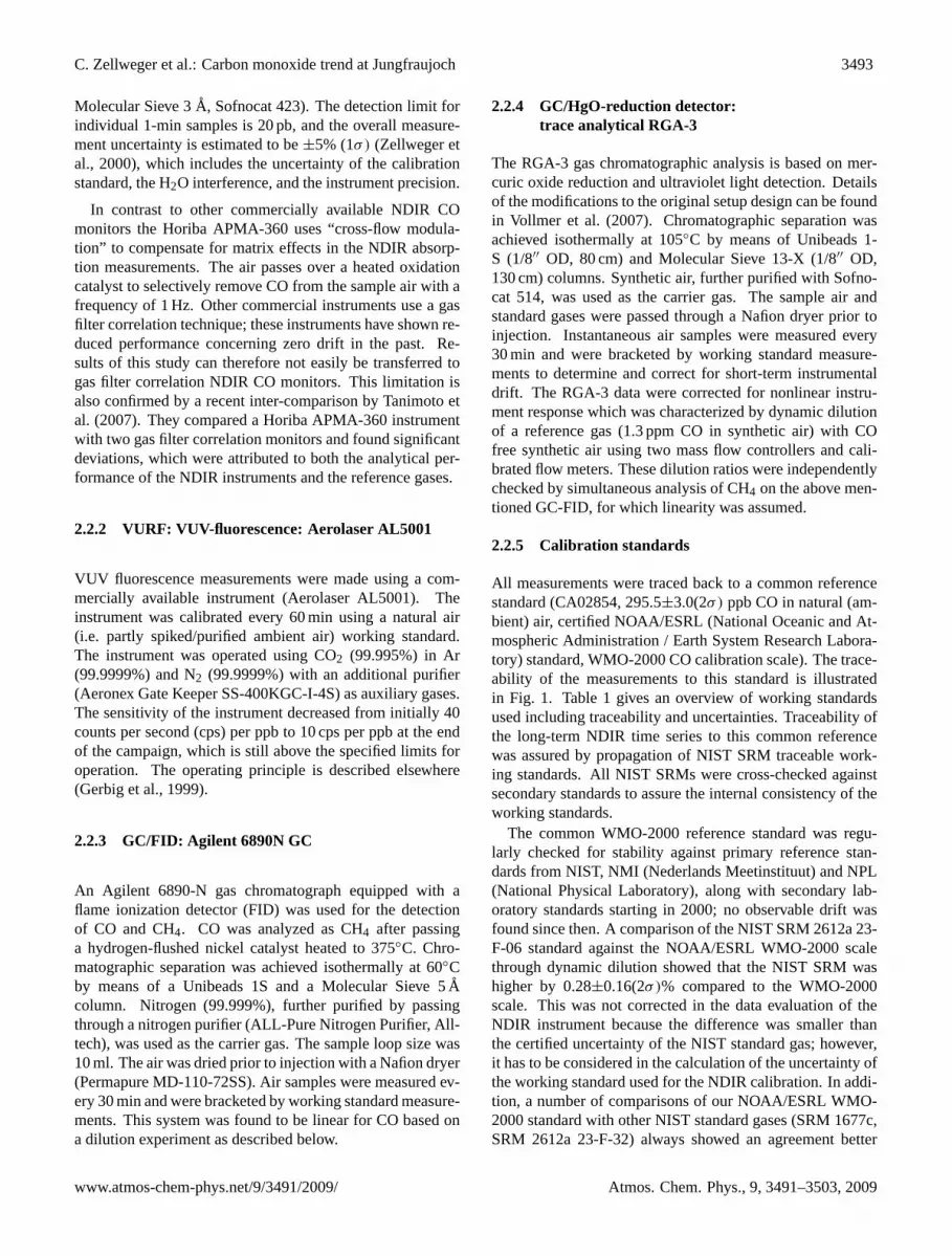
CO has been continuously monitored since 1996 using acommercially available NDIR monitor (APMA-360, Horiba)as part of the Swiss National Air Pollution Monitoring Net-work (NABEL). Modification of the instrument includeddrying of the air by a Nafion dryer in split flow mode (Perma-pure PD-50T-24”). The instrument was calibrated approx-imately in monthly intervals using a commercial CO cali-bration gas referenced against NIST (National Institute ofStandards and Technology) SRM (Standard Reference Mate-rial) standards. Automatic instrument zero checks were per-formed every 49 h using zero air (heated CO/CO2 converter,

Atmos. Chem. Phys., 9, 3491–3503, 2009 www.atmos-chem-phys.net/9/3491/2009/

C. Zellweger et al.: Carbon monoxide trend at Jungfraujoch 3493

Molecular Sieve 3A, Sofnocat 423). The detection limit forindividual 1-min samples is 20 pb, and the overall measure-ment uncertainty is estimated to be±5% (1σ) (Zellweger etal., 2000), which includes the uncertainty of the calibrationstandard, the H2O interference, and the instrument precision.

In contrast to other commercially available NDIR COmonitors the Horiba APMA-360 uses “cross-flow modula-tion” to compensate for matrix effects in the NDIR absorp-tion measurements. The air passes over a heated oxidationcatalyst to selectively remove CO from the sample air with afrequency of 1 Hz. Other commercial instruments use a gasfilter correlation technique; these instruments have shown re-duced performance concerning zero drift in the past. Re-sults of this study can therefore not easily be transferred togas filter correlation NDIR CO monitors. This limitation isalso confirmed by a recent inter-comparison by Tanimoto etal. (2007). They compared a Horiba APMA-360 instrumentwith two gas filter correlation monitors and found significantdeviations, which were attributed to both the analytical per-formance of the NDIR instruments and the reference gases.

2.2.2 VURF: VUV-fluorescence: Aerolaser AL5001

VUV fluorescence measurements were made using a com-mercially available instrument (Aerolaser AL5001). Theinstrument was calibrated every 60 min using a natural air(i.e. partly spiked/purified ambient air) working standard.The instrument was operated using CO2 (99.995%) in Ar(99.9999%) and N2 (99.9999%) with an additional purifier(Aeronex Gate Keeper SS-400KGC-I-4S) as auxiliary gases.The sensitivity of the instrument decreased from initially 40counts per second (cps) per ppb to 10 cps per ppb at the endof the campaign, which is still above the specified limits foroperation. The operating principle is described elsewhere(Gerbig et al., 1999).

2.2.3 GC/FID: Agilent 6890N GC

An Agilent 6890-N gas chromatograph equipped with aflame ionization detector (FID) was used for the detectionof CO and CH4. CO was analyzed as CH4 after passinga hydrogen-flushed nickel catalyst heated to 375◦C. Chro-matographic separation was achieved isothermally at 60◦Cby means of a Unibeads 1S and a Molecular Sieve 5Acolumn. Nitrogen (99.999%), further purified by passingthrough a nitrogen purifier (ALL-Pure Nitrogen Purifier, All-tech), was used as the carrier gas. The sample loop size was10 ml. The air was dried prior to injection with a Nafion dryer(Permapure MD-110-72SS). Air samples were measured ev-ery 30 min and were bracketed by working standard measure-ments. This system was found to be linear for CO based ona dilution experiment as described below.

2.2.4 GC/HgO-reduction detector:trace analytical RGA-3

The RGA-3 gas chromatographic analysis is based on mer-curic oxide reduction and ultraviolet light detection. Detailsof the modifications to the original setup design can be foundin Vollmer et al. (2007). Chromatographic separation wasachieved isothermally at 105◦C by means of Unibeads 1-S (1/8′′ OD, 80 cm) and Molecular Sieve 13-X (1/8′′ OD,130 cm) columns. Synthetic air, further purified with Sofno-cat 514, was used as the carrier gas. The sample air andstandard gases were passed through a Nafion dryer prior toinjection. Instantaneous air samples were measured every30 min and were bracketed by working standard measure-ments to determine and correct for short-term instrumentaldrift. The RGA-3 data were corrected for nonlinear instru-ment response which was characterized by dynamic dilutionof a reference gas (1.3 ppm CO in synthetic air) with COfree synthetic air using two mass flow controllers and cali-brated flow meters. These dilution ratios were independentlychecked by simultaneous analysis of CH4 on the above men-tioned GC-FID, for which linearity was assumed.

2.2.5 Calibration standards

All measurements were traced back to a common referencestandard (CA02854, 295.5±3.0(2σ) ppb CO in natural (am-bient) air, certified NOAA/ESRL (National Oceanic and At-mospheric Administration / Earth System Research Labora-tory) standard, WMO-2000 CO calibration scale). The trace-ability of the measurements to this standard is illustratedin Fig. 1. Table 1 gives an overview of working standardsused including traceability and uncertainties. Traceability ofthe long-term NDIR time series to this common referencewas assured by propagation of NIST SRM traceable work-ing standards. All NIST SRMs were cross-checked againstsecondary standards to assure the internal consistency of theworking standards.

The common WMO-2000 reference standard was regu-larly checked for stability against primary reference stan-dards from NIST, NMI (Nederlands Meetinstituut) and NPL(National Physical Laboratory), along with secondary lab-oratory standards starting in 2000; no observable drift wasfound since then. A comparison of the NIST SRM 2612a 23-F-06 standard against the NOAA/ESRL WMO-2000 scalethrough dynamic dilution showed that the NIST SRM washigher by 0.28±0.16(2σ)% compared to the WMO-2000scale. This was not corrected in the data evaluation of theNDIR instrument because the difference was smaller thanthe certified uncertainty of the NIST standard gas; however,it has to be considered in the calculation of the uncertainty ofthe working standard used for the NDIR calibration. In addi-tion, a number of comparisons of our NOAA/ESRL WMO-2000 standard with other NIST standard gases (SRM 1677c,SRM 2612a 23-F-32) always showed an agreement better

www.atmos-chem-phys.net/9/3491/2009/ Atmos. Chem. Phys., 9, 3491–3503, 2009


Table 1. Overview of standards used for the calibration of the CO instruments. The uncertainty for the individual standards was estimatedincluding the traceability to the common reference (WMO-2000); the expanded uncertainty includes the uncertainty of the NOAA WMO-2000 standard. All uncertainties are given for the 95% confidence level (2σ).

Instrument/WS Mole fraction (ppb) Traceability chain Uncert. (%) Expandeduncert. (%)

VURF / CA06439 438.8 WMO-2000 0.3 1.0NDIR / SL68874 2020.0 NIST – WMO-2000 2.1 2.3GC/FID / CC106830 177.9-180.0a WMO-2000 0.9 1.4GC/HgO / E-033 241.1 CC106830 – CA06439 – WMO-2000 1.7 2.0

a A time dependent drift correction was applied

VURF

NDIR

GC/FID

GC/HgO

NIS

TN

OA

A

ND

IR W

S

Jungfraujoch Working StandardsLaboratory Reference

NIS

T S

RM

23-F

-06

9.7

5 p

pm

CO

in

air

NO

AA

/ES

RL

WM

O-2

000

295.5

pp

b C

O in

air

NDIR Working Standard

2.02 ppm CO in nitrogen (Messer Schweiz GmbH)

VURF Working Standard

438.8 ppb CO in natural air (SMI tank filled with RIX compressor)

GC/FID Working Standard

177.9 – 180.0 ppb CO in natural air (SMI tank filled with RIX compressor)

GC/HgO Working Standard

241.1 ppb CO in natural air (Essex

tank filled with RIX compressor)

VU

RF

WS

GC

/FID

WS

GC

/Hg

O W

S

Fig. 1. Traceability of the four CO instruments to a common ref-erence standard. The black arrows indicate the calibrations madeduring the inter-comparison campaign.

than 0.5% (average 0.15±0.09(2σ)%), which is well withinthe individual stated uncertainties of the NIST SRM stan-dards (0.5–1.2%,2σ). Therefore the NOAA/ESRL WMO-2000 scale based on this particular cylinder is not consideredto be significantly different from the NIST CO scale.

Working standards were calibrated using theNOAA/ESRL and NIST laboratory standards for fieldcalibrations at the JFJ, as illustrated in Fig. 1. The followingworking standards were used for the calibration of theinstruments during the campaign:

NDIR – Horiba APMA 360: A 10 liter aluminum Luxfercylinder (Messer Schweiz GmbH) containing CO in nitro-gen was used as a calibration gas. This cylinder was as-signed 2.02 ppm CO based on initial calibration against aNIST SRM 5-I-04 (9.66 ppm CO in N2) in April 2005. Thisvalue was confirmed after use of the cylinder in December2006 with NIST SRM 23-F-06 (9.75 ppm CO in air). Theuncertainty of the NDIR working standard due to calibration

was estimated to be±2.3%(2σ) from the inter-comparisonbetween the NOAA/ESRL and NIST reference standards(0.56%, 2σ), the contribution of an imperfect calibrationon the laboratory NDIR system due to instrument noise of12 ppb at zero and 16 ppb at span (2.0%, 2σ), and the uncer-tainty of the NOAA/ESRL standard (1%, 2σ).

VURF – Aerolaser AL5001: A 30 l Scott Marrin alu-minum cylinder (Luxfer) containing pressurized ambientair (RIX SA-3 oil free compressor) was used as a cali-bration gas. This standard was calibrated several timesagainst the NOAA/ESRL certified standard (CA02854,295.5±3.0(2σ) ppb CO in natural (ambient) air, WMO-2000scale) before and after the campaign, and was assigned aCO mole fraction of 438.8 ppb. No significant drift was ob-served in this cylinder over its lifetime between July 2005and September 2006. The uncertainty of the VURF work-ing standard was estimated to be 1.0%(2σ) based on multiplecalibrations against the NOAA/ESRL standard. Note that theVURF instrument requires a standard in natural air becausethe UV fluorescence reaction is quenched by oxygen. Nomatrix effects for standards balanced with air or nitrogen areknown for the other analytical techniques.

GC/FID: A working standard with the same cylinder typeand material as the one for the Aerolaser instrument was usedfor automatic calibrations; however, CO in this cylinder wasless stable, and a continuous and constant upward drift of COwas observed over time. The cylinder was calibrated againstthe NOAA/ESRL certified standard described above severaltimes before and after the campaign, and against the work-ing standard of the VURF instrument during the campaign.Based on these measurements, a linear correction was ap-plied, with a CO increase rate of 0.033 ppb per day and aninitial mole fraction of 172.0 ppb on 15 July 2005. This al-lowed the calculation of the working standard mole fractionsat all times during the campaign. The estimated uncertaintyof this standard is 1.4% (2σ) from a linear interpolation ofmultiple calibrations against the NOAA/ESRL standard.

GC/HgO: An electro-polished stainless steel tank (EssexCryogenics) filled with natural ambient air was used as aworking standard. This standard was stable at 241.1 ppb CO



100

150

200

250

CO

[ppb

]

NDIRVURFGC/FIDGC/HgO

●●

●

●●●

●●

●

●

●●

●

●

●●

●●●●●

●●●●●

●

●

●

●

●●●●●●●

●●

●

●

●●

●●●●●●

●●●●

●●●

●

●●●

●●●●●●●●●●●●●

●

●●

●●●●●

●●●●●

●●●

●●●

●

●●●

●●

●

●

●

●●●

●●

●●

●

●

●●●●●●●

●

●

●

●●

●●●●●

●●●●

●●●

●

●

●

●●●

●

●●

●

●

●

●

●●

●

●

●●

●

●●

●●●

●●

●

●●

●●●●●●●

●●

●●●

●

●●●●●●●

●

●

●●

●●

●

●●●●●●

●●

●●

●

●

●●●●

●

●●

●●●

●

●

●

●●

●●●

●

●

●●

●

●●

●●●●●

●●●●●●

●

●●●

●●●

●●●●●

●●●

●●

●

●

●●●●●

●●

●●

●

●●

●●●●

●

●

●

●

●●●●●●●●

●●●

●●

●

●

●

●

●●

●

●●

●

● ●●

●

●●●●

●●●●●

●

●

●●

●●

●

●

●●

●●

●

●

●

●

●●●

●

●

●●

●

●●●●

●

●●

●●●●

●

●●

●●

●●●

●

●●

●

●●

●●

●

●●

●

●

●●

●

●

●

●

●

●

●●●●

●●●●

●

●●

●

●●●●

●

●

●●

●●

●

●

●

●●

●●

●

●●

●●●●●●

●●

●

●●

●●●●●●●

●●●

●

●

●

●●

●

●●●

●●●

●●●

●

●

●●●

●

●●

●●

●

●

●●

●

●

●●●

●

●

●●●●●●●

●●●●

●

●

●

●●●●

●●●

●●●

●

●

●

●●●

●

●

●

●●●●

●●

●

●

●●

●

●

●

●

●●

●●●

●

●

●●●●

●●

●●

●

●●●●

●

●●●

●

●

●●

●

●

●

●●

●●●

●

●

●●

●

●

●

●●

●

●●

●●●●

●●●●●●●

●

●

●

●

●●

●

●●●

●

●●●●●●

●

●●●●

●●

●

●●●●●

●●●

●●●●●●●●●●●

●

●

●●●

●

●

●●●

●

●

●●●

●

●

●

●●

●

●●

●

●

●

●

●●●●

●●●●

●

●●

●●●●

●

●

●●●●

●

●

●●

●

●●●

●●●

●

●

●

●●●

●

●

●●●

●●●

●

●

●

●●●●

●●●

●

●●●●●●●●●●

●

●

●

●

●

●

●●

●●●●

●

●

●

●●●●●●

●●

●●

●

●

●

●●

●

●

●

●●●●

●●●●

●●

●

●●

●

●●

●

●

●●

●

●●

●●●●●●

●●●●

●

●

●

●●

●●●

●

●

●●

●●

●

●●●●

●

●●●

●

●

●●

●●●

●●●●●

●●

●●●●

●

●

●

●

●

●●

●

●●

●●●

●

●●

●●

●

●

●

●

●●

●

●

●

●

●

●

●

●●

●●

●

●

●●

●●●●●

●●●●

●

●

●●●●

●●

●

●●●

●●●●●●●●●●●

●

●●

●●●

●

●●●●

●●●●●

●

●●

●

●

●●●

●●●

●

●●

●

●

●

●●●●

●●●

●

●

●

●●

●●

●

●●●●●●

●

●●

●●

●●●

●

●

●●

●

●

●

●●●

●●●

●

●●●●

●●

●

●

●

●

●●●●

●

●●●●●

●●●

●●●

●●

●

●●

●●●●●●●

●●●●

●●

●

●

●

●

●

●

●●●

●

●●

●●●●

●

●●

●●

●●

●

●

●

●

●●●●

●●●●

●

●●●●●

●

●

●

●

●

●

●●

●

●●

●●

●

●

●

●●●

●

●●●

●●

●●●●●

●●●

●

●●●

●●●

●●

●●

●●

●●

●●

●

●●●

●

●

●

●

●

●●●

●●

●

●●●●●

●●

●●●

●

●●

●●

●●●

●●

●●●●

●●●●●●●

●

●

●●

●

●●●

●

●

●●

●

●

●●

●●

●

●●

●

●

●

●●●●●●

●●●

●

●●●●●●

●

●

●

●

●

●

●

●●●

●

●

●

●●●●●●●

●

●

●

●●

●

●

●

●●●

●

●

●

●

●

●

●

●

●

●●

●

●

●●●●

●●

●

●●●●

●

●

●

●

●

●●●●●

●●●●

●

●

●●

●

●●

●●

●●●●●

●

●●

●

−40

−20

020

40

date [yy−mm−dd]

Dev

iatio

n to

VU

RF

CO

[ppb

]

●●●●●

●●●●

●●●●●

●

●

●●●●●

●

●●●●●●●●●●●●●●

●

●

●

●●●●●●●●●●●●●●●●●●●●●

●●●●●●●●●●●●●●●●

●●●●●

●

●

●

●

●●

●●

●

●

●●●●●●●●

●

●●●●●●●●●

●

●●●●●●●●●

●

●

●

●

●●●●●●●

●

●●●●●●●●

●●

●●

●●●●

●●

●●●●

●●

●●●●●

●

●●●●

●●●●●●●●●

●

●

●

●

●●

●●●●●●●●●●●●●●●●●●●●●●●●●

●

●

●●●●

●

●●●●●●●●●●●

●●

●

●

●●●●

●

●●●●●●

●●●●●

●●●

●●●●

●●●

●

●

●●

●●●●

●

●●●●●

●●●●

●●●

●●●●●●●

●

●

●

●●

●

●

●●

●

●●

●●

●

●●●●

●●●

●●●

●●●

●●

●●

●●●●●●●●

●

●

●●●●

●

●

●

●

●●●

●

●●●●●●●●●●

●●

●●●●●●●

●●

●●

●

●●●●●

●

●

●●●

●

●●●●●●●●●

●

●

●●

●●

●●●

●●●

●●

●●●

●

●

●

●●

●

●●●

●

●●●●●

●●●●●●●

●●●●●●

●

●●●●●

●

●●●

●

●

●●

●●

●

●●●●●●

●●●●

●●

●●

●

●

●

●

●●●

●●

●●●

●

●●

●

●●●●●●●●●

●

●

●●●●●●●

●

●●●●

●

●●

●

●

●

●●●●

●●

●

●

●●●

●●

●●●●●●

●

●

●

●

●

●

●

●

●

●

●●

●●

●

●

●●

●●

●

●

●

●●●

●

●

●●

●

●●

●●●

●●●

●●●●●●

●

●

●●●●

●

●

●

●

●●

●

●

●

●●●

●

●●●

●

●●●●●

●●

●●●●

●●

●●

●

●●●

●

●

●

●

●

●●●

●

●

●

●●

●●●

●●●●

●

●

●

●

●

●●

●

●●●●

●

●●

●●

●

●●●●

●●

●

●

●●

●

●●●●

●

●●●

●

●

●

●

●

●

●

●

●●

●●●

●

●

●

●

●●

●●●●

●

●

●●

●●●

●

●●●

●

●●●●●

●●●●

●●

●

●●●

●

●●

●

●●●

●●

●●●●●

●

●

●

●

●

●●●

●

●

●

●

●

●●

●●

●

●●●

●●

●

●

●

●●

●

●

●●

●

●

●●

●

●

●

●

●

●

●

●

●●

●●

●●●●

●

●

●

●

●

●

●●●●●●●●●●

●

●

●

●

●

●

●

●●

●

●●

●

●●

●

●●●●

●

●●●●

●

●

●

●

●

●●

●

●●●

●●

●

●●

●

●●●

●●

●

●

●●●

●

●

●

●●●●

●

●

●

●●

●●

●●●●●●●

●

●●●

●

●●●●

●●●●●●

●

●●●●●●●

●●●

●●

●●●

●●●

●●●●

●

●●●●

●●

●

●

●●

●

●●●●

●

●●

●

●

●

●●

●

●

●●●

●

●

●

●

●

●

●●

●

●●●

●

●●●

●

●●●●●●●●●●●●

●●●

●●●

●●●

●●●●

●

●●●●

●

●●

●

●

●●●

●●●

●

●

●

●●●

●●

●

●●●●●●

●●

●

●●●

●●

●●●

●●●

●●

●

●

●

●●●●

●●●

●●

●

●

●●

●●

●

●

●●●

●●

●●●●●●●

●

●●

●

●

●

●●●●●●●●●●●●●●●

●

●

●

●●●

●

●

●

●●●

●●●

●●

●

●

●●

●

●

●

●

●

●

●

●

●

●

●

●●

●

●

●●●●

●●

●●

●●

●●

●

●

●

●

●●●●

●

●●●

●

●

●

●

●

●

●●

●●●

●

●●

●

●

●

●

●

●

●

●

●

●

●

●

●●

●

●●

●●●●●●●●●●

●

●

●

●●

●

●

●

●●●●●●●●●●●●●●●●●●●

●●●

●

●●●●●●

●

●

●

●●●●●●

●●●

●

●

●●●●●

●

●

●

●●

●●●●●●●●●

●●●●●●●●

●●●

●●●●

●

●

●●●

●

●

●●●●

●

●●●●●●●●

●

●

●

●

●

●

●

●

●

●●

●

●

●

●

●●

●

●

●

●

●●●●

●

●

●

●●

●

●●

●

●

●●

●●●

●●●●

●

●

●

●

●●

●

●

●●●●●●

●●●

●●

●

●●

●●●●●

●

●

●

●●●●

●●●●●●●●

●●●●●

●

●●

●

●

●●●

●

●●●●

●●

●

●●●●●

●

●

●●

●

●

●

●

●

●

●●●●

●

●●●

●

●

●

●●

●

●

●

●

●

●●

●

●

●

●

●●●●

●

●●

●●●●●

●●

●●

●

●

●

●

●●

●●

●

●

●●

●

●●

●●

●●

●

●

●●●●●

●●●

●

●

●

●

●●●●●●

●●

●●

●

●

●

●●●

●●

●

●

●●

●

●●

●

●

●●

●

●

●

●●

●

●●●

●

●

●

●

●●●●●

●

●

●●

●●

●

●●●●

●

●

●●●●●

●●●●●

●●

●

●●

●

●

●

●

●●●●

●

●●●

●●●●

●

●●

●

●●●●●●

●●

●

●

●

●

●

●

●●

●●●●

●

●

●

●●

●

●●

●●●

●

●●

●●

●

●●●●●

●

●●●●●●

●

●

●

●●●

●

●

●

●●

●

●●●●●●

●

●●

●●●

●●

●●

●

●●

●

●

●

●

●

●

●

●●

●●●●

●●●●●

●●●●

●●

●●

●

●

●●●●●●

●●●

●

●

●

●

●

●●●●

●●●●●

●

●●

●●●●●●●●●●●●●●●

●

●●

●

●●

●

●

●●

●

●

●●●

●

●

●

●

●●●

●●

●●●

●

●●●

●●

●

●

●

●

●

●

●

●●

●

●●

●

●●●●●●●●

●

●

●●●●●●●

●●

●

●

●

●

●

●

●

●

●

●●

●●●●

●

●

●●●●

●●

●●●

●

●

●

●

●

●

●●●

●

●

●●

●

●●●●●●●

●

●

●●●

●●●●

●

●

●

●●●●●

●

●

●

●●●●●●●●

●●●●

●

●

●●

●●

●

●

●

●●●

●

●●

●

●●

●

●

●●●●●

●

●●●●

●

●

●●

●

●

●●

●

●

●

●

●

●

●

●●

●

●

●

●●

●●●

●●

●

●

●

●

●●●●

●●●●

●

●

●●●●

●

●

●

●

●

●

●

●●

●●●●●●

●

●●●

●●

●

●●

●

●

●

●

●

●●●●●●

●

●●

●●●●

●

●

●

●

●●

●

●

●●

●●●●●

●

●●●

●

●●●●●

●●●

●

●

●

●

●

●

●

●

●

●

●●●

●

●●●●

●●●

●

●●

●

●●

●

●

●

●●●●

●●

●

●

●

●

●●●●

●

●●

●

●

●●

●

●

●

●

●

●

●

●

●

●●●●

●●●

●

●●

●

●

●

●●●

●

●

●●●●●

●

●

●●

●

●

●

●●

●

●●

●

●

●●

●

●●

●

●

●

●

●●

●●

●

●●●●●●●●

●●●

●

●

●●

●

●

●

●●

●●

●●●●

●●

●

●●

●●●

●

●

●●

●

●

●

●

●●

●●

●●●●●

●

●●●●

●

●

●●

●

●

●●

●

●●

●

●●●

●

●

●●

●

●●

●

●

●

●

●●●●●●

●●

●●

●

●

●●

●●

●●

●

●

●

●

●

●

●

●

●

●

●

●●●●●●●●●●

●

●●

●

●●●●

●●

●

●●●

●●●●●●●

●●●

●

●

●●

●●

●●

●

●

●●●●●

●

●

●●

●

●●●●●●

●●

●

●●●●

●

●

●●●

●

●●

●●

●

●

●●●●●●

●●

●●●●●●

●●

●●●

●

●

●

●●●●●●●

●●

●

●

●●

●

●

●●

●●

●

●●

●●●

●●

●

●

●

●

●

●

●●

●

●

●

●

●

●

●

●●●●

●●

●●

●●●

●●

●

●

●

●

●

●

●●

●

●

●

●

●●

●●

●●●

●

●

●

●

●

●

●

●

●

●●

●●●●●

●

●

●●

●●

●●

●

●

●

●

●

●

●

●●●●●●

●

●

●

●

●

●

●

●

●

●

●●

06−01−12 06−01−22 06−02−01 06−02−11 06−02−21 06−03−03 06−03−13

Fig. 2. Time series of one-hourly averages for all four CO instru-ments (upper panel) and difference between the NDIR and GC tech-niques to the VURF instrument (lower panel).

for the period of the campaign. The standard was referencedagainst the standard of the GC/FID instrument. The uncer-tainty of the standard was estimated to be 2.0% (2σ).

3 Results and discussion

3.1 Field inter-comparison

Measurements with four CO instruments employing four dif-ferent analytical techniques were performed over a periodof approximately two months between 11 January and 15March 2006. Data availability based on one-hourly aver-ages was 96.7% (NDIR), 86.4% (VURF), 86.7% (GC/FID),and 98.9% (GC/HgO). For the continuous techniques, one-hourly averages were only calculated when at least four 10-min averages were available. Hourly averages of the GC ob-servations typically represent the average of two single in-jections. Figure 2 shows the available time series for all fourtechniques and the difference between the NDIR / GC tech-niques and the VURF instrument. The overall variability waswell captured by all techniques. The CO mole fractions dur-ing the campaign ranged from approximately 100 to 260 pb,which is consistent with other studies at the JFJ site (Forreret al., 2000; Zellweger et al., 2003). Figure 2 shows that theNDIR results were slightly higher throughout the entire cam-paign, with an almost constant bias irrespective of the COlevel. However, the deviations of the NDIR from the VURFresults seem to decrease slightly towards the end of the inter-comparison. The reason for this may be changing NDIR zeroreadings during the campaign. Figure 3 shows the individualzero readings of the NDIR instrument (1-min averages) madeautomatically every 49 h, as well as the corresponding 30 minaverages. These zero readings averaged−0.3±8.4(2σ) ppb

●

●

●

●●

●

●

●

●●

●

●

●

●

●

●

●

●

●●

●

●

●●●

●

●

●●

●

●

●

●

●

●●

●

●●

●

●

●

●●●

●●

●

●

●

●

●

●

●

●●

●

●

●

●●

●

●●●

●

●●●

●●

●

●

●

●

●

●

●●

●

●

●

●

●●

●

●

●

●

●

●

●

●●

●

●

●

●●

●●

●●

●

●

●●

●

●

●

●●

●

●

●

●●

●

●

●

●

●

●

●

●

●

●

●

●●

●

●

●

●

●

●

●●

●

●●

●

●

●

●●●

●

●

●

●

●

●

●

●

●

●

●

●●

●

●

●●●

●●

●

●

●●

●●

●

●

●

●

●●●

●

●

●

●●

●

●

●

●

●

●●●●

●

●

●

●

●●

●

●

●

●●●

●

●

●

●

●

●●

●●

●

●●

●

●

●

●

●●

●●●●

●

●●

●●

●●

●

●●

●

●●

●

●●

●

●

●

●

●

●

●●

●

●

●

●

●

●

●

●

●

●●●

●

●●

●●

●

●

●●●

●

●

●

●

●

●●●

●

●

●●

●●

●●

●

●

●

●●

●

●●

●

●

●

●●

●●

●●

●●●

●

●●●

●

●●●

●

●

●

●●●

●●

●●

●

●●

●

●●●

●●

●●

●●●

●●

●●

●

●

●

●

●●

●●●●

●

●

●● ●

●

●●●

●

●

●

●

●●●

●

●

●●

●

●

●

●

●●

●

●

●●

●

●●

●

●

●

●

●●●

●

●

●

●

●

●

●●

●

●

●●

●

●

●

●

●●

●

●●

●

●

●

●

●●●●

●●

●

●

●

●

●

●

●

●

●

●

●

●

●

●

●●

●

●●

●

●

●

●

●

●

●

●●

●

●

●

●

●

●●

●●

●●●

●

●●

●

●

●

●

●

●

●

●

●

●●

●

●●

●

●

●

●

●

●

●

●

●

●

●

●●

●●

●

●●●

●

●

●●

●

●

●

●

●

●

●

●

●

●

●

●

●

●●

●

●

●

●

●

●

●

●

●

●

●

●

●

●

●●●

●

●●●●

●

●

●

●

●●

●

●

●

●

●

●

●

●●

●●

●●

●

●

●●●●

●

●

●

●

●

●

●●

●

●

●

●

●

●

●●

●

●

●

●

●

●

●

●

●●

●

●

●

●

●

●

●

●

●

●●●●

●

●●●

●

●

●

●

●●

●●●

●●

●

●

●

●

●●

● ●●

●●●

●

●

●

●

●●

●

●

●

●

●●

●

●●

●●●

●●

●

●

●

●

●

●

●

●

●

●

●

●

●●●

●

●

●●

●

●

●

●●

●●

●

●●

●

●

●

●

●

●

●

●

●

●

●

●

●

●

●

●

●

●

●●

●

●

●

●

●

●

●

●

●●●●

●

●

●

●●

●

●

●

●●

●

●

●

●

●

●

●

●●●●●

●

●●●

●●●●●●

●

●

●●

●●

●

●

●

●

●●

●

●

●

●

●

●

●

●

●●

●

●

●

●●

●

●

●

●

●

●

●

●●

●

●

●●

●

●

●

●●

●●

●

●

●

●●

●

●

●

●

●●

●●

●

●

●

●

●

●●●●

●●

●

●

●

●

●

●

●

●

●

●

●●

●●

●

●●

●

●●●

●●●

●

●

●

●

●●●

●

●●●

●

●

●

●

●

●

●

●

●

●●

●●

●

●●

●

●●

●●

●

●

●

●

●

●

●●

●

●●●

●

●

●●

●

●

●●

●●●

●

●

●

●

●

●

●●

●

●

●

●●●

●

●

●●

●

●●

●

●

●●●

●●

●

●

●

●

−60

−20

020

40

date [yy−mm−dd]

ND

IR z

ero

read

ings

[ppb

]

06−01−12 06−01−22 06−02−01 06−02−11 06−02−21 06−03−03 06−03−13

● ●● ● ●

●

●●

●●

● ● ●● ● ● ●

● ● ●●

● ●

●●

●

● ●●

●●

●

●

1 minute values30 min average

Fig. 3. Automatic zero checks of the NDIR instrument. The bluecircles represent 1-min averages and the red dots the corresponding30-min average. The error bars represent the expanded uncertainty(2σ) of the 30-min average.

and were not significantly different from zero over the entireperiod. Consequently, due to the relatively high uncertain-ties of the individual zero readings, no further correction wasapplied to the data. However, neither a potential drift nor anoffset can be excluded based on these data, which potentiallyexplains the small observed difference.

Table 2 shows the parameters obtained from orthogonal re-gression analysis (York, 1966) between different techniquesbased on one-hourly averages. A generally good agreementwas found among all techniques, with the highest correla-tion between the two continuous methods (VURF and NDIR,r2=0.992). A slightly lower but still excellent correlation wasfound between the continuous and the GC methods (r2 be-tween 0.962 and 0.981), while the lowest correlation was ob-served between the two GC methods (GC/FID and GC/HgO,r2=0.935). Due to the large number of measurement points,the estimated uncertainties of slope and intercept were rela-tively small, and significant differences were found betweenall time series. A pair-wise Wilcoxon-Mann-Whitney testbased on one-hourly averages also confirmed significant dif-ferences between all possible combinations (p-value<0.01with Bonferroni correction for multiple testing), with the ex-ception of the VURF-NDIR instrument pair (p-value=0.42).These results suggest that the differences observed by Whal-ley et al. (2004) between the JFJ NDIR system and theirVURF instrument of 20–30 ppb are likely due to the useof calibration standards that were not traceable to NIST orWMO-2000 CO scales, or from instrumental faults, such asleaks.

The agreement between the various time series is furtherillustrated in relative difference histograms (Fig. 4) comparedto the VURF as the reference instrument for averages of1-, 10-, and 60 min respectively. Single injections of theGC techniques were compared to 1 m-in and 10 min data,and the average of (usually) 2 GC injections was used tocompare with for hourly averages. The relative differences(x−xref)/xref are shown wherexref is the CO mole fractionmeasured by the reference instrument (VURF). In addition,the individual uncertainties of the calibration standards (cf.



Table 2. Results of the orthogonal regression analysis between the different measurement techniques, where x and y are the correspondinginstruments, and a and b are the intercept and slope of the regression line with 95% confidence intervals.r2 is the coefficient of determination,and N is the number of data points. In addition, the p-value of the Wilcoxon-Mann-Whitney test is shown. Comparisons are based on one-hourly averages.

y x a [ppb] b r2 N p-value

VURF NDIR −1.9±0.8 0.997±0.005 0.992 1273 0.424VURF GC/FID 6.1±1.2 0.967±0.008 0.981 1165 3.95e-12VURF GC/HgO −4.4±1.5 1.033±0.010 0.970 1292 4.03e-04NDIR GC/FID 9.8±1.3 0.960±0.009 0.975 1271 3.19e-10NDIR GC/HgO −2.0±1.6 1.033±0.010 0.962 1448 1.50e-05GC/FID GC/HgO −1.2±2.2 1.070±0.016 0.935 1299 2.41e-03

Table 1) and the additional uncertainty due to imperfect zerocompensation of the NDIR instrument are shown. The max-imum of the distribution of the differences was in all caseswithin the uncertainty limits of the calibration standards. Itcan therefore be concluded that the mean differences of thevarious time series are due to differences in the calibrationstandards. It can further be seen that the averaging time has asignificant influence on the width of the relative differencedistribution for the NDIR technique. The standard devia-tion of the relative difference distribution is comparable forall techniques for one-hourly averages, with the lowest valuefor the NDIR technique. This implies that the performanceof the NDIR technique for one-hourly averages is equal oreven slightly better compared to the GC methods. At the10 min level the noise of the NDIR technique was signifi-cant, but the performance was still comparable to the GCtechniques. The GC techniques showed a considerable num-ber of values with large deviation compared to the VURFmethod, resulting in long tails of the distribution of the rel-ative differences at the 1– and 10 min levels; this can be ex-plained with the different temporal coverage was different(single injections vs. integration over ten min). The numberof these outliers was relatively insensitive to the level of ag-gregation, but the overall width of the frequency distributionincreased slightly due to the fact that instrument noise wasbecoming more of an issue. This was also the case for theVURF technique. Instrument noise was clearly the dominat-ing factor for the NIDR technique on the 1 min level. Thewidth of the distribution of the 1 min relative differences ofthe NDIR technique was comparable to data obtained fromour laboratory experiments with a Horiba APMA-360 NDIRCO monitor. This was demonstrated through an additionalexperiment, during which the 1 min average noise over 24 hwas determined at a constant mole fraction of 152 ppb, whichis similar to the average mole fraction during the JFJ cam-paign. Based on this experiment a standard deviation of therelative difference for a mole fraction of 152 ppb of 0.0750was calculated during the laboratory experiment compared to0.0768 during the JFJ campaign. For the 10 min and hourly

averages, the corresponding numbers were 0.0336 (0.0310 atJFJ), and 0.0208 (0.0171 at JFJ). This clearly demonstratesthat instrument noise is a limiting factor for the determina-tion of CO levels with the NDIR technique if high temporalresolution is required. It can be seen from Fig. 4 that theaveraging interval has a significant influence on the uncer-tainty of the NDIR measurements. One-hourly averages ofthe NDIR instrument achieve a data quality that is compara-ble to the GC instruments, with even slightly lower relativedifferences because of fewer outliers. This is confirmed bythe Wilcoxon-Mann-Whitney test, which also does not yieldsignificant differences between the NDIR and the GC tech-niques when one-hourly averages are compared.

The mean value of the relative difference is a measure ofthe difference in location of the data points compared to theVURF technique. The largest mean deviation (1.58%) wasobserved between the VURF and NDIR technique. However,the calibration standard of the NDIR instrument also has arelatively high uncertainty, and at least part of the bias canbe explained by differences in the calibration. In addition,imperfect compensation of the zero offset (cf. Fig. 3) mayalso contribute to the observed bias. Automatic zero checkswere made every 49 h, which is potentially insufficient foran accurate compensation of the zero offset. The standarddeviation of the zero readings obtained during the campaignwas 4.2 ppb (31 observations); this results in an additionaluncertainty of the NDIR measurements of 1.0%.

To illustrate the performance as a function of the averag-ing time, a selected time period is shown in Fig. 5. Duringthe period from 11 to 13 March, rapid changes in the ambi-ent mole fractions occurred. Instrument noise of the NDIRtechnique was dominant at the one minute level, but goodagreement was observed between all techniques for 10 minand one-hourly averages. All instruments were able to detectfast changes in the CO mole fractions that occurred in thesecond half of the selected period. More interesting is thefirst half of the period that was characterized by relativelysmall changes of the mole fractions. Part of this period wascharacterized by large short-term variations as apparent from



Fre

quen

cy %

−0.2 −0.1 0.0 0.1 0.2 0.3

05

1015

2025

30 NDIRmeanmedianst.devNP(%)

1 h0.01580.01570.0171127364.9

1 h

−0.2 −0.1 0.0 0.1 0.2 0.3

05

1015

2025

30 GC/FIDmeanmedianst.devNP(%)

1 h−0.0086−0.00970.0237116536.6

−0.2 −0.1 0.0 0.1 0.2 0.3

05

1015

2025

30 GC/HgOmeanmedianst.devNP(%)

1 h−0.0033−0.00580.0307129263.7

Fre

quen

cy %

−0.2 −0.1 0.0 0.1 0.2 0.3

05

1015

2025


10 min0.01590.01590.031763550.5

10 min

−0.2 −0.1 0.0 0.1 0.2 0.3

05

1015

2025


10 min−0.0086−0.01050.0294231632.5

−0.2 −0.1 0.0 0.1 0.2 0.3

05

1015

2025


10 min−0.0032−0.00630.0407253057.2

Relative Difference

Fre

quen

cy %

−0.2 −0.1 0.0 0.1 0.2 0.3

05

1015

2025


1 min0.01590.01580.07687301926.1

1 min

Relative Difference

−0.2 −0.1 0.0 0.1 0.2 0.3

05

1015

2025


1 min−0.008−0.00990.0345222330.6

Relative Difference

−0.2 −0.1 0.0 0.1 0.2 0.3

05

1015

2025


1 min−0.0024−0.00530.0454243255.1

Fig. 4. Relative difference histograms for the NDIR and GC instruments calculated relative to a common reference instrument (VURF). Eachpanel shows the frequency of data falling into 0.01 relative difference bins (normalized to the number of coincident data points). Relativedifferences for one-hourly, 10-min and 1-min averages are shown. 1- and 10-min averages of the GC techniques represent single injections.The red shaded areas represent the uncertainty of the calibration standards, and the blue shaded areas the uncertainty due to imperfect zerocompensation (NDIR only). P(%) is the percentage of data falling within the uncertainty limits.

the one minute VURF data. These fast changes could onlybe detected with the VURF technique because the instrumentnoise of the NDIR monitor is too large to allow detectionof mole fraction changes of a few ppb on a temporal scaleranging from seconds to a few minutes. The GC techniques

were able to accurately reflect the CO mole fraction, but lacktemporal resolution; consequently, differences of integratedvalues between continuous and GC methods may be sig-nificantly higher compared to periods with less pronouncedshort-term variation in the CO mole fractions. The period



100

150

200

250

300

CO

[ppb

]


(a)

1 h

06−03−11 00:00 06−03−11 12:00 06−03−12 00:00 06−03−12 12:00 06−03−13 00:00

100

150

200

250

300

CO

[ppb

]

●

●

● ● ●● ● ● ● ● ● ●

● ● ● ● ●● ● ● ● ●

●●

●●

● ● ●●

● ● ● ● ● ● ● ● ● ● ● ● ● ● ● ●● ●

● ●●

● ●

● ●

●

● ● ● ●●

●

●● ●

●●

●

●

●

●

●● ● ●

●

●●

●●

● ●●

●

●

●

● ●● ●

● ● ●

● ● ●

●

● ● ● ●

● ● ●

●

● ●

●

●

● ●

●

●

●

●●

●

●

●

●

●● ●

●●

●

●

●●

●● ● ●

●●

●●

● ● ● ● ● ●

●

● ●●

● ● ● ● ● ● ●● ●

●● ● ● ● ● ● ● ●

● ●● ● ● ● ● ●

● ● ●● ●

● ●●

● ● ●●

●

● ●● ● ● ●

●

●●

●

●●

●

● ●

●●

●●

● ●

●●

●

●

● ● ● ● ●

●

●

● ●

●●

●

●

●

● ●●

●

●

●

●

●● ●

●

●●

●

●

●●

●

● ● ●● ●

●

●● ●

●

●


(b)

10 min

06−03−11 00:00 06−03−11 12:00 06−03−12 00:00 06−03−12 12:00 06−03−13 00:00

100

150

200

250

300

date [yy−mm−dd HH:MM]

CO

[ppb

]

●

●

● ● ●● ● ● ● ● ● ● ● ● ● ● ●

● ● ● ● ●

●●

●●

● ● ●●

● ● ● ● ● ● ● ● ● ● ● ● ● ● ● ●● ●

● ●●

● ●

● ●

●

● ● ● ●●

●

●● ●

●●

●

●

●

●

●● ● ●

●

●●

●●

● ●●

●

●

●

● ●● ●

● ● ●

● ● ●

●

● ● ● ●

● ● ●

●

● ●

●

●

● ●

●

●

●

●●

●

●

●

●

●● ●

●●

●

●

●●

● ● ●

●●

●●

● ● ● ● ● ●

●

● ●●

● ● ● ● ● ● ●● ●

●● ● ● ● ● ● ● ●

● ●● ● ● ● ● ●

● ● ●● ●

● ●●

● ● ●●

●

● ●● ● ● ●

●

●●

●

●●

●

● ●

●●

●●

● ●

●●

●

●

● ● ● ●●

●

●

● ●

●●

●

●

●

● ●●

●

●

●

●

●●●

●

●●

●

●

●●

●

● ● ●● ●

●

●● ●

●

●


(c)

1 min

06−03−11 00:00 06−03−11 12:00 06−03−12 00:00 06−03−12 12:00 06−03−13 00:00

130

150

170

190

CO

[ppb

]

●

●●

●●●●

●●●●

●●●●●●●●●●●●●●

●●●●●●●●●●●●●●●●●●●●●●●●

●●●●●●●●●●●●●●●●●●●●●●●●

●●●●●●●●●●●●●

●●●●●●●●●●

●

●●●●●●●●

●●●●●●●●●●●●

●●●●●●●●●●●●●●

●●●●●●●●●●●

●●●●●

●

●

●●●●

●

●

●●●●●

●

●

●●●●

●●●●●●●●●●●●●

●●●●●●●●●●●●

●●●●●●●●●●●●

●●●●●●●●●●●●●●●●

●●●●●●●●●●●●●●●●●●●●●●●●

●●●

●●●●●●●●●●

●●●●●●●●●●●●

●●●

●

●●●●●●●●●●●●●●●●●●●●●

●●●●●●

●●●●●●●●●●●●●●●●●●●●●●

●

●

●

●

●●●●●●●●●●●●●●●●●

●●●

●

●●●●●●●●●●●●●●●●●●●●●●

●●●●●●●●●●●●

●

●●●

●●●●●●●●●

●●●●●●●●●●●●●●

●

●●●●●

●

●●●

●●●●●●●●●●●●●●●●●●●●●●●●●●●●●●●

●●●

●●●

●●

●●●●●●●●●●●●

●

●●●●●●●●●●●●●●●●●●●●●●●●●●●●●●●●●●●●

●●●●●●●●

●●●

●●●●●●●●●●●●●●●●●●●●●●●

●

●●●●

●●●●●●●●●●●●●●●●●●●

●

●

●●●●●●●●●●

●●●●●●●●●●●●●

●●●●●●●●●●●●●●●

●●●●●●●●

●●●●●

●●●●●●●●●●●●●●●●●●●●●●●●●●●●●

●●●

●●●●

●●●●●●●●●●●●●●●●●●●●●●●●●●●●●●●

●●●●●●●●●●●●●●●●●●●●●●●●

●●●●●●●●●

●●●●●●●●●●

●●●

●●●●●●●●●●●●●●●●●●●●●●●●

●●●●●●●●●●●●●●●●●●●●●●●●●●●●●●●●●●●●●●●●●●●●●●●●●●●●●

●●●●

●●

●●●●●●●●●●●●●●●●●●●

●

●●

●

●●●●●●●●●●●●●●●●●●

●

●●

●●●

●●●●●●●●●●●●●●●●●●

●

●●●

●●●●●●

●

●●●●●●●●●●●●●●●●●

●●

●●●

●●

●●●●●●●●●●

●●●

●●●●●●●●●●●●●●●●●●●●●●●

●

●●●●●●●●●●●●●●●●●●●●●●●●●●●●●●●●●●

●

●

●

●

●●●●●●●●●●●●●●●●●●●●●●●●

●

●●

●

●●●●●

●●

●●●●●●●●●●●●●●●●●●●●●●●●●●●●●●●●●

●●●●●●●●●●●●

●

●●●●●●●●●●●●●●●●●●

●

●

●

●

●●●●●

●

●

●

●

●

●●●●●●●

●

●

●●

●●

●

●●●●●●●●●●●●●●●●●

●●●●●

●●

●●●●●●●●●●●●●●●●●●

●●●●

●●

●

●

●●●●●●

●

●●

●

●●●●●●●

●

●●

●

●●●●●●●●●●●

●

●●

●

●

●●●●●●●

●

●●

●●●

●●●●●

●

●

●●

●●

●●●●●●●

●●

●●

●

●

●

●●●●●●●●●

●●●

●●●●●

●

●●

●

●●

●●●●

●●●

●●●●●●

●●●

●●●

●●●●●●●●●●●●●●

●

●●●●●

●●

●

●●●●●●●●●●●●●●●●●●●●●●●

●

●●●●

●

●●●

●●●●

●●●●●●●●●●●●●●●●●●●●●

●●●

●●●●●●●●

●●●●●●●●●●●

●

●●●

●

●

●

●●●●●●●●●

●●●●●●●●●●●●

●●●●●●●●●●●●●●●●●●●●●

●

●●●●●●●

●●●●

●

●●

●

●

●●

●●●●●●●

●

●●●●

●

●

●

●●

●●

●

●●

●●●●

●●●●●●

●●●●●●

●

●●●

●●

●

●

●●●

●●

●

●●●●●●●●●●

●●●●●●●

●

●●

●●

●●●

●

●●●●●●●

●●

●

●

●●●●●●

●

●

●

●●

●

●

●●●●●

●●●●●

●

●●●●●●●●●●●

●●●●●

●

●●

●●●●

●

●●●●●●●●●●●●

●

●●

●●

●●

●●●●●●●●●●●●●●●●●●●●●●●●●●●●●●●●●

●●●●●●●●●●●●●

●●●●●●●●●●●●●●●

●●●●●●●●●●

●●●●

●

●●●●●●●●●●●●●●●●●

●

●●

●●●

●

●●●●●●

●●●●

●●

●

●●●●●●

●●●

●●●●●●●●●●●●●

●●●

●●●●●●●●●●●●●●●●●●●●●●●●●●●●●●●●●●●●●●●●●●●●●●●●

●●●●●●●

●●●●●●●●●●●●●●●●●●●●●●●

●●

●

●

●●

●●●●●●●●

●●●

●●

●●●

●●

●

●●●●●●●●●●●●●●●●●●●●●●●●●●

●●●●●●

●●●

●●●●●●●●●●●●●●●●●●●●

●●●

●●●●●●●●●

●

●

●

●●

●●●●●

●

●●●

●●

●

●

●●●●

●

●

●

●

●

●

●●●●●●●●●●●●●●●●●●●●●●●

●

●●●●●●●●●●●●●

●●●

●●●●●●●

●●●●●●●●●●●●●●●●●●●●●●●●●

●

●

●

●

●

●●●●●●●●●

●

●●

●●●●●

●

●

●

●●●

●●●●●●●●●●●●●●●●●●●●●●●●

●●●

●●●●●●●

●●●

●●●●●●●●●●●●●●●●●●●●●●●

●

●

●

●●●●●●●●●●●●●●●●●●●●●●●●●●●●●●●●●●●●●●●●

●●●●●●●●●●●●●●●●●●●●●●●●●●●●●●●●

●

●●●●●●●●●●●●●●●●●●●●●●●●

●

●●●

●●●●●●●●●●●●●●●●●●●●●●●●●●●●●●●●●●●●●●●●●●●●●●●●●●●●●●●●●

●●

●●

●

●

●●●●●●●●●

●

●●

●●●●●●●●●

●●●●●

●

●●

●●●

●

●●

●●●●●●●●●●●●

●●

●●

●

●●●●

●●

●●●●●●●●●●

●

●●

●●●●

●●●●●●●●●●

●●●●●●●●●●●●●●●●●●●●●

●●●

●●

●

●●

●

●●●●●

●●

●

●

●●●●●●●

●

●

●●●●

●

●●●●●●

●

●

●●

●●

●

●●●●●

●●

●

●●

●

●●●●●●

●

●●●●●●●●●●●●●

●

●

●●●●●●●●

●●●●●●●●●●●●●●

●

●●

●

●●●●●●●●●●●●●●●

●●●●●●●

●●●

●●●

●●●●●●●

●

●

●●●●●●●●●●●

●

●●

●

●

●

●●●●●●●●

●●

●●

●

●

●●●●

●●●

●●●

●●●●●●●●●●●●

●

●●●●●●●●●●

●

●●●●●●●●●●●●●●●●●●●●●●●●●●●●●●●●●●●●●●●●●●●●●●●●●●●●●●●●●●●●●●●●●●●●●●●

●●●●●●●●●●●●●●●●●●●●●●●

●

●●●●●●●●●●●●●●●●●●●●●●●

●●●●●

●●●●●●●●●●●●●●●●●●●●●●●●●●●●●●●●●●●●●●●●

●●●

●●●●

●●●●●●●●●●●●●●●●●●●●●●●●●●●●●●●●●●●●●●●●●●●●●●●●

●

●●●●●●●●●●●●●●●●●●●●●●●●●●●●●●●●●●●●

●●●●●●●●●●●

●●●●●●●●●●●●●●●●●●●●●●●●

●●●●●●●●●●●●●●●●●●●●●●●●

●

●●●●●●●●●●●●●●●●●●●●●●

●

●●●●●●●●●●●●●●●●●●●●●●●

●●●●●●●●●●●●●●●●●●●●●●●●●●●●●●●●●●●●●●●●●●●●●●●●●●●●●●●●●●●●●●●●●●●●●●●●●●●●●●●●●●●●●●●●●●●●●●●

●

●

●●

●●●●●●●●●●

●●●●●●●●●●●●●●●●●●●●●●●●●●●●●●●●●●●●●●●●●●●●●●●●●

●●●●●●●●

●●●●●●●●●●●●●●●●●●●●●●

●

●●●●●●●●●●●●●●●●●●●●●●●●●●●●●●●●●●●●●●●●●●●●●●●

●

●●●●●●●●●●●●●●●●●●●●●●●●●●●●●●●●●●●●●●●●●●●●●●●●●●●●●●●●●●●●●●●●●●●●●●

●

●●●●●

●●●●●●●●●●●●●●●●●●

●

●●●●●●●●●●●●●●●●●●●●●●●

●

●●●●●●●●●●●

●●●●●●●●●●●●●●●●●●●●●●●●●●●●●●●●●●●●●●●●●●●●●●●●●●●●●●

●●●

●●

●●●●●●●●●●●●●●●●●●●●●●

●●●●●●●●●●●●●●●●●●●●●●●●

●

●●●●●●●●●●●●●●●●●●●●●●●●●●●●

●●●●●●●●●●●●●●●●●●●●●●●●●●●●●●●●●●●●●●●●●●

●

●●●●●●●●●●●●●●●●●●●●●●●●●●●●●●●●●●●●●●●

●●●

●●●●●

●●●●●●●●●●●●●●●●●●●●●●●●

●●●●●●●●●●●●●●●●●●●●●●●●●●●●●●●●●●●●●●●●●●●●●●●

●

●●●●●●●●●●

●●●●●●●●●●●●●

●

●●●●●●●●●●

●●●●●●●●●●●●●●●●●●●●●●●●●●●●●●●●●●●●●●●●●●●●●●

●●●●●●●●●●●●●●●●●●●●●●●●●●●●●●●●●●●●●●●●●●●●●●●●●●●●●●●●

●●●●

●

●●●●●●●●●●●●●●●●●●●●●●●●●●●●●●●●●●●●●●●●●●●●●●●●

●●●●●●●●●●●●●●●●●●●●●●●

●

●●●●●●●●●●●●●●●●●●●●●●●●●●●●●●●●●●●●●●●●●●●●●●

●

●●●●●●●●●●●●●●●●●●●●●●●

●

●●●●●●●●●

●●●●●●●●●●●●●●

●

●●●

●●●●●●●●●●●●●●●●●●●●●●●●●●●●●●●●●●●●●●●

●●●●●●●●●●●●●●●●●●●●●●●●●●●●●●●●●●●●●●●●●●●●●●●●●●●●

●●●●●●●●●●●●●●●●●●●●●●

●

●●●●●●●●●●●●●●●●●●●●●●●●●●●●●●●●●●●●●●●●●●●●●●●●●●●●●●●●●●●●●●●●●●●●●●

●

●●●●●●●●●●●●●●●●●●●●●●●

●

●●●●●●●●●●●●●●●●●●●●●●●

●●●●●●●●●●●●●●●●●●●●●●●●●●●●●●●●●●●●●●●●●●●●●●●●

●●●●●●●●●●●●●●●●●●●●●●●●●●●●●●●●●●●●●●●●●●●●●●●

●

●●●●●●●●●●●●●●●●●●

●●●●●●

●●●●●●●●●●●●●●●●●●●●●●●●●●●●●●●●●●●●●●●●●●●●●●●●●●●●●●●●●●●●●

●●●●●●●●●●●●●●●●●●●●●●●●●●●●●●●

●

●●●●●●●●●●●●●●●●●

●●

●●●

●●

●●●●●●●●●●●●●●●●●●●●●●●

●●●●●●●●●●●●●●●●●●●●●●●●●●●●●●●●●●●●●●●●●●●●●●●●●●●●●●●

●●●●●●

●●●●●●●●●●

●

●

●●●●●●●●●●●●●●

●●●●●●●●

●

●●●●●●●●●●●●●●●●●

●●●

●●●

●●●●●●●●●●●●●●●●●●●●●●●●●●●●●●●●●●●●●●●●●●●●●●●●●●●

●●●●●●●●●●●●●●●●●●●●

●

●●●●●●●●●●●●●●●●●●●●●●●●

●●●●●●●●●●●●●●●●●●●●●●●

●

●●●●●●●●●●●●●●●●●●●●●

●

●●●●●●●●●●●●●●●●●●●●●●●●●●●●●●●●

●●●●●●●●●●●●●●●●●●●●●●●●●●●●●●●●●●●●●●

●

●●●●●●●●●●●●●●●●●●●●●●●

●

●●●●●●●●●●●●●●●●●●●●●●●

●

●

●●●●●●●●●●●●●●●●●●●●●●

●

●●●●●●●●●●●●●●●●●●●●●●●●●●●●●●●●●●●●●●●●●●●●●●

●

●●●●●●●●●●●●●●●●●●●●●●●●●●●●●●●●●●●●●●●●●●●●●●●

●

●●●●●●●●●●●●●●●●●●●●●●●●●●●●●

●●●●●●●●●●●●●●●●●●●●●●●●●●●●●●●●●●●●●

●●●●●●●●●●●●●●●●●●●●●●●●●●

●

●●●●●●●●●●●●●●●●●●●●●●●

●●●●●●●●●●●●●●●●●●●●●●●●●●●●●●●●●●●●●●●●●●●●●●●●●●●●●●●●●●●●●●●●●●●●●●●●

●

●●●●●●●●●●●●●●●●●●●●●●●●●●●●●●●●●●●●●●●

●●●●●●●●

●●●●●●●●●●●●●●●●●●●

●

●●●

●●●●●●●●●●●●●●●●●●●●●●●●●●●●●●●●●●●●●●●●●●●●●●●●

●●●●●●●●●●●●●●●●●●●●●●●●●●●●●●●●●●●●●●●●●●●●●●●●●●●●●●●●●●●●●●●●●●●●●●●●●●●●●●●●●

●●●●●●●●●●●●●●●●●●●●●●●●●●●●●●●●●●●●

●●●●●●●●●●●●●●●●●●●●●●●●●●●●●●●●●●●●●●●●●●●●●●●

●

●●●●●●●●●●●●●●●●●●●

●●●●

●●●●●●●●●●●●●●●●●●●●●●●●

●●●●●●●●●●●●●●●●●●●●

●●●●

●

●●●●●●●●●●●●●●●●●●●●●●●●

●●●●●●●●●●●●●●●●●●●●●●

●

●●●●●●●●●●●●●●●●●●●●●●●

●

●●●●●●●●●●●

●●●●●●●●●●●●●●●●●●●●●●●●●●●●●●●●●●●●●●●●●●●●●●●●●●●●●●●●●●●●●●●●●●●●●●●●●●●●●●●●●●●●●●●●●●●●

●●●

●●●●●●●●●●

●

●●●●●●●●●●●●●●●●●●●●●●●●

●●●●●●●

●●●●●●●●●●●●●●●●●●●●●●●●●●●●●●●●●●●●●●●●

●●●●●●●●●●●●●●●●●●●●●●●●●

●●●●●●●●●●●●●●●●●●●●●●

●

●●●●●●●●●●●●●●●●●●●●●●●

●

●●●●●●●●●●●●●●●●●●●●●●●●●●●●●●●●●●●●●●●●●●●●●●●●●●●●●●●●●●●●●●●●●●●●●●●●●●●●●●●●●●●●●●●●●●●●●●●●●●●●●●●●●●

●●●●●●●●●●●●●●●●●●●●●●●●●●●●●●●●●●●●

●●●●●●●●●●●●●●●●●●●●●●

●●●●●●●●●●●●●●●●●●●●●●●●●●●●●●●●●●●●●●●●●●●●●●●●●●●●●●●●●●●●●●●●●●●●●●●

●

●●●●●●●●●●●●●●●●●●●●●●●●●●●●●●●●●●●●●●●●●●●●●●●●●●●●●●●●●●●●●●●●●●●●●●●

●●●●●●●●●●●●●●●●●●●●●●●●●●●●●●●●●●●●●●●●●●●●●●●

●●●●●●●●●●●●●●●●●●●●●●●●●●●●●●●●●●●●●●●●●●●●●●●●●●●●●●●●●●●●●●●●●●●●●●●●

●●●●●●●●●●●●●●●●●●●●●●●●●●●●●●●●●●●●●●●●●●●●●●●●

●●●●●●●●●●●●●●●●●●●●●

●

●●●●●●●●●●●●●●●

●●●●●●●●

●●●●●●●●●●●●●●●●●●●●●●●●

●●●●●●●●●●●●●●●●●●●●●●●●●

●●●●●●●●●●●●●●●●●●●●●●●●●●●●●●●●●●●●●●●●●●●●●●●●●●●●●●●●●●●●●●●●●●●●●●

●

●●●●●●●●●●●●●●●●●●●●●●●

●

●●●●●●●●●●●●●●●●●●●●

● ●●

●

● ● ●● ●

●

●

●

●

●●

●

●

● ● ● ● ● ● ● ● ● ●●

●● ● ●

●

● ●●

●●

●●

● ●

●

● ●

●

● ●

●

● ●● ●

●● ●

●●

●

● ●● ●

●●

● ●● ●

●● ●

● ● ●

● ● ●

●●

● ●

●

● ●

●

VURF 10 secVURF 1 minVURF 10 min

GC/FIDGC/HgO

(d)

06−03−11 00:00 06−03−11 04:00 06−03−11 08:00 06−03−11 12:00 06−03−11 16:00

Fig. 5. CO time series with all four techniques for a selected periodin March 2006, for(a) one-hourly averages,(b) 10 min averages(VURF, NDIR)/single injections (GC),(c) 1-min averages (VURF,NDIR)/single injections (GC), and zoomed in period(d) including10 s VURF data.

with pronounced short-term variability is further highlightedin Fig. 5d. In the first six hours of the selected period sig-nificant short-term variability in the CO mole fractions wasobserved, which is visible in the VURF 1 min and 10 s aver-ages. During this period, the agreement between the 10 minVURF average and the single GC injections was consider-ably lower compared to the following hours with more stableCO mole fractions. The lack of temporal coverage of the GCmethods explains to a large extent the lower correlation be-tween the quasi-continuous and continuous techniques. Inconclusion, one-hourly NDIR CO data of the JFJ station canbe considered to be fully comparable to data obtained with aVURF.

010

020

030

040

050

0

CO

(pp

b)

010

020

030

040

050

0

1996 1998 2000 2002 2004 2006 2008

(a)

−40

−20

020

40

CO

ann

ual g

row

th r

ate

(ppb

/yr)

−40

−20

020

40

1996 1998 2000 2002 2004 2006 2008

(b)

Fig. 6. (a)JFJ CO time series (one-hourly data) from 1996 to 2007.The light blue curve represents a fitted baseline and the orange linethe linear trend of the baseline data. Blue points correspond to base-line data, and red points to pollution events (see text for details).(b) CO annual growth rate calculated as the difference between twoannual moving averages (see text for details).

3.2 Carbon monoxide trend at Jungfraujoch between1996 and 2007

The JFJ carbon monoxide time series is one of the longestcontinuous datasets of CO measurements in the remote con-tinental troposphere in Europe. Figure 6a shows the 12-yearCO time series from 1996 to 2007 of JFJ obtained with NDIRinstruments as described in the previous section, and a sum-mary of monthly and yearly mean mole fractions is shown inTable 3. To investigate trends and seasonal behavior, the one-hourly CO data were decomposed into a quadratic trend andaverage seasonal cycle as shown in Eq. (1) (Thoning et al.,1989). This function has been successfully used to determinethe long-term trend of baseline data from the NOAA/ESRLflask sampling network (Novelli et al., 1998; Novelli et al.,2003).

f (t) = a1+a2t+a3t2

+

4∑i=1

[a(2i+2) sin(25it)+a(2i+3) cos(25it)

](1)

The complete fit including the seasonal variation (light blueline) and a linear trend (orange line, see below) are also plot-ted in Fig. 6a. In addition, individual data points were dis-criminated between baseline conditions (blue) and pollution(red) events. These events were defined by assuming normaldistribution of baseline values around the fitted function. To



define conditions for pollution events, the negative residualsof the fit were first mirrored at zero. The standard deviationof the distribution of negative residuals and mirrored neg-ative residuals was then used to calculate the condition forpollution events. Values higher by more than two standarddeviations were considered as pollution events. The annualgrowth rate curve is plotted in Fig. 6b. The growth rate wascalculated as the difference between two annual moving av-erages based on daily data. To avoid a bias in the growthrate due to missing values, a loess fit was applied to the dataand gaps were filled with predicted data based on the fittingparameters. For better comparability of the growth rate withambient data presented in Fig. 6a, the growth rate values arecentered on the time axis such that, for example, the value of1 July 1999 represents the growth rate for the period from 1January 1999 thru 31 December 1999.

It can be seen that the CO mole fractions decreasedsignificantly during the period between 1996 and 2007.The trend part of the fit is close to linear with a fittedvalue of a3=0.050±0.014. Due to the small contributionof the non-linear term a3 Eq. (1) was simplified by set-ting a3=0 to calculate the linear baseline CO trend at JFJ(orange line in Fig. 6a). The result is an average changeof −2.65±0.04 ppb/yr, which corresponds to a decrease inbaseline CO of 21.4% over the period 1996 to 2007 at JFJ.

The average and seasonal diurnal cycles of mean CO molefractions are shown in Fig. 7a. A significant diurnal cy-cle with lowest values in the early morning and maximumvalues in late afternoon local time could only be observedduring the warmer seasons (spring and summer). This is inline with observations from previous studies that documentedthe influence of more polluted atmospheric boundary layerair lifted by thermally induced flow systems (Forrer et al.,2000; Zellweger et al., 2003; Henne et al., 2004). It can alsobe seen from the yearly seasonal cycles (Fig. 7b) that theCO mole fraction decreased over the observation period, andreached its lowest values during summer 2007. Part of thisinter-annual variability can be explained by global biomassburning. Elevated CO mole fractions were observed dur-ing periods with increased biomass burning, e.g. 1996 and1998 (Yurganov et al., 2004; Wotawa et al., 2001), and alsofor the years 2002 and 2003 (Yurganov et al., 2005). Theseevents are well captured by the growth rate as illustrated inFig. 6b. However, elevated mole fractions during the sum-mer of 2003 may also be explained by increased thermallyinduced vertical upward transport due to the extremely highCentral European summer temperatures in 2003 and the for-est fires in Portugal (Luterbacher et al., 2004; Tressol et al.,2008). Despite significant year-to-year variability, the trendover the observation period was rather constant and no signif-icant seasonality was observed in the decrease (not shown).An analysis of the monthly JFJ data showed that the de-crease was significantly lower for February and March at ap-prox. −1.2 ppb/yr for both months. This observation is inline with a model study by Pfister et al. (2004) showing the

Fig. 7. (a)Average and seasonal diurnal cycles of mean CO molefractions of the years 1996 to 2007 at JFJ.(b) Mean CO annualcycle per year. Monthly means are only shown if the data availabil-ity exceeds 75%. The error bars represent the expanded standarduncertainty.

largest contributions of Asian and North American anthro-pogenic CO in Europe between January and May. However,it is in contrast to observations at Zugspitze (ZUG) (Cheva-lier et al., 2008), where the overall annual downward trendwas mainly attributed to a decrease in the winter / spring pe-riod (January–April). Furthermore, the magnitude of the COdecrease is significantly higher at JFJ (−2.65±0.04 ppb/yr,1996–2007) when compared with ZUG (−0.84 ppb/yr,1991–2004) (Chevalier et al., 2008). It should also be noted that the



Table 3. Monthly and yearly mean CO mole fractions (ppb) at Jungfraujoch for the years 1996 to 2007. Monthly mean values were onlycalculated if at least 75% of the data where available. Yearly averages were only calculated if the data coverage was larger than 90%.

MonthYear 1 2 3 4 5 6 7 8 9 10 11 12 AVG

1996 NA NA NA 203.7 NA 162.2 126.4 126.2 126.4 115.4 140.2 134.5 NA1997 148.5 145.2 145.3 159.5 150.0 133.3 115.1 116.4 126.4 130.8 164.4 NA NA1998 197.1 182.6 182.5 208.6 179.5 132.5 139.3 149.4 162.7 148.9 174.3 181.0 168.91999 173.8 172.1 179.2 180.6 148.5 138.2 130.5 NA 135.3 129.9 166.1 139.1 153.22000 NA 134.4 158.1 191.8 171.8 154.1 102.0 127.6 129.6 138.9 146.2 145.6 NA2001 150.8 160.6 149.8 158.6 136.1 109.9 108.2 107.4 99.3 98.0 124.4 127.5 127.32002 NA 156.9 143.6 159.5 146.6 130.0 130.1 116.4 130.4 119.1 147.5 141.5 137.82003 150.8 156.1 145.2 156.6 133.3 117.5 120.7 123.0 124.8 121.4 124.3 130.8 133.72004 135.7 151.2 155.1 163.2 132.3 101.8 112.4 106.2 94.8 102.4 111.0 122.8 124.22005 134.3 166.6 144.8 NA 127.6 103.2 101.8 109.4 110.8 103.6 126.7 136.8 126.02006 148.3 151.8 153.0 148.7 132.7 119.0 115.4 105.6 108.6 98.5 108.7 120.5 125.72007 129.5 140.4 164.6 153.0 132.5 106.7 84.5 86.8 90.5 98.4 132.8 145.2 121.9

AVG 148.4 156.1 156.5 169.8 146.9 124.2 115.5 116.5 120.1 117.0 138.8 139.7

1990 1995 2000 2005

0.0

0.5

1.0

1.5

2.0

YearYea

rly C

O m

ixin

g ra

tios

rel.

to 1

997

(Sta

tions

) / r

el. C

O e

mis

sion

s (C

ount

ries)

BERHAELAULUGSIOZUEJFJ

ATCHDEFRIT

Fig. 8. Emissions reported to the Long-range Transboundary AirPollution (LRTAP) Convention (EMEP) normalized to 1997 forSwitzerland and neighboring countries (grey colors), and yearlymean CO mole fractions normalized to 1997 for JFJ and other sitesin Switzerland (see text for details).

trend at JFJ was calculated using baseline data, whereas thetrend at ZUG was estimated without data filtering. Using thesame method (linear fit through all data) results in an evenlarger annual decrease of−3.32±0.07 ppb at JFJ, which ishigher by a factor of 4 compared to the decrease at ZUG.

These differences are difficult to explain, but may be due toa difference in air mass origin measured at the two sites. Forexample, pollution from the Po Valley was identified to havea significantly greater influence on JFJ compared to ZUGbased on back trajectory analysis (Kaiser et al., 2007).

The observed overall negative trend of CO at JFJ canmainly be explained by the reduction of European emissionsources since the early 1990s. Fossil fuel emissions are thelargest contributor to the CO burden in the northern extra-tropics (Duncan et al., 2007). European CO emissions ofthe EU-15 member states decreased from 39.1 Gt in 1996 to24.2 Gt in 2005 (EEA, 2007), which corresponds to a de-crease of 38.1%. During the same period the measured COmole fraction at JFJ decreased by 17.8%, which is less thanhalf of what would be expected if only European emissionswere contributing to the CO levels observed at JFJ. A com-parison of emission inventory data with CO measurementsfrom sites situated at lower altitudes in Switzerland is shownin Fig. 8. Emission data were taken from the reports to theLong-range Transboundary Air Pollution (LRTAP) Conven-tion (EEA, 2007). Yearly mean values of both station andemission inventory data were normalized to 1997. CO molefractions decreased most at two curbside sites Bern (BER)and Lausanne (LAU). The agreement with the emission in-ventory data is very good if only road transportation emis-sions are considered (not shown). Data of the emission in-ventory also agree well with measured CO mole fractionsat the two urban sites, Lugano (LUG) and Zurich (ZUE), aswell as the two rural sites, Harkingen (HAE) and Sion (SIO),which are both situated adjacent to a highway and thus highlyinfluenced by traffic emissions. The observations at thesestations seem to be representative for European CO emis-sion trends and reliably represent the mixture of traffic and



industrial emissions. The trend at JFJ is significantly lowercompared to the other sites and the inventory data. In addi-tion, global scale events such as increased biomass burningin 1998 are clearly visible in the JFJ data. A possible rea-son for the lower decrease at JFJ is long-range transport ofCO from regions where emissions have not decreased in pro-portion to European emissions. The lifetime of CO is longenough to allow transport over long distances. For exam-ple, several model studies indicate that fossil and biofuel COsources from Asia are significantly underestimated (Duncanet al., 2007). Tanimoto et al. (2008) suggested an increase of16% of the CO emissions in China between 2001 and 2005.Part of the smaller CO decrease at JFJ could also be ex-plained by oxidation of CH4 and non-methane hydrocarbons(NMHC). Holloway et al. (2000b) found that CH4 oxidationprovides a uniform CO background of about 25 ppb in thetroposphere. The oxidation of other biogenic hydrocarbonsalso contributes to global CO, but provides a smaller sourcecompared to CH4 oxidation. Holloway et al. (2000b) esti-mated the biogenic NMHC contribution to be 90% comparedto CH4, whereas Duncan et al. (2007) calculated it to be be-tween 41–51%. Based on these data, we estimate a contribu-tion of 35–48 ppb CO due to oxidation of CH4 and biogenicNMHC. If we subtract this contribution from our JFJ dataseta decrease in baseline CO of−23.3 to−26.3% is calculatedfrom 1996 to 2005. Based on a comparison with emission in-ventory data (38.1% decrease), the fraction of air influencedby source regions outside EU-15 Europe is larger than onethird. This is in agreement with a study using chemical trans-port models (Pfister et al., 2004) to evaluate the origin ofCO over Europe. Pfister et al. (2004) showed that the annualmean contribution to anthropogenic CO mole fractions forsome source regions over Europe is highly dependent on al-titude. Their model estimated significant contributions to an-thropogenic CO from source regions in Asia (∼35%), North-America (∼30%), Europe (∼25%), and North-Africa (∼5%)at the 660 hPa level (corresponding to JFJ altitude), whereasintrusions from other regions were found to be negligible.In addition, a seasonality with largest contributions of Asianand North American anthropogenic CO to Europe betweenJanuary and May was observed (Pfister et al., 2004). There-fore, Asian emissions may offset the CO trend in the freecontinental troposphere over Europe, and are the most likelyreason for the relatively low CO decrease at JFJ compared tolower-elevation sites in Europe. This has to be consideredwhen CO is used in combination with emission inventorydata for source allocation and emission quantification. Theselong-range transport effects are likely altitude dependent andplay a more important role in the upper troposphere. Dils etal. (2009) derived long-term trends at JFJ from remote sens-ing ground-based FTIR measurements in the altitude rangefrom the elevation of JFJ to 7 km and found a negative trendof only about 1 ppb per year for the 1997 to 2005 period. Thiscould potentially be explained by an altitude dependency onair mass origin, with long-range transport becoming more

important at higher altitudes. No significant trend was ob-served from MOPITT retrievals at 700 hPa on average overa 1500 km radius area over Western Europe (Chevalier et al.,2008). However, satellite data capture a larger area and alti-tude range, and results are therefore not always directly com-parable to in-situ measurements.

4 Conclusions

An inter-comparison between four different measurementstechniques (NDIR, VURF, GC/FID, and GC/HgO) for themeasurement of atmospheric CO showed excellent agree-ment among all analytical techniques based on one-hourlyaverages. The observed differences could be explained withremaining biases of calibration standards. Thus, when otherpotential issues such as non-linearity are carefully consideredin the measurement set-up, the limiting factor for accurateCO measurements is the uncertainty of the calibration stan-dards. In addition, the NDIR technique requires careful zerocompensation to achieve data of sufficiently high quality.

The inter-comparison demonstrated that the cross flowmodulation NDIR technique provides reliable data on anhourly basis and is well suited for CO measurements even atremote sites; however, data with higher temporal resolutionmust be interpreted with caution. It should further be notedthat other instruments using gas filter correlation techniqueswere not tested in the current inter-comparison study.

The inter-comparison experiment added to the validationof the 12 year long CO time series made by NDIR techniqueat the JFJ. Results show a clear decrease of the CO burdenover Europe during the past decade, which is in agreementwith decreasing CO emissions in Europe. Further examina-tion of this time series showed that CO decreased by 21.4%in the period from 1996 to 2007 at JFJ. This trend fits wellinto the context of decreasing CO emissions in Europe. How-ever, comparisons with emission inventory data showed thata significantly larger decrease would be expected if Euro-pean emissions alone were driving CO mole fractions at JFJ.Therefore, long-range transport is considered to have a sig-nificant influence on the CO levels at JFJ. It was estimatedthat a least one third of the baseline CO measured at JFJ isof non-European origin after considering the fraction of COproduced by CH4 and NMHC oxidation. This is in agree-ment with model studies that attribute a significant fractionof the European CO budget to non-European sources (Pfisteret al., 2004).

Acknowledgements.The authors would like to thank the Interna-tional Foundation Jungfraujoch and Gornergrat and the custodiansat the JFJ Research Station for their support and hospitality. Partsof the measurements were made by the Swiss National Air Pollu-tion Monitoring Network (NABEL) in collaboration with the SwissFederal Office for the Environment (FOEN). The work was alsosupported by MeteoSwiss through engagement in the Global Atmo-sphere Watch programme.



Edited by: A. Hofzumahaus

References

Chevalier, A., Gheusi, F., Attie, J. L., Delmas, R., Zbinden, R.,Athier, G., and Cousin, J. M.: Carbon monoxide observationsfrom ground stations in France and Europe and long trends in thefree troposphere, Atmos. Chem. Phys. Discuss., 8, 3313–3356,2008,http://www.atmos-chem-phys-discuss.net/8/3313/2008/.

Daniel, J. S. and Solomon, S.: On the climate forcing of carbonmonoxide, J. Geophys. Res. Atmos., 103, 13249–13260, 1998.

Dils, B., Mahieu, E., Demoulin, P., Steinbacher, M., Buchmann,B., and De Maziere, M.: Ground-based CO observations atJungfraujoch: Comparison between FTIR and NDIR measure-ments, in preparation, 2009.

Duncan, B. N., Logan, J. A., Bey, I., Megretskaia, I. A., Yan-tosca, R. M., Novelli, P. C., Jones, N. B., and Rinsland, C. P.:Global budget of CO, 1988–1997: Source estimates and valida-tion with a global model, J. Geophys. Res. Atmos., 112, D22301,doi:10.1029/2007JD008459, 2007.

EEA: Annual European Community LRTAP Convention EmissionInventory report 1990-2005, Technical report No 14/2007, EEA(European Environment Agency)14/2007, 2007.

Folini, D., Ubl, S., and Kaufmann, P.: Lagrangian particle disper-sion modeling for the high Alpine site Jungfraujoch, J. Geophys.Res. Atmos., 113, D18111, doi:10.1029/2007jd009558, 2008.

Forrer, J., Ruttimann, R., Schneiter, D., Fischer, A., Buchmann,B., and Hofer, P.: Variability of trace gases at the high-Alpinesite Jungfraujoch caused by meteorological transport processes,J. Geophys. Res. Atmos., 105, 12241–12251, 2000.

Fried, A., Henry, B., Parrish, D. D., Carpenter, J. R., and Buhr,M. P.: Intercomparison of Tunable Diode-Laser and Gas FilterCorrelation-Measurements of Ambient Carbon-Monoxide, At-mos. Environ. A-Gen., 25, 2277–2284, 1991.

GAWSIS: GAW Station Information System:http://gaw.empa.ch/gawsis, access: May 15, 2009.

Gerbig, C., Schmitgen, S., Kley, D., Volz-Thomas, A., Dewey,K., and Haaks, D.: An improved fast-response vacuum-UV res-onance fluorescence CO instrument, J. Geophys. Res. Atmos.,104, 1699–1704, 1999.

Henne, S., Furger, M., Nyeki, S., Steinbacher, M., Neininger, B.,de Wekker, S. F. J., Dommen, J., Spichtinger, N., Stohl, A., andPrevot, A. S. H.: Quantification of topographic venting of bound-ary layer air to the free troposphere, Atmos. Chem. Phys., 4, 497–509, 2004,http://www.atmos-chem-phys.net/4/497/2004/.

Hoell, J. M., Gregory, G. L., McDougal, D. S., Sachse, G. W., Hill,G. F., Condon, E. P., and Rasmussen, R. A.: Airborne Intercom-parison of Carbon-Monoxide Measurement Techniques, J. Geo-phys. Res. Atmos., 92, 2009–2019, 1987.

Holloway, J. S., Jakoubek, R. O., Parrish, D. D., Gerbig, C., Volz-Thomas, A., Schmitgen, S., Fried, A., Wert, B., Henry, B., andDrummond, J. R.: Airborne intercomparison of vacuum ultra-violet fluorescence and tunable diode laser absorption measure-ments of tropospheric carbon monoxide, J. Geophys. Res. At-mos., 105, 24251–24261, 2000a.

Holloway, T., Levy, H., and Kasibhatla, P.: Global distribution ofcarbon monoxide, J. Geophys. Res. Atmos., 105, 12123–12147,

2000b.Kaiser, A., Schelfinger, H., Spangl, W., Weiss, A., Gilge, S., Fricke,

W., Ries, L., Cemas, D., and Jesenovec, B.: Transport of nitrogenoxides, carbon monoxide and ozone to the Alpine Global Atmo-sphere Watch stations Jungfraujoch (Switzerland), Zugspitze andHohenpeissenberg (Germany), Sonnblick (Austria) and Mt. Kr-vavec (Slovenia), Atmos. Environ., 41, 9273–9287, 2007.

Khalil, M. A. K. and Rasmussen, R. A.: Carbon-Monoxide in theEarths Atmosphere – Indications of a Global Increase, Nature,332, 242–245, 1988.

Khalil, M. A. K. and Rasmussen, R. A.: Global Decrease in Atmo-spheric Carbon-Monoxide Concentration, Nature, 370, 639–641,1994.

Levy, H., Kasibhatla, P. S., Moxim, W. J., Klonecki, A. A., Hirsch,A. I., Oltmans, S. J., and Chameides, W. L.: The global impact ofhuman activity on tropospheric ozone, Geophys. Res. Lett., 24,791–794, 1997.

Logan, J. A., Prather, M. J., Wofsy, S. C., and McElroy, M. B.: Tro-pospheric Chemistry – a Global Perspective, Journal of Geophys-ical Research-Oceans and Atmospheres, 86, 7210–7254, 1981.

Luterbacher, J., Dietrich, D., Xoplaki, E., Grosjean, M., and Wan-ner, H.: European seasonal and annual temperature variability,trends, and extremes since 1500, Science, 303, 1499–1503, 2004.

Meszaros, T., Haszpra, L., and Gelencser, A.: Tracking changes incarbon monoxide budget over Europe between 1995 and 2000,Atmos. Environ., 39, 7297–7306, 2005.

Novelli, P. C., Masarie, K. A., Tans, P. P., and Lang, P. M.: Re-cent Changes in Atmospheric Carbon-Monoxide, Science, 263,1587–1590, 1994.

Novelli, P. C., Masarie, K. A., and Lang, P. M.: Distributions andrecent changes of carbon monoxide in the lower troposphere, J.Geophys. Res. Atmos., 103, 19015–19033, 1998.

Novelli, P. C.: CO in the atmosphere: measurement techniques andrelated issues, Chemosphere – Global Change Science, 1, 115–126, 1999.

Novelli, P. C., Masarie, K. A., Lang, P. M., Hall, B. D., Myers,R. C., and Elkins, J. W.: Re-analysis of tropospheric CO trends:Effects of the 1997–1998 wild fires, J. Geophys. Res.-Atmos.,108, 4464, doi:4410.1029/2002JD003031, 2003.

Pfister, G., Petron, G., Emmons, L. K., Gille, J. C., Edwards,D. P., Lamarque, J. F., Attie, J. L., Granier, C., and Nov-elli, P. C.: Evaluation of CO simulations and the analysisof the CO budget for Europe, J. Geophys. Res. Atmos., 109,doi:10.1029/2004JD004691, 2004.

Reimann, S., Manning, A. J., Simmonds, P. G., Cunnold, D. M.,Wang, R. H. J., Li, J., McCulloch, A., Prinn, R. G., Huang, J.,Weiss, R. F., Fraser, J., O’Doherty, S., Greally, B. R., Stemmler,K., Hill, M., and Folini, D.: Low European methyl chloroformemissions inferred from long-term atmospheric measurements,Nature, 433, 506–508, 2005.

Tanimoto, H., Sawa, Y., Matsueda, H., Yonemura, S., Wada, A.,Mukai, H., Wang, T., Poon, S., Wong, A., Lee, G., Jung, J. Y.,Kim, K. R., Lee, M., Lin, N. H., Wang, J. L., Ou-Yang, C. F., andWu, C. F.: Evaluation of standards and methods for continuousmeasurements of carbon monoxide at ground-based sites in Asia,Papers in Meteorology and Geophysics, 58, 85–93, 2007.

Tanimoto, H., Sawa, Y., Yonemura, S., Yumimoto, K., Matsueda,H., Uno, I., Hayasaka, T., Mukai, H., Tohjima, Y., Tsuboi, K.,and Zhang, L.: Diagnosing recent CO emissions and ozone


http://www.atmos-chem-phys-discuss.net/8/3313/2008/

http://gaw.empa.ch/gawsis

http://gaw.empa.ch/gawsis

http://www.atmos-chem-phys.net/4/497/2004/


evolution in East Asia using coordinated surface observations,adjoint inverse modeling, and MOPITT satellite data, Atmos.Chem. Phys., 8, 3867–3880, 2008,http://www.atmos-chem-phys.net/8/3867/2008/.

Thoning, K. W., Tans, P. P., and Komhyr, W. D.: AtmosphericCarbon-Dioxide at Mauna Loa Observatory. 2. Analysis of theNOAA GMCC Data, 1974–1985, J. Geophys. Res. Atmos., 94,8549–8565, 1989.

Tressol, M., Ordonez, C., Zbinden, R., Brioude, J., Thouret, V.,Mari, C., Nedelec, P., Cammas, J. P., Smit, H., Patz, H. W.,and Volz-Thomas, A.: Air pollution during the 2003 Europeanheat wave as seen by MOZAIC airliners, Atmos. Chem. Phys.,8, 2133–2150, 2008,http://www.atmos-chem-phys.net/8/2133/2008/.

Tsutsumi, Y. and Matsueda, H.: Relationship of ozone and COat the summit of Mt. Fuji (35.35 degrees N, 138.73 degrees E,3776 m above sea level) in summer 1997, Atmos. Environ., 34,553–561, 2000.

Vestreng, V., Breivik, K., Adams, M., Wagener, A., Goodwin, J.,Rozovskkaya, O., and Pacyna, J. M.: Inventory Review 2005,Emission Data reported to LRTAP Convention and NEC Direc-tive, Initial review of HMs and POPs. Technical report MSC-W1/2005, ISSN 0804-2446Technical report MSC-W 1/2005, ISSN0804-2446, 2005.

Vollmer, M. K., Juergens, N., Steinbacher, M., Reimann, S.,Weilenmann, M., and Buchmann, B.: Road vehicle emissions ofmolecular hydrogen (H2) from a tunnel study, Atmos. Environ.,41, 8355–8369, doi:10.1016/j.atmosenv.2007.06.037, 2007.

Whalley, L. K., Lewis, A. C., McQuaid, J. B., Purvis, R. M., Lee, J.D., Stemmler, K., Zellweger, C., and Ridgeon, P.: Two high-speed, portable GC systems designed for the measurement ofnon-methane hydrocarbons and PAN: Results from the Jungfrau-joch High Altitude Observatory, J. Environ. Monit., 6, 234–241,2004.

Wild, O. and Prather, M. J.: Excitation of the primary troposphericchemical mode in a global three-dimensional model, J. Geophys.Res. Atmos., 105, 24647–24660, 2000.

Wotawa, G., Novelli, P. C., Trainer, M., and Granier, C.: Inter-annual variability of summertime CO concentrations in theNorthern Hemisphere explained by boreal forest fires in NorthAmerica and Russia, Geophys. Res. Lett., 28, 4575–4578, 2001.

York, D.: Least-Squares Fitting of a Straight Line, Can. J. Physics,44, 1079–1086, 1966.

Yurganov, L. N., Blumenstock, T., Grechko, E. I., Hase, F., Hyer,E. J., Kasischke, E. S., Koike, M., Kondo, Y., Kramer, I., Le-ung, F. Y., Mahieu, E., Mellqvist, J., Notholt, J., Novelli, P. C.,Rinsland, C. P., Scheel, H. E., Schulz, A., Strandberg, A., Suss-mann, R., Tanimoto, H., Velazco, V., Zander, R., and Zhao, Y.:A quantitative assessment of the 1998 carbon monoxide emissionanomaly in the Northern Hemisphere based on total column andsurface concentration measurements, J. Geophys. Res. Atmos.,109, doi:10.1029/2004JD004559, 2004.

Yurganov, L. N., Duchatelet, P., Dzhola, A. V., Edwards, D. P.,Hase, F., Kramer, I., Mahieu, E., Mellqvist, J., Notholt, J., Nov-elli, P. C., Rockmann, A., Scheel, H. E., Schneider, M., Schulz,A., Strandberg, A., Sussmann, R., Tanimoto, H., Velazco, V.,Drummond, J. R., and Gille, J. C.: Increased Northern Hemi-spheric carbon monoxide burden in the troposphere in 2002 and2003 detected from the ground and from space, Atmos. Chem.Phys., 5, 563–573, 2005,http://www.atmos-chem-phys.net/5/563/2005/.

Zander, R., Demoulin, P., Ehhalt, D. H., Schmidt, U., and Rinsland,C. P.: Secular Increase of the Total Vertical Column Abundanceof Carbon-Monoxide above Central-Europe since 1950, J. Geo-phys. Res. Atmos., 94, 11021–11028, 1989.

Zander, R., Mahieu, E., Demoulin, P., Duchatelet, P., Roland, G.,Servais, C., Maziere, M. D., Reimann, S., and Rinsland, C. P.:Our changing atmosphere: Evidence based on long-term infraredsolar observations at the Jungfraujoch since 1950, Sci. Total En-viron., 391, 184–195, 2008.

Zellweger, C., Ammann, M., Buchmann, B., Hofer, P., Lugauer, M.,Ruttimann, R., Streit, N., Weingartner, E., and Baltensperger, U.:Summertime NOy speciation at the Jungfraujoch, 3580 m abovesea level, Switzerland, J. Geophys. Res. Atmos., 105, 6655–6667, 2000.

Zellweger, C., Forrer, J., Hofer, P., Nyeki, S., Schwarzenbach, B.,Weingartner, E., Ammann, M., and Baltensperger, U.: Parti-tioning of reactive nitrogen (NOy) and dependence on meteoro-logical conditions in the lower free troposphere, Atmos. Chem.Phys., 3, 779–796, 2003,http://www.atmos-chem-phys.net/3/779/2003/.






Inter-comparison of four different carbon monoxide measurement techniques and evaluation of the...

Documents

Transcript of Inter-comparison of four different carbon monoxide measurement techniques and evaluation of the...