Seasonal variability of surface and column carbon monoxide ...

Seasonal variability of surface and column carbonmonoxide over megacity Paris, high altitudeJungfraujoch and Southern Hemispheric WollongongstationsYao Té1, Pascal Jeseck1, Bruno Franco2, Emmanuel Mahieu2, Nicholas Jones3,Clare Paton-Walsh3, David W. T. Griffith3, Rebecca R. Buchholz4,Juliette Hadji-Lazaro5, Daniel Hurtmans6, and Christof Janssen1

1LERMA-IPSL, Sorbonne Universités, UPMC Univ Paris 06, CNRS, Observatoire de Paris, PSLResearch University, F-75005, Paris, France2Institut d’Astrophysique et de Géophysique, Université de Liège, B-4000 Liège, Belgique3Center for Atmospheric Chemistry, Faculty of Science, Medicine & Health, University ofWollongong NSW 2522 Australia4Atmospheric Chemistry Observations & Modelling Laboratory, National Center for AtmosphericResearch, Boulder, CO, USA5Sorbonne Universités, UPMC Univ. Paris 06, Univ. Versailles St-Quentin, CNRS/INSU, UMR8190, LATMOS-IPSL, Paris, France6Spectroscopie de l’Atmosphère, Service de Chimie Quantique et Photophysique, Université Librede Bruxelles, Brussels, Belgium

Correspondence to: Yao Té ([email protected])

Abstract. Carbon monoxide (CO) is an atmospheric key species due to its toxicity and its impact on

the atmospheric oxidizing capacity, both factors affecting air quality. The paper studies the altitude

dependent seasonal variability of CO at the three different sites Paris, Jungfraujoch and Wollon-

gong, with an emphasis on establishing a link between the CO vertical distribution and the nature

of CO emission sources. The CO seasonal variability obtained from the total columns and from the5

free tropospheric partial columns shows a maximum around March-April and a minimum around

September-October in the Northern Hemisphere (Paris and Jungfraujoch). In the Southern Hemi-

sphere (Wollongong) this seasonal variability is shifted by about 6 months. Satellite observations

by IASI-MetOp and MOPITT instruments confirm this seasonality. Ground-based FTIR is demon-

strated to provide useful complementary information due to good sensitivity in the boundary layer. In10

situ surface measurements of CO volume mixing ratios in Paris and at Jungfraujoch reveal a time-lag

of the near surface seasonal variability of about 2 months with respect to the total column variability

at the same sites. The chemical transport model GEOS-Chem is employed to interpret our observa-

tions. GEOS-Chem sensitivity runs allow identifying the emission sources influencing the seasonal

cycle of CO. In Paris and on top of Jungfraujoch, the surface seasonality is mainly driven by anthro-15

pogenic emissions, while the total column seasonality is also controlled by air masses transported

1

Atmos. Chem. Phys. Discuss., doi:10.5194/acp-2015-884, 2016Manuscript under review for journal Atmos. Chem. Phys.Published: 8 March 2016c© Author(s) 2016. CC-BY 3.0 License.

from distant sources. In the case of Wollongong, where the CO seasonality is mainly affected by

biomass burning, no time shift is observed between surface and above the boundary layer.

1 Introduction

Air is one of the most fundamental prerequisites for life and human beings inhale about 1500 litres of20

air per day. This air contains, besides of the major gaseous components nitrogen, oxygen and argon,

reactive trace gases and small particles that are of concern for human health. The survey and control

of these trace components, which affect air quality, have thus become a field of major importance

for environmental research and public health authorities, especially in large cities. The quality of air

is a function of time and space, which depends on many parameters such as geographic location,25

meteorological conditions, as well as sources and sinks of pollutants. It is thus strongly affected by

natural and anthropogenic emissions.

Atmospheric carbon monoxide (CO) is an important trace gas, due to its toxicity and its impact

on the atmospheric oxidizing capacity and air quality. For example, Sam-Laï et al. (2003) have

studied the seasonal phenomenon of CO poisoning mainly due to defect heating systems. Barnett30

et al. (2006) have investigated the link between outdoor air pollution and cardiovascular hospital

admissions. Levy (2015) has studied the effect of CO pollution on the neurodevelopment. The major

sources of CO are fuel and energy related industries, heating, motor vehicle transport, biomass

burning, and the secondary oxidation of methane and of volatile organic compounds (VOCs such as

isoprene and terpene), which are emitted by plants. Due to the fast reaction (R1), carbon monoxide35

is the major sink for the main atmospheric oxidation agent, the hydroxyl radical OH (Weinstock,

1969; Bakwin et al., 1994).

CO +OH→ CO2 + H (R1)

A global increase of atmospheric CO thus leads to a decrease in global OH, which in turn aug-

ments the concentration of other, potentially harmful atmospheric trace gases (Logan et al., 1981;40

Thompson et al., 1990; Thompson, 1992) or potent greenhouse gases sensitive to oxidation such as

methane.

This paper characterizes the CO seasonal variability at three ground-based FTIR sites: Paris

megacity, remote Jungfraujoch and Southern Hemispheric Wollongong. These sites have been se-

lected for their representativeness of different environments (remote vs. moderate and high pollution45

sites, Northern vs. Southern Hemisphere) and meteorological conditions:

– Megacity of Paris (France): A high resolution Fourier transform spectrometer (FTS-Paris)

has been installed in 2006 on the campus of “Université Pierre et Marie Curie” in the centre

of the French capital Paris (48°50’47”N, 2°21’21”E, 60 m asl). Since then, the instrument

2


is continuously operated by LERMA.1 The Île-de-France region covers a surface of about50

12000 km2 with more than 11 million inhabitants (16 % of the French population). The region

has a relatively flat relief with an average elevation of 108 m above sea level (asl) and is

strongly influenced by the Atlantic Ocean. Between 1970 and 1990, levels of ambient CO

were quite high and stable around 3.5 ppmv (Joumard, 2003). After 1990, a strong decrease

was observed due to new European regulations for motorized vehicles (91/441/EEC Council55

Directive) becoming effective in the same year. Since 2008, the CO level in the Paris region

has been quite stable with no significant trends.

– Jungfraujoch (Switzerland): The International Scientific Station of the Jungfraujoch (ISSJ) is

located in the Swiss Alps (46°33’N, 7°58’48”E, 3580 m asl). Two FTIR instruments have been

used at that site, a homemade FTIR from 1984 to 2008 and a commercial Bruker IFS 120 HR60

from the early 1990 to present, providing one of the longest observational time series for a

variety of atmospheric gases. University of Liége (Belgium) is responsible for the operation

of the infrared instruments at Jungfraujoch. Due to its elevation, the site primarily probes the

European free troposphere and layers above.

– Wollongong (Australia): The station is located in the Southern Hemisphere at Wollongong65

University (34°24’22”S, 150°52’44”E, 30 m asl). The instrument is operated by the University

of Wollongong and provides data since 1996.

All three ground-based FTIR (Fourier Transform Infrared) spectrometers are part of NDACC (Net-

work for the Detection of Atmospheric Composition Change) and/or TCCON (Total Carbon Col-

umn Observing Network) networks and monitor the concentration of CO for several years. Here, we70

present NDACC data on the seasonal variations of CO and compare the results from the different

sites. These remote sensing measurements are compared with results from the satellite instruments

IASI-MetOp (Infrared Atmospheric Sounding Interferometer (Tournier et al., 2002)) and MOPITT

(Measurements Of Pollution In The Troposphere (Drummond and Mand, 1996)). With respect to

satellite measurements, ground-based FTIR instruments are more sensitive to the boundary layer75

and can therefore provide complementary data which we compare with surface in situ measure-

ments. Using custom GEOS-Chem model (Goddard Earth Observing System - chemical transport

model (CTM), Bey et al. (2001)) simulations, we investigate the impact of local sources on the

lower partial column and its variability as compared to the total column.

The paper is structured as follows. In section 2, the different ground-based and satellite instru-80

ments will be described. Section 3 presents the measurement data, which are then discussed and

compared in section 4.

1Laboratoire d’études du Rayonnement et de la Matière en Astrophysique et Atmosphères

3


2 Instrument description

2.1 Instrumentation at Paris, France

The Fourier transform spectrometer (FTS-Paris) is a model IFS 125 HR Michelson interferome-85

ter from Bruker Optics, cf. http://www.bruker.com. Its maximum optical path difference is up to

258 cm, which corresponds to a spectral resolution of 2.4× 10−3 cm-1.The instrument is equipped

with IR optical elements (CaF2 entrance window and beamsplitter, InSb detector), suited for ground-

based atmospheric observations (Té et al., 2010). Solar absorption measurements are achieved by

coupling the FTS-Paris instrument to a sun-tracker (model A547 from Bruker Optics) installed on90

the roof terrace. The solar disk is tracked with an accuracy of less than 1 arcmin. The spectra contain

rovibrational signatures of many atmospheric constituents, including numerous atmospheric pollu-

tants. The spectral range determined by the above choice of optical elements and detectors is limited

to the range between 1 and 5.4µm. It is further narrowed down using appropriate band pass filters in

order to optimise the signal to noise ratio when focussing on specific target gases. For CO, the chosen95

optical filter and the InSb detector allow to cover the spectral domain from 3.8 to 5.1µm, which cor-

responds to a typical NDACC configuration. More instrumental details and different measurement

configurations are specified elsewhere (Té et al., 2010, 2012).

Continuous in situ measurements of the CO surface concentration are performed using a commer-

cial CO11M analyser (Environnement SA). The operating principle of the CO analyser is based on100

the CO infrared absorption at 4.67µm, which is the same spectral band covered by the FTS-Paris.

Ambient atmospheric air is drawn from the building rooftop into the analyser via PTFE tubing using

a diaphragm pump, which is limited to a gas flow of 80 litres per hour. The pumped air is analysed

in a 20 cm length multi-path absorption cell with an absorption path length of 5.6 m, using a globar

IR source and a photoconductive PbSe detector. The CO11M analyser has a sensitive range between105

0.1 and 200 ppmv, with an uncertainty of 50 ppbv for each individual measurement. Recorded values

are time averages over 15 minutes.

2.2 Instrumentation at Jungfraujoch, Switzerland

The Jungfraujoch station in Switzerland is currently equipped with a Bruker IFS 120 HR, which is

part of the NDACC network. A thorough description of the instrumentation is given in Zander et al.110

(2008). Infrared solar spectra are recorded under clear-sky conditions and, thanks to the high altitude,

the interference by water vapour is significantly limited in these observations. The instrumental setup

is similar to the one used in Paris, although spanning here the 4.4 to 6µm range. The spectra are

recorded with an optical path difference alternating between 114 and 175 cm. The integration time is

either 135, 404 or 1035 s, corresponding to 3 or 9 scans of 45 s, or 15 scans of 69 s. High resolution115

observations are only recorded under slowly varying geometry, i.e. for zenith angles lower than

∼ 70o.

4


2.3 Instrumentation at Wollongong, Australia

The Wollongong instrument is also an IFS 125 HR Michelson interferometer from Bruker Optics.

Using the NDACC mode, CO total and partial column data are produced using 3 micro-windows120

from the 4.6µm CO band (Zeng et al., 2015). The instrument setup is also similar to the Paris and

Jungfraujoch spectrometers, with an optical path difference of 257 cm, with two spectra co-added

for an integration time of 206 seconds.

Measurements of surface CO at Wollongong are combined from two high-precision in situ FTIR

trace gas analysers (Griffith et al., 2012). The analysers use an IR source, modulated through a125

Michelson interferometer with a CaF2 beamsplitter. The modulated IR beam is passed through a

dried atmospheric sample within a White cell in a 24 metre folded-path and subsequently detected

by thermoelectrically-cooled MCT (Mercury Cadmium Telluride) detector. Ambient air is measured

daily over 23.5 hours, with 30 minutes reserved for calibration using constant composition air. Am-

bient air is flushed through an inlet line at 5 L/min and sample air is continuously drawn from this130

line through the instrument at 1 L/min. The SpectronusTM software (Ecotech P/L, Knoxfield, VIC,

Australia) is used to automate internal valve control and stabilise parameters, such as flow, pressure

and temperature. Recorded spectra are averaged over 3 minutes. Non-linear least-squares fitting of

CO occurs in two broad spectral regions (from 4.33 to 4.65µm and from 4.46 to 4.76µm), using

the program MALT (Multiple Atmospheric Layer Transmission, Griffith (1996)). Data are reported135

as dry-air mole fraction, with a total relative measurement uncertainty below 1%. Wollongong CO

measurements were first analysed by Buchholz et al. (2016) and are publicly available as 10 minute

averages via PANGAEA (doi:10.1594/PANGAEA.848263).

2.4 Satellite instruments

The IASI Michelson interferometer (Infrared Atmospheric Sounding Interferometer, (Tournier et al.,140

2002; Blumstein et al., 2004) is flying on-board the Meteorological operation (MetOp) polar orbit

platform. The first platform (MetOp-A) was launched on October 19, 2006 and data have been

provided operationally since October 2007. It operates at an altitude of around 817 km on a sun-

synchronous orbit with a 98.7o inclination to the equator. It overpasses each region twice a day.

The MetOp platform has a swath of 30 views of 50 km by 50 km comprising four off-axis pixels of145

12 km diameter footprint each at nadir. A second platform (MetOp-B) was launched in September

2012 and the launch of the third and last platform (MetOp-C) is scheduled in October 2018. IASI

observations provide an important contribution to the monitoring of atmospheric composition over

time (Clerbaux et al., 2009).

The MOPITT instrument (Drummond and Mand, 1996; Deeter et al., 2004) is on-board the150

NASA’s Terra spacecraft in a sun-synchronous polar orbit at an altitude of 705 km. The satellite

was launched on December 18, 1999. MOPITT has been operational since March 2000. The instru-

5


ment uses the technique of gas-filter correlation radiometry based on the IR absorption bands of CO

to retrieve the vertical profiles of CO. The horizontal footprint of each MOPITT retrieval is 22 km

by 22 km.155

In order to be compared to the ground-based FTIR data, satellite data were selected when they are

located in a 30 km × 30 km square centered at the site location: 0.15o around the site latitude and

0.23o around the site longitude.

3 Data Analysis

3.1 Column data from Paris160

Solar spectra were recorded within 3 min at the maximum spectral resolution of 0.0024 cm-1. Only

clear sky spectra were admitted to analysis. Available solar spectra cover the time period from May

2009 to the end of 2013, with only very few spectra (about 400 spectra during 19 measurement days)

for the period between 2009 and 2010. Between 2011 and 2013, spectra acquisition became more

regular and more than 4500 spectra from 117 measurement days were recorded and analysed. The165

absorption lines of each atmospheric species observed in the solar spectra are used to retrieve its

abundance in the atmosphere by appropriate radiative transfer and inversion algorithms (Pougatchev

and Rinsland, 1995; Zhao et al., 1997; Hase et al., 2006). We have used the PROFFIT algorithm

developed by F. Hase to analyse the Paris data using HITRAN 2008 (Rothman et al., 2009) as

spectral database. PROFFIT is a code especially adapted for the analysis of solar absorption spectra170

from the ground and it has been widely applied and tested (Hase et al., 2004; Duchatelet et al.,

2010; Schneider et al., 2010; Té et al., 2010; Viatte et al., 2011). For the retrieval of CO, we have

selected two micro-windows. The 2110.4− 2110.5 cm-1 micro-window is centred around the weak13CO R(3) line, which is more sensitive to CO at higher altitudes and the 2111.1− 2112.1 cm-1

micro-window around the strongly saturated 12CO P(8) line. The left and right wings of that line are175

particularly sensitive to CO in the Planetary Boundary Layer (PBL). The retrieval uses a grid with 49

altitude levels. This corresponds to a much thinner atmospheric layering than the effective vertical

resolution indicated by the averaging kernels (Rodgers, 1990). Figure 1. shows that the retrieval

of CO essentially provides two independent measurement points of CO in the troposphere: the

first point delivers maximal information in the altitude range between 0 and 1000 m and thus well180

represents the PBL. The second one is representative of the upper troposphere, with a maximum

around 8-9 km. The uncertainties in the CO column density and the profile stem from a variety of

sources. These sources have been investigated in detail by Té et al. (2012), following the procedure

outlined by Rinsland et al. (2000). According to this evaluation, the random uncertainty is around

2.5%.185

6


0

3

6

9

12

15

18

-0.05 0.00 0.05 0.10 0.15 0.20 0.25

2 independent points located at :a) around 0.5 kmb) around 8 km

0.06 km 0.45 km 0.87 km 1.34 km 1.84 km 2.38 km 2.96 km 3.57 km 4.22 km 4.91 km 5.63 km 6.38 km 7.18 km 8.01 km 9.78 km 10.7 km 11.7 km 12.7 km 13.8 km 14.8 km 16.0 km 17.1 km 18.3 km 19.5 km 20.1 km

Averaging Kernels

Alti

tude

(km

)

Figure 1. CO averaging kernels for each altitude of the a priori profile (from 0.06 to 20 km) using both micro-

windows (Paris site).

3.2 Column data from Jungfraujoch

The Jungfraujoch data set corresponds to an update of the CO time series described in (Dils et al.,

2011). It covers here the January 2009 to December 2013 time period and includes 1733 individ-

ual spectra recorded on 539 different days. Mean signal-to-noise ratio (S/N) is 2930, with the 2nd

percentile still above 1000. We used the SFIT-2 (v3.91) algorithm (Rinsland et al., 1998) which is190

based on the semi-empirical implementation of the Optimal Estimation Method (OEM) of Rodgers

(1990), allowing retrieval of information on the vertical profile of most FTIR target gases. The stan-

dard NDACC approach for the CO retrieval is adopted, fitting simultaneously three micro-windows

spanning the 2057.7−2058.0, 2069.56−2069.76 and 2157.3−2159.15 cm-1 intervals. The line pa-

rameters correspond to the standard release of HITRAN 2004 (Rothman et al., 2005), including the195

August 2006 updates (e.g. Esposito et al., 2007). The a priori mixing ratio profiles for all interfering

molecules (main telluric absorptions by N2O, O3, H2O and CO2) correspond to a mean of the 1975-

2020 version 4 simulation performed for the Jungfraujoch by the WACCM model (the Whole Atmo-

sphere Community Climate Model; https://www2.cesm.ucar.edu/working-groups/wawg). The CO a

priori vertical distribution combines WACCM results above 15.5 km, ACE-FTS occultation measure-200

ments between 6.5 and 15.5 km (version 2.2, Clerbaux et al., 2008) and extrapolation of ACE-FTS

7


data down the station altitude, ending at 137 ppbv in the first retrieval layer (3.58− 4.23 km). Ad-

ditional retrieval settings include a S/N ratio of 150 for inversion, the a priori covariance matrix,

with diagonal elements close to 30%/km in the troposphere and extra-diagonal elements computed

assuming a Gaussian inter-layer correlation half-width length of 4 km. Objective evaluation of the205

resulting typical information content indicates that 2 independent pieces of information are avail-

able (DOFS of 2.2 on average). The second eigenvector provides some vertical resolution and the

determination of partial columns below and above 7.18 km is only marginally impacted by the a

priori (corresponding eigenvalue of 0.92, see Fig. 2 of Barret et al., 2003, showing the shape of the

three leading eigenvectors). Typical random uncertainties have been evaluated at 2-3% for the total210

columns and 5% for the 3.58− 7.18 km partial columns.

01/12/2008 01/12/2009 01/12/2010 01/12/2011 01/12/2012 01/12/2013

1.0x1018

1.5x1018

2.0x1018

5.0x1017

1.0x1018

1.5x1018

1.5x1018

2.0x1018

2.5x1018

Date (dd/mm/yyyy)

G

roun

d-ba

sed

FTIR

CO

tota

l col

umn

(mol

ecul

es.c

m-2)

@Wollongong

@Jungfraujoch

@Paris

Figure 2. CO total columns retrieved by ground-based FTIR instruments at Paris (top), Jungfraujoch (middle)

and Wollongong (bottom). Gray lines present CO seasonal variability at each station fitted with sine functions.

3.3 Column data from Wollongong

The analysis of the Wollongong NDACC data follows very closely the method described above

in section 3.2 for the Jungfraujoch. The algorithm used was SFIT4 v9.4.4 (https://wiki.ucar.edu/

display/sfit4/Infrared+Working+Group+Retrieval+Code,+SFIT), an updated version of SFIT2 used215

in the Jungfraujoch analysis. SFIT4 has inherited the same forward model and inverse method but

8


with a number of enhancements (not required in the CO analysis), and for the CO retrieval gives

the same result. For the Wollongong data, HITRAN 2008 was adopted (Rothman et al, 2009), the

mean of the 1980-2020 WACCM version 4 run used as the a priori CO profile (and a 4 km Gaussian

interlayer correlation), with the a priori covariance matrix set to 1 standard deviation of the WACCM220

profiles. A measurement signal to noise ratio of 200 was assumed. This gave a mean DOFS of 2.7.

The version 4 WACCM profiles were also used for the a priori profiles of all actively fitted inferring

gases (O3, H2O, N2O, CO2, etc.). The error analysis used a NDACC community Python tool to

estimate errors assuming a solar zenith angle of 50.2o, representing the mean zenith angle for all

Wollongong spectra. The resulting CO total column random errors were calculated to be 2.2%.225

3.4 Data from the satellite instruments

The IASI-MetOp is a Fourier transform spectrometer with a medium spectral resolution of 0.5 cm-1

and a radiometric noise of about 0.2 K at 280 K using nadir viewing and working in the ther-

mal infrared (TIR) range extending from 645 to 2760 cm-1 with no gaps. The CO products (L2)

from the IASI sounder on the MetOp satellite are downloaded from the ETHER database, cf. http:230

//www.pole-ether.fr, for the period from 1 January 2009 to 31 December 2013. The total column

data were generated from the IASI radiance spectra in the 4.7µm spectral range and from IASI L2

meteorological data (surface and vertical profile of temperature, humidity vertical profile and cloud

cover) (August et al., 2012), using the Fast Optimal Retrievals on Layers for IASI (FORLI) code

(Hurtmans et al., 2006). The CO total columns were compared to other CO satellite data (George235

et al., 2009), from which a relative uncertainty between 4% and 10% could be estimated. The to-

tal columns are calculated from the ground altitude to 60 km height. For this paper, we have also

additional vertical volume mixing ratio (VMR) profile and partial columns in the PBL and in the

troposphere layers around Île-de-France; as well as the partial columns above 4 km height around

the Jungfraujoch site.240

The MOPITT data were downloaded from the NASA website, cf. https://eosweb.larc.nasa.gov/

datapool. We are using the available data of the version 6 retrievals of CO vertical profiles and total

columns, for the period from the beginning of 2009 to the end of 2013. The MOPITT retrieval history

can be found at the link https://www2.acd.ucar.edu/mopitt/products. Since version 5 of the MOPITT

retrieval algorithm, TIR (4.7µm) radiances are combined with the near IR (2.3µm) daily radiances245

to improve the sensitivity to lower tropospheric CO over land. The retrieved vertical VMR profile is

reported on 10 pressure levels (at the surface and every hundred hPa between 900 and 100 hPa). The

retrieved CO total columns are obtained by integrating the retrieved VMR profile. In this paper, we

are using the level 2 TIR/NIR products.

9


3.5 Data from the GEOS-Chem model250

The global 3-D chemical transport model GEOS-Chem (version 9-02: http://acmg.seas.harvard.edu/

geos/doc/archive/man.v9-02) allows for simulating global trace gas (more than 100 tracers) and

aerosol distributions. The model is driven by the Goddard Earth Observing System v5 (GEOS-5)

assimilated meteorological fields from the NASA Global Modeling Assimilation Office (GMAO),

which are at a native horizontal resolution of 0.5o × 0.667o. The GEOS-5 data describe the atmo-255

sphere from the surface up to 0.01 hPa with 72 hybrid pressure-σ levels, at a 6 h temporal frequency

(3 h for surface properties and mixing depths). In this study, we use the degraded GEOS-5 meteo-

rological fields as model input to a 2o × 2.5o horizontal resolution and 47 vertical levels, lumping

together levels above ∼ 80 hPa. We apply here the standard full chemistry GEOS-Chem simulation,

including detailed O3 – NOx – Volatile Organic Compound (VOC) – aerosol coupled chemistry (Bey260

et al. (2001); Park et al. (2004); with updates by Mao et al. (2010)).

Tropospheric CO is emitted from anthropogenic, biomass burning and biofuel burning sources, as

well as from the degradation of many VOCs. The emission inventory of the emissions database for

Global Atmospheric Research (EDGAR; http://edgar.jrc.ec.europa.eu) v3.2 (Olivier and Berdowski,

2001) is the global reference for anthropogenic emissions of CO, NOx, SOx, and NH3. For global265

anthropogenic sources of Non-Methane VOCs (NMVOCs), GEOS-Chem uses the REanalysis of the

TROpospheric chemical composition (RETRO; http://gcmd.gsfc.nasa.gov/records/GCMD_GEIA_

RETRO) emission inventory (Schultz et al., 2007) for the base year 2000. However, these global

inventories may be overwritten by regional emission inventories such as over Europe, where the

anthropogenic emissions of CO, NOx, SOx, NH3, propene, acetaldehyde, methyl ethyl ketone and270

higher C3 alkanes are provided by the European Monitoring and Evaluation Programme (EMEP;

http://www.ceip.at) regional inventory for the year 2010 (Benedictow et al., 2010). All these global

and regional inventories are scaled to the years of interest according to the method described by van

Donkelaar et al. (2008). Anthropogenic sources of ethane and propane are derived from an offline

simulation (Xiao et al., 2008). The global biomass burning emissions are provided by the Global Fire275

Emissions Database (GFED) v3 (van der Werf et al., 2010) and the global biogenic emissions are

obtained with the Model of Emissions of Gases and Aerosols from Nature (MEGAN) v2.1 (Guenther

et al., 2006)). Methane concentrations in GEOS-Chem are based on measurements from the NOAA

Global Monitoring Division flask measurements.

The GEOS-Chem data set employed in the present work covers the period from January 2009280

to May 2013 and is derived from a July 2005 to May 2013 simulation, for which the GEOS-5

meteorological fields are available. A 1-year run preceding this simulation was used for chemical

initialization of the model. The model outputs consist of CO VMR profiles simulated at the closest

pixel to each station and saved at a 3 h time step. The vertical resolution and the sensitivity of the

FTIR retrievals have been taken into account for the comparisons involving GEOS-Chem results:285

the individual VMR profiles produced by the model have been first regridded onto the vertical layer-

10


scheme adopted at each station, then daily averaged and finally smoothed by convolution with the

FTIR averaging kernels (AVKs) according to the formalism of Rodgers and Connor (2003). The

regridding method used here is a mass conservative interpolation that preserves the CO total mass

simulated above the altitude of the station (the CO mass below is ignored). The AVKs employed for290

smoothing are seasonal averages (over March – May, June – August, September – November and

December – February, respectively) derived from the individual retrievals of the 2009 – 2013 FTIR

data sets.

3.6 Data from in situ surface analysers

At Paris, daily in situ surface CO measurements are available for the whole period between begin-295

ning of 2009 and end of 2013. At Wollongong, we calculate monthly averages of the in situ data,

covering the period from June 2012 to May 2013. Swiss in situ surface data are from the Swiss

National Air Pollution Monitoring Network (NABEL), which is a network of 16 observation sites

distributed throughout Switzerland in order to measure and record long-term measurement series of

air pollutants. The NABEL monitoring network is operated by EMPA (Air Pollution / Environmen-300

tal Technology Department). The monitoring stations are representative of different pollution levels.

The monthly averaged data were obtained from the annual reports published by the Swiss OFEV

(Office fédéral de l’Environnement, http://www.bafu.admin.ch/publikationen/00016). For the paper,

we have focussed on the urban sites (Bern, Lausanne, Lugano and Zürich) and the remote mountain

site of Jungfraujoch.305

4 Seasonal variability

4.1 Remote sensing observations

Figure 2 shows the CO total columns of the three ground-based FTIR sites from 2009 to the end of

2013. The data from Paris are less numerous as compared to the other two sites, because measure-

ments are not yet fully automated and acquisitions are only launched when clear sky is expected for310

more than half of the daytime. Moreover, from 2009 to 2010, Paris CO spectra were recorded only

during intensive measurement campaigns, and not on a regularly basis. As expected, the CO abun-

dance is higher in the Northern Hemisphere. The CO mean value is about 2.1×1018 molecules/cm2

at Paris which is almost twice as high as the value at Wollongong (1.3× 1018 molecules/cm2). The

CO mean value of 1.1×1018 molecules/cm2 at Jungfraujoch is quite low due to the site’s elevation;315

the low altitude layers with the highest concentrations of CO that contribute at the other sites cannot

do so here.

11


All three panels show clearly the seasonal variability of CO. We have used a sine function Eq. (1)

to characterize this seasonal variability.

y = y0 +A sin(πt− tcw

)(1)320

where y represents the abundance of CO (in total or partial columns or volume mixing ratio); y0 is

the mean value (offset); A and w are respectively the amplitude and the half-period of the seasonal

cycle (assumed to be sinusoidal); t and tc the date and the phase shift in days. Table 1 summarizes

the fitted w and A obtained at the three sites.

For the Northern Hemisphere (Paris and Jungfraujoch), the maximum is observed around March-325

April and the minimum around September-October. The amplitude of the seasonal variability is

about (14± 2)%. The average half-cycle is about 184± 4 days. For Paris, the value (w = 191 days)

is slightly, but not significantly higher, probably due to the lack of data before 2011. This seasonal

variability is also observed by Rinsland et al. (2007) at Kitt Peak, which is the US National Solar

Observatory at 2.09 km altitude located in the Northern Hemisphere, by Barret et al. (2003) at the330

Jungfraujoch, and by Zhao et al. (2002) for Northern Japan. Our observations also agree with a recent

11 years climatology on purely tropospheric CO columns at Northern hemispheric sites (Zbinden

et al., 2013), where observed maxima fall within the period from February to April. In the Southern

Hemisphere, we observe an expected shift of 6 months as compared to the Northern Hemisphere,

with a maximum in October and a minimum in April. We also note that the relative amplitude of335

the seasonal variation is slightly higher at Wollongong (16% as compared to 14% at Paris), but still

within error bars. Interestingly, the relative amplitude is lowest at Jungfraujoch, where the impact of

the local surface emissions is small.

The seasonal variability of CO is also observed by the satellite IASI-MetOp and MOPITT in-

struments, cf. Fig. 3 and Table 1. One of the advantages of the satellite measurements is their spatial340

coverage. In general, the period and the amplitude of the seasonal variability obtained from the satel-

lite data agree with the corresponding values from the ground-based FTIR measurements. For the

high altitude site Jungfraujoch, the satellite data need to be recalculated in order to correspond to

the column between the site altitude and the top of the atmosphere (Barret et al., 2003), because

the large satellite footprint does not only include the site, but also neighboring areas of lower alti-345

tude. Concerning the IASI-MetOp data, the contributions from levels below the Jungfraujoch altitude

have been subtracted from the total columns. For the MOPITT data, we extracted the retrieved CO

profile for Jungfraujoch and interpolated between the ten pressure levels for a better vertical reso-

lution. MOPITT measurements are performed for specific ground altitudes which, however, are not

made available. We have assumed a ground altitude of about 1100 m which is the mean altitude350

for the Bern canton,2 to which the Jungfraujoch site belongs. Partial columns above 1100 m were

then calculated using the interpolated CO vertical profiles and daily NCEP meteorological pressure

2https://lta.cr.usgs.gov/GTOPO30 (Global 30 Arc-Second Elevation)

12


01/12/2008 01/12/2009 01/12/2010 01/12/2011 01/12/2012 01/12/2013

1x1018

2x1018

3x1018

1x1018

2x1018

3x1018

1x1018

2x1018

3x1018

Date (dd/mm/yyyy)

R2 (model versus FTIR) = 0.53


C

O to

tal c

olum

n (m

olec

ules

.cm

-2)


Figure 3. Time series of CO columns from satellite instruments and ground based FTIR. Total columns from

IASI-MetOp (black open squares) and MOPITT (blue open circles) for Paris (top panel) and Wollongong (bot-

tom panel); partial columns for Jungfraujoch (middle panel). Ground-based FTIR CO total columns (red stars,

green triangles and cyan diamonds for Paris, Jungfraujoch and Wollongong, respectively). GEOS-Chem CO

total columns are shown as black small full circles.

and temperature profiles. Both interpolated satellite partial columns of CO are plotted in Fig. 3 for

Jungfraujoch. Data from the ground-based FTIR instruments and the satellites are in good agree-

ment. This is demonstrated in Fig. 4, where the satellite data are plotted against the ground-based355

measurements. The good agreement is indicated by robust fits yielding slopes of 0.98 for Paris, 0.91

for Jungfraujoch and 0.99 for Wollongong. The robust fit regression is based on a process called iter-

atively reweighted least squares (Street et al., 1988). The robust fitting method is less sensitive than

ordinary least squares to large changes in small parts of the data.

GEOS-Chem model outputs are presented in Fig. 3 over the entire period from the beginning of360

2009 until June 2013. The model is in good agreement with ground-based observations (reasonable

correlation with R2 values of up to 0.69), even if the observed total atmospheric CO abundance is

underestimated at all three sites: the relative deviations are commensurate: −24% for Paris, −21%

for Jungfraujoch, and −20% for Wollongong. These deviations are consistent with previous inverse

modeling studies (Kopacz et al., 2010; Hooghiemstra et al., 2012) and could originate from an un-365

derestimation of the emissions of CO and of its VOC precursors in the inventories currently imple-

13


1x1018 2x1018 3x1018

1x1018

2x1018

3x1018

1x1018 2x1018 3x1018 1x1018 2x1018 3x1018

@Parisslope = 0.98N = 165 days

@Jungfraujochslope = 0.91N = 456 days

Ground-based total columns (molecule.cm-2)

Sat

ellit

e to

tal c

olum

ns (m

olec

ule.

cm-2)

@Wollongongslope = 0.99N = 978 days

Figure 4. Correlation between satellites (IASI and MOPITT) and ground-based FTIR total columns at the three

different sites, IASI data are in black squares and MOPITT data in blue circles. Slope values are obtained using

robust linear regression using all data. Fitting satellites individually does provide similar results.

mented in GEOS-Chem. Nonetheless, exploring this discrepancy was beyond the scope of this paper

that aims at studying the seasonal variability of CO and not at reproducing observed concentrations.

It has thus to be underlined that the model shows the same seasonal variability as the measurements:

GEOS-Chem simulations reproduce the Northern Hemispheric maximum in March-April and the370

minimum in September-October. Therefore, the model is appropriate for diagnosing the seasonal

variability. Both, the period and the relative amplitude of the variability are comparable to the mea-

surement results, cf. Table 1. The lower correlation factor between GEOS-Chem and ground-based

FTIR for Jungfraujoch and Wollongong as compared to Paris, are probably due to the more complex

orography at these two sites: Jungfraujoch is located in the highest Swiss Alps and the surroundings375

show very large differences in altitude; Wollongong is sandwiched between the ocean (Tasman sea)

and a hilly region (Blue mountains) with a typical altitude of a few hundred meters

4.2 In situ measurements of surface CO

Daily averages of the surface CO concentration during the 2009−2013 period at Paris are plotted in

Fig. 5 (bottom panel) in dark green crosses. Days with strong local influence, indicated by a VMR380

greater than 1 ppmv, are excluded from the analysis. The figure shows a clear seasonal variability

with a maximum around January-February and a minimum around July-August. The amplitude of

the seasonal variation is about 30%, which is higher than the total column variability. This shows

the stronger and direct influence of the local CO emission due to the anthropogenic activities, which

are expected to be particularly high in a megacity. As mentioned in Sect. 3.1, the averaging ker-385

nels indicate a good sensitivity of the FTS-Paris instrument to the PBL. The magenta stars in Fig. 5

(bottom panel) represent the averaged CO VMR obtained by the remote sensing measurements for

the altitude range between the ground (60 m height) and the 1000 m level. The remote sensing mea-

14


01/12/2008 01/12/2009 01/12/2010 01/12/2011 01/12/2012 01/12/20130.0

0.2

0.4

1x1018

2x1018

in situ CO [CO11M] Sine fit from in situ measurement Mean VMR (0.06-1.00 km) [FTS-Paris] Ground mean VMR (0.06-0.45 km) [GEOS-Chem]

Sur

face

in s

itu &

rem

ote

sens

ing

CO

VM

R (p

pmv)

Date (dd/mm/yyyy)

Free

trop

osph

eric

par

tial

colu

mns

(mol

ecul

es.c

m-2)

Free tropospheric column [IASI-MetOp] Sine fit from satellite measurements Free tropospheric column [FTS-Paris] Free tropospheric column [GEOS-Chem]

Figure 5. Correlation between GEOS-Chem model and ground-based FTIR total columns at the three different

sites.

surements are consistent with the in situ data, even if they are much less affected by local pollution

peaks. By comparing Figs. 2 and 5, we notice that the seasonal variability of the total column is390

shifted by about 2 months as compared to the variability at the surface. In order to study the free tro-

pospheric columns, we have recalculated the partial columns of CO between 2 and about 12 km over

Paris, obtained by the ground-based FTS-Paris and the satellite IASI-MetOp instruments. Figure 5

(top panel) compares these free tropospheric partial columns with the output from GEOS-Chem.

The seasonal variability in the free troposphere obtained by the three different kinds of data is also395

shifted by two months as compared to the surface seasonal variation. As the average lifetime of CO

is estimated to be about two to three months, the seasonal variation of the CO in the atmosphere

is not only due to local emissions, but also due to other natural and anthropogenic contributions:

biomass burning, long distance transport, chemical processes, i.e. oxidization of methane. The sur-

face seasonal variability is directly influenced by the local emission due to human activities: fossil400

fuel combustion, warming system, and industrial activities. In comparison the total column seasonal

variability is additionally influenced by distant sources transported to the upper levels of the atmo-

sphere. At Paris, the seasonality introduced by these distant sources outweighs the contribution of

the local surface. The surface CO maximum in January-February corresponds to the winter season,

where domestic heating is strong, where the PBL height is reduced and when oxidation by OH405

15


is lowest. The minimum in July-August corresponds to the summer vacation season during which

Paris inhabitants usually leave the city (by more than 50%, http://www.insee.fr), leading to a drastic

decrease of vehicle traffic. In order to check the consistency of the GEOS-Chem model, we have

plotted the GEOS-Chem surface VMR in the bottom panel of the Fig. 5. The model confirms the

time shift between surface and total column seasonal variability, with a maximum at end of January-410

February and a minimum at end of July-August. We once again notice an underestimation of the

surface CO VMR by the GEOS-Chem model. The discrepancy of about −37% is larger than the

difference of −24% between GEOS-Chem and ground-based total columns, and can probably be

attributed to strong local emissions, which are not in the current emission inventories implemented

in GEOS-Chem.415

0 2 4 6 8 10 12100

200

300

400

500

6000 2 4 6 8 10 12

60

80

100

120

140

160

Month

Sur

face

CO

in s

itu m

easu

rem

ent (

ppbv

) Mountain site@3578 m sine fit GEOS-Chem monthly averaged surface VMR

Sur

face

CO

in s

itu m

easu

rem

ent (

ppbv

)

Urban [email protected] m sine fit

Month

Figure 6. CO VMR in the PBL (bottom panel) from surface in situ (dark green crosses) and FTS-Paris (magenta

stars) data, and from GEOS-Chem model (black circles). Free tropospheric CO columns (top panel) were cal-

culated between 2 and 12 km, from IASI-MetOp (orange squares) and FTS-Paris (purple stars) measurements

as well as from GEOS-Chem (black circles) at Paris.

There is also a temporal shift in seasonal cycles between surface and high altitudes in Switzer-

land, as indicated by the difference between urban and mountain sites. Figure 6 compares the four

NABEL urban sites with an average altitude of 438.25 m asl with the in situ surface CO obtained

at Jungfraujoch with an altitude of 3578 m asl. The low altitude sites located in urban areas show

a similar seasonal variability as the surface CO at Paris, with a maximum around January and a420

16


minimum around July. The surface CO seasonal variation is deeply impacted and driven by local

anthropogenic emissions. In comparison, the high altitude NABEL site at Jungfraujoch presents the

same seasonal variability of the whole atmosphere (as observed in the total column seasonality) with

a time shift of 2 months. The GEOS-Chem monthly averaged surface VMR shows similar variability

as compared to the NABEL surface data at Jungfraujoch. Unlike the Paris case, the GEOS-Chem un-425

derestimation for the CO surface VMR is about −23%, which is similar to the difference of −21%

obtained for the total columns, being consistent with much less influence from low altitude emissions

and from the PBL.

Jun Jul Aug Sep Oct Nov Dec Jan Feb Mar Apri May

60

80

100

120

140

In situ surface measurement at Wollongong Sine fit GEOS-Chem

Mon

thly

ave

rage

d C

O s

urfa

ce V

MR

(ppb

v)

June 2012 to May 2013

Figure 7. Monthly averaged CO surface VMR at Wollongong from in situ measurements (black open squares)

and from GEOS-Chem model (black full circles).

Figure 7 shows the monthly averaged surface CO in situ measurements performed at Wollongong

between June 2012 and May 2013. We observe a surface seasonality with a maximum around Oc-430

tober and a minimum in February-March. The maximum corresponds to elevated biomass burning

levels during the Southern Hemispheric summer (Edwards et al., 2006). This is confirmed by the

GEOS-Chem simulation performed without biomass burning emissions, in which the simulated CO

seasonality at Wollongong is largely reduced (see Sect. 4.3). The after March increase during the end

of autumn and at the beginning of the winter season corresponds to increased anthropogenic emis-435

sions (heating and traffic). The secondary minimum in July can possibly be explained by a reduced

influence of local CO emissions from cars on the university campus (where the measurements are

17


made) during the winter university vacation period. It seems that there is no significant time shift

between the CO seasonal variabilities at the Wollongong surface level and at higher altitudes. This

suggests the Wollongong surface atmosphere is generally representative of the free troposphere. The440

GEOS-Chem monthly averaged surface VMR shows a maximum during the austral spring and a

lower level after the end of the austral summer until the austral winter. The background seasonality

of CO is mainly driven by biomass burning sources modulated by the OH sink, (Buchholz et al.,

2016). Similar to Paris, the surface CO discrepancy between model and measurement of −33% is

slightly increased as compared to the value of −20% for the total columns.445

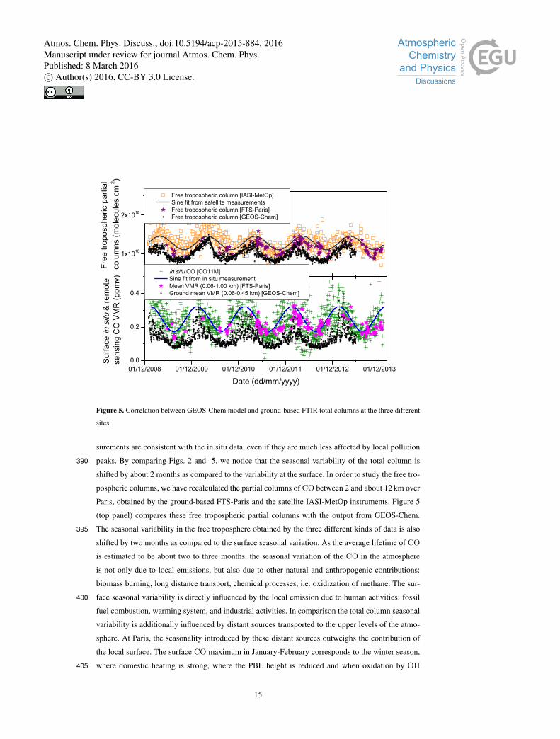
4.3 Emission sources impacting the seasonality of CO columns

01/12/2008 01/12/2009 01/12/2010 01/12/2011 01/12/2012 01/12/2013

1x1018

2x1018

1x1018

2x1018

1x1018

2x1018

Date (dd/mm/yyyy)

GE

OS

-Che

m C

O to

tal c

olum

n (m

olec

ules

.cm

-2)

@Wollongong

@Jungfraujoch

@Paris

Figure 8. GEOS-Chem time series of CO total columns for Paris (top panel), Jungfraujoch (middle panel) and

Wollongong (bottom panel). Different colors indicate standard run (black), run without biomass burning (red),

run without biogenic emissions (green) and run without anthropogenic emissions (blue).

In order to study the influence of the different categories of CO and NMVOC emissions on the

CO total column and its seasonality at the three sites, another three GEOS-Chem simulations were

performed. These relied on the same setup as for the standard run (standard chemistry, horizontal

resolution, time period. . . ), but in each of these runs we turned off either the biogenic, the anthro-450

pogenic (incorporating the biofuel emissions) or the biomass burning emission sources that are im-

18


plemented in the model. These categories include direct emissions of CO (for both anthropogenic

and biomass burning sources) and of its NMVOC precursors, as well as direct emissions of nitric

oxide (NO). In these three sensitivity runs, CH4 concentrations are provided by the NOAA mea-

surements. Hereafter, they are referred to, as the non-biogenic, non-anthropogenic and non-biomass455

burning simulations. The results from these GEOS-Chem sensitivity simulations are compared to the

standard run (results shown in Fig. 3). All four runs cover the mid-2005 to mid-2013 time period,

hence starting a few years before the period under investigation here. This allows us to establish a

stable situation for the period after 2008 (most of the long-lived precursors of CO are removed from

the atmosphere between mid-2005 and 2008). Fig. 8 shows the CO total columns simulated by the460

different runs of GEOS-Chem for the three sites: the standard run in small black circles, together

with the non-biomass burning, non-biogenic and non-anthropogenic runs in red, green and blue cir-

cles, respectively. According to the GEOS-Chem simulations, the results for Paris and Jungfraujoch

are quite similar. At these two sites, the seasonal variability of the CO loadings is mainly driven

by anthropogenic emissions. Indeed, by shutting off the anthropogenic emissions of CO and of its465

NMVOC precursors, the amplitude of the CO seasonal variation and periodicity are radically re-

duced. On the other hand, without either biomass burning or biogenic emissions, the seasonal cycle

and maximum peaks are only weakly affected as compared to the standard run, with CO columns

slightly lower due to missing emissions. At Wollongong, the seasonal variability is mainly influ-

enced by the biomass burning emissions: the highest peaks (e.g. at the end of 2009) disappear when470

the biomass burning component is removed from the simulation. The biogenic emissions provide

more of a large background contribution. Unlike at Paris and Jungfraujoch, anthropogenic emissions

are negligible in Wollongong. For the CO surface VMR, the GEOS-Chem sensitivity runs provide

the same results as compared to the CO total columns for the three studied sites.

5 Conclusions475

This paper investigates the seasonal variability of CO total columns at three NDACC and/or TC-

CON sites: Paris and Jungfraujoch in the Northern Hemisphere and Wollongong in the Southern

Hemisphere. The variability of CO above the PBL has a seasonal maximum in March-April and

a minimum in September-October in the Northern Hemisphere. This seasonal cycle is shifted by 6

months in the Southern Hemisphere. For both Northern-hemispheric sites, the seasonal variability of480

the CO total columns seems to be mainly driven by anthropogenic emissions. On the contrary, the

Southern-hemispheric site Wollongong is mainly influenced by the biomass burning contribution.

We have compared the ground-based FTIR data to satellite measurements from IASI-MetOp and

MOPITT and to GEOS-Chem model outputs, which all of them confirm the observed CO seasonal

variability. The GEOS-Chem model also shows that the CO seasonality at Paris and Jungfraujoch485

is mainly controlled by anthropogenic emissions. This is different to Wollongong, where it is due

19


to biomass burning. For sites that are strongly affected by local anthropogenic emissions, we have

observed a temporal shift in the seasonal patterns at the surface and in the higher atmospheric layers.

This is likely because zonal mixing occurs on a shorter (1 – 2 weeks) timescale as compared to com-

plete vertical tropospheric mixing (1 – 2 months). The observed time-lag between upper altitude and490

surface CO is about 2 months in Paris and at the Jungfraujoch. The 2 months’ shift is also confirmed

by the GEOS-Chem model. In Wollongong, where low local anthropogenic emissions prevail and

which is largely impacted by biomass burning, such a time shift is neither observed nor modelled.

Acknowledgements. We are grateful to Université Pierre et Marie Curie and Région Île-de-France for their

financial contributions and to Institut Pierre-Simon Laplace for support and facilities. We thank the National495

Center for Atmospheric Research MOPITT science team and NASA for producing and archiving the MOPITT

CO product. Thanks are also due to the Swiss National Air Pollution Monitoring Network (NABEL) for deliv-

ering ground data around Switzerland. The University of Liège contribution to the present work has primarily

been supported by the F.R.S. – FNRS, the Fédération Wallonie-Bruxelles and MeteoSwiss (GAW-CH program).

We thank the International Foundation High Altitude Research Stations Jungfraujoch and Gornergrat (HFSJG,500

Bern). We are grateful to all colleagues who contributed to the acquisition of the FTIR data. The NDACC

datasets used here are publicly available from the network database (ftp://ftp.cpc.ncep.noaa.gov/ndacc/station).

The Australian Research Council has provided financial support over the years for the NDACC site at Wol-

longong, most recently as part of project DP110101948. We also acknowledge the important contribution to

the measurement program at Wollongong made by researchers other than those listed as co-authors here, in-505

cluding amongst others, Voltaire Velazco and Nicholas Deutscher. IASI has been developed and built under the

responsibility of the French space agency CNES. It is flown onboard the MetOp satellite as part of the Eumet-

sat Polar System (EPS). The IASI L1 data are received through the Eumetcast near real time data distribution

service. IASI L1 and L2 data are stored in the French atmospheric database Ether (http://ether.ipsl.jussieu.fr).

The National Center for Atmospheric Research (NCAR) is sponsored by the National Science Foundation. Any510

opinions, findings and conclusions or recommendations expressed in the publication are those of the author(s)

and do not necessarily reflect the views of the National Science Foundation.

[Table 1 about here.]

20


References

August, T., Klaes, D., Schlüssel, P., Hultberg, T., Crapeau, M., Arriaga, A., O’Carroll, A., Coppens, D., Munro,515

R., and Calbet, X.: IASI on MetOp-A: Operational Level 2 retrievals after five years in orbit, J. Quant.

Spectroscop. Radiat. Transfer, 113, 1340–1371, doi:10.1016/j.jqsrt.2012.02.028, 2012.

Bakwin, P. S., Tans, P. P., and Novelli, P. C.: Carbon monoxide budget in the northern hemisphere, Geophs.

Res. Lett., 21, 433—436, 1994.

Barnett, A. G., Williams, G. M., Schwartz, J., Best, T. L., Neller, A. H., Petroeschevsky, A. L., and Simpson,520

R. W.: The Effects of Air Pollution on Hospitalizations for Cardiovascular Disease in Elderly People in

Australian and New Zealand Cities, Environ. Health Perspect., 114, 1018–1023, 2006.

Barret, B., Mazière, D. M., and Mahieu, E.: Ground-based FTIR measurements of CO from the Jungfraujoch:

characterisation and comparison with in situ surface and MOPITT data, Atmos. Chem. Phys., 3, 2217–2223,

doi:10.5194/acp-3-2217-2003, 2003.525

Benedictow, A., Berge, H., Fagerli, H., Gauss, M., Jonson, J. E., Nyíri, A., Simpson, D., Tsyro, S., Valdebenito,

A., Shamsudheen, V. S., Wind, P., Aas, W., Hjellbrekke, A.-G., Mareckova, K., Wankmüller, R., Iversen,

T., Kirkevøag, A., Seland, Ø., Haugen, J. E., and Mills, G.: Transboundary acidification, eutrophication and

ground level ozone in Europe in 2008, Tech. rep., The Norwegian Meteorological Institute, Oslo, Norway,

2010.530

Bey, I., Jacob, D. J., Yantosca, R. M., Logan, J. A., Field, B. D., Fiore, A. M., Li, Q., Liu, H. Y., Mickley, L. J.,

and Schultz, M. G.: Global modeling of tropospheric chemistry with assimilated meteorology: model de-

scription and evaluation, J. Geophys. Res.-Atmos., 106, 23 073–23 095, doi:10.1029/2001JD000807, 2001.

Blumstein, D., Chalon, G., Carlier, T., Buil, C., Hebert, P., Maciaszek, T., Ponce, G., Phulpin, T., Tournier, B.,

Simeoni, D., Astruc, P., Clauss, A., Kayal, G., and Jegou, R.: IASI instrument: technical overview and mea-535

sured performances, in: Proc. SPIE 5543, Infrared Spaceborne Remote Sensing XII, doi:10.1117/12.560907,

2004.

Buchholz, R. R., Paton-Walsh, C., Griffith, D. W. T., Kubistin, D., Caldow, C., Fisher, J. A., Deutscher, N. M.,

Kettlewell, G., Riggenbach, M., Macatangay, R., Krummel, P. B., and Langenfelds, R. L.: Source and meteo-

rological influences on air quality (CO, CH4 & CO2) at a Southern Hemisphere urban site, Atmos. Environ.,540

126, 274–289, doi:10.1016/j.atmosenv.2015.11.041, 2016.

Clerbaux, C., George, M., Turquety, S., Walker, K. A., Barret, B., Bernath, P., Boone, C., Borsdorff, T., Cammas,

J. P., Catoire, V., Coffey, M., Coheur, P.-F., Deeter, M., Mazière, D. M., Drummond, J., Duchatelet, P., Dupuy,

E., Zafra, d. R., Eddounia, F., Edwards, D. P., Emmons, L., Funke, B., Gille, J., Griffith, D. W. T., Hannigan,

J., Hase, F., Höpfner, M., Jones, N., Kagawa, A., Kasai, Y., Kramer, I., Flochmoën, L. E., Livesey, N. J.,545

López-Puertas, M., Luo, M., Mahieu, E., Murtagh, D., Nédélec, P., Pazmino, A., Pumphrey, H., Ricaud, P.,

Rinsland, C. P., Robert, C., Schneider, M., Senten, C., Stiller, G., Strandberg, A., Strong, K., Sussmann,

R., Thouret, V., Urban, J., and Wiacek, A.: CO measurements from the ACE-FTS satellite instrument: data

analysis and validation using ground-based, airborne and spaceborne observations, Atmos. Chem. Phys., 8,

2569–2594, doi:10.5194/acp-8-2569-2008, 2008.550

Clerbaux, C., Boynard, A., Clarisse, L., George, M., Hadji-Lazaro, J., Herbin, H., Hurtmans, D., Pommier, M.,

Razavi, A., Turquety, S., Wespes, C., and Coheur, P.-F.: Monitoring of atmospheric composition using the

21


thermal infrared IASI/MetOp sounder, Atmos. Chem. Phys., 9, 6041–6054, doi:10.5194/acp-9-6041-2009,

2009.

Deeter, M., Emmons, L., Francis, G., Edwards, D., Gille, J., Warner, J., Khattatov, B., Ziskin, D., Lamarque, J.-555

F., Ho, S.-P., Yudin, V., Attié, J.-L., Packman, D., Chen, J., Mao, D., Drummond, J., Novelli, P., and Sachse,

G.: Evaluation of operational radiances for the Measurements of Pollution in the Troposphere (MOPITT)

instrument CO thermal band channels, J. Geophys. Res., 109, D03 308, doi:10.1029/2003JD003970, 2004.

Dils, B., Cui, J., Henne, S., Mahieu, E., Steinbacher, M., and Mazière, D. M.: CO trend at the high Alpine site

Jungfraujoch: a comparison between NDIR surface in situ and FTIR remote sensing observations, Atmos.560

Chem. Phys., 11, 6735–6748, doi:10.5194/acp-11-6735-2011, 2011.

Drummond, J. and Mand, G.: The Measurements of Pollution in the Troposphere (MOPITT) Instrument: Over-

all Performance and Calibration Requirements, J. Atmos. Ocean. Technol., 13, 314, 1996.

Duchatelet, P., Demoulin, P., Hase, F., Ruhnke, R., Feng, W., Chipperfield, M. P., Bernath, P. F., Boone,

C. D., Walker, K. A., and Mahieu, E.: Hydrogen fluoride (HF) total and partial column time series565

above the Jungfraujoch from long-term FTIR measurements: impact of the line-shape model, error bud-

get, seasonal cycle and comparison with satellite and model data, J. Geophys. Res., 115, D22 306,

doi:10.1029/2010JD014677, 2010.

Edwards, D. P., Pétron, G., Novelli, P. C., Emmons, L. K., Gille, J. C., and Drummond, J. R.: Southern Hemi-

sphere carbon monoxide interannual variability observed by Terra/Measurement of Pollution in the Tropo-570

sphere (MOPITT), J. Geophys. Res., 111, D16 303, doi:10.1029/2006JD007079, 2006.

Esposito, F., Grieco, G., Masiello, G., Pavese, G., Restieri, R., Serio, C., and Cuomo, V.: Intercomparison of

line-parameter spectroscopic databases using downwelling spectral radiance, Quart. J. Roy. Met. Soc., 133,

191–202, doi:10.1002/qj.131, 2007.

George, M., Clerbaux, C., Hurtmans, D., Turquety, S., Coheur, P.-F., Pommier, M., Hadji-Lazaro, J., Edwards,575

D. P., Worden, H., Luo, M., Rinsland, C., and McMillan, W.: Carbon monoxide distributions from the

IASI/METOP mission: evaluation with other space-borne remote sensors, Atmos. Chem. Phys., 9, 8317–

8330, doi:10.5194/acp-9-8317-2009, 2009.

Griffith, D. W. T.: Synthetic Calibration and Quantitative Analysis of Gas-Phase infrared Spectra, Appl. Spec-

troscop., 50, 59–70, 1996.580

Griffith, D. W. T., Deutscher, N. M., Caldow, C. G. R., Kettlewell, G., Riggenbach, M., and Hammer, S.: A

Fourier transform infrared trace gas and isotope analyser for atmospheric applications, Atmos. Meas. Tech.,

5, 2012.

Guenther, A., Karl, T., Harley, P., Wiedinmyer, C., Palmer, P. I., and Geron, C.: Estimates of global terrestrial

isoprene emissions using MEGAN (Model of Emissions of Gases and Aerosols from Nature), Atmos. Chem.585

Phys., 6, 10–5194, 2006.

Hase, F., Hannigan, J. W., Coey, M. T., Goldman, A., Höpfner, M., Jones, N. B., Rinsland, C. P., and Wood,

S. W.: Intercomparison of retrieval codes used for the analysis of high-resolution: ground-based FTIR mea-

surements, J. Quant. Spectroscop. Radiat. Transfer, 87, 25–52, 2004.

Hase, F., Demoulin, P., Sauval, A. J., Toon, G. C., Bernath, P. F., Goldman, A., Hannigan, J. W., and Rinsland,590

C. P.: An empirical line-by-line model for the infrared solar transmittance spectrum from 700 to 5000 cm−1,

J. Quant. Spectroscop. Radiat. Transfer, 102, 450–463, doi:10.1016/j.jqsrt.2006.02.026, 2006.

22


Hooghiemstra, P. B., Krol, M. C., Bergamaschi, P., de Laat, A. T. J., van der Werf, G. R., Novelli, P. C., Deeter,

M. N., Aben, I., and Röckmann, T.: Comparing optimized CO emission estimates using MOPITT or NOAA

surface network observations, J Geophys. Res., 117, D06 309–23, 2012.595

Hurtmans, D., Coheur, P.-F., Wespes, C., Clarisse, L., Scharf, O., Clerbaux, C., Hadji-Lazaro, J., George, M.,

and Turquety, S.: FORLI radiative transfer and retrieval code for IASI, J. Quant. Spectroscop. Radiat. Trans-

fer, 113, 1391–1408, doi:10.1016/j.jqsrt.2012.02.036, 2006.

Joumard, R.: Les émissions de polluants oscillent entre progrès techniques et explosion du trafic, La Revue

Durable, 3, 30–33, 2003.600

Kopacz, M., Jacob, D. J., Fisher, J. A., Logan, J. A., Zhang, L., Megretskaia, I. A., Yantosca, R. M., Singh, K.,

Henze, D. K., Burrows, J. P., Buchwitz, M., Khlystova, I., McMillan, W. W., Gille, J. C., Edwards, D. P.,

Eldering, A., Thouret, V., and Nedelec, P.: Global estimates of CO sources with high resolution by adjoint

inversion of multiple satellite datasets (MOPITT, AIRS, SCIAMACHY, TES), Atmos. Chem. Phys., 10,

855–876, 2010.605

Levy, R. J.: Carbon monoxide pollution and neurodevelopment: A public health concern, Neurotoxicol. Teratol.,

49, 31–40, 2015.

Logan, J. A., Prather, M. J., Wofsy, F. C., and McElroy, M. B.: Tropospheric Chemistry: A Global Perspective,

J. Geophys. Res., 86, 7210–7254, 1981.

Mao, J., Jacob, D. J., Evans, M. J., Olson, J. R., Ren, X., Brune, W. H., Clair, S. J. M., Crounse, J. D., Spencer,610

K. M., Beaver, M. R., Wennberg, P. O., Cubison, M. J., Jimenez, J. L., Fried, A., Weibring, P., Walega,

J. G., Hall, S. R., Weinheimer, A. J., Cohen, R. C., Chen, G., Crawford, J. H., McNaughton, C., Clarke,

A. D., Jaeglé, L., Fisher, J. A., Yantosca, R. M., Sager, L. P., and Carouge, C.: Chemistry of hydrogen oxide

radicals (HOx) in the Arctic troposphere in spring, Atmos. Chem. Phys., 10, 5823–5838, doi:10.5194/acp-

10-5823-2010, 2010.615

Olivier, J. G. J. and Berdowski, J. J. M.: Global emissions sources and sinks., in: The Climate System, edited

by Berdowski, J., Guicherit, R., and Heij, B., pp. 33–78, A.A. Balkema Publishers/Swets & Zeitlinger Pub-

lishers, Lisse, The Netherlands, 2001.

Park, R. J., Jacob, D. J., Field, B. D., Yantosca, R. M., and Chin, M.: Natural and transboundary pollution

influences on sulfate-nitrate-ammonium aerosols in the United States: implications for policy, J. Geophys.620

Res., 109, D15 204, doi:10.1029/2003JD004473, 2004.

Pougatchev, N. S. and Rinsland, C. P.: Spectroscopic study of the seasonal variation of carbon monoxide vertical

distribution above Kitt Peak, J. Geophys. Res, 100, 1409–1416, 1995.

Rinsland, C. P., Jones, N. B., Connor, B. J., Logan, J. A., Pougatchev, N. S., Goldman, A., Murcray, F. J.,

Stephen, T. M., Pine, A. S., Zander, R., Mahieu, E., and Demoulin, P.: Northern and southern hemisphere625

ground-based infrared spectroscopic measurements of tropospheric carbon monoxide and ethane, J. Geo-

phys. Res., 103, 28 197, doi:10.1029/98JD02515, 1998.

Rinsland, C. P., Mahieu, E., Zander, R., Demoulin, P., Forrer, J., and Buchmann, B.: Free tropospheric CO,

C2H6, and HCN above central Europe: Recent measurements from the Jungfraujoch station including the

detection of elevated columns during 1998, J. Geophys. Res., 105, 24 235–24 249, 2000.630

23


Rinsland, C. P., Goldman, A., Hanniganc, J. W., Wood, S. W., Chiou, L. S., and Mahieu, E.: Long-term trends of

tropospheric carbon monoxide and hydrogen cyanide from analysis of high resolution infrared solar spectra,

J. Quant. Spectroscop. Radiat. Transfer, 104, 40–51, 2007.

Rodgers, C. D.: Characterization and error analysis of profiles retrieved from remote sounding measurements,

J. Geophys. Res., 95, doi:10.1029/JD095iD05p05587, 1990.635

Rodgers, C. D. and Connor, B. J.: Intercomparison of remote sounding instruments, J. Geophys. Res., 108,

4116–4129, doi:10.1029/2002JD002299, 2003.

Rothman, L. S., Jacquemart, D., Barbe, A., Benner, D. C., Birk, M., Brown, L. R., Carleer, M. R., Chackerian,

Jr, C., Chance, K., Coudert, L. H., Dana, V., Devi, V. M., Flaud, J.-M., Gamache, R. R., Goldman, A.,

Hartmann, J.-M., Jucks, K. W., Maki, A. G., Mandin, J.-Y., Massie, S. T., Orphal, J., Perrin, A., Rinsland,640

C. P., Smith, M. A. H., Tennyson, J., Tolchenov, R. N., Toth, R. A., Vander Auwera, J., Varanasi, P., and

Wagner, G.: The HITRAN 2004 Molecular Spectroscopic Database, J. Quant. Spectrosc. Radiat. Trans., 96,

139 – 204, 2005.

Rothman, L. S., Gordon, I. E., Barbe, A., Benner, D. C., Bernath, P. F., Birk, M., Boudon, V., Brown, L. R.,

Campargue, A., Champion, J. P., Chance, K., Coudert, L. H., Dana, V., Devi, V. M., Fally, S., Flaud, J. M.,645

Gamache, R. R., Goldman, A., Jacquemart, D., Kleiner, I., Lacome, N., Lafferty, W. J., Mandin, J. Y., Massie,

S. T., Mikhailenko, S. N., Miller, C. E., Moazzen-Ahmadi, N., Naumenko, O. V., Nikitin, A. V., Orphal, J.,

Perevalov, V. I., Perrin, A., Predoi-Cross, A., Rinsland, C. P., Rotger, M., Simecková, M., Smith, M. A. H.,

Sung, K., Tashkun, S. A., Tennyson, J., Toth, R. A., Vandaele, A. C., and Vander Auwera, J.: The HITRAN

2008 molecular spectroscopic database, J. Quant. Spectrosc. Radiat. Trans., 110, 533–572, 2009.650

Sam-Laï, N., Saviuc, P., and Danel, V.: Carbon monoxide poisoning monitoring network - A five-year

experience of household poisonings in two French regions, J. Toxicol. Clin. Toxicol., 41, 349–353,

doi:10.1081/CLT-120022001, 2003.

Schneider, M., Yoshimura, K., Hase, F., and Blumenstock, T.: The ground-based FTIR network’s potential for

investigating the atmospheric water cycle, Atmos. Chem. Phys., 10, 3427–3442, 2010.655

Schultz, M., Backman, L., Balkanski, Y., Bjoerndalsaeter, S., Brand, R., Burrows, J., Dalsoeren, S., de Vascon-

celos, M., Grodtmann, B., Hauglustaine, D., Heil, A., Hoelzemann, J., Isaksen, I., Kaurola, J., Knorr, W.,

Ladstaetter-Weißenmayer, A., Mota, B., Oom, D., Pacyna, J., Panasiuk, D., Pereira, J., Pulles, T., Pyle, J.,

Rast, S., Richter, A., Savage, N., Schnadt, C., Schulz, M., Spessa, A., Staehelin, J., Sundet, J., Szopa, S.,

Thonicke, K., van het Bolscher, M., van Noije, T., van Velthoven, P., Vik, A., and Wittrock, F.: REanalysis660

of the TROpospheric chemical composition over the past 40 years – A long-term global modeling study

of tropospheric chemistry, final report 48/2007, Max Planck Institute for Meteorology, Hamburg, Germany,

2007.

Street, J. O., Carroll, R. J., and Ruppert, D.: A Note on Computing Robust Regression Estimates via Iteratively

Reweighted Least Squares, Am. Stat., 42, 152–154, 1988.665

Té, Y., Jeseck, P., Payan, S., Pépin, I., and Camy-Peyret, C.: The Fourier transform spectrometer of the UPMC

University QualAir platform, Rev. Sci. Instrum., 81, 103 102–10, doi:10.1063/1.3488357, 2010.

Té, Y., Dieudonné, E., Jeseck, P., Hase, F., Hadji-Lazaro, J., Clerbaux, C., Ravetta, F., Payan, S., Pépin, I.,

Hurtmans, D., Pelon, J., and Camy-Peyret, C.: Carbon monoxide urban emission monitoring: a ground-based

FTIR case study, J. Atmos. Oceanic Technol., 29, 911–921, doi:10.1175/JTECH-D-11-00040.1, 2012.670

24


Thompson, A. M.: The oxidizing capacity of the earth’s atmosphere: Probable past and future changes, Science,

286, 1157–1165, doi:10.1126/science.256.5060.1157, 1992.

Thompson, A. M., Huntley, M. A., and Stewart, R. W.: Perturbations to tropospheric oxidants, 1985–2035:

1. Calculations of ozone and OH in chemically coherent regions, J. Geophys. Res, 95, 9829–9844,

doi:10.1029/JD095iD07p09829, 1990.675

Tournier, B., Blumstein, D., Cayla, F.-R., and Chalon, G.: IASI level 0 and 1 processing algorithms description,

in: Proc. 12th Int. TOVS Study Conf. (ITSC-XII), Lorne, VIC, Australia, 2002.

van der Werf, G. R., Randerson, J. T., Giglio, L., Collatz, G. J., Mu, M., Kasibhatla, P. S., Morton, D. C.,

DeFries, R. S., Jin, Y., and Leeuwen, v. T. T.: Global fire emissions and the contribution of deforestation,

savanna, forest, agricultural, and peat fires, Atmos. Chem. Phys., 10, 11 707–11 735, doi:10.5194/acp-10-680

11707-2010, 2010.

van Donkelaar, A., Martin, R. V., Leaitch, W. R., MacDonald, A. M., Walker, T. W., Streets, D. G., Zhang, Q.,

Dunlea, E. J., Jimenez, J. L., Dibb, J. E., Huey, L. G., Weber, R., and Andreae, M. O.: Analysis of aircraft

and satellite measurements from the Intercontinental Chemical Transport Experiment (INTEX-B) to quantify

long-range transport of East Asian sulfur to Canada, Atmos. Chem. Phys., 8, 10–5194, doi:10.5194/acp-8-685

2999-2008, 2008.

Viatte, C., Schneider, M., Redondas, A., Hase, F., Eremenko, M., Chelin, P., Flaud, J.-M., Blumenstock, T.,

and Orphal, J.: Comparison of ground-based FTIR and Brewer O3 total column with data from two differ-

ent IASI algorithms and from OMI and GOME-2 satellite instruments, Atmos. Meas. Tech., 4, 535–546,

doi:10.5194/amt-4-535-2011, 2011.690

Weinstock, B.: Carbon Monoxide: Residence Time in the Atmosphere, Science, 166, 224–225, 1969.

Xiao, Y., Logan, J. A., Jacob, D. J., Hudman, R. C., Yantosca, R., and Blake, D. R.: Global budget of ethane and

regional constraints on U.S. sources, J. Geophys. Res., 113, 21 306–10, doi:10.1029/2007JD009415, 2008.

Zander, R., Mahieu, E., Demoulin, P., Duchatelet, P., Roland, G., Servais, C., Mazière, D. M., Reimann, S., and

Rinsland, C. P.: Our changing atmosphere: Evidence based on long-term infrared solar observations at the695

Jungfraujoch since 1950, Sci. Tot. Environ., 391, 184–195, doi:10.1016/j.scitotenv.2007.10.018, 2008.

Zbinden, R. M., Thouret, V., Ricaud, P., Carminati, F., Cammas, J.-P., and Nédélec, P.: Climatology of pure

tropospheric profiles and column contents of ozone and carbon monoxide using MOZAIC, Atmos. Chem.

Phys., 13, 12 363–12 388, doi:10.5194/acp-13-12363-2013, 2013.

Zeng, G., Williams, J. E., Fisher, J. A., Emmons, L. K., Jones, N. B., Morgenstern, O., Robinson, J., Smale,700

D., Paton-Walsh, C., and Griffith, D. W. T.: Multi-model simulation of CO and HCHO in the Southern

Hemisphere: comparison with observations and impact of biogenic emissions, Atmos. Chem. Phys., 15,

7217–7245, 2015.

Zhao, Y., Kondo, Y., Murcray, F. J., Liu, X., Koike, M., Kita, K., Nakajima, H., Murata, I., and Suzuki, K.: Car-

bon monoxide column abundances and tropospheric concentrations retrieved from high resolution ground-705

based infrared solar spectra at 43.5°N over Japan, J. Geophys. Res., 102, 23 403–23 411, 1997.

Zhao, Y., Strong, K., Kondo, Y., Koike, M., Matsumi, Y., Irie, Y., Rinsland, H., C, P., Jones, N. B., Suzuki, K.,

Nakajima, H., Nakane, H., and Murata, I.: Spectroscopic measurements of tropospheric CO, C2H6, C2H2

and HCN in Northern Japan, J. Geophy. Res., 107, 4343, 2002.

25


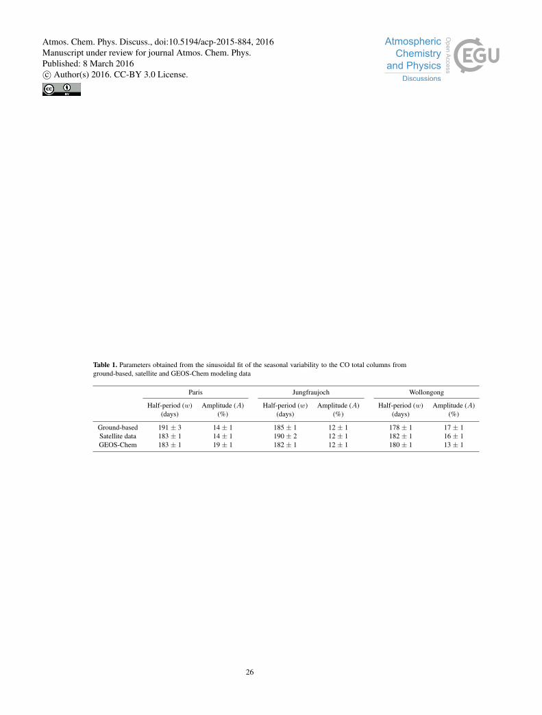
Table 1. Parameters obtained from the sinusoidal fit of the seasonal variability to the CO total columns fromground-based, satellite and GEOS-Chem modeling data

Paris Jungfraujoch Wollongong

Half-period (w) Amplitude (A) Half-period (w) Amplitude (A) Half-period (w) Amplitude (A)(days) (%) (days) (%) (days) (%)

Ground-based 191 ± 3 14 ± 1 185 ± 1 12 ± 1 178 ± 1 17 ± 1Satellite data 183 ± 1 14 ± 1 190 ± 2 12 ± 1 182 ± 1 16 ± 1GEOS-Chem 183 ± 1 19 ± 1 182 ± 1 12 ± 1 180 ± 1 13 ± 1

26


Seasonal variability of surface and column carbon monoxide ...

Documents

Transcript of Seasonal variability of surface and column carbon monoxide ...