Emission factors 2009: Report 1 – a review of methods for ...
116
Published Project Report PPR353 Emission factors 2009: Report 1 – a review of methods for determining hot exhaust emission factors for road vehicles P G Boulter, T J Barlow, S Latham and I S McCrae
-
Upload
khangminh22 -
Category
Documents
-
view
1 -
download
0
Transcript of Emission factors 2009: Report 1 – a review of methods for ...

Published Project Report PPR353
Emission factors 2009: Report 1 – a review of methods for determining hot exhaust emission factors for road vehicles
P G Boulter, T J Barlow, S Latham and I S McCrae


TRL Limited
PUBLISHED PROJECT REPORT PPR353
Emission factors 2009: Report 1 – a review of methods fordetermining hot exhaust emission factors for road vehicles
Version: 7
By P G Boulter, T J Barlow, S Latham and I S McCrae
Prepared for: Department for Transport, Cleaner Fuels & Vehicles 4
Chris Parkin
Copyright TRL Limited, June 2009.
This report has been prepared for the Department for Transport. The views expressed are those of the authorsand not necessarily those of the Department for Transport.
If this report has been received in hard copy from TRL then, in support of the company’s environmentalgoals, it will have been printed on paper that is FSC (Forest Stewardship Council) registered and TCF(Totally Chlorine-Free) registered.
Approvals
Project Manager T Barlow
Quality Reviewed I McCrae

When purchased in hard copy, this publication is printed on paper that is FSC (Forest Stewardship Council) registered and TCF (Totally Chlorine Free) registered.

ContentsPage
Executive summary
1 Introduction ................................................................................................................................ 1
1.1 Background .......................................................................................................................................... 1
1.2 Potential weaknesses in the NAEI model........................................................................................... 11.2.1 Hot exhaust emissions (the UKEFD)................................................................................................. 11.2.2 Cold-start emissions........................................................................................................................... 21.2.3 Evaporative emissions ....................................................................................................................... 31.2.4 Non-exhaust PM emissions................................................................................................................ 3
1.3 Project objectives ................................................................................................................................. 3
1.4 Report structure................................................................................................................................... 3
2 Evaluation of driving cycles ...................................................................................................... 4
2.1 Background .......................................................................................................................................... 42.1.1 The use of driving cycles in the measurement of emissions.............................................................. 42.1.2 The importance of driving cycles in emission modelling .................................................................. 62.1.3 Driving cycles used in the UKEFD.................................................................................................... 6
2.2 Method .................................................................................................................................................. 82.2.1 Compilation of a driving cycle Reference Book................................................................................ 82.2.2 Quantitative assessment of driving cycles ......................................................................................... 9
2.3 Results ................................................................................................................................................. 112.3.1 Driving cycle Reference Book......................................................................................................... 112.3.2 Coarse assessment of driving cycles................................................................................................ 172.3.3 Detailed assessment of driving cycles ............................................................................................. 192.3.4 Summary.......................................................................................................................................... 28
3 A review of emission test parameters ..................................................................................... 29
3.1 Background ........................................................................................................................................ 29
3.2 European type approval procedures ................................................................................................ 293.2.1 Light-duty vehicles .......................................................................................................................... 303.2.2 Heavy-duty vehicles......................................................................................................................... 313.2.3 Two-wheel vehicles ......................................................................................................................... 32
3.3 Effects of different test parameters: cars......................................................................................... 333.3.1 Background...................................................................................................................................... 333.3.2 Experimental work........................................................................................................................... 343.3.3 Driving behaviour parameters.......................................................................................................... 363.3.4 Vehicle-related parameters .............................................................................................................. 423.3.5 Vehicle sampling method ................................................................................................................ 453.3.6 Laboratory-related parameters ......................................................................................................... 463.3.7 Round robin tests ............................................................................................................................. 50
3.4 Effects of different test parameters: heavy-duty vehicles .............................................................. 523.4.1 Background...................................................................................................................................... 523.4.2 Emission-control technology ........................................................................................................... 533.4.3 Alternative fuels............................................................................................................................... 553.4.4 Effects of engine deterioration and maintenance............................................................................. 563.4.5 Effects of fuel quality....................................................................................................................... 56
3.5 Effects of different test parameters: two-wheel vehicles ................................................................ 583.5.1 Round robin test programme ........................................................................................................... 583.5.2 Vehicle categorisation...................................................................................................................... 583.5.3 Other issues...................................................................................................................................... 593.5.4 Driving cycle effects ........................................................................................................................ 593.5.5 Laboratory effects ............................................................................................................................ 603.5.6 Effect of fuel properties ................................................................................................................... 603.5.7 Effect of inspection and maintenance .............................................................................................. 61
4 Summary, conclusions and recommendations....................................................................... 62
4.1 Evaluation of driving cycles .............................................................................................................. 624.1.1 Summary.......................................................................................................................................... 624.1.2 Conclusions and recommendations.................................................................................................. 63
4.2 Review of emission test parameters.................................................................................................. 644.2.1 Summary.......................................................................................................................................... 644.2.2 Recommendations............................................................................................................................ 67
5 References ................................................................................................................................. 70
Appendix A: Abbreviations and terms used in the Task Reports ............................................. 74
Appendix B: NAEI method............................................................................................................ 79
Appendix C: Definitions of Art.Kinema parameters.................................................................... 86
Appendix D: Vehicle speed distributions ..................................................................................... 89
Appendix E: Average Art.Kinema parameters............................................................................. 99
Appendix F: ARTEMIS correction factors................................................................................ 104

Executive summary
TRL Limited was commissioned by the Department for Transport to review the methodology used in theNational Atmospheric Emissions Inventory (NAEI) for estimating emissions from road vehicles. Variousaspects of the methodology were addressed, and new exhaust emission factors for road vehicles were derived(these are described in separate Reports). This Report reviews the experimental methods used to determineemission factors, and provides recommendations for the future development of emission factors in the UK. Itcovers only ‘hot’ exhaust emissions which occur when the engine and any after-treatment devices havereached their full operational temperatures, and includes two main elements: (i) an evaluation of the drivingcycles used in emission tests and (ii) a review of the parameters recorded during emission tests. A distinctionis also made between the improvement of the emission factors in the 2002 UK Emission Factor Database(UKEFD) and the requirements with respect to future tests.
For cars, the assessment indicated that the driving cycles in the UKEFD adequately cover the range ofdriving characteristics observed in the real world. However, a small number of UKEFD driving cyclesappear to have average accelerations which are outside the range of real-world conditions. Furthermore, theWarren Spring Laboratory (WSL) cycles - which are routinely used for emission tests in the UK - do notappear to reproduce the aggressiveness of driving for cars and light goods vehicles (LGVs), and do not coverthe highest speeds encountered on the road. A more representative set of driving cycles should therefore beconsidered for future testing. Alternatively, the WSL cycles could be retained, but supplemented with somehigh-speed cycles, and cycles which have higher average accelerations and decelerations.
For LGVs the database of real-world driving patterns is more limited. However, the cycles used in thecurrent UKEFD appear to cover the range of driving characteristics which are likely to be encountered.However, as with cars some UKEFD cycles may have average accelerations which are not realistic for theUK. This also needs to be investigated further.
In the case of HGVs, some of the low-speed UKEFD driving cycles have relatively high accelerations whichare not apparent in the real-world driving patterns. Some of the UKEFD cycles have more rapiddecelerations than the real-world driving patterns. The FiGE cycle - which is commonly used to test heavy-duty vehicles - does not cover low average speeds and does not reflect the speeds of older, unrestrictedvehicles. The higher-speed FiGE cycles (suburban and motorway) also appear to have low averageaccelerations and have less rapid decelerations than the real-world driving patterns. Again, a morerepresentative set of driving cycles should be considered for future testing.
Urban buses operate at relatively low speeds, and may be unable to attain the higher speeds required forsome driving cycles. Coaches, on the other hand, are likely to operate at higher motorway speeds. Urbanbuses and coaches should therefore be treated separately when deriving emission factors, and morerepresentative driving cycles for these vehicle classes should be used in the derivation of the future UKemission factors.
The use of generic driving cycle in emission tests (as opposed to vehicle-specific cycles) could lead to errorsin emission estimations. Although it would increase the complexity of the test procedure, taking into accountvehicle performance by the use of specific driving cycles would lead to an improvement in the quality ofemission estimates. An alternative may be to develop a test cycle that could be broken down into a largenumber of sub-cycles, and the emissions over each sub-cycle could be calculated. This would allow a limitednumber of test cycles to yield a larger number of data points.
Although continuous emission measurements can aid the understanding of different effects, there is anadditional cost. As emission models are constructed primarily using bag samples there appears to be littlejustification for routinely including continuous emission measurements in the tests used for emission factordevelopment. This recommendation does not apply to ad hoc tests for the evaluation of technical and/orpolicy measures, for which continuous measurements may be beneficial.
When compiling an emission factor database, adjustment factors should be applied in order to standardise thedata for the gear-shift strategy, the vehicle mileage, the ambient temperature and the ambient humidity.
Emission measurements are required for a wider variety of two-wheel vehicles and their associatedoperation, particularly for the most modern vehicles.


TRL Limited 1 PPR353
Emission factors 2009: Report 1 – methods for determining hot exhaust emission factors for road vehicles Version 7
1 Introduction
1.1 Background
Emissions of air pollutants in the United Kingdom are reported in the National Atmospheric EmissionsInventory (NAEI)1. Estimates of emissions are made for the full range of sectors, including agriculture,domestic activity, industry and transport. The results are submitted by the UK under various internationalConventions and Protocols, and are used to assess the need for, and effectiveness of, policy measures to reduceUK emissions. Projections from the road transport model in the NAEI are used to assess the potential benefitsof policies and future emission standards for new vehicles. It is therefore essential that the model is as robustas possible and based on sound data.
TRL Limited has been commissioned by the Department for Transport (DfT) to review the methodologycurrently used in the NAEI to estimate emissions of air pollutants from road vehicles.
In the measurement and modelling of vehicle emissions, various abbreviations and terms are used to describethe concepts and activities involved. Appendix A provides a list of abbreviations and a glossary whichexplains how specific terms are used in the context of this Report (and others produced in the project).
It should also be noted that, in accordance with the legislation, a slightly different notation is used in theReport to refer to the emission standards for light-duty vehicles (LDVs)2, heavy-duty vehicles (HDVs)3 andtwo-wheel vehicles. For LDVs and two-wheel vehicles, Arabic numerals are used (e.g. Euro 1, Euro 2…etc.),whereas for HDVs Roman numerals are used (e.g. Euro I, Euro II…etc.).
1.2 Potential weaknesses in the NAEI model
Details of the NAEI methodology are provided in the UK annual report of greenhouse gas emissions forsubmission under the Framework Convention on Climate Change (Choudrie et al., 2008). The NAEI roadtransport methodology is summarised in Appendix B.
Recent UK and European Union (EU) research projects on road transport emission modelling have identifiedpotential weaknesses in the types of methodology used in the UK. There are also some areas of the NAEI’sroad transport model which are based on rather old data and are due to be updated. Furthermore, concernshave been expressed about so-called ‘off-cycle’4 vehicle emissions performance, and how well this is coveredby the current methods for determining emission factors. It is therefore appropriate to review how well thedriving cycles used in emission tests represent the full range of on-road driving conditions. These concerns arediscussed in more depth in the following paragraphs, in which model weaknesses are identified in relation tothe various types of emission source associated with road vehicles.
1.2.1 Hot exhaust emissions (the UKEFD)
‘Hot’ exhaust emissions are produced by a vehicle when its engine and exhaust after-treatment system are attheir normal operational temperatures. The temperature of engine coolant during normal operation is typicallybetween around 70oC and 90oC, whereas the temperature of the exhaust system reaches several hundreddegrees centigrade. Hot exhaust emission factors for various categories of vehicle and pollutant are given inthe UK Emission Factor Database (UKEFD). These emission factors are used in the NAEI. During 2002, anupdated version of the database, containing emission functions for carbon monoxide (CO), total hydrocarbons(HC), oxides of nitrogen (NOx), PM10
5, benzene, 1,3-butadiene and carbon dioxide (CO2), and functionsdescribing fuel consumption, was prepared by TRL and NETCEN. The database included existing
1http://www.naei.org.uk/
2 Light-duty vehicles are vehicles weighing less than or equal to 3.5 tonnes, including cars and light goods vehicles (LGVs). LGVs aresometimes also referred to as ‘light commercial vehicles’, ‘light trucks’ or ‘vans’ in the literature. The term LGV is used in this report.3 Heavy-duty vehicles are all vehicles heavier than 3.5 tonnes, including heavy goods vehicles (HGVs), buses and coaches.4 The term ‘off-cycle’ relates to vehicle operation and emission behaviour which is not covered in legislative tests.5 PM10 = particulate matter with an aerodynamic diameter of less than 10 µm.

TRL Limited 2 PPR353
Emission factors 2009: Report 1 – methods for determining hot exhaust emission factors for road vehicles Version 7
measurements from an earlier version, data from the EC MEET6 project, and a new set of measurementsreported by TRL (Barlow et al., 2001). With the exception of CO2, the emission functions for the pollutantscovered in the 2002 UKEFD were identical to those given in the procedure for air pollution estimation inVolume 11 of the Design Manual for Roads and Bridges (DMRB) (Highways Agency et al., 2007). The 2002UKEFD is still used as the basis for a wide range of emission and air pollution modelling studies in the UK.
However, a number of specific weaknesses in the 2002 UK database were identified in a TRL Report (Boulteret al., 2005), including the following:
• Robustness of the existing emissions data
- There are very few test results for Euro 3 cars.
- The measurements on Euro 2 LGVs are very limited.
- The measurements on Euro I and Euro II HGVs and buses are limited.
- There is little information on emissions from motorcycles.
• Coverage of vehicle types and fuel types
- There are no emission measurements for Euro 4 cars.
- There are no emission measurements for Euro 3 and Euro 4 LGVs, and Euro III/IV HGVs and buses.
- There are no emission functions for vehicles running on fuels other than petrol or diesel (e.g. CNG,LPG), and for certain engine technologies (e.g. petrol direct-injection).
- There are no emission functions for post-Euro 4/IV vehicles of all types.
- No information is provided on the effects of specific after-treatment technologies, such as particulatetraps, selective catalytic reduction, etc.
• Coverage of pollutants
Only a small number of unregulated compounds are covered, with the emission functions being based onvery limited measurements and various assumptions.
• Coverage of operational conditions
- The emission functions do not include the effects of using ancillary equipment, variations in vehicleload, or gradient effects.
- There are few emission measurements for very low speeds (i.e. less than 5 km/h) and very high speeds(i.e. greater than 130 km/h), as well as for idling.
It should also be stated that there is an absence of detailed methods for taking fuel properties (‘fuel quality’)and lubricant effects into account. Furthermore, although some effort is made in the NAEI to assess theuncertainty in the road transport emission estimates, the reported assessment is somewhat lacking in detail.
There are also considered to be a number of limitations associated with the average-speed modelling approachused in the NAEI. These will be addressed in detail later in the project, although some of the potentialproblems are briefly introduced in Chapter 2.
1.2.2 Cold-start emissions
The emissions produced during the vehicle warm- up phase are often referred to as ‘cold-start’ emissions. Forsome pollutants a large proportion of the total emission from road transport, especially in urban areas, is due tovehicles being driven under cold-start conditions. In the NAEI cold-start emissions are estimated using theCOPERT II methodology. This uses assumptions relating to average trip length, average ambient temperature,and the ratio of cold-start emissions to hot emissions. However, the data used to generate the cold:hot startemissions ratio are now rather old, and may no longer be representative of modern vehicles. COPERT hasrecently been updated, and other models which use more sophisticated approaches and incorporate morerecent data are now available.
6MEET = Methodology for calculating transport emissions and energy consumption (European Commission, 1999).

TRL Limited 3 PPR353
Emission factors 2009: Report 1 – methods for determining hot exhaust emission factors for road vehicles Version 7
1.2.3 Evaporative emissions
Evaporation from petrol vehicle fuel systems makes a significant contribution to emissions of volatile organiccompounds (VOCs). Evaporative emissions are modelled in the NAEI using data from studies by CONCAWE(1987), Barlow (1993) and ACEA (1995), which characterise evaporative emissions from vehicles both withand without evaporative emissions control systems. Again, these data and methodologies are rather old and aredue for revision.
1.2.4 Non-exhaust PM emissions
There are currently no EU regulations specifically designed to control non-exhaust emissions of particulatematter (PM) from road vehicles, such as those arising from tyre wear, brake wear, road surface wear and theresuspension of material previously deposited on the road surface. As exhaust emission-control technologyimproves and traffic levels increase, the proportion of total PM emissions originating from uncontrolled non-exhaust sources will increase. Furthermore, the data relating to the emission rates, physical properties,chemical characteristics, and health impacts of non-exhaust particles are highly uncertain. However, non-exhaust emissions were outside the scope of this project.
1.3 Project objectives
The overall purpose of this project is to propose complete methodologies for modelling UK road transportemissions. The project includes an extensive and detailed review of the current methodology. Specific aimsinclude the identification of approaches which could improve the quality of the model and areas whereexisting methodologies give good quality estimates and should be retained.
The objectives of the project take the form of a list of Tasks. These Tasks, which are self-explanatory, are:
• Task 1: Reviewing the methods used to measure hot exhaust emission factors, including test cycles anddata collection methods (this Report).
• Task 2: Reviewing the use of average vehicle speed to characterise emissions (Barlow and Boulter, 2009).
• Task 3: Development of new emission factors for regulated and non-regulated pollutants (Boulter et al.,2009a).
• Task 4: Review of cold-start emissions modelling (Boulter and Latham, 2009a).
• Task 5: Reviewing the effects of fuel quality on vehicle emissions (Boulter and Latham, 2009b).
• Task 6: Review of deterioration factors and other modelling assumptions (Boulter, 2009).
• Task 7: Review of evaporative emissions modelling (Latham and Boulter, 2009).
• Task 8: Demonstration of new modelling methodologies (Boulter and Barlow, 2009b).
• Task 9: Final report (Boulter et al., 2009b).
1.4 Report structure
This Report presents the findings of Task 1. The overall aim of this Task was to review the experimentalmethods used to determine emission factors, and to provide recommendations for the future development ofemission factors in the UK.
The Report only covers hot exhaust emissions, and includes two main elements: (i) an evaluation of thedriving cycles used in emission tests and (ii) a review of the parameters recorded during emission tests. TheReport is structured according to these two elements, with driving cycles being covered in Chapter 2 and testparameters being described in Chapter 3. Chapter 4 includes a summary of the findings, the conclusions, andrecommendations for future emission factor development. A distinction is made between the improvement ofthe current emission factors in the UKEFD and the requirements with respect to future tests. For the former,large numbers of test results are available for some vehicle categories, and the tests cover a wide range ofvehicle operating conditions. In the case of future tests, a simpler range of test conditions needs to be definedto allow the representative emission factors to be determined in a cost-effective manner.

TRL Limited 4 PPR353
Emission factors 2009: Report 1 – methods for determining hot exhaust emission factors for road vehicles Version 7
2 Evaluation of driving cycles
2.1 Background
The main objective of Task 1 was to review the methods used to derive the hot exhaust emission factors in theUKEFD. This requires that some consideration be given to the emission measurement process, an importantaspect of which is the definition and application of driving cycles to represent different types of vehicleoperation. The central role of the driving cycle in emission measurement and modelling is discussed in moredetail below. The method by which the review was conducted and the results which were obtained aredescribed in Sections 2.2 and 2.3 respectively.
2.1.1 The use of driving cycles in the measurement of emissions
Various atmospheric pollutants are emitted from road vehicles as a result of fuel combustion and otherprocesses. Exhaust emissions of CO, HC, NOx and PM are regulated at type approval by EU Directives, as areevaporative emissions of VOCs. Various unregulated gaseous pollutants are also emitted, but these havegenerally been characterised in less detail (with the exception of CO2).
Emission tests are required at type approval for all new light-duty vehicle models and for the engines used inheavy-duty vehicles. Exhaust emissions are inherently rather variable, and so the best way to ensure that anemission test is reproducible is to perform it under standardised laboratory conditions. The procedures for thecollection and analysis of pollutants are specified in the legislation. Light-duty vehicles are tested using apower-absorbing chassis dynamometer, whereas heavy-duty engines are operated on a test bed. For researchprojects and emission factor development, vehicle-based measurements have also been conducted for heavy-duty vehicles. Indeed, the time and cost involved in setting up an engine on a test bed can be far greater thanthe time and cost associated with the actual test itself, and therefore full-vehicle tests are often more practical.
In tests conducted using a chassis dynamometer the vehicle drive wheels are placed in contact with rollerswhich can be adjusted to simulate frictional and aerodynamic resistance. The sampling of exhaust emissions isthen performed as the vehicle progresses through a pre-defined driving cycle. A driving cycle is a fixedschedule of vehicle operation, and is usually characterised in terms of vehicle speed and gear selection as afunction of time. A trained driver is employed to follow the driving cycle on the chassis dynamometer and a‘driver’s aid’ is provided to ensure that the driven cycle is as close as possible (i.e. within stated tolerances) tothe defined cycle.
Emission levels are dependent upon many parameters, including vehicle-related factors such as model, size,fuel type, technology level and mileage, and operational factors such as speed, acceleration, gear selection androad gradient. Not surprisingly, therefore, different driving cycles have been developed for different types ofvehicle and different types of operation. Driving cycles may also be used for a variety of purposes other thanemissions measurement, such as testing engine or drive-train durability, and may be used on a test track ratherthan in the laboratory.
Depending on the character of the speed and engine load changes, driving cycles can be broadly divided intotwo categories: ‘steady-state’ and ‘transient’. A steady-state cycle is a sequence of constant engine speedmodes and constant load modes. Such cycles can be used to test vehicles, but are mainly used for the testing ofheavy-duty engines. In the case of transient cycles, the vehicle speed and engine load are changingcontinuously. Three types of transient driving cycle are shown in Figure 1, 2 and 3. Figure 1 depicts a drivingcycle which has been specifically designed to fit a particular requirement - the ‘New European Driving Cycle’(NEDC), which is used for type approval of light-duty vehicles in the EU. It is clearly a highly stylised cyclewith periods of constant acceleration, deceleration and speed. Figure 2 shows an example of a driving cyclewhich is based directly upon real-world data collected from vehicles operated on the road. In some cases areal-world cycle might be derived from the actual data from one trip, whereas in other cases segments of datafrom a number of trips may be amalgamated to produce a representative cycle. There is clear contrast betweenthe real-world cycle and the legislative cycle; real-world cycles generally have much more transient operationthan stylised cycles such as the NEDC, which bears little relation to driving patterns on the road. Figure 3shows a ‘pseudo-steady-state’ driving cycle (EMPA T115), which represents an attempt to maintain a constantspeed in free-flowing traffic. When trying to maintain a constant speed, variations in speed occur for a number

TRL Limited 5 PPR353
Emission factors 2009: Report 1 – methods for determining hot exhaust emission factors for road vehicles Version 7
of reasons, including subtle changes in throttle position, direction of travel, and gradient. Driving cycles arealso often divided into sub-cycles which represent different aspects of operation. For example, the NEDC isdivided into an ‘urban’ part and a ‘highway’ part, and separate emission measurements are usually availablefor the sub-cycles.
0
20
40
60
80
100
120
140
0 200 400 600 800 1000 1200Time (s)
Sp
eed
(km
/h)
4 repeats of a low speed urban cycle
Highway driving
0
20
40
60
80
100
120
140
0 200 400 600 800 1000 1200Time (s)
Sp
eed
(km
/h)
4 repeats of a low speed urban cycle
Highway driving
Figure 1: An example of a stylised transient cycle (NEDC).
0
5
10
15
20
25
30
35
40
45
50
0 100 200 300 400 500 600 700 800Time (s)
Sp
eed
(km
/h)
Vehicle response to junctionsand queues
Vehicle response toroad humps
Vehicle response to othertraffic calming measures
0
5
10
15
20
25
30
35
40
45
50
0 100 200 300 400 500 600 700 800Time (s)
Sp
eed
(km
/h)
Vehicle response to junctionsand queues
Vehicle response toroad humps
Vehicle response to othertraffic calming measures
Figure 2: An example of a real-world transient cycle (traffic calming cycle for cars).
0
20
40
60
80
100
120
140
0 50 100 150 200 250 300 350 400Time (s)
Sp
eed
(km
/h)
Figure 3: An example of a pseudo-steady-state cycle (EMPA T115).

TRL Limited 6 PPR353
Emission factors 2009: Report 1 – methods for determining hot exhaust emission factors for road vehicles Version 7
2.1.2 The importance of driving cycles in emission modelling
All emission models must take account of the various factors affecting emissions, although the manner inwhich they do so, and the level of detail involved, can differ substantially from model to model. One of thecommonest approaches - and the one used in the UKEFD - is based upon the principle that the averageemission factor for a certain pollutant and a given type of vehicle varies according to the average speed duringa trip. The emission factor is usually stated in grammes per vehicle-kilometre (g vehicle-1 km-1). A continuous(typically polynomial) function is then fitted to the emission factors measured for several vehicles over a rangeof driving cycles, with each cycle representing a specific type of driving. Average-speed emission functionsfor road vehicles are widely applied in regional and national inventories, but are also currently used in a largeproportion of local air pollution prediction models. The European Environment Agency’s COPERT7 model isprobably the most widely-used model of this type in Europe.
There are now considered to be a number of limitations associated with average-speed models, one of which isthe inability to account for the ranges of vehicle operation and emission behaviour which can be observed for agiven average speed. This is especially relevant in the case of modern catalyst-equipped petrol vehicles, forwhich a large proportion of the total emission during a trip can be emitted as very short, sharp peaks, oftenoccurring during gear changes and periods of high acceleration. One alternative to average-speed modelling isan approach which relates discrete emission factors to specific ‘traffic situations’ (e.g. INFRAS, 2004). Suchan approach is used for national inventories and local applications in Austria, Germany and Switzerland. Asbefore, the emission factors are derived using driving cycles, and in this case the driving cycles clearly need tobe representative of the traffic situations they describe. How this is determined, in a way which is meaningfulin terms of emissions, is rather problematic.
With respect to the issue of representativity posed by average-speed models and traffic situation models, theconcept of driving cycle ‘dynamics’ has become useful for emission model developers (e.g. Sturm et al.,1998). In qualitative terms, cycle dynamics might be thought of as the ‘aggressiveness’ of driving, or theextent of transient operation in a driving pattern. In order to quantify dynamics, various statistical descriptorsof driving cycles have been used, and researchers have attempted to understand the links between suchdescriptors and emissions. However, as the information on vehicle operation available to model users (andoften model developers) has tended to be very limited, and almost invariably speed-based, interest hasinevitably focussed on parameters which describe speed variation in some way. For example, some of themore useful parameters appear to be relative positive acceleration (Ericsson, 2000) and average positiveacceleration (Osses et al., 2002). These descriptors, and others, will be discussed later in the Report.
2.1.3 Driving cycles used in the UKEFD
A total of 70 different driving cycles (including sub-cycles) were used to derive the functions for cars, LGVs,HGVs and buses in the 2002 UKEFD. These cycles are listed in Table 1, and are grouped broadly according totheir origin (programme or organisation). The full list of vehicle categories included in the UKEFD is given inAppendix B. For cars the European legislative driving cycles were not used during the derivation of average-speed functions in the UKEFD, as the emphasis was placed upon emissions data measured over real-worldcycles. Hence, only ‘off-cycle’ driving conditions (i.e. those not covered by legislative test procedures) wereincluded. The emission factors for motorcycles in the 2002 UKEFD were developed some time ago, and norecords are available of the driving cycles used.
A number of the driving cycles used in the development of the 2002 UKEFD are now also rather old. Forexample, the ‘congested traffic’ cycle developed by the Warren Spring Laboratory (‘WSL CT’) pre-dates itsclosure in 1994, and the MODEM cycles were developed in the early 1990s during the European CommissionFourth Framework DRIVE project (André et al., 1991). Many of the cycles used in the UKEFD were alsodeveloped outside the UK. Furthermore, one of the most important and widely-used driving cycles to haveemerged in recent years – the ARTEMIS driving cycle (see Chapter 3), was developed after the UKEFD wasreleased. There is therefore some uncertainty relating to how well the cycles in the UKEFD reflect currentdriving behaviour in the UK, as well as the types of driving expected in the future. Consequently, it wasconsidered appropriate to review how well the emissions factor test cycles represent the range of on-roaddriving conditions in the UK, and to suggest how the methodology might be improved.
7 http://lat.eng.auth.gr/copert/

TRL Limited 7 PPR353
Emission factors 2009: Report 1 – methods for determining hot exhaust emission factors for road vehicles Version 7
Table 1: Driving cycles used in derivation of the 2002 UKEFD.
Group anddriving cycle
DescriptionVehiclecategory a
Group and drivingcycle
DescriptionVehiclecategory
FiGE (Simulated ETC) MODEM cycles
FiGE Urban Urban HGV/Bus/ LGV MODEM 1 Cycle 1 Car
FiGE Suburban Suburban HGV/Bus/ LGV MODEM 2 Cycle 2 Car
FiGE Motorway Motorway HGV/Bus/ LGV MODEM 3 Cycle 3 Car
FiGE Total Overall HGV/Bus/ LGV MODEM 4 Cycle 4 Car
MODEM 5 Cycle 5 Car
M25 High-speed cycles MODEM 6 Cycle 6 Car
M25 High-speed M25 driving cycle Car MODEM 7 Cycle 7 Car
MODEM 567 Cycles 5, 6 & 7 Car
Millbrook heavy-duty truck MODEM 8 Cycle 8 Car
MHDT-Urban Urban HGV MODEM 9 Cycle 9 Car
MHDT-Sub Suburban HGV MODEM 10 Cycle 10 Car
MHDT-Mot Motorway HGV MODEM 11 Cycle 11 Car
MHDT-Total Overall HGV MODEM 12 Cycle 12 Car
MODEM 13 Cycle 13 Car
Millbrook/London Transport bus cycles b MODEM 14 Cycle 14 Car
MLTBus-IL Inner London HGV
MLTBus-OL Outer London HGV MEET and EC/IM cycles
MLTBus-Total Overall HGV bab1000 TÜV full Autobahn cycle Car
bab436 TÜV autobahn sub-cycle Car/LGV
TRL-WSL c bab736 TÜV autobahn sub-cycle Car/LGV
TRL-WSL Mot113 Motorway cycle 113 km h-1 Car mUFF MODEM Free-flow urban Car/LGV
TRL-WSL Mot90 Motorway cycle 90 km h-1 Car mM MODEM motorway Car/LGV
TRL-WSL Rural Rural road cycle Car mR MODEM road Car/LGV
TRL-WSL Sub Suburban road cycle Car route2 INRETS rural cycle Car
TRL-WSL Urb Urban road cycle Car uflui2 INRETS fluid urban cycle Car
WSL CT Congested traffic Car/LGV ulent2 INRETS slow urban cycle Car
cgv INRETS cycle Car
TRRL mShort INRETS short cycle Car
TRRL 1.1 Real-world driving cycle Car/LGV Highway US UWFET cycle Car/LGV
TRRL 1.2 Real-world driving cycle Car/LGV T80 Motorway test 80 km h-1 Car/LGV
TRRL 1.3 Real-world driving cycle Car/LGV T100 Motorway test 100 km h-1 Car/LGV
TRRL 1.4 Real-world driving cycle Car/LGV T115 Motorway test 115 km h-1 Car
TRRL 2.1 Real-world driving cycle Car/LGV T120 Motorway test 120 km h-1 Car/LGV
TRRL 2.2 Real-world driving cycle Car/LGV T130 Motorway test 130 km h-1 Car/LGV
TRRL 2.3 Real-world driving cycle Car/LGV
TRRL 2.4 Real-world driving cycle Car/LGV US legislative
FTP-75(2) FTP bag 2 Car/LGV
WSL Road (on-board emission measurements) FTP-75(3) FTP bag 3 Car/LGV
WSL Mot113 Motorway test 113 km h-1 Car/LGV IM240 Inspection & maintenance Car/LGV
WSL Mot90 Motorway test 90 km h-1 Car/LGV
WSL Mot70 Motorway test 70 km h-1 LGV Millbrook/Westminster Dustcart
WSL Suburban Suburban test Car/LGV MWDust-Com Commercial collection HGV
WSL Urban Urban test Car/LGV MWDust-Depot From depot HGV
WSL Rural Rural test Car/LGV MWDust-Dom Domestic collection HGV
a HGV = heavy goods vehicle.b Emission tests conducted on a single HGV rather than buses.c Developed by TRL after the closure of the Warren Spring Laboratory.
TRL Limited 8 PPR353
Emission factors 2009: Report 1 – methods for determining hot exhaust emission factors for road vehicles Version 7
2.2 Method
An assessment was undertaken of the driving cycles used in the development of the 2002 UKEFD. Theassessment involved two main stages:
(i) The compilation of a driving cycle ‘Reference Book’ in order to characterise driving cycles in asystematic manner for use within the project.
(ii) A quantitative investigation of the extent to which the cycles currently used in the UKEFD and the cyclescommonly used in recent DfT emission test programmes represent the range of driving conditionsexperienced on UK roads.
2.2.1 Compilation of a driving cycle Reference Book
Large numbers of driving cycles have been developed around the world in order to characterise emissionsfrom road vehicles. These include:
• Specific cycles for different types of vehicle (e.g. cars, light goods vehicles, buses).
• Specific cycles for different levels of engine power.
• Cycles which are representative of driving in different types of area or on different types of road inparticular countries.
• Legislative cycles from different countries.
• Constant-speed cycles.
• Cycles used to evaluate aspects such as traffic management, eco-driving and gradient effects.
In some cases adaptations to cycles (or the way in which the tests were conducted) may also have been made,thus increasing the numbers still further. In Europe alone, hundreds, if not thousands, of different drivingcycles have been used. However, the vast majority of emission tests have been conducted over a relativelysmall number of these cycles - most notably the driving cycles defined in legislation.
It appears that there is no single document which comprehensively describes all these cycles, although someefforts have been made to bring together the various legislative cycles used in different countries (e.g.CONCAWE, 2004; DieselNet, 2006). The first activity in Task 1 was therefore the compilation of a ReferenceBook of driving cycles (Barlow et al., 2009).
The collation and characterisation of available driving cycles in a single document potentially involved anenormous amount of work, and for practical purposes the scope of the Reference Book therefore had to belimited according to certain criteria. In fact, the Reference Book focused exclusively on transient, vehicle-based driving cycles used in the laboratory to measure exhaust emissions. Furthermore, the emphasis wasplaced upon those driving cycles which could be relevant to the UK.
Descriptions of 256 driving cycles were produced in a standardised format. An effort was made to compile alist of driving cycles which was as comprehensive as possible, although there are likely to be many omissions.There is an intention to revise the Reference Book at a later date in order to increase the number of cyclesincluded and the depth of coverage for each cycle. The Reference Book was designed primarily for use byTRL within the DfT project, although it is also hoped that it will be a useful source of information for otherresearchers and practitioners in the fields of vehicle emissions and air pollution.
As noted in the introduction, average speed is not necessarily the best indicator of emissions for all types ofvehicle, and the characteristics of driving patterns need to be assessed in a way which ought to be meaningfulin terms of emissions. Consequently, the representativeness of the driving cycles used in the NAEI wasassessed in terms of a much wider range of driving cycle parameters (i.e. descriptors of cycle dynamics). Thisassessment was conducted using an existing tool - the Art.Kinema program - which was produced as part ofthe ARTEMIS project (De Haan and Keller, 2003). Art.Kinema computes a wide range of descriptiveparameters (more than 30) for a user-defined driving cycle. These ‘kinematic’ parameters are listed in Table 2,and their definitions are provided in Appendix C.

TRL Limited 9 PPR353
Emission factors 2009: Report 1 – methods for determining hot exhaust emission factors for road vehicles Version 7
Table 2: Kinematic parameters computed by the Art.Kinema program.
Group Parameter Units Group Parameter Units
Distance-related Total distance m
Acceleration-related
Average negative accel. m s-2
Time-related
Total time s Standard deviation of accel. m s-2
Driving time s Standard dev. of positive accel. m s-2
Cruising time s Accel.: 75th - 25th percentile m s-2
Drive time spent accelerating s Number of accelerations -
Drive time spent decelerating s Number of accel. per km km-1
Time spent braking s
Stop-related
Number of stops -
Standing time s Number of stops per km km-1
% of time driving % Average stop duration s
% of cruising % Average dist. between stops m
% of time accelerating %
Dynamics-related
Relative positive accel. m s-2
% of time decelerating % Positive kinetic energy m s-2
% of time braking % Relative positive speed -
% of time standing % Relative real speed -
Speed related
Average trip speed km h-1 Relative square speed RSS m s-1
Average driving speed km h-1 Relative positive square speed m s-1
Standard deviation of speed km h-1 Relative real square speed m s-1
Speed: 75th - 25th percentile km h-1 Relative cubic speed m2 s-2
Maximum speed km h-1 Relative positive cubic speed m2 s-2
Acceleration-related
Average acceleration m s-2 Relative real cubic speed m2 s-2
Average positive acceleration m s-2 Root mean square of accel. m s-2
Art.Kinema is designed to read an ASCII file containing a speed-time profile, and the program applies anautomatic smoothing function to the speed profile if necessary. The time and speed resolution of drivingcycles can vary, and some Art.Kinema parameters are sensitive to such differences. For example, if a speedprofile has a low resolution, too many extreme changes in the calculated acceleration can occur, and thesmoothing function is designed to avoid this. Up to three iterations of the smoothing function are applied. Thisalso has the advantage of providing a more consistent basis for comparing different cycles.
2.2.2 Quantitative assessment of driving cycles
Six separate sets of data were defined for use in this part of the work:
(i) Real-world driving patterns: This large database contained all driving patterns logged by TRL forvehicles in normal operation on various projects since 1995. The database contained measurements foralmost 10,000 trips (more than 73,000 km). Most of the driving patterns were for cars, although data werealso collected for LGVs, HGVs and buses. The database is summarised in Table 3. The driving patternsfor cars were logged on a variety of routes, ranging from congested urban roads to free-flowingmotorways. The HGV measurements were obtained on urban roads, suburban roads and motorways.There is a wide variety of HGVs in use on the road (e.g. rigid, articulated, draw-bar), with varying weightand load. However, the only vehicles used by TRL to measure real-world driving patterns were a 17-tonne flat-bed rigid truck and a 38-tonne articulated truck with a curtain-sided trailer, both approximatelyhalf-laden. It would be very costly to cover every type of HGV. The data for LGVs and buses wereobtained mainly on urban roads, and therefore the majority of trips had a relatively low average speed(maximum 40 km h-1 for LGVs and 32 km h-1 for buses).
(ii) Reference Book driving cycles: This refers to the 256 driving cycles included in the Reference Book(Section 2.2.1).
(iii) UKEFD driving cycles: The driving cycles used to generate the emission factors in the 2002 UKEmission Factor Database. These represent a sub-set of the driving cycles the Reference Book.

TRL Limited 10 PPR353
Emission factors 2009: Report 1 – methods for determining hot exhaust emission factors for road vehicles Version 7
(iv) WSL driving cycles: The Warren Spring Laboratory cycles, which have been used for testing light-dutyvehicles in previous DfT programmes. There are six WSL cycles: ‘congested traffic’, ‘urban’, ‘suburban’,‘rural’, ‘motorway 90’ and ‘motorway 113’. The WSL cycles represent a sub-set of both the ReferenceBook driving cycles and the UKEFD driving cycles.
(v) FiGE driving cycles: This is the chassis dynamometer simulation of the European legislative test cycle forheavy-duty engines - the European Transient Cycle (ETC) - which has also commonly been used fortesting heavy-duty vehicles in DfT research programmes. The cycle has three sub-cycles (‘urban’,‘suburban’, ‘motorway’). Again, the overall cycle and the three sub-cycles represent a sub-set of both theReference Book driving cycles and the UKEFD driving cycles.
(vi) ARTEMIS driving cycles: This is the set of driving cycles for passenger cars developed within theARTEMIS project. It consists of various sub-cycles, including ‘urban’, ‘rural’ and ‘motorway’. There are‘high-speed’ and ‘low-speed’ variants of the motorway cycle.
Table 3: Numbers of real-world trips by research programme and vehicle category.
Programme(Customer)
Years Location(s) Road types Number of trips Distance(km)
Duration(h)Car LGV Bus HGV Total
AVERT(DfT)
2002 Southampton Wide range ofurban roads
10 - - - 10 187 6
UG106(DfT)
1996-2001 Gloucester Wide range ofurban roads
1,433 - - - 1,433 14,504 459
UG93(DfT)
1997-1998 Havant Urban residentialwith trafficcalming
258 - - - 258 2,767 80
HOV Lane(HA)
2000 A2/A102M25-Blackwall
Trunk Road 24 - - - 24 1,188 23
M25 VSL(HA)
2000-2001 M25 Motorway 809 - - - 809 16,933 271
M42(HA)
2003-2004 M42 Birmingham Motorway 346 - - 203 549 18,987 282
M6(HA)
2000 M6 Birmingham Motorway 242 - - - 242 3,652 66
OSCAR(EC, DfT)
2003 Central London City centre 45 - - - 45 364 28
UG214(DfT)
2000-2001 Kingston, Richmond,S’ampton, Havant, Oxford,Gloucester, Reading
Various urbanroads with trafficcalming
225 367 225 223 1,040 10,219 444
UG127(DfT)
1997-1999 Bracknell, Harrow, Sand-hurst, Slough, Sutton,Walton-on-Thames.
Urban residentialwith trafficcalming
18 - - - 18 106 3
WSL cycles(DfT)
1995 Stevenage, Hitchin,A1(M)
Urban, suburban,rural, motorway
557 - - - 557 4,276 88
Total 3,967 367 225 426 4,985 73,183 1,750
The quantitative assessment proceeded in two stages: a ‘coarse’ assessment and a ‘detailed’ assessment. In thecoarse assessment the properties of the datasets were compared with the average statistics for vehicle typesand road types in Great Britain reported by the Department for Transport (Department for Transport, 2005). Infact, the coarse assessment focussed solely on speed, as other driving cycle parameters are not available on anational basis. In the detailed assessment the characteristics of data sets (ii) to (vi) above - were compared withthe characteristics of the real-world driving patterns in data set (i), based upon the Art.Kinema parameters.

TRL Limited 11 PPR353
Emission factors 2009: Report 1 – methods for determining hot exhaust emission factors for road vehicles Version 7
2.3 Results
2.3.1 Driving cycle Reference Book
A total of 256 driving cycles are presented in the Reference Book (Barlow et al., 2009). As in Table 1, thecycles have been broadly grouped according to the purpose or the measurement programme for which theywere developed or used, and the nomenclature for these groups is described in Table 4. The full list of drivingcycles included in the Reference Book is given in Table 5. The values for the distance, duration and averagespeed of each cycle are also provided. Only the period of each cycle which is associated with emissionsampling is considered. Where the initial speed or the final speed of a cycle is greater than zero, the ‘ramp up’and ‘ramp down’ sections are not included in the analysis. Descriptions of each driving cycle, including agraph showing speed as a function of time as well as the values of the Art.Kinema parameters, are contained inthe Reference Book itself (Barlow et al., 2009).
Table 4: Nomenclature for the driving cycle groups used in the Reference Book
Driving cycle group Comments
EU legislative cycles European test cycles used for type approval purposes – cars, HGVs & buses
US cycles A variety of cycles from the US, including type approval cycles for cars, HGVs and buses
Japanese legislative cycles Test cycles used for type approval purposes in Japan – cars
Legislative motorcycle cycles Harmonised world-wide type approval test cycles for motorcycles
WSL cycles Car test cycles developed by TRL over the Stevenage and Hitchin routes, used by the formerWarren Spring Laboratory for road tests
TRAMAQ UG214 cycles Test cycles developed within the DfT TRAMAQ programme, project UG214 – cars, LGVs,HGVs & buses
Millbrook cycles Test cycles developed by Millbrook Proving Ground – HGVs & buses
OSCAR cycles Test cycles developed within the EC 5th Framework project: OSCAR – cars
ARTEMIS cycles Test cycles developed within the EC 5th Framework project: ARTEMIS - cars
EMPA cycles Swiss test cycles developed by EMPA for the UBA
Handbook cycles The German/Austrian/Swiss (DACH) Handbook of emission factors.
MODEM-IM cycles Short test cycles developed for inspection & maintenance purposes within the JCS project
INRETS cycles Test cycles developed by INRETS from data logged in Lyon, France
INRETS short cycles (cold start) Short versions of the INRETS driving cycles
MODEM cycles Realistic driving cycle developed in the EC 4th Framework MODEM project, based on datafrom 60 cars in normal use in six towns in the UK, France and Germany
ARTEMIS WP3141 cycles Additional test cycles for cars derived within the ARTEMIS project, based on data collected inNaples
Modem-HyZem car cycles Test cycles developed for evaluating hybrid vehicles
Cycles for business cars Test cycles developed by INRETS from data collected from cars used for business purposes
Cycles for small LGVs (1.3 to 1.7 t) Test cycles developed by INRETS for small LGVs
Cycles for 2.5 t LGVs Test cycles developed by INRETS for medium LGVs
Cycles for 3.5 t LGVs Test cycles developed by INRETS for large LGVs
MTC cycles Test cycles developed by MTC for cars
TUG cycles Test cycle developed by TUG to evaluate the effects of gradient
TRRL cycles Stylised test cycles developed by TRRL, based on logged data
TRL M25 cycle High-speed car test cycle developed by TRL, based on data collected on the M25 motorway
BP bus cycle Bus test cycle developed by BP
TNO bus cycle Bus test cycle developed by TNO in the Netherlands
FHB motorcycle cycles Motorcycle test cycles developed by Biel University of applied science, Switzerland

TRL Limited 12 PPR353
Emission factors 2009: Report 1 – methods for determining hot exhaust emission factors for road vehicles Version 7
Table 5: Summary of driving cycles in Reference Book.
No Cycle group Cycle nameVehiclecategory
Distance(m)
Duration(s)
Averagespeed
(km h-1)
1
EUlegislativecycles
ECE 15 Cars 995 195 18.4
2 Extra Urban Driving Cycle (EUDC) Cars 6955 400 62.6
3 EUDC, low power vehicles Cars 6609 400 59.5
4 ECE 15 + EUDC Cars 11017 1220 32.5
5 New European Driving Cycle (NEDC) Cars 11017 1180 33.6
6 Braunschweig City Driving Cycle Buses 10900 1740 22.6
7 FiGE - entire cycle HGVs 29494 1800 59.0
8 FiGE - part 1 HGVs 3871 600 23.2
9 FiGE - part 2 HGVs 11549 600 69.3
10 FiGE - part 3 HGVs 14075 600 84.5
11
US cycles
FTP-72 Cars 11997 1369 31.6
12 FTP-75 Cars 17783 1874 34.2
13 US06 Supplemental FTP Cars 12889 596 77.9
14 SC03 Supplemental FTP Cars 5764 596 34.8
15 EPA New York City Cycle (NYCC) Cars 1900 598 11.4
16 EPA Highway Fuel Economy Test (HWFET) Cars 16503 765 77.7
17 IM240 Cars 3153 240 47.3
18 California LA92 Dynamometer Driving Schedule Cars 15802 1435 39.6
19 UDDS for heavy-duty vehicles HGVs 8931 1060 30.3
20 Transit Coach Operating Duty Cycle - All Buses 22634 2830 28.8
21 Transit Coach Operating Duty Cycle - CBD Buses 3295 560 21.2
22 Transit Coach Operating Duty Cycle - Arterial Buses 3157 270 42.1
23 Transit Coach Operating Duty Cycle - Commuter Buses 6433 310 74.7
24 City Suburban Cycle (CSC) HGVs 10752 1700 22.8
25 New York Composite Cycle HGVs 4020 1029 14.1
26 New York Bus Cycle Buses 994 600 6.0
27 Manhattan Bus Cycle Buses 3333 1089 11.0
28 Orange County Bus (OC Bus) Cycle Buses 10530 1909 19.9
29 WVU 5-Peak (Truck) Cycle HGVs 8069 900 32.3
30 Japaneselegislativecycles
JP 10 Mode Cars 663 135 17.7
31 JP 10-15 Mode (3 x 10-mode + 1 x 15-mode) Cars 4165 660 22.7
32 Japanese New Transient Mode (JE05) HGVs 13897 1829 27.4
33
Legislativemotorcyclecycles
World Motorcycle Test Cycle (WMTC): part 1 Motorcycles 4065 600 24.4
34 World Motorcycle Test Cycle (WMTC): part 2 Motorcycles 9111 600 54.7
35 World Motorcycle Test Cycle (WMTC): part 3 Motorcycles 15736 600 94.4
36 WMTC: part 1, reduced speed Motorcycles 3935 600 23.6
37 WMTC: part 2, reduced speed Motorcycles 8969 600 53.8
38 WMTC: part 3, reduced speed Motorcycles 14436 600 86.6
39
WSL cycles
TRL WSL Urban: large car Cars 6152 1207 18.4
40 TRL WSL Urban: medium car Cars 6152 1207 18.4
41 TRL WSL Urban: small car Cars 6151 1207 18.4
42 TRL WSL Suburban: large car Cars 5516 481 41.3
43 TRL WSL Suburban: medium car Cars 5516 481 41.3
44 TRL WSL Suburban: small car Cars 5516 481 41.3
45 TRL WSL Rural: large car Cars 10945 589 66.9
46 TRL WSL Rural: medium car Cars 10949 589 66.9
47 TRL WSL Rural: small car Cars 10939 588 67.0
48 TRL WSL Motorway 90 Cars 7966 307 93.4
49 TRL WSL Motorway 113 Cars 7972 256 112.1
50 WSL congested traffic cycle Cars 1921 1029 6.7

TRL Limited 13 PPR353
Emission factors 2009: Report 1 – methods for determining hot exhaust emission factors for road vehicles Version 7
Table 5: Summary of driving cycles in Reference Book.(cont.)
No Cycle group Cycle nameVehiclecategory
Distance(m)
Duration(s)
AverageSpeed
(km h-1)
51
TRAMAQUG214 cycles
UG214 Car01: suburban control Cars 8258 805 36.9
52 UG214 Car02: traffic calming (road hump) Cars 6807 804 30.5
53 UG214 Car03: cycle-lane Cars 7925 1117 25.5
54 UG214 Car04: bus-lane Cars 7840 1067 26.5
55 UG214 Car05: one-way Cars 5940 1051 20.3
56 UG214 Car06: mini-roundabout Cars 6901 808 30.8
57 UG214 Car07: urban traffic control Cars 7050 914 27.8
58 UG214 Car08: congested control Cars 3658 1057 12.5
59 UG214 Car09: non-congested control Cars 9922 950 37.6
60 UG214 Car10: traffic calming (other) Cars 7993 824 34.9
61 UG214 LGV01: suburban control LGVs 8816 881 36.0
62 UG214 LGV02: traffic calming (road hump) LGVs 8028 1027 28.1
63 UG214 LGV03: cycle-lane LGVs 8870 1195 26.7
64 UG214 LGV04: bus-lane LGVs 7733 1168 23.8
65 UG214 LGV05: one-way LGVs 6332 1155 19.7
66 UG214 LGV06: mini-roundabout LGVs 7299 842 31.2
67 UG214 LGV07: urban traffic control LGVs 6733 1006 24.1
68 UG214 LGV08: congested control LGVs 3268 1142 10.3
69 UG214 LGV09: non-congested control LGVs 10649 1016 37.7
70 UG214 LGV10: traffic calming (other) LGVs 8492 909 33.6
71 UG214 HGV01: suburban control HGVs 5122 790 23.3
72 UG214 HGV02: traffic calming (road hump) HGVs 5756 1010 20.5
73 UG214 HGV03: cycle-lane HGVs 6828 985 25.0
74 UG214 HGV04: bus-lane HGVs 6560 930 25.4
75 UG214 HGV05: one-way HGVs 4019 947 15.3
76 UG214 HGV06: mini-roundabouts HGVs 5802 927 22.5
77 UG214 HGV07: urban traffic control HGVs 5069 954 19.1
78 UG214 HGV08: congested control HGVs 2514 835 10.8
79 UG214 HGV09: non-congested control HGVs 8810 875 36.3
80 UG214 HGV10: traffic calming (other) HGVs 6706 895 27.0
81 UG214 Bus01: traffic calming (road hump) Buses 5318 944 20.3
82 UG214 Bus02: traffic calming (other) Buses 5938 855 25.0
83 UG214 Bus03: cycle-lane Buses 5652 1080 18.8
84 UG214 Bus04: bus-lane Buses 8345 1192 25.2
85 UG214 Bus05: one-way Buses 4360 941 16.7
86 UG214 Bus06: mini-roundabout Buses 7880 1076 26.4
87 UG214 Bus07: urban traffic control Buses 5413 894 21.8
88 UG214 Bus08: congested control Buses 3079 1051 10.6
89 UG214 Bus09: non-congested control Buses 7610 983 27.9
90 UG214 Bus10: suburban control Buses 6395 886 26.0
91
Millbrookcycles
Millbrook Heavy Duty: urban HGVs 4059 814 18.0
92 Millbrook Heavy Duty: suburban HGVs 11098 889 44.9
93 Millbrook Heavy Duty: motorway HGVs 17649 780 81.5
94 Millbrook Westminster Dust Cart: Depot HGVs 5252 780 24.2
95 Millbrook Westminster Dust Cart: Commercial HGVs 1464 780 6.8
96 Millbrook Westminster Dust Cart: domestic HGVs 124 780 0.6
97 Millbrook W’minster London Bus: outer London Buses 6474 1380 16.9
98 Millbrook W’minster London Bus: inner London Buses 2509 901 10.0

TRL Limited 14 PPR353
Emission factors 2009: Report 1 – methods for determining hot exhaust emission factors for road vehicles Version 7
Table 5: Summary of driving cycles in Reference Book.(cont.)
No Cycle group Cycle nameVehiclecategory
Distance(m)
Duration(s)
Averagespeed
(km h-1)
99
OSCARcycles
OSCAR C Cars 3979 401 35.7
100 OSCAR D1 Cars 2696 429 22.6
101 OSCAR D2 Cars 2328 363 23.1
102 OSCAR E Cars 2055 371 19.9
103 OSCAR F Cars 1601 423 13.6
104 OSCAR G1 Cars 1556 455 12.3
105 OSCAR G2 Cars 1121 350 11.5
106 OSCAR H1 Cars 801 370 7.8
107 OSCAR H2 Cars 952 424 8.1
108 OSCAR H3 Cars 855 374 8.2
109
ARTEMIScycles
Artemis urban_incl_start Cars 4874 993 17.7
110 Artemis rural_incl_pre_post Cars 17275 1082 57.5
111 Artemis mw_150_incl_pre_post Cars 29547 1068 99.6
112 Artemis mw_130_incl_pre_post Cars 28737 1068 96.9
113 Artemis URM150 Cars 51695 3143 59.2
114 Artemis URM130 Cars 50886 3143 58.3
115 Artemis HighMot_urban_total Cars 5438 998 19.6
116 Artemis HighMot_urbdense_total Cars 3084 787 14.1
117 Artemis HighMot_freeurban_total Cars 5378 822 23.6
118 Artemis HighMot_rural_total Cars 16613 1043 57.3
119 Artemis HighMot_motorway_total Cars 30209 1065 102.1
120 Artemis LowMot_urban_total Cars 5319 1028 18.6
121 Artemis LowMot_urbdense_total Cars 3068 761 14.5
122 Artemis LowMot_freeurban_total Cars 5377 808 24.0
123 Artemis LowMot_rural_total Cars 15439 1036 53.7
124 Artemis LowMot_motorway_total Cars 28885 1064 97.7
125
EMPA cycles
EMPA B Cars 27525 2024 49.0
126 EMPA L2 Cars 44622 2290 70.2
127 EMPA BAB Cars 32637 1000 117.5
128 EMPA Beschl Cars 5379 963 20.1
129 EMPA C-1 Cars 1198 1348 3.2
130 EMPA C-2 Cars 17304 828 75.2
131 EMPA C-3 Cars 27377 855 115.3
132 EMPA C-4 Cars 9403 1094 30.9
133 EMPA C-5 Cars 18184 983 66.6
134 EMPA C-6 Cars 29866 1040 103.4
135 EMPA EL1 Cars 34682 1228 101.7
136 EMPA EL2 Cars 15256 1731 31.7
137 EMPA K1 Cars 53218 2190 87.5
138 EMPA K2 Cars 19702 2045 34.7
139 EMPA Kreisel Cars 4878 513 34.2
140 EMPA LSA Cars 6068 770 28.4
141 EMPA Pendel Cars 14068 924 54.8
142 EMPA RX Cars 12394 1169 38.2
143 EMPA T85 Cars 9416 399 85.0
144 EMPA T100 Cars 11086 399 100.0
145 EMPA T115 Cars 12748 399 115.0
146 EMPA T130 Cars 14408 399 130.0

TRL Limited 15 PPR353
Emission factors 2009: Report 1 – methods for determining hot exhaust emission factors for road vehicles Version 7
Table 5: Summary of driving cycles in Reference Book.(cont.)
No Cycle group Cycle nameVehiclecategory
Distance(m)
Duration(s)
Averagespeed
(km h-1)
147
Handbookcycles
Handbook R1 incl pre Cars 45075 1500 108.2
148 Handbook R2 incl pre Cars 25054 1222 73.8
149 Handbook R3 incl pre Cars 15911 1208 47.4
150 Handbook R4 incl pre Cars 6970 1456 17.2
151 Handbook S1 incl pre Cars 76934 2581 107.3
152 Handbook S2 incl pre Cars 55271 2572 77.4
153 Handbook S3 incl pre Cars 31341 2537 44.5
154 Handbook S4 incl pre Cars 10831 2534 15.4
155 Handbook_DrivingPatterns Cars 83493 4820 62.4
156
MODEM-IMcycles
modemIM Urban_Slow Cars 1709 428 14.4
157 modemIM Urban_Free_Flow Cars 2251 355 22.8
158 modemIM Road Cars 8490 712 42.9
159 modemIM Motorway Cars 12683 452 101.0
160 TÜV-A Cars 1970 200 35.5
161 modemIM short Cars 2248 255 31.7
162 EMPA M1 Cars 10199 1140 32.2
163 EMPA M2 Cars 14934 807 66.6
164
INRETS cycles
INRETS urbainlent1 Cars 844 805 3.8
165 INRETS urbainlent2 Cars 1672 814 7.4
166 INRETS urbainfluide1 Cars 1885 680 10.0
167 INRETS urbainfluide2 Cars 5624 1054 19.2
168 INRETS urbainfluide3 Cars 7239 1067 24.4
169 INRETS route1 Cars 7815 888 31.7
170 INRETS route2 Cars 9278 809 41.3
171 INRETS route3 Cars 15695 996 56.7
172 INRETS autoroute1 Cars 15126 734 74.2
173 INRETS autoroute2 Cars 26489 1009 94.5
174INRETS shortcycles (coldstart)
INRETS urbainlentcourt Cars 421 208 7.3
175 INRETS urbainfluidecourt Cars 1002 189 19.1
176 INRETS routecourt (old version) Cars 1438 126 41.1
177 INRETS routecourt Cars 1438 126 41.1
178
MODEM cycles
MODEM urban1 Cars 3449 635 19.6
179 MODEM urban2 Cars 877 168 18.8
180 MODEM urban3 Cars 1086 282 13.9
181 MODEM urban4 Cars 407 132 11.1
182 MODEM urban5 Cars 6336 1027 22.2
183 MODEM urban6 Cars 129 91 5.1
184 MODEM urban7 Cars 840 100 30.2
185 MODEM urban8 Cars 1106 250 15.9
186 MODEM urban9 Cars 201 95 7.6
187 MODEM urban10 Cars 1868 430 15.6
188 MODEM urban11 Cars 11346 962 42.5
189 MODEM urban12 Cars 2445 423 20.8
190 MODEM urban13 Cars 2620 526 17.9
191 MODEM urban14 Cars 3415 383 32.1
192 MODEM MODEM_1 Cars 5819 1217 17.2
193 MODEM MODEM_2 Cars 7305 1218 21.6
194 MODEM MODEM_3 Cars 3175 775 14.8
195 MODEM MODEM_6 Cars 6036 909 23.9
196 MODEM EVAP Cars 2361 553 15.4

TRL Limited 16 PPR353
Emission factors 2009: Report 1 – methods for determining hot exhaust emission factors for road vehicles Version 7
Table 5: Summary of driving cycles in Reference Book.(cont.)
No Cycle group Cycle nameVehiclecategory
Distance(m)
Duration(s)
Averagespeed
(km h-1)197
ARTEMISWP3141cycles
MODEM urban5713 Cars 9082 1426 22.9198 Napoli 6_17 Cars 16469 1038 57.1199 Napoli 15_18_21 Cars 4473 1070 15.1200 Napoli 10_23 Cars 3362 1081 11.2201 Naples Driving Patterns Cars 87270 11061 28.4202
Modem-HyZem carcycles
MODEM HyZem urban Cars 3473 560 22.3
203 MODEM HyZem road_total Cars 11230 843 48.0
204 MODEM HyZem motorway_total Cars 46210 1804 92.2
205 MODEM HyZem urban1 Cars 4188 720 20.9
206 MODEM HyZem urban3 Cars 2917 583 18.0
207 MODEM HyZem road1_total Cars 7827 700 40.3
208 MODEM HyZem road2_total Cars 27331 1494 65.9
209 MODEM HyZem motorway1_total Cars 42703 1868 82.3
210
Cycles forbusiness cars
LDV_PVU commercial cars urban_1 Cars 3325 583 20.5
211 LDV_PVU commercial cars urban_2 Cars 3730 476 28.2
212 LDV_PVU commercial cars urban_3 Cars 2477 502 17.8
213 LDV_PVU commercial cars road_total Cars 14086 917 55.3
214 LDV_PVU commercial cars motorway_1_total Cars 19657 1012 69.9
215 LDV_PVU commercial cars motorway_2_total Cars 26967 1082 89.7
216
Cycles forsmall LGVs(1.3 to 1.7 t)
LDV_PVU light vans-Empty urban1 LGVs 2302 680 12.2
217 LDV_PVU light vans-Loaded urban1 LGVs 3237 832 14.0
218 LDV_PVU light vans-Empty urban2 LGVs 2923 526 20.0
219 LDV_PVU light vans-Loaded urban2 LGVs 2918 516 20.4
220 LDV_PVU light vans-Empty road LGVs 5019 483 37.4
221 LDV_PVU light vans-Loaded road LGVs 5815 482 43.4
222 LDV_PVU light vans-Empty motorway_total LGVs 18059 802 81.1
223 LDV_PVU light vans-Loaded motorway_total LGVs 17669 832 76.5
224
Cycles for2.5 t LGVs
LDV_PVU 2.5t vans-Empty urban1 LGVs 2586 546 17.1
225 LDV_PVU 2.5t vans-Loaded urban1 LGVs 2584 548 17.0
226 LDV_PVU 2.5t vans-Empty urban2 LGVs 4753 640 26.7
227 LDV_PVU 2.5t vans-Loaded urban2 LGVs 5737 817 25.3
228 LDV_PVU 2.5t vans delivery LGVs 2424 633 13.8
229 LDV_PVU 2.5t vans-Empty rural_total LGVs 9964 774 46.3
230 LDV_PVU 2.5t vans-Loaded rural_total LGVs 10525 652 58.1
231 LDV_PVU 2.5t vans-Empty motorway_total LGVs 22653 904 90.2
232 LDV_PVU 2.5t vans-Loaded motorway_total LGVs 27524 1198 82.7
233
Cycles for3.5 t LGVs
LDV_PVU 3.5t vans slow_urban LGVs 2194 649 12.2
234 LDV_PVU 3.5t vans free-flow_urban LGVs 2894 467 22.3
235 LDV_PVU 3.5t vans delivery LGVs 1594 546 10.5
236 LDV_PVU 3.5t vans rural_total LGVs 11474 819 50.4
237 LDV_PVU 3.5t vans motorway_total LGVs 31330 1280 88.1
238 MTC cycles MTC Essing_congested Cars 1426 1049 4.9
239 MTC Essing_freeflow Cars 9609 506 68.4
240 TUG cycles TUG Ries_RoadGradient Cars 6840 510 48.3241
TRRL cycles
TRRL 1.1 Cars 4464 580 27.7242 TRRL 1.2 Cars 11659 551 76.2
243 TRRL 1.3 Cars 12017 566 76.4
244 TRRL 1.4 Cars 6211 573 39.0
245 TRRL 2.1 Cars 6211 573 39.0
246 TRRL 2.2 Cars 13744 532 93.0
247 TRRL 2.3 Cars 13050 501 93.8
248 TRRL 2.4 Cars 4595 592 27.9
TRL Limited 17 PPR353
Emission factors 2009: Report 1 – methods for determining hot exhaust emission factors for road vehicles Version 7
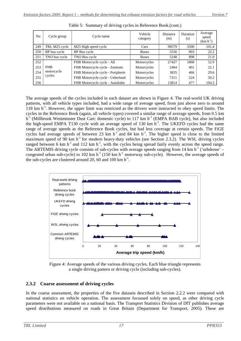
Table 5: Summary of driving cycles in Reference Book.(cont.)
No Cycle group Cycle nameVehiclecategory
Distance(m)
Duration(s)
Averagespeed
(km h-1)
249 TRL M25 cycle M25 High speed cycle Cars 98579 3500 101.4
250 BP bus cycle BP Bus cycle Buses 5556 903 22.2
251 TNO bus cycle TNO Bus cycle Buses 5248 898 21.0
252FHBmotorcyclecycles
FHB Motorcycle cycle - All Motorcycles 27427 1868 52.9
253 FHB Motorcycle cycle - Zentrum Motorcycles 2464 401 22.1
254 FHB Motorcycle cycle - Peripherie Motorcycles 3835 466 29.6
255 FHB Motorcycle cycle - Ueberland Motorcycles 7311 524 50.2
256 FHB Motorcycle cycle - Autobahn Motorcycles 13814 477 104.3
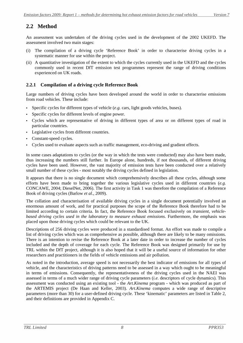
The average speeds of the cycles included in each dataset are shown in Figure 4. The real-world UK drivingpatterns, with all vehicle types included, had a wide range of average speed, from just above zero to around118 km h-1. However, the upper limit was restricted as the drivers were instructed to obey speed limits. Thecycles in the Reference Book (again, all vehicle types) covered a similar range of average speeds, from 0.5 kmh-1 (Millbrook Westminster Dust Cart: domestic cycle) to 117 km h-1 (EMPA BAB cycle), but also includedthe high-speed EMPA T130 cycle with an average speed of 130 km h-1. The UKEFD cycles had the samerange of average speeds as the Reference Book cycles, but had less coverage at certain speeds. The FiGEcycles had average speeds of between 23 km h-1 and 84 km h-1. The higher speed is close to the limitedmaximum speed of 90 km h-1 for modern heavy-duty vehicles (see Section 2.3.2). The WSL driving cyclesranged between 6 km h-1 and 112 km h-1, with the cycles being spread fairly evenly across the speed range.The ARTEMIS driving cycle consists of sub-cycles with average speeds ranging from 14 km h-1 (‘urbdense’ –congested urban sub-cycle) to 102 km h-1 (150 km h-1 motorway sub-cycle). However, the average speeds ofthe sub-cycles are clustered around 20, 60 and 100 km h-1.
0 20 40 60 80 100 120 140
Average trip speed (km/h)
WSL driving cycles
FiGE driving cycles
Reference bookdriving cycles
Real-world drivingpatterns
UKEFD drivingcycles
Common ARTEMISdriving cycles
Figure 4: Average speeds of the various driving cycles. Each blue triangle representsa single driving pattern or driving cycle (including sub-cycles).
2.3.2 Coarse assessment of driving cycles
In the coarse assessment, the properties of the five datasets described in Section 2.2.2 were compared withnational statistics on vehicle operation. The assessment focussed solely on speed, as other driving cycleparameters were not available on a national basis. The Transport Statistics Division of DfT publishes averagespeed distributions measured on roads in Great Britain (Department for Transport, 2005). These are

TRL Limited 18 PPR353
Emission factors 2009: Report 1 – methods for determining hot exhaust emission factors for road vehicles Version 7
summarised for urban roads in Table 6 and for non-urban roads in Table 7. The speed distributions for thevarious vehicle types are also plotted in Appendix D of this Report. It is assumed that these statistics broadlyreflect UK conditions.
From the information given in Table 6 it can be seen that most vehicles on urban roads in Great Britain aretravelling at speeds which are between 20 mph (64 km h-1) and 50 mph (80 km h-1), and only a smallproportion of vehicles are travelling at speeds below 20 mph. This implies that for inventory purposes theaccurate characterisation of emissions at very low speeds is likely to be less important than accuratecharacterisation at higher speeds. However, it is important to note that accurate emission factors at low speedsremain important for air quality assessments, especially those assessments which relate to traffic congestion insome way. Indeed, several of the driving cycles used to derive the UK emission factors do have an averagespeed of less than 32 km h-1.
Table 6: Percentages of vehicles having speeds in excess of a stated speed on urban roadsIn Great Britain (adapted from Department of Transport et al., 2005).
Road type Vehicle type
% of vehicles exceeding a given speed(mph, km h-1 in brackets)
>20(32)
>30(48)
>40(64)
>50(80)
>60(97)
>70(113)
>80(129)
>90(145)
Urban roads:roads with a 40 mph speedlimit
Motorcycles 95% 81% 37% 9% 2% - - -
Cars 97% 85% 27% 3% - - - -
LGVs 96% 84% 29% 4% 1% - - -
Buses/coaches 97% 81% 13% - - - - -
2-axle rigid HGVs 95% 81% 22% 2% - - - -
3-axle rigid HGVs 97% 83% 20% 1% - - - -
4-axle rigid HGVs 98% 88% 26% 1% - - - -
4-axle articulated HGVs 98% 87% 26% 2% - - - -
5+-axle articulated HGVs 98% 88% 25% 1% - - - -
Urban roads:roads with a 30 mph speedlimit
Motorcycles 87% 48% 11% 2% - - - -
Cars 94% 53% 6% - - - - -
LGVs 92% 53% 6% - - - - -
Buses/coaches 91% 28% 1% - - - - -
2-axle rigid HGVs 91% 48% 5% - - - - -
3-axle rigid HGVs 93% 46% 1% - - - - -
4-axle rigid HGVs 96% 54% 2% - - - - -
4-axle articulated HGVs 925 46% 2% - - - - -
5+-axle articulated HGVs 97% 54% 2% - - - - -
The values in Table 7 indicate that around half of the cars on motorways (56%) and dual-carriageways (48%)are travelling at speeds for which emissions have not previously been routinely measured. One area of concernis therefore extent to which the driving cycles currently used for emission measurement cover the higherspeeds encountered in the UK.
The majority of heavy-duty vehicles over 7.5 t GVW have been fitted with speed limiters since the early1990s. A limiter restricts the maximum speed to 56 mph (90 km h-1) for goods vehicles and 62 mph (100 km h-
1) for buses. Prior to 1 January 2005 there was no requirement for goods vehicles under 7.5 t (or buses withmore than 8 passenger seats) to be fitted with a speed limiter8. Vehicles registered between 1 October 2001and 31 December 2004 (inclusive), will also need to be fitted with a speed limiter. This is reflected in thespeed distributions - although the vast majority of large goods vehicles (rigid HGVs with 3 axles or more andarticulated HGVs) have speeds of less than 60 mph (97 km h-1), 2-axle rigid HGVs have higher speeds.
8 http://www.vosa.gov.uk/vosacorp/repository/Speed%20Limiters%20-%20New%20Regulations.pdf

TRL Limited 19 PPR353
Emission factors 2009: Report 1 – methods for determining hot exhaust emission factors for road vehicles Version 7
The highest speed sub-cycle of the FiGE cycle, which is normally used to test HGVs, has an average speed of84 km h-1. The FiGE cycle is therefore suitable for testing speed-limited HGVs and buses, but it does not coverthe highest speeds which could be reached with an unrestricted vehicle (pre-October 2001). In addition, theslowest FiGE sub-cycle has an average speed of 23 km h-1. To determine emissions from such vehicles undercongested traffic conditions, a much slower driving cycle would be required.
Table 7: Percentages of vehicles having speeds in excess of a stated speed for non-urban roadsIn Great Britain (adapted from Department for Transport et al., 2005).
Road type Vehicle type
% of vehicles exceeding a given speed(mph, km h-1 in brackets)
>20(32)
>30(48)
>40(64)
>50(80)
>60(97)
>70(113)
>80(129)
>90(145)
Non-urban roads:motorways
Motorcycles - - - 96% 80% 59% 28% 8%
Cars - - - 97% 85% 56% 19% 3%
LGVs - - - 96% 81% 51% 17% 3%
Buses/coaches - - - 94% 50% 2% - -
2-axle rigid HGVs - - - 94% 47% 18% 4% 1%
3-axle rigid HGVs - - - 88% 6% - - -
4-axle rigid HGVs - - - 87% 1% - - -
4-axle articulated HGVs - - - 92% 2% - - -
5+-axle articulated HGVs - - - 92% 1% - - -
Non-urban roads:dual carriageways
Motorcycles - 100% 98% 87% 69% 48% 21% -
Cars - 100% 100% 97% 82% 48% 14% -
LGVs - 100% 100% 96% 77% 44% 13% -
Buses/coaches - 100% 99% 89% 40% 3% 1% -
2-axle rigid HGVs - 100% 99% 89% 40% 14% 3% -
3-axle rigid HGVs - 100% 99% 78% 7% 3% 1% -
4-axle rigid HGVs - 100% 99% 78% 1% - - -
4-axle articulated HGVs - 99% 98% 80% 3% - - -
5+-axle articulated HGVs - 99% 99% 87% 1% - - -
Non-urban roads:single carriageways
Motorcycles 99% 93% 80% 52% 25% 10% - -
Cars 100% 98% 83% 41% 10% 2% - -
LGVs 100% 97% 81% 40% 11% 2% - -
Buses/coaches 99% 96% 73% 24% 2% - - -
2-axle rigid HGVs 99% 96% 77% 30% 5% 1% - -
3-axle rigid HGVs 99% 93% 69% 18% - - - -
4-axle rigid HGVs 99% 90% 62% 17% - - - -
4-axle articulated HGVs 98% 92% 72% 21% - - - -
5+-axle articulated HGVs 100% 98% 80% 30% 1% - - -
2.3.3 Detailed assessment of driving cycles
In the detailed assessment, all the driving cycles and real-world driving patterns were analysed using theArt.Kinema program. A large number of parameters were generated for each driving cycle or pattern. Thecorrelation of between each parameter and every other parameter was calculated for the entire data set. Theresulting correlation matrix is given in Table 8. The value of the correlation coefficient (r) ranges from -1.0 to+1.0. A perfect positive correlation is indicated by +1.0, and a perfect negative correlation by -1.0. A cut offpoint of plus or minus 0.71 was used to identify the strongest correlations (this being equivalent to an r2 valueof 0.5). The values indicating a strong positive or negative correlation are shown in normal font, with all othervalues being shown in a light font (along with the unity values associated with comparisons between identicalparameters).
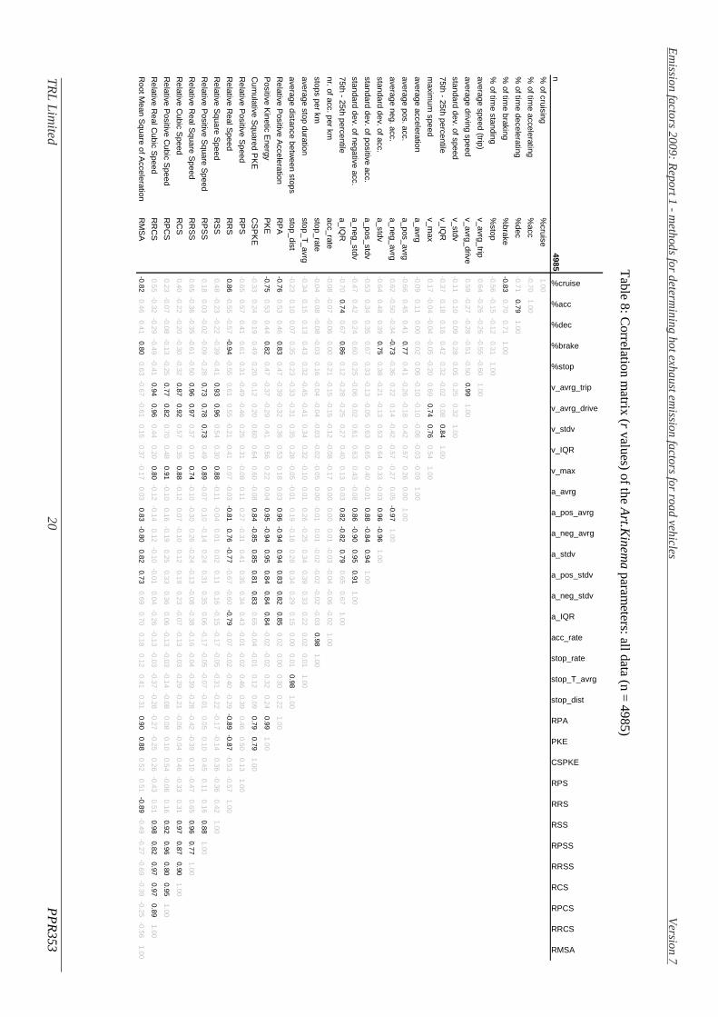
Em
issionfactors
2009:R
eport1-
methods
fordeterm
ininghotexhaustem
issionfactors
forroad
vehiclesV
ersion7
TR
LL
imited
20P
PR
353
Table
8:Correlation
matrix
(rvalues)
ofthe
Art.K
inema
parameters:alldata
(n=
4985)
n4985
%cruise
%acc
%dec
%brake
%stop
v_avrg_trip
v_avrg_drive
v_stdv
v_IQR
v_max
a_avrg
a_pos_avrg
a_neg_avrg
a_stdv
a_pos_stdv
a_neg_stdv
a_IQR
acc_rate
stop_rate
stop_T_avrg
stop_dist
RPA
PKE
CSPKE
RPS
RRS
RSS
RPSS
RRSS
RCS
RPCS
RRCS
RMSA
%ofcruising
%cruise
1.00
%oftim
eaccelerating
%acc
-0.701.00
%oftim
edecelerating
%dec
-0.710.79
1.00
%oftim
ebraking
%brake
-0.830.70
0.711.00
%oftim
estanding
%stop
-0.56-0.15
-0.120.31
1.00
averagespeed
(trip)v_avrg_trip
0.64-0.26
-0.26-0.55
-0.601.00
averagedriving
speedv_avrg_drive
0.59-0.27
-0.28-0.51
-0.500.99
1.00
standarddev.ofspeed
v_stdv-0.11
0.100.09
0.280.05
0.250.32
1.00
75th-
25thpercentile
v_IQR
-0.370.18
0.160.42
0.32-0.02
0.080.84
1.00
maxim
umspeed
v_max
0.17-0.04
-0.04-0.05
-0.200.69
0.740.76
0.541.00
averageacceleration
a_avrg-0.09
0.110.00
0.020.06
-0.10-0.10
-0.06-0.03
-0.091.00
averagepos.acc.
a_pos_avrg-0.66
0.450.41
0.770.41
-0.26-0.18
0.420.57
0.260.00
1.00
averageneg.acc.
a_neg_avrg0.62
-0.50-0.34
-0.73-0.36
0.220.14
-0.42-0.57
-0.270.05
-0.971.00
standarddev.ofacc.
a_stdv-0.64
0.480.39
0.750.38
-0.21-0.13
0.530.64
0.33-0.03
0.96-0.96
1.00
standarddev.ofpositive
acc.a_pos_stdv
-0.530.34
0.350.67
0.33-0.13
-0.050.63
0.650.40
-0.010.88
-0.840.94
1.00
standarddev.ofnegative
acc.a_neg_stdv
-0.470.42
0.240.60
0.25-0.06
0.020.61
0.630.43
-0.080.86
-0.900.95
0.911.00
75th-
25thpercentile
a_IQR
-0.700.74
0.670.86
0.12-0.28
-0.250.27
0.400.13
0.030.82
-0.820.79
0.650.67
1.00
nr.ofacc.perkm
acc_rate-0.08
-0.07-0.06
0.000.21
-0.15-0.15
-0.12-0.08
-0.170.00
0.000.01
-0.03-0.04
-0.06-0.02
1.00
stopsper
kmstop_rate
-0.04-0.08
-0.08-0.03
0.16-0.04
-0.04-0.03
-0.02-0.05
0.00-0.01
0.01-0.02
-0.02-0.02
-0.030.98
1.00
averagestop
durationstop_T
_avrg-0.34
0.150.13
0.430.32
-0.45-0.41
0.340.32
-0.100.01
0.26-0.25
0.340.39
0.330.22
0.020.01
1.00
averagedistance
between
stopsstop_dist
-0.230.10
0.070.35
0.23-0.33
-0.310.35
0.28-0.05
-0.010.19
-0.180.28
0.340.29
0.150.00
0.010.98
1.00
Relative
Positive
Acceleration
RP
A-0.76
0.530.46
0.830.47
-0.39-0.32
0.360.53
0.180.03
0.96-0.94
0.940.83
0.820.85
0.020.00
0.300.22
1.00
Positive
Kinetic
Energy
PK
E-0.75
0.530.44
0.820.47
-0.37-0.29
0.410.56
0.220.04
0.95-0.94
0.950.84
0.840.84
-0.02-0.02
0.320.24
0.991.00
Cum
ulativeS
quaredP
KE
CS
PK
E-0.33
0.240.19
0.490.20
0.120.20
0.600.64
0.60-0.08
0.84-0.85
0.850.81
0.830.65
-0.04-0.01
0.120.09
0.790.79
1.00
Relative
Positive
Speed
RP
S-0.65
0.570.41
0.610.31
-0.49-0.46
0.250.31
-0.080.11
0.27-0.31
0.410.35
0.340.43
-0.01-0.02
0.460.39
0.460.50
0.131.00
Relative
RealS
peedR
RS
0.86-0.55
-0.57-0.94
-0.550.61
0.55-0.21
-0.410.07
-0.03-0.81
0.76-0.77
-0.67-0.60
-0.79-0.07
-0.02-0.40
-0.29-0.89
-0.87-0.53
-0.571.00
Relative
Square
Speed
RS
S0.48
-0.23-0.22
-0.39-0.41
0.930.96
0.540.30
0.88-0.11
-0.040.01
0.020.11
0.16-0.15
-0.17-0.05
-0.31-0.22
-0.17-0.14
0.36-0.36
0.421.00
Relative
Positive
Square
Speed
RP
SS
0.180.03
-0.02-0.09
-0.280.73
0.780.73
0.490.89
-0.070.10
-0.140.24
0.310.35
0.06-0.17
-0.05-0.07
-0.010.05
0.100.45
0.110.16
0.881.00
Relative
RealS
quareS
peedR
RS
S0.65
-0.36-0.35
-0.61-0.50
0.960.97
0.370.10
0.74-0.10
-0.300.26
-0.24-0.13
-0.08-0.38
-0.16-0.04
-0.39-0.28
-0.42-0.39
0.10-0.47
0.650.96
0.771.00
Relative
Cubic
Speed
RC
S0.40
-0.22-0.20
-0.30-0.32
0.870.92
0.570.35
0.88-0.12
0.07-0.10
0.120.19
0.23-0.07
-0.13-0.03
-0.29-0.21
-0.06-0.04
0.46-0.33
0.310.97
0.870.90
1.00
Relative
Positive
Cubic
Speed
RP
CS
0.23-0.07
-0.08-0.13
-0.250.77
0.820.70
0.480.91
-0.100.16
-0.190.25
0.330.36
0.06-0.13
-0.03-0.14
-0.080.08
0.100.54
-0.060.16
0.920.96
0.800.95
1.00
Relative
RealC
ubicS
peedR
RC
S0.55
-0.32-0.29
-0.49-0.41
0.940.96
0.440.20
0.80-0.12
-0.140.12
-0.10-0.01
0.04-0.26
-0.13-0.03
-0.37-0.28
-0.27-0.25
0.26-0.43
0.510.98
0.820.97
0.970.89
1.00
RootM
eanS
quareofA
ccelerationR
MS
A-0.82
0.460.41
0.800.63
-0.67-0.61
0.150.37
-0.170.03
0.83-0.80
0.820.73
0.690.70
0.180.12
0.410.31
0.900.88
0.520.51
-0.89-0.49
-0.27-0.69
-0.39-0.25
-0.561.00

Emission factors 2009: Report 1 - methods for determining hot exhaust emission factors for road vehicles Version 7
TRL Limited 21 PPR353
It should be noted that there are natural relationships between some the parameters which do not differ fordifferent cycles. For example, the average driving speed is generally going to be closely related to the averagetrip speed. Indeed, most of the speed-related parameters have strong correlations with the other speed-relatedparameters, although there are a few exceptions (e.g. relative positive speed and relative real speed do notshow a good correlation, although the latter has a strong correlation with some of the acceleration parameters).Similarly, there are good correlations between the various acceleration-related parameters, including positivekinetic energy.
For each of the datasets listed in Section 2.2.2, each Art.Kinema parameter and each vehicle category (cars,LGVs, HGVs and buses) a frequency distribution was obtained. As average speed is commonly used todescribe driving cycles, each of the Art.Kinema parameters was plotted against the average trip speed. A fewselected examples are discussed below for each vehicle category. The average Art.Kinema parameters for eachdataset and each vehicle category are listed in Appendix E.
Cars
Figure 5 shows the average speed distributions for cars. In the legend, the heading ‘Driving cycles’ refers tothe Reference Book. The x-axis indicates the maximum value of each distribution bin (e.g. ‘20’ contains thespeeds between 10 and 20 km h-1).The y-axis simply defines the relative frequency of driving patterns in eachdatabase. Each distribution of real-world driving patterns is dependent upon the nature of the measurementprogrammes included in the database, and its shape cannot therefore be said to be truly representative of theUK average speed distribution (either in terms of vehicles or vehicle-kilometres driven). However, the rangeof speeds is important, as this range must be covered by the emission factors. In fact, the real-world drivingpatterns, the Reference Book driving cycles and the UKEFD cycles have broadly similar average speeddistributions, with a peak at lower speeds. As there are only six WSL cycles, the distribution is very simple,with each cycle falling in a separate bin. However, the WSL cycles do cover much of the speed rangeobserved in the real-world driving patterns, with only speeds higher than 120 km h-1 not being represented.The ARTEMIS sub-cycles appear to cover most of the range of vehicle speeds in the UK, the exception beingthe highest speeds of the real-world driving patterns.
0
0.05
0.1
0.15
0.2
0.25
0.3
0.35
10 20 30 40 50 60 70 80 90 100 110 120 130
average speed (trip) (km/h)
Rel
ativ
efr
eque
ncy
Real-world driving patterns Driving cycles UKEFD cycles WSL cycles ARTEMIS
Figure 5: Distributions of average trip speed – cars.
The standard deviation is one measure of the amount of speed variation in a cycle. The distributions of thestandard deviation of speed are shown in Figure 6. The distributions for the different data sets were similar,although the WSL cycles may contain less variation in speed compared with real-world driving. TheARTEMIS cycle has a greater proportion of high standard deviations in its sub-cycles than the other cycles.
The standard deviation of the speed within each cycle is shown plotted against average speed in Figure 7.Linear trend lines have been plotted though the data points to highlight similarities and differences between
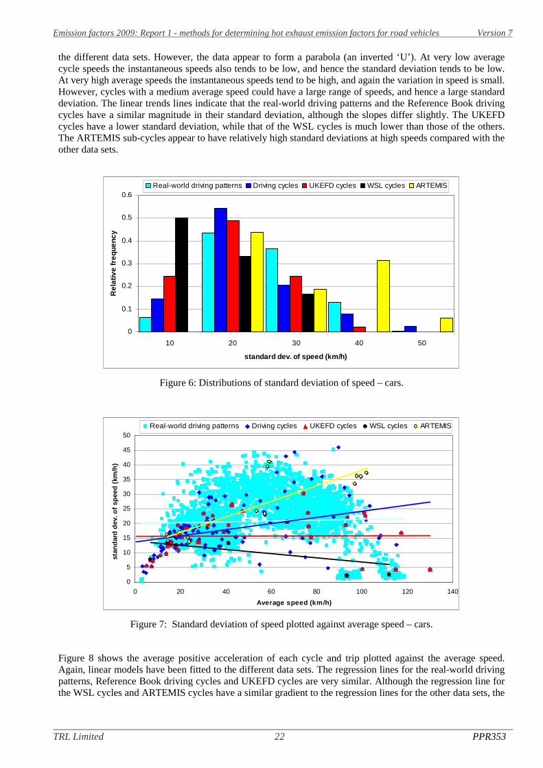
Emission factors 2009: Report 1 - methods for determining hot exhaust emission factors for road vehicles Version 7
TRL Limited 22 PPR353
the different data sets. However, the data appear to form a parabola (an inverted ‘U’). At very low averagecycle speeds the instantaneous speeds also tends to be low, and hence the standard deviation tends to be low.At very high average speeds the instantaneous speeds tend to be high, and again the variation in speed is small.However, cycles with a medium average speed could have a large range of speeds, and hence a large standarddeviation. The linear trends lines indicate that the real-world driving patterns and the Reference Book drivingcycles have a similar magnitude in their standard deviation, although the slopes differ slightly. The UKEFDcycles have a lower standard deviation, while that of the WSL cycles is much lower than those of the others.The ARTEMIS sub-cycles appear to have relatively high standard deviations at high speeds compared with theother data sets.
0
0.1
0.2
0.3
0.4
0.5
0.6
10 20 30 40 50
standard dev. of speed (km/h)
Rel
ativ
efr
eque
ncy
Real-world driving patterns Driving cycles UKEFD cycles WSL cycles ARTEMIS
Figure 6: Distributions of standard deviation of speed – cars.
0
5
10
15
20
25
30
35
40
45
50
0 20 40 60 80 100 120 140
Average speed (km/h)
stan
dar
dd
ev.o
fsp
eed
(km
/h)
Real-world driving patterns Driving cycles UKEFD cycles WSL cycles ARTEMIS
Figure 7: Standard deviation of speed plotted against average speed – cars.
Figure 8 shows the average positive acceleration of each cycle and trip plotted against the average speed.Again, linear models have been fitted to the different data sets. The regression lines for the real-world drivingpatterns, Reference Book driving cycles and UKEFD cycles are very similar. Although the regression line forthe WSL cycles and ARTEMIS cycles have a similar gradient to the regression lines for the other data sets, the

Emission factors 2009: Report 1 - methods for determining hot exhaust emission factors for road vehicles Version 7
TRL Limited 23 PPR353
WSL cycles trend-line is lower and ARTEMIS is higher. Figure 9 shows the equivalent plot for the averagenegative acceleration plotted and average speed, which shows that the WSL cycles have less negativeaccelerations (i.e. the decelerations in the WSL cycles are not as rapid as those in the other cycles and drivingpatterns) and the ARTEMIS cycles have greater negative accelerations. The plots indicate that the WSL cyclesare generally less ‘aggressive’ and the ARTEMIS sub-cycles slightly more ‘aggressive’ than driving patternsin the real world, although on whole the real-world driving cycles appear to be well-represented in theReference Book and the UKEFD. A small number of UKEFD driving cycles appear to have average positiveand negative accelerations which are outside the range of real-world conditions, though these are mainly theold TRRL cycles which were only used in one early test programme. The only important UKEFD outlier is theone at about 30 km h-1, which is the MODEM7 cycle.
0
0.2
0.4
0.6
0.8
1
1.2
0 20 40 60 80 100 120 140
Average speed (km/h)
aver
age
po
s.ac
c.(m
/s2)
Real-world driving patterns Driving cycles UKEFD cycles WSL cycles ARTEMIS
Figure 8: Average positive acceleration plotted against average speed – cars.
-1.2
-1
-0.8
-0.6
-0.4
-0.2
0
0 20 40 60 80 100 120 140
Average speed (km/h)
aver
age
neg
.acc
.(m
/s2)
Real-world driving patterns Driving cycles UKEFD cycles WSL cycles ARTEMIS
Figure 9: Average negative acceleration plotted against average speed – cars.
LGVs
Figure 10 shows the average speed distributions for LGVs. As mentioned earlier, the real-world data for LGVsrelate principally to urban roads, and are therefore biased towards the lower end of the speed range and cannotbe taken to be representative of UK conditions. This is apparent in the graph, with the real-world driving
Emission factors 2009: Report 1 - methods for determining hot exhaust emission factors for road vehicles Version 7
TRL Limited 24 PPR353
patterns being concentrated at the lower end of the speed range. The actual speed range of real-world drivingis likely to be similar to that for cars shown in Figure 5.
As with cars, an assessment of cycle dynamics indicated that the WSL cycles were less aggressive than thereal-world driving patterns, the driving cycles in the reference book and the UKEFD cycles. For example,Figure 11 shows the distributions of average negative acceleration, with the decelerations in the WSL cyclesbeing less rapid than those in the other cycles and driving patterns.
0
0.05
0.1
0.15
0.2
0.25
0.3
0.35
0.4
0.45
0.5
10 20 30 40 50 60 70 80 90 100 110 120 130
average speed (trip) (km/h)
Rel
ativ
efr
eque
ncy
Real-world driving patterns Driving cycles UKEFD cycles WSL cycles
Figure 10: Distributions of average trip speed - LGVs
0
0.1
0.2
0.3
0.4
0.5
0.6
-0.8 -0.7 -0.6 -0.5 -0.4 -0.3 -0.2 -0.1 0
average neg. acc. (m/s2)
Rel
ativ
efr
eque
ncy
Real-world driving patterns Driving cycles UKEFD cycles WSL cycles
Figure 11. Distributions of average negative acceleration – LGVs.
HGVs
Figure 12 shows the distributions of average speed for the HGV driving patterns and cycles. Although some ofthe driving patterns, the Reference Book driving cycles and UKEFD cycles have average speeds lower than 10km h-1, such low average speeds are not represented in the FiGE cycle (which has a minimum average cyclespeed of 23 km h-1). The four data sets have broadly similar standard deviation distributions, as shown inFigure 13. However, there is a gap in the FiGE distribution between the medium and high values, and lowstandard deviations are not well represented.

Emission factors 2009: Report 1 - methods for determining hot exhaust emission factors for road vehicles Version 7
TRL Limited 25 PPR353
Figure 14 shows average positive acceleration plotted against average speed for HGVs. Some of the low-speedReference Book/UKEFD driving cycles have relatively high accelerations which are not apparent in the real-world driving patterns (specifically the Millbrook Heavy Duty: urban cycle and the three MillbrookWestminster Dust Cart cycles). The higher-speed FiGE cycles (suburban and motorway) also appear to havelow average accelerations compared with the real-world driving patterns. From Figure 15 it can be seen thatsome of the UKEFD cycles have more rapid decelerations than the real-world driving patterns. In particular,one of the high-speed UKEFD cycles (Millbrook Heavy Duty: motorway) has a very high averagedeceleration, though this is likely to be due to one long deceleration at the end of the cycle (see Barlow et al.,2009). In addition, the higher-speed FiGE cycles have less rapid decelerations than the real-world drivingpatterns.
0
0.05
0.1
0.15
0.2
0.25
0.3
0.35
0.4
0.45
10 20 30 40 50 60 70 80 90
average speed (trip) (km/h)
Rel
ativ
efr
eque
ncy
Real-world driving patterns Driving cycles UKEFD cycles FiGE cycles
Figure 12. Distributions of average trip speed – HGVs.
0
0.1
0.2
0.3
0.4
0.5
0.6
5 10 15 20 25 30 35
standard dev. of speed (km/h)
Rel
ativ
efr
eque
ncy
Real-world driving patterns Driving cycles UKEFD cycles FiGE cycles
Figure 13. Distributions of standard deviation of speed – HGVs.
Emission factors 2009: Report 1 - methods for determining hot exhaust emission factors for road vehicles Version 7
TRL Limited 26 PPR353
-0.2
-0.1
0
0.1
0.2
0.3
0.4
0.5
0.6
0.7
0 10 20 30 40 50 60 70 80 90
Average speed (km/h)
aver
age
po
s.ac
c.(m
/s2)
Real-world driving patterns Driving cycles UKEFD cycles FiGE cycles
Figure 14. Average positive acceleration plotted against average speed – HGVs.
-0.9
-0.8
-0.7
-0.6
-0.5
-0.4
-0.3
-0.2
-0.1
0
0 10 20 30 40 50 60 70 80 90
Average speed (km/h)
aver
age
neg
.acc
.(m
/s2)
Real-world driving patterns Driving cycles UKEFD cycles FiGE cycles
Figure 15. Average negative acceleration plotted against average speed – HGVs.
Buses and coaches
A single class of vehicles (‘Buses’) is used in the UKEFD to cover all buses and coaches. Figure 16 shows thedistributions of average speed for buses. The Reference Book driving cycles have a similar distribution to thereal-world driving patterns, although there is a small number of driving cycles with higher speeds. However,both the distributions for the UKEFD cycles and the FiGE cycles are biased towards higher speeds. Most ofthe real-world driving patterns for buses were logged on urban routes, and therefore have relatively lowaverage speeds. Even rural buses are likely to have low average speeds. Urban buses may be unable to attainthe higher speeds required for some of the cycles (including the motorway FiGE cycle). Coaches, on the otherhand are likely to operate at higher motorway speeds, and do not generally have speed limiters fitted. Urbanbuses and coaches should therefore be treated separately when deriving emission factors, and morerepresentative driving cycles for these vehicle classes should be used in the derivation of the future UKemission factors.
The distributions of average positive acceleration and average negative acceleration are shown in Figure 17and Figure 18. The UKEFD and FiGE cycles clearly have lower accelerations and decelerations than the othertwo data-sets.

Emission factors 2009: Report 1 - methods for determining hot exhaust emission factors for road vehicles Version 7
TRL Limited 27 PPR353
0
0.1
0.2
0.3
0.4
0.5
0.6
0.7
0.8
10 20 30 40 50 60 70 80 90
average speed (trip) (km/h)
Rel
ativ
efr
eque
ncy
Real-world driving patterns Driving cycles UKEFD cycles FIGE cycles
Figure 16. Distributions of average trip speed – buses
0
0.1
0.2
0.3
0.4
0.5
0.6
0.7
0.8
0.1 0.2 0.3 0.4 0.5 0.6 0.7 0.8 0.9 1 1.1
average pos. acc. (m/s2)
Rel
ativ
efr
eque
ncy
Real-world driving patterns Driving cycles UKEFD cycles FIGE cycles
Figure 17. Distributions of average positive acceleration - buses
0
0.1
0.2
0.3
0.4
0.5
0.6
0.7
0.8
-1.8 -1.7 -1.6 -1.5 -1.4 -1.3 -1.2 -1.1 -1 -0.9 -0.8 -0.7 -0.6 -0.5 -0.4 -0.3 -0.2 -0.1
average neg. acc. (m/s2)
Rel
ativ
efr
eque
ncy
Real-world driving patterns Driving cycles UKEFD cycles FIGE cycles
Figure 18. Distributions of average negative acceleration - buses
Emission factors 2009: Report 1 - methods for determining hot exhaust emission factors for road vehicles Version 7
TRL Limited 28 PPR353
2.3.4 Summary
Most vehicles on urban roads are travelling at speeds which are between 20 mph (64 km h-1) and 50 mph (80km h-1), and only a small proportion of vehicles are travelling at speeds below 20 mph. This implies that forinventory purposes the accurate characterisation of emissions at very low speeds is likely to be less importantthan accurate characterisation at higher speeds. However, it is important to note that accurate emission factorsat low speeds remain important for local air quality assessment.
The real-world driving patterns, with all vehicle types included, have a large number of different averagespeeds, from just above zero to around 118 km h-1, although the upper limit is restricted by the experimentaldesign and it is clear that much higher speeds can actually occur. The driving cycles in the Reference Bookand UKEFD cover a similar range of average speeds, but have a maximum average speed of 130 km h-1.
For cars, the real-world driving patterns, the Reference Book driving cycles and the UKEFD cycles havebroadly similar average speed distributions. The WSL and ARTEMIS cycles cover much of the speed rangeobserved in the driving patterns, with only the highest speeds not being represented. The WSL cycles aregenerally less ‘aggressive’ than driving patterns in the real world, while the ARTEMIS sub-cycles wereslightly more ‘aggressive’. On the whole, the real-world driving cycles appear to be well-represented in theUKEFD. The assessment of cycle dynamics for LGVs also indicated that the WSL cycles were less aggressivethan the real-world driving patterns, the driving cycles in the reference book and the UKEFD cycles.
In the case of HGVs, although some of the driving patterns, the Reference Book driving cycles and UKEFDcycles have average speeds lower than 10 km h-1, such low average speeds are not represented in the FiGEcycle. Furthermore, the FiGE cycles do not cover the highest speeds which could be reached with anunrestricted (pre-October 2001) HGV. Some of the low-speed Reference Book/UKEFD driving cycles haverelatively high average accelerations and average decelerations which are not apparent in the real-worlddriving patterns. On the other hand, the higher-speed FiGE cycles appear to have lower average accelerationsand decelerations than the real-world driving patterns.
A single class of vehicles (‘Buses’) is used in the UKEFD to cover all buses and coaches, even though busesand coaches tend to have different speed ranges. The Reference Book driving cycles have a similar averagespeed distribution to the real-world driving patterns. However, both the distributions for the UKEFD cyclesand the FiGE cycles are biased towards higher speeds. The UKEFD and FiGE cycles clearly have loweraccelerations and decelerations than the real-world driving patterns and the driving cycles in the ReferenceBook.

Emission factors 2009: Report 1 - methods for determining hot exhaust emission factors for road vehicles Version 7
TRL Limited 29 PPR353
3 A review of emission test parameters
The second main element of Task 1 of the Project was a review of the parameters and data recorded duringemission tests. The objective of this part of the work was to provide recommendations relating to how theusefulness of the recorded data might be improved, and which information should be routinely measuredduring testing. For example, in current tests the total mass emission of a pollutant is measured over a completedriving cycle. This allows emissions (in g km-1) to be plotted as a function of average cycle speed. However, ifonly these parameters are recorded the data may be of limited use if there becomes a need to characteriseemissions factors in terms other than g km-1 for an average speed.
3.1 Background
Emissions data can be recorded using a number of different methods, under different ambient conditions, andin different formats. Examples of parameters which can vary from laboratory to laboratory, and fromprogramme to programme, include the length, alignment and temperature of exhaust sample lines, thedynamometer fan height and speed response, the types of analyser used, the recording frequency ofmeasurements, and the temperature, pressure and humidity of the ambient air. It is recognised that many suchparameters affect emission measurements, but their actual impact on the results has not been well quantified.This is especially true for cars equipped with new technology engines and emission control systems.Emissions from these vehicles can be very low, but can also be very sensitive to changes in test conditions.This undermines the production of accurate emission factors (Joumard et al., 2006a).
The first part of this review (Section 3.2) summarises the emission testing protocols which have beenestablished for type approval in Europe. A large proportion of the existing emission data has been obtainedduring tests conducted in accordance with these protocols. However, their objective is not to assess theemissions of the European vehicle fleet but to ensure that compliance can be established for new vehicles (orengines) on an equal basis. Hence, the test conditions are standardised. In order to understand real-worldemissions it is important to determine how variations in sampling conditions affect emission measurements.For cars, probably some of the most comprehensive examinations of the effects of different emission testparameters were those conducted as part of the ARTEMIS project (Joumard et al., 2006a) and thePARTICULATES project (Samaras et al., 2005a). The results and conclusions from these studies aresummarised in Section 3.3. The information for other types of vehicle is generally less extensive, althoughsome of the ARTEMIS work on motorcycles and heavy-duty vehicles has been summarised in Sections 3.4and 3.5.
3.2 European type approval procedures
In recognition of the contribution of vehicle emissions to air pollution, measures have been taken to reduce thequantities emitted. Since the early 1970s, limits have been applied to CO, HC and NOx in vehicle exhaust. Thelimits have been reduced many times since they were first introduced, and changes have been made to the testmethod to make it more realistic and effective. All Member States within the EU are subject to the emissionlimits for road vehicles and engines, and methods of measurement are standardised in European legislation.Some aspects of the procedures were discussed in Section 2.1.1. Emissions of carbon dioxide from passengercars, although not regulated, are controlled through voluntary agreements with the automotive industry9.
For the purpose of emission standards and other vehicle regulations, vehicles are classified according to thecategories listed in Table 9. Light goods vehicles (category N1) are further divided into three weight classes,as shown in Table 10.
9 On 17 December 2008 the European Parliament voted to adopt a Regulation which limits the fleet average exhaust CO2 emissionfrom new cars to 130 g km-1.

Emission factors 2009: Report 1 - methods for determining hot exhaust emission factors for road vehicles Version 7
TRL Limited 30 PPR353
Table 9: Definition of vehicle categories (DieselNet, 2006).
Category Description
L Two- and three-wheel vehicles.
M Motor vehicles with at least four wheels designed and constructed for the carriage of passengers.
M1 Vehicles comprising no more than eight seats in addition to the driver’s seat.
M2 Vehicles comprising more than eight seats in addition to the driver’s seat, and having a maximum mass not
M3 Vehicles comprising more than eight seats in addition to the driver’s seat, and having a maximum mass
N Motor vehicles with at least four wheels designed and constructed for the carriage of goods.
N1 Vehicles having a maximum mass not exceeding 3.5 tonnes.
N2 Vehicles having a maximum mass exceeding 3.5 tonnes but not exceeding 12 tonnes.
N3 Vehicles having a maximum mass exceeding 12 tonnes.
O Trailers (including semi-trailers).
G* Off-Road Vehicles.
* For off-road vehicles the symbol G is combined with either symbol M or N. For example, a vehicle of categoryN1 which is suited for off-road use is designated as N1G.
Table 10: Weight classes for vehicle category N1.
ClassReference weight (RW)
Euro 1-2 Euro 3+
I RW ≤ 1250 kg RW ≤ 1305 kg
II 1250 kg < RW ≤ 1700 kg 1305 kg < RW ≤ 1760 kg
III 1700 kg < RW 1760 kg < RW
3.2.1 Light-duty vehicles
Background
European Union emission regulations for new light-duty vehicles (cars and light goods vehicles) are specifiedin the Directive 70/220/EEC. This Directive has been amended a number of times, with some of the mostrecent amendments including:
• Euro 1 standards (1992) - Directives 91/441/EEC (cars) and 93/59/EEC (cars and light trucks)• Euro 2 standards (1996) - Directives 94/12/EC and 96/69/EC• Euro 3 standards (2000) - Directive 98/69/EC• Euro 4 standards (2005) - Directive 98/69/EC• Euro 5 standards (2009) - Regulation EC 692/2008• Euro 6 standards (2014) - Regulation EC 692/2008
At the Euro 2 stage separate emission limits were introduced for diesel and petrol vehicles.
Petrol vehicles are exempt from the standards for PM up to the Euro 4 stage.
The Euro 5 and Euro 6 standards were recently adopted and the limit values may be found in Tables 1 and 2 ofAnnex XVII to Regulation EC No 692/200810. The earliest compliance date for type approval will beSeptember 2009. The Euro 5 stage includes PM standards for direct-injection petrol cars, and a particlenumber emission limit of 6 × 10¹¹ km-1 is also mandated for all diesel vehicles.
10 http://eur-lex.europa.eu/LexUriServ/LexUriServ.do?uri=OJ:L:2008:199:0001:0136:EN:PDF

Emission factors 2009: Report 1 - methods for determining hot exhaust emission factors for road vehicles Version 7
TRL Limited 31 PPR353
Fuels
The 2000/2005 standards were accompanied by the introduction of more stringent fuel regulations, requiring aminimum diesel cetane number of 51 (2000), a maximum diesel sulphur content of 350 ppm in 2000 and 50ppm in 2005, and a maximum petrol sulphur content of 150 ppm in 2000 and 50 ppm in 2005. ‘Sulphur-free’diesel and petrol fuels (≤ 10 ppm sulphur) had to be available from 2005, and became mandatory from 2009.
Emission testing procedure
For light-duty vehicles the tests are performed on a chassis dynamometer, as briefly summarised in Section2.2.1. Further details of the test procedure are given below.
Emissions are measured over the NEDC (see Figure 1), which is comprised of a low-speed urban part(ECE15) with four segments (also known as the Urban Driving Cycle, or UDC), and a high-speed part knownas the Extra-Urban Driving Cycle (EUDC). The ECE15 is characterised by low vehicle speed, low engineload, and low exhaust gas temperature. The EUDC includes more aggressive driving modes. The maximumspeed of the EUDC cycle is 120 km h-1. The four ECE segments are repeated without interruption, and arefollowed by one EUDC segment. Before the test, the vehicle is allowed to soak for at least six hours at atemperature of 20-30°C. Prior to the introduction of the Euro 3 standard in 2000, the vehicle was then startedand allowed to idle for 40 seconds before sampling began. However, with the introduction of Euro 3 the idlingperiod was eliminated, and sampling began at engine start.
The vehicle exhaust gases are diluted with filtered air to prevent condensation or reactions between thedifferent exhaust gas components. The dilution takes place in a tunnel known as a ‘constant volume sampler’(CVS). The system maintains a constant volumetric flow, controlled by a critical flow venturi, a critical-floworifice or a positive displacement pump. During the emission test a sample of the diluted exhaust gas is drawnfrom the dilution tunnel and collected in a pair of Tedlar sampling bags (sometimes, multiple pairs of bags areused to give results for sub-segments of the cycle). One bag is used for the diluted exhaust gas and the otherfor the dilution air. The latter is used for correction, since the dilution air may also contain small amounts ofthe compounds being measured. After the test, the content of each Tedlar bag is analysed. The analysis of theregulated exhaust gases and CO2 is quite straightforward, and is extensively described in the variousDirectives. Dedicated analysers are used for CO, NOx, HC and CO2. The CO and CO2 analysers operate bynon-dispersive infrared (NDIR). The HC analyser operates by flame ionisation detection (FID) and the NOx
analyser by chemiluminesence. Multiplication of the concentration of a given pollutant by the tunnel air flowgives the emission factor in grammes per kilometre. Again, the calculation procedure is extensively describedin the European Directives.
For diesel vehicles only, PM is collected separately from the other emission components by drawing dilutedexhaust gas from the tunnel through a pair of Pallflex filters. The second filter serves to detect and, ifnecessary, to correct for any sample breakthrough from the first filter. The filters are weighed before and afterthe test (in both cases, following a period of conditioning under a specified temperature and humidity ranges) and their weight increase is used to determine the PM mass emission factor.
For Euro 5 and Euro 6 diesel vehicles particle number emissions are measured according to the proceduredeveloped by the Particle Measurement Programme (PMP). Only solid particles are counted, as volatilematerial is removed from the sample in the PMP procedure. The proposed numerical limit reflects thetechnical capabilities of diesel engines fitted with particulate filters.
No limit values are defined for CO2, although the CO2 concentration is also determined, as is used in thecalculation procedure. The CO2 emission value is also used to calculate the fuel consumption (in l/100km)using the carbon balance method.
3.2.2 Heavy-duty vehicles
Background
The European emission standards apply to all motor vehicles with a ‘technically permissible maximum ladenmass’ of more than 3,500 kg, equipped with compression ignition, positive ignition natural gas or LPGengines. This covers a wide range of vehicles, and the engine and the body are usually built by separate
Emission factors 2009: Report 1 - methods for determining hot exhaust emission factors for road vehicles Version 7
TRL Limited 32 PPR353
companies. In order to avoid the complexity and cost of a separate type approval procedure for all varieties ofvehicle, the responsibility for compliance with emissions regulation is borne by the engine manufacturer.
The regulations for heavy-duty engines were originally introduced by the Directive 88/77/EEC, followed by anumber of amendments. Some of the most recent amendments include the following (the dates for complianceare given in brackets):
• Euro I standards (1992) - Directive 91/542/EEC• Euro II standards (1996) - Directive 91/542/EEC• Euro III standards (2000) - Directive 1999/96/EC• Euro IV/V standards (2005/2008) - Directive 1999/96/EC• Euro VI standards (2013) - proposed in COM(2007)851
Test procedure
The first Directive applicable to heavy-duty diesel engines was a restriction on visible smoke (Directive72/306/EEC). This was determined using a ‘free acceleration smoke’ (FAS) test. The first limits on massemissions of gaseous pollutants were introduced by Directive 88/77/EEC, which set standards for carbonmonoxide (CO), total hydrocarbons (THC) and NOx based on the ECE-R49 test. The ECE-R49 is a 13-modesteady-state test cycle, introduced by ECE Regulation No.49 and then adopted by the EEC Directive 88/77. Itwas used for type approval up to and including Euro II level. The test is normally performed on an enginedynamometer, with the engine being operated through a sequence of 13 engine speed and engine loadconditions, and for a prescribed time in each mode. The exhaust emissions measured during each mode areexpressed in g/kWh, and the final test result is a weighted average of the 13 modes.
The ESC (European Stationary Cycle, also known as OICA/ACEA cycle) was introduced, together with theETC (European Transient Cycle) and the ELR (European Load Response) test, for emission certification ofEuro III heavy-duty diesel engines in October 2000. The ESC replaced the ECE-R49 test, and is also a 13-mode steady-state procedure. The ELR engine test, which consists of a sequence of load steps at constantengine speeds, was introduced for the purpose of smoke opacity measurement.
The ETC test cycle (also known as FiGE cycle) was introduced alongside the ESC for emission certification ofheavy-duty diesel engines in Directive 1999/96/EC. The FiGE Institute developed the cycle in two variants, asa chassis and an engine dynamometer test, though for the purpose of engine certification the ETC cycle isperformed on an engine dynamometer. Different driving conditions are represented by three parts of the ETCcycle. Part one represents city driving with a maximum speed of 50 km/h, and includes frequent starts, stops,and idling periods. Part two represents rural driving, begins with a steep acceleration segment, and has anaverage speed of 72 km h-1. Part three represents motorway driving with an average speed of 88 km h-1.
The European Commission published a proposal for Euro VI emission standards in December 2007(COM(2007)851). This was adopted by the European Parliament on 16 December 2008, but has not yet beenpublished in the Official Journal of the European Union. In addition to introducing more stringent emissionlimits, the Regulation includes a limit of 10 ppm for NH3, which can be emitted due to the use of additive-based emission control systems. A particle number limit is also planned in addition to the mass-based limit,pending the results of the UN/ECE Particulate Measurement Programme. The compliance date for Euro VIwill be during 2013.
3.2.3 Two-wheel vehicles
Due to the regular introduction of new legislation and the tightening of the limits for CO, HC, NOx and PM,the absolute emission levels of passenger cars and HDVs have reduced significantly. There have been fewerchanges in the legislation relating to two-wheel vehicles. Stage 1 (‘Euro 1’) of Directive 97/24/EC, whichbecame effective in 1999, introduced more stringent limits than the existing ECE R40 Regulation. In 2003,stage 2 (Euro 2) of 97/24/EC entered into force. This reduced the limits again without changing the typeapproval test cycle. For 2006 (Euro 3) the emission limits are lower still, and the type approval test cycle hasbeen changed. The ECE-R40 cycle (four urban cycles) has been replaced by a combination of the UDC andEUDC cycles used for passenger cars. Manufacturers and certified agencies are also allowed to use the WorldHarmonised Type Approval Cycle (WMTC) for type approval.

Emission factors 2009: Report 1 - methods for determining hot exhaust emission factors for road vehicles Version 7
TRL Limited 33 PPR353
3.3 Effects of different test parameters: cars
3.3.1 Background
This Section of the Report describes the work conducted in ARTEMIS on exhaust emissions from passengercars. The Section is a summary of the main technical reports on the subject (Joumard et al., 2006a, 2006b).
In the MEET project and the COST 319 Action, emission factors were developed using existing data inEurope (European Commission, 1999). However, one of the main conclusions was that there were largedifferences between the emission levels measured at different laboratories and within individual vehiclecategories. In order to produce accurate emission factors for current and near-future vehicle technologies, atwo-fold strategy was therefore adopted in ARTEMIS:
(i) An investigation of the measurement differences between laboratories
Although many of the parameters influencing emission measurements are well known, their actualeffects have not been well quantified. The ARTEMIS test programme was designed according to thefollowing requirements:
• Specific vehicle models had to be selected according to their contribution to the fleet population.
• Vehicles had to be tested over cycles which covered a wide range of real-world operation.
• The effects of mileage and the deterioration of emission-control equipment had to be investigatedin more detail.
• The systematic differences between laboratories had to be examined in detail.
(ii) Investigating, understanding and modelling the emission differences between comparable vehicles
In MEET, large differences were observed between the emission levels of cars which were compliantwith the same emission standard, were of the same size, had more or less the same mileage, and wereoperated over similar driving cycles. Again, these differences were found to be much more pronouncedfor the most recent vehicles (Euro 2 at the time). The analyses and data from a number of investigationsconducted prior to ARTEMIS indicated that the reasons for these differences included the following:
• Emission levels which were close to the detection limits of analysers.
• Different engine management and emission control concepts.
• Different responses to driving cycles (e.g. speed, acceleration, engine load, idle time).
• Differences in mileage, age and level of maintenance.
• Differences in other parameters, such as the test conditions, laboratory, etc.
The ARTEMIS work led to a new methodology for estimating emissions factors for passenger cars. On thebasis of the above, the main objectives of the work were:
(i) To study the sensitivity of pollutant emissions to key parameters
These parameters were divided into four main categories:
• Driving behaviour parameters, such as the driving cycle and the gear-shift strategy.
• Vehicle-related parameters, such as the engine management and emission control concept, theemission stability, mileage, age, maintenance level, and fuel properties.
• Vehicle sampling parameters, such as the way in which test vehicles are chosen by a laboratory,and the number of vehicles tested in each category.
• Laboratory-related parameters, such as the ambient test conditions, the dynamometer settings andthe analytical equipment used.
Some of these issues were addressed via reviews of the literature, or by the processing of existingemissions data. For others, new laboratory measurements were required.

Emission factors 2009: Report 1 - methods for determining hot exhaust emission factors for road vehicles Version 7
TRL Limited 34 PPR353
(ii) To develop methods which allow the harmonisation of European emission measurements
This involved establishing ‘standard’ conditions in order to obtain comparable data, and building methodsto extend the data to any European condition. The approach was designed to improve the accuracy ofEuropean emission models, and to greatly enlarge the range of application for such models.
3.3.2 Experimental work
A reference set of real-world driving cycles was developed in order to improve the representativeness ofemission tests and the comparability of the measurements made in different laboratories. Three main real-world driving cycles - ‘urban’, ‘rural’, and ‘motorway’ - were constructed to represent driving according to therespective area/road types. Two versions of the motorway cycle were produced, one with a maximum speed of150 km h-1 and one with a maximum speed of 130 km h-1. The latter was developed for use on emission testingfacilities which are not capable of operating at the higher speed. Some of the cycles also included a ‘pre-’ or‘post-’ phase to allow trip start and end conditions to be defined. Different gear-shift strategies were alsoreviewed, with a simplified approach being adopted for ARTEMIS (André, 2004). The main ARTEMIScycles, including a number of sub-cycles, are shown in Figure 19.
As the ARTEMIS driving cycles were constructed using representative real-world driving patterns, it ispossible to estimate emissions for a wide range of traffic situations by combining and weighting the cycles andsub-cycles. A statistical approach of this kind is described by André (2004). The ARTEMIS cycles are nowused extensively in European research projects and national programmes for the measurement and modellingof pollutant emissions.
0
20
40
60
0 200 400 600 800 1000times (s)
Speed(km/h)
urbandense
congested,stops
flowing,stable
free-flowurban
congested,low speed
0
50
100
0 200 400 600 800 1000times (s)
Speed(km/h)
Rural secondary roads
Unsteadyspeed
urbanpre-road
urbanpost-road
Steadyspeed
Main roads
Unsteadyspeed
Steadyspeed
0
40
80
120
0 200 400 600 800 1000times (s)
Speed(km/h)
Unsteadyspeed
Motorway
roadurban
Steadyspeed
post-motorway
road urban
Unsteadyspeed
pre-motorway
Steadyspeed
130 km/h version
Figure 19: The ARTEMIS urban, rural and motorway driving cycles,including sub-cycles and starting conditions (André, 2004).

Emission factors 2009: Report 1 - methods for determining hot exhaust emission factors for road vehicles Version 7
TRL Limited 35 PPR353
Emission tests were conducted at each of the nine participating laboratories using a chassis dynamometer. Thefuels used during the tests were obtained from local petrol stations. The regulated pollutants (CO, HC, NOx
and PM) and CO2 were collected using a constant volume sampler (CVS). Pollutants were collected as bag orfilter samples, and were also usually measured continuously. Standard analytical techniques were used (NDIRfor CO and CO2, chemiluminescence for NOx, flame ionisation detection for HC, and filter weighing for PM),fuel consumption was calculated using the carbon balance method.
The actual parameters studied in ARTEMIS are summarised in Table 11. A separate programme was designedfor each parameter except the vehicle sampling method. The vehicle sample sizes for each task are listed byfuel and emission standard in Table 12. It was also considered necessary to compare the laboratories byperforming a ‘round robin’ test with a single reference vehicle.
A total of 183 vehicles were tested during the ARTEMIS project. The detailed characteristics of all the testvehicles are given by Joumard et al. (2006a). In total, 2,753 tests were carried out, of which:
• 537 tests examined the influence of driving behaviour.
• 1,334 tests examined the influence of vehicle parameters.
• 672 tests examined the influence of laboratory-related parameters.
• 210 tests were conducted during the round robin exercise.
The studies of the individual parameters, including the method used and the results obtained, are brieflysummarised in Sections 3.3.3 to 3.3.6. The tests are described in detail in dedicated reports compiled for eachparameter studied, and references to these reports can be found in the relevant Sections. The methodology forthe round robin test programme is summarised in Section 3.3.7.
Table 11: Parameters studied, with an indication of the approach used (Joumard et al., 2006a)
Type of parameter ParameterLiterature
reviewReprocessing
of old dataNewtests
Driving behaviour Driving cycle � � �
Gear-shift behaviour �
Influence of the driver �
Vehicle-related Technological characteristics � �
Emission stability �
Emission degradation � �
Fuel properties � �
Cooling fan operation �
Vehicle preconditioning �
Vehicle sampling Method of vehicle sampling �
Vehicle sample size � �
Laboratory-related Ambient temperature �
Ambient humidity �
Dynamometer settings �
Dilution ratio �
Sample line temperature �
PM filter preconditioning �
Response time � �
Dilution air conditions �
Round robin test �

Emission factors 2009: Report 1 - methods for determining hot exhaust emission factors for road vehicles Version 7
TRL Limited 36 PPR353
Table 12: Vehicle samples per parameter - vehicles in brackets were tested in former research projects,or represent a sub-sample for more detailed analyses (Joumard et al., 2006a)
Parameter TotalPetrol DieselPre-Euro 1
Euro1
Euro2
Euro3
Euro4
TotalPre-Euro 1
Euro1
Euro2
Euro3
Euro4
Total
Dri
ving
Driving cycle 33(9) 3 7 6(4) 16(4) 2 3(2) 10(2) 2(1) 17(5)
Gear-shift behaviour 15 3 3 2 8 2 4 1 7
Influence of the driver 1 1 1 0
Veh
icle
Tech’cal characteristics 43(13) 3 23(5)a 6(3) a 32(8) b 2 9 (5) 11(5)
Emission stability 12 1 3 6 10 2 2
Emission degradation 2 2 2 0
Fuel properties 2 1 1 1 1
Cooling fan operation 6 4 4 1 1 2
Vehicle preconditioning 5 2 1 3 2 2
Vehicle sample size 80 34 18 3 55 11 9 5 25
Lab
orat
ory
Ambient temperature 31 6 7 7 2 22 8 1 9Ambient humidity 11 4 5 9 2 2
Dynamometer settings 5 3 3 2 2
Dilution ratio 8 2 1 3 3 2 5
Sample line temperature 1 0 1 1
PM filter preconditioning 1 0 1 1
Response time 5 1 1 1 3 1 1 2
Dilution air conditions 2 1 1 2 0
Round robin tests 1 1 1 0
Total 183 7 8 40 55 9 119 2 5 37 20 0 64
a including one CNG vehicleb including two CNG vehicles
3.3.3 Driving behaviour parameters
Driving cycle
The aims of this part of the work were to review and compare existing passenger car driving cycles in relationto their kinematics, their representativeness and their method of development, and to determine the sensitivityof emission measurements to driving cycle characteristics. As far as the relationship between emissions anddriving cycle characteristics was concerned, the three specific objectives were:
• To identify the kinematic parameters that would enable detailed modelling of emissions.
• To harmonise and analyse the complex and varied dataset of passenger car emission factors collectedwithin ARTEMIS, with measurements having been conducted over a wide range of driving cycles.
• To establish an emission modelling approach that could be used at the ‘street’ level.
The work was conducted in three stages:
Stage 1: Analysis of the ARTEMIS driving cycle database for passenger cars.
Stage 2: Analysis of data from an experiment dealing with low-powered and high-powered cars.
Stage 3: Analysis of the full ARTEMIS emission factor database for passenger cars.
Stage 1: Analysis of the ARTEMIS driving cycle database
The first stage of the analysis involved the collection and review of 213 different real-world passenger cardriving cycles or sub-cycles (André et al., 2006). These cycles were characterised in terms of their kinematiccontent - principally a two-dimensional distribution of the instantaneous speed and acceleration. Due to thewide variation in driving cycle dynamics a pre-classification of the cycles was considered necessary. A smallersample of 14 different cycles was therefore selected for this purpose. These 14 driving cycles included themain ARTEMIS cycles, cycles used in HBEFA and cycles from Napoli, and their detailed characteristics are

Emission factors 2009: Report 1 - methods for determining hot exhaust emission factors for road vehicles Version 7
TRL Limited 37 PPR353
given by Joumard et al. (2006a). The cycles were tested on a sample of nine petrol and diesel passenger cars.In Figure 20, the cycles (and sub-cycles) are characterised according to their mean driving speed and averagepositive acceleration. This enabled the identification of three different cycle categories which were associatedwith distinctly different driving behaviour: (i) urban, (ii) suburban/rural and (iii) main roads/motorways.Finally, for each of these three main cycle categories, eight different sub-categories were defined. The sub-categories related to more subtle differences in the type of driving. The findings for Euro 2 and Euro 3vehicles are summarised in Table 13.
0
0.2
0.4
0.6
0.8
1
1.2
0 20 40 60 80 100 120 140
Average driving speed (km/h)
Ave
rag
ep
osi
tive
acce
lera
tion
(m/s
2 )
Motorway cycles (class 1)
Main road cycles (class 2)
Sub-urban and Rural cycles (class 3)
Urban cycles (class 4)
Figure 20: Final selection of the cycles and corresponding sub-cycles and theircoverage as regards running speed and acceleration.
Table 13: Effects of driving type on emissions from Euro 2 and Euro 3 petrol and diesel cars.
Vehicletype
Drivingtype
Observations
Diesel Urban Emissions of all pollutants increase with stop frequency and relative stop duration.
Emissions of all pollutants except CO decrease as speed increases. CO emissions are sensitive tohigh speeds (60-100 km h-1).
NOx and CO2 emissions are sensitive to the frequency and strength of accelerations.
Rural Emissions of all pollutants increase with stop frequency and relative stop duration.
Emissions of all pollutants decrease as speed increases, and are sensitive to low speed (<20-40km h-1) and to acceleration. CO is sensitive to the maximum acceleration or deceleration.
Motorway/main road
NOx and CO2 emissions are sensitive to high speeds (120-140 km h-1) and to the variation inspeed (standard deviation of the speed), but emissions decrease at intermediate speeds (60-100 km h-1).
CO emissions increase with the occurrence of intermediate or low speeds, of stops, and ofaccelerations, and are low at high speeds.
Petrol Urban Emissions of all pollutants are sensitive to acceleration (mean, frequency, strength, time spent athigh accelerations).
CO and HC emissions are sensitive to high speeds (60-100 km h-1) and strong accelerations.
Emissions of CO2 and HC increase with the number of stops. CO2 decreases as the speedincreases.
Rural Emissions of all pollutants are sensitive to acceleration (mean, frequency, strength, time spent athigh accelerations).
Emissions of CO2, HC and NOx increase with the stops duration and frequency.
Emissions of CO2 and NOx decrease as the speed increases.
Motorway/main road
Emissions of all pollutants are sensitive to accelerations at high speeds. CO2 and CO are high athigh speeds (120-140 km h-1 and above) and low at intermediate speeds (60-100 km h-1).
Emission factors 2009: Report 1 - methods for determining hot exhaust emission factors for road vehicles Version 7
TRL Limited 38 PPR353
The findings stated in Table 13 only relate to Euro 2 and Euro 3 vehicles, and were not used in thedevelopment of the ARTEMIS model. Consequently, their validity for Euro 4 (and later) vehicles was notexamined. It is unlikely that the findings will hold for the most modern vehicles because of different responsesof after-treatment technologies to driving conditions. For the whole dataset, the fuel type (petrol, diesel), theemission standard, the main driving type (urban, rural, motorway/main road) and driving cycles, and thevehicle itself were identified as the most important factors. However, the variation associated with the maindriving type or cycle was greater than the variation associated with the other factors. This highlights theimportant effect of the driving cycle on emissions. For diesel cars it appeared that the driving type, the drivingcycle and the vehicle itself were the most important factors determining emissions, whereas for petrol cars thevehicle and the emission standard were the most important factors. A clear contrast was observed between theemission behaviour of diesel vehicles, which were rather sensitive to speed and stop parameters, and petrolcars, which were rather sensitive to accelerations. There was also a certain similarity between the effects ofurban and rural driving for both the categories of vehicle. The analysis for Euro 2 and Euro 3 vehiclesdemonstrated that urban congested driving with many stops resulted in high CO2 emissions for petrol anddiesel cars, and high NOx emissions for diesel cars. During motorway driving, stable high speeds (e.g.ARTEMIS motorway, 150 km h-1, ‘steady speed’ – see Figure 19) generated high CO2 emissions, whilstunstable high speeds (e.g. ARTEMIS motorway, 150 km h-1, ‘unsteady speed’) led to higher NOx emissionsfrom diesel cars and higher CO emissions from petrol cars.
Stage 2: Analysis of data for low-powered and high-powered cars.
Driving cycle characteristics were investigated for cars having different engine power ratings. The objective ofthe study was to examine the differences in emissions between using (i) a generic test cycle for all vehicles,and (ii) vehicle-specific driving cycles. The ARTEMIS cycle was used as the generic cycle. The specificcycles were derived using the same database and principles as the ARTEMIS cycle, but considered two classesof vehicle according to power:mass ratio (low-powered cars with 61 W/kg or less, and high-powered cars withmore than 61 W/kg) and urban, rural and motorway driving conditions (André, 2004). A sample of 30 carsfrom the French fleet was used in the tests.
The analysis demonstrated that the use of a generic test procedure (as in ARTEMIS) could lead to verydifferent emissions estimates, particularly for the most recent vehicle categories. For Euro 2 and 3 vehicles theuse of the generic driving cycles led to significant errors in the emission factors. CO emissions from petrolcars were under-estimated by 15-20%. For diesel cars, emissions of HC and PM were under-estimated, andCO emissions were over-estimated by 20%. The level of under- or over-estimation depended upon the drivingtype and the test procedure. Indeed, the use of the generic cycles led to a significant over-estimation ofemissions for urban driving (6-10% for NOx and CO2, 15-20% for CO and HC), whilst emissions for rural andmotorway driving were slightly under-estimated. Finally, it was found that for low-powered cars, CO2
emissions and fuel consumption were higher (by 11 %) when measured using the generic cycles than whenmeasured using more appropriate cycles. The generic procedure also led to an under-estimation of CO and HCemissions for small cars (by 4-13%) and a slight over-estimation of HC and NOx from the most powerful cars(10%). Consequently, in the future consideration should be given to the use of vehicle-specific driving cyclesto allow pollutant emissions to be measured more accurately.
Stage 3: Analysis of the full ARTEMIS emission factor database for passenger cars
The third set of emission data considered in the assessment was the whole ARTEMIS emission factor database(all tests for which a driving cycle was available). The ARTEMIS database included tests from more than 20European laboratories, and covered measurements from 1980 to 2004. It included 2,800 cars in most of theEuropean legislative categories, 800 different cycles or sub-cycles, and 27,000 emission tests. From thisdatabase, 20,000 emission tests were analysed, covering 217 cycles and 158 sub-cycles. The main purpose ofthis work was to standardise the database in relation to the driving cycle, before the generation of the finalARTEMIS emissions factors, and to develop a suitable modelling approach for use at the street level.
The emissions data obtained using the ARTEMIS cycles were analysed by fuel type, emission regulation andengine size. Taking into account the test number per category, three diesel car classes (Euro 1, 2, 3) and sevenpetrol car classes (Euro 1, Euro 2 1.1-1.4 l, Euro 2 > 1.4 l, Euro 3 1.1-1.4 l, Euro 3 1.4-2.0 l, Euro 3 > 2.0 l,Euro 4) were investigated. A hierarchical model was constructed to explain the logarithm of the total emissionper cycle, as a function of the cycle characteristics. It is not common practice to use the logarithm of theemission - this was justified by the fact that emissions were close to zero with a large coefficient of variation,

Emission factors 2009: Report 1 - methods for determining hot exhaust emission factors for road vehicles Version 7
TRL Limited 39 PPR353
and because emission results are generally distributed according to a log-normal distribution. It would be ofinterest to test the application of this approach in the development of the UK emission factors. The resulting‘high-level’ model combined two individual partial-least-square regression models based on the different setsof kinematic parameters (termed ‘low-level’ models). The first low-level model was based on seven dynamics-related parameters (average speed, square and cubic speed, idling and total running times, the average of thespeed-acceleration product, and the reciprocal of the cycle distance). The second low-level model consideredthe two-dimensional distribution of the instantaneous speed and acceleration. These low- and high-levelmodels were compared with a traditional polynomial regression model. The results demonstrated once againthat the driving cycle is a predominant factor affecting emissions, and that engine size is a significant factorfor CO2 emissions from petrol cars.
For the low-level models the best fit between the observed and predicted emissions was usually obtained usingthe model based on the distribution of the instantaneous speed and acceleration, although the dynamics-relatedmodel produced satisfactory results for CO2 from Euro 1 diesel cars. The high-level model resulted in aslightly better prediction. The average speed model was unable to predict the trends in emissions, and led to anover-prediction of emissions at high speeds. The model fit was generally good for CO2 but less satisfactory forthe other pollutants due to a large variability between vehicles.
The significant influence of the driving conditions on the emissions implied the need to apply a driving cyclecorrection to the emission factors in the ARTEMIS database prior to modelling. An approach based onkinematic similarity was developed, and this consisted of three main steps:
(i) Grouping of cycles by kinematic content through the construction of a classification scheme.
(ii) Selection of appropriate cycles to represent each group.
(iii) The determination of corrections to develop reference emission factors.
More than 800 cycles and sub-cycles were included in the ARTEMIS database, of which 375 were relevant tothis part of the work. The full driving cycles, but not the sub-cycles, are described by André (2006). The mostimportant driving cycles in the database – the 98 cycles or sub-cycles for which there were significantnumbers of emission test results - were used to develop the cycle classification scheme. The other cycles werenot used in the construction of the scheme, but were classified according to it.
The classification scheme was based upon the two-dimensional distribution of the average driving speed andacceleration (Figure 21). A factorial analysis and an automatic clustering procedure were applied to identifydistinct classes by maximising the homogeneity within classes and the contrast between classes. The resulting15 classes were termed ‘Reference Test Cycles’ (RTCs). Thirteen of the RTCs were combinations of theARTEMIS cycles and sub-cycles. The two others represented very congested driving and stable motorwaydriving (Table 14). For each vehicle category and pollutant, an emission factor was allocated to each RTC(Joumard et al., 2006a). RTCs can be combined in order to compute emissions for any traffic situation.
Motorway, Stable
Motorway,Unsteady
Motorway
Motorway, High speed
Rural, Unsteady
Rural, Main roads,unsteady
Rural, Steady
Rural,Main roads
Urban,Stop&go
Rural
Urban, Free-flow,unsteady
Urban, Free-flowing
Urban, Congested,stopsUrban, Congested, low
speeds
Urban, Dense
0.2
0.4
0.6
0.8
1.0
1.2
0 20 40 60 80 100 120 140
Average driving speed (km/h)
Ave
rag
eac
cele
ratio
n(m
/s2 )
Main test cycles
Reference test cycles
Figure 21: Characteristics of the main test cycles and reference testcycles representative of each class of the reference test patterns.

Emission factors 2009: Report 1 - methods for determining hot exhaust emission factors for road vehicles Version 7
TRL Limited 40 PPR353
According to Joumard et al. (2006a), the process of classifying driving cycles and computing emission perreference cycle are important aspects of a robust modelling approach, and should be used as the basis fordefining emission functions in relation to speed and cycle dynamics. For certain pollutants (NOx and CO2) andvehicle categories, the influence of cycle dynamics is illustrated in Figure 22.
Table 14: Classification of the cycles: definition and characteristics of the reference test patternsand reference test cycles RTC (in order of ascending average speed).
Reference test cycles (RTC) Driving patternsAvg. speed
(km h-1)Avg. positiveaccel. (m s-2)
Stop dur-ation (%)
Stopsper km
Urban Stop&go
OSCAR.H1,OSCAR.H2,OSCAR.H3,TRL.WSL_CongestedTraffic
7 0.70 35 16.3
Urban Congested, stops ARTEMIS.urban_3 9 0.98 58 10.2Urban Congested, low speeds ARTEMIS.urban_4 12 0.83 19 16.7
Urban DenseARTEMIS.urban,ARTEMIS.urban_1
17 0.82 29 5.2
Urban Free-flowing ARTEMIS.urban_5 22 0.80 10 4.3Urban Free-flow, unsteady ARTEMIS.urban_2 32 0.84 9 2.3
Rural ARTEMIS.rural_3 43 0.62 3 0.5
Rural UnsteadyARTEMIS.rural,ARTEMIS.rural_1
58 0.71 3 0.3
Rural Steady ARTEMIS.rural_2 66 0.69 0 0.0
Rural Main roads, unsteady ARTEMIS.rural_4 79 0.58 0 0.0
Rural Main roads ARTEMIS.rural_5 88 0.38 0 0.0Motorway Unsteady ARTEMIS.motorway_150_2 104 0.63 0 0.0
Motorway StableEMPA.BAB,modemHyZem.motorway,TRL.MotorwayM113
115 0.32 0 0.0
MotorwayARTEMIS.motorway_130,ARTEMIS.motorway_150_1
119 0.53 0 0.0
Motorway High speedARTEMIS.motorway_150,ARTEMIS.motorway_150_3,ARTEMIS.motorway_150_4
125 0.48 0 0.0
Figure 22: Dynamic influence on the CO2 and NOx emissions.

Emission factors 2009: Report 1 - methods for determining hot exhaust emission factors for road vehicles Version 7
TRL Limited 41 PPR353
Gear-shift behaviour
The effects of five different gear-shift strategies on emissions were evaluated in ARTEMIS, and thesestrategies are briefly summarised in Table 15. The first two strategies were dependent upon the vehiclecharacteristics. The ‘cycle’ strategy was defined within the driving cycle, and was dependent upon the vehiclepower-to-mass ratio. In the 'RPM' strategy the gear changes were defined for specific engine speeds. The‘NEDC’ and ‘record’ strategies imposed gear changes which were independent of the vehicle characteristics.The ‘NEDC’ strategy imposed gear changes for given vehicle speeds, as defined in the NEDC itself. The‘record’ strategy imposed the gear changes actually recorded on the road during the measurement of thecorresponding driving patterns. In the ‘free’ strategy, gear changes were left to the discretion of the laboratorydriver.
Table 15: Description of the five gear-shift strategies tested (André et al., 2003).
Strategyname
Description
‘Cycle’ Gear-shift pattern included in the design of the corresponding driving cycle (e.g. ARTEMIS).
‘RPM’ Gear-shift criteria defined in terms of given engine speeds.
‘NEDC’ Gear-shift criteria defined in terms of given vehicle speeds, as in the NEDC driving cycle.
‘Record’ Gear-shift pattern recorded on the road during data collection.
‘Free’ Gear shifts decided by the driver in the laboratory.
CO2 was found to be the pollutant most sensitive to the gear-shift strategy, with a systematic emissionvariation between strategies of between 2% and 15%. CO and HC showed significant differences betweensome strategies, but NOx emissions were not influenced. It was therefore considered possible to classify gear-shift strategies only according to their CO2 emissions. For the ARTEMIS driving cycles the most pollutingstrategy was the fixed engine speed (RPM) one, whatever the situation, and the least polluting strategyappeared to be the fixed speed (NEDC) one.
Influence of the driver
During an emission test the driver attempts to reproduce the vehicle speed and gear-shift pattern defined in thedriving cycle, but the reproduction is never perfect. The objective of this part of the work was to identify theinfluence of the driver on the accuracy of the emission factors, and to propose guidelines which minimised theassociated errors. A review and statistical analysis of older data was initially undertaken (Schweizer, 1998). Atotal of fifteen driving cycles were then studied using a robot driver (Horiba ADS-1100) and four differenthuman drivers. In order to compare the accuracy of the driving and the emissions obtained using the humandrivers and the robot, four kinematic parameters were selected based on the difference between the referencespeed and the actual speed (the ‘speed error’): the mean standard deviation of the speed error, the meanabsolute speed error, the auto-correlation of the speed error, and the regression coefficient between the actualand reference speeds (Devaux and Weilenmann, 2002).
The robot showed a slightly better repeatability than the human drivers, but the difference was not significant.Some driving cycles were too ‘aggressive’ for the robot, which affected the repeatability. Except for CO2, nosignificant difference was found between emissions over robot-driven or human-driven tests. The CO2
emissions of the human drivers were, on average, 4% higher than for the robot. It was suggested that motionsof the accelerator pedal with frequencies above 0.5 Hz, thus undetectable in the 1 Hz data set, may have beenresponsible. From these results, it was also concluded that the initial goal of separating the variance of theemissions caused by the driver from the variance of the car, test bench and analysers could not be achieved(Devaux and Weilenmann, 2002).
An assessment was also made of the various tolerance ranges and fail criteria applied by each participatinglaboratory to the reference driving cycle. The criteria for failure should be meaningful and achievable inpractice for most tests. However, the tolerance ranges should not be too wide in order to avoid unnecessaryemission variation. It was concluded that, in general, it is possible for a trained driver to follow a real-worldcycle with tolerance of ± 2 km h-1 and ± 1 second, such that the tolerance limits are violated for less than 1%of the test duration. These tolerance ranges were recommended for wider use. A tolerance range of ± 1 km h-1

Emission factors 2009: Report 1 - methods for determining hot exhaust emission factors for road vehicles Version 7
TRL Limited 42 PPR353
and ± 1 second, on the other hand, leads to violation percentages of up to 50%. Higher violation percentagescan arise under a number of conditions, such as when the car has insufficient power to follow the cycle, whenwheel slip occurs, or when the car has a ‘difficult’ gearbox, resulting in slow gear changes.
3.3.4 Vehicle-related parameters
Technological characteristics
A total of 43 cars were tested at different laboratories over the NEDC and the three main ARTEMIS cycles inan attempt to identify potential variation in the response of different emission control technologies to cycleswith different dynamics, engine speed levels and power demand. The cars differed in terms of their emissioncontrol technology, as described by Samaras et al. (2005b):
• Petrol vehicles: palladium three-way catalyst, formulation and loading of three-way catalyst, close-coupledthree-way catalyst, catalyst physical design, exhaust gas recirculation, advanced engine managementstrategies such as rich start and secondary air injection, cold-start spark retard and enleanment, transientadaptive learning.
• Diesel vehicles: oxidation catalyst, exhaust gas recirculation, engine design, engine management.
As the dynamics, engine speed levels, power demand, and engine load patterns in the NEDC are quitedifferent to those in the ARTEMIS cycles, the test programme should have identified any differences betweenthe response characteristics of the various emission control technologies to cycles with different dynamics(Samaras et al., 2005b). However, a basic statistical analysis showed only that the type approval level (Euro 2,3 or 4) and the fuel type (petrol or diesel) had a significant influence on emission levels, and these parametersare already used for vehicle classification in emission models (Samaras et al., 2005b). No correlations betweenemission behaviour and specific emission control technology were observed within the same type approvalcategory. It is therefore unlikely that the introduction of detailed technological characteristics will improve theaccuracy of emission factors for cars up to and including Euro 4. One obvious exception is the dieselparticulate filter. This was not studied here, but can have a large effect on PM emission levels.
Emission stability
The short-term stability of emission measurements was examined at each laboratory involved in ARTEMIS.After a preconditioning with the NEDC, the ARTEMIS urban cycle was driven five times. Each ARTEMIScycle was preceded by a 20-minute break so that the bag samples could be analysed and the dynamometercould be prepared for the next test. The second part of the test involved a similar sequence, but was performedusing the ARTEMIS rural cycle. A total of 12 vehicles were tested, and short-term emission stability wasassessed using the standard deviation and relative standard deviation of the measurements. Using these values,the measurement uncertainty could be divided into the uncertainty due to differences between vehicles (samplestandard deviation) and the uncertainty due to a spread in test results for one vehicle (relative standarddeviation) (Cornelis et al., 2005).
The results showed that the different standard deviations varied considerably according to the pollutant and thevehicle class. The relative standard deviation was lowest for CO2 (variation of 1% over the five repetitions).The relative standard deviations for HC and CO were high for most cars (up to 71%), but the absolute standarddeviation was small. NOx emissions from diesel cars proved to be highly repeatable. The relative standarddeviations for CO, HC and NOx were similar for Euro 2 and Euro 3 petrol cars (Cornelis et al., 2005). Thesample standard deviation was always much higher than the relative standard deviation. This indicated that thedifferences between the test results of several vehicles are larger than the differences one might expect whentesting the same vehicle several times. The results indicate that for the derivation of emission factors using alarge sample of vehicles and a small number of repetitions for each tests cycle is preferable to using a smallvehicle sample with a high number of test repetitions.
Emission degradation
The effects of vehicle age, mileage and level of maintenance over long periods were studied via a review ofthe literature and the analysis of existing data. Two petrol vehicles were chosen for the measurements. Theservice interval defined by the manufacturer for both tested vehicles was 10,000 km, and the measurementswere scheduled at mileage intervals of 20,000 km. Measurements were performed both before and after

Emission factors 2009: Report 1 - methods for determining hot exhaust emission factors for road vehicles Version 7
TRL Limited 43 PPR353
maintenance. The test protocol involved a cold-start NEDC, followed by a EUDC. After the analysis of thebag samples, two repetitions of the EUDC were executed in order to achieve engine warm-up, and the threeARTEMIS cycles were then performed (Geivanidis and Samaras, 2004). The correction factor approach totake into account the degradation of emissions with mileage was retained from the COPERT III model(Ntziachristos and Samaras, 2000a), and is given by the equation:
MCC,i = aM × Mmean + bM (Equation 1)
where:
MCC,i = the mileage correction for a given mileage, pollutant i and a specific cycle
aM = the degradation of the emission performance per kilometre
Mmean = the mean fleet mileage of vehicles for which correction is applied
bM = the emission level of a fleet of brand new vehicles
Brand new vehicles are expected to emit less than the sample average. It was assumed (arbitrarily, it appears,due to lack of data) that emissions do not further degrade above 120,000 km for Euro 1 and 2 vehicles, andabove 160,000 km for Euro 3 and 4 vehicles. The effect of average speed on emission degradation was takeninto account by combining the observed degradation lines over the two driving modes (urban and rural). It wasassumed that for speeds outside the region defined by the average speeds of urban driving (19 kmh-1) and ruraldriving (63 km h-1), the degradation was independent of speed. Linear interpolation between the two valuesprovided the emission degradation in the intermediate speed region.
For Euro 1 and Euro 2 vehicles, the data from MEET could be used, as most of the ARTEMIS data for thesevehicles originated from MEET. In order to estimate the degradation of Euro 3 and Euro 4 vehicles, theARTEMIS data were used. Due to relatively small sample sizes, it was assumed that both Euro 3 and 4vehicles would have the same degradation behaviour, and were not treated separately. Mileage effects wereonly examined for CO, HC and NOx, as CO2 emissions are unaffected by mileage (Samaras and Ntziachristos,1998; Ntziachristos and Samaras, 2000b, 2001). The analysis was performed for two types of driving - urbanand rural. The emissions of all vehicles were plotted against their mileage for three engine capacity ranges(<1.4 l, 1.4-2.0 l, and >2.0 l), and linear regression lines were fitted to the data. The conclusions of the workwere as follows:
• For CO during urban driving, degradation in emissions was observed for each driving mode and for twoengine capacity categories.
• For CO during rural driving, a degradation was observed for vehicles <1.4 l, while no degradation functionwas proposed for vehicles with engine capacity above 1.4 l.
• For HC a considerable degradation was observed only in the case of vehicles <1.4 l in urban driving mode.
• For NOx a considerable degradation is observed only in the case of vehicles >1.4 l in urban driving mode.
Appropriate degradation functions are presented in Chapter 4. On average, the emissions of CO, HC and NOx
increased by a factor of 1.6 between 0 km and 100,000 km for Euro 1 and 2 petrol cars, by 14% for Euro 3and 4 petrol cars. Emission degradation appears to be less important for recent vehicles. For example, NOx
emissions from Euro 3 and 4 petrol cars were not strongly affected by mileage. A series of measurements wasalso conducted on two specific vehicles in order to examine the influence of mileage and regular maintenanceon emissions. No effect of maintenance was observed on the level of emissions, either as a consistentimprovement following maintenance at the service intervals or as a function of mileage.
Fuel properties
The Auto/Oil and EPEFE programmes (hereafter referred to as EPEFE) provided linear equations to determineaverage exhaust emissions of the regulated pollutants from both petrol and diesel vehicles cars, according tofuel properties such as including density, aromatic content, olefin content, sulphur content and cetane number(ACEA and EUROPIA, 1996). In ARTEMIS, the EPEFE equations were used to predict which fuels wouldresult in the minimum, maximum and average emission levels for petrol and diesel vehicles (Renault andAltran, 2002). Each participating laboratory was asked to sample local unleaded petrol and diesel fuel, andthen each fuel was subjected to compositional analysis. Based on the compositional data and the EPEFEformulae, emissions over the NEDC cycle were assessed for each fuel. From the results, it was inferred that

Emission factors 2009: Report 1 - methods for determining hot exhaust emission factors for road vehicles Version 7
TRL Limited 44 PPR353
NOx was the pollutant most strongly influenced by petrol fuel quality, and therefore this pollutant was used asthe criterion for determining which petrol fuels were to be tested. For the diesel fuels, PM was chosen as thecriterion to select the fuels. Three petrol fuels (from Austria, France and Greece) and three diesel fuels (fromFinland, Italy and France) were selected. In addition, two reference Euro 4 fuels were tested - one petrol fueland one diesel fuel. Each fuel was tested with one vehicle, according to the following protocol: (i) a lubricantchange in order to avoid any carry-over effect, (ii) a preconditioning phase: a cold EUDC (followed by aEUDC for diesel fuel), (iii) a cold-start NEDC, (iv) a cold-start ARTEMIS urban cycle and (v) the three hot-start ARTEMIS cycles. All the emission tests were performed twice. When replacing fuels the car was alsodriven for a distance of between 150 and 200 km to remove any carry-over effect from the previous fuel. Thetests conditions complied with standard procedures. The exhaust gas temperatures upstream and downstreamof the catalytic converter, and in the core, were also measured (Renault and Altran, 2002).
For the petrol fuels, the highest CO emissions were obtained using the Austrian fuel over the cold-startARTEMIS urban cycle. The aromatic content of this fuel was the highest of those tested. For HC, the petrolcomposition should have a clear influence on emissions. For example, if the aromatic content of the petrol ishigh, the proportion of such compounds in the HC emissions ought to be high, and under cold-start conditionsthe temperature of the after-treatment system will not be sufficient to oxidise these heavy compounds.However, it was not possible to determine the precise influence of petrol composition on HC emissions, sinceemission levels were very low, particular over the ARTEMIS cycles. For NOx, the influence of the aromaticcontent was similar that for CO and HC. For CO2, no global trend or conclusions could be identified. Althoughthe EPEFE equations have been confirmed in the laboratory for NOx emissions, the situation is clearlydifferent regarding CO and HC, and more important the ARTEMIS cycles. Indeed, the EPEFE formulae havebeen designed to evaluate emissions using the NEDC cycle, and not other driving cycles. The standarddeviations over the ARTEMIS cycles were often too high to allow clear comparison. However, even though itwas not possible to determine any real trend, or to explain the results, the fuel composition is a keyconsideration for the evaluation of NOx emission factors. Indeed, for NOx slight changes in the fuelcomposition (and physical characteristics) may affect the emissions. Furthermore, the Euro 4 petrol fuelalways resulted in the lowest levels for each pollutant. Its chemical and physical characteristics are welldefined, and within a narrower range, than the fuels allowed for Euro 3.
For the diesel fuels the results showed that over hot-start driving cycles CO emissions were very low and therewere no significant differences between the fuels. Over cold-start cycles, on the other hand, significantdifferences between fuels were observed. These results could not be explained in terms of fuel effects. Theresults were similar for HC. For NOx, no significant influence of fuel was observed. However, in the case ofPM, significant differences were observed between the fuels (Figure 23), but the repeatability was sometimesvery poor. For CO2, the fuel composition had a marginal influence on emissions. Therefore, in spite of somesignificant fuel impacts, especially for PM, it was considered inappropriate to propose any correction fortaking into account the fuel influence on emissions.
0
25
50
75
100
125
150
FIN I F market Euro 2005
PM
em
issi
on
fact
or
[mg
/km
]
NEDC cold A. urban cold A. urban hot A. rural hot A. motorway hot
Figure 23: PM emission factors measured for one vehicle using four different fuelsand five different driving cycles.

Emission factors 2009: Report 1 - methods for determining hot exhaust emission factors for road vehicles Version 7
TRL Limited 45 PPR353
Cooling fan operation
The effects of various cooling fan parameters were investigated using six cars over the ARTEMIS urban andrural driving cycles. The parameters included fan type, height above the ground, the control of the air speed(with or without roller speed dependence), and the position of the engine bonnet (closed or open). The coolingfan arrangement was varied using a small blower, conforming with standard emissions test protocols, set at adistance of 30 cm from the front of the car, and used both in the normal position (directed towards the front ofthe vehicle) or directed below the engine. In addition, a large blower with a 1.5 m2 cross-sectional area andregulated air speed was employed. This was used either with fixed air speeds (30 or 60 km h-1, correspondingto 50% and 100% of the average speed of the cycle), or relative to the roller speed. In all tests the targetambient temperature was 23°C.
All the cars showed only small deviations (-3% to +2%) in CO2 emissions, indicating a good basic level ofreproducibility. However, the other exhaust components did not show any clear trends. The height of the smallblower and the position of the bonnet had no significant effect on emissions. For petrol cars, a slight decreasein CO and NOx emissions was generally noted when using the larger cooling fan and a higher air speed,compared with the normal fan, and a slight overall increase in HC emissions was observed with increasedcooling air speed. In addition, the diesel cars tested seemed to be less sensitive to the cooling arrangement thanthe petrol cars. However, these trends were not consistent for all vehicles. Given the small number of carstested, and the ambiguous nature of the results, it was concluded that correction factors for the effects ofvehicle cooling fan arrangement could not be determined. However, a number of observations of the possibledirection of the effects were noted, and these could serve as indicators in the overall evaluation of the sourcesof the disparity between the results obtained in different laboratories (Laurikko, 2005a).
Vehicle preconditioning
Vehicle preconditioning is required prior to emission tests in order to stabilise the thermal condition of theengine, exhaust after-treatment device, transmission, tyres and the dynamometer bearings. The effects ofdifferent preconditioning cycles were studied for five vehicles. The preconditioning cycles which were studiedwere 10 minutes of idling, 10 minutes at a constant speed of 80 km h-1, the NEDC and the ARTEMIS urbandriving cycle. The test protocol was as follows (i) a cold NEDC preconditioning cycle, (ii) a 10-minute delaywith the engine switched off, (iii) the preconditioning test, and (iv) the measurement driving cycle, performedfour times. The measurements were conducted at an ambient temperature of between 20oC and 25ºC, andlocal, commercial grade fuels were used (Olàh, 2005).
The results showed that preconditioning using the 10-minute idling cycle resulted in the largest emissionvalues over all measurement cycles (Olàh, 2005). Emissions over the ARTEMIS rural cycle were influencedto a lesser degree by preconditioning than emissions over the ARTEMIS urban cycle. The emissions of dieselcars were influenced to a lesser degree by preconditioning than those of petrol vehicles. Emissions over theARTEMIS urban cycle were most strongly influenced when the same cycle was used for preconditioning. TheEUDC cycle as measurement cycle was influenced less by preconditioning than the other cycles (the first partof the NEDC cycle can be considered as a kind of preconditioning in itself). The method of preconditioninghad no significant influence on emissions from modern closed-loop-controlled vehicles with a catalyst.
The main conclusion of the work was that the 10-minute cycle at a constant speed of 80 km h-1 was the mostsuitable preconditioning cycle, as it resulted in the lowest emission levels and the lowest standard deviation forthe majority of the measurements. Such a cycle is simple to conduct and is reproducible. The length of thepreconditioning can be modified without changing the cycle characteristics. The average engine load, enginetemperature and tyre temperature can be modified and adjusted by changing the constant speed level.
3.3.5 Vehicle sampling method
Method of vehicle sampling
The vehicle sampling methods used by the ARTEMIS laboratories included different types of randomselection from car rental companies, private owners or car manufacturers. A survey was conducted to identifythe terms used by the laboratories to characterise their sampling methods, to describe the methods used forobtaining vehicles (André, 2002). The surveys revealed that the average number of vehicles per measurementcampaign was between 10 and 25. The choice of the number of vehicles was determined principally from a
Emission factors 2009: Report 1 - methods for determining hot exhaust emission factors for road vehicles Version 7
TRL Limited 46 PPR353
financial perspective (cost of instrumentation, workforce, rent of vehicles, etc.). Other criteria included therepresentativeness of the sample, which was often determined using national or European statistics (e.g. sales,fleet composition, traffic), and the availability of the chassis dynamometer. The minimum number of vehiclesbelow which laboratories did not analyse the results (or did not have confidence in their representativeness)was usually between three and ten. The representativeness of the sample was assessed according to severalparameters, including (broadly in decreasing order of importance) fuel type, emission standard, enginetechnology, engine capacity, age, mileage and vehicle model. Some laboratories used statistical databases forassessing the representativeness of their sample according to these characteristics. The main sources of testvehicles were rental agencies, garages, dealerships or companies. Otherwise, vehicles can be selected from alist of private owners. In such cases, the owners are usually entitled to a financial incentive and a rental vehicleduring the test period. Some laboratories pre-test vehicles, whereas others do not, but all the laboratories rejectvehicles having serious defects.
Vehicle sample size
The influence of the sample size on the average emissions for the different vehicle types was studied via astatistical investigation of existing data. The main outcome was the development of guidelines to determinethe minimum vehicle sample sizes for ensuring the highest possible accuracy of emission factors. The studywas based on the Inspection Maintenance measurement campaigns of 1994 (Samaras et al., 2001), and theHyZem campaigns of 1997 (Joumard et al., 2000). The selected samples were representative of the Frenchvehicle fleet, and were split into three vehicle categories: non-catalyst petrol, catalyst petrol, and non catalystdiesel. It was found that the minimum number of vehicles to obtain a representative emission factor or modelfor a given vehicle category at the highest level of detail (e.g. Euro 3 petrol cars, <1400 cc) usually exceeded10 (Lacour and Joumard, 2001).
3.3.6 Laboratory-related parameters
Ambient temperature
Ambient temperature influences both cold-start and hot-start emissions, but the effects have rarely beenstudied over real-world driving cycles. In total, 31 passenger cars were tested over the ARTEMIS drivingcycles. Firstly, a cold-start test was performed, and when the engine was fully warmed-up a hot-start test wasperformed. The ambient temperatures examined were -20oC, -7oC and 23°C. The tests were conducted at twoseparate laboratories: VTT and EMPA. At VTT, single batches of petrol and diesel fuels were used. The petrolfuel was unleaded (RON95) and the diesel fuel had a maximum sulphur content of 10 ppm. At EMPA twotypes of petrol and one type of diesel were used. The first petrol fuel was unleaded (RON 98), and contained0.6% (vol) benzene and 27.5% (vol) aromatics, whereas the second petrol fuel was unleaded (RON 95) andcontained 3.0% (vol) benzene, 39.4% (vol) aromatics. The diesel fuel had 18.8% (mass) mono-aromatics,3.3% (mass) bi-aromatics and 0.5% (mass) tri-aromatics (Laurikko, 2005b).
The results showed that emissions of CO, HC, NOx and CO2 generally increased at lower ambienttemperatures. However, in some cases a decrease in CO was detected, most notably in the case of petrol-fuelled cars during rural and motorway driving. On average over all tested driving cycles the ratios betweenemissions at -10°C and emissions at 20°C (based on a regression model) for all tested petrol-fuelled cars (Euro2, Euro 3 and Euro 4) were 0.96, 1.54, 1.11 and 1.05 for CO, HC, NOx and CO2 respectively, and for dieselEuro 2 cars the equivalent ratios were 2.14, 1.73, 1.04 and 1.04 (and 1.0 for PM). In general, the ratio wasindependent of the emission standard of the vehicle. However, for urban driving (i.e. low speed and lowengine load) HC emissions showed an increasing sensitivity to low ambient temperature with an advance inEuro standard (i.e. Euro 4 cars were the most sensitive, and the pre-Euro 1 cars were the least affected). Theinfluence of ambient temperature on emissions was generally linear, but in a few cases (urban HC for petrolEuro 4, and motorway HC for diesel Euro 2) an exponential function gave better results (Laurikko, 2005b).
Ambient humidity
The effect of ambient humidity on NOx emissions is recognised, and a correction function is applied to all typeapproval measurements. However, the effect has only been studied for older types of vehicle. It was thereforenecessary to update the NOx correction function for modern vehicles, and to examine the effects on otherpollutants. Emission tests were performed on eleven vehicles using a cell equipped with a humidification
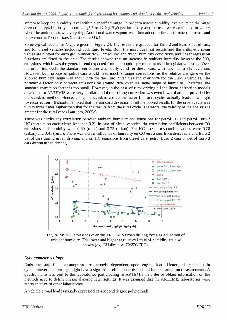
Emission factors 2009: Report 1 - methods for determining hot exhaust emission factors for road vehicles Version 7
TRL Limited 47 PPR353
system to keep the humidity level within a specified range. In order to assess humidity levels outside the rangedeemed acceptable in type approval (5.5 to 12.2 g/H2O per kg of dry air) the tests were conducted in winterwhen the ambient air was very dry. Additional water vapour was then added to the air to reach ‘normal’ and‘above-normal’ conditions (Laurikko, 2005c).
Some typical results for NOx are given in Figure 24. The results are grouped for Euro 2 and Euro 3 petrol cars,and for diesel vehicles including both Euro levels. Both the individual test results and the arithmetic meanvalues are plotted for each group under ‘low’, ‘medium’ and ‘high’ humidity conditions, and linear regressionfunctions are fitted to the data. The results showed that an increase in ambient humidity lowered the NOx
emissions, which was the general trend expected from the humidity correction used in legislative testing. Overthe urban test cycle the standard correction was nearly valid for diesel cars, with less than a 5% deviation.However, both groups of petrol cars would need much stronger corrections, as the relative change over theallowed humidity range was about 35% for the Euro 2 vehicles and over 55% for the Euro 3 vehicles. Thenormative factor only corrects emissions by around 20% over the same range of humidity. Therefore, thestandard correction factor is too small. However, in the case of rural driving all the linear correction modelsdeveloped in ARTEMIS were very similar, and the resulting correction was even lower than that provided bythe standard method. Hence, using the standard correction factor for rural cycles actually leads to a slight‘overcorrection’. It should be noted that the standard deviation of all the pooled results for the urban cycle wastwo to three times higher than that for the results from the rural cycle. Therefore, the validity of the analysis isgreater for the rural case (Laurikko, 2005c).
There was hardly any correlation between ambient humidity and emissions for petrol CO and petrol Euro 2HC (correlation coefficients less than 0.2). In case of diesel vehicles, the correlation coefficients between COemissions and humidity were 0.60 (rural) and 0.73 (urban). For HC, the corresponding values were 0.28(urban) and 0.41 (rural). There was a clear influence of humidity on CO emissions from diesel cars and Euro 2petrol cars during urban driving, and on HC emissions from diesel cars, petrol Euro 2 cars or petrol Euro 3cars during urban driving.
Figure 24: NOx emissions over the ARTEMIS urban driving cycle as a function ofambient humidity. The lower and higher regulatory limits of humidity are also
shown (e.g. EU directive 70/220/EEC).
Dynamometer settings
Emissions and fuel consumption are strongly dependent upon engine load. Hence, discrepancies indynamometer load settings might have a significant effect on emission and fuel consumption measurements. Aquestionnaire was sent to the laboratories participating in ARTEMIS in order to obtain information on themethods used to define chassis dynamometer settings. It was assumed that the ARTEMIS laboratories wererepresentative of other laboratories.
A vehicle’s road load is usually expressed as a second degree polynomial:

Emission factors 2009: Report 1 - methods for determining hot exhaust emission factors for road vehicles Version 7
TRL Limited 48 PPR353
Road load power = A×v2 + B×v + C (Equation 2)
Where:
A = the coefficient for driving resistance, dependent on the square of the speedB = the coefficient for driving resistance, linearly dependent on speedC = the coefficient for driving resistance, independent of speedv = the speed
The coast-down method is commonly used to define the road load of a vehicle, and the procedure is describedin Directive 70/220/EEC. The method is based on the equilibrium of vehicle inertia with vehicle drag androlling resistance during deceleration, with the gear positioned in neutral. The reference mass is determinedeither by weighing or by using information from vehicle registration documents. Alternatively, look-up tablesare provided in Directive 70/220/EEC, in which the coefficients A and C are presented for different referencemass classes. Most of the ARTEMIS laboratories either used road load information derived from coast-downtests or the look-up tables in the Directive.
Two extreme chassis dynamometer settings (minimum and maximum) and one average setting for static roadload and vehicle inertia were defined (Vermeulen, 2005). It was assumed that the polynomial approach of theroad load determined from a coast-down procedure gave the best approximation of the ‘true’ (average) roadload. Potential errors during testing (e.g. reference mass, speed, dynamometer load) were used to determinethe minimum and maximum road loads. The error on the chassis dynamometer load was taken to be ±5%. Thethree sets of settings were used to perform emission tests on five vehicles using the cold-start NEDC and thethree hot-start ARTEMIS driving cycles (Vermeulen, 2005).
There was found to be a statistically significant effect of the dynamometer settings on CO2 emissions and fuelconsumption for both petrol and diesel cars. CO2 and fuel consumption increased with an increase in roadload. Deviations of -12% to -4% were observed for the results of the minimum settings compared with theaverage settings. Deviations of +2% to +25% were observed for the results of the maximum settings comparedwith the average settings. The effect varied with the driving cycle.
Higher loads may cause higher drive line efficiency, but the cycle characteristics determine the share of staticand dynamic situations during the driving cycle. Because the relationship between the chassis dynamometersettings over different driving cycles and FC (or CO2) is not proportional, the results should be used to define arange of uncertainty caused by worst case chassis dynamometer settings. For the regulated components CO,HC and PM, no statistically significant influences were observed for petrol and diesel vehicles. NOx emissionsfrom petrol vehicles were also unaffected. However, a clear positive correlation was observed between NOx
emissions from diesel cars and the road load setting. This was according to expectations, as diesel enginescommonly produce more NOx when they operate at higher engine loads. In the case of CO emissions frompetrol vehicles, an increase was observed over the ARTEMIS rural and motorway cycles using high road loadsettings, but again this effect was not significant. From the theory, however, it would be expected that CO andHC emissions increase at very high engine loads. From the results of this investigation there were no clearindications that altered chassis dynamometer settings explicitly influenced emissions of CO, HC, NOx or PM.The very small size of the vehicle samples (three petrol cars and two diesel cars) did not permit a clearerconclusion. It was found that chassis dynamometer settings may vary depending on the method chosen todetermine the settings, the accuracy of the method and the variation of ambient conditions. Because the effectsof altered settings on CO2 (and fuel consumption) are significant, it is recommended that the methods used todetermine the chassis dynamometer settings should be investigated for systematic errors (Vermeulen, 2005).
Dilution ratio
The dilution of the exhaust gases by non-polluted air forms the basis of the constant volume sampler (CVS).The dilution ratio varies according to the exhaust flow, but must remain within a limited range. The effects ofchanges in the dilution ratio were investigated for a total of eight diesel and petrol vehicles. Between two andfive different dilution ratios were tested per vehicle. When the results were presented as a percentage deviationfrom the reference value - the emission value for the dilution ratio that would be normally selected for therespective measurement – no systematic trends were observed. The only notable exceptions were diesel PMemissions, for which there was a tendency towards higher emissions with an increase in the dilution ratio, andHC, for which the trend was in the opposite direction. The decrease in HC emissions may be attributed to thehigher condensation of particles which is measured as an increase in PM emissions (Geivanidis et al., 2004).
Emission factors 2009: Report 1 - methods for determining hot exhaust emission factors for road vehicles Version 7
TRL Limited 49 PPR353
Sample line temperature
For diesel vehicles the exhaust sample line must be heated to 190°C, according to the standard procedure, inorder to avoid liquefaction of some hydrocarbons. The effects of a lower sample line temperature (160oC)were investigated. The lower temperature resulted in higher HC emission values, but this observation wascontrary to expectations, as the point of heating to the higher temperature is to increase the fraction of HCretained in sample (Geivanidis et al., 2004).
PM filter preconditioning
A diesel passenger car was tested using PM filters preconditioned at different temperatures and humiditylevels. The procedure consisted of reference tests with conditioning and weighing of the particle filters at anaverage temperature and humidity in a conditioning room, and emission tests were conducted using thedefined minimum and maximum values for these conditions. The minimum and maximum values weredefined by the capability of the climate control system to adjust to a certain range of temperature andhumidity. No effects of filter preconditioning were observed, and all variations were within the repeatabilityranges (Geivanidis et al., 2004).
Response time
The delay of emission measurements caused by the CVS system and the analysers is crucial for instantaneousmeasurements and second-by-second emission modelling, but also for standard HC measurements on dieselengines. As delay times may vary due to different concentrations, temperatures and pressures, the gas flowthrough the CVS system was modelled to find a correction function of the recorded emissions.
There are several potential systematic problems associated with instantaneous emission measurement. Theemissions recorded at the analysers are delayed and smoothed compared with the emission events at thelocation of formation due to (i) the transport of the exhaust gas to the analysers, (ii) the mixing of exhaust gasespecially in the silencer and the CVS tunnel and (iii) the response time of the analysers. The transport time ofthe exhaust gas to the analyser is determined by the air flow velocity in the exhaust system of the vehicle andthe CVS tunnel, and in the related connection pipes. The velocity of the undiluted exhaust gas is highlyvariable over time, since it depends on the exhaust gas volume flow. The volume flow mainly depends on theengine speed and engine load. When combined, the varying transport times and the analyser response timescan shift the signal by around 1-10 seconds (depending on the engine, the exhaust system, the CVS system, theanalyser used and the engine load). Mixing effects during the gas transport and the analyser responsebehaviour also add a smoothing effect on the signals. These inaccuracies are usually compensated over thecomplete test cycle, such that the integral of the instantaneous measurement agrees with the bag value.However, in most instantaneous emission models the mapping of emissions is performed by statically relatingthe emission signals to causative variables such as vehicle speed, vehicle acceleration and engine speed. As aresult of this static approach, the emission values can be correlated to the correct engine state of the car only ifthey are at the correct location on the time scale. Thus, instantaneous models are heavily affected byinaccurate time alignments.
It was noted by Weilenmann et al. (2003) that modern petrol cars with three-way catalysts and lambda controlemit most of their pollutants during transient emission peaks. These peaks typically last between 0.5 secondsand 1 second, and show a frequency content of about 3–5 Hz. A significant part of the detail of the signals istherefore lost at the usual sampling rate of 1 Hz. The authors recommend a sampling frequency of 10 Hz.
In order to minimise the errors resulting from inaccurate time alignments, EMPA and TUG developedmethods to compensate for the delay and smoothing of instantaneous emission measurements. Speciallycalibrated for the respective chassis dynamometers, both methods are designed to explain the change in theemission value from their location of formation to the analyser signal by formulae, and to invert theseformulae to produce equations which transform the analyser signal into the engine out (or catalyst-out)emission value (Le Anh et al., 2005). The main difference between the TUG and EMPA models is that theEMPA model is more detailed but needs modal measured data on the exhaust gas volume flow andinformation on the volume of the exhaust gas system of the tested cars. The TUG model has a simplerapproach. However, both methods improve the quality of instantaneous emission signals significantly(Zallinger et al., 2005; Joumard et al., 2006b).
As an example, Figure 25 shows the oxygen signal at the catalyst outlet after it has been reconstructed fromthe analyser signal. The thick blue line is the signal measured by a fast oxygen analyser in situ at the catalyst-

Emission factors 2009: Report 1 - methods for determining hot exhaust emission factors for road vehicles Version 7
TRL Limited 50 PPR353
out location. The thin red line is measured by a standard oxygen analyser attached to a raw gas line, about 10m long, connected to the tailpipe of the car. The dotted green line is the signal which has been reconstructedfrom the red signal by compensating for the transport dynamics of the sampling line. The dashed black line isreconstructed from the green line, compensating for the time-varying transport in the car exhaust system.
Figure 25: Overall inversion of the instantaneous concentration measured bygas analyser, using the EMPA model.
Using signals from the diluted measurements, the quality of the reconstructed signals showed a maximum timeerror of 2.5 seconds, which is significantly better than using the original signal, which had a time error of up to25 seconds, but which is notably worse than using the raw line. From Figure 25 it is clear that usinguncorrected signals from modal measurements leads to huge errors in the allocation of emissions to thecorresponding engine operation conditions. Since the transport time of the undiluted part of the sample systemdepends on the exhaust gas volume flow, and thus on the engine load conditions, the misalignment betweenengine load and emission signal is highly variable over a test cycle. Thus, the constant time shift of measuredsignals used in previous models does not lead to a satisfactory result but to distorted vehicle emission maps.
Dilution air conditions
Measurements with ambient dilution air were compared with measurements using two different levels of‘polluted’ dilution air: a ‘low’ level and a ‘maximum’ level. The values considered as standard (0.4 ppm CO,3-4 ppm HC, 0.1-0.2 ppm NOx) were common to the participating laboratories. The low level of polluteddilution air (2-3 ppm CO, 11-12 ppm HC, 1-1.2 ppm NOx) was representative of the highest concentrationsmeasured in the ARTEMIS laboratories. The high level of polluted dilution air represented improbableconditions (11-12 ppm CO, 20-21 ppm HC, 5.5-6 ppm NOx), which could only been reached because of anincident such as a gas or fuel leak. In both cases, the dilution air pollution was obtained by injecting a specificquantity of CO, HC and NOx upstream of the dilution tunnel. For each of the three pollution levels, tworepetitions of each cycle were performed. Two vehicles were tested over cold-start and hot-start drivingcycles, but with the three levels of polluted dilution air. The significance of the differences between the resultsobtained using the three dilution air pollution levels was investigated using a one-way analysis of variance forCO, HC and NOx emissions. The results showed that for the level of pollution in the dilution air had nostatistically significant effect on the emission factors (with the exception of HC for one car during theARTEMIS urban cycle) (Prati and Costagliola, 2004). However, the work did not include particle numbermeasurements. The conditions of the dilution air (dilution ratio, temperature) do have a significant influenceon particle number measurements.
3.3.7 Round robin tests
In the ARTEMIS round robin, a single vehicle (a Euro 3 petrol car) was tested successively in the nineparticipating laboratories. The test schedule is shown in Table 16. The exercise lasted almost 8 months. Thevehicle started the tour with a full fuel load, and that fuel was continuously used in the successive tests until
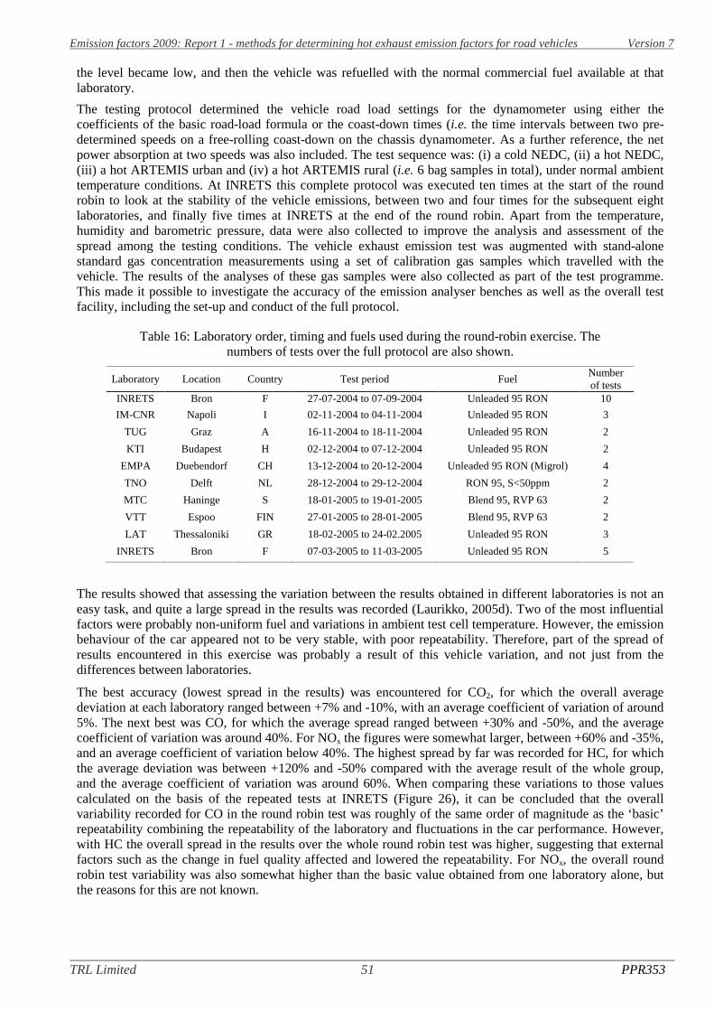
Emission factors 2009: Report 1 - methods for determining hot exhaust emission factors for road vehicles Version 7
TRL Limited 51 PPR353
the level became low, and then the vehicle was refuelled with the normal commercial fuel available at thatlaboratory.
The testing protocol determined the vehicle road load settings for the dynamometer using either thecoefficients of the basic road-load formula or the coast-down times (i.e. the time intervals between two pre-determined speeds on a free-rolling coast-down on the chassis dynamometer. As a further reference, the netpower absorption at two speeds was also included. The test sequence was: (i) a cold NEDC, (ii) a hot NEDC,(iii) a hot ARTEMIS urban and (iv) a hot ARTEMIS rural (i.e. 6 bag samples in total), under normal ambienttemperature conditions. At INRETS this complete protocol was executed ten times at the start of the roundrobin to look at the stability of the vehicle emissions, between two and four times for the subsequent eightlaboratories, and finally five times at INRETS at the end of the round robin. Apart from the temperature,humidity and barometric pressure, data were also collected to improve the analysis and assessment of thespread among the testing conditions. The vehicle exhaust emission test was augmented with stand-alonestandard gas concentration measurements using a set of calibration gas samples which travelled with thevehicle. The results of the analyses of these gas samples were also collected as part of the test programme.This made it possible to investigate the accuracy of the emission analyser benches as well as the overall testfacility, including the set-up and conduct of the full protocol.
Table 16: Laboratory order, timing and fuels used during the round-robin exercise. Thenumbers of tests over the full protocol are also shown.
Laboratory Location Country Test period FuelNumberof tests
INRETS Bron F 27-07-2004 to 07-09-2004 Unleaded 95 RON 10
IM-CNR Napoli I 02-11-2004 to 04-11-2004 Unleaded 95 RON 3
TUG Graz A 16-11-2004 to 18-11-2004 Unleaded 95 RON 2
KTI Budapest H 02-12-2004 to 07-12-2004 Unleaded 95 RON 2
EMPA Duebendorf CH 13-12-2004 to 20-12-2004 Unleaded 95 RON (Migrol) 4
TNO Delft NL 28-12-2004 to 29-12-2004 RON 95, S<50ppm 2
MTC Haninge S 18-01-2005 to 19-01-2005 Blend 95, RVP 63 2
VTT Espoo FIN 27-01-2005 to 28-01-2005 Blend 95, RVP 63 2
LAT Thessaloniki GR 18-02-2005 to 24-02.2005 Unleaded 95 RON 3
INRETS Bron F 07-03-2005 to 11-03-2005 Unleaded 95 RON 5
The results showed that assessing the variation between the results obtained in different laboratories is not aneasy task, and quite a large spread in the results was recorded (Laurikko, 2005d). Two of the most influentialfactors were probably non-uniform fuel and variations in ambient test cell temperature. However, the emissionbehaviour of the car appeared not to be very stable, with poor repeatability. Therefore, part of the spread ofresults encountered in this exercise was probably a result of this vehicle variation, and not just from thedifferences between laboratories.
The best accuracy (lowest spread in the results) was encountered for CO2, for which the overall averagedeviation at each laboratory ranged between +7% and -10%, with an average coefficient of variation of around5%. The next best was CO, for which the average spread ranged between +30% and -50%, and the averagecoefficient of variation was around 40%. For NOx the figures were somewhat larger, between +60% and -35%,and an average coefficient of variation below 40%. The highest spread by far was recorded for HC, for whichthe average deviation was between +120% and -50% compared with the average result of the whole group,and the average coefficient of variation was around 60%. When comparing these variations to those valuescalculated on the basis of the repeated tests at INRETS (Figure 26), it can be concluded that the overallvariability recorded for CO in the round robin test was roughly of the same order of magnitude as the ‘basic’repeatability combining the repeatability of the laboratory and fluctuations in the car performance. However,with HC the overall spread in the results over the whole round robin test was higher, suggesting that externalfactors such as the change in fuel quality affected and lowered the repeatability. For NOx, the overall roundrobin test variability was also somewhat higher than the basic value obtained from one laboratory alone, butthe reasons for this are not known.

Emission factors 2009: Report 1 - methods for determining hot exhaust emission factors for road vehicles Version 7
TRL Limited 52 PPR353
Figure 26: Relative emission deviation for each laboratory, in comparison with theaverage all laboratories considered (average for all cycles together for eachcomponent), as measured during the round robin test, with high-low bars marking thelargest deviations.
A closer assessment of the data revealed that it was not possible to develop any ‘correction factor’ or ‘labfactor’ which could be applied to the full database of results collected in ARTEMIS. This conclusion wasmainly based on two factors. The first of these factors was the quite long temporal span (over one year)between the round-robin exercise and the initial testing phase, during which time some the measurementequipment had been upgraded, and in one case the entire facility upgraded (the CVS, analysers and chassisdynamometer were renewed at TUG). Therefore, it was probable that the results measured in this round robinexercise were different from those that would have been obtained if the round robin test had been executedparallel to the actual testing itself (this was not possible for a number of reasons). Secondly, when differentdriving cycles were used the spread of results became random, and none of the laboratories showedconsistently higher or lower results compared with the average. Instead, laboratories could show resultshigher-than-average in one test case (driving cycle or pollutant), and vice versa when another driving cycle orpollutant was considered. Only if each of the pollutants was considered separately could a few cases be foundin which the results of a laboratory over all cycles tested could be consistently higher or lower than theaverage. This can be seen in Figure 26, which shows the emission variation (all cycles) for each laboratory.Even in those laboratories which appear, overall, to lay above or below the average of the group, high or lowbar ends extend to the other side of the y-axis, indicating that the overestimation (or underestimation) was notconsistent.
3.4 Effects of different test parameters: heavy-duty vehicles
3.4.1 Background
The information in this Section of the Report is derived from the ARTEMIS work on HDVs (Rexeis et al.,2005). The main aims of the work were:
(i) To collect a large amount of HDV emission data from a range of European sources. Emissionmeasurements for 102 heavy-duty engines were obtained from ARTEMIS and other national andinternational programmes, culminating in the most extensive database on HDV emissions in Europe.
(ii) To develop a model capable of accurately simulating emission factors for all types of HDV over anydriving cycle and for various vehicle loads and gradients. The resulting tool – PHEM (Passenger carand Heavy-duty Emission Model) - estimates fuel consumption and emissions (CO, THC, NOx and PM)based on the instantaneous engine power demand and engine speed during a driving cycle specified bythe user. The model combines steady-state engine maps with correction functions for transient operation.

Emission factors 2009: Report 1 - methods for determining hot exhaust emission factors for road vehicles Version 7
TRL Limited 53 PPR353
(iii) To acquire the necessary model input data. Representative driving cycles were developed as modelinputs. These were obtained through a review of the literature, an extensive analysis of all available on-board measurement data from driving behaviour studies, and a tailored measurement programme.
(iv) To generate a database of emission factors for the ARTEMIS inventory model. An emission factor andfuel consumption database for conventional HDVs was compiled using PHEM, based upon typicalvehicle data, engine data and representative driving cycles. Emission factors were produced for almost170,000 combinations of pollutant, vehicle category, Euro class, driving cycle, vehicle load and roadgradient. The effects of fuel quality, level of vehicle maintenance and various other factors were alsoinvestigated in detail.
Although HDVs were studied in great detail in ARTEMIS, the investigation of emission test parameters wasless extensive than that for cars, and there was no round-robin programme. Nevertheless, information wasobtained on a number of different parameters which are important for emission factor development, and thisinformation is summarised below.
3.4.2 Emission-control technology
The newest vehicles tested in ARTEMIS were compliant with the Euro III emission standard. In order toachieve the Euro IV and Euro V limits PM emissions will have to be reduced by approximately 70% to 90%compared with Euro III. The reductions in NOx emissions to reach Euro V range from 50% to nearly 70%. Thetechnologies required to achieve such reductions will make the overall system much more complex.
The assessment of the emission behaviour of engines meeting the Euro IV and Euro V standards was highlyuncertain, as no production vehicles were available for measurement. Furthermore, the effects of newtechnologies (e.g. SCR, particle oxidation catalysts) were difficult to predict. It was concluded from themeasurement programme on Euro II and Euro III engines that simply extrapolating emission factors fromolder engine technologies to future standards according to the future emission limits is not a suitable approach.
Compared with Euro III diesel engines, Euro IV and Euro V engines must also comply with the emissionlimits during the ETC. Consequently, optimisation at the single test points of the ESC will not be sufficient tomeet the emission limits at type approval. With this regulation it can be assumed that emission levels duringreal-world driving conditions may decrease more compared with Euro III than the reduction in the emissionlimit suggests. However, most of the ETC is located in the same region of the engine map as the ESC. Thus, itwill not be absolutely necessary for a manufacturer to optimise the emission levels over the complete enginemap in order to meet the emission limits.
In general, three approaches for meeting the Euro IV and Euro V type approval limits will be available in thenear future: improved engine technology, exhaust gas after-treatment and alternative combustion concepts.Whilst compliance with the Euro IV limits could be achieved with improved conventional engine technologies(fuel injection, exhaust gas recirculation, variable turbine geometry at the turbo charger, etc.), this is ratherunlikely for Euro V. For example, the engine efficiency would be unacceptable for reaching the 2 g/kWh NOx.Using exhaust gas after-treatment systems could reduce NOx and PM to the targeted levels, but the problemswith these systems are their unproven durability and the additional investment costs. Potential technologies forEuro IV and Euro V engines are briefly discussed below
PM-reduction technologies
Various filter-based after-treatment systems are currently being developed to reduce PM emissions fromHDVs – these are collectively known as diesel particulate filters (DPFs). For all these systems, the maintechnological challenges are controlled regeneration of the filter and durability. Particulate filters also haveadditional investment costs, and result in a slight penalty in terms of fuel efficiency (1-3%). Therefore,research is under way to improve engine technology so that PM limit values can be met without the use offilters. The systems described below are examples of current developments.
• Continuously-regenerating trap (CRTTM, Johnson Matthey). This technology uses the NOx in the exhaustgas to continuously regenerate the trap. An oxidation catalyst is placed upstream of the filter to convert NOto NO2. This process requires temperatures above 230°C to start the filter regeneration, and 350°C toachieve equilibrium. Additional systems for active regeneration may be needed, such as electrical or fuelburner heaters, potentially supported by a fuel additive.

Emission factors 2009: Report 1 - methods for determining hot exhaust emission factors for road vehicles Version 7
TRL Limited 54 PPR353
• Fuel-borne catalysed filter. In this system, an additive is used to reduce the soot ignition temperature. Theadditive is introduced into the fuel tank after refuelling. The additives currently used are cerium, iron andstrontium. The main disadvantage of this approach is the need for an additional tank for the additive.
• Diesel particulate catalyst. Besides filter-based systems, in which the exhaust gas flows through a porousmedium, ‘open’ systems have recently been developed. Due to the special shaping of the catalyst, theexhaust gas flows into a storage medium where particles are deposited. If the storage medium is full, theexhaust flows through the open channels of the catalyst without further separation of the particles. As soonas the catalyst reaches the regeneration temperature, the particles are burnt off and the system can work atthe original efficiency level.
NOx-reduction technologies
There are currently two main approaches for reducing NOx emissions: selective catalytic reduction (SCR), andexhaust gas re-circulation (EGR). In the SCR system, urea is dissolved in water and is injected into the exhaustgas stream, where a hydrolysis process converts it into CO2 and NH3. Alternatively, the NH3 can be producedfrom ammonium carbonate. The ammonia is used as a NOx-reducing agent, producing nitrogen and water inthe catalyst. To prevent ammonia from passing into atmosphere (ammonia slip) an oxidation catalyst is usuallyfitted downstream of the SCR catalyst. EGR is used to reduce NOx emissions by recirculating a portion of theexhaust gas back into the combustion chamber. This reduces the oxygen available for combustion, and leads tolower peak temperatures, thus inhibiting the formation of NOx. There are different principles of exhaust gasrecirculation: (i) external high-pressure EGR, (ii) external low-pressure EGR and (iii) internal EGR. All ofthese options may be used in Euro IV and/or Euro V HDV engines. An alternative after-treatment method -NOx adsorption - requires the engine to be run periodically with a rich air:fuel ratio, which increases fuelconsumption. As a consequence, SCR tends to be used in preference to NOx adsorption in HDV applications.No manufacturer is currently planning to introduce NOx-adsorption technology in the European HDV market.
Effects on emission maps
The main issue relating to the determination of emission maps for Euro IV and Euro V engines was whetherthe technologies used would have a varying efficiency over the engine map. High fuel efficiency is the mainaim for HDV engine manufacturers, and is crucial for competitiveness in the sector. For Euro IV and Euro Vvehicles, it must also be assumed that manufacturers will continue to focus on fuel efficiency for lowinvestment and running costs. Consequently, the following assumptions were made in ARTEMIS for Euro IVand Euro V engines (Rexeis et al., 2005):
(i) It was assumed for the development of the basic emission maps that DPFs would not be widely used inEuro IV and Euro V engines. A reduction in PM emissions will be achieved via optimised fuel injectionand combustion processes, in combination with an oxidation or particulate catalyst, but without theapplication of a DPF. Available measurements from a Euro V SCR test engine11 have shown PMemissions 40% lower than the Euro V limit value, over both the ESC and ETC cycles.
(ii) In the ARTEMIS model, the option of ‘DPF-technology’ can be chosen, which assumes a reduction inPM mass of approximately 90%, and an increase in fuel consumption of 3%, compared with the relevantbasic engine emission map.
(iii) For NOx emissions, the basic technology for compliance with the Euro IV limits will be SCR. EGR withPM-cats will be applied mainly to some smaller vehicles. The potentially different pollutant emissionbehaviour associated with SCR and EGR cannot be properly assessed at present. All Euro V HDVs willuse SCR technology.
(iv) The application of SCR will be optimised in the regions of the engine map covered by the type approvaltests (ETC and ESC). It is unlikely that emission-reduction strategies (e.g. urea dosing with SCR) will beapplied to all regions of the engine map where there is no urgent requirement to do so, as this wouldimply penalties in terms of fuel consumption and cost.
11 Measurements of a Euro V test engine with SCR technology, and the corresponding basic Euro III engine, were made available fromthe PARTICULATES project.

Emission factors 2009: Report 1 - methods for determining hot exhaust emission factors for road vehicles Version 7
TRL Limited 55 PPR353
(v) OBD systems will be installed, limiting NOx emissions everywhere on the engine map to 5 g/kWh forEuro IV and to 3.5 g/kWh for Euro V12. Without such control systems, especially at low engine speeds,much higher NOx levels than currently indicated by the emission factors could emerge. This coulddrastically increase the emission factors for urban and rural driving. For this reason, the in-use control offuture-technology vehicles seems to be necessary.
(vi) The application of the SCR system allows for higher raw exhaust NOx emissions. This enables furtheroptimisation of fuel consumption (earlier injection timing). Compared with Euro III engines, reductionsof around 7% (for Euro IV engines) and 5% (Euro V engines) are predicted.
The actual effects applied in PHEM may be rather optimistic, since rational electronic engine control strategiesand a restrictive OBD are assumed for all vehicles everywhere in the engine map. These assumptions are notreflected completely in the actual type approval Directive for Euro IV and Euro V.
3.4.3 Alternative fuels
Currently, the only alternative fuels that have reached appreciable shares of the HDV market are compressednatural gas (CNG), bio-diesel and liquefied petroleum gas (LPG). Emission factors had to be estimated fromthe available literature. For modern LPG-fuelled HDVs, no satisfactory data on emission levels were found, sono emission factors could be provided (Rexeis et al., 2005).
Compressed natural gas (CNG)
CNG is used in SI engines with special fuel injection. Early CNG engines were operated almost exclusivelystoichiometrically, and were able to reach very low emission levels for NOx, CO, HC and PM, at least whennew. Durability tests for modern vehicles are not commonly available, and some early examples showed pooremission stability over time. A disadvantage of CNG is the much lower fuel efficiency compared with dieselengines. Energy consumption from stoichiometric CNG engines is at least 10% higher than that for dieselHDVs. For this reason, modern CNG vehicles tend to equipped with lean-burn engines. A disadvantage of thelean-burn engine is that the catalytic converter does not reduce NOx emissions during lean-burn conditions.Thus, as with diesel engines, the same principle trade-off between NOx and fuel efficiency occurs. Therefore,the use of CNG does not necessarily provide benefits in terms of NOx emissions.
Table 17 summarises the emission levels of modern CNG engines as a percentage of the Euro III emissionfactors. Compared with Euro IV and Euro V diesel engines the advantages of CNG would diminish, since theEuro IV and Euro V limits require clear reductions in NOx and PM emission levels. Of course, furtheremission reductions could also be achieved for CNG vehicles (Rexeis et al., 2005).
Table 17: Emission levels of a CNG-fuelled HDV relative to the emission factors for a Euro IIIHDV (ratios based on real-world cycles; [g km-1] for emission and fuel consumption values).
Technology NOx PM CO THC NMHC FC
Diesel Euro III 100% 100% 100% 100% 100% 100%CNG EEV a 85% 10% 15% 300% 25% 120%
a Enhanced Environmental Friendly Vehicle with lean-burn concept.
Bio-diesel
For the HDV sector, compliance with the European Biofuels Directive – stating that a 5.75% share of the fuelused in 2010 must be biofuel – may, to a large extent, be realised by the use of bio-diesel. If the existingDirectives on fuel quality are met, bio-diesel can be used in many HDVs without major modification, as longas important criteria for the storage of bio-diesel and the method for replacement of fossil diesel areconsidered. While the blending of up to 5% bio-diesel does not affect emission levels very much, the use ofpure bio-diesel certainly has an effect on the emission behaviour of diesel engines. Measurements indicate anincrease in NOx emissions of 10-20% but reduced PM emissions (although for some vehicles and test cycles
12 In the low-load engine map area, this limitation will probably not be practicable, because very low absolute NOx emissions have tobe detected by the OBD system.

Emission factors 2009: Report 1 - methods for determining hot exhaust emission factors for road vehicles Version 7
TRL Limited 56 PPR353
an increase in PM was observed). Also, the source of bio-diesel (vegetable oil from rape seed, palm, soybean,used cooking oil, animal fat from tallow, etc.) influences the emission changes resulting from fossil fuel beingsubstituted by bio-diesel. Therefore, the emission changes associated with a shift from fossil diesel to bio-diesel given in Table 18 have to be seen as average estimates.
Table 18: Emission levels of HDVs driven with bio-diesel instead of fossil diesel(ratios based on g km-1 emission and fuel consumption values).
Fuel NOx PM CO THC NMHC FC
Conventional diesel (Euro III) 100% 100% 100% 100% 100% 100%
Bio diesel a 120% 80% 75% 60% 50% 115%
a Average ratios if fossil diesel is replaced by bio-diesel.
3.4.4 Effects of engine deterioration and maintenance
Emissions from HDVs are influenced by the age of the engine and the maintenance condition. In order todetermine whether this influence had to be taken into account in the ARTEMIS model, the effects of enginedeterioration and maintenance on emissions were assessed using extensive data on pre-Euro I to Euro IIIvehicles from the Dutch and German in-use compliance programmes. For Euro I and Euro II vehicles it wasassumed that maintenance would result in the changes shown in Table 19. The overall effect was calculated bymultiplying the percentage of vehicles needing maintenance by the average reduction in emissions imposed byapplying the necessary maintenance. The reductions were weighted for potential differences in fuelconsumption as a result of maintenance, since this would have had a secondary influence on the emission levelduring the tests.
Table 19: Average emission effects (% change) as a result ofmaintenance activities, and the expected overall effect on
average Euro I and Euro II fleet.
Percentage of vehiclesneeding maintenance
Euro I Euro II
52% 33%
Average effect on PM -15% -23%
Average effect on NOx -3% -2%
Average effect on CO -17% -4%
Average effect on HC 2% -11%
Overall effect on PM -8% -7%
Overall effect on NOx -1% -1%
Overall effect on CO -9% -1%
Overall effect on HC 1% -4%
For Euro III vehicles equipped with electronic fuel pumps and an engine management system, the condition ofthe fuel injectors can be expected to be the main issue. However, none of the Euro III vehicles tested inARTEMIS had injector problems. On the other hand, these vehicles were relatively new, with odometerreadings not exceeding 180,000 km. Based on the Euro II data, around 20% of the vehicles had problemsrelating to the injectors, resulting in an average PM increase of around 18%. Over the vehicle fleet this equatesto an average increase of 3-4% for Euro II vehicles, and probably less for Euro III vehicles. For the otherpollutants the increase in emissions from Euro III vehicles is likely to be insignificant (Rexeis et al., 2005).
3.4.5 Effects of fuel quality
An approach was proposed for including fuel quality effects in the ARTEMIS model (Rexeis et al., 2005 andreferences therein), whereby a percentage change in emissions was applied to the basic emission factors. Thisapproach required a baseline fuel to be defined, from which changes could be evaluated. Baseline fuel

Emission factors 2009: Report 1 - methods for determining hot exhaust emission factors for road vehicles Version 7
TRL Limited 57 PPR353
properties for pre-Euro I, Euro I and Euro II engines were taken from the Worldwide Diesel Fuel QualitySurveys. Baseline fuel properties for Euro III engines were defined based on the average quality of thecorresponding fuels used in the ARTEMIS tests. Baseline fuel properties for Euro IV and Euro V engines wereestimated based on the requirements of vehicle and engine manufacturers, as published in the latest World–Wide Fuel Charter. The proposed baseline fuel properties are summarised in Table 20.
Table 20: Baseline fuel properties (Rexeis et al., 2005).
Emissionlegislation
Density(kg/m3)
Cetanenumber
Cetanedifference
Poly-aromatics
(%)
Totalaromatics
(%)
T10(oC)
T50(oC)
T95(oC)
SulphurContent(ppm)
Oxygencontent(%m)
Pre-Euro1 835 51 0 6 25 205 260 345 1500 0
Euro I 835 51 0 6 25 205 260 340 1300 0
Euro II 830 53 0 5 20 205 260 340 300 0
Euro III 830 53 0 4 20 210 265 340 40 0
Euro IV 830 55 0 2 15 210 265 340 10 0
Euro V 830 55 0 2 15 210 265 340 5 0
The percentage changes in emissions were calculated using the models described below. These could then beapplied to the emission factors estimated by the main model, based on the baseline fuels. According to Rexeiset al. (2005) the most comprehensive investigations of the effects of fuel properties on HDV emissions havebeen carried out within the scope of the following programmes
• European programme on emissions, fuels and engine technology (EPEFE).• US EPA heavy-duty engine working group programme (EPA-HDEWG).• US diesel emission control – sulphur effects programme.• USEPA project on modelling effects of diesel fuel properties on heavy-duty engine emissions (‘New
EPA’).
Rexeis et al. (2005) recommended the use of the following models:
• The EPEFE model for assessment of fuel effects on CO and PM emissions.• The New EPA model for assessment of fuel effects on HC and NOx emissions.
The forms of these models are shown in Table 21.
Table 21: EPEFE and new EPA regression equations.
Pollutant EPEFE [g/kWh] New EPA, [g/hp h]
CO = 2.24407-0.00111D+0.00007P-
0.00768C-0.00087T95
HC = Exp(5.32059-0.1875CN+0.001571CN2-
0.0009809T10-0.002448T50-
0.1880CD+0.003507CN*CD)
NOx = Exp(0.50628-0.002779CD+0.002922A+1.3966G-
0.0004023T50)
PM = (0.06959+0.00006D+0.00065P-
0.00001C)*[1-0.000086(450-S)]
D – density, kg/m3; G – specific gravity; P – poly-aromatics content, % m; A – total aromatics content, %vol; C – cetane number; CN – natural cetane number; CD – cetane difference due to additising; S – sulphurcontent, ppm; T10 – T10 temperature, oF; T50 – T50 temperature, oF; T95 – T95 temperature, oC.
Emission factors 2009: Report 1 - methods for determining hot exhaust emission factors for road vehicles Version 7
TRL Limited 58 PPR353
3.5 Effects of different test parameters: two-wheel vehicles
The ARTEMIS work on emissions from two-wheel vehicles is summarised in the report by Elst et al. (2006).One of the main objectives was to develop a set of representative emission factors, and an extensivemeasurement programme was conducted, involving tests on 90 motorcycles. Before the measurementprogramme began a round robin test programme was carried out to check whether the results over differentdriving cycles were reproducible when measured in different laboratories, and to identify potentialmeasurement difficulties. The sensitivity of emissions to fuel properties and inspection and maintenance wasalso examined. This work is relevant to the development of emission factors for two-wheel vehicles in the UK.
3.5.1 Round robin test programme
Bremmers et al. (2001) described the round robin test programme. Where reference is made to Directive97/24/EC, the status of that Directive in 2001 is implied. The measurement programme was carried out over aperiod of 14 months. Two different motorcycles were used: a two-stroke scooter with no exhaust gas after-treatment and a four-stroke ‘sports bike’ with a three-way catalyst. The round robin began at TNO in Delft.The motorcycles then travelled to KTI (Bucharest), FHB (Biel), TÜV-Nord (Hannover) and back to TNO. Thepetrol fuel used in the programme was similar at all laboratories.
The following general conclusions and recommendations were drawn from the round robin tests:
• The chassis dynamometer emission measurements carried out on motorcycles in the different laboratoriesagreed, depending on the pollutant, within a range of about ±25%.
• The range of emission levels for two-wheel vehicles can be much wider than that for modern passengercars (e.g. 0.3-30 g km-1 for CO). Tests on vehicles with comparable emission levels should be conductedduring the same session using appropriate analyser ranges and tunnel flow rates. Directive 97/24/ECprescribes that the dilution air should be analysed using the same analyser range as that used for the dilutedexhaust gas. Since the selected range for analysing the exhaust gas could be very high, zero values might beobtained for the dilution air. The dilution air should be analysed over a more suitable (lower) range, and theanalyser should be calibrated over both the selected ranges before the bags are analysed.
• Brake load settings can be relatively small and therefore difficult to simulate. A single, easy-to-use methodshould be defined for brake load settings and analyser calibration procedures.
• Highly dynamic test cycles, in combination with a high power:mass ratios and/or the presence of electronicengine management systems or exhaust gas after-treatment, may result in poor repeatability.
• Improvement to the running resistance table prescribed by Directive 97/24/EC13 should be made, since thebrake load settings are not suitable for high-speed cycles.
• Test drivers should be acquainted with the cycles to be driven and the specific behaviour of the testvehicles.
• Improvements to the response times in brake load simulation are required, as test cycles will become moredynamic.
• There should be further investigation of the poor repeatability for modern vehicles equipped with three-waycatalysts.
3.5.2 Vehicle categorisation
Because of the wide variation in vehicle weight, engine capacity, engine type (two- or four-stroke) and exhaustgas after-treatment technology, it is important to define appropriate vehicle categories for emission testingpurposes. The main parameters which were considered are listed below (Rijkeboer, 2000).
Engine capacity: Since 'mopeds' (< 50 cm3) were not taken into account within ARTEMIS, the followingdistinction was made: 50-125 cm3, 126-250 cm3, 251-500 cm3, 501-750 cm3, 750-1000 cm3 and > 1000 cm3.
Engine type: Throughout Europe two-wheel vehicles are equipped with two-stroke and four-stroke petrolengines (except for one diesel model and a few electric models). For the purpose of categorising
13 Directive 2003/77/EC contains a new running resistance table.

Emission factors 2009: Report 1 - methods for determining hot exhaust emission factors for road vehicles Version 7
TRL Limited 59 PPR353
motorcycles, a distinction between these two main engine types was therefore required. Because two-strokeengines tend to have a small engine capacity, and are mostly used on scooters, the distinction was onlyapplied to motorcycles with an engine capacity of less than 250 cm3.
Exhaust gas after-treatment: In time, more two-wheel vehicles will be equipped with exhaust gas after-treatment systems (e.g. oxidation catalyst, ‘coated tube’ or three-way catalyst), but relatively few data wereavailable to evaluate their performance under real-world driving conditions. For categorisation purposes, adistinction between catalyst and non-catalyst motorcycles was therefore applied.
Age, mileage and legislative category: The age of a vehicle is linked to its technology level and the emissionlegislation to which it conforms.
Model: Different types of motorcycle model are currently available on the market. Since each type ofmotorcycle has its own characteristics, a broad division between the following model classes wasestablished: ‘scooters’, ‘off-road’, ‘enduro’, ‘touring’, ‘choppers’, ‘sports’ and ‘super-sports’.
3.5.3 Other issues
During the round robin tests, differences were apparent between the ways in which tests were conducted at thedifferent laboratories (Bremmers et al., 2001). These were addressed as follows:
Dilution ratio: Depending on the motorcycle to be tested, the test cycle to be driven, and the analyser ranges, asuitable dilution ratio should be chosen in order to measure all pollutants with sufficient accuracy.
Procedure for analysing bag samples: The procedure to be used to analyse the bags (for dilution air as well asfor exhaust gas) was improved following the recommendations of the round robin programme. A flow chartdescribing the procedure for emission bag analysis was developed to ensure common understanding.
Vehicle condition: Each motorcycle had to have been driven for at least 1,000 km before the test, but otherwisevehicles were tested in the ‘as received’ condition.
Deceleration phases: In the type approval test, specific operation is required during deceleration phases.However, this specific operation might not be valid for real-world operation, and therefore was not be appliedduring such cycles.
Engine starting, restarting and emission sampling: The procedure was a combination of both European andUS Directives. The pre-conditioning cycle conducted before the type approval cycle included an engine start.All other test cycles were started with a running engine. Again, a detailed procedure was developed.
Choke operation: A specific procedure was included for choke operation, since most of the motorcycles testedwere still equipped with a manual choke.
Data processing: A test report template was developed to ensure consistency.
3.5.4 Driving cycle effects
CO emissions were similar over type approval and real-world test cycles when the emission levels were above20 g km-1. For some cases below 20 g km-1 CO, emissions over the real-world cycles were generally higherthan those over the type approval cycle. For Euro 2 motorcycles CO emissions over the real-world test cycleswere much higher than the emissions over the type approval test cycle. When HC emissions were higher than6 g km-1 (i.e. older motorcycles), the emission levels over type approval cycles and real-world cycles weresimilar. Most of the test vehicles had higher HC emissions over real-world test cycles. In general, NOx
emissions were higher during real-world test cycles, probably as a result of the higher accelerations and engineload. Compared with the type approval test cycle, CO2 emissions were lower over the FHB ‘Zentrum’ real-world cycle, even though the latter was more dynamic and had a higher average speed. However, the FHBZentrum cycle contained fewer and shorter stops, and accelerations from zero speed influenced the CO2
emissions. CO2 emissions over the ARTEMIS urban test cycle were, in general, slightly higher than emissionsover the type approval test cycle.
It appeared that some of the tested motorcycles might have been calibrated for the type approval cycle.Another general conclusion was that the differences in emissions between the real-world test cycles (FHBZentrum and ARTEMIS urban) were not very large for CO, HC and NOx. The emission results over the urban

Emission factors 2009: Report 1 - methods for determining hot exhaust emission factors for road vehicles Version 7
TRL Limited 60 PPR353
test cycles (ARTEMIS Urban, FHB Zentrum and Peripherie) and rural test cycles (ARTEMIS rural and FHBÜberland) were also assessed.
For urban cycles, on average, CO, HC, NOx and CO2 emissions were lower over the FHB cycles comparedwith the ARTEMIS urban cycle. The FHB Zentrum results were slightly lower than the ARTEMIS urbanresults. However, the average speed and RPA did not differ greatly, which indicates that other parametersmight be related more closely to emissions (e.g. percentage of stops). The higher average speed but lessdynamic FHB Peripherie test cycle emission results were the lowest for all pollutants, probably as a result ofthe lower number of rapid accelerations. For rural cycles the CO, NOx and CO2 emissions over the FHBÜberland cycle were lower than those measured over the ARTEMIS rural cycle. However, HC emissions wereslightly higher. Compared with the urban test cycle results, the results over the rural test cycles were morevariable. The general conclusion was that emissions measured over the ARTEMIS urban and rural cycles werehigher than those measured over the FHB cycles. Apart from the results for a few specific motorcycles, onaverage the emissions measured over the various test cycles were of a similar order of magnitude. However,for newer vehicles the differences between type approval and real-world cycles are increasing.
3.5.5 Laboratory effects
Due to restrictions with regard to the motorcycles that were available for testing and the requirement to selectvehicles in order to meet the categorisation that was drawn up, the composition of the vehicles tested in thevarious laboratories differed. Nevertheless, general conclusions could be drawn from the average results of thelaboratories:
• CO and HC emissions differed considerably between the laboratories. However, the averages calculated forthe four-stroke motorcycles tested at TNO and TÜV-Nord showed similar levels for most vehicle classes.
• NOx emissions were very low, and generally well below the Stage 1 limit of Directive 97/24/EC. Theconclusions that were derived for CO and HC were also valid for NOx.
• Average CO2 emissions showed a similar trend when comparing the values of the different laboratories. Inaddition, the absolute averages of the laboratories were closer to each other than for CO, HC and NOx.
• The levels of average fuel consumption were similar in the different laboratories for all vehicle categories.For two-stroke vehicles the high HC emissions had a significant effect on fuel consumption.
Given the variability in emissions, it was hard to draw any conclusions about laboratory comparability.Nevertheless, the results measured at the different laboratories provided an indication of average emissionlevels and fuel consumption for the twelve defined engine capacity/type categories. In addition, the resultsproved to be reliable and may therefore be used as the basic set to be applied for the purpose of emissionmodel development.
3.5.6 Effect of fuel properties
Additional measurements were carried out by KTI to address the effects on emissions of fuel properties. Intotal five motorcycles were tested. The vehicles had a wide range of engine capacities and physicaldimensions, but none of them was equipped with an exhaust gas after-treatment system. The motorcycles weretested over seven driving cycles, and using two different fuels - one fuel which met current requirements andanother which complied with near future requirements. As the measurements were conducted at KTI,Hungarian market fuel was selected as the current fuel. The selected future fuel met the requirements laiddown for Category 4 in the World Wide Fuel Charter14 (WWFC, 2002). The principal differences betweenthese fuels were sulphur content (23 ppm for Hungarian market and 3.4 ppm for WWFC4 fuel), olefins (11.2against 0.4 Vol-%), aromatics (31.9 versus 26.5 Vol-%) and oxygen content (0.58 against 1.74 Vol-%).
The results of the fuel property tests were summarised in a detailed report by Kis et al. (2005). The mainconclusions were as follows:
14 The World Wide Fuel Charter is a joint effort of European, American and Japanese automobile manufacturers and other relatedassociations and recommends global standards for fuel quality taking into account the status of emission technologies. Category 4 fuelswill be applied in future vehicles that should meet very stringent emission limits.

Emission factors 2009: Report 1 - methods for determining hot exhaust emission factors for road vehicles Version 7
TRL Limited 61 PPR353
• For all motorcycles CO emissions were, on average, 15% lower when using the WWFC4 fuel instead ofthe Hungarian market fuel. The effect was highest during the EUDC test cycle, and the trends were similarfor two- and four-stroke engines.
• For HC the WWFC4 fuel generally resulted in slightly lower emissions. Similar trends were observed fortwo- and four-stroke engines.
• For three of the five motorcycles tested, NOx emissions increased by 10-20% when the WWFC4 fuel wasused. NOx emissions from the two-stroke motorcycle tested decreased by around 15%.
• Most of the motorcycles showed a significant increase (around 4%) in exhaust CO2 emissions when theywere tested using the WWFC4 fuel. No differences were observed between two- and four-stroke engines.Fuel consumption was not affected by the change of fuel.
A likely explanation for these results might be that the additional oxygen in the WWFC4 fuel reacted with COand HC and was converted into CO2. However, it is not clear whether only the oxygen content was responsiblefor this effect or if other properties also affected emissions.
3.5.7 Effect of inspection and maintenance
The effects of inspection and maintenance on exhaust emissions from 25 motorcycles were investigated in aproject financed by CITA. The results of the CITA project are summarised by Elst et al. (2002).
Table 22 gives the number of vehicles tested before and after maintenance - also divided by legislativecategory - and the average, minimum and maximum improvements that were calculated for all test cycles overwhich measurements were conducted. Note that negative values represent increases in emissions relative to themeasurements conducted before maintenance. The main conclusion was that the sample sizes were too smallfor the data to be employed for predictive purposes. In addition, the minimum and maximum values showsignificant variation. This implies that the effect is also related to the test cycle that is used.
Table 22: Maintenance conducted and improvement on CO, HC, NOx, ‘ultimate’ CO2 andfuel consumption.
Type of maintenanceNo. of vehicles
Average Minimum MaximumPre-Euro 1 Euro 1
CO improvementAdjustment of carburettor 2 1 24% 15% 33%Oil, air and oil filters 1 - 11% 8% 14%Change of battery - 2 204% 49% 358%Oil, air and oil filters, adjustment of carburettor 1 - -8% -10% -6%
HC improvementAdjustment of carburettor 2 1 22% 16% 26%Oil, air and oil filters 1 - 15% 4% 26%Change of battery - 2 10% -13% 33%Oil, air and oil filters, adjustment of carburettor 1 - -18% -20% -17%
NOx improvementAdjustment of carburettor 2 1 44% -28% 103%Oil, air and oil filters 1 - 23% -14% 59%Change of battery - 2 299% 101% 497%Oil, air and oil filters, adjustment of carburettor 1 - -1% -4% 1%
Ultimate CO2 and fuel consumption improvementAdjustment of carburettor 2 1 19% 10% 31%Oil, air and oil filters 1 - 0% -1% 1%Change of battery - 2 18% 5% 32%Oil, air and oil filters, adjustment of carburettor 1 - -2% -3% -2%
The effects of changing the battery were found to be significant for CO, NOx, ultimate CO2 and fuelconsumption. However, the number of occurrences in reality might be very low since a broken battery - whichcauses much inconvenience for the driver of the motorcycle – will probably be replaced quickly.
Emission factors 2009: Report 1 - methods for determining hot exhaust emission factors for road vehicles Version 7
TRL Limited 62 PPR353
4 Summary, conclusions and recommendations
4.1 Evaluation of driving cycles
4.1.1 Summary
Comparisons were made between the characteristics of several sets of data relating to vehicle operation: (i) alarge database of real-world driving patterns recorded for vehicles in normal operation on UK roads, (ii) aReference Book containing 256 driving cycles from various countries, (iii) the driving cycles in the UKEFD,(iv) the WSL driving cycles for cars and LGVs and (v) the FiGE driving cycles for heavy-duty vehicles.
National statistics indicate that relatively few vehicles on UK roads are travelling at speeds below 20 mph.This implies that for emission inventories the accurate characterisation of emissions at very low speeds islikely to be less important than accurate characterisation at other speeds. However, accurate emission factorsat low speeds remain important for local air quality assessment purposes.
Cars and LGVs
For cars, the real-world driving patterns, the Reference Book driving cycles and the UKEFD cycles havebroadly similar average speed distributions. The real-world driving patterns have average speeds ranging fromjust above zero to around 118 km h-1. However, the upper limit was artificially low as drivers were instructedto obey speed limits, and it is clear that much higher speeds can actually occur. The driving cycles in theReference Book and UKEFD cover a similar range of average speeds, but have a maximum average speed of130 km h-1. The ARTEMIS sub-cycles have average speeds clustered around 20, 60 and 100 km h-1. Some ofthe low-speed Reference Book/UKEFD driving cycles were found to have relatively high averageaccelerations and average decelerations which are not apparent in the real-world driving patterns.
The WSL cycles, which have been routinely used to measure emissions in UK test programmes, cover muchof the speed range observed in the driving patterns. The national statistics show that significant number of carson the road are travelling at speeds which are higher than the maximum average speed of the WSL cycles (112km h-1), and therefore emissions from such cars are not routinely covered in emission test programmes. TheWSL cycles are also generally less ‘aggressive’ than driving patterns in the real world. In contrast, theARTEMIS sub-cycles were generally slightly more ‘aggressive’. On the whole, the characteristics of the real-word driving patterns appear to be well-represented in the UKEFD as a whole.
For LGVs, the real-world driving patterns collected have only relatively low average speeds, and socomparisons with the driving cycles were inconclusive, although the assessment of cycle dynamics againindicated that the WSL cycles were less aggressive than the real-world driving patterns, the driving cycles inthe reference book and the UKEFD cycles.
There are a number of possible explanations for these observations relating to the WSL cycles. For example,the driving patterns used to develop the WSL cycles were logged using a variety of vehicles, ranging fromsmall, low-powered cars to large, powerful cars, and the driving pattern data were then analysed to produce aset of average cycles which were suitable for all cars. These average cycles were subsequently adjusted on achassis dynamometer, and gear-change points added to produce three different cycles for small, medium andlarge cars (the speed traces remained very similar). In addition, the driving patterns were recorded on roadspreviously used by Warren Spring Laboratory for on-board emission testing work. The cars were driven by anex-employee of WSL who was experienced in the test routes used. The other test programmes at TRL haveused a variety of drivers – mainly TRL staff of various age and driving experience and also external drivers.The differences may therefore be due to different driving styles of the various drivers.
HGVs
The FiGE cycle has been routinely used in the UK to measure emissions from heavy-duty vehicles, but thereare some questions concerning its usefulness for emission factor development. Firstly, although some of thereal-world driving patterns, the Reference Book driving cycles and UKEFD cycles have average speeds lowerthan 10 km h-1, such low average speeds are not represented in the FiGE cycle. Secondly, for large modernHGVs the speed covered by the motorway FiGE cycle is similar to the maximum speed which can beachieved, but some older small HGVs (pre-October 2001, < 7.5 tonne GVW) are not required to be fitted with
Emission factors 2009: Report 1 - methods for determining hot exhaust emission factors for road vehicles Version 7
TRL Limited 63 PPR353
a speed limiter, and their speeds are significantly higher. The national statistics show that on motorways 40%of two-axle rigid HGVs exceed 97 km h-1. The FiGE cycle does not cover these higher speeds, but this is notlikely to represent a significant problem as the number of unrestricted vehicles on the road will decrease withtime. Thirdly, the higher-speed FiGE cycles appear to have lower average accelerations and decelerations thanthe real-world driving patterns.
Again, some of the low-speed Reference Book/UKEFD driving cycles were found to have relatively highaverage accelerations and average decelerations which are not apparent in the real-world driving patterns.
Buses and coaches
In the UKEFD all buses and coaches are treated as a single class of vehicle. However, due to their differentoperating characteristics, it would be more useful to consider these vehicles as two distinct groups. In addition,previous tests have shown that some buses are unable to meet the speeds of the motorway FiGE cycle.Therefore, bus-specific cycles should be used when measuring emissions.
The Reference Book driving cycles have a similar average speed distribution to the real-world drivingpatterns. However, the distributions for the UKEFD cycles and the FiGE cycles are biased towards higherspeeds. The UKEFD and FiGE cycles also clearly have lower accelerations and decelerations than the real-world driving patterns and the driving cycles in the Reference Book.
4.1.2 Conclusions and recommendations
In the development of emission factors for the UK, an attempt should be made to use driving cycles which areas representative as possible of real-world driving in the UK, and there appears to be some scope forimproving the current approach.
A distinction needs to be made between the improvement of the current emission factors in the UKEFD andthe requirements with respect to future tests. The current emission factors relate to existing15 types of vehicle,based on tests which have already been conducted. This work has shown that large numbers of test results areavailable for some vehicle categories, and the tests cover a wide range of conditions. For future vehicle types,emission model developers clearly do not have the benefit of this existing information, and further testing willbe required. A simpler range of test conditions therefore needs to be defined to allow the derivation ofrepresentative emission factors in a cost-effective manner. There is a need to specify a small number of drivingcycles which are as representative as possible of real-world driving.
The representativeness of the driving cycles used to generate emission factors should be tested by comparisonwith a large database of real-world driving patterns (ideally, not the driving patterns used to develop thedriving cycles). Such comparisons need to take into account not only the typical average speeds of vehicles onthe road, but also the dynamics of the driving patterns. This approach has not been used in the past, and thework reported here represents the first stage in the process.
The conclusions and recommendations given below have been drawn from this part of the work. These will becarried forward into Task 2.
Existing emission factors
A re-assessment of the driving cycles currently used in the UKEFD has been conducted. This effectivelyequates to an evaluation of the representativeness (in terms of driving characteristics alone) of the existingemission factors in the UKEFD. Although many driving cycle parameters were calculated, the assessment wasmainly based upon average speed, average acceleration and average deceleration. The followingrecommendations apply to the improvement of the existing emission factors in the UKEFD:
• For cars, the assessment has indicated that the driving cycles in the existing UKEFD adequately cover therange of driving characteristics observed in the real world. However, a small number of UKEFD drivingcycles appear to have average positive and negative accelerations which are outside the range of real-worldconditions. The possibility of replacing these cycles with other cycles from the Reference Book, and usingthe latter to fill gaps in the UKEFD, should be further investigated in Task 2.
15 In this context, ‘existing’ types can probably be assumed to be vehicles up to and including Euro III, as measurements on Euro IVvehicles are much more limited.

Emission factors 2009: Report 1 - methods for determining hot exhaust emission factors for road vehicles Version 7
TRL Limited 64 PPR353
• For LGVs the database of real-world driving patterns is more limited, although the cycles used in thecurrent UKEFD appear to cover the range of driving characteristics which are likely to be encountered.However, as with cars some UKEFD cycles may have average accelerations which are not realistic for theUK. This needs to be investigated further.
• In the case of HGVs, some of the low-speed UKEFD driving cycles have relatively high accelerationswhich are not apparent in the real-world driving patterns (specifically the Millbrook Heavy Duty: urbancycle and the three Millbrook Westminster Dust Cart cycles). Some of the UKEFD cycles have more rapiddecelerations than the real-world driving patterns. In particular, one of the high-speed UKEFD cycles(Millbrook Heavy Duty: motorway) has a very high average deceleration.
• For urban buses, coaches and heavy goods vehicles the range of available driving cycles is relativelylimited. Urban buses operate at relatively low speeds, and may be unable to attain the higher speedsrequired for some of the cycles. Coaches, on the other hand, are likely to operate at higher motorwayspeeds. Urban buses and coaches should therefore be treated separately when deriving emission factors,and more representative driving cycles for these vehicle classes should be used in the derivation of thefuture UK emission factors.
Implications for future tests
• The WSL cycles do not appear to reproduce the aggressiveness of driving for cars and LGVs, and do notcover the highest speeds encountered on the road. A more representative set of driving cycles shouldtherefore be considered for future testing. Alternatively, the WSL cycles could be retained, butsupplemented with some high-speed cycles, and cycles which have higher average accelerations anddecelerations.
• Similar conclusions were drawn concerning the FiGE cycle and heavy-duty vehicles. The FiGE cycles donot cover low average speeds, and do not reflect the speeds of older, unrestricted vehicles. Although someof the real-world driving patterns have average speeds lower than 10 km h-1, such low speeds are notrepresented in the FiGE cycle (which has a minimum average cycle speed of 23 km h-1). The higher-speedFiGE cycles (suburban and motorway) also appear to have low average accelerations compared with thereal-world driving patterns. In addition, the higher-speed FiGE cycles have less rapid decelerations than thereal-world driving patterns. Again, a more representative set of driving cycles should be considered forfuture testing.
• For all vehicle types it appears that the driving cycles contained in the Reference Book provide a good levelof coverage of different aspects of vehicle operation. It therefore appears that any new emission factors foruse in the UK could be based on driving cycles which are included in the Reference Book, and there is noneed for new cycles to be developed.
These conclusions and recommendations are only based on an assessment of driving cycle parameters and aretherefore essentially speed-based. Parameters such as engine speed and engine load have not been taken intoaccount as there are few real-world measurements which would enable corresponding assessments to be made.
4.2 Review of emission test parameters
4.2.1 Summary
Cars
The ARTEMIS passenger car study was designed to examine the influence of many different parameters onthe measurement of emission factors. During the test programme, it was found that some parameters did notexert an influence over the measured emission factors. For other parameters, an influence was apparent, butcould not be quantified. Finally, some parameters had a clear and quantifiable influence.
There was no statistically significant influence on emission measurements for the parameters listed in Table23. This does not mean that these parameters have no influence on the emission measurements, but only thatthere is no currently known influence, taking into account the small data sample or the contradictory results.The parameters having a qualitative influence are summarised in Table 24. In the case of parameters having aclear, statistically significant and quantifiable influence on emissions (Table 25), it was possible to normaliseemission measurements from different laboratories using correction factors.

Emission factors 2009: Report 1 - methods for determining hot exhaust emission factors for road vehicles Version 7
TRL Limited 65 PPR353
Table 23: Parameters having no influence on emissions.
Parameter Findings Recommendation
Vehicle-relatedparameters
Emissionsstability
The differences between the test results of several vehicleswere larger than the differences obtained when testing thesame vehicle several times.
A limited number of repeat tests should beconducted on each test vehicle, rather than takinga smaller sample of vehicles and using manyrepeat tests.
Fuel properties In spite of observing significant differences, especially forPM emissions with diesel vehicle, it was not possible topropose an explanation based on the today knowledge offuel effect.
Common fuels should be used, rather thanseparate laboratory fuels in different countries.
Cooling fanoperation
Although the cooling arrangement did affect the emissions,the results proved to be inconclusive. The position of thevehicle bonnet (either open or closed), the height of a smallblower, and the cooling power (i.e. the flow speed of thecooling air) have no clear influence on the measuredemissions.
A high-power cooling system should be used inorder to reproduce, as far as possible, real-worldcooling.
Laboratory-relatedparameters
Sample linetemperature
The observed emission changes contradicted what wasexpected from the physio-chemical properties of the dilutedemissions.
None
PM filterpreconditioning
No significant effects of the filter preconditioning wereobserved.
None
Dilution airconditions
The quality of the dilution air has not a significant influenceon emission measurements
None
Table 24: Parameters having a qualitative influence on emissions.
Parameter Findings Recommendation
Driving cycleparameters
Influence ofthe driver
Only CO2 emissions were significantly higher witha human driver than with a robot driver, but thedifference could not be explained by the drivingcharacteristics. The robot did not give more stableemissions, and some driving cycles are tooaggressive for it.
A human driver can be used for emission tests.Tolerances of ± 2 km h-1 and ± 1 s should be applied. Atest should be accepted if it is within these bands for >99% of the time, and if the driven distance is within 1%of the reference distance. Notes should be made offailures due to insufficient power, wheel slip, etc., or ifthe engine stalls. In all other cases a test should berejected.
Vehicle-relatedparameters
Technologicalcharacteristics
The type approval category and the fuel have aclear influence on the emissions, and the enginecapacity in some cases. No correlations betweenemission behaviour and specific emission controltechnologies were found within the same typeapproval category.
The addition of specific technological characteristics tomodels will not improve the accuracy of emissiondatabases for conventional cars up to Euro 4
Vehiclepreconditioning
The preconditioning conditions have an influencein some cases, but rarely for modern close-loopvehicles.
A 10-minute cycle at a constant speed of 80 km h-1 canbe considered as the most suitable preconditioning cycle.
Vehiclesamplingmethod
Method ofvehicle
sampling
Where possible, test vehicles should be selected from an‘official’ list. The real-world distributions of fuels,emission standards, vehicle size, maximum enginepower, mileage should be taken into account in theselection of vehicles.
Vehicle samplesize
The variability between vehicles is a significantfactor, together with the emitter status. It is notpossible to know the emitter status beforemeasurement, and the high variability betweenvehicles of a same category requires that cars aresamples randomly within a category.
A minimum sample of 10 vehicles should be used toderive emission factors for a given vehicle categorywhich are representative of an average vehiclebehaviour.
Laboratory-relatedparameters
Dynamometersettings
The dynamometer settings have a clear influenceon all emissions, but are only significant for CO2
and fuel consumption, and on NOx for dieselvehicles. Although only few effects were foundsignificant, they still require an accurate simulationof the actual road load.
It is recommended that emissions measured with alteredchassis dynamometer settings are not used to deriveemission factors. For emission factor development, roadload information derived from the coast-down methodperformed by the laboratory and inertia setting should beas close to the on-road values as possible.
Response time In the development of instantaneous emission models,the emission signals must be corrected for dynamicdistortion during measurement.
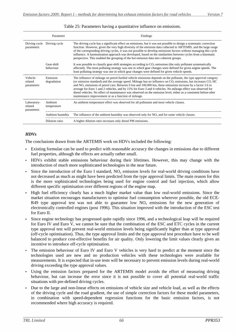
Emission factors 2009: Report 1 - methods for determining hot exhaust emission factors for road vehicles Version 7
TRL Limited 66 PPR353
Table 25: Parameters having a quantitative influence on emissions.
Parameter Findings
Driving cycleparameters
Driving cycle The driving cycle has a significant effect on emissions, but it was not possible to design a systematic correctionfunction. However, given the very high diversity of the emission data collected in ARTEMIS, and the large rangeof the corresponding driving cycles, it was not possible to develop emissions factors without managing this cycleinfluence. A harmonisation approach was developed, based on the similarities between cycles from a kinematicperspective. This enabled the grouping of the hot emission data into coherent groups.
Gear-shiftbehaviour
It was possible to classify gear-shift strategies according to CO2 emissions (the only pollutant systematicallyaffected). The most polluting strategy was one in which gear changes were defined for given engine speeds. Theleast polluting strategy was one in which gear changes were defined for given vehicle speeds.
Vehicle-relatedparameters
Emissiondegradation
The influence of mileage on petrol-fuelled vehicle emissions depends on the pollutant, the type approval category(or emission standard) and the average speed. Mileage has no influence on CO2 emissions, but increases CO, HCand NOx emissions of petrol cars: Between 0 km and 100,000 km, these emissions increase by a factor 3.6 inaverage for Euro 1 and 2 vehicles, and by 15% for Euro 3 and 4 vehicles. No mileage effect was observed fordiesel vehicles. No effect of maintenance was observed on the emission level, either as a consistent before-aftermaintenance improvement or as a function of mileage.
Laboratory-relatedparameters
Ambienttemperature
An ambient temperature effect was observed for all pollutants and most vehicle classes.
Ambient humidity The influence of the ambient humidity was observed only for NOx and for some vehicle classes.
Dilution ratio A higher dilution ratio increases only diesel PM emissions.
HDVs
The conclusions drawn from the ARTEMIS work on HDVs included the following:
• Existing formulae can be used to predict with reasonable accuracy the changes in emissions due to differentfuel properties, although the effects are actually rather small.
• HDVs exhibit stable emissions behaviour during their lifetimes. However, this may change with theintroduction of much more sophisticated technologies in the near future.
• Since the introduction of the Euro I standard, NOx emission levels for real-world driving conditions havenot decreased as much as might have been predicted from the type approval limits. The main reason for thisis the more sophisticated technologies being used for engine control and fuel injection, which allowdifferent specific optimisation over different regions of the engine map.
• High fuel efficiency clearly has a much higher market value than low real-world emissions. Since themarket situation encourages manufacturers to optimise fuel consumption wherever possible, the old ECE-R49 type approval test was not able to guarantee low NOx emissions for the new generation ofelectronically controlled engines (post 1996). This situation improved with the introduction of the ESC testfor Euro II.
• Since engine technology has progressed quite rapidly since 1996, and a technological leap will be requiredfor Euro IV and Euro V, we cannot be sure that the combination of the ESC and ETC cycles in the currenttype approval test will prevent real-world emission levels being significantly higher than at type approval(off-cycle optimisation). Thus, the type approval limits and the type approval test procedure have to be wellbalanced to produce cost-effective benefits for air quality. Only lowering the limit values clearly gives anincentive to introduce off-cycle optimisation.
• The emission behaviour of Euro IV and Euro V vehicles is very hard to predict at the moment since thetechnologies used are new and no production vehicles with these technologies were available formeasurements. It is expected that in-use tests will be necessary to prevent emission levels during real-worlddriving exceeding the type approval values.
• Using the emission factors prepared for the ARTEMIS model avoids the effort of measuring drivingbehaviour, but can increase the error since it is not possible to cover all potential real-world trafficsituations with pre-defined driving cycles.
• Due to the large and non-linear effects on emissions of vehicle size and vehicle load, as well as the effectsof the driving cycle and the road gradient, the use of simple correction factors for these model parameters,in combination with speed-dependent regression functions for the basic emission factors, is notrecommended where high accuracy is required.

Emission factors 2009: Report 1 - methods for determining hot exhaust emission factors for road vehicles Version 7
TRL Limited 67 PPR353
Two-wheel vehicles
The conclusions drawn from the ARTEMIS work on two-wheel vehicles included the following:
• When real-world passenger car and motorcycle driving were compared, the main differences were athigher average speeds. At higher speeds the driving of two-wheel vehicles is much more dynamic thanthat of passenger cars due to the relatively high power:mass ratio.
• The ARTEMIS cycle for passenger cars is very dynamic, and for urban driving has appropriate values ofRPA and average acceleration for motorcycles.
• NOx emissions from two-wheel vehicles were very low over the type approval cycle.
• For motorcycles having high CO and HC emission results, the differences between the results over thetype approval and real-world cycles were negligible. As emission levels over the type approval testdecrease, the differences increase. However, this conclusion is not valid for NOx. Some of the testedmotorcycles were equipped with an exhaust system configuration which appeared to have beenspecifically calibrated for the type approval cycle.
• Emissions over the ARTEMIS urban and rural parts were higher than emissions over the FHB test cycles,and it appeared that the differences were related to driving dynamics. However, for motorcycles equippedwith exhaust gas after-treatment systems (Euro 3), driving dynamics appears to be a less reliabledeterminant of emissions.
• For the measurements in ARTEMIS a Hungarian market fuel and a fuel meeting the WWFC Category 4future requirements were selected. With regard to replacing market fuel by fuel that is compliant withWWFC4 requirements:
- CO emissions were, on average, reduced by 15%,- HC emissions decreased by 5%,- NOx emissions were not affected.- CO2 emissions increased by 4%.- Fuel consumption was not affected.
• The effects of inspection and maintenance ranged from an adverse effect (emission increase aftermaintenance) for all pollutants of one of the motorcycles (range -18% to -1%) to very high for twomotorcycles which had a faulty battery (range 299% to 10%). The effect of inspection and maintenance onemissions may therefore not be neglected. Although measurements were carried out before and aftermaintenance for seven motorcycles, the effect was dependent on the type of maintenance that wasconducted. Therefore, average adjustment factors were derived to address the effects of inspection andmaintenance on emissions.
4.2.2 Recommendations
Cars
When comparing generic and vehicle-specific driving cycles for Euro 2 and 3 vehicles, the use of a generic setof driving cycles leads to a significant underestimation of CO emissions from petrol vehicles and HC and PMfrom diesel vehicles, and to an overestimation of diesel CO emissions. The generic procedure also leads to anunderestimation of CO and HC emissions from small cars and to a slight overestimation of HC and NOx fromthe most powerful cars. The use of generic driving cycles for all the cars could therefore lead to errors inemission estimations. Although it would increase the complexity of the test procedure, taking into accountvehicle performance by the use of specific driving cycles would lead to an improvement in the quality of theemissions estimates. This is especially important for the most recent cars, which are more sensitive to the testconditions.
Additional test cycles would incur additional time and costs when carrying out emission tests on vehicles. Analternative may be to develop a test cycle (or use a number of existing cycles) that could be broken down intoa large number of sub-cycles. If the continuous emissions data are provided, and assuming time delays do notcause a significant error, then the emissions over each sub-cycle could be calculated. This would allow alimited number of test cycles to yield a larger number of data points through which an average speedemissions curve could be fitted.

Emission factors 2009: Report 1 - methods for determining hot exhaust emission factors for road vehicles Version 7
TRL Limited 68 PPR353
In ARTEMIS, a hierarchical model was constructed to explain the logarithm of the total emission per cycle asa function of the cycle characteristics. It is not common practice to use the logarithm of the emission - this wasjustified by the fact that emissions were close to zero with a large coefficient of variation, and becauseemission results are generally distributed according to a log-normal distribution. It would be of interest to testthe application of this approach in the development of the UK emission factors.
The ARTEMIS project identified five parameters for which the effect on emissions could be quantified: Theseparameters were:
• gear-shift strategy• vehicle mileage• ambient air temperature• ambient air humidity• exhaust gas dilution ratio.
When compiling an emission factor database correction factors should be applied to the first four of thesewhere possible in order to standardise the data and examples are given in Appendix F.
Although continuous emission measurements can aid the understanding of different effects, there is anadditional cost. As emission models are constructed primarily using bag samples, and there remain someartefacts in continuous measurements which are difficult to correct, there appears to be little justification forroutinely including continuous emission measurements in the tests used for emission factor development. Thisrecommendation does not apply to ad hoc tests for the evaluation of technical and/or policy measures, forwhich continuous measurements may be beneficial. Where continuous measurements are taken, a hightemporal resolution (e.g. 10 Hz) is recommended, and some effort ought to be made to correct the continuoussignals. For this purpose, a number of experimental settings will need to be recorded.
Two-wheel vehicles
The work conducted within ARTEMIS addressed a wide range of different topics relating to emissions fromtwo-wheel vehicles. Nevertheless, a number of issues remain for future investigation, and somerecommendations were given by Elst et al. (2006). These included the following.
• The available real-world driving data are limited to certain types of two-wheel vehicle and trafficsituation. Real-world data should be recorded for a wider variety of vehicles to obtain more representativedriving patterns for specific traffic situations. These data can then be used to develop test cycles or toselect driving patterns that are representative of specific traffic situations and vehicle categories.
• A detailed system of vehicle categorisation could be defined for in-use motorcycles. However, the moredetailed the categorisation the more vehicles need to be measured to obtain robust emission factors.Therefore, it is recommended that the actual categorisation is adapted to the number of available emissionresults.
• A detailed measurement protocol which defines the measurement procedure and a standard test reporttemplate are vital for assuring comparability of measurements carried out by different laboratories. Thepresence of a ‘test witness’ who is aware of the measurement procedure and preparative actions, baganalysis and data processing could improve the quality and comparability of the emission data.
• It is recommended that test drivers become acquainted to the test cycle and the specific behaviour of thetwo-wheel vehicle to be tested.
• It proved difficult to obtain motorcycles from private users for the main measurement programme.Dealers, rental companies and importers proved to be more co-operative in this respect. Two-wheelvehicles obtained from dealers, rental companies and importers are, however, generally well maintainedand relatively new. Such vehicles are not recommended when addressing topics such as tampering ordeterioration.
• A dedicated measurement programme should be developed to further address fuel effects. Themeasurement programme should begin by evaluating the fuels that are on the European market. From thisassessment, fuels should be selected that are different with regard to specific parameters, and emissiontests should be conducted.

Emission factors 2009: Report 1 - methods for determining hot exhaust emission factors for road vehicles Version 7
TRL Limited 69 PPR353
• In order to obtain a more detailed understanding of inspection and maintenance, it is recommended that adedicated test programme should be conducted. The programme should involve measurements before andafter maintenance on a significant number of motorcycles. In addition, a distinction might be madebetween vehicle categories and types of maintenance.
• Another issue of importance might be the effect of mileage on emissions (or ‘durability’). More datarelating to this issue may become available in the near future, as it is under discussion in several groupsdealing with emission legislation for motorcycles.
• Ideally, an emission modelling methodology should be developed before actual emission measurementstake place in order to provide the necessary input data.
• Due to the lack of emission data for current and future emission categories (Stage 2 and Stage 3) emissionmodels will be improved significantly when emission measurements are conducted on vehicles compliantwith the legislation.
Emission factors 2009: Report 1 - methods for determining hot exhaust emission factors for road vehicles Version 7
TRL Limited 70 PPR353
5 References
ACEA (1995). Evaporative emissions test programme: preliminary report including diurnal test results. ReportAE137/95. European Automobile Manufacturers Association, Brussels.
ACEA and EUROPIA (1996). European programme on emissions, fuels and engine technologies (EPEFE).Final report, ACEA, Brussels.
André M (1997). Driving patterns analysis and driving cycles - European Development of Hybrid Technologyapproaching efficient Zero Emission Mobility (HYZEM). INRETS report LEN 9709. INRETS, Bron, France.
André J-M (2002). Vehicles sampling methods for emission measurement. INRETS Report LTE 0228.INRETS, Bron, France.
André M (2004). Real-world driving cycles for measuring cars pollutant emissions - Part A: The ARTEMISEuropean driving cycles. INRETS report LTE 0411. INRETS, Bron, France.
André M (2006). Real-world driving cycles for measuring cars pollutant emissions - Part B: Driving cyclesfor high- and low-powered vehicles. INRETS report, Bron, France, N°LTE0412, 60 p. INRETS, Bron, France.
André M, Joumard R, Hickman J and Hassel D (1991). Realistic driving cycles for passenger cars.Deliverable No. 4 of the European Commission DRIVE Project V1053 – Modelling of emissions andconsumption in urban areas (MODEM). INRETS, Bron, France.
Andre M, Hassel D, Hickman A J and Joumard R (1993). The Science of the Total Environment, 134, 171.
André J-M, Lacour S, Hugot M, Olàh Z and Joumard R (2003). Impact of the gear-shift strategy onemission measurements - ARTEMIS 3142 report. INRETS report LTE 0307. INRETS, Bron, France.
André M, Rapone M and Joumard R (2006). Analysis of the car pollutant emissions as regards drivingcycles and kinematic parameters. INRETS report LTE 0607, ISBN N° INRETS/RR/06-509-ENG. INRETS,Bron, France.
Barlow T J (1993). Evaporative emissions from petrol fuelled UK light-duty in-Service vehicles. TRL ReportPR/ENV/022/93. Transport Research Laboratory, Crowthorne.
Barlow T J, Hickman A J and Boulter P (2001). Exhaust emission factors 2000: Database and emissionfactors. Project Report PR/SE/230/00. TRL Limited, Crowthorne.
Barlow T J and Boulter P G (2009). Emission factors 2009: Report 2 - A review of the average-speedapproach for estimating hot exhaust emissions from road vehicles. TRL Report 355. TRL limited,Wokingham.
Barlow T J, Latham S, McCrae I S and P G Boulter (2009). A Reference Book of Driving Cycles for Usein the Measurement of Road Vehicle Emissions. TRL Report PPR354. TRL Limited, Wokingham.
Boulter P G (1996). Factors Affecting Cold-Start Emissions: A Review. TRL Report PR/SE/183/96.Transport Research Laboratory, Crowthorne.
Boulter PG, Barlow T J, Latham S and McCrae I S (2005). A review of the road transport emission factorsused in the National Atmospheric Emissions Inventory. TRL Report UPR SEA/07/05 (unpublished). TransportResearch Laboratory, Wokingham.
Boulter P G (2009). Emission factors 2009: Report 6 - deterioration factors and other modelling assumptionsfor road vehicles in the NAEI. TRL Report PPR359. TRL Limited, Wokingham.
Boulter P G, Barlow T J and McCrae I S (2009a). Emission factors 2009: Report 3 - exhaust emissionfactors for road vehicles in the United Kingdom (2009). TRL Report PPR356. TRL Limited, Wokingham.
Boulter P G, Barlow T J, McCrae I S and Latham S (2009b). Emission factors 2009: Final summaryreport. TRL Report PPR361. TRL Limited, Wokingham.

Emission factors 2009: Report 1 - methods for determining hot exhaust emission factors for road vehicles Version 7
TRL Limited 71 PPR353
Boulter P G and Latham S (2009a). Emission factors 2009: Report 4 - a review of methodologies formodelling cold-start emissions from road vehicles. TRL Report PPR357. TRL Limited, Wokingham.
Boulter P G and Latham S (2009b). Emission factors 2009: Report 5 - a review of the effects of fuelproperties on road vehicle emissions. TRL Report PPR358. TRL Limited, Wokingham.
Bremmers D A C M et al. (2001). ARTEMIS WP 530, motorcycle round robin test. TNO-Automotive, Delft.
Choudrie S L, Brown L, Milne R, Murrells T P, Passant N, Thistlethwaite G, Watterson J D andJackson J (2008). UK Greenhouse Gas Inventory, 1990 to 2006. AEA Technology, Harwell, Oxfordshire.ISBN 0-9554823-4-2.
CONCAWE (1987). An investigation into evaporative hydrocarbon emissions from European vehicles.Report 87/60. CONCAWE (The Oil Companies’ European Organisation for Environment, Health and Safety),Boulevard du Souverain, B – 1160 Brussels, Belgium.
CONCAWE (1990). The Effects of Temperature and Fuel Volatility on Vehicle Evaporative Emissions.Report 90/51. CONCAWE (The Oil Companies’ European Organisation for Environment, Health and Safety),Boulevard du Souverain, B – 1160 Brussels, Belgium.
CONCAWE (2004). Motor vehicle mission regulations and fuel specifications: 2002/2003 update. Report9/04. CONCAWE (The Oil Companies’ European Organisation for Environment, Health and Safety),Boulevard du Souverain, B – 1160 Brussels, Belgium.
Cornelis E, Hausberger S, Wiesmayr J and Zallinger M (2005). Emission stability. TUG report, Graz,Austria.
De Haan P and Keller M (2003). Art.Kinema – User Guide to Version (RC1). INFRAS, Berne.
Department for Transport (2005). Transport Statistics for Great Britain (TSGB) 2005 edition: Traffic speeds- data tables. (dft_transstats_041577.xls). Department for Transport.Website: http://www.dft.gov.uk/stellent/groups/dft_transstats/documents/divisionhomepage/031571.hcsp
Department for Transport, Scottish Executive and Welsh Assembly (2005). Transport Statistics GreatBritain 2005, 31st Edition. Department for Transport, London. ISBN: 0-11-552701X
Devaux P and Weilenmann M (2002). Influence of the human driver on vehicle emissions of chassisdynamometer tests. EMPA report, Dübendorf, Switzerland.
DieselNet (2006). Summary of worldwide engine and vehicle test cycles.http://www.dieselnet.com/standards/cycles/#eu
Elst D A M M et al. (2002). TNO report 02.OR.VM.044.1/DE, July 2002. 2nd CITA Research StudyProgramme on Emissions, Study 2 - Motorcycle Exhaust Emission and Noise.
Elst D A M M, Gense N L J, Vermeulen R J and Steven H (2006). ARTEMIS Workpackage 500 FinalReport (Deliverable 5). TNO-Automotive, Delft.
Ericsson E (2000). Variability in urban driving patterns. Transportation Research, Part D 5, pp 337-354.Elsevier Science Ltd.
European Commission (1999). MEET: Methodology for calculating transport emissions and energyconsumption. Office for Official Publications of the European Communities, L-2985 Luxembourg. ISBN 92-828-6785-4.
Geivanidis S and Samaras Z (2004). Investigation of the emission degradation of petrol vehicles. LATReport n°0415, Thessaloniki, Greece.
Geivanidis S, Samaras Z, Pratti V, Pollak I and Merétei T (2004). Effect of sampling parameters onemission measurements. LAT report, n°0416, Thessaloniki, Greece, 52 p.

Emission factors 2009: Report 1 - methods for determining hot exhaust emission factors for road vehicles Version 7
TRL Limited 72 PPR353
Highways Agency, Transport Scotland, Welsh Assembly Government and the Department for RegionalDevelopment Northern Ireland (2007). Design Manual for Roads and Bridges (DMRB) Volume 11 -Environmental Assessment. Section 3, Part 1 – Air Quality.http://www.standardsforhighways.co.uk/dmrb/vol11/section3/ha20707.pdf
INFRAS (2004). Handbook of Emission Factors for Road Transport, Version 2.1. INFRAS, Berne,Switzerland, February 2004.
Joumard R, André M, Vidon R, Tassel P and Pruvost C (2000). Influence of driving cycles on unitemissions from passenger cars. Atmos. Environ., 34, p. 4621-4628.
Joumard R, Andre M, Laurikko J, Le Anh T, Geivanidis S, Samaras Z, Olah Z, Devaux P, Andre J-M,Cornelis E, Rouveirolles P, Lacour S, Prati M V, Vermeulen R and Zallinger (2006a). Accuracy ofexhaust emissions measurements on vehicle bench. ARTEMIS deliverable 2. Report no. LTE 0522, INRETS,Bron.
Joumard R, André J-M, Aakko P, Samaras Z, Roujol S, Zallinger M, Kljun N, Rapone M, MarkewitzK, Weilenmann M and André M (2006b). Emission factor modelling and database for light vehicles -ARTEMIS deliverable 3. INRETS report LTE 0523. INRETS, Bron, France.
Kis J et al. (2005). Influence of fuel parameters to emission characteristics of two-wheel vehicles based onlaboratory measurement.
Lacour S and Joumard R (2001). Emission modelling: The role of vehicle sampling and vehicle-relatedparameters – Draft report. INRETS report LTE 0114. INRETS, Bron, France.
Latham S and Boulter P G (2009). Emission factors 2009 – Report 7 - a review of the NAEI methodologyfor modelling evaporative emissions. TRL Report PPR360. Transport Research Laboratory, Wokingham.
Laurikko J (2005a). The Effect of Vehicle Cooling on Exhaust Emissions. VTT Processes report, Espoo,Finland.
Laurikko J (2005b). The Effect of Ambient Temperature on Emissions. VTT Processes report, Espoo,Finland.
Laurikko J (2005c). The Effect of Ambient Humidity on Emissions. VTT Processes report, Espoo, Finland.
Laurikko J (2005d). Summary Report of the Round-Robin Exercise. VTT Processes report, Espoo, Finland.
Le Anh T, Hausberger S, Ajtay D and Weilenmann M (2005). Response time in instantaneous emissionmeasurement. EMPA and TUG report, Dübendorf, Switzerland, Graz, Austria.
Ntziachristos L and Samaras Z (2000a). COPERT III. Computer program to calculate emissions from roadtransport. Methodology and emission factors (version 2.1). Technical Report No. 49. European EnvironmentAgency, Copenhagen.
Ntziachristos L and Samaras Z (2000b). Speed-dependent representative emissions factors for catalystpassenger cars and influencing parameters. Atmospheric Environment, 34, p. 4611-4619.
Ntziachristos L. and Z. Samaras (2001). An empirical method for predicting exhaust emissions of regulatedpollutants from future vehicle technologies. Atmospheric Environment, 35, p. 1985-1999.
Olàh Z (2005). Vehicle preconditioning. KTI report, Budapest.
Osses M, Henriquez A and Trivino R (2002). Positive mean acceleration for the determination of trafficemissions. Paper presented at the conference ‘Transport and Air Pollution’, Graz, Austria, 19-21 June 2002.
Prati M V and Costagliola M A (2004). Dilution air conditions. Istituto Motori, CNR report, Naples, Italy.
Renault and Altran (2002). Fuel Properties. Renault report, Lardy, France.
Emission factors 2009: Report 1 - methods for determining hot exhaust emission factors for road vehicles Version 7
TRL Limited 73 PPR353
Rexeis M, Hausberger S, Riemersma I, Tartakovsky L, Zvirin Y and Erwin C (2005). Heavy-duty vehicleemissions. Final Report of WP 400 in ARTEMIS (Assessment and Reliability of Transport Emission Modelsand Inventory Systems); DGTREN Contract 1999-RD.10429; University of Technology, Graz; report no. : I02/2005/Hb 20/2000 I680.
Rijkeboer R C (2000). WMTC subreport: statistics about vehicle fleets and use. TNO report00.OR.VM.007.1/RR, 18 January 2000.Samaras Z and Ntziachristos L (1998). Average hot emission factors for passenger cars and light-dutytrucks. LAT report, n°9811, Thessaloniki, Greece, 112 p., 1998.www.inrets.fr/infos/cost319/MEET%20Del_7.pdf
Samaras Z, Zachariadis T, Joumard R, Hassel D, Weber F J and Rijkeboer R (2001). An outline of the1994-1998 European inspection and maintenance study: Part I: design, tests and results of experimentalmethods. J. Air Waste Manag. Assoc., 51, p. 913-938.
Samaras Z, Ntziachristos L, Thompson N, Hall D, Westerholm R and Boulter P (2005a). Characterisationof Exhaust Particulate Emissions from Road Vehicles. Final Report of the European Commission 5th
Framework PARTICULATES project. Laboratory of Applied Theremodynamics, Aristotle University ofThessaloniki, Greece. http://vergina.eng.auth.gr/mech/lat/particulates/private/index.htm
Samaras Z, Kyriakis N, Geivanidis S, Mellios G, Zallinger M and Hausberger S (2005b). Influence of theTechnical Characteristics of the Vehicles on their Real World Emission Behaviour. TUG report, Graz, Austria.
Schweizer T (1998). Nachführung der Emissionsgrundlagen Strassenverkehr, Anwendungsgrenzen vonEmissionsfaktoren, Analyse der Messdatenstreuung. EMPA Bericht, n°166'558, Dübendorf, Switzerland.
Steven H (2001). Development of a World-wide Harmonised Heavy-duty Engine Emissions Test Cycle:Executive Summary Report. ECE-GRPE WHDC Working Group. Document TRANS/WP.29/GRPE/2001/2.
Steven H (2004). Worldwide harmonized motorcycle emissions certification procedure (WMTC) - Technicalreport. TRANS/WP.29/GRPE/2004/10.
Sturm P J, Boulter P, de Haan P, Joumard R, Hausberger S, Hickman A J, Keller M, Niederle W,Ntziachristos L, Reiter C, Samaras Z, Schinagl G, Schweizer T and Pischinger R (1998). 'Instantaneousemission data and their use in estimating passenger car emissions'. EC MEET Project (Methodologies forEstimating Emissions from Transport), Task 1.1:Instationary vehicle emissions, Deliverable no. 6. Publishedby the Technical University of Graz, Institute for Internal Combustion Engines and Thermodynamics, A-8010Graz Inffeldgasse 25, Austria, Editor Univ.-Prof. Dr. R. Pischinger.
Vermeulen R (2005). Chassis dynamometer setting. TNO Automotive report, Delft, the Netherlands.
Weilenmann M, Soltic P and Atjay D (2003). Describing and compensating gas transport dynamics foraccurate instantaneous emission measurement. Atmospheric Environment, Vol 37, pp. 5137-5145.
WWFC (2002). World-Wide Fuel Charter 3rd version, December 2002.
Zallinger M, Hausberger S, Ajtay D and Weilenmann M (2005). Instantaneous emission modellingapplications. EMPA and TUG report, Dübendorf, Switzerland and Graz, Austria, 53 p.
Emission factors 2009: Report 1 - methods for determining hot exhaust emission factors for road vehicles Version 7
TRL Limited 74 PPR353
Appendix A: Abbreviations and terms used in the TaskReports
ACEA European Automobile Manufacturers Association.
ADMS Atmospheric Dispersion Modelling System.
ARTEMIS Assessment and Reliability of Transport Emission Models and Inventory Systems.An EC 5th Framework project, funded by DG TREN and coordinated by TRL.http://www.trl.co.uk/artemis/introduction.htm
AURN Automatic Urban and Rural Network. Automatic monitoring sites for air qualitythat are or have been operated on behalf of the Department for Environment, Foodand Rural Affairs in the UK.
AVERT Adaptation of Vehicle Environmental Response by Telematics. Project funded bythe Foresight Vehicle programme.http://www.foresightvehicle.org.uk/dispproj1.asp?wg_id=1003
BP British Petroleum.
CEN European Standards Organisation.
CERC Cambridge Environmental Research Consultants, the developers of the ADMSmodel suite.
Cetane number(CN)
Cetane number is a measure of the combustion quality of diesel fuel. Cetane is analkane molecule that ignites very easily under compression. All other hydrocarbonsin diesel fuel are indexed to cetane (index = 100) as to how well they ignite undercompression. Since there are hundreds of components in diesel fuel, the overall CNof the diesel is the average of all the components. There is very little actual cetanein diesel fuel. Generally, diesel engines run well with a CN between 40 and 55.
CITA International Motor Vehicle Inspection Committee, based in Brussels.
CNG Compressed natural gas (primarily methane).
CH4 Methane.
CO Carbon monoxide.
CO2 Carbon dioxide.
uCO2 ‘Ultimate’ CO2.
COLDSTART A model for cold-start emissions developed by VTI in Sweden.
CONCAWE The Oil Companies’ European Association for Environment, Health and Safety inRefining and Distribution.
COST European Cooperation in Science and Technology.
CRT Continuously Regenerating Trap – a trademark of Johnson Matthey.
CVS Constant-volume sampler.
COPERT COmputer Program to calculate Emissions from Road Transport.http://lat.eng.auth.gr/copert/
CORINAIR CO-oRdinated INformation on the Environment in the European Community - AIR
DEFRA Department for Environment, Food and Rural Affairs.
DfT Department for Transport, UK.
Emission factors 2009: Report 1 - methods for determining hot exhaust emission factors for road vehicles Version 7
TRL Limited 75 PPR353
DI Direct injection.
DMRB Design Manual for Roads and Bridges.http://www.standardsforhighways.co.uk/dmrb/
DPF Diesel particulate filter.
DTI Department of Trade and Industry (now the Department for Business, Enterpriseand Regulatory Reform – BERR).
Driving cycle The term ‘driving cycle’ (or sometimes ‘duty cycle’ is used to describe how avehicle is to be operated during a laboratory emission test. A driving cycle isdesigned to reflect some aspect of real-world driving, and usually describes vehiclespeed as a function of time.
Driving pattern The term ‘driving pattern’ is used to describe how a vehicle is operated under real-world conditions, based on direct measurement, or the time history of vehicleoperation specified by a model user. In the literature, this is also often referred toas a driving cycle. However, in this work it has been assumed that a driving patternonly becomes a driving cycle once it has been used directly in the measurement ofemissions.
Dynamics Variables which emission modellers use to describe the extent of transient operation(see entry below for ‘transient’) in a driving cycle (e.g. maximum and minimumspeed, average positive acceleration). Can be viewed as being similar to the conceptof the ‘aggressiveness’ of driving.
DVPE Dry vapour pressure equivalent. The difference between DVPR and (the older)RVP is the measurement method. DVPE is measured ‘dry’ after removing allmoisture from the test chamber prior to injection of the sample. This overcomes theunpredictability of results experienced when testing samples containing oxygenatesby the conventional RVP method. The DVPE is measured at a temperature of37.8°C.
EC European Commission.
ECE Economic Commission for Europe.
EGR Exhaust gas recirculation.
EIA Environmental Impact Assessment
EMEP Cooperative Programme for Monitoring and Evaluation of the Long-RangeTransmission of Air Pollutants in Europe.
EMFAC EMission FACtors model, developed by the California Air Resources Board.EMFAC 2007 is the most recent version.
EMPA One of the research institutes of the Swiss ETH organisation.
EPEFE European Programme on Emissions, Fuels and Engine Technologies
ETC European Transient Cycle.
EU European Union.
EUDC Extra Urban Driving Cycle.
EXEMPT EXcess Emissions Planning Tool.
FAME Fatty acid methyl ester.
FHB Fachhochschule Biel (FHB): Biel University of applied science, Switzerland.
FID Flame ionisation detector.
FIGE (or FiGE) Forschungsinstitut Gerausche und Erschutterungen (FIGE Institute), Aachen,Germany. Now TUV Automotive GmbH.

Emission factors 2009: Report 1 - methods for determining hot exhaust emission factors for road vehicles Version 7
TRL Limited 76 PPR353
Fischer-Tropschdiesel (FTD)
Fischer-Tropsch diesel is a premium diesel product with a very high cetane number(75) and zero sulphur content. It is generally produced from natural gas.
FTP Federal Test Procedure – the driving cycle used in US emission tests.
FTIR Fourier-transform infrared spectroscopy.
GC/MS Gas chromatography/mass spectrometry.
GDI Gasoline Direct Injection.
GHG Greenhouse gas.
GVW Gross vehicle weight.
HBEFA/Handbook Handbook Emission Factors for Road Transport (Handbuch Emissionsfaktoren desStrassenverkehrs). An emission model used in Switzerland, Germany and Austria.http://www.hbefa.net/
HDV Heavy-duty vehicles. Road vehicles greater than 3.5 tonnes (GVW), where GVW isthe gross weight of the vehicle, i.e. the combined weight of the vehicle and goods.
HGV Heavy goods vehicles. Goods vehicles greater than 3.5 tonnes GVW.
HOV High-occupancy vehicle.
HyZem HYbrid technology approaching efficient Zero Emission Mobility.
IDI Indirect injection.
IM Inspection and Maintenance: in-service vehicle road worthiness testing.
INFRAS A private and independent consulting group based in Switzerland.
INRETS Institut National de Recherche sur les Transports et leur Sécurité, France.
IUFC-15 INRETS urbain fluide court. Short, urban free-flow driving cycle.
IRC-15 INRETS route courte. Short rural driving cycle.
JCS A European Joint Commission funded project: The inspection of in-use cars inorder to attain minimum emissions of pollutants and optimum energy efficiency,carried out on behalf of EC DGs for Environment (DG XI) Transport (DG VII) andEnergy (DG XVII). Project coordinated by LAT, University of Thessaloniki.
LDV Light-duty vehicles. Road vehicles less than 3.5 tonnes GVW, including cars andlight goods vehicles.
LGV Goods/commercial vehicles less than 3.5 tonnes GVW.
LPG Liquefied petroleum gas.
M25 London orbital motorway.
MEET Methodologies for Estimating air pollutant Emissions from Transport. EuropeanCommission 4th Framework project coordinated by INRETS.
MHDT Millbrook Heavy-Duty Truck (driving cycle).
MLTB Millbrook London Transport Bus (driving cycle).
MOBILE USEPA vehicle emission modelling software.
MODEM Modelling of Emissions and Fuel Consumption in Urban Areas. A research projectwithin the EU DRIVE programme coordinated by INRETS.
MOUDI Micro-orifice uniform deposit impactor.
MPI Multi-point injection.
Emission factors 2009: Report 1 - methods for determining hot exhaust emission factors for road vehicles Version 7
TRL Limited 77 PPR353
MTC AVL MTC Motortestcenter AB, Sweden.
MVEG Motor Vehicle Emission Group.
NAEI National Atmospheric Emissions Inventory (UK).http://www.naei.org.uk/
NEDC New European Driving Cycle.
NETCEN National Environmental Technology Centre.
N2O Nitrous oxide.
NH3 Ammonia.
NMVOC Non-methane volatile organic compounds.
NO Nitric oxide.
NO2 Nitrogen dioxide.
NOx Total oxides of nitrogen.
OBD On-board diagnostics.
OSCAR Optimised Expert System for Conducting Environmental Assessment of UrbanRoad Traffic. A European Fifth Framework research project, funded by DGResearch. Project and coordinated by the University of Hertfordshire.
PAHs Polycyclic aromatic hydrocarbons.
PARTICULATES An EC Fifth Framework research project, funded by DG TREN and coordinated byLAT, Thessaloniki.http://lat.eng.auth.gr/particulates/
PHEM Passenger car and Heavy-duty Emission Model. One of the emission modelsdeveloped in COST Action 346 and the ARTEMIS project.
PM Particulate matter.
PM10 Airborne particulate matter with an aerodynamic diameter of less than 10 µm.
PM2.5 Airborne particulate matter with an aerodynamic diameter of less than 2.5 µm.
PMP Particle Measurement Programme.
POPs Persistent organic pollutants.
ppm Parts per million.
PSV Public Service Vehicle.
Roadcharacteristics
Information relating to the road, such as the geographical location (e.g. urban,rural), the functional type (e.g. distributor, local access), the speed limit, the numberof lanes and the presence or otherwise of traffic management measures.
RME Rapeseed methyl ester.
RTC Reference test cycles.
RTD Real-time diurnal (evaporative emissions).
RTFO Renewable Transport Fuel Obligation.
RVP Reid vapour pressure.
SCR Selective catalytic reduction.
SEA Strategic Environmental Assessment.
SHED Sealed Housing for Evaporative Determination.
SMMT Society of Motor Manufacturers and Traders.

Emission factors 2009: Report 1 - methods for determining hot exhaust emission factors for road vehicles Version 7
TRL Limited 78 PPR353
SO2 Sulphur dioxide.
TEE Traffic Energy and Emissions (model).
THC/HC Total hydrocarbons.
TNO TNO Automotive, The Netherlands. The power train and emissions researchinstitute of the holding company, TNO Companies BV.
Trafficcharacteristics/conditions
Information relating to the bulk properties of the traffic stream – principally itsspeed, composition and volume/flow or density.
TRAMAQ Traffic Management and Air Quality Research Programme. A research programmefunded by the UK Department for Transport.http://www.dft.gov.uk/pgr/roads/network/research/tmairqualityresearch/trafficmanagementandairquali3927
Transient Relates to when the operation of a vehicle is continuously varying, as opposed tobeing in a steady state.
TRL TRL Limited (Transport Research Laboratory), UK.
TRRL Transport and Road Research Laboratory - former name of TRL.
TUG Technical University of Graz, Austria.
TUV TÜV Rheinland, Germany. Exhaust emission testing used to be undertaken at thisinstitute based in Cologne. These activities were transferred to another institute inthe TUV group, based in Essen, in 1999.
TWC Three-way catalyst.
UG214 A project within DfT's TRAMAQ programme which involved the development ofrealistic driving cycles for traffic management schemes.
UKEFD United Kingdom Emission Factor Database (for road vehicles).
UKPIA UK Petroleum Industries Association
ULSD Ultra-low-sulphur diesel.
UROPOL Urban ROad POLlution model.
USEPA United States Environmental Protection Agency.
UTM/UTMC Urban Traffic Management / Urban Traffic Management and Control.
Vehicle operation The way in which a vehicle is operated (e.g. vehicle speed, throttle position, enginespeed, gear selection).
VeTESS Vehicle Transient Emissions Simulation Software.
VOCs Volatile organic compounds.
VOSA Vehicle and Operator Services Agency
WMTC World Motorcycle Test Cycle. A common motorcycle emissions certificationProcedure. The cycle is divided into urban, rural, and highway driving.
WSL Warren Spring Laboratory.
WVU West Virginia University, US.
WWFC World-Wide Fuel Charter. The World Wide Fuel Charter is a joint effort byEuropean, American and Japanese automobile manufacturers and other relatedassociations, and recommends global standards for fuel quality, taking into accountthe status of emission technologies.
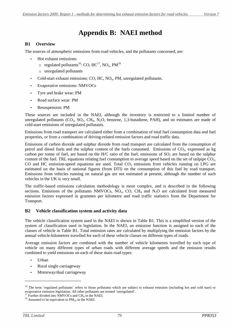
Emission factors 2009: Report 1 - methods for determining hot exhaust emission factors for road vehicles Version 7
TRL Limited 79 PPR353
Appendix B: NAEI method
B1 Overview
The sources of atmospheric emissions from road vehicles, and the pollutants concerned, are:
• Hot exhaust emissions:
o regulated pollutants16: CO, HC17, NOx, PM18
o unregulated pollutants
• Cold-start exhaust emissions: CO, HC, NOx, PM, unregulated pollutants.
• Evaporative emissions: NMVOCs
• Tyre and brake wear: PM
• Road surface wear: PM
• Resuspension: PM
These sources are included in the NAEI, although the inventory is restricted to a limited number ofunregulated pollutants (CO2, SO2, CH4, N2O, benzene, 1,3-butadiene, PAH), and no estimates are made ofcold-start emissions of unregulated pollutants.
Emissions from road transport are calculated either from a combination of total fuel consumption data and fuelproperties, or from a combination of driving-related emission factors and road traffic data.
Emissions of carbon dioxide and sulphur dioxide from road transport are calculated from the consumption ofpetrol and diesel fuels and the sulphur content of the fuels consumed. Emissions of CO2, expressed as kgcarbon per tonne of fuel, are based on the H/C ratio of the fuel; emissions of SO2 are based on the sulphurcontent of the fuel. TRL equations relating fuel consumption to average speed based on the set of tailpipe CO2,CO and HC emission-speed equations are used. Total CO2 emissions from vehicles running on LPG areestimated on the basis of national figures (from DTI) on the consumption of this fuel by road transport.Emissions from vehicles running on natural gas are not estimated at present, although the number of suchvehicles in the UK is very small.
The traffic-based emissions calculation methodology is more complex, and is described in the followingsections. Emissions of the pollutants NMVOCs, NOx, CO, CH4 and N2O are calculated from measuredemission factors expressed in grammes per kilometre and road traffic statistics from the Department forTransport.
B2 Vehicle classification system and activity data
The vehicle classification system used in the NAEI is shown in Table B1. This is a simplified version of thesystem of classification used in legislation. In the NAEI, an emission function is assigned to each of theclasses of vehicle in Table B1. Total emission rates are calculated by multiplying the emission factors by theannual vehicle-kilometres travelled for each of these vehicle classes on different types of roads.
Average emission factors are combined with the number of vehicle kilometres travelled by each type ofvehicle on many different types of urban roads with different average speeds and the emission resultscombined to yield emissions on each of these main road types:
• Urban
• Rural single carriageway
• Motorway/dual carriageway
16 The term ‘regulated pollutants’ refers to those pollutants which are subject to exhaust emission (including hot and cold start) orevaporative emission legislation. All other pollutants are termed ‘unregulated’.17 Further divided into NMVOCs and CH4 in the NAEI.18 Assumed to be equivalent to PM10 in the NAEI.
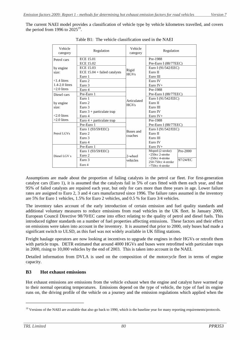
Emission factors 2009: Report 1 - methods for determining hot exhaust emission factors for road vehicles Version 7
TRL Limited 80 PPR353
The current NAEI model provides a classification of vehicle type by vehicle kilometres travelled, and coversthe period from 1996 to 202519.
Table B1: The vehicle classification used in the NAEI
Vehiclecategory
RegulationVehiclecategory
Regulation
Petrol cars
by enginesize:
<1.4 litres1.4-2.0 litres>2.0 litres
ECE 15.01
RigidHGVs
Pre-1988ECE 15.02 Pre-Euro I (88/77EEC)ECE 15.03 Euro I (91/542/EEC)ECE 15.04 + failed catalysts Euro IIEuro 1 Euro IIIEuro 2 Euro IVEuro 3 Euro IV+Euro 4
ArticulatedHGVs
Pre-1988Diesel cars
by enginesize:
<2.0 litres>2.0 litres
Pre-Euro 1 Pre-Euro I (88/77EEC)Euro 1 Euro I (91/542/EEC)Euro 2 Euro IIEuro 3 Euro IIIEuro 3 + particulate trap Euro IVEuro 4 Euro IV+Euro 4 + particulate trap
Buses andcoaches
Pre-1988
Petrol LGVs
Pre-Euro 1 Pre-Euro I (88/77EEC)Euro 1 (93/59/EEC) Euro I (91/542/EEC)Euro 2 Euro IIEuro 3 Euro IIIEuro 4 Euro IV
Diesel LGV s
Pre-Euro 1 Euro IV+Euro 1 (93/59/EEC)
2-wheelvehicles
Moped (2-stroke)<250cc 2-stroke<250cc 4-stroke250-750cc 4-stroke>750cc 4-stroke
Pre-2000Euro 2Euro 3 97/24/ECEuro 4
Assumptions are made about the proportion of failing catalysts in the petrol car fleet. For first-generationcatalyst cars (Euro 1), it is assumed that the catalysts fail in 5% of cars fitted with them each year, and that95% of failed catalysts are repaired each year, but only for cars more than three years in age. Lower failurerates are assigned to Euro 2, 3 and 4 cars manufactured since 1996. The failure rates assumed in the inventoryare 5% for Euro 1 vehicles, 1.5% for Euro 2 vehicles, and 0.5 % for Euro 3/4 vehicles.
The inventory takes account of the early introduction of certain emission and fuel quality standards andadditional voluntary measures to reduce emissions from road vehicles in the UK fleet. In January 2000,European Council Directive 98/70/EC came into effect relating to the quality of petrol and diesel fuels. Thisintroduced tighter standards on a number of fuel properties affecting emissions. These factors and their effecton emissions were taken into account in the inventory. It is assumed that prior to 2000, only buses had made asignificant switch to ULSD, as this fuel was not widely available in UK filling stations.
Freight haulage operators are now looking at incentives to upgrade the engines in their HGVs or retrofit themwith particle traps. DETR estimated that around 4000 HGVs and buses were retrofitted with particulate trapsin 2000, rising to 10,000 vehicles by the end of 2003. This is taken into account in the NAEI.
Detailed information from DVLA is used on the composition of the motorcycle fleet in terms of enginecapacity.
B3 Hot exhaust emissions
Hot exhaust emissions are emissions from the vehicle exhaust when the engine and catalyst have warmed upto their normal operating temperatures. Emissions depend on the type of vehicle, the type of fuel its engineruns on, the driving profile of the vehicle on a journey and the emission regulations which applied when the
19 Versions of the NAEI are available that also go back to 1990, which is the baseline year for many reporting requirements/protocols.
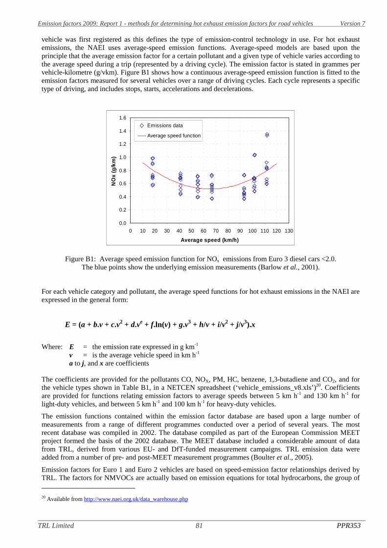
Emission factors 2009: Report 1 - methods for determining hot exhaust emission factors for road vehicles Version 7
TRL Limited 81 PPR353
vehicle was first registered as this defines the type of emission-control technology in use. For hot exhaustemissions, the NAEI uses average-speed emission functions. Average-speed models are based upon theprinciple that the average emission factor for a certain pollutant and a given type of vehicle varies according tothe average speed during a trip (represented by a driving cycle). The emission factor is stated in grammes pervehicle-kilometre (g/vkm). Figure B1 shows how a continuous average-speed emission function is fitted to theemission factors measured for several vehicles over a range of driving cycles. Each cycle represents a specifictype of driving, and includes stops, starts, accelerations and decelerations.
0.0
0.2
0.4
0.6
0.8
1.0
1.2
1.4
1.6
0 10 20 30 40 50 60 70 80 90 100 110 120 130
Average speed (km/h)
NO
x(g
/km
)
Emissions data
Average speed function
Figure B1: Average speed emission function for NOx emissions from Euro 3 diesel cars <2.0.The blue points show the underlying emission measurements (Barlow et al., 2001).
For each vehicle category and pollutant, the average speed functions for hot exhaust emissions in the NAEI areexpressed in the general form:
E = (a + b.v + c.v2 + d.ve + f.ln(v) + g.v3 + h/v + i/v2 + j/v3).x
Where: E = the emission rate expressed in g km-1 v = is the average vehicle speed in km h-1 a to j, and x are coefficients
The coefficients are provided for the pollutants CO, NOX, PM, HC, benzene, 1,3-butadiene and CO2, and forthe vehicle types shown in Table B1, in a NETCEN spreadsheet (‘vehicle_emissions_v8.xls’)20. Coefficientsare provided for functions relating emission factors to average speeds between 5 km h-1 and 130 km h-1 forlight-duty vehicles, and between 5 km h-1 and 100 km h-1 for heavy-duty vehicles.
The emission functions contained within the emission factor database are based upon a large number ofmeasurements from a range of different programmes conducted over a period of several years. The mostrecent database was compiled in 2002. The database compiled as part of the European Commission MEETproject formed the basis of the 2002 database. The MEET database included a considerable amount of datafrom TRL, derived from various EU- and DfT-funded measurement campaigns. TRL emission data wereadded from a number of pre- and post-MEET measurement programmes (Boulter et al., 2005).
Emission factors for Euro 1 and Euro 2 vehicles are based on speed-emission factor relationships derived byTRL. The factors for NMVOCs are actually based on emission equations for total hydrocarbons, the group of
20 Available from http://www.naei.org.uk/data_warehouse.php
Emission factors 2009: Report 1 - methods for determining hot exhaust emission factors for road vehicles Version 7
TRL Limited 82 PPR353
species that are measured in the emission tests. To derive factors for non-methane VOCS, the calculated g km-
1 factors for methane were subtracted from the corresponding THC emission factors.
Due to lack of measured data, emission factors for Euro 3 vehicles (and Euro 4 petrol cars) were estimated byapplying scaling factors to the Euro 2 factors. The scale factors for light duty vehicles take into considerationthe requirement for new vehicles to meet certain durability standards set in the Directives. For heavy-dutyvehicles, the emission scaling factors are taken from COPERT III.
Speed-dependent functions provided by TRL for different sizes of motorcycles are used. Motorcycles soldsince the beginning of 2000 were assumed to meet the Directive 97/24/EC and their emission factors werereduced according to the factors given in the latest version of COPERT III.
Emissions from buses were scaled down according to the proportion running on ultra-low sulphur diesel fuelin each year, the proportion fitted with oxidation catalysts or particulate traps (CRTs) and the effectiveness ofthese measures in reducing emissions from the vehicles.
The older in-service vehicles in the test surveys that were manufactured to a particular emission standardwould have covered a range of different ages. Therefore, an emission factor calculated for a particularemission standard (e.g. ECE 15.04) from the emission functions and coefficients from TRL and COPERT II iseffectively an average value for vehicles of different ages which inherently takes account of possibledegradation in emissions with vehicle age. However, for the more recent emission standards (Euro 1 and 2),the vehicles would have been fairly new when the emissions were measured. Therefore, based on data fromthe European Auto-Oil study, the deterioration in emissions with age or mileage was taken into account forcatalyst cars. It was assumed that emissions of CO and NOX increase by 60% over 80,000 km, whileemissions of NMVOCs increase by 30% over the same mileage. Based on the average annual mileage of cars,80,000 km corresponds to a time period of 6.15 years. Emissions from Euro 3 and 4 light-duty vehicles wereassumed to degrade at rates described earlier, consideration given to the durability requirements of theDirective 98/69/EC.
For methane, factors for pre-Euro 1 and/or Euro 1 standards for each vehicle type were taken from COPERTIII which provided either full speed-emission factor equations or single average factors for urban, rural andhighway roads. Methane emission factors for other Euro standards were scaled according to the ratio in theTHC emission factors between the corresponding Euro standards. This assumes that methane emissions arechanged between each standard to the same extent as total hydrocarbons so that the methane fraction remainsconstant. Emission factors for nitrous oxide (N2O) are the road-type factors taken from COPERT III. Due tolack of available data, no distinction between different Euro standards can be discerned, except for the higherN2O emissions arising from petrol vehicles fitted with a three-way catalyst (Euro 1 onwards). Exhaustemissions of benzene and 1,3-butadiene are calculated by applying speciation mass fractions to the HCemission factors. Values of speciation fractions for different categories of vehicles and fuels were taken fromCOPERT III. Hot emission factors for CH4 and N2O were taken from estimates for European vehicles andemission control technologies published in the IPCC Revised 1996 Guidelines for National Greenhouse GasInventories. Fewer measurements have been made on emissions of these pollutants from vehicles. Therefore,only average emission factors are used, covering all vehicle speed or road types.
B4 Cold-start exhaust emissions
If the temperatures of engine and catalyst components are below those associated with normal operation,inefficiencies in combustion and catalytic conversion tend to result in elevated rates of fuel consumption andemissions. This is particularly true for petrol engines and the effect is even more severe for cars fitted withthree-way catalysts, as the catalyst does not function properly until the catalyst is also warmed up. Theseelevated emissions, which are partly due to fuel enrichment and partly due to increased engine andtransmission friction, are usually termed cold-start emissions, though in theory emission levels can be elevatedeven if component temperatures are only marginally lower than those leading to the optimal removal ofpollutants, and thus cold-start emissions can actually occur after any start event. Emission factors have beenderived for cars and LGVs from tests performed with the engine starting cold and warmed up. The differencebetween the two measurements can be regarded as an additional cold-start penalty, paid on each trip a vehicleis started with the engine (and catalyst) cold.
The procedure for estimating cold-start emissions is taken from COPERT II, taking account of the effects ofambient temperature on emission factors for different vehicle technologies and its effect on the distance
Emission factors 2009: Report 1 - methods for determining hot exhaust emission factors for road vehicles Version 7
TRL Limited 83 PPR353
travelled with the engine cold. A factor, the ratio of cold to hot emissions, is used and applied to the fractionof kilometres driven with cold engines to estimate the cold-start emissions from a particular vehicle type usingthe following formula:
Ecold = ββββ . Ehot . (ecold/ehot - 1)
Where:
Ehot = hot exhaust emissions from the vehicle typeββββ = fraction of kilometres driven with cold enginesecold/ehot = ratio of cold to hot emissions for the particular pollutant and vehicle type
The parameters ββββ and ecold/ehot are both dependent on ambient temperature and ββββ is also dependent on drivingbehaviour in, particular the average trip length, as this determines the time available for the engine and catalystto warm up. The equations relating ecold/ehot to ambient temperature for each pollutant and vehicle type weretaken from COPERT II and were used with an annual mean temperature for the UK of 11oC. This is based onhistoric trends in Met Office data for ambient temperatures over different parts of the UK.The factor ββββ is related to ambient temperature and average trip length by the following equation taken fromCOPERT II:
ββββ = 0.698 - 0.051 . ltrip - (0.01051 - 0.000770 . ltrip) . ta
Where:ltrip = average trip lengthta = average temperature
An average trip length for the UK of 8.4 km was used, taken from Andre et al. (1993). This gives a value forββββ of 0.23.
This methodology is used to estimate annual UK cold-start emissions of NOx, CO and NMVOCs from petroland diesel cars and LGVs. Emissions were calculated separately for catalyst and non-catalyst petrol vehicles.Cold-start emissions data are not available for heavy-duty vehicles, but these are thought to be negligible(Boulter, 1996). All the cold-start emissions are assumed to apply to urban driving. Cold-start emissions dataare not available for the pollutants methane and nitrous oxide.
B5 Evaporative emissions
Evaporative emissions of petrol fuel vapour from the tank and fuel delivery system in vehicles constitute asignificant fraction of total NMVOC emissions from road transport. The procedure for estimating evaporativeemissions of NMVOCs takes account of changes in ambient temperature and fuel volatility. There are threedifferent mechanisms by which petrol fuel evaporates from vehicles:
(i) Diurnal loss. This arises from the increase in the volatility of the fuel and expansion of the vapour in thefuel tank due to the diurnal rise in ambient temperature. Evaporation through “tank breathing” willoccur each day for all vehicles with petrol fuel in the tank, even when stationary.
(ii) Hot soak loss. This represents evaporation from the fuel delivery system when a hot engine is turned offand the vehicle is stationary. It arises from transfer of heat from the engine and hot exhaust to the fuelsystem, where fuel is no longer flowing.
(iii) Running loss. These are evaporative losses that occur while the vehicle is in motion.
Evaporative emissions are dependent on ambient temperature and the volatility of the fuel and, in the case ofdiurnal losses, on the daily rise in ambient temperature. Fuel volatility is usually expressed by the empiricalfuel parameter known as Reid vapour pressure (RVP). For each of these mechanisms, equations relatingevaporative emissions to ambient temperature and RVP were developed by analysis of empirically basedformulae derived in a series of CONCAWE research studies in combination with UK measurements datareported by TRL. Separate equations were developed for vehicles with and without evaporative controlsystems fitted such as carbon canister devices. The overall methodology is similar to that reported byCOPERT II, but the data are considered to be more UK-biased.

Emission factors 2009: Report 1 - methods for determining hot exhaust emission factors for road vehicles Version 7
TRL Limited 84 PPR353
Evaporative emissions are calculated using monthly average temperature and RVP data. Using thisinformation, evaporative emissions are calculated from the car fleet for each month of the year and the valuessummed to derive the annual emission rates. Calculating emissions on a monthly basis enables subtledifferences in the seasonal fuel volatility trends and differences in monthly temperatures to be better accountedfor. Monthly mean temperatures from 1970-2003 were used for the calculations based on Met Office forCentral England (CET data). The monthly average, monthly average daily maximum and monthly averagediurnal rise in temperatures were required. The monthly average RVP of petrol sold in the UK used historictrends data on RVP and information from UKPIA on the RVP of summer and winter blends of fuels suppliedin recent years and their turnover patterns at filling stations. The average RVP of summer blends of petrol inthe UK in 2003 was 68 kPa, 2kPa below the limit set by European Council Directive 98/70/EC for MemberStates with ‘arctic’ summer conditions.
All the equations for diurnal, hot soak and running loss evaporative emissions from vehicles with and withoutcontrol systems fitted developed for the inventory are shown in Table B2. The inventory uses equations forEuro 1 cars with “first generation” canister technology, based on early measurements, but equations takenfrom COPERT III leading to lower emissions were used for Euro 2-4 cars as these better reflected the fact thatmodern cars must meet the 2 grammes per test limit on evaporative emissions by the diurnal loss and hot soakcycles under Directive 98/69/EC.
For diurnal losses, the equations for pre-Euro 1(non-canister) and Euro 1 cars were developed from data andformulae reported by CONCAWE (1987), Barlow (1993) and ACEA (1995). Equations for Euro 2-4 carswere taken from COPERT III. The equations specified in Table B2 give diurnal loss emissions ing/vehicle.day for uncontrolled (DLuncontrolled) and Euro 1 and Euro 2-4 canister controlled vehicles (DLEU1,DLEUII-IV). Total annual diurnal losses were calculated from the equation:
Ediurnal = 365 . N . (DLuncontrolled . Funcontrolled + DLEU1 . FEUI + DLEUII-IV . FEUII-IV)
Where:
N = number of petrol vehicles (cars and LGVs) in the UK parcFuncontrolled = fraction of vehicles not fitted with carbon canisters, assumed to be the same as the fraction
of pre-Euro 1 vehiclesFEUI = fraction of Euro 1 vehicles in the fleetFEUII-IV = fraction of Euro 2-4 vehicles in the fleet
For hot soak losses, the equations were developed from data and formulae reported by CONCAWE (1990),Barlow (1993) and COPERT II. The equations specified in Table B2 give hot soak loss emissions ing/vehicle.trip for uncontrolled (HSuncontrolled) and Euro 1 and Euro 2-4 canister controlled (HSEUI, HSEUII-IV)vehicles. Total annual hot soak losses were calculated from the equation:
Ehot soak = (VKM/ ltrip) . (HSuncontrolled . Funcontrolled + HSEU1 . FEUI + HSEUII-IV . FEUII-IV)
Where:
VKM = total number of vehicle kilometres driven in the UK by the petrol vehicles (cars and LGVs)ltrip = average trip length (8.4 km in the UK)
For running losses, the equations were developed from data and formulae reported by CONCAWE (1990) andCOPERT II. The equations specified in Table B2 give running loss emissions in g/vehicle.km for uncontrolled(RLuncontrolled) and canister controlled (RLcontrolled) vehicles with no distinction made between Euro 1 and Euro2-4 canister cars. Total annual running losses were calculated from the equation:
Erunning loss = VKM. (RLuncontrolled . Funcontrolled + RLcontrolled . Fcontrolled)
Where:
Fcontrolled = FEUI + FEUII-IV

Emission factors 2009: Report 1 - methods for determining hot exhaust emission factors for road vehicles Version 7
TRL Limited 85 PPR353
Table B2: Equations for diurnal, hot soak and running loss evaporative emissionsfrom vehicles with and without control systems fitted
Emission factor Units Uncontrolled vehicle (pre-Euro 1)
Diurnal loss(DLuncontrolled)
g/vehicle.day 1.54 * (0.51*Trise + 0.62*Tmax + 0.22*RVP - 24.89)
Hot soak(HSuncontrolled)
g/vehicle.trip exp(-1.644 + 0.02*RVP + 0.0752*Tmean)
Running loss(RLuncontrolled)
g/vehicle.km 0.022 * exp(-5.967 + 0.04259*RVP + 0.1773*Tmean)
Emission factor Units Carbon canister controlled vehicle (Euro 1)
Diurnal loss(DLEUI)
g/vehicle.day 0.3 * (DLuncontrolled)
Hot soak(HSEUI)
g/vehicle.trip 0.3 * exp(-2.41 + 0.02302*RVP + 0.09408*Tmean)
Running loss(RLcontrolled)
g/vehicle.km 0.1 * (RLuncontrolled)
Emission factor Units Carbon canister controlled vehicle (Euro 2-4)
Diurnal loss(DLEUII-IV)
g/vehicle.day 0.2 * 9.1 * exp(0.0158*(RVP-61.2) + 0.0574*(Tmax-Trise-22.5)+ 0.0614*(Trise-11.7))
Hot soak(HSEUII-IV)
g/vehicle.trip 0
Running loss(RLcontrolled)
g/vehicle.km 0.1 * (RLuncontrolled)
Where:
Trise = diurnal rise in temperature in oCTmax = maximum daily temperature in oCTmean = annual mean temperature in oCRVP = Reid vapour pressure of petrol in kPa
C6 Tyre, brake and road surface wear emissions
PM emissions from tyre wear, brake wear and road surface wear calculated for the NAEI using themethodology presented in the European Environment Agency’s Emission Inventory Guidebook. This methodwas developed jointly by TRL and the Laboratory of Applied Thermodynamics (LAT) of the AristotleUniversity of Thessaloniki.
C7 Resuspension
An emission factor for PM10 of 40 mg/vkm for all types of road and vehicle is quoted in the UK NAEI to aidthe understanding of roadside pollution measurements, but resuspension is not included in official reportedestimates to avoid double counting. Double counting could be an issue given that particles that are re-entrainedin the air have already been emitted and deposited.

Emission factors 2009: Report 1 - methods for determining hot exhaust emission factors for road vehicles Version 7
TRL Limited 86 PPR353
Appendix C: Definitions of Art.Kinema parameters
The following definitions of the parameters in Art.Kinema are taken from De Haan and Keller (2003). Thedefinitions apply to a speed profile consisting of n data rows of time in seconds ti (1 <= i <= n), and speed vi inkm h-1, with (1 <= i < n).
Distance-related
Total distance
Time-
related
Total time
Driving time
Cruise time
Drive time spent accelerating
Drive time spent decelerating
Time spent braking
Standing time
% of time driving
% of cruising
% of time accelerating
% of time decelerating
% of time braking
% of time standing
Speed -
related
Average speed (trip)
Average driving speed

Emission factors 2009: Report 1 - methods for determining hot exhaust emission factors for road vehicles Version 7
TRL Limited 87 PPR353
Standard deviation of speed
Speed: 75th - 25th percentile
Maximum speed
Acceleration-related
Average acceleration
Average positive accel.
Average negative accel.
Standard deviation of accel.
Standard dev. of positive
acceleration
Accel: 75th - 25th percentile
Number of accelerations
Accelerations per km
Stop-
related
Number of stops
Stops per km
Average stop duration
Average distance between
stops
Dynamics-related
Relative positive
acceleration
Positive kinetic energy
Relative positivespeed }Relative real speed

Emission factors 2009: Report 1 - methods for determining hot exhaust emission factors for road vehicles Version 7
TRL Limited 88 PPR353
Relative square speed
}Relative positive square
speed (RPSS)
Relative real square speed
Relative cubic speed
}Relative positive cubic
speed
Relative real cubic speed
Root mean square of acceleration

Emission factors 2009: Report 1 - methods for determining hot exhaust emission factors for road vehicles Version 7
TRL Limited 89 PPR353
Appendix D: Vehicle speed distributions

Emission factors 2009: Report 1 - methods for determining hot exhaust emission factors for road vehicles Version 7
TRL Limited 90 PPR353
Vehicle Speed distributions: Motorcycles
Urban roads: 40 mph speed limit roadsUrban roads: 30 mph speed limit roads
Non-urban roads: Motorways Non-urban roads: Dual carriageways
Non-urban roads: Single carriageways
0
5
10
15
20
25
Und
er50
mph
(<80
km/h
)
50-6
0m
ph(8
0-97
km/h
)
60-6
5m
ph(9
7-10
5km
/h)
65-7
0m
ph(1
05-1
13km
/h)
70-7
5m
ph(1
13-1
21km
/h)
75-8
0m
ph(1
21-1
29km
/h)
80-9
0m
ph(1
29-1
45km
/h)
90m
phan
dov
er(>
145
km/h
)
Per
cen
to
fve
hic
les
59% exceed speed limit
0
5
10
15
20
25
30
Und
er30
mph
(<48
km/h
)
30-4
0m
ph(4
8-64
km/h
)
40-5
0m
ph(6
4-80
km/h
)
50-6
0m
ph(8
0-97
km/h
)
60-6
5m
ph(9
7-10
5km
/h)
65-7
0m
ph(1
05-1
13km
/h)
70-8
0m
ph(1
13-1
29km
/h)
80m
phan
dov
er(>
129
km/h
)
Per
cen
to
fve
hic
les
48% exceed speed limit
0
5
10
15
20
25
30
Und
er20
mph
(<32
km/h
)
20-3
0m
ph(3
2-48
km/h
)
30-4
0m
ph(4
8-64
km/h
)
40-5
0m
ph(6
4-80
km/h
)
50-6
0m
ph(8
0-97
km/h
)
60-6
5m
ph(9
7-10
5km
/h)
65-7
0m
ph(1
05-1
13km
/h)
70m
phan
dov
er(>
113
km/h
)
Per
cen
to
fve
hic
les
25% exceed speed limit
0
5
10
15
20
25
30
35
40
45
Und
er20
mph
(<32
km/h
)
20-3
0m
ph(3
2-48
km/h
)
30-3
5m
ph(4
8-56
km/h
)
35-4
0m
ph(5
6-64
km/h
)
40-4
5m
ph(6
4-72
km/h
)
45-5
0m
ph(7
2-80
km/h
)
50m
phan
dov
er(>
80km
/h)
Per
cen
to
fve
hic
les
48% exceed speed limit
0
5
10
15
20
25
30
Und
er20
mph
(<32
km/h
)
20-
30m
ph(3
2-48
km/h
)
30-
35m
ph(4
8-56
km/h
)
35-
40m
ph(5
6-64
km/h
)
40-
45m
ph(6
4-72
km/h
)
45-
50m
ph(7
2-80
km/h
)
50-
60m
ph(8
0-97
km/h
)
60m
phan
dov
er(>
97km
/h)
Per
cen
to
fve
hic
les
37% exceed speed limit
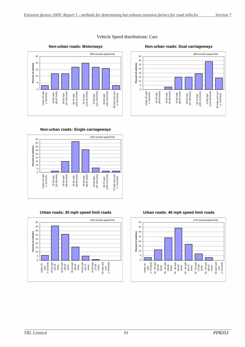
Emission factors 2009: Report 1 - methods for determining hot exhaust emission factors for road vehicles Version 7
TRL Limited 91 PPR353
Vehicle Speed distributions: Cars
Urban roads: 40 mph speed limit roadsUrban roads: 30 mph speed limit roads
Non-urban roads: Motorways Non-urban roads: Dual carriageways
Non-urban roads: Single carriageways
0
5
10
15
20
25
Und
er50
mph
(<80
km/h
)
50-6
0m
ph(8
0-97
km/h
)
60-6
5m
ph(9
7-10
5km
/h)
65-7
0m
ph(1
05-1
13km
/h)
70-7
5m
ph(1
13-1
21km
/h)
75-8
0m
ph(1
21-1
29km
/h)
80-9
0m
ph(1
29-1
45km
/h)
90m
phan
dov
er(>
145
km/h
)
Per
cen
to
fve
hic
les
56% exceed speed limit
0
5
10
15
20
25
30
35
40
Und
er30
mph
(<48
km/h
)
30-4
0m
ph(4
8-64
km/h
)
40-5
0m
ph(6
4-80
km/h
)
50-6
0m
ph(8
0-97
km/h
)
60-6
5m
ph(9
7-10
5km
/h)
65-7
0m
ph(1
05-1
13km
/h)
70-8
0m
ph(1
13-1
29km
/h)
80m
phan
dov
er(>
129
km/h
)
Per
cen
to
fve
hic
les
48% exceed speed limit
0
5
10
15
20
25
30
35
40
45
Und
er20
mph
(<32
km/h
)
20-3
0m
ph(3
2-48
km/h
)
30-4
0m
ph(4
8-64
km/h
)
40-5
0m
ph(6
4-80
km/h
)
50-6
0m
ph(8
0-97
km/h
)
60-6
5m
ph(9
7-10
5km
/h)
65-7
0m
ph(1
05-1
13km
/h)
70m
phan
dov
er(>
113
km/h
)
Per
cen
to
fve
hic
les
10% exceed speed limit
0
5
10
15
20
25
30
35
40
45
Und
er20
mph
(<32
km/h
)
20-3
0m
ph(3
2-48
km/h
)
30-3
5m
ph(4
8-56
km/h
)
35-4
0m
ph(5
6-64
km/h
)
40-4
5m
ph(6
4-72
km/h
)
45-5
0m
ph(7
2-80
km/h
)
50m
phan
dov
er(>
80km
/h)
Per
cen
to
fve
hic
les
53% exceed speed limit
0
5
10
15
20
25
30
35
40
Und
er20
mph
(<32
km/h
)
20-
30m
ph(3
2-48
km/h
)
30-
35m
ph(4
8-56
km/h
)
35-
40m
ph(5
6-64
km/h
)
40-
45m
ph(6
4-72
km/h
)
45-
50m
ph(7
2-80
km/h
)
50-
60m
ph(8
0-97
km/h
)
60m
phan
dov
er(>
97km
/h)
Per
cen
to
fve
hic
les
27% exceed speed limit

Emission factors 2009: Report 1 - methods for determining hot exhaust emission factors for road vehicles Version 7
TRL Limited 92 PPR353
Vehicle Speed distributions: Light goods vehicles
Urban roads: 40 mph speed limit roadsUrban roads: 30 mph speed limit roads
Non-urban roads: Motorways Non-urban roads: Dual carriageways
Non-urban roads: Single carriageways
0
2
4
6
8
10
12
14
16
18
20
Und
er50
mph
(<80
km/h
)
50-6
0m
ph(8
0-97
km/h
)
60-6
5m
ph(9
7-10
5km
/h)
65-7
0m
ph(1
05-1
13km
/h)
70-7
5m
ph(1
13-1
21km
/h)
75-8
0m
ph(1
21-1
29km
/h)
80-9
0m
ph(1
29-1
45km
/h)
90m
phan
dov
er(>
145
km/h
)
Per
cen
to
fve
hic
les
51% exceed speed limit
0
5
10
15
20
25
30
35
Und
er30
mph
(<48
km/h
)
30-4
0m
ph(4
8-64
km/h
)
40-5
0m
ph(6
4-80
km/h
)
50-6
0m
ph(8
0-97
km/h
)
60-6
5m
ph(9
7-10
5km
/h)
65-7
0m
ph(1
05-1
13km
/h)
70-8
0m
ph(1
13-1
29km
/h)
80m
phan
dov
er(>
129
km/h
)
Per
cen
to
fve
hic
les
44% exceed speed limit
0
5
10
15
20
25
30
35
40
45
Und
er20
mph
(<32
km/h
)
20-3
0m
ph(3
2-48
km/h
)
30-4
0m
ph(4
8-64
km/h
)
40-5
0m
ph(6
4-80
km/h
)
50-6
0m
ph(8
0-97
km/h
)
60-6
5m
ph(9
7-10
5km
/h)
65-7
0m
ph(1
05-1
13km
/h)
70m
phan
dov
er(>
113
km/h
)
Per
cen
to
fve
hic
les
11% exceed speed limit
0
5
10
15
20
25
30
35
40
45
Und
er20
mph
(<32
km/h
)
20-3
0m
ph(3
2-48
km/h
)
30-3
5m
ph(4
8-56
km/h
)
35-4
0m
ph(5
6-64
km/h
)
40-4
5m
ph(6
4-72
km/h
)
45-5
0m
ph(7
2-80
km/h
)
50m
phan
dov
er(>
80km
/h)
Per
cen
to
fve
hic
les
53% exceed speed limit
0
5
10
15
20
25
30
35
Und
er20
mph
(<32
km/h
)
20-
30m
ph(3
2-48
km/h
)
30-
35m
ph(4
8-56
km/h
)
35-
40m
ph(5
6-64
km/h
)
40-
45m
ph(6
4-72
km/h
)
45-
50m
ph(7
2-80
km/h
)
50-
60m
ph(8
0-97
km/h
)
60m
phan
dov
er(>
97km
/h)
Per
cen
to
fve
hic
les
29% exceed speed limit

Emission factors 2009: Report 1 - methods for determining hot exhaust emission factors for road vehicles Version 7
TRL Limited 93 PPR353
Vehicle Speed distributions: Buses and coaches
Urban roads: 40 mph speed limit roadsUrban roads: 30 mph speed limit roads
Non-urban roads: Motorways Non-urban roads: Dual carriageways
Non-urban roads: Single carriageways
0
5
10
15
20
25
30
35
40
45
50
Und
er50
mph
(<80
km/h
)
50-6
0m
ph(8
0-97
km/h
)
60-6
5m
ph(9
7-10
5km
/h)
65-7
0m
ph(1
05-1
13km
/h)
70-7
5m
ph(1
13-1
21km
/h)
75-8
0m
ph(1
21-1
29km
/h)
80-9
0m
ph(1
29-1
45km
/h)
90m
phan
dov
er(>
145
km/h
)
Per
cen
to
fve
hic
les
2% exceed speed limit
0
10
20
30
40
50
60
Und
er30
mph
(<48
km/h
)
30-4
0m
ph(4
8-64
km/h
)
40-5
0m
ph(6
4-80
km/h
)
50-6
0m
ph(8
0-97
km/h
)
60-6
5m
ph(9
7-10
5km
/h)
65-7
0m
ph(1
05-1
13km
/h)
70-8
0m
ph(1
13-1
29km
/h)
80m
phan
dov
er(>
129
km/h
)
Per
cen
to
fve
hic
les
3% exceed speed limit
0
10
20
30
40
50
60
Und
er20
mph
(<32
km/h
)
20-3
0m
ph(3
2-48
km/h
)
30-4
0m
ph(4
8-64
km/h
)
40-5
0m
ph(6
4-80
km/h
)
50-6
0m
ph(8
0-97
km/h
)
60-6
5m
ph(9
7-10
5km
/h)
65-7
0m
ph(1
05-1
13km
/h)
70m
phan
dov
er(>
113
km/h
)
Per
cen
to
fve
hic
les
2% exceed speed limit
0
10
20
30
40
50
60
70
Und
er20
mph
(<32
km/h
)
20-3
0m
ph(3
2-48
km/h
)
30-3
5m
ph(4
8-56
km/h
)
35-4
0m
ph(5
6-64
km/h
)
40-4
5m
ph(6
4-72
km/h
)
45-5
0m
ph(7
2-80
km/h
)
50m
phan
dov
er(>
80km
/h)
Per
cen
to
fve
hic
les
28% exceed speed limit
0
5
10
15
20
25
30
35
40
Und
er20
mph
(<32
km/h
)
20-
30m
ph(3
2-48
km/h
)
30-
35m
ph(4
8-56
km/h
)
35-
40m
ph(5
6-64
km/h
)
40-
45m
ph(6
4-72
km/h
)
45-
50m
ph(7
2-80
km/h
)
50-
60m
ph(8
0-97
km/h
)
60m
phan
dov
er(>
97km
/h)
Per
cen
to
fve
hic
les
13% exceed speed limit
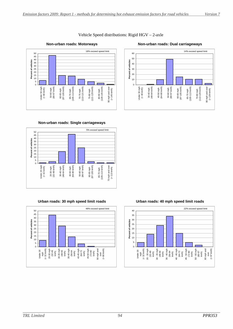
Emission factors 2009: Report 1 - methods for determining hot exhaust emission factors for road vehicles Version 7
TRL Limited 94 PPR353
Vehicle Speed distributions: Rigid HGV – 2-axle
Urban roads: 40 mph speed limit roadsUrban roads: 30 mph speed limit roads
Non-urban roads: Motorways Non-urban roads: Dual carriageways
Non-urban roads: Single carriageways
0
5
10
15
20
25
30
35
40
45
50
Und
er50
mph
(<80
km/h
)
50-6
0m
ph(8
0-97
km/h
)
60-6
5m
ph(9
7-10
5km
/h)
65-7
0m
ph(1
05-1
13km
/h)
70-7
5m
ph(1
13-1
21km
/h)
75-8
0m
ph(1
21-1
29km
/h)
80-9
0m
ph(1
29-1
45km
/h)
90m
phan
dov
er(>
145
km/h
)
Per
cen
to
fve
hic
les
18% exceed speed limit
0
10
20
30
40
50
60
Und
er30
mph
(<48
km/h
)
30-4
0m
ph(4
8-64
km/h
)
40-5
0m
ph(6
4-80
km/h
)
50-6
0m
ph(8
0-97
km/h
)
60-6
5m
ph(9
7-10
5km
/h)
65-7
0m
ph(1
05-1
13km
/h)
70-8
0m
ph(1
13-1
29km
/h)
80m
phan
dov
er(>
129
km/h
)
Per
cen
to
fve
hic
les
14% exceed speed limit
0
5
10
15
20
25
30
35
40
45
50
Und
er20
mph
(<32
km/h
)
20-3
0m
ph(3
2-48
km/h
)
30-4
0m
ph(4
8-64
km/h
)
40-5
0m
ph(6
4-80
km/h
)
50-6
0m
ph(8
0-97
km/h
)
60-6
5m
ph(9
7-10
5km
/h)
65-7
0m
ph(1
05-1
13km
/h)
70m
phan
dov
er(>
113
km/h
)
Per
cen
to
fve
hic
les
5% exceed speed limit
0
5
10
15
20
25
30
35
40
45
50
Und
er20
mph
(<32
km/h
)
20-3
0m
ph(3
2-48
km/h
)
30-3
5m
ph(4
8-56
km/h
)
35-4
0m
ph(5
6-64
km/h
)
40-4
5m
ph(6
4-72
km/h
)
45-5
0m
ph(7
2-80
km/h
)
50m
phan
dov
er(>
80km
/h)
Per
cen
to
fve
hic
les
48% exceed speed limit
0
5
10
15
20
25
30
35
40
Und
er20
mph
(<32
km/h
)
20-
30m
ph(3
2-48
km/h
)
30-
35m
ph(4
8-56
km/h
)
35-
40m
ph(5
6-64
km/h
)
40-
45m
ph(6
4-72
km/h
)
45-
50m
ph(7
2-80
km/h
)
50-
60m
ph(8
0-97
km/h
)
60m
phan
dov
er(>
97km
/h)
Per
cen
to
fve
hic
les
22% exceed speed limit

Emission factors 2009: Report 1 - methods for determining hot exhaust emission factors for road vehicles Version 7
TRL Limited 95 PPR353
Vehicle Speed distributions: Rigid HGV – 3-axle
Urban roads: 40 mph speed limit roadsUrban roads: 30 mph speed limit roads
Non-urban roads: Motorways Non-urban roads: Dual carriageways
Non-urban roads: Single carriageways
0
10
20
30
40
50
60
70
80
90
Und
er50
mph
(<80
km/h
)
50-6
0m
ph(8
0-97
km/h
)
60-6
5m
ph(9
7-10
5km
/h)
65-7
0m
ph(1
05-1
13km
/h)
70-7
5m
ph(1
13-1
21km
/h)
75-8
0m
ph(1
21-1
29km
/h)
80-9
0m
ph(1
29-1
45km
/h)
90m
phan
dov
er(>
145
km/h
)
Per
cen
to
fve
hic
les
0% exceed speed limit
0
10
20
30
40
50
60
70
80
Und
er30
mph
(<48
km/h
)
30-4
0m
ph(4
8-64
km/h
)
40-5
0m
ph(6
4-80
km/h
)
50-6
0m
ph(8
0-97
km/h
)
60-6
5m
ph(9
7-10
5km
/h)
65-7
0m
ph(1
05-1
13km
/h)
70-8
0m
ph(1
13-1
29km
/h)
80m
phan
dov
er(>
129
km/h
)
Per
cen
to
fve
hic
les
3% exceed speed limit
0
10
20
30
40
50
60
Und
er20
mph
(<32
km/h
)
20-3
0m
ph(3
2-48
km/h
)
30-4
0m
ph(4
8-64
km/h
)
40-5
0m
ph(6
4-80
km/h
)
50-6
0m
ph(8
0-97
km/h
)
60-6
5m
ph(9
7-10
5km
/h)
65-7
0m
ph(1
05-1
13km
/h)
70m
phan
dov
er(>
113
km/h
)
Per
cen
to
fve
hic
les
0% exceed speed limit
0
5
10
15
20
25
30
35
40
45
50
Und
er20
mph
(<32
km/h
)
20-3
0m
ph(3
2-48
km/h
)
30-3
5m
ph(4
8-56
km/h
)
35-4
0m
ph(5
6-64
km/h
)
40-4
5m
ph(6
4-72
km/h
)
45-5
0m
ph(7
2-80
km/h
)
50m
phan
dov
er(>
80km
/h)
Per
cen
to
fve
hic
les
46% exceed speed limit
0
5
10
15
20
25
30
35
40
45
Und
er20
mph
(<32
km/h
)
20-
30m
ph(3
2-48
km/h
)
30-
35m
ph(4
8-56
km/h
)
35-
40m
ph(5
6-64
km/h
)
40-
45m
ph(6
4-72
km/h
)
45-
50m
ph(7
2-80
km/h
)
50-
60m
ph(8
0-97
km/h
)
60m
phan
dov
er(>
97km
/h)
Per
cen
to
fve
hic
les
20% exceed speed limit

Emission factors 2009: Report 1 - methods for determining hot exhaust emission factors for road vehicles Version 7
TRL Limited 96 PPR353
Vehicle Speed distributions: Rigid HGV – 4-axle
Urban roads: 40 mph speed limit roadsUrban roads: 30 mph speed limit roads
Non-urban roads: Motorways Non-urban roads: Dual carriageways
Non-urban roads: Single carriageways
0
10
20
30
40
50
60
70
80
90
100
Und
er50
mph
(<80
km/h
)
50-6
0m
ph(8
0-97
km/h
)
60-6
5m
ph(9
7-10
5km
/h)
65-7
0m
ph(1
05-1
13km
/h)
70-7
5m
ph(1
13-1
21km
/h)
75-8
0m
ph(1
21-1
29km
/h)
80-9
0m
ph(1
29-1
45km
/h)
90m
phan
dov
er(>
145
km/h
)
Per
cen
to
fve
hic
les
0% exceed speed limit
0
10
20
30
40
50
60
70
80
90
Und
er30
mph
(<48
km/h
)
30-4
0m
ph(4
8-64
km/h
)
40-5
0m
ph(6
4-80
km/h
)
50-6
0m
ph(8
0-97
km/h
)
60-6
5m
ph(9
7-10
5km
/h)
65-7
0m
ph(1
05-1
13km
/h)
70-8
0m
ph(1
13-1
29km
/h)
80m
phan
dov
er(>
129
km/h
)
Per
cen
to
fve
hic
les
0% exceed speed limit
0
5
10
15
20
25
30
35
40
45
50
Und
er20
mph
(<32
km/h
)
20-3
0m
ph(3
2-48
km/h
)
30-4
0m
ph(4
8-64
km/h
)
40-5
0m
ph(6
4-80
km/h
)
50-6
0m
ph(8
0-97
km/h
)
60-6
5m
ph(9
7-10
5km
/h)
65-7
0m
ph(1
05-1
13km
/h)
70m
phan
dov
er(>
113
km/h
)
Per
cen
to
fve
hic
les
0% exceed speed limit
0
5
10
15
20
25
30
35
40
45
Und
er20
mph
(<32
km/h
)
20-3
0m
ph(3
2-48
km/h
)
30-3
5m
ph(4
8-56
km/h
)
35-4
0m
ph(5
6-64
km/h
)
40-4
5m
ph(6
4-72
km/h
)
45-5
0m
ph(7
2-80
km/h
)
50m
phan
dov
er(>
80km
/h)
Per
cen
to
fve
hic
les
54% exceed speed limit
0
5
10
15
20
25
30
35
40
45
Und
er20
mph
(<32
km/h
)
20-
30m
ph(3
2-48
km/h
)
30-
35m
ph(4
8-56
km/h
)
35-
40m
ph(5
6-64
km/h
)
40-
45m
ph(6
4-72
km/h
)
45-
50m
ph(7
2-80
km/h
)
50-
60m
ph(8
0-97
km/h
)
60m
phan
dov
er(>
97km
/h)
Per
cen
to
fve
hic
les
26% exceed speed limit
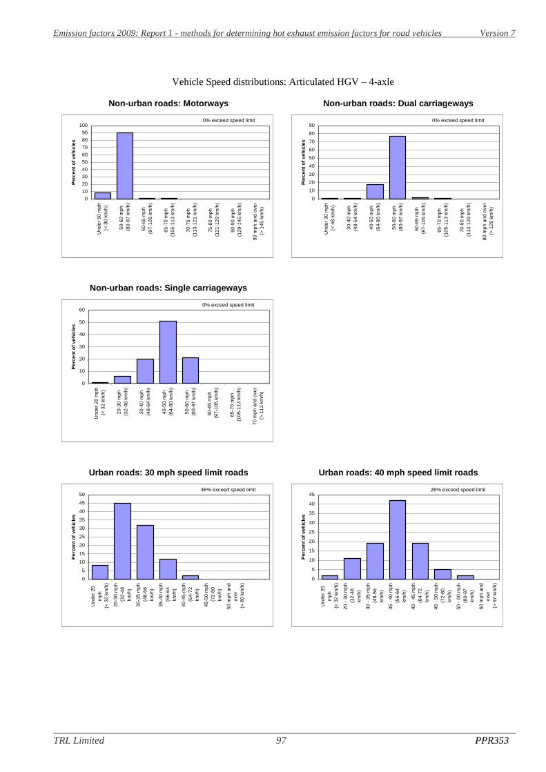
Emission factors 2009: Report 1 - methods for determining hot exhaust emission factors for road vehicles Version 7
TRL Limited 97 PPR353
Vehicle Speed distributions: Articulated HGV – 4-axle
Urban roads: 40 mph speed limit roadsUrban roads: 30 mph speed limit roads
Non-urban roads: Motorways Non-urban roads: Dual carriageways
Non-urban roads: Single carriageways
0
10
20
30
40
50
60
70
80
90
100
Und
er50
mph
(<80
km/h
)
50-6
0m
ph(8
0-97
km/h
)
60-6
5m
ph(9
7-10
5km
/h)
65-7
0m
ph(1
05-1
13km
/h)
70-7
5m
ph(1
13-1
21km
/h)
75-8
0m
ph(1
21-1
29km
/h)
80-9
0m
ph(1
29-1
45km
/h)
90m
phan
dov
er(>
145
km/h
)
Per
cen
to
fve
hic
les
0% exceed speed limit
0
10
20
30
40
50
60
70
80
90
Und
er30
mph
(<48
km/h
)
30-4
0m
ph(4
8-64
km/h
)
40-5
0m
ph(6
4-80
km/h
)
50-6
0m
ph(8
0-97
km/h
)
60-6
5m
ph(9
7-10
5km
/h)
65-7
0m
ph(1
05-1
13km
/h)
70-8
0m
ph(1
13-1
29km
/h)
80m
phan
dov
er(>
129
km/h
)
Per
cen
to
fve
hic
les
0% exceed speed limit
0
10
20
30
40
50
60
Und
er20
mph
(<32
km/h
)
20-3
0m
ph(3
2-48
km/h
)
30-4
0m
ph(4
8-64
km/h
)
40-5
0m
ph(6
4-80
km/h
)
50-6
0m
ph(8
0-97
km/h
)
60-6
5m
ph(9
7-10
5km
/h)
65-7
0m
ph(1
05-1
13km
/h)
70m
phan
dov
er(>
113
km/h
)
Per
cen
to
fve
hic
les
0% exceed speed limit
0
5
10
15
20
25
30
35
40
45
50
Und
er20
mph
(<32
km/h
)
20-3
0m
ph(3
2-48
km/h
)
30-3
5m
ph(4
8-56
km/h
)
35-4
0m
ph(5
6-64
km/h
)
40-4
5m
ph(6
4-72
km/h
)
45-5
0m
ph(7
2-80
km/h
)
50m
phan
dov
er(>
80km
/h)
Per
cen
to
fve
hic
les
46% exceed speed limit
0
5
10
15
20
25
30
35
40
45
Und
er20
mph
(<32
km/h
)
20-
30m
ph(3
2-48
km/h
)
30-
35m
ph(4
8-56
km/h
)
35-
40m
ph(5
6-64
km/h
)
40-
45m
ph(6
4-72
km/h
)
45-
50m
ph(7
2-80
km/h
)
50-
60m
ph(8
0-97
km/h
)
60m
phan
dov
er(>
97km
/h)
Per
cen
to
fve
hic
les
26% exceed speed limit

Emission factors 2009: Report 1 - methods for determining hot exhaust emission factors for road vehicles Version 7
TRL Limited 98 PPR353
Vehicle Speed distributions: Articulated HGV – 5-axle or greater
Urban roads: 40 mph speed limit roadsUrban roads: 30 mph speed limit roads
Non-urban roads: Motorways Non-urban roads: Dual carriageways
Non-urban roads: Single carriageways
0
10
20
30
40
50
60
70
80
90
100
Und
er50
mph
(<80
km/h
)
50-6
0m
ph(8
0-97
km/h
)
60-6
5m
ph(9
7-10
5km
/h)
65-7
0m
ph(1
05-1
13km
/h)
70-7
5m
ph(1
13-1
21km
/h)
75-8
0m
ph(1
21-1
29km
/h)
80-9
0m
ph(1
29-1
45km
/h)
90m
phan
dov
er(>
145
km/h
)
Per
cen
to
fve
hic
les
0% exceed speed limit
0
10
20
30
40
50
60
70
80
90
100
Und
er30
mph
(<48
km/h
)
30-4
0m
ph(4
8-64
km/h
)
40-5
0m
ph(6
4-80
km/h
)
50-6
0m
ph(8
0-97
km/h
)
60-6
5m
ph(9
7-10
5km
/h)
65-7
0m
ph(1
05-1
13km
/h)
70-8
0m
ph(1
13-1
29km
/h)
80m
phan
dov
er(>
129
km/h
)
Per
cen
to
fve
hic
les
0% exceed speed limit
0
10
20
30
40
50
60
Und
er20
mph
(<32
km/h
)
20-3
0m
ph(3
2-48
km/h
)
30-4
0m
ph(4
8-64
km/h
)
40-5
0m
ph(6
4-80
km/h
)
50-6
0m
ph(8
0-97
km/h
)
60-6
5m
ph(9
7-10
5km
/h)
65-7
0m
ph(1
05-1
13km
/h)
70m
phan
dov
er(>
113
km/h
)
Per
cen
to
fve
hic
les
1% exceed speed limit
0
5
10
15
20
25
30
35
40
45
50
Und
er20
mph
(<32
km/h
)
20-3
0m
ph(3
2-48
km/h
)
30-3
5m
ph(4
8-56
km/h
)
35-4
0m
ph(5
6-64
km/h
)
40-4
5m
ph(6
4-72
km/h
)
45-5
0m
ph(7
2-80
km/h
)
50m
phan
dov
er(>
80km
/h)
Per
cen
to
fve
hic
les
54% exceed speed limit
0
5
10
15
20
25
30
35
40
45
50
Und
er20
mph
(<32
km/h
)
20-
30m
ph(3
2-48
km/h
)
30-
35m
ph(4
8-56
km/h
)
35-
40m
ph(5
6-64
km/h
)
40-
45m
ph(6
4-72
km/h
)
45-
50m
ph(7
2-80
km/h
)
50-
60m
ph(8
0-97
km/h
)
60m
phan
dov
er(>
97km
/h)
Per
cen
to
fve
hic
les
25% exceed speed limit

Emission factors 2009: Report 1 - methods for determining hot exhaust emission factors for road vehicles Version 7
TRL Limited 99 PPR353
Appendix E: Average Art.Kinema parameters
The following tables list the average Art.Kinema parameters for cars, LGVs, HGVs and buses per set ofcycles. It should be noted that some of the driving cycles has been analysed both as a complete cycles and asits individual sub-cycles, so some double counting may occur for these cycles. However, the cycles have beenused in this manner (overall and individually) in deriving previous emission functions and could therefore beconsidered to be different cycles.

Emission factors 2009: Report 1 - methods for determining hot exhaust emission factors for road vehicles Version 7
TRL Limited 100 PPR353
Table E1. Average Art.Kinema parameters for:Cars
Ref Bookdriving cycles
UKEFDcycles WSL cycles
ARTEMISdrivingcycles
Realworld
drivingpatterns
Number of cycles 160 45 6 16 3964
Parameter Units Average Average Average Average Averagetotal distance m 12928.1 9211.8 6746.0 18864.1 14499.1
total time s 979.4 622.9 644.8 1244.3 1145.8
driving time s 863.2 558.8 557.2 1100.4 1032.2
drive time s 264.0 191.6 181.7 276.9 263.2
drive time spent accelerating s 312.0 194.0 191.7 435.6 400.7
drive time spent decelerating s 288.0 174.0 184.5 389.0 368.7
time spent braking s 195.1 119.7 111.0 289.8 230.8
standing time s 116.2 64.1 87.7 143.9 113.6
% of time driving - 86.7% 88.3% 92.0% 86.7% 91.8%
% of cruising - 26.1% 31.5% 39.0% 20.8% 24.0%
% of time accelerating - 31.6% 29.8% 26.9% 34.8% 35.5%
% of time decelerating - 29.1% 27.2% 26.1% 31.2% 32.3%
% of time braking - 20.5% 19.5% 13.7% 23.6% 19.6%
% of time standing - 13.3% 11.7% 8.0% 13.3% 8.2%
average speed (trip) km/h 43.3 48.1 56.5 50.9 50.7
average driving speed km/h 47.2 51.1 57.8 55.1 53.9
standard dev. of speed km/h 18.2 15.7 9.9 25.1 20.6
75th - 25th percentile km/h 30.6 26.1 16.3 40.4 32.7
maximum speed km/h 80.2 77.2 77.9 100.1 92.1
average acceleration m/s2 0.002 0.001 0.002 0.000 0.001
average pos. acc. m/s2 0.464 0.455 0.314 0.487 0.410
average neg. acc. m/s2 -0.497 -0.480 -0.321 -0.537 -0.448
standard dev. of acc. m/s2 0.584 0.548 0.438 0.658 0.583
standard dev. of positive acc. m/s2 0.362 0.335 0.287 0.407 0.380
standard dev. of negative acc. m/s2 0.419 0.388 0.350 0.496 0.473
75th - 25th percentile m/s2 0.411 0.388 0.316 0.495 0.424
number of accelerations - 52.96 31.04 37.00 81.63 76.90
nr. of acc. per km /km 8.92 9.89 9.57 7.03 6.10
number of stops - 8.43 5.16 8.17 10.25 7.11
stops per km /km 2.56 2.63 2.99 1.45 0.65
average stop duration# s 12.57 10.87 7.27 11.79 14.33
average distance between stops# m 3912.8 3868.3 3529.4 3786.7 4562.5
Relative Positive Acceleration m/s2 0.186 0.180 0.137 0.201 0.164
Positive Kinetic Energy m/s2 0.347 0.334 0.254 0.373 0.304
Cumulative Squared Positive Kinetic Energy m2/s4 4.888 4.795 2.992 5.941 4.711
Relative Positive Speed - 0.456 0.435 0.446 0.481 0.467
Relative Real Speed - 0.774 0.784 0.851 0.748 0.808
Relative Square Speed m/s 15.603 16.201 17.190 18.715 17.726
Relative Positive Square Speed m/s 7.024 6.744 7.288 8.783 7.987
Relative Real Square Speed m/s 12.925 13.764 15.659 15.066 14.934
Relative Cubic Speed m2/s2 332.7 359.4 394.1 468.5 378.3
Relative Positive Cubic Speed m2/s2 148.8 147.8 162.5 215.6 165.3
Relative Real Cubic Speed m2/s2 288.0 320.1 370.8 395.5 327.8
Root Mean Square of Acceleration m/s2 0.200 0.195 0.159 0.199 0.168
# - Average of only the cycles that have stops within them

Emission factors 2009: Report 1 - methods for determining hot exhaust emission factors for road vehicles Version 7
TRL Limited 101 PPR353
Table E2. Average Art.Kinema parameters for: LGVsRef Bookdrivingcycles
UKEFDcycles
WSLcycles
Real worlddrivingpatterns
Number of cycles 32 26 6 367
Parameter Units Average Average Average Averagetotal distance m 8512.5 9858.6 6746.0 11110.0
total time s 811.5 666.2 644.8 1559.6
driving time s 719.1 615.0 557.2 1303.4
drive time s 203.8 285.6 181.7 448.7
drive time spent accelerating s 280.5 174.3 191.7 464.7
drive time spent decelerating s 235.4 155.7 184.5 390.2
time spent braking s 163.0 99.6 111.0 302.4
standing time s 92.4 51.2 87.7 256.2
% of time driving - 87.3% 93.7% 92.0% 86.7%
% of cruising - 23.1% 46.5% 39.0% 30.4%
% of time accelerating - 34.9% 24.8% 26.9% 30.8%
% of time decelerating - 29.3% 22.5% 26.1% 25.5%
% of time braking - 21.0% 14.1% 13.7% 19.7%
% of time standing - 12.7% 6.3% 8.0% 13.3%
average speed (trip) km/h 35.5 60.4 56.5 27.4
average driving speed km/h 39.0 62.3 57.8 31.1
standard dev. of speed km/h 18.0 15.3 9.9 14.9
75th - 25th percentile km/h 29.3 21.9 16.3 26.9
maximum speed km/h 70.3 84.6 77.9 63.1
average acceleration m/s2 0.000 0.001 0.002 -0.001
average pos. acc. m/s2 0.428 0.355 0.314 0.399
average neg. acc. m/s2 -0.500 -0.379 -0.321 -0.479
standard dev. of acc. m/s2 0.590 0.404 0.438 0.544
standard dev. of positive acc. m/s2 0.336 0.246 0.287 0.320
standard dev. of negative acc. m/s2 0.455 0.303 0.350 0.448
75th - 25th percentile m/s2 0.433 0.248 0.316 0.381
number of accelerations - 49.66 25.88 37.00 93.19
nr. of acc. per km /km 8.81 4.38 9.57 14.05
number of stops - 7.44 4.38 8.17 13.23
stops per km /km 1.85 1.20 2.99 7.15
average stop duration# s 10.77 8.16 7.27 18.46
average distance between stops# m 2121.8 6633.6 3529.4 1759.4
Relative Positive Acceleration m/s2 0.187 0.113 0.137 0.159
Positive Kinetic Energy m/s2 0.350 0.217 0.254 0.292
Cumulative Squared Positive Kinetic Energy m2/s4 4.110 2.771 2.992 2.575
Relative Positive Speed - 0.499 0.392 0.446 0.465
Relative Real Speed - 0.780 0.864 0.851 0.801
Relative Square Speed m/s 13.345 18.927 17.190 10.784
Relative Positive Square Speed m/s 6.419 7.120 7.288 4.944
Relative Real Square Speed m/s 10.954 17.181 15.659 8.825
Relative Cubic Speed m2/s2 240.7 440.3 394.1 130.8
Relative Positive Cubic Speed m2/s2 110.6 164.0 162.5 58.8
Relative Real Cubic Speed m2/s2 205.9 409.6 370.8 108.9
Root Mean Square of Acceleration m/s2 0.201 0.123 0.159 0.188
# - Average of only the cycles that have stops within them
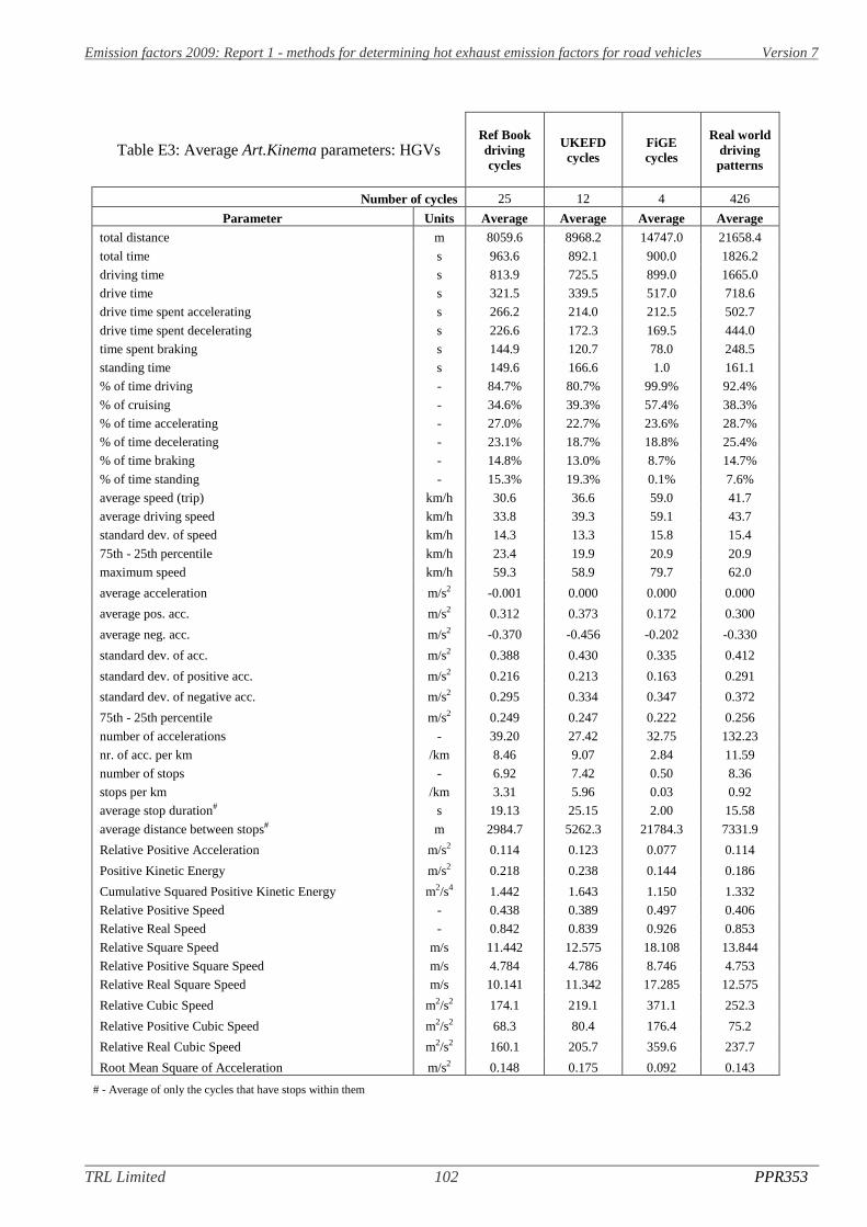
Emission factors 2009: Report 1 - methods for determining hot exhaust emission factors for road vehicles Version 7
TRL Limited 102 PPR353
Table E3: Average Art.Kinema parameters: HGVsRef Bookdrivingcycles
UKEFDcycles
FiGEcycles
Real worlddrivingpatterns
Number of cycles 25 12 4 426
Parameter Units Average Average Average Averagetotal distance m 8059.6 8968.2 14747.0 21658.4
total time s 963.6 892.1 900.0 1826.2
driving time s 813.9 725.5 899.0 1665.0
drive time s 321.5 339.5 517.0 718.6
drive time spent accelerating s 266.2 214.0 212.5 502.7
drive time spent decelerating s 226.6 172.3 169.5 444.0
time spent braking s 144.9 120.7 78.0 248.5
standing time s 149.6 166.6 1.0 161.1
% of time driving - 84.7% 80.7% 99.9% 92.4%
% of cruising - 34.6% 39.3% 57.4% 38.3%
% of time accelerating - 27.0% 22.7% 23.6% 28.7%
% of time decelerating - 23.1% 18.7% 18.8% 25.4%
% of time braking - 14.8% 13.0% 8.7% 14.7%
% of time standing - 15.3% 19.3% 0.1% 7.6%
average speed (trip) km/h 30.6 36.6 59.0 41.7
average driving speed km/h 33.8 39.3 59.1 43.7
standard dev. of speed km/h 14.3 13.3 15.8 15.4
75th - 25th percentile km/h 23.4 19.9 20.9 20.9
maximum speed km/h 59.3 58.9 79.7 62.0
average acceleration m/s2 -0.001 0.000 0.000 0.000
average pos. acc. m/s2 0.312 0.373 0.172 0.300
average neg. acc. m/s2 -0.370 -0.456 -0.202 -0.330
standard dev. of acc. m/s2 0.388 0.430 0.335 0.412
standard dev. of positive acc. m/s2 0.216 0.213 0.163 0.291
standard dev. of negative acc. m/s2 0.295 0.334 0.347 0.372
75th - 25th percentile m/s2 0.249 0.247 0.222 0.256
number of accelerations - 39.20 27.42 32.75 132.23
nr. of acc. per km /km 8.46 9.07 2.84 11.59
number of stops - 6.92 7.42 0.50 8.36
stops per km /km 3.31 5.96 0.03 0.92
average stop duration# s 19.13 25.15 2.00 15.58
average distance between stops# m 2984.7 5262.3 21784.3 7331.9
Relative Positive Acceleration m/s2 0.114 0.123 0.077 0.114
Positive Kinetic Energy m/s2 0.218 0.238 0.144 0.186
Cumulative Squared Positive Kinetic Energy m2/s4 1.442 1.643 1.150 1.332
Relative Positive Speed - 0.438 0.389 0.497 0.406
Relative Real Speed - 0.842 0.839 0.926 0.853
Relative Square Speed m/s 11.442 12.575 18.108 13.844
Relative Positive Square Speed m/s 4.784 4.786 8.746 4.753
Relative Real Square Speed m/s 10.141 11.342 17.285 12.575
Relative Cubic Speed m2/s2 174.1 219.1 371.1 252.3
Relative Positive Cubic Speed m2/s2 68.3 80.4 176.4 75.2
Relative Real Cubic Speed m2/s2 160.1 205.7 359.6 237.7
Root Mean Square of Acceleration m/s2 0.148 0.175 0.092 0.143
# - Average of only the cycles that have stops within them

Emission factors 2009: Report 1 - methods for determining hot exhaust emission factors for road vehicles Version 7
TRL Limited 103 PPR353
Table E4: Average Art.Kinema parameters: BusesRef Bookdrivingcycles
UKEFDcycles
FiGEcycles
Real worlddrivingpatterns
Number of cycles 22 4 4 225
Parameter Units Average Average Average Average
total distance m 6411.6 14747.0 14747.0 10439.1
total time s 1058.8 900.0 900.0 1765.3
driving time s 895.3 899.0 899.0 1501.5
drive time s 272.4 517.0 517.0 305.5
drive time spent accelerating s 345.5 212.5 212.5 608.4
drive time spent decelerating s 277.8 169.5 169.5 587.7
time spent braking s 203.5 78.0 78.0 430.1
standing time s 163.5 1.0 1.0 263.7
% of time driving - 85.1% 99.9% 99.9% 87.3%
% of cruising - 26.9% 57.4% 57.4% 17.0%
% of time accelerating - 32.3% 23.6% 23.6% 35.8%
% of time decelerating - 26.0% 18.8% 18.8% 34.5%
% of time braking - 18.9% 8.7% 8.7% 25.1%
% of time standing - 14.9% 0.1% 0.1% 12.7%
average speed (trip) km/h 23.4 59.0 59.0 22.4
average driving speed km/h 26.8 59.1 59.1 25.4
standard dev. of speed km/h 13.2 15.8 15.8 12.4
75th - 25th percentile km/h 22.0 20.9 20.9 23.6
maximum speed km/h 51.4 79.7 79.7 49.8
average acceleration m/s2 0.000 0.000 0.000 0.000
average pos. acc. m/s2 0.440 0.172 0.172 0.445
average neg. acc. m/s2 -0.682 -0.202 -0.202 -0.458
standard dev. of acc. m/s2 0.584 0.335 0.335 0.520
standard dev. of positive acc. m/s2 0.308 0.163 0.163 0.318
standard dev. of negative acc. m/s2 0.411 0.347 0.347 0.352
75th - 25th percentile m/s2 0.379 0.222 0.222 0.503
number of accelerations - 39.09 32.75 32.75 160.65
nr. of acc. per km /km 7.69 2.84 2.84 24.37
number of stops - 14.95 0.50 0.50 17.17
stops per km /km 3.03 0.03 0.03 14.59
average stop duration# s 11.36 2.00 2.00 17.05
average distance between stops# m 947.3 21784.3 21784.3 1295.7
Relative Positive Acceleration m/s2 0.176 0.077 0.077 0.170
Positive Kinetic Energy m/s2 0.334 0.144 0.144 0.259
Cumulative Squared Positive Kinetic Energy m2/s4 2.785 1.150 1.150 1.835
Relative Positive Speed - 0.494 0.497 0.497 0.423
Relative Real Speed - 0.800 0.926 0.926 0.736
Relative Square Speed m/s 9.398 18.108 18.108 8.849
Relative Positive Square Speed m/s 4.325 8.746 8.746 3.695
Relative Real Square Speed m/s 7.902 17.285 17.285 6.681
Relative Cubic Speed m2/s2 112.9 371.1 371.1 87.8
Relative Positive Cubic Speed m2/s2 45.9 176.4 176.4 36.3
Relative Real Cubic Speed m2/s2 99.3 359.6 359.6 67.5
Root Mean Square of Acceleration m/s2 0.227 0.092 0.092 0.200
# - Average of only the cycles that have stops within them

Emission factors 2009: Report 1 - methods for determining hot exhaust emission factors for road vehicles Version 7
TRL Limited 104 PPR353
Appendix F: ARTEMIS correction factors
Gear-shift behaviour
It was observed in ARTEMIS that the gear-shift strategy affects CO2 emissions by between 2% and 15%. Forother pollutants the effects are smaller. The correction factor (CF) is used for CO2 according to the formula:
(((( ))))(((( ))))strategyotherCOemission
strategyArtemisCOemissionCF
2
2==== (Equation F1)
For all driving cycles other than the NEDC, CF is equal to one. For the NEDC, the values of CF for theARTEMIS rural and motorway cycles are 1.08 and 1.03 respectively.
Emission degradation
The influence of the mileage M1 or M2 [km] is expressed by the formula:
(((( ))))(((( ))))
(((( ))))(((( ))))2
1
2
1
My
My
Memission
Memission==== (Equation F2)
Values of y are given for Euro 1 and 2 petrol cars in Table F1, and for Euro 3 and 4 petrol cars in Table F2, inboth cases for urban and rural situations, i.e. for an average speed lower than 19 km h-1 and higher than 63 kmh-1 respectively. For an intermediate speed V, the following formula has to be used:
(((( )))) (((( )))) (((( )))) (((( )))) (((( ))))(((( ))))44
19 urbanyruralyVurbanyVy
−−−−⋅⋅⋅⋅−−−−++++==== (Equation F3)
Table F1: Emission degradation correction factor y = a x mileage + b, for Euro 1 and Euro 2 petrol vehicles.Mileage expressed in km, y normalised for the corresponding average mileage.
Petrol Euro 1 and 2Capacityclass (l)
Averagemileage (km)
a bValue at
100,000 km
y (urban)
for
V≤19 km h-1
(urban situation)
CO
≤1.4 29,057 1.523E-05 0.557 2.11.4-2.0 39,837 1.148E-05 0.543 1.7
>2.0 47,028 9.243E-06 0.565 1.5
HC
≤1.4 29,057 1.215E-05 0.647 1.91.4-2.0 39,837 1.232E-05 0.509 1.7
>2.0 47,028 1.208E-05 0.432 1.6
NOx All 44,931 1.598E-05 0.282 1.9
y (rural)
for
V≥63 km h-1
(rural situation)
CO
≤1.4 29,057 1.689E-05 0.509 2.2
1.4-2.0 39,837 9.607E-06 0.617 1.6>2.0 47,028 2.704E-06 0.873 1.1
HC
≤1.4 29,057 6.570E-06 0.809 1.5
1.4-2.0 39,837 9.815E-06 0.609 1.6>2.0 47,028 6.224E-06 0.707 1.3
NOx all 47,186 1.220E-05 0.424 1.6
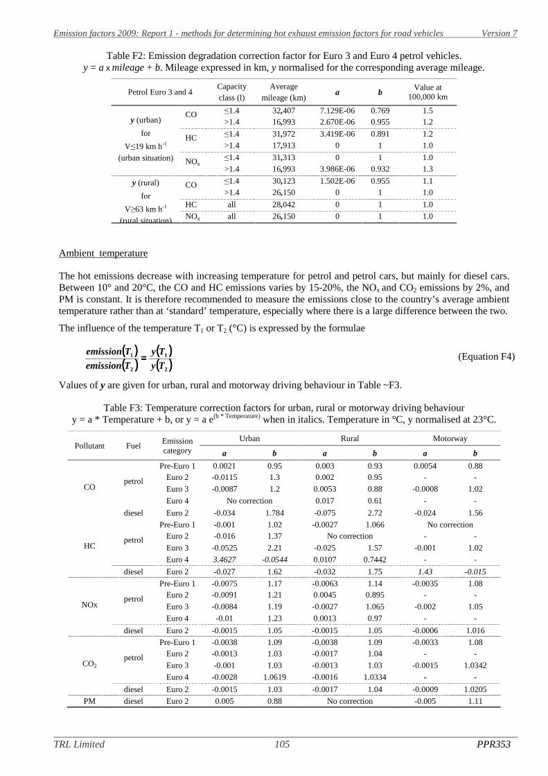
Emission factors 2009: Report 1 - methods for determining hot exhaust emission factors for road vehicles Version 7
TRL Limited 105 PPR353
Table F2: Emission degradation correction factor for Euro 3 and Euro 4 petrol vehicles.y = a x mileage + b. Mileage expressed in km, y normalised for the corresponding average mileage.
Petrol Euro 3 and 4Capacityclass (l)
Averagemileage (km)
a bValue at
100,000 km
y (urban)
for
V≤19 km h-1 (urban situation)
CO ≤1.4 32,407 7.129E-06 0.769 1.5>1.4 16,993 2.670E-06 0.955 1.2
HC ≤1.4 31,972 3.419E-06 0.891 1.2>1.4 17,913 0 1 1.0
NOx≤1.4 31,313 0 1 1.0>1.4 16,993 3.986E-06 0.932 1.3
y (rural)
for
V≥63 km h-1 (rural situation)
CO ≤1.4 30,123 1.502E-06 0.955 1.1>1.4 26,150 0 1 1.0
HC all 28,042 0 1 1.0
NOx all 26,150 0 1 1.0
Ambient temperature
The hot emissions decrease with increasing temperature for petrol and petrol cars, but mainly for diesel cars.Between 10° and 20°C, the CO and HC emissions varies by 15-20%, the NOx and CO2 emissions by 2%, andPM is constant. It is therefore recommended to measure the emissions close to the country’s average ambienttemperature rather than at ‘standard’ temperature, especially where there is a large difference between the two.
The influence of the temperature T1 or T2 (°C) is expressed by the formulae
(((( ))))(((( ))))
(((( ))))(((( ))))2
1
2
1
Ty
Ty
Temission
Temission==== (Equation F4)
Values of y are given for urban, rural and motorway driving behaviour in Table ~F3.
Table F3: Temperature correction factors for urban, rural or motorway driving behavioury = a * Temperature + b, or y = a e(b * Temperature) when in italics. Temperature in °C, y normalised at 23°C.
Pollutant FuelEmissioncategory
Urban Rural Motorway
a b a b a b
COpetrol
Pre-Euro 1 0.0021 0.95 0.003 0.93 0.0054 0.88Euro 2 -0.0115 1.3 0.002 0.95 - -
Euro 3 -0.0087 1.2 0.0053 0.88 -0.0008 1.02
Euro 4 No correction 0.017 0.61 - -
diesel Euro 2 -0.034 1.784 -0.075 2.72 -0.024 1.56
HCpetrol
Pre-Euro 1 -0.001 1.02 -0.0027 1.066 No correctionEuro 2 -0.016 1.37 No correction - -
Euro 3 -0.0525 2.21 -0.025 1.57 -0.001 1.02
Euro 4 3.4627 -0.0544 0.0107 0.7442 - -
diesel Euro 2 -0.027 1.62 -0.032 1.75 1.43 -0.015
NOxpetrol
Pre-Euro 1 -0.0075 1.17 -0.0063 1.14 -0.0035 1.08Euro 2 -0.0091 1.21 0.0045 0.895 - -
Euro 3 -0.0084 1.19 -0.0027 1.065 -0.002 1.05
Euro 4 -0.01 1.23 0.0013 0.97 - -
diesel Euro 2 -0.0015 1.05 -0.0015 1.05 -0.0006 1.016
CO2petrol
Pre-Euro 1 -0.0038 1.09 -0.0038 1.09 -0.0033 1.08Euro 2 -0.0013 1.03 -0.0017 1.04 - -
Euro 3 -0.001 1.03 -0.0013 1.03 -0.0015 1.0342
Euro 4 -0.0028 1.0619 -0.0016 1.0334 - -
diesel Euro 2 -0.0015 1.03 -0.0017 1.04 -0.0009 1.0205
PM diesel Euro 2 0.005 0.88 No correction -0.005 1.11

Emission factors 2009: Report 1 - methods for determining hot exhaust emission factors for road vehicles Version 7
TRL Limited 106 PPR353
Ambient humidity
From the low to the high regulatory limit of humidity (i.e. 5.5 and 12.2 gH2O/kg dry air) NOx emissionsdecrease for the petrol and diesel vehicles by 30% and 15% respectively. This influence of the humidity isdifferent from the legislative correction factor kH. Again it is therefore recommended when possible toperform the tests with an ambient air humidity close to the real-world average. The influence of the humidityon NOx emission is expressed by the formula:
(((( ))))(((( ))))
(((( ))))(((( ))))2
1
2
1
Hy
Hy
Hemission
Hemission==== (Equation F5)
Values of y are available for some vehicle classes and for urban and rural driving behaviour in Table F4. It isrecommended to use the rural figures for motorway driving behaviour, and to use the petrol Euro 2 figures forpetrol Pre-Euro 1 and Euro 1, petrol Euro 3 figures for petrol Euro 4, and diesel Euro 2 figures for the otherdiesel cases. For other pollutants, no correction factors are proposed.
Table F4: Correction factor for NOx emissions corrected or not using the current method,for urban or rural driving behaviour. y = a * Humidity + b. Humidity in gH2O/kg dry air, y
normalised at 10.71 gH2O/kg dry air.
FuelEmissioncategory
urban rural
a b a b
Uncorrected emissionspetrol
Euro 2 -0.052 1.5592 -0.0293 1.31
Euro 3 -0.081 1.8669 -0.0284 1.3
diesel Euro 2 -0.0249 1.2668 -0.0307 1.325
Corrected emissionspetrol
Euro 2 -0.0182 1.1944 0.004 0.9571
Euro 3 -0.0529 1.5654 -0.0093 1.0996
diesel Euro 2 0.0067 0.9281 0.0106 0.8869
Dilution ratio
The dilution ratio (between exhaust air and dilution air), the quality of the dilution air and the PM filterpreconditioning did not seem to have a clear influence on the emissions. This could be due to the low samplesize and to the widely standardised sampling and analysing conditions, respected by the participatinglaboratories. Nevertheless, the pollutant analysing and sampling conditions seem to be an important source oferror, compared with the other parameters studied above. A correction factor could be determined for PM, butit is not applicable to the common ARTEMIS emission data, as the dilution ratio is usually unknown.

TRL Crowthorne House, Nine Mile Ride Wokingham, Berkshire RG40 3GAUnited Kingdom
T: +44 (0) 1344 773131 F: +44 (0) 1344 770356E: [email protected] W: www.trl.co.uk
ISSN 0968-4093
Price code: 4X
Published by IHS Willoughby Road, Bracknell Berkshire RG12 8FB United Kingdom
T: +44 (0) 1344 328038 F: +44 (0) 1344 328005E: [email protected] W: http://emeastore.ihs.com PP
R3
53
Emission factors 2009: Report 1 – a review of methods for determining hot exhaust emission factors for road vehicles
TRL was commissioned by the Department for Transport to review the approach used in the National Atmospheric Emissions Inventory (NAEI) for estimating emissions from road vehicles, and to propose new methodologies. This Report reviews the experimental methods used to determine emission factors, and provides recommendations for the future development of the emission factors in the UK. It includes two main elements: (i) an evaluation of the driving cycles used in emission tests; and (ii) a review of the parameters recorded during emission tests. A distinction is also made between the improvement of the emission factors in the current database and the requirements with respect to future tests. The Report recommends that more representative driving cycles should be considered for future emission testing, that urban buses and coaches should be treated separately when deriving emission factors, and that when compiling an emission factor database adjustment factors should be applied in order to standardise the data for the gear-shift strategy, the vehicle mileage, the ambient temperature and the ambient humidity. In addition, emission measurements are required for a wider variety of two-wheel vehicles and their operation.
Other titles from this subject area
PPR270 Scoping study on the potential for instantaneous emission modelling: summary report. T J Barlow, P G Boulter and I S McCrae. 2007
PPR269 The links between micro-scale traffic, emission and air pollution models. P G Boulter and I S McCrae. 2007
PPR268 An evaluation of instantaneous emission models. T J Barlow, P G Boulter and I S McCrae. 2007
PPR267 A review of instantaneous emission models for road vehicles. P G Boulter, I S McCrae and T J Barlow. 2007
PPR262 Primary NO2 emissions from road vehicles in the Hatfield and Bell Common Tunnels. P G Boulter,
I S McCrae and J Green. 2007
PPR216 An innovative dynamometer: free running rollers to provide a potential cheap representative roadside emission procedure. S Latham. 2007